Embed Size (px)
Citation preview

DISCRETE AND CONTINUOUS doi:10.3934/dcdsb.2011.16.927DYNAMICAL SYSTEMS SERIES BVolume 16, Number 3, October 2011 pp. 927–944
THE LOGISTIC MAP OF MATRICES
Zenonas Navickas
Department of Applied Mathematics, Kaunas University of TechnologyStudentu 50-325, Kaunas LT-51368, Lithuania
Rasa Smidtaite
Department of Applied Mathematics, Kaunas University of TechnologyStudentu 50-325, Kaunas LT-51368, Lithuania
Alfonsas Vainoras
Institute of Cardiology, Kaunas University of MedicineSukileliu av. 17, LT-50009, Kaunas, Lithuania
Minvydas Ragulskis
Research Group for Mathematical and Numerical Analysis of Dynamical Systems
Kaunas University of Technology, Studentu 50-222, Kaunas LT-51368, Lithuania
(Communicated by Miguel Sanjuan)
Abstract. The standard iterative logistic map is extended by replacing thescalar variable by a square matrix of variables. Dynamical properties of such aniterative map are explored in detail when the order of matrices is 2. It is shown
that the evolution of the logistic map depends not only on the control param-eter but also on the eigenvalues of the matrix of initial conditions. Several
computational examples are used to demonstrate the convergence to periodicattractors and the sensitivity of chaotic processes to initials conditions.
1. Introduction. The logistic map is a paradigmatic model often used to demon-strate the onset of chaos and to illustrate how complex behavior can arise from verysimple non-linear dynamical equations [1, 2]:
x(n+1) = ax(n)(
1− x(n))
; (1)
where n is the iteration number; n = 0, 1, 2, . . .; a ∈ R is the parameter of thelogistic map and x(0) is the initial condition (the initial population at year 0). Thelogistic map is thoroughly explored and is used to model [3, 4, 5, 6], encrypt [7, 8],predict [9, 10] different physical systems and processes. A number of extensionsof the logistic map have been proposed. The logistic map in two dimensions isintroduced in [11]; the bi-parameter logistic map is used to model a car followingmodel in [12]; a complex logistic map is used to generate fractals in [13]; the conceptof the random logistic map is introduced in [14]; the interplay between noise andchaos in the stochastic logistic map is investigated in [15]; the coupled logistic mapis used to study the effects of spatial heterogeneity on population dynamics in [16];a two-dimensional logistic coupled map lattice is exploited to describe the Turing
2000 Mathematics Subject Classification. Primary: 58F15, 58F17; Secondary: 53C35.Key words and phrases. The logistic map, attractor, idempotent, nilpotent.
927

928 Z. NAVICKAS, R. SMIDTAITE, A. VAINORAS AND M. RAGULSKIS
instability in [17]; averaged logistic maps are used to construct carrying surfaces ofreturn maps in [18]; the compound logistic map is investigated in [19].
Figure 1. The controversy of the logistic map of matrices: X(0) =[ 0.2 0.30.4 0.7 ] results into 4 stationary processes (A) whileX(0) = [ 0.2 0.3
0.4 0.9 ]yields a violent divergence of iterative processes (B); a = 3.7; dot-
dashed lines stand for x(n)11 ; dashed-dotted lines stand for x
(n)12 ;
dashed lines stand for x(n)21 and thin solid lines stand for x
(n)22 .
The object of this paper is to investigate the extension of the logistic map whenthe discrete scalar variable x(n) is replaced by a square matrix of order 2; the n-thiterate of that matrix is denoted as X(n). Let the matrix of initial conditions reads:
X(0) =
[
x(0)11 x
(0)12
x(0)21 x
(0)22
]
; x(0)kl ∈ R; k, l = 1, 2. Then the iterated map
X(n+1) = aX(n)(
I −X(n))
:=
[
x(n+1)11 x
(n+1)12
x(n+1)21 x
(n+1)22
]
, (2)
represents a logistic map of square matrices of order 2. Eq. (2) produces four scalar
time series{
x(j)kl
}+∞
j=0; k, l = 1, 2. Explicitly,
x(n+1)11 = a
(
x(n)11
(
1− x(n)11
)
− x(n)12 x
(n)21
)
;
x(n+1)12 = ax
(n)12
(
1− x(n)11 − x
(n)22
)
;
x(n+1)21 = ax
(n)21
(
1− x(n)11 − x
(n)22
)
;
x(n+1)22 = a
(
x(n)22
(
1− x(n)22
)
− x(n)12 x
(n)21
)
;
(3)
n = 0, 1, 2, . . . ; and x(0)11 , x
(0)12 , x
(0)21 , x
(0)22 are four scalar initial conditions. Though
such an extension of the classical logistic map seems to be trivial, the apparentsimplicity of the dynamical properties of such an iterative map is misguiding. As anexample let us select two different sets of initial conditions and follow the evolutionof four time series (at fixed parameter value a = 3.7). Initial conditions X(0) =[
0.2 0.30.4 0.7
]
yield 4 fluctuating processes (Fig. 1A - note that some values of

THE LOGISTIC MAP OF MATRICES 929
iterated time series are lower than 0). But initial conditions X(0) =
[
0.2 0.30.4 0.9
]
yield a violent divergence of iterative processes; numerical overflow is reached after10 iterations only (Fig. 1B). The primary object of this paper is to explain suchdynamic behavior of the logistic map of matrices when the scalar discrete variableis replaced by a square matrix or order 2.
2. Auxiliary Results. Several properties of square matrices of order 2 will bediscussed in this section. These properties are essential before continuing with thelogistic map of matrices.
2.1. Algebraic representation of matrices. Let us consider a square matrix oforder 2:
X :=
[
x11 x12
x21 x22
]
, (4)
x11, . . . , x22 ∈ C and its eigenvalues λ1, λ2 ∈ C:
λ1,2 =1
2
(
Tr X ±√dsk X
)
, (5)
where Tr X := x11 + x22; dsk X := (x11 − x22)2+ 4x12x21.
Corollary 1. Let eigenvalues of the matrix X are not equal: λ1 6= λ2. Then it ispossible to construct two matrices Dk:
Dk :=1
λk − λl
(X − λlI) ; k, l = 1, 2; k 6= l; (6)
where I is the identity matrix; I :=
[
1 00 1
]
. Matrices Dk satisfy following equal-
ities:
(i) detDk = 0;(ii) D1 +D2 = I;
(iii) Dk ·Dl = δklDk; k, l = 1, 2 where δkl :=
{
1, k = l;0, k 6= l.
Proof. The equality (i) follows from Eq. (6) because detX −λiI = 0. The equality(ii) holds because D1 +D2 = 1
λ1−λ2(A− λ2I) +
1λ2−λ1
(A− λ1I) = I.
The proof of the equality (iii) is straightforward. Let k = l = 1. Then, Cayley-Hamilton theorem [20] and Eq. (6) yield:
D21 =
1
(λ1 − λ2)2 (X − λ2I)
2=
1
(λ1 − λ2)2
(
X2 − 2λ2X + λ22I)
=1
(λ1 − λ2)2
((
X2 − (λ1 + λ2)X + λ1λ2I)
− λ2X + λ1X + λ22I − λ1λ2I
)
=1
(λ1 − λ2)2 ((λ1 − λ2)X − (λ1 − λ2)λ2I) =
1
λ1 − λ2(X − λ2I) = D1.
Analogously it can be proven that D22 = D2. Let now k = 1 and l = 2. Then,

930 Z. NAVICKAS, R. SMIDTAITE, A. VAINORAS AND M. RAGULSKIS
D1 ·D2 =1
λ1 − λ2(X − λ2I) ·
1
λ2 − λ1(X − λ1I)
= − 1
(λ1 − λ2)2
(
X2 − (λ1 + λ2)X + λ1 · λ2I)
= Θ;
where Θ :=
[
0 00 0
]
. Analogously it can be shown that D2 ·D1 = Θ.
Corollary 2. Let eigenvalues of the matrix X coincide: λ1 = λ2 = λ0. Then thematrix N defined as:
N := X − λ0I (7)
satisfies following relationships:
(i) N2 = Θ;(ii) detN = 0.
Proof. The equality (i) holds because Cayley – Hamilton theorem yields: N2 =
(X − λ0I)2= X2 − 2λ0X + λ2
0I = Θ. The equality (ii) follows from the propertyof a determinant of the product of matrices.
Corollary 3. If λ1 6= λ2 (dsk X 6= 0) then the matrix X can be expressed as:
X = λ1D1 + λ2D2. (8)
If λ1 = λ2 = λ0 (dsk X = 0) then the matrix X can be expressed as:
X = λ0I +N. (9)
Proof. Eq. (9) holds because:
λ1D1 + λ2D2 =λ1
λ1 − λ2(X − λ2I) +
λ2
λ2 − λ1(X − λ1I)
=
(
λ1
λ1 − λ2+
λ2
λ2 − λ1
)
X = X
(10)
The validity of Eq. (9) follows from Eq. (7).
Let D1 is an idempotent (D21 = D1). Then D2 := I −D1 is also an idempotent
because D22 = (I −D1)
2= I2 − 2D1 + D2
1 = I − D1. Analogously, let N is anilpotent. Then cN is a nilpotent also; c ∈ C. Idempotents D and I − D areconjugate idempotents. Nilpotents N and cN ; c ∈ C are similar nilpotents. (N andΘ are similar nilpotents).
Definition 2.1. The matrix X is an idempotent matrix if it can be expressed inthe form of Eq. (8) where λ1;λ2 are eigenvalues of X and D1;D2 are conjugateidempotents (D1 +D2 = I). The matrix X is a nilpotent matrix if its eigenvaluesare equal λ1 = λ2 = λ0 and Eq. (9) holds.
Corollary 4. Matrices D1 = 1 ·D1+0 ·D2 and D2 = 0 ·D1+1 ·D2 are idempotentmatrices, and matrix N = 0 · I +N is a nilpotent matrix.

THE LOGISTIC MAP OF MATRICES 931
Corollary 5. The matrix X is an idempotent matrix if its eigenvalues are notequal; the matrix X is a nilpotent matrix if its eigenvalues are equal. Let us noticethat a scalar matrix X = λ0I can be expressed in the form λ0I = λ0D1 + λ0D2
where D1;D2 is a pair of conjugate idempotents. Thus, λ0I can be interpreted as anilpotent (λ0I = λ0I +Θ) or as an idempotent matrix.
Example 1. This will illustrate that a scalar matrix can interpreted as a nilpotentor an idempotent matrix. Let us assume that λ0 = 0.2. Then,
[
0.2 00 0.2
]
=1
5
[
1 00 1
]
=1
5
([
32
52
− 310 − 1
2
]
+
[
− 12 − 5
2310
32
])
It can be noted that matrices
[
32
52
− 310 − 1
2
]
and
[
− 12 − 5
2310
32
]
are conjugate
idempotents.
Corollary 6. Let idempotents of idempotent matrices X ′1 and X ′′
1 are the same.Then idempotents of X ′
1 · X ′′1 and X ′
1 + X ′′1 are also the same. Analogously, let
nilpotents of nilpotent matrices X ′2 and X ′′
2 are similar. Then the nilpotent of X ′2·X ′′
2
and the nilpotent of X ′2 +X ′′
2 is similar to the nilpotent of X ′2 and the nilpotent of
X ′′2 .
Proof. Let X ′1 = λ′
1D1 + λ′2D2 and X ′′
1 = λ′′1D1 + λ′′
2D2. Then
X ′1 +X ′′
1 = (λ′1D1 + λ′
2D2) + (λ′′1D1 + λ′′
2D2)
= (λ′1 + λ′′
1)D1 + (λ′2 + λ′′
2)D2
(11)
X ′1 ·X ′′
1 = (λ′1D1 + λ′
2D2)(λ′′1D1 + λ′′
2D2)
= λ′1λ
′′1D
21 + λ′
2λ′′1D2D1 + λ′
1λ′′2D1D2 + λ′
2λ′′2D
22
= λ′1λ
′′1D1 + λ′
2λ′′2D2
(12)
Analogously, let X ′2 = λ′
0I + c1N and X ′′2 = λ′′
0I + c2N
X ′2 +X ′′
2 = (λ′0I + c1N) + (λ′′
0I + c2N)
= (λ′0 + λ′′
0)I + (c1 + c2)N.(13)
X ′2 ·X ′′
2 = (λ′0I + c1N)(λ′′
0I + c2N)
= λ′0λ
′′0I · I + c1λ
′′0N + λ′
0c2N + c1c2N2
= λ′0λ
′′0I + (c1λ
′′0 + c2λ
′0)N.
(14)
Corollary 7. Let X1 is an idempotent matrix and X2 is a nilpotent matrix. Thenpowers Xn
1 and Xn2 ; n = 0, 1, 2, . . . read:
Xn1 = λn
1D1 + λn2D2; (15)
Xn2 = λn
0 I + nλn−10 N ; (16)
where D1 and D2 are idempotents of X1 and N is the nilpotent of X2.

932 Z. NAVICKAS, R. SMIDTAITE, A. VAINORAS AND M. RAGULSKIS
Proof.
X21 = (λ1D1 + λ2D2)
2= λ2
1D21 + λ1λ2D1 ·D2 + λ2λ1D2 ·D1 + λ2
2D22
= λ21D1 + λ2
2D2; . . .
X22 = (λ0I +N)
2= λ2
0I + 2λ0N +N2 = λ20I + 2λ0N ; . . . .
Eq. (15) and Eq. (16) hold for n ∈ Z; the proof is analogous to the proof ofCorollary 7.
Complex number theory can be exploited to generalize Eq. (15) and Eq. (16)for n ∈ R, but this is out of scope of interests in this paper.
Corollary 8. Let two conjugate idempotents D1 and D2 and two constants λ1, λ2 ∈C are given. Then λ1,λ2 are eigenvalues and D1,D2 are conjugate idempotents ofa matrix X := λ1D1 + λ2D2.
Proof. Let λ1 6= λ2. Then the matrix characteristic equation
det [(λ1D1 + λ2D2)− λI] = det [(λ1 − λ)D1 + (λ2 − λ)D2] = 0
yields two solutions λ = λ1 and λ = λ2. Therefore λ1 and λ2 are eigenvalues of X.Also, 1
λ1−λ2(λ1D1 + λ2D2 − λ2I) = 1
λ1−λ2(λ1 − λ2)D1 = D1. Therefore D1 and
D2 are idempotents of X. Finally, if λ1 = λ2 = λ0, then X is a scalar matrix andit has one recurrent eigenvalue λ0.
Corollary 9. Let a nilpotent Nand a constant λ0 ∈ C are given. Then a matrixX := λ0I +N has a single recurrent eigenvalue λ0 and its nilpotent is N .
The proof is analogous to the proof of Corollary 8.
2.2. Parametric expressions of idempotents and nilpotents. It can be notedthat eigenvalues λ1 ir λ2 of a second order idempotent matrix X do satisfy thefollowing relationships:
λ1 − λ2 =√dsk X; (17)
x11 − λ2 = x11 −1
2
(
x11 + x22 −√dsk X
)
=1
2
(√dsk X + (x11 − x22)
)
; (18)
and analogously,
x22 − λ1 = −1
2
(√dsk X − (x22 − x11)
)
. (19)
Eq. (6) yields:
D1 =1
2√dsk X
[√dsk X + (x11 − x22) 2x12
2x21
√dsk X + (x22 − x11)
]
; (20)
and
D2 =1
2√dsk X
[√dsk X + (x22 − x11) −2x12
−2x21
√dsk X + (x11 − x22)
]
(21)
when dsk X 6= 0. The expression of the nilpotent follows analogously:

THE LOGISTIC MAP OF MATRICES 933
N =1
2
[
x11 − x22 2x12
2x21 x22 − x11
]
(22)
when dsk X = 0 and λ0 = x11+x22
2 .Let us assume that X is an idempotent matrix. Then the introduction of new pa-
rameters α := x11−x22√dsk X
; β := 2x12√dsk X
and Eq. (5, 6) yield the parametric expression
of idempotents of X:
D1 =1
2
[
1 + α β1−α2
β1− α
]
;D2 =1
2
[
1− α −β
− 1−α2
β1 + α
]
; (23)
because the definition of dsk X yields:(
(x11 − x22)√dsk X
)2
+2x12√dsk X
· 2x21√dsk X
= 1
and2x21√dsk X
=1− α2
β.
It can be noted that α = 2 and β = 5 in Example 1.
Analogously, when X is a nilpotent matrix, notations α = x11 − x22; β := 2x12;Eq. (7) and the equality dsk X = 0 yield:
N =1
2
[
α β
− α2
β−α
]
. (24)
Thus, parametric expressions of idempotents D1, D2 and the nilpotent N exist
for all values of parameters α, α, β, β ∈ C except β, β = 0. It can be noted that othernotions of parameters would lead to different parametric expressions of idempotentsand the nilpotent.
It can be noted that following conditional parametric limits exist:
limα → 1β → 0(
1−α2
β→ 0
)
D1 =
[
1 00 0
]
; limα → 1β → 0(
1−α2
β→ 0
)
D2 =
[
0 00 1
]
;
limα → 0
β → 0(
−α2
2β→ b
)
N =
[
0 0b 0
]
; limα → 0β2 → b
N =
[
0 b
0 0
]
;
where b ∈ C.These limit transformations help to identify all possible second order idempotents
and nilpotents.
3. The dynamics of the logistic map of matrices. We will highlight mainfeatures of the dynamics of the logistic map of square matrices of order 2 in thissection.

934 Z. NAVICKAS, R. SMIDTAITE, A. VAINORAS AND M. RAGULSKIS
3.1. The matrix of initial conditions, its eigenvalues and iterative pro-
cesses.
Theorem 3.1. Four iterated sequences{
x(n)kl
}+∞
n=0; k, l = 1, 2 generated by the
logistic map of matrices defined by Eq. (2) will stay bounded for all n = 0, 1, 2, . . .if following statements hold:
(i) 0 ≤ a ≤ 4;(ii) the matrix of initial conditions X(0) is an idempotent matrix;
(iii) eigenvalues λ(0)1 and λ
(0)2 of X(0) are bounded in the interval [0; 1].
Proof. Since X(0) is an idempotent matrix:
X(0) =
[
x(0)11 x
(0)12
x(0)21 x
(0)22
]
= λ(0)1
1
2
[
1 + α β1−α2
β1− α
]
+λ(0)2
1
2
[
1− α −β
− 1−α2
β1 + α
]
. (25)
Straightforward computations (Eq. (2)) yield: X(1) = λ(1)1 D1 + λ
(1)2 D2; where
D1 and D2 are defined in Eq. (23). Then, X(n+1) takes the following form:
X(n+1) = a(
λ(n)1 D1 + λ
(n)2 D2
)(
I − λ(n)1 D1 − λ
(n)2 D2
)
= a
(
λ(n)1 D1 + λ
(n)2 D2 −
(
λ(n)1
)2
(D1)2 − λ
(n)1 λ
(n)2 D2D1
−λ(n)1 λ
(n)2 D1D2 −
(
λ(n)2
)2
(D2)2
)
= a
(
λ(n)1 D1 + λ
(n)2 D2 −
(
λ(n)1
)2
D1 −(
λ(n)2
)2
D2
)
= a
(
λ(n)1 −
(
λ(n)1
)2)
D1 + a
(
λ(n)2 −
(
λ(n)2
)2)
D2
= λ(n+1)1 D1 + λ
(n+1)2 D2.
(26)
It is clear that the structure of X(n) is identical to the structure of X(0) (theintroduction Eq. (25) into Eq. (2) produces an iterative sequence of matrices):
X(n) =
[
x(n)11 x
(n)12
x(n)21 x
(n)22
]
= λ(n)1
1
2
[
1 + α β1−α2
β1− α
]
+ λ(n)2
1
2
[
1− α −β
− 1−α2
β1 + α
]
.
(27)
Eq. (27) and Eq. (2) yield:

THE LOGISTIC MAP OF MATRICES 935
λ(n+1)1
1
2
[
1 + α β1−α2
β1− α
]
+ λ(n+1)2
1
2
[
1− α −β
− 1−α2
β1 + α
]
=a
(
(
λ(n)1 −
(
λ(n)1
)2)
1
2
[
1 + α β1−α2
β1− α
]
+
(
λ(n)2 −
(
λ(n)2
)2)
1
2
[
1− α −β
− 1−α2
β1 + α
])
.
(28)
Now, Eq. (27) and Eq. (28) yield:
λ(n+1)1 = aλ
(n)1
(
1− λ(n)1
)
;
λ(n+1)2 = aλ
(n)2
(
1− λ(n)2
)
;n = 0, 1, 2, . . . (29)
and
x(n)11 = 1
2
(
λ(n)1 + λ
(n)2
)
+ α2
(
λ(n)1 − λ
(n)2
)
;
x(n)12 = 1
2β(
λ(n)1 − λ
(n)2
)
;
x(n)21 = 1
2 · 1−α2
β
(
λ(n)1 − λ
(n)2
)
;
x(n)22 = 1
2
(
λ(n)1 + λ
(n)2
)
− α2
(
λ(n)1 − λ
(n)2
)
;
n = 0, 1, 2, . . . . (30)
where λ(n)1 and λ
(n)2 are eigenvalues of X(n). It is clear that if 0 ≤ λ
(0)1 , λ
(0)2 ≤ 1 and
0 ≤ a ≤ 4 then 0 ≤ λ(n)1 , λ
(n)2 ≤ 1 for all n = 1, 2, . . . what is a sufficient condition
for x(n)kl ; k, l = 1, 2 to be bounded for all n = 0, 1, 2, . . ..
Theorem 3.2. Four iterated sequences{
x(n)kl
}+∞
n=0; k, l = 1, 2 generated by the
logistic map of matrices defined by Eq. (2) will stay bounded for all n = 0, 1, 2, . . .if following statements hold:
(i) 0 ≤ a ≤ 4;(ii) the matrix of initial conditions X(0) is a nilpotent matrix;
(iii) the eigenvalue λ(0)0 of X(0) is bounded in the interval [0; 1];
(iv) elements of the sequence
{
an+1n∏
k=0
(
1− 2λ(k)0
)
}+∞
n=0
are bounded in the inter-
val [−M ;M ]; 0 ≤ M < +∞; where λ(k)0 is the recurrent eigenvalue of X(k);
k = 0, 1, 2, . . ..
Proof. Since X(0) is a nilpotent matrix:
X(0) =
[
x(0)11 x
(0)12
x(0)21 x
(0)22
]
= λ(0)0
[
1 00 1
]
+1
2
[
α β
− α2
β−α
]
. (31)
The introduction of Eq. (31) into Eq. (2) produces an iterative sequence ofmatrices; balancing appropriate components yields two scalar maps:
λ(n+1)0 = aλ
(n)0
(
1− λ(n)0
)
;
µ(n+1)0 = aµ
(n)0
(
1− 2λ(n)0
)
;n = 0, 1, 2, . . . (32)
936 Z. NAVICKAS, R. SMIDTAITE, A. VAINORAS AND M. RAGULSKIS
where µ(0)0 = 1 and
{
µ(n)0
}+∞
n=1are coefficients at the nilpotent 1
2
[
α β
− α2
β−α
]
in the decomposition of the nilpotent matrices{
X(n)}+∞
n=1. Now, four iterative
sequences take the following form:
x(n)11 = λ
(n)0 + α
2 µ(n)0 ;
x(n)12 = β
2µ(n)0 ;
x(n)21 = − α2
2βµ(n)0 ;
x(n)22 = λ
(n)0 − α
2 µ(n)0 ;
n = 0, 1, 2, . . . (33)
Now, it is sufficient that 0 ≤ λ(0)0 ≤ 1; 0 ≤ a ≤ 4 and
∣
∣
∣µ(n)0
∣
∣
∣< M < +∞ for x
(n)kl ;
k, l = 1, 2 to be bounded for all n = 1, 2, . . .. On the other hand, the boundedness
of coefficients{
µ(n)0
}+∞
n=1is determined by Eq. (32):
µ(n+1)0 = an+1
n∏
k=0
(
1− 2λ(k)0
)
; n = 0, 1, 2, . . . . (34)
Corollary 10. This corollary describes the logistic evolution of square matrices oforder 2 from initial conditions.
(i) If the matrix of initial conditions X(0) is a scalar matrix then iterated matricesX(n) will stay scalar matrices for all n = 1, 2, . . ..
(ii) If the matrix of initial conditions X(0) is an idempotent matrix then iteratedmatrices X(n) stay idempotent matrices for all n = 1, 2, . . . or may becomescalar matrices from n = m,m+ 1, . . .; m ≥ 1.
(iii) If the matrix of initial conditions X(0) is a nilpotent matrix then iteratedmatrices X(n) stay nilpotent matrices for all n = 1, 2, . . . or may become scalarmatrices from n = m,m+ 1, . . .; m ≥ 1.
Proof. (i) If the matrix of initial conditions is a scalar matrix X(0) = λ(0)0
[
1 00 1
]
then iterated matrices stay scalar matrices X(n) = λ(n)0
[
1 00 1
]
for all n = 1, 2, . . .
because λ(n+1)0 = aλ
(n)0 (1− λ
(n)0 ).
(ii) If the matrix of initial conditions X(0) is an idempotent matrix then iteratedmatrices X(n) stay idempotent matrices:
X(n) = λ(n)1
1
2
[
1 + α β1−α2
β1− α
]
+ λ(n)2
1
2
[
1− α −β
− 1−α2
β1 + α
]
(35)
until λ(n)1 6= λ
(n)2 for n = 1, 2, . . . (Theorem 3.1). But if eigenvalues of the iterated
matrix X(m) become equal at m > 0: λ(m)1 = λ
(m)2 = λ
(m)0 then iterated matrices
X(k) become scalar matrices: X(k) = λ(k)0
[
1 00 1
]
; k = m,m+ 1,m+ 2, . . ..
(iii) If the matrix of initial conditions X(0) is a nilpotent matrix then iteratedmatrices X(n) stay nilpotent matrices (Theorem 3.2):

THE LOGISTIC MAP OF MATRICES 937
X(n) = λ(n)0
[
1 00 1
]
+ µ(n)0
1
2
[
α β
− α2
β−α
]
(36)
until µ(n)0 6= 0 for n = 1, 2, . . .. But if µ
(m)0 becomes equal to 0 atm > 0 then iterated
matricesX(k) become scalar matrices: X(k) = λ(k)0
[
1 00 1
]
; k = m,m+1,m+2, . . .
3.2. Computational experiments. First of all it can be noted that the qualita-tive behavior of iterated matrices of order 2 is governed by Eq. (29) or Eq. (32)(depending from the type of the matrix of initial conditions X(0)). Secondly, it isimportant to stress that the evolution of the map differs substantially if X(0) is anidempotent or a nilpotent matrix. If X(0) has two distinct eigenvalues in [0; 1], it isa sufficient condition that the elements of iterated matrices would be bounded for0 ≤ a ≤ 4. But if X(0) has one recurrent eigenvalue in [0; 1], one can be sure thatthe elements of iterated matrices would be bounded only for 0 ≤ a ≤ 1; a separateinvestigation must be done for higher values of the parameter a.
3.2.1. Asymptotic versus nonasymptotic convergence; 1 < a < 3. Let the matrix ofinitial conditions is an idempotent matrix and the parameter of the logistic map a
is bounded in the interval 1 < a < 3 (a scalar logistic map converges to a stablefixed point 1−a−1 then). But then, according to the system of equations (29), both
eigenvalues λ(n)1 and λ
(n)2 will converge to 1− a−1 at increasing n (if, of course, λ
(0)1
and λ(0)2 are bounded in the interval [0; 1]). In other words, the idempotent matrix of
initial conditions will eventually be transformed into a scalar matrix at sufficientlyhigh n. But such a transformation requires additional explanations which are givenbelow.
First of all it can be noted that the convergence of a scalar logistic map to astable fixed point 1 − a−1 can be asymptotic or nonasymptotic. Let us assumethat a current state of the scalar logistic map (Eq. (1)) is x(n). Then a backwarditeration from x(n) can be described by the following equality:
(
x(n−1))
1,2=
1
2
(
1±√
1− 4
ax(n)
)
; (37)
where the necessary condition for the backward iteration is
a− 4x(n) ≥ 0. (38)
Such a backward iterative process generates a backward tree of points (somebranches of the tree are cut as the requirement (38) may not always hold) [21].Therefore there exist such points which would yield the exact value of the stablefixed point 1− a−1 in a finite number of forward iterations (nonasymptotic conver-gence) [22]. All other initial conditions (in the interval [0; 1]) converge to the fixedpoint asymptotically.
Fig. 2 is used to illustrate asymptotic and nonasymptotic convergence of eigen-values to a fixed point at a = 2.5. The idempotent matrix of initial conditions
X(0) =
[
0.2 0.30.4 0.7
]
is gradually transformed into a scalar matrix: limn→∞
X(n) =

938 Z. NAVICKAS, R. SMIDTAITE, A. VAINORAS AND M. RAGULSKIS
Figure 2. Asymptotic versus nonasymptotic convergence to aperiod-1 attractor: X(0) = [ 0.2 0.3
0.4 0.7 ] results into asymptotic con-
vergence (A showing the evolution of x(n)11 , x
(n)12 , x
(n)21 , x
(n)22 and B
showing the evolution of eigenvalues λ(n)1 , λ
(n)2 ); X(0) =
[
2 −0.63.6 −1
]
results into nonasymptotic convergence (C showing the evolutionof elements of the matrix and D showing the evolution of its eigen-values); a = 2.5 in both experiments.
[
0.6 00 0.6
]
(Fig. 2A), while its eigenvalues λ(0)1 = 0.023 and λ
(0)2 = 0.877 con-
verge asymptotically to the fixed point 1− a−1 = 0.6 (Fig. 2B). Alternatively, the
idempotent matrix of initial conditions X(0) =
[
2 −0.63.6 −1
]
is transformed into
a scalar matrix in two steps: X(2) =
[
0.6 00 0.6
]
(Fig. 2C) while its eigenvalues
λ(0)1 = 0.2 and λ
(0)2 = 0.8 converge nonasymptotically to 0.6 (Fig. 2D): λ
(1)1 = 0.4;
λ(1)2 = 0.4; λ
(2)1 = 0.6; λ
(2)2 = 0.6.
It can be noted that only two backward iterations were used to construct eigen-values of X(0) in this computational example. Of course, more complex examplesof nonasymptotic convergence could be used to illustrate the transition from anidempotent matrix to a scalar matrix. In general if eigenvalues of the matrix X(n)
are λ(n)1 and λ
(n)2 a backward iteration reads:

THE LOGISTIC MAP OF MATRICES 939
(
λ(n−1)1
)
1,2= 1
2
(
1±√
1− 4aλ(n)1
)
;
(
λ(n−1)2
)
1,2= 1
2
(
1±√
1− 4aλ(n)2
)
.
(39)
It can be noted that a backward iteration is possible only when a − 4λ(n)1 ≥ 0
and a− 4λ(n)2 ≥ 0.
If X(n) is a nilpotent matrix, a backward iteration reads:
(
λ(n−1)0
)
1,2= 1
2
(
1±√
1− 4aλ(n)0
)
;(
µ(n−1)0
)
1,2= 1
a
(
1−2(
λ(n−1)0
)
1,2
)
(
µ(n)0
)
1,2;
(40)
and the necessary conditions for a backward iteration are then:
a− 4λ(n)0 ≥ 0;
0 ≤(
λ(n−1)0
)
1,2< 1.
(41)
3.2.2. Periodic attractors at a = 3.55; X(0) is an idempotent matrix. A period-4stable attractor exists in a scalar logistic map at a = 3.55 (the convergence to thisattractor again can be asymptotic or nonasymptotic). Then the following questionarises: will any idempotent matrix of initial conditions evolve into a scalar matrixwhen eigenvalues will be gradually (or in a finite number of steps) attracted to theperiod-4 attractor (eigenvalues of X(0) are bounded in [0; 1] of course)?
The answer is negative. Eigenvalues of X(0) will be attracted to the period-4attractor in any case, but a phase difference between iterated eigenvalues can benot necessarily equal to zero. This phase difference is constant (and can be equalto 0, 1, 2 or 3 iterates) when both eigenvalues are in the period-4 regime. For
example, an idempotent matrix X(0) =
[
0.2 0.30.4 0.7
]
is gradually transformed into
a sequence of scalar matrices (4 different scalar matrices in a period) (Fig. 3A)while its eigenvalues asymptotically converge to the period-4 attractor without aphase difference (Fig. 3B).
But the idempotent matrix X(0) =
[
2 34 7
]
·[
0.1 00 0.3
]
·[
2 34 7
]−1
=[
−1.1 0.6−2.8 1.5
]
yields an infinite sequence of idempotent matrices because its ei-
genvalues converge to the period-4 attractor with a constant phase difference notequal to 0 (Fig. 3C and Fig. 3D).
3.2.3. The evolution of the logistic map of matrices when X(0) is a nilpotent matrix.A nilpotent matrix of initial conditions X(0) defined by Eq. (31) will be considered
in this section. Values of parameters λ(0)0 = 0.3; α = 2 and β = 8 yield X(0) =
[
1.3 4−0.25 −0.7
]
. Fig. 4A and Fig. 4B show strong fluctuations of four scalar time
series (Eq. (2)) and appropriate eigenvalues in the interval 0 ≤ n ≤ 50, but theprocesses calm down at higher n. Particularly, Fig. 4C shows that iterated matrices
become scalar matrices. Fig. 4D shows that eigenvalues λ(n)0 oscillate in the interval

940 Z. NAVICKAS, R. SMIDTAITE, A. VAINORAS AND M. RAGULSKIS
Figure 3. An idempotent matrix of initial conditions can yielda sequence of scalar matrices or a sequence of idempotent matri-ces: X(0) = [ 0.2 0.3
0.4 0.7 ] converges to a sequence of scalar matrices (Ashowing the evolution of elements of the matrix and B showing theevolution of its eigenvalues) – the phase difference between eigen-values in the period-4 regime is equal to 0; X(0) =
[
−1.1 0.6−2.8 1.5
]
yieldsan infinite sequence of idempotent matrices (C showing the evolu-tion of elements of the matrix and D showing the evolution of itseigenvalues) because eigenvalues converge to the period-4 regimewith a phase difference; a = 3.55 in both experiments.
between 0 and 1 what is a necessary (but not a sufficient) condition of convergence
of the product in Eq. (32). It is interesting to note that parameters µ(n)0 tend to
zero thus ensuring the boundedness of{
x(n)kl
}+∞
n=0; k, l = 1, 2. A different value of
the parameter a (a = 3.6) yields a violent divergence of iterative processes (Fig. 5).
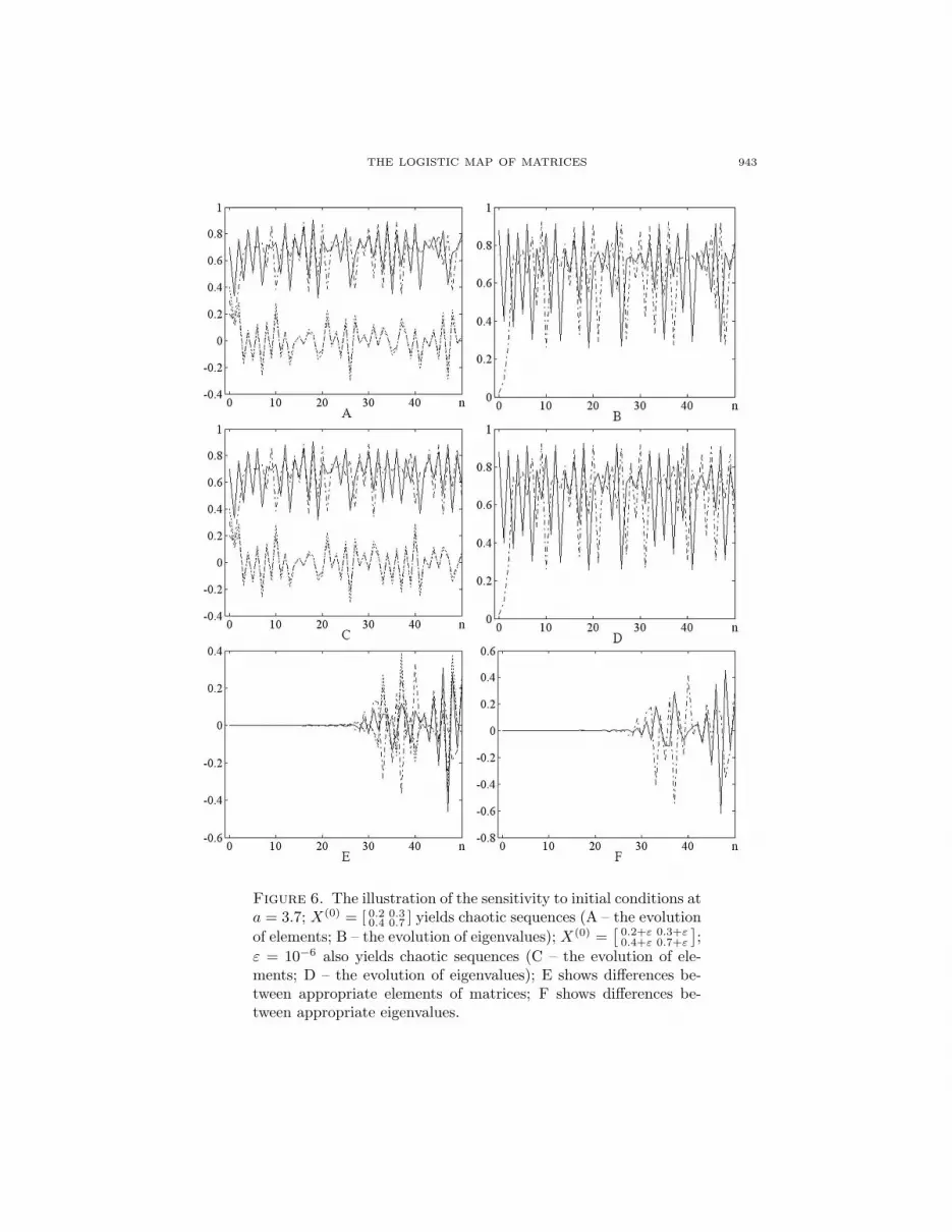
3.2.4. The sensitivity to initial conditions at a = 3.7. It is well known that a scalarlogistic map evolves to chaos after a cascade of period doubling bifurcations. Ata = 3.7 the dynamics of a scalar logistic map is already chaotic. The sensitivity toinitial conditions is one of the characteristic features of the deterministic chaos [2].We will illustrate this feature using the logistic map of matrices.

THE LOGISTIC MAP OF MATRICES 941
Figure 4. The evolution of the logistic map of matrices fromX(0) =
[
1.3 4−0.25 −0.7
]
at a = 3.55 (A and C showing the evolution of
x(n)11 , x
(n)12 , x
(n)21 , x
(n)22 ; B and D showing the evolution of the eigen-
value (a solid line) and the parameter µ(n)0 ) defined by Eq. (30) (a
dashed line). Evolutions in C and D are displayed in the interval180 ≤ n ≤ 200 where n is the iteration number.
The matrix of initial conditions X(0) =
[
0.2 0.30.4 0.7
]
and its eigenvalues yield
chaotic sequences at a = 3.7 (Fig. 6A and Fig. 6B). We construct a perturbed
matrix of initial conditions X(0) =
[
0.2 + ε 0.3 + ε
0.4 + ε 0.7 + ε
]
; ε = 10−6 and follow the
iterative processes (Fig. 6C and Fig. 6D). Differences between values of iteratedelements and iterated eigenvalues of these matrices are shown in Fig. 6E and Fig. 6F.
4. Concluding Remarks. The standard logistic map is extended by replacing thescalar iterative variable by a square matrix of variables. Main dynamical featuresof this iterative map are discussed in detail and illustrated by numerical examples.
One of many applications of the standard logistic map - the encryption of opticalimages - is discussed in the Introduction. The simplest approach comprises 2 iter-ative logistic maps used to generate coordinates of encrypted points (the first onegenerates x-coordinates; the second one - y-coordinates of a sequence of points); 4keys are necessary to initiate the process (2 initial conditions and 2 values of the

942 Z. NAVICKAS, R. SMIDTAITE, A. VAINORAS AND M. RAGULSKIS
Figure 5. The evolution of the logistic map of matrices from
X(0) =[
1.3 4−0.25 −0.7
]
at a = 3.6 (A showing the evolution of x(n)11 ,
x(n)12 , x
(n)21 , x
(n)22 ; B showing the evolution of the eigenvalue (a solid
line) and the parameter µ(n)0 ) defined by Eq. (30) (a dashed line).
parameter a). A single 2-dimensional logistic map of matrices could be used instead.5 keys would be necessary now to initiate the process (4 initial conditions and 1value of the parameter a). But the safety of such an approach and its robustness toa brute force attack would be considerably higher compared to the solution basedon 2 separate standard logistic maps - in many cases initial conditions would leadto a violent divergence or quenching of the iterative process. Of course, detailedanalysis of such an encryption technique is an object of future research.
It appears that the dynamics of the logistic map of matrices of order 2 can beinterpreted exploiting the concept of independent one dimensional logistic maps ofthe eigenvalues of the matrix X0. Two independent scalar logistic maps governthe dynamics of the logistic map of matrices if the matrix of initial conditions isan idempotent matrix. Alternatively, one scalar logistic map and another special(non-logistic) iterative relationship govern the evolution of the system if the matrixof initial conditions is a nilpotent matrix. These results are not trivial at all andexplain complex behavior of this relatively simple dynamical system.
Nevertheless, a number of open questions remain. The first question is aboutthe size of the matrix – what are dynamical properties of the logistic map of squarematrices of order n. The second question is regarding the convergence of the lo-gistic map of matrices. Clocking convergence is a well explored topic in nonlineardynamics of the standard logistic map; the Lyapunov exponent is used to character-ize its stability. The computation of the spectrum of Lyapunov exponents and themeasurement of the speed of convergence towards a stable attractor for the logisticmap of matrices are rather subtle problems. It is not enough to perturb eigenva-lues (consider the nilpotent matrix of initial conditions). The third (and probablythe most important) question is about the potential of applicability of the logisticmap of matrices for similar problems the standard logistic map has been used to –modeling, encryption and prediction of different systems and processes. All thesequestions pose a definite interest and are an object of the future research.
THE LOGISTIC MAP OF MATRICES 943
Figure 6. The illustration of the sensitivity to initial conditions ata = 3.7; X(0) = [ 0.2 0.3
0.4 0.7 ] yields chaotic sequences (A – the evolution
of elements; B – the evolution of eigenvalues); X(0) =[
0.2+ε 0.3+ε0.4+ε 0.7+ε
]
;
ε = 10−6 also yields chaotic sequences (C – the evolution of ele-ments; D – the evolution of eigenvalues); E shows differences be-tween appropriate elements of matrices; F shows differences be-tween appropriate eigenvalues.

944 Z. NAVICKAS, R. SMIDTAITE, A. VAINORAS AND M. RAGULSKIS
Acknowledgements. The study was supported by Agency for International Sci-ence and Technology Development Programs in Lithuania, project ITEA2 08018GUARANTEE.
REFERENCES
[1] R. M. May, Simple mathematical models with very complicated dynamics, Nature, 261 (1976),459–467.
[2] S. H. Strogatz, “Nonlinear Dynamics and Chaos: with applications to physics, biology, chem-istry, and engineering,” Perseus Publishing, Cambridge, 2000.
[3] R. M. B. Young and P. L. Read, Flow transitions resembling bifurcations of the logistic map insimulations of the baroclinic rotating annulus, Physica D: Nonlinear Phenomena, 237 (2008),
2251–2262.[4] A. Dıaz-Mendez, J. V. Marquina-Perez, M. Cruz-Irisson, R. Vazquez-Medina and J. L. Del-
Rıo-Correa, Chaotic noise MOS generator based on logistic map, Microelectron. J., 40 (2009),
638–640.[5] A. Ferretti and N. K. Rahman, A study of coupled logistic map and its applications in chemical
physics, Chem. Phys., 119 (1988), 275–288.[6] A. A. Hnilo, Chaotic (as the logistic map) laser cavity, Opt. Commun., 53 (1985), 194–196.[7] N. Singh and A. Sinha, Optical image encryption using Hartley transform and logistic map,
Opt. Commun., 282 (2009), 1104–1109.
[8] V. Patidar, N. K. Pareek and K. K. Sud, A new substitution–diffusion based image cipherusing chaotic standard and logistic maps, Commun. Nonlinear Sci., 14 (2009), 3056–3075.
[9] T. Nagatani, Vehicular motion through a sequence of traffic lights controlled by logistic map,Phys. Lett. A, 372 (2008), 5887–5890.
[10] J. Miskiewicz and M. Ausloos, A logistic map approach to economic cycles I. The best adaptedcompanies, Physica A: Statistical and Theoretical Physics, 336 (2004), 206–214.
[11] K. P. Harikrishnan and V. M. Nandakumaran, An analogue of the logistic map in two di-mensions, Phys. Lett. A, 142 (1989), 483–489.
[12] M. McCartney, A discrete time car following model and the bi-parameter logistic map, Com-mun. Nonlinear Sci., 14 (2009), 233–243.
[13] M. Rani and R. Agarwal, Generation of fractals from complex logistic map, Chaos Soliton.
Fract., 42 (2009), 447–452.[14] J. J. Dai, A result regarding convergence of random logistic maps, Stat. Probabil. Lett., 47
(2000), 11–14.[15] K. Erguler and M. P. Stumpf, Statistical interpretation of the interplay between noise and
chaos in the stochastic logistic map, Math. Biosci., 216 (2008), 90–99.[16] A. L. Lloyd, The coupled logistic map: a simple model for the effects of spatial heterogeneity
on population dynamics, J. Theor. Biol., 173 (1995), 217–230.[17] L. Xu, G. Zhang, B. Han, L. Zhang, M. F. Li and Y. T. Han, Turing instability for a two-
dimensional logistic coupled map lattice, Phys. Lett. A, 374 (2010), 3447–3450.
[18] R. Bedient and M. Frame, Carrying surfaces for return maps of averaged logistic maps,Comput. Graph., 31 (2007), 887–895.
[19] X. Wang and Q. Liang, Reverse bifurcation and fractal of the compound logistic map, Com-mun. Nonlinear Sci., 13 (2008), 913–927.
[20] D. S. Bernstein, “Matrix Mathematics: Theory, Facts, and Formulas with Application toLinear Systems Theory,” Princeton University Press, 2005.
[21] E. W. Weisstein, Logistic Map, MathWorld - A Wolfram Web Resource, 25 August, 2010.Available from: http://mathworld.wolfram.com/LogisticMap.html.
[22] M. Ragulskis and Z. Navickas, The rank of a sequence as an indicator of chaos in discretenonlinear dynamical systems, Commun. Nonlinear Sci., 16 (2011), 2894–2906.
Received September 2010; revised March 2011.
E-mail address: [email protected]
E-mail address: [email protected] address: [email protected]
E-mail address: [email protected]


