Federal Reserve Bank of MinneapolisResearch Department Staff Report 354

February 2005

The Macroeconomics of Child Labor Regulation∗

Matthias Doepke

UCLAand Federal Reserve Bank of Minneapolis

Fabrizio Zilibotti

Institute for International Economic Studies

ABSTRACT

We develop a positive theory of the adoption of child labor laws. Workers who compete with childrenin the labor market support the introduction of a child labor ban, unless their own working childrenprovide a large fraction of family income. Since child labor income depends on family size, fertilitydecisions lock agents into specific political preferences, and multiple steady states can arise. Theintroduction of child labor laws can be triggered by skill-biased technological change that inducesparents to choose smaller families. The model replicates features of the history of the U.K. in thenineteenth century, when regulations were introduced after a period of rising wage inequality, andcoincided with rapidly declining fertility rates.

∗An earlier version of this paper was presented under the title “Voting with Your Children: A PositiveAnalysis of Child Labor Laws.” The authors thank two anonymous referees, along with Richard Blundell,Moshe Hazan, Narayana Kocherlakota, Dirk Krueger, Robert Lucas, Kiminori Matsuyama, Lee Ohanian,Torsten Persson, Victor Rios-Rull, Richard Rogerson, Jean-Laurent Rosenthal, Ken Sokoloff, Nancy Stokey,Kjetil Storesletten, and seminar participants in several conferences and workshops for helpful comments. Wealso thank Christina Loennblad for editorial assistance. Doepke acknowledges financial support from theNational Science Foundation (grant SES-0217051). Zilibotti acknowledges financial support from the Bankof Sweden and from the Jan Wallander’s and Tom Hedelius’ Research Foundation. Matthias Doepke andFabrizio Zilibotti are, respectively, a research affiliate and a research fellow of the CEPR. Doepke: Departmentof Economics, UCLA, 405 Hilgard Ave, Los Angeles, CA 90095. E-mail address: doepke@econ.ucla.edu.Zilibotti: IIES, Stockholm University, SE 10691 Stockholm, Sweden. E-mail: fabrizio.zilibotti@iies.su.se.The views expressed herein are those of the authors and not necessarily those of the Federal Reserve Bank ofMinneapolis or the Federal Reserve System.

The aim of this paper is to develop a positive theory of child labor regulations (CLR). In thecurrent political debate, the need to regulate child labor is often taken for granted: child laboris portrayed as an evil that ought to be eradicated for humanitarian reasons. From a histori-cal perspective, however, this view of child labor is of a relatively recent origin. In Westerncountries, until the nineteenth century most children worked, and working was generally con-sidered to be beneficial for children. Much more feared than child labor was its opposite,idleness of children, which was thought to lead to disorder, crime, and lack of preparation fora productive working life.1 Opposition to child labor and, ultimately, child labor laws aroseonly after the rise of the factory system. CLR were first introduced in Britain in the nineteenthcentury, and have by now been put into place in all industrialized countries. However, in manydeveloping countries child labor continues to be widespread, CLR are either lacking or weaklyenforced, and public support for the introduction of stringent CLR is low.

These observations raise the question of why, in some countries, attitudes towards child laborshifted over time and led to the adoption of CLR, whereas in other countries child labor con-tinues to be the accepted norm. In this paper, we argue that a society’s views on child labordepend on economic incentives. In our theory, the main motive that leads some people tosupport CLR is the drive to limit competition: unskilled workers compete with children in thelabor market, and therefore stand to gain from higher wages if child labor is restricted. In thissense, we regard CLR as similar to other forms of labor regulation. There is, however, a keyfeature that distinguishes CLR from labor restrictions aimed at, say, union outsiders or foreignworkers: in the case of child labor, the potential competition comes at least partly from insidethe unskilled workers’ families. For this reason, workers’ attitudes regarding CLR depend notonly on the degree to which they compete with children in the labor market, but also on theextent to which their family income relies on child labor.

We analyze the implications of this tradeoff for the political economy of CLR within a dy-namic general equilibrium model. The model economy is populated by overlapping gener-ations of altruistic agents who choose their family size (fertility) and the education of theirchildren, facing a Beckerian quantity-quality tradeoff. The alternative to education is childlabor. We assume that working children compete with unskilled adults in the labor market;2

1Similar arguments were still to be heard in the twentieth century. Opponents of a child labor bill discussedby the state legislature of Georgia in 1900 argued that the “danger to the child was not in work, but in idlenesswhich led to vice and crime.” (Davidson 1939, p. 77). The bill was defeated.

2The fact that child labor and adult labor are substitutable has been documented by Levison, Anker, Ashraf,and Barge (1998) in a case study of India’s carpet making industry, among others. This particular industry isan important example, because carpet making is one of the areas where it is often claimed that children perform

1

more precisely, the participation of children in the labor market increases the wage of skilledworkers and reduces the wage of unskilled workers.

CLR, in the form of a ban on child labor, are introduced when a majority of the adult pop-ulation supports them. When deciding whether to support or oppose CLR, adults weigh twoeffects. First, child labor provides income for parents whose children are working. Second,CLR affect current and future wages. Skilled workers are opposed to CLR, since excludingchildren from the labor market lowers skilled wages. Unskilled workers (the “working class”)face a tradeoff: they weigh the loss of child labor income against the positive effect on adultunskilled wages. This tradeoff can lead to divided opinions on child labor within the workingclass. Young unskilled workers who have not yet chosen fertility have a margin of adjustment:if child labor is banned, they can opt to have smaller families and educate their children. Mostadults, however, have already decided on their number of children in the past, and are stuckwith a given family size. This affects their views on CLR. In particular, the potential loss ofchild-labor income is especially severe for workers who have many children.

We show that the irreversible nature of fertility decisions can lead to multiple politico-economicsteady states. In one steady state, child labor is legal, unskilled workers have many workingchildren, and there is little support for the introduction of CLR. In the other steady state, childlabor is banned, families are small, and CLR enjoy wide support. In each case, the existingpolitical regime induces fertility decisions that lock parents into supporting the status quo. Theexistence of multiple steady states can explain why some developing countries persistently getlocked into equilibria where a large proportion of children work and political support for theintroduction of CLR is weak, while other countries at similar stages of development have strictregulations and a low incidence of child labor. 3

Historically, we observed a change in attitudes towards child labor during the industrial rev-olution, and a growing pressure of the union movement for CLR. How can this change beexplained? According to our theory, the political support for CLR can rise over time if there isan increase in the return to education.4 In an economy where all children of unskilled parents

specialized tasks due to a productivity advantage over adults related to their dexterity and “nimble fingers.”Contrary to these claims, the authors document that adult and child workers perform similar tasks, and are aboutequally productive at them.

3Weiner (1991) provides an example of the political lock-in discussed in this paper. He argues that in Indiathere is very little political pressure there to ban child labor, in spite of the very high incidence of the phenomenonthat is often accompanied by child illiteracy. The resistance against passing and enforcing laws forbidding childlabor is common across politicians with different ideological motivations. Even trade unions, differently fromother countries, are not active on this front, as CLR would be unpopular among poor workers with large families.

4The underlying driving force can be either skill-biased technological change or the partial disappearance of

2

initially work, a steady, gradual increase in the return to schooling eventually induces someof the newly-formed families to have fewer children and send them to school. The proportionof small families keeps increasing until, eventually, a majority of the unskilled workers sup-port CLR. This explanation for the introduction of CLR is consistent with the observation thatCLR were first introduced in Britain (as well as in other Western countries) in the nineteenthcentury after a period of increasing wage inequality. Moreover, the introduction of CLR wasaccompanied by a period of substantial fertility decline and an expansion of education, whichis again consistent with the theory.

A key prediction of the model is that the change in workers’ attitudes to CLR occurs gradually.During the early stages of the transition, the working class does not back CLR unanimously,since families with many children continue to depend on child labor. We would therefore ex-pect to observe conflicting opinions about CLR within the working class before and right afterthe introduction of CLR. Consistent with these predictions, Cunningham (1996) observes thatduring the introduction of the first restrictions in Lancashire “child labor found its strongestand most persistent advocates within the working class, much to the embarrassment of tradeunion leaders.” Similarly, when restrictions on child labor were proposed in the mill villagesin the southern U.S., many workers, particularly those with large families, were opposed pre-cisely because their own children were working: “For an adult male operative whose entirefamily worked in the mill, factory legislation would reduce family income. Such operativestended to oppose child labor laws” (Nardinelli 1990 p. 142).

Our emphasis on the attitudes of unskilled workers is motivated by the observation that inBritain as well as the United States, the trade union movement played a key role in lobbyingfor the introduction of CLR.5 According to Nardinelli (1990), the unions’ actions were drivenmainly by a concern about children competing with unskilled adults in the labor market, andtherefore exerting downward pressure on wages. A natural question to ask is whether thelabor movement had the political strength to impose its desired child labor policy. A thorough

specialized tasks for children. The latter has been argued to be an important feature in the second half of thenineteenth century (see Kirby 1999).

5In Britain, some regulation of child labor was introduced as early as 1802 with the “Factory Health and MoralActs” targeted at apprentices in the cotton and woolen industries. The first effective regulation of the employmentof children was introduced with the Factory Acts of 1833, but the scope of the restriction was limited to the textileindustry. A series of Factory Acts extended the restrictions first to the mines, in 1842, and then to other non-textile industries in the 1860s and 1870s. While humanitarian organizations were a major driving force behindthe first regulations, the labor unions were the main supporters of additional legislation in the second half of thenineteenth century. CLR came later in the U.S., with state regulation being introduced mainly between 1880 and1910, and federal statutes starting to appear in 1910-1920.

3

investigation of the role of political institutions is beyond the scope of our analysis. We note,however, that in spite of the limited voting rights of the poor in the nineteenth century, unionswere able to achieve improvements in labor legislation in favor of their members (such asshorter working hours, safety regulations etc., see Marimon and Zilibotti 2000) through otheractions such as strikes or public campaigns. A complementary argument is that the same forcesthat led unions to campaign for CLR also led other, politically powerful groups to weaken theirresistance against restrictions. We examine this possibility in an extension that analyzes theeffect of skill-biased technological change on capitalists’ views on CLR.

In the next section, we relate our work to the existing literature. Section 2 describes the modeleconomy. In Section 3 we analyze steady states for fixed policies and provide conditions forexistence and uniqueness. Political economy is introduced in Section 4, where we provideconditions for the existence of multiple steady state political equilibria (SSPE). Some empir-ical evidence is also discussed. Section 5 demonstrates how exogenous changes in the skillpremium can trigger the introduction of CLR, and Section 6 considers how capital owners areaffected by this transition. Section 7 concludes.

1 Related Literature

A number of authors have recently developed arguments about why ruling out child labormight be socially desirable. In Basu and Van (1998), CLR can be beneficial because par-ents dislike child labor, but have to send their children to work if their income falls belowa subsistence level. Ruling out child labor can increase the wage sufficiently to push familyincomes above the subsistence level even when children do not work. The model is extendedby Bardhan and Udry (1999) (Ch. 4) to incorporate a fertility decision. They show that multi-ple equilibria with different fertility rates can emerge if preferences are such that poor parentssend their children to work, while richer parents do not. Both models feature static multipleequilibria in the labor market, and CLR can be used to select the “good” equilibrium, rulingout the possibility of a coordination failure. In contrast, our model has a unique equilibriumin the absence of regulation, and the multiplicity of steady states relies on a politico-economicmechanism that is not present in these two papers.

Other reasons why child labor may be inefficient are presented by Baland and Robinson(2000), Dessy and Pallage (2001), and Ranjan (2001), who explore the role of imperfections infinancial markets and additional forms of coordination failure. Krueger and Tjornhom (2004)

4

study, as we do, the distributional conflicts associated with the introduction of CLR. However,they focus on human capital externalities and abstract from fertility choice and endogenouspolicies. Basu (1999) and Brown, Deardorff, and Stern (2003) provide recent overviews of theeconomic literature on child labor.

An important empirical question is whether CLR actually mattered, in the sense of being bind-ing or legally enforced. A number of studies have measured the effects of legal restrictions onlabor supply and the education of children. Peacock (1984) documents that the British FactoryActs of 1833, 1844 and 1847 were actively enforced by inspectors and judges, resulting in alarge number of firms being prosecuted and convicted from 1834 onwards. Galbi (1997) findsthat the number of children employed in English cotton mills fell significantly after the intro-duction of the restrictions in the 1830s. Moving to the U.S., Acemoglu and Angrist (2000)use state-by-state variation in child labor laws to estimate the size of human capital external-ities. Using data from 1920 to 1960, their results suggest that CLR were binding in most ofthis period. Similar findings are reported by Lleras-Muney (2002) and Angrist and Krueger(1991), who show that compulsory schooling laws had a significant effect on schooling inthe twentieth century. Margo and Finegan (1996) focus on earlier data from the 1900 census,and find that the combination of compulsory schooling laws with child labor regulation wasbinding in the sense that it significantly raised school attendance, while compulsory schoolinglaws alone had insignificant effects.6

To the extent that the introduction of CLR in our model coincides with a demographic tran-sition, our analysis is related to a recent macroeconomic literature that examines the causesof fertility decline in the course of development. These include Berdugo and Hazan (2002),Doepke (2004), Galor and Moav (2002), and Galor and Weil (2000). Berdugo and Hazan dis-cuss the effect of an exogenous change in CLR, and show that it may expedite the demographictransition and temporarily foster growth. The ultimate driving force behind the demographictransition in these models is similar to the skill-biased technological change that triggers theintroduction of CLR in our model, although we do not endogenize the source of technologicalprogress. Our theory extends existing theories of demographic change by showing that fertil-ity decline can trigger changes in social policies, which in turn accelerate the progress of thedemographic transition.

Our theory is also related to Galor and Moav (2003), who use a model with financial mar-

6However, Moehling (1999) finds a limited effect of state-by-state differences in minimum age limits from1880 to 1910. In Section 5 we argue that, according to our theory, these results are consistent with binding CLR.

5

ket imperfections to show that an increase in the return to human capital may have inducedcapitalists to support education subsidies for the poor. Since CLR are an instrument to ex-pand education, their theory implies that capitalists might also support CLR. We show in anextension that our theory bears a similar prediction: CLR may benefit capitalists by inducingparents to educate their children and increasing the average skill of the work force. Unlike Ga-lor and Moav, however, we choose to place most of the emphasis on the political preferenceof the working class, since historically unions rather than factory owners were the main activecampaigners for CLR. Nevertheless, the success of the unions’ action may have been possibleonly because of diminished opposition from industrialists. We therefore view explanationsbased on the attitudes of the working class versus the capitalists as complementary.

2 The Model

The model economy is populated by overlapping generations of agents differing in age andskill. There are two skill levels, high and low (h ∈ S, U), and two age groups, young andold. Agents age and die stochastically. Each household consists of one parent and her children,where the number of children depends on the parent’s earlier fertility decisions. Adults die ineach period with probability λ. Whenever a parent dies, her children become adult. As soonas they become adult, agents decide on their number of children. For simplicity, there are onlytwo family sizes, large (grande) and small (petite) (n ∈ G,P, where G and P are integers).

All adults work and supply one unit of (skilled or unskilled) labor. Children may either workor go to school. Working children provide l < 1 units of unskilled labor in each period inwhich they work. Children in school supply no labor, and there is a schooling cost, p, perchild. When they become adult, children who worked in the preceding period become skilledwith probability π0, whereas children who went to school become skilled with probabilityπ1 > π0. For simplicity, we assume that only schooling received in the period before agingdetermines the probability for an agent of becoming skilled. The education choice is denotedby e ∈ 0, 1, where e = 1 corresponds to school and e = 0 to child labor.

In the model economy, all decisions are carried out by adults. Young adults choose once andfor all how many children they want, and they also decide on the education of their children inthe current period. Old adults are locked into the family size that they chose when becomingadult and, consequently, only choose the current education of their children e ∈ 0, 1. Foran adult who has already chosen her number of children, the individual state consists of her

6

skill level and her number of children. Adults are altruistic towards their children, in the sensethat the children’s future (adult) utility enters the parent’s utility function. More precisely,Vnh denotes the utility of an old agent with n children and skill h. Preferences are definedover consumption c, discounted future utility in case of survival, and the average discountedexpected utility of the children in the case of death. The utility of an agent with n children andskill h is then given by

Vnh (Ω) = maxe∈0,1

u (c) + λβz

(πe max

n∈G,PVnS (Ω′) + (1 − πe) max

n∈G,PVnU (Ω′)

)+ (1 − λ) βVnh (Ω′) , (1)

where the maximization is subject to the budget constraint

c+ pne ≤ wh (Ω) + (1 − e)nlwU (Ω) .

Here, u(·) is an increasing and concave function, Ω is the aggregate state of the economy (to bedefined in detail below), Ω′ the state in the following period, wh the wage for skill level h, ande denotes the education decision. Consumption is restricted to be nonnegative. The probabilityof survival is 1 − λ, and future utility is discounted by the factor β. With probability λ, anadult passes away and applies discount factor βz to the children’s utility. The parameter zis allowed to differ from one, so that parents can value their children’s utility more or lessthan they would value their own future utility. For utility to be well-defined, we assume thatβz < 1. With probability πe, which depends on the educational choice e, the offspring willbe skilled. After their skill has been realized in the next period, aging children will have thepossibility of choosing their optimal family size, hence the term maxn∈G,P Vnh (Ω′).

The budget constraint has consumption and, if e = 1, the schooling cost on the expenditureside. The revenue side is made up of the wage income of the adult plus, if e = 0, the wage in-come of the n working children. Note that children do not consume, although this assumptioncould easily relaxed. Once family size has been chosen by a young adult, the only remainingdecision is whether to educate the children or send them to work. In making this decision,parents weigh the higher income and consumption that they can derive in the present whentheir children work against the additional expected utility that their children will enjoy in thefuture if they receive education.

The young adults’ decision problem on fertility n ∈ G,P is simplified by the fact that thenumber of children n does not enter utility directly, since they only care about their children’s

7

average utility. Parents will therefore have a large number of children only if they expect tosend them to work, because in that case having more children results in a higher income. Themodel thus incorporates a particularly stark form of the quantity-quality tradeoff on whichmuch of the economic literature on fertility choice is based. Despite the simple formulationadopted here, the model delivers one of the key implications of quantity-quality fertility mod-els, namely the fact that parents economize on family size when they invest heavily in theeducation of their children. This implication would still hold if parents also had some directconcern about family size, as long as for families who choose education for their children themotive to economize on the education cost is sufficiently strong.

We now move to the production side of the economy. The consumption good is produced witha technology that uses skilled and unskilled labor as inputs. The technology features constantreturns to scale and a decreasing marginal product to each factor. Formally, we can writeoutput per unskilled worker, y, as

y = f (x) ,

where x ≡ XS/XU is the ratio of skilled to unskilled labor supply, and f is an increasing andconcave function. Labor markets are competitive, and wages are equal to the marginal productof each factor:

wS = f ′ (x) , wU = f (x) − f ′ (x) x. (2)

The main role of the production setup is to generate an endogenous skill premium. Notice thatskilled and unskilled labor enter the production technology in an essentially symmetric way.Apart from the fact that education makes a worker more likely to be skilled, the key featurethat distinguishes the two types of labor is that children provide unskilled labor, and thereforeare substitutes for unskilled adult workers. If child labor is restricted, the supply of unskilledlabor falls, and therefore the unskilled wage rises. This wage effect is one of the key motivesthat determines agents’ political preferences regarding CLR (the other motive being potentialchild labor income, which, in turn, depends on the number of children).7

We still need to determine the supply of workers at each skill level. It simplifies the expositionto restrict attention to economies where all children who do not work go to school. This isnecessarily a feature of the equilibrium if the cost of education is sufficiently small. We willdenote by xnh the total number of adults of each type after family size has been determined by

7The unskilled workers would never support child labor laws if child labor and unskilled labor were com-plements instead of substitutes. Interestingly, almost all early child labor laws in Europe and the U.S. explicitlyexcluded agriculture, where it is often argued that adult and child labor are indeed complementary.

8

the young adults, and define

Ω = xPU , xGU , xPS, xGS

as the state vector.8 The child labor supply is equal to

L = l ((1 − eGU) xGU + (1 − eGS)xGS)G+ l ((1 − ePU) xPU + (1 − ePS)xPS)P, (3)

where enh denotes the educational choice of parents of type n, h. Here enh is a group average,and can be between zero and one if positive fractions of parents of type n, h decide to sendtheir children to school and work, respectively. The supply of skilled and unskilled labor isnow given by

XS = xPS + xGS,

XU = xPU + xGU + L.

The state vector Ω follows a Markov process such that

Ω′ = ((1 − λ) · I + λ · Γ (ηU , ηS)) · Ω, (4)

where I is the identity matrix, ηU , ηS denote the proportion of young unskilled and skilledadults, respectively, choosing a small family size, and

Γ (ηU , ηS) ≡⎡⎢⎢⎢⎢⎢⎢⎢⎢⎣

ηU (1 − πe) P ηU (1 − πe)G ηU (1 − πe) P ηU (1 − πe)G

(1 − ηU ) (1 − πe)P (1 − ηU ) (1 − πe)G (1 − ηU ) (1 − πe)P (1 − ηU ) (1 − πe) G

ηSπeP ηSπeG ηSπeP ηSπeG

(1 − ηS)πeP (1 − ηS)πeG (1 − ηS)πeP (1 − ηS) πeG

⎤⎥⎥⎥⎥⎥⎥⎥⎥⎦

is a transition matrix, conditional on the choice of family size of the young adults.9

8Note that young adults choose their family size at the beginning of the period, before anything else happens.After their choice, they become old adults. The state vector summarizes the number of workers of each type afterthis decision has been taken. Thus, formally, this decision is subsumed into the law of motion.

9Consider, for instance, the measure of adult unskilled workers with small families, xPU,t+1. (1 − λ) xPU,t

is the measure of surviving old unskilled adults with small families. The rest consists of young adults:ληU (1 − π1)PxPU,t children of unskilled parents with small families who had given their offspring an edu-

9

We restrict attention to economies where the skilled wage is higher than the unskilled wage. Infact, we impose the stronger requirement that skilled adults always receive higher consumptionthan unskilled adults, even if the former choose a small family and educate their children,whereas the latter choose a large family of working children. To this aim, recall that wagesare given by marginal products and depend on the ratio of skilled to unskilled labor supply.The highest possible ratio of skilled to unskilled labor supply is given by x ≡ π1/ (1 − π1),which yields the lowest possible wage premium. We then formalize the desired restriction bythe following assumption.

Assumption 1f ′(x) − pP > [f(x) − f ′(x)x](1 +Gl)

We are now ready to define an equilibrium for our economy. In the definition, we assumethat the child labor policy is exogenous, i.e., the amount of unskilled labor l that childrencan supply is fixed. It is easy to extend the definition to the case of an exogenous but time-varying policy, by adding a time subscript to l and switching to a sequential definition of anequilibrium. Later on, we will also consider equilibria with an endogenous policy choice.

Definition 1 (Recursive Competitive Equilibrium) An equilibrium consists of functions (of

the state vector Ω) Vnh , enh, wh, and ηh, where n ∈ G,P and h ∈ U, S , and a law of

motion m for the state vector, such that:

• Utilities Vnh satisfy the Bellman equation (1), and education decisions enh attain the

maximum in (1).

• Decisions of young adults are optimal, i.e., for h ∈ U, S:

If ηh(Ω) = 0 : VGh(Ω) ≥ VPh(Ω),

if ηh(Ω) = 1 : VGh(Ω) ≤ VPh(Ω),

if ηh(Ω) ∈ (0, 1) : VGh(Ω) = VPh(Ω),

cation, ληU (1 − π0)GxGU,t children of unskilled parents with large families who had given their offspring noeducation, ληU (1 − π1)PxPS,t children of skilled parents with small families who had given their offspring aneducation, and, finally, ληU (1 − π0)GxGS,t children of skilled parents with large families who had given theiroffspring no education. A similar reasoning applies to the remaining variables.

10

• Wages wh are given by (2).

• For Ω′ = m(Ω), the law of motion m satisfies (4).

We conclude the description of our theoretical framework with a discussion of the model as-sumptions. The modeling strategy is aimed at preserving analytical tractability, while allowinga quantitative exploration of the economic issues analyzed. The model focuses on three dimen-sions of heterogeneity in the population: age, family size, and skills. Heterogeneity in familysize and skills is essential to our theory, since it is along these dimensions that attitudes to CLRdiffer across agents. Age heterogeneity is introduced to distinguish between three states of anindividual: childhood, young adulthood (before fertility is chosen), and old adulthood (afterfertility is chosen). The distinction between young and old adulthood is an essential ingredientas well, since it is the irreversible nature of fertility decisions (i.e., decisions that old adultsmade in the past) that locks agents into particular attitudes to CLR, and ultimately gives rise tomultiple politico-economic steady states. Our specific formulation with stochastic aging waschosen because it generates the three stages of life in a parsimonious way, while abstractingfrom additional life-cycle aspects that are unrelated to the issue at hand. As an alternative, theanalysis could have been cast in a multi-period OLG model with deterministic aging. Such amodel, however, would be much more complicated, since we would have to explicitly distin-guish multiple periods of adulthood. In our stochastic formulation, in contrast, once fertilityis chosen age does not matter, and families are only distinguished by their skill type and theirnumber of children.10 Despite the fact that stochastic aging is not realistic in a literal sense,the model captures the essential distinction between young and old adults.

A number of assumptions concerning the reproduction and upbringing process are motivatedby tractability and by the desire to facilitate the computation of political equilibria. First, weassume that the fertility choice is made in the first period of adulthood. This assumption avoidscomplicated interactions between the age of an individual and the number of children she canhave, which would dramatically increase the dimension of the state space. Second, we assumethat a child ages only when her parent dies. Without this assumption, additional types of agentswould have to be introduced (namely, parents without dependent children and orphans). Theassumption can be justified economically if we interpret age not literally, but as a particular

10We also could have cast the analysis into the framework of a stylized two-period OLG model, where agentshave children in the beginning of the second period. However, in such a model, the entire adult population wouldbe replaced in every period, preventing smooth demographic transitions accompanied by a gradual change ofattitudes towards CLR. Moreover, static multiple self-fulfilling equilibria would be an endemic feature of such aspecification.

11

role in life that children have to fill once their parents pass away. Third, while the structureof the model entails a Beckerian quantity-quality trade-off, our setup differs from the standardaltruistic family model of Becker and Barro (1988) in that, in our model, altruism does notdepend on the number of children, and only two choices each for education and fertility arepossible. Despite the simplifications, the key implications of our model are similar to richermodels with a continuous fertility choice.11 We restrict ourselves to a particularly simplestructure in order to keep the model sufficiently tractable to allow the computation of dynamicpolitical equilibria.

The heterogeneity in skill is introduced in the form of a stochastic return to education (i.e., forsome agents education turns out not to be effective). This is in our view a realistic descriptionof the mapping between education and skill acquisition, which encompasses the more tradi-tional model where education always leads to skill acquisition. Our more general specificationis consistent with steady-state equilibria where all agents educate their children, and allows usto characterize economies where, as in the real world, child labor disappears altogether. Theassumption that skill is solely determined by education received in the final period of child-hood (right before turning adult) also simplifies the analysis, because otherwise additionalstate variables would have to be introduced. The economic interpretation of this assumptionis that skill is subject to depreciation, and therefore renewed education is necessary if skill isnot immediately put to use. The basic mechanism in our model does not depend on this as-sumption, and we conjecture that a model where education takes place over multiple periodswould lead to similar results.

3 Steady States with Fixed Policies

We begin the analysis of the model by examining steady states with exogenous policies. For-mally, we assume child labor to be unrestricted. However, the analysis also comprises steadystates with CLR, since ruling out child labor amounts to setting the parameter l that denotes

11Doepke (2004) considers the choice of education versus child labor in an otherwise standard Barro-Beckermodel with skilled and unskilled workers. As in our model, unskilled workers are more likely to choose childlabor, and fertility is higher conditional on choosing child labor. The main difference is that in Doepke (2004)the fertility differential is endogenous, while it is exogenously fixed in our setup.

One can interpret the large family size in our model as corresponding to a physiological upper bound on thenumber of children an individual can have. In our model, agents who do not educate their children would liketo have as many children as possible, so this would be a corner solution of the fertility choice. The number ofchildren in the small family can instead be related to the cost of rearing and educating children.

12

the amount of labor supplied by children to zero.

A steady state is an equilibrium where the fraction of each type of adult in the population isconstant, and a constant fraction ηU of unskilled parents decide to have small families. DefineNt = xPU,t + xGU,t + xPS,t + xGS,t to be total number of adults. The steady-state fractionsof a given type of adult is given by ξj ≡ xj/N , the vector of these fractions is denoted byΞ = ξPU , ξGU , ξPS, ξGS and the population growth rate is denoted by gt = Nt+1/Nt − 1.Using this notation, in steady state the law of motion (4) specializes to

(1 + g) · Ξ = ((1 − λ) · I + λ · Γ (ηU , ηS)) · Ξ, (5)

1 · Ξ = 1. (6)

Note that, given preferences as defined in (1), in steady state all agents with small familieseducate their children, and all agents with large families choose child labor. Equations (5) and(6) define a system of five linear equations in five unknowns, ξPU , ξGU , ξPS, ξGS and g. Thefractions ηU and ηS have to satisfy the usual equilibrium conditions. In Appendix A.2, weformally establish the following intuitive properties of steady states:

1. If at least some skilled parents choose to have large families, all unskilled parents strictlyprefer the large family size; conversely, if at least some unskilled parents choose smallfamilies, all skilled parents have small families (Lemma 1).

2. In the solution of the system (5)–(6), the average population growth rate falls in thefraction of agents deciding to have small families (Lemma 2).

3. In the solution of the system (5)–(6), the fraction of skilled adults in the populationstrictly increases in both ηU and ηS, i.e., more education implies a larger skilled-to-unskilled ratio (Lemma 3).

The intuition for Lemma 1 is that since skilled adults have a higher income, their utility cost ofproviding education to their children is smaller. Therefore, skilled parents are generally moreinclined towards educating their children than unskilled parents, and educating the childrenimplies choosing the small family size. The lemma allows potential steady states to be indexedby the sum η ≡ ηS + ηU , where η ∈ [0, 2] (recall that ηi is the fraction of adults of skill typei who choose to have small families). Furthermore, Lemma 3 implies the steady state skillpremium is decreasing in η. 12 Five candidate types of steady states can be distinguished:

12Note that whenever η takes on an integer value, i.e., η ∈ 0, 1, 2 all agents in (at least) one group strictly

13

1. All agents educate their children, η = 2.

2. All skilled workers and a positive proportion of the unskilled workers educate theirchildren, η ∈ (1, 2) .

3. All skilled workers and no unskilled workers educate their children, η = 1.

4. A positive proportion of the skilled workers and no unskilled workers educate theirchildren, η ∈ (0, 1) .

5. No agents educate their children, η = 0.

In steady states with either η = 2 or η = 0, all agents behave identically. When η = 2,the wage premium is at its lower bound, all children receive an education, and all familiesare small. Conversely, when η = 0, the wage premium is at its upper bound, all childrenwork, and all families are large. In the steady state with η = 1, at the equilibrium wage, allunskilled parents have large families and make their children work, while skilled workers findit optimal to educate their children. Finally, when η ∈ (1, 2) or η ∈ (0, 1) either the skilled orthe unskilled parents are just indifferent between having large uneducated or small educatedfamilies. The formal conditions for each of the steady states to obtain as an equilibrium areprovided in the appendix.

We now analyze the conditions for the existence and uniqueness of a steady state. In particular,we want to show that under an additional condition that bounds the curvature of utility, aunique steady state exists. This can be done by establishing that, for all adult agents, thedifference between the utilities from having a small educated versus a large uneducated familyis strictly increasing in the wage premium.

The argument can be illustrated with the aid of Figure 1. In the plot, the downward-slopingschedule SS1 represents the negative relationship between the wage premium wS/wU and ηthat follows from Lemma 3. Intuitively, an increase in the relative supply of skills, param-eterized by η, decreases the skill premium because of decreasing marginal returns to skilledlabor in the production function. The piecewise linear schedule EE, in contrast, representsthe optimal steady state educational choice of parents as a function of the wage premium.13

prefer one of the two educational choices. If η ∈ (0, 1) , skilled workers are indifferent, whereas if η ∈ (1, 2) ,unskilled workers are indifferent.

13Educational decisions not only depend on the ratio, but also on the level of both the skill and unskilled wage.In the particular case of CRRA utility and no cost of education (p = 0), the educational choice only depends on

14

In particular, for a range of low wage premia, all agents prefer not to educate their children(η = 0), because the returns to education are too low. For an intermediate range of wagepremia, education is chosen only by skilled agents (η = 1). For a range of high wage premia,all agents prefer education (η = 2). Between these regions, there exist threshold wage premiawS/wU and wS/wU at which, respectively, either skilled workers (η ∈ (0, 1)) or unskilledworkers (η ∈ (1, 2)) are indifferent.

A steady state is characterized by an intersection of the SS1 and EE schedules, because herethe fertility and education choices of the agents are optimal given the wage premium impliedby these choices. If the difference between the utilities from educating or not educating chil-dren is strictly increasing in the wage premium, the thresholdswS/wU and wS/wU are unique,theEE schedule is monotonically increasing, and the SS1 andEE schedules intersect exactlyonce, as in Figure 1. We then obtain a unique steady state.

In general, however, there could be multiple thresholds (i.e., the EE curve could be locallydecreasing), implying the possibility of multiple steady states. While the threshold wS/wU isalways unique, there may be multiple thresholds wS/wU . The source of this potential multi-plicity is the ambivalent effect of an increase of the skill premium on the incentives for un-skilled parents to provide education for their children. On the one hand, a high skill premiumrenders education more attractive, since the utility derived from skilled children increases. Onthe other hand, a high skill premium also implies that unskilled parents earn a lower wage,which increases the utility cost of paying the fixed cost of education. If the curvature of utilityis high, the latter effect may dominate, giving rise to the multiplicity. As an extreme example,consider a case where the unskilled wage falls to a level where the education cost for the chil-dren exceeds the income of the parent. Clearly, in this case the parents will not educate theirchildren, despite the fact that the return to education is high.

The underlying cause for the possibility of multiple steady states in our model is closely relatedto the mechanisms described by Bardhan and Udry (1999), Kremer and Chen (2002), andMoav (2005). In what follows, we want to concentrate on an alternative source of multiplicitythat arises only if CLR are endogenous. In order not to confuse the effects of endogenous CLRwith more traditional sources of multiplicity, we now impose a parameter restriction that rulesout multiple steady states in the absence of endogenous policies. Assumption 2 ensures, under

the ratio, however. While the figure is correct for a given technology, comparative statics (e.g., a change in theskill bias of technology that shifts the SS schedule while not affecting the EE schedule) are legitimate only underCRRA utility and p = 0.

15

CRRA preferences, the uniqueness of the steady state by imposing bounds on the curvature ofutility in the relevant range:

Assumption 2

(1 +Gl)1 − β (1 − λ)

1 − β (1 − λ (1 − z (π1 − π0)))>

u′(wU,2 − pP )

u′ (wU,2(1 +Gl))).

Given this assumption, the uniqueness of steady states in the absence of endogenous CLR canbe established (the proof of the proposition is provided in Appendix A.3.).

Proposition 1 Under Assumption (2) and CRRA preferences, there exists a unique steady

state.

Later on, we will analyze the effects of a shift in the skill bias of the technology on outcomesin a political economy framework. With the uniqueness of steady states established, we canuse Figure 1 to assess the implications of such a change for the steady state given a fixed,exogenous child labor policy. Consider, for example, a Cobb-Douglas technology, where theskill bias can be parameterized by the share of output that is used to compensate skilled labor.Suppose that, initially, the share of skilled labor is low. The corresponding supply schedule isdescribed by the SS0 line, so that η = 0 obtains in the steady state. An increase in the share ofskilled labor shifts the SS schedule to the right (i.e., the ratio of skilled to unskilled wages forany given relative supply of skills increases), while the EE curves remain unaffected. Thus,in the new steady state η will be higher. If the supply schedule shifts to SS1, in the newsteady state all skilled and some unskilled workers educate their children, i.e., η ∈ (1, 2). Fora sufficiently large shift in the skill bias, all workers eventually educate their children (seeschedule SS2).

An increase in skill bias therefore induces more families to educate their children, even ifchild labor continues to be legal. We will see below that if CLR are endogenous, an increasein skill bias can also trigger the introduction of stringent CLR, even at a level of the skill biaswhere, absent regulation, many families would still find it optimal to send their children towork. Before turning to transition of this type, however, we first need to discuss steady stateswith endogenous CLR.

16

4 Steady States with Endogenous Policies

So far, we have established that the model has a unique steady state when parents can choosefreely whether to make their children work. Imposing a child labor ban corresponds to settingl to zero. More generally, we can think of CLR as equivalent to reducing the parameterl: for instance, CLR may impose restrictions on the maximum working hours or forbid theuse of child labor in “dangerous activities” (e.g., mines) where children have a comparativeadvantage, forcing parents to shift child labor to other working activities. Therefore, the resultsof the previous section can be interpreted as showing that there is a unique steady state for anychild labor policy that is exogenously fixed.14

We now want to establish that multiple steady states can exist if CLR are determined endoge-nously. It is easy to construct examples where, for instance, all parents choose large familieswith working children (η = 0) if there are no CLR, but the introduction of CLR moves theeconomy to a steady state equilibrium where all parents choose small families with educatedchildren (η = 2). Assume that the cost of schooling is infinitesimal (p → 0) and that CLRtakes the form of a complete ban, i.e., l = 0. Then, it is immediate that, under CLR, all parentswould choose small families and send their children to school (in Figure 1, theEE line wouldbe horizontal at η = 2). In the absence of CLR, an equilibrium with η = 0 holds if parentsvalue the current consumption that can be derived from making their children work more thanthe additional expected utility their children would obtain through education.15 This conditionis satisfied if the weight z that parents attach to the utility of their children is sufficiently low.Thus, we can construct cases in which all families are small and children go to school if CLRare in place, whereas the steady state features widespread child labor if CLR are lacking.

While CLR was treated as exogenous in this example, the objective of this section is to estab-lish the possibility of multiple steady states with different policies when the choice of policyis endogenous. In other words, in addition to showing that different child labor policies resultin different steady-state behavior, we conversely need to establish that in each steady state thecorresponding policy has the required political support. In order to carry out this analysis, we

14Note that decreasing l moves both the SS and the EE curves to the left in Figure 1. Thus, the wage premiumunambiguously falls, whereas the effect on the educational choice is, in principle, ambiguous.

15The precise condition is given by equation (14) in the appendix. If preferences are logarithmic, for instance,this can be expressed as

ln (1 + Gl) ≥ βλzπ1 − π0

1 − β (1 − λ)ln(

wS0

wU0

), (7)

where the wage premium depends on G, π0 and π1, but not on the discount factor βλz.

17

must specify a political mechanism in the model. We assume that CLR can be irreversiblyintroduced when a majority of adult agents support them. This “referendum” decision is astand-in for more complicated decision processes wherein different groups in society can exertpolitical pressure to introduce restricting laws. A possible interpretation of our reduced-formpolitical mechanism is that unions can impose their will on the issue of CLR. Unions representthe interests of all workers, and decide according to the will of the majority of their members,where the majority is unskilled.16 In reality, of course, the situation is more complex, andthe effectiveness of unions’ actions are mediated by a variety of political institutions. We stillregard it as useful to focus on the interests of unskilled workers, as in our model this is theonly group that could potentially gain from (and which indeed historically supported) CLR.In short, our analysis pins down under which conditions the “working class” supports the in-troduction of CLR. We will also ask the opposite question. Namely, would a majority in aneconomy where CLR have been in effect for a long time prefer that CLR be abandoned?

The main result is that, under certain parameter restrictions, the economy is such that in asteady state with no CLR, a majority of the adults (the skilled and some or all of the unskilled)will be opposed to the introduction of CLR. Conversely, if CLR exist, a majority of the adults(some or all of the unskilled) will prefer to keep the restrictions in place. Thus, each pol-icy leads to a steady state that implies political support for the same policy. The source ofthis multiplicity is that old adults are locked into the family size that they chose previously,which in turn determines their policy preferences. As in the example above, absent CLR un-skilled workers choose large families and make their children work, whereas, if CLR were inplace, they choose small families and educate their children. This feedback between politicaldecisions and family size gives rise to multiple steady states. For simplicity, we will statethe analytical results under the assumption that the child labor policy includes compulsoryschooling.17

Definition 2 (Steady State Political Equilibrium) A steady state political equilibrium

(SSPE) consists of a child labor policy (child labor is either ruled out or not), η ∈ [0, 2]

denoting the distribution of educational choices, utilities VPS, VGS, VPU , VGU of each type

of family, a child labor supply L, constant fractions ξPS, ξGS, ξPU , and ξGU of each type of

family, and a population growth rate g that:

16We could alternatively assume that skilled and unskilled workers are unequally represented within the union.This would not change the qualitative results.

17If the CLR does not include a compulsory schooling provision, the result establishing multiplicity of steadystates still goes through, but requires additional, if natural, assumptions on the production function.

18

• Given the policy, the steady state satisfies all equilibrium conditions in Definition 1.

• A majority of adults obtain higher utility under the current child labor policy than if the

opposite policy were permanently in place.

From the perspective of old unskilled agents, CLR imply both gains (higher wages) and losses(no child labor income). The tradeoff determines whether they support CLR. The key factorleading to multiple SSPE is the lock-in in terms of family size decisions. The loss of childlabor income is larger for families with many children. CLR induce smaller families whosupport CLR, while the absence of CLR induces larger families, who oppose CLR. Assumethat unskilled agents are pivotal (if skilled agents were pivotal, there would be no equilibriumwith CLR). Consider, first, an SSPE where child labor is unrestricted. In this steady state,unskilled families are large, and their children work. If CLR were introduced, there wouldbe an immediate increase in the unskilled wage since children are withdrawn from the laborforce. For the SSPE to be sustained, the gain from this general equilibrium effect must be morethan offset by the loss of child labor income. The fact that families are large and earn a largefraction of their income from child labor makes it more likely that unskilled workers preferthe status quo. Conversely, in a candidate SSPE where child labor is unrestricted, familiesare initially smaller. If CLR were lifted, unskilled families would have little to gain frommaking their children work. Once again, agents would prefer the status quo (CLR in thiscase). Building on this intuition, Proposition 2, proven in Appendix A.3, formally establishesthe existence of multiple SSPE.

Proposition 2 The model parameters can be chosen such that:

• The old unskilled are the majority.

• In the absence of CLR, the steady state features η < 2.

• Both CLR and no CLR are SSPE.

We now illustrate the theoretical results obtained so far by analyzing steady states in a pa-rameterized version of our economy. Table 1 displays the parameter values used. Preferencesare CRRA with risk-aversion parameter σ = 0.5. The production function is of the constant-elasticity-of-substitution form

Y = [αXκS + (1 − α)Xκ

U ]1κ .

19

The fertility values for small and large families are P = 1 and G = 3. A family of twowould therefore have two children if they prefer education, or six children if they opt for childlabor. This fertility differential approximates the fertility differential between mothers in thelowest and highest income quintiles in countries with widespread child labor, such as Brazil orMexico (see Kremer and Chen 2002). The choice for λ implies that adults on average live for62

3periods. Assuming that a model period corresponds to six years, people survive 40 years

on average after becoming adults. The probabilities π0 = 0.05 and π1 = 0.4 of becomingskilled are chosen so that the fractions of skilled agents in a pre-industrial (i.e., where nochildren receive formal education) and post-industrial (i.e., where all children receive formaleducation) societies are, respectively, 5 percent and 40 percent. The choices of λ, π0, andπ1 jointly imply that the old unskilled always constitute the majority of the population. β ischosen so that it implies a rate of time preference that would generate an annual interest rate of4 percent per year (if assets could be traded), which is the standard basis for calibrating β in theRBC literature. The choice l = 0.1 for the supply of child labor implies that a large family withworking children derives about a quarter of family income from children, which is in line withevidence from Britain in the period of early industrialization (Horrell and Humphries 1995)and recent data from developing countries. The elasticity parameter κ = 0.5 sets the elasticityof substitution half way between the Cobb-Douglas and the linear production technology. Theweight α of skilled labor in the production function is left unspecified for now. We will use αto parameterize the skill premium and compute outcomes for a variety of α.

We start by determining which steady states and SSPE exist for different values of α. Recallfrom Section 3 that as long as Assumption 2 is satisfied, there is a unique steady state in theeconomy without CLR. Figure 2 displays the steady state η as a function of α. For low α, theskill premium is low. Consequently, education is not very attractive, and there is a range of αwhere all parents prefer child labor (η = 0). As the skill premium rises, we reach a thresholdfor α at which a fraction of skilled adults educates their children (η ∈ (0, 1)), and ultimatelyall skilled parents choose education (η = 1). For even higher α, there is a wide region in whichunskilled parents are indifferent between education and child labor (η ∈ (1, 2)). Throughoutthis region, higher α are offset by a higher supply of skilled labor, which keeps the unskilledparents indifferent. Ultimately, all parents educate their children (η = 2 ).

Figure 3 considers the model with endogenous policy choice, and shows which SSPE exist asa function of α. For low values of α, the only SSPE is no CLR. In other words, the return toeducation is so low that even a population of adults all of whom have small families wouldprefer to abandon CLR. For an intermediate range of α, there are multiple SSPE: both CLR

20

and no CLR are steady states supported by a majority of the population. In the range ofmultiplicity, in the absence of CLR at least a fraction of unskilled agents would choose childlabor and large families. However, if CLR are already in place, unskilled parents are lockedinto having small families, and therefore prefer to keep CLR. As the wage premium increases,we enter a region where CLR is the only SSPE. In this region, even unskilled parents with largefamilies prefer to introduce CLR. The immediate income loss after the introduction of CLR ismade up for by higher unskilled wages in the present (because other parents’ children can nolonger work) and in the future (which they care about because they care for their children).

To establish that the multiplicity result depends on endogenous fertility choice, we also com-puted outcomes without fertility differentials by setting P = G = 1, i.e., families of workingand educated children are of the same size. We still find that, for low α’s, no CLR is an SSPE,and for high α’s CLR is an SSPE. However, there is no overlap, i.e., in no region can bothpolicies be supported in steady state, since the policies no longer lock agents into differentfertility choices. In fact, there is a region where neither policy is an SSPE. The reason for thenon-existence of SSPE for some α is the endogenous skill premium. If CLR are in place, thesupply of skilled labor is high, and the skill premium is low. The low skill premium makeschild labor attractive relative to education, so that a majority are in favor of abandoning CLR.If there are no restrictions, however, the supply of skilled labor is low and the skill premiumis high. This makes education more attractive, and increases the gain from removing otherparents’ children from the labor market. As a consequence, a majority are in favor of intro-ducing CLR. The endogenous skill premium therefore works against multiplicity of steadystates. In the model with endogenous fertility, this effect is overcome since parents choosea different family size in each political regime, which induces them to favor the status quo.Fertility choice provides a powerful lock-in effect, both because fertility decisions are irre-versible, and because children are important economically: households with working childrenderive a substantial share of their income from child labor, whereas households with childrenin school need to spend a lot on the children’s education.

We conclude this section with a brief discussion of the empirical implications of our analysis.According to our theory, countries can get locked into different political steady states, whereone SSPE features high fertility, high incidence of child labor, and little political support forthe introduction of CLR, whereas another SSPE features low fertility, low (or no) child labor,and widespread support for CLR. In today’s developing countries, we observe large cross-country differences in child labor rates, even among countries that are at similar levels ofincome per capita. If our mechanism were an important factor behind cross-country variation

21

in child labor rates, we would expect to find a positive correlation between fertility and childlabor rates, even after controlling for other variables that might affect child labor or fertility.To examine the empirical validity of this prediction, we regressed child labor rates on fertilityrates for a panel of 125 countries from 1960 to 1990, with observations at ten-year intervals,controlling for time dummies, log(GDP ), log(GDP ) squared, the share of agriculture inemployment, and the share of agriculture in employment squared.18 The coefficient on thefertility rate is positive and highly significant. The point estimate is 1.3, and the White standarderror is 0.29 (the R2 of the regression is 0.89).19 The estimate implies that a one standarddeviation increase in fertility is associated with an increase in the child labor rate of 2.5 percent(the child labor rate varies in the sample between 0 and 59 percent with a standard deviation of15 percent). If we add a measure of income inequality (Gini coefficient), the point estimate ofthe effect of inequality on child labor is positive, but statistically insignificant. If, in addition,we include country fixed-effects, the coefficient on fertility becomes smaller (point estimateof 0.41, with a standard error of 0.20), but remains statistically significant.

The evidence of a positive correlation between fertility and child labor incidence across coun-tries is only a preliminary step in providing empirical support for our theory. Ideally, onewould like to find additional evidence based on cross-country comparisons of direct measuresof CLR. This is far from straightforward since regulations (and their enforcement) are difficultto measure and compare across countries. Given this difficulty, a more thorough empiricalinvestigation is left to future research.

18The child labor rate is defined as the percentage of children aged 10–14 who are economically active. Thetotal fertility rate is defined as the sum of age-specific fertility rates, i.e., the number of births divided by thenumber of women of a given age. The fertility rate and the share of agriculture in employment are from theWorld Bank Development Indicators, Ginis are from the Deininger-Squire data set, GDP per capita is from thePenn World Tables, and child labor rates are from the ILO. We control for the share of agriculture because it iswell known that child labor is more widespread in the agricultural sector. We ignore endogeneity problems; theregression is simply meant to document correlation between the variables of interest.

19Similar results hold if one runs four separate cross-country regressions. The coefficient on fertility is alwayspositive and highly significant, except in 1960 when it is positive but not significant. Including measures ofdemocracy does not change the results. An additional observation that is consistent with our lock-in predictionis that cross-country differences in child labor are highly persistent over time. To demonstrate this, we sortedcountries into quintiles according to the size of the residual in the decade-by-decade child-labor regressions.Among the 20 percent of countries with the highest child labor rate relative to the predicted value, on average 71percent are still in the highest quintile 10 years later. Over the entire period 1960 to 1990, we find that 85 percentof the countries in the highest quintile in 1960 are still in the top two quintiles in 1990.

22

5 Transitions: The Introduction of CLR

So far, we have shown that the interaction of fertility choice and political preferences can leadto a lock-in effect, resulting in multiple SSPE, either with child labor and high fertility or nochild labor and low fertility. This feature of the model can explain why there is a great deal ofvariation in the incidence of child labor around the world, even when controlling for incomeper capita. However, we also need to explain why many countries have adopted child laborbans over the last two centuries, starting from a situation where child labor was common allover the world. In our model, a transition from no CLR to CLR is possible if technologicalchange increases the skill premium, and therefore the return to education. If the increase inthe return to education is large, even some unskilled adults will prefer to have small familiesand educate their children, which ultimately creates a majority in favor of the introduction ofCLR.

This explanation of the introduction of CLR is consistent with the evidence on the evolutionof the skill premium in the U.K. before the introduction of CLR. Figure 4 shows that the ratioof skilled to unskilled wages increased sharply at the beginning of the nineteenth century.20

The skill premium reached a peak in 1850, declined subsequently, and by 1910 it had returnedto its 1820 level. To show how an increase of the skill premium can trigger the introduction ofCLR in our model, we computed a transition path for an economy that starts out in the steadystate without CLR, and then experiences a phase of skill-biased technological change (whichcan be parameterized as an increase in the technology parameter α). We chose the specifictransition path such that in the steady state without CLR, the ratio of skilled to unskilledwages in the model matches the observed value of 2.5 in the U.K. around 1820 (see Figure 4).This is achieved by setting the initial α to 0.33 (apart from α, the model is parameterized asin Section 4, see Table 1). The endpoint of the transition was chosen such that in the steadystate with CLR, the wage ratio matches 2.5 as well, as in the data around 1910. This implies afinal value for α of 0.65. Notice that in the new steady state with CLR there is a higher supplyof skilled labor, so that α has to be higher than at the beginning of the transition to generatethe same skill premium. In the computed transition path, α is at 0.33 until period 2, and thenincreases linearly until the maximum of 0.65 is reached in period 9. Given that one model

20The skill-premium data, from Williamson 1985, is computed as the ratio of the wages in twelve skilled andsix unskilled professions, weighted by employment shares. This data source is criticized by Feinstein (1988),who presents alternative estimates indicating a smaller hump in skill premia. Even a flatter profile of the skillpremium, however, would indicate a significant increase in the demand for skills, given the simultaneous increasein their supply associated with rising education in the labor force.

23

period is interpreted as lasting six years, the simulations represent a phase of skill-biasedtechnological change that stretches out over a little more than 40 years.

Generally, the problem of computing transitions paths with an endogenous policy choice iscomplicated. Agents’ decisions depend on the entire path of expected future policies. Futurepolicies therefore partly determine the evolution of the state vector of the economy which, inturn, affects the political preferences over these same policies. In principle, this interdepen-dence can lead to multiple equilibria (not just multiplicity of steady states), or the nonexistenceof equilibria. It turns out, however, that unique results are obtained for the calibrated versionof our model. To limit the number of time paths of future policies, we assume that once CLRare introduced, they cannot be revoked. 21 Future policies can therefore be indexed by theperiod when CLR are introduced.

The conditions for the introduction of CLR to occur in a given period T can therefore bechecked as follows. We assume that the economy starts in the steady state corresponding tothe initial value of α. First, we compute private decisions and the evolution of the state vectorunder the assumption that CLR are indeed introduced at time T . In period T , we check whethera majority prefer the introduction of CLR to the alternative. The relevant alternative here isnot to never introduce CLR, but to expect their introduction at T + 1 (the skill premium andtherefore the incentive to introduce CLR increases over time, therefore if T is the equilibriumswitching time, a fortiori a majority in favor of the introduction of CLR also exists at timeT + 1.). We also must check that CLR are not introduced before T . Once more, because theincentive to introduce CLR increases over time, it is sufficient to check that given the path forthe state variable resulting from expecting the switch at T , there is still a majority opposedto introducing CLR at time T − 1. In summary, for T to be an equilibrium switching time,conditional on agents expecting CLR to be introduced at time T, a majority must oppose CLRat time T − 1, and a majority must prefer CLR at time T . Since the evolution of the statevector depends on the expected policies, there could be, in principle, multiple or none suchswitching times, but in our parameterization there is a unique switching time.

In the computed transition path, a majority continues to oppose the introduction of CLR inthe first periods of the increasing skill premium. Beginning in period 5, however, all youngunskilled adults start to choose education and small families, in response to the increasing skillpremium and the expected future introduction of CLR. Old unskilled families are stuck with

21We conjecture that in our specific application the results would not change if we allowed CLR to be revokablein later periods, because we focus on an episode where the skill premium is increasing over time, which togetherwith the lock-in effect of endogenous fertility choice tends to increase support for CLR over time.

24

many children and therefore continue to choose child labor. In periods 5 and 6, the numberof unskilled parents with small families is still too small to successfully lobby for a policychange, but in period 7, unskilled families with a small number of children form the majorityof the population and decide to introduce CLR.

The solid line in Figure 5 displays the evolution of the skill premium during the transitionwith endogenous policy choice. Initially, the skill premium increases due to an increasing α.Once CLR are introduced and children are withdrawn from the labor market the skill premiumdrops, however, since the increase in α is offset by the smaller supply of unskilled labor. Afterα stops increasing, the skill premium declines further, as the number of skilled workers con-tinues to increase. The introduction of CLR also leads to a sharp decline in population growth(Figure 6). Notice, however, that the decline in population growth starts before CLR are intro-duced, because young unskilled parents start to have small families already in period 5. Theswitch in the decisions of young unskilled parents also triggers an immediate decline in thesupply of child labor, as shown by Figure 7. Thus, child labor declines even before CLR areintroduced.

The dashed lines in Figures 5 to 7 show the outcomes that would have occurred without theendogenous introduction of CLR, i.e., under the assumption that child labor continues to belegal throughout. Even without the introduction of CLR, the increase in the skill premiumultimately induces some parents to educate their children, resulting in temporarily lower pop-ulation growth, less child labor, and a reversal of the increase in inequality. At the same time,the decline in child labor is only a fraction of what is achieved with the introduction of CLR,and inequality remains much higher. Thus, in the model, neither technological change norCLR are solely responsible for the decline in child labor; rather, both explanations are com-plementary. Given that the child labor rate levels out at 80 percent in the absence of CLR, inour example the introduction of CLR is responsible for four-fifth of the overall decline in childlabor.

The simulations reproduce key features of the data. First, both the simulation and the data ex-hibit a hump-shape profile in the skill premium (see Figure 4). Second the model predicts thatfertility rates start declining before the introduction of CLR. This timing is also featured bythe data in the history of the introduction of CLR in Britain. The first major child labor restric-tions (the “Factory Acts”) were put into place in 1833 and 1842, and were extended to othernon-textile industries in the 1860s and 1870s.22 The total fertility rate (see Figure 8) peaked

22The initial Factory Acts, however, only applied to some industries (textiles and mining), and Nardinelli

25

around 1820, then started declining before the introduction of the Factory Acts. Then, a sec-ond, more pronounced decline in fertility is observed after 1880, which continued throughoutthe first quarter of the twentieth century. Figure 9 shows the corresponding decline in childlabor rates (the fraction of 10 to 14 year-olds who were economically active) and increase inschooling rates (the fraction of children aged 5–14 at school). The data are consistent withthe predictions that fertility starts falling before CLR are introduced, and that CLR cause anacceleration in the fertility decline.23

A similar pattern can be observed in other European countries such as France, Germany andItaly. In these countries, as in Britain, CLR were introduced in the second half of the nineteenthcentury.24 Moreover, the introduction of CLR is more closely related to changes in the fertilitybehavior than to structural characteristics of these economies. In Germany and Italy, CLRwere introduced soon after the beginning of the demographic transition, and were followed bylarge further reductions in fertility (in France, however, the demographic transition had startedsubstantially earlier). At the time of the introduction of CLR, England was an industrializedcountry, with the share of agriculture near ten percent, while in Italy, for instance, well overhalf of employment was still accounted for by agriculture. The differences in living standardswere also large.25

(1980) argues that while the laws effectively restricted the employment of young children in these industries, theeffect on overall child labor was short lived. The Factory Acts were extended to other non-textile industries in the1860s and 1870s. The introduction of compulsory schooling in 1880 put an additional constraint on child labor.Compulsion was effectively enforced: in the 1880s, close to 100,000 cases of truancy were prosecuted every year(see Cunningham 1996), which made truancy the second-most popular offense in terms of cases brought beforethe courts (drunkenness being the first).

23However, the transition is sharper and more rapid in the simulation than in the data. This discrepancy may bedue to the fact that in the simulation CLR are introduced and perfectly enforced instantaneously, whereas, in thedata, this happens progressively. Also, our model does not allow for combinations of schooling with part-timework, while this practice was relatively widespread at the time.

24Both Germany and Italy introduced pervasive regulation after unification. Prussia had a child labor law in1839, which was extended to the whole German Empire after 1871. It was not until 1878, however, that theminimum age in factories was raised to 12, and enforcement became active (see Nardinelli 1990). In Italy, thefirst child labor law was passed in Lombardy in 1843, before unification. Education became compulsory in 1859,but initially there was little enforcement of this law. A national child labor law was passed in 1873. In France,a law passed in 1841 mandated a minimum age of eight for employment and specified a maximum workday ofeight hours for children aged eight to twelve. In addition, working children under the age of twelve were alsorequired to attend school. The law applied only to firms with at least 20 workers, however, and no effectiveprovisions for enforcement were made (Weissbach 1989). In 1874, a law was passed that applied to all firms,set the minimum age to twelve, with minimum schooling conditions for workers under the age of 15. In 1892the minimum age for employment was raised to 13. Inequality trends were also similar across Western countriesin the nineteenth century, see Williamson (1985) on Britain, Williamson and Lindert (1980) on the U.S., andBrenner, Kaelble, and Thomas (1991) on Belgium, Germany, and Sweden.

25According to Maddison (1995), in 1890 GDP per capita in Italy was only 40 percent as high as in the U.K.,

26

In the U.S., birth rates and total fertility rates were falling from the beginning of the nineteenthcentury. However, the overall numbers mask substantial variation across states and regions.Since until about 1910 all child labor restrictions were state laws, this variation can be relatedto political developments. Most states introduced laws mandating a minimum age for employ-ment in the period from 1880 to 1920. In 1880, only seven states had such laws; by 1910, 43states did. The first states to introduce child labor restrictions were also the first to experiencesubstantial fertility decline. Consider the comparison of the eight states which introduced aminimum age of employment of 14 before 1900 and the 14 states which introduced this limitonly after 1910.26 In the middle of the nineteenth century, birth rates were slightly higher inthe group of early adopters (in 1860, the birth rate was 30 in the early group and 29 in thelate group). However, after 1870 fertility decline progressed faster in the states which adoptedchild labor laws early. By 1890, the average birth rate had fallen to 25 in the early group, butwas still at 30 in the late group. This birth-rate differential persisted throughout the first partof the twentieth century; in 1928, the difference was still 19 to 24.

Our results also suggest a reason why econometric studies which find that child labor lawsonly have a relatively small effect on the supply of child labor may be misleading. Moehling(1999), for example, uses state-by-state variation in the introduction of CLR in the U.S. toestimate the effects of regulations, employing a “difference-in-difference” estimator. In ourmodel, child labor declines even before CLR are introduced, since young families start tohave small families of educated children in response to a higher return on education. Thisprediction is a robust implication of the theory, since a decline in the dependence of unskilledfamilies on child labor income is exactly what is required to create a constituency in favor ofCLR. The relative speed of the decline in child labor before and after the introduction of re-strictions depends on average family size, the number of young families, and the enforcementof CLR. To a large extent, CLR work indirectly by reducing family size and changing fami-lies’ education decisions, as opposed to directly removing children from the labor market whowould otherwise have worked. It is possible that from an econometrician’s perspective, themeasured impact of the legislation appears to be small (i.e., there is a small or no differencein the decline of child labor before and after the introduction of CLR, either within or across

and lower than GDP per capita in the U.K. in 1820. Relative to the U.K., in 1890 France and Germany were at57 and 62 percent, respectively.

26The states in the first group are Illinois, Indiana, Massachusetts, Michigan, Minnesota, Missouri, New York,and Wisconsin. The group of late adopters is made up of Alabama, Delaware, Florida, Georgia, Mississippi, NewHampshire, New Mexico, North Carolina, South Carolina, Texas, Utah, Vermont, Virginia, and West Virginia.Birth rate figures are from the U.S. Census.

27

states). The true effect of CLR would be larger than this empirical measure, since it is notgenerally true that the child labor rate would have continued to decrease without a law. In ourexample, if no CLR are introduced, child labor rates remain at 60 to 80 percent throughout.The restrictions therefore account for the major part of the ultimate decline in child labor. Adifference-in-difference estimator would have compared the decline in child labor before andafter the introduction of the law, which would suggest, misleadingly, a much smaller effect ofthe legislation.

6 Would Capitalists Support CLR?

A possible objection to the analysis of the previous section is that in the nineteenth century,unskilled workers may not have had the political power to impose CLR over the resistanceof more wealthy and politically powerful groups. As discussed earlier, we believe that theunions’ political activism may have played an important role, despite the lack of universalsuffrage. In this section, we explore the complementary argument that other groups may havealso benefited from the introduction of CLR. In particular, our analysis has not yet consideredthe political preferences of factory owners (capitalists). As pointed out by Galor and Moav(2003), if capital is complementary to skilled labor, it may be in the capitalists’ interest tosupport, and even finance, policies that foster human capital accumulation. We now show thatthis possibility arises naturally in an extension of our model.

Consider the following generalization of the production technology:

Y = Kθ [αXκS + (1 − α)Xκ

U ]1−θ

κ .

This technology implies that, if markets are competitive, the owners of capital K appropriatea constant share θ of the total output. We assume that there is a constant stock of capital,which is owned by a separate class of agents. This feature is for simplicity; regardless ofthe amount of capital, the total income of capitalists depends on the composite labor input[αXκ

S + (1 − α)XκU ] . Therefore, the political preferences of capitalists would be similar if

capital could be accumulated and responded to changes in its productivity.

We consider the following experiment. We analyze the same transition discussed above to-wards an expected date at which CLR are introduced. We then calculate the share of output ac-cruing to the capitalists conditional on the alternative assumptions that CLR are either passed

28

or rejected. This comparison would determine the capitalists’ choice if they had the power toveto CLR.

As Figure 10 shows, conditional on CLR (solid line) there is an initial drop (in period 7) inthe capitalists’ income after the introduction of CLR. This is due to children of large familiesbeing forced out of the labor force. However, this is followed by a recovery triggered byincreasing education and a larger proportion of skilled workers in the population. In contrast,under no CLR (dashed line) there is no initial drop in output, and the skill ratio does not grow.Despite the increase in education under CLR, from period 11 onwards there is a clear outputdivergence in favor of the economy without CLR. This is due to the fact that fertility is higherin the long-run under no CLR. Although output per worker is higher in the economy withCLR, total output is smaller. Since capitalists appropriate a constant share of total output,their interests are harmed by the introduction of CLR in this example.

The outcome would be different if the increase in the skill bias of the technology were suffi-ciently large to push the economy to a steady state where all families educate their childreneven when CLR are never introduced. In this case, long-run population growth does not de-pend on the policy, and the income of the capitalists depends only on the relative supply ofthe two skills. To illustrate this case, Figure 11 shows the capitalists’ income under the twopolicies if α increases to 0.85 instead of 0.65, resulting in a steady state where all families aresmall. A similar effect could be reached by a policy that subsidizes education. As before, theintroduction of CLR initially harms the capitalists (solid line) due to the declining supply ofunskilled labor. From the first period after the reform onwards, however, the capitalists gainfrom CLR due to the higher supply of skilled labor. In the steady state, the two policies yieldthe same income for the capitalists. Clearly, the capitalists would prefer CLR in this example,unless they are very impatient.

The analysis of this section could be further extended by distinguishing different types of cap-italists who operate different technologies. From a historical perspective, the most importantdistinction is the one between land owners and factory owners, who were both politically in-fluential in the period of the introduction of CLR in Britain (as evidenced by the debates onthe Corn Laws and the Poor Laws). If we assume that land is complementary to child la-bor, whereas skill-biased technological change leads to complementarity between industrialcapital and skilled labor, a conflict of interest between landowners and factory owners arises.The support for CLR would therefore also depend on the relative political power of these twogroups. It is still the case, however, that skill-biased technological change would increase the

29

likelihood of the introduction of CLR.

In summary, this section demonstrates that the same type of technological change that leadsunskilled workers to support CLR may also shift capitalists’ views in favor of CLR. Histor-ically, we observe little evidence that capitalists actively supported the introduction of CLR,which is why we put most emphasis on the attitudes of the working class. Nevertheless, evenif capitalists did not literally gain from restrictions, skill-biased technical change could makecapitalists less adamant in their opposition. Changing views of the working class and thecapitalists are therefore complementary explanations for the introduction of CLR.

7 Conclusions

The aim of this paper was to shed light on the political economy of child labor laws. The keynovelty of our model is an interaction between demographic variables (the number of childrenper family) and political preferences. While it may seem obvious that whether or not a workerhas working children will influence opinions about child labor laws, our model shows thatthis fact leads to surprising implications. Since children are long-lived, fertility decisions canlock agents into specific political preferences. Multiple steady states can then arise, becauseCLR induce individual behavior which, in turn, increases the support for maintaining therestrictions. This “lock-in” effect can explain why we observe large variations in the incidenceof child labor and child labor laws across countries of similar income levels.

To account for the initial introduction of child labor laws, we extend the model to allow for achange in the economy which shifts political preferences in favor of CLR. Here, our preferredexplanation is technological progress which raises the return to skilled labor, thereby providingincentives for parents to choose small families and educate their children even while childlabor continues to be legal. We concentrate on skill-biased technological change because thisexplanation is consistent with evidence on trends in wage inequality in major industrializingcountries in the nineteenth century. However, other factors can trigger a similar transition,e.g., a fall in the relative productivity of child labor, or exogenous factors affecting fertilityrates.

Our theory can provide some guidance in the debate on the introduction of child labor laws indeveloping countries. The model predicts that even in countries where the majority currentlyopposes the introduction of CLR, the constituency in favor of these laws may increase over

30

time once the restrictions are in place. However, for this to be true two conditions have tobe met. First, if the cost of schooling is too high, poor parents may decide not to send theirchildren to school even if CLR are in place. Second, if despite the introduction of CLRchildren continue to be productive in household or marginal activities, the policy may failto reduce fertility and induce the switch from quantity to quality. Everyone, including thechildren, might in this case be worse off after CLR have been introduced. CLR are morelikely to be successful, and enjoy increasing political support, if they are accompanied bypolicies that reduce the cost or increase the accessibility of schools.

31

A Mathematical Appendix

A.1 Characterization of Steady States

In this section, we develop conditions under which each of the five types of steady statesdescribed in Section 3 obtains as an equilibrium. Each steady state prescribes which educationand fertility decisions are optimal for each type of parent. The conditions for a candidatesteady state to be an equilibrium can be checked by computing the steady-state utility thatan agent receives under the prescribed decisions, and then verifying whether the agent couldgain by making other than the prescribed choices. To simplify notation, we introduce averagediscounted probabilities, where ΠeU ,eS

h→h′ denotes the average discounted probability for an agentwho is currently of skill level h to have descendants of skill level h′. The superscripts denotewhether the skilled and unskilled parents educate their children. These probabilities are givenby the following expressions:

Π1,1U→S =

βzλπ1

1 − β(1 − λ), Π0,1

U→S =λβzπ0

(1 − β (1 − λ (1 − z (π1 − π0)))),

Π0,0S→U =

λβz (1 − π0)

(1 − β (1 − λ)), Π0,1

S→U =λβz(1 − π1)

(1 − β (1 − λ (1 − z (π1 − π0)))).

We start with the steady state in which all workers educate their children, η = 2. In this steadystate, xGU = xGS = 0 and ePU = ePS = 1. Hence, L = 0. The necessary and sufficientcondition for this steady state to be an equilibrium is that, given wages, the unskilled adultsfind it optimal to educate their children. By Lemma 1, this implies, a fortiori, that the skilledadults also choose to educate their children. The steady state utility of unskilled adults in thesteady state where all children receive education is given by:

VPU,2 = u (wU,2 − pP ) + λβz (π1VPS,2 + (1 − π1)VPU,2) + (1 − λ)βVPU,2,

where Vnh,η denotes the steady-state utility of an agent of family size n and skill h conditionalon η. A similar notation is used for wages. This equation can be solved and expressed as:

VPU,2 =u(wU,2 − pP ) − Π1,1

U→S[u (wU,2 − pP ) − u (wS,2 − pP )]

1 − β(1 − λ(1 − z)). (8)

For the candidate steady state to be sustained, deviations must be unprofitable, i.e., no agentcan increase her utility by choosing a large family and making her children work. Consideran unskilled adult who deviates and chooses a large family and child labor. If this deviationis profitable for the parent, it would also be profitable for a potential unskilled child. Wetherefore check a continued deviation of an entire dynasty, i.e., we assume that the parent and

32

all future unskilled descendants choose a large family and child labor. The resulting utility is:

VGU,2 =u(wU,2(1 +Gl)) − Π0,1

U→S[u(wU,2(1 +Gl)) − u (wS,2 − pP )]

1 − β(1 − λ(1 − z)).

Comparing VPU,2 and VGU,2, we find that the deviation is not profitable as long as

u(wU,2(1 +Gl)) − u(wU,2 − pP ) ≤ Π0,1U→S [u(wU,2(1 +Gl)) − u (wS,2 − pP )]

− Π1,1U→S [u (wU,2 − pP ) − u(wS,2 − pP )] . (9)

Note that, since we consider individual deviations, we have held wages constant at the steadystate level. Inequality (9) is a necessary and sufficient condition for a steady state equilibriumwhere all agents educate their children (η = 2) to be sustained.

The steady state where all skilled and some unskilled workers educate their children exists if,for some η ∈ (1, 2), the skilled and unskilled wages are such that VGU,η = VPU,η, i.e.,

u (wU,η (1 +Gl)) − u(wU,η − pP ) = Π0,1U→S [u (wU,η (1 +Gl)) − u (wS,η − pP )]

− Π1,1U→S [u (wU,η − pP ) − u (wS,η − pP )] . (10)

Recall that, by Lemma 1, VGU,η = VPU,η implies that VGS,η < VPS,η. Hence, if the conditionis satisfied, skilled adults strictly prefer small families with educated children. Equation (10)is therefore necessary and sufficient for this type of steady state to exist.

We now move to the steady state where all skilled and no unskilled workers educate theirchildren, η = 1. In this steady state, xPU = 0, xGS = 0, eGU = 0, and ePS = 1. Hence,L = lGxGU . Two conditions need to be checked: skilled workers must prefer to educate theirchildren, and unskilled workers must prefer not to educate. Proceeding as before, we get thefollowing two conditions:

u(wU,1(1 +Gl)) − u(wU,1 − pP ) ≥ Π0,1U→S [u(wU,1(1 +Gl)) − u (wS,1 − pP )]

− Π1,1U→S [u (wU,1 − pP ) − u(wS,1 − pP )] , (11)

u (wS,1 + wU,1Gl) − u(wS,1 − pP ) ≤ Π0,0S→U [u (wS,1 + wU,1Gl) − u (wU,1 (1 +Gl))]

− Π0,1S→U [u (wS,1 − pP ) − u (wU,1 (1 +Gl))]. (12)

For our candidate steady state equilibrium to be sustained, both (11) and (12) must hold si-multaneously.

The next case is that some skilled and no unskilled workers educate their children, η ∈ (0, 1).

33

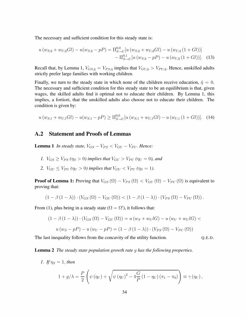
The necessary and sufficient condition for this steady state is:

u (wS,η + wU,ηGl) − u(wS,η − pP ) = Π0,0S→U [u (wS,η + wU,ηGl) − u (wU,η (1 +Gl))]

− Π0,1S→U [u (wS,η − pP ) − u (wU,η (1 +Gl))]. (13)

Recall that, by Lemma 1, VGS,η = VPS,η implies that VGU,η > VPU,η. Hence, unskilled adultsstrictly prefer large families with working children.

Finally, we turn to the steady state in which none of the children receive education, η = 0.The necessary and sufficient condition for this steady state to be an equilibrium is that, givenwages, the skilled adults find it optimal not to educate their children. By Lemma 1, thisimplies, a fortiori, that the unskilled adults also choose not to educate their children. Thecondition is given by:

u (wS,1 + wU,1Gl)− u(wS,1 − pP ) ≥ Π0,0S→U [u (wS,1 + wU,1Gl) − u (wU,1 (1 +Gl))]. (14)

A.2 Statement and Proofs of Lemmas

Lemma 1 In steady state, VGS − VPS < VGU − VPU . Hence:

1. VGS ≥ VPS (ηS > 0) implies that VGU > VPU (ηU = 0), and

2. VGU ≤ VPU (ηU > 0) implies that VGU < VPU (ηS = 1).

Proof of Lemma 1: Proving that VGS (Ω) − VPS (Ω) < VGU (Ω) − VPU (Ω) is equivalent toproving that:

(1 − β (1 − λ)) · (VGS (Ω) − VGU (Ω)) < (1 − β (1 − λ)) · (VPS (Ω) − VPU (Ω)) .

From (1), plus being in a steady state (Ω = Ω′), it follows that:

(1 − β (1 − λ)) · (VGS (Ω) − VGU (Ω)) = u (wS + wU lG) − u (wU + wU lG) <

u (wS − pP ) − u (wU − pP ) = (1 − β (1 − λ)) · (VPS (Ω) − VPU (Ω))

The last inequality follows from the concavity of the utility function. Q.E.D.

Lemma 2 The steady state population growth rate g has the following properties.

1. If ηS = 1, then

1 + g/λ =P

2

(ψ (ηU ) +

√ψ (ηU)2 − 4

G

P(1 − ηU) (π1 − π0)

)≡ γ (ηU) ,

34

where ψ (ηU) ≡ 1 + (1 − ηU)(

GP

(1 − π0) − (1 − π1)) ≥ 1 , and γ (1) = P. The

population growth rate g is a strictly decreasing function of the fraction ηU of unskilledadults with small families.

2. If ηS < 1, then

1 + g/λ =G

2

(ψS (ηS) +

√ψS (ηS)2 − 4

P

GηS (π1 − π0)

)≡ γS (ηS) ,

where ψS (ηS) ≡ 1 + ηS

(PGπ1 − π0

), γS (0) = G and γS (1) = γ (0) . The population

growth rate g is a strictly decreasing function of the fraction ηS of skilled adults withsmall families.

Proof of Lemma 2: Define q ≡ G/P > 1.

Part 1: The law of motion (5), together with the restriction that ηS = 1 and xGS,t+1 = 0, definesa system of four equations in four unknowns. The unique solution with nonnegative fractionsof each type yields a solution for the growth rate of the population such that 1+g/λ ≡ γ (ηU),where γ (ηU) is as defined above. It is useful to note that:

ψ (ηU ) ≥ (1 + (1 − ηU) q ((1 − π0) − (1 − π1))) ≡ ψ (ηU) ,

with strict inequality for any ηU < 1 (whereas ψ (1) = ψ (1) = 1), and that ψ′ (ηU) <ψ′ (ηU) < 0. Next, define:

γ (ηU) ≡ P

2

(ψ (ηU) +

√ψ (ηU)2 − 4q (1 − ηU) (π1 − π0)

)≤ γ (ηU) ,

and observe that, using the definition of ψ (ηU):

γ (ηU) =P

2

((1 + (1 − ηU) q (π1 − π0)) +

√(1 − (1 − ηU) q (π1 − π0))

2

)= P ≤ γ (ηU) .

Thus, λ (P − 1) is a lower bound to the growth rate of the population. Note also that ψ (ηU)2−4q (1 − ηU) (π1 − π0) = (1 − (1 − ηU) q (π1 − π0))

2 > 0 , hence, ψ (ηU)2−4q (1 − ηU) (π1 − π0) >0, i.e., γ (ηU) ∈ R+. Furthermore, γ′ (ηU) < γ′ (ηU) = 0, proving that g is uniformly decreas-ing in ηU .

Part 2: The law of motion (5), together with the restriction that η = 0 and xPU,t+1 = 0 definesa system of four equations in four unknowns. The unique solution with nonnegative fractionsof each type yields a solution for the growth rate of the population such that 1+g/λ ≡ γS (ηS),where γS (ηS) is as defined above. First, note that the discriminant in the definition of γS (ηS)

35

is positive, since:

ψS (η)2 − 4qηS (π1 − π0) ≥ (1 + ηSq (π1 − π0))2 − 4ηSq (π1 − π0) =

(1 − ηSq (π1 − π0))2 ≥ 0.

Next, observe that:

γS (η) ≤ γS (η) ≡ G

2

(ψS (η) +

√ψS (η)2 − 4ηS

(P

Gπ1 − π0

)),

and, moreover, γ′S (ηS) < γ′S (ηS) . Finally, note that:

γS (η) ≡ G

2

(ψS (η) +

√ψS (η)2 − 4ηS

(P

Gπ1 − π0

))=

=G

2

⎛⎝1 + ηS

(P

Gπ1 − π0

)+

√(1 − ηS

(P

Gπ1 − π0

))2⎞⎠ = G,

implying that γ′S (ηS) = 0. This establishes that γ′S (ηS) < 0, i.e., g is uniformly decreasing inηS . Q.E.D.

Lemma 3 The fraction ξPS of skilled adults with small families is strictly increasing in ηU .The fraction ξGU of unskilled adults with large families is strictly decreasing in ηS . The ratioof skilled to unskilled labor supply increases with both ηU and ηS . Hence, the equilibriumskilled (unskilled) wage decreases (increases) with both ηU and ηS .

Proof of Lemma 3: Once more, the two cases of ηU ∈ (0, 1) and ηS ∈ (0, 1) are parallel. Wetherefore concentrate on the case ηU ∈ (0, 1) (which implies ηS = 1). Using the solution for gand the definition of γ (ηU) defined in the proof of Lemma 2, we can solve for the steady stateproportion of each type, as a function of ηU :

ξPU (ηU) =GηU ((1 − π0) − P (π1 − π0) /γ (ηU))

γ (ηU) + (G− P ) ηU + (Gπ0 − Pπ1) (1 − ηU),

ξGU (ηU) =γ (ηU) − P (ηU + π1 (1 − ηU))

γ (ηU) + (G− P ) ηU + (Gπ0 − Pπ1) (1 − ηU),

ξPS (ηU) =Gπ0 +GPηU (π1 − π0) /γ (ηU)

γ (ηU) + (G− P ) ηU + (Gπ0 − Pπ1) (1 − ηU).

36

We now calculate the total derivative of ξPS (ηU) :

ξ′PS (ηU) = 2P 2 (π1 − π0)λ3[

F (ηU)P + (G (1 − π0) − P (π1 − π0))

√ψ (ηU)2 − 4q (1 − ηU ) (π1 − π0)

],

where:

F (ηU) = q2 (1 − ηU) (1 − π0)2

+ q(ηU (1 − π0)

2 + π0 (3 − π0) − 2π1

)+ (π1 − π0) (ηU + π1 (1 − ηU)) .

We want to prove that ξ′PS (ηU) ≥ 0 for all ηU ∈ [0, 1]. To this aim, we define the function:

ξ (ηU ) =2P 3 (π1 − π0)λ3[

F (ηU ) + (q (1 − π0) − (π1 − π0))

√ψ (ηU)2 − 4q (1 − ηU) (π1 − π0)

]

=2P 3 (π1 − π0)λ3 (1 − π1)

[(1 − ηU)

(q2 (1 − π0) − (π1 − π0)

)+

q (2 (π0 (1 − ηU) + ηU) + (1 − π1) (1 − ηU))],

where we have that ξ (ηU) ≥ ξ (ηU). It is immediate to verify that ξ (ηU) ≥ 0, with strictinequality holding whenever π0 < π1 < 1. Hence, ξ′PS (ηU) ≥ 0. In fact, ξ′PS (ηU) > 0whenever π0 < π1 < 1. A parallel argument applies to the case ηS ∈ (0, 1). It thereforefollows that ratio of skilled to unskilled labor supply increases with both ηU and ηS. Q.E.D.

A.3 Proofs of Propositions

Proof of Proposition 1: We begin by defining the utility differential for unskilled and skilledadults between having large and small families in steady state:

∆U (η) = VGU,η − VPU,η,

∆S (η) = VGS,η − VPS,η.

According to conditions (9), (10), (11), (12), (13), and (14), a steady state of type η = 2exists if ∆U(2) ≤ 0, type η ∈ (1, 2) exists if ∆U(η) = 0 for some η ∈ (1, 2), type η = 1exists if ∆U(η) ≥ 0 and ∆S(η) ≤ 0, type η ∈ (0, 1) exists if ∆S(η) = 0 for some η ∈ (0, 1),and, finally, type η = 0 exists if ∆S(0) ≥ 0. A unique steady state therefore exists if ∆U (η)and ∆S (η) are strictly monotonically increasing in η. Given that Lemma 3 establishes that thewage premium is strictly decreasing in η, for the skilled adults this monotonicity is immediate.The situation is more complicated for the unskilled adults, since there are two opposing effects:as the skill premium rises, education becomes more attractive, but also less affordable. Writing

37

steady state utilities for unskilled adults as a function of η we get:

VGU,η =u (wU,η (1 +Gl)) − Π0,1

U→S (u (wU,η (1 +Gl)) − u (wS,η − pP ))

1 − β (1 − λ (1 − z)),

VPU,η =u(wU,η − pP ) − Π1,1

U→S[u (wU,η − pP ) − u (wS,η − pP )]

1 − β(1 − λ(1 − z)).

Here we assume that skilled adults educate their children, which is the relevant case. We nowhave

∆′U (η) =

1

1 − β(1 − λ(1 − z))

[u′ (wU,η (1 +Gl))

(1 − Π0,1

U→S

)(1 +Gl)w′

U,η

− u′ (wU,η − pP )(1 − Π1,1

U→S

)w′

U,η − u′ (wS,η − pP )(Π1,1

U→S − Π0,1U→S

)w′

S,η

],

where w′U,η > 0, w′

S,η < 0, and Π1,1U→S − Π0,1

U→S > 0. It therefore suffices to show that:

u′ (wU,η (1 +Gl))(1 − Π0,1

U→S

)(1 +Gl) > u′ (wU,η − pP )

(1 − Π1,1

U→S

)or:

(1 +Gl)1 − Π0,1

U→S

1 − Π1,1U→S

>u′(wU,η − pP )

u′ (wU,η(1 +Gl))).

Under CRRA, the right-hand side is increasing in the wage and, therefore, Assumption 2 is asufficient condition for a unique steady state to exist. Q.E.D.

Proof of Proposition 2: To begin, set β = 0 (to be relaxed later), choose an arbitrary G > 0,and choose λ > 0, π0 > 0, and π1 > π0 such that the old unskilled are always in majority(i.e., (1− λ)(1− π1) > 0.5), which satisfies the first condition in the proposition. Since givenβ = 0 the future is not valued, there is no incentive for education. Therefore without CLR, forany positive values of the remaining parameters p and P the steady state with η = 0 prevails(all families are large), satisfying the second part of the proposition. Conversely, when CLRare in place (combined with a compulsory education policy) the steady state is η = 2, as allfamilies are small to economize on the educational cost.

We still need to show that we can choose p and P such that both CLR and no CLR are SSPE,and that the assumption β = 0 can be relaxed. First, assume that the steady state without CLRprevails. We want to find conditions such that the (old unskilled) majority would oppose CLRif a referendum occurred. In the steady state without CLR, the ratio of skilled to unskilledlabor supply is:

x0 =π0

1 − π0 +Gl,

and the corresponding unskilled wage is wU,0 = f(x0) − f ′(x0)x0. If CLR are introduced, all

38

children are withdrawn from the labor market. The new skill ratio is:

x0 =π0

1 − π0,

and the corresponding wage wU,0 = f(x0) − f ′(x0)x0 satisfies wU,0 < wU,0. However, theunskilled workers also lose child labor income and have to pay the schooling cost. The oldunskilled majority oppose CLR if their consumption is lower under CLR, i.e., if:

wU,0(1 +Gl) > wU,0 − pG

is satisfied. Clearly, the education cost p can always be chosen sufficiently high such thatthe majority of unskilled agents opposes the introduction of CLR. Also notice that the smallfamily size P has not entered any equations yet; we are free to choose P independently tomeet the final condition in the proposition.

Now consider the case where currently the steady state with CLR prevails. We want to findconditions under which the (old unskilled) majority would prefer to keep CLR in place. In thesteady state with CLR, the ratio of skilled to unskilled labor supply is:

x2 =π1

1 − π1,

and the corresponding unskilled wage is wU,2 = f(x2) − f ′(x2)x2. If CLR are abandoned, allchildren will enter the labor market, and young families will choose the large family size G.The ensuing skill ratio is:

x2 =π1

1 − π1 + (1 − λ)P l + λGl,

and the corresponding wage wU,2 = f(x2)− f ′(x2)x2 satisfies wU,2 < wU,2. The old unskilledwill prefer to maintain CLR if their consumption falls if CLR are abandoned, i.e.:

wU,2 − pP > wU,2(1 + P l).

This condition can be satisfied by choosing P sufficiently small. Notice that wU,2 does notconverge to wU,2 as P goes to zero, because the young adults choose the large family size G.By choosing P , we can therefore ensure that the majority prefers to keep CLR in place. Wehave therefore found a set of parameters for which multiple SSPE exist. Finally, since utilityis continuous in β, the same result can be obtained for positive β, sufficiently close to zero,and the same remaining parameters. Q.E.D.

39

ReferencesAcemoglu, Daron and Joshua D. Angrist. 2000. “How Large are Human Capital Exter-

nalities? Evidence from Compulsory Schooling Laws.” NBER Macroeconomics Annual2000, pp. 9–59.

Angrist, Joshua D. and Alan B. Krueger. 1991. “Does Compulsory School Attendance AffectSchooling and Earnings?” The Quarterly Journal of Economics 106 (4): 979–1014.

Baland, Jean-Marie and James Robinson. 2000. “Is Child Labor Inefficient?” Journal ofPolitical Economy 108 (4): 663–679.

Bardhan, Pranab and Christopher Udry. 1999. Development Microeconomics. Oxford Uni-versity Press.

Basu, Kaushik. 1999. “Child Labor: Cause, Consequence, and Cure, with Remarks onInternational Labor Standards.” Journal of Economic Literature 37 (3): 1083–1117.

Basu, Kaushik and Pham Hoang Van. 1998. “The Economics of Child Labor.” AmericanEconomic Review 88 (3): 412–427.

Becker, Gary S. and Robert J. Barro. 1988. “A Reformulation of the Economic Theory ofFertility.” Quarterly Journal of Economics 103 (1): 1–25.

Berdugo, Binyamin and Moshe Hazan. 2002. “Child Labor, Fertility and Economic Growth.”Economic Journal 112 (482): 810–28.

Brenner, Y. Simon, Harmut Kaelble, and Mark Thomas, eds. 1991. Income Distribution inHistorical Perspective. Cambridge: Cambridge University Press.

Brown, Drusilla, Alan V. Deardorff, and Robert M. Stern. 2003. “Child Labor: Theory,Evidence, and Policy.” In International Labour Standards: History, Theory, and PolicyOptions, edited by Kaushik Basu, Henrik Horn, Lisa Roman, and Judith Shapiro. Oxford:Blackwell Publishing.

Chesnais, Jean Claude. 1992. The Demographic Transition. Oxford: Oxford UniversityPress.

Cunningham, Hugh. 1996. “Combating Child Labor: The British Experience.” In ChildLabor in Historical Perspective: Case Studies from Europe, Japan, and Colombia, 41–55. UNICEF.

Davidson, Elizabeth H. 1939. Child Labor Legislation in the Southern Textile States. ChapelHill: The University of North Carolina Press.

Dessy, Sylvain and Stephane Pallage. 2001. “Child Labor and Coordination Failures.” Jour-nal of Development Economics 65 (2): 469–476.

Doepke, Matthias. 2004. “Accounting for Fertility Decline During the Transition to Growth.”Journal of Economic Growth 9 (3): 347–83.

Feinstein, Charles. 1988. “The Rise and Fall of the Williamson Curve.” Journal of EconomicHistory 48 (3): 699–729.

40

Galbi, Douglas A. 1997. “Child Labor and the Division of Labor in the Early English CottonMills.” Journal of Population Economics 10:357–375.

Galor, Oded and Omer Moav. 2002. “Natural Selection and the Origin of Economic Growth.”Quarterly Journal of Economics 117 (4): 1133–91.

. 2003. “Das Human Kapital: A Theory of the Demise of the Class Structure.”Unpublished Manuscript, Brown University.

Galor, Oded and David N. Weil. 2000. “Population, Technology, and Growth: From Malthu-sian Stagnation to the Demographic Transition and Beyond.” American Economic Review90 (4): 806–28.

Horrell, Sara and Jane Humphries. 1995. “The Exploitation of Little Children: Child Laborand the Family Economy in the Industrial Revolution.” Explorations in Economic History32:485–516.

Kirby, Peter. 1999. “The Historic Viability of Child Labor and the Mines Act of 1842.”Chapter 4 of A Thing of the Past? Child Labour in Britain in the Nineteenth and TwentiethCenturies, edited by Michael Lavalette. Liverpool: Liverpool University Press.

Kremer, Michael and Daniel L. Chen. 2002. “Income Distribution Dynamics with Endoge-nous Fertility.” Journal of Economic Growth 7 (3): 227–58.

Krueger, Dirk and Jessica Tjornhom. 2004. “Economic Inequality and the Emergence ofChild Labor Laws.” Forthcoming, International Economic Review.

Lee, Ronald D. and Roger S. Schofield. 1981. “British Population in the Eighteenth Century.”In The Economic History of Britain since 1700, edited by Richard Floud and DonaldMcCloskey. Cambridge: Cambridge University Press.

Levison, Deborah, Richard Anker, Shahid Ashraf, and Sandhya Barge. 1998. “Is ChildLabour Really Necessary in India’s Carpet Industry?” Chapter 5 of Economics of ChildLabour in Hazardous Industries of India, edited by R. Anker, S. Barge, S. Rajagopal, andM.P. Joseph. New Delhi: Hindustan Publishing.

Lleras-Muney, Adriana. 2002. “Were Compulsory Attendance and Child Labor Laws Effec-tive? An Analysis from 1915 to 1939.” Journal of Law and Economics 45 (2): 401–435.

Maddison, Angus. 1995. Monitoring the World Economy, 1820-1992. Paris: OECD.

Margo, Robert A. and T. Aldrich Finegan. 1996. “Compulsory Schooling Legislation andSchool Attendance in Turn-of-the-Century America: A ‘Natural Experiment’ Approach.”Economics Letters 53 (1): 103–10.

Marimon, Ramon and Fabrizio Zilibotti. 2000. “Employment and Distributional Effects ofRestricting Working Time.” European Economic Review 44 (7): 1291–326.

Moav, Omer. 2005. “Cheap Children and the Persistence of Poverty.” Economic Journal115 (500): 88–110.

Moehling, Caroline M. 1999. “State Child Labor Laws and the Decline of Child Labor.”Explorations in Economic History 36 (1): 72–106.

41

Nardinelli, Clark. 1980. “Child Labor and the Factory Acts.” Journal of Economic History40 (4): 739–755.

. 1990. Child Labor and the Industrial Revolution. Bloomington: Indiana UniversityPress.

Peacock, A.E. 1984. “The Successful Prosecution of the Factory Acts, 1833–55.” EconomicHistory Review 37 (2): 197–210.

Ranjan, Priya. 2001. “Credit Constraints and the Phenomenon of Child Labor.” Journal ofDevelopment Economics 64 (1): 81–102.

Weiner, Myron. 1991. The Child and the State in India: Child Labor and Education Policyin Comparative Perspective. Princeton University Press.

Weissbach, Lee Shai. 1989. Child Labor Reform in Nineteenth-Century France. BatonRouge: Louisiana State University Press.

Williamson, Jeffrey G. 1985. Did British Capitalism Breed Inequality? Boston: Allen andUnwin.

Williamson, Jeffrey G. and Peter H. Lindert. 1980. American Inequality: A MacroeconomicHistory. New York: Academic Press.

42

Parameter β z σ λ P G π0 π1 p l κ

Value 0.8 1 0.5 0.15 1 3 0.05 0.4 0.013 0.1 0.5

Table 1: Parameter Values for the Model Simulations

wS/wU

η

0

1

2

.....................................................................................................................

....

....

....

....

....

....

....

....

....................................................................

EE

EESS0 SS1

SS2

wS/wU wS/wU

Figure 1: Uniqueness of Steady States with Fixed Policies

Figure 2: η in Steady State as a Function of Skill Bias α

0.3 0.4 0.5 0.6 0.7 0.8alpha

0

0.5

1

1.5

2

eta

tilde

0.3 0.4 0.5 0.6 0.7 0.8alpha

SSPE

No CLRCLR

Figure 3: Regions of Existence for each SSPE as a Function of Skill Bias α

Figure 4: Skill Premium (Ratio of Skilled to Unskilled Wages) in the U.K.

2

3

4

1800 1820 1840 1860 1880 1900 1920

Wage Ratio

Source: Williamson (1985)

2 4 6 8 10 12Time

3

4

5

6

7

Wage

Ratio

Figure 5: Skill Premium in the Model under Endogenous Policy (Solid) and without CLR(Dashed)

Figure 6: Population Growth in the Model under Endogenous Policy (Solid) and without CLR(Dashed)

2 4 6 8 10 12Time

5

10

15

20

25

30Population

Growth

2 4 6 8 10 12Time

0

0.2

0.4

0.6

0.8

1

Working

Children

Figure 7: Fraction of Children Working in the Model under Endogenous Policy (Solid) andwithout CLR (Dashed)

Figure 8: The Total Fertility Rate in the U.K.

2

3

4

5

6

1800 1820 1840 1860 1880 1900 1920

Total Fertility Rate

Source: Lee and Schofield (1981), Chesnais (1992)

0

20

40

60

80

1840 1860 1880 1900 1920

Schooling Rate

10

20

30

Child Labor Rate

Schooling Child Labor

Source: Cunningham (1996)

Figure 9: Schooling Rates (Percentage of Children Aged 5–14 in School) and Child LaborRates (Percentage of Children Aged 10–14 Economically Active) in the U.K.

Figure 10: Capitalists’ Income in the Baseline Model under Endogenous Policy (Solid) andwithout CLR (Dashed)

0 2 4 6 8 10 12Time

0.25

0.3

0.35

0.4

0.45

0.5

0.55

0.6

Capital

Income

0 2 4 6 8 10 12Time

0.25

0.3

0.35

0.4

0.45

Capital

Income

Figure 11: Capitalists’ Income in the Model with Larger Increase in Skill Bias under Endoge-nous Policy (Solid) and without CLR (Dashed)