Divergence-Free Reconstruction of Magnetic Fields and WENO

Schemes for Magnetohydrodynamics

By

Dinshaw S. Balsara

(dbalsara@nd.edu)

Department of Physics, University of Notre Dame,

Notre Dame, IN 46556

Abstract

Balsara (2001, J. Comput. Phys., 174, 614) showed the importance of divergence-

free reconstruction in adaptive mesh refinement problems for magnetohydrodynamics

(MHD) and the importance of the same for designing robust second order schemes for

MHD was shown in Balsara (2004, ApJS, 151, 149). Second order accurate divergence-

free schemes for MHD have shown themselves to be very useful in several areas of

science and engineering. However, certain computational MHD problems would be much

benefited if the schemes had third and higher orders of accuracy. In this paper we show

that the reconstruction of divergence-free vector fields can be carried out with better than

second order accuracy. As a result, we design divergence-free weighted essentially non-

oscillatory (WENO) schemes for MHD that have order of accuracy better than second. A

multistage Runge-Kutta time integration is used to ensure that the temporal accuracy

matches the spatial accuracy. Accuracy analysis is carried out and it is shown that the

schemes meet their design accuracy for smooth problems. Stringent tests are also

presented showing that the schemes perform well on those tests.

1

1) Introduction

The Magnetohydrodynamic (MHD) equations play an important role in many

areas of astrophysics, space physics and engineering. Typical applications in those areas

require one to capture flow on a range of scales in a way that is as dissipation-free as

possible. As a result, there has been considerable interest in bringing accurate and reliable

numerical methods to bear on this problem. The MHD system of equations can be written

as a set of hyperbolic conservation laws. As a result, early efforts concentrated on

straightforwardly applying second order total variation diminishing (TVD) techniques to

the MHD equations. This was done by Brio & Wu [13], Zachary, Malagoli & Colella

[34], Powell [27], Dai & Woodward [16], Ryu & Jones [29], Roe & Balsara [28], Balsara

[1] and [2], Falle, Komissarov & Joarder [22] and Crockett et al [15]. Recent efforts have

focused on understanding the structure of the induction equation:

( ) + c = 0t

∂∇×

∂B E (1)

and the divergence-free evolution that it implies for the magnetic field. In eqn. (1), B is

the magnetic field, E is the electric field and c is the speed of light. The magnetic field

starts out divergence-free because of the absence of magnetic monopoles and eqn. (1)

ensures that it remains divergence-free for all time. The electric field is given by:

c = − ×E v B

E

(2)

where v is the fluid velocity. For the rest of this paper we will simplify the notation by

making the transcription c . Brackbill & Barnes [11] have shown that violating

the constraint leads to unphysical plasma transport orthogonal to the magnetic

field. This comes about because violating the constraint results in the addition of extra

source terms in the momentum and energy equations. Yee [33] was the first to formulate

divergence-free schemes for electromagnetism. Brecht et al [12] and DeVore [19] did the

same for flux corrected transport (FCT)-based MHD. Dai & Woodward [17], Ryu et al

→E

= 0∇⋅ B

2

[30], Balsara & Spicer [9] and [10], Balsara [4] and Londrillo and DelZanna [26] showed

that simple extensions of higher order Godunov schemes permit one to formulate

divergence-free time-update strategies for the magnetic field. Balsara & Kim [6]

intercompared divergence-cleaning and divergence-free schemes for numerical MHD.

They found that if the test problems are made stringent enough the schemes that are

based on divergence-cleaning show significant inadequacies when used for astrophysical

applications. Thus it is advantageous to design robust schemes for numerical MHD that

are divergence-free, as was done in Balsara [4]. Balsara [4] used the divergence-free

reconstruction of vector fields from Balsara (2001) to present a formulation that

overcame several inconsistencies in previous formulations. Balsara et al [5] a new class

of higher order schemes for the Euler equations. In such formulations the lower moments

of the solution are retained while the higher moments are reconstructed, resulting in low

storage schemes with better than second order accuracy.

Higher order schemes for MHD have been attempted. Jiang & Wu [26] and

Balsara & Shu [8] experimented with weighted essentially non-oscillatory (WENO)

schemes. Another line of effort stems from the work of Londrillo and DelZanna [26].

These schemes were based on a finite difference formulation. For certain types of

applications, especially those involving non-uniform meshes or adaptive solution

strategies, finite volume formulations become essential. We therefore present a finite

volume, divergence-free scheme for MHD that goes beyond second order of accuracy.

We rely on efficient WENO interpolation strategies that were designed in Balsara et al

[7] to make a high order reconstruction. The novel element introduced in this paper

consists of extending the divergence-free reconstruction of magnetic fields from Balsara

[3] and [4] to all orders up to fourth. When coupled with an appropriately accurate

Runge-Kutta (RK) time integration scheme by Shu & Osher [31] and [32], we get a set of

WENO schemes that have a spatial and temporal accuracy that exceeds that of second

order schemes.

In Section 2 we catalogue the divergence-free reconstruction of vector fields for

higher order schemes. In Section 3 we provide a step by step description of the scheme.

3

In Section 4 we provide an accuracy analysis and in Section 5 we present several test

problems.

2) Higher Order Divergence-Free Reconstruction of Vector Fields

In this section we study the divergence-free reconstruction of a divergenceless

vector field for schemes with better than second order accuracy. In particular, we focus

on the third and fourth order cases because they can be catalogued succinctly and are

likely to be generally useful. The second order accurate divergence-free reconstruction of

vector fields was studied for Cartesian meshes in Balsara [3]. In Balsara [4] we extended

this to logically rectangular meshes with diagonal metrics. Balsara [4] also considered the

second order accurate divergence-free reconstruction of vector fields on tetrahedral

meshes and that too can be extended to higher orders. Since the method was described in

detail in Balsara [3], in this paper we will focus on cataloguing results for the higher

order case. The reader who wants a pedagogical introduction is referred to Balsara [3]

and [4].

For the rest of this work we assume that each zone has been mapped to a unit

cube with local coordinates (x,y,z) [ 1/ 2,1/ 2] [ 1/ 2,1/ 2] [ 1/ 2,1/ 2]∈ − × − × − . A natural

set of modal basis functions within that zone or on its faces would consist of tensor

products of the Legendre polynomials P0 (x), P1 (x) and P2 (x) . The first few Legendre

polynomials are given by:

2 30 1 2 3

4 24

1 3P (x) = 1 ; P (x) = x ; P (x) = x ; P (x) = x x ; 12 20

3 3P (x) = x x + 14 560

− −

− (3)

The above Legendre polynomials have just been suitably scaled to the local coordinates

of the zone being considered. The x-component of the magnetic field in the upper and

lower x-faces of this zone can be projected into these bases as:

4

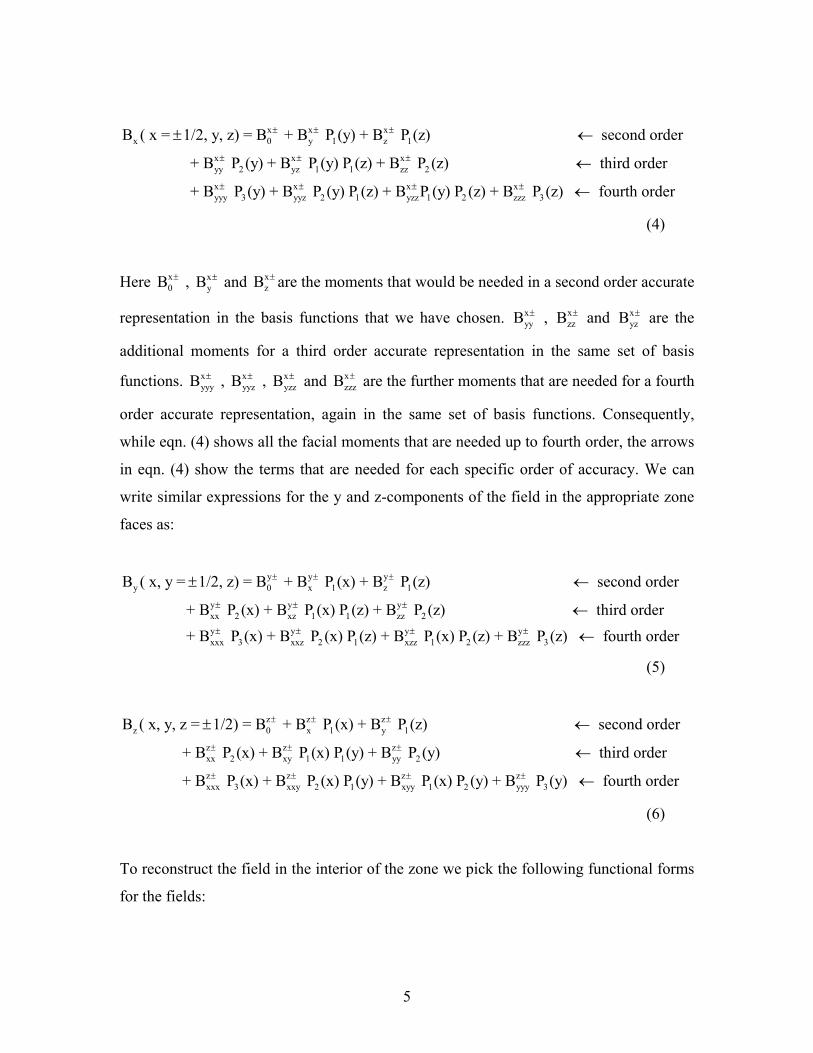
x x x

x 0 y 1 z 1

x x xyy 2 yz 1 1 zz 2

B ( x = 1/2, y, z) = B + B P (y) + B P (z) second order

+ B P (y) + B P (y) P (z) + B P (z) th

± ± ±

± ± ±

± ←

←x x x xyyy 3 yyz 2 1 yzz 1 2 zzz 3

ird order

+ B P (y) + B P (y) P (z) + B P (y) P (z) + B P (z) fourth order± ± ± ± ←

(4)

Here , and are the moments that would be needed in a second order accurate

representation in the basis functions that we have chosen.

x0B ± x

yB ± xzB ±

xyyB ± , and are the

additional moments for a third order accurate representation in the same set of basis

functions. , B , and

xzzB ± x

yzB ±

xyyyB ± x

yyz± Bx

yzz± x

zzzB ± are the further moments that are needed for a fourth

order accurate representation, again in the same set of basis functions. Consequently,

while eqn. (4) shows all the facial moments that are needed up to fourth order, the arrows

in eqn. (4) show the terms that are needed for each specific order of accuracy. We can

write similar expressions for the y and z-components of the field in the appropriate zone

faces as:

y y y

y 0 x 1 z 1

y y yxx 2 xz 1 1 zz 2

B ( x, y = 1/2, z) = B + B P (x) + B P (z) second order

+ B P (x) + B P (x) P (z) + B P (z) thi

± ± ±

± ± ±

± ←

←y y y yxxx 3 xxz 2 1 xzz 1 2 zzz 3

rd order

+ B P (x) + B P (x) P (z) + B P (x) P (z) + B P (z) fourth order± ± ± ± ←

(5)

z z z

z 0 x 1 y 1

z z zxx 2 xy 1 1 yy 2

B ( x, y, z = 1/2) = B + B P (x) + B P (z) second order

+ B P (x) + B P (x) P (y) + B P (y) th

± ± ±

± ± ±

± ←

←z z z zxxx 3 xxy 2 1 xyy 1 2 yyy 3

ird order

+ B P (x) + B P (x) P (y) + B P (x) P (y) + B P (y) fourth order± ± ± ± ←

(6)

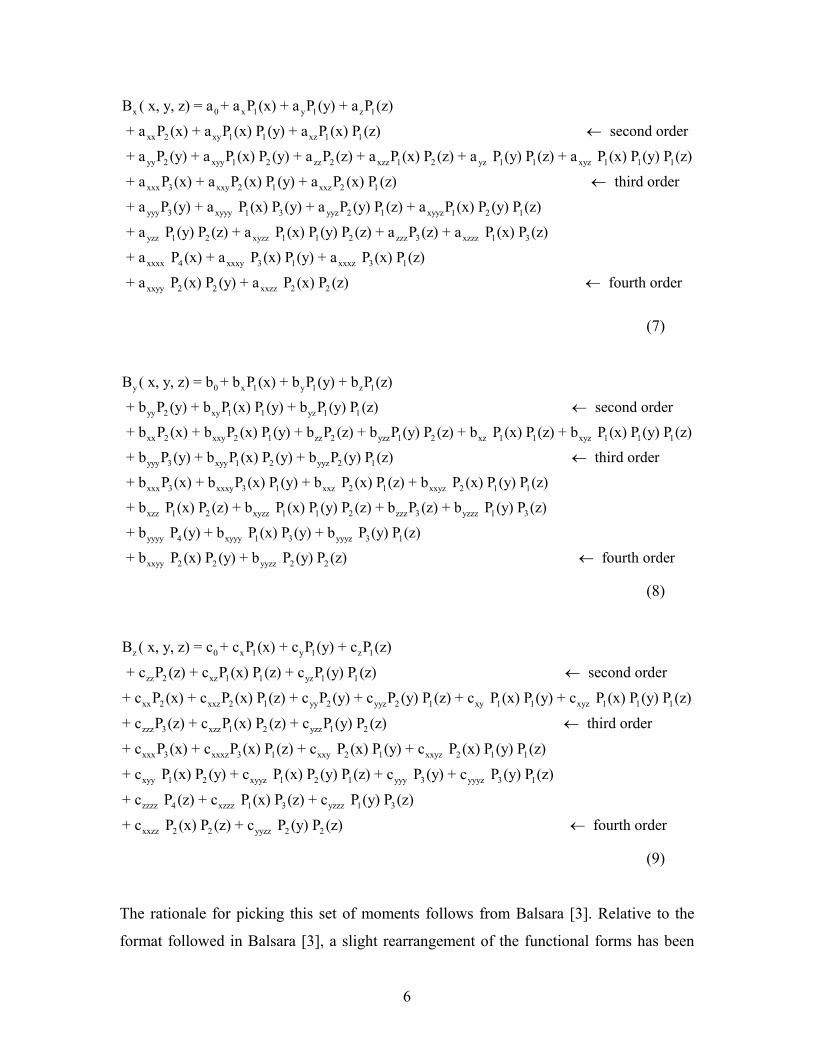
To reconstruct the field in the interior of the zone we pick the following functional forms

for the fields:

5

x 0 x 1 y 1 z 1

xx 2 xy 1 1 xz 1 1

yy 2 xyy 1 2 zz 2

B ( x, y, z) = a + a P (x) + a P (y) + a P (z)

+ a P (x) + a P (x) P (y) + a P (x) P (z) second order

+ a P (y) + a P (x) P (y) + a P (z)

←

xzz 1 2 yz 1 1 xyz 1 1 1

xxx 3 xxy 2 1 xxz 2 1

yyy 3 xyyy 1 3

+ a P (x) P (z) + a P (y) P (z) + a P (x) P (y) P (z)

+ a P (x) + a P (x) P (y) + a P (x) P (z) third order

+ a P (y) + a P (x) P

←

yyz 2 1 xyyz 1 2 1

yzz 1 2 xyzz 1 1 2 zzz 3 xzzz 1 3

xxxx 4 xxxy 3 1 xxxz 3 1

xxyy 2 2

(y) + a P (y) P (z) + a P (x) P (y) P (z)

+ a P (y) P (z) + a P (x) P (y) P (z) + a P (z) + a P (x) P (z)

+ a P (x) + a P (x) P (y) + a P (x) P (z)

+ a P (x) P (y) xxzz 2 2+ a P (x) P (z) fourth order

←

(7)

y 0 x 1 y 1 z 1

yy 2 xy 1 1 yz 1 1

xx 2 xxy 2 1 zz 2

B ( x, y, z) = b + b P (x) + b P (y) + b P (z)

+ b P (y) + b P (x) P (y) + b P (y) P (z) second order

+ b P (x) + b P (x) P (y) + b P (z) + b

←

yzz 1 2 xz 1 1 xyz 1 1 1

yyy 3 xyy 1 2 yyz 2 1

xxx 3 xxxy 3 1 x

P (y) P (z) + b P (x) P (z) + b P (x) P (y) P (z)

+ b P (y) + b P (x) P (y) + b P (y) P (z) third order

+ b P (x) + b P (x) P (y) + b

←

xz 2 1 xxyz 2 1 1

xzz 1 2 xyzz 1 1 2 zzz 3 yzzz 1 3

yyyy 4 xyyy 1 3 yyyz 3 1

xxyy 2 2 yyzz

P (x) P (z) + b P (x) P (y) P (z)

+ b P (x) P (z) + b P (x) P (y) P (z) + b P (z) + b P (y) P (z)

+ b P (y) + b P (x) P (y) + b P (y) P (z)

+ b P (x) P (y) + b 2 2P (y) P (z) fourth order←

(8)

z 0 x 1 y 1 z 1

zz 2 xz 1 1 yz 1 1

xx 2 xxz 2 1 yy 2 yyz

B ( x, y, z) = c + c P (x) + c P (y) + c P (z)

+ c P (z) + c P (x) P (z) + c P (y) P (z) second order

+ c P (x) + c P (x) P (z) + c P (y) + c P

←

2 1 xy 1 1 xyz 1 1 1

zzz 3 xzz 1 2 yzz 1 2

xxx 3 xxxz 3 1 xxy 2

(y) P (z) + c P (x) P (y) + c P (x) P (y) P (z)

+ c P (z) + c P (x) P (z) + c P (y) P (z) third order

+ c P (x) + c P (x) P (z) + c P (x

←

1 xxyz 2 1 1

xyy 1 2 xyyz 1 2 1 yyy 3 yyyz 3 1

zzzz 4 xzzz 1 3 yzzz 1 3

xxzz 2 2 yyzz 2 2

) P (y) + c P (x) P (y) P (z)

+ c P (x) P (y) + c P (x) P (y) P (z) + c P (y) + c P (y) P (z)

+ c P (z) + c P (x) P (z) + c P (y) P (z)

+ c P (x) P (z) + c P (y) P (z) fourth order←

(9)

The rationale for picking this set of moments follows from Balsara [3]. Relative to the

format followed in Balsara [3], a slight rearrangement of the functional forms has been

6

made in the previous three equations to cast them in terms of the basis functions.

Analogous to eqn. (4), eqn. (7) shows the terms that have to be included to achieve

second, third and fourth order accuracy. Eqns. (8) and (9) have a structure that is similar

to eqn. (7) and the corresponding terms that are needed with increasing accuracy are

easily identified. The procedure for enforcing the divergence-free constraint is entirely

similar to the one in Balsara [3] and will not be repeated here.

We now provide the formulae for obtaining the coefficients in eqn. (7) using the

coefficients in eqns. (4), (5) and (6). To obtain the coefficients in eqn. (8) make the cyclic

rotation of variables, a b, b c, c a, x y, y z and z x , in the formulae

below. Similarly, to obtain the coefficients in eqn. (9) make the cyclic rotation of

variables, a c, b a, c b, x z, y x and z y . Note that the formulae in this

Section should be implemented in code in the same sequence as described here.

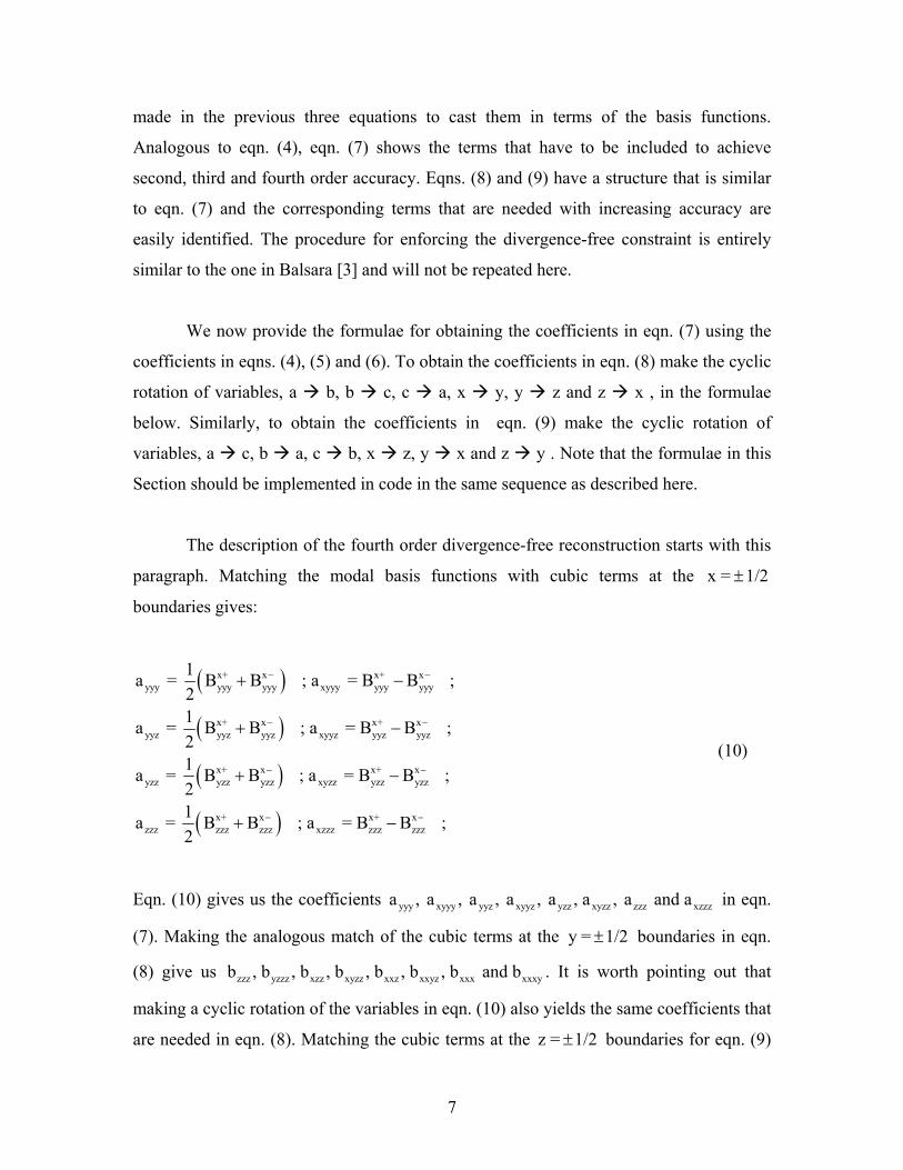
The description of the fourth order divergence-free reconstruction starts with this

paragraph. Matching the modal basis functions with cubic terms at the x = 1/2±

boundaries gives:

( )

( )

( )

( )

x+ x x+ xyyy yyy yyy xyyy yyy yyy

x+ x x+ xyyz yyz yyz xyyz yyz yyz

x+ x x+ xyzz yzz yzz xyzz yzz yzz

x+ x x+zzz zzz zzz xzzz zzz

1a = B B ; a = B B ; 21a = B B ; a = B B ; 21a = B B ; a = B B ; 21a = B B ; a = B2

− −

− −

− −

−

+ −

+ −

+ −

+ xzzzB ; −−

(10)

Eqn. (10) gives us the coefficients in eqn.

(7). Making the analogous match of the cubic terms at the

yyy xyyy yyz xyyz yzz xyzz zzz xzzza , a , a , a , a , a , a and a

y = 1/2± boundaries in eqn.

(8) give us zzz yzzz xzz xyzz xxz xxyz xxx xxxyb , b , b , b , b , b , b and b

z = 1/2

. It is worth pointing out that

making a cyclic rotation of the variables in eqn. (10) also yields the same coefficients that

are needed in eqn. (8). Matching the cubic terms at the ± boundaries for eqn. (9)

7

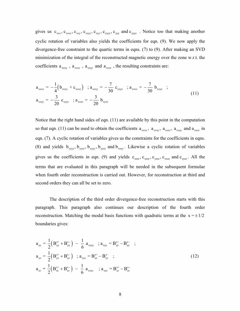
gives us . Notice too that making another

cyclic rotation of variables also yields the coefficients for eqn. (9). We now apply the

divergence-free constraint to the quartic terms in eqns. (7) to (9). After making an SVD

minimization of the integral of the reconstructed magnetic energy over the zone w.r.t. the

coefficients , and , the resulting constraints are:

xxx xxxz xxy xxyz xyy xyyz yyy yyyzc , c , c , c , c , c , c and c

xxxya xxxza , xxyya xxzza

( )xxxx xxxy

xyyz

b

c

xxxz

xxzz

+ c

; a

yyyy yyyz

x ; a

3 3 = − −

xyyy

xxy xxyz xxxz xxyz

xxyy

7a = = c ; a = b ; 0 30

a = b20 20

−

xyzz

1 74 3

− −

yyzz

(11)

Notice that the right hand sides of eqn. (11) are available by this point in the computation

so that eqn. (11) can be used to obtain the coefficients in

eqn. (7). A cyclic rotation of variables gives us the constraints for the coefficients in eqns.

(8) and yields

xxxx xxxy xxxz xxyy xxzza , a , a , a and a

xxyyb , b , b , b nd b a . Likewise a cyclic rotation of variables

gives us the coefficients in eqn. (9) and yields c . All the

terms that are evaluated in this paragraph will be needed in the subsequent formulae

when fourth order reconstruction is carried out. However, for reconstruction at third and

second orders they can all be set to zero.

zzzz xzzz yzzz xxzz yyzz, c , c , c and c

The description of the third order divergence-free reconstruction starts with this

paragraph. This paragraph also continues our description of the fourth order

reconstruction. Matching the modal basis functions with quadratic terms at the x = 1/2±

boundaries gives:

( )

( )

( )

x+ xyy y

x+ xyz yz

x+ xzz

B

B

B

x+ xyy y yy yy

x+yz x yz

x+ xzz zz zz zz

1 1a = B ; a B ; 2 61a = B ; a21 1a = B ; a B 2 6

− −

−

− −

+ − −

+ −

+ − −

xxyy

yz

xxzz

a

= B

a

−

xyy

xyz

xzz

= B

B ;

= B

(12)

8

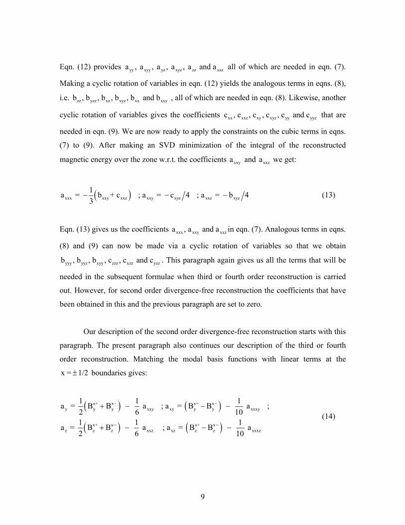
Eqn. (12) provides all of which are needed in eqn. (7).

Making a cyclic rotation of variables in eqn. (12) yields the analogous terms in eqns. (8),

i.e.

yy xyy yz xyz zz xzza , a , a , a , a and a

yz xx xxyzz yzz xz xb , b , b , b , b and b

c

, all of which are needed in eqn. (8). Likewise, another

cyclic rotation of variables gives the coefficients that are

needed in eqn. (9). We are now ready to apply the constraints on the cubic terms in eqns.

(7) to (9). After making an SVD minimization of the integral of the reconstructed

magnetic energy over the zone w.r.t. the coefficients and we get:

xx xxz xy xyz yy yyz, c , c , c , c and c

xxya xxza

( )xxx xxy xxz xxy xyz xxz xyz1a = b + c ; a = c 4 ; a = b 43

− − − (13)

Eqn. (13) gives us the coefficients in eqn. (7). Analogous terms in eqns.

(8) and (9) can now be made via a cyclic rotation of variables so that we obtain

xxx xxy xxza , a and a

yyy yyz xyy zzz xzz yzzb , b , b , c , c and c . This paragraph again gives us all the terms that will be

needed in the subsequent formulae when third or fourth order reconstruction is carried

out. However, for second order divergence-free reconstruction the coefficients that have

been obtained in this and the previous paragraph are set to zero.

Our description of the second order divergence-free reconstruction starts with this

paragraph. The present paragraph also continues our description of the third or fourth

order reconstruction. Matching the modal basis functions with linear terms at the

boundaries gives: x = 1/2±

( ) ( )

( ) ( )

x+ x x+ xy y y xxy xy y y xxxy

x+ x x+ xz z z xxz xz z z xxxz

1 1 1a = B B a ; a = B B a ; 2 6 101 1 1a = B B a ; a = B B a 2 6 10

− −

− −

+ − − −

+ − − − (14)

9

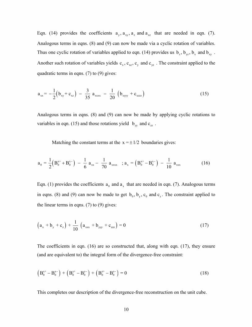
Eqn. (14) provides the coefficients that are needed in eqn. (7).

Analogous terms in eqns. (8) and (9) can now be made via a cyclic rotation of variables.

Thus one cyclic rotation of variables applied to eqn. (14) provides us

y xy z xa , a , a and a z

z yz x xyb , b , b and b .

Another such rotation of variables yields . The constraint applied to the

quadratic terms in eqns. (7) to (9) gives:

x xz yc , c , c and cyz

( ) (xx xy xz xxxx xyyy xzzz1 3 1a = b + c a b + c2 35 20

− − − ) (15)

Analogous terms in eqns. (8) and (9) can now be made by applying cyclic rotations to

variables in eqn. (15) and those rotations yield yy zzb and c .

Matching the constant terms at the x = 1/2± boundaries gives:

( ) ( )x+ x x+ x0 0 0 xx xxxx x 0 0 xxx

1 1 1a = B B a a ; a = B B a2 6 70 10

− −+ − − − −1

x

z

(16)

Eqn. (1) provides the coefficients that are needed in eqn. (7). Analogous terms

in eqns. (8) and (9) can now be made to get

0a and a

0 y 0b , b , c and c . The constraint applied to

the linear terms in eqns. (7) to (9) gives:

( ) (x y z xxx yyy zzz1a + b + c + a + b + c = 0

10) (17)

The coefficients in eqn. (16) are so constructed that, along with eqn. (17), they ensure

(and are equivalent to) the integral form of the divergence-free constraint:

( ) ( ) ( )x+ x y+ y z+ z0 0 0 0 0 0B B + B B + B B = 0− − −− − − (18)

This completes our description of the divergence-free reconstruction on the unit cube.

10

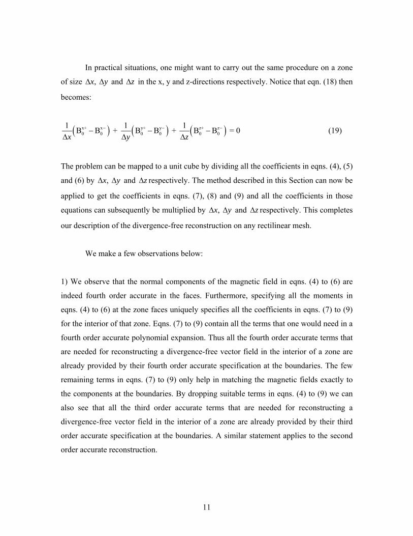
In practical situations, one might want to carry out the same procedure on a zone

of size , x yΔ Δ and in the x, y and z-directions respectively. Notice that eqn. (18) then

becomes:

zΔ

( ) ( ) ( )x+ x y+ y z+ z0 0 0 0 0 0

1 1 1B B + B B + B B = 0x y z

− −− − −Δ Δ Δ

− (19)

The problem can be mapped to a unit cube by dividing all the coefficients in eqns. (4), (5)

and (6) by , x yΔ Δ and respectively. The method described in this Section can now be

applied to get the coefficients in eqns. (7), (8) and (9) and all the coefficients in those

equations can subsequently be multiplied by

zΔ

, x yΔ Δ and zΔ respectively. This completes

our description of the divergence-free reconstruction on any rectilinear mesh.

We make a few observations below:

1) We observe that the normal components of the magnetic field in eqns. (4) to (6) are

indeed fourth order accurate in the faces. Furthermore, specifying all the moments in

eqns. (4) to (6) at the zone faces uniquely specifies all the coefficients in eqns. (7) to (9)

for the interior of that zone. Eqns. (7) to (9) contain all the terms that one would need in a

fourth order accurate polynomial expansion. Thus all the fourth order accurate terms that

are needed for reconstructing a divergence-free vector field in the interior of a zone are

already provided by their fourth order accurate specification at the boundaries. The few

remaining terms in eqns. (7) to (9) only help in matching the magnetic fields exactly to

the components at the boundaries. By dropping suitable terms in eqns. (4) to (9) we can

also see that all the third order accurate terms that are needed for reconstructing a

divergence-free vector field in the interior of a zone are already provided by their third

order accurate specification at the boundaries. A similar statement applies to the second

order accurate reconstruction.

11

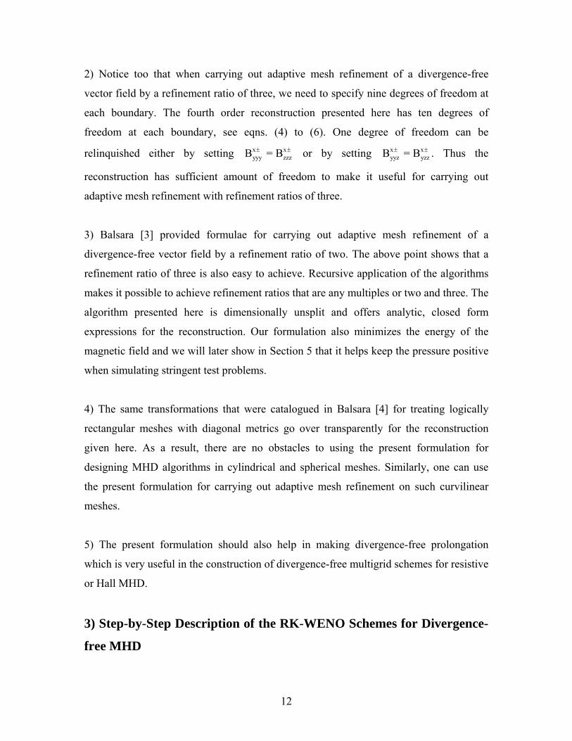
2) Notice too that when carrying out adaptive mesh refinement of a divergence-free

vector field by a refinement ratio of three, we need to specify nine degrees of freedom at

each boundary. The fourth order reconstruction presented here has ten degrees of

freedom at each boundary, see eqns. (4) to (6). One degree of freedom can be

relinquished either by setting xyyy zzzB = Bx± ± or by setting x

yyz yzzB = Bx± ± . Thus the

reconstruction has sufficient amount of freedom to make it useful for carrying out

adaptive mesh refinement with refinement ratios of three.

3) Balsara [3] provided formulae for carrying out adaptive mesh refinement of a

divergence-free vector field by a refinement ratio of two. The above point shows that a

refinement ratio of three is also easy to achieve. Recursive application of the algorithms

makes it possible to achieve refinement ratios that are any multiples or two and three. The

algorithm presented here is dimensionally unsplit and offers analytic, closed form

expressions for the reconstruction. Our formulation also minimizes the energy of the

magnetic field and we will later show in Section 5 that it helps keep the pressure positive

when simulating stringent test problems.

4) The same transformations that were catalogued in Balsara [4] for treating logically

rectangular meshes with diagonal metrics go over transparently for the reconstruction

given here. As a result, there are no obstacles to using the present formulation for

designing MHD algorithms in cylindrical and spherical meshes. Similarly, one can use

the present formulation for carrying out adaptive mesh refinement on such curvilinear

meshes.

5) The present formulation should also help in making divergence-free prolongation

which is very useful in the construction of divergence-free multigrid schemes for resistive

or Hall MHD.

3) Step-by-Step Description of the RK-WENO Schemes for Divergence-

free MHD

12

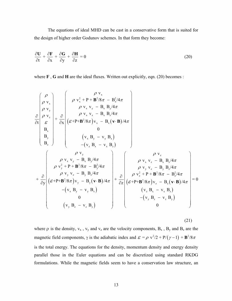
The equations of ideal MHD can be cast in a conservative form that is suited for

the design of higher order Godunov schemes. In that form they become:

+ + + = 0t x y z

∂ ∂ ∂ ∂∂ ∂ ∂ ∂U F G H (20)

where F , G and H are the ideal fluxes. Written out explicitly, eqn. (20) becomes :

( ) ( )

( )( )

x2 2 2x x

x

x y x yy

x z x zz

2x x

x

y x y y x

z z x x z

v v + P + /8 B /4 v

v v B B /4 v v v B B /4 v

+ +P+ /8 v B /4t x0B

B v B v BB v B v B

ρρρ π πρ

ρ πρρ πρ

π πεε

⎛ ⎞⎛ ⎞ ⎜ ⎟⎜ ⎟ −⎜ ⎟⎜ ⎟ ⎜ ⎟−⎜ ⎟ ⎜ ⎟⎜ ⎟ −⎜ ⎟∂ ∂⎜ ⎟ ⎜ ⎟− ⋅⎜ ⎟∂ ∂ ⎜ ⎟⎜ ⎟ ⎜ ⎟⎜ ⎟ ⎜ ⎟⎜ ⎟ −⎜ ⎟⎜ ⎟⎜ ⎟ ⎜ ⎟⎜ ⎟⎝ ⎠ − −⎝ ⎠

B

B v B

( ) ( )( )

( )

y z

x y x y x z x z2 2 2y y y z y z

y z y z z2

y y

x y y x

y z z y

v v v v B B /4 v v B B /4

v + P + /8 B /4 v v B B /4 v v B B /4 v

+ + +P+ /8 v B /4y zv B v B

0

v B v B

ρ ρρ π ρ π

ρ π π ρ πρ π ρ

π πε

⎛ ⎞⎜ ⎟− −⎜ ⎟⎜ ⎟− −⎜ ⎟−⎜ ⎟∂ ∂⎜ ⎟− ⋅∂ ∂⎜ ⎟⎜ ⎟− −⎜ ⎟⎜ ⎟⎜ ⎟⎜ ⎟−⎝ ⎠

B

B v B ( ) ( )( )( )

2 2 2z

2z z

z x x z

y z z y

+ P + /8 B /4= 0+P+ /8 v B /4

v B v B

v B v B

0

π π

π πε

⎛ ⎞⎜ ⎟⎜ ⎟⎜ ⎟⎜ ⎟−⎜ ⎟⎜ ⎟− ⋅⎜ ⎟⎜ ⎟−⎜ ⎟

− −⎜ ⎟⎜ ⎟⎜ ⎟⎝ ⎠

B

B v B

(21)

where ρ is the density, vx , vy and vz are the velocity components, Bx , By and Bz are the

magnetic field components, γ is the adiabatic index and ( )2 2= v /2 + P/ 1 + /8 ρ γ πε − B

is the total energy. The equations for the density, momentum density and energy density

parallel those in the Euler equations and can be discretized using standard RKDG

formulations. While the magnetic fields seem to have a conservation law structure, an

13

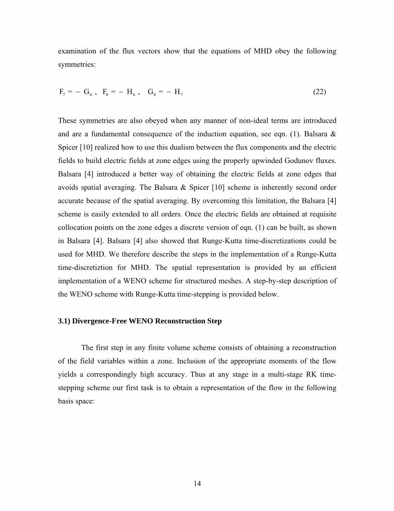
examination of the flux vectors show that the equations of MHD obey the following

symmetries:

7 6 8 6 8F = G , F = H , G = H − − − 7 (22)

These symmetries are also obeyed when any manner of non-ideal terms are introduced

and are a fundamental consequence of the induction equation, see eqn. (1). Balsara &

Spicer [10] realized how to use this dualism between the flux components and the electric

fields to build electric fields at zone edges using the properly upwinded Godunov fluxes.

Balsara [4] introduced a better way of obtaining the electric fields at zone edges that

avoids spatial averaging. The Balsara & Spicer [10] scheme is inherently second order

accurate because of the spatial averaging. By overcoming this limitation, the Balsara [4]

scheme is easily extended to all orders. Once the electric fields are obtained at requisite

collocation points on the zone edges a discrete version of eqn. (1) can be built, as shown

in Balsara [4]. Balsara [4] also showed that Runge-Kutta time-discretizations could be

used for MHD. We therefore describe the steps in the implementation of a Runge-Kutta

time-discretiztion for MHD. The spatial representation is provided by an efficient

implementation of a WENO scheme for structured meshes. A step-by-step description of

the WENO scheme with Runge-Kutta time-stepping is provided below.

3.1) Divergence-Free WENO Reconstruction Step

The first step in any finite volume scheme consists of obtaining a reconstruction

of the field variables within a zone. Inclusion of the appropriate moments of the flow

yields a correspondingly high accuracy. Thus at any stage in a multi-stage RK time-

stepping scheme our first task is to obtain a representation of the flow in the following

basis space:

14

( ) ( ) ( ) ( )( ) ( ) ( ) ( ) ( ) ( ) ( ) ( ) ( )( ) ( ) ( ) ( ) ( ) ( ) ( ) ( ) ( )( ) ( ) ( ) ( ) ( ) ( ) ( ) ( ) ( )

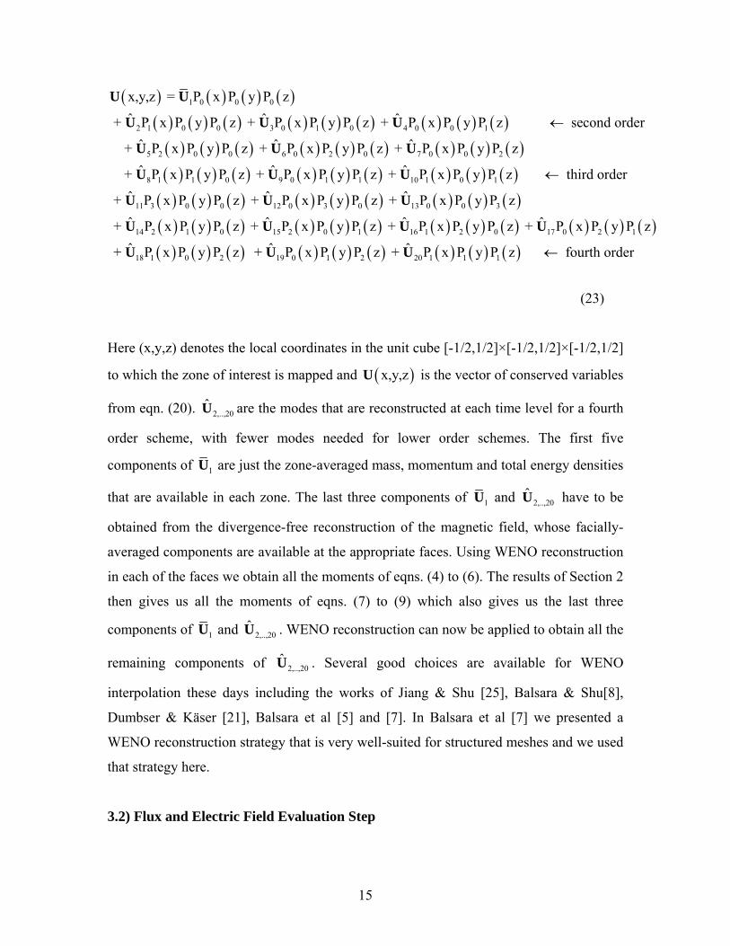
1 0 0 0

2 1 0 0 3 0 1 0 4 0 0 1

5 2 0 0 6 0 2 0 7 0 0 2

8 1 1 0 9 0 1 1 10 1 0 1

x,y,z = P x P y P zˆ ˆ ˆ + P x P y P z + P x P y P z + P x P y P z second order

ˆ ˆ ˆ + P x P y P z + P x P y P z + P x P y P zˆ ˆ ˆ + P x P y P z + P x P y P z + P x P y P z third

←

←

U U

U U U

U U U

U U U

( ) ( ) ( ) ( ) ( ) ( ) ( ) ( ) ( )( ) ( ) ( ) ( ) ( ) ( ) ( ) ( ) ( ) ( ) ( ) ( )( ) ( ) ( ) ( ) ( ) ( ) ( ) ( ) ( )

11 3 0 0 12 0 3 0 13 0 0 3

14 2 1 0 15 2 0 1 16 1 2 0 17 0 2 1

18 1 0 2 19 0 1 2 20 1 1 1

orderˆ ˆ ˆ + P x P y P z + P x P y P z + P x P y P zˆ ˆ ˆ ˆ + P x P y P z + P x P y P z + P x P y P z + P x P y P zˆ ˆ ˆ + P x P y P z + P x P y P z + P x P y P z fourth order←

U U U

U U U U

U U U

(23)

Here (x,y,z) denotes the local coordinates in the unit cube [-1/2,1/2]×[-1/2,1/2]×[-1/2,1/2]

to which the zone of interest is mapped and ( )x,y,zU is the vector of conserved variables

from eqn. (20). are the modes that are reconstructed at each time level for a fourth

order scheme, with fewer modes needed for lower order schemes. The first five

components of

2,..,20U

1U are just the zone-averaged mass, momentum and total energy densities

that are available in each zone. The last three components of 1U and have to be

obtained from the divergence-free reconstruction of the magnetic field, whose facially-

averaged components are available at the appropriate faces. Using WENO reconstruction

in each of the faces we obtain all the moments of eqns. (4) to (6). The results of Section 2

then gives us all the moments of eqns. (7) to (9) which also gives us the last three

components of

2,..,20U

1U and . WENO reconstruction can now be applied to obtain all the

remaining components of . Several good choices are available for WENO

interpolation these days including the works of Jiang & Shu [25], Balsara & Shu[8],

Dumbser & Käser [21], Balsara et al [5] and [7]. In Balsara et al [7] we presented a

WENO reconstruction strategy that is very well-suited for structured meshes and we used

that strategy here.

2,..,20U

U2,..,20

3.2) Flux and Electric Field Evaluation Step

15

A higher order scheme should also evaluate fluxes and electric fields with suitably

high accuracy. Traditionally this has been done by solving a large number of Riemann

problems at a large number of quadrature points as was done in Cockburn & Shu [14]. A

substantially simpler strategy was presented in Dumbser, Enaux & Toro [20] where the

flux is viewed as a linear combination of four vectors. The four vectors are: a) the

conserved variables to the left of the zone boundary given by , b) the

conserved variables to the right of the zone boundary given by , c) the

flux to the left of the zone boundary given by

(; 1/2, , y,zL i j k+U

(; 1/2, , y,zR i j k+U

)

)

( ); 1/2, , y,zL i j k+F and d) the flux to the right

of the zone boundary given by ( )z; 1/2, , y,R i j k+F . The strategy proposed by Dumbser,

Enaux & Toro [20] applies to the space-time domain. We specialize it for the case where

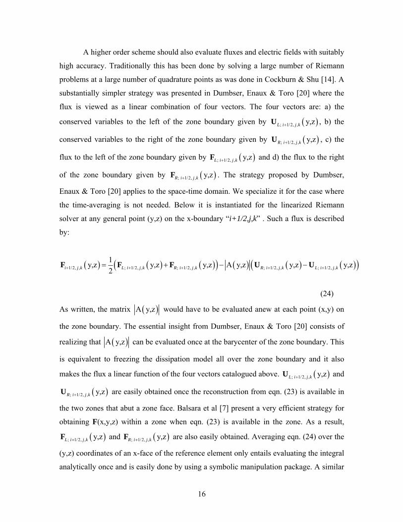
the time-averaging is not needed. Below it is instantiated for the linearized Riemann

solver at any general point (y,z) on the x-boundary “i+1/2,j,k” . Such a flux is described

by:

( ) ( ) ( )( ) ( ) ( ) ( )( )1/2, , ; 1/2, , ; 1/2, , ; 1/2, , ; 1/2, ,1y,z y,z y,z A y,z y,z y,z2i j k L i j k R i j k R i j k L i j k+ + + + += + − −F F F U U

(24)

As written, the matrix ( )A y,z would have to be evaluated anew at each point (x,y) on

the zone boundary. The essential insight from Dumbser, Enaux & Toro [20] consists of

realizing that ( )A y,z can be evaluated once at the barycenter of the zone boundary. This

is equivalent to freezing the dissipation model all over the zone boundary and it also

makes the flux a linear function of the four vectors catalogued above. and

are easily obtained once the reconstruction from eqn. (23) is available in

the two zones that abut a zone face. Balsara et al [7] present a very efficient strategy for

obtaining F(x,y,z) within a zone when eqn. (23) is available in the zone. As a result,

and are also easily obtained. Averaging eqn. (24) over the

(y,z) coordinates of an x-face of the reference element only entails evaluating the integral

analytically once and is easily done by using a symbolic manipulation package. A similar

(; 1/2, , y,zL i j k+U )

)

)

(; 1/2, , y,zR i j k+U

( ); 1/2, , y,zL i j k+F (; 1/2, , y,zR i j k+F

16

strategy can be applied at the y and z-faces. The electric fields are also easily obtained by

averaging eqn. (24) suitably over the edges of the reference element and picking out the

appropriate components of the fluxes. Four electric field contributions are available at

each edge, one from each of the four faces that come together at that edge. These electric

fields are averaged, as in Balsara [4] to obtain the final electric field at the zone of

interest. This completes our description of the fluid flux and the electric field evaluation

for any stage in our multi-stage RK time-update.

3.3) Multi-Stage Runge Kutta Time Update Step

The strong stability preserving Runge Kutta schemes from Shu & Osher [31] and

[32] are used for carrying out a time update. At each stage of the multi-stage RK update,

we apply the steps from Sub-Sections 3.1 and 3.2 to obtain the fluxes at each face and the

electric field components at each edge. The Runge-Kutta time-stepping schemes consist

of writing eqn. (1) for the magnetic field evolution and eqn. (20) for the evolution of the

mass, momentum and energy densities in the form

( )d = Ld t

U U (25)

Where L(U) is a discretization of the spatial operator. The second order TVD Runge-

Kutta scheme is simply the Heun scheme:

( )( )

(1) n n

n+1 n (1)

1 = + t L2

= + t L

Δ

Δ

U U U

U U U (26)

The third order TVD Runge-Kutta scheme is given by:

17

( )( )

( )

(1) n n

(2) n (1) (1)

n+1 n (2) (2)

= + t L

3 1 1 = + + t L4 4 41 2 2 = + + t L3 3 3

Δ

Δ

Δ

U U U

U U U U

U U U U

(27)

The fourth order RK scheme from Shu & Osher [31] is rather complicated to implement

and was not implemented here. As a result, the temporal update of the spatially fourth

order scheme was always done with eqn. (27). For most applications this yields a

serviceable scheme that functions at a robust Courant number. However when

demonstrating the order of accuracy at fourth order in Section 4 we had to reduce the

Courant number by a factor of ~ 0.396 for every doubling of the number of zones. This

had to be done so that the third order temporal accuracy from eqn. (27) keeps step with

the fourth order spatial accuracy. This deficiency is ameliorated by the ADER (for

Arbitrary Derivative Riemann Problem) schemes presented in Balsara et al [7].

4) Accuracy Analysis

The schemes presented here handily meet their design accuracies in one

dimension. It is therefore interesting to present multi-dimensional tests showing high

order of accuracy. Here we present a couple of demonstrations of high accuracy in two

and three dimensions. A more extensive accuracy analysis for hydrodynamic and MHD

problems has been catalogued in Balsara et al [7] for a new class of ADER-WENO

schemes.

A couple of points need to be made about the simulations presented here. First,

following Balsara [4] we used the slopes from the r=3 WENO reconstruction of Jiang &

Shu [25] for our second order scheme. As a result, the slopes have one more order of

accuracy than the accuracy that would be furnished by a TVD-preserving limiter. This

yields a very superior second order scheme. Second, for all the accuracy analyses

18

presented in this section involving the spatially fourth order scheme, the Courant number

was always decreased by a factor of 0.396 for every doubling of the number of zones.

4.1) Magnetized Isodensity Vortex in Two Dimensions

This test problem as described in Balsara [4] consists of a magnetized vortex

moving across a domain given by [-5, 5] x [-5, 5] at an angle of 45° for a time of 10 units.

For the fourth order scheme the domain is increased to [-10, 10] x [-10, 10] and the

simulation time is increased to 20 units. This is done because the magnetic field has a

Gaussian decay with radius and the smaller domain retains a small but significant amount

of magnetic field at the boundary. Had we used the smaller domain for the fourth order

scheme, this small but spurious magnetic field would actually have been picked up by the

scheme and its order property would have been damaged. The problem is initialized with

an unperturbed flow of ( , , , , , ) (1, 1, 1, 1, 0, 0)x y x yP v v B Bρ = . All boundaries are

periodic. The ratio of the specific heat is set to 5 / 3γ = . The vortex is set up as a

fluctuation of the unperturbed flow in the velocities and the magnetic field given by:

20.5(1 )( , ) ( ,2

rx yv v e y xκδ δ

π−= − )

20.5(1 )( , ) ( ,2

rx y )B B e y xμδ δ

π−= −

The pressure fluctuation can be written as

2 22 2 (1 ) 2 (1 )1 1( ) (1 ) ( )8 2 2 2

r rP r e eμ κδπ π π

− −= − −

The density is set to unity. A Courant number of 0.4 was used for all the second and third

order test problems and also for the coarsest mesh in the fourth order test problem. A

linearized Riemann solver was used.

TABLE I

Method Number of zones L1 error L1 order L∞ error L∞ order

19

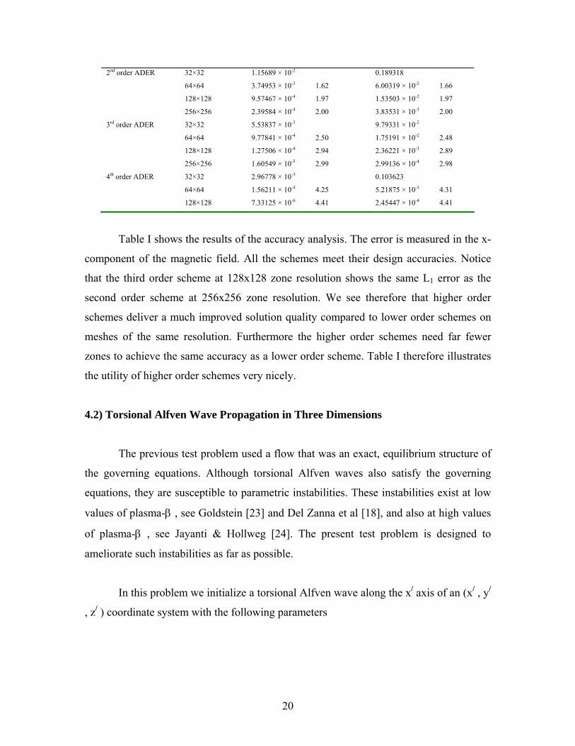
2nd order ADER 32×32 1.15689 × 10-2 0.189318

64×64 3.74953 × 10-3 1.62 6.00319 × 10-2 1.66

128×128 9.57467 × 10-4 1.97 1.53503 × 10-2 1.97

256×256 2.39584 × 10-4 2.00 3.83531 × 10-3 2.00

3rd order ADER 32×32 5.53837 × 10-3 9.79331 × 10-2

64×64 9.77841 × 10-4 2.50 1.75191 × 10-2 2.48

128×128 1.27506 × 10-4 2.94 2.36221 × 10-3 2.89

256×256 1.60549 × 10-5 2.99 2.99136 × 10-4 2.98

4th order ADER 32×32 2.96778 × 10-3 0.103623

64×64 1.56211 × 10-4 4.25 5.21875 × 10-3 4.31

128×128 7.33125 × 10-6 4.41 2.45447 × 10-4 4.41

Table I shows the results of the accuracy analysis. The error is measured in the x-

component of the magnetic field. All the schemes meet their design accuracies. Notice

that the third order scheme at 128x128 zone resolution shows the same L1 error as the

second order scheme at 256x256 zone resolution. We see therefore that higher order

schemes deliver a much improved solution quality compared to lower order schemes on

meshes of the same resolution. Furthermore the higher order schemes need far fewer

zones to achieve the same accuracy as a lower order scheme. Table I therefore illustrates

the utility of higher order schemes very nicely.

4.2) Torsional Alfven Wave Propagation in Three Dimensions

The previous test problem used a flow that was an exact, equilibrium structure of

the governing equations. Although torsional Alfven waves also satisfy the governing

equations, they are susceptible to parametric instabilities. These instabilities exist at low

values of plasma-β , see Goldstein [23] and Del Zanna et al [18], and also at high values

of plasma-β , see Jayanti & Hollweg [24]. The present test problem is designed to

ameliorate such instabilities as far as possible.

In this problem we initialize a torsional Alfven wave along the x/ axis of an (x/ , y/

, z/ ) coordinate system with the following parameters

20

( )/ / /

/ / /

/

x y z

x y z

21 , P = 1000 , x 2 t

v 1 , v cos , v sin

B 4 , B 4 cos , 4 sinB

πρλ

ε ε

πρ ε πρ ε πρ

= Φ = −

= = Φ = Φ

= = − Φ = − Φ

Here we take 0.02ε = and 3λ = . The magnetic vector potential is also useful when

initializing a divergence-free magnetic field on a mesh and is given by

/ / //

x y zA 0 , A cos , A 4 y sinελ ρ π πρ ελ ρ π= = Φ = + Φ

The actual problem is solved on a unit cube in the (x,y,z) coordinate frame which is

rotated relative to the (x/ , y/ , z/ ) coordinate system. The rotation matrix is called A and

is given by

cos cos cos sin sin cos sin cos cos sin sin sin = sin cos cos sin cos sin sin cos cos cos cos sin

sin sin sin cos cos

ψ φ θ φ ψ ψ φ θ φ ψ ψ θψ φ θ φ ψ ψ φ θ φ ψ ψ

θ φ θ φ θ

− +⎡ ⎤⎢ ⎥− − − +⎢ ⎥⎢ ⎥−⎣ ⎦

A θ

where / 4φ π= − , (1sin 2 3θ −= − ) and ( )( )1sin 2 6 4ψ −= − . As a result, the

position vector r/ in the primed frame transforms to the position vector r in the unprimed

frame as r = A r/ . Other vectors transform similarly. Application of the rotation matrix

makes the wave propagate along the diagonal of the unit cube. The wave propagates at a

speed of 2 units. The problem is stopped at a time of 3 2 by which time the wave has

propagated once around the unit cube. A Courant number of 0.3 was used for all the

second and third order test problems and also for the coarsest mesh in the fourth order

test problem. A linearized Riemann solver was used.

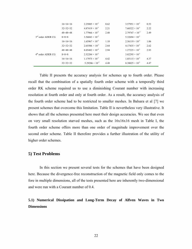
Table II Method Number of zones L1 error L1 order L∞ error L∞ order

2nd order ADER CG 8×8×8 3.46827 × 10-2 5.17569 × 10-2

21

16×16×16 2.25885 × 10-2 0.62 3.57951 × 10-2 0.53

32×32×32 4.87419 × 10-3 2.21 7.68322 × 10-3 2.22

48×48×48 1.77966 × 10-3 2.48 2.79747 × 10-3 2.49

3rd order ADER CG 8×8×8 3.56043 × 10-2 5.32694 × 10-2

16×16×16 1.65967 × 10-2 1.10 2.56119 × 10-2 1.06

32×32×32 2.65506 × 10-3 2.64 4.17435 × 10-3 2.62

48×48×48 8.05482 × 10-4 2.94 1.27225 × 10-3 2.93

4th order ADER CG 8×8×8 2.52284 × 10-2 3.82295 × 10-2

16×16×16 1.17975 × 10-3 4.42 1.85115 × 10-3 4.37

32×32×32 5.29206 × 10-5 4.48 8.38025 × 10-5 4.47

Table II presents the accuracy analysis for schemes up to fourth order. Please

recall that the combination of a spatially fourth order scheme with a temporally third

order RK scheme required us to use a diminishing Courant number with increasing

resolution at fourth order and only at fourth order. As a result, the accuracy analysis of

the fourth order scheme had to be restricted to smaller meshes. In Balsara et al [7] we

present schemes that overcome this limitation. Table II is nevertheless very illustrative. It

shows that all the schemes presented here meet their design accuracies. We see that even

on very small resolution starved meshes, such as the 16x16x16 mesh in Table I, the

fourth order scheme offers more than one order of magnitude improvement over the

second order scheme. Table II therefore provides a further illustration of the utility of

higher order schemes.

5) Test Problems

In this section we present several tests for the schemes that have been designed

here. Because the divergence-free reconstruction of the magnetic field only comes to the

fore in multiple dimensions, all of the tests presented here are inherently two-dimensional

and were run with a Courant number of 0.4.

5.1) Numerical Dissipation and Long-Term Decay of Alfven Waves in Two

Dimensions

22

This test problem was first presented in Balsara [4] and examines the dissipation

of torsional Alfven waves in two dimensions. Here the torsional Alfven waves propagate

at an angle of to the y-axis through a domain given by [-

r/2, r/2] x [-r/2, r/2] with r = 6. The problem was initialized on a computaitonal domain

with 120 x 120 zones. Periodic boundary conditions were enforced. The pressure and

density are uniformly initialized as

1 1tan (1/ ) tan (1/ 6) 9.462r− −= =

0 1P

°

= and 0 1ρ = . The unperturbed velocity and

unperturbed magnetic field are given by 0 0v = and 0B 1= . The amplitude of the Alfven

waves is parametrized by ε , which is set to 0.2. The simulation was stopped at 129 time

units by which time the waves had crossed the domain several times. The CFL number

was set to 0.4 for all the schemes presented here. The direction of the wave propagation

along the unit vector can be written as

2 2

1ˆ ˆ ˆˆ1 1

x yrn n i n j i j

r r= + = +

+ +ˆ .

The phase of the waves is given by

2 ( )x y Ay

n x n y V tnπφ = + − , where 0

04ABVπρ

= .

The velocity is given by

0 0ˆˆ ˆ( cos ) ( cos ) six y y xv n n i v n n j knε φ ε φ ε= − + − +v φ .

The magnetic field is given by

0 0 0 0 0ˆˆ ˆ( 4 cos ) ( 4 cos ) 4 sinx y y xB n n i B n n j kε πρ φ ε πρ φ ε πρ φ= + + − −B .

The corresponding vector potential is given by

23

000 0

44 ˆˆcos ( sin )2 2

yy x

ni B n x B n y

ε πρε πρkφ φ

π π= − + − + +A

and is used to initialize the magnetic field.

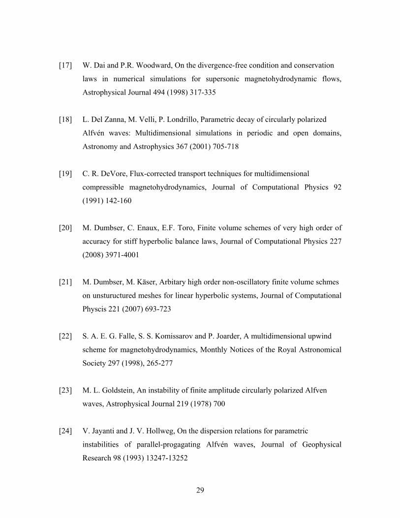
Fig. 1 shows the time-evolution of the maximum of the z-velocity and the

maximum of the z-component of magnetic field. All the panels in Fig. 1 use log-linear

scaling. To explore the effect of Riemann solvers on this problem, the HLL and

linearized Riemann solvers were used with the second, third and fourth order schemes.

For comparison purposes, we also present results from a second order TVD scheme using

vanLeer’s MC limiter. We see that regardless of the Riemann solver used, increasing the

order of accuracy provides a substantial reduction in the numerical dissipation. Thus

higher order schemes are favored for the simulation of complex phenomena involving

wave propagation. For the lower order schemes the linearized Riemann solver offers a

significant improvement over the HLL Riemann solver. However, this advantage is

diminished with increasing order. We therefore see that higher order schemes allow us to

get by with less expensive Riemann solvers.

5.2) The Rotor Problem in Two Dimensions

The two dimensional rotor problem was presented in Balsara & Spicer [10] and in

Balsara [4]. The description in Balsara [4] is quite thorough. As a result the problem

description is not repeated here. As in Balsara [4] the problem was set up on a 200x200

zone mesh and was run with a Courant number of 0.4 to a completion time of 0.29 units.

The spatially fourth order WENO scheme with a third order RK time-stepping strategy

and a linearized Riemann solver were used. Fig. 2 shows the density, pressure, Mach

number and the magnitude of the magnetic field. The results are very consistent with

those from Balsara & Spicer [10] showing that the divergence-free reconstruction

presented here performs well on multi-dimensional MHD problems.

5.3) The Blast Problem in Two Dimensions

24

This two-dimensional problem was first presented by Balsara & Spicer [10]. It

has also been catalogued in detail in Balsara [4] and we do not repeat the same

description here. The fourth order WENO scheme with a third order RK time-stepping

strategy and an HLL Riemann solver was applied to a mesh having 200 × 200 zones. The

problem was run with a Courant number of 0.4 and was stopped at a time of 0.01 units.

The problem results in an extremely strong, almost circular fast magnetosonic shock

propagating at all possible angles to the magnetic field in the low-β ambient plasma. The

plasma-β is 0.000251 making this a challenging test problem. Fig. 3 shows the logarithm

(base 10) of the density, the logarithm of the pressure, the magnitude of the velocity and

the magnitude of the magnetic field. We see that all structures are captured crisply. The

positivity of the pressure is maintained even in regions where the strong shock propagates

obliquely to the mesh. This shows that the divergence-free reconstruction strategies and

the resultant high order schemes presented here perform well on stringent multi-

dimensional MHD problems involving low-β plasmas.

6) Conclusions

The work presented here enables us to come to the following conclusions:

1) Following a line of development begun in Balsara [3], we show that the problem of

reconstructing divergence-free vector fields can be carried out to higher orders.

2) Following a line of development begun in Balsara [4], we show that the above

development yields divergence-free WENO schemes with order of accuracy that is better

than second. In particular, we explore the third and fourth order accurate schemes here.

3) When applied to smooth test problems, the schemes have been shown to meet their

design accuracies.

25

4) Using a stringent set of test problems we show that the schemes presented here

effectively combine the dual, and often-conflicting demands of capturing very strong

shocks and retaining low dissipation in contact discontinuities and Alfven waves. This

shows the effectiveness of our schemes for numerical MHD.

Acknowledgements

DSB acknowledges support via NSF grant AST-0607731. DSB also acknowledges

NASA grants HST-AR-10934.01-A, NASA-NNX07AG93G and NASA-NNX08AG69G.

The majority of simulations were performed on PC clusters at UND but a few initial

simulations were also performed at NASA-NCCS.

26

References

[1] D. S. Balsara, Linearized formulation of the Riemann problem for adiabatic and

isothermal magnetohydrodynamics, Astrophysical Journal Supplement 116

(1998) 119

[2] D.S. Balsara, Total variation diminishing algorithm for adiabatic and isothermal

magnetohydrodynamics, Astrophysical Journal Supplement 116 (1998) 133

[3] D.S. Balsara , Divergence-free adaptive mesh refinement for

magnetohydrodynamics, Journal of Computational Physics 174 (2001) 614-648

[4] D. S. Balsara, Second-order-accurate schemes for magnetohydrodynamics with

divergence-free reconstruction, Astrophysical Journal Supplement 151 (2004)

149-184

[5] D. S. Balsara, C. Altmann, C.D. Munz, M. Dumbser, A sub-cell based indicator

for troubled zones in RKDG schemes and a novel class oh hybrid

RKDG+HWENO schemes, Journal of Computational Physics 226 (2007) 586-

620

[6] D.S. Balsara & J.S. Kim, An Intercomparison Between Divergence-Cleaning and

Staggered Mesh Formulations for Numerical Magnetohydrodynamics ,

Astrophysical Journal 602 (2004) 1079

[7] D.S. Balsara, T. Rumpf, M. Dumbser and C.-D. Munz, Efficient, high accuracy

ADER-WENO schemes for hydrodynamics and divergence-free

magnetohydrodynamics, submitted, Journal of Computational Physics (2008)

27

[8] D. S. Balsara and C.-W. Shu, Monotonicity Preserving Weighted Non-oscillatory

schemes wirh increasingly High Order of Accuracy, Journal of Computational

Physics 160 (2000) 405-452

[9] D. S. Balsara and D. S. Spicer, Maintaining pressure positivity in

magnetohydrodynamic simulations, Journal of Computational Physics 148

(1999) 133-148

[10] D. S. Balsara and D. S. Spicer, A staggered mesh algorithm using high order

Godunov fluxes to ensure solenoidal magnetic fields in magnetohydrodynamic

simulations, Journal of Computational Physics 149 (1999) 270-292

[11] J. U. Brackbill and D. C. Barnes, The effect of nonzero · B on the numerical

solution of the magnetohydrodynamic equations, Journal of Computational

Physics 35 (1980) 426-430

[12] S. H. Brecht, J. G. Lyon, J. A. Fedder, K. Hain, A simulation study of east-west

IMF effects on the magnetosphere, Geophysical Reserach Lett. 8 (1981) 397

[13] M. Brio & C.C. Wu , An upwind differencing scheme for the equations of ideal

magnetohydrodynamics, Journal of Computational Physics 75 (1988) 400

[14] B. Cockburn and C.-W. Shu, The Runge-Kutta discontinuous Galerkin method for

Conservation Laws V, Journal of Computational Physics 141 (1998) 199-224

[15] R. K. Crockett, P. Colella, R. T. Fisher, R. I. Klein & C. F. McKee, An unsplit

cell-centered Godunov method for ideal MHD, Journal of Computational Physics

203 (2005) 422

[16] W. Dai and P.R. Woodward, An approximate Riemann solver for ideal

magnetohydrodynamics, Journal of Computational Physics 111 (1994) 354-372

28

[17] W. Dai and P.R. Woodward, On the divergence-free condition and conservation

laws in numerical simulations for supersonic magnetohydrodynamic flows,

Astrophysical Journal 494 (1998) 317-335

[18] L. Del Zanna, M. Velli, P. Londrillo, Parametric decay of circularly polarized

Alfvén waves: Multidimensional simulations in periodic and open domains,

Astronomy and Astrophysics 367 (2001) 705-718

[19] C. R. DeVore, Flux-corrected transport techniques for multidimensional

compressible magnetohydrodynamics, Journal of Computational Physics 92

(1991) 142-160

[20] M. Dumbser, C. Enaux, E.F. Toro, Finite volume schemes of very high order of

accuracy for stiff hyperbolic balance laws, Journal of Computational Physics 227

(2008) 3971-4001

[21] M. Dumbser, M. Käser, Arbitary high order non-oscillatory finite volume schmes

on unstuructured meshes for linear hyperbolic systems, Journal of Computational

Physcis 221 (2007) 693-723

[22] S. A. E. G. Falle, S. S. Komissarov and P. Joarder, A multidimensional upwind

scheme for magnetohydrodynamics, Monthly Notices of the Royal Astronomical

Society 297 (1998), 265-277

[23] M. L. Goldstein, An instability of finite amplitude circularly polarized Alfven

waves, Astrophysical Journal 219 (1978) 700

[24] V. Jayanti and J. V. Hollweg, On the dispersion relations for parametric

instabilities of parallel-progagating Alfvén waves, Journal of Geophysical

Research 98 (1993) 13247-13252

29

[25] G.-S. Jiang and C.-W. Shu, Efficient implementation of weighted ENO schemes,

Journal of Computational Physics 126 (1996) 202-228

[26] G.-S. Jiang & C.C. Wu, A high-order WENO finite difference scheme for the

equations of ideal magnetohydrodynamics, J. Comput. Phys., 150(2) (1999)

561-594

[26] P. Londrillo and L. DelZanna, On the divergence-free condition in Godunov-type

schemes for ideal magnetohydrodynamics: the upwind constrained transport

method, Journal of Computational Physics 195 (2004) 17-48

[27] Powell, K.G. An Approximate Riemann Solver for MHD ( that actually works in

more than one dimension), ICASE Report No. 94-24, Langley VA, (1994)

[28] P. L. Roe and D. S. Balsara, Notes on the eigensystem of magnetohydrodynamics,

SIAM Journal of applied Mathematics 56 (1996), 57

[29] D. Ryu and T.W. Jones, Numerical MHD in astrophysics: algorithm and tests for

one-dimensional flow, Astrophysical Journal 442 (1995) 228

[30] D. Ryu, F. Miniati, T. W. Jones, and A. Frank, A divergence-free upwind code for

multidimensional magnetohydrodynamic flows, Astrophysical Journal 509 (1998)

244-255

[31] C.-W. Shu and S. J. Osher, Efficient implementation of essentially non-oscillatory

shock capturing schemes, Journal of Computational Physics 77 (1988) 439-471

[32] C.-W. Shu and S. J. Osher, Efficient implementation of essentially non-oscillatory

shock capturing schemes II, Journal of Computational Physics 83 (1989) 32-78

30

31

[33] K.S. Yee, Numerical Solution of Initial Boundary Value Problems Involving

Maxwell Equation in an Isotropic Media, IEEE Trans. Antenna Propagation 14

(1966) 302

[34] A.L. Zachary, A. Malagoli & P. Colella, A higher-order Godunov method for multi-dimensional ideal Magnetohydrodynamics, SIAM J. Sci. Comput., 15 (1994) 263

Fig

1) T

he lo

g-lin

ear p

lots

sho

w th

e de

cay

of to

rsio

nalA

lfven

wav

es th

at

prop

agat

e ob

lique

ly o

n a

two

dim

ensi

onal

squ

are.

The

top

two

pane

ls s

how

the

deca

y of

the

max

imum

z-v

eloc

ity a

nd th

e m

axim

um z

-com

pone

nt o

f the

m

agne

tic fi

eld

whe

n se

cond

, thi

rd a

nd fo

urth

ord

er s

chem

es a

re u

sed

with

an

HLL

E R

iem

ann

solv

er. T

he b

otto

m tw

o pa

nels

sho

w th

e sa

me

info

rmat

ion

whe

n a

linea

rized

Rie

man

n so

lver

is u

sed.

For

com

paris

on

purp

oses

, the

resu

lts fr

om a

TV

D s

chem

e w

ith M

C li

mite

r are

als

osh

own.

Te

mpo

rally

third

ord

er R

K u

pdat

es w

ere

used

for t

he s

patia

lly fo

urth

ord

er

sche

me.

Obs

erve

that

the

deca

y is

sub

stan

tially

redu

ced

with

incr

easi

ng

spat

ial o

rder

. Als

o ob

serv

e th

at th

e lin

eariz

edR

iem

ann

solv

er p

rovi

des

a su

bsta

ntia

l im

prov

emen

t to

the

solu

tion,

esp

ecia

lly a

t low

er o

rder

s.

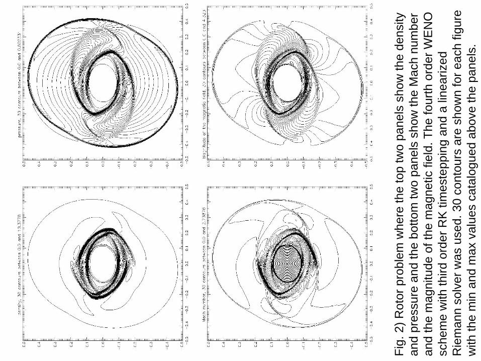
Fig.

2) R

otor

pro

blem

whe

re th

e to

p tw

o pa

nels

sho

w th

e de

nsity

an

d pr

essu

re a

nd th

e bo

ttom

two

pane

ls s

how

the

Mac

h nu

mbe

r an

d th

e m

agni

tude

of t

he m

agne

tic fi

eld.

The

four

th o

rder

WE

NO

sc

hem

e w

ith th

ird o

rder

RK

tim

este

ppin

gan

d a

linea

rized

Rie

man

n so

lver

was

use

d. 3

0 co

ntou

rs a

re s

how

n fo

r eac

h fig

ure

with

the

min

and

max

val

ues

cata

logu

ed a

bove

the

pane

ls.

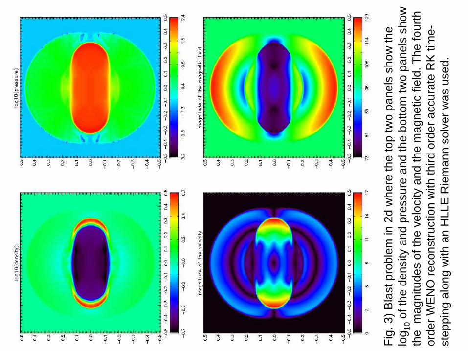
Fig.

3) B

last

pro

blem

in 2

d w

here

the

top

two

pane

ls s

how

the

log 1

0of

the

dens

ity a

nd p

ress

ure

and

the

botto

m tw

o pa

nels

sho

w

the

mag

nitu

des

of th

e ve

loci

ty a

nd th

e m

agne

tic fi

eld.

The

four

th

orde

r WE

NO

reco

nstru

ctio

n w

ith th

ird o

rder

acc

urat

e R

K ti

me-

step

ping

alo

ng w

ith a

n H

LLE

Rie

man

n so

lver

was

use

d.