The marine diversity spectrum

Daniel C. Reuman1,2*, Henrik Gislason3, Carolyn Barnes4, Fr�ed�eric M�elin5 and

Simon Jennings4,6

1Department of Life Sciences, Imperial College London, Silwood Park Campus, Ascot SL5 7PY, UK; 2Laboratory of

Populations, Rockefeller University, 1230 York Ave, New York, NY 10065, USA; 3Technical University of Denmark,

Charlottenlund Slot, DK-2920, Charlottenlund, Denmark; 4Centre for Environment, Fisheries and Aquaculture Science,

Lowestoft, Suffolk, NR33 OHT, UK; 5European Commission, Joint Research Centre, Institute for Environment and

Sustainability, 21027, Ispra (VA), Italy; and 6School of Environmental Sciences, University of East Anglia, Norwich,

NR4 7TJ, UK

Summary

1. Distributions of species body sizes within a taxonomic group, for example, mammals, are

widely studied and important because they help illuminate the evolutionary processes that

produced these distributions. Distributions of the sizes of species within an assemblage delin-

eated by geography instead of taxonomy (all the species in a region regardless of clade) are

much less studied but are equally important and will illuminate a different set of ecological

and evolutionary processes.

2. We develop and test a mechanistic model of how diversity varies with body mass in marine

ecosystems. The model predicts the form of the ‘diversity spectrum’, which quantifies the dis-

tribution of species’ asymptotic body masses, is a species analogue of the classic size spectrum

of individuals, and which we have found to be a new and widely applicable description of

diversity patterns.

3. The marine diversity spectrum is predicted to be approximately linear across an asymptotic

mass range spanning seven orders of magnitude. Slope �0�5 is predicted for the global marine

diversity spectrum for all combined pelagic zones of continental shelf seas, and slopes for

large regions are predicted to lie between �0�5 and �0�1. Slopes of �0�5 and �0�1 represent

markedly different communities: a slope of �0�5 depicts a 10-fold reduction in diversity for

every 100-fold increase in asymptotic mass; a slope of �0�1 depicts a 1�6-fold reduction. Stee-

per slopes are predicted for larger or colder regions, meaning fewer large species per small

species for such regions.

4. Predictions were largely validated by a global empirical analysis.

5. Results explain for the first time a new and widespread phenomenon of biodiversity.

Results have implications for estimating numbers of species of small asymptotic mass, where

taxonomic inventories are far from complete. Results show that the relationship between

diversity and body mass can be explained from the dependence of predation behaviour,

dispersal, and life history on body mass, and a neutral assumption about speciation and

extinction.

Key-words: biodiversity, body mass, community, neutral theory, power law, size spectrum

Introduction

Most species are small. The nature of this bias and its

causes and ramifications have been a focus of ecological

and evolutionary research for decades (e.g. Hutchinson &

MacArthur 1959; Van Valen 1973; May 1978; Dial &

Marzluff 1988; Maurer & Brown 1988; Blackburn & Gas-

ton 1994; Loder, Blackburn & Gaston 1997; Purvis, Orme

& Dolphin 2003; Marquet et al. 2005; Clauset & Erwin

2008). As well as illuminating ecological and evolutionary

processes, body mass–diversity relationships are important

for conservation because they help quantify existing diver-

sity. Most past work has considered these relationships in

species assemblages delineated by taxon (e.g. mammals).

We approach the topic from a fundamentally different*Correspondence author. E-mail: d.reuman@imperial.ac.uk

© 2014 The Authors. Journal of Animal Ecology published by John Wiley & Sons Ltd on behalf of British Ecological Society.This is an open access article under the terms of the Creative Commons Attribution License, which permits use, distribution andreproduction in any medium, provided the original work is properly cited.

Journal of Animal Ecology 2014 doi: 10.1111/1365-2656.12194

but equally important perspective: how can body mass-

diversity relationships be explained for geographically

delineated but taxon-inclusive assemblages, that is, all the

species in a region? Different mechanisms will take pri-

macy in this new context. For instance, while patterns in

taxon-specific global assemblages will be strongly affected

by evolutionary history and physiological constraints of

the taxon, patterns in geographically constrained assem-

blages will be more affected by community assembly. We

here offer a first empirical description and explanatory

model of mass-diversity patterns in an important class of

geographically constrained assemblages: those in the

world’s continental shelf seas.

We consider a community consisting of individuals in

any specified focal region in the world’s continental shelf

seas and with asymptotic mass in any specified focal

range. Diversity of the community is influenced by four

main quantities that form the main structural components

of our model: (1) the number of individuals in the com-

munity; (2) the number of individuals in a much larger

‘metacommunity’ that is outside the focal region but that

is delimited by the same asymptotic mass range; (3) com-

monness of dispersal between the community and meta-

community; and (4) a speciation rate. These determinants

of diversity are well known from the theory of island bio-

geography (MacArthur & Wilson 2001) and the neutral

theory of biodiversity (Hubbell 2001). By unifying and

extending life history and size spectrum theory from sev-

eral sources (e.g. Ware 1978; West, Brown & Enquist

2001; Andersen & Beyer 2006), our model makes predic-

tions from first principles for how these four quantities

depend on the asymptotic mass bounds used and the envi-

ronment in the focal region. The model then combines the

results using formulas from neutral theory (Etienne & Olff

2004) to predict community diversity. Diversity refers to

numbers of species throughout.

Our model answers several specific questions. What is

the diversity in the focal community and how does it

depend on the asymptotic mass range used? How is the

relationship between diversity and mass affected by the

environmental characteristics of the focal region? What

are the individual- and population-level mechanisms con-

trolling these patterns?

The main assumption of our model is that organisms of

similar asymptotic mass in marine pelagic realms can be

approximated to be equivalent competitors – this is the

neutral assumption. Our theory applies principally to

pelagic environments because the neutral assumption and

model parameterizations of life history, predation and dis-

persal are more likely accurate there. ‘Pelagic’ is used here

and throughout to encompass organisms living or inter-

acting primarily in the water column, including bottom-

dwelling species which live on or near the sea bed but are

not permanently constrained to the substrate. We exclude

coral reefs and reef-associated species. Each species is

assigned a characteristic body mass (the asymptotic mass)

and counted as belonging to the mass category of its

characteristic mass. Asymptotic mass is used as the

characteristic mass because many aspects of life history

and predation and dispersal behaviour of a species are

strongly related to asymptotic mass. The approach of

using characteristic masses is consistent with prior work,

although much past work was based on groups exhibiting

determinate growth and therefore used average mass as

the characteristic mass.

As a unification of size-based life history and popula-

tion growth theory with neutral theory within size catego-

ries, our model is inspired and influenced by earlier

theoretical approaches such as the models of Etienne &

Olff (2004), O’Dwyer et al. (2009) and Rossberg (2012,

2013). Our model is more targeted to a particular ecosys-

tem type than some of these and is more directly con-

fronted with data. Our model also builds upon and is

heavily influenced by the model of Andersen & Beyer

(2006). It extends theirs to address questions of diversity

through the use of neutral theory. Our model has some

similar features to models of Rossberg (2013), but is more

focussed on diversity spectra and biogeographical varia-

tion in the diversity spectrum. Our approach goes beyond

a body of prior statistical work on the biogeography of

marine diversity (e.g. Alroy 2010; Barton et al. 2010;

Beaugrand, Edwards & Legendre 2010; Tittensor et al.

2010), because the focus is on how diversity varies with

body size and also because the model is explicitly mecha-

nistic. Our work is part of a broad effort to unify species-

and size-based research approaches in community ecology

(e.g. Jennings et al. 2001; Brose et al. 2006; Reuman

et al. 2008, 2009b; Rossberg 2012, 2013; Trebilco et al.

2013). An earlier version of the diversity spectrum, similar

to but distinct from that used here, was defined by Rice

& Gislason (1996) and Gislason & Rice (1998). The diver-

sity spectrum as used here was defined for the first time

by (Reuman et al. 2008, 2009b) and was shown there to

have consistent properties among ecosystems with system-

atic variation in parameters.

The empirical and theoretical descriptions of the diver-

sity spectrum we provide are important for several rea-

sons. First, and perhaps most importantly, we found that

the diversity spectrum, described systematically here for

the first time for marine systems, captures very wide-

spread phenomena of diversity and reflects how abiotic

factors influence diversity. It therefore merits empirical

and mechanistic theoretical description. Secondly, data

and theory about the diversity spectrum are useful for

estimating numbers of species in small mass categories,

where taxonomic inventories are far from complete. We

provide such estimates for all continental shelf-sea regions

in aggregate and for specific regions. Estimates such as

these, as well as the general form and systematic variation

in the diversity spectrum that we describe, may be useful

for establishing baselines in conservation and monitoring

efforts, including planning aimed at marine reserve design.

Finally, by formulating a mechanistic model, this study

tests the hypothesis that well-known patterns of life his-

© 2014 The Authors. Journal of Animal Ecology published by John Wiley & Sons Ltd on behalf of British Ecological Society. Journal of

Animal Ecology

2 D. C. Reuman et al.

tory, predation and dispersal of marine organisms com-

bined with a neutral null assumption for speciation and

extinction can explain patterns of marine diversity. Our

model is a useful approximating model that illuminates

the main mechanisms behind a new set of important glo-

bal diversity phenomena.

Model formulation

preliminaries: spectra and distributions

Diversity–body mass relationships can be characterized

using the diversity spectrum and a mathematically equiva-

lent but superficially different species asymptotic-size

distribution, defined here along with related concepts

(Fig. 1). Let R be the focal shelf-sea region, and let m

denote the body mass of an individual and m∞ the asymp-

totic body mass of a species or an individual.

The individual size distribution is defined as the proba-

bility density function (pdf) of m for individuals in R,

regardless of species (Fig. 1c). The classic size spectrum

(also called the abundance spectrum; Kerr & Dickie 2001)

is usually obtained by dividing the log(m) axis into bins

of equal width and plotting against bin centres the log

numbers of individuals (again regardless of species) in R

in each bin (the logarithmic base used here and elsewhere

in this section makes no substantive difference). If

g = log(m), one can alternatively use the equivalent defi-

nition that the size spectrum is the log of the pdf of g for

the region (Fig. 1d). We adopt the latter definition

because of statistical weaknesses of the bin-based defini-

tion (White, Enquist & Green 2008). The size spectrum is

linear if and only if the individual size distribution is a

power-law distribution, in which case its slope is 1 plus

the exponent of the power law (Andersen & Beyer 2006;

White, Enquist & Green 2008; Reuman et al. 2008;

Appendix S2�1).The individual asymptotic-size distribution and the

asymptotic-size spectrum can be defined in an analogous

way to the individual size distribution and size spectrum.

The individual asymptotic-size distribution is the pdf of

m∞ for individuals in R, regardless of species. The asymp-

totic-size spectrum can be obtained by dividing the indi-

vidual log(m∞) axis into bins of equal width and plotting

against bin centres the log numbers of individuals in R

with m∞ in each bin. If g∞ = log(m∞), then the statistically

preferable but conceptually equivalent definition of the

asymptotic-size spectrum that we adopt is the log of the

pdf of g∞ for individuals. The asymptotic-size spectrum is

linear if and only if the individual asymptotic-size distri-

bution is a power law, and then its slope is 1 plus the

exponent (Appendix S2�1).The species asymptotic-size distribution is the pdf of

m∞ for species in R (Reuman et al. 2008, 2009b;

Reuman, Cohen & Mulder 2009a; Fig. 1e). A bin-based

definition of the diversity spectrum exists, but the statisti-

cally preferable definition is the log of the pdf of g∞ for

species (Fig. 1f). The diversity spectrum is linear if and

only if the species asymptotic-size distribution is a

power-law distribution, and then its slope is 1 plus the

exponent (Appendix S2�1). The individual size distribu-

tion and size spectrum quantify the distribution of

sp. 1sp. 2 ...

asymp. mass

(a) Linear−scale data

Den

sity

(c) Individual size distribution(ISD)

0 400 800

Den

sity

Body mass

(e) Species asymptotic−sizedistribution (SASD)

(b) Log−scale data

Log

dens

ityLo

g de

nsity

(d) Size spectrum

0 1 2 3

Log body mass

(f) Diversity spectrum

Fig. 1. Schematic illustration of basic definitions of spectra and distributions. Each species occurring in a region has an asymptotic mass

(large dots), and the individuals of that species have masses less than or equal to the asymptotic mass (small dots, linear scale, (a); sepa-

rate data on the log scale, (b)). Individuals of a species are all growing towards the species asymptotic mass, indicated by the thin col-

oured lines in (a) and (b). The individual size distribution (ISD; c) describes how the body sizes of all individuals in the region,

regardless of species, are distributed. The size spectrum (d) provides equivalent information in different form – it is the log of the distri-

bution of log individual body sizes. The species asymptotic-size distribution (SASD; e) is a species analogue of the ISD, and the diversity

spectrum (f) is a species analogue of the size spectrum – these tools indicate how species asymptotic sizes are distributed.

© 2014 The Authors. Journal of Animal Ecology published by John Wiley & Sons Ltd on behalf of British Ecological Society. Journal of

Animal Ecology

The marine diversity spectrum 3

individuals’ m, the individual asymptotic-size distribution

and the asymptotic-size spectrum quantify the distribu-

tion of individuals’ m∞, and the species asymptotic-size

distribution and diversity spectrum quantify the distribu-

tion of species’ m∞.

model conceptual framework andassumptions

Beginning with notation, denote the asymptotic mass

range boundaries for the community by m∞,l and am∞,l,

where l stands for ‘lower bound’ and a is a factor >1.This range has width log(a) on a logarithmic scale, and

represents a moving window on that scale. Denote by

f(m∞) a minimum mass cut-off larger than the eggs of

individuals of asymptotic mass m∞ – this describes egg

mass as a function of asymptotic mass. Denote by C(m∞,l,

am∞,l) the community of individuals in region R with

asymptotic body mass, m∞, in the range m∞,l to am∞,l and

body mass, m, in the range f(m∞) ≤ m ≤ m∞. Denote by

M(m∞,l, am∞,l) the metacommunity, delimited by the same

ranges of m∞ and m, but in the region outside R instead

of in R. The region R is assumed to be 10000 km2 or lar-

ger. Denote by JC(m∞,l, am∞,l) and JM(m∞,l, am∞,l) the

numbers of individuals in the community and metacom-

munity, respectively, and denote by SC(m∞,l, am∞,l) and

SM(m∞,l, am∞,l) the numbers of species represented in

each. The abbreviations C, M, JC, JM, SC and SM are

used when m∞,l and am∞,l are understood from context.

T and AR denote the average temperature and area,

respectively, of R.

Model dynamics assume fixed numbers of individuals in

the community (JC) and metacommunity (JM), with

deaths occurring at random. Dead individuals in the

metacommunity are replaced, with probability m by an

individual of an entirely new species, and with probability

1�m by the offspring of a randomly chosen individual

from the metacommunity. Dead individuals in the com-

munity are also replaced, with probability m by the off-

spring of a randomly chosen individual from the

metacommunity, and with probability 1�m by the off-

spring of a random individual from the community. So mis a speciation rate parameter and m is an immigration

rate; these parameters are borrowed from the neutral

model (Hubbell 2001). The four model components out-

lined in the Introduction and derived in the following sec-

tions correspond to (1) JC; (2) JM; (3) m; and (4) m.Model parameters are introduced in the text and summa-

rized in Table S1. Following common practice, mathemat-

ical symbols in different fonts or with different

capitalization are different; notational conventions are

explained in full in Appendix S1.

To represent multispecies dynamics in C and M by the

neutral model, we assume the same mortality and repro-

duction probabilities for all individuals in C and M,

regardless of species (Hubbell 2001). This assumption is

not strictly met because niche differences resulting in life-

history variation are inevitable, but the assumption is a

reasonable first approximation because m∞ explains much

of the variation in life history in marine organisms: the

growth trajectory (West, Brown & Enquist 2001), survival

probability and reproductive output of an individual can

all be predicted from m∞ (Charnov 1993; Charnov &

Gillooly 2004). Because growth trajectory is determined

by m∞ and because body mass, m, which is governed by

the growth trajectory, largely explains what a marine

organism eats and what eats it (Jennings et al. 2001), all

organisms in C and M are considered by our model to

face approximately equivalent competitive landscapes, on

average, over their lifetimes. There is some variation in

egg mass among organisms of asymptotic mass m∞, which

could affect the functional equivalence assumption. How-

ever, by defining C and M as those individuals that have

grown past the threshold mass f(m∞), recruitment to C or

M only occurs at f(m∞). The factor a must be larger than

1, but not so large as to violate the assumption that indi-

viduals in C(m∞,l, am∞,l) can be treated as functionally

equivalent. The precise value of a does not affect our

results.

derivation of model components 1 and 2:numbers of indiv iduals JC AND JM

Theoretical predictions for JC and JM are based on a for-

mula of Andersen & Beyer (2006) for the joint distribu-

tion, N(m, m∞), of individual m and m∞. Derivation of the

formula, with augmentations for the current application, is

in Appendix S4. The distribution N(m, m∞) is defined, as

for any distribution, such that N(m, m∞)dmdm∞ is the den-

sity in the marine community of individuals with body

masses between m and m + dm and asymptotic body

masses between m∞ and m∞ + dm∞, for small dm and dm∞.

The formula for N(m, m∞) incorporates several well-

known parameterizations of aspects of the life history and

behaviour of marine organisms. Field metabolic rate, IF,

depends on body mass as a power law, IF / meIF (Appen-

dix S3 and S8�1; see also Clarke & Johnston 1999; White,

Phillips & Seymour 2006; Hudson, Isaac & Reuman

2013). Optimal swimming speed, uopt, has been theoreti-

cally predicted to be a power law of body mass,

uopt / meuopt (Ware 1978; Appendix S3), with empirical

support provided by Peters (1983). Ontogenetic growth

rate, g, of marine organisms is known to be well approxi-

mated by the formula g ¼ kgmeIF ð1� ðm=m1Þ1�eIF Þ (West,

Brown & Enquist 2001; Andersen & Beyer 2006; Appen-

dix S4.5). Predation mortality risk in marine systems, d,

has been parameterized in past work as d ¼ kdmed (Loren-

zen 1996; Gislason et al. 2010). Large teleost fish have

small eggs that do not covary in size with species m∞

(Duarte & Alcaraz 1989; Kamler 2005); and small fish

and organisms smaller than fish have egg sizes that scale

as a power law of body size (Duarte & Alcaraz 1989;

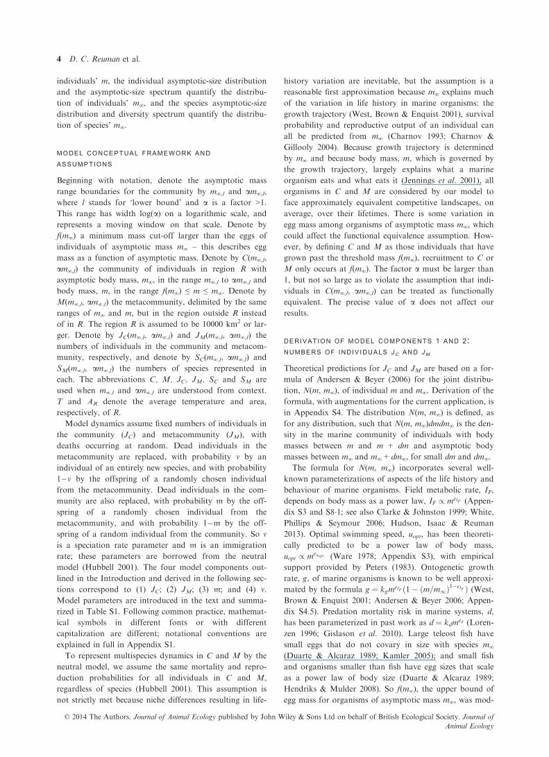
Hendriks & Mulder 2008). So f(m∞), the upper bound of

egg mass for organisms of asymptotic mass m∞, was mod-

© 2014 The Authors. Journal of Animal Ecology published by John Wiley & Sons Ltd on behalf of British Ecological Society. Journal of

Animal Ecology

4 D. C. Reuman et al.

elled as kfmef1 for m∞ less than a threshold mcut, and equal

to a constant, megg, for m∞ ≥ mcut.

The formula for N(m, m∞) is

Nðm;m1Þ /

m2eIF�euopt�11=3þkdg1 m�eIF�kdg 1� m

m1

� �1�eIF ! kdg

1�eIF�1

eqn 1

where kdg = kd/kg. The formula holds for any m∞ > megg

and m in the range f(m∞) to m∞. The marginal distribu-

tionR1m Nðm;m1Þdm1 is proportional to the individual

size distribution for m > megg. The other marginal distri-

bution,Rm1fðm1Þ Nðm;m1Þdm, is proportional to the individ-

ual asymptotic-size distribution, henceforth denoted

Nm1ðm1Þ, for m1 [megg.

Via the above proportionality for the individual asymp-

totic-size distribution, theory predicts how JC and JMscale with m∞,l. The numbers of individuals JC and JM in

the asymptotic mass bounds m∞,l to am∞,l are propor-

tional toR am1;l

m1;lNm1ðm1Þdm1. Because Nm1ðm1Þ can be

computed numerically for m∞ > megg, this integral can

also be computed numerically for m∞,l > megg, providing

the predictions for the scaling of JC and JM.

The derivation of the scaling of JC and JM also reveals

that this scaling is independent of the temperature

and area of R and its metaregion: although the constants

of proportionality relating JC and JM toR am1;l

m1;lNm1ðm1Þdm1 will differ from each other and may

vary from one region, R, to another, the proportionalities

themselves are the same for all regions. Eqn 1 and hence

the proportionalities for the individual asymptotic-size

distribution, JC, and JM, were derived regardless of tem-

perature and region area (Andersen & Beyer 2006;

Appendix S4). The parameters in eqn 1 also do not

depend on these environmental factors (Appendix S4�6).The quotient JC/JM turns out to be important for the

diversity spectrum and its variation among regions. It will

later be shown to be proportional to the ‘size of C relative

to speciation’, a quantity defined as the number of indi-

viduals in the community C compared to a total number

of speciation events in the metacommunity per generation.

Therefore, we now explore the dependence of JC/JM on

m∞,l, T and AR. The m∞,l dependence of JC/JM follows

immediately: because JC and JM scale with m∞,l in the

same way, JC/JM is independent of m∞,l.

The parameter JC/JM is smaller for regions with higher

T. In marine ecosystems, temperature and primary pro-

duction are not strongly positively related on the spatial

scales we consider because low nutrient availability limits

primary production in areas with intense solar radiation

and because currents as well as local solar heating drive

sea temperature (Sarmiento & Gruber 2006). Thus, in

warm regions, resource supply rate at the base of the

food web is not systematically larger than in cold

regions. Because the metabolic demands of heterotrophic

marine ectotherms are greater in warmer regions, JC will

be smaller, on average, in warmer regions. A similar

result is obtained by Jennings et al. (2008). But the meta-

regions will not vary appreciably in their average temper-

atures from one region, R, to the next because the

metaregions themselves will not vary much: the metare-

gion is the area outside the region, and the area outside

one reasonably sized region nearly coincides with the

area outside another. Therefore, the metacommunity

sizes, JM, will be nearly constant for reasonably sized

regions. Because JC is smaller and JM nearly the same

for warmer regions, JC/JM will be smaller for warmer

regions, as claimed.

The quotient JC/JM is also larger for regions with larger

area AR. In fact, for each increase in AR by an arbitrary

factor, c, the ratio JC/JM will be larger by a factor of at

least c: JC is proportional to AR and JM shrinks as AR

increases because the metaregion is the area outside the

region.

derivation of model component 3: dispersal, m

In the neutral model, deaths occur at random and each

dead individual in the community is replaced from the

metacommunity with probability m and from the commu-

nity with probability 1�m. For a tractable derivation of

m, we idealize the layout of R as a disc, D, of effective

radius rR ¼ ffiffiffiffiffiffiffiffiffiffiffiffiAR=p

pin the real Euclidean plane. The disc

D contains the community, C, and the region in the

Euclidean plane outside D contains the metacommunity,

M. In the event of a death at location v1 = (x1, y1) in D,

let uðv1; v2Þ ¼ expðððx1 � x2Þ2 þ ðy1 � y2Þ2Þ=ð�2r2dÞÞ be

the relative pressure from any other point v2 = (x2, y2) to

fill the vacancy resulting from this death; u is a dispersal

kernel, and rd is a dispersal distance parameter for organ-

isms in C and M. The average total replacement pressure

from outside D divided by that from inside D is

m

1�m¼R

v12DR

v2 62Duðv1; v2Þdv2dv1Rv12DR

v22Duðv1; v2Þdv2dv1 : eqn 2

This quotient simplifies to provide an expression for m

(eqn S5�1�8, Appendix S5�1) that can be computed numer-

ically given rR/rd, therefore providing theoretical predic-

tions for the dependence of m on m∞,l, T and AR if we

can now predict how rR/rd depends on these variables.

But a relationship of the form rR=rd / rRm�erd1;l =krd

ðTÞcan be derived, where erd

is positive and krdðTÞ is smaller

for larger T. We here derive it by deriving the formula

rd / krdðTÞmerd

1;l, from which the formula for rR/rd fol-

lows immediately. The formula for rd is empirically and

theoretically supported for both larval and adult dispersal.

A large portion of dispersal in a marine environment is

via planktonic or weakly swimming larvae. Species dis-

persal distances, rd, as inferred from genetic data and the

expansion rates of invasive species, or as measured

directly for dispersing larvae, have been found to be

strongly related to larval duration by a power law

© 2014 The Authors. Journal of Animal Ecology published by John Wiley & Sons Ltd on behalf of British Ecological Society. Journal of

Animal Ecology

The marine diversity spectrum 5

(Shanks, Grantham & Carr 2003; Siegel et al. 2003). Lar-

val duration is in turn related to maximum body mass via

a power law (Bradbury et al. 2008) and has also been

shown to decrease with increasing T both within and

among species (O’Connor et al. 2007; Bradbury et al.

2008). Combining these patterns supports the stated

dependence of rd on m∞,l and T if dispersal is primarily

larval. Adult dispersal is reasonably assumed to be pro-

portional to uopt times life span. Theory in Appendix S3

shows uoptðm1;l;TÞ / e�Euopt

kT meuopt1;l . Life span is known to

scale approximately as inverse mass-specific metabolic

rate, which scales as eEIFkT m

1�eIF1;l because metabolic rate is

proportional to e�EIFkT m

eIF1;l (Gillooly et al. 2001). Multiply-

ing the expressions for uopt and life span gives

eðEIF�Euopt Þ

kT meuoptþ1�eIF1;l . This product is a positive-exponent

power law of m∞,l, as claimed, as long as

euopt þ 1� eIF [ 0, and it decreases as T increases, as

claimed, as long as EIF � Euopt [ 0, supporting the stated

dependence of rd on m∞,l and T if dispersal is primarily

by adults. See Appendix S5�2 for a more detailed theoreti-

cal development that comes to the same conclusions. A

positive relationship between dispersal and asymptotic

body mass was further empirically supported by a

negative correlation between the genetic differentiation

within species and species’ maximum body size (Bradbury

et al. 2008). Decreased dispersal at higher T was sup-

ported in the same study by a negative correlation

between species’ genetic differentiation and their maxi-

mum latitude.

Given the relationship rR=rd / rRm�erd1;l =krd

ðTÞ, we let

the unknown value of rR/rd for the reference asymptotic

massmegg be denotedK1, so that rR=rd ¼ K1ðm1;l=meggÞ�erd

and K1 / rR=ðkrdðTÞmerd

eggÞ. Given values for K1, megg and

erd, rR/rd and therefore m can be computed for any m∞,l.

Theory thereby provides predictions for how m depends

on m∞,l. We call K1 the relative radius of the region R. It

is the effective radius of the region relative to the dis-

persal kernel of the smallest mass category, and turns out

to be important for the diversity spectrum of R. The

dependence of m on the environmental variables T and

AR is through K1 because rR/rd depends on T and AR

through K1. K1 is larger for warmer or larger regions. The

expression K1 / rR=ðkrdðTÞmerd

eggÞ makes it clear that

higher T implies larger K1, because krdðTÞ is smaller for

higher T; and increasing AR by an arbitrary factor cincreases rR and therefore K1 by a factor of

ffiffiffic

p.

model component 4: speciation, m

Prior work suggestively but not irrefutably supports the

assumption that m is independent of m∞,l and T. Gillooly

et al. (2005) showed that molecular evolution rates, in

units of nucleotide substitutions per unit time and per site

in a genome, are proportional to species characteristic

body mass to the power of �1/4, times expð�EkTÞ, where E

is about the same as the Arrhenius activation energy of

metabolism. As generation time is approximately propor-

tional to the inverse of this product, molecular evolution

rates expressed in units of nucleotide substitutions per

generation and per site are independent of body mass and

temperature. Thus, rates of molecular evolution per

recruit are mass and temperature independent. Because

the parameter m is a per-recruit rate, this reasoning would

support the constancy of m if speciation rates are primarily

controlled by rates of genetic divergence, as suggested by

Allen et al. (2006). Thomas et al. (2006) found that rates

of molecular evolution in invertebrate taxa do not depend

systematically on body mass, casting doubt on the gener-

ality of the results of Gillooly et al. (2005), but Thomas

et al. (2006) did not control for temperature. Perhaps

more importantly, the link between molecular evolution

and morphological change and speciation is uncertain

(Bromham et al. 2002). Several of these points were made

by Mittelbach et al. (2007). Nevertheless, because the

assumption of constant m is better supported than alterna-

tive assumptions and is also more parsimonious, we

explore the consequences of this assumption for our

model instead of alternative assumptions.

the unifying model component: numbers ofspecies, SC AND SM

Formulas were provided by Etienne & Olff (2004) for the

numbers of species SM and SC, depending on the quanti-

ties JC, JM, m and m derived above. The formulas provide

expected numbers of species at stochastic equilibrium in

the neutral model. The formulas can be well approxi-

mated by

SM � JMv logeð1=vÞ

1� veqn 3

SC � JMv

1� vloge 1�m logeðmÞ

1�m

JCð1� vÞJMv

� �� �eqn 4

(Appendix S6�2). These approximations are used below to

develop testable predictions. The inaccuracies of the for-

mulas and their effects on our conclusions are quantified

and shown to be negligible in Appendix S9. We use

approximations in place of the original formulas of Eti-

enne & Olff (2004) because it simplifies analysis and inter-

pretations.

Because m is very small, the expression JC (1 � m)/(JMm)in eqn 4 is approximately JC/(JMm), the number of

individuals in C relative to the number of speciation

events in M per generation. We denote this constant by

K2, which we name the size of C relative to speciation. K2

is constant with respect to m∞,l because m is constant and

we showed that JC and JM scale in the same way with

respect to m∞,l. K2 is smaller for regions with higher T,

and, for each increase in AR by an arbitrary factor, c, K2

is larger by a factor of at least c; these facts hold because

m is constant and we showed that JC/JM has the same

properties.

© 2014 The Authors. Journal of Animal Ecology published by John Wiley & Sons Ltd on behalf of British Ecological Society. Journal of

Animal Ecology

6 D. C. Reuman et al.

Model parameterization

model parameters

The model was parameterized from data in the literature.

The values eIF ¼ 0:7982 and EIF ¼ 0:5782 were derived

from our own theoretical and empirical analyses (Appen-

dix sections S3 and S8.1). Similar values were estimated

from a large data set in prior work (Clarke & Johnston

1999). The value euopt ¼ 0:1342 was derived theoretically

(Ware 1978; Appendix sections S3 and S8.5) and sup-

ported empirically by Peters (1983), who obtained the

value 0�13. Euopt ¼ 0:2816 was obtained from the same the-

ory. Because kdg is a function of eIF , euopt , bf, rf and a

food conversion efficiency, the value kdg = 0�737 was

derived from literature estimates of these parameters

(Appendix S8.5). To parameterize f(m∞), data from

several sources on the sizes of the eggs of fish and other

marine organisms were used to support the values megg =6�5 9 10�5 kg, mcut = 0�316 kg, ef = 0�5 and kf ¼ 1:16 �10�4kg1�ef (Appendix S8.4).

We adopted a range of values for the dispersal parame-

ter erdbecause it was the parameter known with the least

certainty from the literature and because it can comprise

both larval and adult dispersal. Dispersal distance is

related to larval duration by a power law with exponent 1

(Siegel et al. 2003; Shanks, Grantham & Carr 2003), and

larval duration is related to maximal body mass by a

power law with exponent 0�25 (Bradbury et al. 2008).

Thus erd¼ 0:25 if dispersal is primarily larval. For adults,

we derived erd¼ euopt þ 1� eIF in the section ‘Derivation

of model component 3’, the value of which is 0�336. Thesame or very similar values were obtained by the more

detailed reasoning in Appendix S5�2 (see also Appendix

S8�6). We considered the range 0�2 to 0�4 for erd. The

value EIF � Euopt , which if positive indicates that adult dis-

persal is theoretically expected to be reduced at higher

temperatures (see section ‘Derivation of model component

3’), is 0�5782–0�2816 = 0�2966 > 0. Additional details on

model parameters are given in Appendix S8, and parame-

ter values are summarized in Table S1.

bounds for K1 AND K2

Two bounds can be derived within which K1, the relative

radius of the region, and K2, the size of C relative to spe-

ciation, must reasonably lie for any of the regions we con-

sider. These bounds are important for understanding the

range of possibilities for diversity spectra because K1 and

K2 affect the diversity spectrum of R. By definition, K2 =JC(1�m)/(mJM), where mJM is a measure of the common-

ness of speciation and JC (1�m) � JC is large for large

regions R. Because speciation is rare and we consider only

regions of area more than 10 000 km2, it is safe to assume

K2 > 10, that is, that the number of new species per gener-

ation is not more than 1/10th the population of the region

R. This seems likely to be a conservative bound. The

bound applies for the smallest regions we consider (those

of area 10 000 km2); the higher bound K2 > (AR/

10 000 km2)10 therefore holds for larger regions. An

upper bound for K1 that depends on AR can also be pro-

duced: solving rR=rd ¼ K1ðm1;l=meggÞ�erd for K1 and

substitutingffiffiffiffiffiffiffiffiffiffiffiffiAR=p

pfor rR gives K1 ¼

ð ffiffiffiffiffiffiffiAR

p=ð ffiffiffi

pp

rdÞÞðm1;l=meggÞerd . Using the reasonable

assumption that rd > 10 km for organisms of asymptotic

mass 1000 kg (and rd is certain to be larger than 10 km

for such large organisms, which on energetic grounds

alone would need to forage over extensive areas), we have

K1\ð ffiffiffiffiffiffiffiAR

p=ð ffiffiffi

pp

10kmÞÞð1000kg=meggÞerd . This bound for

K1 can be combined with the bound for K2 by

algebraically eliminating AR to get K2[K21p

megg

1000kg

� �0:6110

� �¼ 1:54�10�5K21, using the central value 0�3

for erd: Both bounds are linear on log(K2)-versus-log(K1)

axes. Details of the derivation are in Appendix S8�7.

Model predictions

abundance predictions

Linearity of the size spectrum and slope about �1 have

been empirically supported (e.g. Sheldon, Sutcliff & Prak-

ash 1972; Kerr & Dickie 2001). Our model predicts this,

providing reassurance of model reasonableness. The distri-

bution N(m, m∞), using the parameters of section ‘Model

parameters’, is pictured in Fig. 2a. The marginal distribu-

tionR1m Nðm;m1Þdm1, proportional to the individual size

distribution, was shown by Andersen & Beyer (2006) to

be a power-law distribution with exponent �2�003. The

model of Andersen & Beyer (2006) is included in our

model; hence, our model also predicts a power-law

individual size distribution with exponent �2�003 and

–4−2

0

2

0

1

2

3

0

10

20

30

log10(m

, kg)log

10 (m∞ , kg)

log10(IASD) + constlog10(ISD) + const

−4 −2 0 1 2 3

−4

02

46

8

log10((m∞∞,, kg))

log 1

0((IA

SD

))++co

nsta

nt y = −1·49 *x+ 2·36

IASDlinear approx.

(a) (b)

Fig. 2. (a) The joint distribution of individual mass, m, and asymp-

totic mass, m∞, expressed as log10(N(m, m∞)) + constant (see eqn

1) for m between megg (upper bound fish egg size) and 1000 kg and

m∞ between 1 and 1000 kg. The marginal distributions, which are

the individual size distribution (ISD) and the individual asymptotic-

size distribution (IASD), are labelled. The dashed line in the

individual size distribution indicates the part of the plot to which

organisms with m∞ < 1 kg contribute. (b) The log10 individual

asymptotic-size distribution plotted and linearly approximated for

m∞ between megg and 1000 kg, illustrating the theoretical prediction

that the individual asymptotic-size distribution is approximately a

power law in m∞ with exponent about �1�49.

© 2014 The Authors. Journal of Animal Ecology published by John Wiley & Sons Ltd on behalf of British Ecological Society. Journal of

Animal Ecology

The marine diversity spectrum 7

therefore a linear size spectrum of slope �1�003 (Fig. 2a).

The derivation is reproduced in Appendix S4�3.The other marginal distribution of N(m, m∞), computed

numerically and proportional to the individual asymp-

totic-size distribution, is shown in Fig. 2b. The predicted

log10 individual asymptotic-size distribution is approxi-

mately linear in log10(m∞), of slope �1�49. Hence, theory

predicts that the individual asymptotic-size distribution is

a power law in m∞ with exponent �1�49, and the asymp-

totic-size spectrum is linear with slope �0�49.

diversity spectra

Because the individual asymptotic-size distribution is

approximately a power law in m∞ with exponent �1�49,JC and JM are approximately proportional toR am1;l

m1;lm�1:49

1 dm1 / m�0:491;l . As m is constant with respect

to m∞,l, eqn 3 implies that SM should scale with m∞,l in

the same way JM does, leading to Prediction 1: The num-

ber of species SM in the metacommunity M is approxi-

mately a power law in m∞,l with exponent �0�49.

Equivalently, the diversity spectrum of the metaregion is

approximately linear with slope �0�49. This prediction is

for m∞,l > megg, a limitation which comes from the same

limitation for eqn 1. Thus, theory predicts that the num-

ber of species in a category of log asymptotic mass in the

metaregion will be proportional to the number of individ-

uals in that category.

Predictions for the dependence of SC on m∞,l can be

computed numerically using eqn 4 for any given values of

erd. K1 and K2. We plotted log10(SC) against log10(m∞,l)

(the diversity spectrum) for values of erdin the range 0�2

to 0�4 and for K1 and K2 in a region bounded by the con-

straints of the section ‘Bounds for K1 and K2’. Plots were

always close to linear: root mean squared deviations

between linear approximations to the plots and the plots

themselves were always < 0�175 (Fig. 3a–c for example

plots). Slopes were always shallower than (greater than)

�0�49 and were steeper than (less than) about �0�1 for

reasonable values of K1 and K2 (Fig. 3d–f). These results

precipitate two predictions. Prediction 2: The number of

species SC in the community C is approximately a power

−4 −2 0 1 2 3

−7

−5

−3

−1

0

log10(m∞, l, kg) log10(m∞, l, kg) log10(m∞, l, kg)

log 1

0(SC)+

con s

t

slope = −0·43

log10(SC) + constlinear approx.

−4 −2 0 1 2 3

−7

−5

−3

−1

0 slope = −0·42

log10(SC) + constlinear approx.

−4 −2 0 1 2 3

−7

−5

−3

−1

0

slope = −0·41

log10(SC) + constlinear approx.

log10(K1)

log 1

0(K2)

log 1

0(SC)+

con s

tlo

g 10(K

2)

log 1

0(SC)+

con s

tlo

g 10(K

2)

−0·47

−0·43

−0·39

−0·35 −0·23

−1 0 1 2 3 4 5

02

46

810

12 min: −0·49max: −0·23

log10(K1)

−0·

47

−0·43

−0·39

−0·35 −0·19

−0·15

−1 0 1 2 3 4 5

02

46

810

12 min: −0·49max: −0·14

log10(K1)

−0·

47

−0·43

−0·39

−0·35 −0·19

−0·15

−1 0 1 2 3 4 5

02

46

810

12 min: −0·49max: −0·081

(a) (c)

(e)

(b)

(d) (f)

Fig. 3. Predicted regional diversity spectra and their slopes for different values of K1 (the relative radius of the region), K2 (the size of

the community relative to speciation) and erd (the dispersal distance scaling exponent). Examples of predicted regional diversity spectra

(a–c) were close to linear. These panels show the log10 number of species in the region R (i.e. SC(m∞,l, am∞,l)) plotted for lower-bound

asymptotic mass m∞,l between megg and 1000 kg. SC is computed using eqn 4. K1 = 102�5 and K2 = 104 were used for a–c; erd ¼ 0:2, 0�3and 0�4 were used for a, d; b, e; and c, f, respectively, spanning the range selected in the section ‘Model Parameters’. The relationship

between log10(SC) and log10(m∞,l) was always close to linear, not just in the examples shown (see text). Panels d–f are contour plots

showing slopes of log10(SC) versus log10(m∞,l) for a range of values of erd , K1, and K2. Dashed lines in d–f delineate the bounds for K1

and K2 given in the section ‘Bounds for K1 and K2’. The minimum slope and maximum slope occurring in the bounds are given, and

indicate that regional diversity spectrum slopes should be between �0�5 and about �0�1 for real regions.

© 2014 The Authors. Journal of Animal Ecology published by John Wiley & Sons Ltd on behalf of British Ecological Society. Journal of

Animal Ecology

8 D. C. Reuman et al.

law in m∞,l. Equivalently, the diversity spectrum of the

region R is linear. Prediction 3: The power-law exponent

is greater than �0�49 and likely less than �0�1 for large

regions. Equivalently, the diversity spectrum slope for R

is between �0�49 and �0�1. These predictions are for m∞,l

> megg. A derivation that does not use the approximations

used here is in Appendix sections S9�2 and S9�3; results

are substantially the same.

environmental gradients in diversity spectra

Suppose given a collection of continental shelf-sea regions

with different average temperatures, T, and areas, AR; the

collection of regions has a collection of associated metare-

gions, each metaregion being the area outside its region.

We showed that K1 is predicted to be larger and K2 smal-

ler for warmer regions than for colder ones. Therefore,

Fig. 3d–f leads to Prediction 4: Diversity spectrum slopes

will be shallower (less negative) in warmer regions. Mov-

ing to the right (increasing K1) and down (decreasing K2)

on any of the panels d–f of Fig. 3 implies a shallower pre-

dicted slope (see Fig. 4 for a detailed depiction for the

central value erd ¼ 0:3). This prediction is for m∞,l > megg.

It holds as long as T and net primary productivity are

truly not positively related among regions; the derivation

of the T dependence of JC/JM, and therefore K1, relied on

this expectation.

We showed that across a gradient of increasing AR,

both K1 and K2 are predicted to increase, with K1 being

larger by a factor offfiffiffic

pand K2 being larger by a factor

of at least c for each factor-of-c increase in AR. The net

effect is Prediction 5: The diversity spectrum of larger

regions will be steeper (more negative) than that of smal-

ler regions (Fig. 4). This prediction is for m∞,l > megg. The

prediction matches with intuition because larger regions

are closer in size to their associated metaregions, which

have predicted diversity spectrum slope �0�49, at the

steep end of the range of predicted regional slopes. A der-

ivation of predictions 4 and 5 that does not use the

approximations used here is in Appendix S9�3; results are

substantially the same.

Methods for testing model predictions

To test theoretical predictions, we empirically estimated

diversity spectra of 63 of the 64 large marine ecosystems

(LMEs) that partition the world’s continental shelf seas

(Sherman, Alexander & Gold 1993). LME boundaries are

standardized and are delineated by downloadable GIS

shapefiles from the United States National Oceanic and

Atmospheric Administration (NOAA; Table S3 and Fig.

S7). LMEs are large, the smallest having area

1�52 9 1011 m2. The Arctic LME was excluded because

environmental variables were unavailable.

The range of variation in LME areas was modest

(1�52 9 1011 to 4�17 9 1012 m2, a factor of 27�3). There-fore, to examine the influence of region area on diversity

spectra, LMEs were also aggregated to form larger

regions for which diversity spectra were estimated. LMEs

were aggregated to form 15 ‘provinces’ of area

9�77 9 1011 to 1�85 9 1013 m2, 7 ‘basins’ of area 2�53 9

1012 to 2�55 9 1013 m2, 3 ‘latitudinal bands’ of area

1�69 9 1013 to 3�13 9 1013 m2 and a single aggregate of

all 63 LMEs, the ‘global region’ (area 7�58 9 1013 m2).

Regions are listed and mapped in Appendix S10�1, TableS4 and Figs S8 to S10.

Our theory applies to the entire community for m∞,l >megg and is not constrained to a taxonomic group. How-

ever, taxonomically inclusive data are very difficult to

obtain. To test our theory, we use the fact that fish domi-

nate the biomass and diversity of marine pelagic ecosys-

tems over the asymptotic mass range 1 to 1000 kg and

are likely to provide an adequate representation of the

whole community in that range (Jennings et al. 2008).

Theory was tested using fish data in that range. The effect

of including other groups such as mammals, cephalopods

and scyphozoans was considered to the extent possible.

Data on the asymptotic sizes of fish species and their

occurrence by LME were downloaded from FishBase

(Froese & Pauly 2006, August 2013). FishBase provides

the maximum length ever observed in any ecosystem for

each species. This was taken as a surrogate for species

asymptotic length, l∞. Asymptotic lengths were converted

to asymptotic masses via the relationship m∞=101.038

l∞2.541, where l∞ is in metres and m∞ is in kilograms. This

relationship was determined from mass and length

data for world-record fish caught by angling, for 526 spe-

cies, from the International Game Fish Association;

log10(K1)

log 1

0(K

2)

−0·

45

−0·

39

−0·

35

1·5 2·0 2·5 3·0 3·5

3·0

3·5

4·0

4·5

5·0

Fig. 4. Predicted variation in regional diversity spectrum slopes

along environmental gradients. Contour lines show diversity spec-

trum slopes, enlarging part of Fig. 3e. Starting from reference

values of K1 and K2 (solid dot), arrows show the predicted varia-

tion in K1, K2 and diversity spectrum slope along gradients of

increasing temperature, T (solid arrows, several possible out-

comes shown) and increasing region area, AR (dashed arrow).

Diversity spectrum slopes are predicted to become shallower with

increasing T and steeper with increasing AR. Arrows show direc-

tions of predicted effects but not magnitudes. Results are similar

for other values of erd (Fig. 3).

© 2014 The Authors. Journal of Animal Ecology published by John Wiley & Sons Ltd on behalf of British Ecological Society. Journal of

Animal Ecology

The marine diversity spectrum 9

world-record lengths and masses are taken as surrogates

for asymptotic lengths and masses for a species, and an

interspecific regression was carried out to approximate the

relationship between asymptotic mass and length (Appen-

dix S11�1 for details). The same value of m∞ was used for

a species in all LMEs in which it occurred. We excluded

species in the FishBase life-type category ‘reef-associated’

because our theory is for pelagic species. The number of

LME species occurrence records extracted from FishBase

was 27 817. Lists of species for larger regions (provinces,

basins, etc.) were compiled by combining the species lists

for component LMEs and removing duplicates.

The diversity spectrum of a region was estimated by

estimating the mathematically equivalent species asymp-

totic-size distribution. A truncated Pareto (tP) distribution

was fitted by maximum likelihood (Aban, Meerschaert &

Panorska 2006) to the species asymptotic mass data

between 1 and 1000 kg for each region that had at least

30 species in that range (58 LMEs and all the larger

regions).

The quality of fit of the tP distribution, and hence the

correctness of theoretical predictions about the linearity

of diversity spectra, was assessed with statistical tests and

plots. For each region, we tested the composite hypothesis

that data came from a tP distribution with truncation

points 1 and 1000 kg and unknown exponent. The statis-

tical test used is based on the Kolmogorov–Smirnov

statistic (Appendix S10�2). Tests such as this one can

detect very small deviations from the null hypothesis for

large sample sizes. For the speciose LMEs and for the lar-

ger regions, sample sizes were large, so we also produced

plots that depict the magnitude of deviations from linear-

ity. These plots were produced using a simple transforma-

tion that converts the cumulative distribution function

(cdf) of a tP distribution to the associated diversity spec-

trum (Appendix S10�2). The transformation was applied

to the empirical cdf of each region, producing a plot

we call the empirical diversity spectrum. The plot was

compared to the diversity spectrum associated with the fit-

ted tP distribution. Agreement between the plots was

assessed visually and also using a coefficient of determina-

tion, 1 � SSE/SST, where SSE was the sum of squared

differences between the two plots, and SST was the sum

of squared deviations of the empirical diversity spectrum

from its mean. This statistic, which we call the spectrum

linearity statistic, is the fraction of the variation in the

empirical diversity spectrum that is explained by the linear

hypothesis. If the spectrum linearity statistic was greater

than 98% for a region, the diversity spectrum of that

region was deemed linear for the purposes of this study

even if the tP distribution was statistically rejected by the

above test. This is reasonable because we are trying to

understand the most important determinants of diversity

patterns.

For regions for which the tP distribution was statisti-

cally rejected, a quadratic generalization of the tP distri-

bution, here called the quadratic truncated Pareto (qtP)

distribution (Reuman et al. 2008; Appendix S2�2), was

also fitted for confirmation. Its fit was compared with that

of the tP distribution using a likelihood ratio test. The

qtP is mathematically equivalent to a quadratic diversity

spectrum; hence, our comparison of the tP and qtP distri-

butions constituted a comparison of the hypothesis of a

linear diversity spectrum against a quadratic alternative.

The qtP distribution is the same as a log-normal distribu-

tion truncated on both sides, and the log-normal distribu-

tion is a commonly considered hypothesis for species size

distributions. The quality of fit of both the tP and qtP

distributions was judged visually by plotting log10 asymp-

totic body masses, sorted in ascending order, against

log10-scale medians of the order statistics of the fitted dis-

tributions, to provide log10-scale probability plots. When

these plots were straight it indicated that the distribution

used was a good fit. When the plot for the qtP distribu-

tion was not substantially straighter than that for the tP

distribution, it indicated that the null hypothesis of a lin-

ear diversity spectrum was at least as good as the curved

alternative. For regions for which the tP distribution was

statistically rejected, the diversity spectra corresponding to

both the fitted tP and qtP distributions were also plotted

and compared visually. The dual use of formal hypothesis

tests and visual comparisons is again appropriate because

we are interested in whether theory and data agree on

major patterns, but minor deviations can cause statistical

rejection of hypotheses for large data sets.

Slopes of diversity spectra that were deemed linear

(either the tP distribution was not statistically rejected or

the spectrum linearity statistic was > 98%) were retrieved

from the parameters of the best-fitting tP distribution.

The tP distribution has pdf proportional to m�ðbþ1Þ1 where

b is the fitted parameter. The diversity spectrum is linear,

and �b is the diversity spectrum slope if the tP distribu-

tion is a good fit (see section ‘Preliminaries: Spectra and

Distributions’; Appendix S2�1). Confidence intervals for b

and therefore for diversity spectrum slope were obtained

by a resampling scheme. For each region, m∞ values in

the range 1 to 1000 kg were resampled 1000 times with

replacement, and b was estimated for each resampling,

with quantiles providing confidence intervals.

Estimates of average sea surface temperature, used as a

surrogate for T, and primary production in the LMEs

were obtained from remote sensing data. T estimates were

averages of 1997–2007 outputs of the version 5�0Advanced Very High Resolution Radiometer Pathfinder

project conducted by the University of Miami’s Rosenstiel

School of Marine and Atmospheric Science and the

NOAA National Oceanographic Data Center. The Path-

finder data set is distributed by the Physical Oceanography

Data Active Archive Center (PODAAC) of the United

States National Aeronautics and Space Administration

Jet Propulsion Laboratory. Net primary productivity was

depth-integrated primary production (mg C m�2 d�1) and

was calculated from chlorophyll concentration following

the approach of Platt & Sathyendranath (1988) as

© 2014 The Authors. Journal of Animal Ecology published by John Wiley & Sons Ltd on behalf of British Ecological Society. Journal of

Animal Ecology

10 D. C. Reuman et al.

implemented by M�elin & Hoepffner (2004). Model inputs

of surface chlorophyll concentration were obtained from

the Sea-viewing Wide Field-of-view Sensor (SeaWiFS)

time series for the years 1997–2007. Averaging procedures

are in Appendix S10�3. The Arctic LME was not included

because near-continuous cloud and ice cover prevented

adequate estimates of environmental variables (Gregg &

Casey 2007).

Dependence of diversity spectrum slopes on environ-

mental variables was examined with linear models, using

those LMEs deemed to have adequately linear diversity

spectra. A linear model with predictors log10(AR) and T

was used. AR was log-transformed because the trans-

formed variable appeared symmetrically and unimodally

distributed. For verification of results, a linear model was

also used in which the importance of individual systems

for fitting was weighted according to the inverse variances

of the diversity spectrum slope estimates.

Results of testing model predictions

Prediction 1 was validated in main substance: the metare-

gion diversity spectrum was approximately linear with

slope close to �0�49. The metaregion corresponding to

any of our regions, R, is the area of the global region out-

side R, which is well approximated by the whole global

region. So we tested prediction 1 for the global region.

Although the tP distribution was statistically rejected at

the 1% level (Table S6 for P-values), the empirical diver-

sity spectrum was very close to linear (Fig. 5a), and the

spectrum linearity statistic was greater than 98% (Table

S6 for spectrum linearity statistics). Because sample size

was large for the global region (n = 2885), very small

deviations from linearity were detected by the test of fit of

the tP distribution. Probability plots indicated that the tP

distribution was a good, but not perfect fit for the global

region (Fig. 5b). A likelihood ratio test showed that the

qtP distribution was statistically preferred (1% level) to

the tP distribution, but the qtP probability plot was only

slightly straighter than the tP plot (Fig. 5c), and the diver-

sity spectrum corresponding to the best-fitting qtP was

hardly different from that of the best-fitting tP (Fig. 5d).

Thus, the spectrum deviated significantly but only slightly

from linearity. These deviations are real features of the

data, but they do not influence our understanding of

broad patterns in diversity, because they are small com-

pared with the overall pattern.

The diversity spectrum slope estimated by fitting the tP

distribution was �0�561, with 95% confidence intervals

(�0�585, �0�536) and 99% intervals (�0�590, �0�532).These intervals did not contain the predicted slope, �0�49,but were close to it, possibly indicating that the model

contains the most important mechanisms controlling the

diversity spectrum but omits some less influential mecha-

nisms. Alternatively, model-data deviations may be

because we used fish to approximate the whole commu-

nity. Although fish are expected to dominate marine pela-

gic biomass and diversity in the m∞ range 1 to 1000 kg

(Jennings et al. 2008), to precisely evaluate the accuracy

of this approximation would require the compilation of a

large amount of data for other groups, probably not cur-

rently possible for the global region. We instead examined

the approximation by looking at the group other than fish

that seems most likely to contribute diversity that may

affect estimates of diversity spectrum slopes: marine mam-

mals. Marine mammals are large and hence contribute

diversity to the upper end of the range 1 to 1000 kg.

Estimates of slope are most sensitive to additional diver-

0·0 1·5 3·0

−1·

5−

0·5

log10(m∞, kg)

Div

. spe

ct.

1

0·0 1·5 3·0

0·0

1·5

3·0

log10(m∞, kg)

log 1

0(m

ed o

rder

, kg)

log 1

0(m

ed o

rder

, kg)

log 1

0(m

ed o

rder

, kg)

log 1

0(m

ed o

rder

, kg)

log 1

0(m

ed o

rder

, kg)

log 1

0(m

ed o

rder

, kg)

1, tP

0·0 1·5 3·0

0·0

1·5

3·0

log10(m∞, kg)

1, qtP

0·0 1·5 3·0

−1·

00·

0

log10(m∞, kg)

log10(m∞, kg) log10(m∞, kg) log10(m∞, kg) log10(m∞, kg)

log10(m∞, kg) log10(m∞, kg) log10(m∞, kg) log10(m∞, kg)

Div

. spe

ct +

con

st. 1

0·0 1·5 3·0

−1·

2−

0·6

0·0

Div

. spe

ct.

16

0·0 1·5 3·0

0·0

1·5

3·0

16, tP

0·0 1·5 3·0

0·0

1·5

3·0

16, qtP

0·0 1·5 3·0

−0·

60·

00·

6

Div

. spe

ct +

con

st.

16

0·0 1·5 3·0

−1·

0−

0·4

Div

. spe

ct. 18

0·0 1·5 3·0

0·0

1·5

3·0

18, tP

0·0 1·5 3·0

0·0

1·5

3·0

18, qtP

0·0 1·5 3·0

−1·

50·

0

Div

. spe

ct +

con

st.

18

(a) (c)

(e)

(b) (d)

(f) (g) (h)

(i) (j) (k) (l)

Fig. 5. Example results for testing the

hypothesis that diversity spectra are linear.

Empirical diversity spectra (see the section

‘Methods for testing model predictions’)

and diversity spectra corresponding to

fitted tP distributions for selected regions

(a, e, i). Log-scale probability plots for

truncated Pareto (tP; b, f, j) and quadratic

truncated Pareto (qtP; c, g, k) fits. Com-

parison of diversity spectra corresponding

to tP and qtP fits (d, h, l). Panels are as

follows: a–d, the global region (all 63

LMEs combined); e–h, the Brazil Shelf;

i–l the West Greenland Shelf. Numeric

codes in the upper corners also identify

regions – Tables S3 and S4 list the system

names that correspond to the codes. See

Fig. S11 for other regions.

© 2014 The Authors. Journal of Animal Ecology published by John Wiley & Sons Ltd on behalf of British Ecological Society. Journal of

Animal Ecology

The marine diversity spectrum 11

sity at the upper end of the range, where there are few

species. Of approximately 120 known, extant marine

mammals, body mass data were provided by Smith et al.

(2003) for 113, of which 80 had average body mass in the

range 1 to 1000 kg. When these 80 mammals were com-

bined with the 2885 fish species in the global region, the

tP distribution was still a good description, with spectrum

linearity statistic greater than 98% (Fig. S12; Table S5),

and the slope was even closer to model predictions (slope

�0�521, 95% confidence intervals (�0�544, �0�498) and

99% intervals (�0�551, �0�494)).Prediction 2 was generally validated, but with a few

interesting exceptions: regional diversity spectra were usu-

ally, but not always linear or very close to linear. Of the

58 LMEs for which sufficient data were available, the tP

distribution was statistically rejected (1% level) and spec-

trum linearity statistics were less than 98% for only five

LMEs, namely the Baltic Sea, the Faroe Plateau, the Ice-

land Shelf, the Norwegian Sea and the West Greenland

Shelf. Empirical diversity spectra were close to linear

except for these examples (Figs 5 and S11). Probability

plots confirmed that the tP distribution was a reasonable

fit, and comparison between tP and qtP fits revealed only

small differences, except for the five exceptional examples

(Figs 5 and S11). These five systems had empirical diver-

sity spectra that were clearly not straight, spectrum linear-

ity statistics less than 98% and probability plots that

indicated substantial nonlinearity (Figs 5i–l and S11 and

Table S6). The qtP was preferred to the tP for these sys-

tems, that is, spectra were curved. These systems violated

theoretical predictions for unknown reasons. These LMEs

were all located in the same area. Three of them (the West

Greenland Shelf, the Iceland Shelf and the Norwegian

Sea) were part of the North Atlantic province, which was

the only province for which the tP distribution was

rejected and the spectrum linearity statistic was less than

98%. Basins and latitudinal bands were deemed linear

(either the tP was not rejected or the spectrum linearity

statistic was greater than 98%), except for the South

Atlantic basin, which was close to linear, with spectrum

linearity statistic 0�978. Diversity spectra were thus gener-

ally close to linear, validating prediction 2, except for

some atypical LMEs in the North Atlantic.

Prediction 3 was validated: estimates of regional diver-

sity spectrum slopes were broadly consistent with the pre-

dicted range �0�5 to �0�1. Of the 53 LMEs with

adequately linear diversity spectra, none had estimated

slope above �0�1, only six had slopes below �0�5, only

three had 95% confidence intervals of the slope that did

not overlap with the range �0�5 to �0�1, and only two

had 99% intervals that did not overlap with the range

(the Antarctic and Sea of Okhotsk). Other than the Ant-

arctic, all provinces, basins and latitudinal bands had con-

fidence intervals that overlapped with the range �0�5 to

�0�1 (Table S5).

Before testing predictions 4 and 5, we tested the under-

lying assumption about the regions, R, that is, that

temperature, T, for the regions was not positively related

to net primary productivity. Across the 53 LMEs for

which sufficient data were available to estimate diversity

spectra and for which diversity spectra were linear, T and

net primary productivity were actually significantly nega-

tively related (R = �0�326, P = 0�017). The association

was weak. Similar results held using log10 net primary

productivity (R = �0�347, P = 0�011). T andffiffiffiffiffiffiffiAR

p / rRwere not significantly related (Pearson’s R = 0�113,P = 0�419). Similar results held using log10(AR)

(R = 0�112, P = 0�426) or AR (R = 0�108, P = 0�443) in

place offfiffiffiffiffiffiffiAR

p. Net primary productivity and AR were not

significantly related (R = �0�184, P = 0�188).Predictions 4 and 5 were validated: warmer or smaller

regions had shallower diversity spectrum slopes. A linear

model with predictors log10(AR) and T explained 30�4%of the variation in slopes, and the coefficients of both pre-

dictors were significantly different from 0 (t-tests,

P = 6�82 9 10�5 for T, P = 0�032 for log10(AR)). The T

coefficient was positive (5�86 9 10�3, standard error

1�35 9 10�3) and the log10(AR) coefficient was negative

(�0�086, standard error 0�039), as predicted by theory.

Results were qualitatively the same when models were

used in which LMEs were weighted by the inverses of the

variances of diversity spectrum slope estimates (Appendix

S10�4). The effects of area may have appeared weak in

the linear model because variation in area among LMEs

was modest. But area effects were clearly seen across spa-

tial scales, by comparing diversity spectrum slopes of

LMEs, provinces, basins, latitudinal bands and the global

region (Fig. 6). Diversity spectrum slopes for LMEs are

mapped in Fig. 7.

Discussion

We proposed a mechanistic theory of the diversity spec-

trum and showed that it predicts: linearity of the diversity

spectrum; its slope for the world’s continental shelf seas;

the range of possible slopes for smaller regions; and shal-

lower slopes for warmer or smaller regions. To test our

theory, we provided the first systematic global empirical

estimates of the diversity spectrum and its geographical

variation. Theoretical predictions were correct, broadly

speaking, but with deviations in some details and with a

few exceptional systems in the North Atlantic. Our princi-

pal qualitative conclusion is that variation in diversity

with body mass can be explained, in large part, from

well-known life history, predation and dispersal informa-

tion and a neutral null assumption about speciation and

extinction.

Our theory predicted that diversity spectra are linear,

with slopes between �0�5 and �0�1; a similar range was

found empirically. Slopes �0�5 and �0�1 are strikingly

different. For every species in the mass category m∞,l to

am∞,l, a community with diversity spectrum slope �0�5has 3�2 species in the category m∞,l/10 to am∞,l/10 and 10

species in the category m∞,l/100 to am∞,l/100. Diversity

© 2014 The Authors. Journal of Animal Ecology published by John Wiley & Sons Ltd on behalf of British Ecological Society. Journal of

Animal Ecology

12 D. C. Reuman et al.

spectrum slope �0�1 means only 1�3 and 1�6 species,

respectively, in the smaller categories for each species in

the largest category.

During any period of time, individuals of a given

asymptotic mass compete with other individuals of the

same asymptotic mass and also with other individuals of

the same mass but different asymptotic mass. It is an

important feature of our theory that it includes both of

these types of competition. We accounted for competition

among categories of asymptotic mass by incorporating the

theory of Andersen & Beyer (2006). That theory provides

the joint distribution N(m, m∞), and therefore its marginal

distribution Nm1ðm1Þ, which is a complete account of the

relative abundances of asymptotic mass categories and

hence of the outcome of competition among categories.

What Andersen & Beyer (2006) did not attempt is to

describe the outcome of competition within each category,

that is, into how many species is an asymptotic mass cate-

gory partitioned? Our model accounts for this.

How can we intuitively understand the results that

diversity spectrum slopes are steeper for larger or colder

regions? Soininen, Lennon & Hillebrand (2007) argued

that more dispersive assemblages should show less varia-

tion in species composition among habitats in a region

(beta diversity), and provided evidence in a major

meta-analysis that larger organisms show lower beta

diversity. Although exceptions exist, larger organisms in

the systems we study are generally more dispersive because

they have longer larval durations and higher adult mobility

(Siegel et al. 2003; Shanks, Grantham & Carr 2003; Brad-

bury et al. 2008; see section ‘Derivation of model compo-

nent 3’); so beta diversity is expected to be a lesser

contributor to total regional diversity (gamma diversity)

for categories of large sizes than it is for categories of smal-

ler sizes. But for larger regions, the contribution of beta

diversity to gamma diversity is greater because spatial

turnover will play a more important role in large regions

(Soininen, Lennon & Hillebrand 2007). Thus, because beta

diversity contributes a bigger portion of gamma diversity

0·0 1·0

−0·

55−

0·45

−0·

35

Mean log10(Area, m2)

Mea

n di

v. s

pect

. slo

pe

Fig. 6. Diversity spectrum slopes for regions with linear diversity

spectra as a function of spatial scale. From left to right, dots rep-

resent LME, province, basin, latitudinal band and global region

means for log10 area (horizontal axis) and diversity spectrum

slope (vertical axis). Error bars indicate standard deviations.

There are no error bars for the global region point (the right

point) because there was only one global region. Nonlinear

regions were excluded.

–0·731 – –0·658–0·657 – –0·585–0·584 – –0·512–0·511 – –0·439–0·438 – –0·366–0·365 – –0·293–0·292 – –0·219–0·218 – –0·146–0·145 – –0·073Not available

Pacific ocean

Atlantic ocean

Indian ocean

Fig. 7. Diversity spectrum slope estimates for LMEs, excluding LMEs for which insufficient species were present to estimate the diver-

sity spectrum or for which the diversity spectrum was nonlinear.

© 2014 The Authors. Journal of Animal Ecology published by John Wiley & Sons Ltd on behalf of British Ecological Society. Journal of

Animal Ecology

The marine diversity spectrum 13

for smaller size categories than for larger size categories,

and because the overall importance of beta diversity is

accentuated in larger regions, it is intuitively understand-

able that larger regions should have steeper diversity spec-

trum slopes. Another view of the same logic is that more

large species can be found per small species in subglobal

regions than in the global region because larger species

have larger range sizes; a greater fraction of the global list

of species in a large size category will be represented in any

subglobal region compared to a smaller size category. In

colder regions, there is evidence (see section ‘Derivation of

model component 3’) that dispersal is generally greater for

all sizes because larval durations and life spans are longer

(Gillooly et al. 2001; O’Connor et al. 2007; Bradbury et al.

2008). So the relative advantages large species have in

ensuring their presence in more smaller regions through

greater range size are less important, providing an intuitive

interpretation of steeper diversity spectrum slopes in colder

regions.

theoretical assumptions revis ited

An assumption implicit in model structure is that numbers

of pelagic marine species are in stochastic equilibrium, that

is, not showing sustained trends over recent evolutionary

time. This assumption is manifested in equations 3 and 4,

which provide expected numbers of species at stochastic

equilibrium. The assumption of stochastic equilibrium is

consistent with available paleontological data: Benton

(2009) states that ‘The equilibrium model has prevailed,

among marine paleobiologists at least, for a long time…’

(see also Alroy 2008; Alroy et al. 2008). At regional scales,

rates of migration and community assembly will primarily

control the speed with which stochastic equilibrium is

reached, and these rates are much higher than rates of spe-

ciation and extinction. The locations of continents and the

thermohaline circulation have been approximately stable

for the last 3 myr since the formation of the Isthmus of

Panama. More recently, glacial cycles changed LME areas

through sea level rise and fall and changed their average

temperatures; but the gradient of LME temperatures has

been broadly maintained through the cycles. The time since

the end of the last glacial period, 10 000 years, appears

long enough for any migration-related transients in regio-

nal diversity distributions to have passed, given that marine

pelagic organisms generally disperse readily. LME areas,

average temperatures and productivities have likely been

approximately stable since then, except for recent anthro-

pogenic climate change (Spicer & Parrish 1986; Frakes,

Probst & Ludwig 1994; Scotese 1997).

The dispersal model (see section ‘Derivation of model

component 3’) idealized the region R as a disc, and migra-

tion was assumed to be non-directional (the dispersal ker-

nel u was radially symmetric). In contrast, for real shelf-

sea regions, region shape and directional ocean currents

can play a role in dispersal. Geographic and oceano-

graphic details may be worth incorporating into a future

model, although such a model would not be amenable to

analytic solution and may require enormous computa-

tional resources. Our model shows what fraction of the

variation in diversity spectrum slopes can be explained

mechanistically by gross properties (temperature and

area), without taking into account difficult-to-parameter-

ize detailed information: about a third of the variation

was explainable.

data revis ited

Fish were used as a proxy for the whole community in the

asymptotic mass range 1 to 1000 kg. This choice relies on

the assumptions that fish have been adequately sampled in

that range and that fish truly represent almost all or a con-

sistent fraction of the diversity in that range. Mora, Titten-

sor & Myers (2008) estimated that about 80% of the

world’s marine fish diversity has been described, consider-

ing all fish species regardless of size. Species in the asymp-

totic mass range 1 to 1000 kg are very heavily sampled

because they are more noticeable and often have economic

importance. Thus, it is reasonable to expect that consider-

ably more than 80% of the fish species in the range are

known. This is enough for this study, which examines log-

scale species richness patterns.

Although fish are expected to dominate marine pelagic

biomass and diversity in the m∞ range 1 to 1000 kg (Jen-

nings et al. 2008), to precisely evaluate the accuracy of this

approximation would require the compilation of a large

amount of data for other groups. We have instead exam-

ined the approximation by looking at the few groups other

than fish that seem most likely to contribute non-negligible

diversity to the range. Marine mammals were examined in

Results and Table S5. Diversity patterns that could be eval-

uated with marine mammal data included were in even

better agreement with theory. Cephalopods are another

group which may appear to violate the assumption, but

this was shown not to be the case in Appendix S11�2, wherescyphozoans are also discussed. These analyses support as

reasonable the assumption that fish adequately represent

pelagic diversity over the range 1 to 1000 kg (see also sec-

tion ‘Caveats and epistemological goals’ below).

Our model does not explicitly address the effects of

fishing and climate change on distributions of species’

sizes. Fishing has caused reductions in abundances of

many fish stocks (Worm et al. 2009) and extirpations of a

few species from LME-scale regions (Dulvy, Sadovy &

Reynolds 2003; Wonham & Carlton 2005; del Monte-

Luna et al. 2007). Climate change has caused shifts in

species ranges (Beaugrand et al. 2002; Perry et al. 2005;

Sumaila et al. 2011). These changes have the potential to

modify diversity spectra at LME scales but, on decadal

timescales, rates of change in the species present in LMEs

are expected to be small in relation to the total species

pool. LME-scale fish species occurrence data are unlikely

to have yet been markedly influenced by fishing or other

anthropogenic impacts given that known extinctions com-

© 2014 The Authors. Journal of Animal Ecology published by John Wiley & Sons Ltd on behalf of British Ecological Society. Journal of

Animal Ecology

14 D. C. Reuman et al.

prise a small portion of diversity (Dulvy, Sadovy & Rey-

nolds 2003; Wonham & Carlton 2005; del Monte-Luna

et al. 2007). However, if impacts continue, diversity spec-

tra may be affected and the analyses of this study can

provide a baseline.

The quality of some data in the Ocean Biogeographic

Information System (OBIS) has been criticized, and OBIS

draws on FishBase, the source of our data (Robertson

2008). The OBIS data criticized were at the level of sight-

ings of individuals of fish species; hence, documented

errors in OBIS are at much higher resolution than the

LME-level species occurrence data we use. However,

many of the documented errors are large in the sense of

comprising reports of fish sightings that are far outside

the species actual range. We explored if the reported

errors could have affected our use of the coarser data,

finding this to be very unlikely (Appendix S11�3).Maximum lengths ever recorded were used as surro-

gates for asymptotic lengths. We checked the reasonability

of this approximation by comparing FishBase maximum

lengths with maximum lengths from an independent data

set, the International Game Fish Association world

angling records. For 525 species for which a comparison

was possible, 97�3% of species had a FishBase log10 maxi-

mum length value that exceeded the log10 angling record

length minus 0�1 (Appendix S11�1). Although this is a

rough check of suitability, it provides evidence that short-

comings in the data, although they may have added noise,

are not sufficient to have artifactually created the promi-

nent patterns we observed.

caveats and epistemological goals

Although we made all reasonable efforts to ensure that

shortcomings in the data and approximations in the

model did not affect conclusions, our data and model

remain approximations of reality. The value of the work

stands in spite of its unavoidable approximate nature

because we provide a first comparison between data and a

mechanistic theory explaining a newly described global-

scale diversity phenomenon, the diversity spectrum. A the-

ory including every known biological mechanism that

may influence diversity is not possible and is probably not

desirable. A problem-free data set of community diversity

for all LMEs is not close to achievable and will probably

never be available. We view our work as a first step and

suggest that other researchers try to explain diversity spec-

tra by comparing model-data agreement after formulating

models with additional or alternative mechanisms and/or

compiling improved data.

further implications and future directions

Our model makes additional predictions which could be

tested if additional data were assembled. First, the model

predicts that the global diversity spectrum for the asymp-

totic mass range megg to 1 kg should be approximately

linear with slope about �0�5, as it was for the range 1 to

1000 kg. To get specific predictions for global numbers of

species in various ranges of asymptotic mass, we consid-

ered a tP distribution with exponent corresponding to

diversity spectrum slope �0�5 (exponent �1�5, b = 0�5)and with lower bound megg and upper bound 1000 kg. The

distribution was normalized so that its integral from 1 to

1000 kg was 2885, the number of known species of pelagic

fish with m∞ in that range. We then integrated this distri-

bution from 0�1 to 1 kg to get the prediction that there are

about 6400 species in the pelagic marine environment with

m∞ in this range. Integrating from 0�01 to 0�1 kg provides

the prediction that there are about 20 400 species with m∞

in this smaller range. Similarly, there are predicted to be

about 64 400 species with m∞ in the range 0�001 to

0�01 kg. These are order-of-magnitude predictions. Predic-

tions may be less accurate for the categories of smallest

asymptotic mass, because they represent a longer extrapo-

lation. Predictions for specific LMEs can be calculated by

a similar procedure. For instance, the predicted numbers

of species in the North Sea in the m∞ categories 0�1 to 1,

0�01 to 0�1 and 0�001 to 0�01 were 125, 232 and 431,

respectively. Some predictions could be tested in future

work if comprehensive data on crustaceans and other pela-

gic marine faunas with m∞ in the range megg to 1 kg were

assembled. Predictions would also be straightforward

regarding how diversity varies across trophic levels and

regarding variation in trophic vulnerability and generality

with size, and could be tested (Appendix S12).

Studies of distributions of species’ body sizes for a speci-

fied taxonomic group have been much more common than

approaches that consider all species in geographically

delimited regions regardless of taxonomy. For instance,

Hutchinson & MacArthur (1959); May (1978); Blackburn

& Gaston (1994); Loder, Blackburn & Gaston (1997);

Marquet et al. (2005) and Brown & Nicoletto (1991) have

all studied clade-specific species mass distributions either

theoretically, empirically or both. Our theory differs in

approach by considering all taxa, although we approxi-

mated the whole community by a single clade in a mass

range to test theory. Clade-specific theory must explicitly

or implicitly consider physiological limits that constrain

the sizes of species in that clade by virtue of their traits.

For instance, mammals probably cannot be smaller than

some threshold because endothermy is difficult to maintain

at small sizes. Further, competition and predation between

the focal clade and other clades may need to be under-

stood but is rarely considered in clade-specific studies. An

interesting subject for future research would be to theoreti-

cally explain and empirically test how clade-specific distri-

butions combine to form whole community distributions.

We are aware of only one prior study (Reuman et al.

2008) that systematically examined distributions of species

characteristic masses from a geographically delimited,

taxonomically inclusive viewpoint. That study considered

systems on much smaller spatial scales and of very differ-

ent ecological types from the marine systems of this study:

© 2014 The Authors. Journal of Animal Ecology published by John Wiley & Sons Ltd on behalf of British Ecological Society. Journal of

Animal Ecology

The marine diversity spectrum 15

149 freshwater pelagic, estuarine and soil systems. Never-

theless, Reuman et al. (2008) found diversity spectra that

were typically (though not always) approximately linear,

with a range of slopes that overlapped substantially with

the range of this study. The slopes of their 129 linear sys-

tems had 2�5th and 97�5th percentiles �0�316 and �0�099,respectively. Only two systems had 99% or 95% confi-

dence intervals not overlapping the range �0�5 to �0�1predicted by our theory for marine systems.

It may be possible in future work to generalize our the-

ory to ecosystems of other types. Important components

of the theory appear to generalize readily. For instance,

the growth model of West, Brown & Enquist (2001) is a

general model. Regularity in predation behaviour, as

assayed by predator-prey mass ratios, has also been docu-

mented in non-marine systems (Brose et al. 2006). Other

components of our theory, such as the neutrality assump-

tion, appear more difficult to generalize but may be suit-

able approximations for some ecosystem types. It may

also be possible to judiciously modify model structure to

make the neutral approximation more reasonable for

other systems. We here used asymptotic mass to delimit

categories within which functional equivalence of individ-

uals is a reasonable first approximation. In systems of

other types, traits in addition to or instead of body size

(e.g. metabolic category, stoichiometry, leaf area, shade

tolerance) may be necessary to delimit categories of

approximate functional equivalence. If the relative abun-

dance of categories can then be modelled, the same broad

approach of our theory could be applied. These observa-

tions and the coincidence of our predictions with the

empirical results of Reuman et al. (2008) suggest it may

be possible to generalize our theory to freshwater, soil,

estuarine and perhaps other ecosystems.

Acknowledgements

The authors thank Lawrence Hudson, Ken Andersen, Grant Bigg, Julia

Blanchard, Mick Crawley, Rampal Etienne, Rodney Forster, Bernardo

García-Carreras, Shai Meiri, David Orme, Albert Phillimore, Andy Pur-

vis, James Rosindell, Van Savage, Andrew Clark, Gavin Thomas, and

contributors to FishBase and the International Game Fish Association

world records database. We thank editors and anonymous reviewers for

useful feedback. DCR was partly supported by the U.K. Natural Envi-

ronment Research Council grants NE/H020705/1, NE/I010963/1, and

NE/I011889/1. CB and SJ were supported by the U.K. Department of

Environment, Food and Rural Afairs (MF1001, MF1225) and the

European Commission. HG was supported by the Danish research net-

work Fishnet. This paper is part of the Grand Challenges in Ecosystems

and the Environment initiative at Silwood Park, Imperial College

London. The research benefitted from author participation in the

European Science Foundation SIZEMIC (www.esf.org/sizemic) Research

Networking Programme.

References

Aban, I., Meerschaert, M. & Panorska, A. (2006) Parameter estimation

for the Truncated Pareto distribution. Journal of the American Statisti-

cal Association, 101, 270–277.Allen, A.P., Gillooly, J.F., Savage, V.M. & Brown, J.H. (2006) Kinetic

effects of temperature on rates of genetic divergence and speciation.

Proceedings of the National Academy of Sciences, 103, 9130–9135.

Alroy, J. (2008) Dynamics of origination and extinction in the marine fossil

record. Proceedings of the National Academy of Sciences, 105, 11536–11542.Alroy, J. (2010) The shifting balance of diversity among major marine ani-

mal groups. Science, 329, 1191–1194.Alroy, J., Aberhan, M., Bottjer, D.J., Foote, M., F€ursich, F.T., Harries,

P.J. et al. (2008) Phanerozoic trends in the global diversity of marine

invertebrates. Science, 321, 97–100.Andersen, K.H. & Beyer, J.E. (2006) Asymptotic size determines species

abundance in the marine size spectrum. American Naturalist, 168, 54–61.Barton, A.D., Dutkiewicz, S., Flierl, G., Bragg, J. & Follows, M.J. (2010)

Patterns of diversity in marine phytoplankton. Science, 327, 1509–1511.Beaugrand, G., Edwards, M. & Legendre, L. (2010) Marine biodiversity,

ecosystem functioning, and carbon cycles. Proceedings of National Acad-

emy of Sciences, 107, 10120–10124.Beaugrand, G., Reid, P., Ibanez, F., Lindley, J. & Edwards, M. (2002)

Reorganization of North Atlantic marine copepod biodiversity and cli-

mate. Science, 296, 1692–1694.Benton, M.J. (2009) The red queen and the court jester: species diversity

and the role of biotic and abiotic factors through time. Science, 323,

728–732.Blackburn, T.M. & Gaston, K.J. (1994) Animal body size distributions:

patterns, mechanisms and implications. Trends in Ecology and Evolution,

9, 471–474.Bradbury, I.R., Laurel, B., Snelgrove, P.V.R., Bentzen, P. & Campana,

S.E. (2008) Global patterns in marine dispersal estimates: the influence

of geography, taxonomic category, and life history. Proceedings of the

Royal Society B, 275, 1803–1809.Bromham, L., Woolfit, M., Lee, M. & Rambaut, A. (2002) Testing the

relationship between morphological and molecular rates of change along

phylogenies. Evolution, 56, 1921–1930.Brose, U., Jonsson, T., Berlow, E.L., Warren, P., Bana�sek-Richter, C.,

Bersier, L.F. et al. (2006) Consumer-resource body-size relationships in

natural food webs. Ecology, 87, 2411–2417.Brown, J.H. & Nicoletto, P.F. (1991) Spatial scaling of species composi-

tion: body masses of North American land mammals. The American

Naturalist, 138, 1478–1512.Charnov, E. (1993) Life History Invariants: Some Explorations of Symme-

try in Evolutionary Ecology. Oxford University Press, Oxford.

Charnov, E.L. & Gillooly, J.F. (2004) Size and temperature in the evolu-

tion of fish life histories. Integrative and Comparative Biology, 44, 494–497.

Clarke, A. & Johnston, N.M. (1999) Scaling of metabolic rate with body

mass and temperature in teleost fish. Journal of Animal Ecology, 68,

893–905.Clauset, A. & Erwin, D.H. (2008) The evolution and distribution of spe-

cies body size. Science, 321, 399–401.Dial, K.P. & Marzluff, J.M. (1988) Are the smallest organisms the most

diverse? Ecology, 69, 1620–1624.Duarte, C. & Alcaraz, M. (1989) To produce many small or few large eggs:

a size-independent reproductive tactic of fish. Oecologia, 80, 401–404.Dulvy, N.K., Sadovy, Y. & Reynolds, J. (2003) Extinction vulnerability in

marine populations. Fish and Fisheries, 4, 25–64.Etienne, R.S. & Olff, H. (2004) How dispersal limitation shapes spe-

cies-body size distributions in local communities. American Naturalist,

163, 69–83.Frakes, L.A., Probst, J.L. & Ludwig, W. (1994) Latitudinal distribution of

paleotemperatures on land and sea from early Cretaceous to middle Mio-

cene. Comptes Rendus de l’Academie des Sciences Serie II, 318, 1209–1218.Froese, R. & Pauly, D.E. (2006) FishBase. World Wide Web electronic

publication, http://www. fishbase. org.

Gillooly, J.F., Brown, J.H., West, G.B., Savage, V.M. & Charnov, E.L.

(2001) Effects of size and temperature on metabolic rate. Science, 293,

2248–2251.Gillooly, J.F., Allen, A.P., West, G.B. & Brown, J.H. (2005) The rate of

DNA evolution: effects of body size and temperature on the molecular

clock. Proceedings of the National Academy of Sciences, 102, 140–145.Gislason, H. & Rice, J. (1998) Modelling the response of size and diversity

spectra of fish assemblages to changes in exploitation. ICES Journal of

Marine Science, 55, 362–370.Gislason, H., Daan, N., Rice, J. & Pope, J. (2010) Size, growth, tempera-

ture and the natural mortality of marine fish. Fish and Fisheries, 11,

149–158.Gregg, W.W. & Casey, N.W. (2007) Sampling biases in MODIS and

SeaWiFS ocean chlorophyll data. Remote Sensing of Environment, 111,

25–35.

© 2014 The Authors. Journal of Animal Ecology published by John Wiley & Sons Ltd on behalf of British Ecological Society. Journal of

Animal Ecology

16 D. C. Reuman et al.

Hendriks, A.J. & Mulder, C. (2008) Scaling of offspring number and mass

to plant and animal size: model and metanalysis. Oecologia, 155, 705–716.Hubbell, S.P. (2001) The Unified Neutral Theory of Biodiversity and Bioge-

ography. Princeton University Press, Princeton.

Hudson, L., Isaac, N. & Reuman, D. (2013) The relationship between

body mass and field metabolic rate among individual birds and mam-

mals. Journal of Animal Ecology, 82, 1009–1020.Hutchinson, G.E. & MacArthur, R.H. (1959) A theoretical ecological

model of size distributions among species of animals. The American

Naturalist, 93, 117–125.Jennings, S., Pinnegar, J., Polunin, N. & Boon, T. (2001) Weak cross-spe-

cies relationships between body size and trophic level belie powerful

size-based trophic structuring in fish communities. Journal of Animal

Ecology, 70, 934–944.Jennings, S., M�elin, F., Blanchard, J., Forster, R., Dulvy, N. & Wilson,

R. (2008) Global-scale predictions of community and ecosystem proper-

ties from simple ecological theory. Proceedings of the Royal Society B,

275, 1375–1383.Kamler, E. (2005) Parent-egg-progeny relationships in teleost fishes: an ener-

getic perspective. Reviews in Fish Biology and Fisheries, 15, 399–421.Kerr, S. & Dickie, L. (2001) The Biomass Spectrum: A Predator-Prey The-

ory of Aquatic Production. Columbia University Press, New York.

Loder, N., Blackburn, T.M. & Gaston, K.J. (1997) The slippery slope:

towards an understanding of the body size frequency distribution.

Oikos, 78, 195–201.Lorenzen, K. (1996) The relationship between body weight and natural

mortality in juvenile and adult fish: a comparison of natural ecosystems

and aquaculture. Journal of Fish Biology, 49, 627–647.MacArthur, R.H. & Wilson, E.O. (2001) The Theory of Island Biogeogra-

phy. Princeton University Press, Princeton.

Marquet, P.A., Quinones, R.A., Abades, S., Labra, F., Tognelli, M.,

Arim, M. et al. (2005) Scaling and power-laws in ecological systems.

Journal of Experimental Biology, 208, 1749–1769.Maurer, B.A. & Brown, J.H. (1988) Distribution of energy use and bio-

mass among species of North American terrestrial birds. Ecology, 69,

1923–1932.May, R.M. (1978) The dynamics and diversity of insect faunas. Diversity

of Insect Faunas. (eds L.A. Mound & N. Waloff), pp. 188–204. Sympo-

sium No. 9 of the British Ecological Society, Blackwell Science, Oxford.

Mélin, F. & Hoepffner, N. (2004) Global marine primary production: a sat-

elite view. European Communities Technical Report EUR 21084 pp. 211.

Mittelbach, G., Schemske, D., Cornell, H., Allen, A., Brown, J., Bush, M.

et al. (2007) Evolution and the latitudinal diversity gradient: speciation,

extinction, and biogeography. Ecology Letters, 10, 315–331.del Monte-Luna, P., Lluch-Belda, D., Serviere-Zaragoza, E., Carmona,

R., Reyes-Bonilla, H., Aurioles-Gamboa, D., Castro-Aguirre, J.L. et al.

(2007) Marine extinctions revisited. Fish and Fisheries, 8, 107–122.Mora, C., Tittensor, D.P. & Myers, R.A. (2008) The completeness of taxo-

nomic inventories for describing the global diversity and distribution of

marine fishes. Proceedings of the Royal Society of London B, 275, 149–155.O’Connor, M., Bruno, J., Gaines, S., Halpern, B., Lester, S., Kinlan, B.

et al. (2007) Temperature control of larval dispersal and the implica-

tions for marine ecology, evolution, and conservation. Proceedings of

the National Academy of Sciences, 104, 1266–1271.O’Dwyer, J., Lake, J., Ostling, A., Savage, V. & Green, J. (2009) An inte-

grative framework for stochastic, size-structured community assembly.

Proceedings of the National Academy of Sciences, 106, 6170–6175.Perry, A., Low, P., Ellis, J. & Reynolds, J. (2005) Climate change and dis-

tribution shifts in marine fishes. Science, 308, 1912–1915.Peters, R.H. (1983) The Ecological Implications of Body Size. Cambridge

University Press, Cambridge.

Platt, T. & Sathyendranath, S. (1988) Oceanic primary production: estimation

by remote sensing at local and regional scales. Science, 241, 1613–1620.Purvis, A., Orme, C.D.L. & Dolphin, K. (2003) Why are Most Species

Small-Bodied? Macroecology: Concepts and Consequences, pp. 155–173.Oxford University Press, Oxford.

Reuman, D., Cohen, J. & Mulder, C. (2009a) Human and environmental

factors influence soil faunal abundance-mass allometry and structure.

Advances in Ecological Research, 41, 45–85.Reuman, D.C., Mulder, C., Raffaelli, D. & Cohen, J.E. (2008) Three allo-

metric relations of population density to body mass: theoretical integra-

tion and empirical tests in 149 food webs. Ecology Letters, 11, 1216–1228.Reuman, D., Mulder, C., Bana�sek-Richter, C., Cattin Blandenier, M.F.,

Breure, A., Den Hollander, H. et al. (2009b) Allometry of body size and

abundance in 166 food webs. Advances in Ecological Research, 41, 1–44.

Rice, J. & Gislason, H. (1996) Patterns of change in the size spectra of

numbers and diversity of the North Sea fish assemblage, as reflected in

surveys and models. ICES Journal of Marine Science, 53, 1214–1225.Robertson, D.R. (2008) Global biogeographical data bases on marine

fishes: caveat emptor. Diversity and Distributions, 14, 891–892.Rossberg, A. (2012) A complete analytic theory for structure and dynam-

ics of populations and communities spanning wide ranges in body size.

Advances in Ecological Research, 46, 427–521.Rossberg, A. (2013) Food Webs and Biodiversity: Foundations, Models,

Data. Wiley, Oxford.

Sarmiento, J. & Gruber, N. (2006) Ocean Biogeochemical Dynamics.

Princeton University Press, Princeton.

Scotese, C.R. (1997) Continental Drift, 7th edn. PALEOMAP Project,

Arlington.

Shanks, A.L., Grantham, B.A. & Carr M.H. (2003) Propagule dispersal

distance and the size and spacing of marine reserves. Ecological Applica-

tions, 13 (Suppl. S.), S159–S169.Sheldon, R.W., Sutcliff, W.H. & Prakash, A. (1972) Size distribution of

particles in the ocean. Limnology and Oceanography, 17, 327–340.Sherman, K., Alexander, L. & Gold, B. (1993) Large Marine Ecosystems:

Stress, Mitigation and Sustainability. American Association for the

Advancement of Science Press, Washington.

Siegel, D.A., Kinlan, B.P., Gaylord, B. & Gaines, S.D. (2003) Lagrangian

descriptions of marine larval dispersion. Marine Ecology Progress

Series, 260, 83–96.Smith, F.A., Lyons, S.K., Ernest, S.K.M., Jones, K.E., Kaufman, D.M.,

Dayan, T. et al. (2003) Body mass of late quaternary mammals. Ecol-

ogy, 84, 3403.

Soininen, J., Lennon, J. & Hillebrand, H. (2007) A multivariate analysis

of beta diversity across organisms and environments. Ecology, 88, 2830–2838.

Spicer, R.A. & Parrish, J.T. (1986) Paleobotanical evidence for cool north

polar climates in middle cretaceous (albian-cenomanian) time. Geology,

14, 703–706.Sumaila, U., Cheung, W., Lam, V., Pauly, D. & Herrick, S. (2011) Cli-

mate change impacts on the biophysics and economics of world fisher-

ies. Nature Climate Change, 1, 449–456.Thomas, J.A., Welch, J.J., Woolfit, M. & Bromham, L. (2006) There is no

universal molecular clock for invertebrates, but rate variation does not

scale with body size. Proceedings of the National Academy of Sciences,

103, 7366–7371.Tittensor, D.P., Mora, C., Jetz, W., Lotze, H.K., Ricard, D., Vanden Ber-

ghe, E. et al. (2010) Global patterns and predictors of marine biodiver-

sity across taxa. Nature, 466, 1098–1101.Trebilco, R., Baum, J., Salomon, A. & Dulvy, N. (2013) Ecosystem ecol-

ogy: size-based constraints on the pyramids of life. Trends in Ecology

and Evolution, 28, 423–431.Van Valen, L. (1973) Body size and numbers of plants and animals. Evolu-

tion, 27, 27–35.Ware, D. (1978) Bioenergetics of pelagic fish: theoretical change in swim-

ming speed and ration with body size. Journal of the Fisheries Research

Board of Canada, 35, 220–228.West, G.B., Brown, J.H. & Enquist, B.J. (2001) A general model for onto-

genetic growth. Nature, 413, 628–631.White, E.P., Enquist, B.J. & Green, J.L. (2008) On estimating the expo-

nent of power-law frequency distributions. Ecology, 89, 905–912.White, C., Phillips, N. & Seymour, R. (2006) The scaling and temperature

dependence of vertebrate metabolism. Biology Letters, 2, 125–127.Wonham, M.J. & Carlton, J.T. (2005) Trends in marine biological inva-

sions at local and regional scales: the Northeast Pacific Ocean as a

model system. Biological Invasions, 7, 369–392.Worm, B., Hilborn, R., Baum, J., Branch, T., Collie, J., Costello, C. et al.

(2009) Rebuilding global fisheries. Science, 325, 578–585.

Received 9 July 2012; accepted 11 December 2013

Handling Editor: Tom Webb

Supporting Information

Additional Supporting Information may be found in the online version

of this article.

Data S1. Supporting information.

© 2014 The Authors. Journal of Animal Ecology published by John Wiley & Sons Ltd on behalf of British Ecological Society. Journal of

Animal Ecology

The marine diversity spectrum 17