BIS Working Papers No 974

The natural rate of interest through a hall of mirrors by Phurichai Rungcharoenkitkul and Fabian Winkler

Monetary and Economic Department

November 2021

JEL classification: E43, E52, E58, D82, D83.

Keywords: natural rate of interest, learning, misperception, overreaction, dispersed information, long-term rates, demand shocks, monetary policy shocks.

BIS Working Papers are written by members of the Monetary and Economic Department of the Bank for International Settlements, and from time to time by other economists, and are published by the Bank. The papers are on subjects of topical interest and are technical in character. The views expressed in them are those of their authors and not necessarily the views of the BIS. This publication is available on the BIS website (www.bis.org). © Bank for International Settlements 2021. All rights reserved. Brief excerpts may be

reproduced or translated provided the source is stated. ISSN 1020-0959 (print) ISSN 1682-7678 (online)

The Natural Rate of Interest Through a Hall of Mirrors∗

Phurichai Rungcharoenkitkul† Fabian Winkler‡

October 20, 2021

Abstract

Prevailing justifications of low-for-long interest rates appeal to a secular decline inthe natural interest rate, or r-star, due to factors outside monetary policy’s control.We propose informational feedback via learning as an alternative explanation forpersistently low rates, where monetary policy plays a crucial role. We extend thecanonical New Keynesian model to an incomplete information setting where the centralbank and the private sector must learn about r-star and infer each other’s informationfrom observed macroeconomic outcomes. An informational feedback loop emerges wheneach side underestimates the effect of its own action on the other’s inference, leadingto large and persistent changes in perceived r-star disconnected from fundamentals.Monetary policy, through its influence on the private sector’s beliefs, endogenouslydetermines r-star as a result. We simulate a calibrated model and show that this ‘hall-of-mirrors’ effect can explain much of the decline in real interest rates since 2008.

JEL Classification: E43, E52, E58, D82, D83Keywords : Natural rate of interest, learning, misperception, overreaction, dispersedinformation, long-term rates, demand shocks, monetary policy shocks.

∗We thank Claudio Borio, Jenny Chan, Giovanni Favara, Etienne Gagnon, Ben Johannsen, AfrasiabMirza, Hyun Song Shin, Min Wei, and participants at the conference on Expectations in Dynamic Macroe-conomic Models at the Czech National Bank, the CEF 2021 conference, the EEA Annual Congress 2021, the52nd MMF Annual Conference, the Bank for International Settlements and Federal Reserve Board for helpfulcomments. All remaining errors are ours. The views herein are solely the responsibility of the authors andshould not be interpreted as reflecting the views of the Board of Governors of the Federal Reserve System,the Bank for International Settlements, or of any other person associated with the Federal Reserve Systemor the Bank for International Settlements.

†Bank for International Settlements (Basel, Switzerland): phurichai.rungcharoenkitkul at bis.org‡Board of Governors of the Federal Reserve System (Washington, DC, U.S.A.): fabian.winkler at frb.gov

1

1 Introduction

Few concepts have had a greater influence on monetary policy in the past decade than thenatural rate of interest, or r-star—the real interest rate consistent with output equalingpotential and stable inflation. Since the 1980s, real interest rates in advanced economieshave fallen by more than 5 percentage points. The great financial crisis (GFC) in 2008prompted major central banks to cut their policy interest rates to record lows in a bid tosupport economic recovery. Global inflation has nonetheless remained subdued for over adecade. Standard macroeconomic theory can rationalise the co-existence of persistent lackof price pressure and very low interest rates by a decline in r-star. A fall in r-star to verylow levels poses a problem because, given an effective lower bound on the nominal interestrate, it limits the scope of monetary policy accommodation that central banks can provide.Such concerns have led some central banks to introduce unconventional policy measures, andmore recently to review their monetary policy frameworks with a view to regaining policyspace.

Several deep factors driving a persistent fall in r-star have been proposed, including afall in trend economic growth, demographic shifts and higher demand for safe assets, amongothers. These explanations invoke different changes in economic fundamentals that raise realdesired savings or lower desired investment, putting downward pressure on the equilibriumlevel of real interest rate. Empirically, there is little consensus, however, on the relativeimportance of these factors. The literature that provides an independent empirical evaluationof these competing explanations is relatively scant, and tends to find only limited explanatorypower of various saving-investment factors consistently over long samples (see Borio et al.(2017) and Lunsford and West (2019)). The lack of solid empirical evidence is perhapsnot surprising given the inherent identification challenge: Not only is r-star unobservable,but it is also a theoretical construct—it can only be estimated by taking a stand on thecorrect model of the economy. This leaves open the possibility that other factors may wellbe relevant secular drivers of real interest rates.

This paper proposes an alternative explanation of persistent movements in r-star thatis based on endogenous beliefs and informational feedback. The basic environment is thecanonical New Keynesian model with a twist: The exogenous determinants of r-star are notobservable, and both the private sector and the central bank must learn about them. Eachside learns on the basis of their own information, but also through observing equilibriummacroeconomic outcomes, which partially reveal the information of the other side. Thissetup, which is new to the r-star literature, is arguably a good description of a world inwhich central banks infer r-star at least partly from macroeconomic and financial market

2

outcomes, while markets, firms and households form their expectations of future interestrates at least partly from current interest rates and policy communications.

While our extension is simple, its implications are not. We show that r-star—whichis really the private sector’s belief of long-run real rates— now becomes endogenous, inparticular to monetary policy. Furthermore, when both sides overestimate the quality of theinformation of the other, the mutual learning process can lead both astray. We characterisethis misperception equilibrium and show that it implies persistent overreaction of r-starbeliefs to noise, in particular to purely cyclical macroeconomic shocks. This overreactioneffect can be likened to a hall of mirrors. As an example, suppose that, in a recession,the central bank reduces interest rates. The private sector mistakenly attributes the fall ininterest rates to the central bank’s knowledge about the long-run real rate in the economy andreacts by lowering its estimate of r-star. As a result, output and inflation fall. The centralbank itself mistakenly interprets this demand shortfall as an indication of the private sector’sknowledge about r-star, and further lowers interest rates. The private sector then lowers itsown r-star beliefs further and so on. Both sides end up misperceiving the macroeconomiceffects of their own actions as genuine information: They are staring into a hall of mirrors.

Despite its simplicity, our model is capable of explaining a range of salient empiricalfacts in the post-GFC period, including some that are otherwise difficult to rationalise. Inparticular, the excess sensitivity of long-term forward real rates to short-term interest ratemovements runs counter to the natural rate hypothesis, which postulates a convergence ofreal interest rates to r-star in the long run. Such sensitivity is a general property of ourmodel, as the private sector (i.e. financial market participants) learns about the long-runreal rate from the central bank’s actions. Moreover, the model can quantitatively explainthe evolution of several macroeconomic variables after the GFC, including the entire declineof US real interest rates between 2008 and 2019.

The hall-of-mirrors effect has far-reaching implications for current monetary policydebates. The extraordinary monetary policy accommodation over the past decade was guidedin no small part by policymakers’ beliefs that r-star has substantially fallen for reasons outsidetheir control. But with the hall-of-mirrors effect operating, an aggressive policy strategy maybe less effective in reviving spending, and worse could even exacerbate the very problempolicymakers are trying to solve. When the central bank eases monetary policy becauseit believes r-star to have fallen, it not only lowers the short-term interest rate, but also itsexpected long-run level, thus weakening the degree of policy accommodation. Our model thuscalls for greater recognition of the unintended consequences of policy communications. Theseconsequences are more severe the more the private sector and the central bank overestimateeach other’s knowledge of the economy.

3

To our knowledge, our paper is the first in which both the central bank and the privatesector are learning about uncertain long-run economic fundamentals from each other. Themacroeconomic literature has extensively studied cases in which only the central bank learnsabout economic fundamentals from the private sector. Prominent contributions in this areaare Orphanides (2003), Cukierman and Lippi (2005) and Primiceri (2006) and Nimark (2008).Orphanides and Williams (2007, 2008) additionally allow for imperfect information on behalfof the private sector, though only about the short-run dynamics of the economy. On theempirical side, the well-known r-star estimation procedures of Laubach and Williams (2003)and others (e.g. Holston et al., 2017; Johannsen and Mertens, 2021) also belong in thiscategory, since they estimate r-star from macroeconomic and financial outcomes, whichdepend on the private sector’s information and expectations. Crucially, these empiricalstudies implicitly assume that r-star is exogenous to monetary policy.

On the flip side, a more recent strand of the literature has examined the case in whichonly the private sector learns about economic fundamentals from the central bank. Thisdirection of learning is the signalling channel of monetary policy, which has been prominentlydocumented empirically by Nakamura and Steinsson (2018). On the theory side, there havebeen several structural models of the information channel, for example Tang (2015), Melosi(2016), Angeletos and La’O (2020) and Angeletos et al. (2020). Our paper forms a bridgebetween these two strands of the literature by considering the case in which the informationsets of the central bank and the private sector are not nested within each other, thus givingrise to learning by both sides.

An older literature in monetary economics has discussed informational feedback betweenthe private sector and the central bank that are related to the hall-of-mirrors effect. Bernankeand Woodford (1997) argue that if the central bank targets private sector inflation forecaststo steer actual inflation, indeterminacy can obtain from a positive feedback loop betweenexpectations. In our model, the equilibrium is always determinate because observed r-starfundamentals anchor expectations, but amplification of noise can still be unbounded. Morrisand Shin (2002) argue that the information provided by monetary policy communicationscan crowd out dispersed information in the private sector, preventing an efficient aggregationof information. In our model, too, information aggregation is inefficient, but the main sourceof inefficiency comes from misperception about the quality of information.

Our model also relates to an emerging literature on the possibility that r-star couldbe endogenous to monetary policy. In Rungcharoenkitkul et al. (2019), a monetary policyregime that focuses unduly on short-term output can exacerbate the financial boom-bustcycle, resulting in lower equilibrium output and interest rates in the long run. In Mian et al.(2020), the natural rate of interest is lower when demand is constrained by over-indebtedness,

4

which can be result from monetary policy accommodation. Similarly in Beaudry andMeh (2021), low interest rates can push the economy into an ELB trap in which r-star isendogenously low. In our model, r-star is endogenous not because of fundamental economicmechanisms, but because of mutual learning and endogenous information acquisition. Thenotorious practical difficulties in assessing r-star speak to the importance of having a modelwhere learning is a central feature.

Finally, the analysis in our paper shares some features with Caballero and Simsek (2021),who discuss the setting of optimal monetary policy when the central bank and the privatesector disagree about the state of the economy. In their model, disagreement arises fromdifferent priors: The central bank and the private sector agree to disagree without learningfrom each other. In our model, priors are identical but disagreement still arises fromasymmetrically observed shocks and learning. Moreover, the central bank and the privatesector can even end up agreeing on the wrong thing because of the hall-of-mirrors effect:Each side can become convinced that the other side’s actions reveal a shift in r-star, eventhough the true fundamentals for the economy have not changed at all.

The remainder of this paper is organised as follows. The next section discusses motivatingempirical evidence. Section 3 sets up the basic macroeconomic framework modified toaccommodate incomplete information, and establishes the modified r-star concept. Section4 builds intuition by analysing a tractable static version of the model and deriving keyqualitative results. The full dynamic version of our model is laid out in Section 5, andSection 6 discusses our quantitative simulation results. Section 7 concludes.

2 Motivating evidence

Is our proposed hall-of-mirrors effect on r-star simply a theoretical curiosity with no relevancein practice? The answer would be yes if the natural rate hypothesis and the rationalexpectations hypothesis both held true. The natural rate hypothesis states that the short-term real interest rate will converge in the long run to a natural rate that is independent ofmonetary policy. The rational expectations hypothesis then implies that the real interest rateexpected to prevail in the long run should reflect only r-star movements. In particular, shiftsin current monetary policy should have no bearing on these expectations. This prediction,if validated empirically, would indeed rule out the hall-of-mirrors effect.

There is however some evidence that monetary policy affects market expectations oververy long horizons. Hanson and Stein (2015) and Hanson et al. (2018) document thatchanges in monetary policy have a surprisingly strong effects on forward real interest ratesin the distant future. Hanson and Stein (2015) explain this by movements in term premia.

5

1992 1996 2000 2004 2008 2012 2016 2020

0

1

2

3

4

5

6

7

Perc

ent

1-year Treasury yield1-year risk-neutral forward rate after 9 years

(a) Correlation between long and short rates.

10 5 0 5 10 15 20Monetary policy shocks (bps)

30

20

10

0

10

20

30

Cha

nges

in fo

rwar

d ra

tes

(bps

)

1-year risk-neutral forward rate after 9 years5y5y TIPS forward rate

(b) Sensitivity of long rates to policy surprises.

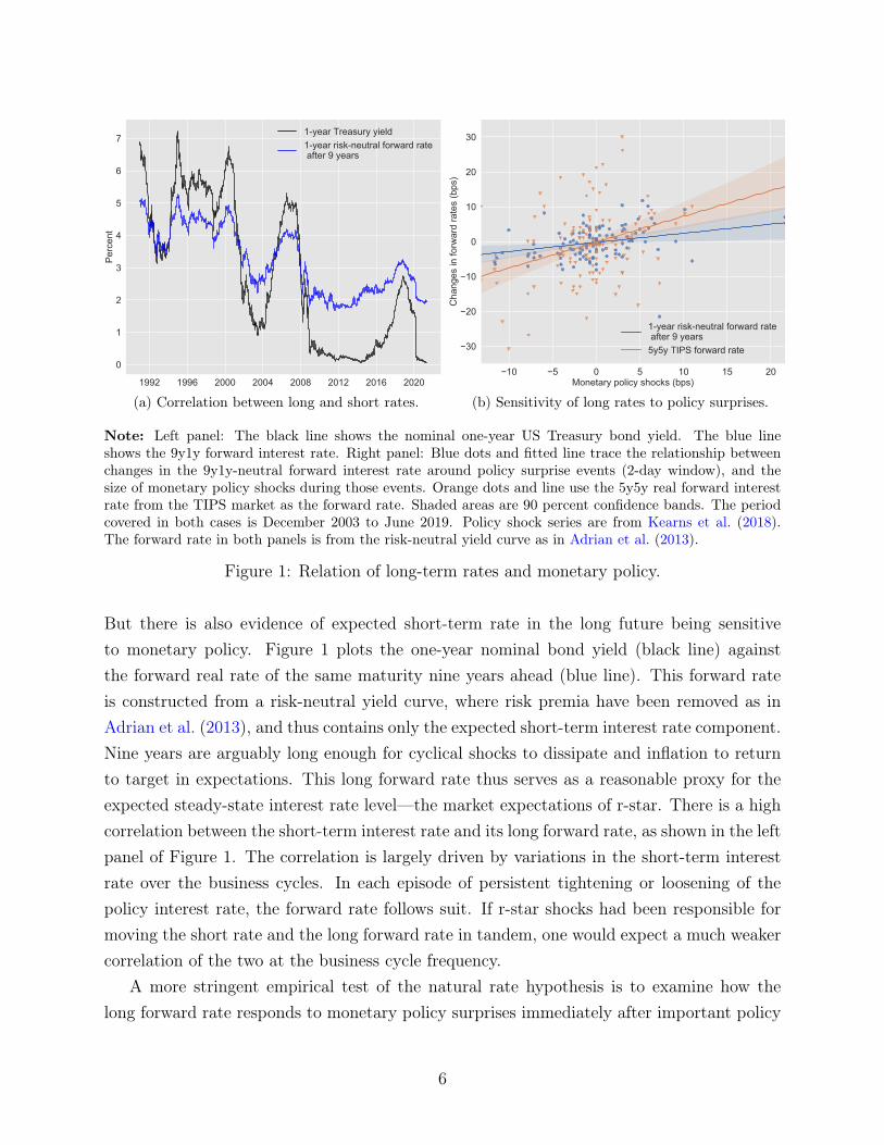
Note: Left panel: The black line shows the nominal one-year US Treasury bond yield. The blue lineshows the 9y1y forward interest rate. Right panel: Blue dots and fitted line trace the relationship betweenchanges in the 9y1y-neutral forward interest rate around policy surprise events (2-day window), and thesize of monetary policy shocks during those events. Orange dots and line use the 5y5y real forward interestrate from the TIPS market as the forward rate. Shaded areas are 90 percent confidence bands. The periodcovered in both cases is December 2003 to June 2019. Policy shock series are from Kearns et al. (2018).The forward rate in both panels is from the risk-neutral yield curve as in Adrian et al. (2013).

Figure 1: Relation of long-term rates and monetary policy.

But there is also evidence of expected short-term rate in the long future being sensitiveto monetary policy. Figure 1 plots the one-year nominal bond yield (black line) againstthe forward real rate of the same maturity nine years ahead (blue line). This forward rateis constructed from a risk-neutral yield curve, where risk premia have been removed as inAdrian et al. (2013), and thus contains only the expected short-term interest rate component.Nine years are arguably long enough for cyclical shocks to dissipate and inflation to returnto target in expectations. This long forward rate thus serves as a reasonable proxy for theexpected steady-state interest rate level—the market expectations of r-star. There is a highcorrelation between the short-term interest rate and its long forward rate, as shown in the leftpanel of Figure 1. The correlation is largely driven by variations in the short-term interestrate over the business cycles. In each episode of persistent tightening or loosening of thepolicy interest rate, the forward rate follows suit. If r-star shocks had been responsible formoving the short rate and the long forward rate in tandem, one would expect a much weakercorrelation of the two at the business cycle frequency.

A more stringent empirical test of the natural rate hypothesis is to examine how thelong forward rate responds to monetary policy surprises immediately after important policy

6

10y Treasury yield

SPF forecasts

Note: The solid line is the 10-year Treasury yield, while dotted lines represent the projected paths of 10-yearTreasury yield according to the Survey of Professional Forecasters. The start of each line marks the currentyield as of the survey date, and is hence on the solid line by definition.

Figure 2: Trend decline in long-term yield largely unforeseen

events. This event-study analysis is arguably better at tracing the causal impact of monetarypolicy surprises than simple time-series correlations. The right panel in Figure 1 showssignificant positive responses of long forward rates to monetary policy surprises. The positiveresponse is stronger if one uses the 5-year 5-year real forward rates from the TIPS market,though part of this responsiveness may owe to the risk premium component as noted inHanson and Stein (2015). At the same time, the result rules out excess sensitivity of long-run inflation expectations to monetary policy as an explanation. Monetary policy thus seemsto impart a significant effect on the market expectations of steady-state interest rate.

There is also evidence that expectations about long-term rates do not conform to therational expectations hypothesis, as has been documented previously in the literature (e.g.Coibion and Gorodnichenko, 2015). Figure 2 plots the time-series of 10-year US Treasuryyield alongside its projection from the Survey of Professional Forecasters. The long-terminterest rate declined continuously throughout the sample, by over 3 percentage points fromits peak. Yet, analysts consistently expected the decline in long-term yields to reverse eachtime they were surveyed, leading to systematic forecast errors. In light of these findings, weexplore small deviations from full information rational expectations that can neverthelessinduce large effects on expectations of long-run rates.

The model we propose in this paper provides a parsimonious explanation of these stylised

7

facts as well as the secular decline in real interest rates. To be clear, it is not the onlypossible explanation. The excess sensitivity of long-term yields to monetary policy couldstem from financial market participants being unduly attentive to short-term factors, whilereal interest rates may have declined for other unrelated reasons. What our model offers is aunified perspective tying all the described phenomena to a common cause. It can moreoverbe formalised within a standard workhorse macroeconomic model and the usual naturalinterest rate concept.

3 Macroeconomic environment

We now introduce the model and show how expectations are the determinant of the de factonatural interest rate. By influencing how agents make consumption and saving decisions,these expectations also dictate how inflation and the output gap respond to monetary policy.

3.1 The New Keynesian model with unobserved r-star

Our model is the standard New Keynesian model, but with incomplete information aboutnatural interest rate determinants. A representative household solves the life-time utilitymaximisation problem

maxCt,Nt,Bt∞t=0

Eh0

∞∑t=0

βtΞt

(C1−σt

1− σ− A1−σ

t

N1+ϕt

1 + ϕ

)s.t. PtCt +Bt = (1 + it−1)Bt−1 + Pt (WtNt + Tt + Πt)

by choosing consumption Ct, labour supply Nt and nominal bond holdings Bt which arein zero net supply and yield a nominal return of it. Consumption Ct is an aggregate ofdifferentiated goods:

Ct ≡(∫ 1

0

Cε−1ε

it di

) εε−1

which gives rise to a standard CES demand function. The household takes as given the pricelevel Pt, the real wage Wt, dividends from firms Πt and any lump-sum transfers from thegovernment Tt. The utility function is affected by shocks to the rate of time preference Ξt.To ensure a balanced growth path with trend productivity shocks, utility also depends onA1−σt .Importantly, the expectation operator Eh is conditional on the information set of private

8

agents, namely the household and firms. This information set is potentially incomplete anddifferent from that of the central bank. The expectations also need not coincide with rationalexpectations once we introduce misperception later on.

Differentiated goods are produced by a continuum of firms i ∈ [0, 1] with the technology

Yit = AtN1−αit

and sold at the price Pit (whose CES sum over i equals Pt). Firms are subject to Calvo pricingfrictions and can only re-optimise their prices with probability 1 − θ. Firms’ revenues aresubsidized at a rate τt. In steady state, this subsidy is set to the value τ that ensures efficiency,while random fluctuations around this value act as cost-push shocks. Firms distribute theirprofits to the household.

The government consists of a central bank that sets the nominal interest rate it, and afiscal authority that collects taxes on firms and distributes the proceeds lump-sum to thehousehold.

Productivity growth is made up of permanent and temporary components (respectivelya random walk and an iid process). Defining at ≡ log(At), we posit:

∆at+1 = gt + εat+1, εat+1 ∼ N(0, σ2

a

)∆gt+1 = εgt+1, εgt+1 ∼ N

(0, σ2

g

).

The time preference ξt ≡ log(Ξt) similarly consists of permanent and temporary components,but also a persistent part:1

∆ξt+1 = −zt − uht − εξ,t+1, εξ,t+1 ∼ N(0, σ2

ξ

)∆zt+1 = εzt+1, εz,t+1 ∼ N

(0, σ2

z

)uht+1 = ρhuht + εht+1, εh,t+1 ∼ N

(0, σ2

h

).

A key departure from the standard setup arises from agents’ incomplete informationabout the at and ξt processes. In particular, the household and firms can observe the currentproductivity level at and the current preference shifter ξt as well as uht. But they cannotseparately observe the subcomponents gt, εat, zt, εξt. As a result, agents cannot disentanglemovements in at and ξt that are attributable to the permanent components gt and zt fromthose that are due to the temporary shocks εat and εξt.

1Technically, ξt has to be bounded in order to guarantee that expected discounted utility remains finite.Imposing such bounds would introduce a non-linearity that would render the filtering problems in the modelcomputationally prohibitive. We abstract from this constraint in what follows.

9

3.2 The belief-driven natural interest rate

We now derive the natural interest rate with incomplete information. Log-linearising thefirst-order conditions and solving the model leads to the familiar Euler equation:

Eht [∆yt+1] =

1

σ

(it − Eh

t [πt+1] + Eht [∆ξt+1]

)(3.1)

where it − Eht [πt+1] is the ex-ante real interest rate from the perspective of private agents.

Evaluating this equation under flexible prices, where log output is at its natural level y∗t = at

and Eht

[∆y∗t+1

]= Eh

t [gt], one can work out the corresponding level of the real interest rateunder flexible prices as:

Eht [σgt + zt] + uh,t. (3.2)

Following Laubach and Williams (2003), we define r-star as the low-frequency component ofthis real interest rate:

r∗t ≡ Eht [σgt + zt] . (3.3)

Substituting this expression back into the Euler equation (3.1), and denoting the outputgap by yt ≡ yt − y∗t , one obtains the familiar IS curve:

Eht [∆yt+1] =

1

σ

(it − Eh

t [πt+1]− r∗t − uht). (3.4)

The second equation of the linearised model is the Phillips curve, which also takes thestandard form up to the expectation operator:

πt = βEht [πt+1] + κyt + upt (3.5)

where κ > 0 is a function of other primitive parameters (see Appendix A and Galí (2015) fordetailed derivation). The cost-push shock upt ∼ log τt, which is observed by private sectoragents, is assumed to follow a normal AR(1) process with autocorrelation ρp and innovationvariance σ2

p.We close the model by assuming that the central bank sets the nominal interest rate

according to a standard Taylor-type rule:

it = ρiit−1 + (1− ρi) (r∗t + φππt + φyyt + uct) . (3.6)

The monetary policy shock uct is observed by the central bank but not by the private sector.It is assumed to follow a normal AR(1) process with autocorrelation ρc and innovation

10

variance σ2c .

Like private agents, the central bank cannot directly observe the r-star and must forman estimate to set policy:

r∗t ≡ Ect [σgt + zt] (3.7)

where Ect denotes the expectation with respect to the central bank’s information set and

inference. In general, these do not necessarily coincide with those of private agents, andhence Ec

t and Eht need not be identical.

This recast of the New Keynesian model to incomplete information yields two key insights:

1. The de facto natural rate of interest relevant to the economy, r∗t , is belief-dependent.It is whatever private agents expect the long-run level of interest rates to be. It is onlyin the special case where private agents perfectly observe gt and zt (and understandthe model correctly), that r∗t is exogenous.

2. The de facto natural interest rate r∗ is not necessarily the same as the estimate r∗ usedby the central bank to guide monetary policy. The two coincide only when the centralbank and the private sector share the same beliefs, so that Ec

t = Eht .

These results mean r∗ is endogenous to learning by the private sector. In the next section,we let both the central bank and the private sector learn from each other through observingthe macroeconomic outcomes, such that their beliefs evolve in an interdependent way. Wewill show that, as a result, r∗ can become endogenous to both monetary policy and cyclicalmacroeconomic shocks.

4 The hall-of-mirror effect: Building intuition

In this section, we illustrate the hall-of-mirror effect under the simplest possiblemacroeconomic setting: a 2-period version of the New Keynesian model discussed above.This allows us to focus on the mutual learning problem and develop intuition for how themechanism operates. The central insights carry over to the dynamic setting, which we dealwith in the next section.

4.1 The 2-period model

Assume that the economy returns to full employment from period 1 onwards, so that Eh0 [yt] =

Ec0 [yt] = 0 for all t ≥ 1, and that the Taylor rule has no inertia, ρi = 0. By the Phillips

curve equation 5.8, both the central bank and households expect inflation to return to zero

11

in period 1. We will also assume that the cost-push shock upt is absent. The model thenbecomes effectively static, and can be summarised in terms of period-0 variables, omittingtime subscripts:

y = − 1

σ(i− r∗ − uh) (4.1)

π = κy (4.2)

i = r∗ + φππ + φyy + uc (4.3)

where r∗ ≡ Eh[ζ] and r∗ ≡ Ec[ζ]. We assume ζ and macroeconomic shocks are white noise:

ζ ∼ N (0, 1) (4.4)

ui ∼ N(0, σ2

ui

), i = c, h. (4.5)

The stochastic terms (ζ, uc, uh) are mutually independent. The prior on ζ has zero meanand unit variance without loss of generality.

Beliefs about ζ have important macroeconomic implications. Solving (4.1)-(4.3) gives

y =1

λ(r∗ − r∗ + uh − uc) (4.6)

i =σ

λ(r∗ + uc) +

(1− σ

λ

)(r∗ + uh) (4.7)

where λ = σ + φπκ+ φy. The output gap (and hence inflation) increases with the differencer∗ − r∗, because a higher r-star belief by the central bank implies a tighter monetary policy,all else equal. As a result, a disagreement about r-star can cause the output gap to deviatefrom zero, even in the absence of demand and monetary policy shocks. Furthermore, theinterest rate that prevails in equilibrium becomes a weighted average between the beliefs ofthe private sector r∗ and those of the central bank r∗.

To form beliefs about the natural interest rate, the private sector and the central bankrely on different sources of information. First, the private sector “h”, and the central bank“c” each receives a signal about ζ:

si = ζ + εi, εi ∼ N(0, σ2

εi

), i = c, h (4.8)

where εc and εh are mutually independent.2 The variance σ2εi can be zero, which corresponds

to i having full information about ζ; it can also be infinity, which corresponds to i havingno private information about ζ. Each side can only observe their own signal.

2In the fully dynamic model, we allow for correlated private signals as well as public signals about r-star.

12

The second information source comes from macroeconomic outcomes y, π and i.Observing these outcomes allows each side to extract information about the private signal ofthe other. The information content can be summarized easily by rearranging the equilibriumconditions (4.6) and (4.7) in terms of two sufficient statistics:

ac ≡ Ec [ζ] + uc = i− (φy + φπκ)y (4.9)

ah ≡ Eh [ζ] + uh = i− (φy − σ)y. (4.10)

Here, ac and ah are noisy signals of Ec[ζ] and Eh[ζ] respectively. These endogenous signals arepublicly observable through observations the nominal interest rate and the output gap. Theprivate sector can thus condition its beliefs on ac, which embeds the unobserved informationof the central bank. Similarly, the central bank can take advantage of the private sector’sinformation by conditioning its belief on ah.

4.2 Inference problem

We can cast the mutual learning problem in terms of the two “agents” in our model—the private sector and the central bank—forming expectations about the random variable ζconditional on (si, ui, aj) where j 6= i. The inference problem of agent i is non-trivial becauseaj is endogenous to i’s expectations.

Due to the Gaussian structure of the fundamentals and signals, beliefs in equilibrium willdepend linearly on the signals and noises. We therefore conjecture, and subsequently verify,that agent i’s belief of agent j’s expectation takes the following linear form:

Ej [ζ] = αjsj + βjsi + γjuj + δjui. (4.11)

We solve agent i’s signal extraction problem given this belief. Agent i’s expectation is

Ei [ζ] = E [ζ | si, ui, aj]

where aj = Ej [ζ] + uj with Ej [ζ] given by (4.11). We can simplify this problem bytransforming aj into aj using a linear combination of agent i’s observables:

aj ≡ aj − βjsi − δjui. (4.12)

Under agent i’s beliefs, the vector (ζ, si, aj)′ is normally distributed with zero mean and

13

variance

V[(ζ, si, aj)

′] =

1 1 αj

1 1 + σ2εi αj

αj αj α2j

(1 + σ2

εj

)+ (1 + γj)

2 σ2uj

. (4.13)

The optimal filtering solution then obtains as

Ei [ζ] = gsisi + gaiaj (4.14)

with the following gain parameters:(gsi

gai

)=

1

α2j

(σ2εi + σ2

εj + σ2εiσ

2εj

)+ (1 + γj)

2 σ2uj (σ2

εi + 1)

(α2jσ

2εj + (1 + γj)

2 σ2uj

αjσ2εi

).

(4.15)

4.3 Common knowledge equilibrium

In an equilibrium with common knowledge, agent i’s conjecture (4.11) coincides with theactual expectation formation of agent j. Substituting (4.11) and (4.12) into (4.14) yields:

Ei [ζ] = gsisi + gai (αjsj + (1 + γj)uj) . (4.16)

Indeed, this has the functional form of the conjecture in (4.11). Comparing coefficients fori = c, h yields the following equilibrium conditions:

αi

βi

γi

δi

=

gsi

gaiαj

0

gai (1 + γj)

. (4.17)

The equilibrium expectation under common knowledge is thus given by:

Ei [ζ] = gsisi + gai (gsjsj + uj) . (4.18)

The equilibrium conditions (4.17) are a non-linear system of equations because gsi andgai depend on αj through (4.15). The following proposition shows that an equilibrium alwaysexists3 and that the parameters of the reaction functions are bounded.

3We can also rule out “nonfundamental” equilibria in which expectations would not conform to the formconjectured in (4.11) and instead coordinate on a sunspot variable (Benhabib et al., 2015; Chan, 2020).

14

Proposition 1 (Common knowledge equilibrium). The equilibrium defined by (4.15) and(4.17) exists and satisfies 0 ≤ gsi ≤ 1 and 0 ≤ gai < 1. Furthermore, gsi = 1 if and only ifσεi = 0.

Proof. See Appendix B.1

It is instructive to consider some special cases. The first arises when the private sectorhas perfect information, while the central bank has no direct source of information andmust only rely on macroeconomic outcomes (encompassed in ah) to infer r-star. This caseunderlies the empirical approach of filtering r-star with a macroeconomic model to gauge theneutral stance of monetary policy (e.g. Laubach and Williams, 2003, Holston et al., 2017and others). In our setting, this situation is captured by σ2

εh = 0 and σ2εc =∞, yielding:

Central bank learning: Ec [ζ] = gac(Eh [ζ] + uh

)(4.19)

Eh [ζ] = ζ. (4.20)

The left panel of Figure 3 depicts the two reaction functions above. The red line traces thecentral bank’s estimate r∗ ≡ Ec [ζ] as a function of ah = r∗+uh, and has a positive slope gac.Intuitively, when ah increases, the central bank observes higher output and inflation for agiven level of interest rate and revises its own estimate r∗ upwards. Meanwhile, the blue lineplots the de facto r-star r∗ ≡ Eh [ζ] as a function of ac = r∗ + uc, a vertical line because theprivate sector is already perfectly informed about ζ. Note how the central bank’s estimate r∗

fluctuates with cyclical shocks. In the figure, a negative demand shock uh shifts the red linedown, resulting in lower r∗. As in Laubach and Williams (2003), the central bank cannotreadily distinguish between cyclical and permanent economic forces, and as a result assignssome weight to the possibility of a reduction in the natural interest rate.

The second special case is the reverse of the second: The central banks has perfectinformation, while the private sector has no direct information and has to rely on the centralbank’s policy actions to infer r-star. This situation gives rise to the signalling channel ofmonetary policy (Nakamura and Steinsson, 2018). In this instance, we have σ2

εh > 0 andσ2εc = 0, yielding:

Private sector learning: Ec [ζ] = ζ (4.21)

Eh [ζ] = gah (Ec [ζ] + uc) + gshsh (4.22)

The right panel of Figure 3 plots these reaction functions. In this case, the reaction functionr∗ is flat, as the central bank forms expectation independently. Meanwhile, the schedule r∗

has a positive slope 1/gah. Intuitively, when ah increases, the private sector observes higher

15

Figure 3: Determination of expectations with one-sided learning.

(a) Central bank learning.

r∗

r∗

r∗(r∗ + uh)

r∗(r∗ + uc)

(b) Private sector learning.

r∗

r∗

r∗(r∗ + uh)

r∗(r∗ + uc)

Note: Each panel shows the central bank’s estimate of r-star r∗ ≡ Ec [ζ] as a function of the noisy observationof the private sector expectation ah ≡ r∗+uh, and the private sector’s de facto r-star r∗ ≡ Ec [ζ] as a functionof the noisy observation of the central bank expectation ac ≡ r∗ + uc.

interest rates for given levels of output and inflation and revises up its own beliefs of long-term interest rates. This de facto r-star now becomes endogenous to monetary policy shocks.In the figure, a negative interest rate shock uc shifts the blue line to the left, leading to a fallin r∗. The private sector cannot readily differentiate between monetary policy shocks andchanges to the central bank’s information about r-star, and thus assigns some weight to thepossibility that the natural real interest rate has declined.

The general case, where both agents learn about the determinants of r-star fromeach other, is unexplored in the literature as of yet. Under common knowledge, we canrearrange the equilibrium expression (4.16) to write agent i’s expectation as a function ofher observables:

Ei [ζ] = (1− gaigaj) gsisi − gaigajui + gai(Ej [ζ] + uj

). (4.23)

This general case is depicted in the left panel of Figure 4, where the de facto r∗ of theprivate sector and the central bank’s estimate r∗ are both increasing functions of each other.In this case, both sides have useful private information about r-star and try to learn fromeach other. The r-star beliefs of both sides now depend on cyclical shocks. In the figure, anegative demand shock uh shifts the red line down, as the imperfectly informed central bankassigns some weight to the possibility that r-star has fallen. At the same time, the privatesector observes the demand shock and knows that it has no bearing on r-star. It rationally

16

Figure 4: Determination of expectations with two-sided learning.

(a) Common knowledge.

r∗(r∗ + uh)

r∗

r∗

r∗(r∗ + uc)

(b) Hall of mirrors.

r∗(r∗ + uh)

r∗

r∗

r∗(r∗ + uc)

Note: Each panel shows the central bank’s estimate of r-star r∗ ≡ Ec [ζ] as a function of the noisy observationof the private sector expectation ah ≡ r∗+uh, and the private sector’s de facto r-star r∗ ≡ Ec [ζ] as a functionof the noisy observation of the central bank expectation ac ≡ r∗ + uc.

corrects its reaction function in anticipation of the decline in r∗: The blue line shifts slightlyto the right. In equilibrium, r∗ is unchanged, as shown in equation (4.16). Thus, only thecentral bank’s expectations are affected by cyclical demand shocks. Conversely, only theprivate sector’s expectations are affected by monetary policy shocks (not shown).

The equilibrium under common knowledge illustrates how an agent can misconstrue anunobserved cyclical perturbation as a r-star shock. But the informational feedback loop islimited because each side correctly understands the other’s reaction function. This correctunderstanding of the informational environment helps limit the informational feedback loop,ruling out the hall-of-mirrors effect. In the next section, we explore a richer setting whereit is possible for agents to confuse all cyclical shocks with shifts in r-star, because theyunderestimate the impact of their own actions on endogenous signals.

4.4 Hall-of-mirrors equilibrium

We now consider a case where agents misperceive the quality of information about thedeterminants of r-star. Specifically, they are overly optimistic about the information thatthey can only observe indirectly: The central bank overestimates the private sector’sknowledge of economic fundamentals, and the private sector likewise overestimates thecentral bank’s knowledge. As we show, this kind of misperception has two effects: First,agents overestimate the amount of information contained in observable macroeconomic

17

outcomes, and thus pay too much attention to them them when they form their beliefs.Second, agents underestimate how much attention the other agent pays to macroeconomicoutcomes, and thus fail to internalize how much their own actions influence the actions ofothers. As a result, everyone’s actions end up reinforcing their incorrect subjective beliefs,generating a positive feedback loop that distorts the exchange of information and amplifiesnoise.

As an example, suppose that the central bank revises its r-star estimate downward andreduces interest rates. The private sector reacts by strongly lowering its own estimate of r-starbecause it overestimates the precision of the central bank’s information about the economy.Output and inflation fall. Because the central bank is ignorant to the private sector’smisperception and itself overestimates the precision of the private sector’s information, itinterprets this demand shortfall as a further indication that r-star has fallen and furtherlowers its own estimate. But in reality, the central bank is merely reacting to a reflectionof its own initial revision. Worse, the ensuing further reduction in interest rates promptsthe private sector to lower its own r-star beliefs a second time, even though it was entirelyprompted by the initial reduction in aggregate demand. Both sides end up misperceivingreactions to their own actions as genuine information: They are staring into a hall of mirrors.4

To formalise the hall-of-mirrors equilibrium, we postulate that each agent i = c, h has asubjective beliefs σ|iεj < σεj about the noise in the private signals of the other side. As before,we conjecture that agent i’s belief of agent j’s expectation takes the form in (4.11), so thatthe solution to her signal extraction problem is still given by Equations (4.14) and (4.15).In addition, agent i mistakenly believes that her beliefs are shared by agent j, and that theeconomy will be in a common knowledge equilibrium. Thus, she also believes that agent j’sexpectation in (4.11) follow (4.17), but where the coefficients are given by the values thatwould obtain if agent j had the same beliefs about the private signal precisions as agent iherself.5

In sum, the solution of agent i’s filtering problem in this misperception equilibrium isrepresented by the following modification of (4.23):

Ei [ζ] =(

1− g|iaig|iaj

)g|isisi − g

|iaig|iajui + g

|iai

(Ej [ζ] + uj

)(4.24)

Here, Ei [ζ] denotes the expectation in the misperception equilibrium, and superscripts i on4Thinking of the equilibrium as a sequence of revisions and reactions is a useful but only narrative device.

In the model, the equilibrium is the fixed point of agents’ reaction functions and the revisions are all realizedwithin one period.

5Unlike in Caballero and Simsek, 2021, agents in our model do not “agree to disagree”: They are unawarethat they disagree about the distribution of information in the economy, and mistakenly attribute all theirobservable disagreements to differences in private information.

18

the gain parameters denote the subjective beliefs of agent i about the gain parameters ofeither agent. The subjective beliefs of these parameters under misperception are given by amodification6 of (4.15):

(g|isi

g|iai

)=

1(g|isj

)2 (σ2εi + σ

2|iεj + σ2

εiσ2|iεj

)+ σ2

uj (σ2εi + 1)

(g|isj

)2

σ2|iεj + σ2

uj

g|isjσ

2εi

(4.25)

(g|isj

g|iaj

)=

1(g|isi

)2 (σ2εi + σ

2|iεj + σ2

εiσ2|iεj

)+ σ2

ui

(σ

2|iεj + 1

) (

g|isi

)2

σ2εi + σ2

ui

g|isiσ

2|iεj

(4.26)

The first equation describes the solution of the filtering problem of agent i undermisperception, while the second line describes agent i’s perceived solution of the filteringproblem of agent j. Agent j herself also solves her own problem and guesses agent i’ssolution according to the same formula.

In the equilibrium with misperception, neither agent has the correct beliefs about howfundamentals and beliefs are related. Equation (4.24) relates the equilibrium beliefs of agenti = c to those of agent j = h, and those of agent i = h to those of agent j = c. This system oftwo linear equations allows to solve for the equilibrium expectations of both agents, leadingto the following expression:

Ei [ζ] = g|isisi + g

|iai

(g|jsjsj + uj

)+

g|iai

1− g|iaig|jaj

[(g|jaj − g

|iaj

)(g|isisi + ui

)+(g|iai − g

|jai

)g|jaj

(g|jsjsj + uj

)](4.27)

The equilibrium beliefs differ from beliefs under common knowledge (4.18) in two ways.First, the gain parameters in the first line of (4.27) differ because agents misjudge theinformativeness of signals. Second, each side also misperceives the reaction function of theother, which gives rise to the terms on the second line of (4.27). Agents no longer gauge theimpact of their actions on their opponents’ beliefs correctly.

As an example, consider a temporary negative demand shock uh < 0. The private sector(i = h) takes no direct signal from this shock, as it is known to be unrelated to r-star. Theexpectation of the central bank (j = c), however, decreases by g|jajui. Because the privatesector misperceives the central bank’s reaction function, it only expects this expectation to

6Relative to (4.15), we have substituted αj with g|isj , using the equilibrium relation (4.17) as perceived by

agent i; and, switching around the roles of i and j in (4.15), we have substituted αi with g|isi.The variances

of εi and εjas well as the gain parameters carry superscripts to denote the subjective beliefs of agent i.

19

fall by g|iajui, resulting in a surprise of ∆ =(g|jaj − g

|iaj

)ui. This initial misperception is now

subject to a multiplier effect: The private sector adjusts its expectation by g|iai∆. The centralbank, seeing this change, adjusts its expectation further by an amount g|jajg

|iai∆, resulting in

a further adjustment g|iaig|jajg|iai∆ of the private sector and so on. In equilibrium, the initial

surprise ∆ is multiplied by the term g|iai/(

1− g|iaig|jaj

)in (4.27).

This multiplier effect embodies what we call the hall-of-mirrors effect. Its strengthdepends on how much attention agents are paying to each other’s expectations in formingtheir own beliefs and can in principle be unboundedly large if the misperception is strongenough.

Proposition 2 (Hall-of-mirrors effect). If σ|iεj is sufficiently small, then:

1. Beliefs overreact to demand and monetary policy shocks uc and uh relative to thecommon knowledge equilibrium: g|iai < gai and g

|iaj < g

|iai.

2. This overreaction can be arbitrarily large: g|cac and g|hah can be arbitrarily close to one.

Proof. See Appendix B.2.

The proposition is graphically illustrated in the right panel of Figure 4. The slope of thecentral bank’s reaction function (red line) is g|cac and the slope of the private sector’s reactionfunction (blue line) is 1/g

|hah. In the hall-of-mirrors equilibrium, both slopes are close to one.

After a negative demand shock uh, the central bank’s reaction function shifts down. Theprivate sector’s reaction function shifts to the right, but unlike in the common knowledge casethe shift is insufficient to offset the decrease in r-star expectations. The reason is that theprivate sector mistakenly thinks that the central bank has very good private information andwill not react much to private sector expectations. This (mis)perceived reaction function isrepresented by the red dashed line in Figure 4, which has slope g|hac < g

|cac. The private sector

adjusts its own expectation to this perceived reaction function. In equilibrium, however, thecentral bank pays a lot of attention to private sector expectations. The result is a decreasein r-star expectations by both sides that can in principle become arbitrarily large.

4.5 Macroeconomic implications

We now turn to the macroeconomic implications of imperfect knowledge and misperception.Recall that (4.6) relates the output gap y (and inflation π = κy) to the macroeconomicshocks as well as the difference of r-star beliefs between the household and the central bank:

y =1

λ(r∗ − r∗ + uh − uc) .

20

This difference in beliefs depends in turn on the macroeconomic shocks as well as the signals:

r∗ − r∗ = bhg|hshsh − bcg

|cscsc − (1− bh)uh + (1− bc)uc (4.28)

with bi =(

1− g|jaj) 1− g|iaig

|iaj

1− g|iaig|jaj

.

The following proposition shows that, while expectations can overreact to shocks due to thehall-of-mirrors effect, the output gap and inflation underreact to shocks.

Proposition 3. If σ|cεh and σ|iεh are sufficiently small, then the difference of r-star beliefs r∗−r∗

comoves negatively with demand shocks uh and positively with policy shocks uc: 0 < bc, bh < 1.Moreover, the effects of these shocks on the output gap and inflation are dampened relativeto the full information case where bh = bc = 1.

Proof. See Appendix B.3.

As an illustration, consider again a negative demand shock uh < 0. The direct effect ofthis shock is to lower the output gap. The indirect informational effect is that the centralbank revises down its r-star estimate r∗ as it sees demand falling. The private sector will alsorevise down its estimate r∗, but by less than the central bank. Even though the economyhas weakened due to lower r∗, the more accommodative policy due to lower r∗ more thanoffsets this weakness, so that output and inflation fall less than under full information.7

By the same token, misperception weakens the transmission of monetary policyaccommodation to output. As usual, a negative interest rate shock uc < 0 has a directexpansionary effect on the output gap. But the indirect learning effect induces a fall in theterm r∗ − r∗, as the private sector revises down their r-star belief by more than the centralbank. This has a negative impact on output as the central bank lowers the interest rate byless than needed to offset the shock. As a result, the shock stimulates aggregate demand lessthan under full information.

While incomplete information and the hall-of-mirrors effect tend to dampen movementsin output and inflation, they also amplify movements in expectations of r-star and interestrates. An outside observer may conclude that the structural relation between interest ratesand real activity is weak. However, this pattern in our model is entirely consistent witha standard Euler equation and particular correlations between r-star beliefs and cyclicalshocks.

7This output-dampening effect would reverse once policy is constrained by the ZLB, as the interest ratecould no longer fall to compensate for a lower r-star. The interaction of the hall-of-mirrors effect and theZLB is an interesting question which we leave to future research.

21

5 Dynamic model

We now turn to the full, dynamic version of our model. The information structure andthe associated qualitative equilibrium results all carry over from the static model presentedabove. To make the model more general, we add a public source of information observable byall agents, and also allow for a general autocorrelation structure of economic fundamentalsand signal noise. We will show that the hall-of-mirrors effect not only amplifies noise tor-star beliefs, but also generates misperception that can be very persistent under plausibleparameters.

5.1 Fundamentals and exogenous signals

In the dynamic model, the central bank and the private sector need to form expectationsof the fundamental determinants of real interest rates, ζt = σgt + zt, which forms a randomwalk process

ζt = ζt−1 + vt, vt ∼ N(0, σ2

ζ

)(5.1)

with σ2ζ = σ2σ2

g + σ2z .

At the start of each period t, the central bank and the private sector (i = c, h) receiveprivately observed signals sit about the fundamentals:

sit = ζt + eit (5.2)

eit = ρeieit−1 + εit, εit ∼ N(0, σ2

εi

). (5.3)

In addition, both observe a public signal xt of the same form:

xt = ζt + ft (5.4)

ft = ρfft−1 + ηt, ηt ∼ N(0, σ2

η

). (5.5)

Apart from these signals, there are three transient macroeconomic shocks in the model: Thedemand shock uht, the cost-push shock upt and the monetary policy shock uct. Each followsan AR(1) process:

ukt = ρkukt−1 + νkt, νkt ∼ N(0, σ2

uk

).

The private sector is assumed to observe the demand and cost-push shocks uht and uptbut not the policy shock uct. Meanwhile, the central bank observes the policy shock uct, butnot the demand and cost-push shocks uht and upt.

We collect the vector of exogenous states in Zt = (ζt, eht, ect, ft, uht, upt, uct)′ and the

22

vector of exogenous shocks in qt = (vt, εsht, εct, ηt, νht, νpt, νct)′. Then we can write

Zt = AzZt−1 + qt, qt ∼ N (0,Σq) (5.6)

with Az = diag (1, ρe1, ρe2, ρf , ρuh, ρup, ρuc) and Σq = diag(σ2ζ , σ

2ε1, σ

2ε2, σ

2η, σ

2uh, σ

2up, σ

2uc

).

5.2 Macroeconomic outcomes and endogenous signals

The private sector determines inflation and output according to the system of equationsconsisting of (3.4)–(3.6). We write this system of equations entirely from the perspective ofthe private sector information set:

yt = Eht [yt+1] +

1

σEht [πt+1 + ζt] +

1

σ(uht − it) (5.7)

πt = βEht [πt+1] + κyt + upt (5.8)

it = ρiit−1 + (1− ρi)(Eht E

ct ζt + φππt + φyyt + Eh

t [uct])

(5.9)

The private sector observes the nominal interest rate it in addition to its private signal shtand the public signal xt, and it also observes the demand and cost-push shocks uht and upt.But it does not separately observe Ec

t ζt and uct in the policy rule (5.9) and has to estimatethese objects.

The central bank observes current inflation πt and the output gap yt in addition to itsprivate signal sct and the public signal xt. It determines the nominal interest rate it accordingthe Taylor rule as a function of inflation, the output gap, its current-period estimate of r-star, as well as the monetary policy shock uct. We assume that the coefficients φπ and φy

in the monetary policy rule yield a unique solution to (5.7)–(5.9), given expectations of theexogenous fundamentals.

5.3 Solution with common knowledge

Solving the dynamic model requires keeping track of higher-order beliefs explicitly. We definethe “zero-th order beliefs” as the true fundamentals: E(0)

it [Zt] = Zt. The first-order beliefsof agent i = c, h are her expectations about the fundamentals: E

(1)it [Zt] = Eit [Zt]. For

n ≥ 1, her n + 1-th order belief is defined as the belief about the n-th order belief of agentj: E(n+1)

it [Zt] = Eit

[E

(n)jt [Zt]

], j 6= i.

For each agent i = c, h, we denote with Xit the states that agent i does not observe,

23

which are the beliefs of all orders n = 0, 1, 2, . . . of Zt of the other agent j:

Xit =(E

(n)jt Zt

)∞n=0

. (5.10)

Agent i has to form beliefs about Xit. She enters period t with a prior belief about Xit−1

which is distributed as N (mit−1, Pi).8 She then observes her own private signal sit, thepublic signal xt, as well as the macroeconomic outcomes (yt, πt, it). Additionally, the centralbank observes uct, while the private sector observes uht and upt.

Agent i’s posterior belief takes the form

Xit | i, t− 1 ∼ N (mit, Pi) . (5.11)

To characterize this belief, we solve the signal extraction problem using a conjecture on theother agent’s belief mjt. We guess, and later verify, that agent j’s belief evolves accordingto:

mjt = Φjmjt−1 + Ψjmit−1 + ΩjZt. (5.12)

We can rewrite the state Xit that player i has to learn about in a recursive form:

Xit = AiXit−1 +Biqt + Cimit−1. (5.13)

where the matrices Ai, Bi and Ci depend on the guess in (5.12) as well as Az in (5.6). Theexact expressions are provided in Appendix C.

We also guess, and later verify, that the signals agent i receives in period t are a linearcombination of the current state:

Yit = HiXit. (5.14)

Equations (5.13) and (5.14) form a standard linear filtering problem, the solution of which isgiven by the Kalman filter. The optimal filtering equation describing the evolution of beliefsis:

mit = (I −GiHi) (Ai + CmΨj)mit−1 +GiYit (5.15)

The Kalman gain Gi, as well as the time-invariant posterior covariance matrix Pi, can becomputed using standard formulas, also detailed in Appendix C.

We can now find the equilibrium with common knowledge and verify our conjectures(5.12) and (5.14). In a common knowledge equilibrium, agent i’s beliefs of (5.12) and of the

8We assume that enough time has passed for the prior variance to reach its time-invariant level, in keepingwith much of the literature.

24

signal matrix Hi are correct. We can thus express the vector of signals Yit in terms of pastbeliefs and the current state:

Yit = Hi (CzZt + Cmmjt)

= Hi ((Cz + CmΩj)Zt + CmΦjmjt−1 + CmΨjmit−1) . (5.16)

Substituting this expression into (5.15) gives an expression for mit that verifies our guess(5.12). The equilibrium coefficients can be found using the following system of equations:

Φi = (I −GiHi)Ai + CmΨj (5.17)

Ψi = GiHiCmΦj (5.18)

Ωi = GiHi (Cz + CmΩj) . (5.19)

Finally, we need to compute the observation matrices Hi. This step is more involvedthan in the static model because the endogenous signals provided by observations ofmacroeconomic outcomes now depend on the fundamentals as well as first- and higher-orderbeliefs. For example, the output gap, which the central bank uses as an endogenous signalabout r-star, depends on the private sector’s expectation of the future interest rate path,which depend on its expectations about the central bank’s expectation of r-star. AppendixC solves for the macroeconomic outcomes of the model as a function of private sector beliefs,and shows that the signal matrix for the central bank Hc is a function of the macroeconomicmodel parameters, as well as the matrices Az,Φh,Ψh,Ωh. The signal matrix for the privatesector Hh does not depend on other parameters in the model.

To compute the equilibrium numerically, we use the following iterative algorithm:

1. Start with an initial guess (Φi,Ψi,Ωi, Hi)i=c,h.

2. For i = c, h:

(a) compute the law of motion for Xit from (C.4);

(b) compute the Kalman matrices P−i , Si, Gi, Pi from (C.6)–(C.9);

(c) compute Φi,Ψi,Ωi from (5.17)–(5.19).

3. Compute the signal matrix Hc according to (C.11). The matrix Hh stays the sameacross iterations.

4. Iterate on steps 2. and 3. until convergence.

25

For our computations, we have to truncate the infinite sequence of higher-order beliefscontained inmit to some finite levelN . Our numerical results show that whenN is sufficientlylarge, the choice of N does not affect the equilibrium dynamics.

5.4 Misperceptions equilibrium

As in the static version of our model, we can compute the corresponding equilibrium withmisperception. In this case, each agent i = c, h has own beliefs about the properties A andΣq of the fundamentals and/or signals Zt in (5.6). We denote these beliefs with A|i and Σ

|iq .

For the purpose our simulations, we only consider the “hall-of-mirrors” case in which eachagent believes that σ|isj < σsj, but the solution below applies to other types of misperceptionas well. Furthermore, agent i believes that the other agent j = h, c shares her own beliefsabout the fundamentals. That is, both agents mistakenly assume common knowledge oftheir own beliefs about the fundamentals, when in fact they disagree about them.

To solve agent i’s perceived law of motion of beliefs, we first solve a common knowledgeequilibrium where we substitute subjective beliefs A|i and Σ

|iq for the true values A and Σq,

respectively. This solution yields a perceived law of motion (4.11) for mkt with coefficientsΦ|ik , Ψ

|ik and Ω

|ik , k = c, h, as well as perceived gains G|ik and signal matrices H |ik .

To proceed from the perceived law of motions to the equilibrium, we then write thefiltering equation (5.15) as:

mit =(

Φ|ii −G

|iiH|ii CmΨ

|ij

)mit−1 +G

|ii Yit

=(

Φ|ii −G

|iiH|ii CmΨ

|ij

)mit−1 +G

|iiH|ji (CzZt + Cmmjt) . (5.20)

To obtain the second line, we substitute out the actual signals Yit that agent i receives,which depend on the expectations of agent j and are hence given by Yit = H

|ji Xit. The

above expression also holds when the roles of i and j are reversed, and we can use this factto substitute out mjt. We then obtain the actual law of motion of beliefs describing theequilibrium under misperception:

mit = Φimit−1 + Ψimjt−1 + ΩiZt (5.21)

26

where the actual transition coefficients are given by:

Φi =(I −G|iiH

|ji CmG

|jj H

|ij Cm

)−1 (Φ|ii −G

|iiH|ii CmΨ

|ij

)(5.22)

Ψi =(I −G|iiH

|ji CmG

|jj H

|ij Cm

)−1

G|iiH|ji Cm

(Φ|jj −G

|jj H

|jj CmΨ

|ji

)(5.23)

Ωi =(I −G|iiH

|ji CmG

|jj H

|ij Cm

)−1

G|iiH|ji

(I + CmG

|jj H

|ij

)Cz. (5.24)

The macroeconomic outcomes in the misperception equilibrium are again determined by theprivate sector’s beliefs, and we relegate this formula to Appendix C.

6 Simulation results

We will now use a calibrated version of our dynamic model to explore the potentialquantitative implications of the hall-of-mirrors effect. How much can cyclical shocks toaggregate demand and monetary policy affect the de facto r-star? As the preceding analysissuggests, the answer will depend in part on the degree of misperception. Our benchmarkcalibration will imply a large degree of misperception, but we also document the sensitivityof our results to the information parameters including misperception.

Table 1: Calibrated parameters.

Parameter Symbol Value

Inverse EIS σ 6Phillips curve slope κ 0.015Discount factor β 0.9941Rule coefficient on inflation φπ 1.5Rule coefficient on output gap φy 0.125Rule coefficient on lagged rate ρi 0.7Autocorr. of policy shock ρuc 0.7S.d. of policy shock σuc 0.1Autocorr. of demand shock ρuh 0.8S.d. of demand shock σuh 0.2

Parameter Symbol Value

Initial value of ζ ζ0 2.4 %S.d. of ζ shock σζ 0.05Steady-state inflation π∗ 2 %Autocorr. of cost-push shock ρuπ 0.8S.d. of cost-push shock σuπ 0.1Autocorr. of public signal noise ρf 0Autocorr. of private signal noise ρei 0S.d. of public signal noise ση 3S.d. of private signal noise σεi ∞Perceived — σ

|jεi 0.2

To conduct our simulations, we calibrate the model parameters as in Table 1.Macroeconomic parameters are standard in the literature (e.g. Billi, 2011). The standarddeviation of changes to r-star fundamentals is set to 0.05 percent quarterly, in line withthe estimates by Holston et al. (2017). The public signal about these fundamentals isassumed to be quite noisy, with a standard deviation of 3, and true private informationis assumed to be absent (σεi =∞). The resulting uncertainty about r-star in the absence of

27

misperception corresponds to 90% confidence intervals of subjective r-star beliefs of ±2.5%,which is large but within the range of empirical studies.9 In addition, we assume a largedegree of misperception: Despite there being no useful private information at all, each sidebelieves that the other side has valuable private information (σ|jεi = 0.2). The resultinguncertainty about r-star corresponds to a 90% confidence interval of ±0.9% for the privatesector, and ±1.4% for the central bank, which is again close to the empirical estimates byHolston et al..

6.1 A demand-driven recession

In the first simulation exercise, we focus on the decade following the GFC, a periodcommonly associated with a notable decline in the natural interest rate, large adverse demandshocks, and extraordinary monetary policy accommodation. We simulate a sequence ofadverse transient demand shocks lasting 12 quarters. The size of the shocks is chosen toreduce inflation by about 1% and output gap by 5% at their peaks, yielding a reasonableapproximation of the strong demand headwinds in the immediate aftermath of the GFC.

Figure 5 depicts the simulation outcomes of key variables in our benchmark calibration(solid red and yellow lines), and also in a counterfactual simulation where the central bankand the private sector both have full information about the determinants of r-star (solid bluelines). In this full information counterfactual, r-star is unchanged throughout the simulationas everyone understands that the adverse demand shocks are not permanent. Inflation andthe output gap decline and the central bank responds by lowering the nominal interest rate.

With incomplete information and misperception, the perceived r-star from the the centralbank’s perspective (solid yellow line) declines steeply, by almost 2.5 percentage points withinthe first few years. The reason is that the central bank misinterprets the transient shock tooutput as being partly driven by a decline in r-star, prompting the central bank to lowerits r-star estimate as well as to cut its policy rate by more than the policy rule reaction toinflation and the output gap would imply (top right panel). This policy action is observedand interpreted by the private sector as signaling a fall in r-star, prompting the privatesector to revise its r-star estimate as well. As a result, the de facto r-star (red line) declinessteadily, though not as sharply as the one perceived by the central bank. This sets in motiona positive learning feedback that keeps both agents’ estimates of r-star low throughout thefollowing decade. This result shows that the hall-of-mirrors effect does not only affect r-starperceptions temporarily, but in fact very persistently.

9The equilibrium subjective variance of the states is Pi and the first element of that matrix is the varianceof ζ, which corresponds to the variance r-star at quarterly rate. The size of a symmetric confidence intervalof size α at annual rate is then given by 4zα

√Pi,11. For α = 0.9, zα ≈ 1.68.

28

Note: Simulation of macroeconomic variables based on a sequence of negative demand shocks over 8 quarters.Parameters used for the calibration are shown in Table 1.

Figure 5: Responses of macroeconomic variables to an adverse demand shock.

29

The paths of the simulated variables under misperception exhibit the same patterns asthe data in the aftermath of the GFC quite well. By construction of the shocks in thesimulation, the output gap and inflation fall by similar amounts as in the data. Theysubsequently recover more quickly, howeer, partly due to the simplicity of the standardNew-Keynesian model that does not feature intrinsic inertia, and partly due to the fact thatour model is linear and cannot capture the contractionary effects of the binding zero lowerbound in the aftermath of the GFC. Indeed, our simulated path of the nominal interest ratebecomes negative for four quarters. At the end of the period shown, however, the levels ofthe simulated nominal rate and the federal funds rate align well.

Most strikingly, the r-star estimate based on Holston et al. (2017), a popular benchmarkmeasure of r-star estimated from inflation and output, lines up well with the model’sprediction of the central bank’s estimate of r-star. At the same time, the private sector’sexpectation of long-term real rates, e.g. based on the Blue Chip survey, declines in tandembut at a slower pace than the Holston et al. (2017) measure, consistent with the model’sprediction. This result confirms that our relatively simple model can can quantitativelyexplain the entire fall in perceived r-star from persistent misperception of temporary shocksdue to the hall-of-mirrors effect.

It is also noteworthy that the reductions in inflation and the output gap are slightly lesspronounced under misperception than under full information. As in the static model, thesedifferences reflect two countervailing forces. First, misperception generates a deflationaryforce by lowering de facto r-star. Conditional on the same interest rate path, the hall-of-mirrors case is therefore associated with lower output and inflation. Second, the centralbank’s perceived r-star declines by more than that of the private sector, which makesthe monetary policy stance more accommodative than what the inertial Taylor rule wouldprescribe. This second force dominates in the simulation. If our model incorporated aneffective lower bound on the nominal interest rate, only the first force would operate and thehall-of-mirrors equilibrium would likely result in an unambiguously inferior macroeconomicoutcome.

We can also use the model to simulate longer-term interest rates and their subjectiveexpectations, providing another avenue for empirical evaluation. We use the simulatedinterest rate paths to generate a series of yield curves.10 We compare these simulated yieldcurves with the data. The model is able to replicate the stylised facts discussed in section 2.The top-left panel of Figure 6 shows that, just as in the data, yield forecasts systematicallyfail to predict the persistent decline in the actual yield. Note that expectations of interestrates underreact, even though expectations of r-star overreact in our model. The reason is

10The model implicitly embeds the assumption that term premia are zero.

30

that private sector agents in the model are ignorant of the predictable overreaction of theirown r-star expectations, and therefore expect interest rates to recover for a long time. Itis only when r-star expectations stop falling that the bias in interest rate forecasts all butdisappears in our model.

The top right panel of Figure 6 shows that long-term forward real rates reacts to monetarypolicy surprises, as in the data.11 In the model, this correlation arises from the signallingchannel: The private sector interprets downward surprises in nominal interest rates assignalling information on behalf of the central bank that r-star has declined.

Finally, the bottom two panels of the figure show that the broad movements of theyield curve match up with the data as well. As discussed in section 2, these stylised factscollectively are difficult to explain if one maintains that r-star must be independent fromcyclical phenomena.

6.2 Monetary policy shocks

Temporary monetary policy shocks can set off a similar chain reaction that prompts apersistent fall in r-star. We show the effects of an expansionary shock to the Taylor rule inFigure 7.

The central bank initially believes correctly that r-star remains constant. But as it easespolicy, the private sector reacts by revising down its perception of r-star, pushing the relevantnatural rate for the economy lower. This creates demand headwinds, which the central bankthen attributes partly to a decline in r-star, not realising the endogenous impact of its ownpolicy action. Again, the information feedback is set in motion, leading to persistently lowr-star as perceived by both parties.

The figure also shows that the hall-of-mirrors effect in this case is unambiguouslycontractionary relative to the full information case, limiting the effectiveness of the shock instimulating aggregate demand. The supposed tell-tale signs of overly accommodative policysuch as inflation pressure become unreliable, as the hall-of-mirrors effect distorts the privatesector’s beliefs. What’s more, the misperception set in motion by expansionary policy takesvery long to dissipate. A dilemma consequently emerges: A more aggressive monetary policyaccommodation may boost output in the short run, but may also worsen demand headwindsover time.

11In the data, monetary policy surprises are defined as changes in short-term interest rates aroundannouncement dates. In the model, macroeconomic shocks and monetary policy surprises are realizedsimultaneously. Therefore, we use a decomposition of the overall surprise in each period, and of thecorresponding movements in yields, that best isolates the policy surprise component. The constructionof this decomposition is documented in Appendix C.1.

31

Simulated 10y nominal yield

Simulated expectations

10y Treasury yield

SPF forecasts

(a) Yield and forecasts; data and simulationmonetary policy surprise (bps)

ch

an

ge

in

9y1

y f

orw

ard

re

al ra

te (

bp

s)

Model

Data, 2007m8-2019m6

(b) Excess sensitivity of long forward rate

Nom

inal yie

ld

1

2

3

4

5

6

7

8

9

10

Matu

rity

(years

)

(c) Yield curve data

Nom

inal yie

ld

1

2

3

4

5

6

7

8

9

10

Matu

rity

(years

)(d) Yield curve simulation

Note: Simulation of yield curves and forward interest rates, constructed using expected path of interest rateand assuming that the expectation hypothesis holds. For the construction of monetary policy surprises andassociated yield movements see Appendix C.1. Results are based on a sequence of negative demand shocksover 8 quarters. Parameters used for the calibration are shown in Table 1.

Figure 6: Responses of yield curve to an adverse demand shock.

32

Note: Simulation results based on an accommodative monetary policy shock. Parameters used for thecalibration are shown in Table 1.

Figure 7: Responses to an expansionary monetary policy shock.

33

6.3 Sensitivity to alternative information structures

How much misperception is needed to generate a notable fall in r-star? The answer is,not much, as a sensitivity analysis to key information parameters reveals. We repeatthe simulation of Figure 5, keeping the shocks constants, but changing the informationparameters. The corresponding simulated outcomes on the private sector’s de factor r-starand the output gap are shown in Figure 8.

In the first simulation labeled “less misperception”, we reduce the perceived quality ofprivate information by increasing σ

|ij tenfold, thus reducing the amount of misperception

considerably. In this simulation, r-star still falls by over a percentage point within five years,about half the decline in the baseline simulation.

In the second simulation labeled “better information”, we improve the actual quality ofprivate information, by lowering σi drastically from infinity to one. This change, too, reducesthe amount of misperception, but also leads both the private sector and the central bank topay more attention to their own information. The result is a decline in r-star of a similarmagnitude as in the first simulation, but which dissipates more quickly.

The third simulation labeled “more volatile fundmantals” shows a case in which theunderlying fundamentals determining r-star (that is, the trends of productivity and discountfactor changes) becom mroe volatile. Our baseline calibration has σζ = 0.05, correspondingto quarterly changes in annualized r-star of 0.2 percent, which is at the lower end of theestimates in Holston et al. (2017). If we increase this value to σζ = 0.07, towards the upperbound of their estimates, this would push r-star down by a further full percentage point.Intuitively, when it is harder to pin down the true drivers of r-star, agents rely more onlearning from each other, strengthening the hall-of-mirrors effect.

Finally, we note that the impact on output and inflation (not shown) of these changes tothe information structure is small. These outcomes are mainly determined by the differencebetween the central bank’s and the private sector’s estimates of r-star, which stay relativelysimilar across the simulations.

7 Conclusion

We have extended the canonical New-Keynesian model to an incomplete information setupwhere agents have to learn about the determinants of r-star. Our analysis highlights thepotentially important role of beliefs and two-way learning feedback as an independent driverof persistent changes in real interest rates. Crucially, it is difficult to determine if r-starshifts come from structural saving and investment factors, or instead from endogenous

34

Note: The simulation labeled “baseline” refers to the simulation shown in Figure 5. In each of the othersimulations, one parameter is changed relative to this baseline. For “less misperception”, the perceived noisein private signals is set to σ

|ji = 2 instead of σ|ji = 0.2. For “better information”, the actual noise in

private signals is set to σi = 1 instead of σi = ∞. For “more volatile fundamentals”, the volatility of r-starfundamentals is set to σζ = 0.07 instead of σζ = 0.05.

Figure 8: Alternative simulations with an adverse demand shock.

misperception by both the private sector and the central bank. Both cases produce similarmacroeconomic outcomes, but the policy implications could not be more different. Ifmisperception is indeed responsible for a trend decline in real interest rates, then reactingto negative demand shocks with an overly aggressive policy accommodation could becounterproductive. Such a strategy would prompt the private sector to revise down itsperception of r-star, and further raise the bar for what it takes to keep the economy ona sustainable path. The problem likely becomes more severe the closer the economy is tothe policy lower bound, as the very act of aggressive policy easing could lower the naturalinterest rate and make that constraint more likely to bind. Our finding sounds caution onthe conventional policy recommendation that central banks should ease policy aggressivelyin the vicinity of the effective lower bound to avoid a liquidity trap.

Our results point to several promising avenues of further research. First, exploring furtherways of taking the model to the data and quantifying the hall-of-mirrors effect in practicewould enhance our understanding of its importance. Second, it could be fruitful to explorenormative implications of the hall-of-mirrors effect for the design of monetary policy. Third,our model abstracts from ways in which r-star misperception may affect decisions such asinvestment or R&D, decisions that have a long-term impact. Adding these channels wouldlikely imply that even temporary misperception of r-star could have longer-lasting economicconsequences that are hard to reverse.

35

ReferencesAdrian, T., R. Crump, and E. Moench (2013): “Pricing the Term Structure with LinearRegressions,” Journal of Financial Economics, 110, 110–38.

Angeletos, G.-M., L. Iovino, and J. La’O (2020): “Learning over the business cycle:Policy implications,” Journal of Economic Theory, 190, 105115.

Angeletos, G.-M. and J. La’O (2020): “Optimal Monetary Policy with InformationalFrictions,” Journal of Political Economy, 128, 1027–1064.

Beaudry, P. and C. Meh (2021): “Monetary policy, trends in real interest rates anddepressed demand,” Bank of Canada Staff Working Papers 2021-27.

Benhabib, J., P. Wang, and Y. Wen (2015): “Sentiments and Aggregate DemandFluctuations,” Econometrica, 83, 549–585.

Bernanke, B. and M. Woodford (1997): “Inflation Forecasts and Monetary Policy,”Journal of Money, Credit and Banking, 29, 653–84.

Billi, R. M. (2011): “Optimal Inflation for the US Economy,” American Economic Journal:Macroeconomics, 3, 29–52.

Borio, C., P. Disyatat, J. Juselius, and P. Rungcharoenkitkul (2017): “Why soLow for so Long? A Long-Term View of Real Interest Rates,” BIS Working Paper 685.

Caballero, R. J. and A. Simsek (2021): “Monetary Policy with Opinionated Markets,”NBER Working Papers 27313.

Chan, J. (2020): “Monetary Policy and Sentiment-Driven Fluctuations,” working paper.

Coibion, O. and Y. Gorodnichenko (2015): “Information Rigidity and the ExpectationsFormation Process: A Simple Framework and New Facts,” American Economic Review,105, 2644–78.

Cukierman, A. and F. Lippi (2005): “Endogenous monetary policy with unobservedpotential output,” Journal of Economic Dynamics and Control, 29, 1951–1983.

Galí, J. (2015): Monetary policy, inflation, and the business cycle: an introduction to thenew Keynesian framework and its applications, Princeton University Press.

Hanson, S. G., D. O. Lucca, and J. H. Wright (2018): “The Excess Sensitivity ofLong-term Rates: A Tale of Two Frequencies,” Staff Report 810, Federal Reserve Bank ofNew York.

Hanson, S. G. and J. C. Stein (2015): “Monetary Policy and Long-term Real Rates,”Journal of Financial Economics, 115, 429–48.

36

Holston, K., T. Laubach, and J. C. Williams (2017): “Measuring the Natural Rateof Interest: International Trends and Determinants,” Journal of International Economics,108, S59–S75.

Johannsen, B. K. and E. Mertens (2021): “A Time-Series Model of Interest Rates withthe Effective Lower Bound,” Journal of Money, Credit and Banking, 53, 1005–1046.

Kearns, J., A. Schrimpf, and D. Xia (2018): “Explaining Monetary Spillovers: TheMatrix Reloaded,” BIS Working Papers 757.

Laubach, T. and J. C. Williams (2003): “Measuring the Natural Rate of Interest,”Review of Economics and Statistics, 85, 1063–1070.

Lunsford, K. G. and K. D. West (2019): “Some Evidence on Secular Drivers of US SafeReal Rates,” American Economic Journal: Macroeconomics, 11, 113–39.

Melosi, L. (2016): “Signalling Effects of Monetary Policy,” Review of Economic Studies,84, 853–884.

Mian, A., L. Straub, and A. Sufi (2020): “Indebted demand,” NBER Working Papers26940.

Morris, S. and H. S. Shin (2002): “Social Value of Public Information,” AmericanEconomic Review, 92, 1521–1534.

Nakamura, E. and J. Steinsson (2018): “High-Frequency Identification of MonetaryNon-Neutrality: The Information Effect,” Quarterly Journal of Economics, 133, 1283–1330.

Nimark, K. (2008): “Monetary policy with signal extraction from the bond market,” Journalof Monetary Economics, 55, 1389–1400.

Orphanides, A. (2003): “Monetary policy evaluation with noisy information,” Journal ofMonetary Economics, 50, 605–631.

Orphanides, A. and J. C. Williams (2007): “Robust monetary policy withimperfect knowledge,” Journal of Monetary Economics, 54, 1406–1435, carnegie-RochesterConference Series on Public Policy: Issues in Current Monetary Policy Analysis November10-11, 2006.

——— (2008): “Learning, expectations formation, and the pitfalls of optimal controlmonetary policy,” Journal of Monetary Economics, 55, S80–S96.

Primiceri, G. E. (2006): “Why Inflation Rose and Fell: Policy-Makers’ Beliefs and U. S.Postwar Stabilization Policy*,” Quarterly Journal of Economics, 121, 867–901.

Rungcharoenkitkul, P., C. Borio, and P. Disyatat (2019): “Monetary policyhysteresis and the financial cycle,” BIS Working Papers 817.

Tang, J. (2015): “Uncertainty and the Signaling Channel of Monetary Policy,” WorkingPaper 15-8, Federal Reserve Bank of Boston.

37

Appendix A New Keynesian Model with IncompleteInformation

A.1 Model building blocks

Households

The representative household solves

maxCt,Nt

Eh0

∞∑t=0

βteξt(C1−σt

1− σ− A1−σ

t

N1+ϕt

1 + ϕ

)(A.1)

s.t. PtCt +QtBt ≤ Bt−1 +WtNt +Dt (A.2)

where Ct is aggregate consumption. Importantly, Eh is the mathematical expectations takenwith respect to households’ information set, economic model and beliefs about the relativeaccuracy of their information. We elaborate on this in the next section.

Solving this problem leads to the first-order conditions

Wt

Pt= Cσ

t A1−σt Nϕ

t (A.3)

Qt = βEht

[(Ct+1

Ct

)−σPtPt+1

e∆ξt+1

](A.4)

plus a transversality condition. These conditions can be written in log-linear form as

wt − pt = σct + (1− σ)at + ϕnt (A.5)

ct = Eht (ct+1)− 1

σ

[it − Eh

t (πt+1)− ρ+ ∆ξt+1)]

(A.6)

where it ≡ − logQt, ρ ≡ − log(β), πt+1 ≡ pt+1 − pt, and small letters denote logs of relevantvariables. Households also solve a sub-problem, which arises from their preference for variety.The aggregate consumption is posited to be a CES sum of differentiated goods

Ct ≡(∫ 1

0

Ct(i)ε−1ε di

) εε−1

(A.7)

Households maximise this for a given level of expenditure∫ 1

0

Pt(i)Ct(i)di (A.8)

which gives rise to

Ct(i) =

(Pt(i)

Pt

)−εCt (A.9)

38

and can be used to verify that equation A.8 is equal to PtCt, consistent with the budgetconstraint A.2.

Production

Firms i ∈ [0, 1] produce differentiated goods, with an identical technology

Yt(i) = AtNt(i)1−α (A.10)

where we leave the process for at ≡ log(At) unspecified for now (this will be one source ofpotential misperception, along with zt).

Price setting

Assume Calvo pricing where firms can re-optimise and adjust prices with probability 1− θ.This gives rise to the sticky price formulation of aggregate price in a log-linearised term(around steady-state inflation of zero):

πt = (1− θ)(p∗t − pt−1) (A.11)

where p∗t is the log price set by re-optimising firms, which must take into account how longthey will remain with the price once it has been reset. This can be shown to be given by

p∗t = µ+ (1− βθ)∞∑k=0

(βθ)kEht (ψt+k|t) (A.12)

where ψt+k|t is the log marginal cost in period t+ k for a firm that last reset in period t, andµ ≡ log( ε

ε−1) is desired gross markup. Note that again we use the expectations operator Eh

t ,with the assumption that firms and households share the same information set, economicmodel, and perception about the accuracy of their signals relative to the central bank’s.

Equilibrium

Consider first the derivation of the Phillips curve. The individual firm’s marginal cost ψt+k|tis wage at t + k minus marginal product of labour in t + k for a firm resetting in t. Theseneed to be solved in the general equilibrium, and will depend on future employment, henceoutput and price. It can be shown that

ψt+k|t = ψt+k −αε

1− α(p∗t − pt+k) (A.13)

where ψt+k ≡∫ 1

0ψt(i)di is the cross-sectional average marginal cost.

Combining equations A.12 and A.13, one can write p∗t in a recursive form as

p∗t = βθEht (p∗t+1) + (1− βθ)

(pt −

1− α1− α + αε

µ

)(A.14)

39

where µ ≡ µt − µ is the deviation between the average markup µt ≡ pt − ψt and the desiredmarkup. Plugging this into equation A.11, we get

πt = βEht (πt+1)−

((1− θ)(1− βθ)(1− α)

θ(1− α + αε)

)µt (A.15)

To derive µ, note that the average markup µt depends on output and productivity:

µt =

(σ +

ϕ+ α

1− α

)(at − yt) at + log(1− α) (A.16)

Under flexible prices, µt = µ obtains as firms can set markup frictionlessly. Inverting theequation leads to the natural output ynt definition:

ynt = at + ψy (A.17)

where ϕy ≡ −(1− α)(µ− log(1− α))/(σ(1− α) + ϕ+ α). Thus:

µt = −(σ +

ϕ+ α

1− α

)(yt − ynt ) (A.18)

Substituting this into A.15 results in the New Keynesian Phillips curve

πt = βEht (πt+1) + κyt (A.19)

where yt ≡ yt − ynt is the output gap and κ ≡(

(1−θ)(1−βθ)(1−α)θ(1−α+αε)

) (σ + ϕ+α

1−α

).

To derive the IS curve, note that the goods market equilibrium condition

Yt = Ct (A.20)

implies that the Euler equation A.6 is given by

yt = Eht (yt+1)− 1

σ

[it − Eh

t (πt+1)− ρ+ ∆ξt+1

](A.21)

We use the following specification for productivity process at and that of the stochasticdiscount factor ξt:

at = at−1 + gt−1 + εy∗t

gt = gt−1 + εgt

ξt = ξt−1 − zt−1 − σuht−1 − εξtuht = ρhuht−1 + εht

zt = zt−1 + εzt

40

We can now rewrite the Euler equation in terms of output gaps to make r-star appear:

yt = Eht (yt+1) + Eh

t (ynt+1)− ynt −1

σ

[it − Eh

t πt+1 + Eht ∆ξt+1 − ρ

](A.22)

= Eht (yt+1) + ψyaE

ht ∆at+1 −

1

σ

[it − Eh

t πt+1 + Eht ∆ξt+1 − ρ

](A.23)

= Eht (yt+1)− 1

σ

[it − Eh

t πt+1 − Eht (r∗t )

]+ εyt (A.24)

where the natural interest rate is defined by

r∗t = ρ+ σgt+1 + zt+1 (A.25)

Remark 1. The natural rate r∗t depends on how agents perceive the zt and at processes.There is thus a distinction between the de facto r∗t as defined here, and the perfect-informationcounterpart, r∗∗t .

The model is closed by the Taylor rule

it = Ect (r∗t ) + φππt + φyyt + εmt (A.26)

where Ec is the mathematical expectations taken with respect to the central bank’sinformation set, economic model and beliefs about the accuracy of its information relativeto that of households.

Appendix B Proofs

B.1 Proof of Proposition 1

Proof. The coefficients gsi and gai are given by (4.15); moreover, (4.17) implies γj = 0 andαj = gsj. Therefore:(

gsigai

)=

1

g2sj

(σ2εi + σ2

εj + σ2εiσ

2εj

)+ σ2

uj (σ2εi + 1)

(g2sjσ

2εj + σ2

uj

gsjσ2εi

).

It is immediate that gsi ≥ 0. By symmetry then, gsj ≥ 0 and this in turn implies gai ≥ 0 aswell. It is also clear that

g2sjσ

2εj + σ2

uj ≤ g2sj

(σ2εi + σ2

εj + σ2εiσ

2εj

)+ σ2

uj

(σ2εi + 1

)and therefore gsi ≤ 1. The above inequality is binding if and only if

0 = σ2εi

(g2sj

(1 + σ2

εj

)+ σ2

uj

).

Because we assume σ2uj > 0, this can be the case if and only if σ2

εi = 0. This establishes thatgsi = 1 if and only if σ2

εi = 0.

41

We now show that gai < 1. Because σ2uj > 0, we have that

gai <gsjσ

2εi

g2sj

(σ2εi + σ2

εj + σ2εiσ

2εj

)=

1

gsj

σ2εi(

σ2εi + σ2

εj + σ2εiσ

2εj

)=g2si

(σ2εi + σ2

εj + σ2εiσ

2εj

)+ σ2

ui

(σ2εj + 1

)g2siσ

2εi + σ2

ui

σ2εi(

σ2εi + σ2

εj + σ2εiσ

2εj

)≤σ2εig

2si

(σ2εi + σ2

εj + σ2εiσ

2εj

)+(σ2εi + σ2

εj + σ2εiσ

2εj

)σ2ui(

σ2εi + σ2

εj + σ2εiσ

2εj

)(g2siσ

2εi + σ2

ui)

= 1.

To show existence, note that gsi ∈ [0, 1] and that it is a non-increasing function of gsj, infact:

∂gsi∂gsj

= −2gsjσ

2ujσ

2εi(

g2sj

(σ2εi + σ2

εj + σ2εiσ

2εj

)+ σ2

uj (σ2εi + 1)

)2 .

Because this holds for i = c, h, there exists at least one pair (gsh, gsc) that satisfies theequilibrium conditions. The second derivative of gsi with respect to gsj is:

∂2gsi∂g2

sj

= −2σ2ujσ

2εi

σ2uj (σ2

εi + 1)− 3g2sj

(σ2εi + σ2

εj + σ2εiσ

2εj

)(g2sj

(σ2εi + σ2

εj + σ2εiσ

2εj

)+ σ2

uj (σ2εi + 1)

)3

Therefore, gsi has at most one inflection point. It follows that there are at most three pairs(gsh, gsc) that satisfy the equilibrium conditions.

B.2 Proof of Proposition 2

Proof. Suppose that σ2|iεj = 0 < σ2

εj for i = c, h and j 6= i. Because σ2εj > 0, gsj < 1 in the

case without misperception by Proposition 1. The same proposition also implies g|isj = 1.Therefore:

g|iai =

σ2εi

σ2εi + σ2

uj (σ2εi + 1)

.

As σ2uj → 0, g|iai → 1 and this shows that both g|cac and g|hah can be arbitrarily close to one.

42

Next, we compare the corresponding parameter without misperception and obtain:

gai =gsjσ

2εi

g2sj

(σ2εi + σ2

εj + σ2εiσ

2εj

)+ σ2

uj (σ2εi + 1)

=1

gsj

σ2εi

σ2εi + σ2

εj + σ2εiσ

2εj +

σ2uj

g2sj(σ2

εi + 1)

=g2siσ

2εi

(σ2εi + σ2

εj + σ2εiσ

2εj

)+ σ2

ui

(σ2εi + σ2

εjσ2εi

)g2siσ

2εi + σ2

ui

1

σ2εi + σ2

εj + σ2εiσ

2εj +

σ2uj

g2sj(σ2

εi + 1)

<σ2εi + σ2

εj + σ2εiσ

2εj

σ2εi + σ2

εj + σ2εiσ

2εj +

σ2uj

g2sj(σ2

εi + 1)

<σ2εi + σ2

εj + σ2εiσ

2εj

σ2εi + σ2

εj + σ2εiσ

2εj + σ2

uj (σ2εi + 1)

<σ2εi

σ2εi + σ2

uj (σ2εi + 1)

= g|iai.

Finally, σ2|jεi = 0 also implies that g|jai = 0, so g|iai > g

|jai. By a continuity argument, these

inequalities also hold for σ2|jεi close enough to zero.

B.3 Proof of Proposition 3

Proof. Recall the expression for bi:

bi =(

1− g|jaj) 1− g|iaig

|iaj

1− g|iaig|jaj

Because g|iai, g|iaj < 1 for i = c, h and j 6= i, it is immediate that bi > 0. For sufficiently strong

misperception (σ2|iεj close enough to zero), g|iaj < g

|jaj by Proposition 2, and therefore

bi <(

1− g|jaj)< 1.

In the case of full information of both agents, g|iai = g|iaj = 1 for i = c, h and j 6= i.

Therefore bi = 1.

43

Appendix C Details on the solution of the dynamicmodel

The solution to the macro side of the model (5.7)–(5.9) can be written in the following form: ytπtit

= Γit−1 + ΘEht Zt +

∞∑s=0

θsEht

[Ect+s [Zt+s]

]. (C.1)

The coefficient matrices Γ,Θ and θs depend on the parameters as well as on the matrixAz. Their values can be computed using standard solution methods. We use Chris Sims’sGensys procedure, which has the advantage that it directly yields the coefficients θs withoutthe need to specify a process for Eh

t

[Ect+s [Zt+s]

]. Future values Eh

t

[Ect+s [Zt+s]

]for s ≥ 0

need to be carried over because the evolution of these expectations will be endogenous tothe belief formation process.

The coefficient matrices in 5.13 can be found as follows. Start by observing that Xit =(Z ′t,m

′jt

)′, so that we can define linear maps Cz,Cm, Dz and Dm for which

Xit = CzZt + Cmmjt (C.2)(Ztmjt

)=

(Dz

Dm

)Xit. (C.3)

With this notation and the guess (5.12), we can write

Xit = CzZt + Cm (Φjmjt−1 + Ψjmjt−1 + ΩjZt)

= ((Cz + CmΩj)AzDz + CmΦjDm)Xit−1 + (Cz + CmΩj) qt + CmΨjmit−1

= AiXit−1 +Biqt + Cimit−1. (C.4)

Equations (5.13) and (5.14) form a standard linear filtering problem, the solution of which isgiven by the Kalman filter. The optimal filtering equation describing the evolution of beliefsis:

mit = (I −GiHi) (Ai + CmΨj)mit−1 +GiYit (C.5)

The Kalman gain Gi, as well as the time-invariant posterior covariance matrix Pi, can becomputed using the following formula:

P−i = AiPiA′i +BiΣqB

′i (C.6)

Si = HiP−i H

′i (C.7)

Gi = P−i H′iS−1i (C.8)

Pi = P−i −GiSiG′it (C.9)

In practice, one iterates on these four equations to find the fixed point of this system ofequations.

Finally, we will describe how to find the signal matrices Hi. The household’s observation

44

problem is straightforward. The household observes sht, xt, uht, upt, as well as the nominalinterest rate it. From the monetary policy rule (5.9), one can see that observing it, as wellas yt and πt (which are the household’s own choice variables) is equivalent to observingEct zt + uct each period. We can therefore write the household observation as Yht = HhXht

with a matrix Hh that is independent of equilibrim beliefs:

Hh =

1 1 01 0 0 1 0

0 1 00 1 0

0 1

Dz +

0 0 · · ·0 0 · · ·0 0 · · ·0 0 · · ·1 0 · · ·

Dm. (C.10)

The central bank’s signalling problem is more complicated. Its information about thehousehold’s expectation comes from observing yt and πt, which are themselves equilibriumoutcomes that depend on the household’s beliefs in a non-trivial way. We first note that it−1

is also in the central bank’s information set. Using (C.1), we can express the macroeconomicoutcomes of the model as: yt

πtit

− Γit−1 = ΘEht [Zt] +

∞∑s=0

θsEht

[Ect+s [Zt+s]

]= ΘDzmht +

∞∑s=0

θsDzEht [mct+s]

= ΘDzmht +∞∑s=0

θsDz (Ah + CmΨc)smht

=

(ΘDz +

∞∑s=0

θsDz (Ah + CmΨc)s

)︸ ︷︷ ︸

=Mh

DmXct.

Therefore Yct = HcXct, where the matrix Hc is endogenous to the belief formation process:

Hc =

1 0 11 0 0 1 0

0 0 100

Dz +

0001 0 00 1 0

(

ΘDz +∞∑s=0

θsDzMs

)Dm. (C.11)

The household’s expectations of future macroeconomic outcomes, which we use to computenominal and real yields in the simulations, can be found through the recursion:

Eht

yt+sπt+sit+s

= ΓEht it+s−1 +Mh (Ah + CmΨc)

smht, s ≥ 0. (C.12)

45

Finally, macroeconomic outcomes in a misperception equilibrium are again given by(C.12), but where Ah and Ψc are replaced by A

|hh and Ψ

|hc , respectively, in (C.12) and in

the formula for Mh above.

C.1 Model counterpart to high-frequency policy surprises

In the empirical literature, monetary policy surprises and their effects on asset prices areconstructed by measuring changes in short- term interest rates and other asset pricesin narrow intra-day windows around announcement dates. Identification obtains fromthe making sure that during the window, no macroeconomic news other than the policyannouncement are realized. In our model, there is no direct counterpart to an announcementwindow, as all macroeconomic shocks are realized simultaneously, at the same time asexpectations are updated.

To construct a counterpart to policy surprises in the model, we proceed as follows. Ineach period, we construct the household’s belief about the state Xht after observing thepublic signal xt, the private signal sht, as well as the demand and cost-push shocks uht, upt,but before observing the current interest rate it. Denote this belief by mht. When the prioris distributed as N (mht−1, Ph), then the posterior mht can be found using the analogousequations to (C.5)–(C.8) of the Kalman filter:

mht =(I − GhHh

)(Ah + CmΨc)mht−1 + GhYht (C.13)

Gh = P−h H′h

(HhP

−h H

′h

)−1. (C.14)

Here, the signals before the observation of the interest rate are:

Yht =

shtxtuhtupt

= HhXht =

1 1 01 0 0 1 0

0 1 00 1 0

0 1

DzXht. (C.15)

We now take the information that is revealed through observing the current interest rate asthe policy surprise, which comprises both information about the policy shock uct as well asabout the central bank’s beliefs r∗t . The effect of the surprise on private sector expectationsis simply mht − mht. The surprise in Eh

t (yt+s, πt+s, it+s), which can be used to compute theshort-term policy surprise in it as well as the announcement effects on the nominal and realyield curve, then takes the form:

Mh (Ah + CmΨc)s (mht − mht) , s ≥ 0. (C.16)

46

All volumes are available on our website www.bis.org.

Previous volumes in this series

973 October 2021

What does digital money mean for emerging market and developing economies?

Erik Feyen, Jon Frost, Harish Natarajan and Tara Rice

972 October 2021

Non-bank financial intermediaries and financial stability

Sirio Aramonte, Andreas Schrimpf and Hyun Song Shin

971 October 2021

Do term premiums matter? Transmission via exchange rate dynamics

Mitsuru Katagiri and Koji Takahashi

970 October 2021

Big techs in finance: on the new nexus between data privacy and competition

Frederic Boissay, Torsten Ehlers, Leonardo Gambacorta and Hyun Song Shin

969 October 2021

Inter-agency coordination bodies and the speed of prudential policy responses to the Covid-19 pandemic

Michael Brei and Blaise Gadanecz

968 October 2021

Indebted demand Atif Mian, Ludwig Straub and Amir Sufi

967 October 2021

Joined at the hip: monetary and fiscal policy in a liquidity-driven world

Guillermo A Calvo and Andrés Velasco

966 October 2021

The Treasury market in spring 2020 and the response of the Federal Reserve

Annette Vissing-Jørgensen

965 October 2021

Technological capacity and firms' recovery from Covid-19

Sebastian Doerr, Magdalena Erdem, Guido Franco, Leonardo Gambacorta and Anamaria Illes

964 September 2021

Macroeconomic policy under a managed float: a simple integrated framework

Pierre-Richard Agénor and Luiz A Pereira da Silva

963 September 2021

The Fed takes on corporate credit risk: an analysis of the efficacy of the SMCCF

Simon Gilchrist, Bin Wei, Vivian Z Yue and Egon Zakrajšek

962 August 2021

Global lending conditions and international coordination of financial regulation policies

Enisse Kharroubi

961 August 2021

Private equity buyouts and firm exports: evidence from UK firms

Paul Lavery, Jose-Maria Serena, Marina-Eliza Spaliara and Serafeim Tsoukas

960 August 2021

Is window dressing by banks systemically important?

Luis Garcia, Ulf Lewrick,and Taja Sečnik