DOCUMENT RESUME

ED 075 484 TM 002 562

AUTHOR Whitely, Susan E.; Dawis, Rene V.TITLE The Nature of Objectivity with the Rasch Model.INSTITUTION Minnesota Univ., Minneapolis. Center for the Study of

Organizational Performance and HumanEffectiveness.

SPONS AGENCY Office of Naval Research, Washington, D.C. Personneland Training Research Programs Office.

REPORT NO TR-3008PUB EATE 2 Jan 73NOTE 29p.

EDRS PRICE MF-$0.65 HC-$3.29DESCRIPTORS *Equivalency Tests; *Item Analysis; *Mathematical

Models; *Measurement Instruments; Psychometrics;Statistical Studies; Technical Reports; *TestConstruction

IDENTIFIERS *Rasch Model

ABSTRACTAlthough it has been claimed that the Rasch model

leads to a higher degree of objectivity in measurement than has beenpreviously possible, this model has had little impact on testdevelopment. Population-invariant item and ability calibrations alongwith the statistical equivalency of any two item subsets are.supposedly possible if the item pool has been calibrated by the Raschmodel. Initial research has been encouraging, but the relation ofunderlying assumptions and computations in the Rasch model to traittheory and trait measurement has not been clear from previous work.The current paper presents an analysis of the conditions under whichthe claims of objectivity will be substantiated, with specialemphasis on the nature of equivalent forms. It is concluded that thereal advantages of the Rasch model will nct be apparent until thetechnology of trait measurement becomes more sophisticated.(Author)

i;N;, E rii FDUI::. ?.iti

I

FILMED FROM BEST AVAILABLE COPY

THE CENTER FOR THE STUDY OF

ORGANIZATIONAL PERFORMANCE

AND

HUMAN EFFECTIVENESS

University of MinnesotaMinneapolis, Minnesota

Office of Naval Research CcatractONR N00014-68-A-0141-0003

Approved for public release; distribution unlimited

Prepared for

PERSONNEL AND TRAINING RESEARCH PROGRAMSPSYCHOLOGICAL SCIENCES DIVISION

OFFICE OF NAVAL RESEARCH

Contract No. 00014-68-A0141-0003Contract Authority Identification Number, NR No. 151-323

THE NATURE OF OBJECTIVITYWITH THE RASCH MODEL

Susan E. Whitely and Rene° V. Dawis

Technical Report No. 3008

This document has been approved for public release and sale; itsdistribution is unlimited. Reproduction in whole or in Part ispermitted for any purpose of the United States Government.

SI, 11,11v ( III,

DOCUMENT CONTROL DATA - R & D.- Witt. . Li. ,f,f ..1, .4 01e. ,...ott .1 .111. trot f .111 I mob %Ill,' .sollo,r.st,,11 lev, I f ,v 4:11 Edell Whet, the ..,,f.tii rcr.,1 i . 1.,,,,f j,,t,

I 0 tL,11.4 A t It4L. AL II VI I . COITIJI., to Otilh,4)

The Center for the Study of Organizational Performanceand Human Effectiveness

University of Minnesota, Minneapolis, Minnesota 55455

.:P. ki.Pc.,u1 51-CL-.1111 'V C t A.-F ICA II ON

UNCLAgRTFTEn2b. GROUP

3 REPOR1 TITLE

The Nature of Objectivity with the Rasch Model

DESCRipr,VE NOTES (Type 01 report mid.iorlosive dates)Technical Report .No. 3008

5 AUTHOR'S) (First name. middle initial. lase name)

Susan E. Whitely and Rene' V. Dawis

6 REPORT DAZE

2 January 197378. TOTAL NO OF PAGES

257b. NO. OF REFS

11Be. CONTRACT OR GRANT NO.

N00014-68-A-0141-0003b. PROJECT NO.

NR 151-323.C.

d

9a. ORIGINATOR'S REPORT NUMBER'S)

3008

9b. OTHER REPORT NOIS) (Any other numbers that may be assignedthis report)

10. DISTRIBUTION STATEMENT

Approved for public release; distribution unlimited

11. SUPPLEMENTARY NOTES 12 SPONSORING MILITARY ACTIVITY

Personnel and Training Research ProgramsOffice of Naval Research .

Arlington, Virginia 2221713 ABSTRACT

-.

Although it has been claimed that the Rasch model leads to a higher degree ofobjectivity in measurement than has been previously possible, this model has hadlittle impact on test development. Population-invariant item and ability cali-brations along with the statistical equivalency of any two item subsets aresupposedly possible if the item pool has been calibrated by the Rasch model. Initialresearch has been encouraging, but the relation of underlying assumptions andcomputations in the Rasch model to trait theory and trait measurement has not beenclear from previous work. The current paper presents an analysis of the conditionsunder which the claims of objectivity will be substantiated, with special emphasison the nature of equivalent forms. It is concluded that the real advantages of theRasch model will not be apparent until the technology of trait measurement becomesmore sophisticated.

-.- ---.- - ........-.....

, NOV 5 (PAGE I)ntl n1 n1 - "7

lgsificalion

KEY WORDSLINK LINK 0

LA..LINK C

ROLE wet ROLE Yet ROLE AT

Rasch modelTest equivalenceObjective measurementTest development.

..

DD ,T.%.1473 (BACK)

5/N 0101-807.6821 Security Classification A'31409

The Nature of ObjectivityWith the Rasch Model

Susan E. Whitely and Rene' V. Davis

A new kind of item analysis, originally formulated by Rasch (1960, 1966a,

1966b), is now available for use in developing measures of unidimensional

traits. Wright (1968), one of the first researchers to operationalize the

Rasch model, claims that the use of this model leads to an objectivity in

measurement which is not possible under classical approaches to test develop-

ment. According to Wright (1968), tests calibrated by the Rasch model will

have the following characteristics: 1) the calibration of the measuring in-

strument is independent of the sample and 2) the measurement of a person on

the latent trait is independent of the particular instrument used. A psy-

chological test having these objective characteristics would become directly

analogous to a yardstick that measures the length of objects. That is, the

intervals on the yardstick are independent of the length of the objects and

the length of individual objects is interpretable without respect to which

particular yardstick is used. In contrast, tests developed according to

the classical model have neither characteristic. The score obtained by a

person is not interpretable without referring to both some norm group and

the particular test form used.

Wright and Panchapakesan (1969) claim that objective measurement is

now possible because the Reach model has the following properties: 1) the

estimates of the item difficulty parameter will not vary significantly over

different populations of people, 2) the estimates of a person's ability,

given a certain rem score, will be invariant over different populations

and 3) estimates of a person's ability from any calibrated subset of items

will be statistically equivalent. If these properties are truly character-

-2-

istic of, the Rasch technique, it would seem that mental measurement would

be revolutionized. No longer would equivalent forms need to be carefully

developed, since measurement is instrument independent and any subset of

the calibrated item pool could be used as alternative instruments. Simi-

larly, independence of measurement from a particular population norm im-

plies that tests can be used for persons dissimilar from the standardization

population without the necessity of collecting new norms.

To date, however, the Reach technique has had little apparent impact.

No major attempt at test development has yet been reported. The reasons for

this are not clear, particularly since initial research has been encouraging.

Both item and ability parameters have been found to be population-invariant

(Anderson, Kearney and Everett, 1968; Brooks, 1965; Tinsley, 1971). Further-

more, the model appears to be robust with respect to several of the under-

lying assumptions (Panchapakesan, 1968). However, little evidence on the

equivalency of item subsets has been presented, nor is it clear from Wright

and Panchapakesan's (1969) paper how the model accomplishes either item-

invariance or population-invariance of the estimated parameters.

The major purpose of the present paper is to determine how the Rasch

model's underlying assumptions, computational procedures and trait theory

interact to produce item- and population-invariant parameters. The equiva-

lency of item subsets will be given special attention by presenting some

empirical data in addition to determining thoroughly the nature of subset

equivalency.

The Rasch Model

The Rasch model is a latent structure model which is based on the out-

come of the encounter between persons and items. The model seeks to repro-

duce, as accurately as possible, the probabilities (of passing) in the cells

-3-

of an item-by-score-group matrix, in which persons obtaining the same raw

score are grouped together. Table 1 presents an item-by-score-group matrix

in which k items are ordered by their difficulty level and k-1 score groups

by obtained raw scores. The score groups for which all items are either

passed or failed are excluded from the matrix, since these extreme score

groups provide no differential information about the items. The cell entries

represent the probability, Pij, that item i will be passed by score group j.

The Rasch model is a function which is designed to reproduce these propor-

tions or probabilities 'ay use of only two parameters, item easiness and per-

son ability, in the following manner:

A x E. where(1) P.

1 + A. x E,Aj = ability parameter for score

i group jand

Ei= easiness parameter for item i

Assumptions. The most basic assumption made by the Rasch model is uni-

dimensionality of the item pool. If subjects are grouped according to total

score, within each group there should be no remaining significant correlations

between items. This means that all of the covariation between the items is

accounted for by variation of persons on the latent trait to be measured.

Referring again to Table 1, the item-by-score-group matrix, unidimen-

sionality implies that for each item, Pit is less then P12 and Pit is less

than Pi3

and so on to Pi,k-1

, so that the probability of passing the item

increases regularly with total score. Each item, then, orders subjects in

the same way.

A second aencumption, required far conjoint mcasuremAnt of subjects and

items, is that items are ordered in the fiame way within each score group,

On the item-by-score-group matrix, this Laplies that Pli is less than P2i

and P2j is less than P3i. etc. to Pkj, within each score grov. It is as-

sumed that both of these ordering conditions will bold true for any popula-

tion, regardless of the mean value of the latent trait.

Two additional assumptions must be made in order to apply the simple

logistic model proposed by Rasch. All items must have equal discrimination,

that is, the rate at which the probability of passing the item increases with

total score must be equal for all items. Also, there must be minimal guessing

so that the probability of passing an item by chance is minimized.

As summarized by Wright and Panchapakesan (1969), it is assumed that the

only way in which items differ is in easiness. Although on the surface this

seems to lead to a very restricted applicability of the model, several re-

searchers have claimed the model is robust with respect to significant depar-

tures from these assumptions (Anderson, Kearney and Everett, 1968; Panchapa-

kesan, 1969; Wright and Panchapakesan, 1969). However, as will be pointed out

in this paper, the population-invariance feature of the Rasch model with re-

spect to item calibration is actually an assumption, and the amount of depar-

ture from this feature depends directly on the degree to which there is an

"interaction effect" between populations and items.

Estimating the parameters. An understanding of how the item and person

parameters are determined necessitates converting the cell probabilities into

likelihood ratios.1

Likelihood ratios are simply betting odds, the ratio of

the probability of passing to the probability of failing. In terms 'of likeli-

hoods, the cells are to be reproduced by the simple product of item easiness

and person ability values as follows:

P44(2) -A xE

1 - Pij

Accordingly, the likelihoods in the cells of the item-by-score-group matrix

are reproduced from the values associated with the row and column marginals.

-5-

The person ability value represents an indication of the likelihood that a

person will pass an item in the set, whereas the item easiness value indicates

the likelihood the item will be passed. How these likelihoods are derived

constitute the major concern in this section.

The initial values for ability and easiness are directly derived from

the values in the corresponding row or column. Item easiness is estimated

by the k-1 root of the product of the score group likelihoods, as follows:2

- P.

Pi, 'N\Pit Pi k-1 \

where k-1 = the(3) , number of score

il/1 - P 1

i

\

2)1 - P

i,k-1, groups

Thus, the item parameters are initially estimated by the geometric mean of

the likelihoods across score groups. The comparable initial values for per-

son ability can be similarly obtained by taking the geometric mean across

items, as follows:

(4) A -= IY(2-111(/ . / Plci

j 1 - Plj 1 - p2j

(1 - Pk.)

3/1

Thus, it can be seen that the initial ability estimate for a score group is

the "average" likelihood of passing an item in the set.

Both the initial values and the final values are usually reported as log

likelihoods rather than simple likelihoods. The log likelihood for an item

easiness estimate, di, is simply the arithmetic mean of the log likelihoods

over score groups, as follows:

Et.,(5) d

i k-1= where t. = cell log likelihoods

and, of course, the antilog of this value is Ei. Similarly, the arithmetic

mean of the log likeliho-is over items estimate the log ability estimates,

b , as follows:

Zt(6) b -

j k

-6-

The log likelihood scale for item easiness and person ability is re!ated to

the probability a score group will pass an item, as given by the following

equation:

exp (b + di)

(7) Pij 1 + exp (lb + di)

Using log likelihoods rather than simple likelihoods has two advantages.

The first is the obvious computational advantage. Second, the estimate of

the log likelihood of any cell in the matrix is the simple sum of log A. and

log Ei as follows:

(8) t = bj + di

Thus, on the logarithmic scale, the likelihood that a person will pass an

item is given by the simple addition of his ability and the item's easiness.

A computational step in the model which is important in the final inter-

pretation is the anchoring of the parameters. Since item and person param-

eters are conjointly estimated from the same function, a unique solution is

not specified. To provide an anchor for the item easiness estimates, the

mean of the item log likelihoods is set equal to zero by subtracting the

grand mean of the matrix, t , as follows:

(9) log Ei = di = t - t

Similarly, the person ability estimates must also be adjusted to correspond

to the anchoring of the item easiness estimates by setting the mean log like-

lihood for ability equal to zero as follows:

(10) log A. = b. = t... t3 J 3

Thus, as with items, the grand mean is subtracted from the parameter esti-

mated for each score group.

In terms of simple likelihoods, both the mean item easiness likelihood

and mean person ability likelihood is set at 1.0. The importance of this

-7-

anchoring will become clear in the discussion on precision of item subsets.

The final item and person parameter estimates are determined by the

maximum likelihood procedure developed by Wright and Panchapakesan (1969).

This procedure simultaneously solves two sets of equations until the esti-

mates converge from one iteration to the next. The first condition to be

satisfied is maximum predictability of the observed frequencies of passing

each item for each score group from the estimated parameters of the model.

This is given by the following equation:

k-1(11) a = E (r. exp [b. + d.])/(1 + exp [1) + di])

ti 3 1

where r. = number of persons in scoregroup j

and a = number of persons passingti

it i

The second condition is maximum predictability of obtained raw scores from

asumofthepredictedprebabilities,P.,that the score group will pass

each individual item. This condition is given by the following equation:

k(12) j = E (exp [bj di1)/(1 + exp [b. + di])

i=1

where j = raw score for score group

The final estimated parameters, then, maximize the fit of the model to the

data in the item-by-score-group matrix.

Item calibration and unweighted score groups. Whetner the model is

conceptualized in terms of simple likelihoods or log likelihoods, it is

important to notice that each cell in the item-by-score-group matrix has

equal weight in determining the initial estimates of the parameters. The

observed likelihoods of passing an item are summed over to estimate the in-

itial item easiness parameters, without respect to the size of the groups

obtaining each raw score. It makes no difference, then, if the estimates

come from a high-ability population, where high scores are obtained more fre-

43-

#1 :han low scores, or from a low-ability population, where the reverse

.se. The Rasch model is concerned with reproducing the observed pat-

trn of likelihoods associated with raw score groups. In contrast, traditional

item analysis techniques are concerned with the likelihood or probability that

a member of a given population can pass an item.

This particular feature of the Rasch model is critical with respect to

claims about the invariance of item parameters over populations. When the

specific characteristics of a population with respect to a latent trait are

not permitted to weight the estimates, the item parameters will be population-

free. However, it is important to notice that this is true only if there is

no "interaction effect" between populations and items. The item parameters

will be invariant only if the same likelihoods are associated with items for

each score group in different populations. The more "culturally-biased" the

items are, the less likely item parameters are to be invariant over popula-

tions. In the final analysis, then, population-invariance of items is an

assumption of the model.

The shift in emphasis from populations to score groups has one important

operational implication: huge N's are required. Unlike classical item analy-

sis, each score group is used to give independent estimates of the item param-

eters. However, even when as many as 500 persons are used for item calibra-

tion, extreme scores may not be obtained frequently enough to provide very

stable estimates of the Pij

's. Even if scores on a 50-item test formed a

perfectly rectangular distribution, for instance, a total N of 500 would pro-

duce no more than 10 persons per score group. Typically, however, mid-range

score groups have very high frequencies and extreme score groups may have few

or no observations at all. Although the Pi 's from the extremes can be esti-

mated from the model, the need for very large N's during test development

-9-

should be obvious.

Anchoring and interpreting ability scores. The key to the population-

invariant interpretability of ability scores and to item-invariant equiva-

lency of forms is the manner in which scores are anchored. The subtraction

of the grand mean during the computation of the initial item easiness esti-

mates results in the standardization of the item set to a mean likelihood

value of 1.0. Ability estimates are correspondingly adjusted such that a

person performing at the mean level of the item set would have an ability of

1.0. When the parameters are anchored in this way, ability scores can be

interpreted as the odds the person will pass an item in the calibrated set.

The claimed advantages of using Rasch ability parameters rather than

the more traditional z-scores or percentiles actually derives from the use of

this "domain-referenced" rather than the usual "norm-referenced" interpreta-

tion of test scores (cf. Popham and Husek, 1969, for this distinction). If

the simplest domain- referenced score, percentage correct, is used as an esti-

mate of the ability associated with each raw score, it is easy to see that

this scorl- 1) will have the same interpretation regardless of what population

the individual belongs to, and 2) estimates ability on a ratio scale since

the zero point can be interpreted as not passing any items. The population-

invariant interpretability of Rasch ability parameters is only slightly more

involved than the direct interpretability of percentage correct scores, dif-

fering mainly as to the amount of information used to derive the ability esti-

mates.

Unlike percentage correct scores, however, the anchoring of the Rasch

ability parameters on the item set means that a person's ability can be esti-

mated by using any subset from the calibrated item pool. The major prereq-

uisite is that the item parameters' errors of estimate are known by simulta-

-10-

neously calibrating all the items on some population. These values are then

fixed, and the ability associated with each of the possible k-1 scores fc,r any

set of k items can be estimated by maximizing the predictability of these raw

scores from a sum of the estimated probabilities of passing items for each

score group, equation (6). The equivalency of item subsets results from the

item parameters being fixed relative to the likelihoods associated with the

whole set of items, rather than the particular subset. Thus, the ability

parameters will estimate the likelihoods of passing items in the whole set,

rather than the particular subset which may not represent the difficulty of

the whole set.

To compare these instantaneously equivalent forms to those obtained under

the more painstaking traditional techniques, three important differences must

be noted. The first is that the goals of estimation are limited in the Rasch

model. What is being estimated is not some abstract "true" score; rather,

ability is defined as the likelihood of solving items in some pre-defined set.

The second difference from traditional techniques is that items which fit the

Rasch model differ only on difficulty level. Classical item techniques for

constructing equivalent forms allow items to differ on other characteristics,

such as slope or discrimination. The third, and perhaps most important dif-

ference, is the precision with which ability is estimated. This will be con-

sidered more fully in the following section.

Precision of measurement. Wright (1968) suggested that since statisti-

cally equivalent forms can be obtained by using any item subset, the use of

the Rasch model eliminates the need to painstakingly equate items on tests to

create equivalent forms. However, there is quite a difference between statis-

tically equivalent forms in the traditional sense and the narrow kind of sta-

tistical equivalency that may be obtained from Rasch-calibrated item subsets.

A claim of statistical equivalency between Rasch-calibrated item subsets

merely means that the difference in ability estimation between the forms is

no greater than would be expected from measurement error. In contrast, the

traditional kind of statistical equivalency results in alternate forms being

what might be called "maximally equivalent". The correlations between the

test forms are as high as possible so that the precision of ability estimates

from one form to the other is maximized. How errors of measurement are esti-

mated in the Rasch model, and what this implies for statistically and maxi-

mally equivalent forms, are the major concerns in this section.

For each item and score group (ability) parameter there is an error asso-

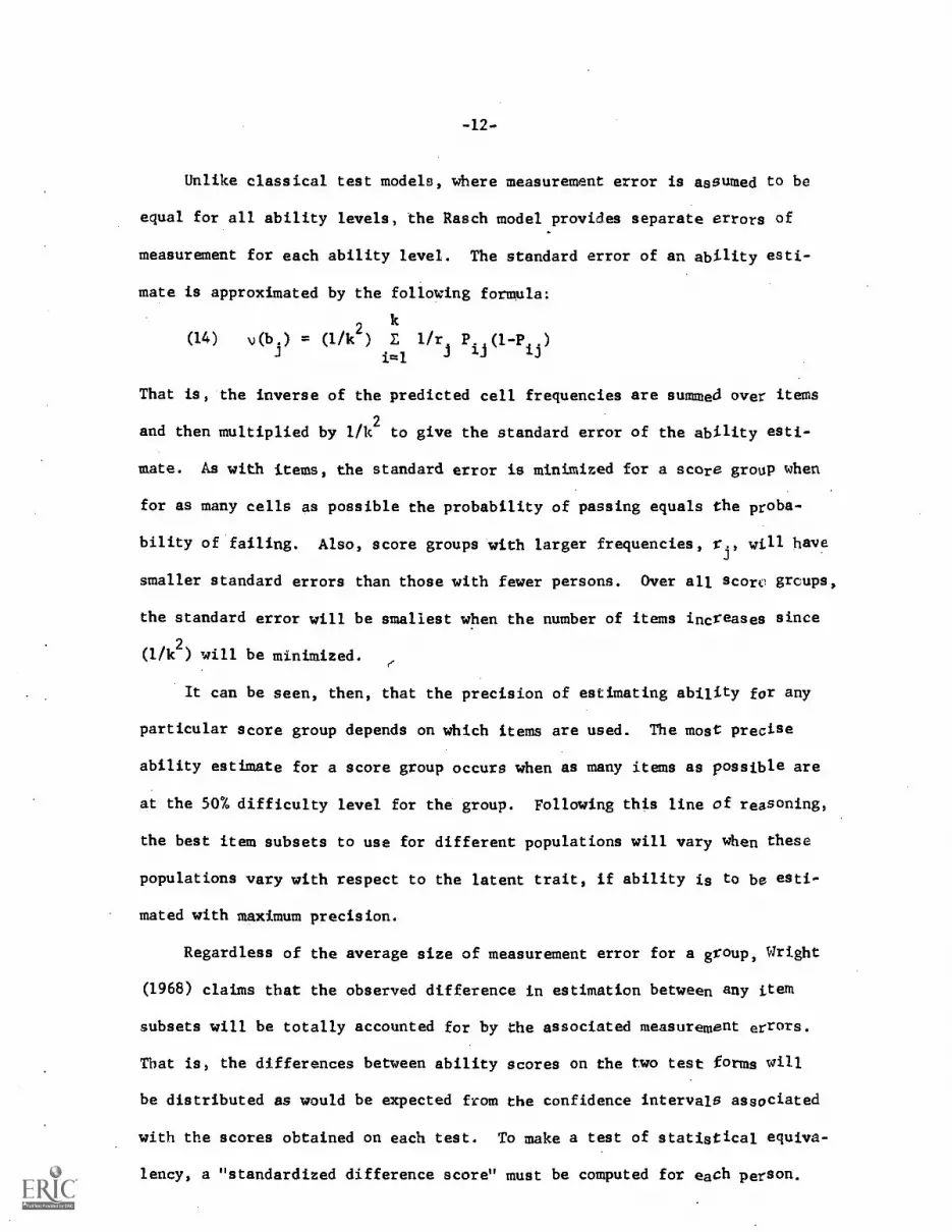
ciated with the estimate. The standard error of estimate for items is approx-

imated by the following equation:

2 k-1(13) v(di) = (1/[k-1] )

jE 1

1/(r. P [1-P ])

=

where probability of correct responsePij

= as estimated by parameters for

cell ij

It can be seen that the standard' error of the item becomes small as

rjPii(1-P..1.3 )increases. Given equal frequencies in the score groups, this

term is maximized when the probability of passing the item is as close as

possible to the probability of failing the item for each score group. Obvi-

ously, the difficulty level of the item will increase as a score group's

total raw score decreases. So, the standard error of the item will take on

its smallest value when the probability of passing the item is .50 for the

score group with the largest frequency, r.. The correspondence to the clas-

sical test approach of selecting items with a difficulty level of .50 for the

population (to maximize reliability) should be obvious, if the mode and mean

of the distribution are equal. So, item error in the Rasch model turns out

to be population specific.

-12-

Unlike classical test models, where measurement error is assumed to be

equal for all ability levels, the Rasch model provides separate errors of

measurement for each ability level. The standard error of an ability esti-

mate is approximated by the following formula:

(14)03.)., (1 /k2

) E lir, P.i(1-P)i=1 "

That is, the inverse of the predicted cell frequencies are summed over items

and then multiplied by 1 /k2

to give the standard error of the ability esti-

mate. As with items, the standard error is minimized for a score group when

for as many cells as possible the probability of passing equals the proba-

bility of failing. Also, score groups with larger frequencies, rj, will have

smaller standard errors than those with fewer persons. Over all score groups,

the standard error will be smallest when the number of items increases since

(1/k2) will be minimized.

It can be seen, then, that the precision of estimating ability for any

particular score group depends on which items are used. The most precise

ability estimate for a score group occurs when as many items as possible are

at the 50% difficulty level for the group. Following this line of reasoning,

the best item subsets to use for different populations will vary when these

populations vary with respect to the latent trait, if ability is to be esti-

mated with maximum precision.

Regardless of the average size of measurement error for a group, Wright

(1968) claims that the observed difference in estimation between any item

subsets will be totally accounted for by the associated measurement errors.

That is, the differences between ability scores on the two test forms will

be distributed as would be expected from the confidence intervals associated

with the scores obtained on each test. To make a test of statistical equiva-

lency, a "standardized difference score" must be computed for each person.

-13-

This is given by the following formula:

(15) D12 =x2p

sE2 sE2xlp x2p

where D12

= standardized difference

x1p'

x2p

= ability score obtained byperson p. on test 1 and test 2

respectively

SE2xl

SE2x2p

= measurement errors associatedp

,

with x1p'

x2p

The observed difference between the ability estimates given by the two tests

is divided by the standard error of the score differences. The standardized

difference score computed for each person can be interpreted as a z score of

his observed difference between item subset scores on a distribution of the

differences that would be expected-from the measurement error associated with

each score. If the error between the two forms is random, then when the

standardized differences are summed over persons in the population, these

scores should be normally distributed with a mean of 0 and standard deviation

of 1.0.

Statistical equivalency of any item subsets, then, merely means that the

observed differences between subset scores are distributed as would be expected

from measurement error alone. However, even if this claim can be substantiated

for item pools calibrated by the Rasch technique, there is no guarantee that

statistically equivalent forms are also maximally equivalent forms. The prob-

lem of precision, as shown above, is still a population-specific problem. To

have "maximally equivalent forms" the measurement error between forms must be

minimized and it is not possible to use just any subset of items from the

calibrated pool, Items must be as carefully selected as in classical tech-

niques of test development. In fact, the same criteria must be met. Average

item difficulty should be at .50, and the test means and variances should be

equal if the average standard error of estimate, weighted by frequency, is to

be minimized over score groups for each test.

-14-

Equivalency of Calibrated Item Subsets

Tinsley (1971) compared the equivalency of item subsets on four tests

and concluded that the Rasch ability estimates were not invariant over item

subsets. However, Tinsli did t ase standardized differenus in his cam-

parisons and confounded maximal equivalency with statistical equivalency.

Data from one of Tinsley's tests were re-analyzed to determine how well the

observed differences between item subsets are accounted for by the errors of

measuTement for each score and the relative degree of precision of measure-

ment between subsets.

Procedure. Test protocols for a 60-item verbal analogies test were

calibrated by the Reach technique. All items were multiple-choice, with five

alternatives. The items on this teat had been selected from s group of 96

items which were administered to college students. The items had been se-

lected according to mixed criteria, with fit of the data to the Rasch model

as one of these criteria.

Data from 949 subjects were available on the final 60-item analogies

test. Approximately two-thirds of the sample were college students, while

the remaining one-third of the sample consisted of suburban high school

students. The 60-item test had a mean of 34.86 and a variance of 89.32 on

the combined sample. Hoyt reliability was found to equal .877, showing a

good degree of internal consistency in the item pool. However, 307 of the

items did not fit the model at the .01 level, while 407 of the items did

not fit when the more stringent criterion of .05 was used. Thus, the claims

with respect to equivalent forms were to be given a stringent test, since

several items do not fit the model.

Three different divisions of the pool of 60 calibrated items resulted

in the following subset comparisons: 1) odd versus even items, 2) easy

versus hard items and 3) randomly selected subsets with no item ovefiAp.

-15-

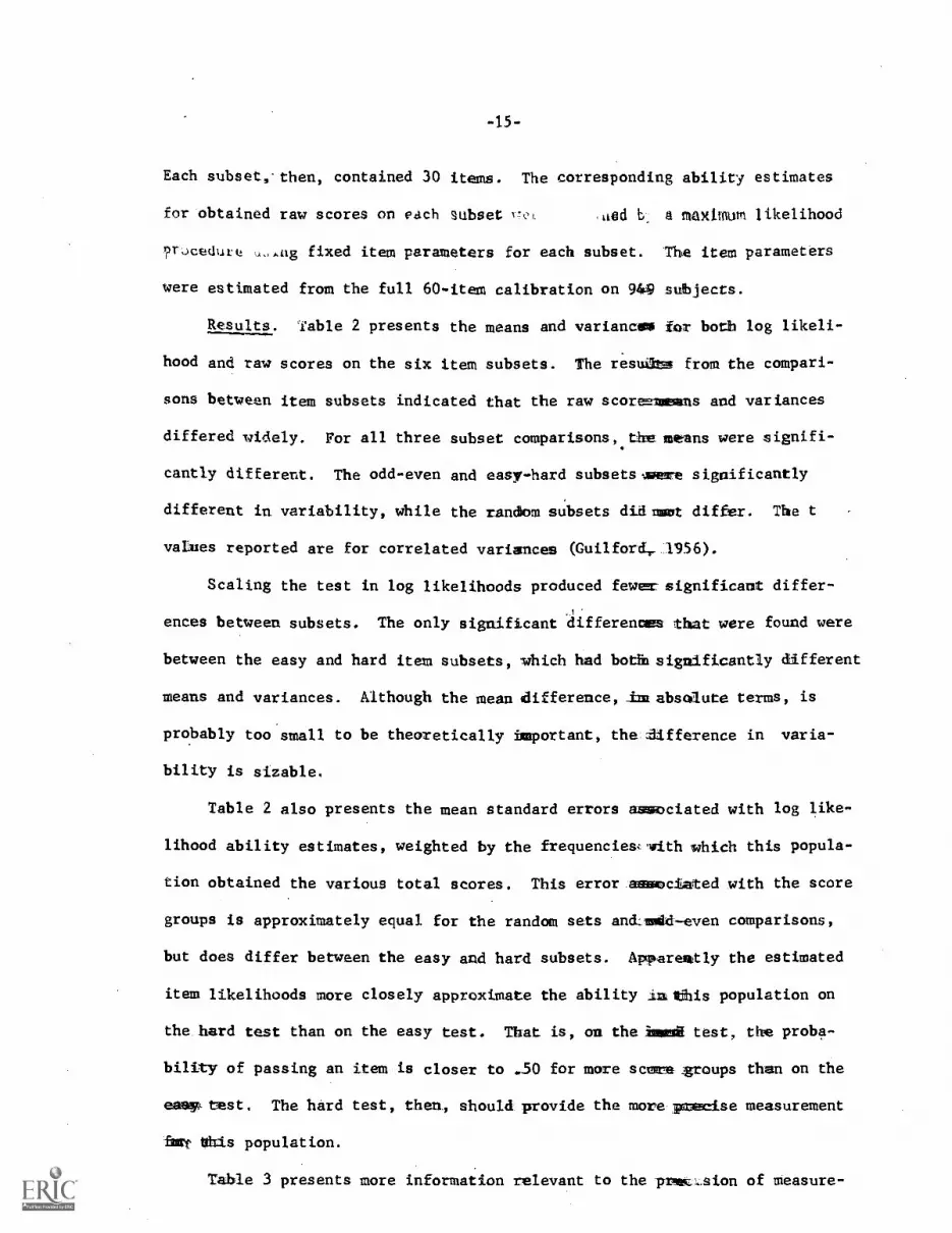
Each subset, then, contained 30 items. The corresponding ability estimates

for obtained raw scores on each Subset 1=A ittd b- maximum likelihood

?rJoedute ,Aug fixed item parameters for each subset. The item parameters

were estimated from the full 60-item calibration on 949 subjects.

Results. Table 2 presents the means and variancas for both log likeli-

hood and raw scores on the six item subsets. The resufts from the compari-

sons between item subsets indicated that the raw scorns and variances

differed widely. For all three subset comparisons, the seAns were signifi-

cantly different. The odd-even and easy-hard subsetsmeme significantly

different in variability, while the random subsets did want differ. The t

wanes reported are for correlated variances (Guilford, 1956).

Scaling the test in log likelihoods produced fewem-significant differ-

ences between subsets. The only significant differences that were found were

between the easy and hard item subsets, which had bothI significantly different

means and variances. Although the mean difference, inzabsoaute terms, is

probably too small to be theoretically important, the difference in varia-

bility is sizable.

Table 2 also presents the mean standard errors associated with log like-

lihood ability estimates, weighted by the frequencies:vith which this popula-

tion obtained the various total scores. This error associated with the score

groups is approximately equal for the random sets anctiodd-even comparisons,

but does differ between the easy and hard subsets. Apparently the estimated

item likelihoods more closely approximate the ability dulthis population on

the hard test than on the easy test. That is, on the Immo* test, the proba-

bility of passing an item is closer to -50 for more scorn :groups than on the

eaay,test. The hard test, then, should provide the more pmevise measurement

hart this population.

Table 3 presents more information relevant to the prc.sion of measure-

-16-

ment. It can be seen that although the subset mean differences are very small,

there is a large variance between the tests. The correlations between the sub-

sets show that the largest percentage of variance shared is only 58% (r=.76).

Thus, none of the item subsets are maximally equivalent.

Table 3 also presents the standardized difference for the three compari-

sons. In no case are the means significantly greater than zero. The variances

are very close to 1.0 for both the random sets and odd-even comparisons, but

are somewhat larger for the easy versus hard test comparison.

This variance is significantly different from 1.0 (F=1.3, p<.01) and is

large enough to have some theoretical importance.

Discussion. The results from two of the subset comparisons, odd-even and

random sets, support the claim of statistical equivalency between item subsets

calibrated by the Rasch technique. The standardized differences between these

subsets were distributed as would be expected from measurement error alone.

The results from the standardized differences between the easy and hard sub-

sets, however, indicate that these differences i:annot be fully explained by

estimated measurement error. Although the reason for this difference is not

entirely clear, it is quite likely that the large number of items not fitting

the model was the major influence. To determine the plausibility of this

interpretation, the percentage of items not fitting the model on the separate

subsets was computed. It was found that 23% of the items on the easy subset

and 57% of the items on the. hard subset did not fit the model. It is likely,

then, that both ability and measurement error were underestimated on the hard

subset, since many of the difficult items did not adequately measure the per-

son's ability.

Apparently only under the most extreme conditions does the Rasch model

fail to produIce statistically equivalent forms for any item subsets. How-

ever, none of the item subsets-resulted in the maximal equivalency charac-

-17-

teristic of tests developed by classical techniques, since the correlations

between subsets were only moderate. Some increase in precision could have

been gained by more efficient item selection, as evidenced by the varying

average measurement error between forms. The variance of the Rasch ability

estimates was significantly different between the easy and the hard item

subsets. The more extreme estimates were obtained from the easy subset, as

would be expected, when the population is of relatively high ability.

Conclusion and Summary

Although the Rasch model apparently can potentially provide the popula-

tion- and item-invariant scaling needed for objective measurement, it is

certainly no panacea for the test developer's problems. Some of the claimed

advantages of Rasch scaling depend directly on the characteristics of the

item pool, rather than the model. For an item pool fully to possess the prop-

erties of objective measurement, a set of rigorous assumptions must be met.

The most direct influence of item characteristics is on the population-

invariance of item calibrations. The Rasch item parameter estimates will be

invariant only under a special condition. Individuals with the same raw score

must have the same probabilities of passing each item, regardless of the pop-

rlation to which they belong. Thus, item parameters will not be population-

tavartant when there is cultural bias which differentially affects the item

probabilities. Since it is well known that many popular ability tests have

items which differ in cultural loadings, the special condition required for

item parameter invariance may be difficult to obtain. Compared with the

classical model, however, the Rasch model is superior since difficulty level

is never population- invariant.

Although population-invariance of ability estimates is probably attain-

able for any item pool, how much of an advantage this is depends on the theo-

-18-

retical interpretability of the item pool. The Rasch ability parameter esti-

mates are nearly as invariant as percentage correct scores, but have the same

disadvantage. Interpretation is possible only relative to the existing set

of items, the calibrated item pool. As with domain-referenced testing, the

items in the set must have a priori validity. In general, the current expli-

cation of most trait constructs does not even approach the kind of precision

required for a domain- referenced interpretation. Again, the Rasch model

offers a potentiality, but does not Solve basic theoretical problems in test

interpretability.

The major focus of this paper has been on the construction of equivalent

forms from a calibrated item pool. The Rasch model was found to have many

more parallels to traditional criteria for the development of equivalent forms

than would have been anticipated from previous explanations (Wright and Pan-

chapakesan, 1969). To understand the characteristics of the Rasch model in

developing equivalent forms, it was found necessary to distinguish between

statistical equivalency, in the narrow sense, and maximal equivalency. Item

subsets are statistically equivalent if the differences obtained on some sam-

ple are distributed as would be expected from the measurement error associated

with each score. Maximal equivalency, however, means that the measurement

differences between tests is as small as possible. It was pointed out that

using any subset from an item pool calibrated by the Rasch model would lead

to statistical equivalency but not necessarily maximal equivalency between

subsets.

The empirical results generally substantiated this interpretation of

the nature of equivalent forms from the Rasch model. Only under extreme con-

ditions did the measurement errors fail to account for the observed differ-

ences between subsets. None of the subsets were maximally equivalent and

precision might have been increased by using more efficient techniques in

-19-

selecting items. The classical techniques of having item difficulties close

to .50 for the population and matching extreme item difficulties would then

apply if the tests are to be equally precise at each score level.

It may be wondered, then, what advantages the Rasch model really offers,

if maximally equivalent forms necessitate using classical item selection cri-

teria. The real strength of the special statistical equivalency of Rasch-

calibrated item subsets is the possibility of individualized selection of

items rather than the construction of fixed content tests. The unusual char-

acteristics of Reach measurement errors allow the desired degree of precision

for any person to be obtained from the fewest possible items. Estimates of

ability and measurement error associated with each possible raw score for any

subset of items can easily be determined. If items are administered by a

computer, ability and measurement error can be estimated after the person re-

sponds to each item. The next item selected, then, will be as close to the

ability estimate as possible and will give the largest increase in precision.

Tests developed according to classical techniques are not suitable for indi-

vidualized item selection since measurement error can only be estimated for

a whole test actually administered to some population.

In conclusion, the lack of impact of the Rasch model is due more to the

current status of trait measurement than to the features of the model. The

true advantages of the Rasch model necessitate a more sophisticated technology

in trait measurement than is now characteristic of the field. Explicit trait-

item theory, culturally-fair items alai computer administration of tests would

be part of the necessary technological sophistication.

-20-

References

Anderson, J., Kearney, G. E., and Everett, A. V. An evaluation of Rasch's

structural model for test items. The British Journal of Mathematical

and Statistical Psychology, 1968, 21, 231-238.

Brooks, R. D. An empirical investigation of the Rasch ratio-scale model

for item difficulty indexes. (Doctoral dissertation, University of

Iowa.) Ann Arbor, Michigan: University microfilms, 1965, No. 65-

434.

Guilford, J. P. Fundamental statistics in psychology and education. New

York: McGraw-Hill, 1956.

Panchapakesan, N. The simple logistic model and mental measurement.

Unpublished Doctoral dissertation, University of Chicago, 1969.

Popham, W. J. and Husek, T. R. Implications of criterion-referenced mea-

surement. Journal of Educational Measurement, 1969, 6, 1-9.

Rasch, G. Probabilistic models for some intelligence and attainment tests.

Copenhagen: Danish Institute for Educational Research, 1960.

Rasch,.G. An item analysis which takes individual difference& into account.

British Journal of Mathematical and Statistical Psychology, 1966a, 19,

49-57.

Rasch, G. An individualistic approach to item analysis. In P. F. Lazarsfeld

and N. W. Henry (Eds.), Readings in mathematical social science.

Chicago: Science Research Associates, 1966b, Pp. 89-108.

Tinsley, H. E. A. An investigation of the Rasch simple logistic model for

tests of intelligence or attainment. Unpublished Doctoral dissertation,

University of Minnesota, 1971.

-21-

Wright, B. Sample-free test calibration and person measurement. Pro-

ceedings of the 1967 Invitational Conference on Testing Problems.

Princeton, N. J.: Educational Testing Service, 1967. Pp. 85-101.

Wright, B., and Panchapakesan, N. A procedure for sample-free item analy-

sis. Educational and Psychological Measurement, 1969, 29, 23 -48.

Footnotes

1. The cell values actually used in computations are not the simple

likelihoods. A correction is made to prevent infinite values from

occurring when all members of the score group pass the item. The

cell likelihood values are corrected by the relative frequency of

the score group, as given by the following equation:

L+ w

rij

- aij

+ w whereL = corrected cell likelihood

aij = number of persons in scoregroup j passing item i

rij

- aij

= number of persons in scoregroup j failing item i

w = percentage of total cali-brating sample obtainingscore j

2. This interpretation is oversimplified to maintain conceptual clarity.

The actual cell values used in computation are corrected cell likeli-

hoods.

Item

i=1,k

-23-

Table 1

Item-by-Score-Group Probability Matrix

Total-Score Group(Raw Score)

2 3

j=1,k-1

k-1

ijPi2

Pik-1

2j

2k

Table 2

Means, Variances and Measurement Errors

,of Item Subsets for Log Likelihood and Raw Scores

Subset

Raw Score

t-

s2

xi x2

tu2

Log Likelihood

t-

-s2

xl x2

to2

SE msmt.

Odd

19.38

23.67

.432

.873

.453

17.78

2.99

.86

.51

Even

15.47

26.85

.415

.892

.433

Easy

22.31

29.43

.469

1.178

.503

42.52

6.23

2.15

13.76

Hard

12.53

22.18

.415

.663

.419

Random Set I

17.79

24.25

.427

.882

.447

2.86

.69

.43

.67

Random Set II

17.06

25.83

.436

.857

.433

-25-

Table 3

Precision of Measurement and Standardized DifferencesBetween Item Subsets

Subset Comparison Log Likelihood2

s- - r_

xl x2

Standardized Difference2

lc -il s_ - s_ _xl x21 2 x

1-x

2-

Odd, Even .425 .76 .007 1.028 1.014

Easy, Hard .590 .76 -.057 1.313 1.146

Random Sets .410 .76 -.020 .995 .998