Icarus146, 176–189 (2000)

doi:10.1006/icar.2000.6391, available online at http://www.idealibrary.com on

The Near-Earth Object Population

Brett Gladman, Patrick Michel, and Christiane Froeschl´e

Departement Cassini, Observatoire de la Cote d’Azur, BP 4229, 06304 Nice Cedex 4, FranceE-mail: gladman@obs-nice.fr

Received February 12, 1999; revised January 19, 2000

We examine the dynamics of a sample of 117 near-Earth objects(NEOs) over a time scale of 60 Myr. We find that while 10–20%end their lifetimes by striking a terrestrial planet (usually Venus orEarth), more than half end their lives in a Sun-grazing state, andabout 15% are ejected from the Solar System. The median lifetimeof our (biased) sample is about 10 Myr. We discuss the exchange ofthese objects between the various orbital classes and observe the cre-ation of orbits entirely interior to that of Earth. A variety of resonantprocesses operating in the inner Solar System, while not dominantin determining the dynamical lifetimes, are crucial for understand-ing the orbital distribution. Several dynamical mechanisms existwhich are capable of significantly increasing orbital eccentricitiesand inclinations. In particular, we exhibit important new routes tothe Sun-grazing end-state, provided by the ν5 and ν2 secular reso-nances at high eccentricity between a= 1.3 and 1.9 AU. We find nodynamical reason to demand that any significant component of theNEO population must come from a cometary source, although sucha contribution cannot be ruled out by this work. c© 2000 Academic Press

Key Words: asteroids; comets; impacts; near-Earth objects.

1. INTRODUCTION

o

t

t

a

lb

l

n

orbital element space they occupy as the AAA region. Althoughy andoesichvs.g therth

dis-to

ion.998forldtedthe

rte-thisidsce

olu-ionWeress.

p-ects,

is-veper-dofof

The near-Earth object (NEO) population consists of thastronomical bodies which are on orbits which bring them “nethe Earth. Besides being telescopically more accessible dutheir occasional close passages to our planet, these objecalso of special interest because (1) their dynamical lifetimesshorter than the age of the Solar System, and thus they muresupplied by some more stable source (Opik 1963, Wetherill1979), and (2) some fraction of these objects will impactterrestrial planets. The ultimate supply source for most NEis likely to be the main asteroid belt (and thus most NEOs hrocky compositions), although some undetermined fractionthe NEOs are almost certainly of cometary origin (Wethe1988).

Historically, these objects have been divided into the ApoAmor, and Aten classes, based on their current osculating orelements (Table I), and with the restriction ofa< 5.2 AU toeliminate objects with semimajor axes outside of Jupiter (Halley or long-period comets). Below we shall refer to thethree classes together as the AAA objects and the regio

17

0019-1035/00 $35.00Copyright c© 2000 by Academic PressAll rights of reproduction in any form reserved.

sear”e tos arearest be

heOsveof

rill

lo,ital

ikese

of

objects change between these classes (sometimes rapidlrepeatedly) as their orbital elements vary, this classification dallow an immediate distinction between those objects whmight impact Earth over a human lifespan (Atens/ApollosAmors) and between those that have succeeded in makinlong and hazardous journey to orbits largely interior to Ea(Atens vs Apollos).

It is clearly useful to have a class name for the as-yet uncovered group of objects whose orbits lie entirely interiorEarth’s orbit (apheliaQ< 0.983 AU), which Wetherill (1979)suggested should comprise from 1 to 3% of the NEO populatTholen and Whiteley (1998) reported the candidate object 1DK36 as a potential first member of this class in a surveyEarth Trojans (Whitely and Tholen 1998), but the orbit counot be reliably established. Boattini and Carusi (1998) adopthe name Arjunas for this class; this adoption is a misuse ofterm originally proposed by T. Gehrels for the small (<100 m),low-e Earth-approaching objects reported by Rabinowitzet al.(1993). Michelet al. (2000) propose “inner-Earth objects,” oIEOs, which intends to indicate objects on orbits entirely inrior to that of Earth’s as opposed to inside Earth. Because ofconfusion, in this paper we will use the name “Anon” asterofor this class (a whimsical abbreviation of “anonymous,” sinthe class will be named after its first confirmed member).

The subject of this paper is to examine the dynamical evtion of the population of NEOs as a whole, with special attentto be paid to their ultimate dynamical fate and their lifetimes.will also attempt to say something about their origin and addissues regarding the cometary component of the population

2. THE SAMPLE

In order to examine the dynamical evolution of the NEO poulation, we have integrated a sample of 117 cataloged objobtained from the catalog of Bowellet al. (1994), whose orbitswere considered to be of high quality. Their current orbital dtribution is shown in Fig. 1, where it is evident that we haonly considered objects which have at the current epochihelia q< 1.3 AU (that is, belong to the AAA classes listein Table I). The 1.3-AU boundary created by the definitionthe Amor objects is highly arbitrary; on time scales of tens

6

O

cit

e

teAy

c

esn-ot

e(

p

d to

ttkeh atri-ludewell

plendu-herende ofical

isanduse, on.g.,

theups,d totwole isliablenif-e

singh weula-h the

thethate inthe

bytedther.was

ect-Sun.

of

We find a very rapid decay of the number of objects with re-

THE NEO P

TABLE IDefinitions of the Classes in Terms of Their Current

Osculating Orbital Elements

Class a (AU) Other

Amor >1 1.017<q< 1.3Apollo ≥1 q< 1.017Aten <1 Q> 0.983Anon(?) <1 Q< 0.983

millions of years the large population of Mars-crossing objewith q> 1.3 AU reaches Amor, and eventually Apollo, orb(Shoemakeret al. 1979, Michelet al. 2000). Additionally, theNEO population receives continuous feeding from the mabelt asteroid population (Miglioriniet al. 1998), as well as som(probably smaller) contribution from the Jupiter-family compopulation (Wetherill 1988). Thus, our initial sample is “unsble” in the sense that some of its members leave the region ding the population, and we expect new objects to enter the Aregions on time scales of 105–107 years. However, in a steadstate situation this flux in and out of the population will not affethe fraction of objects which suffer certain fates; that is, wecalculate what fraction of our well-defined Apollo/Amor/Atepopulation terminate their lives impacting Earth (for exampl

Of more concern than fluctuations across the boundariethe AAA region is the worry that the 117 objects used area representative sample of thereal objects populating this region. Telescopic observations of near-Earth objects are knto be biased against the detection of objects with high eccenities and inclinations (e.g., Rabinowitzet al. 1994). Since thesobjects also tend to have the longest dynamical lifetimesdiscussion below) our sample may be biased toward the mrapidly evolving NEOs.

FIG. 1. Current heliocentric orbital elements for our 117-particle samused as the initial conditions for our simulation. The pericenter and nodetributions (not shown) appear uniformly distributed. The curves correspon

lines of perihelia or aphelia at the semimajor axis of a planet.

PULATION 177

tss

in-

eta-fin-A

ctann).of

ot

wnric-

seeost

le,dis-

Our sample was selected on the basis of orbit quality. Boet al. (1998) plot a sample of 197 Apollo and Aten objects witless restrictive orbit-quality requirement; our Apollo/Aten disbution shows no obvious differences. Our sample did not incP/Encke, because the dynamical evolution of this comet isstudied (see Valsecchiet al. 1995).

3. APPROACH

We numerically integrated the orbital histories of our samforward in time in order to study their dynamical evolution athe distribution of fates. A NEO typically suffers tens of thosands of planetary close approaches (within several Hill spradii) during a 107-year sojourn in the inner Solar System, aso a numerical integrator for the problem must be capablefficiently treating planetary encounters. The only numeralgorithm we are aware of that is capable of integrating a∼100-particle sample of planet-crossing objects for 107–108 orbits isthe RMVS3 algorithm of Levison and Duncan (1994), whichbased on the symplectic integration algorithm of WisdomHolman (1991). We included gravitational forces only, becathe orbits of kilometer-scale NEOs are presumably immunetime scales of tens of millions of years to nongravitational (eradiation pressure) or collisional effects.

The effects of all the planets except Pluto were included insimulations. We integrated the 117 objects into two subgroeach of about half the total sample. No differences judgebe particularly important between the evolutions of thegroups were found, implying that even a 60-object samplarge enough for the present purposes to extract some reinformation, and also implying that neither group had a sigicantly different initial orbital distribution. We integrated onof the groups twice, comparing the results of simulations u(base) time steps of 7.5 and 3.7 days; no differences whicbelieve to be significant were found between the two simtions, and so the second subgroup was integrated only wit7.5-day time step. In reporting results below, we have used3.8-day step-size simulation for the first subgroup. (NoteRMVS3 automatically changes time step or reference framorder to more accurately follow close approaches, and sotime steps reported above are actually themaximumused.)

Our integrations proceeded for 60 Myr of simulated time,which time all but 19 of the original particles had been elimina(see the next section); 11 in one subgroup, and 8 in the oWe decided that continued integration of this small sampleunwarranted.

4. FATES

Particles were removed from the simulation if they were ejed from the Solar System or if they impacted a planet or theThe fraction of particles directly observed to finish in eachthese end states is listed in Table II.

spect to time. Previous studies of long-term (>5 Myr) NEO

,

d

r

,

r

ret

b

erth

re

ssahb

tw

ese

d

ant

de

thees inrlo

astheyr.

m-f thehalf

me-isd sotemte-Wes byting

178 GLADMAN, MICHEL

TABLE IIFraction of End-States for NEOs

Directly observedAverage Impact rate,t = 0 rate

Fate (within 60 Myr) N % prob. (%) (NEO−1 Myr−1)

Impact Mercury 1 0.9 1.3 2.3± 1.0× 10−4

Impact Venus 12 10.1 6.8 3.5± 0.7× 10−3

Impact Earth 5 4.3 4.7 4.7± 1.3× 10−3

Impact Mars 2 1.8 0.4 2.6± 0.1× 10−3

Impact Jupiter 0 0.0 0.5 2.8± 2.6× 10−3

Impact Saturn 1 0.9 0.02 2.4± 2.4× 10−4

Ejected from S.S. 12 10.3 — —Sun-grazing 65 55.6 — —Survivors (60 Myr) 19 16.0 — —

dynamics were all based onOpik–Arnold Monte Carlo cal-culations of the encounter and collision time scales, basethe equations ofOpik (1976). These studies estimated the dnamical lifetime (sometimes without any analytic or numecalculation, or reference) to be 108–109 years (Opik 1963),30 Myr (Chapmanet al. 1978), 100–200 Myr (Wetherill 1979)∼108 years (Wetherill 1988), 30–100 Myr (Weissmanet al.1989), 108 years (Greenberg and Nolan 1989), and∼107–108 years (Rabinowitz 1997). There is room for confusion heas some studies compute only thepartial collision half-livesagainst planetary impacts (e.g.,∼108 years for Shoemakeret al.(1979) and Bottkeet al. (1994), 107–108 years for Steel andBaggaley (1985), 106–108 years for Chyba (1993)); these acorrect as far as they go, but some make the implicit assumpthat this is the dominant end state and thus also the mediannamical lifetime of the population, which we show below toincorrect. As Fig. 2a shows, our direct integration finds a mdian dynamical lifetime of only about 10 Myr. This 10-Myr timscale has a mild dependence on the sample selection critein a preliminary integration of 155 Apollo (only) asteroids wia less restrictive orbital quality criterion, we found a∼15-Myrmedian lifetime, which has been partially elevated by the pence of a larger fraction of highly inclined anda< 2 particles.All the integrations show very similar (logarithmic) decay law

The reason for the short dynamical lifetime is easily surmiafter examining Table II, which shows that over half of the pticles are eliminated by the process of Sun-grazing, that is, tperihelia are lowered to the solar radius. This occurs largelycause resonant phenomena, especially those operating be2.0 and 2.5 AU such as the 3 : 1 mean-motion andν6 secularresonances, increase particle eccentricities to unity (Farinet al. 1994, Gladmanet al. 1997). Since most of the previoulifetime estimates relied onOpik’s equations, which do not takresonant phenomena into account, it is not surprising thatlack of this dominant phenomenon produced long estimatesthe characteristic time scale. Wetherill (1979) discussed the

gers of interpretation involved in calling this median lifetime“half-life” since the decay is not an exponential.

AND FROESCHLE

ony-ic

e,

iondy-ee-

ion;

s-

.edr-eire-een

lla

theforan-

To gain additional insight into the importance of the resonphenomena, we conducted anOpik–Arnold Monte Carlo cal-culation of our initial conditions using the Monte Carlo coof Melosh and Tonks (discussed in Doneset al. 1999). In thisMonte Carlo code, no approximate modeling of some ofresonances is incorporated (as was done in varying degreWetherill’s work and Rabinowitz (1997)); thus the Monte Cacode “sees” only close encounters. Each initial condition wcomputed 10 times (picking different random numbers forMonte Carlo process) and evolutions were computed for 60 M

FIG. 2. Decay of number of integrated NEOs with time. The panels copare the results of the integrations (solid and dotted lines) with those oMonte Carlo simulation. The two integrations correspond to the subsets ofthe NEO sample. (Top) The unmodified Monte Carlo algorithm predicts adian lifetime of'60 Myr, whereas the real half-life of our NEO sample∼10 Myr. Only close encounters are modeled in the Monte Carlo code, anparticle removal occurs only due to collisions or ejection from the Solar Sys(removal ate= 1 is checked for, but does not occur). In contrast, most ingrated particles (Table II) end their lives in a Sun-grazing state. (Bottom)have artificially introduced a zeroth-order model of the Sun-grazing procesimmediately removing from the simulation any particle which has an oscula

asemimajor axis of between 2.0 and 2.2 AU or between 2.4 and 2.6 AU, roughlycorresponding to theν6 and 3 : 1 resonances, respectively.

O

o

ehi(tiv

ih2crin

roi

h

2iniioc

ion

ocxt

inosr

ta

i

utit

t

by

ed60-19ceticsall

sianth

vean

am-os-ednap-chilitycal

ofonnetom-f thethan.itharendt inre 3-isavenu-cayeer ofbertith

tion)that

nsa-teped

nyth-

THE NEO P

Figure 2a shows the result of the calculation; just slightly mthan half of the particles remain after 60 Myr, a much lowmortality rate than observed in the integration.

A question we find interesting is: what is dominantly detmining the 10-Myr time scale of the population? We know tresonant phenomena are important in the 2.0- to 2.5-AU regand it is clear from the end states and from the evolutionsnext section) that the particles mostly terminate their evoluby solar collisions in this region. However, how are NEOs mofrom the evolved region (a< 1.8 AU, see Gladmanet al. 1997)out past 2 astronomical units? Are resonant phenomena imtant to this process? We answered these questions by runnsecond Monte Carlo calculation, in which we (rather harsapproximated the resonance regions by “traps” between2.2 AU (for theν6) and 2.4–2.6 AU (for the 3 : 1); any objeentering one of these traps was immediately eliminated fthe simulation. This approximation has the known shortcomthat (1) the semimajor axis of the center of theν6 is inclinationdependent, and (2) particles can escape resonances befoing eliminated. However, if even this dramatic “death’s doapproach failed to bring the decay rate of the Monte Carlo sulation down to at least as fast as the integration, we wouldproof that resonant phenomena insidea= 1.8 AU are crucial fordelivering NEOs out to the Sun-grazing region. In fact, Fig.shows that this rough model brings the two simulationsdecent agreement. The abrupt drop at the start of the modMonte Carlo simulation results from the immediate eliminatof all particles in the “resonant regions,” after which the delaw is only slightly slower than in the integration. The numbof impacts detected in the “modified” Monte Carlo simulatdrops by about a factor of 3, with these particles dominaredirected into Sun-grazing fates.

Therefore, to a first approximation, the general pictureNEO evolution consists of these objects being dominantly ctrolled by close encounters while interior to 1.8 AU, whithen deliver them to the region of powerful resonances erior to 2 AU, where they are efficiently disposed of, mosinto the Sun. This result was not clear before this work, sit was known that secular and mean-motion resonancesate (and are frequently seen in numerical integrations) in2 AU (Michel and Froeschl´e 1997, Gladman 1997). Howevesometimes these resonances serve as sources of meta-sby temporarily extracting particles onto regions where closecounters are less frequent, while in other cases they areto take particles from meta-stable regions into quickly evolvones (Michel and Froeschl´e 1997, Gladmanet al. 1997). Theresult of this comparison with the Monte Carlo model allowsto conclude that on average these effects tend to cancel othe purposes of semimajor axis transport, and that the lifeof the population is set by the rate at which close encoundeliver the population out toa> 2 AU. The reader shouldnot,however, conclude that resonant effects are not importan

determining the orbital distribution of the NEOs, as we shshow below.

PULATION 179

reer

r-aton,seeoned

por-ng aly).0–tomgs

e be-r”m-ave

btofiedn

ayerntly

ofn-

hte-lyceper-ide,bility

en-ableng

ust formeers

for

4.1. Impacts

Due to the efficient destruction of the NEO populationdelivery to Sun-grazing orbits, only a minority (∼10–15%) ac-tually impact a terrestrial planet (Table II). In our integratsample of 117 NEOs we found 21 planetary impacts in ourMyr experiment, and it is likely that a similar 10–20% of thesurviving particles would end their evolutions in impacts. Sinthere are only 21 directly observed impacts, deriving statisfor the relative impact rates on the planets is difficult due to smnumber statistics; for example, is the larger number of venuimpacts (12) relative to Earth impacts (5) significant if they bohave√

N errors? The answer, even at only the 2σ level, is no.In order to place this discussion on a firmer footing, we ha

employed a procedure first used in Morbidelli and Gladm(1998) to calculate an “expected number of impacts” from a sple of orbital histories. Our numerical integrations have theculating orbital elements of all surviving test particles recordevery 5 or 10 thousand years, and thus we have a set of “sshots” of the time evolution of the orbital distribution. For eaof these output intervals, we compute the collisional probabof the surviving population with each planet using a numericode of Farinella and Davis (1994) based on the algorithmWetherill (1967). This algorithm computes “average” collisiprobabilities in the sense that the orbits of both the target plaand the particle are assumed to uniformly precess through a cplete precessional cycle of the node and pericenter; some oNEOs may have their orbits change on time scales shorterthis (few× 104 years), so this procedure is only approximate

The algorithm applied gives results which are consistent wthe number of directly observed impacts when the latteralso large enough to be statistically reliable (Morbidelli aGladman 1998), and when the majority of particles are noorbits almost identical to that of a planet (Dones 1999). Figureports thecumulativeimpact probability of the integrated sample of particles with Earth for three simulations; this quantityidentical to the average number of impacts we expect to hrecorded in the simulations as a function of time, for all threemerical simulations performed. In contrast to the similar dein the number of particles with time (Fig. 2), which is in all threcases determined on a roughly 60-particle sample, the numbexpected impacts is determined by the relatively small numof particles (∼5–15) in each simulation that live for significanamounts of time in the Earth-crossing state. A comparison wthe observed number of impacts in this case (see figure capshows acceptable agreement. Upon inspection, it was seenthe two simulations which shared the same initial conditioexhibited slightly different orbital distributions over the durtion of the simulation; the integration with the shorter time shad many of its long-lived particles remaining for an extendperiod in Earth-like orbits, while in the other integration maof the longest-living particles were removed from the Ear

allcrossing state betweent = 10 Myr andt = 20 Myr, explainingthe differences in the impact statistics. The quantitative results

h.

n

a

il

eo

%,ion

irsus

hees,ean

heyr

ultwothat

bee

EOop-itzc-

.g.,

),. Thetedr-highanyntil-eationarthur bi-ort be

enus-lly,sicndlcu-

nd

ve-lli-riorfor

hiched

180 GLADMAN, MICHEL

FIG. 3. The cumulative collisional probability with Earth, and thus taverage number of impacts expected, for our three numerical simulationsdashed and dotted curves show results for the two 7.5-day step-size simulawhile the solid curve gives the result for the 3.8-day time step (the same inconditions as the dotted curve). From top to bottom, the number of impdirectly recorded in the simulations was 4, 2, and 1. See text for discussio

on the impact probability are thus poorly determined compato the median lifetime, since we are forced to base them osmall number of particles. The three integrations show gencally similar behavior, and we estimate the collision resultsbe accurate to a factor of 2.

Table II compares the percentage of directly observed imp(over 60 Myr) with the fraction expected from the probabilialgorithm; given Poisson errors for the numberN of observedimpacts, the results are statistically identical to the direct ingration. This similarity of the number of detected collisions wthat predicted by theOpik equations in the collision probabiity algorithm indicates that in those cases whereOpik–ArnoldMonte Carlo algorithms fail (see Doneset al. 1999), it isnotdue to the fact that theOpik formulae incorrectly calculate thclose-encounter probability, but rather that the orbital evolutipredicted via the patched conic approach are in error. As

cussed in Doneset al. (1999), because of finite sampling of thorbital histories the collision probability algorithm may unde

, AND FROESCHLE

eThe

tions,itialacts.

redn aeri-to

ctsty

te-th-

nsdis-e

estimate the actual collision rate by a relative error of 10–30due to the sampling missing the rare states of very high collisprobability.

The cumulative collision probability plots provide, via theslope, the evolution of the impact rate with the planet vertime. The current impact rateof our sampleof NEOs can beestimated by the initial slope, which is roughly constant for tfirst few million years. Because of the finite number of particlwe have estimated these impact rates by extracting the mnumber of impacts expected after 1 Myr and dividing by tnumber of particles to obtain the expected impact rate per Mper NEO (Table II). We have estimated the error on this resby computing the mean of the impact rate provided by the tsamples, and quoting an error of the difference betweenmean and either sample.

The impact rate per year onto a given planet can nowobtained by multiplying the estimate given in Table II by threader’s preferred value for the number of objects in the Npopulation larger than a certain size. Using an estimated pulation of∼2000 Earth crossers larger than 1 km (Rabinowet al. 1994), one predicts impact rates similar (to within a fator of 2) but slightly higher than previous published values (eSteel and Baggaley 1985, Wetherill 1989, Morrisonet al. 1994).Using the most recent unpublished estimates of 750± 250(Rabinowitzet al. 2000, Bottke and Morbidelli pers. commun.produces values more comparable to the previous estimatesinterpretation is complicated due to the fact that when integraover a million-year time interval our population “smears” in obital element space as objects move in and out of especiallycollision probability states. Since it has been remarked by mauthors (e.g., Milaniet al. 1990, Chyba 1993) that the currecollision probability is dominated by the few highest probabity objects, which will not stay in this state for very long, wsuggest that our impact rates may be a better representover the time scale of precessional motions in the near-Espace. Of course, because our rates are computed using oased sample, theset = 0 rates must be cautiously interpreted; fexample, the venusian impact rate calculated this way musan underestimate since there are doubtless undiscovered Vcrossing asteroids with orbits in the Anon class. Additionathe inefficiently discovered Aten asteroids have higher intrincollisional probability with Earth (Steel and Baggely 1985), athus are underrepresented in our computation. Last, our calations address only the impact ratefrom the NEO populationand ignore the contribution from the Earth-crossing long- ashort-period comets.

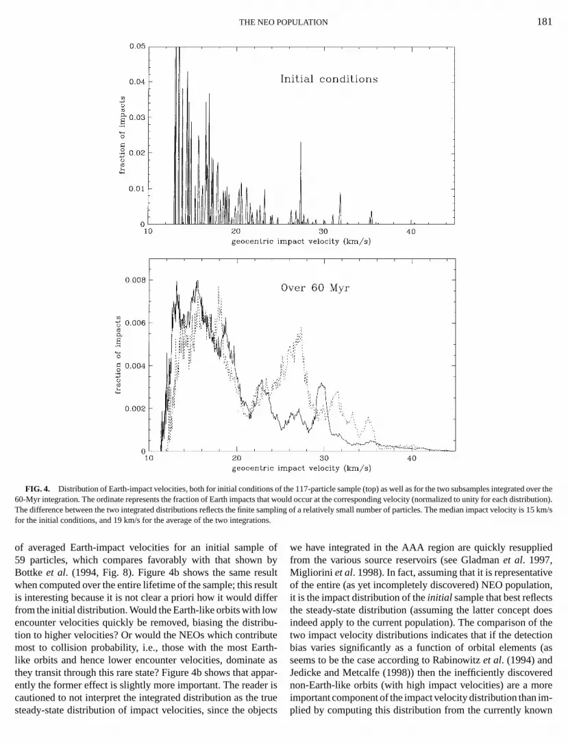
We can also compute the distribution of average impactlocities using the same algorithm which calculated the cosion probability. Bottke and Greenberg (1993) discuss a supemethod which computes instantaneous collision probabilitiesa sample. We compute the average encounter velocity (wvaries slightly due to the eccentricity of Earth’s orbit) weight

r-by the average collision probability in order to compute the dis-tribution of impact velocities. Figure 4a shows the distribution

o

THE NEO POPULATION 181

FIG. 4. Distribution of Earth-impact velocities, both for initial conditions of the 117-particle sample (top) as well as for the two subsamples integratedver the60-Myr integration. The ordinate represents the fraction of Earth impacts that would occur at the corresponding velocity (normalized to unity for each distribution).

The difference between the two integrated distributions reflects the finite sampling of a relatively small number of particles. The median impact velocity is 15 km/s

s

sf

b

th

rt

lied

tiveion,tsdoesf theion(as

redoreim-

for the initial conditions, and 19 km/s for the average of the two integration

of averaged Earth-impact velocities for an initial sample59 particles, which compares favorably with that shownBottke et al. (1994, Fig. 8). Figure 4b shows the same reswhen computed over the entire lifetime of the sample; this reis interesting because it is not clear a priori how it would diffrom the initial distribution. Would the Earth-like orbits with lowencounter velocities quickly be removed, biasing the distrition to higher velocities? Or would the NEOs which contribumost to collision probability, i.e., those with the most Earlike orbits and hence lower encounter velocities, dominatethey transit through this rare state? Figure 4b shows that apently the former effect is slightly more important. The readecautioned to not interpret the integrated distribution as the

steady-state distribution of impact velocities, since the obje

.

ofbyultult

er

u-te-as

par-is

rue

we have integrated in the AAA region are quickly resuppfrom the various source reservoirs (see Gladmanet al. 1997,Migliorini et al. 1998). In fact, assuming that it is representaof the entire (as yet incompletely discovered) NEO populatit is the impact distribution of theinitial sample that best reflecthe steady-state distribution (assuming the latter conceptindeed apply to the current population). The comparison otwo impact velocity distributions indicates that if the detectbias varies significantly as a function of orbital elementsseems to be the case according to Rabinowitzet al. (1994) andJedicke and Metcalfe (1998)) then the inefficiently discovenon-Earth-like orbits (with high impact velocities) are a mimportant component of the impact velocity distribution than

ctsplied by computing this distribution from the currently known

d

ed

atrit

o

hritln

,

o

d

u

0sth

th

eao

hh

uu

g

eme

le I

e.nlied

isheostre

ssesere

. 6,ave

ajorenntu-laro-

rbit,after which close encounters deliver it to the resonances outside

182 GLADMAN, MICHEL

objects. We have calculated the steady-state impact velocitytribution for a large sample of test particles initially placedthe 3 : 1 resonance (see Morbidelli and Gladman 1998); thistribution contains a larger fraction of impact velocities abo20 km/s, implying that if this resonance is the ultimate sourcNEOs then the detected sample is heavily biased against finobjects in the resonance ata= 2.5 AU.

Although the statistics internal to these NEO simulationsnot strong enough to establish the result, we have noted thawide variety of other simulations done by our group the craterate per unit time on Venus is slightly (∼30–50%) larger than thaon Earth. In the present simulation we note that even thoughsample is biased against Atens and does not include the undedly existing population of solely Venus-crossing asteroids,still find (Table II) more Venus impacts. We suggest that tdifference is predominantly due just to the shorter orbital peof Venus, since collision probabilities per unit time scale asplanetarya−3/2

pl (Opik 1976), rather than anything fundamentarelated to the orbital distribution. This somewhat larger vesian cratering rate has important implications for the age ofplanetary surface (see McKinnonet al. 1997 for a discussion)pushing the ages of cratered surfaces down.

5. EVOLUTION TYPES

We now proceed to examine the types of orbital evolutiand some specific cases, exhibited in our sample. We visuexamined the orbital histories of the osculating elements anthe secular argumentsν2–ν6 andν12–ν16 for all of the integratedparticles. One is naturally led to ask the question if a moreful classification of the orbital behavior than Apollo/Amor/Atecould be developed, in the spirit of the Milaniet al. (1989)Spaceguard classification, which was roughly valid over 15-year time scales. However, we have found no useful clascation for our particles on the 10-Myr time scales whichparticles voyage throughout the NEO region. The Tisserandrameter does not provide a useful discriminant over thesescales (Gladmanet al. 1997) due to the chaotic nature of torbits and the plentiful presence of resonances in the innerlar System (Michel and Froeschl´e 1997). In the end we havdecided to remain with the AAA classification, which at lehas the virtue of delimiting Earth-impacting behavior over shtime scales.

Figure 5 shows how the number of members of each of thclassifications evolved with time for a 59-particle sample, eitdue to changing class or leaving the integration. There is notof great interest here, except to note that it is the abundant Appopulation that most closely follows the decay law of the fpopulation, largely because only Apollo objects become Sgrazers. Some objects clearly escape into the non-AAA reof non-Earth-crossing orbits outside theq= 1.3 AU line, wherethey tend to be somewhat more stable. We note the transfa few objects into the Anon class; the rapid transfer of so

objects into this class implies it is of order 1–5% of the tot

, AND FROESCHLE

dis-inis-

veofing

rein ang

ourubt-weisodhelyu-the

n,allyall

se-n

ifi-e

pa-imeeSo-

strt

eseeringollolln-

ion

r of

FIG. 5. Number of particles in the various orbital classifications (see Tabfor definitions) as a function of time.

AAA population, in agreement with Wetherill’s (1979) estimatMichel et al. (2000) estimate that 6–7% of the AAA populatiowould be in the Anon class in a steady state if they were suppfrom a Mars-crossing source.

The variety of orbital evolutions exhibited in our samplevery large. Below we will attempt to summarize some of tmost important types of behaviors, which seem to be the mimportant to the evolution of the overall population. There amany interesting specific cases, illustrating dynamical proceoperating in the inner Solar System, that we will not discuss hdue to space limitations.

An example of the common Sun-grazing fate is given in Figwhich serves as a typical example of how NEOs arrive and lethe terrestrial region. Beginning ata= 2.3 AU, this object suf-fers several close encounters which random-walk its semimaxis down to just outside the orbit of Mars. This object is thextracted into the Amor region (see section below) and eveally reaches a nearly circular orbit exterior to Mars; the secueffects of theν3 andν4 resonances are important during this prcess. After a residence at low eccentricity it is again theν3 andν4

resonances which deliver the object to an Earth-crossing o

al2 AU, which drive it into the Sun (in this case the ultimate culprit

O

la

a

io

n

ae

n,hesince

heldaleenatisionra-

osen-tside

dese ofsr so

ly inrs

THE NEO P

FIG. 6. Evolution of an object which terminates with a solar colsion. From top to bottom we show the time evolution of the semimajor(AU), eccentricity, inclination (degrees), and the critical arguments forsecular resonancesν3, ν4, and ν16. These secular arguments are definedσ3=$ − (g3t +α3), σ4=$ − (g4t +α4), andσ16=Ä− (s6t +β6), wheretis time,$ andÄ are the particle’s longitude of perihelion and ascending nogj andsj are the proper secular frequencies of the Solar System (see L1990), andα j andβ j are the latters’ initial phases.

is the 3 : 1 resonance). We shall discuss inclination oscillatcaused by theν16 resonance in Section 5.2.

5.1. New Routes to Sun-Grazing

It has already been well-established that the dominantstate for planet-crossing objects witha> 2 AU is solar impact(Farinellaet al. 1994, Gladmanet al. 1997). We have established above that even NEOs beginning witha< 2 AU alsopredominantly terminate their evolution by migrating outa> 2 AU and being raised toe= 1 by well-established resonaphenomena.

However, we have identified in the present integrationsother route to Sun-grazing which occurs while objects ha< 2 AU. Ten percent of our initial conditions suffer this fatTheν2 or ν5, and sometimes the overlapping of both, produ

eccentricity oscillations capable of producing perihelia smalthan the solar radius for a range of semimajor axes betw

PULATION 183

i-xistheby

de,skar

ns

end

-

tot

an-ve.

ce

a= 1.3 and 1.9 AU. Figure 7 gives an example of this evolutiowhere it is theν5 resonance that is clearly responsible for tlarge-scale eccentricity oscillations at highe. These resonancehave not been located at such high eccentricities before, ssemianalytical methods (Morbidelli and Henrard 1991, Micand Froeschl´e 1997) break down due to the occurrence of nocrossing during orbital precessional cycles, nor have they bidentified numerically to our knowledge. Of minor note is thif the additional 10% of the initial conditions terminating in thfate were removed from Fig. 2b, the Monte Carlo simulatwould come into even closer agreement with the direct integtion. We thus conclude that a combination of planetary clencounters and theν2 or ν5 resonances supply a route to Sugrazing independent of the known processes operating ou2 AU.

FIG. 7. An example of a particle driven to a Sun-grazing orbit insia= 2 AU. Close encounters with Earth and Venus appear to be the cauthe initial increase in eccentricity beforet = 4 Myr. The particle then passethrough theν2 resonance, which pushes the mean eccentricity even highethat theν5 resonance is entered. The eccentricity oscillation is then perfectphase with the libration of theσ5 secular argument, and mild close encountemodulate its amplitude until solar collision occurs. At the higheportions of thee

lereencycle it is the Kozai resonance which temporarily produces the large inclinationvariations.

so

tr

c

e

e

.

li-

g the

inofthe

,nduc-

s isin

ecity,theongtimee ofuffereoftheor-

ses,s forn of

ids

ingingusweids

beltre

rs-oved

184 GLADMAN, MICHEL

5.2. Inclinations

It has long been known that the AAA population containlarger fraction of high-inclination orbits than the main asterbelt (Wetherill 1988, Weissmanet al. 1989). We discuss belowin Section 6 the important argument that this implies a comesource for these highly inclined NEOs. Here we show thatonant phenomena in the inner Solar System appear capabtaking low-inclination orbits from an asteroidal source (in fafrom any source) and increasing their orbital inclinations wabove 30◦.

Figure 8 shows an example of this process. This NEOgins on a low inclination orbit which then undergoes moderamplitude oscillations in the Amor state caused by theν13 andν14 secular resonances neara= 1.4 AU; the inclination wherethis occurs (10◦) is that predicted semianalytically by Michand Froeschl´e (1997). Close encounters then produce an Eacrossing particle which random walks the semimajor axis

FIG. 8. Time evolution of a NEO which has its orbital inclination dramaically increased by resonant phenomena, in this case theν14 andν16 secularresonances. Theσ13 resonant history (not shown) is similar to that ofσ14, indi-cating an overlapping of the two (Michel 1997). The argument of pericentωserves as the critical argument for the Kozai resonance which causes thee andi oscillations after 20 Myr; particles in this highe/ i state tend to be long-lived

The eccentricity increase between 17 and 18 Myr is caused by theν2 resonance(not shown). See text for further discussion.

, AND FROESCHLE

aid

aryes-le oft,

ell

be-ate

lrth-be-

t-

r

tween 1.2 and 1.8 AU. During this process the particle’s incnation is strongly affected by theν16 resonance, which quicklyraises the mean inclination from 10◦ to 40◦. Wetherill (1988)suggested that this resonance may be capable of producinNEOs with inclinations>30◦, and we confirm that not only isthis process possible, it is in fact very common. We showSection 6 the inclination distribution produced by the totalityinclination-pumping mechanisms as particles journey intoNEO region.

Besidesν16, the overlapping of resonancesν13 andν14 is capa-ble of producing∼10◦-amplitude oscillations in the inclinationsas illustrated in Fig. 8 fromt ' 5–15 Myr and as discussed iMichel (1997). We rarely observe these two resonances proing inclinations larger than about 30◦. However, their presenceis important because they serve as a “bridge” betweeni < 10◦

orbits (which they can pump toi ' 20◦) and theν16’s action ateven higher inclinations.

One of the few general behaviors seen in the integrationthe (unsurprising) relatively long lifetime of NEOs which begin or eventually reach orbits of high eccentricities (e> 0.6) orinclinations (i > 40◦). These orbits tend to be longer lived sincplanetary close encounters then occur at high relative velomeaning that only small orbital changes are possible duringclose encounter. If the NEO enters such a state without strresonant phenomena nearby, then it can remain there forscales of tens of millions of years. Figure 8 gives an examplsuch an object, which also illustrates that such objects can sout-of-phase oscillations ine andi due to the Kozai resonanc(Michel and Thomas 1996); however, the relative stabilitythese states is provided by the high inclination and not byKozai resonance. Because such high inclination/eccentricitybits are less likely to be discovered due to observational biaand because they are seen to be populated in our simulationlong periods, we predict that there is a substantial populatiosuch objects in the NEO region.

5.3. Amor Creation

The origin of Amor asteroids and of Mars-crossing asteroexterior to the Amor region (i.e.,q> 1.3 AU) has been recentlydiscussed by Miglioriniet al. (1998) and Michelet al. (2000),who calculate that the current population of large Mars-crossasteroids (D> 5 km) may be able to replenish the Earth-crosspopulation in this size range over its dynamical lifetime, thkeeping the Earth-crossing population in steady state. Hereaddress only the specific question of how most Amor asterowith semimajor axes smaller than the inner edge of the main-(a< 2 AU) arrive in that region of orbital element space. Thewould seem to be two main possibilities:

(1) Asteroids have their eccentricities increased to Macrossing orbits by resonant phenomena, and are then remfrom the resonances and transported to smallera by martian

close encounters (Greenberg and Nolan 1989, see Fig. A2 ofBottke et al. 1996). Note thatOpik (1963) showed that this

hote

n

i

onhmn1j

nse

rbits

likeging

nd

bitalen-

)qui-it

?

eteEOan

astbelt

all

finer an

e of88)

de-C)

ants.

00–

ateou-dionrialof

re-EOert-this

THE NEO P

process alone cannot then supply the Apollo asteroids (win this model reach Earth-crossing orbits only via martian clencounters); the time scale for this process is so long tharatio of Amors to Apollos would be much larger than observUnlike Opik, we now know that resonance canalsoincreasee’sto Earth-crossing values, so perhaps Amors could just besmall fraction of the asteroids “removed” by Mars and traported by close encounters toa< 2 AU. However, Gladmanet al. (1997) showed that this is an extremely rare and inefficprocess.

(2) Rather, the dynamics producea< 2 AU Amors via the“extraction” by resonant phenomena of Apollo asteroids frEarth-crossing orbits (cf. Michelet al. 2000). Figure 9 shows aexample. Theν3 andν4 resonances are often important in tprocess, as in the case shown in Fig. 9 (cf. Fig. 6). Glad(1997) discusses two second-order secular resonances iregion, originally located by Morbidelli and Henrard (199which can produce similar effects. Once extracted, these oboften remain decoupled from Earth for millions to tens of m

FIG. 9. An example of the temporary creation of long-lived Amor aMars-crossing orbits, for the object shown in Fig. 6. The NEO begina= 2.3 AU and journeys down to be extracted from Earth-crossing space, ring an almost circular orbit just exterior to Mars. The curves show loci of perih

at each terrestrial planet; this object spends a fair amount of time withq= 1 AU.Squares are orbital elements sampled at 104-year intervals.

tion

OPULATION 185

ichsethed.

thes-

ent

m

isanthis

),ectsil-

dat

ach-elia

lions of years. These Amors are returned to Earth-crossing oby the same resonant processes which extracted them.

5.4. The Near-Earth Region

Although we observe cases of the production of Earth-orbits via resonant phenomena and close encounters brinobjects down toa' 1 AU, e< 0.2, and smalli , we see no evi-dence of any kind of dynamical mechanism which would teto concentrate objects in this region (cf. Bottkeet al. 1996).Figure 10 shows an example of such an object, whose orhistory we plot ina/e space. Does the proposed populationhancement in the “SEA” (or “Arjuna”) region 0.9<q< 1.1 AUandQ< 1.4 AU (see Rabinowitzet al. 1993, Rabinowitz 1997imply an unknown source, a recent near-Earth event, or nonelibrium feeding from the main belt (Rabinowitz 1997), or isan artifact of detection biases (Jedicke and Metcalfe 1998)

6. ORIGIN

What fraction of the NEOs are actually devolatilized comnuclei? This is a difficult topic for the following reasons. Wknow that there is at least one active comet (Encke) in an Norbit, proving the existence of such a population (Weissmet al. 1989). Input flux calculations seem to imply that at lehalf of the NEOs can be supplied by the main asteroid(Wetherill 1988 and references therein, Miglioriniet al. 1998,Menichellaet al. 1996) and could perhaps provide effectivelyof the estimated 750–2000 objects withD> 1 km (Rabinowitzet al. 1994, Rabinowitzet al. 2000). However, calculations othe input flux (in number of NEOs per unit time) from the mabelt are fraught with complications which yield it difficult to bmore accurate than a factor of two, always leaving space foalmost equal cometary component. Also, the injection ratone comet-like Encke every 60,000 years (e.g., Wetherill 19may seem relatively modest.

However, to our knowledge no one has demonstrated thecoupling of an object starting on a Jupiter-Family comet (JForbit into the non-Jupiter-crossing region for any significlength of time (>105 years) under purely gravitational dynamicHarris and Bailey (1996) found two examples of transient (103000 years) decoupling to perihelia with 4.0 AU< Q< 4.2 AU,but which returned to Jupiter-crossing thereafter; they estiman upper bound to the transition probability from JFCs to decpled NEOs of 3× 10−3. Levison and Duncan (1994) also founsome examples of temporary decoupling into the NEO reg(for 103–105 years). Clearly close encounters with the terrestplanets provide a method for doing this, but the probabilitythis very rare event is difficult to estimate. Valsecchiet al. (1995)show a purely gravitational orbit which transits from the JFCgion to the decoupled region, obtained by integrating the N2212 Hephaistos until it reached a JFC orbit and then inving time (since Newton’s equations are time reversible), butmethod of course cannot provide the probability of a transi

from JFCs to Encke-like orbits.

ion, afty

186 GLADMAN, MICHEL, AND FROESCHLE

FIG. 10. An example of a NEO which resides temporarily in the “SEA” region. Though this particle spends some fraction of its time with 0.9<q< 1.1 AUandQ< 1.4 AU, it does so in several short visits, continuously entering and exiting this region. In fact, a much longer time is spent in the Aten/Anon regerwhich the particle journeys out to the main belt for a short visit to theν resonance (horizontal feature ata' 2 AU) and then is finally pushed into the Sun b

6

the 3 : 1 resonance (a= 2.5 AU). Notice that the excursions into theQ< 0.983 AU Anon region are dominantly caused by resonant phenomena decoupling the

y

)eme

u

dper

ofilyer of

thena-Oetseasier

o-lar System will naturally be pumped to the observed inclina-

aphelion from Earth.

It is sometimes postulated that nongravitational forces maable to lower the perihelia and thus decouple comets whichjust marginally Jupiter crossing (Valsecchiet al. 1995, Harrisand Bailey 1996, Steel and Asher 1996)). Valsecchi (1999views this problem. These forces are difficult to study systatically because they appear to be highly variable from coto comet (Marsdenet al. 1973). Harris and Bailey (1998) usthe Marsdenet al. (1973) model to simulate the orbital evoltion of a sample of test particles all with initial orbital elemenof q= 1 AU, Q= 5.2 AU, i = 0◦, finding∼3% of the objects“decoupling” from Jupiter within 103 perihelion passages anconcluding that 300 decoupled NEOs could be produced

million years. However, the assumed initial distribution is un

beare

re-m-et

-ts

realistic and is essentially “perfect” to maximize the effectsthe nongravitational forces; the real fraction of Jupiter-famcomets that undergo this decoupling must be at least an ordmagnitude lower.

Our integrations show that dynamical mechanisms exist interrestrial planet region which are capable of pumping inclitions of low-i objects to values like those exhibited by the NEpopulation. Thus, there is no a priori reason to favor comover asteroids as the source objects because it may seemto supply the high-i NEOs from JFC orbits (Weissmanet al.1989). Any population of objects injected into the inner S

-tion distribution.

h

pt

t

er

1er

llo,

eby

e to

be-

tionherceis-

ent

s int il-the

an-

o-

lyfluxes are probably lower limits, implying that almost all NEOs

THE NEO P

Wetherill (1988) also pointed out that high-eccentricity ojects (specifically,a> 2.2 AU andq< 0.8 AU) seemed to bein short supply in his simulations; however, we believe thisbe an artifact of theOpik–Arnold Monte Carlo model, whicdid not allow for the variety of eccentricity pumping mechnisms toe> 0.5 provided by resonant phenomena. Figureshows an approximation to the steady-state distribution inihelion/semimajor axis space, computed from a 1000-parsample begun in the 3 : 1 mean-motion resonance (Gladet al. 1997), to be compared with Wetherill (1988, Fig. 3)Rabinowitz (1997, Fig. 5). The “real” dynamics populatehigh eccentricity regions of orbital element space much mefficiently than the Monte-Carlo models predicted, and in pticular supply a very strong signature from the resonanc2.5 AU. While the latter feature is specific to a supply soufrom the 3 : 1 resonance, the elevated production of highe ob-jects is generic to the process of escaping from the asteroidsince the resonances are generically “passed” through atonce for all escaping asteroids. Also of note in Fig. 11 is

FIG. 11. Steady-statea/q distribution of NEOs coming from the 3 :mean-motion resonance. The line shows the circular orbits; points to thper left are unphysical. The obvious vertical band at 2.5 AU is the signatuthe 3 : 1 resonance. Note the particles witha< 2 AU that are decoupled fromEarth via resonances (q> 1) and the many objects witha> 2.2 AU and high ec-centricities (q< 0.8 AU). The percentages of steady-state Anon, Aten, Apo

and Amors (q< 1.3 AU) in this figure are 1, 2, 71, and 26, respectively.

OPULATION 187

b-

to

a-11er-

iclemanorheorear-

atce

beltleastthe

up-e of

FIG. 12. Steady-state inclination distribution of NEOs coming from th3 : 1 mean-motion resonance. The fraction of high inclination objects shownthis distribution is expected to be elevated with respect to the real NEOs dudetection biases against finding such objects.

existence of concentrations of objects in the Amor regiontweena= 1.3 AU anda= 1.8 AU, produced mostly by extrac-tions from Earth-crossing space via theν3 andν4 resonances;this feature also appears to be present in the orbital distribuof Earth-approaching asteroids (Rabinowitz 1997, Fig. 7b). Tsteady-state inclination distribution produced by this 3 : 1 souis shown in Fig. 12, which is grossly similar to the observed dtribution as shown in Weissmanet al. (1989).

This brings us back to the question of cometary componof the NEO population. At this point we see nodynamicalrea-son to require a cometary input component. Recent progresunderstanding the expulsion of asteroids from the main bellustrates that more abundant mechanisms exist for supplyingNEO population than previously discussed, through the chnels of the main resonances (reviewed in Gladmanet al. 1997),the Mars-crossing population (Miglioriniet al. 1998), and thelatter’s gradual replenishment from the main belt by the scalled “three-body” resonances (Nezvorn´y and Morbidelli 1998,Murray et al. 1998). Thus, the previously calculated supp

could come from an asteroidal source.

u

tr-

e

a

osw

ed.

t

is

r

ie

n

s

r

an-

the

-

the,

arth

er-

ribu-

iod

rth

tional

urce

ajor

for

roids

of

ive

t-

hes

e-

belt:

he

on

188 GLADMAN, MICHEL

However, Encke exists. It is always troubling to argue frostatistics of one, although Wetherill (1988), Weissmannet al.(1989), and Lupishko and Di Martino (1998) convincingly argon spectroscopic grounds that there are other exinct comeobjects present in the population. Our opinion on the issue isit is extremely unlikely that two utterly different sets of delivephysics (collisions and resonances for asteroids from a mainsource versus Jupiter encounters and nongravitational forcecomets from a Kuiper Belt source) could fortuitously give NEinjection rates within a factor of three of each other, much lequality. Since it seems that asteroids can supply the inputin quantitive and relatively complete models, while cometinput models have to be pushed to supply even half the NEthe former are likely to make up the bulk of the population.

We feel that the most likely way to make progress is to cstruct more complete models of the steady-state orbital dibution from various possible sources, and combine theseobservational biases in an attempt to find the best match,ing into consideration estimates for the injection rate from thsources (although a complete fit of the steady-state orbittribution could in principledeterminethe relative input rates)Further remote-sensing observations of near-Earth objectsof course also provide valuable information, although it is uclear how volatile-rich asteroids should differ from low-activicomets. Of course, the best answer is to go and land on mNEOs and see what fraction of them are cometary, but thunlikely to happen anytime in the near future.

ACKNOWLEDGMENTS

We thank H. Levison for providing us with the sample of initial conditionWe thank B. Bottke, A. Morbidelli, and G. Valsecchi for helpful discussions aL. Dones for comments as a reviewer.

REFERENCES

Boattini, A., and A. Carusi 1998. Atens: Importance among near-Earth asteand search strategies.Vistas Astron.41, 527–541.

Bottke, W. F., and R. Greenberg 1993. Asteroidal collision probabilitJ. Geophys. Res.20, 878–881.

Bottke, W. F., M. Nolan, R. Greenberg, and R. Kolvoord 1994. Collisiolifetimes and impact statistics of near-Earth asteroids. InHazards due toComets and Asteroids(T. Gehrels, Ed.), pp. 337–358. Univ. Arizona PresTucson.

Bottke, W. F., M. C. Nolan, H. J. Melosh, A. M. Vickery, and R. Greenbe1996. Origin of the Spacewatch small Earth-approaching asteroids.Icarus122, 406–427.

Bottke, W. F., D. Richardson, and S. G. Love 1998. Production of Tungusized bodies by Earth’s tidal forces.Planet. Space Sci.46, 311–322.

Bowell, E., K. Muinonen, and L. H. Wasserman 1994. A public-domain astedata base. InAsteroids, Comets, Meteors(A. Milani, M. DiMartino, and A.Cellino, Eds.), pp. 477–481. Kluwer, Dordrecht, Netherlands.

Chapman, C., J. G. Williams, and W. K. Hartmann 1978. The asteroids.Annu.Rev. Astron. Astrophys.16, 33–75.

Chyba, C. 1993. Explosions of small Spacewatch objects in the Earth’s atsphere.Nature363, 701–703.

, AND FROESCHLE

m

etaryhatybelts forOss

fluxryOs,

n-tri-ith

tak-seis-

willn-yanyis

s.nd

oids

s.

al

s,

rg

ka-

oid

Dones, L., B. Gladman, H. J. Melosh, B. Tonks, H. Levison, and M. Dunc1999. A comparison ofOpik-Arnold Monte Carlo methods with direct integrations.Icarus142, 509–524.

Farinella, P., and D. R. Davis 1994. Collision rates and impact velocities inmain asteroid belt.Icarus97, 111–123.

Farinella, P., Ch. Froeschl´e, C. Froeschl´e, R. Gonczi, G. Hahn, A. Morbidelli,and G. B. Valsecchi 1994. Asteroids falling into the Sun.Nature371, 314–317.

Gladman, B. 1997. Destination Earth: Martian meteorite delivery.Icarus130,228–246.

Gladman, B. J., F. Migliorini, A. Morbidelli, V. Zappal`a, P. Michel, A. Cellino,Ch. Froeschl´e, H. Levison, M. Bailey, and M. Duncan 1997. Dynamical lifetimes of objects injected into asteroid belt resonances.Science277, 197–201.

Greenberg, R., and M. Nolan 1989. Delivery of asteroids and meteorites toinner Solar System. InAsteroids II(R. Binzel, T. Gehrels, and M. S. MatthewsEds.), pp. 778–804. Univ. of Arizona Press, Tucson.

Harris, N. W., and M. E. Bailey 1996. The cometary component of the near-Eobject population.Irish Astron. J.23, 151–156.

Harris, N. W., and M. E. Bailey 1998. Dynamical evolution of cometary astoids.Mon. Not. R. Astron. Soc.297, 1227–1236.

Jedicke, R., and T. Metcalfe 1998. The orbital and absolute magnitude disttions of main belt asteroids.Icarus131, 245–260.

Laskar, J. 1990. The chaotic motion of the Solar System.Icarus88, 266–291.

Levison, H., and M. Duncan 1994. The long-term behavior of short-percomets.Icarus108, 18–36.

Lupishko, D. F., and M. Di Martino 1998. Physical properties of near-Eaasteroids.Planet. Space Sci.46, 47–74.

Marsden, B., Z. Sekanina, and D. Yeomans 1973. Comets and nongravitaforces. V.Astrophys. J.78, 211–225.

Menichella, M., P. Paolicchi, and P. Farinella 1996. The main belt as a soof near-Earth asteroids.Earth Moon Planets72, 133–149.

Michel, P. 1997. Effects of linear secular resonances in the region of semimaxes smaller than 2 AU.Icarus129, 348–366.

Michel, P., and Ch. Froeschl´e 1997. The location of secular resonancessemimajor axes smaller than 2 AU.Icarus128, 230–240.

Michel, P., and F. Thomas 1996. The Kozai resonance for near-Earth Astewith semimajor axes smaller than 2 AU.Astron. Astrophys.307, 310–318.

Michel, P., F. Migliorini, A. Morbidelli, and V. Zappal`a 2000. The population ofMars-crossers: Classification and dynamical evolution.Icarus145, 332–347.

Michel, P., V. Zappal`a, A. Cellino, and P. Tanga 2000. Estimated abundanceAtens and asteroids evolving on orbits between Earth and Sun.Icarus 143,421–424.

Migliorini, F., P. Michel, A. Morbidelli, D. Nesvorn´y, and V. Zappal`a 1998.Origin of multikilometer Earth- and Mars-crossing asteroids: A quantitatsimulation.Science281, 2022–2024.

Milani, A., M. Carpino, G. Hahn, and A. Nobili 1989. Dynamics of planecrossing asteroids: Classes of orbital behavior.Icarus78, 212–269.

Milani, A., M. Carpino, and F. Marzari 1990. Statistics of close approacbetween asteroids and planets: Project SPACEGUARD.Icarus88, 292–335.

Morbidelli, A., and B. Gladman 1998. Orbital and temporal distribution of mteorites originating in the asteroid belt.Met. Plan. Sci.33, 999–1016.

Morbidelli, A., and J. Henrard 1991. Secular resonances in the asteroidTheoretical perturbation approach and the problem of their location.Celest.Mech.51, 131–167.

Morrison, D., C. Chapman, and P. Slovic 1994. The impact hazard. InHazardsDue to Comets and Asteroids(T. Gehrels, Ed.), pp. 59–91. Univ. of ArizonaPress, Tucson.

Murray, N., M. Holman, and M. Potter 1998. On the origin of chaos in tasteroid belt.Astron. J.116, 2583–2589.

McKinnon, W. B., K. Zahnle, B. Ivanov, and H. J. Melosh 1997. Cratering

mo-Venus: Models and observations. InVenus II(S. W. Bougher, D. M. Hunten,

and R. J. Phillips, Eds.), pp. 969–1014. Univ. Arizona Press, Tucson.

O

c

u

kr

rn.

a

solar

cke.

or-

73.

n ofs,

ds of

THE NEO P

Nesvorny, D., and A. Morbidelli 1998. Three-body mean motion resonanand the chaotic structure of the asteroid belt.Astron. J.116, 3029–3037.

Opik, E. J. 1963. Survival of comet nuclei and the asteroids.Adv. Astron. Astro-phys.2, 219–262.

Opik, E. J. 1976.Interplanetary Encounters. Elsevier, New York.

Rabinowitz, D. 1997. Are main-belt asteroids a sufficient source for the Eaapproaching asteroids? I. Predicted vs observed orbital distributions.Icarus127, 33–54.

Rabinowitz, D., E. Helin, K. Lawrence, and P. Steven 2000. A reduced estimof the number of kilometre-sized near-Earth asteroids.Nature403, 165–166.

Rabinowitz, D., E. Bowell, E. Shoemaker, and K. Muinonen 1994. The poption of Earth-crossing asteroids. InHazards du to Comets and Asteroids(T.Gehrels, Ed.), pp. 285–312. Univ. Arizona Press, Tucson.

Rabinowitz, D., T. Gehrels, J. V. Scotti, R. McMillan, M. Perry, W. WisniewsS. Larson, E. Howell, and B. Mueller 1993. Evidence for a near-Earth astebelt.Nature363, 704–706.

Shoemaker, E. M., J. G. Williams, E. F. Helin, and R. E. Wolfe 1979. Eacrossing asteroids: Orbital classes, collision rates with Earth, and origiAsteroids(T. Gehrels, Ed.), pp. 253–282. Univ. of Arizona Press, Tucson

Steel, D. I., and D. J. Asher 1996. On the origin of comet Encke.Mon. Not. R.Astron. Soc.281, 937–944.

Steel, D. I., and W. J. Baggaley 1985. Collisions in the Solar System. I. Imp

of the Apollo–Amor–Aten asteroids upon the terrestrial planets.Mon. Not. R.Astron. Soc.212, 817–836.

PULATION 189

es

rth-

ate

la-

i,oid

th-. In

cts

Tholen, D., and R. J. Whiteley 1998. Results from NEO searches at smallelongationBull. Am. Astron. Soc.30, 1041. [Abstract]

Valsecchi, G., A. Morbidelli, R. Gonczi, P. Farinella, Ch. Froeschl´e, and Cl.Froeschle 1995. The dynamics of objects in orbits resembling that of P/EnIcarus118, 169–180.

Valsecchi, G. 1999. From Jupiter-family comets to objects in Encke-likebits. In Evolution and Source Regions of Asteroids and Comets(J. Svoren,E. M. Prittich, and H. Rickman, Eds.), pp. 353–364. IAU Colloquim 1Astron. Inst. of the Slovak Academy of Sciences, Tatransk´a Lomnica, SlovakRepublic.

Weissman, P., M. A’Hearn, L. McFadden, and H. Rickman 1989. Evolutiocomets into asteroids. InAsteroids II(R. Binzel, T. Gehrels, M. S. MatthewEds.), pp. 880–920. Univ. of Arizona Press, Tucson.

Wetherill, G. 1979. Steady state populations of Apollo–Amor objects.Icarus37, 96–112.

Wetherill, G. 1988. Where do the Apollo objects come from?Icarus76, 1–18.

Wetherill, G. 1989. Cratering of the terrestrial planets by Apollo objects.Mete-oritics 24, 15–22.

Wetherill, G. W. 1967. Collisions in the asteroid belt.J. Geophys. Res.72, 2429–2444.

Whiteley, R. J., and D. Tholen 1998. A CCD search for Lagrangian asteroithe Earth–Sun system.Icarus136, 154–167.

Wisdom, J., and M. Holman 1991. Symplectic maps for the N-body problem.Astron. J.102, 1528–1538.