The odd generalized exponential family of distributions with applications

Tahir et al. Journal of Statistical Distributions andApplications (2015) 2:1 DOI 10.1186/s40488-014-0024-2

METHODOLOGY Open Access

The odd generalized exponential family ofdistributions with applicationsMuhammad H Tahir1*†, Gauss M Cordeiro2†, Morad Alizadeh3†, Muhammad Mansoor4†,Muhammad Zubair4† and Gholamhossein G Hamedani5†

*Correspondence:[email protected]†Equal contributors1Department Statistics, BaghdadCampus, The Islamia University ofBahawalpur, 63100 Bahawalpur,PakistanFull list of author information isavailable at the end of the article

Abstract

We propose a new family of continuous distributions called the odd generalizedexponential family, whose hazard rate could be increasing, decreasing, J, reversed-J,bathtub and upside-down bathtub. It includes as a special case the widely knownexponentiated-Weibull distribution. We present and discuss three special models in thefamily. Its density function can be expressed as a mixture of exponentiated densitiesbased on the same baseline distribution. We derive explicit expressions for the ordinaryand incomplete moments, quantile and generating functions, Bonferroni and Lorenzcurves, Shannon and Rényi entropies and order statistics. For the first time, we obtainthe generating function of the Fréchet distribution. Two useful characterizations of thefamily are also proposed. The parameters of the new family are estimated by themethod of maximum likelihood. Its usefulness is illustrated by means of two reallifetime data sets.

AMS Subject Classification: Primary 60E05; secondary 62N05; 62F10

Keywords: Generalized exponential; Hazard function; Maximum likelihood; Moments;Order statistic; Rényi entropy

1 IntroductionThe art of proposing generalized classes of distributions has attracted theoretical andapplied statisticians due to their flexible properties. Most of the generalizations aredeveloped for one or more of the following reasons: a physical or statistical theoreticalargument to explain the mechanism of the generated data, an appropriate model that haspreviously been used successfully, and a model whose empirical fit is good to the data. Thelast decade is full on new classes of distributions that become precious for applied statis-ticians. There are two main approaches for adding new shape parameter(s) to a baselinedistribution.

1.1 Approach 1: Adding one shape parameter

The first approach of generalization was suggested by Marshall and Olkin (1997) byadding one parameter to the survival function G(x) = 1 − G(x), where G(x) is the cumu-lative distribution function (cdf) of the baseline distribution. Gupta et al. (1998) addedone parameter to the cdf, G(x), of the baseline distribution to define the exponentiated-G (“exp-G” for short) class of distributions based on Lehmann-type alternatives (see

© 2015 Tahir et al.; licensee Springer. This is an Open Access article distributed under the terms of the Creative CommonsAttribution License (http://creativecommons.org/licenses/by/4.0), which permits unrestricted use, distribution, and reproductionin any medium, provided the original work is properly credited.

mailto:[email protected]

http://creativecommons.org/licenses/by/4.0

Tahir et al. Journal of Statistical Distributions and Applications (2015) 2:1 Page 2 of 28

Lehmann 1953). Following Gupta et al. ’s class, Gupta and Kundu (1999) studied the two-parameter generalized-exponential (GE) distribution as an extension of the exponentialdistribution based on Lehmann type I alternative. The GE distribution is also known asthe exponentiated exponential (EE) distribution. Since it is the most attractive generaliza-tion of the exponential distribution, the GE model has received increased attention andmany authors have studied its various properties and also proposed comparisons withother distributions. Some significant references are: Gupta and Kundu (2001a; 2001b;2002; 2003; 2004; 2006; 2007; 2008; 2011), Kundu et al. (2005), Nadarajah and Kotz (2006),Dey and Kundu (2009), Pakyari (2010) and Nadarajah (2011). In fact, the GE model hasbeen proven to be a good alternative to the gamma, Weibull and log-normal distribu-tions, all of them with two-parameters. The GE distribution can be used quite effectivelyfor analyzing lifetime data which have monotonic hazard rate function (hrf ) but unfortu-nately it cannot be used if the hrf is upside-down, J or reversed-J shapes. Differently, thenew family can have increasing, decreasing, J, reversed-J, bathtub and upside-down bath-tub and, therefore, it can be used effectively for analyzing lifetime data of various types.The generalization of the exp-G class to other distributions is beyond the scope of thepaper.

1.2 Approach 2: Adding two or more shape parameters

A second approach of generalization was pioneered by Eugene et al. (2002) and Jones(2004) by defining the beta-generated (beta-G) class from the logit of the beta distribu-tion. Further works on generalized distributions were the Kumaraswamy-G (Kw-G) byCordeiro and de Castro (2011), McDonald-G (Mc-G) by Alexander et al. (2012), gamma-G type 1 by Zografos and Balakrishanan (2009) and Amini et al. (2014), gamma-G type2 by Ristic and Balakrishanan (2012) and Amini et al. (2014), odd-gamma-G type 3 byTorabi and Montazari (2012), logistic-G by Torabi and Montazari (2014), odd exponen-tiated generalized (odd exp-G) by Cordeiro et al. (2013), transformed-transformer (T-X)(Weibull-X and gamma-X) by Alzaatreh et al. (2013), exponentiated T-X by Alzaghal etal. (2013), odd Weibull-G by Bourguignon et al. (2014), exponentiated half-logistic byCordeiro et al. (2014a), T-X{Y}-quantile based approach by Aljarrah et al. (2014) and T-R{Y} by Alzaatreh et al. (2014), Lomax-G by Cordeiro et al. (2014b), logistic-X by Tahir etal. (2015a), a new Weibull-G by Tahir et al. (2015b) and Kumaraswamy odd log-logistic-Gby Alizadeh et al. (2015).

We propose a new class of distributions called the odd generalized exponential (“OGE”for short) family, which is flexible because of the hazard rate shapes: increasing, decreas-ing, J, reversed-J, bathtub and upsidedown bathtub. In Section 2, we define the OGEfamily of distributions. Two special cases of this family are presented in Section 3. Thedensity and hazard rate functions are described analytically in Section 4. A useful mix-ture representation for the pdf of the new family is derived in Section 5. In Section 6, weobtain explicit expressions for the moments, generating function, mean deviations andentropies. In Section 7, we determine a power series for the quantile function (qf ). InSection 8, we investigate the order statistics. Section 9 refers to some characterizationsof the OGE family. In Section 10, the parameters of the new family are estimated by themethod of maximum likelihood. In Section 11, we illustrate its performance by means oftwo applications to real life data sets. The paper is concluded in Section 12.


2 The new familyConsider a parent distribution depending on a parameter vector ξ with cdf G(x; ξ), sur-vival function G(x; ξ) = 1 − G(x; ξ) and probability density function (pdf) g(x; ξ). Thecdf of the GE model with positive parameters λ and α is given by �(x) = (

1 − e−λ x)α(for x > 0). For α = 1, it reduces to the exponential distribution with mean λ−1. In fact,the density and hazard functions of the GE and gamma distributions are quite similar.The GE density function is always right-skewed and can be used quite effectively to ana-lyze skewed data. Its hrf can be increasing, decreasing and constant depending on theshape parameter in a similar manner of the gamma distribution. Its applications have beenwide-spread as a model to power system equipment, rainfall data, software reliability andanalysis of animal behavior, among others.

We define the cdf of the OGE family by replacing x by G(x; ξ)/G(x; ξ) in the cdf �(x)

leading to

F(x) = F(x; α, λ, ξ) =(

1 − e−λG(x,ξ)

G(x,ξ)

)α

, (1)

where α > 0 and λ > 0 are two additional parameters.The pdf corresponding to (1) is given by

f (x) = f (x; α, λ, ξ) = λα g(x, ξ)

G(x, ξ)2e−λ

G(x,ξ)

G(x,ξ)

(1 − e−λ

G(x,ξ)

G(x,ξ)

)α−1, (2)

where g(x; ξ) is the baseline pdf. We can omit the dependence on the vector of parametersξ and write simply G(x) = G(x; ξ). Equation 2 will be most tractable when the cdf G(x)

and pdf g(x) have explicit expressions. Hereafter, a random variable X with density func-tion (2) is denoted by X ∼ OGE(α, λ, ξ). The main motivations for using the OGE familyare to make the kurtosis more flexible (compared to the baseline model) and possible toconstruct heavy-tailed distributions that are not long-tailed for modeling real data. Thefamily (1) contains some special models as those listed in Table 1. In particular, it includesas a special case the widely known exponentiated Weibull (EW) distribution pioneered byMudholkar and Srivastava (1993) and Mudholkar et al. (1995). For a detail survey on theEW model, the reader is referred to Nadarajah et al. (2013). It has been well-established inthe literature that the EW distribution gives significantly better fits than the exponential,gamma, Weibull and lognormal distributions.

We offer a physical interpretation of X when α is an integer. Consider a system formedby α independent components following the odd exponential-G class (Bourguignon et al.2014) given by

H(x; λ, ξ) = 1 − e−λG(x;ξ)

G(x;ξ) .

Suppose the system fails if all α components fail and let X denote the lifetime of theentire system. Then, the cdf of X is F(x; α, λ, ξ ) = H(x; λ, ξ)α , which is identical to (1).

Table 1 Some OGE models

SN α λ G(x; ξ) Reduced distribution

1 1 - G(x; ξ) Odd exponential-G family (Bourguignon et al. 2014)

2 - - x1+x Generalized exponential distribution (Gupta and Kundu 1999)

3 1 - xc

1+xc Exponentiated Weibull distribution (Mudholkar and Srivastava 1993)

4 - - 1 − e−a x Generalized Gompertz distribution (El-Gohary et al. 2013)


In Table 1, we provide some members of the OGE family.The hrf of X is given by

h(x) = h(x; α, λ, ξ) = λα g(x; ξ) e−λG(x;ξ)

G(x;ξ)

G(x; ξ)2{

1 −(

1 − e−λG(x;ξ)

G(x;ξ)

)α} (1 − e− λ G(x;ξ)

G(x;ξ)

)α−1. (3)

Theorem 1 provides some relations of the OGE family with other distributions.

Theorem 1. Let X ∼ OGE(α, λ, ξ).(a) If Y = G(X; ξ), then FY (y) =

(1 − e−λ

y1−y)α

, 0 < y < 1, and

(b) If Y = G(X; ξ)

G(X; ξ), then Y ∼ GE(α, λ).

The OGE family is easily simulated by inverting (1) as follows: if U has a uniform U(0, 1)

distribution, then

x = QG

⎡⎣ − log(

1 − u1α

)λ − log

(1 − u

1α

)⎤⎦ (4)

has the density function (2), where QG(·) = G−1(·) is the baseline qf.

3 Special OGE distributionsLifetime distributions play a fundamental role in survival analysis, biomedical science,engineering and social sciences. Typically, lifetime refers to human life length, the lifespan of a device before it fails or the survival time of a patient with serious disease fromthe diagnosis to the death. Here, we present three special OGE distributions that can beuseful in applied survival analysis.

3.1 The OGE-Weibull (OGE-W) distribution

The OGE-W distribution is defined from (2) by taking G(x; ξ) = 1 − e−θ xβ and g(x; ξ) =β θ xβ−1 e−θ xβ to be the cdf and pdf of the Weibull distribution with positive parametersβ and θ , respectively, and ξ = (β , θ).

The cdf and pdf of the OGE-W distribution are given by (for x > 0)

F(x; α, λ, β , θ) =(

1 − e−λ(eθ xβ −1)

)α

and

f (x; α, λ, β , θ) = αλθβ xβ−1 eθ xβ

e−λ(eθ xβ −1)

(1 − e−λ

(eθ xβ −1

))α−1, (5)

respectively, where α > 0 and β > 0 are shape parameters and λ > 0 and θ > 0 are scaleparameters.

The applications of the OGE-W and EW distributions can be directed to model extremevalue observations in floods, software reliability, insurance data, tree diameters, carbonfibrous composites, firmware system failure, reliability prediction and fracture toughness,among others.


3.2 The OGE-Fréchet (OGE-Fr) distribution

The OGE-Fr distribution is defined from (2) by taking G(x; ξ) = e−(b/x)a and g(x; ξ) =a ba x−(a+1) e−(b/x)a to be the cdf and pdf of the Fréchet distribution with parameters aand b, respectively, and ξ = (a, b).

The cdf and pdf of the OGE-Fr distribution are given by (for x > 0)

F(x; α, λ, a, b) ={

1 − e−λ(

e(b/x)a −1)−1}α

and

f (x; α, λ, a, b) = α λ a ba x−(a+1) e−(b/x)ae−λ

(e(b/x)a −1

)−1 {1 − e−(b/x)a

}−2

×{

1 − e−λ[e(b/x)a −1

]−1}α−1

, (6)

respectively, where α > 0 and a > 0 are shape parameters and λ > 0 and b > 0 are scaleparameters.

The OGE-Fr distribution has applications ranging from accelerated life testing, rainfalland floods, queues in supermarkets, sea currents, wind speeds, and track race records,among others.

3.3 The OGE-Normal (OGE-N) distribution

The OGE-N distribution is defined from (2) by taking G(x; ξ) = � [(x − μ)/σ ] andg(x; ξ) = σ−1 φ [(x − μ)/σ ] to be the cdf and pdf of the normal distribution withparameters μ and σ , respectively, and ξ = (μ, σ).

The cdf and pdf of the OGE-N distribution are given by (for x ∈ �)

F(x; α, λ, μ, σ) =[

1 − e−λ{

�[(x−μ)/σ ]1−�[(x−μ)/σ ]

}]α

and

f (x; α, λ, μ, σ) = α λ

σ

φ [(x − μ)/σ ]{1 − � [(x − μ)/σ ]}2 e−λ

{�[(x−μ)/σ ]

1−�[(x−μ)/σ ]

}

×[

1 − e−λ{

�[(x−μ)/σ ]1−�[(x−μ)/σ ]

}]α−1, (7)

respectively, where α > 0 is a shape parameter, μ ∈ � is a location parameter, and λ > 0and σ > 0 are scale parameters.

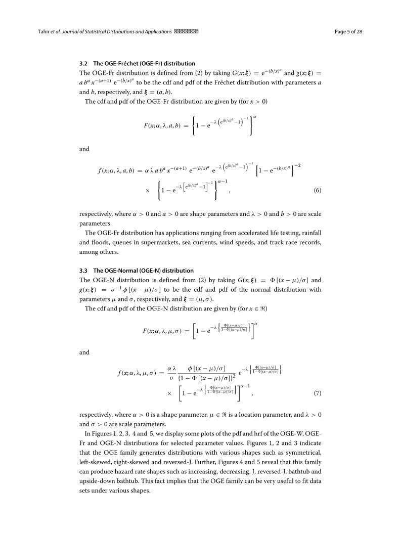
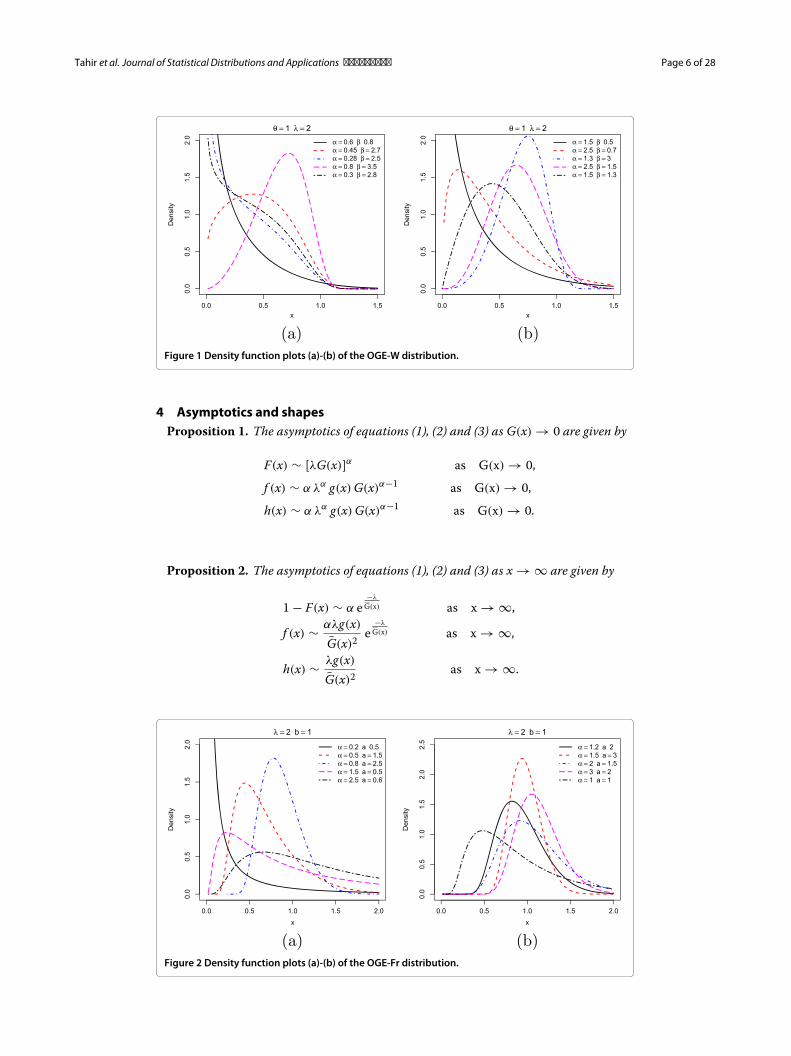
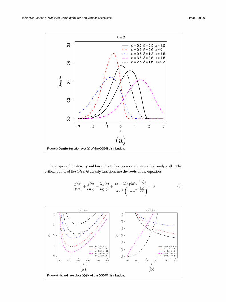
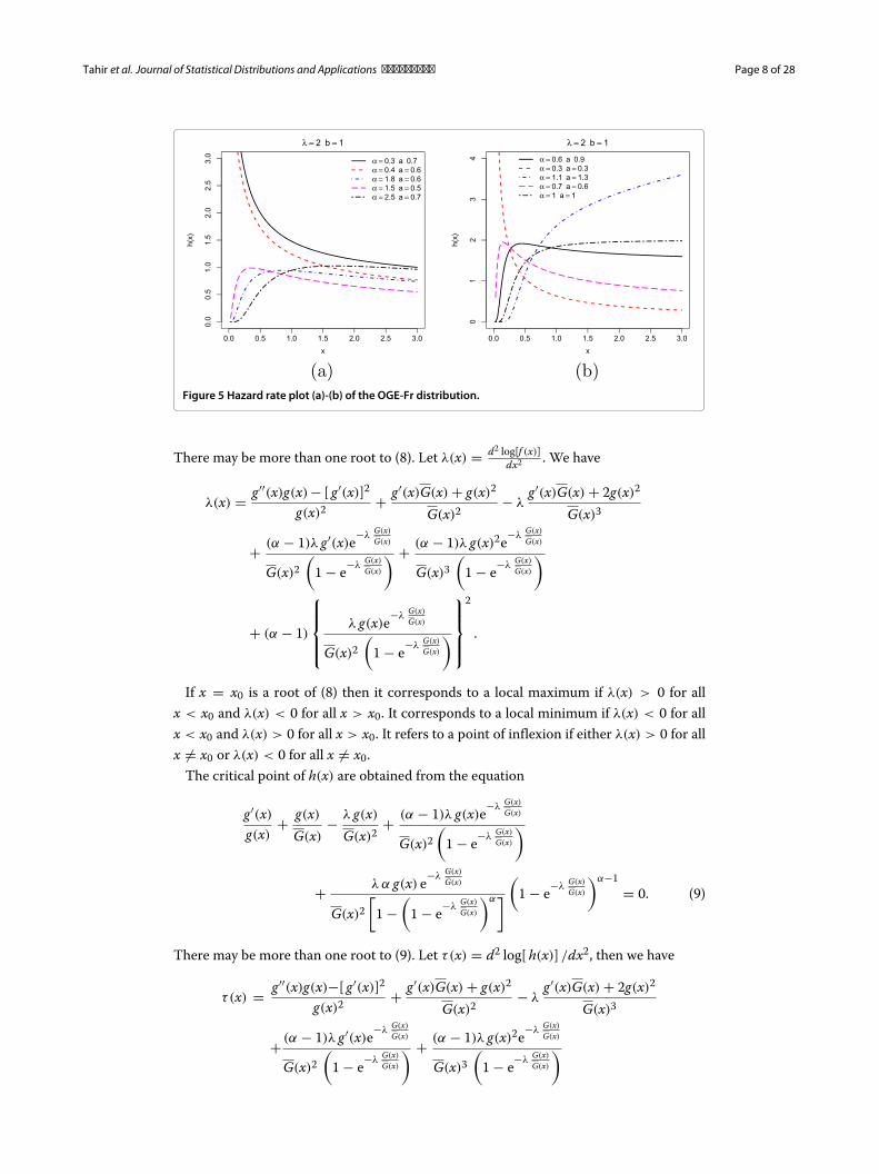
In Figures 1, 2, 3, 4 and 5, we display some plots of the pdf and hrf of the OGE-W, OGE-Fr and OGE-N distributions for selected parameter values. Figures 1, 2 and 3 indicatethat the OGE family generates distributions with various shapes such as symmetrical,left-skewed, right-skewed and reversed-J. Further, Figures 4 and 5 reveal that this familycan produce hazard rate shapes such as increasing, decreasing, J, reversed-J, bathtub andupside-down bathtub. This fact implies that the OGE family can be very useful to fit datasets under various shapes.


Figure 1 Density function plots (a)-(b) of the OGE-W distribution.

4 Asymptotics and shapesProposition 1. The asymptotics of equations (1), (2) and (3) as G(x) → 0 are given by

F(x) ∼ [λG(x)]α as G(x) → 0,

f (x) ∼ α λα g(x) G(x)α−1 as G(x) → 0,

h(x) ∼ α λα g(x) G(x)α−1 as G(x) → 0.

Proposition 2. The asymptotics of equations (1), (2) and (3) as x → ∞ are given by

1 − F(x) ∼ α e−λ

G(x) as x → ∞,

f (x) ∼ αλg(x)

G(x)2 e−λ

G(x) as x → ∞,

h(x) ∼ λg(x)

G(x)2 as x → ∞.

Figure 2 Density function plots (a)-(b) of the OGE-Fr distribution.


Figure 3 Density function plot (a) of the OGE-N distribution.

The shapes of the density and hazard rate functions can be described analytically. Thecritical points of the OGE-G density functions are the roots of the equation:

g′(x)

g(x)+ g(x)

G(x)− λ g(x)

G(x)2+ (α − 1)λ g(x)e−λ

G(x)

G(x)

G(x)2(

1 − e−λG(x)

G(x)

) = 0. (8)

Figure 4 Hazard rate plots (a)-(b) of the OGE-W distribution.


Figure 5 Hazard rate plot (a)-(b) of the OGE-Fr distribution.

There may be more than one root to (8). Let λ(x) = d2 log[f (x)]dx2 . We have

λ(x) = g′′(x)g(x) − [ g′(x)]2

g(x)2 + g′(x)G(x) + g(x)2

G(x)2− λ

g′(x)G(x) + 2g(x)2

G(x)3

+ (α − 1)λ g′(x)e−λG(x)

G(x)

G(x)2(

1 − e−λG(x)

G(x)

) + (α − 1)λ g(x)2e−λG(x)

G(x)

G(x)3(

1 − e−λG(x)

G(x)

)

+ (α − 1)

⎧⎪⎪⎨⎪⎪⎩λ g(x)e−λ

G(x)

G(x)

G(x)2(

1 − e−λG(x)

G(x)

)⎫⎪⎪⎬⎪⎪⎭

2

.

If x = x0 is a root of (8) then it corresponds to a local maximum if λ(x) > 0 for allx < x0 and λ(x) < 0 for all x > x0. It corresponds to a local minimum if λ(x) < 0 for allx < x0 and λ(x) > 0 for all x > x0. It refers to a point of inflexion if either λ(x) > 0 for allx �= x0 or λ(x) < 0 for all x �= x0.

The critical point of h(x) are obtained from the equation

g′(x)

g(x)+ g(x)

G(x)− λ g(x)

G(x)2+ (α − 1)λ g(x)e−λ

G(x)

G(x)

G(x)2(

1 − e−λG(x)

G(x)

)

+ λα g(x) e−λG(x)

G(x)

G(x)2[

1 −(

1 − e−λG(x)

G(x)

)α] (1 − e−λG(x)

G(x)

)α−1= 0. (9)

There may be more than one root to (9). Let τ(x) = d2 log[ h(x)] /dx2, then we have

τ(x) = g′′(x)g(x)−[ g′(x)]2

g(x)2 + g′(x)G(x) + g(x)2

G(x)2− λ

g′(x)G(x) + 2g(x)2

G(x)3

+ (α − 1)λ g′(x)e−λG(x)

G(x)

G(x)2(

1 − e−λG(x)

G(x)

) + (α − 1)λ g(x)2e−λG(x)

G(x)

G(x)3(

1 − e−λG(x)

G(x)

)


+(α − 1)

⎧⎪⎪⎨⎪⎪⎩λ g(x)e−λ

G(x)

G(x)

G(x)2(

1 − e−λG(x)

G(x)

)⎫⎪⎪⎬⎪⎪⎭

2

+ λα g′(x) e−λG(x)

G(x)

G(x)2[

1 −(

1 − e−λG(x)

G(x)

)α] (1 − e−λG(x)

G(x)

)α−1

− λ2 α g(x)2 e−λG(x)

G(x)

G(x)4[

1 −(

1 − e−λG(x)

G(x)

)α] (1 − e−λG(x)

G(x)

)α−1

+ 2λα g(x)2 e−λG(x)

G(x)

G(x)4[

1 −(

1 − e−λG(x)

G(x)

)α] (1 − e−λG(x)

G(x)

)α−1

+ λ2 α(α − 1) g(x)2 e−2λG(x)

G(x)

G(x)4[

1 −(

1 − e−λG(x)

G(x)

)α] (1 − e−λG(x)

G(x)

)α−2

+ λ2 α2 g(x)2 e−2λG(x)

G(x)

G(x)4[

1 −(

1 − e−λG(x)

G(x)

)α]2

(1 − e−λ

G(x)

G(x)

)2α−2.

If x = x0 is a root of (9) then it refers to a local maximum if τ(x) > 0 for all x < x0 andτ(x) < 0 for all x > x0. It corresponds to a local minimum if τ(x) < 0 for all x < x0 andτ(x) > 0 for all x > x0. It gives an inflexion point if either τ(x) > 0 for all x �= x0 orτ(x) < 0 for all x �= x0.

5 Useful expansions

First, we consider the quantity M = 1 − e−λG(x;ξ)

G(x;ξ) . By expanding the exponential functionin power series and using the generalized binomial expansion, we obtain

M =∞∑

i=1

(−1)i+1 λi

i!

[G(x; ξ)

G(x; ξ)

]i=

∞∑i=1,j=0

(−1)i+j+1 λi

i!

(−ij

)G(x; ξ)i+j.

The quantity M can be expressed as

M =∞∑

k=1ak G(x; ξ)k = G(x; ξ)

∞∑k=0

bk G(x; ξ)k , (10)

where, for k ≥ 0, bk = ak+1, and, for k ≥ 1, ak = ∑(i,j)∈Ik

(−1)i+j+1λi

i!

(−ij

), Ik = {(i, j)|i+

j = k; i = 1, 2, . . . , j = 0, 1, 2, . . .}.Second, we can expand zα in Taylor series as

zα =∞∑

l=0(α)l (z − 1)l/l! =

∞∑m=0

fm zm, (11)

where fm = fm(α) = ∑∞l=m

(−1)l−m

l!( l

m)(α)l. Here and from now on, we use the notation

(α)l = α(α − 1) . . . (α − l + 1) for the descending factorial with (α)0 = 1.


We use throughout the paper a result of Gradshteyn and Ryzhik (2000, Section 0.314)for a power series raised to a positive integer n (for n ≥ 1)( ∞∑

i=0bi ui

)n

=∞∑

i=0cn,i ui, (12)

where the coefficients cn,i (for n = 1, 2, . . .) can be determined from the recurrenceequation cn,i = (i b0)−1 ∑i

m=1 [m(n + 1) − i] bm cn,i−m (for i ≥ 1), and cn,0 = bn0.

Third, based on Eqs. (10)-(12), the cdf (1) can be expressed as

F(x; α, λ, ξ) = G(x; ξ)α

[ ∞∑k=0

bk G(x; ξ)k]α

= G(x; ξ)α∞∑

m=0fm

[ ∞∑k=0

bk G(x; ξ)k]m

= G(x; ξ)α∞∑

m=0fm

∞∑k=0

cm,k G(x; ξ)k , (13)

where cm,k can be obtained from the quantities b0, . . . , bk as in equation (12).

Then, we have

F(x) = F(x; α, λ, ξ ) =∞∑

k=0dk G(x; ξ)α+k =

∞∑k=0

dk Hα+k(x), (14)

where dk = ∑∞m=0 fm cm,k (for k ≥ 0), Hα+k(x) = G(x)α+k denotes the cdf of the exp-G

distribution with power parameter α + k.Finally, the density function of X can be expressed in the mixture form

f (x) = f (x; α, λ, ξ) =∞∑

k=0dk hα+k(x), (15)

where hα+k(x) = (α + k) G(x; ξ)α+k−1 g(x; ξ) is the exp-G density function with powerparameter α + k. Equation (15) reveals that the OGE density function is a linear combi-nation of exp-G densities. Thus, some mathematical properties of the new model suchas the ordinary and incomplete moments, and moment generating function (mgf) can bederived from those properties of the exp-G distribution. Some exp-G structural proper-ties are studied by Mudholkar and Srivastava (1993), Mudholkar et al. (1995), Mudholkarand Hutson (1996), Gupta et al. (1998), Gupta and Kundu (2001a; 2001b), Nadarajah andKotz (2006) and Nadarajah (2011).

6 Mathematical properties6.1 Moments

The need for necessity and the importance of moments in Statistics especially in applica-tions is obvious. Some of the most important features and characteristics of a distributioncan be studied through moments. Let Yk be a random variable having the exp-G pdfhα+k(x) with power parameter α + k.

A first formula for the nth moment of X follows from (15) as

μ′n = E(Xn) =

∞∑k=0

dk E(Y nk ). (16)


Expressions for moments of several exp-G distributions are given by Nadarajah and Kotz(2006), which can be used to obtain μ′

n.We provide two applications of (16) for the OGE-W and OGE-Fr models discussed in

Section 3. First, the moments of the OGE-W model can be derived from closed-formsmoments of the EW distribution given by Choudhury (2005). We obtain

μ′n = θ−n/β �(n/β + 1)

∞∑k=0

(α + k) dk

⎡⎣1 +∞∑

j=0Aj,k (j + 1)−n/β−1

⎤⎦ , (17)

where the quantities Aj,k (for j, k ≥ 0) are given by

Aj,k = (−1)j (α + k)

j! (α + k)j+1.

The double infinite series on the right-hand side converges for all parameter values.Second, the moments of the OGE-Fr model (for n < a) follow immediately from the

moments of the Fréchet distribution as

μ′n = bn �(1 − n/a)

∞∑k=0

dk (α + k)n/a.

A second alternative formula for μ′n is obtained from (16) in terms of the baseline qf as

μ′n =

∞∑k=0

(α + k) dk τ(n, α + k − 1), (18)

where (for a > 0) τ(n, a) = ∫ 10 QG(u)n uadu. Cordeiro and Nadarajah (2011) obtained

τ(n, a) for some well-known distribution such as the normal, beta, gamma and Weibulldistributions, which can be applied to obtain raw moments of the corresponding OGEdistributions.

The central moments (μs) and cumulants (κs) of X can be determined from the ordinarymoments using the recurrence equations

μs =s∑

k=0(−1)k

(sk

)μ′s

1 μ′s−k , κs = μ′

s −s−1∑k=1

(s − 1k − 1

)κk μ′

s−k ,

where κ1 = μ′1. The skewness ρ1 = κ3/κ

3/22 and kurtosis ρ2 = κ4/κ

22 can be calculated

from the third and fourth standardized cumulants.For empirical purposes, the shapes of many distributions can be usefully described by

what we call the first incomplete moment which plays an important role for measuringinequality, for example, income quantiles and Lorenz and Bonferroni curves.

The nth incomplete moment of X can be expressed as

mn(y) =∞∑

k=0(α + k) dk

∫ G(y)

0QG(u)n uα+k−1du. (19)

The last integral can be computed for most G distributions.

6.2 Generating function

The generating function provides the basis of an alternative route to analytical resultscompared with working directly with the pdf and cdf and it is widely used in the


characterization of the distributions, and the application of goodness-of-fit tests. LetM(t) = E(et X) be the mgf of X. Then, we can write from (15)

M(t) =∞∑

k=0dk Mk(t), (20)

where Mk(t) is the mgf of Yk . Hence, M(t) can be determined from the exp-G generatingfunction.

Now, we provide two applications of (20) for the OGE-W and OGE-Fr models. Nadara-jah et al. (2015) derived a formula for the mgf of Yk which holds for the OGE-W modeldepending on the complex parameter Wright generalized hypergeometric function withp numerator and q denominator parameters (Kilbas et al. 2006, Equation (1.9)) given by

p�q

[(α1, A1) , . . . ,

(αp, Ap

)(β1, B1) , . . . ,

(βq, Bq

) ; z]

=∞∑

n=0

p∏j=1

�(αj + Ajn

)q∏

j=1�(βj + Bjn

) zn

n!

for z ∈ C, where αj, βk ∈ C, Aj, Bk �= 0, j = 1, . . . , p, k = 1, . . . , q, which converges for1 +∑q

j=1 Bj −∑pj=1 Aj > 0.

Nadarajah et al. (2015) demonstrated that the mgf of Yk can be expressed as

Mk(t) = (α + k)

∞∑j=0

(−1) j

( j + 1)

(α + k − 1

j

)1�0

[ (1, β−1)

− ; t [( j + 1)1/β θ1/β ]−1]

.

Combining (20) and the last equation gives the mgf of the OGE-W distribution.The mgf of the Fréchet distribution can be obtained by

M(t) = a ba∫ ∞

0x−a−1 e−ba x−a+tx dx. (21)

The calculations of the integral in (21) involve the generalized hypergeometric functiondefined in equation (2.3.1.14) (Prudnikov et al. 1986, p. 322).

For a > 0 and s > 0, if b = p/q (with p ≥ 1 and q ≥ 1 are co-primes integers), we canwrite

J(a, γ , b, s) =∫ ∞

0xa−1 e−γ x−b−sx dx

=q−1∑j=0

(−γ )j

j!�

(1 + p(1 + j)

q

)s−(

1+ p(1+j)q

)

× 1Fp+q

(1;

(p, 1 + p(1 + j)

q

), (q, 1 + j); z

)

+p−1∑j=0

q (−s)j

p j!�

(1 + q(1 + j)

p

)γ

−(

1+ q(1+j)p

)

× 1Fp+q

(1,

(q, 1 + q(1 + j)

p

), (p, 1 + j); z

),

(22)

where z = (−1)p+q sp aq/ (pp qq), (k, a) denote the sequence

(k, a) = (a/k, (a + 1)/k, . . . , (a + k − 1)/k),


mFn denotes the generalized hypergeometric function defined by

mFn (α1, α2 . . . , αm; β1, β2 . . . , βn; z) =∞∑

k=0

(α1)k , (α2)k . . . , (αm)k(β1)k , (β2)k . . . , (βn)k

zk

k!

and (c)k = c(c + 1) . . . (c + k − 1) denotes the ascending factorial.Numerical routines for computing the generalized hypergeometric function are avail-

able in most mathematical packages, e.g., Maple, Mathematica and Matlab. Nadarajahand Kotz (2005), and Nadarajah (2007) used also this result to obtain the properties of thedistribution of the difference between two independent Gumbel variates, and to Iacbellisand Fiorentino (2000), and Fiorentino et al. (2006)’s model for peak streamflow.

By using (22), the mgf of the Fréchet distribution follows as

M(t) = a ba J(−a, ba, b, −t). (23)

Using (15), the mgf of the OGE-Fr model can be expressed as

M(t) =∞∑

k=0a ba dk

∫ ∞

0h(α+k)(z) etz dz

=∞∑

k=0a(α + k) ba dk

∫ ∞

0z−a−1 e−(b/z)a

e−(b/z)a(α+k−1)

etz g(z) dz

and then

M(t) =∞∑

k=0a (α + k) ba dk

∫ ∞

0z−a−1 e−ba(α+k) z−a(α+k)+tz dz.

By using (23), M(t) reduces to

M(t) =∞∑

l=0a(α + k) ba dk J

(−a, ba(α+k), b(α + k), −t

).

A second alternative formula for M(t) can be derived from (15) as

M(t) =∞∑

k=0(α + k) dk ρ(t, α + k − 1), (24)

where (for a > 0) ρ(t, a) = ∫∞−∞ et x G(x)a g(x)dx = ∫ 1

0 exp[t QG(u)] ua du.

We can obtain the mgf ’s of several OGE distributions directly from equation (24).Equations (20) and (24) are the main results of this section.

6.3 Mean deviations

The mean deviations about the mean (δ1 = E(|X − μ′

1|)) and about the median (δ2 =

E(|X − M|)) of X can be expressed as

δ1(X) = 2μ′1 F(μ′

1)− 2m1

(μ′

1)

and δ2(X) = μ′1 − 2m1(M), (25)

respectively, where μ′1 = E(X), M = Median(X) = Q(0.5) is the median which comes

from (4), F(μ′

1)

is easily calculated from the cdf (1) and m1(z) is the first incompletemoment determined from (19) with n = 1.


Now, we provide two alternative ways to compute δ1 and δ2. A general formula for m1(z)can be derived from equation (15) as

m1(z) =∞∑

k=0dk Jk(z), (26)

where Jk(z) = ∫ z−∞ x hα+k(x)dx is the first incomplete moment of Yk . Hence, the mean

deviations in (25) depend only on quantity Jk(z).We give two applications of Jk(z) for the the OGE-W and OGE-Fr distributions. For the

first model, the EW pdf (for x > 0) with power parameter α + k is given by

hα+k(x) = λ (α + k) βλ xλ−1 exp{−(βx)λ

} [1 − exp

{−(βx)λ}]α+k−1

and then

Jk(z) = λ (α + k) βλ

∫ z

0xλ exp

{−(βx)λ} [

1 − exp{−(βx)λ

}]α+k−1 dx

= λ (α + k) βλ∞∑

r=0(−1)r

(α + k − 1

r

)∫ z

0xλ exp

{−(r + 1)(βx)λ}

dx.

The last integral is equal to the incomplete gamma function and then the meandeviation for the OGE-W distribution is given by

m1(z) = β−1∞∑

k,r=0

(−1)r (α + k) dk

(r + 1)1+λ−1

(α + k − 1

r

)γ (1 + λ−1, (r + 1)(βz)λ),

where γ (a, z) = ∫ z0 wa−1 e−wdw is the incomplete gamma function.

The first incomplete moment of the Fréchet distribution is given by

μ′(1,Y )(z) = b �

(1 − 1

a ,(

bx

)a).

So, the first incomplete moment of the OGE-Fr model can be derived from the lastequation and (15) as

m1(z) = b∞∑

k=0(α + k)1/a dk �

(1 − 1

a ,[

b (α+k)1/a

x

]a),

where �(a, z) = ∫∞z wa−1 e−wdw is the complementary incomplete gamma function.

A second general formula for m1(z) can be derived by setting u = G(x) in (15)

m1(z) =∞∑

k=0(α + k) dk Tk(z), (27)

where Tk(z) = ∫ G(z)0 QG(u) uα+k−1du depends on the baseline qf.

Applications of equations (26) and (27) can be directed to the Bonferroni and Lorenzcurves defined for a given probability π by B(π) = m1(q)/(πμ′

1) and L(π) = m1(q)/μ′1,

respectively, where μ′1 = E(X) and q = Q(π) is the qf of X at π .

6.4 Entropies

An entropy is a measure of variation or uncertainty of a random variable X. Two popularentropy measures are the Rényi and Shannon entropies (Rényi 1961; Shannon 1948). TheRényi entropy of a random variable with pdf f (x) is defined by

IR(γ ) = 11 − γ

log(∫ ∞

0f γ (x)dx

),


for γ > 0 and γ �= 1. The Shannon entropy of a random variable X is defined byE{− log

[f (X)

]}. It is the special case of the Rényi entropy when γ ↑ 1. Direct calculation

yields

E{− log

[f (X)

]} = − log(α λ) − E{

log[g(X; ξ)

]}+ 2E{

log[G(X; ξ)

]}+ λE

{G(X)

G(X)

}+ (1 − α)E

{log

[1 − e

−λG(X)

G(X)

]}.

First, we define

A(a1, a2, a3; λ) =∫ 1

0

xa1 e−λ(

x1−x

) [1 − e−λ

(x

1−x

)]a3

(1 − x)a2dx.

Using Taylor and generalized binomial expansions, and after some algebraic manipula-tions, we obtain

A(a1, a2, a3; λ) =∞∑

i,j,k=0

(−1)i+j+k [λ(1 + i)]j

j! (a1 + j + k + 1)

(a3i

)(−a2 − jk

).

So, we can write:

Proposition 3. Let X be a random variable with pdf (2). Then,

E{

log[G(X)

]} = αλ∂

∂tA(0, 2 − t, α − 1; λ)

∣∣∣t=0

,

E

{G(X)

G(X)

}= αλ A(1, 3, α − 1; λ),

E

{log

[1 − e

−λG(X)

G(X)

]}= αλ

∂

∂tA(0, 2, t + α − 1; λ)

∣∣∣t=0

.

The simplest formula for the entropy of X can be reduced to

E{− log[ f (X)]

} = − log(αλ) − E{

log[ g(X; ξ)]}

+ 2αλ∂

∂tA(0, 2 − t, α − 1; λ)

∣∣∣t=0

+ αλ2 A(1, 3, α − 1; λ)

+ (1 − α)αλ∂

∂tA(0, 2, t + α − 1; λ)

∣∣∣t=0

.

After some algebraic developments, we obtain an expression for IR(γ )

IR(γ ) = γ

1 − γlog(αλ) + 1

1 − γlog

⎧⎨⎩∞∑

j,k=0wj,k EYj,k [ gγ−1[ G−1(Y )] ]

⎫⎬⎭ , (28)

where Yj,k has a beta distribution with parameters j + k + 1 and one, and

wj,k =∞∑

i=0

(−1)i+j+k [λ(γ + i)]j

j! (j + k + 1)

(γ (α − 1)

i

)(−2γ − jk

).

7 Quantile power seriesPower series methods are at the heart of many aspects of applied mathematics and statis-tics. Here, we derive a power series for the qf x = Q(u) = F−1(u) of X by expanding (4). If


the baseline qf QG(u) does not have a closed-form expression, it can usually be expressedin terms of a power series as

QG(u) =∞∑

i=0ai ui, (29)

where the coefficients ai’s are suitably chosen real numbers which depend on the parame-ters of the G distribution. For several important distributions, such as the normal, Studentt, gamma and beta distributions, QG(u) does not have explicit expressions but it can beexpanded as in equation (29). As a simple example, for the normal N(0, 1) distribution,ai = 0 for i = 0, 2, 4, . . . and a1 = 1, a3 = 1/6, a5 = 7/120 and a7 = 127/7560, . . .

Next, we derive an expansion for the argument of QG(·) in equation (4)

A = − log(1 − u1α )

λ − log(1 − u1α )

.

For |u| < 1, we have − log(1 − u) = ∑∞i=0 ui+1/(i + 1). Then, using the generalized

binomial expansion, we obtain

− log(1 − u1α ) =

∞∑k=0

α∗k uk ,

where (for k ≥ 0)

α∗k =

∞∑i=0

∞∑j=k

(−1)j+k

(i + 1)

( i+1α

j

)(jk

).

Using the generalized binomial expansion again, we can write

A =

∞∑k=0

α∗k uk

∞∑k=0

b∗k uk

=∞∑

k=0δk uk ,

where b∗0 = λ+α∗

0 , b∗k = α∗

k for k ≥ 1 and the coefficient δk (for k ≥ 0) can be determinedfrom the recurrence equation (for k ≥ 1 and δ0 = α∗

0/b∗0)

δk = 1b∗

0

⎛⎝α∗k − 1

b∗0

k∑r=1

b∗r δk−r

⎞⎠ .

Then, the qf of X can be expressed from (4) as

Q(u) = QG

( ∞∑k=0

δk uk)

. (30)

Combining (29) and (30), we obtain

Q(u) =∞∑

i=0ai

( ∞∑m=0

δm um)i

,

and then

Q(u) =∞∑

m=0em um, (31)

where em = ∑∞i=0 ai di,m and, for i ≥ 0, di,0 = δi

0 and, for m > 1, di,m =(m δ0)−1 ∑m

n=1[ n(i + 1) − m] δn di,m−n.


Let W (·) be any integrable function in the positive real line. We can write∫ ∞

−∞W (x) f (x)dx =

∫ 1

0W( ∞∑

m=0em um

)du. (32)

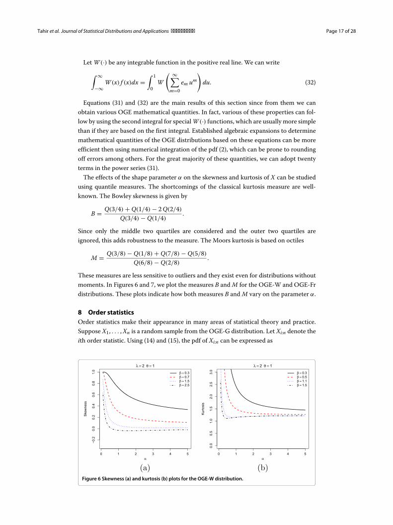
Equations (31) and (32) are the main results of this section since from them we canobtain various OGE mathematical quantities. In fact, various of these properties can fol-low by using the second integral for special W (·) functions, which are usually more simplethan if they are based on the first integral. Established algebraic expansions to determinemathematical quantities of the OGE distributions based on these equations can be moreefficient then using numerical integration of the pdf (2), which can be prone to roundingoff errors among others. For the great majority of these quantities, we can adopt twentyterms in the power series (31).

The effects of the shape parameter α on the skewness and kurtosis of X can be studiedusing quantile measures. The shortcomings of the classical kurtosis measure are well-known. The Bowley skewness is given by

B = Q(3/4) + Q(1/4) − 2 Q(2/4)

Q(3/4) − Q(1/4).

Since only the middle two quartiles are considered and the outer two quartiles areignored, this adds robustness to the measure. The Moors kurtosis is based on octiles

M = Q(3/8) − Q(1/8) + Q(7/8) − Q(5/8)

Q(6/8) − Q(2/8).

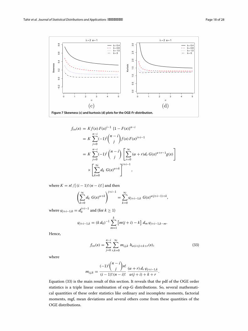
These measures are less sensitive to outliers and they exist even for distributions withoutmoments. In Figures 6 and 7, we plot the measures B and M for the OGE-W and OGE-Frdistributions. These plots indicate how both measures B and M vary on the parameter α.

8 Order statisticsOrder statistics make their appearance in many areas of statistical theory and practice.Suppose X1, . . . , Xn is a random sample from the OGE-G distribution. Let Xi:n denote theith order statistic. Using (14) and (15), the pdf of Xi:n can be expressed as

Figure 6 Skewness (a) and kurtosis (b) plots for the OGE-W distribution.


Figure 7 Skewness (c) and kurtosis (d) plots for the OGE-Fr distribution.

fi:n(x) = K f (x) F(x)i−1 {1 − F(x)}n−i

= Kn−i∑j=0

(−1)j(

n − ij

)f (x) F(x)j+i−1

= Kn−i∑j=0

(−1)j(

n − ij

) [ ∞∑r=0

(α + r)dr G(x)α+r−1g(x)

]

×[ ∞∑

k=0dk G(x)α+k

]j+i−1

,

where K = n! /[ (i − 1)! (n − i)! ] and then( ∞∑k=0

dk G(x)α+k)j+i−1

=∞∑

k=0ϕj+i−1,k G(x)α(j+i−1)+k ,

where ϕj+i−1,0 = dj+i−10 and (for k ≥ 1)

ϕj+i−1,k = (k d0)−1

k∑m=1

[m(j + i) − k

]dm ϕj+i−1,k−m.

Hence,

fi:n(x) =n−i∑j=0

∞∑r,k=0

mi,j,k hα(i+j)+k+r(x), (33)

where

mi,j,k =(−1)j

(n − i

j

)n!

(i − 1)! (n − i)!(α + r) dr ϕj+i−1,k

α(j + i) + k + r.

Equation (33) is the main result of this section. It reveals that the pdf of the OGE orderstatistics is a triple linear combination of exp-G distributions. So, several mathemati-cal quantities of these order statistics like ordinary and incomplete moments, factorialmoments, mgf, mean deviations and several others come from these quantities of theOGE distributions.


9 Characterization of the OGE familyCharacterizations of distributions are important to many researchers in the applied fields.An investigator will be vitally interested to know if their model fits the requirements of aparticular distribution. To this end, one will depend on the characterizations of this distri-bution which provide conditions under which the underlying distribution is indeed thatparticular distribution. Various characterizations of distributions have been establishedin many different directions. In this section, two main characterizations of the OGE fam-ily are presented. These characterizations are based on: (i) a simple relationship betweentwo truncated moments; (ii) a single function of the random variable.

9.1 Characterizations based on truncated moments

In this subsection we present characterizations of the OGE family in terms of a sim-ple relationship between two truncated moments. Our characterization results presentedhere will employ an interesting result due to Glänzel (1987) (Theorem 2, below). Theadvantage of these characterizations is that, the cdf F(x) does not require to have a closed-form and are given in terms of an integral whose integrand depends on the solution ofa first order differential equation, which can serve as a bridge between probability anddifferential equation.

Theorem 2. Let (�, �, P) be a given probability space and let H = [a, b] be an intervalfor some a < b

(a = −∞, b = ∞ might as well be allowed

). Let X : � → H be a con-

tinuous random variable with the distribution function F and let q1 and q2 be two realfunctions defined on H such that E

[q1 (X) |X ≥ x

] = E[q2 (X) |X ≥ x

]η (x) , x ∈ H, is

defined with some real function η. Consider that q1, q2 ∈ C1 (H), η ∈ C2 (H) and F(x)

is twice continuously differentiable and strictly monotone function on the set H. Finally,assume that the equation q2η = q1 has no real solution in the interior of H. Then, F isuniquely determined by the functions q1, q2 and η, particularly

F (x) =∫ x

aC∣∣∣∣ η′ (u)

η (u) q2 (u) − q1 (u)

∣∣∣∣ exp (−s (u)) du,

where the function s is a solution of the differential equation s′ = η′q2ηq2−q1

and C is a constantchosen to make

∫H dF = 1.

Clearly, Theorem 2 can be stated in terms of two functions q1 and η by taking q2 (x) ≡ 1,which will reduce the condition given in Theorem 2 to E

[q1 (X) |X ≥ x

] = η (x). How-ever, adding an extra function will give a lot more flexibility, as far as its application isconcerned.

Proposition 4. Let X : � → (0, ∞) be a continuous random variable and let q2 (x) =[1 − e−λ

(G(x;ξ)

G(x;ξ)

)]1−α

and q1 (x) = q2 (x) e−λ(

G(x;ξ)

G(x;ξ)

)for x > 0. The pdf of X is (2) if and

only if the function η defined in Theorem 2 has the form

η (x) = 12

{1 + e−λ

(G(x;ξ)

G(x;ξ)

)}, x > 0.


Proof. Let X has density (2), then

[1 − F (x)] E[q2 (X) |X ≥ x

] = α

{1 − e−λ

(G(x;ξ)

G(x;ξ)

)}, x > 0,

and

[1 − F (x)] E[q1 (X) |X ≥ x

] = α

2

{1 − e−2λ

(G(x;ξ)

G(x;ξ)

)}, x > 0.

Finally,

η (x) q2 (x) − q1 (x) = 12

q2 (x)

{1 − e−λ

(G(x;ξ)

G(x;ξ)

)}> 0 for x > 0.

Conversely, if η is given as above, then

s′ (x) = η′ (x) q2 (x)

η (x) q2 (x) − q1 (x)=

−λ

(g(x;ξ)(

G(x;ξ))2)

e−λ(

G(x;ξ)

G(x;ξ)

){

1 − e−λ(

G(x;ξ)

G(x;ξ)

)} , x > 0

and hence

s (x) = − ln{

1 − e−λ(

G(x;ξ)

G(x;ξ)

)}x > 0.

Now, in view of Theorem 2, X has density (2).

Corollary 1. Let X : � → R be a continuous random variable and let q2 (x) be as inProposition 4. The pdf of X is (2) if and only if there exist functions q1 and η defined inTheorem 2 satisfying the differential equation

η′ (x) q2 (x)

η (x) q2 (x) − q1 (x)=

−λ

(g(x;ξ)(

G(x;ξ))2)

e−λ(

G(x;ξ)

G(x;ξ)

){

1 − e−λ(

G(x;ξ)

G(x;ξ)

)} , x > 0.

Remark 1. (a) The general solution of the differential equation in Corollary 1 is

η (x) ={

1 − e−λ(

G(x;ξ)

G(x;ξ)

)}−1 [∫λq1 (x)

(g (x; ξ)(

G (x; ξ))2

)e−λ

(G(x;ξ)

G(x;ξ)

) [q2 (x)

]−1 dx + D]

,

where D is a constant. One set of appropriate functions is given in Proposition 4 withD = 1

2 .

(b) Clearly there are other triplets of functions (q2, q1, η) satisfying the conditions ofTheorem 2. We presented one such triplet in Proposition 4.

9.2 Characterizations based on single function of the random variable

In this subsection we employ a single function ψ of X and state characterization resultsin terms of ψ (X).

Proposition 5. Let X : � → (0, ∞) be a continuous random variable with cdf F(x). Letψ (x) be a differentiable function on (0, ∞) with limx→∞ ψ (x) = 1. Then for δ �= 1,

E [ψ (X) |X < x] = δψ (x) , x ∈ (0, ∞)


if and only if

ψ (x) = (F (x))1δ−1 , x ∈ (0, ∞) .

Proof. Proof is straightforward.

Remark 2. For ψ (x) =[

1 − e−λ(

G(x;ξ)

G(x;ξ)

)] α(1−δ)δ

, x ∈ (0, ∞), Proposition 5 will give a cdf

F(x) given by (1).

10 EstimationInference can be carried out in three different ways: point estimation, interval estimationand hypothesis testing. Several approaches for parameter point estimation were proposedin the literature but the maximum likelihood method is the most commonly employed.The maximum likelihood estimates (MLEs) enjoy desirable properties and can be usedwhen constructing confidence intervals and also in test-statistics. Large sample theory forthese estimates delivers simple approximations that work well in finite samples. Statis-ticians often seek to approximate quantities such as the density of a test-statistic thatdepend on the sample size in order to obtain better approximate distributions. The result-ing approximation for the MLEs in distribution theory is easily handled either analyticallyor numerically.

Here, consider the estimation of the unknown parameters of the OGE family by themethod of maximum likelihood from complete samples only. Let x1, . . . , xn be observedvalues from this family with parameters α, λ and ξ . Let � = (α, λ, ξ)� be the (r × 1)

parameter vector. The total log-likelihood function for � is given by

�n = �n(�) = n log(α λ) +n∑

i=1log

[g(xi; ξ)

]− 2n∑

i=1log

[G(xi; ξ)

]−λ

n∑i=1

V (xi; ξ) + (α − 1)

n∑i=1

log{

1 − e−λ V (xi;ξ)}

, (34)

where V (xi; ξ) = G(xi; ξ)/G(xi; ξ).The components of the score function Un(�) = (

Uα , Uλ, Uξk

)� are

Uα = nα

+n∑

i=1log

{1 − e−λV (xi;ξ)

},

Uλ = nλ

−n∑

i=1V (xi; ξ) + (α − 1)

n∑i=1

{V (xi; ξ) e−λ V (xi;ξ)

1 − e−λ V (xi;ξ)

},

Uξk =n∑

i=1

g(ξk)(xi, ξ)

g(xi, ξ)− 2

n∑i=1

G(ξk)(xi, ξ)

G(xi, ξ)− λ

n∑i=1

V (ξk)(xi, ξ)

+λ (α − 1)

n∑i=1

{V (ξk)(xi; ξ) e−λ V (xi;ξ)

1 − e−λ V (xi;ξ)

},

where v(ξ)(·) means the derivative of the function v with respect to ξ .Setting these equations to zero and solving them simultaneously yields the MLEs � =

(α, λ, ξ )� of � = (α, λ, ξ)�. These equations cannot be solved analytically, and analyticalsoftwares are required to solve them numerically.


For interval estimation of the parameters, we obtain the 3 × 3 observed informationmatrix J(�) = {Urs} (for r, s = α, λ, ξk), whose elements are listed in Appendix A.Under standard regularity conditions, the multivariate normal N3(0, J(�)−1) distributionis used to construct approximate confidence intervals for the parameters. Here, J(�) isthe total observed information matrix evaluated at �. Then, the 100(1 − γ )% confidenceintervals for α, λ and ξk are given by α ± zγ ∗/2 × √

var(α), λ ± zγ ∗/2 ×√

var(λ) and

ξk ± zγ ∗/2 ×√

var(ξk), respectively, where the var(·)’s denote the diagonal elements ofJ(�)−1 corresponding to the model parameters, and zγ ∗/2 is the quantile (1 − γ ∗/2) ofthe standard normal distribution.

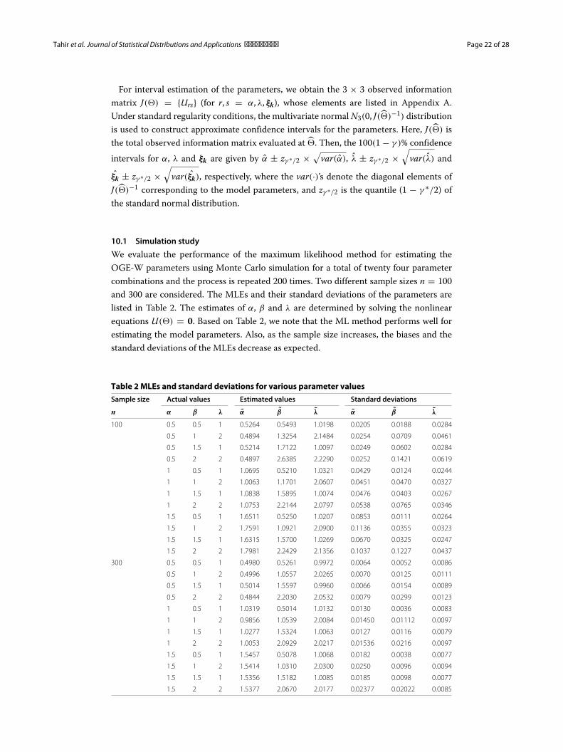
10.1 Simulation study

We evaluate the performance of the maximum likelihood method for estimating theOGE-W parameters using Monte Carlo simulation for a total of twenty four parametercombinations and the process is repeated 200 times. Two different sample sizes n = 100and 300 are considered. The MLEs and their standard deviations of the parameters arelisted in Table 2. The estimates of α, β and λ are determined by solving the nonlinearequations U(�) = 0. Based on Table 2, we note that the ML method performs well forestimating the model parameters. Also, as the sample size increases, the biases and thestandard deviations of the MLEs decrease as expected.

Table 2 MLEs and standard deviations for various parameter values

Sample size Actual values Estimated values Standard deviations

n α β λ α β λ α β λ

100 0.5 0.5 1 0.5264 0.5493 1.0198 0.0205 0.0188 0.0284

0.5 1 2 0.4894 1.3254 2.1484 0.0254 0.0709 0.0461

0.5 1.5 1 0.5214 1.7122 1.0097 0.0249 0.0602 0.0284

0.5 2 2 0.4897 2.6385 2.2290 0.0252 0.1421 0.0619

1 0.5 1 1.0695 0.5210 1.0321 0.0429 0.0124 0.0244

1 1 2 1.0063 1.1701 2.0607 0.0451 0.0470 0.0327

1 1.5 1 1.0838 1.5895 1.0074 0.0476 0.0403 0.0267

1 2 2 1.0753 2.2144 2.0797 0.0538 0.0765 0.0346

1.5 0.5 1 1.6511 0.5250 1.0207 0.0853 0.0111 0.0264

1.5 1 2 1.7591 1.0921 2.0900 0.1136 0.0355 0.0323

1.5 1.5 1 1.6315 1.5700 1.0269 0.0670 0.0325 0.0247

1.5 2 2 1.7981 2.2429 2.1356 0.1037 0.1227 0.0437

300 0.5 0.5 1 0.4980 0.5261 0.9972 0.0064 0.0052 0.0086

0.5 1 2 0.4996 1.0557 2.0265 0.0070 0.0125 0.0111

0.5 1.5 1 0.5014 1.5597 0.9960 0.0066 0.0154 0.0089

0.5 2 2 0.4844 2.2030 2.0532 0.0079 0.0299 0.0123

1 0.5 1 1.0319 0.5014 1.0132 0.0130 0.0036 0.0083

1 1 2 0.9856 1.0539 2.0084 0.01450 0.01112 0.0097

1 1.5 1 1.0277 1.5324 1.0063 0.0127 0.0116 0.0079

1 2 2 1.0053 2.0929 2.0217 0.01536 0.0216 0.0097

1.5 0.5 1 1.5457 0.5078 1.0068 0.0182 0.0038 0.0077

1.5 1 2 1.5414 1.0310 2.0300 0.0250 0.0096 0.0094

1.5 1.5 1 1.5356 1.5182 1.0085 0.0185 0.0098 0.0077

1.5 2 2 1.5377 2.0670 2.0177 0.02377 0.02022 0.0085


11 ApplicationsIn this section, we provide two applications to real data to illustrate the importance of theOGE family by means of the OGE-W, OGE-Fr and OGE-N models presented in Section 3.We consider θ = 1, b = 1 and μ = 0 for the OGE-W, OGE-Fr and OGE-N models,respectively, due to the fact that one scale parameter is enough for fitting these univari-ate models. The MLEs of the parameters for the these models are calculated and fourgoodness-of-fit statistics are used to compare the new family with its sub-models.

The first real data set represents the survival times of 121 patients with breast cancerobtained from a large hospital in a period from 1929 to 1938 (Lee 1992). The data exam-ined by Ramos et al. (2013) are: 0.3, 0.3, 4.0, 5.0, 5.6, 6.2, 6.3, 6.6, 6.8, 7.4, 7.5, 8.4, 8.4, 10.3,11.0, 11.8, 12.2, 12.3, 13.5, 14.4, 14.4, 14.8, 15.5, 15.7, 16.2, 16.3, 16.5, 16.8, 17.2, 17.3, 17.5,17.9, 19.8, 20.4, 20.9, 21.0, 21.0, 21.1, 23.0, 23.4, 23.6, 24.0, 24.0, 27.9, 28.2, 29.1, 30.0, 31.0,31.0, 32.0, 35.0, 35.0, 37.0, 37.0, 37.0, 38.0, 38.0, 38.0, 39.0, 39.0, 40.0, 40.0, 40.0, 41.0, 41.0,41.0, 42.0, 43.0, 43.0, 43.0, 44.0, 45.0, 45.0, 46.0, 46.0, 47.0, 48.0, 49.0, 51.0, 51.0, 51.0, 52.0,54.0, 55.0, 56.0, 57.0, 58.0, 59.0, 60.0, 60.0, 60.0, 61.0, 62.0, 65.0, 65.0, 67.0, 67.0, 68.0, 69.0,78.0, 80.0,83.0, 88.0, 89.0, 90.0, 93.0, 96.0, 103.0, 105.0, 109.0, 109.0, 111.0, 115.0, 117.0,125.0, 126.0, 127.0, 129.0, 129.0, 139.0, 154.0.

The second data set consists of 63 observations of the strengths of 1.5 cm glass fibres,originally obtained by workers at the UK National Physical Laboratory. Unfortunately, theunits of measurement are not given in the paper. The data are: 0.55, 0.74, 0.77, 0.81, 0.84,0.93, 1.04, 1.11, 1.13, 1.24, 1.25, 1.27, 1.28, 1.29, 1.30, 1.36, 1.39, 1.42, 1.48, 1.48, 1.49, 1.49,1.50, 1.50, 1.51, 1.52, 1.53, 1.54, 1.55, 1.55, 1.58, 1.59, 1.60, 1.61, 1.61, 1.61, 1.61, 1.62, 1.62,1.63, 1.64, 1.66, 1.66, 1.66, 1.67, 1.68, 1.68, 1.69, 1.70, 1.70, 1.73, 1.76, 1.76, 1.77, 1.78, 1.81,1.82, 1.84, 1.84, 1.89, 2.00, 2.01, 2.24. These data have also been analyzed by Smith andNaylor (1987).

The MLEs are computed using the Limited-Memory Quasi-Newton Code for Bound-Constrained Optimization (L-BFGS-B) and the log-likelihood function evaluated at theMLEs (�). The measures of goodness of fit including the Akaike information criterion(AIC), Anderson-Darling (A∗), Cramér–von Mises (W ∗) and Kolmogrov-Smirnov (K-S) statistics are computed to compare the fitted models. The statistics A∗ and W ∗ aredescribed in details in Chen and Balakrishnan (1995). In general, the smaller the values ofthese statistics, the better the fit to the data. The required computations are carried outin the R-language.

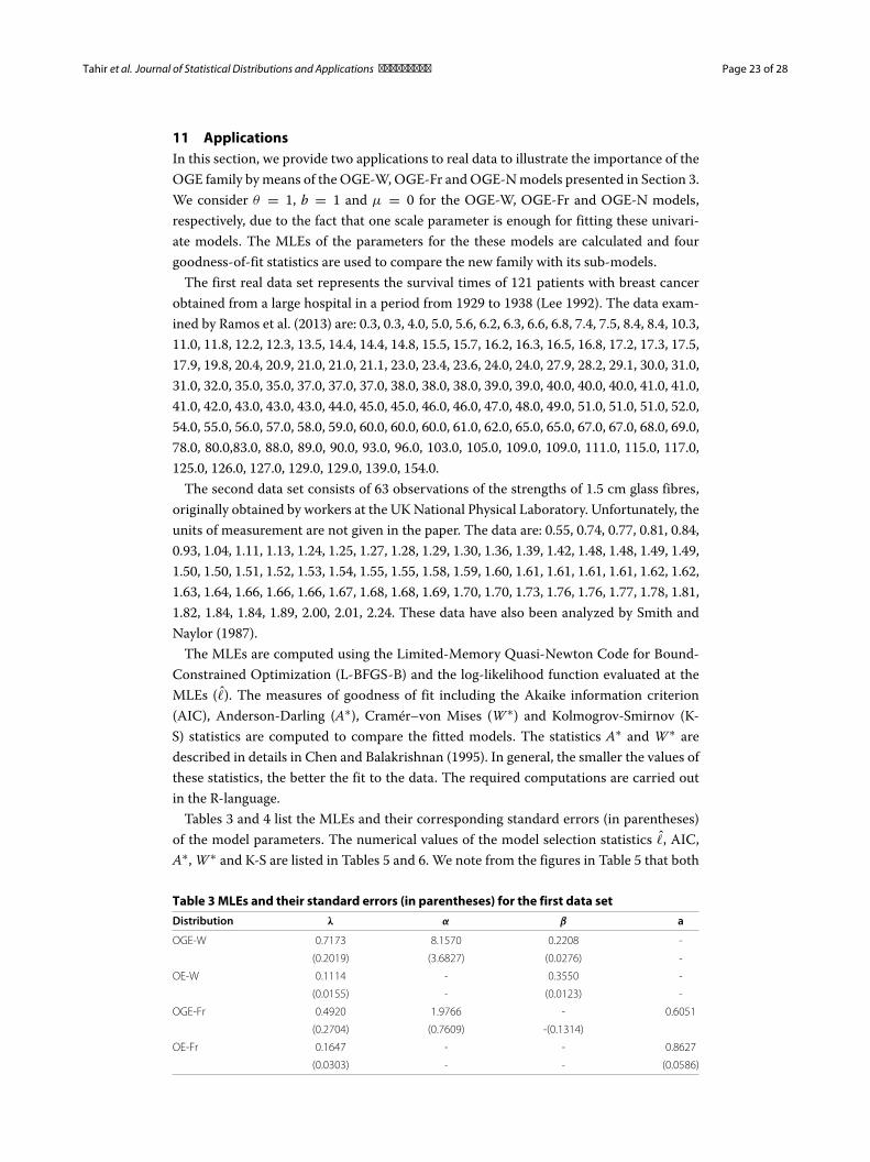
Tables 3 and 4 list the MLEs and their corresponding standard errors (in parentheses)of the model parameters. The numerical values of the model selection statistics �, AIC,A∗, W ∗ and K-S are listed in Tables 5 and 6. We note from the figures in Table 5 that both

Table 3 MLEs and their standard errors (in parentheses) for the first data set

Distribution λ α β a

OGE-W 0.7173 8.1570 0.2208 -

(0.2019) (3.6827) (0.0276) -

OE-W 0.1114 - 0.3550 -

(0.0155) - (0.0123) -

OGE-Fr 0.4920 1.9766 - 0.6051

(0.2704) (0.7609) -(0.1314)

OE-Fr 0.1647 - - 0.8627

(0.0303) - - (0.0586)


Table 4 MLEs and their standard errors (in parentheses) for the second data set

Distribution λ α β σ

OGE-W 0.7173 8.1570 0.2208 -

(0.2019) (3.6827) (0.0276) -

OE-W 0.0721 - 1.9603 -

(0.0162) - (0.0940) -

OGE-N 0.1010 3.1230 - 0.9884

(0.0798) (1.5660) - (0.1484)

OE-N 0.0121 - - 0.7385

(0.0043) - - (0.0364)

Table 5 The statistics �, AIC, A∗, W ∗ K-S and K-S p-value for the first data set

Distribution � AIC A∗ W∗ K-S p-value (K-S)

OGE-W -410.8347 827.6693 0.3111 0.0472 0.0460 0.9498

OE-W -431.1625 866.3251 2.6578 0.4510 0.1430 0.0107

OGE-Fr -414.2511 834.5023 0.6838 0.1011 0.0651 0.6492

OE-Fr -416.3539 836.7078 0.8991 0.1367 0.0939 0.2095

Table 6 The statistics �, AIC, A∗, W ∗, K-S and K-S p-value for the second data set

Distribution � AIC A∗ W∗ K-S p-value (K-S)

OGE-N -14.1653 34.3306 0.8755 0.1548 0.1286 0.2483

OE-N -17.5979 39.1958 0.9684 0.1557 0.1232 0.2945

OGE-W -14.2733 34.5465 0.9645 0.1717 0.1334 0.2119

OE-W -16.4613 36.9227 0.9619 0.1614 0.1377 0.1832

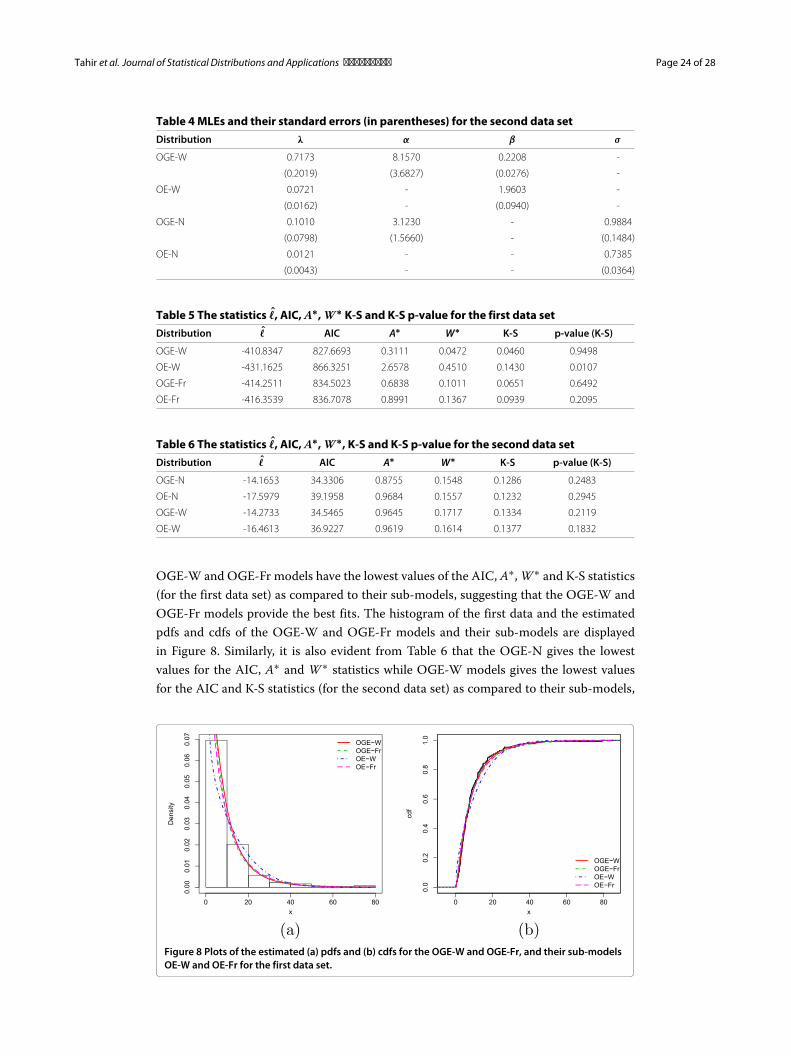
OGE-W and OGE-Fr models have the lowest values of the AIC, A∗, W ∗ and K-S statistics(for the first data set) as compared to their sub-models, suggesting that the OGE-W andOGE-Fr models provide the best fits. The histogram of the first data and the estimatedpdfs and cdfs of the OGE-W and OGE-Fr models and their sub-models are displayedin Figure 8. Similarly, it is also evident from Table 6 that the OGE-N gives the lowestvalues for the AIC, A∗ and W ∗ statistics while OGE-W models gives the lowest valuesfor the AIC and K-S statistics (for the second data set) as compared to their sub-models,

Figure 8 Plots of the estimated (a) pdfs and (b) cdfs for the OGE-W and OGE-Fr, and their sub-modelsOE-W and OE-Fr for the first data set.


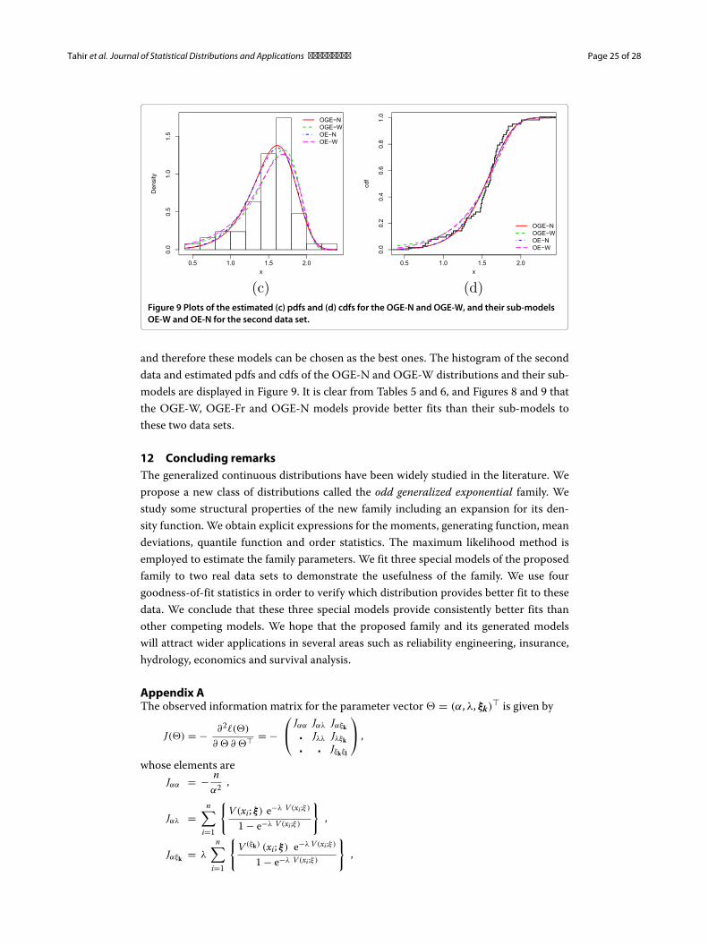
Figure 9 Plots of the estimated (c) pdfs and (d) cdfs for the OGE-N and OGE-W, and their sub-modelsOE-W and OE-N for the second data set.

and therefore these models can be chosen as the best ones. The histogram of the seconddata and estimated pdfs and cdfs of the OGE-N and OGE-W distributions and their sub-models are displayed in Figure 9. It is clear from Tables 5 and 6, and Figures 8 and 9 thatthe OGE-W, OGE-Fr and OGE-N models provide better fits than their sub-models tothese two data sets.

12 Concluding remarksThe generalized continuous distributions have been widely studied in the literature. Wepropose a new class of distributions called the odd generalized exponential family. Westudy some structural properties of the new family including an expansion for its den-sity function. We obtain explicit expressions for the moments, generating function, meandeviations, quantile function and order statistics. The maximum likelihood method isemployed to estimate the family parameters. We fit three special models of the proposedfamily to two real data sets to demonstrate the usefulness of the family. We use fourgoodness-of-fit statistics in order to verify which distribution provides better fit to thesedata. We conclude that these three special models provide consistently better fits thanother competing models. We hope that the proposed family and its generated modelswill attract wider applications in several areas such as reliability engineering, insurance,hydrology, economics and survival analysis.

Appendix AThe observed information matrix for the parameter vector � = (α, λ, ξk)� is given by

J(�) = − ∂2�(�)

∂ � ∂ �� = −⎛⎝ Jαα Jαλ Jαξk

� Jλλ Jλξk� � Jξkξl

⎞⎠ ,

whose elements areJαα = − n

α2 ,

Jαλ =n∑

i=1

{V (xi; ξ) e−λ V (xi ;ξ)

1 − e−λ V (xi ;ξ)

},

Jαξk = λ

n∑i=1

{V (ξk) (xi; ξ) e−λ V (xi ;ξ)

1 − e−λ V (xi ;ξ)

},


Jλλ = − nλ2 + (α − 1)

n∑i=1

{V 2 (xi; ξ) e−λ V (xi ;ξ){

1 − e−λ V (xi ;ξ)}2

},

Jλ ξk = −n∑

i=1V (ξk) (xi; ξ)

+(α − 1)

n∑i=1

{V (ξk) (xi; ξ) e−λ V (xi ;ξ)

[1 − λ V (xi; ξ) − e−λ V (xi ;ξ)

]{1 − e−λ V (xi ;ξ)

}2

},

Jξkξl =n∑

i=1

{ g(xi; ξ) g′′kl(xi; ξ) − g′

k(xi; ξ) g′l(xi; ξ)

g2(xi; ξ)

}

−2n∑

i=1

{G(xi; ξ) G′′

kl(xi; ξ) − G′k(xi; ξ) G′

l(xi; ξ)

G2(xi; ξ)

}− λ

n∑i=1

V ′′kl (xi; ξ)

+λ(α − 1)

n∑i=1

1{1 − e−λ V (xi ;ξ)

}2 ×

{e−λ V (xi ;ξ)

[V ′′

kl(xi; ξ) − λ V ′k(xi; ξ) V ′

l (xi; ξ) − V ′′kl(xi; ξ) e−λ V (xi ;ξ)

]},

where t′k(·, ξ) = ∂ t(·, ξ)/∂ ξk and t′′kl(·, ξ) = ∂2 t(·, ξ)/∂ ξk ∂ ξl .

AcknowledgementsThe authors would like to thank the Editor and the two referees for careful reading and for their comments which greatlyimproved the paper.

Competing interestsThe authors declare that they have no competing interests.

Authors’ contributionsThe authors, viz MHT, GMC, MA, MM, MZ and GGH with the consultation of each other carried out this work and draftedthe manuscript together. All authors read and approved the final manuscript.

Author details1Department Statistics, Baghdad Campus, The Islamia University of Bahawalpur, 63100 Bahawalpur, Pakistan.2Departamento de Estatística, Universidade Federal de Pernambuco, PE 50740-540 Recife, Brazil. 3Department ofStatistics, Persian Gulf University of Bushehr, Bushehr, Iran. 4Department Statistics, The Islamia University of Bahawalpur,63100 Bahawalpur, Pakistan. 6Department of Mathematics, Statistics and Computer Science Marquette University, WI53201-1881 Milwaukee, USA.

Received: 1 September 2014 Accepted: 15 December 2014

ReferencesAlexander, C, Cordeiro, GM, Ortega, EMM, Sarabia, JM: Generalized beta-generated distributions. Comput. Statist. Data.

Anal. 56, 1880–1897 (2012)Alizadeh, M, Emadi, M, Doostparast, M, Cordeiro, GM, Ortega, EMM, Pescim, RR: A new family of distributions: the

Kumaraswamy odd log-logistic, properties and applications. Hacet. J. Math Stat (2015). forthcomingAljarrah, MA, Lee, C, Famoye, F: On generating T-X family of distributions using quantile functions. J. Stat. Dist. Appl. 1, Art.

2 (2014)Alzaatreh, A, Lee, C, Famoye, F: A new method for generating families of continuous distributions. Metron. 71, 63–79

(2013)Alzaatreh, A, Lee, C, Famoye, F: T-normal family of distributions: A new approach to generalize the normal distribution. J.

Stat. Dist. Appl. 1, Art, 16 (2014)Alzaghal, A, Famoye, F, Lee, C: Exponentiated T-X family of distributions with some applications. Int. J. Probab. Statist. 2,

31–49 (2013)Amini, M, MirMostafaee, SMTK, Ahmadi, J: Log-gamma-generated families of distributions. Statistics. 48, 913–932 (2014)Bourguignon, M, Silva, RB, Cordeiro, GM: The Weibull-G family of probability distributions. J. Data Sci. 12, 53–68 (2014)Chen, G, Balakrishnan, N: A general purpose approximate goodness-of-fit test. J. Qual. Tech. 27, 154–161 (1995)Choudhury, A: A simple derivation of moments of the exponentiated Weibull distribution. Metrika. 62, 17–22 (2005)Cordeiro, GM: de Castro, M: A new family of generalized distributions. J. Stat. Comput. Simul. 81, 883–893 (2011)Cordeiro, GM, Nadarajah, S: Closed-form expressions for moments of a class of beta generalized distributions. Braz. J.

Probab. Stat. 25, 14–33 (2011)Cordeiro, GM, Ortega, EMM, da Cunha, DCC: The exponentiated generalized class of distributions. J. Data Sci. 11, 1–27

(2013)


Cordeiro, GM, Alizadeh, M, Ortega, EMM: The exponentiated half-logistic family of distributions: Properties andapplications. J. Probab. Statist. Art.ID. 864396, 21 (2014a)

Cordeiro, GM, Ortega, EMM, Popovic, BV, Pescim, RR: The Lomax generator of distributions: Properties, minificationprocess and regression model. Appl. Math. Comput. 247, 465–486 (2014b)

Dey, AK, Kundu, D: Discriminating among the log-normal, Weibull and generalized exponential distributions. IEEE Trans.Reliab. 58, 416–424 (2009)

El-Gohary, A, Alshamrani, A, Al-Otaibi, AN: The generalized Gompertz distribution. Appl. Math. Model. 37, 13–24 (2013)Eugene, N, Lee, C, Famoye, F: Beta-normal distribution and its applications. Commun. Stat. Theory Methods. 31, 497–512

(2002)Fiorentino, M, Gioia, A, Iacobellis, V, Manfreda, S: Analysis on flood generation processes by means of a continuous

simulation model. Adv. Geosci. 7, 231–236 (2006)Glänzel, W: A characterization theorem based on truncated moments and its application to some distribution families. In:

Mathematical Statistics and Probability Theory (Bad Tatzmannsdorf, 1986), Vol. B, Reidel, Dordrecht, pp. 75–84, (1987)Gradshteyn, IS, Ryzhik, IM: Table of Integrals, Series, and Products. 6th eds. Academic Press, San Diego (2000)Gupta, RC, Gupta, PI, Gupta, RD: Modeling failure time data by Lehmann alternatives. Commun. Stat. Theory Methods. 27,

887–904 (1998)Gupta, RD, Kundu, D: Generalized exponential distribution. Aust. N. Z. J. Stat. 41, 173–188 (1999)Gupta, RD, Kundu, D: Generalized exponential distribution: An alternative to Gamma and Weibull distributions. Biom. J.

43, 117–130 (2001a)Gupta, RD, Kundu, D: Generalized exponential distribution: Different methods of estimations. J. Stat. Comput. Simul. 69,

315–337 (2001b)Gupta, RD, Kundu, D: Discriminating between the Weibull and the GE distributions. Comput. Stat. Data Anal. 43, 179–196

(2002)Gupta, RD, Kundu, D: Closeness of gamma and generalized exponential distributions. Commun. Stat. Theory Methods.

32, 705–721 (2003)Gupta, RD, Kundu, D: Discriminating between the gamma and generalized exponential distributions. J. Stat. Comput.

Simul. 74, 107–121 (2004)Gupta, RD, Kundu, D: On comparison of the Fisher information of the Weibull and GE distributions. J. Stat. Plann.

Inference. 136, 3130–3144 (2006)Gupta, RD, Kundu, D: Generalized exponential distribution: Existing results and some recent developments. J. Stat. Plann.

Inference. 137, 3537–3547 (2007)Gupta, RD, Kundu, D: Generalized exponential distribution: Bayesian Inference. Comput. Stat. Data Anal. 52, 1873–1883

(2008)Gupta, RD, Kundu, D: An extension of generalized exponential distribution. Stat. Methodol. 8, 485–496 (2011)Iacobellis, V, Fiorentino, M: Derived distribution of floods based on the concept of partial area coverage with a climatic

appeal. Water Resour. Res. 36, 469–482 (2000)Jones, MC: Families of distributions arising from the distributions of order statistics. Test. 13, 1–43 (2004)Kilbas, AA, Srivastava, HM, Trujillo, JJ: Theory and applications of fractional differential equations. Elsevier, Amsterdam (2006)Kundu, D, Gupta, RD, Manglick, A: Discriminating between the log-normal and the generalized exponential distributions.

J. Stat. Plann. Inference. 127, 213–227 (2005)Lee, ET: Statistical Methods for Survival Data Analysis. John Wiley, New York (1992)Lehmann, EL: The power of rank tests. Ann. Math. Statist. 24, 23–43 (1953)Marshall, AN, Olkin, I: A new method for adding a parameter to a family of distributions with applications to the

exponential and Weibull families. Biometrika. 84, 641–652 (1997)Mudholkar, GS, Hutson, AD: The exponentiated Weibull family: Some properties and a flood data application. Commun.

Stat. Theory Methods. 25, 3059–3083 (1996)Mudholkar, GS, Srivastava, DK: Exponentiated Weibull family for analyzing bathtub failure data. IEEE Trans. Reliab. 42,

299–302 (1993)Mudholkar, GS, Srivastava, DK, Freimer, M: The exponentiated Weibull family: A reanalysis of the bus-motor failure data.

Technometrics. 37, 436–445 (1995)Nadarajah, S: Exact distribution of the peak streamflow. Water Resour. Res. 43(2), W02501 (2007).

doi:10.1029/2006WR005300Nadarajah, S: The exponentiated exponential distribution: a survey. AStA Adv. Stat. Anal. 95, 219–251 (2011)Nadarajah, S, Cordeiro, GM, Ortega, EMM: The exponentiated Weibull distribution: a survey. Stat. Papers. 54, 839–877

(2013)Nadarajah, S, Cordeiro, GM, Ortega, EMM: The Zografos-Balakrishnan–G family of distributions: Mathematical properties

and applications. Commun. Stat. Theory Methods. 44, 186–215 (2015)Nadarajah, S, Kotz, S: A generalized logistic distribution. Int. J. Math. Math. Sci. 19, 3169–3174 (2005)Nadarajah, S, Kotz, S: The exponentiated type distributions. Acta Appl. Math. 92, 97–111 (2006)Pakyari, R: Discriminating between generalized exponential, geometric extreme exponential and Weibull distribution. J.

Stat. Comput. Simul. 80, 1403–1412 (2010)Prudnikov, AP, Bruychkov, YA: Marichev, Vol. 1. Gordon and Breach, New York (1986)Ramos, MWA, Cordeiro, GM, Marinho, PRD, Dias, CRB, Hamedani, GG: The Zografos-Balakrishnan log-logistic distribution:

Properties and applications. J. Stat. Theory Appl. 12, 225–244 (2013)Rényi, A: On measures of entropy and information. In: Proceedings of the Fourth Berkeley Symposium on Mathematical

Statistics and Probability-I, pp. 547–561. University of California Press, Berkeley, (1961)Ristic, MM, Balakrishnan, N: The gamma-exponentiated exponential distribution. J. Stat. Comput. Simul. 82, 1191–1206

(2012)Shannon, CE: A mathematical theory of communication. Bell Sys. Tech. J. 27, 379–432 (1948)Smith, RL, Naylor, JC: A comparison of maximum likelihood and Bayesian estimators for the three-parameter Weibull

distributuion. Appl. Statist. 36, 358–369 (1987)


Tahir, MH, Cordeiro, GM, Alzaatreh, A, Mansoor, M, Zubair, M: The Logistic-X family of distributions and its applications.Commun. Stat. Theory Methods (2015a). forthcoming

Tahir, MH, Zubair, M, Mansoor, M, Cordeiro, GM, Alizadeh, M, Hamedani, GG: A new Weibull-G family of distributions.Hacet. J. Math. Stat. (2015b). forthcoming

Torabi, H, Montazari, NH: The gamma-uniform distribution and its application. Kybernetika. 48, 16–30 (2012)Torabi, H, Montazari, NH: The logistic-uniform distribution and its application. Commun. Stat. Simul. Comput. 43,

2551–2569 (2014)Zografos, K, Balakrishnan, N: On families of beta- and generalized gamma-generated distributions and associated

inference. Stat. Methodol. 6, 344–362 (2009)

Submit your manuscript to a journal and benefi t from:

7 Convenient online submission

7 Rigorous peer review

7 Immediate publication on acceptance

7 Open access: articles freely available online

7 High visibility within the fi eld

7 Retaining the copyright to your article

Submit your next manuscript at 7 springeropen.com

Documents

The odd generalized exponential family of distributions with applications