Embed Size (px)
Citation preview
arX
iv:g
r-qc
/010
5063
v1 1
7 M
ay 2
001
1
THE QUANTUM PHYSICS OF BLACK
HOLES: Results from String Theory ∗
Sumit R. Das
Tata Institute of Fundamental Research, Homi Bhabha Road, Mumbai 400005, India; e-mail:[email protected]
Samir D. Mathur
Department of Physics, Ohio State University, Columbus, Ohio 43210; e-mail:[email protected]
KEYWORDS: black holes, information loss, string theory, D-branes, holography
ABSTRACT: We review recent progress in our understanding of the physics of black holes.In particular, we discuss the ideas from string theory that explain the entropy of black holes froma counting of microstates of the hole, and the related derivation of unitary Hawking radiationfrom such holes.
CONTENTS
INTRODUCTION . . . . . . . . . . . . . . . . . . . . . . . . . . . . . . . . . . . . 2The Entropy Problem . . . . . . . . . . . . . . . . . . . . . . . . . . . . . . . . . . . . 4Hawking Radiation . . . . . . . . . . . . . . . . . . . . . . . . . . . . . . . . . . . . . . 5The Information Problem . . . . . . . . . . . . . . . . . . . . . . . . . . . . . . . . . . 5Difficulties with Obtaining Unitarity . . . . . . . . . . . . . . . . . . . . . . . . . . . . 7
STRING THEORY AND SUPERGRAVITY . . . . . . . . . . . . . . . . . . . . . 9Kaluza-Klein Mechanism . . . . . . . . . . . . . . . . . . . . . . . . . . . . . . . . . . 1011-Dimensional and 10-Dimensional Supergravities . . . . . . . . . . . . . . . . . . . . 11
BRANES IN SUPERGRAVITY AND STRING THEORY . . . . . . . . . . . . . . 13Branes in Supergravity . . . . . . . . . . . . . . . . . . . . . . . . . . . . . . . . . . . . 13BPS States . . . . . . . . . . . . . . . . . . . . . . . . . . . . . . . . . . . . . . . . . . 14The Type IIB Theory . . . . . . . . . . . . . . . . . . . . . . . . . . . . . . . . . . . . . 15D-Branes in String Theory . . . . . . . . . . . . . . . . . . . . . . . . . . . . . . . . . 16Duality . . . . . . . . . . . . . . . . . . . . . . . . . . . . . . . . . . . . . . . . . . . . 19
BLACK HOLE ENTROPY IN STRING THEORY: THE FUNDAMENTAL STRING 20
THE FIVE-DIMENSIONAL BLACK HOLE IN TYPE IIB THEORY . . . . . . . 22The Classical Solution . . . . . . . . . . . . . . . . . . . . . . . . . . . . . . . . . . . . 22Semiclassical Thermodynamics . . . . . . . . . . . . . . . . . . . . . . . . . . . . . . . 23
∗With permission from the Annual Review of Nuclear and Particle Science. Final version ofthis material appears in the Annual Review of Nuclear and Particle Science Vol. 50, publishedin December 2000 by Annual Reviews, http://AnnualReviews.org.

Extremal and Near-Extremal Limits . . . . . . . . . . . . . . . . . . . . . . . . . . . . 23Microscopic Model for the Five-Dimensional Black Hole . . . . . . . . . . . . . . . . . 24The Long String and Near-Extremal Entropy . . . . . . . . . . . . . . . . . . . . . . . 25A More Rigorous Treatment for Extremal Black Holes . . . . . . . . . . . . . . . . . . 28The Gauge Theory Picture . . . . . . . . . . . . . . . . . . . . . . . . . . . . . . . . . . 31Other Extremal Black Holes . . . . . . . . . . . . . . . . . . . . . . . . . . . . . . . . . 32
BLACK HOLE ABSORPTION/DECAY AND D-BRANES . . . . . . . . . . . . . 33Classical Absorption and grey-body Factors . . . . . . . . . . . . . . . . . . . . . . . . 33D-brane Decay . . . . . . . . . . . . . . . . . . . . . . . . . . . . . . . . . . . . . . . . 35Why Does It Work? . . . . . . . . . . . . . . . . . . . . . . . . . . . . . . . . . . . . . 39
ABSORPTION BY THREE-BRANES . . . . . . . . . . . . . . . . . . . . . . . . . 39Classical Solution and Classical Absorption . . . . . . . . . . . . . . . . . . . . . . . . 39Absorption in the Microscopic Model . . . . . . . . . . . . . . . . . . . . . . . . . . . . 40Nonextremal Thermodynamics . . . . . . . . . . . . . . . . . . . . . . . . . . . . . . . 41
AdS/CFT CORRESPONDENCE AND HOLOGRAPHY . . . . . . . . . . . . . . 41The Maldacena Conjecture . . . . . . . . . . . . . . . . . . . . . . . . . . . . . . . . . . 42Calculations Using the Conjecture . . . . . . . . . . . . . . . . . . . . . . . . . . . . . 44Holography and the Bekenstein Entropy Bound . . . . . . . . . . . . . . . . . . . . . . 45Near-Horizon Limit of 5D Black Hole . . . . . . . . . . . . . . . . . . . . . . . . . . . 46A Suggestive Model of Holography . . . . . . . . . . . . . . . . . . . . . . . . . . . . . 46
DISCUSSION . . . . . . . . . . . . . . . . . . . . . . . . . . . . . . . . . . . . . . . 46
1 INTRODUCTION
Black holes present us with a very deep paradox. The path to resolving this para-dox may well be the path to a consistent unified theory of matter and quantizedgravity.
In classical gravity, a black hole is a classical solution of the equations of mo-tion such that there is a region of spacetime that is causally disconnected fromasymptotic infinity (see e.g. Reference [1]). The boundary of such a region iscalled the event horizon.
Consider a large collection of low-density matter, in an asymptotically flatspacetime. For simplicity, we take the starting configuration to be sphericallysymmetric and nonrotating (these restrictions do not affect the nature of theparadox that emerges). This ball of matter will collapse toward smaller radiiunder its self-gravitation. At some point, the matter will pass through a criticalradius, the Schwarzschild radius Rs, after which its further collapse cannot behalted, whatever the equation of state. The final result, in classical generalrelativity, is that the matter ends up in an infinite-density singular point, whilethe metric settles down to the Schwarzschild form
ds2 = −(1 − 2GNM
rc2)dt2 + (1 − 2GNM
rc2)−1dr2 + r2dΩ2. (1)
Here GN is Newton’s constant of gravity, and c is the speed of light. The horizonradius of this hole is
Rs =2GNM
c2→ 2M, (2)
where the last expression arises after we set GN = 1, c = 1. (In what follows, weadopt these units unless otherwise explicitly indicated; we also set h = 1.)
2
D-Branes and Black Holes 3
Classically, nothing can emerge from inside the horizon to the outside. A testmass m has effective energy zero if it is placed at the horizon; it has rest energymc2, but a negative gravitational potential energy exactly balances this positivecontribution. For a rough estimate of the horizon size, we may put this negativeenergy to be the Newtonian value −GNMm/r, for which Rs ∼ GNM/c2.
It may appear from the above that the gravitational fields at the horizon ofa black hole are very large. This is not true. For a neutral black hole of massM , the magnitude of the curvature invariants, which are the measure of localgravitational forces, is given by
|R| ∼ GNM
r3. (3)
Thus, at the horizon r = rH = 2GNM , the curvature scales as 1/M2. As a result,
for black holes with masses M ≫ G−1/2N , the curvatures are very small and the
spacetime is locally rather close to flat spacetime. In fact, an object falling into ablack hole will not experience any strong force as it crosses the horizon. However,an asymptotic observer watching this object will see that it takes an infinite timeto reach the horizon. This is because there is an infinite gravitational red-shiftbetween the horizon and the asymptotic region.
An important point about black hole formation is that one does not need tocrush matter to high densities to form a black hole. In fact, if the hole has massM , the order of magnitude of the density required of the matter is
ρ ∼ M
R3s
∼ 1
M2. (4)
Thus, a black hole of the kind believed to exist at the center of our galaxy (108
solar masses) could form from a ball with the density of water. In fact, given anydensity we choose, we can make a black hole if we take a sufficient total masswith that density. This fact makes it very hard to imagine a theory in whichblack holes do not form at all because of some feature of the interaction betweenthe matter particles. As a consequence, if black holes lead to a paradox, it ishard to bypass the paradox by doing away with black holes in the theory.
It is now fairly widely believed that black holes exist in nature. Solar-massblack holes can be endpoints of stellar evolution, and supermassive black holes(∼ 105 − 109 solar masses) probably exist at the centers of galaxies. In somesituations, these holes accrete matter from their surroundings, and the collisionsamong these infalling particles create very powerful sources of radiation that arebelieved to be the source of the high-energy output of quasars. In this arti-cle, however, we are not concerned with any of these astrophysical issues. Weconcentrate instead on the quantum properties of isolated black holes, with aview toward understanding the problems that arise as issues of principle whenquantum mechanical ideas are put in the context of black holes.
For example, the Hawking radiation process discussed below is a quantum pro-cess that is much weaker than the radiation from the infalling matter mentionedabove, and it would be almost impossible to measure even by itself. (The onepossible exception is the Hawking radiation at the last stage of quantum evapora-tion. This radiation emerges in a sharp burst with a universal profile, and thereare experiments under way to look for such radiation from very small primordialblack holes.)
4 Das & Mathur
1.1 The Entropy Problem
Already, at this stage, one finds what may be called the entropy problem. Oneof the most time-honored laws in physics has been the second law of thermody-namics, which states that the entropy of matter in the Universe cannot decrease.But with a black hole present in the Universe, one can imagine the followingprocess. A box containing some gas, which has a certain entropy, is droppedinto a large black hole. The metric of the black hole then soon settles down tothe Schwarzschild form above, though with a larger value for M , the black holemass. The entropy of the gas has vanished from view, so that if we only countthe entropy that we can explicitly see, then the second law of thermodynamicshas been violated!
This violation of the second law can be avoided if one associates an entropy tothe black hole itself. Starting with the work of Bekenstein [2], we now know thatif we associate an entropy
SBH =AH
4GN(5)
with the black hole of horizon area AH , then in any Gedanken experiment inwhich we try to lose entropy down the hole, the increase in the black hole’sattributed entropy is such that
d
dt(Smatter + SBH) ≥ 0
(for an analysis of such Gedanken experiments, see e.g. [3]). Furthermore, an“area theorem” in general relativity states that in any classical process, the totalarea of all black holes cannot decrease. This statement is rather reminiscent ofthe statement of the second law of thermodynamics—the entropy of the entireUniverse can never decrease.
Thus the proposal (Equation 5) would appear to be a nice one, but now weencounter the following problem. We would also like to believe on general groundsthat thermodynamics can be understood in terms of statistical mechanics; inparticular, the entropy S of any system is given by
S = log Ω, (6)
where Ω denotes the number of states of the system for a given value of themacroscopic parameters. For a black hole of one solar mass, this implies thatthere should be 101078
states!But the metric (Equation 1) of the hole suggests a unique state for the geometry
of the configuration. If one tries to consider small fluctuations around this metric,or adds in, say, a scalar field in the vicinity of the horizon, then the extra fieldssoon flow off to infinity or fall into the hole, and the metric again settles down tothe form of Equation 1.
If the black hole has a unique state, then the entropy should be ln 1 = 0, whichis not what we expected from Equation 5. The idea that the black hole configura-tion is uniquely determined by its mass (and any other conserved charges) arosefrom studies of many simple examples of the matter fields. This idea of unique-ness was encoded in the statement “black holes have no hair.” (This statementis not strictly true when more general matter fields are considered.) It is a veryinteresting and precise requirement on the theory of quantum gravity plus matterthat there be indeed just the number (Equation 5) of microstates correspondingto a given classical geometry of a black hole.
D-Branes and Black Holes 5
1.2 Hawking Radiation
If black holes have an entropy SBH and an energy equal to the mass M , then ifthermodynamics were to be valid, we would expect them to have a temperaturegiven by
TdS = dE = dM. (7)
For a neutral black hole in four spacetime dimensions, AH = 4π(2GNM)2, whichgives
T = (dS
dM)−1 =
1
8πGNM. (8)
Again assuming thermodynamical behavior, the above statement implies that ifthe hole can absorb photons at a given wave number k with absorption crosssection σ(k), then it must also radiate at the same wave number at the rate
Γ(k) =σ(k)
eh|k|kT − 1
ddk
(2π)d. (9)
In other words, the emission rate is given by the absorption cross section multi-plied by a standard thermal factor (this factor would have a plus sign in place ofthe minus sign if we were considering fermion emission) and a phase space factor
that counts the number of states in the wave number range ~k and ~k + d~k. (ddenotes the number of spatial dimensions.)
Classically, nothing can come out of the black hole horizon, so it is tempting tosay that no such radiation is possible. However, in 1974, Hawking [4] found thatif the quantum behavior of matter fields is considered, such radiation is possible.The vacuum for the matter fields has fluctuations, so that pairs of particles andantiparticles are produced and annihilated continuously. In normal spacetimes,the pair annihilates quickly in a time set by the uncertainty principle. However,in a black hole background, one member of this pair can fall into the hole, whereit has a net negative energy, while the other member of the pair can escape toinfinity as real positive energy radiation [4]. The profile of this radiation is foundto be thermal, with a temperature given by Equation 8.
Although we have so far discussed the simplest black holes, there are blackhole solutions that carry charge and angular momentum. We can also considergeneralizations of general relativity to arbitrary numbers of spacetime dimensions(as will be required below) and further consider other matter fields in the theory.
It is remarkable that the above discussed thermodynamic properties of blackholes seem to be universal. The leading term in the entropy is in fact given byEquation 5 for all black holes of all kinds in any number of dimensions. Further-more, the temperature is given in terms of another geometric quantity called thesurface gravity at the horizon, κ, which is the acceleration felt by a static object atthe horizon as measured from the asymptotic region. The precise relation—alsouniversal—is
T =κ
2π. (10)
1.3 The Information Problem
“Hawking radiation” is produced from the quantum fluctuations of the mattervacuum, in the presence of the gravitational field of the hole. For black holes ofmasses much larger than the scale set by Newton’s constant, the gravitational
6 Das & Mathur
field near the horizon, where the particle pairs are produced in this simple picture,is given quite accurately by the classical metric of Equation 1. The curvatureinvariants at the horizon are all very small compared with the Planck scale, soquantum gravity seems not to be required. Further, the calculation is insensitiveto the precise details of the matter that went to make up the hole. Thus, ifthe hole completely evaporates away, the final radiation state cannot have anysignificant information about the initial matter state. This circumstance wouldcontradict the assumption in usual quantum mechanics that the final state ofany time evolution is related in a one-to-one and onto fashion to the initial state,through a unitary evolution operator. Worse, the final state is in fact not evena normal quantum state. The outgoing member of a pair of particles created bythe quantum fluctuation is in a mixed state with the member that falls into thehole, so that the outgoing radiation is highly “entangled” with whatever is leftbehind at the hole. If the hole completely evaporates away, then this final stateis entangled with “nothing,” and we find that the resulting system is describednot by a pure quantum state but by a mixed state.
If the above reasoning and computations are correct, one confronts a set ofalternatives, none of which are very palatable (for a survey see e.g. Reference [7]).The semiclassical reasoning used in the derivation of Hawking radiation cannotsay whether the hole continues to evaporate after it reaches Planck size, since atthis point quantum gravity would presumably have to be important. The holemay not completely evaporate away but leave a “remnant” of Planck size. Theradiation sent off to infinity will remain entangled with this remnant. But thisentanglement entropy is somewhat larger [8] than the black hole entropy SBH,which is a very large number (as we have seen above). Thus, the remnant willhave to have a very large number of possible states, and this number will growto infinity as the mass of the initial hole is taken to infinity. It is uncomfortableto have a theory in which a particle of bounded mass (Planck mass) can have aninfinite number of configurations. One might worry that in any quantum process,one can have loops of this remnant particle, and this contribution will diverge,since the number of states of the remnant is infinite. But it has been arguedthat remnants from holes of increasingly large mass might couple to any givenprocess with correspondingly smaller strength, and then such a divergence canbe avoided.
Another possibility, advocated most strongly by Hawking, is that the hole doesevaporate away to nothing, and the passage from an intial pure state to a finalmixed state is a natural process in any theory of quantum gravity. In this view,the natural description of states is in fact in terms of density matrices, and thepure states of quantum mechanics that we are used to thinking about are onlya special case of this more general kind of state. Some investigations of thispossibility have suggested, however, that giving up the purity of quantum statescauses difficulties with maintaining energy conservation in virtual processes ([9];for a counterargument, see Reference [10]).
The possibility that would best fit our experience of physics in general wouldbe that the Hawking radiation does manage to carry out the information of thecollapsing matter [11]. The hole could then completely evaporate away, and yetthe process would be in line with the unitarity of quantum mechanics. TheHawking radiation from the black hole would not fundamentally differ from theradiation from a lump of burning coal—the information of the atomic structureof the coal is contained, though it is difficult to decipher, in the radiation and
D-Branes and Black Holes 7
t ~ M3
t = 0 A
C
B
r = 0r ->
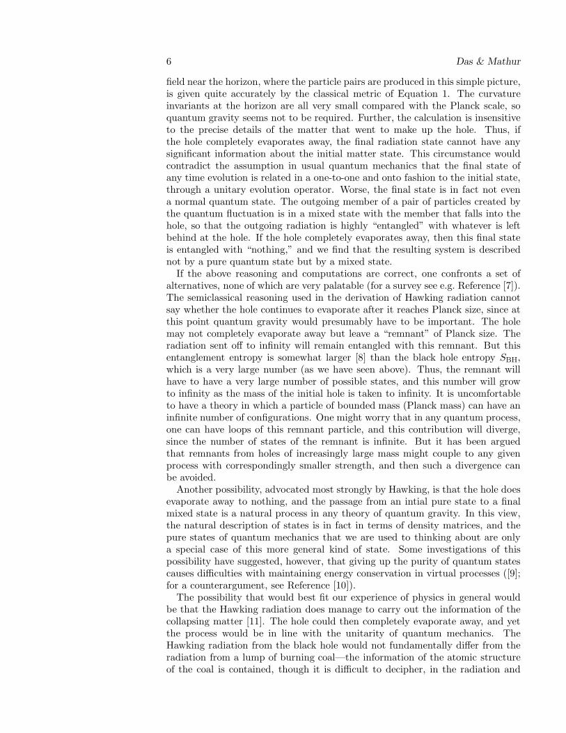
Figure 1: Foliation of the black hole spacetime.
other products that emerge when the coal burns away.
1.4 Difficulties with Obtaining Unitarity
Let us review briefly the difficulties with having the radiation carry out theinformation.
To study the evolution, we choose a foliation of the spacetime by smoothspacelike hypersurfaces. This requires that the spatial slices be smooth and thatthe embedding of neighboring slices changes in a way that is not too sharp.
As we evolve along this foliation, we see the matter fall in toward the center ofthe hole, while we see the radiation collect at spatial infinity. It is important torealize that the information in the collapsing matter cannot also be copied intothe radiation—in other words, there can be no quantum “Xeroxing.” The reasonis as follows. Suppose the evolution process makes two copies of a state
|ψI〉 → |ψI〉 × |ψi〉,where the |ψi〉 are a set of basis states. Then, as long as the linearity of quantummechanics holds, we will find
|ψ1〉 + |ψ2〉 → |ψ1〉 × |ψ1〉 + |ψ2〉 × |ψ2〉and not
|ψ1〉 + |ψ2〉 → (|ψ1〉 + |ψ2〉) × (|ψ1〉 + |ψ2〉).Thus, a general state cannot be “duplicated” by any quantum process.
Figure 1 shows the spacetime in a symbolic way. We use a foliation of spacetimeby the following kind of spacelike hypersurfaces. Away from the black hole, sayfor r > 4M , we let the hypersurface be a t = t0 surface (this description uses theSchwarzschild coordinates of Equation 1). Inside the black hole, an r =constantsurface is spacelike; let us choose r = M so that this part of the surface is neitherclose to the horizon (r = 2M) nor close to the singularity (r = 0). This part ofthe hypersurface will extend from some time t = 0 near the formation of the holeto the value t = t0. Finally, we can connect these two parts of the hypersurfaceby a smooth interpolating region that is spacelike as well. Each of the spacelikehypersurfaces shown in
8 Das & Mathur
Figure 1 is assumed to be of this form. The lower one has t = 0, whereasthe upper one corresponds to a time t0 ∼ M3, where a mass ∼ M has beenevaporated away as radiation. We assume, however, that at t0 the black hole isnowhere near its endpoint of evaporation, either by assuming that a slow dose ofmatter was continually fed into the black hole to maintain its size (the simplestassumption) or by considering a time t0 where say a quarter of the hole hasevaporated (and modifying the metric to reflect the slow decrease of black holemass).
On the lower hypersurface, we have on the left the matter that fell in to makethe hole. There is no radiation yet, so there is nothing else on this hypersurface.Let us call this matter “A.” On the upper hypersurface, we expect the followingsources of stress energy, in a semiclassical analysis of the Hawking process. Onthe left, we will still have the matter that fell in to make the hole, since this partof the surface is common to both hypersurfaces. On the extreme right, we willhave the Hawking radiation that has emerged in the evaporation process; let uscall this “C.” In the middle are the infalling members of the particle-antiparticlepairs. These contribute a negative value to the total mass of the system becauseof the way the hypersurface is oriented with respect to the coordinate t—thismaintains overall energy conservation in the process. Let us call this part of thestate “B.”
The semiclassical process gives a state for the light matter fields, which isentangled between components B and C. On the other hand, components A andB are expected to somehow vanish together (or leave a Planck mass remnant),since their energies cancel each other. At the end of the process, the radiation Cwill have the energy initially present in A. But since C will be entangled with B,the final state will not be a pure state of radiation.
We can now see explicitly the difficulties with obtaining in any theory a unitarydescription of the process of black hole formation and evaporation. In a generalcurved spacetime, we should be able to evolve our hypersurfaces by differentamounts at different points—this is the “many-fingered time” evolution of generalrelativity extended to include the quantum matter on the spacetime. By using anappropriate choice of this evolution, we have captured both the infalling matter Aand the outgoing radiation C on the same spacelike hypersurface. If we want theradiation C to carry the information of the matter A, then we will need “quantumxeroxing,” which, as mentioned above, cannot happen if we accept the principleof superposition of quantum mechanics. It would have been very satisfactory ifwe just could not draw a smooth hypersurface like the upper one in Figure 1, ahypersurface that includes both the infalling matter and the outgoing radiation.For example, we could have hoped that any such surface would need to be non-spacelike at some point, or that it would need a sharp kink in one or more places.But it is easy to see from the construction of surfaces described above that all thehypersurfaces in the evolution are smooth. In fact, the later one is in some sensejust a time translate of the earlier one—the part t = constant in each surfacehas the same intrinsic (and extrinsic) geometry for each hypersurface, and thesegment that connects this part to the r = constant part can be taken to be thesame as well. The only difference between the hypersurfaces is that the later onehas a larger r = constant part. One can further check that the infalling matter hasfinite energy along each hypersurface and that scalar quantities such as dr/ds arebounded and smooth along each surface (s is the proper length along the surface).In the above calculations, spacetime was treated classically, but the conclusions
D-Branes and Black Holes 9
do not change even if we let the evolution of spacelike surfaces be described by theWheeler–de Witt equation, which gives a naive quantization of gravity; quantumfluctuations of the spacetime may appear large in certain coordinates [12], butsuch effects cancel out in the computation of Hawking radiation [13].
It thus appears that in order to have unitarity one needs a nonlocal mechanism(which operates over macroscopic distances ∼ M) that moves the informationfrom A to C. Even though the spacetime appears to have no regions of Planck-scale curvature, we must alter our understanding of how information in one setof low-energy modes (A) moves into another set of low energy modes (C). A keypoint appears to be that, in the semiclassical calculation, the radiation C emergesfrom modes of the quantum field that in the past had a frequency much higherthan Planck frequency. A naive model of the quantum field would have thesemodes at all frequencies, but if the complete theory of matter and gravity hasan inbuilt cutoff at the Planck scale, then the radiation C must have had itsorigins somewhere else—possibly in some nonlocal combination of modes withsub-Planckian energy. If some such possibility is true, we would obtain unitarity,while also obtaining some nontrivial insight into the high-energy structure of thequantum vacuum.
Basic to such an approach would be some way of understanding a black hole asa complicated version of usual matter states, and not as an esoteric new objectthat must be added to a theory of “regular” matter. It would still be true that thefinal state of a system changes character significantly when its density changesfrom that of a star, for instance, to the density at which it collapses to form ablack hole, but the resulting hole should still be described by the same essentialprinciples of quantum mechanics, density of states, statistical mechanics, etc, asany other matter system. As we show below, string theory provides not only aconsistent theory of quantized gravity and matter, but also a way of thinkingabout black holes as quantum states of the matter variables in the theory.
2 STRING THEORY AND SUPERGRAVITY
In a certain regime of parameters, string theory is best thought of as a theoryof interacting elementary strings (for expositions of superstring theory, see Ref-erence [14]). The basic scale is set by the string tension Ts or, equivalently, the“string length”
ls =1√
2πTs. (11)
The quantized harmonics of a string represent particles of various masses andspins, and the masses are typically integral multiples of 1/ls. Thus, at energiesmuch smaller than 1/ls, only the lowest harmonics are relevant. The interactionbetween strings is controlled by a dimensionless string coupling gs, and the abovedescription of the theory in terms of propagating and interacting strings is agood description when gs ≪ 1. Even in weak coupling perturbation theory,quantization imposes rather severe restrictions on possible string theories. Inparticular, all consistent string theories (a) live in ten spacetime dimensions and(b) respect supersymmetry. At the perturbative level, there are five such stringtheories, although recent developments in nonperturbative string theory showthat these five theories are in fact perturbations around different vacua of asingle theory, whose structure is only incompletely understood at this point (for
10 Das & Mathur
a review of string dualities, see Reference [16]).Remarkably, in all these theories there is a set of exactly massless modes that
describe the very-low-energy behavior of the theory. String theories have thepotential to provide a unified theory of all interactions and matter. The mostcommon scenario for this is to choose ls to be of the order of the Planck scale,although there have been recent suggestions that this length scale can be consid-erably longer without contradicting known experimental facts [15]. The masslessmodes then describe the observed low-energy world. Of course, to describe thereal world, most of these modes must acquire a mass, typically much smaller than1/ls.
It turns out that the massless modes of open strings are gauge fields. Thelowest state of an open string carries one quantum of the lowest vibration modeof the string with a polarization i; this gives the gauge boson Ai. The effectivelow-energy field theory is a supersymmetric Yang-Mills theory. The closed stringcan carry traveling waves both clockwise and counterclockwise along its length.In closed string theories, the state with one quantum of the lowest harmonicin each direction is a massless spin-2 particle, which is in fact the graviton: Ifthe transverse directions of the vibrations are i and j, then we get the gravitonhij . The low-energy limits of closed string theories thus contain gravity and aresupersymmetric extensions of general relativity—supergravity. However, unlikethese local theories of gravity, which are not renormalizable, string theory yieldsa finite theory of gravity—essentially due to the extended nature of the string.
2.1 Kaluza-Klein Mechanism
How can such theories in ten dimensions describe our 4-dimensional world? Thepoint is that all of the dimensions need not be infinitely extended—some of themcan be compact. Consider, for example, the simplest situation, in which the 10-dimensional spacetime is flat and the “internal” 6-dimensional space is a 6-torusT 6 with (periodic) coordinates yi, which we choose to be all of the same period:0 < yi < 2πR. If xµ denotes the coordinates of the noncompact 4-dimensionalspacetime, we can write a scalar field φ(x, y) as
φ(x, y) =∑
ni
φni(x) ei
niyi
R , (12)
where ni denotes the six components of integer-valued momenta ~n along theinternal directions. When, for example, φ(x, y) is a massless field satisfying thestandard Klein-Gordon equation (∇2
x + ∇2y)φ = 0, it is clear from Equation 12
that the field φni(x) has (in four dimensions) a mass m~n given by m~n = |n|/R.
Thus, a single field in higher dimensions becomes an infinite number of fields inthe noncompact world. For energies much lower than 1/R, only the ~n = 0 modecan be excited. For other kinds of internal manifolds, the essential physics is thesame. Now, however, we have more complicated wavefunctions on the internalspace. What is rather nontrivial is that when one applies the same mechanismto the spacetime metric, the effective lower-dimensional world contains a metricfield as well as vector gauge fields and scalar matter fields.
D-Branes and Black Holes 11
2.2 11-Dimensional and 10-Dimensional Supergravities
Before the advent of strings as a theory of quantum gravity, there was an attemptto control loop divergences in gravity by making the theory supersymmetric. Thegreater the number of supersymmetries, the better was the control of divergences.But in four dimensions, the maximal number of supersymmetries is eight; moresupersymmetries would force the theory to have fields of spin higher than 2 in thegraviton supermultiplet, which leads to inconsistencies at the level of interactions.Such D = 4, N = 8 supersymmetric theories appear complicated but can be ob-tained in a simple way from a D = 11, N = 1 theory or a D = 10, N = 2 theoryvia the process of dimensional reduction explained above. The gravity multipletin the higher-dimensional theory gives gravity as well as matter fields after di-mensional reduction to lower dimensions, with specific interactions between allthe fields.
The bosonic part of 11-dimensional supergravity consists of the metric gMN
and a 3-form gauge field AMNP with an action
S11 =1
(2π)8l9p[
∫
d11x√−g[R− 1
48FMNPQF
MNPQ]+1
6
∫
d11x A∧F ∧F ]], (13)
where R is the Ricci scalar and FMNPQ is the field strength of AMNP . lp denotesthe 11-dimensional Planck length so that the 11-dimensional Newton’s constantis G11 = l9p. This theory has no free dimensionless parameter. There is only one
scale, lp. Now consider compactifying one of the directions, say x10. The lineinterval may be written as
ds2 = e−φ
6 gµνdxµdxν + e
4φ
3 (dx11 −Aµdxµ)2. (14)
In Equation 14, the indices µ, ν run over the values 0 · · · 9. The various compo-nents of the 11-dimensional metric have been written in terms of a 10-dimensionalmetric, a field Aµ and a field φ. Clearly, from the point of view of the 10-dimensional spacetime, Aµ ∼ Gµ,10 is a vector and φ = 3
4 log G10,10 is a scalar. Ina similar way, the 3-form gauge field splits into a rank-2 gauge field and a rank-3gauge field in ten dimensions, Aµν,10 → Bµν and Aµνλ → Cµνλ. The field Aµ
behaves as a U(1) gauge field. The bosonic massless fields are thus
1. The metric gµν ;
2. A real scalar, the dilaton φ;
3. A vector gauge field Aµ with field strength Fµν ;
4. A rank-2 antisymmetric tensor gauge field Bµν with field strength Fµνλ;
5. A rank-3 antisymmetric tensor gauge field Cµνλ with field strength Fµνλρ.
At low energies, all the fields in the action (Equation 13) are independent ofx10 and the 10-dimensional action is
S = 1(2π)7g2l8s
∫
d10x√g(R− 1
2(∇φ)2 − 1
12e−φFµναF
µνα − 1
4e
3φ
2 FµνFµν
+1
48eφ/2FµναβF
µναβ) + · · · (15)
12 Das & Mathur
where the ellipsis denotes the terms that come from the dimensional reductionof the last term in Equation 13. F denotes the field strength of the appropriategauge field. The action (Equation 15) is precisely the bosonic part of the actionof Type IIA supergravity in ten dimensions. The scalar field φ is called a dilatonand plays a special role in this theory. Its expectation value is related to thestring coupling
gs = exp (〈φ〉). (16)
The overall factor in Equation 15 follows from the fact that the 11-dimensionalmeasure in Equation 13 is related to the 10-dimensional measure by a factor ofthe radius of x10 (which is R), giving
2πR
(2π)8l9p=
1
(2π)7g2l8s, (17)
which defines the string length ls. From the 11-dimensional metric, it is clearthat R = g2/3lp, so that Equation 17 gives lp = g1/3ls.
The 10-dimensional metric gµν used in Equations 14 and 15 is called the “Ein-stein frame” metric because the Einstein-Hilbert term in Equation 15 is canonical.Other metrics used in string theory, most notably the “string frame” metric, dif-fer from this by conformal transformations. In this article we always use theEinstein frame metric.
Although we have given the explicit formulae for dimensional reduction of thebosonic sector of the theory, the fermionic sector can be treated similarly. Thereare two types of gravitinos—fermionic partners of the graviton. One of them haspositive 10-dimensional chirality whereas the other has negative chirality. Theresulting theory is thus nonchiral.
There is another supergravity in ten dimensions, Type IIB supergravity. Thiscannot be obtained from D=11 supergravity by dimensional reduction. Thebosonic fields of this theory are
1. The metric gµν
2. Two real scalars : the dilaton φ and the axion χ
3. Two sets of rank-2 antisymmetric tensor gauge fields: Bµν and B′µν with
field strengths Hµνλ and H ′µνλ
4. A rank-4 gauge field Dµνλρ with a self-dual field strength Fµναβδ .
Both the gravitinos of this theory have the same chirality.Because of the self-duality constraint on the 5-form field strength, it is not pos-
sible to write down the action for Type IIB supergravity, although the equationsof motion make perfect sense. If, however, we put the 5-form field strength tozero, we have a local action given by
S = 1(2π)7g2l8s
∫
d10x[√g(R− 1
2(∇φ)2 − 1
12e−φHµναH
µνα
− 1
12eφ(H ′
µνα − χHµνα)(H ′µνα − χHµνα)].
(18)
D-Branes and Black Holes 13
Of course, these supergravities cannot be consistently quantized, since they arenot renormalizable. However, they are the low-energy limits of string theories,called the Type IIA and Type IIB string.
3 BRANES IN SUPERGRAVITY AND STRING THEORY
Although string theory removes ultraviolet divergences leading to a finite theoryof gravity, such features as the necessity of ten dimensions and the presence ofan infinite tower of modes above the massless graviton made it unpalatable tomany physicists. Furthermore, some find the change from a pointlike particle toa string somewhat arbitrary—if we accept strings, then why not extended objectsof other dimensionalities?
Over the past few years, as nonperturbative string theory has developed, it hasbeen realized that the features of string theory are actually very natural and alsoperhaps essential to any correct theory of quantum gravity. A crucial ingredientin this new insight is the fact that higher-dimensional extended objects—branes—are present in the spectrum of string theory.
3.1 Branes in Supergravity
A closer look at even supergravity theories leads to the observation that theexistence of extended objects is natural within those theories (and in fact turnsout to be essential to completing them to unitary theories at the quantum level).
Consider the case of 11-dimensional supergravity. The supercharge Qα is aspinor, with α = 1 . . . 32. The anticommutator of two supercharge componentsshould lead to a translation, so we write
Qα, Qβ = (ΓAC)αβPA,
where C is the charge conjugation matrix. Because the anticommutator is sym-metric in α, β, we find that there are (32 × 33)/2 = 528 objects on the left-handside of this equation, but only 11 objects (the PA) on the right-hand side. Ifwe write down all the possible terms on the right that are allowed by Lorentzsymmetry, then we find [17]
Qα, Qβ = (ΓAC)αβPA + (ΓAΓBC)αβZAB + (ΓAΓBΓCΓDΓEC)αβZABCDE ,(19)
where the Z are totally antisymmetric. The number of ZAB is 11C2 = 55, whereasthe number of ZABCDE is 11C5 = 478, and now we have a total of 528 objects onthe right, in agreement with the number on the left.
Although, for example, P1 6= 0 implies that the configuration has momentumin direction X1, what is the interpretation of Z12 6= 0? It turns out that thiscan be interpreted as the presence of a “sheetlike” charged object stretched alongthe directions X1,X2. It is then logical to postulate that there exists in thetheory a 2-dimensional fundamental object (the 2-brane). Similarly, the chargeZABCDE corresponds to a 5-brane in the theory. The 2-brane has a 2 + 1 = 3-dimensional world volume and couples naturally to the 3-form gauge field presentin 11-dimensional supergravity, just as a particle with 1-dimensional world linecouples to a 1-form gauge field as
∫
Aµdxµ. The 5-brane is easily seen to be the
14 Das & Mathur
magnetic dual to the 2-brane, and it couples to the 6-form that is dual to the3-form gauge field in 11 dimensions.
Thus, it is natural to include some specific extended objects in the quantizationof 11-dimensional supergravity. But how does this relate to string theory, whichlives in ten dimensions? Let us compactify the 11-dimensional spacetime on asmall circle, thus obtaining 10-dimensional noncompact spacetime. Then, if welet the 2-brane wrap this small circle, we get what looks like a string in tendimensions. This is exactly the Type IIA string that had been quantized by thestring theorists! The size of the small compact circle turns out to be the couplingconstant of the string.
We can also choose not to wrap the 2-brane on the small circle, in which casethere should be a two-dimensional extended object in Type IIA string theory.Such an object is indeed present—it is one of the D-branes shown to exist instring theory by Polchinski [18]. Similarly, we may wrap the 5-brane on the smallcircle, getting a 4-dimensional D-brane in string theory, or leave it unwrapped,getting a solitonic 5-brane, which is also known to exist in the theory.
Thus, one is forced to a unique set of extended objects in the theory, withspecified interactions between them—in fact, there is no freedom to add or removeany object, nor to change any couplings.
3.2 BPS States
A very important property of such branes is that when they are in an unexcitedstate, they preserve some of the supersymmetries of the system, and are thusBogomolny-Prasad-Sommerfield saturated (BPS) states. Let us see in a simplecontext what a BPS state is.
Consider first a theory with a single supercharge Q = Q†:
Q,Q = 2Q2 = 2H, (20)
where H is the Hamiltonian. These relations show that the energy of any statecannot be negative. If
H|ψ〉 = E|ψ〉 (21)
thenE = 〈ψ|H|ψ〉 = 〈ψ|Q2|ψ〉 = 〈Qψ|Qψ〉 ≥ 0, (22)
where the equality holds in the last step if and only if
Q|ψ〉 = 0, (23)
that is, the state is supersymmetric. Nonsupersymmetric states occur in a “mul-tiplet” containing a bosonic state |B〉 and a fermionic state |F 〉 of the sameenergy:
Q|B〉 ≡ |F 〉, Q|F 〉 = Q2|B >= E|B〉. (24)
Supersymmetric states have E = 0 and need not be so paired.Now suppose there are two such supersymmetries:
Q†1 = Q1, Q†
2 = Q2, Q21 = H, Q2
2 = H, Q1, Q2 = Z, (25)
where Z is a “charge”; it will take a c number value on the states that we considerbelow. In a spirit similar to the calculations above, we can now conclude
0 ≤ 〈ψ|(Q1 ±Q2)2|ψ〉 = 2E ± 2Z. (26)
D-Branes and Black Holes 15
This implies thatE ≥ |Z|, (27)
with equality holding if and only if
(Q1 −Q2)|ψ〉 = 0, or (Q1 +Q2)|ψ〉 = 0. (28)
Now we have three kinds of states:
1. States with Q1|ψ〉 = Q2|ψ〉 = 0. These have E = 0 and do not fall intoa multiplet. By Equation 26, they also have Z|ψ〉 = 0, so they carry nocharge.
2. States not in category 1, but satisfying Equation 28. For concreteness,take the case (Q1 − Q2)|ψ〉 = 0. These states fall into a “short multiplet”described by, say, the basis |ψ〉, Q1|ψ〉. Note that
Q2|ψ〉 = Q1|ψ〉, Q2Q1|ψ〉 = Q21|ψ〉 = E|ψ〉, (29)
so that we have no more linearly independent states in the multiplet. Suchstates satisfy
E = |Z| > 0 (30)
and are called BPS states. Note that by Equation 26, the state with Z〉0satisfies (Q1−Q2)|ψ〉 = 0 while the state with Z < 0 satisfies (Q1+Q2)|ψ〉 =0.
3. States that are not annihilated by any linear combination of Q1, Q2. Theseform a “long multiplet” |ψ〉, Q1|ψ〉, Q2|ψ〉, Q2Q1|ψ〉. They must haveE > |Z| > 0.
In the above discussion, we have regarded the BPS states as states of a quantumsystem, but a similar analysis applies to classical solutions. In 10-dimensional su-pergravity, the branes mentioned above appear as classical solutions of the equa-tions of motion, typically with sources. They are massive solitonlike objects andtherefore produce gravitational fields. Apart from that, they produce the p-formgauge fields to which they couple and, in general, a nontrivial dilaton. A brane ina general configuration would break all the supersymmetries of the theory. How-ever, for special configurations—corresponding to “unexcited branes”—there aresolutions which retain some of the supersymmetries. These are BPS saturatedsolutions, and since they have the maximal charge for a given mass, they arestable objects. We use such branes below in constructing black holes.
3.3 The Type IIB Theory
Instead of using the 11-dimensional algebra, we could have used the 10-dimensionalalgebra and arrived at the same conclusions. In a similar fashion, the existence ofBPS branes in Type IIB supergravity follows from the corresponding algebra. Foreach antisymmetric tensor field present in the spectrum, there is a correspondingBPS brane. Thus we have
1. D(−1)-brane, or D-instantons, carrying charge under the axion field χ;
2. NS1-brane, or elementary string, carrying electric charge under Bµν ;
3. D1-brane, carrying electric charge under B′µν ;
16 Das & Mathur
4. 3-brane, carrying charge under Dµνρλ;
5. NS5-brane, carrying magnetic charge under Bµν ;
6. D5-brane, carrying magnetic charge under B′µν ;
7. D7-brane, the dual of the D(−1) brane.
We have denoted some of the branes as D-branes. These play a special role instring theory, as explained below.
3.4 D-Branes in String Theory
Consider the low-energy action of the supergravity theories. We have remarkedabove that the equations of motion for the massless fields admit solitonic solu-tions, where the solitons are not in general pointlike but could be p-dimensionalsheets in space [thus having (p+ 1)-dimensional world volumes in spacetime]. Ineach of these cases, the soliton involves the gravitational field and some other(p + 1)-form field in the supergravity multiplet so that the final solution carriesa charge under this (p + 1)-form gauge field. In fact, in appropriate units, thissoliton is seen to have a mass equal to its charge and is thus an object satisfyingthe BPS bound of supersymmetric theories. This fact implies that the solitonis a stable construct in the theory. The possible values of p are determined en-tirely by the properties of fermions in the Type II theory. It turns out that forType IIA, p must be even (p = 0, 2, 4, 6), whereas for Type IIB p must be odd(p = −1, 1, 3, 5, 7). Recalling the massless spectrum of these theories, we find thatfor each antisymmetric tensor field there is a brane that couples to it. Becausethe brane is not pointlike but is an extended object, we can easily see that therewill be low-energy excitations of this soliton in which its world sheet suffers smalltransverse displacements that vary along the brane (in other words, the branecarries waves corresponding to transverse vibrations). The low-energy action isthus expected to be the tension of the brane times its area. For a single 1-brane,for instance, the action for long-wavelength deformations is
S =T1
2
∫
d2ξα√
det(gαβ), (31)
where ξα, with α = 1, 2, denotes an arbitrary coordinate sytem on the D1-braneworld sheet and gαβ denotes the induced metric on the brane,
gαβ = ∂αXµ∂βX
νηµν . (32)
The Xµ, with µ = 0, · · · , 9, denotes the coordinates of a point on the brane.This action is invariant under arbitrary transformations of the coordinates ξα onthe brane. To make contact with to the picture discussed above, it is best towork in a static gauge by choosing ξ1 = X0 and ξ2 = X9. The induced metric(Equation 32) then becomes
gαβ = ηαβ + ∂αφi∂βφ
jδij , (33)
where φi = Xi with i = 1, · · · 8, are the remaining fields. The determinant inEquation 31 may be then expanded in powers of ∂φi. The lowest-order term isjust the free kinetic energy term for the eight scalar fields φi.
It is now straightforward to extend the above discussion for higher-dimensionalbranes. Now we can have both transverse and longitudinal oscillations of the
D-Branes and Black Holes 17
brane. For a p-brane we have (9 − p) transverse coordinates, labeled by I =1, · · · (9 − p), and hence as many scalar fields on the (p + 1)-dimensional braneworld volume, φi. It turns out that the longitudinal waves are carried by aU(1) gauge field Aα with the index α = 0, 1, · · · p ranging over the world volumedirections. The generalization of Equation 31 [called the Dirac-Born-Infeld (DBI)action] is
S =Tp
2
∫
dp+1ξ√
det(gαβ + Fαβ), (34)
where Fαβ is the gauge field strength. Once again, one can choose a static gaugeand relate the fields directly to a string theory description. The low-energyexpansion of the action then leads to electrodynamics in (p+ 1) dimensions withsome neutral scalars and fermions.
In the above description, we had obtained the branes as classical solutions of thesupergravity fields; this is the analog of describing a point charge by its classicalelectromagnetic potential. Such a description should apply to a collection of alarge number of fundamental branes all placed at the same location. But wewould like to obtain also the microscopic quantum physics of a single brane. Howdo we see such an object in string theory?
The mass per unit volume of a D-brane in string units is 1/g, where g is thestring coupling. So the brane would not be seen as a perturbative object at weakcoupling. But the excitations of the brane will still be low-energy modes, andthese should be seen in weakly coupled string theory. In fact, when we quantizea free string we have two choices: to consider open strings or closed strings. If wehave an open string then we need boundary conditions at the ends of the stringthat do not allow the energy of vibration of the string to flow off the end. Thereare two possibilities: to let the ends move at the speed of light, which correspondsto Neumann (N) boundary conditions, or to fix the end, which corresponds toDirichlet (D) boundary conditions. Of course we can choose different types ofconditions for different directions of motion in spacetime. If the ends of the openstrings are free to move along the directions ξα but are fixed in the other directionsXi, then the ends are constrained to lie along a p-dimensional surface that wemay identify with a p-brane, and such open strings describe the excitations ofthe p-brane [18]. Because these branes were discovered through their excitations,which were in turn a consequence of D-type boundary conditions on the openstrings, the branes are themselves called D-branes. (For a review of properties ofD-branes, see Reference [19].)
An interesting effect occurs when two such branes are brought close to eachother. The open strings that begin and end on the first brane will describeexcitations of the first brane, and those that begin and end on the second branewill describe excitations of the second brane. But, as shown in Figure 2, an openstring can also begin on the first brane and end on the second, or begin on thesecond and end on the first, and this gives two additional possibilities for theexcitation of the system. These four possibilities can in fact be encoded into a2×2 matrix, with the (ij) element of the matrix given by open strings that beginon the ith brane and end on the jth brane. This structure immediately extendsto the case where N branes approach each other.
The low-energy limits of open string theories are generally gauge theories. In-deed the low-energy worldbrane theory of a collection of N parallel Dp-branesturns out to be described by a non-Abelian U(N) gauge theory in (p + 1) di-mensions [21]. The N2 gauge fields are best written as an N × N matrix Aα
ab,
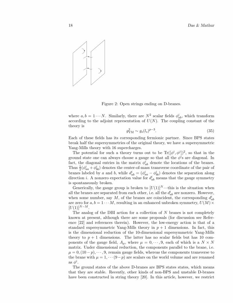
18 Das & Mathur
Figure 2: Open strings ending on D-branes.
where a, b = 1 · · ·N . Similarly, there are N2 scalar fields φiab, which transform
according to the adjoint representation of U(N). The coupling constant of thetheory is
g2YM ∼ gs(ls)
p−3. (35)
Each of these fields has its corresponding fermionic partner. Since BPS statesbreak half the supersymmetries of the original theory, we have a supersymmetricYang-Mills theory with 16 supercharges.
The potential for such a theory turns out to be Tr([φi, φj ])2, so that in theground state one can always choose a gauge so that all the φis are diagonal. Infact, the diagonal entries in the matrix φi
ab denote the locations of the branes.Thus 1
2(φiaa +φi
bb) denotes the center-of-mass transverse coordinate of the pair of
branes labeled by a and b, while diab = (φi
aa − φibb) denotes the separation along
direction i. A nonzero expectation value for diab means that the gauge symmetry
is spontaneously broken.Generically, the gauge group is broken to [U(1)]N—this is the situation when
all the branes are separated from each other, i.e. all the diab are nonzero. However,
when some number, say M , of the branes are coincident, the corresponding diab
are zero for a, b = 1 · · ·M , resulting in an enhanced unbroken symmetry, U(M)×[U(1)]N−M .
The analog of the DBI action for a collection of N branes is not completelyknown at present, although there are some proposals (for discussion see Refer-ence [22] and references therein). However, the low-energy action is that of astandard supersymmetric Yang-Mills theory in p + 1 dimensions. In fact, thisis the dimensional reduction of the 10-dimensional supersymmetric Yang-Millstheory to p + 1 dimensions. The latter has no scalar fields but has 10 com-ponents of the gauge field, Aµ, where µ = 0, · · · , 9, each of which is a N × Nmatrix. Under dimensional reduction, the components parallel to the brane, i.e.µ = 0, (10− p), · · · , 9, remain gauge fields, whereas the components transverse tothe brane with µ = 1, · · · (9−p) are scalars on the world volume and are renamedas φi.
The ground states of the above D-branes are BPS states states, which meansthat they are stable. Recently, other kinds of non-BPS and unstable D-braneshave been constructed in string theory [20]. In this article, however, we restrict
D-Branes and Black Holes 19
ourselves to BPS branes and their excitations.Not all the branes that were listed for Type IIA and Type IIB theory are D-
branes. Consider the Type IIA theory. It arises from a dimensional reductionof 11-dimensional supergravity on a circle. The 11-dimensional theory has 5-branes and 2-branes, and the 2-brane can end on the 5-brane. If we wrap onthe compact circle both the 5-brane and the 2-brane that ends on it, then in theType IIA theory we get a D4-brane and an open string ending on the D4-brane.But if we do not wrap the 5-brane on the circle, and thus get a 5-brane in theType IIA theory, then the open string cannot end on this brane, since there isno corresponding picture of such an endpoint in 11 dimensions. The physics ofthe 5-brane in Type IIA theory is an interesting one, but we will not discuss itfurther. Much more is known about the physics of D-branes in Type IIA and IIBtheories, since they can be studied through perturbative open string theory.
Branes of different kinds can also form bound states, and for specific instancesthese can be threshold bound states. A useful example is a bound state of Q1
D1-branes and Q5 D5-branes. When these branes are not excited, they are in athreshold bound state. The open strings that describe this system are (a) (1, 1)strings with both endpoints on any of the D1-branes; (b) (5, 5) strings with bothendpoints on D5-branes; and (c) (1, 5) and (5, 1) strings with one endpoint onany of the D1-branes and the other endpoint on one of the D5-branes.
3.5 Duality
A remarkable feature of string theory is the large group of symmetries calleddualities (see Reference [16] for review). Consider Type IIA theory compactifiedon a circle of radius R. We can take a graviton propagating along this compactdirection; its energy spectrum would have the form |np|/R. But we can alsowind an elementary string on this circle; the spectrum here would be 2πTs|nw|R,where nw is the winding number of the string and Ts its tension. We note thatif we replace R→ 1/2πTsR, then the energies of the above two sets of states aresimply interchanged. In fact this map, called T-duality, is an exact symmetry ofstring theory; it interchanges winding and momentum modes, and because of aneffect on fermions, it also turns a Type IIA theory into Type IIB and vice versa.
The Type IIB theory also has another symmetry called S-duality, there thestring coupling gs goes to 1/gs. At the same time, the role of the elementary stringis interchanged with the D1-brane. Such a duality, which relates weak coupling tostrong coupling while interchanging fundamental quanta with solitonic objects, isa realization of the duality suggested for field theory by Montonen & Olive [23].The combination of S- and T-dualities generates a larger group, the U-dualitygroup.
There are other dualities, such as those that relate Type IIA theory to heteroticstring theory, and those that relate these theories to the theory of unorientedstrings. In this article, we do not use the idea of dualities directly, but we notethat any black hole that we construct by using branes is related by duality mapsto a large class of similar holes that have the same physics, so the physics obtainedis much more universal than it may at first appear.
20 Das & Mathur
4 BLACK HOLE ENTROPY IN STRING THEORY: THE FUN-DAMENTAL STRING
String theory is a quantum theory of gravity. Thus, black holes should appearin this theory as excited quantum states. An idea of Susskind [24] has provedvery useful in the study of black holes. Because the coupling in the theory isnot a constant but a variable field, we can study a state of the theory at weakcoupling, where we can use our knowledge of string theory. Thus we may computethe “entropy” of the state, which would be the logarithm of the number of stateswith the same mass and charges. Now imagine the coupling to be tuned tostrong values. Then the gravitational coupling also increases, and the object mustbecome a black hole with a large radius. For this black hole we can compute theBekenstein entropy from (Equation 5), and ask if the microscopic computationagrees with the Bekenstein entropy.
For such a calculation to make sense, we must have some assurance that thedensity of states would not shift when we change the coupling. This is whereBPS states come in. We have shown above that the masses of BPS saturatedstates are indeed determined once we know their charges, which are simply theirwinding numbers on cycles of the compact space. Thus, for such states, we maycalculate the degeneracy of states at weak coupling and, since the degeneracycan be predicted also at strong coupling, compare the result with the Bekenstein-Hawking entropy of the corresponding black hole. Such states give, at strongcoupling, black holes that are “extremal”—they have the minimal mass for theircharge if we require that the metric does not have a naked singularity.
The extended objects discussed in the previous section have played an impor-tant role in understanding black holes in string theory.
An example of such an object is a fundamental string in Type IIA or IIB stringtheory. Let some of the directions of the 10-dimensional spacetime be compacti-fied on small circles. Take a fundamental string and wrap it n1 times around oneof these circles, say along the 9 direction, which has a radius R. This will producea rank-2 NS field B09 with a charge n1, which is a “winding charge.” The energyof the state is E = 2πn1TsR, which saturates the BPS bound. From the point ofview of the noncompact directions, this looks like a massive point object carryingelectric charge under the gauge field that results from the dimensional reductionof the rank-2 field. From the microscopic viewpoint, the state of such a string isunique (it does have a 256-fold degeneracy due to supersymmetry, but we can ig-nore this—it is not a number that grows with n1). Thus, the microscopic entropyis zero.
If we increase the coupling, we expect a charged black hole. Furthermore, thisis an extremal black hole, since for a given charge n1 this has the lowest allowedmass given by the energy given above. However, this black hole turns out to havea vanishing horizon area. One way to understand this is to note that the tensionof the string “pinches” the circle where the string was wrapped. Thus, entropy iszero from both the microscopic and the black hole viewpoints, which is consistentbut not really interesting.
To prevent this pinching, we can put some momentum along the string, whichamounts to having traveling waves move along the string. The momentum modeshave an energy that goes as 1/R, so now this circle attains a finite size. If we putwaves that are moving only in one of the directions, we still have a BPS saturatedstate, but with a further half of the supersymmetries broken. The total energy of
D-Branes and Black Holes 21
the state is now given by E = 2πn1Ts + n2/R, where the second term is now thecontribution from the momentum waves. Because of the winding, the effectivelength of the string is Leff = 2πn1R, so that the momentum may be written asP = (2πn1n2)/Leff . Thus, for given values of n1 and n2, a large number of stateshave the same energy. These correspond to the various ways one can get theoscillator level n0 = n1n2. In addition, it is necessary to consider the fact thatthere are eight possible polarizations, and there are fermionic oscillators as well.The resulting degeneracy of states has been known since the early days of stringtheory. For large n1 and n2, the number of states asymptotes to
n(n1, n2) ∼ exp[2√
2√n1n2]. (36)
From the viewpoint of the noncompact directions, we have an object with twoquantized charges n1 and n2. The charge n1 is due to the winding of the string,as mentioned above. The second charge is due to the presence of momentum,which results in a term in the 10-dimensional metric proportional to dx9dx0.Then, by the Kaluza-Klein mechanism explained in the previous section, thisis equivalent to a gauge field A′
0 from the viewpoint of the noncompact world.The corresponding charge is n2 and is an integer since the momentum in thecompact direction is quantized. At strong coupling, this object is described byan extremal black hole solution with two charges. The identification of suchfundamental string states with the corresponding classical solution was proposedby Dabholkar & Harvey [25]. The horizon area is still zero and the curvaturesare large near the horizon.
In an important paper, Sen [27] argued that the semiclassical entropy (for sim-ilar black holes in heterotic string theory) is given not by the area of the eventhorizon but by the area of a “stretched horizon.” This is defined as the locationwhere the curvature and local temperature reach the string scale. It is indeedinconsistent to trust a classical gravity solution beyond this surface, since thecurvatures are much larger than the string scale and stringy corrections to su-pergravity become relevant. There is a great deal of ambiguity in defining thestretched horizon precisely. However, Sen found that the area of the stretchedhorizon in units of the gravitational constant is proportional to
√n1n2, which is
precisely the logarithm of the degeneracy of states given by Equation 36. Thiswas the first indication that degeneracy of states in string theory may accountfor Bekenstein-Hawking entropy. However, in this example, the precise coeffi-cient cannot be determined, since the definition of the stretched horizon is itselfambiguous.
It is clear that what we need is a black hole solution that (a) is BPS and (b)has a nonzero large horizon area. The BPS nature of the solution would ensurethat degeneracies of the corresponding string states are the same at strong andweak couplings, thus allowing an accurate computation of the density of states.A large horizon would ensure that the curvatures are weak and we can thereforetrust semiclassical answers. In that situation, a microscopic count of the statescould be compared with the Bekenstein-Hawking entropy in a regime where bothcalculations are trustworthy.
It turns out that this requires three kinds of charges for a 5-dimensional blackhole and four kinds of charges for a 4-dimensional black hole.
22 Das & Mathur
5 THE FIVE-DIMENSIONAL BLACK HOLE IN TYPE IIBTHEORY
The simplest black holes of this type are in fact 5-dimensional charged blackholes. Extremal limits of such black holes provided the first example where thedegeneracy of the corresponding BPS states exactly accounted for the Bekenstein-Hawking entropy [28]. There are several such black holes in Type IIA and IIBtheory, all related to each other by string dualities. We describe below one suchsolution in Type IIB supergravity.
5.1 The Classical Solution
We start with 10-dimensional spacetime and compactify on a T 5 along (x5, x6,· · · x9). The noncompact directions are then (x0. · · · x4). There is a solution ofType IIB supergravity that represents (a) D5-branes wrapped around the T 5,(b) D1-branes wrapped around x5, and (c) some momentum along x5. Finally,we perform a Kaluza-Klein reduction to the five noncompact dimensions. Theresulting metric is1
ds2 = −[f(r)]−2/3
(
1 − r20r2
)
dt2 + [f(r)]1/3
dr2
1 − r20
r2
+ r2dΩ23
, (37)
where
f(r) ≡(
1 +r20 sin2 α1
r2
)(
1 +r20 sin2 α5
r2
)(
1 +r20 sinh2 σ
r2
)
. (38)
Here r is the radial coordinate in the transverse space, r2 =∑4
i=1(xi)2, and dΩ2
3
is the line element on a unit 3-sphere S3. The solution represents a black holewith an outer horizon at r = r0 and an inner horizon at r = 0. The backgroundalso has nontrivial values of the dilaton φ, and there are three kinds of gaugefields:
1. A gauge field A(1)0 , which comes from the dimensional reduction of the rank-
2 antisymmetric tensor gauge field B′05 in 10 dimensions. This is nonzero,
since we have D1-branes along x5.
2. A gauge field A(2)0 , which comes from the dimensional reduction of an off-
diagonal component of the 10-dimensional metric g05. This is nonzero, sincethere is momentum along x5.
3. A rank-2 gauge field B′ij with i and j lying along the 3-sphere S3. This is
the dimensional reduction of a corresponding B′ij in ten dimensions, since
there are 5-branes along (x5 · · · x9).
The presence of these gauge fields follows in a way exactly analogous to the di-mensional reduction from 11-dimensional supergravity discussed in Equations 13and 14. The corresponding charges Q1, Q5, N are given by
Q1 =V r20 sinh 2α1
32π4gl6sQ5 =
r20 sinh 2α5
2gl2sN =
V R2
32π4l8sg2r20 sinh 2σ, (39)
1We use the notation of Horowitz et al [26].
D-Branes and Black Holes 23
where V is the volume of the T 4 in the x6 · · · x9 directions, R is the radius of thex5 circle, and g is the string coupling.
The charge N comes from momentum in the x5 direction. If we look at thehigher-dimensional metric before dimensional reduction, it is straightforward toidentify the Arnowitt-Deser-Misner (ADM) momentum as
PADM =N
R(40)
The ADM mass of the black hole is given by
M =RV r20
32π4g2l8s[cosh 2α1 + cosh 2α5 + cosh 2σ]. (41)
5.2 Semiclassical Thermodynamics
The semiclassical thermodynamic properties of the black hole may be easily ob-tained from the classical solution using Equations 5 and 10 and the relationship
G5 =4π5g2l8sRV
(42)
between the 5-dimensional Newton’s constant G5 and V,R, g, ls.The expressions are
SBH =AH
G5=
RV r308π3l8sg
2coshα1 coshα5 coshσ
and (43)
TH =1
2πr0 coshα1 coshα5 coshσ. (44)
5.3 Extremal and Near-Extremal Limits
The solution given above represents a general 5-dimensional black hole. Theextremal limit is defined by
r20 → 0 α1, α5, σ → ∞Q1, Q5, N = fixed. (45)
In this limit, the inner and outer horizons coincide. However, it is clear from theabove expressions that ADM mass and entropy remain finite while the Hawkingtemperature vanishes. Of particular interest is the extremal limit of the entropy,
Sextremal = 2π√
Q1Q5N. (46)
This is a function of the charges alone and is independent of other parameters,such as the string coupling, volume of the compact directions, and string length.
In the following, we are interested in a special kind of departure from extremal-ity. This is the regime in which α1, α5 ≫ 1, but r0 and σ are finite. In this case,the total ADM mass may be written in the suggestive form
E =RQ1
gl2s+
16π4RV Q5
l6s+ EL + ER. (47)
24 Das & Mathur
Here we have defined
EL =N
R+V Rr20e
−2σ
64π4g2l8sand ER =
V Rr20e−2σ
64π4g2l8s, (48)
and used the approximations
r21 ≡ r20 sinh2 α1 ∼ r202
sinh 2α1 =16π4gl6sQ1
V,
r25 ≡ r20 sinh2 α5 ∼ r202
sinh 2α5 = gl2sQ5, (49)
and the expressions for the charges (Equation 39). The meaning of the subscriptsL and R will be clear soon. In a similar fashion, the thermodynamic quantitiesmay be written as
S = SL + SR1
TH=
1
2
(
1
TL+
1
TR
)
, (50)
where
SL,R =RV r1r5r0e
±σ
16π3g2l8sTL,R =
r0e±σ
2πr1r5. (51)
The above relations are highly suggestive. The contribution to the ADM massfrom momentum along x5 is Em = EL+ER. In the extremal limit σ → ∞, it thenfollows from Equations 48 and 40 that Em → PADM, which implies that the wavesare moving purely in one direction. This is the origin of the subscripts L andR—we have denoted the direction of momentum in the extremal limit as left, L.For finite σ we have both right- and left-moving waves, but the total momentumis still N/R. The splitting of various quantities into left- and right-moving partsis typical of waves moving at the speed of light in one space dimension. In fact,using Equations 50, 51, and 39, we can easily see that the following relationshold:
Ti =1
π
√
Ei
RQ1Q5=
Si
2π2RQ1Q5, i = L,R. (52)
Finally, we write the expressions that relate the temperature T and the entropyS to the excitation energy over extremality ∆E = Em −N/R:
∆E =π2
2(RQ1Q5) T
2
and S = Sextremal[1 + (R∆E
2N)
1
2 ]. (53)
5.4 Microscopic Model for the Five-Dimensional Black Hole
This solution and the semiclassical properties described above are valid in regionswhere the string frame curvatures are small compared with l−2
s . If we require thisto be true for the entire region outside the horizon, we can study the regime ofvalidity of the classical solution in terms of the various parameters. A shortcalculation using Equations 37, 38, and 39 shows that this is given by
(gQ1), (gQ5), (g2N) ≫ 1. (54)
D-Branes and Black Holes 25
In this regime, the classical solution is a good description of an intersecting setof D-branes in string theory.
However, in string theory, the way to obtain a state with large D-brane chargeQ is to have a collection of Q individual D-branes. Thus, the charges Q1 andQ5 are integers, and we have a system of Q1 D1-branes and Q5 D5-branes. Thethird charge is from a momentum in the x5 direction equal to N/R. Thus, N isquantized in the microscopic picture to ensure a single valued wave function.
In the extremal limit (Equation 45), these branes are in a threshold boundstate, i.e. a bound state with zero binding energy. This is readily apparent fromthe classical solution. The total energy (Equation 47) is then seen to be the sumof the masses of Q1 D1-branes, Q5 D5-branes and the total momentum equal toN/R.
The low-energy theory of a collection of Q Dp-branes is a (p+ 1)-dimensionalsupersymmetric gauge theory with gauge group U(Q). However, now we havea rather complicated bound state of intersecting branes. The low-energy theoryis still a gauge theory but has additional matter fields (called hypermultiplets).Instead of starting from the gauge theory itself, we first present a physical pictureof the low-energy excitations.
5.5 The Long String and Near-Extremal Entropy
The low-energy excitations of the system become particularly transparent in theregime where the radius of the x5 circle, R, is much larger than the size ofthe other four compact directions V 1/4. Then the effective theory is a (1 + 1)-dimensional theory living on x5. The modes are essentially those of the oscil-lations of the D1-branes. These, however, have four rather than eight polariza-tions. This is because it costs energy to pull a D1-brane away from the D5-brane,whereas the motions of the D1-branes along the four directions parallel to theD5-branes, but transverse to the D1-branes themselves (i.e. along x6 · · · x8), aregapless excitations.
Even though a system of static D1- and D5-branes is marginally bound, thereis a nonzero binding energy whenever the D1-branes try to move transverse tothe D5-branes. If we had a single D1-brane and a single D5-brane, the quantizedwaves would be massless particles with four flavors. Since we have a supersym-metric theory, we have four bosons and four fermions. When we have manyD1-branes and D5-branes, it would appear at first sight that there should be4Q1Q5 such flavors: Each of the D1-branes can oscillate along each of the D5-branes, and there are four polarizations for each such oscillation. This is indeedthe case if the D1-branes are all separate.
However, there are other possible configurations. These correspond to severalof the D1-branes joining up to form a longer 1-brane, which is now multiplywound along the compact circle. In fact, if we only have some number nw of D1-branes without anything else wrapping a compact circle, they would also preferto join into a long string, which is of length 2πnwR. This was discovered in ananalysis of the nonextremal excitations of such D1-branes [29]. S-duality relatesD1-branes to fundamental wrapped strings. If one requires that the nonextremalexcitations of the D1 brane are in one-to-one correspondence with the knownnear-extremal excitations of the fundamental string and therefore yield the samedegeneracy of states, one concludes that the energies of the individual quanta ofoscillations of the D1 string must have fractional momenta pi = ni/(nwR), which
26 Das & Mathur
simply means that the effective length of the string is 2πnwR.For the situation we are discussing, i.e. D1-branes bound to D5-branes, the
entropically favorable configuration turns out to be that of a single long stringformed by the D1-branes joining up to wind around the x5 direction Q1Q5, i.e. aneffective length of Leff = 2πRQ1Q5 [30]. We thus arrive at a gas of four flavors ofbosons and four flavors of fermions living on a circle of size Leff . Since the stringis relativistic, these particles are massless. The problem is to count the number ofstates with a given energy E and given total momentum P = N/R and see if theresults agree with semiclassical thermodynamics of black holes. This approach tothe derivation of black hole thermodynamics comes from Callan & Maldacena [31]and Horowitz & Strominger [32], with the important modification of the multiplywound D-string proposed by Maldacena & Susskind [30]. Our treatment belowfollows Reference [33].
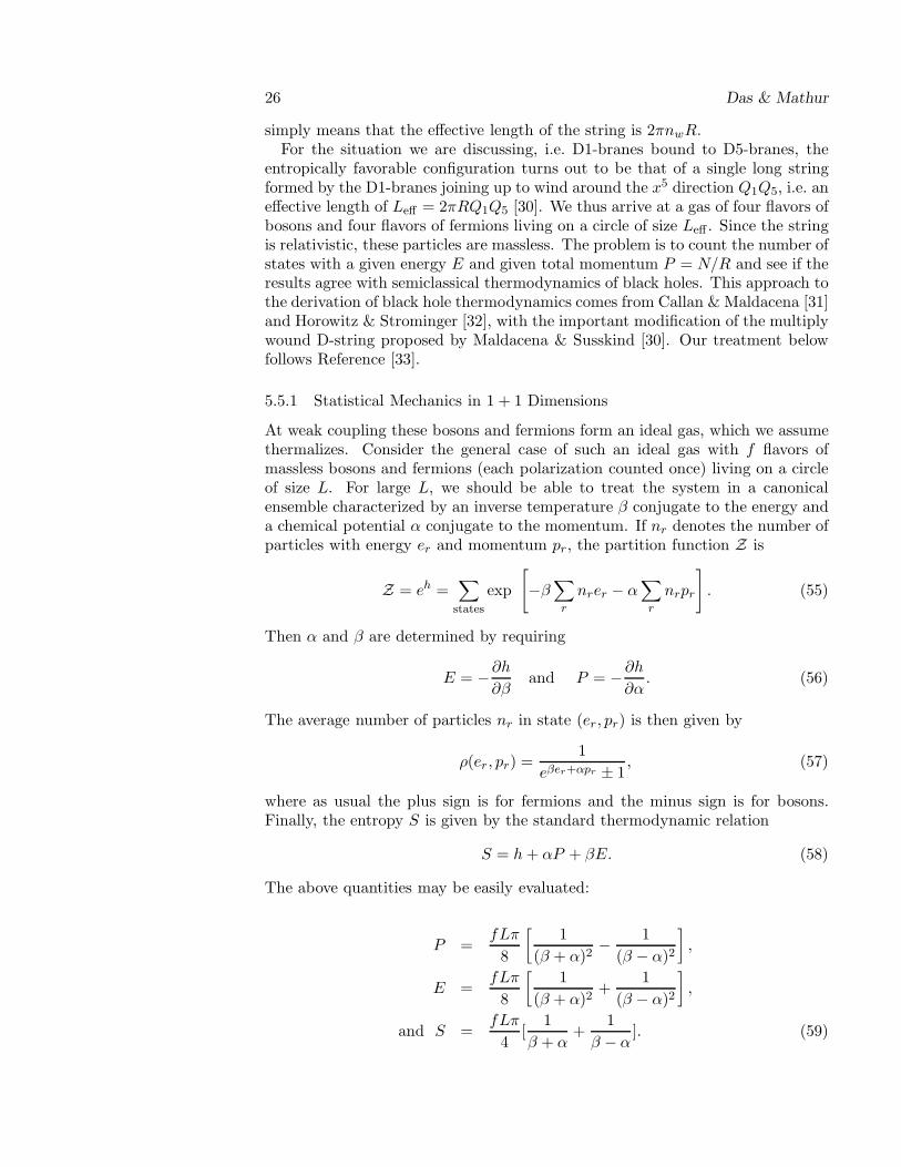
5.5.1 Statistical Mechanics in 1 + 1 Dimensions
At weak coupling these bosons and fermions form an ideal gas, which we assumethermalizes. Consider the general case of such an ideal gas with f flavors ofmassless bosons and fermions (each polarization counted once) living on a circleof size L. For large L, we should be able to treat the system in a canonicalensemble characterized by an inverse temperature β conjugate to the energy anda chemical potential α conjugate to the momentum. If nr denotes the number ofparticles with energy er and momentum pr, the partition function Z is
Z = eh =∑
states
exp
[
−β∑
r
nrer − α∑
r
nrpr
]
. (55)
Then α and β are determined by requiring
E = −∂h∂β
and P = −∂h∂α
. (56)
The average number of particles nr in state (er, pr) is then given by
ρ(er, pr) =1
eβer+αpr ± 1, (57)
where as usual the plus sign is for fermions and the minus sign is for bosons.Finally, the entropy S is given by the standard thermodynamic relation
S = h+ αP + βE. (58)
The above quantities may be easily evaluated:
P =fLπ
8
[
1
(β + α)2− 1
(β − α)2
]
,
E =fLπ
8
[
1
(β + α)2+
1
(β − α)2
]
,
and S =fLπ
4[
1
β + α+
1
β − α]. (59)
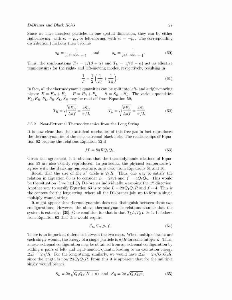
D-Branes and Black Holes 27
Since we have massless particles in one spatial dimension, they can be eitherright-moving, with er = pr, or left-moving, with er = −pr. The correspondingdistribution functions then become
ρR =1
e(β+α)er ± 1and ρL =
1
e(β−α)er ± 1. (60)
Thus, the combinations TR = 1/(β + α) and TL = 1/(β − α) act as effectivetemperatures for the right- and left-moving modes, respectively, resulting in
1
T=
1
2
(
1
TL+
1
TR
)
. (61)
In fact, all the thermodynamic quantities can be split into left- and a right-movingpieces: E = ER + EL P = PR + PL S = SR + SL. The various quantitiesEL, ER, PL, PR, SL, SR may be read off from Equation 59,
TR =
√
8ER
Lπf=
4SR
πfLTL =
√
8EL
Lπf=
4SL
πfL. (62)
5.5.2 Near-Extremal Thermodynamics from the Long String
It is now clear that the statistical mechanics of this free gas in fact reproducesthe thermodynamics of the near-extremal black hole. The relationships of Equa-tion 62 become the relations Equation 52 if
fL = 8πRQ1Q5. (63)
Given this agreement, it is obvious that the thermodynamic relations of Equa-tion 53 are also exactly reproduced. In particular, the physical temperature Tagrees with the Hawking temperature, as is clear from Equations 61 and 50.
Recall that the size of the x5 circle is 2πR. Thus, one way to satisfy therelation in Equation 63 is to consider L = 2πR and f = 4Q1Q5. This wouldbe the situation if we had Q1 D1-branes individually wrapping the x5 direction.Another way to satsify Equation 63 is to take L = 2πQ1Q5R and f = 4. This isthe content for the long string, where all the D1-branes join up to form a singlemultiply wound string.
It might appear that thermodynamics does not distinguish between these twoconfigurations. However, the above thermodynamic relations assume that thesystem is extensive [30]. One condition for that is that TLL, TRL≫ 1. It followsfrom Equation 62 that this would require
SL, SR ≫ f. (64)
There is an important difference between the two cases. When multiple branes areeach singly wound, the energy of a single particle is n/R for some integer n. Thus,a near-extremal configuration may be obtained from an extremal configuration byadding n pairs of left- and right-handed quanta, leading to an excitation energy∆E = 2n/R. For the long string, similarly, we would have ∆E = 2n/Q1Q5R,since the length is now 2πQ1Q5R. From this it is apparent that for the multiplesingly wound branes,
SL = 2π√
Q1Q5(N + n) and SR = 2π√
Q1Q5n, (65)
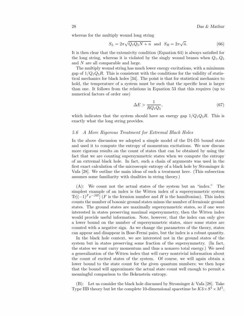
28 Das & Mathur
whereas for the multiply wound long string
SL = 2π√
Q1Q5N + n and SR = 2π√n. (66)
It is then clear that the extensivity condition (Equation 64) is always satisfied forthe long string, whereas it is violated by the singly wound branes when Q1, Q5
and N are all comparable and large.The multiply wound string has much lower energy excitations, with a minimum
gap of 1/Q1Q5R. This is consistent with the conditions for the validity of statis-tical mechanics for black holes [34]. The point is that for statistical mechanics tohold, the temperature of a system must be such that the specific heat is largerthan one. It follows from the relations in Equation 53 that this requires (up tonumerical factors of order one)
∆E >1
RQ1Q5, (67)
which indicates that the system should have an energy gap 1/Q1Q5R. This isexactly what the long string provides.
5.6 A More Rigorous Treatment for Extremal Black Holes
In the above discussion we adopted a simple model of the D1-D5 bound stateand used it to compute the entropy of momentum excitations. We now discussmore rigorous results on the count of states that can be obtained by using thefact that we are counting supersymmetric states when we compute the entropyof an extremal black hole. In fact, such a chain of arguments was used in thefirst exact calculation of the microscopic entropy of a black hole by Strominger &Vafa [28]. We outline the main ideas of such a treatment here. (This subsectionassumes some familiarity with dualities in string theory.)
(A): We count not the actual states of the system but an “index.” Thesimplest example of an index is the Witten index of a supersymmetric systemTr[(−1)F e−βH ] (F is the fermion number and H is the hamiltonian). This indexcounts the number of bosonic ground states minus the number of fermionic groundstates. The ground states are maximally supersymmetric states, so if one wereinterested in states preserving maximal supersymmetry, then the Witten indexwould provide useful information. Note, however, that the index can only givea lower bound on the number of supersymmetric states, since some states arecounted with a negative sign. As we change the parameters of the theory, statescan appear and disappear in Bose-Fermi pairs, but the index is a robust quantity.
In the black hole context, we are interested not in the ground states of thesystem but in states preserving some fraction of the supersymmetry. (In fact,the states we want carry momentum and thus a nonzero total energy.) We needa generalization of the Witten index that will carry nontrivial information aboutthe count of excited states of the system. Of course, we will again obtain alower bound to the state count for the given quantum numbers; we then hopethat the bound will approximate the actual state count well enough to permit ameaningful comparison to the Bekenstein entropy.
(B): Let us consider the black hole discussed by Strominger & Vafa [28]. TakeType IIB theory but let the complete 10-dimensional spacetime be K3×S1×M5,
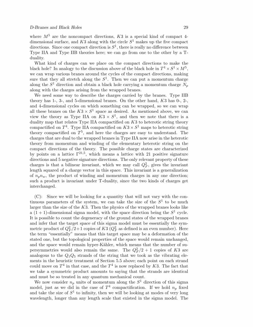
D-Branes and Black Holes 29
where M5 are the noncompact directions, K3 is a special kind of compact 4-dimensional surface, and K3 along with the circle S1 makes up the five compactdirections. Since one compact direction is S1, there is really no difference betweenType IIA and Type IIB theories here; we can go from one to the other by a T-duality.
What kind of charges can we place on the compact directions to make theblack hole? In analogy to the discussion above of the black hole in T 4×S1×M5,we can wrap various branes around the cycles of the compact directions, makingsure that they all stretch along the S1. Then we can put a momentum chargealong the S1 direction and obtain a black hole carrying a momentum charge Np
along with the charges arising from the wrapped branes.We need some way to describe the charges carried by the branes. Type IIB
theory has 1-, 3-, and 5-dimensional branes. On the other hand, K3 has 0-, 2-,and 4-dimensional cycles on which something can be wrapped, so we can wrapall these branes on the K3 × S1 space as desired. As mentioned above, we canview the theory as Type IIA on K3 × S1, and then we note that there is aduality map that relates Type IIA compactified on K3 to heterotic string theorycompactified on T 4. Type IIA compactified on K3×S1 maps to heterotic stringtheory compactified on T 5, and here the charges are easy to understand. Thecharges that are dual to the wrapped branes in Type IIA now arise in the heterotictheory from momentum and winding of the elementary heterotic string on thecompact directions of the theory. The possible charge states are characterizedby points on a lattice Γ21,5, which means a lattice with 21 positive signaturedirections and 5 negative signature directions. The only relevant property of thesecharges is that a bilinear invariant, which we may call Q2
F , gives the invariantlength squared of a charge vector in this space. This invariant is a generalizationof npnw, the product of winding and momentum charges in any one direction;such a product is invariant under T-duality, since the two kinds of charges getinterchanged.
(C): Since we will be looking for a quantity that will not vary with the con-tinuous parameters of the system, we can take the size of the S1 to be muchlarger than the size of the K3. Then the physics of the wrapped branes looks likea (1 + 1)-dimensional sigma model, with the space direction being the S1 cycle.It is possible to count the degeneracy of the ground states of the wrapped branesand infer that the target space of this sigma model must be essentially the sym-metric product of Q2
F/2+1 copies of K3 (Q2F as defined is an even number). Here
the term “essentially” means that this target space may be a deformation of thestated one, but the topological properties of the space would remain unchanged,and the space would remain hyper-Kahler, which means that the number of su-persymmetries would also remain the same. The Q2
F/2 + 1 copies of K3 areanalogous to the Q1Q5 strands of the string that we took as the vibrating ele-ments in the heuristic treatment of Section 5.5 above; each point on each strandcould move on T 4 in that case, and the T 4 is now replaced by K3. The fact thatwe take a symmetric product amounts to saying that the strands are identicaland must be so treated in any quantum mechanical count.
We now consider np units of momentum along the S1 direction of this sigmamodel, just as we did in the case of T 4 compactification. If we hold np fixedand take the size of S1 to infinity, then we will be looking at modes of very longwavelength, longer than any length scale that existed in the sigma model. The
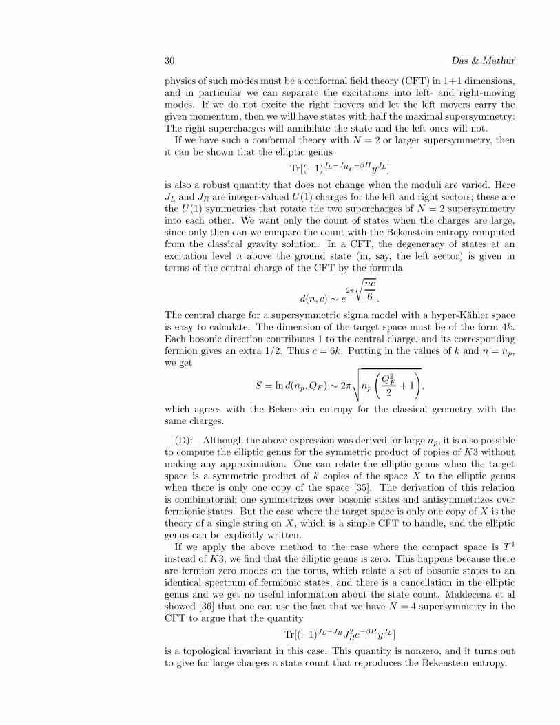
30 Das & Mathur
physics of such modes must be a conformal field theory (CFT) in 1+1 dimensions,and in particular we can separate the excitations into left- and right-movingmodes. If we do not excite the right movers and let the left movers carry thegiven momentum, then we will have states with half the maximal supersymmetry:The right supercharges will annihilate the state and the left ones will not.
If we have such a conformal theory with N = 2 or larger supersymmetry, thenit can be shown that the elliptic genus
Tr[(−1)JL−JRe−βHyJL]
is also a robust quantity that does not change when the moduli are varied. HereJL and JR are integer-valued U(1) charges for the left and right sectors; these arethe U(1) symmetries that rotate the two supercharges of N = 2 supersymmetryinto each other. We want only the count of states when the charges are large,since only then can we compare the count with the Bekenstein entropy computedfrom the classical gravity solution. In a CFT, the degeneracy of states at anexcitation level n above the ground state (in, say, the left sector) is given interms of the central charge of the CFT by the formula
d(n, c) ∼ e2π
√
nc
6 .
The central charge for a supersymmetric sigma model with a hyper-Kahler spaceis easy to calculate. The dimension of the target space must be of the form 4k.Each bosonic direction contributes 1 to the central charge, and its correspondingfermion gives an extra 1/2. Thus c = 6k. Putting in the values of k and n = np,we get
S = ln d(np, QF ) ∼ 2π
√
√
√
√np
(
Q2F
2+ 1
)
,
which agrees with the Bekenstein entropy for the classical geometry with thesame charges.
(D): Although the above expression was derived for large np, it is also possibleto compute the elliptic genus for the symmetric product of copies of K3 withoutmaking any approximation. One can relate the elliptic genus when the targetspace is a symmetric product of k copies of the space X to the elliptic genuswhen there is only one copy of the space [35]. The derivation of this relationis combinatorial; one symmetrizes over bosonic states and antisymmetrizes overfermionic states. But the case where the target space is only one copy of X is thetheory of a single string on X, which is a simple CFT to handle, and the ellipticgenus can be explicitly written.
If we apply the above method to the case where the compact space is T 4
instead of K3, we find that the elliptic genus is zero. This happens because thereare fermion zero modes on the torus, which relate a set of bosonic states to anidentical spectrum of fermionic states, and there is a cancellation in the ellipticgenus and we get no useful information about the state count. Maldecena et alshowed [36] that one can use the fact that we have N = 4 supersymmetry in theCFT to argue that the quantity
Tr[(−1)JL−JRJ2Re
−βHyJL ]
is a topological invariant in this case. This quantity is nonzero, and it turns outto give for large charges a state count that reproduces the Bekenstein entropy.
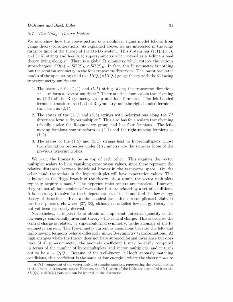
D-Branes and Black Holes 31
5.7 The Gauge Theory Picture
We now show how the above picture of a nonlinear sigma model follows fromgauge theory considerations. As explained above, we are interested in the long-distance limit of the theory of the D1-D5 system. This system has (1, 1), (5, 5),and (1, 5) strings and has (4, 4) supersymmetry when viewed as a 1-dimensionaltheory living along x5. There is a global R symmetry which rotates the varioussupercharges: SO(4) = SU(2)L × SU(2)R. In fact, this R symmetry is nothingbut the rotation symmetry in the four transverse directions. The lowest oscillatormodes of the open strings lead to a U(Q1)×U(Q5) gauge theory with the followingsupersymmetry multiplets:
1. The states of the (1, 1) and (5, 5) strings along the transverse directionsx1 · · · x4 form a “vector multiplet.” There are thus four scalars transformingas (2, 2) of the R symmetry group and four fermions. The left-handedfermions transform as (1, 2) of R symmetry, and the right-handed fermionstransform as (2, 1).
2. The states of the (1, 1) and (5, 5) strings with polarizations along the T 4
directions form a “hypermultiplet.” This also has four scalars transformingtrivially under the R-symmetry group and has four fermions. The left-moving fermions now transform as (2, 1) and the right-moving fermions as(1, 2).
3. The states of the (1, 5) and (5, 1) strings lead to hypermultiplets whosetransformation properties under R symmetry are the same as those of theprevious hypermultiplets.
We want the branes to be on top of each other. This requires the vectormultiplet scalars to have vanishing expectation values, since these represent therelative distances between individual branes in the transverse space. On theother hand, the scalars in the hypermultiplet will have expectation values. Thisis known as the Higgs branch of the theory. As a result, the vector multipletstypically acquire a mass.2 The hypermultiplet scalars are massless. However,they are not all independent of each other but are related by a set of conditions.It is necessary to solve for the independent set of fields and find the low-energytheory of these fields. Even at the classical level, this is a complicated affair. Ithas been pursued elsewhere [37, 38], although a detailed low-energy theory hasnot yet been rigorously derived.
Nevertheless, it is possible to obtain an important universal quantity of thelow-energy conformally invariant theory—the central charge. This is because thecentral charge is related, by superconformal symmetry, to the anomaly of the R-symmetry current. The R-symmetry current is anomalous because the left- andright-moving fermions behave differently under R-symmetry transformations. Athigh energies where the theory does not have superconformal invariance but doeshave (4, 4) supersymmetry, the anomaly coefficient k may be easily computedin terms of the number of hypermultiplets and vector multiplets, and it turnsout to be k = Q1Q5. Because of the well-known ’t Hooft anomaly matchingconditions, this coefficient is the same at low energies, where the theory flows to
2A U(1) component of the vector multiplet remains massless, representing the overall motionof the branes in transverse space. However, the U(1) parts of the fields are decoupled from theSU(Q1)× SU(Q5) part and can be ignored in this discussion.
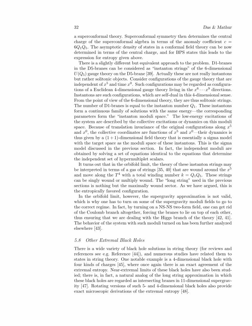
32 Das & Mathur
a superconformal theory. Superconformal symmetry then determines the centralcharge of the superconformal algebra in terms of the anomaly coefficient c =6Q1Q5. The asymptotic density of states in a conformal field theory can be nowdetermined in terms of the central charge, and for BPS states this leads to theexpression for entropy given above.
There is a slightly different but equivalent approach to the problem. D1-branesin the D5-branes can be considered as “instanton strings” of the 6-dimensionalU(Q5) gauge theory on the D5-brane [39]. Actually these are not really instantonsbut rather solitonic objects. Consider configurations of the gauge theory that areindependent of x5 and time x0. Such configurations may be regarded as configura-tions of a Euclidean 4-dimensional gauge theory living in the x6 · · · x9 directions.Instantons are such configurations, which are self-dual in this 4-dimensional sense.From the point of view of the 6-dimensional theory, they are thus solitonic strings.The number of D1-branes is equal to the instanton number Q1. These instantonsform a continuous family of solutions with the same energy—the correspondingparameters form the “instanton moduli space.” The low-energy excitations ofthe system are described by the collective excitations or dynamics on this modulispace. Because of translation invariance of the original configurations along x5
and x0, the collective coordinates are functions of x5 and x0—their dynamics isthus given by a (1 + 1)-dimensional field theory that is essentially a sigma modelwith the target space as the moduli space of these instantons. This is the sigmamodel discussed in the previous section. In fact, the independent moduli areobtained by solving a set of equations identical to the equations that determinethe independent set of hypermultiplet scalars.
It turns out that in the orbifold limit, the theory of these instanton strings maybe interpreted in terms of a gas of strings [35, 40] that are wound around the x5
and move along the T 4 with a total winding number k = Q1Q5. These stringscan be singly wound or multiply wound. The “long string” used in the previoussections is nothing but the maximally wound sector. As we have argued, this isthe entropically favored configuration.
In the orbifold limit, however, the supergravity approximation is not valid,which is why one has to turn on some of the supergravity moduli fields to go tothe correct regime. In fact, by turning on a NS-NS two-form field, one can get ridof the Coulomb branch altogether, forcing the branes to lie on top of each other,thus ensuring that we are dealing with the Higgs branch of the theory [42, 41].The behavior of the system with such moduli turned on has been further analyzedelsewhere [43].
5.8 Other Extremal Black Holes
There is a wide variety of black hole solutions in string theory (for reviews andreferences see e.g. Reference [44]), and numerous studies have related them tostates in string theory. One notable example is a 4-dimensional black hole withfour kinds of charges [45], where once again there is an exact agreement of theextremal entropy. Near-extremal limits of these black holes have also been stud-ied; there is, in fact, a natural analog of the long string approximation in whichthese black holes are regarded as intersecting branes in 11-dimensional supergrav-ity [47]. Rotating versions of such 5- and 4-dimensional black holes also provideexact microscopic derivations of the extremal entropy [48].
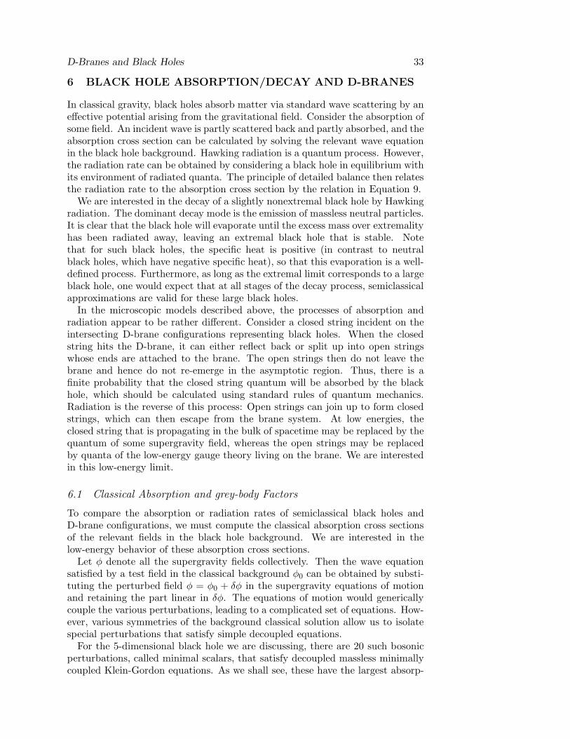
D-Branes and Black Holes 33
6 BLACK HOLE ABSORPTION/DECAY AND D-BRANES
In classical gravity, black holes absorb matter via standard wave scattering by aneffective potential arising from the gravitational field. Consider the absorption ofsome field. An incident wave is partly scattered back and partly absorbed, and theabsorption cross section can be calculated by solving the relevant wave equationin the black hole background. Hawking radiation is a quantum process. However,the radiation rate can be obtained by considering a black hole in equilibrium withits environment of radiated quanta. The principle of detailed balance then relatesthe radiation rate to the absorption cross section by the relation in Equation 9.
We are interested in the decay of a slightly nonextremal black hole by Hawkingradiation. The dominant decay mode is the emission of massless neutral particles.It is clear that the black hole will evaporate until the excess mass over extremalityhas been radiated away, leaving an extremal black hole that is stable. Notethat for such black holes, the specific heat is positive (in contrast to neutralblack holes, which have negative specific heat), so that this evaporation is a well-defined process. Furthermore, as long as the extremal limit corresponds to a largeblack hole, one would expect that at all stages of the decay process, semiclassicalapproximations are valid for these large black holes.
In the microscopic models described above, the processes of absorption andradiation appear to be rather different. Consider a closed string incident on theintersecting D-brane configurations representing black holes. When the closedstring hits the D-brane, it can either reflect back or split up into open stringswhose ends are attached to the brane. The open strings then do not leave thebrane and hence do not re-emerge in the asymptotic region. Thus, there is afinite probability that the closed string quantum will be absorbed by the blackhole, which should be calculated using standard rules of quantum mechanics.Radiation is the reverse of this process: Open strings can join up to form closedstrings, which can then escape from the brane system. At low energies, theclosed string that is propagating in the bulk of spacetime may be replaced by thequantum of some supergravity field, whereas the open strings may be replacedby quanta of the low-energy gauge theory living on the brane. We are interestedin this low-energy limit.
6.1 Classical Absorption and grey-body Factors
To compare the absorption or radiation rates of semiclassical black holes andD-brane configurations, we must compute the classical absorption cross sectionsof the relevant fields in the black hole background. We are interested in thelow-energy behavior of these absorption cross sections.
Let φ denote all the supergravity fields collectively. Then the wave equationsatisfied by a test field in the classical background φ0 can be obtained by substi-tuting the perturbed field φ = φ0 + δφ in the supergravity equations of motionand retaining the part linear in δφ. The equations of motion would genericallycouple the various perturbations, leading to a complicated set of equations. How-ever, various symmetries of the background classical solution allow us to isolatespecial perturbations that satisfy simple decoupled equations.
For the 5-dimensional black hole we are discussing, there are 20 such bosonicperturbations, called minimal scalars, that satisfy decoupled massless minimallycoupled Klein-Gordon equations. As we shall see, these have the largest absorp-
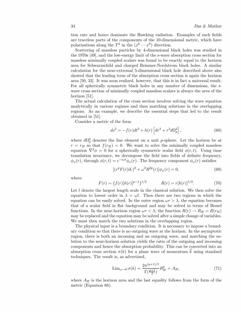
34 Das & Mathur
tion rate and hence dominate the Hawking radiation. Examples of such fieldsare traceless parts of the components of the 10-dimensional metric, which havepolarizations along the T 4 in the (x6 · · · x8) direction.
Scattering of massless particles by 4-dimensional black holes was studied inthe 1970s [49], and the low-energy limit of the s-wave absorption cross section formassless minimally coupled scalars was found to be exactly equal to the horizonarea for Schwarzschild and charged Reissner-Nordstrom black holes. A similarcalculation for the near-extremal 5-dimensional black hole described above alsoshowed that the leading term of the absorption cross section is again the horizonarea [50, 33]. It was soon realized, however, that this is in fact a universal result:For all spherically symmetric black holes in any number of dimensions, the s-wave cross section of minimally coupled massless scalars is always the area of thehorizon [51].
The actual calculation of the cross section involves solving the wave equationanalytically in various regimes and then matching solutions in the overlappingregions. As an example, we describe the essential steps that led to the resultobtained in [51].
Consider a metric of the form
ds2 = −f(r)dt2 + h(r)[
dr2 + r2dΩ2p
]
, (68)
where dΩ2p denotes the line element on a unit p-sphere. Let the horizon be at
r = rH so that f(rH) = 0. We want to solve the minimally coupled masslessequation ∇2φ = 0 for a spherically symmetric scalar field φ(r, t). Using timetranslation invariance, we decompose the field into fields of definite frequency,φω(r), through φ(r, t) = e−iωtφω(r). The frequency component φω(r) satisfies
[(rpF (r)∂r)2 + ω2R2p(r)]φω(r) = 0, (69)
whereF (r) = f(r)[h(r)]p−11/2 R(r) = r[h(r)]1/2. (70)
Let l denote the largest length scale in the classical solution. We then solve theequation to lowest order in λ = ωl. Then there are two regions in which theequation can be easily solved. In the outer region ωr > λ, the equation becomesthat of a scalar field in flat background and may be solved in terms of Besselfunctions. In the near-horizon region ωr < λ, the function R(r) → RH = R(rH)may be replaced and the equation may be solved after a simple change of variables.We must then match the two solutions in the overlapping region.
The physical input is a boundary condition. It is necessary to impose a bound-ary condition so that there is no outgoing wave at the horizon. In the asymptoticregion, there is both an incoming and an outgoing wave, and matching the so-lution to the near-horizon solution yields the ratio of the outgoing and incomingcomponents and hence the absorption probability. This can be converted into anabsorption cross section σ(k) for a plane wave of momentum ~k using standardtechniques. The result is, as advertised,
Limω→0 σ(k) =2π(p+1)/2
Γ(p+12 )
RpH = AH , (71)
where AH is the horizon area and the last equality follows from the form of themetric (Equation 68).
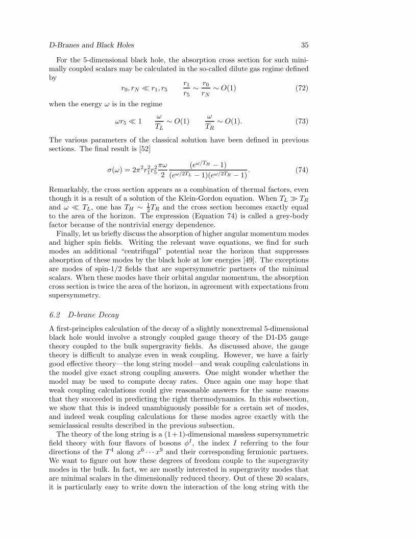
D-Branes and Black Holes 35
For the 5-dimensional black hole, the absorption cross section for such mini-mally coupled scalars may be calculated in the so-called dilute gas regime definedby
r0, rN ≪ r1, r5r1r5
∼ r0rN
∼ O(1) (72)
when the energy ω is in the regime
ωr5 ≪ 1ω
TL∼ O(1)
ω
TR∼ O(1). (73)
The various parameters of the classical solution have been defined in previoussections. The final result is [52]
σ(ω) = 2π2r21r25πω
2
(eω/TH − 1)
(eω/2TL − 1)(eω/2TR − 1). (74)
Remarkably, the cross section appears as a combination of thermal factors, eventhough it is a result of a solution of the Klein-Gordon equation. When TL ≫ TR
and ω ≪ TL, one has TH ∼ 12TR and the cross section becomes exactly equal
to the area of the horizon. The expression (Equation 74) is called a grey-bodyfactor because of the nontrivial energy dependence.
Finally, let us briefly discuss the absorption of higher angular momentum modesand higher spin fields. Writing the relevant wave equations, we find for suchmodes an additional “centrifugal” potential near the horizon that suppressesabsorption of these modes by the black hole at low energies [49]. The exceptionsare modes of spin-1/2 fields that are supersymmetric partners of the minimalscalars. When these modes have their orbital angular momentum, the absorptioncross section is twice the area of the horizon, in agreement with expectations fromsupersymmetry.
6.2 D-brane Decay
A first-principles calculation of the decay of a slightly nonextremal 5-dimensionalblack hole would involve a strongly coupled gauge theory of the D1-D5 gaugetheory coupled to the bulk supergravity fields. As discussed above, the gaugetheory is difficult to analyze even in weak coupling. However, we have a fairlygood effective theory—the long string model—and weak coupling calculations inthe model give exact strong coupling answers. One might wonder whether themodel may be used to compute decay rates. Once again one may hope thatweak coupling calculations could give reasonable answers for the same reasonsthat they succeeded in predicting the right thermodynamics. In this subsection,we show that this is indeed unambiguously possible for a certain set of modes,and indeed weak coupling calculations for these modes agree exactly with thesemiclassical results described in the previous subsection.
The theory of the long string is a (1+1)-dimensional massless supersymmetricfield theory with four flavors of bosons φI , the index I referring to the fourdirections of the T 4 along x6 · · · x9 and their corresponding fermionic partners.We want to figure out how these degrees of freedom couple to the supergravitymodes in the bulk. In fact, we are mostly interested in supergravity modes thatare minimal scalars in the dimensionally reduced theory. Out of these 20 scalars,it is particularly easy to write down the interaction of the long string with the
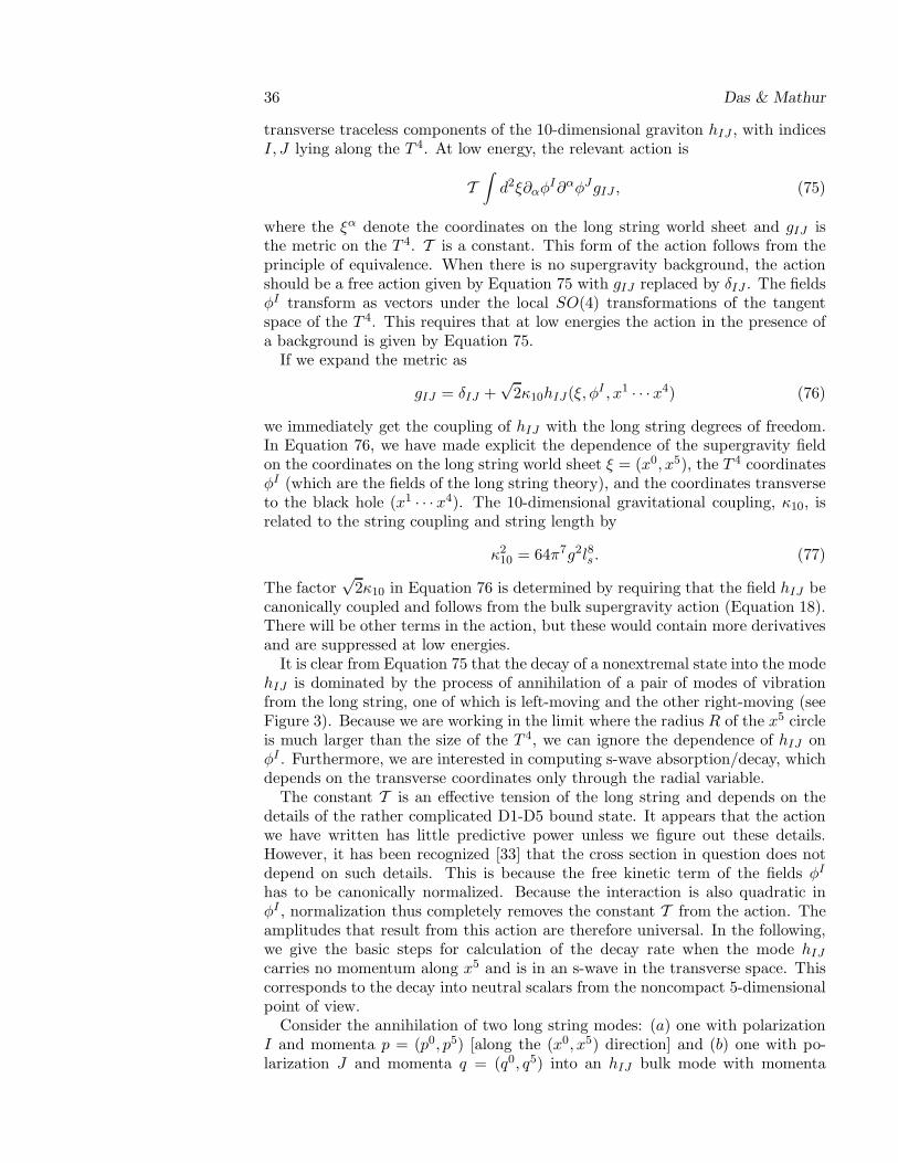
36 Das & Mathur
transverse traceless components of the 10-dimensional graviton hIJ , with indicesI, J lying along the T 4. At low energy, the relevant action is
T∫
d2ξ∂αφI∂αφJgIJ , (75)
where the ξα denote the coordinates on the long string world sheet and gIJ isthe metric on the T 4. T is a constant. This form of the action follows from theprinciple of equivalence. When there is no supergravity background, the actionshould be a free action given by Equation 75 with gIJ replaced by δIJ . The fieldsφI transform as vectors under the local SO(4) transformations of the tangentspace of the T 4. This requires that at low energies the action in the presence ofa background is given by Equation 75.
If we expand the metric as
gIJ = δIJ +√
2κ10hIJ(ξ, φI , x1 · · · x4) (76)
we immediately get the coupling of hIJ with the long string degrees of freedom.In Equation 76, we have made explicit the dependence of the supergravity fieldon the coordinates on the long string world sheet ξ = (x0, x5), the T 4 coordinatesφI (which are the fields of the long string theory), and the coordinates transverseto the black hole (x1 · · · x4). The 10-dimensional gravitational coupling, κ10, isrelated to the string coupling and string length by
κ210 = 64π7g2l8s . (77)
The factor√
2κ10 in Equation 76 is determined by requiring that the field hIJ becanonically coupled and follows from the bulk supergravity action (Equation 18).There will be other terms in the action, but these would contain more derivativesand are suppressed at low energies.
It is clear from Equation 75 that the decay of a nonextremal state into the modehIJ is dominated by the process of annihilation of a pair of modes of vibrationfrom the long string, one of which is left-moving and the other right-moving (seeFigure 3). Because we are working in the limit where the radius R of the x5 circleis much larger than the size of the T 4, we can ignore the dependence of hIJ onφI . Furthermore, we are interested in computing s-wave absorption/decay, whichdepends on the transverse coordinates only through the radial variable.
The constant T is an effective tension of the long string and depends on thedetails of the rather complicated D1-D5 bound state. It appears that the actionwe have written has little predictive power unless we figure out these details.However, it has been recognized [33] that the cross section in question does notdepend on such details. This is because the free kinetic term of the fields φI
has to be canonically normalized. Because the interaction is also quadratic inφI , normalization thus completely removes the constant T from the action. Theamplitudes that result from this action are therefore universal. In the following,we give the basic steps for calculation of the decay rate when the mode hIJ
carries no momentum along x5 and is in an s-wave in the transverse space. Thiscorresponds to the decay into neutral scalars from the noncompact 5-dimensionalpoint of view.
Consider the annihilation of two long string modes: (a) one with polarizationI and momenta p = (p0, p5) [along the (x0, x5) direction] and (b) one with po-larization J and momenta q = (q0, q5) into an hIJ bulk mode with momenta
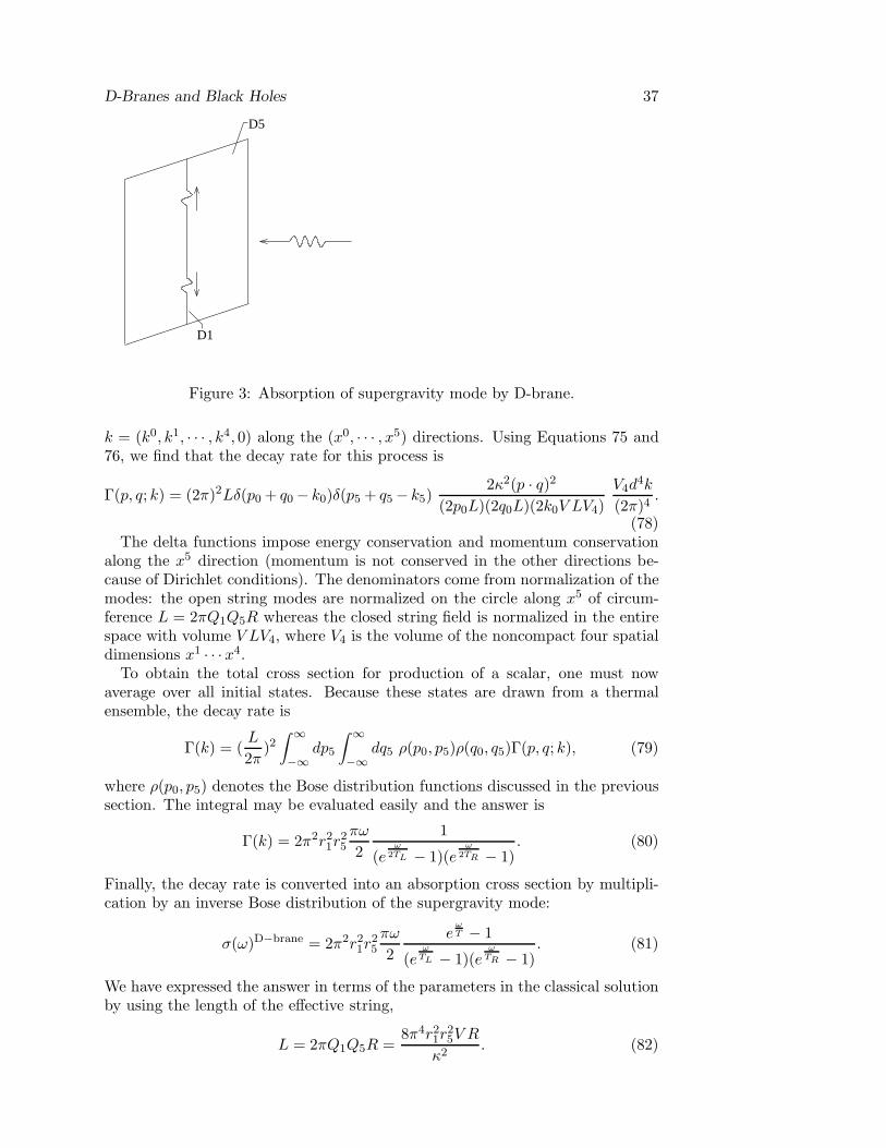
D-Branes and Black Holes 37
D5
D1
Figure 3: Absorption of supergravity mode by D-brane.
k = (k0, k1, · · · , k4, 0) along the (x0, · · · , x5) directions. Using Equations 75 and76, we find that the decay rate for this process is
Γ(p, q; k) = (2π)2Lδ(p0 + q0 − k0)δ(p5 + q5 − k5)2κ2(p · q)2
(2p0L)(2q0L)(2k0V LV4)
V4d4k
(2π)4.
(78)The delta functions impose energy conservation and momentum conservation
along the x5 direction (momentum is not conserved in the other directions be-cause of Dirichlet conditions). The denominators come from normalization of themodes: the open string modes are normalized on the circle along x5 of circum-ference L = 2πQ1Q5R whereas the closed string field is normalized in the entirespace with volume V LV4, where V4 is the volume of the noncompact four spatialdimensions x1 · · · x4.
To obtain the total cross section for production of a scalar, one must nowaverage over all initial states. Because these states are drawn from a thermalensemble, the decay rate is
Γ(k) = (L
2π)2∫ ∞
−∞dp5
∫ ∞
−∞dq5 ρ(p0, p5)ρ(q0, q5)Γ(p, q; k), (79)
where ρ(p0, p5) denotes the Bose distribution functions discussed in the previoussection. The integral may be evaluated easily and the answer is
Γ(k) = 2π2r21r25
πω
2
1
(eω
2TL − 1)(eω
2TR − 1). (80)
Finally, the decay rate is converted into an absorption cross section by multipli-cation by an inverse Bose distribution of the supergravity mode:
σ(ω)D−brane = 2π2r21r25
πω
2
eωT − 1
(eω
TL − 1)(eω
TR − 1). (81)
We have expressed the answer in terms of the parameters in the classical solutionby using the length of the effective string,
L = 2πQ1Q5R =8π4r21r
25V R
κ2. (82)
38 Das & Mathur
The physical temperature T is related to TL and TR by Equation 61. Thus, whenTL ≫ TR, we have T ∼ 2TR. However, we know that the quantities TL and TR
above are in fact exactly the same as the semiclassical quantities and T = TH .For very low energies ω ≪ TL, one of the thermal factors above can be simplified.Using Equations 49 through 51, we see that in this limit
σ(ω) = 2π2(r1r5)2TL =
(r1r5)2SL
RQ1Q5= AH . (83)
We have used Equation 52 and the fact that in the regime TL ≫ TR we have SL =S = SBH = 2πAH/κ
25, where κ2
5 = κ210/2πRV and κ2
10 is given by Equation 77.We have also used Equation 49 to express r1, r5 in terms of g, ls, V,Q1, Q5. Thisis exactly the low-energy classical result. The fact that the cross section turnsout to be proportional to the horizon area was already known [31]. The precisecalculation outlined above was performed in Reference [33].
Even before taking this low-energy limit, the entire result (Equation 81) is inexact agreement with the semiclassical grey-body factor [52].
It is clear from Equation 80 that the thermal factor in the decay rate comesfrom the thermal factors of the long string modes. In the strict classical limit,we can have absorption but no Hawking radiation; this comes about because thetemperature in this limit is zero, so the corresponding thermal factor suppressesemission completely while absorption is still nonzero [50].
The supergravity mode can also split into a pair of fermions. However, thenthe thermal factors that appear in Equation 80 are Fermi-Dirac distributions andthese go to a constant at low energies, rather than diverging as Bose factors do.As a result, the corresponding cross section is suppressed at low energies. Ina similar way, we may consider emission/absorption of a fermionic supergravitymode. This would require one left-moving bosonic mode of the long string witha right-moving fermionic mode. Following the above calculations, it is apparentthat the thermal factor of the left-moving long string mode gives the right powersof energy to lead to a nonzero low-energy cross section, and the thermal factor forthe right-moving mode provides the thermal factor of the emitted supergravityfermion—and this is a Fermi-Dirac factor as expected [31].
Classical emission of higher angular momentum modes is suppressed by cen-trifugal barriers provided by the gravitational field. In the microscopic model,such emission is again suppressed, but for a different reason. Note that thebosonic degrees of freedom of the long string are all vectors under the internalSO(4) of the T 4 but are scalars under the tangent space SO(4) of the transversespace. Therefore, these can never collide to give rise to modes with nonzero angu-lar momentum in transverse space. Fermions on the long string, however, carrytransverse tangent space indices (typically as a R-symmetry index) since they aredimensional reductions of 10-dimensional fermions. Thus, multifermion processesare responsible for emission of higher angular momentum modes. However, thesecan be seen to be necessarily suppressed, since they involve more than two fermionfields and therefore correspond to higher-dimension operators on the long stringworld sheet. Angular-momentum–mode emission is not completely understood inthe long string picture—although the qualitative aspects have been understood[54].
Similar calculations have been performed for several other situations, e.g. forabsorption/emission of charged scalars from both 5- and 4-dimensional blackholes [53, 52].
D-Branes and Black Holes 39
The low-energy effective action used above follows from a Dirac-Born-Infeld(DBI) action of the long string in the presence of supergravity backgrounds. Onemight wonder whether this DBI action can be used to predict absorption ratesfor other supergravity modes. It turns out that this can be done for several otherminimal scalars, namely the dilaton and the components of the NS B field alongthe T 4. There are four other minimal scalars in this background, the couplings ofwhich cannot be obtained from the DBI action. Perhaps more significantly, thereis a set of other scalar fields that do not obey minimal Klein-Gordon equations—e.g. the fluctuations of the volume of the T 4. If we trust the DBI action to obtainthe couplings of these fields, we get answers that do not agree with supergravitycalculations [55]. These cross sections are suppressed at low energies and it isprobably not surprising that the simplest low-energy effective theory does notwork.
6.3 Why Does It Work?
The agreement of the low-energy limit of the absorption cross section—or, equiv-alently, decay rate—is strong evidence for the contention that Hawking radiationis an ordinary, unitary quantum decay process. This is, however, surprising—like the agreement of near-extremal thermodynamics—since our weak couplingcalculation agreed with a strong coupling expectation. The agreement of non-trivial grey-body factors is even more surprising because now not just a singlenumber but an entire function of energy is correctly predicted by a weak couplingcalculation.
Weak coupling calculations also gave the correct answer for the extremal en-tropy, but that case involves BPS states and supersymmetry guarantees the agree-ment. In nonextremal situations, supersymmetry is broken. However, for smallamounts of nonextremality, we have small excitations over a supersymmetricbackground and we may still expect nonrenormalization theorems to ensure thathigher-loop effects vanish at low energies. A complete understanding of this is stilllacking. Explicit one-loop calculations [56] seem to support this scenario. Thereis also some evidence for nonrenormalization theorems of the type required [57].
7 ABSORPTION BY THREE-BRANES
The above discussion has addressed extremal solutions with large horizon areasand their excitations. Extremal solutions with vanishing horizon areas generallyhave singular horizons, for which semiclassical results cannot be trusted. Thereare, however, several exceptions to this rule. In this section we consider one ofthem—the 3-brane in Type IIB supergravity.
7.1 Classical Solution and Classical Absorption
The classical solution for N parallel extremal 3-branes along (x7 · · · x9) is givenby the (Einstein-frame) metric
ds2 = [f(r)]−1/2[−dt2 + d~x2] + [f(r)]1/2[dr2 + r2dΩ25], (84)
where r = (∑6
i=1(xi)2)1/2 is the radial coordinate in the transverse space, ~x =
(x7, · · · , x9) are the coordinates on the brane, and dΩ5 is the measure on a unit
40 Das & Mathur
5-sphere. The harmonic function f(r) is given by
f(r) = 1 +
(
R
r
)4
R4 = 4πgsNl4s . (85)
The dilaton is a constant and the only other nontrivial field is the 4-form gaugefield with a field strength
F0789r =4R4
gsr5[f(r)]−2. (86)
The horizon is at r = 0 and the horizon area is indeed zero. However, thespacetime is completely nonsingular. In the near-horizon or near-brane regionr ≪ R, the metric (Equation 86) becomes, in terms of coordinates z = R2/r,
ds2 =
(
R
z
)2
[−dt2 + d~x2 + dz2] +R2dΩ25. (87)
This is the metric of the space AdS5 × S5, the first factor being composed of(t, ~x, z) while the sphere S5 has a constant radius R. The AdS5 has a constantnegative curvature 1/R2, whereas the sphere S5 has a constant positive curvature.Thus, near the horizon the spacetime approaches a “throat geometry,” where thelength of the throat is along the AdS5 coordinates and the cross sections are5-spheres of constant radii R.
From Equation 85 it follows that this curvature is much smaller than the stringscale when gsN ≫ 1. This is thus the regime where semiclassical supergravity isvalid.
It is possible to calculate the classical absorption cross section of various su-pergravity modes by the extremal 3-brane. For s-wave absorption of minimallycoupled scalars, the leading-order result is [58]
σ =1
8π4R8ω3 =
1
32π(κN)2ω3, (88)
where we have used Equation 85. The cross section of course vanishes at ω = 0,since the horizon area vanishes. Also note that we are dealing with an extremalsolution that has zero temperature, so we have absorption but no Hawking ra-diation. It turns out that in this case one can also analytically calculate thelow-energy absorption cross section of such scalars for arbitrary angular momen-tum [59].
7.2 Absorption in the Microscopic Model
The microscopic theory of N 3-branes is a U(N) gauge theory in 3 + 1 dimen-sions with 16 supersymmetries, or N = 4 supersymmetry. This is a well-studiedtheory and is known to be conformally invariant with zero beta function. Itis the dimensional reduction of N = 1 supersymmetric Yang-Mills in ten di-mensions. As we will see below, a natural symmetry argument determines thecoupling of some of the supergravity modes to the brane degrees of freedom.However, if we consider modes like the dilaton and longitudinal traceless partsof the 10-dimensional graviton, the coupling can be once again read off from theequivalence principle. For example, the longitudinal graviton has to couple to theenergy-momentum tensor of the Yang-Mills theory. Thus, one can perturbatively
D-Branes and Black Holes 41
calculate the absorption cross section of such modes (which are minimal scalarsfrom the 7-dimensional point of view) along the lines of the calculation in the5-dimensional black hole. Again, an exact agreement was found for s-waves [58],and the agreement was found to extend to all angular momenta [59].
In this case, the reason for the agreement of the weak coupling calculationwith supergravity answers is much better understood. In particular, it is knownthat the two-point function of the energy-momentum tensor of N = 4 Yang-Millstheory is not renormalized, so that the lowest-order result is exact [60]. Theimaginary part of the two-point function in Euclidean space is in turn relatedto the absorption cross section, which is thus also protected from higher-ordercorrections. There are similar nonrenormalization theorems known for operatorscoupling to other modes as well.
7.3 Nonextremal Thermodynamics
The extremal 3-brane of supergravity described above is of course a limit of ageneral nonextremal solution with finite horizon area and finite temperature. Itis thus natural to expect that the microscopic description of this is in terms of aYang-Mills theory at finite temperature. The thermodynamics of this Yang-Millstheory was calculated [61] at lowest order in the coupling constant (i.e. a free gas),and it was found that although the dependence of the thermodynamic quantitieson the energy, volume, and N is the same as in semiclassical thermodynamics ofthe corresponding black brane, the precise coefficient differs by a factor of 4/3. Weknow of no reason why the thermodynamic quantities are not renormalized as wego from weak to strong coupling, so the discrepancy is not unexpected. However,it is significant that the dependences agree—although the dependence on theenergy and the volume is dictated by scaling arguments (this is a conformallyinvariant theory), the dependence on N is not. At weak coupling, we know thatthere are N2 degrees of freedom; there is no known argument why this shouldcontinue at strong coupling.
8 AdS/CFT CORRESPONDENCE AND HOLOGRAPHY
We have presented a unitary description of black hole evaporation in terms of theemission of closed strings from the branes. This description was at weak coupling;in order to describe absorption by the black hole of quanta with arbitrary energies,one must imagine that it is continued to strong coupling.
Let us see what form this continuation to higher energies might take. In thelowest-order calculation, there was only one string interaction, where two openstrings joined up to the emitted closed string. At higher orders in the coupling,we expect the emitted string to interact several times with the branes beforeescaping to infinity as radiation. Let us consider for simplicity the case of theD3-branes described above. Each such interaction gives one “hole” on the stringworld sheet, with the boundary of the hole being constrained to the branes.
From the viewpoint of the dynamics of open strings on the 3-branes, each holelooks like an open string loop. Thus, as we increase the coupling, we encounterhigher loop processes among the open strings, in the process of emitting a closedstring.
On the other hand, a loop of open strings can be interpreted as a propagationof a closed string at tree level (see Figure 4). Thus, these open string multiloop
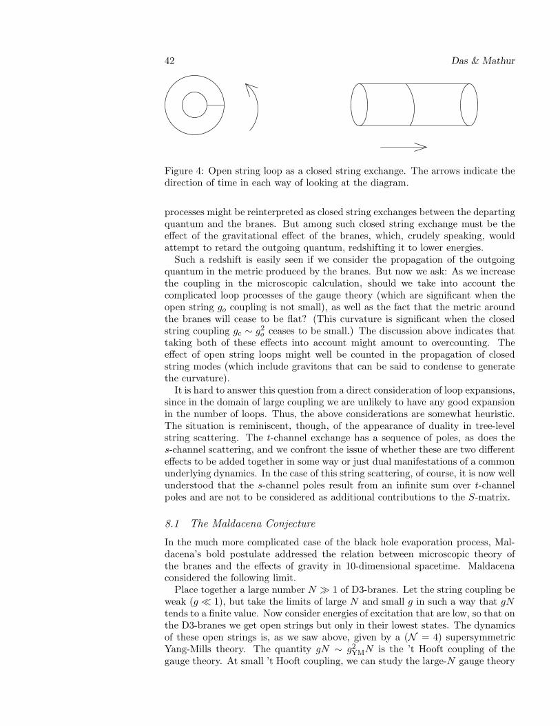
42 Das & Mathur
Figure 4: Open string loop as a closed string exchange. The arrows indicate thedirection of time in each way of looking at the diagram.
processes might be reinterpreted as closed string exchanges between the departingquantum and the branes. But among such closed string exchange must be theeffect of the gravitational effect of the branes, which, crudely speaking, wouldattempt to retard the outgoing quantum, redshifting it to lower energies.
Such a redshift is easily seen if we consider the propagation of the outgoingquantum in the metric produced by the branes. But now we ask: As we increasethe coupling in the microscopic calculation, should we take into account thecomplicated loop processes of the gauge theory (which are significant when theopen string go coupling is not small), as well as the fact that the metric aroundthe branes will cease to be flat? (This curvature is significant when the closedstring coupling gc ∼ g2
o ceases to be small.) The discussion above indicates thattaking both of these effects into account might amount to overcounting. Theeffect of open string loops might well be counted in the propagation of closedstring modes (which include gravitons that can be said to condense to generatethe curvature).
It is hard to answer this question from a direct consideration of loop expansions,since in the domain of large coupling we are unlikely to have any good expansionin the number of loops. Thus, the above considerations are somewhat heuristic.The situation is reminiscent, though, of the appearance of duality in tree-levelstring scattering. The t-channel exchange has a sequence of poles, as does thes-channel scattering, and we confront the issue of whether these are two differenteffects to be added together in some way or just dual manifestations of a commonunderlying dynamics. In the case of this string scattering, of course, it is now wellunderstood that the s-channel poles result from an infinite sum over t-channelpoles and are not to be considered as additional contributions to the S-matrix.
8.1 The Maldacena Conjecture
In the much more complicated case of the black hole evaporation process, Mal-dacena’s bold postulate addressed the relation between microscopic theory ofthe branes and the effects of gravity in 10-dimensional spacetime. Maldacenaconsidered the following limit.
Place together a large number N ≫ 1 of D3-branes. Let the string coupling beweak (g ≪ 1), but take the limits of large N and small g in such a way that gNtends to a finite value. Now consider energies of excitation that are low, so that onthe D3-branes we get open strings but only in their lowest states. The dynamicsof these open strings is, as we saw above, given by a (N = 4) supersymmetricYang-Mills theory. The quantity gN ∼ g2
YMN is the ’t Hooft coupling of thegauge theory. At small ’t Hooft coupling, we can study the large-N gauge theory
D-Branes and Black Holes 43
perturbatively; at large ’t Hooft coupling g2YMN ≫ 1 such a perturbative analysis
is not possible.But for gN ≫ 1 we are in a regime where the D3-branes produce an appreciable
gravitational field around themselves, and in fact distort the spacetime into theform of Equation 84. In particular, as shown above, as we approach the horizonthe geometry becomes the throat geometry AdS5 × S5 given by Equation 87.
Maldacena postulated that we can consider either (a) the gauge theory on thebranes (which is given by the open string interactions at a perturbative level)or (b) no branes, but the space AdS5 × S5 and closed string theory (which hasgravity as a low-energy limit) on this curved manifold. These two theories weredual descriptions of exactly the same underlying theory.
If the gauge theory of the branes and gravity on the 10-dimensional spacetimeare indeed exactly dual descriptions of the same theory, then we must have a wayof computing the same quantity in two dual ways, and thus to see manifestly theconsequences of this duality. To do this, we need an operational definition of thedual map, which was provided by Gubser et al [62] and Witten [63]. Let us rotatethe signature of the spacetime to a Euclidean one. In this case, the space spannedby ~x, r, which is now Euclidean AdS5, has r = 0 as a regular point in the interiorof the space. Thus, there is no singularity that might represent the place wherethe D3-branes were placed in a gauge theory description. But this space has aboundary at r → ∞, which has the topology of S4. The conjecture now statesthat string theory on this smooth AdS5 × S5 is dual to N = 4 supersymmetricSU(N) Yang-Mills on the 4-dimensional boundary of the AdS space.
Note that in this formulation of the conjecture, all reference to D3-branes hasdisappeared. In fact, a geometry that is AdS5 × S5 everywhere (and not just atsmall r) is an exact solution of string theory without any branes present. We takethe 5-form field strength F present in Type IIB string theory to have a constantvalue with integral N on the S5; since this field must be self-dual, it also has aconstant value on the AdS5. The energy density of this field yields the equal andopposite curvatures of the S5 and the AdS5 spaces; the radius of curvature ineach case is R ∼ (gN)1/4ls (ls is the string length). If we had taken a collectionof D3-branes as above, then the flux of F on the sphere surrounding the braneswould have been N , but only the near-brane geometry would have resembledAdS5×S5—at large r the space becomes flat. Thus, it seems better to formulatethe duality without reference to any D-branes, although, as we discuss below, thismakes the issues related to black hole information loss somewhat more difficultto access.
An important fact that led Maldacena to the duality conjecture was the agree-ment of global symmetries between the gravity theory and the gauge theory.AdS5 is a maximally symmetric space with a 15-parameter isometry group. Thegauge theory is in four dimensions, so one may expect a 10-dimensional set ofsymmetries, which are the translations and rotations on S4. But the N = 4supersymmetric SU(N) Yang-Mills theory is a conformal theory, and the con-formal group in four dimensions is indeed isomorphic to the 15-parameter groupof isometries of AdS5 space. Further, the N = 4 gauge theory has four super-charges forming, having an SU(4) symmetry of rotations among themselves. Thegravity theory has an internal space that is S5. Thus, when we decompose fieldsin harmonics on this space in the process of Kaluza-Klein reduction, the multi-plets obtained fall into representations of SO(6). But SO(6) ≈ SU(4), so boththe theories have the same R-symmetry group. Further, because of conformal
44 Das & Mathur
invariance, the gauge theory has 16 conformal supercharges in addition to its 16regular supercharges; this agrees with the 32 supercharges of the gravity theoryon AdS5 × S5.
8.2 Calculations Using the Conjecture
Let us return to the issue of how to compare quantities in the two dual theories.Let Ω be the AdS space, and ∂Ω its boundary. Let us consider for simplicity ascalar field, the dilaton φ, present in the string theory. If we specify the valueφb of φ on the boundary ∂Ω, then we can solve for φ in the interior of Ω andcompute the action SSUGRA of supergravity on this solution. The field φ, on theother hand, will be dual to an operator in the Yang-Mills theory, and in this casesymmetries fix this operator to be TrF 2. The duality relation is
e−SΩ
SUGRA[φb] =
∫
∂ΩDA e−SYM+∫
dξφb(ξ)TrF 2(ξ)
∫
∂ΩDA e−SYM
. (89)
Here∫
DA represents the path integral over the gauge theory variables. Theaction on the left-hand side is a string action in general, but at the leading orderit can be replaced by the supergravity action.
Using the above relation, it is possible in principle to compute n-point corre-lation functions from supergravity and compare the results to calculations in thegauge theory. The gravity theory is simple (perturbative classical supergravity tolowest order) when N is large (loops of gravity are suppressed by 1/N2) and gNis large (because then the AdS space has a large radius, and stringy corrections,which depend on ls/R, can be ignored to leading order). Thus it is difficult tocompare results on the gravity side with explicit computations in the Yang-Millstheory, which has a well-known treatment of the large-N limit but no simple wayto handle a regime with g2
Y MN ∼ gN ≫ 1. However, supersymmetry protectsthe values of some quantities from changing when the coupling is varied, andhere agreement is indeed found. Thus, anomalous dimensions of chiral operators[62, 63] and three-point functions of chiral operators [65] are found to have thesame value when computed from the gauge theory or from the gravity dual usingEquation 89. For quantities that are not protected in this fashion, the gravitycalculation gives a prediction for the strongly coupled gauge theory. Examples ofsuch predictions are the potential between external quarks placed in the gaugetheory [66], four-point correlation functions, and anomalous dimensions of com-posite operators (which can be deduced from the four-point functions) [67]. If oneconsiders the gauge theory at a finite temperature by compactifying the “time”direction, then one obtains a nonsupersymmetric theory with a discrete spectrumof glueball states [68]. In this case, the strong coupling calculation has no directphysical meaning, and only a weak coupling calculation would give the true glue-ball masses (the coupling flows with scale after supersymmetry is broken; withsupersymmetry intact, it does not, and each value of the coupling gives a dif-ferent well-defined theory). Nevertheless, there is a surprising agreement of thequalitative features of the glueball spectrum between the gravity calculation andlattice simulations [69].
D-Branes and Black Holes 45
8.3 Holography and the Bekenstein Entropy Bound
The AdS/CFT correspondence has been studied extensively over the past twoyears [see [70] for review]. This section explains how this correspondence illus-trates another important property of holography that is in fact its very essence:the Bekenstein bound [71]. A general argument states that in any theory of grav-ity, the total entropy S of anything in a large box of volume V and surface areaA is bounded by
S ≤ A
G, (90)
where G is Newton’s constant. Numerical constants are ignored in this relation.The form of this bound appears surprising, since in the absence of gravity we knowthat entropy is an extensive quantity and should scale as V . However, the resultfollows from the existence of black holes. Suppose we start with a state whoseentropy is bigger than this bound, but whose energy is smaller than the massof a black hole that fills the entire box. Then we slowly add matter, increasingthe energy. At some stage, gravitational collapse takes over and a black hole isformed, which then continues to grow until it fills up the box. We know that theentropy of a black hole is proportional to the area of the horizon measured in unitsof Newton’s constant. However, for this black hole, the area of the horizon is thesame as the area of the box A, i.e. the right-hand side of Equation 90. Thus, wehave managed to decrease the entropy in this process and hence have violated thesecond law. ’t Hooft [72] and Susskind [73] have proposed a radical interpretationof the holographic bound (Equation 90), namely, a (d+ 1)-dimensional theory ofgravity should be equivalent to a d-dimensional theory that lives on the boundaryof space, and this d-dimensional theory must have one degree of freedom perPlanck area. If this is true, the Bekenstein bound naturally follows.
We have seen that supergravity in AdS5 × S5 is dual to a strongly coupledlarge-N Yang-Mills theory in 3+1 dimensions. Is it then true that the latter hasone degree of freedom per Planck area? This is indeed true [74]. In the AdS5×S5
metric (Equation 87) the boundary is at z = 0 and continuum Yang-Mills theoryliving on this boundary is dual to supergravity in the whole space. But supposewe impose an infrared cutoff at z = z0. Then it turns out that supergravity inthe region z > z0 is dual to a Yang-Mills theory with a position space ultravioletcutoff δ = z0. In fact, renormalization group flows of the gauge theory becomemotion in the fifth dimension.
Consider a large patch of this boundary of coordinate size L (in terms of the ~xcoordinates). It follows from Equation 87 that the physical area of this boundaryis
A ∼ R3
z30
L3. (91)
Using the expression for R in Equation 85 and the fact that the 5-dimensionalNewton’s constant G5 is given by G5 ∼ G10/R
5 ∼ (g2l8s)/R5, we see that
A
G5∼ N2L
3
z30
. (92)
Now the Yang-Mills theory has N2 degrees of freedom per unit cell. This is man-ifest at weak coupling, but the result for the entropy of near-extremal 3-branesshows that this must also be true in strong coupling. Furthermore, the cutoff of
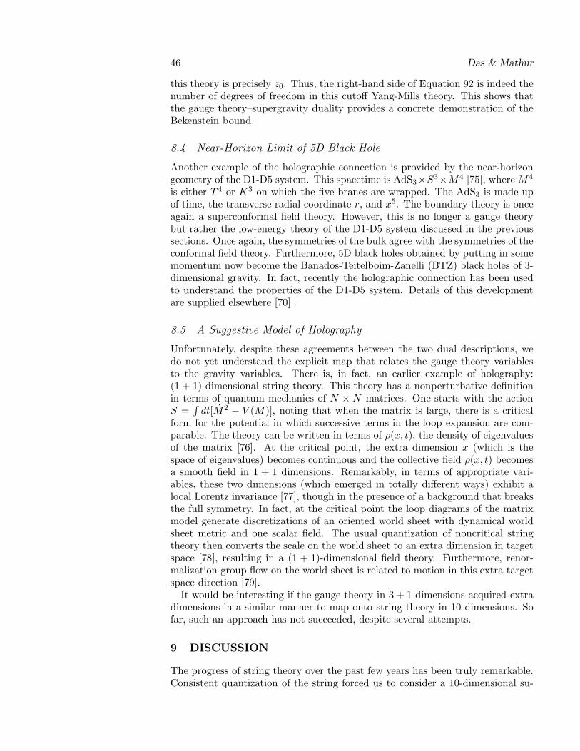
46 Das & Mathur
this theory is precisely z0. Thus, the right-hand side of Equation 92 is indeed thenumber of degrees of freedom in this cutoff Yang-Mills theory. This shows thatthe gauge theory–supergravity duality provides a concrete demonstration of theBekenstein bound.
8.4 Near-Horizon Limit of 5D Black Hole
Another example of the holographic connection is provided by the near-horizongeometry of the D1-D5 system. This spacetime is AdS3×S3×M4 [75], where M4
is either T 4 or K3 on which the five branes are wrapped. The AdS3 is made upof time, the transverse radial coordinate r, and x5. The boundary theory is onceagain a superconformal field theory. However, this is no longer a gauge theorybut rather the low-energy theory of the D1-D5 system discussed in the previoussections. Once again, the symmetries of the bulk agree with the symmetries of theconformal field theory. Furthermore, 5D black holes obtained by putting in somemomentum now become the Banados-Teitelboim-Zanelli (BTZ) black holes of 3-dimensional gravity. In fact, recently the holographic connection has been usedto understand the properties of the D1-D5 system. Details of this developmentare supplied elsewhere [70].
8.5 A Suggestive Model of Holography
Unfortunately, despite these agreements between the two dual descriptions, wedo not yet understand the explicit map that relates the gauge theory variablesto the gravity variables. There is, in fact, an earlier example of holography:(1 + 1)-dimensional string theory. This theory has a nonperturbative definitionin terms of quantum mechanics of N × N matrices. One starts with the actionS =
∫
dt[M2 − V (M)], noting that when the matrix is large, there is a criticalform for the potential in which successive terms in the loop expansion are com-parable. The theory can be written in terms of ρ(x, t), the density of eigenvaluesof the matrix [76]. At the critical point, the extra dimension x (which is thespace of eigenvalues) becomes continuous and the collective field ρ(x, t) becomesa smooth field in 1 + 1 dimensions. Remarkably, in terms of appropriate vari-ables, these two dimensions (which emerged in totally different ways) exhibit alocal Lorentz invariance [77], though in the presence of a background that breaksthe full symmetry. In fact, at the critical point the loop diagrams of the matrixmodel generate discretizations of an oriented world sheet with dynamical worldsheet metric and one scalar field. The usual quantization of noncritical stringtheory then converts the scale on the world sheet to an extra dimension in targetspace [78], resulting in a (1 + 1)-dimensional field theory. Furthermore, renor-malization group flow on the world sheet is related to motion in this extra targetspace direction [79].
It would be interesting if the gauge theory in 3 + 1 dimensions acquired extradimensions in a similar manner to map onto string theory in 10 dimensions. Sofar, such an approach has not succeeded, despite several attempts.
9 DISCUSSION
The progress of string theory over the past few years has been truly remarkable.Consistent quantization of the string forced us to consider a 10-dimensional su-
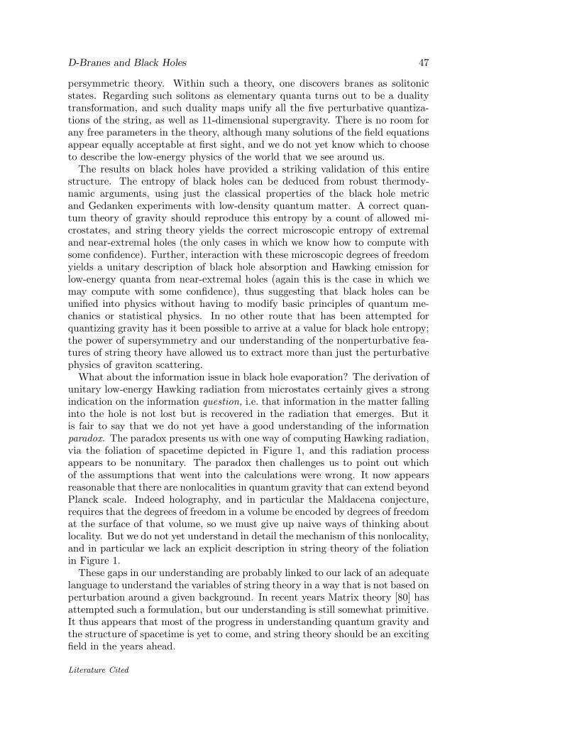
D-Branes and Black Holes 47
persymmetric theory. Within such a theory, one discovers branes as solitonicstates. Regarding such solitons as elementary quanta turns out to be a dualitytransformation, and such duality maps unify all the five perturbative quantiza-tions of the string, as well as 11-dimensional supergravity. There is no room forany free parameters in the theory, although many solutions of the field equationsappear equally acceptable at first sight, and we do not yet know which to chooseto describe the low-energy physics of the world that we see around us.
The results on black holes have provided a striking validation of this entirestructure. The entropy of black holes can be deduced from robust thermody-namic arguments, using just the classical properties of the black hole metricand Gedanken experiments with low-density quantum matter. A correct quan-tum theory of gravity should reproduce this entropy by a count of allowed mi-crostates, and string theory yields the correct microscopic entropy of extremaland near-extremal holes (the only cases in which we know how to compute withsome confidence). Further, interaction with these microscopic degrees of freedomyields a unitary description of black hole absorption and Hawking emission forlow-energy quanta from near-extremal holes (again this is the case in which wemay compute with some confidence), thus suggesting that black holes can beunified into physics without having to modify basic principles of quantum me-chanics or statistical physics. In no other route that has been attempted forquantizing gravity has it been possible to arrive at a value for black hole entropy;the power of supersymmetry and our understanding of the nonperturbative fea-tures of string theory have allowed us to extract more than just the perturbativephysics of graviton scattering.
What about the information issue in black hole evaporation? The derivation ofunitary low-energy Hawking radiation from microstates certainly gives a strongindication on the information question, i.e. that information in the matter fallinginto the hole is not lost but is recovered in the radiation that emerges. But itis fair to say that we do not yet have a good understanding of the informationparadox. The paradox presents us with one way of computing Hawking radiation,via the foliation of spacetime depicted in Figure 1, and this radiation processappears to be nonunitary. The paradox then challenges us to point out whichof the assumptions that went into the calculations were wrong. It now appearsreasonable that there are nonlocalities in quantum gravity that can extend beyondPlanck scale. Indeed holography, and in particular the Maldacena conjecture,requires that the degrees of freedom in a volume be encoded by degrees of freedomat the surface of that volume, so we must give up naive ways of thinking aboutlocality. But we do not yet understand in detail the mechanism of this nonlocality,and in particular we lack an explicit description in string theory of the foliationin Figure 1.
These gaps in our understanding are probably linked to our lack of an adequatelanguage to understand the variables of string theory in a way that is not based onperturbation around a given background. In recent years Matrix theory [80] hasattempted such a formulation, but our understanding is still somewhat primitive.It thus appears that most of the progress in understanding quantum gravity andthe structure of spacetime is yet to come, and string theory should be an excitingfield in the years ahead.
Literature Cited

48 Das & Mathur
1. Misner C, Thorne W, Wheeler J. Gravitation. New York: Freeman (1978); Wald R. General
Relativity. Chicago: Univ. Chicago Press (1984)2. Bekenstein JD. Phys. Rev. D 7:2333 (1973); Bekenstein JD. Phys. Rev. D 9:3292 (1974)3. Pelath MA, Wald RM. gr-qc/9901032 (1999)4. Hawking S. Commun. Math. Phys. 43:199 (1975)5. Hawking S. Phys. Rev. D 13:191 (1976)6. Hawking S. Phys. Rev. D 14:2460 (1976)7. Giddings SB. hep-th/9508151 (1995)8. Zurek WH. Phys. Rev. Lett. 49:1683 (1982)9. Banks T, Peskin M, Susskind L. Nucl. Phys. B244:135 (1984)
10. Unruh WG, Wald RM. Phys. Rev. D 52:2176 (1995)11. ’t Hooft G. Nucl. Phys. B256:727 (1985)12. Keski-Vakkuri E, Lifschytz G, Mathur SD, Ortiz M. Phys. Rev. D 51:1764 (1995)13. Keski-Vakkuri E, Mathur SD. Phys. Rev. D 54:7391 (1996)14. Green M, Schwarz J, Witten E. Superstring Theory, Vols. 1, 2. Cambridge, UK: Cambridge
Univ. Press (1987); Polchinski J. String Theory, Vols. 1, 2. Cambridge, UK: CambridgeUniv. Press (1998)
15. Arkani-Hamed N, Dimopolous S, Dvali G. Phys. Rev. D 59:086004 (1999); Randall L, Sun-drum R. Phys. Rev. Lett. 83:3370 (1999)
16. Sen A. hep-th/9802051 (1998)17. Townsend P. hep-th/9507048 (1995)18. Polchinski J. Phys. Rev. Lett. 75:4724 (1995)19. Polchinski J. hep-th/9611050 (1996)20. Sen A. hep-th/9904027 (1999)21. Witten E. Nucl. Phys. B460:335 (1996)22. Tseytlin A. hep-th/9908105 (1999)23. Montonen C, Olive D. Phys. Lett. B72:117 (1977)24. Susskind L. hep-th/9309145 (1993)25. Dabholkar A, Harvey J. Phys. Rev. Lett. 63:478 (1989); Dabholkar A, Gibbons G, Harvey
J, Ruiz F. Nucl. Phys. B340:33 (1990)26. Horowitz G, Maldacena J, Strominger A. Phys. Lett. B383:151 (1996)27. Sen A. Nucl. Phys. B440:421 (1995); Sen A. Mod. Phys. Lett. A10:2081 (1995)28. Strominger A, Vafa C. Phys. Lett. B379:99 (1996)29. Das SR, Mathur SD. Phys. Lett. B375:103 (1996)30. Maldacena J, Susskind L. Nucl. Phys. B475:679 (1996)31. Callan C, Maldacena J. Nucl. Phys. B472:591 (1996)32. Horowitz G, Strominger A. Phys. Rev. Lett. 77:2368 (1996)33. Das SR, Mathur SD. Nucl. Phys. B478:561 (1996); Das SR, Mathur SD. Nucl. Phys.
B482:153 (1996)34. Preskill J et al. Mod. Phys. Lett. A6:2353 (1991)35. Dijkgraaf R, Moore G, Verlinde E, Verlinde H. Commun. Math. Phys. 185:197 (1997)36. Maldacena J, Moore G, Strominger A. hep-th/9903063 (1999)37. Maldacena J. PhD thesis. hep-th/9607235 (1996)38. Hassan SF, Wadia SR. Phys. Lett. B402:43 (1997); Hassan SF, Wadia SR. Nucl. Phys.
B526:311 (1998)39. Douglas M. hep-th/9512077 (1995)40. Dijkgraaf R, Verlinde E, Verlinde H. Nucl. Phys. B486:77 (1997)41. Dijkgraaf R. Nucl. Phys B543:545 (1999)42. Seiberg N, Witten E. J. High Energy Phys. 9904:017 (1999)43. Larsen F, Martinec E. J. High Energy Phys. 9906:019 (1999); Larsen F, Martinec E. J. High
Energy Phys. 9911:002 (1999); Dhar A, Mandal G, Wadia SR, Yogendran K. hep-th/9910194(1999)
44. Cvetic M. Nucl. Phys. Proc. Suppl. 56B:1 (1997); Youm D. Phys. Rep. 316:1 (1999)45. Maldacena J, Strominger A. Phys. Rev. Lett. 77:428 (1996); Horowitz G, Lowe D, Maldacena
J. Phys. Rev. Lett. 77:430 (1996)46. Balasubramanium V, Larsen F. Nucl. Phys. B478:199 (1996)47. Tseytlin A. Nucl. Phys. B475:149 (1996); Klebanov I, Tseytlin A. Nucl. Phys. B475:179
(1996); Gauntlett J, Kastor D, Traschen J. Nucl. Phys. B478:544 (1996)48. Brekenridge J, Myers R, Peet A, Vafa C. Phys. Lett. B391:93 (1996); Brekenridge J, et al.

D-Branes and Black Holes 49
Phys. Lett. B381:423 (1996)49. Page D. Phys. Rev. D 13:198 (1976); Unruh W. Phys. Rev. D 14:3251 (1976)50. Dhar A, Mandal G, Wadia SR. Phys. Lett. B388:51 (1996)51. Das SR, Gibbons G, Mathur SD. Phys. Rev. Lett 78:417 (1997)52. Maldacena J, Strominger A. Phys. Rev. D 55:861 (1997)53. Gubser S, Klebanov I. Nucl. Phys. B482:173 (1996); Gubser S, Klebanov I. Phys. Rev. Lett.
77:4491 (1996)54. Mathur SD. Nucl. Phys. B514:204 (1998)55. Callan CG, Gubser S, Klebanov I, Tseytlin A. Nucl. Phys B489:65 (1997); Klebanov I,
Krasnitz M. Phys. Rev. D 55:3250 (1997); Krasnitz M, Klebanov I. Phys. Rev. D 56:2173(1997)
56. Das SR. Phys. Rev. D 56:3582 (1997); Das SR. Nucl. Phys. Proc. Suppl. 68:119 (1998)57. Maldacena J. Phys. Rev. D 55:7645 (1997)58. Klebanov I. Nucl. Phys. B496:231 (1997); Gubser S, Klebanov I, Tseytlin A. Nucl. Phys.
B499:217 (1997)59. Klebanov I, Taylor W. Nucl. Phys. B560:207 (1999)60. Gubser S, Klebanov I. Phys. Lett. B413:41 (1997)61. Gubser S, Peet A, Klebanov I. Phys. Rev. D 54:3915 (1996)62. Gubser S, Klebanov I, Polyakov A. Phys. Lett. B428:105 (1998)63. Witten E. Adv. Theor. Math. Phys. 2:253 (1998)64. Maldacena J. Adv. Theor. Math. Phys. 2:231 (1998)65. Freedman D, Mathur SD, Rastelli L, Matusis A. Nucl. Phys. B546:96 (1999); Lee S, Minwalla
S, Rangamani M, Seiberg N. Adv. Theor. Math. Phys. 2:697 (1998)66. Maldacena J. Phys. Rev. Lett. 80:4859 (1998), S.J. Rey and J. Yee, hep-th/9803001.67. d’Hoker E, et al. Nucl. Phys. B562:353 (1999); d’Hoker E, et al. hep-th/9911222 (1999)68. Witten E. Adv. Theor. Math. Phys. 2:505 (1998)69. Csaki C, Ooguri H, Oz Y, Terning J. JHEP 9901:017 (1999)70. Aharony O, et al. hep-th/9905111 (1999)71. Bekenstein J. Phys. Rev. D 27:2262 (1983); Bekenstein J. Phys. Rev. D 49:1912 (1994)72. ’t Hooft G. hep-th/9310026 (1993); Stephens CR, ’t Hooft G, Whiting B. Class. Quant.
Grav. 11:621 (1994)73. Susskind L. J. Math. Phys. 36:6377 (1995)74. Susskind L, Witten E. hep-th/9805114 (1998)75. Maldacena J, Strominger A. JHEP 9812:005 (1998)76. Jevicki A, Sakita B. Nucl. Phys. B165:511 (1980)77. Das SR, Jevicki A. Mod. Phys. Lett. A5:1639 (1990)78. Das SR, Naik S, Wadia SR. Mod. Phys. Lett. A4:1033 (1989)79. Das SR, Dhar A, Wadia SR. Mod. Phys. Lett. A5:799 (1990)80. Banks T, Fischler W, Shenker SH, Susskind S. Phys. Rev. D 55:5112 (1997)


