Bayesian Regression Using a Prior on theModel Fit: The R2-D2 Shrinkage Prior

Yan Dora Zhang1, Brian P. Naughton2, Howard D. Bondell3, and Brian J. Reich2

1Department of Statistics and Actuarial Science, The University of Hong Kong2Department of Statistics, North Carolina State University

3School of Mathematics and Statistics, University of Melbourne

July 9, 2020

Abstract

Prior distributions for high-dimensional linear regression require specifying a jointdistribution for the unobserved regression coefficients, which is inherently difficult.We instead propose a new class of shrinkage priors for linear regression via specifyinga prior first on the model fit, in particular, the coefficient of determination, andthen distributing through to the coefficients in a novel way. The proposed methodcompares favorably to previous approaches in terms of both concentration aroundthe origin and tail behavior, which leads to improved performance both in posteriorcontraction and in empirical performance. The limiting behavior of the proposedprior is 1/x, both around the origin and in the tails. This behavior is optimal in thesense that it simultaneously lies on the boundary of being an improper prior bothin the tails and around the origin. None of the existing shrinkage priors obtain thisbehavior in both regions simultaneously. We also demonstrate that our proposedprior leads to the same near-minimax posterior contraction rate as the spike-and-slabprior.

Keywords: Global-Local Shrinkage, High-dimensional regression, Beta-prime distribution,Coefficient of Determination

1

arX

iv:1

609.

0004

6v3

[st

at.M

E]

8 J

ul 2

020

1 Introduction

Consider the linear regression model,

Yi = xTi β + εi, i = 1, · · · , n, (1)

where Yi is the ith response, xi is the p-dimensional vector of covariates for the ith obser-

vation, β = (β1, · · · , βp)T is the coefficient vector, and the εi’s are the error terms assumed

be normal and independent with E(εi) = 0 and var(εi) = σ2. High-dimensional data with

p > n in this context is common in diverse application areas. It is well known that max-

imum likelihood estimation performs poorly in this setting, and this motivates a number

of approaches in shrinkage estimation and variable selection. In the Bayesian framework,

there are two main approaches to address such problems: two component discrete mixture

prior (also referred as spike and slab prior) and continuous shrinkage priors. The discrete

mixture priors (George & McCulloch 1993, Ishwaran & Rao 2005, Mitchell & Beauchamp

1988, Narisetty & He 2014) put a point mass (spike) at βj = 0 and a continuous prior

(slab) for the terms with βj 6= 0. Although these priors have an intuitive and appealing

representation, they lead to computational issues due to the spread of posterior probability

over the 2p models formed by including subsets of the coefficients to zero. Implementation

instead can proceed instead by applying approximation methods, such as stochastic search

variable selection (George & McCulloch 1993), shotgun stochastic search (Hans et al. 2007),

variational Bayes (Ormerod et al. 2017), and EM (Rockova & George 2014) all of which

have improved the computational feasibility and include theoretical underpinnings.

The computation issues with discrete mixture priors motivate continuous shrinkage

priors. The shrinkage priors are essentially written as global-local scale mixture Gaussian

family as summarized in Polson & Scott (2010), i.e.,

βj | φj, ω ∼ N(0, ωφj), φj ∼ π(φj), (ω, σ2) ∼ π(ω, σ2),

where ω represents the global shrinkage, while φj’s are the local variance components. Cur-

rent existing global-local priors exhibit desirable theoretic and empirical properties. They

can shrink the overall signal, while varying the amount of shrinkage on different compo-

nents. These continuous priors exhibit both heavy tails and high concentration around

2

zero. The heavy tail reduces the bias in estimation of large coefficients, while the high

concentration around zero shrinks the irrelevant coefficients heavily to zero, thus reduc-

ing the noise. Some examples include Normal-Gamma mixtures (Griffin & Brown 2010),

Horseshoe (Carvalho et al. 2009, 2010), generalized Beta (Armagan et al. 2011), general-

ized double Pareto (Armagan, Dunson & Lee 2013), Dirichlet-Laplace (Bhattacharya et al.

2015), Horseshoe+ (Bhadra et al. 2016), normal-beta prime prior (Bai & Ghosh 2019).

In general, it is difficult to specify a p-dimensional prior on β, particularly with high

dimensional data. Instead, we propose to first construct a prior on the coefficient of deter-

mination, R2, for which the model-based version is defined as the square of the correlation

coefficient between the dependent variable and its modeled expectation. A prior on this

one-number summary forms a prior on a function of the parameter vector, and is then

distributed through to the individual parameters in a natural way. We develop a class of

priors that are constructed via marginalizing over the design, as well as those condition-

ing on the design. By viewing things in this framework, our proposed class of priors are

induced by a Beta(a, b) prior on R2 and lead to priors having desirable properties both

asymptotically and in finite samples.

We show that our class of priors, which we term the R2-induced Dirichlet Decomposition

(R2-D2) priors, simultaneously obtain both heavier tails and tighter concentration around

zero than all previously proposed approaches. This optimal result translates into improved

performance in estimation and inference. We also offer a theoretical framework to compare

different global-local priors. The proposed method compares favorably to the other global-

local shrinkage priors in terms of both its concentration around the origin and its tail

behavior obtaining a limiting behavior of 1/x in both regions. This behavior is optimal in

the sense that it simultaneously lies on the boundary of being an improper prior in both

areas, and translates into improved theoretical and empirical performance.

The rest of the paper is outlined as follows. Section 2 motivates the idea of inducing

a prior via R2, and distinguishes between a marginal and conditional version. Section

3 presents the details of the conditional version in both the low- and high-dimensional

settings. Section 4 details the marginal version and provides theoretical properties of both

3

the prior and the posterior. Section 5 discusses novel MCMC algorithms for computation

of both the conditional and marginal versions, while Section 6 provides simulation results.

Section 7 provides real data examples. All proofs are given in the Appendix.

2 Motivation

The typical Bayesian approach specifies a joint distribution on the model parameters,

namely for the regression coefficients and error variance. Instead, we specify a distribution

for R2 with practical meaning, and then induce a prior on the p-dimensional β.

Suppose that the predictor vector for each observation x ∼ H(·), with E(x) = µ and

cov(x) = Σ. Assume that x is independent of the error, ε, and then the marginal variance

of y = xTβ + ε is var(xTβ) + σ2. For simplicity, we assume that the response is centered

and covariates are standardized so that µ = 0, there is no intercept term in (1), and all

diagonal elements of Σ are 1. The coefficient of determination, R2, can be calculated as the

square of the correlation coefficient between the dependent variable, y, and the modeled

value, xTβ, i.e.,

R2 =cov2(y,xTβ)

var(y)var(xTβ)=

cov2(xTβ + ε,xTβ)

var(xTβ + ε)var(xTβ)=

var(xTβ)

var(xTβ) + σ2. (2)

A hypothesized value of R2 has been used previously to tune informative priors, and

to select hyper-parameters for regularization problems. Scott & Varian (2014) elicit an

informative distribution for the error variance, σ2, based on elicitation of the expected

R2, and the response. Zhang & Bondell (2018) proposed to choose hyper-parameters for

shrinkage priors by empirically minimizing the Kullback-Leibler divergence between the

expected distribution of R2 and a Beta distribution. Here, in contrast, we develop our

approach from first principles via placing a prior distribution on R2 directly, rather than

using a hypothesized value as a tool to tune parameters in already existing priors.

Based on this representation of R2, two alternative approaches can be taken to construc-

tion of the prior. A conditional version places a Beta prior on the conditional distribution

of R2 which depends on the model design, X. Conversely, a marginal version assumes that

the marginal distribution of R2 (after integrating out β and X) has a Beta distribution.

4

The former has the interpretation of the usual sample-based version of R2, while the

latter allows for more direct asymptotic analysis of the posterior, as the design is inte-

grated out. We will show that both versions lead to priors having different, but desirable

properties.

3 Conditional R2 Prior

3.1 R2 as Elliptical Contours

We now introduce the conditional version, which, conditioning on the design points, yields

R2(β) =βTXTXβ

βTXTXβ + nσ2. (3)

We specifically write R2(β) to reflect the fact that R2 depends on the unknown vector β

(as well as σ2). Notice that (3) will reduce to the familiar sample statistic, R2, if the least-

squares estimates were substituted for β and σ2. Conditional on σ2 and X, a distribution

on R2 induces a distribution on the quadratic form, βTXTXβ.

We choose a Beta(a, b) prior for R2, where the choices of shape parameters a and b

will determine the posterior behavior and will be discussed in more detail in the theoretical

results and the implementation. An Inverse-Gamma(a1, b1) prior is used for σ2, but we note

that other choices may also be applied. A prior for β given (R2, σ2) then must be defined

on the surface of the ellipsoid:{β : βTXTXβ = nR2σ2/(1−R2)

}. When XTX is full

rank we may choose β to be uniformly distributed on this ellipsoid; that is, the distribution

of β is constant given the quadratic form. We call this choice the “uniform-on-ellipsoid”

prior for β, and show a connection to a variation on a mixture of g-priors. The following

proposition shows that β given σ2 has an elliptical distribution after integrating out R2.

Proposition 1. If R2 | σ2 has a Beta(a,b) distribution and β | R2 has a uniform prior on

the ellipsoid, then β | σ2 has the probability density function:

p(β | σ2) =Γ (p/2) |ΣX |1/2

B(a, b) πp/2(σ2)−a (

βTΣXβ)a−p/2 (

1 + βTΣXβ/σ2)−(a+b)

, (4)

where β ∈ Rp,ΣX = XTX/n, and B(·, ·) denotes the Beta function.

5

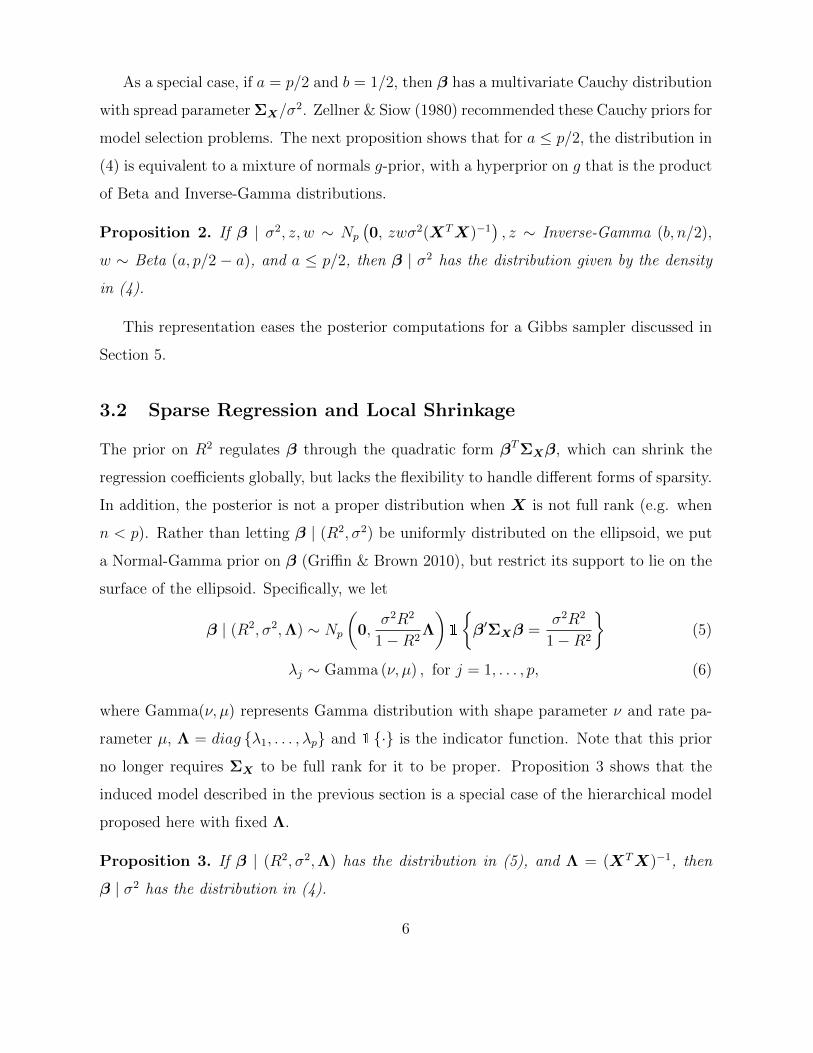
As a special case, if a = p/2 and b = 1/2, then β has a multivariate Cauchy distribution

with spread parameter ΣX/σ2. Zellner & Siow (1980) recommended these Cauchy priors for

model selection problems. The next proposition shows that for a ≤ p/2, the distribution in

(4) is equivalent to a mixture of normals g-prior, with a hyperprior on g that is the product

of Beta and Inverse-Gamma distributions.

Proposition 2. If β | σ2, z, w ∼ Np

(0, zwσ2(XTX)−1

), z ∼ Inverse-Gamma (b, n/2),

w ∼ Beta (a, p/2 − a), and a ≤ p/2, then β | σ2 has the distribution given by the density

in (4).

This representation eases the posterior computations for a Gibbs sampler discussed in

Section 5.

3.2 Sparse Regression and Local Shrinkage

The prior on R2 regulates β through the quadratic form βTΣXβ, which can shrink the

regression coefficients globally, but lacks the flexibility to handle different forms of sparsity.

In addition, the posterior is not a proper distribution when X is not full rank (e.g. when

n < p). Rather than letting β | (R2, σ2) be uniformly distributed on the ellipsoid, we put

a Normal-Gamma prior on β (Griffin & Brown 2010), but restrict its support to lie on the

surface of the ellipsoid. Specifically, we let

β | (R2, σ2,Λ) ∼ Np

(0,

σ2R2

1−R2Λ

)1

{β′ΣXβ =

σ2R2

1−R2

}(5)

λj ∼ Gamma (ν, µ) , for j = 1, . . . , p, (6)

where Gamma(ν, µ) represents Gamma distribution with shape parameter ν and rate pa-

rameter µ, Λ = diag {λ1, . . . , λp} and 1 {·} is the indicator function. Note that this prior

no longer requires ΣX to be full rank for it to be proper. Proposition 3 shows that the

induced model described in the previous section is a special case of the hierarchical model

proposed here with fixed Λ.

Proposition 3. If β | (R2, σ2,Λ) has the distribution in (5), and Λ = (XTX)−1, then

β | σ2 has the distribution in (4).

6

That is, if the contours of the Normal distribution align with the ellipsoid, then we

recover the uniform-on-ellipsoid prior.

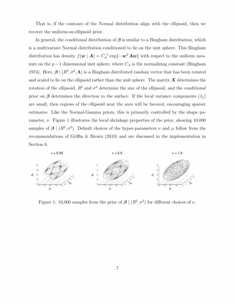
In general, the conditional distribution of β is similar to a Bingham distribution, which

is a multivariate Normal distribution conditioned to lie on the unit sphere. This Bingham

distribution has density f(w | A) = C−1A exp{−wTAw} with respect to the uniform mea-

sure on the p− 1 dimensional unit sphere, where CA is the normalizing constant (Bingham

1974). Here, β | (R2, σ2,Λ) is a Bingham distributed random vector that has been rotated

and scaled to lie on the ellipsoid rather than the unit sphere. The matrix X determines the

rotation of the ellipsoid, R2 and σ2 determine the size of the ellipsoid, and the conditional

prior on β determines the direction to the surface. If the local variance components (λj)

are small, then regions of the ellipsoid near the axes will be favored, encouraging sparser

estimates. Like the Normal-Gamma priors, this is primarily controlled by the shape pa-

rameter, ν. Figure 1 illustrates the local shrinkage properties of the prior, showing 10,000

samples of β | (R2, σ2). Default choices of the hyper-parameters ν and µ follow from the

recommendations of Griffin & Brown (2010) and are discussed in the implementation in

Section 6.

Figure 1: 10,000 samples from the prior of β | (R2, σ2) for different choices of ν.

7

4 Marginal R2 Prior

4.1 The R2-D2 Global-Local Shrinkage Prior

Rather than conditioning on the design X, we now instead show how to construct a prior

while marginalizing out both β and the design. While the conditional version retains the

interpretation of R2 as elliptical contours in the design space, the marginal version allows

for an in depth study of the asymptotic properties of both the prior and the resulting

posterior.

Consider a prior for β satisfying E(β) = 0 and cov(β) = σ2Λ, where Λ is a diagonal

matrix with diagonal elements λ1, · · · , λp. Then

var(xTβ) = Ex{varβ(xTβ | x)}+ varx{Eβ(xTβ | x)} = Ex(σ2xTΛx) + varx(0)

= σ2Ex{tr(xTΛx)} = σ2tr{ΛEx(xxT )} = σ2tr(ΛΣ) = σ2

p∑j=1

λj.

Then R2 is represented as

R2 =var(xTβ)

var(xTβ) + σ2=

σ2p∑j=1

λj

σ2p∑j=1

λj + σ2

=

p∑j=1

λj

p∑j=1

λj + 1

≡ W

W + 1, (7)

where W ≡∑p

j=1 λj is the sum of the prior variances scaled by σ2.

Similarly as conditional R2 prior, we also assume R2 ∼ Beta(a, b), a Beta distribution

with shape parameters a and b. Then in this case, the induced prior density for W =

R2/(1 − R2) is a Beta Prime distribution (Johnson et al. 1995) denoted as BP(a, b), with

probability density function

πW (x) =Γ(a+ b)

Γ(a)Γ(b)

xa−1

(1 + x)a+b, (x > 0).

Therefore W ∼ BP(a, b) is equivalent to R2 ∼ Beta(a, b). The following section will induce

a prior on β based on the distribution of the sum of prior variances, W .

Any prior of the form E(β) = 0, cov(β) = σ2Λ and W =∑p

j=1 λj ∼ BP(a, b) induces a

Beta(a, b) prior on R2. To construct a prior with such properties, we follow the global-local

8

prior framework and express λj = φjω with∑p

j=1 φj = 1. Then W =∑p

j=1 φjω = ω is

the total prior variability, and φj is the proportion of total variance allocated to the j-th

covariate. It is natural to assume that ω ∼ BP(a, b) and the variances across covariates

have a Dirichlet prior with concentration parameter (aπ, · · · , aπ), i.e., φ = (φ1, · · · , φp) ∼

Dir(aπ, · · · , aπ). Since∑p

j=1 φj = 1, E(φj) = 1/p, and var(φj) = (p−1)/{p2(paπ+1)}, then

smaller aπ would lead to larger variance of φj, j = 1, · · · , p, thus more φj would be close to

zero with only a small proportion of larger components; while larger aπ would lead to smaller

variance of φj, j = 1, · · · , p, thus producing a more uniform φ, i.e., φ ≈ (1/p, · · · , 1/p).

So aπ controls the sparsity of the model.

To fully define the global-local prior, we further need to assign a kernel distribution on

each dimension of β. Since the Laplace distribution ensures more mass around zero and

heavier tails than the normal kernel, we consider a Laplace prior on βj for j = 1, · · · , p.

The prior is then summarized as

βj | σ2, φj, ω ∼ DE(σ(φjω/2)1/2), φ ∼ Dir(aπ, · · · , aπ), ω ∼ BP(a, b), (8)

where DE(δ) denotes a double-exponential distribution (i.e., Laplace distribution) with

mean 0 and variance 2δ2. Such prior is induced by a prior on R2 and the total prior

variance of β is decomposed through a Dirichlet prior, therefore we refer to the prior as the

R2-induced Dirichlet Decomposition (R2-D2) prior. Here ω controls the global shrinkage

degree through a and b, while φj controls the local shrinkage through aπ. Assume the

variance σ2 ∼ Inverse-Gamma(a1, b1), an inverse Gamma distribution with shape and scale

parameters a1 and b1 respectively.

Proposition 4. If ω | ξ ∼ Ga(a, ξ) and ξ ∼ Ga(b, 1), then ω ∼ BP(a, b), where Ga(µ, ν)

is the Gamma random variable with shape µ and rate ν.

By applying above Proposition 4, the prior in (8) can also be written as

βj | σ2, φj, ω ∼ DE(σ(φjω/2)1/2), φ ∼ Dir(aπ, · · · , aπ), ω | ξ ∼ Ga(a, ξ), ξ ∼ Ga(b, 1).

Proposition 5. If ω | ξ ∼ Ga(a, ξ), (φ1, · · · , φp) ∼ Dir(aπ, · · · , aπ), and a = paπ, then it

follows φjω | ξ ∼ Ga(aπ, ξ), j = 1, . . . , p independently.

9

Thus, by Proposition 5, when a = paπ, prior in (8) can also be written as

βj | σ2, λj ∼ DE(σ(λj/2)1/2), λj ∼ BP(aπ, b). (9)

or equivalently

βj | σ2, λj ∼ DE(σ(λj/2)1/2), λj | ξ ∼ Ga(aπ, ξ), ξ ∼ Ga(b, 1). (10)

We set a = paπ in the rest of the paper for the R2-D2 prior.

4.2 Properties of the R2-D2 Prior

In this section, the marginal density as well as its theoretical properties of the proposed

R2-D2 prior are established. The properties of the Horseshoe (Carvalho et al. 2009, 2010),

Horseshoe+ (Bhadra et al. 2016), generalized double Pareto prior (Armagan, Dunson & Lee

2013) and Dirichlet-Laplace prior (Bhattacharya et al. 2015) are provided as a comparison.

Proofs and technical details are given in the Appendix.

For simplicity of comparison across different priors, the variance term σ2 is fixed at 1.

Proposition 6. Given the R2-D2 prior (9), the marginal density of βj for any j = 1, · · · , p

is

πR2-D2(βj) =G3,1

1,3

(β2j

2

∣∣∣ 12−baπ− 1

2,0, 1

2

)(2π)1/2Γ(aπ)Γ(b)

=G1,3

3,1

(2β2j

∣∣∣ 32−aπ ,1, 1212

+b

)(2π)1/2Γ(aπ)Γ(b)

where Γ(·) denotes the Gamma function and Gm,np,q

(z∣∣∣b1,...,bqa1,...,ap

)denotes the Meijer G-function

(see Appendix for the detailed definition).

Now we would like to compare the theoretical properties with our proposed R2-D2 prior

with a couple of common global-local shrinkage priors. We first listed these priors.

The Horseshoe prior proposed in Carvalho et al. (2009, 2010) is

βj | λj ∼ N(0, λ2j), λj | τ ∼ C+(0, τ),

where C+(0, τ) denotes a half-Cauchy distribution with scale parameter τ , with density

π(y | τ) = 2/{πτ(1 + (y/τ)2)}.

10

The Horseshoe+ prior proposed in Bhadra et al. (2016) is

βj | λj ∼ N(0, λ2j), λj | τ, ηj ∼ C+(0, τηj), ηj ∼ C+(0, 1).

The Dirichlet-Laplace prior proposed in Bhattacharya et al. (2015) is

βj | ψj ∼ DE(ψj), ψj ∼ Ga(a∗, 1/2). (11)

The normal-beta prime prior proposed in Bai & Ghosh (2019) is as follows:

βj | τj ∼ N(0, τj), τj ∼ BP(a#, b#). (12)

−0.4 −0.2 0.0 0.2 0.4

0.0

0.5

1.0

1.5

2.0

2.5

3.0

β

Mar

gina

l den

sity

R2−D2NBPCauchyHorseshoeHorseshoe+DL

5 10 15 20

0.00

00.

002

0.00

40.

006

0.00

80.

010

β

Mar

gina

l den

sity

R2−D2NBPCauchyHorseshoeHorseshoe+DL

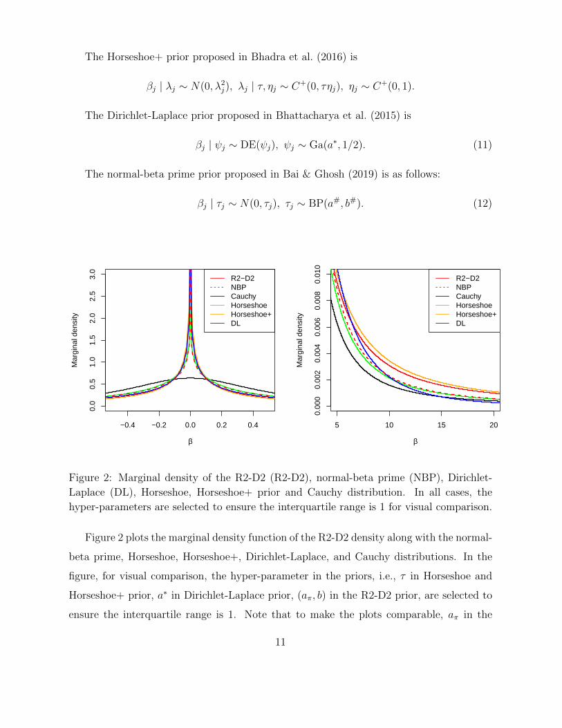
Figure 2: Marginal density of the R2-D2 (R2-D2), normal-beta prime (NBP), Dirichlet-

Laplace (DL), Horseshoe, Horseshoe+ prior and Cauchy distribution. In all cases, the

hyper-parameters are selected to ensure the interquartile range is 1 for visual comparison.

Figure 2 plots the marginal density function of the R2-D2 density along with the normal-

beta prime, Horseshoe, Horseshoe+, Dirichlet-Laplace, and Cauchy distributions. In the

figure, for visual comparison, the hyper-parameter in the priors, i.e., τ in Horseshoe and

Horseshoe+ prior, a∗ in Dirichlet-Laplace prior, (aπ, b) in the R2-D2 prior, are selected to

ensure the interquartile range is 1. Note that to make the plots comparable, aπ in the

11

proposed R2-D2 prior is set as a∗/2, which is half of the hyper-parameter in the Dirichlet-

Laplace prior. It will be shown later that this results in the same behavior around the

origin for the two priors. The other hyper-parameter b in the R2-D2 prior is then tuned to

ensure the interquartile range of 1 to match the others. For the normal-beta prime prior,

we follow the values in Bai & Ghosh (2019), i.e., a# = 0.48 and b# = 0.52 which also

ensures an interquartile range of 1.

From the plot, it appears that the R2-D2 prior can obtain both the highest concentration

around zero and heaviest tail simultaneously. We will quantify these rates exactly in the

next subsection, in Table 1. In particular, we will see that the R2-D2 prior is the only one

obtaining polynomial behavior in both regions.

In the normal means model, van der Pas et al. (2014) and van der Pas et al. (2017a)

investigate the Horseshoe posterior contraction rate, Bhattacharya et al. (2015) shows the

optimal posterior concentration results for Dirichlet-Laplace prior, Bhadra et al. (2016)

proves that the Horseshoe+ posterior concentrates at a faster rate than Horseshoe in the

Kullback-Leibler sense, and Bai & Ghosh (2019) shows that normal-beta prime prior leads

to a near minimax posterior concentration rate.

In this paper, we examine the concentration around zero and tail behaviors of the

marginal densities of a number of priors, and show that our proposed approach simulta-

neously achieves high concentration at the origin and heavy tails. We will also study the

posterior consistency and contraction properties in the high-dimensional regression model

setup. As shown in Figure 2, all five global-local shrinkage priors have a marginal density

with a singularity at zero while with different concentration rate. Except for the Dirichlet-

Laplace prior, all other priors’ marginal density have a heavier tail than the Cauchy dis-

tribution. We formally investigate their marginal densities’ properties in the following

sections.

4.2.1 Asymptotic tail behaviors

We examine the behavior of the tails of the proposed R2-D2 prior in this section. A prior

with heavy tails is desirable in high-dimensional regression to allow the posterior to estimate

12

large values for important predictors.

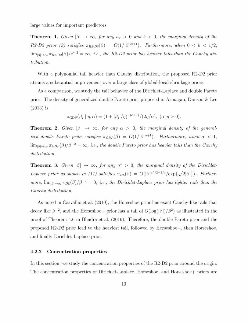
Theorem 1. Given |β| → ∞, for any aπ > 0 and b > 0, the marginal density of the

R2-D2 prior (9) satisfies πR2-D2(β) = O(1/|β|2b+1). Furthermore, when 0 < b < 1/2,

lim|β|→∞ πR2-D2(β)/β−2 = ∞, i.e., the R2-D2 prior has heavier tails than the Cauchy dis-

tribution.

With a polynomial tail heavier than Cauchy distribution, the proposed R2-D2 prior

attains a substantial improvement over a large class of global-local shrinkage priors.

As a comparison, we study the tail behavior of the Dirichlet-Laplace and double Pareto

prior. The density of generalized double Pareto prior proposed in Armagan, Dunson & Lee

(2013) is

πGDP(βj | η, α) = (1 + |βj|/η)−(α+1)/(2η/α), (α, η > 0).

Theorem 2. Given |β| → ∞, for any α > 0, the marginal density of the general-

ized double Pareto prior satisfies πGDP(β) = O(1/|β|α+1). Furthermore, when α < 1,

lim|β|→∞ πGDP(β)/β−2 =∞, i.e., the double Pareto prior has heavier tails than the Cauchy

distribution.

Theorem 3. Given |β| → ∞, for any a∗ > 0, the marginal density of the Dirichlet-

Laplace prior as shown in (11) satisfies πDL(β) = O(|β|a∗/2−3/4/exp{√

2|β|}). Further-

more, lim|β|→∞ πDL(β)/β−2 = 0, i.e., the Dirichlet-Laplace prior has lighter tails than the

Cauchy distribution.

As noted in Carvalho et al. (2010), the Horseshoe prior has exact Cauchy-like tails that

decay like β−2, and the Horseshoe+ prior has a tail of O(log(|β|)/β2) as illustrated in the

proof of Theorem 4.6 in Bhadra et al. (2016). Therefore, the double Pareto prior and the

proposed R2-D2 prior lead to the heaviest tail, followed by Horseshoe+, then Horseshoe,

and finally Dirichlet-Laplace prior.

4.2.2 Concentration properties

In this section, we study the concentration properties of the R2-D2 prior around the origin.

The concentration properties of Dirichlet-Laplace, Horseshoe, and Horseshoe+ priors are

13

also given. We favor priors with high concentration near zero to reflect the prior that most

of the covariates do not have a substantial effect on the response. We now show that R2-D2

prior has higher concentration at zero to go along with heavier tails than other global-local

priors.

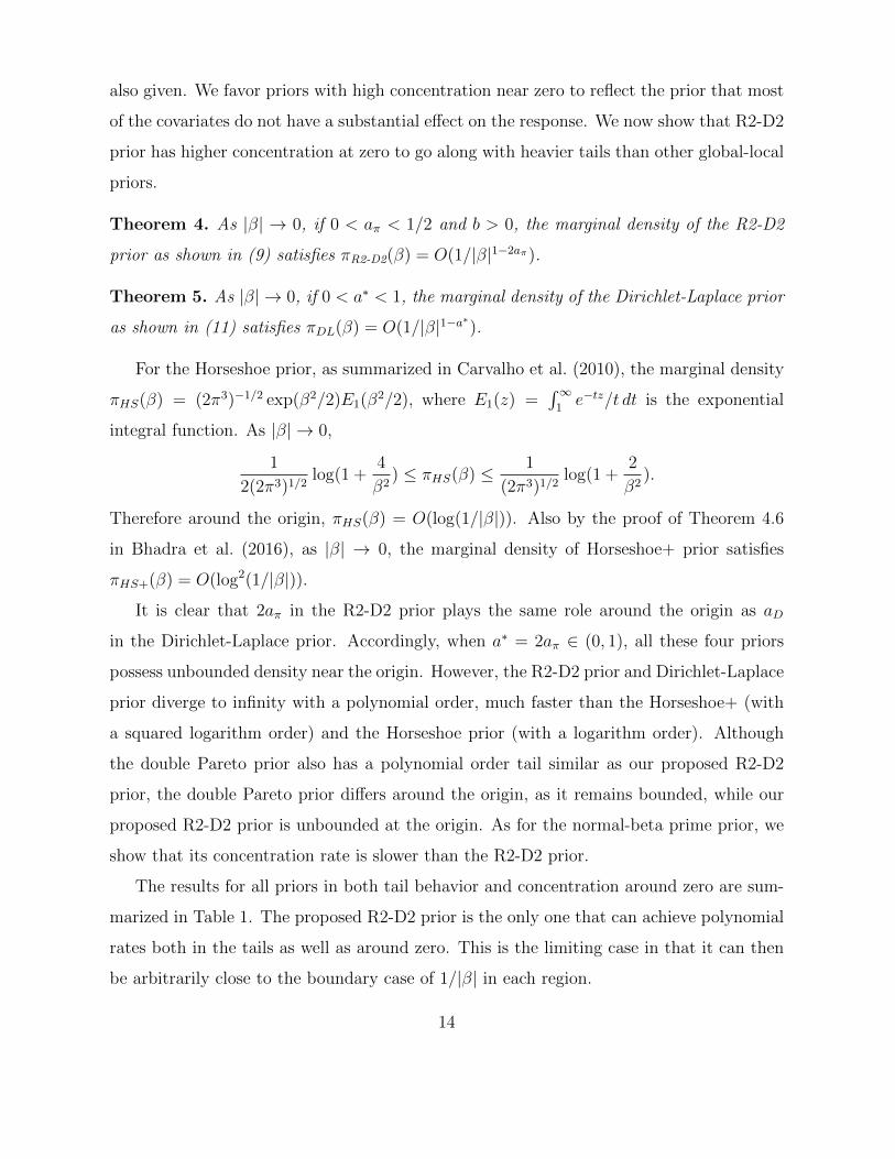
Theorem 4. As |β| → 0, if 0 < aπ < 1/2 and b > 0, the marginal density of the R2-D2

prior as shown in (9) satisfies πR2-D2(β) = O(1/|β|1−2aπ).

Theorem 5. As |β| → 0, if 0 < a∗ < 1, the marginal density of the Dirichlet-Laplace prior

as shown in (11) satisfies πDL(β) = O(1/|β|1−a∗).

For the Horseshoe prior, as summarized in Carvalho et al. (2010), the marginal density

πHS(β) = (2π3)−1/2 exp(β2/2)E1(β2/2), where E1(z) =∫∞

1e−tz/t dt is the exponential

integral function. As |β| → 0,

1

2(2π3)1/2log(1 +

4

β2) ≤ πHS(β) ≤ 1

(2π3)1/2log(1 +

2

β2).

Therefore around the origin, πHS(β) = O(log(1/|β|)). Also by the proof of Theorem 4.6

in Bhadra et al. (2016), as |β| → 0, the marginal density of Horseshoe+ prior satisfies

πHS+(β) = O(log2(1/|β|)).

It is clear that 2aπ in the R2-D2 prior plays the same role around the origin as aD

in the Dirichlet-Laplace prior. Accordingly, when a∗ = 2aπ ∈ (0, 1), all these four priors

possess unbounded density near the origin. However, the R2-D2 prior and Dirichlet-Laplace

prior diverge to infinity with a polynomial order, much faster than the Horseshoe+ (with

a squared logarithm order) and the Horseshoe prior (with a logarithm order). Although

the double Pareto prior also has a polynomial order tail similar as our proposed R2-D2

prior, the double Pareto prior differs around the origin, as it remains bounded, while our

proposed R2-D2 prior is unbounded at the origin. As for the normal-beta prime prior, we

show that its concentration rate is slower than the R2-D2 prior.

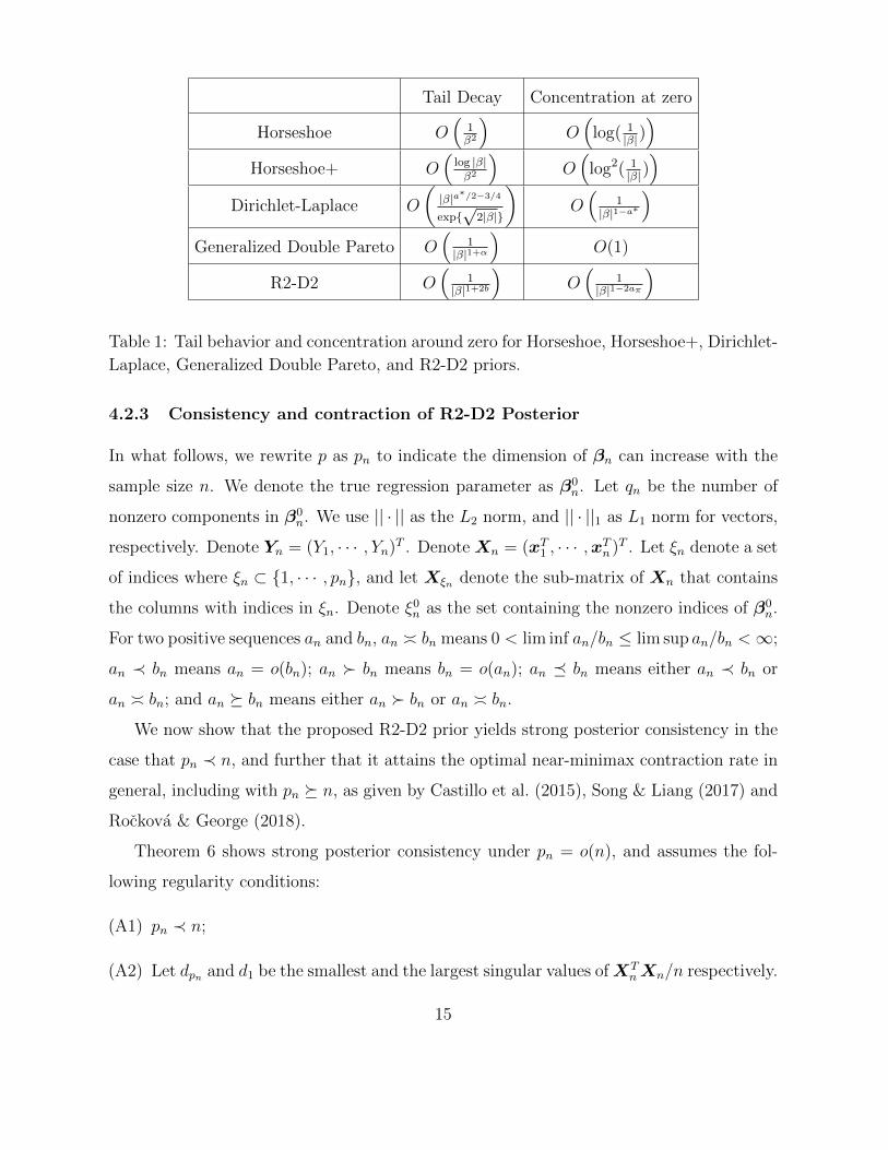
The results for all priors in both tail behavior and concentration around zero are sum-

marized in Table 1. The proposed R2-D2 prior is the only one that can achieve polynomial

rates both in the tails as well as around zero. This is the limiting case in that it can then

be arbitrarily close to the boundary case of 1/|β| in each region.

14

Tail Decay Concentration at zero

Horseshoe O(

1β2

)O(

log( 1|β|))

Horseshoe+ O(

log |β|β2

)O(

log2( 1|β|))

Dirichlet-Laplace O

(|β|a∗/2−3/4

exp{√

2|β|}

)O(

1|β|1−a∗

)Generalized Double Pareto O

(1

|β|1+α

)O(1)

R2-D2 O(

1|β|1+2b

)O(

1|β|1−2aπ

)Table 1: Tail behavior and concentration around zero for Horseshoe, Horseshoe+, Dirichlet-

Laplace, Generalized Double Pareto, and R2-D2 priors.

4.2.3 Consistency and contraction of R2-D2 Posterior

In what follows, we rewrite p as pn to indicate the dimension of βn can increase with the

sample size n. We denote the true regression parameter as β0n. Let qn be the number of

nonzero components in β0n. We use || · || as the L2 norm, and || · ||1 as L1 norm for vectors,

respectively. Denote Yn = (Y1, · · · , Yn)T . Denote Xn = (xT1 , · · · ,xTn )T . Let ξn denote a set

of indices where ξn ⊂ {1, · · · , pn}, and let Xξn denote the sub-matrix of Xn that contains

the columns with indices in ξn. Denote ξ0n as the set containing the nonzero indices of β0

n.

For two positive sequences an and bn, an � bn means 0 < lim inf an/bn ≤ lim sup an/bn <∞;

an ≺ bn means an = o(bn); an � bn means bn = o(an); an � bn means either an ≺ bn or

an � bn; and an � bn means either an � bn or an � bn.

We now show that the proposed R2-D2 prior yields strong posterior consistency in the

case that pn ≺ n, and further that it attains the optimal near-minimax contraction rate in

general, including with pn � n, as given by Castillo et al. (2015), Song & Liang (2017) and

Rockova & George (2018).

Theorem 6 shows strong posterior consistency under pn = o(n), and assumes the fol-

lowing regularity conditions:

(A1) pn ≺ n;

(A2) Let dpn and d1 be the smallest and the largest singular values ofXTnXn/n respectively.

15

Assume 0 < dmin < lim infn→∞ dpn ≤ lim supn→∞ d1 < dmax < ∞, where dmin and

dmax are fixed;

(A3) maxj=1,··· ,pn{|β0nj|} ≤ En for some nondecreasing sequence, En, with log(En) =

O(log n);

(A4) qn = o(n/ log n).

Theorem 6. Under assumptions (A1)–(A4), for any b > 0, given the linear regression

model (1) with known σ2, if aπ = C/(pb/2n nrb/2 log n) for finite r > 0 and C > 0, then the

R2-D2 prior (9) yields a strongly consistent posterior, i.e., for any ε > 0,

Prβ0n

{πn(βn : ||βn − β0

n|| ≥ ε | Yn)→ 0}

= 1 as n→∞.

Theorem 6 shows the posterior strong consistency of the R2-D2 prior under pn ≺ n.

Furthermore, in the high dimensional case, with pn � n, we place an inverse-Gamma prior

on σ2, and denote σ0 as the true parameter value which is unknown but fixed. Theorem 7

shows that the R2-D2 prior contracts at the near-minimax rate in this regime, under the

following regularity conditions:

(B1) All the covariates are uniformly bounded. For simplicity, we assume they are all

bounded by 1;

(B2) pn � n;

(B3) There exists some integer pn and fixed constant d0 such that pn � qn and the smallest

singular value of matrix XTξnXξn/n is no smaller than d0 for any subset model of size

|ξn| ≤ pn;

(B4) maxj=1,...,pn{|β0nj/σ

0|} ≤ En for some nondecreasing sequence, En, with log(En) =

O(log pn).

(B5) qn = o(n/ log pn);

Theorem 7. Assume that (B1)-(B5) hold. Denote εn = M√qn(log pn)/n where M > 0 is

sufficiently large, and let kn �√qn(log pn)/n/pn. Given the linear regression model (1),

16

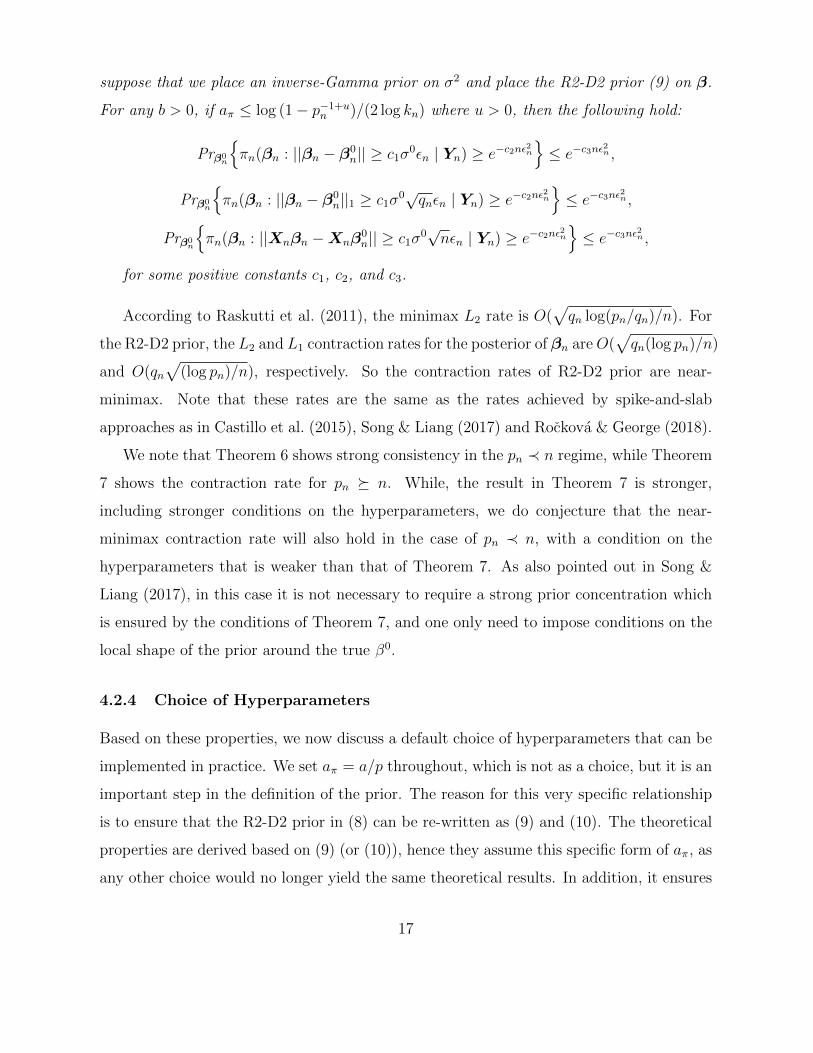
suppose that we place an inverse-Gamma prior on σ2 and place the R2-D2 prior (9) on β.

For any b > 0, if aπ ≤ log (1− p−1+un )/(2 log kn) where u > 0, then the following hold:

Prβ0n

{πn(βn : ||βn − β0

n|| ≥ c1σ0εn | Yn) ≥ e−c2nε

2n

}≤ e−c3nε

2n ,

Prβ0n

{πn(βn : ||βn − β0

n||1 ≥ c1σ0√qnεn | Yn) ≥ e−c2nε

2n

}≤ e−c3nε

2n ,

Prβ0n

{πn(βn : ||Xnβn −Xnβ

0n|| ≥ c1σ

0√nεn | Yn) ≥ e−c2nε

2n

}≤ e−c3nε

2n ,

for some positive constants c1, c2, and c3.

According to Raskutti et al. (2011), the minimax L2 rate is O(√qn log(pn/qn)/n). For

the R2-D2 prior, the L2 and L1 contraction rates for the posterior of βn areO(√qn(log pn)/n)

and O(qn√

(log pn)/n), respectively. So the contraction rates of R2-D2 prior are near-

minimax. Note that these rates are the same as the rates achieved by spike-and-slab

approaches as in Castillo et al. (2015), Song & Liang (2017) and Rockova & George (2018).

We note that Theorem 6 shows strong consistency in the pn ≺ n regime, while Theorem

7 shows the contraction rate for pn � n. While, the result in Theorem 7 is stronger,

including stronger conditions on the hyperparameters, we do conjecture that the near-

minimax contraction rate will also hold in the case of pn ≺ n, with a condition on the

hyperparameters that is weaker than that of Theorem 7. As also pointed out in Song &

Liang (2017), in this case it is not necessary to require a strong prior concentration which

is ensured by the conditions of Theorem 7, and one only need to impose conditions on the

local shape of the prior around the true β0.

4.2.4 Choice of Hyperparameters

Based on these properties, we now discuss a default choice of hyperparameters that can be

implemented in practice. We set aπ = a/p throughout, which is not as a choice, but it is an

important step in the definition of the prior. The reason for this very specific relationship

is to ensure that the R2-D2 prior in (8) can be re-written as (9) and (10). The theoretical

properties are derived based on (9) (or (10)), hence they assume this specific form of aπ, as

any other choice would no longer yield the same theoretical results. In addition, it ensures

17

that the MCMC algorithm is fully Gibbs sampling. With any other choice of aπ, this would

not be the case, and a Metropolis step would be needed in the algorithm.

Hence there are then two parameters to set, a and b. Based on the consistency results,

we suggest to set a as a function of b based on the condition of Theorem 6. This leads to just

one tuning parameter b. This determines the tail behavior and then all other parameters

are fixed from that. For a fully default method, we set b = 0.5 to yield Cauchy-like tails,

but other choices of tail behavior are possible if desired.

To determine a and aπ from a choice of b, note that the condition for consistency in

Theorem 6 requires that aπ = C/(pb/2n nrb/2 log n), where C and r are arbitrary constants.

For a default approach, given the choice of b, we set aπ exactly at C/(pb/2n nrb/2 log n)

choosing the arbitrary constants C and r each to be 1. This is now the default choice and

has been implemented in all of the examples to follow.

5 Posterior Computation

In this section we develop novel Markov chain Monte Carlo (MCMC) samplers for both

the conditional and marginal R2-D2 approaches. The development of these samplers are

of interest directly on their own, as after some transformation and reparametrization, we

are able to obtain efficient feasible methods. In particular, the marginal version and the

conditional uniform on ellipsoid version allow for fully Gibbs samplers. The conditional

version with local shrinkage requires a Metropolis-Hastings sampler and we show how to

sample from this posterior even in the case where p > n and hence XTX is not full rank.

5.1 Gibbs Sampler for the Conditional Uniform-on-Ellipsoid Prior

In Proposition 2, we showed that β | σ2 has a mixture of normals representation for a ≤ p/2.

In practice, we recommend choosing a = p/n as a default, and hence this applies as long

as n > 1. If σ2 is Inverse-Gamma(a1, b1) distributed, then β, σ2, z and w are drawn from

their full conditional distributions in the Gibbs sampler described as follows:

(a) Set initial values for β, σ2, z and w.

18

(b) Sample w | β, σ2, z, by first sampling u ∼ Gamma(p/2− a, βTXTXβ/ (2gσ2)

), and

setting w = 1/(1 + u).

(c) Sample z | β, σ2, w ∼ Inverse-Gamma(p/2 + b, βTXTXβ/ (2wσ2) + 1/2

).

(d) Sample σ2 | β, z, w ∼ Inverse-Gamma((n+ p)/2 + a1, SSE/2 + βTXTXβ/ (2wz) + b1

),

where SSE = (y −Xβ)T (y −Xβ).

(e) Sample β | σ2, z, w ∼ Normal(cβLS, cσ

2(XTX)−1)

, where c = zwzw+1

is the shrinkage

factor, and βLS is the least-squares estimate of β.

(f) Repeat steps b-e until convergence.

5.2 MCMC for the Conditional Local Shrinkage Model

5.2.1 Full-rank case

We now develop a novel MCMC algorithm for the local shrinkage model, sampling from the

full conditionals using a Metropolis-Hastings sampler. First, we take the eigen-decomposition

of ΣX = XTX/n = V DV T , where Vp×p is an orthogonal matrix of eigenvectors, andDp×p

is a diagonal matrix of eigenvalues. R2 is transformed such that θ = R2/(1−R2) has a

Beta-Prime (or Inverted-Beta distribution), with density p(θ) = θa−1 (1 + θ)−a−b /B(a, b).

We also transform β to lie on the unit sphere conditional on the other variables; that is,

γ = D1/2V Tβ/√θσ2. Then γ|Λ has a Bingham distribution, and we can write the full

model as follows.

y | γ, σ2, θ ∼ Nn

(√θσ2XVD−1/2γ, σ2I

)γ | Λ ∼ Bingham

(D−1/2V TΛ−1V D−1/2

)σ2 ∼ Inverse-Gamma(a1, b1)

θ ∼ Beta-Prime(a, b)

λj ∼ Gamma(ν, µ), for j = 1, . . . , .p

19

This parametrization of the prior models the direction of β independently of σ2 and R2.

However, the Bingham distribution of the direction, γ | Λ, contains an intractable normaliz-

ing constant, CX,Λ, depending onX and Λ. Specifically, CX,Λ is a confluent hypergeometric

function with matrix argument A = D−1/2V TΛ−1V D−1/2/2.

The full conditional posterior distribution of γ is a Fisher-Bingham(µ,A) distribution

(Kent 1982), where µ = yTXVD−1/2√θ/σ2. This is equivalent to a Np(A

−1µ,A−1) dis-

tribution conditioned to lie on the p−1 dimensional unit sphere. We sample from this using

the rejection sampler proposed by Kent et al. (2013) with an Angular Central Gaussian

(ACG) envelope distribution. Sampling efficiently from the ACG distribution is possible

because it is just the marginal unit direction of a multivariate Normal distribution with

mean 0, and thus only requires draws from a Normal distribution. Any standard MCMC

algorithm can sample θ and σ2, but the Adaptive Metropolis algorithm (Haario et al. 2001)

automatically accounts for the strong negative correlation between the parameters without

the need for manual tuning. A bivariate Normal proposal distribution is used for (σ2, θ)

with covariance proportional to the running covariance of the samples during the burn-in

phase.

The density function of the full conditional posteriors for variance parameters, λj, al-

most have Generalized Inverse Gaussian distributions (GIG) if it were not for the intractable

term CX,Λ. A Metropolis-Hastings algorithm would require computing this quantity. Our

solution is to propose each candidate λ∗j from a GIG distribution, and introduce auxil-

iary variables, γ∗|Λ∗, from a Bingham distribution in which the constant, CX,Λ∗ , appears

in the density. We calculate the Metropolis-Hastings acceptance probability for (Λ∗,γ∗),

and since CX,Λ∗ appears in the posterior and the proposal distribution, we avoid comput-

ing it. This is the so-called “Exchange Algorithm” proposed by Murray et al. (2006) for

doubly-intractable distributions, and also used by Fallaize & Kypraios (2016) for Bayesian

inference of the Bingham distribution.

The entire sampler for the local shrinkage model is described as follows:

(a) Set initial values for γ, σ2, θ, and Λ.

(b) Sample γ | Λ from a Fisher-Bingham(µ,A) distribution, where µ = yTXVD−1/2√θ/σ2

20

and A = D−1/2V TΛ−1V D−1/2/2.

(c) Sample (σ2, θ) jointly using an Adaptive Metropolis algorithm from a bivariate Nor-

mal distribution.

(d) Exchange algorithm to sample Λ:

(i) Sample λ∗j | uj ∼ GIG(ν, 2µ, u2j), for j = 1, . . . , p, where u = V D−1/2γ.

(ii) Sample u∗ from a Bingham(A∗) distribution, whereA∗ = D−1/2V TΛ∗−1V D−1/2/2

(iii) Accept (Λ∗,u∗) with probability:

p(Λ∗|u)

p(Λ|u)× q(Λ|u)

q(Λ∗|u)× q(u∗|Λ)

q(u∗|Λ∗)= exp

{p∑j=1

u∗2j(1/λ∗2j − 1/λ2

j

)}

(e) Repeat steps (b)-(d) until convergence, and calculate β =√θσ2V D−1/2γ for each

sample.

In step (d), p(Λ | u) is the conditional posterior distribution of Λ; q(Λ | u) is the GIG

proposal distribution with density: p(x; d, a, b) ∝ xd−1exp {−(ax+ b/x)/2},

for −∞ < d < ∞, and a, b > 0; and q(u | Λ) is the Bingham proposal distribution which

has the same constant as in p(Λ | u). We only need to keep Λ∗ at each step, and can

discard u∗. We can efficiently sample from the Bingham distribution because it is a special

case of the Fisher-Bingham with µ = 0 (Kent et al. 2013). All modeling is done in terms

of γ, σ2, θ and Λ, and we calculate β outside the sampler.

5.2.2 Non full-rank case

Next we address how to fit these models with high-dimensional data, where p > n and

XTX is not full rank. The restriction on β : βTΣXβ = σ2θ, is no longer an ellipsoid,

but an unbounded subspace in p-dimensions (e.g. parallel lines for p = 2, and an infinite

cylinder for p = 3). We assume that the rank(X) = n, and partition D =(D1 00 0

)and

V = (V1,V2). Note that D1 is the n× n diagonal matrix of positive eigenvalues, V1 is the

matrix of corresponding eigenvectors, and V2 is the matrix of the p−n eigenvectors spanning

the null space of X. We define γ = (γ1,γ2)T = (D1/21 V T

1 β,VT

2 β)T/√θσ2, so that γ is

21

multivariate Normal with the constraint that γT1 γ1 = 1. Marginally, γ1 = D1/21 V T

1 β/√θσ2

is defined on the n − 1 dimensional unit sphere, and has a Fisher-Bingham distribution

just like the full rank case. However, the reverse transformation β =√θσ2V1D

−1/21 γ1

is defined on the lower n − 1 dimensional ellipsoid within the entire constrained space

{β : βTΣXβ = σ2θ}. For example, if p = 3 and n = 2, this is the slice of the 3-dimensional

ellipsoid with the minimum L2-norm. The problem is that this lower dimensional ellipsoid

may not be able to favor the sparsity or local shrinkage encouraged by Λ. That would

be equivalent to principal components regression using the top n principal components.

To allow for shrinkage of the original coefficients and not the principal components, we

sample γ2 | γ1, which is multivariate Normal, and make the reverse transformation β =√θσ2

(V1D

−1/21 γ1 + V2γ2

). Since V2 spans the null space ofX, β is still in the constrained

region, but offers more flexibility in shrinking βj.

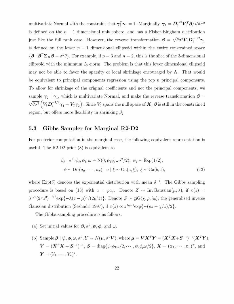
5.3 Gibbs Sampler for Marginal R2-D2

For posterior computation in the marginal case, the following equivalent representation is

useful. The R2-D2 prior (8) is equivalent to

βj | σ2, ψj, φj, ω ∼ N(0, ψjφjωσ2/2), ψj ∼ Exp(1/2),

φ ∼ Dir(aπ, · · · , aπ), ω | ξ ∼ Ga(a, ξ), ξ ∼ Ga(b, 1), (13)

where Exp(δ) denotes the exponential distribution with mean δ−1. The Gibbs sampling

procedure is based on (13) with a = paπ. Denote Z ∼ InvGaussian(µ, λ), if π(z) =

λ1/2(2πz3)−1/2

exp{−λ(z − µ)2/(2µ2z)}. Denote Z ∼ giG(χ, ρ, λ0), the generalized inverse

Gaussian distribution (Seshadri 1997), if π(z) ∝ zλ0−1exp{−(ρz + χ/z)/2}.

The Gibbs sampling procedure is as follows:

(a) Set initial values for β, σ2,ψ,φ, and ω.

(b) Sample β | ψ,φ, ω, σ2,Y ∼ N(µ, σ2V ), where µ = V XTY = (XTX+S−1)−1(XTY ),

V = (XTX + S−1)−1, S = diag{ψ1φ1ω/2, · · · , ψpφpω/2}, X = (x1, · · · ,xn)T , and

Y = (Y1, · · · , Yn)T .

22

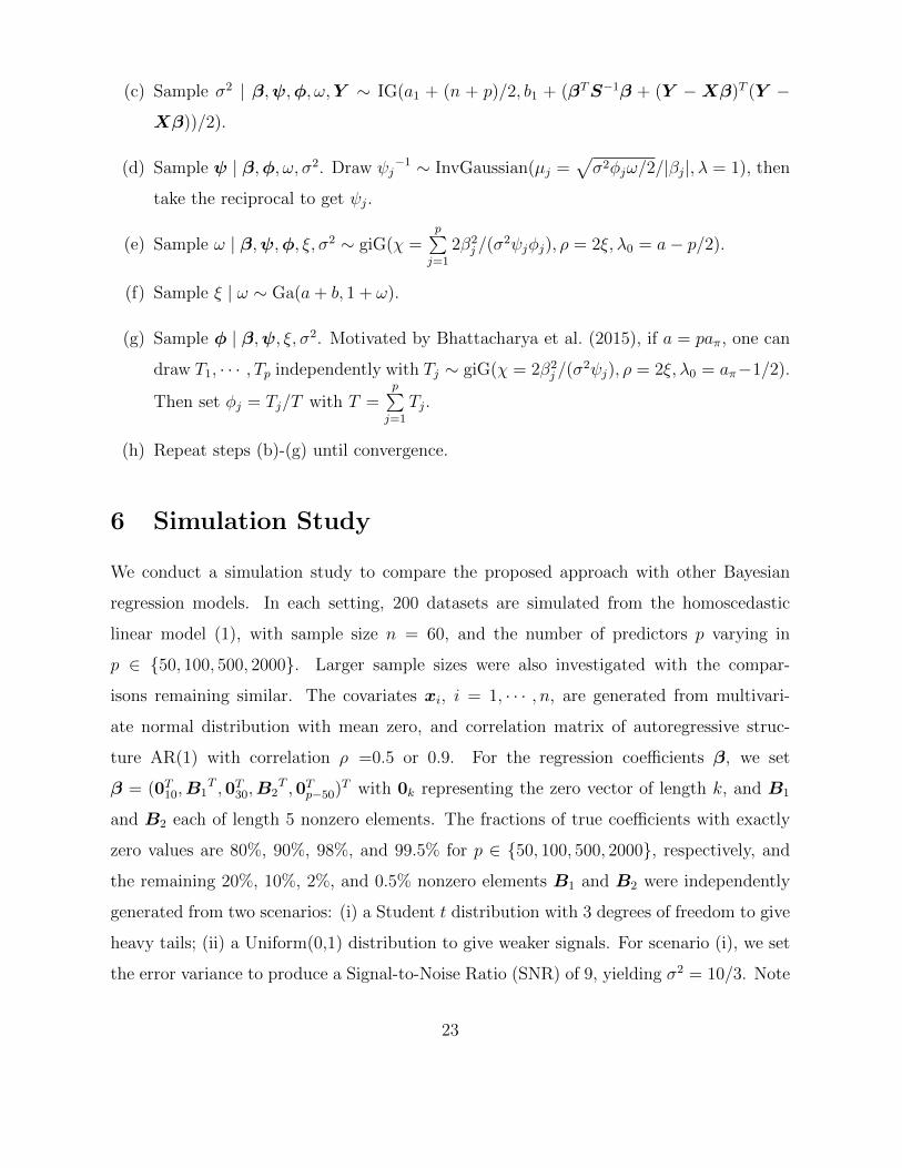
(c) Sample σ2 | β,ψ,φ, ω,Y ∼ IG(a1 + (n + p)/2, b1 + (βTS−1β + (Y −Xβ)T (Y −

Xβ))/2).

(d) Sample ψ | β,φ, ω, σ2. Draw ψj−1 ∼ InvGaussian(µj =

√σ2φjω/2/|βj|, λ = 1), then

take the reciprocal to get ψj.

(e) Sample ω | β,ψ,φ, ξ, σ2 ∼ giG(χ =p∑j=1

2β2j /(σ

2ψjφj), ρ = 2ξ, λ0 = a− p/2).

(f) Sample ξ | ω ∼ Ga(a+ b, 1 + ω).

(g) Sample φ | β,ψ, ξ, σ2. Motivated by Bhattacharya et al. (2015), if a = paπ, one can

draw T1, · · · , Tp independently with Tj ∼ giG(χ = 2β2j /(σ

2ψj), ρ = 2ξ, λ0 = aπ−1/2).

Then set φj = Tj/T with T =p∑j=1

Tj.

(h) Repeat steps (b)-(g) until convergence.

6 Simulation Study

We conduct a simulation study to compare the proposed approach with other Bayesian

regression models. In each setting, 200 datasets are simulated from the homoscedastic

linear model (1), with sample size n = 60, and the number of predictors p varying in

p ∈ {50, 100, 500, 2000}. Larger sample sizes were also investigated with the compar-

isons remaining similar. The covariates xi, i = 1, · · · , n, are generated from multivari-

ate normal distribution with mean zero, and correlation matrix of autoregressive struc-

ture AR(1) with correlation ρ =0.5 or 0.9. For the regression coefficients β, we set

β = (0T10,B1T ,0T30,B2

T ,0Tp−50)T with 0k representing the zero vector of length k, and B1

and B2 each of length 5 nonzero elements. The fractions of true coefficients with exactly

zero values are 80%, 90%, 98%, and 99.5% for p ∈ {50, 100, 500, 2000}, respectively, and

the remaining 20%, 10%, 2%, and 0.5% nonzero elements B1 and B2 were independently

generated from two scenarios: (i) a Student t distribution with 3 degrees of freedom to give

heavy tails; (ii) a Uniform(0,1) distribution to give weaker signals. For scenario (i), we set

the error variance to produce a Signal-to-Noise Ratio (SNR) of 9, yielding σ2 = 10/3. Note

23

that since the generated coefficients have expectation of zero, the SNR does not depend

on the correlation structure of the covariates. For scenario (ii), the nonzero expectation

of the Uniform(0,1) then entails a different SNR for the 2 different correlation setups. For

this scenario, we set σ2 = 6 to yield SNR ≈ 0.5 and 0.7 in the ρ = 0.5 and 0.9 cases,

respectively.

To implement both the marginal and conditional R2-D2 priors, as discussed as a default

choice in Section 4.2.4, we set b = 0.5 to yield Cauchy-like tails, and aπ = C/(pb/2n nrb/2 log n)

with choosing the arbitrary constants C and r to be 1. We also set b = 0.1 to give

heavier tails (then setting aπ in the same manner). The results for b = 0.1 were similar

to b = 0.5 and thus not shown, and we recommend as a default to use b = 0.5 as a fully

automatic approach. For the conditional R2-D2, the choices of ν and µ in the Gamma prior

are based on the recommendations for implementation of Normal-Gamma priors given in

Griffin & Brown (2010). The choice is based on the degree of sparsity, which we choose as

min{n, 0.1p} so that we set the expected number of non-zero coefficients to be 10% of the

total, or the sample size, whichever is smaller. Details of how ν and µ relate to the sparsity

level are given in the Appendix.

The comparisons are made to some current state-of-the-art global-local priors: Horse-

shoe, Horseshoe+, Normal-Beta Prime and Dirichlet-Laplace.

For the Horseshoe, Dirichlet-Laplace, and Normal-Beta Prime, the implementation is

done via the R packages horseshoe, dlbayes, and NormalBetaPrime, respectively. The

Horseshoe+ is implemented through Stan in R using the code provided by the author of

Bhadra et al. (2016). The proposed R2-D2 approaches are implemented in R, based on the

discussed MCMC sampling.

In all cases, 10, 000 samples are collected with the first 5, 000 samples discarded as

burn-in.

Estimation error and AUC. The average sum of squared error corresponding to the

posterior mean across the 200 replicates is provided in Table 2 for simulation setting i for

p =100 and 500 and in Table 3 for simulation setting ii. In addition, the averaged area

under the Receiver-Operating Characteristic (ROC) curve (AUC) based on the posterior

24

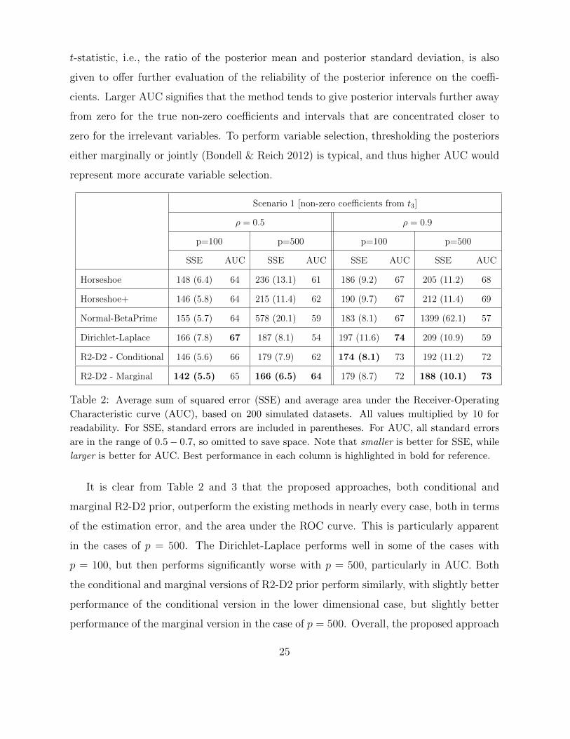
t-statistic, i.e., the ratio of the posterior mean and posterior standard deviation, is also

given to offer further evaluation of the reliability of the posterior inference on the coeffi-

cients. Larger AUC signifies that the method tends to give posterior intervals further away

from zero for the true non-zero coefficients and intervals that are concentrated closer to

zero for the irrelevant variables. To perform variable selection, thresholding the posteriors

either marginally or jointly (Bondell & Reich 2012) is typical, and thus higher AUC would

represent more accurate variable selection.

Scenario 1 [non-zero coefficients from t3]

ρ = 0.5 ρ = 0.9

p=100 p=500 p=100 p=500

SSE AUC SSE AUC SSE AUC SSE AUC

Horseshoe 148 (6.4) 64 236 (13.1) 61 186 (9.2) 67 205 (11.2) 68

Horseshoe+ 146 (5.8) 64 215 (11.4) 62 190 (9.7) 67 212 (11.4) 69

Normal-BetaPrime 155 (5.7) 64 578 (20.1) 59 183 (8.1) 67 1399 (62.1) 57

Dirichlet-Laplace 166 (7.8) 67 187 (8.1) 54 197 (11.6) 74 209 (10.9) 59

R2-D2 - Conditional 146 (5.6) 66 179 (7.9) 62 174 (8.1) 73 192 (11.2) 72

R2-D2 - Marginal 142 (5.5) 65 166 (6.5) 64 179 (8.7) 72 188 (10.1) 73

Table 2: Average sum of squared error (SSE) and average area under the Receiver-Operating

Characteristic curve (AUC), based on 200 simulated datasets. All values multiplied by 10 for

readability. For SSE, standard errors are included in parentheses. For AUC, all standard errors

are in the range of 0.5− 0.7, so omitted to save space. Note that smaller is better for SSE, while

larger is better for AUC. Best performance in each column is highlighted in bold for reference.

It is clear from Table 2 and 3 that the proposed approaches, both conditional and

marginal R2-D2 prior, outperform the existing methods in nearly every case, both in terms

of the estimation error, and the area under the ROC curve. This is particularly apparent

in the cases of p = 500. The Dirichlet-Laplace performs well in some of the cases with

p = 100, but then performs significantly worse with p = 500, particularly in AUC. Both

the conditional and marginal versions of R2-D2 prior perform similarly, with slightly better

performance of the conditional version in the lower dimensional case, but slightly better

performance of the marginal version in the case of p = 500. Overall, the proposed approach

25

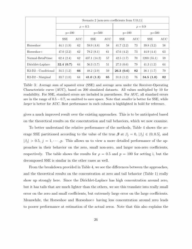
Scenario 2 [non-zero coefficients from U(0,1)]

ρ = 0.5 ρ = 0.9

p=100 p=500 p=100 p=500

SSE AUC SSE AUC SSE AUC SSE AUC

Horseshoe 44.1 (1.9) 62 59.9 (4.8) 58 41.7 (2.2) 73 39.8 (3.2) 58

Horseshoe+ 47.0 (2.2) 62 79.2 (8.1) 61 47.6 (4.2) 73 44.9 (4.4) 63

Normal-BetaPrime 62.4 (2.4) 62 437.1 (14.2) 57 42.5 (1.7) 70 1203 (55.1) 59

Dirichlet-Laplace 32.4 (0.7) 64 56.3 (5.7) 51 27.3 (0.6) 79 41.3 (1.2) 64

R2-D2 - Conditional 34.5 (1.2) 66 48.2 (2.9) 59 26.3 (0.6) 82 38.1 (1.7) 79

R2-D2 - Marginal 33.7 (1.0) 64 41.0 (1.3) 65 31.8 (1.2) 76 34.5 (1.0) 82

Table 3: Average sum of squared error (SSE) and average area under the Receiver-Operating

Characteristic curve (AUC), based on 200 simulated datasets. All values multiplied by 10 for

readability. For SSE, standard errors are included in parentheses. For AUC, all standard errors

are in the range of 0.5− 0.7, so omitted to save space. Note that smaller is better for SSE, while

larger is better for AUC. Best performance in each column is highlighted in bold for reference.

gives a much improved result over the existing approaches. This is to be anticipated based

on the theoretical results on the concentration and tail behaviors, which we now examine.

To better understand the relative performance of the methods, Table 4 shows the av-

erage SSE partitioned according to the value of the true β at βj = 0, |βj| ∈ (0, 0.5], and

|βj| > 0.5, j = 1, · · · , p. This allows us to view a more detailed performance of the ap-

proaches in their behavior on the zero, small non-zero, and larger non-zero coefficients,

respectively. The table shows the results for ρ = 0.5 and p = 100 for setting i, but the

decomposed SSE is similar in the other cases as well.

From the breakdown provided in Table 4, we see the differences between the approaches,

and the theoretical results on the concentration at zero and tail behavior (Table 1) really

show up strongly here. Since the Dirichlet-Laplace has high concentration around zero,

but it has tails that are much lighter than the others, we see this translate into really small

error on the zero and small coefficients, but extremely large error on the large coefficients.

Meanwhile, the Horseshoe and Horseshoe+ having less concentration around zero leads

to poorer performance at estimation of the actual zeros. Note that this also explains the

26

β = 0 |β| ∈ (0, 0.5] |β| > 0.5 Total

Horseshoe 21 24 103 148

Horseshoe+ 18 22 106 146

Normal-BetaPrime 35 38 82 155

Dirichlet-Laplace 4 6 156 166

R2D2 - Conditional 14 18 114 146

R2D2 - Marginal 10 13 119 142

Table 4: Average sum of squared error broken down by zero coefficients (β = 0), small

coefficients (|β| ∈ (0,0.5]), large coefficients (|β| >0.5]), and Total. Results are based on

the 200 datasets from Table 2 with p = 100 and ρ = 0.5.

reason for the Horseshoe and Horseshoe+ having worse AUC, as it does not push the zeros

close enough to zero in order to distinguish them from the small coefficients. Note that

the R2-D2 was set with b = 0.5 giving it the Cauchy-like tails as is the case with the

Horseshoe. Thus we see similar estimation ability for the larger coefficients. Overall, the

proposed R2-D2 approach achieves a strong performance in both regions simultaneously as

anticipated by the theory.

Credible Interval Coverage. We also examine the coverage properties of using 95%

marginal credible intervals for each approach. For this same scenario, table 5 reports

the average width of the intervals, the proportion of coverage, the Specificity, and the

Sensitivity. This gives a broader picture of the posterior inference properties. Although,

there is no promise of 95% Frequentist coverage by the 95% intervals, we see that in this

case of n = 60 and p = 100, the coverage of most of the approaches are close to 95%, with

the proposed approaches and the Horseshoe+ being almost right on the value, while the

Horseshoe and DL are a bit lower than the target, and the NBP being a bit large. For

the n = 60 case, this is a very difficult problem even when p = 100, and we see that the

sensitivity (power) for all approaches are quite low due to the intervals containing zero

even for the majority of the true non-zeros. The sensitivity for the R2-D2 approaches

are highest, along with the Horseshoe+ and Normal-Beta Prime. However, in order to do

so, the Horseshoe+ and Normal-Beta Prime intervals are quite wide in comparison, thus

27

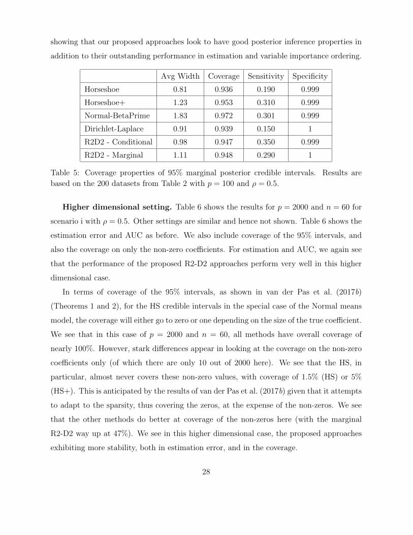
showing that our proposed approaches look to have good posterior inference properties in

addition to their outstanding performance in estimation and variable importance ordering.

Avg Width Coverage Sensitivity Specificity

Horseshoe 0.81 0.936 0.190 0.999

Horseshoe+ 1.23 0.953 0.310 0.999

Normal-BetaPrime 1.83 0.972 0.301 0.999

Dirichlet-Laplace 0.91 0.939 0.150 1

R2D2 - Conditional 0.98 0.947 0.350 0.999

R2D2 - Marginal 1.11 0.948 0.290 1

Table 5: Coverage properties of 95% marginal posterior credible intervals. Results are

based on the 200 datasets from Table 2 with p = 100 and ρ = 0.5.

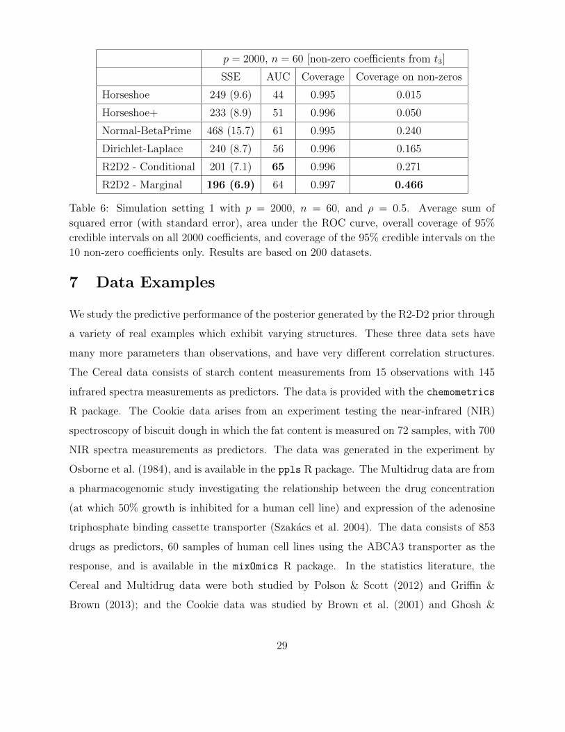
Higher dimensional setting. Table 6 shows the results for p = 2000 and n = 60 for

scenario i with ρ = 0.5. Other settings are similar and hence not shown. Table 6 shows the

estimation error and AUC as before. We also include coverage of the 95% intervals, and

also the coverage on only the non-zero coefficients. For estimation and AUC, we again see

that the performance of the proposed R2-D2 approaches perform very well in this higher

dimensional case.

In terms of coverage of the 95% intervals, as shown in van der Pas et al. (2017b)

(Theorems 1 and 2), for the HS credible intervals in the special case of the Normal means

model, the coverage will either go to zero or one depending on the size of the true coefficient.

We see that in this case of p = 2000 and n = 60, all methods have overall coverage of

nearly 100%. However, stark differences appear in looking at the coverage on the non-zero

coefficients only (of which there are only 10 out of 2000 here). We see that the HS, in

particular, almost never covers these non-zero values, with coverage of 1.5% (HS) or 5%

(HS+). This is anticipated by the results of van der Pas et al. (2017b) given that it attempts

to adapt to the sparsity, thus covering the zeros, at the expense of the non-zeros. We see

that the other methods do better at coverage of the non-zeros here (with the marginal

R2-D2 way up at 47%). We see in this higher dimensional case, the proposed approaches

exhibiting more stability, both in estimation error, and in the coverage.

28

p = 2000, n = 60 [non-zero coefficients from t3]

SSE AUC Coverage Coverage on non-zeros

Horseshoe 249 (9.6) 44 0.995 0.015

Horseshoe+ 233 (8.9) 51 0.996 0.050

Normal-BetaPrime 468 (15.7) 61 0.995 0.240

Dirichlet-Laplace 240 (8.7) 56 0.996 0.165

R2D2 - Conditional 201 (7.1) 65 0.996 0.271

R2D2 - Marginal 196 (6.9) 64 0.997 0.466

Table 6: Simulation setting 1 with p = 2000, n = 60, and ρ = 0.5. Average sum of

squared error (with standard error), area under the ROC curve, overall coverage of 95%

credible intervals on all 2000 coefficients, and coverage of the 95% credible intervals on the

10 non-zero coefficients only. Results are based on 200 datasets.

7 Data Examples

We study the predictive performance of the posterior generated by the R2-D2 prior through

a variety of real examples which exhibit varying structures. These three data sets have

many more parameters than observations, and have very different correlation structures.

The Cereal data consists of starch content measurements from 15 observations with 145

infrared spectra measurements as predictors. The data is provided with the chemometrics

R package. The Cookie data arises from an experiment testing the near-infrared (NIR)

spectroscopy of biscuit dough in which the fat content is measured on 72 samples, with 700

NIR spectra measurements as predictors. The data was generated in the experiment by

Osborne et al. (1984), and is available in the ppls R package. The Multidrug data are from

a pharmacogenomic study investigating the relationship between the drug concentration

(at which 50% growth is inhibited for a human cell line) and expression of the adenosine

triphosphate binding cassette transporter (Szakacs et al. 2004). The data consists of 853

drugs as predictors, 60 samples of human cell lines using the ABCA3 transporter as the

response, and is available in the mixOmics R package. In the statistics literature, the

Cereal and Multidrug data were both studied by Polson & Scott (2012) and Griffin &

Brown (2013); and the Cookie data was studied by Brown et al. (2001) and Ghosh &

29

Ghattas (2015).

The three datasets nicely represent 3 different correlation structures among the predictor

variables. The Multidrug covariates have low to moderate pairwise correlations, the Cookie

covariates are highly positively correlated, and the Cereal covariates have a wide range that

are both positively and negatively correlated. Figure 3 shows histograms of all pairwise

correlations for each of the data sets.

Figure 3: Histograms of pairwise correlations among the predictor variables for the three

datasets.

Cereal Cookie Multidrug

n 15 72 60

p 145 700 853

Horseshoe 14.1 (1.0) 8.3 (0.2) 15.6 (0.5)

Horseshoe+ 14.2 (0.9) 9.1 (0.3) 15.0 (0.5)

Normal-BetaPrime 25.4 (1.5) 11.9 (0.4) 18.4 (0.6)

Dirichlet-Laplace 15.1 (1.2) 12.1 (0.5) 12.2 (0.3)

R2-D2 - Conditional 12.2 (0.5) 9.8 (0.3) 12.7 (0.3)

R2-D2 - Marginal 12.1 (0.5) 8.1 (0.2) 12.6 (0.3)

Table 7: Average mean square prediction error (and standard errors) for each of the data

examples.

We randomly split each data set into a training and testing sets to evaluate the out-

of-sample predictive performance. For each data set, 75% of the observations were used

for training, and the remaining 25% were used for estimating the mean squared prediction

30

error (MSPE) between the test sample and predictions. This process was repeated to create

200 data sets for each example. The same 5 approaches as in the simulations were used on

each of the datasets. Due to the various correlation structures and dimensions, this gives

a range of potential data structures for comparison of the approaches.

The average MSPE results are given in Table 7. We see that the R2-D2 approaches

consistently outperform the existing methods across the datasets. Note that the Horseshoe

and Horseshoe+ perform well on the Cookie data, but are significantly worse than the

others on the other 2 datasets.

8 Discussion

In this paper, we propose a shrinkage prior motivated by assuming a prior on R2. The

prior exhibits polynomial behavior both around the origin and in the tails and compares

favorably with other global-local shrinkage priors. Although the motivation of our R2-D2

prior is via starting with a prior on R2, the resultant prior is simply a member of the

class of global-local shrinkage priors, which can then be applied directly to other models,

as with other priors. The prior is represented by a hierarchical scale mixture of normals,

which can then be implemented in a generalized linear model or other regression setting.

The hyperparameters would no longer have the interpretation as parameters of a Beta

prior on the R2 of the model. But the form and properties of the resulting prior, such as

tail behavior and concentration around zero remain directly useable as is with the other

global-local priors.

There is scope for further advances in algorithms for MCMC sampling for these poste-

riors, just as there has been for sampling from other prior proposals, as for example, key

sampling approaches for the high-dimensional case as in Bhattacharya et al. (2016).

References

Armagan, A., Clyde, M. & Dunson, D. B. (2011), Generalized beta mixtures of Gaussians,

in ‘Advances in neural information processing systems’, pp. 523–531.

31

Armagan, A., Dunson, D. B. & Lee, J. (2013), ‘Generalized double Pareto shrinkage’,

Statistica Sinica 23(1), 119.

Armagan, A., Dunson, D. B., Lee, J., Bajwa, W. U. & Strawn, N. (2013), ‘Posterior

consistency in linear models under shrinkage priors’, Biometrika 100(4), 1011–1018.

Bai, R. & Ghosh, M. (2019), ‘Large-scale multiple hypothesis testing with the normal-beta

prime prior’, Statistics 53(6), 1210–1233.

Bateman, H. (1953), Higher Transcendental Functions [Volumes I-III], Vol. 1, McGraw-Hill

Book Company.

Bhadra, A., Datta, J., Polson, N. G. & Willard, B. (2016), ‘The horseshoe+ estimator of

ultra-sparse signals’, Bayesian Analysis .

Bhattacharya, A., Chakraborty, A. & Mallick, B. (2016), ‘Fast sampling with gaussian

scale-mixture priors in high-dimensional regression’, Biometrika 103(4), 985–991.

Bhattacharya, A., Pati, D., Pillai, N. S. & Dunson, D. B. (2015), ‘Dirichlet–laplace priors

for optimal shrinkage’, Journal of the American Statistical Association 110(512), 1479–

1490.

Bingham, C. (1974), ‘An antipodally symmetric distribution on the sphere’, The Annals of

Statistics pp. 1201–1225.

Bondell, H. D. & Reich, B. J. (2012), ‘Consistent high-dimensional bayesian variable se-

lection via penalized credible regions’, Journal of the American Statistical Association

107(500), 1610–1624.

Brown, P. J., Fearn, T. & Vannucci, M. (2001), ‘Bayesian wavelet regression on curves with

application to a spectroscopic calibration problem’, Journal of the American Statistical

Association 96(454), 398–408.

Carvalho, C. M., Polson, N. G. & Scott, J. G. (2009), Handling sparsity via the horseshoe,

in ‘International Conference on Artificial Intelligence and Statistics’, pp. 73–80.

32

Carvalho, C. M., Polson, N. G. & Scott, J. G. (2010), ‘The Horseshoe estimator for sparse

signals’, Biometrika 97, 465–480.

Castillo, I., Schmidt-Hieber, J. & van der Vaart, A. (2015), ‘Bayesian linear regression with

sparse priors’, The Annals of Statistics 43(5), 1986–2018.

DLMF (2015), ‘NIST Digital Library of Mathematical Functions’, http://dlmf.nist.gov/,

Release 1.0.10 of 2015-08-07. Online companion to Olver et al. (2010).

URL: http://dlmf.nist.gov/

Fallaize, C. J. & Kypraios, T. (2016), ‘Exact bayesian inference for the bingham distribu-

tion’, Statistics and Computing 26(1-2), 349–360.

Fields, J. L. (1972), ‘The asymptotic expansion of the Meijer G-function’, Mathematics of

Computation pp. 757–765.

George, E. I. & McCulloch, R. E. (1993), ‘Variable selection via Gibbs sampling’, Journal

of the American Statistical Association 88(423), 881–889.

Ghosh, J. & Ghattas, A. E. (2015), ‘Bayesian variable selection under collinearity’, The

American Statistician 69(3), 165–173.

Griffin, J. E. & Brown, P. J. (2010), ‘Inference with normal-gamma prior distributions in

regression problems’, Bayesian Analysis 5(1), 171–188.

Griffin, J. E. & Brown, P. J. (2013), ‘Some priors for sparse regression modelling’, Bayesian

Analysis 8(3), 691–702.

Haario, H., Saksman, E. & Tamminen, J. (2001), ‘An adaptive metropolis algorithm’,

Bernoulli pp. 223–242.

Hans, C., Dobra, A. & West, M. (2007), ‘Shotgun stochastic search for large p regression’,

Journal of the American Statistical Association 102(478), 507–516.

Ishwaran, H. & Rao, J. S. (2005), ‘Spike and slab variable selection: Frequentist and

Bayesian strategies’, Annals of Statistics pp. 730–773.

33

Johnson, N., Kotz, S. & Balakrishnan, N. (1995), ‘Continuous univariate distributions,

volume 2. john wiley&sons’, Inc., 75.

Kent, J. T. (1982), ‘The fisher-bingham distribution on the sphere’, Journal of the Royal

Statistical Society. Series B (Methodological) pp. 71–80.

Kent, J. T., Ganeiber, A. M. & Mardia, K. V. (2013), ‘A new method to simulate the

bingham and related distributions in directional data analysis with applications’, arXiv

preprint arXiv:1310.8110 .

Miller, P. D. (2006), Applied asymptotic analysis, Vol. 75, American Mathematical Soc.

Mitchell, T. J. & Beauchamp, J. J. (1988), ‘Bayesian variable selection in linear regression’,

Journal of the American Statistical Association 83(404), 1023–1032.

Murray, I., Ghahramani, Z. & MacKay, D. (2006), Mcmc for doubly-intractable distribu-

tions, in ‘Proceedings of the 22nd annual conference on uncertainty in artificial intelli-

gence’, AUAI Press, pp. 359–366.

Narisetty, N. N. & He, X. (2014), ‘Bayesian variable selection with shrinking and diffusing

priors’, The Annals of Statistics 42(2), 789–817.

Olver, F. W. J., Lozier, D. W., Boisvert, R. F. & Clark, C. W., eds (2010), NIST Hand-

book of Mathematical Functions, Cambridge University Press, New York, NY. Print

companion to DLMF (2015).

Ormerod, J. T., You, C. & Muller, S. (2017), ‘A variational bayes approach to variable

selection’, Electronic Journal of Statistics 11(2), 3549–3594.

Osborne, B. G., Fearn, T., Miller, A. R. & Douglas, S. (1984), ‘Application of near infrared

reflectance spectroscopy to the compositional analysis of biscuits and biscuit doughs’,

Journal of the Science of Food and Agriculture 35(1), 99–105.

Polson, N. G. & Scott, J. G. (2010), ‘Shrink globally, act locally: Sparse bayesian regular-

ization and prediction’, Bayesian Statistics 9, 501–538.

34

Polson, N. G. & Scott, J. G. (2012), ‘Local shrinkage rules, levy processes and regularized

regression’, Journal of the Royal Statistical Society: Series B (Statistical Methodology)

74(2), 287–311.

Raskutti, G., Wainwright, M. J. & Yu, B. (2011), ‘Minimax rates of estimation for high-

dimensional linear regression over `q-balls’, IEEE transactions on information theory

57(10), 6976–6994.

Rockova, V. & George, E. I. (2014), ‘Emvs: The em approach to bayesian variable selection’,

Journal of the American Statistical Association 109(506), 828–846.

Rockova, V. & George, E. I. (2018), ‘The spike-and-slab lasso’, Journal of the American

Statistical Association 113(521), 431–444.

Scott, S. L. & Varian, H. R. (2014), ‘Predicting the present with bayesian structural time

series’, International Journal of Mathematical Modelling and Numerical Optimisation

5(1-2), 4–23.

Seshadri, V. (1997), ‘Halphen’s laws’, Encyclopedia of statistical sciences .

Song, Q. & Liang, F. (2017), ‘Nearly optimal bayesian shrinkage for high dimensional

regression’, arXiv preprint arXiv:1712.08964 .

Szakacs, G., Annereau, J.-P., Lababidi, S., Shankavaram, U., Arciello, A., Bussey, K. J.,

Reinhold, W., Guo, Y., Kruh, G. D. & Reimers, M. (2004), ‘Predicting drug sensitivity

and resistance: profiling abc transporter genes in cancer cells’, Cancer cell 6(2), 129–137.

van der Pas, S. L., Kleijn, B. J. & van der Vaart, A. W. (2014), ‘The horsveshoe estimator:

Posterior concentration around nearly black vectors’, Electronic Journal of Statistics

8(2), 2585–2618.

van der Pas, S., Szabo, B. & van der Vaart, A. (2017a), ‘Adaptive posterior contraction

rates for the horseshoe’, Electronic Journal of Statistics 11(2), 3196–3225.

35

van der Pas, S., Szabo, B. & van der Vaart, A. (2017b), ‘Uncertainty quantification for the

horseshoe (with discussion)’, Bayesian Analysis 12(4), 1221–1274.

Zellner, A. & Siow, A. (1980), ‘Posterior odds ratios for selected regression hypotheses’,

Trabajos de estadıstica y de investigacion operativa 31(1), 585–603.

Zhang, Y. & Bondell, H. D. (2018), ‘Variable selection via penalized credible regions with

dirichlet–laplace global-local shrinkage priors’, Bayesian Analysis 13(3), 823–844.

Zhou, M. & Carin, L. (2015), ‘Negative binomial process count and mixture modeling’,

Pattern Analysis and Machine Intelligence, IEEE Transactions on 37(2), 307–320.

Zwillinger, D. (2014), Table of integrals, series, and products, Elsevier.

36

A Appendix: Technical Details

Definition of the Meijer G-function.

A general definition of the Meijer G-function is given by the following line integral in

the complex plane (Bateman 1953):

Gm,np,q

(z∣∣∣a1,...,apb1,...,bq

)=

1

2πi

∫L

∏mj=1 Γ(bj − s)

∏nj=1 Γ(1− aj + s)∏q

j=m+1 Γ(1− bj + s)∏p

j=n+1 Γ(aj − s)zs ds

where Γ(·) denotes the gamma function and L in the integral represents the path to be

followed while integrating. The definition holds under the following assumptions:

• 0 ≤ m ≤ q and 0 ≤ n ≤ p, where m,n, p and q are integer numbers

• ak − bj 6= 1, 2, 3, . . . for k = 1, 2, . . . , n and j = 1, 2 . . . ,m

• z 6= 0.

Proof of Proposition 1. Derivation of Equation (4): Let γ be uniformly distributed on

the p− 1 dimensional unit sphere. That is,

p(γ) =Γ(p/2)

2πp/21{γTγ = 1

}.

Define θ = R2

1−R2 ∼ BP(a, b). Make the transformation r =√θ:

p(γ, θ) = p(γ)p(θ) =Γ(p/2)

2πp/2B(a, b)θa−1 (1 + θ)−a−b 1

{γTγ = 1

},

and p(γ, r) =Γ(p/2)

2πp/2B(a, b)r2a−2

(1 + r2

)−a−b1{γTγ = 1

}|2r|

=Γ(p/2)

πp/2B(a, b)r2a−1

(1 + r2

)−a−b1{γTγ = 1

}.

Make the transformation z = rγ. The Jacobian is rp−1 when decomposing a vector (sup-

ported on Rp) to a radius (supported in R+) and a unit direction (supported on the p− 1

unit sphere, Sp−1), so the reciprocal Jacobian is |(zTz)p−12 |−1 = (zTz)

1−p2 . Thus,

p(z) =Γ(p/2)

πp/2B(a, b)(zTz)a−1/2

(1 + zTz

)−a−b × (zTz)1−p2

=Γ(p/2)

πp/2B(a, b)(zTz)a−p/2

(1 + zTz

)−a−b37

Finally, make the transformation β = V D−1/2zσ, so that zTz = βTXTXβ/(σ2n), where

V DV T is the eigendecomposition of XTX/n = ΣX :

p(β | σ2) =Γ(p/2)

πp/2B(a, b)

(βTXTXβ/(σ2n)

)a−p/2 (1 + βTXTXβ/(σ2n)

)−a−b |V D−1/2σ|−1

=Γ (p/2) |ΣX |1/2

B(a, b) πp/2(σ2)−a (

βTΣXβ)a−p/2 (

1 + βTΣXβ/σ2)−(a+b)

.

Proof of Proposition 2. Mixture of normals representation for a ≤ p/2.

Let β | z, w,Σ ∼ N(

0, zwσ2(XTX

)−1),

z ∼ Inverse-Gamma (b, n/2) , and

w ∼ beta (a, p/2− a) .

Define θ = 1−ww

, so θ ∼ BP(p/2 − a, a). To simplify notation let Σ = XTX/σ2 and

ΣX = XTX/n. Then we have

p(β, θ, z | Σ) = (2π)−p/2z−p/2(1 + θ)p/2|Σ|1/2 exp

{−1 + θ

2zβTΣβ

}× nb2−b

Γ(b)z−b−1 exp {−n/2z} Γ(p/2)

Γ(a)Γ(p/2− a)θp/2−a−1(1 + θ)−p/2

=2−p/2−bnb|Σ|1/2Γ(p/2)

πp/2Γ(a)Γ(b)Γ(p/2− a)z−p/2−b−1θp/2−a−1 exp

{−n+ βTΣβ + θβTΣβ

2z

},

and

p(β, z | Σ) =2−

p2−bnb|Σ|1/2Γ(p

2)

πp2 Γ(a)Γ(b)Γ(p

2− a)

z−p2−b−1 exp

{−n+ βTΣβ

2z

}∫θp2−a−1 exp

{−θβ

TΣβ

2z

}dθ

=2−a−bnb|Σ|1/2Γ(p

2)

πp2 Γ(a)Γ(b)

z−a−b−1 exp

{−n+ βTΣβ

2z

}(βTΣβ

)a− p2 .

Hence then

p(β | Σ) =2−a−bnb|Σ|1/2Γ(p/2)

πp/2Γ(a)Γ(b)

(βTΣβ

)a−p/2 ∫z−a−b−1 exp

{−n+ βTΣβ

2z

}dz

=2−a−bnb|Σ|1/2Γ(p/2)

πp/2Γ(a)Γ(b)

(βTΣβ

)a−p/2 (n+ βTΣβ

)−a−b2a+bΓ(a+ b)

=|nΣ|1/2Γ(p/2)

πp/2B(a, b)

(βTΣβ/n

)a−p/2 (1 + βTΣβ/n

)−(a+b)

=Γ (p/2) |ΣX |1/2

B(a, b)πp/2(σ2)−a (

βTΣXβ)a−p/2 (

1 + βTΣXβ/σ2)−(a+b).

38

Proof of Proposition 3. If we let Λ−1 = XTX = nV DV T , then

p(γ) = CX,Λ exp{−γTD−1/2V TV DV TV D−1/2γ/2

}1{γTγ = 1

}=

1

C1{γTγ = 1

}where the constant C =

∫1{γTγ = 1

}dγ = 2πp/2

Γ(p/2), the surface area of the a p− 1 dimen-

sional unit sphere. The rest of the proof is identical to that of Proposition 1 deriving the

distribution in (4). It is clear that β is uniform given the ellipsoid, because it’s an elliptical

distribution, but it also comes from putting a uniform distribution on γ.

Proof of Proposition 4. The proposition follows from below derivations. For ω > 0,

π(ω) =

∫ ∞0

π(ω | ξ)π(ξ)dξ =

∫ ∞0

ξa

Γ(a)ωa−1e−ξω

1

Γ(b)ξb−1e−ξdξ

=1

Γ(a)Γ(b)ωa−1

∫ ∞0

ξa+b−1e−(1+ω)ξdξ

=1

Γ(a)Γ(b)ωa−1 Γ(a+ b)

(1 + ω)a+b

=Γ(a+ b)

Γ(a)Γ(b)

ωa−1

(1 + ω)a+b.

Proof of Proposition 5 . The proposition follows from Lemma IV.3 of Zhou & Carin

(2015): Suppose y and (y1, · · · , yK) are independent with y ∼ Ga(φ, ξ), and (y1, · · · , yK) ∼

Dir(φp1, · · · , φpK), where∑K

k=1 pk = 1. Let xk = yyk, then xk ∼ Ga(φpk, ξ) independently

for k = 1, · · · , K.

Proof of Proposition 6 . The marginal density of β for the R2-D2 prior is

πR2-D2(β)

=Γ(aπ + b)

Γ(aπ)Γ(b)

∫ ∞0

1

2(λ/2)1/2exp{− |β|

(λ/2)1/2} λaπ−1

(1 + λ)aπ+bdλ

=2aπΓ(aπ + b)

Γ(aπ)Γ(b)

∫ ∞0

exp(−|β|x)x2b

(x2 + 2)aπ+bdx. (14)

39

Let µ = |β|, ν = b + 1/2, u2 = 2, and ρ = 1 − aπ − b, since |arg u| < π/2, Reµ > 0, and

Reν > 0, so we have

πR2-D2(β) =2aπΓ(aπ + b)

Γ(aπ)Γ(b)

∫ ∞0

exp(−µx)x2ν−1(x2 + u2)ρ−1 dx

=2aπΓ(aπ + b)

Γ(aπ)Γ(b)

u2ν+2ρ−2

2π1/2Γ(1− ρ)G3,1

1,3

(µ2u2

4

∣∣∣1−ν1−ρ−ν,0, 1

2

)=

2aπΓ(aπ + b)

Γ(aπ)Γ(b)

21/2−aπ

2π1/2Γ(aπ + b)G3,1

1,3

(β2

2

∣∣∣ 12−baπ− 1

2,0, 1

2

)=

1

(2π)1/2Γ(aπ)Γ(b)G3,1

1,3

(β2

2

∣∣∣ 12−baπ− 1

2,0, 1

2

)=

1

(2π)1/2Γ(aπ)Γ(b)G1,3

3,1

(2

β2

∣∣∣ 32−aπ ,1, 1212

+b

)whereG(.) denotes the Meijer G-Function, the second equality follows from equation 3.389.2

in Zwillinger (2014), and the last equality follows from 16.19.1 in DLMF (2015). Proposition

6 follows.

Proof of Theorem 1. For the proof of Theorem 1, we will use the following lemma found

in Miller (2006).

Lemma 1. (Watson’s Lemma) Suppose F (s) =∫∞

0e−stf(t) dt, f(t) = tαg(t) where g(t)

has an infinite number of derivatives in the neighborhood of t = 0, with g(0) 6= 0, and

α > −1. Suppose |f(t)| < Kect for any t ∈ (0,∞), where K and c are independent of t.

Then, for s > 0 and s→∞,

F (s) =n∑k=0

g(k)(0)

k!

Γ(α + k + 1)

sα+k+1+O(

1

sα+n+2).

According to equation (14) in the proof of Proposition 6, we denote F (|β|) ≡ πR2-D2(β),

as follows,

F (|β|) =2aπΓ(aπ + b)

Γ(aπ)Γ(b)

∫ ∞0

exp(−|β|x)x2b

(x2 + 2)aπ+bdx =

∫ ∞0

e−|β|xf(x) dx,

where f(t) = C∗t2b/(t2 + 2)aπ+b ≡ t2bg(t), C∗ = 2aπΓ(aπ + b)/{Γ(aπ)Γ(b)}, and g(t) =

C∗(t2 + 2)−aπ−b with g(t) has an infinite number of derivatives in the neighborhood of

t = 0, with g(0) 6= 0. So the marginal density of R2-D2 prior is the Laplace transforms

40

of f(·). By Watson’s Lemma, since |f(t)| < Kect for any t ∈ (0,∞), where K and c are

independent of t, then as |β| → ∞,

F (|β|) =n∑k=0

g(k)(0)

k!

Γ(2b+ k + 1)

|β|2b+k+1+O(

1

|β|2b+n+2),

and setting n = 2 gives

F (|β|) = C∗{

Γ(2b+ 1)

2aπ+b|β|2b+1+ 0

Γ(2b+ 2)

|β|2b+2− aπ + b)Γ(2b+ 3)

2aπ+b|β|2b+3

}+O(

1

|β|2b+4)

= C∗2−aπ−b{

Γ(2b+ 1)

|β|2b+1− (aπ + b)

Γ(2b+ 3)

|β|2b+3

}+O(

1

|β|2b+4) (15)

= O(1

|β|2b+1).

Hence, when b < 1/2, as |β| → ∞, we have

πR2-D2(β)1β2

=C∗

2aπ+b

{Γ(2b+ 1)

|β|2b−1− (aπ + b)

Γ(2b+ 3)

|β|2b+1+O(

1

|β|2b+2)

}→∞.

Proof of Theorem 2. It is obvious based on the marginal density of the generalized

double Pareto prior.

Proof of Theorem 3. According to 10.25.3 in DLMF (2015), when both ν and z are

real, if z → ∞, then Kν(z) ≈ π1/2(2z)−1/2e−z. Then as |β| → ∞, the marginal density of

the Dirichlet-Laplace prior given in Bhattacharya et al. (2015) satisfies

πDL(β) =1

2(1+a∗)/2Γ(a∗)|β|(a∗−1)/2K1−a∗((2|β|)1/2)

≈ 1

2(1+a∗)/2Γ(a∗)|β|(a∗−1)/2π1/22−3/4|β|−1/4 exp{−

√2|β|}

= C0|β|a∗/2−3/4 exp{−

√2|β|} = O(

|β|a∗/2−3/4

exp{√

2|β|}),

where C0 = π1/22−3/4/{2(1+a∗)/2Γ(a∗)} is a constant value. Furthermore, as |β| → ∞,

πDL(β)

1/β2≈ C0|β|a

∗/2+5/4 exp{−√

2|β|} → 0.

41

Proof of Theorem 4. For the proof of Theorem 4, we use the following lemma from

Fields (1972). Some useful notations used in the below proof: Denote aP = (a1, · · · , ap),

as a vector, similarly, bQ = (b1, · · · , bq), cM = (c1, · · · , cm), and so on. Let Γn(cP − t) =∏pk=n+1 Γ(ck−t), with Γn(cP −t) = 1 when n = p, Γ(cM−t) = Γ0(cM−t) =

∏mk=1 Γ(ck−t),

Γ∗(ai − aN) =∏n

k=1;k 6=i Γ(ai − ak), and

pFq

(aPbQ| w)

=∞∑k=0

Γ(aP + k)Γ(bQ)

Γ(bQ + k)Γ(aP )

wk

k!=∞∑k=0

p∏j=1

Γ(aj + k)q∏j=1

Γ(bj)

q∏j=1

Γ(bj + k)p∏j=1

Γ(aj)

wk

k!.

Lemma 2. (Theorem 1 in Fields (1972)) Given (i) 0 ≤ m ≤ q, 0 ≤ n ≤ p; (ii) ai − bkis not a positive integer for j = 1, · · · , p and k = 1, .s, q; (iii) ai − ak is not an integer for

i, k = 1, · · · , p, and i 6= k; and (iv) q < p or q = p and |z| > 1, we have

Gm,np,q

(z∣∣∣a1,··· ,apb1,··· ,bq

)=

n∑i=1

Γ∗(ai − aN)Γ(1 + bM − ai)z−1+ai

Γn(1 + aP − ai)Γm(ai − bQ)q+1Fp

(1,1+bQ−ai1+aP−ai

∣∣∣∣(−1)q−m−n

z

).

Now to prove Theorem 4, we have from Proposition 6 that, the marginal density of the

R2-D2 prior has πR2-D2(βj) = (2π)−1/2{Γ(aπ)Γ(b)}−1Gm,np,q (z|.) with m = 1, n = 3, p =

3, q = 1, a1 = 3/2− aπ, a2 = 1, a3 = 1/2, b1 = 1/2 + b, and z = 2/β2. Conditions (i)-(iv)

in Lemma 2 are satisfied for |β| near 0, since 0 < aπ < 1/2. Denote

C∗0 = (2π)−1/2(Γ(aπ)Γ(b))−1,

C∗1 = C∗0Γ(1

2− aπ)Γ(1− aπ)Γ(aπ)Γ(

1

2+ aπ) > 0,

C∗2 = C∗0Γ(aπ −1

2)Γ(

1

2)Γ(

1

2)Γ(

3

2− aπ) < 0,

C∗3 = C∗0Γ(aπ − 1)Γ(−1

2)Γ(

3

2)Γ(2− aπ) > 0,

U1(β2) =∞∑k=0

(−1)ku1(k, β2), u1(k, β2) =Γ(aπ + b+ k)

Γ(12

+ aπ + k)Γ(aπ + k)

(β2

2)k+aπ−1/2

k!,

U2(β2) =∞∑k=0

(−1)ku2(k, β2), u2(k, β2) =Γ(1

2+ b+ k)

Γ(32− aπ + k)Γ(1

2+ k)

(β2

2)k

k!,

and U3(β2) =∞∑k=0

(−1)ku3(k,β2), u3(k,β2) =Γ(1 + b+ k)

Γ(2− aπ + k)Γ(32

+ k)

(β2

2)k+1/2

k!.

42

Then

πR2-D2(β) = C∗0G1,33,1

(2

β2

∣∣∣ 32−aπ ,1, 1212

+b

)= C∗0

3∑i=1

Γ∗(ai − aN)Γ(1 + bM − ai)Γ3(1 + aP − ai)Γ1(ai − bQ)

(2

β2)−1+ai

2F3

(1,1+bQ−ai1+aP−ai

∣∣∣∣−β2

2

)

= C∗0

3∑i=1

3∏k=1;k 6=i

Γ(ai − ak)Γ(1 + b1 − ai)

3∏k=3+1

Γ(1 + ak − ai)1∏

k=1+1

Γ(ai − bk)(

2

β2)−1+ai

2F3

(1,1+b1−ai1+aP−ai

∣∣∣∣−β2

2

)

= C∗0

3∑i=1

3∏

k=1;k 6=iΓ(ai − ak)Γ(1 + b1 − ai)

1(

2

β2)−1+ai×

∞∑k=0

Γ(1 + k)Γ(1 + b1 − ai + k)3∏j=1

Γ(1 + aj − ai)

3∏j=1

Γ(1 + aj − ai + k)Γ(1)Γ(1 + b1 − ai)

(−β2

2)k

k!

= C∗0 ×{

Γ(1

2− aπ)Γ(1− aπ)

∞∑k=0

Γ(aπ + b+ k)Γ(12

+ aπ)Γ(aπ)

Γ(12

+ aπ + k)Γ(aπ + k)

(−1)k(β2

2)k+aπ−1/2

k!

+Γ(aπ −1

2)Γ(

1

2)Γ(

1

2)∞∑k=0

Γ(12

+ b+ k)Γ(32− aπ)

Γ(32− aπ + k)Γ(1

2+ k)

(−1)k(β2

2)k

k!

+Γ(aπ − 1)Γ(−1

2)Γ(

3

2)∞∑k=0

Γ(1 + b+ k)Γ(2− aπ)

Γ(2− aπ + k)Γ(32

+ k)

(−1)k(β2

2)k+1/2

k!

}

≡ C∗0 ×{

Γ(1

2− aπ)Γ(1− aπ)Γ(aπ)Γ(

1

2+ aπ)U1(β2)+

Γ(aπ −1

2)Γ(

1

2)Γ(

1

2)Γ(

3

2− aπ)U2(β2) + Γ(aπ − 1)Γ(−1

2)Γ(

3

2)Γ(2− aπ)U3(β2)

}≡ C∗1U1(β2) + C∗2U2(β2) + C∗3U3(β2).

For fixed β near the neighborhood of zero, u1(k, β2), u2(k, β2), and u3(k, β2) are all mono-

tone decreasing, and converge to zero as k →∞. Thus, by alternating series test, U1(β2),

U2(β2), and U3(β2) all converge. Also, we have

C0|β|2aπ−1 − C1|β|2aπ+1 = u1(0, β2)− u1(1, β2) ≤ U1(β2) ≤ u1(0, β2) = C0|β|2aπ−1

43

C2 − C3|β|2 = u2(0, β2)− u2(1, β2) ≤ U2(β2) ≤ u2(0, β2) = C2

C4|β| − C5|β|3 = u3(0, β2)− u3(1, β2) ≤ U3(β2) ≤ u3(0, β2) = C4|β|

where C0, C1, C2, C3, and C4 are all positive constants. So given that |β| in the neigh-

borhood of zero and aπ ∈ (0, 12), C∗1(C0|β|2aπ−1−C1|β|2aπ+1)+C∗2C2 +C∗3(C4|β|−C5|β|3) ≤

πR2-D2(β) ≤ C∗1C0|β|2aπ−1 + C∗2(C2 − C3|β|2) + C∗3C4|β|, then πR2-D2(β) = O(|β|2aπ−1).

Proof of Theorem 5. According to 10.30.2 in DLMF (2015), when ν > 0, z → 0 and z

is real, Kν(z) ≈ Γ(ν)(z/2)−ν/2. So given 0 < a∗ < 1 and |β| → 0,

πDL(β) =|β|(a∗−1)/2K1−a∗((2|β|)1/2)

2(1+a∗)/2Γ(a∗)

≈|β|(a∗−1)/2 1

2Γ(1− a∗)( (2|β|)1/2

2)a

∗−1

2(1+a∗)/2Γ(a∗)= C|β|a∗−1,

where C = Γ(1− a∗)/21+a∗Γ(a∗) is a constant value. Theorem 5 follows then.

Proof of Theorem 6. The proof of this theorem depends on Theorem 1 in Armagan,

Dunson, Lee, Bajwa & Strawn (2013). We will restate this theorem in the following Lemma.

Lemma 3. Under Assumptions (A1) and (A2), the posterior of βn under prior πn(βn) is

strongly consistent, that is, for any ε > 0, as n→∞,

Prβ0n

{πn(βn : ||βn − β0

n|| > ε | Yn)→ 0}

= 1

if

πn(βn : ||βn − β0n|| <

∆

nr/2) > exp(−dn)

for all 0 < ∆ < ε2dmin/(48dmax) and 0 < d < ε2dmin/(32σ2) − 3∆dmax/(2σ2) and some

r > 0.

Denote the estimated set of non-zero coefficients as An = {j : βnj 6= 0, j = 1, · · · , pn}.

Given the R2-D2 prior (9), we need to calculate the probability assigned to the region

{β : ||β − β0|| < tn} where tn = ∆/nr/2 with 0 < ∆ < ε2dmin/(48dmax).

44

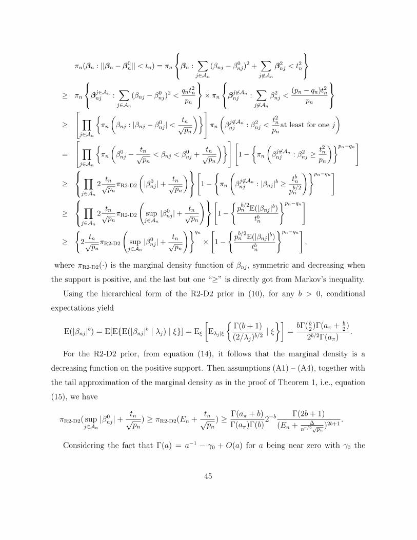
πn(βn : ||βn − β0n|| < tn) = πn

βn :∑j∈An

(βnj − β0nj)

2 +∑j 6∈An

β2nj < t2n

≥ πn

βj∈Annj :∑j∈An

(βnj − β0nj)

2 <qnt

2n

pn

× πnβj 6∈Annj :

∑j 6∈An

β2nj <

(pn − qn)t2npn

≥

∏j∈An

{πn

(βnj : |βnj − β0

nj | <tn√pn

)}πn(βj 6∈Annj : β2nj <

t2npn

at least for one j

)

=

∏j∈An

{πn

(β0nj −

tn√pn

< βnj < β0nj +

tn√pn

)}[1−{πn

(βj 6∈Annj : β2

nj ≥t2npn

)}pn−qn]

≥

∏j∈An

2tn√pnπR2-D2

(|β0nj |+

tn√pn

)[

1−

{πn

(βj 6∈Annj : |βnj |b ≥

tbn

pb/2n

)}pn−qn]

≥

∏j∈An

2tn√pnπR2-D2

(supj∈An

|β0nj |+

tn√pn

)[

1−

{pb/2n E(|βnj |b)

tbn

}pn−qn]

≥

{2tn√pnπR2-D2

(supj∈An

|β0nj |+

tn√pn

)}qn×

[1−

{pb/2n E(|βnj |b)

tbn

}pn−qn],

where πR2-D2(·) is the marginal density function of βnj, symmetric and decreasing when

the support is positive, and the last but one “≥” is directly got from Markov’s inequality.

Using the hierarchical form of the R2-D2 prior in (10), for any b > 0, conditional

expectations yield

E(|βnj|b) = E[E{E(|βnj|b | λj) | ξ}] = Eξ

[Eλj |ξ

{Γ(b+ 1)

(2/λj)b/2| ξ}]

=bΓ( b

2)Γ(aπ + b

2)

2b/2Γ(aπ).

For the R2-D2 prior, from equation (14), it follows that the marginal density is a

decreasing function on the positive support. Then assumptions (A1) – (A4), together with

the tail approximation of the marginal density as in the proof of Theorem 1, i.e., equation

(15), we have

πR2-D2( supj∈An|β0nj|+

tn√pn

) ≥ πR2-D2(En +tn√pn

) ≥ Γ(aπ + b)

Γ(aπ)Γ(b)2−b

Γ(2b+ 1)

(En + ∆nr/2√pn

)2b+1.

Considering the fact that Γ(a) = a−1 − γ0 + O(a) for a being near zero with γ0 the

45

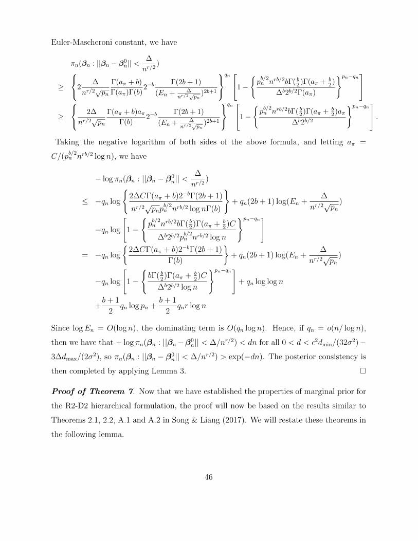
Euler-Mascheroni constant, we have

πn(βn : ||βn − β0n|| <

∆

nr/2)

≥

2∆

nr/2√pn

Γ(aπ + b)

Γ(aπ)Γ(b)2−b

Γ(2b+ 1)

(En + ∆nr/2√pn

)2b+1

qn 1−

{pb/2n nrb/2bΓ( b2)Γ(aπ + b

2)

∆b2b/2Γ(aπ)

}pn−qn≥

2∆

nr/2√pn

Γ(aπ + b)aπΓ(b)

2−bΓ(2b+ 1)

(En + ∆nr/2√pn

)2b+1

qn 1−

{pb/2n nrb/2bΓ( b2)Γ(aπ + b

2)aπ

∆b2b/2

}pn−qn .Taking the negative logarithm of both sides of the above formula, and letting aπ =

C/(pb/2n nrb/2 log n), we have

− log πn(βn : ||βn − β0n|| <

∆

nr/2)

≤ −qn log

{2∆CΓ(aπ + b)2−bΓ(2b+ 1)

nr/2√pnp

b/2n nrb/2 log nΓ(b)

}+ qn(2b+ 1) log(En +

∆

nr/2√pn

)

−qn log

[1−

{pb/2n nrb/2bΓ( b

2)Γ(aπ + b

2)C

∆b2b/2pb/2n nrb/2 log n

}pn−qn]

= −qn log

{2∆CΓ(aπ + b)2−bΓ(2b+ 1)

Γ(b)

}+ qn(2b+ 1) log(En +

∆

nr/2√pn

)

−qn log

[1−

{bΓ( b

2)Γ(aπ + b

2)C

∆b2b/2 log n

}pn−qn]+ qn log log n

+b+ 1

2qn log pn +

b+ 1

2qnr log n

Since logEn = O(log n), the dominating term is O(qn log n). Hence, if qn = o(n/ log n),

then we have that − log πn(βn : ||βn−β0n|| < ∆/nr/2) < dn for all 0 < d < ε2dmin/(32σ2)−

3∆dmax/(2σ2), so πn(βn : ||βn − β0

n|| < ∆/nr/2) > exp(−dn). The posterior consistency is

then completed by applying Lemma 3.

Proof of Theorem 7. Now that we have established the properties of marginal prior for

the R2-D2 hierarchical formulation, the proof will now be based on the results similar to

Theorems 2.1, 2.2, A.1 and A.2 in Song & Liang (2017). We will restate these theorems in

the following lemma.

46

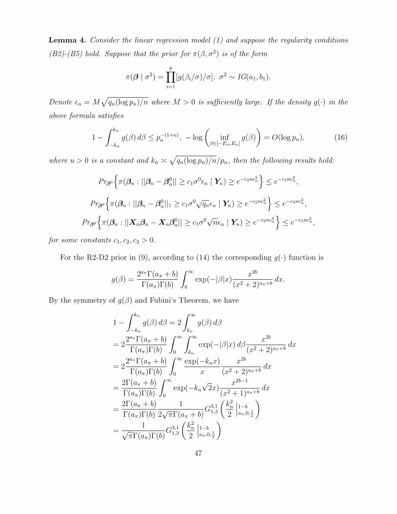
Lemma 4. Consider the linear regression model (1) and suppose the regularity conditions

(B2)-(B5) hold. Suppose that the prior for π(β, σ2) is of the form

π(β | σ2) =

p∏i=1

[g(βi/σ)/σ], σ2 ∼ IG(a1, b1).

Denote εn = M√qn(log pn)/n where M > 0 is sufficiently large. If the density g(·) in the

above formula satisfies

1−∫ kn

−kng(β) dβ ≤ p−(1+u)

n , − log

(inf

β∈[−En,En]g(β)

)= O(log pn), (16)

where u > 0 is a constant and kn �√qn(log pn)/n/pn, then the following results hold:

Prβ0

{π(βn : ||βn − β0

n|| ≥ c1σ0εn | Yn) ≥ e−c2nε

2n

}≤ e−c3nε

2n ,

Prβ0

{π(βn : ||βn − β0

n||1 ≥ c1σ0√qnεn | Yn) ≥ e−c2nε

2n

}≤ e−c3nε

2n ,

Prβ0

{π(βn : ||Xnβn −Xnβ

0n|| ≥ c1σ

0√nεn | Yn) ≥ e−c2nε

2n

}≤ e−c3nε

2n ,

for some constants c1, c2, c3 > 0.

For the R2-D2 prior in (9), according to (14) the corresponding g(·) function is

g(β) =2aπΓ(aπ + b)

Γ(aπ)Γ(b)

∫ ∞0

exp(−|β|x)x2b

(x2 + 2)aπ+bdx.

By the symmetry of g(β) and Fubini’s Theorem, we have

1−∫ kn

−kng(β) dβ = 2

∫ ∞kn

g(β) dβ

= 22aπΓ(aπ + b)

Γ(aπ)Γ(b)

∫ ∞0

∫ ∞kn

exp(−|β|x) dβx2b

(x2 + 2)aπ+bdx

= 22aπΓ(aπ + b)

Γ(aπ)Γ(b)

∫ ∞0

exp(−knx)

x

x2b

(x2 + 2)aπ+bdx

=2Γ(aπ + b)

Γ(aπ)Γ(b)

∫ ∞0

exp(−kn√

2x)x2b−1

(x2 + 1)aπ+bdx

=2Γ(aπ + b)

Γ(aπ)Γ(b)

1

2√πΓ(aπ + b)

G3,11,3

(k2n

2

∣∣∣1−baπ ,0,

12

)=

1√πΓ(aπ)Γ(b)

G3,11,3

(k2n

2

∣∣∣1−baπ ,0,

12

)47

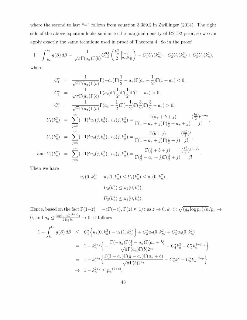
where the second to last “=” follows from equation 3.389.2 in Zwillinger (2014). The right

side of the above equation looks similar to the marginal density of R2-D2 prior, so we can

apply exactly the same technique used in proof of Theorem 4. So in the proof

1−∫ kn

−kng(β) dβ =

1√πΓ(aπ)Γ(b)

G3,11,3

(k2n

2

∣∣∣1−baπ ,0,

12

)= C∗1U1(k2

n) + C∗2U2(k2n) + C∗3U3(k2

n),

where

C∗1 =1√

πΓ(aπ)Γ(b)Γ(−aπ)Γ(

1

2− aπ)Γ(aπ +

1

2)Γ(1 + aπ) < 0,

C∗2 =1√

πΓ(aπ)Γ(b)Γ(aπ)Γ(

1

2)Γ(

1

2)Γ(1− aπ) > 0,

C∗3 =1√

πΓ(aπ)Γ(b)Γ(aπ −

1

2)Γ(−1

2)Γ(

3

2)Γ(

3

2− aπ) > 0,

U1(k2n) =

∞∑j=0

(−1)ju1(j, k2n), u1(j, k2

n) =Γ(aπ + b+ j)

Γ(1 + aπ + j)Γ(12

+ aπ + j)

(k2n

2)j+aπ

j!,

U2(k2n) =

∞∑j=0

(−1)ju2(j, k2n), u2(j, k2

n) =Γ(b+ j)

Γ(1− aπ + j)Γ(12

+ j)

(k2n

2)j

j!,

and U3(k2n) =

∞∑j=0

(−1)ju3(j, k2n), u3(j, k2

n) =Γ(1

2+ b+ j)

Γ(32− aπ + j)Γ(3

2+ j)

(k2n

2)j+1/2

j!.

Then we have

u1(0, k2n)− u1(1, k2

n) ≤ U1(k2n) ≤ u1(0, k2

n),

U2(k2n) ≤ u2(0, k2

n),

U3(k2n) ≤ u3(0, k2

n).

Hence, based on the fact Γ(1−z) = −zΓ(−z), Γ(z) ≈ 1/z as z → 0, kn �√

(qn log pn)/n/pn →

0, and aπ ≤ log(1−p−(1+u)n )

2 log kn→ 0, it follows

1−∫ kn

kn

g(β) dβ ≤ C∗1

{u1(0, k2

n)− u1(1, k2n)}

+ C∗2u2(0, k2n) + C∗3u3(0, k2

n)

= 1− k2aπn

{−

Γ(−aπ)Γ(12− aπ)Γ(aπ + b)

√πΓ(aπ)Γ(b)2aπ

− C∗4k2n − C∗5k1−2aπ

n

}= 1− k2aπ

n

{Γ(1− aπ)Γ(12− aπ)Γ(aπ + b)

√πΓ(b)2aπ

− C∗4k2n − C∗5k1−2aπ

n

}→ 1− k2aπ

n ≤ p−(1+u)n ,

48

where C∗4 , C∗5 ≥ 0. Hence for aπ ≤ log(1−p−(1+u)

n )2 log kn

→ 0, we proved the first condition in (16)

holds.

Now let’s prove that the second condition in (16) also holds. By Theorem 1, g(β) =

O(|β|−2b−1) as |β| → ∞. Since log(En) = O(log pn),

infβ∈[−En,En]

g(β) = g(En) ≈ O(E−2b−1n ).

So

− log(

infβ∈[−En,En]

g(β))

= (2b+ 1) log(En) = O(log pn),

i.e., the second condition in (16) holds. Hence, all conditions in Lemma 4 are satisfied.

Theorem 7 is proven.

B Appendix: Choosing Hyper-parameters ν and µ

Assume that q of the p variance components (λj) account for (1 − ε) proportion of the

variability. That is,∑qj=1 λ(j)∑pj=1 λ(j)

= 1 − ε, where λ(j) is the j-th largest value. Suppose that

λj ∼ Gamma (ν, µ). The degree of sparsity, i.e. the number of relevant components, q can

then be viewed as finding q such that the proportion achieves 1− ε. Since the proportion

is a random quantity, we seek q such that the median of the distribution of the proportion

reaches equality. Note that since, µ is a scale parameter, the distribution of the proportion

is unaffected by µ. Hence a grid search can be achieved to find ν such that the equation

is satisfied by the median of the distribution, this just requires sampling from a Gamma

(ν, 1) distribution to approximate the distribution for a given ν.

After choosing ν, we then choose the scale parameter, µ, we seek to ensure that the

prior distribution for β is near zero at p−q directions. To do so, recall that the distribution

must lie on the ellipsoid given by βTΣXβ = θσ2. Hence, we wish to push p− q directions

to be inside the ellipsoid, i.e. near zero. So, we set µ such that the probability of βj under

the unrestricted Normal distribution, being inside the ellipsoid is 1 − q/p. Note that this

49

probability is just P (β2j < θσ2). Now

P (β2j < θσ2) = P

(wj <

1

λj

)=

∫ ∞0

∫ 1/nλj

0

fw(wj)fλ(λj)dwjdλj

=

∫ ∞0

1

Γ(1/2)γ

(1

2,

1

2λj

)fλ(λj)dλj

=1

Γ(1/2)Eλ

[γ

(1

2,

1

2λj

)],

where wj is a χ21 random variable, and γ is the lower incomplete gamma function. This

can again be evaluated on a grid. This time a grid of µ.

50