THE ROLES OF GREENHOUSE GASES IN GLOBAL WARMINGOllila-EE-GH gas roles.pdf

MULTI-SCIENCE PUBLISHING CO. LTD.5 Wates Way, Brentwood, Essex CM15 9TB, United Kingdom

Reprinted from

ENERGY &ENVIRONMENT

VOLUME 23 No. 5 2012

THE ROLES OF GREENHOUSE GASES IN GLOBAL WARMING

by

Antero Ollila (Finland)

781

THE ROLES OF GREENHOUSE GASES IN GLOBALWARMING

Antero V.E. OllilaAdj Assoc Prof, Department of Civil and Environmental Engineering, School of Engineering,

Aalto University, Espoo, FinlandOtakaari 1, Box 11000, 00076 AALTO, Finland; e-mail: [email protected]

ABSTRACTScientists are still debating the reasons for “global warming”. The author questionsthe validity of the calculations for the models published by the IntergovernmentalPanel on Climate Change (IPCC) and especially the future scenarios. Throughspectral calculations, the author finds that water vapour accounts forapproximately 87% of the greenhouse (GH) effect and only 10% of CO2. Adoubling of the present level of CO2 would increase the global temperature by only0.51 °C without water feedback. The IPCC claims that a temperature increase of0.76 °C for 2005 was caused in part by water (about 50%), because relativehumidity (RH) stays constant in their model. The calculations prove that CO2

would have increased the temperature by only 0.2 °C since 1750 and that themeasured decrease in water since 1948 has compensated for this increase. Thisstudy has also produced results indicating a negative feedback for relativehumidity. The simulations of this study propose that the IPCC’s modelatmospheres could be approximately 50% too dry.

Keywords: climate change, global warming, greenhouse phenomenon,greenhouse gases, warming potentials, humidity, water vapour.

1. INTRODUCTIONThe greenhouse (GH) effect is a natural phenomenon that can be studied throughtheoretical calculations and temperature and radiation measurements. The outgoinglong-wave (LW) flux to space (value 239 Wm-2) has been measured using ERBE(Earth Radiation Budget Experiment) satellites and it corresponds to a theoreticalsurface temperature of -18 °C for the Earth. The greenhouse effect is a reality becausethe observed surface temperature of the Earth is about 15 °C. The differencebetween the theoretical and the real surface temperatures of the Earth is thegreenhouse effect in degrees. The most cited value is 33 °C, which can be found inthe scientific literature on the topic.[1, 2]

Utilising Planck’s function of radiation, one can calculate that the required energyflux emitted by the Earth’s surface must be approximately 391 Wm-2. It is difficult tocalculate an accurate value for the surface temperature according to radiation lawsbecause the Earth is not a black body. At any rate, the observed recent changes couldbe regarded as signs of global warming.

2. SPECTRAL CALCULATION TOOL The author has utilized a spectral calculation tool prepared and maintained by GATSInc., which is available on the Internet.[3] This tool is quite flexible and the mostaccurate absorption line lists for the common GH gas molecules are available. In thisarticle, the author uses the name SpectralCalc for this tool; the official name used forit by GATS Inc. is the Spectral Calculator.

2.1 Molecular spectra calculationsMolecules emit and absorb radiation only at certain frequencies or wavenumbers,thereby creating changes in their quantum energy levels. This produces a uniquespectrum for each gas molecule species. According to Kirchhoff’s law, theabsorptivity is the compliment of transmittance, which eqn 1 below shows:

Absorptivity = 1- transmittance (1)

The SpectCalc tool produces the transmittance values only; the absorptivity values caneasily be calculated using eqn 1. The absorption lines appear as dips in thetransmittance spectrum lines. Each line has a width and a depth, which are determinedby the quantum mechanical properties of the molecule in question.

The spectrum of a gas molecule can be calculated using the basic physical laws, butit is not accurate enough for practical calculations. The collection of line parametersfor a group of absorption lines is called a line list; the list has been derived by fittinglaboratory spectra measured in various conditions. In this way, each absorption line isspecified by a set of parameters. Using this data, an absorption line can be calculatedfor a given concentration, temperature and pressure. HITRAN is probably the mostcomprehensive and commonly used line list for atmospheric applications and it isavailable when using the SpectralCalc tool. [4]

In order to simulate the transmittance spectrum of a gas mixture over a givenspectral range, the absorption lines of each gas must be calculated. The completespectrum is the product of the individual, absorption-line spectra. The individual linespectra cannot be directly summarized in the case of overlapping frequencies.

The algorithms that calculate molecular spectra in this way are known as line-by-line models, and they produce the most accurate values for molecular absorption. TheSpectralCalc tool uses line-by-line modelling for the molecular transmission andemission calculations. In actual calculations SpectralCalc uses LinepakTM algorithms,which Gordley et al. have described in detail. [5] Many international researchinstitutes, including NASA, use LinepakTM software for spectral calculations, whichproves the correctness and validity of SpectralCalc.

782 Energy & Environment · Vol. 23, No. 5, 2012

2.2 Atmospheric spectral calculationsCalculating the spectrum in a complicated path, like through the planetary atmosphere,requires special arrangements. SpectralCalc divides the path into segments, which areapproximated by constant temperature, pressure and gas concentrations. [3] Thetransmittance spectrum of the whole path is the product of individual spectra of thesegments. These calculations may become computationally very intensive and,therefore, SpectralCalc has been designed to maximize efficiency without losingaccuracy.

The SpectralCalc tool offers an opportunity for individual researchers to calculateand analyze the GH phenomenon. Atmospheric path calculations are possible from aminimum height of 1 km to a maximum height of 600 km. Six different atmosphericmodels are readily available: standard, tropical, mid-latitude summer, mid-latitudewinter, polar summer and polar winter. Users can modify the GH concentrationprofiles by scale factors and the temperature by offset changes.

The author has used the SpectralCalc tool to verify some basic features of the GHphenomenon and especially the effects of GH gas concentration changes. Even thoughSpectralCalc is a very powerful calculation tool, a user cannot calculate thetransmission or absorption spectrum, for example in the range of 4-100 micrometres(µm), with one calculation operation only. The author calculated the absorption valuesin the ranges of 4-5, 5-6, 6-7, 7-10, 10-15, 15-20, 20-30 and 30-100 µm in an aircolumn of 11 km. Each calculation produced a list of transmission and wavelengthvalues varying from 403 to 564 points. The absorption of radiation energy for eachwavelength was calculated by multiplying the absorption values by the calculatedradiance values emitted by the Earth’s surface at a given temperature.

Two test runs were carried out for checking the correctness of radiation absorptionprocedures of integration. By selecting the transmission value as zero and thetemperature as 255.2 K, the total absorption in an air column of 11 km was 238.61Wm-2. SpectralCalc’s black body calculator for the same temperature gave a readingof 240.52 Wm-2, which indicates 0.79% accuracy. The SpectralCalc tool does notrecalculate the temperature profile if there is radiation absorption in the atmospherethat causes a temperature change. This problem will be discussed in Chapter 5.

3. AVERAGE CLIMATE OF THE EARTHWhen we specify the concentrations of GH gases, we need to specify the part of theatmosphere where the GH phenomenon actually happens and the actual averagecomposition of the average atmosphere.

3.1 The height of the atmosphere in GH phenomenonMany spectral radiation calculations include the whole atmosphere, because satellitesmonitoring radiation values are orbiting above the atmosphere. Scientists believe thatthe GH phenomenon happens in the troposphere at a height below that of 11kilometres2. The height of the troposphere varies between 8 and 15 kilometres, withthe standard height being 11 km. Limiting the GH effect to just the troposphere canalso be justified by the fact that global warming has taken place in the lower parts ofthe atmosphere.

The roles of greenhouse gases in global warming 783

The author calculated the radiation flux absorption values (W/m2) using theSpectralCalc tool for the average atmosphere, which will be discussed in more detaillater on, for the air columns extending from the surface to different heights in clear skyconditions. The flux absorption value for 120 km was 308.34 Wm-2 (100 %), for 11km 302.71 Wm-2 (98.0%), for 2 km 287.90 (93.3%), and for 1 km it was 272.22 Wm-

2 (88.1%). These results confirm that a height of 11 km for atmospheric calculationsis a sound choice.

3.2 The average global atmosphere profilesBecause the SpectralCalc tool can calculate radiation absorption values only for asingle atmosphere composition at a time, it is essential to define the average globalatmosphere (AGA). There is a standard climate model for this in SpectralCalc [3], butit is actually the U.S. standard atmosphere for the year 1976. While the gasconcentration values are applicable for the year 1976, the water concentration turnedout to only be approximately 50% of the true global actual values.

There is no generally accepted AGA model known to the author and that is why theAGA profiles had to be calculated. The calculations are based on the five availableatmospheric models in SpectralCalc, which were originally produced by Ellingson et al. [6]

The AGA values were calculated in a step-by-step process. The first step producedthe average values for polar and mid-latitude atmospheres by averaging the summerand winter profiles. Then, the preliminary AGA profiles were produced by combiningthe three atmospheres according to their average geographical areas. One way of doingthis is to define the tropical belt as being between 23.5 degrees North and South, themid-latitudes as being from 23.5 degrees to 60 degrees and the Polar Regions as beingbetween 60 and 90 degrees. By utilizing these definitions, the calculations producedweighting factors of 0.391, 0.461 and 0.148 for these regions. Finally, the weightingfactors were fine-tuned to produce an average surface temperature of 288.2 K. Afterthis fine-tuning, the following weighting factors were achieved: tropical climate 0.4,mid-latitude climate 0.45 and polar climate 0.15.

One restriction of the SpectralCalc tool is that a user cannot freely define theatmospheric profiles. One has to select one of the six available atmospheres. Theauthor selected the polar summer atmosphere (PSA) because it is closest to the AGAvalues. Table 1 summarizes the AGA and PSA atmosphere profiles. Actually, thetemperature profile for the PSA is 2.6 degrees colder than the one for the AGA profileand the pressure profile is 5.4 mbar lower than the AGA profile in the troposphere.The pressure profile cannot be adjusted and the difference has no practical impact. Thetemperature profile could be adjusted by a temperature off-set. Because the surfacetemperature is the same as the AGA value and 88% of the absorption takes placebelow 1 km, the PSA temperature profile has not been adjusted.

The AGA profile for water resulted in a total content of water in the troposphere of2.69 prcm (precipitable water in centimetres). Miskolczi has calculated from TIGR(The Thermodynamic Initial Guess Retrieval) climatological balloon observationlibrary and from NOAA (National Oceanic and Atmospheric Administration) data thatthe total precipitable water amount in the average global atmosphere is 2.6 cm. [7] Thecalculated AGA water amount is only 3.5% higher than this value. Finally, the PSAwater profile was adjusted to 2.6 prcm.


Table 1. Average global atmosphere profiles and modified polar summeratmosphere profiles.

In its latest report, the IPCC has reported accurate concentration values for CO2, CH4and N2O for the years 1750 (before industrialization) and 2005, but not for O3. [8]Vingartzan has surveyed the numerous studies on O3 surface concentrations; [9] theaverage value for the year 1750 is 0.02 ppm, while the average value for the year 2000is between 0.04 and 0.05 ppm. The O3 values of the SpectralCalc tool vary frombetween 0.024 and 0.091 ppm in the troposphere and these O3 profiles has beenapplied in the AGA simulation calculations.

The other GH gas concentrations in the SpectralCalc climate models are almost thesame as those reported by the IPPC, except for that of CO2, whose value is 330 ppm.Table 2 provides a summary of the GH gas concentrations and the final scale factorsapplied in the SpectralCalc tool for the AGA simulations.

Table 2. Surface GH gas concentrations reported by IPCC [8] and the scalefactors applied in SpectralCalc [3] for the average global atmosphere (year 2005).

GH gas IPPC value (ppmv) Polar Summer (ppmv) Scale factor

H2O not reported 11900 1.2384 CO2 379 330 1.149 CH4 1.774 1.700 1.044 N2O 0.319 0.310 1.029 O3 not reported 0.0241 1.0

Altitude

Polar summer

atm.

Average global atm.

Polar summer

atm.

Average global atm.

Mod. Polar summer

atm.

Average global atm.

(km) T (K) T(K) P (mbar) P (mbar) Hum. (g/m3) Hum. (g/m3)

0 288.20 288.23 1010.0 1013.9 11.112 12.037

1 281.70 283.68 896.0 900.2 7.403 8.264

2 276.30 278.84 792.9 797.9 5.194 5.756

3 270.90 274.45 700.0 705.3 3.348 3.122

4 265.50 268.29 616.0 622.0 2.112 1.607

5 260.10 262.00 541.0 547.1 1.245 0.999

6 253.10 255.58 474.0 479.5 0.672 0.571

7 246.10 249.10 413.0 418.9 0.361 0.316

8 239.20 242.58 359.0 364.8 0.162 0.166

9 232.20 236.31 310.8 316.4 0.047 0.082

10 225.20 230.36 267.7 273.6 0.014 0.037

11 225.20 226.02 230.0 235.7 0.004 0.013


4. RADIATION ABSORPTION CAPACITIES OF GREENHOUSE GASESEach GH gas has its own absorption band. The warming caused by a GH gas dependson the gas concentration and the radiation absorption at each band.

In order to illustrate the magnitudes of the absorption bands of the GH gases, theauthor has produced the absorption bands using the SpectralCalc tool for the AGA.The graphical presentations of the absorption bands are depicted in Fig. 1 and Fig. 2.

Figure 1. The black body absorption spectra of the Earth at 15 ºC and the absorptionbands of H2O and CO2 based on the average global atmosphere (AGA) conditions.

Figure 2. The absorption bands of O3, N2O, and CH4 gases based on the AGAconditions.


The band areas give rough estimates of the warming capacities of GH gases. Theseillustrations make it clear that H2O and CO2 play the major roles in the absorption ofradiation flux energy. Because the presentations in Fig.1 and 2 are calculated for oneGH gas at a time, they do not take into account the overlapping phenomenon. This isvery essential in wavelengths from 13 to 18 µm for H2O and CO2.

The IPCC does not treat H2O in the same way that it does the other GH gases. Inits view, the other GH gases produce radiative forcing, but H2O produces positivefeedback. In its last report, [10] the IPCC admits that H2O is the strongest GH gas, butit does not report concentrations or warming potentials for it.

The essential difference is that the IPCC model does not use the direct radiationabsorption capacities of the GH gas molecules. It also uses a time-scale characterisingfactor, which is a measure of the retaining time of a GH gas in the atmosphere.Combining the absorption potentials and the retaining time produces a factor called theGlobal Warming Potential (GWP). [11,12] Water has a very short retaining time -evaporation and precipitation can happen in days or even in hours - but, for example,CH4 and N2O are stable gases that remain in the atmosphere for decades. This meansthat it would take a very long time to remove these GH gases from the atmosphere.The IPCC has not reported the way in which it uses GWP values in its calculations orwhether these GWP values are only an artificial means of emphasising the roles ofanthropogenic GH gases.

The author’s opinion is that the methodology of combining two totally differentproperties of GH gases into one factor is not needed or justified in global warmingmodels. The calculation for or estimation of the concentrations of GH gases in thefuture will entail a separate process, and those values can easily be applied in anymodels, as can be the absorption potentials, which are stable constants by nature basedpurely on the molecular properties of GH gases. The combination of molecularproperties and retaining times produces a value that can give the wrong idea about thewarming effects now occurring.

Regarding H2O as a less powerful GH gas can be criticized, too. Even though itsresidence time is very short when compared with other GH gases, H2O is ever-presentin various concentrations but seldom constant at any particular concentration for apredictable period of time and at a predictable location.

5. RADIATION ABSORPTION AND SURFACE TEMPERATUREIn each different atmosphere a situation has been established where the surfacetemperature and radiation absorption in the atmosphere are in balance. The mainvariables are the surface temperature and the atmospheric humidity, which affect theradiation flux absorption.

The author has calculated the radiation absorption for five different atmospheremodels, which are available in SpectralCalc. Also, two extra simulations were carriedout: one for a surface temperature of -18 °C in polar winter conditions and another fora surface temperature of 36.6 °C in tropical climate conditions. In these calculationsthe relative humidity was kept the same as in the original polar and tropical climatemodels. The results of these calculations are presented in Fig.3.


Figure 3. Simulation results for five different atmospheres showing the relationshipbetween radiative flux absorption and surface temperature. The straight line indicates

the relationship around the average global atmosphere (AGA).

The dependency of the surface temperature on radiation absorption is slightlynonlinear. The straight line in Fig. 3 illustrates this linear relationship around anaverage temperature of 15 °C, which is expressed in eqn 2:

∆Ts = ∆E/5.35, (2)

where ∆Ts is the surface temperature change and ∆E is the radiation absorption changecaused by a GH gas or gases. This value has been used to transform the absorbedradiation fluxes into surface temperatures. The AGA simulation, which produced thepoint 15 °C/302.71 Wm-2, is almost exactly on the linear line. It should be noticed thatthe term “radiative forcing” used by IPCC has its own definition – for example thereare no feedback elements – and that is the reason, why radiation flux and surfacetemperature relationship as calculated above has different value than that of IPCC.

It should be noted that all other values in these calculations represent real climateconditions, except for the radiation absorbed value, which is calculated theoretically.One problem when calculating the radiation absorption is that, for example, CO2increase will increase the temperature, but the SpectralCalc tool does not adjust thetemperature profile during the calculation. A user should carry out iterativecalculations. The relationship between absorbed energy and the surface temperature inFig.3 is important, because it is an experimental relationship. It can be used tocalculate the new surface temperature, which is in balance with the radiationabsorption change in the atmosphere without repeated calculations.

The author carried out a mathematical analysis to determine the nature of therelationship if the surface temperature would be linearly dependent on the absorbed


radiation, H2O concentration (prcm) and relative humidity (RH). One could select thesurface values for these variables, but in this analysis values at the height of 1 km wereused. The justification for this selection is that at a height of 1 km, approximately 88%of the radiative energy flux has been absorbed. Table 3 shows the above variables forfive different atmospheric models.

Table 3. Atmosphere model conditions at a height of 1 km. The absorbedradiation has been calculated for an air column of 11 km.

The achieved multiple linear regression, eqn 3, is as follows:

Ts = 279.195186 + 0.111723 * E + 1.78532587 * C – 0.4941032 * RH, (3)

where Ts is the surface temperature (K), E is the absorbed radiation (Wm-2), C is theH2O concentration (prcm) and the RH is the relative humidity (%). The correlation r2is 0.9999 and the standard error for the estimate is 0.215 K. This linear fitting indicatesa very high correlation.

This correlation clearly shows that absorbed radiation is the major factor inexplaining the surface temperatures. The roles of H2O can be explained according toits two functions: it is a major contributor to infrared radiation absorption (see Chapter7) in the troposphere and, at the same time, via moist air thermodynamics, relativehumidity has a strong negative impact on the climate system mechanism. Thismechanism has been proposed by several climate researchers, such as Miskolczi7 andPaltridge et al. [13]

The limitations of this analysis are that the amount of input material is very narrowand that this is a mathematical exercise without an impact mechanism. At any rate, itprovides a fairly good indication that a negative feedback mechanism for relativehumidity could exist. This mechanism can explain why the surface temperatureremains stable in the cases of increased concentrations of other GH gases like CO2.

6. SATURATION AND OVERLAPPING PHENOMENA GH gas concentrations affect the radiative absorption. The IPCC has stated that theradiative effect of absorption by water vapour is roughly proportional to the logarithmfor its concentration. [10] The IPCC does not specify this relationship in detail.

-------------------------------------------------------------------------------------------------------- Atmospheric model

Pressure, hPa

Tempe- rature, K

Rad. abs., Wm-2

H2O, prcm RH, %

-----------------------------------------------------------------------------------------------------------Polar winter 887.8 259.1 163.68 0.4209 79.33 Mid-latitude winter 897.3 268.7 216.57 0.8616 73.01 Polar summer 896.0 281.7 293.53 2.0964 69.14 Mid-latitude summer 902.0 289.7 334.24 2.9456 64.95 Tropical 904.0 293.7 379.11 4.1223 71.18


When a GH gas concentration increases, the absorption no longer increases in alinear fashion at a certain point; rather, the curve begins to bend downwards. Thisphenomenon is called saturation, which begins when a GH gas like CO2 or H2O hascaptured nearly all of the available photons within a certain LW band.

There is no simple way to calculate the degree of saturation. The practical way isto carry out simulation calculations with different GH gas concentrations. Thesecalculations are easy to do when using the SpectralCalc properties. Only CO2 and H2Oare interesting gases. Surface temperatures have been calculated using eqn 2.

Fig. 4 shows the results for the CO2 calculations. The linear part of radiative fluxabsorption is linear until approximately 50 ppm; thereafter, the saturation phenomenonincreases.

Figure 4. The absorption energy fluxes in the average global atmosphere (AGA) asa function of the CO2 concentration.

Fig. 5 shows the results for H2O calculations. The linear part of radiative fluxabsorption is linear until approximately 0.1 prcm; thereafter, the saturationphenomenon increases.

The overlapping phenomenon of absorption bands is another inaccuracy factorexisting in brief absorption calculations. It is a fact that the overall warming effectcannot be calculated by merely summarizing the warming effects on the basis ofdirectly multiplying the concentrations and absorption potentials if they haveoverlapping bands.

An important benefit of the SpectralCalc tool is that it can utilize calculationmethods, as described in Chapter 2, which are advanced enough that saturation and theoverlapping phenomenon will not cause inaccuracies. [5]


Figure 5. The absorption energy fluxes in the average global atmosphere (AGA) asa function of the H2O concentration.

To illustrate the impact of a warmer climate and a higher concentration of H2O andCO2, the author has produced the radiation emission of the Earth, the H2O absorptiongraph and the CO2 absorption graph for a concentration of 800 ppm for the tropicalatmosphere. The results are depicted in Fig. 6.

Figure 6. The black body absorption spectra of the Earth at 26.4 ºC and theabsorption bands of H2O and CO2 (800 ppm) in the tropical atmosphere.


We can see that the increase of water in the warmer climate means a bigger bandarea, resulting in higher radiation absorption. The CO2 concentration is an artificialchoice and it illustrates that the increase in the CO2 concentration does not result in theso big change in its band area. Fig. 6 reveals also that H2O can almost totally (76-100%) absorb radiation flux in the waveband from 13 to 18 µm without CO2. Thismeans that these two major GH gases overlap heavily and it has a clear impact on theGH effect contribution.

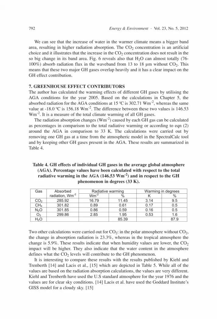
7. GREENHOUSE EFFECT CONTRIBUTORSThe author has calculated the warming effects of different GH gases by utilising theAGA conditions for the year 2005. Based on the calculations in Chapter 5, theabsorbed radiation for the AGA conditions at 15 ºC is 302.71 Wm-2, whereas the samevalue at -18.0 ºC is 156.18 Wm-2. The difference between these two values is 146.53Wm-2. It is a measure of the total climate warming of all GH gases.

The radiation absorption changes (Wm-2) caused by each GH gas can be calculatedas percentages in comparison to the total radiative warming or according to eqn (2)around the AGA in comparison to 33 K. The calculations were carried out byremoving one GH gas at a time from the atmospheric model in the SpectralCalc tooland by keeping other GH gases present in the AGA. These results are summarized inTable 4.

Table 4. GH effects of individual GH gases in the average global atmosphere(AGA). Percentage values have been calculated with respect to the totalradiative warming in the AGA (146.53 Wm-2) and in respect to the GH

phenomenon in degrees (33 K).

Two other calculations were carried out for CO2: in the polar atmosphere without CO2,the change in absorption radiation is 23.3%, whereas in the tropical atmosphere thechange is 5.9%. These results indicate that when humidity values are lower, the CO2impact will be higher. They also indicate that the water content in the atmospheredefines what the CO2 levels will contribute to the GH phenomenon.

It is interesting to compare these results with the results published by Kiehl andTrenberth [14] and Lacis et al., [15] which are depicted in Table 5. While all of thevalues are based on the radiation absorption calculations, the values are very different.Kiehl and Trenberth have used the U.S standard atmosphere for the year 1976 and thevalues are for clear sky conditions. [14] Lacis et al. have used the Goddard Institute’sGISS model for a cloudy sky. [15]


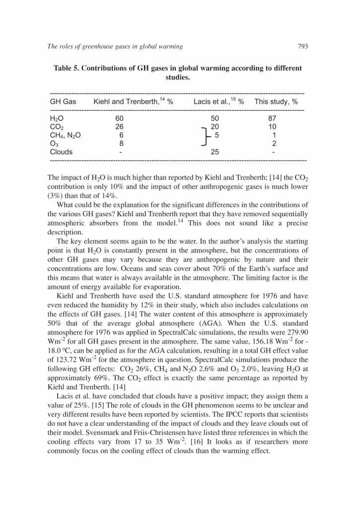
Table 5. Contributions of GH gases in global warming according to differentstudies.

The impact of H2O is much higher than reported by Kiehl and Trenberth; [14] the CO2contribution is only 10% and the impact of other anthropogenic gases is much lower(3%) than that of 14%.

What could be the explanation for the significant differences in the contributions ofthe various GH gases? Kiehl and Trenberth report that they have removed sequentiallyatmospheric absorbers from the model.14 This does not sound like a precisedescription.

The key element seems again to be the water. In the author’s analysis the startingpoint is that H2O is constantly present in the atmosphere, but the concentrations ofother GH gases may vary because they are anthropogenic by nature and theirconcentrations are low. Oceans and seas cover about 70% of the Earth’s surface andthis means that water is always available in the atmosphere. The limiting factor is theamount of energy available for evaporation.

Kiehl and Trenberth have used the U.S. standard atmosphere for 1976 and haveeven reduced the humidity by 12% in their study, which also includes calculations onthe effects of GH gases. [14] The water content of this atmosphere is approximately50% that of the average global atmosphere (AGA). When the U.S. standardatmosphere for 1976 was applied in SpectralCalc simulations, the results were 279.90Wm-2 for all GH gases present in the atmosphere. The same value, 156.18 Wm-2 for -18.0 ºC, can be applied as for the AGA calculation, resulting in a total GH effect valueof 123.72 Wm-2 for the atmosphere in question. SpectralCalc simulations produce thefollowing GH effects: CO2 26%, CH4 and N2O 2.6% and O3 2.0%, leaving H2O atapproximately 69%. The CO2 effect is exactly the same percentage as reported byKiehl and Trenberth. [14]

Lacis et al. have concluded that clouds have a positive impact; they assign them avalue of 25%. [15] The role of clouds in the GH phenomenon seems to be unclear andvery different results have been reported by scientists. The IPCC reports that scientistsdo not have a clear understanding of the impact of clouds and they leave clouds out oftheir model. Svensmark and Friis-Christensen have listed three references in which thecooling effects vary from 17 to 35 Wm-2. [16] It looks as if researchers morecommonly focus on the cooling effect of clouds than the warming effect.

--------------------------------------------------------------------------------------------------------- GH Gas Kiehl and Trenberth,14 % Lacis et al.,15 % This study, % --------------------------------------------------------------------------------------------------------- H2O 60 50 87 CO2 26 20 10 CH4, N2O 6 5 1 O3 8 2 Clouds - 25 - ----------------------------------------------------------------------------------------------------------


8. CLIMATE CHANGEThe IPCC has concluded that climate change – a temperature increase of about 0.76 °Cbetween 1750 and 2005 – is caused by an increase in the anthropogenic GH gases.

8.1 Full Scale TestWe can say that mankind has carried out a full-scale scientific test by increasing theCO2 content from 280 ppm to 379 ppm (99 ppm increase) during the period from 1750to 2005, producing approximately a 0.76 °C increase in the temperature according toIPCC reported values. [8] Thus, we can obtain a rough estimate that 389 ppm of CO2produces a total maximum GH effect of 3.0 K, assuming a linear relationship. Becausethe general estimate for the total GH effect is 33 K, [1,2] the total impact of CO2 isonly 9%, leaving 91% for H2O and other GH gases, assuming a linear dependency.

8.2 Calculation of global warming from 1750 to 2005 by simulationsThe change in anthropogenic GH gases has been significant if we are thinking in termsof percentage values. The IPCC’s report reveals that the total net anthropogenicforcing is 1.6 Wm-2, which is practically same as the CO2 forcing of 1.66 Wm-2

because the other radiative forcing factors eliminate each other. [8] That is why it isenough to calculate the radiative absorption change caused by the increase in CO2from 280 ppm to 379 ppm. A simulation of this change in the AGA produces aradiation absorption flux change of 1.05 Wm-2, which is equal to a temperatureincrease of 0.2 K.

Because water has the biggest role in radiation absorption, it is important to analysewhether or not there is any data available about the atmospheric water trends as wellas the way in which way the IPPC has actually calculated the H2O impact for thischange.

In the IPCC’s model the relative humidity (RH) remains constant if the temperaturechanges. [10] When an increase in the CO2 raises the global temperature, the constantRH means more water content. According to the IPCC, the net effect of water vapourin amplifying the warming effect of CO2 is about 50%. [10] The calculations with theSpectralCalc tool in the U.S. standard climate for a change in CO2 of between 280ppm and 379 ppm produces a radiation absorption flux change of 1.73 Wm-2, whichcorresponds to a temperature change of 0.32 K. If the constant relative humidity isassumed, the increase in temperature rise would be 0.30 K. The net warming effectwould be 0.62 K, which is close to the IPCC’s value of 0.76 K.

It should be noticed that calculating an increase in the temperature in the waydescribed above includes the problem of positive feedback. Because there is a positivefeedback from H2O, the procedure described above will never end. That is why theabove calculation represents a simplified estimate of this mechanism.

The positive feedback of H2O is not a generally accepted scientific fact. Someresearchers, such as Held and Soden, [17] have proposed a positive feedback, butmany researchers have found that the RH has a negative feedback [7, 13], as discussedin Chapter 5.

If there is no CO2 in the atmosphere, according the SpectralCalc simulation in theAGA the absorbed radiation would be 285.92 Wm-2 (see Fig. 4), which is equal to a


3.1 K decrease in temperature (10% effect). Interestingly enough, Miskolczi andMlynczak have arrived at approximately the same conclusion (9% decrease in the GHeffect and a 2.5 K decrease) based on their spectral radiation calculations. [18]

As mentioned in Section 3.2, Miskolczi has analysed the TIGR and NOAAdatabases, which provide atmospheric time series data for global temperature, H2Oand CO2 trends from the years 1948 to 2008. [7] He has calculated that the H2Ocontent has decreased by 0.0106%/year, which produces a total decrease of 0.6466%over the course of 61 years. When the SpectralCalc simulation is carried out applyingthe 280 ppm CO2 concentration and the above water content, the radiation absorptionvalue is 302.24 Wm-2. When this is compared to the present AGA value of 302.71, itis equal to a temperature change of +0.09 K only. This means that, according toSpectralCalc simulations, it is impossible to find real temperature rise based on a CO2increase of 99 ppm.

There is a debate about the reliability of radiosonde humidity trends [13]. Theformer Product Manager of Vaisala – the worldwide market leader manufacturer-Veijo Antikainen told in the interview that Humicap® sensor technology introduced inthe beginning of 80’s improved the accuracy in comparison to the old hygrometertechnology. Every sensor has been always calibrated individually and any systematicerrors have never been noticed19.

8.3 Future scenariosThe SpectralCalc tool can be used to evaluate how the impact of a GH gas changes asits concentration increases. The results for CO2 changes in the average globalatmosphere are depicted in Fig. 4. An increase of CO2 to a value of 550 ppm is equalto a 0.23 K increase in temperature. An increase of CO2 to 800 ppm would increasethe GH warming by 2.75 Wm-2, which corresponds to an increase in the averageglobal surface temperature of 0.53 K. Miskolczi and Mlynczak have calculated thatdoubling the CO2 would increase the same temperature by 0.48 K (2.53 W/m-2

warming), which is practically the same result. [18]The IPCC has reported temperature changes based on six different scenarios

leading up to the year 2100. [8] Scenario B1 has the lowest increase of CO2; itincreases to 550 ppm, producing a temperature change of 1.8 K. This value can beassessed on the basis of a present increase in temperature of 0.76 K, which was causedby an increase in the CO2 of 99 ppm. If the same mechanism would be applicable, themaximum increase would be 1.3 K only. Because the increasing concentrations of CO2are in nonlinear portions, the effect should be even smaller than 1.3 K.

CONCLUSIONS AND DISCUSSIONBased on the analyses in this study, the GH effects on GH gases are found to be radicallydifferent (H2O 87% and CO2 10%) from the effects found by Kiehl and Trenberth (H2O60% and CO2 26%), [14] which have been referred to on many occasions.

According to the radiation absorption calculations done by Freidenreich andRamaswamy, [20] the H2O heating rate from the ground up to 9 km (<300 mbar) isalmost exactly the same as the combined effect of H2O+CO2 and in the uppertroposphere (< 180 mbar) CO2 has a greater impact than H2O.


We should note that in carrying out the radiation absorption calculations based onthe measured values in space, the measuring sensors cannot define an absorbing GHgas for each wavelength. Researchers must connect the absorbing GH gases to themeasurement results based on the available molecular spectroscopic data.

Based on the different results, it looks as though researchers have treated theoverlapping absorption bands of H2O and CO2 in different ways, which they have notreported. Kiehl and Trenberth’s results14 could at least be partially explained if, in thecases of bands overlapping with H2O, the absorption had always been linked to otherGH gases. In the SpectralCalc calculations, this problem does not exist because of thecalculation methods and the simulation done in an artificial atmosphere.

An important finding of this study is the saturation of CO2 absorption. An increaseof CO2 to 550 ppm from the present level produces a temperature increase of 0.23 °C,whereas doubling the CO2 to a value of 800 ppm causes a temperature increase of only0.53 °C without any water feedback effects. According to these results, globalwarming would be considerably lower than in the past because of increasing CO2values, even though the only reasons for warming would be the GH gases.

Pierrehumbert has stated: “Modern spectroscopy shows that CO2 is nowhere nearbeing saturated”. [21] The calculations done with the SpectralCalc tool show that thewarming effects caused by increasing CO2 values are moderate compared withincreasing CO2 concentrations. The explanation is that in an altitude range of from 0to 1 km where 88 % of radiation absorption happens, the H2O concentration in theaverage global atmosphere is between 14851 and 10858 ppm, respectively, which is28-39 greater than a CO2 concentration of 379 ppm (2005).

In a waveband region that ranges from 13 to 18 µm, H2O and CO2 absorb theradiation about in equal amounts – not only CO2 as usually stated. In the upperatmosphere above the troposphere, it would still be possible for CO2 to absorbradiation, but in the average global atmosphere the absorption would already be closeto complete in the troposphere at a waveband range between 13 and 22. The radiationabsorption would only be 2% higher if it is calculated up till 120 km in comparisonwith the value for 11 km.

If the atmosphere applied in the simulations would be considerably drier - like theU.S. standard atmosphere for the year 1976, with only 7750 ppmv of H2O at thesurface level – the effects of CO2 would be 26% in the GH phenomenon – exactly thesame figure as reported by Kiehl and Trenberth. [14]

The global warming simulation from the years 1750 to 2005 gives results for theaverage global atmosphere such that the temperature rise has only been 0.2 K and thatit has nearly been compensated for by a water decrease of 0.6464% in the atmospheresince 1948. On the other hand, if these simulations would be carried out in the U.S.standard atmosphere for the year 1976, with the same constant relative humidity, thewarming effect would be 0.62 K (50% caused by H2O), which is close to the IPCCresults (0.76 K). [8]

The analyses provided in this study reveal that the IPCC’s model contains problemsand contradictions concerning the behaviour and the role of H2O: (1) the IPCC has notreported any brief concentration values for H2O; (2) the IPCC has not reported anywarming potential values for H2O; and, (3) if H2O were to have a positive feedback,


it would result in a situation in which the temperature would spin out of control. Thereare several simulations in this study which would roughly explain the IPCC results,figuring the IPCC has utilized an atmosphere that is approximately 50% drier than theaverage global atmosphere based on the TIGR and NOAA humidity libraries. This isa kind of speculation, but it is justified as long as the IPCC does not report thehumidity values applied in its model.

The studies by Paltridge et al. on balloon-borne radiosonde humidity measurementsin the troposphere during the last 35 years reveal that the RH trends are negative in allother layers except at the ground level, and that the magnitude of the RH decreaseglobally is about 1.5 RH per cent [13], which is the author’s estimate based on thegraphical presentations. The TIGR and NOAA humidity libraries also prove adecrease in the H2O values of 0.6466 during the last 61 years, as calculated byMiskolczi. [7]

The fact that the humidity in the troposphere behaves in a different way than isassumed by the IPCC indicates that we need to understand the role and the behaviourof water vapour in the climate in more detail. It appears that water vapour plays oneof the key roles in explaining the climate’s warming processes. Some researchers, suchas Miskolczi, [7] have concluded, on the basis of some experimental data, that watervapour has no positive feedback, which contradicts the IPCC’s model. However, watervapour is a very strong compensating element with a negative feedback. Thecorrelation analysis of this study has also produced results which indicate a negativefeedback of increasing relative humidity.

There are two approaches that offer competing explanations for climate behaviour.Beck has collected a large data bank on the former standard chemical CO2 analysisresults since 1810. [22] The measurement results cannot be regarded as totallyunreliable because the standard error is only about 3%. These results show, forexample, that in the 1940s the CO2 concentrations were over 400 ppm. This wouldmean that the climate behaves in a very different way than that assumed by the IPCC.

Another theory is the so-called “sun theory”, which Svensmark & Christensen haveanalysed. [16] The impact mechanism of the sun through cosmic rays and cloudinessmay have increased the temperature during the last 150 years. According toSvensmark, [23] a 2% change in low cloud cover can cause a warming effect of 1.2Wm-2 – as compared to a total anthropogenic warming effect of 1.6 Wm-2 reported bythe IPCC. Now it looks as if the sun has come into a lower level of activity. Evenincluding this change the correlation between cosmic rays and the global temperaturechange may have remained high [24]. The latest global temperatures seem to trenddownwards.

A more comprehensive model on GH effects is needed, one that is in line withwater vapour measurement data for the atmosphere.


REFERENCES1. Peixoto, J.P and Oort, A.H. Physics of climate. Springer-Verlag, New York, (1992).

2. Kushnir, Y. Solar radiation and the earth’s energy balance; http://eesc.columbia.edu/courses/ees/climate/lectures/radiation/ (2011).

3. Gats, Inc. Spectral calculations tool; http://www.spectralcalc.com/info/about.php (2011).

4. Harvard-Smithsonian Center for Astrophysics, The Hitran database;http://www.cfa.harvard.edu/HITRAN/ (2011).

5. Gordley L.L., Marshall, B.T., Chu, D. LINEPAK: Algorithm for Modeling SpectralTransmittance and Radiance. J. Quant. Spectrosc. Radiat. Transfer 52, 563-580 (1994).

6. Ellingson, R.G., Ellis, J., Fels. S. The intercomparison of radiation codes used in climatemodels, J. Geophys. Res. 96, 8929-8953 (1991).

7. Miskolczi, F. The stable stationary value of the earth’s global average atmosphericPlanck-weighted greenhouse-gas optical thickness, Ener. & Envir. 21, 243-262 (2010).

8. IPPC, 2007: Summary for policymakers in Climate Change 2007: The Physical ScienceBasis. Contribution of Working Group I to the Fourth Assessment Report of theIntergovernmental Panel on Climate Change. Cambridge University Press, Cambridge,(2007).

9. Vingarzan, R. A. review of surface ozone background levels and trends. Atm. Env. 38,3431-3442 (2004).

10. IPPC, 2007: Water vapor and lapse late and in radiative forcing in Climate Change 2007:The Physical Science Basis. Contribution of Working Group I to the Fourth AssessmentReport of the Intergovernmental Panel on Climate Change. Cambridge University Press,Cambridge, (2007).

11. IPPC, 2007: Direct global warming potentials in Climate Change 2007: The PhysicalScience Basis. Contribution of Working Group I to the Fourth Assessment Report of theIntergovernmental Panel on Climate Change. Cambridge University Press, Cambridge,(2007).

12. IPPC, 2007: Global warming potentials and other metrics for comparing differentemissions in Climate Change 2007: The Physical Science Basis. Contribution of WorkingGroup I to the Fourth Assessment Report of the Intergovernmental Panel on ClimateChange. Cambridge University Press, Cambridge, (2007).

13. Paltridge, G., Arking, A., Pook, M. Trends in middle- and upper-level tropospherichumidity from NCEP reanalysis data, Theor. Appl. Climatol. 98, 351–359 (2009).

14. Kielh, J.T. and Trenbarth, K. E. Earth’s Annual Global Mean Energy Budget, Bull. Amer.Meteor. Soc. 90, 311-323 (2009).

15. Lacis, A.A., Schmidt, G.A., Rind, D. and Ruedy, R.A. Atmospheric CO2: Principalcontrol knob governing Earth’s temperature. Sc 330, 356-359 (2011).

16. Svensmark, H. and Friis-Christensen, E. Variation of cosmic ray flux and global cloudcoverage – a missing link in solar-climate relationships, J. Atmos. Solar Terr. Phys. 59,1225-1232 (1997).


17. Held, I.M. and Soden, B.J. Water vapour feedback and global warming, Annu. Rev.Energy Environ. 25, 441-475 (2000).

18. Miskolczi, F.M. and Mlynczak, M.G. The greenhouse effect and the spectraldecomposition of the clear-sky terrestrial radiation, Idöjaras 108, 209-251 (2004).

19. Antikainen, V., Vaisala radiosonde humidity technology. Interview, 30th of Jan, 2012.

20. Freidenreich, S.M. and Ramaswamy, V. Solar radiation absorption by CO2, overlap withH2O, and a parameterization for general circulation models, J. Geophys. Res. 98, 7255-7264 (1993).

21. Pierrehumbert, R.T. Infrared radiation and planetary temperature, Ph. Today, 64, 33-38(2011).

22. Beck, E-G. 180 years of atmospheric CO2 gas analysis by chemical methods. Ener. &Envir. 18, 259-282 (2007).

23. Svensmark, H. Cosmoclimatology: A new theory emerges, A&G 48, 1.18-1.24 (2007).

24. Ollila, A. Changes in cosmic ray fluxes improve correlation to global warming.Int.J.Ph.Sc. 7, 822-826 (2012).


Documents

THE ROLES OF GREENHOUSE GASES IN GLOBAL WARMINGOllila-EE-GH gas roles.pdf