The structural dynamics of US output and inflation: what

explains the changes?

Luca Gambetti, UPF Evi Pappa, LSE and IGIER

Fabio Canova, IGIER, UPF and CEPR ∗

This version, June 2005

Abstract

We examine the dynamics of US output and inflation using a structural time varying

coefficient VAR. We show that there are changes in the volatility of both variables and

in the persistence of inflation. Technology shocks explain changes in output volatility,

while a combination of technology, demand and monetary shocks explain variations in

the persistence and volatility of inflation. We detect changes over time in the trans-

mission of technology shocks and in the variance of technology and of monetary policy

shocks. Hours and labor productivity always increase in response to technology shocks.

JEL classification: C11, E12, E32, E62

Key Words: Variability, Persistence, Transmission, Structural time varying VARs.

∗We would like to thank T. Cogley, T. Zha, C. Sims, E. Leeper, D. Giannone and the participants ofseminars and conferences for comments and suggestions.

1

1 Introduction

There is considerable evidence suggesting that the US economy has fundamentally changed

over the last couple of decades. For example, Blanchard and Simon (2000), McConnell

and Perez Quiroz (2001), Sargent and Cogley (2001) and Stock and Watson (2003) have

reported a marked decline in the volatility of real activity and inflation since the early 1980s

and a reduction in the persistence of inflation over time. What causes these changes? One

possibility is that there have been alterations in the mechanism through which exogenous

disturbances spread across sectors and propagate over time. Since the transmission mecha-

nism depends on the features of the economy, this means that structural characteristics, such

as the behavior of consumers and firms or the preferences of policymakers, have changed

over time. The recent literature has paid particular attention to changes in policymakers’

preferences. For example, Clarida, Gali and Gertler (2000), Cogley and Sargent (2001)

and (2005), Boivin and Giannoni, (2002), Lubik and Schorfheide (2004) have argued that

monetary policy was ”loose” in fighting inflation in the 1970s but became more aggressive

since the early 1980s. Leeper and Zha (2003), Sims and Zha (2004), Primicieri (2004) and

Canova and Gambetti (2004) are critical of this view since they estimate a stable policy

rule and find the transmission of policy shocks roughly unchanged over time.

There has been a resurgence of interest in the last few years in analyzing the dynamics

induced by technology shocks, following the work of Gali (1999), Francis and Ramey (2002),

Christiano, Eichenbaum and Vigfusson (2003), Uhlig (2003), Dedola and Neri (2004) and

others. However, to the best of our knowledge, the link between structural changes in the

US economy and the way technology shocks are transmitted to the economy has not been

made. This is a bit surprising given that the trend increase in productivity of the 1990s

was to a large extent unexpected (see e.g. Gordon (2003)) and that it may have produced

changes in the way firms (see e.g. McConnell and Perez Quiroz (2001)) and consumers

responded to economic disturbances. Similarly, the way fiscal policy was conducted in

the 1970s and the early 1980s differed considerably from the way it was conducted in the

1990s. For example, large deficits in the early period were turned into surpluses in the 1990s.

Furthermore, benign neglect about the size of the public debt has been substituted by a keen

awareness of the wealth effects and of the inflation consequences that large debts may have.

Studying whether the dynamics induced by technology and fiscal shocks have changed over

time may help to clarify which structural feature of the US economy changed and whether

the variations in output and inflation reflect changes in the propagation mechanism or to

changes in the variance of the exogenous shocks.

2

This paper provides evidence on these issues investigating the contribution of technology,

government expenditure and monetary disturbances to the changes in the volatility and in

the persistence of US output and inflation. We employ a time varying coefficients VAR

model (TVC-VAR), where coefficients evolve according to a nonlinear transition equation,

which puts zero probability on paths associated with explosive roots, and the variance of the

forecast errors is allowed to vary over time. As in Cogley and Sargent (2001), (2005) we use

Markov Chain Monte Carlo (MCMC) methods to estimate the posterior distributions of the

quantities of interest. However, contrary to these authors and as in Canova and Gambetti

(2004), we analyze the time evolution of structural relationships. To do so, we identify

structural disturbances which are allowed to have different features at different points in

time. In particular, we permit time variations in the characteristics of the shocks, in their

variance and in their transmission to the economy.

Our analysis is recursive. That is, we can construct posterior distributions for structural

statistics, using the information available at that point in time. This complicates the com-

putations significantly - a MCMC routine is needed at each t where the analysis is conducted

- but provides a clearer picture of the time evolution of structural relationships. With this

strategy our analysis becomes comparable with the one of Canova (2004), where a small

scale DSGE model featuring three types of shocks with similar economic interpretations, is

recursively estimated with MCMC methods.

We identify structural disturbances using robust sign restrictions obtained from a DSGE

model featuring monopolistic competitive firms, distorting taxes, government expenditure

for consumption and investment purposes and rules describing fiscal and monetary policy

actions. The model encompasses RBC style and New-Keynesian style models as special

cases and features utility yielding government expenditure and private productivity boosting

government investments. We construct robust restrictions allowing the parameters to vary

within a range which is consistent with statistical evidence and economic considerations.

We focus on sign restrictions, as opposed to more standard magnitude or zero restrictions,

for several reasons. First, magnitude restrictions typically depend on the parameterization

of the model while the sign restrictions we employ are less prone to such problem. Second,

our model fails to deliver the full set of zero restrictions needed to identify the three shocks

of interest. Third, standard decompositions impose restrictions on the structure of time

variations which could bias our view about the evolution of structural dynamics. Finally,

with model-based robust sign restrictions, the link between the empirical analysis and the

theory is clear therefore making the analysis transparent and inference more credible.

Because time variations in the coefficients induce important non-linearities, standard

3

response analysis to structural shocks is inappropriate. For example, since at each t the

coefficient vector is perturbed by a shock, assuming that between t+1 and t+ k no shocks

other than the disturbance under consideration hit the system may give misleading conclu-

sions. To trace out the evolution of the economy when perturbed by structural shocks, we

define impulse responses as the difference between two conditional expectations, differing

in the arguments of their conditioning sets. Such a definition reduces to the standard one

when coefficients are constant, allows us to condition on the history of the data and of the

parameters, and permits the size and the sign of the shocks to matter for the dynamics of

the model (see e.g. Canova and Gambetti (2004)).

Our results are as follows. While there is evidence of structural variations in both the

volatility of output and inflation and in the persistence of inflation, our posterior analy-

sis fails to detect significant changes because of the large standard errors associated with

posterior estimates at each t. Technology shocks account for the largest portion of out-

put variability at frequency zero and, on average, across frequencies, while real demand

and monetary shocks account for the bulk of inflation variations at frequency zero and,

on average, across frequencies. We show that output has become less volatile because the

contribution of technology shocks has declined most and that changes in the persistence

and volatility of inflation can be only partially accounted for by a combination of the three

structural shocks. We detect changes in the transmission of technology shocks and in the

variances of technology and monetary policy shocks. Finally, we provide novel evidence on

the effects of technology shocks on labor market variables: in our estimated system, technol-

ogy shocks always imply positive contemporaneous comovements of hours and productivity

but the correlation turns negative after a few lags.

All in all, our analysis attributes to variations in the magnitude and the transmission of

technology shocks an important role in explaining changes in output volatility. Therefore

our results are consistent with the analyses of McConnell and Perez Quiroz (2001) and

Gordon (2003). Furthermore, variations in the magnitude of both technology and monetary

shocks and the transmission of technology shocks are important in explaining changes in the

volatility and in the persistence of inflation. Therefore our results complement with those

of Sims and Zha (2004), Primicieri (2004) and Gambetti and Canova (2004), who focused

on the role only of monetary policy to explain observed changes.

The rest of the paper is organized as follows. The next section describes the empirical

model. Section 3 presents a DSGE model which produces the restrictions used to identify

structural shocks. Section 4 briefly deals with estimation - all technical details are confined

to the appendix. Section 5 presents the results and section 6 concludes.

4

2 The empirical model

Let yt be a 5× 1 vector of time series including real output, hours, inflation and the federalfunds rate and M1 with the representation

yt = A0,t +A1,tt+A2,tyt−1 +A3,tyt−2 + ...+Ap+1,tyt−p + εt (1)

where A0,t, A1,t are a 5 × 1 vectors; Ai,t, are 5 × 5 matrices, i = 2, ..., p + 1, and εt is

a 5 × 1 Gaussian white noise process with zero mean and covariance Σt. Letting At =

[A0,t, A1,t, A2,t...Ap+1,t], x0t = [15, 15 ∗ t, y0t−1...y0t−p], where 15 is a row vector of ones of

length 5, vec(·) denotes the stacking column operator and θt = vec(A0t), rewrite (1) as

yt = X 0tθt + εt (2)

where X 0t = (I5

Nx0t) is a 5 × (5p + 2)5 matrix, I5 is a 5 × 5 identity matrix, and θt is a

(5p+ 2)5× 1 vector. We assume that θt evolves according to

p(θt|θt−1,Ωt) ∝ I(θt)f(θt|θt−1,Ωt) (3)

where I(θt) discards explosive paths of yt and f(θt|θt−1,Ωt) is represented as

θt = θt−1 + ut (4)

where ut is a (5p+2)5× 1 Gaussian white noise process with zero mean and covariance Ωt.We select this specification because more general AR and/or mean reverting structures were

always discarded in out-of-sample model selection exercises. We assume that corr(ut, εt) =

0, and that Ωt is diagonal. The first assumption imply conditional linear responses to

changes in εt, while the second is made for computational ease - structural coefficients are

allowed to change in a correlated fashion. Note that our model implies that the forecast

errors are non-normal and heteroschedastic even when Σt = Σ and Ωt = Ω. In fact,

substituting (4) into (2) we have that yt = X 0tθt−1+vt where vt = εt+X

0tut. Such a structure

is appealing since whatever alters coefficients also imparts heteroschedastic movements to

the variance of the forecasts errors. Since also Ωt is allowed to vary over time, the model

permits various form of stochastic volatility in the forecast errors of the model (see Sims

and Zha (2004) and Cogley and Sargent (2005) for alternative specifications).

Let St be a square root of Σt, i.e., Σt = StS0t and let Ht be an orthonormal matrix,

independent of εt, such that HtH0t = I and set J−1t = H 0

tS−1t . Jt is a particular decomposi-

tion of Σt which transforms (2) in two ways: it produces uncorrelated innovations (via the

5

matrix St) and it gives a structural interpretation to the equations of the system (via the

matrix Ht). Premultiplying yt by J−1t we obtain

J−1t yt = J−1t A0,t + J−1t A1,tt+Xj

J−1t Aj+1,tyt−j + et (5)

where et = J−1t εt satisfies: E(et) = 0, E(ete0t) = I5. Equation (5) represents the class of

”structural” representations of interest: for example, a Choleski system is obtained choosing

St = S to be lower triangular matrix and Ht = I5, and more general patterns, with non-

recursive zero restrictions, result choosing St = S to be non-triangular and Ht = I5.

In this paper, since we choose St to be an arbitrary square root matrix, identifying

structural shocks is equivalent to choosing Ht. Here we select it so that the sign of the

responses at t+ k, k = 1, 2, . . . ,K1, K1 fixed, matches the robust model-based sign restric-

tions presented in the next section. We choose sign restrictions to identify structural shocks

for two reasons. First, the contemporaneous zero restrictions conventionally used are absent

from the theoretical (DSGE) model presented in the next section. Second, standard decom-

positions have an undesirable property whenever Σt = Σ,∀t. Take, for example, a Choleskidecomposition. If Σt is time invariant, its Choleski factor St is time invariant. Hence, since

Ht = I, the contemporaneous effects of structural shocks is restricted to be time-invariant.

Our identification approach allows for time variations in both contemporaneous and lagged

effects even when Σt is time invariant.

Letting Ct = [J−1t A0t, . . . , J

−1t Ap+1t], and γt = vec(C 0t), (5) can be written as

J−1t yt = X 0tγt + et (6)

As in fixed coefficient VARs there is a mapping between the structural coefficients γt and

the reduced form coefficients θt since γt = (J−1t

NI5p))θt. Whenever I(θt) = 1, we have

γt = γt−1 + ηt (7)

where ηt = (J−1t

NI5p)ut satisfies E(ηt) = 0, E(ηtη

0t) = E((J−1t

NI5p)utu

0t(J

−1t

NI5p)

0).

Hence, the vector of structural shocks ξ0t = [e0t, η0t]0 is a white noise process with zero

mean and covariance matrix Eξtξ0t =

"I5 0

0 E((J−1t

NI5p)utu

0t(J

−1t

NI5p)

0)

#. Since each

element of γt depends on several uit via the matrix Jt, shocks to structural parameters are

no longer independent. Note that the model (6)-(7) contains two types of structural shocks:

VAR disturbances, et, and structural parameters disturbances, ηt. While, in general, the

latters have little interpretation, for the equation representing the monetary policy rule, they

capture changes in the preferences of the monetary authorities with respect to developments

6

in the rest of the economy. Such shocks will not be dealt with here and are analyzed in

details in Canova and Gambetti (2004).

To study the transmission of disturbances in a fixed coefficient model one typically

employs impulse responses. Impulse responses are generally computed as the difference

between two realizations of yi,t+k which are identical up to time t, but one assumes that

between t and t + k a shock in the j-th component of et+k occurs only at time t, and the

other that no shocks take place at all dates between t and t+ k, k = 1, 2, . . . ,.

In a TVC model, responses computed this way disregard the fact that structural coeffi-

cients may also change. Hence, meaningful response functions ought to measure the effects

of a shock in ejt on yit+k, allowing future shocks to the structural coefficients to be non-zero.

The responses we present are obtained as the difference between two conditional expecta-

tions of yit+k. In both cases we condition on the history of the data and of the coefficients,

on the structural parameters of the transition equation (which are function of Jt) and all

future shocks. However, in one case we condition on a draw for the current shock, while in

the other the current shock is set to zero.

Formally, let yt be a history for yt; θt be a trajectory for the coefficients up to t, yt+kt+1 =

[y0t+1, ...y0t+k]0 a collection of future observations and θt+kt+1 = [θ0t+1, ...θ

0t+k]

0 a collection of

future trajectories for θt. Let Vt = (Σt,Ωt); recall that ξ0t = [e

0t, η

0t]. Let ξ

δj,t+1 be a realization

of ξj,t+1 of size δ and let F1t = yt, θt, Vt, Jt, ξδj,t, ξ−j,t, ξt+τt+1 and F2t = yt, θt, Vt, Jt, ξt, ξt+τt+1be two conditioning sets, where ξ−j,t indicates all shocks, excluding the one in the j-th

component. Then a response to ξδj,t, j = 1, . . . , 5 is defined as:1

IRjy(t, k) = E(yt+k|F1t )−E(yt+k|F2t ) k = 1, 2, . . . (8)

While (8) resembles the impulse response function suggested by Gallant et al. (1996), Koop

et al. (1996) and Koop (1996), three important differences need to be noted. First, our

responses are history dependent but state independent - histories are not random variables.

Second, the size and the sign of shocks may, in principle, matter for the dynamics of the

system. Third, since θt+1 is a random variable, IRjy(t, k) is also random variable.

When ξδj,t = eδj,t, which is the case considered in the paper, responses are given by:

IRjy(t, 1) = J−1,it ej,t

IRjy(t, k) = Ψj

t+k,k−1ej,t k = 2, 3, . . . (9)

1One could alternatively average out future shocks. Our definition is preferrable for two reasons: it is

easier to compute and produces numerically more stable distributions; it produces impulses responses which

are similar to those generated by constant coefficient impulse responses when shocks to the measurement

equations are considered. Note also that since future shocks are not averaged out, our impulse responses

will display larger variability.

7

whereΨt+k,k−1 = Sn,n[(Qk−1

h=0At+k−h)×Jt+k−(k−1)],At is the companion matrix of the VAR

at time t; Sn,n is a selection matrix which extracts the first n×n block of [(Qk−1

h=0At+k−h)×Jt+k−(k−1)] and Ψ

jt+k,k−1 is the column of Ψt+k,k−1 corresponding to the j−th shock.

When the coefficients are constant,Q

hAt+k−h = Ak and Ψt+k,k−1 = Sn,n(Ak × J) for

all k, so that (9) collapses to the traditional impulse response function to unitary structural

shocks. In general, IRjy(t, k) depends on the identifying matrix Jt, the history of the data

and the dynamics of the reduced form coefficients up to time t.

3 The identification restrictions

The restrictions we use to identify the VAR come from a general equilibrium model that

encompasses flexible price RBC and New-Keynesian sticky price setups as special cases. The

restrictions we consider are robust, in the sense that there are generated by a wide range of

parametrizations, and uncontroversial, in the sense that they are shared by both the RBC

and New-Keynesian versions of the model. We use a subset of the large number of model’s

predictions and, as in Canova (2002), we focus only on qualitative (sign) restrictions, as

opposed to quantitative (magnitude) restrictions, to identify shocks. While it is relatively

easy to find robust sign restrictions, magnitude restrictions are much more fragile and

depend on the exact parametrization of the model.

The economy is the same as in Pappa (2004). It features a representative household, a

continuum of firms, a monetary and a fiscal authority. The fiscal authority spends for both

consumption and investment purposes. Government consumption may yield utility for the

agents and government investment may alter the productive capacity of the economy.

3.1 Households

Households derive utility from private, Cpt , and public consumption, C

gt , leisure, 1 − Nt

and real balances Mtpt. They maximize E0

∞Pt=0

βt[(aC

p ς−1ςt +(1−a)Cg ς−1ς

t )ς

ς−1 (1−Nt)1−θn ]1−σ−11−σ +

11−ϑM (

Mtpt)1−ϑM choosing sequences for private consumption, hours, private capital to be

used next period Kpt+1, nominal state-contigent bonds, Dt+1, nominal balances and gov-

ernment bonds, Bt+1. Here 0 < β < 1 is the subjective discount factor and σ > 0 a risk

aversion parameter. Public consumption is exogenous from the point of view of house-

holds. The degree of substitutability between private and public consumption is regulated

by 0 < ς ≤ ∞. The parameter 0 < a ≤ 1 controls the share of public and private goods inconsumption: when a = 1, public consumption is useless from private agents’ point of view.

ϑM > 0 regulates the elasticity of money demand. Time is normalized to one at each t.

8

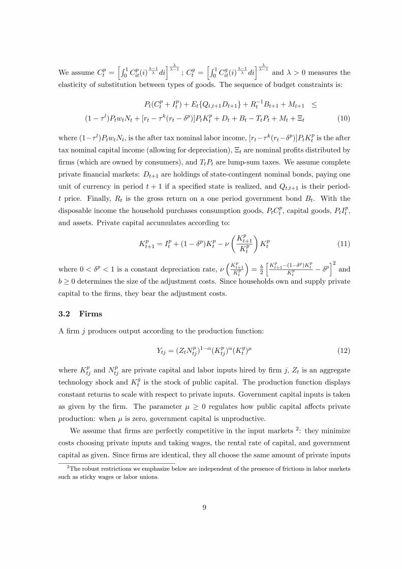
We assume Cpt =

hR 10 C

pit(i)

λ−1λ di

i λλ−1

; Cgt =

hR 10 C

git(i)

λ−1λ di

i λλ−1

and λ > 0 measures the

elasticity of substitution between types of goods. The sequence of budget constraints is:

Pt(Cpt + Ipt ) +EtQt,t+1Dt+1+R−1t Bt+1 +Mt+1 ≤

(1− τ l)PtwtNt + [rt − τk(rt − δp)]PtKpt +Dt +Bt − TtPt +Mt + Ξt (10)

where (1−τ l)PtwtNt, is the after tax nominal labor income, [rt−τk(rt−δp)]PtKpt is the after

tax nominal capital income (allowing for depreciation), Ξt are nominal profits distributed by

firms (which are owned by consumers), and TtPt are lump-sum taxes. We assume complete

private financial markets: Dt+1 are holdings of state-contingent nominal bonds, paying one

unit of currency in period t + 1 if a specified state is realized, and Qt,t+1 is their period-

t price. Finally, Rt is the gross return on a one period government bond Bt. With the

disposable income the household purchases consumption goods, PtCpt , capital goods, PtI

pt ,

and assets. Private capital accumulates according to:

Kpt+1 = Ipt + (1− δp)Kp

t − ν

µKpt+1

Kpt

¶Kpt (11)

where 0 < δp < 1 is a constant depreciation rate, ν³Kpt+1

Kpt

´= b

2

hKpt+1−(1−δp)Kp

t

Kpt

− δpi2and

b ≥ 0 determines the size of the adjustment costs. Since households own and supply privatecapital to the firms, they bear the adjustment costs.

3.2 Firms

A firm j produces output according to the production function:

Ytj = (ZtNptj)1−α(Kp

tj)α(Kg

t )µ (12)

where Kptj and Np

tj are private capital and labor inputs hired by firm j, Zt is an aggregate

technology shock and Kgt is the stock of public capital. The production function displays

constant returns to scale with respect to private inputs. Government capital inputs is taken

as given by the firm. The parameter µ ≥ 0 regulates how public capital affects private

production: when µ is zero, government capital is unproductive.

We assume that firms are perfectly competitive in the input markets 2: they minimize

costs choosing private inputs and taking wages, the rental rate of capital, and government

capital as given. Since firms are identical, they all choose the same amount of private inputs

2The robust restrictions we emphasize below are independent of the presence of frictions in labor markets

such as sticky wages or labor unions.

9

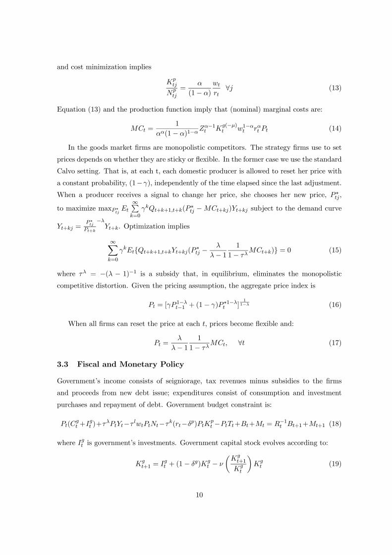
and cost minimization implies

Kptj

Nptj

=α

(1− α)

wt

rt∀j (13)

Equation (13) and the production function imply that (nominal) marginal costs are:

MCt =1

αα(1− α)1−αZα−1t K

g(−µ)t w1−αt rαt Pt (14)

In the goods market firms are monopolistic competitors. The strategy firms use to set

prices depends on whether they are sticky or flexible. In the former case we use the standard

Calvo setting. That is, at each t, each domestic producer is allowed to reset her price with

a constant probability, (1−γ), independently of the time elapsed since the last adjustment.When a producer receives a signal to change her price, she chooses her new price, P ∗tj ,

to maximize maxP∗tj Et

∞Pk=0

γkQt+k+1,t+k(P∗tj −MCt+kj)Yt+kj subject to the demand curve

Yt+kj =P∗tjPt+k

−λYt+k. Optimization implies

∞Xk=0

γkEtQt+k+1,t+kYt+kj(P∗tj −

λ

λ− 11

1− τλMCt+k) = 0 (15)

where τλ = −(λ − 1)−1 is a subsidy that, in equilibrium, eliminates the monopolisticcompetitive distortion. Given the pricing assumption, the aggregate price index is

Pt = [γP1−λt−1 + (1− γ)P ∗1−λt ]

11−λ (16)

When all firms can reset the price at each t, prices become flexible and:

Pt =λ

λ− 11

1− τλMCt, ∀t (17)

3.3 Fiscal and Monetary Policy

Government’s income consists of seigniorage, tax revenues minus subsidies to the firms

and proceeds from new debt issue; expenditures consist of consumption and investment

purchases and repayment of debt. Government budget constraint is:

Pt(Cgt +I

gt )+τ

λPtYt−τ lwtPtNt−τk(rt−δp)PtKpt −PtTt+Bt+Mt = R−1t Bt+1+Mt+1 (18)

where Igt is government’s investments. Government capital stock evolves according to:

Kgt+1 = Igt + (1− δg)Kg

t − ν

µKgt+1

Kgt

¶Kgt (19)

10

where 0 < δg < 1 is a constant and ν(.) is the same as for the private sector and Igt is

stochastic. We treat tax rates on labor and capital income parametrically; assume that

the government takes market prices, private hours and private capital as given, and that Bt

endogenously adjusts to ensure that the budget constraint is satisfied. In order to guarantee

a non-explosive solution for debt (see e.g., Leeper (1991)), we assume a tax rule of the form:

TtT ss

= [(Bt

Yt)/(

Bss

Y ss))]φb (20)

where the superscript ss indicates steady states. Finally, there is an independent monetary

authority which sets the nominal interest rate according to the rule:

Rt

Rss=

πφπt

πssut (21)

where πt is current inflation, ut is a monetary policy shock. Given this rule, the authority

stands ready to supply nominal balances that the private sector demands.

3.4 Closing the model

There are two types of aggregate constraints. First, labor supply must equate labor em-

ployed by the private firms. Second, aggregate production must equate the demand for

goods from the private and public sector, that is Yt = Cpt + Ipt + Cg

t + Igt .

We assume that the four exogenous processes St = [Zt, Cgt , I

gt , ut]

0, evolve according to

log(St) = (I4 − %) log(S) + % log(St−1) + Vt (22)

where I4 is a 4× 4 identity matrix, % is a 4× 4 diagonal matrix with all the roots less thanone in modulus, S is the mean of S and the 4×1 innovation vector Vt is a zero-mean, whitenoise process. Let A = (A1,A2) represent the vector of parameters of the model.

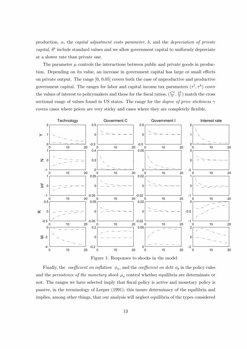
Figure 1 presents impulse responses produced by the four shocks to the model when

the parameters are allowed to vary within the ranges presented in table 1. To be precise,

each box reports 68% of the 10000 paths generated randomly drawing Aj , j = 1, 2, . . .

independently from a uniform distribution covering the range appearing in table 1. The

first column represents responses to technology shocks, the second responses to government

expenditure shocks, the third responses to government investment shocks and the fourth

responses to monetary shocks. Since our VAR includes output, hours, inflation, nominal

rate and money, figure 1 only plots the responses of these variables to the shocks.

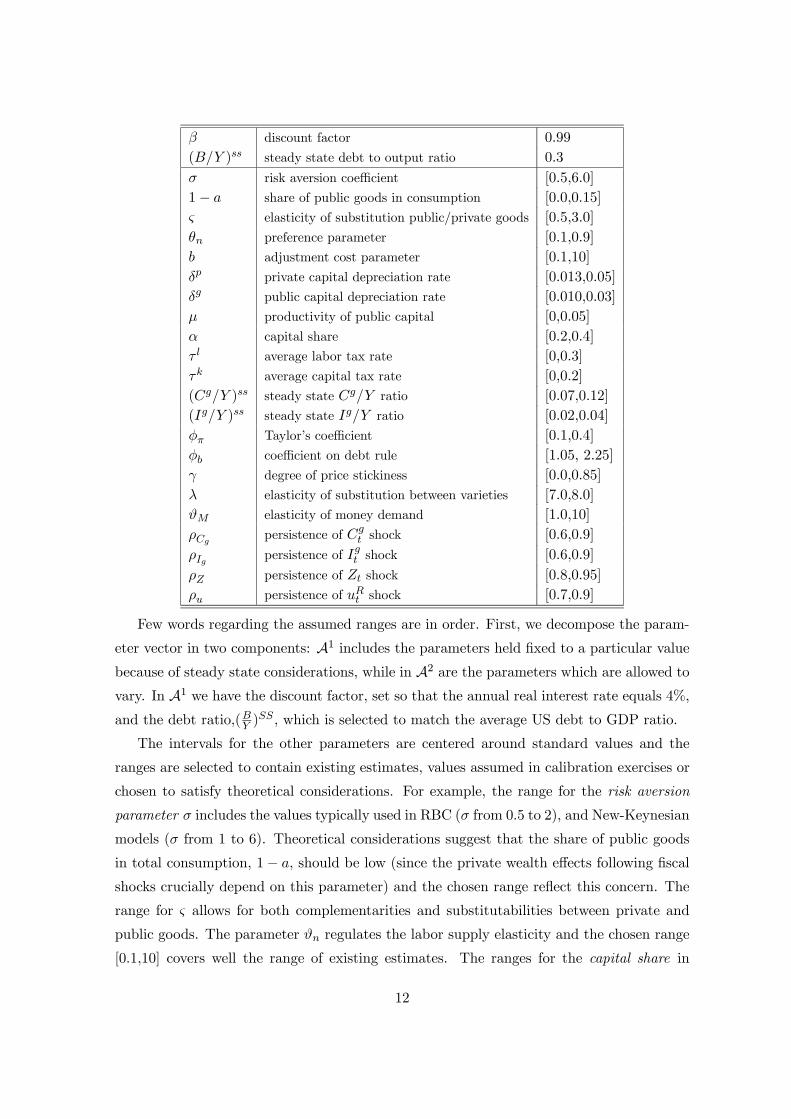
Table 1: Parameter values or ranges

11

β discount factor 0.99

(B/Y )ss steady state debt to output ratio 0.3

σ risk aversion coefficient [0.5,6.0]

1− a share of public goods in consumption [0.0,0.15]

ς elasticity of substitution public/private goods [0.5,3.0]

θn preference parameter [0.1,0.9]

b adjustment cost parameter [0.1,10]

δp private capital depreciation rate [0.013,0.05]

δg public capital depreciation rate [0.010,0.03]

µ productivity of public capital [0,0.05]

α capital share [0.2,0.4]

τ l average labor tax rate [0,0.3]

τk average capital tax rate [0,0.2]

(Cg/Y )ss steady state Cg/Y ratio [0.07,0.12]

(Ig/Y )ss steady state Ig/Y ratio [0.02,0.04]

φπ Taylor’s coefficient [0.1,0.4]

φb coefficient on debt rule [1.05, 2.25]

γ degree of price stickiness [0.0,0.85]

λ elasticity of substitution between varieties [7.0,8.0]

ϑM elasticity of money demand [1.0,10]

ρCg persistence of Cgt shock [0.6,0.9]

ρIg persistence of Igt shock [0.6,0.9]

ρZ persistence of Zt shock [0.8,0.95]

ρu persistence of uRt shock [0.7,0.9]

Few words regarding the assumed ranges are in order. First, we decompose the param-

eter vector in two components: A1 includes the parameters held fixed to a particular valuebecause of steady state considerations, while in A2 are the parameters which are allowed tovary. In A1 we have the discount factor, set so that the annual real interest rate equals 4%,and the debt ratio,(BY )

SS , which is selected to match the average US debt to GDP ratio.

The intervals for the other parameters are centered around standard values and the

ranges are selected to contain existing estimates, values assumed in calibration exercises or

chosen to satisfy theoretical considerations. For example, the range for the risk aversion

parameter σ includes the values typically used in RBC (σ from 0.5 to 2), and New-Keynesian

models (σ from 1 to 6). Theoretical considerations suggest that the share of public goods

in total consumption, 1− a, should be low (since the private wealth effects following fiscal

shocks crucially depend on this parameter) and the chosen range reflect this concern. The

range for ς allows for both complementarities and substitutabilities between private and

public goods. The parameter ϑn regulates the labor supply elasticity and the chosen range

[0.1,10] covers well the range of existing estimates. The ranges for the capital share in

12

production, α, the capital adjustment costs parameter, b, and the depreciation of private

capital, δp include standard values and we allow government capital to uniformly depreciate

at a slower rate than private one.

The parameter µ controls the interactions between public and private goods in produc-

tion. Depending on its value, an increase in government capital has large or small effects

on private output. The range [0, 0.05] covers both the case of unproductive and productive

government capital. The ranges for labor and capital income tax parameters (τ l, τk) cover

the values of interest to policymakers and those for the fiscal ratios, (Cg

Y , Ig

Y ) match the cross

sectional range of values found in US states. The range for the degree of price stickiness γ

covers cases where prices are very sticky and cases where they are completely flexible.

0 10 200

1

2

Y

Technology

0 10 20-1

0

1

N

0 10 20-1

0

1

Inf

0 10 20-0.5

0

0.5

R

0 10 20-4

-2

0

M

0 10 20-0.5

0

0.5Goverment C

0 10 200

0.2

0.4

0 10 20-0.05

0

0.05

0 10 20-0.05

0

0.05

0 10 20-0.2

0

0.2

0 10 20-0.5

0

0.5Government I

0 10 200

0.05

0 10 20-0.02

0

0.02

0 10 20-0.02

0

0.02

0 10 200

0.05

0 10 200

1

2Interest rate

0 10 20-5

0

5

0 10 20-1

0

1

0 10 20-1

-0.5

0

0 10 20-2

0

2

Figure 1: Responses to shocks in the model

Finally, the coefficient on inflation φπ, and the coefficient on debt φb in the policy rules

and the persistence of the monetary shock ρu control whether equilibria are determinate or

not. The ranges we have selected imply that fiscal policy is active and monetary policy is

passive, in the terminology of Leeper (1991); this insure determinacy of the equilibria and

implies, among other things, that our analysis will neglect equilibria of the types considered

13

in Lubik and Schorfheide (2004). Therefore the interpretation of our monetary policy shocks

is somewhat different from theirs.

The model produces several robust sign implications in responses to various shocks.

For example, a persistent technological disturbance increases output, decreases inflation,

nominal rates and nominal balances and the sign of the response is independent of the

horizon. Note, instead, that the sign of the hours response is not robustly pinned down.

This does not depend on the fact that we have allow prices to be flexible: the same pattern

is obtained when the lower bound of the range for γ is increased to 0.35.

The model delivers robust implications also in response to the three demand shocks.

When government consumption expenditure or government investment expenditure in-

crease, output, hours, inflation, nominal interest rates and nominal balances all increase,

while surprise decreases in the interest rate increase output, hours, inflation and nominal

balances. Note, in particular, that these patterns obtain for a wide range of values of the

elasticity of substitution between private and public goods, the share of capital in the pro-

duction function, the strength of the reaction of interest rates and taxes to inflation and

debt and the degree of price stickiness. In other words, except for monetary policy shocks,

responses are independent of whether sticky or flexible prices or whether the RBC or the

New-Keynesian versions of the model are considered.

Since the dynamics produced by government consumption and government investment

shocks are qualitatively similar - the sign of dynamic responses of the five variables is the

same for both shocks - we will identify a technology shock, a monetary shock and only one

government shock, without attempting to distinguish between consumption or investment

disturbances. The identification restrictions used at each t are summarized in table 2. Note

that the dynamics of hours (and labor productivity) are unrestricted in all cases.

Table 2: Identification restrictions

Output Inflation Interest rate Money

Technology ≥ 0 ≤ 0Government ≥ 0 ≥ 0 ≥ 0 ≥ 0Monetary ≥ 0 ≥ 0 ≤ 0 ≥ 0

There are many ways of implementing the restrictions presented in table 2. The results

we present are obtained using an acceptance sampling scheme where draws that jointly

satisfy the restrictions for all three shocks are kept and draws that do not are discarded. Tim

Cogley pointed out to us that, since the bands presented in figure 1 do not insure that some

parameter combinations may fail to satisfy the restrictions, an importance sampling scheme,

which gives positive but different weights to different types of draws is, in principle, more

14

appropriate. Since there are several ways to implement an acceptance sampling scheme, we

have tried a few alternatives. First, we have weighted draws in proportion to the number of

horizons at which restrictions are satisfied. Thus, if we impose restrictions at three horizons,

we give weight 0.5/n1 to draws that satisfy restrictions at all horizons, weight 0.33/n2 to

draws that satisfy restrictions at two horizons, and weight 0.17/n3 to draws that satisfy

restrictions at one horizon,n1 + n2 + n3 + n4 = n, where n is the total number of draws.

Second, we have weighted the draws satisfying all the restrictions by 0.68/n1 and draws

which do not satisfy all the restrictions by 0.32/n2, n1+n2 = n. The results we present are

qualitatively independent of the scheme used to weight draws even though, quantitatively,

some conclusions become more or less significant. An appendix available on request contains

the results obtained with these alternatives.

Since the sign restrictions we use are robust to the horizon, we are free to choose how

many responses to restrict. However, there is an important trade-off to be considered, since

the smaller is the number of restrictions, the larger is the number of draws consistent with

the restrictions but, potentially, the weaker is the link between the model and the empirical

analysis. Hence, we could obtain more precise estimates of responses which may only be

partially related to those of the model. As the number of restricted responses increases,

we tight up the empirical analysis to the model more firmly. However, it may be the case

that the number of draws satisfying the restrictions drops dramatically, making estimates

of standard errors inaccurate. Since the relationship between number of restrictions and

number of accepted draws is highly nonlinear, there is no straightforward way to optimize

this trade-off. We present results obtained imposing restrictions at two horizons (0 and 1)

since this choice seems to account for both concerns.

4 Estimation

The model (6)-(7) is estimated using Bayesian methods. We specify prior distributions for

θ0,Σ0,Ω0, and H0 and use data up to t to compute posterior estimates of the structural

parameters and of continuous functions of them. Since our sample goes from 1960:1 to

2003:2, we initially estimate the model for the period 1960:1-1970:2 and then reestimate it

33 times moving the terminal date by one year up to 2003:2

Posterior distributions for the structural parameters are not available in a closed form.

MCMC methods are used to simulate posterior sequences consistent with the information

available up to time t. Estimation of reduced form TVC-VAR models with or without time

variations in the variance of VAR shocks is now standard (see e.g. Cogley and Sargent

15

(2005)): it requires treating the parameters which are time varying as a block in a Gibbs

sampler algorithm. Hence, at each t and in each Gibbs sampler cycle, one runs the Kalman

filter/smoother, conditional on the draw of the other time invariant parameters. In our

setup the calculations are complicated by the fact that at each cycle, we need to obtain

structural estimates of the time varying features of the model. This means that, in each

cycle, we discard paths which are explosive and paths which do not satisfy the restrictions.

Convergence was checked using a CUMSUM statistic. The results we present are based

on 20,000 draws for each t - of these, after the non-explosive and the identification filters

are used, about 200 are kept for inference. The methodology used to construct posterior

distributions for the unknowns is contained, together with the prior specifications, in the

appendix. The data comes from the FREDII data base of the Federal Reserve Bank of St.

Louis and consists of GDP (GDPC1), GDP deflator inflation (∆GDPDEF), the Federal

funds rate (FEDFUNDS), hours of all persons in the non-farm business sector (HOANBS)

and M1 (M1SL). In parenthesis are the mnemonic used by FREDII.

5 The Results

5.1 The dynamics of volatility and persistence

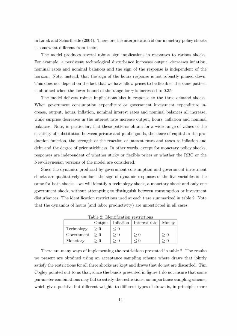
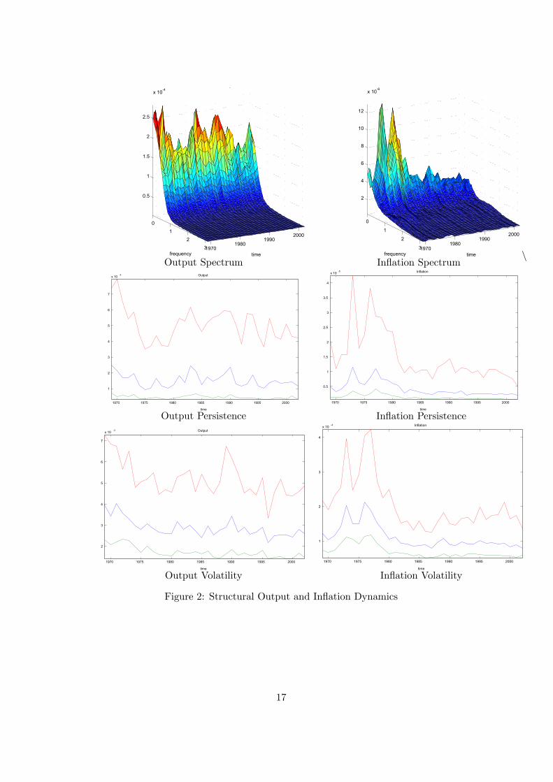
We start our analysis presenting in figure 1 the evolution of the structural spectrum of

output and inflation from 1970:1 to 2003:2 (first panel) and the 68% central posterior bands

for structural persistence (second panel) and for structural volatility (third panel), for the

same two variables. The former is measured by the height of the spectrum at frequency

zero; the latter by the value of the cumulative spectrum. McConnell and Perez Quiroz

(2001), Sargent and Cogley (2001), Stock and Watson (2003), Pivetta and Reis (2003)

among others, have documented using reduced form, non-recusive and mostly univariate

techniques, that output and inflation volatility and inflation persistence declined over time.

Our analysis differs from theirs in the sense that it is multivariate, recursive, and explicitly

structural.

Several interesting features emerge from figure 1. First, the spectrum of inflation is

relatively stable over time, except for the zero frequency. Therefore, structural changes in

inflation volatility are closely associated with changes in its persistence. The spectrum of

output is also relatively stable over time at almost all frequencies. However, variations

16

01

231970

19801990

2000

0.5

1

1.5

2

2.5

x 10-4

time

p

frequency

Output Spectrum

0

1

2

319701980

19902000

2

4

6

8

10

12

x 10-6

timefrequency

Inflation Spectrum\

1970 1975 1980 1985 1990 1995 2000

1

2

3

4

5

6

7

x 10 -4

time

Output

Output Persistence

1970 1975 1980 1985 1990 1995 2000

0.5

1

1.5

2

2.5

3

3.5

4

x 10 -5

time

Inflation

Inflation Persistence

1970 1975 1980 1985 1990 1995 2000

2

3

4

5

6

7

x 10 -3

time

Output

Output Volatility

1970 1975 1980 1985 1990 1995 2000

1

2

3

4

x 10 -4

time

Inflation

Inflation Volatility

Figure 2: Structural Output and Inflation Dynamics

17

in structural volatility are not necessarily linked to changes in its persistence. In fact, most of

the variations in the spectrum of output are located in the frequencies corresponding to three

to five years cycles (ω ∈ [0.314, 0.52]). Second, inflation persistence shows a marked hump-shaped pattern: it displays a five fold increase in 1973-1974 and then again in 1977-1978,

it drops dramatically after that date, and since 1982 the posterior distribution of inflation

persistence displays marginal variations. Interestingly, while the mean of the posterior shows

a clear declining trend since the mid-1970s - the drop in the mean of the posterior persistence

from the peak is about 66 percent - the pattern is not statistically significant because of

the large uncertainty associated with the mean increase in the 1970s. Third, variations over

time in output persistence are relatively small and there is little posterior evidence that the

difference between the mean estimate obtained at any two dates in the sample is significantly

different from zero. Interestingly, there seems to be a negative correlation between the

time path of the means of the posterior of inflation and of output persistence, and this

is particularly evident in the mid-1970s. Fourth, as expected from previous discussion,

the dynamics of the posterior 68% band of structural inflation volatility reflect those of

structural inflation persistence. Fifth, although output volatility declines by roughly 25

percent from the beginning to the end of the sample, the change is statistically insignificant.

The standard error around the statistics we report are larger than those obtained by

other authors. One relevant question is therefore which of feature of our approach is re-

sponsible for this outcome. We singled out three possibilities which appear to be relevant.

First, it could be that some parameter draws are more consistent than others with the sign

restrictions. If these draws imply larger volatility in the coefficients it could be that the

estimated variance of the error in the law of motion of the coefficients could be larger for

accepted than rejected draws. This turns out not to be the case: the two variances are statis-

tically indistinguishable. Furthermore, similarly large bands obtain when a non-structural

Choleski decomposition is used. Second, figure 2 is constructed using recursive analysis.

Therefore our estimates are consistent with the information available at each t and contains

less information than those of others which are produced using smoothed estimated of the

parameters from the full sample. Although standard errors are reduced when smoothed

estimates are considered, the pattern of changes is qualitative unaltered. Third, since our

spectral estimates are constructed allowing future coefficients to be random, it could be the

case that this source of uncertainty is responsible for the large standard errors we report.

We have therefore repeated the analysis averaging out future shocks to the coefficients and

found that standard errors are smaller by about 30 percent. Hence, recursive analysis and

the methodology use to compute impulse responses appear to be responsible for the larger

18

standard error we produce.

In summary, three points can be made. First, while there is visual evidence of a decline

in the point estimates of output and inflation volatility, the case for evolving volatility is

considerably reduced once posterior standard errors are taken into account. This evidence

should be contrasted with the one obtained with univariate, in-sample, reduced form meth-

ods, which overwhelmingly points to the presence of a significant structural break in the

variability of the two series. Second, the case for evolving posterior distributions of persis-

tence measures is far weaker. The posterior mean of inflation persistence shows a declining

trend but posterior uncertainty is sufficiently large to make mean differences irrelevant

while the posterior distribution of output persistence displays neither breaks nor evolving

dynamics. Third, perhaps more importantly, the timing of the changes in persistences and

volatilities do not appear to be synchronized. Hence, it is unlikely that we can account for

the changes in output and inflation with a single and common explanation.

5.2 What drives changes in volatility and in persistence?

Recall that our structural model has implications for three types of disturbances, roughly

speaking, supply, real demand and monetary shocks. Therefore, the model allows us to

identify at most three of the five structural shocks driving the VAR. The share of the

variability in output and inflation explained by these shocks can then be used to gauge the

soundness of our analysis.

Given that the spectrum at frequency ω is uncorrrelated with the spectrum at frequency

ω0, where both ω and ω0 are Fourier frequencies, it is easy to compute the relative contribu-

tion of each of the three structural shocks to changes in the volatility and in the persistence

of output and inflation. In fact, the (time varying) structural MA representation of the

system is yit =P5

j=1 Bjt( )ejt where eit is orthogonal to ei0t, i0 6= i, i = 1, . . . , 5. Since

structural shocks are independent, the spectrum of yit at frequency ω can be written as

Syi(ω)(t) =P5

j=1 |Bjt(ω)|2Sej (ω)(t). Therefore, the fraction of the persistence in yit due tostructural shock j is Sj

yi(ω = 0)(t) =|Bjt(ω=0)|2Sej (ω=0)(t)

Syi(ω=0)(t)and the fraction of the volatility in

yit due to structural shock j isP

ω Sjyi(ω)(t). Intuitively, these measures are comparable to

variance decomposition shares: while the latter tells us the relative contribution of different

shocks at various forecasting horizons, these evaluate the contribution of structural shock

j to the variability of yit at either one frequency or for all frequencies.

There is considerable stability in the relative contribution of different shocks over time.

That is, relatively speaking, sources of fluctuations in output and inflation have been quite

similar over time. Interestingly, different shocks dominate at different frequencies. For

19

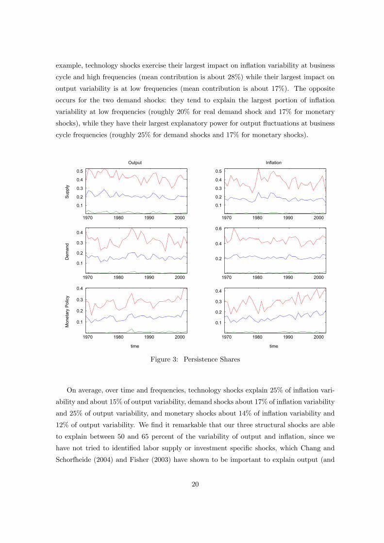
example, technology shocks exercise their largest impact on inflation variability at business

cycle and high frequencies (mean contribution is about 28%) while their largest impact on

output variability is at low frequencies (mean contribution is about 17%). The opposite

occurs for the two demand shocks: they tend to explain the largest portion of inflation

variability at low frequencies (roughly 20% for real demand shock and 17% for monetary

shocks), while they have their largest explanatory power for output fluctuations at business

cycle frequencies (roughly 25% for demand shocks and 17% for monetary shocks).

1970 1980 1990 2000

0.1

0.2

0.3

0.4

0.5

Sup

ply

Output

1970 1980 1990 2000

0.1

0.2

0.3

0.4

Dem

and

1970 1980 1990 2000

0.1

0.2

0.3

0.4

time

Mon

etar

y P

olic

y

1970 1980 1990 2000

0.1

0.2

0.3

0.4

0.5

Inflation

1970 1980 1990 2000

0.2

0.4

0.6

1970 1980 1990 2000

0.1

0.2

0.3

0.4

time

Figure 3: Persistence Shares

On average, over time and frequencies, technology shocks explain 25% of inflation vari-

ability and about 15% of output variability, demand shocks about 17% of inflation variability

and 25% of output variability, and monetary shocks about 14% of inflation variability and

12% of output variability. We find it remarkable that our three structural shocks are able

to explain between 50 and 65 percent of the variability of output and inflation, since we

have not tried to identified labor supply or investment specific shocks, which Chang and

Schorfheide (2004) and Fisher (2003) have shown to be important to explain output (and

20

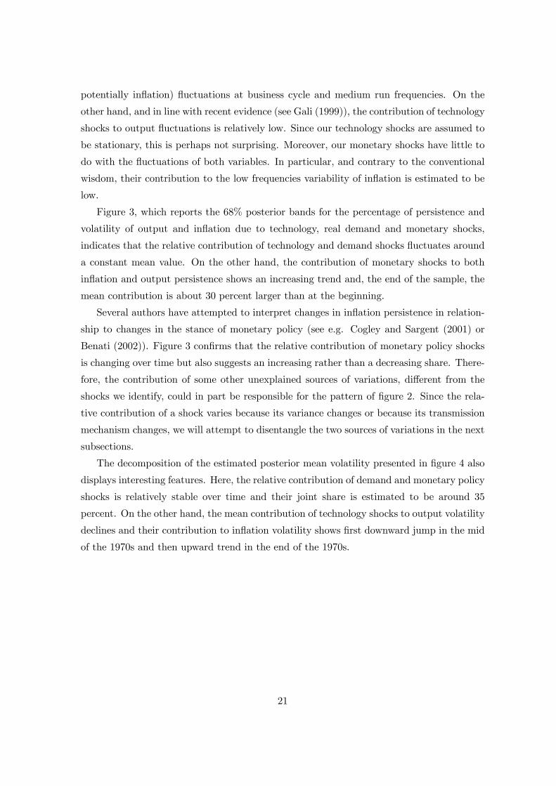
potentially inflation) fluctuations at business cycle and medium run frequencies. On the

other hand, and in line with recent evidence (see Gali (1999)), the contribution of technology

shocks to output fluctuations is relatively low. Since our technology shocks are assumed to

be stationary, this is perhaps not surprising. Moreover, our monetary shocks have little to

do with the fluctuations of both variables. In particular, and contrary to the conventional

wisdom, their contribution to the low frequencies variability of inflation is estimated to be

low.

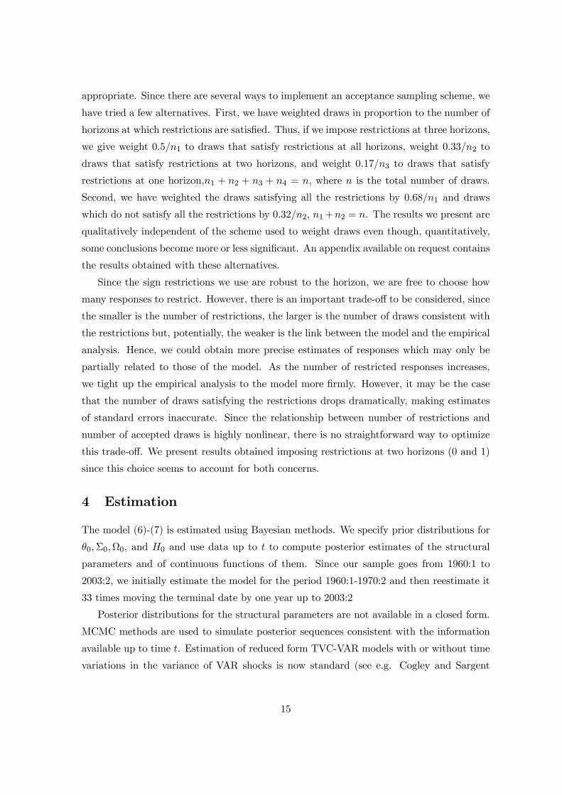
Figure 3, which reports the 68% posterior bands for the percentage of persistence and

volatility of output and inflation due to technology, real demand and monetary shocks,

indicates that the relative contribution of technology and demand shocks fluctuates around

a constant mean value. On the other hand, the contribution of monetary shocks to both

inflation and output persistence shows an increasing trend and, the end of the sample, the

mean contribution is about 30 percent larger than at the beginning.

Several authors have attempted to interpret changes in inflation persistence in relation-

ship to changes in the stance of monetary policy (see e.g. Cogley and Sargent (2001) or

Benati (2002)). Figure 3 confirms that the relative contribution of monetary policy shocks

is changing over time but also suggests an increasing rather than a decreasing share. There-

fore, the contribution of some other unexplained sources of variations, different from the

shocks we identify, could in part be responsible for the pattern of figure 2. Since the rela-

tive contribution of a shock varies because its variance changes or because its transmission

mechanism changes, we will attempt to disentangle the two sources of variations in the next

subsections.

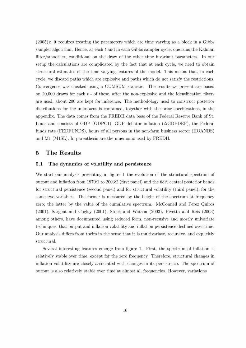
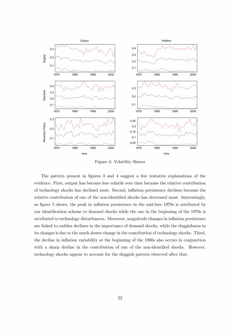
The decomposition of the estimated posterior mean volatility presented in figure 4 also

displays interesting features. Here, the relative contribution of demand and monetary policy

shocks is relatively stable over time and their joint share is estimated to be around 35

percent. On the other hand, the mean contribution of technology shocks to output volatility

declines and their contribution to inflation volatility shows first downward jump in the mid

of the 1970s and then upward trend in the end of the 1970s.

21

1970 1980 1990 2000

0.1

0.2

0.3

Sup

ply

Output

1970 1980 1990 2000

0.1

0.2

0.3

0.4

Dem

and

1970 1980 1990 2000

0.1

0.2

0.3

time

Mon

etar

y P

olic

y

1970 1980 1990 2000

0.1

0.2

0.3

0.4

Inflation

1970 1980 1990 2000

0.1

0.2

0.3

1970 1980 1990 2000

0.05

0.1

0.15

0.2

0.25

time

Figure 4: Volatility Shares

The pattern present in figures 3 and 4 suggest a few tentative explanations of the

evidence. First, output has become less volatile over time because the relative contribution

of technology shocks has declined most. Second, inflation persistence declines because the

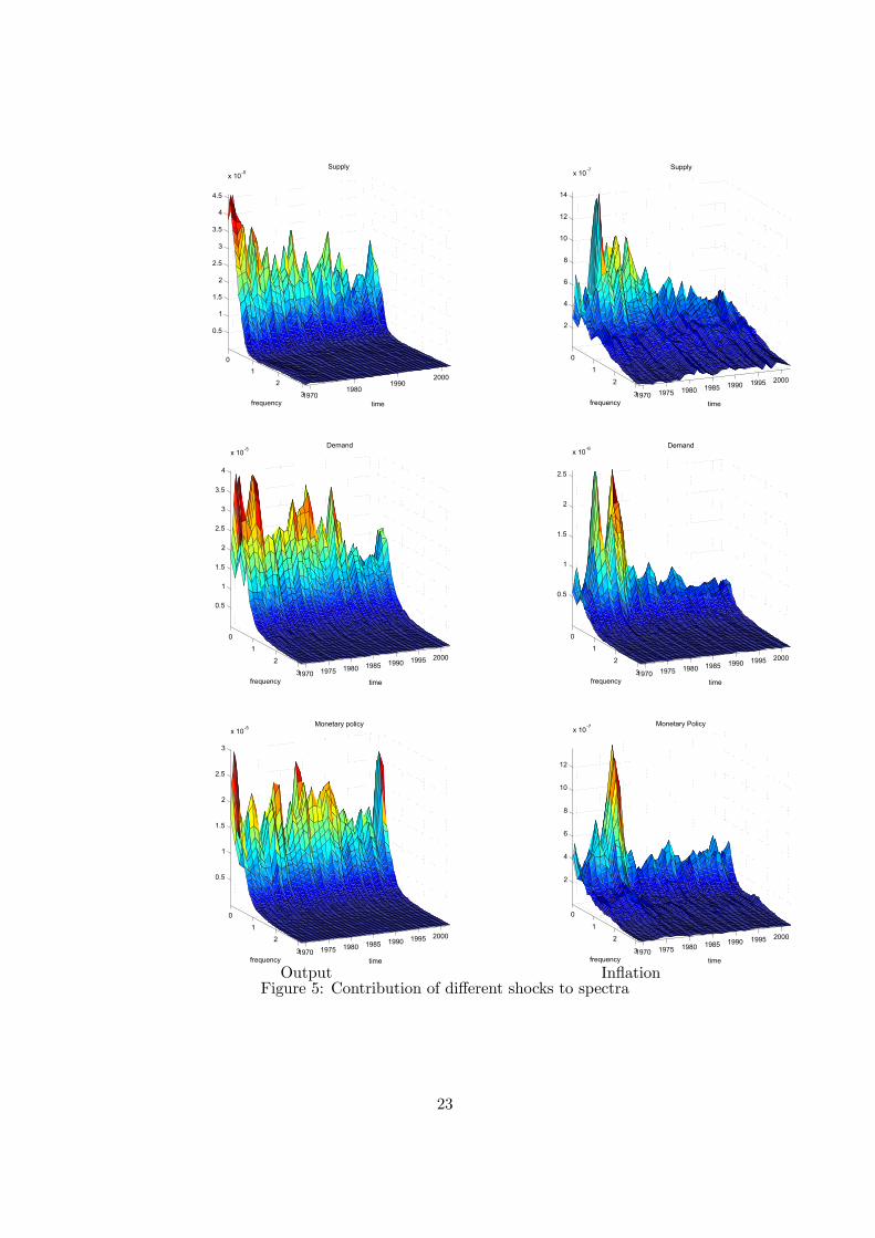
relative contribution of one of the non-identified shocks has decreased most. Interestingly,

as figure 5 shows, the peak in inflation persistence in the mid-late 1970s is attributed by

our identification scheme to demand shocks while the one in the beginning of the 1970s is

attributed to technology disturbances. Moreover, magnitude changes in inflation persistence

are linked to sudden declines in the importance of demand shocks, while the sluggishness in

its changes is due to the much slower change in the contribution of technology shocks. Third,

the decline in inflation variability at the beginning of the 1980s also occurs in conjunction

with a sharp decline in the contribution of one of the non-identified shocks. However,

technology shocks appear to account for the sluggish pattern observed after that.

22

01

231970

19801990

2000

0.5

1

1.5

2

2.5

3

3.5

4

4.5

x 10-5

time

Supply

frequency

0

1

2

31970 1975 1980 1985 1990 1995 2000

2

4

6

8

10

12

14

x 10-7

time

Supply

frequency

0

1

2

31970 1975 1980 1985 1990 1995 2000

0.5

1

1.5

2

2.5

3

3.5

4

x 10-5

time

Demand

frequency

0

1

2

31970 1975 1980 1985 1990 1995 2000

0.5

1

1.5

2

2.5

x 10-6

time

Demand

frequency

0

1

2

31970 1975 1980 1985 1990 1995 2000

0.5

1

1.5

2

2.5

3

x 10-5

time

Monetary policy

frequency

Output

0

1

2

31970 1975 1980 1985 1990 1995 2000

2

4

6

8

10

12

x 10-7

time

Monetary Policy

frequency

InflationFigure 5: Contribution of different shocks to spectra

23

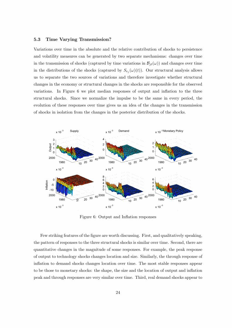
5.3 Time Varying Transmission?

Variations over time in the absolute and the relative contribution of shocks to persistence

and volatility measures can be generated by two separate mechanisms: changes over time

in the transmission of shocks (captured by time variations in Bjt(ω)) and changes over timein the distributions of the shocks (captured by Sej (ω)(t)). Our structural analysis allows

us to separate the two sources of variations and therefore investigate whether structural

changes in the economy or structural changes in the shocks are responsible for the observed

variations. In Figure 6 we plot median responses of output and inflation to the three

structural shocks. Since we normalize the impulse to be the same in every period, the

evolution of these responses over time gives us an idea of the changes in the transmission

of shocks in isolation from the changes in the posterior distribution of the shocks.

10 20 30 401980

2000

0123

x 10 -3 Supply

Out

put

10 20 30 401980

2000

-10

-5

0

x 10 -4

Infla

tion

x 10 -3

10 20 30 401980

2000

0

2

4

x 10 -3 Demand

10 20 30 401980

2000

02468

x 10 -4

x 10 -3

10 20 30 401980

2000

012

x 10 -3 Monetary Policy

10 20 30 401980

2000

0246

x 10 -4

x 10 -3

Figure 6: Output and Inflation responses

Few striking features of the figure are worth discussing. First, and qualitatively speaking,

the pattern of responses to the three structural shocks is similar over time. Second, there are

quantitative changes in the magnitude of some responses. For example, the peak response

of output to technology shocks changes location and size. Similarly, the through response of

inflation to demand shocks changes location over time. The most stable responses appear

to be those to monetary shocks: the shape, the size and the location of output and inflation

peak and through responses are very similar over time. Third, real demand shocks appear to

24

produce the largest displacements of the two variables followed by technology and monetary

shocks. Fourth, and relatively speaking, the largest changes in the transmission appear to

be associated with output responses to technology shocks. For example, the magnitude of

contemporaneous responses is 50% larger in the 1990s than in the 1970s.

Hence, while the qualitatively features of the transmission of technology, real demand

and monetary shock are similar over time, changes in the quantitative features, involv-

ing the magnitude of the responses and, at times, the location of the peak/through are

present. Also, while responses to monetary disturbances appear to be similar over time, the

transmission of technology disturbances shows important instabilities.

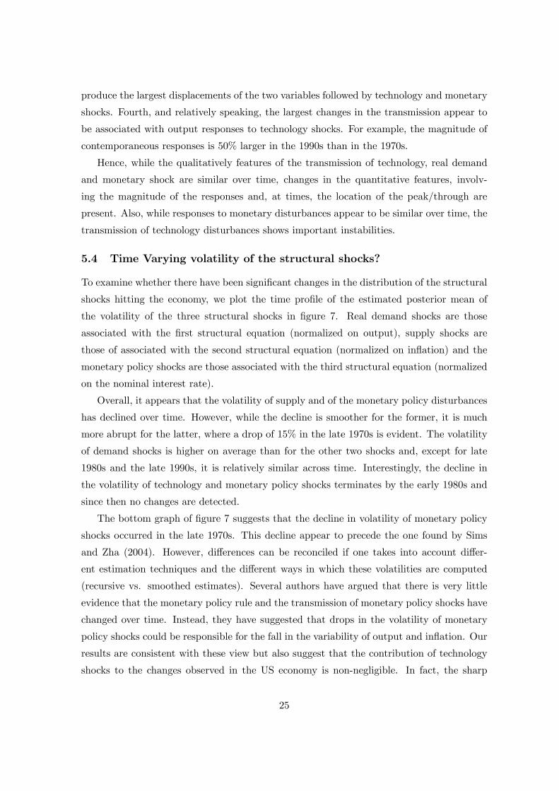
5.4 Time Varying volatility of the structural shocks?

To examine whether there have been significant changes in the distribution of the structural

shocks hitting the economy, we plot the time profile of the estimated posterior mean of

the volatility of the three structural shocks in figure 7. Real demand shocks are those

associated with the first structural equation (normalized on output), supply shocks are

those of associated with the second structural equation (normalized on inflation) and the

monetary policy shocks are those associated with the third structural equation (normalized

on the nominal interest rate).

Overall, it appears that the volatility of supply and of the monetary policy disturbances

has declined over time. However, while the decline is smoother for the former, it is much

more abrupt for the latter, where a drop of 15% in the late 1970s is evident. The volatility

of demand shocks is higher on average than for the other two shocks and, except for late

1980s and the late 1990s, it is relatively similar across time. Interestingly, the decline in

the volatility of technology and monetary policy shocks terminates by the early 1980s and

since then no changes are detected.

The bottom graph of figure 7 suggests that the decline in volatility of monetary policy

shocks occurred in the late 1970s. This decline appear to precede the one found by Sims

and Zha (2004). However, differences can be reconciled if one takes into account differ-

ent estimation techniques and the different ways in which these volatilities are computed

(recursive vs. smoothed estimates). Several authors have argued that there is very little

evidence that the monetary policy rule and the transmission of monetary policy shocks have

changed over time. Instead, they have suggested that drops in the volatility of monetary

policy shocks could be responsible for the fall in the variability of output and inflation. Our

results are consistent with these view but also suggest that the contribution of technology

shocks to the changes observed in the US economy is non-negligible. In fact, the sharp

25

increase and rapid decline in the variability of reduced form output and inflation forecast

errors observed at the end of the 1970s is due, in part, to variations in the distribution from

which technology shocks are drawn.

1970 1975 1980 1985 1990 1995 2000

4

5

6

7x 10-3 Supply

1970 1975 1980 1985 1990 1995 20000.015

0.02

0.025Demand

1970 1975 1980 1985 1990 1995 2000

6

7

8x 10-3

time

Monetary Policy

Figure 7: Structural shock variances

5.5 The dynamics of hours and labor productivity

Although this paper is primarily interested in studying the structural determinants of

changes in output and inflation, our estimated system allows us to also briefly discuss a

controversial issue which has been at the center of attention in the macroeconomic litera-

ture since work by Gali (1999), Christiano, et. al. (2003), Uhlig (2003), Dedola and Neri

(2004) and others: the dynamics of hours and productivity in response to technology shocks.

Although the empirical evidence is far from clear, it appears that under some identification

and some data transformations (in particular, identification via long run restrictions and

variables in the VAR in growth rates) technology disturbances increase labor productiv-

ity and decrease hours while with other identifications and other data transformations (in

particular, hours quadratically detrended and identification based on short or medium run

26

restrictions) both labor productivity and hours increase.

The dynamics of hours and labor productivity are thought to provide important infor-

mation about sources of business cycle dynamics. In fact, a negative response of hours to

technology disturbances is considered by some to be inconsistent with RBC-flexible price

based explanations of business cycles (a point disputed e.g. by Francis and Ramey (2002)).

In a basic RBC model, in fact, technology shocks act as a supply shiftier and therefore have

positive effects on hours, output and productivity. On the other hand, in a basic sticky

price model, technology shocks act as labor demand shifters. Therefore, firms experience a

decline in their marginal costs but given that price are sticky, aggregate demand increases

less than proportionally than the increase in output so that hours decline. These patterns

are partially present in the general model we have presented in section 3: when prices are

flexible technology disturbances imply robust positive contemporaneous hours responses.

When prices are sticky, the contemporaneous response of hours is mostly negative, but

there are parameters configurations which produce positive hours responses.

Our estimated structural model allows us to investigate two interesting questions which

can shed light on the issue. First, what are the dynamics of hours and labor productivity

when sign restrictions derived from a general model are used to identify technology shocks?

It is well known, at least since Faust and Leeper (1997), that long run restrictions are only

weakly identifying and that the outcome depends on largely unverifiable assumptions about

the time series properties of finite stretches of data. Model based robust restrictions can

therefore offer a viable and more reliable alternative to identify technology shocks. Second,

is there any evidence that the responses of hours to technology shocks displays a time

varying pattern? In other words, could it be that the contemporaneous response of hours

changes sign as the sample changes?

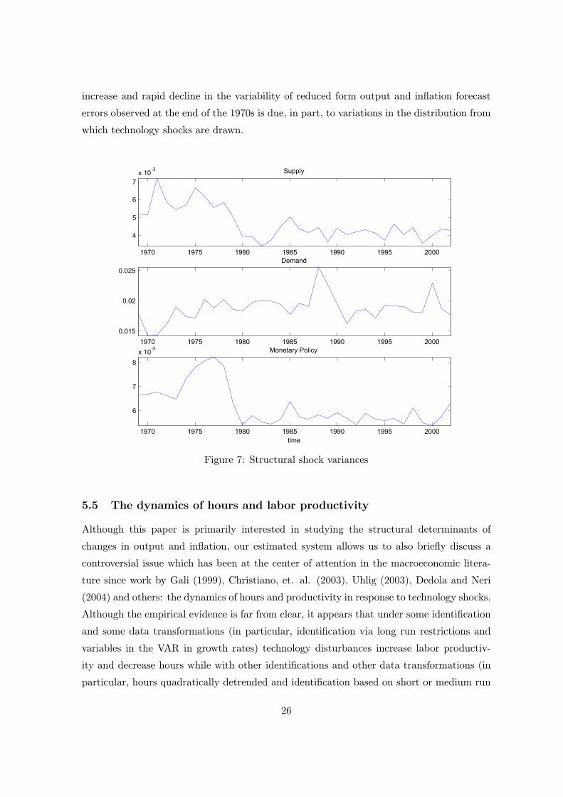
Figure 8 indicates that the contemporaneous response of hours and productivity to

technology shocks is always positive. Interestingly, the response of hours is humped shaped,

with the peak occurring after 2 or 3 quarters and this, combined with a smoothly declining

output responses, implies that labor productivity becomes negative after some periods.

Hence, the results we obtain are fully consistent with a RBC-flexible price explanation of

the propagation of technology shocks. Furthermore, while there are quantitative variations

in the responses of hours and productivity over time, the sign of the responses is the same

at every date in the sample. Therefore, the mixed results found in the literature can not be

due to time variations in the response of hours. Note that, consistent with both RBC and

sticky price models, we find that hours positively comove with output in response to both

demand shocks. However the magnitude of the changes is such that in response to demand

27

shocks productivity responds positively instantaneously but turns negative afterwards while

in response to monetary policy shocks, productivity responses are instantaneously negative

and the sign of the response changes with the horizon of the analysis.

1020

3040

1980

2000

0

10

20

x 10 -4Supply

Hou

rs

1020

3040

1980

2000

-1

0

1

2

3

x 10 -3

quarterstime

Prod

uctiv

ity

1020

3040

1980

2000

-1

0

1

2

3

x 10 -3

quarterstime 1020

3040

1980

2000

-15

-10

-5

0

5

x 10 -4

quarterstime

1020

3040

1980

2000-2

0

2

x 10 -3Demand

1020

3040

1980

2000

0

1

2

x 10 -3Monetary Policy

Figure 8: Hours and Productivity Responses

6 Conclusions

In this paper we examined structural sources of output and inflation volatility and persis-

tence and attempted to draw some conclusions about the causes of the variations experi-

enced in the US economy over the last 25-30 years. There has been a healthy discussion in

the literature on this issue, thanks to the work of Clarida, Gali and Gertler (2000), Cogley

and Sargent (2001) (2003), Boivin and Giannoni, (2002), Leeper and Zha (2003), Sims and

Zha (2004), Lubik and Schorfheide (2004), Primicieri (2004) and Canova and Gambetti

(2004) among others, and although opinions differ, remarkable methodological improve-

ments occurred trying to study questions having to do with time variations in structure of

the economy and in the distributions of the shocks.

Here we contribute to advance the technical frontiers estimating a structural time vary-

28

ing coefficient VAR model; identifying a number of structural shocks using sign restrictions

derived from a general DSGE model; providing recursive analysis, consistent with infor-

mation available at each point in time; and using frequency domain tools to address time

variation issues. In our opinion, the paper also contributes to advance our understanding

of the cause of the observed variations in output and inflation. In particular, we show that

while there are time variations in both the volatility of output and inflation and in the

persistence of inflation, differences are statistically insignificant because of the large stan-

dard errors associated with posterior estimates at each t. Standard errors are larger then in

other studies for two reasons: our recursive analysis makes them depend on the information

available at each t; shocks to future parameters are not averaged out.

We show that the output has become less volatile because the contribution of technol-

ogy shocks has declined over time and that changes in the persistence and the volatility

of inflation can be partially explained by changes in the contribution of technology, real

demand and monetary policy shocks. Furthermore, we show that there are changes in the

transmission of technology shocks and that the variance of both technology and monetary

policy shocks has declined over time. We also provide novel evidence on the effects of tech-

nology shocks on labor market variables. In our estimated system, they robustly imply

positive contemporaneous comovements of hours and labor productivity, even though the

correlation between the two variables turns negative after a few lags.

All in all, our analysis indicates that variations in both the magnitude and the trans-

mission of technology shocks are important to explain observed variations in US output.

Therefore, our conclusions are consistent with those of McConnell and Perez Quiroz (2001)

and Gordon (2003). Our analysis also indicates that both technology and monetary shocks

are responsible for the changes in inflation variability and persistence. But while the mag-

nitude and the transmission of technology shocks has changed over time, only changes in

the magnitude of monetary policy shocks are evident. Therefore, our results agree with

Sims and Zha (2004) and Gambetti and Canova (2004).

Few words of caution are important to put our results in the correct perspective. First,

by construction, our analysis excludes the possibility that in one period of history the mone-

tary policy rule produced indeterminate equilibria. Therefore our analysis is not necessarily

inconsistent with the one of Lubik and Schorfheide (2004) even though it points out that

we can account for a large portion of the observed variations without the need to resort to

sunspot explanations. Second, while the fact that the volatility of the shocks has declined

is consistent with exogenous explanations of the changes in the properties of output and

inflation in the US, such a phenomena is also consistent with an explanations which give

29

policy actions an important role. For example, if monetary policy had a better control

of inflation expectations over the last 20 years and no measure of inflation expectations

is included in the VAR, such an effect may show up as a reduction of the variance of the

shocks. Therefore, caution should be used to interpret our results one way or another.

Clearly, much work still needs to be done. We think it would be particularly useful to try

to identify other structural shocks, for example, labor supply or investment specific shocks,

and examine their relative contribution to changes in output and inflation volatility and

persistence. It would also be interesting to study in details what are the technology shocks

we have extracted, how do they correlate with what economists think are technological

sources of disturbances and whether they proxy for missing variables or shocks. Finally,

the model has implications for a number of variables. Enlarging the size of our VAR could

provide additional evidence on the reasonableness of the structural disturbances we have

extracted. Since until there is life, there is time to work, we leave these extensions for future

research.

30

Appendix

Priors

We choose prior densities which gives us analytic expressions for the conditional posteriors

of subvectors of the unknowns. Let Tbe the end of the estimation sample and let K1be

the number of periods for which the identifying restrictions must be satisfied. Let HT =

ρ(ϕT )be a rotation matrix whose columns represents orthogonal points in the hypershere

and let ϕTbe a vector in R6whose elements are U [0, 1]random variables. Let MTbe the

set of impulse response functions at time T satisfying the restrictions and let F (MT )be

an indicator function which is one if the identifying restrictions are satisfied, that is, if

(ΨiT+1,1, ...,Ψ

iT+K1,K1

) ∈ MT , and zero otherwise. Let the joint prior for θT+K1 , ΣT ,

ΩTand HTbe

p(θT+K1 ,ΣT ,ΩT , ωT ) = p(θT+K |ΣT ,ΩT )p(ΣT ,ΩT )F (MT )p(HT ) (23)

Assume that p(θT+K |ΣT ,ΩT ) ∝ I(θT+K)f(θT+K |ΣT ,ΩT )where f(θT+K |ΣT ,ΩT ) = f(θ0)QT+Kt=1 f(θt|θt−1,Σt,Ωt)and I(θT+K) =

QT+Kt=0 I(θt). Since f(θT+K |ΣT ,ΩT ), is normal

p(θT+K |Σ,ΩT )is truncated normal.We assume that Σ0and Ω0have independent inverse Wishart distributions with scale

matrices Σ−10 , Ω−10 and degrees of freedom ν01and ν02, and assume that Σt = α1Σt−1 +

α2Σ0and Ωt = α3Ωt−1 + α4Ω0, ∀t, where αi, i = 1, 2, 3, 4are fixed. We also assume that

the prior for θ0is truncated Gaussian independent of ΣTand ΩT , i.e. f(θ0) ∝ I(θ0)N(θ, P ).

Finally we assume a uniform prior p(HT ), since all rotation matrices are a-priori equally

likely. Collecting pieces, the joint prior is:

p(θT+K1 ,ΣT ,ΩT , ωT ) ∝ I(θT+K)F (MT )[f(θ0)T+KYt=1

f(θt|θt−1,Σt,Ωt)]p(Σt)p(Ωt) (24)

Note that when Ht = In,the prior reduces to

p(θT+K1 ,ΣT ,ΩT ,HT ) = I(θT+K)[f(θ0)T+KYt=1

f(θt|θt−1,Σt,Ωt)]p(Σt)p(Ωt) (25)

We ”calibrate” prior parameters by estimating a fixed coefficients VAR using data from

1960:1 up to 1969:1. We set θequal to the point estimates of the coefficients and P to

the estimated covariance matrix. Σ0is equal to the estimated covariance matrix of VAR

innovations, Ω0 = Pand ν10 = ν20 = 4(so as to make the prior close to non-informative).

After some experimentation we select α2 = α2 = 0, α2 = α4 = 1. The parameter measures

how much the time variation is allowed in coefficients. Although as Tgrows the likelihood

31

dominates, the choice of matters in finite samples. We choose as a function of T i.e.

for the sample 1969:1-1981:2, = 0.0025; for 1969:1-1983:2, = 0.003; for 1969:1-1987:2,

= 0.0035; for 1969:1-1989:2, = 0.004; for 1969:1-1995:4, = 0.007; for 1969:1-1999:1,

= 0.008, and for 1969:1-2003:2, = 0.01. This range of values implies a quiet conservative

prior coefficient variations: in fact, time variation accounts between 0.35 and a 1 percent of

the total coefficients standard deviation.

Since impulse response functions depend on ΦT+k,k, Sand HT , we first characterize the

posterior of θT+K ,ΣT ,ΩT , which are used to construct ΦT+k,kand S, and then describe an

approach to sample from them.

Posteriors

To draw posterior sequences we need p(HT , θT+KT+1 , θ

T ,ΣT ,ΩT |yT ), which is analyticallyintractable. However, we can decompose it into simpler tractable conditional components.

First, note that

p(HT , θT+KT+1 , θ

T ,ΣT ,ΩT |yT ) ≡ p(HT , θT+K ,ΣT ,ΩT |yT )

∝ p(yT |HT , θT+K ,ΣT ,ΩT )p(HT , θ

T+K ,Σ,ΩT ) (26)

Second, since the likelihood is invariant to any orthogonal rotation p(yT |HT , θT+K ,ΣT ,ΩT ) =

p(yT |θT+K ,ΣT ,ΩT ). Third, p(HT , θT+K ,ΣT ,ΩT ) = p(θT+K ,ΣT ,ΩT )F (MT )p(HT ). Thus

p(HT , θT+K ,ΣT ,ΩT |yT ) ∝ p(θT+K ,ΣT ,ΩT |yT )F (MT )p(HT ) (27)

where p(θT+K ,ΣT ,ΩT |yT )is the posterior distribution for the reduced form parameters,

which, in turn can be factored as

p(θT+K ,ΣT ,ΩT |yT ) = p(θT+KT+1 |yT , θT ,ΣT ,ΩT )p(θT ,ΣT ,ΩT |yT ) (28)

The first term on the right hand side of (29) represents beliefs about the future and the sec-

ond term the posterior density for states and hyperparameters. Note that p(θT+KT+1 |yT , θT ,ΣT ,ΩT ) =p(θT+KT+1 |θT ,ΣT ,ΩT ) =

QKk=1 p(θT+k|θT+k−1,ΣT ,ΩT )because the states are Markov. Fi-

nally, since θT+kis conditionally truncated normal with mean θT+k−1and variance ΩT ,

p(θT+KT+1 |θT ,ΣT ,ΩT ) = I(θT+KT+1 )KYk=1

f(θT+k|θT+k−1,ΣT ,ΩT )

= I(θT+KT+1 )f(θT+KT+1 |θT ,ΣT ,ΩT ) (29)

The second term in (29) can be factored as

p(θT ,ΣT ,ΩT |yT ) ∝ p(yT |θT ,ΣT ,ΩT )p(θT ,ΣT ,ΩT ) (30)

32

The first term in (31) is the likelihood function which, given the states, has a Gaussian

shape so that p(yT |θT ,ΣT ,ΩT ) = f(yT |θT ,ΣT ,ΩT ). The second term is the joint posterior

for states and hyperparameters. Hence:

p(θT ,ΣT ,ΩT |yT ) ∝ f(yT |θT ,ΣT ,ΩT )p(θT |ΣT ,ΩT )p(ΣT ,ΩT ) (31)

Furthermore, since p(θT |ΣT ,ΩT ) ∝ I(θT )f(θT |ΣT ,ΩT )where f(θT |ΣT ,ΩT ) = f(θ0|ΣT ,Ω0)QTt=1 f(θt|θt−1,Σt,Ωt)and I(θT ) =

QTt=0 I(θt), we have

p(θT ,Σ,ΩT |yT ) ∝ I(θT )f(yT |θT ,ΣT ,ΩT )f(θT |ΣT ,ΩT )p(ΣT ,ΩT ) = I(θT )pu(θT ,ΣT ,ΩT |yT )

(32)

where pu(θT ,ΣT ,ΩT |yT ) ≡ f(yT |θT ,ΣT ,ΩT )f(θT |ΣT ,ΩT )p(ΣT ,ΩT )is the posterior densityobtained if no restrictions are imposed. Collecting pieces we finally have

p(HT , θT+KT+1 , θ

T ,ΣT ,ΩT |yT ) ∝"

TYt=0

I(θt)f(θT+KT+1 |θT ,ΣT ,ΩT )I(θT )pu(θT ,ΣT ,ΩT |yT )

#F (MT )p(HT ) (33)

Note that forHt = I, p(θT+KT+1 , θT ,ΣT ,ΩT |yT ) =

QTt=0 I(θt)f(θ

T+KT+1 |θT ,ΣT ,ΩT )pu(θT ,ΣT ,ΩT |yT ).

Drawing structural parameters

Given (34) draws for the structural parameters can be obtained as follows

1. Draw (θT ,ΣT ,ΩT ) from the unrestricted posterior pu(θT , σT ,ΩT |yT ) via the Gibbs

sampler (see below). Apply the filter I(θT ).

2. Given (θT ,ΣT ,ΩT ), draw future states θT+KT+1 , i.e. obtain draws of uT+k from N(0,ΩT )

and iterate in θT+k = θT+k−1 + uT+k, K times. Apply the filter I(θT+K).

3. Draw ϕi,T for i = 1, ..., 6 from a U [0, 1]. Draw HT = ρ(ϕT ).

4. Given Σ, find the matrix ST , such that ΣT = STS0T . Construct J

−1T .

5. Compute (Ψi,T+1,1, ...,Ψ

i,T+K,K) for each replication . Apply the filter F (MT ) and

keep the draw if the identification restrictions are satisfied.

Drawing reduced form parameters

The Gibbs sampler we use to compute the posterior for the reduced form parameters iterate

on two steps. The implementation is identical to Cogley and Sargent (2001).

33

• Step 1: States given hyperparametersConditional on (yT ,ΣT ,ΩT ), the unrestricted posterior of the states is normal and pu(θ

T |yT ,ΣT ,ΩT ) =f(θT |yT ,ΣT ,ΩT )

QT−1t=1 f(θt|θt+1, yt,Σt,Ωt). All densities on the right end side are Gaussian

they their conditional means and variances can be computed using the Kalman smoother.

Let θt|t ≡ E(θt|yt,Σt,Ωt);Pt|t−1 ≡ V ar(θt|yt−1,Σt,Ωt);Pt|t ≡ V ar(θt|yt,Σt,Ωt). GivenP0|0, θ0|0, Ω0 and Σ0, we compute Kalman filter recursions

Pt|t−1 = Pt−1|t−1 +Σt

Kt = (Pt|t−1Xt)(X0tPt|t−1Xt +Ωt)

−1

θt|t = θt−1|t−1 +Kt(yt −X 0tθt−1|t−1)

Pt|t = Pt|t−1 −Kt(X0tPt|t−1) (34)

The last iteration gives θT |T and PT |T which are the conditional means and variance of

f(θt|yT ,Σ,ΩT ). Hence f(θT |yT ,Σ,ΩT ) = N(θT |T , PT |T ).

• Step 2: Hyperparameters given statesConditional on the states and the data εt and ut are observable and Gaussian. Combining

a Gaussian likelihood with an inverse-Wishart prior results in an inverse-Wishart posterior,

so that p(Σt|θT , yT ) = IW (Σ−11t , ν11); p(Ωt|θT , yT ) = IW (Ω−11t , ν12) where Σ1t = Σ0 + ΣT ,

Ω1t = Ω0 + ΩT , ν11 = ν01 + T , ν12 = ν02 + T and ΣT and ΩT are proportional to the

covariance estimator 1TΣT =

1T

PTt=1 εtε

0t;1TΩT =

1T

PTt=1 utu

0t. Under regularity conditions

and after a burn-in period, iterations on these two steps produce draw from pu(θT ,Σ,Ω|yT ).

In our exercises T varies from 1970:2 to 2003:2. For each of these T , 20000 iterations of

the Gibbs sampler are made. CUMSUM graphs are used to check for convergence and we

found that the chain had converged roughly after 2000 draws for each date in the sample.

The densities for the parameters obtained with the remaining draws are well behaved and

none is multimodal. We keeping one every four of the remaining 8000 draws and discard

all the draws generating explosive paths. The autocorrelation function of the 2000 draws

which are left is somewhat persistent but this is not a problem since only about 10% of

these draws satisfy the identification restrictions in each sample.

Computing structural impulse responses and spectra

Given a draw from the posterior of the structural parameters, calculation of impulse re-

sponses to VAR shocks is straightforward. In fact, given a draw for (θT+K ,Σ,ΩT ,HT+1)

we calculate ΨT+k,k, compute the posterior median and the 68% central credible set at each

horizon k across draws. then, spectra are computed as described in section 5.2.

34

References

Benati L. (2002) ”Evolving Post WWI UK economic Performance”, Bank of England, work-

ing paper.

Blanchard, O.J. and J. Simon (2000), ”The Long and Large Decline in U.S. Output

Volatility”, Brookings Papers on Economic Activity, 1, 135-147.

Boivin, J. and M. Giannoni (2002), ”Has Monetary Policy Become Less Powerful?”,

Columbia Business School, mimeo.

Canova F. (2002), ”Validating two dynamic stochastic general equilibrium monetary

models through VARs,” CEPR working paper.

Canova, F. (2004) ”Monetary Policy and the evolution of the US economy: 1948-2002”,

available at www.igier.uni-bocconi.it/ Canova.

Canova, F. and Gambetti, L. (2004) ” Structural changes in the US economy: Bad Luck

or Bad Policy?” , available at www.igier.uni-bocconi.it/ Canova.

Christiano, L., Eichenbaum, M. and Vigfusson, R. (2003) ”What happens after a tech-

nology shock”, Northwestern University.

Chang, Y and Schorfheide, F. (2004) ”Labor Supply Shifts and Economic Fluctuations”,

Journal of Monetary Economics, 50, 1751-1768.

Clarida, R., J. Gali and M. Gertler (2000) ”Monetary Policy Rule and Macroeconomic

Stability: Evidence and Some Theory”, Quarterly Journal of Economics, CXV, 147-180.

Cogley, T. and T.J. Sargent (2001) ”Evolving Post-World War II U.S. Inflation Dynam-

ics”, NBER Macroeconomic Annual, 16,

Cogley, T. and T.J. Sargent (2005) ”Drifts and Volatilities: Monetary Policies and

Outcomes in the Post WWII U.S. ”, New York University, Review of Economic Dynamics,

8, 262-302.

Dedola, L. and Neri, S. (2004), ”What does a technology shock do? A VAR analysis

with model-based sign restrictions,” CEPR Working Paper No. 4537.

Faust, J. and Leeper, E. (1997) ”When do long Run Restrictions give Reliable Results”,

Journal of Business and Economic Statistics, 15, 345-353.

Fisher, J. (2003) ”Technology Shocks Matter”, Fed of Chicago, working paper

Francis, N. and Ramey, V. (2002) ”Is the technology-Driven RBC hypothesis dead?

Shocks and Aggregate Fluctuations Revisited”, NBER working paper 8726.

Gali, J. (1999), ”Technology, Employment, and the Business Cycle: ”Do Technology

Shocks Explain Aggregate Fluctuations?” American Economic Review, 81, No. 1, 249-271.

Gali, J. and P. Rabanal (2004), ”Technology Shocks and Aggregate Fluctuations: How

35

well does the RBC model fit postwar U.S. data?” NBER Working Paper 10636.

Gallant, R., P. Rossi and G. Tauchen (1993), ”Non Linear Dynamic Structures”, Econo-

metrica, 61, 871-907.

Gordon, R. (2003) ”Two Centuries of Economic Growth: Europe Chasing the American

Frontier”, available at http://faculty-web.at.northwestern.edu/economics /Gordon

Koop, G (1996), ”Parameter Uncertainty and Impulse Response Analysis”, Journal of

Econometrics, 72:135-149.

Koop, G., H. Pesaran and S. Potter (1996), ”Impulse Response Analysis in Non-Linear

Multivariate Models”, Journal of Econometrics 74:119-147

Leeper, E. (1991), ”Equilibria under Active and Passive Monetary and Fiscal Policies,”

Journal of Monetary Economics, 27, 129-147.

Leeper, E. and Zha, T. (2003) ”Small Policy Interventions”, Journal of Monetary Eco-

nomics, 50, 1673-1700.

Lubik, T. and Schorfheide, F. (2004) ”Testing for Indeterminacy: An application to US

monetary Policy”, American Economic Review, 94, 190-217

McConnell, M. and Perez Quiroz, G. (2001) ”Output fluctuations in the US: what has

changed since the early 1980s? ”, American Economic Review, 90, 1464-1476.

Pappa, E. (2004) ” New-Keynesian or RBC transmission? The effects of fiscal shocks

in labor markets”, available at http://www.igier.uni-bocconi.it/ Pappa.

Primicieri, G. (2004), ”Time Varying Structural VAR and Monetary Policy, forthcoming,

Review of Economic Studies.

Pivetta, F. and Reis, R.(2003) ”The Persistence of Inflation in the US”, Harvard Uni-

versity, mimeo

Sims, C. (2001) Comment to ”Evolving post WWII US inflation dynamics”, NBER

Macroeconomic Annual, 16,

Sims, C.A. and T. Zha (2004), ”Were there Regime Switches in US Monetary Policy”,

Federal Reserve Bank of Atlanta, working paper 2004-14.

Stock, J. and Watson, M (2003) ”Understanding Changes in Business Cycle Dynamics”,

Harvard University, mimeo.

36