arX

iv:a

stro

-ph/

0608

454v

1 2

2 A

ug 2

006

The WASP Project and the SuperWASP Cameras

D.L. Pollacco 7, I. Skillen 3, A. Collier Cameron 8, D.J. Christian 7, C. Hellier 4, J. Irwin 1,

T.A. Lister 8,4, R.A. Street 7, R.G West 5, D. Anderson 4, W.I. Clarkson6, H. Deeg 2, B.

Enoch 6, A. Evans 4, A. Fitzsimmons 7, C.A. Haswell 6, S. Hodgkin 1, K. Horne 8, S.R.

Kane 8, F.P. Keenan 7, P.F.L. Maxted 4, A.J. Norton 6, J. Osborne 5, N.R.Parley 6, R.S.I.

Ryans 7, B. Smalley 4, P.J. Wheatley 5,9 D.M. Wilson 4

Received ; accepted

1The Wide Field Survey Unit, Institute of Astronomy, Madingley Road, Cambridge, CB3

0HA, UK

2Instituto de Astrofisica de Canarias, C/Via Lactea, s/n, E-38200 La Laguna, Tenerife,

Spain

3Isaac Newton Group of Telescopes, Apartado de Correos 321, E-38700 Santa Cruz de

La Palma, Tenerife, Spain

4Astrophysics Group, Keele University, Keele, Staffordshire, ST5 5BG, UK

5Department of Physics and Astronomy, University of Leicester, Leicester, LE1 7RH, UK

6Department of Physics and Astronomy, The Open University, Walton Hall, Milton

Keynes, MK7 6AA, UK

7Department of Physics and Astronomy, Queen’s University of Belfast, University Road,

Belfast BT7 1NN, UK

8School of Physics and Astronomy, University of St Andrews, North Haugh, St Andrews,

KY16 9SS, UK

9Department of Physics, University of Warwick, Coventry CV4 7AL, UK

– 2 –

ABSTRACT

The SuperWASP Cameras are wide-field imaging systems sited at the Obser-

vatorio del Roque de los Muchachos on the island of La Palma in the Canary

Islands, and the Sutherland Station of the South African Astronomical Observa-

tory. Each instrument has a field of view of some 482 square degrees with an

angular scale of 13.7 arcsec per pixel, and is capable of delivering photometry

with accuracy better than 1% for objects having V ∼ 7.0 − 11.5. Lower quality

data for objects brighter than V ∼ 15.0 are stored in the project archive. The

systems, while designed to monitor fields with high cadence, are capable of sur-

veying the entire visible sky every 40 minutes. Depending on the observational

strategy, the data rate can be up to 100GB per night. We have produced a ro-

bust, largely automatic reduction pipeline and advanced archive which are used

to serve the data products to the consortium members. The main science aim of

these systems is to search for bright transiting exo-planets systems suitable for

spectroscopic followup observations. The first 6 month season of SuperWASP-

North observations produced lightcurves of ∼6.7 million objects with 12.9 billion

data points.

Subject headings: instrumentation: photometers — techniques: photometric —

(stars:) planetary systems

– 3 –

1. Introduction

In recent years, interest has grown in relatively small aperture and inexpensive

wide-field imaging systems, essentially composed of large CCDs mounted directly to

high-quality wide-angle camera optics. The first prominent success of such an instrument

was the spectacular discovery of the neutral sodium tail of comet Hale-Bopp (Cremonese

et al. 1997), with a temporary purpose-built camera system (CoCam). Since then, similar

cameras have resulted in imaging of a gamma-ray burst during the burst period (Akerlof

et al. 1999), and the first detection of the transits of an extra-solar planet in front of its

parent star, HD 209458 (Charbonneau et al. 2000). Such instruments are ideal for projects

requiring photometry of bright but rare objects (see Pinfield et al. 2005).

1.1. Extra-solar planetary transits

The first extra-solar (exo-) planets were discovered in 1992 by pulsar timing

experiments (Wolszczan & Frail 1992). Whilst this technique is sensitive to the detection

of terrestrial-sized planets, its limited applicability has restricted its use to just a few

objects. Mayor & Queloz (1995) discovered the first exo-planet, 51Peg, from optical radial

velocity studies, and since that time the field has been dominated by this technique. One

of the surprises of these surveys (e.g. Marcy et al. 2005) is the existence of a significant

population of solar-type stars accompanied by relatively rapidly orbiting Jupiter-sized

planets. However, spectral measurements alone cannot determine unambiguously the true

mass or radius of the planet as the orbital inclination is unknown. These surveys have

discovered Jupiter-sized objects in orbits out to 3AU around 6% of the nearby Sun-like

stars surveyed. Of these, some 30% are Hot Jupiters situated in ∼4-day 0.05AU orbits,

where the equilibrium temperature is ∼ 1500K. About 10% of Hot Jupiters in randomly

inclined orbits will transit their host star. Therefore, in random Galactic fields, roughly 1

– 4 –

in every 1000 solar-type stars should exhibit transits lasting roughly 2 hours with a period

of a few days.

Given that the radius of Jupiter is ≃ 0.1R⊙, these transits should result in a dimming of

the parent star by ≃ 0.01 mag. The first transits were discovered in late 1999 (Charbonneau

et al. 2000). The V = 7.7 star HD 209458 is dimmed by 0.016mag for 2 hours every 3.5

days, hence both proving the existence of the planet detected by a radial velocity search,

and resulting in a precise measurement of its radius, mass and bulk density. Because of

the multiplexing advantage of imaging, this technique promises to be the fastest way of

detecting exo-planets, and could over the next few years dictate which candidates are

followed up by radial velocity studies (rather than vice-versa as at present).

Initially, groups trying to find transits of exo-planets reported disappointing results.

For example the Vulcan Project (Jenkins et al. 2002) searched some 6000 stars, finding

only 7 transit like variables. Followup observations of these showed them all to be stellar in

origin. More recent surveys have have had more success with published transit detections

reported by the OGLE survey (Udalski et al., 2002a/b), TrES-1 (Alonso et al. 2004),

HD 189733 (Bouchy et al. 2005) and most recently, XO-1 (McCullough et al. 2006).

Part of the reason for the apparent lack of transits stems from the difficulty in obtaining

photometry of sufficient numbers of solar and late type main sequence stars. To increase

the numbers of stars sampled wide-field surveys have often concentrated on low galactic

latitude fields. However, while the number of observable stars is undoubtedly increased,

we suspect the stellar population in such surveys is dominated by more distant K giants.

Brown (2003) showed that the number of bona fide exo-planet transits (as opposed to

stellar impostors) is consistent with expected numbers of binary and multiple stellar and

exo-planet systems.

Horne (2003) lists some 23 photometric transit projects either in operation or under

– 5 –

construction at that time. While many of these are pencil-beam surveys from traditional

telescopes, a number, no doubt encouraged by the relative cheapness of the equipment, are

employing novel wide field cameras.

1.2. The WASP Consortium

The Wide Angle Search for Planets (WASP) Consortium was established in 2000 by

a group of primarily UK-based astronomers with common scientific interests. In order to

reduce the development cycle time and be on sky rapidly, we use commercially available

hardware and hence limit development work as much as possible. Our ethos is therefore

quite distinct from other apparently similar projects e.g. the HAT Project (Bakos et al.

2004).

The WASP Consortium’s first venture was the production of the WASP0 camera. Our

experience with these types of systems stems from the CoCAM series of cameras at the

Isaac Newton Group of Telescopes from 1996 – 1998, one of which was responsible for the

discovery of the so-called Sodium Tail in Comet Hale-Bopp 1995 (Cremonese et al. 1997).

WASP0 is composed completely of commercial parts, and utilizes a Nikon 200mm, f2.8

telephoto lens coupled to an Apogee AP10 CCD detector. WASP0 was used in 2000 and

2001 in La Palma and Kryoneri (Greece) respectively, and has been shown to easily detect

the extrasolar transit of HD 209458b, amongst other variables (Kane et al., 2004, 2005a/b).

On the strength of the WASP0 success the Consortium was able to raise sufficient

funding for a more ambitious project – the multi-detector SuperWASP cameras. The limited

development required is reflected in the aggressive project timescale: for the La Palma

instrument funding was approved in March 2002 and first light achieved in November 2003,

while for the South African Astronomical Observatory (hereafter SAAO) sited instrument

– 6 –

funding was secured in April 2004 and first light in December 2005.

In this paper, we describe the SuperWASP facilities at the Observatorio del Roque

de los Muchachos on La Palma (SuperWASP-N) and the recently commissioned system at

the Sutherland Station of the SAAO (SuperWASP-S). Along with the hardware and data

acquisition system, we outline the SuperWASP reduction pipeline and archiving system for

the data products.

2. The Hardware System

In outline each SuperWASP instrument consists of an equatorial mount on which up

to eight wide-field cameras can be deployed. Each is housed within a two-roomed enclosure

which incorporates a roll-off roof design. Fig. 1 and 2 shows the enclosure at SuperWASP-N

and detector system at SuperWASP-S. For both facilities all observatory functions are

under computer control, including data taking.

2.1. The Robotic Mount

Both systems employ a traditional equatorial fork mount constructed by Optical

Mechanics Inc. (Iowa, USA; formerly Torus Engineering). The mount is manufactured

within their Nighthawk Telescope range. When properly configured, the mounts give a

pointing accuracy of 30 arc seconds rms over the whole sky, and a tracking accuracy of

better than 0.01 arc seconds per second. The mounts are easily capable of slewing at a rate

of 10 degrees per second. On site the mounts are attached to a concrete pier.

For our project we do not have a conventional optical tube assembly but instead we

employ a cradle structure to hold the individual cameras. The cradle allows limited camera

– 7 –

movement in 3 dimensions for balance and alignment purposes.

2.2. The Enclosure

The rapid slewing of the mount and large field of view make a traditional dome

impractical and inefficient, hence we have a custom roll-off roof structure. In most

deployments of this design the roof is moved on to rails overhanging the building, however,

in our design the space under the rails is utilized as a fully temperature-controlled

control and computer room, with the rails integrated into the roof. The building itself

was constructed by Glendall-Rainford Products (Cornwall, UK), and is manufactured in

laminated fiber-glass strengthened with wood, making the structure extremely rigid. The

likely absence of a crane during the building erection meant that the size of the roof panels

was optimized to be liftable by 3 people. The moving roof is controlled by a hydraulically

operated ram and associated electrics. In the case of SuperWASP-N, to fully retract the

roof takes ∼19 seconds, and ∼54 seconds to fully close. The modular design of the building

meant the enclosure could be prefabricated by the manufacturer and then re-erected on site.

With the enclosure roof fully retracted, objects with declinations −20 < δ < 55 degrees

are visible for the entire period when their altitude is > 30 degrees. For δ > 55 degrees the

movable roof may obstruct visibility at some hour angles. For the SuperWASP-S instrument

we designed a longer enclosure to give better southern access.

2.3. The CCDs

The SuperWASP CCD cameras were manufactured by Andor Technology (Belfast, UK)

and marketed under the product code DW436. The CCDs themselves are manufactured

by e2v and consist of 2048 × 2048 pixels each of 13.5µm in size. These devices are back

– 8 –

illuminated with a peak quantum efficiency of >90%. Andor use a five stage thermoelectric

cooler to reach an operating temperature of -75C. At this temperature the dark current is

∼11 e/pix/h – comparable to cryogenically cooled devices. As our exposure times are only

30 seconds we do not require this level of performance, and hence we cool the devices to

-50C at which the dark current is a ∼72 e/pix/h.

Andor Technology also provide a 32-bit PCI Controller card that is used to control

all CCD functions. These cards (one per detector) allow the devices to be read out at

mega-pixel rates so that even after all overheads (e.g. header collection, disk write etc),

a new image can be initiated within ∼5 seconds of the commencement of readout of the

previous image. Even at this speed the 16-bit images have good noise characteristics (gain

∼2, read out noise ∼8-10 electrons and linearity better than 1% for the whole of the

dynamic range). To simplify operations, we have not tuned detectors to controllers in any

way.

The original design of SuperWASP-N conceived of using a renovated existing enclosure

with instrument control occurring from a nearby building. Hence, our shielded data cables

are 15m in length. Exhaustive testing showed that at this length data collection was

reliable and mains pickup rarely seen. The detector power supplies are stored next to the

mount.

2.4. The Telephoto Lenses

In common with other similar projects, the SuperWASP cameras use Canon 200mm,

f/1.8 telephoto lenses. These lenses are amongst the fastest commercially available and have

excellent apochromatic qualities. Funding constraints dictated that we initially purchased

5 lenses from a local supplier before this format became obsolete. We subsequently used

– 9 –

www.ebay.com to track down the remaining units needed for both instruments. With the

above detectors they give a field size of ∼ 64 square degrees and an angular scale of 13.7

arcsec per pixel. In the first year of operations for SuperWASP-N our observations were

unfiltered (white light) with the spectral transmission effectively defined by the optics,

detectors and atmosphere. Subsequently we have deployed broad band filters at both

facilities which define a passband from 400 – 700 nm (see Fig. 3).

2.5. The Data Acquisition Computing Cluster

The easiest method to accommodate the high data rate from 8 cameras is via a

distributed data acquisition cluster, with each detector controlled by a dedicated DAS

(Data Acquisition System) PC with local storage disks. Data taking itself is initiated by

a central machine called the TCS (Telescope Control System), which also controls more

general observatory functions such as pointing the mount and roof control. The TCS

machine also has serial interfaces to a time service (supplied from a GPS receiver) and

weather station. The DAS machines synchronize time with the TCS through the Network

Time Protocol daemon. Overall the relative time on the cluster is accurate to <0.1 second,

while the GPS system ensures that the absolute time is accurate to better than 1 second.

As the operation of the TCS is vital to the running of the instrument, a heart-beat system

continually monitors the machine with any break in communication initiating a close down

of the enclosure.

During the night data are stored locally on each DAS machine. At the end of observing

the data are compressed and moved to a RAID system ready to be copied to tape (LTO2)

for transportation back to the UK (recently SuperWASP-N has begun sending data back

via the Internet).

– 10 –

The weather station is provided by Vaisala (foreground in Fig. 1) and has sensors for

internal/external temperature and humidity, wind direction and strength, precipitation and

pressure. A cloud sensor (IR activated) is also utilized.

3. Data Acquisition Software

High-level software control of the entire SuperWASP system (robotic mount, CCD

cameras and roll-off roof) is provided by a modified version of the commercial Linux

software Talon (now Open Source), produced by Optical Mechanics Inc. (hereafter OMI)

for use with the Torus mount. Extensions to the software include support for multiple

CCD cameras (developed by OMI) and some in-house modifications to add a command-line

interface to supplement the standard graphical interface.

Talon supports two modes of operation: one for manual control with an observer

present, using the graphical interface (or the new command-line interface), and the other

for automatic observing, where a dynamic scheduler takes control of the telescope and

performs observations from a pre-defined queue.

In the first season of operation, the observer was responsible for taking bias and dark

frames, opening and closing the dome, and taking twilight flat fields, automated using

a driver script for the command-line interface. Science observations were taken using

the telrun daemon within Talon, driven from a Perl script. A new dynamic scheduler,

waspsched, developed in-house by the Consortium, and using the command-line interface,

has recently been commissioned. This has increased observational efficiency by allowing

continuous operation of the equipment (previously a number of delays were required during

observing to synchronize the interactions with the existing Talon scheduler, allowing about

one 30 second integration per minute despite the 10 degree per second slew speed of the

– 11 –

mount). The dynamic scheduler also allows us to intersperse all-sky survey fields with the

exo-planet fields. Support for alternative observing modes may also be added, in particular

the ability to interrupt the scheduled observing and follow up transient events (e.g. gamma

ray bursts) without user interaction.

Data from the site weather station is fed into the software. Talon has a number

of configurable conditions on which a weather alert is issued, for example, high wind or

excessive humidity. On triggering a weather alert, the telescope is immediately slewed

to a predefined park position (to avoid collisions with the roof), and the roof is then

closed. After the alert condition finishes, the software waits for a short period (typically 20

minutes), and then opens the roof and continues observing if it is still dark. Other alerts are

generated by the cloud and lightning sensors. In the event of failure to operate the roll-off

roof, an alert condition is reached sending a radio signal to a receiver in a neighboring

operator attended telescope dome.

As Andor Technology provides a Linux-based software development kit all aspects of

the CCD control and data collection are integrated within Talon.

4. The Reduction Pipeline

The SuperWASP data analysis pipeline employs the same general techniques described

by Kane et al. (2004) for the prototype WASP0 project. We use the USNO-B1.0 catalog

(Monet et al. 2003) as the photometric input catalog. We carry out aperture photometry

at the positions of all stars in the catalog brighter than a given limiting magnitude. This

has two important advantages for subsequent data retrieval and analysis; all photometric

measurements are associated with known objects from the outset, and the aperture for

every object is always centered at a precisely-determined and consistent position on the

– 12 –

CCD.

4.1. Calibration frames

Bias frames, thermal dark-current exposures and twilight-sky flat-field exposures are

secured at dusk and dawn on every night of observation. The pipeline carries out a number

of statistical validity tests on each type of calibration frame, rejecting suspect frames before

constructing master bias, dark and flat-field frames.

Master bias frames and thermal dark-current frames are computed by taking iteratively

sigma-clipped means of the ten to twenty frames of each type taken on each night. The

master bias frame is subtracted from all thermal darks, flat-field frames and science frames.

Temporal drifts in the DC bias level are removed using the sigma-clipped mean counts in

the overscan region. The overscan strip is then trimmed off the bias-subtracted frames.

The thermal dark frame is scaled according to the exposure time and subtracted from all

flat-field and science frames.

The twilight sky flats are exposed automatically in a sequence of fifteen pre-programmed

exposures ranging in duration from 1 to 30 seconds. They are timed so as to be uniformly

exposed to a maximum of about 28000ADU in the frame center. The mount is driven

to slightly different positions on the sky between exposures to facilitate removal of

stellar images when the images are combined. The flat-fields show a circularly-symmetric

vignetting pattern, caused by a sequence of baffles of similar size within each lens. Gradients

in the sky brightness across each flat-field image are removed by rotating each image

through 180 degrees about the center of the vignetting pattern, subtracting the rotated

image, and performing a planar least-squares fit to the residuals. The gradient is then

divided out from each flat field exposure.

– 13 –

The sky brightness distribution on the short-exposure flat fields is slightly distorted by

the finite travel time of the CCD camera shutters, which are of the five-leaved iris type. At

each pixel position, we must determine both the correction δt(x, y) to the exposure time

and the normalized flat-field value N∞(x, y) that would be obtained for an infinite exposure

time. The normalized counts N(x, y) in an image with exposure time texp are modified by

the shutter travel correction δt(x, y):

N(x, y) = N∞(x, y)

(

1 +δt(x, y)

texp

)

.

At each pixel position (x, y), we determine the combined flat-field and vignetting map

N∞(x, y) and the shutter time correction map δt(x, y) via an inverse variance weighted

linear least-squares fit to N verses 1/texp. An iterative rejection loop eliminates outliers,

which are usually caused by a stellar image or cosmic ray falling on the pixel concerned in

one or more of the frames. We then smooth the map of δt using a two-dimensional spline

fit and use this to recover an improved map of

N∞(x, y) =N(x, y)

1 + δt(x, y)/texp

for each individual exposure. We then average these corrected exposures, again using

iterative sigma clipping to eliminate stellar images in individual frames. The shutter

correction is applied to the science frames as well as to the flat fields. In general, for a 30

second integration the shutter corrections are between +0.02 and -0.01 and with a sigma of

0.006. While flat fields are obtained on a twice daily basis (weather dependent) we use an

exponential weighting scheme to produce a daily master flat field (Cameron et al. 2006).

– 14 –

4.2. Astrometry

In order to derive adequate astrometry, we must establish a precise astrometric solution

for every CCD image. The celestial coordinates of the image center can be established to a

precision of a few minutes of arc from the mount coordinates recorded in the data headers,

and from the known offsets of the individual cameras from the mount position. Subsets of

the TYCHO-2 (Høg et al. 2000) and USNO-B1.0 catalogs are made and retained for every

pre-programmed pointing of the mount, and for every camera. The sub-catalogs cover a

slightly larger region of sky than the images with which they are associated, to allow for

pointing uncertainty.

We use the Starlink extractor package, which is derived from SExtractor (Bertin &

Arnouts 1996), to create a catalog of the 104 or so stellar images detected at 4σ or greater

significance on each frame. We project the TYCHO-2 sub-catalog on the plane tangent to

the celestial sphere at the nominal coordinates of the field center. We attempt to recognize

star-patterns formed by the brightest 100 stars in both catalogs, and establish a preliminary

plate solution consisting of a translation, rotation and scaling. Further stars are then

cross-identified, and the solution is refined by solving for the barrel distortion coefficient

and the location of the optical axis on both the sky and the CCD. The RMS scatter of the

extractor positions, relative to the computed image positions of TYCHO-2 stars on the

CCD, is always close to 0.2 pixel.

Once the plate solution is established, the pipeline software creates a photometric

input catalog from the list of all USNO-B1.0 objects brighter than magnitude R = 15 (in

the USNO system) whose positions fall within the boundaries of the CCD image. Positional

and rough magnitude matching yields USNO-B1.0 identifications for all but a few dozen

of the objects found by extractor. These “orphan” objects, some of which are likely to

be transient variables or minor solar-system bodies, are added to the photometric input

– 15 –

catalog at their observed pixel locations. In addition, the positions of the bright planets are

computed and, if they fall within the image area, they are added to the input catalog.

4.3. Aperture photometry

The photometric input catalog gives the precise CCD (x, y) coordinates of up to 210 500

objects, together with their USNO-B1.0 magnitude estimates. We create an exclusion mask

for fitting the sky background, by flagging all pixels within a magnitude-dependent radius

about every object in the input catalog. A quadratic surface is then fit to all remaining

pixels in an iterative procedure. On the second iteration, the fit is refined by clipping

outliers to remove cosmic rays and faint stars, and adding their locations to the exclusion

mask.

Gradients and curvature in the sky background illumination are removed by subtracting

the quadratic sky fit from the image. Images are rejected if more than 50% of the pixels are

clipped or have too high a χ2 value - usually indications of significant cloud effecting the

observations. Aperture photometry is then performed in three circular apertures of radius

2.5, 3.5 and 4.5 pixels (these apertures were selected by inspection of images of known

blended and unblended objects, at this spatial resolution). Since the aperture is centered on

the actual star position, the weights assigned to pixels lying partially outside the aperture

are computed using a Fermi-Dirac-like function. This is tuned to drop smoothly from 1.0

half a pixel inside the aperture boundary to 0.0 half a pixel outside it. The weights of these

edge pixels are renormalized to ensure that the effective area of the aperture is πr2 where r

is the aperture radius in pixel units.

The sky background is computed in an annulus of inner radius 13 pixels and outer

radius 17 pixels, so that the sky annulus has ten times the area of the 3.5 pixel aperture.

– 16 –

Pixels flagged in the exclusion mask as being occupied by stellar images or cosmic rays are

excluded from the sky background calculation.

For a given star, the ratios of the fluxes in the various apertures contain information

on the point-spread function. We define two wing-to-core flux ratios: r1 = (f3 − f1)/f1 and

r2 = (f3 − f2)/f2 where f1, f2, f3 are the flux measurements in each of the three apertures

defined above, respectively. Fig. 4 is a plot of r2 against r1 which reveals that for unblended

stellar images, the two wing-core ratios are related by a constant scaling factor. Stars

whose wing-core flux ratios lie close to the main locus for unblended stars are flagged as

such, while outliers are flagged as likely blends. The photometric measurements for blended

images are very sensitive to small errors in the astrometric fit. Their light-curves therefore

tend to be substantially noisier than those of unblended objects.

4.4. Post-Pipeline Calibration - ppwasp

When the photometric input catalog file is created, each object is labeled with its

airmass and catalog magnitudes. The heliocentric time is calculated on a per object basis

(the heliocentric time varies significantly over the field of view of the instrument). The

photometry modules add information on the sky background level, aperture radius, raw

instrumental aperture fluxes and their associated variances, and blending information,

outputting the results in FITS binary tables. These tables are then read into the

post-pipeline calibration module ppwasp for reduction from raw instrumental to calibrated

standard magnitudes.

ppwasp calibrates and removes four main trends in the photometry: the effects

of primary and secondary extinction, the instrumental color response and the system

zero-point. The nightly mean primary and secondary extinction coefficients are determined

– 17 –

from an iterative least-squares fit to the variation of raw magnitude with airmass through

the night for a sample of stars with colors defined in the TYCHO-2 catalog. Bayesian

priors are used to stabilize the fits on nights where the airmass range is insufficient

to yield a reliable least-squares fit. Stars showing excessive variance (determined by a

maximum-likelihood procedure) about the mean trends are down-weighted by including

the excess variance caused by intrinsic variability in the inverse-variance weights at each

iteration. A time-dependent adjustment to the primary extinction coefficient is then

computed for each frame, by determining the mean deviation of the ensemble of calibration

stars in each frame from the nightly extinction trend.

Once the instrumental magnitudes have been corrected to a standard airmass near

the middle of the observed range, a linear equation for the instrumental color response

and zero-point of each camera is used to transform the instrumental magnitudes to a

system defined by the TYCHO-2 Vt bandpass. Approximately 100 bright, non-variable

stars are adopted as secondary standards within each field. Their standardized magnitudes

as determined over a few photometric nights are subsequently used to define the “WASP

V” magnitude system for the field concerned. This allows the final zero-point correction

to be determined to a precision of one or two thousandths of a magnitude for every frame

on every night. This eliminates biases that would otherwise arise if one or more of the

standards were rendered unusable by saturation or a cosmic-ray hit.

The calibrations are calculated and applied separately for the measurements from each

of the three apertures applied by the aperture photometry program. Once post-processing

is complete, the calibrated fluxes are added to the binary FITS tables ready to be ingested

into the archive.

– 18 –

5. The Archive

The SuperWASP archive plays a central role in the efforts of the Consortium, as it is

the only long-term repository for the full set of the WASP photometric data. The archive

interfaces have been specifically designed to facilitate the distributed, collaborative mode of

working that typifies the efforts of the Consortium.

Conceptually the archive comprises three major classes of data: the bulk processed

photometry, the raw images, and an extensible catalog which can be augmented with the

results of various analyses on the object lightcurves. Simple command-line tools are made

available to the users of the archive to allow access to each of these three data classes.

5.1. Archive server hardware configuration

The architecture chosen for the archive server is a storage cluster, i.e. Beowulf-style

cluster comprised of commodity compute nodes with Gigabit Ethernet inter-connect,

wherein each cluster node is fitted with a large disc capacity (1.2TB per node in the

first incarnation). This model has a number of benefits – not least in that it provides

the compute power required for large-scale data-mining activities in a cost-effective

manner. Perhaps as important however is that by embedding and distributing the storage

throughout the cluster all of the nodes act both as data servers and data consumers. There

are multiple independent network paths between the servers and their potential consumers.

This alleviates potential network bottlenecks associated with a more traditional model in

which data is stored on and served by a small number of high capacity storage nodes and

consumed by a large number of client nodes. It also adds resiliency, in that the failure

of a single node impairs archive performance for only as long as it takes to restore the

relevant data to a different node. Lastly this model allows us to scale total capacity simply

– 19 –

by adding more nodes, with each additional node contributing additional storage, compute

power and overall network bi-section bandwidth.

5.2. Data storage

Within the archive the raw images and the processed photometric data are held in the

form of FITS files on the archive server. These files are then indexed using a Relational

Database Management System (RDBMS) which allows the data relevant to a user query to

be found in a fast and efficient manner. The RDBMS is also used to store and to support

queries on the WASP catalog. MySQL was chosen ahead of PostgreSQL during the design

phase based on performance measurements for typical queries anticipated at that time.

An early and important design decision made during the development of the archive

was to separate the image and photometric data from the catalog and indexing information

stored within the tables in the RDBMS. Whilst in principle it would be possible to store

images and lightcurves as BLOBs (Binary Large OBjects) within the RDBMS itself, we

felt that for the data volumes to which the WASP archive is expected to scale (30TB

photometry and >100TB images over three years) such an implementation would be

risky, with many potential performance and data integrity issues arising as the collection

accumulated. The choice of FITS as a format to store the data was motivated by the wide

acceptance of this format within astronomy, and the availability of stable and efficient

third-party libraries and tools (for example CFITSIO) to read and write these files.

The arrangement of the raw image data within the archive is relatively straightforward

– the image files as processed by the pipeline are stored in their original form, and are

located within a directory hierarchy on a hierarchical storage management system. An

entry into the RDBMS allows images matching a user query to be identified rapidly.

– 20 –

For the photometric data the situation is rather more complex. The WASP pipeline at

its heart operates on a single image at a time; the output of the pipeline is a collection of

files, each of which contains the calibrated photometry for all of the stars detected in a given

image. A typical delivery of data from the pipeline to the archive will be a collection of such

files representing the results of processing the data from a single night of observations. The

end-user of the archive will in the overwhelming majority of cases be interested in obtaining

true light-curves of objects of interest, i.e. a single file containing the photometry of a single

object, collated from a large number of images taken over many weeks or months. For this

reason it is necessary for the archive to re-order the photometric data before it is presented

to an archive user.

To create a lightcurve of an object from the pipeline products it is necessary to be

able to associate each photometric data point with a unique object; by matching object

identifiers from image to image, it is then straightforward to build up a complete lightcurve.

This process is greatly aided by the catalog-driven nature of the WASP pipeline – each

data point can be uniquely and unambiguously assigned an identifier based on its place

in the source catalog (USNO-B1.0). This obviates the need for complex and potentially

error-prone cross-identification between photometric points based on positional coincidence,

for example.

The collation of photometric data points into complete lightcurves takes place in two

stages within the archive. The first stage occurs during the ingest phase, and involves the

re-ordering of the data from a given night (comprising several thousand files) into a smaller

number of new files in which the photometric points for each object are stored contiguously

within the rows of a FITS binary table. These files are also indexed internally by object

name, which allows the table rows containing the photometry for a given object to be

located rapidly. To ensure that the size of these bulk storage files is kept within manageable

– 21 –

bounds the archive divides the sky into sky-tiles, based on a Plate Carree projection of

equatorial co-ordinates. The size of these files is chosen to be 5×5 degrees, as this will

typically limit the size of the storage files to be ∼100MB to ∼1GB. So the result of this

re-ordering step in the ingest phase is a relatively small number of bulk storage files, each

containing a single night of photometric data for all stars in a given sky-tile (typically

numbering thousands), presented in object order. These bulk files are then assigned a

location on the storage cluster, and indexed in the RDBMS.

For each sky-tile a meta-index is created by collating the internal indexes in the

per-night files associated with that sky tile. This meta-index lists, for each cataloged object,

which files contain data pertaining to that object, and the numeric indices of the first and

last rows in the table in each file holding the data. The sky-tile meta-index is written to

disc as a FITS binary table file, however to improve access times the meta-index files are

also copied into a ram-disk on the archive server cluster nodes.

The second phase of lightcurve collation occurs during the extraction process in

response to a user query. A search of the RDBMS determines in which sky-tile the object

of interest falls. A scan of the meta-index for that sky-tile then yields the names of the bulk

photometry files containing photometry for the object of interest, plus the row offsets into

the binary table. These files are then opened in turn, the photometric data points are read

and collated in memory into a FITS format lightcurve which, once complete, is presented

to the user. This three-stage indexing process is highly efficient; tests on the system have

demonstrated that a lightcurve comprising ∼10,000 data points and spanning 130 days can

be extracted in a little as 850 milliseconds. This speed of access is of critical importance

to many of the data-mining activities that will take place on the WASP archive, some of

which will potentially need to access millions of lightcurves.

The pipeline processing of WASP images also yields detections of transient and/or

– 22 –

uncatalogued objects. These “orphan” data-points are handled separately from the

standard catalogue-driven photometry, and are stored in a table within the RDBMS for

later analysis.

5.3. The catalog

The second key element of the archive is the WASP catalog. At its core this provides

very basic information about each object observed by SuperWASP, for example equatorial

co-ordinates and its relation to the entry in the USNO-B1.0 catalog that is used to drive the

photometric pipeline. The catalog has been designed to be extensible however, recognizing

that it is nigh on impossible to define a priori the additional per-object attributes that the

catalog might be called upon to store as the understanding and exploitation of the WASP

data proceeds.

The catalog extensibility is implemented by storing newly derived attributes in separate

tables in the RDBMS, alongside a WASP object identifier that acts as a key. By making

use of table joins within the RDBMS at query-time the root catalog can appear to the

end-user to be extended on-the-fly to include these new attributes. The implication of

this is that the results of any data-mining effort, for example variability testing or period

searches, can be loaded into a table in the RDBMS and immediately become visible to

all users of the archive as additional per-object attributes which can be used in queries in

a transparent manner. In situations where different groups have different algorithms for

attacking a problem (a notable example being planet-transit searches), these results can

be ingested into different tables, and the choice of which set of results to use for any given

query is left to the end-user, rather than the architect of the archive. This flexibility means

that the archive will potentially become a very powerful tool in the exploitation of the

WASP dataset, evolving to meet the needs of the end-users.

– 23 –

Internally to the archive queries of the RDBMS are constructed using the industry-

standard Structured Query Language (SQL). To obviate the need for non-expert users of the

archive to formulate SQL queries directly (queries which can become very complex when

involving table joins), we have developed a simpler language in which queries can be defined

as a set of filters on object attributes using a much simpler syntax than SQL. This language

(which we call WQL, the WASP Query Language) can be readily compiled into SQL

queries by the archive software. Amongst other features, WQL allows users to: perform

cone searches by object co-ordinate (including on-the-fly name resolution using SIMBAD);

to filter on object attributes; to select which attributes will be displayed in the output

and to sort the output on a selected attribute. The results from the query are returned

either as formatted ASCII tables in a number of user-selectable flavors, or as HTML. WQL

is not directly comparable to other query languages, for example the Astronomy Data

Query Language (ADQL) which has an SQL-like syntax. While ADQL is undoubtedly

more powerful and flexible than WQL, it suffers in that it is not very user-friendly. The

design goals of WQL were to create a query language which provides sufficient power and

flexibility for most normal use cases, but does so using a syntax which is amenable to use

by astronomers without a computer science background. As a future development the WQL

compiler may be retargetted to generate ADQL rather than SQL queries.

5.4. The user interface

The primary mechanism by which users will access the WASP archive is by means

of three command-line tools which enable the querying of the catalog, the extraction of

lightcurves, and the extraction of raw images. These tools communicate with the archive

server using the HTTP protocol. HTTP was chosen as it potentially enables a wide variety

of other clients (in particular web browsers) to be used in the future, and also because

– 24 –

HTTP requests generally pass unmolested through network firewalls (which would not be

guaranteed of a bespoke protocol on an arbitrary TCP/IP port).

The advantage of HTTP is that every WASP image and lightcurve have a unique

and predictable URL, which can be accessed using any tool capable of retrieving a file

via HTTP. Tools which are capable of opening FITS files directly from URLs (e.g. any

application built on top of CFITSIO) can therefore request and open a lightcurve or image

from the WASP archive across the Internet with no more difficulty than if it was on local

disc, simply by specifying a URL rather than a filename. In this respect the WASP archive

acts as a web service.

6. Observatory Performance

6.1. Hardware

The integrity of each observatory is checked remotely on a daily basis using interior

and exterior network cameras, and manually on a weekly basis as part of a comprehensive

preventative maintenance plan. Furthermore, during routine observing, the operation of

the various subsystems can be monitored remotely using HTTP clients. No significant

malfunctions have occurred to date. On La Palma, the enclosure has withstood three

harsh winters, which included near 200 km/h winds in a tropical storm, and 1.5-m of snow,

without adverse effect. After the first season of operations we found some indications of

wear on the hour angle friction wheel manifesting itself as vibration while slewing. After

some investigation we realized that during this first season we had some inexperienced

observers that were moving the mount without disengaging the clamps. For subsequent

seasons we have avoided this problem by redoing the pointing model and using the unused

half of the friction wheel. Other problems arose in the declination axis: the original design

– 25 –

of the mount expected a normal telescopic optical tube assembly, but the need to be able

to insert the SuperWASP cradle meant that some movement was required. In the original

design the declination axis encoder was held at the other end to the drive. As this encoder

is not a packaged product but a reader and glass disc movement of the axis meant it

was difficult to keep the encoder focused (or worse). For the second mount we therefore

requested OMI move the encoder to the drive end of the axis. For SuperWASP-N this

problem only manifests itself when we are servicing the cradle unit. In normal operations

these mounts are made to work extremely hard. For SuperWASP-N the first season

of operations regularly led to more than 600 movements per clear night. Similarly, the

thermoelectrically cooled detectors have proved to be extremely reliable, and operate stably

at -50C even when the ambient nighttime summer temperature is in the mid 20C’s.

6.2. Pipeline

The pipeline has proved robust and runs in an unattended fashion. For example, an

average night during the 2004 season produced around 550 frames per camera of 16 fields.

After the post-processing and data quality control around 25 were rejected as outliers

in the astrometric or point spread profile fits (e.g. trailed images). From the 16 fields

around 710000 star-like objects were accepted with good certainty and statistics while a

further 220000 were rejected as they had a below threshold number of data points (either

because they were too faint or that they saturated the detector). Each frame produced

from ∼200 orphan objects (mostly cataloged objects in the USNO-B1.0 but with discrepant

brightnesses). We find that on an average Pentium-4 (3GHz processor, 1Gb memory, SCSI

disk system) class machine one night of data from one camera takes about 11 hours to

reduce.

For the 6 months that SuperWASP-N was operational in 2004, the instrument produced

– 26 –

lightcurves for ∼6.7 million objects containing 12.9 billion data points.

6.3. Archive

A typical archive catalog query will return results within 1-10 seconds, depending on

the complexity of the query and the number of matches. The RDBMS makes extensive

use of in-memory caching of database tables, so repeating a query with small changes to

the clauses will often result in much improved performance for the second and subsequent

queries.

Extraction of an arbitrary lightcurve will typically take ∼1 second, however the

operating system in the storage cluster nodes will take the opportunity to cache some of the

contents of the bulk photometry files in memory. Subsequent queries for lightcurves from

nearby objects on the sky can often return much more quickly than the initial request. The

clustered nature of the archive server allows dozens of independent requests to be served

simultaneously without noticeable loss in performance.

Initially the WASP archive will remain a private facility, however, if and when

additional resources become available we will make the data publicly available.

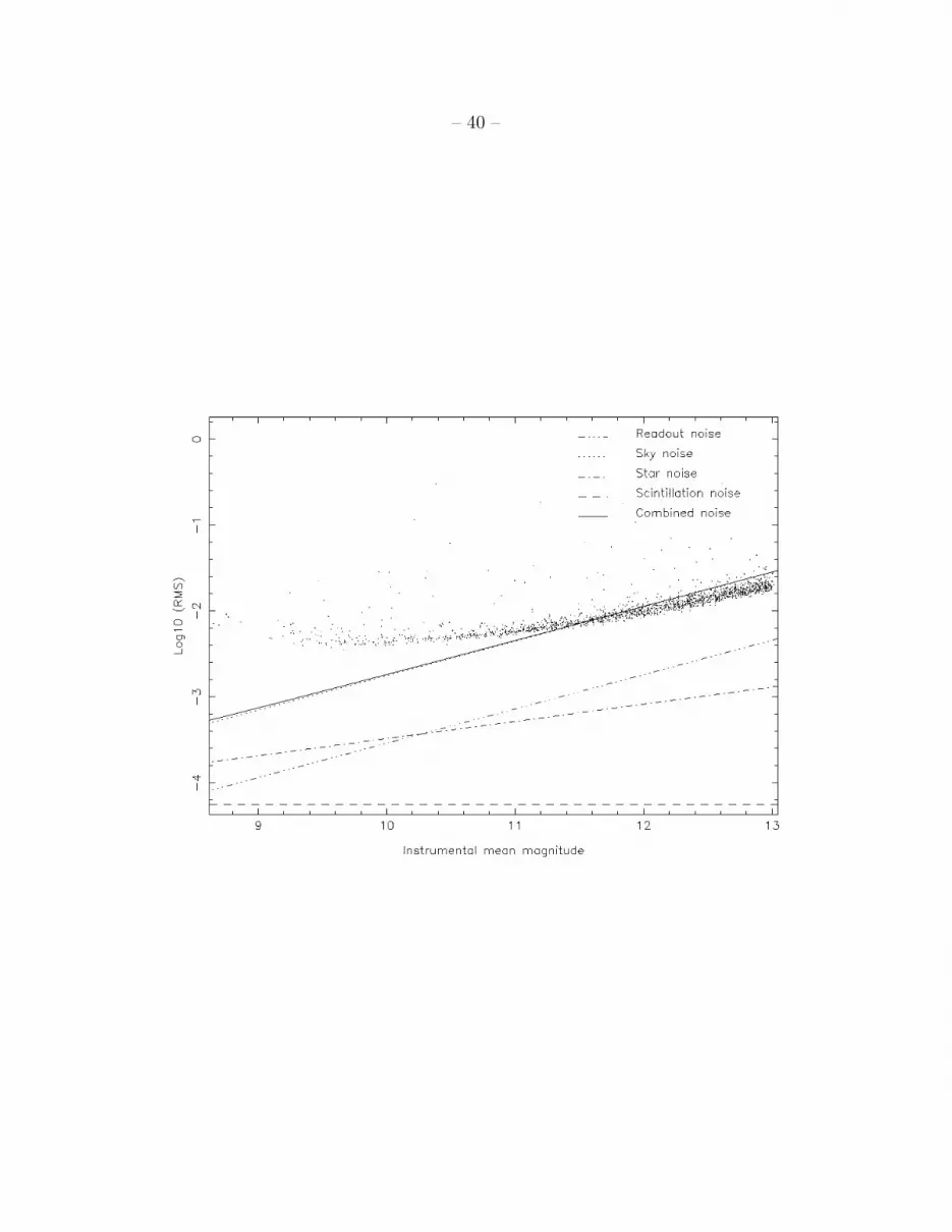
6.4. Photometric Performance

While our design goal was to reach 1% photometry for stars brighter than V ∼ 12.5,

in practice we reach this level of precision for stars brighter than V ∼ 11.5. Stars brighter

than V ∼ 9.4 have a precision better than 0.004 mag. Equally important, the night to

night variations are < 0.002 mag. Objects with V < 15.0 are stored in the archive. Fig. 5

shows the rms errors as a function of magnitude over the 2004 season and demonstrate that

– 27 –

the complete system delivers good precision over an extended period. The faint end of our

magnitude range is dictated by the sky brightness: in dark conditions the integrated sky

brightness in one of our pixels is ∼16.5.

6.5. Example Lightcurves

For relatively large amplitude variations (∆V > 0.05) data from the archive is of

sufficient quality for identification of variable stars (etc). Fig. 6 is an example of a large

amplitude eclipsing system extracted from the archive. We stress this figure is composed

completely of raw extracted data and has not undergone any further processing. In this

figure there are 3873 data points taken over a 6 month period through all prevailing

weather conditions. Close inspection shows that after ignoring outliers the rms errors are

around 0.015 magnitudes at the quadratures where it has a higher than normal noise for its

magnitude.

Our primary design goal has always been to identify transit amplitudes with

∆V ∼ 0.01. In this regime secondary effects can make the photometry less reliable. Rather

than analytically trying to remove these we use the SYSREM algorithm discussed by

Tamuz et al. (2005) to de-trend the data. This algorithm removes time and position

dependent trends from the lightcurves by computing the weighted average of magnitude

residuals over all stars to calculate a time-dependent variation. We added an additional

weighting to the magnitude uncertainties to down-weight known variable stars and

poorer-quality images. Note the SYSREM algorithm does not identify the causes of the

trend, but removes it blindly, using all the stars available; for this reason it should be

applied with caution where finding genuine photometric variables is the desired outcome.

After some experimentation we remove four trends from the data. Fig. 7 is an example of

a transit candidate with and without the SYSREM algorithm applied. This candidate

– 28 –

is identified as 1SWASP J133339.36+494321.6 and has V t = 11.154 mag. Out of transit

the rms scatter in the lightcurve is 0.0076 mag. Other exo-planet candidates from the first

SuperWASP-N season of observations are now becoming available (e.g. Christian et al.

2006). For details of our SYSREM implementation and transit candidate identification

algorithm see Cameron et al. (2006).

7. Summary and Future Development

The original SuperWASP Camera was constructed at Observatory of the Roque de

los Muchachos on la Palma in 2003. Since then we have also constructed a clone facility

at SAAO which has recently seen first light. Each system has a total field of view of 482

square degrees and is capable of monitoring the sky down to ∼ 15th magnitude every ∼ 40

minutes. For the La Palma facility, in the first season of operation the instrument was

used solely to monitor fields with high cadence (∼10 minutes). In subsequent seasons the

development of the dynamic scheduler will allow all sky monitoring interspersed with the

high cadence exo-planet fields (we expect complete sky coverage once per night).

The reduction pipeline is a continued development from the WASP0 instrument now

generalized and expanded to cater for both facilities. The rms plots show that the precision

at the bright end of our magnitude range reaches 3-4 milli-magnitudes over an extended

period and stars brighter than ∼11.5 magnitude have errors less than 1%. An average

night’s data of 50Gb, produces some 6×106 records in the archive.

We have developed an archive system capable of storing tens to hundreds of terabytes

of raw and processed data, the results of high-level analyses of those data, but doing so in a

manner that provides rapid access to individual lightcurves and images. The central catalog

is designed to remain flexible and responsive to evolving user requirements despite the

– 29 –

burgeoning data volume. The choice of HTTP as an interface protocol allows the end-user

a great deal of flexibility in the choice of access clients, and facilitates truly distributed,

collaborative working within the Consortium.

From the start of operations in 2006 at both facilities we have begun an all-sky survey

mode. As the exo-planet program will continue we have integrated these different survey

modes (with only a small loss to the exo-planet survey efficiency) enabling once a night

coverage of the entire visible sky. To do this effectively we will eventually deploy a reduction

pipeline at the sites themselves. By compromising performance slightly we will be able to

use this to grade the quality of the night, directly feeding back to the dynamic scheduler in

order to modify the observing queue, hence matching the science to the prevailing weather

conditions. In principle this could also provide a real time alert system and if sufficient

software resources become available we could use this to arrange followup observations on

other nearby facilities.

The SuperWASP Cameras are now surveying large parts of the sky primarily in search

of bright, transiting exo-planets. In the near future we will present large numbers of high

quality light curves suitable for followup and expect to at least double the numbers of known

transiting exo-planets. Interests of the Consortium members also cover other “secondary”

science areas and publications in these areas will be forthcoming. For non-members of the

consortium we also offer the opportunity to present ideas to the Project Steering Committee

and hence achieve a Guest Observer status in this area.

8. Acknowledgements

The WASP Consortium comprises scientists primarily from the University of Cambridge

(Wide Field Astronomy Unit), the Instituto de Astrofisica de Canarias, the Isaac Newton

– 30 –

Group of Telescopes, the University of Keele, the University of Leicester, The Open

University, Queen’s University of Belfast and the University of St Andrews.

The SuperWASP Cameras were constructed and are operated with funds made

available from the Consortium Universities and the UK’s Particle Physics and Astronomy

Research Council. We would also like to thank the UK’s STARLINK project (and site

managers) for their invaluable support in the development of the pipeline.

We thank the Administrador del Observatorio del Roque de los Muchachos, Sr. Juan

Carlos Perez, and the Director of the Isaac Newton Group of Telescopes, Dr Rene Rutten,

and staff, for their invaluable support in the construction and operation of SuperWASP-N.

We would also like to thank SAAO for hosting SuperWASP-S and thank SAAO personnel for

their generous assistance in the planning, construction and maintenance of SuperWASP-S.

We would like to acknowledge the anonymous referee who made an important contribution

to this paper.

This publication makes use of data products from the Two Micron All Sky Survey,

which is a joint project of the University of Massachusetts and the Infrared Processing and

Analysis Centre/California Institute of Technology, funded by the National Aeronautics

and Space Administration and the National Science Foundation.

– 31 –

REFERENCES

Akerlof, C., Balsano, R., Barthelmy, S., Bloch, J., Butterworth, P., Casperson, D., Cline,

T., Fletcher, S., Frontera, F., Gisler, G., Heise, J., Hills, J., Kehoe, R., Lee, B.,

Marshall, S., McKay, T., Miller, R., Piro, L., Priedhorsky, W., Szymanski, J., &

Wren, J., 1999, Nature, 398, 400

Alonso, R., Brown, T.M., Torres, G., Latham, D.W., Sozzetti, A., Mandushev, G.,

Belmonte, J.A., Charbonneau, D., Deeg, H.J., Dunham, E.W., O’Donovan, F.T., &

Stefanik, R.P., 2004, ApJ, 613, L153

Bakos, G., Noyes, R.W., Kovacs, G., Stanek, K. Z., Sasselov, D. D., & Domsa, I., 2004,

PASP, 116, 266

Bertin, E., & Arnouts, S., 1996, A&AS, 117, 393

Bouchy, F., Udry,S., Mayor, M., Moutou, C., Pont, F., Iribarne, N., Da Silva, S., Ilovaisky,

S., Queloz, D., Santos, N.C., Segransan, D., & Zucker, S., 2005, A&A, 444, L15

Brown, T.M., 2003, ApJ, 593, L125

Collier Cameron, A. Pollacco, D., Street, R.A., Lister, T.A., West, R.G., Wilson, D.M.,

Pont, F., Christian, D.J., Clarkson, W.I., Evans, A., Haswell, C.A., Hellier, C.,

Horne, K., Irwin, J., Kane, S.R., Norton, A.J., Skillen, I., & Wheatley, P.J., 2006,

MNRAS, in press.

Charbonneau, D., Brown, T., Latham, D.W., & Mayor, M., 2000, ApJ, 529, L45

Christian, D.J., Pollacco, D.L., Skillen, I., Street, R.A., Keenan, F.P., Clarkson, W.I.,

Collier Cameron, A., Kane, S.R., Lister, T.A., West, R.G., Enoch, B., Evans, A.,

Fitzsimmons, A., Haswell, C.A., Hellier, C., Hodgkin, S.T., Horne, K., Irwin, J.,

– 32 –

Norton, A., Osbourne, J., Ryans, R., Wheatley, P.J., Wilson, D.M., 2006, MNRAS

in press (astro-ph/0608142)

Cremonese, G., Boehnhardt, H., Crovisier, J., Rauer, H., Fitzsimmons, A., Fulle, M.,

Licandro, J., Pollacco, D., Tozzi, G.P., & West, R.M., 1997, ApJ, 490, L199

Høg, E., Fabricius, C., Makarov, V.V., Urban, S., Corbin, T., Wycoff, G., Bastian, U.,

Schweekendiek, P., & Wicenec, A., 2000, A&A, 355, L27

Horne, K., Scientific Frontiers in Research on Extrasolar Planets, 2003, Vol. 294, 361, eds.

D.Deming, S.Seager

Jenkins, J.M., Caldwell, D.A., & Borucki, W.J., 2002, ApJ, 564, 495

Kane, S.R., Collier Cameron, A., Horne, K., James, D., Lister, T., Pollacco, D., Street,

R.A., & Tsapras, Y., 2004, MNRAS, 353, 689

Kane, S.R., Lister, T., Collier Cameron, A., Horne, K., James, D., Pollacco, D., Street,

R.A., & Tsapras, Y., 2005a, MNRAS, 362, 117

Kane, S.R., Collier Cameron, A., Horne, K., James, D., Lister, T., Pollacco, D., Street,

R.A., & Tsapras, Y., 2005b, MNRAS, 364, 1091

Marcy, G., Butler, R.P., Fischer, D., Vogt, S., Wright, J.T., Tinney, C.G., & Jones, H.R.A.,

2005, Progress of Theoretical Physics Supplement No 158, 24

Mayor, M. & Queloz, D., 1995, Nature, 378, 355

McCullough, P.R., Stys, J.E., Valenti Jeff A., Johns-Krull, C.M., James, K.A., Heasley,

J.N., Bye, B.A., Dodd, C., Fleming, S.W., Pinnick, A., Bissinger, R., Gary, B.L.,

Howell, P.J., & Vanmunster, T., 2006, ApJ in press (astro-ph/0605414v1)

– 33 –

Monet, D.G., Levine, S.E., Canzian, B., Ables, H.D., Bird, A.R., Dahn, C.C., Guetter,

H.H., Harris, H.C., Henden, A.A., Leggett, S.K., Levison, H.F., Luginbuhl, C.B.,

Martini, J., Menet, A.K.B., Munn, J.A., Pier, J.R., Rhodes, A.R., Riepe, B., Sell,

S., Sone, R.C., Vrba, F.J., Walker, R.L., Westerhout, G., Brucato, R.J., Reid, I.N.,

Schoening, W., Hartley, M., Read, M.A., & Tritton, S.B., 2003, Astron. J., 125, 984

Pinfield, D.J., Jones, H.R.A., & Steele, I.A., 2005, PASP, 117, 173

Tamuz, O., Mazeh, T., & Zucker, S., 2005, MNRAS, 356, 1466

Udalski, A., Paczynski, B., Zebrun, K., Szymaski, M., Kubiak, M., Soszynski, I., Szewczyk,

O., Wyrzykowski, L., & Pietrzynski, G., 2002a, Acta Astron., 52, 1

Udalski, A., Zebrun, K., Szymanski, M., Kubiak, M., Soszynski, I., Szewczyk, O.,

Wyrzykowski, L., & Pietrzynski, G., 2002b, Acta Astron., 52, 115

Wolszczan, A. & Frail, D., 1992, Nature, 255, 145

This manuscript was prepared with the AAS LATEX macros v5.2.

– 34 –

Fig. 1.— The SuperWASP-N enclosure at the Roque de los Muchachos Observatory on la

Palma. The weather station is in the background.

Fig. 2.— The SuperWASP-S instrument with eight cameras mounted. The field of view of

the instrument is ∼482 square degrees.

Fig. 3.— Passband of the new SuperWASP filter (top panel) plotted alongside the atmo-

spheric transmission, CCD response and lens transmission. The bottom panel shows the

original unfiltered system alongside those of the new filter and the Tycho 2 V filter.

Fig. 4.— Graph showing that wing-to-core ratios defined from different sized apertures

are related by a constant scaling factor. This plot does not include all stars in a field.

Instead only those that are brighter than V = 15.0 and have reasonable values for the r1

and r2 indices (< 0.5 for both) are included. The pipeline actually flags 9 different types

of “blended” object ranging from type 0 (unblended) to 9 (saturated star or a bad pixel).

The types shown in this figure correspond to extremely red objects (1) or those indices that

suggest nearby companions or distorted images (2-4). The vertical line shows when the

effect of nearby companion stars is detectable in the r1 index and was derived from real

SuperWASP-N data in conjuction with 2MASS and DSS data.

Fig. 5.— An rms error verses magnitude diagram for the 2004 season. Stars brighter than

about V ∼11.5 reach better than 1% accuracy. Also shown is a theoretical model which shows

that the noise is dominated by the sky contribution (uncertainties in the sky contribution

are apparent at fainter magnitudes).

Fig. 6.— An example of a eclipsing binary star (GNBoo) from WASP data. This object has

a period of 0.301601 days. This light curve is composed of 3873 data points obtained over

the 2003 season obtained in all weather conditions and has not undergone any post archive

processing.

– 35 –

Fig. 7.— A typical transit candidate, 1SWASP J133339.36+494321.6 found in SuperWASP

data. The top lightcurve shows the archived data, while that below shows the same data

after detrending through the SYSREM algorithm. This candidate has a transit of amplitude

∼1.5% and duration 2.8 hr. The data is phased on a period of 3.63 days. Published data for

this object available in the Tycho-2 and 2MASS catalogs suggest the host has a spectral type

of F7 (from the Vt(SW )−K2MASS color index; the 2MASS J −H index give a spectral type of

F8). Consequently, the radius of the companion is 1.23RJ . As these values are derived from

photometry they serve as a guide, but further observations of this target will be necessary

to confirm its status.

– 36 –

– 37 –

– 38 –

– 39 –

– 40 –

– 41 –

– 42 –