Embed Size (px)
Citation preview
Volume 12 Number 32
EJTP Electronic Journal of Theoretical Physics
ISSN 1729-5254
Editors
Ignazio Licata Ammar Sakaji http://www.ejtp.com January, 2015 E-mail:[email protected]
Volume 12 Number 32
EJTP Electronic Journal of Theoretical Physics
ISSN 1729-5254
Editors
Ignazio Licata Ammar Sakaji http://www.ejtp.com January, 2015 E-mail:[email protected]

Editor in Chief
Ammar Sakaji
Theoretical Condensed Matter, Mathematical Physics International Institute for Theoretical Physics and Mathematics (IITPM), Prato, Italy Naval College, UAE And Tel:+971557967946 P. O. Box 48210 Abu Dhabi, UAE Email: info[AT]ejtp.com info[AT]ejtp.info
Co-Editor
Ignazio Licata
Foundations of Quantum Mechanics, Complex System & Computation in Physics and Biology, IxtuCyber for Complex Systems , and ISEM, Institute for Scientific Methodology, Palermo, Sicily – Italy
editor[AT]ejtp.info Email: ignazio.licata[AT]ejtp.info
ignazio.licata[AT]ixtucyber.org
Editorial Board
Gerardo F. Torres del Castillo
Mathematical Physics, Classical Mechanics, General Relativity, Universidad Autónoma de Puebla, México, Email:gtorres[AT]fcfm.buap.mx Torresdelcastillo[AT]gmail.com
Leonardo Chiatti
Medical Physics Laboratory AUSL VT Via Enrico Fermi 15, 01100 Viterbo (Italy) Tel : (0039) 0761 1711055 Fax (0039) 0761 1711055 Email: fisica1.san[AT]asl.vt.it chiatti[AT]ejtp.info

Francisco Javier Chinea
Differential Geometry & General Relativity, Facultad de Ciencias Físicas, Universidad Complutense de Madrid, Spain, E-mail: chinea[AT]fis.ucm.es
Maurizio Consoli
Non Perturbative Description of Spontaneous Symmetry Breaking as a Condensation Phenomenon, Emerging Gravity and Higgs Mechanism, Dip. Phys., Univ. CT, INFN,Italy
Email: Maurizio.Consoli[AT]ct.infn.it
Avshalom Elitzur
Foundations of Quantum Physics ISEM, Institute for Scientific Methodology, Palermo, Italy Email: Avshalom.Elitzur[AT]ejtp.info
Elvira Fortunato
Quantum Devices and Nanotechnology:
Departamento de Ciência dos Materiais CENIMAT, Centro de Investigação de Materiais I3N, Instituto de Nanoestruturas, Nanomodelação e Nanofabricação FCT-UNL Campus de Caparica 2829-516 Caparica Portugal
Tel: +351 212948562; Directo:+351 212949630 Fax: +351 212948558 Email:emf[AT]fct.unl.pt elvira.fortunato[AT]fct.unl.pt
Tepper L. Gill
Mathematical Physics, Quantum Field Theory Department of Electrical and Computer Engineering Howard University, Washington, DC, USA
Email: tgill[AT]Howard.edu tgill[AT]ejtp.info
Alessandro Giuliani
Mathematical Models for Molecular Biology Senior Scientist at Istituto Superiore di Sanità Roma-Italy
Email: alessandro.giuliani[AT]iss.it

Vitiello Giuseppe
Quantum Field Theories, Neutrino Oscillations, Biological Systems Dipartimento di Fisica Università di Salerno Baronissi (SA) - 84081 Italy Phone: +39 (0)89 965311 Fax : +39 (0)89 953804 Email: [email protected]
Richard Hammond
General Relativity High energy laser interactions with charged particles Classical equation of motion with radiation reaction Electromagnetic radiation reaction forces Department of Physics University of North Carolina at Chapel Hill, USA Email: rhammond[AT]email.unc.edu
Arbab Ibrahim
Theoretical Astrophysics and Cosmology Department of Physics, Faculty of Science, University of Khartoum, P.O. Box 321, Khartoum 11115, Sudan
Email: aiarbab[AT]uofk.edu arbab_ibrahim[AT]ejtp.info
Kirsty Kitto
Quantum Theory and Complexity Information Systems | Faculty of Science and Technology Queensland University of Technology Brisbane 4001 Australia
Email: kirsty.kitto[AT]qut.edu.au
Hagen Kleinert
Quantum Field Theory Institut für Theoretische Physik, Freie Universit¨at Berlin, 14195 Berlin, Germany
Email: h.k[AT]fu-berlin.de
Wai-ning Mei
Condensed matter Theory Physics Department University of Nebraska at Omaha,
Omaha, Nebraska, USA Email: wmei[AT]mail.unomaha.edu physmei[AT]unomaha.edu

Beny Neta
Applied Mathematics Department of Mathematics Naval Postgraduate School 1141 Cunningham Road Monterey, CA 93943, USA Email: byneta[AT]gmail.com
Peter O'Donnell
General Relativity & Mathematical Physics, Homerton College, University of Cambridge, Hills Road, Cambridge CB2 8PH, UK E-mail: po242[AT]cam.ac.uk
Rajeev Kumar Puri
Theoretical Nuclear Physics, Physics Department, Panjab University Chandigarh -160014, India Email: drrkpuri[AT]gmail.com rkpuri[AT]pu.ac.in
Haret C. Rosu
Advanced Materials Division Institute for Scientific and Technological Research (IPICyT) Camino a la Presa San José 2055 Col. Lomas 4a. sección, C.P. 78216 San Luis Potosí, San Luis Potosí, México Email: hcr[AT]titan.ipicyt.edu.mx
Zdenek Stuchlik
Relativistic Astrophysics Department of Physics, Faculty of Philosophy and Science, Silesian University, Bezru covo n´am. 13, 746 01 Opava, Czech Republic Email: Zdenek.Stuchlik[AT]fpf.slu.cz
S.I. Themelis
Atomic, Molecular & Optical Physics Foundation for Research and Technology - Hellas P.O. Box 1527, GR-711 10 Heraklion, Greece Email: stheme[AT]iesl.forth.gr
Yurij Yaremko
Special and General Relativity, Electrodynamics of classical charged particles, Mathematical Physics, Institute for Condensed Matter Physics of Ukrainian National Academy of Sciences 79011 Lviv, Svientsytskii Str. 1 Ukraine Email: yu.yaremko[AT]gmail.com yar[AT]icmp.lviv.ua
yar[AT]ph.icmp.lviv.ua
Nicola Yordanov
Physical Chemistry Bulgarian Academy of Sciences, BG-1113 Sofia, Bulgaria Telephone: (+359 2) 724917 , (+359 2) 9792546
Email: ndyepr[AT]ic.bas.bg ndyepr[AT]bas.bg
Former Editors:
Ammar Sakaji, Founder and Editor in Chief (2003- October 2009)
Ignazio Licata, Editor in Chief (October 2009- August 2012)
Losé Luis López-Bonilla, Co-Editor (2008-2012)
Ammar Sakaji, Editor in Chief (August 2012- )
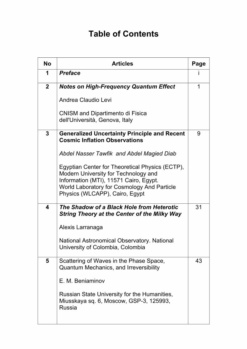
Table of Contents
No Articles Page 1 Preface
i
2 Notes on High-Frequency Quantum Effect Andrea Claudio Levi CNISM and Dipartimento di Fisica dell'Università, Genova, Italy
1
3 Generalized Uncertainty Principle and Recent Cosmic Inflation Observations Abdel Nasser Tawfik and Abdel Magied Diab Egyptian Center for Theoretical Physics (ECTP), Modern University for Technology and Information (MTI), 11571 Cairo, Egypt. World Laboratory for Cosmology And Particle Physics (WLCAPP), Cairo, Egypt
9
4 The Shadow of a Black Hole from Heterotic String Theory at the Center of the Milky Way Alexis Larranaga National Astronomical Observatory. National University of Colombia, Colombia
31
5 Scattering of Waves in the Phase Space, Quantum Mechanics, and Irreversibility E. M. Beniaminov Russian State University for the Humanities, Miusskaya sq. 6, Moscow, GSP-3, 125993, Russia
43
6 Frequency Distribution of Spontaneous Emission Saul. M. Bergmann Potomac, Maryland, USA
61
7 Spatially Homogeneous Cosmological Models in $f(R,T)$ Theory of Gravity S. Chandel and Shri Ram Department of Applied Mathematics, Indian Institute of Technology, (Banaras Hindu University), Varanasi 221 005, India
69
8 Relativistic Pentametric Coordinates from Relativistic Localizing Systems and the Projective Geometry of the Spacetime Manifold Jacques L. Rubin Université de Nice--Sophia Antipolis, UFR Sciences Institut du Non-Linéaire de Nice, UMR7335 1361 route des Lucioles, F-06560 Valbonne, France
83
9 Theoretical Calculations for Predicted States of Heavy Quarkonium Via Non-Relativistic Frame Work T. A. Nahool, A. M. Yasser and G. S. Hassan Physics Department, Faculty of Science at Qena, South Valley University, Egypt Physics Department, Faculty of Science, Assuit University, Egypt
113
10 The One-dimensional Thermal Properties for the Relativistic Harmonic Oscillators Abdelmalek Boumali Laboratoire de Physique Appliquée et Théorique, Université de Tébessa, 12000, W. Tébessa, Algeria
121
11 The Effectiveness of Hénon Map for Chaotic Optimization Algorithms Using a Global Locally Averaged Strategy Tayeb Hamaizia Department of Mathematics, Faculty of Sciences, University Constantine -1-, Algeria
131
12 Weakton Model of Elementary Particles and Decay Mechanisms Tian Ma and Shouhong Wang Department of Mathematics, Sichuan University, Chengdu, P. R. China Department of Mathematics, Indiana University, Bloomington, IN 47405, USA
139
13 Physics of Currents and Potentials II. Classical Singlet-Triplet Electroweak Theory with Non-point Particles Valerii Temnenko Tavrian National University, 95004, Simferopol, Crimea, Ukraine
179
14 From Quantum Mechanics to Intelligence Michail Zak Jet Propulsion Laboratory California Institute of Technology, Pasadena, CA 91109, USA
295

Electronic Journal of Theoretical Physics 12, No. 32 (2015) i
Welcome to the Year of Light 2015!
Dear EJTP Friends,
We start the new year with very rich issue with high quality papers, as a New Year
Greeting and celebration, we are working with our special project on the international
year of light 2015 entitled ” Bohr-Einstein Debates in the Year of Light 2015 ”. In fact,
the UNESCO General assembly has proclaimed 2015 as the International Year of Light
and Light-based Technology (IYL 2015). The opening ceremony will be held in Paris on
19-20 January 2015.
EJTP will celebrate the event with a Special Issue (http://www.ejtp.com/iyl2015.html),
in parallel with other contingent matters. The year of the photon is also the year of the
electrodynamics of the moving bodies, the magic triad of 1905 Einstein’s papers, respec-
tively: Uber einen die Erzeugung und Verwandlung des Lichtes betreffenden heuristischen
Gesichtspunk, Annalen der Physik 17, 132 (1905) [17 pp.] & Zur Elektrodynamik be-
wegter Korper, Annalen der Physik 17, 891 [31 pp]. From the contemporary viewpoint,
it is not just a coincidence at all.
The modern view of light nowadays is to look at highly complex matters regarding
the Gauge Theories’ underlying symmetries. R. Laughlin has effectively summed up: “If
Einstein were alive today, he would be horrified at this state of affairs (...) It would be
perfectly a challenge for him to re-examine the facts, toss them over in his mind, and
conclude that his beloved principle of relativity was not fundamental at all but emergent-a
collective property of the matter constituting space-time that becomes increasingly exact
at long length scales but fails at short ones”. [I am working at Planck scale just now!
(IL)].
It is an emergence that lead us to another important theme set by the Year of Light:
when Nature finds a good trick, it plays on different scales! The correspondences between
the BCS Theory of superconductivity and the Physics of Higgs boson, the mysterious cor-
nerstone supporting the gauge theories, are things too beautiful to be left unexplained.
At present, the physics of the analogy of GR & QM systems in Condensed Matter has
undergone a great development phase and the future of the field will give unexpected
theoretical and experimental possibilities to test theories born in microscopic and cos-
mological context in the mesoscopic one, promising technological scenarios that were
unthinkable few years ago.
Without forgetting the modern core of physics, last but not least, the problems of QM
foundation. A generalized crisis of Copenhagen (in a recent mail to a colleague I called
it poetically “the burning walls of Copenhagen”), should remind us that the so-called
QM interpretation is not a quirk for out of service physicists or recycling philosophers, a
game of intellectual exercises is to try imposing a meta-physics guarding the formalism.
It should be just a formalism to suggest the beables and the possibilities of our language,
as N. Bohr – who got a not operatively shortsighted vision of QM – warned. Actually,
the interpretation work of a physical theory cannot be isolated from the theoretical and
ii Electronic Journal of Theoretical Physics 12, No. 32 (2015)
experimental problems and its developments.
Naturally, taking in mind that the Optics by Newton (1704) is a masterpiece where
theory and experiment are intimately fused, we wish the pact between theoreticians and
experimentalists, it is an important to minimize the barriers and deviations, because
Physics is One science.
Now, I “pass the ball” to Ammar Sakaji who will present you the issue.
I would like to thank all editors and reviewers for helping me to prepare this issue
(Vo.12, No.32, 2015) of the Electronic Journal of Theoretical Physics EJTP, especially
my brother and friend Ignazio Licata, I greatly appreciate his notes and comments. I’ve
spent a lot of time sifting and editing the manuscripts of this issue, which covers impor-
tant topics: from Chaos Theory, Quantum Mechanics (relativistic and non-relativistic),
Elementary Particles Physics, Quantum Gravity at Planck’s Scale, String Theory, Gravi-
tational Cosmological Models, Black Holes, Weak Interaction up to Quantum Intelligence.
Most of the editorial work done in Abu Dhabi and the other part at Iowa.
This Issue includes 13 reviewed research papers on mathematical and theoretical
physics with the efforts of 18 authors in addition to the reviewers, referees and edi-
tors: Levi in his paper on the high–frequency quantum effect discuses the quantum phase
mechanism, energy exchange, and decoherence. Tawfik and Diab figure the GUP at the
Planck scale with view of latest experimental observations. Larranaga in his paper on
black holes addresses the Shadow of a Black Hole from Heterotic String theory to the
Center of the Milky Way. Beniaminov reviews some useful formalism of quantum me-
chanics, reversibility and Phase Space. Bergmann figures the spontaneous emission via
Fock space techniques. Chandel and Ram discus some gravitational cosmological mod-
els. Rubin describes in very beautiful way the relativistic pentametric coordinates with
generalized Cartan space. Nahool et al. show in their paper the non-relativistic Heavy
Quarkonium computations. Boumali derives some thermal properties of relativistic har-
monic oscillator. Hamaizia shows the map of optimization Algorithms especially Henon
map. Ma and Wang show the decay mechanisms of elementary particles via Weakton
Model. Temnenko addresses a comprehensive study of the singlet-triplet electroweak
theory. Finally Zak with his attractive paper on Quantum Mechanics and Intelligence
demonstration.
Enjoy reading
Ignazio Iicata & Ammar Sakaji.
EJTP 12, No. 32 (2015) 1–8 Electronic Journal of Theoretical Physics
Notes on High–Frequency Quantum Effect
Andrea Claudio Levi∗
CNISM and Dipartimento di Fisica dell’Università, Genova, Italy
Received 07 ○ctober 2014, Accepted 19 December 2014, Published 10 January 2015
Abstract: Although any quantum system subject to disturbances tends to approach aclassical behaviour because of decoherence, such decoherence may be largely quenched whenthe perturbations are characterized by high-frequency oscillations. This is related to a simpleproperty of Fourier transforms: if, as usually happens, the time dependence of the process issmooth, this implies a rapid decrease of the omega-dependent quantities at high frequencies. Asa consequence, in the case of scattering of a particle with a solid (surface or bulk) the contributionof high-frequency vibrations to the Debye-Waller factor is small. But the effect is much moregeneral: it is shown that, whenever a particle interacts with a large system, high-frequencyoscillations of the latter contribute little to decoherence, both in the absence (elastic case) andin the presence of energy exchange (thus, if such high-frequency oscillations are the only relevantperturbation, the process maintains quantum- mechanical features).c○ Electronic Journal of Theoretical Physics. All rights reserved.
Keywords: High Frequency Quantum Effect; Quantum Phase; Energy Exchange; decoherencePACS (2010): 03.65.-w; 03.65.Vf; 03.65.Yz
1. Introduction
Any quantum system subject to disturbances tends to approach a classical behaviourbecause of decoherence, but it is interesting to see that, when the perturbations affectingit are characterized by high–frequency oscillations, decoherence may be largely quenchedand the system may behave almost coherently, i. e. quantum–mechanically. This can beconsidered as an instance of the so–called Zeno effect [1, 2]2.
∗ Email:[email protected] The Zeno effect is often described as the confirmation of quantum behaviour via repeated acts ofmeasurement, but in fact measurement (the intervention of a physicist!) has probably little to do with it.To confirm quantum behaviour it is important rather for disturbances to appear as repeated oscillations,whose effect is ultimately averaged out.
2 Electronic Journal of Theoretical Physics 12, No. 32 (2015) 1–8
In a different context, the fact that decoherence can be inhibited by subjecting thesystem to a sequence of very frequent pulses has been discussed by Viola and Lloyd [3]and by Vitali and Tombesi [4] (similar phenomena and techniques have been well–knownin nuclear magnetic resonance for many years [5, 6]).
Indeed, the quantum phase can be written as an action divided by �, and its randompart (representing the perturbation due to the relevant oscillating modes) tends to becomesmall at high frequencies, at least if the process under consideration can be written as theintegral of a convenient Lagrangian. In [7] some properties of the action for the case of amaterial particle (e. g. an atom) scattered off a large system are discussed (in that casethe main quantity on which the attention is to be focused is the Debye–Waller factor),but in the present study I will keep a more general point of view, trying to discuss theconditions under which the effect considered takes place.
An essential point is that, unless some discontinuous or catastrophic event occurs,the time dependence of the process is smooth, and that, due to well–known mathema-tical properties of Fourier transforms, this implies a rapid decrease of the ω–dependentquantities at high frequencies. Such mathematical properties are the following:
If a real function f(t) can be extended to an analytic function f(z) whose closestsingularity has a distance b from the real axis and which behaves at infinity as O(e−|(β−ε)x|)(for any ε), then its Fourier transform F(ω) behaves at infinity as O(e−|(b−δ)Rεω|) (for anyδ) (and its closest singularity has a distance β from the real axis).
If, on the other hand, f(z) is an entire function, then its Fourier transform tends tozero faster than any exponential for large |ω|.
This corresponds to, and follows from, Theorem 26 of Titchmarsh, page 44 [8]. Now itis clear that a number of physical processes (including most scattering processes) involvephysical quantities which vary with time in a continuous fashion, and take place within awell–defined time interval, so that the interactions are vanishingly small before and afterthat interval. Thus it is reasonable to assume that, for an extensive class of processes,the conditions of the above theorem are fulfilled. As a consequence, relevant physicalquantities describing such processes have Fourier transforms that tend to zero at leastexponentially at high |ω|.
2. The Phase
In the present Section, I will reconsider in a simple fashion the quantum–mechanical phaseη (or equivalently the action S, since there is only a factor � between the two quantities),as well as the physical role of these quantities. It is well known that under extremelygeneral conditions the quantum–mechanical amplitude can be formally written as a path
integral of a phase factor exp(iη) [9], so that the complications lie in the somewhatmysterious procedure of path integration, while the phase factor itself, in many cases, isrelatively simple. I mention this only to indicate that a semiclassical treatment of η = S/�
is often meaningful and that the mechanical properties of S can be considered and shownoften to possess the properties of continuity in time and limitation to a well–defined time
Electronic Journal of Theoretical Physics 12, No. 32 (2015) 1–8 3
interval mentioned in the Introduction.Two obvious complications, however, are to be discussed. First of all, to obtain the
amplitude an integral (in principle, a path integral, but in practical approximations anintegral over some set of relevant variables) is to be performed. Secondly, probabilitiesare of course not amplitudes, but are obtained from amplitudes taking the absolute valuessquared. These questions will be dealt with, in simple ways, in the following.
If the perturbations are sufficiently weak, the phase η may be written as a sum
η = η0 + δη (1)
where η0 is the unperturbed phase and δη is in some sense linear in the perturbations.The effect of η0 may be assumed to be coherent, while decoherence will arise from thestatistical properties of δη, i. e. of the perturbations.
The amplitude of a physical process will be the integral of a phase factor exp(iη)
along a path, integrated subsequently over paths; and the corresponding probability willbe the statistical average
P =< |∫eiηdV |2 >, (2)
where∫
dV indicates a (complex, but here unspecified) integration procedure.Splitting η as in (1), (2) may be rewritten as
P =∫ ∫
ei[η0(x)−η0(x′)] < ei[δη(x)−δη(x
′)] > dV dV ′ (3)
where all decoherence properties arise from the statistical average involving the δη’s.Let me focus on such average.
In many interesting cases, δη may be assumed to be linear in the disturbances (e.g.phonons or other relevant quanta), and the latter to have a harmonic nature and thereforea Gaussian distribution of amplitudes. In this case the well–known theorem for theaverages of Gaussian variables of zero mean
< eia >= e−12<a2> = e−
12<a∗a>, (4)
(valid for both real c-numbers and self–adjoint quantum variables) may be applied,with the result that (3) takes the simpler form
P =∫ ∫
ei[η0(x)−η0(x′)]e−
12<|δη(x)−(δη(x′)|2>dV dV ′, (5)
where all statistical properties appear only in the exponent.
4 Electronic Journal of Theoretical Physics 12, No. 32 (2015) 1–8
3. Time Dependence
In (5) x, x′, dV, dV ′ are unspecified and may imply space and time variables or moregenerally path variables. A very simple, but important case is that where x′ differs fromx in time only along a path, so that the average occurring in (5) may be written
2W (t, t′) =< |δη(t)− δη(t′)|2 > (6)
(the factor of 2 is written here to respect the Debye–Waller tradition. . . ). Theproperties of W (t, t′) are considered below.
It is possible to write δη as an integral over frequencies
δη(t) =1
2πQ(t) =
1
2π
∫ ∞
−∞eiωta(ω)F (ω)dω (7)
where F (ω) is the Fourier transform of a function f(t) of time describing, say, ascattering event, while a(ω) is the amplitude of the (harmonic) disturbances.
The latter is a random quantity. If α∗ and α are creation and annihilation operatorsfor disturbances (e. g. phonons) of frequency ω, then |a(ω)|2 may typically be assumedto be proportional to �|ω|α∗α = �|ω|n(|ω|)g(|ω|), and
< a∗(ω)a(ω′) >= �ω < n(|ω)| > g(|ω|)δ(ω′ − ω), (8)
where g(ω) is the spectrum of disturbances. It is reasonable to assume that onlya(ω) has nontrivial statistical properties, related e. g. to the expectation values of thephonon variables at the temperature of interest, while (for a small amplitude of distur-bances) f(t) and F (ω) are mechanical quantities of a deterministic nature, f(t) beingthe time dependence of the mechanical process taking place and F (ω) being its Fouriertransform. The mechanical process considered (scattering or otherwise) is expected to behighly regular and strictly limited in time, so that the conditions for the validity of themathematical properties considered in the Introduction may be assumed to be fulfilled.As a consequence, F (ω) tends to zero at least exponentially at high frequencies.
Due to the form of (6) and (7), it is clear that W (t, t′) actually depends only on thetime difference t′ − t = τ , and will henceforth be indicated as such. Indeed
W (t, t′) =1
8π2
∫ ∫ ∞
−∞(e−iωt − e−iωt
′)(eiω
′t − eiω′t′) < a∗(ω)a(ω′) > F ∗(ω)F (ω′)dωdω′ (9)
which, because of (8), gives
W (t, t′) = W (τ) =�
2π2
∫ ∞
0(1− cosωτ) < n(ω) > g(ω)|F (ω)|2ωdω. (10)
(10) is the main result of the present Section.
Electronic Journal of Theoretical Physics 12, No. 32 (2015) 1–8 5
4. Single Frequency
It is instructive (although obviously too simple) to consider the elementary case wherethe disturbance occurs at a single frequency ω0, g(ω) = δ(ω − ω0): a physical exampleof this might be the “Einstein model” of crystal vibrations. In this single–frequency caseW (τ) reduces to
W (τ) =�ω0
2π2(1− cosω0τ) < n(ω0) > |F (ω0)|2, (11)
exceedingly small if the frequency ω0 is high. At high frequencies, indeed, W becomessmall because F decreases exponentially. Notice that �ω0 < n(ω0) > is the mean energyof the disturbance (with the zero–point energy subtracted).
For example, if
f(t) =B
cosh(2t/τc)(12)
(a reasonable behaviour for a process having a duration of the order of τc), then
W (τ) =1
32τ 2cB
2 �ω0 < n(ω0) >
cosh2(πω0τc/4)(1− cosω0τ). (13)
5. Asymptotic Behaviour
Let us come back to the general formula (10) and consider the asymptotic behaviourat long τ ’s. This corresponds to vanishing energy exchange: for example, in scatteringphenomena, to elastic scattering.
Indeed, as I shall show in the next Section, the probability of a process with energyexchange Δ is proportional to the Fourier transform, with the exp(−iτΔ/�) factor, ofexp[−2W (τ)], with W (τ) given by (10). If τ is very long, only the Δ = 0 contributionsurvives.
But if τ is very long, in the integrals Q and Q∗ vastly different frequencies are relevant(except in the case, already considered, where a single frequency occurs), so that Q andQ∗ become uncorrelated and
< |Q|2 >=< Q∗Q >→ | < Q > |2. (14)
The elastic probability depends thus only on
< Q(τ) >=<∫
eiωτa(ω)F (ω)dω >=∫eiωτ < a(ω) > F (ω)dω, (15)
where, as above, I have supposed (as is reasonable) that only a(ω) has nontrivialstatistical properties.
In the case of elastic scattering, exp(−2| < Q > |2) has the meaning of a Debye–Wallerfactor, but the present formulation is in principle much more general.
6 Electronic Journal of Theoretical Physics 12, No. 32 (2015) 1–8
6. General Case and Energy Exchange
In the previous section I have considered the case where the energy exchange vanishes;in general, however, there is of course a nonvanishing energy exchange Δ. I have givensuch general theory in several articles, through the years [10, 11, 12]. To fix ideas, letme assume that a particle (elementary or otherwise) interacts with a large system: if theparticle loses the energy Δ, then the latter goes to excite the large system from an initialstate α to a final state β such that Eβ = Eα +Δ (the large system will be assumed to belarge enough, and its levels dense enough, that this is possible for any Δ).
The probability for this to occur will be proportional to
∑α
Pα
∑β
|Tβ←α|2δ(Eβ − Eα −Δ), (16)
where T is the quantum–mechanical operator for the transition of the large systemfrom α to β, (while at the same time the particle loses the energy Δ), and Pα is thestatistical (e. g. canonical, Gibbs–Boltzmann) probability for the large system to be instate α.
A van Hove transformation [13] may now be applied3.Expanding the absolute value squared, and expressing the δ–function as an integral,
(16) becomes
1
2π�
∫ ∑a
Pα
∑β
(α|T ∗|β)eiEβt/�(β|T |α)e−iEαt/�e−itΔ/�dt. (17)
But eiEαt/� multiplying state |α) and eiEβt/� multiplying state |β) are equivalent tothe operator eiHt/� operating respectively on such states (where H is the Hamiltonian ofthe large system), so that the quantity considered amounts to
1
2π�
∫ ∑α
Pα
∑β
(α|T ∗eiHt/�|β)(β|Te−iHt/�|α)e−itΔ/�dt. (18)
The sum of |β) over all states is 1 and the sum of Pα|α) over all states correspondsto a statistical average, so that the result
1
2π�
∫< T ∗eiHt/�Te−iHt/� > e−itΔ/�dt (19)
is obtained; this may best be written in terms of time correlations:
1
2π�
∫e−itΔ/� < T ∗(0)T (τ) > dτ. (20)
3 In his original article [13], van Hove dealt with a perturbation approximation (valid for neutron singlescattering from condensed matter), but in fact his method is exact, provided the exact T operator isconsidered . Notice that the present discussion is nonperturbative in the variables describing the process(e.g. it may be applied to multiple scattering), although it is perturbative (linear) in the disturbances.
Electronic Journal of Theoretical Physics 12, No. 32 (2015) 1–8 7
Time correlations depend on the time difference (which, in agreement with eq. (10),may be called τ). If the essential part of T (t) is a time–dependent4 phase factor exp[iη(t)],then the time correlation occurring in (20) appears to be simply proportional to< exp[i(η(0)− η(τ))] >. Using then eq. (1) and the methods leading to eq.’s (6) and (7),this may be written as
ei[η0(0)−η0(τ)]e−1/2<[δη(0)−δη(τ)]2>, (21)
in agreement with Section 1.Asymptotically, for long τ ’s, < δη(0)δη(τ) > vanishes and (21) becomes
ei[η0(0)−η0(τ)]e−<δη2>. (22)
δη may be replaced by an integral of the form 12πQ(τ) (see (7)) (strictly the latter is
complex, however) and the expression (10) for W (τ) = 12< δη2 > holds; from this the
discussion given in Section 4 follows. Alternatively, one may say that, in the elastic limitwhere Δ vanishes, the correlation between T–matrices effectively disappears:
< T ∗(0)T (τ) >→ | < T > |2, (23)
in agreement with (14), but this time without any restriction on frequencies.On the other hand, for finite τ , the average < [δη(0)− δη(τ)]2 > is typically less than
the asymptotic value 2 < δη2 >, so that the conclusion, according to which the exponentappearing as an average in (21) rapidly decreases for high frequencies ω, is a fortiori valid.
7. Conclusions
I have shown that, under quite general circumstances, perturbations corresponding tohigh–frequency oscillations scarcely cause decoherence. To be more precise, processeslasting for a long time τc, such that many oscillations take place during the process andthat ωτc is a large number, suffer little decoherence and behave quantum–mechanically.The oscillations are effectively averaged out. This has been used by me in [14, 15] toexplain the quantum behaviour of neon scattering from surfaces (due to the relativelyslow motion of neon atoms), and in particular the visibility of diffraction peaks.
References
[1] P. Facchi and S. Pascazio, J. Phys. A: Math. Gen. 41 (2008) 493001
[2] A. C. Levi, J. Phys.: Condens. Matter 22 (2010) 304003
[3] L. Viola and S. Lloyd, Phys. Rev. A58 (1998) 2733
[4] D. Vitali and P. Tombesi, Phys. Rev. A59 (1999) 4178
4 For each path time integration is to be performed, while further properties of T (t) correspond tointegration over a set of different paths.
8 Electronic Journal of Theoretical Physics 12, No. 32 (2015) 1–8
[5] S. Pascazio, private communication
[6] P. Slichter, Principles of magnetic resonance, 3rd ed., Springer–Verlag, Berlin 1990
[7] A. C. Levi, J. Phys.: Condens. Matter 21 (2009) 405004
[8] E. C. Titchmarsh, Introduction to the theory of Fourier integrals, Clarendon Press,Oxford 1948
[9] R. P. Feynman and A: R: Hibbs, Quantum mechanics and path integrals, McGrawHill, New York 1965
[10] A. C. Levi, C. R. Acad. Sc. Paris 259 (1964) 3975
[11] A. C. Levi, Nuovo Cim. B54 (1979) 357
[12] V. Bortolani and A. C. Levi, Riv. Nuovo Cim. 9, n. 11(1986)
[13] L. van Hove, Phys. Rev. 95 (1954) 249
[14] A. C. Levi and H. Suhl, Surf. Sci. 88 (1979) 221
[15] A. C. Levi, Huang Congcong, W. Allison and D. A. MacLaren, J. Phys.:Condens. Matter 21 (2009) 225009
EJTP 12, No. 32 (2015) 9–30 Electronic Journal of Theoretical Physics
Generalized Uncertainty Principle and RecentCosmic Inflation Observations
Abdel Nasser Tawfik∗† and Abdel Magied Diab
Egyptian Center for Theoretical Physics (ECTP), Modern University for Technology andInformation (MTI), 11571 Cairo, Egypt
World Laboratory for Cosmology And Particle Physics (WLCAPP), Cairo, Egypt
Received 2 January 2015, Accepted 9 January 2015, Published 10 January 2015
Abstract: The recent background imaging of cosmic extragalactic polarization (BICEP2) observations
are believed as an evidence for the cosmic inflation. BICEP2 provided a first direct evidence for the
inflation, determined its energy scale and debriefed witnesses for the quantum gravitational processes.
The ratio of scalar-to-tensor fluctuations r which is the canonical measurement of the gravitational
waves, was estimated as r = 0.2+0.07−0.05. Apparently, this value agrees well with the upper bound value
corresponding to PLANCK r ≤ 0.012 and to WMAP9 experiment r = 0.2. It is believed that the
existence of a minimal length is one of the greatest predictions leading to modifications in the Heisenberg
uncertainty principle or a generalization of the uncertainty principle (GUP) at the Planck scale. In
the present work, we investigate the possibility of interpreting recent BICEP2 observations through
quantum gravity or GUP. We estimate the slow-roll parameters, the tensorial and the scalar density
fluctuations which are characterized by the scalar field φ. Taking into account the background (matter
and radiation) energy density, φ is assumed to interact with the gravity and with itself. We first
review the Friedmann-Lemaitre-Robertson-Walker (FLRW) Universe and then suggest modification in
the Friedmann equation due to GUP. By using a single potential for a chaotic inflation model, various
inflationary parameters are estimated and compared with the PLANCK and BICEP2 observations. While
GUP is conjectured to break down the expansion of the early Universe (Hubble parameter and scale
factor), two inflation potentials based on certain minimal supersymmetric extension of the standard
model result in r and spectral index matching well with the observations. Corresponding to BICEP2
observations, our estimation for r depends on the inflation potential and the scalar field. A power-law
inflation potential does not.c© Electronic Journal of Theoretical Physics. All rights reserved.
Keywords: Inflationary Universe; Quantum Gravity; Early Universe
PACS (2010): 98.80.Cq; 04.60.-m; 98.80.Cq
∗ Email:[email protected], [email protected], [email protected]† http://atawfik.net/
10 Electronic Journal of Theoretical Physics 12, No. 32 (2015) 9–30
1. Introduction
Constrains to the inflationary cosmological models can be set by cosmological observations [1, 2].
The inflationary expansion not only solves various problems, especially in the early Universe such
as the Big Bang cosmology [3, 4, 5, 6, 7], but also provides an explanation for the large-scale
structure from the quantum fluctuation of an inflationary field, φ [8, 9, 10]. Furthermore, the
gravitational waves and the polarization due to the existence of the inflation was discovered in the
cosmic microwave background (CMB) [11].
Not only the physicists around the world are very aware of the existence of the background
imaging of cosmic extragalactic polarization (BICEP2) telescope at the south pole, but the world
public as well. It is believed that the BICEP2 observations offer an evidence for the cosmic inflation
[11]. Other confirmations from Planck [12, 13] and WMAP9 [14] measurements, for instance, are
likely in near future. BICEP2 did not only provide the first direct evidence for the inflation, but
also determined its energy scale and furthermore debriefed witnesses for the quantum gravitational
processes in the inflationary era, in which a primordial density and gravitational wave fluctuations
are created from the quantum fluctuations [15, 16]. The ratio of scalar-to-tensor fluctuation, r,
which is a canonical measurement of the gravitational waves [1, 2], was estimated by BICEP2,
r = 0.2+0.07−0.05 [11]. This value is apparently comparable with the upper bound value corresponding
to PLANCK r ≤ 0.012 and to WMAP9 experiment r = 0.2. On the other hand, the PLANCK
satellite [12, 13] has reported the scalar spectral index ns ≈ 0.96.
If these observations are true, then the hypothesis that our Universe should go through a
period of cosmic inflation will be confirmed and the energy scale of inflation should be very near
to the Planck scale [17]. The large value of tensor-to-scalar ratio, r, requires inflation fields as
large as the Planck scale. This idea is known as the Lyth bound [18, 19, 20], which estimates the
change of the inflationary field Δφ,
Δφ
Mp
=
√r
8ΔN, (1)
where Mp is the Planck mass and ΔN denotes the number of e-folds corresponding to the observed
scales in the CMB left the inflationary horizon. Since the Planckian effects become important and
need to be taken into account during the inflation era, as indicated by the Lyth bound, then Δφ
should be smaller than or comparable with the Planck scale | Δφ |�Mp. This constrain suggests
focusing on concrete inflation field models. In this case, the many corrections suppressed by the
Planck scale appear less problematic but come in tension with BICEP2 discovery. Thus, more
observations are required to confirm this conclusion.
Various approaches to the quantum gravity (QG) offer quantized description for some prob-
lems of gravity, for details readers can consult Ref. [21]. The effects of minimal length and
maximal momentum which are likely applicable at the Planck scale (inflation era) which lead to
modifications in the Heisenberg uncertainty principle appear in quadratic and/or linear terms of
momentum. These can be implemented at this energy scale. The quadratic GUP was predicted
in different theories such as string theory, black hole physics and loop QG [21, 22, 23, 24, 25, 26,
27, 28, 29, 30, 31, 32, 33, 34, 35]. The latter, the linear GUP, was introduced by doubly Special
Relativity (DSR), which suggests a minimal uncertainty in position and a maximum measurable
momentum [36, 37, 38, 21]. Accordingly, a minimum measurable length and a maximum measur-
able momentum [39, 40, 41] are simultaneously likely. This offers a major revision of the quantum
Electronic Journal of Theoretical Physics 12, No. 32 (2015) 9–30 11
phenomena [42, 21, 43]. This approach has the genetic name, Generalized (gravitational) Uncer-
tainty Principle (GUP). Recently, various implications of GUP approaches on different physical
systems have been carried out [44, 45, 46, 47, 48, 49, 50], App. A.
In the present work, we estimate various inflationary parameters which are characterized by
the scalar field φ and apparently contribute to the total energy density. Taking into account the
background (matter and radiation) energy density, the scalar field is assumed to interact with
the gravity and with itself. The coupling of φ to gravity is assumed to result in total inflation
energy. We first review the Friedmann-Lemaitre-Robertson-Walker (FLRW) Universe and then
suggest modifications in the Friedmann equation due to GUP. Using modified Friedmann equation
and a single potential for a chaotic inflation model, the inflationary parameters are estimated and
compared with PLANCK and BICEP2 observations.
The applicability of the GUP approaches in estimating inflationary parameters comparable
with the recent BICEP2 observations will be discussed. In section 2., we present Friedmann-
Lemaitre-Robertson-Walker (FLRW) Universe and introduce the modification of Friedmann equa-
tion due to GUP at planckian scale in matter and radiation background. In section 3., the modified
Friedmann equation in cosmic inflation will be introduced. Some inflation potentials for chaotic
inflation models will be surveyed. We suggest to implement the single inflationary field φ. In
the cosmic inflation models and quantum fluctuations, the inflationary parameters are given in
section 4.. The discussion and final conclusions will be outlined in section 5.. Appendix A1 gives
details about the higher order GUP with minimum length uncertainty and maximum measurable
momentum in Hilbert space. The applicability of GUP to the cosmic inflation will be elaborated
in Appendix A2. The modified dispersion relation (MDR) as an alternative to the GUP will be
introduced in App. B.
2. Generalized Uncertainty Principle in FLRW Background
In (n+ 1)-dimensional FLRW Universe, the metric can be described by the line element as [51]
ds2 = c2dt2 + a(t)2(
dr2
1− κ r2+ r2 dθ2 + r2sin2 dφ2
), (2)
where a(t) is the scale factor and κ is the curvature constant that measures the spatial flatness
±1 and 0. In Einstein-Hilbert space, the action reads
S =
∫ (1
8 π GLG + Lφ
)dΩ, (3)
where dΩ = dθ + sinθ dφ , G is the gravitational constant, LG is the geometrical Lagrangian
related to the line element of the FLRW Universe and Lφ [52] is Lagrangian coupled to the scalar
field φ
Lφ = − [gμ ν ∂μφ ∂νφ+ V (φ)] , (4)
where V (φ) is the potential and gμ ν is diagonal matrix diag {1,−1,−1,−1}. Under the assump-
tion of homogeneity and isotropy, a standard simplification of the variables leads to the FLRW
metric, where the gradient of the scalar field vanishes. The integration of the action, Eq. (3),
12 Electronic Journal of Theoretical Physics 12, No. 32 (2015) 9–30
over a unit volume results in Lφ = −12a3φ2 − a3V (φ). Since the FLRW Lagrangian of scalar field
evaluated at vanishing mass, results in,
L =1
2a3 φ2 − 3
8 π G
(a a2 − a κ
), (5)
and the energy-momentum tensor reads
T μν = ∂ν ∂L
∂(∂μ φ)− gμ νL, (6)
while the four momentum tensor is given by P μ = T μ 0 and the Hamiltonian constraint H = P 0 =
T 0 0
H = π∂L
∂(∂0φ)− L, (7)
where the π = ∂L/∂φ is known as the canonical momentum conjugate for the scalar field φ. Thus,
the total Hamiltonian is given as
h =
∫d3 xH. (8)
The scalar field becomes equivalent to a perfect fluid with respectively energy density and pressure
ρ =φ
2+ V (φ), (9)
p =φ
2− V (φ). (10)
When taking into account the cosmological constant Λ, then the energy density ρ → ρ + ρv,
with ρv = Λ/8 π G. Using Eq. (5) and taking into account Eq. (9), the dynamics of such models
are summarized in the Hamiltonian constraint
H = −2π G
3
p2aa− 3
8 π Gκa + a3ρ ≡ 0. (11)
This equation is equivalent to the estimation for FLRW Universe [53, 54, 55], where the momenta
pa associated with the scalar factor are defined as
pa :=∂L∂a
=−34 π G
a a. (12)
The standard Friedmann equations can be extracted from the equations of motion which can be
derived from the extended Hamiltonian by exchanging the negative sign in Eq. (11) in order to
estimate the exact form of Friedmann equations
HE =2π G
3
p2aa
+3
8 π Gκa− a3ρ. (13)
Based on the relationship between the commutation relation and the Poisson bracket which was
first proposed by Dirac [56], we get for two quantum counterparts A and B and two observables
A and B that
[A, B] = i � {A,B}. (14)
Electronic Journal of Theoretical Physics 12, No. 32 (2015) 9–30 13
In the standard case, the canonical uncertainty relation for variables of scale factor a and momenta
pa satisfies the Poisson bracket {a, pa } = 1. Then, the equations of motion read
a = {a, HE} = {a, pa}∂HE
∂pa=
(4 π G
3
)paa, (15)
pa = {pa, HE} = −{a, pa}∂HE
∂a=
(2 π G
3
)p2aa2− 3
8 π Gκ + 3 a2ρ + a3
∂ρ
∂a. (16)
From Eqs. (15) and (16) and the Hamiltonian constrain, Eq. (11), then the Friedmann equation
is given as
H2 =
(8 π G
3
)ρ − κ
a2, (17)
where H = a/a is the Hubble parameter. For a cosmic fluid, the energy density is combined from
a contribution due to the inflation ρ(φ), Eq. (9) and another part related to the inclusion of the
cosmological constant, ρv.
Now, we consider the higher-order GUP in deformed Poisson algebra in order to study classical
approaches, such as Friedmann equations, Appendix A. We introduce GUP in terms of first order
α [21]. Accordingly, the Poisson bracket between the scale factor a and momenta pa reads
{a , pa} = 1− 2α pa. (18)
We follow the same procedure as in Eq. (17), but for a modified term of QG, we will use the
extended Hamiltonian with the Poisson brackets to get the modified equations of motion
a = {a, pa}∂HE
∂pa= (1− 2αpa)
4πG
3
paa, (19)
pa = {a, pa}∂HE
∂a= (1− 2αpa)
(2πG
3
p2aa2− 3
8πGκ+ 3a2ρ+ a3
dρ
da
). (20)
By using Eqs. (19) and (20) with the Hamiltonian constraint, Eq. (11), we obtain the modified
Friedmann equation
H2 =
(8πG
3ρ− κ
a2
) [1 − 3α a2
πG
(8πG
3ρ− κ
a2
)1/2]. (21)
By considering the standard case, Eq. (17), in which α vanishes and for κ = 0, we find that the
modified Friedmann equation reads
H2 =8 π G
3ρ
[1− 3α a2
√8
3 π Gρ1/2
]. (22)
2.1 Bounds on GUP Parameter
The GUP parameter is given as α = α0/(Mpc) = α0�p/�, where c, � and Mp are speed of light
and Planck constant and mass, respectively. The Planck length �p ≈ 10−35 m and the Planck
energy Mpc2 ≈ 1019 GeV. α0, the proportionality constant, is conjectured to be dimensionless
[39]. In natural units c = � = 1, α will be in GeV−1, while in the physical units, α should be
14 Electronic Journal of Theoretical Physics 12, No. 32 (2015) 9–30
in GeV−1 times c. The bounds on α0, which was summarized in Ref. [41, 57, 58], should be a
subject of precise astronomical observations, for instance gamma ray bursts [48].
• Other alternatives were provided by the tunnelling current in scanning tunnelling microscope
and the potential barrier problem [59], where the energy of the electron beam is close to the
Fermi level. We found that the varying tunnelling current relative to its initial value is shifted
due to the GUP effect [57, 59], δI/I0 ≈ 2.7×10⁻³⁵ times α20 . In case of electric current density
J relative to the wave function Ψ, the current accuracy of precision measurements reaches the
level of 10−5. Thus, the upper bound α0 < 1017. Apparently, α tends to order 10−2 GeV−1 innatural units or 10−2 GeV−1 times c in physical units. This quantum-mechanically-derived
bound is consistent with the one at the electroweak scale [57, 59, 58]. Therefore, this could
signal an intermediate length scale between the electroweak and the Planck scales [57, 59, 58].
• On the other hand, for a particle with mass m mass, electric charge e affected by a constant
magnetic field �B = Bz ≈ 10 Tesla, vector potential �A = B x y and cyclotron frequency
ωc = eB/m, the Landau energy is shifted due to the GUP effect [57, 59] by
ΔEn(GUP )
En
= −√8m α (�ωc)
12
(n+
1
2
) 12
≈ −10−27 α0. (23)
Thus, we conclude that if α0 ∼ 1, then ΔEn(GUP )/En is too tiny to be measured. But with the
current measurement accuracy of 1 in 103, the upper bound on α0 < 1024 leads to α = 10−5
in natural units or α = 10−5 times c in the physical units.
• Similarly, for the Hydrogen atom with Hamiltonian H = H0 +H1, where standard Hamilto-
nian H0 = p20/(2m) − k/r and the first perturbation Hamiltonian H1 = −α p30/m, it can be
shown that the GUP effect on the Lamb Shift [57, 59] reads
ΔEn(GUP )
ΔEn
≈ 10−24 α0. (24)
Again, if α0 ∼ 1, then ΔEn(GUP )/En is too small to be measured, while the current measure-
ment accuracy gives 1012. Thus, we assume that α0 > 10−10.In light of this discussion, should we assume that the dimensionless α0 has the order of unity in
natural units, then α equals to the Planck length ≈ 10−35 m. The current experiments seem not
be able to register discreteness smaller than about 10−3-th fm, ≈ 10−18 m [57, 59]. We conclude
that the assumption that α0 ∼ 1 seems to contradict various observations [48] and experiments
[57, 59]. Therefore, such an assumption should be relaxed to meet the accuracy of the given
experiments. Accordingly, the lower bounds on α ranges from 10−10 to 10−2 GeV−1. This means
that α0 ranges between 109 c to 1017 c.
2.2 Standard Model Solution of Universe Expansion
In a toy model [60, 61], the prefect cosmic fluid contributing to the stress tensor Tμν can be
characterized by symmetries of the metric, homogeneity and isotropy of the cosmic Universe.
Thus, the total stress-energy tensor Tμν must be diagonal and the spatial components will be
given as
Tμν = diag(ρ,−p,−p,−p). (25)
Electronic Journal of Theoretical Physics 12, No. 32 (2015) 9–30 15
Assuming that all types of energies in the early Universe are heat Q captured in a closed sphere
with radius equal to scale factor a of volume V = 4π a3/3, the energy density during the expansion
ρ = U/V , where U is internal energy [60, 61]. The first law of thermodynamic satisfies of the total
energy conservation
dQ = dU + p dV = 0. (26)
By substituting the totally differential of the energy density, d ρ = dU/V −U dV/V 2 into Eq. (26),
we get
d ρ = −3daa(ρ+ p). (27)
Dividing both sides over dt results in
ρ = −3H(ρ+ p). (28)
For a very simple equation of state, ω = p/ρ, where ω is independent of time, the energy density
reads
ρ ∼ a−3(1+ω). (29)
The radiation-dominated phase is characteristic by ω = 1/3 or p = ρ/3. Therefore, ρ ∼ a−4, thescaling factor, a ∼ const. t1/2 and the Hubble parameter, H = 1/(2t). In the matter-dominated
phase, ω = 0, i.e. p� ρ. Therefore, ρ ∼ a−3, a ∼ const. t2/3 and H = 2/(3t).
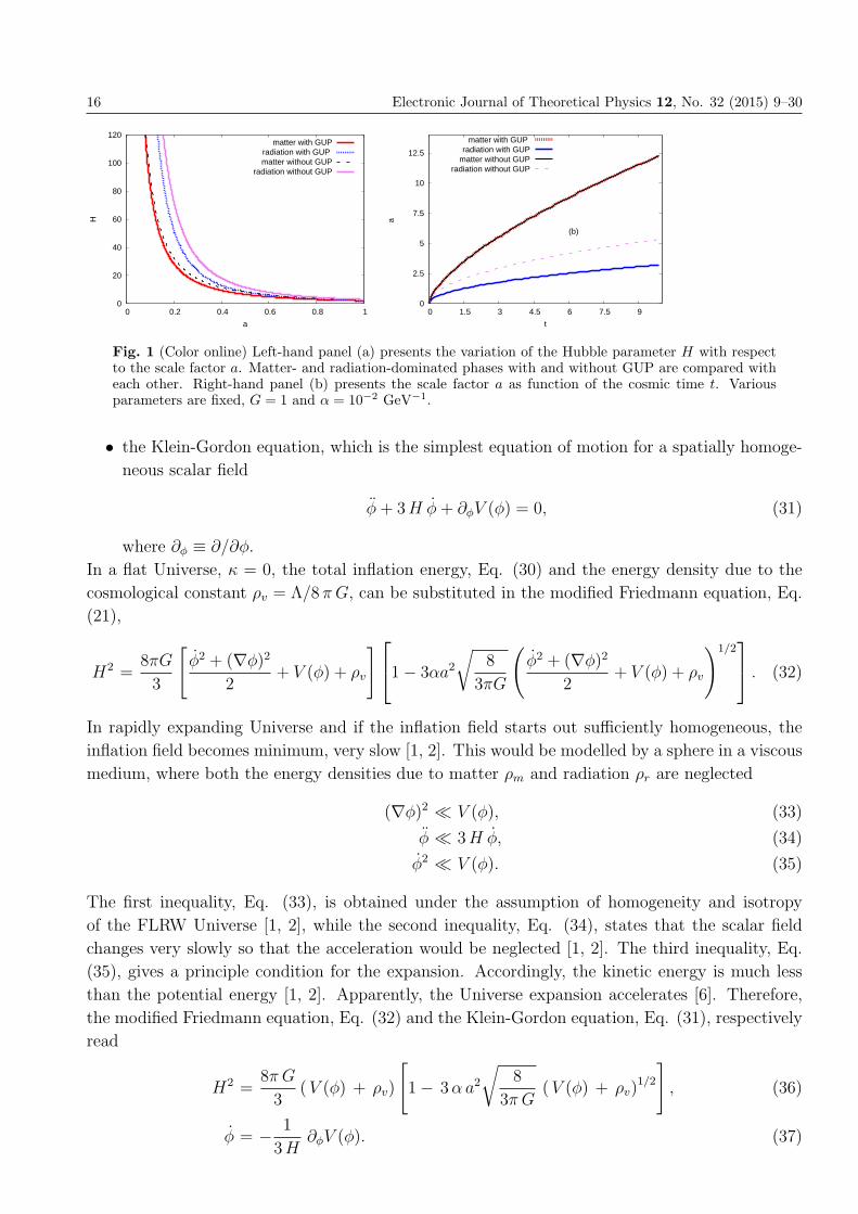
The left-hand panel (a) of Fig. 1 shows the Hubble parameter, H in dependence on the scale
factor, a. The standard (without GUP), Eq. (17) are compared with the modified (with GUP)
characterizations of the cosmic fluid, Eq. (22) in the flat universe. It is obvious that H in both
cases (with/without GUP) diverges at vanishing a. This would mean that a singularity exists at
the beginning. The GUP has the effect to slightly slow down the expansion rate of the Universe.
This is valid for both cases of cosmic background, radiation and matter.
In the right-panel (b) of Fig. 1, the dependence of the scale factor, a, on the cosmic time, t, is
given for both cases of cosmic matters, radiation and matter with and without GUP. Apparently,
the GUP is not sensitive to the matter-dominated phase but has a clear effect on the radiation-
dominated phase. The GUP breaks down the expansion.
3. Cosmic Inflation
Here, we estimate various inflation parameters, which are characterized by the scalar field φ and
apparently contribute to the total energy density [1, 2]. Also, taken into account the background
(matter and radiation) energy density, the scalar field is assumed to interact with the gravity and
with itself [6, 62, 63, 1, 2]. In order to reproduce the basics of the field theory, the coupling of φ
to gravitation results in total inflation energy
1
2
(φ2 + (∇φ)2
)+ V (φ). (30)
The dynamics of the inflation can be described by two types of equations:
• the Friedmann equation, which describes the contraction and expansion of the Universe and
16 Electronic Journal of Theoretical Physics 12, No. 32 (2015) 9–30
0
20
40
60
80
100
120
0 0.2 0.4 0.6 0.8 1
H
a
matter with GUPradiation with GUP
matter without GUPradiation without GUP
0
2.5
5
7.5
10
12.5
0 1.5 3 4.5 6 7.5 9
a
t
(b)
matter with GUP radiation with GUP
matter without GUP radiation without GUP
Fig. 1 (Color online) Left-hand panel (a) presents the variation of the Hubble parameter H with respectto the scale factor a. Matter- and radiation-dominated phases with and without GUP are compared witheach other. Right-hand panel (b) presents the scale factor a as function of the cosmic time t. Variousparameters are fixed, G = 1 and α = 10−2 GeV−1.
• the Klein-Gordon equation, which is the simplest equation of motion for a spatially homoge-
neous scalar field
φ+ 3H φ+ ∂φV (φ) = 0, (31)
where ∂φ ≡ ∂/∂φ.
In a flat Universe, κ = 0, the total inflation energy, Eq. (30) and the energy density due to the
cosmological constant ρv = Λ/8 π G, can be substituted in the modified Friedmann equation, Eq.
(21),
H2 =8πG
3
[φ2 + (∇φ)2
2+ V (φ) + ρv
] ⎡⎣1− 3αa2√
8
3πG
(φ2 + (∇φ)2
2+ V (φ) + ρv
)1/2⎤⎦ . (32)
In rapidly expanding Universe and if the inflation field starts out sufficiently homogeneous, the
inflation field becomes minimum, very slow [1, 2]. This would be modelled by a sphere in a viscous
medium, where both the energy densities due to matter ρm and radiation ρr are neglected
(∇φ)2 � V (φ), (33)
φ � 3H φ, (34)
φ2 � V (φ). (35)
The first inequality, Eq. (33), is obtained under the assumption of homogeneity and isotropy
of the FLRW Universe [1, 2], while the second inequality, Eq. (34), states that the scalar field
changes very slowly so that the acceleration would be neglected [1, 2]. The third inequality, Eq.
(35), gives a principle condition for the expansion. Accordingly, the kinetic energy is much less
than the potential energy [1, 2]. Apparently, the Universe expansion accelerates [6]. Therefore,
the modified Friedmann equation, Eq. (32) and the Klein-Gordon equation, Eq. (31), respectively
read
H2 =8π G
3(V (φ) + ρv)
[1− 3α a2
√8
3π G(V (φ) + ρv)
1/2
], (36)
φ = − 1
3H∂φV (φ). (37)
Electronic Journal of Theoretical Physics 12, No. 32 (2015) 9–30 17
The cosmological constant characterizes the minimum mass that is related to the Planck mass
MP =√�c/G. The Planck length �p =
√�G/c3 [64] is also related to the mass quanta, where
quantized mass [65] is proportional to the GUP parameter α. The cosmological constant Λ is
one of the foundation of gravity [65]. It related the Planck (quantum scale) and the Einstein (in
cosmological scale) masses, MP and ME, respectively, with each other [65]
Mp =
(h
c
)(Λ
3
)1/2
, (38)
ME =
(c2
G
)(3
Λ
)1/2
. (39)
By using natural units � = c = 1, the modified Friedmann equation, Eq. (36), becomes
H2 =4π
3 M2p
{[V (φ) +
3M4p
4 π
]− 3α a2
√16M2
p
3 π
[V (φ) +
3M4p
4 π
]3/2}. (40)
There are various inflation models such as chaotic inflation models, which suggest different inflation
potentials [6, 62, 63]. Now, it is believed that they are better motivated than other models
[6, 62, 63]. In this context, there are two main types of models; one with a single inflation field
and the other one combines two inflation fields. Here, we summarize some models requiring a
single inflation-field φ which in some regions satisfies the slow-roll conditions,
Polynomial chaotic inflation V (φ) =1
2m2φ2, V (φ) = λφ4, (41)
Power-law inflation V (φ) = V0 exp
[√16π G
pφ
], (42)
Natural inflation V (φ) = V0
(1 + cos
φ
f
), V (φ) ∝ φ−β. (43)
Based on this concept, we select three different inflation potential models, Eqs. (45), (46) and
(47). The first one is based on certain minimal supersymmetric extensions of the standard model
for elementary particles [66] and the related effects have been studied, recently [66, 68]. It has
two free parameters, m and λ,
V (φ) =
(m2
2
)φ2 −
(√2λ (n− 1)m
n
)φn +
(λ
4
)φ2(n−1), (44)
where n > 2 is an integer. At n = 3,
V1(φ) =
(m2
2
)φ2 −
(2√λm
3
)φ3 +
(λ
4
)φ4, (45)
which is an S-dual inflationary potential [69] with a free parameter f . The S duality has its origin
in the Dirac quantization condition of the electric and magnetic charges [70]. This would suggest
an equivalence in the description of the quantum electrodynamics [70],
V2(φ) = V0 sech
(φ
f
). (46)
18 Electronic Journal of Theoretical Physics 12, No. 32 (2015) 9–30
For a power-law inflation with the free parameter d [71, 62],
V3(φ) =3M2
pd2
32π
[1− exp
(− 16π
3M2p
1/2
φ
)]2
. (47)
For these inflation potentials, Eqs. (45), (46) and (47), the inflation parameters such as
potential slow-roll parameters ε, η, tensorial pt and scalar ps density fluctuations, the ratio of
tensor-to-scalar fluctuations r, scalar spectral index ns and the number of e-folds with the inflation
era Ne can be estimated.
0
0.2
0.4
0.6
0.8
1
1.2
1.4
0 0.05 0.1 0.15 0.2 0.25 0.3 0.35
V/V
0
φ/Mp
V1(φ)V2(φ)v3(φ)
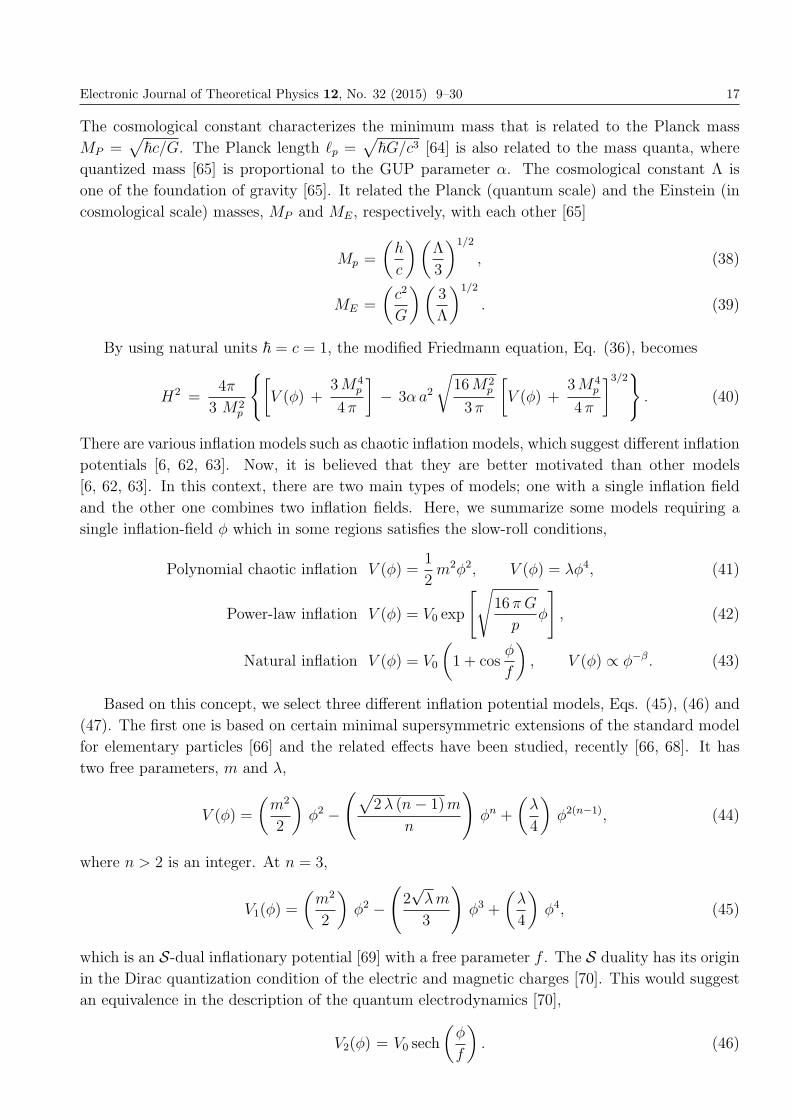
Fig. 2 (Color online) The variation of inflation potentials V/V0 is given in dependence on scalar fieldφ/Mp at limited free constants. The solid, long-dashed and dotted line stands for V1(φ), V2(φ) and V3(φ),respectively.
Fig. 2 shows the variation of the different inflation potentials, Eqs. (45), (46) and (47),
normalized with respect to initial potential V0 with the single inflation field φ according to Lyth
bound during the inflation era [18, 19, 20] and normalized with respect to Mp. The inflation
field, φ ≡ Δφ = (φ0 − φend) should be smaller than or comparable with the Planck scale Mp.
This was confirmed by the BICEP2 observation conditionally with this bound of small scalar field
[18, 19, 20]. The potentials, Eqs. (45) and (47) increase with φ/Mp, while the third potential,
Eq. (46) , decreases. This means that the latter is finite at vanishing inflation field, φ, while the
earlier vanishes.
4. Fluctuations and Slow-roll Parameters in the Inflation Era
In very early Universe, the scaler field φ is assumed to derive the inflation [6, 62, 63]. The main
potential slow-roll parameters are given as
ε ≡M2
p
16 π
(∂φV (φ)
V (φ)
)2
, (48)
η ≡M2
p
8π
(∂2φV (φ)
V (φ)
). (49)
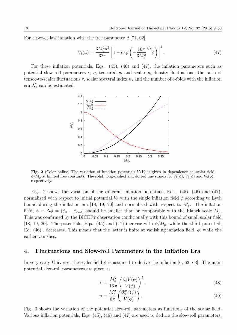
Fig. 3 shows the variation of the potential slow-roll parameters as functions of the scalar field.
Various inflation potentials, Eqs. (45), (46) and (47) are used to deduce the slow-roll parameters,
Electronic Journal of Theoretical Physics 12, No. 32 (2015) 9–30 19
Eqs. (48) and (49). The scalar fields in left- (a) and right-hand panel (c) result in slow-roll
parameters, which start from large values at small field. Then, they rapidly decline (vanish) as
the scalar field increases. The field presented in the middle panel gives slow-roll parameters with
relatively very small values, but seem to remain stable with the field.
0
200
400
600
800
0 0.02 0.04 0.06 0.08 0.1
ε,η
φ/Mp
(a)slow roll parameters for V1(φ)
εη
-4.5
-3
-1.5
0
1.5
3
4.5
0 0.08 0.16 0.24 0.32 0.4
ε,η
φ/Mp
(b)slow roll parameters for V2(φ)
εη
0
200
400
600
800
0 0.02 0.04 0.06 0.08 0.1
ε,η
φ/Mp
(c)slow roll parameters for V3(φ)
εη
Fig. 3 (Color online) From the left- (a) middle (b) and right-hand (c) panels present the slow-roll param-eters associated with V1(φ) from Eq. (45), V2(φ) from Eq. (46) and V3(φ) from (47), respectively. Thesolid and dot-dashed curves represent ε and η parameters, respectively.
The tensorial and scalar density fluctuations are given as [6, 62, 63]
pt =
(H
2π
)2 [1− H
Λsin
(2Λ
H
)]=
(H
2 π
)2 [1− H
3M2p
sin
(6M2
p
H
)], (50)
ps =
(H
φ
)2 (H
2π
)2 [1− H
Λsin
(2Λ
H
)]=
(H
φ
)2 (H
2 π
)2 [1− H
3M2p
sin
(6M2
p
H
)]. (51)
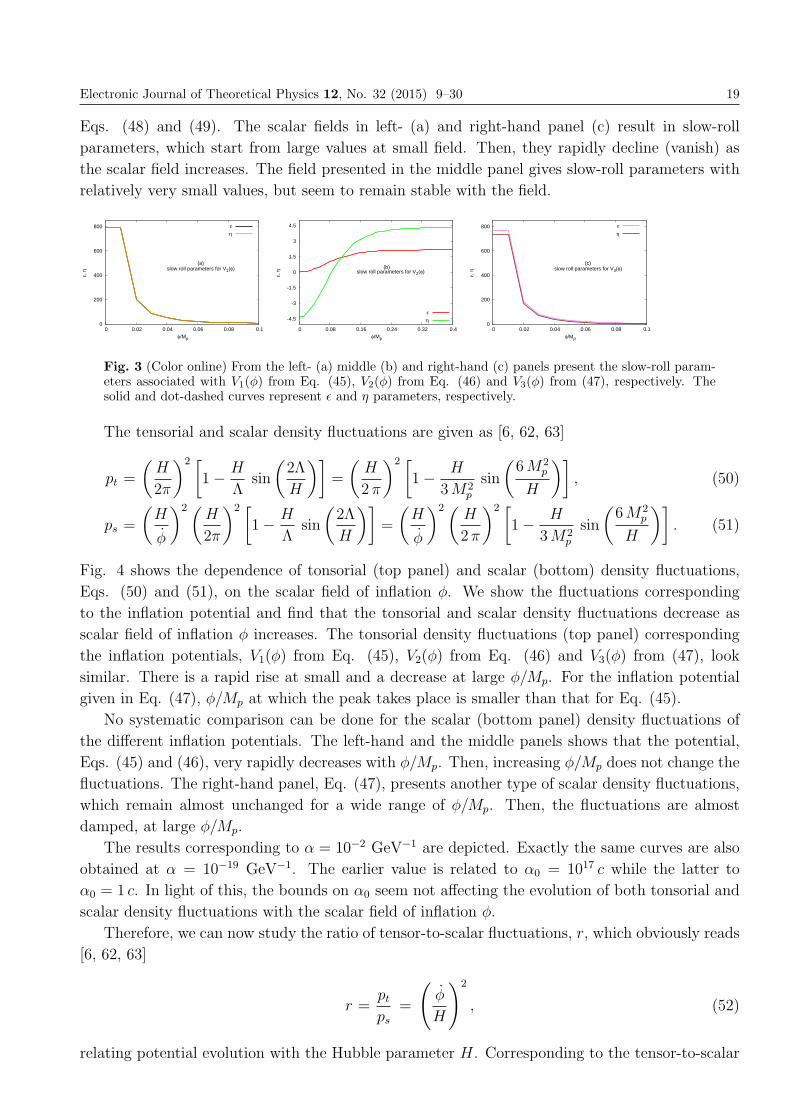
Fig. 4 shows the dependence of tonsorial (top panel) and scalar (bottom) density fluctuations,
Eqs. (50) and (51), on the scalar field of inflation φ. We show the fluctuations corresponding
to the inflation potential and find that the tonsorial and scalar density fluctuations decrease as
scalar field of inflation φ increases. The tonsorial density fluctuations (top panel) corresponding
the inflation potentials, V1(φ) from Eq. (45), V2(φ) from Eq. (46) and V3(φ) from (47), look
similar. There is a rapid rise at small and a decrease at large φ/Mp. For the inflation potential
given in Eq. (47), φ/Mp at which the peak takes place is smaller than that for Eq. (45).
No systematic comparison can be done for the scalar (bottom panel) density fluctuations of
the different inflation potentials. The left-hand and the middle panels shows that the potential,
Eqs. (45) and (46), very rapidly decreases with φ/Mp. Then, increasing φ/Mp does not change the
fluctuations. The right-hand panel, Eq. (47), presents another type of scalar density fluctuations,
which remain almost unchanged for a wide range of φ/Mp. Then, the fluctuations are almost
damped, at large φ/Mp.
The results corresponding to α = 10−2 GeV−1 are depicted. Exactly the same curves are also
obtained at α = 10−19 GeV−1. The earlier value is related to α0 = 1017 c while the latter to
α0 = 1 c. In light of this, the bounds on α0 seem not affecting the evolution of both tonsorial and
scalar density fluctuations with the scalar field of inflation φ.
Therefore, we can now study the ratio of tensor-to-scalar fluctuations, r, which obviously reads
[6, 62, 63]
r =ptps
=
(φ
H
)2
, (52)
relating potential evolution with the Hubble parameter H. Corresponding to the tensor-to-scalar
20 Electronic Journal of Theoretical Physics 12, No. 32 (2015) 9–30
0
0.02
0.04
0.06
0.08
0.1
0 0.08 0.16 0.24 0.32 0.4
P t
φ/Mp
(a): pt for V1(φ)
0
0.02
0.04
0.06
0.08
0.1
0 0.08 0.16 0.24 0.32 0.4
n s
φ/Mp
(b): Pt for V2(φ)
0
0.02
0.04
0.06
0.08
0.1
0 0.08 0.16 0.24 0.32 0.4
P t
φ/Mp
(c): Pt for V3(φ)
0
1
2
3
4
5
0 0.08 0.16 0.24 0.32 0.4
Ps
φ/Mp
(a): ps for V1(φ)
0
4
8
12
16
20
0 0.08 0.16 0.24 0.32 0.4
Ps
φ/Mp
(b): Ps for V2(φ)
-2.4
-1.2
0
1.2
2.4
0 0.08 0.16 0.24 0.32 0.4
Ps
φ/Mp
(c): Ps for V3(φ)
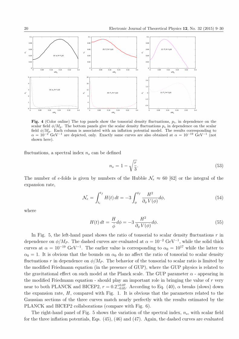
Fig. 4 (Color online) The top panels show the tonsorial density fluctuations, pt, in dependence on thescalar field φ/Mp. The bottom panels give the scalar density fluctuations ps in dependence on the scalarfield φ/Mp. Each column is associated with an inflation potential model. The results corresponding toα = 10−2 GeV−1 are depicted, only. Exactly same curves are also obtained at α = 10−19 GeV−1 (notshown here).
fluctuations, a spectral index ns can be defined
ns = 1−√
r
3. (53)
The number of e-folds is given by numbers of the Hubble Ne ≈ 60 [62] or the integral of the
expansion rate,
Ne =
∫ tf
ti
H(t) dt = −3∫ φf
φ
H2
∂φ V (φ)dφ, (54)
where
H(t) dt =H
φdφ = −3 H2
∂φ V (φ)dφ. (55)
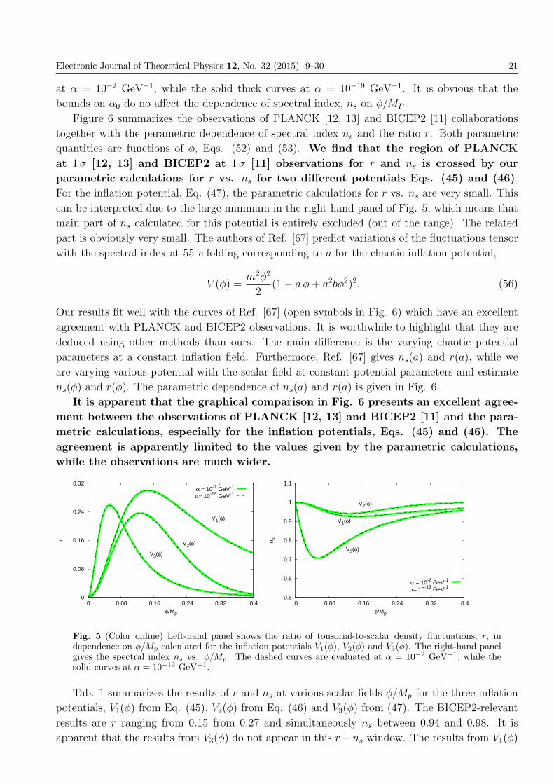
In Fig. 5, the left-hand panel shows the ratio of tonsorial to scalar density fluctuations r in
dependence on φ/MP . The dashed curves are evaluated at α = 10−2 GeV−1, while the solid thick
curves at α = 10−19 GeV−1. The earlier value is corresponding to α0 = 1017 while the latter to
α0 = 1. It is obvious that the bounds on α0 do no affect the ratio of tonsorial to scalar density
fluctuations r in dependence on φ/MP . The behavior of the tonsorial to scalar ratio is limited by
the modified Friedmann equation (in the presence of GUP), where the GUP physics is related to
the gravitational effect on such model at the Planck scale. The GUP parameter α - appearing in
the modified Friedmann equation - should play an important role in bringing the value of r very
near to both PLANCK and BICEP2, r = 0.2+0.07−0.05. According to Eq. (40), α breaks (slows) down
the expansion rate, H, compared with Fig. 1. It is obvious that the parameters related to the
Gaussian sections of the three curves match nearly perfectly with the results estimated by the
PLANCK and BICEP2 collaborations (compare with Fig. 6).
The right-hand panel of Fig. 5 shows the variation of the spectral index, ns, with scalar field
for the three inflation potentials, Eqs. (45), (46) and (47). Again, the dashed curves are evaluated
Electronic Journal of Theoretical Physics 12, No. 32 (2015) 9–30 21
at α = 10−2 GeV−1, while the solid thick curves at α = 10−19 GeV−1. It is obvious that the
bounds on α0 do no affect the dependence of spectral index, ns on φ/MP .
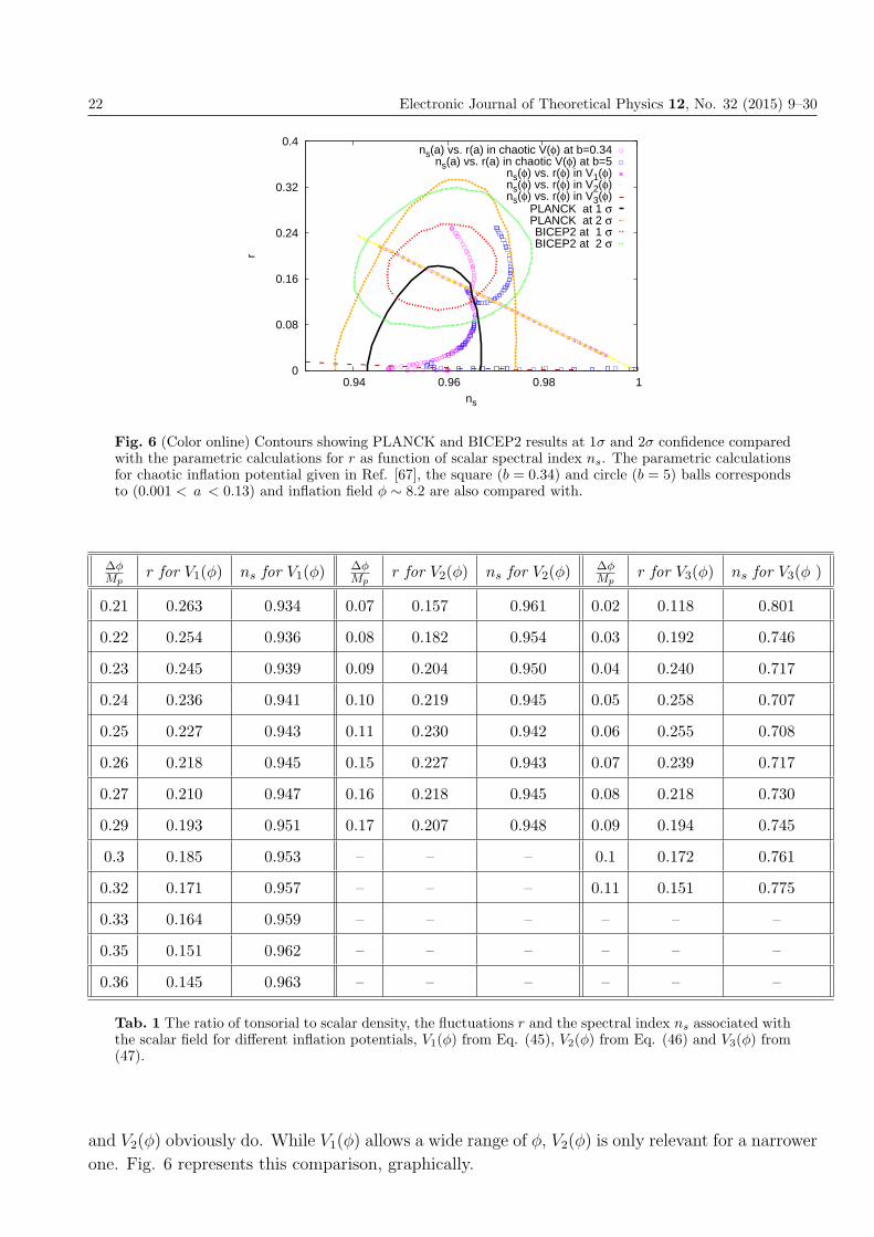
Figure 6 summarizes the observations of PLANCK [12, 13] and BICEP2 [11] collaborations
together with the parametric dependence of spectral index ns and the ratio r. Both parametric
quantities are functions of φ, Eqs. (52) and (53). We find that the region of PLANCK
at 1 σ [12, 13] and BICEP2 at 1 σ [11] observations for r and ns is crossed by our
parametric calculations for r vs. ns for two different potentials Eqs. (45) and (46).
For the inflation potential, Eq. (47), the parametric calculations for r vs. ns are very small. This
can be interpreted due to the large minimum in the right-hand panel of Fig. 5, which means that
main part of ns calculated for this potential is entirely excluded (out of the range). The related
part is obviously very small. The authors of Ref. [67] predict variations of the fluctuations tensor
with the spectral index at 55 e-folding corresponding to a for the chaotic inflation potential,
V (φ) =m2φ2
2(1− a φ+ a2bφ2)2. (56)
Our results fit well with the curves of Ref. [67] (open symbols in Fig. 6) which have an excellent
agreement with PLANCK and BICEP2 observations. It is worthwhile to highlight that they are
deduced using other methods than ours. The main difference is the varying chaotic potential
parameters at a constant inflation field. Furthermore, Ref. [67] gives ns(a) and r(a), while we
are varying various potential with the scalar field at constant potential parameters and estimate
ns(φ) and r(φ). The parametric dependence of ns(a) and r(a) is given in Fig. 6.
It is apparent that the graphical comparison in Fig. 6 presents an excellent agree-
ment between the observations of PLANCK [12, 13] and BICEP2 [11] and the para-
metric calculations, especially for the inflation potentials, Eqs. (45) and (46). The
agreement is apparently limited to the values given by the parametric calculations,
while the observations are much wider.
0
0.08
0.16
0.24
0.32
0 0.08 0.16 0.24 0.32 0.4
r
φ/Mp
V1(φ)
V2(φ)
V3(φ)
α = 10-2 GeV-1
α= 10-19 GeV-1
0.5
0.6
0.7
0.8
0.9
1
1.1
0 0.08 0.16 0.24 0.32 0.4
n s
φ/Mp
V2(φ)
V1(φ)
V3(φ)
α = 10-2 GeV-1
α= 10-19 GeV-1
Fig. 5 (Color online) Left-hand panel shows the ratio of tonsorial-to-scalar density fluctuations, r, independence on φ/Mp calculated for the inflation potentials V1(φ), V2(φ) and V3(φ). The right-hand panelgives the spectral index ns vs. φ/Mp. The dashed curves are evaluated at α = 10−2 GeV−1, while thesolid curves at α = 10−19 GeV−1.
Tab. 1 summarizes the results of r and ns at various scalar fields φ/Mp for the three inflation
potentials, V1(φ) from Eq. (45), V2(φ) from Eq. (46) and V3(φ) from (47). The BICEP2-relevant
results are r ranging from 0.15 from 0.27 and simultaneously ns between 0.94 and 0.98. It is
apparent that the results from V3(φ) do not appear in this r−ns window. The results from V1(φ)
22 Electronic Journal of Theoretical Physics 12, No. 32 (2015) 9–30
0
0.08
0.16
0.24
0.32
0.4
0.94 0.96 0.98 1
r
ns
ns(a) vs. r(a) in chaotic V(φ) at b=0.34ns(a) vs. r(a) in chaotic V(φ) at b=5
ns(φ) vs. r(φ) in V1(φ)ns(φ) vs. r(φ) in V2(φ)ns(φ) vs. r(φ) in V3(φ)
PLANCK at 1 σPLANCK at 2 σBICEP2 at 1 σ
BICEP2 at 2 σ
Fig. 6 (Color online) Contours showing PLANCK and BICEP2 results at 1σ and 2σ confidence comparedwith the parametric calculations for r as function of scalar spectral index ns. The parametric calculationsfor chaotic inflation potential given in Ref. [67], the square (b = 0.34) and circle (b = 5) balls correspondsto (0.001 < a < 0.13) and inflation field φ ∼ 8.2 are also compared with.
ΔφMp
r for V1(φ) ns for V1(φ)ΔφMp
r for V2(φ) ns for V2(φ)ΔφMp
r for V3(φ) ns for V3(φ )
0.21 0.263 0.934 0.07 0.157 0.961 0.02 0.118 0.801
0.22 0.254 0.936 0.08 0.182 0.954 0.03 0.192 0.746
0.23 0.245 0.939 0.09 0.204 0.950 0.04 0.240 0.717
0.24 0.236 0.941 0.10 0.219 0.945 0.05 0.258 0.707
0.25 0.227 0.943 0.11 0.230 0.942 0.06 0.255 0.708
0.26 0.218 0.945 0.15 0.227 0.943 0.07 0.239 0.717
0.27 0.210 0.947 0.16 0.218 0.945 0.08 0.218 0.730
0.29 0.193 0.951 0.17 0.207 0.948 0.09 0.194 0.745
0.3 0.185 0.953 – – – 0.1 0.172 0.761
0.32 0.171 0.957 – – – 0.11 0.151 0.775
0.33 0.164 0.959 – – – – – –
0.35 0.151 0.962 – – – – – –
0.36 0.145 0.963 – – – – – –
Tab. 1 The ratio of tonsorial to scalar density, the fluctuations r and the spectral index ns associated withthe scalar field for different inflation potentials, V1(φ) from Eq. (45), V2(φ) from Eq. (46) and V3(φ) from(47).
and V2(φ) obviously do. While V1(φ) allows a wide range of φ, V2(φ) is only relevant for a narrower
one. Fig. 6 represents this comparison, graphically.
Electronic Journal of Theoretical Physics 12, No. 32 (2015) 9–30 23
5. Discussion and Conclusions
The BICEP2 results announced on March 17, 2014 made the physicists around the globe having
another view about the evidence of Universe and its expansion, especially at about the inflation
era. The cosmic inflation is based on the assumption that an extreme inflationary phase should
take place after the Big Bang (at about the Planck time). Thus, the Universe should expand at a
superluminal speed. On the other hand, the inflation would result from a hypothetical field acting
as a cosmological constant to produce an acceleration expansion of the Universe.
Argumentation about the applicability of GUP on the inflation era will be elaborated in Ap-
pend. A2. Due to the very high energy (quantum or Planck scale), the Heisenberg uncertainty
principle should be modified in terms of momentum uncertainty. The QG approach in form of
GUP appears in the modified Friedmann equation - in terms of α. This term reduces the Hubble
parameter, which appears in the denominator of the ratio of tonsorial-to-scalar density fluctua-
tions. Thus, the fluctuations ratio increases due to decreasing H. The fluctuations ratio r has
been evaluated as function of the spectral index ns. We found that the calculations match well
with the PLANCK and BICEP2 observations. This is the main conclusion of the present work.
We believe that the results point to the importance of quantum correlation during the inflation
era.
The estimation of the ns(a) and r(a) at 55 e-folds for a chaotic potential for different values of
b and varying inflation as function of a. The parameters b = 0.34 (open squares) and b = 5 (open
circles) are corresponding to (0.001 < a < 0.13) and inflation field φ ∼ 8.2ss [67]. The authors
predict the variation of the fluctuation tensor with the spectral index. The best curves in Ref.
[67] agree well with PLANCK and BICEP2. These are deduced using another method, varying
a and selecting out the suitable scalar field. The main difference with our method is the is the
varying chaotic potential parameters at constant inflation field. We vary the inflation potential
with the scalar field at constant potential parameters.
We have reviewed different inflationary potentials and estimated the modifications of the Fried-
mann equation due to the GUP approach. We found that
• the first potential, Eq. (45), gives a power law of the scalar inflation-field. This is based on
certain minimal supersymmetric extensions of the standard model [66].
• The second potential, Eq. (46), hypothesizes that the potential should be invariant un-
der the S-duality constraint g → 1/g, or φ → −φ, where φ is the dilation/inflation and
g ≈ exp (φ/M) [69]. The S-duality had its roots in the Dirac quantization condition for the
electromagnetic field. Thus, it should be equivalence to the description of quantum electro-
dynamics as either a weakly coupled theory of electric charges or a strongly coupled theory
of magnetic monopoles [72]. The latter, Eq. (47) appeared in an exponential form with a
power-law inflation field. These inflationary potentials seem to agree well with of the ob-
servations of PLANCK and BICEP2 collaborations at different 1σ and 2 σ. In the range of
spectral index and fluctuation ratio.
• The potential, Eq. (47) disagrees. Few remarks are now in order. The agreement should
be limited to the values given by the parametric calculations. The PLANCK and BICEP2
observations are much wider but have uncertainties in r of order 25%. We have presented
through a conceivable way the effects of reasonably-sized GUP parameter of our estimation
for r.
24 Electronic Journal of Theoretical Physics 12, No. 32 (2015) 9–30
We conclude that depending on the inflation potential V (φ) and the scalar field, φ, the GUP
approach seems to reproduce the BICEP2 observations r = 0.2+0.07−0.05, which also have been fitted
by using 55 e-folds for a chaotic potential for varying inflation and seem to agree well with the
upper bound value corresponding to PLANCK and to WMAP9 experiment.
A Generalized uncertainty principle (GUP)
A1 Minimal length uncertainty and maximum measurable momentum
The commutator relation [39, 40, 41], which are consistent with the string theory, the black holes
physics and DSR leads to
[xi, pj] = i�
[δij − α
(pδij +
pipjp
)+ α2
(p2δij + 3pipj
)], (A.1)
implying a minimal length uncertainty and a maximum measurable momentum when implement-
ing convenient representation of the commutation relations of the momentum space wave-functions
[42, 21]. The constant coefficient α = α0/(Mp c) = α0 lp/� is referring to the quantum-gravitational
effects on the Heisenberg uncertainty principle. The momentum pj and the position xi operators
are given as
xi Ψ(p) = x0i(1− α p0 + 2α2 p20)Ψ(p),
pj Ψ(p) = p0j Ψ(p). (A.2)
We notice that p20 =∑3
j p0j p0j satisfies the canonical commutation relations [x0i, p0j] = i � δij.
Then, the minimal length uncertainty [39, 40, 41] and maximum measurable momentum [42, 21],
respectively, read
Δx ≥ (Δx)min ≈ �α,
pmax ≈1
4α, (A.3)
where the maximum measurable momentum agrees with the value which was obtained in the
doubly special relativity (DSR) theory [36, 21]. By using natural units, the one-dimensional
uncertainty reads [39, 40, 41]
ΔxΔp ≥ �
2
(1− 2αΔp+ 4α2Δp2
). (A.4)
This representation of the operators product satisfies the non-commutative geometry of the space-
time [42]
[pi, pj] = 0,
[xi, xj] = −i �α(4α− 1
p
) (1− α p0 + 2α2 �p0
2)Lij. (A.5)
The rotational symmetry does not break by the commutation relations [42, 32]. In fact, the
rotation generators can still be expressed in terms of position and momentum operators as [42, 21]
Lij =Xi Pj − Xj Pi
1− α p0 + 2α2 �p02 . (A.6)
Electronic Journal of Theoretical Physics 12, No. 32 (2015) 9–30 25
A2 Applicability of GUP to the cosmic inflation
The quantum aspects of the gravitational fields can emerge in the limit, where strong, weak
and electromagnetic interactions can be distinguished from each other. In the view of gedanken
experiments that have been designed to measure the apparent horizon area of a black hole in
QG [26], the uncertainty relation is found preformed [25]. The deformed or modified Heisenberg
algebra, which was suggested to investigate GUP, introduces a relation between QG and Poincare
algebra [26]. Nevertheless, GUP given in quadratic forms [25, 27], which fits well with the string
theory and the black hole physics and introduces a minimal length uncertainty and additional
linear terms of momenta [36] agrees also well with DSR and assumes that the momenta approach
maximum value at very high energy (Planck scale) [36].
There are several observations supporting the concept of GUP approaches and offering a possi-
bility of studying the influence of the minimal length on the properties of a wide range of physical
systems, especially at quantum scale [25, 26, 34]. The effects of linear GUP approach have been
studied on compact stars [46], Newtonian law of gravity [45], inflationary parameters and thermo-
dynamics of the early Universe [47], Lorentz invariance violation [48] and measurable maximum
energy and minimum time interval [73]. Furthermore, the effects of QG on the quark-gluon plasma
(QGP) are studied [49]. It was found that the GUP can potentially explain the small observed
violations of the weak equivalence principle in neutron interferometry experiments [74]. Also, it
was suggested [75] that GUP can be measured directly in Quantum Optics Lab [40, 41]. The cur-
rent researches of the quantum problems in the presence of gravitational field at very high energy
near to the Planck scale implies new physical laws and even corrections of the spacetime of our
Universe [27]. The quantum field theory in curved background can be normalized by introducing
a minimal observable length as an effective cut-off in ultraviolet domain [27]. It is conjectured
that the string can’t probe distances smaller than its own length. For cosmic inflation, is the
expansion of space in the early Universe. The inflationary epoch lasted from 10−36 seconds after
the Big Bang to sometime between 10−33 and 10−32 seconds near to Planck scale. Following the
inflationary period, the universe continues to expand, but at a less accelerated rate. Actually,
the GUP at very high energy Planck scale would likely be applicable to contract these approach
interpret of the quantum study of the inflationary of the universe.
B Modified Dispersion Relation (MDR)
Various observations support the conjectured that the Lorentz invariance might be violated. The
velocity of light should differ from c. Any tiny adjustment leads to modification of the energy-
momentum relation and modifies the dispersion relation in vacuum state by δv [76, 77, 78, 79].
In particular, at the Planck scale, the modifications of energy-momentum dispersion relation have
been considered in Refs. [80, 81]. Two functions p(E) as expansions with leading Planck-scale
correction of order Lp E3 and L2
pE4 respectively, reads [82],
�p2 � E2 −m2 + α1 Lp E3, (B.1)
�p2 � E2 −m2 + α2 L2p E
4. (B.2)
These are valid for a particle of mass M at rest, whose position is being measured by a procedure
involving a collision with a photon of energy E and momentum p. Since the relations are originated
26 Electronic Journal of Theoretical Physics 12, No. 32 (2015) 9–30
from Heisenberg uncertainty principle for position with precision δx, one should use a photon with
momentum uncertainty δp ≥ 1/δx. Based on the argument of Ref. [83] in loop QG, we convert
δp ≥ 1/δx into δE ≥ 1/δx. By using the special-relativistic dispersion relation and δE ≥ 1/δx,
then M ≥ δE. If indeed loop QG hosts a Planck-scale-modified dispersion relation, Eq. (B.2),
thenδpγ ≥ 1/δx and this required that [82],
M ≥ 1
δx
(1− α2
3L2p
2(δx)2
). (B.3)
These results apply only to the measurement of the position of a particle at rest [83]. We can
generalize these results to measurement of the position of a particle of energy E.
• In case of standard dispersion relation, one obtains that E ≥ 1/δx as required for a linear
dependence of entropy on area, Eq. (B.2)
• For the dispersion relation, Eq. (B.2)
E ≥ 1
δx
(1− α2
3L2p
2(δx)2
). (B.4)
The requirements of these derivation lead in order of correction of log-area form.
• Furthermore,
E ≥ 1
δx
(1 + α1
Lp
δx
). (B.5)
In case of string theory, the ”reversed Bekenstein argument” leads to quadratic GUP, that fits well
with the string theory [84] and black holes physics,
δx ≥ 1
δp+ λ2
sδp. (B.6)
The scale λs in Eq. (B.6) is an effective string length giving the characteristic length scale which
be identical with Planck length. Many researches of loop QG [80, 81] support the possibility of the
existence of a minimal length uncertainty and a modification in the energy-momentum dispersion
relation at Planck scale.
References
[1] A. R. Liddle, ”Introduction to modern cosmology” (Wiley, UK, 2003).
[2] A. D. Linde, (ed. S. Bonometto, V. Gorini and U. Moschella) ”Inflationary cosmology andcreation of matter in the Universe. In Modern cosmology”, (Institute of Physics Publishing,Bristol, 2002).
[3] A. A. Starobinsky, JETP Lett. 30, 682 (1979) [Pisma Zh. Eksp. Teor. Fiz. 30, 719 (1979)].
[4] K. Sato, Mon. Not. Roy. Astron. Soc. 195, 467 (1981).
[5] A. Albrecht and P. J. Steinhardt, Phys. Rev. Lett. 48, 1220 (1982).
[6] A. D. Linde, Phys. Lett. B 108, 389 (1982).
[7] A. H. Guth, Phys. Rev. D 23, 347 (1981).
[8] S. W. Hawking, Phys. Lett. B 115, 295 (1982).
Electronic Journal of Theoretical Physics 12, No. 32 (2015) 9–30 27
[9] A. H. Guth and S. Y. Pi, Phys. Rev. Lett. 49, 1110 (1982).
[10] A. A. Starobinsky, Phys. Lett. B 117, 175 (1982).
[11] [BICEP2 Collaboration], P. Ade et al., Phys. Rev. Lett. 112, 241101 (2014).
[12] [Planck Collaboration], P. Ade et al.,1303.5076 [astro-ph.CO].
[13] [Planck Collaboration], P. Ade et al.,1303.5082 [astro-ph.CO].
[14] [WMAP Collaboration], G. Hinshaw et al., Astrophys. J. Suppl. 208, 19 (2013).
[15] V. F. Mukhanov and G. V. Chibisov, JETP Lett. 33, 532 (1981).
[16] J. M. Bardeen, P. J. Steinhardt and M. S. Turner, Phys. Rev. D 28, 679 (1983).
[17] U. Amaldi, W. de Boer and H. Furstenau, Phys. Lett. B 260, 447 (1991).
[18] D. H. Lyth, Phys. Rev. Lett. 78, 1861 (1997).
[19] D. H. Lyth and A. Riotto, Phys. Rept. 314, 1 (1999).
[20] D. Baumann and D. Green, JCAP 1205, 017 (2012).
[21] A. Tawfik and A. Diab, Int.J.Mod.Phys. D23, 1430025 (2014)
[22] D. Amati, M. Ciafaloni and G. Veneziano, Int. J. Mod. Phys. A 3, 1615 (1988).
[23] D. Amati, M. Ciafaloni and G. Veneziano, Phys. Lett. B 197, 81 (1987).
[24] D. Amati, M. Ciafaloni and G. Veneziano, Nucl. Phys. B 347, 550 (1990).
[25] M. Maggiore, Phys. Lett. B 304, 65 (1993).
[26] M. Maggiore, Phys. Rev. D 49, 5182 (1994).
[27] A. Kempf, DAMTP-96-10, (1995) hep-th/9603115.
[28] A. Kempf, J. Phys. A 30, 2093 (1997).
[29] A. Kempf, Phys. Rev. D 63, 083514 (2001).
[30] A. Kempf, J. Math. Phys. 35, 4483 (1994).
[31] A. Kempf, DAMTP-94-33 (1994) hep-th/9405067.
[32] A. Kempf, G. Mangano and R. B. Mann, Phys. Rev. D 52, 1108 (1995).
[33] A. Kempf, J. Math. Phys. 38, 1347 (1997).
[34] F. Scardigli, Phys. Lett. B 452, 39 (1999).
[35] F. Scardigli and R. Casadio, Int. J. Mod. Phys. D 18, 319 (2009).
[36] J. Cortes and J. Gamboa, Phys. Rev. D 71, 065015 (2005).
[37] L. Smolin and J. Magueijo, Phys. Rev. D 67, 044017 (2003).
[38] G. Amelino-Camelia, Int. J. Mod. Phys. D 11, 35 (2002); Int. J. Mod. Phys. D 11, 1643(2002).
[39] A. F. Ali, S. Das and E. C. Vagenas, Phys. Lett. B 678, 497 (2009).
[40] S. Das, E. C. Vagenas and A. F. Ali, Phys. Lett. B 690, 407 (2010).
[41] A. Farag Ali, S. Das and E. C. Vagenas, Phys. Rev. D 84, 044013 (2011).
[42] K. Nozari and A. Etemadi, Phys. Rev. D 85, 104029 (2012).
28 Electronic Journal of Theoretical Physics 12, No. 32 (2015) 9–30
[43] P. Pedram, Phys. Lett. B 714, 317 (2012); Phys. Lett. B 718, 638 (2012).
[44] A. Tawfik, JCAP 1307, 040 (2013).
[45] A. F. Ali and A. Tawfik, Adv. High Energy Phys. 2013, 126528 (2013).
[46] A. F. Ali and A. Tawfik, Int. J. Mod. Phys. D 22, 1350020 (2013).
[47] A. Tawfik, H. Magdy and A.Farag Ali, Gen. Rel. Grav. 45, 1227 (2013).
[48] A. Tawfik, H. Magdy and A.F. Ali, ”Lorentz Invariance Violation and Generalized UncertaintyPrinciple”, 1205.5998 [physics.gen-ph].
[49] I. Elmashad, A.F. Ali, L.I. Abou-Salem, Jameel-Un Nabi and A. Tawfik, Trans. Theor. Phys,1, 106 (2014).
[50] A. Tawfik and A. Diab, ”Black Hole Corrections due to Minimal Length and ModifiedDispersion Relation”, in press.
[51] Roy D’Inverno, ”Introducing Einstein’s Relativity”, (Clarendon Press, Oxford, 1992).
[52] Rong-Gen Cai and Sang Pyo Kim, JHEP 0502 (2005) 050.
[53] G.W. Gibbons S.W. Hawking and J.M. Stewart, Nucl. Phys. B 281, 736 (1987).
[54] R. Steigl and R. Hinterleitner, Class. Quantum Grav. 23, 3879 (2006).
[55] A. F. Ali and B. Majumder,Class.Quant.Grav. 31, 215007 (2014).
[56] P. A. M. Dirac, ”The Principles of Quantum Mechanics”, (Clarendon Press, Oxford, 1958).
[57] W. Chemissany, S. Das, A. F. Ali, E. C. Vagenas, JCAP 1112, 017 (2011).
[58] S. Das, E. C. Vagenas, Phys. Rev. Lett. 101, 221301 (2008); Can. J. Phys. 87, 233 (2009).
[59] A. F. Ali, S. Das and E. C. Vagenas, ”The Generalized Uncertainty Principle and QuantumGravity Phenomenology”, 1001.2642 [hep-th].
[60] A. Tawfik and H. Magdy, Can. J. Phys. 90, 433 (2012).
[61] A. Tawfik, Can. J. Phys. 88, 825 (2010).
[62] A. R. Liddle, D. H. Lyth, Phys. Rept. 231, 1 (1993).
[63] J. E. Lidsey, A. R. Liddle, E. W. Kolb, E. J. Copeland, T. Barreiro and M. Abney, Rev. Mod.Phys. 69, 373 (1997);D. Baumann, ”TASI lectures on inflation”, 0907.5424 [hep-th].
[64] C. G. Bohmer and T. Harko, Phys. Let. B 630, 73 (2005); Found. Phys. 38, 216 (2006).
[65] P. S. Wesson, Mod. Phys. Lett. A 19, 1995 (2004).
[66] R. Allahverdi, J. Garcia-Bellido, K. Enqvist and A. Mazumdar, Phys. Rev. Lett. 97, 191304(2006);R. Allahverdi, K. Enqvist, J. Garcia-Bellido, A. Jokinen and A. Mazumdar, JCAP 0706, 019(2007);R. Allahverdi, A. Mazumdar and T. Multamaki, ”Large tensor-to-scalar ratio and low scaleinfrlation”, 0712.2031 [astro-ph].
[67] R. Kallosh, A. Linde and A. Westphal, ”Chaotic inflation in supergravity after Planck andBICEP2”, Phys. Rev. D. 90 (2014) 023534.
[68] J. C. B. Sanchez, K. Dimopoulos and D. H. Lyth, JCAP 0701, 015 (2007).
[69] Luis A. Anchordoqui,V. Barger, H. Goldberg, Xing Huang and D. Marfatia, Phys. Lett. B734, 134-136 (2014).
Electronic Journal of Theoretical Physics 12, No. 32 (2015) 9–30 29
[70] C. Montonen and D. I. Olive, Phys. Lett. B 72, 117 (1977).
[71] Alexei A. Starobinsky, Phys. Lett. B 91, 99-102 (1980).
[72] S. M. Leach, A. R. Liddle, J. Martin and D. JSchwarz, Phys. Rev. D 66, 023515 (2002).
[73] A. Tawfik and E. Abou El Dahab, Canadian J. Phys. [doi: 10.1139/cjp-2013-0661] (2014).
[74] R. Collela, A. W. Overhauser and S. A. Werner, Phys. Rev. Lett. 34, 1472 (1975);K. C. Littrell, B. E. Allman and S. A. Werner, Phys. Rev. A 56, 1767 (1997);A. Camacho and A. Camacho-Galvan, Rep. Prog. Phys. 70, 1-56 (2007).
[75] I. Pikovski, M. R. Vanner, M. Aspelmeyer, M. S. Kim and C. Brukner, Nature Phys. 8, 393(2012).
[76] S. Coleman and S. L. Glashow, Phys. Rev. D 59, 116008 (1999);D. Colladay and V. A. Kostelecky, Phys. Rev. D 58, 116002 (1998).
[77] F. W. Stecker and S. L. Glashow, Astropart. Phys. 16 97 (2001).
[78] S. R. Coleman and S. L. Glashow, Phys. Lett. B 405, 249 (1997).
[79] G. Amelino-Camelia, J. Ellis, N. F. Mavromatos, D. V. Nanopoulos and S. Sarkar, Nature393, 763 (1998).
[80] R. Gambini and J. Pullin, Phys. Rev. D 59, 124021 (1999);J. Alfaro, H.A. Morales-Tecotl and L.F. Urrutia, Phys. Rev. Lett. 84, 2318 (2000).
[81] G. Amelino-Camelia, L. Smolin and A. Starodubtsev, Class. Quant. Grav. 21, 3095 (2004).
[82] G. Amelino-Camelia, M. Arzano and A. Procaccini, Int. J. Mod. Phys. D 13, 2337 (2004).
[83] E. M. Lifshitz, L. P. Pitaevskii and V. B. Berestetskii, ”Landau-Lifshitz Course of TheoreticalPhysics”, Volume 4: Quantum Electrodynamics” (Reed Educational and ProfessionalPublishing, 1982).
[84] G. Veneziano, Europhys.Lett. 2, 199 (1986);D.J. Gross and P.F. Mende, Nucl. Phys. B 303, 407 (1988);D. Amati, M. Ciafaloni and G. Veneziano, Phys. Lett. B 216, 41 (1989).

EJTP 12, No. 32 (2015) 31–42 Electronic Journal of Theoretical Physics
The Shadow of a Black Hole from Heterotic StringTheory at the Center of the Milky Way
Alexis Larranaga∗
National Astronomical Observatory. National University of Colombia
Received 24 October 2014, Accepted 20 December 2014, Published 10 January 2015
Abstract: We study the shadow produced by a charged rotating black hole arising from the
heterotic string theory. The size and the shape of the shadow, depending on the mass, electric
charge and angular momentum, are calculated. We find that very-long baseline interferometry
(VLBI) in the near future will be enough to extract the information about the electric charge
of this kind of black hole.c© Electronic Journal of Theoretical Physics. All rights reserved.
Keywords: Black Holes; Strings; Branes
PACS (2010): 04.70.-s; 11.25.-w; 98.35.Jk
1. Introduction
Black holes are one of the most interesting predictions of general relativity, as well as
of other gravitational theories, and it is widely believed that there exist supermassive
black holes in the center of many galaxies. Due to the rotation of the host galaxies, these
black holes are generally thought to possess a spin parameter. In fact, the center of our
galaxy host the best constrained supermassive black hole known up to date, Sagittarius
A*. Its mass and the distance from us have been accurately determined but, unfortu-
nately, other characteristics such as its spin or electric charge are not known. Recently,
a possible method to constrains such parameters has emerged: the observation of black
hole shadows. The shadow of a black hole corresponds to the lensed image of the event
horizon and it is a two-dimensional dark zone seen from the observer, so it can be, in
principle, easily measured. For a non-rotating black hole, the shadow is a perfect circle
while for the rotating case, it has an elongated shape in the direction of the rotation axis
due to the dragging effect [1, 2].
∗ Email:[email protected]
32 Electronic Journal of Theoretical Physics 12, No. 32 (2015) 31–42
This subject has gained attention recently [3, 4, 5, 6, 7, 8] because it is expected
that very long baseline radio interferometry can resolve it and observation results may
be obtained in the near future [9]. In the literature, the optical properties and apparent
shape of different rotating black holes have been investigated. For example, the shadow
of a Kerr black hole and a Kerr naked singularity was examined by Hioki and Maeda
[10] where it was suggested that the spin parameter of the black hole can be determined
from the observation. Schee and Stuchlik[11] studied the phenomena in a braneworld Kerr
black hole, and applied their results to Sagittarius A∗ (see also [12]). The same treatment
was extended to the rotating black hole in extended Chern-Simons modified gravity [13],
the Kaluza-Klein rotating dilaton black hole [14], rotating traversable wormholes [15], the
Einstein-Maxwell-Dilaton-Axion black hole [16], some cosmic strings solutions [17] and
regular black holes [18]. These results show that, beside the spin, other parameters (as
for example coupling constants or tidal charges) also affect the shadow of a black hole,
and therefore, observation of its characteristics provides a possible way to determine such
parameters.
On the other hand, it has been realized that the low-energy effective field theory
describing heterotic string theory contains black hole solutions which can have properties
which are qualitatively different from those that appear in Einstein gravity. In this work,
we propose that the observation of the shadow will be very useful to determine the true
nature of a particular black hole and to decide whether it comes from general relativity
or from string theory. Using the observables proposed in [10], we will study the apparent
shape of the shadow of the Sen black hole, which comes from heterotic string theory.
Assuming that the supermassive black hole Sagittarius A∗ can be described by the Sen
black hole metric, the astronomical observables and angular radius of the shadow are
obtained. The result shows that the resolution of 1 μas expected with the very-long
baseline interferometry (VLBI) in the near future [19, 20] will be enough to extract the
information about the electric charge of the black hole and thus discriminating the string
theory solution from the corresponding general relativity counterpart.
2. The Sen Black Hole
Sen [21, 22] found a charged, stationary, axially symmetric solution of the field equations
of heterotic string theory by using target space duality, applied to the classical Kerr
solution. The line element of this solution can be written, in generalized Boyer-Lindquist
coordinates, as
ds2 = −(1− 2Mr
ρ2
)dt2 + ρ2
(dr2
Δ+ dθ2
)− 4Mra sin2 θ
ρ2dtdϕ
+
(r (r + rα) + a2 +
2Mra2 sin2 θ
ρ2
)sin2 θdϕ2, (1)
where
Electronic Journal of Theoretical Physics 12, No. 32 (2015) 31–42 33
Δ = r (r + rα)− 2Mr + a2 (2)
ρ2 = r (r + rα) + a2 cos2 θ. (3)
Here M is the mass of the black hole, a = JM
is the specific angular momentum of the
black hole and the electric charge is represented by the quantity
rα =Q2
M. (4)
Note that taking a = 0, the metric (1) coincides with the (Gibbons-Maeda-Garfinkle-
Horowitz-Strominger) GMGHS solution [23, 24, 25, 26] while setting rα = 0 in (1) gives
the Kerr solution. The Sen spacetime has a spherical event horizon given as the biggest
root of the equation Δ = 0,
rH =2M − rα +
√(2M − rα)
2 − 4a2
2
or in terms of the black hole parameters M,Q and J ,
rH = M − Q2
2M+
√(M − Q2
2M
)2
− J2
M2. (5)
Here one distinguishes three interesting cases. First, for a < 12|2M − rα| the event
horizon exists and the solution represents a black hole. Second, when a > 12|2M − rα|
the metric represents a naked singularity. Finally, the critical condition a = 12|2M − rα|
results in an extremal black hole. In this work we will restrict our considerations to the
existence of the event horizon. For simplicity, in what follows we will adopt M = 1 in all
equations, which is equivalent to adimensionalize all physical quantities with the mass of
the black hole.
3. Photon Orbits
When a photon coming from infinity passes near a black hole, there are two cases that
can be considered. The first one corresponds to a photon with large orbital angular
momentum. At some turning points, it will turn back to be received by an observer
located at infinity. The second case corresponds to a photon with small orbital angular
momentum, which falls into the black hole, without reaching the observer. This simple
analysis shows that there is a dark zone in the sky called the shadow of the black hole
and the boundary of such region is determined by the two cases described above. In order
to determine the motion of the photons in the black hole background, we will use the
Hamilton-Jacobi equation,
∂S
∂λ= −1
2gμν
∂S
∂xμ
∂S
∂xν, (6)
34 Electronic Journal of Theoretical Physics 12, No. 32 (2015) 31–42
to determine the geodesic equation. In this equation λ is an affine parameter along
the geodesics, and S is the Jacobi action. In general, for a particle with rest mass m0
in the background of the Sen black hole described by the metric in equation (1), the
Hamilton-Jacobi equation is separable and it possesses a solution of the form
S =1
2m2
0λ− Et+ Lϕ+ Sr (r) + Sθ (θ) , (7)
where Sr and Sθ are the radial and angular contributions, respectively. The constants
of motion E and L are the energy at infinity and the angular momentum with respect
to the axis of symmetry of the spacetime, respectively. Obviously, the rest mass for the
photon is zero, m0 = 0, and therefore replacing the action (7) into equation (6) gives the
null geodesic equation
ρ2dt
dλ=
[a2 + r (r + rα)] [a2E − aL+ r(r + rα)E]
Δ+ aL− a2E sin2 θ (8)
ρ2dϕ
dλ=
a [a2E − aL+ r (r + rα)E]
Δ+ L csc2 θ − aE (9)
ρ2dr
dλ= ±
√R (r) (10)
ρ2dθ
dλ= ±
√Θ(θ) (11)
where we have defined
R (r) = −Δ[K + (L− aE)2
]+
[a2E − aL+ Er (r + rα)
]2(12)
and
Θ (θ) = K +
[a2E2 − L2
sin2 θ
]cos2 θ, (13)
and K is a separation constant. Note that taking rα = 0, we recover the null geodesic
equations for the Kerr black hole [10].
In order to obtain the boundary of the shadow of the black hole, we need to study
the radial motion. Equation (10) can be rewritten as
ρ4r2 + Veff = 0, (14)
where the effective potential Veff is
Veff
E2=
[a2 + r (r + rα)− aξ
]2 − [r2 + a2 + 2r
(rα2− 1
)] [η + (ξ − a)2
], (15)
with the impact parameters defined as ξ = LE
and η = KE2 . The motion of the photon
is parameterized only by ξ and η which are conserved quantities according to the null
Electronic Journal of Theoretical Physics 12, No. 32 (2015) 31–42 35
geodesics. Since the boundary of the shadow of the black hole is determined by the
circular photon orbits, we impose the conditions defining these,{Veff = 0dVeff
dr= 0.
(16)
3.1 The non-rotating case
For a non-rotating black hole (a = 0) and using equation (15), the parameters ξ and η
satisfy the condition
ξ2 + η =r30 + 2rαr
20 + r2αr0
r0 + rα − 2, (17)
where r0 is the solution of equations (16),
r0 =1
2
[3− 3rα
2+
√(rα2
)2
− 5rα + 9
]. (18)
Note that when rα = 0, the radius of the circular orbit becomes the well known radius
of the Schwarzschild’s photon sphere, r0 = 3.
3.2 The rotating case
For the rotating black hole (a �= 0), we obtain the parameters
ξ = −(r + rα
2+ 1
)a2 + r
[Δ− a2 +
(rα2− 1
)(r + rα)
]a
(r + rα
2− 1
) (19)
η = r24a2
(r + rα
2
)−
[Δ− a2 +
(rα2− 1
)(r + rα)
]2a2
(r + rα
2− 1
)2 . (20)
Taking rα = 0 in this equation reproduces the result for the Kerr black hole obtained
by Hioki and Maeda [10].
4. The Shadow of the Black Hole
Now we will analyze the above equations in order to determine the shadow of the Sen black
hole. As discussed in the first section, the existence of the event horizon is determined by
the condition a ≤ 12|2− rα|. Since our interest goes into the astrophysical observation,
we introduce the celestial coordinates using the functions (8) and (11),
α = limr→∞
(− r2 sin θ0
dϕ
dr
∣∣∣∣θ→θ0
)= −ξ csc θ0, (21)
β = limr→∞
(r2dθ
dr
∣∣∣∣θ→θ0
)= ±
√η + a2 cos2 θ0 − ξ2 cot2 θ0, (22)
36 Electronic Journal of Theoretical Physics 12, No. 32 (2015) 31–42
where θ0 is the angle between the rotation axis of the black hole and the line of sight of
the observer, i. e. the observer is located at infinity with angular coordinate θ0. The
coordinate α corresponds to the apparent perpendicular distance of the image as seen
from the axis of symmetry and β is the apparent perpendicular distance of the image
from its projection on the equatorial plane (a detailed derivation of such coordinates for
the Kerr metric can be found in [27]). These coordinates give the apparent position of the
image in the plane that passes through the center of the black hole and that is orthogonal
to the line joining the observer and the black hole.
The shadow of the black hole corresponds to the region in the parameter space (α, β)
not illuminated by the photon sources located at infinity and distributed uniformly in
all directions. From the dependence of equations (21) and (22), it can be seen that
the gravitational effects on the shadow are larger when the observer is situated in the
equatorial plane. Also, it is clear that for the supermassive black hole Sagittarius A* the
inclination is expected to lie close to θ0 =π2, as seen from the Earth. Hence, the celestial
coordinates take the simpler form
α = −ξ (23)
β = ±√η (24)
for equatorial obervers. Note that from this equation it is clear that α and β are inde-
pendent of the angular coordinate ϕ (because the black hole is axisymmetric).
The shadow of the non-rotating black hole, a = 0, is determined by the radius of
the photon sphere. Hence, the condition in equation (17) for the parameters ξ and η
describing the photon sphere gives
α2 + β2 =r30 + 2rαr
20 + r2αr0
r0 + rα − 2= R2
C . (25)
This expression implies that the shadow of the black hole in the (α, β) parameter
space is a circle with the radius RC =√
r30+2rαr20+r2αr0r0+rα−2 depending on the electric charge
of the Sen black hole rα. In Figure 1(a) we plot this shadow for the electric charge
rα = 0 (continuous line) which corresponds to the circle with radius RC = 3√3. For non-
vanishing electric charge, the radius of the shadow decreases until it shrinks to a point,
RC = 0, when the extremal black hole is reached, at the value rα = 2. This behavior
distinguishes the GMGHS black hole from the Reissner-Nordstrom solution because in
the latter case it reaches a minimum radius of Rs = 4 in the extremal case. However
this behavior of the GMGHS black hole is similar to the obtained for the Kaluza-Klein
rotating dilaton black hole by Amarilla and Eiroa [14].
For the rotating black hole, a �= 0, we replace the parameters ξ and η from equations
(19) and (20) into the parameters α and β. The result is a shadow that will be a deformed
circle, as plotted in Figure 1 (b) and (c). In all cases, the size of the shadow reduces
when there is a non-vanishing electric charge rα for a fixed spin a. The behavior with the
spin is such that when a increases, the shadow will shift to the right.
It is important to note that when the black hole approaches the extremal case, the
shadow will be distorted more away from a circle and it will reach different sizes for a
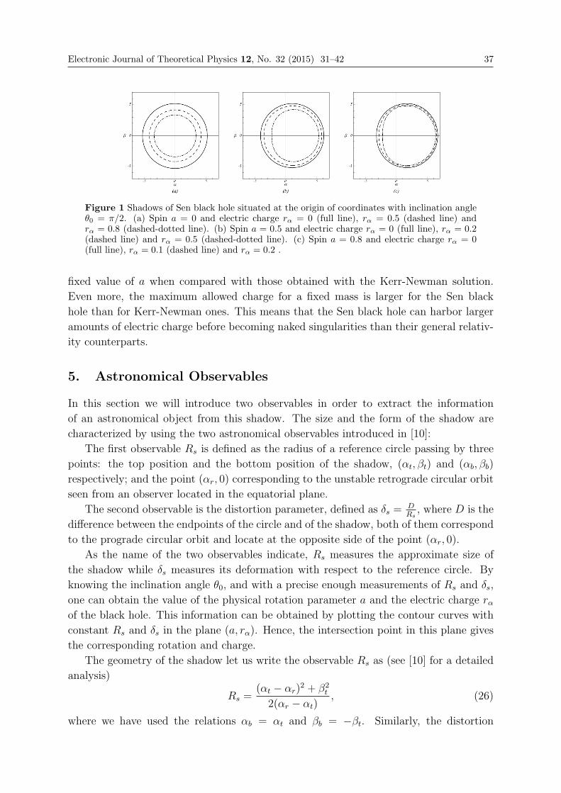
Electronic Journal of Theoretical Physics 12, No. 32 (2015) 31–42 37
Figure 1 Shadows of Sen black hole situated at the origin of coordinates with inclination angleθ0 = π/2. (a) Spin a = 0 and electric charge rα = 0 (full line), rα = 0.5 (dashed line) andrα = 0.8 (dashed-dotted line). (b) Spin a = 0.5 and electric charge rα = 0 (full line), rα = 0.2(dashed line) and rα = 0.5 (dashed-dotted line). (c) Spin a = 0.8 and electric charge rα = 0(full line), rα = 0.1 (dashed line) and rα = 0.2 .
fixed value of a when compared with those obtained with the Kerr-Newman solution.
Even more, the maximum allowed charge for a fixed mass is larger for the Sen black
hole than for Kerr-Newman ones. This means that the Sen black hole can harbor larger
amounts of electric charge before becoming naked singularities than their general relativ-
ity counterparts.
5. Astronomical Observables
In this section we will introduce two observables in order to extract the information
of an astronomical object from this shadow. The size and the form of the shadow are
characterized by using the two astronomical observables introduced in [10]:
The first observable Rs is defined as the radius of a reference circle passing by three
points: the top position and the bottom position of the shadow, (αt, βt) and (αb, βb)
respectively; and the point (αr, 0) corresponding to the unstable retrograde circular orbit
seen from an observer located in the equatorial plane.
The second observable is the distortion parameter, defined as δs =DRs, where D is the
difference between the endpoints of the circle and of the shadow, both of them correspond
to the prograde circular orbit and locate at the opposite side of the point (αr, 0).
As the name of the two observables indicate, Rs measures the approximate size of
the shadow while δs measures its deformation with respect to the reference circle. By
knowing the inclination angle θ0, and with a precise enough measurements of Rs and δs,
one can obtain the value of the physical rotation parameter a and the electric charge rαof the black hole. This information can be obtained by plotting the contour curves with
constant Rs and δs in the plane (a, rα). Hence, the intersection point in this plane gives
the corresponding rotation and charge.
The geometry of the shadow let us write the observable Rs as (see [10] for a detailed
analysis)
Rs =(αt − αr)
2 + β2t
2(αr − αt), (26)
where we have used the relations αb = αt and βb = −βt. Similarly, the distortion
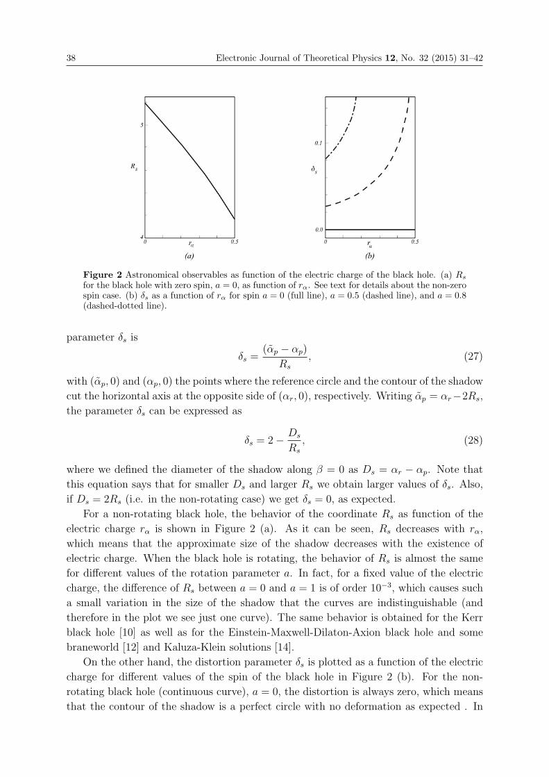
38 Electronic Journal of Theoretical Physics 12, No. 32 (2015) 31–42
Figure 2 Astronomical observables as function of the electric charge of the black hole. (a) Rs
for the black hole with zero spin, a = 0, as function of rα. See text for details about the non-zerospin case. (b) δs as a function of rα for spin a = 0 (full line), a = 0.5 (dashed line), and a = 0.8(dashed-dotted line).
parameter δs is
δs =(αp − αp)
Rs
, (27)
with (αp, 0) and (αp, 0) the points where the reference circle and the contour of the shadow
cut the horizontal axis at the opposite side of (αr, 0), respectively. Writing αp = αr−2Rs,
the parameter δs can be expressed as
δs = 2− Ds
Rs
, (28)
where we defined the diameter of the shadow along β = 0 as Ds = αr − αp. Note that
this equation says that for smaller Ds and larger Rs we obtain larger values of δs. Also,
if Ds = 2Rs (i.e. in the non-rotating case) we get δs = 0, as expected.
For a non-rotating black hole, the behavior of the coordinate Rs as function of the
electric charge rα is shown in Figure 2 (a). As it can be seen, Rs decreases with rα,
which means that the approximate size of the shadow decreases with the existence of
electric charge. When the black hole is rotating, the behavior of Rs is almost the same
for different values of the rotation parameter a. In fact, for a fixed value of the electric
charge, the difference of Rs between a = 0 and a = 1 is of order 10−3, which causes such
a small variation in the size of the shadow that the curves are indistinguishable (and
therefore in the plot we see just one curve). The same behavior is obtained for the Kerr
black hole [10] as well as for the Einstein-Maxwell-Dilaton-Axion black hole and some
braneworld [12] and Kaluza-Klein solutions [14].
On the other hand, the distortion parameter δs is plotted as a function of the electric
charge for different values of the spin of the black hole in Figure 2 (b). For the non-
rotating black hole (continuous curve), a = 0, the distortion is always zero, which means
that the contour of the shadow is a perfect circle with no deformation as expected . In
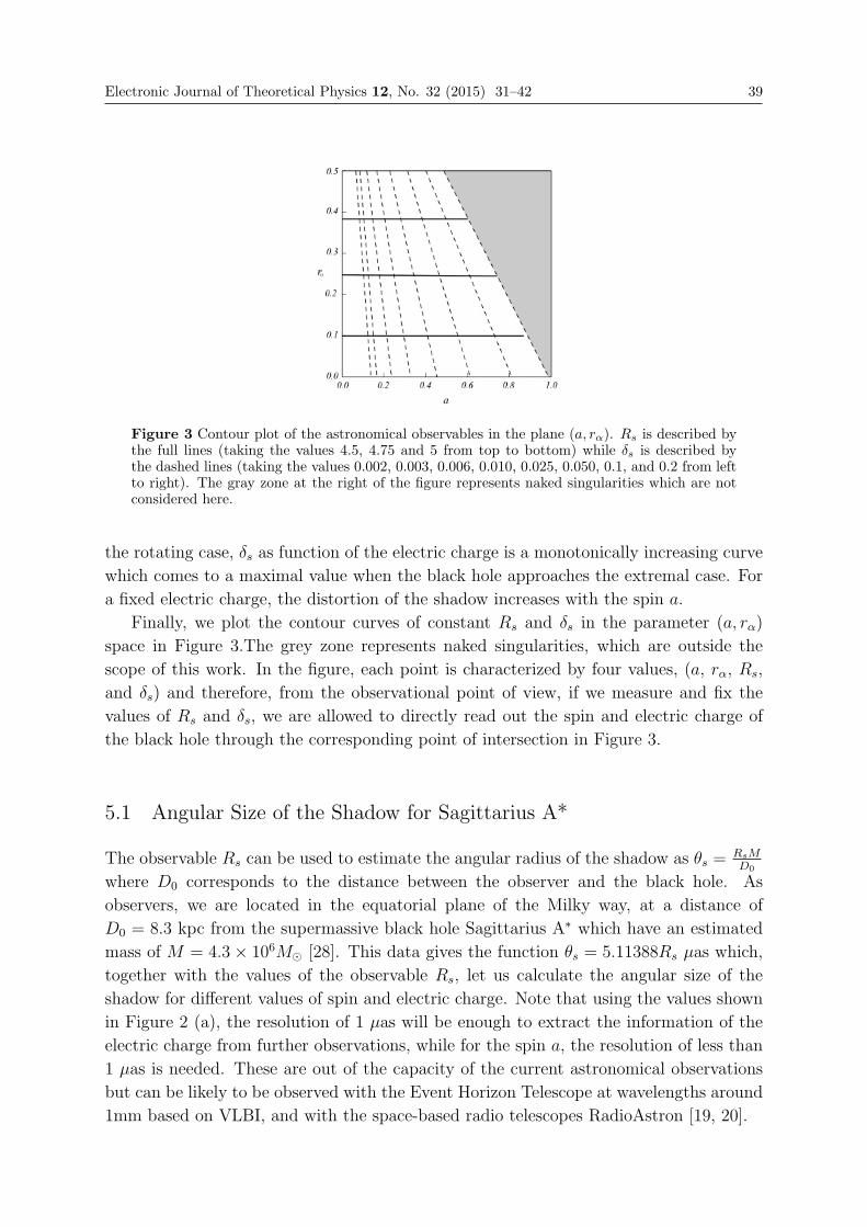
Electronic Journal of Theoretical Physics 12, No. 32 (2015) 31–42 39
Figure 3 Contour plot of the astronomical observables in the plane (a, rα). Rs is described bythe full lines (taking the values 4.5, 4.75 and 5 from top to bottom) while δs is described bythe dashed lines (taking the values 0.002, 0.003, 0.006, 0.010, 0.025, 0.050, 0.1, and 0.2 from leftto right). The gray zone at the right of the figure represents naked singularities which are notconsidered here.
the rotating case, δs as function of the electric charge is a monotonically increasing curve
which comes to a maximal value when the black hole approaches the extremal case. For
a fixed electric charge, the distortion of the shadow increases with the spin a.
Finally, we plot the contour curves of constant Rs and δs in the parameter (a, rα)
space in Figure 3.The grey zone represents naked singularities, which are outside the
scope of this work. In the figure, each point is characterized by four values, (a, rα, Rs,
and δs) and therefore, from the observational point of view, if we measure and fix the
values of Rs and δs, we are allowed to directly read out the spin and electric charge of
the black hole through the corresponding point of intersection in Figure 3.
5.1 Angular Size of the Shadow for Sagittarius A*
The observable Rs can be used to estimate the angular radius of the shadow as θs =RsMD0
where D0 corresponds to the distance between the observer and the black hole. As
observers, we are located in the equatorial plane of the Milky way, at a distance of
D0 = 8.3 kpc from the supermassive black hole Sagittarius A∗ which have an estimated
mass of M = 4.3× 10⁶M� [28]. This data gives the function θs = 5.11388Rs μas which,
together with the values of the observable Rs, let us calculate the angular size of the
shadow for different values of spin and electric charge. Note that using the values shown
in Figure 2 (a), the resolution of 1 μas will be enough to extract the information of the
electric charge from further observations, while for the spin a, the resolution of less than
1 μas is needed. These are out of the capacity of the current astronomical observations
but can be likely to be observed with the Event Horizon Telescope at wavelengths around
1mm based on VLBI, and with the space-based radio telescopes RadioAstron [19, 20].
40 Electronic Journal of Theoretical Physics 12, No. 32 (2015) 31–42
6. Conclusions
In this paper, we studied the size and shape of the shadow cast by a charged rotating
black hole from the low-energy effective field theory describing heterotic string theory,
which have properties which are qualitatively different from those that appear in Einstein
gravity. We have found that, for a fixed mass and rotation parameter, the presence of of
electric charge leads to a shadow that is slightly smaller and more deformed.
Supposing that the black hole is situated at the origin of the coordinate system and the
observer is located in the equatorial plane, we use the null geodesics to obtain the celestial
coordinates α and β in order to visualize the black hole’s shadow. To analyze the shadow
in detail, we define two astronomical observables: Rs that describes the approximate size
of the shadow and δs that measures its deformation. These quantities are functions of
the electric charge and the spin of the black hole. Our study shows that, for a fixed value
of the spin, the size of the shadow described by Rs decreases when increasing the electric
charge but its value is always smaller than that of the Kerr black hole. On the other hand,
the observable δs is a monotonically increasing function of the electric charge and takes
its maximal value for the extremal black hole. Also, for a fixed value of rα, an increase
in the value of the spin results in a greater distortion of the shadow. Finally, we plot the
contour curves of constant Rs and δs in the (a, rα) plane because careful measurements
of the astronomical observables allow to read out the spin and the electric charge of the
black hole from this figure.
It is expected that direct observation of the shadow of black holes will be possible
in the near future by using the very long baseline interferometer technique in (sub)
millimeter wavelengths [29, 30]. The Event Horizon Telescope will reach a resolution
of 15 μas at 345 GHz, while the RadioAstron mission will be capable to resolve1 − 10
μas and the Millimetron mission may provide a resolution of 0.3 μas or less at 0.4 mm.
Following our estimates for the angular size of the shadow, these instruments will be
capable of observing the shadow of the supermassive galactic black hole Sagittarius A*
to distinguish the presence of electric charge as described by the Sen black hole and
maybe to discriminate the string theory solution from the corresponding general relativity
counterpart.
Acknowledgements
This work was supported by the Universidad Nacional de Colombia. Hermes Project
Code 18140.
References
[1] J. Bardeen. Ecole d’ete de Physique Theorique, Les Houches, 1972, edited by C. DeWitt and B. S. De Witt, (Gordon and Breach Science Publishers, New York, 1973).
[2] S. Chandrasekhar, The Mathematical Theory of Black Holes, (Oxford UniversityPress, New York, 1992).
[3] H. Falcke, F. Melia, and E. Agol. Astrophys. J. 528, L13 (2000)
Electronic Journal of Theoretical Physics 12, No. 32 (2015) 31–42 41
[4] A. de Vries. Class. Quant. Grav. 17, 123 (2000).
[5] R. Takahashi. Astrophys. J. 611, 996 (2004)
[6] C. Bambi and K. Freese. Phys. Rev. D 79, 043002 (2009)
[7] C. Bambi and N. Yoshida. Class. Quant. Grav. 27, 205006 (2010)
[8] G. V. Kraniotis. Class. Quant. Grav. 28, 085021 (2011)
[9] A. F. Zakharov, A. A. Nucita, F. DePaolis, and G. Ingrosso. New Astron. Rev. 10,479 (2005)
[10] K. Hioki and K. I. Maeda. Phys. Rev. D 80, 024042 (2009)
[11] J. Schee and Z. Stuchlik. Int. J. Mod. Phys. D 18, 983 (2009)
[12] L. Amarilla and E. F. Eiroa. Phys. Rev. D 85, 064019 (2012)
[13] L. Amarilla, E. F. Eiroa, and G. Giribet. Phys. Rev. D 81, 124045 (2010)
[14] L. Amarilla and E. F. Eiroa. Phys. Rev. D 87, 044057 (2013)
[15] P. G. Nedkova, V. Tinchev, and S. S. Yazadjiev. [arXiv:1307.7647[gr-qc]]
[16] S.W. Wei and Y.X. Liu. JCAP 11, 063 (2013)
[17] V. K. Tinchev and S. S. Yazadjiev. [arXiv:1311.1353[gr-qc]]
[18] Z. Li and C. Bambi. JCAP 01, 041 (2014)
[19] http://www.eventhorizontelescope.org
[20] http://www.asc.rssi.ru/radioastron.
[21] A. Sen, Phys. Rev. Lett. 69, 1006 (1992)
[22] S. Yazadjiev, Gen. Relativ. Gravit. 32, 2345 (2000)
[23] G.W. Gibbons, Nucl. Phys. B 207, 337 (1982)
[24] G.W. Gibbons and K. Maeda. Nucl. Phys. B 298, 741 (1988);
[25] D. Garfinkle, G.T. Horowitz, and A. Strominger, Phys. Rev. D 43, 3140 (1991)
[26] D. Garfinkle, G.T. Horowitz, and A. Strominger, Phys. Rev. D 45, 3888(E) (1992)
[27] S. E. Vazquez and E. P. Esteban. Nuovo Cim. B 119, 489-519 (2004)
[28] S. Gillessen, F. Eisenhauer, S. Trippe, T. Alexander, R. Genzel, F. Martins, and T.Ott. Astrophys. J. 692, 1075 (2009)
[29] V. L. Fish and S. S. Doelman, in Proceedings of the International Astronomical Union,Symposium S261-2009. Cambridge University Press, Cambridge, England. Vol. 5 271-276 (2010)
[30] T. Johannsen, D. Psaltis, S. Gillesen, D. P. Marrone, F. Ozel, S. S. Doelman and V.L. Fish. Astrophys. J. 758, 30 (2012)

EJTP 12, No. 32 (2015) 43–60 Electronic Journal of Theoretical Physics
Scattering of Waves in the Phase Space, QuantumMechanics, and Irreversibility
E. M. Beniaminov∗†
Russian State University for the Humanities, Miusskaya sq. 6, Moscow, GSP-3,125993, Russia
Received 29 November 2014, Accepted 19 December 2014, Published 10 January 2015
Abstract: We give an example of a mathematical model describing quantum mechanical
processes interacting with medium. As a model, we consider the process of heat scattering
of a wave function defined on the phase space. We consider the case when the heat diffusion
takes place only with respect to momenta. We state and study the corresponding modified
Kramers equation for this process. We consider the consequent approximations to this equation
in powers of the quantity inverse to the medium resistance per unit of mass of the particle in
the process. The approximations are constructed similarly to statistical physics, where from
the usual Kramers equation for the evolution of probability density of the Brownian motion of
a particle in the phase space, one deduces an approximate description of this process by the
Fokker–Planck equation for the density of probability distribution in the configuration space. We
prove that the zero (invertible) approximation to our model with respect to the large parameter
of the medium resistance, yields the usual quantum mechanical description by the Schrodinger
equation with the standard Hamilton operator. We deduce the next approximation to the model
with respect to the negative power of the medium resistance coefficient. As a result we obtain
the modified Schrodinger equation taking into account dissipation of the process in the initial
model, and explaining the decoherence of the wave function.c© Electronic Journal of Theoretical Physics. All rights reserved.
Keywords: Quantum Mechanics; Kramers Equation; Waves in the Phase Space; Diffusion
Scattering; Asymptotic Solutions; Decoherence
PACS (2010): 03.65.-w; 03.65.Nk; 66.30.Ma; 03.65.Yz; 02.60.-x
1. Introduction
In this paper we continue the study of the generalized Kramers equation introduced in
the paper [1].
∗ Email: [email protected]† Tel:+79162231515
44 Electronic Journal of Theoretical Physics 12, No. 32 (2015) 43–60
In [1], the generalized Kramers equation arose as a mathematical model of the scat-
tering process of waves in the phase space under the action of medium in the heat equi-
librium. This process is irreversible. In [1] it has been shown that, for certain parameters
of the model, the process described by the generalized Kramers equation, is the compo-
sition of a rapid transitional process and a slow process. The slow process, as proved in
loc. cit., is approximately described by the Schrodinger equation used for description of
quantum processes. The obtained approximation of the slow process is reversible. Thus,
we have given an example of an irreversible process (heat scattering of waves in the phase
space), for which it has been shown that the standard reversible quantum mechanical
description of the motion of a particle arises as the asymptotic description of this process
in the zeroth approximation.
The purpose of the present paper is to construct an approximate equation describing
the slow part of the process given by the generalized Kramers equation, with the precision
showing dissipative effects in this process. As a result, we derive the modified Schrodinger
equation taking into account dissipation of the process.
The paper consists of four Sections and the Appendix.
In the next Section we present the setting of the problem, the generalized Kramers
equation for the heat scattering process of waves on the phase space, and the properties
of the operators involved in the generalized Kramers equation.
In Section 3 we recall our earlier results describing the process given by the generalized
Kramers equation. We also give a method for the approximate description of this process
in negative powers of the medium resistance coefficient, and state the main result of
the paper, Theorem 4. In this Theorem we write down an equation describing the slow
component of the studied process, taking into account dissipation. This equation is the
modified Schrodinger equation, in which the process is not invertible. We show that
consequences of the modified Schrodinger equation are the effects of decoherence and
spontaneous jumps between the levels.
In Section 4 we state some further possible directions of research and possibilities of
comparison of the presented model with experiment.
Proof of the main Theorem 4 of the paper is given in the Appendix.
2. Mathematical Setting of the Problem, and the Main Prop-
erties of the Operators in the Equation
Thus, we consider the following mathematical model of a process. A state of the process
at each moment of time t ∈ R is given by a complex valued function ϕ[x, p, t] on the phase
space (x, p) ∈ R2n, where n is the dimension of the configuration space. Coordinates in
the configuration space are given by a tuple of numbers x ∈ Rn, and momenta by a tuple
of numbers p ∈ Rn. (Below everywhere we will write the arguments of a function in the
square brackets, in order to distinguish an argument of a function from multiplication by
a variable.)
The generalized Kramers equation for a function ϕ[x, p, t] is defined as the following
Electronic Journal of Theoretical Physics 12, No. 32 (2015) 43–60 45
equation:∂ϕ
∂t= Aϕ+ γBϕ, (1)
where Aϕ =n∑
j=1
(∂V
∂xj
∂ϕ
∂pj− pj
m
∂ϕ
∂xj
)− i
�
(V −
n∑j=1
p2j2m
)ϕ (2)
and Bϕ =n∑
j=1
∂
∂pj
((pj + i�
∂
∂xj
)ϕ+ kBTm
∂ϕ
∂pj
);
m is the mass of the particle; V [x] is the potential function of external forces acting on
the particle; i is the imaginary unit; � is the Planck constant; γ = β/m is the medium
resistance coefficient β per unit of mass of the particle; kB is the Boltzmann constant; T
is the temperature of the medium.
If we pass in equation (1) to the following dimensionless variables:
p′ =p√
kBTm, x′ =
√kBTm
�x, V ′[x] =
V [x]
kBT, (3)
then in the new variables equation (1) takes the following form:
∂ϕ
∂t= A′ϕ+ γB′ϕ, (4)
where A′ϕ =kBT
�
( n∑j=1
(∂V ′
∂x′j
∂ϕ
∂p′j− p′j
∂ϕ
∂x′j
)− i
(V ′ −
n∑j=1
(p′j)2
2
)ϕ
)(5)
and B′ϕ =n∑
j=1
∂
∂p′j
((p′j + i
∂
∂x′j
)ϕ+
∂ϕ
∂p′j
).
Note that the operator A′ is skew Hermitian, and the operator B′ is neither skew
Hermitian neither self-adjoint. The operator B′ determines the scattering process of the
wave function with respect to momenta and hence non-invertibility of the process. In this
paper we consider the case when γ is a large quantity, i. e. the impact of the operator B′
on the general evolution process of the wave function is large. Properties of the operator
B′ are presented in the following Theorem.
Theorem 1. The operator B′ given by expression (5) has a full set of eigenfunc-
tions (in the class of functions ϕ[x, p] tending to zero at infinity) with the eigenvalues
0,−1,−2, . . . . Respectively, the operator B′ is presented in the following form:
B′ = −∞∑k=0
kPk, (6)
where Pk are the projection operators onto the eigenspaces of the operator B′ with eigen-
values −k.The projection operators Pk satisfy the relations
PkPk = Pk, PkPk′ = 0 for k �= k′, PkB′ = B′Pk = −kPk (7)
46 Electronic Journal of Theoretical Physics 12, No. 32 (2015) 43–60
and E =∞∑k=0
Pk, (8)
where E is the identity operator.
Proof of this Theorem will be given simultaneously with the proof of the following
Theorem describing the form of the projection operators Pk.
Denote by Hkk1...kn
[p]def= Hk1 [p1]...Hkn [pn] the product of Hermite polynomials [7]
of the corresponding variables, where k = k1 + ... + kn is the sum of degrees of the
Hermite polynomials in the product. By definition, the Hermite polynomial is given by
the expression
Hkj [pj]def= exp
(p2
2
)(− ∂
∂pj
)kj
exp
(−p2
2
). (9)
Let Sk1,...,kn and Ik1,...,kn be the operators given by the expressions
ψk1,...,kn = Sk1,...,kn [ϕ]def=
∫Rn
Hkk1...kn
[p′′ + i
∂
∂x′′
]ϕ[x′′, p′′]dp′′, (10)
ϕk1,...,kn = Ik1,...,kn [ψk1,...,kn ]def= (11)
1
(2π)3n/21
k1!...
1
kn!
∫R2n
ψk1,...,kn [x′′]Hk
k1...kn[p′ − s′]e−
(p′−s′)22 eis
′(x′−x′′)ds′dx′′.
Theorem 2. The projection operators Pk have the form
Pk =k∑
k1,...,kn=0
k1+...+kn=k
Ik1,...,knSk1,...,kn , (12)
and the operators Sk′1,...,k′n, Ik1,...,kn satisfy the relations
Sk′1,...,k′nIk1,...,knψk1,...,kn = δk′1,k1 ...δk′n,knψk1,...,kn , (13)
where δk′iki equals 0 if k′i �= ki, and equals 1 if k′i = ki.
In particular, formulas (10), (11) and Theorem 2 imply that
ψ[x′] = S0[ϕ]def=
∫Rn
ϕ[x′, p′]dp′, (14)
ϕ0[x′, p′] = I0[ψ]
def=
1
(2π)3n/2
∫R2n
ψ[x′′]e−(p′−s′)2
2 eis′(x′−x′′)ds′dx′′, (15)
P0ϕ =1
(2π)3n/2
∫R3n
ϕ[x′′, p′′]dp′′e−(p′−s′)2
2 eis′(x′−x′′)ds′dx′′, (16)
P1ϕ =n∑
j=1
1
(2π)3n/2
∫R3n
(p′′j + i
∂
∂x′′j
)ϕ[x′′, p′′]dp′′ ×
(p′j − s′j)e− (p′−s′)2
2 eis′(x′−x′′)ds′dx′′. (17)
Electronic Journal of Theoretical Physics 12, No. 32 (2015) 43–60 47
Note that the operators I0 and S0 given by formulas (15) and (14) make a bijection
between the set of functions ψ[x′] and the set of eigenfunctions ϕ0[x′, p′] of the operator
B′ with eigenvalue 0. We shall call the function ψ[x′] = S0[ϕ0[x′, p′]] by the presentation
of the eigenfunction ϕ0[x′, p′].
Proof of Theorems 1 and 2. Let us substitute into expression (5) the presentation
ϕ[x′, p′, t′] in the form of composition of the Fourier integral with respect to x′ and the
inverse Fourier transform:
ϕ[x′, p′, t′]=1
(2π)n/2
∫Rn
ϕ[s′, p′, t′]eis′x′ds′, (18)
where ϕ[s′, p′, t′]def=
1
(2π)n/2
∫Rn
ϕ[x′′, p′, t′]e−is′x′′
dx′′, (19)
and we denoted by s′x′ the expression s′x′def=
∑nj=1 s
′jx′j.
We obtain that the operator B′ has the form
B′[ϕ[x′′, p′]] =1
(2π)n
∫R2n
n∑j=1
∂
∂p′j
((p′j − s′j)ϕ+
∂ϕ
∂p′j
)eis
′(x′−x′′)ds′dx′′. (20)
Computing the integral over x′′ in the left hand side of the obtained expression, taking
into account equality (19), we obtain:
B′[ϕ[x′′, p′]] =1
(2π)n/2
∫Rn
n∑j=1
∂
∂p′j
((p′j − s′j)ϕ+
∂ϕ
∂p′j
)eis
′x′ds′. (21)
The operatorn∑
j=1
∂
∂p′j
((p′j − s′j)ϕ+
∂ϕ
∂p′j
), (22)
under the sign of integral in the previous expression, is well known (see, for example, [6]).
This operator has a full set of eigenfunctions in the space of functions tending to zero as
|p′ − s′| tends to infinity. The eigenvalues of this operator are the non-positive integers.
The eigenvalue 0 corresponds to eigenfunctions of the form
ϕ0[s′, p′] = ψ[s′]e−
(p′−s′)22 ,
where ψ[s′] is an arbitrary complex valued function of s′ ∈ Rn.
The remaining eigenfunctions are obtained (as it is easy to check) by differentiation
of the functions ϕ0[s′, p′] with respect to p′j, j = 1, . . . , n, and have the eigenvalues
equal respectively to −1,−2, . . ., depending on the degree of the derivative. Thus, the
eigenfunctions with eigenvalues −k = −(k1 + ...+ kn) are the functions of the form
ψk1...kn [s′](−1)k ∂k1
∂p′k11
. . .∂kn
∂p′knn
e−(p′−s′)2
2 = ψk1...kn [s′]Hk
k1...kn[p′ − s′]e−
(p′−s′)22 ,
where ψk1...kn [s′] are arbitrary complex valued functions of s′ ∈ Rn, and Hk
k1...kn[p′] =
Hk1 [p′1]...Hkn [p
′n] is the product of Hermite polynomials of the corresponding variables,
48 Electronic Journal of Theoretical Physics 12, No. 32 (2015) 43–60
and k = k1 + ...+ kn is the sum of degrees of the polynomials. The Hermite polynomials
of small degrees have the form
H0 = 1, H1[pj] = pj, H2[pj] = p2j − 1. (23)
Let us represent also the functions ψk1...kn [s′] in the form of Fourier integrals:
ψk1...kn [s′] =
1
(2π)n/2
∫Rn
ψk1...kn [x′′]e−is
′x′′dx′′.
From this formula, taking into account representation (18) of the function ϕ[x′, p′, t′]through ϕ[s′, p′, t′], we obtain that the eigenfunctions ϕk1...kn [x
′, p′] of the operator B′ havethe form (differing only by inessential constant factors from formula (11) of Theorem 1):
ϕk1...kn [x′, p′] =
1
(2π)n
∫R2n
ψk1...kn [x′′]Hk
k1...kn[p′ − s′]e−
(p′−s′)22 eis
′(x′−x′′)ds′dx′′.
It is known [7] that the Hermite polynomials form a complete system of functions and
satisfy the following orthogonality relations:
1
(2π)n/21
k1!...
1
kn!
∫Rn
Hk′k′1...k′n
[p′]Hkk1...kn
[p′]e−p′22 dp′ = δk′1k1 ...δk′nkn , (24)
where δk′iki are equal to 0 if k′i �= ki and equal to 1 if k′i = ki (in these formulas it is
assumed that 0!=1).
This directly implies the statements of Theorems 1 and 2. In particular, the latter
equality of Theorem 1 follows from completeness of the set of eigenspaces of the operator
B′.Note that in representation of the eigenfunctions of the operator B′ in the form (11)
one can compute the integral over s′. To this end, let us substitute into this formula the
expression defining the Hermite polynomials (9). We obtain
ϕk1,...,kn = Ik1,...,kn [ψk1,...,kn ]= (25)
1
(2π)3n/21
k1!...
1
kn!
(−1)k∂k
∂p′1k1 ...∂p′n
kn
∫R2n
ψk1,...,kn [x′′]e−
(p′−s′)22 eis
′(x′−x′′)ds′dx′′.
Further, let us make the change of variables s′ = s′′+ p′ under the integral, and compute
the integral over s′′, using the well known equality that the Fourier transform of the
function exp(−s′′2/2) is the function of the same form. We obtain
ϕk1,...,kn = Ik1,...,kn [ψk1,...,kn ]=
1
(2π)n1
k1!...
1
kn!
(−1)k∂k
∂p′1k1 ...∂p′n
kn
∫Rn
ψk1,...,kn [x′′]e−
(x′−x′′)22 eip
′(x′−x′′)dx′′ =
(−i)k(2π)n
1
k1!...
1
kn!
∫Rn
ψk1,...,kn [x′′]
n∏j=1
(x′ − x′′)kje−(x′−x′′)2
2 eip′(x′−x′′)dx′′. (26)
Electronic Journal of Theoretical Physics 12, No. 32 (2015) 43–60 49
The latter equality is obtained after differentiation with respect to p′ required in the
formula, but under the sign of the integral.
The latter equality, in the particular case of eigenfunctions of the operator B′ withthe zero eigenvalue, implies the following expression:
ϕ0 = I0[ψ0]=1
(2π)n
∫Rn
ψ0[x′′]e−
(x′−x′′)22 eip
′(x′−x′′)dx′′. (27)
3. The Schrodinger Equation for the Scattering Process of Waves
and its Refinement
In the papers [1, 3] the following Theorem has been proved.
Theorem 3. The motion described by equation (1) asymptotically splits for large γ
into rapid motion and slow motion.
1) After the rapid motion, an arbitrary wave function ϕ[x, p, 0] approximately goes at
the time of order 1/γ to the function ϕ0 = P0ϕ which, after normalization and in the
initial coordinates, has the following form:
ϕ0[x, p] =1
(2π�)n/2
∫Rn
ψ[y]χ[x− y]eip(x−y)/�dy, (28)
where ψ[x] =
(1
4πkBTm
)n/4∫Rn
ϕ[x, p, 0]dp and (29)
χ[x− y] =
(kBTm
π�2
)n/4
e−kBTm(x−y)2/(2�2). (30)
The wave functions of kind (28) form the linear subspace of eigenfunctions of the operator
B given by (2) with eigenvalue zero. The elements of this subspace are parameterized by
wave functions ψ[y, 0] =∫Rn ϕ[y, p]dp depending only on coordinates y ∈ Rn.
2) The slow motion starting at the moment t = 0 with the function ϕ0[x, p] of the form
(28) with nonzero function ψ[y] = ψ[y, t]|t=0, goes along the subspace of such functions
and is parameterized by the wave function ψ[y, t] depending on coordinates and time. The
function ψ[y, t] satisfies the following Schrodinger equation: i�∂ψ/∂t = Hψ, where the
action of the operator H for γ →∞ has the form
Hψ = − �2
2m
( n∑k=1
∂2ψ
∂y2k
)+ V [y]ψ − kBT
2nψ +O(γ−1). (31)
The coefficient in formula (30) is chosen so that the mapping given by formula (28)
preserves the standard scalar product in the Hilbert spaces of functions ψ and ϕ0.
Proof of the first part of Theorem 3 is given in [3]. Proof of the second part of this
Theorem is given in [1]. (This formula will be also obtained in the Appendix to the
present paper in the course of proof of Theorem 4.)
Theorem 3 describes a solution of equation (1) and respectively of equation (4) in the
zero deterministic approximation in the parameter 1/γ after the transitional process in
50 Electronic Journal of Theoretical Physics 12, No. 32 (2015) 43–60
time of order 1/γ. The purpose of the present paper is proof of a Theorem refining the
result of the part of Theorem 3 describing the slow motion. To this end, we construct
the next approximation of equation (4) with respect to the parameter 1/γ.
Thus, let us pass to approximate description of the generalized Kramers equation (4)
for large γ by means of systematic decomposition over powers of γ−1. The method used
here is similar to the method given in the book by van Kampen [5]. In this book, from the
Kramers equation describing the Brownian motion of a particle in the phase space, one
deduces the Fokker–Planck equation describing approximately the same process, but in
the form of the Brownian motion of the particle in configuration space after certain time
of transitional process. During this process the distribution with respect to momenta
becomes the Maxwell distribution.
Let us rewrite equation (4) in the following form:
B′ϕ =1
γ
(∂ϕ
∂t− A′ϕ
). (32)
Let us look for solution of this equation in the form
ϕ = ϕ0 + γ−1ϕ1 + γ−2ϕ2 + ... (33)
Let us substitute expression (33) into equation (32), and write out the equations for
coefficients before equal powers of γ−1. We obtain:
for γ0 : B′ϕ0 = 0; (34)
for γ−1 : B′ϕ1 =∂ϕ0
∂t− A′ϕ0; (35)
for γ−2 : B′ϕ2 =∂ϕ1
∂t− A′ϕ1; . . . . (36)
Equation (34) implies that ϕ0 belongs to the subspace of eigenfunctions of the operator
B′ with eigenvalue 0, i. e. ϕ0 = P0ϕ0, where P0 is the projection operator onto the
eigenspace of the operator B′ with eigenvalue 0.
Let us apply to both parts of equality (35) the projection operator P0 from the left.
Taking into account equalities P0B′ = 0 and ϕ0 = P0ϕ0, we obtain:
0 =∂ϕ0
∂t− P0A
′P0ϕ0, so∂ϕ0
∂t= P0A
′P0ϕ0. (37)
(Note that the operator P0A′P0 corresponds to the Schrodinger operator H ′ in Theo-
rem 3.)
Provided equality (37) holds, equation (35) has a solution which we represent in the
form
ϕ1 = ϕ1,0 + f1, where P0f1 = 0, ϕ1,0 = P0ϕ1 = P0ϕ1,0,
f1 = B′−1(P0A
′P0ϕ0 − A′P0ϕ0), (38)
and B′−1 is the inverse operator to B′ on the subspace spanned by eigenfunctions of the
operator B′ with nonzero eigenvalues. Formula (6) for B′ implies that the operator B′−1
Electronic Journal of Theoretical Physics 12, No. 32 (2015) 43–60 51
has the form
B′−1 = −
∞∑k=1
k−1Pk. (39)
This and the properties (7) of projection operators imply that P0B′−1 = 0 and PkB
′−1 =−k−1Pk.
By the equality B′−1P0 = 0 the expression for f1 in formula (38) takes the form
f1 = −B′−1A′P0ϕ0. (40)
Let us substitute the expression ϕ1 = ϕ1,0 + f1 from formula (38) into equality (36), and
apply to both parts of equality (36) the projection operator P0 from the left. Using the
equalities P0B′ = 0, P0f1 = 0, and ϕ1,0 = P0ϕ1,0, and equality (40), after the substitutions
mentioned above and opening the brackets we obtain:
0 = P0
(∂ϕ1
∂t− A′ϕ1
)or
0 =∂ϕ1,0
∂t− P0A
′P0ϕ1,0 + P0A′B
′−1A′P0ϕ0. (41)
Let us now sum up equations (37) and (41) multiplied respectively by 1 and γ−1. Then
for the function ϕ≤1,0, defined by the equality
ϕ≤1,0def= ϕ0 + γ−1ϕ1,0, (42)
we obtain the following equation up to summands of order γ−1:
0=∂ϕ≤1,0∂t
− P0A′P0ϕ≤1,0 + γ−1P0A
′B′−1A′P0ϕ≤1,0 +O[γ−2]. (43)
Respectively, for function ϕ≤1def= ϕ0 + γ−1ϕ1, which takes into account only first two
summands in the decomposition (33) for ϕ, using the equality ϕ1 = ϕ1,0+f1 in expression
(38) and substituting into it expression (40) for f1, we obtain the following equality up
to summands of order γ−1:
ϕ≤1 = ϕ≤1,0 − γ−1B′−1A′P0ϕ≤1,0 +O[γ−2]. (44)
Since ϕ≤1,0 = P0ϕ≤1,0, that is, ϕ≤1,0 is an eigenfunction of the operator B′ witheigenvalue 0, then, in accordance with formulas (14) and (15) and Theorem 2, this function
is completely determined by the function ψdef= S0[ϕ≤1,0] by the formula ϕ≤1,0 = I0[ψ],
where S0 and I0 are the operators defined by formulas (14) and (15). As above, let us
call the function ψ by the presentation of the eigenfunction ϕ≤1,0.In order to obtain the ψ-presentation of equation (43), let us substitute into it, instead
of function ϕ≤1,0 the equal expression I0[ψ], let us act on both parts of equation by the
operator S0, and let us use the following equalities deduced from relations of Theorem 2:
P0ϕ≤1,0 = I0S0[ϕ≤1,0] = I0[ψ], S0P0 = S0, and ψ = S0I0[ψ].
52 Electronic Journal of Theoretical Physics 12, No. 32 (2015) 43–60
We obtain:
0 =∂ψ
∂t− S0A
′I0ψ + γ−1S0A′B
′−1A′I0ψ +O[γ−2]. (45)
Respectively, expression (44) for function ϕ≤1[x′, p′], presented through the function
ψ[x′], without account of summands of order γ−2, reads
ϕ≤1 = I0[ψ]− γ−1B′−1A′I0[ψ] +O[γ−2]. (46)
Note that this equality implies S0ϕ≤1 = ψ. Thus, expression (46) and the operator
S0 yield mutually inverse bijections between the set of functions ϕγ1[x′, p′] and the set of
functions ψ[x′]. Thus, function ψ[x′] is also a presentation of the function ϕ≤1[x′, p′] byformula (46). And the function ψ[x′] evolves in time according to equation (45).
Thus, from equation (45) and relation P0 = I0S0 of Theorem 2 we obtain the following
approximate equation, with account of summands up to order γ−1, for the slow subprocess
in the process described by the modified Kramers equation (4):
∂ψ
∂t= S0A
′I0ψ − γ−1S0A′B
′−1A′I0ψ +O[γ−2]. (47)
(The form of the first summand in the right hand side of the equation, namely, the
operator S0A′I0, is known to us from Theorem 3.) The complete description of the right
hand side of this equation is given by the following Theorem.
Theorem 4. The slow motion mentioned in Theorem 3, starting from the wave
function ϕ0[x, p] of the form (28) with nonzero function ψ[y, 0], and parameterized by the
wave function ψ[y, t], satisfies the modified Schrodinger equation of the form i�∂ψ/∂t =
H1ψ, where action of the operator H1 is the following:
H1ψ=− �2
2m
n∑k=1
∂2ψ
∂y2k+ V ψ − kBTn
2ψ +
iγ−1
4
( n∑j=1
�
m
∂2V
∂y2j− (kBT )
2n
�
)ψ +
+O[γ−2]. (48)
Proof of Theorem 4 is given in the Appendix.
Since for description of behavior of the system, only the differences between the
eigenvalues of the operator are essential, the constant summands in operators H and
H1 of Theorems 3 and 4 can be neglected.
Using the standard method of perturbation theory [9], let us compute the corrections
to the eigenvalues and eigenfunctions of the Hamilton operator for the operator H1.
Let E(0)n be the eigenvalues of the Hamilton operator H, and ψ
(0)n be the corresponding
eigenfunctions. Let En and ψn be the eigenvalues and eigenfunctions of the operator
H1. Then by definition of eigenfunctions, one has the equalities Hψ(0)n = E
(0)n ψ
(0)n and
H1ψn = Enψn. Let us look for En and ψn in the form
En = E(0)n + γ−1E(1)
n +O(γ−2) (49)
ψn = ψ(0)n + γ−1
∑k
k =n
cnkψ(0)k +O(γ−2). (50)
Electronic Journal of Theoretical Physics 12, No. 32 (2015) 43–60 53
Let us substitute these expressions into equality (48). In the obtained expression, let us
equate coefficients before the corresponding powers of γ−1, and take the scalar products
of both parts of the obtained equalities with ψ(0)n or ψ
(0)k . Using the orthonormality of
the system of eigenfunctions ψ(0)k with respect to the scalar product 〈 ; 〉 given by
〈ψk;ψm〉 =∫Rn
ψk[y]ψ∗m[y]dy, (51)
we obtain:
E(1)n =
i�
4m〈Δ2V ψ(0)
n ;ψ(0)n 〉 (52)
cnk =i�
4m
〈Δ2V ψ(0)n ;ψ
(0)k 〉
E(0)n − E
(0)k
, (53)
where Δ2V =n∑
k=1
∂2V
∂y2k. (54)
These equalities and the modified Schrodinger equation i�∂ψ/∂t = H1ψ imply that the
eigenfunction ψn evolves in time according to the following expression:
ψn[t] = ψn[0] exp
(− iEnt
�
)= ψn[0] exp
(− iE
(0)n t
�− iγ−1E(1)
n t
�
),
where − iγ−1E(1)n
�=
γ−1
4m〈Δ2V ψ(0)
n ;ψ(0)n 〉 is real.
Therefore, the absolute value of the eigenfunction ψn changes in time exponentially with
the exponent (γ−1/4m)〈Δ2V ψ(0)n ;ψ
(0)n 〉t. Thus, if the system at the initial moment of time
is in the state ψ[0], where ψ[0] =∑∞
n anψn is a certain superposition of eigenstates of
the operator H1, then after the time t the system will be in the state ψ[t]/|ψ[t]|, whereψ[t] =
∑∞n anψn[t]. Since the absolute values of the eigenstates ψn[t] change exponentially
with different velocities, then after large enough time the state ψ[t]/|ψ[t]| will be close tocertain eigenstate ψk, for which the value −iE(1)
k is maximal among the values −iE(1)n for
n with nonzero an in the sum∑∞
n anψn. This phenomenon has been called decoherence
and has been studied in a series of papers [10, 11, 12]. The time of decoherence in our
model can be estimated as the time t for which akexp(−iE(1)k t/�) >> ak1 exp(−iE
(1)k1
t/�),
where −iE(1)k1
is the next value after the maximal value −iE(1)k among the numbers −iE(1)
n
for n with nonzero an in the sum∑∞
n anψn.
Besides that, formulas (50) and (53) imply that the eigenfunctions ψn of the operator
H1 are in general case not orthogonal to each other. We have:
〈ψn;ψk〉 = γ−1(cnk + c∗kn) +O[γ−2] = 2γ−1cnk +O[γ−2].
Let ϕn[x, p] and ϕk[x, p] be wave functions on the phase space corresponding to func-
tions ψn and ψk by formula (46). According to the assumptions of the model, the square
of the absolute value of the scalar product of normalized functions ϕn[x, p] and ϕk[x, p]
yields the probability to find the system in the state ψk, if it is in the state ψn. The latter
equality and formula (46) imply that this probability is nonzero if cnk �= 0.
54 Electronic Journal of Theoretical Physics 12, No. 32 (2015) 43–60
4. Conclusion
In this paper we have constructed an approximate description of the slow phase of the
scattering process of the wave function up to γ−1, where γ is the resistance of the medium
per unit of mass of a particle–wave. The obtained approximation is described by the
Schrodinger equation, supplemented with a summand with coefficient γ−1. In this ap-
proximation one has effects of decoherence and spontaneous jumps from one level to
another.
Note that for a free particle, when V = 0, and for harmonic oscillator, when the
second derivatives of the potential are constant, the summand of the operator H1 with
the factor γ−1 in Theorem 4 is a constant. Therefore, in the approximation up to γ−1,due to this summand, in these cases all wave functions decrease in amplitude with the
same velocity, and dissipation is non-observable. Hence, to take into account dissipation
in this model either for free particle or for harmonic oscillator, one should consider the
summands with factors γ−2 and γ−3. Note also that the method of construction of the γ−1
summand in the modified Schrodinger equation used in this paper, allows, in principle,
to construct also the summands with factors γ−2 and γ−3.The next phenomenon which can appear in this model, is the occurrence of nonzero
width of spectral lines. The interaction of a quantum particle with medium should
cause occurrence of width of energy levels for the energy operator. That is, if ψj is
an eigenfunction of the Hamilton operator with eigenvalue Ej, then the corresponding
wave function ϕj[x′, p′] in the phase space is given by the formula (46). According to the
assumption of the model, the function ϕj[x′, p′] defines the density function of probability
distribution in the phase space in the form ϕj[x′, p′]ϕ∗j [x
′, p′]. Respectively, the average
value of the energy function H[x′, p′] in this case is given by the following expression:
Ej =
∫R2n
H[x′, p′]ϕj[x′, p′]ϕ∗j [x
′, p′]dx′dp′. (55)
Then (ΔEj)2, the average of square of deviation from the average energy, is computed
by the formula
(ΔEj)2 =
∫R2n
(H[x′, p′]− Ej)2ϕj[x
′, p′]ϕ∗j [x′, p′]dx′dp′. (56)
These computations can be completed for concrete quantum systems, to obtain the
dependence of ΔEj on T and γ. After that, the obtained data can be compared with the
experimental data on the width of spectral lines.
Other directions of research on this subject can be found in [13].
Appendix. Proof of Theorem 4
To prove Theorem 4 one should compute the right hand side of equation (47), and pass
to the initial coordinates.
Electronic Journal of Theoretical Physics 12, No. 32 (2015) 43–60 55
The first summand in the right hand side of this equation reads as follows:
S0A′I0ψ = −ikBT
�
(−1
2
n∑j=1
∂2
∂(x′j)2+ V ′ − n
2
)ψ.
We are going to compute the operator S0A′B
′−1A′I0 which stands in equation (47) with
the factor γ−1.Let us first transform this expression using the equality
B′−1 = −
∞∑k=1
k−1Pk
obtained above (39), the relations Pk =∑
k1+...+kn=k Ik1,...,knSk1,...,kn from Theorem 2, and
PkP0 = 0 for k > 0 .
We obtain:
S0A′B
′−1A′I0 =−∞∑k=1
k−1S0A′PkA
′I0 =−∞∑
k1,...,kn=0
k1+...+kn=k≥1
k−1S0A′Ik1,...,knSk1,...,knA
′I0. (57)
Let us now compute the operator A′Ik1,...,kn , where the operator A′ is given by expres-
sion (5), and the operator Ik1,...,kn is defined by expression (11).
We have
A′Ik1,...,knψ=kBT
�
( n∑j=1
(∂V ′
∂x′j
∂
∂p′j− p′j
∂
∂x′j
)− i
(V ′ −
n∑j=1
p′2j
2
))◦ (58)
1
(2π)3n/21
k1!...
1
kn!
∫R2n
ψ[x′′]Hkk1...kn
[p′ − s′]e−(p′−s′)2
2 eis′(x′−x′′)ds′dx′′.
Let us put the summands of the operator A′ in this expression under the sign of
integral, and let us decompose the functions of (p′ − s′) under the sign of integral over
Hermite polynomials H ll1...ln
[p′ − s′]. Using the equalities
∂
∂p′j
(Hk
k1...kn[p′ − s′]e−
(p′−s′)22
)def= −Hk+1
k1...kj+1...kn[p′ − s′]e−
(p′−s′)22 , (59)
∂
∂x′jeis
′(x′−x′′) = is′jeis′(x′−x′′), (60)
p′2j = ((p′j − s′j)
2 − 1) + 2p′js′j − s
′2j + 1 = H2[p
′j − s′j] + 2p′js
′j − s
′2j + 1, (61)
we obtain:
A′Ik1,...,knψ=kBT
�
1
(2π)3n/21
k1!...
1
kn!
∫R2n
(−
n∑j=1
∂V ′
∂x′jHk+1
k1...kj+1...kn[p′ − s′]
−in∑
j=1
p′js′jH
kk1...kn
[p′ − s′]− iV ′[x′]Hkk1...kn
[p′ − s′]
+i
2
n∑j=1
(H2[p′j − s′j] + 2p′js
′j − s
′2j + 1)Hk
k1...kn[p′ − s′]
)×ψ[x′′]e−
(p′−s′)22 eis
′(x′−x′′)ds′dx′′. (62)
56 Electronic Journal of Theoretical Physics 12, No. 32 (2015) 43–60
After opening the brackets in the latter summand and summing up the terms similar to
the second summand, we obtain:
A′Ik1,...,knψ=kBT
�
1
(2π)3n/21
k1!...
1
kn!
∫R2n
(−
n∑j=1
∂V ′
∂x′jHk+1
k1...kj+1...kn[p′ − s′]
−iV ′[x′]Hkk1...kn
[p′ − s′]+i
2
n∑j=1
H2[p′j − s′j]H
kk1...kn
[p′ − s′]
− i
2
n∑j=1
(s′2j − 1)Hk
k1...kn[p′ − s′]
)ψ[x′′]e−
(p′−s′)22 eis
′(x′−x′′)ds′dx′′. (63)
Lemma 1. The operators S0A′Ik1,...,kn read as follows:
S0A′I0[ψ] =
kBT
�
(−iV ′ψ +
i
2
n∑j=1
∂2ψ
∂x′2j
+in
2ψ
); (64)
S0A′Ik1,...,kn [ψ] =
i
2
kBT
�ψ, when k = k1 + ...+ kn = 2
and only one of k1, ..., kn equals 2; (65)
In the remaining cases S0A′Ik1,...,kn = 0.
Proof. According to formula (14) the operator S0 is an integration over p. Hence for
proof of the formulas of Lemma 1 one should compute integral over p of expression (63)
for the operator A′Ik1,...,kn . To this end, let us use the orthogonality formula (24) for
Hermite polynomials and the fact that H00 = 1. This implies that integral over p of the
first summand of expression (63) equals 0. Integral of Hkk1...kn
[p′−s′] in the second and the
fourth summand with respect to 1/(2π)(n/2) exp[−(p′ − s′)2/2]dp equals 1 only for k = 0,
and in the other cases also equals 0. Integral of H2[p′j − s′j]H
kk1...kn
[p′ − s′] in the third
summand with respect to 1/(2π)(n/2) exp[−(p′−s′)2/2]dp differs from 0 and equals 2 only
when k = 2, kj = 2, and the rest of k1, ..., kn equal 0. Then in the obtained expression we
compute integrals over s′ and x′′, using the fact that integral of 1/(2π)neis′(x′−x′′) over s′
is the delta function at the point x′, and integral of expression 1/(2π)ns′2eis′(x′−x′′) over
s′ is the delta function at the point x′ with −∂2/∂x′′2. As a result of these computations
we get the statement of Lemma 1.
Since by Lemma 1 the operators S0A′Ik1,...,kn with k = k1 + ... + kn > 0 are not
equal to 0 only when k = 2, kj = 2 (and therefore the remaining k1, ..., kn equal 0), then
for computation of operator S0A′B
′−1A′I0 by formula (57) it remains to compute the
operators Sk1,...,knA′I0 for the same values of k1, ..., kn.
Lemma 2. The operators Sk1,...,knA′I0, in the case when kj = 2 and k1 + ...+ kn = 2,
read as follows:
Sk1,...,knA′I0[ψ] =
kBT
�
(−i∂
2V ′
∂x′2j
ψ + iψ
). (66)
Electronic Journal of Theoretical Physics 12, No. 32 (2015) 43–60 57
Proof. Under the conditions of Lemma 2, when k = kj = 2, the operator Sk1,...,kn
reads, by formula (10), as follows:
Sk1,...,kn [ϕ]def=
∫Rn
Hkk1...kn
[p′ + i
∂
∂x′
]ϕ[x′, p′]dp′
=
∫Rn
H2
(p′j + i
∂
∂x′j
)ϕ[x′, p′]dp′. (67)
This and formula (63) for A′I0 imply that
Sk1,...,knA′I0[ψ]=
kBT
�
1
(2π)3n/2
∫R3n
H2
(p′j + i
∂
∂x′j
)◦
◦(−
n∑j′=1
∂V ′[x′]∂x′j′
H1[p′j′ − s′j′ ]− iV ′[x′]+
i
2
n∑j′=1
H2[p′j′ − s′j′ ]
− i
2
n∑j′=1
(s′2j′ − 1)
)ψ[x′′]e−
(p′−s′)22 eis
′(x′−x′′)ds′dx′′dp′. (68)
Taking into account that by definition of Hermite polynomials we have
H2
(p′j + i
∂
∂x′j
)=
((p′j + i
∂
∂x′j
)2
− 1
),
and by the equality i∂
∂x′jeis
′(x′−x′′) = −s′jeis′(x′−x′′), we obtain:
Sk1,...,knA′I0[ψ]=
kBT
�
1
(2π)3n/2
∫R3n
H2
(p′j − s′j
)×
(−
n∑j′=1
∂V ′[x′]∂x′j′
H1[p′j′ − s′j′ ]− iV ′[x′]+
i
2
n∑j′=1
H2[p′j′ − s′j′ ]
− i
2
n∑j′=1
(s′2j′ − 1)
)ψ[x′′]e−
(p′−s′)22 eis
′(x′−x′′)ds′dx′′dp′ (69)
+kBT
�
1
(2π)3n/2
∫R3n
(−2i(p′j − s′j)
n∑j′=1
∂2V ′[x′]∂x′j∂x
′j′H1[p
′j′ − s′j′ ]
+n∑
j′=1
∂3V ′[x′]∂2x′j∂x
′j′H1[p
′j′ − s′j′ ] + 2(p′j − s′j)
∂V ′[x′]∂x′j
+ i∂2V ′[x′]
∂x′j2
)×ψ[x′′]e−
(p′−s′)22 eis
′(x′−x′′)ds′dx′′dp′. (70)
Further, let us integrate over p′ in each integral in the obtained expression, using the
orthogonality relation (24) for Hermite polynomials and the equalities 1 = H0(p′j − s′j)
58 Electronic Journal of Theoretical Physics 12, No. 32 (2015) 43–60
and (p′j − s′j) = H1(p′j − s′j). We obtain:
Sk1,...,knA′I0[ψ] =
kBT
�
1
(2π)n
∫R2n
(−0− 0 +
i
22− 0
)ψ[x′′]eis
′(x′−x′′)ds′dx′′
+kBT
�
1
(2π)n
∫R2n
(−2i∂
2V ′[x′]
∂x′j2 + 0 + 0 + i
∂2V ′[x′]
∂x′j2
)ψ[x′′]eis
′(x′−x′′)ds′dx′′. (71)
After computing the integrals over s′ and x′′ in the obtained expression and summing
up similar terms, we obtain the equality required in Lemma 2:
Sk1,...,knA′I0[ψ] =
kBT
�
(−i∂
2V ′[x′]∂x
′2j
ψ[x′] + iψ[x′]). (72)
Now we are ready to compute S0A′B
′−1A′I0 using Lemmas 1 and 2, by formula (57).
By Lemma 1 the summands in formula (57) can be nonzero only if kj = 2 for some
j ∈ {1, ..., n}, and the rest of k1, ..., kn equal 0. Lemmas 1 and 2 yield expressions for
operators S0A′Ik1,...,kn and Sk1,...,knA
′I0 in this case. So, by formula (57) and Lemmas 1, 2
we have:
S0A′B
′−1A′I0[ψ] = −∞∑
k1,...,kn=0
k1+...+kn=k≥1
k−1S0A′Ik1,...,knSk1,...,knA
′I0[ψ]
= −∑
k1,...,kn∈{0;2}k1+...+kn=2
2−1S0A′Ik1,...,knSk1,...,knA
′I0[ψ]
= −n∑
j=1
2−1i
2
kBT
�
kBT
�
(−i∂
2V ′
∂x′2j
ψ + iψ
)
= −1
4
(kBT
�
)2( n∑j=1
∂2V ′
∂x′2j
ψ − nψ
). (73)
If in this expression we return to the initial coordinates by formula (3), then we obtain
the equality
S0A′B
′−1A′I0)[ψ] = −1
4
(1
m
n∑j=1
∂2V
∂x2j
−(kBT
�
)2
n
)ψ. (74)
Thus, we have computed the operator in the second summand in equation (47). This
operator gives, after multiplying by −ihγ−1, the second summand in the operator H1
from Theorem 4.
Acknowledgments. The author is thankful to Professor G. L. Litvinov for support
of the work in this direction, and mourns for loss of this wonderful person and friend.
References
[1] Beniaminov E.M. Quantum Mechanics as Asymptotics of Solutions of GeneralizedKramers Equation.
Electronic Journal of Theoretical Physics 12, No. 32 (2015) 43–60 59
Electronic Journal of Theoretical Physics (EJTP) 8, No. 25 195-210 (2011).http://www.ejtp.com/articles/ejtpv8i25p195.pdf
[2] Beniaminov E. M. Diffusion processes in phase spaces and quantum mechanics.Doklady Mathematics (Proceedings of the Russian Academy of Sciences), 2007,vol.76, No. 2, 771–774.
[3] Beniaminov E. M. Quantization as asymptotics of a diffusion process in the phasespace. Proc. Intern. Geom. Center 2(4), 7-50 (2009).http://arxiv.org/abs/0812.5116v1
[4] Kramers H. A. Brownian motion in a field of force and the diffusion model of chemicalreactions. Physica. 7, 284–304. (1940)
[5] Van Kampen N.G. Stochastic Processes in Physics and Chemistry, North Holland,Amsterdam, 1981.
[6] Kamke E., Differentialgleichungen: Losungsmethoden und Losungen, I, GewohnlicheDifferentialgleichungen, B. G. Teubner, Leipzig, 1977.
[7] Weisstein Eric W. Hermite Polynomial From MathWorld — A Wolfram WebResource.http://mathworld.wolfram.com/HermitePolynomial.html
[8] Beniaminov E.M. A Method for Justification of the View of Observables in QuantumMechanics and Probability Distributions in Phase Space. http://arxiv.org/abs/quant-ph/0106112 (2001).
[9] Landau L. D., Lifschitz E. M., Quantum mechanics (non-relativistic theory).Theoretical physics, vol. 3, Nauka, Moscow, 1989 (in Russian).
[10] Zeh H.D. Roots and Fruits of Decoherence. In: Quantum Decoherence, Duplantier, B.,Raimond, J.-M., and Rivasseau, V., eds. (Birkhauser, 2006), p. 151-175 (arXiv:quant-ph/0512078v2).
[11] Zurek W. H. Decoherence and the transition from quantum to classical - revisited.arXiv:quant-ph/0306072v1, 2003. (An updated version of Physics Today, 44:36-44(1991).)
[12] Menskij M. B. Dissipation and decoherence of quantum systems. Physics-Uspekhi(Advances in Physical Sciences), 2003, vol.173, 1199-1219.
[13] Beniaminov E.M. Diffusion Scattering of Waves is a Model of Subquantum Level.Electronic Journal of Theoretical Physics(EJTP) 11, No. 30, 35–48 (2014)http://www.ejtp.com/articles/ejtpv11i30p35.pdf.

EJTP 12, No. 32 (2015) 61–68 Electronic Journal of Theoretical Physics
Frequency Distribution of Spontaneous Emission
Saul. M. Bergmann∗†
Potomac, Maryland USA
Received 13 October 2014, Accepted 20 December 2014, Published 15 September 2014
Abstract: A two-level system, originally in the excited state, is irradiated by an incident beam
whose frequency bandwidth is narrow compared with the natural linewidth. A generalised
Weisskopf-Wigner treatment is developed by means of which the probability distribution of the
frequency of spontaneous emission is found. It is shown under which circumstances the beam
can influence this probability distribution. A broadening of the natural line occurs.c© Electronic Journal of Theoretical Physics. All rights reserved.
Keywords: Quantum Mechanics, Fock Space; Weisskopf-Wigner Treatment; Spontaneous
Emission Spectrum; Induced Emission
PACS (2010): 03.65.-w; 03.67.a; 03.67.Bg; 42.50.Ct; 32.30.-r; 32.50.+d
1. Introduction
In ordinary perturbation theory, for a two-level system irradiated by a feeble incident
beam, the probability of induced emission and spontaneous emission, as a first order
process is being made to be proportional to n + 1, where n is the number of photons
in the incident Fock state, and “1” is regarded as an immutable contribution of spon-
taneous emission. What is striking in this result is that no matter how high n may be,
(for the range of validity of this perturbation method), the beam has no influence on the
probability of spontaneous emission. The drawback of perturbation theory, historically
speaking, has been its inability to describe neither the natural line shape nor the expo-
nential decay of a two-level system. Weisskopf and Wigner remedied this situation and
were able to describe both features by using a non-perturbational method. In retrospect,
their task may be viewed as an “exercise”, since they knew what the final result should
be. However, they treated only spontaneous emission. Since then, it has been tempting
to generalize their first-order treatment to the case of the presence of an incident beam.
∗ Email:[email protected]† Tel:3013401655
62 Electronic Journal of Theoretical Physics 12, No. 32 (2015) 61–68
2. Equations in Interaction Representation
The subject of interest is a two-level atomic system having an excited state |e〉 and a
ground state |g〉. One assumes that the system is originally in the excited state and is
irradiated by an incident beam whose frequency bandwidth is narrow compared with the
natural linewidth of the atomic system. Since decay is involved, the exact equations of
motion in the interaction representation is given by
ih∂
∂tU = HU (1a)
with the subsidiary boundary condition
U(t = 0) = 1 (1b)
See e.g. Kallen. The latter presents a modern version of the Weisskopf-Wigner ap-
proximation for electromagnetic interactions. Refs. 3-5 deal with the same subject for
weak and strong interactions. Further referenes are given in refs. (9-12). Here H is the
Hamiltonian, and U is the unitary time displacement operator. The latter is defined by
|t〉 = U(t) |t = 0〉 (2)
3. Generalised Weisskopf-Wigner Approximation
The generalised Weisskopf-Wigner approximation includes the rule that in the matrix
multiplication, HU , only Fock states are retained whose number of photons are at most
one more than are contained in the Fock state of the incident beam of radiation.
The Hamiltonian H is here described as a scalar product of the quantised vector
potential �A(�r, t) and an atomic vector. Subsequently, for the vector potential, we are
mostly concerned with a plane-wave expansion, appropriate to a cubical volume V , such
as
�A(�r, t) = c∑�k,α
(h
2ωkV
) 12
�ε�k,α
[a�k,αe
i(�k·�r−ωkt) + a†�k,αe−i(�k·�r−ωkt)
](3)
where �ε�k,α is the unit polarization vector and a�k,α and a†�k,α are the usual photon
annihilation and creation operators, respectively; ωk = ck = c|�k| is the angular frequency.The Fock state of the incident beam is given by
∏k
a†nk
k√nk!|0〉 (4)
where nk is the photon occupation number for the mode k.
Electronic Journal of Theoretical Physics 12, No. 32 (2015) 61–68 63
4. The Weisskopf-Wigner Approximation
The first dynamical equation in the Weisskopf-Wigner approximation to Eqs. (1a) and
(1b) is
ih∂
∂t〈0|
∏k
ankk√nk!〈e|U |e〉
∏k
a†nk
k√nk!|0〉 =
∑k
〈0| ankk√nk!
∏λ =k
anλλ√nλ!〈e|H |g〉
∏λ =k
a†nk
λ√nλ!
a†nk+1k√nk + 1
|0〉×
〈0| ank+1k√
(nk + 1)!
∏λ =k
anλλ√nλ!〈g|U |e〉
∏k
a†nk
k√nk!|0〉+
∑k′ =k
〈0| 〈e|H |g〉 a†k′ |0〉 〈0| ak′ 〈g|U |e〉 |0〉 .
(5)
Here
〈0|∏k
ankk√nk!〈e|U |e〉
∏k
a†nk
k√nk!|0〉 ≡ a(t) (6)
is the probability amplitude for the system to remain in its original state,
〈0| ank+1k√
(nk + 1)!
∏λ =k
anλλ√nλ!〈g|U |e〉
∏k
a†nk
k√nk!|0〉 ≡ bnk+1 (7)
is the probability amplitude for induced or spontaneous emission in the forward di-
rection of the incident beam, and
〈0| ak′ 〈g|U |e〉 |0〉 ≡ bk(t) (8)
is the probability amplitude for spontaneous emission in a direction other than the
forward direction. The second dynamical equation is
ih∂
∂tbnk+1(t) =
ank+1k√
(nk + 1)!
∏λ =k
anλλ√nλ!〈g|H |e〉
∏λ =k
a†nλ
λ√nλ!
a†nk
k√nk!|0〉 a(t) , (9)
and the third dynamical equation is
ih∂
∂tbk′(t) = 〈0| ak′ 〈g|H |e〉 a(t) . (10)
5. Evaluation of the Matrix Elements Containing H in Eqs. (5),
(9) and (10)
After evaluating Eq. (5), it becomes:
ih∂
∂ta(t) =
∑k
√h
2ωkVc∗ke
−i(ωk−ωo)t√nk + 1 bnk+1(t) +
∑k′ =k
√h
2ωk′Vc∗ke
−i(ωk′−ωo)tbk′(t)
(11)
64 Electronic Journal of Theoretical Physics 12, No. 32 (2015) 61–68
where
ck = −ieh
m
∫d3r Ψ∗g(r)e
i�k·�rtαk · ∇ Ψl(r) , (12)
is the atomic matrix element, and ωo is the resonant angular frequency 2πνo of the
two-level system. Similar processing is done to Eqs. (9) and (10). After ∂∂tbnk+1 and
∂∂tbk′ , are integrated from 0 to t, we have
bnk+1(t) =1
ih
√h
2ωkVc∗k√nk + 1
∫ t
0
dt′ei(ωk−ωo)t′a(t′) , (13)
and
bk′(t) =1
ih
√h
2ωkVck′
∫ t
0
dt′ei(ωk−ωo)t′a(t′) . (14)
After inserting Eqs. (13) and (14) into Eq. (11), the latter becomes
∂
∂ta(t) =− 1
h2
∑k
h
2ωkV|ck|2(nk + 1)e−i(ωk−ωo)t
∫ t
0
dt′ei(ωk−ωo)t′a(t′)
− 1
h2
∑k′ =k
h
2ωkV|ck′ |2e−i(ωk′−ωo)t
∫ t
0
dt′ei(ωk′−ωo)t′a(t′) .
(15)
Please note that the spontaneous emission in the forward direction appearing as “1”
in nk + 1 can be fused together with the spontaneous emission in all other directions, so
that Eq. (15) takes the form
∂
∂ta(t) =− 1
h2
∑k
h
2ωkV|ck|2nke
−i(ωk−ωo)t
∫ t
0
dt′ei(ωk−ωo)t′a(t′)
− 1
h2
∑k1
h
2ωk1V|ck|2e−i(ωk1
−ωo)t
∫ t
0
dt′ei(ωk1−ωo)t′a(t′) .
(16)
Eq. (16) is the fundamental integral equation governing the generalised Weisskopf-
Wigner Equation. Note that for nk = 0 the equation reverts to the conventional Weisskopf-
Wigner equation for emission in the absence of an incident beam. This is reassuring, albeit
not compelling. Eq. (16) must be solved for a(t).
6. Solution of Eq. (16)
In order to solve Eq. (16), we postulate the solution
a(t) = e−12Γt (17)
After inserting a(t) into Eq. (16), the time function on the r.h.s. becomes
Electronic Journal of Theoretical Physics 12, No. 32 (2015) 61–68 65
e−Γ2t(1− e−i[(ωk−ωo)t+iΓ
2t])
i(ωk − ωo) + iΓ2
≡ e−Γ2tf(ωk) (18)
With this abbreviation Eq. (16) becomes
−Γ
2e−
Γ2t = − 1
h2
∑k
h
2ωkVnk|ck|2e−
Γ2tf(ωk)−
1
h2
∑k1
h
2ωk1V|ck1 |2e−
Γ2tf(ωk1) . (19)
Hence
−Γ
2= − 1
h2
∑k
h
2ωkVnk|ck|2f(ωk)−
1
h2
∑k1
h
2ωk1V|ck|2f(ωk1) . (20)
7. Transition of summation in k to a continuum in ω
In order to achieve a continuum in ω, the r.h.s of Eq. (20) is written as
−∫ ∞
0
1
h2
h
2ωV|ck|2n
ν2V
c3f(ω)dν −
∫ ∞
0
1
h2
h
2ωV
4πν2
c3|ck|2f(ω)dν =
−∫ ∞
0
I(ν)|ck|2
2(hν)2cf(ω)dν −
∫ ∞
0
2πν
hc3f(ω)dν .
(21)
where I(ν) is the spectral density of the intensity of the incident radiation beam. We
rewrite f(ω) as
f(ω) =1− e−i[(ω−ωo)t+iΓ
2t]
i[(ω − ωo) + iΓ2]
. (22)
We neglect Γ which is small compared with νo, and only retain the “i sin” term. The
real term only contributes to a phase shift, which is of no interest here.
On the other hand, we have the well-known relationship
t→∞ sin(ω − ωo)t
ω − ωo
=1
2δ(ν − νo) (23)
After inserting Eq. (23) into Eqs. (20, 21) and some manipulation one finds
Γ =
∫ ∞
0
I(ν)|ck|2
2(hν)2cδ(ν − νo)dν +
∫ ∞
0
|ck|2δ(ν − νo)dν
= I(νo)|ck|2
2(hνo)2c+
2πνohc3|ck|2
≡ γi + γ
(24)
Here, γ is the conventional natural line damping term, and is the inverse of the lifetime
of the excited state |e〉; whereas γi is the damping term due to induced emission.
66 Electronic Journal of Theoretical Physics 12, No. 32 (2015) 61–68
8. Probability of Induced Emission and Spontaneous Emission
From Eq. (13) we can deduce that the probability of induced emission Wi is
Wi =∑k
1
h2
h
2ωkV|ck|2nk
∣∣∣∣∫ t
0
dt′ei(ωk−ωo)t′a(t′)
∣∣∣∣2 (25)
and the probability of spontaneous emission Ws is
Ws =∑k1
h
2ωk1V|ck1 |2nk
∣∣∣∣∫ t
0
dt′ei(ωk1−ωo)t′a(t′)
∣∣∣∣2 (26)
The time function in (25) and (26) yields, for large t
1
(ω − ωo)2 +14Γ2≡ [g] . (27)
After moving to the continuous ω, and integrating with respect to ν, one has
Wi +Ws =
∫ ∞
0
dνI(ν)|ck|2[g]2(hν)2c
+
∫ ∞
0
dν2πν
hc3|ck|2[g] . (28)
For (28) to be normalized
I(ν)
2(hν)2must become
I(νo)
2(hνo)2(29)
and
2πν must become 2πνo . (30)
Consequently, the probability Pi for induced emission per unit frequency, and the
probability Ps for spontaneous emission per unit frequency, both taken at a given fre-
quency ν is, respectively
Pi =γi
(ω − ωo)2 +14(γi + γ)2
(31)
Ps =γ
(ω − ωo)2 +14(γi + γ)2
(32)
9. Line Broadening
A glance at Eq. (32) reveals that the line has broadened by an amount of γi. The total
breadth of the line is Δω = γ + γi. From Eq. (24) it follows that the bandwidth Δν is
δν =δω
2π=
γ
2π+
πI(νo)
h2νo2c(33)
This simple result, arrived at after all of the above, could be “reasoned away” by
arguing that it is in agreement with the uncertainty principle, owing to the shortened
Electronic Journal of Theoretical Physics 12, No. 32 (2015) 61–68 67
lifetime of the state |e〉 caused by the incident beam. This argument could not, however,
serve as a substitute for the development set forth above.
10. Frequency Domain Two-Level First Order Emission Exper-
iment
The preceding treatment describes a process in which a two-level system, originally in the
excited state, is illuminated by a resonant external beam. A photon is emitted and the
system transitions to the ground state, thereby terminating the process. It is important
to compare this process with the extensive literature on two-level systems as given by
refs. (6-8). It deals with the theory and experiments of resonance fluorescence and higher
order processes. In e.g. resonance fluorescence, assuming the initial state is in the ground
state, the incident beam excites the system into the upper level with subsequent emission
activated by the beam, and a return to the ground state, thereby terminating the process.
Consequently, such a process is a second order process.
Now, returning to the first order process just mentioned, how is such a process exper-
imentally implemented?
In a frequency domain two-level emission experiment, the population must be in-
verted, so that the upper level is largely over-populated with respect to the lower level.
Once a population inversion has been generated and maintained, no atoms are available,
statistically speaking, in the ground state to be excited into the upper level by the beam
as occurs in the resonance fluorescence experiment. Here the process includes an excited
upper level, and incident beam followed by and emission and transition to the ground
state, thereby terminating the process. Such an experimental set-up corresponds to a
frequency domain two-level first order emission process.
References
[1] D. Ito, K. Mori, E. Carriere, An example of dynamical systems with linear trajectory,Nuovo Cimento A 51 (1967) 1119-1121.

EJTP 12, No. 32 (2015) 69–82 Electronic Journal of Theoretical Physics
Spatially Homogeneous Cosmological Models inf (R, T ) Theory of Gravity
S. Chandel and Shri Ram∗†
Department of Applied Mathematics, Indian Institute of Technology,(Banaras Hindu University), Varanasi 221 005, India
Received 8 January 2014, Accepted 27 October 2014, Published 10 January 2015
Abstract: In this paper, we study a general spatially homogeneous and anisotropic Bianchi
space-time model in the presence of a perfect fluid within the framework of f(R, T ) gravity
theory. To obtain deterministic solutions of the field equations, we choose the average scale
factor of the model as a(t) =√tnet, which yields a time-dependent deceleration parameter
(DP). We find that solutions represent a class of models which generate a transition of the
universe from the early decelerating phase to recent accelerating phase in conformity with the
present day observations. For different positive values of n, we can generate a class of physically
viable perfect fluid models of the universe in f(R, T ) gravity theory. We discuss the stability
of the model by cosmological perturbations and find that it is completely stable for describing
a model of the universe. The physical and geometrical aspects of the cosmological model are
discussed.c© Electronic Journal of Theoretical Physics. All rights reserved.
Keywords: Gravity ; Bianchi Space ; Variable Deceleration Parameter ; Perfect Fluid
PACS (2010): 98.80.-k; 95.36.+x; 98.80.Cq; 04.20.-q
1. Introduction
General Relativistic cosmological models provide a framework for the investigation of
evolution of the universe. Present cosmology is based on the Friedmann-Robertson-
walker(FRW) model. In this model, the universe is completely homogeneous and isotropic
which is in good agreement with the observational data about the large scale structure
of the universe. The adequacy of a FRW model for describing the present state of the
universe is no basis for expecting that it is equally suitable for describing the early stages
of evolution of the universe. There are theoretical arguments (Misner [1], Chimento [2])
∗ Corresponding Author† Email:[email protected]
70 Electronic Journal of Theoretical Physics 12, No. 32 (2015) 69–82
and recent experimental data of the cosmic microwave background radiation which sup-
port the existence of an anisotropic phase that approaches an isotropic one (Land and
Maguejo [3]). This stipulates search for anisotropic cosmologically acceptable models of
the universe at least in its early stages of evolution.
It is believed that the early universe evolved through some phase transitions thereby
yielding a vacuum energy density which is at present is at least 118 orders of magnitudes
smaller than in plank time (Weinberg [4]). Such a discrepancy between theoretical ex-
pectations and empirical observations constitutes a fundamental problem in the interface
uniting astrophysics, particles physics and cosmology is the cosmological constant prob-
lem. The recent cosmological observations obtained by type Ia supernova (Riess et al.
[5, 6], Perlmutter et al. [7], Tonry et al. [8]), large scale structure (Tegmark et al. [9],
Seljak et al. [10], Percival et al. [11], Kamatsu et al. [12]), baryon oscillation (Eisenstein
et al. [13]) and weak lens (Jain and Tayler [14]) have suggested that the expansion of
the universe is accelerating. These observations seem to change the entire picture of our
matter filled universe. It has been observed that a fluid known as dark energy with large
negative pressure is responsible for this acceleration. Many dark energy models have
been proposed to explain the cosmic accelerated expansion (Copeland et al. [15]). The
cosmological constant Λ, responsible for cosmic accelerated expansion, is the simplest
candidate of dark energy (Sahni and Starobinsky [16], Padmnabhan [17]).
In recent years, modifications of general relativity are attracting more and more atten-
tion to explain the present time acceleration of the universe and dark energy. Noteworthy
amongst them is f(R) theory of gravity formulated by Nojiri and Odintsov [18].This the-
ory provides a natural gravitational alternative to dark energy. It has been suggested
that cosmic acceleration can be achieved by replacing the Einstein-Hilbert action of gen-
eral relativity with a general function of Ricci scalar f(R). The f(R) theory of gravity
has been shown equivalent to scalar-tensor theory of gravity that is incompatible with
solar system tests of general relativity as long as the scalar field propagates over solar
system scales. The f(R) model is a modified gravity model constructed by replacing the
gravitational Lagrangian with a general function of the Ricci scalar R. It provides a very
natural unification of early -time inflation and late-time acceleration. It describes the
transition from deceleration to acceleration in the evolution of the universe(Nojiri and
Odintsov [19,20]). Sharif and Shamir [21] have studied the vacuum solutions of Bianchi
types-I and V space-times in the framework of f(R) gravity by using the variation law
of Hubble parameter. Shamir [22] studied the exact vacuum solutions of Bianchi Type I,
III and Kantowski-Sachs space-times in modified f(R) gravity theory. Recently, Singh
and Singh [23] have obtained an Bianchi type-I space time in f(R) theory of gravity in
the presence of a perfect fluid distribution and have shown that the function f(R) is
completely stable for describing the decelerating phase of the universe.
Harko et al.[24] developed a generalized f(R, T ) gravity theory where the gravita-
tional Lagrangian is given in terms of any arbitrary function of the Ricci scalar R and
the trace T of the energy-momentum tensor Tij and obtained field equations in metric
formalism from Einstein- Hilbert type variational principle. They have presented several
Electronic Journal of Theoretical Physics 12, No. 32 (2015) 69–82 71
models corresponding to three explicit forms of the function f(R, T ). Adhav [25] has
obtained LRS Bianchi type-I cosmological model in the presence of a perfect fluid in
f(R, T ) gravity theory. Reddy et al. [26] have also presented a five dimensional Kaluza-
Klein cosmological model with perfect fluid. Also, Reddy et al. [27] have investigated a
Bianchi type-III dark energy cosmological model in f(R, T ) theory in the presence of a
perfect fluid with the assumption that the shear scalar is proportional to the expansion
scalar. Chaubey and Shukla [28] have studied a new class of Bianchi types III, V V I0and V Ih cosmological models filled with a perfect fluid in f(R, T ) gravity theory. Shri
Ram et al. [29] have presented a class of non-singular bouncing cosmological models for
a general Bianchi spaces filled with perfect fluid in this theory. Chandel and Shri Ram
[30] have derived an algorithm for generating new class of solutions of Einstein’s field
equations with perfect fluid of Bianchi type III.
Motivated by these works, we investigate, in this paper a general Bianchi space-time
model filled with a perfect fluid in f(R, T ) gravity theory. Exact solutions of the field
equations are obtained explicitly by choosing the average factor a(t) =√tnet, where n is a
positive constant.The paper is organized as follows: In Sect. 2, we present the space-time
metric and the field equations for a perfect fluid distribution in f(R, T ) gravity theory for
the particular form of f(R, T ) = R+ 2λT , where λ is a constant. We obtain a new class
of exact solutions of the field equations in Sect. 3. In Sect. 4, we discuss some physical
and dynamical properties of the model. In sect.5 we study the stability of the solution
by invoking a cosmological perturbative approach. Finally, conclusions are summarized
in the last Sect.6.
2. The Metric and Field Equations
We consider the diagonal form of the metric of general class of Bianchi cosmological
models given by
ds2 = dt2 − a21dx2 − a22e
−2xdy2 − a23e−2mxdz2 (1)
where a1(t), a2(t), a3(t) are cosmic scale factors and m is a constant. The metric (1)
corresponds to a Bianchi type-III model for m = 0, type-V model for m = 1, type-VI0model for m = −1 and type- VIh model for all other m = h− 1.
The field equations in f(R, T ) theory of gravity for the function f(R, T ) = R+2f(T )
when the matter source is perfect fluid and given by (Harko et al. [24]);
Rij −1
2Rgij = 8πTij + 2f ′(T )Tij + [2pf ′(T ) + f(T )]gij (2)
where the prime indicates differentiation with respect to argument. The matter tensor
for perfect fluid is
Tij = (ρ+ p)vivj − pgij (3)
where ρ is the stress energy density of matter, p is the pressure and vi is the 4-velocity
vector. Here we take
f(T ) = λT (4)
72 Electronic Journal of Theoretical Physics 12, No. 32 (2015) 69–82
where λ is a constant.
Now choosing comoving coordinates, the field equations (2), with the help of equation
(3) and (4) for the metric (1), can be written as:
a1a2a1a2
+a2a3a2a3
+a3a1a3a1
− m2 +m+ 1
a21= λp− (8π + 3λ)ρ, (5)
a2a2
+a3a3
+a2a3a2a3
− m
a21= (8π + 3λ)p− λρ, (6)
a1a1
+a3a3
+a1a3a1a3
− m2
a21= (8π + 3λ)p− λρ, (7)
a1a1
+a2a2
+a1a2a1a2
− 1
a21= (8π + 3λ)p− λρ, (8)
(m+ 1)a1a1− a2
a2−m
a3a3
= 0 (9)
where an over dot stands for ordinary derivative with respect to t.
Equations (5)− (9) are highly nonlinear differential equations with five unknowns a1,
a2, a3, ρ and p. To obtain deterministic solutions of these equations, we shall need two
extra conditions based on physical and mathematical grounds.
The average scale factor a(t) is defined by
a(t) = (a1a2a3)13 . (10)
The spatial volume is given by
V = a3. (11)
The mean Hubble parameter H for the metric (1)is given by
H =a
a=
1
3(H1 +H2 +H3) (12)
where H1, H2 and H3 are the directional Hubble parameters in the x, y and z directions
respectively defined as
H1 =a1a1
, H2 =a2a2
, H3 =a3a3
. (13)
The dynamical scalars such as expansion scalar (θ), shear scalar (σ) and the mean
anisotropy parameter (Am) defined as usual
θ = 3H =a1a1
+a2a2
+a3a3
, (14)
σ2 =1
2
(a21a21
+a22a22
+a23a23
)− 1
6θ2, (15)
Am =1
3
3∑i=1
(ΔHi
H
)2
(16)
Electronic Journal of Theoretical Physics 12, No. 32 (2015) 69–82 73
where ΔHi = Hi −H, i=1,2,3.
An observational quantity is the deceleration parameter q, which is defined as
q = −V V
V 2= − a
aH2. (17)
For constructing physically relevant cosmological models, the Hubble parameter and the
deceleration parameter (DP) play important roles. It has been the common practice to
use a constant DP. Berman [31], Berman and Gomide [32] proposed a law of variation of
Hubble parameter in FRW model that yields a constant value of DP, which subsequently
leads to power-law and exponential forms of the average scale factor. The recent obser-
vations of SNe Ia (Riess et al. [5], Perlmutter et al. [7] etc.) indicate that universe is
accelerating at present while there was decelerated expansion in the past, and the universe
undergoes transition from decelerated expansion to accelerated expansion at present. So,
in general, DP is not a constant but rather a function of time. Some authors proposed
the time-dependent forms of the DP and then derived different forms of the scale factor
(Abdussattar and Prajapati [33], Akarsu and Dereli [34] etc.). However, some authors
first choose the average scale factor and then derive the time-dependent DP.
Now, we take the following ansatz for the average scale factor where the increase in
term of time evolution is
a(t) =√tnet, (18)
n being a positive constant. Pradhan and Amirhashchi [35] and Saha et al. [36] exam-
ined this form of the scale factor to study accelerating dark energy models in Bianchi
type−V space-time and a two-fluid scenario for dark energy models in an FRW universe
respectively. Pradhan [37] assumed this form of a(t) to discuss some features of Bianchi
type-V I0 models in the presence of a perfect fluid that has an anisotropic equation of
state parameter in general relativity. This choice of average scale factor yields a time- de-
pendent deceleration parameter such that before the DE era, the corresponding solution
gives the inflation and radiation/matter dominated era, with subsequent transition from
deceleration to acceleration. For n = 0, this choice of scale factor gives an exponential law
of variation for the scale factor. The choice (18) of the average scale factor is physically
acceptable. From equations (17) and (18), the time-dependent q(t) is obtained as
q(t) =2n
(n+ t)2− 1. (19)
From equation (19), it is clear that q > 0 for t <√2n−n and q < 0 for t >
√2n−n. For
0 < n < 2, the model is evolving from deceleration phase to acceleration phase.Recent
observations of SNe Ia have shown that the present universe is accelerating and q lies
in the range −1 < q < 0. Thus, the model has accelerated expansion at present epoch
which in consistent with recent observations of Type Ia supernova .It follows that in our
derived model, one can choose the value of DP consistent with the observation.Figure 1
depicts the deceleration parameter (q) versus time which gives the behavior of q from
decelerating to accelerating phase for different values of n.
74 Electronic Journal of Theoretical Physics 12, No. 32 (2015) 69–82
3. Cosmological Solutions
We now obtain physically realistic cosmological models to describe the decelerating and
accelerating phases of the universe. We assume that a3 = V b where b be any constant
number. Then, from equations (9), (10) and (18), we obtain the explicit solutions of a1,
a2 and a3 as follows:
a1(t) = (tnet)3(1+mb−b)
2(m+2) , (20)
a2(t) = (tnet)3(1+m−b−2mb)
2(m+2) , (21)
a3(t) = (tnet)3b2 . (22)
Thus,the metric (1) can be written in the form
ds2 = dt2 − (tnet)3(1+mb−b)
(m+2) dx2 − (tnet)3(1+m−b−2mb)
(m+2) e−2xdy2 − (tnet)3be−2mxdz2. (23)
4. Physical and Geometrical Behaviors of the Model
The Hubble parameters H1, H2 and H3 have values given by
H1 =3(1− b+mb)
2(m+ 2)
(1 +
n
t
), (24)
H2 =3(1 +m− b− 2mb)
2(m+ 2)
(1 +
n
t
), (25)
H3 =3b
2
(1 +
n
t
). (26)
From (12), the average Hubble’s parameter H has the value given by
H =1
2
(1 +
n
t
). (27)
The dynamical scalars σ, θ and anisotropy parameter Am are given by
σ2 =3[18m2b2 + 18mb2 − 12m2b− 12mb+ 2m2 + 18b2 + 2m− 12b+ 2]
8(m+ 2)2
(1 +
n
t
)2
,
(28)
θ =3
2
(1 +
n
t
), (29)
Am =2[9m2b2 + 9mb2 − 6m2b− 6mb+m2 + 9b2 +m− 6b+ 1]
(m+ 2)2. (30)
The expressions for energy density and isotropic pressure of the model are obtained as
ρ =1
8(λ2 + 6πλ+ 8π2)
[3
4t2(m+ 2)2{3(n+ t)2(λA1 − 8πA2 − 3λA2)
+2nλ(m2b+mb−m2 − 3m− 2b− 2)}+{(8π + 3λ)(m2 +m+ 1)−mλ}(ettn)
−3(1+mb−b)(m+2)
], (31)
Electronic Journal of Theoretical Physics 12, No. 32 (2015) 69–82 75
p =1
8(λ2 + 6πλ+ 8π2)
[3
4t2(m+ 2)2{3(n+ t)2(8πA1 + 3λA1 − λA2)
+(16nπ + 6nλ)(m2b+mb−m2 − 3m− 2b− 2)}+{m(8π + 2λ)− (m2 + 1)λ}(ettn)
−3(1+mb−b)(m+2)
](32)
where
A1 = 3b2(m2 +m+ 1)− 3b(m2 +m) + (m2 + 2m+ 1),
A2 = −3b2(m2 +m+ 1) + 2b(m2 +m+ 1) + (1 +m).
The scalar curvature R for the model is given by
R = 2
[a1a1
+a2a2
+a3a3
+a1a2a1a2
+a2a3a2a3
+a3a1a3a1
− (m2 +m+ 1)
a21
]
=9(n+ t)2
2t2(m+ 2)2{(1+mb−b)2+(1+m−b−2mb)2+b2(m+2)2+(1+mb−b)(1+m−b−2mb)
+b(m+ 2)(2−mb− 2b+m)} − 3n
t2− (m2 +m+ 1)(tnet)
−3(1+mb−b)(m+2) . (33)
From the above results, we observe that the spatial volume is zero at t = 0 and it
increases with increase of t. The expansion scalar is infinite at t = 0. These show that
the universe starts evolving with zero volume at t = 0 and expands with cosmic time t.
All the three directional Hubble’s parameters and the average Hubble parameter diverge
at t = 0. These indicate that the model has a point-type singularity at t = 0. All the
other physical parameters p, ρ and σ diverge at t = 0. As t → ∞, the scale factors and
volume become infinite where ρ, p approach to zero. Since the anisotropy parameter Am
is constant throughout the passage of time, the model is anisotropic for all time. We also
find that scaler curvature R is positive throughout the whole evolution of the universe
and R→ 0 as t→∞ and R→∞ when t→ 0 showing initial singularity at t = 0.
It is interesting to note that in this model for n = 0, we get q = −1, indicating that
the universe is accelerating which is consistent with the present day observations that
universe is undergoing the accelerated expansion.
For the physical acceptability of the solutions, firstly it is required that the velocity of
the sound vs = dpdρ
should be less than velocity of light c. As we are working in the
gravitational units with unit speed of light, the velocity of sound must exist within the
range 0 ≤ vs ≤ 1. Here the speed of sound is obtained as
vs =P (t)
Q(t), (34)
where
P (t) = 18(8πA1 + 3λA1 − λA2)(n2 + nt) + (16nπ + 6nλ)(m2b+mb−m2 − 3m− 2b− 2)
+12(nt2 + t3)(m+ 2)(1 +mb− b){m(8π + 2λ)− (m2 + 1)λ}(tnet)−3(1+mb−b)
(m+2) (35)
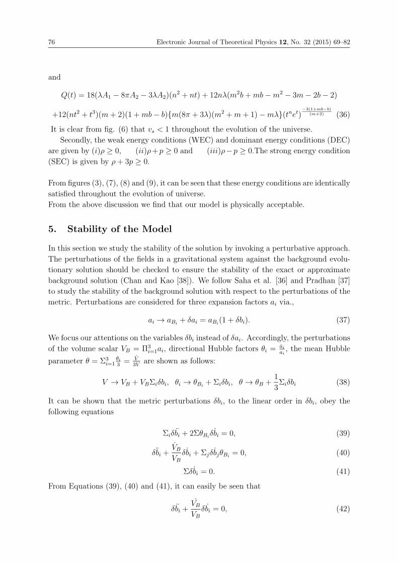
76 Electronic Journal of Theoretical Physics 12, No. 32 (2015) 69–82
and
Q(t) = 18(λA1 − 8πA2 − 3λA2)(n2 + nt) + 12nλ(m2b+mb−m2 − 3m− 2b− 2)
+12(nt2 + t3)(m+ 2)(1 +mb− b){m(8π + 3λ)(m2 +m+ 1)−mλ}(tnet)−3(1+mb−b)
(m+2) (36)
It is clear from fig. (6) that vs < 1 throughout the evolution of the universe.
Secondly, the weak energy conditions (WEC) and dominant energy conditions (DEC)
are given by (i)ρ ≥ 0, (ii)ρ+p ≥ 0 and (iii)ρ−p ≥ 0.The strong energy condition
(SEC) is given by ρ+ 3p ≥ 0.
From figures (3), (7), (8) and (9), it can be seen that these energy conditions are identically
satisfied throughout the evolution of universe.
From the above discussion we find that our model is physically acceptable.
5. Stability of the Model
In this section we study the stability of the solution by invoking a perturbative approach.
The perturbations of the fields in a gravitational system against the background evolu-
tionary solution should be checked to ensure the stability of the exact or approximate
background solution (Chan and Kao [38]). We follow Saha et al. [36] and Pradhan [37]
to study the stability of the background solution with respect to the perturbations of the
metric. Perturbations are considered for three expansion factors ai via.,
ai → aBi+ δai = aBi
(1 + δbi). (37)
We focus our attentions on the variables δbi instead of δai. Accordingly, the perturbations
of the volume scalar VB = Π3i=1ai, directional Hubble factors θi =
aiai, the mean Hubble
parameter θ = Σ3i=1
θi3= V
3Vare shown as follows:
V → VB + VBΣiδbi, θi → θBi+ Σiδbi, θ → θB +
1
3Σiδbi (38)
It can be shown that the metric perturbations δbi, to the linear order in δbi, obey the
following equations
Σiδbi + 2ΣθBiδbi = 0, (39)
δbi +VB
VB
δbi + ΣjδbjθBi= 0, (40)
Σδbi = 0. (41)
From Equations (39), (40) and (41), it can easily be seen that
δbi +VB
VB
δbi = 0, (42)
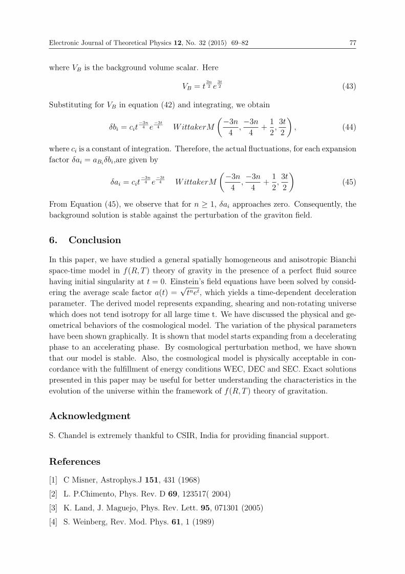
Electronic Journal of Theoretical Physics 12, No. 32 (2015) 69–82 77
where VB is the background volume scalar. Here
VB = t3n2 e
3t2 (43)
Substituting for VB in equation (42) and integrating, we obtain
δbi = cit−3n4 e
−3t4 WittakerM
(−3n4
,−3n4
+1
2,3t
2
), (44)
where ci is a constant of integration. Therefore, the actual fluctuations, for each expansion
factor δai = aBiδbi,are given by
δai = cit−3n4 e
−3t4 WittakerM
(−3n4
,−3n4
+1
2,3t
2
)(45)
From Equation (45), we observe that for n ≥ 1, δai approaches zero. Consequently, the
background solution is stable against the perturbation of the graviton field.
6. Conclusion
In this paper, we have studied a general spatially homogeneous and anisotropic Bianchi
space-time model in f(R, T ) theory of gravity in the presence of a perfect fluid source
having initial singularity at t = 0. Einstein’s field equations have been solved by consid-
ering the average scale factor a(t) =√tnet, which yields a time-dependent deceleration
parameter. The derived model represents expanding, shearing and non-rotating universe
which does not tend isotropy for all large time t. We have discussed the physical and ge-
ometrical behaviors of the cosmological model. The variation of the physical parameters
have been shown graphically. It is shown that model starts expanding from a decelerating
phase to an accelerating phase. By cosmological perturbation method, we have shown
that our model is stable. Also, the cosmological model is physically acceptable in con-
cordance with the fulfillment of energy conditions WEC, DEC and SEC. Exact solutions
presented in this paper may be useful for better understanding the characteristics in the
evolution of the universe within the framework of f(R, T ) theory of gravitation.
Acknowledgment
S. Chandel is extremely thankful to CSIR, India for providing financial support.
References
[1] C Misner, Astrophys.J 151, 431 (1968)
[2] L. P.Chimento, Phys. Rev. D 69, 123517( 2004)
[3] K. Land, J. Maguejo, Phys. Rev. Lett. 95, 071301 (2005)
[4] S. Weinberg, Rev. Mod. Phys. 61, 1 (1989)
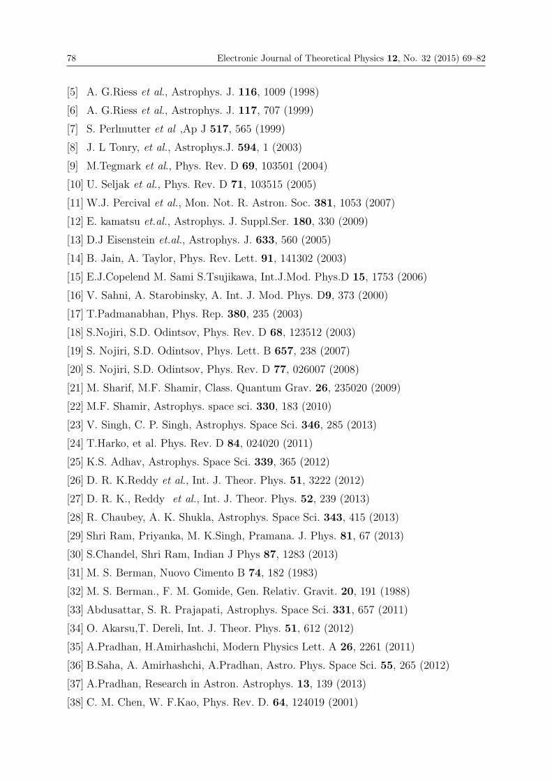
78 Electronic Journal of Theoretical Physics 12, No. 32 (2015) 69–82
[5] A. G.Riess et al., Astrophys. J. 116, 1009 (1998)
[6] A. G.Riess et al., Astrophys. J. 117, 707 (1999)
[7] S. Perlmutter et al ,Ap J 517, 565 (1999)
[8] J. L Tonry, et al., Astrophys.J. 594, 1 (2003)
[9] M.Tegmark et al., Phys. Rev. D 69, 103501 (2004)
[10] U. Seljak et al., Phys. Rev. D 71, 103515 (2005)
[11] W.J. Percival et al., Mon. Not. R. Astron. Soc. 381, 1053 (2007)
[12] E. kamatsu et.al., Astrophys. J. Suppl.Ser. 180, 330 (2009)
[13] D.J Eisenstein et.al., Astrophys. J. 633, 560 (2005)
[14] B. Jain, A. Taylor, Phys. Rev. Lett. 91, 141302 (2003)
[15] E.J.Copelend M. Sami S.Tsujikawa, Int.J.Mod. Phys.D 15, 1753 (2006)
[16] V. Sahni, A. Starobinsky, A. Int. J. Mod. Phys. D9, 373 (2000)
[17] T.Padmanabhan, Phys. Rep. 380, 235 (2003)
[18] S.Nojiri, S.D. Odintsov, Phys. Rev. D 68, 123512 (2003)
[19] S. Nojiri, S.D. Odintsov, Phys. Lett. B 657, 238 (2007)
[20] S. Nojiri, S.D. Odintsov, Phys. Rev. D 77, 026007 (2008)
[21] M. Sharif, M.F. Shamir, Class. Quantum Grav. 26, 235020 (2009)
[22] M.F. Shamir, Astrophys. space sci. 330, 183 (2010)
[23] V. Singh, C. P. Singh, Astrophys. Space Sci. 346, 285 (2013)
[24] T.Harko, et al. Phys. Rev. D 84, 024020 (2011)
[25] K.S. Adhav, Astrophys. Space Sci. 339, 365 (2012)
[26] D. R. K.Reddy et al., Int. J. Theor. Phys. 51, 3222 (2012)
[27] D. R. K., Reddy et al., Int. J. Theor. Phys. 52, 239 (2013)
[28] R. Chaubey, A. K. Shukla, Astrophys. Space Sci. 343, 415 (2013)
[29] Shri Ram, Priyanka, M. K.Singh, Pramana. J. Phys. 81, 67 (2013)
[30] S.Chandel, Shri Ram, Indian J Phys 87, 1283 (2013)
[31] M. S. Berman, Nuovo Cimento B 74, 182 (1983)
[32] M. S. Berman., F. M. Gomide, Gen. Relativ. Gravit. 20, 191 (1988)
[33] Abdusattar, S. R. Prajapati, Astrophys. Space Sci. 331, 657 (2011)
[34] O. Akarsu,T. Dereli, Int. J. Theor. Phys. 51, 612 (2012)
[35] A.Pradhan, H.Amirhashchi, Modern Physics Lett. A 26, 2261 (2011)
[36] B.Saha, A. Amirhashchi, A.Pradhan, Astro. Phys. Space Sci. 55, 265 (2012)
[37] A.Pradhan, Research in Astron. Astrophys. 13, 139 (2013)
[38] C. M. Chen, W. F.Kao, Phys. Rev. D. 64, 124019 (2001)
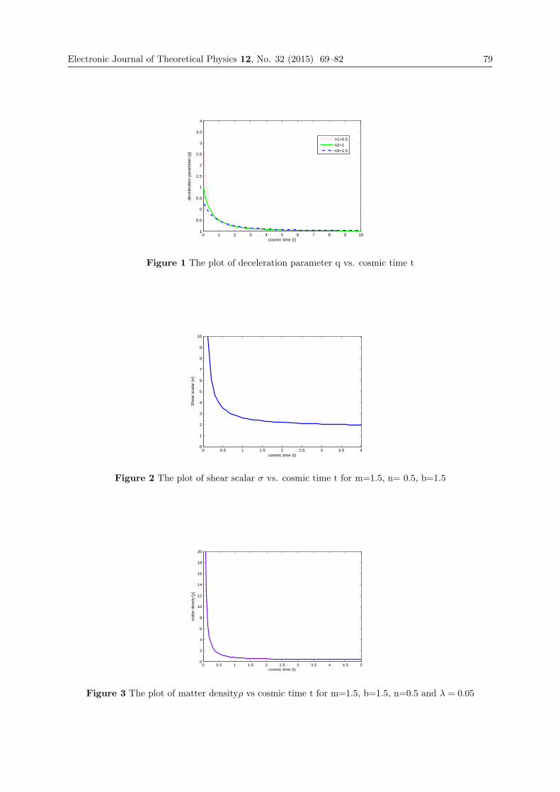
Electronic Journal of Theoretical Physics 12, No. 32 (2015) 69–82 79
0 1 2 3 4 5 6 7 8 9 101
0.5
0
0.5
1
1.5
2
2.5
3
3.5
4
cosmic time (t)
dece
lera
tion
para
met
er (q
)
n1=0.5n2=1n3=1.5
Figure 1 The plot of deceleration parameter q vs. cosmic time t
0 0.5 1 1.5 2 2.5 3 3.5 40
1
2
3
4
5
6
7
8
9
10
cosmic time (t)
Shea
r sca
lar (
σ)
Figure 2 The plot of shear scalar σ vs. cosmic time t for m=1.5, n= 0.5, b=1.5
0 0.5 1 1.5 2 2.5 3 3.5 4 4.5 50
2
4
6
8
10
12
14
16
18
20
cosmic time (t)
mat
ter d
ensit
y (ρ
)
Figure 3 The plot of matter densityρ vs cosmic time t for m=1.5, b=1.5, n=0.5 and λ = 0.05
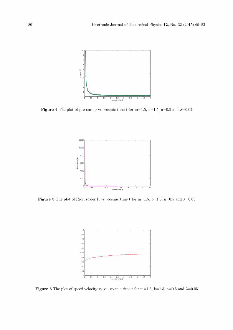
80 Electronic Journal of Theoretical Physics 12, No. 32 (2015) 69–82
0 0.5 1 1.5 2 2.5 3 3.5 4 4.5 50
1
2
3
4
5
6
7
8
9
10
cosmic time (t)
pres
urre
(p)
Figure 4 The plot of pressure p vs. cosmic time t for m=1.5, b=1.5, n=0.5 and λ=0.05
0 0.5 1 1.5 2 2.5 3 3.5 4 4.50
2000
4000
6000
8000
10000
12000
cosmic time (t)
Ric
ci s
cala
r(R)
Figure 5 The plot of Ricci scaler R vs. cosmic time t for m=1.5, b=1.5, n=0.5 and λ=0.05
0 0.5 1 1.5 2 2.5 3 3.5 4 4.5 50
0.1
0.2
0.3
0.4
0.5
0.6
0.7
0.8
0.9
1
cosmic time (t)
v s
Figure 6 The plot of speed velocity vs vs. cosmic time t for m=1.5, b=1.5, n=0.5 and λ=0.05
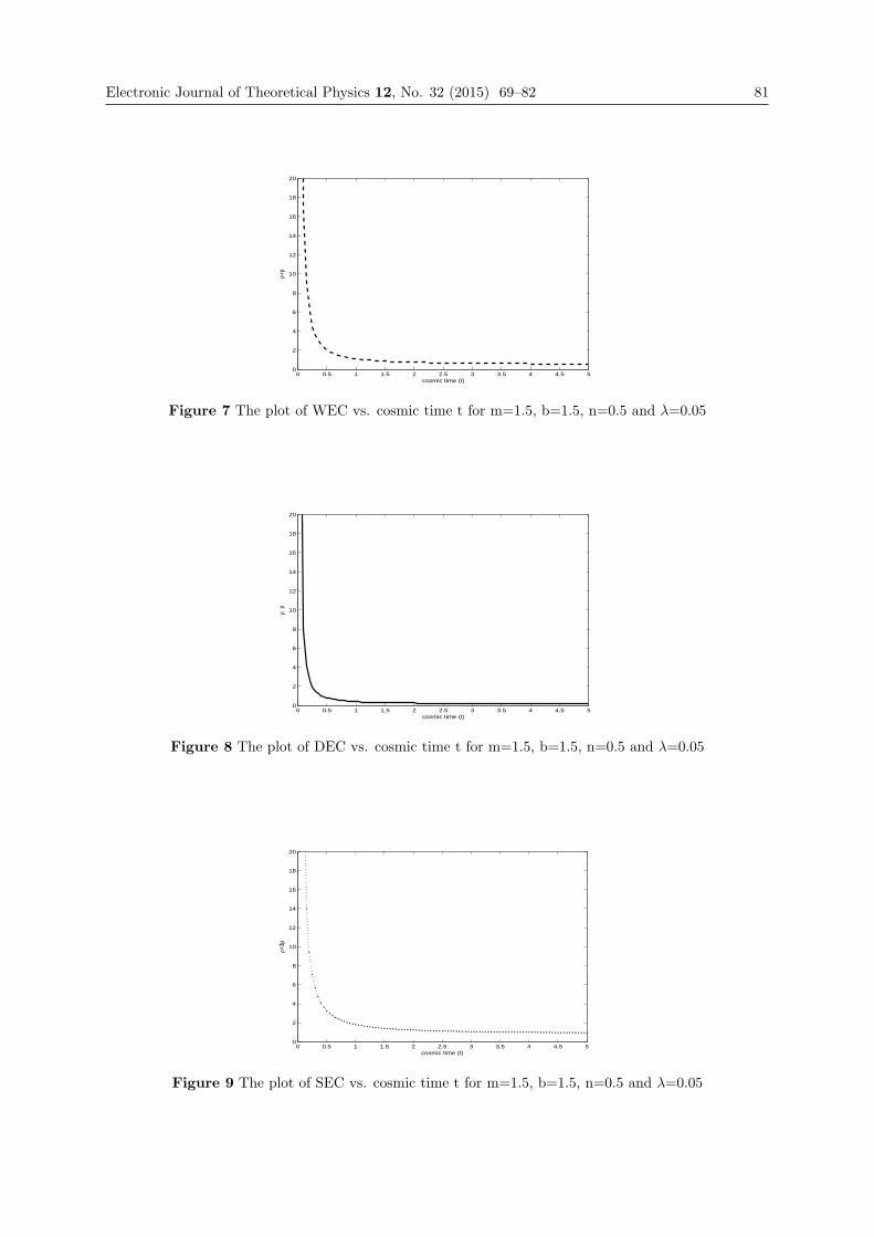
Electronic Journal of Theoretical Physics 12, No. 32 (2015) 69–82 81
0 0.5 1 1.5 2 2.5 3 3.5 4 4.5 50
2
4
6
8
10
12
14
16
18
20
cosmic time (t)
ρ+p
Figure 7 The plot of WEC vs. cosmic time t for m=1.5, b=1.5, n=0.5 and λ=0.05
0 0.5 1 1.5 2 2.5 3 3.5 4 4.5 50
2
4
6
8
10
12
14
16
18
20
cosmic time (t)
ρp
Figure 8 The plot of DEC vs. cosmic time t for m=1.5, b=1.5, n=0.5 and λ=0.05
0 0.5 1 1.5 2 2.5 3 3.5 4 4.5 50
2
4
6
8
10
12
14
16
18
20
cosmic time (t)
ρ+3p
Figure 9 The plot of SEC vs. cosmic time t for m=1.5, b=1.5, n=0.5 and λ=0.05

EJTP 12, No. 32 (2015) 83–112 Electronic Journal of Theoretical Physics
Relativistic Pentametric Coordinates fromRelativistic Localizing Systems and the Projective
Geometry of the Spacetime Manifold
Jacques L. Rubin∗
Universite de Nice–Sophia Antipolis, UFR SciencesInstitut du Non-Lineaire de Nice, UMR7335
1361 route des Lucioles, F-06560 Valbonne, France
Received 5 November 2014, Accepted 20 December 2014, Published 10 September 2015
Abstract: Relativistic pentametric coordinates supplied by relativistic auto-locating
positioning systems made up of four satellites supplemented by a fifth one are defined in
addition to the well-known emission and reception coordinates. Such a constellation of five
satellites defines a so-called relativistic localizing system. The determination of such systems
is motivated by the need to not only locate (within a grid) users utilizing receivers but, more
generally, to localize any spacetime event. The angles measured on the celestial spheres of the
five satellites enter into the definition. Therefore, there are, up to scalings, intrinsic physical
coordinates related to the underlying conformal structure of spacetime. Moreover, they indicate
that spacetime must be endowed everywhere with a local projective geometry characteristic of
a so-called generalized Cartan space locally modeled on four-dimensional, real projective space.
The particular process of localization providing the relativistic pentametric coordinates is based,
in a way, on an enhanced notion of parallax in space and time generalizing the usual parallax
restricted to space only.c© Electronic Journal of Theoretical Physics. All rights reserved.
Keywords: Emission Coordinates; Generalized Cartan Space; Projective Geometry; Relativistic
Positioning Systems
PACS (2010): 04.20.Cv; 02.40.Dr; 04.50.-h; 04.20.Gz
1. A Protocol Implemented by Users to Localize Events
Almost simultaneously, Bahder [1], Blagojevic et al. [2], Coll [3] and Rovelli [4] laid, from
different approaches, the foundations of the relativistic positioning systems (RPS) and,
∗ Email:[email protected]
84 Electronic Journal of Theoretical Physics 12, No. 32 (2015) 83–112
in particular, following Coll’s terminology,2 “primary” RPSs, i.e., RPSs which satisfy the
three following criteria: they are 1) “generic,” i.e., the system of coordinates they provide
must exist independently of the spacetime geometry for each given class of spacetime, 2)
they are “free,” i.e., their structures do not need the knowledge of the gravitational field,
and 3) they are “immediate,” i.e., the users know their positions without delay at the
instant they receive the four “time stamps τα” sent by the four emitting satellites of the
RPS satellite constellation.
Among this set of primary RPSs, there exists the sub-class of the so-called “auto-
locating RPSs,” i.e., those RPSs in which each satellite broadcasts its own time stamp
but also the time stamps it receives from its neighboring satellites. The SYPOR system
(“SYsteme de POsitionnement Relativiste”), developed by Coll and Tarantola [5], belongs
to this category, but we ask, more generally, for an enhanced RPS and a supplementary
protocol to allow any located user to localize any event in the spacetime region covered
by this particular enhanced RPS.
We make the following strict distinction between location and localization. To locate
an event, a protocol (of location) is needed to build a coordinate grid, and then, to position
this event in this grid once the coordinates of this event are known. To localize an event, a
protocol (of localization) is needed that effectively obtains the coordinates of the event to
be then, only, located in a given coordinate grid. Auto-locating positioning systems only
allow building the coordinate grids from the users’ knowledge of the satellites’ worldlines,
and then, to position the users in these grids, but they do not supply the coordinates of
events. Upstream, non auto-locating systems only allow knowing the users’ coordinates
but without location and, more generally, without localization of events in the users’
surroundings.
Furthermore, downstream, the sub-class of the so-called “autonomous systems,” con-
tained in the sub-class of auto-locating systems, includes those auto-locating systems
allowing, from “autonomous data,” the users to draw (from Coll’s definition [3]) the
satellites’ worldlines in the spacetime where these users are living. Beside, we consider
rather another sub-class contained in the sub-class of auto-locating systems, namely, the
sub-class of “relativistic localizing systems” of which the satellites broadcast also, in ad-
dition to their time stamps, data to localize events. In the present paper, we define such a
relativistic localizing system made up of four satellites constituting an auto-locating sys-
tem supplemented by an ancillary fifth satellite providing data (actually, supplementary
time stamps) to localize events. These five satellites can define five different auto-locating
systems connected by ten changes of coordinate grids but only one of the five is required
to operate.
Besides, the goal for seeking such an enhanced RPS, viz., a relativistic localizing
system, provided with a tracking, localizing protocol is also to find a process to break
the underlying arbitrariness in scaling that is due, in a way, to the arbitrary choice
2 Throughout the present paper, we use terms such as primary, local, intrinsic, location system, reference
system, positioning system, auto-locating system, autonomous system or data, laws of physics, emission
and reception coordinates, etc., as defined in [3]
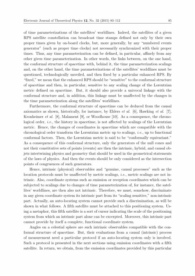
Electronic Journal of Theoretical Physics 12, No. 32 (2015) 83–112 85
of time parameterizations of the satellites’ worldlines. Indeed, the satellites of a given
RPS satellite constellation can broadcast time stamps defined not only by their own
proper times given by on-board clocks, but, more generally, by any “numbered events
generator” (such as proper time clocks) not necessarily synchronized with their proper
times. Thus, any time parameterization can be defined, in particular, affinely from any
other given time parameterization. In other words, the links between, on the one hand,
the conformal structure of spacetime with, behind it, the time parameterization scalings
and, on the other hand, the time parameterizations of the satellites’ worldlines must be
questioned, technologically unveiled, and then fixed by a particular enhanced RPS. By
“fixed,” we mean that the enhanced RPS should be “sensitive” to the conformal structure
of spacetime and then, in particular, sensitive to any scaling change of the Lorentzian
metric defined on spacetime. But, it should also provide a univocal linkage with the
conformal structure and, in addition, this linkage must be unaffected by the changes in
the time parameterization along the satellites’ worldlines.
Furthermore, the conformal structure of spacetime can be deduced from the causal
axiomatics as shown, historically, for instance, by Ehlers et al. [6], Hawking et al. [7],
Kronheimer et al. [8], Malament [9], or Woodhouse [10]. As a consequence, the chrono-
logical order, i.e., the history in spacetime, is not affected by scalings of the Lorentzian
metric. Hence, the changes of coordinates in spacetime which are compatible with the
chronological order transform the Lorentzian metric up to scalings, i.e., up to functional
conformal factors. Then, the Lorentzian metric is said to be “conformally equivariant.”
As a consequence of this conformal structure, only the generators of the null cones and
not their constitutive sets of points (events) are then the intrinsic, hybrid, and causal ob-
jets intertwining physics and geometry that should be used in the geometrical statements
of the laws of physics. And then the events should be only considered as the intersection
points of congruences of such generators.
Hence, intrinsic (physical) observables and “genuine, causal processes” such as the
location protocols must be unaffected by metric scalings, i.e., metric scalings are not in-
trinsic. Also, coordinate systems such as emission or reception coordinates which can be
subjected to scalings due to changes of time parameterization of, for instance, the satel-
lites’ worldlines, are then also not intrinsic. Therefore, we must, somehow, discriminate
in any given coordinate system its intrinsic part from its “scaling sensitive,” non-intrinsic
part. Actually, an auto-locating system cannot provide such a discrimination, as will be
shown in what follows. A fifth satellite must be attached to this positioning system. Us-
ing a metaphor, this fifth satellite is a sort of cursor indicating the scale of the positioning
system from which an intrinsic part alone can be excerpted. Moreover, this intrinsic part
cannot provide by itself a complete, functional coordinate system.
Angles on a celestial sphere are such intrinsic observables compatible with the con-
formal structure of spacetime. But, their evaluations from a causal (intrinsic) process
of measurement need a particular protocol if an auto-locating system only is involved.
Such a protocol is presented in the next sections using emission coordinates with a fifth
satellite. In return, we obtain, from the emission coordinates provided by this particular
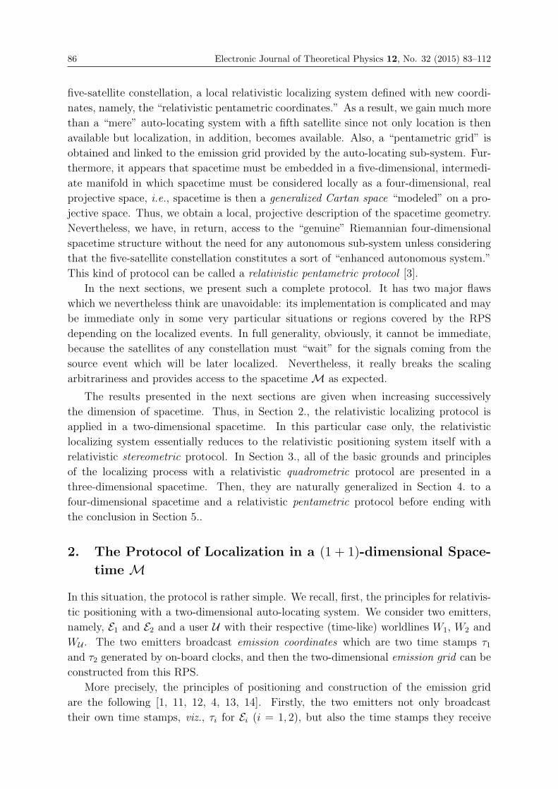
86 Electronic Journal of Theoretical Physics 12, No. 32 (2015) 83–112
five-satellite constellation, a local relativistic localizing system defined with new coordi-
nates, namely, the “relativistic pentametric coordinates.” As a result, we gain much more
than a “mere” auto-locating system with a fifth satellite since not only location is then
available but localization, in addition, becomes available. Also, a “pentametric grid” is
obtained and linked to the emission grid provided by the auto-locating sub-system. Fur-
thermore, it appears that spacetime must be embedded in a five-dimensional, intermedi-
ate manifold in which spacetime must be considered locally as a four-dimensional, real
projective space, i.e., spacetime is then a generalized Cartan space “modeled” on a pro-
jective space. Thus, we obtain a local, projective description of the spacetime geometry.
Nevertheless, we have, in return, access to the “genuine” Riemannian four-dimensional
spacetime structure without the need for any autonomous sub-system unless considering
that the five-satellite constellation constitutes a sort of “enhanced autonomous system.”
This kind of protocol can be called a relativistic pentametric protocol [3].
In the next sections, we present such a complete protocol. It has two major flaws
which we nevertheless think are unavoidable: its implementation is complicated and may
be immediate only in some very particular situations or regions covered by the RPS
depending on the localized events. In full generality, obviously, it cannot be immediate,
because the satellites of any constellation must “wait” for the signals coming from the
source event which will be later localized. Nevertheless, it really breaks the scaling
arbitrariness and provides access to the spacetimeM as expected.
The results presented in the next sections are given when increasing successively
the dimension of spacetime. Thus, in Section 2., the relativistic localizing protocol is
applied in a two-dimensional spacetime. In this particular case only, the relativistic
localizing system essentially reduces to the relativistic positioning system itself with a
relativistic stereometric protocol. In Section 3., all of the basic grounds and principles
of the localizing process with a relativistic quadrometric protocol are presented in a
three-dimensional spacetime. Then, they are naturally generalized in Section 4. to a
four-dimensional spacetime and a relativistic pentametric protocol before ending with
the conclusion in Section 5..
2. The Protocol of Localization in a (1 + 1)-dimensional Space-
time M
In this situation, the protocol is rather simple. We recall, first, the principles for relativis-
tic positioning with a two-dimensional auto-locating system. We consider two emitters,
namely, E1 and E2 and a user U with their respective (time-like) worldlines W1, W2 and
WU . The two emitters broadcast emission coordinates which are two time stamps τ1and τ2 generated by on-board clocks, and then the two-dimensional emission grid can be
constructed from this RPS.
More precisely, the principles of positioning and construction of the emission grid
are the following [1, 11, 12, 4, 13, 14]. Firstly, the two emitters not only broadcast
their own time stamps, viz., τi for Ei (i = 1, 2), but also the time stamps they receive
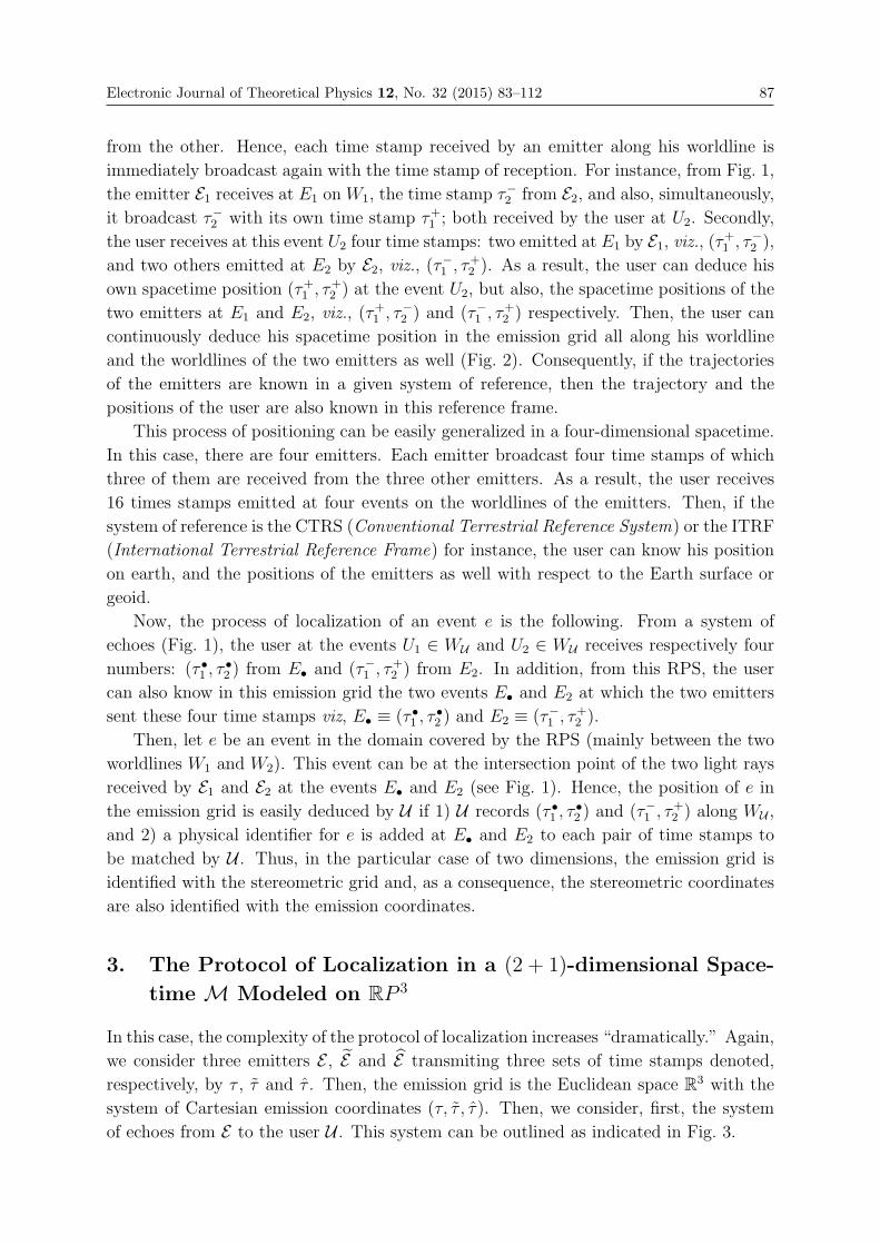
Electronic Journal of Theoretical Physics 12, No. 32 (2015) 83–112 87
from the other. Hence, each time stamp received by an emitter along his worldline is
immediately broadcast again with the time stamp of reception. For instance, from Fig. 1,
the emitter E1 receives at E1 on W1, the time stamp τ−2 from E2, and also, simultaneously,
it broadcast τ−2 with its own time stamp τ+1 ; both received by the user at U2. Secondly,
the user receives at this event U2 four time stamps: two emitted at E1 by E1, viz., (τ+1 , τ−2 ),and two others emitted at E2 by E2, viz., (τ−1 , τ+2 ). As a result, the user can deduce his
own spacetime position (τ+1 , τ+2 ) at the event U2, but also, the spacetime positions of the
two emitters at E1 and E2, viz., (τ+1 , τ
−2 ) and (τ−1 , τ
+2 ) respectively. Then, the user can
continuously deduce his spacetime position in the emission grid all along his worldline
and the worldlines of the two emitters as well (Fig. 2). Consequently, if the trajectories
of the emitters are known in a given system of reference, then the trajectory and the
positions of the user are also known in this reference frame.
This process of positioning can be easily generalized in a four-dimensional spacetime.
In this case, there are four emitters. Each emitter broadcast four time stamps of which
three of them are received from the three other emitters. As a result, the user receives
16 times stamps emitted at four events on the worldlines of the emitters. Then, if the
system of reference is the CTRS (Conventional Terrestrial Reference System) or the ITRF
(International Terrestrial Reference Frame) for instance, the user can know his position
on earth, and the positions of the emitters as well with respect to the Earth surface or
geoid.
Now, the process of localization of an event e is the following. From a system of
echoes (Fig. 1), the user at the events U1 ∈ WU and U2 ∈ WU receives respectively four
numbers: (τ •1 , τ•2 ) from E• and (τ−1 , τ
+2 ) from E2. In addition, from this RPS, the user
can also know in this emission grid the two events E• and E2 at which the two emitters
sent these four time stamps viz, E• ≡ (τ •1 , τ•2 ) and E2 ≡ (τ−1 , τ
+2 ).
Then, let e be an event in the domain covered by the RPS (mainly between the two
worldlines W1 and W2). This event can be at the intersection point of the two light rays
received by E1 and E2 at the events E• and E2 (see Fig. 1). Hence, the position of e in
the emission grid is easily deduced by U if 1) U records (τ •1 , τ•2 ) and (τ−1 , τ
+2 ) along WU ,
and 2) a physical identifier for e is added at E• and E2 to each pair of time stamps to
be matched by U . Thus, in the particular case of two dimensions, the emission grid is
identified with the stereometric grid and, as a consequence, the stereometric coordinates
are also identified with the emission coordinates.
3. The Protocol of Localization in a (2 + 1)-dimensional Space-
time M Modeled on RP 3
In this case, the complexity of the protocol of localization increases “dramatically.” Again,
we consider three emitters E , E and E transmiting three sets of time stamps denoted,
respectively, by τ , τ and τ . Then, the emission grid is the Euclidean space R3 with the
system of Cartesian emission coordinates (τ, τ , τ). Then, we consider, first, the system
of echoes from E to the user U . This system can be outlined as indicated in Fig. 3.
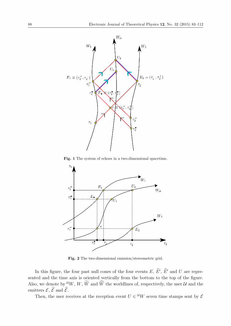
88 Electronic Journal of Theoretical Physics 12, No. 32 (2015) 83–112
Fig. 1 The system of echoes in a two-dimensional spacetime.
Fig. 2 The two-dimensional emission/stereometric grid.
In this figure, the four past null cones of the four events E, E ′, E ′ and U are repre-
sented and the time axis is oriented vertically from the bottom to the top of the figure.
Also, we denote by UW , W , W and W the worldlines of, respectively, the user U and the
emitters E , E and E .Then, the user receives at the reception event U ∈ UW seven time stamps sent by E
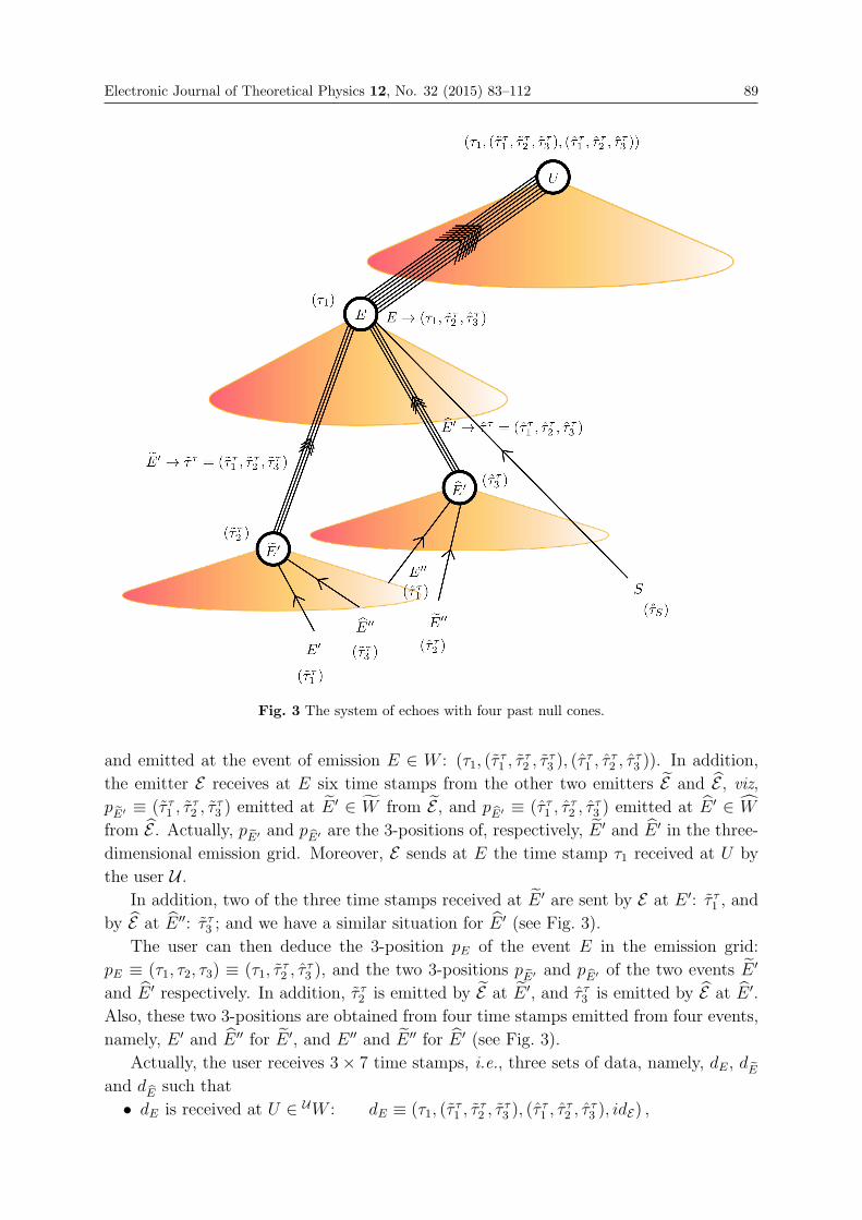
Electronic Journal of Theoretical Physics 12, No. 32 (2015) 83–112 89
Fig. 3 The system of echoes with four past null cones.
and emitted at the event of emission E ∈ W : (τ1, (ττ1 , τ
τ2 , τ
τ3 ), (τ
τ1 , τ
τ2 , τ
τ3 )). In addition,
the emitter E receives at E six time stamps from the other two emitters E and E , viz,p˜E′ ≡ (τ τ1 , τ
τ2 , τ
τ3 ) emitted at E ′ ∈ W from E , and p
E′ ≡ (τ τ1 , ττ2 , τ
τ3 ) emitted at E ′ ∈ W
from E . Actually, p˜E′ and p
E′ are the 3-positions of, respectively, E ′ and E ′ in the three-
dimensional emission grid. Moreover, E sends at E the time stamp τ1 received at U by
the user U .In addition, two of the three time stamps received at E ′ are sent by E at E ′: τ τ1 , and
by E at E ′′: τ τ3 ; and we have a similar situation for E ′ (see Fig. 3).
The user can then deduce the 3-position pE of the event E in the emission grid:
pE ≡ (τ1, τ2, τ3) ≡ (τ1, ττ2 , τ
τ3 ), and the two 3-positions p
˜E′ and pE′ of the two events E ′
and E ′ respectively. In addition, τ τ2 is emitted by E at E ′, and τ τ3 is emitted by E at E ′.Also, these two 3-positions are obtained from four time stamps emitted from four events,
namely, E ′ and E ′′ for E ′, and E ′′ and E ′′ for E ′ (see Fig. 3).
Actually, the user receives 3× 7 time stamps, i.e., three sets of data, namely, dE, d ˜E
and dE such that
• dE is received at U ∈ UW : dE ≡ (τ1, (ττ1 , τ
τ2 , τ
τ3 ), (τ
τ1 , τ
τ2 , τ
τ3 ), idE) ,
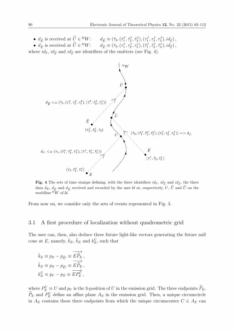
90 Electronic Journal of Theoretical Physics 12, No. 32 (2015) 83–112
• d˜E is received at U ∈ UW : d
˜E ≡ (τ2, (ττ1 , τ
τ2 , τ
τ3 ), (τ
τ1 , τ
τ2 , τ
τ3 ), id˜E) ,
• dE is received at U ∈ UW : d
E ≡ (τ3, (ττ1 , τ
τ2 , τ
τ3 ), (τ
τ1 , τ
τ2 , τ
τ3 ), idE) ,
where idE , id˜E and idE are identifiers of the emitters (see Fig. 4).
Fig. 4 The sets of time stamps defining, with the three identifiers idE , id˜E and idE , the three
data dE , d ˜E and dE received and recorded by the user U at, respectively, U , U and U on the
worldline UW of U .
From now on, we consider only the sets of events represented in Fig. 3.
3.1 A first procedure of localization without quadrometric grid
The user can, then, also deduce three future light-like vectors generating the future null
cone at E, namely, kE, kE and kUE , such that
kE ≡ pE − pE′ ≡
−−→EPE ,
kE ≡ pE − p˜E′ ≡
−−→EPE ,
kUE ≡ pU − pE ≡
−−−→EPU
E ,
where PUE ≡ U and pU is the 3-position of U in the emission grid. The three endpoints PE,
PE and PUE define an affine plane AE in the emission grid. Then, a unique circumcircle
in AE contains these three endpoints from which the unique circumcenter C ∈ AE can
Electronic Journal of Theoretical Physics 12, No. 32 (2015) 83–112 91
be deduced by standard formulas.3
Now, let e be an event to be localized in the emission grid (in this first procedure,
the quadrometric grid is not defined). It is featured and identified by a set se of physical,
non-geometrical characteristics such as, for instance, its spectrum, its shape, its temper-
ature, etc. We assume also that this event e can be detected and almost instantaneously
physically analyzed by the emitters at the events E, E and E from signals carried by
light rays (for instance) coming from e. Also, we assume that these light rays (which
carry this various physical information) manifest themselves in “bright points” on their
respective “celestial circles” of the emitters at the events E, E and E. For the sake of
illustration, we consider only the celestial circle C � S1 of the emitter E at the event E.
Also, we provide E with an apparatus made of an optical device and a compass to locate
the event e on the celestial circle C.4 For this, we need also to define a projective frame
for C. For this purpose, the two other satellites E and E manifest themselves in “bright
points” on C ascribed to the two events E ′ and E ′ in the past null cone of E. Then, the
projective point [0]E ∈ C is ascribed to E ′ and kE, and the projective point [∞]E ∈ C is
ascribed to E ′ and kE:
E ′ ←→ [0]E ←→ kE ,
E ′ ←→ [∞]E ←→ kE .
Then, we assume that RP 1 � C = S1. Note that we cannot ascribe to kUE and U a
projective point [1]E ∈ C since U is in the future null cone of E, and thus, no corresponding
“bright points” exists on C. Therefore, we need a fourth satellite, namely, S, in addition
to E , E and E . A priori, S does not need to broadcast a supplementary time stamp, but
it must be clearly identified with an identifier idS .
3 That is, we define the two relative vectors with origin U : r = kE − kUE and r = kE − kUE . Then, in R3,
the circumcenter C is the point C ∈ AE such that
−−→UC =
(‖r‖2 r − ‖r‖2 r) ∧ (r ∧ r)
2 ‖r ∧ r‖2 .
4 The only remaining step utilizing material objects is the angle measurement by compasses. Their use
implies that the angles remain invariant regardless of the size of the compass. And then, this also implies
that there is an absolute notion of angle in contrast to the notions of time and length which depend
on frames. This has historically been considered by Weyl and Godel with their concepts of “inertial
compass” or “star compass” in objection to Mach’s principle. This absolute feature cannot come from
any geometry of space-time. It is therefore possible that it comes from a different physics, such as
quantum mechanics. Thus, a true compass would be based on the use of a quantum phenomenon of
angle measurement, i.e., a quantum compass. This can be done with a Michelson interferometer (see for
example [15, 16]) or interferences in cold atomic gases. Nevertheless, we think that the compass should
be rather graduated by fractional numbers, for instance, such as those appearing in the fractional Hall
effect.
92 Electronic Journal of Theoretical Physics 12, No. 32 (2015) 83–112
Then, another fourth “bright point” ascribed to the third projective point [1]E ∈ C is
observable on C due to S sending its identifier idS from the event S (see Fig. 3):
S ←→ [1]E .
Now, e can be localized in the emission grid by applying the following procedure.
From the “bright points” [∞]E, [0]E and [1]E, and the optical device and compass
embarked on E , the optical observation of e on C provides a projective point [tanα]E ∈ Cwith α clearly, numerically evaluated from the projective frame FE ≡ {[∞]E, [0]E, [1]E}.5Moreover, to [tanα]E there correspond two vectors �v+
E and �v−E such that
�v±E ≡−−−→EV ±E ≡
−−→EC ±
(−−→CPE + tanα
−−→CPE
),
where C is the circumcenter in AE and, in addition,−−→CPE and
−−→CPE are ascribed to the
following projective points:
−−→CPE ←→ [0]E ,−−→CPE ←→ [∞]E .
Now, the two vectors �v±E define a two dimensional affine plane Pe containing e such that
−→Ee = a+ �v+
E + a− �v−E ∈ Pe
for two reals a± to be determined by applying the same procedure with the two emitters
E and E at, respectively, E and E. Indeed, we deduce the two other analogous affine
planes Pe and Pe and two relations as
−→Ee = a+ �v+
E + a− �v−E ∈ Pe ,−→Ee = a+ �v+
E + a− �v−E ∈ Pe .
Then, e is the intersection point of P , Pe and Pe. Therefore, we obtain six algebraic
linear equations determining completely the a’s and then e in the emission grid. Neither
quadrometric coordinates nor, a fortiori, a quadrometric grid need to be defined. But,
this procedure cannot be generalized to higher dimensional spacetime manifolds: it is
specific to the three dimensional case. Indeed, the intersection point of three, two by two
non-parallel planes always exists in R3 whereas four, two by two parallel, two-dimensional
hyperplanes do not always have intersection points in R4.
5 In this definition of [tanα]E , the angles α vary over the interval [−π/2, π/2] of range π on the celestial
circle rather than over the usual interval [0, 2π] of range 2π. Another viewpoint is to consider the “angles”
to vary within the extended set of real numbers R ≡ [+∞,−∞], and then, to write [α]E with α ∈ R
instead of [tanα]E with α ∈ [−π/2, π/2] .
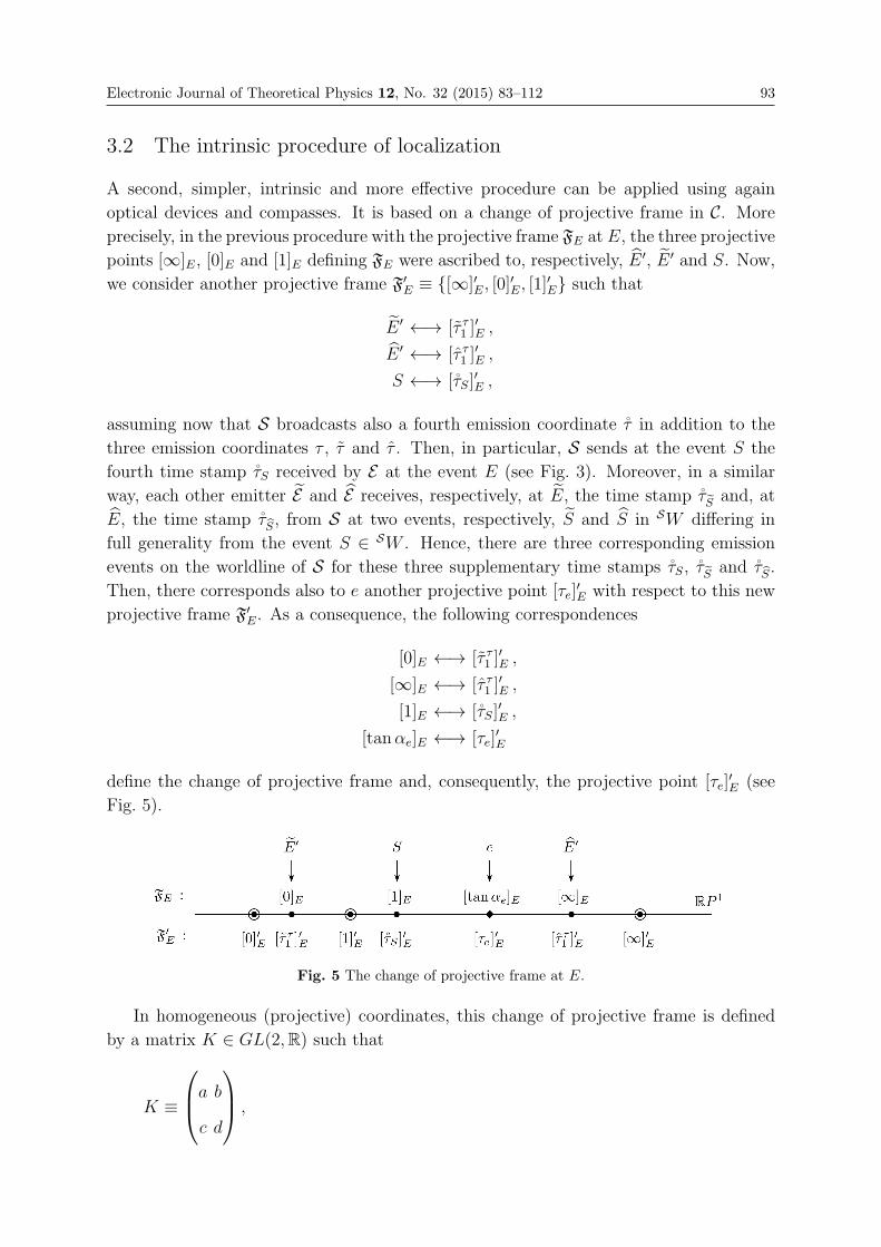
Electronic Journal of Theoretical Physics 12, No. 32 (2015) 83–112 93
3.2 The intrinsic procedure of localization
A second, simpler, intrinsic and more effective procedure can be applied using again
optical devices and compasses. It is based on a change of projective frame in C. More
precisely, in the previous procedure with the projective frame FE at E, the three projective
points [∞]E, [0]E and [1]E defining FE were ascribed to, respectively, E ′, E ′ and S. Now,
we consider another projective frame F′E ≡ {[∞]′E, [0]′E, [1]
′E} such that
E ′ ←→ [τ τ1 ]′E ,
E ′ ←→ [τ τ1 ]′E ,
S ←→ [τS]′E ,
assuming now that S broadcasts also a fourth emission coordinate τ in addition to the
three emission coordinates τ , τ and τ . Then, in particular, S sends at the event S the
fourth time stamp τS received by E at the event E (see Fig. 3). Moreover, in a similar
way, each other emitter E and E receives, respectively, at E, the time stamp τ˜S and, at
E, the time stamp τS, from S at two events, respectively, S and S in SW differing in
full generality from the event S ∈ SW . Hence, there are three corresponding emission
events on the worldline of S for these three supplementary time stamps τS, τ˜S and τS.
Then, there corresponds also to e another projective point [τe]′E with respect to this new
projective frame F′E. As a consequence, the following correspondences
[0]E ←→ [τ τ1 ]′E ,
[∞]E ←→ [τ τ1 ]′E ,
[1]E ←→ [τS]′E ,
[tanαe]E ←→ [τe]′E
define the change of projective frame and, consequently, the projective point [τe]′E (see
Fig. 5).
Fig. 5 The change of projective frame at E.
In homogeneous (projective) coordinates, this change of projective frame is defined
by a matrix K ∈ GL(2,R) such that
K ≡
⎛⎜⎝a b
c d
⎞⎟⎠ ,
94 Electronic Journal of Theoretical Physics 12, No. 32 (2015) 83–112
and satisfying the four following additional correspondences:
[0]E ≡
⎛⎜⎝0
1
⎞⎟⎠ K−−−−−−−−→
⎛⎜⎝a
c
⎞⎟⎠ ≡ [τ τ1 ]′E where τ τ1 = a/c ,
[∞]E ≡
⎛⎜⎝1
0
⎞⎟⎠ K−−−−−−−−→
⎛⎜⎝b
d
⎞⎟⎠ ≡ [τ τ1 ]′E where τ τ1 = b/d ,
[1]E ≡
⎛⎜⎝1
1
⎞⎟⎠ K−−−−−−−−→
⎛⎜⎝a+ b
c+ d
⎞⎟⎠ ≡ [τS]′E where τS =
(a+ b
c+ d
),
[tanαe]E ≡
⎛⎜⎝tanαe
1
⎞⎟⎠ K−−−−−−−−→
⎛⎜⎝a tanαe + b
c tanαe + d
⎞⎟⎠ ≡ [τe]′E where τe =
(a tanαe + b
c tanαe + d
).
Therefore, we obtain⎧⎪⎪⎨⎪⎪⎩a = − τ τ1 [ τ τ1 : τ τ1 : τS ] d ,
b = τ τ1 d ,
c = [ τ τ1 : τ τ1 : τS ] d ,
where [ τ τ1 : τ τ1 : τS ] is such that
[ τ τ1 : τ τ1 : τS ] ≡(τ τ1 − τSτ τ1 − τS
).
Then, we deduce τe such that
τe ≡(
τ τ1 − τ τ1 [ τ τ1 : τ τ1 : τS ] tanαe
1− [ τ τ1 : τ τ1 : τS ] tanαe
). (1)
This is a birational continuous function, and thus bijective. In particular, we obtain the
following important property:
If tanαe = 0, 1 or ∞, then we find that τe = τ τ1 , τS or τ τ1 .
Also, from the other emitters at E and E, the user can compute the three time stamps
pe ≡ (τe, τe, τe) ascribed to the 3-position pe of the event e; therefore localized as expected.
However, it is important to note that the event e is not strictly located in the emission
grid but in a new grid, namely, the quadrometric grid. More precisely, the quadrometric
grid shares with the emission grid 1) the three Cartesian time axes associated with the
three emission coordinates τ , τ and τ , and also, from the property above, 2) the three
emitter worldlines only which are therefore common, point-to-point, to the two grids.
Therefore, rigorously, if e is not a point on an emitter worldline, then, pe must not be
positioned (located) in the emission grid. Moreover, we begin the procedure with time
stamps associated with events located in the emission grid, and we produce sets of time
Electronic Journal of Theoretical Physics 12, No. 32 (2015) 83–112 95
stamps to localize events. Then, because the process of location strictly differs from the
process of localization, we must consider that any triplet (τe, τe, τe) constitutes the three
quadrometric coordinates ascribed to the event e positioned in the quadrometric grid
only. This procedure can be outlined with the following diagram:
Emission
coordinates−−−→ Intrinsic angles
+ non-intrinsic time stamps−−−→ quadro/pentametric
coordinates
Also, it is important to note that given E, E and E, the event e is unique since it is the
intersection point of three two-dimensional past null cones. Moreover, we can say that
there exists a unique set of three events E, E and E “attached” to e, i.e., we have a
fibered product of past null cones (over the set of localized events e inM) homeomorphic
toM.
Hence, we need four satellites E , E , E and S with their four emission coordinates to
localize an event in the quadrometric grid, and thus, the three dimensional spacetimeMmust be embedded in R4. For instance, we have the following coordinates in R4:
E ←→ (τ1, ττ2 , τ
τ3 , τS) , (2a)
E ←→ (τ τ1 , τ2, ττ3 , τ˜S) , (2b)
E ←→ (τ τ1 , ττ2 , τ3, τS) . (2c)
Also, the data sent by the satellites E , E and E to the user U are reduced. We just need
the following reduced data:
dE ≡ ((τ1, ττ2 , τ
τ3 , τS), idE , αe, se) ,
d˜E ≡ ((τ τ1 , τ2, τ
τ3 , τ˜S), id˜E , αe, se) ,
dE ≡ ((τ τ1 , τ
τ2 , τ3, τS), idE , αe, se) ,
where se allows matching the three first data sets dE, d ˜E and dE ascribed to e.
Besides, the question arises to know if a fourth coordinate τe can be ascribed also
to the event e as for the three events E, E and E. A coordinate τe could be easily
obtained from the 3-position of e in the quadrometric grid if 1) e is in the future horismos
[8, 17] of a point p on the worldline of S, and then, τp ≡ τe, and 2) S broadcasts also,
in particular to the user, the coordinates of p in the quadrometric grid obtained from
the three other emitters E , E and E . The first condition cannot always be physically
or technologically satisfied since there necessarily exists an origin event o at which the
fourth satellite S begins to run. Hence, we can expect to know the positions of S in the
quadrometric grid only beyond this starting point o on the future worldline SW+o ≡ {o�
p,where p is an emission event of S} of S contained in the chronological future of o (the
symbol � denotes the chronological order. See [8, 17] for instance).
Nevertheless, it is easy to circumvent this difficulty, assuming that we define the
prolongation SW−o of the worldline of S in the causal past of o by a given, arbitrary,
nevertheless well-defined by geometric conventions, curve in the quadrometric grid. Now,
96 Electronic Journal of Theoretical Physics 12, No. 32 (2015) 83–112
from a given time parameterization of SW−o , we can also ascribe to any event e a fourth
time stamp τe from the message function f−SW−o: e −→ τe [6]. Then, the worldline
SW of
S is such that SW = SW−o ∪ {o} ∪ SW+
o and we obtain the complete message function
f−SW : e ∈ M −→ τe ∈ R � SW . As a consequence, from f−SW , we obtain an embedding
ofM in R4. This embedding is explicit since we cannot localize events without giving a
fourth time stamp such as, for instance, τ˜S.
Furthermore, we recall that we have a local chart μ : ([tanαe], [tan αe], [tan αe]) ∈(RP 1)3 −→ pe = (τe, τe, τe) ∈ R3, and we consider now the action of PGL(4,R) on the
triplets (tanαe, tan αe, tan αe). Before, we denote by αi (i = 1, 2, 3) the three angles such
that αe ≡ α1, αe ≡ α2 and αe ≡ α3, and by τj (j = 1, 2, 3) the three time stamps such
that τe ≡ τ1, τe ≡ τ2 and τe ≡ τ3. We put below the list of formulas we start with.
In particular, we have a first set of formulas from the formulas such as (1) at E ≡ E1,
E ≡ E2 and E ≡ E3:
τi =
(uQi tanαi + vQiw�
i tanαi + k�i
)at Ei , (3)
where we assume w�i �= 0 and where the superscripts Q and � indicate, respectively,
that uQi , v
Qi , w
�i and k�
i are homogeneous polynomials of degree 2 (Q ≡ quadratic) and
homogeneous polynomials of degree 1 (� ≡ linear) with respect to the set of time stamps
collected at the three events Ei for the localization of e. Also, we consider that any
element [P ] ∈ PGL(4,R) acts on the three tangents tanαi of the angles αi to give three
other tangents of angles tanα′j such that
tanαi =
( ∑3j=1 P
ji tanα′j + P 4
i∑3k=1 P
k4 tanα′k + P 4
4
), (4)
where P ≡ (P ab ) ∈ GL(4,R) and a, b = 1, . . . , 4 . Then, replacing the three tangents
tanαi in the formulas (3) by the three tangents tanαi given in the formulas (4), we
obtain the following second set of formulas:
τi =
( ∑3j=1 K
ji tanα′j +K4
i∑3k=1 H
ki tanα′k +H4
i
), (5)
where the coefficientsKab andHa
b (a, b = 1, . . . , 4) are linear with respect to the coefficients
of P ≡ (P ab ). But, we can easily verify that these formulas can be rewritten in the
following general form:
τi =
(pQi tanα′i + qQir�i tanα
′i + s�i
), (6)
which are of the same form as (3) where pQi , qQi , r
�i and s�i depend on the remaining angles
differing from α′i . In other words, any projective transformation [P ] provides admissible
changes of projective frames from the given projective frames FEito other projective
Electronic Journal of Theoretical Physics 12, No. 32 (2015) 83–112 97
frames F•Eion the celestial circles at the events Ei. These changes of projective frames
are defined from the whole of the time stamps collected at the three events Ei and not
only at a given particular one. Thus, these changes differ from those from which we
obtained, for instance, the formulas (3). As a consequence, the coefficients pQi , qQi , r
�i and
s�i depend on all of the time stamps and not only of those collected at the event Ei. In
addition, because we obtain admissible changes of projective frames, then any [P ] is an
admissible projective transformation which can be, therefore, applied to the complete set
of tangents, viz, the set of tangents ([tanα′1], [tanα′2], [tanα
′3]) in the present case or the
set of tangents ([tanα1], [tanα2], [tanα3]) as well.
Besides, remarkably, the (non-unique) element P ∈ GL(4,R) such that, for instance,
P aa = P i
4 = P 43 = 1 , (7a)
P 41 = P 3
1 , P 42 = P 3
2 , (7b)
P ji =
1
w�i
(w�j + k�
j − k�i ) , (7c)
where a = 1, . . . , 4, i �= j and i, j = 1, 2, 3, gives the formulas (5) with the same denomi-
nator for all the τi, i.e., we have
3∑k=1
Hk1 tanα
′k +H4
1 =3∑
k=1
Hk2 tanα
′k +H4
2
=3∑
k=1
Hk3 tanα
′k +H4
3 .
(8)
More precisely, we obtain
Hki = w�
k + k�k , H4
i = w�3 + k�
3 , (9)
for all i, j = 1, 2, 3, and
Kai =
1
w�i
Lai (10)
for all i = 1, 2, 3 and a = 1, . . . 4, where the L’s are homogeneous polynomials of degree 2
with respect to the coefficients wQi , u
Qi , v
�i and k�
i . The element P is not unique and we
can obtain from other elements in GL(4,R) such a common denominator for the τ ’s.
Beside, from this admissible definition of P , we define the virtual time stamps τ vpi to
be the limits obtained when the tangents tanα′i go to infinity. Then, we get quadromet-
ric points denoted by τ vp which are “aligned” in (element of) a two-dimensional affine
subspace in the three-dimensional quadrometric grid. We call such points τ vp vanishing
points or, equivalently, points at infinity. In addition, this subspace of vanishing points
is (locally) homeomorphic to the two-dimensional projective real space RP 2. It is impor-
tant to note that any set of parallel infinite lines in the three-dimensional space (locally
only homeomorphic to RP 3) of the “3-tangents” ([tanα′1], [tanα′2], [tanα
′3]) ∈ (RP 1)3 are
98 Electronic Journal of Theoretical Physics 12, No. 32 (2015) 83–112
transformed by any [P ] into a congruence of infinite lines all crossing at a unique com-
mon vanishing point τ vp in the quadrometric grid. Hence, we can say, somehow, that
each vanishing point is virtually “spangled” by a congruence of crossing lines defining
the extended notions of spatio-temporal perspective or spatio-temporal parallax. In addi-
tion, it is the so-called vanishing point of the projective geometry well-known by painters
drawing perspectives on their canvas; hence the terminology. We suggest the existence of
a sort of “Big-Bang (visual) effect” due to the “spatio-temporal perspective” relative to
these vanishing points. We can note also, for example, that the particular event E ′ canbe possibly identified by localization with a vanishing point because one of its projective
coordinates is [∞]E.
3.3 Remarks and consequences
From all these preliminary results, we can now deduce the following.
(1) We have shown that any projective transformation [P ] ∈ PGL(4,R) applied on the
3-tangents ([tanαi])i=1,2,3 is compatible with changes of projective frames on the
celestial circles of the three events, viz., E, E and E (see Fig. 4), attached to any
localized event e.
(2) There always exists a particular projective transformation [P ] equalizing the denom-
inators of the relations (5) and such that these relations express another projective
transformation (PT) in PGL(4,R) from the space of 3-tangents to the space of
localized events. This has two consequences:
(a) The relations (5) with the denominators equalized are the defining relations of a
soldering map from the projective space RP 3 of 3-tangents to the quadrometric
grid of localized events in the spacetime manifoldM. This soldering is a bira-
tional local map from RP 3 to the quadrometric grid ofM. From (5), it is only
a local map because
(i) if the 3-tangent θe ≡ ([tanα′1], [tanα′2], [tanα
′3]) is considered as an ele-
ment of (RP 1)3, i.e., θe ∈ (RP 1)3 and θe goes to the unique limit θ∞ ≡([∞], [∞], [∞]) in (RP 1)3, then, there corresponds to θ∞ only one event
e∞ ∈M, and, on the contrary,
(ii) if θe is considered as an element of RP 3, then θe has an infinite set of
possible limits θ∞ ≡ ([λ], [ρ]) ∈ RP 2.
Hence, assuming the soldering map to be non-local would involve 1) the wrong
equivalence (RP 1)3 � RP 3, and 2), that any direction θ∞ ∈ RP 2 is completely
identified with a unique corresponding spacetime event e∞ ∈ M. Thus, we
would go wrong in identifying a spacetime direction (i.e., a topological set of
“parallel” lines inM) with a particular (unique) event in spacetime.
(b) If e� is another localized event attached to three other events E�, E� and E�,
then, there exists a PT from the quadrometric coordinates τ �i of e� to the
quadrometric coordinates τi of e. Thus, M is a so-called generalized Cartan
space “modeled” (locally) on the projective space RP 3 (and not modeled on
Electronic Journal of Theoretical Physics 12, No. 32 (2015) 83–112 99
the vector space Rn usually associated with any tangent vector space defined at
every point of a differentiable manifold) [18, 19].
(3) The PTs (5) with (8) can be recast within the framework of the Lie groupoid
structures. For, we define, first, the data-point Te to be the set of all of the time
stamps collected at the events E, E and E to localize e, and, moreover, we denote
by T the set of all such data-points Te as the localized event e varies. We assume Tto be locally a smooth manifold. We shown that given two data-points Te and Te� ,
then, the 3-position pe� is obtained from the 3-position pe by a PT defined explicitly
and univocally from Te and Te� . Hence, we can define the Lie groupoid G ⇒ Ts×Ttof PTs such that πs : G −→ Ts ≡ T is the source map and πt : G −→ Tt ≡ T is the
target map of the groupoid. Then, the PTs deduced from any pair (Te, Te�) ∈ Ts×Ttdefine sections of G. We can say that the translations from the source Te ∈ Ts to
the target Te� ∈ Tt are in one-to-one correspondence with a PT defining pe� from
pe. In other words, the projective structure given by this set of PTs is not, a priori,
strictly defined onM but rather on the data manifold T . Nevertheless, to any data-
point Te there corresponds a unique localized event e relative to the given RPS. The
reciprocal is less obvious but it is also true. Indeed, e is the unique intersection point
of three past null cones and only one triplet of such null cones have their apexes E,
E and E on the worldlines of the three emitters E , E and E . Therefore, once the
worldlines of E , E and E , S are known from this given RPS, then all the data needed
to localize e can be reached, and thus, Te. Hence, we can say also that we have a
Lie groupoid structure onM meaning that given pe and pe� only we can deduce the
unique PT compatible with the localization process to pass from pe to pe� . This PT
is not applied to the whole of the events in the quadrometric grid. It is not a PT of
the quadrometric grid.
Also, we can say that a mere translation from pe to pe� in the quadrometric grid
is, somehow, “converted” to a PT “compatible” with the localization process. By
“compatible,” we mean that the translations, for instance, in the quadrometric grid
cannot be directly and physically observed by the use of an explicit causal proto-
col, unlike the admissible PTs on the celestial circles. And, moreover, assuming
that we are not permanently drunk, “lucidly” looking at two simultaneous realities
hierarchized according to our degree of consciousness into an “appearance” and a
“reality,” then, if we see only one “manifest image” [20, 21] on each celestial circle,
then, this is just “the” reality... Thus, those transformations, such as the transla-
tions or any transformation in the affine group, must be interpreted or, somehow,
“converted” into a manifest PT. But, we can avoid such conversion or interpretation
considering that the grid has the structure of a projective space onto which trans-
formations in the affine group, for instance, are forbidden, useless or not physical
because physically not manifest or obervable via a causal protocol.
From a more mathematical viewpoint, if, on the one hand, the (finite) local PTs
are defined as elements of a Lie groupoid G overM×M, then, on the other hand,
from the present particular groupoid structure, the corresponding Lie algebroid is
100 Electronic Journal of Theoretical Physics 12, No. 32 (2015) 83–112
just identified with the module of vector fields onM. In other words, the tensorial
calculus must be a projective tensorial calculus over M. As a consequence, the
connections onM must be projective Cartan connections.
Moreover, the latter can be restricted to reduced projective connections on each
celestial circle in accordance with a mathematical procedure/computation analogous
to the one giving the transformation formulas (6) on each celestial circle from the
general transformation formulas (5) on the whole ofM.
Hence, because the data space T is locally homeomorphic toM (we assume that
it is, actually, diffeomorphic), we can make the geometrical computations on Min an abstract way, i.e., avoid considering the full set of time stamps of Te and
considering only the restricted set of time stamps directly identified with pe as much
as only infinitesimal, tensorial computations are carried out; and thus, the origin of
the “infinitesimal” projective geometry ofM (but the finite projective geometry on
M×M via the groupoid G).Lastly, we call the worldline SW of the emitter S an anchoring worldline, and we call
the event a ∈ SW such that the time stamp τa emitted by S at a is such that τa = f−SW (e)
and τa ≡ τe the anchor a of e.
4. The Protocol of Localization in a (3 + 1)-dimensional Space-
time M Modeled on RP 4
The generalization of the previous protocol follows a similar process with five emitters
E , E , E , E and E associated with five emission coordinates, respectively, τ , τ , τ , τ and
τ . They constitute five RPSs made up, each, of four emitters among these five with
the fifth one used for the localization of spacetime events denoted by e. Also, as in the
preceding sections, we denote the user by U and the celestial spheres of the five emitters
by, respectively, C, C, C, C and C. The five emission grids of these five RPSs are Euclidean
spaces R4. The passage from any emission grid to another one among the four others is
a change of chart which is well-defined once the dated trajectories of the five emitters in
the grids are obtained from each RPS and recorded.
For the sake of argument, we consider only the RPS made with the first four emitters,
namely, E , E , E and E and its associated emission grid with the four time stamps τ , τ , τ
and τ defining the so-called 4-positions of the events in this emission grid. Then, the fifth
emitter E ≡ S is used to complement this, for the localization process. Consequently, the
worldline W of E is the anchoring worldline of the relativistic localization system.
Now, we consider only the set of particular events represented in Figs. 6, 7 and 8 with
their corresponding tables of 4-positions.
Fig. 6 shows the different events, namely, E on the worldline W of E , E on the
worldline W of E , E on the worldline W of E and E on the worldline W of E , at whichthe event e is manifest on their respective celestial spheres. We assume that the data of
localization for e collected at the events E, E, E and E are sent to the user and they are
received at the events, respectively, U , U , U and U on the worldline UW of U .
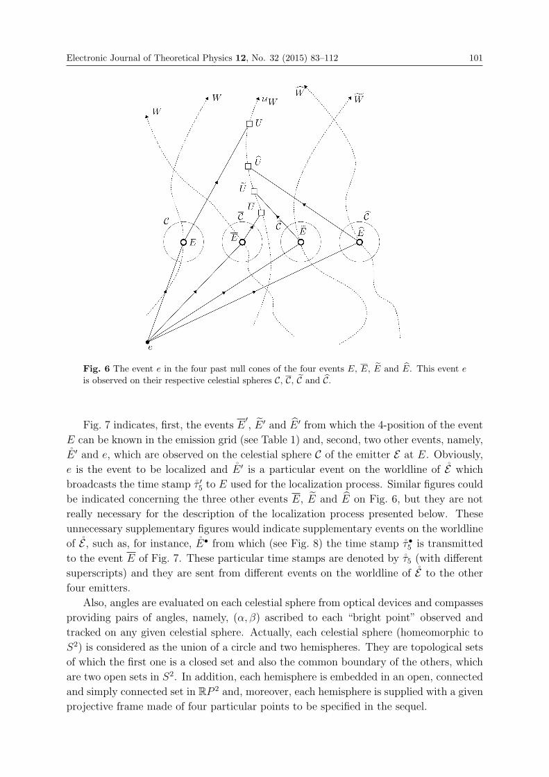
Electronic Journal of Theoretical Physics 12, No. 32 (2015) 83–112 101
Fig. 6 The event e in the four past null cones of the four events E, E, E and E. This event e
is observed on their respective celestial spheres C, C, C and C.
Fig. 7 indicates, first, the events E′, E ′ and E ′ from which the 4-position of the event
E can be known in the emission grid (see Table 1) and, second, two other events, namely,
E ′ and e, which are observed on the celestial sphere C of the emitter E at E. Obviously,
e is the event to be localized and E ′ is a particular event on the worldline of E which
broadcasts the time stamp τ ′5 to E used for the localization process. Similar figures could
be indicated concerning the three other events E, E and E on Fig. 6, but they are not
really necessary for the description of the localization process presented below. These
unnecessary supplementary figures would indicate supplementary events on the worldline
of E , such as, for instance, E• from which (see Fig. 8) the time stamp τ •5 is transmitted
to the event E of Fig. 7. These particular time stamps are denoted by τ5 (with different
superscripts) and they are sent from different events on the worldline of E to the other
four emitters.
Also, angles are evaluated on each celestial sphere from optical devices and compasses
providing pairs of angles, namely, (α, β) ascribed to each “bright point” observed and
tracked on any given celestial sphere. Actually, each celestial sphere (homeomorphic to
S2) is considered as the union of a circle and two hemispheres. They are topological sets
of which the first one is a closed set and also the common boundary of the others, which
are two open sets in S2. In addition, each hemisphere is embedded in an open, connected
and simply connected set in RP 2 and, moreover, each hemisphere is supplied with a given
projective frame made of four particular points to be specified in the sequel.
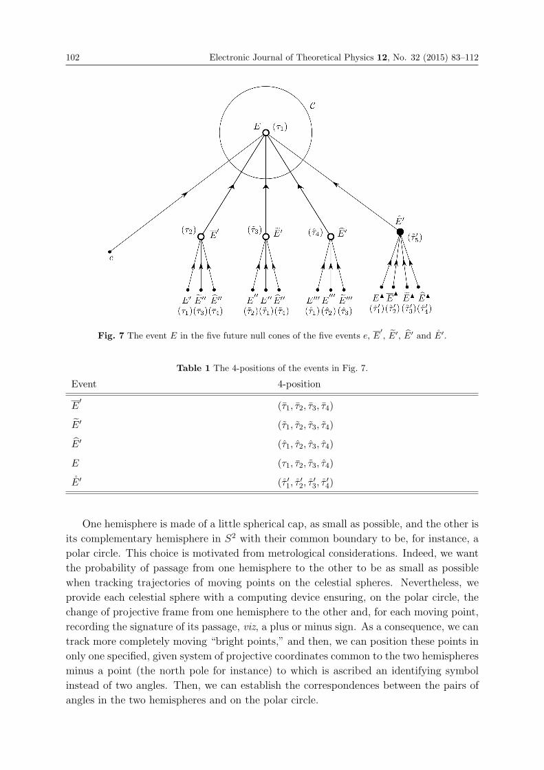
102 Electronic Journal of Theoretical Physics 12, No. 32 (2015) 83–112
Fig. 7 The event E in the five future null cones of the five events e, E′, E′, E′ and E′.
Table 1 The 4-positions of the events in Fig. 7.
Event 4-position
E′
(τ1, τ2, τ3, τ4)
E′ (τ1, τ2, τ3, τ4)
E′ (τ1, τ2, τ3, τ4)
E (τ1, τ2, τ3, τ4)
E′ (τ ′1, τ ′2, τ ′3, τ ′4)
One hemisphere is made of a little spherical cap, as small as possible, and the other is
its complementary hemisphere in S2 with their common boundary to be, for instance, a
polar circle. This choice is motivated from metrological considerations. Indeed, we want
the probability of passage from one hemisphere to the other to be as small as possible
when tracking trajectories of moving points on the celestial spheres. Nevertheless, we
provide each celestial sphere with a computing device ensuring, on the polar circle, the
change of projective frame from one hemisphere to the other and, for each moving point,
recording the signature of its passage, viz, a plus or minus sign. As a consequence, we can
track more completely moving “bright points,” and then, we can position these points in
only one specified, given system of projective coordinates common to the two hemispheres
minus a point (the north pole for instance) to which is ascribed an identifying symbol
instead of two angles. Then, we can establish the correspondences between the pairs of
angles in the two hemispheres and on the polar circle.
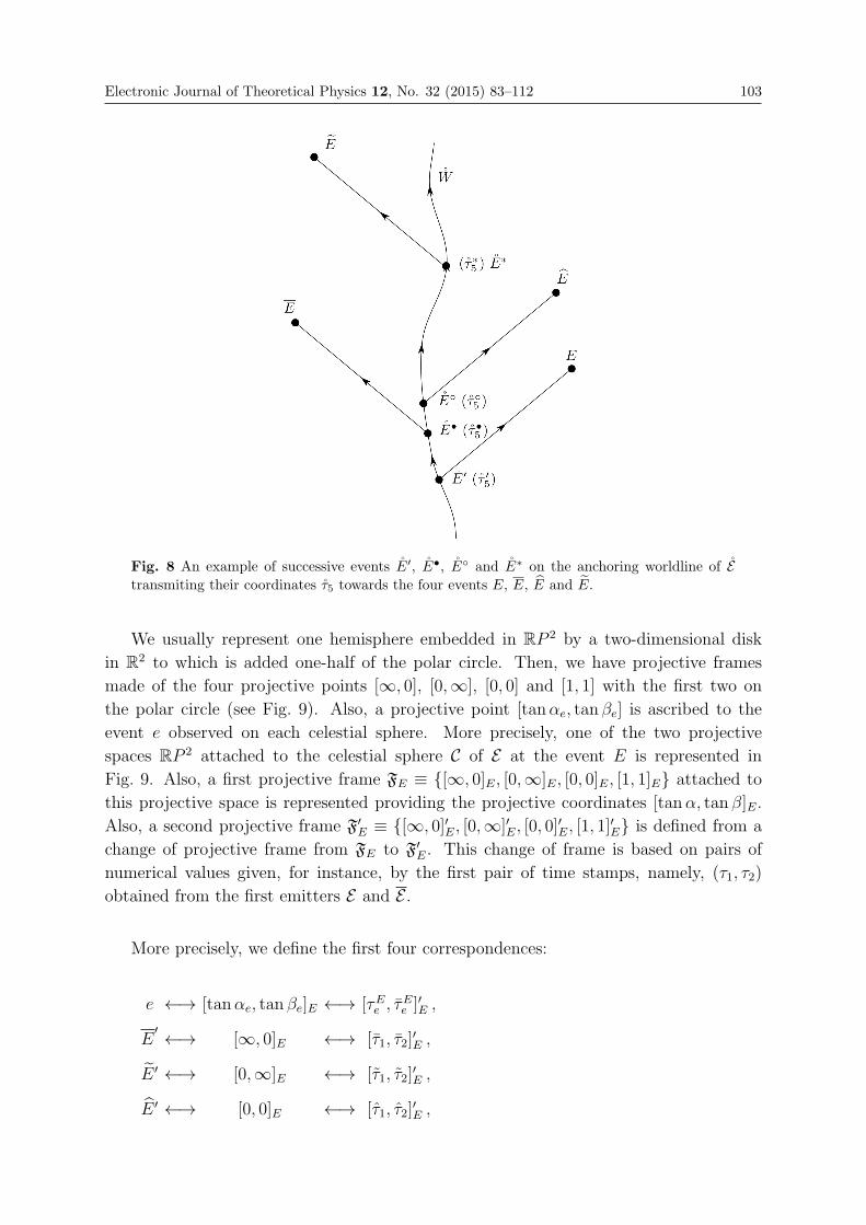
Electronic Journal of Theoretical Physics 12, No. 32 (2015) 83–112 103
Fig. 8 An example of successive events E′, E•, E◦ and E∗ on the anchoring worldline of Etransmiting their coordinates τ5 towards the four events E, E, E and E.
We usually represent one hemisphere embedded in RP 2 by a two-dimensional disk
in R2 to which is added one-half of the polar circle. Then, we have projective frames
made of the four projective points [∞, 0], [0,∞], [0, 0] and [1, 1] with the first two on
the polar circle (see Fig. 9). Also, a projective point [tanαe, tan βe] is ascribed to the
event e observed on each celestial sphere. More precisely, one of the two projective
spaces RP 2 attached to the celestial sphere C of E at the event E is represented in
Fig. 9. Also, a first projective frame FE ≡ {[∞, 0]E, [0,∞]E, [0, 0]E, [1, 1]E} attached to
this projective space is represented providing the projective coordinates [tanα, tan β]E.
Also, a second projective frame F′E ≡ {[∞, 0]′E, [0,∞]′E, [0, 0]′E, [1, 1]
′E} is defined from a
change of projective frame from FE to F′E. This change of frame is based on pairs of
numerical values given, for instance, by the first pair of time stamps, namely, (τ1, τ2)
obtained from the first emitters E and E .
More precisely, we define the first four correspondences:
e ←→ [tanαe, tan βe]E ←→ [τEe , τEe ]′E ,
E′ ←→ [∞, 0]E ←→ [τ1, τ2]
′E ,
E ′ ←→ [0,∞]E ←→ [τ1, τ2]′E ,
E ′ ←→ [0, 0]E ←→ [τ1, τ2]′E ,
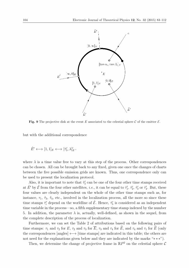
104 Electronic Journal of Theoretical Physics 12, No. 32 (2015) 83–112
Fig. 9 The projective disk at the event E associated to the celestial sphere C of the emitter E .
but with the additional correspondence
E ′ ←→ [1, 1]E ←→ [τ ′5, λ]′E,
where λ is a time value free to vary at this step of the process. Other correspondences
can be chosen. All can be brought back to any fixed, given one once the changes of charts
between the five possible emission grids are known. Thus, one correspondence only can
be used to present the localization protocol.
Also, it is important to note that τ ′5 can be one of the four other time stamps received
at E ′ by E from the four other satellites, i.e., it can be equal to τ ′1, τ′2, τ
′3 or τ
′4. But, these
four values are clearly independent on the whole of the other time stamps such as, for
instance, τ1, τ3, τ4, etc., involved in the localization process, all the more so since these
time stamps τ ′i depend on the worldline of E . Hence, τ ′5 is considered as an independent
time variable in the process—so, a fifth supplementary time stamp indexed by the number
5. In addition, the parameter λ is, actually, well-defined, as shown in the sequel, from
the complete description of the process of localization.
Furthermore, we can set the Table 2 of attributions based on the following pairs of
time stamps: τ1 and τ2 for E, τ2 and τ3 for E, τ3 and τ4 for E, and τ4 and τ1 for E (only
the correspondences [angles]←→ [time stamps] are indicated in this table; the others are
not need for the explanations given below and they are indicated by the marks “∗ ∗ ∗”).Then, we determine the change of projective frame in RP 2 on the celestial sphere C
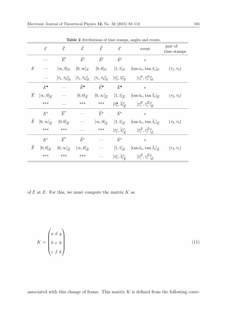
Electronic Journal of Theoretical Physics 12, No. 32 (2015) 83–112 105
Table 2 Attributions of time stamps, angles and events.
E E E E E eventpair of
time stamps
— E′
E′ E′ E′ e
E — [∞, 0]E [0,∞]E [0, 0]E [1, 1]E [tanαe, tanβe]E (τ1, τ2)
— [τ1, τ2]′E [τ1, τ2]
′E [τ1, τ2]
′E [τ ′5, λ]′E [τEe , τEe ]′E
E• — E• E• E• e
E [∞, 0]E — [0, 0]E [0,∞]E [1, 1]E [tan αe, tan βe]E (τ2, τ3)
*** — *** *** [τ•5 , λ]′E [τEe , τEe ]′E
E∗ E∗
— E∗ E∗ e
E [0,∞]˜E
[0, 0]˜E
— [∞, 0]˜E
[1, 1]˜E
[tan αe, tan βe] ˜E (τ3, τ4)
*** *** — *** [τ∗5 , λ]′˜E [τ˜Ee , τ
˜Ee ]′
˜E
E◦ E◦
E◦ — E◦ e
E [0, 0]E
[0,∞]E
[∞, 0]E
— [1, 1]E
[tan αe, tan βe] E (τ4, τ1)
*** *** *** — [τ◦5 , λ]′E [τEe , τ
Ee ]′
E
of E at E. For this, we must compute the matrix K as
K =
⎛⎜⎜⎜⎜⎝a d g
b e h
c f k
⎞⎟⎟⎟⎟⎠ (11)
associated with this change of frame. This matrix K is defined from the following corre-
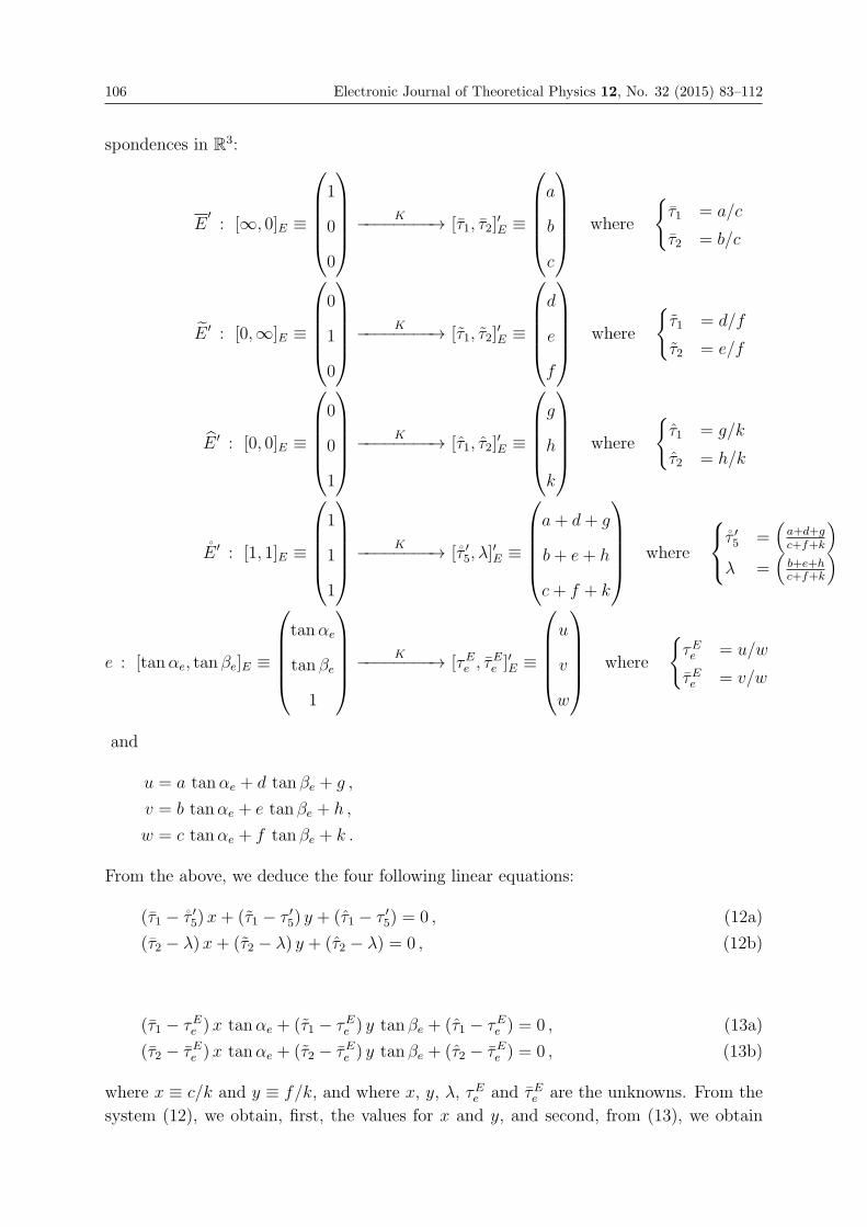
106 Electronic Journal of Theoretical Physics 12, No. 32 (2015) 83–112
spondences in R3:
E′: [∞, 0]E ≡
⎛⎜⎜⎜⎜⎝1
0
0
⎞⎟⎟⎟⎟⎠ K−−−−−−−−→ [τ1, τ2]′E ≡
⎛⎜⎜⎜⎜⎝a
b
c
⎞⎟⎟⎟⎟⎠ where
{τ1 = a/c
τ2 = b/c
E ′ : [0,∞]E ≡
⎛⎜⎜⎜⎜⎝0
1
0
⎞⎟⎟⎟⎟⎠ K−−−−−−−−→ [τ1, τ2]′E ≡
⎛⎜⎜⎜⎜⎝d
e
f
⎞⎟⎟⎟⎟⎠ where
{τ1 = d/f
τ2 = e/f
E ′ : [0, 0]E ≡
⎛⎜⎜⎜⎜⎝0
0
1
⎞⎟⎟⎟⎟⎠ K−−−−−−−−→ [τ1, τ2]′E ≡
⎛⎜⎜⎜⎜⎝g
h
k
⎞⎟⎟⎟⎟⎠ where
{τ1 = g/k
τ2 = h/k
E ′ : [1, 1]E ≡
⎛⎜⎜⎜⎜⎝1
1
1
⎞⎟⎟⎟⎟⎠ K−−−−−−−−→ [τ ′5, λ]′E ≡
⎛⎜⎜⎜⎜⎝a+ d+ g
b+ e+ h
c+ f + k
⎞⎟⎟⎟⎟⎠ where
⎧⎨⎩τ ′5 =(
a+d+gc+f+k
)λ =
(b+e+hc+f+k
)
e : [tanαe, tan βe]E ≡
⎛⎜⎜⎜⎜⎝tanαe
tan βe
1
⎞⎟⎟⎟⎟⎠ K−−−−−−−−→ [τEe , τEe ]′E ≡
⎛⎜⎜⎜⎜⎝u
v
w
⎞⎟⎟⎟⎟⎠ where
{τEe = u/w
τEe = v/w
and
u = a tanαe + d tan βe + g ,
v = b tanαe + e tan βe + h ,
w = c tanαe + f tan βe + k .
From the above, we deduce the four following linear equations:
(τ1 − τ ′5) x+ (τ1 − τ ′5) y + (τ1 − τ ′5) = 0 , (12a)
(τ2 − λ) x+ (τ2 − λ) y + (τ2 − λ) = 0 , (12b)
(τ1 − τEe ) x tanαe + (τ1 − τEe ) y tan βe + (τ1 − τEe ) = 0 , (13a)
(τ2 − τEe ) x tanαe + (τ2 − τEe ) y tan βe + (τ2 − τEe ) = 0 , (13b)
where x ≡ c/k and y ≡ f/k, and where x, y, λ, τEe and τEe are the unknowns. From the
system (12), we obtain, first, the values for x and y, and second, from (13), we obtain
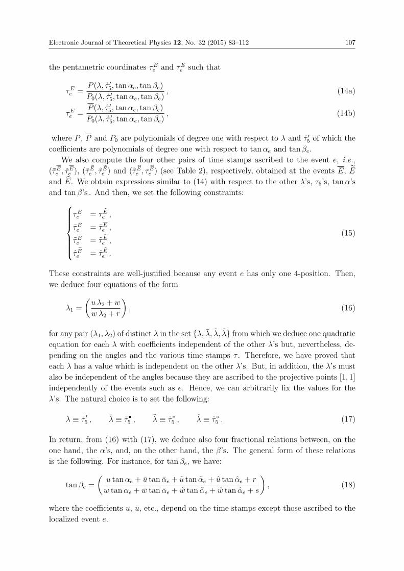
Electronic Journal of Theoretical Physics 12, No. 32 (2015) 83–112 107
the pentametric coordinates τEe and τEe such that
τEe =P (λ, τ ′5, tanαe, tan βe)
P0(λ, τ ′5, tanαe, tan βe), (14a)
τEe =P (λ, τ ′5, tanαe, tan βe)
P0(λ, τ ′5, tanαe, tan βe), (14b)
where P , P and P0 are polynomials of degree one with respect to λ and τ ′5 of which the
coefficients are polynomials of degree one with respect to tanαe and tan βe.
We also compute the four other pairs of time stamps ascribed to the event e, i.e.,
(τEe , τEe ), (τ˜Ee , τ
˜Ee ) and (τ
Ee , τ
Ee ) (see Table 2), respectively, obtained at the events E, E
and E. We obtain expressions similar to (14) with respect to the other λ’s, τ5’s, tanα’s
and tan β’s . And then, we set the following constraints:⎧⎪⎪⎪⎪⎪⎨⎪⎪⎪⎪⎪⎩τEe = τ
Ee ,
τEe = τEe ,
τEe = τ˜Ee ,
τ˜Ee = τ
Ee .
(15)
These constraints are well-justified because any event e has only one 4-position. Then,
we deduce four equations of the form
λ1 =
(uλ2 + w
w λ2 + r
), (16)
for any pair (λ1, λ2) of distinct λ in the set {λ, λ, λ, λ} from which we deduce one quadratic
equation for each λ with coefficients independent of the other λ’s but, nevertheless, de-
pending on the angles and the various time stamps τ . Therefore, we have proved that
each λ has a value which is independent on the other λ’s. But, in addition, the λ’s must
also be independent of the angles because they are ascribed to the projective points [1, 1]
independently of the events such as e. Hence, we can arbitrarily fix the values for the
λ’s. The natural choice is to set the following:
λ ≡ τ ′5 , λ ≡ τ •5 , λ ≡ τ ∗5 , λ ≡ τ ◦5 . (17)
In return, from (16) with (17), we deduce also four fractional relations between, on the
one hand, the α’s, and, on the other hand, the β’s. The general form of these relations
is the following. For instance, for tan βe, we have:
tan βe =
(u tanαe + u tan αe + u tan αe + u tan αe + r
w tanαe + w tan αe + w tan αe + w tan αe + s
), (18)
where the coefficients u, u, etc., depend on the time stamps except those ascribed to the
localized event e.
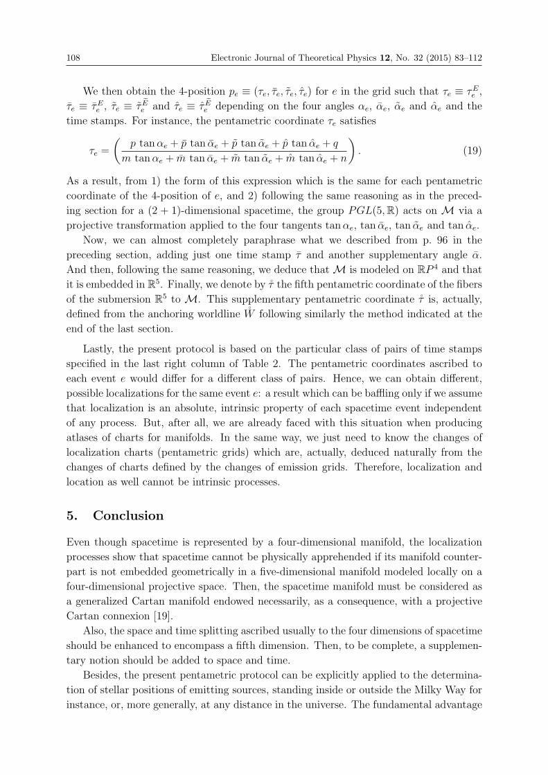
108 Electronic Journal of Theoretical Physics 12, No. 32 (2015) 83–112
We then obtain the 4-position pe ≡ (τe, τe, τe, τe) for e in the grid such that τe ≡ τEe ,
τe ≡ τEe , τe ≡ τ˜Ee and τe ≡ τ
˜Ee depending on the four angles αe, αe, αe and αe and the
time stamps. For instance, the pentametric coordinate τe satisfies
τe =
(p tanαe + p tan αe + p tan αe + p tan αe + q
m tanαe + m tan αe + m tan αe + m tan αe + n
). (19)
As a result, from 1) the form of this expression which is the same for each pentametric
coordinate of the 4-position of e, and 2) following the same reasoning as in the preced-
ing section for a (2 + 1)-dimensional spacetime, the group PGL(5,R) acts on M via a
projective transformation applied to the four tangents tanαe, tan αe, tan αe and tan αe.
Now, we can almost completely paraphrase what we described from p. 96 in the
preceding section, adding just one time stamp τ and another supplementary angle α.
And then, following the same reasoning, we deduce thatM is modeled on RP 4 and that
it is embedded in R5. Finally, we denote by τ the fifth pentametric coordinate of the fibers
of the submersion R5 to M. This supplementary pentametric coordinate τ is, actually,
defined from the anchoring worldline W following similarly the method indicated at the
end of the last section.
Lastly, the present protocol is based on the particular class of pairs of time stamps
specified in the last right column of Table 2. The pentametric coordinates ascribed to
each event e would differ for a different class of pairs. Hence, we can obtain different,
possible localizations for the same event e: a result which can be baffling only if we assume
that localization is an absolute, intrinsic property of each spacetime event independent
of any process. But, after all, we are already faced with this situation when producing
atlases of charts for manifolds. In the same way, we just need to know the changes of
localization charts (pentametric grids) which are, actually, deduced naturally from the
changes of charts defined by the changes of emission grids. Therefore, localization and
location as well cannot be intrinsic processes.
5. Conclusion
Even though spacetime is represented by a four-dimensional manifold, the localization
processes show that spacetime cannot be physically apprehended if its manifold counter-
part is not embedded geometrically in a five-dimensional manifold modeled locally on a
four-dimensional projective space. Then, the spacetime manifold must be considered as
a generalized Cartan manifold endowed necessarily, as a consequence, with a projective
Cartan connexion [19].
Also, the space and time splitting ascribed usually to the four dimensions of spacetime
should be enhanced to encompass a fifth dimension. Then, to be complete, a supplemen-
tary notion should be added to space and time.
Besides, the present pentametric protocol can be explicitly applied to the determina-
tion of stellar positions of emitting sources, standing inside or outside the Milky Way for
instance, or, more generally, at any distance in the universe. The fundamental advantage
Electronic Journal of Theoretical Physics 12, No. 32 (2015) 83–112 109
of this protocol is that patterns of, for instance, starfields can be obtained directly with no
use of any intermediate method or model of light bending by massive stellar bodies such
as the PPN method for instance [22, 23, 24, 25, 26, 27]. With the pentametric protocol,
the evaluations of the patterns of starfields are direct (no mathematical simulations) since
the stellar positions are not obtained from measurements of spatial parallaxes followed
by a simulated model-dependent reconstruction of the light ray trajectories. Moreover,
the pentametric localization protocol provides spacetime positions which encompass and
are sensitive to the whole of physical phenomena producing light ray deflections. Hence,
these spacetime positions are, somehow, “nature-dependent” (e.g., Jupiter in [25]) mean-
ing not absolute in an abstract way and meaning also that they follow what we call the
“Whitehead’s paradigm” on the systems of measurements (see pp.196–197, Chap. IX,
“The Ultimate Physical Concepts” in [28]):
“ Furthermore the admission of stratifications of nature bears on the formulation of
the laws of nature. It has been laid down that these laws are to be expressed in dif-
ferential equations which, as expressed in any general system of measurement, should
bear no reference to any other particular measure-system. This requirement is purely
arbitrary. For a measure-system measures something inherent in nature; otherwise it
has no connexion with nature at all. And that something which is measured by a par-
ticular measure-system may have a special relation to the phenomenon whose law is
being formulated. For example the gravitational field due to a material object at rest in
a certain time-system may be expected to exhibit in its formulation particular reference
to spatial and temporal quantities of that time-system. The field can of course be ex-
pressed in any measure-systems, but the particular reference will remain as the simple
physical explanation.”
And this paradigm is, in some way, the opposite of the “Hilbert’s paradigm” inherent to
the present day general relativity (see p.61 in [29]):
“Was nun das Kausalitatsprinzip betrifft, so mogen fur die Gegenwart in irgend einem
gegebenen Koordinatensystem die physikalischen Großen und ihre zeitlichen Ableitun-
gen bekannt sein: dann wird eine Aussage nur physikalischen Sinn haben, wenn sie
gegenuber allen denjenigen Transformationen invariant ist, bei denen eben die fur
die Gegenwart benutzten Koordinaten unverandert bleiben; ich behaupte, daß die
Aussagen dieser Art fur die Zukunft samtlich eindeutig bestimmt sind d. h. das
Kausalitatsprinzip gilt in dieser Fassung:
Aus der Kenntnis der 14 physikalischen Potential gμν, qs in der Gegenwart folgen alle
Aussagen uber dieselben fur die Zukunft notwendig und eindeutig, sofern sie physikalis-
chen Sinn haben.”6
6 “As for the principle of causality, the physical quantities and their time-rates of change may be known
at the present time in any given coordinate system; a prediction will then have a physical meaning only
when it is invariant with respect to all those transformations for which exactly those coordinates used for
the present time remain unchanged. I declare that predictions of this kind for the future are all uniquely
determined; that is, that the causality principle holds in this formulation:
From the knowledge of the 14 physical potentials gμν , qs, in the present, all predictions about the same
quantities in the future follow necessarily and uniquely insofar as they have physical meaning.”(translation
110 Electronic Journal of Theoretical Physics 12, No. 32 (2015) 83–112
References
[1] T. B. Bahder, Navigation in curved space–time, Amer. J. Math. 69(3), 315–321(2001).
[2] M. Blagojevic, J. Garecki, F. Hehl, and Y. Obukhov, Real null coframes in generalrelativity and GPS type coordinates, Phys. Rev. D 65(4), 044018(6) (2002).
[3] B. Coll, Relativistic positioning systems: Perspectives and prospects,arXiv:1302.5782v1 [gr-qc] (2013).
[4] C. Rovelli, GPS observables in general relativity, Phys. Rev. D 65(4), 044017(6)(2002).
[5] B. Coll and A. Tarantola, A Galactic Positioning System, in Proceedings ofthe “Journees Systemes de Reference Spatio-Temporels” (JSR-2003), edited byA. Finkelstein and N. Capitaine, pages 333–334, St. Petersburg, Russia, 22–25September 2003, Institute of Applied Astronomy, St.-Petersburg.
[6] J. Ehlers, F. Pirani, and A. Schild, The geometry of free fall and light propagation,in General relativity, papers in honour of J.L. Synge, edited by L. O’Raifeartaigh,pages 63–84, Oxford, 1972, Clarendon Press.
[7] S. Hawking, A. King, and P. McCarthy, A new topology for curved space-time whichincorporates the causal, differential, and conformal structures, J. Math. Phys. 17(2),174–181 (1976).
[8] E. Kronheimer and R. Penrose, On the structure of causal spaces, Math. Proc.Cambridge 63(2), 481–501 (1967).
[9] D. Malament, The class of continuous timelike curves determines the topology ofspacetime, J. Math. Phys. 18(7), 1399–1404 (1977).
[10] N. Woodhouse, The differential and causal structures of space-time, J. Math. Phys.14(4), 495–501 (1973).
[11] B. Coll, Elements for a Theory of Relativistic Coordinate Systems: Formal andPhysical Aspects, in Reference Frames and Gravitomagnetism, edited by J.-F.Pascual-Sanchez, L. Florıa, A. S. Miguel, and F. Vicente, Proceedings of the XXIIISpanish Relativity Meeting (EREs2000), pages 53–65, World Scientific PublishingCompany, Incorporated, (Valladolid, 6–9 September 2000) 2001.
[12] B. Coll, A Principal Positioning System for the Earth, in Proceedings of the“Journees 2002 Systemes de Reference Spatio-Temporels (JSR-2002) – “Astrometryfrom ground and from space”, edited by N. Capitaine and M. Stavinschi, volume 14,pages 34–38, Bucharest, Romania, 25–28 September 2002, Astronomical Institute ofthe Romanian Academy and Observatoire de Paris.
[13] B. Coll and J. Pozo, Relativistic positioning systems: the emission coordinates, Class.Quant. Grav. 23(24), 7395–7416 (2006).
[14] B. Coll, J. Ferrando, and J. Morales-Lladosa, Newtonian and relativistic emissioncoordinates, Phys. Rev. D 80(6), 064038–1–064038–10 (2009).
[15] E. Schrodinger, Measurement of Length and Angle in Quantum Mechanics, Nature173, 442 (1954).
given p.434 in [30])
Electronic Journal of Theoretical Physics 12, No. 32 (2015) 83–112 111
[16] S. Shepard, Quantum phase measurements and a general method for the simulationof random processes, Nonlinear Anal. 71, e1160–e1168 (2009).
[17] A. Garcıa-Parrado and J. Senovilla, Causal structures and causal boundaries, Class.Quant. Grav. 22(9), R1–R84 (2005).
[18] E. Cartan, Les groupes d’holonomie des espaces generalises, Acta Math. 48(1–2),1–42 (1925).
[19] C. Ehresmann, Les connexions infinitesimales dans un espace fibre differentiable,Seminaire N. Bourbaki, 1948–1951, Vol. 1, Exp. no. 24, 153–168 (1950).
[20] B. C. van Fraassen, The Manifest Image and the Scientific Image,in Einstein Meets Magritte : The White Book – An InterdisciplinaryReflection, edited by D. Aerts, pages 29–52, Dordrecht : Kluwer, 1999,http://webware.princeton.edu/vanfraas/mss/manifest.htm.
[21] C. Rosset, The Real and its Double, Seagull Books, London, New York, 2012.
[22] M. T. Crosta, A. Vecchiato, F. de Felice, M. G. Lattanzi, and B. Bucciarelli, Someaspects of relativistic astrometry from within the Solar System, Celestial Mech. 87,209–218 (2003).
[23] E. Fomalont and S. Kopeikin, The measurement of the light deflection from Jupiter:experimental results, Astrophys. J. 598(1), 704 (2003).
[24] F. De Felice, M. Crosta, A. Vecchiato, M. Lattanzi, and B. Bucciarelli, A generalrelativistic model of light propagation in the gravitational field of the solar system:the static case, Astrophys. J. 607(1), 580 (2004).
[25] M. Crosta and F. Mignard, Microarcsecond light bending by Jupiter, Class. Quant.Grav. 23(15), 4853 (2006).
[26] M. Crosta, Tracing light propagation to the intrinsic accuracy of spacetime geometry,Class. Quant. Grav. 28(23), 235013 (2011).
[27] S. Kopeikin and E. Fomalont, Gravimagnetism, causality, and aberration of gravity inthe gravitational light-ray deflection experiments, Gen. Rel. Grav. 39(10), 1583–1624(2008).
[28] A. N. Whitehead, The Concept of Nature, Tarner lectures, Cambridge UniversityPress, Cambridge, UK, 1920.
[29] D. Hilbert, Die Grundlagen der Physik. (Zweite Mitteilung.), Nachr. Konigl. Gesell.Wiss. Gottingen, Math.-Phys. Kl. 1917(1), 53–76 (1917).
[30] C. Misner, K. Thorne, and J. Wheeler, Gravitation, W. H. Freeman and Compagny,San Francisco, 1973.

EJTP 12, No. 32 (2015) 113–120 Electronic Journal of Theoretical Physics
Theoretical Calculations for PredictedStates of Heavy Quarkonium ViaNon-Relativistic Frame Work
T. A. Nahool1∗, A. M. Yasser1† and G. S. Hassan2‡
1Physics Department, Faculty of Science at Qena, South Valley University, Egypt2Physics Department, Faculty of Science, Assuit University, Egypt
Received 18 October 2014, Accepted 20 December 2014, Published 10 January 2015
Abstract: We calculate the mass spectra of heavy quarkonium by using matrix Numerov’s
method to make the predictions of F and G states for further experiments. The method gives
a very reasonable result which is in a good agreement with other methods and with recently
published theoretical data. From the yielded wave functions we calculate the root mean square
radius rms and β coefficients of heavy quarkoniumc© Electronic Journal of Theoretical Physics. All rights reserved.
Keywords: Quark Model; heavy quarkonium; Numerov’s method
PACS (2010): 12.40.Yx, 14.40.Pq, 02.60.Cb, 12.39.Jh
1. Introduction
The theoretical studies of the heavy quarkonium system [1] and its applications to bot-
tomonium [2] and char-monium [3] is one of the special interest because of its relies
entirely on the first principles of quantum chromo dynamics( QCD). From the view-
point of the ”heavy quarkonium” spectra, we calculate the theoretical mass spectra via
non-relativistic frame work [4], [5], [6] by using matrix Numerov’s method [7], [8] in two
levels F and G. Many studies investigate ”heavy quarkonium” properties within the quark
model [9-15]. An essential progress has been made in the theoretical investigation of the
non-relativistic heavy quark dynamics. Our point of departure is to calculate the spectra
of heavy quarkonium and the corresponding wave functions of nn states (n = c, b) for
the predicted F and G states. Actually, we dont have any experimental data of F and G
∗ Email:[email protected]† Email:[email protected]‡ Email: [email protected]
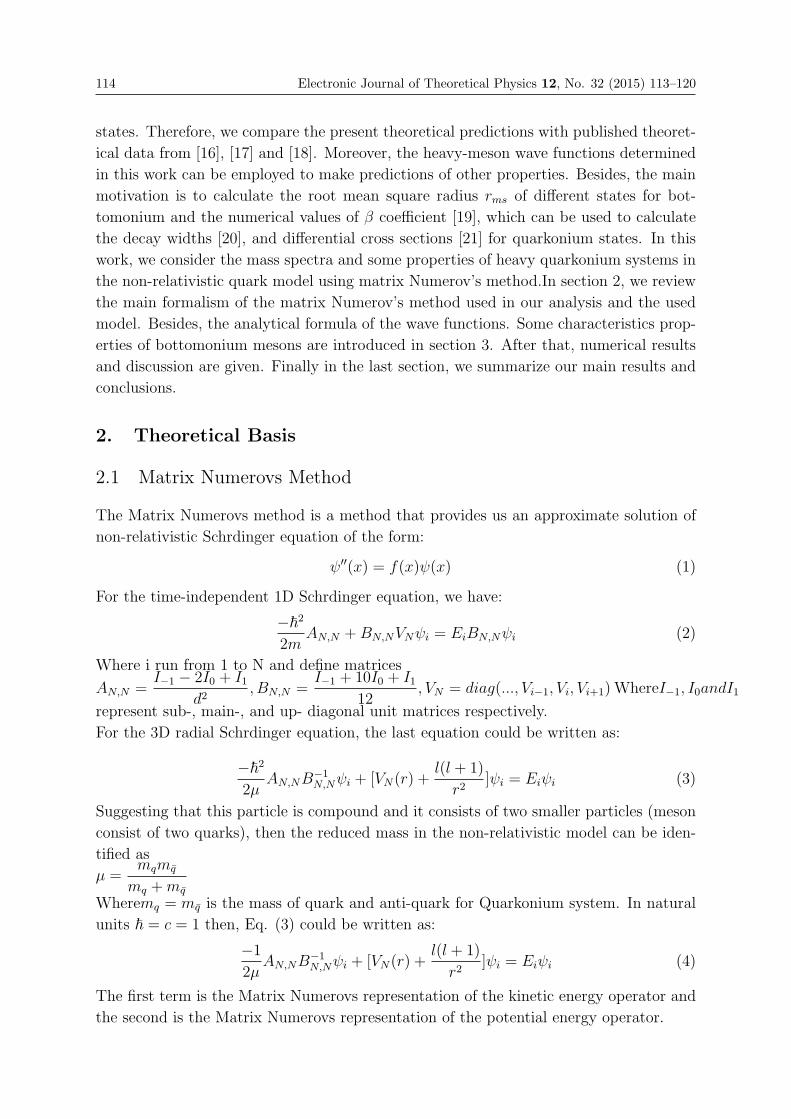
114 Electronic Journal of Theoretical Physics 12, No. 32 (2015) 113–120
states. Therefore, we compare the present theoretical predictions with published theoret-
ical data from [16], [17] and [18]. Moreover, the heavy-meson wave functions determined
in this work can be employed to make predictions of other properties. Besides, the main
motivation is to calculate the root mean square radius rms of different states for bot-
tomonium and the numerical values of β coefficient [19], which can be used to calculate
the decay widths [20], and differential cross sections [21] for quarkonium states. In this
work, we consider the mass spectra and some properties of heavy quarkonium systems in
the non-relativistic quark model using matrix Numerov’s method.In section 2, we review
the main formalism of the matrix Numerov’s method used in our analysis and the used
model. Besides, the analytical formula of the wave functions. Some characteristics prop-
erties of bottomonium mesons are introduced in section 3. After that, numerical results
and discussion are given. Finally in the last section, we summarize our main results and
conclusions.
2. Theoretical Basis
2.1 Matrix Numerovs Method
The Matrix Numerovs method is a method that provides us an approximate solution of
non-relativistic Schrdinger equation of the form:
ψ′′(x) = f(x)ψ(x) (1)
For the time-independent 1D Schrdinger equation, we have:
−�22m
AN,N +BN,NVNψi = EiBN,Nψi (2)
Where i run from 1 to N and define matrices
AN,N =I−1 − 2I0 + I1
d2, BN,N =
I−1 + 10I0 + I112
, VN = diag(..., Vi−1, Vi, Vi+1) WhereI−1, I0andI1represent sub-, main-, and up- diagonal unit matrices respectively.
For the 3D radial Schrdinger equation, the last equation could be written as:
−�22μ
AN,NB−1N,Nψi + [VN(r) +
l(l + 1)
r2]ψi = Eiψi (3)
Suggesting that this particle is compound and it consists of two smaller particles (meson
consist of two quarks), then the reduced mass in the non-relativistic model can be iden-
tified as
μ =mqmq
mq +mq
Wheremq = mq is the mass of quark and anti-quark for Quarkonium system. In natural
units � = c = 1 then, Eq. (3) could be written as:
−12μ
AN,NB−1N,Nψi + [VN(r) +
l(l + 1)
r2]ψi = Eiψi (4)
The first term is the Matrix Numerovs representation of the kinetic energy operator and
the second is the Matrix Numerovs representation of the potential energy operator.
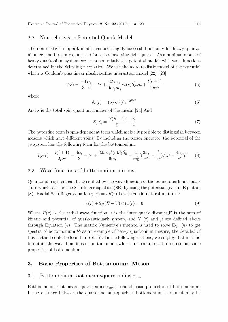
Electronic Journal of Theoretical Physics 12, No. 32 (2015) 113–120 115
2.2 Non-relativistic Potential Quark Model
The non-relativistic quark model has been highly successful not only for heavy quarko-
nium cc and bb states, but also for states involving light quarks. As a minimal model of
heavy quarkonium system, we use a non relativistic potential model, with wave functions
determined by the Schrdinger equation. We use the more realistic model of the potential
which is Coulomb plus linear plushyperfine interaction model [22], [23]
V(r) =−43
αs
r+ br +
32παs
9mqmq
δσ(r)�Sq.�Sq +l(l + 1)
2μr2(5)
where
δσ(r) = (σ/√π)3e−σ
2r2 (6)
And s is the total spin quantum number of the meson [24] And
SqSq =S(S + 1)
2− 3
4(7)
The hyperfine term is spin-dependent term which makes it possible to distinguish between
mesons which have different spins. By including the tensor operator, the potential of the
qq system has the following form for the bottomonium:
VN(r) =l(l + 1)
2μr2− 4αs
3+ br +
32παsδ(r)SbSb
9mb
+1
m2b
[(2αs
r3− b
2r)�L.�S +
4αs
r3T ] (8)
2.3 Wave functions of bottomonium mesons
Quarkonium system can be described by the wave function of the bound quark-antiquark
state which satisfies the Schrdinger equation (SE) by using the potential given in Equation
(8). Radial Schrdinger equation,ψ(r) = rR(r) is written (in natural units) as:
ψ(r) + 2μ(E − V (r))ψ(r) = 0 (9)
Where R(r) is the radial wave function, r is the inter quark distance,E is the sum of
kinetic and potential of quark-antiquark system, and V (r) and μ are defined above
through Equation (8). The matrix Numerove’s method is used to solve Eq. (8) to get
spectra of bottomonium bb as an example of heavy quarkonium mesons, the detailed of
this method could be found in Ref. [7]. In the following sections, we employ that method
to obtain the wave functions of bottomonium which in turn are used to determine some
properties of bottomonium.
3. Basic Properties of Bottomonium Meson
3.1 Bottomonium root mean square radius rms
Bottomonium root mean square radius rms is one of basic properties of bottomonium.
If the distance between the quark and anti-quark in bottomonium is r fm it may be
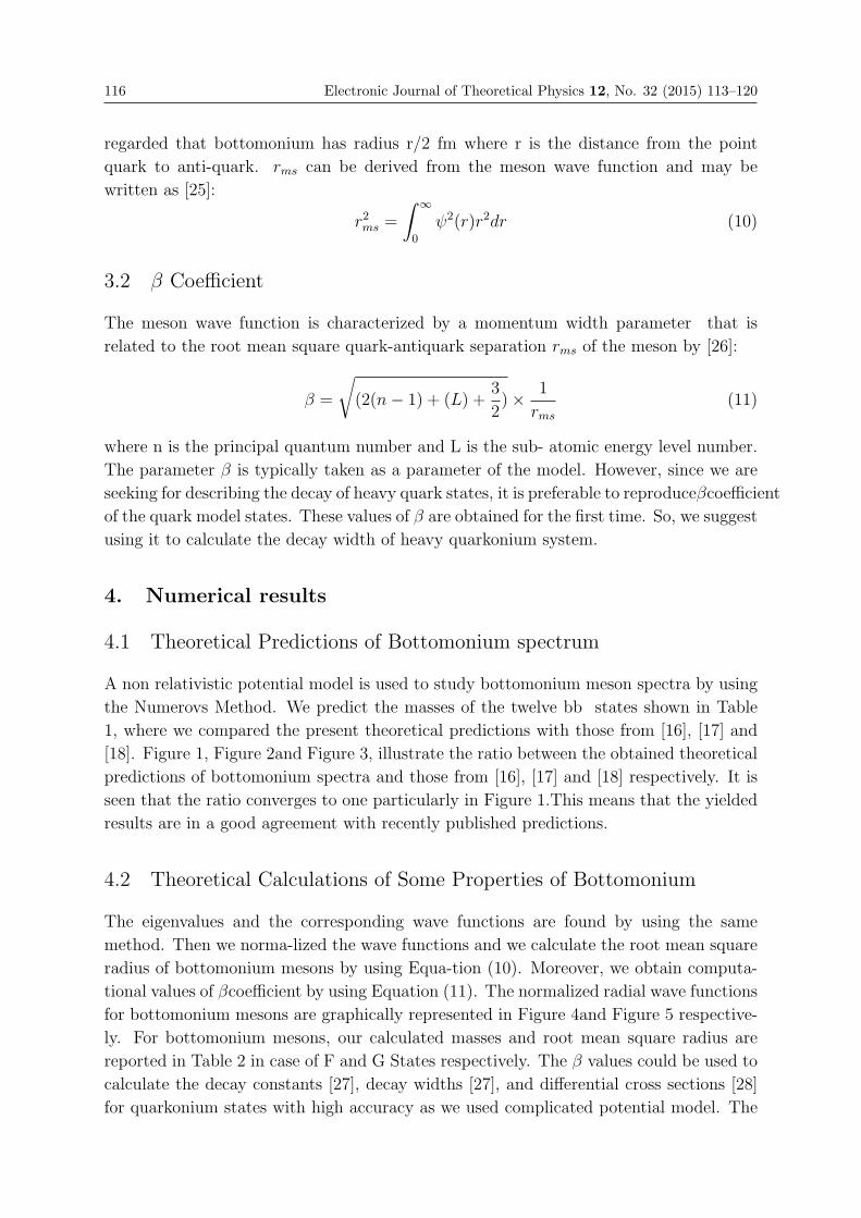
116 Electronic Journal of Theoretical Physics 12, No. 32 (2015) 113–120
regarded that bottomonium has radius r/2 fm where r is the distance from the point
quark to anti-quark. rms can be derived from the meson wave function and may be
written as [25]:
r2ms =
∫ ∞
0
ψ2(r)r2dr (10)
3.2 β Coefficient
The meson wave function is characterized by a momentum width parameter that is
related to the root mean square quark-antiquark separation rms of the meson by [26]:
β =
√(2(n− 1) + (L) +
3
2)× 1
rms
(11)
where n is the principal quantum number and L is the sub- atomic energy level number.
The parameter β is typically taken as a parameter of the model. However, since we are
seeking for describing the decay of heavy quark states, it is preferable to reproduceβcoefficient
of the quark model states. These values of β are obtained for the first time. So, we suggest
using it to calculate the decay width of heavy quarkonium system.
4. Numerical results
4.1 Theoretical Predictions of Bottomonium spectrum
A non relativistic potential model is used to study bottomonium meson spectra by using
the Numerovs Method. We predict the masses of the twelve bb states shown in Table
1, where we compared the present theoretical predictions with those from [16], [17] and
[18]. Figure 1, Figure 2and Figure 3, illustrate the ratio between the obtained theoretical
predictions of bottomonium spectra and those from [16], [17] and [18] respectively. It is
seen that the ratio converges to one particularly in Figure 1.This means that the yielded
results are in a good agreement with recently published predictions.
4.2 Theoretical Calculations of Some Properties of Bottomonium
The eigenvalues and the corresponding wave functions are found by using the same
method. Then we norma-lized the wave functions and we calculate the root mean square
radius of bottomonium mesons by using Equa-tion (10). Moreover, we obtain computa-
tional values of βcoefficient by using Equation (11). The normalized radial wave functions
for bottomonium mesons are graphically represented in Figure 4and Figure 5 respective-
ly. For bottomonium mesons, our calculated masses and root mean square radius are
reported in Table 2 in case of F and G States respectively. The β values could be used to
calculate the decay constants [27], decay widths [27], and differential cross sections [28]
for quarkonium states with high accuracy as we used complicated potential model. The
Electronic Journal of Theoretical Physics 12, No. 32 (2015) 113–120 117
predictions about these quantities are also reported in Table 2 for bottomonium F and
G States respectively.
4.3 Figures and Tables
Fig. 1 Ratios of the obtained theoretical masses of bottomonium F and G states to the theoreticaldata in [18].
Fig. 2 Ratios of the obtained theoretical masses of bottomonium F state to the theoretical datain [16].
Fig. 3 Ratios of the obtained theoretical masses of bottomonium F state to the theoretical datain [17].
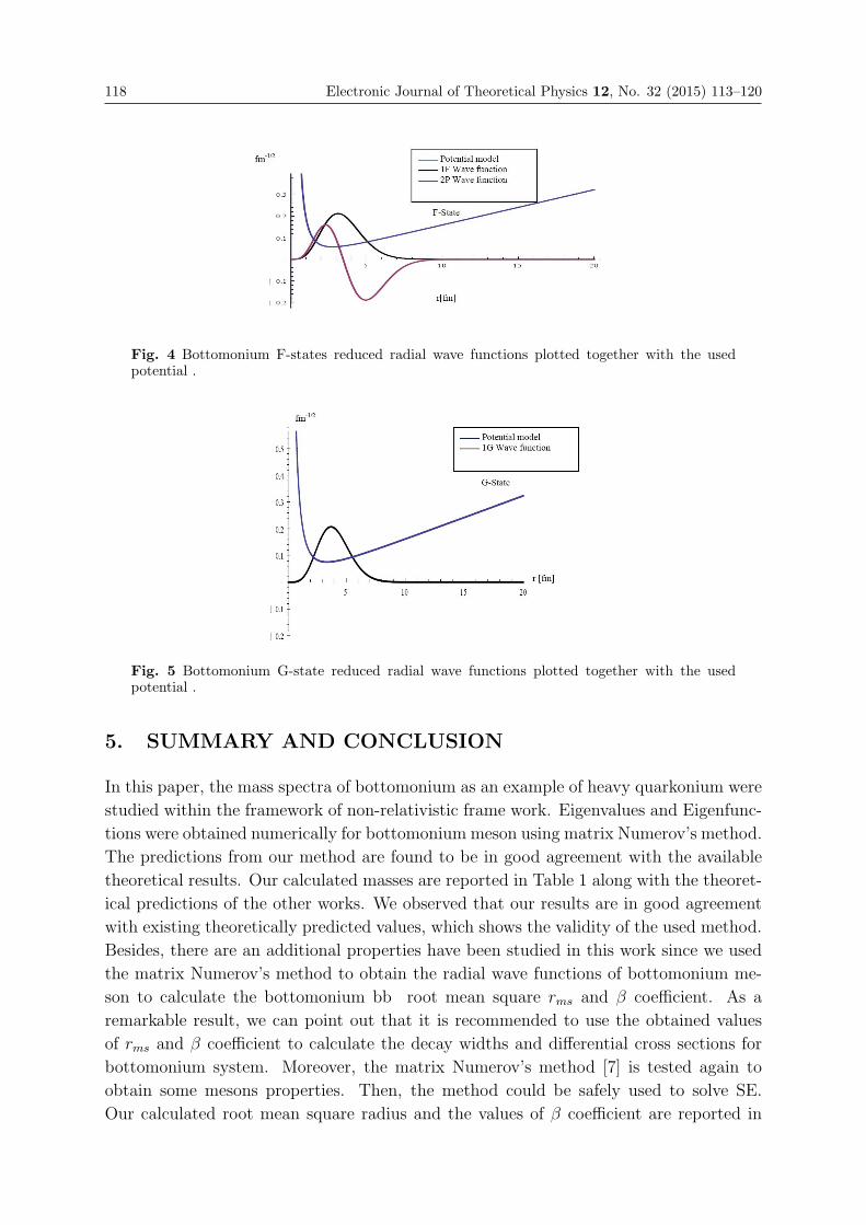
118 Electronic Journal of Theoretical Physics 12, No. 32 (2015) 113–120
Fig. 4 Bottomonium F-states reduced radial wave functions plotted together with the usedpotential .
Fig. 5 Bottomonium G-state reduced radial wave functions plotted together with the usedpotential .
5. SUMMARY AND CONCLUSION
In this paper, the mass spectra of bottomonium as an example of heavy quarkonium were
studied within the framework of non-relativistic frame work. Eigenvalues and Eigenfunc-
tions were obtained numerically for bottomonium meson using matrix Numerov’s method.
The predictions from our method are found to be in good agreement with the available
theoretical results. Our calculated masses are reported in Table 1 along with the theoret-
ical predictions of the other works. We observed that our results are in good agreement
with existing theoretically predicted values, which shows the validity of the used method.
Besides, there are an additional properties have been studied in this work since we used
the matrix Numerov’s method to obtain the radial wave functions of bottomonium me-
son to calculate the bottomonium bb root mean square rms and β coefficient. As a
remarkable result, we can point out that it is recommended to use the obtained values
of rms and β coefficient to calculate the decay widths and differential cross sections for
bottomonium system. Moreover, the matrix Numerov’s method [7] is tested again to
obtain some mesons properties. Then, the method could be safely used to solve SE.
Our calculated root mean square radius and the values of β coefficient are reported in
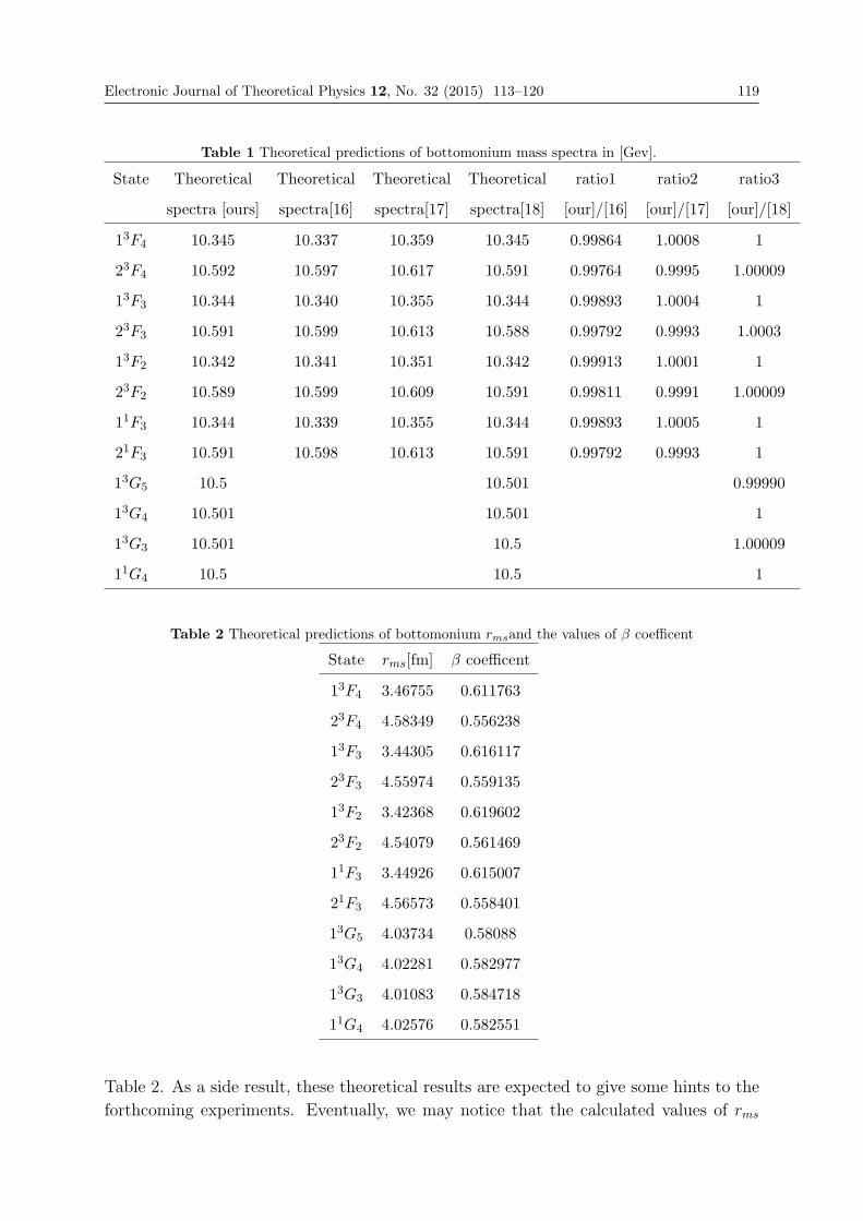
Electronic Journal of Theoretical Physics 12, No. 32 (2015) 113–120 119
Table 1 Theoretical predictions of bottomonium mass spectra in [Gev].
State Theoretical Theoretical Theoretical Theoretical ratio1 ratio2 ratio3
spectra [ours] spectra[16] spectra[17] spectra[18] [our]/[16] [our]/[17] [our]/[18]
13F4 10.345 10.337 10.359 10.345 0.99864 1.0008 1
23F4 10.592 10.597 10.617 10.591 0.99764 0.9995 1.00009
13F3 10.344 10.340 10.355 10.344 0.99893 1.0004 1
23F3 10.591 10.599 10.613 10.588 0.99792 0.9993 1.0003
13F2 10.342 10.341 10.351 10.342 0.99913 1.0001 1
23F2 10.589 10.599 10.609 10.591 0.99811 0.9991 1.00009
11F3 10.344 10.339 10.355 10.344 0.99893 1.0005 1
21F3 10.591 10.598 10.613 10.591 0.99792 0.9993 1
13G5 10.5 10.501 0.99990
13G4 10.501 10.501 1
13G3 10.501 10.5 1.00009
11G4 10.5 10.5 1
Table 2 Theoretical predictions of bottomonium rmsand the values of β coefficent
State rms[fm] β coefficent
13F4 3.46755 0.611763
23F4 4.58349 0.556238
13F3 3.44305 0.616117
23F3 4.55974 0.559135
13F2 3.42368 0.619602
23F2 4.54079 0.561469
11F3 3.44926 0.615007
21F3 4.56573 0.558401
13G5 4.03734 0.58088
13G4 4.02281 0.582977
13G3 4.01083 0.584718
11G4 4.02576 0.582551
Table 2. As a side result, these theoretical results are expected to give some hints to the
forthcoming experiments. Eventually, we may notice that the calculated values of rms
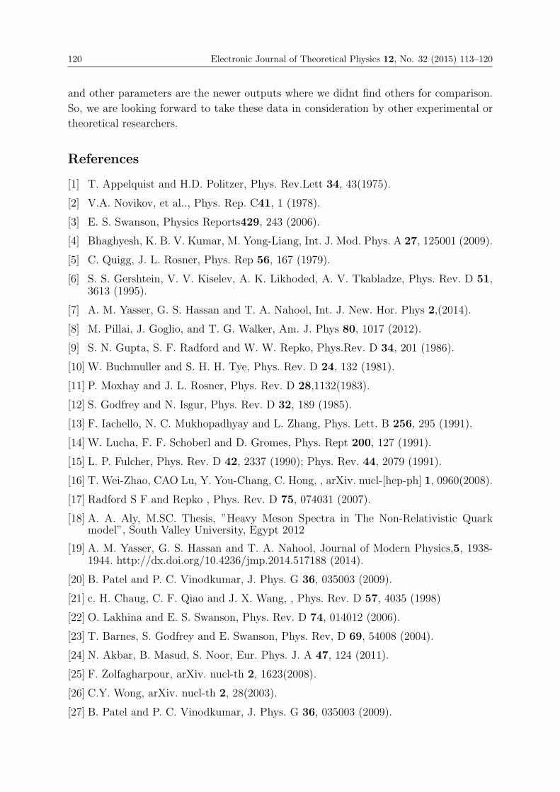
120 Electronic Journal of Theoretical Physics 12, No. 32 (2015) 113–120
and other parameters are the newer outputs where we didnt find others for comparison.
So, we are looking forward to take these data in consideration by other experimental or
theoretical researchers.
References
[1] T. Appelquist and H.D. Politzer, Phys. Rev.Lett 34, 43(1975).
[2] V.A. Novikov, et al.., Phys. Rep. C41, 1 (1978).
[3] E. S. Swanson, Physics Reports429, 243 (2006).
[4] Bhaghyesh, K. B. V. Kumar, M. Yong-Liang, Int. J. Mod. Phys. A 27, 125001 (2009).
[5] C. Quigg, J. L. Rosner, Phys. Rep 56, 167 (1979).
[6] S. S. Gershtein, V. V. Kiselev, A. K. Likhoded, A. V. Tkabladze, Phys. Rev. D 51,3613 (1995).
[7] A. M. Yasser, G. S. Hassan and T. A. Nahool, Int. J. New. Hor. Phys 2,(2014).
[8] M. Pillai, J. Goglio, and T. G. Walker, Am. J. Phys 80, 1017 (2012).
[9] S. N. Gupta, S. F. Radford and W. W. Repko, Phys.Rev. D 34, 201 (1986).
[10] W. Buchmuller and S. H. H. Tye, Phys. Rev. D 24, 132 (1981).
[11] P. Moxhay and J. L. Rosner, Phys. Rev. D 28,1132(1983).
[12] S. Godfrey and N. Isgur, Phys. Rev. D 32, 189 (1985).
[13] F. Iachello, N. C. Mukhopadhyay and L. Zhang, Phys. Lett. B 256, 295 (1991).
[14] W. Lucha, F. F. Schoberl and D. Gromes, Phys. Rept 200, 127 (1991).
[15] L. P. Fulcher, Phys. Rev. D 42, 2337 (1990); Phys. Rev. 44, 2079 (1991).
[16] T. Wei-Zhao, CAO Lu, Y. You-Chang, C. Hong, , arXiv. nucl-[hep-ph] 1, 0960(2008).
[17] Radford S F and Repko , Phys. Rev. D 75, 074031 (2007).
[18] A. A. Aly, M.SC. Thesis, ”Heavy Meson Spectra in The Non-Relativistic Quarkmodel”, South Valley University, Egypt 2012
[19] A. M. Yasser, G. S. Hassan and T. A. Nahool, Journal of Modern Physics,5, 1938-1944. http://dx.doi.org/10.4236/jmp.2014.517188 (2014).
[20] B. Patel and P. C. Vinodkumar, J. Phys. G 36, 035003 (2009).
[21] c. H. Chaug, C. F. Qiao and J. X. Wang, , Phys. Rev. D 57, 4035 (1998)
[22] O. Lakhina and E. S. Swanson, Phys. Rev. D 74, 014012 (2006).
[23] T. Barnes, S. Godfrey and E. Swanson, Phys. Rev, D 69, 54008 (2004).
[24] N. Akbar, B. Masud, S. Noor, Eur. Phys. J. A 47, 124 (2011).
[25] F. Zolfagharpour, arXiv. nucl-th 2, 1623(2008).
[26] C.Y. Wong, arXiv. nucl-th 2, 28(2003).
[27] B. Patel and P. C. Vinodkumar, J. Phys. G 36, 035003 (2009).
EJTP 12, No. 32 (2015) 121–130 Electronic Journal of Theoretical Physics
The One-dimensional Thermal Properties for theRelativistic Harmonic Oscillators
Abdelmalek Boumali∗
Laboratoire de Physique Appliquée et Théorique,Université de Tébessa, 12000, W. Tébessa, Algeria
Received 19 ○ctober 2014, Accepted 20 December 2014, Published 10 January 2015
Abstract: In this paper, we want to improved the calculations of the thermodynamic quantitiesof the relativistic Harmonic oscillator using the Hurwitz zeta function. The comparison of ourresults with those obtained by a method based on the Euler-MacLaurin approach has been made.c© Electronic Journal of Theoretical Physics. All rights reserved.
Keywords: Klein-Gordon Oscillator ;Dirac Oscillator ; Euler-MacLaurin Formula ; Hurwitz ZetaFunctionPACS (2010): 03.65.-w ; 03.65.Ge ; 03.65.Pm ; 03.65.Pm ; 02.60.-x ; 02.70.-c ; 05.70.-a
1. Introduction
The relativistic harmonic oscillator is one of the most important quantum system, asit is one of the very few that can be solved exactly.
The Dirac relativistic oscillator (DO) interaction is an important potential both fortheory and application. It was for the first time studied by Ito et al [1]. They considereda Dirac equation in which the momentum �p is replaced by �p − imβω�r, with �r beingthe position vector, m the mass of particle, and ω the frequency of the oscillator. Theinterest in the problem was revived by Moshinsky and Szczepaniak [2], who gave it thename of Dirac oscillator (DO) because, in the non-relativistic limit, it becomes a harmonicoscillator with a very strong spin-orbit coupling term. Physically, it can be shown thatthe (DO) interaction is a physical system, which can be interpreted as the interaction ofthe anomalous magnetic moment with a linear electric field [3, 4]. The electromagneticpotential associated with the DO has been found by Benitez et al[5]. The Dirac oscillatorhas attracted a lot of interest both because it provides one of the examples of the Dirac’sequation exact solvability and because of its numerous physical applications [6, 7, 8, 9].
∗. Email :[email protected]
122 Electronic Journal of Theoretical Physics 12, No. 32 (2015) 121–130
Fortunately Franco-Villafane et al [10], in order to vibrate this oscillator, exposed theproposal of the first experimental microwave realization of the one-dimensional (DO).
The thermal properties of the one-dimensional Dirac equation in a Dirac oscillatorinteraction was at first considered by Pacheco et al [11] . The authors have been calcu-lated the all thermal quantities of the oscillator by using the Euler-MacLaurin formula.Although this method allows to obtain the all thermal properties of the system, the ex-pansion of the partition function using it could be valid only for higher temperaturesregime, but not otherwise. Also, the partition function at T = 0K reveals a total diver-gence (see Annexe A). Encouraged by the experimental realization of a Dirac oscillator,we are interested in : (i) to improve the calculations of the thermodynamics properties forthe relativistic harmonic oscillators in all range of temperatures, and (ii) to remove thedivergence appears in the partition function at T = 0K. Both objectives can be achievedby using a method based on the zeta function [12, 13]. This method has been used by [14]with the aim of calculating the partition function in the case of the graphene. We notehere that the zeta function has been applied successfully in different areas of physics, andthe examples vary from ordinary quantum and statistical mechanics to quantum fieldtheory (see for example [15]).
Thus, the main goal of this paper is the improvement of the calculations of all thermalquantities of the one-dimensional Dirac oscillator. This work is organized as follows : Insection. 2, we review the solutions of both Dirac and Klein-Gordon oscillators in onedimension. Section. 3 is devoted to our numerical results and discussions. Finally, Section.4 will be a conclusion.
2. Review of the Solutions of both Dirac and Klein-Gordon Os-cillators in One-dimension
2.1 One-dimensional Klein-Gordon Oscillator
The free Klein-Gordon oscillator is written by(p2x −
E2 −m20c
4
c2
)φ = 0. (1)
In the presence of the interaction of the type of Dirac oscillator, it becomes[c2 (px + im0ωx) · (px − im0ωx)− E2 +m2
0
]φ (x) = 0, (2)
or (p2x2m0
+m0ω
2
2x2
)φ (x) =
(m0c
2�ω + E2 −m20c
4
2m0c2
)φ (x) ≡ Eφ (x) , (3)
with
E =m0c
2�ω + E2 −m20c
4
2m0c2. (4)
Electronic Journal of Theoretical Physics 12, No. 32 (2015) 121–130 123
The equation (3) is the standard equation of a harmonic oscillator in 1D. The energylevels are well known, and the solutions are
εn = ±m0c2√1 + 2rn (5)
with r = �ωm0c2
being a parameter which controls the non relativistic limit.The eigenfunctions may be expressed in terms of Hermite Polynomial of Degree n as
φ (x) = Nnorm(m0ω
π�
) 14H
(√m0ω
�x
)e−
m0ω2�
x2
. (6)
where the functions H is the so called Hermite polynomials, and Nnorm is a normalizingfactor [16].
2.2 One-dimensional Dirac Oscillator
The one-dimensional Dirac oscillator is{c · αx · (px − imωβ · x) + βmc2
}ψD = EψD, (7)
with ψD =
(ψ1 ψ2
)T
, αx = σx and β = σz.
From Eq. (7), we get a set of coupled equations as follows :(E −mc2
)ψ1 = c (px + imωx)ψ2, (8)(
E +mc2)ψ2 = c (px − imωx)ψ1. (9)
Using Eq. (9), we have
ψ2 (x) =c (px − imωx)
E +mc2ψ1 (x) . (10)
Putting Eq. (10) into (8), we get
[c2 (px + imωx) (px − imωx)− E2 +m2
]ψ1 (x) = 0, (11)
or (p2x2m
+mω2
2x2
)ψ1 (x) =
(�ωmc2 + E2 −m2c4
2mc2
)ψ1 (x) ≡ Eψ1. (12)
The equation (12) is the standard equation of a harmonic oscillator in 1D. The energylevels are well-known, and are given by
εn = ±mc2√1 + 2rn (13)
with r = �ωmc2
is a parameter which controls the non relativistic limit. The eigenfunctionsmay be expressed in terms of Hermite Polynomial of Degree n a
ψ1 (x) = N′norm
(mω
π�
) 14H
(√mω
�x
)e−
mω2�
x2
. (14)
124 Electronic Journal of Theoretical Physics 12, No. 32 (2015) 121–130
with N′norm is a normalizing factor. The total associated wave function is
ψD (x) = N′norm
⎡⎢⎣ 1
c(px−imωx)E+mc2
⎤⎥⎦H
(√mω
�x
)e−
mω2�
x2
. (15)
3. Thermal Properties of the Relativistic Harmonic Oscillator
Before we study the thermodynamic properties of both oscillators, we can see thatthe form of the spectrum of energy (see Eqs. (5) and (13)), for both cases, is the same.As consequently, the numerical thermal quantities found, for both oscillators, are similar. Thus, we focus, firstly, on the study of the thermal properties of a Dirac oscillator, andthen all results obtained can be extended to the case of the one-dimensional Klein-Gordonoscillator.
3.1 Methods
In order to obtain all thermodynamic quantities of the relativistic harmonic oscillator,we concentrate, at first, on the calculation of the partition function Z. The last is definedby
Z =∑n
e−βEn =∑n
e−√
1+2rnτ (16)
With the following substitutions :
α =1
2r, γ =
√2r, (17)
it becomesZ =
∑n
e−γτ
√α+n, (18)
with τ = kBTmc2
denotes the reduce temperature.Using the formula [12, 13]
e−x =1
2πi
ˆC
dsx−sΓ (s) , (19)
the sum in Eq. (18) is transformed into∑n
e−γτ
√α+n =
1
2πi
ˆC
ds(γτ
)−s ∑n
(n+ α)−s2 Γ (s) =
1
2πi
ˆC
ds(γτ
)−sζH
(s
2, α
)Γ (s) ,
(20)with x = γ
τ
√α + n, and Γ (s) and ζH
(s2, α
)are respectively the Euler and Hurwitz zeta
function. Applying the residues theorem, for the two poles s = 0 and s = 2, the desiredpartition function is written down in terms of the Hurwitz zeta function as follows :
Z (τ) =τ 2
2r+ ζH (0, α) . (21)
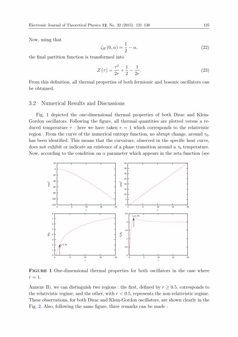
Electronic Journal of Theoretical Physics 12, No. 32 (2015) 121–130 125
Now, using that
ζH (0, α) =1
2− α, (22)
the final partition function is transformed into
Z (τ) =τ 2
2r+
1
2− 1
2r. (23)
From this definition, all thermal properties of both fermionic and bosonic oscillators canbe obtained.
3.2 Numerical Results and Discussions
Fig. 1 depicted the one-dimensional thermal properties of both Dirac and Klein-Gordon oscillators. Following the figure, all thermal quantities are plotted versus a re-duced temperature τ : here we have taken r = 1 which corresponds to the relativisticregion . From the curve of the numerical entropy function, no abrupt change, around τ0,has been identified. This means that the curvature, observed in the specific heat curve,does not exhibit or indicate an existence of a phase transition around a τ0 temperature.Now, according to the condition on α parameter which appears in the zeta function (see
-120
-100
-80
-60
-40
-20
0
20
0 5 10 15 20
F/m
c2
τ
0
5
10
15
20
25
30
35
40
0 5 10 15 20
U/m
c2
τ
0
1
2
3
4
5
6
7
8
0 5 10 15 20
S/k B
τ
τ0=1.70
0
0.5
1
1.5
2
2.5
0 5 10 15 20
Cv/
k B
τ
τ0=1.70
Figure 1 One-dimensional thermal properties for both oscillators in the case wherer = 1.
Annexe B), we can distinguish two regions : the first, defined by r ≥ 0.5, corresponds tothe relativistic regime, and the other, with r < 0.5, represents the non-relativistic regime.These observations, for both Dirac and Klein-Gordon oscillators, are shown clearly in theFig. 2. Also, following the same figure, three remarks can be made :
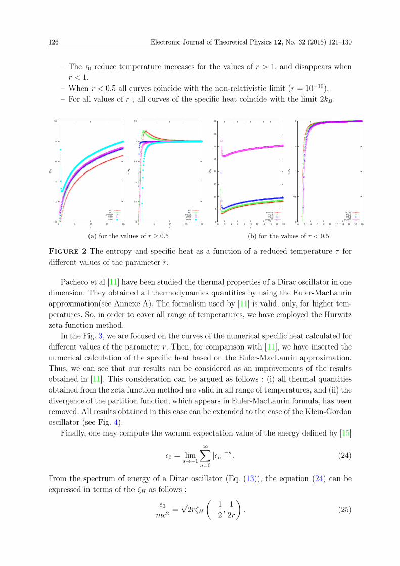
126 Electronic Journal of Theoretical Physics 12, No. 32 (2015) 121–130
– The τ0 reduce temperature increases for the values of r > 1, and disappears whenr < 1.
– When r < 0.5 all curves coincide with the non-relativistic limit (r = 10−10).– For all values of r , all curves of the specific heat coincide with the limit 2kB.
0
2
4
6
8
10
0 5 10 15 20
S/k B
τ
r=2r=1
r=0.99r=0.9r=0.5
0
0.5
1
1.5
2
2.5
0 5 10 15 20
Cv/
k B
τ
r=2r=1
r=0.99r=0.9r=0.5
(a) for the values of r ≥ 0.5
0
5
10
15
20
25
30
35
40
0 2 4 6 8 10 12 14 16 18 20
S/k B
τ
r=0.45r=0.3r=0.1
r=10-10
0
0.5
1
1.5
2
0 2 4 6 8 10 12 14 16 18 20
Cv/
k B
τ
r=0.45r=0.3r=0.1
r=10-10
(b) for the values of r < 0.5
Figure 2 The entropy and specific heat as a function of a reduced temperature τ fordifferent values of the parameter r.
Pacheco et al [11] have been studied the thermal properties of a Dirac oscillator in onedimension. They obtained all thermodynamics quantities by using the Euler-MacLaurinapproximation(see Annexe A). The formalism used by [11] is valid, only, for higher tem-peratures. So, in order to cover all range of temperatures, we have employed the Hurwitzzeta function method.
In the Fig. 3, we are focused on the curves of the numerical specific heat calculated fordifferent values of the parameter r. Then, for comparison with [11], we have inserted thenumerical calculation of the specific heat based on the Euler-MacLaurin approximation.Thus, we can see that our results can be considered as an improvements of the resultsobtained in [11]. This consideration can be argued as follows : (i) all thermal quantitiesobtained from the zeta function method are valid in all range of temperatures, and (ii) thedivergence of the partition function, which appears in Euler-MacLaurin formula, has beenremoved. All results obtained in this case can be extended to the case of the Klein-Gordonoscillator (see Fig. 4).
Finally, one may compute the vacuum expectation value of the energy defined by [15]
ε0 = lims→−1
∞∑n=0
|εn|−s . (24)
From the spectrum of energy of a Dirac oscillator (Eq. (13)), the equation (24) can beexpressed in terms of the ζH as follows :
ε0mc2
=√2rζH
(−1
2,1
2r
). (25)
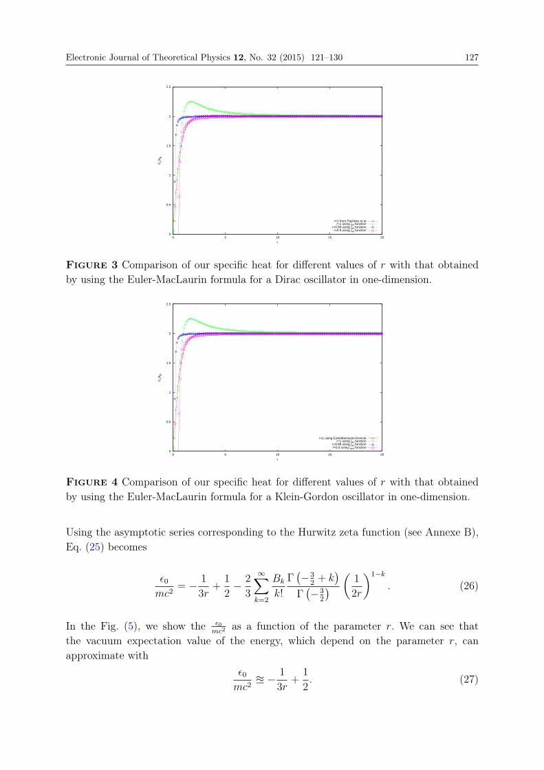
Electronic Journal of Theoretical Physics 12, No. 32 (2015) 121–130 127
0
0.5
1
1.5
2
2.5
0 5 10 15 20
Cv/
k B
τ
r=1 from Pacheko et alr=1 using ζH function
r=0.99 using ζH functionr=0.9 using ζH function
Figure 3 Comparison of our specific heat for different values of r with that obtainedby using the Euler-MacLaurin formula for a Dirac oscillator in one-dimension.
0
0.5
1
1.5
2
2.5
0 5 10 15 20
Cv/
k B
τ
r=1 using EulerMaclaurin formula r=1 using ζH function
r=0.99 using ζH function r=0.9 using ζitH function
Figure 4 Comparison of our specific heat for different values of r with that obtainedby using the Euler-MacLaurin formula for a Klein-Gordon oscillator in one-dimension.
Using the asymptotic series corresponding to the Hurwitz zeta function (see Annexe B),Eq. (25) becomes
ε0mc2
= − 1
3r+
1
2− 2
3
∞∑k=2
Bk
k!
Γ(−3
2+ k
)Γ
(−3
2
) (1
2r
)1−k. (26)
In the Fig. (5), we show the ε0mc2
as a function of the parameter r. We can see thatthe vacuum expectation value of the energy, which depend on the parameter r, canapproximate with
ε0mc2
� − 1
3r+
1
2. (27)
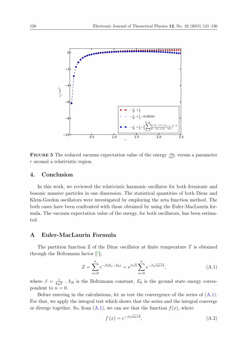
128 Electronic Journal of Theoretical Physics 12, No. 32 (2015) 121–130
0.5 1.0 1.5 2.0 2.5r
−10
−8
−6
−4
−2
0
ε 0/mc2
−
13r+1
2
−
13r+1
2−0.0833r
−
13r+1
2−
23
k=6∑
k=2
Bk
k!
Γ(−1.5+k)
Γ(−1.5)( 12r)1−k
Figure 5 The reduced vacuum expectation value of the energy ε0mc2
versus a parameterr around a relativistic region.
4. Conclusion
In this work, we reviewed the relativistic harmonic oscillator for both fermionic andbosonic massive particles in one dimension. The statistical quantities of both Dirac andKlein-Gordon oscillators were investigated by employing the zeta function method. Theboth cases have been confronted with those obtained by using the Euler-MacLaurin for-mula. The vacuum expectation value of the energy, for both oscillators, has been estima-ted.
A Euler-MacLaurin Formula
The partition function Z of the Dirac oscillator at finite temperature T is obtainedthrough the Boltzmann factor [7],
Z =n∑
n=0
e−β(En−E0) = eβ√b
n∑n=0
e−β√an+b, (A.1)
where β = 1kBT
, kB is the Boltzmann constant, E0 is the ground state energy corres-pondent to n = 0.
Before entering in the calculations, let us test the convergence of the series of (A.1).For that, we apply the integral test which shows that the series and the integral convergeor diverge together. So, from (A.1), we can see that the function f(x), where
f (x) = e−β√an+b, (A.2)
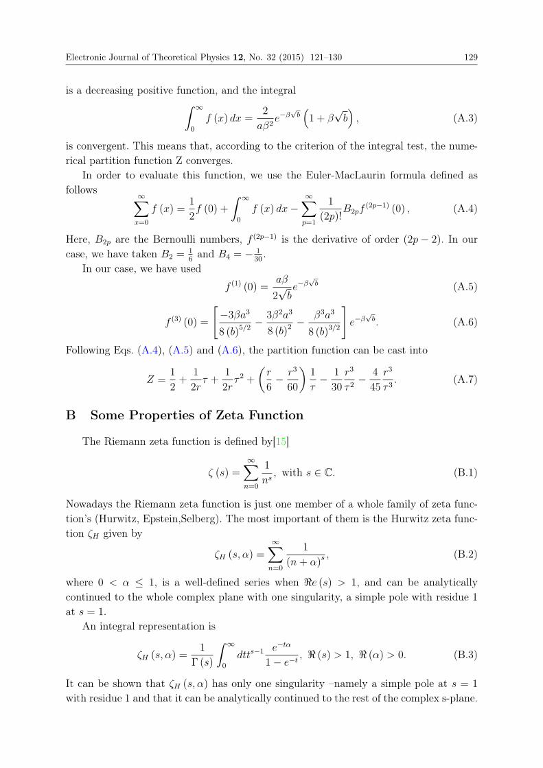
Electronic Journal of Theoretical Physics 12, No. 32 (2015) 121–130 129
is a decreasing positive function, and the integralˆ ∞
0
f (x) dx =2
aβ2e−β
√b(1 + β
√b), (A.3)
is convergent. This means that, according to the criterion of the integral test, the nume-rical partition function Z converges.
In order to evaluate this function, we use the Euler-MacLaurin formula defined asfollows ∞∑
x=0
f (x) =1
2f (0) +
ˆ ∞
0
f (x) dx−∞∑p=1
1
(2p)!B2pf
(2p−1) (0) , (A.4)
Here, B2p are the Bernoulli numbers, f (2p−1) is the derivative of order (2p− 2). In ourcase, we have taken B2 =
16
and B4 = − 130
.In our case, we have used
f (1) (0) =aβ
2√be−β
√b (A.5)
f (3) (0) =
[−3βa3
8 (b)5/2− 3β2a3
8 (b)2− β3a3
8 (b)3/2
]e−β
√b. (A.6)
Following Eqs. (A.4), (A.5) and (A.6), the partition function can be cast into
Z =1
2+
1
2rτ +
1
2rτ 2 +
(r
6− r3
60
)1
τ− 1
30
r3
τ 2− 4
45
r3
τ 3. (A.7)
B Some Properties of Zeta Function
The Riemann zeta function is defined by[15]
ζ (s) =∞∑n=0
1
ns, with s ∈ C. (B.1)
Nowadays the Riemann zeta function is just one member of a whole family of zeta func-tion’s (Hurwitz, Epstein,Selberg). The most important of them is the Hurwitz zeta func-tion ζH given by
ζH (s, α) =∞∑n=0
1
(n+ α)s, (B.2)
where 0 < α ≤ 1, is a well-defined series when �e (s) > 1, and can be analyticallycontinued to the whole complex plane with one singularity, a simple pole with residue 1at s = 1.
An integral representation is
ζH (s, α) =1
Γ (s)
ˆ ∞
0
dtts−1e−tα
1− e−t, � (s) > 1, � (α) > 0. (B.3)
It can be shown that ζH (s, α) has only one singularity –namely a simple pole at s = 1
with residue 1 and that it can be analytically continued to the rest of the complex s-plane.
130 Electronic Journal of Theoretical Physics 12, No. 32 (2015) 121–130
Also, we can shown that ζH (s, α) have the following properties :
ζH (0, α) =1
2− α, (B.4)
ζH (−m,α) = −Bm+1 (α)
m+ 1, m ∈ N, (B.5)
Br(a) being the Bernoulli polynomials. The asymptotic series corresponding the Hurwitzzeta function is given by
ζH (1 + z, α) =1
zα−z +
1
2α−1−z +
1
z
∞∑k=2
Bk
k!
Γ (z + k)
Γ (z)α−z−k, (B.6)
with Bkare Bernoulli’s numbers.
Références
[1] D. ItÃŽ, K. Mori and E. Carriere, Nuovo Cimento A, 51, 1119 (1967). 1.
[2] M. Moshinsky and A. Szczepaniak, J. Phys. A : Math. Gen, 22, L817 (1989). 1.
[3] R. P. Martinez-y-Romero and A. L. Salas-Brito, J. Math. Phys, 33 , 1831 (1992). 1.
[4] M. Moreno and A. Zentella, J. Phys. A : Math. Gen, 22 , L821 (1989). 1.
[5] J. Benitez, P. R. Martinez y Romero , H. N. Nunez-Yepez and A. L. Salas-Brito,Phys.Rev. Lett, 64, 1643–5 (1990). 1.
[6] C. Quesne and V. M. Tkachuk, J. Phys. A : Math. Gen, 41 , 1747–65 (2005). 1.
[7] A. Boumali and H. Hassanabadi, Eur. Phys. J. Plus. 128, 124 (2013). 1., A
[8] C. Quimbay and P. Strange, arXiv:1311.2021 (2013). 1.
[9] C. Quimbay and P. Strange, arXiv:1312.5251 (2013). 1.
[10] A. Franco-Villafane, E. Sadurni, S. Barkhofen, U. Kuhl, F. Mortessagne, and T. H.Selig- man, Phys. Rev. Lett. 111, 170405 (2013). 1.
[11] M. H. Pacheco, R. R. Landim and C. A. S Almeida, Phys. Lett. A, 311, 93–96 (2003).1., 3.2
[12] Marina-Aura Dariescu and C. Dariescu, J. Phys. : Condens. Matter 19, 256203(2007). 1., 3.1
[13] Marina-Aura Dariescu and C. Dariescu, Chaos. Solitons and Fractals 33 , 776–781(2007). 1., 3.1
[14] Marina-Aura Dariescu and C. Dariescu, Rom. Journ. Phys, 56, 1043–1052, (2011).1.
[15] E. Elizalde, Ten physical applications of spectral zeta functions, Springer-VerlagBerlin Heidelberg (1995). 1., 3.2, B
[16] W. Greiner, Quantum Mechanics: An Introduction, 4th ed, Springer-Verlag, Berlin,(2001). 2.1
EJTP 12, No. 32 (2015) 131–138 Electronic Journal of Theoretical Physics
The Effectiveness of Hénon Map for Chaotic Optimization
Algorithms Using a Global Locally Averaged Strategy
Tayeb Hamaizia ∗
Department of Mathematics, Faculty of Sciences, University Constantine -1-, Algeria
Received 27 February 2014, Accepted 20 December 2014, Published 10 January 2015
Abstract: Chaos has three important dynamic properties : the sensitive dependence on initial conditions,the intrinsic stochastic property and ergodicity. So it was applied to optimization problems. In mostoptimization methods such as the COA [1] and [4], variables chaos generated by different typesof applications such as the Logistic, the application Tent, Lozi, Ikeda and others have shown veryinteresting results that random application. The main idea is to improve the convergence of theoptimization chaotic. In this paper, a chaotic strategy is proposed based on a Hénon application chaotic.c© Electronic Journal of Theoretical Physics. All rights reserved.
Keywords: Chaos ; Chaos optimization ; Hénon map ; Global optimizationPACS (2010): 05.45.-a ; 05.10.-a ; 05.45.Gg ; 05.45.Pq ; 02.70.-c ; 02.60.-x ; 87.55.de
1. Introduction
Theory of chaos is one of the most important achievements of nonlinear system research.The term chaos was coined par Li and Yorke [7] are recognized as very useful in many en-gineering applications. Chaotic dynamical systems have many interesting properties, such asno periodic and complex temporal behavior, sensitive dependence on initial conditions or theso-called butterfly effect, fractal structure, and long-term unpredictability [7], [8], [9] and [11].The references included above show interactive demonstrations of these properties. With thesecharacteristics of chaos, we can apply it in optimization calculation. Chaotic optimization isa novel stochastic optimization algorithm, which directly utilizes chaotic variables to searchthe optimal solution. The ergodic, regularity and intrinsic stochastic property of chaos makechaotic optimization to obtain the global optimal solution more possible than the method ha-ving been adopted before. It can more easily escape from local minima than other stochasticalgorithms. Bing Li firstly proposed chaos optimization algorithm (Chaos Optimization Algo-
∗. Email :[email protected]
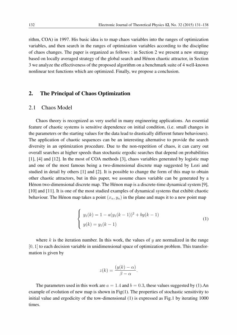
132 Electronic Journal of Theoretical Physics 12, No. 32 (2015) 131–138
rithm, COA) in 1997. His basic idea is to map chaos variables into the ranges of optimizationvariables, and then search in the ranges of optimization variables according to the disciplineof chaos changes. The paper is organized as follows : in Section 2 we present a new strategybased on locally averaged strategy of the global search and Hénon chaotic attractor, in Section3 we analyze the effectiveness of the proposed algorithm on a benchmark suite of 4 well-knownnonlinear test functions which are optimized. Finally, we propose a conclusion.
2. The Principal of Chaos Optimization
2.1 Chaos Model
Chaos theory is recognized as very useful in many engineering applications. An essentialfeature of chaotic systems is sensitive dependence on initial condition, (i.e. small changes inthe parameters or the starting values for the data lead to drastically different future behaviours).The application of chaotic sequences can be an interesting alternative to provide the searchdiversity in an optimization procedure. Due to the non-repetition of chaos, it can carry outoverall searches at higher speeds than stochastic ergodic searches that depend on probabilities[1], [4] and [12]. In the most of COA methods [3], chaos variables generated by logistic mapand one of the most famous being a two-dimensional discrete map suggested by Lozi andstudied in detail by others [1] and [2]. It is possible to change the form of this map to obtainother chaotic attractors, but in this paper, we assume chaos variable can be generated by aHénon two-dimensional discrete map. The Hénon map is a discrete-time dynamical system [9],[10] and [11]. It is one of the most studied examples of dynamical systems that exhibit chaoticbehaviour. The Hénon map takes a point (xn, yn) in the plane and maps it to a new point map
⎧⎪⎨⎪⎩ y1(k) = 1− a(y1(k − 1))2 + by(k − 1)
y(k) = y1(k − 1)(1)
where k is the iteration number. In this work, the values of y are normalized in the range[0, 1] to each decision variable in unidimensional space of optimization problem. This transfor-mation is given by
z(k) =(y(k)− α)
β − α.
The parameters used in this work are a = 1.4 and b = 0.3, these values suggested by (1).Anexample of evolution of new map is shown in Fig(1). The properties of stochastic sensitivity toinitial value and ergodicity of the tow-dimensional (1) is expressed as Fig.1 by iterating 1000times.
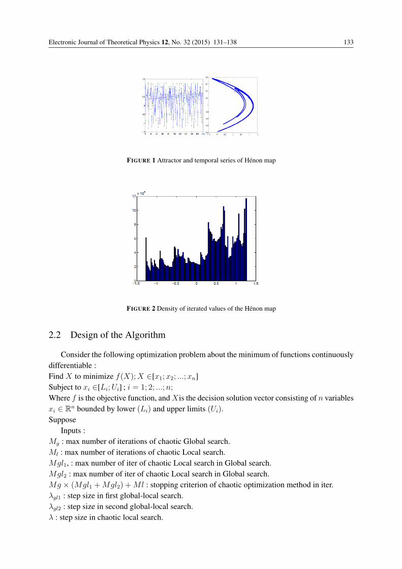
Electronic Journal of Theoretical Physics 12, No. 32 (2015) 131–138 133
FIGURE 1 Attractor and temporal series of Hénon map
FIGURE 2 Density of iterated values of the Hénon map
2.2 Design of the Algorithm
Consider the following optimization problem about the minimum of functions continuouslydifferentiable :Find X to minimize f(X);X ∈[x1; x2; ...; xn]Subject to xi ∈[Li;Ui] ; i = 1; 2; ...;n;
Where f is the objective function, and Xis the decision solution vector consisting of n variablesxi ∈ Rn bounded by lower (Li) and upper limits (Ui).Suppose
Inputs :Mg : max number of iterations of chaotic Global search.Ml : max number of iterations of chaotic Local search.Mgl1, : max number of iter of chaotic Local search in Global search.Mgl2 : max number of iter of chaotic Local search in Global search.Mg × (Mgl1 +Mgl2) +Ml : stopping criterion of chaotic optimization method in iter.λgl1 : step size in first global-local search.λgl2 : step size in second global-local search.λ : step size in chaotic local search.
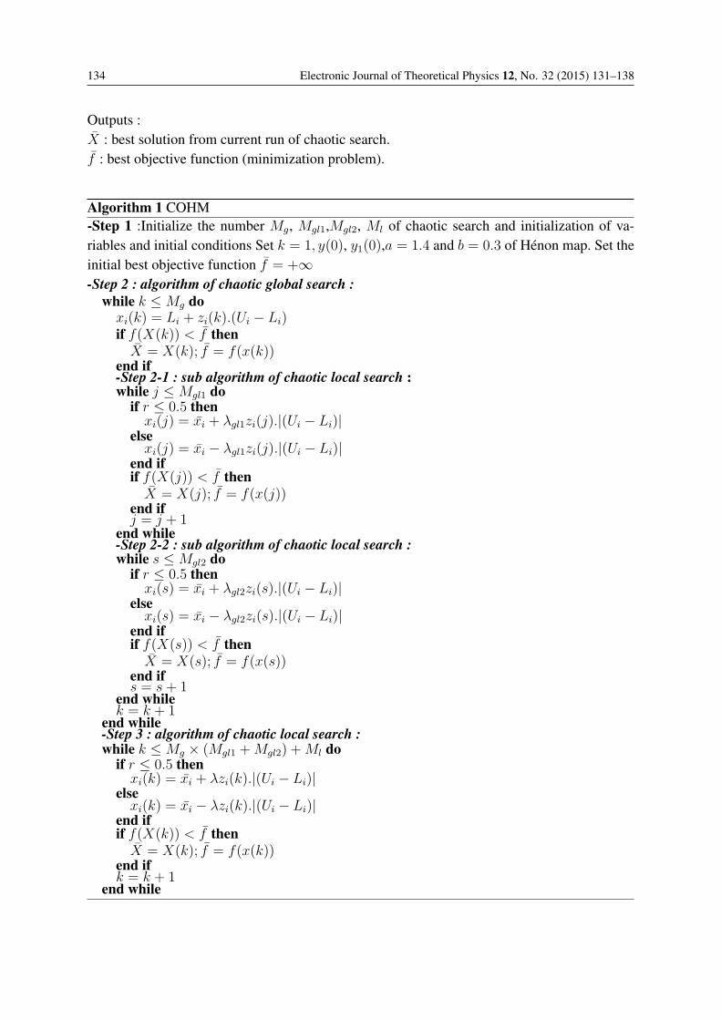
134 Electronic Journal of Theoretical Physics 12, No. 32 (2015) 131–138
Outputs :X : best solution from current run of chaotic search.f : best objective function (minimization problem).
Algorithm 1 COHM-Step 1 :Initialize the number Mg, Mgl1,Mgl2, Ml of chaotic search and initialization of va-riables and initial conditions Set k = 1, y(0), y1(0),a = 1.4 and b = 0.3 of Hénon map. Set theinitial best objective function f = +∞-Step 2 : algorithm of chaotic global search :
while k ≤Mg doxi(k) = Li + zi(k).(Ui − Li)if f(X(k)) < f then
X = X(k); f = f(x(k))end if-Step 2-1 : sub algorithm of chaotic local search :while j ≤Mgl1 do
if r ≤ 0.5 thenxi(j) = xi + λgl1zi(j).|(Ui − Li)|
elsexi(j) = xi − λgl1zi(j).|(Ui − Li)|
end ifif f(X(j)) < f then
X = X(j); f = f(x(j))end ifj = j + 1
end while-Step 2-2 : sub algorithm of chaotic local search :while s ≤Mgl2 do
if r ≤ 0.5 thenxi(s) = xi + λgl2zi(s).|(Ui − Li)|
elsexi(s) = xi − λgl2zi(s).|(Ui − Li)|
end ifif f(X(s)) < f then
X = X(s); f = f(x(s))end ifs = s+ 1
end whilek = k + 1
end while-Step 3 : algorithm of chaotic local search :while k ≤Mg × (Mgl1 +Mgl2) +Ml do
if r ≤ 0.5 thenxi(k) = xi + λzi(k).|(Ui − Li)|
elsexi(k) = xi − λzi(k).|(Ui − Li)|
end ifif f(X(k)) < f then
X = X(k); f = f(x(k))end ifk = k + 1
end while
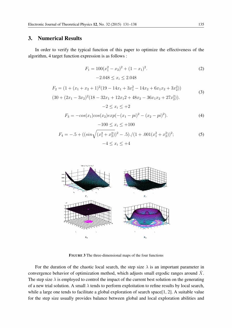
Electronic Journal of Theoretical Physics 12, No. 32 (2015) 131–138 135
3. Numerical Results
In order to verify the typical function of this paper to optimize the effectiveness of thealgorithm, 4 target function expression is as follows :
F1 = 100(x21 − x2)
2 + (1− x1)2. (2)
−2.048 ≤ xi ≤ 2.048
F2 = (1 + (x1 + x2 + 1)2(19− 14x1 + 3x21 − 14x2 + 6x1x2 + 3x2
2))
(30 + (2x1 − 3x2)2(18− 32x1 + 12x12 + 48x2 − 36x1x2 + 27x2
2)).(3)
−2 ≤ xi ≤ +2
F3 = −cos(x1)cos(x2)exp(−(x1 − pi)2 − (x2 − pi)2). (4)
−100 ≤ xi ≤ +100
F4 = −.5 + ((sin√
(x21 + x2
2))2 − .5)./(1 + .001(x2
1 + x22))
2; (5)
−4 ≤ xi ≤ +4
FIGURE 3 The three-dimensional maps of the four functions
For the duration of the chaotic local search, the step size λ is an important parameter inconvergence behavior of optimization method, which adjusts small ergodic ranges around X .The step size λ is employed to control the impact of the current best solution on the generatingof a new trial solution. A small λ tends to perform exploitation to refine results by local search,while a large one tends to facilitate a global exploration of search space[1, 2]. A suitable valuefor the step size usually provides balance between global and local exploration abilities and
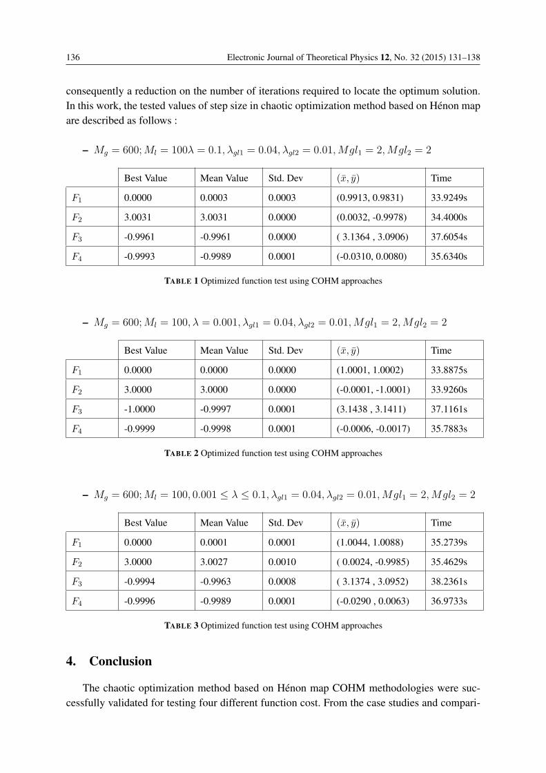
136 Electronic Journal of Theoretical Physics 12, No. 32 (2015) 131–138
consequently a reduction on the number of iterations required to locate the optimum solution.In this work, the tested values of step size in chaotic optimization method based on Hénon mapare described as follows :
– Mg = 600;Ml = 100λ = 0.1, λgl1 = 0.04, λgl2 = 0.01,Mgl1 = 2,Mgl2 = 2
Best Value Mean Value Std. Dev (x, y) Time
F1 0.0000 0.0003 0.0003 (0.9913, 0.9831) 33.9249s
F2 3.0031 3.0031 0.0000 (0.0032, -0.9978) 34.4000s
F3 -0.9961 -0.9961 0.0000 ( 3.1364 , 3.0906) 37.6054s
F4 -0.9993 -0.9989 0.0001 (-0.0310, 0.0080) 35.6340s
TABLE 1 Optimized function test using COHM approaches
– Mg = 600;Ml = 100, λ = 0.001, λgl1 = 0.04, λgl2 = 0.01,Mgl1 = 2,Mgl2 = 2
Best Value Mean Value Std. Dev (x, y) Time
F1 0.0000 0.0000 0.0000 (1.0001, 1.0002) 33.8875s
F2 3.0000 3.0000 0.0000 (-0.0001, -1.0001) 33.9260s
F3 -1.0000 -0.9997 0.0001 (3.1438 , 3.1411) 37.1161s
F4 -0.9999 -0.9998 0.0001 (-0.0006, -0.0017) 35.7883s
TABLE 2 Optimized function test using COHM approaches
– Mg = 600;Ml = 100, 0.001 ≤ λ ≤ 0.1, λgl1 = 0.04, λgl2 = 0.01,Mgl1 = 2,Mgl2 = 2
Best Value Mean Value Std. Dev (x, y) Time
F1 0.0000 0.0001 0.0001 (1.0044, 1.0088) 35.2739s
F2 3.0000 3.0027 0.0010 ( 0.0024, -0.9985) 35.4629s
F3 -0.9994 -0.9963 0.0008 ( 3.1374 , 3.0952) 38.2361s
F4 -0.9996 -0.9989 0.0001 (-0.0290 , 0.0063) 36.9733s
TABLE 3 Optimized function test using COHM approaches
4. Conclusion
The chaotic optimization method based on Hénon map COHM methodologies were suc-cessfully validated for testing four different function cost. From the case studies and compari-
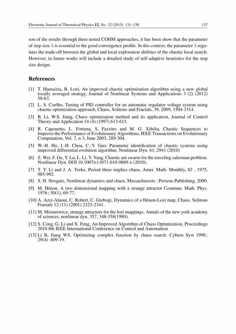
Electronic Journal of Theoretical Physics 12, No. 32 (2015) 131–138 137
son of the results through three tested COHM approaches, it has been show that the parameterof step size λ is essential to the good convergence profile. In this context, the parameter λ regu-lates the trade-off between the global and local exploration abilities of the chaotic local search.However, in future works will include a detailed study of self-adaptive heuristics for the stepsize design.
References
[1] T. Hamaizia, R. Lozi, An improved chaotic optimization algorithm using a new globallocally averaged strategy, Journal of Nonlinear Systems and Applications 3 (2) (2012)58-63.
[2] L. S. Coelho, Tuning of PID controller for an automatic regulator voltage system usingchaotic optimization approach, Chaos, Solitons and Fractals, 39, 2009, 1504-1514.
[3] B. Li, W.S. Jiang, Chaos optimization method and its application, Journal of ControlTheory and Application 14 (4) (1997) 613-615.
[4] R. Caponetto, L. Fortuna, S. Fazzino and M. G. Xibilia, Chaotic Sequences toImprove the Performance of Evolutionary Algorithms, IEEE Transactions on EvolutionaryComputation, Vol. 7, n 3, June 2003, 289-304.
[5] W.-H. Ho, J.-H. Chou, C.-Y. Guo, Parameter identification of chaotic systems usingimproved differential evolution algorithm. Nonlinear Dyn. 61, 2941 (2010)
[6] Z. Wei, F. Ge, Y. Lu, L. Li, Y. Yang, Chaotic ant swarm for the traveling salesman problem.Nonlinear Dyn. DOI 10.1007/s11071-010-9889-x (2010).
[7] T. Y. Li and J. A. Yorke, Period three implies chaos, Amer. Math. Monthly, 82 , 1975,985-992.
[8] S. H. Strogatz, Nonlinear dynamics and chaos, Massachussets : Perseus Publishing, 2000.
[9] M. Hénon. A two dimensional mapping with a strange attractor Commun. Math. Phys.1976 ; 50(1), 69-77.
[10] A. Aziz-Alaoui, C. Robert, C. Grebogi, Dynamics of a Hénon-Lozi map, Chaos, SolitonsFractals 12 (11) (2001) 2323-2341.
[11] M. Misiurewicz, strange attractors for the lozi mappings. Annals of the new york academyof sciences, nonlinear dyn. 357, 348-358(1980).
[12] S. Cong, G. Li and X. Feng, An Improved Algorithm of Chaos Optimization, Proceedings2010 8th IEEE International Conference on Control and Automation
[13] Li B, Jiang WS. Optimizing complex function by chaos search. Cybern Syst 1998 ;29(4) :409-19.

EJTP 12, No. 32 (2015) 139–178 Electronic Journal of Theoretical Physics
Weakton Model of Elementary Particlesand Decay Mechanisms∗
Tian Ma1 and Shouhong Wang2†
1Department of Mathematics, Sichuan University, Chengdu, P. R. China2Department of Mathematics, Indiana University, Bloomington, IN 47405, USA
Received 15 April 2014, Accepted 20 December 2014, Published 10 January 2015
Abstract: Sub-atomic decays and electron radiations indicate that there must be interior
structures for charged leptons, quarks and mediators. The main objectives of this article are 1)
to propose a sub-leptons and sub-quark model, which we call weakton model, and 2) to derive
a mechanism for all sub-atomic decays and bremsstrahlung. The theory is based on 1) a theory
on weak and strong charges, 2) different levels of weak and strong interaction potentials, 3)
a new mass generation mechanism, and 4) an angular momentum rule. The weakton model
postulates that all matter particles (leptons, quarks) and mediators are made up of massless
weaktons. The weakton model offers a perfect explanation for all sub-atomic decays and all
generation/annihilation precesses of matter-antimatter. In particular, the precise constituents
of particles involved in all decays both before and after the reaction can now be precisely derived.
In addition, the bremsstrahlung phenomena can be understood using the weakton model. Also,
the weakton model offers an explanation to the baryon asymmetry problem, and provides an
alternate explanation of the solar neutrino problem.c© Electronic Journal of Theoretical Physics. All rights reserved.
Keywords: Elementary Particles; Sub-Quark; Sub-Lepton; Sub-Mediators; Weakton Model;
Subatomic Decay; Matter And Antimatter Creation And Annihilation; Weakton Exchange; Weak
Interaction; Strong Interaction; Weak Charge; Strong Charge
PACS (2010): 12.40.-y; 12.15.-y ; 14.60.-z; 14.65.-q; 13.30.-a; 14.20.Dh; 12.39.-x; 24.85.+p;
12.15.Ff; 13.90.+i
∗ The work was supported in part by the Office of Naval Research, by the US National Science Founda-
tion, and by the Chinese National Science Foundation.† Email:[email protected], http://www.indiana.edu/ fluid
140 Electronic Journal of Theoretical Physics 12, No. 32 (2015) 139–178
1. Introduction
The matter in the universe is made up of a number of fundamental constituents. The
current knowledge of elementary particles shows that all forms of matter are made up of
6 leptons and 6 quarks, and their antiparticles. The basic laws governing the dynamical
behavior of these elementary particles are the laws for the four interactions/forces: the
electromagnetism, the gravity, the weak and strong interactions. Great achievements and
insights have been made for last 100 years or so on the understanding of the structure
of subatomic particles and on the fundamental laws for the four interactions; see among
many others [3, 2, 5, 12, 10].
However, there are still many longstanding open questions and challenges. Here are
a few fundamental questions which are certainly related to the deepest secret of our
universe:
Q1 What is the origin of four forces?
Q2 Why do leptons not participate in strong interactions?
Q3 What is the origin of mass?
Q4 What is the mechanism of subatomic decays and reactions?
Q5 Why can massless photons produce massive particles? Or in general, why can lepton
and anti-lepton pairs produce hadron pairs?
Q6 Are leptons and quarks true elementary particles? Do leptons and quarks have
interior structure?
Q7 Why are there more matters than anti-matters? This is the classical baryon asym-
metry problem.
Q8 What are the strong and weak force formulas?
Q9 Why, in the same spatial scale, do strong and weak interactions exhibit both repelling
and attraction?
Q10 Why are the weak and strong interactions short-ranged, and what are the ranges of
the four interactions?
Q11 What is the mechanism of quark confinement?
Q12 What is the mechanism of bremsstrahlung?
Q13 Why is there a loss of solar neutrinos?
The main objectives of this article are 1) to study the mechanism of subatomic decays,
2) to propose a weakton model of elementary particles, and 3) to explain the above
questions Q1–Q13. We proceed as follows.
1. The starting point of the study is the puzzling decay and reaction behavior of sub-
atomic particles. For example, the electron radiations and the electron-positron anni-
hilation into photons or quark-antiquark pair clearly shows that there must be interior
structure of electrons, and the constituents of an electron contribute to the making of
photon or the quark in the hadrons formed in the process. In fact, all sub-atomic decays
and reactions show clearly the following conclusion:
There must be interior structure of charged leptons, quarks and mediators. (1)
2. The above conclusion motivates us to propose a model for sub-lepton, sub-quark, and
Electronic Journal of Theoretical Physics 12, No. 32 (2015) 139–178 141
sub-mediators. It is clear that any such model should obey four basic requirements.
The first is the mass generation mechanism. Namely, the model should lead to con-
sistency of masses for both elementary particles, which we call weaktons to be introduced
below, and composite particles (the quarks, leptons and mediators). Since the media-
tors, the photon γ and the eight gluons gk (k = 1, · · · , 8), are all massless, a natural
requirement is that
the proposed elementary particles—weaktons— are massless. (2)
Namely, these proposed elementary particles must have zero rest mass.
The second requirement for the model is the consistency of quantum numbers for
both elementary and composite particles. The third requirement is the exclusion of
nonrealistic compositions of the elementary particles, and the fourth requirement is the
weakton confinement.
3. Careful examinations of these requirements and subatomic decays/reactions lead us
to propose six elementary particles, which we call weaktons, and their anti-particles:
w∗, w1, w2, νe, νμ, ντ ,
w∗, w1, w2, νe, νμ, ντ ,(3)
where νe, νμ, ντ are the three generation neutrinos, and w∗, w1, w2 are three new particles,
which we call w-weaktons. These are massless, spin-12particles with one unit of weak
charge gw. Both w∗ and w∗ are the only weaktons carrying strong charge gs.
With these weaktons at our disposal, the weakton constituents of charged leptons and
quarks are then given as follows:
e = νew1w2, μ = νμw1w2, τ = ντw1w2,
u = w∗w1w1, c = w∗w2w2, t = w∗w2w2,
d = w∗w1w2, s = w∗w1w2, b = w∗w1w2,
(4)
where c, t and d, s, b are distinguished by the spin arrangements; see (59) and (60).
4. Using the duality given in the unified field theory for four interactions, the mediators
of strong, weak and electromagnetic interactions include the photon γ, the vector bosons
W± and Z, and the gluons gk, together with their dual fields φγ, φ±W , φ0
Z , and φkg . The
constituents of these mediators are given by
γ = cos θww1w1 − sin θww2w2 (�,�),
Z0 = cos θww2w2 + sin θww1w1 (�,�),
W− = w1w2(�,�),
W+ = w1w2(�,�),
gk = w∗w∗(�,�), k = color index,
(5)
142 Electronic Journal of Theoretical Physics 12, No. 32 (2015) 139–178
and the dual bosons:
φγ = cos θww1w1 − sin θww2w2(↑↓, ↓↑),φ0Z = cos θww2w2 + sin θww1w1(↑↓, ↓↑),
φ−W = w1w2(↑↓, ↓↑),φ+W = w1w2(↑↓, ↓↑),
φkg = w∗w∗(↑↓, ↓↑),
(6)
where θw ∼= 28.76◦ is the Weinberg angle.
Remarkably, both the spin-1 mediators in (5) and the spin-0 dual mediators in (6)
have the same weakton constituents, differing only by their spin arrangements. The
spin arrangements clearly demonstrate that there must be spin-0 particles with the same
weakton constituents as the mediators in (5). Consequently, there must be dual mediators
with spin-0. This observation clearly supports the unified field model presented in [8, 7].
Conversely, the existence of the dual mediators makes the weakton constituents perfectly
fit.
5. Also, a careful examination of weakton constituents predicts the existence of an
additional mediator, which we call the ν-mediator:
φ0ν =
∑l
αlνlνl(↓↑),∑l
α2l = 1, (7)
taking into consideration of neutrino oscillations. When examining decays and reactions
of sub-atomic particles, it is apparent for us to predict the existence of this mediator.
6. One important conclusion of the aforementioned weakton model is that all particles—
both matter particles and mediators—are made up of massless weaktons. A fundamental
question is how the mass of a massive composite particle is generated. In fact, based on
the Einstein formulas:
d
dt�P =
√1− v2
c2�F , m =
√1− v2
c2E
c2, (8)
we observe that a particle with an intrinsic energy E has zero mass m = 0 if it moves in
the speed of light v = c, and possess nonzero mass if it moves with a velocity v < c. Hence
by this mass generation mechanism, for a composite particle, the constituent massless
weaktons can decelerate by the weak force, yielding a massive particle.
In principle, when calculating the mass of the composite particle, one should also
consider the bounding and repelling energies of the weaktons, each of which can be very
large. Fortunately, the constituent weaktons are moving in the “asymptotically-free” shell
region of weak interactions as indicated by the weak interaction potential/force formulas,
so that the bounding and repelling contributions to the mass are mostly canceled out.
Namely, the mass of a composite particle is due mainly to the dynamic behavior of the
constituent weaktons.
7. As we mentioned earlier, one requirement for the weakton model is the consistency
of quantum numbers for both elementary particles and composite particles. In fact, the
Electronic Journal of Theoretical Physics 12, No. 32 (2015) 139–178 143
weakton model obeys a number of quantum rules, which can be used to exclude unrealistic
combinations of weaktons. The following rules are introduced for this purpose:
a) Weak color neutral rule: each weakton is endowed with a weak color quantum num-
ber, and all weakton composite particles must be weak color neutral.
b) BL = 0, LiLj = 0 (i �= j), where B is the baryon number and L is the lepton
number.
c) L+Qe = 0 if L �= 0 and |B +Qe| ≤ 1 if B �= 0.
d) Angular Momentum Rule: Only the fermions with spin s = 12can rotate around a
center with zero moment of force. The particles with s �= 12will move in a straight
line unless there is a nonzero moment of force present.
The angular momentum is a consequence of the Dirac equations, and it is due to
this rule that there are no spin-3/2 quarks.
8. Remarkably, the weakton model offers a perfect explanation for all sub-atomic de-
cays. In particular, all decays are achieved by 1) exchanging weaktons and consequently
exchanging newly formed quarks, producing new composite particles, and 2) separating
the new composite particles by weak and/or strong forces.
One aspect of this decay mechanism is that we know now the precise constituents of
particles involved in all decays/reactions both before and after the reaction. It is therefore
believed that the new decay mechanism provides clear new insights for both experimental
and theoretical studies.
9. The weakton theory, together with the unified field theory developed in [8, 7], provides
sound explanations and new viewpoints for the twelve fundamental questions given at
the beginning of the Introduction.
We end this Introduction by mentioning that there have been numerous studies on
sub-quark and sub-lepton models; see among others [9, 1, 11, 4]
The paper is organized as follows. A brief introduction to the current understanding
of elementary particles is given in Section 2, focusing on 1) the constituents of subatomic
particles, and 2) decays. Section 3 addresses a few theoretical foundations needed for
introducing the weakton model, which is then introduced in Section 4. All decays are
then perfectly explained using the weakton model in Section 5. An application of the
weakton model to bremsstrahlung is given in Section 6. Section 7 summaries conclusions
of this article, focusing on answers and explanations to the 13 open questions.
2. Current Knowledge of Elementary Particles
The current view on subatomic particles classifies all particles into two basic classes,
bosons and fermions:
bosons = integral spin particles,
fermions = fractional spin particles.
144 Electronic Journal of Theoretical Physics 12, No. 32 (2015) 139–178
However, based on their properties and laws in Nature, all particles are currently classified
into four types:
leptons, quarks, mediators, hadrons.
Hereafter we recapitulate the definitions and the quantum characterizations of these par-
ticles.
2.1 Leptons
Leptons are fermions which do not participate in strong interaction, and have three
generations with two in each generation:⎛⎜⎝ e
νe
⎞⎟⎠ ,
⎛⎜⎝ μ
νμ
⎞⎟⎠ ,
⎛⎜⎝ τ
ντ
⎞⎟⎠ ,
where e, μ, τ are the electron, the muon, the tau, and νe, νμ, ντ are the e neutrino, the μ
neutrino, the τ neutrino. Together with antiparticles, there are total 12 leptons:
particles: (e−, νe), (μ−, νμ), (τ−, ντ ),
antiparticles: (e+, νe), (μ+, νμ), (τ+, ντ ).
The quantum numbers of leptons include the mass m, the charge Q, the lifetime τ ,
the spin J , the e-lepton number Le, the μ-lepton number Lμ, and the τ -lepton number
Lτ . Table 1 lists typical values of these quantum numbers, where the mass is in MeV/c2,
lifetime is in seconds, and the charge is in the unit of proton charge. Also, we remark
that the left-hand property of neutrinos is represented by J = −12for ν, and J = +1
2for
ν.
2.2 Quarks
Based on the Standard Model, there are three generations of quarks containing 12 parti-
cles, which participate in all interactions:
quarks: (u, d), (c, s), (t, b),
antiquarks: (u, d), (c, s), (t, b).
The celebrated quark model assets that three quarks are bounded together to form
a baryon, and a pair of quark and antiquark are bounded to form a meson. Quarks are
confined in hadrons, and no free quarks have been found in Nature. This phenomena
is called quark confinement, which can be very well explained using the three levels of
strong interaction potentials derived using a unified field theory developed recently in
[8, 7]; see discussions in Section 3.4.
The quantum numbers of quarks include the mass m, the charge Q, the baryon
number B, the spin J , the strange number S, the isospin I and its third component I3,
the supercharge Y , and the parity P . These quantum numbers are listed in Table 2.
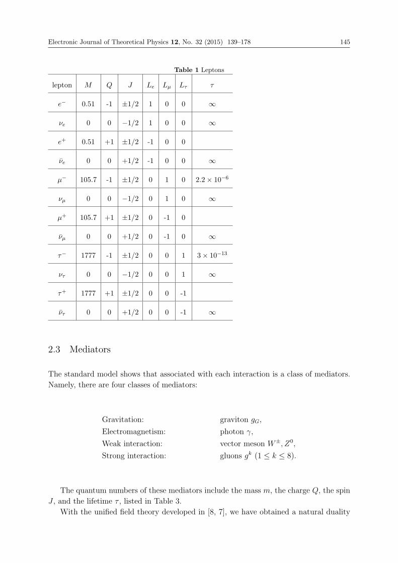
Electronic Journal of Theoretical Physics 12, No. 32 (2015) 139–178 145
Table 1 Leptons
lepton M Q J Le Lμ Lτ τ
e− 0.51 -1 ±1/2 1 0 0 ∞
νe 0 0 −1/2 1 0 0 ∞
e+ 0.51 +1 ±1/2 -1 0 0
νe 0 0 +1/2 -1 0 0 ∞
μ− 105.7 -1 ±1/2 0 1 0 2.2× 10⁻⁶
νμ 0 0 −1/2 0 1 0 ∞
μ+ 105.7 +1 ±1/2 0 -1 0
νμ 0 0 +1/2 0 -1 0 ∞
τ− 1777 -1 ±1/2 0 0 1 3× 10⁻¹³
ντ 0 0 −1/2 0 0 1 ∞
τ+ 1777 +1 ±1/2 0 0 -1
ντ 0 0 +1/2 0 0 -1 ∞
2.3 Mediators
The standard model shows that associated with each interaction is a class of mediators.
Namely, there are four classes of mediators:
Gravitation: graviton gG,
Electromagnetism: photon γ,
Weak interaction: vector meson W±, Z0,
Strong interaction: gluons gk (1 ≤ k ≤ 8).
The quantum numbers of these mediators include the mass m, the charge Q, the spin
J , and the lifetime τ , listed in Table 3.
With the unified field theory developed in [8, 7], we have obtained a natural duality
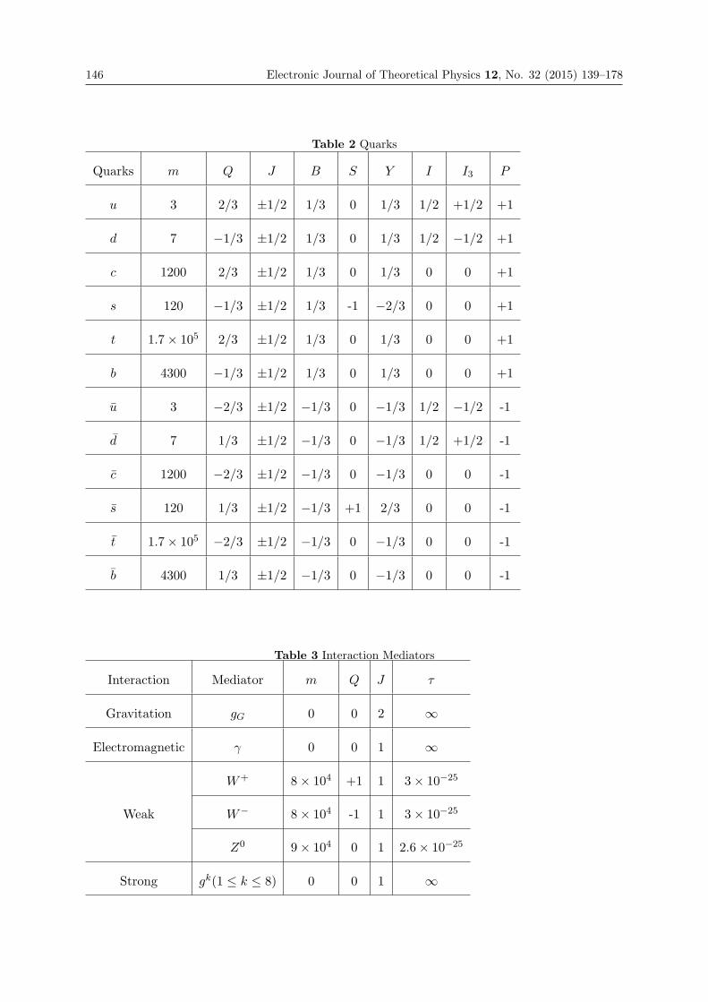
146 Electronic Journal of Theoretical Physics 12, No. 32 (2015) 139–178
Table 2 Quarks
Quarks m Q J B S Y I I3 P
u 3 2/3 ±1/2 1/3 0 1/3 1/2 +1/2 +1
d 7 −1/3 ±1/2 1/3 0 1/3 1/2 −1/2 +1
c 1200 2/3 ±1/2 1/3 0 1/3 0 0 +1
s 120 −1/3 ±1/2 1/3 -1 −2/3 0 0 +1
t 1.7× 10⁵ 2/3 ±1/2 1/3 0 1/3 0 0 +1
b 4300 −1/3 ±1/2 1/3 0 1/3 0 0 +1
u 3 −2/3 ±1/2 −1/3 0 −1/3 1/2 −1/2 -1
d 7 1/3 ±1/2 −1/3 0 −1/3 1/2 +1/2 -1
c 1200 −2/3 ±1/2 −1/3 0 −1/3 0 0 -1
s 120 1/3 ±1/2 −1/3 +1 2/3 0 0 -1
t 1.7× 10⁵ −2/3 ±1/2 −1/3 0 −1/3 0 0 -1
b 4300 1/3 ±1/2 −1/3 0 −1/3 0 0 -1
Table 3 Interaction Mediators
Interaction Mediator m Q J τ
Gravitation gG 0 0 2 ∞
Electromagnetic γ 0 0 1 ∞
W+ 8× 10⁴ +1 1 3× 10⁻²⁵
Weak W− 8× 10⁴ -1 1 3× 10⁻²⁵
Z0 9× 10⁴ 0 1 2.6× 10⁻²⁵
Strong gk(1 ≤ k ≤ 8) 0 0 1 ∞
Electronic Journal of Theoretical Physics 12, No. 32 (2015) 139–178 147
between the interacting fields {gμν , Aμ,Waμ , S
kμ} and their dual field {ΦG
μ , φE, φaw, φ
ks}:
{gμν} ←→ ΦGμ ,
Aμ ←→ φE,
{W aμ} ←→ {φa
w},{Sk
μ} ←→ {φks}.
This duality leads to four classes of new dual bosonic mediators:
graviton gG ←→ vector boson ΦG,
photon γ ←→ scalar boson φγ ,
vector bosons W±, Z ←→ scalar bosons φ±W , φ0Z ,
gluons gk (1 ≤ k ≤ 8) ←→ scalar bosons φkg (1 ≤ k ≤ 8)
(9)
These dual mediators are crucial not only for the weak and strong potential/force formulas
given in the next section, but also for the weakton model introduced in this article. In
addition, the dual vector field ΦG gives rise to a unified theory for dark matter and dark
energy [6].
The quantum numbers of these dual mediators are given as follows:
ΦG : m = 0, J = 1, Q = 0, τ =∞,
φe : m = 0, J = 0, Q = 0, τ =∞,
φ±W (Higgs) : m ∼ 105, J = 0, Q = ±1, τ ∼ 10−21s,
φ0Z(Higgs) : m ∼ 1.25× 10⁵, J = 0, Q = 0, τ ∼ 10−21s,
φkg : m =?, J = 0, Q = 0, τ =?.
(10)
2.4 Hadrons
Hadrons are classified into two types: baryons and mesons. Baryons are fermions and
mesons are bosons, which are all made up of quarks:
Baryons = qiqjqk, mesons = qiqj,
where qk = {u, d, c, s, t, b}. The quark constituents of main hadrons are listed as follows:
• Baryons (J = 12) : p, n,Λ,Σ±,Σ0,Ξ0,Ξ−.
p(uud), n(udd), Λ(s(du− ud)/√2),
Σ+(uus), Σ−(dds), Σ0(s(du+ ud)/√2),
Ξ−(uss), Ξ0(dss).
(11)
• Baryons (J = 32) : Δ++,Δ±,Δ0,Σ∗±,Σ∗0,Ξ∗0,Ξ∗−,Ω−.
Δ++(uuu), Δ+(uud), Δ−(ddd), Δ0(udd),
Σ∗+(uus), Σ∗−(dds), Σ∗0(uds),
Ξ∗0(uss), Ξ∗−(dss), Ω−(sss).
(12)
148 Electronic Journal of Theoretical Physics 12, No. 32 (2015) 139–178
• Mesons (J = 0) : π±, π0, K±, K0, K0, η,
π+(ud), π−(ud), π0((uu− dd)/√2),
K+(us), K−(us), K0((ds), K0(ds),
η((uu+ dd− 2ss)/√6).
(13)
• Mesons (J = 1) : ρ±, ρ0, K∗±, K∗0, K∗0, ω, ψ,Υ,
ρ+(ud), ρ−(ud), ρ0((uu− dd)/√2),
K∗+(us), K∗−(us), K∗0(ds), K∗0(ds),
ω((uu+ dd)/√2), ψ(cc), Υ(bb).
(14)
2.5 Principal decays
Decays are the main dynamic behavior for sub-atomic particles, and reveal the interior
structure of particles. We now list some principal decay forms.
• Lepton decays:
μ− → e− + νe + νμ,
μ+ → e+ + νe + νμ,
τ− → e− + νe + ντ ,
τ− → μ− + νμ + ντ ,
τ− → π− + ντ ,
τ− → ρ− + ντ ,
τ− → K− + ντ .
• Quark decays:
d→ u+ e− + νe,
s→ u+ e− + νe,
s→ d+ g + γ (g the gluons),
c→ d+ s+ u,
• Mediator decays:
2γ → e+ + e−, qq,
W+ → e+ + νe, μ+ + νμ, τ+ + ντ ,
W− → e− + νe, μ− + νμ, τ− + ντ ,
Z0 → e+ + e−, μ+ + μ−, τ+ + τ−, qq.
Electronic Journal of Theoretical Physics 12, No. 32 (2015) 139–178 149
• Baryon decays:
n→ p+ e− + νe,
Λ→ p+ π−, n+ π0,
Σ+ → p+ π0, n+ π+,
Σ0 → Λ + γ, Σ− → n+ π−,
Ξ0 → Λ + π0, Ξ− → Λ + π−,
Δ++ → p+ π+, Δ+ → p+ π0,
Δ0 → n+ π0, Δ− → n+ π−,
Σ∗± → Σ± + π0, Ξ∗0 → Σ0 + π0,
Ξ∗0 → Ξ0 + π0, Ξ∗− → Ξ− + π0.
• Meson decays:
π+ → μ+ + νμ, π0 → 2γ,
π− → μ− + νμ,
K+ → μ+ + νμ, π+ + π0, π+ + π+ + π−,
K− → μ− + νμ, π− + π0, π− + π+ + π−,
K0 → π+ + e− + νe, π+ + π−, π+ + π− + π0,
η → 2γ, π+ + π− + π0,
ρ± → π0, ρ0 → π+ + π−,
K∗± → K± + π0, K∗0 → K0 + π0,
ω → π0 + γ, π+ + π− + π0,
ψ → e+ + e−, μ+ + μ−,
Υ→ e+ + e−, μ+ + μ−, τ+ + τ−.
3. Theoretical Foundations for the Weakton Model
3.1 Angular momentum rule
It is known that the dynamic behavior of a particle is described by the Dirac equations:
i�∂ψ
∂t= Hψ, ψ = (ψ1, ψ2, ψ3, ψ4)
T (15)
where H is the Hamiltonian
H = −i�c(αk∂k) +mc2α0 + V (x), (16)
150 Electronic Journal of Theoretical Physics 12, No. 32 (2015) 139–178
V is the potential energy, and α0, αk (1 ≤ k ≤ 3) are the Dirac matrices
α0 =
⎛⎜⎜⎜⎝1 0
1
−10 −1
⎞⎟⎟⎟⎠ , α1 =
⎛⎜⎜⎜⎝0 0 0 1
0 0 1 0
0 1 0 0
1 0 0 0
⎞⎟⎟⎟⎠ ,
α2 =
⎛⎜⎜⎜⎝0 0 0 −i0 0 i 0
0 −i 0 0
i 0 0 0
⎞⎟⎟⎟⎠ , α3 =
⎛⎜⎜⎜⎝0 0 1 0
0 0 0 −11 0 0 0
0 −1 0 0
⎞⎟⎟⎟⎠ .
By the conservation laws in relativistic quantum mechanics, if a Hermitian operator L
commutes with H in (16):
LH = HL,
then the physical quantity L is conservative.
The main objective of this section is to prove the following angular momentum rule
for quantum systems.
Quantum Rule of Angular Momentum. Only the fermions with spin J = 12and the
bosons with J = 0 can rotate around a center with zero moment of force, and particles
with J �= 0, 12will move on a straight line unless there is a nonzero moment of force
present.
This quantum rule is very useful in describing how elementary particles are binding
together forming subatomic particles. This rule offers a mathematical foundation of the
weakton model and the theory of mediator cloud structure of charged leptons and quarks,
and explains why all stable fermions with mediator clouds possess spin J = 12.
To prove this quantum rule, we first recall the total angular momentum �J of a particle
defined by�J = �L+ s�S,
where �L = �r × �p is the orbital angular momentum, �p = −i�∇, s is the spin, and
�S = (S1, S2, S3), Sk = �
(σk 0
0 σk
).
Here σk (1 ≤ k ≤ 3) are the Pauli matrices.
Conservation laws based on quantum Hamiltonian dynamics (QHD)
Let H be the Hamiltonian energy of a conservative quantum system, which can be
described by the following Hamiltonian equations:
∂Ψ
∂t= HΦ(Ψ,Φ),
∂Φ
∂t= −HΨ(Ψ,Φ),
(17)
Electronic Journal of Theoretical Physics 12, No. 32 (2015) 139–178 151
where
HΦ =δH
δΦ, HΨ =
δH
δΨ.
Let L be an observable physical quantity with the corresponding Hermitian operator
L for the conjugate fields (Ψ,Φ)T of (17), and L is expressed as
L =
(L11 L12
L21 L22
), LT
12 = L∗21.
Then the physical quantity L of system (17) is given by
L =
∫(Ψ†,Φ†)L
(Ψ
Φ
)dx =
∫ [Ψ†L11Ψ+ Φ†L22Φ + 2Re(Ψ†L12Φ)
]dx. (18)
It is clear that the quantity L of (18) is conserved if for the solution (Ψ,Φ)T of (17)
we havedL
dt= 0,
which is equivalent to∫ [H†
ΦL11Ψ+Ψ†L11HΦ − H†ΨL22Φ− Φ†L22HΨ (19)
+ 2Re(H†ΦL12Φ−Ψ†L12HΨ)]dx = 0.
We remark here that if the QHD is described by a complex valued wave function:
ψ = Ψ+ iΦ,
and its dynamic equation is linear, then (17) can be written as
i�∂ψ
∂t= Hψ, H =
∫ψ†Hψdx. (20)
In this case, the physical quantity L in (18) is in the form
L =
∫ψ†Lψdx, (21)
and the conservation law (19) of L is equivalent to
LH − HL = 0. (22)
The formulas (20)-(22) are the conservation laws of the classical quantum mechanics.
Hence, the conservation laws in (19) are the generalization to the classical quantum
mechanics, which are applicable to all conservative quantum systems, including the Klein-
Gordon systems and nonlinear systems.
Fermions
152 Electronic Journal of Theoretical Physics 12, No. 32 (2015) 139–178
Consider fermions which obey the Dirac equations as (20) with the Hamiltonian
H = −i�c(αk∂k) +mc2α0 + V (r), (23)
where V is the potential energy of a central field, and α0, αk (1 ≤ k ≤ 3) are the Dirac
matrices
α0 =
(I 0
0 −I
), αk =
(0 σk
σk 0
)for 1 ≤ k ≤ 3, (24)
and σk are the Pauli matrices.
The total angular momentum J of a particle is
J = L+ sS,
where s is the spin, L is the orbital angular momentum
L = (L1, L2, L3) = r × p, p = −i�∇,L1 = −i�(x2∂3 − x3∂2),
L2 = −i�(x3∂1 − x1∂3),
L3 = −i�(x1∂2 − x2∂1),
(25)
and S is the spin operator
S = (S1, S2, S3), Sk = �
(σk 0
0 σk
)for 1 ≤ k ≤ 3. (26)
By (23)-(26), we see that
HL1 − L1H =�2c[(x2∂3 − x3∂2)(α
2∂2 + α3∂3)− (α2∂2 + α3∂3)(x2∂3 − x3∂2)]
=�2c[α2∂3(x2∂2 − ∂2x2)− α3∂2(x3∂3 − ∂3x3)].
Notice that
x2∂2 − ∂2x2 = x3∂3 − ∂3x3 = −1.
Hence we get
HL1 − L1H = �2c(α3∂2 − α2∂3). (27)
Similarly we haveHL2 − L2H = �
2c(α1∂3 − α3∂1),
HL3 − L3H = �2c(α2∂1 − α1∂2).
(28)
On the other hand, we infer from (33) and (26) that
HSj − SjH = −i�2cγ5[∂k(σ
kσj − σjσk)]= −i�2cγ5(2iεkjlσ
l)∂k = 2�2cεkjlαl∂k,
where γ5 is defined by
γ5 = iγ0γ1γ2γ3 =
(0 I
I 0
).
Electronic Journal of Theoretical Physics 12, No. 32 (2015) 139–178 153
Hence we haveHS1 − S1H = −2�2c(α3∂2 − α2∂3),
HS2 − S2H = −2�2c(α1∂3 − α3∂1),
HS3 − S3H = −2�2c(α2∂1 − α1∂2).
(29)
For J = L+ sS, we derive from (27)-(29) that
HJ − JH = 0 ⇐⇒ spin s =1
2. (30)
When fermions move on a straight line,
H = cα3p3, L = 0.
In this case, by (27)-(28), for straight line motion,
HJ − JH = 0 for any s. (31)
Thus, by the conservation law (22), the assertion of Angular Momentum Rule for fermions
follows from (30) and (31).
Bosons
Now, consider bosons which bey the Klein-Gordon equation in the form (17). It is
known that the spins J of bosons depend on the types of Klein-Gordon fields (Ψ,Φ):
(Ψ
Φ
)=
⎧⎪⎪⎪⎪⎪⎪⎨⎪⎪⎪⎪⎪⎪⎩
a scalar field ⇒ J = 0,
a 4-vector field ⇒ J = 1,
a 2nd-order tensor field ⇒ J = 2,
a real valued field ⇒ neutral bosons,
a complex valued field ⇒ charged bosons.
(32)
For the Klein-Gordon fields (Ψ,Φ)T , the Hamiltonian for a central force field is given
by
H =1
2
∫ [|Φ|2 + c2|∇Ψ|2 + 1
�2(m2c4 + V (r))|Ψ|2
]dx (33)
The Hamiltonian energy operator H of (33) is given by
H =
(HΨ 0
0 HΦ
), HΦ = Φ, HΨ =
[−c2Δ+
1
�2(m2c4 + V )
]Ψ. (34)
The angular momentum operator J is
J =
(L 0
0 L
)+ s�σ, σ = (σ1, σ2, σ3). (35)
where s is the spin of bosons, and L is as in (25).
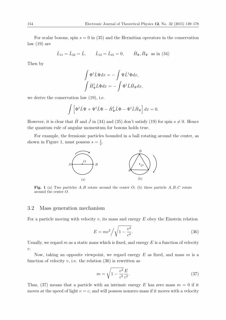
154 Electronic Journal of Theoretical Physics 12, No. 32 (2015) 139–178
For scalar bosons, spin s = 0 in (35) and the Hermitian operators in the conservation
law (19) are
L11 = L22 = L, L12 = L21 = 0, HΦ, HΨ as in (34)
Then by ∫Φ†LΨdx = −
∫ΨL†Φdx,∫
H†ΨLΦdx = −
∫Φ†LHΨdx,
we derive the conservation law (19), i.e.∫ [Φ†LΨ+Ψ†LΦ− H†
ΨLΦ− Φ†LHΨ
]dx = 0.
However, it is clear that H and J in (34) and (35) don’t satisfy (19) for spin s �= 0. Hence
the quantum rule of angular momentum for bosons holds true.
For example, the fermionic particles bounded in a ball rotating around the center, as
shown in Figure 1, must possess s = 12.
A B
O
(a)
A
B
O
(b)
Fig. 1 (a) Two particles A,B rotate around the center O; (b) three particle A,B,C rotatearound the center O.
3.2 Mass generation mechanism
For a particle moving with velocity v, its mass and energy E obey the Einstein relation
E = mc2/√
1− v2
c2. (36)
Usually, we regardm as a static mass which is fixed, and energy E is a function of velocity
v.
Now, taking an opposite viewpoint, we regard energy E as fixed, and mass m is a
function of velocity v, i.e. the relation (36) is rewritten as
m =
√1− v2
c2E
c2. (37)
Thus, (37) means that a particle with an intrinsic energy E has zero mass m = 0 if it
moves at the speed of light v = c, and will possess nonzero mass if it moves with a velocity
Electronic Journal of Theoretical Physics 12, No. 32 (2015) 139–178 155
v < c. All particles including photons can only travel at the speed sufficiently close to
the speed of light. Based on this viewpoint, we can think that if a particle moving at the
speed of light (approximately) is decelerated by an interaction field, obeying
d�P
dt=
√1− v2
c2�F ,
then this massless particle will generate mass at the instant. In particular, by this mass
generation mechanism, several massless particles can yield a massive particle if they are
bounded in a small ball, and rotate at velocities less than the speed of light.
From this mass generation mechanism, we can also understand the neutrino oscillation
phenomena. Experiments show that each of the three neutrinos νe, ντ , νμ can transform
from one to another, although the experiments illustrate that neutrinos propagate at
the speed of light. This oscillation means that they generate masses at the instant of
transformation. This can be viewed as the neutrinos decelerate at the instant when they
undergo the transformation/oscillation, generating instantaneous masses, and after the
transformation, they return to the usual dynamic behavior–moving at the speed of light
with zero masses. In other words, by the mass generation mechanism, we can assert that
neutrinos have no static masses, and their oscillations give rise to instantaneous masses.
3.3 Interaction charges
In the unified field model developed in [8, 7], we derived that both weak and strong
interactions possess charges, as for gravity and electromagnetism:
gravitation: mass charge m
electromagnetism: electric charge e,
weak interaction: weak charge gw,
strong interaction: strong charge gs.
(38)
If Φ is a charge potential corresponding to an interaction, then the interacting force
generated by its charge C is given by
F = −C∇Φ, (39)
where ∇ is the spatial gradient operator.
The charges in (38) possess the physical properties:
1) Electric charges Qe, weak charges Qw, strong charges Qs are conservative. The
energy is a conserved quantity, but the mass M is not a conserved quantity due to
the mass generation mechanism as mentioned earlier.
2) There is no interacting force between two particles without common charges. For
example, if a particle A possesses no strong charge, then there is no strong interacting
force between A and any other particles.
3) Only the electric charge Qe can take both positive and negative values, and other
charges can take only nonnegative values.
156 Electronic Journal of Theoretical Physics 12, No. 32 (2015) 139–178
4) Only the mass charge is continuous, and the others are discrete, taking discrete
values.
5) We emphasize that the continuity of mass is the main obstruction for quantizing the
gravitational field, and it might be essential that gravity cannot be quantized.
3.4 Strong interaction potentials
Three levels of strong interacting potentials are derived in [7] using the field equations, and
they are called the quark potential Sq, the hadron potential Sh, and the atom/molecule
potential Sa:
Sq = gs
[1
r− Bk2
0
ρ0e−k0rϕ(r)
], (40)
Sh = N0
(ρ0ρ1
)3
gs
[1
r− B1
ρ1k21e−k1rϕ(r)
], (41)
Sa = 3N1
(ρ0ρ1
)3 (ρ1ρ2
)3
gs
[1
r− B1
ρ2k21e−k1rϕ(r)
], (42)
where N0 is the number of quarks in hadrons, N1 is the number of nucleons in an
atom/molecule, gs is the strong charge, B and B1 are constants, ρ0 is the effective quark
radius, ρ1 is the radius of a hadron, ρ2 is the radius of an atom/molecule, and
k0 ∼= 1013cm−1, k1 ∼= 1016cm−1.
It is natural to approximately take
ρ0 ∼= 10−21cm, ρ1 ∼= 10−16cm, ρ2 ∼= 10−8cm. (43)
The function ϕ(r) in (40)-(42) is a power series, approximately given by
ϕ(r) =r
2+ o(r).
Formula (40) and (41) lead to the following conclusions for quarks and hadrons:
1) Based on (38), it follows from (40) that the quark interacting force F has the prop-
erties
F
⎧⎪⎨⎪⎩> 0 for 0 < r < R0
= 0 for r = R0,
< 0 for R0 < r < ρ1,
(44)
where R0 is the quark repelling radius, ρ1 is the radius of a hadron as in (43). Namely,
in the region r < R0 the strong interacting force between quarks is repelling, and in
the annulus R0 < r < ρ1, the quarks are attracting, as shown in Figure 2.
2) In the attracting annulus R0 < r < ρ1 as shown in Figure 2, the binding energy
of quarks is in the Planck level, which explains the quark confinement; see [7] for
details.
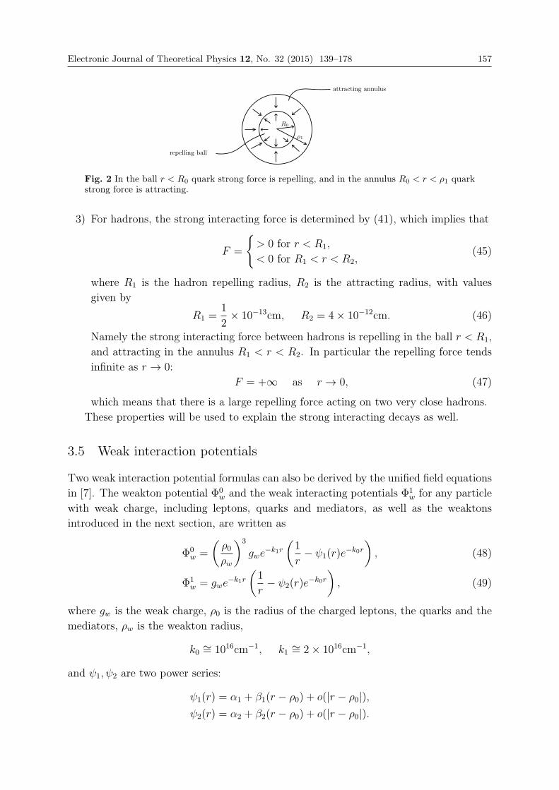
Electronic Journal of Theoretical Physics 12, No. 32 (2015) 139–178 157
R0
attracting annulus
ρ1
repelling ball
Fig. 2 In the ball r < R0 quark strong force is repelling, and in the annulus R0 < r < ρ1 quarkstrong force is attracting.
3) For hadrons, the strong interacting force is determined by (41), which implies that
F =
{> 0 for r < R1,
< 0 for R1 < r < R2,(45)
where R1 is the hadron repelling radius, R2 is the attracting radius, with values
given by
R1 =1
2× 10⁻¹³cm, R2 = 4× 10⁻¹²cm. (46)
Namely the strong interacting force between hadrons is repelling in the ball r < R1,
and attracting in the annulus R1 < r < R2. In particular the repelling force tends
infinite as r → 0:
F = +∞ as r → 0, (47)
which means that there is a large repelling force acting on two very close hadrons.
These properties will be used to explain the strong interacting decays as well.
3.5 Weak interaction potentials
Two weak interaction potential formulas can also be derived by the unified field equations
in [7]. The weakton potential Φ0w and the weak interacting potentials Φ1
w for any particle
with weak charge, including leptons, quarks and mediators, as well as the weaktons
introduced in the next section, are written as
Φ0w =
(ρ0ρw
)3
gwe−k1r
(1
r− ψ1(r)e
−k0r), (48)
Φ1w = gwe
−k1r(1
r− ψ2(r)e
−k0r), (49)
where gw is the weak charge, ρ0 is the radius of the charged leptons, the quarks and the
mediators, ρw is the weakton radius,
k0 ∼= 1016cm−1, k1 ∼= 2× 1016cm−1,
and ψ1, ψ2 are two power series:
ψ1(r) = α1 + β1(r − ρ0) + o(|r − ρ0|),ψ2(r) = α2 + β2(r − ρ0) + o(|r − ρ0|).
158 Electronic Journal of Theoretical Physics 12, No. 32 (2015) 139–178
Here α1, β1, α2, β2 are the initial values of a system of second order ordinary differential
equations satisfied by ψ1 and ψ2, and they are determined by the physical conditions or
experiments.
We remark that (49) was derived in [7], and (48) can be derived in the same fashion
as the three level of strong interaction potentials (40)–(42) in [7].
Based on physical facts, phenomenologically we take ρ0, ρw, α1, α2, β1, β2 as
ρw ∼= 10−26cm, ρ0 ∼= 10−21cm, ρ1 ∼= 10−16cm,
α1∼=
2
ρ0, α2 =
1
ρ1, β1 = 0, β2 > 0.
(50)
The potentials (48) and (49) imply following assertions:
1) Weaktons are confined in the interior of charged leptons, quarks and mediators. In
fact, the bound energy of the weaktons has the level
E = gwΦ0w(ρ0)
∼= −1
ρ0
(ρ0ρw
)3
g2w = −1036g2w/cm.
By the Standard Model,
g2w =8√2Gf
(mwc
�
)2
= 10−1�c. (51)
Hence the bound energy is
E = −1035�c/cm = −1021GeV.
This is the Planck level, to sufficiently confine the weaktons in their composite
particles.
2) By (48) and (50), for the weak interacting force F0 between weaktons, we have
F0
{> 0 for 0 < r < 1
2ρ0,
< 0 for 12ρ0 < r < ρ1,
(52)
where ρ0, ρ1 are as in (43).
3) By (49) and (50), for the weak interacting force F1 of a composite particle, we have
F1
{> 0 for 0 < r < ρ1,
< 0 for ρ1 < r < ρ2.(53)
Hence the weak force is repelling if the particles are in the ρ1-ball, and is attracting
if they are in the annulus ρ1 < r < ρ2.
4) F0 and F1 tend to infinite as r → 0:
F0, F1 → +∞ as r → 0.
Namely, the weak interacting force between two very close particles is large and
repelling.
We shall see that these properties of the weak interacting force are crucial for the
weakton model presented in the next few sections.
Electronic Journal of Theoretical Physics 12, No. 32 (2015) 139–178 159
4. Weakton Model of Elementary Particles
4.1 Decay means the interior structure
From Section 2.5, it is clear that all charged leptons, quarks and mediators can undergo
decay as follows:
• Charged lepton decay:
e− → e− + γ,
μ− → e− + νe + νμ,
τ− → μ− + νμ + ντ .
(54)
• Quark decay:
d → u+ e− + νe,
s → d+ g + γ,
c → d+ s+ u.
(55)
• Mediator decay:
2γ → e+ + e−,
W± → l± + νl± ,
Z0 → l+ + l−.
(56)
All leptons, quarks and mediators are currently regarded as elementary particles.
However, the decays in (54)-(56) show that these particles must have interior structure,
and consequently they should be considered as composite particles rather than elementary
particles:
Decay Means Interior Structure.
4.2 Weaktons and their quantum numbers
The above observation on the interior structure of quarks, charged leptons and mediators
leads us to propose a set of elementary particles, which we call weaktons. These are
massless, spin-12particles with one unit of weak charge gw.
The introduction of weaktons is based on the following theories and observational
facts:
(a) the interior structure of charged leptons, quarks and mediators demonstrated by the
decays of these particles as shown in (54)-(56),
(b) the new quantum numbers of weak charge gw and strong charge gs introduced in
(38),
(c) the mass generating mechanism presented in Section 3.2, and
(d) the weakton confinement theory given by the weak interacting potentials (48).
The weaktons consist of 6 elementary particles and their antiparticles, total 12 parti-
cles:w∗, w1, w2, νe, νμ, ντ ,
w∗, w1, w2, νe, νμ, ντ ,(57)
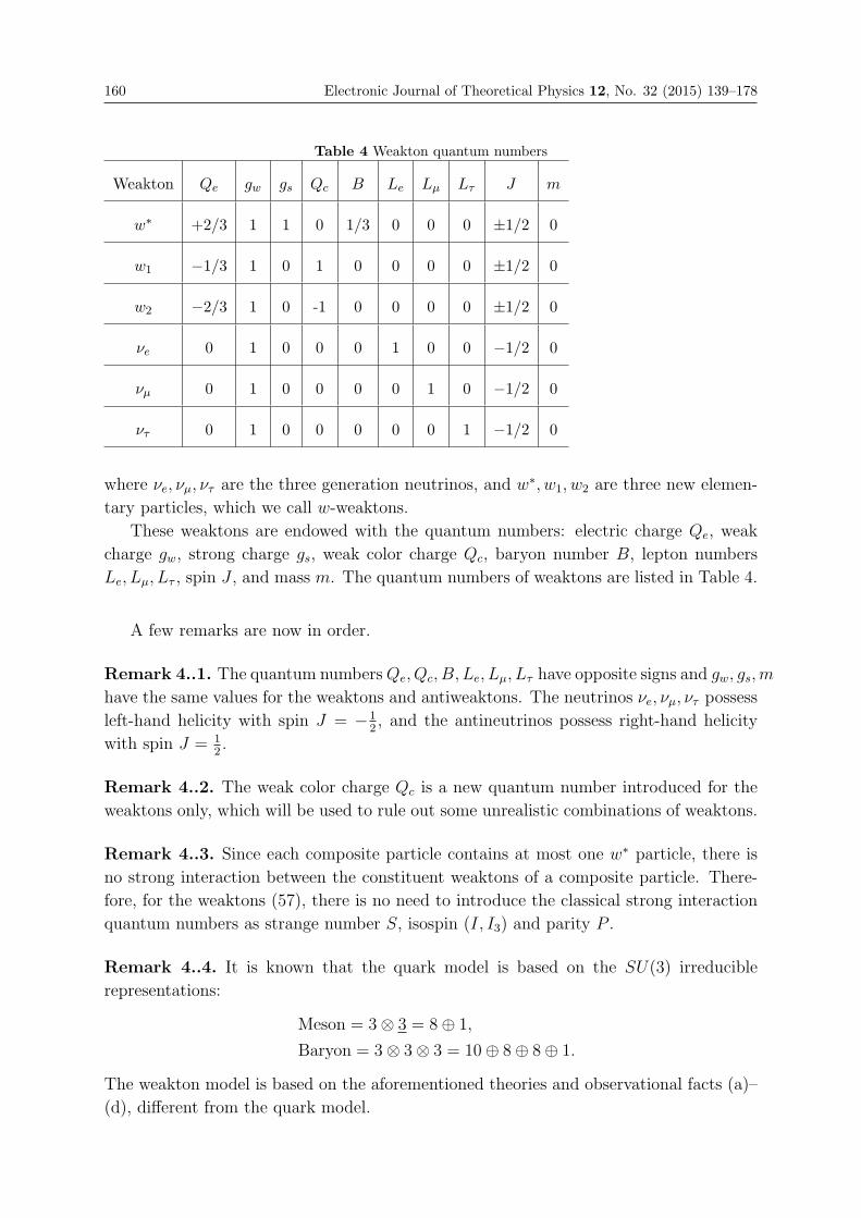
160 Electronic Journal of Theoretical Physics 12, No. 32 (2015) 139–178
Table 4 Weakton quantum numbers
Weakton Qe gw gs Qc B Le Lμ Lτ J m
w∗ +2/3 1 1 0 1/3 0 0 0 ±1/2 0
w1 −1/3 1 0 1 0 0 0 0 ±1/2 0
w2 −2/3 1 0 -1 0 0 0 0 ±1/2 0
νe 0 1 0 0 0 1 0 0 −1/2 0
νμ 0 1 0 0 0 0 1 0 −1/2 0
ντ 0 1 0 0 0 0 0 1 −1/2 0
where νe, νμ, ντ are the three generation neutrinos, and w∗, w1, w2 are three new elemen-
tary particles, which we call w-weaktons.
These weaktons are endowed with the quantum numbers: electric charge Qe, weak
charge gw, strong charge gs, weak color charge Qc, baryon number B, lepton numbers
Le, Lμ, Lτ , spin J , and mass m. The quantum numbers of weaktons are listed in Table 4.
A few remarks are now in order.
Remark 4..1. The quantum numbersQe, Qc, B, Le, Lμ, Lτ have opposite signs and gw, gs,m
have the same values for the weaktons and antiweaktons. The neutrinos νe, νμ, ντ possess
left-hand helicity with spin J = −12, and the antineutrinos possess right-hand helicity
with spin J = 12.
Remark 4..2. The weak color charge Qc is a new quantum number introduced for the
weaktons only, which will be used to rule out some unrealistic combinations of weaktons.
Remark 4..3. Since each composite particle contains at most one w∗ particle, there is
no strong interaction between the constituent weaktons of a composite particle. There-
fore, for the weaktons (57), there is no need to introduce the classical strong interaction
quantum numbers as strange number S, isospin (I, I3) and parity P .
Remark 4..4. It is known that the quark model is based on the SU(3) irreducible
representations:
Meson = 3⊗ 3 = 8⊕ 1,
Baryon = 3⊗ 3⊗ 3 = 10⊕ 8⊕ 8⊕ 1.
The weakton model is based on the aforementioned theories and observational facts (a)–
(d), different from the quark model.
Electronic Journal of Theoretical Physics 12, No. 32 (2015) 139–178 161
4.3 Weakton constituents
In this section we give the weakton compositions of charged leptons, quarks and mediators
as follows.
Charged leptons and quarks. The weakton constituents of charged leptons and
quarks are given by
e = νew1w2, μ = νμw1w2, τ = ντw1w2,
u = w∗w1w1, c = w∗w2w2, t = w∗w2w2,
d = w∗w1w2, s = w∗w1w2, b = w∗w1w2,
(58)
where c, t and d, s, b are distinguished by the spin arrangements. We suppose that
u = w∗w1w1(�↓,�↑, ↑↓↑, ↓↑↓),c = w∗w2w2(�↓,�↑),t = w∗w2w2(↑↓↑, ↓↑↓),
(59)
and
d = w∗w1w2(�↓, ↓↓↑),s = w∗w1w2(↑�, ↓�), (60)
b = w∗w1w2(↑↓↑, ↓↑↓).
Mediators. The duality between mediators given in (9) plays an important role in
the weakton model. In fact, the mediators in the classical interaction theory have spin
J = 1 (graviton has spin J = 2), and are apparently not complete. The unified field
theory in [8, 7] leads to complement mediators with spin J = 0 (graviton dual particle
is J = 1). Thus, the spin arrangements of weaktons in the mediators become perfectly
reasonable.
For convenience, we only write the dual relation for the mediators of electromagnetism,
weak interaction, and strong interaction in the following:
J = 1 J = 0
photon γ ↔ electro-dual boson φγ,
vector bosons W±, Z ↔ weak-dual bosons φ±W , φ0Z ,
gluons gk (1 ≤ k ≤ 8) ↔ strong-dual bosons φkg .
(61)
In view of this duality, we propose the constituents of the mediators as follows:
γ = cos θww1w1 − sin θww2w2 (�,�),
Z0 = cos θww2w2 + sin θww1w1 (�,�),
W− = w1w2(�,�), (62)
W+ = w1w2(�,�),
gk = w∗w∗(�,�), k = color index,
162 Electronic Journal of Theoretical Physics 12, No. 32 (2015) 139–178
and the dual bosons:
φγ = cos θww1w1 − sin θww2w2(↑↓, ↓↑),φ0Z = cos θww2w2 + sin θww1w1(↑↓, ↓↑),
φ−W = w1w2(↑↓, ↓↑), (63)
φ+W = w1w2(↑↓, ↓↑),
φkg = w∗w∗(↑↓, ↓↑),
where θw ∼= 28.76◦ is the Weinberg angle. Here φ0Z corresponds to the Higgs particle in
the standard model, found in LHC. As all the dual mediators in our theory have the
same constituents as the classical mediators, distinguished by spin arrangements, each
mediator and its dual should possess masses in the same level with slight difference, as
evidence by the masses of Z0 and φ0Z .
Remark 4..5. The reason why we take γ, Z0 and their dualities φγ, φ0Z as the linear
combinations in (62) and (63) is that by the Weinberg-Salam electroweak theory, the
U(1)× SU(2) gauge potentials are
Zμ = cos θwW3μ + sin θwBμ,
Aμ = − sin θwW3μ + cos θwBμ
sin2 θw = 0.23.
Here Aμ, Zμ represent γ and Z0.
The ν-mediator. Now the neutrino pairs
νeνe, νμνμ, ντ ντ (↓↑) (64)
have not been discovered, and it should be a mediator. Due to the neutrino oscillations,
the three pairs in (64) should be indistinguishable. Hence, they will be regarded as a
particle, i.e. their linear combination
φ0ν =
∑l
αlνlνl(↓↑),∑l
α2l = 1, (65)
is an additional mediator, and we call it the ν-mediator. We believe that φ0ν is an
independent new mediator.
4.4 Weakton confinement and mass generation
Since the weaktons are assumed to be massless, we have to explain the mass generation
mechanism for the massive composite particles, including the charged leptons e, τ, μ, the
quarks u, d, s, c, t, b, and the vector bosons W±, Z0, φ±W , φ0Z .
The weakton confinement derived in Section 3.5 and the mass generation mechanism
in Section 3.3 can help us to understand why no free w∗, w1, w2 are found and to explain
the mass generation of the composite particles.
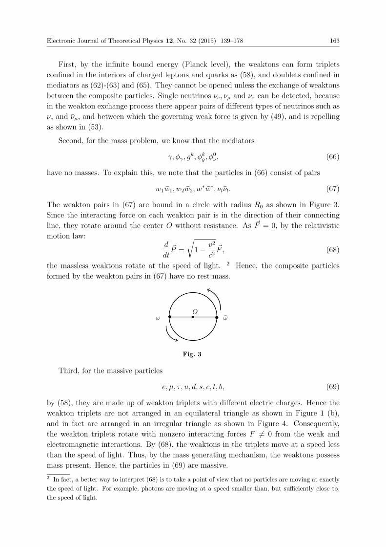
Electronic Journal of Theoretical Physics 12, No. 32 (2015) 139–178 163
First, by the infinite bound energy (Planck level), the weaktons can form triplets
confined in the interiors of charged leptons and quarks as (58), and doublets confined in
mediators as (62)-(63) and (65). They cannot be opened unless the exchange of weaktons
between the composite particles. Single neutrinos νe, νμ and ντ can be detected, because
in the weakton exchange process there appear pairs of different types of neutrinos such as
νe and νμ, and between which the governing weak force is given by (49), and is repelling
as shown in (53).
Second, for the mass problem, we know that the mediators
γ, φγ, gk, φk
g , φ0ν , (66)
have no masses. To explain this, we note that the particles in (66) consist of pairs
w1w1, w2w2, w∗w∗, νlνl. (67)
The weakton pairs in (67) are bound in a circle with radius R0 as shown in Figure 3.
Since the interacting force on each weakton pair is in the direction of their connecting
line, they rotate around the center O without resistance. As �F = 0, by the relativistic
motion law:d
dt�P =
√1− v2
c2�F , (68)
the massless weaktons rotate at the speed of light. 2 Hence, the composite particles
formed by the weakton pairs in (67) have no rest mass.
ωωO
Fig. 3
Third, for the massive particles
e, μ, τ, u, d, s, c, t, b, (69)
by (58), they are made up of weakton triplets with different electric charges. Hence the
weakton triplets are not arranged in an equilateral triangle as shown in Figure 1 (b),
and in fact are arranged in an irregular triangle as shown in Figure 4. Consequently,
the weakton triplets rotate with nonzero interacting forces F �= 0 from the weak and
electromagnetic interactions. By (68), the weaktons in the triplets move at a speed less
than the speed of light. Thus, by the mass generating mechanism, the weaktons possess
mass present. Hence, the particles in (69) are massive.
2 In fact, a better way to interpret (68) is to take a point of view that no particles are moving at exactly
the speed of light. For example, photons are moving at a speed smaller than, but sufficiently close to,
the speed of light.
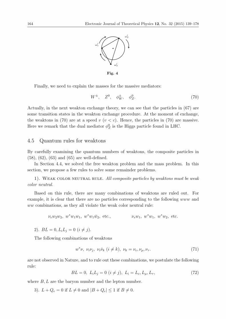
164 Electronic Journal of Theoretical Physics 12, No. 32 (2015) 139–178
ω′
2
ω′
1
ω′
3
Fig. 4
Finally, we need to explain the masses for the massive mediators:
W±, Z0, φ±W , φ0Z . (70)
Actually, in the next weakton exchange theory, we can see that the particles in (67) are
some transition states in the weakton exchange procedure. At the moment of exchange,
the weaktons in (70) are at a speed v (v < c). Hence, the particles in (70) are massive.
Here we remark that the dual mediator φ0Z is the Higgs particle found in LHC.
4.5 Quantum rules for weaktons
By carefully examining the quantum numbers of weaktons, the composite particles in
(58), (62), (63) and (65) are well-defined.
In Section 4.4, we solved the free weakton problem and the mass problem. In this
section, we propose a few rules to solve some remainder problems.
1). Weak color neutral rule. All composite particles by weaktons must be weak
color neutral.
Based on this rule, there are many combinations of weaktons are ruled out. For
example, it is clear that there are no particles corresponding to the following www and
ww combinations, as they all violate the weak color neutral rule:
νew2w2, w∗w1w1, w∗w1w2, etc., νew1, w∗w1, w∗w2, etc.
2). BL = 0, LiLj = 0 (i �= j).
The following combinations of weaktons
w∗ν, νiνj, νiνk (i �= k), νk = νe, νμ, ντ . (71)
are not observed in Nature, and to rule out these combinations, we postulate the following
rule:
BL = 0, LiLj = 0 (i �= j), Li = Le, Lμ, Lτ , (72)
where B,L are the baryon number and the lepton number.
3). L+Qe = 0 if L �= 0 and |B +Qe| ≤ 1 if B �= 0.
Electronic Journal of Theoretical Physics 12, No. 32 (2015) 139–178 165
The following combinations of weaktons
νw1w1, νw2w2, νw1w2, w∗w∗ etc (73)
cannot be found in Nature. It means the lepton number L, baryon number B, and electric
charge Qe obey
L+Qe = 0 if L �= 0 and |B +Qe| ≤ 1 if B �= 0. (74)
Thus (73) are ruled out by (74).
4). Spin selection.
In reality, there are no weakton composites with spin J = 32as
w∗w1w1(↑↑↑, ↓↓↓), w∗w2w2(↑↑↑, ↓↓↓), w∗w1w2(↑↑↑, ↓↓↓) (75)
and as
νw1w2(↑↑↑, ↓↓↓). (76)
The cases (75) are excluded by the Angular Momentum Rule in Section 3.1. The
reasons for this exclusion are two-fold. First, the composite particles in (75) carries one
strong charge, and consequently, will be confined in a small ball by the strong interaction
potential (40), as shown in Figure 1 (b). Second, due to the uncertainty principle, the
bounding particles will rotate, at high speed with almost zero moment of force, which
must be excluded for composite particles with J �= 12based on the angular momentum
rule.
The exclusion for (76) is based on the observation that by the left-hand helicity of
neutrinos with spin J = −12, one of w1 and w2 must be in the state with J = +1
2to
combine with ν, i.e. in the manner as
νww(↓�, ↓↑↓).
In summary, under the above rules 1)-4), only the weakton constitutions in (58), (62),
(63) and (65) are allowed.
5). Eight quantum states of gluons.
It is known that the gluons have eight quantum states
gk : g1, · · · , g8.
In (62), gk have the form
w∗w∗(�,�).
According to QCD, quarks have three colors
red (r), green (g), blue (b),
166 Electronic Journal of Theoretical Physics 12, No. 32 (2015) 139–178
and anti-colors r, g, b. They obey the following rules
bb = rr = gg = w(white),
br = g, rb = g,
bg = r, gb = r,
rg = b, gr = b,
rr = r, bb = b, gg = g,
rb = g, rg = b, gb = r.
(77)
Based on (58), w∗ is endowed with three colors
w∗b , w∗r , w∗g .
Thus, by (77) we give the eight gluons as
g1 = (w∗w∗)w, g2 = w∗b w∗r , g3 = w∗b w
∗g , g4 = w∗rw
∗g , (78)
g5 = (w∗w∗)w, g6 = w∗rw∗b , g7 = w∗gw
∗b , g8 = w∗gw
∗r , (79)
where (w∗w∗)w is a linear combination of w∗b w∗b , w
∗rw
∗r , w
∗gw
∗g . Namely, the gluons in (79)
are the antiparticles of those in (78).
In summary, all of the most basic problems in the weakton model have a reasonable
explanation.
5. Mechanism of Sub-atomic Decays
5.1 Weakton exchanges
We conclude that all particle decays are caused by exchanging weaktons. The exchanges
occur between composite particles as mediators, charged leptons, and quarks.
5.1.1 Weakton exchange in mediators
First we consider one of the most important decay processes in particle physics, the
electron-positron pair creation and annihilation:
2γ → e+ + e−,e+ + e− → 2γ.
(80)
In fact, the reaction formulas in (80) are not complete, and the correct formulas should
be as follows
2γ + φ0ν � e+ + e−. (81)
Note that the weakton component of γ is as
γ = cos θww1w1 − sin θww2w2, (82)
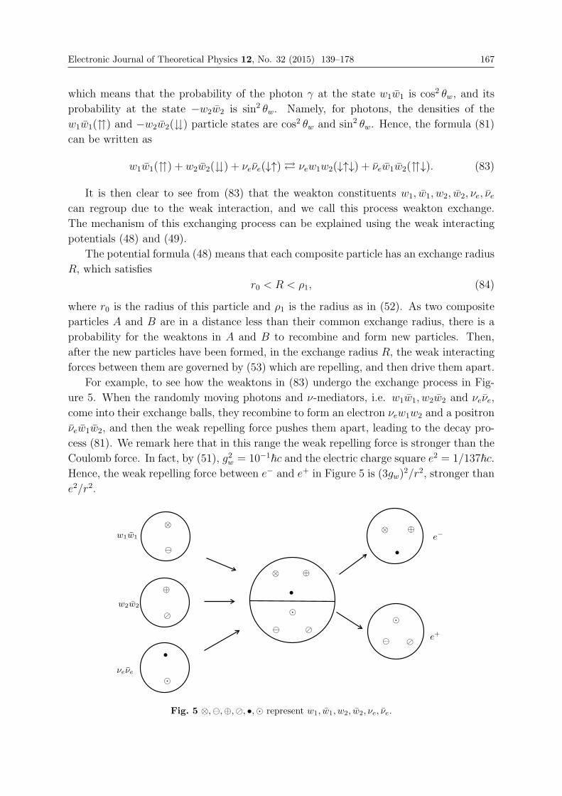
Electronic Journal of Theoretical Physics 12, No. 32 (2015) 139–178 167
which means that the probability of the photon γ at the state w1w1 is cos2 θw, and its
probability at the state −w2w2 is sin2 θw. Namely, for photons, the densities of the
w1w1(�) and −w2w2(�) particle states are cos2 θw and sin2 θw. Hence, the formula (81)
can be written as
w1w1(�) + w2w2(�) + νeνe(↓↑) � νew1w2(↓↑↓) + νew1w2(�↓). (83)
It is then clear to see from (83) that the weakton constituents w1, w1, w2, w2, νe, νecan regroup due to the weak interaction, and we call this process weakton exchange.
The mechanism of this exchanging process can be explained using the weak interacting
potentials (48) and (49).
The potential formula (48) means that each composite particle has an exchange radius
R, which satisfies
r0 < R < ρ1, (84)
where r0 is the radius of this particle and ρ1 is the radius as in (52). As two composite
particles A and B are in a distance less than their common exchange radius, there is a
probability for the weaktons in A and B to recombine and form new particles. Then,
after the new particles have been formed, in the exchange radius R, the weak interacting
forces between them are governed by (53) which are repelling, and then drive them apart.
For example, to see how the weaktons in (83) undergo the exchange process in Fig-
ure 5. When the randomly moving photons and ν-mediators, i.e. w1w1, w2w2 and νeνe,
come into their exchange balls, they recombine to form an electron νew1w2 and a positron
νew1w2, and then the weak repelling force pushes them apart, leading to the decay pro-
cess (81). We remark here that in this range the weak repelling force is stronger than the
Coulomb force. In fact, by (51), g2w = 10−1�c and the electric charge square e2 = 1/137�c.
Hence, the weak repelling force between e− and e+ in Figure 5 is (3gw)2/r2, stronger than
e2/r2.
⊗
�
⊕
�
•
�
w1w1
w2w2
νeνe
⊗ ⊕
•
�
� �
⊗ ⊕
•
�
� �
e−
e+
Fig. 5 ⊗,!,⊕,", •,# represent w1, w1, w2, w2, νe, νe.
168 Electronic Journal of Theoretical Physics 12, No. 32 (2015) 139–178
5.1.2 Weakton exchanges between leptons and mediators
The μ-decay reaction formula is given by
μ− → e− + νe + νμ. (85)
The complete formula for (85) is
μ− + φν → e− + νe + νμ,
which is expressed in the weakton components as
νμw1w2 + νeνe −→ νew1w2 + νe + νμ. (86)
By the rule LeLμ = 0, the μ neutrino νμ and the e antineutrino νe can not be combined
to form a particle. Hence, νe and νμ appear as independent particles, leading to the
exchange of νμ and νe as shown in (86).
5.1.3 Weakton exchanges between quarks and mediators
The d-quark decay in (55) is written as
d→ u+ e− + νe. (87)
The correct formula for (87) is
d+ γ + φν → u+ e− + νe,
which, in the weakton components, is given by
w∗w1w2 + w1w1 + νeνe → w∗w1w1 + νew1w2 + νe, (88)
In (88), the weakton pair w2 and w1 is exchanged, and νe is captured by the new doublet
w1w2 to form an electron νew1w2.
5.2 Conservation laws
The weakton exchanges must obey some conservation laws, which are listed in the fol-
lowing.
5.2.1 Conservation of weakton numbers
The total weaktons given in (57) are elementary particles, which cannot undergo any
decay. Also, the w-weaktons cannot be converted between each other. Although the
neutrino oscillation converts one type of neutrino to another, at the moment of a particle
decay, the neutrino number is conserved, i.e. the lepton numbers Le, Lμ, Lτ are conserved.
Therefore, for any particle reaction:
A1 + · · ·+ An = B1 + · · ·+Bm, (89)
the number of each weakton type is invariant. Namely, for any type of weakton w, its
number is conserved in (89):
NAw = NB
w ,
where NAw and NB
w are the numbers of the w weaktons in two sides of (89).
Electronic Journal of Theoretical Physics 12, No. 32 (2015) 139–178 169
5.2.2 Spin conservation
The spin of each weakton is invariant. The conservation of weakton numbers implies that
the spin is also conserved:
JA1 + · · ·+ JAn = JB1 + · · ·+ JBm ,
where JA is the spin of particle A.
In classical particle theories, the spin is not considered as a conserved quantity. The
reason for the non-conservation of spin is due to the incompleteness of the reaction for-
mulas given in Section 2.5. Hence spin conservation can also be considered as an evidence
for the incompleteness of those decay formulas. The incomplete decay interaction formu-
las can be made complete by supplementing some massless mediators, so that the spin
becomes a conserved quantum number.
5.2.3 Other conservative quantum numbers
From the invariance of weakton numbers, we derive immediately the following conserved
quantum numbers:
electric charge Qe, weak charge Qw, strong charge Qs,
baryon number B, lepton numbers Le, Lμ, Lτ .
5.3 Decay types
In particle physics, the reactions as in Section 2.5 are classified into two types: the weak
interacting type and the strong interacting type. However there is no clear definition to
distinguish them. Usual methods are by experiments to determine reacting intensity, i.e.
the transition probability Γ. In general, the classification is derived based on
Weak type: i) presence of leptons in the reactions,
ii) change of strange numbers,
Strong type: otherwise.
With the weakton model, all decays are carried out by exchanging weaktons. Hence
decay types can be fully classified into three types: the weak type, the strong type, and
the mixed type, based on the type of forces acting on the final particles after the weakton
exchange process.
For example, the reactions
νμ + e− → μ− + νe,
n → p+ e− + νe,
π0 → 2γ,
(90)
are weak decays,
Δ++ → p+ + π+ (91)
170 Electronic Journal of Theoretical Physics 12, No. 32 (2015) 139–178
is a strong decay, and
Λ→ p+ + π−(i.e. Λ + g + 2γ + φγ → p+ + π− + γ) (92)
is a mixed decay.
In view of (90)-(92), the final particles contain at most one hadron in a weak decay,
contain no leptons and no mediators in a strong decay, and contain at least two hadrons
and a lepton or a mediator in a mixed decay. Namely, we derive the criteria based on the
final particle content:
Weak Decay: at most one hadron,
Strong Decay: no leptons and no mediators,
Mixed Decay: otherwise.
5.4 Weak decays
Decays and scatterings are caused by weakton exchanges. The massless mediators
γ, φγ, g, φg (g the gluons), φν (93)
spread over the space in various energy levels, and most of them are at low energy states.
It is these random mediators in (93) entering the exchange radius of matter particles that
generate decays. In the following we shall discuss a few typical weak decays.
5.4.1 νμe− → νeμ
− scattering
First we consider the scattering
νμ + e− → μ− + νe,
which is rewritten in the weakton components as
νμ + νew1w2 → νμw1w2 + νe. (94)
Replacing the Feynman diagram, we describe the scattering (94) using Figure 6. It is
clear that the scattering (94) is achieved by exchanging weaktons νμ and νe.
5.4.2 β-decay
Consider the classical β-decay process
n→ p+ e− + νe. (95)
With the quark constituents of n and p
n = udd, p = uud,
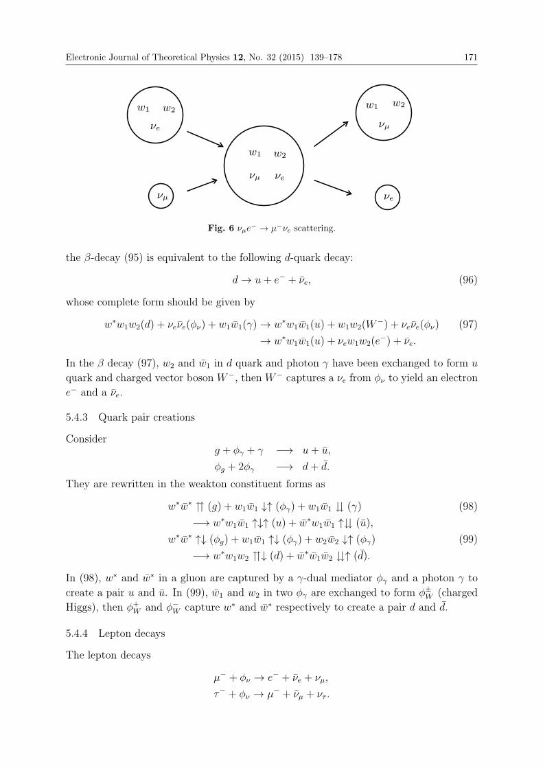
Electronic Journal of Theoretical Physics 12, No. 32 (2015) 139–178 171
νe
w1 w2
νμ νe
w1w2
νμ
w1 w2
νe
νμ
Fig. 6 νμe− → μ−νe scattering.
the β-decay (95) is equivalent to the following d-quark decay:
d→ u+ e− + νe, (96)
whose complete form should be given by
w∗w1w2(d) + νeνe(φν) + w1w1(γ)→ w∗w1w1(u) + w1w2(W−) + νeνe(φν) (97)
→ w∗w1w1(u) + νew1w2(e−) + νe.
In the β decay (97), w2 and w1 in d quark and photon γ have been exchanged to form u
quark and charged vector boson W−, then W− captures a νe from φν to yield an electron
e− and a νe.
5.4.3 Quark pair creations
Considerg + φγ + γ −→ u+ u,
φg + 2φγ −→ d+ d.
They are rewritten in the weakton constituent forms as
w∗w∗ � (g) + w1w1 ↓↑ (φγ) + w1w1 � (γ) (98)
−→ w∗w1w1 ↑↓↑ (u) + w∗w1w1 ↑� (u),
w∗w∗ ↑↓ (φg) + w1w1 ↑↓ (φγ) + w2w2 ↓↑ (φγ) (99)
−→ w∗w1w2 �↓ (d) + w∗w1w2 �↑ (d).
In (98), w∗ and w∗ in a gluon are captured by a γ-dual mediator φγ and a photon γ to
create a pair u and u. In (99), w1 and w2 in two φγ are exchanged to form φ±W (charged
Higgs), then φ+W and φ−W capture w∗ and w∗ respectively to create a pair d and d.
5.4.4 Lepton decays
The lepton decays
μ− + φν → e− + νe + νμ,
τ− + φν → μ− + νμ + ντ .
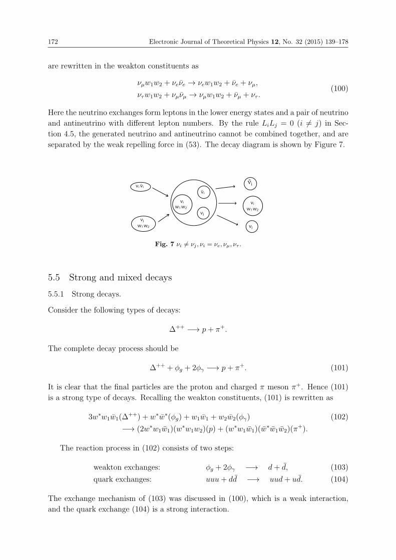
172 Electronic Journal of Theoretical Physics 12, No. 32 (2015) 139–178
are rewritten in the weakton constituents as
νμw1w2 + νeνe → νew1w2 + νe + νμ,
ντw1w2 + νμνμ → νμw1w2 + νμ + ντ .(100)
Here the neutrino exchanges form leptons in the lower energy states and a pair of neutrino
and antineutrino with different lepton numbers. By the rule LiLj = 0 (i �= j) in Sec-
tion 4.5, the generated neutrino and antineutrino cannot be combined together, and are
separated by the weak repelling force in (53). The decay diagram is shown by Figure 7.
νi-
Fig. 7 νi �= νj , νi = νe, νμ, ντ .
5.5 Strong and mixed decays
5.5.1 Strong decays.
Consider the following types of decays:
Δ++ −→ p+ π+.
The complete decay process should be
Δ++ + φg + 2φγ −→ p+ π+. (101)
It is clear that the final particles are the proton and charged π meson π+. Hence (101)
is a strong type of decays. Recalling the weakton constituents, (101) is rewritten as
3w∗w1w1(Δ++) + w∗w∗(φg) + w1w1 + w2w2(φγ) (102)
−→ (2w∗w1w1)(w∗w1w2)(p) + (w∗w1w1)(w
∗w1w2)(π+).
The reaction process in (102) consists of two steps:
weakton exchanges: φg + 2φγ −→ d+ d, (103)
quark exchanges: uuu+ dd −→ uud+ ud. (104)
The exchange mechanism of (103) was discussed in (100), which is a weak interaction,
and the quark exchange (104) is a strong interaction.
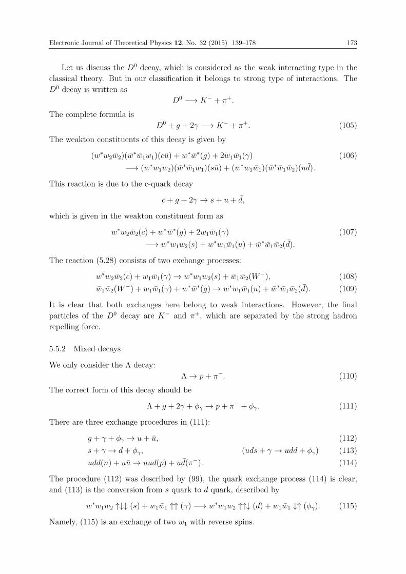
Electronic Journal of Theoretical Physics 12, No. 32 (2015) 139–178 173
Let us discuss the D0 decay, which is considered as the weak interacting type in the
classical theory. But in our classification it belongs to strong type of interactions. The
D0 decay is written as
D0 −→ K− + π+.
The complete formula is
D0 + g + 2γ −→ K− + π+. (105)
The weakton constituents of this decay is given by
(w∗w2w2)(w∗w1w1)(cu) + w∗w∗(g) + 2w1w1(γ) (106)
−→ (w∗w1w2)(w∗w1w1)(su) + (w∗w1w1)(w
∗w1w2)(ud).
This reaction is due to the c-quark decay
c+ g + 2γ → s+ u+ d,
which is given in the weakton constituent form as
w∗w2w2(c) + w∗w∗(g) + 2w1w1(γ) (107)
−→ w∗w1w2(s) + w∗w1w1(u) + w∗w1w2(d).
The reaction (5.28) consists of two exchange processes:
w∗w2w2(c) + w1w1(γ)→ w∗w1w2(s) + w1w2(W−), (108)
w1w2(W−) + w1w1(γ) + w∗w∗(g)→ w∗w1w1(u) + w∗w1w2(d). (109)
It is clear that both exchanges here belong to weak interactions. However, the final
particles of the D0 decay are K− and π+, which are separated by the strong hadron
repelling force.
5.5.2 Mixed decays
We only consider the Λ decay:
Λ→ p+ π−. (110)
The correct form of this decay should be
Λ + g + 2γ + φγ → p+ π− + φγ. (111)
There are three exchange procedures in (111):
g + γ + φγ → u+ u, (112)
s+ γ → d+ φγ, (uds+ γ → udd+ φγ) (113)
udd(n) + uu→ uud(p) + ud(π−). (114)
The procedure (112) was described by (99), the quark exchange process (114) is clear,
and (113) is the conversion from s quark to d quark, described by
w∗w1w2 ↑↓↓ (s) + w1w1 ↑↑ (γ) −→ w∗w1w2 ↑↑↓ (d) + w1w1 ↓↑ (φγ). (115)
Namely, (115) is an exchange of two w1 with reverse spins.
174 Electronic Journal of Theoretical Physics 12, No. 32 (2015) 139–178
6. Electron Radiations
6.1 Electron structure
The weakton constituents of an electron are νew1w2, which rotate as shown in Figure 4.
Noting that
electric charge: Qνe = 0, Qw1
e = −1
3, Qw2
e = −2
3,
weak charge: Qνw = 1, Qw1
w = 1, Qw2w = 1,
we see that the distribution of weaktons νe, w1 and w2 in an electron is in an irregular
triangle due to the asymptotic forces on the weaktons by the electramagnetic and weak
interactions, as shown in Figure 8.
ρ
Fig. 8 Electron structure.
In addition, by the weak force formula (53), there is an attracting shell region of weak
force:
ρ1 < r < ρ2, ρ1 = 10−16 cm (116)
with small weak force. Outside this region, the weak force is repelling:
Fw > 0 for r < ρ1 and r > ρ2. (117)
Since the mediators γ, φγ, g, φg and φν contain two weak charges 2gw, they are attached
to the electron in the attracting shell region (116), forming a cloud of mediators. The
irregular triangle distribution of the weaktons νe, w1 and w2 generate a small moment
of force on the mediators in the shell region, and there exist weak forces between them.
Therefore the bosons will rotate at a speed lower than the speed of light, and generate a
small mass attached to the naked electron νew1w2.
6.2 Mechanism of Bremsstrahlung
It is known that an electron emits photons as its velocity changes. This is called
bremsstrahlung, and the reasons why bremsstrahlung can occur is unknown in classical
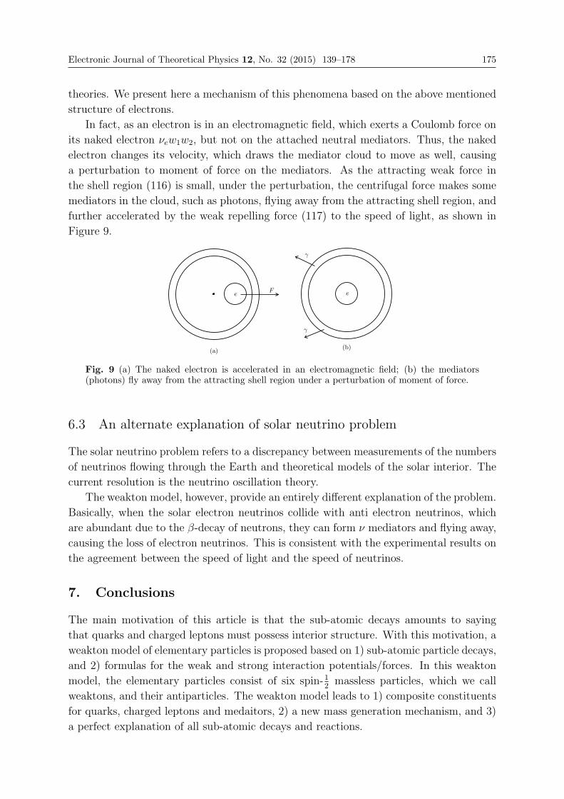
Electronic Journal of Theoretical Physics 12, No. 32 (2015) 139–178 175
theories. We present here a mechanism of this phenomena based on the above mentioned
structure of electrons.
In fact, as an electron is in an electromagnetic field, which exerts a Coulomb force on
its naked electron νew1w2, but not on the attached neutral mediators. Thus, the naked
electron changes its velocity, which draws the mediator cloud to move as well, causing
a perturbation to moment of force on the mediators. As the attracting weak force in
the shell region (116) is small, under the perturbation, the centrifugal force makes some
mediators in the cloud, such as photons, flying away from the attracting shell region, and
further accelerated by the weak repelling force (117) to the speed of light, as shown in
Figure 9.
e
(a)
Fe
(b)
γ
γ
Fig. 9 (a) The naked electron is accelerated in an electromagnetic field; (b) the mediators(photons) fly away from the attracting shell region under a perturbation of moment of force.
6.3 An alternate explanation of solar neutrino problem
The solar neutrino problem refers to a discrepancy between measurements of the numbers
of neutrinos flowing through the Earth and theoretical models of the solar interior. The
current resolution is the neutrino oscillation theory.
The weakton model, however, provide an entirely different explanation of the problem.
Basically, when the solar electron neutrinos collide with anti electron neutrinos, which
are abundant due to the β-decay of neutrons, they can form ν mediators and flying away,
causing the loss of electron neutrinos. This is consistent with the experimental results on
the agreement between the speed of light and the speed of neutrinos.
7. Conclusions
The main motivation of this article is that the sub-atomic decays amounts to saying
that quarks and charged leptons must possess interior structure. With this motivation, a
weakton model of elementary particles is proposed based on 1) sub-atomic particle decays,
and 2) formulas for the weak and strong interaction potentials/forces. In this weakton
model, the elementary particles consist of six spin-12massless particles, which we call
weaktons, and their antiparticles. The weakton model leads to 1) composite constituents
for quarks, charged leptons and medaitors, 2) a new mass generation mechanism, and 3)
a perfect explanation of all sub-atomic decays and reactions.
176 Electronic Journal of Theoretical Physics 12, No. 32 (2015) 139–178
With this weakton model and the unified field theory [8, 7], we now present our expla-
nations and viewpoints to the twelve fundamental questions stated in the Introduction.
Q1: Our current view on four interactions is that each interaction has its own charge,
the mass charge m, the electric charge e, the weak charge gw and the strong charge gs,
which are introduced in Section 3.3. Each weakton carries one unit of weak charge, hence
the name weakton, and only w∗ carries a unit of strong charge gs. A particular interaction
can only occur between two particles if they both carry charges of the corresponding
interaction.
The dynamic laws for four interactions are the unified field model, which can be easily
decoupled to study individual interactions. Our theory shows that each interaction has
both attractive and repulsive regions, leading the stability of matter in our universe.
Q2: With the weakton model, it is clear that leptons do not participate strong in-
teractions, as they do not carry any strong charge–the weakton constituents of charged
leptons (58) do not include w∗.
Q3: The weakton model postulates that all matter particles (leptons, quarks) and
mediators are made up of massless weaktons. The basic mass generation mechanism is
presented in Section 3.2. Namely, for a composite particle, the constituent massless weak-
tons can decelerate by the weak force, yielding a massive particle, based on the Einstein
mass-energy relation. Also, the constituent weaktons are moving in an “asymptotically-
free” shell region of weak interactions as indicated by the weak interaction potential/force
formulas, so that the bounding and repelling contributions to the mass are mostly can-
celed out. Hence the mass of a composite particle is due mainly to the dynamic behavior
of the constituent weaktons.
Q4 & Q5: In Sections 5.1-5.5, the weakton model offers a perfect explanation for
all sub-atomic decays and all generation/annihilation precesses of matter-antimatter. In
particular, all decays are achieved by 1) exchanging weaktons and consequently exchang-
ing newly formed quarks, producing new composite particles, and 2) separating the new
composite particles by weak and/or strong repelling forces. Also, we know now the precise
constituents of particles involved in all decays both before and after the reaction.
Q6: Again, the sub-atomic decays and reactions offer a clear evidence for the existence
of interior structure for quarks and leptons, as well as for mediators. The consistency of
the weakton model with all reactions and decays, together with conservations of quan-
tum numbers, demonstrates that both quarks and charged leptons are not elementary
particles.
Q7 (Baryon Asymmetry): Conventional thinking was that the Big Bang should
have produced equal amounts of matter and antimatter, which will annihilate each other,
resulting a sea of photons in the universe, a contradiction to reality. The weakton model
offers a complete different view on the formation of matter in our universe. The weakton
model says that what the Big Bang produced was a sea of massless elementary weaktons
and anti-weaktons, forming all the matter, including mediators such as photon, in the
Electronic Journal of Theoretical Physics 12, No. 32 (2015) 139–178 177
universe. Hence with the weakton model, the baryon asymmetry problem is no longer a
right question to ask.
Q8–Q11: The decoupled unified field model leads to three levels of strong interaction
potentials and two levels of weak interaction potentials as recalled in (40)–(42), (48)
and (49). These formulas give a natural explanation of both the short-range nature
and confinements for both strong and weak interactions. The different levels of each
interaction demonstrate that in the same spatial region, the interaction can be attracting
between weaktons, and be repelling for newly formed hadrons and leptons. This special
feature of weak and strong interactions plays a crucial rule for decays.
Q12 (Bremsstrahlung): The weak interaction force formulas show that the attract-
ing shell region near a naked electron can contain a cloud of neutral mediators as photon.
As the naked electron changes its velocity due to the presence of an electromagnetic field,
which has no effect on the neutral mediator cloud. The change of velocity of electron gen-
erates a perturbation to moment of force on the mediators causing some of the mediators
flying out from the attracting shell region. This is the mechanism of bremsstrahlung; see
Sections 6.1 and 6.2.
Q13 (Solar neutrino problem): When the solar electron neutrinos collide with anti
electron neutrinos, which are abundant due to the β-decay of neutrons, they can form ν
mediators and flying away, causing the loss of electron neutrinos. This is consistent with
the experimental results on the agreement between the speed of light and the speed of
neutrinos.
References
[1] E. J. Eichten, K. D. Lane, and M. E. Peskin, New tests for quark and leptonsubstructure, Phys. Rev. Lett., 50 (1983), pp. 811–814.
[2] D. Griffiths, Introduction to elementary particles, Wiley-Vch, 2008.
[3] F. Halzen and A. D. Martin, Quarks and leptons: an introductory course inmodern particle physics, John Wiley and Sons, New York, NY, 1984.
[4] H. Harari, A schematic model of quarks and leptons, Physics Letters B, 86 (1979),pp. 83–86.
[5] G. Kane,Modern elementary particle physics, vol. 2, Addison-Wesley Reading, 1987.
[6] T. Ma and S. Wang, Gravitational field equations and theory of dark matterand dark energy, Discrete and Continuous Dynamical Systems, Ser. A, 34:2 (2014),pp. 335–366; see also arXiv:1206.5078v2.
[7] , Unified field theory and principle of representation invariance, AppliedMathematics and Optimization, 69:3 (2014), pp. 359–392; see also version 1 ofarXiv:1212.4893.
[8] , Unified field equations coupling four forces and principle of interactiondynamics, Discrete and Continuous Dynamical Systems, Ser. A, 35:3 (2015),pp. 1103–1138; see also arXiv:1210.0448.
178 Electronic Journal of Theoretical Physics 12, No. 32 (2015) 139–178
[9] J. C. Pati and A. Salam, Lepton number as the fourth ”color”, Phys. Rev. D, 10(1974), pp. 275–289.
[10] C. Quigg, Gauge theories of the strong, weak, and electromagnetic interactions, 2ndedition, Princeton Unversity Press, 2013.
[11] M. A. Shupe, A composite model of leptons and quarks, Physics Letters B, 86 (1979),pp. 87–92.
[12] N.-S. Zhang, Particle Physics, vol. I & II, in Chinese, Chinese Academic Press,1994.
EJTP 12, No. 32 (2015) 179–294 Electronic Journal of Theoretical Physics
Physics of Currents and PotentialsII. Classical Singlet-Triplet Electroweak Theory with
Non-point Particles
Valerii Temnenko∗
Tavrian National University, 95004, Simferopol, Crimea, Ukraine
Received 16 March 2014, Accepted 19 July 2014, Published 10 January 2015
Abstract: The formulation of classical singlet-triplet (electroweak) theory, in which point
particles are replaced by continual current fields, has been presented. The expression for the
Lagrangian of the theory and complementary algebraic and differential constraints, imposed on
the currents of the theory, have been suggested. Classification of stationary and wave states
for the singlet-triplet theory has been given. Stationary states correspond to massive particles
with the current zone of a finite volume. The theory contains a number of wave states, both
one-sector (singlet or triplet waves) and compound two-sector ones (singlet-triplet waves). Wave
states differ in number of currents: zero-current waves (free singlet or free triplet waves), one-
current, two-current, three-current and four-current ones. Wave states also differ in character
of four-dimensional wave vector (the waves with time-like and space-like wave vector). Some
forms of waves may have negative density of energy. Some wave states can be treated as
classical models of a neutrino. Neutrino states are classified in accordance with the character of
the current which forms the state: singlet (maxwellian) neutrino, Yang-Mills triplet neutrino,
Maxwell-Yang-Mills singlet-triplet neutrino.c© Electronic Journal of Theoretical Physics. All rights reserved.
Keywords: Lagrangian; Singlet-Triplet Theory; Classification of the States in the Singlet-Triplet
Theory; Yang-Mills Triplet Waves; Classical Models of Neutrino
PACS (2010): 03.50.-z; 03.50.Kk; 11.10.-z; 12.15.-y
1. Introduction
Let us extend the approach stated in the article [1] over the unified theory of electroweak
interaction. Within the framework of this extension we should postulate the existence
of two sectors of physics of currents and potentials: singlet (or maxwellian) sector and
triplet (or Yang-Mills) sector. Each sector contains a dyad ”current/potential”. Singlet
180 Electronic Journal of Theoretical Physics 12, No. 32 (2015) 179–294
sector contains singlet (maxwellian) current Jν and singlet (maxwellian) potential Wν
which is dynamically conjugated with it. Triplet sector contains Yang-Mills triplet of
currents Jν =
{a
J ν
}and dynamically conjugated with it Yang-Mills triplet of potentials
Wν =
{a
W ν
}. Over-letter indices a, b, c number the components of Yang-Mills triplets:
a = 1, 2, 3. Greek indices μ, ν, . . . number Lorentz components of 4-vectors. They run
over values 0, 1, 2, 3.
The adjectives ”singlet” and ”maxwellian”, which are synonyms and often appear in
the text, will be sometimes expressed by symbols S- or M-, for example, ”S-current”
or ”M-current” instead of the term ”singlet current”. Generally speaking, the terms
”triplet” and ”Yang-Mills” are not synonyms: octuplet (chromodynamical) sector of
physics deals with Yang-Mills octuplet of currents and dynamically conjugated with it
Yang-Mills octuplet of potentials. However, within the framework of the present article,
which is devoted to classical electroweak theory, we shall treat the terms ”triplet” and
”Yang-Mills” as synonyms, and if necessary, we shall denote them with symbols T- or
YM-, for example, ”T-current” or ”YM-current” instead of the term ”triplet current”.
YM-geometry is Euclidian: there is no necessity to introduce contravariant and covariant
indices. YM-vectors are denoted with bold type in indexless notation. In some cases we
have to use bold type for indexless notation of the three space components of Lorentz
4-vectors. We hope that the reader will be able to tell these objects from YM-vectors.
Twice repeating YM-indices imply summation, such as, for example, scalar YM-product
of YM-vectors Jν and Wν :
Jμ ·Wν ≡a
Jμa
W ν ≡3∑
a=1
a
Jμa
W ν .
In the three-dimensional space of YM-vectors it is possible to enter a vector product
through Levi-Civita 3-symbolabcε in a conventional way: if Cμν = Aμ ×Bν ,
a
Cμν =abcε
b
Aμc
B ν ,
while objecta
Cμν is Yang-Mills 3-vector and Lorentz tensor of the second rank in Minkov-
ski four-dimensional space-time.
Singlet M-potential Wν does not coincide with the electromagnetic potential Aν con-
sidered in the article [1]. Singlet M-current Jν also does not coincide with the electro-
magnetic current which we will denote as Jem
ν . However, as we will show later, in the
”mixed” Maxwell-Yang-Mills’ singlet-triplet world there are ”pure” maxwellian (singlet)
states in which electromagnetic potential Aν , proportional to singlet potential Wν , and
electromagnetic current, proportional to singlet current Jν , can be introduced to describe
a state, thereby we will revert to the classical electromagnetic theory of non-point parti-
cles, formulated in the article [1]. With description of an arbitrary mixed singlet-triplet
state, such extraction of electromagnetic potential in the form of some linear combination
of singlet and triplet potential is also possible, but it is irrational: it overloads simple and
Electronic Journal of Theoretical Physics 12, No. 32 (2015) 179–294 181
natural algebra of YM-vectors.
Dynamics of the two field dyads ”currents/potentials” of the singlet-triplet world is de-
rived from the principle of the least action at minimization of action functional S:
S =
∫L′dΩ. (1)
The total space-time integration is implied in this expression; L′ is the effective La-
grangian consisting of the sum of the base Lagrangian L and the addition to the La-
grangian Lad, which is caused by the necessity of accounting differential and algebraic
constraints, which are a priori imposed on the four currents (Jν ,Jν).
The base LagrangianL consists of the sum of two sector Lagrangians - the singlet La-
grangian LS and the triplet Lagrangian LT :
L = LS + LT . (2)
The relation (2) means that singlet and triplet sectors of physics do not intermingle with
each other on the level of the base Lagrangian.
Each of the two sector terms of the base Lagrangian (2), in its turn, consists of three terms,
which correspondently describe the current part of the Lagrangian Lcur, the Lagrangian
of current and potential Lint interaction, and the free field Lagrangian Lf :
LS = LS,cur + LS,int + LS,f ,
LT = LT,cur + LT,int + LT,f .(3)
Integrals in (1), containing the Lagrangians of free fields, are taken from all over the
4-space. Integrals in (1), containing the current Lagrangian Lcur and the interaction
Lagrangian Lint are taken over current 4-zones ΩJ , in which at least one of the four
currents is nonzero. It is supposed that in the current zones each of the four currents is
space-like:
JνJν ≤ 0, (4)
1
J ν1
J ν ≤ 0;2
J ν2
J ν ≤ 0;3
J ν3
J ν ≤ 0. (5)
The condition of form (4) was substantiated for electromagnetic current in the previous
article [1]. Current inequalities (4) and (5) are taken here by analogy with the inequality
for Jem
ν as the postulates of physics without which the construction of the classical theory
of non-point particles is impossible.
At the three-dimensional boundaries σJ of the four-dimensional current zones ΩJ at least
one of the currents becomes isotropic, and, correspondingly, the sign of equality is reached
at least in one of the relations (4). Such boundary, termed in the article [1] a ”pomerium”,
can be common for some currents or can disintegrate into different boundaries for different
currents. Beyond such boundary, on which isotropization of one of the four currents took
place, this current is identically zero. At the boundary itself, this isotropic current is
orthogonal to 4-vector of normal to the boundary nμ.
According to the reasons given in the article [1], we have to accept that pseudo-Euclidian
182 Electronic Journal of Theoretical Physics 12, No. 32 (2015) 179–294
modules of space-like currents are limited by absolute value. Thereby, we must postulate
the existence of such fundamental constant jS, that
−JνJν ≤ j2S (6)
and of such fundamental constant jT , that
−1
J ν1
J ν ≤ j2T ;
−2
J ν2
J ν ≤ j2T ;
−3
J ν3
J ν ≤ j2T .
(7)
It is unlikely that God would have been so wasteful to have created two different fun-
damental constants of the same dimension, and the equality jS = jT does not seem
impossible.
The reasons, given below in p.3.4, make it possible to come to conclusion that jT ≤ jS2.
Adoption of inequalities (6) and (7) is necessary for obtaining finite mass of particles
within the framework of the classical theory under consideration.
The equality sign in relations (6) and (7) is reached at some three-dimensional boundaries
of the four-dimensional current zones. Some cavitated no-current tubes are limited by
these boundaries inside the current zone. Let us call such cavitated no-current tube with
a term ”latebra”. This word was translated from the language of the ancient Romans
as a ”sheltered place”, ”hiding place” and it also had the meaning ”inner cavity”. The
boundary of a cavitated tube will be termed ”latens” (hidden, invisible).
According to the reasons provided in the article [1], it can be expected that diametrical di-
mensions of latebra are of the order of Planckian length rp. The longitudinal dimension
of latebra is determined by the appearing in the theory unknown fundamental constant
of length dimension r0: r0 > rp.
Latebra and latens are inaccessible in any laboratory experiment – as one of the few
survived Heraclitus’ fragments reads, ”nature likes hiding”. Late Roman commentator
Macrobius, while interpreting this idea one thousand years after Heraclitus, said that
”nature feels disgusted to be exposed open and naked”. However, to give sense to the
classical theory of currents and potentials discussed here, we must consider currents and
potentials as measurable physical quantities even in case if the only device, which had
already been known to Isaac Newton, Sensorium Dei, is applicable for their measuring.
According to the reasons given in the article [1], when constructing the theory of non-
point particles, we should take into account Riemannian space-time curvature, generated
by large quantities of energy-momentum tensor components in the region occupied by
currents and inside the cavitated no-current latebrae .
As in the article [1], we will suppose that this account of curvature can be provided
according to Einsteinian recipe:
• obtain the field theory equations in Minkowski coordinates, ignoring the space-time
curvature;
2 See the form below (292), which determines the relation between the constants jS and jT .
Electronic Journal of Theoretical Physics 12, No. 32 (2015) 179–294 183
• rewrite the obtained equations in arbitrary curvilinear coordinates with arbitrary
metric tensor which possesses Minkowski signature (+– – –) at each point of the
four-dimensional space-time continuum;
• subordinate the metric tensor to Einstein equations, which read that the Ricci ten-
sor is proportional to energy-momentum tensor; the proportionality coefficient is
determined by gravitation constant.
When solving the wave states problems, where the boundaries of pomerium and latens are
missing, the space-time curvature can be ignored, supposing that energy density in the
wave is insufficient for forming substantial deviations from Minkowski plane geometry.
The singlet-triplet theory, constructed here, assumes the existence of the states where
the conditions of isotropy of currents (4) or (5) for one or a few currents are satisfied
in some four-dimensional zone ΩN rather than on the three-dimensional hyper-surface of
pomerium σJ. We shall name these states ”neutrino states”; the corresponding isotropic
currents will be named ”neutrino currents”. Neutrino states should be treated as non-
stationary, transitional states generated by some instability of ”neutrinoless” states. How-
ever, the theory also admits the existence of the model wave neutrino states, in which
neutrino zone ΩN coincides with the whole four-dimensional space. While considering
such states, we have to sacrifice the condition of currents and fields disappearance ”at
infinity”. Generally speaking, these conditions must be always supposed to be satisfied
at minimization of the action functional (1).
Summing up the ”Introduction”, we would like to remind the reader that the constructed
theory, as in the article [1], includes the unknown fundamental dimension constant r0.
This constant is further assumed as a length unit. Velocity of light c is also assumed as
a unit. Constants r0 and c do not explicitly appear in the theory formulas.
2. The Base Lagrangian of the Singlet-triplet Theory
2.1 The Interaction Lagrangian. The Weinberg Angle
Let us suppose, as in classical electrodynamics, that the singlet interaction Lagrangian
LS,int is proportional to scalar product of singlet current Jν and singlet potential Wν :
LS,int ∼ JνWν , (8)
and, similarly, the triplet interaction Lagrangian LT,int is proportional to ”twice scalar”
product of the triplet current Jν and the triplet potential Wν :
LT,int ∼ Jν ·Wν . (9)
The expression (9) implies summation by unwritten explicitly YM-indices and summation
by Lorentz indices (Euclidean scalar product in three-dimensional Euclidean space of
YM-vectors and pseudo-Euclidean scalar product of 4-vectors in four-dimensional pseudo-
Euclidean Minkowski space-time).
Proportionality coefficients in formulas (8) and (9) are negative [2]. We do not have any
184 Electronic Journal of Theoretical Physics 12, No. 32 (2015) 179–294
a priori grounds to suggest that the expressions (8) and (9) must enter into the general
interaction Lagrangian with identical weight. We shall assume that singlet and triplet
contributions to Lint have different weight factors pS and pT :
Lint = −1
2pSJνWν −
1
2pTJν ·Wν . (10)
(pS > 0; pT > 0).
In the units of measurement used here, currents and potentials have an electric charge
dimension. The Lagrangian and the action functional have a dimension of an electric
charge square. The singlet interaction constant of pS and triplet interaction constant
pT are dimensionless, although their numerical values are determined by selecting an
electric charge unit of measurement (as it is possible to introduce an arbitrary coefficient
of proportionality between the left and the right parts of the relation (1), which determine
the action functional). It is convenient to normalize the sum of squares of constants pSandpT per unit:
p2S + p2T = 1. (11)
The relation (11), implying a definite selection of an electric charge unit of measurement,
by normalizing the general contribution of the interaction Lagrangian (10) to the total
Lagrangian, keeps us from a temptation to consider the model ”one-sector” worlds: the
singlet world with the triplet sector (pT → ∞) ”switched off” or the triplet world with
the singlet sector (pS → ∞) ”switched off”. The relation (11) allows us to use one con-
stant instead of two fundamental constants pS and pT . If we assume that pT = sin θw(0 < θw <
π
2), according to (11) we should assume that pS = cos θw.
The fundamental constant θw is usually called Weinberg angle. It would be more correct
(but more ponderous) to call this constant ”the angle of the singlet-triplet mixing” and,
correspondingly, to denote it with θST .
The same electric charge unit that was used in (11) for Weinberg parameters normaliz-
ing, is used to measure currents and potentials. Accordingly, further the currents and
potentials are considered dimensionless.
2.2 The Current Lagrangian
Based on the results of the preceding article [1], we shall assume that the contribution
of each current to the base Lagrangian in neutrinoless state is proportional to pseudo-
Euclidean square of current. ”Assigning” corresponding weight factors, we shall write
the current part of the Lagrangian as follows:
Lcur = −1
8p2SJνJν −
1
8p2TJν · Jν . (12)
The weight factor in the singlet part of the current Lagrangian (12) is set on the basis
of compliance with the electromagnetic theory of non-point particles, constructed in the
preceding article [1]. Weight factor in the triplet part of the current Lagrangian (12) is
Electronic Journal of Theoretical Physics 12, No. 32 (2015) 179–294 185
set on the basis of current ”singlet-triplet equality”, by means of substitution of pS → pT ,
Jν → Jν in the singlet part of the current Lagrangian.
In the state which is neutrino by some current, the pseudo-Euclidean square of this
current in the neutrino 4-zone ΩN is equal to zero, and the contribution of this current
to the current Lagrangian is missing (12). However, the pseudo-Euclidean square of a
neutrino current appears in the additional Lagrangian Lad with an arbitrary Lagrange’s
multiplier.
2.3 The Field Lagrangian
The field Lagrangian in (2) and (3) is constructed in the form of the expression which is
quadratic by tensors of the singlet and triplet field Wμν and Wμν with identical weight
factors:
Lf = − 1
16πWμνW
μν − 1
16πWμν ·Wμν . (13)
The singlet field tensor Wμν is constructed in the same way as it is constructed in classical
electrodynamics [2]
Wμν = ∂μWν − ∂νWμ. (14)
Yang-Mills triplet field tensor was constructed in the classical article of these two authors
[3]3. In the symbols we have accepted, it looks as follows:
Wμν = ∂μWν − ∂νWμ + pTWμ ×Wν , (15)
or, with explicitly specified YM-indices:
a
Wμν= ∂μa
Wν −∂νa
Wμ +pTabcε
b
Wμ
c
Wν . (16)
The choice of expressions (15), (16) for YM-field tensor was in due time motivated by
considerations of SU(2) – gauge invariance (in the era of Yang-Mills they spoke of an
”isotopic gauge invariance” [3]). However, the explicit construction of YM-potential and
YM-field tensor , in this way, requires appealing to the notion ”wave function phase” of
point particles and it is inadmissible in the classical theory of non-point charges, which is
developed here. Within the framework of this classical theory it is reasonable to treat the
potential and current as primary, irredundant and non-interpreted concepts, and to treat
YM-field tensor (15) (in the spirit of ”pedagogical” motivations typical for the course of
Landau and Lifshitz [2]), as the simplest antisymmetric Lorentz second-rank tensor (and,
at the same time, YM-vector), which can be constructed from YM-vector.
Fixation of the multiplicative constant in (15) before the nonlinear term suggests a certain
choice of measurement unit for the electric charge. Change of the unit charge in (15)
requires re-scaling of this multiplier and violates unit coefficient normalization (11). The
3 Wolfgang Pauli, as pointed by N. Straumann [4], developed the main aspects and formulas known now
as ”Yang-Mills theory” already in summer 1953, but he didn’t publish his results.
186 Electronic Journal of Theoretical Physics 12, No. 32 (2015) 179–294
fact that this unit of charge measurement, connecting (11) and (15), coincides with the
charge value of the electron, can be treated as a casual gift4.
2.4 The Total Base Lagrangian of the Singlet-triplet Theory
By substituting the written out expressions for separate terms of the base Lagrangian
(10), (12), (13) into (2) and (3), we obtain the total base Lagrangian of a neutrinoless
state:
L = − 1
8p2SJνJν−
1
8p2TJνJν−
1
2pSJνWν−
1
2pTJν ·Wν−
1
16π(WμνW
μν +Wμν ·Wμν) . (17)
In this Lagrangian the singlet field tensor Wμν is calculated by the formula (14) through
the components of the singlet potential Wμ. The triplet field tensor Wμν is calculated
through the components of the triplet potential Wμ by formula (15). Weight factors
pS and pT (”Weinberg parameters”) are expressed by the formulas mentioned in p. 2.1
through the fundamental constant θw which is exterior for this theory. Currents Jν and
Jν , potentials Wν and Wν are primary, non-interpreted variables of the theory, which
are inexpressible by other more elementary physical concepts. If, in accordance with the
specific initial conditions, the formation of the neutrino 4-zone ΩN , occupied by isotropic
current, is possible in the singlet-triplet problem, within this zone the contribution of
a corresponding neutrino (isotropic) current falls out of the two first terms in the base
Lagrangian (17), but this contribution is restored (with an arbitrary Lagrange’s multi-
plier) in the additional Lagrangian Lad, since the condition of current isotropy must be
considered as holonomic constraint imposed on the solution of the singlet-triplet problem.
3. The Algebraic and Differential Constraints
for Currents. The Additional Lagrangian
3.1 Differential Condition for Singlet Current Conservation
As in the classical electrodynamics [1], the condition for S-current conservation is adopted
in the singlet sector of the theory:
∂μJμ = 0. (18)
The condition (18) requires appearing of the term in the form of1
2p2Sχ∂νJ
ν in the addi-
tional Lagrangian Lad, where χ is the arbitrary Lagrange’s multiplier depending on the
space-time coordinates xμ, and the multiplier1
2p2Sis introduced for the convenience of
the additional and base Lagrangian combination. By extracting from this term the total
4 This ”gift” faintly signifies that the singlet-triplet theory is possibly not a final and unimprovable
version of physics of electroweak interactions.
Electronic Journal of Theoretical Physics 12, No. 32 (2015) 179–294 187
4-divergence1
2p2S∂ν(χJ
ν), which disappears after the Lagrangian integration over the en-
tire 4-space, we can denote the corresponding contribution to the additional Lagrangian
as follows
Lad(χ) = −1
2p2SJν∂νχ.
As it is known, the differential constraint (18) is natural for the Lagrangian (17). This
constraint is the result of Maxwell field equations, appearing with minimization of the
action functional with the Lagrangian (17) under any Lagrange’s multiplier χ. So, it
would be reasonable to assume from the outset that χ = 0 and not to include the term
Lad(χ) into the additional Lagrangian.
3.2 Differential Condition for the Triplet Current
Generally speaking, the triplet YM-current, by contrast to the singlet M-current, is not
conserved. Differential constraint, imposed on YM-current [3], can be described in the
form of the relation which we are free to adopt as a postulate:
∂μJμ + pTWμ × Jμ = 0. (19)
Multiplying the equation (19) by the arbitrary Lagrange’s multiplier χ (Lorentz scalar
and YM-vector), after the extraction of total 4-divergence, we obtain a corresponding
contribution to the additional Lagrangian coupled with the Lagrange’s multiplier χ:
Lad(χ) =1
2p2T(−Jμ∂μχ+ pTχ · (Wμ × Jμ)) .
In this expression the multiplicative constant1
2p2Tis introduced for the convenience of
combination of the base Lagrangian and the Lagrangian Lad(χ).
By varying the total Lagrangian L with addition of Lad(χ) it is not difficult to estab-
lish that the differential constraint (19) for YM-current is the result of Yang-Mills field
equations with any option of the Lagrange’s multiplier χ which satisfies the condition
∂μχ+ pTWμ × χ = 0.
Supposing that χ = 0, we are satisfying this condition. Such option of χ may be not
convenient enough to solve some problems, but its use is acceptable in any problem.
Consequently, we may avoid including term Lad(χ) into the additional Lagrangian.
Let us call the choice of the Lagrange’s multipliers χ = 0 and χ = 0 the Lorentz gauge.
The possibility of Lorentz gauge choice is connected with the idea of the gauge symmetry,
the essence of which can be expressed in the following way: construct the field tensor
from potentials in such a way that the differential constraints, which are a priori imposed
on the currents and express physical laws of current conservation/interconversion, would
be natural constraints for the base Lagrangian.
188 Electronic Journal of Theoretical Physics 12, No. 32 (2015) 179–294
When using Lorentz gauge, the differential constraints (18) and (19) should not be in-
cluded into the list of solvable problems under the numerical solution of field problems.
They can be used as a tool for monitoring of accuracy and stability of the computation
process.
3.3 Algebraic condition for the Singlet
and Triplet Current Coupling
Existence of singlet current Jν violates the isotropy of YM-space; it violates the equality
of the three currents of YM-triplet Jν , selecting from three YM-currents the one which
the singlet current Jν is closely coupled with. We shall denote this ”selected” current by3
J ν . Algebraic condition for S-current Jν coupling with the selected third component of
YM-triplet of currents3
J ν has the following form:
3
J ν
(3
Jν −Jν)
= 0. (20)
The algebraic postulate (20) specifies the holonomic constraint, imposed on the currents
of the singlet-triplet theory. It is based on the current structure of Weinberg-Salam elec-
troweak theory (”WS theory”, e.g. [5]). But the current structure of WS theory per se
cannot be a ”legal” basis for the classical theory that we are constructing. The currents
in WS theory are algebraic expressions which are bilinear by the spinor wave functions of
fermions. Point fermions are primary, non-interpretable objects of WS theory. They are
built into the theory ”manually”. In WS theory, just as in the modern relativistic quan-
tum theory in general, the totally quantum object – spinor wave function of a fermion –
is implicitly interpreted as some true classical field under construction of the classical
Lagrangian which afterwards, following the procedure of the secondary quantization (or
Feinman integration by all possible configurations of all fields of the theory), transforms
into a carrier of all the information about the quantum system. Such inconsistency, a
latent ”dragging” of the quantum object into the classical Lagrangian, dating back to the
pioneer works of 1930th (V. Heisenberg, W. Pauli, V. Veiskopf), generates the condition
of modern quantum relativistic physics, which was uncompromisingly described by a se-
vere judge Paul Dirac as ”an ugly and incomplete one” [6].
Here we are constructing the classical theory, in which the wave functions of particles can
not appear in any way; and the massive particles are not built into the theory ”manually”.
They are missing ”at the entrance” of the theory, but they must appear as computable,
constructed objects ”at the exit” of the theory. ”At the entrance” of the theory there are
only currents and potentials, plus the base Lagrangian structure, as well as the holonomic
and differential constraints which are imposed on the currents.
According to these remarks, the algebraic constraint, imposed on the currents of the the-
ory (20), must be considered a postulate of the theory, without any apparent references
to the existing WS theory. The accounting of this constraint leads to appearance in the
Electronic Journal of Theoretical Physics 12, No. 32 (2015) 179–294 189
additional Lagrangian of a term which we shall denote as Lad(ψ):
Lad(ψ) = −1
2p2Tψ
3
J ν
(3
Jν −Jν). (21)
In formula (21), ψ is the Lagrange’s multiplier, which is the functional of the space-time,
coordinates xμ. This very term in the Lagrangian ”entangles” physics of the singlet
maxwellian sector with physics of triplet Yang-Mills sector in case if current3
J ν is differ-
ent from identical zero. The base Lagrangian (17) splits into singlet and triplet parts.
The terms of the additional Lagrangian Lad(χ) and Lad(χ), generated by the differential
constraints imposed on currents (if these terms are proper to calculate technically by
numerical solution of a definite problem), are also placed according to the principle ”each
one in its own sector”. And only the term (21) in the additional Lagrangian mixes two
sectors of physics.
3.4 Algebraic ”2→ 3” Decomposition of the Coupled Pair of currents Jν
and3
J ν
The algebraic condition (20), coupling S-current Jν with the third YM-component of T-
current Jν , and the conditions for the space-likeness of currents (4), (5) make it possible
to conduct an effective decomposition of a couple of currents Jν ,3
J ν , by representing
them in the form of a linear combination of the triple of mutually orthogonal currents
Nν , lν ,rν , where current Nν is isotropic and currents lν and rν are space-like:
Jν = Nν + lν + 2rν ,3
J ν = lν −Nν ,
N νNν = 0,
lνNν = 0,
rνNν = 0,
lνrν = 0,
lνlν < 0, rνrν < 0.
(22)
It is not difficult to see that the problem (22) has two one-parametric families of solutions.
The condition for the existence of these solutions is the inequalities
JνJν <3
J ν3
Jν< 0. (23)
It is proper to construct an explicit solution to the problem (22) within the ”intrinsic
frame of reference” of current3
J ν , where time component of current3
J 0 is missing and
3-vector of the current space components is oriented along the axisx1:
3
J ν = {0, α, 0, 0}. (24)
190 Electronic Journal of Theoretical Physics 12, No. 32 (2015) 179–294
With regard to (24) and condition (20), the singlet current Jν can be represented in this
frame of reference in the following form:
Jν = {τ, α, β, 0} ; τ 2 < β2. (25)
In (25) it is established that through the rotation about axis x1 we oriented axes x2 and
x3 in a way that J3 = 0.
Inequality, connecting τ and β, results from the inequality (23).
Thus, rν , which at decomposition (22) enters only into the singlet current Jν , is generally
called the right-handed current . Thus, lν , which enters into both S-current Jν and
the third component of YM-triplet3
J ν , is called the left-handed current . The isotropic
current Nν will be called a neutrino current . The solution to the problem (22) for the
neutrino current can have the following form:
N ν = N{β, 0, τ, ±
√β2 − τ 2
}, (26)
where N is an arbitrary normalization multiplier. It is proper to assume that N = 1.
Fixation of parameter N in a specific frame of reference does not influence Lorentz-
invariance of the solution: for transition to another frame of reference it is enough to
make Lorentz-transformation of 4-vector (26). Under such gauge of Nν , the left-handed
and the right-handed currents have the following form:
lν ={β, α, τ, ±
√β2 − τ 2
},
rν =
{τ
2− β, 0,
β
2− τ, ∓
√β2 − τ 2
}.
(27)
Currents lν and rν depend on the arbitrarily chosen gauge of parameter N , but their sum
jν = lν + rν (”electromagnetic current”) does not depend on the choice of N :
jν =
{τ
2, α,
β
2, 0
}.
Combination of currents qν also does not depend on the choice of normalization constant
N :
qν = rν +N ν .
Electromagnetic current jν and current qν are reduced to the half-sum and, correspond-
ingly, to the half-difference of currents Jν and3
J ν , and, consequently, they are as well-
defined physical quantities as currents Jν and3
J ν . Currents Nν , lν , rν themselves in the
arbitrary singlet-triplet state are not well-defined physical quantities.
The procedure of ”2 → 3”-decomposition of currents, presented by formulas (26) and
(27), does not only depend on the arbitrary gauge of parameter (and the choice of sign
in z-components of vectors N3, l3, r3) – this procedure is also not P-invariant. Indeed,
the inversion of spatial axes means the reversal of sign of spatial components of any
vector, including transformation α → −α, β → −β in the components of currents Jν
Electronic Journal of Theoretical Physics 12, No. 32 (2015) 179–294 191
and3
J ν (formulas (24) and (25)). But, y-components of vectors N2 and l2, described
by the formulas (26) and (27), do not change sign in the process, but time components
N0 and l0 change the sign. Thus, under the inversion of spatial axes, all three currents
Nν , lν and rν turn into other physical entities. To restore the invariance of the theory
relatively to discrete transformations, it is necessary to make T-transformation (change
of the time coordinate sign) and C-transformation (change of sign of all currents and po-
tentials) along with P-transformation (inversion of spatial coordinates). In so doing, to
follow PCT-invariance of the theory in z-components of the currents (N3, l3, r3) we have
to transit to the second branch of the square root5. PCT-inversion leaves the procedure
of ”2 → 3”-decomposition of currents invariant. This procedure itself is not necessary
for the classical theory. Of course, there are such physical states, in which the terms
”right-hand current”, ”left-handed current”, ”neutrino current” describe the observable
physical quantities. The simplest of these states is a pure singlet state with a nonde-
generate singlet current J (JνJν < 0) and an empty triplet sector (Jν = 0;Wν = 0). In
this case we can assume that lν = 0, Nν = 0, consequently, the singlet current Jν is
reduced to the right-hand current: Jν = 2rν . The extraction of a neutrino current is
effective in special limit conditions when one or both inequality signs in formula (23) are
replaced by equality signs. For example, if currents Jν and3
J ν have identical nonzero
pseudo-Euclidean modules:
JνJν =3
J ν3
Jν< 0, (28)
and, accordingly, in formula (25) τ = β, the system of equations (22) has no solution
which would satisfy the condition of space-likeness of the right-hand current rν . The
condition (28) describes ”left-hand state”:
rν = 0,
lν =
{1
2β, α,
1
2β, 0
},
Nν =
{1
2β, 0,
1
2β, 0
},
and decomposition of currents has a simple form:
Jν = lν +Nν ,3
J ν = lν −N ν .(29)
In the left-hand singlet-triplet state (29) the left-hand current lν and neutrino current
Nν must be regarded as observable physical quantities. In the process, currents1
J ν ,2
J ν
are sure to be present in the triplet sector.
One more special limit condition is a combined isotropization of both currents Jν and3
J ν :
JνJν =3
J ν3
Jν= 0.
5 In language usually used in theoretical physics, this transition to the second branch of square root in the
expression for neutrino current Nν (26) can be interpreted as transition from neutrino to antineutrino.
192 Electronic Journal of Theoretical Physics 12, No. 32 (2015) 179–294
In this condition, in formulas (23) we should suppose that lν = 0 and rν = 0, and,
consequently, according to (22), we should accept that:
Jν = N ν ,3
J ν = −Nν .(30)
In such mixed singlet-triplet state, the same neutrino current Nν is present both in the
singlet and triplet sector (”Maxwell-Yang-Mills neutrino”).
There are two more special one-sector neutrino states.
The first one is the singlet neutrino state with ”empty” triplet sector:
Jν = Nν ; N νNν = 0
Jν = 0; Wν = 0.
In this state the decomposition formula (22) ”does not work” – there is no triplet partner
for current Jν .
This one-sector singlet neutrino state (”maxwellian neutrino”) is studied in detail in the
article [1] of this series6. Algebraic condition (20), imposed on the currents, will be also
satisfied at the ”empty” singlet sector in case if current3
J ν is a neutrino one:
Jν = 0; Wν = 0.3
J ν = Nν ; NνNν = 0.(31)
In this case the decomposition formulas (22) ”do not work”: current3
J ν does not have a
singlet partner.
Relations (31) describe a one-sector triplet neutrino state (one of the variants of ”Yang-
Mills neutrino”).
3.5 Algebraic Condition for the Inner Normalization
of Yang-Mills Triplet
The current structure of the standard version of electroweak WS-theory with point par-
ticles indicates the existence of one more algebraic constraint, imposed on the three
components of YM-triplet:
21
J ν2
Jν=3
J ν3
Jν . (32)
While we take the condition (32) as a postulate of the triplet theory, it registers some
kind of ”auto-normalization” of the currents inside YM-triplet. This condition creates
its own contribution Lad(η) to the additional Lagrangian Lad:
Lad(η) =η
2p2T
(2
1
J ν2
Jν −3
J ν3
Jν
), (33)
6 The description of this state in [1] contained reservations expressing a doubt as to reality of such
neutrino state: the principal text of the article [1] was already written in the late 1970s, and it took the
author a long period of time to put up with such Maxwellian model of neutrino.
Electronic Journal of Theoretical Physics 12, No. 32 (2015) 179–294 193
in which η is a Lagrange’s multiplier which depends on the space-time coordinates xν .
This contribution to the Lagrangian is totally placed in YM-sector of the theory.
The very fact of appearing of the algebraic constraints (20) and (32) in the theory, which
are beyond the base Lagrangian of the theory, is rather unpleasant from the point of
view of an estimation of the completeness and correctness of our ideas of fundamentals
of physics. The Lagrange’s multipliers ψ and η, entering into the additional Lagrangian,
actually correspond to some outer ”Higgs-like” fields, which influence the real physical
fields. In the language of Newtonian mechanics they correspond to the ”constraints
force”, imposed on the current fields by someone from outside. The theory could be
rehabilitated by constructing such solutions for the theory equations, for which algebraic
constraints (20) and (32) are natural , i.e. are satisfied under the absence of ”Higgs-like”
fields ψ and η: ψ ≡ 0 and η ≡ 0.
3.6 About Quality Criteria of the Classical Physical Theory
We can assume that a good classical physical theory has to satisfy two of the following
quality criteria:
• the theory contains a short , not requiring any extension, list of primary objects of
the theory which form the base Lagrangian;
• the theory does not contain any external to the Lagrangian constraints imposed on
the primary objects, or these constraints are natural for the Lagrangian of the
theory and do not generate any external ”Higgs-like” constraint forces, at least for
some quite wide range of solutions.
The existing version of theoretical physics – both Weinberg-Salam electroweak theory
and the Standard Model – actually does not satisfy the first criterion. Point fermions
with their wave functions are built into the theory ”manually” as primary objects. There
can be as many fundamental fermions as possible: only experimental data restricts the
length of the list of primary objects of the theory. The existing version of physics also
does not satisfy the second criterion, as it contains external Higgs objects.
The version of classical field theory, developed here, satisfies the first criterion. In this
version the short list of primary objects of the theory is a priori fixed: they are currents
only the singlet and triplet ones (and octuplet, if strong interactions are taken into
account). There is nothing in nature except them and dynamically conjugated with them
potentials with the same Yang-Mills dimension (singlet, triplet and octuplet). Particles
and waves are secondary, derivative, calculated entities; they are the objects ”at the exit”
of the theory – there can be as many of them as possible.
We do not know if the theory, developed here, satisfies the second criterion. We have no
theorem which would contain the proof of the fact that there exists quite a wide range
of solutions to the equations of singlet-triplet theory, such as that algebraic constraints
(20) and (32), imposed on the currents, are natural for the base Lagrangian of the theory
194 Electronic Journal of Theoretical Physics 12, No. 32 (2015) 179–294
and can be satisfied under zero values of ”Higgs-like” fields ψ and η7. These solutions
describe all singlet-triplet states, which are realized in nature.
Two more criteria have to be added to the two quality criteria of the fundamental physical
theory, formulated above.
• The theory naturally incorporates the accounting of Riemann space-time curvature.
• The theory must contain the solutions with finite energy and should not require
renormalization or regularization.
The theory, developed here, satisfies these criteria, while Weinberg-Salam theory and the
Standard Model do not.
And, finally, a good physical theory has to satisfy the fifth, Einsteinian, quality criterion:
• The theory should not contain arbitrarily specified dimensionless ”empirical” con-
stants. The fine structure constant, the mixing angles, the mass ratio of particles,
etc. must be calculated within the theory8.
There is no theory satisfying this Einsteinian criterion in modern physics. The theory,
developed here, partly satisfies this criterion, apparently, allowing calculating mass ratio
of the particles.
4. Discrete Transformations
in the Singlet-Triplet Theory
4.1 Charge Conjugation in the Singlet-Triplet Theory
The field theory, constructed here, – and its base Lagrangian L (17) and additional
Lagrangian Lad, consisting of the sum of Lad(ψ) (21) and Lad(η) (33), - are invariant
relative to the charge conjugation consisting of two operations:
(1) Sign reversal for all currents and potentials;
(2) Permutation of Yang-Mills indices 1↔ 2.
Formally it can be written with help of two sector operators of the charge conjugation,
operator CS, affecting the singlet vectors and reduced to change of their sign:
Jν → J′ν = CSJν = −Jν ,Wν →W′
ν = CSWν = −Wν ,
and operator CT , affecting YM-triplets of vectors. Operator CT is YM-matrix, changing
vector signs and permutating YM-indices 1↔ 2:
Jν → J′ν = CTJν ,
Wν →W′ν = CTWν ,
7 We also do not know if there exists at least one mathematician who is able to get interested in this
problem.8 ”God had no choice”, – this is probably the answer that must be given by good physical theory to the
famous Albert Einsteins question.
Electronic Journal of Theoretical Physics 12, No. 32 (2015) 179–294 195
where CT =
⎛⎜⎜⎜⎜⎝0 −1 0
−1 0 0
0 0 −1
⎞⎟⎟⎟⎟⎠.
The structure of singlet-triplet theory itself demonstrates ”inequality” of Lorentz vectors
entering YM-triplet. The third YM-component of current3
Jν is connected with singlet
current Jν by relation (20) and is thereby distinguished in Yang-Mills triple. It is obvious
that this extraction has to be also transferred to the third YM-component of potential3
Wν . ”Inequality” of YM-indices 1 and 2 (”chiral inequality”) is connected with the
availability of the vector YM-product in determining of the triplet field tensor Wμν (15)
and differential constraint (19). In these expressions vector YM-product is summed up
with YM-vector. For this summation operation to make invariant geometric sense in YM-
space, the vector YM-product should not be an axial YM-vector, but a true YM-vector.
Therefore, with the specified third YM-vectors component we must absolutely definitely
choose the numbering scheme of the first and the second components. We should suppose
that we have a possibility to provide a chiral consistency, i.e. to choose the right-handed
(or the left-handed) coordinate system simultaneously and consistently in the coordinate
space and YM-vector space9. To provide chiral consistency at the inversion of a sign of
YM-currents and YM-potentials, we have to permutate YM-indices 1↔ 2.
At the performing of the described transformation of charge conjugation, field tensors
are transformed in the same way as the currents and potentials:
Wμν →W′μν = CSWμν ,
Wμν →W′μν = CTWμν .
The base Lagrangian, quadratic by currents, potentials and field tensors, does not change
with charge conjugation.
To conclude paragraph 4.1, we will dare to make two anticipatory remarks. Probably,
these remarks will help the reader to estimate the defiant beauty and complexity of
Yang-Mills physics.
(1) In octuplet sector of physics, which is responsible for strong interactions and is the
subject for discussion in the subsequent article of this series, there is no octuplet
matrix of charge conjugation similar to triplet matrix CT by its characteristics. In
other words, in contrast to the singlet and triplet sector, the octuplet sector of
physics is charge-asymmetrical. No permutation of vector numbers in Yang-Mills
octuplet provides invariance of the octuplet Lagrangian relative to the inversion of
currents.
No doubt, this fact is not psychologically easy to put up with. Perhaps, it is as
hard to do as it was for the physicists of 1956 to put up with the parity violation.
However, the charge asymmetry, latent in the octuplet algebra itself, obviously makes
9 ”Only a theory defines what can be observable”, – Albert Einstein once said to Werner Heinsenberg.
196 Electronic Journal of Theoretical Physics 12, No. 32 (2015) 179–294
it possible to understand the reason of the evident and defiant charge asymmetry of
the Universe: in the octuplet sector God had a choice .
(2) The requirement to observe chiral definiteness of the solutions of Yang-Mills equa-
tions actually imposes some unilateral (releasing) constraint on variables of the
triplet and octuplet sectors of physics. Such constraint is not something unusual
for the problems of classical mechanics, for example, the constraint between two
material points, established by means of a nonstretchable line. Problems of mechan-
ics with such unilateral constraint lead to solutions, discontinuous by the velocity
vector: at the moments of ”constraint activation” some velocity components change
a sign for the opposite. If you do not like solutions with velocity discontinuity, you
are free to complicate the constraint model for example, to consider line stretcha-
bility.
However, in the problems of mathematical physics and the field theory, unilateral con-
straints, apparently, did not occur before. Besides, unlike a mechanical problem with
nonstretchable line, we do not have any more accurate and adequate model in reserve:
there is nothing beyond Yang-Mills physics at all, this is all physics.
In particular, considering the problems of Yang-Mills free no-current waves, we easily find
out that Yang-Mills nonlinear wave equations possess chiral symmetry, despite the chiral
asymmetry of the field tensor and the Lagrangian. Accordingly, the solutions of these
equations possess chiral symmetry. Here we encounter not a very pleasant dilemma:
a) to take beautiful, continuous and smooth chiral-symmetric solutions which contain the
most difficult and unpredictable chaotic oscillations and to shut our eyes to the require-
ment of chiral determinacy of the solution;
or
b) to take into account the requirement of chiral determinacy and ”to impose” chiral de-
terminacy upon the solution by means of rough ”chiralization” procedure; the solutions
become discontinuous by derivatives, lose their chaotic character and gain a rather boring
periodicity10.
Choosing the first alternative leads to good Yang-Mills mathematical physics, but to
the knowingly incorrect Yang-Mills physics which violates the requirement of chiral de-
terminacy of solutions.
The choice of the second alternative correctly reproduces physical requirements of Yang-
Mills chiral definiteness, but generates rather ugly version of Yang-Mills mathematics of
solutions with derivatives discontinuities.
The very necessity for discussion of this ”mathematics-physical” dilemma seems strange
after half-a-century existence of Yang-Mills equations. Apparently, it is connected with
the fact that during these fifty years there has been made no serious attempt to turn Yang-
Mills classical field theory into the similar minutely developed section of mathematical
physics and applied mathematics, which is classical electrodynamics, for example.
10 In the subsequent articles of this series the examples of numerical solutions to the problems of Yang-
Mills triplet and octuplet waves both chaotic chiral-symmetric solutions and periodic solutions generated
by the procedure of chiralization will be provided.
Electronic Journal of Theoretical Physics 12, No. 32 (2015) 179–294 197
4.2 Combined Coordinate Inversion
in the Singlet-Triplet Theory
When making the operation of inversion of coordinate system:
xν → x′ν = −xν , (34)
it should be taken into account that occurring transformation of the three-dimensional
right-handed coordinate system to the left-handed one (or vice versa) requires the same
transformation in YM-space, i.e. permutation of YM-indices 1↔ 2. However, during the
performance of the transformation (34) and YM-permutation, different terms in the ex-
pression for YM-tensor of field Wμν (15) behave differently. In the coordinate inversion,
Lorentz vectors of currents and potentials reverse signs, consequently, the expressions in
the form of ∂νJν or ∂νWμ do not reverse a sign. However, vector products in the form
of Wμ × Jμ or Wμ ×Wν do reverse a sign due to permutation of YM-indices 1↔ 2.
One more operation has to be provided for restoration of the consistency of transfor-
mational qualities of different terms in the same formula – sign inversion of currents
and potentials (without repeated permutation of the indices 1 ↔ 2). As a result, both
the base Lagrangian and additional Lagrangian of the singlet-triplet theory prove to be
invariant relative to this three-way combined coordinate inversion:
(1) Inversion of signs xν , generating the inversion of signs Jν , Wν , Jν and Wν .
(2) Permutation of YM-indices 1↔ 2.
(3) Repeated inversion of the signs of currents and potentials.
Finally, when performing such combined inversion, currents and potentials do not change,
field tensors reverse a sign (with regard to permutation of YM-indices 1 ↔ 2); the
Lagrangian does not change.
Coordinate inversion (34) per se, not accompanied by charge inversion, is not a correctly
determined procedure in the triplet sector of physics11.
5. About the Name of the Theory
The standard name of this branch of physics, going back to Abdul Salam, is ”electroweak
theory”. This name is absolutely justified from the historical point of view: unification
within the framework of one theory of electromagnetic and weak interaction was a great
achievement at the time of WS theory creation. However, from the point of view of logical
structure of this theory, we believe that it is possible to leave the terms ”electromagnetic
interaction” and ”weak interaction” in the past and to speak about ”singlet-triplet the-
ory” (ST theory) or, at least, about ”Maxwell and Yang-Mills theory” (MYM theory).
11The triviality of this statement within the framework of Yang-Mills structure of physics deserves
real amazement. This statement is equivalent to so-called ”Law of parity non-conservation in weak
interactions”. The formulation of this ”law” in due time required some courage from T. D. Lee and C.
N. Yang. Probably, Yang, partly under the influence of Wolfgang Pauli’ unfair criticism, who was always
confident of his own innocence, did not treat Yang-Mills equations, named after him, with due trust.
198 Electronic Journal of Theoretical Physics 12, No. 32 (2015) 179–294
In fact, besides the idea of C.N. Yang and R.L. Mills about the existence of triplet of
YM- currents and triplet of YM potentials [3] conjugated with it, the idea of Sheldon Lee
Glashow about the necessity of joint interpretation of Maxwell singlet and Yang-Mills
triplet [7] was also needed, so, from the point of view of personification of the theory it
would be, perhaps, better to speak about ”Maxwell-YangMills-Glashow theory”. It was
S. Glashow’s work, in which angle , later called ”Weinberg angle”, appeared for the first
time. Glashow’s work, performed six years after the publication of C.N. Yang and R.L.
Mills’ article [3], did not contain any mentioning of the article [3] at all, so to a certain
extent it is possible to say that anyway, the electroweak theory would have probably
been constructed without C.N. Yang and R.L. Mills’ contribution. However, Yang-Mills’
approach goes beyond the framework of the triplet sector of physics without any slightest
changes in its essence and extends to the octuplet strong interaction. The only technical
change necessary here is the replacement of Levi-Civita three-index three-dimensional
symbol (which is a structural symbol of the group SU(2)) in the definition of vector prod-
uct of YM-vectors by a three-index eight-dimensional structural symbolabc
f of the group
SU(3). (Over-letter YM indices in the octuplet sector of physics run values from one to
eight). Therefore, personification of the name of the theory in this case seems doubtful,
so the best way to name the theory is by its basic algebraic structure: the singlet-triplet
theory (ST -theory) or, with regard to the octuplet sector of physics, a ”singlet-triplet-
octuplet theory” (STO-theory).
The commonly acknowledged version of electroweak theory existing today, Weinberg-
Salam theory, has also added Higgs sector to the singlet and triplet sectors of physics.
Within the framework of the classical field approach, developed in this article, and the
previous article of this series [1], the introduction to the theory of Higgs’ fields seems
needless12: the theory does not require Higgs’ spontaneous symmetry violation for gen-
eration of particles’ own weight; masses of particles are directly present in the ST theory
as its computable parameters ”at the exit” of the theory.
6. The Effective Lagrangian
of the Singlet-Triplet Theory
By coupling the base Lagrangian of the ST - theory (17) with the additional Lagrangian,
which accounts the constraints, imposed on the variables of ST - theory, and accepting
Lorentz gauge of the theory (i.e. omitting terms Lad(χ) and Lad(χ)), we obtain the effective
12 If Steven Weinberg asked me why Higgs’ field is missing from this theory, just like emperor Napoleon
asked Pierre Simon de Laplace about the reason of the Creator’s absence in Laplace’s ”Mecanique
celeste”, I would respond with Laplace’s words: ”Sire, je n’ai pas en besoin de cette hypothese” (”I had
no need of that hypothesis, Your Majesty”) [8]. But Higgs’ fields were inseparable part of theoretical
physics of the recent decades. It is hard to imagine that physicists would easily refuse to use Higgs
language. ”Laplace’s Escapade has never been what belongs to the masses”, – Pierre Chaunu [9] once
said.
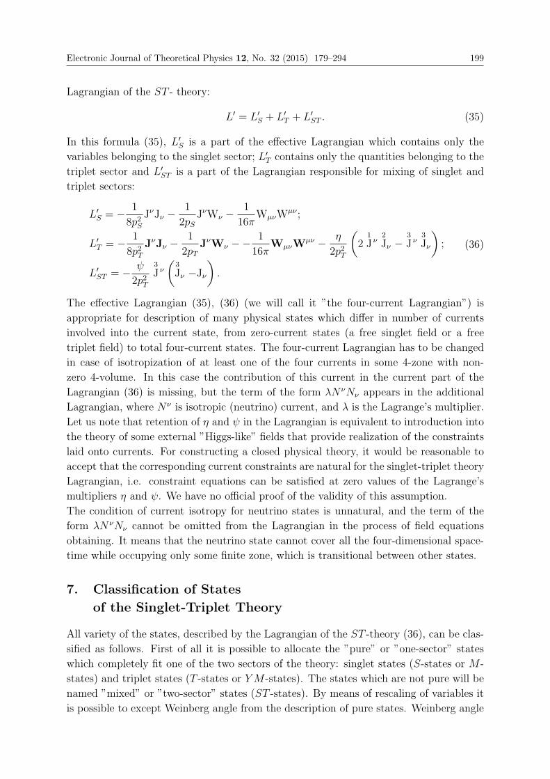
Electronic Journal of Theoretical Physics 12, No. 32 (2015) 179–294 199
Lagrangian of the ST - theory:
L′ = L′S + L′T + L′ST . (35)
In this formula (35), L′S is a part of the effective Lagrangian which contains only the
variables belonging to the singlet sector; L′T contains only the quantities belonging to the
triplet sector and L′ST is a part of the Lagrangian responsible for mixing of singlet and
triplet sectors:
L′S = − 1
8p2SJνJν −
1
2pSJνWν −
1
16πWμνW
μν ;
L′T = − 1
8p2TJνJν −
1
2pTJνWν −−
1
16πWμνW
μν − η
2p2T
(2
1
J ν2
Jν −3
J ν3
Jν
);
L′ST = − ψ
2p2T
3
J ν
(3
Jν −Jν).
(36)
The effective Lagrangian (35), (36) (we will call it ”the four-current Lagrangian”) is
appropriate for description of many physical states which differ in number of currents
involved into the current state, from zero-current states (a free singlet field or a free
triplet field) to total four-current states. The four-current Lagrangian has to be changed
in case of isotropization of at least one of the four currents in some 4-zone with non-
zero 4-volume. In this case the contribution of this current in the current part of the
Lagrangian (36) is missing, but the term of the form λN νNν appears in the additional
Lagrangian, where Nν is isotropic (neutrino) current, and λ is the Lagrange’s multiplier.
Let us note that retention of η and ψ in the Lagrangian is equivalent to introduction into
the theory of some external ”Higgs-like” fields that provide realization of the constraints
laid onto currents. For constructing a closed physical theory, it would be reasonable to
accept that the corresponding current constraints are natural for the singlet-triplet theory
Lagrangian, i.e. constraint equations can be satisfied at zero values of the Lagrange’s
multipliers η and ψ. We have no official proof of the validity of this assumption.
The condition of current isotropy for neutrino states is unnatural, and the term of the
form λNνNν cannot be omitted from the Lagrangian in the process of field equations
obtaining. It means that the neutrino state cannot cover all the four-dimensional space-
time while occupying only some finite zone, which is transitional between other states.
7. Classification of States
of the Singlet-Triplet Theory
All variety of the states, described by the Lagrangian of the ST -theory (36), can be clas-
sified as follows. First of all it is possible to allocate the ”pure” or ”one-sector” states
which completely fit one of the two sectors of the theory: singlet states (S-states or M -
states) and triplet states (T -states or YM -states). The states which are not pure will be
named ”mixed” or ”two-sector” states (ST -states). By means of rescaling of variables it
is possible to except Weinberg angle from the description of pure states. Weinberg angle
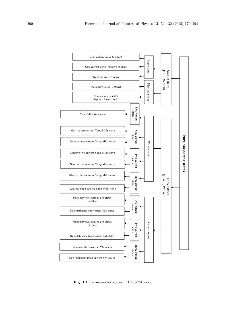
200 Electronic Journal of Theoretical Physics 12, No. 32 (2015) 179–294
Fig. 1 Pure one-sector states in the ST -theory
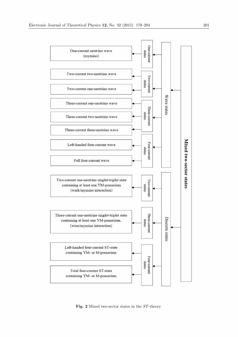
Electronic Journal of Theoretical Physics 12, No. 32 (2015) 179–294 201
Fig. 2 Mixed two-sector states in the ST -theory
202 Electronic Journal of Theoretical Physics 12, No. 32 (2015) 179–294
cannot be excepted from the description of mixed states. Further the states of the ST -
theory can be classified by the number of nonzero currents: zero-current states, i.e. free
fields are maxwellian free field in pure S-state and Yang-Mills free field in pure T -state;
one-current states, two-current, three-current and four-current states. Singlet states can
be only zero-current or one-current. All states, except zero-current ones, can be classified
by number of pomeriums, i.e. outer boundaries of the current zones. ”Wave” states have
no pomerium at all (the current zone is unbounded). Photon, and also massive photon
and maxwellian neutrino, described in article [1] of this series, relate to the wave states
in the singlet sector. In the triplet sector there are wave states which are similar to them.
The states which have at least one pomerium will be named ”discrete states”. The most
important of the discrete states is a ”stationary state”, i.e. a state with one pomerium
for which there is such an intrinsic frame of reference where currents and fields do not
depend on time. Stationary states describe current structure of massive single particles.
Stationary states exist only as pure one-sector states, mixed stationary states do not
exist.
It is possible to distinguish a special case of ”neutrino states” among current wave states
– i.e. the states in which pseudo-Euclidean square of 4-current vector is everywhere equal
to zero.
There are mixed neutrino states simultaneously fitting two sectors of the theory, Maxwel-
lian and Yang-Mills’ (”Maxwell-Yang-Mills neutrino”, or mymino in abbreviated form).
There is a pure singlet neutrino state (makswellian neutrino, or mino in abbreviated
form). There are pure neutrino states which completely fit Yang-Mills sector (”Yang-
Mills neutrino”, or ymino in abbreviated form). We do not know whether this theo-
retical classification of neutrino states – mino, ymino, mymino – corresponds to the
empirical fact of distinction of the lepton neutrinos (electronic neutrino, muonic neutrino,
τ -neutrino)13.
The described classification of states, possible in the ST -theory, is reflected in fig. 1 (pure
states) and fig. 2 (mixed states). These pictures illustrate a variety of particular prob-
lems, which can be formulated and solved within the framework of the ST -theory, and
thereby, the inner wealth of the ST -theory as a section of mathematical and computer
physics.
By describing formulations of the problems of the ST -theory further in the text of this
article, we restrict ourselves to only two types of the problems: the wave problems con-
taining no pomerium at all and stationary problems with one pomerium.
Wave problems are quite correct as problems of classical mathematical physics, however
the search for correspondence between a variety of their solutions and real quantum ob-
jects of the micro-world may appear a difficult task14.
13 For complete description of neutrino states it can be noted that a priori nothing forbids to allow
the possibility of izotropization of any of eight currents of the octuplet sector of physics which is not
considered in this article, and thereby to enter into consideration one more set of neutrinos different from
mino, ymino and mymino.14Within the framework of the wave problems, for example, it is not difficult to consider the theory of
standing Yang-Mills waves – triplet and octuplet (gluon) ones. But how, by means of what equipment,
Electronic Journal of Theoretical Physics 12, No. 32 (2015) 179–294 203
Stationary classical single-particle problems allow to calculate, in principle, masses, char-
ges and spins of particles and to study the inner structure of massive particles. The
particles of one physical class consisting of one current, differ in topology of the outer
boundaries of pomerium, and also in number and topology of the inner boundaries of
latens. Particles of different physical classes differ in currents they consist of. Within the
framework of this article we are not going to consider the formulations of the problems
which describe the states with more than one pomerium. Within classical physics they
are obviously non-stationary states. These states are the key ones for modern treatment
of physics of micro-world. They are the states of particles interaction, including the states
corresponding to spontaneous decay of unstable particles. The possibility of correct de-
scription of such states within the framework of the classical ST -theory, constructed here,
seems rather doubtful. However, without studying such classical problems, it is difficult
to count on successful construction of the proper quantum theory of non-point particles.
The following restrictions on the variables, entering into the Lagrangian of the singlet-
triplet theory (36), are used for extraction of the particular states reflected in figures 1
and 2.
A. Wave states
A1. One-sector wave states
• Zero-current singlet wave (free maxwellian wave, photon):
Jν ≡ 0; Wν ≡ 0; Jν ≡ 0.
• One-current singlet wave (heavy photon):
Jν ≡ 0; Wν ≡ 0; JνJν < 0.
• Neutrino singlet wave (maxwellian neutrino, myno):
Jν ≡ 0; Wν ≡ 0; Jν �= 0; JνJν = 0.
• Zero-current triplet wave (Yang-Mills free wave):
Jν ≡ 0; Wν ≡ 0; Jν ≡ 0.
• One-current triplet wave (Yang-Mills heavy one-current wave):
Jν ≡ 0; Wν ≡ 0;1
J ν1
Jν< 0;2
J ν ≡ 0;3
J ν ≡ 0.15
• Neutrino one-current triplet wave (Yang-Mills neutrino, ymino):
Jν ≡ 0; Wν ≡ 0;1
J ν �= 0;1
J ν1
Jν= 0;2
J ν = 0;3
J ν = 0.16
• Two-current triplet wave (Yang-Mills heavy two-current wave):
Jν ≡ 0; Wν ≡ 0;1
J ν2
Jν= 0;1
J ν1
Jν< 0;2
J ν2
Jν< 0;3
J ν ≡ 0.
• Neutrino two-current triplet wave:
Jν = 0; Wν = 0;1
J ν �= 0;1
J ν1
Jν< 0;2
J ν �= 0;2
J ν2
Jν= 0;1
J ν2
Jν= 0;3
J ν ≡ 0.
• Three-current triplet wave (Yang-Mills heavy three-current wave):
would it be possible to conduct Yang-Mills analogue of maxwellian experiment on observation of standing
singlet waves which was conducted by O. Wiener for the first time already in 1890th? For observing
standing gluon waves it is necessary to arrange reflecting surfaces in a baryon. And, even if this arrange-
ment is possible at baryon collisions, the characteristic dimensions of atomic nuclei are enormously high
in comparison with the fundamental length r0, appearing in the theory of currents and potentials.15Also two analogous wave states with arbitrary permutation of YM-indices.16Also two analogous neutrino states with arbitrary permutation of YM-indices.
204 Electronic Journal of Theoretical Physics 12, No. 32 (2015) 179–294
Jν ≡ 0; Wν ≡ 0;1
J ν1
Jν< 0;2
J ν2
Jν< 0;2
J ν3
Jν< 0; 21
J ν2
Jν=3
J ν3
Jν .
• Neutrino three-current triplet wave:
Jν ≡ 0; Wν ≡ 0;1
J ν �= 0;1
J ν1
Jν= 0;2
J ν �= 0;2
J ν2
Jν= 0;1
J ν2
Jν= 0;3
J ν �= 0;3
J ν3
Jν= 0.
A2. Two-sector wave states
• One-current two-sector neutrino wave (Maxwell-Yang-Mills neutrino, mymino):
Jν = N ν ;3
J ν = −N ν ; NνNν = 0;1
J ν ≡ 0;2
J ν ≡ 0.
• Two-current two-sector one-neutrino wave:
Jν = N ν ;3
J ν = −N ν ; NνNν = 0;1
J ν1
Jν< 0;2
J ν ≡ 0.17
• Two-current two-sector two-neutrino wave:
Jν = N ν ;3
J ν = −N ν ; NνNν = 0;1
J ν �= 0;1
J ν1
Jν= 0;2
J ν ≡ 0.18
• Left-handed four-current wave:
Jν = lν +N ν ;3
J ν = lν −Nν ; Nν �= 0; NνNν = 0; lνNν = 0; lνlν < 0;
21
J ν2
Jν= lνlν ;1
J ν1
Jν< 0;2
J ν2
Jν< 0.
• Full four-current wave:
JνJν < 0;1
J ν1
Jν< 0;2
J ν2
Jν< 0;3
J ν3
Jν< 0; 21
J ν2
Jν=2
J ν3
Jν< 0;3
J ν
(3
Jν −Jν)
= 0.
B. Discrete states
B1. One-sector discrete states
• Singlet stationary state (lepton):
JνJν ≤ 0; Jν ≡ 0; Wν ≡ 0; there is only one pomerium; there is intrinsic reference
system of a state in which∂
∂t≡ 0.
• Singlet non-stationary state (electromagnetic interaction of leptons):
JνJν ≤ 0; Jν ≡ 0; Wν ≡ 0; there is more than one pomerium.
• Stationary one-current triplet state (hypothetical particle wark):
Jν ≡ 0; Wν ≡ 0;2
J ν ≡ 0;3
J ν ≡ 0;1
J ν1
Jν≤ 0; there is only one YM-pomerium; there
is intrinsic reference system of state in which∂
∂t≡ 0.19
• Non-stationary one-current triplet state (YM-interaction of warks):
Jν ≡ 0; Wν ≡ 0;2
J ν ≡ 0;3
J ν ≡ 0;1
J ν1
Jν≤ 0; there are more than one YM-
pomeriums20.
• Stationary two-current triplet state(hypothetical particle wion):
Jν ≡ 0; Wν ≡ 0;3
J ν ≡ 0;1
J ν1
Jν≤ 0;2
J ν2
Jν≤ 0;1
J ν2
Jν= 0; there is one YM-pomerium,
common for currents1
J ν and2
J ν ; there is intrinsic state reference system in which∂
∂t≡ 0.
• Non-stationary two-current triplet state (YM-interaction of warks or/and wions):
Jν ≡ 0; Wν ≡ 0;1
J ν1
Jν≤ 0;2
J ν2
Jν≤ 0;3
J ν ≡ 0;1
J ν2
Jν= 0; there is more than one
17Also analogous one-neutrino wave with permutation of YM-indices 1↔ 2.18Also analogous two-neutrino wave with permutation of YM-indices 1↔ 2.19Also analogous stationary state with permutation of YM-indices 1↔ 2.20Also analogous non-stationary state with permutation of YM-indices 1↔ 2.
Electronic Journal of Theoretical Physics 12, No. 32 (2015) 179–294 205
YM-pomerium.
• Stationary three-current triplet state:
Jν ≡ 0; Wν ≡ 0;1
J ν1
Jν≤ 0;2
J ν2
Jν≤ 0;3
J ν3
Jν≤ 0; 21
J ν2
Jν=3
J ν3
Jν ; there is one YM-
pomerium which is common for the three YM-currents; there is intrinsic reference
system of state in which∂
∂t≡ 0.
• Non-stationary three-current triplet state:
Jν ≡ 0; Wν ≡ 0;1
J ν1
Jν≤ 0;2
J ν2
Jν≤ 0;3
J ν3
Jν≤ 0;1
J ν2
Jν=3
J ν3
Jν ; there is more than
one pomerium.
B2. Two-sector discrete states
• Two-current one-neutrino singlet-triplet state containing at least one YM-pomerium
(wark/mymino interaction):
Jν = N ν ;3
J ν = −N ν ; NνNν = 0;1
J ν1
Jν≤ 0;2
J ν = 0.21
• Three-current one-neutrino singlet-triplet state containing at least one YM-pome-
rium, common for currents1
J ν and2
J ν (wion/mymino interaction):
Jν = N ν ;3
J ν = −N ν ; NνNν = 0;1
J ν1
Jν≤ 0;2
J ν2
Jν≤ 0;1
J ν2
Jν= 0.
• Left-handed four-current singlet-triplet state containing at least one pomerium:
Jν = lν +N ν ;3
J ν = lν −Nν ; lνNν = 0; N νNν = 0; lνlν ≤ 0;1
J ν1
Jν≤ 0;2
J ν2
Jν≤ 0; 21
J ν2
Jν= lνlν .
• Total four-current singlet-triplet state containing at least one pomerium:
JνJν ≤ 0;1
J ν1
Jν≤ 0;3
J ν3
Jν≤ 0; 21
J ν2
Jν=3
J ν3
Jν ;3
J ν
(3
Jν −Jν)
= 0.
The provided classification of the states of singlet-triplet theory is rather formal. It
describes possible states on the basis of a set of non-zero currents. Each state, allocated
in the classification, needs some existence theorem which would claim that the algebraic
conditions, imposed on currents, are compatible22.
Wave states can be researched quite minutely, at least, for the plane waves. Plane waves
can be described by a system of ordinary differential equations. The solutions to the
problems of plane waves within the framework of the singlet-triplet theory can be ob-
tained analytically or numerically.
Discrete states in the singlet-triplet theory are described by an equation system in partial
derivatives which include a priori unknown boundaries of current zones (pomerium and
latens). The lack of existence theorems causes some difficulties for the development of
numerical methods of solving problems of discrete states.
The given classification does not include transitional neutrino states, i.e. such states, in
which 4-zone, occupied with the neutrino current, is finite and non-stationary.
The given classification for some discrete states is not unambiguously definite. For exam-
ple, the state, described as a ”singlet non-stationary state”, describes both the state of
21Also analogous one-neutrino state with permutation of YM-indices 1↔ 2.22But stationary states also need some spectral theorem claiming non-uniqueness of stationary state
with the given set of algebraic conditions for currents.
206 Electronic Journal of Theoretical Physics 12, No. 32 (2015) 179–294
scattering of a lepton on a lepton, for which the classical theory, constructed here, can
be quite correct, and the state of annihilation of two leptons, for which, probably, the
classical theory can prove to be as unacceptable as Newtonian mechanics for description
of atoms.
However, we believe that classical singlet-triplet theory is worth careful and detailed
development as a section of mathematical physics for clarification of prognostic opportu-
nities of the theory and limits of its applicability.
8. Pure one-sector states: Maxwellian Singlet States
8.1 Getting Rid of Weinberg Angle:
the Electromagnetic Lagrangian
In pure S-state all triplet currents Jν and all triplet potentials Wν are equal to zero.
Only L′S will remain in the effective ST -Lagrangian (36). Supposing that in L′S:
jem
ν =1
2Jν ;
Aν = pSWν ;
Aμν = ∂μAν − ∂νAμ = pSWμν ,
(37)
we can rewrite the singlet Lagrangian L′S in the following form:
L′S =1
p2SLem,
where
Lem
= −1
2jem
ν jνem
− jem
νAν −1
16πAμνA
μν . (38)
Therefore, the singlet Lagrangian L′S differs from the standard Lagrangian of classical
electrodynamics of non-point particles [1] only in insignificant common multiplier.
The electromagnetic Lagrangian (38) comprises the description of both the wave prob-
lems without current boundaries (an ordinary no-current electromagnetic wave – photon;
”heavy” current electromagnetic wave – ”heavy photon”; neutrino wave – maxwellian
neutrino [1]), and the discrete problems containing outer and inner boundaries of current
zones (pomerium and latens). The discrete problems, as a subset, comprise stationary
singlet problems which solution describes inner structure of massive leptons [1].
”Deductibility” of the electromagnetic Lagrangian (38) from the effective ST -Lagrangian
(36) in one-sector maxwellian problem is an absolutely trivial mathematical fact. But this
fact comprises the profound physical meaning: intrinsic characteristics of massive
leptons are formed in the singlet sector of the theory and do not depend
on the triplet interactions . In particular, the formulas of heavy lepton mass ratios,
provided in the article [1], remain reasonable in the ST -theory. The triplet sector of
the theory influences the stability of stationary states of the singlet sector, but does not
Electronic Journal of Theoretical Physics 12, No. 32 (2015) 179–294 207
influence the stationary states themselves.
Now we do not know whether the correct formulation of the problem on stability of the
singlet stationary discrete state within the framework of the classical theory, considered
here, is possible. Perhaps, the effective ST -Lagrangian (36) comprises the description
of such instability connected with spontaneous ”swelling” of the bubble of the neutrino
triplet currents and this bubble’s ”splashing” beyond the limits of pomerium of a discrete
singlet object.
8.2 Estimate of the Fundamental Constant r0
The classical theory of non-point particles, constructed here, contains as ”entrance” pa-
rameters of the theory the fundamental length r0, the velocity of light c, the fundamental
constant j0 which determines the top limit of the current density, and the dimensionless
constant k which forms Einstein equations and is proportional to the constant of gravity
G [1].
If we had a numerical solution of the stationary one-sector singlet problem, we would
have a possibility to express the intrinsic characteristics of massive leptons – mass m,
charge e and angular momentum M – through these ”entrance” parameters. But now
we have neither such numerical solution, nor even the existence theorem which would
guarantee the existence of at least one solution; nor the spectral theorem which would
guarantee the existence of some finite or countable set of the intrinsic solutions, differing
in topological characteristics. In such situation everything we can afford is dimensional
estimates.
The mass of a lepton can be estimated by the order of magnitude by means of the fol-
lowing formula:
mc2 ≈ r20c2
j20 r2P r0,
and the electrical charge e – by means of the formula:
e ≈ 1
cj0 r
30.
These formulas are based on the following ideas. The main contribution to the total
energy of the massive lepton is made by a small part of the lepton volume in small neigh-
borhood of the ”cavitated” tube latebra, on the boundary of which the current density
achieves a peak value j0. We believe that the diametrical dimension of cavitated tubes is
of the order of Planckian length rP , and the typical diametrical dimension of the current
high density zone, bordering upon latens, is approximately the same. The longitudinal
dimension of this zone is of the order of the general outer dimension of the lepton, and
this dimension, in its turn, is close to the fundamental constant r0. The first dimensional
factor(r20
/c2
)in the formula for the lepton mass is the proportionality coefficient which
forms the expression of the tensor components of energy-momentum the current field (see
[1]).
208 Electronic Journal of Theoretical Physics 12, No. 32 (2015) 179–294
The expression for charge dimension e, linear by current density, means that the notice-
able contribution to the total value of an electric charge is made not only by a narrow
zone in the neighborhood of ”cavitated” tube latebra, but by the whole lepton volume
as well. The assumptions, on which basis the above mass and charge estimates are con-
structed, are open to criticism. But let us see the consequences these estimates lead to.
From the given estimates for m and e we find out that
e2
mc2≈ r30
r2P,
bute2
mc2= rT ,
where rT is a classical Thomson lepton radius.
So, on the grounds of these lepton mass and charge estimates, we get a possibility to
estimate the unknown fundamental constant r0:
r0 ≈(rT r
2P
)1/3. (39)
If we use Thomson electron radius rT ≈ 2.8 · 10−13 cm as a quantity rT , (39) gives the
following estimate for r0:
r0 ≈ 0.9 · 10−26cm. (40)
The given estimate (40) is probably not too cogent. Formula (39) contains not only the
fundamental Planckian length rP , but also Thomson radius of a specific lepton; the di-
mension r0 itself has to be fundamental, i.e. to have no ”binding” to any specific particle.
However, we have no other estimate of the fundamental constant r0.
Quantity r0 (40) is enormously small from the point of view of the possibility ever ”to
consider” the electron structure in any feasible physical experiment. However, this quan-
tity is quite large in comparison with Planckian length rP determining the diametrical
dimensions of latebrae. Physics of leptons contains two dimensionless constants: the
constant of fine structure α and ratio rP/r0. Undoubtedly, these two constants have to
be somehow connected with each other.
By estimating, within the framework of the same ”naive estimate”, the own angular mo-
mentum of lepton M by the formulas provided in the article [1], it is possible to find
that
M ≈ r20c2· 1c· j20 · r40.
Determining ratioe2
Mcby means of this estimate, we get the estimate which is not very
substantial:e2
Mc= O(1), (41)
at the same time, as the correct estimate could be M ≈ � ande2
Mc≈ α, where �
is Planckian constant and α is a fine structure constant. We do not know now whether
Electronic Journal of Theoretical Physics 12, No. 32 (2015) 179–294 209
estimate (41) is the evidence of a rough and not removable imperfection of the constructed
theory, or whether this estimate can be improved under the accurate numerical solution
of a stationary discrete singlet problem and accurate calculation of quantities e and M.
9. Pure One-sector States: Yang-Mills Triplet States
9.1 Getting Rid of Weinberg Angle: the Weak Lagrangian
The set of pure YM-states, represented in fig.1 have an ”empty” singlet sector: Jν = 0;
Wν = 0. The missing of the singlet current, in accordance with the algebraic condition
(20), means that3
J ν3
Jν= 0. (42)
Condition (42) means that current3
J ν , if it is not identically zero, can be only a neu-
trino one. Algebraic condition of the inner normalization of currents of YM-triplet (32)
requires, in this case, the orthogonality of the first and second components of YM-triplet.
1
J ν2
Jν= 0. (43)
Weinberg angle can be eliminated from the triplet part of the effective ST -Lagrangian
by means of scaling which comprises the triplet interaction coefficient pT :
pTWν = Aν ;
Aμν = ∂μAν − ∂νAμ +Aμ ×Aν = pTWμν ,(44)
Let us also re-scale the triplet currents, assuming that:
1
j ν =1
2
1
J ν ;2
j ν =1
2
2
J ν ; Nν =1
2
3
J ν , (45)
and, in accordance with (42) and (43):
1
j ν2
jν= 0, (46)
NνNν = 0. (47)
After substitution of the relations (44) and (45), with regard to (46) and (47), the triplet
Lagrangian L′T (36) can be formulated in the following form:
L′T =1
p2TLw, (48)
Lw =− 1
2
(1
j ν1
jν +2
j ν2
jν
)−
(1
j ν1
Aν +2
j ν2
Aν +Nν3
Aν
)− 1
16πAμν ·Aμν − η
1
j ν2
jν −1
2λN νNν .
(49)
210 Electronic Journal of Theoretical Physics 12, No. 32 (2015) 179–294
The Lagrangian Lw does not include Weinberg angle θw.
Let us name the Lagrangian Lw ”weak Lagrangian”, the triplet of currents
(1
j ν ,2
j ν , N ν
),
which satisfies the conditions (46) and (47), – ”weak currents triplet”, triplet Aν – ”weak
potentials triplet”, and tensor Aμν – ”weak field tensor”. Coefficients η and λ under
corresponding terms in the weak Lagrangian are Lagrange’s multipliers.
9.2 Zero-current Triplet States: Yang-Mills Free Triplet Waves
9.2.1 Yang-Mills Wave Equation
All the currents of YM-triplet are missing in the wave triplet state:
1
j ν =2
j ν = Nν = 0.
The Lagrangian of such zero-current state is reduced to Yang-Mills free field Lagrangian
Lw,f :
Lw,f = − 1
16πAμν ·Aμν . (50)
Variation of action functional with the Lagrangian (50) by weak potentials Aμ gives the
equations of the free weak field:
∂μAμν +Aμ ×Aμν = 0. (51)
By eliminating field tensor Aμν from Yang-Mills field equations (51) by means of (44),
we can present the equations (51) in the following form:
−�Aν +Aμ × (2∂μAν − ∂νAμ +Aμ ×Aν) = ∂ν�+Aν × �. (52)
In equations (52) � is 4-divergence of the weak potential Aμ:
� = ∂μAμ,
and � is D’Alembert operator:
� = −∂μ∂μ.
One arbitrary gauge condition can be imposed on potentials Aμ. It is proper to assume
that 4-divergence � is identically zero. This equation is compatible with the field equations
(52). Finally, the free weak field of the zero-current triplet state is described by the
following system of the equations:
�Aν = Aμ × (2∂μAν − ∂νAν +Aμ ×Aν) ; (53)
∂μAμ = 0. (54)
Electronic Journal of Theoretical Physics 12, No. 32 (2015) 179–294 211
9.2.2 Yang-Mills Plane Zero-current Wave
The simplest solution to field equations (53), (54) can be tried in the form of a plane
wave with wave vector kν , supposing that 12 unknown functions of Aμ depend only on a
single argument – a wave phase φ:
φ = kμxμ.
For the plane wave, the field equations (53), (54) transform into a system of ordinary
differential equations:
kμkμAν ′′ + 2kμA
μ ×Aν ′ − kνAμ ×Aμ′ +Aμ × (Aμ ×Aν) = 0. (55)
kμAμ′ = 0. (56)
In these equations the prime next to the potentials stands for the derivative with respect
to wave phase φ.
The plane wave equations (55) have apparent scale invariance with respect to wave vector
kμ.
Let kμ be a time-like vector:
kμkμ = ε2 > 0.23
Let us make scale transformation of potentials Aμ, coordinates xμ and wave vector kμ,
supposing thatkν = εkν ; kν kν = 1.
Aν = εAν; xν =
1
εxν .
At this transformation the wave phase remains invariable:
φ = kνxν = kν xν .
The specified scale transformation turns a wave vector into a unit vector without changing
the form of the wave equations (55), (56). Let us rewrite these equations with new
variables, omitting the symbol ∼ over the corresponding quantities in the form:
Aν ′′ + 2kμAμ ×Aν ′ − kνAμ ×Aμ
′ +Aμ × (Aμ ×Aν) = 0; (57)
23The fact that both W. Pauli and C.N. Yang with R.L. Mills in 1953-1954 passed by the classical Yang-
Mills wave theory with the time-like wave vector, can be considered an inexplicable historical paradox.
With persistence, that is worth regrets, there was considered only the version of the theory with isotropic
wave vector kμkμ = 0, generating the idea of zero mass of Yang-Mills field quantum (”one will always
obtain vector mesons with rest mass zero”, wrote Wolfgang Pauli in 1953 December [4]) under general
quantum treatment.
It is obvious that the construction of the solution (55) does not require any wave vector isotropy at
all. This sight aberration of the triplet theory authors is probably caused by the tendency of the
physicists of that time to treat nonlinear equations by means of perturbation methods, which is absolutely
unacceptable for Yang-Mills essentially nonlinear equations.
Finally, this stable aberration led to the introduction of Higgs mechanism for explanation of particles
masses. The possibility of the correct treatment of Yang-Mills waves with time-like wave vector, described
in this article, shows the existence of a rest mass of such waves, but within the framework of the classical
theory, this mass, proportional to the pseudo-Euclidean module of the wave 4-vector, remains arbitrary.
212 Electronic Journal of Theoretical Physics 12, No. 32 (2015) 179–294
kμAμ′ = 0; (58)
kμkμ = 1. (59)
From the condition (58) follows that convolution kμAμ does not depend on the wave
phase:
kμAμ = q = const;
which allows to rewrite the plane YM-wave equation in the form:
Aν ′′ + 2q×Aν − kνAμ ×Aμ′ +Aμ × (Aμ ×Aν) = 0. (60)
9.2.3 Energy Integral for Yang-Mills Plane Zero-current Wave
By multiplying the wave equation (60) scalarly by the derivative of potential A′ν , and
integrating by the wave phase φ, it is possible to obtain the first integral of the wave
equation (60) which is appropriate to be called ”energy integral”:
K+ U = E = const;
K = −1
2Aν ′ ·Aν
′;
U =1
4
((Aν ·Aν)
2 − (Aμ ·Aν) (Aμ ·Aν)
).
(61)
It is easy to show that physical quantity U, which can be treated as a potential wave
energy density, is positive-definite. Physical quantityK is the first term in the energy
conservation law (61) which can be interpreted as the density of kinetic wave energy; it
is also positive-defined. Therefore, wave energy is positive.
In wave equation (60) and energy integral (61) it is easy to see that Yang-Mills plane
wave has a self-similarity relative to the energy quantity E.
The scale transformation which uses E as a parameter:
Aν = E1/4∗A ν ,
φ = −E1/4∗φ,
q = E1/4 ∗q,
(62)
normalizes the wave energy to unit value without altering the form of the wave equation
(60) and energy integral (61).
We will afford once again to rewrite almost tautologically the problem formulation of
Yang-Mills plane wave in variables∗A ν ,
∗φ,
∗q introduced by the scale transformation (62)
omitting symbol * over the letters:
Aν ′′ + 2q×Aν ′ − kνAμ ×Aμ′ +Aμ (A
μ ·Aν)−Aν (Aμ ·Aμ) = 0, (63)
−1
2Aν ′ ·Aν
′ +1
4
((Aν ·Aν)
2 − (Aμ ·Aν) (Aμ ·Aν)
)= 1, (64)
kμAμ = q, (65)
Electronic Journal of Theoretical Physics 12, No. 32 (2015) 179–294 213
kμkμ = 1. (66)
Let us pay attention to the fact that the invariance of Yang-Mills plane wave theory, rel-
ative to scale transformations generated by pseudo-Euclidean module of the wave vector
and energy (or wave amplitude), means that Yang-Mills wave theory has neither geo-
metrical optics approximation, nor asymptotics of small amplitudes (low energies). Both
wave vector and wave energy can always be re-scaled to unit values.
9.2.4 Nonholonomic Constraint Equations for Yang-MillsPlane Zero-current Wave
By multiplying the wave equation (63) scalarly by wave vector kν , taking into account
(65) and (66), we will get the identity which has to be satisfied with the solution (63):
Aμ ×Qμ = 0. (67)
where
Qμ = A′μ +Aμ × q. (68)
The equation (67) with vector Qμ (68) can be treated as a non-holonomic constraint
imposed on Yang-Mills dynamic system (63). It is sufficient to require the initial data to
meet the condition (67).
9.2.5 Yang-Mills Plane Zero-current Wave in the Intrinsic Frame of Reference
It is proper to make further analysis of Yang-Mills plane wave in the intrinsic frame of
reference of the wave, in which the wave vector kμ has the form:
kμ = {1; 0; 0; 0} . (69)
In this frame of reference the wave phase coincides with the intrinsic time of the frame,
and the phase derivatives coincide with the intrinsic time derivatives. We shall denote
these derivatives with a dot as a dot upper index after Lorentz indices. In this frame
none of the potential components depend on spatial coordinates: the wave ”flashes” and
”dies out” simultaneously over the whole infinite three-dimensional space.
Our deep-rooted Lorentz intuition, undoubtedly, protests against this picture, however
there is no violation of Lorentz-invariance: Yang-Mills plane wave with a fixed wave
vector kν is the artificial mathematical entity which fills up the whole three-dimensional
space. Such object requires the infinite stock of energy for its formation. The real wave,
covering the finite spatial domain and bearing the finite total energy, is a wave packet,
i.e. superposition of waves with different wave vectors. Such wave can be presented in
the form of Fourier integral on four-dimensional space of the wave vectors. The more
compact the space-time localization of the wave packet is, the wider is the spread of
waves within the space of wave vectors. The notion ”intrinsic frame of reference” makes
sense only for a plane wave with a fixed wave vector. For a wave packet this notion has
no sense. However, the mathematics of Yang-Mills wave packets, which requires Fourier
transformation of Yang-Mills wave equations (63), seems to us almost ”uninterpretable” in
214 Electronic Journal of Theoretical Physics 12, No. 32 (2015) 179–294
the continual situation. The problem of Yang-Mills stationary waves, requiring a discrete
Fourier transformation of the wave equation (63), is quite ”interpreted”. However, we do
not know whether the engineering-physical problem of creation of ”resonators” of Yang-
Mills waves, which are analogous to the radio engineering resonators of electromagnetic
waves, is solvable in principle.
Let us enter ordinary ”1+3” notations for the components of the weak potential Aν :
a
A ν =
{a
T;a
U
}, (70)
wherea
T is a time component of YM-potential vector a,a
U is the three spatial components
of YM-potential vector a. Vectorsa
U (for each a) are ordinary three-dimensional vectors
in Euclidean three-dimensional coordinate space. The separation of the components of 4-
vector into time and spatial part is not Lorentz - invariant. Let us assume that separation
(70) is carried out in YM-wave intrinsic frame of reference. Transition to any other frame
of reference is carried out by means of Lorentz- transformation of 4-vectora
A ν .
Substituting a ”separation formula” (70) into the condition (65) and taking into account
the mode of the wave vector in the wave intrinsic frame of reference (69), we find that all
the time components of YM-potentials are constant:
a
T=aq= const.
Further we will assume that allaq are zero:
aq= 0. (71)
A non-zero value of constantsaq would mean the presence of some outer stationary field,
which is hardly compatible with the problem of studying Yang-Mills free wave .
By substituting (70) and (71) into the wave equation (63) and nonholonomic constraint
(67), (68), we can represent the formulation of the problem of Yang-Mills plane wave in
the following form:a
U ••+b
U ×(
a
U ×b
U
)= 0; (72)
abcε
b
U ·c
U • = 0. (73)
In these formulasa
U is the triple of ordinary three-dimensional vectors, the symbol ”×”means the ordinary three-dimensional vector product; a, b, c are Yang-Mills indices taking
the values 1, 2, 3;abcε is a three-dimensional Levi-Civita symbol; summation is made by
YM-indices. Opening the triple vector product in (72), Yang-Mills equation (72) can be
rewritten as follows:a
U ••+ab
Sb
U −bb
Sa
U= 0. (74)
Yang-Mills matrixab
S appears in the relation (74):
ab
S=a
A νb
Aν=a
Tb
T −a
U ·b
U, (75)
Electronic Journal of Theoretical Physics 12, No. 32 (2015) 179–294 215
or, regarding the condition (71) in the wave intrinsic system:
ab
S= −a
U ·b
U . (76)
A more compact notation (74) is formed if Yang-Mills ”inertia tensor”ab
I is introduced:
ab
I=ab
S −ab
δcc
S, (77)
whereab
δ is Kronecker symbol in the space of YM-indices. In the intrinsic wave system,
Yang-Mills inertia tensorab
I with (76) looks as follows:
ab
I= U2ab
δ −a
U ·b
U, (78)
where U2 =∑a
a
U 2. By using tensorab
I , introduced here, Yang-Mills equations (74) can
be rewritten in the form which remotely resembles the form of Euler equations in the
dynamics of a perfectly rigid body:
a
U ••+ab
Ib
U= 0. (79)
Yang-Mills equations (79) (which would probably be appropriate to be called Yang-Mills-
Euler ones) describe a three-vector dynamical system with nine degrees of freedom, where
three nonholonomic constraints are imposed on this system’s behavior (73). Let us name
this dynamical system ”tripletic Yang-Mills’ oscillator” (tymos). During quantization of
triplet Yang-Mills wave24 there must appear a particle with a nonzero rest mass. By
analogy with a photon – the singlet field quantum – this particle can be named ymon .
There are no reasons for identification of ymon with W- and Z-particles of Weiberg-
Salam theory.
In notations (70) and (75) energy integral for tymos (79) has the following form:
1
2
a
U •·a
U • +1
4
((ab
S
)2
−ab
Sab
S
)= 1, (80)
or, using formula (76) for YM-matrixab
S:
1
2
a
U •·a
U • +1
2
((1
U ×2
U
)2
+
(2
U ×3
U
)2
+
(3
U ×1
U
)2)
= 1. (81)
24 In the article on the classical theory of Yang-Mills fields it is irrelevant to discuss these rules of
quantization: it is sufficient to assume that they exist.
216 Electronic Journal of Theoretical Physics 12, No. 32 (2015) 179–294
9.2.6 The Detailed Notation of the Tymos Dynamic Equations
Let us present here the detailed notation of Yang-Mills-Euler equations (79) with explic-
itly written Yang-Mills’ and vector indices in Cartesian coordinates:
1
U1••+
11
I1
U1 +12
I2
U1 +13
I3
U1= 0,1
U2••+
11
I1
U2 +12
I2
U2 +13
I3
U2= 0,1
U3••+
11
I1
U3 +12
I2
U3 +13
I3
U3= 0,2
U1••+
21
I1
U1 +22
I2
U1 +23
I3
U1= 0,2
U2••+
21
I1
U2 +22
I2
U2 +23
I3
U2= 0,2
U3••+
21
I1
U3 +22
I2
U3 +23
I3
U3= 0,3
U1••+
31
I1
U1 +32
I2
U1 +33
I3
U1= 0,3
U2••+
31
I1
U2 +32
I2
U2 +33
I3
U2= 0,3
U3••+
31
I1
U3 +32
I2
U3 +33
I3
U3= 0.
(82)
In the system of equations (82) the subscripts number Cartesian coordinates of the vectora
U; the over-letter indices are Yang-Mills indices.
The explicit notation of the components of YM-inertia tensor tymos , according to (76),
has the following form:
11
I =2
U 2+3
U 2 =2
U12+
2
U22+
2
U32+
3
U12+
3
U22+
3
U32,
22
I =3
U 2+1
U 2 =3
U12+
3
U22+
3
U32+
1
U12+
1
U22+
1
U32,
33
I =1
U 2+2
U 2 =1
U12+
1
U22+
1
U32+
2
U12+
2
U22+
2
U32,
12
I =21
I = −1
U ·2
U= −(
1
U1
2
U1 +1
U2
2
U2 +1
U3
2
U3
),
13
I =31
I = −1
U ·3
U= −(
1
U1
3
U1 +1
U2
3
U2 +1
U3
3
U3
),
23
I =32
I = −2
U ·3
U= −(
2
U1
3
U1 +2
U2
3
U2 +2
U3
3
U3
).
(83)
Electronic Journal of Theoretical Physics 12, No. 32 (2015) 179–294 217
The explicit notation of energy integral (81) has the following form:
K+ U = 1,
K =1
2
((1
U1•)2
+
(1
U2•)2
+
(1
U3•)2
+
(2
U1•)2
+
+
(2
U2•)2
+
(2
U3•)2
+
(3
U1•)2
+
(3
U2•)2
+
(3
U3•)2
),
U =1
2
((1
U1
2
U2 −1
U2
2
U1
)2
+
(2
U1
3
U2 −2
U2
3
U1
)2
+
(1
U1
3
U2 −1
U2
3
U1
)2
+
+
(1
U1
2
U3 −1
U3
2
U1
)2
+
(2
U1
3
U3 −2
U3
3
U1
)2
+
(1
U1
3
U3 −1
U3
3
U1
)2
+
+
(1
U2
2
U3 −1
U3
2
U2
)2
+
(2
U2
3
U3 −2
U3
3
U2
)2
+
(1
U2
3
U3 −1
U3
3
U2
)2).
(84)
The explicit form of three nonholonomic constraints (73) notation looks as follows:
2
U ·3
U •−3
U ·2
U • =(
2
U1
3
U1•+
2
U2
3
U2•+
2
U3
3
U3•)−
(3
U1
2
U1•+
3
U2
2
U2•+
3
U3
2
U3•)
= 0,
3
U ·1
U •−1
U ·3
U • =(
3
U1
1
U1•+
3
U2
1
U2•+
3
U3
1
U3•)−
(1
U1
3
U1•+
1
U2
3
U2•+
1
U3
3
U3•)
= 0,
1
U ·2
U •−2
U ·1
U • =(
1
U1
2
U1•+
1
U2
2
U2•+
1
U3
2
U3•)−
(2
U1
1
U1•+
2
U2
1
U2•+
2
U3
1
U3•)
= 0.
(85)
The nonholonomic constraints (85) are the restrictions imposed on derivativesa
U • at theinitial time. If they are satisfied at the initial time, they are always satisfied under the
equations of motion (82).
It is easy to specify two trivial methods of meeting the constraint conditions (85) at the
initial time.
1) Zero initial conditions for all potentials area
U:a
U (0) at the arbitrary initial conditions
for derivativesa
U •(0)25. Let us name this method ZIPO (”zero-initial-potentials”).
2) Zero initial conditions for all derivatives of potentials area
U •(0) = 0 at the arbitrary
initial conditions for the potentials26. Let us name this method ZIDE (”zero-initial-
derivatives”).
In general case it is possible to cope with a problem of conditions (85) as follows:
(1) To set arbitrarily the trial initial values for all nine component of the three vectors
of YM-potential triplet ∗a
Ui (0),(a = 1, 3; i = 1, 3
).
(2) To set arbitrarily the trial initial values of six ”non-diagonal” components of the
derivatives from time potentials ∗a
Ui• (a �= i).
(3) To solve the system of equations (85) as a system of the three linear equations
relative to the three ”missing” initial values of the derivatives from time potentials
25Excepting the requirement of unit normalization by energy tymos.26The proviso, restricting this arbitrary rule, is the same as for ZIPO.
218 Electronic Journal of Theoretical Physics 12, No. 32 (2015) 179–294
∗ a
Ui•(0) (a = i).
It is easy to demonstrate that the condition for this linear system solvability is the
following condition:
Δ =1
U2
2
U3
3
U1 −2
U1
3
U2
1
U2 �= 0,
imposed on the ”trial” initial values of potentials ∗a
Ui.
(4) To calculate the ”trial” energy value ∗E through formulas (84) for kinetic energy K
and potential energy U. This value will be arbitrary, and will not be equal to unit.
(5) To set the ”correct” initial conditionsa
Ui (0) anda
Ui•(0) by means of scale transfor-
mation of the ”trial” initial conditions:
a
Ui (0) =∗ a
Ui (0) · (∗E)−14 ,
a
Ui•(0) =∗
a
Ui•(0) · (∗E)−
12 .
With these ”correct” initial conditions the equations of nonholonomic constraints (85)
will be satisfied and tymos energy will be normalized to a unit.
The positive definiteness of diagonal elements of matrixab
I (83) and the positive definite-
ness of potential energy U (84) allow to claim that the solution to a nonlinear system
of the ordinary differential equations of the 18th order (82), describing tymos dynamics,
have oscillating character. Numerical solutions of the system (82) which will be presented
in one of the subsequent articles of this series show that these ostsillations have a diffi-
cult, almost unpredictable character. Dependences of potential componentsa
Ui on time
are subjected to a ”butterfly effect”. All reliable data on tymos dynamics is concentrated
in statistical characteristics of these dependences. The conservative system (82) does not
have attractors. The solution trajectory gradually fills some area in the nine-dimensional
configurational spacea
Ui. The density of this filling is an important characteristic of ty-
mos dynamics. It is convenient to use energy integral (84) and nonholonomic constraints
(85) as a prover of accuracy and stability of calculations in numerical solution of the
differential equation system (82).
9.2.7 Chirality problem
Yang-Mills-Euler equations (82) are chiral-symmetric, i.e. they do not distinguish the
right-hand and the left-hand. Their solutions are also chiral-symmetric. But the original
variables of the free triplet field Lagrangian (50) have no chiral symmetry. This problem
has been previously mentioned, in p.4.1.
The very fact of the presence of Yang-Mills’ vector product in the triplet theory means
that we have no right to renumber the vectors in YM-triple arbitrarily: this triple must
have a fixed orientation. In particular, for the problem on the plane wave, considered here,
it means that orientation of the triple of three-dimensional vectorsa
U must coincide with
the chosen orientation of the three-dimensional spatial coordinate system (”the principle
of chiral consistency”). It is convenient to watch the triple orientationa
U by the sign of
Electronic Journal of Theoretical Physics 12, No. 32 (2015) 179–294 219
the mixed scalar-vector product of three vectorsa
U. Let us call this product a ”chiral
determinant” CD:
CD
(1
U,2
U,3
U
)=
(1
U ×2
U
)·
3
U=1
U ·(
2
U ×3
U
). (86)
The chirality determinacy condition, or to be short, ”chirality condition” looks as follows:
CD
(1
U,2
U,3
U
)≥ 0. (87)
The value of CD (86) is not Lorentz-invariant, since the procedure of separation of the
components of 4-potential vectora
Aμ into time and space parts is not Lorentz-invariant.
But CD sign (and it is only this sign that is important in chiral condition (87)) is Lorentz-
invariant.
We can control the sign of CD, calculating CD in any Lorentz system, for example, in
the intrinsic frame of the triplet wave.
The initial conditions for the system (82) must satisfy the condition (87). In addition, the
condition (87) should be satisfied at any time. However, the continuous smooth solutions
of Yang-Mills-Euler equations (82) do not obey to the chiral condition (87): the value of
CD oscillates in time, changing the sign. It is possible to satisfy the condition (87) only
by sacrificing the continuity or smoothness of the solutions.
The method, based on the loss of continuity of the solution, consists of permutation of
vectors1
U and2
U when CD = 0. Component3
U should not be affected by this permutation
on the following reasons. The third YM-component of YM-current is coupled with the
singlet current. In other words, the third component of the YM-triplet vector is initially
distinguished and ”unequal” with the components number 1 and number 2. Components
1 and 2 are equal in the condition of inner normalization of the triplet of currents (32) and
differ only in the condition of chiral determinacy (87). When this condition is violated,
these vectors should be just rearranged to satisfy the condition again. Let us name this
rearrangement ”the hard chiralization of solution”.
Dwelling on the reasonableness of the ”hard chiralization” in the framework of classical
(non-quantum) physics would be as useless as dwelling on the reasonableness of Pauli
Exclusion Principle in non-relativistic quantum mechanics: for non-relativistic theory,
Pauli principle is a phenomenological principle which is a part of the theory, but has no
justification within the theory. The procedure of ”hard chiralization” within the frame-
work of non-quantum theory should also be taken as a phenomenological rule. ”Hard
chiralization” generates discontinuous solutions, which are as chaotic as continuous and
smooth chiralo-symmetric solutions of the equations (82). Actually, these are the same
chiral -symmetric solutions, but they have been re-interpreted by the sporadic permuta-
tions 1↔ 2 in YM-indices.
However, this ”hard chiralization”, a shocking but a valid method to provide chiral deter-
minacy of the solutions, acceptable in the triplet sector of physics, is inadmissible for the
octuplet sector. In order to ensure the chiral definiteness in the group of eight Yang-Mills
220 Electronic Journal of Theoretical Physics 12, No. 32 (2015) 179–294
vectors of the octuplet wave (such wave is a classical model of a quantum object, gluon),
it is necessary to provide a vector permutation in several triples of vectors simultaneously
(the structure of these triples is no more determined by Levi-Civita symbol, but by the
structure constants of the group SU(3),specifying the analogue of vector product in the
eight-dimensional YM-space), which is found to be impossible.
Therefore, let us turn to studying another method for providing chiral determinacy (87),
which is based on the use of continuous, but not smooth, solutions.
This method, which we will call ”the soft chiralization”, is generated by the possibility
of mechanical interpretation of the condition (87) as a one-sided, unilateral constraint,
imposed on the equations solution (82).
Such constraint, set by inequality, appears, for example, in the problem of the plane
motion of mathematical pendulum on nonstretchable line. If the line is stretched, the
point pendulum swings, moving along the circular arc of the radius equal to the line’s
length. But if the line is not stretched, the point pendulum, as a free material point,
moves along the arc of parabola in the homogeneous gravitational field. At the moments
when the line stretches, the radial velocity component of the pendulum reverses the sign
abruptly, the azimuthal velocity component remains the same. If there is no dissipation
in the line, such swings of the pendulum along the parabolic trajectories continue for
unlimitedly long time.
Based on this mechanical analogy, we will formulate the following method for ”chiralizat-
sion” of the solution: at the moments when CD
(1
U,2
U,3
U
)= 0, the signs of all velocity
vectorsa
U • are reversed.
This method of ”soft chiralization” generates continuous, but not smooth, chiral-determi-
ned solutions: the condition of the chiral determinacy is always satisfied; and at the mo-
ment of ”nulling” of the chiral CD determinant (86), the velocitiesa
U • discontinue.This method of ”soft chiralization” is literally transferred into the octuplet sector of
physics: at ”nulling” of at least one of the set of chiral determinants of the octuplet
sector, the signs of rates of change for all eight Yang-Mills octuplet vectors are reversed.
As it was previously noted in p. 4.1., in the problem of mathematical pendulum motion,
it is possible to get rid of the solutions with velocity discontinuity by introducing a more
complex model of constraint, for example, taking into account the resilient extensibility
of the fiber on which the pendulum is hung. There is no such possibility in the problems
of Yang-Mills physics: we have no more accurate physics beyond Yang-Mills physics.
We have to put up with the roughness of the chiral-determined YM-solutions. These
discontinuities in derivatives mean a sudden, instantaneous occurrence and vanishing of
YM-currents in a zero-current problem. The dependence of these currents on time is
described by δ-delta function.
In general, CD disappears when the three YM-vectorsa
U are in the same plane. This is
a ”reflection plane” – hitting against it, all three vectorsa
U rebound resiliently, providing
chiral definiteness of the solutions for the equations (82). Two of such fixed ”planes of re-
flection” appear at the arbitrary initial conditions, and the points representing the termini
Electronic Journal of Theoretical Physics 12, No. 32 (2015) 179–294 221
of the three YM-vectorsa
U, make periodic motions between the two planes. Numerical
solutions of the equations (82), accounting the conditions of the chiral determinacy (87),
will be presented later in one of the articles of this series.
9.2.8 Yang-Mills Orthogonal Zero-current Triplet Oscillator
The problem of Yang-Mills plane wave takes especially simple and attractive form if we
assume thata
Ui= 0, with i �= a. (88)
The condition (88) means that all three Yang-Mills vectorsa
U are orthogonal to one
another and each of them has a stationary direction, which, according to (88), we will
identify with the direction of the corresponding coordinate axis of the three-dimensional
Euclidean space in the intrinsic wave system.
When the condition of orthogonality (88) is fulfilled, the equations of non-holonomic
constraints (85) are identically satisfied and YM-inertia tensor (83) becomes diagonal.
Taking into account the condition (88), we no longer need to use two kinds of indices –
the over-letter YM-indices, labeling the vectors of YM-triplet, and the subscripts labeling
the spatial Cartesian components of each YM-triplet vector.
In the problems of tymos dynamics, considering the orthogonality condition (88), there
remain only three non-trivial dynamic variables which have the same Yang-Mills and
spatial indices. In the process it is convenient to use one- index notation system, assuming
that
ui ≡a
Ui
(i = a = 1, 3
). (89)
In this recording Yang-Mills-Euler equations (82) take the following ”canonical” form:
u1 + u1
(u22 + u2
3
)= 0,
u2 + u2
(u23 + u2
1
)= 0,
u3 + u3
(u21 + u2
2
)= 0.
(90)
In such one-index notation, due to the absence of explicit YM-indices, it is proper to put
a dot which labels the intrinsic wave time derivative, over the corresponding letter.
Energy integral (84) for the system (90) also takes an elegant ”canonical” form:
1
2
((u1)
2 + (u2)2 + (u3)
2) + 1
2
(u21 u
22 + u2
2 u23 + u2
3 u21
)= 1. (91)
Let us name the three-dimensional system of motion (90) with energy integral (91) a
”Yang-Mills orthogonal triplet oscillator”, denoting it with ”⊥ −tymos”. With certain
conditionality we can treat the three one-index values (89) as three Cartesian components
of one vector depicting tymos in a three-dimensional configuration space, which allows
us to treat ⊥ −tymos as a ”one-vector tymos” (1-vector-tymos).
Assuming that in (90) one of the components, for example u3, is identically zero, we get
even simpler problem of two-dimensional tymos:
u1 + u1u22 = 0,
u2 + u2u21 = 0,
(92)

222 Electronic Journal of Theoretical Physics 12, No. 32 (2015) 179–294
with the energy integral:
1
2
((u1)
2 + (u2)2) + 1
2u21 u
22 = 1. (93)
Let us call the system of motion (92) with energy integral (93) a ”doubletic Yang-Mills’
oscillator”, dymos .
The essential nonlinearity of the equations (90) or (92), as well as of the whole Yang-Mills
wave theory should be noted. Such problems in principle do not allow any interpretation
within the framework of the perturbation theory. The linearization of these problems
by neglecting nonlinear terms in (90) or (92) leads to such significant degeneracy of the
problem that it can not be corrected by constructing a chain of successive approximations.
9.2.9 Yang-Mills Plane Zero-current Wave with Space-like Wave Vector
There are no a priori reasons that allow to regard Yang-Mills waves only with time-like
wave vector.
Let us make the transformations, made previously in pp. 9.2.2. – 9.2.6. and p. 9.2.8.
again, now supposing that the wave vector of the plane zero-current wave kμ is space-like:
kμkμ = −ε2 < 0.
After performing the scale transformation (p. 9.2.2) which normalizes the wave vector
per unit, and the subsequent scale transformation (p. 9.2.3) which normalizes the wave
energy per unit27, assuming that there is not any stationary field external to the wave,
we can reduce the problem of Yang-Mills plane zero-current triplet wave with a space-like
wave vector kμ to the following form:
a
A ν ′′−ab
Ib
A ν = 0,
abcε
b
Aμc
A′μ= 0,
kμa
Aμ= 0,
kμ kμ = −1.
(94)
Yang-Mills inertia tensorab
I is determined by formulas (75) and (77).
The energy integral for system of motion (94) differs from formula (61) which is fair for
the wave with time-like wave vector kμ, in ”the wrong” sign in ”kinetic” energy K and in
the absence of energy E sign-definiteness:
1
2
(a
A′ν ·a
A ν ′)+
1
4
((a
Aν ·a
A ν
)2
−(
a
Aμ ·a
Aν
) (b
Aμ·b
A ν
))= signE = ± 1.28 (95)
27 In this transformation, in contrast to formulas (62) which are fair for the wave with a time-like wave
vector kμ and sign-definite energy E, it is not energy E that appears, but its module | E |, since energy
E loses its sign-definiteness for the wave with space-like wave vector kμ. A particular case E = 0 must
be considered separately.28The wave under consideration also can have zero energy.
Electronic Journal of Theoretical Physics 12, No. 32 (2015) 179–294 223
In relations (94) and (28) the sign ′ on the right side from potentiala
A ν means the wave
phase φ derivative.
Dynamical system (94) with ”the wrong” sign does not have any oscillate solutions, in
contrast to the system of motion (79).
9.2.10 Yang-Mills Plane Zero-current Wave with the Space-like Wave Vector in theIntrinsic Frame of Reference
Let us call the frame of reference, in which a space-like wave vector, normalized per unit,
has the following form, the intrinsic frame of reference:
kμ = {0; 1; 0; 0}.
In this frame of reference, axis x is directed along the wave vector, and the wave phase
derivative coincides with the arbitrary coordinate x derivative. The wave in this frame
of reference is static, its characteristics do not depend on time.
Longitudinal components of 4-potential triplet in this frame of reference are equal to zero.
The notation of the potentials in the form ”1+3” (70) looks as follows:
a
A ν = {a
T; 0;au2;
au3}.
Substitution of this formula into the equations of motion (94) results in the following nine-
component dynamical problem relative to the nine nontrivial components of Yang-Mills
triplet:
−1
T ′′+11
I1
T +12
I2
T +13
I3
T= 0,
− 1u2′′+
11
I1u2 +
12
I2u2 +
13
I3u2= 0,
− 1u3′′+
11
I1u3 +
12
I2u3 +
13
I3u3= 0,
−2
T ′′+21
I1
T +22
I2
T +23
I3
T= 0,
− 2u2′′+
21
I1u2 +
22
I2u2 +
23
I3u2= 0,
− 2u3′′+
21
I1u3 +
22
I2u3 +
23
I3u3= 0,
−3
T ′′+31
I1
T +32
I2
T +33
I3
T= 0,
− 3u2′′+
31
I1u2 +
32
I2u2 +
33
I3u2= 0,
− 3u3′′+
31
I1u3 +
32
I2u3 +
33
I3u3= 0.
(96)
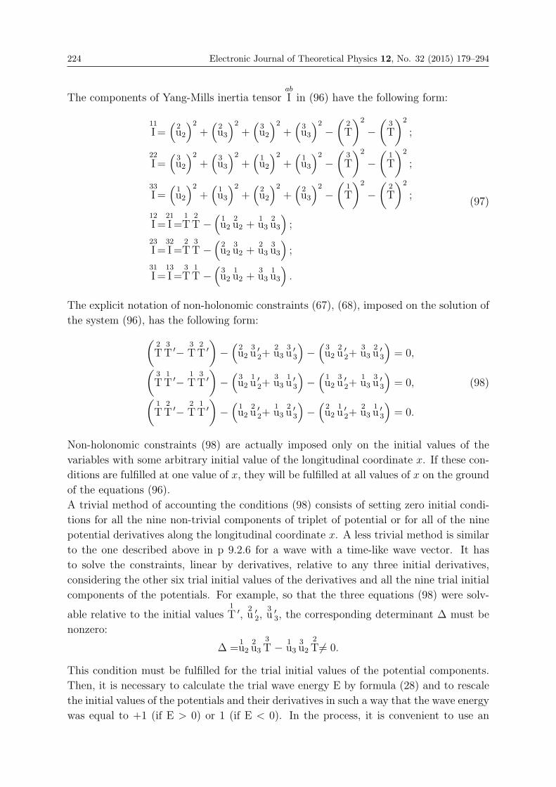
224 Electronic Journal of Theoretical Physics 12, No. 32 (2015) 179–294
The components of Yang-Mills inertia tensorab
I in (96) have the following form:
11
I =(
2u2
)2
+(
2u3
)2
+(
3u2
)2
+(
3u3
)2
−(
2
T
)2
−(
3
T
)2
;
22
I =(
3u2
)2
+(
3u3
)2
+(
1u2
)2
+(
1u3
)2
−(
3
T
)2
−(
1
T
)2
;
33
I =(
1u2
)2
+(
1u3
)2
+(
2u2
)2
+(
2u3
)2
−(
1
T
)2
−(
2
T
)2
;
12
I =21
I =1
T2
T −(
1u2
2u2 +
1u3
2u3
);
23
I =32
I =2
T3
T −(
2u2
3u2 +
2u3
3u3
);
31
I =13
I =3
T1
T −(
3u2
1u2 +
3u3
1u3
).
(97)
The explicit notation of non-holonomic constraints (67), (68), imposed on the solution of
the system (96), has the following form:(2
T3
T ′−3
T2
T ′)−
(2u2
3u ′2+
2u3
3u ′3
)−
(3u2
2u ′2+
3u3
2u ′3
)= 0,(
3
T1
T ′−1
T3
T ′)−
(3u2
1u ′2+
3u3
1u ′3
)−
(1u2
3u ′2+
1u3
3u ′3
)= 0,(
1
T2
T ′−2
T1
T ′)−
(1u2
2u ′2+
1u3
2u ′3
)−
(2u2
1u ′2+
2u3
1u ′3
)= 0.
(98)
Non-holonomic constraints (98) are actually imposed only on the initial values of the
variables with some arbitrary initial value of the longitudinal coordinate x. If these con-
ditions are fulfilled at one value of x, they will be fulfilled at all values of x on the ground
of the equations (96).
A trivial method of accounting the conditions (98) consists of setting zero initial condi-
tions for all the nine non-trivial components of triplet of potential or for all of the nine
potential derivatives along the longitudinal coordinate x. A less trivial method is similar
to the one described above in p 9.2.6 for a wave with a time-like wave vector. It has
to solve the constraints, linear by derivatives, relative to any three initial derivatives,
considering the other six trial initial values of the derivatives and all the nine trial initial
components of the potentials. For example, so that the three equations (98) were solv-
able relative to the initial values1
T ′,2u ′2,
3u ′3, the corresponding determinant Δ must be
nonzero:
Δ =1u2
2u3
3
T − 1u3
3u2
2
T�= 0.
This condition must be fulfilled for the trial initial values of the potential components.
Then, it is necessary to calculate the trial wave energy E by formula (28) and to rescale
the initial values of the potentials and their derivatives in such a way that the wave energy
was equal to +1 (if E > 0) or 1 (if E < 0). In the process, it is convenient to use an
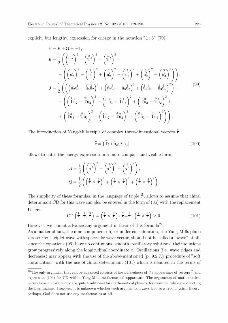
Electronic Journal of Theoretical Physics 12, No. 32 (2015) 179–294 225
explicit, but lengthy, expression for energy in the notation ”1+3” (70):
E = K+ U = ±1,
K =1
2
((1
T ′)2
+
(2
T ′)2
+
(3
T ′)2
−
−((
1
u′2
)2
+
(1
u′3
)2
+
(2
u′2
)2
+
(2
u′3
)2
+
(3
u′2
)2
+
(3
u′3
)2))
,
U =1
2
(((1u2
2u3 −
1u3
2u2
)2
+(
1u2
3u3 −
1u3
3u2
)2
+(
2u2
3u3 −
2u3
3u2
)2)−
−((
1
T2u2 −
2
T1u2
)2
+
(1
T2u3 −
2
T1u3
)2
+
(1
T3u2 −
3
T1u2
)2
+
+
(1
T3u3 −
3
T1u3
)2
+
(2
T3u2 −
3
T2u2
)2
+
(2
T3u3 −
3
T2u3
)2))
.
(99)
The introduction of Yang-Mills triple of complex three-dimensional vectorsaτ :
aτ= {
a
T; iau2; i
au3}− (100)
allows to enter the energy expression in a more compact and visible form:
K =1
2
((1
τ ′)2
+
(2
τ ′)2
+
(3
τ ′)2
);
U =1
2
((1τ × 2
τ)2
+(
2τ × 3
τ)2
+(
3τ × 1
τ)2
).
The simplicity of these formulas, in the language of tripleaτ , allows to assume that chiral
determinant CD for this wave can also be entered in the form of (86) with the replacementa
U→ aτ :
CD(
1τ ,
2τ ,
3τ)=
(1τ × 2
τ)· 3τ=
1τ ·
(2τ × 3
τ)≥ 0. (101)
However, we cannot advance any argument in favor of this formula29.
As a matter of fact, the nine-component object under consideration, the Yang-Mills plane
zero-current triplet wave with space-like wave vector, should not be called a ”wave” at all,
since the equations (96) have no continuous, smooth, oscillatory solutions; their solutions
grow progressively along the longitudinal coordinate x. Oscillations (i.e. wave ridges and
decreases) may appear with the use of the above-mentioned (p. 9.2.7.) procedure of ”soft
chiralization” with the use of chiral determinant (101) which is denoted in the terms of
29The only argument that can be advanced consists of the naturalness of the appearance of vectorsaτ and
expression (100) for CD within Yang-Mills mathematical apparatus. The arguments of mathematical
naturalness and simplicity are quite traditional for mathematical physics, for example, while constructing
the Lagrangians. However, it is unknown whether such arguments always lead to a true physical theory:
perhaps, God does not use any mathematics at all.
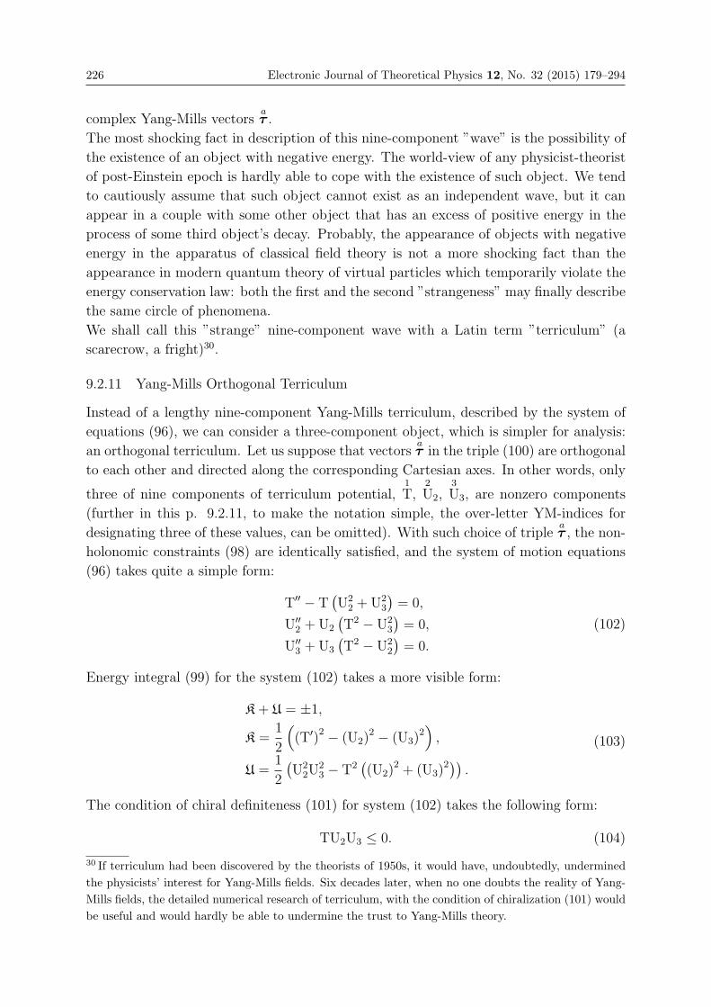
226 Electronic Journal of Theoretical Physics 12, No. 32 (2015) 179–294
complex Yang-Mills vectorsaτ .
The most shocking fact in description of this nine-component ”wave” is the possibility of
the existence of an object with negative energy. The world-view of any physicist-theorist
of post-Einstein epoch is hardly able to cope with the existence of such object. We tend
to cautiously assume that such object cannot exist as an independent wave, but it can
appear in a couple with some other object that has an excess of positive energy in the
process of some third object’s decay. Probably, the appearance of objects with negative
energy in the apparatus of classical field theory is not a more shocking fact than the
appearance in modern quantum theory of virtual particles which temporarily violate the
energy conservation law: both the first and the second ”strangeness” may finally describe
the same circle of phenomena.
We shall call this ”strange” nine-component wave with a Latin term ”terriculum” (a
scarecrow, a fright)30.
9.2.11 Yang-Mills Orthogonal Terriculum
Instead of a lengthy nine-component Yang-Mills terriculum, described by the system of
equations (96), we can consider a three-component object, which is simpler for analysis:
an orthogonal terriculum. Let us suppose that vectorsaτ in the triple (100) are orthogonal
to each other and directed along the corresponding Cartesian axes. In other words, only
three of nine components of terriculum potential,1
T,2
U2,3
U3, are nonzero components
(further in this p. 9.2.11, to make the notation simple, the over-letter YM-indices for
designating three of these values, can be omitted). With such choice of tripleaτ , the non-
holonomic constraints (98) are identically satisfied, and the system of motion equations
(96) takes quite a simple form:
T′′ − T(U2
2 +U23
)= 0,
U′′2 +U2
(T2 − U2
3
)= 0,
U′′3 +U3
(T2 − U2
2
)= 0.
(102)
Energy integral (99) for the system (102) takes a more visible form:
K+ U = ±1,
K =1
2
((T′)2 − (U2)
2 − (U3)2),
U =1
2
(U2
2U23 − T2
((U2)
2 + (U3)2)) .
(103)
The condition of chiral definiteness (101) for system (102) takes the following form:
TU2U3 ≤ 0. (104)
30 If terriculum had been discovered by the theorists of 1950s, it would have, undoubtedly, undermined
the physicists’ interest for Yang-Mills fields. Six decades later, when no one doubts the reality of Yang-
Mills fields, the detailed numerical research of terriculum, with the condition of chiralization (101) would
be useful and would hardly be able to undermine the trust to Yang-Mills theory.
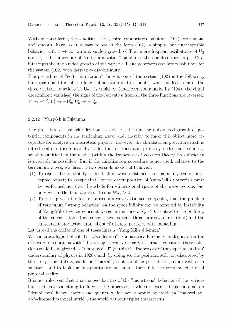
Electronic Journal of Theoretical Physics 12, No. 32 (2015) 179–294 227
Without considering the condition (104), chiral-symmetrical solutions (102) (continuous
and smooth) have, as it is easy to see in the form (102), a simple, but unacceptable
behavior with x → ∞: an unbounded growth of T at more frequent oscillations of U2
and U3. The procedure of ”soft chiralization” similar to the one described in p. 9.2.7,
interrupts the unbounded growth of the variable T and generates oscillatory solutions for
the system (102) with derivative discontinuity.
The procedure of ”soft chiralization” for solution of the system (102) is the following:
for those quantities of the longitudinal coordinate x, under which at least one of the
three decision functions T, U2, U3 vanishes, (and, correspondingly, by (104), the chiral
determinant vanishes) the signs of the derivative from all the three functions are reversed:
T′ → −T′, U′2 → −U′2, U′3 → −U′3.
9.2.12 Yang-Mills Dilemma
The procedure of ”soft chiralization” is able to interrupt the unbounded growth of po-
tential components in the terriculum wave, and, thereby, to make this object more ac-
ceptable for analysis in theoretical physics. However, the chiralization procedure itself is
introduced into theoretical physics for the first time, and, probably, it does not seem rea-
sonably sufficient to the reader (within the framework of classical theory, its sufficiency
is probably impossible). But if the chiralization procedure is not used, relative to the
terriculum waves, we discover two possible modes of behavior:
(1) To reject the possibility of terriculum wave existence itself as a physically unac-
cepted object; to accept that Fourier decomposition of Yang-Mills potentials must
be performed not over the whole four-dimensional space of the wave vectors, but
only within the boundaries of 4-cone kμkμ > 0.
(2) To put up with the fact of terriculum wave existence, supposing that the problem
of terriculum ”wrong behavior” on the space infinity can be removed by instability
of Yang-Mills free zero-current waves in the cone kμkμ < 0, relative to the build-up
of the current states (one-current, two-current, three-current, four-current) and the
subsequent production from them of discrete particles with pomerium.
Let us call the choice of one of these lines a ”Yang-Mills dilemma”.
We can cite a hypothetical ”Dirac’s dilemma” as a historically remote analogue: after the
discovery of solutions with ”the wrong” negative energy in Dirac’s equation, these solu-
tions could be neglected as ”non-physical” (within the framework of the experimentalists’
understanding of physics in 1928), and, by doing so, the positron, still not discovered by
those experimentalists, could be ”missed”; or it could be possible to put up with such
solutions and to look for an opportunity to ”build” them into the common picture of
physical reality.
It is not ruled out that it is the peculiarities of the ”monstrous” behavior of the terricu-
lum that have something to do with the processes in which a ”weak” triplet interaction
”demolishes” heavy leptons and quarks, which per se would be stable in ”maxwellian-
and-chromodynamical world”, the world without triplet interactions.
228 Electronic Journal of Theoretical Physics 12, No. 32 (2015) 179–294
9.2.13 Yang-Mills Photon: Plane Zero-current Triplet Wavewith Isotropic Wave Vector
Let us have a look at the plane triplet wave with isotropic wave vector kν :
kνkν = 0.
Wave vector isotropy means that the phase velocity of a wave is equal to the velocity
of light. We shall call this wave (to be precise, the quantum object, hypothetically
corresponding to it) ”The Yang-Mills’ photon” (ymiton).
Ymiton is a degenerate object of Yang-Mills mathematical wave theory. The condition of
a wave vector isotropy removes higher derivatives from the wave equation (55), turning
it into the first-order equation:
2kμAμ ×Aν ′ − kνAμ ×Aμ′ +Aμ × (Aμ ×Aν) = 0. (105)
The gauge condition (56), imposed on 4-potential divergence, means that
kμAμ = q = const = 0. (106)
As in other wave problems considered above, we suppose that vector q (106) is vanishing.
Availability of nonzero q would correspond to the wave propagation on the background
of some external stationary field.
With regard to (106), the first term in the wave equation (105) vanishes, and the wave
equation takes the form:abcε kν
b
Aμ
c
Aμ′+ab
Ib
A ν = 0. (107)
whereab
I is Yang-Mills inertia tensor, introduced above.
The twelve equations (107) are not independent from each other. The scalar multipli-
cation (107) by the wave vector kν gives three identities of the form 0 = 0. The scalar
multiplication (107) by the potential Aν generates the algebraic identity, which should
be followed by the solution (107):
U =ab
Sab
S −(
bb
S
)2
= 0. (108)
The expression (108) is a certain ”pale shadow” of the energy conservation law for ymiton.
For the degenerate wave (107) it is impossible to introduce anything resembling the kinetic
energy K. The analogue of potential energy, determined by formula (108), is identically
zero.
The system, in which
kν = {1; 1; 0; 0},will be named the ymiton ”intrinsic frame of reference”.
This is a ”frame of unit frequency”, in which axis x is directed along the wave direction.
In this frame φ = t− x. Using the notation of the form ”1+3” for potentiala
A ν again:
a
A ν = {a
T;a
U},
Electronic Journal of Theoretical Physics 12, No. 32 (2015) 179–294 229
we can reduce the ymiton wave problem to the following form:
a
T=a
U1; (109)
ab
Ib
U2= 0; (110)
ab
Ib
U3= 0; (111)
ab
Ib
U1=ag . (112)
The equations (109) allow to exclude time componentsa
T of all the three potentials of
YM -triplet from consideration.
YM -vector g, entering into (112), similarly to the components of YM -inertia tensorab
I ,
is expressed by spatial triplet componentsa
Ui
(i = 2, 3
):
1g=
3
U2
2
U2′+
3
U3
2
U3′ −
(2
U2
3
U2′+
2
U3
3
U3′);
2g=
1
U2
3
U2′+
1
U3
3
U3′ −
(3
U2
1
U2′+
3
U3
1
U3′);
3g=
2
U2
1
U2′+
2
U3
1
U3′ −
(1
U2
2
U2′+
1
U3
2
U3′).
Yang-Mills inertia tensorab
I for the ymiton wave problem looks as follows:
11
I =
(2
U2
)2
+
(2
U3
)2
+
(3
U2
)2
+
(3
U3
)2
;
22
I =
(3
U2
)2
+
(3
U3
)2
+
(1
U2
)2
+
(1
U3
)2
;
33
I =
(1
U2
)2
+
(1
U3
)2
+
(2
U2
)2
+
(2
U3
)2
;
12
I =21
I = −(
1
U2
2
U2 +1
U3
2
U3
);
13
I =31
I = −(
1
U2
3
U2 +1
U3
3
U3
);
23
I =32
I = −(
2
U2
3
U2 +2
U3
3
U3
).
The expression for ”potential energy” U (108) is reduced to the form which contains the
sum of three squares:
U = p21 + p2
2 + p23,
where
p1 =1
U2
2
U3 −2
U2
1
U3;
p2 =1
U2
3
U3 −1
U3
3
U2;
p3 =2
U2
3
U3 −2
U3
3
U2 .
230 Electronic Journal of Theoretical Physics 12, No. 32 (2015) 179–294
The equality U = 0 forms three algebraic conditions, imposed on the spatial components
of the potential:p1 = 0;
p2 = 0;
p3 = 0.
(113)
The relations, provided here, allow formulating the following algorithm of the construction
of ymiton wave parameters:
(1) The equations (110) and (113) give, with regard to the expressions forab
I and pi, the
system of six algebraic equations for determination of ”six-vector”a
Ui, (a = 1,2,3; i = 2,3)
three homogeneous cubic equations (110) and three homogeneous equations of the
second-order (113). Let us assume that there is at least one solution to this algebraic
system. Apparently, this solution will also satisfy the equations (111) which result
from (110) by substitution of the Cartesian subscripts 2↔ 3 in the equations (110)
and in tensorab
I which is invariant relative to such substitution.
Due to homogeneity of the equations (110) and (113), ifa
Ui=aκi is some solution to
these equations, the expression
a
Ui= f(φ)aκi (a = 1,2,3; i = 2,3) .
is also a solution to this system under the arbitrary function f(φ), which depends
on the wave phase, but does not depend on Yang-Mills and Cartesian indices. It
goes without saying that it is worth speaking about a ”wave” only in case if f(φ) is
a bounded oscillatory function.
(2) By substituting the relation fora
Ui into the expressions which determine YM-vector g
and matrixab
I , we solve the equations (112) as a system of three linear heterogeneous
algebraic equations relative to the longitudinal components of potentialsa
U1.
It is easy to see that the components of the inertia tensorab
I are proportional to the
square of arbitrary function f(φ), and the components of vector g are proportional to
the product of f(φ) · f′(φ). Therefore, the dependence of the longitudinal components
of the potential on the wave phase φ has the following form:
a
U1≈f′
f,
which inevitably generates singularities in the longitudinal componentsa
U1 with the
continuous function f(φ) oscillating around zero.
The condition of chiral determinacy for this wave, in forms (86) and (87), imposes
restriction on the behavior of f(φ).
This restriction requires a constant sign of product f · f′, which, actually, requiresdiscontinuous oscillations of function f(φ).
On the whole, the provided description of ”Yang-Mills photon” looks rather confusing.
Unlike tymos wave (kνkν > 0) and terriculum wave (kνkν < 0), isotropic YM-ymiton
Electronic Journal of Theoretical Physics 12, No. 32 (2015) 179–294 231
wave is an ”algebraic object” which does not require differential wave equations for its
description.
9.2.14 About Free Zero-current Triplet Field Statistics
In the preceding parts of this article (9.2.10-9.2.13) some certain difficulties in the descrip-
tion of Yang-Mills waves in the wave cone kνkν ≤ 0 were mentioned. These difficulties
include unbounded growth of potentials in the terriculum wave – if the procedure of chi-
ralization is not used, and the discontinuous behavior of waves ymiton. These difficulties
may indicate that the problem of describing the free wave state of Yang-Mills triplet is
not a correctly-set problem in theoretical physics. The ”free field” can probably turn into
a ”non-free” field in space-like cone kνkν < 0 of the four-dimensional space of the wave
vectors, generating YM -currents. In the linear singlet sector of physics there is nothing
similar to this phenomenon.
But, at the very least, the description of the free triplet waves in time-like cone kνkν > 0
is quite correct mathematically - no matter whether we use the chaotic chiral-symmetric
solutions of the wave equations, or impose chiral determinacy to a solution by using the
procedure of ”soft chiralization”.
Consequently, we can formulate a classical problem of the statistical characteristics of
the free triplet field in thermodynamic equilibrium - the problem, similar to the one
that Max Planck successfully solved in 1900 for maxwellian singlet by constructing the
frequency energy distribution function. Unlike the one-dimensional Planck distribution,
the corresponding Yang-Mills distribution must be two-dimensional, due to the absence
of constraint between frequency ω and three-dimensional wave vector |k| in the triplet
sector.
It can be supposed that the study of the thermodynamics of the triplet field is an un-
conventional problem. The language of Fourier expansion of the triplet field into plane
waves may not appear to be very convenient language for the nonlinear theory.
”Photon” in the electromagnetic theory retains its identity from one process of inter-
action with matter (emission or scattering) to the other one (absorption or scattering).
Due to the lack of dispersion, wave packets in the electromagnetic theory spread with-
out changing the profile, while retaining its identity. All these identities make Fourier
language useful for the singlet sector of physics. All these identities are not retained in
Yang-Mills nonlinear theory of the triplet waves. Yang-Mills wave packets spread and
interact with each other, changing the profiles and absorbing other packets. Perhaps, the
thermodynamics of Yang-Mills fields requires some other variables for its description.
9.3 One-current Triplet States
9.3.1 Classification and Lagrangians of One-current Triplet States
According to the scheme of the pure states, demonstrated in figure 1, and the structure
of the weak Lagrangian Lw (49), we can describe all the possible pure triplet one-current
states in the following way.
232 Electronic Journal of Theoretical Physics 12, No. 32 (2015) 179–294
1. There are two similar ”heavy” current states with a space-like current vector. The
Lagrangian of these states, according to (49), can be formulated in the following way:
Lw =1
2jν jν − jν
k
Aν −1
16πAμν ·Aμν , (114)
where jν = 12
k
j ν ; k = 1 or k = 2.
In these states only one of the three YM-currents with YM-number equal to 1 or 2, is
nonzero.
There are three types of states, described by the Lagrangian (114):
• ”Heavy” wave states, in which the current vector is nonzero all over the 4-dimensio-
nal space (there is no one pomerium).
• Stationary states, in which there is one stationary pomerium in a certain intrinsic
system of states the current zone boundaries in which current isotropization jν
(jν jν = 0) takes place; there is no current beyond this boundary; inside the current
zone there are cavitated zones (latebrae) inside which there is no current; on the
boundaries of these cavitated tubes, the pseudo-Euclidean square of 4-current has
the maximum possible value (7).
While solving the problems of stationary one-current states, it is worth taking into
account the curved space-time, generated by a high density of energy-momentum
inside the current zone and around it. As well as quarks, the stationary one-current
states of the triplet sector (in contrast to leptons – the stationary states of the singlet
sector) may turn out to be physically unrealizable due to the ”wrong behavior” of
stationary potential triplet Aν away from the current zone, resulting in divergence
of the total energy of the stationary state.
• Non-stationary states, or the ”interaction states”, in which there is one, or more
than one, non-stationary boundary of the current zones31.
Varying the action functional with the Lagrangian (114) by the triple of potentials Aν
and by current jν , we obtain the following field equations for a ”heavy” one-current triplet
state:
∂μAμν +Aμ ×Aμν = 4π jν
ke, (115)
jν+k
A ν = 0. (116)
In Yang-Mills equations (115)ke is a Yang-Mills unit vector of k YM-direction, i.e. YM-
vector with YM-components {1; 0; 0} for k = 1 and {0; 1; 0} for k = 2.
The second field equation, connecting the current and potential, is true in the current
zone, where j �= 0.
One gauge condition can be imposed on the solution of Yang-Mills equations. As in the
problem on Yang-Mills free fields, it is convenient to apply potential 4-divergence gauge:
∂νAν = 0. (117)
31Currently having no numerical solutions to stationary problems and having no version of the existence
theorem which would guarantee the existence of solutions to stationary problems, we are not going to
deal with formulation of non-stationary problems in this article.
Electronic Journal of Theoretical Physics 12, No. 32 (2015) 179–294 233
The differential condition for triplet currents (19), which, by means of the symbols applied
here, can be written in the form:
ke ∂νj
ν + jνAν×ke ν = 0, (118)
gives the following relation in YM-projections:
∂νjν = 0, (119)
3
Aν jν = 0,kAν jν = 0, (120)
where � k = 1 with k = 2; � k = 2 with k = 1.
The condition of current conservation jν (119) is compatible with gauge (117) and the
field equation (116).
The orthogonality conditions (120) are the result of differential condition for currents
(118), which, in its turn, is the result of the field equations (115) and (116). Therefore,
the orthogonality conditions (120) should not be included (together with undetermined
Lagrange’s multipliers) into the Lagrangian expansion of one-current problem (114).
The following dilemma can be formulated: either there are solutions to field equations
(115), (116), (117), (119), compatible with the orthogonality conditions (120) at zero
Lagrange’s multipliers, or one-current triplet states should not be treated as real physical
states at all – they exist only on the background of some external non-physical ”Higgs-
like” field which is mathematically reflected in the Lagrange’s multipliers for the extended
Lagrangian.
Getting rid of the weak field tensor Aμν in the equations (115) and considering the gauge
(117), we can formulate the Yang-Mills equations of one-current problem in the following
way:
−�Aν + 2Aμ × ∂μAν −Aμ × ∂νAμ + IAν = 4π jνke, (121)
where YM-inertia tensor I, according to (75) and (77) has the following YM-components
ab
I=a
Aμb
Aμ −ab
δc
Aμ
c
Aμ, (122)
2. Besides the two ”heavy” one-current triplet states, there are three similar neutrino
states, with isotropic current vector Nν (NνNν = 0). The Lagrangian of these neutrino
YM-states, which were named ymino above, looks as follows:
Lw,N = −Nνk
Aν −1
16πAμν ·Aμν −
1
2λN νNν , (123)
(k = 1, 2, 3).
The last term in (123) is the ”penalty” for current isotropy condition, λ is a Lagrange’s
multiplier. The current N ν in (123) corresponds to a nonzero k – YM-component of
YM-current triplet. With k = 1 or k = 2 along with the neutrino states (123), there are
current states with the Lagrangian (114). If k = 3, there is only neutrino state with the
Lagrangian (123).
234 Electronic Journal of Theoretical Physics 12, No. 32 (2015) 179–294
The field equations, following from the Lagrangian (123), look similar to the equations
(115), (116) and (121):
∂μAμν +Aμ ×Aμν = 4π N ν k
e, (124)
−�Aν + 2Aμ × ∂μAν −Aμ × ∂νAμ + IAν = 4π N ν ke, (125)
λN ν+k
A ν = 0, (126)
∂νAν = 0, (127)
∂νNν = 0, (128)
NνkAν= 0, (129)
NνNν = 0. (130)
In orthogonality conditions (129) � k = 2 and 3 with k = 1; � k = 3 and 1 with k = 2;
� k = 1 and 2 with k = 3.
From field equation (126) and the condition of neutrino current isotropy (130) there
follows the orthogonality condition
Nνk
Aν= 0. (131)
Condition (131), combined with condition (129), means that neutrino current Nν must
be orthogonal to all the three triplet potentials. Besides this, as it follows from (126),
potentialk
A ν is an isotropic vector.
Differentiating the field equation (126) by coordinates xν , and taking into account (127)
and (128), we find that 4-gradient of the Lagrange’s multiplier λ satisfies the orthogonality
condition:
N ν∂νλ = 0. (132)
This condition will be anyway satisfied, if λ = const.
9.3.2 ”Heavy” One-current Plane Triplet Wave
We will try the solution to Yang-Mills wave equations (121) in the form of a plane wave,
supposing that current jν and potential Aν depend on the only argument – the wave
phase φ = kμxμ. The wave equation (121) for a plane wave gets the following form
kμkμAν ′′ + 2kμAμ ×Aν ′ − kνAμ ×Aμ ′ + IAν + 4π
k
A ν ke= 0. (133)
In equation (133) the prime denotes a wave phase derivative. In the last term, field
equation (116) is taken into account. The summation by ”stationary” index k is not
made in this term.
If homogeneous equations (133) are solved, the current is calculated by field equation
(116).
Gauge condition (117) in the plane wave is reduced to the condition:
kνAν ′ = 0,
Electronic Journal of Theoretical Physics 12, No. 32 (2015) 179–294 235
with integral:
kνAν = q = const,
but, as in the other wave problems, we will assume that q = 0: nonzeroness of q would
correspond to a wave propagation on the background of a certain external stationary
field. Considering zero value of q, the second term in the equation (133) vanishes:
kμkμAν ′′ − kνAμ ×Aμ ′ + IAν + 4π
k
A ν ke= 0. (134)
By scalar multiplying the plane one-current wave equation (134) by wave vector kν , we
find with anisotropic vector kν (kνkν �= 0) that:
Aμ ×Aμ ′ = 0. (135)
As in Yang-Mills free wave problem, relation (135) can be considered a non-holonomic
constraint, imposed on the initial values of potentials and their derivatives. Considering
condition (135), the wave equation (134) takes even a simpler form:
kμkμAν ′′ + IAν + 4π
k
A ν ke= 0. (136)
Let ε be a non-Euclidean module of wave vector kν :
kνkν = ±ε2,
where a plus sign corresponds to the wave with a time-like wave vector, but a minus sign
corresponds to the wave with a space-like wave vector. Making a scale transformation in
(136),
kν → εkν ; φ→ εφ,
normalizing wave vector k for a unit module, we get rid of the module of wave vector ε
in equation (136):
±Aν •• + IAν + 4πk
A ν ke= 0. (137)
A plus sing in (137) corresponds to the wave with time-like wave vector kν , normalized
for unit:
kνkν = 1.
A minus sign in (137) corresponds to the wave with space-like wave vector kν , normalized
for unit:
kνkν = −1.
The dots on the right-side of the potential symbol imply the derivative with respect to ε
- rescaled wave phase. In the wave intrinsic frame of reference, wave vector kν has the
form:
kμ = {1; 0; 0; 0}−
for time-like vector kν and
kμ = {0; 1; 0; 0}−
236 Electronic Journal of Theoretical Physics 12, No. 32 (2015) 179–294
for space-like vector kν .
In the wave intrinsic frame of reference the phase derivative coincides with the time
derivative (all wave characteristics in the intrinsic frame depend only on time) – for the
time-like wave vector, or with longitudinal coordinate x derivatives – for the wave with a
space-like wave vector (in such wave all the characteristics depend only on longitudinal
coordinate; in the intrinsic frame of reference such a wave is a kind of ripple of current
and potentials stiffed in space).
Multiplying one-current plane wave equation (137) by Aν • and integrating by the wave
phase, we can obtain the energy integral for this wave:
K+ U = E = const,
where
U =1
4
((aa
S
)2
−ab
Sab
S +8πk
A νk
Aν
)−
is a wave potential energy, andab
S=a
Aμb
Aμ .
In the expression for potential energy U, the summation is made by YM-repetitive indices
a, b. But the summation by the ”stationary” YM-index k is missing.
”Kinetic” energy K for the waves with space-like and time-like wave vector differs in sign:
K = Kt = −1
2Aν • ·A•
ν , (time-like wave),
K = Ks =1
2Aν • ·A•
ν , (space-like wave).
For time-like wave, energy E is positive, but for a space-like wave the energy sign E can
be either positive, or negative.
In the expression for potential energy U the first two terms have the fourth order by
potentialsa
Aμ, and the last term, generated by current availability in the wave, is quadratic
by potentials.
Availability of this term destroys the self-similarity of a plane wave relative to the energy
that is inherent to a zero-current wave. For a one-current wave, energy E is a significant
parameter (not just the scale one).
Equations (137) describe some dynamical system. By analogy with dynamical system
(79), which describes a zero-current wave, let us call dynamical system (137) with time-
like vector kν a ”1c-tymos” (one-current-tripletic-yang-mills’ oscillator). The choice of
a plus sign before the first term of the equation corresponds to 1-tymos object (137).
The choice of a minus sign before this term, corresponding to space-like wave-vector kν ,
generates a one-current analogue of the ”terriculum” object. Let us name this object a
1c-terriculum.
9.3.3 Detailed Notation of the 1-tymos Dynamics Equations
Let us use ”1+3” – the notations for the components of weak potentiala
A ν (70). In these
notations, it follows from the condition (117) that in the intrinsic frame of reference of
Electronic Journal of Theoretical Physics 12, No. 32 (2015) 179–294 237
1-tymos wave all the time components of the potential are vanishing:
a
T= 0, a = 1, 3.
By choosing ”fixed” YM-index k equal to one, for definiteness, we can write the equations
of a plane wave (137) as a system of equations for the three three-dimensional vectorsa
U
which specify the spatial components of YM-potentials
a
U ••+ab
Ib
U +4π1
U ·1a
δ= 0, (138)
where tensorab
I has the same form (78), (83) as for the zero-current wave. If in system
(138) we explicitly write out the YM-indices of all vectorsa
U and all their Cartesian
indices, we will get a system of nine differential equations, in which only the first three
equations with a unit YM-index are different from the analogous system for a zero-current
wave (82):1
U1•• +
(11
I +4π
)1
U1 +12
I2
U1 +13
I3
U1= 0,
1
U2•• +
(11
I +4π
)1
U2 +12
I2
U2 +13
I3
U2= 0,
1
U3•• +
(11
I +4π
)1
U3 +12
I2
U3 +13
I3
U3= 0,
(139)
but the other six equations for YM-indices 2 and 3 coincide with the corresponding
equations (82).
Energy integral for system (138) has the form which is analogous to the energy integral
for zero-current wave (81):
1
2
a
U •·a
U • +1
2
((1
U ×2
U
)+
(2
U ×3
U
)+
(3
U ×1
U
)+ 4π
1
U 2
)= E.
In contrast to a zero-current wave problem, the 1c-wave cannot be ”scaled” by energy E.
The equations of non-holonomic constraints (135) in this problem have the same form
(85) as in the problem on a zero-current wave. Chiral determinacy conditions (87) also
coincide in these problems.
As in the case of a zero-current wave, the one-current wave problem takes especially
simple form for the ”orthogonal” wave, in which
a
Ui= 0, with i �= a.
For such wave the equations of non-holonomic constraints are satisfied identically, and
for the three nontrivial potential componentsa
Ui with i = a, it is possible to formulate
the system of equations, similar to the system (90):
U••1 +U1
(4π +U2
2 +U23
)= 0,
U••2 +U2
(U2
3 +U21
)= 0,
U••3 +U3
(U2
1 +U22
)= 0.
(140)
238 Electronic Journal of Theoretical Physics 12, No. 32 (2015) 179–294
Energy integral for (140) looks as follows:
1
2
( •U1
2+•U2
2+•U3
2
)+
1
2
(U2
1U22 +U2
2U23 +U2
3U21 + 4πU2
1
)= E.32 (141)
The chiral determinacy condition for the solution (140) has a simple form:
U1U2U3 ≥ 0. (142)
The procedure of ”soft chiralization” for (140) includes the sign reverse for derivatives•Ui(
i = 1, 3)at vanishing of any potential component Ui.
Probably, with higher energy of E the one-current wave behaves like a zero-current wave:
in equations (140) constant terms 4π, compared to the large (average) squares of po-
tentials, can be neglected. At low oscillation amplitude of potentials, the first equation
(140) turns into harmonic oscillator equation, and the second and third equations are
transformed into Mathieu equations. In the situation with small-amplitudes the three-
component system (140) is similar to the behavior described in the article [1] maxwellian
”heavy photon”, but modulated by the energy exchange ”heavy photon” U1 with two
other YM-degrees of freedom U2 and U3 in the mode as it is dictated by the Mathieu
equation. In particular, without taking into account the condition of the chiral determi-
nacy (142), system (140) may have periodic solutions.
9.3.4 Dynamics of a One-current-terriculum
Repeating the calculations, described in p.9.2.10 for zero-current terriculum, as applied
to the problem of a one-current wave with space-like wave vector, we find that all of the
longitudinal components of the potentials are equal to zero:a
U1= 0, and nine non-trivial
componentsa
T,a
Ui with i = 2, 3 satisfy the system of equations similar to the system of
equations (96), which describes zero-current terriculum. In the equations of a one-current
wave only the three first equations, corresponding to YM-index 1, differ from the system
of equations (96). These equations take the form:
−1
T •• +(
11
I +4π
)1
T +12
I2
T +13
I3
T= 0,
−1
U2•• +
(11
I +4π
)1
U2 +12
I2
U2 +13
I3
U2= 0,
−1
U3•• +
(11
I +4π
)1
U3 +12
I2
U3 +13
I3
U3= 0.
(143)
The other six equations of the system (96) are transferred into the problem of a one-
current wave terriculum unchanged. No changes take place while the components of
tensorab
I (97) and the equations of nonholonomic constraints (98) are transferred into
this problem. As in case of the zero-current terriculum problem, the energy integral of a
32 It can be noted that the ”energy” of oscillator (140), determined by the formula (32), differs from the
wave energy density in the intrinsic frame of reference in multiplier 4π.
Electronic Journal of Theoretical Physics 12, No. 32 (2015) 179–294 239
one-current terriculum is proper to formulate by using three complex potentialsaτ (100).
When using vectorsaτ , the energy integral for (143) takes the following form:
K+ U = E,
K =1
2
((1τ •
)2
+(
2τ •
)2
+(
3τ •
)2),
U =1
2
((1τ × 2
τ)2
+(
2τ × 3
τ)2
+(
3τ × 1
τ)2
+ 4π(
1τ)2
).
Chiral determinant CD for this problem is defined by the same formula (101) as for the
zero-current problem. When CD is vanishing, all derivativesaτ • signs must be reversed. If
we do not appeal to the chiralization procedure, the potential components in one-current
wave terriculum grow indefinitely along the longitudinal coordinates of the wave.
The problem of 1c-terriculum object takes particularly simple form for the ”orthogonal
wave”, in which1τ= {T; 0; 0},2τ= {0; iU2; 0},3τ= {0; 0; iU3}.
For this three-component wave the equations of nonholonomic constraints are satisfied
identically. The wave equations take the form:
− T•• + E(4π +U2
2 +U23
)= 0,
− U••2 +U2
(U2
3 − T2)= 0,
− U••3 +U3
(U2
2 − T2)= 0.
(144)
Energy integral for (144) looks as follows:
K+ U = E,
K =1
2
((T•)2 − (U•2)
2 − (U•3)2) ,
U =1
2
(U2
2U23 + T
(4π − U2
2 − U23
)).
Chiral determinant CD(
1τ ,
2τ ,
3τ)has the form of (104). The ”soft chiralization” proce-
dure for orthogonal one-current terriculum wave is similar to the zero-current orthogonal
terriculum wave, described above.
We do not provide here a description of a one-current triplet wave with an isotropic wave
vector. This description leads to the results which are completely analogous to those given
in part 9.2.13 for zero-current triplet wave with isotropic wave vector. Such a wave is a
degenerate ”algebraic” object which behavior is not controlled by differential equations.
9.3.5 One-neutrino Plane Triplet Wave
The four-dimensional neutrino zone, which state of currents and potentials is described
by the one-neutrino Lagrangian (123) and, correspondingly, by the field equations (125) –
240 Electronic Journal of Theoretical Physics 12, No. 32 (2015) 179–294
(130), must border the zones in which there are anisotropic currents on some unknown in
advance three-dimensional boundaries. The conditions for solutions splicing on the three-
dimensional boundaries of these different types of 4-zones must allow to determine not
only the currents / potentials, but also the Lagrange’s multipliers λ. By abstracting from
the existence of these boundaries and expanding the area of the one-neutrino Lagrangian
(123) over the whole space-time, we get some hypothetical state that does not exist in a
”pure form” in nature. Let us name this state a ”Yang-Mills neutrino” (ymino). In the
state of ymino the Lagranges multiplier remains arbitrary, obeying only to the condition
of orthogonality (132).
Isotropization of any of the four currents of the singlet-triplet theory in some 4-zone
generates a neutrino state. Consequently, the ST-theory contains a few types of neutrino:
a pure maxwellian neutrino, totally located in the singlet sector; three indistinguishable
YM-neutrinos, located in the triplet sector of the theory (ymino); and a mixed Maxwell-
Yang-Mills neutrino, appearing under the simultaneous isotropization of singlet current
Jν and the third component of YM-current3
J ν . This mixed neutrino state, not fitting
into either singlet or triplet sectors, occupies the both sectors of the theory.
It can be assumed that historically determined binding of a neutrino type to a massive
lepton type (”electron neutrino”, ”muonic neutrino”, ”τ -neutrino”) is incorrect since it
does not find a natural reflection in the apparatus of the ST-theory. The interpretation
of a neutrino as a lepton is also incorrect itself. Within the framework of the theory
constructed here, leptons are pure, stationary singlet states. Neutrino states cannot be
stationary.
It should be noted that there is no a priori forbidding for the possibility of isotropization
of any of the eight currents of the Yang-Mills octuplet which is responsible for the strong
interaction. So, there are no reasons to except the existence of ”quark” or ”gluon”
neutrinos, which are not connected with the triplet sector of physics.
We will try a solution to the field equations of one-neutrino state of ymino (125) – (130)
in the form of a plane wave with wave vector kν . All of the physical variables in a plane
wave depend only on wave phase φ = kνxν . The wave equation (125) for the plane wave
takes the form:
kμkμAν ′′ + 2kμAμ ×Aν ′ − kνAμ ×Aμ ′ + IAν − 4π p
k
A ν ke= 0, (145)
kνAν ′ = 0, (146)
k
A νa
Aν= 0, (a = 1, 2, 3) . (147)
In these equations p = −1
λ, p = const; the prime denotes a wave phase derivative; Yang-
Mills inertia tensor I is determined by formula (122); YM-index ”k” is ”immovable”, the
summation is not made by it. This index denotes the YM-component which contains
the only current of a one-current problem. Further we will fix k = 1. If homogeneous
equations (145) - (147) are solved, the neutrino current is determined from the condition
Nν = pk
Aν .
Electronic Journal of Theoretical Physics 12, No. 32 (2015) 179–294 241
From the condition (146) it follows that
kνAν = q = const.
As in other wave problems, we will assume that q = 0. If vector q was nonzero, it would
mean that we deal with a neutrino wave on the background of some stationary field.
With q = 0 the second term vanishes from the field equation (145):
kμkμAν ′′ − kνAμ ×Aμ ′ + IAν − 4π p
k
A ν ke= 0. (148)
By scalar multiplying (148) by wave vector kν , with anisotropic wave vector kν we find
that:
Aμ ×Aμ ′ = 0. (149)
Relation (149) is a standard Yang-Mills nonholonomic constraint, which also appears in
the other wave problems studied above. With regard to (149), the equation (148) is
simplified:
kμkμAν ′′ + IAν − 4π p
1
A ν 1e= 0. (150)
From relation (147) follows that potential1
A ν is an isotropic 4-vector:1
A ν1
Aν= 0, or in
the notation of the form ”1+3”:1
T 2−1
U 2 = 0.
Consequently, the three spatial components1
U of 4-vector1
A ν can be formulated as
follows:1
U=1
T e; e2 = 1,
where e is some three-dimensional unit vector. Using wave vector kν in the notation of
the form ”1+3”, kν = {ω; k}, the orthogonality condition
kν1
Aν= 0
can be presented this way:1
T (ω − ke) = 0,
or ω = ke. But | ke |≤| k |, so, ω2 ≤ k2, i.e. the wave vector of the neutrino wave ymino
(as well as the wave vector of the maxwellian neutrino wave, considered in the article [1])
cannot be time-like. Leaving aside the degenerate case of isotropic wave vector, let us
suppose that
kνkν = −k2S,
where kS is a Lorentz-invariant pseudo-Euclidean module of space-like wave vector kν ;
kS �= 0.
By making the scale transformation, which we have also used for the wave problems
above,
φ→ kSφ, kν → kSkν ,
242 Electronic Journal of Theoretical Physics 12, No. 32 (2015) 179–294
we can normalize a wave vector for unit in the field equations (150):
−Aν ′′ + IAν − 4π p1
A ν 1e= 0, (151)
kνkν = −1, (152)
kνAν = 0, (153)
1
A νAν = 0. (154)
System (151) – (154) together with nonholonomic constraint (149) makes formulation of
the problem of Yang-Mills neutrino – ymino.
By scalar multiplying the field equation (151) by A′ν and integrating by the wave phase,
we find, with regard to (154), the energy integral of the neutrino ymino wave, which
identically coincides with the energy integral of a zero-current wave with a space-like
vector. Like for a zero-current wave with nonzero energy, it is possible to rescale the
variables per unit energy without changing field equations (151):
Aν →| E | 14 Aν ,
φ→| E |− 14 φ,
p→| E | 12 p.
As for a zero-current wave with space-like wave vector, the energy of a neutrino wave does
not have a fixed sign – the energy sign is determined by arbitrarily set initial conditions.
It is hardly doubtful that here the reader’s relativistic intuition is also ready to protest
angrily against the theory in which there appear some objects with negative energy and,
therefore, negative mass. But perhaps the appearance of such objects is just a different
way of description in the classical language of those phenomena which in the language of
quantum are described as the production of virtual particles off-mass-shell surface with a
virtual violation of the energy conservation law for short time intervals: the shorter this
time interval is, the higher, according to the uncertainty relation, the uncertainty in the
energy of state is.
For example, the process of transformation of a muon into an electron is described in the
language of quantum through the transformation of a muon into a virtual W-particle with
the mass exceeding the muon mass on three decimal orders, with concomitant production
of a muon neutrino and fast subsequent transformation of W-particle into an electron and
concomitant electron neutrino.
The classical theory, developed here, presupposes the continuous dependence of all phys-
ical variables of the theory on the space-time arguments.
It requires a different language to describe such processes, since the classical theory does
not allow virtual particles: this is a non-stationary transformation of a particle (i.e. an
object with the current boundary pomerium) into another, more massive particle, ac-
companied by generation of a non-stationary neutrino zone with negative energy – in this
case the energy conservation law is not violated.
Electronic Journal of Theoretical Physics 12, No. 32 (2015) 179–294 243
Undoubtedly, there is a considerable distance between this speculative picture and a clear
formulation of the initial boundary value problem, describing the muon decay in the clas-
sical theory under consideration: it is even unobvious that this distance generally can
be surmountable in the classical theory framework by combining the total four-current
Lagrangian with neutrino Lagrangians in some previously unknown 4-zones. However,
the opening possibility to use the language of waves with negative energy an alternative
one to the language of virtual particles – seems fruitful in itself.
In the ymino intrinsic frame of reference, in which kν = {0; 1; 0; 0}, anda
A ν = {a
T;a
U ν},from the orthogonality condition (153) follows that all longitudinal potential components
vanish:a
U1= 0,
and the other 9 components of YM-triplet of potentials are controlled by the system of
equations (151), which in notation ”1+3” take the following form:
v′′ + v
(4πp−
11
I
)= 0, (155)
where v =1
T,1
U2,1
U3 is any of the three nonzero components of vector1
A ν , and
11
I =2
U 2+3
U 2−2
T 2−3
T 2,
(in vectors2
U and3
U the longitudinal components2
U1 and3
U1 are missing).
Equations for the two other time components of 4-vector Aμ, according to (151), have
the form:2
T ′′−2
T3
U 2+3
T2
U ·3
U= 0,3
T ′′+2
T2
U ·3
U −3
T2
U 2 = 0,
(156)
and the equations for spatial components of 4-vector Aμ have the form:
2
U ′′+2
U3
T 2−3
U2
T3
T +3
U ×(
3
U ×2
U
)= 0,
3
U ′′+3
U2
T 2−2
U2
T3
T +2
U ×(
2
U ×3
U
)= 0.
(157)
The orthogonality conditions (147) in notations ”1+3” have the form:
1
T 2−1
U 2 = 0,1
T2
T −1
U ·2
U= 0,1
T3
T −1
U ·3
U= 0.
(158)
Nonholonomic constraints (149) in the language of variablesa
T anda
U take the form:
2
T3
T ′−3
T2
T ′ −(
2
U ·3
U ′−3
U ·2
U ′)
= 0. (159)
244 Electronic Journal of Theoretical Physics 12, No. 32 (2015) 179–294
and two more equations are obtained from (159) by means of cyclic permutation of YM-
indices: 1 → 2 → 3 → 1. For a plane-polarized ymino wave, the drawn wave equations
allow further simplifications. In such wave all spatial vectorsa
U have fixed directions.
By turning axes y and z around axis x, oriented along wave vector k, it is possible to
combine axis y with the direction of vector1
U oscillations.
Then, with regard to (158), we can formulate all the three-dimensional vectorsa
U as
follows:1
U= {0;1
T; 0},2
U= {0;2
T; u},3
U= {0;3
T; v},
(160)
where u and v are z-components of vectors1
U and2
U. The choice of the axes orientation
(160) turns the ymino wave into a ”five-component” mathematical object, characterized
by five functions1
T,2
T,3
T, u, v.
Subject to the form of vectorsa
U (160), the orthogonality conditions (158) become iden-
tities. Field equations (155), (156), (157) subject to (160) are simplified:
1
T ′′+1
T(4πp− u2 − v2
)= 0, (161)⎧⎨⎩
2
T ′′−2
T v2+3
T uv = 0,3
T ′′−3
T v2+2
T uv = 0.
(162)
{u′′ = 0,
v′′ = 0.(163)
Only trivial solutions to equations (163) are physically acceptable:
u = 0; v = 0. (164)
General solution (163) with linear growth of components u and v along longitudinal co-
ordinate x, in accordance with equations (162) and (161), result in exponential growth of
time componentsa
T. For ymino wave we have no possibility to stop the solution growth
and to transfer it into an oscillating regime by means of ”soft chiralization” procedure,
since chiral determinant CD (101) for such a wave is identically zero. So, we have either
to accept (164) as the only solution that has a physical meaning, or to assume that the
ymino wave turns into a wave with anisotropic current due to some instability which is
not reflected in the neutrino Lagrangian (123).
Accepting solution (164), we have to, due to the same reasons, accept a zero solution for
components2
T and3
T, which are controlled by equations (162). Equation (161) for compo-
nent1
T turns into the equation of a harmonic oscillator with frequency ω =√4πp (p > 0).
What is the physical meaning of the obtained solution?
Electronic Journal of Theoretical Physics 12, No. 32 (2015) 179–294 245
Subject to (160), the two YM-potential components2
A ν and2
A ν vanish, and the compo-
nent2
A ν describes the ”stiffed” in the wave intrinsic frame of reference sinusoidal ripple,
i.e. the ymino wave, nominally located in the triplet sector of physics, is actually a one-
component singlet object, which does not differ from the maxwellian neutrino described
in the article [1]. When calculating the energy of this one-component ymino by formula
(28), applicable to the triplet wave with space-like wave vector, we find that the energy
of ymino is equal to zero.
Indeed, ymino wave with such properties is a strange, confusing object. This object is
generated by the Lagrangian (123) and we have no a priori reasons to throw ymino away
from physics, to recognize it as a non-existent object. Even the total ”five component”
ymino wave (161), (162) with potentials growing along the wave longitudinal coordinate
should probably be considered as a real physical object, as the description of the tran-
sition state associated with the decay of one current state with anisotropic current and
the production of another current state.
9.3.6 One-current Stationary Triplet State
One-current stationary triplet state is described by the one-current Lagrangian (114)
in the zone, occupied by current jν , and by the zero-current Lagrangian of Yang-Mills
free field (50), where the current is missing. At the outer boundary of the current zone
(pomerium), the isotropization of current jν is taking place. At the inner boundary of the
current zone (latens) the pseudo-Euclidean module of the space-like current jν reaches
its maximum value (7). In the cavitated tubes of latebra, which have latens as the outer
boundary, there is only a free triplet field. At the boundaries of pomerium and latens,
3-current j has no component normal to the surface. At these boundaries potentials and
their space-like coordinate derivatives are continuous.
While deriving the one-current triplet state equations, we will use the Lagrangians (50)
and (114), written in Minkowski coordinates. To account the Riemannian space curva-
ture, generated by a high density of energy-momentum in the current zone, the equations
of stationary one-current state, presented below, must be rewritten in arbitrary curvi-
linear coordinates and the metric tensor must be subjugated to the Einstein equations.
Accounting of this curvature can significantly change the quantitative characteristics of
the solutions, but can hardly influence the fact of the existence or non-existence of a
solution.
The equations of one-current stationary state are convenient to write in the intrinsic
frame of reference of this state. In this frame, the pomerium and latens boundaries are
stationary and the time derivatives of all physical values are equal to zero. Fixation of
the frame of reference and separation of time and spatial vector components deprives
field equation (53) and (121) of Lorentz and Yang-Mills elegance, but makes them more
convenient for numerical investigations.
To write the field equations in the intrinsic frame of reference, it is convenient to intro-
duce into this frame a special mathematical object – Yang-Mills bracket.
246 Electronic Journal of Theoretical Physics 12, No. 32 (2015) 179–294
Let u and v be two YM-vectors depending on spatial coordinates xk (k = 1, 2, 3). We
do not explicitly write out YM-indices over u and v. Geometrical nature of u and v is
inessential: with respect to the transformations of spatial coordinates, u and v may be
either scalars or vectors. Let us call Yang-Mills bracket over u and v YM-vector {u, v}such that its YM-component of number a is as follows:
{u, va
}=abcε
bu ∇ c
v . (165)
In formula (165) ∇ is the gradient operator in spatial coordinates. Yang-Mills bracket,
introduced in (165), is a bilinear differential form of the first order.
Using the Yang-Mills bracket, the equations of stationary one-current state in the intrinsic
frame of reference, derived from the Lorentz-invariant notation of the field equations (53)
and (121), can be written in the following form:
a) In the current zone:
∇a
T −2{U, Ta
} −ab
Ib
T −4π1
T1a
δ= 0,
∇a
U −2{U, Ua
} +{Uk, Uk
a
} −{T, Ta
} −ab
Ib
U −4π1
U1a
δ= 0.
(166)
∇·a
U= 0. (167)
1
T2
T −1
U ·2
U= 0,1
T3
T −1
U ·3
U= 0,
−(1
2jT
)2
≤1
T 2−1
U 2 ≤ 0.
(168)
Yang-Mills inertia tensor has the form
ab
I=a
Tb
T −a
U ·b
U −ab
δ ·∑c
(T2
c −U2c
), (169)
and, subject to orthogonality conditions (168), it has some zero components inside the
current zone:12
I =21
I = 0,13
I =31
I = 0.
(170)
If equations (166) are solved, the current j = {ρ, j} is determined by its coupling with
potential1
A ν (116):
ρ = −1
T;
j = −1
U .
(171)
b) In current-free zone, potentialsa
A ν obey the equations of the free stationary triplet
field, i.e. equations (166) without the last term in each of equations (166), without
Electronic Journal of Theoretical Physics 12, No. 32 (2015) 179–294 247
orthogonality conditions (168) and without the condition of ”nulling” of some tensorab
I
elements (170):
∇a
T −2{U, Ta
} −ab
Ib
T= 0,
∇a
U −2{U, Ua
} +{Uk, Uk
a
} −{T, Ta
} −ab
Ib
U= 0.
(172)
Vectorsa
U obey the condition (167).
) The continuity conditions fora
T,a
U and their derivatives are fulfilled at the boundaries
between zones a and b. The vector component1
U, normal to the boundary, vanishes at
these boundaries:1
U ·n = 0, (173)
where n is the unit vector of normal to the surface.
Vector1
A ν becomes isotropic on the pomerium:
1
T 2−1
U 2 = 0. (174)
The current jν reaches its peak value jT on latens:
1
T 2−1
U 2 = −(1
2jT
)2
. (175)
Pomerium and latens boundaries are not pre-set and must be found in the process of the
problem solving.
We would like to remind that the system of twelve field equations (166) or (172) must
be written in curvilinear coordinates and supplemented with ten Einstein field equations,
as it has been noted previously for the similar stationary problem of electrodynamics [1].
We do not have any version of the theorem of existence / non-existence of the solutions
to this problem. Perhaps this is one of the most cumbersome problems in mathematical
physics.
It is obvious that the set problem (166) – (175) does not withstand the charge inversiona
T→ −a
T,a
U→ −a
U due to the presence of the Yang-Mills bracket, but it is invari-
ant relative to the charge conjugation method, described in part 4.1, which requires the
permutation of YM-indices 1↔ 2 simultaneously with the charge inversion. This permu-
tation transforms the one-current problem with the current having a YM-number 1 into
a similar problem with the current number 2.
The problem of constructing chiral-definite solutions for the stationary one-current prob-
lem causes certain difficulties. If we formulate the condition for solution chiral-determina-
cy in the same form (86), (87) as it was formulated in part 9.2.7 for the wave zero-current
problem, i.e. if we require sign-definiteness of the chiral determinant, formed by Yang-
Mills triple of spatial components of the 4-potentials, the question will arise: what is to
be done when this determinant turns into zero?
248 Electronic Journal of Theoretical Physics 12, No. 32 (2015) 179–294
Some fixed surfaces in the intrinsic frame of reference of a stationary one-current prob-
lem will correspond to zero values of the chiral determinant. At the intersection of such
surface we have not only to reverse all the signs of spatial derivatives for all the twelve
potential componentsa
T anda
U, but also to permute YM-indices 1 ↔ 2. Such chiraliza-
tion procedure looks deformed, but the change of sign for gradients, without YM-indices
permutation, does not preserve the form of the equations of a stationary one-current
problem.
By agreeing to such chiralization procedure, we distort the very term ”one-current state”,
making it conventional. If in the zone, occupied by the current , there are surfaces on
which the chiral CD determinant vanishes, this zone splits into sub-zones occupied by
currents1
J ν or2
J ν . Such picture of one-current stationary state can hardly be called
inspiring. However, the choice is limited: we either put up with such picture (and thus,
generally speaking, recognize the non-terminality and imperfection of Yang-Mills’ descrip-
tion of nature), or we ignore the problem of chiral determinacy and construct continuous
solutions to the stationary one-current triplet problem, despite probable violation of the
terms of chiral determinacy (87).
The problem of the stationary one-current triplet state (if it has a solution) provides a
classical description of a particle33. In order not to increase the number of new terms,
we shall call this particle a ”wark”, removing the first sound from the word ”quark”. In
the subsequent article of this series, we shall demonstrate that in the octuplet sector of
physics there are one-current states with triplet field shell which contains only three of
eight potentials of the octuplet sector34. Such stationary states in the octuplet sector of
physics are a classical model of quarks. The mathematical formulations of the problems
of quark and wark structure completely coincide. The physical difference between the
wark and quark particles is that wark is made of currents and potentials of the triplet
sector of physics and quark – of currents and potentials of the octuplet sector of physics.
The fact of free quarks (and hence, the warks) non-existence, which is known from the
experience, means that the corresponding one-current stationary triplet problem has no
solution with finite energy. This divergence may be connected with ”bad” asymptotic
behavior of solutions of the free stationary triplet field equations (172) away from the
wark’s pomerium, with r → ∞ (r is the distance from the center of the particle wark):
components of the potentials do not decrease with increasing, Yang-Mills field tensor
components (15) decrease proportionally to r−1, and the integral of YM-field energy den-
sity diverges at infinity.
Despite this divergence, the problem of one-current stationary triplet state is of interest.
Its solution, which does not allow normalization of energy, can be normalized with respect
to a charge and magnetic moment [1].
33Or, to be precise, the classical description of some Yang-Mills’ particle family, where particles differ
from each other in pomerium topology, as well as in a number and topology of cavitated tubes latebrae.
This family is a kind of Yang-Mills triplet ”parallel” to a singlet lepton family.34While describing such states, a mathematician would say about sub-algebras of Lie algebra, corre-
sponding to the group SU (3).
Electronic Journal of Theoretical Physics 12, No. 32 (2015) 179–294 249
We cannot say whether there is such a particle in the vast empirical multitude of ”ele-
mentary” particles which would more or less correspond to the model of wark.
9.4 Two-current Triplet States
9.4.1 Classification and the Lagrangians of Two-current Triplet States
In compliance with the general classification of the singlet-triplet states (p.7 of the present
article) and the overall view of the ”weak” triplet three-current Lagrangian (49), we can
consider the following forms of two-current triplet states: two-current neutrinoless state,
two-current one-neutrino state and two-current two-neutrino state.
9.4.1.1 Two-current Neutrinoless State
The third component of YM-current is missing; components1
j ν and2
j ν are space-like and
orthogonal to each other by (46).
Such state can exist in two forms: in the form of a wave that has no boundaries of the
current zone, or in the form of a stationary state that has common for both currents
inner and outer zone boundaries occupied by currents; this stationary state corresponds
to a certain particle existing in the triplet sector of physics.
A more general treatment of the two-current problem allows simultaneous existence of
two non-overlapping or partly overlapping one-current zones with different pomeriums
for current1
j ν and currents2
j ν : this is the problem of nonstationary interaction of the two
particles. This interaction can hardly allow an adequate treatment in the framework of
the classical field theory. The Lagrangian of two-current neutrinoless state has the form
(see (49)):
Lw = −1
2
(1
j ν1
jν +2
j ν2
jν
)−
(1
j ν1
Aν +2
j ν2
Aν
)− 1
16πAμν ·Aμν − η
1
j ν2
jν . (176)
The last term in (176) is a ”penalty” for orthogonality of currents1
j ν and2
j ν (46), η is
the Lagrange’s multiplier.
Probably, the concept of the two-current state per se has scientific sense only in case if
the condition of current orthogonality (46) is a ”natural” condition for the Lagrangian
(176), i.e. in case if the field equations, following from (176), have a solution satisfying
(46) at η = 0. On this basis, while varying (176), we will omit the last term.
The field equations for two-current problem have the form which is similar to the equations
of the one-current problem (121) and (116):
−�Aν + 2Aμ × ∂μAν −Aμ × ∂νAμ + IAν = 4π
(1
j ν1e +
2
j ν2e
); (177)
(Yang-Mills equations);
1
j ν+1
A ν = 0,2
j ν+2
A ν = 0.
(178)
250 Electronic Journal of Theoretical Physics 12, No. 32 (2015) 179–294
(current equations).
Due to current equations, potentials1
A ν and2
A ν are space-like and orthogonal to each
other.
The current equations (178) are satisfied in the zone occupied by currents. Outside this
zone, potentialsa
A ν obey Yang-Mills homogeneous equation (177) with a zero right-hand
side.
Differential conditions of the first-order must be added to the field equations (177) and
(178): the gauge condition for 4-divergence of potentiala
A ν (117) and the condition for the
triplet current (19), from which two orthogonality conditions follow for the two-current
problem:1
A ν3
Aν= 0,2
A ν3
Aν= 0.
(179)
The third orthogonality condition must be added to the conditions (179):
1
A ν2
Aν= 0, (180)
which follows from the condition of current orthogonality (46) and current equations
(178).
Under relations (179) and (180) in the zone, occupied by the two currents, all three
4-vectors of YM-potential are orthogonal to each other.
9.4.1.2 Two-current One-neutrino State
In this state, one of YM-triplet currents is identically zero, and one of the other two is
isotropic and the second one is space-like35. This state can be considered in two variants:
V ariant”1/2”
3
j ν ≡ 0;2
j ν = Nν ; NνNν = 0;1
j ν = jν ; jνjν < 0; jνNν = 0. (181)
The last relation in (181) expresses the requirement for currents jν and2
j ν orthogonality
in pure triplet states (43).
According to (49), the Lagrangian of this state has the form:
Lw = −1
2
1
j ν1
jν −jν1
Aν −N ν2
Aν −1
16πAμν ·Aμν −
λ
2NνNν . (182)
The last term in (182) is a ”penalty” for neutrino (isotropic) character of current2
j ν , λ
is the Lagranges multiplier.
The field equations of this state only slightly differ from the equations of the two-current
problem (177) and (178):
−�Aν + 2Aμ × ∂μAν −Aμ × ∂νAμ + IAν = 4π(jν
1e +N ν 2
e); (183)
35Current3
Jν in pure triplet state cannot be a space-like vector.
Electronic Journal of Theoretical Physics 12, No. 32 (2015) 179–294 251
jν+1
A ν = 0,
λN ν+2
A ν = 0.
(184)
Gauge condition (117) must be added to these equations.
Similarly to the neutrinoless two-current problem, the condition of pairwise orthogonal-
ity of all the three YM-components of potentials (179), (180) must be added to these
equations:1
A ν2
Aν= 0,2
A ν3
Aν= 0,3
A ν1
Aν= 0. (185)
Besides these conditions, the neutrino problem includes isotropy condition2
A ν :
2
A ν2
Aν= 0. (186)
Relations (185) and (186) specify a set of holonomic constraints for dynamical system
(183), (184). These constraints are generated by the conditions of two-current one-
neutrino problem and differential conditions for YM-triplet currents (19). The same
conditions (19) of the given problem explicitly fix the Lagranges multiplier λ:
λ = 1. (187)
Conditions (185), (186) and (187) appear to be ”rigid” and incompatible with condition
jνjν < 0. Therefore, the two-current state does not exist in variant ”1/2”.
V ariant”1/3”2
j ν ≡ 0;3
j ν = N ν ; NνNν = 0;1
j ν = jν ; jνjν < 0. (188)
In this variant the orthogonality condition of currents jν and Nν vanishes.
The Lagrangian of this state has the form:
Lw = −1
2jνjν − jν
1
Aν −Nν3
Aν −1
16πAμν ·Aμν −
λ
2NνNν . (189)
The field equations of this problem almost do not differ from the equations of variant
”1/2”:
−�Aν + 2Aμ × ∂μAν −Aμ × ∂νAμ + IAν = 4π
(jν
1e +Nν 3
e); (190)
jν+1
A ν = 0,
λN ν+3
A ν = 0.
(191)
Condition for 4-divergence (117) must be added to these equations.
Similarly to variant ”1/2”, in variant ”1/3”, according to (19), λ = 1, and the additional
conditions for the potentials analogous to conditions (185) and (186), take the form:
1
A ν2
Aν= 0,2
A ν3
Aν= 0,3
A ν3
Aν= 0. (192)
In this variant of the two-current one-neutrino state, the number of holonomic constraints
(192), imposed on the solution of the field equations (190) and (191), is one unit less than
252 Electronic Journal of Theoretical Physics 12, No. 32 (2015) 179–294
in variant ”1/2” (185), (186).
It is possible to construct the solution to field equations (190) and (191), satisfying the
conditions (192), in the form of a plane wave with a space-like wave vector. This solution
grows unrestrictedly along the longitudinal wave coordinate. In this case, the solution
growth cannot be stopped through chiralization procedure since the chiral determinant
(101) for this wave is identically zero. But the current growth is restricted by the condition
(7). Application of this condition allows to construct restricted solutions with derivative
discontinuity.
9.4.1.3 Two-current Two-neutrino State
In this state both currents are isotropic. This state can also be considered in two variants:
variant ”1/2” (isotropic currents1
j ν and2
j ν , orthogonal to each other, are nonzero), and
variant ”1/3” (isotropic currents1
j ν and3
j ν are nonzero, but their orthogonality is not a
necessary condition).
V ariant”1/2”1
j ν =1
Nν ;
2
j ν =2
Nν ; ,
3
j ν ≡ 0.1
Nν
1
Nν= 0;2
Nν
2
N ν= 0;1
Nν
2
Nν= 0.(193)
The Lagrangian of this state has the form:
Lw = −1
Nν
1
Aν −2
Nν
2
Aν −1
16πAμν ·Aμν −
λ1
2
1
Nν
1
Nν −λ2
2
2
Nν
2
Nν . (194)
In (194), λ1 and λ2 are the Lagranges multipliers.
The field equations of a two-neutrino problem with the Lagrangian (194) are similar to
the field equations of the two-current neutrinoless problem (177) and (178):
−�Aν + 2Aμ × ∂μAν −Aμ × ∂νAμ + IAν = 4π
(1
Nν 1e +
2
Nν 2e
); (195)
λ1
1
Nν+
1
A ν = 0,
λ2
2
Nν+
2
A ν = 0.
(196)
Under the current equations (196) and current conditions (193), potentials1
A ν and2
A ν
are isotropic and orthogonal to each other:
1
A ν2
Aν= 0,2
A ν2
Aν= 0,1
A ν2
Aν= 0. (197)
The differential condition (19), which must be satisfied by YM-triplet currents, will pro-
vide three more relations for the physical variables of the two-neutrino problem:
1
A ν3
Aν= 0,2
A ν3
Aν= 0, λ1 = λ2 = λ. (198)
The relations (197) and (198) are five holonomic constraints, which are imposed on the 12
components of triplet potentiala
A ν , satisfying Yang-Mills equations (195). The Lagranges
Electronic Journal of Theoretical Physics 12, No. 32 (2015) 179–294 253
multiplier λ remains arbitrary in this problem.
It is easy to see that the wave with at least one isotropic current can have only a space-
like wave vector. In the intrinsic system of such wave, we can try solutions to the field
equations (195) as follows:1
A ν =
{1
T, 0,1
T, 0
},
2
A ν =
{2
T, 0,2
T, 0
},
3
A ν =
{3
T, 0,3
T, v
},
(199)
Potentials of the form (199) satisfy the holonomic constraints (197), (198) and the non-
holonomic constraints which appear in the plane wave theory. The substitution of (199)
into (195) gives, subject to (196) and (198):
1
T ′′+1
T(4πp− v2
)= 0,
2
T ′′+2
T(4πp− v2
)= 0.
(200)
3
T ′′ = 0,
v′′ = 0,(201)
where p = −1
λ, and the prime stands for the longitudinal coordinate x derivative.
The general solution (201) gives linear growth of components3
T and v along the longi-
tudinal coordinate. With substitution of this solution into (200), we get the exponential
growth of components1
T and2
T. This growth cannot be stopped by means of chiralization
procedure, since the chiral determinant CD (101) is identically zero for this wave.
So, we have to choose only a trivial solution (201):3
T= 0, v = 0. In this case, potential3
A ν
vanishes, and the two-component couple1
A ν and2
A ν , in accordance with (200), at p > 0
splits into two independent harmonious waves – two non-interacting singlet maxwellian
neutrinos with the same spatial period.
V ariant”1/3”1
j ν =1
Nν ;
2
j ν ≡ 0; ,3
j ν =3
Nν .
1
Nν
1
Nν= 0;3
Nν
3
Nν= 0.(202)
The Lagrangian of this state has the following form:
Lw = −1
Nν
1
Aν −3
Nν
3
Aν −1
16πAμν ·Aμν −
λ1
2
1
Nν
1
Nν −λ3
2
3
Nν
3
Nν . (203)
Field equations, generated by the Lagrangian (203), get the following form:
−�Aν + 2Aμ × ∂μAν −Aμ × ∂νAμ + IAν = 4π
(1
Nν 1e +
3
Nν 3e
); (204)
254 Electronic Journal of Theoretical Physics 12, No. 32 (2015) 179–294
λ1
1
Nν+
1
A ν = 0,
λ3
3
Nν+
3
A ν = 0.
(205)
Potentials1
A ν and2
A ν are isotropic:
1
A ν1
Aν= 0,3
A ν3
Aν= 0. (206)
Differential relations for the triplet currents (19) generate three other conditions for the
state (202), (205):1
A ν2
Aν= 0,2
A ν3
Aν= 0, λ1 = λ3 = λ. (207)
The Lagranges multiplier λ remains arbitrary in this state.
Trying partial solution (204), (205) in the form of a plane wave with a wave vector , we
can suggest that1
A ν =
{1
T, 0,1
T, 0
},
2
A ν =
{2
T, 0,2
T, v
},
3
A ν =
{3
T, 0,3
T, 0
},
(208)
When choosing a potential in the form (208), the holonomic constraints (206), (207),
as well as nonholonomic ones, will be satisfied, and the field equations (204) with (205)
give the system of equations which is completely analogous to the system (200), (201)
p = −1
λ:
1
T ′′+1
T(4πp− v2
)= 0,
3
T ′′+3
T(4πp− v2
)= 0.
(209)
2
T ′′ = 0,
v′′ = 0.(210)
For the same reasons that have been formed for variant ”1/2”, we have to choose the
trivial solution (210):3
T= 0, v = 0, at which potential2
A ν vanishes, and potentials1
A ν and3
A ν form a couple
of interacting singlet harmonic waves (a couple of maxwellian neutrino) with spatial
frequency√4πp.
9.4.2 Two-current Triplet Neutrinoless State as a Plane Wave
9.4.2.1 Triplet Plane Wave with a Time-like Wave Vector
and Linear Polarization
Let us write the equations of two-current neutrinoless wave in the intrinsic frame of
reference of the wave, supposing that the time-like wave vector is normalized for a unit.
Electronic Journal of Theoretical Physics 12, No. 32 (2015) 179–294 255
In this frame of reference all the time components of the potentials and currents are
vanishing, and the spatial components of potentialsa
U, subject to (179) and (180) are
orthogonal to each other. Considering the wave with linear polarization, we can direct
the spatial coordinate axes in their intrinsic wave system so that each of the three vectorsa
U would oscillate along the same coordinate axis. It allows us to use one Cartesian index
for numbering all the potential components while omitting YM-indices:
a
Ui= 0 for i �= a;a
Ui≡ ui for i = a. (211)
For the three values of ui introduced by the relation (211) from Yang-Mills equations
(177) and current equations (178), we can obtain the following system of differential
equations:u1 +
(4π + u2
2 + u23
)u1 = 0,
u2 +(4π + u2
3 + u21
)u2 = 0,
u3 +(u21 + u2
2
)u3 = 0.
(212)
The dots in the equations (212) denote differentiation with respect to the intrinsic time
of the wave. While choosing potential components in the form (211), the holonomic
constraints (179) and (180) are satisfied. The nonholonomic constraints, imposed on the
triplet potential, are also satisfied. For the two-current wave, these constraints have the
same form as for the zero-current wave. The chiral determinant CD for the wave (211)
has the form
CD = u1 u2 u3,
and, correspondingly, the condition of chiral determinacy for the system (212) has the
form:
u1 u2 u3 ≥ 0. (213)
The procedure of ”soft” chiralization for this wave is the replacement of of those instants of
time when at least one of the values vanishes. The procedure of ”hard” chiralization would
be a permutation of the Cartesian indices 1↔ 2 in solutions to the system of equations
(212) at these instants of time. The system (212) ”does not notice” such permutation.
The dynamical system (212), which we call ”two-current Yang-Mills oscillator”, has an
obvious energy integral:
1
2
(u21 + u2
2 + u23
)+
1
2
(u21 u
22 + u2
2 u23 + u2
3 u21 + 4π
(u21 + u2
2
))= E. (214)
System (212) is not self-similar by energy. We cannot normalize the wave energy (214)
per unit by scale transformation. Therefore, for a two-current wave, unlike a zero-current
wave, it is possible to talk about the ”wave of high energy” or the ”wave of low energy”.
The wave of high energy behaves like a zero-current wave. For the wave of low energy
in the potential wave energy, the values of the fourth order can be neglected in contrast
to the values of the second order. Yang-Mills two-current oscillator (if we ignore the
condition of chiral determinacy and not provide a ”soft” chiralization) generally has
a chaotic behavior. However, there are also initial conditions, under which periodic
256 Electronic Journal of Theoretical Physics 12, No. 32 (2015) 179–294
solutions to the equations (212) appear. ”Soft” chiralization ”kills” the chaos, turning
chaotic solutions into periodic, but does it at the expense of appearance of derivative
discontinuities ui.
9.4.2.2 Doublet Plane Wave with Time-like Wave Vector
and Circular Polarization
Along with linear-polarized wave (212) it is possible to consider degenerate doublet wave
in which3
A ν ≡ 0, and vectors1
U and2
U rotate around axis being orthogonal to each other
and to the axis:1
U= X {0, cosψ, sinψ} ;2
U= X {0, −sinψ, cosψ} ;3
U= 0.
(215)
In relations (215) X is the wave amplitude, ψ is the phase angle of the wave. The
amplitude and phase angle depend on time.
Yang-Mills equations (177) and (178) for the doublet wave (215) take the following form:
X + X(4π +X2 − ψ2
)= 0, (216)
X2ψ = M = const. (217)
The integral of the doublet wave M (217) can be identified with the angular momentum
of this wave. Substitution of (217) into the equation of motion (216) transforms the
problem of the doublet wave into quite a simple one-dimensional problem:
X + X
(4π +X2 − M2
X4
)= 0, (218)
One-dimensional oscillator (218) has an obvious energy integral:
K+ U = E = const,
K =1
2X2,
U = 2πX2 +X4
4+
M2
2X2 .
(219)
The problem (218) describes periodic radial oscillations of doublet vectors in the potential
well with potential energy U (219), followed by rotation of vectors around axis x according
to (217). The energy of the doublet wave cannot be less than the minimum value of Emin:
Emin = 2πX2∗ +
X4∗4
+M2
2X2∗,
where X∗, in accordance with (218), is the root of the equation
X6∗ + 4πX4
∗ = M2.
Electronic Journal of Theoretical Physics 12, No. 32 (2015) 179–294 257
In the state with minimum energy, doublet vectors1
U and2
U, rotate around axis with a
constant angular velocity ψ, conserving a constant length.
This doublet problem is simply appealing for the naive Bohrs wave angular momentum
quantization. But, probably, it would be premature to leave the territory of Yang-Mills
classical waves, not fully opened by us yet, for the sake of this ”Bohr adventure”.
9.4.2.3 Two-current Triplet Neutrinoless State as a Plane Wave
with a Space-like Wave Vector and Linear Polarization
For a two-current neutrinoless wave with space-like wave vector kν = {0; 1; 0; 0}, nor-malized for unit, Yang-Mills field equations (177), subject to the current equations (178),
can be written as follows:
1
τ ′′ − 1τ
(4π− 2
τ 2− 3τ 2
)= 0,
2
τ ′′ − 2τ
(4π− 3
τ 2− 1τ 2
)= 0,
3
τ ′′ − 3τ
(− 1
τ 2− 2τ 2
)= 0,
(220)
whereaτ=
{a
T; ia
U
}are the three-dimensional complex YM-vectors, that have been in-
troduced here before, in which spatial componentsa
U are orthogonal to the wave direction:
a
U=
{0;
a
U2;a
U3
}.
The primes in (220) stand for differentiation along the longitudinal coordinate .
Non-holonomic constraints for the waves (220) have the following form:
abcε
bτ · c
τ ′ = 0,
and holonomic constraints (179) and (180) take the form:
1τ · 2
τ= 0,2τ · 3
τ= 0,3τ · 1
τ= 0,
or:1
T ·2
T −1
U ·2
U= 0,2
T ·3
T −2
U ·3
U= 0,3
T ·1
T −3
U ·1
U= 0.
Obviously, these equations are compatible only in case of satisfying the condition of
solvabilityD ≥ 0,
where D =
(1
U ·2
U
)(2
U ·3
U
)(3
U ·1
U
),
or cosα12 · cosα23 · cosα31 ≥ 0,
258 Electronic Journal of Theoretical Physics 12, No. 32 (2015) 179–294
where αab is the angle between vectorsa
U andb
U.
IfD �= 0, the equations of holonomic constraints can be solved relative to time components
of potentialsa
T:1
T= ±√D∣∣ 2
U ·3
U∣∣ ;
2
T= ±√D∣∣ 3
U ·1
U∣∣ ;
3
T= ±√D∣∣ 1
U ·2
U∣∣ .
In these relations, the sign of one of valuesa
T can be chosen arbitrarily, the signs of the
other two time components are determined by the equations of holonomic constraints.
These explicitly written relations fora
T can be used instead of differential equations fora
T of the system of nine equations of motion (220), using only six spatial components of
vectorsaτ at the numerical solution of (220).
Nonholonomic constraints must be taken into account only at the formation of the initial
conditions for the system (220) with some arbitrarily chosen value of longitudinal coor-
dinate x.
The condition for chiral determinacy of such wave is formed as a condition, imposed on
complex vectorsaτ (see formulas (100) and (101)).
It is easy to construct a partial solution to this problem, formed by three orthogonal
vectorsaτ , in which vectors
aτ have the following form:
1τ= {0; 0; iv},2τ= {0; iu; 0},3τ= {T; 0; 0}.
For this type of wave, the equations of holonomic and nonholonomic constraints are
identically satisfied, and the dynamic equations (220) take the following form:
T′′ − T(u2 + v2
)= 0,
v′′ − v(4π + u2 − T2
)= 0,
u′′ − u(4π + v2 − T2
)= 0.
(221)
Energy integral for system (220) has the form:
1
2
((T′)2 − (u′)2 − (v′)2
)+
1
2
(u2v2 +
(4π − T2
) (u2 + v2
))= E.
The energy of such wave is not positively determined.
Chiral determinant for such orthogonal wave has the form:
CD = Tu v.
The procedure of soft chiralization of the solutions to system (221) consists in a sign
change of derivatives T′, u′, v′, with those values of the longitudinal coordinate , for
which at least one of functions T, u or v, vanishes.
The same procedure must be applied when one of the two or both currents reach their
limiting value, i.e. the signs of derivatives T′, u′, v′ are changed if |u| = 1
2jT or |v| = 1
2jT.
Electronic Journal of Theoretical Physics 12, No. 32 (2015) 179–294 259
9.4.2.4 Doublet Plane Wave with Space-like Wave Vector
and Circular Polarization
A doublet wave with circular polarization can be considered as a partial solution to the
equations of motion (220). In this wave, the third YM-component of potential3
A ν is
identically zero (i.e.3τ≡ 0), and doublet
1τ ,
2τ can be written in a form similar to (215):
1τ= iX{0; cosψ; sinψ},2τ= iX{0; −sinψ; cosψ},
where X = X (x) is the doublet wave amplitude and ψ = ψ (x) is the phase angle of
the doublet wave. With phase angle change, vectors1τ and
2τ rotate around the wave
direction, while remaining orthogonal to axis and to each other. Yang-Mills equations
(220) for the doublet wave look as follows:
X′′ − X(4π +X2 + (ψ′)2
)= 0; (222)
X2ψ′ = M = const. (223)
Constant M in the integral of motion (223) can be identified with the angular momentum
of circularly – polarized wave in the intrinsic system of the wave.
By extracting angular velocity ψ′ from (222) with help of (223), we reduce the problem
of the doublet wave to some one-dimensional amplitude problem:
X′′ − X
(4π +X2 +
M2
X4
)= 0; (224)
Equation (224) has an obvious energy integral:
1
2(X′)2 − 2πX2 − X4
4+
M2
2X2 = −E = const. (225)
Equations (224) and (225) describe a wave with amplitude X, infinitely growing along
the longitudinal wave coordinate. However, the growth of the current is limited by the
condition (7):
|X| ≤ 1
2jT. (226)
When in relation (226) the sign of equality is reached at a certain value of the longitudinal
coordinate x = x∗, the current growth ceases, and we have no right to continue solving
the equation (224) uninterruptedly further along the longitudinal coordinate of the wave
with x > x∗.Here we find ourselves faced with a choice of one of two options, A and B:
A) We can assume that, with x > x∗, currents1
j and2
j are missing, and there is only a
free zero-current doublet stationary Yang-Mills field which is available;
B) We can accept that with x = x∗ there is a sign change of derivatives1τ ′ and
2τ ′, i.e.
X′ → −X′ and ψ′ → −ψ′. Wave energy does not change, but the angular momentum
260 Electronic Journal of Theoretical Physics 12, No. 32 (2015) 179–294
changes its sign.
By accepting the alternative A, we assume that an external observer can see the surface
x = x∗, on which the current takes its maximum value.
We tend to introduce some exclusion principle, which requires that the surface of the
current maximum value should be only within the current zone, and would be inacces-
sible for an external observer located outside the current zone. Accepting this exclusion
principle, we have to reject the alternative A and to accept the alternative B, which
allows discontinuity of the derivatives of currents and potentials, and even discontinuity
(non-conservation) of the angular momentum of the wave. This is a hard and unpleasant
choice: since Maxwell’s time the classical field theory has always dealt only with contin-
uous solutions.
The alternative B turns a continuous and unlimitedly growing solution of the equation
(224), into periodic ripple: the amplitude of doublet wave X oscillates along the wave di-
rection, from some certain minimum value, reached at X′ = 0, up to the maximum value
(226). Wave energy, according to (225) can be either positive or negative. Equations
(224) and (225), together with condition B, give, probably, qualitatively correct descrip-
tion of the doublet wave with circular polarization. For correct quantitative description,
it is necessary to take into account the space curvature generated by the wave itself with
large amplitude of current X.
9.4.3 Stationary Two-current State
For stationary two-current state, there is an allocated intrinsic frame of reference in
which neither current nor field components depend on time. The position and the shape
of current zone boundaries (the outer boundary – pomerium and internal boundaries –
latens) do not depend on time as well. We will assume that these boundaries are common
for the two orthogonal currents of the two-current state.
The equations, describing distribution of fields in the current zone, can be borrowed from
the equations of a one-current stationary problem, by adding the terms, generated by the
presence of the second current, to equations (166):
Δa
T −2{U, Ta
} −ab
Ib
T −4π(
1
T1a
δ +2
T2a
δ
)= 0,
Δa
U −2{U, Ua
} +{Uk, Uk
a
} −{T, Ta
} −ab
Ib
U −4π(
1
U1a
δ +2
U2a
δ
)= 0.
(227)
In these equations, as before,a
T is the time components of YM-potentials in the intrinsic
frame of reference,a
U is their spatial components; {u, va
} is Yang-Mills bracket (165),
introduced before,ab
I is ,Yang-Mills inertia tensor (169).
Similarly to the one-current problem, the conditions for vector (j) (167) divergence must
be added to Yang-Mills stationary equations (227):
∇·a
U= 0.
Electronic Journal of Theoretical Physics 12, No. 32 (2015) 179–294 261
Instead of the two orthogonality conditions (168) that were present in the one-current
problem, in the two-current problem there are three of such conditions (179), (180) im-
posing three holonomic constraint equations to the twelve components of the triplet of
potentialsa
A ν :1
T2
T −1
U ·2
U= 0,2
T3
T −2
U ·3
U= 0,3
T1
T −3
U ·1
U= 0.
(228)
These orthogonality conditions mean that Yang-Mills inertia tensorab
I is diagonal:
ab
I= 0 a �= b.
Currents1
j ν and2
j ν , and, consequently, the corresponding YM-components of potentials,
are space-like and module-limited everywhere in the current zone:
−(1
2jT
)2
≤1
T 2−1
U 2 ≤ 0,
−(1
2jT
)2
≤2
T 2−2
U 2 ≤ 0,
(229)
and the limiting values for the first and second currents are reached simultaneously, at
the boundaries of the current zone which are common for two currents.
We tend to believe that this joint achievement of the limiting current values will be pro-
vided only if on currents (and potentials) there is imposed one more holonomic constraint,
which would require the equality of pseudo-Euclidean modules of the two currents, not
only at the boundaries, but everywhere in the current zone:
1
T 2−1
U 2 =2
T 2−2
U 2. (230)
This condition36 means that Yang-Mills inertia tensorab
I has axial symmetry:
11
I =22
I .
Similarly to the one-current problem, if the equations (227) are solved and the components
of YM-triplet potentials are found, time (ρ) and spatial (j) components of YM-doublet of
currents of the two-current problem can be determined by the current equations (110):
1ρ= −
1
T;1
j= −1
U;
2ρ= −
2
T;2
j= −2
U .
(231)
36We have no existence theorem for a two-current stationary problem available, and we cannot conclude
whether the system of four holonomic constraints (228) and (230) is too tough and blocks the existence
of solutions.
262 Electronic Journal of Theoretical Physics 12, No. 32 (2015) 179–294
In the zone, free of the currents, (i.e. inside the cavitated tubes latebrae, restricted by the
current boundary latens, and outside the outer boundary of the current zone- pomerium),
potentialsa
A ν obey the equations of a free stationary triplet field (172), without holonomic
constraints (228) and (230), and without restrictions on pseudo-Euclidean module (229).
At the boundaries of the current zone, the spatial components of currents do not have a
component which would be normal to the boundary:
1
U ·n = 0;2
U ·n = 0, (232)
where n is a unit normal vector to the surface.
At the pomerium boundary, both of the currents are isotropic:
1
T 2−1
U 2 =2
T 2−2
U 2 = 0,
and at the latens boundary, both of the currents rech their maximum value(175):
1
T 2−1
U 2 =2
T 2−2
U 2 = −(1
2jT
)2
.
For two-current stationary state we can literally reproduce everything that has been said
above for the one-current state due to the need for consideration of the Riemannian space
curvature (not reflected in the equations (227)) and due to the need for consideration of
the chiral determinacy condition (87).
The considered formulation of the problem of the two-current stationary state (if this
problem has a solution) provides a classical description of a certain particle37. We do not
know whether some real particle corresponds to this hypothetical model. In the octuplet
sector of physics there can be also set a problem of the stationary two-current state in
the triplet shell of potentials. This problem is described by the same system of partial
differential equations (227) with the same holonomic constraints (228), (230)), as the
two-current problem in the triplet sector of physics, considered above. Probably, some
real particles – charged pions and other charged ”two-quark” bosons – correspond to
stationary two-current states of the octuplet sector of physics. We can not specify any
known particles, resembling pions of the octuplet sector, in the triplet sector of physics38.
9.5 Three-current Triplet States
9.5.1 One-neutrino Three-current Triplet State
In three-current state, one of the currents –3
j ν – is neutrino. Two other currents are space-
like and orthogonal to each other. However, with variation of the ”weak Lagrangian” (49),
we will omit term η1
j ν2
j ν – ”the penalty for currents orthogonality”. We will adhere to
the minimalist position: either it is possible to construct solutions to the field equations
37Or, to be precise, a particle family. See the similar application for a one-current problem.38Except for W-bosons, but they are enormously massive in comparison to pions.
Electronic Journal of Theoretical Physics 12, No. 32 (2015) 179–294 263
that arise with variation of the Lagrangian (49) with zero Lagranges multiplier η, or
the corresponding three-current states cannot exist in a ”pure” form, being transitional
between the states with other current formulas.
The states, containing neutrino current, cannot be stationary. However, the nonstationar-
ity of these states can manifest itself in different ways. For example, a set of three-current
triplet states includes the state with distinct current zones for currents1
j ν and2
j ν : there
is a triplet one-current zone with current1
j ν and another triplet current zone with current2
j ν ; each of these zones has its outer boundary – pomerium, and the Lagrangian (49)
describes the interaction of these two zones (two ”triplet particles”) through the third
neutrino current.
Description of these ”exchange” interactions within the framework of the classical field
theory may turn out to be incomparable to any particular experimental situation. But
the classical description of all triplet wave states that do not have a pomerium, seems
to be relevant – as relevant as the description of the singlet wave states, which include
ordinary electromagnetic wave and also a ”heavy photon” and ”maxwellian neutrino”,
considered in the article above [1]. Considering three-current triplet state as a plane
wave, we can use the weak Lagrangian (49) and Yang-Mills equations which arise from
this Lagrangian:
−�Aν + 2Aμ × ∂μAν −Aμ × ∂νAμ + IAν = 4πJν . (233)
In equation (233), the triplet of YM-currents, according to (49), has the form:
Jν =
{1
j ν ;2
j ν ; Nν
};
1
j ν2
j ν = 0; NνNν = 0.
(234)
Current equations, supplementing Yang-Mills systems of equations (233), have the fol-
lowing form for the three-current problem:
1
j ν+1
A ν = 0;2
j ν+2
A ν = 0;
λNν+3
A ν = 0.
(235)
From relations (234) and (235) follows that potentialsa
A ν obey the following constraint
relations:1
A ν2
Aν= 0;3
A ν3
Aν= 0. (236)
The potentials also obey the gauge condition by 4-divergence:
∂νa
A ν = 0. (237)
264 Electronic Journal of Theoretical Physics 12, No. 32 (2015) 179–294
Besides this, physical variables of the three-current problem obey the differential relation
(19):
∂νJν +Aν × Jν = 0. (238)
Comparison of (238) with (237), (236) and (235) allows to fix the undetermined Lagranges
multiplier :
λ = 1. (239)
Since neutrino current N ν is present in the formation of the three-current triplet state,
the corresponding plane wave can only have a space-like wave vector kν (kνkν < 0). This
vector can be normalized to unit by scale transformation. In the wave intrinsic frame of
reference, vector kν has the form:
kν = {0; 1; 0; 0} . (240)
Subject to (237) and (240), none of YM-potentialsa
A ν has a longitudinal component:
a
A 1 = 0. (241)
Considering (241), Yang-Mills equations (233) for a plane wave with wave vector (240)
are easy to write in the form of the equation for Yang-Mills triple of three-dimensional
complex vectorsaτ=
{a
T; ia
U
}, introduced above, (
a
T is a time component of potential
a
A 0, anda
U is two-dimensional vectors of spatial components of potentiala
A, orthogonal
to the wave direction):
1
τ ′′ −(4π− 2
τ 2)
1τ −
(1τ · 3
τ)
3τ= 0,
2
τ ′′ −(4π− 1
τ 2)
2τ −
(2τ · 3
τ)
3τ= 0,
3
τ ′′ −(4π− 1
τ 2− 2τ 2
)3τ −
(1τ · 3
τ)
1τ −
(2τ · 3
τ)
2τ= 0.
(242)
Holonomic constraints for vectorsaτ (234) have the following form:
3τ 2 = 0,
1τ · 2
τ= 0. (243)
Nonholonomic constraints, resulted from Yang-Mills equations (233), have the form:
abcε
bτ · c
τ ′ = 0, (244)
It is sufficient to account the constraints (244) while forming the initial conditions for the
system of motion (242) at some initial value of longitudinal coordinate .
Energy integral for the system (242) has the form:
+1
2
∑a
(aτ ′
)2
− 1
2
(4π
(1τ 2+
2τ 2
)+
(1τ · 3
τ)2
+(
2τ · 3
τ)2
− 1τ 2· 2
τ 2
)= E. (245)
Electronic Journal of Theoretical Physics 12, No. 32 (2015) 179–294 265
Energy E in (245) can have any sign.
While constructing solutions for the systems (242), we also have to take into account the
restrictions imposed on the currents (5) and (7):
−(1
2jT
)2
≤ 1τ 2 < 0,
−(1
2jT
)2
≤ 1τ 2 < 0,
(246)
It is also necessary to take into account the condition for chiral determinacy, imposed on
chiral determinant CD, composed of three YM-vectorsaτ (101).
Conditions (246) and (101) can be treated as unilateral (”releasing”) holonomic con-
straints, imposed on the solution of the system (242). As it is known, such unilateral
constraints generate solutions which have derivatives discontinuities.
For problem (242) it is not difficult to construct a degenerate doublet solution, supposing
that3τ≡ 0. This solution has been considered above (p. 9.4.2.4). We have not managed
to construct any other, vector3τ nondegenerate, partial solutions to the problem (242),
compatible with conditions (243) and inequalities (246). However, we also have not man-
aged to prove formally the statement of nonexistence of the three-current solutions to the
equations (242), which obey conditions (243) and inequalities (246).
9.5.2 Three-neutrino Three-current Triplet State
Let us consider such a triplet state, where all of the three currents are neutrino:
1
j ν =1
Nν ;
2
j ν =2
Nν ;
3
j ν =3
Nν ;
1
Nν
1
N ν= 0;2
Nν
2
Nν= 0;3
Nν
3
Nν= 0;1
Nν
2
Nν= 0.(247)
Upon obtaining Yang-Mills equations for this condition in the basic Lagrangian (49),
we have to omit the ”current part” of Lw and to add a ”penalty” to the basic weak
Lagrangian (49) for isotropy of all the three currents of Lad:
Lad = −1
2λ1
1
Nν
1
Nν −1
2λ2
2
Nν
2
Nν −1
2λ3
3
Nν
3
N ν , (248)
where λ1, λ2, λ3 are the Lagranges multipliers.
The term Lad (248) restores the current part in the Lagrangian, but with arbitrary
multipliers λa.
Yang-Mills field equations and the current equations can be obtained from the weak
Lagrangian (49) subject to Lad (248). Yang-Mills equations in the neutrino problem
coincide with the equations (233), at the notation of the right sides (i.e. current) on the
basis of (247). The current equation with regard to (248) have the form:
λ1
1
Nν+
1
Aν= 0;
λ2
2
Nν+
2
Aν= 0;
λ3
3
Nν+
3
Aν= 0.
(249)
266 Electronic Journal of Theoretical Physics 12, No. 32 (2015) 179–294
From the current equations (249) and differential current condition (237), the statement
of the equality of all Lagranges multipliers λa can be obtained as a consequence:
λ1 = λ2 = λ3 (= λ) . (250)
For a plane three-neutrino wave with wave vector (240), the differential equations for
Yang-Mills triple of three-dimensional complex vectorsaτ can be obtained from the field
equations (233) and current equations (249):
1
τ ′′ +4π p1τ −
(1τ · 3
τ)
3τ= 0,
2
τ ′′ +4π p2τ −
(2τ · 3
τ)
3τ= 0,
3
τ ′′ +4π p3τ −
(1τ · 3
τ)
1τ −
(2τ · 3
τ)
2τ= 0.
(251)
In these equations p = −1/λ (λ remains undefined). Nonholonomic constraints (243) are
imposed on the solution of the system (251).
These equations (251) are structurally identical to the equations (242), but they account
the neutrino character of the currents:1τ 2 = 0;
2τ 2 = 0;
3τ 2 = 0. (252)
and the orthogonality condition of1τ and
2τ :
1τ · 2
τ= 0. (253)
It is easy to construct a partial ”three-fold degenerate” solution for the system (251),
where all three YM-potentials coincide with each other39.
1τ=
2τ=
3τ . (254)
In this solution, all three complex isotropic vectors are at the same time parallel (254)
and orthogonal (252) to each other - the geometry is quite strange for those who are used
to real vectors in the Euclidean space. Each of the vectors obeys the elementary oscillator
equation:a
τ ′′ +4πpaτ= 0, (255)
which, with p > 0, describes a sinusoidal ripple with spatial frequency√4πp, that is
stationary in the intrinsic frame of the wave.
The solution (254), (255) describes a system of three non-interacting and not noticing
each other maxwellian neutrinos, described in the article [1]. The Lagrangian parameter
p remains undefined in this solution: it is controlled by the processes which occur outside
the neutrino zone40.
39 In spite of the fact that in this solution1
A ν =2
A ν =3
A ν , we have to suggest that each of the three
YM-potentialsa
A ν and each of the three YM-currentsa
N ν can be measured independently from each
other by means of different (and still unknown) measuring devices: if you do not believe it, there is no
need for you to study the theory of Yang-Mills fields.40We did not manage to construct any solutions to the system (251), which are less trivial than (254),
(255).
Electronic Journal of Theoretical Physics 12, No. 32 (2015) 179–294 267
10. Composite Wave Singlet-triplet States
10.1 One-current Composite Singlet-Triplet Neutrino State
(Maxwell-Yang-Mills Neutrino – mymino)
10.1.1 The mymino Lagrangian and Field Equations
The simplest singlet-triplet state contains only one isotropic current Nν which is simul-
taneously located in the two sectors of physics. This current is the singlet current and
the third component of YM-triplet of currents:
Jν = N ν ;3
J ν = −Nν ; NνNν = 0. (256)
Two other components of YM-triplet of currents in the neutrino state do not exist. We
will call the state (256) ”Maxwell-Yang-Mills neutrino” or mymino. Using the basic
Lagrangian of the singlet-triplet theory (17) and taking into account (256), the Lagrangian
mymino can be presented as follows:
Lmym = − 1
2 pS pTNνZ
ν − 1
16π(WμνW
μν +Wμν ·Wμν)−λ
4 pS pTNνNν . (257)
In the Lagrangian (257), potential Zν is a linear combination of singlet potential Wν and
the third component of YM-potential3
W ν :
Zν = pT Wν − pS3
W ν . (258)
Potential Zν appears in (257), since current N ν interacts with both singlet potential Wν
and the third component of YM- triplet of potentials.
Field tensors Wμν and Wμν are determined by the relations (14) and (15).
The last term in (257) was introduced as a ”penalty” for the isotropy of current Nν . In
this term λ is the undefined Lagranges factor. The denominator 4pSpT is introduced into
this term for the relative easiness of further calculations.
Occurrence of the last term in (257) with the Lagranges multiplier λ, which is necessary
from the mathematical point of view for the problem of conditional extremum of the
action functional, causes certain concern in terms of physical interpretation of the the-
ory. It is equivalent to the occurrence of some external field (”Higgs-like-field”), affecting
current directly so as to ensure that it is isotropic. The external field itself is not affected
by physical fields and currents occurring in the problem.
Probably, it should be assumed that the neutrino state mymino, described by the La-
grangian (257), can not occupy the whole four-dimensional space – time, but can exist
only in a finite and non-stationary four-dimensional area which is a buffer between the
areas filled with space-like currents Jν and Jν and the areas of free fields Wν and Wν
which contain no currents Jν and Jν . Such ”multi-zone” problem would describe, in clas-
sical language, the process of neutrino exchange between some of the massive particles.
The formulation of such ”multi-zone” problem is not considered in the article. We treat
268 Electronic Journal of Theoretical Physics 12, No. 32 (2015) 179–294
the mymino state as a model problem, extending the scope of the Lagrangian (257) appli-
cation all over the space-time continuum. In such model problem, the ”Lagrange’s field”
λ becomes an uninterpreted external parameter, a kind of a ”constraint force”. Varying
the action functional with the Lagrangian (257) by current Nν and potentials Wν , we
obtain the following equations that describe the mymino state:
λN ν + Zν = 0 (”current equation”), (259)
∂μWμν =
2π
pSNν (”maxwellian equations”), (260)
∂μWμν +Wμ ×Wμν = −2π
pTNν 3
e (”Yang-Mills equations”). (261)
In equation (261)3e is the unit vector of the third YM- direction with YM-components
{0; 0; 1}.Mymino problem solution must satisfy, besides the recorded field equations, the following
conditions:
∂νNν = 0 (current conservation), (262)
∂νWν = 0, ∂νW
ν = 0 (zero 4-divergence gauge of potentials). (263)
Besides these differential equations, the algebraic orthogonality condition, resulting from
missing of currents1
J ν ,2
J ν and the differential condition (19) for Yang-Mills triplet of
currents, are imposed on the solution of the mymino problem:
Nνa
Wν= 0, (a = 1, 2) ,
or, subject to (259):
Zνa
Wν= 0, (a = 1, 2) . (264)
By means of current equation (259) and the definition of compound Z-field (258), current
Nν and maxwellian singlet Wν can be excluded from consideration, reducing the problem
of mymino to the solution of the system of nonlinear wave equations for YM-triplet Wν
and singlet-triplet compound potential Zν :
−�Zν +2πq
pSpTZν = −pTpS
(3
h ν + pT3b
Ib
W ν
);
−�a
W ν = pT
(a
h ν + pTab
Ib
W ν +2πq
p2TZν
3a
δ
); (a = 1, 2, 3) .
(265)
where q = −1
λ;
hν = Wμ × (2∂μWν − ∂νWμ) , (266)
Electronic Journal of Theoretical Physics 12, No. 32 (2015) 179–294 269
hν is an auxiliary object (YM-vector and Lorentz vector), vanishing for plane waves.
All additional algebraic and differential conditions of the problem, in terms of four po-
tentials Zν , Wν , entering into (265), take the following form:
∂νZν = 0, (a)
∂νWν = 0, (b)
ZνZν = 0, (c)
Zνa
Wν (a = 1, a = 2) . (d)
(267)
10.1.2 Mymino as a Plane Wave
As for the other wave problems, considered above, we shall try the solution for a mymino
problem in the form of a plane wave. For such solution, all the problem variables depend
only on a single scalar argument φ (”wave phase”):
φ = kμxμ,
where kμ is a wave vector.
Wave equations (265) for the plane wave take the following form:
k2S (Z
ν)•• +2πq
pSpTZν = −pTpS
(3
h ν + pT3b
Ib
W ν
);
k2S
(a
W ν
)••= pT
(a
h ν + pTab
Ib
W ν +2πq
p2TZν
3a
δ
); (a = 1, 2, 3) .
(268)
kν (Zν)• = 0,
kν (Wν)• = 0.
(269)
In these equations the ”dot” symbol, following the variable, means a wave phase φ dif-
ferentiation; k2S is a Lorentz invariant of wave vector kν :
kνkν = −k2S. (270)
Wave vector kν in the mymino wave, containing isotropic vectors Nν and Zν , can be only
space-like.
As in the other wave problems, we shall omit the differentiation symbol in the equations
(269), assuming that there are no external constant fields:
kνZν = 0,
kνWν = 0.
(271)
Vectors hν for the plane wave, according to the definition of hν (266), have the form:
hν = 2kμWμ × (Wν)• − kνWμ × (Wμ)• . (272)
In view of (271), the first term in (272) vanishes. The convolution of the equations (268)
with wave vector demonstrates, subject to (271), that the second term in (272) should
also vanish:
Wμ × (Wμ)• = 0. (273)
270 Electronic Journal of Theoretical Physics 12, No. 32 (2015) 179–294
As in other wave problems, the equations (273) are nonholonomic constraints, imposed
on the initial conditions of the problem.
Vanishing of vector hν simplifies the mymino equation (268):
k2S (Z
ν)•• +2πq
pSpTZν = −pSp2T
3b
Ib
W ν ;
k2S
(a
W ν
)••= p2T
ab
Ib
W ν +2πq
pTZν
3a
δ .
(274)
While solving wave equations (274), it is convenient to use the mymino intrinsic frame of
reference, in which wave vector has the only non-zero component directed along axis :
kν = kS {0; 1; 0; 0} . (275)
In this frame φ = kSx and in field equations (274) it is convenient to move from phase φ
differentiation to the differentiation of longitudinal coordinate :
(Zν)• =1
kS(Zν)′;
(a
W ν
)•=
1
kS
(a
W ν
)′,
where the prime stands for coordinate differentiation. The wave equations take the form:
(Zν)′′ +2πq
pSpTZν = −pSp2T
3b
Ib
W ν ;(a
W ν
)′′= p2T
ab
Ib
W ν +2πq
pT
3a
δ Zν .
(276)
From conditions (271) follows that in the mymino intrinsic frame of reference, the longi-
tudinal components of potentials disappear:
Z1 = 0;a
W 1 = 0.
The simplest partial solution of a mymino problem can be constructed by assuming that
potentials1
W ν and2
W ν are missing, and potentials Zν and3
W ν are isotropic. Trying the
solution for the problem in the form of linear-polarized wave:
Zν = {T; 0; T; 0} ;3
W ν =
{3
T; 0;3
T; 0
},
(277)
we find that all holonomic and nonholonomic constraints for the solution of the form
(277) are satisfied, Yang-Mills inertia tensor is identically zero, and the dynamic system
(276) turns into a couple of linear differential equations:
T′′ +2πq
pSpTT = 0; (278)
3
T ′′ =2πq
pTT. (279)
Electronic Journal of Theoretical Physics 12, No. 32 (2015) 179–294 271
From (278) follows that, with q > 0:
T = Q · sin(x
√2πq
pSpT+ α
), (280)
where Q and α are arbitrary constants.
Since the solution of a mymino problem should depend only on phase kSx, from (210)
can be concluded that the pseudo-Euclidean module of the wave number of a mymino
wave has a specified value:
k2S =
2πq
pSpT. (281)
But due to the Lagranges multiplier q indeterminacy, the relation (281) can hardly be
subjected to any experimental trial.
By choosing for3
T the solution to the equation (279), bounded at infinity, we can present
the partial solution of the mymino problem, constructed here, in the following form:
1
W ν = 0;2
W ν = 0;
Zν = Qξνf; Nν = Qqξνf;
Wν = QpT ξνf;
3
W ν = −QpSξνf.
(282)
In formulas (282) f-phase wave function is f = sin (kSx+ α); ξν = {1; 0; 1; 0} is isotropic4-vector, which specifies 4-orientation of the linear-polarized mymino wave, Q is the
arbitrary amplitude multiplier.
From formulas (282) follows that the linear combination of potentials Wν and3
W ν ,
identified with electromagnetic potential Aν :
Aν = pSWν + pT
3
W ν ,
is identically zero in the mymino wave.
On seeing the formulas (282), the reader may exclaim in disbelief: can it really be the
neutrino? Perhaps, one has just to get used to this description: there is no other classical
picture for neutrino in physics. Formulas (282) give a complete description of the object
in its intrinsic frame of reference. Similarly to the maxwellian neutrino, described in
the article [1], mixed singlet-triplet neutrino (282) in the intrinsic frame is the current
and field ripple that does not change in time. According to the mathematical model,
constructed here, we can give the following description of mymino: Maxwell-Yang-
Mills neutrino is isotropic current Nν, which couples two potentials Wν and3
W ν from the two sectors of physics- singlet and triplet; the constraint of
these three isotropic vectors N ν, Wν and3
W ν is so strong that it ”switches
off” two other components of YM-triplet of potentials and ”switches off”
the nonlinearity which is inherent to the triplet sector of physics; this closely
coupled triple of vectors generates one physical object - mymino wave .
Within the framework of the classical theory, constructed here, it would be incorrect to
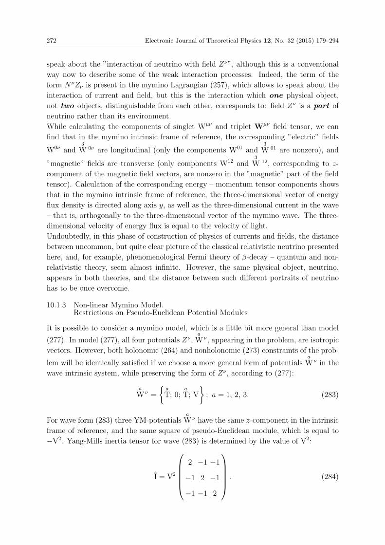
272 Electronic Journal of Theoretical Physics 12, No. 32 (2015) 179–294
speak about the ”interaction of neutrino with field Zν”, although this is a conventional
way now to describe some of the weak interaction processes. Indeed, the term of the
form NνZν is present in the mymino Lagrangian (257), which allows to speak about the
interaction of current and field, but this is the interaction which one physical object,
not two objects, distinguishable from each other, corresponds to: field Zν is a part of
neutrino rather than its environment.
While calculating the components of singlet Wμν and triplet Wμν field tensor, we can
find that in the mymino intrinsic frame of reference, the corresponding ”electric” fields
W0ν and3
W 0ν are longitudinal (only the components W01 and3
W 01 are nonzero), and
”magnetic” fields are transverse (only components W12 and3
W 12, corresponding to z-
component of the magnetic field vectors, are nonzero in the ”magnetic” part of the field
tensor). Calculation of the corresponding energy – momentum tensor components shows
that in the mymino intrinsic frame of reference, the three-dimensional vector of energy
flux density is directed along axis y, as well as the three-dimensional current in the wave
– that is, orthogonally to the three-dimensional vector of the mymino wave. The three-
dimensional velocity of energy flux is equal to the velocity of light.
Undoubtedly, in this phase of construction of physics of currents and fields, the distance
between uncommon, but quite clear picture of the classical relativistic neutrino presented
here, and, for example, phenomenological Fermi theory of β-decay – quantum and non-
relativistic theory, seem almost infinite. However, the same physical object, neutrino,
appears in both theories, and the distance between such different portraits of neutrino
has to be once overcome.
10.1.3 Non-linear Mymino Model.Restrictions on Pseudo-Euclidean Potential Modules
It is possible to consider a mymino model, which is a little bit more general than model
(277). In model (277), all four potentials Zν ,a
W ν , appearing in the problem, are isotropic
vectors. However, both holonomic (264) and nonholonomic (273) constraints of the prob-
lem will be identically satisfied if we choose a more general form of potentialsa
W ν in the
wave intrinsic system, while preserving the form of Zν , according to (277):
a
W ν =
{a
T; 0;a
T; V
}; a = 1, 2, 3. (283)
For wave form (283) three YM-potentialsa
W ν have the same z-component in the intrinsic
frame of reference, and the same square of pseudo-Euclidean module, which is equal to
−V2. Yang-Mills inertia tensor for wave (283) is determined by the value of V2:
I = V2
⎛⎜⎜⎜⎜⎝2 −1 −1
−1 2 −1
−1 −1 2
⎞⎟⎟⎟⎟⎠ . (284)
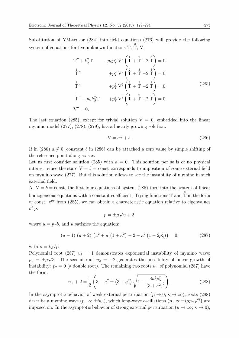
Electronic Journal of Theoretical Physics 12, No. 32 (2015) 179–294 273
Substitution of YM-tensor (284) into field equations (276) will provide the following
system of equations for five unknown functions T,a
T, V:
T′′ + k2ST −pSp2T V2
(1
T +2
T −23
T
)= 0;
1
T ′′ +p2T V2
(2
T +3
T −21
T
)= 0;
2
T ′′ +p2T V2
(3
T +1
T −22
T
)= 0;
3
T ′′ − pSk2ST +p2T V2
(1
T +2
T −23
T
)= 0;
V′′ = 0.
(285)
The last equation (285), except for trivial solution V = 0, embedded into the linear
mymino model (277), (278), (279), has a linearly growing solution:
V = ax+ b. (286)
If in (286) a �= 0, constant b in (286) can be attached a zero value by simple shifting of
the reference point along axis x.
Let us first consider solution (285) with a = 0. This solution per se is of no physical
interest, since the state V = b = const corresponds to imposition of some external field
on mymino wave (277). But this solution allows to see the instability of mymino in such
external field.
At V = b = const, the first four equations of system (285) turn into the system of linear
homogeneous equations with a constant coefficient. Trying functions T anda
T in the form
of const · epx from (285), we can obtain a characteristic equation relative to eigenvalues
of p:
p = ±μ√u+ 2,
where μ = pT b, and u satisfies the equation:
(u− 1) (u+ 2)(u2 + u
(1 + κ2
)− 2− κ2
(1− 2p2S
))= 0, (287)
with κ = kS/μ.
Polynomial root (287) u1 = 1 demonstrates exponential instability of mymino wave:
p1 = ±μ√3. The second root u2 = −2 generates the possibility of linear growth of
instability: p2 = 0 (a double root). The remaining two roots u± of polynomial (287) have
the form:
u± + 2 =1
2
(3− κ2 ±
(3 + κ2
) √1− 8κ2p2S
(3 + κ2)2
). (288)
In the asymptotic behavior of weak external perturbation (μ→ 0; κ→∞), roots (288)
describe a mymino wave (p− ∝ ±ikS), which long-wave oscillations(p+ ∝ ±iμpS
√2)are
imposed on. In the asymptotic behavior of strong external perturbation (μ→∞; κ→ 0),
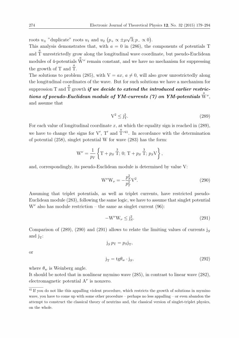
274 Electronic Journal of Theoretical Physics 12, No. 32 (2015) 179–294
roots u± ”duplicate” roots u1 and u2
(p+ ∝ ±μ
√3; p− ∝ 0
).
This analysis demonstrates that, with a = 0 in (286), the components of potentials T
anda
T unrestrictedly grow along the longitudinal wave coordinate, but pseudo-Euclidean
modules of 4-potentialsa
W ν remain constant, and we have no mechanism for suppressing
the growth of T anda
T.
The solutions to problem (285), with V = ax, a �= 0, will also grow unrestrictedly along
the longitudinal coordinates of the wave. But for such solutions we have a mechanism for
suppression T anda
T growth if we decide to extend the introduced earlier restric-
tions of pseudo-Euclidean module of YM-currents (7) on YM-potentialsa
W ν ,
and assume that
V2 ≤ j2T. (289)
For each value of longitudinal coordinate x, at which the equality sign is reached in (289),
we have to change the signs for V′, T′ anda
T ′41. In accordance with the determination
of potential (258), singlet potential W for wave (283) has the form:
Wν =1
pT
{T + pS
3
T; 0; T + pS3
T; pSV
},
and, correspondingly, its pseudo-Euclidean module is determined by value V:
WνWν = −p2Sp2T
V2. (290)
Assuming that triplet potentials, as well as triplet currents, have restricted pseudo-
Euclidean module (283), following the same logic, we have to assume that singlet potential
Wν also has module restriction – the same as singlet current (96):
−WνWν ≤ j2S. (291)
Comparison of (289), (290) and (291) allows to relate the limiting values of currents jSand jT:
jS pT = pSjT,
or
jT = tgθw · jS, (292)
where θw is Weinberg angle.
It should be noted that in nonlinear mymino wave (285), in contrast to linear wave (282),
electromagnetic potential Aν is nonzero.
41 If you do not like this appalling violent procedure, which restricts the growth of solutions in mymino
wave, you have to come up with some other procedure – perhaps no less appalling – or even abandon the
attempt to construct the classical theory of neutrino and, the classical version of singlet-triplet physics,
on the whole.
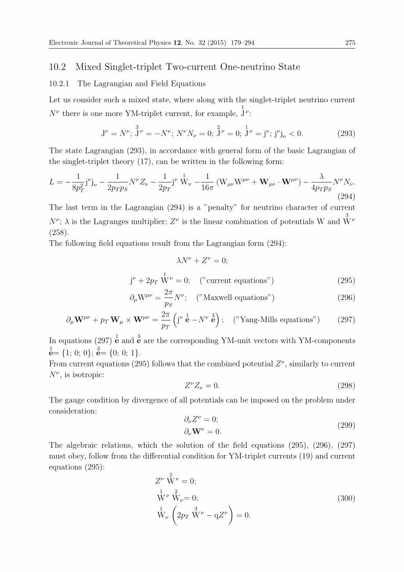
Electronic Journal of Theoretical Physics 12, No. 32 (2015) 179–294 275
10.2 Mixed Singlet-triplet Two-current One-neutrino State
10.2.1 The Lagrangian and Field Equations
Let us consider such a mixed state, where along with the singlet-triplet neutrino current
Nν there is one more YM-triplet current, for example,1
J ν :
Jν = Nν ;3
J ν = −Nν ; NνNν = 0;2
J ν = 0;1
J ν = jν ; jνjν < 0. (293)
The state Lagrangian (293), in accordance with general form of the basic Lagrangian of
the singlet-triplet theory (17), can be written in the following form:
L = − 1
8p2Tjνjν −
1
2pTpSNνZν −
1
2pTjν
1
Wν −1
16π(WμνW
μν +Wμν ·Wμν)− λ
4pTpSN νNν .
(294)
The last term in the Lagrangian (294) is a ”penalty” for neutrino character of current
Nν ; λ is the Lagranges multiplier; Zν is the linear combination of potentials W and3
W ν
(258).
The following field equations result from the Lagrangian form (294):
λN ν + Zν = 0;
jν + 2pT1
W ν = 0; (”current equations”) (295)
∂μWμν =
2π
pSNν ; (”Maxwell equations”) (296)
∂μWμν + pT Wμ ×Wμν =
2π
pT
(jν
1e −Nν 3
e); (”Yang-Mills equations”) (297)
In equations (297)1e and
3e are the corresponding YM-unit vectors with YM-components
1e= {1; 0; 0}; 3
e= {0; 0; 1}.From current equations (295) follows that the combined potential Zν , similarly to current
Nν , is isotropic:
ZνZν = 0. (298)
The gauge condition by divergence of all potentials can be imposed on the problem under
consideration:∂νZ
ν = 0;
∂νWν = 0.
(299)
The algebraic relations, which the solution of the field equations (295), (296), (297)
must obey, follow from the differential condition for YM-triplet currents (19) and current
equations (295):
Zν2
W ν = 0;1
W ν2
Wν= 0;1
Wν
(2pT
3
W ν − qZν
)= 0.
(300)
276 Electronic Journal of Theoretical Physics 12, No. 32 (2015) 179–294
In the last equation (300) it is indicated that q = −1/λ.
Relations (298) and (300) specify the system of holonomic constraints, imposed on the
solution of the field equations of the problem.
Extracting currents jν , Nν and singlet potential Wν through current equations, we can
reduce the problem under consideration to the system of wave equations relative to four
potentials Zν and Wν :
�Zν + k2SZ
ν + pSp2T
3b
Ib
W ν = −pSpT3
h ν ;
�Wν −(4π
1e
1
W ν + k2SpSZ
ν 3e
)− p2T IW = pTh.
(301)
In the equations (301), parameter kS is determined by formula (281), and vector hν – by
relation (266). Nonholonomic constraint (273) is imposed on YM-potentials Wν .
10.2.2 Solution in the Form of a Plane Wave
Let us consider the solution of the problem (301) in the form of a plane wave. In such
solution potentials Zν and Wν depend only on a single argument, the wave phase φ =
kνxν . Since in the problem (301) there is isotropic vector Zν , wave vector kν can only be
space-like. In the wave intrinsic system, wave vector kν has only one nonzero component
in longitudinal coordinate x. D’Alembert operator in (301) is reduced to the operator of
the twofold differentiation in the longitudinal coordinate. Vector hν in the plane wave
vanishes. Field equations (301) turn into the system of ordinary differential equations:
Zν ′′ + k2SZ
ν +pSp2T
3b
Ib
W ν = 0;1
W ν ′′ − 4π1
W ν −p2T1b
Ib
W ν = 0;2
W ν ′′ −p2T2b
Ib
W ν = 0;3
W ν ′′ − k2SpSZ
ν −p2T3b
Ib
W ν = 0.
(302)
In equations (302), the prime stands for longitudinal coordinate x derivative.
Differential conditions (299), as well as in other problems of the waves with space-like
wave vector, mean that no potential has a longitudinal component:
Z1 = 0;a
W 1 = 0; a = 1, 3. (303)
Considering the wave with linear polarization, we can assume, without restricting gener-
ality, that isotropic vector Zν in the wave intrinsic system has the form:
Zν = T {1; 0; 1; 0} , (304)
where T is some desired function of longitudinal coordinate x.
Both holonomic and nonholonomic constraints, imposed on solution (302), will be satisfied
Electronic Journal of Theoretical Physics 12, No. 32 (2015) 179–294 277
if we try YM-potentialsa
W ν in the following form:
1
W ν =
{1
T; 0;1
T; V
},
2
W ν =2
T {1; 0; 1; 0} ,3
W ν =3
T {1; 0; 1; 0} .
(305)
In five-component solution (304), (305), functions T,1
T,2
T,3
T and V are desired ones.
The choice of five-component structure of the solution is not the only possible method to
satisfy all the constraint equations. However, this partial choice of the solution structure
allows seeing the fundamental problem of unrestricted growth of the solutions to equations
(302).
YM-inertia tensor I for wave (305) has the form:
I = V2
⎛⎜⎜⎜⎜⎝0 0 0
0 1 0
0 0 1
⎞⎟⎟⎟⎟⎠ . (306)
Substitution of tensor (306) into field equations (302) for wave (304), (305) gives the
following system of differential equations:
V′′ − 4πV = 0,1
T ′′ − 4π1
T = 0,2
T ′′ − p2T V22
T = 0,3
T ′′ − p2T3
T −k2SpST = 0,
T′′ + k2ST + pSp
2T V2
3
T = 0.
(307)
The possible, but uninteresting situation of choice of the trivial solutions to the first three
equations of system (307) is: V = 0;1
T= 0,2
T= 0, returns us to the mymino wave consid-
ered above. Except for this degenerate situation, system (307) has no solutions restricted
at the growing of longitudinal coordinate x. The first two equations of the system (307),
linear and independent from the rest of the equations (307), have solutions, exponentially
growing with growth of x. Substitution of these growing solutions as coefficients of other
equations of the system generates unrestricted growth of the rest of the problem variables
(307).
10.2.3 Two Methods of Allowing for Current Restriction.Neutrino Instability
Is it possible to cope with this non-physical solution growth?
It is possible to take into account the restriction on pseudo-Euclidean module of current
278 Electronic Journal of Theoretical Physics 12, No. 32 (2015) 179–294
jν (7). From current equations (295) and (305) follows that
jν jν = 4p2T1
W ν1
Wν= −4p2T V2,
consequently,
V2 ≤(
jT2pT
)2
. (308)
The growing solution of the system (307) is applicable only for such values of longitudinal
coordinate x while inequality (308) is satisfied.
At obtaining the equality in (308) with some x = xe, we have to reverse the signs of
all the derivatives of potentials V′, T′,1
T ′,2
T ′,3
T ′, while maintaining the continuity of
the potentials themselves and to continue the solution further along the longitudinal
coordinate x, with x > xe under the new initial conditions. This barbaric method
generates a restricted solution with discontinuities of derivatives in the form of some
ripple of potentials and currents, frozen in the intrinsic system of the wave. For correct
numerical description of this ripple, the curvature of space, caused by the wave itself
(307), should be taken into account.
The second, and probably, the deeper interpretation of inequality (308) consists of refusal
of the plane wave picture, covering the whole space-time. At obtaining the equality in
(308), the plane wave vanishes, the formation of some cavitated latebrae zones, not
containing current jν , takes place, and then the formation of the pomerium’s system,
specifying the outer boundaries of current zones, takes place. In other words, the two-
current wave turns into one or a few massive triplet particles, described in part 9.3.6,
surrounded by neutrino fields. However, it would be naive to expect that such an intimate
and, undoubtedly, quantum process of massive particle’s production permits the adequate
numerical description in terms of the classical Lagrangians.
Comparison of the equations, which describe mymino neutrino wave (10.1) with the
system of equations (307), describing the two-current singlet-triplet wave, allows to make
the following assumption.
Mymino neutrino wave (282), stable in itself, is unstable against the buildup of the two-
current state: no matter how small initial perturbations are (i.e. no matter how small
”inoculating” values of current1
J ν components are), the solution of the neutrino problem
turns fast into the solution of two-current singlet-triplet problem due to the exponential
growth of1
T and V, but this two-current wave without latens and pomerium quickly turns
into a massive YM-particle having inner latebrae voids, inner latens boundaries and outer
pomerium boundary. Within the framework of this picture, the neutrino production in
any process must be accompanied by the production of a massive YM-particle with a
very small time delay (probably, with delay of about r0/c ∝ 10−36 seconds)42.
42According to beliefs common for modern physics, such massive ”satellite” of neutrino is W-boson. We
do not know whether identification of W-boson with massive one-current particle is acceptable (p.9.3.6.)
W-boson is treated as massive quantum of free (zero-current) YM-field. The particle described in p.
Electronic Journal of Theoretical Physics 12, No. 32 (2015) 179–294 279
10.3 Mixed Singlet-triplet Three-current One-neutrino State
10.3.1 The Lagrangian and Field Equations
Let us turn to the study of such a mixed state, where, besides neutrino singlet-triplet
current Nν , there are two more YM-currents:
Jν = N ν ;3
J ν = −N ν ; NνNν = 0;1
J ν1
Jν< 0;2
J ν2
Jν< 0;1
J ν2
Jν= 0. (309)
The last equality in the description of this state (309) results from current3
J ν isotropy
and the condition of the inner normalization of YM-triplet currents (32).
The Lagrangian of the state (309), in accordance with the type of base Lagrangian of
ST-theory (17), can be denoted in the form:
L =− 1
8p2T
(1
J ν1
Jν +2
J ν2
Jν
)− 1
2pT
(1
J ν1
Wν +2
J ν2
Wν
)− 1
2pTpSNνZν−
− 1
16π(WμνW
μν +Wμν ·Wμν)− λ
4pTpSN νNν .
(310)
In (310), Zν is the linear combination of potentials Wν and3
W ν (258) introduced before;
λ is the Lagranges multiplier. The last term in (310) is the ”penalty” for the current’s
neutrino character. Besides this ”penalty”, the Lagrangian (310) must contain one more
term – ”penalty” for currents1
J ν and2
J ν orthogonality. For the reasons expressed above,
in p. 9.4.1, we do not include this penalty into the Lagrangian (310), supposing that the
condition of currents1
J ν and2
J ν orthogonality is ”natural” for this problem.
Field equations, following from the Lagrangian (310), have the following form:
λN ν + Zν = 0;1
J ν + 2pT1
W ν = 0;2
J ν + 2pT2
W ν = 0; (”current equations”)
(311)
∂μWμν =
2π
pSNν ; (”Maxwell equations”)
∂μWμν + pT Wμ ×Wμν =
2π
pT
(1
J ν 1e +
2
J ν 2e −N ν 3
e
). (”Yang-Mills equations”)
(312)
In equations (312)ae is YM-unit vectors.
From current equations (311) follows that the mixed potential Zν is isotropic, and YM-
potentials1
W ν and2
W ν are orthogonal to each other (under the orthogonality of the
corresponding currents (309)):
ZνZν = 0;1
W ν2
Wν= 0.(313)
9.3.6, consists of mixture of YM-current and YM-field, similarly to massive leptons, which are a mixture
of singlet current and singlet field.
280 Electronic Journal of Theoretical Physics 12, No. 32 (2015) 179–294
Differential conditions for the currents of YM-triplet (19) and current equations (311)
generate algebraic conditions for potentials Zν anda
W ν :
1
Wν
(2pT
3
W ν − qZν
)= 0;
2
Wν
(2pT
3
W ν − qZν
)= 0.
(314)
In equation (314) it is denoted that q = −1/λ.
Relations (313) and (314) are holonomic constraints, which the solution of the field equa-
tions (312) obeys.
Extraction of currents and singlet potential from field equations (312) leads to the fol-
lowing system of wave equations relative to potentials Zν anda
W ν :
�Zν + k2SZ
ν + pSp2T
3b
Ib
W ν = 0;
�Wν − 4π
(1
W ν 1e +
2
W ν 2e
)− k2
SpSZν 3e −p2T IWν = pTh
ν .(315)
In system (315), describing the three-current state, all notations are the same as in the
similar system of equations (301), describing the two-current state.
10.3.2 Solution in the Form of a Plane Wave
For plane wave hν ≡ 0, all variables of the problem depend on longitudinal coordinate x,
and wave equations take the form which is similar to equations (302), introduced for the
two-current problem:
Zν ′′ + k2SZ
ν + pSp2T
3b
Ib
W ν = 0;1
W ν ′′ − 4π1
W ν − p2T1b
Ib
W ν = 0;2
W ν ′′ − 4π2
W ν − p2T2b
Ib
W ν = 0;3
W ν ′′ − k2SpSZ
ν − p2T3b
Ib
W ν = 0.
(316)
All the potentials of Zν anda
W ν , have zero longitudinal potential Z1 anda
W 1.
Solution to problem (316) has to satisfy the four holonomic constraints (313), (314) and
the three nonholonomic constraints (273). We do not know whether there are any solu-
tions to the system of differential equations (316), burdened with so many constraints,
anyway, we cannot construct a solution of some simple structure, which would automati-
cally account all the constraint equations. If solutions do exist, they grow unrestrictedly
along the wave direction. Taking into account the restriction on the growth of pseudo-
Euclidean current module, as described in p. 10.2.2, it is possible to construct restricted
solutions having discontinuities of the variables.
Electronic Journal of Theoretical Physics 12, No. 32 (2015) 179–294 281
10.4 Mixed Singlet-triplet Three-current Neutrinoless State
(the left-hand three-current state)
10.4.1 The Lagrangian of the Left-hand Three-current State
Let us consider such a mixed triplet-singlet state, where the same space-like current lν
(lνlν < 0) is present both as singlet current J and the third component of YM-triplet of
currents3
J ν :
Jν = lν ;3
J ν = lν . (317)
This current state is compatible with formulas of current decomposition (22). Within
the framework of this decomposition, current lν is the ”left-hand” current. The right-
hand current rν and neutrino current Nν are missing from the state (317). The algebraic
conditions of coupling of currents Jν and3
J ν (20) in state (317) turn into identity.
In state (317) two other YM-currents,1
J ν and2
J ν , must be present, since, due to the
conditions of the inner normalization of YM-triplet currents (32), their scalar product is
nonzero:
21
J ν2
Jν= lνlν . (318)
The substitution of formulas (317) into the base Lagrangian of the ST-theory (17) allows
us to write the Lagrangian of the left-hand three-current states in the following form:
L = Lcur + Lint + Lf , (319)
where the current Lagrangian Lcur contains pseudo-Euclidean squares of all three currents
of state:
Lcur = −lνlν
8pSpT− 1
8p2T
(1
J ν1
Jν +2
J ν2
Jν
). (320)
The interaction Lagrangian Lint is convenient to be written as follows:
Lint = −1
2pSpTlνQν −
1
2pT
(1
J ν1
Wν +2
J ν2
Wν
), (321)
where Qν is the linear combination of potentials Wν and3
W ν :
Qν = pTWν + pS
3
W ν .
The field Lagrangian Lf in (319) has an ordinary form (13).
We have to note that usually in Weinberg-Salam theory it is not potential Qν itself that
is used, but its decomposition into electromagnetic potential Aν
(Aν = pTW
ν + pS3
W ν
)and ”neutral” potential Zν
(Zν = pTW
ν − pS3
W ν
):
Qν = 2pSpTAν −
(p2S − p2T
)Zν ,
or Qν = sin2ϑW · Aν − cos2ϑW · Zν .(322)
282 Electronic Journal of Theoretical Physics 12, No. 32 (2015) 179–294
If we use decomposition (322), the interaction Lagrangian (321) can be denoted as:
Lint = −lνAν + ctg2ϑW · lνZν −1
2pT
(1
J ν1
Wν +2
J ν2
Wν
), (323)
Expression (323) allows us to speak, using the generally accepted ”jargon” of theoreti-
cal physics, about the fact that the left-hand current lν ”interacts” with electromagnetic
potential Aν (the first term in (323)), and ”interacts” with neutral field Zν (the second
term in (323)). At full formal equality of (321) and (323), formula (321) seems more
convenient and compact: the interaction Lagrangian (321) contains only one scalar prod-
uct, which includes current and combined potential Qν – it is the one that the left-hand
current lν ”interacts” with43.
While recording the three-current state Lagrangian (319), it is convenient to introduce
rescaled currents, assuming that
mν =1
2pSpTlν ;
1
j ν =1
2pT
1
J ν ;2
j ν =1
2pT
2
J ν ,(324)
and also the conventional YM-triplet of currents jν with zero third YM-component:
jν =
{1
j ν ;2
j ν ; 0
}. (325)
In notations (324), (325), the three-current state Lagrangian takes the form which is
compact enough:
L = −1
2mνmν −
1
2jνjν −mνQν − jν ·Wν −
1
16π(WμνW
μν +Wμν ·Wμν) . (326)
Weinberg coefficients pS and pT , which are missing from the Lagrangian (326) an explicit
form, of course, cannot be excluded from the description of mixed singlet-triplet state by
any scale transformation. They remain in the determination of potential Qν (322), in the
expression for YM-field tensor Wμν (15) and in normalizing condition (318), which has
the following form in the notations (324):
21
j ν2
jν= p2S mνmν . (327)
43Acknowledging the acceptability of using the stable term ”interaction Lagrangian”, rooted due to his-
torical reasons, we tend to consider the term ”interaction” (of currents and fields) itself, as an archaic
and inaccurate one. In three-current state, current lν and potential Qν , while interweaving, form an
integrated physical object – a ”three-current state”, and it would be incorrect to speak about ”inter-
action” of current and field – as well as, by reasons, cited in p. 10.1.2, it is incorrect to speak about
interaction of neutrino current Nν and neutral potential Zν , which form an integrated physical object
– Maxwell-Yang-Mills neutrino. The term ”interaction” is appropriate only as a term that allows to
provide approximate description of quasi-stationary states that have two or more current zones where
each of them has its own pomerium, and these zones are located far enough from each other.
Electronic Journal of Theoretical Physics 12, No. 32 (2015) 179–294 283
Condition (327) is a holonomic constraint, imposed on functional arguments of the La-
grangian (326). Generally speaking, accounting of this constraint requires additional term
Lad for the base Lagrangian of the three-current problem (326):
Lad = η
(2
1
j ν2
jν −p2S mνmν
), (328)
with undetermined Lagrange’s multiplier η.
By introducing additional term (328) into the Lagrangian, with η �= 0, we actually
introduce some ”Higgs-like” field η which stimulates us to satisfy the condition (327).
It is reasonable to try to construct a theory of three-current states on the basis of the
Lagrangian (326), supposing that condition (327) is ”natural”, i.e. can be also satisfied
with η = 0. If non-trivial solutions to the three-current problem do not exist with η = 0,
three-current states may exist only as non-stationary transition states between other
states.
10.4.2 Field Equations of the Left-hand Three-current State
The independent functional arguments of the Lagrangian are currents mν and jν , and
potentials Wν and Wν . By varying the Lagrangian (326) by these arguments, we obtain
field equations of the left-hand three-current state:
mν +Qν = 0;1
j ν+1
W ν = 0;2
j ν+2
W ν = 0. (”current equations”)
(329)
∂μWμν = 4πpTm
ν . (”Maxwell equations”) (330)
∂μWμν + pT Wμ ×Wμν = 4π
(1
j ν1e +
2
j ν2e +pSm
ν 3e
). (”Yang-Mills equations”) (331)
General gauge conditions by 4-divergence of potentials should be added to field equations
(329), (330), (331):
∂μWμ = 0; ∂μW
μ = 0. (332)
Conditions (332) are combined with the conditions for conservation of all the three cur-
rents of the problem:
∂νmν = 0; ∂ν
1
j ν = 0; ∂ν2
j ν = 0. (333)
and, in their turn, conditions (333), along with general differential condition for triplet
current, generate the system of holonomic constraints imposed on the solution of the field
equations of the left-hand three-current state:
pSmν
1
Wν=1
j ν3
Wν ;
pSmν
2
Wν=2
j ν3
Wν ;1
Wν
2
j ν =2
Wν
1
j ν .
(334)
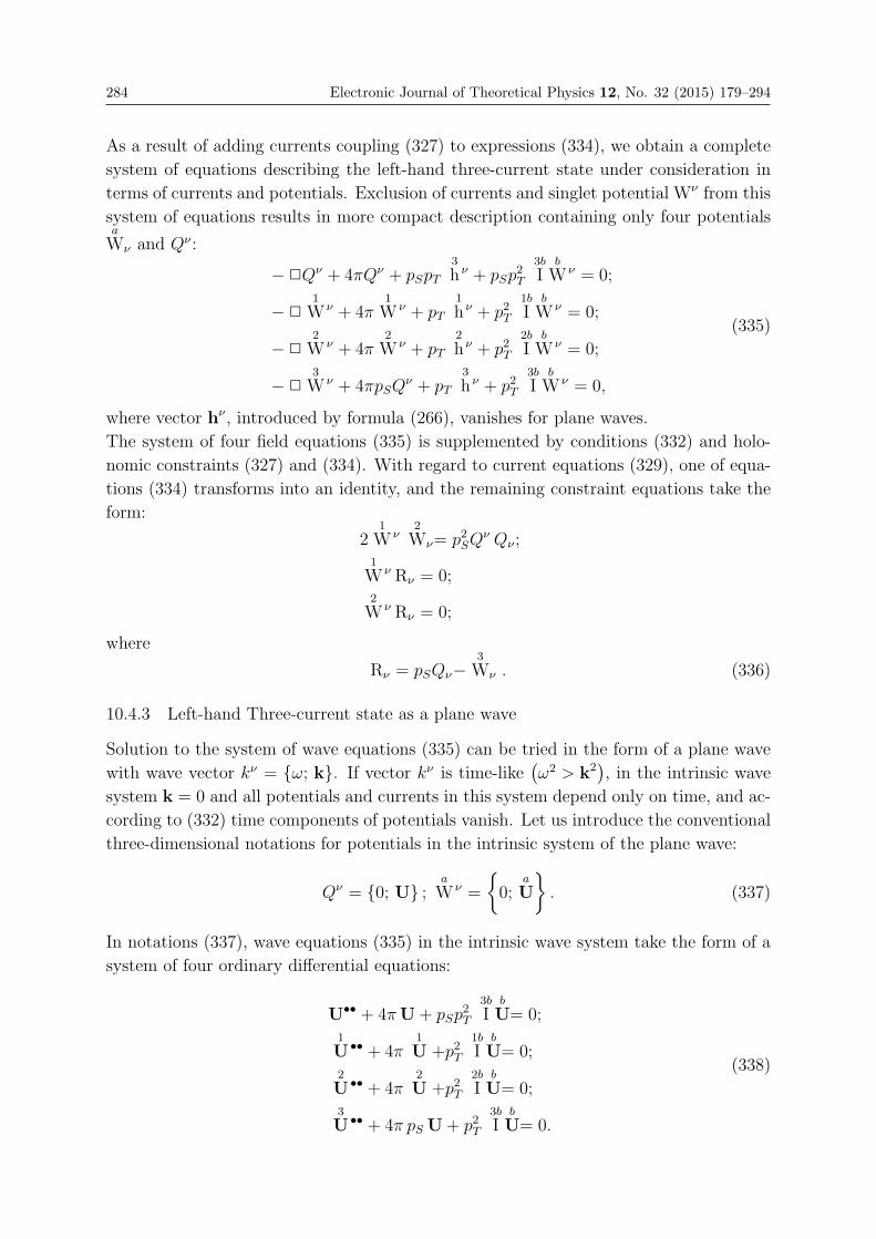
284 Electronic Journal of Theoretical Physics 12, No. 32 (2015) 179–294
As a result of adding currents coupling (327) to expressions (334), we obtain a complete
system of equations describing the left-hand three-current state under consideration in
terms of currents and potentials. Exclusion of currents and singlet potential Wν from this
system of equations results in more compact description containing only four potentialsa
Wν and Qν :
−�Qν + 4πQν + pSpT3
h ν + pSp2T
3b
Ib
W ν = 0;
−�1
W ν + 4π1
W ν + pT1
h ν + p2T1b
Ib
W ν = 0;
−�2
W ν + 4π2
W ν + pT2
h ν + p2T2b
Ib
W ν = 0;
−�3
W ν + 4πpSQν + pT
3
h ν + p2T3b
Ib
W ν = 0,
(335)
where vector hν , introduced by formula (266), vanishes for plane waves.
The system of four field equations (335) is supplemented by conditions (332) and holo-
nomic constraints (327) and (334). With regard to current equations (329), one of equa-
tions (334) transforms into an identity, and the remaining constraint equations take the
form:
21
W ν2
Wν= p2SQν Qν ;
1
W ν Rν = 0;2
W ν Rν = 0;
where
Rν = pSQν−3
Wν . (336)
10.4.3 Left-hand Three-current state as a plane wave
Solution to the system of wave equations (335) can be tried in the form of a plane wave
with wave vector kν = {ω; k}. If vector kν is time-like(ω2 > k2
), in the intrinsic wave
system k = 0 and all potentials and currents in this system depend only on time, and ac-
cording to (332) time components of potentials vanish. Let us introduce the conventional
three-dimensional notations for potentials in the intrinsic system of the plane wave:
Qν = {0; U} ;a
W ν =
{0;
a
U
}. (337)
In notations (337), wave equations (335) in the intrinsic wave system take the form of a
system of four ordinary differential equations:
U•• + 4πU+ pSp2T
3b
Ib
U= 0;1
U •• + 4π1
U +p2T1b
Ib
U= 0;2
U •• + 4π2
U +p2T2b
Ib
U= 0;3
U •• + 4π pS U+ p2T3b
Ib
U= 0.
(338)
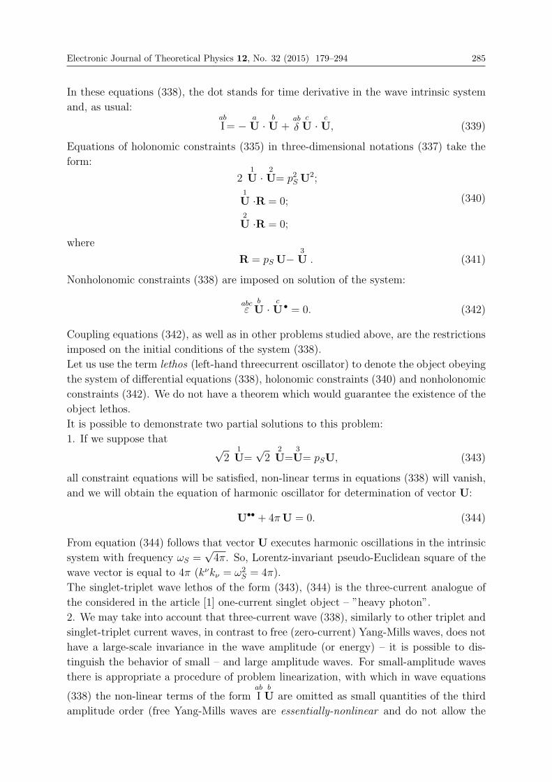
Electronic Journal of Theoretical Physics 12, No. 32 (2015) 179–294 285
In these equations (338), the dot stands for time derivative in the wave intrinsic system
and, as usual:ab
I= −a
U ·b
U +ab
δc
U ·c
U, (339)
Equations of holonomic constraints (335) in three-dimensional notations (337) take the
form:
21
U ·2
U= p2S U2;
1
U ·R = 0;2
U ·R = 0;
(340)
where
R = pS U−3
U . (341)
Nonholonomic constraints (338) are imposed on solution of the system:
abcε
b
U ·c
U • = 0. (342)
Coupling equations (342), as well as in other problems studied above, are the restrictions
imposed on the initial conditions of the system (338).
Let us use the term lethos (left-hand threecurrent oscillator) to denote the object obeying
the system of differential equations (338), holonomic constraints (340) and nonholonomic
constraints (342). We do not have a theorem which would guarantee the existence of the
object lethos.
It is possible to demonstrate two partial solutions to this problem:
1. If we suppose that√2
1
U=√2
2
U=3
U= pSU, (343)
all constraint equations will be satisfied, non-linear terms in equations (338) will vanish,
and we will obtain the equation of harmonic oscillator for determination of vector U:
U•• + 4πU = 0. (344)
From equation (344) follows that vector U executes harmonic oscillations in the intrinsic
system with frequency ωS =√4π. So, Lorentz-invariant pseudo-Euclidean square of the
wave vector is equal to 4π (kνkν = ω2S = 4π).
The singlet-triplet wave lethos of the form (343), (344) is the three-current analogue of
the considered in the article [1] one-current singlet object – ”heavy photon”.
2. We may take into account that three-current wave (338), similarly to other triplet and
singlet-triplet current waves, in contrast to free (zero-current) Yang-Mills waves, does not
have a large-scale invariance in the wave amplitude (or energy) – it is possible to dis-
tinguish the behavior of small – and large amplitude waves. For small-amplitude waves
there is appropriate a procedure of problem linearization, with which in wave equations
(338) the non-linear terms of the formab
Ib
U are omitted as small quantities of the third
amplitude order (free Yang-Mills waves are essentially-nonlinear and do not allow the
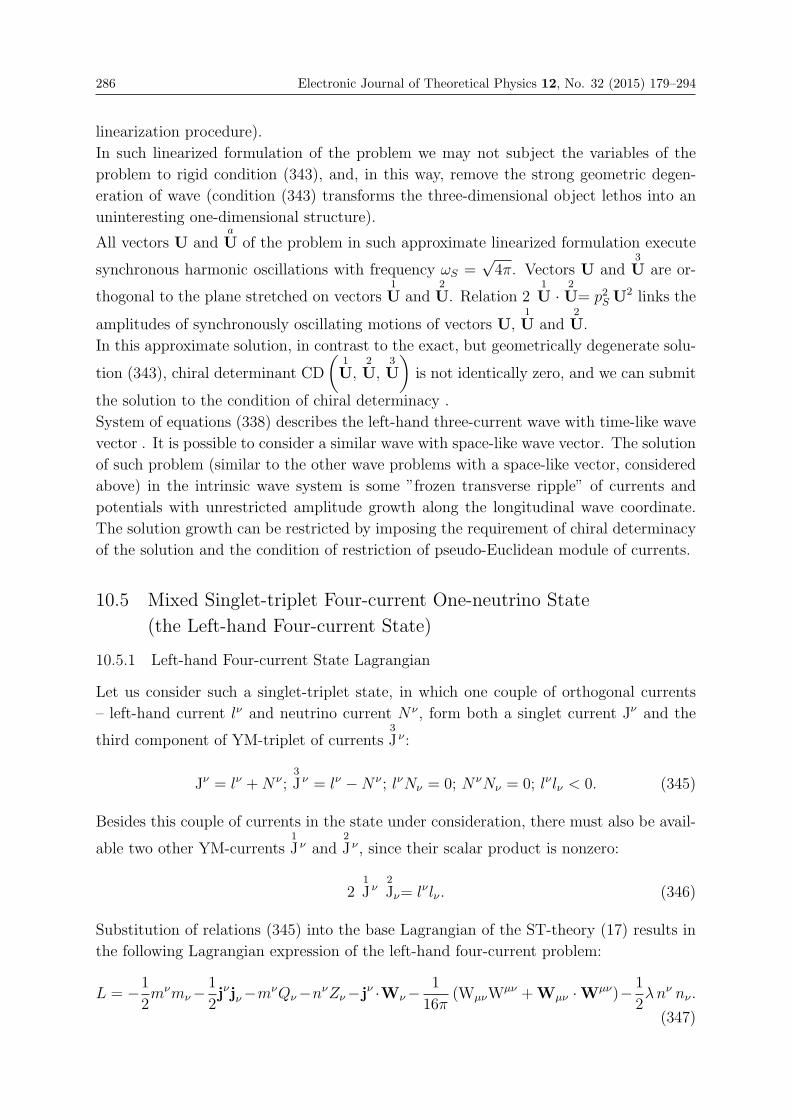
286 Electronic Journal of Theoretical Physics 12, No. 32 (2015) 179–294
linearization procedure).
In such linearized formulation of the problem we may not subject the variables of the
problem to rigid condition (343), and, in this way, remove the strong geometric degen-
eration of wave (condition (343) transforms the three-dimensional object lethos into an
uninteresting one-dimensional structure).
All vectors U anda
U of the problem in such approximate linearized formulation execute
synchronous harmonic oscillations with frequency ωS =√4π. Vectors U and
3
U are or-
thogonal to the plane stretched on vectors1
U and2
U. Relation 21
U ·2
U= p2S U2 links the
amplitudes of synchronously oscillating motions of vectors U,1
U and2
U.
In this approximate solution, in contrast to the exact, but geometrically degenerate solu-
tion (343), chiral determinant CD
(1
U,2
U,3
U
)is not identically zero, and we can submit
the solution to the condition of chiral determinacy .
System of equations (338) describes the left-hand three-current wave with time-like wave
vector . It is possible to consider a similar wave with space-like wave vector. The solution
of such problem (similar to the other wave problems with a space-like vector, considered
above) in the intrinsic wave system is some ”frozen transverse ripple” of currents and
potentials with unrestricted amplitude growth along the longitudinal wave coordinate.
The solution growth can be restricted by imposing the requirement of chiral determinacy
of the solution and the condition of restriction of pseudo-Euclidean module of currents.
10.5 Mixed Singlet-triplet Four-current One-neutrino State
(the Left-hand Four-current State)
10.5.1 Left-hand Four-current State Lagrangian
Let us consider such a singlet-triplet state, in which one couple of orthogonal currents
– left-hand current lν and neutrino current Nν , form both a singlet current Jν and the
third component of YM-triplet of currents3
J ν :
Jν = lν +Nν ;3
J ν = lν −N ν ; lνNν = 0; NνNν = 0; lνlν < 0. (345)
Besides this couple of currents in the state under consideration, there must also be avail-
able two other YM-currents1
J ν and2
J ν , since their scalar product is nonzero:
21
J ν2
Jν= lνlν . (346)
Substitution of relations (345) into the base Lagrangian of the ST-theory (17) results in
the following Lagrangian expression of the left-hand four-current problem:
L = −1
2mνmν−
1
2jνjν−mνQν−nνZν−jν ·Wν−
1
16π(WμνW
μν +Wμν ·Wμν)− 1
2λnν nν .
(347)
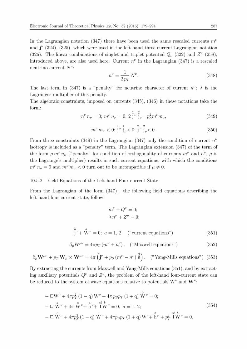
Electronic Journal of Theoretical Physics 12, No. 32 (2015) 179–294 287
In the Lagrangian notation (347) there have been used the same rescaled currents mν
and jν (324), (325), which were used in the left-hand three-current Lagrangian notation
(326). The linear combinations of singlet and triplet potential Qν (322) and Zν (258),
introduced above, are also used here. Current nν in the Lagrangian (347) is a rescaled
neutrino current Nν :
nν =1
2 pTNν . (348)
The last term in (347) is a ”penalty” for neutrino character of current nν ; λ is the
Lagranges multiplier of this penalty.
The algebraic constraints, imposed on currents (345), (346) in these notations take the
form:
nν nν = 0; mν nν = 0; 21
j ν2
jν= p2Smνmν , (349)
mν mν < 0;1
j ν1
jν< 0;2
j ν2
jν< 0. (350)
From three constraints (349) in the Lagrangian (347) only the condition of current nν
isotropy is included as a ”penalty” term. The Lagrangian extension (347) of the term of
the form μmν nν (”penalty” for condition of orthogonality of currents mν and nν , μ is
the Lagrange’s multiplier) results in such current equations, with which the conditions
mν nν = 0 and mν mν < 0 turn out to be incompatible if μ �= 0.
10.5.2 Field Equations of the Left-hand Four-current State
From the Lagrangian of the form (347) , the following field equations describing the
left-hand four-current state, follow:
mν +Qν = 0;
λnν + Zν = 0;
a
j ν+a
W ν = 0; a = 1, 2. (”current equations”) (351)
∂μWμν = 4πpT (mν + nν) . (”Maxwell equations”) (352)
∂μWμν + pT Wμ ×Wμν = 4π
(jν + pS (m
ν − nν)3e). (”Yang-Mills equations”) (353)
By extracting the currents from Maxwell and Yang-Mills equations (351), and by extract-
ing auxiliary potentials Qν and Zν , the problem of the left-hand four-current state can
be reduced to the system of wave equations relative to potentials Wν and Wν :
−�Wν + 4πp2T (1− q)Wν + 4π pSpT (1 + q)3
W ν = 0;
−�a
W ν + 4πa
W ν+a
h ν+ab
Ib
W ν = 0, a = 1, 2;
−�3
W ν + 4πp2S (1− q)3
W ν + 4πpSpT (1 + q)Wν+3
h ν + p2T3b
Ib
W ν = 0,
(354)
288 Electronic Journal of Theoretical Physics 12, No. 32 (2015) 179–294
where q = −1/λ, vector h
ν is determined in (266),ab
I is Yang-Mills inertia tensor.
Potentials Wν and Wν have zero 4-divergences and obey the holonomic constraints fol-
lowing from the conditions (349):
p2TWνWν = p2S
3
W ν3
Wν ;
pS3
W ν3
Wν= pTWν
3
Wν ;
pTWνWν = pSW
ν3
Wν ;
21
W ν2
Wν= 4p2Tp2SW
νWν .
(355)
It is obvious that equations (355) are not independent.
Besides the constraints (355), the potentials obey two auxiliary constraints following from
the condition for YM-currents (19):
a
W νRν = 0; a = 1, 2, (356)
where
Rν = pSpT (1 + q)Wν −(p2T + qp2S
) 3
Wν . (357)
10.5.3 Left-hand Four-current State as a Plane Wave
Having an intention to construct the solution to the system of wave equations (354) in
the form of a plane wave, we have to consider only transverse waves with space-like vector
kν . (The presence of isotropic vectors nν and Zν in the problem excepts the existence of
a wave with a time-like wave vector). In the plane wave, vectora
h ν vanishes. In the wave
intrinsic system, D’Alembert operator � is reduced to the second longitudinal coordinate
derivative. By using complex three-dimensional YM-vectors τ ,aτ instead of 4-potentials
Wν anda
W ν , the system of equations (354) can be reduced to the system of ordinary
differential equations:
− τ ′′ + 4πp2T (1− q) τ + 4πpSpT (1 + q)3τ= 0;
− aτ ′′ + 4π
aτ +
bτ ×
(aτ × b
τ)= 0; a = 1, 2
− 3τ ′′ + 4πp2S (1− q)
3τ +4πpSpT (1 + q) τ+
bτ ×
(3τ × b
τ)= 0.
(358)
Coupling equations (355) and (356) for vectors τ ,aτ take the form:
2p2Tτ · τ = p2S3τ · 3
τ
pS3τ · 3
τ= pTτ ·3τ ;
pTτ · τ = pSτ ·3τ ;
1τ · 2
τ= 4p2Tp2Sτ · τ ,
(359)
Electronic Journal of Theoretical Physics 12, No. 32 (2015) 179–294 289
andaτ ·ρ = 0; a = 1, 2, (360)
where
ρ = pSpT (1 + q) τ −(p2T + qp2S
) 3τ . (361)
Besides holonomic constraints (359), (360), nonholonomic constraints, which are sufficient
to take into account in the initial conditions for (358), are also imposed on the system of
motion (358):abcε
bτ · c
τ ′ = 0; a = 1, 2, 3. (362)
The system of motion (358) is so overloaded with auxiliary algebraic conditions (359),
(360), that the very fact of the existence of solutions is doubtful. But if solutions (358),
satisfying the constraints (359), (360), do exist, they grow unrestrictedly along the lon-
gitudinal coordinate of the wave. To restrict the solution growth, like in the other wave
problems, it is possible to use the condition of chiral determinacy of the solution and the
condition of restriction of pseudo-Euclidean module of currents.
10.6 Total Four-current Wave State
The base Lagrangian of four-current state is determined by the formula (17):
L = − 1
8p2SJνJν −
1
8p2TJν · Jν −
1
2pSJνWν −
1
2pTJν ·Wν −
1
16π(WμνW
μν +Wμν ·Wμν) .
(363)
Additional algebraic conditions, imposed on the four-current state, are determined by
formulas (20) and (32):3
J ν
(3
Jν −Jν)
= 0;
21
J ν2
Jν=3
J ν3
Jν .
(364)
Like in other wave problems, considered above, at the derivation of the field equations,
we will directly use the base Lagrangian (363), without ”extending” it with additional
conditions up to the ”effective” Lagrangian (36). By doing so, we interpret the conditions
(364) as ”natural constraints” for some of the four-current states and as the conditions
for forbidding the existence of other states which are incompatible with the constraints
(364).
The Lagrangian (363) generates the following current and field equations of the four-
current state:Jν + 2pSW
ν = 0;
Jν + 2pTWν = 0;
(”current equations”).
(365)
∂μWμν =
2π
pSJν , (”Maxwell equations”) (366)
290 Electronic Journal of Theoretical Physics 12, No. 32 (2015) 179–294
∂μWμν + pT Wμ ×Wμν =
2π
pTJν . (”Yang-Mills equations”) (367)
By extracting currents from field equations (366) and (367), by means of current equations
(365), it is possible to reduce the problem of four-current state to the system of wave
equations relative to the potentials Wν and Wν :
−�Wν + 4πWν = 0; (368)
−�Wν + 4πWν + pThν + p2T I ·Wν = 0, (369)
where, as previously,
hν = Wμ × (2∂μWν − ∂νWμ) ;
ab
I=a
Wμb
Wμ −ab
δc
Wμ
c
Wμ.
The solutions to wave equations (368) and (369) obey the conditions of zero 4-divergence
of potentials:
∂μWμ = 0; ∂μW
μ = 0.
Wave equations (368) and (369) are independent from each other, but their solutions
obey the constraints following from (364) and (365):
pT3
W ν3
Wν= pS3
W νWν ; (370)
21
W ν2
Wν=3
W ν3
Wν . (371)
By constructing solution to the four-current problem in the form of a plane wave with
time-like wave vector, we can reduce equations (368) and (369) to the system of ordinary
differential equations relative to four three-dimensional vectors U,a
U in the wave frame
of reference (the dot next to the letter stands for a time derivative in the wave intrinsic
system):
U•• + 4πU = 0; (372)
a
U •• + 4πa
U +p2Tab
Ib
U= 0, (a = 1, 2, 3) . (373)
In the wave intrinsic system there are no time components of potentials:
Wν = {0; U} ;a
W ν =
{0;
a
U
}.
Yang-Mills inertia tensor has the form:
ab
I=ab
δc
U ·c
U −a
U ·b
U .
Coupling equations ((370), (371) take the form:
pT3
U 2 = pS3
U ·U; (374)
Electronic Journal of Theoretical Physics 12, No. 32 (2015) 179–294 291
21
U ·2
U=3
U 2. (375)
The system of equations (372), (373) with conditions (374), (375) has one obvious and
rather primitive solution of the following form:
1
U=1√2V;
2
U=1√2V;
3
U= V; U =pTpS
V. (376)
For solution (376) all four vectors U,a
U are parallel, the coupling equations (374) and
(375) are satisfied, non-linear terms in (377) vanish:
ab
Ib
U= 0, (377)
vector V is a harmonic vector, oscillating at frequency√4π:
V•• + 4πV = 0. (378)
Four-current wave (376), (378) disappoints with its primitiveness it is just a four-time
replicated ”heavy photon” considered in the article [1]. In this wave, Yang-Mills’ non-
linearity vanishes due to relation (377). But the constraint condition, coordinating the
dynamics of a nonlinear triplet oscillator (374) with the dynamics of a linear singlet os-
cillator (374), is so rigid that, apparently, there are no other four current states besides
the state (376), (378): the four currents of the singlet-triplet theory are too ”tight” in
the same point of the four-dimensional space-time continuum. This fact causes trouble
and doubt of the usefulness of the four-current Lagrangian itself.
If we afford to neglect the condition (374), intermixing currents of the singlet and triplet
sectors, there appears possibility in the triplet sector to construct the waves of a more
complicated form than a linear wave (376). For example, it is possible to construct a
solution, where vector3
U is orthogonal to vectors1
U and2
U which coincide with each
other:1
U=2
U= u {1; 0; 0};3
U= u {0; 0;√2}. (379)
For the wave of the form (379) the condition of triplet auto-normalization (375) is satis-
fied, and Yang-Mills inertia tensor has the form:
I = u2
⎛⎜⎜⎜⎜⎝3 −1 0
−1 3 0
0 0 2
⎞⎟⎟⎟⎟⎠ . (380)
Substitution of (379) and (380) into Yang-Mills equations (373) gives Duffing equation
for the amplitude function u:
u•• + 4πu+ p2Tu3 = 0. (381)
292 Electronic Journal of Theoretical Physics 12, No. 32 (2015) 179–294
The system described by (379), (381) can be named Duffing-Yang-Mills’ oscillator (duy-
mos). The object duymos, undoubtedly, belongs to Yang-Mills’ mathematics, however
it does not exist as an object of Maxwell-Yang-Mills’ singlet-triplet physics, in view of
impossibility to construct a solution to Maxwell’s equations (372) which would match it
by (374).
Summary
In the present article we have made an extensive attempt of a consistent interpretation of
the singlet-triplet theory as a sector of the classical field theory. Each field (both singlet
and triplet) is treated as a dyad consisting of a current and a potential. Particles and
waves emerge as solutions to field equations. There have been considered a number of
wave states, – in contrast to electrodynamics, there are about two dozens of wave types in
the singlet-triplet theory. Numerical investigations of some wave states will be provided
in the other articles of this series. It is unknown how to compare these objects of the
theory with some objects of experimental physics that allow observation.
The most vulnerable point of the theory, developed here, is the absence of theorems of the
existence of stationary problems solutions. It is these problems that provide a classical
description of massive elementary particles. If stationary states exist, the corresponding
solutions can be constructed numerically. If solutions to stationary problems do not exist,
the current part of the Lagrangian has to be complicated with addition of, for example,
an expression, quadratic in the tensor of currents Gμν , Gμν , into the Lagrangian of each
sector of physics:
Gμν = ∂μJν − ∂νJμ, (singlet current tensor)
Gμν = ∂μJν − ∂νJμ + pTJμ × Jν (triplet current tensor).
However, this Lagrangian extension dramatically changes the current equations of the
theory, and to some extent makes the postulate of space-like character of any currents
that appear in the classical field theory, less convincing.
Hopefully, among the readers of this article there will appear a mathematician able to
formulate correctly and prove the existence theorem for stationary states.
The second vulnerable point of the theory is the method of accounting the chirality prob-
lem suggested in the article (soft chiralization procedure). This method forms unsmooth
solutions with derivative discontinuities. Not every physicist will agree to pay such a
price for the chiral definitiveness of solutions to field equations.
References
[1] Temnenko V.A., Physics of currents and potentials. I. Classical electrodynamics withnon-point charge. – Electronic Journal of Theoretical Physics, 11, No. 31, 2014. –pp. 221–256.
[2] Landau L.D., Lifshitz E.M., The classic theory of fields. 4th ed. Butterworth -Heinemann, 1975.
Electronic Journal of Theoretical Physics 12, No. 32 (2015) 179–294 293
[3] Yang C.N., Mills R.L., Conservation of isotopic spin and isotopic gauge invariance.- Phys. Rev., 1954, 96, 1. pp. 191–195.
[4] Straumann N., On Paulis invention of non-abelian Kalutza-Klein theory in 1953.Arhiv: gr-qc/002054v1, 15 Dec. 2000.
[5] Kane G., Modern elementary particle physics. Perseus Books, Addison-Wesley Pubc.Co., Inc., 1987.
[6] Dirac P.A.M., A new classical theory of electrons. - Proc. Roy. Soc. A, 1951, vol. 209,pp. 291–296.
[7] Glashow S.L., Partial symmetries of weak interactions. Nuclear Physics, 1961, 22,pp. 579-588.
[8] Rouse Ball W.W., Histoire des mathematiques. Paris, Libraire Scientifique A.Hermann., 1906, pp. 104-105.
[9] Chaunu P., La cuvilization de l’Europe des lumieres. Paris, Arthad, 1971.

EJTP 12, No. 32 (2015) 295–320 Electronic Journal of Theoretical Physics
From Quantum Mechanics to Intelligence
Michail Zak∗
Jet Propulsion Laboratory California Institute of Technology, Pasadena, CA 91109,USA
Received 06 September 2014, Accepted 19 December 2014, Published 10 January 2015
Abstract: The challenge of this work is to connect quantum mechanics with the concept of
intelligence. By intelligence we understand a capability to move from disorder to order without
external resources, i.e. in violation of the second law of thermodynamics. The objective is to find
such a mathematical object described by ODE that possesses such a capability. The proposed
approach is based upon modification of the Madelung version of the Schrodinger equation by
replacing the force following from quantum potential with non-conservative forces that link to
the concept of information. A mathematical formalism suggests that a hypothetical intelligent
particle, besides the capability to move against the second law of thermodynamics, acquires
such properties like self-image, self-awareness, self- supervision, etc. that are typical for Livings.
However since this particle being a quantum-classical hybrid acquires non-Newtonian and non-
quantum properties, it does not belong to the physics matter as we know it: the modern physics
should be complemented with the concept of the information force that represents a bridge to
intelligent particle. It has been suggested that quantum mechanics should be complemented by
the intelligent particle as an independent entity, and that will be the necessary step to physics of
Life. At this stage, the intelligent particle is introduced, as an abstract mathematical concept
that is satisfied only mathematical rules and assumptions, and its physical representation is still
an open problem.c© Electronic Journal of Theoretical Physics. All rights reserved.
Keywords: Quantum Mechanics; Intelligence; Thermodynamics; Quantum Information;
Madelung equation
PACS (2010): 03.65.-w; 03.67.-a; 05.70.-a; 47.35.-i; 07.05.Mh
1. Introduction
The recent statement about completeness of the physical picture of our Universe made in
Geneva raised many questions, and one of them is the ability to create Life and Mind out
of physical matter without any additional entities. The main difference between living and
∗ Email:[email protected]
296 Electronic Journal of Theoretical Physics 12, No. 32 (2015) 295–320
non-living matter is in directions of their evolution: it has been recently recognized that
the evolution of livings is progressive in a sense that it is directed to the highest levels of
complexity if the complexity is measured by an irreducible number of different parts that
interact in a well-regulated fashion. Such a property is not consistent with the behavior
of isolated Newtonian systems that cannot increase their complexity without external
forces. That difference created so called Schrodinger paradox: in a world governed by the
second law of thermodynamics, all isolated systems are expected to approach a state of
maximum disorder; since life approaches and maintains a highly ordered state – one can
argue that this violates the Second Law implicating a paradox,[1].
But livings are not isolated due to such processes as metabolism and reproduction:
the increase of order inside an organism is compensated by an increase in disorder outside
this organism, and that removes the paradox. Nevertheless it is still tempting to find a
mechanism that drives livings from disorder to order. The purpose of this paper is to
demonstrate that moving from a disorder to order is not a prerogative of open systems:
an isolated system can do it without help from outside. However such system cannot
belong to the world of the modern physics: it belongs to the world of living matter, and
that lead us to a concept of an intelligent particle – the first step to physics of livings.
In order to introduce such a particle, we start with an idealized mathematical model
of livings by addressing only one aspect of Life: a biosignature, i.e. mechanical
invariants of Life, and in particular, the geometry and kinematics of intelligent
behavior disregarding other aspects of Life such as metabolism and reproduction. By
narrowing the problem in this way, we are able to extend the mathematical formalism of
physics’ First Principles to include description of intelligent behavior. At the same time,
by ignoring metabolism and reproduction, we can make the system isolated, and it will
be a challenge to show that it still can move from a disorder to the order.
2. Starting with Quantum Mechanics
The starting point of our approach is the Madelung equation that is a hydrodynamical
version of the Schrodinger equation
∂ρ
∂t+∇ • ( ρ
m∇S) = 0 (1)
∂S
∂t+ (∇S)2 + F −
�2∇2√ρ2m√ρ
= 0 (2)
Here ρ and S are the components of the wave functionψ =√ρeiS/�, and � is the Planck
constant divided by 2π. The last term in Eq. (2) is known as quantum potential.
From the viewpoint of Newtonian mechanics, Eq. (1) expresses continuity of the flow
of probability density, and Eq. (2) is the Hamilton-Jacobi equation for the action S of
the particle. Actually the quantum potential in Eq. (2), as a feedback from Eq. (1) to
Eq. (2), represents the difference between the Newtonian and quantum mechanics, and
therefore, it is solely responsible for fundamental quantum properties.
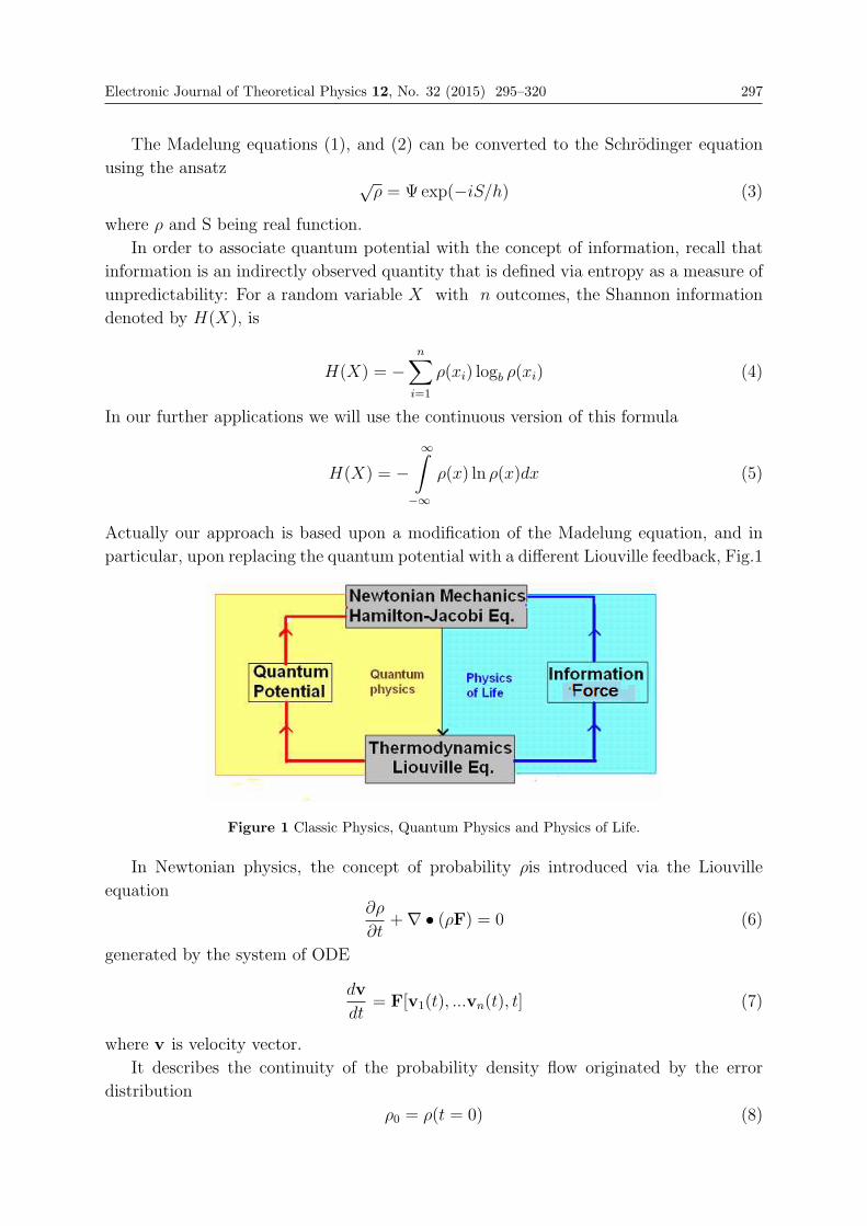
Electronic Journal of Theoretical Physics 12, No. 32 (2015) 295–320 297
The Madelung equations (1), and (2) can be converted to the Schrodinger equation
using the ansatz √ρ = Ψexp(−iS/h) (3)
where ρ and S being real function.
In order to associate quantum potential with the concept of information, recall that
information is an indirectly observed quantity that is defined via entropy as a measure of
unpredictability: For a random variable X with n outcomes, the Shannon information
denoted by H(X), is
H(X) = −n∑
i=1
ρ(xi) logb ρ(xi) (4)
In our further applications we will use the continuous version of this formula
H(X) = −∞∫
−∞
ρ(x) ln ρ(x)dx (5)
Actually our approach is based upon a modification of the Madelung equation, and in
particular, upon replacing the quantum potential with a different Liouville feedback, Fig.1
Figure 1 Classic Physics, Quantum Physics and Physics of Life.
In Newtonian physics, the concept of probability ρis introduced via the Liouville
equation∂ρ
∂t+∇ • (ρF) = 0 (6)
generated by the system of ODE
dv
dt= F[v1(t), ...vn(t), t] (7)
where v is velocity vector.
It describes the continuity of the probability density flow originated by the error
distribution
ρ0 = ρ(t = 0) (8)
298 Electronic Journal of Theoretical Physics 12, No. 32 (2015) 295–320
in the initial condition of ODE (8).
Let us rewrite Eq. (2) in the following form
dv
dt= F[ρ(v)] (9)
where v is a velocity of a hypothetical particle.
This is a fundamental step in our approach: in Newtonian dynamics, the probability
never explicitly enters the equation of motion, [2,3]. In addition to that, the Liouville
equation generated by Eq. (9) is nonlinear with respect to the probability density ρ
∂ρ
∂t+∇ • {ρF[ρ(V)]} = 0 (10)
and therefore, the system (9),(10) departs from Newtonian dynamics. However although
it has the same topology as quantum mechanics (since now the equation of motion is
coupled with the equation of continuity of probability density), it does not belong to it
either. Indeed Eq. (9) is more general than the Hamilton-Jacoby equation (2): it is not
necessarily conservative, and F is not necessarily the quantum potential although further
we will impose some restriction upon it that links F to the concept of information, [3].
The relation of the system (9), (10) to Newtonian and quantum physics is illustrated in
Fig.1.
Remark. Here and below we make distinction between the random variable v(t) and
its values V in probability space.
Prior to considering a specific form of the force F, we will make a comment concerning
the normalization constrain satisfaction∫V
ρdV = 1 (11)
in which V is the volume where Eqs. (9) and (10) are defined.
Turning to Eq. (10) and integrating it over the volume V
∂
∂t
∫V
ρdV = −∫V
dV∇ • {ρF[ρ(V)]} = −∮Φ
dΦ∇ • (ρF) = 0 (12)
if
ρ = 0, |F| <∞ at Φ (13)
where Φ is the surface bounding the volume V.
Therefore, if the normalization constraint (9) is satisfied at t = 0, it is satisfied for all
the times.
3. Information Force Instead of Quantum Potential
In this section we propose the structure of the force F that plays the role of a feed-
back from the Liouville equation (10) to the equation of motion (9). Turning to one-
dimensional case, let us specify this feedback as
F = c0 +1
2c1ρ−
c2ρ
∂ρ
∂v+
c3ρ
∂2ρ
∂v2(14)
Electronic Journal of Theoretical Physics 12, No. 32 (2015) 295–320 299
c0 > 0, c1 > 0, c3 > 0 (15)
Then Eq.(9) can be reduced to the following:
v = c0 +1
2c1ρ−
c2ρ
∂ρ
∂v+
c3ρ
∂2ρ
∂v2(16)
and the corresponding Liouville equation will turn into the following PDE
∂ρ
∂t+ (c0 + c1ρ)
∂ρ
∂V− c2
∂2ρ
∂v2+ c3
∂3ρ
∂V 3= 0 (17)
This equation is known as the KdV-Bergers’ PDE. The mathematical theory behind
the KdV equation became rich and interesting, and, in the broad sense, it is a topic of
active mathematical research. A homogeneous version of this equation that illustrates
its distinguished properties is nonlinear PDE of parabolic type. However a fundamental
difference between the standard KdV-Bergers equation and Eq. (17) is that Eq. (17)
dwells in the probability space , and therefore, it must satisfy the normalization
constraint ∞∫−∞
ρdV = 1 (18)
However as shown in [4], this constraint is satisfied: in physical space it expresses conser-
vation of mass, and it can be easily scale-down to the constraint (18) in probability space.
That allows one to apply all the known results directly to Eq. (17). However it should
be noticed that all the conservation invariants have different physical meaning: they are
not related to conservation of momentum and energy, but rather impose constraints upon
the Shannon information.
In physical space, Eq. (17) has many applications from shallow waves to shock waves
and solitons. However, application of solutions of the same equations in probability
space is fundamentally different. In the next sections we present two phenomena that
exist neither in Newtonian nor in quantum physics.
Remark . Another version of an intelligent particle that is based upon a feedback
different from that expressed by Eq. (14) was considered in [2,3,8].
4. Emergence of Randomness
In this section we discuss a fundamentally new phenomenon: transition from determinism
to randomness in ODE that coupled with their Liouville PDE.
In order to complete the solution of the system (16), (17), one has to substitute the
solution of Eq. (17):
ρ = ρ(V, t) at V = v (19)
into Eq.(16). Since the transition from determinism to randomness occurs at t → 0, let
us turn to Eq. (17) with sharp initial condition
ρ0(V ) = δ(V ) at t = 0, (20)
300 Electronic Journal of Theoretical Physics 12, No. 32 (2015) 295–320
Then applying one of the standard analytical approximations of the delta-function, one
obtains the asymptotic solution
ρ =1
t√πe−
V 2
t2 at t→ 0 (21)
Substitution this solution into Eq. (14) shows that
O(c0 +12c1ρ) =
1t, O( c2
ρ∂ρ∂v) = 1
t2,
and O( c3ρ
∂2ρ∂v2
) = 1t4
at t→ 0, v �= 0(22)
i.e.
c0 +1
2c1ρ <<
c2ρ
∂ρ
∂v<<
c3ρ
∂2ρ
∂v2at t→ 0, v �= 0 (23)
and therefore, the first three terms in Eq. (16) can be ignored
v =c3ρ
∂2ρ
∂v2at t→ 0, v �= 0 (24)
or after substitution of eq. (21)
v =4c3v
2
t4at t→ 0, v �= 0 (25)
Eq. (35) has the following solution (see Fig. 2)
v =t3
4c3 + Ct3at t→ 0, v �= 0 (26)
where C is an arbitrary constant.
This solution has the following property: the Lipchitz condition at t→ 0 fails
∂v
∂v=
8c3v
t4=
8c3t3
t4(4c3 + Ct3)→∞ at t→ 0, v �= 0 (27)
and as a result of that, the uniqueness of the solution is lost. Indeed, as follows from
Eq. (36), for any value of the arbitrary constant C, the solutions are different, but they
satisfy the same initial condition
v → 0 at t→ 0 (28)
Due to violation of the Lipchitz condition (27), the solution becomes unstable. That
kind of instability when infinitesimal errors lead to finite deviations from basic motion
(the Lipchitz instability) has been discussed in [2,3,5]. This instability leads to unpre-
dictable shift of solution from one value of Cto another. It means that appearance of any
specified solution out of the whole family is random, and that randomness is controlled
by the feedback (14) from the Liouville equation (17). Indeed if the solution (26) runs
independently many times with the same initial conditions, and the statistics is collected,
the probability density will satisfy the Liouville equation (17), Fig.3.
Remark . It should be emphasized that with the probability density defined by Eq.
(20), the point v = 0 must be excluded from consideration since at this point Eq. (16)
is meaningless.
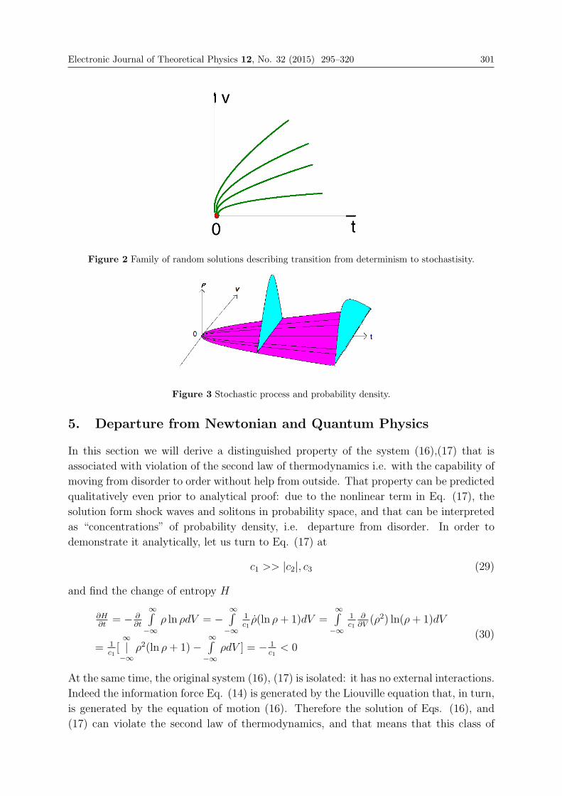
Electronic Journal of Theoretical Physics 12, No. 32 (2015) 295–320 301
Figure 2 Family of random solutions describing transition from determinism to stochastisity.
Figure 3 Stochastic process and probability density.
5. Departure from Newtonian and Quantum Physics
In this section we will derive a distinguished property of the system (16),(17) that is
associated with violation of the second law of thermodynamics i.e. with the capability of
moving from disorder to order without help from outside. That property can be predicted
qualitatively even prior to analytical proof: due to the nonlinear term in Eq. (17), the
solution form shock waves and solitons in probability space, and that can be interpreted
as “concentrations” of probability density, i.e. departure from disorder. In order to
demonstrate it analytically, let us turn to Eq. (17) at
c1 >> |c2|, c3 (29)
and find the change of entropy H
∂H∂t
= − ∂∂t
∞∫−∞
ρ ln ρdV = −∞∫−∞
1c1ρ(ln ρ+ 1)dV =
∞∫−∞
1c1
∂∂V
(ρ2) ln(ρ+ 1)dV
= 1c1[∞|−∞
ρ2(ln ρ+ 1)−∞∫−∞
ρdV ] = − 1c1
< 0(30)
At the same time, the original system (16), (17) is isolated: it has no external interactions.
Indeed the information force Eq. (14) is generated by the Liouville equation that, in turn,
is generated by the equation of motion (16). Therefore the solution of Eqs. (16), and
(17) can violate the second law of thermodynamics, and that means that this class of
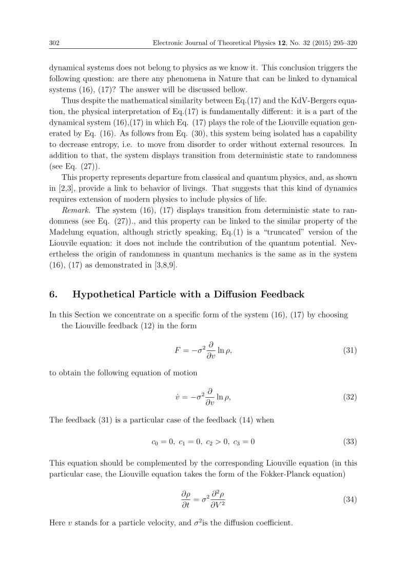
302 Electronic Journal of Theoretical Physics 12, No. 32 (2015) 295–320
dynamical systems does not belong to physics as we know it. This conclusion triggers the
following question: are there any phenomena in Nature that can be linked to dynamical
systems (16), (17)? The answer will be discussed bellow.
Thus despite the mathematical similarity between Eq.(17) and the KdV-Bergers equa-
tion, the physical interpretation of Eq.(17) is fundamentally different: it is a part of the
dynamical system (16),(17) in which Eq. (17) plays the role of the Liouville equation gen-
erated by Eq. (16). As follows from Eq. (30), this system being isolated has a capability
to decrease entropy, i.e. to move from disorder to order without external resources. In
addition to that, the system displays transition from deterministic state to randomness
(see Eq. (27)).
This property represents departure from classical and quantum physics, and, as shown
in [2,3], provide a link to behavior of livings. That suggests that this kind of dynamics
requires extension of modern physics to include physics of life.
Remark. The system (16), (17) displays transition from deterministic state to ran-
domness (see Eq. (27))., and this property can be linked to the similar property of the
Madelung equation, although strictly speaking, Eq.(1) is a “truncated” version of the
Liouvile equation: it does not include the contribution of the quantum potential. Nev-
ertheless the origin of randomness in quantum mechanics is the same as in the system
(16), (17) as demonstrated in [3,8,9].
6. Hypothetical Particle with a Diffusion Feedback
In this Section we concentrate on a specific form of the system (16), (17) by choosing
the Liouville feedback (12) in the form
F = −σ2 ∂
∂vln ρ, (31)
to obtain the following equation of motion
v = −σ2 ∂
∂vln ρ, (32)
The feedback (31) is a particular case of the feedback (14) when
c0 = 0, c1 = 0, c2 > 0, c3 = 0 (33)
This equation should be complemented by the corresponding Liouville equation (in this
particular case, the Liouville equation takes the form of the Fokker-Planck equation)
∂ρ
∂t= σ2 ∂
2ρ
∂V 2(34)
Here v stands for a particle velocity, and σ2is the diffusion coefficient.
Electronic Journal of Theoretical Physics 12, No. 32 (2015) 295–320 303
6.1 Emergence of Randomness
In this sub-section we describe the random solution not only at t→ 0, but also in whole
time interval.
if σ2 = const. (35)
the solution of Eq. (34) subject to the sharp initial condition
ρ =1
2σ√πt
exp(− V 2
4σ2t) (36)
describes diffusion of the probability density, and that is why the feedback (31) can be
called a diffusion feedback.
Substituting this solution into Eq. (32) at V = v, one arrives at the differential
equation with respect to v(t)
v =v
2t(37)
and therefore,
v = C√t (38)
whereC is an arbitrary constant. Since v = 0 at t = 0 for any value of C, the solution (38)
is consistent with the sharp initial condition for the solution (36) of the corresponding
Liouvile equation (34). The solution (38) describes the simplest irreversible motion: it is
characterized by the “beginning of time” where all the trajectories intersect (that results
from the violation of Lipcsitz condition at t =0, Fig.3), while the backward motion
obtained by replacement of t with (−t) leads to imaginary values of velocities. One can
notice that the probability density (36) possesses the same properties.
It is easily verifiable that the solution (36) has the same structure as the solution (27).
Further analysis of the solution (38) demonstrates that this solution is unstable since
dv
dv=
1
2t> 0 (39)
and therefore, an initial error always grows generating randomness. Initially, at t =0,
this growth is of infinite rate since the Lipchitz condition at this point is violated
∂v
∂v→∞ at t→ 0 (40)
This type of instability has been introduced and analyzed in [5]. The unstable equilibrium
point (v = 0) has been called a terminal repeller, and the instability triggered by the
violation of the Lipchitz condition – non-Lipchitz, or terminat instability. The basic
property of the non- Lipchitz instability is the following: if the initial condition is infinitely
close to the repeller, the transient solution will escape the repeller during a bounded time
while for a regular repeller the time would be unbounded. Indeed, an escape from the
simplest regular repeller can be described by the exponentv = v0et. Obviously v → 0 if
v0 → 0, unless the time period is unbounded. On the contrary, the period of escape from
304 Electronic Journal of Theoretical Physics 12, No. 32 (2015) 295–320
the terminal repeller (38) is bounded (and even infinitesimal) if the initial condition is
infinitely small, (see Eq. (40)).
Considering first Eq. (38) at fixedC as a sample of the underlying stochastic process
(36), and then varying C, one arrives at the whole ensemble characterizing that process,
(see Fig. 3). The curves that envelope the cross-sectional blue areas at t∗ = const present
the probability density distribution at fixed times. One can verify that, as follows from
Eq. (36), [6], the expectation and the variance of this process are, respectively
v = 0, v = 2σ2t (41)
The same results follow from the ensemble (38) at−∞ ≤ C ≤ ∞. Indeed, the first
equality in (41) results from symmetry of the ensemble with respect to v = 0 ; the second
one follows from the fact that
v ∝ v2 ∝ t (42)
It is interesting to notice that the stochastic process (35) is an alternative to the following
Langevin equation, [6]
v = Γ(t), Γ = 0, Γ = σ (43)
that corresponds to the same Fokker-Planck equation (33). Here Γ(t) is the Langevin
(random) force with zero mean and constant variance σ.
Thus, the emergence of self-generated stochasticity is the first basic non-Newtonian
property of the dynamics with the Liouville feedback.
6.2 Second Law of Thermodynamics
In order to demonstrate another non-Newtonian property of the systems considered
above, let us start with the dimensionless form of the Langevin equation for a one-
dimensional Brownian motion of a particle subjected to a random force
v = Γ(t), < Γ(t) >= 0, < Γ(t)Γ(t′) >= 2σδ(t− t′), [Γ] = 1/s (44)
Here v is the dimensionless velocity of the particle (referred to a representative velocity
v0), and Γ(t) is the Langevin (random) force per unit mass,σ >0 is the noise strength.
The representative velocity v0 can be chosen, for instance, as the initial velocity of the
motion under consideration.
The corresponding continuity equation for the probability density ρ is the following
Fokker-Planck equation
∂ρ
∂t= σ
∂2ρ
∂V 2,
∞∫−∞
ρdV = 1 (45)
Obviously without external control, the particle cannot escape the Brownian motion.
Let us now introduce a new force (referred to unit mass and divided by v0) as a
Liouville feedback
f = σ exp√D
∂
∂vln ρ, [f ] = 1/s (46)
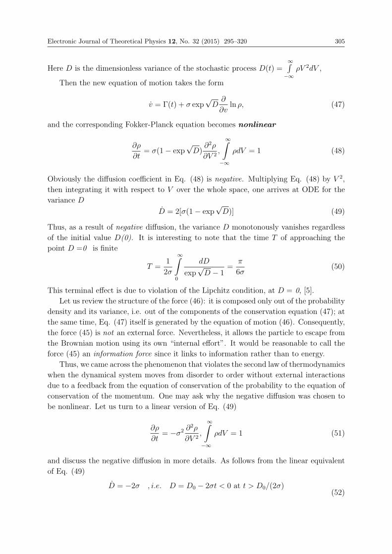
Electronic Journal of Theoretical Physics 12, No. 32 (2015) 295–320 305
Here D is the dimensionless variance of the stochastic process D(t) =∞∫−∞
ρV 2dV ,
Then the new equation of motion takes the form
v = Γ(t) + σ exp√D
∂
∂vln ρ, (47)
and the corresponding Fokker-Planck equation becomes nonlinear
∂ρ
∂t= σ(1− exp
√D)
∂2ρ
∂V 2,
∞∫−∞
ρdV = 1 (48)
Obviously the diffusion coefficient in Eq. (48) is negative. Multiplying Eq. (48) by V 2,
then integrating it with respect to V over the whole space, one arrives at ODE for the
variance D
D = 2[σ(1− exp√D)] (49)
Thus, as a result of negative diffusion, the variance D monotonously vanishes regardless
of the initial value D(0). It is interesting to note that the time T of approaching the
point D =0 is finite
T =1
2σ
∞∫0
dD
exp√D − 1
=π
6σ(50)
This terminal effect is due to violation of the Lipchitz condition, at D = 0, [5].
Let us review the structure of the force (46): it is composed only out of the probability
density and its variance, i.e. out of the components of the conservation equation (47); at
the same time, Eq. (47) itself is generated by the equation of motion (46). Consequently,
the force (45) is not an external force. Nevertheless, it allows the particle to escape from
the Brownian motion using its own “internal effort”. It would be reasonable to call the
force (45) an information force since it links to information rather than to energy.
Thus, we came across the phenomenon that violates the second law of thermodynamics
when the dynamical system moves from disorder to order without external interactions
due to a feedback from the equation of conservation of the probability to the equation of
conservation of the momentum. One may ask why the negative diffusion was chosen to
be nonlinear. Let us turn to a linear version of Eq. (49)
∂ρ
∂t= −σ2 ∂
2ρ
∂V 2,
∞∫−∞
ρdV = 1 (51)
and discuss the negative diffusion in more details. As follows from the linear equivalent
of Eq. (49)
D = −2σ , i.e. D = D0 − 2σt < 0 at t > D0/(2σ)(52)
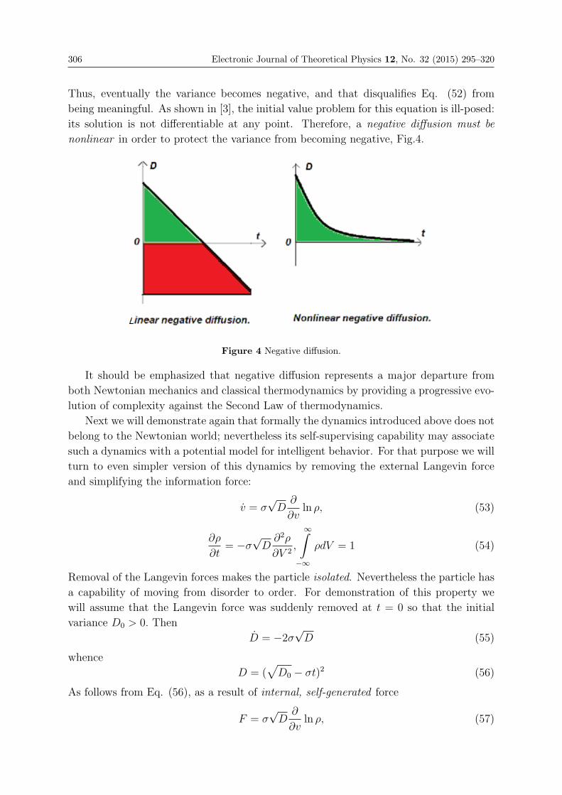
306 Electronic Journal of Theoretical Physics 12, No. 32 (2015) 295–320
Thus, eventually the variance becomes negative, and that disqualifies Eq. (52) from
being meaningful. As shown in [3], the initial value problem for this equation is ill-posed:
its solution is not differentiable at any point. Therefore, a negative diffusion must be
nonlinear in order to protect the variance from becoming negative, Fig.4.
Figure 4 Negative diffusion.
It should be emphasized that negative diffusion represents a major departure from
both Newtonian mechanics and classical thermodynamics by providing a progressive evo-
lution of complexity against the Second Law of thermodynamics.
Next we will demonstrate again that formally the dynamics introduced above does not
belong to the Newtonian world; nevertheless its self-supervising capability may associate
such a dynamics with a potential model for intelligent behavior. For that purpose we will
turn to even simpler version of this dynamics by removing the external Langevin force
and simplifying the information force:
v = σ√D
∂
∂vln ρ, (53)
∂ρ
∂t= −σ
√D
∂2ρ
∂V 2,
∞∫−∞
ρdV = 1 (54)
Removal of the Langevin forces makes the particle isolated. Nevertheless the particle has
a capability of moving from disorder to order. For demonstration of this property we
will assume that the Langevin force was suddenly removed at t = 0 so that the initial
variance D0 > 0. Then
D = −2σ√D (55)
whence
D = (√
D0 − σt)2 (56)
As follows from Eq. (56), as a result of internal, self-generated force
F = σ√D
∂
∂vln ρ, (57)
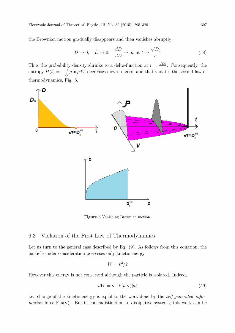
Electronic Journal of Theoretical Physics 12, No. 32 (2015) 295–320 307
the Brownian motion gradually disappears and then vanishes abruptly:
D → 0, D → 0,dD
dD→∞ at t→
√D0
σ(58)
Thus the probability density shrinks to a delta-function at t =√D0
σ. Consequently, the
entropy H(t) = −∫V
ρ ln ρdV decreases down to zero, and that violates the second law of
thermodynamics, Fig. 5.
Figure 5 Vanishing Brownian motion.
6.3 Violation of the First Law of Thermodynamics
Let us turn to the general case described by Eq. (9). As follows from this equation, the
particle under consideration possesses only kinetic energy
W = v2/2
However this energy is not conserved although the particle is isolated. Indeed,
dW = v · F[ρ(v)]dt (59)
i.e. change of the kinetic energy is equal to the work done by the self-generated infor-
mation force F[ρ(v)]. But in contradistinction to dissipative systems, this work can be
308 Electronic Journal of Theoretical Physics 12, No. 32 (2015) 295–320
positive, i.e. an information force can increase the kinetic energy of the particle. In
particular, that would happen in case of negative diffusion.
The significance of Eq. (59) is fundamental: it relates the change of energy to change
of information.
Since the particle velocity as a solution of Eq. ((9) is random, its kinetic energy (59) is
also random, and it is more convenient to operate with the average value W =∞∫−∞
ρWdV .
Then for a particular case of the information force (31), with reference to Eq. (5), Eq.
(59) can be written in the form of conservation energy/information
W + σ2H = const (60)
and that make relation between energy and information for the intelligent particle more
transparent.
7. Hypothetical Particle with Soliton Feedback
In this section we introduce the structure of the force F that is a particular case of the
feedback (14) at
c2 = 0 (61)
i.e.
F = c0 +1
2c1ρ+
c3ρ
∂2ρ
∂v2(62)
Then Eq.(16) can be reduced to the following:
v = c0 +1
2c1ρ+
c3ρ
∂2ρ
∂v2(63)
and the corresponding Liouville equation will turn into the following PDE
∂ρ
∂t+ (c0 + c1ρ)
∂ρ
∂V+ c3
∂3ρ
∂V 3= 0 (64)
that is a celebrated Korteweg-de Vries (KdV) equation.
However a fundamental difference between the standard KdV equation and Eq. (64)
is that Eq. (64) dwells in the probability space , and therefore, it must satisfy the
normalization constraint ∞∫−∞
ρdV = 1 (65)
But since the KdV equation has the conservation invariants, [7]
∞∫−∞
ρdV = Const., (66)
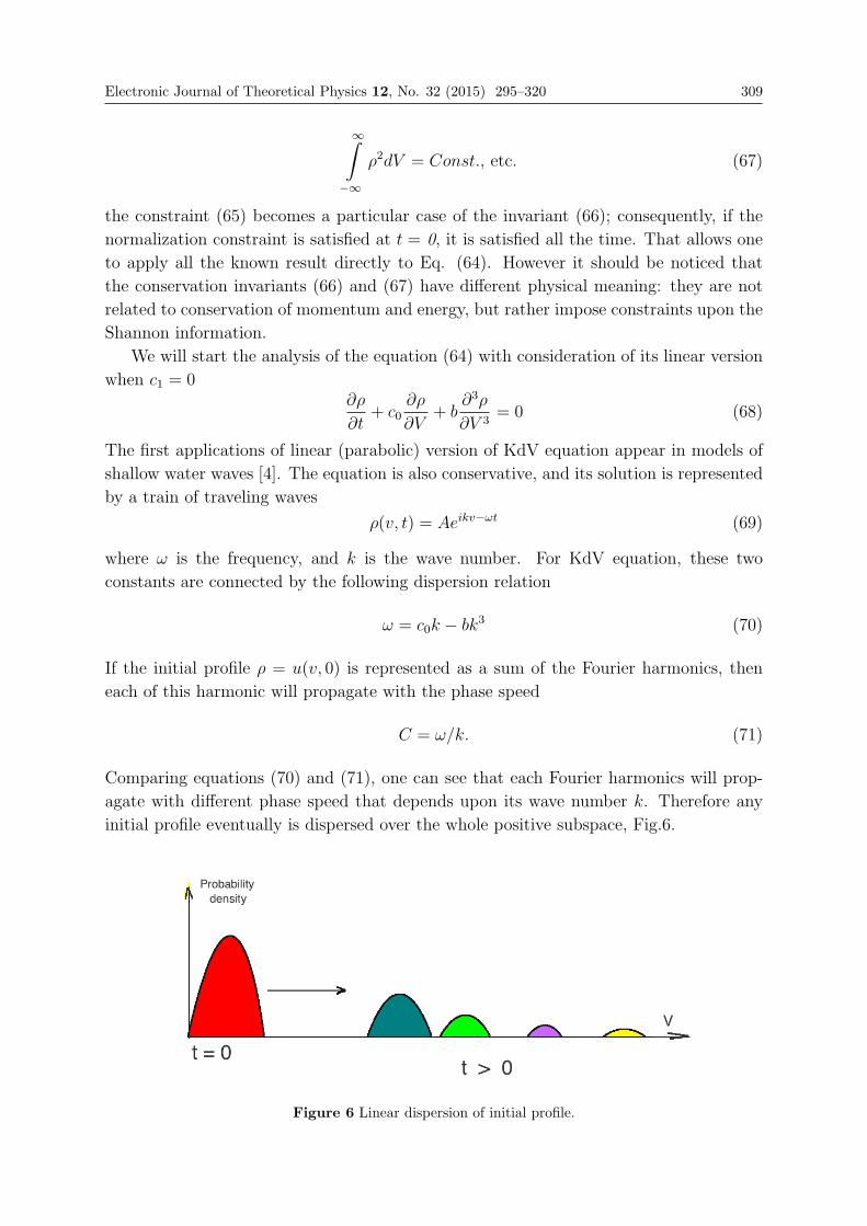
Electronic Journal of Theoretical Physics 12, No. 32 (2015) 295–320 309
∞∫−∞
ρ2dV = Const., etc. (67)
the constraint (65) becomes a particular case of the invariant (66); consequently, if the
normalization constraint is satisfied at t = 0, it is satisfied all the time. That allows one
to apply all the known result directly to Eq. (64). However it should be noticed that
the conservation invariants (66) and (67) have different physical meaning: they are not
related to conservation of momentum and energy, but rather impose constraints upon the
Shannon information.
We will start the analysis of the equation (64) with consideration of its linear version
when c1 = 0∂ρ
∂t+ c0
∂ρ
∂V+ b
∂3ρ
∂V 3= 0 (68)
The first applications of linear (parabolic) version of KdV equation appear in models of
shallow water waves [4]. The equation is also conservative, and its solution is represented
by a train of traveling waves
ρ(v, t) = Aeikv−ωt (69)
where ω is the frequency, and k is the wave number. For KdV equation, these two
constants are connected by the following dispersion relation
ω = c0k − bk3 (70)
If the initial profile ρ = u(v, 0) is represented as a sum of the Fourier harmonics, then
each of this harmonic will propagate with the phase speed
C = ω/k. (71)
Comparing equations (70) and (71), one can see that each Fourier harmonics will prop-
agate with different phase speed that depends upon its wave number k. Therefore any
initial profile eventually is dispersed over the whole positive subspace, Fig.6.
Figure 6 Linear dispersion of initial profile.
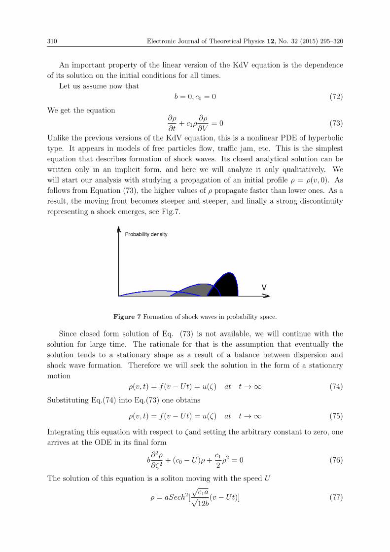
310 Electronic Journal of Theoretical Physics 12, No. 32 (2015) 295–320
An important property of the linear version of the KdV equation is the dependence
of its solution on the initial conditions for all times.
Let us assume now that
b = 0, c0 = 0 (72)
We get the equation∂ρ
∂t+ c1ρ
∂ρ
∂V= 0 (73)
Unlike the previous versions of the KdV equation, this is a nonlinear PDE of hyperbolic
type. It appears in models of free particles flow, traffic jam, etc. This is the simplest
equation that describes formation of shock waves. Its closed analytical solution can be
written only in an implicit form, and here we will analyze it only qualitatively. We
will start our analysis with studying a propagation of an initial profile ρ = ρ(v, 0). As
follows from Equation (73), the higher values of ρ propagate faster than lower ones. As a
result, the moving front becomes steeper and steeper, and finally a strong discontinuity
representing a shock emerges, see Fig.7.
Figure 7 Formation of shock waves in probability space.
Since closed form solution of Eq. (73) is not available, we will continue with the
solution for large time. The rationale for that is the assumption that eventually the
solution tends to a stationary shape as a result of a balance between dispersion and
shock wave formation. Therefore we will seek the solution in the form of a stationary
motion
ρ(v, t) = f(v − Ut) = u(ζ) at t→∞ (74)
Substituting Eq.(74) into Eq.(73) one obtains
ρ(v, t) = f(v − Ut) = u(ζ) at t→∞ (75)
Integrating this equation with respect to ζand setting the arbitrary constant to zero, one
arrives at the ODE in its final form
b∂2ρ
∂ζ2+ (c0 − U)ρ+
c12ρ2 = 0 (76)
The solution of this equation is a soliton moving with the speed U
ρ = aSech2[
√c1a√12b
(v − Ut)] (77)
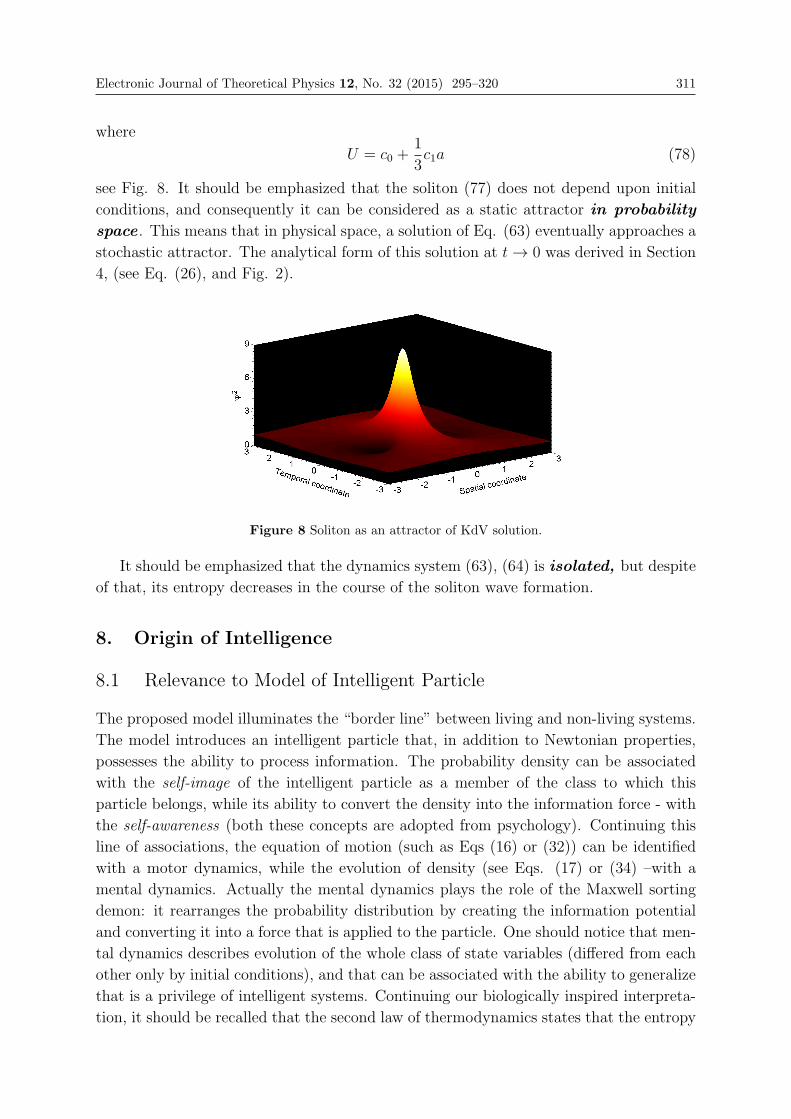
Electronic Journal of Theoretical Physics 12, No. 32 (2015) 295–320 311
where
U = c0 +1
3c1a (78)
see Fig. 8. It should be emphasized that the soliton (77) does not depend upon initial
conditions, and consequently it can be considered as a static attractor in probability
space . This means that in physical space, a solution of Eq. (63) eventually approaches a
stochastic attractor. The analytical form of this solution at t→ 0 was derived in Section
4, (see Eq. (26), and Fig. 2).
Figure 8 Soliton as an attractor of KdV solution.
It should be emphasized that the dynamics system (63), (64) is isolated, but despite
of that, its entropy decreases in the course of the soliton wave formation.
8. Origin of Intelligence
8.1 Relevance to Model of Intelligent Particle
The proposed model illuminates the “border line” between living and non-living systems.
The model introduces an intelligent particle that, in addition to Newtonian properties,
possesses the ability to process information. The probability density can be associated
with the self-image of the intelligent particle as a member of the class to which this
particle belongs, while its ability to convert the density into the information force - with
the self-awareness (both these concepts are adopted from psychology). Continuing this
line of associations, the equation of motion (such as Eqs (16) or (32)) can be identified
with a motor dynamics, while the evolution of density (see Eqs. (17) or (34) –with a
mental dynamics. Actually the mental dynamics plays the role of the Maxwell sorting
demon: it rearranges the probability distribution by creating the information potential
and converting it into a force that is applied to the particle. One should notice that men-
tal dynamics describes evolution of the whole class of state variables (differed from each
other only by initial conditions), and that can be associated with the ability to generalize
that is a privilege of intelligent systems. Continuing our biologically inspired interpreta-
tion, it should be recalled that the second law of thermodynamics states that the entropy
312 Electronic Journal of Theoretical Physics 12, No. 32 (2015) 295–320
of an isolated system can only increase. This law has a clear probabilistic interpretation:
increase of entropy corresponds to the passage of the system from less probable to more
probable states, while the highest probability of the most disordered state (that is the
state with the highest entropy) follows from a simple combinatorial analysis. However,
this statement is correct only if there is no Maxwell’ sorting demon, i.e., nobody inside
the system is rearranging the probability distributions. But this is precisely what the
Liouville feedback is doing: it takes the probability density ρ from Equation (17), creates
functionals and functions of this density, converts them into the information force and
applies this force to the equation of motion (16). As already mentioned above, because
of that property of the model, the evolution of the probability density can become non-
linear, and the entropy may decrease “against the second law of thermodynamics”, Fig.7.
Actually the proposed model represents governing equations for interactions of intelligent
agents. In order to emphasize the autonomy of the agents’ decision-making process, we
will associate the proposed models with self-supervised (SS) active systems. By
an active system we will understand here a set of interacting intelligent agents capable
of processing information, while an intelligent agent is an autonomous entity, which ob-
serves and acts upon an environment and directs its activity towards achieving goals.
The active system is not derivable from the Lagrange or Hamilton principles, but it is
rather created for information processing. One of specific differences between active and
physical systems is that the former are supposed to act in uncertainties originated from
incompleteness of information. Indeed, an intelligent agent almost never has access to the
whole truth of its environment. Uncertainty can also arise because of incompleteness and
incorrectness in the agent’s understanding of the properties of the environment. That is
why quantum-inspired SS systems represented by the particles under consideration are
well suited for representation of active systems, and the hypothetical particle introduced
above can be associated with the term “intelligent” particle. It is important to empha-
size that self-supervision is implemented by the feedback from mental dynamics, i.e. by
internal force, since the mental dynamics is generated by intelligent particle itself.
8.2 Comparison with Control Systems
In this sub-section we will establish a link between the concepts of intelligent control and
phenomenology of behavior of intelligent particle.
Example One of the limitations of classical dynamics, and in particular, neural net-
works, is inability to change their structure without an external input. As will be shown
below, an intelligent particle can change the locations and even the type of the attractors
being triggered only by information forces i.e. by an internal effort. We will start with a
simple dynamical system
v = 0, v = 0 at t = 0 (79)
and than apply the following control
F = −kv + a¯v − σ∂
∂vln ρ, (80)
Electronic Journal of Theoretical Physics 12, No. 32 (2015) 295–320 313
where
¯V =
∞∫−∞
ρ(V − V )2dV , V =
∞∫−∞
ρV dV , (81)
and k, a, σ are constant coefficients.
Then the controlled version of the motor dynamics (79) is changed to
v = −kv + a¯v − σ∂
∂vln ρ (82)
while F represents the information forces that play the role of internal actuator.
Let us notice that the internal actuator (80) is a particular case of the information
force (14) at
c0 = −kv + a¯v, c1 = 0, c2 = σ, c3 = 0 (83)
For a closure, Eq. (82) is complemented by the corresponding Liouville equation
∂ρ
∂t= kV
∂ρ
∂V− a ¯V
∂ρ
∂V+ σ
∂2ρ
∂V 2, (84)
to be solved subject to sharp initial condition
ρ0(V ) = δ(V ) at t = 0, (85)
As shown in Section 4, the solution of Eq.(82) is random, (see Eq. (26) and Fig. 2)
while this randomness is controlled by Eq. (84). Therefore in order to describe it, we
have to transfer to the mean values vand ¯v. For that purpose, let us multiply Eq.(84)
by V .Then integrating it with respect to V over the whole space, one arrives at ODE for
the expectation v(t)˙v = −kv + a¯v (86)
Multiplying Eq.(84) by V 2, then integrating it with respect to V over the whole space,
one arrives at ODE for the variance ¯v(t)
˙v = −2k¯v + 2av ¯v + 2σ (87)
Let us find fixed points of the system (86) and (87) by solving the system of algebraic
equations:
0 = −kv + a¯v (88)
0 = −2k¯v + 2av ¯v + 2σ (89)
By selecting
σ =k3
2a2(90)
we arrive at the following single fixed point
v∗ =k
2a, ¯v∗ =
k2
2a2(91)
314 Electronic Journal of Theoretical Physics 12, No. 32 (2015) 295–320
In order to establish whether this fixed point is an attractor or a repeller, we have to
analyze stability of the homogeneous version of the system (86), (87) linearized with
respect to the fixed point (91)˙v = −kv + a¯v (92)
˙v = −k¯v + k2
av (93)
Analysis of its characteristic equation shows that it has non-positive roots:
λ1 = 0, λ2 = −2k < 0 (94)
and therefore, the fixed point (91) is a stochastic attractor with stationary mean and
variance. However the higher moments of the probability density are not necessarily
stationary: they can be found from the original PDE (84).
Thus as a result of a mental control, an isolated dynamical system (79) that prior
to control was at rest, moves to the stochastic attractor (91) having the expectation
v∗and the variance ¯v∗.The distinguished property of the particle introduced above definitely fits into the
concept of intelligence. Indeed, the evolution of intelligent living systems is directed
toward the highest levels of complexity if the complexity is measured by an irreducible
number of different parts that interact in a well-regulated fashion. At the same time, the
solutions to the models based upon dissipative Newtonian dynamics eventually approach
attractors where the evolution stops while these attractors dwell on the subspaces of lower
dimensionality, and therefore, of the lower complexity (until a “master” reprograms the
model). Therefore, such models fail to provide an autonomous progressive evolution of
intelligent systems (i.e. evolution leading to increase of complexity). At the same time, a
self-controlled particle can create its own complexity based only upon an internal effort.
Thus the actual source of intelligent behavior of the particle introduced above is a
new type of force - the information force - that contributes its work into the Law of
conservation of energy. However this force is internal: it is generated by the particle itself
with help of the Liouvile equation. The machinery of the intelligence is similar to that
of control system with the only difference that control systems are driven by external
actuators while the intelligent particle is driven by a feedback from the Liouvile equation
without any external resources.
c. Application to performance of human mind has been introduced and
discussed in [7]. The proposed model deals with rules of mind activity rather than with
it’s content, i.e.with grammar, but not semantic. The model is represented by a system
of differential equations with terminal attractors and repellers, [5], that provide the capa-
bility to process discrete-event-based flow of information. This system has master-slave
architecture: the master equations describe dynamics of the corresponding intelligent
particle (in the form similar to Eqs. (32) and (34)), while the slave equations present
dynamics of Boolean functions that capture the mind activity such as mathematical logic
and linguistic. The Boolean dynamics consists of a sequence of two-step cycles during
which a new values of the uncorrelated Boolean functions are exposed. It should be
Electronic Journal of Theoretical Physics 12, No. 32 (2015) 295–320 315
recalled that in terms of mathematical logic, each Boolean function is characterized by
the truth table, which is simply a list of all the values of the function at 2n values of its
arguments. If these arguments are listed in a certain order, every Boolean function has
a unique truth table, and as a consequence, the same logical meaning. In this context,
the dynamics spontaneously generates new uncorrelated logical statements that expose a
choice for making common sense decisions.
9. Comparison with Quantum Mechanics
9.1 Mathematical Viewpoint
The model of intelligent particle is represented by a nonlinear ODE (9) and a nonlinear
parabolic PDE (10) coupled in a master-slave fashion: Eq. (10) is to be solved inde-
pendently, prior to solving Eq. ((9). The coupling is implemented by a feedback that
includes the probability density and its space derivatives, and that converts the first order
PDE (the Liouville equation) to the second or higher order nonlinear PDE. As a result of
the nonlinearity, the solutions to PDE can have attractors (static, periodic, or chaotic)
in probability space. The solution of ODE (9) represents another major departure from
classical ODE: due to violation of Lipchitz conditions at states where the probability den-
sity has a sharp value, the solution loses its uniqueness and becomes random. However,
this randomness is controlled by the PDE (10) in such a way that each random sample
occurs with the corresponding probability, Fig.3.
9.2 Physical Viewpoint
The model of intelligent particle represents a fundamental departure from both Newtonian
and quantum mechanics. The fundamental departure of all the modern physics is the
violation of the first and the second laws of thermodynamics,(see Eqs.(60), (30), (58),
Figs. 5 and 7). However the model has some similarity to quantum mechanics, and these
similarities are outlined below.
α.Superposition. In quantum mechanics, any observable quantity corresponds to an
eigenstate of a Hermitian linear operator. The linear combination of two or more eigen-
states results in quantum superposition of two or more values of the quantity. If the
quantity is measured, the projection postulate states that the state will be randomly
collapsed onto one of the values in the superposition (with a probability proportional to
the square of the amplitude of that eigenstate in the linear combination). Let us compare
the behavior of the model of intelligent particle from that viewpoint. As follows from Eq.
(38), all the particular solutions intersect at the same point v = 0 at t = 0, and that
leads to non-uniqueness of the solution due to violation of the Lipcshitz condition (see
Eq. (40). Therefore, the same initial condition v = 0 at t = 0 yields infinite number
of different solutions forming a family (38); each solution of this family appears with a
certain probability guided by the corresponding Fokker-Planck equation. For instance,
316 Electronic Journal of Theoretical Physics 12, No. 32 (2015) 295–320
in case of Eq. (38), the “winner” solution is v ≡ 0 since it passes through the maxima
of the probability density (36). However, with lower probabilities, other solutions of the
family (38) can appear as well. Obviously, this is a non-classical effect. Qualitatively,
this property is similar to those of quantum mechanics: the system keeps all the solutions
simultaneously and displays each of them “by a chance”, while that chance is controlled
by the evolution of probability density (36).
β. Entanglement. Quantum entanglement is a phenomenon in which the quantum
states of two or more objects have to be described with reference to each other, even
though the individual objects may be spatially separated. This leads to correlations
between observable physical properties of the systems. For example, it is possible to
prepare two particles in a single quantum state such that when one is observed to be
spin-up, the other one will always be observed to be spin-down and vice versa, this
despite the fact that it is impossible to predict, according to quantum mechanics, which
set of measurements will be observed. As a result, measurements performed on one
system seem to be instantaneously influencing other systems entangled with it.
Qualitatively similar effect can be found in the model of intelligent particle. In order
to demonstrate that, we start with Eqs.(32) and (34) and generalize them to the two-
dimensional case
v1 = −a11∂
∂v1ln ρ− a12
∂
∂v2ln ρ, (95)
v2 = −a21∂
∂v1ln ρ− a22
∂
∂v2ln ρ, (96)
∂ρ
∂t= a11
∂2ρ
∂V 2+ (a12 + a21)
∂2ρ
∂V1∂V2
+ a22∂2ρ
∂V2
, (97)
As in the one- dimensional case, this system describes diffusion without a drift
The solution of Eq. (97) has a closed form
ρ =1√
2π det[aij]texp(− 1
4tb′ijViVj), i = 1, 2. (98)
Here
[b′ij] = [aij]−1 , a11 = a11, a22 = a22, a12 = a21 = a12 + a21, aij = aji, b
′ij = b′ji, (99)
Substituting the solution (98) into Eqs. (95) and (96), one obtains
v1 =b11v1 + b12v2
2t(100)
v2 =b21v1 + b22v2
2t, bij = b′ij aij (101)
Eliminating t from these equations, one arrives at the ODE in configuration space
dv2dv1
=b21v1 + b22v2b11v1 + b12v2
, v2 → 0 at v1 → 0, (102)
This is a classical singular point treated in textbooks on ODE.
Electronic Journal of Theoretical Physics 12, No. 32 (2015) 295–320 317
Its solution depends upon the roots of the characteristic equation
λ2 − 2b12λ+ b212 − b11b22 = 0 (103)
Since both the roots are real in our case, let us assume for concreteness that they are of
the same sign, for instance,λ1 = 1, λ2 = 1. Then the solution of Eq. (102) is presented
by the family of straight lines
v2 = Cv1, C = const. (104)
Substituting this solution into Eq. (100) yields
v1 = Ct12(b11+Cb12) v2 = CCt
12(b11+Cb12) (105)
Thus, the solutions of Eqs. (95) and (96) are represented by two-parametrical families of
random samples, as expected, while the randomness enters through the time-independent
parameters C and C that can take any real numbers. Let us now find such a combination
of the variables that is deterministic. Obviously, such a combination should not include
the random parameters C or C. It easily verifiable that
d
dt(ln v1) =
d
dt(ln v2) =
b11 + Cb122t
(106)
and therefore,
(d
dtln v1)/(
d
dtln v2) ≡ 1 (107)
Thus, the ratio (107) is deterministic although both the numerator and denominator are
random,(see Eq.(106). This is a fundamental non-classical effect representing a global
constraint. Indeed, in theory of stochastic processes, two random functions are considered
statistically equal if they have the same statistical invariants, but their point-to-point
equalities are not required (although it can happen with a vanishingly small probability).
As demonstrated above, the diversion of determinism into randomness via instability (due
to a Liouville feedback), and then conversion of randomness to partial determinism (or
coordinated randomness) via entanglement is the fundamental non-classical paradigm.
γ . Decoherence. In quantum mechanics, decoherence is the process by which quantum
systems in complex environments exhibit classical behavior. It occurs when a system
interacts with its environment in such a way that different portions of its wavefunction
can no longer interfere with each other.
Qualitatively similar effects are displayed by the intelligent particle. In order to
illustrate that, let us turn to Eqs. (32), (34), and notice that, as soon as the feedback (31)
disappears, the system becomes classical, i.e. fully deterministic, while the deterministic
solution is a continuation of the corresponding “chosen” random solution.
δ . Uncertainty Principle. In quantum physics, the Heisenberg uncertainty principle
states that one cannot measure values (with arbitrary precision) of certain conjugate
quantities that are pairs of observables of a single elementary particle. These pairs include
318 Electronic Journal of Theoretical Physics 12, No. 32 (2015) 295–320
the position and momentum. Similar (but not identical) relationship follows from Eq.
(38):
vv = C2/2 (108)
i.e. the product of the velocity and the acceleration is constant along a fixed trajectory.
In particular, at t = 0, v and v can not be defined separately.
ε. Wave–particle duality. In physics, wave–particle duality is a conceptualization
that all objects in our universe exhibit properties of both waves (such as non-locality)
and of particles (such as quantization of some of their properties). As shown by Max
Born, the wave associated with the electron is not a tangible ’matter wave’, but one that
determines the probability of scattering of the electron in different directions. Similar
“duality” follows from the model of intelligent particle. Indeed, Eq. (32) describes the
“trajectories” of particles, while Eq. (34) represents the wave of probability that captures
the particle “scattering”.
η.Interference of probabilities. In Newtonian physics, the probability is introduced
via the Liouville equation describing the continuity of the probability density flow. This
equation is linear with respect to the probability density, and therefore, according to the
superposition principle, the probabilities are combined by summation: when an event
can occur in several alternative ways, the probability of the event is the sum of the
probabilities for each way considered separately, i.e.
ρ = ρ1 + ρ2 (109)
In quantum physics, the probability is introduced via the Schrodinger equation that is
linear with respect to probability amplitude, i.e. with respect to the square root of the
probability density. Therefore, when an event can occur in several alternative ways, the
probability amplitude of the event is the sum of the probability amplitudes for each way
considered separately
The probability interference in quantum mechanics follows from the linearity of the
Schrodinger equation with respect to the probability amplitudes ψi as state variables.
Due to linear superposition of these amplitudes, the following rule can be formulated
ψ = ψ1 + ψ2, ρi = |ψi|2, ρ = |ψ1 + ψ2|2 �= ρ1 + ρ2 (110)
and this phenomenon is known as interference of probabilities: the probabilities are
combined as the intensities of waves.
The situation with interference of probabilities in the model of intelligent particle is
more complex: it depends upon the type of information forces. Indeed, in the diffu-
sion and the integral feedbacks cases, Eqs.(32), and (34) are linear with respect to the
probability density, and the probabilities are combined according to Eq. (109). i.e. with-
out interference. But in the shock/soliton feedback, the Liouville equation is nonlinear
with respect to the probability density, and consequently, the probabilities interfere, (see
Eqs.(64) and (73)). However, this interference is different from the quantum one and it
will be discussed below.

Electronic Journal of Theoretical Physics 12, No. 32 (2015) 295–320 319
Indeed, following [4] and reinterpreting confluence of shock waves in physical space to
confluence of densities in probability space obtain the rule of combining the probabilities
ρ =ρ1f1 + ρ2f2f1 + f2
, ρ2 > ρ1 (111)
where
fi = exp(−ρiV
2σ+
ρ2i t
4σ), i = 1, 2. (112)
This means that when an event can occur in several alternative ways, the probability of
the event is the sum of nonlinear combinations of the probabilities for each way considered
separately.
The concept of interference of probabilities in more details is considered in [8].
10. Discussions and Conclusion
The discovery of the Higgs boson and the following from it completeness of the physical
picture of our Universe roused many questions, and one of them is the ability to create Life
and Mind out of physical matter without any additional entities. The primary objective
of this paper is to presents amathematical answer to the ancient philosophical question,
“How mind is related to matter” in connection with this outstanding accomplishment in
physics. The paper is inspired by analysis of the Madelung equation and discovery of the
origin of randomness in quantum mechanics, [3,9]. It turns out that replacement of the
quantum potential by the information force, while preserving some quantum properties,
introduces fundamental changes in the first and the second laws of thermodynamics, and
that leads to a mathematical model that captures behavior of livings. The idea of an
intelligent particle has been introduced as a first step of physics of life since it does not
include such properties as metabolism and reproduction. Instead it concentrates attention
to intelligent behavior. At the same time, by ignoring metabolism and reproduction, we
can make the system isolated, and it will be a challenge to show that it still can move
from a disorder to the order.
Thus the paper introduces and discusses a possible extension of modern physics to
include a concept of intelligent particle as the first step to physics of Life since all attempts
to create livings from non-living matter failed. It has been proven that there exists a
fundamentally new type of dynamical systems (represented by intelligent particles) that
can evolve from disorder to order without external forces thereby violating the second
law of thermodynamics. It has been demonstrated that these systems belong neither to
Newtonian, nor to quantum mechanics. Their departure from Newtonian mechanics is
due to a feedback from the underlying Liouville equation to the equations of motion that
represents an additional (internal) information force. Topologically this feedback shifts
intelligent particles towards quantum mechanics. However since the information force
is different from forces produced by quantum potential, the intelligent particles are not
quantum, and they can be identified as quantum-classical hybrids. Therefore intelligent
particles dwell in an abstract mathematical world rather than in the physical world, as
320 Electronic Journal of Theoretical Physics 12, No. 32 (2015) 295–320
we know it. This means that intelligent particles, in principle, cannot be composed out of
physical particles. It also means that their behavior can be computed, but not simulated
using Newtonian or quantum resources.
Since the model of intelligent particle fits well into the mathematical formalism of
modern physics, it can be consider as a new branch of quantum mechanics, and that
rouses a belief that intelligent particle is not only a mathematical abstraction, but a
reality as well.
In this context, we will comment on the recent statement made by Stephen Hawk-
ing on December 2, 2014, in which he warns that artificial intelligence (AI) could end
mankind. Based upon our work, part of which is presented in this paper, it can be
stated that machines composed only out of physical components and without any digital
devices being included, CANNOT, in principle, overperform a human in creativity, re-
gardless of the level of technology, since such machines cannot violate the Second Law of
thermodynamics. Therefore in our opinion, the danger of AI for mankind is exaggerated.
References
[1] Schrodinger, E. What is life, Cambridge University Press, 1944
[2] Zak, M., 2013, Information: Forgotten Variable in Physics Models, EJTP 10, No. 28,199–220,
[3] Zak, M., 2013, Particle of life: mathematical abstraction or reality? , Nova publishers,NY.
[4] G. Whitham, Linear and Nonlinear Waves Wiley-Interscience, New York, 1974.
[5] Zak, M., ”Terminal Model of Newtonian Dynamics,” Int. J. of Theoretical Physics,No.32, 159-190, 1992.
[6] Risken,H., 1989, The Fokker-Planck Equation, Springer, NY.
[7] Zak, M., 2014, Toward quantum-inspired model of mind. Journal of QuantumInformation Science, 2014, 4, 22-43,
[8] Zak,M., 2014, Interference of probabilities in dynamics, AIP Advances 4, 087130.
[9] Zak, M., 2014, The Origin of Randomness in Quantum Mechanics, EJTP 11, No. 31(2014) 1–16


