1

Theory of pricing as relativistic kinematics

Melnyk S.I., Tuluzov I.G. Abstract

The algebra of transactions as fundamental measurements is constructed on the basis of the analysis of their properties and represents an

expansion of the Boolean algebra. The notion of the generalized economic measurements of the economic “quantity” and “quality” of objects of

transactions is introduced. It has been shown that the vector space of economic states constructed on the basis of these measurements is

relativistic. The laws of kinematics of economic objects in this space have been analyzed and the stages of constructing the dynamics have been

formulated. In particular, the “principle of maximum benefit”, which represents an economic analog of the principle of least action in the

classical mechanics, and the principle of relativity as the principle of equality of all possible consumer preferences have been formulated. The

notion of economic interval between two economic objects invariant to the selection of the vector of consumer preferences has been introduced.

Methods of experimental verification of the principle of relativity in the space of economic states have been proposed.

Contents

Introduction

1. Multidimensionality of the space of economic states

1.1. One-dimensional model of the space of states of economic objects based on the measurement approach

1.2. Drawbacks of the one-dimensional model of the space of states of economic objects

1.3. Multidimensional space of states of economic objects

2. Definition of the main notions of the theory of fundamental economic measurements

2.1. Economic objects

2.2. Fundamental economic measurement

2.3. Result of the fundamental economic measurement

2.4. Indistinguishability of economic objects and fundamental economic measurements

3. Algebra of fundamental economic measurements

3.1. Comparison of the algebra of fundamental economic measurements with the Boolean algebra

4. Generalized economic measurements

4.1. Properties of the scale of volumes of transaction

4.2. Equivalence of economic objects

4.3. Relativity of estimate of the “quantity” and “quality” of economic objects

4.4. Proper scale of “quantity”

5. Space of states of economic objects

5.1. Brief analysis of properties of the obtained mathematical structure

5.2. Classical limit of generalized economic measurements

5.3. Vector space of states of economic objects and reference systems in it

6. Analogies between the physical relativistic space and the relativistic space of economic states

6.1. Non-relativistic limit of the space of economic states

7. Mathematical apparatus of kinematics in the relativistic space of economic states

7.1. Laws of transformation of coordinates and velocities

7.2. Analog of velocity in the relativistic space of economic states

7.3. Economic interval in the relativistic space of economic states

7.4. Analysis of possibilities of experimental observation of relativistic properties of economic objects in the

relativistic space of economic states

7.4.1. Time dilation in a moving reference system (twin paradox) in the relativistic space of

economic states

7.4.2. Relativistic Doppler effect in the relativistic space of economic states

8. Possible mechanisms of interconnection of the relativistic space of economic states and physical space-time

8.1. Model of «transportations»

8.2. Model of an enclosed system of interacting companies

9. Further stages of constructing the dynamics of economic objects in the framework of the measurement approach

9.1. Special features of using the monetary equivalent in the process of exchange and modeling of “ideal money”

9.2. Notion of «Proprietor» in the framework of the measurement approach

9.3. Proceeding from the principle of least action to the principle of maximum benefit

9.4. Two main types of interaction in physics and in economics

Conclusion

References

Introduction

Currently, an increasing attention is paid to the problems

connected with subjective factors of economic relations. Thus,

the Nobel Prize in economics in 2014 was awarded to J.M.

Tirole for the development of the “Theory of Collective

Reputations”. The general task of the theory of pricing can be

determined as the calculation of a “fair” price for a specific

product depending on its quality, volume of transaction,

demand for this product and supply of this product. In some

currently existing theories the account of other factors

influencing the price is possible. In the majority of the existing

theories the following assumptions are accepted explicitly or

implicitly:

2

Fair (true) price for a specific product exists, and it is the

same for all consumers (purchasers), thought it can be

unknown to them.

Fair price does not depend on the direction of transaction

(purchase or sale).

The demand and supply are determined unambiguously

and do not depend on the price.

The quality of the product is identical for all purchasers

and is characterized not by economic, but by physical

parameters, i.e. it is independent.

The purpose of the present paper is the construction of

the mathematical apparatus, which will allow solving the

problem of pricing without these limitations and will be based

only on the results of economic measurements, which will be

defined further in the paper. Such approach is based on the

authors’ profound internal conviction that the fundamental

approach to the construction of the mathematical apparatus of

economics must be based on the properties of symmetry of the

space of states of economic objects, which, in turn, are based

on the properties of measurements performed on them. Then

the equations of dynamics (which are the ultimate objective of

any fundamental theory) can be obtained as a sequence of the

following scheme (Fig.1). In the present paper we will limit

ourselves to the analysis of the first part of this scheme up to

the construction of the kinematics of economic objects in the

space of states and introduction of the economic invariants. In

the final chapter of the present paper we will briefly discuss

the perspectives of further development of this theory. Refusal

from the aforesaid idealizations in the framework of the

discussed (measurement) approach requires not only a formal

expansion of the mathematical apparatus, but also a principally

new approach to the definition of such notions as equivalence,

relative (subjective) price, quality of product, volume of

transaction, demand and supply. We will define them

regardless of any additional assumptions of the mechanisms of

price formation, i.e. only on the basis of the results of

economic measurements. Actually, such approach corresponds

to the ideology of geometric dynamics, which was actively

developed in the physical theory in the first half of the 20th

century.

Fig.1. Scheme of construction of the dynamics of states of economic objects on the basis of the measurement approach

1. Мultidimensionality of the space of economic

states

Before proceeding to the description of the theory, let us

discuss the principal question on the dimensionality of the

economic space. The point is that in the process of its

construction we must be guided only by the measurable

values. In economics, such value is primarily the price of an

economic object. If we express it in conventional units of

“ideal money”, it will be the only quantitative characteristic of

a specific product. On the other hand, products of equal cost

can significantly vary in consumer properties. In this case, the

necessity of introducing additional (not monetary) parameters

of economic objects arises. For the description of the latter,

additional dimensions of the space of states are required. We

state that these characteristics of “quality” can also be

expressed only on the basis of the results of economic

measurements (cost of products). However, for this purpose

we will have to refuse from illusions of existence of the “true”

cost and proceed to a multidimensional space, in which all

acceptable estimates of cost will appear to be equivalent.

First, we will illustrate on a simple example the ratio of

cost for several economic objects represented in the form of

points in one-dimensional and multidimensional economic

spaces. The illustration describes to a significant degree the

logics of the subsequent steps in the construction of the

rigorous theory.

1.1. One-dimensional model of the space of states of

economic objects based on the measurement

approach.

We have previously postulated [1] that the result of a

transaction-type measurement is the proportion of exchange of

two economic objects. At certain additional idealizations, this

definition of the economic measurement allows constructing a

trivial space of states of economic objects and calculating the

results of transactions.

Let us assume, for instance, that the transaction of

exchange of gasoline for sugar is characterized by a certain

dimension value 7

6(𝑙.𝑔.

𝑘𝑔.𝑠.). It means that in the conditions of

the discussed transaction 7 liters of gasoline (l.g.) are equal to

6 kg of sugar (kg.s.). In this case we can write down the

following - 𝑆(7 𝑙. 𝑔. ) ≡ 𝑆(6 𝑘𝑔. 𝑠. ), from which it formally

follows that 𝑆(1 𝑘𝑔.𝑠.)

𝑆(1 𝑙.𝑔.)=

7

6, i.e. the proportion of exchange 7/6

characterizes the ratio of values of 1 kg of sugar and 1 liter of

gasoline. Let us also assume that the transaction of exchange

of sugar for loafs of bread (l.b.) is characterized by the

proportion 3/2, i.e. 𝑆(1 𝑘𝑔.𝑠.)

𝑆(1 𝑙.𝑏.)=

2

3. Then we can expect that the

Fundamental economic

measurements

Algebra of the

fundamental

economic

measurements

Generalized

fundamental

economic

measurements

Space of states of

economic objects

Kinematics of

economic objects

Invariants of motion of

economic objects in the

relativistic space of

economic states

Variational principle

in the relativistic

space of economic

states

Equations of dynamics of

economic objects in the

relativistic space of

economic states

Performed

transactions as instant

interactions

(collisions)

Competitive and partner

relations as non-local

interactions

3

transaction of exchange of gasoline for bread will be

characterized by the value 7

6(𝑙.𝑔.

𝑘𝑔.𝑠.) ∙

3

2(𝑘𝑔.𝑠.

𝑙.𝑏.) =

7

4(𝑙.𝑔.

𝑙.𝑏.)

Using the properties of logarithmic function and canceling

the dimensional units, we can write down: log [7

6] + log [

3

2] =

log [7

4] and connect each of the summands with the distance

between the corresponding economic objects in a certain space

(Fig.2). For instance, the summand 𝛿𝑙𝑔𝑠 = log [7

6] can be

considered as a distance between the economic object “g” –

one liter of gasoline and the economic object “s” – one kg of

sugar.

Fig.2. One-dimensional space of economic objects

The we can state that the formula of addition of distances

𝛿𝑙𝑔𝑠 + 𝛿𝑙𝑠𝑏 = 𝛿𝑙𝑔𝑏

fulfils the task set in the theory of pricing – allows calculating

the price (proportion of exchange of two economic objects) on

the basis of other known prices. Even such a simple ratio

allows us obtaining a series on non-trivial results in the

process of analysis of an economic system with a preset

matrix of technologies [1].

Let us note that in this space we can use any economic

object taken in any quantity (for instance, 3 kg of sugar) as a

reference point. Then the cost of the remaining objects will be

expressed in conventional units of cost equal to the cost of 3

kg of sugar. Thus, the obtained space acts as a uniform price

scale. However, it does not represent a number of significant

properties of economic objects.

1.2. Drawbacks of the one-dimensional model of the

space of states of economic objects

The main drawback of the constructed model is the

Indistinguishability of economic objects equal in cost

(exchanged for each other). Thus, for instance, in the aforesaid

example 7 liters of gasoline, 6 kg of sugar and 4 loafs of bread

correspond to the same point in the scale of values.

However, in the process of exchange of these objects each

of the participants of the transaction assumes that he obtains a

bigger value than he returns. Otherwise (in case of equality of

these values), the transaction loses its sense. Therefore it is

necessary to modify (expand) the one-dimensional space of

states in order to fulfill the following requirements:

Two different exchanged economic objects correspond

to different points of the space of states;

For two participants of the transaction, the object

obtained as a result of exchange is to be of bigger

value.

1.3. Multidimensional space of states of economic

objects

These two requirements can be satisfied by introducing a

set of various scales of values (one for each of the consumers).

Then the ratio “more expensive-less expensive” will depend

not only on the position of the objects in the space, but also on

the axis (scale), in relation to which they are evaluated.

If for such evaluation we compare the positions of the

projection of points corresponding to the economic objects,

then the possibility of performing transactions, in which each

of the consumers considers them profitable for himself,

appears. This situation is illustrated in Fig.3

Fig.3 Possibility of a mutually-beneficial exchange in a

multidimensional space of economic objects

For consumer X the objects “A” and “B” appear to be of equal

value, as illustrated in Fig.1, for consumer Х1 «А» is more

valuable than «В», but for consumer Х2 the situation is

reverse.

Any of the consumer directions (vector in the space of

states) can be determined by a pair of points. For instance,

points «C» and «D» determine the consumer direction «х», for

each the project of the segment «CD» (proportion of exchange

of these economic objects) is maximum. (Fig.4).

Fig.4. Quantitative estimate of the relative cost of two economic

objects («С» and «D» as represented in the Figure) is possible

only in relation to the selected scale. Projection of points «С»

and «D» on this scale corresponds to the equal objects «С1»

and «D1», which differ only in quantity.

For the quantitative definition of the length of the

projection С1D1 it is necessary that points С1 and D1

correspond to the economic objects of equal dimensionality

(quantitatively comparable). Therefore, from the whole set of

consumer directions we will point out those, which are

connected with the economic object (bread, for instance),

different quantity of which corresponds to different points of

this axis. For instance, point «С1» in Fig. 4 corresponds to 1

loaf of bread, while «D1» corresponds to 3 loafs of bread.

Then we can state that according to the “bread” scale of values

𝛿𝑙𝑠𝑏

1 liter of gasoline

1 kg of sugar

1 loaf of bread

𝛿𝑙𝑔𝑠

𝛿𝑙𝑔𝑏 7 l of gasoline 6 kg of sugar 4 loafs of bread

7 l of gasoline

6 kg of sugar

X1

X

X2

A

B

С

D

x

-x

3 loafs of bread 1 loaf of bread

С1 D1

4

the economic object “D” is 8 times (log2 8 = 3) more

expansive compared to object “C”. Such consumer directions

will be further referred to as proper directions.

Let us note that not all possible consumer preferences

(directions in the space of state) have an equivalent real

economic object, the quantitative scale of which allows

measuring the length of projection of the segment. In this case

we can state the existence of such consumer direction;

however, measurement of the projection on it is impossible.

Further we will propose a consecutive construction of the

multidimensional space of economic states in accordance with

the scheme illustrated in Fig.1.

2. Definition of the main notions of the theory of

fundamental economic measurements

Before proceeding to the construction of the axiomatic of

fundamental economic measurements, partially developed by

us earlier [2-4], let us define the list notions used hereafter. Let

us note that they can both match with the notions, generally

accepted in the economic theory, and vary from them.

Nevertheless, we will further adhere to the definitions given

below.

2.1. Economic objects

We will define the economic objects as such objects,

which can be exchanged for each other (perform transactions

with them) completely or partially. These can be both material

calculable values (cars, minerals, labor resources) and various

services (information, certain actions or refusal from certain

actions). Besides, the subject of transactions can be rights and

obligations notarized in the form of securities or agreements

for non-material assets. In the proposed theory we will not be

interested in the physical essence of an economic object or its

properties measured in any form other than the economic

parameters.

2.2. Fundamental economic measurement

We will associate any pair of economic objects with an

offer of transaction of their exchange and define it as the

fundamental economic measurement. We will denote the

fundamental economic measurement, in which a certain

subject of economic relations is offered to deliver “B” and

receive “A” in return as [𝐴𝐵]. Let us note that the fundamental economic measurements

include only the transactions of natural exchange of economic

objects. At the same time, in modern economics the majority

of transactions are performed indirectly (using money). We

will further introduce the additional notion of “ideal money”

and analyze their role in the construction of the theory. But

first let us discuss only the transactions of natural exchange.

2.3. Result of the fundamental economic measurement

We will consider the result of the fundamental economic

measurement as a subject’s consent for the proposed

transaction or refusal of it. At the same time, the result of

measurement depends both on the objects of the transaction

and on the consumer preferences of subject adopting the

decision on the transaction. We will denote the subjects

different in their consumer preferences by different small

Latin symbols. If a consent is received for the transaction

[AB] offered to subject “c”, then we will write down the result

of this measurement as: [𝐴𝑐 > 𝐵𝑐]. In case of refusal, we will

write it down as [𝐴𝑐 ≤ 𝐵𝑐]. Thus, the symbol 𝐴𝑐 can be

interpreted as an evaluation cost of object “A” by the subject

“c”. For the transaction [BA] we will obtain [𝐵𝑐 > 𝐴𝑐] and [𝐵𝑐 ≤ 𝐴𝑐], accordingly. At the same time, let us note that if [Ac ≤ Bc], then [Bc > Ac], however, for different subjects

from [Ac ≤ Bc] does not follow [Bd > Ad]. Moreover, the

transaction [AB] can be performed in case if and only if the

consent of both subjects of the transaction is received. This

means that the simultaneous fulfillment of the two results is

required: [Ac > Bc] for the purchaser and [Bd > 𝐴𝑑] for the

purchaser.

2.4. Indistinguishability of economic objects and

fundamental economic measurements

We will consider two economic objects «𝐴1» and «𝐴2»

indistinguishable if the result of the transaction [𝐴1𝐵] is

indistinguishable from the result of the transaction [𝐴2𝐵], the

result of the transaction [𝐵𝐴1] is indistinguishable from the

result of the transaction [𝐵𝐴2] for any economic object «𝐵».

We will consider two fundamental economic

measurements [𝐴𝐵] and [𝐶𝐷] indistinguishable if for any

subject “c” their results will be identical. Either [𝐶𝑐 > 𝐷𝑐] follows from [𝐴𝑐 > 𝐵𝑐] or vice verse, for any “c”.

3. Algebra of fundamental economic measurements

It is obvious that different economic objects are

interconnected by the relation of attribute, as a certain set of

economic objects can also be an economic object (can be a

subject of transaction). Besides, it is obvious that qualitatively

and quantitatively similar (almost indistinguishable) economic

objects will almost always have the same results of the

fundamental economic measurements.

On the other hand, the results of different fundamental

economic measurements can be interconnected by specific

conditions and form new transactions with more complex

conditions. Essentially, the main task of the theory of pricing

is to calculate the results of certain transactions knowing the

results of other transactions connected with those transactions

in some way.

As the construction of the theory is based on the

measurement approach, we will begin the construction of the

space of economic states with the construction of the

mathematical formalism of interconnections between various

fundamental economic measurements, rather than economic

objects. We will introduce the binary operations of addition

and multiplication of the fundamental economic

measurements with obvious (for transactions) properties.

Let us note that the result of operation on two transactions

is also a transaction, in which the solution is adopted by one

subject. Therefore, the sign of equality in the identities

represented below means that the fundamental economic

measurements in the right and left parts of the identity give the

same results if they will be offered to any of the possible

subjects “c”.

We will consider the sum of two fundamental economic

measurements [𝐴1𝐵1] and [𝐴2𝐵2] as a fundamental economic

measurement (transaction) [𝐴1𝐵1] + [𝐴2𝐵2], consent for

which means that the consent for at least one of the

transactions [𝐴1𝐵1] and [𝐴2𝐵2] is obtained. Otherwise (in

case of two refusals), we will consider that the transaction [𝐴1𝐵1] + [𝐴2𝐵2] is refused.

It is obvious that in this case the following ratios, which

we will accept as axioms defining the properties of the

5

operation of addition in the fundamental economic

measurement, are valid:

Commutativity [𝐴1𝐵1] + [𝐴2𝐵2] = [𝐴2𝐵2] + [𝐴1𝐵1] Transitivity ([𝐴1𝐵1] + [𝐴2𝐵2]) + [𝐴3𝐵3] =

[𝐴1𝐵1] + ([𝐴2𝐵2] + [𝐴3𝐵3]) If [0] is a transaction which is always refused and [1] is a

transaction which is always accepted, then:

[𝐴1𝐵1] + [0] = [0] + [𝐴1𝐵1] = [𝐴1𝐵1] [𝐴1𝐵1] + [𝐵1𝐴1] = [1] or [𝐴1𝐵1] = [1] − [𝐵1𝐴1] [𝐴1𝐵1] + [𝐴1𝐵1] ≠ [𝐴1𝐵1]

We will consider the product of two fundamental economic

measurement [𝐴1𝐵1] and [𝐴2𝐵2] as a fundamental economic

measurement (transaction) [𝐴1𝐵1] ∙ [𝐴1𝐵1], consent for which

means that the consent for both transactions [𝐴1𝐵1] and [𝐴2𝐵2] is obtained. Refusal means that at least one of the

transactions is refused.

For this operation the following ratios (further referred to

as axioms) are valid:

Commutativity [𝐴1𝐵1] ∙ [𝐴2𝐵2] = [𝐴2𝐵2] ∙ [𝐴1𝐵1] Transitivity ([𝐴1𝐵1] ∙ [𝐴2𝐵2]) ∙ [𝐴3𝐵3] =

[𝐴1𝐵1] ∙ ([𝐴2𝐵2] ∙ [𝐴3𝐵3]) [𝐴1𝐵1] ∙ [1] = [1] ∙ [𝐴1𝐵1] = [𝐴1𝐵1] [𝐴1𝐵1] ∙ [𝐵1𝐴1] = [0] [𝐴1𝐵1] ∙ [𝐴1𝐵1] = [𝐴1𝐵1]

2 ≠ [𝐴1𝐵1]

Besides, for the pair of the introduced operations the axiom

of associativity is valid:

([𝐴1𝐵1] + [𝐴2𝐵2]) ∙ [𝐴3𝐵3] = [𝐴1𝐵1][𝐴3𝐵3] +[𝐴2𝐵2] ∙ [𝐴3𝐵3]

3.1. Comparison of the algebra of fundamental

economic measurements with the Boolean algebra

Let us note that the obtained algebra of the fundamental

economic measurements closely resembles the Boolean

algebra, as the result of any fundamental economic

measurement can possess only two values. At the same time,

the significant difference between them is the fact that for the

algebra of fundamental economic measurements the product

of two identical transactions (indistinguishable in economic

sense) means not the same transaction, but a transaction with a

doubled volume. If a certain buyer agrees to exchange his

property “A” (a bicycle, for instance) for a certain economic

object “B” (red telephone), it does not mean that he will agree

for a second identical transaction (he may not have a second

bicycle or he may not need two identical red telephones).

At the same time, the sum of two identical transactions

may not be equal to a single transaction, as it would be in the

Boolean algebra. In the aforesaid example it means that the

purchaser will agree for two transactions (transaction of

doubled volume), but will refuse from each of them

separately.

This difference arises because in the Boolean algebra the

answer to the same question does not depend on the number of

times this question is asked. In the algebra of fundamental

economic measurements we have rejected this assumption and

we consider that the quantity of positive answers (consents for

identical transactions of the same subject) can depend on the

quantity of these transactions (volume of the aggregate

transaction). Thus, [𝐴1𝐵1]𝑛 means a transaction of 𝑛-times

larger volume compared to [𝐴1𝐵1], not equivalent to it in the

general case.

Let us note that none of the introduced operations allows

considering a set of fundamental economic measurements as a

vector space, because neither the sum, nor the product of the

transactions allow introducing a reverse elements, for which

the following identity is valid [𝐴1𝐵1] + [𝐵1𝐴1] = [0] or [𝐴1𝐵1] ∙ [𝐵1𝐴1] = [1] In this connection we will further introduce the notion of

the generalized economic measurements, derived from the

fundamental economic measurements, allowing to construct

the vector space of states of economic objects. .

4. Generalized economic measurements

4.1. Properties of the scale of volumes of transaction

The continuous scale of volumes of transaction can be

obtained in the process of additional studying of the fractional

“quantities” of economically indistinguishable transactions.

Thus, for instance, we will define the transaction [𝐴𝐵]1

2 as a

transaction, for which the following equality is valid:

[𝐴𝐵]1

2[𝐴𝐵]1

2 = [𝐴𝐵]. Thus, any pair of economic objects «А»

and «В» can be associated with a continuous set of

homogeneous transactions.

We will consider the number 𝜏 = log2 𝑛 as a coordinate

on this scale. If we select the transaction [𝐴𝐵]𝑘as an initial

fundamental economic measurement, we will obtain a scale

offset by 𝜏 = log2 𝑘 compared to the first scale. Thus, the

selection of the unit of measurement of the volume of

transaction is reduced to the selection of a reference point on

the logarithmic scale of the “quantity”. We will designate the

transactions belonging to this set as homogeneous.

The subsets of homogeneous transactions do not intersect,

as otherwise we would have a transaction satisfying the

condition [𝐴𝐵]𝑘 = [𝐶𝐷]𝑙 in the point of intersection, meaning

that [𝐴𝐵]𝑘/𝑙 = [𝐶𝐷], and that the transactions [𝐴𝐵]and [𝐶𝐷] belong to the same subset of homogeneous transactions.

4.2. Equivalence of economic objects

Let us consider a pair of economic objects «А» and «В»,

for which a transaction with positive result (consent of both

participants) is possible. This means that at least one consumer

“c” exists, who considers that [𝐴𝑐 > 𝐵𝑐], and at least one

consumer “d”, who considers that [𝐵𝑑 > 𝐴𝑑]. Assuming that

the consumer preferences are continuously changed, we can

state the following. A certain set of consumer preferences «s»

exists (real or virtually possible consumer), for which these

two objects possess equal value [𝐴𝑠 = 𝐵𝑠]. The problem of

uniqueness of such set will be discussed later.

Let us consider the scale of volume of this transaction. It

is obvious (due to the symmetry of the relation of

indifference) that for the consumer “s” the objects exchanged

for each other in any of the transactions from this scale [𝐴𝐵]𝑛

will be also equivalent. Thus, [𝑛𝐴𝑠 = 𝑛𝐵𝑠]. This means that the considered set of consumer

preferences can be associated with an infinite continuous set

of pairs of equivalent objects differing only in the parameter

𝑛. This parameter acts as the volume of the transaction, if we

consider the initial pair as the unit volume. The validity of

natural axioms is required for the introduced relation of

indifference. We will assume that for any subject «s»

if [𝐴𝑠 = 𝐵𝑠] and [𝐵𝑠 = 𝐶𝑠], then [𝐴𝑠 = 𝐶𝑠] if [𝐴𝑠 = 𝐵𝑠], then [𝐵𝑠 = 𝐴𝑠]

Then it can be shown that the whole set of economic

objects relative to any of the subjects of economic relations

6

disintegrates into non-intersecting equivalent subsets. Any pair

of these objects allows constructing the scale of volumes of

the corresponding transaction. The axioms of the relation of

indifference ensure synchronization of these scales.

Let us note that the relations of indifference are associated

with the fixed set of consumer preference “s”. Therefore, for

various subjects the division of the set of economic objects

into equivalent subsets and the estimate of the volumes of

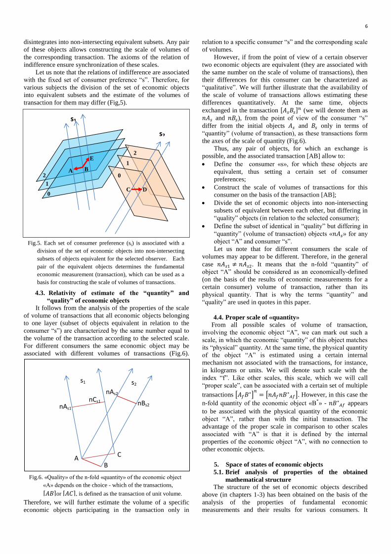
transaction for them may differ (Fig,5).

4.3. Relativity of estimate of the “quantity” and

“quality” of economic objects

It follows from the analysis of the properties of the scale

of volume of transactions that all economic objects belonging

to one layer (subset of objects equivalent in relation to the

consumer “s”) are characterized by the same number equal to

the volume of the transaction according to the selected scale.

For different consumers the same economic object may be

associated with different volumes of transactions (Fig.6).

Therefore, we will further estimate the volume of a specific

economic objects participating in the transaction only in

relation to a specific consumer “s” and the corresponding scale

of volumes.

However, if from the point of view of a certain observer

two economic objects are equivalent (they are associated with

the same number on the scale of volume of transactions), then

their differences for this consumer can be characterized as

“qualitative”. We will further illustrate that the availability of

the scale of volume of transactions allows estimating these

differences quantitatively. At the same time, objects

exchanged in the transaction [𝐴𝑠𝐵𝑠]𝑛 (we will denote them as

𝑛𝐴𝑠 and 𝑛𝐵𝑠), from the point of view of the consumer “s”

differ from the initial objects 𝐴𝑠 and 𝐵𝑠 only in terms of

“quantity” (volume of transaction), as these transactions form

the axes of the scale of quantity (Fig.6).

Thus, any pair of objects, for which an exchange is

possible, and the associated transaction [AB] allow to:

Define the consumer «s», for which these objects are

equivalent, thus setting a certain set of consumer

preferences;

Construct the scale of volumes of transactions for this

consumer on the basis of the transaction [AB];

Divide the set of economic objects into non-intersecting

subsets of equivalent between each other, but differing in

“quality” objects (in relation to the selected consumer);

Define the subset of identical in “quality” but differing in

“quantity” (volume of transaction) objects «𝑛𝐴𝑠» for any

object “A” and consumer “s”.

Let us note that for different consumers the scale of

volumes may appear to be different. Therefore, in the general

case 𝑛𝐴𝑠1 ≠ 𝑛𝐴𝑠2. It means that the n-fold “quantity” of

object “A” should be considered as an economically-defined

(on the basis of the results of economic measurements for a

certain consumer) volume of transaction, rather than its

physical quantity. That is why the terms “quantity” and

“quality” are used in quotes in this paper.

4.4. Proper scale of «quantity»

From all possible scales of volume of transaction,

involving the economic object “A”, we can mark out such a

scale, in which the economic “quantity” of this object matches

its “physical” quantity. At the same time, the physical quantity

of the object “A” is estimated using a certain internal

mechanism not associated with the transactions, for instance,

in kilograms or units. We will denote such scale with the

index “f”. Like other scales, this scale, which we will call

“proper scale”, can be associated with a certain set of multiple

transactions [𝐴𝑓𝐵∗]𝑛= [𝑛𝐴𝑓𝑛𝐵

∗𝐴𝑓]. However, in this case the

n-fold quantity of the economic object «В*» - 𝑛𝐵∗𝐴𝑓 appears

to be associated with the physical quantity of the economic

object “A”, rather than with the initial transaction. The

advantage of the proper scale in comparison to other scales

associated with “A” is that it is defined by the internal

properties of the economic object “A”, with no connection to

other economic objects.

5. Space of states of economic objects

5.1. Brief analysis of properties of the obtained

mathematical structure

The structure of the set of economic objects described

above (in chapters 1-3) has been obtained on the basis of the

analysis of the properties of fundamental economic

measurements and their results for various consumers. It

Fig.6. «Quality» of the n-fold «quantity» of the economic object

«А» depends on the choice - which of the transactions,

[𝐴𝐵]or [𝐴𝐶], is defined as the transaction of unit volume.

A C

nAs1

nAs2

B

s1 s2

nCs1 nBs2

Fig.5. Each set of consumer preference (si) is associated with a

division of the set of economic objects into non-intersecting

subsets of objects equivalent for the selected observer. Each

pair of the equivalent objects determines the fundamental

economic measurement (transaction), which can be used as a

basis for constructing the scale of volumes of transactions.

s1

s2

A B

E

0

1

2 0

1

2

C D

7

allows performing a certain ordering of the economic objects.

However, this ordering is obviously insufficient for solving

the main problem of pricing formulated above. Our further

aims include:

Construction of vector space of states of economic objects

on the basis of the generalized economic measurements,

Introduction of reference systems associated with specific

consumers in this space of states,

Determining the methods of measurement of the

coordinates of “quantity” and “quality” of the product in

this space in the selected reference system,

Deriving of the laws of transformation of coordinates

from one reference system into another.

As a result we will obtain the mathematical apparatus for

calculating the prices, which are considered fair by specific

consumers, allowing us to predict his choice in a particular

transaction. The consumer properties in this case can be set by

the results of additional measurements. From mathematical

point of view, this task is equivalent to the task of calculating

the coordinates of a particular point relative to the selected

system of coordinates, if its position relative another system of

coordinates in the geometric space is known. Actually, we can

obtain the geometry of space of economic states. With account

of the special character of the axis of “quantity”, which in a

certain sense acts as the economic time, it can be considered

the “economic kinematics”.

Rigorous and successive execution of this program first

and foremost requires a detailed analysis of the generalized

economic measurements. We have previously [2-4] analyzed

the logics of transition from fundamental economic

measurements to generalized economic measurements. At the

same time it has been shown that each such measurement can

be correctly described only in the framework of the quantum-

mechanical formalism. Let us note that similar results of

studying the generalized measurements in physics have been

obtained by Schwinger [5]. However, while he postulates their

properties, in the process of the discussion of the generalized

measurements in economics, the phenomenon of superposition

of alternatives occurs as their natural combination in the

subject’s consciousness in the process of adopting a decision

on a transaction. The difference of the superposition of

alternatives from their mix occurs due to the fact that in the

situation of a delayed choice there is an equal possibility for

each of the alternatives of being realized, while in case of their

mix we can only speak of a lack of information.

The program of rigorous mathematical construction of the

space of states on the basis of the fundamental economic

measurements and correct transition to the generalized

economic measurements requires a separate research and is

beyond the framework of this publication. Our further papers

will be dedicated to this problem. Nevertheless, even now we

can “guess” the classical limit of such space and verify the

conformity of its properties with the natural requirements.

5.2. Classical limit of generalized economic

measurements

According to N. Bohr, any measurement is based on the

comparison with an etalon. Thus, a fundamental measurement

can result in one of two answers (“yes” or “no”). Despite this,

both physics and other exact sciences operate not with the

fundamental measurements, but with secondary measured

parameters, such as length, time, etc. We will refer to such

measurements as the generalized measurements, meaning their

profound interconnection with the theory of generalized

measurements of Schwinger [5].

In the application to economics it means that the

generalized economic measurements represent a certain

combination of the fundamental economic measurements,

transformed from them using the previously derived

operations of the algebra of measurements. An example of the

generalized economic measurements is, for instance, an

auction.

Further we will discuss the generalized economic

measurements of two types: “ideal sale” and “ideal purchase”

«Ideal sale» assumes that the seller is a monopolist and

therefore sales his property at the maximum price, for

which the purchasers agree.

«Ideal purchase» assumes that the purchaser is a

monopolist and purchases the product at the minimum

price offered by the sellers.

At the same time, the price of a certain economic object

«А0» relative to an economic object «В» will be considered as

the quantity “B”, for which it can be exchanged. Thus, in the

generalized economic measurement introduced by us, any

economic object “A” is associated with the maximum and

minimum price according to the scale associated with a set of

homogeneous (differing only in quantity) objects “B”. These

two values of quantity “B” correspond to the generalized

economic measurements “Ideal sale” and “Ideal purchase” for

the economic object “A”.

These generalized measurements combine the results of

an infinite set of homogeneous fundamental measurements

(transactions of exchange of various quantities of products).

The result of these measurements is no longer a consent or a

refusal, but a number characterizing the whole set of received

answers. Let us note that for obtaining this number it is

necessary to construct a scale of quantity of product “B” using

a certain set of consumer preferences. Therefore, in the

procedure of the generalized economic measurements, a third

economic object “C” must be present, which is used for

constructing the scale of “quantity” “B” according to the

algorithm described above.

As a result it appears that for each pair of economic

objects “A” and “B” a certain interval of quantity of economic

object “B” exists, for which various consumers are ready to

exchange the economic object “A”. It is characterized by the

limit values: 𝜏𝐵𝑚𝑖𝑛and 𝜏𝐵𝑚𝑎𝑥. This result of the generalized

economic measurements can be conventionally written down

as an inequality: [Вmin ≤ 𝐴 ≤ Вmax]. Let us note that the limit values no longer depend on the

choice of the observer (consumer which evaluates the objects),

as in the process of their definition (in the conditions of the

transactions of “ideal sale” and “ideal purchase”) all possible

consumers with various sets of consumer preferences are

being questioned. Thus, the obtained characteristics are

absolute, unlike the relations of indifference.

Nevertheless, the problem of pricing requires defining not

these characteristics, but the subjective relations of

indifference of the selected consumer. These relations allow

predicting his choice in a particular transaction.

In accordance with this result, we will introduce two

numbers characterizing the position of the economic object

“A” relative to the scale of the economic object “B” in the

space of economic states:

8

number 𝜏𝐴/𝐵 =𝜏𝐵𝑚𝑖𝑛+𝜏𝐵𝑚𝑎𝑥

2 will be denoted as the

volume of transaction («quantity») of the economic object

«В», equal to the economic object «А»

number 𝑙𝐴/𝐵 =𝜏𝐵𝑚𝑖𝑛

−𝜏𝐵𝑚𝑎𝑥

2 will be denoted as the

distance (difference in “quality”) from the economic object

“A” to the equal volume of transaction of the economic

object “B”

Fig. 7 illustrates the introduced parameters and explains

the names selected for them. The quantity of “B” equal to “A”

has a transparent economic sense. It is a geometric average

(with account of the logarithmic scale) between the maximum

and minimum price “A” according to the scale “B”.

It is clear from the Figure that the larger is the distance

from point “A” to axis “B”, the larger is the difference

between the distance between 𝜏𝑚𝑎𝑥 and 𝜏𝑚𝑖𝑛. Therefore, this distance can be determined according to

the method described above. On the other hand, following

from the general economic considerations, we can conclude

that the smaller is the difference of the consumer properties of

two products, the smaller will be the difference of prices

offered for them by different consumers. Thus, the geometric

interpretation of the distance and the economic interpretation

of the qualitative differences coincide and correspond to the

above mentioned formula.

The factor of principal importance is that the aforesaid

definition of equality and distances is self-consistent for three

objects, minimally required for performing the generalized

economic measurements. Let us first note that if 𝜏(𝐵2) is the

logarithm of the maximum price (in units В), offered for the

object «С», and 𝜏(𝐴4) is the logarithm of the maximum price

(in units A), offered for the object «B2», then 𝜏(𝐴4) is the

logarithm of the maximum price which can be received for

“C” (Fig.8). Similar statement is valid for minimum prices.

Then

𝜏(𝐶0) = 𝜏(𝐵0) =𝜏(𝐵1)+𝜏(𝐵2)

2=

1

2(𝜏(𝐴1)+𝜏(𝐴2)

2+𝜏(𝐴3)+𝜏(𝐴4)

2) =

𝜏(𝐴1)+𝜏(𝐴4)

2= 𝜏(𝐴0)

under the condition that 𝜏(𝐴4) − 𝜏(𝐴3) = 𝜏(𝐴2) − 𝜏(𝐴1). However, this condition means that the distance between equal

quantities of objects A and B defined as

𝑙𝐴 𝐵⁄ =𝜏𝐵min

−𝜏𝐵max

2 ,

does not depend on these quantities and that the corresponding

scales can be constructed on the basis of any of the three pairs

of the fundamental economic measurements [𝐴0𝐵0], [𝐴0𝐶0], [𝐵0𝐶0]. The obtained axes of “quantity” in the relativistic

space of economic states appear to be parallel to each other (as

illustrated in Figure 8).

5.3. Vector space of states of economic objects and

reference systems in it

Thus, the results of the introduced generalized economic

measurements “ideal sale” and “ideal purchase” allow

ariphmetize in a consistent way the set of economic objects

(set a method of determining their coordinates in the selected

reference system). Considering the set of coordinates as a

vector and introducing procedures of addition and

multiplication by scalar, typical for the vector space, we can

construct a vector space of states of economic objects. In the

general case, it is multidimensional with a dedicated axis of

“quantity” in each of the reference systems.

Comparing the vector space of states with the set of

generalized economic measurements, let us note two

differences:

Each transaction (pair of exchanged economic objects) is

associated with a certain vector of the space of states, but

one and the same vector can be associated with a set of

different transactions. Equality of their projections on the

axis of coordinates is still insufficient to make them

economically indistinguishable.

The procedure of addition of vectors of the space of states

differs from the previously discussed procedure of

addition of transactions.

Figure 8 illustrates the two-dimensional space of states of

economic objects (one axis of “quantity” and one axis of

“quality”). In order to set a reference system in this space, it is

sufficient to set a pair of economic objects and a transaction

associated with them (the transaction illustrated in the figure is

A B C

B1

B2

A2

A1

A3

A4

A0 B0

𝑙𝐴𝐵 𝑙𝐵𝐶

Fig.8. Self-consistence of the definition of equality for different

scales corresponding to the same vector of consumer

preferences

C0

𝜏𝑚𝑎𝑥

𝜏𝑚𝑖𝑛

𝜏𝐴/𝐵 𝐴

𝑙

"𝐵"

Fig.7. Qualitative difference between the equal quantity of the

economic objects “A” and “B” is the larger, the larger is the

difference of evaluations of equal quantities of these objects

provided by different consumers.

9

[𝐴0𝐵0]). Multiple transactions [𝐴0𝐵0]𝑛 form the axis of

“quantity” or the volume of the transaction, while the set of

economic objects equal to each other and to objects 𝐴0 and 𝐵0

form the axis of “quality”. Any of the objects, 𝐴0 or 𝐵0, can

be accepted as a reference point and the distance between

these equal (in the selected reference system) objects – as the

scale of measurement of distances. Let us also note that the set

of reference systems differing only by the reference point and

scale correspond to one and the same set of consumer

preferences. Therefore, the latter can be considered a vector

coinciding with the direction of the scale of “quantity”.

In order to complete the construction of the geometric and

kinematics in the space of states of economic objects it is

primarily necessary to obtain the laws of transformation of

coordinates from on reference point into another. For the

purposes of reducing the volume of the present publication,

we omit the calculations performed by us on the basis of the

aforesaid axioms and definitions. Let us note that from

mathematical point of view, they are equivalent to the

derivation of Lorentz transformations in physics. Therefore,

we will further use the obvious analogies with the relativistic

physical space and will denote the space of states of economic

objects as the relativistic space of economic states.

6. Analogies between the physical relativistic space

and the relativistic space of economic states

The most reasonable argument for attracting the physical-

economic analogies for the purposes of our further analysis is

the similarity of the methods of measuring of quantitative and

qualitative differences between two economic objects with the

measurements of time intervals and distance between two

events in physical space. At the same time, the latter can be

reformulated in order to avoid the light signal (as it was

originally proposed by A. Einstein).

Thus, for instance, if the event “A” is a transmission of a

light signal and event “B” is its reception, then we can state

that an observer exists, for which the time interval between

these events is minimal and tends to 0 (with the increase of the

observer’s velocity). Thus, the events “A” and “B” for him are

almost simultaneous. At the same time, if the event “B” is

linked to the state of some physical object (detector), then it is

the latest of all events that can be simultaneous with the event

“A”. And vice verse, the event “A” linked to the source of

emission appears to be the earliest of all events, which can be

simultaneous with the event “B” for any of the observers.

Such formulations completely correspond to the economic

definitions of the “ideal purchase” and “ideal sale” given

above. Besides, the principle of relativity (absence of a

dedicated in space inertial reference system) can be

reformulated in the economic context in a practically

unchanged form:

The laws of transformation of quantitative and qualitative characteristics of economic objects (coordinates) must not depend on the consumer preferences of the subject

Systematizing these and other analogies, let us construct a

correspondence table of physical and economic terms in the

discussed spaces.

Table 1. Correspondence table of the objects of the relativistic

physical space and the objects of the relativistic space of economic

states

Physics Economics Event Economic object

Time interval

between events

Differences in the “quantity” of economic

objects (logarithm of the ratio of volumes

of homogeneous transactions with the

participation of the economic objects)

Distance between

events

Differences in the “quality” of economic

objects evaluated according to the width of

the range of the proposed proportions of

exchange of these economic objects.

Simultaneity of two

events

Equality of 2 economic objects in relation

to a certain consumer

Time of a certain

event in hours,

associated with a

certain reference

system.

Price of one economic object in the

measurement units of another economic

object evaluated in accordance with the

transaction associated with this economic

object.

Trajectory of the

material point in the

selected reference

system

Dependence of the coordinate of “quality”

of products on the quantity of this product

exchanged in one transaction (volume of

transaction).

Inertial reference

frame

Set of consumer preferences (and the

associated consumer)

Space-like events Economic objects, which can be equal at

least for one of the consumers and cannot

be indistinguishable for either of them.

Time-like events Economic objects, which cannot be equal

for either consumer, but which are

indistinguishable at least for one of them.

Proper reference

system

Reference system based on the proper

(physical) scale of volumes of transaction.

6.1. Non-relativistic limit of the space of economic

states

Let us discuss, similarly to physics, the non-relativistic

limit of the obtained space and prove that it can be used as an

idealized model of the theory of pricing. In physics such

transition is performed by means of virtual increasing of the

velocity of light up to the infinity. In our model the notion of

light signals is not used, but an equivalent effect occurs due to

the fact that for different consumers different estimates of

value of a particular economic object are possible. These

estimates continuously fill a certain interval between 𝜏(𝐴𝑚𝑖𝑛) and 𝜏(𝐴𝑚𝑎𝑥). It is obvious that in case of increase of the

velocity of light this interval reduces and in the limit turns into

0. The notion of simultaneity becomes absolute and the

relativity only influences the selection of the inertial reference

system, which is taken as stationary. In this case the law of

transformation from one reference system into another is

described by the Galilean transformations. Comparison of

relativistic and non-relativistic ratios of secondary variable

parameters is illustrated in Fig.9.

10

In physics the transition to a non-relativistic limit no

longer allows using the light signal for measurement of

distances. Instead, the “absolutely rigid line” is used. In the

economic space there is no simple analog of such method of

measurement. Therefore, it remains unclear how to measure

the difference in quality between two equal objects in a non-

relativistic limit.

A more substantial drawback of the non-relativistic limit

is the fact that in this limit the notion of equality is absolute,

i.e. all consumers have absolutely identical opinion of the

value of particular economic objects. It completely excludes

any profit in transactions and ruins the initial essence of

economics (mutual benefit of transactions).

Thus, an adequate consideration of economic relations,

unlike physics, is possible only in the relativistic space of

states.

7. Mathematical apparatus of kinematics in the

relativistic space of economic states

7.1. Laws of transformation of coordinates and

velocities

For practical use of the kinematics of the relativistic space

of economic states it is primarily necessary to derive the laws

of transformation of coordinates (results of the generalized

measurements), obtained in one reference system, into

another. In the economic context it means that if we know the

value of the economic object according to the scale of a

certain consumer «S1» (associated with the specified set of

consumer preferences) and the economic equivalent of its

velocity in relation to another consumer «S2», then we can

calculate the value of the economic object according to the

scale of consumer «S2».

We will not describe the derivation of these ratios as they

completely coincide with the laws of transformation of

coordinates in the relativistic space (Lorentz transformations).

The reason of such coincidence is the mathematical

equivalence of the definition of the generalized economic

measurements and the mechanism of measurement of space-

time coordinates using the light signal in the physical space.

Though such coincidence may seem to be “fit” for the already

existing formalism, we state that both the initial axioms of

economic measurements and the conclusions from them can

be obtained on the basis of natural (obvious) properties of the

fundamental economic measurements, irrelatively to their

physical analogs, only on the basis of the methodology of the

information approach.

Therefore, we will further represent these ratios in their

standard form (assuming that 𝑐 = 1), but will emphasize on

their economic interpretation.

{𝑥 =

𝑥′+𝑣𝑡′

√1−𝑣2

𝑡 =𝑡′+𝑣𝑥′

√1−𝑣2

(1)

The coordinates and velocities used in these

transformations are secondary results of measurements.

Proceeding to the primary results, we obtain, accordingly:

{

𝜏𝑚𝑎𝑥 = 𝜏𝑚𝑎𝑥′√

1+𝑣

1−𝑣

𝜏𝑚𝑖𝑛 = 𝜏𝑚𝑖𝑛′√

1−𝑣

1+𝑣

(2)

Let us note that both (1) and (2) are related to measurements

in synchronized reference systems with matching reference

points. In particular, if 𝜏 = 0, then 𝜏′ = 0.

At the same time, the notion of velocity remains

undefined using the primary results of the generalized

economic measurements. It will be discussed in the following

chapter. Let us note that in case of changing the direction

(sign) of the velocity in the formula (2) 𝜏𝑚𝑎𝑥 and

𝜏𝑚𝑖𝑛interchange symmetrically. It corresponds to the change

of the direction of the scale of quantity (analog of time

reversion in physics), as could be expected.

7.2. Analog of velocity in the relativistic space of

economic states

The principal differences of the relativistic space of

economic states from its non-relativistic analog occur as a

result of changing of the laws of transformation of velocities.

Therefore, the notion of velocity is fundamental, and in this

subchapter we are going to discuss its economic meaning.

First of all, let us note that both in physics and in economics it

makes sense to speak only about relative velocities. They can

be expressed using the initial results of measurements. By

substituting the expressions for economic analogs of distance

and time interval between two events, we obtain:

𝑣𝐴𝐵 =𝑑𝑙𝐴𝐵

𝑑𝜏𝐴𝐵=

𝑑(𝜏𝑚𝑎𝑥−𝜏𝑚𝑖𝑛)

𝑑(𝜏𝑚𝑎𝑥+𝜏𝑚𝑖𝑛)=

𝑘−1

𝑘+1 (3)

where 𝑘 =𝑑𝜏𝑚𝑎𝑥

𝑑𝜏𝑚𝑖𝑛=

1+𝑣

1−𝑣.

Similar formula has been obtained in physics as well [6]:

𝑣𝐴𝐵 =𝑘𝑓2−1

𝑘𝑓2+1

𝜏(𝐴) 𝜏(𝐴) 𝜏(𝐵) 𝜏(𝐵) 𝜏(𝐴) 𝜏(𝐴) 𝜏(𝐵) 𝜏(𝐵)

Fig 9. In the non-relativistic space (a) only the space coordinates and velocities are relative. The ratios of equality (analog of

physical time) and quantitative differences (analog of physical distance) are absolute. In the non-relativistic space

(b) these parameters of motion are relative.

𝑙(𝐴) 𝑙(𝐴)

𝑙(𝐴) 𝑙(𝐴)

𝑙(𝐵) 𝑙(𝐵) 𝑙(𝐵)

𝑙(𝐵)

COA COA COB

COB

11

If «А0» is the minimum quantity of the economic object

“A”, for which «В0» can be exchanged, then «В0» is in turn

the maximum quantity of the economic object “B”, for which

«A0» can be exchanged. Making simple calculations, we can

obtain the simple ratio for the coefficients 𝑘: 𝑘𝐴𝐵 ∙ 𝑘𝐵𝐶 = 𝑘𝐴𝐶.

And from it, with account of (3), we can obtain the relativistic

law of transformation of velocities.

Let us note that the distance (differences in quality)

between the object “B” and the equivalent object “A” is

completely determined by the ratio of maximum and

minimum prices of exchange of “B” for “A” (in the units of

measurement of the natural scale “A”). We will call it the

relative interval of prices. Therefore, the relative velocity of

these objects in the relativistic space of economic states is

completely determined by the dependence of the relative

interval of prices on the average price. Proceeding from

logarithms of prices to the relative prices S, we can obtain the

following expression for 𝑘:

𝑘 =𝑑𝜏𝑚𝑎𝑥

𝑑𝜏𝑚𝑖𝑛=

𝑑𝑆𝑚𝑎𝑥

𝑑𝑆𝑚𝑖𝑛

𝑆𝑚𝑎𝑥

𝑆𝑚𝑖𝑛⁄

It follows from this expression that for the relative fixity

of two economic objects the following condition must be

valid:

𝑆𝑚𝑎𝑥

𝑆𝑚𝑖𝑛= 𝑐𝑜𝑛𝑠𝑡 (𝑆 = √𝑆𝑚𝑎𝑥𝑆𝑚𝑖𝑛)

On the contrary, any changing of the relative interval of

prices in case of changing the volume of transaction means

that the qualitative differences between the objects have

changed (depending on the volume of transaction). This is the

economic essence of velocity in the relativistic space of

economic states. Any variation of this velocity can be

associated with a certain force acting on the economic object

in the selected reference system

7.3. Economic interval in the relativistic space of

economic states

Let us note that in the special theory of relativity the

statement of the relativity of the results of measurements in

different reference systems is non-constructive. It only

“prohibits” the absoluteness of the calculable physical

parameters (simultaneity of events, length of section, time

interval between the events, etc.). At the same time, the events

(as a fact that has already happened) remain absolute. In the

economic concept developed by us the results of fundamental

economic measurements act as such facts. If a certain

consumer agrees for a transaction, his consent is absolute and

is acknowledged as a fact by all other consumers. However,

the evaluation of this fact can be different. Some consumers

will suppose that he “made a bad deal”.

Therefore, the mathematical apparatus of the theory is

based on the requirements of invariance (irrespective of the

observer’s choice). In physics it is the postulate on the

invariance of the velocity of light, and in our theory – the

postulate of invariance of the maximum and minimum

quantity of the economic object “A”, for which a fixed

quantity of the economic object “B” can be exchanged.

Formally, we could limit ourselves to these invariant

results of economic measurements. However, the obvious

image of space and time and the associated trajectory of

“motion” arise in the process of the transition to the results of

the generalized (calculable) measurements. Therefore, by

substituting the expressions of space and time relative

coordinates of an economic object into the Lorentz

transformations with the help of the absolute results of its

measurements, we can obtain an invariant value (interval).

Reverse calculations are also possible and allow defining the

range of available prices for a particular economic object

relative to a random consumer.

Thus, we can calculate the economic analog of the interval

between two economic objects “A” and “B” on the basis of the

generalized economic measurements using the following

formula:

(𝛿𝑠𝐴𝐵)2 = (𝜏𝐴 − 𝜏𝐵)

2 − (𝑙𝐴 − 𝑙𝐵)2 (4)

where 𝜏𝐴, 𝜏𝐴, 𝑙𝐴, 𝑙𝐵 are the volume and quality coordinates of

the economic objects “A” and “B” relative to any of the

consumers. By substituting the expressions of these

coordinates using the results of the initial measurements, we

obtain:

(𝛿𝑠𝐴𝐵)2 = (𝜏𝐴𝑚𝑖𝑛 − 𝜏𝐵𝑚𝑖𝑛)(𝜏𝐴𝑚𝑎𝑥 − 𝜏𝐵𝑚𝑎𝑥) (5)

For more obviousness of the obtained formula, we can

proceed from the logarithmic scale of volume (𝜏) to the

ordinary scale (𝐶). Then we obtain:

𝛿𝑠𝐴𝐵 = √log2𝐶𝐴𝑚𝑖𝑛

𝐶𝐵𝑚𝑖𝑛log2

𝐶𝐴𝑚𝑎𝑥

𝐶𝐵𝑚𝑎𝑥 (6)

We can also give a verbal definition of the

Economic interval, as the geometric average of the logarithms of ratios of minimum and maximum prices of

two economic objects.

Its value, unlike the prices, does not depend on the scale,

which is used for measuring them.

Let us note that in practice for the estimate of quantity of a

particular product its physical scale is normally used, i.e. the

volume of transaction is measured in physical values (kg, m2,

pieces). Therefore, the consumer associates the scale of values

with the physical scale (proper scale) of a particular economic

object. As we have previously noted, such scale may not

correspond to the inertial reference system, while the Lorentz

transformations have been obtained for inertial systems.

Therefore, we should expect that the interval calculated

according to the formula (3) will remain only for sections of

the world line of the economic object that are close to inertial.

We state that in the relativistic space of economic states

the value 𝛿𝑠𝐴𝐵 of the economic interval between two

economic objects is invariant for various consumers. Thus, in

the relativistic space of economic states we had to reject the

possibility of finding out the fair (true) price of a particular

product and even the fact of existence of such price. Instead,

we have obtained a certain invariant, which no longer depends

on the consumer preferences and represents an absolute

quantitative characteristic of difference of two economic

objects, which allows predicting the results of the relative

price of these two objects by any of the consumers with the set

properties.

7.4. Analysis of possibilities of experimental observation

of relativistic properties of economic objects in the

relativistic space of economic states

First of all, let us note that in physics the majority of

relativistic effects are observed only in superaccurate

measurements or at large (close to light) velocities. As it has

been previously shown, the main criterion of the relative

motion of economic objects in the relativistic space of

12

economic states is the dependence of proportions of exchange

of two valuable items on the volume of the transaction.

Let us note that in the non-relativistic approximation

(Fig.9a) the relation of indifference is absolute. It means that

even in case of relative motion of two economic objects their

scales of value (proper economic clock) are synchronized and

the proportions of their exchange cannot depend on the

volume of the transaction. Besides, in this case the maximum

and minimum prices should match and the measurement of

qualitative differences of two economic objects requires using

a classical instrument (analog of a rigorous meter in physics).

Therefore, all economic systems, in which the

proportions of exchange depend on the volume of transactions,

are relativistic and can be described only with account of the

relativistic effects. We should also note that in this case there

must be a difference in the estimate by the proprietors of

equivalent proportions of exchange of economic objects

moving relative to each other.

On the other hand, we should note that both these effects

are very weak in the majority of economic systems. Thus, for

instance, the dependence of the currency exchange rates on the

volumes of transactions is so weak, that it is not normally

indicated in the stock exchange quotes. As for the second

effect (subjectivity of estimate), such information is mainly

confidential and cannot be used directly.

Thus, we can make a conclusion that in real economics,

like in Earth mechanics, we often deal with very small

velocities of relative motion. Let us assume, for instance, that

a twofold increase of the qualitative difference (economic

“distance”) between two economic objects requires a thousand

times increase of the volume of transaction (interval of

economic “time”). In this case the relative velocity will be

approximately log2 2

log2 1000= 0.1 . The relativistic corrections to

the expected result (conservation of the proportions of

exchange) in this case will not exceed [1 − √1 − (0.1)2 ≈ 0.005].

Therefore, so far we have been unable to find convincing

quantitative confirmations of the relativistic character of the

relative motion of economic objects in the relativistic space of

economic states. Nevertheless, below we will describe some

qualitative economic effects, which, as follows from the

aforesaid, can occur only if the relativism is present. By

calculating the value of the interval between two states of

economic objects, we will obtain the possibility of

experimental validation of the proposed theory. Let us note

that when we deal with proper scales of two economic objects,

the formulas 3 and 4 are simplified. Thus, for instance, in case

of exchange of two currencies (which can also have different

value for different consumers and therefore cannot be

considered “ideal money”), we obtain the following relation:

(𝜏𝐵𝑚𝑎𝑥 − 𝜏𝐵)(𝜏𝐵𝑚𝑖𝑛 − 𝜏𝐵) = (𝜏𝐴 − 𝜏𝐴𝑚𝑎𝑥)(𝜏𝐴 − 𝜏𝐴𝑚𝑖𝑛) With account of the logarithmic scale for the measured prices

(visually illustrated in Fig.10), we obtain, accordingly:

𝑙𝑛0.710

0.705∙ 𝑙𝑛

0.702

0.705≅ 𝑙𝑛

1.007

1.001∙ 𝑙𝑛

0.996

1.001

As the maximum and minimum prices differ

insignificantly, we can use the linear approximation of the

logarithm and obtain:

0.005∙0.003

(0.705)2≅

0.006∙0.005

(1.001)2

Like in physics, the sign of the calculated economic

interval between the two different economic objects allows

unambiguously attribute this pair to the “quality-like” (space-

like in the special theory of relativity) or “quantity-like” (time-

like in the special theory of relativity).

In the first case we can state that there is at least one set of

consumer preferences, in relation to which these objects are

equal in value. But there is not a single consumer, in relation

to which they are equal in quality.

In the second case, on the contrary, at least one set of

consumer preferences exists, in relation to which these objects

are equal in quality. But there is not a single consumer, in

relation to which they are equal in value.

Let us note that real currency exchange rates very

insignificantly depend on the volume of transactions and the

maximum price of purchase and the minimum price of sale of

a particular currency are measured with large error. Therefore,

the values stated above are only an illustration of the

principally possible market situation. In real data on currency

exchange rates the verification of invariance appear very

difficult from the technical aspect. And still, we assume that in

the relativistic space of economic states the relativistic effects

will occur much more often compared to physics, due to the

fact that the differences in the estimate of equivalence

(significant relativism of the system) are the incentive reason

for concluding mutually-beneficial transactions.

Besides strictly practical applications, the economic

invariant introduced by us allows writing down the main

equations of “motion” of economic objects in the relativistic

space of economic states in the invariant form relative to the

consumer, and thus create the basis for constructing the

economic dynamics. Further we will briefly describe these

stages in accordance with scheme 1. But first we will provide

examples of some relativistic economic effects, for the

interpretation of which the economic objects must be

considered as points in the relativistic space of economic

states.

7.4.1. Time dilation in a moving reference system

(twin paradox) in the relativistic space of

economic states

As is known, in case of relative motion of two observers in

physics each of them thinks that the clock of the other

observer runs behind. This effect is most clearly manifested in

case if one of them is moving with acceleration (there and

back) relative to the other. Then the clock of the “moving

twin” will run behind the clock of the stationary (inertial)

observer.

€ €$$

0.705

0.702

0.710

0.705

1.001

1.007

0.996

1.001

0.996

1.007

0.702

0.710

Fig.10. Illustration of the invariance of the economic interval

relative to the selection of the inertial reference system.

13

Observation of a similar effect in the relativistic space of

economic states requires considering two economic objects,

the qualitative differences between which remain identical in

certain sections of the scale of “volume of transaction”

(Fig.11).

In these sections the “economic clocks” of both economic

objects run with the same speed. It means that the increments

in the logarithmic scales of the relative price are identical. At

the same time, the ratio of the prices (proportion of exchange)

does not depend on the volume of the transaction. This

condition guarantees the preservation of estimates of

equivalent quantities for both proprietors of these economic

objects and corresponds to equal velocities of motion of these

economic objects in the selected reference system. Besides,

the economic distance between equivalent quantities of these

objects calculated as the logarithm of relation of the maximum

and minimum prices must remain unchanged in case of

changing the volume of transaction. We can say that in these

sections the economic objects move with identical velocity or

that they are fixed relative to each other.

If in a certain section of the scale these proportions at first

increase and then decrease (or vice verse) due to the effect of

external factors, we can describe it as the relative motion of

these economic objects “there and back”.

It follows from the Lorentz transformations that after such

a section of relative motion the qualitative differences between

the “twins” (logarithm of relation of the maximum and

minimum prices) return to the initial value and do not change

further, however the remaining proportions of exchange

become different (economic “clock” of one of the economic

objects run behind).

7.4.2. Relativistic Doppler effect in the relativistic

space of economic states

The difference of the relativistic effect from its classical

approximation is that in the relativistic case the relation of

frequencies of the transmitted and the received reflected

signals is determined only by the relative velocities of the two

economic objects and does not depend o their velocity relative

to the “environment”, like in the classical case. For the

experimental verification of this relation we need to perform

the economic analog of the Michelson-Morley experiment,

which is to demonstrate the absence of velocity of reference

system relative to the hypothetical environment – “economic

environment”. At the same time, like in the original

experiment, the main problem is to ensure the constancy of the

distance between the “economic mirrors” by independent

method. Possibility of performing such experiment and some

schemes of its realization in economics will be discussed in a

separate publication.

8. Possible mechanisms of interconnection of the

relativistic space of economic states and physical

space-time

So far we have been speaking only about the formal

mathematical analogy of the constructed space and the

physical relativistic space-time. Various points in the

relativistic space of economic states were not associated in any

way either with the moment of transaction, or with the

distance between the seller and the purchaser. In this

connection, a principally different interpretation of the

kinematics and dynamics of economic systems in the space

constructed by us arises. Thus, for instance, the entire infinite

trajectory (world line) of a particular economic object can

correspond to one and the same physical moment of time, as it

only describes the dependence of the price of transaction on its

volume. On the other hand, economic objects located in

opposite points of the Earth (for instance, computer programs)

can have similar consumer properties and can be located at

close points in the relativistic space of economic states.

Altogether, we can state that neither the physical time, nor

the physical space is directly connected with the coordinates

of economic objects in the relativistic space of economic

states. However, a deep metaphysical connection between

them exists due to the fact that the fundamental measurements

in physics (comparison with the etalon, as Bohr stated)

possess properties similar to the properties of transactions in

the economic theory. In our opinion, the closest approach to

the construction of the physical theory on the basis of the

fundamental measurements (binary relations as analogs of

generalized transactions) has been made by the followers of

the relational approach, for instance, Vladimirov [7].

However, the first and the most fruitful attempt of such

construction we can consider the theory of generalized

measurements of Schwinger [5].

Nevertheless, in some economic systems the volumes of

transactions appear to be connected with the physical time due

to technological, rather than economic, properties. As well as

the differences according to the scale of economic quality

appear to be connected with the physical distance between the

objects. Examples, which we are going to represent below,

allow visually illustrating the relativistic effects in the

discussed economic systems. However, they can be considered

as a exception, rather than a rule, and do not allow interpreting

the “economic” space-time as a particular case of the physical

space-time, and vice verse.

8.1. Model of «transportations»

Let us consider a certain economic object – bread, for

instance. We will assume that there are several manufacturers

of this product, located in different points of the physical

space. Moreover, we can consider mobile bakeries as the

manufacturers of bread as well. Also, for simplicity, we will

assume that all manufacturers produce loafs of bread

indistinguishable in their physical properties.

In this situation it is obvious that the purchaser of bread

will prefer the product that is manufactured in the vicinity, as

Fig.11. Economic analog of the “twin paradox” shows itself in

the changing of proportions of exchange (lagging of the economic

“clock”) for the economic object, the motion of which is not

inertial.

1

2

3

4

5

1

2

3

3,

5

4

𝜏(𝐴) 𝜏(𝐵)

14

its delivery requires less labor and material resources. It is also

natural to assume that the cost of additional expenditures for

transportation will be proportional to the quantity of the

transported bread and the physical distance between the

manufacturer and the purchaser. We will write down these

assumptions as 𝑆𝐵 𝐴⁄ = 𝑆𝐴 + 𝑘 ∙ 𝑙𝐴𝐵, where 𝑆𝐴 is the cost (in

the conventional units) of one loaf of bread in point 𝐴, 𝑘 is the

cost of transportation of one loaf of bread for 1 km, 𝑙𝐴𝐵 is the

distance between points A and B, 𝑆𝐵 𝐴⁄ is the cost of one loaf

of bread produced in A for the consumer located in point B.

In order to reduce the sum of overall expenditures, the

transporter can spend the resources more optimally. For this

purpose he must buy them not in the beginning of the route,

but as may be necessary, at the same time exchanging part of

the transported bread. Then for a small section of the distance

𝑑𝑥 we can write down: 𝑆(𝑥)𝑑𝑛 = 𝑘 ∙ 𝑛(𝑥) ∙ 𝑑𝑥, where

𝑆(𝑥)𝑑𝑛 is the funds received for the sale of a part of the

amount of bread, 𝑛(𝑥) is the quantity of bread remaining after

the sale. From this equation it follows that: 𝑑

𝑑𝑥ln 𝑛 = 𝑘

𝑆(𝑥). Let

us make one more assumption that all consumers and all

points in the map, in which they are located, are equivalent. It

means that the cost of a loaf of bread located in the same point

with the consumer will be the same for all points. We will

denote it as 𝑆0. By integrating the aforesaid expression along

the whole route, we obtain:

ln 𝑛𝐵𝑛𝐴= 𝑘

𝑆0𝑙𝐴𝐵 (7)

Thus the consumer located in point B can exchange a

certain valuable item 𝐵0 for different quantity of bread

produced in A depending on the question who is paying for

the transportation of bread. If the transportation is paid by the

seller (proprietor A), the price of bread is minimum and equals

𝐴𝑚𝑖𝑛. If it is paid by the purchaser (proprietor B), it is

maximum and equals 𝐴𝑚𝑎𝑥. The rest of the variants of

agreements of exchange will provide intermediate values. In

the “compromise” variant of exchange each of the participants

of the transaction pays for his half of the distance of

transportation (the exchange is performed in the middle of the

distance AB). In this case, the quantity of bread exchanged for

𝐵0, equals 𝐴0 = √𝐴𝑚𝑖𝑛𝐴𝑚𝑎𝑥 ≅ 𝐵0. At the same time,

ln 𝐴0 = (ln 𝐴𝑚𝑖𝑛 + ln 𝐴𝑚𝑎𝑥)/2 ≅ ln 𝐵0. In accordance with

the previously introduced definition, the quantity of bread 𝐴0

is equivalent to the value of 𝐵0 according to the scale

associated with the bread produced in 𝐴. Besides, it follows

from (7) that ln 𝐴𝑚𝑎𝑥𝐴𝑚𝑖𝑛

= 2 𝑘

𝑆0𝑙𝐴𝐵. Therefore, the value

(ln 𝐴𝑚𝑎𝑥−ln 𝐴𝑚𝑖𝑛)

2=

𝑘

𝑆0𝑙𝐴𝐵 can be used as a economic method of

measurement of the distance 𝑙𝐴𝐵. In the discussed model the

value 𝑆0 𝑘⁄ acts as the “economic velocity of light” and ln 𝐴0 as the “economic moment of time” simultaneous with the

“economic event” 𝐵0. As 𝑘 depends on the unit of

measurement of the distance, we can select this unit so as to

satisfy the equality 𝑆0 𝑘⁄ = 1. Then the numerical values of

the physical and economic distance will be identical.

It is obvious that the value ln 𝐴0 does not depend on the

distance, in which a stationary bakery A is located from B.

However, if we consider a mobile bakery 𝐴∗ moving with the

velocity 𝑣 in relation to the proprietor B, then both the

quantity of bread 𝐴0, equivalent to 𝐵0, and the economic

distance between 𝐴0 and 𝐵0 will depend on this velocity in

accordance with the formulas of the relativistic kinematics. In

this case we can also coordinate the physical and economic

spaces, if we assume that the velocity of light in the physical

space equals 𝑆0 𝑘⁄ .

In the model the sense of limitation of the maximum

velocity of motion of economic objects in the relativistic space

of economic states becomes obvious. If, for instance, it

appears that the physical and proportional to it economic

distances between A and B depend on the volume of

transaction (economic analog of time), so that |𝑑𝑙𝐴𝐵

𝑑 ln 𝑛𝐴| ≥

𝑆0

𝑘,

then a contradiction arises:

In case of increase of distance between A and B, for

receiving a larger quantity of bread in point B it is more

profitable to purchase in point 𝐴 a smaller quantity of

bread manufactured there. In this case the margin of

expenditures for transportation will be larger that the

margin between the purchased quantities.

In case of decrease of distance between A and B, delivery

appears to be impossible at all, as the integral

expenditures for the transportation require the sale of a

larger quantity of bread than the transported quantity.

Such situation results in the refusal of any transportation

and makes transactions impossible. In physics, a similar

situation is observed for the objects located at distances

exceeding the radius of the visible universe. In accordance

with the Hubble formula, their relative velocity exceeds the

velocity of light and exchange of any signals between them

becomes impossible.

8.2. Model of an enclosed system of interacting

companies

Previously, in paper [1], we have discussed the dynamics

of manufacturing companies with rigid technological links.

The main assumptions in this model included:

The set constant coefficients 𝑘𝑖𝑗 of the matrix of

technologies determining the quantity of the i-th resource

required for the manufacturing of the j-th product in one

production cycle;

Requirement of complete distribution of all resources

manufactured in each production cycle.

In the process of fulfillment of these conditioned it turned

out that both the volumes of transactions after each cycle and

the corresponding relative prices (proportions of exchange) are

unambiguously determined by the initial states of objects and

the coefficients of the matrix of technologies. In the conditions

of an extended reproduction the initial volumes of production

corresponding to the proper vectors of the matrix provide their

proportional exponential growth. Accordingly, the volumes of

transactions, concluded upon completion of each cycle, also

increase exponentially.

Thus, in the conditions of the balanced growth, the

economic time determined as a logarithm of the volume of

transactions increases proportionally to the physical time

(quantity of the production cycles). At the same time, due to

the conservation of the proportions of exchange, the economic

distances between the objects remain unchanged and the

system remains static in the relativistic space of economic

states.

At other initial conditions, the proportions of exchange are

different and become connected via the matrix of technologies

15

with the volumes of transactions. Such connection allows

associating each of the economic objects with a certain

trajectory in the relativistic space of economic states. For

illustration purposes, we will consider the simplest system of

two companies with rigid connection described by the matrix

of technologies ][ ijk . The evolution of state of each of the

companies can be described as a sequence of exchanges and

technological processes. As a result of exchange the

qualitative state changes abruptly, while as a result of

technology of production it changes smoothly. The scheme of

such evolution is illustrated in Figure 12.

Let us note that in the end of each production cycle using

the technology ТА only a part of the product А is exchanged

for the resource B, which is used in the next production cycle

together with the remaining part of A. The production cycle

using the technology ТВ is identical. As a result of

superposition of these processes (their conditional summation)

an analog of economic clock is originated on the basis of the

repeating transaction [AB] of exchange of economic objects

“A” and “B”. If the initial state of the system (vector of

productivities) is proportional to the proper vector of the

matrix of technologies, then this “clock” will run evenly

relative to the physical time, as the volumes of production and

the corresponding volumes of transactions are measured in

time in accordance with the exponential law. The running

speed of the obtained economic “clock” is determined by the

profitability, which is in this case identical for companies A

and B. If the initial state of the system is not balanced, then, as

it has been illustrated in [1], the evolution of such system

either asymptomatically brings it to the balanced state, or

results in the collapse of one of its parts (Fig.13). After a

sufficient period of time, only the companies forming stable

(quasi-stable) complexes of technologies will remain in the

economic space. The profitability of each of them is

determines the running speed of the “proper economic clock”.

Due to the economic analog of the principle of relativity,

any of them can be accepted as a reference point. Then the

relative profitability of the rest of them will determine their

relative velocity in the relativistic space of economic states in

accordance with the relativistic formula of time dilation.

Thus, in the process of discussion of real economic

systems, both the “economic distance” and the “economic

time” can be found to be connected with the physical space

and physical time. However, such connection is determined

by the properties of the considered system and in each case

requires additional analysis.

We can say that in real economic systems the physical time

imposes a dedicated reference system, relative to which the

velocities of “economic clocks” of various companies are

considered. On the other hand, the physical distance inevitably

influences the qualitative differences of economic objects as

well. Even in case if they are otherwise indistinguishable,

from the point of view of the measurement approach their

economic quality is different (the same consumer will offer

different price for them). Nevertheless, the economic space of

“quality” is not limited only by these differences.

9. Further stages of constructing the dynamics of

economic objects in the framework of the

measurement approach

The history of physics as an exact science is several

hundred years long. At the same time, the economic theory, as

a science about motion, only begins its existence. Can we

expect the development of the fundamental theory of motion

of economic objects to the level of physics in the near future?

Undoubtedly, yes. In the first place, due to the fact that both

physics and economics can be based on equivalent principles

based on the properties of fundamental measurements used in

these theories. Using the measurement approach we can obtain

equivalent mathematical structures with similar (and often

identical) laws. Thus, in the process of construction of the

kinematics and dynamics of economic objects and

introduction of field and quantum notions, we can use a

number of ready “hints” from physics, which in due time

required many years of enormous efforts of a great number of

scientists.

In this chapter of the paper we will propose the economic

interpretation of some of them, which seems to us rather

obvious and natural. Nevertheless, let us note that the final

construction of each of the chapters of the future theory of

motion of economic objects is a complex task. It will require,

similarly to physics, introducing the corresponding axiomatic,

necessary mathematical calculations and experiments. The

complexity of interpretation of the processes in the proposed

economic space is conditioned by the absence of visual

images. Moreover, the physical space-time imposes its images

and schemes of modeling. Nevertheless, we take it upon

Fig. 13. Trajectories of a system consisting of two companies

interconnected by rigid technological links in the coordinates of their

production capacities.

PА

PВ

T

T

T

T

T

T

T

T

T

T

T

T

T

T

T

T

A A A B B B

Fig.12 Scheme of interconnection of trajectories of economic

objects with rigid technological connection of their

manufacturers.

16

ourselves to outline some of the trends of future researches

even now.

So far we have been discussing only the kinematical tasks

of the theory of pricing. They are actually limited to

describing the trajectories of relative motions of some

economic objects set in the same reference system relative to

others. Or to calculate the trajectory using some of its

generalized preset characteristics (velocity, acceleration, etc.).

At the same time, we were not discussing the question of what

“forces” the economic objects move along a particular

trajectory in the relativistic space of economic states. Such

tasks are attributed to the tasks of dynamics and require the

introduction of new postulates. Above we have represented the

scheme of further construction of the theory. In this paper we

will limit ourselves to a brief analysis of some propositions

and postulates required for this purpose.

9.1. Special features of using the monetary equivalent

in the process of exchange and modeling of “ideal

money”

The fundamental economic measurements introduced by

us for modeling the results of economic measurements

represent transactions of exchange of two economic objects.

They completely describe the situation of natural exchange in

economic relations. However, in real economics practically all

such transactions are performed in two stages: exchange of

product for money an exchange of money for product.

Therefore, our further efforts will be concentrated on

including money, as a fundamental mechanism of economic

relations, into the consideration. For finding an adequate

analog of the “ideal money” in the relativistic space of states,

let us first analyze its economic properties.

First of all, the ideal money is not a product in the full

sense of this word, as it is directly used for satisfying the

needs of a subject. Any sum of ideal money earned as a result

of sale has a value only insofar as it can be used for

purchasing another product. As the ideal money is an

abstraction, their role is always performed by real money –

economic objects, the physical (and consumer) properties of

which can be neglected.

Thus, the ideal money results in the notion of the “delayed

transaction”, previously introduced by us in the process of

discussion of the fundamental economic measurements [3]. By

selling a certain economic object for ideal money, the subject

of the transaction acquires the economic ability of making

purchases for the received sum. And vice verse, the purchaser

loses this ability as he pays the ideal money for the purchased

product. At the same time, the ideal money is characterized

only by the quantity and does not contain information on the

properties of the economic object for which it was received.

Thus, the interrelations between the proprietors of various

economic objects take place indirectly, by means of the ideal

money.

There is an analog of such interaction between material

bodies in physics – the field interaction. Instead of directly

considering the forces acting between two physical bodies, an

intermediary of such interaction is introduced in the form of

the physical field. In case of field description it is considered

that each physical body creates by its presence in a certain

point of the space-time a physical field in the rest of the space,

while other bodies appearing in a certain point of the space-

time are influenced by the effect of this field.

Following this analogy, the ideal money in the economic

space must be described not as material points (economic

objects), but as fields created by them. We will state that each

of the “sellers”, by offering a transaction, creates a field in the

surrounding space, which is unambiguously characterized by

the position of the economic object offered for sale and the

equivalent quantity of the ideal money. Superposition of such

fields, created by the sale of particular economic objects, in

each point of the space-time, unambiguously determines the

possibility of purchase of the economic object located in the

considered point.

Field interactions require consideration of the forces

acting on the bodies, and such tasks relate to the problems of

dynamics. So far the problem of possible transactions was not

of interest to us. The asked “questions” ant the received

“answers” were only used for determining the hierarchy of

values, but did not change the properties of the economic

objects or their proprietors. In case of presence of force action,

we should distinguish the results of completed transactions

and their influence on the economic properties of objects from

the results of rejected transactions. We have previously

analyzed in detail the mechanism of such influence and have

shown that the rejected transactions also change the state of a

subject. This influence is of information nature and should be

described in the framework of the quantum-mechanical

formalism [2]. Therefore, a consecutive and complete

consideration of the ideal money in the relativistic space of

economic states must be based on the mathematical apparatus

of the quantum field theory. However, similarly to physics, in

the idealized model we can neglect the influence of the

rejected transactions on the economic state of the proprietors

and consider a non-classical limit of such field. But even in

this simplified case we need to write down the relativistic

invariant equations of the classical field with account of its

connection with the sources (sold economic objects). This task

is beyond the framework of the first paper dedicated to the

introduction of the relativistic space of economic states, and

will be discussed in detail in our further publications.

However, in the following chapters of the present paper we

will outline the procedure of constructing the equations of

dynamics in the relativistic space of economic states.

Let us note that the ideal money, which can be used for

purchasing an economic object, is indistinguishable, but the

decision on purchase is made by their proprietors. Therefore,

the possibility of making a purchase depends not only on the

summary quantity of free assets, but also on the consumer

preferences of their proprietors. Below we will formalize the

notion of proprietor.

9.2. Notion of «Proprietor» in the framework of the

measurement approach

In the framework of the measurement approach we will not

consider the mechanism of formation of property rights or the

methods of its use. In order to introduce the category of

proprietor in the discussion, it is sufficient to define him as a

subject, which has rights to make decisions on a transaction of

exchange of a particular economic object. This decision is

made by the proprietor on the basis of a certain set of

consumer preferences. We have previously associated an

inertial reference system in the relativistic space of economic

states with each such set.

In physics such inertial reference system can be

interpreted in two ways:

17

As a mathematical grid of coordinates not associated with

a material object (can exist even in an empty space);

As a physically realizable system of clocks and rules,

associated with a minimally required set of material

bodies.

By analogy with them we can consider two approaches to

the introduction of the reference system in the relativistic

space of economic states.

In the first approach the evaluation of an object does not

require the ownership of this object. In the second approach a

subject is able to realize his choice by exchanging the object

for the ideal money or for another economic object. In this

case the possibility of realization of a transaction can

principally influence the subject’s behavior even in case of

rejection of a transaction. On the assumption of these

analogies, we will define «proprietor» as a subject, which

makes a decision on a transaction with an economic object

belonging to him on the basis of a set of consumer

preferences.

These preferences are set by the vector in the relativistic space

of economic states.

Taking into account this quite natural definition of the

notion of proprietor, the mechanism of formation of a certain

set of consumer preferences of the proprietor is beyond the

framework of the constructed mathematical structure.

Following from the general considerations, it is obvious that it

should depend on the availability of a particular property in

the subject’s possession. Moreover, the aforesaid generalized

definition of economic objects allows attributing even the

subject itself (i.e. its body, capabilities, time, etc.) to this set,

at least, in the sense that any choice of a particular action of a

subject can be considered as a consent or refusal of a

“transaction” offered to him by the current circumstances. By

accepting this hypothesis (on the possibility of modeling a

proprietor using a complex system of economic objects), we

can close the logical links in the chain of price formation and

consider that the set of consumer preferences is

unambiguously determined by the economic properties of the

available objects of property of a subject. At the same time, it is essential that the properties of

economic objects owned by a subject are completely

determined on the basis of the results of the fundamental and

generalized economic measurements. Then the set of

consumer preferences of a subject (proprietor) will also be

completely determined by them.

9.3. Proceeding from the principle of least action to the

principle of maximum benefit

One of the most fundamental principles of constructing

the dynamics in the physical theory is the principle of least

action. Considering a proper scale for a certain economic

object “A”, we assume that a certain consumer exists, which

evaluates his subjective benefit in accordance with this scale.

Keeping in mind that the construction of such scale is based

on the transaction [𝐴0𝐵0], we can state that the consumer also

owns a certain economic object “B”, which has a secondary

role for calculating the quantity of “A”.

In physics a pair of mirrors can be used for a similar

purpose by an observer linked with a certain material object (a

spaceship, for instance). The light beam moving between them

counts its own time in the reference system of the spaceship.

In the economic space such scale can be the quantity of

diamonds stored up by a subject in the course of his life (in

carats), the number of wins in sport competitions, the number

of published articles, etc. In both cases the proper scales are

associated with a certain non-economic (“physical”) method

of measurement of the obtained benefit.

In a more general sense, each consumer can be associated

with a certain technological process – a nominal “company

producing subjective benefit”, the owner of which is the

consumer himself. The quantitative estimate of this benefit by

the consumer provides the proper scale of quantity.

The reverse is also true. Each real company producing a

certain product can be considered as a nominal consumer,

whose set of consumer preferences is determined by the

produced quantity of this product. For such company the

principle of maximum benefit is limited to the production of

the maximum quantity of product with the set limitations for

the initial and finite state.

Summarizing this brief discussion, we can formulate the

principle of maximum benefit in the following form:

If two states of the same economic object are set, then

the transition from one state to the other is described by

the dependence of quality on quantity, for which the

ratio of own quantity in the finite and initial states is

maximum.

At the same time, the obtained dependence can be

considered as the trajectory of motion in the relativistic space

of economic states. The own quantity is estimated using a

“physical” method not related to economic measurements. We

will designate the logarithm of ratio of the own quantity in the

finite and initial states as the increment of benefit associated

with the considered economic object.

9.4. Two main types of interaction in physics and in

economics

In the physical theory four types of fundamental

interactions are known. However, in the process of

consideration of the interaction of macroscopic bodies in the

classical mechanics, only one of them is used – the

gravitational interaction. The remaining three are latent and

are observed only in the properties of solid bodies. Namely, in

the forces of elasticity and friction, which are set

phenomenologically. At the same time, the gravitational field

is an example of the “long-range interaction”, while the

friction and elasticity are considered the forces of “short-range

interaction”. At the initial state of development of the theory

of interaction in the relativistic space of economic states we

will also limit ourselves only to such “mechanical”

interactions. But even with such a limited description,

fundamental differences between the forces of long-range

interaction (gravitational forces) and short-range interaction

(contact forces of elasticity and friction) are observed.

Possibly, it is a result of random coincidence, but in

economics we can mark out two principally different types of

interaction between economic objects as well. The first class

includes the economic interactions resulting in the exchange

of property as a result of transaction. We will further call

them exchange interactions. The second class includes

interactions not connected with the exchange of property, for

instance, the influence of competition on the price formation.

Such interactions are of informational nature as they only

influence the evaluation by the proprietor of the economic

objects in his possession, without changing their list. We can

draw an analogy of such interactions with field interactions,

18

when the influence of one body on the other is conditioned

only by their presence in close proximity to each other.

Moreover, we can state that the closer is the distance between

these objects, the smaller are the qualitative differences

between them, and the stronger is their influence on each other

(they are competitors in the market).

Further development of the dynamics of economic objects

in the relativistic space of economic states requires

introducing new notions and studying of their properties. For

instance, the economic mass, force, impulse, kinetic and

potential energy, etc. We have previously passed this path in

the process of consideration of the simplified (non-relativistic)

economic space. Besides, in this space we used the physical

time as the time axis and did not consider such notion as the

qualitative differences between economic objects. Now we

can review these notions in the view of the new approach to

the description of the dynamics of economic objects.

However, it requires a separate publication. Therefore, in this

paper we will limit ourselves to the remarks on possible ways

of description of these interactions and the corresponding

scheme (Fig.1). As a conclusion, we will summarize the main

points of constructing the kinematics in the relativistic space

of economic states.

Conclusion

The constructed model of the relativistic space of

economic states has the same advantages compared to the

alternative models, as the relativistic kinematics in physics

compared to common non-relativistic kinematics. Below we

will list some of them. The relativistic space of economic

states:

• Allows solving the main problem of price formation

in systems, which do not satisfy the accepted standard

assumptions, but represent economic objects in the

generalized (defined above) sense.

• Provides evaluation of the “fair price” with account

of the consumer’s specific characteristics (subjective

estimate).

• Allows rejecting the necessity of defining the system

of absolute values (absolute reference system in physics) or its

analog in the existing models.

• Allows including into consideration such economic

objects, the properties of which cannot be described

quantitatively or qualitatively using a standard approach.

• And finally, the theory of money can be constructed

consistently only in the framework of the relativistic

formalism, in the same way as the propagation of light

requires considering the relativistic space for eliminating the

paradoxes.

Generally, the relativistic space of economic states can

be used as a basis for constructing the closed theory of

“motion” and interaction of economic objects, i.e. the basis for

modeling economic systems of any complexity.

References

1. Tuluzov I. and Melnyk S. Methodology for Economic Systems Modeling. EJTP 2010; 24 (7): 57-79

2. Melnyk S. and Tuluzov I. Modeling in economics and in the theory of consciousness on the basis of generalized measurements.

NeuroQuantology 2014; 12 (2): 297-312

3. Tuluzov I. and Melnyk S. Manifestation of Quantum Mechanical Properties of a Proprietor’s Consciousness in Slit Measurements of

Economic Systems. NeuroQuantology 2014; 12 (3): 398-411

4. Igor G. Tuluzov, Sergiy Melnyk4. Tuluzov I, Melnyk S. Algebra of fundamental measurements as a basis of dynamics of economic systems,

arXiv:1209.1831

5. Schwinger J. Quantum kinematics and dynamics, Addison-Wesley Pub. Co. Advanced Book Program, 1991

6. Bondi H. Assumption and Myth in Physical Theory, Cambridge University Press. 1967

7. Vladimirov Yu.S. Structure of physical space-time. On the Way to understanding the Time Phenomenon: the Constructions of Time in

Natural Science. Part 1. Interdisciplinary Time Studies. Singapore, New Jersey, London, Hong Kong: World Scientific. 1995. Pp. 17-25