Embed Size (px)
Citation preview

THEORY OF THERMOMECHANICAL PROCESSES IN WELDING
Theory of ThermomechanicalProcesses in Welding
by
Andrzej SłużalecTechnical University of Czestochowa,Poland
A C.I.P. Catalogue record for this book is available from the Library of Congress.
ISBN 1-4020-2990-X (HB)ISBN 1-4020-2991-8 (e-book)
Published by Springer,P.O. Box 17, 3300 AA Dordrecht, The Netherlands.
Printed on acid-free paper
springeronline.com
All Rights Reserved© 2005 SpringerNo part of this work may be reproduced, stored in a retrieval system, or transmittedin any form or by any means, electronic, mechanical, photocopying, microfilming, recordingor otherwise, without written permission from the Publisher, with the exceptionof any material supplied specifically for the purpose of being enteredand executed on a computer system, for exclusive use by the purchaser of the work.
Printed in the Netherlands.
Contents
Preface ....................................................................................................... ix
Part I FUNDAMENTALS OF WELDING THERMOMECHANICS
Chapter 1. Description of Welding Deformations................................. 3
1.1 Introduction.................................................................................... 3
1.2 The Referential and Spatial Description ........................................ 3
1.3 The Deformation Gradient ............................................................. 4
1.4 Strain Tensors ................................................................................ 7
1.5 Particulate and Material Derivatives............................................ 12
1.6 Mass Conservation....................................................................... 14
Chapter 2. Stress Tensor ....................................................................... 17
2.1 Momentum................................................................................... 17
2.2 The Stress Vector......................................................................... 18
2.3 Momentum Balance ..................................................................... 21
2.4 Properties of the Stress Tensor .................................................... 24
2.5 The Virtual Work Rate................................................................. 26
2.6 The Piola-Kirchhoff Stress Tensor .............................................. 28
2.7 The Kinetic Energy Theorem....................................................... 29
Chapter 3. Thermodynamical Background of Welding Processes.... 31
3.1 Introduction.................................................................................. 31
3.2 The First Law of Thermodynamics.............................................. 32
3.3 The Energy Equation ................................................................... 33
3.4 The Second Law of Thermodynamics ......................................... 35
vi Theory of Thermomechanical Processes in Welding
3.5 Dissipations.................................................................................. 38
3.6 Equations of State for an Elementary System.............................. 40
3.7 The Heat Conduction Law........................................................... 42
3.8 Thermal Behaviour ...................................................................... 44
3.9 Heat Transfer in Cartesian Coordinates ....................................... 45
3.10 Heat Convection ........................................................................ 46
3.11 Heat Radiation ........................................................................... 47
3.12 Initial and Boundary Conditions ................................................ 48
Chapter 4. Motion of Fluids.................................................................. 51
4.1 Viscous Fluids.............................................................................. 51
4.2 Navier-Stokes Equation ............................................................... 54
Chapter 5. Thermomechanical Behaviour .......................................... 57
5.1 Thermoelasticity .......................................................................... 57
5.2 Plastic Strain ................................................................................ 58
5.3 State Equations ............................................................................ 59
5.4 Plasticity Criterion ....................................................................... 62
5.5 The Plastic Flow Rule.................................................................. 66
5.6 Thermal Hardening ...................................................................... 71
5.7 The Hypothesis of Maximal Plastic Work................................... 73
5.8 The Associated Flow Rule ........................................................... 74
5.9 Incremental Formulation for Thermal Hardening........................ 75
5.10 Models of Plasticity ................................................................... 76
Part II NUMERICAL ANALYSIS OF WELDING PROBLEMS
Chapter 6. Numerical Methods in Thermomechanics........................ 83
6.1 Introduction.................................................................................. 83
6.2 Finite-Element Solution of Heat Flow Equations ........................ 83
6.2.1 Weighted Residual Method................................................. 83
6.2.2 Variational Formulation...................................................... 87
6.3 Finite-Element Solution of Navier-Stokes Equations .................. 89
6.4 Time Discretization...................................................................... 92
6.5 Time Integration Schemes for Nonlinear Heat Conduction......... 92
6.6 Solution Procedure for Navier-Stokes Equation.......................... 96
6.7 Modeling of the Phase Change Process ....................................... 97
6.8 The Theorem of Virtual Work in Finite Increments .................... 99
6.9 The Thermo-Elasto-Plastic Finite Element Model .................... 100
6.10 Solution Procedure for Thermo-Elasto-Plastic Problems ........ 101
Contents vii
Part III HEAT FLOW IN WELDING
Chapter 7. Analytical Solutions of Thermal Problems in Welding . 105
7.1 Introduction................................................................................ 105
7.2 Heat Flow in Spot Welding........................................................ 106
7.3 Temperature Distribution in a Thin Plate .................................. 109
7.4 Temperature Distributions in an Infinitely Thick Plate ............. 116
7.5 Heat Flow in Friction Welding .................................................. 118
7.5.1 Thermal Effects in Friction Welding ................................ 118
7.5.2 Analytical Solutions.......................................................... 120
Chapter 8. Numerical Solutions of Thermal Problems in Welding 129
8.1 Introduction................................................................................ 129
8.2 Temperature Distributions in Laser Microwelding.................... 129
8.3 Temperature Distribution in Electroslag Welding ..................... 141
Part IV WELDING STRESSES AND DEFORMATIONS
Chapter 9 Thermal Stresses in Welding ............................................ 147
9.1 Changes of Stresses During Welding ........................................ 147
9.2 Residual Stresses........................................................................ 149
9.2.1 Two-Dimensional Case..................................................... 149
9.2.2 Plug Weld ......................................................................... 151
9.2.3 Circular Patch Weld.......................................................... 152
9.2.4 Welded Structures............................................................. 153
Chapter 10 Welding Deformations..................................................... 157
10.1 Distortion ................................................................................. 157
10.2 Deformations in Friction Welding .......................................... 159
References and Further Reading.......................................................... 165
Subject Index.......................................................................................... 171
Preface
The main purpose of this book is to provide a unified and systematic
continuum approach to engineers and applied physicists working on models
of deformable welding material. The key concept is to consider the welding
material as an thermodynamic system.
Significant achievements include thermodynamics, plasticity, fluid flow
and numerical methods.
Having chosen point of view, this work does not intend to reunite all the
information on the welding thermomechanics. The attention is focused on
the deformation of welding material and its coupling with thermal effects.
Welding is the process where the interrelation of temperature and
deformation appears throughout the influence of thermal field on material
properties and modification of the extent of plastic zones. Thermal effects
can be studied with coupled or uncoupled theories of thermomechanical
response. A majority of welding problems can be satisfactorily studied
within an uncoupled theory. In such an approach the temperature enters the
stress-strain relation through the thermal dilatation and influences the
material constants. The heat conduction equation and the relations governing
the stress field are considered separately.
In welding a material is either in solid or in solid and liquid states. The
flow of metal and solidification phenomena make the welding process very
complex. The automobile, aircraft, nuclear and ship industries are
in the last two decades, because of the vigorous development of numerical
methods for thermal and mechanical analysis.
Welding Thermomechanics is devoted to the description of the deformation
of the welding material. Both the Lagrangian and the Eulerian standpoints
experiencing a rapidly-growing need for tools to handle welding problems.
The book has been divided into four parts. Part I Fundamentals of
The effective solutions of complex problems in welding became possible
x Theory of Thermomechanical Processes in Welding
are considered. The concept of stress is introduced. The derivations of the
theorem of virtual work rate and the kinetic energy theorem are provided. A
general thermodynamic framework for the formulation of all constitutive
equations is given. In this framework the laws governing the heat flow are
formulated. The background of plasticity in welding is introduced.
Hardening and softening phenomena are refined in the global context of
thermodynamics and the modeling of thermal hardening in welding is
discussed. In Part II Numerical Solutions of Welding Problems all the
constitutive models of the previous chapters are discussed extending well-
established standard procedures for solid and liquid media. The numerical
approach to thermo-elastic-plastic material model is discussed. The phase-
change problems are analyzed. The numerical solution of fluid flow in
welding is presented. Part III Heat Flow in Welding presents in details the
solution of heat transfer equations under conditions of interest in welding.
The restrictive assumptions will however limit the practical utility of the
results. Nevertheless the results are useful in that they emphasize the
variables involved and approximate the way in which they are related. In
addition, such solutions provide the background for understanding more
complicated solutions obtained numerically and provide guidance in making
judgements. The numerical solutions of welding problems are focused on
laser and electroslag welding. In Part IV Welding Stresses and
Deformations coupled thermomechanical phenomena are discussed. First of
all thermal stresses being the result of complex temperature changes and
plastic strains in regions near the weld are analyzed. Deformations and
residual stresses in welding structures are considered for chosen welding
processes and geometry of elements.
Cz stochowa Andrzej S u alec
May 2004
Part I
FUNDAMENTALS OF WELDING
THERMOMECHANICS
Chapter 1
DESCRIPTION OF WELDING DEFORMATIONS
1.1 Introduction
A material in the welding process can be considered by way of the
concept of a body. In the course of thermal and mechanical loadings the
body changes its geometrical shape. The consequences of welding processes
are small deformations of the welded body and large deformations as it is in
friction and spot welding. The deformation and the motion of welding
material is described as standard continuum.
1.2 The Referential and Spatial Description
Consider a body Bt being a set of elements with the points of a region B
of a Euclidean point space at current time t. The elements of Bt are called
particles. A point in B is said to be occupied by a particle of Bt if a given
particle of Bt corresponds with the point.
The position of any particle X is located by the position X of the point,
relative to the origin. The components of X are called the referential
coordinates of X. The terms Lagrangian and material are also used to
describe these coordinates. After deformation of the body, the material is in
a new configuration, called current configuration. In this configuration the
points of the Euclidean point space are identified by their position vector x.
In a motion of a body, the configuration changes with the time t. The
terms Eulerian or spatial coordinates are used to describe the motion. In a
motion of a body Bt, a representative particle X occupies a succession of
points which together form a curve in Euclidean point space.
4 Theory of Thermomechanical Processes in Welding
The motion of the body is given as a function of the position in the
reference configuration
x = x(X,t) (1.2.1)
The referential position X and the time t defined on a reference
configuration are the independent variables and the fields are said to be
given in the referential description. The independent variables are x and t
and the fields defined on the configurations constituting a motion of Bt are
said to be given in the spatial description. A system of general referential
and spatial coordinates in space is setup by adjoining to the respective
origins 0 and o and the bases G ( = 1,2,3) and gi (i = 1,2,3) in referential
and spatial descriptions respectively. Referential coordinates are denoted by
X ( = 1,2,3) and spatial by x i (i = 1,2,3).
Eq. (1.2.1) may be expressed in the form
xk = xk (X ,t) (1.2.2)
A vector field u and any tensor field A have the form
u = uk gk = u G (1.2.3)
A = Akl gk gl =A v G Gv = Ak g G (1.2.4)
where the symbol stands for the tensorial product.
1.3 The Deformation Gradient
A deformation is the mapping of a reference configuration into a current
configuration. The fundamental kinematic tensor introduced in modern
continuum mechanics is the deformation gradient F defined by
F = Grad x (1.3.1)
which can be expressed in component form as
F = F g G (1.3.2)
Fi = xi, (1.3.3)
1. Description of Welding Deformations 5
In Eq. (1.3.1) Grad denotes the gradient operator with regard to position
in the reference configuration. Since Eq. (1.2.1) has an inverse and the
mapping has continuous derivatives, it implies that F has an inverse F-1
defined by
F-1 = grad X (1.3.4)
or in the component form
F-1 = (F-1) G g (1.3.5)
where
(F-1) =X , (1.3.6)
In Eq. (1.3.4) grad denotes the gradient operator with regard to position
in the current configuration of the body Bt.
Eq. (1.3.1) can be expressed in the equivalent form
dx = F dX (1.3.7)
The Jacobian of the mapping F is
J = det F 0 (1.3.8)
Consider unit tangent vectors N and n to any material curve in the current
and reference configurations respectively, then
dx = n da dX = N dA (1.3.9)
where da and dA are infinitesimal surfaces in current and reference
configurations.
By (1.3.9) and (1.3.7) we get
11
dA
danBnNN C (1.3.10)
where
C = FTF C = F i Fi (1.3.11)
and
6 Theory of Thermomechanical Processes in Welding
B = F FT Bij = Fi F j (1.3.12)
are deformation tensors.
If v is the velocity,then the tensor L given by
vx
vL grad Lij = vi,j (1.3.13)
is called the tensor of velocity gradients.
L can be decomposed into a symmetric part written as D and an
antisymmetric part written as W. Thus
L = D + W (1.3.14)
where
T
21 LLD (1.3.15)
T
21 LLW (1.3.16)
D is called the stretching tensor or rate of deformation tensor and W the spin
tensor.
Let the element of area dS of a material surface in the reference
configuration be carried into the element of surface ds in the current
configuration.
The following relations hold
n ds = J (F-1)TN dS (1.3.17)
From Eq. (1.3.17) we get
1212
2
JJdS
dsnBnNN C (1.3.18)
and if we change in area occurs, then
21 JNN C2JnBn (1.3.19)
which imposes a restriction on F.
1. Description of Welding Deformations 7
Consider the element of volume dVr in the reference configuration which
be carried into the element of volume dV.
We have
dV = det F dVr dV = J dVr (1.3.20)
A motion in which dVr = dV i.e.
J = 1 (dVr = dV) (1.3.21)
is called an isochoric, or volume-preserving motion.
The condition for isochoric flow is
tr L = tr D = Dii =div v = vi,i = 0 (1.3.22)
1.4 Strain Tensors
The classical strain measures are the Almansi-Hamel strain e and the
Green-Lagrange strain E.
The Almansi strain is defined by
2e = I – B-1 2eij = gij – X ,i X ,j (1.4.1)
where gij is an important quantity characterizing the geometrical properties
of space and is called metric tensor, gij = gi gj where ( ) is the scalar product
of base vectors gi and gj, B-1 is the inverse of B defined by Eq. (1.3.12) and
the Green-Lagrange strain is defined by
2E = C – I 2E = xk, xk, – G (1.4.2)
where G = G G is the scalar product of base vectors G and G and C is
defined by Eq. (1.3.11).
Consider the expression
EIFFFIFFeF 22 1T1TTC (1.4.3)
from which the relation between the two classical strain measures is given
by
E = FTe F (1.4.4)
8 Theory of Thermomechanical Processes in Welding
Noting that
FLF (1.4.5)
it follows that
TTT
21
1TT1TT
21TT
21
FDFFLLF
FFFFFFFFFFFFE (1.4.6)
By (1.4.4) and (1.4.6) we get
FLeeLeF
FeFFeFFeFDFFE
TT
TTTT
(1.4.7)
Hence
DLeeLeT (1.4.8)
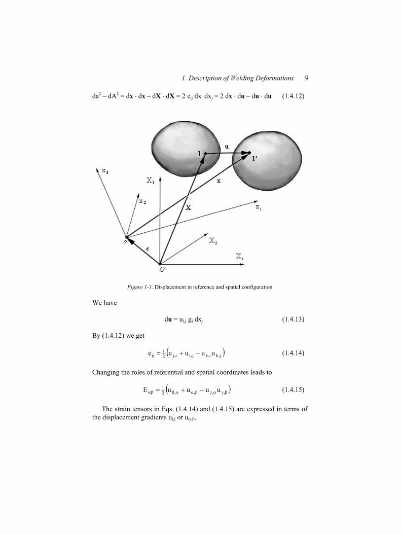
Let a material point be displaced from the position 1 to the position 1’
and let the origins of the referential and spatial coordinates be at 0 and o
respectively. The vectors X, x, c and displacement u are shown in the Figure
1-1. We have
uXcx (1.4.9)
At a neighboring point
(x + dx) + c = (X + dX) + (u + du) (1.4.10)
By (1.4.10)
dx = dX + du
If
da2 = dx dx and dA2 = dX dX (1.4.11)
and, from Eq. (1.4.10)
1. Description of Welding Deformations 9
da2 – dA2 = dx dx – dX dX = 2 eij dxi dxj = 2 dx du – du du (1.4.12)
Figure 1-1. Displacement in reference and spatial configuration
We have
du = ui,j gi dxj (1.4.13)
By (1.4.12) we get
jkikjiij21
ij uuuue ,,,, (1.4.14)
Changing the roles of referential and spatial coordinates leads to
,,,, uuuuE21 (1.4.15)
The strain tensors in Eqs. (1.4.14) and (1.4.15) are expressed in terms of
the displacement gradients ui,j or u , .
10 Theory of Thermomechanical Processes in Welding
If the displacement gradients are infinitesimal
1u ji, (1.4.16)
then Eq. (1.4.14) reduces to
jiij21
ij uu ,, (1.4.17)
The infinitesimal strain defined by Eq. (1.4.16) is known as Cauchy
strain tensor.
The relation (1.4.16) is called the hypothesis of infinitesimal
transformation. With this assumption the Green-Lagrange strain is
ijji gg (1.4.18)
and the principal values of both strains are the same. Thus for infinitesimal
transformation there is no difference between spatial and referential strain
measures.
Consider the elements dX which defined a sphere of radius Ro at X.
If radius is constant, then
2o
2 RdXdXGdA (1.4.19)
Since
da2 = dx dx dA2 = dX dX (1.4.20)
Eq. (1.3.10) can be rearranged to the form
jiij12 dxdxBdA (1.4.21)
Substituting dA from Eq. (1.4.19) we get
jiij12
o dxdxBdXdXGR (1.4.22)
The rotation is characterized by the R tensor
ijji21
ij uuR ,, (1.4.23)
1. Description of Welding Deformations 11
The dual or axial vector is given by
i2
1k,jijk2
1
k,jikj4
1k,jijk4
1j,kk,jijk4
1jkijk2
1i
ucurlu
uuuuR (1.4.24)
The symbol ijk is given by
geijkijk (1.4.25)
where g = det gij and eijk is so-called a permutation symbol defined by the set
of equations
1eee
1eee
213321132
312231123 (1.4.26)
and all other values of i,j and k make eijk zero.
By (1.4.17) and (1.4.23)
ijijji Ru , (1.4.27)
kijkijjiu , (1.4.28)
If the space is Euclidean, making use of Eq. (1.4.17)
likjjikl21
ikjl
kjliijlk21
jlik
lijkkijl21
ijkl
jkliiklj21
klij
uu
uu
uu
uu
,,,
,,,
,,,
,,,
(1.4.29)
By Eqs. (1.4.29) we find the so-called compatibility conditions
0ikjljlikijklklij ,,,, (1.4.30)
This set of equations reduces to six independent equations when the
symmetry of is taken into account.
12 Theory of Thermomechanical Processes in Welding
1.5 Particulate and Material Derivatives
Let G (X, t) be a field in a Lagrange description. The time derivative of a
field G (X, t) multiplied by the infinitesimal time interval dt is equal to the
variation between times t and t + dt of the function G (X, t), which would be
recorded by an observer attached to the material particle which is located in
the reference configuration by position vector x. In terms of Euler variables
the particulate derivative with respect to the material is the total time
derivative of the field g [x (X, t)] = G (X, t)
vggradt
g
dt
dg (1.5.1)
For example, substituting v for g in Eq. (1.5.1) the expression for
acceleration a in Euler variables can be written as
vvvv
gradtdt
da (1.5.2)
Consider the volume integral
dVtg
V
x,G (1.5.3)
where g (x, t) is the volume density in the current configuration.
Let G(X, t) be the volume Lagrangian density, then the corresponding
Eulerian density is g(x, t)
rdVtGdVtg X,x, (1.5.4)
where the volume Vr refers to the reference configuration of the volume V in
the current configuration.
The time derivation of Eq. (1.5.3) throughout the relation (1.5.4) has the
form
rV
rdVdt
dG
dt
dG (1.5.5)
The expression (1.5.5) represents the particulate derivative of the volume
integral G in terms of Lagrange variables.
1. Description of Welding Deformations 13
In order to obtain the particulate time derivative in Eulerian variables the
equality (1.5.4) must be taken.
By Eqs. (1.3.20) and (1.5.1) and the expression
vvv ggraddivggdiv (1.5.6)
we get
dVgdivt
gdV
dt
dGr v (1.5.7)
The particulate derivative of the volume integral G with respect to the
material derived in Eulerian variables yields
dVgdivt
g
dt
d
V
vG
(1.5.8)
The alternative form of Eq. (1.5.8) can be obtained by using the
divergence theorem. Thus
dagdVt
g
dt
d
V a
r nvG
(1.5.9)
where a is the surface of the volume V.
The first term of the right-hand side of Eq. (1.5.9) represents the variation
of the field g between time t and t + dt in volume V, and the other one due to
the movement of the same material volume.
The material derivative is used to determine the variation between time t
and t + dt of any physical quantity attached to the whole material, which is
contained at time t in volume V. The particulate derivative with respect to
the material only partially takes into account this variation. It ignores any
mass particles leaving the volume V, which is followed in the material
movement.
In the infinitesimal time interval dt = Dt the variation of quantity g
attached to the whole matter at time t in the volume V as the variation DG of
the integral G given by Eq. (1.5.5) involves
V
dVtgdt
d
Dt
Dx,
G (1.5.10)
14 Theory of Thermomechanical Processes in Welding
Substituting Eq. (1.5.9) of the particulate derivatives with respect to the
material of the volume integral we obtain
V a
dagdVt
g
Dt
Dnv
G (1.5.11)
1.6 Mass Conservation
Let be a scalar field defined on body B, where is referred to the mass
density of the material of which the body is composed. The mass contained
in the infinitesimal volume dV is equal to dV. We assume no overall mass
creation, which implies the global mass balance
V
0dVDt
D (1.6.1)
By Eqs. (1.5.11) and (1.6.1) the mass balance reads
V a
0dadVdt
nv (1.6.2)
Applying the divergence theorem to Eq. (1.6.2) we get the local mass
balance equation or continuity equation
0divt
v (1.6.3)
or equivalently
0divt
v (1.6.4)
The mass dV, which is contained in volume dV, may be written as
dV = o dVr (1.6.5)
where o and are the mass densities in the reference and current
configurations respectively.
The mass conservation may now be written as
1. Description of Welding Deformations 15
0dVDt
D
rV
ro (1.6.6)
From the transport formula it is evident that the conservation of mass in
Lagrange variables can be expressed in the form
J = o (1.6.7)
Chapter 2
STRESS TENSOR
2.1 Momentum
The linear momentum p of the material occupying the volume V in the
configuration at time t by a moving material body Bt is defined by the
relation
V
dVvp (2.1.1)
where v is the velocity of the material particle at the point x.
Another important quantity is the angular momentum H which is defined
by the relation
V
dVvxH
V
kjijki dVvxH (2.1.2)
where x is the position of a representative point of V relative to an origin o
and H being the angular momentum with respect to o.
Equations of motion in Euler description is given in the form of the two
principles. The first one is: the rate of change of linear momentum p is equal
to the total applied force F
Fp (2.1.3)
The second one says: the rate of change of angular momentum H is
equal to the total applied torque , i.e.
18 Theory of Thermomechanical Processes in Welding
H = (2.1.4)
Two types of external forces are assumed to act on a body B. The first
are body forces, such as gravity acting on material element throughout the
body and can be described by a vector field f which is referred to as the body
force per unit mass and which is defined on the configurations of B. The
second are surface forces such as friction which act on the surface elements
of area and can be described by a vector t which is referred to as the surface
fraction per unit area and which is defined on the surface a of the material.
The total force F is defined as
aV
dadV tfF (2.1.5)
The second integral on the right-hand side of Eq. (2.1.5) represents the
contribution to F of the contact force acting on the boundary a of the
arbitrary material region of the volume V.
The total torque about the origin o is defined as
dadV
aV
txfx (2.1.6)
The second integral on the right-hand side of Eq. (2.1.6) represents the
contribution to of the contact forces acting on the boundary a of the
arbitrary region.
2.2 The Stress Vector
In the course of deformation of solids, on account of volume and
geometrical shape changes, interactions between molecules come into being
that oppose these changes. The concept that the action of the rest of the
material upon any volume element of it was of the same form as distributed
surface forces was introduced by Cauchy. In other words the effect of the
material on one side of a surface a, on the material on the other side is
equivalent to a distribution of force vector t per unit area. The force vector
per unit area t is also called the surface traction or stress vector.
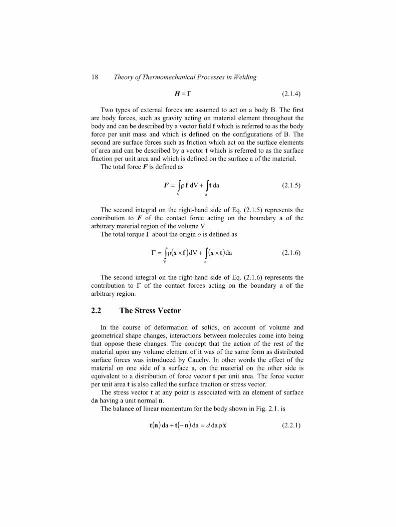
The stress vector t at any point is associated with an element of surface
da having a unit normal n.
The balance of linear momentum for the body shown in Fig. 2.1. is
xntnt dadada d (2.2.1)
2. Stress Tensor 19
Figure 2-1. The stress vector on body surface
when the dependence of the stress vector on direction is written in the form
nt and xda are peripheral forces.
In the case when d tends to zero, then by Eq. (2.2.1)
ntnt (2.2.2)
The above has the same form as Newton’s third law, i.e. action and
reaction are equal and opposite.
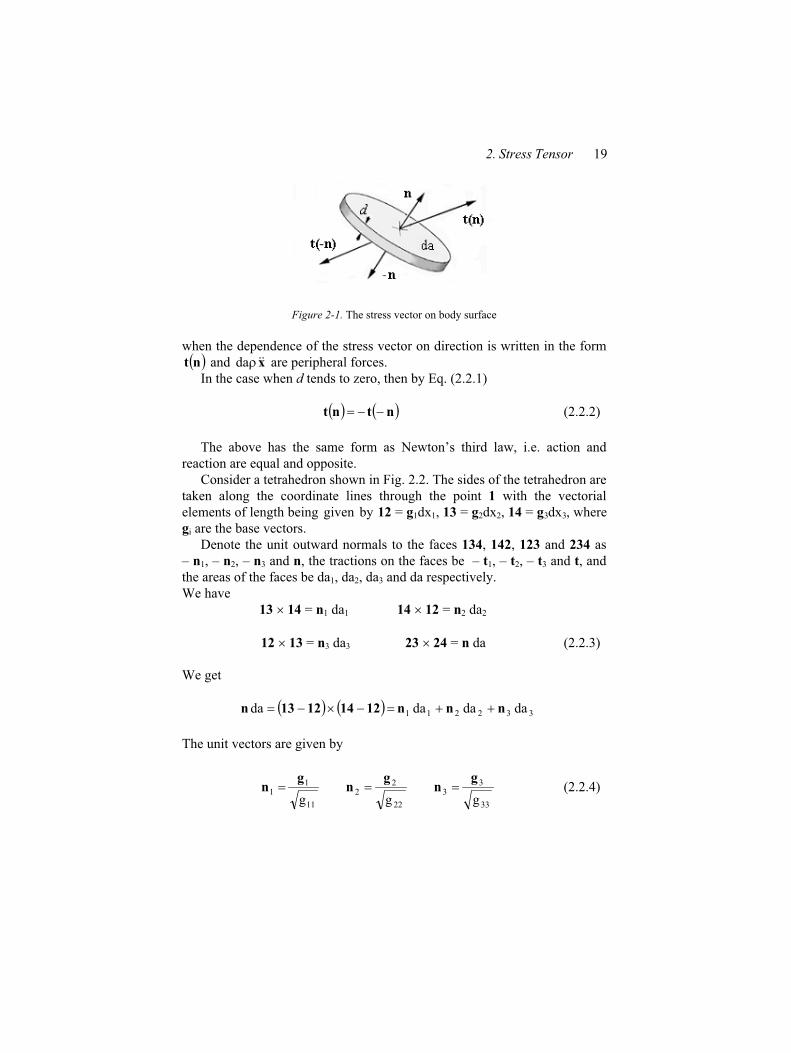
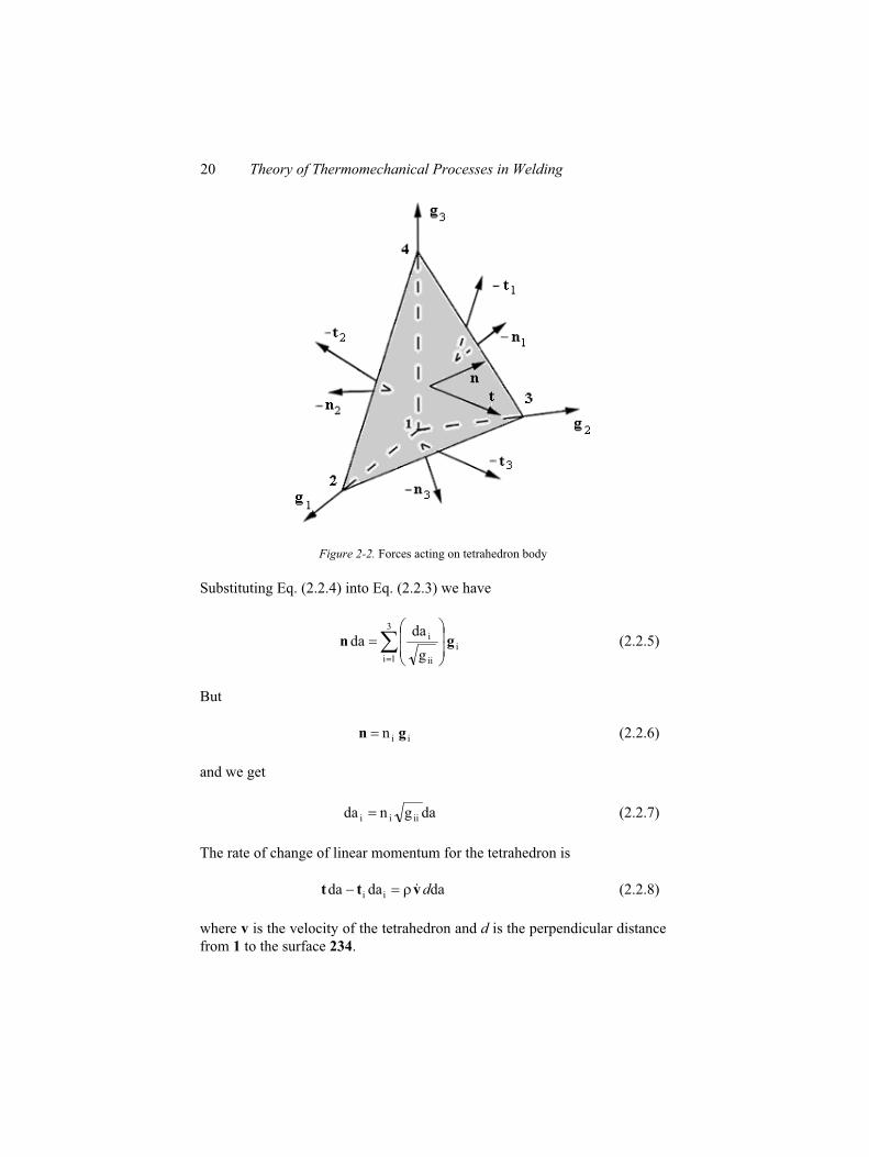
Consider a tetrahedron shown in Fig. 2.2. The sides of the tetrahedron are
taken along the coordinate lines through the point 1 with the vectorial
1 1 2 2 3 3
gi are the base vectors.
Denote the unit outward normals to the faces 134, 142, 123 and 234 as
– n1, – n2, – n3 and n, the tractions on the faces be – t1, – t2, – t3 and t, and
the areas of the faces be da1, da2, da3 and da respectively.
We have
13 14 = n1 da1 14 12 = n2 da2
12 13 = n3 da3 23 24 = n da (2.2.3)
We get
332211 dadadada nnn12141213n
The unit vectors are given by
33
33
22
22
11
11
ggg
gn
gn
gn (2.2.4)
elements of length being given by 12 = g dx , 13 = g dx , 14 = g dx , where
20 Theory of Thermomechanical Processes in Welding
Figure 2-2. Forces acting on tetrahedron body
Substituting Eq. (2.2.4) into Eq. (2.2.3) we have
3
1i
i
ii
i
g
dada gn (2.2.5)
But
iin gn (2.2.6)
and we get
dagnda iiii (2.2.7)
The rate of change of linear momentum for the tetrahedron is
dadada ii dvtt (2.2.8)
where v is the velocity of the tetrahedron and d is the perpendicular distance
from 1 to the surface 234.
2. Stress Tensor 21
By Eqs. (2.2.8) and (2.2.7) we get
3
1i
iiii gntt (2.2.9)
Since
jjjijiii tTg gtgt (2.2.10)
it is evident, that Eq. (2.2.9) implies that t must be a linear transformation of
n; i.e.
nTtT (2.2.11)
which relates the stress vector to the unit normal n, it being noted that T is
defined on the configurations of the material body and in particular does not
depend upon n.
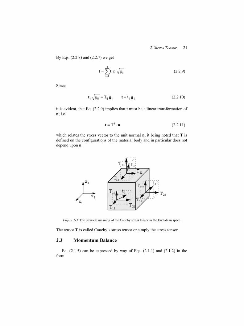
Figure 2-3. The physical meaning of the Cauchy stress tensor in the Euclidean space
The tensor T is called Cauchy’s stress tensor or simply the stress tensor.
2.3 Momentum Balance
Eq. (2.1.5) can be expressed by way of Eqs. (2.1.1) and (2.1.2) in the
form
22 Theory of Thermomechanical Processes in Welding
V aV
dadVdVDt
Dtfv (2.3.1)
V aV
dadVdVDt
Dtxfxvx (2.3.2)
Equation (2.3.1) shows that the creation rate due to the external forces
acting on material is the instantaneous time derivatives of the linear
momentum of the material in the volume V.
Equation (2.3.2) states the same, but concerns the angular momentum. In
Eulerian expression of the material derivative of the volume integral, the
left-hand side of Eq. (2.3.1) can be expressed as
dadVt
dVDt
D
aVV
nvvvv (2.3.3)
In Eq. (2.3.3) the volume integral corresponds to the time variation of
linear momentum in elementary volume V, and the surface integral
corresponds to the momentum carried away by the material leaving the same
geometrical volume.
Similarly, if g = x ( v) the right-hand side of (2.3.2) can be rewritten as
aVV
dadVt
dVDt
Dnvvxvxvx (2.3.4)
Altogether Eqs. (2.3.1) – (2.3.4) describe the Euler theorem, which can
be stated as follows. In a referential frame, for any material subdomain V the
resultant of the elementary body and surface forces and the resultant of the
corresponding elementary moments are respectively equal to the resultant
and the overall moment of vectors
dVt
v (2.3.5)
distributed in the volume V, and the resultant and the overall moment of
vectors
danvv (2.3.6)
2. Stress Tensor 23
distributed on the surface a of the domain V.
By the divergence theorem, Eqs. (2.3.3) and (2.3.4) are rewritten in the form
dVdivdVt
dVDt
D
VVV
vvvv (2.3.7)
dVdivdVt
dVDt
D
VVV
vvxvxvx (2.3.8)
By the relation
vv*vv*vv* divgraddiv (2.3.9)
we get
vvvvv
vvv divt
gradt
divt
(2.3.10)
By Eq. (1.5.2) we get
dt
ddiv
t
vvvv (2.3.11)
The expressions (2.3.7), (2.3.8) and (2.3.11) give a new form of the
momentum balance namely the dynamic theorem
aVV
aVV
dadVdVdt
d
dadVdVdt
d
txfxv
x
tfv
(2.3.12)
which states that the resultant of the elementary body and surface forces and
the resultant of the corresponding elementary moments are equal
respectively to the resultant and the overall movement of the elementary
dynamic forces.
Substituting from Eq. (2.2.11) for t in Eq. (2.3.1) and rearranging by way of
Eq. (1.6.4) gives
24 Theory of Thermomechanical Processes in Welding
aV
dadVdt
dTnf
v (2.3.13)
Using the divergence theorem Eq. (2.3.13) can be rearranged into the
form
0dVdivdt
d
V
Tfv
(2.3.14)
The condition that Eq. (2.3.14) holds for all arbitrary material regions V
leads to the field equation form of the balance of linear momentum
fTv
divdt
d (2.3.15)
which is Cauchy’s equation of motion.
2.4 Properties of the Stress Tensor
Consider the components of the stress tensor Tij at some point x in the
current configuration Bt. By Eqs. (2.2.9) and (2.2.11) it follows that
jiiiiT
jjiij gT gtgTgTgg (2.4.1)
From Eq. (2.4.1) it is seen that Tij can be interpreted as the j component of
the force per unit area in Bt acting on a surface segment which outward
normal at x is in the i direction. At a given point x, there exists in general
three mutually perpendicular principal directions 321aa ,,n , with
components 321inia ,, which are the solutions of equation
0nT jijij (2.4.2)
corresponding to the roots 321aa ,, which are called the principal
stresses.
The stress tensor at x have the representations
3
1a
aaa nnT (2.4.3)
2. Stress Tensor 25
The stress vector can be resolved into a component normal to the surface
element t(n) and a component t(s) tangential to the surface element. The
component t(n) is called the normal stress and t(s) the shearing stress.
The magnitude (n) of t(n) is given by
jiijii(n)(n) nnTntntt (2.4.4)
Using Eq. (2.4.4), (n) can be written in the form
233
222
211(n) nnn (2.4.5)
The shearing stress t(s) can be written as
(n)(s) ttt (2.4.6)
and its magnitude (s) is given by
2233
222
211
23
23
22
22
21
21
2(n)
2(s)(s)
2(s)
nnnnnn
ttt (2.4.7)
Let n1 = 0 and 2
1nn 2
322 . Substituting in Eq. (2.4.7) we get
32(s)2
1 (2.4.8)
The values of (s) satisfying such relations are called the principal
shearing stresses. The maximum shearing stress is thus equal to half the
difference between the maximum and minimum principal stresses and acts
on a plane which makes an angle of 45 with the directions of these principal
stresses.
The characteristic equation for T is
0JJJ a2a
3a T3T2T1 for a = 1, 2, 3 (2.4.9)
when J1T, J2T, J3T are called the invariants.
Taking the coordinate axes as the principal directions it can be shown that T
has the form
26 Theory of Thermomechanical Processes in Welding
3
2
1
ij
00
00
00
T (2.4.10)
The invariants can be written as
321
133221
321
T3
T2
T1
J
J
J
(2.4.11)
The deviator of the stress tensor 'T is defined as
ITTT tr3
1' (2.4.12)
The expression Ttr3
10T is called the mean normal stress.
2.5 The Virtual Work Rate
Let v* be any velocity field. Owing to its definition, the strain work rate
RSR (v*) associated with any velocity field v* and relative to material
domain V, reads
VaV
SR dV*da*dV**R avtvfvv (2.5.1)
The last term of Eq. (2.5.1) represents the work rate of inertia forces and
the first two integrals of the right-hand side of Eq. (2.5.1) represent the work
rate of the external body and surface forces.
The symmetry of the stress tensor T and the divergence theorem applied
yield the identity
Va
dVdiv**da* TvDTnTv (2.5.2)
where *ijijDT*DT and D* is the strain rate associated with velocity field
v*
2. Stress Tensor 27
T***2 LLD (2.5.3)
where L* = grad v*.
By the motion equation (2.3.15) and Eq. (2.5.2) the strain work rate
RSR (v*) defined by (2.5.1) can be written as
dV**dr*dr*R SR
V
SRSR DTvvv (2.5.4)
where drSR (v*) is the infinitesimal strain work rate of the elementary
material domain dV.
If velocity field v* is equal to velocity v i.e. it is an actual velocity of the
material particle, then
dVdrSR DTv (2.5.5)
The work rate of the internal forces denoted as RIF is the opposite of the
strain work rate RSR i.e.
SRIFSRIF dr*dr*R*R vvv (2.5.6)
The strain work rate of external forces is defined as
aV
EF da*dV**R tvfvv (2.5.7)
and the work rate of inertia forces is
V
IN dV**R avv (2.5.8)
The virtual work rate theorem is simply rewriting Eq. (2.5.1) in terms of
(2.5.7.) and (2.5.8)
0*R*R*R IFINEF vvv (2.5.9)
for every volume V and velocity v*.
It states that for any actual or virtual velocity field v* and for any
material domain V, the sum of the external forces REF (v*), inertia forces
RIN (v*) and internal forces RIF (v*) is equal to zero.
28 Theory of Thermomechanical Processes in Welding
2.6 The Piola-Kirchhoff Stress Tensor
The strain work rate drSR defined by (2.5.5) is independent of the choice
of the coordinate system used to describe the motion. The definition (2.5.5)
corresponds to a Eulerian description.
By Eqs. (1.3.20) and (1.3.22) the expression (2.5.5) can be written as
r
T11SR dV
dt
dJdVdr
EFFDv (2.6.1)
where dE/dt is the transformation of D in the reference configuration
1T1
dt
dF
EFD (2.6.2)
Equation (2.6.1) serves to introduce the symmetric Piola-Kirchhoff stress
tensor S defined by
T11J FTFS (2.6.3)
The tensors D and dt
d E represent the same material tensor in different
configurations.
Using Eqs. (2.6.1) and (2.6.3), the Lagrangian description of the
elementary and overall strain work rates drSR (v) and RSR (v) are given,
respectively, by
rSR dVdt
ddr
ESv
rV
rSRSR dVdrR vv (2.6.4)
The definition (2.6.3) of Piola-Kirchhoff stress tensor S gives
F S N dA = T n da (2.6.5)
The dynamic theorem Eq. (2.3.12) throughout Eqs. (2.2.11) and (2.6.5)
expresses the equality between the dynamical resultant of external forces for
the material domain V in a Lagrangian description as
0dVdt
ddA
rV
ro
A
vfNSF (2.6.6)
2. Stress Tensor 29
where the domain Vr and the surface A enclosing this domain in reference
configuration correspond to the domain V and the surface a enclosing it in
the current configuration.
The equation of motion in a Lagrangian description is obtained by the
transformation of the surface integral into volume integral throughout the
divergence theorem
0dt
dDiv o
vfSF (2.6.7)
0dt
dvfS
X
x
X
iio
i (2.6.8)
The body force f and the accelerations dt
d vare evaluated in the above
equations at point x in the current configuration.
2.7 The Kinetic Energy Theorem
The kinetic energy K of the whole matter of the volume V is represented
by the expression
dV2
1K
V
2v (2.7.1)
The kinetic energy expression can be written in reference configuration as
r2
o
V
dV2
1K
r
v (2.7.2)
The definition of the material derivative of the integral of an extensive
quantity yields
dt
dK
Dt
DK (2.7.3)
The definition of material acceleration dt
d v given by Eq. (1.5.2) lead to
the following form of Eq. (2.7.1)
30 Theory of Thermomechanical Processes in Welding
dVdt
d
Dt
DK vv (2.7.4)
The material derivative of the kinetic energy corresponds to the opposite
of the work rate of the inertia forces, which they develop in the actual
movement. The inertia forces relative to the material develop their work rate
in their own movement.
Let the velocity field v* be the actual material velocity field v in the
virtual work rate theorem (2.5.9). Together with Eq. (2.7.4) it gives the
kinetic energy theorem
vv EFSR RRDt
DK (2.7.5)
It states that in the actual movement and for any domain V, the work rate
of the external forces is equal to the sum of the material derivative of the
kinetic energy and of the strain work rate associated with the material strain
rate.
Chapter 3
THERMODYNAMICAL BACKGROUND OF
WELDING PROCESSES
3.1 Introduction
In order to derive the thermal and mechanical equations of welding
processes it is necessary to consider welding as a thermodynamical process.
In such an approach the thermodynamical state of material system is
characterized by the value of a finite set of state variables.
The characterization of a material leads to the characterization of its
energy state, except kinetic energy. Thermostatics studies reversible and
infinitely slow evolutions between two equilibrium states of homogeneous
systems. The state variable necessary for the description of the evolutions
throughout the first and the second laws of thermodynamics are directly
observable and are linked by state equations through state functions
characterizing the energy of the material system. Thermodynamics in
contrast with thermostatics is the study of homogeneous systems in any
evolution process. These evolutions are reversible, or not, and occur at any
rate. The postulate of local state is to extend the concepts of thermostatics to
these evolutions.
The postulate of local state for a homogeneous system is the following.
The present state of a homogeneous system in any evolution can be
characterized by the same variables as at equilibrium, and is independent of
the rate of evolution.
The equilibrium fields of mechanical variables in a closed continuum,
considered as a thermomechanical system are generally not homogeneous.
The state of a continuum is characterized by fields of state variables. The
local values of these variables characterize the state of the material particles,
32 Theory of Thermomechanical Processes in Welding
which constitute the continuum, and are considered as an elementary
subsystem in homogeneous equilibrium.
The local state postulate for closed continua says that the elementary
systems satisfy the local state postulate of a homogeneous system. The
thermodynamics of closed continua is the study of material, which satisfies
the extended local state postulate.
The local state postulate for closed continua is local in two aspects. It is
local considering the time scale relative to the evolution rates and it refers to
the space scale, which defines the dimensions of the system.
3.2 The First Law of Thermodynamics
The conservation of energy is expressed by the first law of
thermodynamics. It states that the material derivative of energy E of the
material body contained in any domain V at any time is equal to the sum of
the work rate REF of the external forces acting on this body, and of the rate
Qo of external heat supply.
The kinetic energy K of the body and the internal energy E together gives
the total energy of body E. The energy has an additive character. The
internal energy E can be expressed by a volume density e such that edV is
the internal energy of the whole body contained in the elementary domain
dV.
The energy E of the body volume V is expressed as
VV
2 edVdV2
1vEKE (3.2.1)
where e is a volume density, not a density per mass unit.
The hypothesis of external heat supply assumes that the external heat
supply is due to contact effects, with the exterior through surface a limiting
the material volume V which is the external heat provided by conduction.
The external heat supply is also due to external volume heat sources. The
rate Qo can be written as
Va
o rdVqdaQ (3.2.2)
where q is the surface rate density of heat supply by conduction. The
quantity q is assumed to be a function of position vector x, time t and
outward unit normal n to the surface a
3. Thermodynamical Background of Welding Processes 33
) t,,(qq nx (3.2.3)
In Eq. (3.2.2) the density r = r (x, t) is a volume rate density of the heat
provided to V.
The total work rate REF (v) of the external forces in the whole body in
volume V is
Va
EF dVdaR fvtvv (3.2.4)
then for any volume V the first law of thermodynamics reads
oEF QR
Dt
D
Dt
D
Dt
D EKE (3.2.5)
Combining the first law (3.2.5) and the kinetic energy theorem (2.7.5)
yields
oSR QR
Dt
DE (3.2.6)
which expresses that the internal energy variation DE in time interval dt is
due to the total strain work RSRdt and the external heat supply Qdt.
3.3 The Energy Equation
The material derivative of the internal energy is obtained by letting g = e
in Eq. (1.5.8) of the material derivative of a volume integral
dVedivt
eedV
Dt
D
Dt
D
VV
vE
(3.3.1)
Making use of (3.2.2), (2.5.4), (3.1.1) and the energy balance (3.2.6) we get
aV
qdadVredivt
eDv (3.3.2)
Letting for f (x, t, n) = – q (x, t, n) in the relation
34 Theory of Thermomechanical Processes in Welding
aV
datfdVth n,x,x, (3.3.3)
we get
nqq (3.3.4)
where q is the heat flux vector. Using the expression (1.5.1) of the
particulate derivative for the internal energy e, the local expression for the
first law of thermodynamics in the Eulerian approach is
qDTv divrdivedt
de (3.3.5)
The expression (3.3.5) is called the Eulerian energy equation.
Multiplying Eq. (3.3.5) by dV and using Eq. (2.6.4) we have
dVdivrdredVdt
dSR q (3.3.6)
The expression (3.3.5) corresponds to a balance of internal energy for the
elementary material system dV. In Eq. (3.3.6) the term d (e dV) represents
the variation of internal energy of the body observed from the material
particle between time t and t + dt. Equation (3.3.6) indicates that this
variation is equal to the energy supplied to the open system during the same
interval.
The energy supply is the sum of two terms: the elementary strain work
drSR, that corresponds to the part of the external mechanical energy given to
the system and not converted into kinetic energy and the external heat
provided both by conduction given by the term – div q dt dV and by external
volume heat sources given by the term r dt dV.
Define the Lagrangian vector Q by the relation
dadA nqNQ (3.3.7)
The expression (3.3.7) represents the heat flux q n d a throughout the
oriented material surface d a = n d a in terms of the oriented surface
dAr = N dA.
By (1.3.17) we get
JQ/Fq (3.3.8)
3. Thermodynamical Background of Welding Processes 35
The Lagrangian volume density of internal energy E = E (x, t) is given by
E dVr = e dV (3.3.9)
By using Eq. (3.3.9)
rdVdt
ddV
ESDT rRdVrdV (3.3.10)
From Eq. (3.3.6) finally we get
QE
S DivRdt
d
dt
dE (3.3.11)
which corresponds to the Lagrangian formulation of the Eulerian energy
equation (3.3.5).
3.4 The Second Law of Thermodynamics
The conservation of energy is expressed by the first law. The second law
is of a different kind. It states that the quality of energy can only deteriorate.
The quantity of energy transformed to mechanical work can only decrease
irreversibly. In the second law a new physical quantity is introduced,
entropy, which represents a measure of this deterioration and which can
increase when considering an isolated system. In a system that is no longer
isolated, the second law defines a lower bound to the entropy increase,
which takes into account the external entropy supply. The latter is defined in
term of a new variable, the temperature. The second law can be formulated
as below.
The material derivative of a thermodynamic function S, called entropy
attached to any material system V is equal or superior to the rate of entropy
externally supplied to it. The external entropy rate supply can be defined in
terms of a universal scale of absolute temperature denoted by r and
positively defined.
The external entropy rate is then defined as the ratio of the heat supply
rate and the absolute temperature at which the heat is provided to the
considered subsystem. We denote by s the entropy volume density, such that
the quantity sdV represents the entropy of all the matter presently contained
in the open elementary system dV.
36 Theory of Thermomechanical Processes in Welding
The total entropy S of all the matter contained in V is
V
sdVS (3.4.1)
The second law reads
V ra
dVr
daTDt
D nqS (3.4.2)
The right-hand side of inequality (3.4.2) represents the rate of external
entropy supply. This external rate is composed of both the entropy influx
associated with the heat provided by conduction through surface a enclosing
the considered material volume V, and of the volume entropy rate associated
with the external heat sources distributed within the same volume.
Eq. (3.4.2) implies that the internal entropy production rate cannot be
negative in real evolutions. The entropy S of a material system V at q = 0
and r = 0 cannot spontaneously decrease.
The material derivative of a volume integral in the Eulerian expression
for g = s reads
dVsdivt
ssdV
Dt
D
Dt
D
VV
vS
(3.4.3)
By Eqs. (3.4.2) and (3.4.3) it follows that the volume integral must be
non-negative for any system V,
0r
divsdivt
s
rr
qv (3.4.4)
where the surface integral has been transformed to the volume integral. The
expression (3.4.4) can be rewritten as
0r
divdivst
s
rr
qv (3.4.5)
Multiplying Eq. (3.4.5) by dV, the above inequality becomes
3. Thermodynamical Background of Welding Processes 37
0dVr
divdVsdt
d
rr
q (3.4.6)
In Eq. (3.4.6) the term sdVdt
d represents the variation in entropy of this
open system, during the infinitesimal time interval dt observed from any
material point.
By energy equation (3.3.5), the fundamental inequality (3.4.5) can be
written as
0graddivsedt
de
dt
dsr
r
rr
qvDT (3.4.7)
Now we define the free volume energy of the open system dV
= e – r s (3.4.8)
By Eqs. (3.4.8) and (3.4.7) we get
0graddivdt
d
dt
ds r
r
r qvDT (3.4.9)
The Eq. (3.4.9) is the fundamental inequality or so-called Clausius-
Duhem inequality. It corresponds to a Eulerian approach.
The Lagrangian approach of the fundamental inequality leads to
expressing DS/Dt in terms of the Lagrangian entropy density S defined by
S dVr = s dV (3.4.10)
By transport formula (3.3.7) and (3.3.10) together with a Lagrangian
expression of the material derivative of the integral of an extensive variable,
the inequality (3.4.2) can be rewritten as
r rr V V
r
r
r
r
r
V
r dVR
dAdVdt
dSdVS
Dt
D
Dt
D NQS (3.4.11)
The expression (3.4.11), which holds for any domain Vr can be written in
Lagrangian formulation of the Eulerian inequality in the form
38 Theory of Thermomechanical Processes in Welding
0R
Divdt
dS
rr
Q (3.4.12)
By the Lagrangian energy equation (3.3.11) and the positiveness at
absolute temperature r, from the inequality (3.4.12) it follows that
0Graddt
dE
dt
dS
dt
dr
r
r
QES (3.4.13)
We define the free Lagrangian energy density as
dVr = dV = E – r S (3.4.14)
By Eqs. (3.4.13) and (3.4.14) we get
0Graddt
d
dt
dS
dt
dr
r
r QES (3.4.15)
The expression (3.4.15) is the Lagrangian formulation of the Clausius-
Duhem inequality.
3.5 Dissipations
The left-hand side of Eq. (3.4.15) which will be noted is the
dissipation per unit of initial volume dVr. The second law requires the
dissipation and the associated internal entropy production / r to be non-
negative. The dissipation is the sum of two terms
= 1 + 2 (3.5.1)
where
dt
d
dt
dS
dt
d r1
ES (3.5.2)
The local state postulate assumes that all the quantities appearing in Eq.
(3.5.2) depend only on the state variables characterizing the free energy
dVr of the open elementary system dVr.
3. Thermodynamical Background of Welding Processes 39
The second dissipation 2 is defined as
r
r
2 GradQ
(3.5.3)
and is called the thermal dissipation associated with heat conduction. By
definition (3.4.14) of and definition of 1 (3.5.2), the Lagrangian energy
equation (3.3.11) is rewritten as
1r DivRdt
dSQ (3.5.4)
The expression (3.5.4) is called the Lagrangian thermal equation. Using
Eqs. (3.5.3) and (3.5.4) we get
r
r
r
rr
r dVdVDivR
dVSdt
d Q (3.5.5)
The thermal equation (3.5.4) or equivalently Eq. (3.5.5) corresponds to a
balance in entropy for the elementary system dVr. The term d(SdVr) is the
entropy variation, during the time interval dt, observed from the point of the
open system dVr.
The internal source of entropy ( / r) dt dVr is the sum of the production
( 2/ r) dt dVr associated with heat conduction and the production ( 1/ r) dt
dVr associated with the mechanical dissipation 1 dVr dt. As it will be seen
later, 2 dVr dt corresponds to a mechanical energy converted into heat by
mechanical dissipation. Thus, the mechanical dissipation 1 appears as a
heat source in thermal equation (3.5.4).
A Lagrangian approach to thermal equation is introduced below. If i is
the Eulerian dissipation volume densities, then
i dV = i dVr J i = i (3.5.6)
The respective expressions can be written as
r
r
2
r1
grad
divdt
d
dt
ds
q
vDT
(3.5.7)
40 Theory of Thermomechanical Processes in Welding
By Eqs. (3.5.1) and (3.5.6), for the densities i the following relation
holds
1 + 2 0 (3.5.8)
The Eulerian thermal equation takes the form
1r divrdivsdt
dsqv (3.5.9)
3.6 Equations of State for an Elementary System
For any evolution of the continuum the energy states of the elementary
systems depend on the same state variables as at equilibrium. The free
energy volume density depends locally on the state variables, but not on
their rates nor on their spatial gradients. We assume that it is also true for the
Piola-Kirchhoff stress tensor S. In Eq. (3.5.1) the dissipation 2 depends on
Grad T. Let Grad T = 0 ( 2 = 0), then the non-negativeness of intrinsic
dissipation 1 is derived independently of the non-negativeness of total
dissipation
0dt
d
dt
dS
dt
d r1
ES (3.6.1)
The expression (3.6.1) is derived from the second law and the local state
postulate.
In Eq. (3.6.1) the energy S dE represents the energy supplied to the
elementary system dVr, not in the form of heat and not converted into kinetic
energy during the time interval dt. It is actually supplied if positive,
extracted if negative. The energy d + Sd r = dE – rdS is the part of the
previous energy that the system effectively stores in the time interval dt in
any other form but heat. It is actually stored if positive, extracted if negative.
The Lagrangian expression of the particulate derivatives used here do not
involve gradients, contrary to the corresponding Eulerian expression, which
has importance in this reasoning.
The free energy can be written as
= ( r, E , m1, …, mn) (3.6.2)
based on the local state postulate.
3. Thermodynamical Background of Welding Processes 41
The variables r, E , m1, …, mn constitute a set of state variables
characterizing the state of the open system dVr. By the local state postulate,
these state variables are macroscopic variables.
The non-negativeness of the intrinsic dissipation expressed by (3.6.1)
gives
0dt
dS
dt
d
dt
d r
r
m
m
E
ES (3.6.3)
In Eq. (3.6.3) E stands for the tensor of components E and
I
I
mmdt
dm
m
m
m (3.6.4)
where
dt
d mm (3.6.5)
The inequality (3.6.3) is relative only to this elementary open system dVr
under consideration.
We state that a set of state variables characterizing an elementary system
is normal if variations of this particular state can occur independently of the
variations of the other variables of the set.
The hypothesis introduced by Helmholtz states that it is possible to find a
set of variables, which is normal with respect to absolute temperature r. In
Eq. (3.6.3) with such a set of variables, real evolution can occur with
arbitrary variations d r and zero variations for the other variables of the set.
From Eq. (3.6.3) it follows that
r
S (3.6.6)
because the inequality (3.6.3) must remain satisfied for these particular real
evolutions, and assuming that the present value of entropy S is independent
of the temperature rate d r/dt.
Assume that the variable set is normal with respect to the state variables
E , and that the present value of the Piola-Kirchoff stress tensor S is
independent of the rates dE/dt.
42 Theory of Thermomechanical Processes in Welding
Then we have
ES (3.6.7)
Equation (3.6.7) associates the state variables r, E with their dual
thermodynamic variables –S and S. They are called the state equations of the
system. They still hold for a system of evolution in holding at equilibrium.
3.7 The Heat Conduction Law
By the second law of thermodynamics and the local state postulate we
get the relation
1 + 2 0 1 0 (3.7.1)
where the Eulerian dissipations 1 and 2 are the intrinsic dissipation and the
dissipations associated with transport phenomena, per unit volume dV in the
current configuration expressed by (3.5.6). The internal entropy production
rate 2/ r is due to the assembly of adjacent elementary systems that ensures
the continuity of the medium, contrary to the intrinsic internal entropy
production rate 1/ r related to the elementary system, which is considered
independently of the other system.
The hypothesis of dissipation decoupling which is more restrictive than
the above assumes
1 0 2 0 (3.7.2)
The heat conduction law will be formulated on the basis of hypothesis
(3.7.2).
By (3.6.2) and (3.6.7) the dissipation 1 fulfills the expression
01 mm
(3.7.3)
The above equation can be written in the form
0m1 mBm
Bm (3.7.4)
thermodynamical forces ImB .IThe rates m of the internal variables are associated with the
3. Thermodynamical Background of Welding Processes 43
The hypothesis of normality of a dissipative mechanism consists of
introducing the existence of both a set of internal variables Im and a
function H of their rates
mBm
H (3.7.5)
The function H is called the dissipation potential.
The hypothesis (3.7.2) requires the non-negativeness of thermal dissipation
2
0r
r
qB /q rgrad
r/qB (3.7.6)
From Eq. (3.7.6) the entropy vector q / r and the thermodynamic force –
grad r are associated as in Eq. (3.7.6). The decoupling hypothesis (3.7.2)
and the resulting inequality (3.7.6) states that the heat flows from high
temperatures. The positiveness of the associated internal entropy production
rate 2/ r expresses that it is not-less evident to find a cold source to extract
efficient mechanical work from this heat.
Let H2 (q/ r) be the dissipation potential. Assume the normality of the
associated dissipative mechanism. From Eq. (3.7.6) we get the heat
conduction law
r
2r
Hgrad
/q (3.7.7)
If we define H2 as
qkqq 1
rr
22
1H (3.7.8)
where k is a symmetric tensor, Eqs. (3.7.7) and (3.7.8) give the linear heat
conduction law called the Fourier law
q = – k grad r (3.7.9)
where k is the so-called thermal conductivity tensor, relative to the current
configuration. Since H2 defined by Eq. (3.7.8) is a quadratic function, the
corresponding irreversible process is linear and the thermal dissipation
associated with heat transport is 2 = H2 per unit volume dV.
44 Theory of Thermomechanical Processes in Welding
In Lagrangian approach we have
r
r
2
r
2 dVHdVHQq
(3.7.10)
QKQQ 1
rr
22
1H (3.7.11)
r
2r
HGrad
Q (3.7.12)
and finally we get
Q = – K Grad r (3.7.13)
where
T11J FkFK (3.7.14)
For isotropic material in reference configuration the tensor K is written as
FF/k1KTJKK (3.7.15)
3.8 Thermal Behaviour
The thermal behaviour of material is defined by assuming the dissipation
being equal to zero in any evolution, and thus by the absence of internal
variables. The constitutive equations of the thermal system reduce the state
equation to
r
S (3.8.1)
where the energy depends on the external variable r
3. Thermodynamical Background of Welding Processes 45
r (3.8.2)
The expression (3.8.2) has to be specified to get the constitutive
equations. The linearization presented here assumes small temperature
variations = r – or . Under this assumption the expression of the free
energy = ( r) as a second-order expansion with regard to argument is
assumed as
2o b
2
1S (3.8.3)
By Eq. (3.8.3) we get
S = So + b (3.8.4)
The time differentiation of Eq. (3.8.4) gives
dt
db
dt
dS or
or (3.8.5)
In the physical linearization limit, the thermal Eq. (3.5.4) reads
QDivRdt
dSor (3.8.6)
In Eq. (3.8.6) R – Div Q represents the external rate of heat supply to the
elementary open system and C = or b is the volume heat capacity per unit
of initial volume, so that the heat needed to produce a temperature variation
in an iso-deformation (E = 0) is equal to C .
3.9 Heat Transfer in Cartesian Coordinates
In the case of infinitesimal transformation in Cartesian coordinates the
point of the space is described by the position vector x = x (x1, x2, x3). Under
the assumption of infinitesimal transformation the reference configuration is
equal to the current configuration, and the following relations hold x = x,
F = 1, J = 1 and r = R, q = Q. Moreover for simplicity let or = 0.
By Eqs. (3.8.5) and (3.8.6) we get
qDivrdt
dC (3.9.1)
46 Theory of Thermomechanical Processes in Welding
By Eq. (3.7.6) we get from (3.9.1)
graddivrdt
dC k
j
ij
i xk
xr
dt
dC (3.9.2)
Using the definition of particulate derivative, Eq. (3.9.2) becomes
j
ij
ii
ix
kx
rx
vt
C
graddivrgradt
C kv
(3.9.3)
If v = 0, then we get the following form of heat transfer equation
graddivrt
C k (3.9.4)
3.10 Heat Convection
A frequently encountered case of practical significance in welding is the
heat exchange between a material wall and an adjacent gas or liquid. Heat
exchange in fluids takes place by convection, but near a wall there exists a
very thin layer in which heat exchange takes place by conduction. In the case
where heat exchange is stationary, the heat is transferred from the wall
towards the center of the fluid. If the intensity of heat transferred is higher,
then the drop in temperature per unit length in a direction perpendicular to the
wall is lower. Near the wall one observes a significant drop of temperature
because in the thin boundary layer conduction plays a decisive role and heat
exchange is less intensive in the boundary layer than in areas remote from
the wall, where convection also takes place.
The phenomenon described above is known as heat convection.
Mathematically it is described by the Newton equation
q = h ( w – f) (3.10.1)
where w is the wall temperature, f is the fluid temperature at a sufficiently
great distance from the wall, and the method of determination of f is usually
precisely laid down. The magnitude h determining the heat exchange
intensity is called the heat convection coefficient.
3. Thermodynamical Background of Welding Processes 47
3.11 Heat Radiaton
A black body which is essential to radiation theory is a hypothetical body
which absorbs all radiant energy falling onto it, transmitting and reflecting
nothing. Heat radiation occurs in accordance with the Stefan-Boltzmann law,
which states that the energy radiated by a black body is proportional to the
fourth power of the absolute temperature of that body. Mathematically this
law is expressed by the formula
4
ro
100Cq (3.11.1)
where Co is the so-called radiation coefficient of the black body and r is the
absolute temperature. The heat radiated through the surface A per unit time
is
4
roh
100ACq (3.11.2)
Real bodies are not black bodies and at a given temperature will radiate
less energy than a black body. If the ratio of the energy radiated by the real
body to the energy radiated by the black body in the same conditions does
not depend on radiation wavelength, then this body is called a gray body.
The heat exchange between gray bodies is described by the equation
42r
41r
211o21100100
ACq (3.11.3)
where 1r and 2
r are the absolute temperatures of the bodies radiating the
heat, A1 is the surface of the body at temperature 1r , and 1–2 is the
coefficient taking into consideration the deviation of the properties of the
analyzed body from the properties of the black body and the geometrical
system of the two bodies.
Heat exchange based on pure conduction, convection or radiation holds
during welding very rarely. These three fundamental kinds of heat exchange
normally appear in various combinations. A common case is the exchange of
heat through a solid wall by a combination of radiation and convection. In this
case a substitute coefficient of heat exchange by radiation hr is introduced
which is defined as follows
48 Theory of Thermomechanical Processes in Welding
0r
1r1
21r
A
qh (3.11.4)
where q1– 2 is the heat exchanged by radiation, given by Eq. (3.11.3), 1r is
the wall temperature, and 0r is the reference temperature. The reference
temperature 0r does not have to be equal to the temperature 2
r appearing
in Eq. (3.11.3), and in the case of convection and radiation one puts it equal
to the fluid temperature fr . The expression (3.11.4) can then be rewritten in
the form
fr
1r
42r
41r
21o
r
100100C
h (3.11.5)
Heat exchange by both convection and radiation can be described by the
relation
fr
wrrhhq (3.11.6)
where hr is the heat radiation coefficient described by Eq. (3.11.4) or
(3.11.5), and wr and f
r are wall and fluid temperatures respectively.
3.12 Initial and Boundary Conditions
The initial and boundary conditions are necessary to solve the heat
condition equation. The initial condition prescribes the temperature at time
t = 0, that is
(x, 0) = f (x) (3.12.1)
The boundary conditions describe the heat exchange at the boundary of
the body and are given by one of three possible cases.
1. The temperature distribution on the boundary of the body at any time t
ttwr g (3.12.2)
where twr is the body surface temperature. This condition is called a
boundary condition of the first kind.
3. Thermodynamical Background of Welding Processes 49
2. The heat flux is determined at each point of the body surface
qw (t) = h (t) (3.12.3)
This condition is called a boundary condition of the second kind.
3. The temperature of the surrounding medium and the relation describing
the heat exchange between the heat-conducting material and the
surroundings are known. The heat exchange between the heat-
conducting body and its surroundings takes place by convection,
radiation or by both of these phenomena and is most conveniently
described by the Newton equation (3.10.1)
The Newton equation written for the surface element da
dadq fr
wrh (3.12.4)
shows the amount of heat exchanged by the element with the surroundings. On the
other hand the same amount of heat has to be conducted at the boundary of
the body, i.e.
dqh = – k (grad )w da (3.12.5)
where (grad )w denotes the magnitude of the temperature gradient between
the boundary of the body and the surroundings. Comparison of the above
two expressions for dqh gives
fwwk
grad (3.12.6)
The above condition is called the boundary condition of the third kind. In
the mathematical theory of heat conduction the ratio /k is often denoted by
h and is called the heat exchange coefficient.
A fourth kind of boundary condition covers heat exchange with
surroundings by conduction. In heat exchange with surroundings by
conduction the material surface temperature 'w and the surroundings material
temperature "w are identical
tt ww''' (3.12.7)
Moreover magnitudes of heat fluxes on the surface separating the
materials considered are identical
50 Theory of Thermomechanical Processes in Welding
'''
ww n''k
n'k (3.12.8)
Chapter 4
MOTION OF FLUIDS
4.1 Viscous Fluids
In welding processes a material is analyzed either in solid or fluid state.
If under the action of forces the deformation of the body increases
continuously and indefinitely with time we say that a material flows. In the
case of a purely viscous material, a stress is only generated if the amount of
strain is changing, the stress generated by strain being considered to relax
instantaneously.
Euler’s equation of motion of an ideal fluid can be written in the form
divt
v (4.1.1)
where
vvIP (4.1.2)
is the momentum flux density tensor and P is the thermodynamic pressure.
The momentum flux given by Eq. (4.1.2) represents a completely reversible
transfer of momentum, due to the mechanical transport of the different
particles of fluid from one point to another and to the pressure forces acting
on the fluid.
The viscosity (i.e. internal friction) is due to another, irreversible transfer
of momentum from points where the velocity is larger to those where it is
small. The equation of motion of a viscous fluid may be obtained by adding
to the ideal momentum flux of Eq. (4.1.1) a term –TE which gives the
52 Theory of Thermomechanical Processes in Welding
irreversible transfer of momentum in the fluid. Thus the momentum flux
density tensor in a viscous fluid is written in the form
vvT
TvvIP E (4.1.3)
The tensor
EP TIT (4.1.4)
is the stress tensor and the tensor TE is called the extra stress.
For the no-flow condition the stress must be of the form
IT 00 P (4.1.5)
where 0P is the hydrostatic pressure. For an ideal nonviscous fluid, 0PP
where P is the thermodynamic pressure.
A definition of a purely viscous fluid was proposed by Stokes. It was
based on the assumption that the difference between the stress in a
deforming fluid and the static equilibrium stress given by Eq. (4.1.5), i.e.,
the extra stress TE depends only on the relative motion of the fluid.
Thus, the constitutive assumption of Stokes may be expressed in the form
DT fE (4.1.6)
that is
DIT fP 00f (4.1.7)
where P is the thermodynamic pressure.
When the function f is linear, the fluid is referred to as a Newtonian fluid
and the constitutive equation can be expressed in the form
ADIT P (4.1.8)
Eq. (4.1.8) can be transformed to the form
DIDIT )2()1( A2trAP (4.1.9)
where A(1) and A(2) are scalars and (trD) is the first invariant of the rate of
strain tensor.
4. Motion of Fluids 53
Eq. (4.1.9) can be expressed in the form
DIDIT 2trP (4.1.10)
where A(1) = = const and A(2) = = const.
Eq. (4.1.10) is the Navier-Poisson law. It is evident from Eq. (4.1.10) that
two constants and characteristic the material properties, are required to
define the properties of the Newtonian fluid. Since the shearing components
of TE are given by the term 2 Dij (i j), the coefficient is called the shear,
or dynamic viscosity.
Eq. (4.1.10) can be expressed in terms of the deviators
ITTT tr3
1' (4.1.11)
IDDD tr3
1' (4.1.12)
to give the constitutive equation for a Newtonian fluid in the form
'2tr3
2PP' DIDTT (4.1.13)
where
Ttr3
1P (4.1.14)
is the mean pressure. Since 0'tr T , and 0'tr D , Eq. (4.1.13) gives
0tr3
2PP D (4.1.15)
The condition of Eq. (4.1.15) together with the equation of continuity
expressed in the form
Dt
D1divtr vD (4.1.16)
54 Theory of Thermomechanical Processes in Welding
reduces Eq. (4.1.13) to the relation
'2' DT (4.1.17)
Dt
D1PtrPP D (4.1.18)
when3
2 is the bulk viscosity.
From Eq. (4.1.18) it is evident that the mean pressure P equals the
thermodynamic pressure P if the following two conditions is satisfied
0tr D (4.1.19)
or the bulk viscosity
03
2 (4.1.20)
which is called the Stokes condition.
For an incompressible fluid Eq. (4.1.10) reduces to
DIT 2P (4.1.21)
4.2 Navier-Stokes Equation
A fluid obeying Fourier’s law of heat conduction satisfies the thermal
equation
rkt
C v (4.2.1)
Density changes are allowed to occur in the fluid in response to changes
in the temperature according to the relation
00 1 (4.2.2)
4. Motion of Fluids 55
where is the coefficient of volumetric thermal expansion and subscript o
refers to the reference conditions.
For the incompressible case the conservation of mass equation is written
in the form
div v = 0 (4.2.3)
If g is the acceleration due to gravity, then
0gf (4.2.4)
and we get the equation of motion in the form
0gdivdt
dT
v (4.2.5)
To complete the formulation of the boundary-value problem, suitable
boundary conditions for the dependent variables are required. For the
hydrodynamic part of the problem either velocity components or the total
surface stress (or traction) must be specified on the boundary of the fluid
region. The thermal part of the problem requires a temperature or heat flux
to be specified on all parts of the boundary. Symbolically, these conditions
are expressed by
sfv ii on av (4.2.6)
snst jiji on at tv aaa (4.2.7)
In Eqs. (4.2.6) and (4.2.7) s denotes a generic point on the boundary, and
nj are the components of the outward unit normal to the boundary.
Chapter 5
THERMOMECHANICAL BEHAVIOUR
5.1 Thermoelasticity
In the weld and base material complex strains occur being the result of
welding heat source acting on the welded structure. The deformation of
welded structure is thermo-elastic or thermo-elastic-plastic. Thermo-
mechanical coupling in thermo-elastic material is described by the following
state equations
ES
r
S (5.1.1)
In thermo-elasticity the free energy depends on temperature r and strain
E
= ( r, E) (5.1.2)
Assume small temperature variations 0rr . The free energy is
expressed in the form
2o
o b2
1E
2
1S AECEES (5.1.3)
where C, A, b are material characteristics. Tensor C, which is a tensor of the
fourth order, is called the elasticity tensor
C = C g g g g (5.1.4)
58 Theory of Thermomechanical Processes in Welding
Tensor C is symmetric
C = C = C = C = C (5.1.5)
Appearing in Eq. (5.1.3) tensor A is a symmetric second-order. The term
– A represents the stress variation S – So produced by the temperature
variation in deformation when E = 0.
The constitutive equations are obtained by Eqs. (5.1.1) and (5.1.3) to give
AECSSo (5.1.6)
bSS o EA (5.1.7)
Differentiation of Eq. (5.1.7) with respect to time t gives
dt
db
dt
d
dt
dS 0r
0r
0r
EA (5.1.8)
Thus the thermal equation (3.5.4) reads
10r QDivR
dt
dS (5.1.9)
where
dt
d
dt
dS
dt
d r1 ES (5.1.10)
is the intrinsic volume dissipation associated with the open system dVr. The
dissipation 1 due to the non-dissipative character of thermo-elastic
behaviour is equal to zero.
5.2 Plastic Strain
Plastic strains are typical for welding processes. In order to describe
these irreversible evolutions we have to know both external variables i.e. the
strain tensor , temperature r and internal variables.
Any elementary system in a present state is characterized by the stress
tensor T and the temperature r. Let dT and d r be incremental loading
5. Thermomechanical Behaviour 59
variations in stress and temperature, respectively, and d the incremental
strain.
In the elementary unloading process defined by the opposite increments –
dT, – d r, the reversible elastic strain increments – d e is observed.
The plastic strain increment d p is defined by
d = d e + d p (5.2.1)
In the initial configuration, for which = 0 the initial stress T0 and the
temperature 0r are given. The plastic strain is defined as the integrals of
increments d p
= e + p (5.2.2)
The plastic strain p can be measurable in the unloading process from the
current state. This state restores the initial stress denoted by T0 and the
temperature 0r . According to its definition and to the experiments needed
for its determination, plastic variable p is an internal state variable, since it
is not accessible to direct observation. The increment d of the external
variable can be measured in experiments. The increment d e of the internal
variable is obtained by subtracting the successive value of the external
variable increment in experiments that correspond to the opposite variation
of the loading. The incremental nature of plasticity is observed as the
internal plastic variable p measured only as integrals of increments, contrary
to the external variable , which is directly measurable.
5.3 State Equations
The infinitesimal transformation is defined by the relation
1Grad u (5.3.1)
where u = x – X is the displacement vector. In infinitesimal transformation
the displacement gradients are infinitesimal and we use the linearized
approximation of the Green-Lagrange strain tensor E
2E 2 = grad u + grad uT (5.3.2)
The Jacobian J of the transformation is
J 1 + tr (5.3.3)
60 Theory of Thermomechanical Processes in Welding
The relation combining the Cauchy stress tensor T and the Piola-
Kirchhoff stress tensor S is
T = J-1F S F
T (5.3.4)
where F = 1 + Grad u
By the infinitesimal transformation hypothesis
T = (– tr ) S + grad u S + S grad uT (5.3.5)
The thermodynamic states of a plastic material in infinitesimal
transformation are characterized by the external variables r, and the
internal variables p and mI (I = 1, …, N). The free energy is a function of
the external and internal variables
= ( r, , p, m) (5.3.6)
The variables m in Eq. (5.3.6) characterize the hardening state. The state
equations are expressed in the form
r
S (5.3.7)
The expressions (5.3.7) are based on the normality of external variables
r, with regard to the whole set of state variables. In plastic behaviour
actual evolutions of these external variables varies independently from the
other and must correspond to infinitesimal elastic evolutions from the
present state in which 0d p . The validity of state equations (5.3.7) on the
border of the elasticity domain is ensured so long as free energy is
continuously differentiable with respect to the external variables. The
expression of free energy is presented as the second-order expansion with
respect to the variables r, , p close to the initial state.
mA
C
UT
C
2
1
2
1S
2
o
p
ppo
po
(5.3.8)
with = r – 0r . From Eqs. (5.3.7) and (5.3.8) the elastic state equations are
ACTTpo (5.3.9)
5. Thermomechanical Behaviour 61
0r
po CSS A (5.3.10)
In an isotropic case Eq. (5.3.9) reads
11 K32tr32K ppo (5.3.11)
0r
po CKtr3SS (5.3.12)
Through thermo-mechanical coupling, – A represents the stress variation
T – To produced by temperature variation in deformation when – p = 0.
K appearing in Eq. (5.3.11) is the bulk modulus and C is the volume heat
capacity per unit of initial volume, is the thermal dilatation coefficient and
is the Lame constant. The above state equations can be obtained for an
elastic case by assuming p = 0. The frozen energy U (m) appearing in
Eq. (5.3.8) is the energy due to hardening and is assumed to be independent
of the external state variable .
Assume that the function U (m) is independent of temperature r thus, the
evolution of entropy S is decoupled from the hardening evolution and the
hardening latent heat is assumed to be zero. The case when the function U
depends on temperature (i.e. for a non-zero hardening latent heat) is
discussed in Section 5.6. Expression (5.3.8) of free energy is based on a
hypothesis of separation of energies. The sum of an energy depends only on
reversible variables and frozen energy.
Introduce the definition of the reduced potential in the form
po
pppo
2
1W CAT (5.3.13)
which leads to rewriting the state equations (5.3.9) and (5.3.10) in the form
ep
WWT (5.3.14)
Let W*(T) be the Legendre-Fenchel transform of W ( e) defined as
W* = T e – W (5.3.15)
where T and e are linked by relation (5.3.14). Equations (5.3.13) – (5.3.15)
yield
62 Theory of Thermomechanical Processes in Welding
o1o
oo
o2oo
2
1
2
1W TTCTTTTA* (5.3.16)
where
o1
oo AC (5.3.17)
By the properties of the Legendre-Fenchel transform
*Wep (5.3.18)
The expressions (5.3.16) and (5.3.17) yield
oo1
op
TTC (5.3.19)
which in the isotropic case give
11TTTT oo
o
oo
o
op trEE
1 (5.3.20)
where is the Poisson ratio and E is the Young modulus with the subscript
o referring to the initial state.
5.4 Plasticity Criterion
In modeling of welding process it is important to assume the appropriate
material characteristic of the weld and base material. The plasticity criterion,
hardening effects and plastic flow rule should be assumed in such a way to
describe the process as realistic as possible.
The stress T at any loading state characterizes any open elementary
system. The loading point (T) in the stress space {T} represents the present
loading state. Denote the domain of elasticity in initial state by CD. It
contains the zero loading point (T) = (0). In the elasticity domain the strain
increase remains reversible or elastic, for any path of the loading point (T)
starting from the origin of space and lying inside this domain (Fig. 5-1.).
A hardening frozen energy is absent in ideal plastic material without any
hardening effect. The initial domain of elasticity for this material is not
changed by the appearance of plastic strain. The elasticity domain is
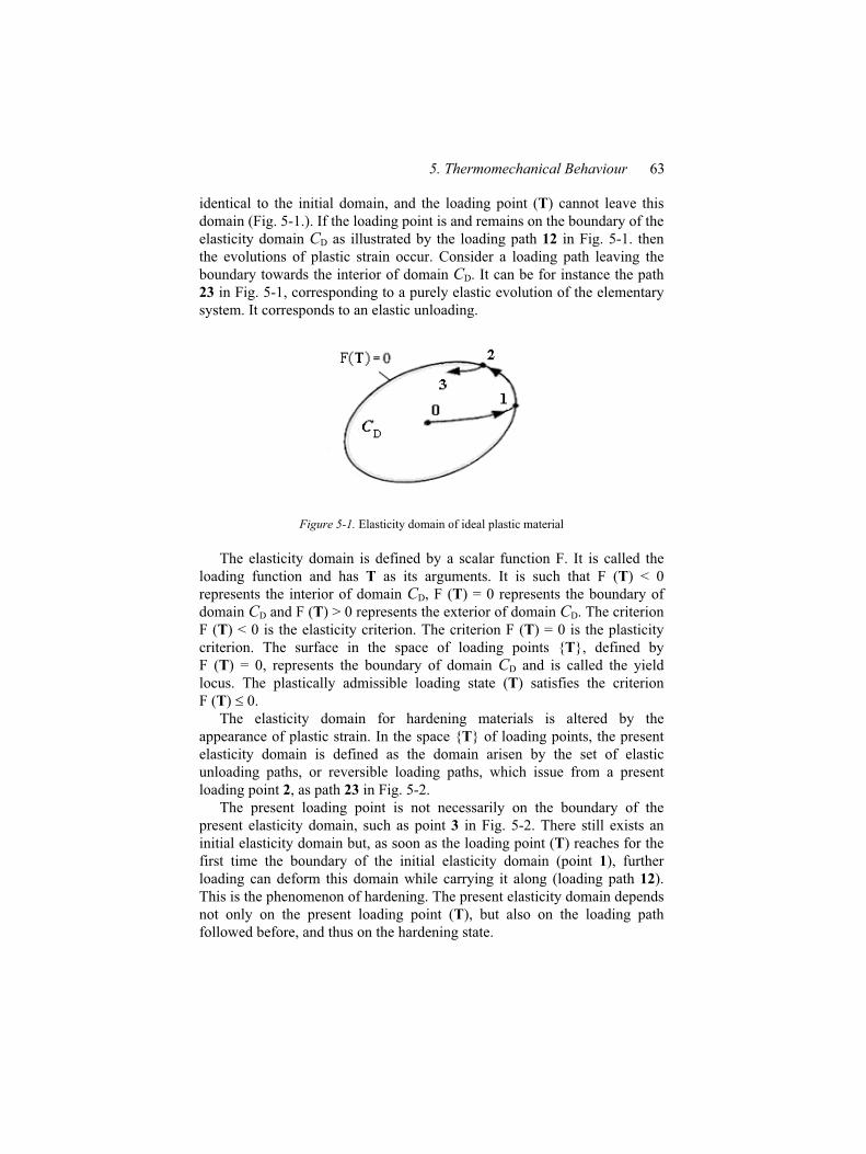
5. Thermomechanical Behaviour 63
identical to the initial domain, and the loading point (T) cannot leave this
domain (Fig. 5-1.). If the loading point is and remains on the boundary of the
elasticity domain CD as illustrated by the loading path 12 in Fig. 5-1. then
the evolutions of plastic strain occur. Consider a loading path leaving the
boundary towards the interior of domain CD. It can be for instance the path
23 in Fig. 5-1, corresponding to a purely elastic evolution of the elementary
system. It corresponds to an elastic unloading.
Figure 5-1. Elasticity domain of ideal plastic material
The elasticity domain is defined by a scalar function F. It is called the
loading function and has T as its arguments. It is such that F (T) < 0
represents the interior of domain CD, F (T) = 0 represents the boundary of
domain CD and F (T) > 0 represents the exterior of domain CD. The criterion
F (T) < 0 is the elasticity criterion. The criterion F (T) = 0 is the plasticity
criterion. The surface in the space of loading points {T}, defined by
F (T) = 0, represents the boundary of domain CD and is called the yield
locus. The plastically admissible loading state (T) satisfies the criterion
F (T) 0.
The elasticity domain for hardening materials is altered by the
appearance of plastic strain. In the space {T} of loading points, the present
elasticity domain is defined as the domain arisen by the set of elastic
unloading paths, or reversible loading paths, which issue from a present
loading point 2, as path 23 in Fig. 5-2.
The present loading point is not necessarily on the boundary of the
present elasticity domain, such as point 3 in Fig. 5-2. There still exists an
initial elasticity domain but, as soon as the loading point (T) reaches for the
first time the boundary of the initial elasticity domain (point 1), further
loading can deform this domain while carrying it along (loading path 12).
This is the phenomenon of hardening. The present elasticity domain depends
not only on the present loading point (T), but also on the loading path
followed before, and thus on the hardening state.
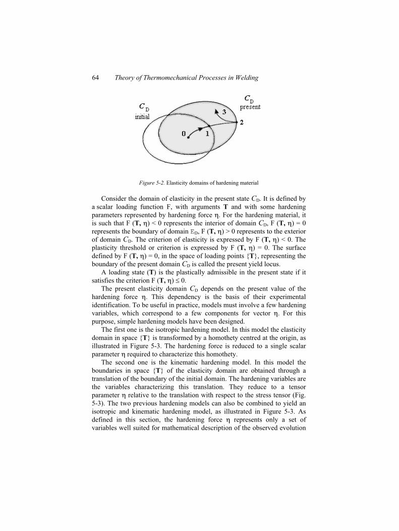
64 Theory of Thermomechanical Processes in Welding
Figure 5-2. Elasticity domains of hardening material
Consider the domain of elasticity in the present state CD. It is defined by
a scalar loading function F, with arguments T and with some hardening
parameters represented by hardening force . For the hardening material, it
is such that F (T, ) < 0 represents the interior of domain CD, F (T, ) = 0
represents the boundary of domain ED, F (T, ) > 0 represents to the exterior
of domain CD. The criterion of elasticity is expressed by F (T, ) < 0. The
plasticity threshold or criterion is expressed by F (T, ) = 0. The surface
defined by F (T, ) = 0, in the space of loading points {T}, representing the
boundary of the present domain CD is called the present yield locus.
A loading state (T) is the plastically admissible in the present state if it
satisfies the criterion F (T, ) 0.
The present elasticity domain CD depends on the present value of the
hardening force . This dependency is the basis of their experimental
identification. To be useful in practice, models must involve a few hardening
variables, which correspond to a few components for vector . For this
purpose, simple hardening models have been designed.
The first one is the isotropic hardening model. In this model the elasticity
domain in space {T} is transformed by a homothety centred at the origin, as
illustrated in Figure 5-3. The hardening force is reduced to a single scalar
parameter required to characterize this homothety.
The second one is the kinematic hardening model. In this model the
boundaries in space {T} of the elasticity domain are obtained through a
translation of the boundary of the initial domain. The hardening variables are
the variables characterizing this translation. They reduce to a tensor
parameter relative to the translation with respect to the stress tensor (Fig.
5-3). The two previous hardening models can also be combined to yield an
isotropic and kinematic hardening model, as illustrated in Figure 5-3. As
defined in this section, the hardening force represents only a set of
variables well suited for mathematical description of the observed evolution
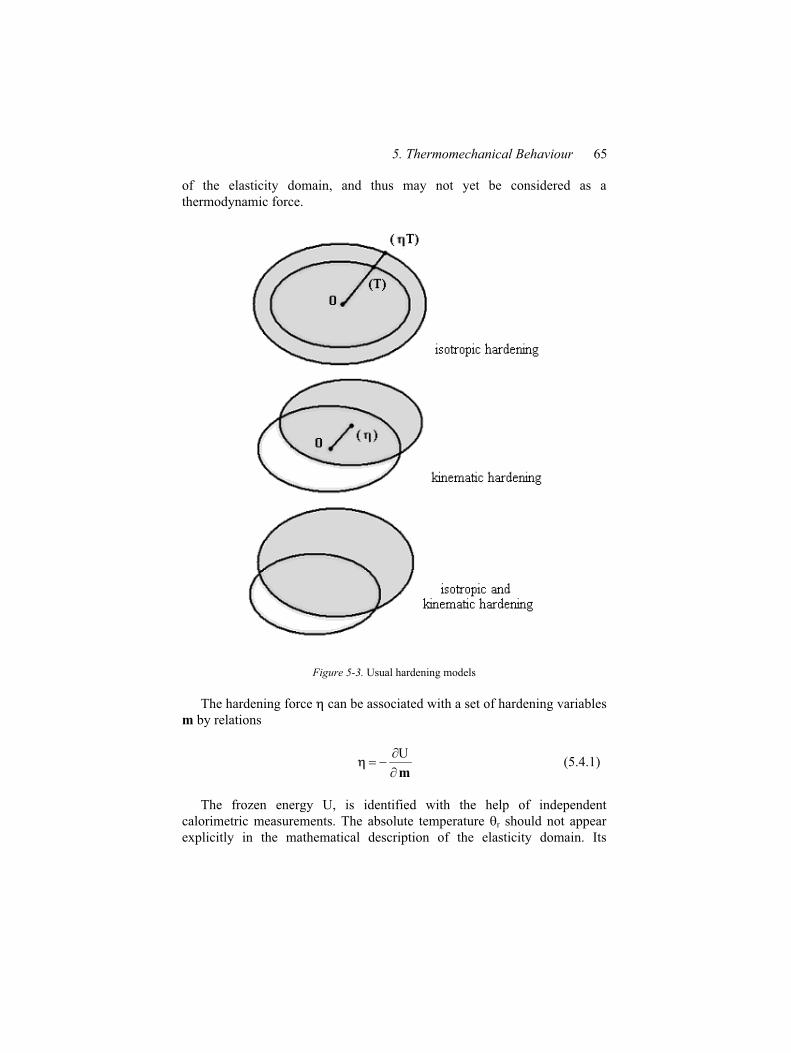
5. Thermomechanical Behaviour 65
of the elasticity domain, and thus may not yet be considered as a
thermodynamic force.
Figure 5-3. Usual hardening models
The hardening force can be associated with a set of hardening variables
m by relations
m
U (5.4.1)
The frozen energy U, is identified with the help of independent
calorimetric measurements. The absolute temperature r should not appear
explicitly in the mathematical description of the elasticity domain. Its
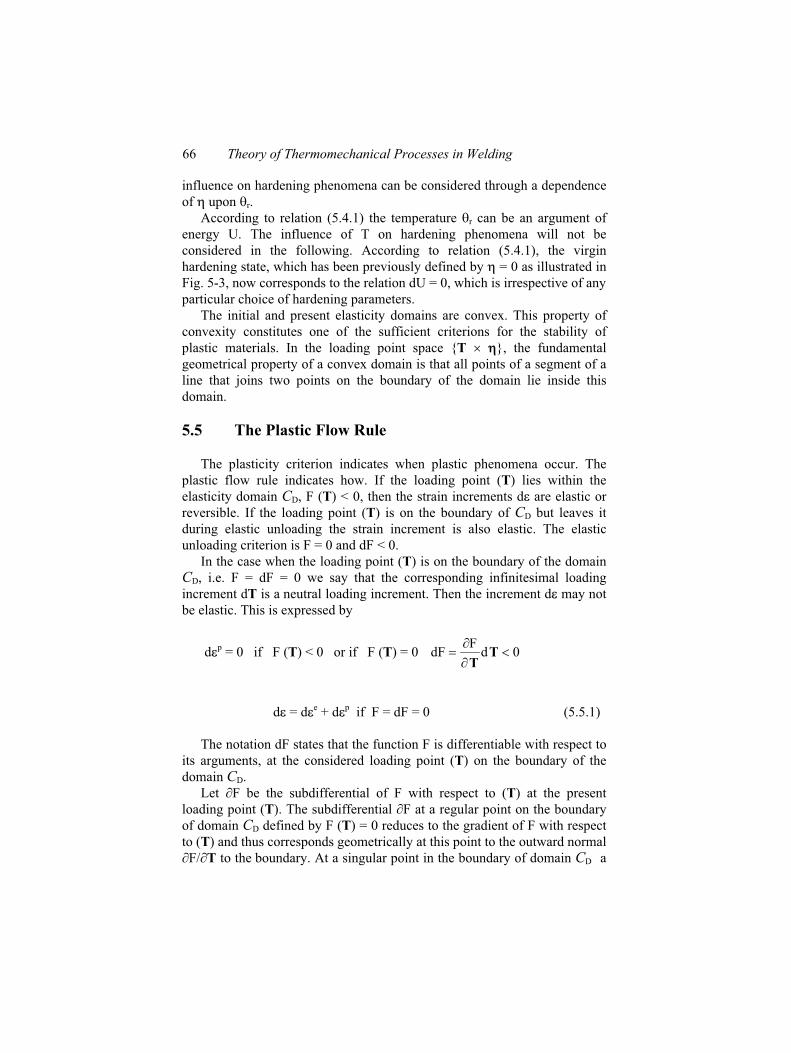
66 Theory of Thermomechanical Processes in Welding
influence on hardening phenomena can be considered through a dependence
of upon r.
According to relation (5.4.1) the temperature r can be an argument of
energy U. The influence of T on hardening phenomena will not be
considered in the following. According to relation (5.4.1), the virgin
hardening state, which has been previously defined by = 0 as illustrated in
Fig. 5-3, now corresponds to the relation dU = 0, which is irrespective of any
particular choice of hardening parameters.
The initial and present elasticity domains are convex. This property of
convexity constitutes one of the sufficient criterions for the stability of
plastic materials. In the loading point space {T }, the fundamental
geometrical property of a convex domain is that all points of a segment of a
line that joins two points on the boundary of the domain lie inside this
domain.
5.5 The Plastic Flow Rule
The plasticity criterion indicates when plastic phenomena occur. The
plastic flow rule indicates how. If the loading point (T) lies within the
elasticity domain CD, F (T) < 0, then the strain increments d are elastic or
reversible. If the loading point (T) is on the boundary of CD but leaves it
during elastic unloading the strain increment is also elastic. The elastic
unloading criterion is F = 0 and dF < 0.
In the case when the loading point (T) is on the boundary of the domain
CD, i.e. F = dF = 0 we say that the corresponding infinitesimal loading
increment dT is a neutral loading increment. Then the increment d may not
be elastic. This is expressed by
d p = 0 if F (T) < 0 or if F (T) = 0 0dF
dF TT
d = d e + d p if F = dF = 0 (5.5.1)
The notation dF states that the function F is differentiable with respect to
its arguments, at the considered loading point (T) on the boundary of the
domain CD.
Let F be the subdifferential of F with respect to (T) at the present
loading point (T). The subdifferential F at a regular point on the boundary
of domain CD defined by F (T) = 0 reduces to the gradient of F with respect
to (T) and thus corresponds geometrically at this point to the outward normal
F/ T to the boundary. At a singular point in the boundary of domain CD a
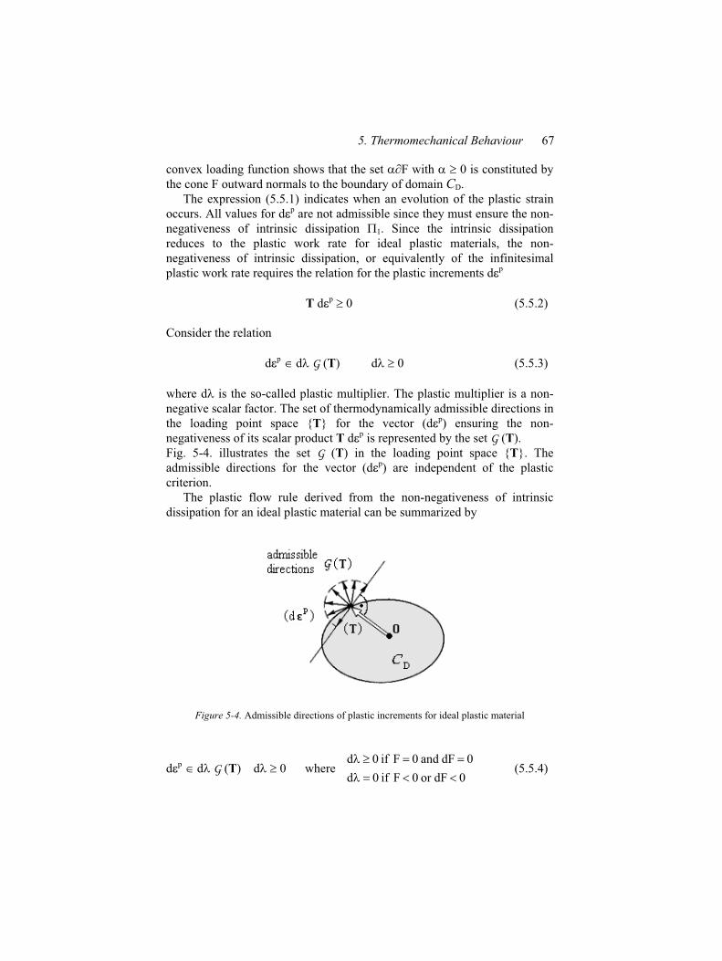
5. Thermomechanical Behaviour 67
convex loading function shows that the set F with 0 is constituted by
the cone F outward normals to the boundary of domain CD.
The expression (5.5.1) indicates when an evolution of the plastic strain
occurs. All values for d p are not admissible since they must ensure the non-
negativeness of intrinsic dissipation 1. Since the intrinsic dissipation
reduces to the plastic work rate for ideal plastic materials, the non-
negativeness of intrinsic dissipation, or equivalently of the infinitesimal
plastic work rate requires the relation for the plastic increments d p
T d p 0 (5.5.2)
Consider the relation
d p d G (T) d 0 (5.5.3)
where d is the so-called plastic multiplier. The plastic multiplier is a non-
negative scalar factor. The set of thermodynamically admissible directions in
the loading point space {T} for the vector (d p) ensuring the non-
negativeness of its scalar product T d p is represented by the set G (T).
Fig. 5-4. illustrates the set G (T) in the loading point space {T}. The
admissible directions for the vector (d p) are independent of the plastic
criterion.
The plastic flow rule derived from the non-negativeness of intrinsic
dissipation for an ideal plastic material can be summarized by
Figure 5-4. Admissible directions of plastic increments for ideal plastic material
d p d G (T) d 0 where0dFor0Fif0d
0dFand0Fif0d (5.5.4)
68 Theory of Thermomechanical Processes in Welding
If the plastic increments d p have non-zero values, then we say that the
loading is plastic.
The evolution for hardening materials is elastic with no change of the
hardening state, if in the space {T } the present extended loading point
(T, ) lies inside the fixed domain C (F < 0) or on its boundary F = 0 and
leaves it (dF < 0). The above can be written in the form
(d p, dm) d G (T, ) d 0 where0dFor0Fif0d
0dFand0Fif0d (5.5.5)
If the increments (d p, dm) have non-zero values, then we say that the
loading is plastic. The scalar d in Eq. (5.5.5) is the plastic multiplier, and
G (T, ) are the set of thermodynamically admissible directions for the
increments (d p, dm) satisfying the relation of the non-negativeness of the
intrinsic dissipation
T d p + dm 0 (5.5.6)
The increment dm of the hardening variable is written in the form
dm = d Gm (T, ) (5.5.7)
In the above Gm (T, ) are the actual directions of the permissible
directions for dm.
In the case of hardening plasticity the loading function depends on the
hardening force . Then the expression for dF is
dF = d F + dTF (5.5.8)
with
TT
dF
Fd (5.5.9)
dF
Fd T (5.5.10)
If the plastic increments d p have non-zero values, then we say that the
loading is plastic.
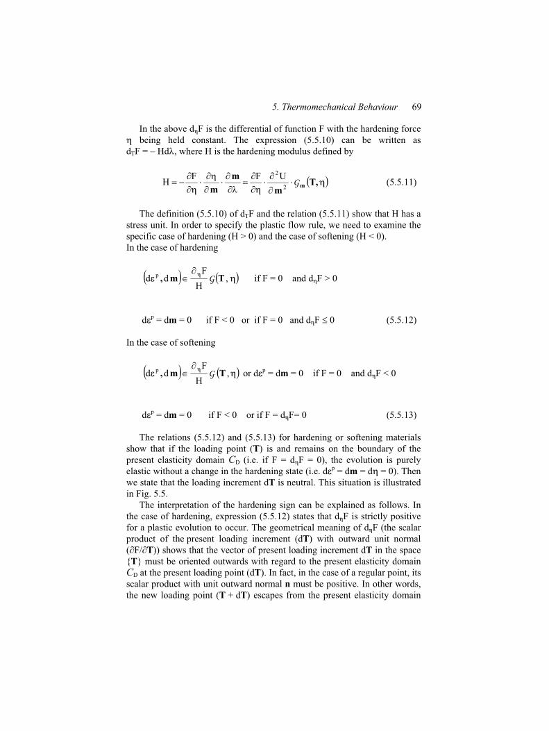
5. Thermomechanical Behaviour 69
In the above d F is the differential of function F with the hardening force
being held constant. The expression (5.5.10) can be written as
dTF = – Hd , where H is the hardening modulus defined by
T,m
m
mmG2
2 UFFH (5.5.11)
The definition (5.5.10) of dTF and the relation (5.5.11) show that H has a
stress unit. In order to specify the plastic flow rule, we need to examine the
specific case of hardening (H > 0) and the case of softening (H < 0).
In the case of hardening
,H
Fdd p
Tm, G if F = 0 and d F > 0
d p = dm = 0 if F < 0 or if F = 0 and d F 0 (5.5.12)
In the case of softening
,H
Fdd p
Tm, G or d p = dm = 0 if F = 0 and d F < 0
d p = dm = 0 if F < 0 or if F = d F= 0 (5.5.13)
The relations (5.5.12) and (5.5.13) for hardening or softening materials
show that if the loading point (T) is and remains on the boundary of the
present elasticity domain CD (i.e. if F = d F = 0), the evolution is purely
elastic without a change in the hardening state (i.e. d p = dm = d = 0). Then
we state that the loading increment dT is neutral. This situation is illustrated
in Fig. 5.5.
The interpretation of the hardening sign can be explained as follows. In
the case of hardening, expression (5.5.12) states that d F is strictly positive
for a plastic evolution to occur. The geometrical meaning of d F (the scalar
product of the present loading increment (dT) with outward unit normal
( F/ T)) shows that the vector of present loading increment dT in the space
{T} must be oriented outwards with regard to the present elasticity domain
CD at the present loading point (dT). In fact, in the case of a regular point, its
scalar product with unit outward normal n must be positive. In other words,
the new loading point (T + dT) escapes from the present elasticity domain
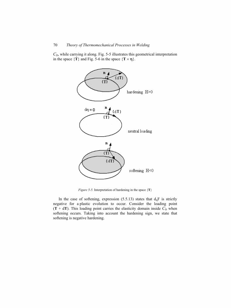
70 Theory of Thermomechanical Processes in Welding
CD, while carrying it along. Fig. 5-5 illustrates this geometrical interpretation
in the space {T} and Fig. 5-6 in the space {T }.
Figure 5-5. Interpretation of hardening in the space {T}
In the case of softening, expression (5.5.13) states that d F is strictly
negative for a plastic evolution to occur. Consider the loading point
(T + dT). This loading point carries the elasticity domain inside CD when
softening occurs. Taking into account the hardening sign, we state that
softening is negative hardening.
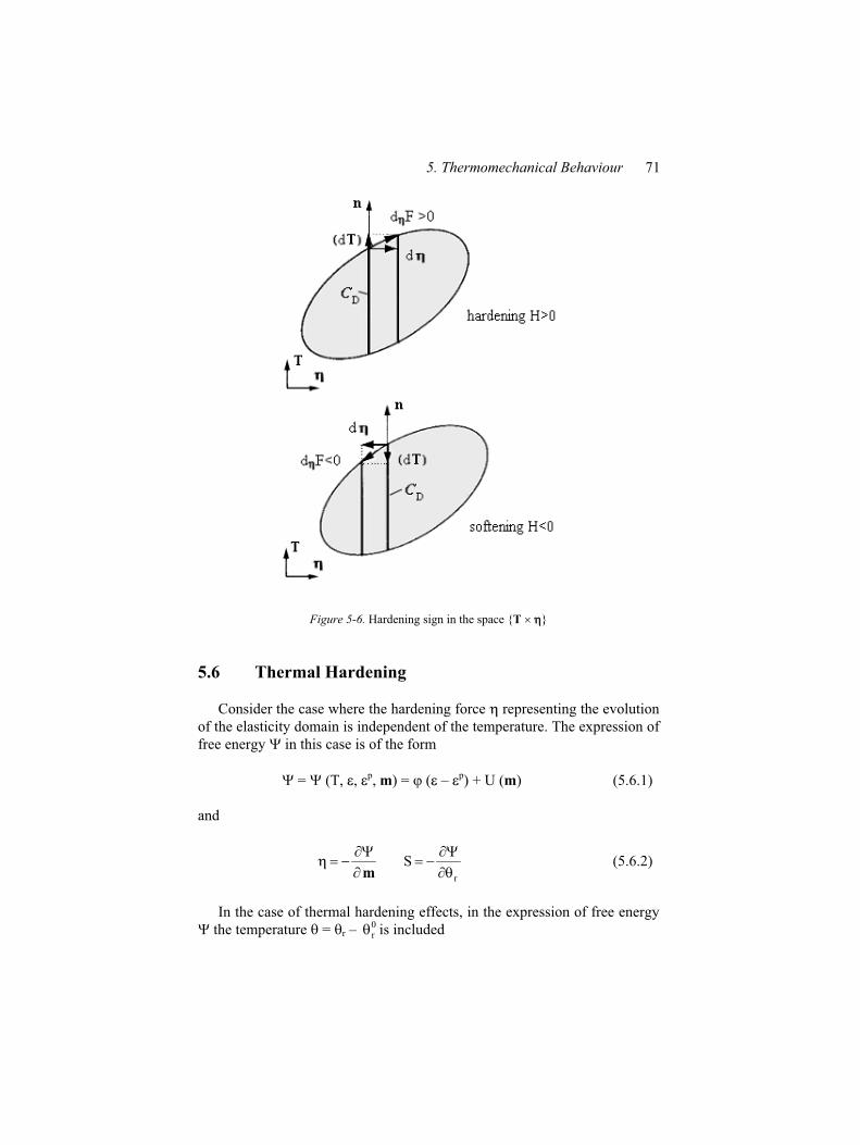
5. Thermomechanical Behaviour 71
Figure 5-6. Hardening sign in the space {T }
5.6 Thermal Hardening
Consider the case where the hardening force representing the evolution
of the elasticity domain is independent of the temperature. The expression of
free energy in this case is of the form
= (T, , p, m) = ( – p) + U (m) (5.6.1)
and
m r
S (5.6.2)
In the case of thermal hardening effects, in the expression of free energy
the temperature = r – 0r is included
72 Theory of Thermomechanical Processes in Welding
= ( = r – 0r , , p, m) = ( – p, ) + U* (m, ) (5.6.3)
and
mS (5.6.4)
Substituting expression (5.6.3) into (5.6.4) shows that the hardening force
depends on temperature variation = r – 0r .
Assume that the temperature variation is small. The function U* (m, )
can be expressed as
U*(m, ) = U(m) – S*(m) (5.6.5)
The function U(m) is interpreted as the frozen free energy. By (5.6.3),
(5.6.4) and (5.6.5) we get
m
*
m
SUm*SS (5.6.6)
Consider the elasticity domain CD in the loading space {T} defined by
F = F (T, ) 0 (5.6.7)
According to Eq. (5.6.6), due to the temperature variation d , the
hardening force and the elasticity domain CD may change. Thermal
hardening occurs for a zero frozen free energy U (m) = 0. An inverse
temperature variation – d restores the previous elasticity domain. The
second relation (5.6.6) shows also that there is an unrecovered change in
entropy, yielding the frozen entropy term S*(m). With respect to the
linearized thermal equation (3.8.6) the quality 0r S*(m) can easily be related
to a hardening latent heat effect. The flow rule can be expressed as
(d p, dm) d G(T, ) d 0 where0dFor0Fif0d
0dFand0Fif0d (5.6.8)
where the plastic multiplier d and the hardening modulus H are now
expressed in the form
H
Fdd m ,
m
m
mmG2
2 UFFH (5.6.9)
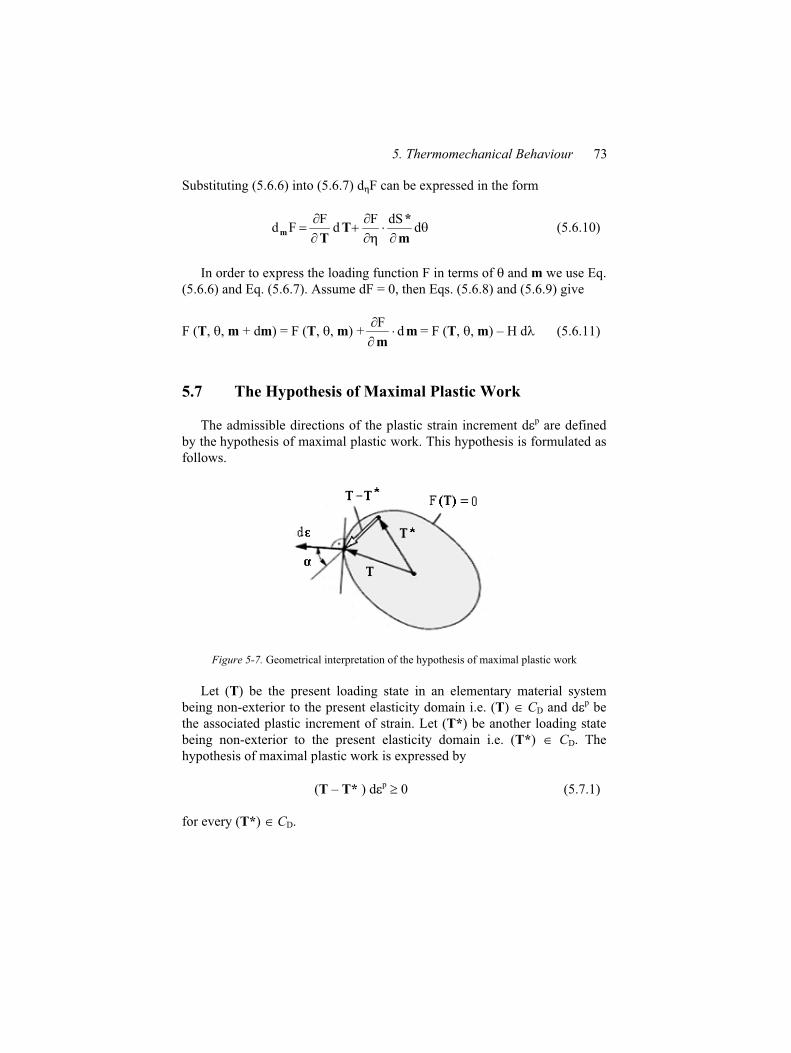
5. Thermomechanical Behaviour 73
Substituting (5.6.6) into (5.6.7) d F can be expressed in the form
ddSF
dF
Fdm
*T
Tm (5.6.10)
In order to express the loading function F in terms of and m we use Eq.
(5.6.6) and Eq. (5.6.7). Assume dF = 0, then Eqs. (5.6.8) and (5.6.9) give
F (T, , m + dm) = F (T, , m) + mm
dF
= F (T, , m) – H d (5.6.11)
5.7 The Hypothesis of Maximal Plastic Work
The admissible directions of the plastic strain increment d p are defined
by the hypothesis of maximal plastic work. This hypothesis is formulated as
follows.
Figure 5-7. Geometrical interpretation of the hypothesis of maximal plastic work
Let (T) be the present loading state in an elementary material system
being non-exterior to the present elasticity domain i.e. (T) CD and d p be
the associated plastic increment of strain. Let (T*) be another loading state
being non-exterior to the present elasticity domain i.e. (T*) CD. The
hypothesis of maximal plastic work is expressed by
(T – T* ) d p 0 (5.7.1)
for every (T*) CD.
74 Theory of Thermomechanical Processes in Welding
This means that the loading state (T) to be associated with the present
plastic increment of strain (d p) is the one among those admitted by the
present plastic criterion, maximizing the infinitesimal plastic work.
Fig 5-7 represents the geometrical interpretation of the hypothesis of
maximal plastic work. The directions of vectors (T – T* ) and d p form the
non-obtuse angle.
The hypothesis of maximal plastic work can be geometrically represented
in the loading point space {T} by the convexity of the elasticity domain ED
and by the directions permissible for the plastic increment (d p).
The flow rule reads
d p d F(T) or d p d F (T, ) d 0 (5.7.2)
where F (T) and F (T, ) represent the subdifferential of F(T) and F
(T, ) respectively with respect to T.
The hypothesis of maximal plastic work implies both the normality of the
flow rule and the convexity of the plastic criterion. The hypothesis of
maximal plastic work and the hypothesis of both the normality of the flow
rule and the convexity of the plastic criterion with respect to T are
equivalent.
A material is said to be standard if it satisfies the maximal plastic work
hypothesis. The plastic criterion is then convex and the flow rule is normal.
5.8 The Associated Flow Rule
If a material satisfies the maximal plastic work hypothesis, then we say
that the material is standard. The plasticity criterion is then convex and the
flow rule is normal and we say that the flow rule is associated with the
criterion of plasticity.
Consider an ideal plastic standard material. Eqs. (5.5.4) and (5.7.2) lead
to write the flow rule as
d p d F(T) d 0 where0dFand0Fif0d
0dFand0Fif0d (5.8.1)
and for any regular point on the boundary of the elasticity domain in the case
of plastic loading
T
Fdd p d 0 if F = dF = 0 (5.8.2)
5. Thermomechanical Behaviour 75
Consider a hardening standard material. Eqs. (5.5.12), (5.5.13) and
(5.8.2) give for a hardening standard material
(d p, dm) T,FFd
if F = 0 and d F > 0
d p = dm = 0 if F < 0 or if F = 0 and d F 0 (5.8.3)
For softening (H < 0) we get
(d p, dm) ,,
FFd
or d p = dm = 0 if F = 0 and d F < 0
d p = dm = 0 if F < 0 or if F = 0 and d F = 0 (5.8.4)
Consider a regular point on the boundary of the elasticity domain and
non-zero plastic increments d p. Then we have
T
FFdd p (5.8.5)
5.9 Incremental Formulation for Thermal Hardening
In solution of welding thermomechanical problems an important is the
incremental formulation for thermal hardening. Consider Eq. (5.3.9) with its
incremental form
dT = C (d – d p) – Ad (5.9.1)
By Eq. (5.5.12) and (5.6.10) we get
dT = C d – AdT
Cm
*
T
Fd
SFF
H
1 (5.9.2)
By contracting Eq. (5.9.1) with the tensor F/ T and adding the result to the
quantity dSF
m
*gives
76 Theory of Thermomechanical Processes in Welding
TC
T
ATm
*C
T
mT FF
H
11
dFSF
dF
dSFF f
(5.9.3)
By substituting (5.9.3) into (5.9.2) we get
TC
T
TC
TA
m
*C
TACT
FFH
Fd
FSFd
F
FYddd (5.9.4)
where Y(x) is the Heaviside function defined by
0xY if x < 0 and 1xY if x 0 (5.9.5)
By (5.9.4) we get
d
Wd
* (5.9.6)
where W*(d ) is the incremental potential defined by
TC
T
TA
m
*C
T
AC*
FFH
dFSF
dF
FY2
1
dddd2
1W
2
(5.9.7)
5.10 Models of Plasticity
In modeling of welding processes we should consider the appropriate
models of plasticity. In isotropic material the loading function F involves the
principal components of symmetric stress tensor T, i.e. the three principal
stresses T1, T2 and T3. The principal stresses can be expressed in terms of the
three first invariants of the stress tensor. We denote the first invariant of the
5. Thermomechanical Behaviour 77
stress tensor by J1T, the second invariant of the stress deviator tensor
'T = T – (tr T/3)1 by J2T’ and the third invariant of the stress deviator tensor
by J3T’
J1T (T) = tr T = 3p (5.10.1)
''tr2
1'T'T
2
1Jh jiij'2
2TTTT (5.10.2)
kljkij'3 'T'T'T3
1J TT (5.10.3)
By (5.10.2) we have
2
32
2
31
2
212 TTTTTT
6
1h (5.10.4)
The loading function for isotropic models of plasticity can be represented by
F = F (h, p) (5.10.5)
In the case of isotropic hardening materials, the loading function F is
expressed in the form
F = F (h, p, ) (5.10.6)
where is the hardening force describing the evolution of the yield surface
in loading point space {Ti}. In isotropic hardening the yield surface is
derived through a homothety of center 0 in the loading point space {Ti}.
Then the hardening force reduces to a scalar variable which defines this
homothety.
The loading function given by (5.10.6) can be expressed as a
homogeneous polynome of degree n with regard to h and
F = F (h, p, ) = n F (h/ , p/ , 1) (5.10.7)
where by convection is specified as the ratio of the homothety that
transforms the yield surface defined by = 1 into the present yield surface.
In kinematic hardening, the yield surfaces are defined from each other
78 Theory of Thermomechanical Processes in Welding
through a translation in the loading point space {Ti}. The hardening force
reduces to a second-order symmetric tensor that defines this translation
F = F [J2T’ (T + ), J1T (T + )] (5.10.8)
In space {Ti} vector ( ) represents the vector of translation that
transforms the yield surface defined by ( ) = (0) into the present yield
surface.
Assume the convex loading function for the isotropic plastic material
F (h, p) = h + p – q (5.10.9)
where and q are material characteristics. The constant q is necessarily non-
negative to ensure that the zero loading point satisfies F (0,0) 0. The
coefficient is non-negative to describe an infinite tensile stress. The yield
surface given by (5.10.9) is an axisymmetric surface around the trisector in
principal stress space {Ti}. If = 0 the loading function reduces to the
Huber-Mises loading function.
The form of the Huber-Mises loading function is
qTTT3TTTTTTTTT3
1F 2
31223
212113333222211
233
222
211
(5.10.10)
or for principal directions
qTTTTTTTTT3
1F 133221
23
22
21 (5.10.11)
The Huber-Mises loading function can be transformed to the equivalent
forms if we introduce material parameter 0T3
1q , where T0 is the yield
point of the material in uniaxial tension.
Then the Huber-Mises loading function is expressed in the frequently
met form
0
231
223
212
2
1133
2
3322
2
2211
T3
1
TTT6TTTTTT6
1F
(5.10.12)
5. Thermomechanical Behaviour 79
or
0
2
13
2
32
2
21 T3
1TTTTTT
6
1F (5.10.13)
The previous loading function (5.10.9) for an isotropic material that
exhibits isotropic hardening is extended in the form
F = h + p – q (5.10.14)
The yield surface that corresponds to the loading function (5.10.14) is an
axisymmetric cone around the trisector in principal stress space {Ti}. In this
space, the three coordinates of the vertex of the cone are equal to q / . In the
loading point space {Ti} the singular points are located on a line given by
the equation T1 = T2 = T3 = q / . The present yield surface is the transform
of the surface defined by = 1, through the homothety centred at the origin
with as the ratio. For an isotropic material exhibiting kinematic hardening
qpss2
1F iijijiijij (5.10.15)
where the symmetric tensor is the deviator of the tensor
1tr31 (5.10.16)
In the loading point space {Ti} the present yield surface is the transform
of the surface defined by = 0 through the translation defined by the vector
with and the eigenvalues 1, 2, 3 of the tensor as components. In the
loading point space {Ti} the singular points are located on the line given by
the equation T1 + 1 = T2 + 2 = T3 + 3 = q/ . The expression (5.10.14)
and (5.10.15) may be combined to obtain
'qpss2
1F iijijiijij (5.10.17)
In the loading space {Ti} the present yield surface is the transform of the
surface defined by = 0 and ’ = 1 through the translation defined by the
vector with ( 1, 2, 3) as components followed by the homothety of ratio ’
and centred at the point ( 1, 2, 3), the translated point of origin.
80 Theory of Thermomechanical Processes in Welding
In the loading point space {Ti} the singular points are located on the line
given by the equation
T1 + 1 = T2 + 2 = T3 + 3 = q ’/ (5.10.18)
Part II
NUMERICAL ANALYSIS OF WELDING
PROBLEMS
Chapter 6
NUMERICAL METHODS IN
THERMOMECHANICS
6.1 Introduction
Most of the thermo-mechanical problems in welding can only be solved
by using numerical procedures. In realistic model the thermal conductivity
and specific heat should be considered as a function of temperature which
complicates analytical solutions. Because of possible phase change the
analytical methods have a limited range of applications. In most types of
welding melting will occur and there will also be convective heat transfer in
addition to conductive heat transfer. The heat sources in welding in realistic
model are not concentrated in point or line.
In this section the general data concerning the numerical solving methods
applied to welding processes are given. The non-linearity of the constitutive
equations describing welding process and its time-dependence require the
advanced solution technique.
6.2 Finite-Element Solution of Heat Flow Equations
6.2.1 Weighted Residual Method
Heat transfer problems can be formulated either by a given differential
equation with boundary conditions or by a given functional equivalent to the
differential equation. The weighted residual method is an approximate
solution method for differential equations. This method widens the range of
84 Theory of Thermomechanical Processes in Welding
problems amenable to solution since it does not require a variational
formulation of the problem. Consider the heat flow equation
tCrk (6.2.1)
with boundary conditions
0B w1 on a1 (6.2.2)
w2 qn
kB on a2 (6.2.3)
0hn
kB f3 on a3 (6.2.4)
where w is the temperature of the body surface and f is the fluid
temperature. We look for a solution of the problem (6.2.1) – (6.2.4) in the
class of functions , fulfilling the boundary conditions (6.2.2) – (6.2.4).
These functions in general do not fulfill the differential equation (6.2.1).
Substituting one of these functions into Eq. (6.2.1) we get
0Et
Crk (6.2.5)
The best approximation for the solution will be a function which
minimizes the residuum E. The simplest method of obtaining the solution is
to make use of the fact that if E is identically equal to zero, then
0wEdV
V
(6.2.6)
where V is the volume of the body under consideration and w is an arbitrary
function.
A similar procedure is used for boundary conditions. We get
V
0dVt
Crkw (6.2.7)
6. Numerical Methods in Thermomechanics 85
and
3
1i a
iii 0daBw
i
(6.2.8)
The above conditions may be replaced by the single condition
V
3
1i a
iii0 0daBwdVt
Crkw
i
(6.2.9)
Since we are dealing with a second-order partial differential operator the
function must be continuous with continuous first-order derivatives. If we
use the divergence theorem to lessen the order of differentiation in (6.2.9)
then we may simply require the temperature to be of class of zero-order.
Then we can express it in terms of shape functions, for which this condition
is fulfilled. Using the divergence theorem, the requirements as to the
function w increase; it now has to be a condition function. Making use of the
divergence theorem for Eq. (6.2.9) we get
0dahn
kwdaqn
kw
dan
wkdVt
wCdVwrdVkw
32
i
a
f3
a
w2
V aVV (6.2.10)
where 321 aaaa is the total surface of the body.
Since functions wi are arbitrary continuous functions, we can put
www 32 (6.2.11)
Finally we get
0dan
wkdawh
dawqdVt
wCdVwrdVkw
i3
2
aa
f
a
w
V VV (6.2.12)
86 Theory of Thermomechanical Processes in Welding
Assume that the temperature can be approximated by the expression
I
1i
iiH (6.2.13)
where Hi are shape functions, i are nodal temperatures and I stands for the
number of nodes. The expression (6.2.13) is sometimes shown in matrix
notation as
TH (6.2.14)
where H is the vector of shape functions and is the vector of nodal
temperatures. Functions w in Eq. (6.2.12) can be taken as
iHw (6.2.15)
This assumption reduces the weighted residual method to the classical
Galerkin method. The particular advantage of such an approach is that for
heat exchange problems in non-moving bodies the matrix of the symmetric
and banded.
Substitute in Eq. (6.2.12) the functions
iHw i = 1, 2, …, I (6.2.16)
By substitution of temperature in the form of (6.2.13) we get a system
i
FCK (6.2.17)
where
13 a
j
i
a
ji
V
jiij dan
HkHdahHHdVHkHK (6.2.18)
V
jiij dVHCHC (6.2.19)
of I equations with I unknowns,
6. Numerical Methods in Thermomechanics 87
32 a
fi
a
wi
V
ii dahHdaqHrdVHF (6.2.20)
As we see, the matrix K is symmetric. Integrals in expressions (6.2.18)
and (6.2.19) are different from zero only in the sub-domains where Hi 0,
e.g. in the elements which possess the i-th node.
6.2.2 Variational Formulation
The heat exchange problem is uniquely defined by the partial differential
equation with boundary conditions. It is however possible to formulate the
problem using the extreme variational principle. According to Euler’s
theorem the solution of the partial differential equation of heat transfer
tCr
xk
xk
xk
23
2
3322
2
2221
2
11 (6.2.21)
may be found by minimizing the functional
dVC2Cr2
xk
xk
xk
2
1
02
V
2
3
33
2
2
22
2
1
11H
(6.2.22)
with assumptions that the function fulfils the given boundary conditions
w on a1 (6.2.23)
0qn
k w on a2 (6.2.24)
0hn
k f on a3 (6.2.25)
and 0 is the initial temperature distribution.
88 Theory of Thermomechanical Processes in Welding
The condition (6.2.23) can be easily fulfilled. However, the remaining
conditions create significant difficulties. Therefore one adds to the functional
(6.2.22) the surface integral, which in the process of minimization leads to
(6.2.24) or (6.2.25). In general it has the form
32 a
f2
a
w da2hdaq22
1 (6.2.26)
or
32 a
f2
a
w da2hdaq22
1HH (6.2.27)
and at the same time the function has to fulfill the condition (6.2.23).
The functional in the form (6.2.27) can be expressed as the sum of
functionals determined for each differential element
n
nHH (6.2.28)
It reaches a minimum, if all components of the sum are minimal. Assume
that the temperature is expressed by shape functions and nodal
temperatures
i
iiH (6.2.29)
Since all shape functions are continuous functions, derivatives appearing
in the functional (6.2.27) are determined in order to minimize this functional
with respect to parameters i, we should solve the following system of
equations
0i
H for i = 1, 2, …, I (6.2.30)
Finally we get
FCK (6.2.31)
6. Numerical Methods in Thermomechanics 89
where
13 a
j
i
a
ji
V
jiij dan
HkHdaHhHdVHkHK (6.2.32)
V
jiij dVHCHC (6.2.33)
32 a
fi
a
wi
V
ii dahHdaqHdVrHF (6.2.34)
and at the same time the surface integrals appear only in the cases where
nodes are placed on the body boundary.
6.3 Finite-Element Solution of Navier-Stokes Equations
Navier-Stokes equations (4.2.1) – (4.2.3) with boundary conditions given
by (4.2.6) and (4.2.7) form a complete set for the determination of the
velocity, pressure and temperature fields in a moving fluid
rkt
C v (6.3.1)
0v (6.3.2)
0gt
Tvvv
(6.3.3)
where
ijjiijij vvT ,,p (6.3.4)
In matrix notation we can write
vITTp (6.3.5)
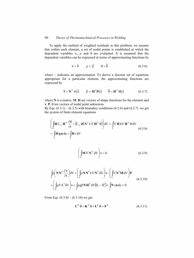
90 Theory of Thermomechanical Processes in Welding
To apply the method of weighted residuals to this problem, we assume
that within each element, a set of nodal points is established at which the
dependent variables vi, p and are evaluated. It is assumed that the
dependent variables can be expressed in terms of approximating functions by
v~v pp ~ ~ (6.3.6)
where ~ indicates an approximation. To derive a discrete set of equations
appropriate for a particular element, the approximating functions are
expressed by
tTvNv~ tT
PM~p tTH
~ (6.3.7)
where N is a matrix, M, H are vectors of shape functions for the element and
v, P, are vectors of nodal point unknowns.
By Eqs. (6.3.1) – (6.3.5) with boundary conditions (4.2.6) and (4.2.7) we get
the system of finite element equations
Va
V
T
V
TTT
dVrda
dVkdVCt
C
HnqH
HHHvNHHH
(6.3.8)
0dV
V
TvNM (6.3.9)
0dadVgdV
dVdVdVt
aV
0rr
T
V
T
V V
T
V
TTT
nNHNv
PMNvNvNNv
NN
(6.3.10)
From Eqs. (6.3.8) – (6.3.10) we get
FLKC (6.3.11)
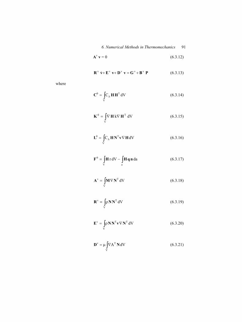
6. Numerical Methods in Thermomechanics 91
Av v = 0 (6.3.12)
PBGvDvEvRvvvvv (6.3.13)
where
V
T dVC HHC (6.3.14)
V
T dVk HHK (6.3.15)
V
T dVC HvNHL (6.3.16)
aV
dadVr nqHHF (6.3.17)
V
Tv dVNMA (6.3.18)
V
Tv dVNNR (6.3.19)
V
TTv dVNvNNE (6.3.20)
V
Tv dVND (6.3.21)
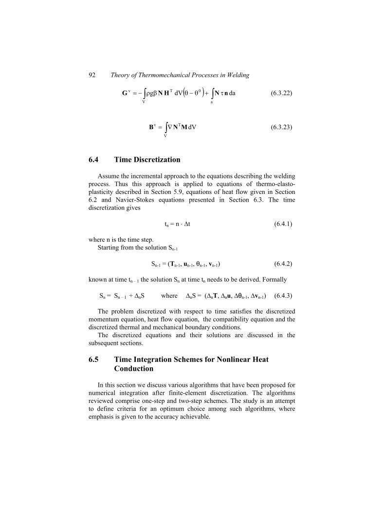
92 Theory of Thermomechanical Processes in Welding
aV
0Tv dadVg nNHNG (6.3.22)
V
Tv dVMNB (6.3.23)
6.4 Time Discretization
Assume the incremental approach to the equations describing the welding
process. Thus this approach is applied to equations of thermo-elasto-
plasticity described in Section 5.9, equations of heat flow given in Section
6.2 and Navier-Stokes equations presented in Section 6.3. The time
discretization gives
tn = n t (6.4.1)
where n is the time step.
Starting from the solution Sn-1
Sn-1 = (Tn-1, un-1, n-1, vn-1) (6.4.2)
known at time tn – 1 the solution Sn at time tn needs to be derived. Formally
Sn = Sn – 1 + nS where nS = ( nT, nu, n-1, vn-1) (6.4.3)
The problem discretized with respect to time satisfies the discretized
momentum equation, heat flow equation, the compatibility equation and the
discretized thermal and mechanical boundary conditions.
The discretized equations and their solutions are discussed in the
subsequent sections.
6.5 Time Integration Schemes for Nonlinear Heat
Conduction
In this section we discuss various algorithms that have been proposed for
numerical integration after finite-element discretization. The algorithms
reviewed comprise one-step and two-step schemes. The study is an attempt
to define criteria for an optimum choice among such algorithms, where
emphasis is given to the accuracy achievable.
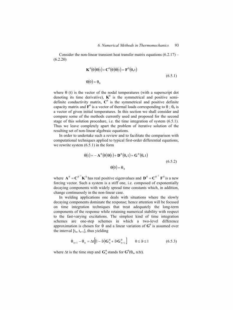
6. Numerical Methods in Thermomechanics 93
Consider the non-linear transient heat transfer matrix equations (6.2.17) –
(6.2.20)
00
ttt ,FCK
(6.5.1)
where (t) is the vector of the nodal temperatures (with a superscript dot
denoting its time derivative), K is the symmetrical and positive semi-
definite conductivity matrix, C is the symmetrical and positive definite
capacity matrix and F is a vector of thermal loads corresponding to ; 0 is
a vector of given initial temperatures. In this section we shall consider and
compare some of the methods currently used and proposed for the second
stage of this solution procedure, i.e. the time integration of system (6.5.1).
Thus we leave completely apart the problem of iterative solution of the
resulting set of non-linear algebraic equations.
In order to undertake such a review and to facilitate the comparison with
computational techniques applied to typical first-order differential equations,
we rewrite system (6.5.1) in the form
00
tttt ,G,DA
(6.5.2)
where KCA1
has real positive eigenvalues and FCD1
is a new
forcing vector. Such a system is a stiff one, i.e. composed of exponentially
decaying components with widely spread time constants which, in addition,
change continuously in the non-linear case.
In welding applications one deals with situations where the slowly
decaying components dominate the response; hence attention will be focused
on time integration techniques that treat adequately the long-term
components of the response while retaining numerical stability with respect
to the fast-varying excitations. The simplest kind of time integration
schemes are one-step schemes in which a two-level difference
approximation is chosen for and a linear variation of G is assumed over
the interval [tn, tn+1], thus yielding
1nnn1n 1t GG 10 (6.5.3)
where t is the time step and nG stands for G ( n, n t).
94 Theory of Thermomechanical Processes in Welding
These methods will be referred to as generalized trapezoidal schemes. A
slightly different form of one-step scheme is obtained from the same two-
level difference approximation for and from an assumed linear behaviour
of over [tn, tn+1]
tttn1n ,GG (6.5.4)
in which
tttt1t
10
1
n1nn
1nn
(6.5.5)
They will be referred to as generalized mid-point schemes. the two
families reduce to one if G is a linear function of the unknown (e.g. linear
heat conduction): the so-called ‘ -method’. Particular cases are well known
scheme.backwardEulerorimplicitfully1
scheme,Galerkin
scheme,rule)point-(midNicolson-Crankorpezoidaleither tra
scheme,(forward)explicitEuler0
32
21
All the schemes are consistent ones of the first order, except for 21 , in
which case the two families are second-order accurate in the time step size.
Applied to system (6.5.2), the schemes (6.5.3) and (6.5.4) yield the
following set of nonlinear algebraic equations, with I denoting the identity
matrix
1nnnn1n1n tt1t1t DDAIAI (6.5.6)
for trapezoidal schemes
DAIAI tt1t n1n (6.5.7)
for mid-point schemes.
Thus every step involves the construction and solution of a new set of
equations; therefore iterative solution techniques (except for = 0) are
required in which tangent or secant approximations may be used.
A straight linearization has been proposed over a time step by assuming
6. Numerical Methods in Thermomechanics 95
n1n AA 1nn1n t,DD (6.5.8)
for trapezoidal schemes
or
nAA tn ,DD (6.5.9)
for mid-point schemes. This corresponds obviously to a secant or initial load
method of solution of the non-linear systems (6.5.6) or (6.5.7).
An extrapolation technique for the mid-point schemes family has been
proposed by taking
1nn1 (6.5.10)
A predictor-corrector technique has been proposed for the mid-point
schemes family in which a predicted value *1n stems from (6.5.7), by
assuming (6.5.9); a corrected value is then obtained by again solving (6.5.7)
with
*1nn
* 1
The procedure thus requires the solution of two linear systems of
equations per time step.
In two-step methods we consider the expression
*
*
D
A
t21
t2
n21n2
2n2n21
1n2n21
(6.5.11)
Clearly every step implies the construction and solution of a new system
of linear equations with the positive definite system matrix
*AI t221 . A different starting procedure is needed since the first
application of (6.5.11) requires knowledge of 1. One of the previous one-
step schemes can be used for this purpose, but the problems associated with
that changeover (e.g. step length change) will not be considered here.
Table 6.1 shows how most of the two-step schemes that have been
presented in the literature are derived from (6.5.11) by particular choice of
and 2. It should be noted that some of these schemes are equivalent to
particular one-step schemes: this is the case for the Dupont I scheme
(Dupont et al. 1974) when 21 and the Dupont II scheme (6.5.15) when
= 0, that both restore the Crank – Nicolson algorithm (scheme (6.5.7) with
96 Theory of Thermomechanical Processes in Welding
21 ). In addition a linearization of the unknown with [tn, tn+2], i.e. the
assumption that
2n2n1n / (6.5.12)
also restores particular one-step schemes. These are known as the Crank–
Nicolson scheme for (6.5.13) and (6.5.14) for whatever the value of , the
mid-point scheme (6.5.7) with 43 for (6.5.15) for whatever the value of ,
and the fully implicit mid-point scheme ( = 1) for (6.5.16).
The two-step methods are widely used in solutions of problems involving
phase change.
Table 6-1. Linearized two-step schemes
2 * t* Algorithm
name
Integration scheme
031 n+1 tn+1 Lee
1nn1n31
21
1n1n31
2n1n31
21
tt
t
t
DA
IA
AI
(6.5.13)
0
41
n+1 tn+1 Dupont I
nn1n21
1n1n
2n1n21
tt
t21
t
DAI
A
AI
(6.5.14)
21
21
0
n21
1n23
2
3nt Dupont II
*n*
1n*21
2n*21
tt
t2
t
DA
AI
AI
(6.5.15)
1 1 n1n2 tn+2 Linearized
fully implicit
*n21
1n2n*23
t
2t
D
AI(6.5.16)
6.6 Solution Procedure for Navier-Stokes Equation
Thermal field and fluid flow field can be found using the factorial step
method. With the solution known everywhere at time tn we determine the
solution of the fluid flow equation at the next time level tn + 1. In this method
an intermediate velocity field v* is calculated to satisfy only a discretized
version of Eq. (6.3.13) without the pressure term. We have
nv
nvvv 1
t vDvEGRv (6.6.1)
6. Numerical Methods in Thermomechanics 97
vvv n* (6.6.2)
The required velocity and pressure fields vn + 1 and Pn + 1 are then obtained
by adding to v* the dynamic effect of pressure determined to ensure that the
incompressibility condition remains satisfied
*t v1n
vv 1
vEPERE (6.6.3)
With the velocity and pressure at time tn + 1 so determined the solution is
completed by evaluating the temperature at this time from Eq. (6.3.11).
LKFC1
t (6.6.4)
n1n (6.6.5)
6.7 Modeling of the Phase Change Process
Two major problems make the welding stress analysis of materials
involving phase change difficult to handle. The first is the method of
accounting for latent heat absorption or release during the phase change. The
second one is the kinematics of the phase boundary. The abrupt change of
properties during phase change (Fig. 6-1) for most materials undoubtedly
causes numerical instability in the analysis.
Attempts have been made to solve this type of problem by the classical
method using the heat conduction equation with the latent heat and moving
solid-liquid interface included in the boundary conditions. But only a limited
number of problems involving simple geometries can be solved in this way.
A different concept is the so-called enthalpy method.
In constructing the solution of problems involving phase change a
possible approach is to track accurately the position of the phase boundary
and then to solve Eq. (6.2.1) for the solid region and Eqs. (6.3.1) – (6.3.5)
for the fluid region. Consider the case when the phase change process is
modeled by a variant of the enthalpy method. In this method the phase
change is assumed to occur over a temperature range and the associated
latent heat effects is handled by increasing suitably the specific heat in this
range. Thus if the phase change is assumed to occur over the temperature
interval [ s, l], where l is the liquidus and s the solidus temperature, then
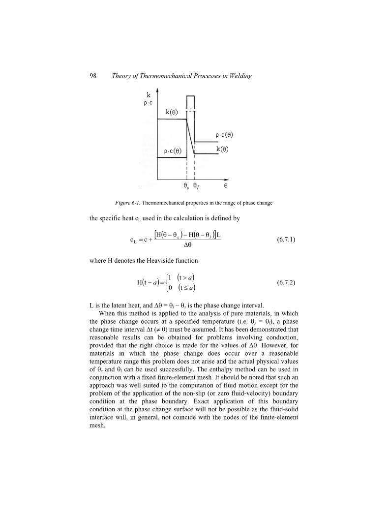
98 Theory of Thermomechanical Processes in Welding
Figure 6-1. Thermomechanical properties in the range of phase change
the specific heat cL used in the calculation is defined by
LHHccL
ls (6.7.1)
where H denotes the Heaviside function
a
aa
t0
t1tH (6.7.2)
L is the latent heat, and = l – s is the phase change interval.
When this method is applied to the analysis of pure materials, in which
the phase change occurs at a specified temperature (i.e. s = l), a phase
change time interval t ( 0) must be assumed. It has been demonstrated that
reasonable results can be obtained for problems involving conduction,
provided that the right choice is made for the values of . However, for
materials in which the phase change does occur over a reasonable
temperature range this problem does not arise and the actual physical values
of s and l can be used successfully. The enthalpy method can be used in
conjunction with a fixed finite-element mesh. It should be noted that such an
approach was well suited to the computation of fluid motion except for the
problem of the application of the non-slip (or zero fluid-velocity) boundary
condition at the phase boundary. Exact application of this boundary
condition at the phase change surface will not be possible as the fluid-solid
interface will, in general, not coincide with the nodes of the finite-element
mesh.
6. Numerical Methods in Thermomechanics 99
We overcame this problem by using a smearing approach in which the
viscosity was greatly increased in the phase change region. The problem can
be also overcome by adopting the simpler, but perhaps less accurate
approach of reducing the nodal velocity to zero whenever the nodal
temperature lies below the liquidus.
6.8 The Theorem of Virtual Work in Finite Increments
Consider a field of finite stress increments nT that satisfies momentum
equation
div nT = 0 (6.8.1)
with relation nT n = nt on the boundary a of the considered domain V.
Let nu* and n * be respectively, a field of virtual finite increments of
material displacement and a field of virtual strain finite increments which are
linked through compatibility relation
2 n = grad nu + (grad nu)T (6.8.2)
A theorem of virtual work in finite stress increments nT and in virtual
finite displacement increments nu* can be derived from the time-
discretized equations in a similar way to the derivation of the theorem of
virtual work (2.5.9) from the non-discretized equations of the problem
0da*dV
a
nn
V
nn ut (6.8.3)
In (6.8.3) n u has the dimension of a displacement, and the integrals in
Eq. (6.8.3) represent work quantities. Consider two fields of kinematically
admissible finite displacement increments n u and n uo. The difference n u
– n uo is kinematically admissible with zero finite displacement increments
imposed on the boundary a. By (6.8.3) applied to these fields we get
0dadV
a
onnn
V
onnn uut (6.8.4)
for every statically admissible n and nu and kinematically admissible
nuo. Consider the statically admissible finite increment fields of stress nT
and nTo. Their differences nT and nT
o are also statically admissible with
zero data imposed on a. By (6.8.3) applied to fields of finite increments
100 Theory of Thermomechanical Processes in Welding
onnn * uuu (6.8.5)
and to fields of auto-equilibrated stress ( nT – nTo)
0dV
V
onn
onn (6.8.6)
for every statically admissible nT, nTo and kinematically admissible nu,
nuo. By expression (6.8.6) the sum of the virtual works of auto-equilibrated
finite increments of all the forces, which are developed in fields of virtual
displacements kinematically admissible with zero data, is zero.
6.9 The Thermo-Elasto-Plastic Finite Element Model
Consider the virtual work equation for a finite element assemblage for a
thermo-elastic-plastic material model at time t + t (step n+1)
V
1n1nT dV RB (6.9.1)
1np
1n1n1n1n C (6.9.2)
nnpn D (6.9.3)
R1n1n (6.9.4)
where
1n1n BU (6.9.5)
and B is the total strain-displacement transformation matrix, Un+1 is the
nodal point displacement vector, Rn+1 is nodal point external load vector, D
is the deviatoric stress operator matrix and T is [1,1,1,0,0,0]. Substituting
Eqs. (6.9.2) and (6.9.5) into Eq. (6.9.1) we get
dV
V
p1n
T1n1n CBRKU (6.9.6)
6. Numerical Methods in Thermomechanics 101
where
V
1nT dVBCBK (6.9.7)
is the elastic stiffness matrix.
6.10 Solution Procedure for Thermo-Elasto-Plastic
Problems
The solution of thermo-elasto-plastic problems in welding using the
finite-element method is a complicated process. Certain numerical
difficulties have been apparent for some classes of problem, particularly
when gross section yielding has been involved. The method of dealing with
the constitutive equations governing the material behaviour is very
important. The original formulations concentrated on forward Euler
schemes, but more recently the advantages of backward Euler schemes and
the radial return algorithms have been realized. For incremental finite-
element analysis, the previous equations of state have to be processed within
each time step tn during load incrementation and iteration. Given the values
of stress, strain, displacement and temperature at tn, a vector of nodal loads is
used to find displacements and total strains at tn+1. From these, using the
constitutive law which expresses the plasticity rate equations, the stress and
plastic strains can be evaluated to furnish a complete solution at tn+1. Load
residuals may be calculated to assess the current state of convergence and
then to decide whether further iterations are required before completing the
current load increment.
From the algorithmic point of view, the way in which p is calculated is
extremely important. Using the -method we have
nnpn
p tt TD (6.10.1)
where
1nnn 1 TTT (6.10.2)
...,,, nnnnn T (6.10.3)
and
102 Theory of Thermomechanical Processes in Welding
ttttt 1nnn ,,, XXXXXX (6.10.4)
for arbitrary X.
The values of decide which type of procedure is relevant. Three main
categories exist, differing by the direction of the flow vector at current time
values thereby affecting accuracy and stability. The first method is called
tangent stiffness, radial corrector where = 0. The second one it is mean
normal where 21 and the last one elastic predictor, radial return where
= 1.
The tangent stiffness-radial corrector ( = 0) method is the original
method and has been used extensively. The mean normal (21 ) method
uses a mean plastic flow direction, and conceptually lies between methods 1
and 3. The elastic predictor-radial return ( = 1) algorithm assumes the
stress can be corrected to lie on the yield surface by applying a fixed scaling
factor to all components of deviatoric stress. The radial return method, has
received much attention in recent years because of the high accuracy and
quadratic convergence rate when used in conjunction with a consistent
tangent stiffness matrix. The value of indicates the character of the method
of numerical integration. Thus > 0 implies an implicit method. For Huber-
Mises criterion the method is unconditionally stable if 21 but
unconditionally stable otherwise.
An important factor in accumulating the state variables over iterations
within a load increment is the point of reference of the data. Given an
increment t = tn+1 – tn , the plasticity algorithms produce in each time-step
updates for displacements, total strains, stresses and plastic strains in that
order. If each is a straight update of the values at tn , then path-dependent
updating takes place. If, however, all such updates are referred back to the
start of the load increment, say tN , with each value such as dT reflecting the
rate value from that time, path-independent updating occurs.
Path dependence was invariably used with the older, radial correction
type algorithms but because of the somewhat oscillatory and self-
compensating behaviour of the increments in the main field values
particularly over the early iterations of each load step, unfortunate effects
could occur. Because plasticity is a discontinuous process, Gauss points
which were nearly plastic had stresses oscillating into and out of a yielded
state. The unnatural unloading associated with this has the effect of
producing local point-wise divergence that could grow over several
iterations to render a completely divergent solution.
Part III
HEAT FLOW IN WELDING
Chapter 7
ANALYTICAL SOLUTIONS OF THERMAL
PROBLEMS IN WELDING
7.1 Introduction
The solution of heat flow equations for welding conditions is a
complicated problem. In a realistic model the thermal conductivity and
specific heat should be considered as a functions of temperature. In most
types of welding melting occurs and convective heat transfer in addition to
conductive heat transfer takes place. In general, the source of heat is not
concentrated at a point or line but is spread out over the workpiece with an
unknown distribution of heat input. In addition, most realistic welding
problems have heat losses at the boundaries caused by convection, radiation
and contact with other bodies, so the precise boundary conditions are often
unknown. In order to find analytical solutions to the equations, it is therefore
necessary to make many simplifying assumptions. The purpose of this
chapter is to present analytical solutions to the heat transfer equations under
conditions of interest in welding. The restrictive assumptions will however
limit the practical utility of the results. Nevertheless the results are useful in
that they emphasize the variables involved and approximate the way in
which they are related. In addition, such solutions provide the background
for understanding more complicated solutions obtained numerically and
provide guidance in making judgments.
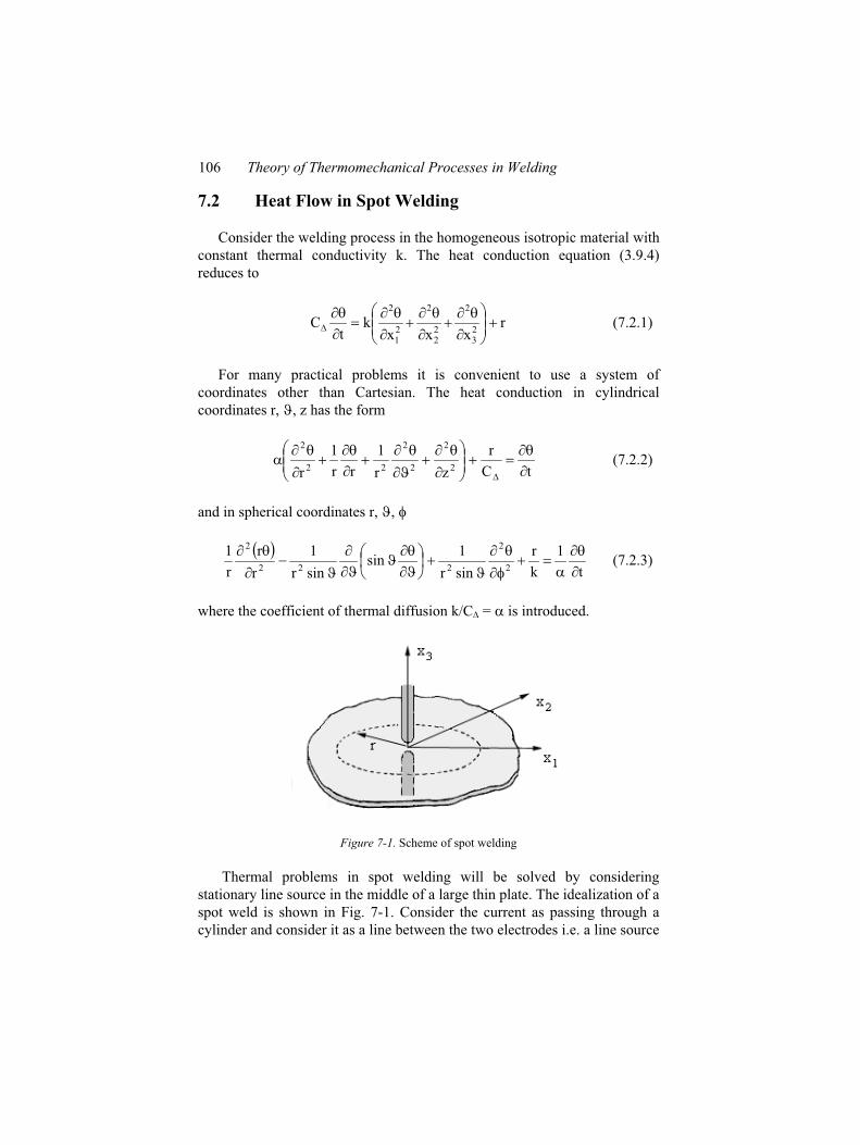
106 Theory of Thermomechanical Processes in Welding
7.2 Heat Flow in Spot Welding
Consider the welding process in the homogeneous isotropic material with
constant thermal conductivity k. The heat conduction equation (3.9.4)
reduces to
rxxx
kt
C23
2
22
2
21
2
(7.2.1)
For many practical problems it is convenient to use a system of
coordinates other than Cartesian. The heat conduction in cylindrical
coordinates r, , z has the form
tC
r
zr
1
rr
1
r 2
2
2
2
22
2
(7.2.2)
and in spherical coordinates r, ,
t
1
k
r
sinr
1sin
sinr
1
r
r
r
12
2
222
2
(7.2.3)
where the coefficient of thermal diffusion k/C = is introduced.
Figure 7-1. Scheme of spot welding
Thermal problems in spot welding will be solved by considering
stationary line source in the middle of a large thin plate. The idealization of a
spot weld is shown in Fig. 7-1. Consider the current as passing through a
cylinder and consider it as a line between the two electrodes i.e. a line source

7. Analytical Solutions of Thermal Problems in Welding 107
along the x3 axis of length g. Assume the current to pass through the material
in zero time an instantaneous stationary line source along the x3 axis.
The plates being welded are assumed to be of the same material and at
some reference temperature equal to zero prior to the passage of the current.
Consider two dimensional case of heat flow equation and cylindrical
coordinate system (r, , t).
The initial condition is
00,,rt,,r 0 (7.2.4)
The boundary conditions are
0trr r
,, (7.2.5)
We have
0g
Qdt
rkr2 (7.2.6)
where Q is the heat input and g is the thickness of the plate.
The solution of Eq. (7.2.1) under these conditions is
t4
rexp
kt4
1
g
Q 2
s (7.2.7)
where the introduced subscript s refers to spot welding.
It is convenient to write Eq. (7.2.7) in dimensionless form as
t
rexp
t
12s
s (7.2.8)
where
QCg
grr
gt4t
3s
s
2
(7.2.9)
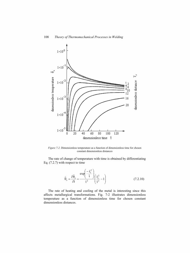
108 Theory of Thermomechanical Processes in Welding
Figure 7-2. Dimensionless temperature as a function of dimensionless time for chosen
constant dimensionless distances
The rate of change of temperature with time is obtained by differentiating
Eq. (7.2.7) with respect to time
1t
r
t
t
rexp
t 2
2s
2
2s
ss (7.2.10)
The rate of heating and cooling of the metal is interesting since this
affects metallurgical transformations. Fig. 7-2 illustrates dimensionless
temperature as a function of dimensionless time for chosen constant
dimensionless distances.
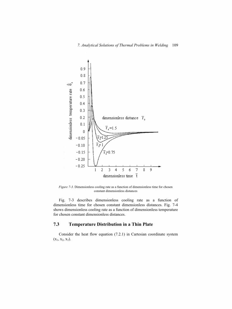
7. Analytical Solutions of Thermal Problems in Welding 109
Figure 7-3. Dimensionless cooling rate as a function of dimensionless time for chosen
constant dimensionless distances
Fig. 7-3 describes dimensionless cooling rate as a function of
dimensionless time for chosen constant dimensionless distances. Fig. 7-4
shows dimensionless cooling rate as a function of dimensionless temperature
for chosen constant dimensionless distances.
7.3 Temperature Distribution in a Thin Plate
Consider the heat flow equation (7.2.1) in Cartesian coordinate system
(x1, x2, x3).
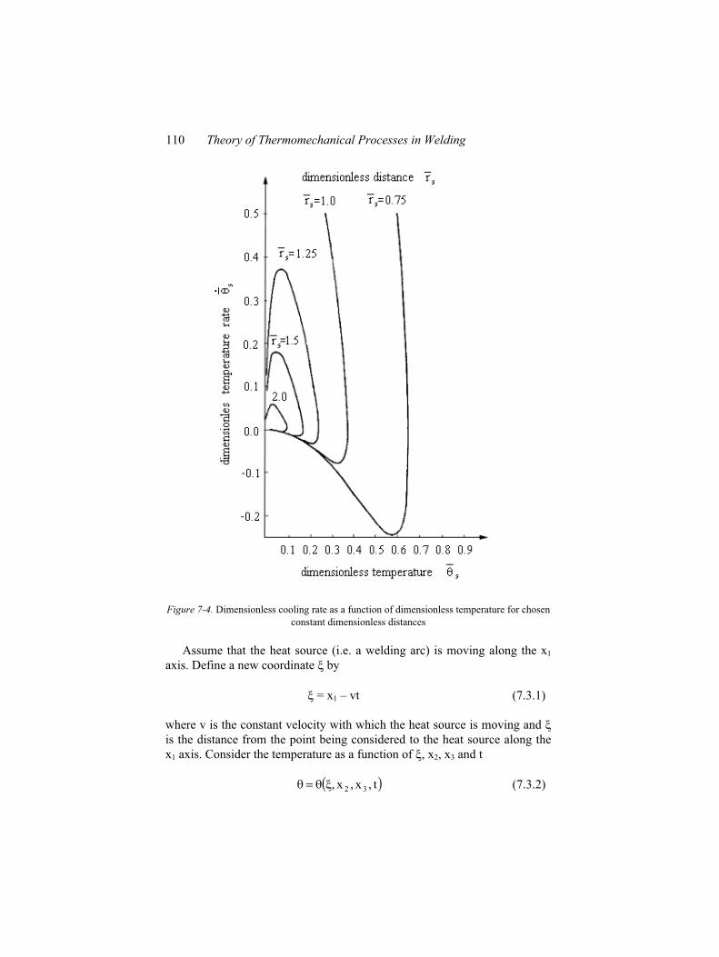
110 Theory of Thermomechanical Processes in Welding
Figure 7-4. Dimensionless cooling rate as a function of dimensionless temperature for chosen
constant dimensionless distances
Assume that the heat source (i.e. a welding arc) is moving along the x1
axis. Define a new coordinate by
= x1 – vt (7.3.1)
where v is the constant velocity with which the heat source is moving and
is the distance from the point being considered to the heat source along the
x1 axis. Consider the temperature as a function of , x2, x3 and t
t,x,x, 32 (7.3.2)
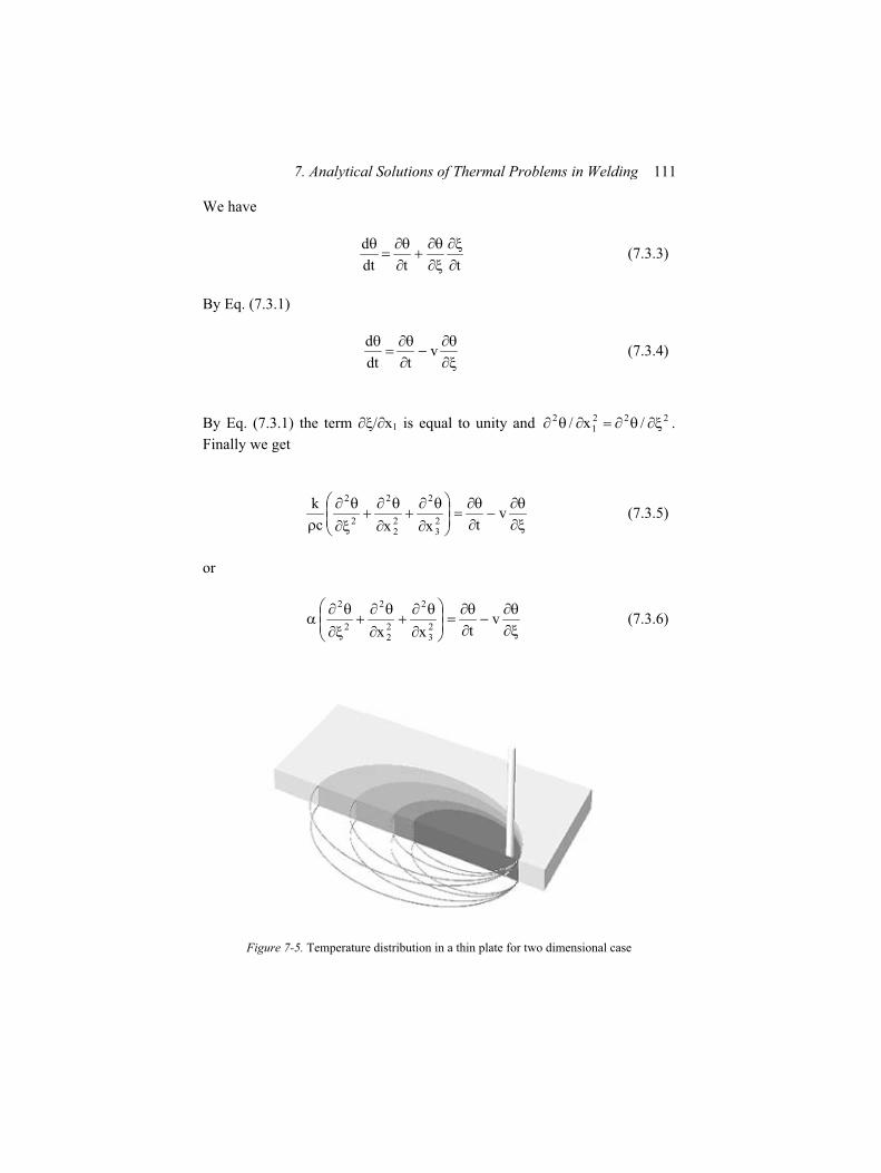
7. Analytical Solutions of Thermal Problems in Welding 111
We have
ttdt
d (7.3.3)
By Eq. (7.3.1)
vtdt
d (7.3.4)
By Eq. (7.3.1) the term / x1 is equal to unity and 2221
2 /x/ .
Finally we get
vtxxc
k23
2
22
2
2
2
(7.3.5)
or
vtxx 2
3
2
22
2
2
2
(7.3.6)
Figure 7-5. Temperature distribution in a thin plate for two dimensional case
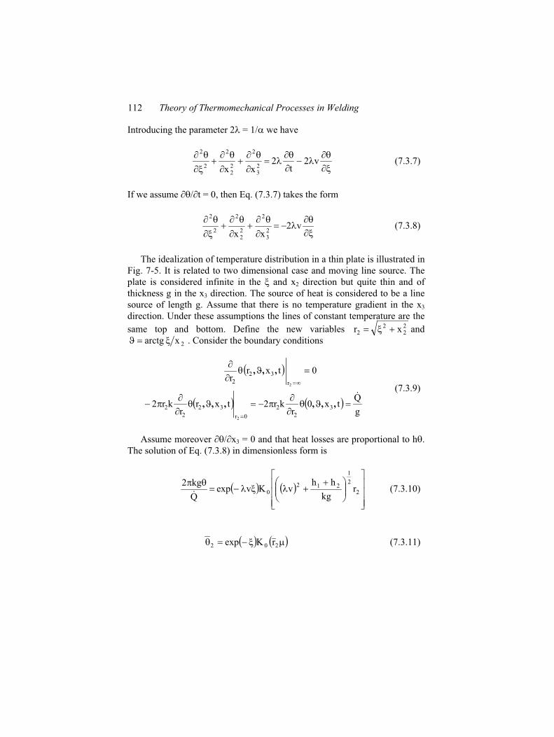
112 Theory of Thermomechanical Processes in Welding
Introducing the parameter 2 = 1/ we have
v2t
2xx 2
3
2
22
2
2
2
(7.3.7)
If we assume / t = 0, then Eq. (7.3.7) takes the form
v2xx 2
3
2
22
2
2
2
(7.3.8)
The idealization of temperature distribution in a thin plate is illustrated in
Fig. 7-5. It is related to two dimensional case and moving line source. The
plate is considered infinite in the and x2 direction but quite thin and of
thickness g in the x3 direction. The source of heat is considered to be a line
source of length g. Assume that there is no temperature gradient in the x3
direction. Under these assumptions the lines of constant temperature are the
same top and bottom. Define the new variables 22
22 xr and
2xarctg . Consider the boundary conditions
g
Qtx0
rkr2txr
rkr2
0txrr
3
2
2
0r
32
2
2
r
32
2
2
2
,,,,,,
,,,
(7.3.9)
Assume moreover / x3 = 0 and that heat losses are proportional to h .
The solution of Eq. (7.3.8) in dimensionless form is
2
2
1
212
0 rkg
hhvKvexp
Q
kg2 (7.3.10)
202 rKexp (7.3.11)
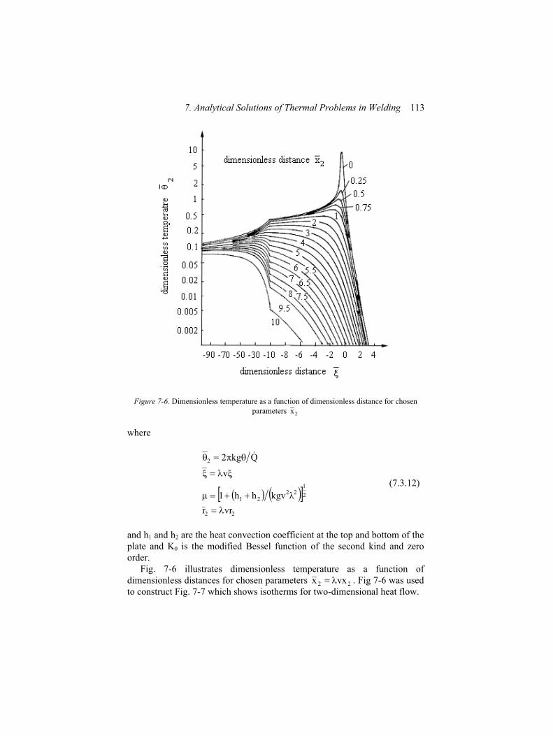
7. Analytical Solutions of Thermal Problems in Welding 113
Figure 7-6. Dimensionless temperature as a function of dimensionless distance for chosen
parameters 2x
where
22
2
122
21
2
vrr
kgvhh1
v
Qkg2
(7.3.12)
and h1 and h2 are the heat convection coefficient at the top and bottom of the
plate and K0 is the modified Bessel function of the second kind and zero
order.
Fig. 7-6 illustrates dimensionless temperature as a function of
dimensionless distances for chosen parameters 22 vxx . Fig 7-6 was used
to construct Fig. 7-7 which shows isotherms for two-dimensional heat flow.
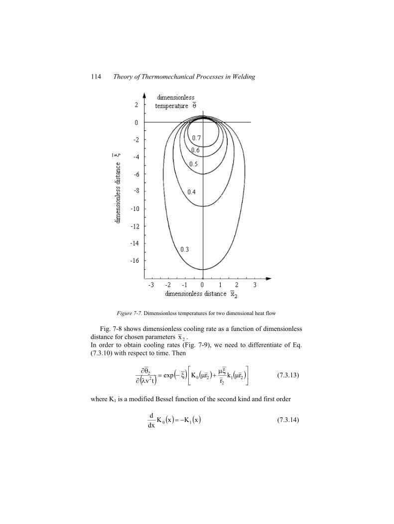
114 Theory of Thermomechanical Processes in Welding
Figure 7-7. Dimensionless temperatures for two dimensional heat flow
Fig. 7-8 shows dimensionless cooling rate as a function of dimensionless
distance for chosen parameters 2x .
In order to obtain cooling rates (Fig. 7-9), we need to differentiate of Eq.
(7.3.10) with respect to time. Then
21
2
202
2 rkr
rKexptv
(7.3.13)
where K1 is a modified Bessel function of the second kind and first order
xKxKdx
d10 (7.3.14)
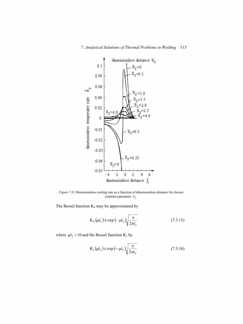
7. Analytical Solutions of Thermal Problems in Welding 115
Figure 7-8. Dimensionless cooling rate as a function of dimensionless distance for chosen
constant parameter 2x
The Bessel function K0 may be approximated by
2
220r2
rexprK (7.3.15)
where 10r2 and the Bessel function K1 by
2
221r2
rexprK (7.3.16)
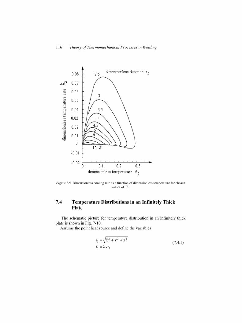
116 Theory of Thermomechanical Processes in Welding
Figure 7-9. Dimensionless cooling rate as a function of dimensionless temperature for chosen
values of 2r
7.4 Temperature Distributions in an Infinitely Thick
Plate
The schematic picture for temperature distribution in an infinitely thick
plate is shown in Fig. 7-10.
Assume the point heat source and define the variables
33
2223
vrr
zyr (7.4.1)
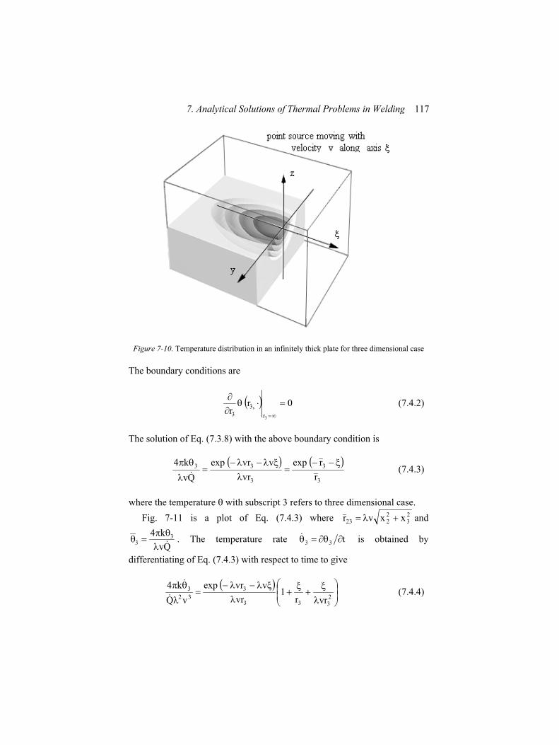
7. Analytical Solutions of Thermal Problems in Welding 117
Figure 7-10. Temperature distribution in an infinitely thick plate for three dimensional case
The boundary conditions are
0rr
3r
3
3
, (7.4.2)
The solution of Eq. (7.3.8) with the above boundary condition is
3
3
3
33
r
rexp
vr
vvrexp
Qv
k4 (7.4.3)
where the temperature with subscript 3 refers to three dimensional case.
Fig. 7-11 is a plot of Eq. (7.4.3) where 23
2223 xxvr and
Qv
k4 33 . The temperature rate t33 is obtained by
differentiating of Eq. (7.4.3) with respect to time to give
2333
3
32
3
vrr1
vr
vvrexp
vQ
k4 (7.4.4)
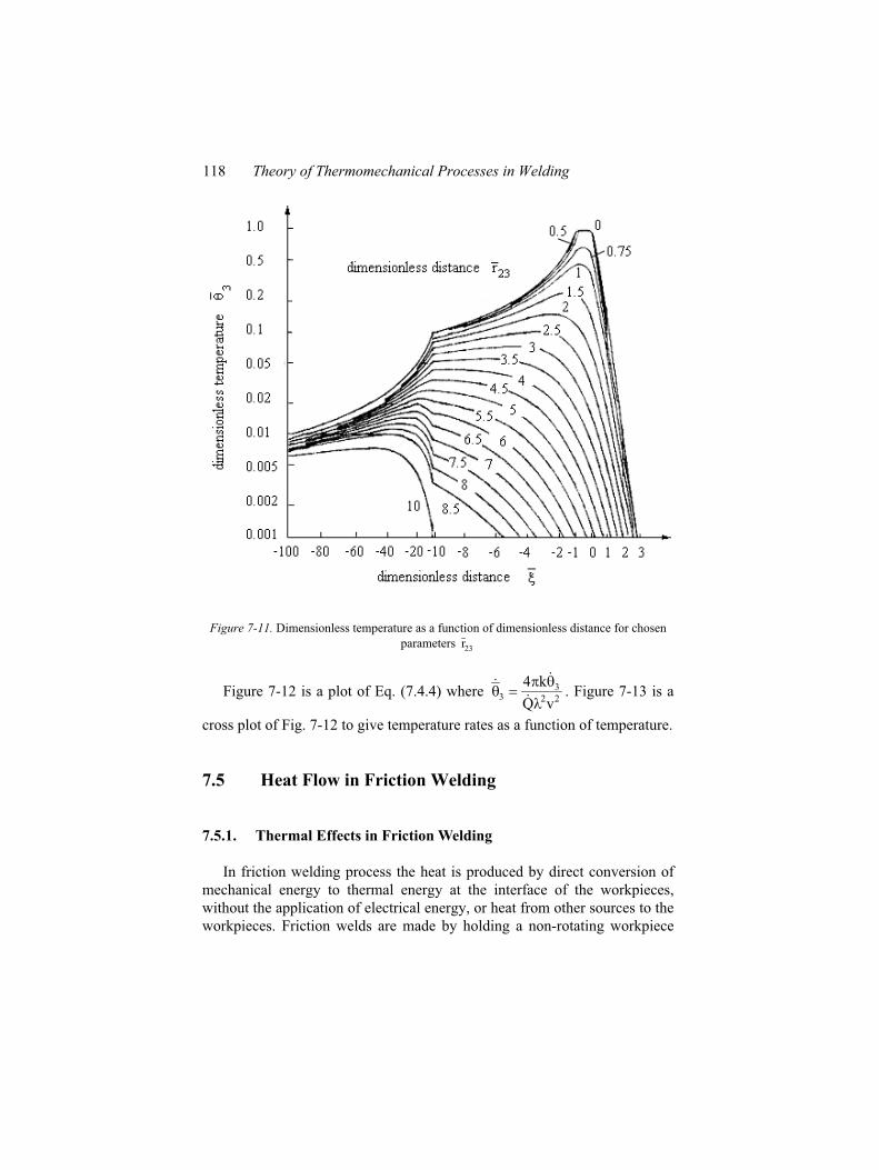
118 Theory of Thermomechanical Processes in Welding
Figure 7-11. Dimensionless temperature as a function of dimensionless distance for chosen
parameters23
r
Figure 7-12 is a plot of Eq. (7.4.4) where 22
33
vQ
k4. Figure 7-13 is a
cross plot of Fig. 7-12 to give temperature rates as a function of temperature.
7.5 Heat Flow in Friction Welding
7.5.1. Thermal Effects in Friction Welding
In friction welding process the heat is produced by direct conversion of
mechanical energy to thermal energy at the interface of the workpieces,
without the application of electrical energy, or heat from other sources to the
workpieces. Friction welds are made by holding a non-rotating workpiece
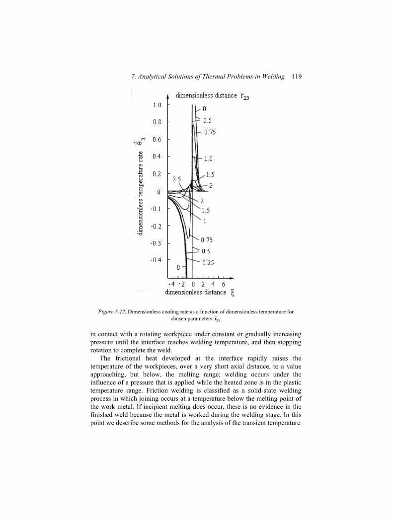
7. Analytical Solutions of Thermal Problems in Welding 119
Figure 7-12. Dimensionless cooling rate as a function of dimensionless temperature for
chosen parameters 23
r
in contact with a rotating workpiece under constant or gradually increasing
pressure until the interface reaches welding temperature, and then stopping
rotation to complete the weld.
The frictional heat developed at the interface rapidly raises the
temperature of the workpieces, over a very short axial distance, to a value
approaching, but below, the melting range; welding occurs under the
influence of a pressure that is applied while the heated zone is in the plastic
temperature range. Friction welding is classified as a solid-state welding
process in which joining occurs at a temperature below the melting point of
the work metal. If incipient melting does occur, there is no evidence in the
finished weld because the metal is worked during the welding stage. In this
point we describe some methods for the analysis of the transient temperature
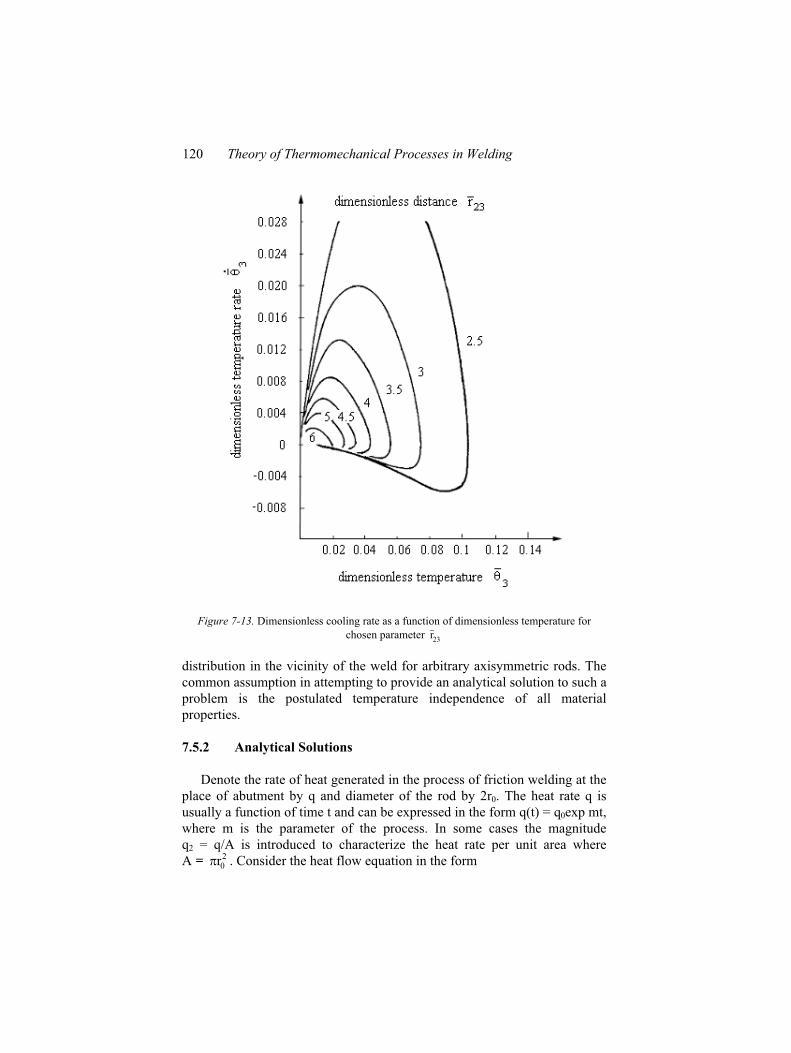
120 Theory of Thermomechanical Processes in Welding
Figure 7-13. Dimensionless cooling rate as a function of dimensionless temperature for
chosen parameter 23
r
distribution in the vicinity of the weld for arbitrary axisymmetric rods. The
common assumption in attempting to provide an analytical solution to such a
problem is the postulated temperature independence of all material
properties.
7.5.2 Analytical Solutions
Denote the rate of heat generated in the process of friction welding at the
place of abutment by q and diameter of the rod by 2r0. The heat rate q is
usually a function of time t and can be expressed in the form q(t) = q0exp mt,
where m is the parameter of the process. In some cases the magnitude
q2 = q/A is introduced to characterize the heat rate per unit area where
A = 20r . Consider the heat flow equation in the form
7. Analytical Solutions of Thermal Problems in Welding 121
xmtexpC
qb
xt
0
2
2
(7.5.1)
where x is the coordinate, (x) is the Dirac function, b = 2h/C r0 and h is the
surface film conductance.
The boundary conditions are
00x0tx
,, (7.5.2)
Using a Laplace transformation
0
st dtetxsx ,,~
(7.5.3)
we get
0msC
qsxsbsx'' 0,
~,
~ (7.5.4)
0s,'~
(7.5.5)
Since
sxsx ,~
,~
(7.5.6)
we have
0xx
bsexp
bsmskA2
qsx 0,
~
(7.5.7)
122 Theory of Thermomechanical Processes in Welding
Hence we obtain
tmbt2
xerfcx
mbexp
tmbt2
xerfc
xmb
expmb2
mtexp
kA2
qtx 0,
(7.5.8)
Introduce the new function
2erfcexp
2
1
2erfc
2
1
ll
2
lll ,
(7.5.9)
where
tbmxmb
l (7.5.10)
Then we get from equation (7.5.8)
tmb,xmb
A
mbxmtexp
mbkA2
qtx
l
0,
(7.5.11)
For m = 0, b > 0 and then Eq. (7.5.11) has the form
7. Analytical Solutions of Thermal Problems in Welding 123
0xbt,xb
bxexp
bkA2
qtx
l
0,
(7.5.12)
For small values of the x Eq. (7.5.8) can be expressed with sufficient
accuracy in the following form
0 x
xtmberfmb
mtexpkA2
qtx 0,
(7.5.13)
Consider the case (b + m) = 0. Then Eq. (7.5.8) has the form
0 xt2
xierfc
tbtexpkA
qtx 0,
(7.5.14)
where
u
x
u
0erfcdxe2
uerfcduuerfcuierfc2
(7.5.15)
At the place of contact when bt << 1 the temperature can be expressed as
tbtexpkA
qt,0 0 (7.5.16)
If m = b = 0 and q0 = const, then the temperature in the rods at the place
of abutment can be described by the equation
AkC
tqt,0 0 (7.5.17)
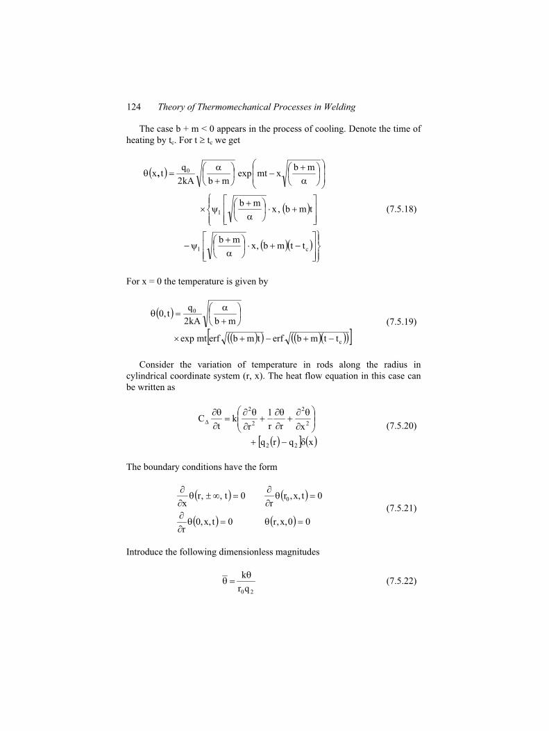
124 Theory of Thermomechanical Processes in Welding
The case b + m < 0 appears in the process of cooling. Denote the time of
heating by tc. For t tc we get
cl
l
0
ttmb,xmb
tmb,xmb
mbxmtexp
mbkA2
qtx,
(7.5.18)
For x = 0 the temperature is given by
c
0
ttmberftmberfmtexp
mbkA2
qt0,
(7.5.19)
Consider the variation of temperature in rods along the radius in
cylindrical coordinate system (r, x). The heat flow equation in this case can
be written as
xqrq
xrr
1
rk
tC
22
2
2
2
2
(7.5.20)
The boundary conditions have the form
00x,,r0tx,,0r
0tx,,rr
0t,,rx
0
(7.5.21)
Introduce the following dimensionless magnitudes
20qr
k (7.5.22)
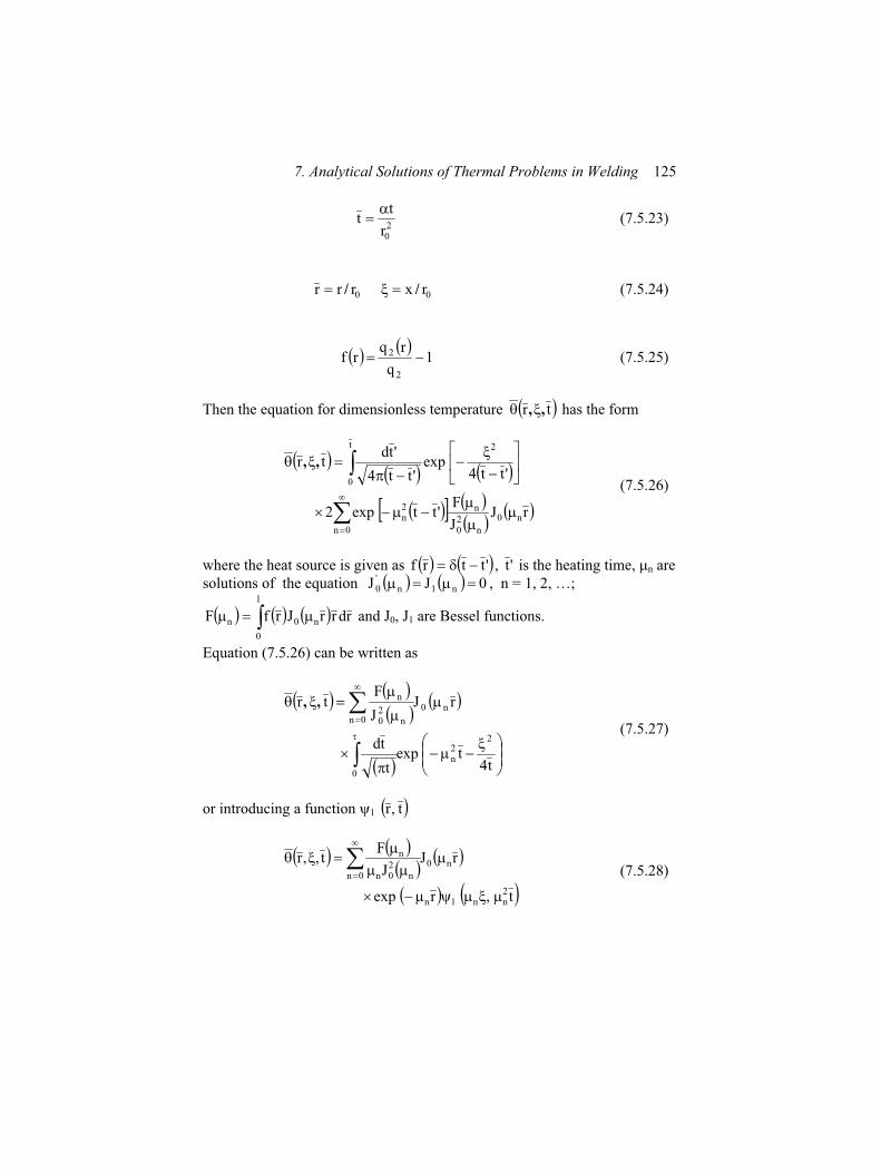
7. Analytical Solutions of Thermal Problems in Welding 125
20r
tt (7.5.23)
00 rxrrr // (7.5.24)
1q
rqrf
2
2 (7.5.25)
Then the equation for dimensionless temperature tr ,, has the form
rJJ
F'ttexp2
'tt4exp
'tt4
'tdtr
n0
n20
n
0n
2n
t
0
2
,,
(7.5.26)
where the heat source is given as 'ttrf , 't is the heating time, n are
solutions of the equation 0JJ n1n'0 , n = 1, 2, …;
rdrrJrfF
l
0
n0n and J0, J1 are Bessel functions.
Equation (7.5.26) can be written as
t4texp
t
td
rJJ
Ftr
22n
0
n0
0n n20
n,,
(7.5.27)
or introducing a function 1 t,r
t,rexp
rJJ
Ft,,r
2nn1n
n0
0n n20n
n
(7.5.28)
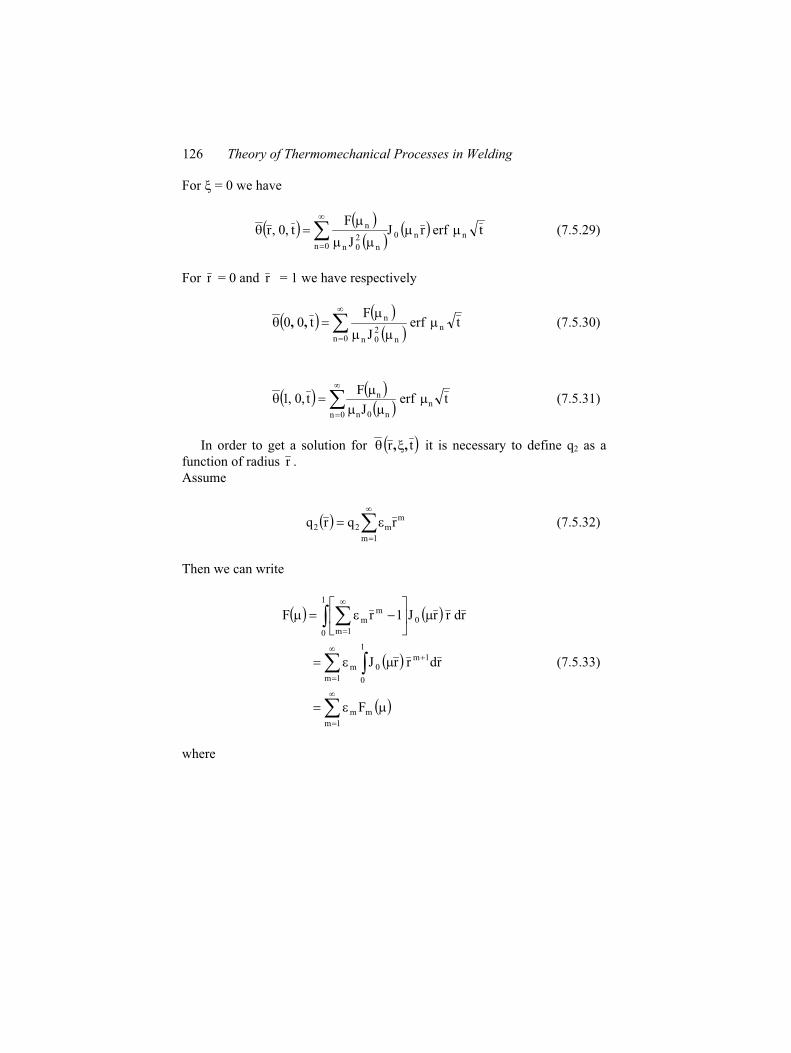
126 Theory of Thermomechanical Processes in Welding
For = 0 we have
terfrJJ
Ft,0,r nn0
0n n20n
n (7.5.29)
For r = 0 and r = 1 we have respectively
0n
n
n20n
n terfJ
Ft00 ,, (7.5.30)
0n
n
n0n
n terfJ
Ft,0,1 (7.5.31)
In order to get a solution for tr ,, it is necessary to define q2 as a
function of radius r .
Assume
1m
mm22 rqrq (7.5.32)
Then we can write
1m
mm
1m
1m
1
0
0m
1
0
0
1m
mm
F
rdrrJ
rdrrJ1rF
(7.5.33)
where
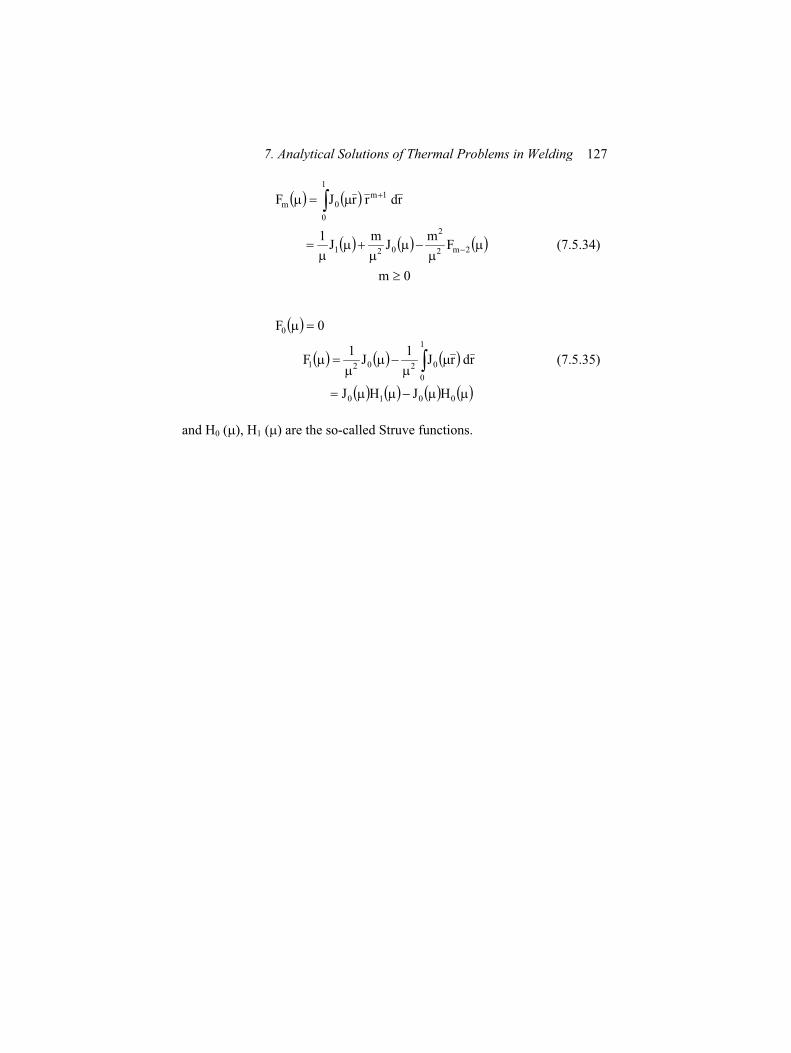
7. Analytical Solutions of Thermal Problems in Welding 127
0m
Fm
Jm
J1
rdrrJF
2m2
2
021
1
0
1m0m
(7.5.34)
0010
1
0
02021
0
HJHJ
rdrJ1
J1
F
0F
(7.5.35)
and H0 ( ), H1 ( ) are the so-called Struve functions.
Chapter 8
NUMERICAL SOLUTIONS OF THERMAL
PROBLEMS IN WELDING
8.1 Introduction
The effective solutions of complex thermal problems in welding only
recently has become possible. In the last two decades one observes the
vigorous development of effective numerical methods of analysis.
Automobile, aircraft, nuclear and ship industry are experiencing a rapidly-
growing need for the numerical tools to handle complex problems of
welding. Efficient numerical methods for nonlinear welding problems are
needed because experimental testing in such cases is often prohibitively
expensive or physically impossible.
The intention of this chapter is to discuss numerical solutions of heat
flow in chosen welding processes. The choice of topics is by no means
comprehensive and is based on the authors results concerning laser and
electroslag welding. In this chapter heat flow problems in arc-welding and
friction welding are omitted to do not repeat the results which are in
agreement with analytical solutions of there problems presented in Chapter
7.
8.2 Temperature Distributions in Laser Microwelding
Laser welding has a wide application in industry. The pulsed lasers allow
the production of impulses of radiation in the time intervals 10-3 – 10-12 sec,
obtaining the peak power in the range of gigawatts and radiation intensity to
1017 W/m2. It is an important problem in laser welding to determine both
130 Theory of Thermomechanical Processes in Welding
temperature field within welded material and changes of material’s shape
during melting process for a given laser impulse.
Optical properties of metals are implied directly from their electrical
properties. An electric conductivity, which is dependent on material
properties, its temperature and frequency of falling electro-magnetic wave,
has important significance. The plasma frequency p for metals implying
from quantity of electrons of conduction per unit volume (N = 1028 – 1029
elec/m3) is equal to 1015 – 1016 /sec. For wave frequency < p the
reflection coefficient is very high and a part of absorbed wave is strongly
dumped. Its intensity decreases in an exponential way. For waves of
frequency > p metals are to be transparent, and for instance for
p = 5.7 1015 /sec a material becomes transparent for waves shorter than
330 nm (i.e. in ultraviolet). In the range of visible infrared radiation for
almost all metals the reflection coefficient is high and reaches values up to
90% and more. However, it is strongly dependent on wave frequency and,
for instance, for silver, in the visible range is equal to 95%, and in
ultraviolet 4.2%. The value of reflection coefficient depends in a significant
way on the kind of machining and the cleanliness of the material surface.
For temperatures in which the electric super-conductivity appears, optical
properties change because of abnormal skin effect and need be considered in
another way. Using a simplified model of monochromatic radiation
absorption (only by free electrons) on the surface of a semi-infinite body we
may assume that in the visual and infrared parts of the radiation spectrum the
absorption is in the layer of thickness < 0.1 m.
In the absorption model the value of the absorption coefficient for metals
is equal to 108 – 107 [1/m], and within the body by the Bouguer law the heat
source is
za etEt,zA (8.2.1)
where Ea is absorbed, changed in time radiation intensity of the source, is
the absorption coefficient for given material, t is the time variable and z is
the coordinate.
Assuming Eq. (8.2.1) we may easily determine the thickness of the layer
in which fixed part of radiation will be absorbed, The results of calculations
for extremal values of are given in Table 8-1. Experimental data confirm
that visual and infrared radiation is absorbed in metal within the layer of
thickness 0.01 – 0.1 m. In a large number of papers the model of laser
radiation absorption on surface of body is analyzed. Assuming such a model
we should analyze the time intervals for which this model is correct,
because, for instance, the laser impulses of duration 10 – 12 – 10 – 3 sec cannot
be treated in the same way. For laser impulses of duration 10 – 8 sec and
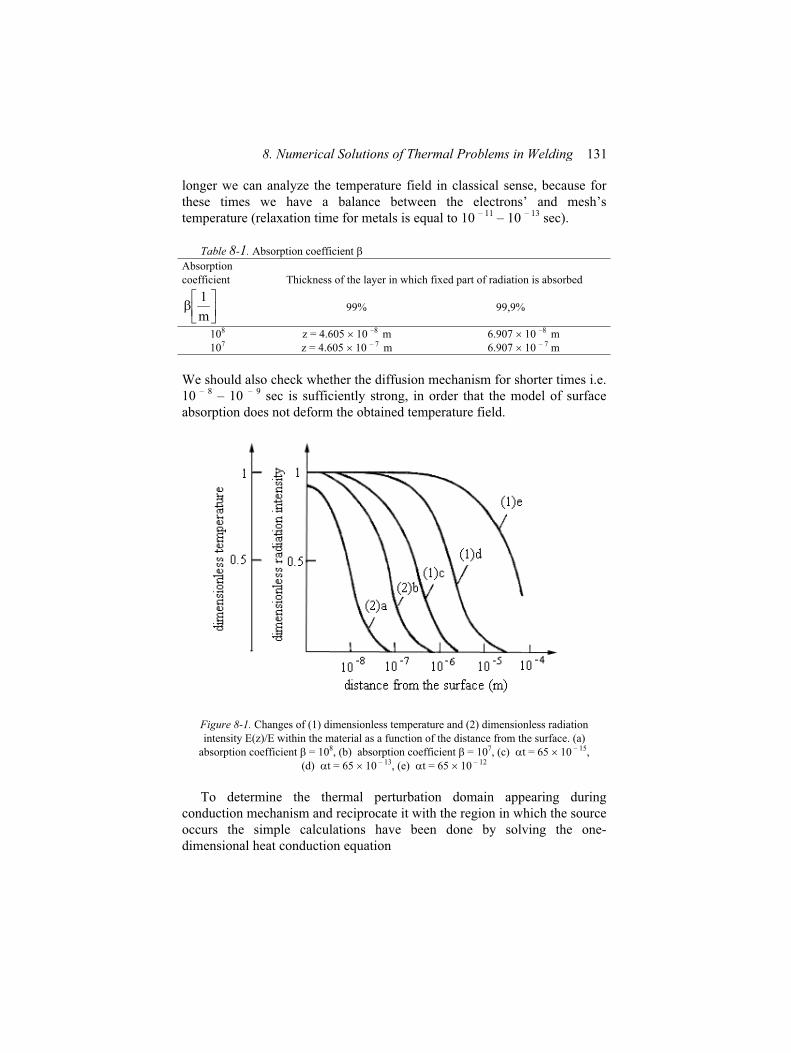
8. Numerical Solutions of Thermal Problems in Welding 131
longer we can analyze the temperature field in classical sense, because for
these times we have a balance between the electrons’ and mesh’s
temperature (relaxation time for metals is equal to 10 – 11 – 10 – 13 sec).
Table 8-1. Absorption coefficient
Absorption
coefficient
m
1
Thickness of the layer in which fixed part of radiation is absorbed
99% 99,9%
108 z = 4.605 10 –8 m 6.907 10 –8 m
107 z = 4.605 10 – 7 m 6.907 10 – 7 m
We should also check whether the diffusion mechanism for shorter times i.e.
10 – 8 – 10 – 9 sec is sufficiently strong, in order that the model of surface
absorption does not deform the obtained temperature field.
Figure 8-1. Changes of (1) dimensionless temperature and (2) dimensionless radiation
intensity E(z)/E within the material as a function of the distance from the surface. (a)
absorption coefficient = 108, (b) absorption coefficient = 107, (c) t = 65 10 – 15,
(d) t = 65 10 – 13, (e) t = 65 10 – 12
To determine the thermal perturbation domain appearing during
conduction mechanism and reciprocate it with the region in which the source
occurs the simple calculations have been done by solving the one-
dimensional heat conduction equation
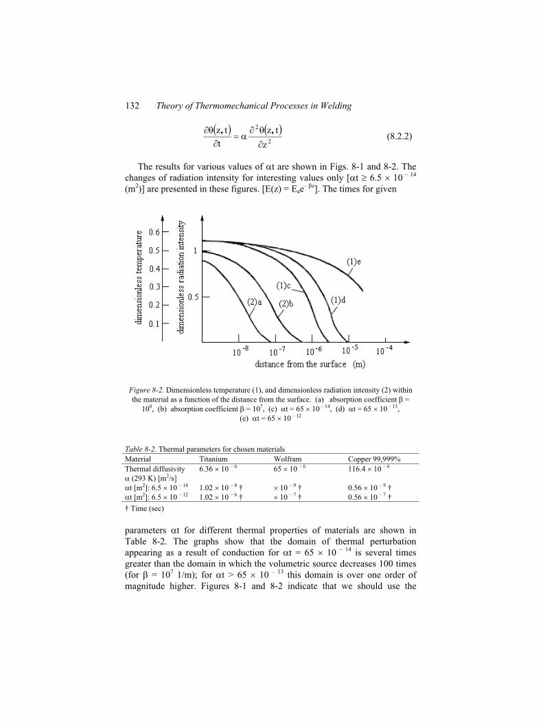
132 Theory of Thermomechanical Processes in Welding
2
2
z
tz
t
tz ,, (8.2.2)
The results for various values of t are shown in Figs. 8-1 and 8-2. The
changes of radiation intensity for interesting values only [ t 6.5 10 – 14
(m2)] are presented in these figures. [E(z) = Eae– z]. The times for given
Figure 8-2. Dimensionless temperature (1), and dimensionless radiation intensity (2) within
the material as a function of the distance from the surface. (a) absorption coefficient =
108, (b) absorption coefficient = 107, (c) t = 65 10 – 14, (d) t = 65 10 – 13,
(e) t = 65 10 – 12
Table 8-2. Thermal parameters for chosen materials
Material Titanium Wolfram Copper 99,999%
Thermal diffusivity 6.36 10 – 6 65 10 – 6 116.4 10 – 6
(293 K) [m2/s]
t [m2]: 6.5 10 – 14 1.02 10 – 8 † 10 – 9 † 0.56 10 – 9 †
t [m2]: 6.5 10 – 12 1.02 10 – 6 † 10 – 7 † 0.56 10 – 7 †
† Time (sec)
parameters t for different thermal properties of materials are shown in
Table 8-2. The graphs show that the domain of thermal perturbation
appearing as a result of conduction for t = 65 10 – 14 is several times
greater than the domain in which the volumetric source decreases 100 times
(for = 107 1/m); for t > 65 10 – 13 this domain is over one order of
magnitude higher. Figures 8-1 and 8-2 indicate that we should use the
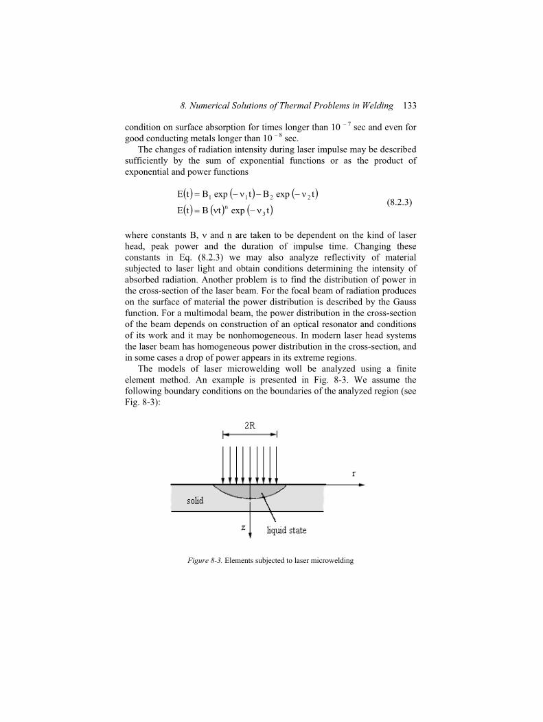
8. Numerical Solutions of Thermal Problems in Welding 133
condition on surface absorption for times longer than 10 – 7 sec and even for
good conducting metals longer than 10 – 8 sec.
The changes of radiation intensity during laser impulse may be described
sufficiently by the sum of exponential functions or as the product of
exponential and power functions
texptBtE
texpBtexpBtE
3
n
2211 (8.2.3)
where constants B, and n are taken to be dependent on the kind of laser
head, peak power and the duration of impulse time. Changing these
constants in Eq. (8.2.3) we may also analyze reflectivity of material
subjected to laser light and obtain conditions determining the intensity of
absorbed radiation. Another problem is to find the distribution of power in
the cross-section of the laser beam. For the focal beam of radiation produces
on the surface of material the power distribution is described by the Gauss
function. For a multimodal beam, the power distribution in the cross-section
of the beam depends on construction of an optical resonator and conditions
of its work and it may be nonhomogeneous. In modern laser head systems
the laser beam has homogeneous power distribution in the cross-section, and
in some cases a drop of power appears in its extreme regions.
The models of laser microwelding woll be analyzed using a finite
element method. An example is presented in Fig. 8-3. We assume the
following boundary conditions on the boundaries of the analyzed region (see
Fig. 8-3):
Figure 8-3. Elements subjected to laser microwelding
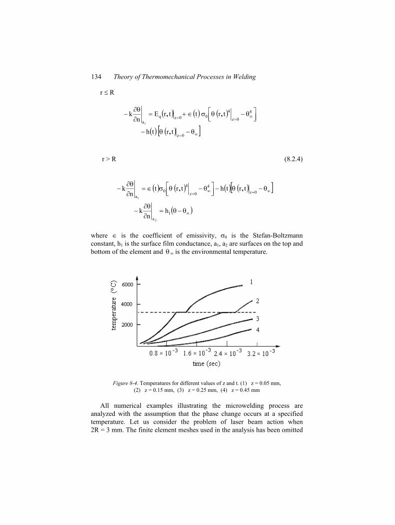
134 Theory of Thermomechanical Processes in Welding
r R
0z
4
0z
4
00zq
a
trth
trttrEn
k
1
,
,,
r > R (8.2.4)
1
a
0z
4
0z
4
0
a
hn
k
trthtrtn
k
2
1
,,
where is the coefficient of emissivity, 0 is the Stefan-Boltzmann
constant, h1 is the surface film conductance, a1, a2 are surfaces on the top and
bottom of the element and is the environmental temperature.
Figure 8-4. Temperatures for different values of z and t. (1) z = 0.05 mm,
(2) z = 0.15 mm, (3) z = 0.25 mm, (4) z = 0.45 mm
All numerical examples illustrating the microwelding process are
analyzed with the assumption that the phase change occurs at a specified
temperature. Let us consider the problem of laser beam action when
2R = 3 mm. The finite element meshes used in the analysis has been omitted
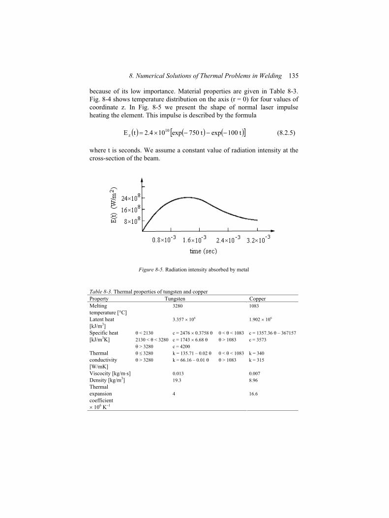
8. Numerical Solutions of Thermal Problems in Welding 135
because of its low importance. Material properties are given in Table 8-3.
Fig. 8-4 shows temperature distribution on the axis (r = 0) for four values of
coordinate z. In Fig. 8-5 we present the shape of normal laser impulse
heating the element. This impulse is described by the formula
t100expt750exp104.2tE 10z (8.2.5)
where t is seconds. We assume a constant value of radiation intensity at the
cross-section of the beam.
Figure 8-5. Radiation intensity absorbed by metal
Table 8-3. Thermal properties of tungsten and copper
Property Tungsten Copper
Melting
temperature [ C]
3280 1083
Latent heat
[kJ/m3]
3.357 106 1.902 106
Specific heat
[kJ/m3K]
< 2130
2130 < < 3280
> 3280
c = 2476 0.3758
c = 1743 6.68
c = 4200
0 < < 1083
> 1083
c = 1357.36 – 367157
c = 3573
Thermal
conductivity
[W/mK]
3280
> 3280
k = 135.71 – 0.02
k = 66.16 – 0.01
0 < < 1083
> 1083
k = 340
k = 315
Viscocity [kg/m s] 0.013 0.007
Density [kg/m3] 19.3 8.96
Thermal
expansion
coefficient
106 K–1
4 16.6
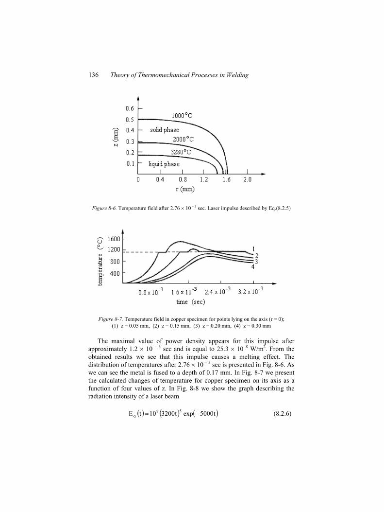
136 Theory of Thermomechanical Processes in Welding
Figure 8-6. Temperature field after 2.76 10 – 3 sec. Laser impulse described by Eq.(8.2.5)
Figure 8-7. Temperature field in copper specimen for points lying on the axis (r = 0);
(1) z = 0.05 mm, (2) z = 0.15 mm, (3) z = 0.20 mm, (4) z = 0.30 mm
The maximal value of power density appears for this impulse after
approximately 1.2 10 – 3 sec and is equal to 25.3 10 8 W/m2. From the
obtained results we see that this impulse causes a melting effect. The
distribution of temperatures after 2.76 10 – 3 sec is presented in Fig. 8-6. As
we can see the metal is fused to a depth of 0.17 mm. In Fig. 8-7 we present
the calculated changes of temperature for copper specimen on its axis as a
function of four values of z. In Fig. 8-8 we show the graph describing the
radiation intensity of a laser beam
t5000expt320010tE59 (8.2.6)
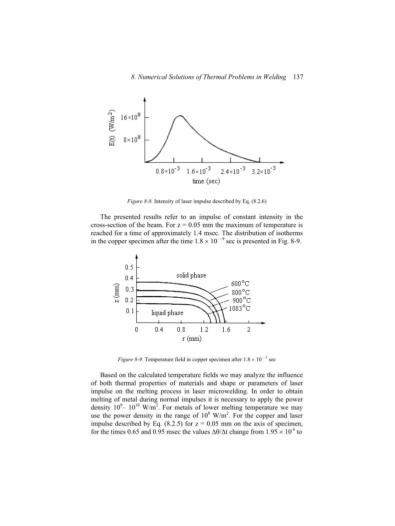
8. Numerical Solutions of Thermal Problems in Welding 137
Figure 8-8. Intensity of laser impulse described by Eq. (8.2.6)
The presented results refer to an impulse of constant intensity in the
cross-section of the beam. For z = 0.05 mm the maximum of temperature is
reached for a time of approximately 1.4 msec. The distribution of isotherms
in the copper specimen after the time 1.8 10 – 9 sec is presented in Fig. 8-9.
Figure 8-9. Temperature field in copper specimen after 1.8 10 – 3 sec
Based on the calculated temperature fields we may analyze the influence
of both thermal properties of materials and shape or parameters of laser
impulse on the melting process in laser microwelding. In order to obtain
melting of metal during normal impulses it is necessary to apply the power
density 109– 1010 W/m2. For metals of lower melting temperature we may
use the power density in the range of 108 W/m2. For the copper and laser
impulse described by Eq. (8.2.5) for z = 0.05 mm on the axis of specimen,
for the times 0.65 and 0.95 msec the values / t change from 1.95 10 6 to
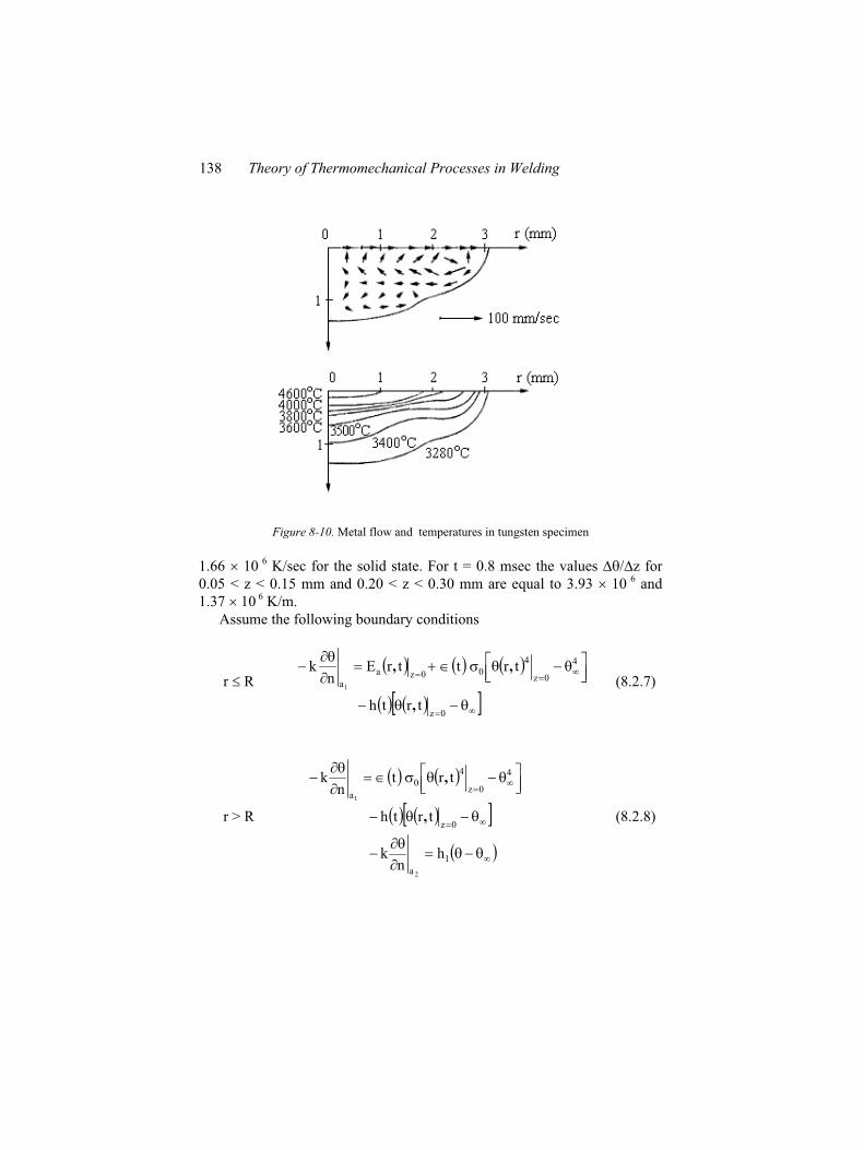
138 Theory of Thermomechanical Processes in Welding
Figure 8-10. Metal flow and temperatures in tungsten specimen
1.66 10 6 K/sec for the solid state. For t = 0.8 msec the values / z for
0.05 < z < 0.15 mm and 0.20 < z < 0.30 mm are equal to 3.93 10 6 and
1.37 10 6 K/m.
Assume the following boundary conditions
r R
0z
4
0z
4
00za
a
trth
trttrEn
k
1
,
,, (8.2.7)
r > R
1
a
0z
4
0z
4
0
a
hn
k
trth
trtn
k
2
1
,
,
(8.2.8)
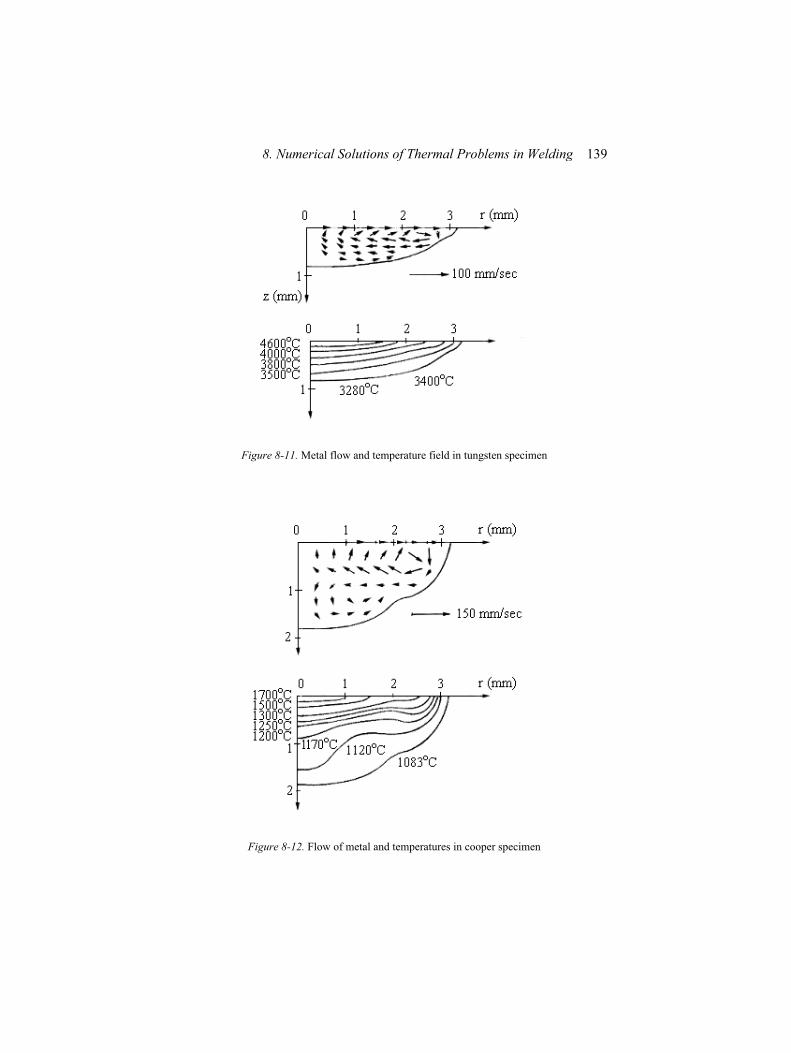
8. Numerical Solutions of Thermal Problems in Welding 139
Figure 8-11. Metal flow and temperature field in tungsten specimen
Figure 8-12. Flow of metal and temperatures in cooper specimen
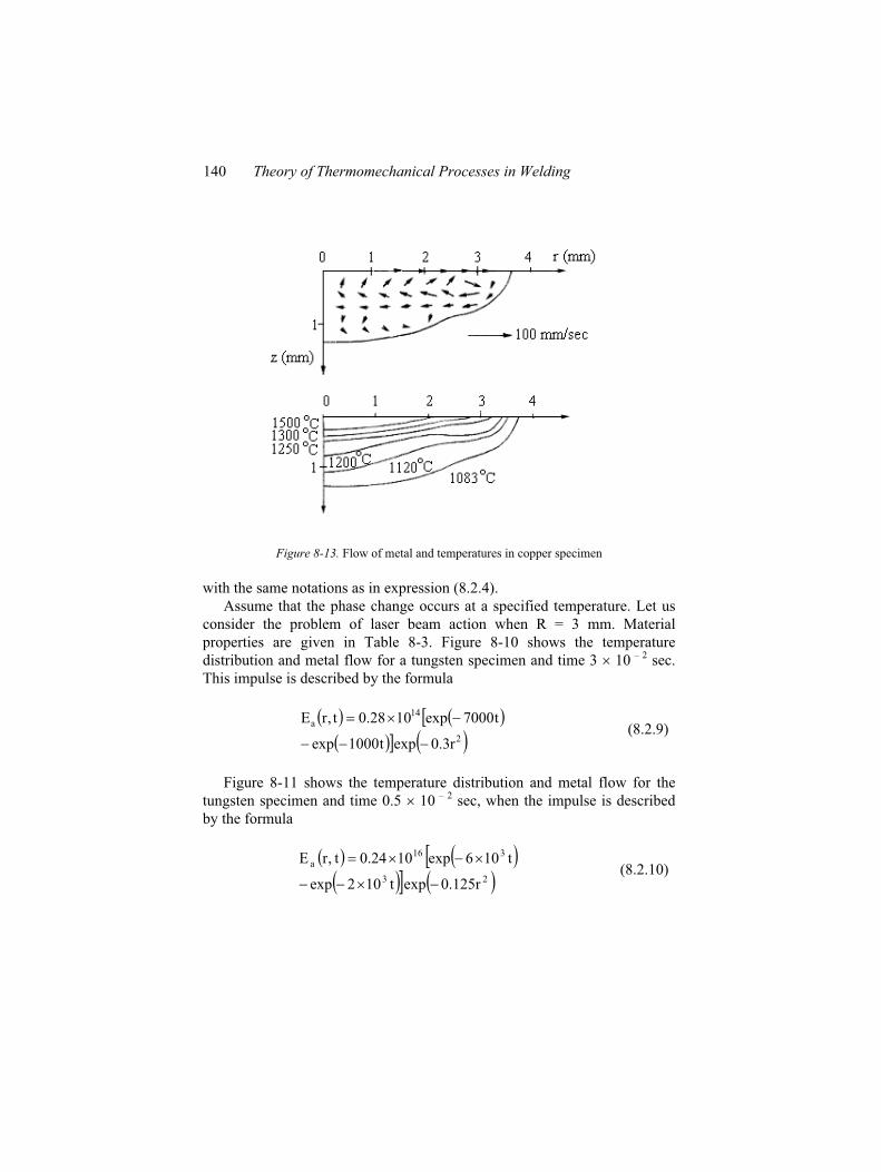
140 Theory of Thermomechanical Processes in Welding
Figure 8-13. Flow of metal and temperatures in copper specimen
with the same notations as in expression (8.2.4).
Assume that the phase change occurs at a specified temperature. Let us
consider the problem of laser beam action when R = 3 mm. Material
properties are given in Table 8-3. Figure 8-10 shows the temperature
distribution and metal flow for a tungsten specimen and time 3 10 – 2 sec.
This impulse is described by the formula
2
14a
r3.0expt1000exp
t7000exp1028.0t,rE (8.2.9)
Figure 8-11 shows the temperature distribution and metal flow for the
tungsten specimen and time 0.5 10 – 2 sec, when the impulse is described
by the formula
23
316a
r125.0expt102exp
t106exp1024.0t,rE (8.2.10)
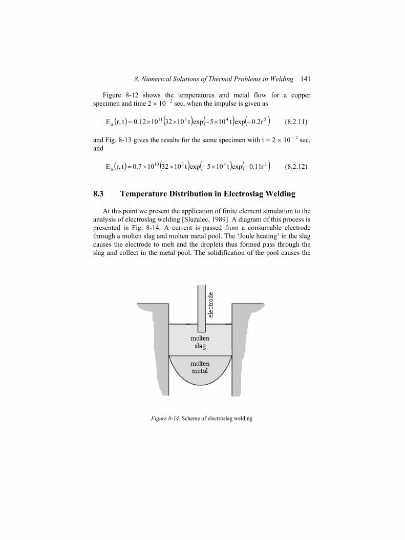
8. Numerical Solutions of Thermal Problems in Welding 141
Figure 8-12 shows the temperatures and metal flow for a copper
specimen and time 2 10 – 2 sec, when the impulse is given as
24311a r2.0expt105expt10321012.0t,rE (8.2.11)
and Fig. 8-13 gives the results for the same specimen with t = 2 10 – 2 sec,
and
24310a r11.0expt105expt1032107.0t,rE (8.2.12)
8.3 Temperature Distribution in Electroslag Welding
At this point we present the application of finite element simulation to the
analysis of electroslag welding [Sluzalec, 1989]. A diagram of this process is
presented in Fig. 8-14. A current is passed from a consumable electrode
through a molten slag and molten metal pool. The ‘Joule heating’ in the slag
causes the electrode to melt and the droplets thus formed pass through the
slag and collect in the metal pool. The solidification of the pool causes the
Figure 8-14. Scheme of electroslag welding
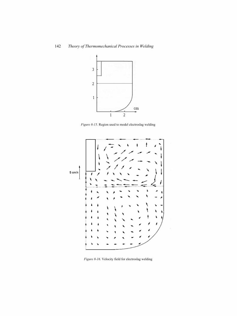
142 Theory of Thermomechanical Processes in Welding
Figure 8-15. Region used to model electroslag welding
Figure 8-16. Velocity field for electroslag welding
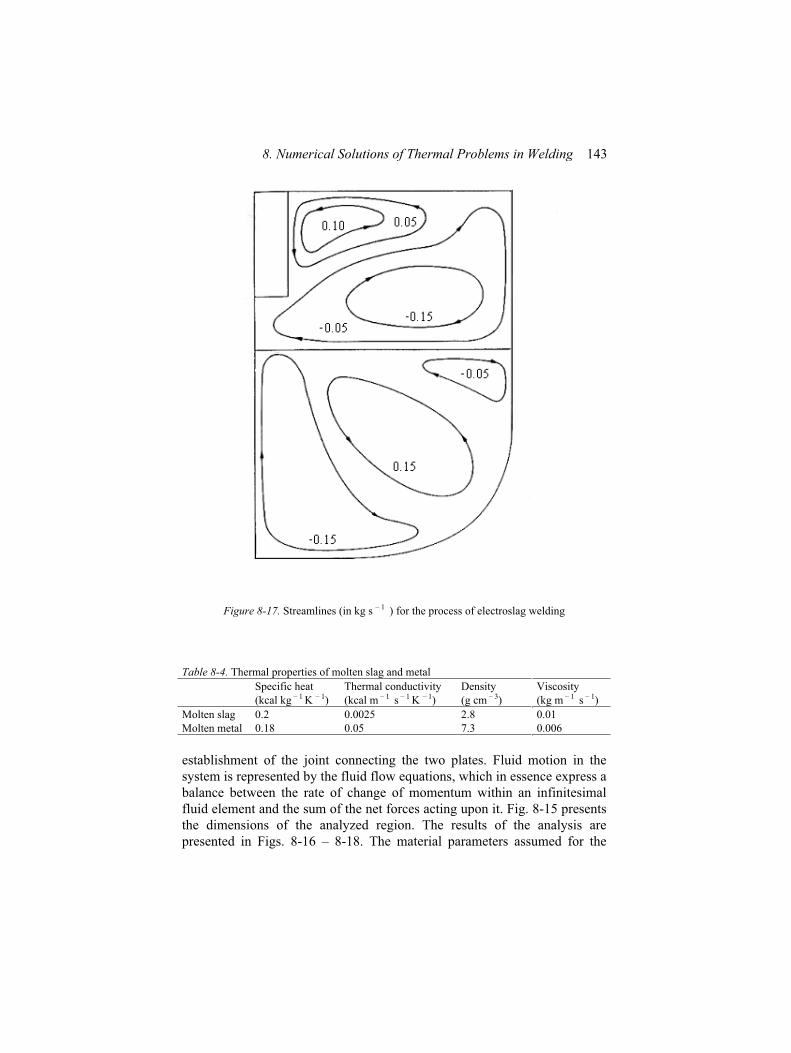
8. Numerical Solutions of Thermal Problems in Welding 143
Figure 8-17. Streamlines (in kg s – 1 ) for the process of electroslag welding
Table 8-4. Thermal properties of molten slag and metal
Specific heat
(kcal kg – 1 K – 1)
Thermal conductivity
(kcal m – 1 s – 1 K – 1)
Density
(g cm – 3)
Viscosity
(kg m – 1 s – 1)
Molten slag 0.2 0.0025 2.8 0.01
Molten metal 0.18 0.05 7.3 0.006
establishment of the joint connecting the two plates. Fluid motion in the
system is represented by the fluid flow equations, which in essence express a
balance between the rate of change of momentum within an infinitesimal
fluid element and the sum of the net forces acting upon it. Fig. 8-15 presents
the dimensions of the analyzed region. The results of the analysis are
presented in Figs. 8-16 – 8-18. The material parameters assumed for the
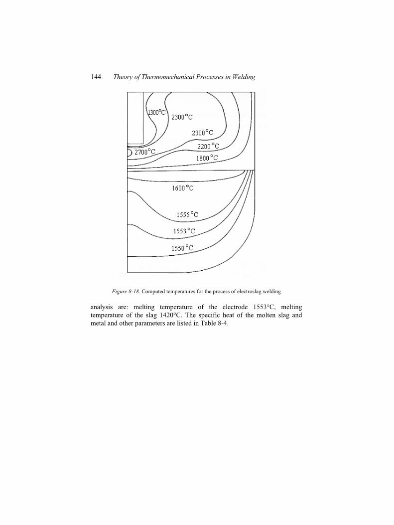
144 Theory of Thermomechanical Processes in Welding
Figure 8-18. Computed temperatures for the process of electroslag welding
analysis are: melting temperature of the electrode 1553 C, melting
temperature of the slag 1420 C. The specific heat of the molten slag and
metal and other parameters are listed in Table 8-4.
Part IV
WELDING STRESSES AND DEFORMATIONS
Chapter 9
THERMAL STRESSES IN WELDING
9.1 Changes of Stresses During Welding
Changes of stresses during welding both in the weld and the base
material are the result of welding heat source acting on the welded structure.
This chapter analyses thermal stresses during welding. The changes of
temperature and resulting stresses that occur during welding are presented in
Fig. 9-1. It is assumed that the weld is made along the axis x and the moving
welding heat source is located at point 0.
The mentioned figure shows the distribution of stresses along chosen
cross sections. At cross-section 1-1 thermal stresses are almost zero. At
cross-section 2-2 the stress near the welding heat source is equal to zero,
because of existence of molten metal at this point.
Stresses in short distance from heat source are compressive, because the
expansion of these areas is restrained by the surrounding metal where the
temperatures are lower. Since the temperatures of these areas are high and
the yield strength of the material low, stresses in these areas are as high as
the yield strength of the material at corresponding temperatures.
The magnitude of compressive stress passes through a maximum
increasing distance from the weld or with decreasing temperature. Stresses
in regions away from the weld are tensile and balance with compressive
stresses in areas near the weld.
At cross-section 3-3 the weld metal and base metal regions near the weld
have cooled, they contract and cause tensile stresses in regions close to the
weld. As the distance from the weld increases, the stresses first change to
compressive and then become tensile.
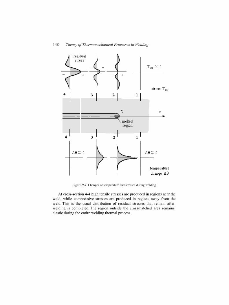
148 Theory of Thermomechanical Processes in Welding
Figure 9-1. Changes of temperature and stresses during welding
At cross-section 4-4 high tensile stresses are produced in regions near the
weld, while compressive stresses are produced in regions away from the
weld. This is the usual distribution of residual stresses that remain after
welding is completed. The region outside the cross-hatched area remains
elastic during the entire welding thermal process.
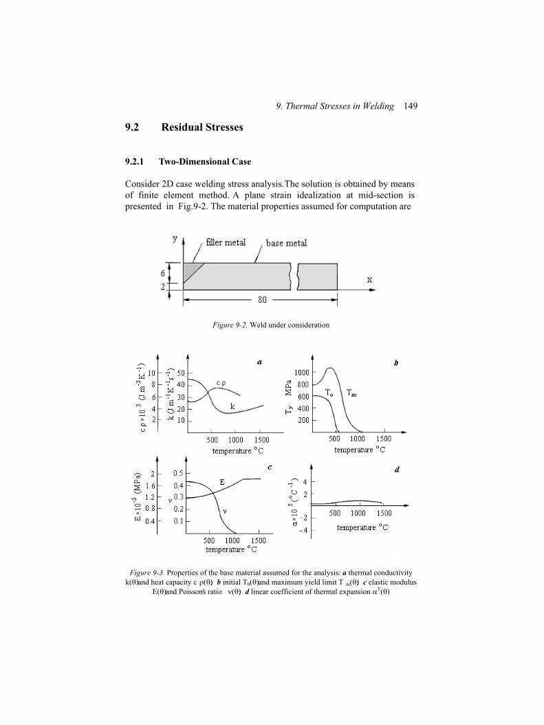
9. Thermal Stresses in Welding 149
9.2 Residual Stresses
9.2.1 Two-Dimensional Case
Consider 2D case welding stress analysis. The solution is obtained by means
of finite element method. A plane strain idealization at mid-section is
presented in Fig. 9-2. The material properties assumed for computation are
Figure 9-2. Weld under consideration
Figure 9-3. Properties of the base material assumed for the analysis: a thermal conductivity
k( ) and heat capacity c ( ); b initial T0( ) and maximum yield limit T m( ); c elastic modulus
E( ) and Poisson's ratio ( ); d linear coefficient of thermal expansion T( )
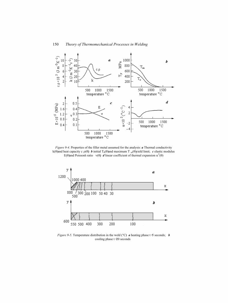
150 Theory of Thermomechanical Processes in Welding
Figure 9-4. Properties of the filler metal assumed for the analysis: a Thermal conductivity
k( ) and heat capacity c ( ); b initial T0( ) and maximum T m( ) yield limit; c elastic modulus
E( ) and Poisson's ratio ( ); d linear coefficient of thermal expansion T( )
Figure 9-5. Temperature distribution in the weld ( C): a heating phase t = 5 seconds; b
cooling phase t = 20 seconds
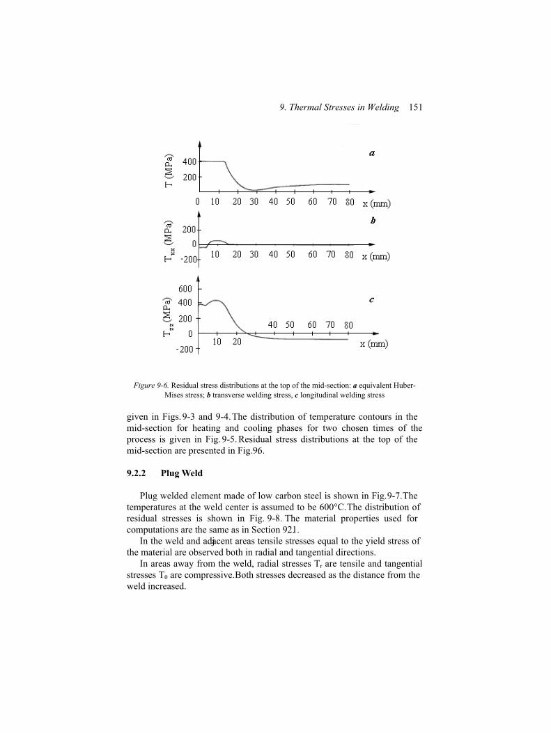
9. Thermal Stresses in Welding 151
Figure 9-6. Residual stress distributions at the top of the mid-section: a equivalent Huber-
Mises stress; b transverse welding stress, c longitudinal welding stress
given in Figs. 9-3 and 9-4. The distribution of temperature contours in the
mid-section for heating and cooling phases for two chosen times of the
process is given in Fig. 9-5. Residual stress distributions at the top of the
mid-section are presented in Fig. 9.6.
9.2.2 Plug Weld
Plug welded element made of low carbon steel is shown in Fig. 9-7. The
temperatures at the weld center is assumed to be 600 C. The distribution of
residual stresses is shown in Fig. 9-8. The material properties used for
computations are the same as in Section 9.2.1.
In the weld and adjacent areas tensile stresses equal to the yield stress of
the material are observed both in radial and tangential directions.
In areas away from the weld, radial stresses Tr are tensile and tangential
stresses T are compressive. Both stresses decreased as the distance from the
weld increased.
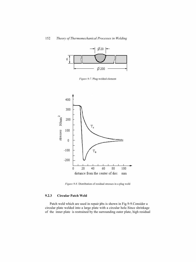
152 Theory of Thermomechanical Processes in Welding
Figure 9-7. Plug-welded element
Figure 9-8. Distribution of residual stresses in a plug weld
9.2.3 Circular Patch Weld
Patch weld which are used in repair jobs is shown in Fig. 9-9. Consider a
circular plate welded into a large plate with a circular hole. Since shrinkage
of the inner plate is restrained by the surrounding outer plate, high residual
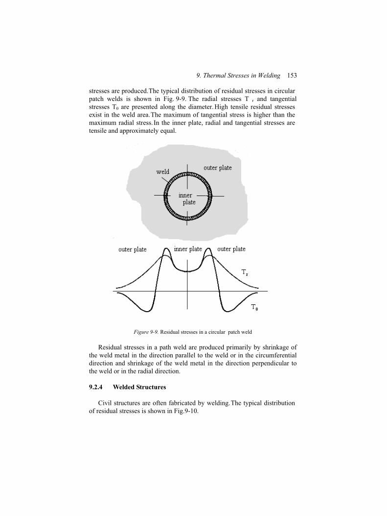
9. Thermal Stresses in Welding 153
stresses are produced. The typical distribution of residual stresses in circular
patch welds is shown in Fig. 9-9. The radial stresses T r and tangential
stresses T are presented along the diameter. High tensile residual stresses
exist in the weld area. The maximum of tangential stress is higher than the
maximum radial stress. In the inner plate, radial and tangential stresses are
tensile and approximately equal.
Figure 9-9. Residual stresses in a circular patch weld
Residual stresses in a path weld are produced primarily by shrinkage of
the weld metal in the direction parallel to the weld or in the circumferential
direction and shrinkage of the weld metal in the direction perpendicular to
the weld or in the radial direction.
9.2.4 Welded Structures
Civil structures are often fabricated by welding. The typical distribution
of residual stresses is shown in Fig. 9-10.
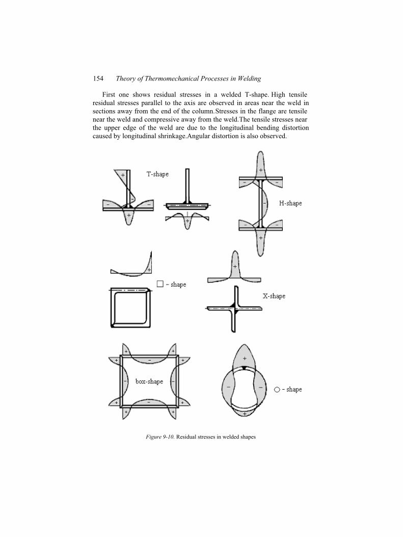
154 Theory of Thermomechanical Processes in Welding
First one shows residual stresses in a welded T-shape. High tensile
residual stresses parallel to the axis are observed in areas near the weld in
sections away from the end of the column. Stresses in the flange are tensile
near the weld and compressive away from the weld. The tensile stresses near
the upper edge of the weld are due to the longitudinal bending distortion
caused by longitudinal shrinkage. Angular distortion is also observed.
Figure 9-10. Residual stresses in welded shapes
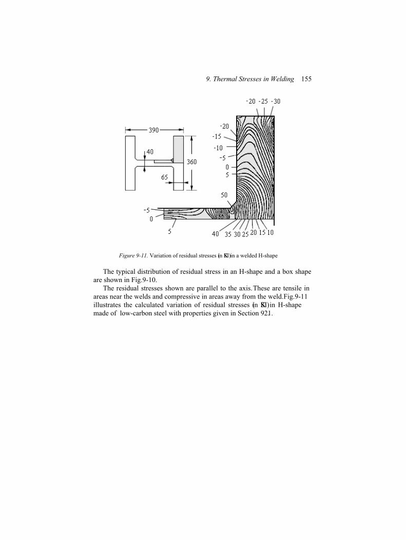
9. Thermal Stresses in Welding 155
Figure 9-11. Variation of residual stresses (in KSI) in a welded H-shape
The typical distribution of residual stress in an H-shape and a box shape
are shown in Fig. 9-10.
The residual stresses shown are parallel to the axis. These are tensile in
areas near the welds and compressive in areas away from the weld. Fig. 9-11
illustrates the calculated variation of residual stresses (in KSI) in H-shape
made of low-carbon steel with properties given in Section 9.2.1.
Chapter 10
WELDING DEFORMATIONS
10.1 Distortion
In the course of heating and cooling processes during welding thermal
strains occur in the weld metal and base metal near the weld. The stresses
resulting from thermomechanical loadings cause bending, buckling and
rotation. These displacements are called distortion in weldments. In welding
process three fundamental changes of the shape of welded structure are
observed. These transverse shrinkage perpendicular to the weld line,
longitudinal shrinkage parallel to the weld line and angular distortion
(rotation around the weld line). These changes of welded structure are shown
in Fig. 10-1 where classification of distortion has been introduced.
The first figure on the left shows transverse shrinkage. It is shrinkage
perpendicular to the weld line. The second figure on the top presents
rotational distortion. It is an angular distortion in the plane of the plate due to
thermal expansion. The figure in the middle illustrates angular change i.e.
transverse distortion. A non-uniform temperature field in the thickness
direction causes distortion (angular) close to the weld line. The second figure
in the middle shows longitudinal bending distortion. Distortion in a plane
through the weld line and perpendicular to the plate. The first figure on the
bottom illustrates longitudinal shrinkage, i.e. shrinkage in the direction of
the weld line. In the second figure on the bottom thermal compressive
stresses cause instability when the plates are thin. It is called buckling
distortion.
A typical structural component in ships, aerospace vehicles, and other
structures is shown in Fig. 10-2. It is a panel structure where a flat plate with
longitudinal and transverse stiffness fillet is welded to the bottom. In the
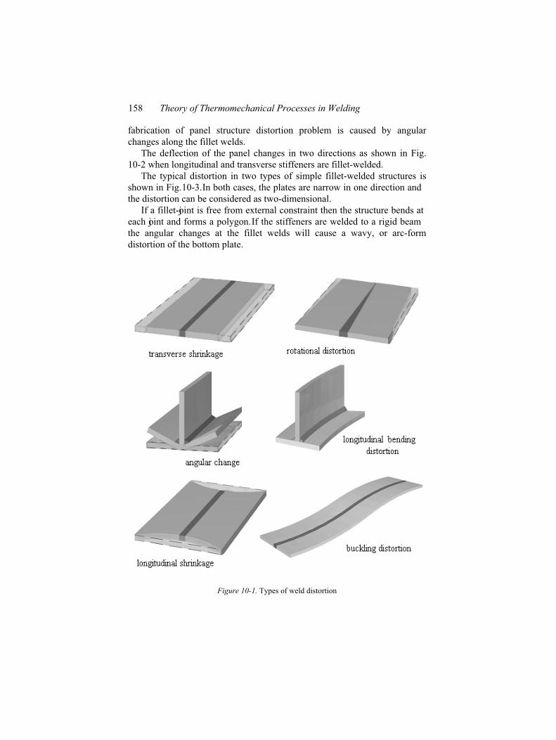
158 Theory of Thermomechanical Processes in Welding
fabrication of panel structure distortion problem is caused by angular
changes along the fillet welds.
The deflection of the panel changes in two directions as shown in Fig.
10-2 when longitudinal and transverse stiffeners are fillet-welded.
The typical distortion in two types of simple fillet-welded structures is
shown in Fig. 10-3. In both cases, the plates are narrow in one direction and
the distortion can be considered as two-dimensional.
If a fillet-joint is free from external constraint then the structure bends at
each joint and forms a polygon. If the stiffeners are welded to a rigid beam
the angular changes at the fillet welds will cause a wavy, or arc-form
distortion of the bottom plate.
Figure 10-1. Types of weld distortion
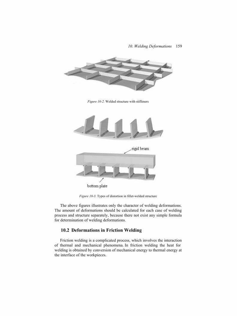
10. Welding Deformations 159
Figure 10-2. Welded structure with stiffeners
Figure 10-3. Types of distortion in fillet-welded structure
The above figures illustrates only the character of welding deformations.
The amount of deformations should be calculated for each case of welding
process and structure separately, because there not exist any simple formula
for determination of welding deformations.
10.2 Deformations in Friction Welding
Friction welding is a complicated process, which involves the interaction
of thermal and mechanical phenomena. In friction welding the heat for
welding is obtained by conversion of mechanical energy to thermal energy at
the interface of the workpieces.
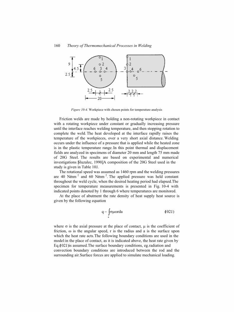
160 Theory of Thermomechanical Processes in Welding
Figure 10-4. Workpiece with chosen points for temperature analysis
Friction welds are made by holding a non-rotating workpiece in contact
with a rotating workpiece under constant or gradually increasing pressure
until the interface reaches welding temperature, and then stopping rotation to
complete the weld. The heat developed at the interface rapidly raises the
temperature of the workpieces, over a very short axial distance. Welding
occurs under the influence of a pressure that is applied while the heated zone
is in the plastic temperature range. In this point thermal and displacement
fields are analyzed in specimens of diameter 20 mm and length 75 mm made
of 20G Steel. The results are based on experimental and numerical
investigations [Sluzalec, 1990]. A composition of the 20G Steel used in the
study is given in Table 10.1.
The rotational speed was assumed as 1460 rpm and the welding pressures
are 40 N/mm 2 and 60 N/mm 2. The applied pressure was held constant
throughout the weld cycle, when the desired heating period had elapsed. The
specimen for temperature measurements is presented in Fig. 10-4 with
indicated points denoted by 1 through 6 where temperatures are monitored.
At the place of abutment the rate density of heat supply heat source is
given by the following equation
a
rdaq (10.2.1)
where is the axial pressure at the place of contact, is the coefficient of
friction, is the angular speed, r is the radius and a is the surface upon
which the heat rate acts. The following boundary conditions are used in the
model: in the place of contact, as it is indicated above, the heat rate given by
Eq. (10.2.1) is assumed. The surface boundary conditions, e.g. radiation and
convection boundary conditions are introduced between the rod and the
surrounding air. Surface forces are applied to simulate mechanical loading.
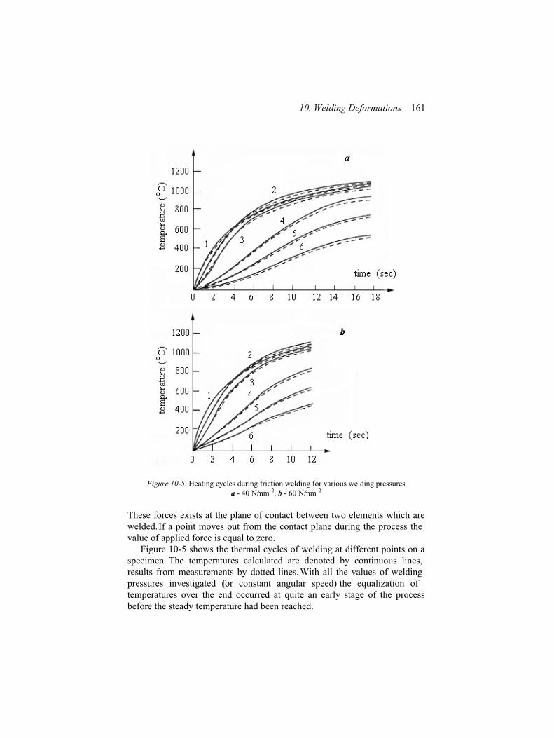
10. Welding Deformations 161
Figure 10-5. Heating cycles during friction welding for various welding pressures
a - 40 N/mm 2, b - 60 N/mm 2
These forces exists at the plane of contact between two elements which are
welded. If a point moves out from the contact plane during the process the
value of applied force is equal to zero.
Figure 10-5 shows the thermal cycles of welding at different points on a
specimen. The temperatures calculated are denoted by continuous lines,
results from measurements by dotted lines. With all the values of welding
pressures investigated (for constant angular speed) the equalization of
temperatures over the end occurred at quite an early stage of the process
before the steady temperature had been reached.
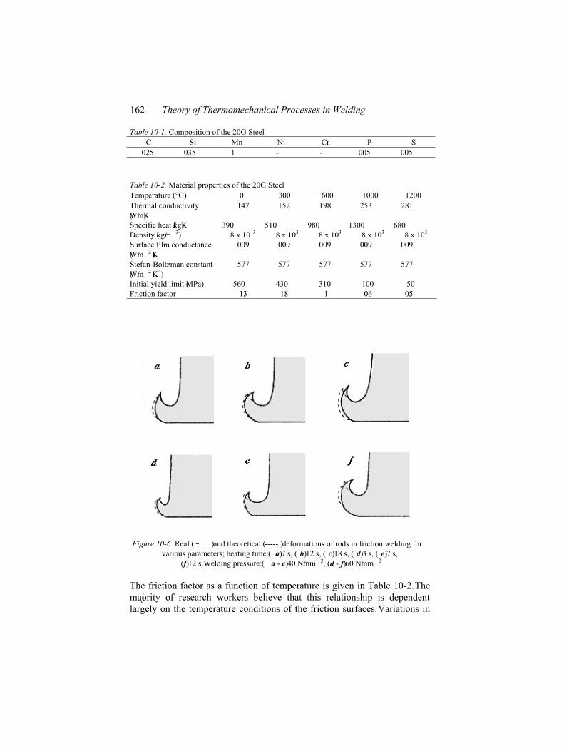
162 Theory of Thermomechanical Processes in Welding
Table 10-1. Composition of the 20G Steel
C Si Mn Ni Cr P S
0.25 0.35 1 - - 0.05 0.05
Table 10-2. Material properties of the 20G Steel
Temperature ( C) 0 300 600 1000 1200
Thermal conductivity
(W/mK)
14.7 15.2 19.8 25.3 28.1
Specific heat (J/kgK) 390 510 980 1300 680
Density (kg/m 3) 8 x 10 3 8 x 10³ 8 x 10³ 8 x 10³ 8 x 10³
Surface film conductance
(W/m 2 K)
0.09 0.09 0.09 0.09 0.09
Stefan-Boltzman constant
(W/m 2 K4)
5.77 5.77 5.77 5.77 5.77
Initial yield limit (MPa) 560 430 310 100 50
Friction factor 1.3 1.8 1 0.6 0.5
Figure 10-6. Real ( _____ ) and theoretical ( ----- ) deformations of rods in friction welding for
various parameters; heating time: ( a) 7 s, ( b) 12 s, ( c) 18 s, ( d) 3 s, ( e) 7 s,
(f) 12 s. Welding pressure: ( a - c) 40 N/mm 2, (d - f) 60 N/mm 2
The friction factor as a function of temperature is given in Table 10-2. The
majority of research workers believe that this relationship is dependent
largely on the temperature conditions of the friction surfaces. Variations in
10. Welding Deformations 163
welding pressures primarily affect the rate of deformation of the rubbing
surfaces and the temperature gradient. The temperature in turn has a
substantial effect on the mechanical properties of the material. It is suggested
that the limiting steady temperature in the joint cannot be higher than the
temperature at which the yield point of the material is equal to the pressure
used in the experiment. The maximum temperature in the joint during
frictional heating depends not only on the pressure, but also on the
temperature gradient which depends on the rotational speed in particular.
Figure 10-6 compares numerical results with experimental observations as to
the shape of upset metal. Irregularities in the shape of the extruded material
in a circumferential direction are not analyzed. These irregularities do not
appear if specimens undergoing pressure during friction welding have
exactly the same axis of symmetry and parallel surfaces of contact. Non-
uniform properties of the material also can lead to irregularities in these
shapes.
References and Further Reading
Adams, C. M., Jr., Cooling rate and peak temperatures in fusion welding, Welding Journal,
37 (5), Research Supplement, 210-215 (1958).
Alpsten, G. A., Tall, L., Residual stresses in heavy welded shapes, Welding Journal, 39 (3),
Research Supplement, 93-105 (1970).
Anderson, J. E., Jackson J. E., Theory and application of pulsed laser welding, Welding
Journal, 12, (1965).
Apps, R. L., Milner D. R., Heat flow in argon-arc welding, Brit. Weld. Journal, 475-485
(October 1955).
Bentley, K. P., Greenwood, J. A., McKnowlson, P., Bakes, R. G., Temperature distributions
in spot welds, Brit. Weld. Journal, 613-619 (1963).
Brown, S., Song, H., Finite element simulation of welding of large structures, ASME Journal
of Engineering for Industry, 114, (4), 441-451 (1992).
Brown, S., Song, H., Implications of three-dimensional numerical simulations of welding of
large structures, Welding Journal, 71, 55-62 (1992).
Brust, F. W., Dong, P., Zhang, J., A constitutive model for welding process simulation using
finite element methods, Advances in Computational Engineering Science, S. N. Atluri &
G. Yagawa, Eds., 51-56 (1997).
Brust, F. W., Kanninen, M. F., Analysis of residual stresses in girth welded type 304-stainless
pipes, ASME Journal of Materials in Energy Systems, 3 (3) (1981).
Carslaw, H. S., Jaeger J. C., Conduction of heat in Solids, Oxford University Press, (1959).
Christensen, N., Davis, V. de L., Giermundsen, K., Distribution of temperatures in arc
welding, British Welding Journal, 12 (2), 54-75 (1965).
Dilthey, U., Habedank, G., Reichel, T., Sudnik, W., Ivanov, W. A., Numeric simulation of the
metal-arc active gas welding process, Welding & Cutting, 45, E50-E53 (1993).
Doty, W. D., Childs, W. J., A summary of the spot welding of high-tensile carbon and low-
alloy steels, Welding Journal, 25 (10), Research Supplement, 625-630 (1946).
Eager, T. W., Tsai N. S., Temperature fields produced by traveling distributed heat sources,
Welding Journal, 62 (12), 346-355 (1983).
166 Theory of Thermomechanical Processes in Welding
Earvolino, L. P., Kennedy, J. R., Laser welding of aerospace structural alloys, Welding
Journal, 3, (1966).
Flugge, W., Four-place tables of transcendental functions, McGraw-Hill, New York, N. Y.
(1954).
Goldak, J., Chakravarti, A., Bibby, M., A new finite model for welding heat sources,
Metallurgical Transaction, 15B, 299-305 (1984).
Goldenberg, B. H., A problem in radial heat flow, Brit. Int. Appl. Phys., 2, 233-237 (1951).
Goldsmith, A., Waterman, T. E., Hisschhorn, H. J., Handbook of thermo-physical properties
of solid materials, Vol. I and Vol. II, Pergamon Press, (1961)-(1963).
Greenwood, J. A., Temperature in spot welding, Brit. Weld. Journal, 316-322 (1961).
Grosh, R. J., Trabant, E. A., Arc-welding temperatures, Welding Journal, 35 (8), Research
Supplement, 396-400 (1956). Cheng, C. J., Transient temperature during friction welding
of similar materials in tubular form, Welding Journal, 41 (12), Research Supplement, 542-
550 (1962).
Grosh, R. J., Trabant, E. A., Hawkins, G. A., Temperature distribution in solids of variable
thermal properties heated by moving heat sources, Quart. Appl. Math., 13 (2), 161-167
(1955).
Hess, W. F., Merrill, L. L., Nippes, E. F., Jr., Bunk, A. P., The measurement of cooling rates
associated with arc welding and their application to the selection of optimum welding
conditions, Welding Journal, 22 (9), Research Supplement, 377-422 (1943).
Jackson, C. E., Shrubsall, A. E., Energy distribution in electric welding, Welding Journal, 29
(5), Research Suppl., 232-242 (1950).
Jeong,S. K., Cho, H. S., An analytical solution to predict the transient temperature distribution
in fillet arc welds, Welding Journal, 76 (6), 223-232 (1997).
Jhaveri Pravin Moffatt, W. G., Adams, C. M., Jr., The effect of plate thickness and radiation
on heat flow in welding and cutting, Welding Journal, 41 (1), Research Supplement, 12-16
(1962).
Karman, T. V., Biot, M. A., Mathematical methods in engineering, McGraw-Hill, New York,
N. Y. (1940).
Kasuya, T., Yurioka, N., Prediction of welding thermal history by a comprehensive solution,
Welding Journal, 72 (3), 107-115 (1993).
Kawai, T., A study on residual stresses and distortion in welded structures, Journal of the
Japan Welding Society, 33 (3), 314 (1964).
Kawai, T., Yoshimura, N., A study on residual stresses and distortion in welded structures
(Part 2), Journal of the Japan Welding Society, 34 (2), 214 (1965), and Part 3, 34 (12), 215
(1965).
Lancaster, J. F., Energy distribution in argon-shielded welding arcs, Brit. Weld. Journal, 1,
412-426 (1954).
Lesnewich, A., Control of melting rate and metal transfer in gas-shielded metal-arc welding:
Part I, Control of electrode melting rate, Welding Journal, 37 (8), Research Supplement,
343-353 (1958); Part II: Control of metal transfer, Welding Journal, 37 (9), 418-425
(1958).
References and Further Reading 167
Murray J. D., Welding of high yield point steels, Welding and Metal Fabrication, 8, (1966).
Myers, P. S., Uyehara, O. A., Borman, G. L., Fundamentals of heat flow in welding, Welding
Research Council Bulletin, 123 (July 1967).
Nagaraja Rao, N. R., Esatuar, F. R., Tall, L., Residual stresses in welded shapes, Welding
Journal, 43 (7), Research Supplement, 295-306 (1964).
Nguyen, N. T., Ohta, A., Matsuoka, K., Suzuki,N., Maeda, Y., Analytical solutions for
transient temperature of semi-infinite body subjected to 3-D moving heat sources, Welding
Journal, 78 (8) (1999).
Nippes, E. F., Merrill, L. L., Savage, W. F., Cooling rates in arc welds in ½ inch plate,
Welding Journal, 28 (11), Research Supplement, 556-563 (1949).
Prokhorov, N. N., Samotokhin, S. S., Effect of artifical flowing off of Heat on processes of
developing internal stresses and strain in welding, Avt. Proiz., 5, 63-69 (1977).
Pugin, A. I., Pertsovskii, G. A., Calculation of the thermal cycle in the HAZ when welding
very thick steel by the electroslag process, Avt. Svarka, 6, 14-23 (1963).
Rabkin, D. M., Temperature distribution through the weld pool in the automatic welding of
aluminium, British Welding Journal, 6 (8), 132-137 (1959).
Ramsey, P. W., Chyle J. J., Kuhr J. N., Myers, P. S., Weiss, M., Groth, W., Infra-red
temperature sensing for automatic fusion welding, Welding Journal, 42 (8), Research
Supplement, 337-346 (1963).
Roberts, Doris K., Wells, A. A., Fusion welding of aluminum alloys, Part V, A mathematical
examination of the effect of bounding planes on the temperature distribution due to
welding, Brit. Weld. Journal, 553-560 (December 1954).
Robinson, M. H., Observations on electrode melting rates during submerged-arc welding,
Welding Journal, 40 (11), Research Supplement, 503-515 (1961).
Rosenthal, D., Cambridge, M., The theory of moving source of heat and its application to
metal treatments, Trans. ASME, 68 (11), 849-866 (1946).
Rosenthal, D., Mathematical theory of heat distribution during welding and cutting, Welding
Journal, 20 (5), Research Supplement, 220-234 (1941).
Rosenthal, D., The theory of moving sources of heat and its application to metal treatments,
ASME Trans., 849-866, (1946).
Rykalin, N. N., Berechnung der Wärmevorgänge beim Schweissen, Verlag Technik, Berlin,
68-69 (1957).
Rykalin, N. N., Calculation of heat processes in welding, Lecture the presented before the
American Welding Society, (April 1961).
Rykalin, N. N., Calculations of thermal processes in welding, Mashgiz, Moscow (1951).
S u alec, A., A new finite element approach to heat flow analysis in 3D developable
structures, Journal of Thermal Analysis, 30, 1063-1069 (1985).
S u alec, A., An analysis of thermal phenomena in electromagnetic field during electroslag
welding, Int. J. Computers & Fluids, 17 (2), 411-418 (1989).
S u alec, A., An analysis of titanium weld failure, Proceed. Int. Conf. JOM-4, Denmark,
(1989).
S u alec, A., An evaluation of the internal dissipation factor in coupled thermo-plasticity, Int.
J. Nonlinear Mechanics, 25 (4), 395-403 (1990).
168 Theory of Thermomechanical Processes in Welding
S u alec, A., An influence of laser beam intensity on the flow of metal, Proceeding Int. Conf.
Laser Materials Processing for Industry, ed. S.K.Ghosh, LASER-5, (1989).
S u alec, A., Bruhns, O. T., Thermal effects in thermo-plastic metal with internal variables,
Computers & Structures, 33 (6), 1459-1464 (1989).
S u alec, A., Computational methods for diffusion problems in welded joints, Proceedings
International Conference JOM-2, Denmark, 322-327 (1984).
S u alec, A., Computer analysis of melting processes in metals undergoing laser irradiation,
Proceeding Int. Conf. High Power Lasers in Metal Processing, ed. S.K.Ghosh and
T.Ericsson, LASER-4, (1988).
S u alec, A., Flow of metal undergoing laser irradiation, Numerical Heat Transfer, 253-263,
(1988).
S u alec, A., Grzywi ski, M., Stochastic convective heat transfer equations in finite
differences method, Int. J. of Heat & Mass Transfer, 43, 4003-4008 (2000).
S u alec, A., Kleiber, M., Finite element analysis of heat flow in friction welding, Eng.
Transac., 32, (1), 107-113 (1984).
S u alec, A., Kleiber, M., Numerical analysis of heat flow in flash welding, Arch. Mech., 35,
(5-6), 687-699 (1983).
S u alec, A., Kubicki, K., Sensitivity analysis in thermo-elastic-plastic problems, J. Thermal
Stresses, 25, 705-718 (2002).
S u alec, A., Kysiak, A., An analysis of weld geometry in creep of welded tube undergoing
internal pressure, Computer & Structures, 40 (4), 931-938 (1991).
S u alec, A., Kysiak, A., Creep of welded tubes undergoing internal pressure, Archive. of
Mechanical Engineering (in Polish), 3, 169-179 (1992).
S u alec, A., Moving heat source analyzed by finite elements and its application in welding,
Indian Journal of Technology, 24, 303-308 (1986).
S u alec, A., Random heat flow with phase change, Int. J. of Heat & Mass Transfer, 43,
2303-2312 (2000).
S u alec, A., Shape optimization of weld surface, Int. J. Solids & Structures, 25 (1), 23-31
(1989).
S u alec, A., Simulation of the friction welding process, ed. A.Niku-Lari, SAS World
Conference, IITI-International, 333-340 (1988).
S u alec, A., Solution of thermal problems in friction welding - comparative study, Int. J.
Heat & Mass Transfer, 36 (6) 1583 - 1587 (1993).
S u alec, A., Temperature field in random conditions, Int. J. Heat & Mass Transfer, 34 (1),
55-58 (1991).
S u alec, A., Temperature rise in elastic-plastic metal, Comp. Meth. Appl. Mech. Eng. 96,
293-302 (1992).
S u alec, A., Thermal effects in laser microwelding, Computers & Structures, 25 (1), 29-
34 (1987).
S u alec, A., Thermal effects in friction welding, Int. J. Mech. Sci., 32 (6), 467-478 (1990).
S u alec, A., Thermoplastic effects in friction welding analyzed by finite element method,
Proceedings International Conference on the Effects of Fabrication Related Stresses, Ed.
The Welding Institute, England, Paper 8, P8-1 – P8 -8 (1985).
Stoeckinger, G. R., Calabrese, R. A., Menaul, R. F., Computerized prediction of heat
distribution in weld tooling, Welding Journal, 49 (1 and 6), Research Supplement, 14-26
and 272-277 (1970).
Sudnik, W., Ivanov, A., Mathematical model of the heat source in GMAW. Part I. Normal
process, Welding International, 13, 215-221 (1999).
Sudnik, W., Radaj, D., Erofeew, W., Computerized simulation of laser beam welding, model
and verification, J. Phys. D: Appl. Phys., 29, 2811-2817 (1996).
References and Further Reading 169
Sudnik, W., Research into fusion welding technologies based on physical-mathematical
models, Welding & Cutting, 43, E216-E217 (1991).
Sutherland, J. D., High yield strength waterquenched and tempered steel plate, Welding and
Metal Fabrication, 1, (1967).
The Physical Properties of a Series of Steels, Part II, Jnl. Iron and Steel Inst., 154 (2), 83-121
(1946).
Veron, C. W. J., Ultrasonic welding, Welding and Metal Fabrication, 11, (1965).
Vogel, L. E., Lyens, J. V., Pumphrey, W. I., Temperature and hardness distribution in welded
Al-4% Cu alloy sheet, Brit. Weld. Journal, 252-259 (June 1954).
Wayman, S. M., Stout R. D., A study of factors effecting the strength and ductility of weld
metal, Welding Journal, 5, (1958).
Weiss. S., Ramsey, J. N., Udin, H., Evaluation of weld-cracking tests on armor steel, Welding
Journal, 35 (7), Research Supplement, 348-356 (1956).
Wells, A. A., Heat flow in welding, Welding Journal, 31 (5), Research Supplement, 263-267
(1952).
Wells, A. A., Oxygen cutting, Brit. Weld. Journal, 86-92 (1961).
Wilson, J. L., Claussen, G. E., Jackson, C. E., The effect of I2Rheating on electrode melting
rate, Welding Journal, 35 (1), Research Supplement, 1-8 (1956).
Wilson, W. M., Hao, C. C., Residual stresses in welded structures, The Welding Journal, 26
(5), Research Supplement, 295-320 (1974).
Yang, Y. P., Brust, F. W., Welding-induced distortion control techniques in heavy industries,
Symposium on Weld Residual Stresses and Fracture 2000, ASME Pressure Vessels and
Piping Conference, Seatle, WA, USA, July 23-27 (2000).
Yoshida, T., Abe, T., Onoue, H., Residual stresses in circular-patch-welds, Journal of the
Society of Naval Architects of Japan, 105 (1959).
Subject Index
Absolute temperature, 35, 38, 41, 47,
65
Absorption coefficient, 130-132
model, 130
Aerospace vehicles, 157
Almansi-Hamel strain, 7
Analytical solution, 83, 105, 120, 129
Angular change, 157, 158
distortion 154, 157
speed, 160, 161
Axial pressure, 160
vector, 11
Base material, 57, 62, 147, 149
Bending distortion, 154, 157
Bessel function, 113-115, 125
Bouguer law, 130
Boundary conditions, 48, 55, 83, 84,
87, 89, 92, 97, 98, 105, 107,
112, 117, 121, 124, 133, 138,
160
Box shape, 155
Buckling distortion, 157
Capacity matrix, 93
Carbon steel, 151, 155
Cauchy equation of motion, 24
stress tensor, 21, 60
Characteristic equation, 25
Circular hole, 152
patch weld, 152, 153
plate, 152
Clausius-Duhem inequality, 37, 38
Coefficient of friction, 160
Compatibility conditions, 11
equations, 92
Compressive stresses, 147, 148, 151,
157
Convection boundary condition, 160
Cooling rate, 109, 110, 114-116, 119,
120
Coordinates, 3, 4, 8, 9, 79, 106
Cartesian, 45, 109, 131, 132
cylindrical, 106
spherical, 106
Crank-Nicolson scheme, 96
Cross-hatched area, 148
Density, 12, 14, 20, 32, 33, 35, 37,
38, 40, 51, 52, 54, 135-137,
143, 160, 162
Deviatoric stress matrix operator, 100
Dimensionless distance, 108-110,
113 -115, 118
Subject Index172
Dimensionless temperature, 108-110,
113, 114, 116, 118-120, 125
time, 108, 109
Dirac function, 121
Dissipation, 38-44, 58, 67, 69
potential, 43
Distortion, 154, 157-159
Divergence theorem, 13, 14, 23, 24,
26, 29, 85
Dupont scheme, 95
Eigenvalues, 79, 93
Elastic modulus, 149, 150
Elasticity domain, 60, 62-66, 69-72,
74, 75
tensor, 57
Electric conductivity, 130
Electro-magnetic wave, 130
Electroslag welding, 129, 141-144
Emissivity coefficient, 134, 140
Energy density, 38, 40
equation, 33-35, 37-39
Entropy, 35-39, 41-43
Environmental temperature, 134, 140
Euclidean space, 3, 21
Euler scheme, 101
External
forces, 32, 33
heat supply, 32, 33, 45
Extra stress, 52
Fillet weld, 157-159
First law of thermodynamics, 32
First-order differential equations, 32-
34
Flow rule, 62, 66, 67, 69, 72, 74
Fluid temperature, 46, 48, 84
Fourier law, 43, 54
Free energy, 38, 40, 45, 57, 60, 61,
71, 72
Friction welding, 118-120, 129, 159,
161-163
Galerkin method, 86
Green-Lagrange strain, 7, 10, 59
Hardening, 61-72, 75, 77, 78
force, 64, 65, 68, 69, 71, 72,
77, 78
sign, 69-71
Heat
capacity, 61, 149, 150
conduction equation, 54, 97,
106, 131
convection, 46
flux, 34, 49, 55
radiation, 47, 48
rate, 120, 160
Heating time, 125, 162
Homogeneous material, 106
H-shape, 155
Huber-Mises loading function, 78
Hydrostatic pressure, 52
Identity matrix, 94
Incompressible fluid, 54
Incremental analysis, 101
strain, 59
stress, 59
temperature, 59
Infinitesimal strain, 10, 27
Initial conditions, 48, 107
load method, 95
Integration schemes, 92, 93
Intermediate velocity field, 96
Internal energy, 32-35
Isotropic hardening, 64, 77, 79
Iterative solution, 43, 94
Lagrange variables, 12, 15
formulation, 35, 37, 38
Laplace transform, 121
Laser beam, 133, 134, 136, 140
microwelding, 129, 133, 137
Latent heat, 61, 72, 97, 98, 135
Line source, 106, 107, 112
Linear transformation, 21
Liquidus temperature, 97
Longitudinal bending distortion, 154,
157
Subject Index 173
Longitudinal bending shrinkage, 154,
157
Mass conservation, 14, 54
Material derivative, 12, 22, 29, 30,
32, 33, 35-37
Mean normal stress, 26
pressure, 53, 54
Mechanical boundary conditions, 92
Mechanical energy, 34, 39, 118, 159
Melting temperature, 135, 137, 144
Metal pool, 141
Metric tensor, 7
Mid-point schemes, 94-96
Molten metal, 141, 143, 144, 147
slag, 141, 143, 144
Momentum equation, 92,99
Monochromatic radiation, 130
Moving fluid, 89
heat source, 110, 147
Navier-Stokes equations, 54, 89, 92,
96
Neutral loading, 66
Newton equation, 46, 49
Nodal temperatures, 86, 88, 93, 99
Numerical stability, 93
One-step schemes, 92-96
O-shape, 154
Panel structure, 157, 158
Particulate derivative, 12-14, 34, 40,
46
Permutation symbol, 11
Phase change interval, 98
Plasma frequency, 130
Plastic flow rule, 62, 66, 67, 69
Plasticity algorithms, 102
Plasticity criterion, 64
Plug weld, 151, 152
Poisson ratio, 62, 149, 150
Predictor-corrector technique, 95
Pressure, 51-54, 89, 96, 97, 119, 160-
163
Principal directions, 24, 25, 78
Principal stresses, 24, 25, 77
Pulsed lasers, 129
Radial stresses, 151, 153
Radiation boundary condition, 160
coefficient, 47, 48
intensity, 129-133, 135, 136
Reduced potential, 61
Referential description, 3, 4
Reflection coefficient, 130
Relaxation time, 131
Residual stress, 148, 149, 151-155
Rotation, 10, 119, 157, 160
Rotational distortion, 157
speed 160, 163
Scalar field, 14
Ships, 157
Skin effect, 130
Softening, 69, 70, 75
Solid-liquid interface, 97
Solidus temperature, 97
Solution procedure, 93, 96, 101
Spatial description, 3, 4
Specific heat, 83, 97, 98, 105, 135,
143, 144, 162
Spot weld, 106
welding, 3, 106, 107
Stationary line source, 106, 107
Strain-displacement matrix, 100
Streamlines, 143
Stress
deviator tensor, 77
invariants, 26
tensor, 17, 21, 24, 26, 28, 40, 41,
52, 58, 60, 64, 77
vector, 18, 19, 21, 35
Struve function, 127
Tangent stiffness matrix, 102
Tangential stress, 152, 153
Temperature, 35, 41, 46-49, 54, 55,
57-59, 66, 71, 83-89, 93, 97,
99, 101, 105, 108-119, 123-
125, 130, 131, 134, 137,
Subject Index174
147, 148, 150, 151, 157,
160-163
gradient, 49, 112, 163
variation, 45, 57, 58, 61, 72
Tensile stresses, 78, 147, 148, 151,
153, 154
Tensorial product, 4
Theorem of virtual work, 30, 99
Thermal
boundary conditions, 92
conductivity, 43, 83, 105,
106, 135, 143, 149, 150, 162
cycle, 161
diffusion, 106
energy, 118, 159
equations, 31, 39, 54, 58, 72,
92
expansion coefficient, 135
hardening, 71, 72, 75
phenomena, 159
Thermo-elasto-plasticity, 92, 100,
101
Thermomechanical loading, 157
Time discretization, 92
integration, 92,93
step, 92-95, 102
Transient temperature, 119
Transport formula, 15, 37
Transverse distortion, 157
shrinkage, 157
Trapezoidal schemes, 94,95
T-shape, 154
Tungsten specimen, 138-140
Two-step schemes, 92, 95, 96
Velocity field, 26, 27, 30, 96, 142
Virtual work rate, 26, 27, 30
Viscosity, 51, 53, 54, 99, 143
Viscous fluid, 51, 52
Volume heat capacity, 45, 61
rate density, 33
Wave frequency, 130
Weighted residual method, 83, 86
Weld, 57, 62, 106, 119, 120, 147,
148, 150-155, 157, 158
cycle, 160
Welded structure, 57, 147, 153, 157,
159
Welding
arc, 110, 129
heat source, 57, 147
pressure, 160-163
strains, 157
stresses 97, 147, 149, 151
Yield locus, 63, 64
strength, 147
surface, 77-80


