Three-Dimensional Network Topologies yJohn Nguyen1, John Pezaris2, Gill Pratt2, and Steve Ward21 University of Michigan2 Massachusetts Institute of Technologyjohnn@eecs.umich.edupz; gill;ward@lcs.mit.eduAbstract. This paper presents the derivation and performance resultsof several new three-dimensional topologies. Various transformations canbe applied to the conventional six-neighbor mesh in order to constructthese topologies, which vary both in number of neighbors (degree) andlogical connectivity. Analysis shows that after normalization for con-stant pin-count, lower-degree topologies yield lower latencies for longmessages on unloaded networks, while higher-degree topologies possesshigher bandwidth capacities. Although simulation results generally ver-ify these �ndings, we also observe a surprising amount of di�erence inthe performance between distinct topologies of the same degree.1 IntroductionThe past few years have seen a rise in popularity of multiprocessors using di-rect networks that span two or three dimensions. Such networks typically followthe topology of a two or three-dimensional mesh or torus. Although topologiesother than the mesh have been studied for two-dimensional space[7], there havebeen few investigations of alternate topologies in three-dimensional space. Thispaper proposes �ve such alternate topologies and presents some analytical andempirical performance results.We restrict our study to direct topologies whose nodes all possess the samenumber of neighbors, or degree. Furthermore, the node degree for any topologyremains constant no matter how many nodes are in the network. Thus non-constant degree topologies such as hypercubes are not considered. Also elimi-nated are indirect topologies such as butter ies and fat-trees.Since high-degree topologies require a larger number of channels on eachswitch, we must somehow normalize performance to the hardware complexityrequired by the degree of the topology. This can be accomplished by requiring aconstant switch complexity through reducing the channel width of higher-degreetopologies. On such topologies, the narrower data path can in turn degrade per-formance by increasing the number of its required by long messages. Conversely,a network requiring a small number of channels per node allows one to increasey This research is sponsored by DARPA contract #DABT63-93-C-0008.

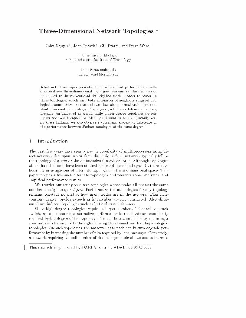
the data path size without increasing switch complexity and thus possibly de-crease the latency of long messages. Many of the topologies that are presentedhere can be viewed as an attempt to reduce the degree of each node.In the following sections, we present several new three-dimensional topologiesas well as a formal de�nition of a topology, derive analytical results to predictperformance, and discuss results of some routing simulations.2 TopologiesWe present in this section �ve topologies can be derived from various mod-i�cations to the conventional six-neighbor mesh. These modi�cations includesplitting each six-neighbor node into several nodes as well as adding and remov-ing links from the six-neighbor topology. Although physical representations arepresented for clarity, the topologies are really de�ned by the logical connectivityof the nodes. The following section will focus on a more formal treatment oftopologies.Topology A: In the standard three-dimensional mesh, each node is representedas a point (n1; n2; n3) in the cartesian three-dimensional space where each niis an integer. The six neighbors of a node are de�ned as nodes with pointscorresponding to +1 and �1 o�sets in one of the three axes. Such a network isillustrated in Figure 1.y

z

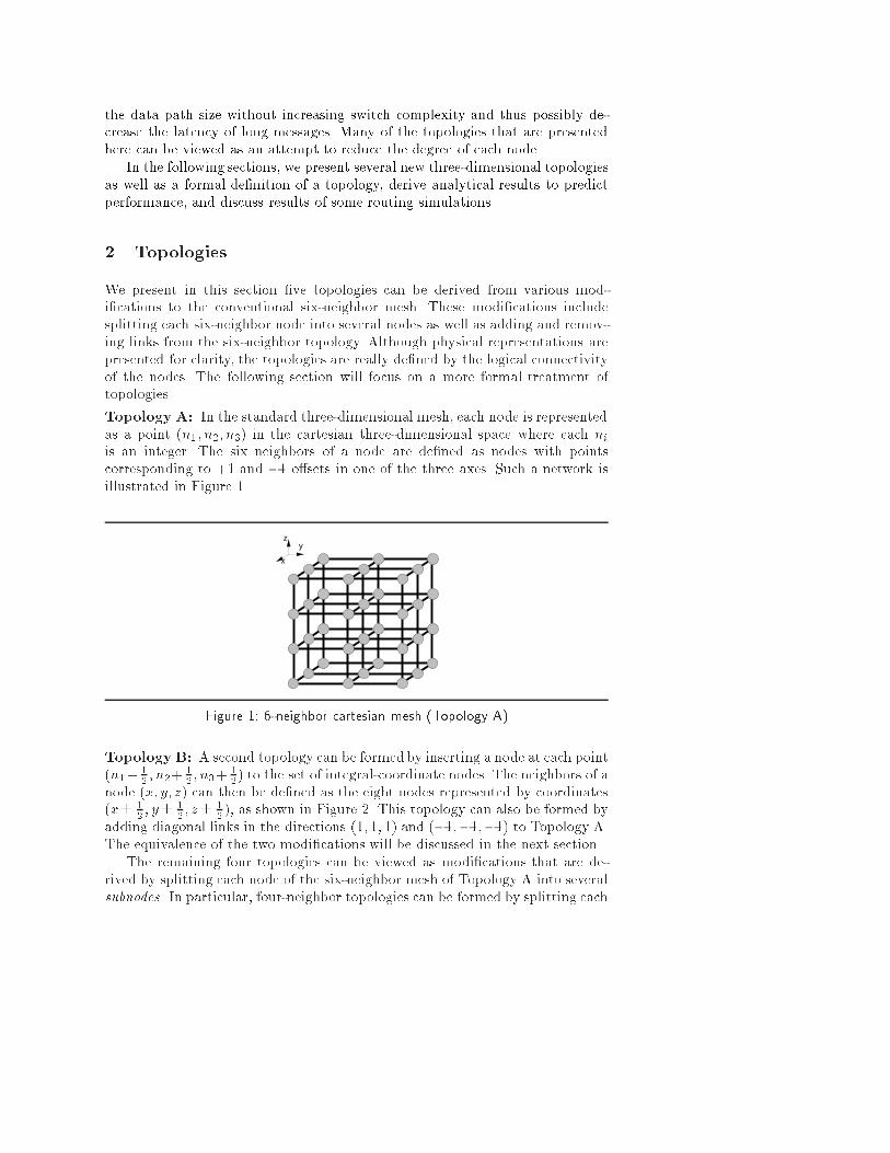
xFigure 1: 6-neighbor cartesian mesh (Topology A)Topology B: A second topology can be formed by inserting a node at each point(n1+ 12 ; n2+ 12 ; n3+ 12) to the set of integral-coordinate nodes. The neighbors of anode (x; y; z) can then be de�ned as the eight nodes represented by coordinates(x� 12 ; y� 12 ; z� 12 ), as shown in Figure 2. This topology can also be formed byadding diagonal links in the directions (1; 1; 1) and (�1;�1;�1) to Topology A.The equivalence of the two modi�cations will be discussed in the next section.The remaining four topologies can be viewed as modi�cations that are de-rived by splitting each node of the six-neighbor mesh of Topology A into severalsubnodes. In particular, four-neighbor topologies can be formed by splitting each

y

x

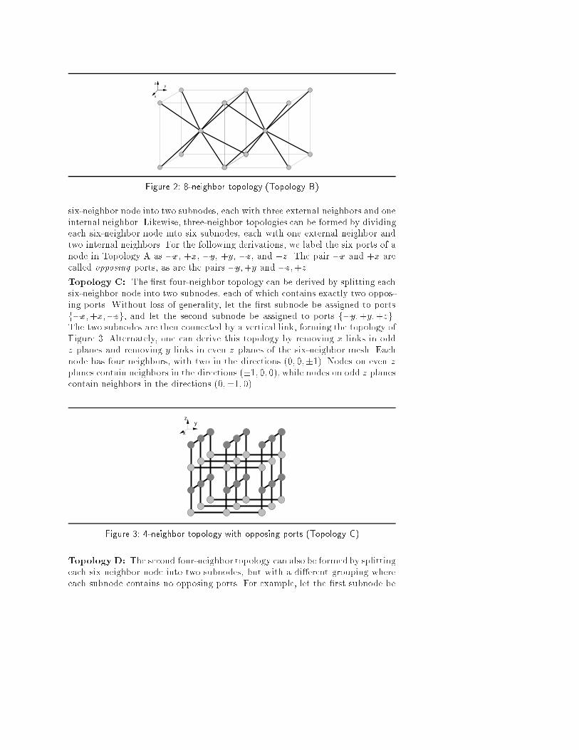
zFigure 2: 8-neighbor topology (Topology B)six-neighbor node into two subnodes, each with three external neighbors and oneinternal neighbor. Likewise, three-neighbor topologies can be formed by dividingeach six-neighbor node into six subnodes, each with one external neighbor andtwo internal neighbors. For the following derivations, we label the six ports of anode in Topology A as �x, +x, �y, +y, �z, and +z. The pair �x and +x arecalled opposing ports, as are the pairs �y;+y and �z;+z.Topology C: The �rst four-neighbor topology can be derived by splitting eachsix-neighbor node into two subnodes, each of which contains exactly two oppos-ing ports. Without loss of generality, let the �rst subnode be assigned to portsf�x;+x;�zg, and let the second subnode be assigned to ports f�y;+y;+zg.The two subnodes are then connected by a vertical link, forming the topology ofFigure 3. Alternately, one can derive this topology by removing x links in oddz planes and removing y links in even z planes of the six-neighbor mesh. Eachnode has four neighbors, with two in the directions (0; 0;�1). Nodes on even zplanes contain neighbors in the directions (�1; 0; 0), while nodes on odd z planescontain neighbors in the directions (0;�1; 0).x

yz

Figure 3: 4-neighbor topology with opposing ports (Topology C)Topology D: The second four-neighbor topology can also be formed by splittingeach six neighbor node into two subnodes, but with a di�erent grouping whereeach subnode contains no opposing ports. For example, let the �rst subnode be

assigned to ports f�x;�y;�zg, and the second subnode be assigned to portsf+x;+y;+zg. If one connects the two subnodes with a vertical link, then thetopology can be viewed as the removal of alternating x and y links from thesix-neighbor mesh, as shown in Figure 4.x

yz

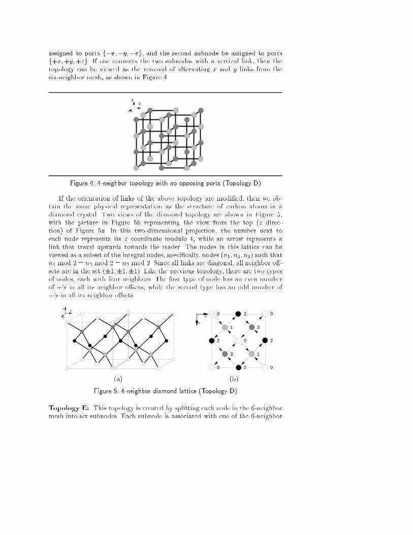
Figure 4: 4-neighbor topology with no opposing ports (Topology D)If the orientation of links of the above topology are modi�ed, then we ob-tain the same physical representation as the structure of carbon atoms in adiamond crystal. Two views of the diamond topology are shown in Figure 5,with the picture in Figure 5b representing the view from the top (z direc-tion) of Figure 5a. In this two-dimensional projection, the number next toeach node represents its z coordinate modulo 4, while an arrow represents alink that travel upwards towards the reader. The nodes in this lattice can beviewed as a subset of the integral nodes, speci�cally, nodes (n1; n2; n3) such thatn1 mod 2 = n2 mod 2 = n3 mod 2. Since all links are diagonal, all neighbor o�-sets are in the set (�1;�1;�1). Like the previous topology, there are two typesof nodes, each with four neighbors. The �rst type of node has an even numberof +'s in all its neighbor o�sets, while the second type has an odd number of+'s in all its neighbor o�sets.y

z

x (a) 0

0

2 0

02

2 20

1

1

3

3

x

y (b)Figure 5: 4-neighbor diamond lattice (Topology D)Topology E: This topology is created by splitting each node in the 6-neighbormesh into six subnodes. Each subnode is associated with one of the 6-neighbor

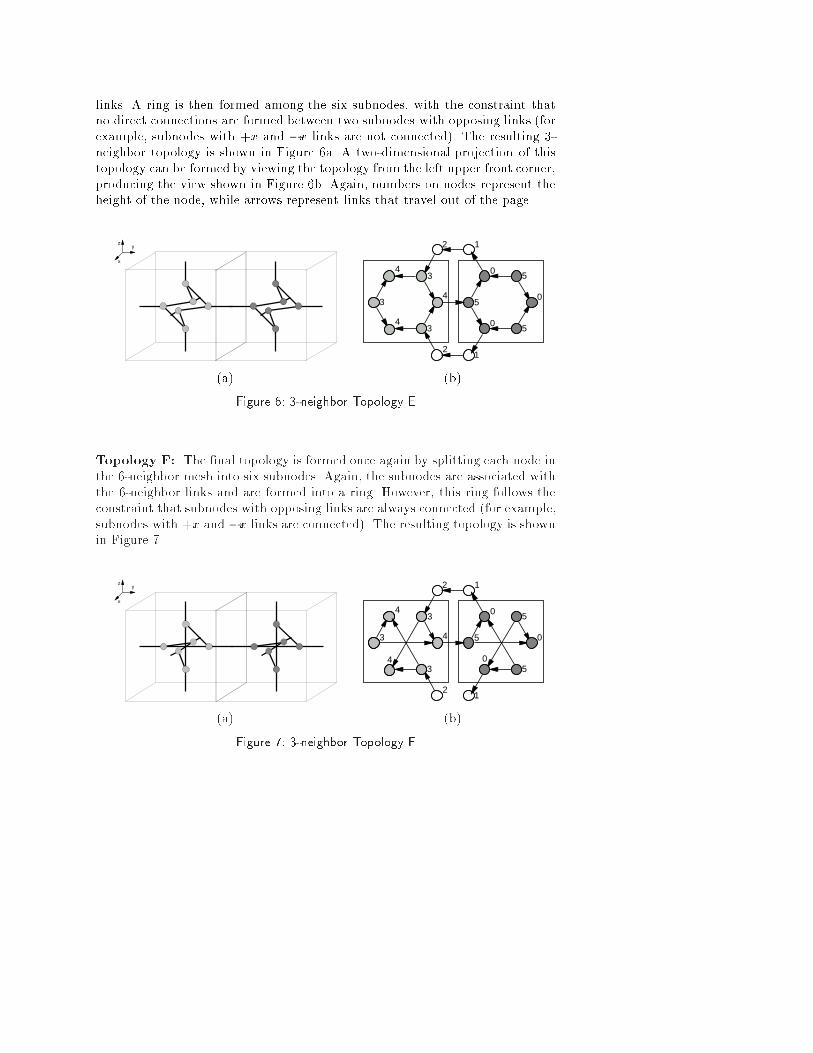
links. A ring is then formed among the six subnodes, with the constraint thatno direct connections are formed between two subnodes with opposing links (forexample, subnodes with +x and �x links are not connected). The resulting 3-neighbor topology is shown in Figure 6a. A two-dimensional projection of thistopology can be formed by viewing the topology from the left upper front corner,producing the view shown in Figure 6b. Again, numbers on nodes represent theheight of the node, while arrows represent links that travel out of the page.y

x

z (a) 4

4

4

3

3

3 5

5

5

0

0

0

21

2 1(b)Figure 6: 3-neighbor Topology ETopology F: The �nal topology is formed once again by splitting each node inthe 6-neighbor mesh into six subnodes. Again, the subnodes are associated withthe 6-neighbor links and are formed into a ring. However, this ring follows theconstraint that subnodes with opposing links are always connected (for example,subnodes with +x and �x links are connected). The resulting topology is shownin Figure 7.y

x

z (a) 4

4

4

3

3

3 5

5

5

0

0

0

21

2 1(b)Figure 7: 3-neighbor Topology F

3 Topology isomorphismSince topologies are de�ned in terms of the logical node connectivity, manyphysical representations may exist for a particular topology. However, it may bevery di�cult to determine whether some of these physical representations areindeed equal. In this section, we present a strategy for formally de�ning topolo-gies in terms of the logical connectivity. From this, a technique can be derivedto detect isomorphism between di�erent physical representations of topologies.Readers who are primarily interested in the performance comparisons betweentopologies may wish to defer this section until later.A topology T = [L;M ] is de�ned as a set of links L and a set of paths Mthat can be reached by some traversals of the links from a reference node. Wede�ne the group S(T ) to represent all paths using the links in L. Thus each linkin L can be viewed as generators for S(T ), and the group operator is merely theconcatenation of paths. Since the links can be represented by vectors in space,S(T ) must be abelian (commutative).As an example, consider Topology A (TA), whose links can be de�ned asthe set fX;Y; Zg. The mapping fA from logical links to physical links can bede�ned as: fA(X) = (1; 0; 0), fA(Y ) = (0; 1; 0), fA(Z) = (0; 0; 1). Any ele-ment in S(TA) can be represented in the form XaY bZc, which is translated tophysical coordinates as the path from (0; 0; 0) to (a; b; c). For a more complexexample, consider Topology B (TB). Let the links of TB be fW;X; Y; Zg, withthe mapping fA to physical links as: fB(W ) = (12 ; 12 ; 12 ), fB(X) = (12 ;�12 ;�12),fB(Y ) = (�12 ;�12 ; 12), fB(Z) = (�12 ; 12 ;�12). Again, the group S(TB ) can berepresented by the elements of the form W aXbY cZd. However, there is an im-portant di�erence: whereas each representation XaY bZc of S(TA) represents adi�erent element for di�erent values of a; b; c, the same is not true for S(TB ).Notably, for any a,W aXaY aZa is equal to W 0X0Y 0Z0 or the identity element,representing a null path. This can be veri�ed by using the mapping to vectors.In the above two examples, each path in S(T ) from the reference node is alsoin the set of topology pathsM . However, this is not the case for other topologies,such as the diamond topology TD . Although four links fW;X; Y; Zg also existfor TD , with S(TD) = S(TB) and fD = fB , the topologies are di�erent. This canbe explained by observing that not all paths in S(TD) from the reference nodeare legal. Indeed, any of the eight links fW�1; X�1; Y �1; Z�1g are legal fromany node in TB , while only four of the links are available from any node in TD.Thus only a subset of the paths in S(TD) can be considered legal paths from thereference node. In this case, we allow links fW;X; Y; Zg to be used at any evennumber of hops from the reference node, and links fW�1; X�1; Y �1; Z�1g to beused at an odd number of hops away. From this, we derive the constraint thatany legal path for TD must be of the formW aXbY cZd where a+b+c+d 2 f0; 1g.Note that the case of W aXaY aZa = W 0X0Y 0Z0 for TB is no longer relevantfor TD.In summary, a topology T is de�ned as a tuple [L;M ] consisting of links andpaths from a reference node. The links of L can be used as generators for anabelian group S(T ) which de�nes all paths from the reference node. The set M

is a subset of S(T ) and represents the actual legal paths that can be taken fromthe reference node to form the topology.This formalismof a topology can then be used to prove isomorphism betweendi�erent physical representations of topologies. As an example, let us considerthe two representations of Topology D, one formed from removing alternate xand y links from the six-neighbor mesh, and the other de�ned as the physicalstructure of the diamond lattice. Since a de�nition for TD is already derivedabove, we can show isomorphismmerely by showing two consistent mappings tothe two physical representations. The mapping to the diamond lattice representa-tion is already discussed above, with fD(W ) = (12 ; 12 ; 12), fD(X) = (12 ;�12 ;�12),fD(Y ) = (�12 ;�12 ; 12), fD(Z) = (�12 ; 12 ;�12 ). The second mapping can be de-�ned as follows: f 0D(W ) = (0; 0;�1), f 0D(X) = (1; 0; 0), f 0D(Y ) = (0; 1; 0),f 0D(Z) = (0; 0; 1). Note that the restriction of using fW;X; Y; Zg on an evennumber of hops from the reference node and fW�1; X�1; Y �1; Z�1g on an oddnumber of hops is consistent with the illustration in Figure 4.4 Analytical comparisonsWe �rst compare topologies by applying the conventional analytical measure-ments of maximum latency and minimumbisection bandwidth. In the followingcomparisons, we assume that pin-count forms the primary constraint on com-plexity of the routing chip, and thus normalize the topologies by keeping thepin-count constant. For a number of pins P , a k-neighbor topology requires k+1ports for connections to neighbors and the local processor. Thus the number ofbits in the communication path for each channel is P=(k + 1).4.1 LatencyFor a given topology, let the volume growth function V (r) be the number of nodesreachable within a distance r from a center node. The set of nodes counted byV (r) can be viewed as a \sphere" of radius r in the given topology. Thus foran n-dimensional topology, V (r) grows as rn. The maximum latency lmax of atopology can then be measured as the maximumdistance between any two nodesin the \sphere", and can be calculated using the inverse of the growth function:lmax = 2V �1(N ) for N nodes. The following section discusses strategies forcomputing the volume growth of di�erent topologies and presents some resultsof these computations.For Topology A, the \sphere" of radius r actually resembles the shape of anoctahedron with vertices at (�r; 0; 0), (0;�r; 0), and (0; 0;�r). The number ofnodes in the octahedron can then be estimated by multiplying its volume by thedensity of nodes in space. The volume of the octahedron is equal to twice thevolume of the pyramid formed from all points above the plane z = 0, which hasbase area 2r2 and height r. The volume of the octahedron is thus 43r3, and sincethe density of nodes in space is equal to one per unit volume, the number ofnodes in the sphere grows as 43r3.

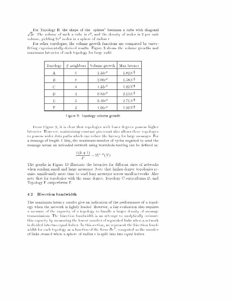
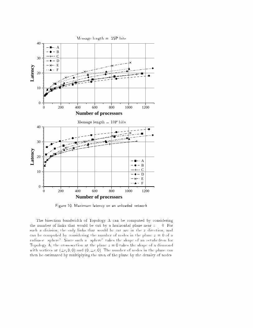
For Topology B, the shape of the \sphere" becomes a cube with diagonalp3r. The volume of such a cube is r3, and the density of nodes is 2 per unitvolume, yielding 2r3 nodes in a sphere of radius r.For other topologies, the volume growth functions are computed by curve-�tting experimentally-derived results. Figure 8 shows the volume growths andmaximum latencies of each topology for large radii.Topology # neighbors Volume growth Max latencyA 6 1:33r3 1:82N 13B 8 2:00r3 1:58N 13C 4 1:33r3 1:82N 13D 4 0:83r3 2:13N 13E 3 0:40r3 2:71N 13F 3 1:06r3 1:96N 13Figure 9: Topology volume growthFrom Figure 9, it is clear that topologies with lower degrees possess higherlatencies. However, maintaining constant pin-count also allows these topologiesto possess wider data paths which can reduce the latency for large messages. Fora message of length L bits, the maximum number of cycles required to send themessage across an unloaded network using wormhole routing can be de�ned as:L(k + 1)P + 2V �1(N )The graphs in Figure 10 illustrate the latencies for di�erent sizes of networkswhen sending small and large messages. Note that higher-degree topologies re-quire signi�cantly more time to send long messages across small networks. Alsonote that for topologies with the same degree, Topology C outperforms D, andTopology F outperforms E.4.2 Bisection bandwidthThe maximum latency results give an indication of the performance of a topol-ogy when the network is lightly loaded. However, a fair evaluation also requiresa measure of the capacity of a topology to handle a larger density of messagetransmissions. The bisection bandwidth is an attempt to analytically estimatethis capacity by measuring the lowest number of separated links when a networkis divided into two equal halves. In this section, we represent the bisection band-width for each topology as a function of the form Br2, computed as the numberof links crossed when a sphere of radius r is split into two equal halves.

Message length = .25P bits0 200 400 600 800 1000 1200

Number of processors

0

10

20

30

40

Lat

ency

ABCDEF

Message length = 10P bits0 200 400 600 800 1000 1200

Number of processors

0

10

20

30

40

Lat

ency

ABCDEFFigure 10: Maximum latency on an unloaded networkThe bisection bandwidth of Topology A can be computed by consideringthe number of links that would be cut by a horizontal plane near z = 0. Forsuch a division, the only links that would be cut are in the z direction, andcan be computed by considering the number of nodes in the plane z = 0 of aradius-r \sphere". Since such a \sphere" takes the shape of an octahedron forTopology A, the cross-section at the plane z = 0 takes the shape of a diamondwith vertices at (�r; 0; 0) and (0;�r; 0). The number of nodes in the plane canthen be estimated by multiplying the area of the plane by the density of nodes.

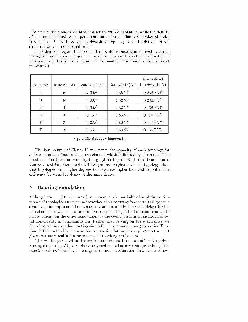
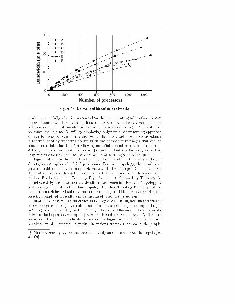
The area of the plane is the area of a square with diagonal 2r, while the densityof each node is equal to one per square unit of area. Thus the number of nodesis equal to 2r2. The bisection bandwidth of Topology B can be derived with asimilar strategy, and is equal to 4r2.For other topologies, the bisection bandwidth is once again derived by curve-�tting computed results. Figure 11 presents bandwidth results as a function ofradius and number of nodes, as well as the bandwidth normalized to a constantpin-count P . NormalizedTopology # neighbors Bandwidth(r) Bandwidth(N ) Bandwidth(N )A 6 2:00r2 1:65N 23 0:236PN 23B 8 4:00r2 2:52N 23 0:280PN 23C 4 1:00r2 0:83N 23 0:166PN 23D 4 0:75r2 0:85N 23 0:170PN 23E 3 0:32r2 0:59N 23 0:148PN 23F 3 0:65r2 0:63N 23 0:156PN 23Figure 12: Bisection bandwidthThe last column of Figure 12 represents the capacity of each topology fora given number of nodes when the channel width is limited by pin-count. Thisfunction is further illustrated by the graph in Figure 13, derived from simula-tion results of bisection bandwidth for particular spheres of each topology. Notethat topologies with higher degrees tend to have higher bandwidths, with littledi�erence between topologies of the same degree.5 Routing simulationAlthough the analytical results just presented give an indication of the perfor-mance of topologies under some scenarios, their accuracy is constrained by somesigni�cant assumptions. The latency measurement only represents delays for theunrealistic case when no contention arises in routing. The bisection bandwidthmeasurement, on the other hand, assumes the overly-pessimistic situation of to-tal non-locality in communication. Rather than relying on these extremes, wefocus instead on a random routing simulation to measure message latencies. Eventhough this method is not as accurate as a simulation of true program traces, itgives us a more realistic measurement of topology performance.The results presented in this section are obtained from a uniformly randomrouting simulation. At every clock tick, each node has a certain probability (theinjection rate) of injecting a message to a random destination. In order to achieve

0 200 400 600 800 1000 1200

Number of processors

0

10

20

30B

andw

idth

(in

P b

its)

ABCDEF

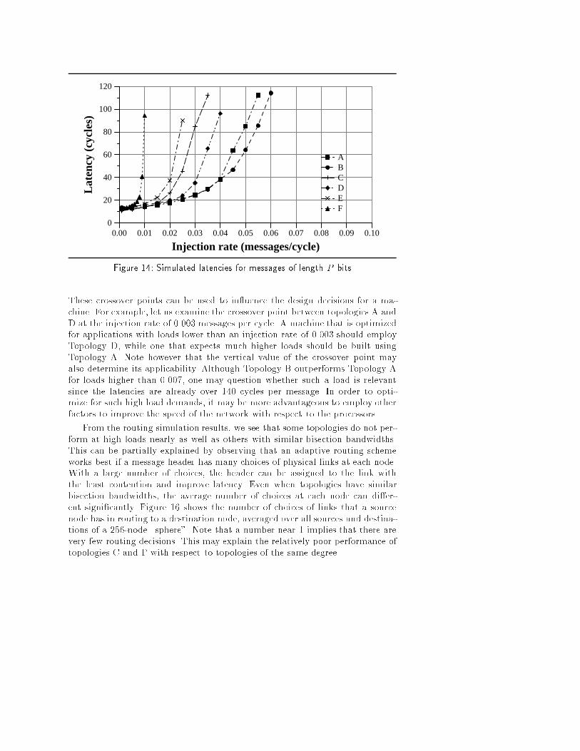
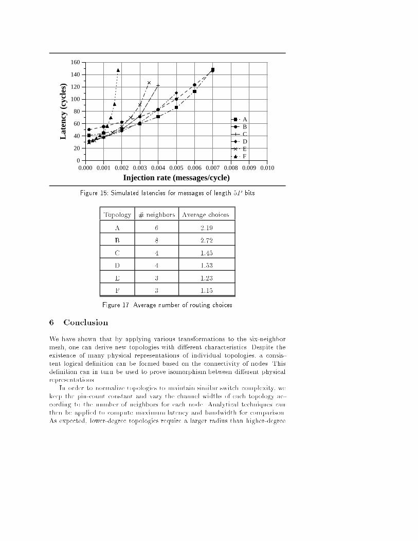
Figure 13: Normalized bisection bandwidthsa minimal and fully adaptive routing algorithm [8], a routing table of size N�Nis precomputed which contains all links that can be taken for any minimal pathbetween each pair of possible source and destination nodes.z. The table canbe computed in time O(N3) by employing a dynamic programming approachsimilar to those for computing shortest paths in a graph. Deadlock avoidanceis accomplished by imposing no limits on the number of messages that can beplaced on a link, thus in e�ect allowing an in�nite number of virtual channels.Although an abort-and-retry approach [5] could potentially be used, we had noeasy way of ensuring that no livelocks would arise using such techniques.Figure 14 shows the simulated average latency of short messages (lengthP bits) using \spheres" of 256 processors. For each topology, the number ofpins are held constant, causing each message to be of length k + 1 its for adegree-k topology with k+1 ports. Observe that latencies for low loads are verysimilar. For larger loads, Topology B performs best, followed by Topology A,as indicated by the bisection bandwidth measurements. However, Topology Dperforms signi�cantly better than Topology C, while Topology F is only able tosupport a much lower load than any other topologies. This discrepancy with thebisection bandwidth results will be discussed later in this section.In order to observe any di�erence in latency due to the higher channel widthsof lower-degree topologies, results from a simulation on longer messages (length5P bits) is shown in Figure 15. For light loads, a di�erence in latency existsbetween the higher-degree topologies A and B and other topologies. As the loadincreases, the higher bandwidth of some topologies impose lighter contentionpenalties on the latencies, resulting in various crossover points in the graph.z Minimal routing algorithms that do not rely on tables also exist for topologiesA-D[9]

0.00 0.01 0.02 0.03 0.04 0.05 0.06 0.07 0.08 0.09 0.10

Injection rate (messages/cycle)

0

20

40

60

80

100

120L

aten

cy (

cycl

es)

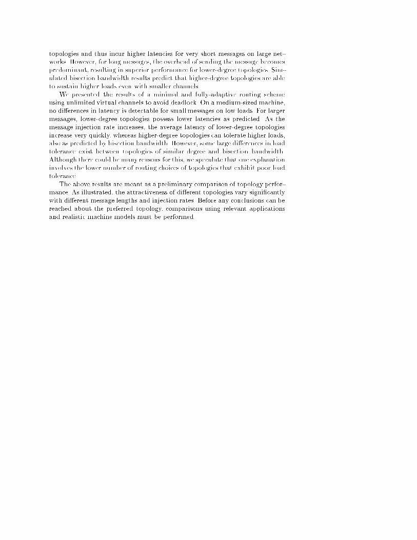
ABCDEFFigure 14: Simulated latencies for messages of length P bitsThese crossover points can be used to in uence the design decisions for a ma-chine. For example, let us examine the crossover point between topologies A andD at the injection rate of 0.003 messages per cycle. A machine that is optimizedfor applications with loads lower than an injection rate of 0.003 should employTopology D, while one that expects much higher loads should be built usingTopology A. Note however that the vertical value of the crossover point mayalso determine its applicability. Although Topology B outperforms Topology Afor loads higher than 0.007, one may question whether such a load is relevantsince the latencies are already over 140 cycles per message. In order to opti-mize for such high load demands, it may be more advantageous to employ otherfactors to improve the speed of the network with respect to the processors.From the routing simulation results, we see that some topologies do not per-form at high loads nearly as well as others with similar bisection bandwidths.This can be partially explained by observing that an adaptive routing schemeworks best if a message header has many choices of physical links at each node.With a large number of choices, the header can be assigned to the link withthe least contention and improve latency. Even when topologies have similarbisection bandwidths, the average number of choices at each node can di�er-ent signi�cantly. Figure 16 shows the number of choices of links that a sourcenode has in routing to a destination node, averaged over all sources and destina-tions of a 256-node \sphere". Note that a number near 1 implies that there arevery few routing decisions. This may explain the relatively poor performance oftopologies C and F with respect to topologies of the same degree.

0.000 0.001 0.002 0.003 0.004 0.005 0.006 0.007 0.008 0.009 0.010

Injection rate (messages/cycle)

0

20

40

60

80

100

120

140

160L

aten

cy (

cycl

es)

ABCDEFFigure 15: Simulated latencies for messages of length 5P bitsTopology # neighbors Average choicesA 6 2:19B 8 2:72C 4 1:45D 4 1:53E 3 1:23F 3 1:15Figure 17: Average number of routing choices6 ConclusionWe have shown that by applying various transformations to the six-neighbormesh, one can derive new topologies with di�erent characteristics. Despite theexistence of many physical representations of individual topologies, a consis-tent logical de�nition can be formed based on the connectivity of nodes. Thisde�nition can in turn be used to prove isomorphism between di�erent physicalrepresentations.In order to normalize topologies to maintain similar switch complexity, wekeep the pin-count constant and vary the channel widths of each topology ac-cording to the number of neighbors for each node. Analytical techniques canthen be applied to compute maximum latency and bandwidth for comparison.As expected, lower-degree topologies require a larger radius than higher-degree

topologies and thus incur higher latencies for very short messages on large net-works. However, for long messages, the overhead of sending the message becomespredominant, resulting in superior performance for lower-degree topologies. Sim-ulated bisection bandwidth results predict that higher-degree topologies are ableto sustain higher loads even with smaller channels.We presented the results of a minimal and fully-adaptive routing schemeusing unlimited virtual channels to avoid deadlock. On a medium-sized machine,no di�erences in latency is detectable for small messages on low loads. For largermessages, lower-degree topologies possess lower latencies as predicted. As themessage injection rate increases, the average latency of lower-degree topologiesincrease very quickly, whereas higher-degree topologies can tolerate higher loads,also as predicted by bisection bandwidth. However, some large di�erences in loadtolerance exist between topologies of similar degree and bisection bandwidth.Although there could be many reasons for this, we speculate that one explanationinvolves the lower number of routing choices of topologies that exhibit poor loadtolerance.The above results are meant as a preliminary comparison of topology perfor-mance. As illustrated, the attractiveness of di�erent topologies vary signi�cantlywith di�erent message lengths and injection rates. Before any conclusions can bereached about the preferred topology, comparisons using relevant applicationsand realistic machine models must be performed.

References[1] Anant Agarwal. Limits on interconnection network performance. IEEETransactions on Parallel and Distributed Systems, 2(4):398{412, 1991.[2] Thomas H. Cormen, Charles E. Leiserson, and Ronald L. Rivest. Introduc-tion to Algorithms. MIT Press, Cambridge, Massachusetts, 1990.[3] WilliamDally. Virtual channel ow control. IEEE Transactions on Paralleland Distributed Systems, 3(2):194{205, 1992.[4] William Dally and Charles Seitz. Deadlock-free message routing in mul-tiprocessor interconnection networks. IEEE Transactions on Computers,C-36(5), 1987.[5] Jae H. Kim, Ziqiang Liu, and Andrew A. Chien. Compressionless routing.In The 21st Annual International Symposium on Computer Architecture,pages 289{300, 1994.[6] D. Linder and J. Harden. An adaptive and fault tolerant wormhole routingstrategy for k-ary n-cubes. IEEE Transactions on Computers, C-40(1):2{12,1991.[7] Allen D. Malony. Regular processor arrays. In The 2nd Symposium on theFrontiers of Massively Parallel Computation, pages 499{502, 1988.[8] Lionel M. Ni and Philip K. McKinley. A survey of wormhole routing tech-niques in direct networks. Computer, 26(2):62{76, 1993.[9] Gill Pratt, Steve Ward, John Nguyen, and Chris Metcalf. The diamondinterconnect. In press.[10] Supercomputing Research Center. Five year review, March 1991.[11] Steve Ward, et al. A scalable, modular, 3D interconnect. In 1993 Interna-tional Conference on Supercomputing, pages 230{239, 1993.