Embed Size (px)
Citation preview

THREE ESSAYS ON ECONOMIC AND POLITICAL INSTITUTIONS
Daniel Lema
UNIVERSIDAD DEL CEMA 2006

Jorge Miguel Streb ........................................................... Germán Coloma ........................................................... Guillermo Marcos Gallacher ........................................................... Juan Jorge Medina …………………………………….
ii

DEDICATION
To my wife, Patricia
iii

TABLE OF CONTENTS PageLIST OF TABLES AND FIGURES viPREFACE viii 1. Contracts, Transaction Costs and Agricultural Production in the Pampas I. Introduction 1II. Literature Review and Theoretical Background 2III. Study Area and Data 4IV. Econometric Analysis 6V. Final Comments 11References 13 2. Discretional Political Budget Cycles and Separation of Powers I. Introduction 14II. Empirical literature 15A. Shi and Svensson 15B. Persson and Tabellini 16C. Brender and Drazen 17III. Theoretical framework 17IV. Data and Econometric Specification 19V. Empirical Evidence 22A. Effective Checks and Balances and Discretional Component of PBC 24B. OECD and non-OECD countries 28C. Budget Balance, Expenditures and Revenues: Persistence Effects 31D. Rich Established Democracies and Poor Young Democracies 33VI. Final remarks 36References 38 3. Conditional Political Budget Cycles in Argentine Provinces I. Introduction 40II. The Political Budget Cycle 41A. Previous Literature 41B. Theoretical Framework 42III. Data 44IV. Empirical Analysis 46V. Unconditional Budget Cycles 48A. Budget Balance 48B. Expenditures: Total and Composition 51C. Revenues: Total, Federal and Provincial 56VI. Conditional Findings: Political Alignment Between Provincial and Federal Executives 63A. Budget Balance 63B. Expenditures: Total and Composition 65C. Revenues: Total, Federal and Provincial 68
iv

VII. Conclusions 72References 73Appendix. Chapter 3 Econometric Estimation Output 74
v

LIST OF TABLES AND FIGURES
PageChapter 1 Tables 1. Definition of Variables 62. Probit (Conservation Practices) and Tobit (No Till - Fertilization) Estimates 73. Wald Test of Coefficients Equality (Fixed Rent and Sharecropping Contracts)
8
4. Tobit Estimates (Cereals and Oilseeds Fertilization) 10Figures 1. The Study Area 52. Frequency Distribution of Farms and Area 5 Chapter 2 Tables 1. Definition of Variables 202. Country Characteristics 233. Descriptive Statistics 244. Discretional PBC in All Democracies 265. Discretional PBC in OECD Countries 296. Discretional PBC in Non-OECD Countries 307. Discretional PBC in All Democracies: Budget Balance, Expenditure and Revenues
32
8. Discretional PBC in Established OECD Democracies 349. Discretional PBC in Young Non-OECD Democracies Figures 1. Time Path of Budget Balance around Elections 28 Chapter 2 Tables 1. Definition of Variables 452: Fiscal Variables: Descriptive Statistics 463. Elections and Fiscal Balance 494. Elections and Fiscal Balance 505. Elections and Total Expenditure 526. Elections and Total Expenditure 537. Elections and Composition Effect 548. Elections and Composition Effect 559. Elections and Total Revenue 5710. Elections and Total Revenue 5811. Elections and Revenue from Federal Government 5912. Elections and Revenue from Federal Government 6013. Elections and Revenue from Provincial Taxes 6114. Elections and Revenue from Provincial Taxes 6215. Elections and Fiscal Balance conditional on alignment of provincial and federal government
64
vi

16. Elections and Total Expenditure conditional on alignment of provincial and federal government
66
17. Elections and Composition Effect conditional on alignment of provincial and federal government
67
18. Elections and Total Revenue conditional on alignment of provincial and federal government
69
19. Elections and Revenue from Federal Government conditional on alignment of provincial and federal government
70
20. Elections and Revenue from Provincial Taxes conditional on alignment of provincial and federal government
71
vii

PREFACE
This thesis is a study on the behavioral incentives and control mechanisms defined by
economic and political institutions. The three essays are empirical quantifications of the
economic effects implied by different institutional arrangements. We examine the
economic implications of legal and political structures using economic theory,
econometric analysis and hypothesis testing.
The first essay is a study of incentives for resource use under different
contractual arrangements in the Argentinean agricultural production. Using a transaction
costs approach, we contend that in a context of modern agriculture, with well defined
property rights, agricultural contracts must balance costs and benefits, aligning tenant
and landlord incentives towards a similar objective. The study debates the potential
effects of tenancy status and duration of contracts, over soil conservation and input use.
We present empirical evidence about the effects over the soil and input use in tenant and
owner-operator farms using farm level data from the 2002 National Agricultural Census
of Argentina. Contrary to the conventional wisdom, the empirical results do not support
a general and clear negative effect for tenancy arrangements. Our intuition is that the
interaction among specific characteristics of farmers, natural resources endowment and
institutional environment are more important factors than the land tenancy or contract
type itself.
The second essay looks at the relationship between electoraly motivated fiscal
policy cycles and separation of powers. Previous empirical work on electoral cycles
implicitly assumes the executive has full discretion over fiscal policy. In contrast, we
contend that an unaligned legislature may have a moderating role under separation of
powers. Focusing on the budget surplus, we find that stronger effective checks and
balances explain why cycles are weaker in developed and established democracies.
Once the discretional component of executive power is isolated, there are significant
cycles in all democracies. Hence, what we add to the ongoing debate about the factors
behind conditional Political Budget Cycles is a study of the role of effective checks and
balances that reduce the discretion of the executive.
The third essay presents evidence of electoraly-motivated changes in the budget
balance, public expenditures, composition of public expenditures and provincial
revenues in Argentine provinces. The empirical study is made using panel data analysis
viii

for 22 Argentine provinces during the period 1985-2001. Results show that conditioning
on the alignment of provincial and federal executives (same political party in power)
there is evidence of systematic changes in fiscal policies around elections. The observed
changes support the predictions of rational opportunistic models of Political Budget
Cycles. In election years, total provincial expenditures increase in aligned provinces,
without affecting the fiscal balance, because to the increased discretional transfers from
the federal government supporting the provincial incumbent federal revenues. By
contrast, deficit increases for unaligned provinces. In addition, expenditure shifts toward
current spending and away from capital spending for unaligned provinces in electoral
years.
Finally, I wish to thank the members of my Thesis Committee Professors Jorge
M.Streb (Chairman), Germán Coloma, Marcos Gallacher and Juan Jorge Medina for
their insightful suggestions. A special acknowledgement I owe to Professor Streb for
helpful, deep and extensive discussions on issues contained (and not) in this study. I
also wish to thank the Director of the Department of Economics, Professor Mariana
Conte Grand, for their warm and continuous encouragement. The Instituto de Economía
y Sociología at INTA (Instituto Nacional de Tecnología Agropecuaria) has provided
important support for developing this study. I am very grateful for it.
ix

1
Chapter 1
Contracts, Transaction Costs and Agricultural Production in the Pampas
I. Introduction
Land tenure and contractual arrangements are controversial issues in the Pampean
agriculture. The early colonial pattern of large land holdings dictated the system of
sharecropping agriculture with immigrant farmers that developed after 1860. Some
authors describe the sharecropper system as a rational economic arrangement that
favored landlords and tenants. There was no collusion on the part of large landholders to
bar access to land by the newly arrived European farmers and the land market was open
and competitive without legal or economic barriers to entrance (Cortés Conde, 1995).
However, other authors contend that tenure regime and sharecropping arrangements had
negative social and productive consequences (Scobie, 1964; Ferrer, 1965).
Eventually, through inheritance or sale, many of the very large “estancias”
(cattle ranch) were broken up, but the original pattern of land occupation resulted in
larger landholdings than in similar regions of the U.S. as the “Corn Belt”. In spite of
these differences in land tenure arrangements, Gallacher et. al. (2003) suggests that a
similar overall performance is observed in agricultural production in both countries
because farmers are efficient in resource allocation (including land tenure
arrangements).
During the last 15 years, Argentine agricultural production has been rising and
land rental (both fixed rent and sharecropping) is a growing practice, implying a greater
separation between the property and control of land. In this paper, our objective is to
show that land tenure arrangements in the Pampean agriculture align interests and
incentives in an efficient way. Using a transaction costs approach, we present empirical
evidence about the effects of agricultural contracts (fixed rent, sharecropping) on soil
conservation practices and input use (fertilizers).
The organization of the paper is the following. Section II briefly reviews the
literature and presents the theoretical background. Section III describes the
characteristics of the study area and the data set from the 2002 National Agricultural
Census (NAC). Section IV presents the econometric analysis. Section IV has the final
comments.

2
II. Literature Review and Theoretical Background
The analysis of fixed rent and sharecropping contracts has been extensively developed
in the literature. In a fixed rent contract, the tenant pays a fixed amount not related to
farm production. On the other hand, the sharecropping contract allows the tenant only a
fraction of the total product (e.g., between 65 and 70% in Pampean grain production).
In a sharecropping contract the tenant has incentives to under-utilize inputs, this
is widely known as the sharecropping problem in its “Marshallian” version (Johnson,
1950). Several reasons have been proposed to explain the use of sharecropping
contracts. One incorporates risk in the analysis of contracts (Stiglitz 1988). Under this
explanation, sharecropping is a way to share risk between the landlord and the tenant
and the sharecropping contract appears as a choice in order to avoid risks. Therefore, the
tenant shares not only the product but also part of the risk associated with agricultural
production. One reply to this argument is that if there are no restrictions to make
multiple fixed rent contracts, it is possible to avoid risk diversifying the use of fixed
contracts (Newbery 1977). Alternatively, the “moral hazard” approach suggests that
efficient contracts balance the exchange between the costs associated with the risk and
the benefits derived from generating optimal incentives for both parties. A
sharecropping contract can be seen as a result of this balance (Stiglitz 1988).
These models have been considerably developed in the literature and empirically
applied in the study of the contractual relations. Empirical results are mixed about
efficiency under fixed and sharecropping contracts, with studies focused on developing
countries with traditional agricultural sectors.
Our analysis will concentrate on the relationship between the landlord and the
tenant using a theoretical framework associated with the transaction costs approach.
Cheung (1968) shows that with well defined property rights the type of contracts does
not affect efficient resource allocation. A critical assumption is the absence of
transaction costs and in particular the inexistence of monitoring costs in the use of
inputs or the effort made by the tenant.
Following Allen and Lueck (2002), we do not consider risk and we add to the
analysis the use of specific characteristics of land. Specifically, the soil attributes are
treated as an additional input in the production process. When a producer carries out the
production in his own land, he manages the resources taking into account the present
and future implications of his decisions. By contrast, a tenant with a fixed rent contract
will only worry about his current results. Then, if greater yields could be obtained by

3
putting aside adequate soil management, applications of fertilizers or other practices, the
tenant has incentives in this direction.
In sharecropping contracts, if effort is observed imperfectly and there are
monitoring costs, there would be incentives to underutilize inputs by the tenant. This
implies, also that he may have less incentives to use the soil attributes excessively or to
carry out actions with potential harmful effects over the natural resources. This could be
seen as a potential benefit of sharecropping contracts (Allen and Lueck 2002).
However, this does not imply that sharecropping is always the most convenient
arrangement for the landlord. Transaction costs are important in controlling and
dividing the output, because the tenant has incentives to underreport the quantity of crop
to the landlord. Of course, the landlord is aware of this problem and he will do all that
he can to avoid this behavior.
The relative advantage of a fixed rent contract is to avoid the quantity control.
However, it presents the problem of over-utilization of soil attributes. The
sharecropping contract reduces the incentives to dig the soil, but it has costs related to
the control of quantity and quality of crop.
Some other factors can lead the actions of tenants and landlords to the optimal
use of the resources. For example, repeated transactions can build a reputation and
reduce the costs of control. If transactions are less frequent but the landlord has good
knowledge of the activity, he can reduce the monitoring costs. If control of production is
relatively more costly, then he can opt for fixed rent contracts.
It is often argued that short-term contracts do not generate adequate incentives
for both the conservation of resources and investments. However, when an owner-
operator decides how to manage his land, he has as an inter-temporal profit-maximizing
objective. When he considers the option of renting the land to a tenant, the analysis
cannot be different. The landlord surely is aware of the incentives that the tenant has to
make an over use of the soil attributes in the short term.
Our working hypothesis is that the design of the contracts should align interests
of tenants and landlords, minimizing transaction costs. The contract design should make
the actions converge in such a way that the results for a tenant will be similar to those of
an owner or landlord-operator. However, a greater alignment of interests tends to
increase the complexity and the costs of the contracts. Longer contracts may stimulate
the conservation of assets and soil, but at the same time require more detailed conditions
that are costly to control and enforce.

4
Pampean agricultural production is based mostly on short-term contracts, but the
transactions are repeated and frequent. The incentive to build a reputation can act as an
alternative mechanism for long-term contracts. A repeated short term contract can have
implicit renovation if the tenant carries out the expected actions, but it is revoked easily
if not. Our intuition is that we should not observe a systematic bias in resource
allocation between annual tenants (fixed rent or sharecropping) vis à vis landlord-
operators1.
Hence, our principal conjecture is that contractual arrangements must balance
costs and benefits, aligning incentives towards an objective similar to a producer-
landlord with full interest in maximizing and conserving his wealth. We do not expect
major differences between owner operators and tenants in input use or natural resources
conservation.
If the crop share contracts do not give full incentives for the optimal use of
inputs, and there are monitoring and control costs, some differences in input use (e.g.,
fertilizers) could be found in case of fixed rent contracts with respect to sharecropping
contracts.
These conjectures are empirically tested in section IV.
III. Study Area and Data
The geographic focus of this study is the central-eastern region of Argentina known as
the Pampas, one of the most productive agricultural areas in the world and of major
importance to the Argentine economy (85% of the total grain production). Wheat and
corn have been the principal crops for the last 100 years and soybean is a more recent
crop.
The empirical analysis is carried out using farm level data from the National
Agricultural Census 2002 (NAC 2002) of Pergamino County, Province of Buenos
Aires.
Cropping systems include maize, soybean, wheat-soybean double crop and
characteristic rotations include maize and soybean. Pergamino is representative of the
1 In Pampean agriculture, annual contracts prevail. According to current legislation, all agrarian contracts must
be signed for three years and registered in courts. Even though detailed statistical information is not available on the fulfilment of this requirement, it is a well-know fact in the rural media that the majority of contracts do not comply with this formality. The evidence points out that for different reasons, surely linked to the transaction costs, farmers have opted to set up informal contracts. In this sense, we consider that the actual legal framework is neutral for the selection of the contracts and the productive decisions.

5
Pampas and it presents characteristics of modern agriculture (defined property rights,
modern inputs and technological knowledge) which makes it comparable, for example,
with the American “Corn Belt”. Figure 1 displays the location of the study area.
The available micro data includes productive, economic and management
variables for 1117 farms in a total area of 285,992 hectares, averaging 256 hectares per
farm. Figure 2 presents the frequency distribution of farms and area.
Figure 2. Frequency Distribution of Farms and Area
Frequency Distribution of Farms and AreaPergamino 2002
0.00%
5.00%
10.00%
15.00%
20.00%
25.00%
30.00%
0-25 25.1-50 50.1-100 100.1-200 200.1-500 500.1-1000 1000.1-2500 more than 2500
Hectares
%
% Area % Farms

6
IV. Econometric Analysis
We carry out estimations of binary election models (Probit) to explain the utilization of
soil conservation practices (no tillage or reduced tillage). Selection models (Tobit) are
used to explain the cultivated area with no till practices and total fertilized area. From
the 1117 farms we considered those that produced at least some of the four principal
crops (soybeans, corn, wheat and sunflower). The result is a total of 944 observations
available for the study. Dependent and independent variables and their definitions are
presented in Table 1.
Table 1. Definition of Variables Dependent Variables: CONS: Dummy variable that assumes the value of one if on the cultivated area some conservationist practice is carried out (e.g. no tillage, reduced tillage,). AREANT: Area with no till practice as percentage of the total area cultivated with soybeans, corn, wheat and sunflower. TOTFERT: Total fertilized area as percentage of the cultivated area in corn, wheat and sunflower. CWFERT: Fertilized area in corn and wheat crops as percentage of the total implanted area with corn and wheat. SSFERT: Fertilized area in soybeans and sunflower crops as percentage of the total implanted area with soybeans and sunflower. Independent Variables: T: Dummy variable for tenant farms. It assumes the value of one if the ratio between the own cultivated area (OA) and the total area of the farm (ATOT) is less o equal to 0.20 (0.20 ≥ OA/ATOT). TF: Dummy variable for type T farms with fixed rent contract. It assumes the value of one if the rent is fixed in a proportion greater or equal than 0.80 with respect to the total rented area. TS: Dummy variable for type T farms with sharecropping contract. It assumes the value of one if the sharecropped area is a proportion greater or equal than 0.80 with respect to the total area rented. T_OTHER: Dummy variable that takes value of one for type T farms that belong neither to the category TF nor to the category TS (T_OTHER = T – TF – TS). OWN_TEN: Dummy variable for farms that combine own land and tenancy. It assumes the value of one if 0.20 < OA/ATOT < 0.80. CULTA: Total cultivated area with wheat, corn, soybeans and sunflower, in thousands of hectares. SOY: Dummy variable that assumes the value of one if the farm produces only soybeans SUMM: Dummy variable that assumes the value of one if the farm carries out just summer crops (corn-soybeans) PLOWS: Total number of plows (or similar equipment) TRACT: Dummy variable that takes the value one if the farm has one or more tractors. DIR: Total number of machinery for direct seed-planting (no till machinery) SERV: Total area contracted for services of plowing and soil preparation in thousand of hectares MAINT: Total area contracted for maintenance work and conservation of the crops, in thousands of hectares. EDU: Education of the producer measured in a scale between 1 and 7.5 (1: no education; 7.5: complete college education) (this variable assumes the value of zero when the farm is some type of partnership or corporation). EDUD: Dummy variable that assumes the value of one when the variable EDU assumes the value of zero ( it controls for possible bias in the coefficient associated with EDU due to the inclusion of zeros) RESID: Dummy variable that assumes the value of one if the producer or any of the partners resides on the farm. MANAG: Dummy variable that assumes the value of one if the farm keeps formal accounting and productive records. PUBEXT: Dummy variable that assumes the value one if the farm receives extension services from some public organization (state or federal). PRIVADV: Dummy variable that assumes the value of one if the farm uses some private technical advise (independent professionals, companies, NGOs)

7
CONS is a binary variable that identifies the use of the conservation practices (when
CONS=1). A group of four continuous variables measures the relative adoption of no
till practices (AREANT) and fertilizing (TOTFER), the relative fertilization in cereals
(CWFER), and fertilization in oilseeds (SSFER). Table 2 presents the probit estimation
for the binary dependent variable CONS.
Table 2. Probit (Conservation Practices) and Tobit (No Till - Fertilization) Estimates
Variables
CONS (1)
CONS (2)
AREANT (3)
AREANT (4)
TOTFERT (5)
TOTFERT (6)
T -0.177 (-1.55)
-2.654 (-0.56)
-7.593 (-1.91)*
TF -0.251A
(-1.63) -11.192B
(-1.75)* -5.901C
(-1.13) TS 0.119A
(0.59) 4.867B
(0.57) -11.034C
(-1.47) A_OTHER -0.300
(-1.68)* 3.426
(0.48) -7.845
(-1.30) OWN_TEN -0.103
(-0.89) -0.106 (-0.92)
-1.986 (-0.42)
-2.035 (-0.43)
-2.347 (-0.62)
-2.342 (-0.62)
CULTA -0.365 (-2.43)**
-0.361 (-2.39)**
-2.964 (-0.50)
-20.754 (-0.47)
-7.036 (-1.40)
7.119 (-1.42)
SUMM -0.156 (-1.62)
-0.165 (-1.71)*
-23.440 (-5.82)***
-23.825 (-5.92)***
SOY -63.220 (-15.58)***
-63.122 (-15.54)***
PLOWS -0.177 (-5.42)***
-0.177 (-5.42)***
-6.291 (-4.85)***
-6.192 (-4.78)***
TRACT -0.676 (-5.12)***
-0.670 (-5.04)***
-27.386 (-4.91)***
-28.174 (-5.04)***
-7.798 (-1.78)*
-7.770 (-1.77)*
DIR 0.585 (6.87)***
0.594 (6.93)***
23.749 (7.76)***
23.893 (7.80)***
4.333 (1.84)*
4.299 (1.83)*
SERV 0.552 (2.34)**
0.557 (2.36)**
20.453 (2.18)**
21.407 (2.28)**
MAINT 5.635 (2.70)***
5.578 (2.67)***
EDU 0.107 (3.36)***
0.111 (3.50)***
4.738 (3.53)***
4.860 (3.62)***
2.593 (2.32)**
2.548 (2.27)**
EDUD 0.627 (3.20)***
0.650 (3.30)***
20.461 (2.45)**
20.322 (2.44)**
16.190 (2.36)**
16.104 (2.35)**
MANAG 0.241 (2.25)**
0.238 (2.21)**
6.436 (1.44)
7.136 (1.60)
13.906 (3.73)***
13.843 (3.69)***
PUBEXT 0.458 (2.16)**
0.452 (2.13)**
13.312 (1.57)
13.260 (1.56)
9.621 (1.37)
9.695 (1.38)
PRIVADV 0.221 (2.00)**
0.210 (1.90)*
9.725 (2.13)**
9.514 (2.08)**
4.441 (1.15)
4.569 (1.18)
RESID -0.271 (-2.45)**
-0.270 (-2.42)**
-14.960 (-3.28)***
-14.897 (-3.28)***
-7.642 (-2.07)**
-7.673 (2.07)**
Constant -0.224 (-1.05)
-0.236 (-1.11)
44.939 (5.00)***
44.695 (4.99)***
19.833 (2.61)***
19.956 (2.62)***
Method of Estimation Probit Probit Tobit Tobit Tobit Tobit No. Observations 944 944 944 944 944 944
Censored Observations (Dep. Var.<=0)
-
-
324 324 353 353
Not Censored Obs. - - 620 620 591 591 Log-Likelihood -524.05 -521.15 -3620.897 -3618.903 -3243.137 -3242.953
LR Test 213.44*** 219.26*** 240.12*** 244.11*** 390.10*** 390.46*** Pseudo R2 0.171 0.174 0.0321 0.0326 0.0567 0.0568
Notes: z statistics in parentheses; *** Significant at the 1%; **Significant at the 5%; *Significant at the 10%; A and B: see Table 3 for Wald test of coefficients equality

8
The independent variables are grouped in those measuring the type of land
tenancy (T, TF, TS, T_OTHER, OWN_TEN) and those that control by productive
characteristics (CULTA, SOY, SUMM, SERV, MAINT), physical capital (PLOWS,
TRACT, DIR), human capital and management (EDU, RESID, MANAG, PUBEXT,
PRIVADV).
In the first model, the variables T and OWN_TEN were included to estimate the
effect of these two forms of tenancy on CONS (controlling for covariates). In the
second equation the tenancy status is distinguished by type of contract, including the
variables TF, TSP and A_OTHER. Our main interest is on coefficients associated with
tenancy variables (T, TF and TS), and we observe that those coefficients are not
significant in any of the estimations. Only the coefficient associated with the category
T_OTHER appears with negative sign and marginally significant at 10% in estimation
2. The estimated coefficient of TS has a positive sign and that of TF has a negative sign
(and marginally significant at 11%). Following the theoretical conjecture that there are
greater incentives to over use soil attributes in fixed rent contracts, this finding may
imply a differential effect between fixed rent and crop share contracts. Table 3 (line A)
presents a Wald test that contrasts the hypothesis of equality of both coefficients.
Table 3. Wald Test of Coefficients Equality (Fixed Rent and Sharecropping Contracts) Statistic p-value Statistic p-value
A chi2(1)= 2.44 0.11 D F(1, 570)= 0.66
0.42
B F (1, 928) = 2.64 0.10 E F(1, 929) = 2.81
0.09
C F(1, 929) = 0.36 0.55 - - -
The result shows that (marginally) at 11% we can reject the null hypothesis of equality.
This suggests some differential effect of greater adoption of conservation practices in
cases of sharecropping contracts. So, the tenancy status appears relatively neutral in
terms of conservation practices, with a slightly superior adoption of conservation
practices in crop share contracts.
Regarding control variables, it is clear that the quantity and type of available
machinery affects the adoption of conservation practices, since the effect of PLOWS
and TRACT over CONS appears to be systematically negative and significant, while the

9
effect of DIR is positive and significant. Variables related with human capital and
management presents a positive and significant effect over the adoption of conservation
practices.
Columns 3 to 6 in Table 2, present the estimations using no till area (AREANT)
and fertilized area (TOTFERT) as a percentage of the total farming area as dependent
variables. Farms that do not carry out soil conservation practices or do not fertilize
always have a percentage equal to zero. To address this problem of sample selection, we
used models of simultaneous selection (Tobit) to perform the estimations.
Equation 3, with no till practices (AREANT) as dependent variable, shows that
the estimated coefficient for variable T is not significant. On the other hand, in equation
4, the coefficient associated with fixed rent (TF) is negative and significant. This result
is similar to the conservation practices equation. In the same way, we perform a Wald
test to contrast equality between the estimated coefficients for TF and TS. Results (line
B Table 4) suggest a greater use of no till practices for crop share tenants.
The coefficient associated with tenancy (T) is negative and significant at 10% in
equation 5. However, controlling by contract type, there are no significant differential
effects relative to the base category (landlords). We also tested the null hypothesis of
equality between these coefficients (line C Table 4). The Wald test does not reject the
null hypothesis of coefficients equality.
The effect of the dummy variable SOY, that controls farms dedicated only to
soybean production, appears negative and significant in fertilization equations.
Fertilization in soybeans is much less frequent, since marginal yield response is
reduced. In order to control this effect we analyzed the practice of fertilization in two
sub samples. One sub sample includes farms producing cereal crops and the other those
producing oilseeds. Estimation results for each sub sample are presented in Table 4
(equations 7 to 10).
Equation 7, shows that the tenancy variable is significant and positive when
fertilization in corn and wheat (CWFERT) is the dependent variable. Equation 8
includes dummy variables for sharecropping and fixed rent contracts, and the Wald test
(line D in Table 4) suggests equality between estimated coefficients.
For oilseed crops fertilization (SSFRT, equation 9) the coefficient associated
with T is negative and significant. When the effects are separated by contract type
(equation 10), the negative effect on fertilization by the tenants is explained principally

10
by the group of sharecropping tenants. The Wald test (line E in Table 4) allows the
rejection of the null hypothesis of equality. Table 4. Tobit Estimates (Cereals and Oilseeds Fertilization)
Variables CWFERT (7)
CWFERT (8)
SSFERT (9)
SSFERT (10)
T 15.757 (2.65)***
-44.403 (-2.33)**
TF 12.054D
(1.59) -31.592E
(-1.30) TS 22.316D
(1.97)** -129.616E
(-2.34)** A_OTHER 17.491
(1.91)*** -28.223
(-0.98) OWN_TEN 9.995
(1.83)* 10.032 (1.84)*
13.518 (0.82)
13.680 (0.83)
CULTA -3.316 (-0.95)
-6.111 (-0.92)
-40.744 (-1.41)
-42.146 (-1.45)
TRACT -2.447 (-0.35)
-2.732 (-0.39)
-25.239 (-1.39)
-27.166 (-1.50)
DIR 10.007 (3.03)***
10.049 (3.05)***
-0.068 (-0.01)
-0.316 (-0.03)
MAINT 3.033 (1.12)
3.124 (1.15)
25.986 (2.47)**
25.666 (2.43)**
EDU 3.613 (2.15)**
3.675 (2.19)**
5.124 (1.05)
4.339 (0.89)
EDUD 24.803 (2.46)**
24.937 (2.24)**
18.245 (0.60)
14.485 (0.47)
MANAG 20.514 (3.72)***
20.742 (3.73)***
54.670 (2.98)***
55.606 (3.03)***
PUBEXT 24.788 (2.42)**
24.706 (2.41)**
-5.005 (-0.16)
-4.807 (-0.16)
PRIVADV 9.158 (1.53)
8.821 (1.47)
9.492 (0.56)
10.924 (0.67)
RESID -11.683 (-2.17)**
-11.544 (-2.15)**
-32.624 (-1.85)*
-33.204 (-1.88)*
Constant 61.878 (5.35)***
61.840 (5.26)***
-185.040 (-5.09)***
-180.928 (-4.98)***
Method of Estimation Tobit Tobit Tobit Tobit No. Observations 584 584 943 943
Censored Observations (Var. Dep.<=0)
51 51 824 824
Not Censored Observatons 533 533 119 119 Log likelihood -2951.476 -2951.1134 -965.845 -963.829
Likelihood Ratio Test 79.87*** 80.59*** 35.79*** 38.92*** Pseudo R2 0.013 0.013 0.018 0.020
Notes: z statistics in parentheses; *** Significant at the 1%; **Significant at the 5%; *Significant at the 10%; C, D and E: see Table 3 for Wald test of coefficients equality.
Though the tenancy effect on fertilization is negative when all crops are
considered together, it appears to be reasonable to differentiate the effect analyzing
separately the cereal and oilseed crops, because they have a different marginal response.
Cereal crops present a greater response to nitrogen fertilization. On the other hand, for
soybeans this fertilizer has little marginal effect on yields. The application of
phosphorus an element with positive residual effects for subsequent crops is more
frequent.

11
The fertilization decision includes two criteria: sufficiency and replacement. The
sufficiency criterion is to fertilize only when the level of nutrients in the soil is below
the critical value. On the other hand, the replacement criterion, is to fertilize
systematically, adding the quantities of nutrients that the crops extract.
We interpret the empirical findings as follows: for cereal crops, even though the
tenants do not have incentives to apply the replacement criteria (because they only have
a temporary property right on the land) they do have strong incentives to apply the
sufficiency criterion to increase yields. Empirical results show that the effect of
sufficiency criterion seems to be important, implying that tenants tend to fertilize, on
average, more than the owner operators. We can conjecture that owner operators will
resort to other practices that substitute the application of fertilizers in cereals (e.g. crop
rotations or soybean fertilization as precedent crop).
The theoretical analysis indicates that incentives for fertilizing could be lower in
sharecropping contracts. This situation is not clearly distinguished in the estimations
since we do not find significant differences between coefficients. Perhaps, greater
information about contracts is necessary to distinguish the effects. It is observed that in
oilseed crops (soybeans) the effect of the tenancy category is clearly negative over
fertilization, particularly in the case of the sharecropping contracts. In this case the
sufficiency criteria may have a low impact, since the effects of fertilizers are reduced,
and also there are low incentives for replacement, resulting in a clear negative effect.
Summarizing, for cereal crops the tenants (fixed rent or sharecroppers) tend to
fertilize more than owners. For oilseed, due to the lower marginal response and the
greater residual effect of phosphorus, a negative effect is observed for tenants, in
particular for sharecroppers.
V. Final Comments
Land tenancy and contract arrangements used in the Pampean agricultural production
are important and controversial issues. However, at least to the best of our knowledge,
there are no studies that approach the subject with a transaction costs analytical
framework and empirically contrast the conjectures. Our study debates the potential
effects over soil conservation or input use of tenancy and duration of contracts. The
empirical results show some differential effects but do not support a general and clear
negative effect in tenant farms.

12
Finally, our empirical results are consistent with the theoretical conjecture that
the different contract arrangements tend to minimize transaction costs, resulting in a
similar resource allocation without superiority of land ownership over land rental by
tenants.

13
References
Allen, Douglas W. and Dean Lueck (2002), The Nature of the Farm: Contracts, Risk
and Organization in Agriculture. Cambridge, Massachusetts, The MIT Press.
Cheung, Steven N. S.(1968), “Private Property Rights and Sharecropping”. Journal of
Political Economy, Vol. 76, no. 6, 1107-1122.
Cortés Conde, Roberto (1995), La Economía Argentina en el Largo Plazo. Buenos
Aires, Argentina, Universidad de San Andrés.
Ferrer, Aldo (1965), La Economía Argentina. México-Buenos Aires, Fondo de Cultura
Económica.
Gallacher, Marcos; Daniel Lema; Elena Barrón and Víctor Brescia (2002) “Decision-
Environment and Land Tenure: A Comparison of Argentina and U.S.”, CEMA
Working Paper N° 229, Universidad del CEMA, Buenos Aires, Argentina.
Johnson, D. Gale (1950), “Resource Allocation under Share Contracts”. Journal of
Political Economy, Vol 58, no.6, 111-23.
Newbery, D.M.G. (1977), “Risk Sharing, Sharecropping and Uncertain Labour
Markets”. Review of Economic Studies 44, 585-94.
Scobie, James (1964), “Revolution on the Pampas. A Social History of Argentine
Wheat”. Austin, Texas, University of Texas Press.
Stiglitz, Joseph (1988), “Economic Organization, Information and Development”. In H.
Chenery and T.N. Srinivasan eds., Handbook of Development Economics, Chapter
5, Vol. I, Elsevier Science Publishers, Amsterdam.

14
Chapter 2
Discretional Political Budget Cycles and Separation of Powers ∗
I. Introduction
Without discretionary power, there is no room for political budget cycles (PBC). Unlike
asymmetric information, the degree of discretion of the executive has been overlooked
in the empirical literature on PBC, perhaps because theoretical papers on opportunistic
cycles usually model fiscal policy in terms of a single policy maker with full discretion.
However, in the U.S. two-party system Alesina and Rosenthal (1995) show how divided
government is a tool to moderate the executive. A similar logic might apply in an
opportunistic framework, where an opposition legislature may play a special role in
moderating PBC. Indeed, Schuknecht (1996) suggests that stronger PBC in developing
countries might be due to the existence of weaker checks and balances there.
Hence, what we add to the ongoing debate in Shi and Svensson (2002a, 2002b),
Persson and Tabellini (2002), and Brender and Drazen (2004) about the factors behind
conditional PBC is a study of the role of effective checks and balances that reduce the
discretion of the executive. To measure the nominal presence of a legislative veto
player, we use the Henisz (2000) political constraints index. We then construct a
measure of effective checks and balances, as the product of the presence of a legislative
veto player and the International Country Risk Guide (ICRG) measures of rule of law.
We focus on the behavior of the budget surplus, because it is the most sensitive
indicator of aggregate PBC. We also look at the effect of checks and balances on the
persistence of the budget surplus, taking into account the literature on the costs of
coalition governments and divided government in terms of slower adjustment to shocks
(Sachs and Roubini 1989, Alt and Lowry 1994), and more generally the suggestion in
Tsebelis (2002) that more veto players imply that it is harder to change the status quo.
∗ This chapter is based in a research project on Political Budget Cycles developed in collaborationwith Jorge M. Streb and Gustavo Torrens. We specially thank Alejandro Saporiti for helping to start this project. Adi Brender and Allan Drazen provided their database on political budget cycles. It was great to receive insightful suggestions from Marco Bonomo and Sebastián Galiani. We benefited from comments by María Laura Alzúa, Mauricio Cárdenas, Alejandro Corbacho, Andrés Escobar, Marcela Eslava, Leonardo Hernández, Jorge Nougués, Ernesto Stein, and participants at the meetings of the LACEA Political Economy Group in Cartagena, the AAEP in Buenos Aires, and the Encontro Brasileiro de Econometria in João Pessoa, at the Conference on Monetary and International Economics of La Plata and at seminars at UdeSA, UTDT, UCEMA and UNLP.

15
Section II briefly reviews the empirical literature on PBC most closely
connected to our study. Section III presents the theoretical framework behind this study.
Section IV describes the dataset, which draws mainly on the Brender and Drazen (2004)
cross-country panel of democracies, and the Henisz (2002) political constraints dataset.
Section V presents econometric evidence on electoral budget cycles, isolating the
discretional PBC. Section VI has the conclusions and questions for further research.
II. Empirical literature
There is a rich empirical literature on electoral cycles in fiscal policy. Tufte (1978)
provides early evidence on opportunistic fiscal cycles in the United States and other
countries. Recently, there has been a wave of empirical work on aggregate PBC using
panels of countries. We concentrate on the studies by Shi and Svensson (2002a, 2002b),
Persson and Tabellini (2002), and Brender and Drazen (2004), which are the foundation
of our research.
We describe these studies below. Briefly stated, Shi and Svensson (2002a,
2002b) find PBC are particularly pronounced in developing countries, relating this to
greater corruption and less informed voters. In the subset of democratic countries,
Persson and Tabellini (2002) find PBC are stronger in presidential countries and in
countries with proportional elections. Brender and Drazen (2004), who also analyze
democratic countries, find that new democracies have strong PBC, but in the remnant
countries, whether developed or developing, and whatever their form of government,
electoral rules, or level of democracy, PBC are not significant.
A. Shi and Svensson
Shi and Svensson (2002b) analyze, for a panel of 91 countries over the 1975-1995
period, the influence of a variable ele that takes value 1 in electoral years, and 0
elsewhere. They find that there is a pre-electoral cycle in the fiscal surplus that is much
stronger in developing countries: the surplus falls 1.4 percentage points (p.p.) of GDP,
against 0.6 p.p. in developed countries. The reason for this difference is not the revenue
cycle, which falls 0.3 p.p. in both groups, but rather that spending rises much more
strongly in developing countries. They are able to explain these differences across
groups of countries in terms of larger rents for incumbents in developing countries,
using as proxies either the Transparency International measure of degree of corruption,
or an average of five ICRG institutional indicators (rule of law, corruption in

16
government, quality of the bureaucracy, risk of expropriation of private investment, and
risk of repudiation of contracts).
Shi and Svensson (2002a) look at a panel of 123 countries over the 1975-1995
period. Besides the pre-electoral effects captured with ele, they look at the combined
pre- and post-electoral effects with a variable pbc that equals 1 in electoral years, -1 in
post-electoral years, and 0 otherwise. The variable pbc, which imposes the restriction
that the contraction after elections is of the same magnitude as the expansion prior to
elections, almost invariably turns out to be more significant in statistical terms than the
ele variable. They again find that PBC are pervasive, and that cycles are stronger in
developing countries: pbc has a coefficient of –1.0 in developing countries, and -0.4 in
developed countries. They explain the differences in terms of a variable sum, a weighted
average of two indicators. First, the variable rents, an average of the five ICRG
indicators mentioned above. The rationale is that low rents (i.e., a higher value of rents)
indicate smaller incentives to remain in power. Second, the variable informed voters,
the product of number of radios per capita and a dummy that measures the freedom of
broadcasting. The rationale is that a greater proportion of informed voters can reduce
the problems of asymmetric information that allow cycles to take place. They find that
the composite variable sum explains the differences between developing and developed
cycles in regard to ele (however, they overlook to report the results with pbc).
B. Persson and Tabellini
Persson and Tabellini (2002) restrict their panel to 60 democratic countries over the
1960-1998 period. They distinguish between the pre-electoral component of electoral
cycles in fiscal policy, ele, and the post-electoral component, ele(+1), which takes value
1 in post-electoral years, and 0 elsewhere.
Though they do not test whether the differences are statistically significant, there
appears to be a clear asymmetry in government expenditure, which is significantly cut
the year after elections, while there is no pattern in the year before elections. On the
other hand, tax cuts before elections are followed by similar hikes after elections. This
pattern is reflected in the electoral behavior of the budget surplus, which falls 0.1 p.p. of
GDP before elections, and rises 0.4 p.p. afterwards. Controlling for the effect of the
level of democracy, they find cycles not only in the whole range of democracies (polity
index from the Polity IV dataset between 1 and 10), but also in the countries with the
best democratic institutions (polity index of 9 or 10).

17
Persson and Tabellini also analyze the effect of electoral rules and forms of
government on PBC. As to electoral rules, they find a statistically significant difference
in the case of spending before elections, which tends to fall in majoritarian countries,
and to rise in proportional countries (though these effects are not statistically significant
in themselves, the difference is). As to the form of government, the differences are more
prominent. In presidential countries, the post-electoral effects of a fall in expenditure,
and a rise of taxes and surplus, are stronger than in parliamentary countries, and the
differences tend to be statistically significant.
C. Brender and Drazen
Brender and Drazen (2004) study a panel of 68 democratic countries over the 1960-
2001 period. They concentrate on pre-electoral effects using the ele variable. They
distinguish between new and old democracies. Countries are new democracies during
the first four competitive elections, before becoming established democracies. The idea
behind this is that voting may require a local learning process that matures with
electoral experience, so the problems of asymmetric information may be alleviated over
time.
When all countries are pooled, the electoral effect on the budget surplus of the
first four competitive elections is between -1 and -1.2 percentage points of GDP, while
the rest of the elections have a negligible effect on the budget surplus. When they
partition the data, Brender and Drazen find that PBC are statistically significant in new
democracies. On the other hand, old democracies show no evidence of cycles using the
ele variable, whether in OECD countries or not, and whatever the level of democracy
(countries with a polity index between 0 and 9, or an index of 10), the form of
government (presidential or parliamentary), or the electoral rules (majoritarian or
proportional).
III. Theoretical framework
Two key references on rational electoral cycles are Rogoff (1990) and Lohmann
(1998a). They have different implications on the likelihood of PBC, and on the effects
of PBC on the probability of reelection. Rogoff (1990) models electoral cycles in fiscal
policy building on earlier work by Rogoff and Sibert (1988). Under asymmetric
information, he shows that cycles can be interpreted as a signal of the competency of the
incumbent. In equilibrium, only competent incumbents engage in PBC, and PBC

18
increase the probability of reelection. Lohmann (1998a) models electoral cycles in
monetary policy. She makes the nice point that even if one abstracts from the signaling
problem, there will still be cycles under asymmetric information about the policy
process. The underlying issue is a credibility problem, by which the executive cannot
credible commit to not pursue expansionary policy before elections. This credibility
problem carries over to fiscal policy. Shi and Svensson (2002a), in a setup that includes
government debt, show that the incumbent will have an incentive to raise total
expenditure and lower taxes, thereby increasing the budget deficit. In equilibrium, all
types of incumbents engage in cycles, so cycles do not increase the probability of
reelection.
The standard results on rational PBC not only require asymmetric information,
but also a fiscal authority with discretion over fiscal policy; once one drops the
assumption of a single fiscal authority, the possibility of PBC will depend on the leeway
that the legislature allows the executive in pursuing electoral destabilization (Streb
(2003)). This may be empirically relevant, since Alesina, Roubini, and Cohen (1997,
chaps. 4 and 6) trace the lack of recent evidence on opportunistic cycles in the United
States back to the fact that after 1980 many federal transfer programs have become
mandatory by acts of Congress, so they cannot be easily manipulated for short run
purposes.
Persson, Roland and Tabellini (1997) sparked off fruitful research on the
implications of separation of powers for fiscal policy, but they did not consider its
specific implications for PBC. Saporiti and Streb (2004) formally analyze the
implications for PBC of considering that in constitutional democracies the process of
drafting, revising, approving and implementing the budget requires the concourse of the
legislature.2 In a framework of asymmetric information on the budgetary process similar
to the Lohmann (1998a) timing, the moderating influence of the legislature is largest
when the status quo is given by the previous period’s budget. In terms of the time-
consistency literature on “rules versus discretion” stemming from Kydland and Prescott
(1977), which discusses how to solve the credibility problems faced by policy-makers,
separation of powers is needed to make the budget rule credible, i.e., to commit the
executive to not doing stimulative policies in electoral periods.
2 In the case of monetary policy, Lohmann (1998b) and Drazen (2001) study how the delegation to an independent central bank can moderate electoral cycles. However, a single authority decides fiscal policy.

19
The interpretation we follow here is that separation of powers has a bite in the
fiscal process when the executive and legislative branches are not perfectly aligned.
This draws on the insight of Alesina and Rosenthal (1995) on the moderating influence
of an opposition legislature. Through the metric of veto players (Tsebelis (2002)), this
insight applies not only to divided government in presidential systems, but more
generally to coalition governments. Coalition members start to compete among
themselves for votes, so it is particularly hard for different political parties to collude
close to elections. Given this interpretation, the Saporiti and Streb (2004) model has
sharp empirical implications: if there is perfect compliance with the budget law, the
budget rule is credible if the party of the executive’s leader does not control the
legislature.3 On the other hand, if there is imperfect compliance, the budget rule is never
credible. Consequently, PBC should be larger either in countries with low legislative
checks and balances, or low observance of the rule of law. We explore this conjecture.
IV. Data and Econometric Specification
We use the Brender and Drazen (2004) dataset. Additionally, we resort to the Henisz
(2002) POLCON dataset. The precise definitions and sources of the variables used in
the regressions are given in Table1.
Brender and Drazen (2004) compile a panel data set that covers 68 developed
and developing democracies, with annual observations for the period between 1960 and
2001. The sample is restricted to years in which the polity index from the Polity IV
Project is non-negative, when the country is a democracy with competitive elections.
They construct election dates with data from the Institute for Democracy and Electoral
Assistance, the International Foundation for Electoral Systems, the Database of Political
Institutions (DPI) Version 3, and several other sources.
Brender and Drazen depurate the IMF International Financial Statistics (IFS)
fiscal series on government surplus, total expenditure, and total revenue and grants, and
calculate them as percentage of GDP (drawn from the IFS). They draw on the World
Bank World Development Indicators for control variables like per capita GDP, GDP
growth rates and share of international trade.
3 This is related to the approach in Lohmann (1998b) on the conditions for independent monetary policy in Germany.

20
Table 1. Definition of Variables
Variable Description Source
Texp Total government expenditure as a percentage of GDP B&D(2004)
Trg Total government revenue and grants as a percentage of GDP B&D(2004)
Bal Fiscal balance as a percentage of GDP, given by trg-texp B&D(2004)
lngdp_pc Natural log of GDP per capita B&D(2004)
Gdpr Annual growth rate of real GDP B&D(2004)
Trade Share of international trade as a percentage of GDP B&D(2004)
pop65 Fraction of population above 65 B&D(2004)
pop1564 Fraction of population between 15 and 64 B&D(2004)
ln(1+pi) Natural log of 1 plus the inflation rate IFS
Polcon3 Political constraints index H(2002)
vetoplayer Takes value 1 if polcon3 ≥ 2/3, and 3/2*polcon3 otherwise O.C.
Law Law and Order index, combined with the ICRG Rule of Law index in the early
years when the former is not available, divided by 6
H(2002) and
ICRG
Lawd Dummy, takes value 1 for country if law≥4 always, 0 otherwise O.C.
Checks Effective veto player, given by vetoplayer*law O.C.
Checksd Alternative measure of effective veto player, given by vetoplayer*lawd O.C.
Ele Takes value 1 in election year, 0 otherwise B&D(2003)
Pbc ele minus its lead ele(+1), takes value 1 in election year, -1 in the following
year, and 0 otherwise
O.C.
pbc_dis Discretional component of cycle, given by pbc* (1 – checks) O.C.
pbc_disd Discretional component of cycle, given by pbc* (1 – checksd) O.C.
Demo Takes value 1 if Polity Index≥0. B&D(2004)
Oecd Takes value 1 if country belongs to OECD, 0 otherwise B&D(2004)
Newd Takes value 1 if country is new democracy, 0 otherwise B&D(2004)
Pres Takes value 1 if form of government is presidential, 0 if parliamentary B&D(2004)
Prop Takes value 1 if electoral rule is proportional, 0 if majoritarian B&D(2004)
Notes: B&D(2003) refers to Brender and Drazen (2003), and similarly for B&D(2004); H(2002), to Henisz (2002); IFS, to the IMF International Financial Statistics; O.C., to variables that are our own construction.
From the Henisz (2002) POLCON dataset, we use the political constraints index
polcon3. This index takes into account the extent of alignment across the executive and

21
legislative branches of government, and was designed by Henisz (2000) to measure the
political constraints facing the executive when implementing a policy. More alignment
increases the feasibility of policy change and implies less political constraints for the
executive. The minimum is a value of 0, which implies no constraints and absolute
political discretion for the executive. As the value of polcon3 increases, more political
constraints are implied. With a single legislative chamber, polcon3 may reach a
maximum of 2/3; while with two chambers the maximum is 4/5, when neither of the
chambers is aligned with the executive.4
The Henisz (2000) political constraints measure is derived in a spatial model
under the assumption that the status quo policy is uniformly distributed over the policy
space [0,1]. Instead, based on the approximation that in many countries the status quo
policy is given by the previous budget, and the fact that a legislature can prevent PBC
provided that the status quo is given by the previous non-electoral year budget (Saporiti
and Streb (2004)), our variable of interest is whether a legislative veto player exists or
not. Hence, we define a variable vetoplayer that rescales polcon3, dividing it by 2/3, and
which equals 1 for values of polcon3 equal to 2/3 or more, because values of 2/3 or
more imply that the executive faces at least one veto player. In consequence, vetoplayer
varies in the [0,1] interval.
We do not have a direct measure of adherence to the budget law. Instead, the
POLCON dataset reports the ICRG index on Law and Order, which measures the
degree of rule of law based on a scale from 0 (low) to 6 (high) characterizing the
strength and impartiality of the legal system and the general observance of the law. In
earlier years when the Law and Order index is not available, we use instead the ICRG
Rule of Law index.5 We divide these indices by 6, so law varies in the [0,1] interval.
Our measure of effective checks and balances is checks=vetoplayer*law, which
combines vetoplayer with law to capture both the legislative checks and balances and
the degree of compliance with the law. This is our main variable to condition PBC.
Following the theoretical framework and previous empirical literature on
electoral cycles in fiscal policy, a relation between a given fiscal variable y in country i
and year t (yi,t) and the electoral cycle can be described as follows:
4 Henisz (2000, 2002) has another measure of political constraints, polcon5, that takes into account whether the country is a federal system or not, and whether the judicial system is independent or not. Federalism might be double-counted there, since it is already included in a second chamber of a legislature (Tsebelis (2002), chap. 8). 5 When there are overlapping observations, Rule of Law is an unbiased predictor of Law and Order, since the intercept is zero and the coefficient is 1. Therefore, we use the more recent series on Law and Order, supplementing it with Rule of Law when the former has missing observations.

22
where Ei,t is a dummy election variable, xi,t is a vector of m controls, zi,t is a proxy
variable for effective checks and balances conditioning the electoral policy
manipulations, µi is a specific country effect, and the term εi,t is a random error that is
assumed i.i.d. This specification represents a dynamic panel model, where the
dependent variable is a function of its own lagged levels, a set of controls and the
electoral timing conditioned by effective checks and balances.
Estimates are performed using two methods, Fixed Effects (FE) and Generalized
Method of Moments (GMM) for dynamic models of panel data using the procedure
developed by Arellano and Bond (1991).
V. Empirical Evidence
We now turn to the evidence on aggregate PBC, focusing on the budget surplus. We
first introduce effective checks and balances, to isolate the influence of discretional
executive power on PBC. We then look at the sensitivity of the results when restricted
to developed or developing countries. To make sure the impact of executive discretion
on electoral cycles is not driven by a larger degree of uninformed and inexperienced
voters, we then contrast, at one corner, developed countries that are established
democracies with, at the other, less developed countries that are new democracies.
Finally, we partition these subsets according to form of government and electoral rules.
We use the same control variables as Brender and Drazen (2004), except for the
use the growth rate of real GDP to control for cyclical effects.6 We additionally control
for the effect of inflation and its square, ln(1+pi) and ln(1+pi)sq, to account for issues
like lack of indexation of tax bases and tax collection lags. We exclude Sweden from
the sample, due to a jump in the fiscal series in the early 1990s, so our panel is reduced
to 67 countries (see Table 2). The data is annual, though monthly data would be ideal,
since the estimates with annual data are downward biased and may lead to
underestimate the size of PBC.7 Descriptive statistics are presented in Table 3.
6 The use of the output gap measured with the Hodrick-Prescott filter does not affect the results. Since a lagged budget surplus term is included, this captures the negative effects of low growth (and hence a recession with below-trend output) on future budget surpluses. 7 As Akhmedov and Zhuravskaya (2004) show for Russia, the effects of PBC are strongest in the months closest to elections, and shifts of opposite sign in fiscal policies around elections partly cancel out with low frequency (quarterly or annual) data. In the Latin American environment where inflation is a means of taxation, Stein, Streb and Ghezzi (2004) also find that the manipulation of nominal exchange rate policy follows a short-run PBC, where on average the changes are concentrated in the four months up to elections, and the four months that follow (the
)1(,,1,,,,,,,,1
,1
, tiititititititiEtij
m
jjjti
k
jjti yzEzzExyy εµϕηλδγβ +++++++= −
=−
=∑∑

23
Table 2. Country Characteristics
Country oecd newd pres prop Years with demo ≥ 0 checks checksd
Argentina 0 1 1 1 1973-75; 83-2001 0.41 0.00 Australia 1 0 0 1 1960-2001 0.74 0.71 Austria 1 0 0 1 1960-2001 0.64 0.64 Belgium 1 0 0 1 1960-2001 0.98 0.89 Bolivia 0 1 1 1 1982-2001 0.22 0.00 Brazil 0 1 1 1 1960-63; 85-2001 0.23 0.00 Bulgaria 0 1 1 1 1990-2001 0.47 0.59 Canada 1 0 0 0 1960-2001 0.64 0.63 Chile 0 1 1 0 1960-72; 89-2001 0.56 0.62 Colombia 0 0 1 1 1960-2001 0.15 0.00 Costa Rica 0 0 1 1 1960-2001 0.38 0.56 Cyprus 0 0 1 1 1960-62; 68-2001 0.33 0.00 Czech Rep. 0 1 1 1 1990-2001 0.73 0.78 Denmark 1 0 0 1 1960-2001 0.80 0.79 Dominican Rep. 0 1 1 1 1978-2001 0.36 0.00 Ecuador 0 1 1 1 1960; 68-71; 79-2001 0.24 0.00 El Salvador 0 1 1 1 1984-2001 0.21 0.00 Estonia 0 1 1 1 1991-2001 0.49 0.00 Fiji 0 1 1 0 1970-86; 90-99 n.a. n.a. Finland 1 0 0 1 1960-2001 0.81 0.81 France 1 0 0 1 1960-2001 0.56 0.59 Germany 1 0 0 1 1960-2001 0.60 0.61 Greece 1 1 1 1 1960-66; 75-2001 0.37 0.00 Guatemala 0 1 1 1 1966-73; 86-2001 0.15 0.00 Honduras 0 1 1 1 1982-2001 0.18 0.00 Hungary 0 1 0 1 1990-2001 0.63 0.70 Iceland 1 0 0 1 1960-2001 0.77 0.75 India 0 0 0 1 1960-2001 0.35 0.00 Ireland 1 0 0 1 1960-2001 0.54 0.64 Israel 0 0 1 1 1960-2001 0.43 0.00 Italy 1 0 0 1 1960-2001 0.66 0.74 Japan 1 0 0 1 1960-2001 0.75 0.77 Korea 0 1 0 1 1960; 63-71; 88-2001 0.35 0.00 Lithuania 0 1 1 1 1991-2001 0.47 0.64 Luxembourg 1 0 0 1 1960-2001 0.74 0.73 Madagascar 0 1 1 1 1992-2001 0.37 0.00 Malaysia 0 0 0 0 1960-2001 0.31 0.00 Mali 0 1 1 0 1992-2001 0.20 0.00 Mauritius 0 0 0 0 1968-2001 n.a. n.a. Mexico 0 1 1 1 1988-2001 0.23 0.00 Nepal 0 1 0 0 1990-2001 n.a. n.a. Netherlands 1 0 0 1 1960-2001 0.73 0.79 New Zealand 1 0 0 1 1960-2001 0.53 0.52 Nicaragua 0 1 1 1 1990-2001 0.30 0.00
exchange rate becomes 3% more appreciated than average in the run-up to presidential elections and 3% more depreciated after, because the government first steps down on the monthly rate of depreciation and then releases it).

24
Table 2. Country Characteristics (Cont.)
Country oecd newd pres prop Years with demo ≥ 0 checks checksd
Norway 1 0 0 1 1960-2001 0.73 0.72 Pakistan 0 1 0 0 1962-68; 73-76; 88-98 0.24 0.00 Panama 0 1 1 1 1960-67; 89-2001 0.18 0.00 Papua 0 0 0 1 1975-2001 0.46 0.00 Paraguay 0 1 1 1 1989-2001 0.31 0.00 Peru 0 1 1 1 1960-67; 80-99 0.15 0.00 Philippines 0 1 1 0 1960-71; 87-2001 0.24 0.00 Poland 0 1 1 1 1989-2001 0.39 0.46 Portugal 1 1 1 1 1976-2001 0.54 0.63 Romania 0 1 0 1 1990-2001 0.47 0.00 Russia 0 1 1 1 1992-2001 0.07 0.00 Slovakia 0 1 0 1 1993-2001 0.69 0.76 Slovenia 0 1 0 1 1991-2001 0.68 0.79 South Africa 0 0 1 1 1960-91; 94-2001 0.21 0.00 Spain 1 1 1 1 1978-2001 0.56 0.71 Sri Lanka 0 0 1 1 1960-2001 0.14 0.00 Switzerland 1 0 0 1 1960-2001 0.54 0.58 Trinidad 0 0 0 0 1962-2001 0.42 0.60 Turkey 1 1 1 1 1961-70; 73-79; 83-2001 0.38 0.00 UK 1 0 0 0 1960-2001 0.48 0.53 US 1 0 1 0 1960-2001 0.61 0.59 Uruguay 0 1 1 1 1960-70; 85-2001 0.39 0.00 Venezuela 0 0 1 1 1960-2001 0.33 0.00 Total 23 36 37 55 0.45 0.33
Notes: n.a. stands for not available; checks and checksd are computed for years with demo≥0. Table 3. Descriptive Statistics
OECD countries Non-OECD countries Total
I bal texp trg checks I bal texp trg checks I bal texp trg checks
Old
democracies
19 -1.8
(3.6)
29.7
(10.3)
28.2
(9.5)
0.68
(0.15)
12 -2.8
(4.6)
25.7
(11.0)
22.6
(9.9)
0.32
(0.18)
31 -2.1
(4.0)
28.2
(10.7)
26.1
(10.0)
0.55
(0.23)
New
democracies
4 -5.1
(3.2)
27.9
(13.2)
22.9
(11.9)
0.47
(0.14)
32 -1.9
(2.9)
22.4
(9.9)
20.6
(9.4)
0.32
(0.21)
36 -2.4
(3.2)
23.4
(10.7)
21.0
(9.9)
0.34
(0.20)
Total 23 -2.2
(3.7)
29.5
(10.7)
27.5
(10.0)
0.64
(0.17)
44 -2.3
(3.8)
23.9
(10.5)
21.5
(9.7)
0.32
(0.20)
67 -2.2
(3.8)
26.6
(11.0)
24.4
(10.3)
0.45
(0.24)
Note: I refers to number of countries in each group; standard deviation reported in parenthesis below mean values.
A. Effective Checks and Balances and Discretional Component of PBC
We look at the influence of electoral cycles on the behavior of the budget surplus as a
percentage of GDP, bal. We concentrate on the electoral dummy pbc, which takes value

25
1 in electoral years, –1 in post-electoral years, and 0 otherwise. This variable is meant to
capture both pre and post-electoral effects, following the approach in Shi and Svensson
(2002a). It is constructed with the ele variable in Brender and Drazen (2003), which
only takes elections when the polity index is non-negative, combined with its lead,
ele(+1).8
Persson and Tabellini (2002) remark that pre and post electoral effects may
differ, so we first check if the restriction that the coefficient estimate of ele is equal to
the coefficient estimate of minus ele(+1) is not rejected by the data.
Column (1) of Table 4 shows that the restriction that the pos-electoral
contraction in the budget surplus as a percentage of GDP (bal) is of the same size as the
pre-electoral expansion is not rejected by the annual data. We can interpret the effect of
PBC as short-run displacements: the surplus falls below its trend, and then jumps above
it, if expenditures are speeded up, and taxes postponed, around elections.
Column (2) of Table 4 shows that the electoral cycle measured by the pbc
dummy variable shows a fall of 0.3 p.p. of GDP in the surplus before elections, and an
equivalent rise after elections. The pattern observed by Shi and Svensson (2002a,b) that
electoral cycles are stronger in developing countries appears here, though the difference
is not statistically significant.9
Column (5) tests whether effective checks and balances
(checks=vetoplayer*law) have a moderating influence on PBC, i.e., whether the
coefficient estimate of the compound variable pbc_checks=pbc*checks shows the
theoretically expected positive sign. We also use in column (3) an alternative measure
pbc_checksd=pbc*checksd, where we define a dummy variable lawd that takes value 1
if law is larger than 4 in all years that are reported for a given country, and 0 otherwise,
so checksd=vetoplayer*lawd. This treatment implies treating rule of law as a fixed
characteristic, so each country has either low or high rule of law. This has the advantage
of extending the available data to the whole period, since the data on rule of law is only
available since 1982. The disadvantage is losing the variation over time of rule of law.
Columns (3) and (5) of Table 4 show that either version of effective checks and
balances moderate PBC, though in column (5) they do not have a significant influence
by themselves (the probability value is 0.113).
8 Brender and Drazen (2004) adjust the election years in several countries, based on the difference between fiscal and calendar year. We prefer to stick to the original election dates in Brender and Drazen (2003). 9 Dividing pbc in column (2) of Table 1 into pbc_oecd=pbc*oecd and pbc_noecd=pbc*(1-oecd), the coefficients are –0.214 (t=-2.14) and –0.401(t=-3.60). With p-value 0.2118, an F-test cannot reject the equality of both coefficients.

26
Table 4. Discretional PBC in All Democracies
Dependent variable: bal (1) (2) (3) (4) (5) (6)
bal(-1) 0.613 0.613 0.615 0.615 0.469 0.469 (31.57)*** (31.57)*** (30.74)*** (30.76)*** (16.17)*** (16.19)***
Lngdp_pc 0.463 0.475 0.578 0.578 0.400 0.406 (1.37) (1.40) (1.64)* (1.64)* (0.55) (0.56)
gdpr 0.091 0.091 0.106 0.106 0.107 0.107 (5.01)*** (4.99)*** (5.57)*** (5.57)*** (4.27)*** (4.27)***
trade 0.003 0.003 0.001 0.001 0.010 0.010 (0.62) (0.61) (0.24) (0.24) (1.08) (1.07)
Pop65 -0.031 -0.034 -0.062 -0.062 0.341 0.341 (-0.39) (-0.44) (-0.76) (-0.76) (1.85)* (1.85)*
Pop1564 0.037 0.037 0.036 0.036 0.013 0.014 (0.98) (0.99) (0.87) (0.87) (0.15) (0.16)
ln(1+pi) 1.504 1.499 1.612 1.607 1.555 1.545 (2.54)** (2.53)** (2.68)*** (2.67)*** (2.13)** (2.12)**
ln(1+pi)sq -0.095 -0.091 -0.107 -0.105 -0.187 -0.184 (-0.55) (-0.53) (-0.62) (-0.61) (-0.93) (-0.91)
checks -0.975 -0.978 (-1.42) (-1.43) checksd -0.043 -0.032 (-0.05) (-0.04) Ele -0.223 (-1.75)* ele(+1) 0.371 (2.92)*** Pbc -0.297 -0.465 -0.793 (-3.99)*** (-3.91)*** (-3.30)***
Pbc_checks 0.700 (1.59)
Pbc_checksd 0.398 (1.82)*
Pbc_dis -0.851 (-4.61)***
Pbc_disd -0.483 (-4.30)***
constant -8.065 -8.105 -8.622 -8.633 -10.236 -10.345 (-2.12)* (-2.13)** (-2.06)** (-2.06)** (-1.30) (-1.32)
Method of estimation
Fixed-effects
Fixed-effects
Fixed-effects
Fixed-effects
Fixed-effects
Fixed-effects
R2 within 0.4822 0.4820 0.4850 0.4849 0.3547 0.3546 R2 between 0.8577 0.8577 0.8601 0.8600 0.2907 0.2891 R2 overall 0.6533 0.6534 0.6589 0.6590 0.3131 0.3118 No. countries 67 67 64 64 64 64 No. observations 1575 1575 1488 1488 860 860 p-value F-test: ele = -ele(+1) 0.4733 - - - - - Pbc = -pbc_checks - - - - 0.7061 -
pbc=-pbc_checksd - - 0.6538 - - - Notes: t statistics in parentheses; * significant at the 10% level, ** significant at the 5% level, *** significant at the 1% level. To control for time effects, dummies are included for each five-year period from 1960-64 to 1995-99, while the years 2000-01 are the base level. These coefficients are not reported.
Our main interest is in the net effect of checks and balances, given our
conjecture that at least one effective veto player will prevent PBC. Specifically, the
variable that isolates what can be called the discretional component of cycles is
pbc_dis=pbc*(1-checks), or pbc_disd=pbc*(1-checksd). The discretional component of

27
PBC is an adjustment that implies, at one extreme, that if the legislature is perfectly
aligned with the executive (vetoplayer=0), or if the observance of rule of law is very
low (law=0, lawd=0), the original pbc variable is unchanged. At the other extreme, if
the legislature is not aligned with the executive and constitutes a veto player
(vetoplayer=1), and there is a high value of rule of law (law=1, lawd=1), an election
year would not be counted as such because the electoral cycle would be completely
counteracted by the legislative checks and balances.
Given that the coefficients of pbc and pbc_checks (pbc_checksd) are of the
similar magnitude but opposite sign, we formally test the hypothesis that the coefficient
of pbc is equal to minus the coefficient of pbc_checks (pbc_checksd). The F-tests in
Table 4 do not allow to reject this.10 Columns (4) and (6) present the estimates with the
discretional component of cycles.
The effects of discretional PBC are significant at the 1% level, as are those of
standard PBC in column (2). However, once we isolate the discretional component, the
estimated impact is larger for a country with no effective checks and balances: in
contrast to the base estimate of 0.30 p.p. of GDP using pbc, the effect is 0.48 p.p. of
GDP according to pbc_disd, and 0.85 p.p. of GDP according to pbc_dis. Part of the
difference is due to different time periods: when pbc_disd in (4) is restricted to the same
period as (6), the coefficient rises to 0.66 p.p. of GDP. As to the remainder, pbc_disd
captures average rather than marginal effects, showing the influence of political
constraints with switch from a low rule of law to a high rule of law country. In what
follows we focus on pbc_dis.
There are elections on average every four years. Figure 1 depicts the time path
around a year of elections t of the average budget surplus implied by pbc (-0.45) and by
the discretional component pbc_dis (-0.85), around the mean value of bal= –2.50 in the
1982-2001 period (a common set of observations are used for comparability).
10 This also avoids multicollinearity, given the pair-wise correlation of 0.90 between pbc and pbc_checks, and 0.77 between pbc and pbc_checksd.

28
Figure 1. Time Path of Budget Balance around Elections
B. OECD and non-OECD countries
Our aim now is to review the Schuknecht (1996) conjecture that stronger PBC in
developing countries might be related to weaker checks and balances there.
Effective checks and balances are indeed smaller in developing countries: checks
equals 0.32 in non-OECD countries, compared to 0.64 in OECD countries (see Table 3).
Consequently, discretionality is larger in non-OECD countries, which implies stronger
PBC in non-OECD countries: multiplying the average degree of discretionality in each
group by the coefficient estimate in column (6) of Table 4 implies that PBC in
developing countries have an impact of -0.6 p.p. of GDP in non-OECD countries,
against -0.3 p.p. of GDP in OECD countries. This agrees with Shi and Svensson (2002a,
b), though the channel is that conjectured by Schuknecht (1996): larger checks and
balances moderate cycles in developed countries.
-4,00
-3,50
-3,00
-2,50
-2,00
-1,50
-1,00
-0,50
0,00
t-1 t t+1 t+2
Discretional PBC
PBC

29
Table 5. Discretional PBC in OECD Countries
Dependent variable: bal (1) (2) (3) (4) (5) (6)
bal(-1) 0.781 0.781 0.783 0.783 0.777 0.777 (35.26)*** (35.29)*** (35.38)*** (35.41)*** (23.97)*** (23.99)***
lngdp_pc 0.672 0.675 0.678 0.678 0.375 0.384 (1.35) (1.36) (1.36) (1.37) (0.41) (0.42)
Gdpr 0.153 0.153 0.153 0.154 0.198 0.199 (6.28)*** (6.29)*** (6.31)*** (6.31)*** (4.81)*** (4.84)***
Trade -0.004 -0.004 -0.004 -0.004 -0.002 -0.002 (-0.55) (--0.55) (-0.57) (-0.57) (-0.11) (-0.12)
pop65 -0.023 -0.023 -0.026 -0.026 0.229 0.228 (-0.30) (-0.31) (-0.34) (-0.34) (1.42) (1.42)
pop1564 0.028 0.028 0.028 0.278 -0.956 -0.097 (0.61) (0.61) (0.60) (0.60) (-0.81) (-0.82)
ln(1+pi) -2.882 -2.886 -2.818 -2.828 -2.947 -2.999 (-1.24) (-1.24) (-1.22) (-1.22) (-0.76) (-0.77)
ln(1+pi)sq 2.710 2.721 2.614 2.629 5.025 5.161 (0.68) (0.68) (0.66) (0.66) (0.88) (0.90)
checks -0.441 -0.456 (-0.50) (-0.51) checksd -0.116 -0.120 (-0.16) (-0.17) ele -0.225 (-1.87)* ele(+1) 0.246 (2.03)** pbc -0.236 -0.703 -1.250 (-3.40)*** (-3.15)*** (-3.03)***
pbc_checks 1.396 (2.25)**
pbc_checksd 0.730 (2.20)**
pbc_dis -1.061 (-4.02)***
pbc_disd -0.675 (-4.06)***
constant -8.238 -8.248 -8.217 -8.218 -0.549 -0.518 (-1.42) (-1.42) (-1.42) (-1.42) (-0.05) (-0.05)
Method of estimation
Fixed-effects
Fixed-effects
Fixed-effects
Fixed-effects
Fixed-effects
Fixed-effects
R2 within 0.7348 0.7348 0.7366 0.7366 0.7100 0.7097 R2 between 0.9821 0.9820 0.9824 0.9824 0.9770 0.9771 R2 overall 0.8466 0.8465 0.8474 0.8474 0.8504 0.8503 No. countries 23 23 23 23 23 23 No. observations 779 779 779 779 387 387 p-value F-test: ele = -ele(+1) 0.9152 - - - - - pbc= - pbc_checks - - - - 0.5519 - pbc= -pbc_checksd - - 0.8461 - - -
Notes: t statistics in parentheses; * significant at the 10% level, ** significant at the 5% level, *** significant at the 1% level. To control for time effects, dummies are included for each five-year period from 1960-64 to 1995-99, while the years 2000-01 are the base level. These coefficients are not reported.

30
Table 6. Discretional PBC in Non-OECD Countries Dependent variable: bal (1) (2) (3) (4) (5) (6)
bal(-1) 0.483 0.482 0.472 0.472 0.199 0.205 (15.90)*** (15.91)*** (14.43)*** (14.45)*** (4.62)*** (4.75)***
lngdp_pc 0.021 0.033 0.172 0.173 -0.093 -0.016 (0.04) (0.07) (0.34) (0.34) (-0.09) (-0.02)
Gdpr 0.057 0.056 0.069 0.069 0.056 0.056 (2.21)*** (2.18)** (2.44)** (2.44)** (1.80)* (1.80)*
Trade 0.010 0.010 0.010 0.010 0.029 0.277 (1.43) (1.43) (1.22) (1.22) (2.50)** (2.37)**
pop65 0.301 0.297 0.188 0.186 -0.190 -0.222 (1.36) (1.34) (0.74) (0.74) (-0.33) (-0.39)
pop1564 0.021 0.021 0.027 0.027 -0.071 -0.048 (-0.34) (0.34) (0.40) (0.41) (-0.44) (-0.30)
ln(1+pi) 1.219 1.209 1.322 1.325 0.079 0.083 (1.57) (1.56) (1.64) (1.64) (0.09) (0.09)
ln(1+pi)sq -0.133 -0.128 -0.155 -0.155 -0.010 -0.004 (-0.61) (-0.59) (-0.68) (-0.68) (-0.04) (-0.02)
Checks -0.698 -0.756 (-0.75) (-0.81) Checksd 0.970 0.972 (0.48) (0.48) Ele -0.270 (-1.21) ele(+1) 0.439 (1.97)* Pbc -0.355 -0.396 -0.317 (-2.67)*** (-2.54)** (-0.96)
pbc_checks -0.631 (-0.75)
pbc_checksd 0.191 (0.34)
pbc_dis -0.697 (-3.00)***
pbc_disd -0.405 (-2.61)***
Constant -6.066 -6.102 -7.179 -7.211 0.657 -0.940 (-1.19) (-1.20) (-1.23) (-1.24) (0.06) (-0.08)
Method of estimation Fixed-effects
Fixed-effects
Fixed-effects
Fixed-effects
Fixed-effects
Fixed-effects
R2 within 0.3232 0.3230 0.3082 0.3080 0.1933 0.1882 R2 between 0.2728 0.2764 0.3275 0.3310 0.2812 0.3196 R2 overall 0.3489 0.3504 0.3743 0.3757 0.2279 0.2438 No. countries 44 44 41 41 41 41 No. observations 796 796 709 709 473 473 p-value F-test: ele = - ele(+1) 0.6379 - - - - - pbc = - pbc_checks - - - - 0.1029 - pbc = - pbc_checksd - - 0.6957 - - - Notes: t statistics in parentheses; * significant at the 10% level, ** significant at the 5% level, *** significant at the 1% level. To control for time effects, dummies are included for each five-year period from 1960-64 to 1995-99, while the years 2000-01 are the base level. These coefficients are not reported.
Discretional PBC do not give the slightest hint that cycles are different in OECD
and non-OECD countries.11 However, as a sensitivity test we divide the estimates into
11 For example, breaking down pbc_dis in column (6) of Table 1 into pbc_dis_oecd=pbc_dis*oecd and pbc_dis_noecd=pbc_dis*(1-oecd), the coefficients are –0.856 (t=-2.31) and –0.850 (t=-3.99). With p-value 0.9875, an F-test cannot reject the hypothesis that both coefficients are identical.

31
separate two groups. Table 5 shows the same estimates as Table 1, but restricted to
OECD countries, while Table 6 shows non-OECD countries.
The results for OECD countries basically parallel those for the complete set of
democracies. The differences appear for non-OECD countries, where our measures of
legislative checks and balances in columns (3) and (5) of Table 6 are not statistically
significant. Part of the explanation might be a threshold effect: when using the variable
checksd=vetoplayer*lawd, this variable mostly takes value zero in non-OECD countries
because they have low values for rule of law, so a veto player might be ineffective
unless a certain minimum threshold of rule of law is surpassed.
What is clear from Tables 5 and 6 is that the model works a lot better in OECD
countries, in great extent due to the larger persistence of the budget surplus in OECD
countries, which makes it more predictable.
C. Budget Balance, Expenditures and Revenues: Persistence Effects
Besides the direct effect of checks and balances on the level of electoral cycles,
we additionally consider their indirect effect on persistence, given the observation in
Tsebelis (2002) that more veto players should lead to more persistence of policies.
Column (1) of Table 7 only differs from column (6) of Table 4 in the inclusion
of the lagged term bal(-1)_dis=bal(-1)*(1-checks), where the past surplus interacts with
the current degree of discretionary power. More discretion (less effective checks and
balances) decreases the persistence of budget surpluses (deficits), which can help
explain why the budget balance in OECD countries has more persistence than non-
OECD countries. As in the literature on the costs of coalition governments and divided
government, this might be an indication of how checks and balances can make it harder
for governments to adjust the budget surplus (or deficit) in any year. However, this
specific variable does not explain the variation within the group of OECD or non-
OECD countries, something that is discussed further in the next Sub-section.

32
Table 7. Discretional PBC in All Democracies: Budget Balance, Expenditure and Revenues
y = bal y= texp y= trg Dependent variable: y (1) (2) (3) (4) (5) (6)
y(-1) 0.791 1.099 0.720 0.995 0.569 0.440 (11.87)*** (9.11)*** (9.61)*** (9.15)*** (6.71)*** (5.48)***
Lngdp_pc 0.342 -1.74 -1.737 -0.474 -2.091 -1.379 (0.48) (-0.61) (-1.21) (-0.21) (-1.63) (-0.80)
Gdpr 0.105 0.159 -0.111 -0.118 0.003 0.004 (4.25)*** (4.35)*** (-2.26)** (-4.22)*** (0.06) (0.20)
Trade 0.016 0.027 0.014 0.041 0.002 0.017 (1.75)* (1.56) (0.74) (3.30) (0.12) (1.97)**
pop65 0.258 2.988 1.422 5.615 1.859 -0.120 (1.42) (0.96) (3.89)*** (1.70)* (5.61)*** (-0.07)
pop1564 0.058 0.101 0.181 -0.685 0.157 -2.481 (0.66) (0.11) (1.02) (-0.96) (0.98) (-3.22)***
ln(1+pi) 1.096 3.996 -2.245 -1.540 0.044 -2.681 (1.52) (2.21)** (-1.57) (-0.80) (0.03) (-2.23)**
ln(1+pi)sq -0.141 -0.862 0.396 0.401 0.139 0.770 (-0.71) (-2.32)** (1.00) (1.09) (0.39) (2.26)**
Checks 0.326 2.835 -1.088 -18.201 0.825 -0.895 (0.46) (1.94)* (-0.37) (-3.40)*** (0.29) (-0.26) pbc_dis -0.787 -0.697 0.645 0.637 -0.231 -0.682
(-4.33)*** (-6.01)*** (1.79)* (2.51)** (-0.71) (-1.75)* y(-1)_dis -0.604 -1.041 -0.007 -0.645 0.093 -0.053
(-5.34)*** (-5.30)**** (-0.07) (4.14)*** (0.93) (-0.48) Constant -12.783 -0.176 -0.979 0.096 1.843 0.380 (-1.65)* (-0.71) (-0.06) (0.57) (0.13) (2.79)***
Method of estimation Fixed-effects Arellano-
Bond Two-Step
Fixed-effects Arellano-
Bond Two-Step
Fixed-effects Arellano-
Bond Two-Step
R2 within 0.3773 - 0.3006 - 0.2228 - R2 between 0.3392 - 0.8497 - 0.7606 - R2 overall 0.3557 - 0.7621 - 0.6867 - Sargan Testb - 1.000 - 1.000 - 1.0000 2nd Order Serial Correlation Testc - 0.1107 - 0.9598 - 0.6452
No. countries 64 62 64 62 64 62 No. observations 860 725 868 733 860 725
Notes: For fixed effects estimates, t statistics in parentheses; * significant at the 10% level, ** significant at the 5% level, *** significant at the 1% level. To control for time effects, dummies are included for each five-year period from 1980-84 to 1995-99, while the years 2000-01 are the base level. These coefficients are not reported. For GMM estimates, z statistics in parentheses; * significant at the 10% level, ** significant at the 5% level, *** significant at the 1% level. The instruments used in GMM regressions are two lags of the dependent variable and one lag of covariates. Reported coefficients correspond to the lagged first difference of the dependant variable (second lag not reported) and the first difference of covariates (lagged differences not reported). All instruments are treated as strictly exogenous. (a) Using heteroskedastic-consistent estimator of the variance-covariance matrix of the parameter estimates. (b) P-values for rejecting the null hypothesis in test of the over identifying restrictions, asymptotically distributed as a χ2 under the null hypothesis of instruments uncorrelated with the residuals. In one-step estimations p-values come from the one step homoskedastic estimator. (c) P-values for rejecting the null hypothesis in test for second order serial correlation in the first-difference residuals, asymptotically distributed as N(0,1) under the null of no serial correlation.

33
To track the possible sources of discretional PBC in the budget surplus, columns
(3) and (5) show the results with total expenditure (texp) and total revenue and grants
(trg) as dependant variables. The discretional PBC cycle is related to a tendency of
expenditure to go up, and revenues to go down, in election years (a pattern that is
reversed after elections). These effects are not always statistically significant by
themselves in the FE estimates. However, it is clear that their combined effect leads to a
significant electoral cycle in the budget in column (1). In this sense, the budget surplus
is a more sensitive indicator of PBC than its components.
All the regressions so far use country fixed effects. The use of fixed effects
estimators in a regression with lagged dependent variables, as in our case with bal(-1),
introduces a potential bias. Since the order of the bias is 1/T, were T is the length of the
panel, we expect a small bias.12 The Arellano-Bond procedure addresses this bias.
Nevertheless, it makes use of the lagged values of the explanatory variables as
instruments, and this reduces the set of observations. To make sure the estimates are
robust to different econometric methodologies, results from the two methods are
reported.
Columns (2), (4) and (6) were carried out with the GMM estimator using the
Arellano-Bond procedure. We used the one step heteroskedastic-consistent estimator of
the variance-covariance matrix of the parameter estimates and the two-step estimator,
presenting the best results according to the Sargan test and the second order correlation
test. The results from the GMM estimates confirm the results from FE estimates for the
relevant variables. Indeed, the GMM estimates of Table 7 show more clearly that
effective checks and balances have significant impacts on PBC in the budget surplus,
expenditures and revenues. On the other hand, effective checks and balances do not
affect the persistence of revenues, only of the budget surplus and expenditures.
D. Rich Established Democracies and Poor Young Democracies
Given the fact that voters in established democracies might behave as fiscal
conservatives that punish deficit spending, Brender and Drazen (2004) designed a filter
variable newd to take into account whether a country is a new democracy or not. We
classify a country as newd if, according to Brender and Drazen (2004), any of the
elections in the sample period belongs to the first four competitive elections.
12 There are on average between 13 and 14 observations per country in columns (1), (3) and (5).

34
The fact that new democracies have lower effective checks and balances than
old democracies (checks of 0.34 vs. 0.55) can help explain the results in Brender and
Drazen (2004) on PBC being significant in new democracies. Taking into account newd,
we present estimates for the two most typical groups: OECD countries that are
established democracies (19 out of 23 OECD countries fall into that category) and non-
OECD countries that are new democracies (32 out of 44 non-OECD countries).
Table 8. Discretional PBC in Established OECD Democracies
Dependent variable: bal
Total (1)
Total (2)
Parliamentary (3)
Proportional (4)
Majoritarian (5)
bal(-1) 0.716 0.774 0.716 0.722 0.767 (10.75)*** (5.29)*** (10.54)*** (10.14)*** (1.74)*
lngdp_pc -0.104 0.573 -0.447 -0.437 -0.044 (-0.12) (0.17) (-0.48) (-0.43) (-0.02)
gdpr 0.231 0.235 0.235 0.238 0.228 (5.12)*** (3.15)*** (4.98)*** (4.66)*** (2.02)*
trade -0.002 -0.020 -0.007 -0.017 -0.011 (-0.16) (-0.83) (-0.48) (-0.90) (-0.18)
pop65 0.517 0.483 0.566 0.534 1.658 (2.90)*** (0.61) (3.07)*** (2.75)*** (1.48)
pop1564 0.021 0.223 0.092 0.143 -0.642 (0.14) (0.58) (0.59) (0.80) (-0.75)
ln(1+pi) 4.719 8.600 4.732 4.224 21.956 (1.17) (0.99) (1.14) (0.97) (0.69)
ln(1+pi)sq -9.611 -16.442 -9.421 -8.557 -30.952 -1.33 (-1.50) (-1.28) (-1.10) (-0.10)
checks -0.954 -0.373 -0.816 -0.833 -9.359 (-0.93) (-0.25) (-0.78) (-0.72) (-2.11)** pbc_dis -0.817 -0.749 -0.821 -0.802 -0.912
(-2.89)*** (-3.32)*** (-2.76)*** (-2.41)** (-1.91)* bal(-1)_dis 0.218 -0.382 0.208 0.202 -0.387
(1.17) (-1.03) (1.09) (0.97) (-0.37) Constant -7.138 0.022 -8.864 -11.219 25.137 (-0.60) (0.31) (-0.71) (-0.84) (0.38)
Method of estimation Fixed-effects Arellano-
Bond One-Stepa
Fixed-effects Fixed-effects Fixed-effects
R2 within 0.7844 - 0.7836 0.7797 0.8739 R2 between 0.8790 - 0.8353 0.7996 0.9918 R2 overall 0.8292 - 0.8065 0.7900 0.3091 Sargan Testb - 1.000 2nd Order Serial Correlation Testc - 0.2276
No. countries 19 19 18 16 3 No. observations 319 279 302 266 53
Note: For fixed effects estimates and GMM estimates, see notes below Table 4.

35
Table 9. Discretional PBC in Young Non-OECD Democracies
Dependent variable: bal
Total (1)
Total (2)
Presidential (3)
Parliamentary (4)
Proportional (5)
Majoritarian (6)
bal(-1) 0.347 0.263 0.307 0.415 0.274 1.040 (1.73)* (1.07) (1.22) (1.14) (1.21) (2.68)**
lngdp_pc -1.948 1.490 -3.489 -1.834 -1.728 -12.802 (-1.00) (0.35) (-1.55) (-0.34) (-0.80) (-1.37)
Gdpr 0.114 0.097 0.126 0.038 0.106 0.106 (2.88)*** (1.27) (2.77)*** (0.40) (2.41)** (1.06)
Trade -0.005 0.002 -0.008 -0.032 -0.005 0.009 (-0.26) (0.06) (-0.35) (-0.72) (-0.24) (0.18)
Pop65 0.081 9.437 0.709 -0.187 0.154 -1.326 (0.12) (1.84) (0.86) (-0.09) (0.21) (-0.29)
Pop1564 -0.005 -1.264 0.306 0.678 0.008 -1.050 (-0.02) (-1.31) (0.13) (0.71) (0.04) (-0.90)
ln(1+pi) 1.294 0.256 1.330 -14.020 1.027 12.236 (1.25) (0.16) (1.19) (-1.38) (0.93) (0.88)
ln(1+pi)sq -0.391 -0.214 -0.407 10.888 -0.349 -95.469 (-1.46) (-0.87) (-1.42) (1.58) (-1.22) (-1.37)
Checks -2.485 -1.952 -1.981 -1.170 -3.693 5.427 (-1.96)** -(1.49) (-1.27) (-0.48) (-2.52)** (1.92)* Pbc_dis -0.626 -0.755 -0.583 -0.986 -0.807 0.107
(-2.01)** (-2.91)*** (-1.70)* (-1.08) (-2.26)** (0.26) bal(-1)_dis -0.423 0.327 -0.396 -0.084 -0.344 -1.140
(1.44) (1.03) (-1.10) (-0.10) (-1.04) (-2.13)** Constant 12.398 0.037 18.960 -23.638 10.192 158.757 (0.81) (0.27) (1.13) (-0.48) (0.60) (1.41)
Method of estimation Fixed-effects
Arellano-Bond One-
Stepa
Fixed-effects Fixed-effects
Fixed-effects
Fixed-effects
R2 within 0.1379 - 0.1410 0.3828 0.1481 0.6023 R2 between 0.0394 - 0.2876 0.9269 0.0263 0.5365 R2 overall 0.0011 - 0.0176 0.8230 0.0249 0.4363 Sargan Testb - 1.000 2nd Order Serial Correlation Testc - 0.1134
No. countries 30 28 24 6 26 4 No. observations 294 235 251 43 255 39
Note: For fixed effects estimates and GMM estimates, see notes below Table 4.
Columns (1) and (2) of Table 8 show that PBC are significant even if one
restricts the sample to rich established democracies, where Shi and Svensson (2002a)
and Brender and Drazen (2004) note that voters are more informed and experienced.
The main difference with column (1) of Table 7 is that the degree of discretion does not
significantly affect the persistence of the budget deficit. Similar remarks hold for poor
new democracies in Table 9.
Persson and Tabellini (2002) focus on the effects of different forms of
government (presidential or parliamentary) and electoral rules (proportional or
majoritarian) on PBC. The approach followed here in principle attempts to reduce these
institutional differences to a common metric of veto players (Tsebelis (2002)).
The finding in Persson and Tabellini (2002) of stronger PBC in countries with
presidential systems can be linked in our framework to lower effective checks and

36
balances compared to countries with parliamentary systems (checks of 0.33 vs. 0.60).13
We cannot explain differences between countries with proportional or majoritarian
electoral rules, because they do not differ much according to checks and balances
(checks of 0.46 vs. 0.41).
Introducing dummies to condition discretional PBC for form of government or
electoral rules leads to find that cycles do not differ significantly between these groups.
Given the large standard errors of coefficients, we do not present the full results, but
rather show the sensitivity of the estimates in Tables 8 and 9 when they are restricted to
subgroups of countries. The results on discretional PBC in Table 8 for rich established
democracies remain unchanged, except for the subset of presidential countries where
there are insufficient degrees of freedom to run a separate regression. As for poor new
democracies in Table 9, we are not able to get significant results for parliamentary and
majoritarian countries, but we have few observations (and large standard errors).
Our results always show clear evidence of discretional PBC in countries with
proportional electoral rules, but this might be simply due to the fact that this is the group
with the most observations (in our complete sample, 55 of the 67 countries have this
electoral rule). In poor new democracies, presidential countries have significant
discretional PBC, and in rich established democracies, parliamentary and majoritarian
countries have significant discretional PBC.
VI. Final remarks
Aggregate electoral cycles are more controversial than electoral cycles in the
composition of government spending, due to the weak evidence on aggregate PBC in
OECD countries. Following the insight in Alesina and Rosenthal (1995) that divided
government moderates executive discretion, we use the Henisz political constraints
index to derive the presence of a legislative veto player, and combine it with the degree
of rule of law to have a measure of the effective checks and balances that the executive
faces and isolate the discretional component of PBC.
Given the literature on how coalition governments and divided government can
make it harder to adjust to shocks (Roubini and Sachs (1989), Alt and Lowry (1994)),
we also control for the influence of effective checks and balances on the persistence of
the budget surplus. Though we find that less discretion indeed increases the persistence
13 18 of the 37 presidential systems are in Latin America, a region characterized by developing countries that are almost all new democracies

37
of the budget surplus, this result vanishes when we consider OECD and non-OECD
countries separately.
Our main finding is that effective checks and balances play a significant role in
moderating PBC in OECD countries, reducing the size of cycles. After conditioning for
this, discretional PBC are still present in the countries with the best-informed and
experienced voters, namely, OECD countries that are established democracies. This
points to a promising path using more detailed measures of veto players and budget
institutions.
Our results complement those of Alt and Lassen (2004), who find electoral
cycles in fiscal balance in advanced industrialized democracies when there is low
transparency, while no such cycles can be observed with high transparency. Together
with asymmetric information and learning by voters (and policy players), the message
here is that discretionality matters. Incidentally, transparency might not be independent
from checks and balances, since the requirement of reliable information on government
activities is usually a demand of opposition parties.
Finally, our results can be given an econometric interpretation. There is a errors-
in-variables problem in the existing literature if the discretionary component of PBC is
the relevant variable. We can also give an omitted variable interpretation, where
effective checks and balances is the missing variable. This omission is particularly
serious in OECD countries that are established democracies, because they are positively
correlated with high checks and balances, biasing the estimate of PBC downwards.

38
References
Akhmedov, Akhmed And Zhuravskaya, Ekaterina (2004), “Opportunistic Political
Cycles: Test in a Young Democracy Setting”, Quarterly Journal of Economics,
119, 1301-1338.
Alesina, Alberto, And Rosenthal, Howard (1995), Partisan Politics, Divided
Government and the Economy (Cambridge, UK: Cambridge University Press).
Alesina, Alberto, Roubini, Nouriel And Cohen, Gerald D. (1997), Political Cycles and
the Macroeconomy (Cambridge, MA: MIT Press).
Alt, James E., And Lassen, David D. (2004), “The Electoral Cycle in Debt is Where
You Can’t See It: Fiscal Transparency and Electoral Policy Cycles in Advanced
Industrialized Democracies” (Manuscript, Harvard University and University of
Copenhagen).
Alt, James E., And Lowry, Robert C. (1994), “Divided Government, Fiscal Institutions,
and Budget Deficits: Evidence from the States”, American Political Science
Review, 88, 811-828.
Arellano, Manuel And Bond, Stephen (1991), “Some Tests Of Specification For Panel
Data: Monte Carlo Evidence and an Application to Employment Equations”,
Review of Economic Studies, 58, 277-297.
Brender, Adi And Drazen, Allan (2003), “Where Does The Political Budget Cycle
Really Come From?” (Discussion Paper 4049, CEPR).
Brender, Adi And Drazen, Allan (2004) “Political Budget Cycles In New Versus
Established Democracies” (Working Paper 10539, NBER).
Drazen, Allan (2001), “Laying Low During Elections: Political Pressure And Monetary
Accommodation” (Manuscript, University of Maryland).
Henisz, Witold J. (2000), “The Institutional Environment For Growth”, Economics and
Politics, 12, 1-31.
Henisz, Witold J. (2002), “Polcon_2002 Codebook” (Manuscript, University Of
Pennsylvania).
Kydland, Finn E., And Prescott, Edward C. (1977), “Rules Rather Than Discretion: The
Inconsistency of Optimal Plans”, Journal of Political Economy, 85, 473-91.
Lohmann, Suzanne (1998a), “Rationalizing the Political Business Cycle: A Workhorse
Model”, Economics and Politics, 10, 1-17.

39
Lohmann, Suzanne (1998b), “Institutional Checks and Balances and the Political
Control of the Money Supply”, Oxford Economic Papers, 30, 360-377.
Persson, Torsten, Roland, Gerard And Tabellini, Guido (1997), “Separation of Powers
and Political Accountability”, Quarterly Journal of Economics, 112, 1163-1202.
Persson, Torsten And Tabellini, Guido (2002), “Do Electoral Cycles Differ Across
Political Systems?” (Manuscript, IGIER and Bocconi University).
Rogoff, Kenneth (1990), “Equilibrium Political Budget Cycles”, American Economic
Review , 80, 21-36.
Rogoff, Kenneth and Sibert, Anne (1988), “Elections and Macroeconomic Policy
Cycles”, Review of Economic Studies, 55, 1-16.
Roubini, Nouriel And Sachs, Jeffrey D. (1989), “Political and Economic Determinants
of Budget Deficits in the Industrial Democracies”, European Economic Review,
33, 903-33.
Saporiti, Alejandro D. And Streb, Jorge M. (2004), “Separation of Powers and Political
Budget Cycles” (Manuscript, Universidad del CEMA).
Schuknecht, Ludger (1996), “Political Business Cycles in Developing Countries”,
Kyklos, 49, 155-70.
Shi, Min And Svensson, Jakob (2002a), “Conditional Political Budget Cycles”
(Discussion Paper 3352, CEPR).
Shi, Min And Svensson, Jakob (2002b), “Political Budget Cycles in Developed and
Developing Countries” (Manuscript, IIES, Stockholm University).
Stein, Ernesto H., Streb, Jorge M. And Ghezzi, Piero (2004), “Real Exchange Rate
Cycles around Elections”, Economics & Politics, forthcoming.
Streb, Jorge M. (2005), “Signaling in Political Budget Cycles. How Far are You Willing
to Go?”, Journal of Public Economic Theory, 7, 229-252.
Tufte, Edward R. (1978), Political Control of the Economy (Princeton, NJ: Princeton
University Press).
Tsebelis, George (2002), Veto Players. How Political Institutions Work (New York,
NY: Russell Sage Foundation).

40
Chapter 3
Conditional Political Budget Cycles in Argentine Provinces
I. Introduction
In this paper, we investigate the presence of electoraly-motivated manipulations in fiscal
outcomes in Argentine provinces. We empirically address two main questions:
Are political budget manipulations present in executive election periods in Argentine
provinces? And, are there any systematic differences in the size and composition of
expenditures and revenues in provinces politically aligned with the federal executive?
The political budget cycles literature relates elections and policy makers’
behavior conjecturing that by rising public expenditures in election periods the
incumbent can increase his chance of reelection. The first generation studies were based
on the idea of adaptive expectations, assuming that in the future the voter will act partly
based on what happened in the past. Thus, he or she can systematically be deceived.
Later on, following the trend in economic analysis, rational expectations were
introduced in formal models. Rational voters builds conjectures related to the
competency of the politician and by increasing spending the incumbent can signal his
level of competence. Regarding the incumbent motivations, there is a division between
opportunist politicians and partisan politicians; namely, those who want to rule for the
sake of power itself and those who want to do so in order to put their preferred policies
into practice.
In Argentina, the literature has not yet deeply analyzed the phenomenon of
budget cycles in election times. Meloni (2001) explores this issue by analyzing the
change in provincial current expenditure and its relation with the votes obtained by the
governing party. However, this study was not explicitly performed within the
framework of the political budget cycle theory.
Considering the federal organization of Argentine provinces, it might seem
relevant to sort out evidence about the existence of cycles in fiscal variables that may
represent some kind of opportunist behavior on the part of the incumbent looking for
reelection. This paper empirically analyzes the evidence of cycles in fiscal balance,
expenditures and revenues in 22 Argentine provinces during the period between 1985
and 2001, using econometric methods for panel data. We consider the executive election
date as the main explanatory variable for budget cycles. The rest of this paper is
structured as follows. The next section briefly summarizes the theoretical framework on

41
political budget cycles. Section III presents the data set. Section IV describes the
empirical specification and econometric techniques. The empirical results and
discussion are reported in section V. Finally, Section VI concludes.
II. The Political Budget Cycle
A. Previous Literature
The first models that formalize the political behavior that generates cycles in economic
variables in relation to the electoral calendar can be separated into two different views.
One of them, called `Opportunistic Political Business Cycle´ makes emphasis on the
opportunistic nature of the politician. This means that they have no other preference but
to hold office, for which reason they act in such a manner to maximize the chances of
being re-elected. The pioneering work of Nordhaus (1975) is within this trend, depicting
the politician as a manipulator of pre-electoral outcomes. Lindbeck (1976) also follows
this line.
There is another branch of the literature, the one in `Partisan Political Business
Cycle´ that stresses the partisan nature – as an ideological aspect- of the incumbent
(Hibbs 1977). In this case, cycles in economic variables are originated in the ideological
preferences of the politician.
First generation models are based on adaptive expectations. This behavior is
sometimes called `myopic´ (or irrational) on the part of the voter since, once the
politician adopts expansive policies, the voter does not remember or does not take into
account those recessive policies adopted by the incumbent in the past that they are likely
to repeat in the future. It is worth noting that these models are based on the assumption
of a negative relation between unemployment and inflation; that is, the possibility of
exploiting a `Phillips curve´.
Models based on rational expectations (Kydland and Prescott 1977; and Barro
and Gordon 1983) started to appear in the 80s. During the 90s -as well as in the present
work- emphasis is made on fiscal policy rather than on monetary policy as the generator
of cycles. Among the papers that are representative of this period are those by Rogoff
and Sibert (1988) and Rogoff (1990). Here, the opportunist politician manipulates the
expenditure policy during electoral years with the sole purpose of showing that they are
competent, thus increasing their chances of winning the elections.
Recently, the literature has explored not only the level effect on fiscal variables
but also the so-called composition effect; that is, how expenditure components (such as

42
consumption and investment) change during this cycle of electoral origin. Among the
contributions, those of Schucknecht (2000) and Block (2002) can be mentioned.
Research into how institutional variables can impose (or relax) constraints on the cycle
is not less relevant. That is, how strong institutions should temper the cycle and how, on
the other hand, weak institutions would make way for the opportunist politician to
distort policies. This kind of study, based on the exploration of institutional variables
and their effects on the level and composition of the cycle can be seen in Shi and
Svensson (2002) and in Block (2002).
This paper follows the line of models called `opportunist –rational´ that,
according to the definition by Alesina, Rubini and Cohen (1997), present the following
distinctive characteristics:
(i) Short-term manipulation of fiscal or monetary policy.
(ii) Strengthening of policies after the elections.
(iii) Non-systematic effects on unemployment.
(iv) Politicians struggling for re-election.
B. Theoretical Framework
According to the Rogoff (1990) approach, opportunistic politicians generates cycles in
the economic variables while trying to show their competency, which cannot be directly
observed by the voter. In this way, they are trying to increase their chances of being re-
elected. One of the main issues is asymmetry in information: if the voters were able to
directly observe the capacity or ability of the politician, their decision would be
obvious.
The fact is that if ability is not easily observable then there is some possibility
that the politicians manipulate fiscal policy in such a manner that they might seem to
have more competency than the one they really have, thus augmenting the chances of
winning the election. Rogoff´s model could be outlined as follows: the politician
produces a public good using two inputs, taxes and their competency. The latter can be
thought of as a parameter of productivity, since capable incumbents need fewer
resources to make more things and vice-versa.
The voters observe taxes and expenditure (which have different grades of
visibility) and use that information to make inferences about the politician’s capacity,
which is not directly observable since other factors also influence elections vote is
probabilistic and, there is some likelihood q that the politicians might be re-elected, and
43
(1-q) that might not. This information is known by them, for which reason they are
tempted to take political steps so as to augment their chances for re-election q.
Rogoff concludes that given the informational asymmetries regarding the politician’s
capacity, expenditure will be increased by competent politicians - particularly the most
clearly perceived by the voter- so as to pretend to be the most capable politician. In
equilibrium, this behavior increases reelection chances of competent politicians.
Some aspects of visible and non-visible expenditures are worth noting. We have
so far only referred to biases in expenditure towards its most visible components. Which
type of expenditure are the most visible is not a clear-cut classification. Rogoff states
that at election times, expenditure biases towards current expenditure, and this means an
increase in current expenditure as a percentage of total expenditure. This point of view
is not universally shared and empirical evidence appears divided.
Schuknecht (2000) assumes that the bias in expenditure in developing countries
is towards capital goods. He states that starting great public works right before the
elections, and then bringing them to a halt immediately after seems to be easier than
increasing current expenditure, since the latter can entail short and long term
commitments.
In the same vein, Krueger and Turán (1993) -when analyzing the electoral
process in Turkey- argue that there are pre-electoral increases in both investment and
infrastructure programs.
The empirical analysis in Schuknecht´s study is performed using relative per
capita levels of expenditures. Current expenditure and capital expenditure (as
percentage of per capita GDP), both increase before elections. Nevertheless, the
composition effect, that is, the current (or capital) expenditure as a percentage of total
expenditure is not directly analyzed. Consequently, what is in fact found out that total
expenditure increases before elections. However, nothing clear can be stated regarding
the bias of the composition effect. Similarly, the work by Krueger and Turán does not
test the composition effect either.
On the other hand, Block (2002) follows Rogoff´s line of thought and argues
that the bias in the composition effect moves towards current expenditure. However, he
admits that the evidence accounting for his hypothesis becomes stronger when only the
richest countries in the sample – controlling by per capita GDP– are taken into account.

44
In this paper we follow the approach presented by Block (2002) using current
expenditure as percentage of total expenditures in order to test the possible bias in the
expenditure composition (“composition effect”) in election periods.
The idea that electoral budget cycles can be found at a sub-national level lies in
the federal organization of Argentina. The Argentine Constitution, under sections 122
and 123 states: `The provinces provide their own local institutions and are governed by
them. They choose their governors, legislators and the rest of the provincial officers,
without intervention of the Federal Government´ and `each province writes its own
constitution....regulating its scope and content in the institutional, political,
administrative, economic and financial orders´. The fiscal autonomy of provinces from
the federal government is a factor that allows the potential existence of electoral budget
cycles at a local level.
III. Data
We construct a panel data set to test the existence of electoral cycles in provincial fiscal
variables. Our data set includes data on provincial government budget balance, spending
and revenues, political data on provincial executive election dates and political party in
power, per capita Gross Geographic Product (GGP) and GGP growth. Our database has
annual observations for 22 provinces for the period between 1985 and 2001, averaging
four provincial executive elections.
Two provinces were excluded from the original sample. First, the City of
Buenos Aires is excluded from the analysis since it was only in the year 1996 that the
elections for Chief of Government (i.e. governor) were held. Up to that moment, the
City Mayor was directly appointed by the national executive power. Second, the
province of Corrientes is the other exception, because it had to undergo two federal
interventions during the 90s. The first one, in 1991, was due to disagreement between
the provincial electors; and the one in 1999 was due to serious social disturbances. Both
provinces were excluded from the database to perform the econometric estimation.
The source of the fiscal data is the Ministry of Economy (“Dirección Nacional
de Coordinación Fiscal con las Provincias, Secretaría de Hacienda del Ministerio de
Economía y Producción de la Nación”). Geographic Gross Product (GGP) estimates
were taken from Mirabella (2002), who approach the provincial GGP using residential
electricity consumption. Table 1 presents the variables used for the estimates and Table
2 presents descriptive statistics of the dependent fiscal variables.
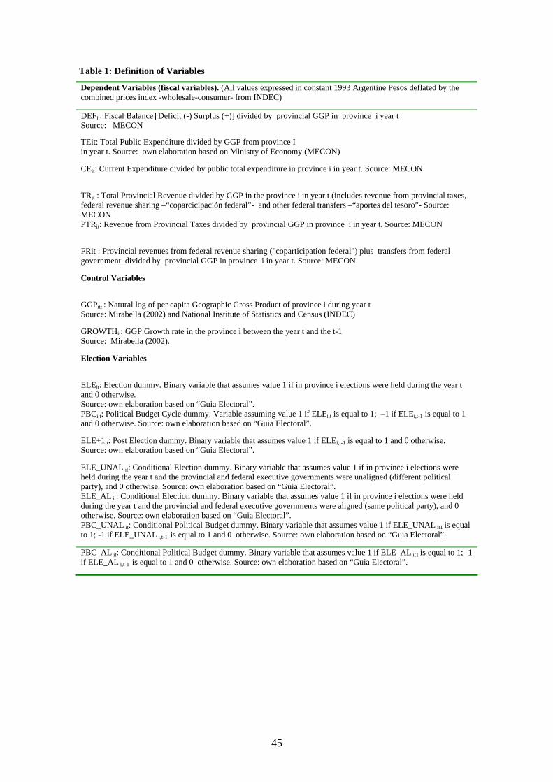
45
Table 1: Definition of Variables
Dependent Variables (fiscal variables). (All values expressed in constant 1993 Argentine Pesos deflated by the combined prices index -wholesale-consumer- from INDEC)
DEFit: Fiscal Balance [Deficit (-) Surplus (+)] divided by provincial GGP in province i year t Source: MECON
TEit: Total Public Expenditure divided by GGP from province I in year t. Source: own elaboration based on Ministry of Economy (MECON)
CEit: Current Expenditure divided by public total expenditure in province i in year t. Source: MECON
TRit : Total Provincial Revenue divided by GGP in the province i in year t (includes revenue from provincial taxes, federal revenue sharing –“coparcicipación federal”- and other federal transfers –“aportes del tesoro”- Source: MECON PTRit: Revenue from Provincial Taxes divided by provincial GGP in province i in year t. Source: MECON
FRit : Provincial revenues from federal revenue sharing ("coparticipation federal") plus transfers from federal government divided by provincial GGP in province i in year t. Source: MECON
Control Variables
GGPit: : Natural log of per capita Geographic Gross Product of province i during year t Source: Mirabella (2002) and National Institute of Statistics and Census (INDEC)
GROWTHit: GGP Growth rate in the province i between the year t and the t-1 Source: Mirabella (2002).
Election Variables
ELEit: Election dummy. Binary variable that assumes value 1 if in province i elections were held during the year t and 0 otherwise. Source: own elaboration based on “Guia Electoral”. PBCi,t: Political Budget Cycle dummy. Variable assuming value 1 if ELEi,t is equal to 1; –1 if ELEi,t-1 is equal to 1 and 0 otherwise. Source: own elaboration based on “Guia Electoral”.
ELE+1it: Post Election dummy. Binary variable that assumes value 1 if ELEi,t-1 is equal to 1 and 0 otherwise. Source: own elaboration based on “Guia Electoral”.
ELE_UNAL it: Conditional Election dummy. Binary variable that assumes value 1 if in province i elections were held during the year t and the provincial and federal executive governments were unaligned (different political party), and 0 otherwise. Source: own elaboration based on “Guia Electoral”. ELE_AL it: Conditional Election dummy. Binary variable that assumes value 1 if in province i elections were held during the year t and the provincial and federal executive governments were aligned (same political party), and 0 otherwise. Source: own elaboration based on “Guia Electoral”. PBC_UNAL it: Conditional Political Budget dummy. Binary variable that assumes value 1 if ELE_UNAL it1 is equal to 1; -1 if ELE_UNAL i,t-1 is equal to 1 and 0 otherwise. Source: own elaboration based on “Guia Electoral”.
PBC_AL it: Conditional Political Budget dummy. Binary variable that assumes value 1 if ELE_AL it1 is equal to 1; -1 if ELE_AL i,t-1 is equal to 1 and 0 otherwise. Source: own elaboration based on “Guia Electoral”.

46
Table 2: Fiscal Variables: Descriptive Statistics
Mean Std. Dev. Min. Max. No. Obs DEF -0.022 0.031 -0.155 0.058 374
TE 0.237 0.123 0.052 0.812 374
CE 0.807 0.091 0.445 0.952 374
TR 0.215 0.113 0.046 0.825 374
PTR 0.028 0.014 0.004 0.121 374
FR 0.186
0.110 0.024 0.704 374
The electoral budget cycle is analyzed through the variables fiscal balance, total
expenditure, expenditure composition1, total provincial revenue, revenue from
provincial taxes and revenue from the federal government2. The period of analysis
ranges from 1985 to 2001.
IV. Empirical Analysis
The theoretical and empirical literature on political budget cycles suggests that the
timing of elections should influence fiscal outcomes. The relationship between a fiscal
variable, yit , and the electoral cycle can be stated as follows:
yi,t = α+ Σkj=1
βj yi t-j + Σmj=1
γj xj i t + δ1 e + ηi + εit (1)
for i = 1..N, t = 1...T, j= 1 ...k, where e is a binary election variable indicating if an
election took place in province i during the year t; x is a vector of control variables that
in our estimations include per capita Geographic Gross Product (GGP) and the growth
rate of the Geographic Gross Product (GROWTH).
This specification represents a standard dynamic panel, where the dependent
variable is a function of its own lagged levels, of set of controls (xj), of the time when
elections take place and of a specific effect per province (ηi). The term εit is a random
error that is assumed iid.
Assuming that the unobserved province-specific effects are identical across
provinces, that the error term is not serially correlated, and that the explanatory
variables are strictly exogenous then it is possible to estimate this relation consistently 1 Ratio of current expenditure relative to total public expenditure. The most important component of current expenditure are salaries of provincial public servants. On the other hand, construction is the most important item of capital expenditure. 2Provincial revenues from federal revenue sharing ("coparticipation federal") plus special (discretional) transfers from federal government (“Aportes del Tesoro Nacional” – ATN).

47
through OLS. However, these assumptions may not hold in the panel, particularly the
assumption of equality of the unobservable effects per province. This being so, then
OLS estimates are inconsistent since the lagged dependent variable is correlated to the
error term wi, t= ηi + εit.
It is possible to control the specific effects using the panel data Fixed Effects
(FE) estimator. However, the transformed error term will still be correlated with the
lagged dependent variable. The bias will depend on T (the length of the panel); and
provided T tends to infinite, the FE estimator of the coefficients will be consistent.
Considering these problems, the Generalized Method of Moments (GMM) designed for
dynamic models by Arellano and Bond (1991) is performed in the estimations. The
Arellano-Bond strategy consists in the differentiation of the equations to eliminate the
specific effects and solve the inconsistency using the lagged values of the dependent
variable as instruments. Assuming the error term is not serially correlated, the
dependent variable lagged two periods or more constitute valid instruments for the new
dependent variable in differences. Likewise, the same can be said for the control
variables.
It will be assumed in our particular case that the vector from variables xjit is
slightly exogenous or predetermined; that is to say, it is not correlated with future
realizations of the error term. The elections variable will be considered strictly
exogenous.
Estimates are performed using three methods: OLS, Fixed Effects and GMM
Arellano-Bond for dynamic panel data. The GMM method seems to be preferable due to
the characteristics previously mentioned. Nevertheless, since it makes use of the lagged
values of the variables as instruments, the set of observations available is smaller. For
this reason and for comparative purposes, results from the three methods are reported.
The political cycle is modeled including the binary variable ELE that assumes
value 1 in election years, and 0 in the rest of the years.
As usual in the empirical literature, the variable PBC (Political Budget Cycle) is also
used, taking value 1 during the election year, -1 in the following year and 0 in the
remaining ones. This variable imposes the restriction that the pre-electoral increase in
spending or deficit is equivalent in magnitude to the posterior contraction.
Additionally, we also run the non-restricted regressions with the election dummy
ELE and the post election dummy ELE+1, and test the validity of the restriction
imposed by the use of PBC.

48
Our analysis includes six fiscal outcomes as dependent variables to test the
electoral manipulation, its origins and consequences: ratio of provincial budget balance
to GGP (DEF), ratio of total public expenditure to GGP (TE), current public
expenditure relative to total public expenditure (CE), total provincial revenue relative to
GGP (TR), revenue from provincial taxes relative to GGP (PTR) and provincial
revenues from federal revenue sharing plus transfers from federal government relative
to GGP (FR). Two basic controls will be included in the regressions: the per capita
geographic gross product (GGP) and growth rate of the GGP (GROWTH).
V. Unconditional Budget Cycles
This section presents the empirical analysis of electoral cycles in fiscal variables,
focusing on the provincial budget surplus, expenditures and revenues. We first present
the unconditional results of elections over the fiscal variables. We then look at the
conditional results, controlling for the alignment between the provincial and federal
executives.
A. Budget Balance
Table 3 shows the main unconditional results with respect to the provincial budget
balance (deficit); that is equation (1) including the election dummies ELE and PBC and
using as controls the GGP and the growth of GGP per capita3.
In the columns 1 to 3, with the three different estimation methods, ELE has the
expected negative sign, although is not statistically significant in any case.
In columns 4, 5 and 6 the results are obtained making use of the variable PBC as a
regressor for the elections. In this case, the coefficients estimated by OLS, Fixed Effects
(FE) and GMM are significantly negative, suggesting that the level of electoral cycle –
defined as the increase in deficit during the election year and the contraction in the
following- is approximately 0.6% of GGP. For GMM estimation the Sargan test is
reported, where the null hypothesis is that the instrumental variables are uncorrelated
with the residuals. In addition, the serial correlation test is presented, where the null
hypothesis is the absence of second order serial correlation in the first-difference
residuals. Estimates satisfy both tests (no rejection of null hypothesis).
3 Full econometric estimation results presented in the Chapter 3 Appendix.

49
Table 3: Elections and Fiscal Balance
Equation 1 2 3 4 5 6 Estimation
Method OLS FIXED
EFFECTSGMM OLS FIXED
EFFECTS GMM
ELE -0.0037 -0.0031 -0.0030 (-1.17) (-0.91) (-0.97) PBC -0.0064 -0.0060 0.0062 (-3.22)** (-3.08)** (-3.33)** F-testa p-value
2.07 0.0045
2.07 0.0045
Sargan testb 283.73 285.22 p-value 0.9994 0.9993 Serial Corrc -0.04 0.210 p-value 0.9677 0.8359 No.obs. 308 304 302 308 308 308
No. provinces 22 22 22 22 22 22
R2 (adj.) 0.36 0.38
Notes: Dependent variable DEF is ratio of government surplus to Geographic Gross Product (PBG). Estimated Regressions:
DEFit = α+ β1DEFit-1 + β2DEFit-2 + β3DEFit-3 + γ1PBGit + γ2CRECit + +γ3ELEit + ηi + εit
DEFit = α+ β1DEFit-1 + β2DEFit-2 + β3DEFit-3 + γ1PBGit + γ2CRECit + +γ3PBCit + ηi + εit The coefficient estimates on the lagged dependent variables add up to a value less than unity. OLS imposes the restriction ηi = η ∀ i. t statistics reported in parentheses, calculated using heteroskedastic-consistent standard errors for OLS. In GMM estimation (Arellano-Bond One Step) z statistics in parentheses. The election dummy variables are treated as strictly exogenous. Variables CREC and PBG are treated as predetermined and levels lagged one or more periods are used as instruments. Two lags of the dependent are included. * significant at the 10% level, ** significant at the 5% level, *** significant at the 1% level (a) F-test is an F test of the null hypothesis that all province-specific effects in the FE-specification are equal. (b) P-values for rejecting the null hypothesis in test of the over identifying restrictions, asymptotically distributed as a χ2 under the null hypothesis of instruments uncorrelated with the residuals. (c) P-values for rejecting the null hypothesis in test for second order serial correlation in the first-difference residuals, asymptotically distributed as N(0,1) under the null of no serial correlation.

50
Table 4: Elections and Fiscal Balance
Equation 1 2 3 Estimation Method OLS FIXED EFFECTS GMM
ELE 0.0020 0.0023 0.0016 (0.60) (0.66) (0.50) ELE+1 0.0140 0.0135 0.0141 (3.98)*** (4.07)*** (4.34)*** F-test: ELE =-ELE+1
8.27
7.71 8.78
p-value 0.0043 0.0059 0.0030 F-testa
p-value 2.11
0.0036
Sargan testb 277.02 p-value 0.9998 Serial Corrc 1.25 p-value 0.2131 No. obs. 308 308 308
No. provinces 22 22 22
R2 (adj.) 0.40
Notes: Dependent variable DEF is ratio of government surplus to Geographic Gross Product (PBG). Estimated Regressions:
DEFit = α+ β1DEFit-1 + β2DEFit-2 + β3DEFit-3 + γ1PBGit + γ2CRECit + +γ3ELEit + ηi + εit
DEFit = α+ β1DEFit-1 + β2DEFit-2 + β3DEFit-3 + γ1PBGit + γ2CRECit + +γ3PBCit + ηi + εit The coefficient estimates on the lagged dependent variables add up to a value less than unity. OLS imposes the restriction ηi = η ∀ i. t statistics reported in parentheses, calculated using heteroskedastic-consistent standard errors for OLS. In GMM estimation (Arellano-Bond One Step) z statistics in parentheses. The election dummy variables are treated as strictly exogenous. Variables CREC and PBG are treated as predetermined and levels lagged one or more periods are used as instruments. Two lags of the dependent are included. * significant at the 10% level, ** significant at the 5% level, *** significant at the 1% level (a) F-test is an F test of the null hypothesis that all province-specific effects in the FE-specification are equal. (b) P-values for rejecting the null hypothesis in test of the over identifying restrictions, asymptotically distributed as a χ2 under the null hypothesis of instruments uncorrelated with the residuals. (c) P-values for rejecting the null hypothesis in test for second order serial correlation in the first-difference residuals, asymptotically distributed as N(0,1) under the null of no serial correlation.
The PBC variable is meant to capture both pre and post-electoral effects.
However as Persson and Tabellini (2002) remark, pre and post electoral effects may
differ, so we check if the restriction that the coefficient estimate of ELE is equal to the

51
coefficient estimate of minus ELE in t+1, is not rejected by the data. Estimate results
are presented in Table 4.
Table 4 shows that the electoral dummy ELE is non significant and the post
electoral dummy ELE+1 is positive and significant. In all estimates, the F test soundly
rejects the restriction imposed by the PBC variable, that the post-electoral contraction in
the budget surplus as a percentage of GGP is of the same size as the pre-electoral
expansion. We can interpret the results as follows: a) there is no evidence of surplus
falling in election periods, b) the restriction that surplus falls below its trend, and then
jumps above it, is not supported by the data and, c) the significant effect of PBC is
driven by the jump of surplus in post electoral periods.
B. Expenditures: Total and Composition
Tables 5 and 6 show the effects of the electoral cycle over total public expenditure in
the provinces, measured as a proportion of GGP.
In the OLS and GMM regressions, the coefficients are positive and significant
for ELE, with a value indicating that the expenditure over GGP increases approximately
one percentage point during the year of elections. We found a short run cycle in
spending, approximately of 0.6-0.8 percentage points of GGP, in the OLS, FE and
GMM regressions with PBC as explanatory variable.
Results in Table 6 also suggest that the PBC significance is due to reductions in
expenditure in the post election years, and the F tests does not reject the null hypothesis
of equality between ELE and -ELE+1.
Tables 7 and 8 shows the estimates performed to evaluate the “composition
effect” in provincial expenditure around elections. The dependent variable CE
represents the expenditure in consumption goods as a proportion of total provincial
expenditure. None of the estimates present statistically significant results to provide
evidence supporting the hypothesis of a shift in spending towards consumption goods or
investment goods in election years. The case of the PBC shows similar results, even
though the coefficient estimated by GMM shows some evidence of a slight bias towards
capital goods in electoral years and towards consumption goods in post electoral years.

52
Table 5: Elections and Total Expenditure
Equation 1 2 3 4 5 6 Estimation
Method OLS FIXED
EFFECTS GMM OLS FIXED
EFF. GMM
ELE 0.0115 0.0057 0.0100 (2.50)** (1.50) (2.34)*** PBC 0.0082 0.0057 0.0074 (3.15)*** (2.55)** (2.83)*** F-testa
p-value 11.30
0.0000 11.47
0.0000
Sargan testb 254.35 250.02 p-value 1.0000 1.0000 Serial Corr.c 1.00 1.41 p-value 0.3166 0.1600 No. obs. 308 308 308 308 308 308
No. provinces 22 22 22 22 22 22
R2 (adj.) 0.90 0.90
Notes: Dependent variable TE is the ratio of total provincial expenditure to Geographic Gross Product (PBG). Estimated Regressions:
TEit = α+ β1TEit-1 + β2TEit-2 + β3TEit-3 + γ1PBGit + γ2CRECit + +γ3ELEit + ηi + εit
TEit = α+ β1TEit-1 + β2TEit-2 + β3TEit-3 + γ1PBGit + γ2CRECit + +γ3PBCit + ηi + εit The coefficient estimates on the lagged dependent variables add up to a value less than unity. OLS imposes the restriction ηi = η ∀ i. t statistics reported in parentheses, calculated using heteroskedastic-consistent standard errors for OLS. In GMM estimation (Arellano-Bond One Step) z statistics in parentheses. The election dummy variables are treated as strictly exogenous. Variables CREC and PBG are treated as predetermined and levels lagged one or more periods are used as instruments. Two lags of the dependent variable are included. * significant at the 10% level, ** significant at the 5% level, *** significant at the 1% level (a) F-test is an F test of the null hypothesis that all province-specific effects in the FE-specification are equal. (b) P-values for rejecting the null hypothesis in test of the over identifying restrictions, asymptotically distributed as a χ2 under the null hypothesis of instruments uncorrelated with the residuals. (c) P-values for rejecting the null hypothesis in test for second order serial correlation in the first-difference residuals, asymptotically distributed as N(0,1) under the null of no serial correlation.

53
Table 6: Elections and Total Expenditure
Equation 1 2 3 Estimation Method OLS FIXED EFFECTS. GMM
ELE 0.0086 0.0026 0.0074 (1.63) (0.64) (1.59) ELE+1 -0.0078 -0.0087 -0.0073 (-1.44) (-2.26)** (-1.61) F-test: ELE =-ELE+1
0.01
0.88 0.00
p-value 0.9271 0.3484 0.9961 F-testa
p-value 11.51
0.0000
Sargan testb 249.74 p-value 1.0000 Serial Corrc 1.42 p-value 0.1568 No. obs. 308 308 308
No. provinces 22 22 22
R2 (adj.) 0.90 Notes: Dependent variable TE is the ratio of total provincial expenditure to Geographic Gross Product (PBG). Estimated Regressions:
TEit = α+ β1TEit-1 + β2TEit-2 + β3TEit-3 + γ1PBGit + γ2CRECit + +γ3ELEit + ηi + εit
TEit = α+ β1TEit-1 + β2TEit-2 + β3TEit-3 + γ1PBGit + γ2CRECit + +γ3PBCit + ηi + εit The coefficient estimates on the lagged dependent variables add up to a value less than unity. OLS imposes the restriction ηi = η ∀ i. t statistics reported in parentheses, calculated using heteroskedastic-consistent standard errors for OLS. In GMM estimation (Arellano-Bond One Step) z statistics in parentheses. The election dummy variables are treated as strictly exogenous. Variables CREC and PBG are treated as predetermined and levels lagged one or more periods are used as instruments. Two lags of the dependent variable are included. * significant at the 10% level, ** significant at the 5% level, *** significant at the 1% level (a) F-test is an F test of the null hypothesis that all province-specific effects in the FE-specification are equal. (b) P-values for rejecting the null hypothesis in test of the over identifying restrictions, asymptotically distributed as a χ2 under the null hypothesis of instruments uncorrelated with the residuals. (c) P-values for rejecting the null hypothesis in test for second order serial correlation in the first-difference residuals, asymptotically distributed as N(0,1) under the null of no serial correlation.

54
Table 7: Elections and Composition Effect
Equation 1 2 3 4 5 6 Estimation
Method OLS FIXED
EFFECTS GMM OLS FIXED
EFFECTS GMM
ELE 0.0000 0.0014 -0.0058 (0.00) (0.21) (-0.90) PBC -0.0039 -0.0025 -0.0066 (-0.99) (-0.65) (-1.69)* F-testa
p-value 2.18
0.0025 2.16
0.0028
Sargan testb 244.93 243.05 p-value 1.0000 1.0000 Serial Corr.c -0.89 -0.52 p-value 0.3739 0.6014 No. obs. 308 308 308 308 308 308
No. provinces 22 22 22 22 22 22
R2 (adj.) 0.60 0.60
Notes: Dependent variable CE is the ratio of current expenditure to total provincial expenditure. Estimated Regressions:
CEit = α+ β1CEit-1 + β2CEit-2 + β3CEit-3 + γ1PBGit + γ2CRECit + +γ3ELEit + ηi + εit
CEit = α+ β1CEit-1 + β2CEit-2 + β3CEit-3 + γ1PBGit + γ2CRECit + +γ3PBCit + ηi + εit The coefficient estimates on the lagged dependent variables add up to a value less than unity. OLS imposes the restriction ηi = η ∀ i. t statistics reported in parentheses, calculated using heteroskedastic-consistent standard errors for OLS. In GMM estimation (Arellano-Bond One Step) z statistics in parentheses. The election dummy variables are treated as strictly exogenous. Variables CREC and PBG are treated as predetermined and levels lagged one or more periods are used as instruments. Two lags of the dependent variable are included. * significant at the 10% level, ** significant at the 5% level, *** significant at the 1% level (a) F-test is an F test of the null hypothesis that all province-specific effects in the FE-specification are equal. (b) P-values for rejecting the null hypothesis in test of the over identifying restrictions, asymptotically distributed as a χ2 under the null hypothesis of instruments uncorrelated with the residuals. (c) P-values for rejecting the null hypothesis in test for second order serial correlation in the first-difference residuals, asymptotically distributed as N(0,1) under the null of no serial correlation.

55
Table 8: Elections and Composition Effect
Equation 1 2 3 Estimation Method OLS FIXED EFFECTS GMM
ELE 0.0039 0.0046 -0.0016 (0.53) (0.66) (-0.23) ELE+1 0.0108 0.0090 0.0112 (1.64) (1.37) (1.67)* F-test: ELE =-ELE+1
1.60 1.49 0.76
p-value 0.2073 0.2228 0.3831 F-testa
p-value 2.15
0.0030
Sargan testb 244.37 p-value 1.0000 Serial Corrc -0.36 p-value 0.7182 No. obs. 308 308 308 No. provinces 22 22 22 R2 (adj.) 0.58 Notes: Dependent variable CE is the ratio of current expenditure to total provincial expenditure. Estimated Regressions:
CEit = α+ β1CEit-1 + β2CEit-2 + β3CEit-3 + γ1PBGit + γ2CRECit + +γ3ELEit + ηi + εit
CEit = α+ β1CEit-1 + β2CEit-2 + β3CEit-3 + γ1PBGit + γ2CRECit + +γ3PBCit + ηi + εit The coefficient estimates on the lagged dependent variables add up to a value less than unity. OLS imposes the restriction ηi = η ∀ i. t statistics reported in parentheses, calculated using heteroskedastic-consistent standard errors for OLS. In GMM estimation (Arellano-Bond One Step) z statistics in parentheses. The election dummy variables are treated as strictly exogenous. Variables CREC and PBG are treated as predetermined and levels lagged one or more periods are used as instruments. Two lags of the dependent variable are included. * significant at the 10% level, ** significant at the 5% level, *** significant at the 1% level (a) F-test is an F test of the null hypothesis that all province-specific effects in the FE-specification are equal. (b) P-values for rejecting the null hypothesis in test of the over identifying restrictions, asymptotically distributed as a χ2 under the null hypothesis of instruments uncorrelated with the residuals. (c) P-values for rejecting the null hypothesis in test for second order serial correlation in the first-difference residuals, asymptotically distributed as N(0,1) under the null of no serial correlation.

56
C. Revenues: Total, Federal and Provincial
To track the possible changes in fiscal revenues around elections Tables 9, 10, 11, 12,
13 and 14 present the estimates considering as dependent variables total provincial
revenue (TR) and its components: revenue from federal sources (FR), that includes
federal tax sharing and other federal transfers (mostly discretional) and revenue from
provincial taxes (PTR).
Tables 9 to 12 show the results with total revenue (TR) and federal revenue (FR)
as dependant variables. The electoral years are related to a significant tendency of
revenues to go up, explained by the increase in federal revenue, and is important to note
that federal revenue is 90% of total provincial revenues.
The PBC variable is non significant in all regressions, so there is no evidence of cycles
around elections. The most significant effect is the revenue increase in election years,
and the discretional transfers from the federal government could explain that. The
federal tax sharing is mostly determined by fixed coefficients and cannot be easily
manipulated.
Results in Tables 13 and 14 show non significant manipulations in provincial
taxes; in all regressions revenue from this source is not sensitive to the election and
PBC dummy variables. This seems reasonable, because in most provinces local taxes
are a very small part of total revenues. Changes (reductions) in this variable may have a
non relevant effect over the voter’s perceptions about competency of the incumbent,
reducing his incentives to engage in electoral manipulations over provincial taxes.

57
Table 9: Elections and Total Revenue
Equation 1 2 3 4 5 6 Estimation
Method OLS FIXED
EFFECTS GMM OLS FIXED
EFFECTS GMM
ELE 0.0111 0.0051 0.0095 (2.62)* (1.59) (2.44)** PBC 0.0025 0.0004 0.0019 (0.90) (0.21) (0.83) F-testa
p-value 17.19
0.0000 17.41
0.0000
Sargan testb 270.19 273.64 p-value 0.9999 0.9999 Serial Corr.c 1.25 0.98 p-value 0.2096 0.3289 No. obs. 308 308 308 308 308 308
No. provinces 22 22 22 22 22 22
R2 (adj.) 0.89 0.89
Notes: Dependent variable TR is the ratio of current expenditure to total provincial expenditure. Estimated Regressions:
TRit = α+ β1TRt-1 + β2TRit-2 + β3TRit-3 + γ1PBGit + γ2CRECit + +γ3ELEit + ηi + εit
TRit = α+ β1TRit-1 + β2TRit-2 + β3TRit-3 + γ1PBGit + γ2CRECit + +γ3PBCit + ηi + εit The coefficient estimates on the lagged dependent variables add up to a value less than unity. OLS imposes the restriction ηi = η ∀ i. t statistics reported in parentheses, calculated using heteroskedastic-consistent standard errors for OLS. In GMM estimation (Arellano-Bond One Step) z statistics in parentheses. The election dummy variables are treated as strictly exogenous. Variables CREC and PBG are treated as predetermined and levels lagged one or more periods are used as instruments. Two lags of the dependent variable are included. * significant at the 10% level, ** significant at the 5% level, *** significant at the 1% level (a) F-test is an F test of the null hypothesis that all province-specific effects in the FE-specification are equal. (b) P-values for rejecting the null hypothesis in test of the over identifying restrictions, asymptotically distributed as a χ2 under the null hypothesis of instruments uncorrelated with the residuals. (c) P-values for rejecting the null hypothesis in test for second order serial correlation in the first-difference residuals, asymptotically distributed as N(0,1) under the null of no serial correlation.

58
Table 10: Elections and Total Revenue
Equation 1 2 3 Estimation Method OLS FIXED EFFECTS. GMM
ELE 0.0138 0.0070 0.0125 (2.91)*** (2.08)** (3.05)*** ELE+1 0.0075 0.0055 0.0085 (1.44) (1.75)* (2.07)** F-test: ELE =-ELE+1
6..30 5.59 9.76
p-value 0.0126 00187 0.0018 F-testa
p-value 17.18
0.0000
Sargan testb 274.97 p-value 0.9999 Serial Corrc 1.00 p-value 0.3194 No. obs. 305 305 302
No. provinces 22 22 22
R2 (adj.) 0.89
Notes: Dependent variable TR is the ratio of current expenditure to total provincial expenditure. Estimated Regressions:
TRit = α+ β1TRt-1 + β2TRit-2 + β3TRit-3 + γ1PBGit + γ2CRECit + +γ3ELEit + ηi + εit
TRit = α+ β1TRit-1 + β2TRit-2 + β3TRit-3 + γ1PBGit + γ2CRECit + +γ3PBCit + ηi + εit The coefficient estimates on the lagged dependent variables add up to a value less than unity. OLS imposes the restriction ηi = η ∀ i. t statistics reported in parentheses, calculated using heteroskedastic-consistent standard errors for OLS. In GMM estimation (Arellano-Bond One Step) z statistics in parentheses. The election dummy variables are treated as strictly exogenous. Variables CREC and PBG are treated as predetermined and levels lagged one or more periods are used as instruments. Two lags of the dependent variable are included. * significant at the 10% level, ** significant at the 5% level, *** significant at the 1% level (a) F-test is an F test of the null hypothesis that all province-specific effects in the FE-specification are equal. (b) P-values for rejecting the null hypothesis in test of the over identifying restrictions, asymptotically distributed as a χ2 under the null hypothesis of instruments uncorrelated with the residuals. (c) P-values for rejecting the null hypothesis in test for second order serial correlation in the first-difference residuals, asymptotically distributed as N(0,1) under the null of no serial correlation.

59
Table 11: Elections and Revenue from Federal Government4
Equation 1 2 3 4 5 6 Estimation
Method OLS FIXED
EFFECTS GMM OLS FIXED
EFFECTS GMM
ELE 0.0114 0.0053 0.0097 (2.89)*** (1.74)* (2.73)*** PBC 0.0028 0.0004 -0.0023 (1.09) (0.23) (1.06) F-testa
p-value 15.51
0.0000 15.76
0.0000
Sargan testb 254.86 258.41 p-value 1.0000 1.0000 Serial Corr.c 1.49 1.25 p-value 0.1355 0.2115 No. obs. 308 308 308 308 308 308
No. provinces 22 22 22 22 22 22
R2 (adj.) 0.90 0.90
Notes: Dependent variable FR is the ratio of federal revenues to Gross Geographic Product (PBG). Estimated Regressions:
FRit = α+ β1FRit-1 + β2FRit-2 + β3FRit-3 + γ1PBGit + γ2CRECit + +γ3ELEit + ηi + εFR
FRit = α+ β1FRit-1 + β2FRit-2 + β3FRit-3 + γ1PBGit + γ2CRECit + +γ3PBCit + ηi + εFR The coefficient estimates on the lagged dependent variables add up to a value less than unity. OLS imposes the restriction ηi = η ∀ i. t statistics reported in parentheses, calculated using heteroskedastic-consistent standard errors for OLS. In GMM estimation (Arellano-Bond One Step) z statistics in parentheses. The election dummy variables are treated as strictly exogenous. Variables CREC and PBG are treated as predetermined and levels lagged one or more periods are used as instruments. Two lags of the dependent variable are included. * significant at the 10% level, ** significant at the 5% level, *** significant at the 1% level (a) F-test is an F test of the null hypothesis that all province-specific effects in the FE-specification are equal. (b) P-values for rejecting the null hypothesis in test of the over identifying restrictions, asymptotically distributed as a χ2 under the null hypothesis of instruments uncorrelated with the residuals. (c) P-values for rejecting the null hypothesis in test for second order serial correlation in the first-difference residuals, asymptotically distributed as N(0,1) under the null of no serial correlation.
4Provincial revenues from revenue sharing ("coparticipation") plus (discretional) transfers from federal government (i.e.“Aportes del Tesoro Nacional” – ATN).

60
Table 12: Elections and Revenue from Federal Government5
Equation 1 2 3 Estimation Method OLS FIXED EFFECTS. GMM
ELE 0.0138 0.0073 0.0124 (3.25)*** (2.28)** (3.33)*** ELE+1 0.0071 0.0057 0.0078 (1.54)* (1.92)* (2.09)** F-test: ELE =-ELE+1
8.03 6.69 10.92
p-value 0.0049 0.0102 0.0456 F-testa
p-value 15.55
0.0000
Sargan testb 258.52 p-value 1.0000 Serial Corrc 1.30 p-value 0.1944 No. obs. 308 308 308
No. provinces 22 22 22
R2 (adj.) 0.91 Notes: Dependent variable FR is the ratio of federal revenues to Gross Geographic Product (PBG). Estimated Regressions:
FRit = α+ β1FRit-1 + β2FRit-2 + β3FRit-3 + γ1PBGit + γ2CRECit + +γ3ELEit + γ4ELE+1it + ηi + εit FRit = α+ β1FRit-1 + β2FRit-2 + β3FRit-3 + γ1PBGit + γ2CRECit + +γ3ELEit + ηi + εit
The coefficient estimates on the lagged dependent variables add up to a value less than unity. OLS imposes the restriction ηi = η ∀ i. t statistics reported in parentheses, calculated using heteroskedastic-consistent standard errors for OLS. In GMM estimation (Arellano-Bond One Step) z statistics in parentheses. The election dummy variables are treated as strictly exogenous. Variables CREC and PBG are treated as predetermined and levels lagged one or more periods are used as instruments. Two lags of the dependent variable are included. * significant at the 10% level, ** significant at the 5% level, *** significant at the 1% level (a) F-test is an F test of the null hypothesis that all province-specific effects in the FE-specification are equal. (b) P-values for rejecting the null hypothesis in test of the over identifying restrictions, asymptotically distributed as a χ2 under the null hypothesis of instruments uncorrelated with the residuals. (c) P-values for rejecting the null hypothesis in test for second order serial correlation in the first-difference residuals, asymptotically distributed as N(0,1) under the null of no serial correlation.
5Provincial revenues from revenue sharing ("coparticipation") plus (discretional) transfers from federal government.

61
Table 13: Elections and Revenue from Provincial Taxes
Equation 1 2 3 4 5 6 Estimation
Method OLS FIXED
EFFECTS GMM OLS FIXED
EFFECTS GMM
ELE 0.0002 0.0002 0.0002 (0.23) (0.22) (0.23) PBC -0.0002 -0.0002 -0.0003 (-0.55) (-0.51) (-0.70) F-testa
p-value 3.30
0.0000 3.30
0.0000
Sargan testb 338.55 340.42 p-value 0.8362 0.8476 Serial Corr.c 0.26 -0.09 p-value 0.7969 0.9280 No. obs. 308 308 308 308 308 308
No.° provinces
22 22 22 22 22 22
R2 (adj.) 0.84 0.84
Notes: Dependent variable PTR is the ratio of provincial revenues to Geographic Gross Product (PBG). Estimated Regressions:
PTRit = α+ β1PTRit-1 + β2PTRit-2 + β3PTRit-3 + γ1PBGit + γ2CRECit + +γ3ELEit + ηi + εit
PTRit = α+ β1PTRit-1 + β2PTRit-2 + β3PTRit-3 + γ1PBGit + γ2CRECit + +γ3PBCit + ηi + εit The coefficient estimates on the lagged dependent variables add up to a value less than unity. OLS imposes the restriction ηi = η ∀ i. t statistics reported in parentheses, calculated using heteroskedastic-consistent standard errors for OLS. In GMM estimation (Arellano-Bond One Step) z statistics in parentheses. The election dummy variables are treated as strictly exogenous. Variables CREC and PBG are treated as predetermined and levels lagged one or more periods are used as instruments. Two lags of the dependent variable are included. * significant at the 10% level, ** significant at the 5% level, *** significant at the 1% level (a) F-test is an F test of the null hypothesis that all province-specific effects in the FE-specification are equal. (b) P-values for rejecting the null hypothesis in test of the over identifying restrictions, asymptotically distributed as a χ2 under the null hypothesis of instruments uncorrelated with the residuals. (c) P-values for rejecting the null hypothesis in test for second order serial correlation in the first-difference residuals, asymptotically distributed as N(0,1) under the null of no serial correlation.

62
Table 14: Elections and Revenue from Provincial Taxes
Equation 1 2 3 Estimation Method OLS FIXED EFFECTS. GMM
ELE 0.0005 0.0004 0.0005 (0.66) (0.56) (0.66) ELE+1 0.0009 0.0008 0.0011 (1.10) (1.12) (1.51) F-test: ELE =-ELE+1
1.30 1.049 1.78
p-value 0.2559 0.3083 0.1823 F-testa
p-value 3.28
0.0000
Sargan testb 344.69 p-value 0.7708 Serial Corrc -0.13 p-value 0.8958 No. obs. 304 304 302
No. provinces 22 22 22
R2 (adj.) 0.84 Notes: Dependent variable PTR is the ratio of provincial revenues to Geographic Gross Product (PBG). Estimated Regressions:
PTRit = α+ β1PTRit-1 + β2PTRit-2 + β3PTRit-3 + γ1PBGit + γ2CRECit + +γ3ELEit + ηi + εit
PTRit = α+ β1PTRit-1 + β2PTRit-2 + β3PTRit-3 + γ1PBGit + γ2CRECit + +γ3PBCit + ηi + εit The coefficient estimates on the lagged dependent variables add up to a value less than unity. OLS imposes the restriction ηi = η ∀ i. t statistics reported in parentheses, calculated using heteroskedastic-consistent standard errors for OLS. In GMM estimation (Arellano-Bond One Step) z statistics in parentheses. The election dummy variables are treated as strictly exogenous. Variables CREC and PBG are treated as predetermined and levels lagged one or more periods are used as instruments. Two lags of the dependent variable are included. * significant at the 10% level, ** significant at the 5% level, *** significant at the 1% level (a) F-test is an F test of the null hypothesis that all province-specific effects in the FE-specification are equal. (b) P-values for rejecting the null hypothesis in test of the over identifying restrictions, asymptotically distributed as a χ2 under the null hypothesis of instruments uncorrelated with the residuals. (c) P-values for rejecting the null hypothesis in test for second order serial correlation in the first-difference residuals, asymptotically distributed as N(0,1) under the null of no serial correlation.

63
VI. Conditional Findings: Political Alignment Between Provincial and Federal
Executives
The results reported in the previous section suggest that there are some systematic
increase in expenditures and federal revenues in electoral years, but no electoral or
cyclical effects were detected over the budget balance. Decisions over spending are
clearly taken at provincial level, but the federal revenues are not a decision variable for
the provincial executive. If this is so, how can the provincial executive manipulate at
the same time expenditures and federal revenues? What can explain this pattern?
In this section, we will focus on explaining these facts, looking for differences in
the behavior of incumbents conditioning for the political alignment between the
provincial and federal executive. Our conjecture is that when both executives are
members of the same political party (political alignment), the more probable the federal
executive increases the discretional transfers to the province, allowing the provincial
executive to increase spending without significant effects over the budget balance.
When both executives (provincial and federal) are not aligned, and with an
aligned candidate running for the provincial election, the federal government is not
interested in increasing the discretional transfers to the incumbent. On the contrary,
probably the federal government can reduce the transfers, rending spending
manipulations more difficult to the provincial executive and inducing budget deficits.
We then look at the sensitivity of the previous results when conditioned to
political alignment between provincial and federal executives. The conditional election
variables ELE_UNAL, ELE_AL and the conditional cycle variables PBC_UNAL,
PBC_AL are now included in the regressions to estimate the differential effect of
political alignment.
A. Budget Balance
Table 15 presents the results with the budget balance as the dependent variable. In
columns 1 to 3 the coefficients estimates for the conditional election variable are
presented. The coefficients associated to the unaligned provinces are all negative and
significant at 10% in OLS and GMM regressions and marginally significant (11%) in
FE. The election year has no significant effect over fiscal balance in aligned provinces.
The regression results indicates that while the election increases the deficit
between 0.8 to 1.0 percentage points in unaligned provinces, the election effect is not
relevant in aligned provinces.

64
Table 15: Elections and Fiscal Balance conditional on alignment of provincial and federal government
Equation 1 2 3 4 5 6 Estimation
Method OLS FIXED
EFFECTS.GMM OLS FIXED
EFF. GMM
ELE_UNAL -0.0106 -0.0091 -0.0084 (-1.93)* (-1.61) (-1.80)* ELE_AL -0.0003 -0.0002 0.0003 (-0.09) (-0.04) (0.09) PBC_UNAL -0.0085 -0.0079 -0.0091 (-2.34)** (-2.51)** (-3.19)***PBC_AL -0.0052 -0.0048 -0.0043 (-2.31)** (-1.97)* (-1.82)* F-testa p-value
2.03 0.0056
2.07 0.0045
Sargan testb 283.40 284.92 p-value 0.9994 0.9993 Serial Corrc -0.19 0.10 p-value 0.8472 0.9165 No. obs. 308 304 302 308 308 308
No. provinces 22 22 22 22 22 22
R2 (adj.) 0.37 0.38
Notes: Dependent variable DEF is ratio of government surplus to Geographic Gross Product (PBG). Estimated Regressions:
DEFit = α+ β1DEFit-1 + β2DEFit-2 + β3DEFit-3 + γ1PBGit + γ2CRECit + +γ3ELEit + ηi + εit
DEFit = α+ β1DEFit-1 + β2DEFit-2 + β3DEFit-3 + γ1PBGit + γ2CRECit + +γ3PBCit + ηi + εit The coefficient estimates on the lagged dependent variables add up to a value less than unity. OLS imposes the restriction ηi = η ∀ i. t statistics reported in parentheses, calculated using heteroskedastic-consistent standard errors for OLS. In GMM estimation (Arellano-Bond One Step) z statistics in parentheses. The election dummy variables are treated as strictly exogenous. Variables CREC and PBG are treated as predetermined and levels lagged one or more periods are used as instruments. Two lags of the dependent are included. * significant at the 10% level, ** significant at the 5% level, *** significant at the 1% level (a) F-test is an F test of the null hypothesis that all province-specific effects in the FE-specification are equal. (b) P-values for rejecting the null hypothesis in test of the over identifying restrictions, asymptotically distributed as a χ2 under the null hypothesis of instruments uncorrelated with the residuals. (c) P-values for rejecting the null hypothesis in test for second order serial correlation in the first-difference residuals, asymptotically distributed as N(0,1) under the null of no serial correlation.

65
The conditional PBC coefficient estimates, columns 4 to 6, result in all cases
negative and significant for aligned and unaligned provinces. These results are driven
mostly by an increase in budget surplus in post electoral years in both aligned an
unaligned provinces, and are consistent with those obtained in the unconditional
regressions.
B. Expenditures: Total and Composition
Table 16 shows the effects of the conditional electoral variables over total public
expenditure. Results in columns 1 to 3 show that in electoral years, when the province is
politically aligned with federal government spending rises significantly. Depending on
estimation method, the increasing in spending ranges between 0.8 to 1.4 percentage
points of GGP. For unaligned provinces the estimates are non-significant in all
regressions.
The estimated coefficients for the conditional PBC variable are significant, but
the effect is driven, as in the unconditional estimates, by the spending contraction in the
post electoral period in both, aligned and unaligned provinces.Regarding the
composition of expenditures, Table 17, in columns 1 to 3, shows a positive and
significant increase in current spending in electoral years for unaligned provinces.
However, there are no significant effects over spending composition in aligned
provinces. The coefficients associated to the conditional cycle variable, in columns 4 to
6, are non significant in all specifications.
These results suggest that an important shift happens in the expenditure composition
towards current goods in unaligned provinces during electoral years. The magnitude of
the shift is approximately 1.9 percentage points of total expenditure, reassigned from
investment to consumption goods.

66
Table 16: Elections and Total Expenditure conditional on alignment of provincial and federal government
Equation 1 2 3 4 5 6 Estimation
Method OLS FIXED
EFFECTS.GMM OLS FIXED
EFF. GMM
ELE_UNAL 0.0062 0.0005 0.0015 (0.70) (0.07) (0.28) ELE_AL 0.0140 0.0082 0.0101 (3.05)*** (1.81)* (2.59)*** PBC_UNAL 0.0107 0.0073 0.0034 (2.10)** (1.99)** (1.05) PBC_AL 0.0068 0.0049 0.0045 (2.31)** (1.74)* (1.87)* F-testa p-value
11.29 0.0000
11.42 0.0000
Sargan testb 354.41 350.88 p-value 0.5287 0.5813 Serial Corrc -0.61 -0.59 p-value 0.5406 0.5567 No. obs. 308 308 286 308 308 286
No. provinces 22 22 22 22 22 22
R2 (adj.) 0.90 0.90
Notes: Dependent variable TE is ratio of total provincial expenditure to Geographic Gross Product (PBG). Estimated Regressions:
TEit = α+ β1TEit-1 + β2TEit-2 + β3TEit-3 + γ1PBGit + γ2CRECit + +γ3ELEit + ηi + εit
TEit = α+ β1TEit-1 + β2TEit-2 + β3TEit-3 + γ1PBGit + γ2CRECit + +γ3PBCit + ηi + εit The coefficient estimates on the lagged dependent variables add up to a value less than unity. OLS imposes the restriction ηi = η ∀ i. t statistics reported in parentheses, calculated using heteroskedastic-consistent standard errors for OLS. In GMM estimation (Arellano-Bond One Step) z statistics in parentheses. The election dummy variables are treated as strictly exogenous. Variables CREC and PBG are treated as predetermined and levels lagged two or more periods are used as instruments. One lag of the dependent variable is included. * significant at the 10% level, ** significant at the 5% level, *** significant at the 1% level (a) F-test is an F test of the null hypothesis that all province-specific effects in the FE-specification are equal. (b) P-values for rejecting the null hypothesis in test of the over identifying restrictions, asymptotically distributed as a χ2 under the null hypothesis of instruments uncorrelated with the residuals. (c) P-values for rejecting the null hypothesis in test for second order serial correlation in the first-difference residuals, asymptotically distributed as N(0,1) under the null of no serial correlation.

67
Table 17: Elections and Composition Effect conditional on alignment of provincial and federal government
Equation 1 2 3 4 5 6 Estimation
Method OLS FIXED
EFFECTS.GMM OLS FIXED
EFF. GMM
ELE_UNAL 0.0190 0.0195 0.0198 (1.85)* (1.76)* (1.82)* ELE_AL -0.0092 -0.0072 -0.0084 (-1.16) (-0.92) (-1.12) PBC_UNAL 0.0012 0.0031 0.0012 (0.20) (0.49) (0.20) PBC_AL -0.0068 -0.0058 -0.0073 (-1.41)** (-1.19) (-1.57) F-testa p-value
2.14 0.0030
2.17 0.0026
Sargan testb 235.44 230.71 p-value 1.0000 1.0000 Serial Corrc -0.09 0.01 p-value 0.9250 0.9897 No. obs. 308 308 286 308 308 286
No. provinces 22 22 22 22 22 22
R2 (adj.) 0.60 0.60
Notes: Dependent variable CEis the ratio of current expenditure to total provincial expenditure. Estimated Regressions:
CEit = α+ β1CEit-1 + β2CEit-2 + β3CEit-3 + γ1PBGit + γ2CRECit + +γ3ELEit + ηi + εit
CEit = α+ β1CEit-1 + β2CEit-2 + β3CEit-3 + γ1PBGit + γ2CRECit + +γ3PBCit + ηi + εit The coefficient estimates on the lagged dependent variables add up to a value less than unity. OLS imposes the restriction ηi = η ∀ i, t statistics reported in parentheses, calculated using heteroskedastic-consistent standard errors for OLS. In GMM estimation (Arellano-Bond One Step) z statistics in parentheses. The election dummy variables are treated as strictly exogenous. Variables CREC and PBG are treated as predetermined and levels lagged two or more periods are used as instruments. One lag of the dependent variable is included. * significant at the 10% level, ** significant at the 5% level, *** significant at the 1% level (a) F-test is an F test of the null hypothesis that all province-specific effects in the FE-specification are equal. (b) P-values for rejecting the null hypothesis in test of the over identifying restrictions, asymptotically distributed as a χ2 under the null hypothesis of instruments uncorrelated with the residuals. (c) P-values for rejecting the null hypothesis in test for second order serial correlation in the first-difference residuals, asymptotically distributed as N(0,1) under the null of no serial correlation.

68
C. Revenues: Total, Federal and Provincial
Tables 18, 19 and 20 present the conditional estimates considering as dependent
variables the total provincial revenue (TR), revenue from federal source (FR) and
revenue from provincial taxes (PTR).
There is a strong positive relationship between elections in aligned provinces
and federal revenues in the data, independent of the estimation technique. In politically
aligned provinces, a positive and significant effect over revenues is present in electoral
years, explained by the increase in discretional federal revenues. The magnitude of the
effect is important, from 0.8 to 1.6 percentage points of GGP of increase in federal
revenues depending on the estimation technique.
By contrast, for the conditional election dummy in unaligned provinces, the estimated
coefficients are non significant in all cases. The conditional cycle dummy is non
significant in all regressions, suggesting that there is no evidence of cycles around
elections, independently of political alignment.
Results in Table 20 are similar to those obtained in the unconditional
regressions. For aligned or unaligned provinces, in all regressions revenue from
provincial taxes is not sensitive to the election dummy or the PBC dummy.
To sum up, the findings reported above fit the conjectures about the behavior of
federal and provincial governments considering the political alignment. If the provincial
executive is aligned with the federal government, the discretional transfers from this
source are bigger in electoral years, and the provincial incumbent is able to increase the
total expenditures proportionally, without increasing the fiscal deficit. Our empirical
results show that discretional transfers from the federal governments allows the
provincial incumbent to increase the spending in 0.8 – 1.4 percentage points of GGP.
On the other side, if the provincial executive is unaligned, the federal transfers
remain approximately constant. With constant revenues from provincial taxes, if the
incumbent increases the spending he also increases the fiscal deficit, but in this case he
is constrained by the borrowing alternatives. The other alternative action available to the
incumbent is to change the expenditure composition, from investment goods to more
visible consumption goods. Our empirical results suggest that this last alternative
appears to be the more relevant discretional decision for unaligned provincial
executives. Estimates show that the redirection of spending toward consumption goods
in electoral years is about 1.9 percentage points of total expenditure for unaligned
provinces.

69
Table 18: Elections and Total Revenue conditional on alignment of provincial and federal government
Equation 1 2 3 4 5 6 Estimation
Method OLS FIXED
EFFECTS.GMM OLS FIXED
EFF. GMM
ELE_UNAL 0.0005 -0.0067 -0.0061 (0.08) (-1.25) (-1.20) ELE_AL 0.0162 0.0108 0.0090 (3.37)*** (-2.85)*** (2.57)* PBC_UNAL -0.00005 -0.0014 -0.0057 (-0.01) (-0.46) (-1.96)* PBC_AL 0.0039 0.0014 -0.0003 (1.16) (0.62) (-0.15) F-testa p-value
17.60 0.0000
17.36 0.0000
Sargan testb 364.10 373.00 p-value 0.3863 0.2693 Serial Corrc -0.75 -1.09 p-value 0.4523 0.2770 No. obs. 308 308 286 308 308 286
No. provinces 22 22 22 22 22 22
R2 (adj.) 0.89 0.89
Notes: Dependent variable TR is the ratio of current expenditure to total provincial expenditure. Estimated Regressions:
TRit = α+ β1TRt-1 + β2TRit-2 + β3TRit-3 + γ1PBGit + γ2CRECit + +γ3ELEit + ηi + εit
TRit = α+ β1TRit-1 + β2TRit-2 + β3TRit-3 + γ1PBGit + γ2CRECit + +γ3PBCit + ηi + εit The coefficient estimates on the lagged dependent variables add up to a value less than unity. OLS imposes the restriction ηi = η ∀ i, t statistics reported in parentheses, calculated using heteroskedastic-consistent standard errors for OLS. In GMM estimation (Arellano-Bond One Step) z statistics in parentheses. The election dummy variables are treated as strictly exogenous. Variables CREC and PBG are treated as predetermined and levels lagged two or more periods are used as instruments. One lag of the dependent variable is included. * significant at the 10% level, ** significant at the 5% level, *** significant at the 1% level (a) F-test is an F test of the null hypothesis that all province-specific effects in the FE-specification are equal. (b) P-values for rejecting the null hypothesis in test of the over identifying restrictions, asymptotically distributed as a χ2 under the null hypothesis of instruments uncorrelated with the residuals. (c) P-values for rejecting the null hypothesis in test for second order serial correlation in the first-difference residuals, asymptotically distributed as N(0,1) under the null of no serial correlation.

70
Table 19: Elections and Revenue from Federal Government6 conditional on alignment of provincial and federal government
Equation 1 2 3 4 5 6 Estimation
Method OLS FIXED
EFFECTS.GMM OLS FIXED
EFF. GMM
ELE_UNAL 0.0007 -0.0066 -0.0064 (0.11) (-1.30) (-1.35) ELE_AL 0.0166 0.0110 0.0082 (3.66)*** (3.07)*** (2.49)** PBC_UNAL 0.0003 -0.0014 -0.0051 (0.08) (-0.50) (-1.88)* PBC_AL 0.0042 0.0015 -0.0004 (1.30) (0.68) (-0.21) F-testa p-value
15.94 0.0000
15.72 0.0000
Sargan testb 346.63 353.74 p-value 0.6431 0.5387 Serial Corrc -0.36 -0.58 p-value 0.7156 0.5629 No. obs. 308 308 286 308 308 286
No. provinces 22 22 22 22 22 22
R2 (adj.) 0.91 0.90
Notes: Dependent variable FR is the ratio of federal revenues to Gross Geographic Product (PBG). Estimated Regressions:
FRit = α+ β1FRit-1 + β2FRit-2 + β3FRit-3 + γ1PBGit + γ2CRECit + +γ3ELEit + γ4ELE+1it + ηi + εit FRit = α+ β1FRit-1 + β2FRit-2 + β3FRit-3 + γ1PBGit + γ2CRECit + +γ3ELEit + ηi + εit
The coefficient estimates on the lagged dependent variables add up to a value less than unity. OLS imposes the restriction ηi = η ∀ i. t statistics reported in parentheses, calculated using heteroskedastic-consistent standard errors for OLS. In GMM estimation (Arellano-Bond One Step) z statistics in parentheses. The election dummy variables are treated as strictly exogenous. Variables CREC and PBG are treated as predetermined and levels lagged two or more periods are used as instruments. One lag of the dependent variable is included. * significant at the 10% level, ** significant at the 5% level, *** significant at the 1% level (a) F-test is an F test of the null hypothesis that all province-specific effects in the FE-specification are equal. (b) P-values for rejecting the null hypothesis in test of the over identifying restrictions, asymptotically distributed as a χ2 under the null hypothesis of instruments uncorrelated with the residuals. (c) P-values for rejecting the null hypothesis in test for second order serial correlation in the first-difference residuals, asymptotically distributed as N(0,1) under the null of no serial correlation.
6Provincial revenues from revenue sharing ("coparticipation") plus special (discretional) transfers from federal government.

71
Table 20: Elections and Revenue from Provincial Taxes conditional on alignment of provincial and federal government
Equation 1 2 3 4 5 6 Estimation
Method OLS FIXED
EFFECTS.GMM OLS FIXED
EFF. GMM
ELE_UNAL 0.0003 0.0001 0.0008 (0.29) (0.13) (0.82) ELE_AL 0.0001 0.0001 -0.0002 (0.14) (0.19) (-0.34) PBC_UNAL 0.0000 0.0000 0.0000 (0.00) (0.04) (0.15) PBC_AL -0.0004 0.0003 -0.0005 (-0.98) (-0.68) (-1.05) F-testa p-value
3.29 0.0000
3.28 0.0000
Sargan testb 337.35 338.36 p-value 0.8475 0.8380 Serial Corrc 0.33 -0.02 p-value 0.7379 0.9852 N° obs. 308 308 308 308 308 308
N° provinces 22 22 22 22 22 22
R2 (adj.) 0.84 0.84
Notes: Dependent variable PTR is the ratio of provincial revenues to Geographic Gross Product (PBG). Estimated Regressions:
PTRit = α+ β1PTRit-1 + β2PTRit-2 + β3PTRit-3 + γ1PBGit + γ2CRECit + +γ3ELEit + ηi + εit
PTRit = α+ β1PTRit-1 + β2PTRit-2 + β3PTRit-3 + γ1PBGit + γ2CRECit + +γ3PBCit + ηi + εit The coefficient estimates on the lagged dependent variables add up to a value less than unity. OLS imposes the restriction ηi = η ∀ i. t statistics reported in parentheses, calculated using heteroskedastic-consistent standard errors for OLS. In GMM estimation (Arellano-Bond One Step) z statistics in parentheses. The election dummy variables are treated as strictly exogenous. Variables CREC and PBG are treated as predetermined and levels lagged one or more periods are used as instruments. Two lags of the dependent variable are included. * significant at the 10% level, ** significant at the 5% level, *** significant at the 1% level (a) F-test is an F test of the null hypothesis that all province-specific effects in the FE-specification are equal. (b) P-values for rejecting the null hypothesis in test of the over identifying restrictions, asymptotically distributed as a χ2 under the null hypothesis of instruments uncorrelated with the residuals. (c) P-values for rejecting the null hypothesis in test for second order serial correlation in the first-difference residuals, asymptotically distributed as N(0,1) under the null of no serial correlation.

72
VII. Conclusions
This paper presents empirical evidence of systematic effects in fiscal balance, public
expenditures and revenues in Argentine provinces as a function of elections and
political alignment. Our findings are consistent with the predictions of the theoretical
literature on rational opportunist political cycles: there are fiscal policy manipulations
during elections, and there is a strengthening of the policies after elections.
The data also reveals that there are important systematic differences between
provinces in the size and composition of the electoral manipulations, depending on the
political alignment with the federal executive. Specifically, the political alignment
between provincial and federal executives implies more discretional transfer of federal
revenues and increases the election induced provincial spending without increasing the
fiscal deficit. Politically unaligned provinces are constrained by constant federal
transfers and fiscal deficits are more frequent in election years. In addition, an important
spending switch from capital goods to consumption goods is present in election years
for unaligned provinces.
Finally, we believe that our conditional findings fit the predictions of the
theoretical models of opportunistic rational behavior and reveals that the institutional
and political features are important issues to explain the electoral motivated policy
cycles. It is highly likely that further work in the identification of institutional control
variables as the effective division of powers and institutional development of the
provinces could contribute to study the quantitative effects of electoral cycles more in
depth.

73
References
Alesina A.; Roubini N. and Cohen G (1997): “Political Cycles and the
macroeconomy”; Cambridge: MIT Press.
Arellano, M., and S. Bond (1991): “Some Tests of Specifications for Panel Data:
Monte Carlo Evidence and an Application to Employment Equations”,
Review of Economic Studies ) 58:277-97.
Block S (2002): “Elections, Electoral Competitiveness, and Political Budget Cycles
in Developing Countries”; CID Working Paper N° 78.
Hibbs, D. (1977): “Political Parties and Macroeconomic Policy,” American Political
Science Review, 71:467-87.
Krueger, A. and I. Turan (1993): “The Politics and Economics of Turkish Policy
Reform in the 1980's,” in R.Bates and A. Krueger, eds., Political and
Economic Interactions in Economic Policy Reform: Evidence from Eight
Countries, Oxford: Basil Blackwell.
Lindbeck, A. (1976): “Stabilization Policies in Open Economies with Endogenous
Politicians,” American Economic Review Papers and Proceedings, p. 1-19.
Meloni, O. (2001): “Gobernadores y elecciones: ¿Es “negocio” ser austero?
Evidencia a partir de Data en Panel”; XXXVI Reunión Anual de la AAEP.
Mirabella de Sant, M.(2002):”Diferencias de bienestar entre provincias de
Argentina”;XXXVII Reunión Anual de la AAEP.
Nordhaus, W.(1975): “The Political Business Cycle,” Review of Economic Studies
42:169-90.
Persson, Torsten and Tabellini, Guido (2002), “Do Electoral Cycles Differ Across
Political Systems?” (Manuscript, IGIER and Bocconi University).
Rogoff, K.(1990): “Equilibrium political budget cycles”; American Economic
Review; v. 80; N° 1; p. 21-36.
Shi M. and Svensson J.(2001): “Conditional Political Business Cycles”; Working
Paper; IIES Stockholm University.
Schucknecht, L.(2000) “Fiscal Policy Cycles and Public Expenditure in Developing
Countries”; Public Choice, 102 115 130.

Appendix Chapter 3
Econometric Estimation Output
74

TABLES 3 and 4 - Elections and Fiscal Balance . *OLS . regress def def_1 def_2 def_3 growth lggp ele, robust Regression with robust standard errors Number of obs = 308 F( 6, 301) = 21.28 Prob > F = 0.0000 R-squared = 0.3627 Root MSE = .02471 ------------------------------------------------------------------------------ | Robust def | Coef. Std. Err. t P>|t| [95% Conf. Interval] -------------+---------------------------------------------------------------- def_1 | .4501836 .0612624 7.35 0.000 .3296268 .5707405 def_2 | .0273253 .0706419 0.39 0.699 -.1116893 .1663398 def_3 | .1371861 .0657659 2.09 0.038 .0077669 .2666053 grow | .0964675 .0203988 4.73 0.000 .056325 .1366099 lggp | .0008223 .0022823 0.36 0.719 -.003669 .0053136 ele | -.0036922 .0031471 -1.17 0.242 -.0098854 .002501 _cons | -.0178905 .0197735 -0.90 0.366 -.0568022 .0210212 ------------------------------------------------------------------------------ . regress def def_1 def_2 def_3 grow lggp pbc, robust Regression with robust standard errors Number of obs = 308 F( 6, 301) = 25.03 Prob > F = 0.0000 R-squared = 0.3817 Root MSE = .02434 ------------------------------------------------------------------------------ | Robust def | Coef. Std. Err. t P>|t| [95% Conf. Interval] -------------+---------------------------------------------------------------- def_1 | .4580231 .0589188 7.77 0.000 .3420781 .5739681 def_2 | .0400662 .0694408 0.58 0.564 -.0965847 .1767171 def_3 | .1196514 .0653006 1.83 0.068 -.0088522 .248155 grow | .0877438 .0202285 4.34 0.000 .0479367 .1275509 lggp | .0008499 .0022743 0.37 0.709 -.0036257 .0053254 pbc | -.0064528 .0020012 -3.22 0.001 -.0103908 -.0025147 _cons | -.0190134 .0196672 -0.97 0.334 -.057716 .0196891 ------------------------------------------------------------------------------ . regress def def_1 def_2 def_3 grow lggp ele ele1,robust Regression with robust standard errors Number of obs = 308 F( 7, 300) = 23.47 Prob > F = 0.0000 R-squared = 0.3965 Root MSE = .02408 ------------------------------------------------------------------------------ | Robust def | Coef. Std. Err. t P>|t| [95% Conf. Interval] -------------+---------------------------------------------------------------- def_1 | .4963217 .0581574 8.53 0.000 .3818737 .6107697 def_2 | .043854 .0675271 0.65 0.517 -.0890327 .1767407 def_3 | .0789868 .0658754 1.20 0.231 -.0506495 .2086232 grow | .0823988 .0196784 4.19 0.000 .0436736 .1211239 lggp | .0009685 .0022395 0.43 0.666 -.0034385 .0053756 ele | .0019633 .0032787 0.60 0.550 -.0044889 .0084155 ele1 | .0140562 .0035301 3.98 0.000 .0071093 .0210031 _cons | -.0238065 .0195584 -1.22 0.224 -.0622954 .0146824 ------------------------------------------------------------------------------ . test ele=-ele1
75

( 1) ele + ele1 = 0 F( 1, 300) = 8.27 Prob > F = 0.0043 . regress def def_1 def_2 def_3 grow lggp ele_1, robust Regression with robust standard errors Number of obs = 308 F( 6, 301) = 22.53 Prob > F = 0.0000 R-squared = 0.3704 Root MSE = .02456 ------------------------------------------------------------------------------ | Robust def | Coef. Std. Err. t P>|t| [95% Conf. Interval] -------------+---------------------------------------------------------------- def_1 | .4554651 .0581458 7.83 0.000 .3410413 .5698889 def_2 | .0587623 .0716794 0.82 0.413 -.0822939 .1998184 def_3 | .0998277 .0707205 1.41 0.159 -.0393415 .2389969 grow | .0965407 .0200904 4.81 0.000 .0570053 .136076 lggp | .0008047 .0022336 0.36 0.719 -.0035908 .0052002 ele_1 | -.0079034 .0031948 -2.47 0.014 -.0141905 -.0016164 _cons | -.0168815 .0192939 -0.87 0.382 -.0548496 .0210865 ------------------------------------------------------------------------------ . . . *FE . xtreg def def_1 def_2 def_3 grow lggp ele,fe Fixed-effects (within) regression Number of obs = 308 Group variable (i): id Number of groups = 22 R-sq: within = 0.2168 Obs per group: min = 14 between = 0.1758 avg = 14.0 overall = 0.1926 max = 14 F(6,280) = 12.92 corr(u_i, Xb) = -0.2074 Prob > F = 0.0000 ------------------------------------------------------------------------------ def | Coef. Std. Err. t P>|t| [95% Conf. Interval] -------------+---------------------------------------------------------------- def_1 | .3177049 .057287 5.55 0.000 .2049371 .4304727 def_2 | -.0530212 .0610658 -0.87 0.386 -.1732275 .0671851 def_3 | .024791 .0575514 0.43 0.667 -.0884974 .1380794 grow | .0828221 .0199167 4.16 0.000 .0436166 .1220276 lggp | .0237088 .0111388 2.13 0.034 .0017824 .0456352 ele | -.0030769 .003379 -0.91 0.363 -.0097283 .0035745 _cons | -.2222733 .0965414 -2.30 0.022 -.4123124 -.0322341 -------------+---------------------------------------------------------------- sigma_u | .01619047 sigma_e | .02383394 rho | .3157495 (fraction of variance due to u_i) ------------------------------------------------------------------------------ F test that all u_i=0: F(21, 280) = 2.07 Prob > F = 0.0045 . xtreg def def_1 def_2 def_3 grow lggp pbc,fe Fixed-effects (within) regression Number of obs = 308 Group variable (i): id Number of groups = 22 R-sq: within = 0.2402 Obs per group: min = 14 between = 0.1815 avg = 14.0 overall = 0.2099 max = 14
76

F(6,280) = 14.75 corr(u_i, Xb) = -0.2075 Prob > F = 0.0000 ------------------------------------------------------------------------------ def | Coef. Std. Err. t P>|t| [95% Conf. Interval] -------------+---------------------------------------------------------------- def_1 | .3254006 .0558988 5.82 0.000 .2153653 .4354359 def_2 | -.039916 .0602769 -0.66 0.508 -.1585694 .0787373 def_3 | .0106597 .0563708 0.19 0.850 -.1003047 .1216241 grow | .0739673 .0198411 3.73 0.000 .0349106 .1130241 lggp | .0240468 .0109716 2.19 0.029 .0024495 .0456441 pbc | -.005962 .0019374 -3.08 0.002 -.0097757 -.0021483 _cons | -.2258234 .0950851 -2.37 0.018 -.4129958 -.038651 -------------+---------------------------------------------------------------- sigma_u | .01616389 sigma_e | .02347551 rho | .32161581 (fraction of variance due to u_i) ------------------------------------------------------------------------------ F test that all u_i=0: F(21, 280) = 2.07 Prob > F = 0.0045 . xtreg def def_1 def_2 def_3 grow lggp ele ele1,fe Fixed-effects (within) regression Number of obs = 308 Group variable (i): id Number of groups = 22 R-sq: within = 0.2606 Obs per group: min = 14 between = 0.1755 avg = 14.0 overall = 0.2205 max = 14 F(7,279) = 14.05 corr(u_i, Xb) = -0.2158 Prob > F = 0.0000 ------------------------------------------------------------------------------ def | Coef. Std. Err. t P>|t| [95% Conf. Interval] -------------+---------------------------------------------------------------- def_1 | .3626414 .0568463 6.38 0.000 .2507393 .4745436 def_2 | -.0362964 .0595818 -0.61 0.543 -.1535834 .0809906 def_3 | -.0304867 .0576452 -0.53 0.597 -.1439614 .0829881 grow | .0681588 .019719 3.46 0.001 .0293419 .1069756 lggp | .0246348 .0108446 2.27 0.024 .0032873 .0459824 ele | .00233 .0035477 0.66 0.512 -.0046536 .0093137 ele1 | .0134629 .0033113 4.07 0.000 .0069445 .0199812 _cons | -.2346324 .0940198 -2.50 0.013 -.4197106 -.0495542 -------------+---------------------------------------------------------------- sigma_u | .01631482 sigma_e | .02319926 rho | .3309053 (fraction of variance due to u_i) ------------------------------------------------------------------------------ F test that all u_i=0: F(21, 279) = 2.11 Prob > F = 0.0036 . test ele=-ele1 ( 1) ele + ele1 = 0 F( 1, 279) = 7.71 Prob > F = 0.0059 . xtreg def def_1 def_2 def_3 grow lggp ele_1, fe Fixed-effects (within) regression Number of obs = 308 Group variable (i): id Number of groups = 22 R-sq: within = 0.2296 Obs per group: min = 14 between = 0.1707 avg = 14.0 overall = 0.1995 max = 14 F(6,280) = 13.91 corr(u_i, Xb) = -0.2044 Prob > F = 0.0000
77

------------------------------------------------------------------------------ def | Coef. Std. Err. t P>|t| [95% Conf. Interval] -------------+---------------------------------------------------------------- def_1 | .3204663 .0563163 5.69 0.000 .2096092 .4313233 def_2 | -.0205643 .0623507 -0.33 0.742 -.1433 .1021714 def_3 | -.0139053 .0583848 -0.24 0.812 -.1288342 .1010235 grow | .0827858 .0197053 4.20 0.000 .0439964 .1215752 lggp | .0236165 .0110473 2.14 0.033 .0018702 .0453629 ele_1 | -.0081503 .0034749 -2.35 0.020 -.0149907 -.00131 _cons | -.2204952 .0957485 -2.30 0.022 -.4089734 -.032017 -------------+---------------------------------------------------------------- sigma_u | .01624652 sigma_e | .02363812 rho | .32082923 (fraction of variance due to u_i) ------------------------------------------------------------------------------ F test that all u_i=0: F(21, 280) = 2.14 Prob > F = 0.0031 . . *GMM . xtabond def l(0).ele , lags(2) pre(grow, lag(1,.)) pre(lggp, lag(1,.)) Arellano-Bond dynamic panel-data estimation Number of obs = 308 Group variable (i): id Number of groups = 22 Wald chi2(7) = 81.59 Time variable (t): y Obs per group: min = 14 avg = 14 max = 14 One-step results ------------------------------------------------------------------------------ def | Coef. Std. Err. z P>|z| [95% Conf. Interval] -------------+---------------------------------------------------------------- def | LD | .3408471 .0566994 6.01 0.000 .2297183 .4519759 L2D | -.0208584 .0558308 -0.37 0.709 -.1302847 .0885679 grow | D1 | .0475126 .046633 1.02 0.308 -.0438864 .1389115 LD | .016412 .0204578 0.80 0.422 -.0236846 .0565085 lggp | D1 | .04739 .0457473 1.04 0.300 -.0422731 .1370532 LD | -.0469277 .0442286 -1.06 0.289 -.1336142 .0397587 ele | D1 | -.0030125 .0030957 -0.97 0.330 -.00908 .003055 _cons | .0007439 .000439 1.69 0.090 -.0001166 .0016044 ------------------------------------------------------------------------------ Sargan test of over-identifying restrictions: chi2(365) = 283.73 Prob > chi2 = 0.9994 Arellano-Bond test that average autocovariance in residuals of order 1 is 0: H0: no autocorrelation z = -12.96 Pr > z = 0.0000 Arellano-Bond test that average autocovariance in residuals of order 2 is 0: H0: no autocorrelation z = -0.04 Pr > z = 0.9677 . xtabond def l(0).pbc , lags(2) pre(grow, lag(1,.)) pre(lggp, lag(1,.)) Arellano-Bond dynamic panel-data estimation Number of obs = 308 Group variable (i): id Number of groups = 22 Wald chi2(7) = 94.84 Time variable (t): y Obs per group: min = 14 avg = 14 max = 14 One-step results
78
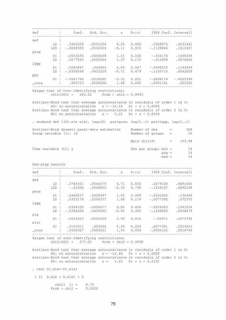
------------------------------------------------------------------------------ def | Coef. Std. Err. z P>|z| [95% Conf. Interval] -------------+---------------------------------------------------------------- def | LD | .3450258 .0551634 6.25 0.000 .2369075 .4531441 L2D | -.0058309 .0546304 -0.11 0.915 -.1129046 .1012427 grow | D1 | .0553255 .0456648 1.21 0.226 -.034176 .1448269 LD | .0277843 .0203464 1.37 0.172 -.012094 .0676626 lggp | D1 | .0283867 .044903 0.63 0.527 -.0596215 .1163949 LD | -.0306544 .0433259 -0.71 0.479 -.1155715 .0542628 pbc | D1 | -.0061786 .0018565 -3.33 0.001 -.0098174 -.0025399 _cons | .000723 .0004296 1.68 0.092 -.0001191 .001565 ------------------------------------------------------------------------------ Sargan test of over-identifying restrictions: chi2(365) = 285.22 Prob > chi2 = 0.9993 Arellano-Bond test that average autocovariance in residuals of order 1 is 0: H0: no autocorrelation z = -12.18 Pr > z = 0.0000 Arellano-Bond test that average autocovariance in residuals of order 2 is 0: H0: no autocorrelation z = 0.21 Pr > z = 0.8359 . xtabond def l(0).ele ele1, lags(2) pre(grow, lag(1,.)) pre(lggp, lag(1,.)) Arellano-Bond dynamic panel-data estimation Number of obs = 308 Group variable (i): id Number of groups = 22 Wald chi2(8) = 103.48 Time variable (t): y Obs per group: min = 14 avg = 14 max = 14 One-step results ------------------------------------------------------------------------------ def | Coef. Std. Err. z P>|z| [95% Conf. Interval] -------------+---------------------------------------------------------------- def | LD | .3785501 .0564379 6.71 0.000 .2679338 .4891663 L2D | -.01835 .0548835 -0.33 0.738 -.1259197 .0892198 grow | D1 | .0466037 .0458397 1.02 0.309 -.0432405 .136448 LD | .0323178 .0204377 1.58 0.114 -.0077395 .072375 lggp | D1 | .0358335 .0450477 0.80 0.426 -.0524583 .1241254 LD | -.0394206 .0435052 -0.91 0.365 -.1246892 .0458479 ele | D1 | .0016323 .0032359 0.50 0.614 -.00471 .0079745 ele1 | D1 | .0141011 .003246 4.34 0.000 .0077391 .0204631 _cons | .0008327 .0004321 1.93 0.054 -.0000142 .0016796 ------------------------------------------------------------------------------ Sargan test of over-identifying restrictions: chi2(365) = 277.02 Prob > chi2 = 0.9998 Arellano-Bond test that average autocovariance in residuals of order 1 is 0: H0: no autocorrelation z = -12.40 Pr > z = 0.0000 Arellano-Bond test that average autocovariance in residuals of order 2 is 0: H0: no autocorrelation z = 1.25 Pr > z = 0.2131 . test D1.ele=-D1.ele1 ( 1) D.ele + D.ele1 = 0 chi2( 1) = 8.78 Prob > chi2 = 0.0030
79

. xtabond def l(0).ele_1 , lags(2) pre(grow, lag(1,.)) pre(lggp, lag(1,.)) Arellano-Bond dynamic panel-data estimation Number of obs = 308 Group variable (i): id Number of groups = 22 Wald chi2(7) = 84.27 Time variable (t): y Obs per group: min = 14 avg = 14 max = 14 One-step results ------------------------------------------------------------------------------ def | Coef. Std. Err. z P>|z| [95% Conf. Interval] -------------+---------------------------------------------------------------- def | LD | .3477119 .0565205 6.15 0.000 .2369337 .45849 L2D | -.0147656 .0559278 -0.26 0.792 -.124382 .0948509 grow | D1 | .0433804 .0466379 0.93 0.352 -.0480282 .134789 LD | .0126031 .0204134 0.62 0.537 -.0274065 .0526127 lggp | D1 | .0567226 .0452583 1.25 0.210 -.031982 .1454273 LD | -.0541481 .0437954 -1.24 0.216 -.1399854 .0316893 ele_1 | D1 | -.0072052 .0033172 -2.17 0.030 -.0137068 -.0007036 _cons | .0007185 .000441 1.63 0.103 -.0001459 .0015829 ------------------------------------------------------------------------------ Sargan test of over-identifying restrictions: chi2(365) = 276.99 Prob > chi2 = 0.9998 Arellano-Bond test that average autocovariance in residuals of order 1 is 0: H0: no autocorrelation z = -13.21 Pr > z = 0.0000 Arellano-Bond test that average autocovariance in residuals of order 2 is 0: H0: no autocorrelation z = 1.59 Pr > z = 0.1118
80

TABLES 5 and 6 - Elections and Total Expenditure . *OLS . regress te te_1 te_2 te_3 grow lggp ele, robust Regression with robust standard errors Number of obs = 308 F( 6, 301) = 127.26 Prob > F = 0.0000 R-squared = 0.8975 Root MSE = .03556 ------------------------------------------------------------------------------ | Robust te | Coef. Std. Err. t P>|t| [95% Conf. Interval] -------------+---------------------------------------------------------------- te_1 | .8529785 .121196 7.04 0.000 .6144797 1.091477 te_2 | -.1169038 .1443267 -0.81 0.419 -.400921 .1671133 te_3 | .1654418 .0681497 2.43 0.016 .0313317 .299552 grow | -.1441292 .0274022 -5.26 0.000 -.1980534 -.090205 lggp | .0015893 .0037383 0.43 0.671 -.0057672 .0089458 ele | .0114646 .00458 2.50 0.013 .0024518 .0204774 _cons | .0078443 .0348913 0.22 0.822 -.0608174 .0765061 ------------------------------------------------------------------------------ . regress te te_1 te_2 te_3 grow lggp pbc, robust Regression with robust standard errors Number of obs = 308 F( 6, 301) = 115.39 Prob > F = 0.0000 R-squared = 0.8984 Root MSE = .03542 ------------------------------------------------------------------------------ | Robust te | Coef. Std. Err. t P>|t| [95% Conf. Interval] -------------+---------------------------------------------------------------- te_1 | .8758927 .1205354 7.27 0.000 .638694 1.113091 te_2 | -.1268693 .1412937 -0.90 0.370 -.4049177 .1511792 te_3 | .1526218 .0657014 2.32 0.021 .0233295 .2819141 grow | -.1394992 .0269941 -5.17 0.000 -.1926203 -.0863781 lggp | .0014448 .0036981 0.39 0.696 -.0058325 .0087221 pbc | .0082134 .0026115 3.15 0.002 .0030743 .0133525 _cons | .0120095 .0346679 0.35 0.729 -.0562126 .0802317 ------------------------------------------------------------------------------ . regress te te_1 te_2 te_3 grow lggp ele ele1,robust Regression with robust standard errors Number of obs = 308 F( 7, 300) = 118.04 Prob > F = 0.0000 R-squared = 0.8984 Root MSE = .03547 ------------------------------------------------------------------------------ | Robust te | Coef. Std. Err. t P>|t| [95% Conf. Interval] -------------+---------------------------------------------------------------- te_1 | .8744431 .1288108 6.79 0.000 .620956 1.12793 te_2 | -.1257908 .1460104 -0.86 0.390 -.4131252 .1615435 te_3 | .152989 .0654962 2.34 0.020 .0240987 .2818792 grow | -.1395424 .0269902 -5.17 0.000 -.1926564 -.0864284 lggp | .0014549 .0036944 0.39 0.694 -.0058152 .0087251 ele | .0086581 .0053059 1.63 0.104 -.0017835 .0190996 ele1 | -.0078012 .005399 -1.44 0.150 -.018426 .0028236 _cons | .0117077 .0342289 0.34 0.733 -.0556516 .0790669 ------------------------------------------------------------------------------ . test ele=-ele1
81
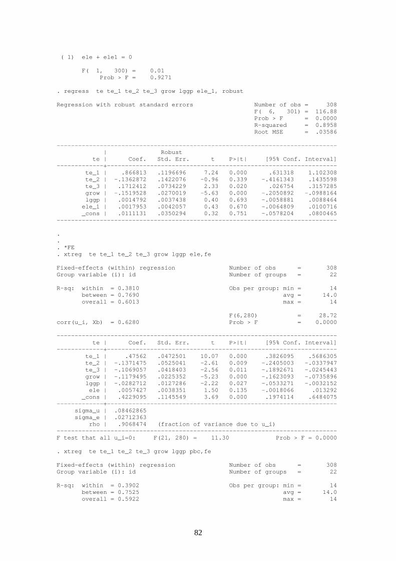
( 1) ele + ele1 = 0 F( 1, 300) = 0.01 Prob > F = 0.9271 . regress te te_1 te_2 te_3 grow lggp ele_1, robust Regression with robust standard errors Number of obs = 308 F( 6, 301) = 116.88 Prob > F = 0.0000 R-squared = 0.8958 Root MSE = .03586 ------------------------------------------------------------------------------ | Robust te | Coef. Std. Err. t P>|t| [95% Conf. Interval] -------------+---------------------------------------------------------------- te_1 | .866813 .1196696 7.24 0.000 .631318 1.102308 te_2 | -.1362872 .1422076 -0.96 0.339 -.4161343 .1435598 te_3 | .1712412 .0734229 2.33 0.020 .026754 .3157285 grow | -.1519528 .0270019 -5.63 0.000 -.2050892 -.0988164 lggp | .0014792 .0037438 0.40 0.693 -.0058881 .0088464 ele_1 | .0017953 .0042057 0.43 0.670 -.0064809 .0100716 _cons | .0111131 .0350294 0.32 0.751 -.0578204 .0800465 ------------------------------------------------------------------------------ . . . *FE . xtreg te te_1 te_2 te_3 grow lggp ele,fe Fixed-effects (within) regression Number of obs = 308 Group variable (i): id Number of groups = 22 R-sq: within = 0.3810 Obs per group: min = 14 between = 0.7690 avg = 14.0 overall = 0.6013 max = 14 F(6,280) = 28.72 corr(u_i, Xb) = 0.6280 Prob > F = 0.0000 ------------------------------------------------------------------------------ te | Coef. Std. Err. t P>|t| [95% Conf. Interval] -------------+---------------------------------------------------------------- te_1 | .47562 .0472501 10.07 0.000 .3826095 .5686305 te_2 | -.1371475 .0525041 -2.61 0.009 -.2405003 -.0337947 te_3 | -.1069057 .0418403 -2.56 0.011 -.1892671 -.0245443 grow | -.1179495 .0225352 -5.23 0.000 -.1623093 -.0735896 lggp | -.0282712 .0127286 -2.22 0.027 -.0533271 -.0032152 ele | .0057427 .0038351 1.50 0.135 -.0018066 .013292 _cons | .4229095 .1145549 3.69 0.000 .1974114 .6484075 -------------+---------------------------------------------------------------- sigma_u | .08462865 sigma_e | .02712363 rho | .9068474 (fraction of variance due to u_i) ------------------------------------------------------------------------------ F test that all u_i=0: F(21, 280) = 11.30 Prob > F = 0.0000 . xtreg te te_1 te_2 te_3 grow lggp pbc,fe Fixed-effects (within) regression Number of obs = 308 Group variable (i): id Number of groups = 22 R-sq: within = 0.3902 Obs per group: min = 14 between = 0.7525 avg = 14.0 overall = 0.5922 max = 14
82

F(6,280) = 29.86 corr(u_i, Xb) = 0.6150 Prob > F = 0.0000 ------------------------------------------------------------------------------ te | Coef. Std. Err. t P>|t| [95% Conf. Interval] -------------+---------------------------------------------------------------- te_1 | .4894211 .0470915 10.39 0.000 .3967228 .5821193 te_2 | -.1395606 .0516395 -2.70 0.007 -.2412115 -.0379096 te_3 | -.1182188 .0418429 -2.83 0.005 -.2005853 -.0358522 grow | -.1124959 .0225231 -4.99 0.000 -.156832 -.0681599 lggp | -.0295899 .012621 -2.34 0.020 -.0544339 -.0047458 pbc | .0057465 .0022564 2.55 0.011 .0013048 .0101881 _cons | .4357615 .1134771 3.84 0.000 .212385 .659138 -------------+---------------------------------------------------------------- sigma_u | .08470662 sigma_e | .02692198 rho | .90825408 (fraction of variance due to u_i) ------------------------------------------------------------------------------ F test that all u_i=0: F(21, 280) = 11.47 Prob > F = 0.0000 . xtreg te te_1 te_2 te_3 grow lggp ele ele1,fe Fixed-effects (within) regression Number of obs = 308 Group variable (i): id Number of groups = 22 R-sq: within = 0.3921 Obs per group: min = 14 between = 0.7295 avg = 14.0 overall = 0.5751 max = 14 F(7,279) = 25.71 corr(u_i, Xb) = 0.5971 Prob > F = 0.0000 ------------------------------------------------------------------------------ te | Coef. Std. Err. t P>|t| [95% Conf. Interval] -------------+---------------------------------------------------------------- te_1 | .497696 .0479183 10.39 0.000 .4033686 .5920234 te_2 | -.1474147 .052323 -2.82 0.005 -.2504126 -.0444168 te_3 | -.1227199 .0421252 -2.91 0.004 -.2056435 -.0397963 grow | -.1116561 .0225456 -4.95 0.000 -.1560371 -.0672751 lggp | -.0307563 .0126846 -2.42 0.016 -.0557259 -.0057867 ele | .0025798 .0040573 0.64 0.525 -.0054069 .0105666 ele1 | -.008665 .0038406 -2.26 0.025 -.0162252 -.0011049 _cons | .4482897 .1142822 3.92 0.000 .223325 .6732545 -------------+---------------------------------------------------------------- sigma_u | .08528202 sigma_e | .02692765 rho | .90934139 (fraction of variance due to u_i) ------------------------------------------------------------------------------ F test that all u_i=0: F(21, 279) = 11.51 Prob > F = 0.0000 . test ele=-ele1 ( 1) ele + ele1 = 0 F( 1, 279) = 0.88 Prob > F = 0.3484 . xtreg te te_1 te_2 te_3 grow lggp ele_1, fe Fixed-effects (within) regression Number of obs = 308 Group variable (i): id Number of groups = 22 R-sq: within = 0.3782 Obs per group: min = 14 between = 0.7292 avg = 14.0 overall = 0.5681 max = 14 F(6,280) = 28.38 corr(u_i, Xb) = 0.5971 Prob > F = 0.0000
83

------------------------------------------------------------------------------ te | Coef. Std. Err. t P>|t| [95% Conf. Interval] -------------+---------------------------------------------------------------- te_1 | .4804651 .0474058 10.14 0.000 .3871481 .573782 te_2 | -.1400705 .0528345 -2.65 0.008 -.2440737 -.0360672 te_3 | -.1180047 .0440876 -2.68 0.008 -.2047899 -.0312195 grow | -.1215008 .0224652 -5.41 0.000 -.165723 -.0772786 lggp | -.0297466 .0127572 -2.33 0.020 -.0548588 -.0046344 ele_1 | .0039702 .0040691 0.98 0.330 -.0040398 .0119802 _cons | .438336 .1146815 3.82 0.000 .2125887 .6640833 -------------+---------------------------------------------------------------- sigma_u | .08593566 sigma_e | .02718584 rho | .90902645 (fraction of variance due to u_i) ------------------------------------------------------------------------------ F test that all u_i=0: F(21, 280) = 11.61 Prob > F = 0.0000 . . *GMM . xtabond te l(0).ele , lags(2) pre(grow, lag(1,.)) pre(lggp, lag(1,.)) Arellano-Bond dynamic panel-data estimation Number of obs = 308 Group variable (i): id Number of groups = 22 Wald chi2(7) = 261.18 Time variable (t): y Obs per group: min = 14 avg = 14 max = 14 One-step results ------------------------------------------------------------------------------ te | Coef. Std. Err. z P>|z| [95% Conf. Interval] -------------+---------------------------------------------------------------- te | LD | .6642248 .0520248 12.77 0.000 .562258 .7661915 L2D | -.2526925 .0519487 -4.86 0.000 -.35451 -.150875 grow | D1 | -.1017775 .0638095 -1.60 0.111 -.2268418 .0232868 LD | .1231811 .0287537 4.28 0.000 .0668249 .1795374 lggp | D1 | -.0872688 .062897 -1.39 0.165 -.2105447 .036007 LD | -.0131114 .0604702 -0.22 0.828 -.1316307 .105408 ele | D1 | .0100806 .0043157 2.34 0.020 .001622 .0185392 _cons | .0022204 .0005992 3.71 0.000 .0010461 .0033947 ------------------------------------------------------------------------------ Sargan test of over-identifying restrictions: chi2(365) = 254.35 Prob > chi2 = 1.0000 Arellano-Bond test that average autocovariance in residuals of order 1 is 0: H0: no autocorrelation z = -9.70 Pr > z = 0.0000 Arellano-Bond test that average autocovariance in residuals of order 2 is 0: H0: no autocorrelation z = 1.00 Pr > z = 0.3166 . xtabond te l(0).pbc , lags(2) pre(grow, lag(1,.)) pre(lggp, lag(1,.)) Arellano-Bond dynamic panel-data estimation Number of obs = 308 Group variable (i): id Number of groups = 22 Wald chi2(7) = 262.49 Time variable (t): y Obs per group: min = 14 avg = 14 max = 14 One-step results
84

------------------------------------------------------------------------------ te | Coef. Std. Err. z P>|z| [95% Conf. Interval] -------------+---------------------------------------------------------------- te | LD | .6816699 .0517816 13.16 0.000 .5801799 .7831599 L2D | -.2665863 .0507628 -5.25 0.000 -.3660795 -.167093 grow | D1 | -.1016196 .0638553 -1.59 0.112 -.2267738 .0235345 LD | .1157484 .02918 3.97 0.000 .0585566 .1729401 lggp | D1 | -.0825743 .0629637 -1.31 0.190 -.2059809 .0408323 LD | -.0163862 .0604938 -0.27 0.786 -.1349519 .1021794 pbc | D1 | .0073755 .0026063 2.83 0.005 .0022673 .0124837 _cons | .0021614 .0005987 3.61 0.000 .000988 .0033349 ------------------------------------------------------------------------------ Sargan test of over-identifying restrictions: chi2(365) = 250.02 Prob > chi2 = 1.0000 Arellano-Bond test that average autocovariance in residuals of order 1 is 0: H0: no autocorrelation z = -9.86 Pr > z = 0.0000 Arellano-Bond test that average autocovariance in residuals of order 2 is 0: H0: no autocorrelation z = 1.41 Pr > z = 0.1600 . xtabond te l(0).ele ele1, lags(2) pre(grow, lag(1,.)) pre(lggp, lag(1,.)) Arellano-Bond dynamic panel-data estimation Number of obs = 308 Group variable (i): id Number of groups = 22 Wald chi2(8) = 261.95 Time variable (t): y Obs per group: min = 14 avg = 14 max = 14 One-step results ------------------------------------------------------------------------------ te | Coef. Std. Err. z P>|z| [95% Conf. Interval] -------------+---------------------------------------------------------------- te | LD | .6826108 .0533813 12.79 0.000 .5779854 .7872361 L2D | -.265755 .0528449 -5.03 0.000 -.3693291 -.1621809 grow | D1 | -.1016882 .0640968 -1.59 0.113 -.2273157 .0239392 LD | .1155703 .029261 3.95 0.000 .0582198 .1729208 lggp | D1 | -.0823109 .063254 -1.30 0.193 -.2062865 .0416647 LD | -.016232 .0607757 -0.27 0.789 -.1353502 .1028863 ele | D1 | .0073918 .0046407 1.59 0.111 -.0017038 .0164873 ele1 | D1 | -.0073544 .0045725 -1.61 0.108 -.0163164 .0016077 _cons | .002157 .0006031 3.58 0.000 .000975 .003339 ------------------------------------------------------------------------------ Sargan test of over-identifying restrictions: chi2(365) = 249.74 Prob > chi2 = 1.0000 Arellano-Bond test that average autocovariance in residuals of order 1 is 0: H0: no autocorrelation z = -10.20 Pr > z = 0.0000 Arellano-Bond test that average autocovariance in residuals of order 2 is 0: H0: no autocorrelation z = 1.42 Pr > z = 0.1568 . test D1.ele=-D1.ele1 ( 1) D.ele + D.ele1 = 0 chi2( 1) = 0.00 Prob > chi2 = 0.9961
85

. xtabond te l(0).ele_1 , lags(2) pre(grow, lag(1,.)) pre(lggp, lag(1,.)) Arellano-Bond dynamic panel-data estimation Number of obs = 308 Group variable (i): id Number of groups = 22 Wald chi2(7) = 250.92 Time variable (t): y Obs per group: min = 14 avg = 14 max = 14 One-step results ------------------------------------------------------------------------------ te | Coef. Std. Err. z P>|z| [95% Conf. Interval] -------------+---------------------------------------------------------------- te | LD | .6882782 .0531348 12.95 0.000 .5841358 .7924205 L2D | -.2839229 .0512149 -5.54 0.000 -.3843022 -.1835436 grow | D1 | -.087486 .064571 -1.35 0.175 -.2140429 .0390709 LD | .1358809 .0288623 4.71 0.000 .0793119 .1924499 lggp | D1 | -.1172843 .0627715 -1.87 0.062 -.2403143 .0057457 LD | .011062 .0605704 0.18 0.855 -.1076537 .1297777 ele_1 | D1 | .0038208 .0046096 0.83 0.407 -.0052139 .0128555 _cons | .0021637 .0006088 3.55 0.000 .0009705 .003357 ------------------------------------------------------------------------------ Sargan test of over-identifying restrictions: chi2(365) = 248.75 Prob > chi2 = 1.0000 Arellano-Bond test that average autocovariance in residuals of order 1 is 0: H0: no autocorrelation z = -10.29 Pr > z = 0.0000 Arellano-Bond test that average autocovariance in residuals of order 2 is 0: H0: no autocorrelation z = 1.72 Pr > z = 0.0848
86

TABLES 7 and 8 - Elections and Composition Effect . *OLS . regress ce ce_1 ce_2 ce_3 grow lggp ele, robust Regression with robust standard errors Number of obs = 308 F( 6, 301) = 68.17 Prob > F = 0.0000 R-squared = 0.5964 Root MSE = .04868 ------------------------------------------------------------------------------ | Robust ce | Coef. Std. Err. t P>|t| [95% Conf. Interval] -------------+---------------------------------------------------------------- ce_1 | .597824 .0629698 9.49 0.000 .4739073 .7217407 ce_2 | -.0213287 .0697938 -0.31 0.760 -.1586743 .116017 ce_3 | .1615112 .0522125 3.09 0.002 .0587634 .264259 grow | .0682283 .0422724 1.61 0.108 -.0149585 .1514152 lggp | -.0076872 .0052917 -1.45 0.147 -.0181006 .0027262 ele | .0000105 .0068845 0.00 0.999 -.0135374 .0135585 _cons | .2929964 .058347 5.02 0.000 .1781766 .4078161 ------------------------------------------------------------------------------ . regress ce ce_1 ce_2 ce_3 grow lggp pbc, robust Regression with robust standard errors Number of obs = 308 F( 6, 301) = 67.85 Prob > F = 0.0000 R-squared = 0.5976 Root MSE = .0486 ------------------------------------------------------------------------------ | Robust ce | Coef. Std. Err. t P>|t| [95% Conf. Interval] -------------+---------------------------------------------------------------- ce_1 | .5959227 .0627891 9.49 0.000 .4723615 .7194839 ce_2 | -.0103155 .0694357 -0.15 0.882 -.1469564 .1263255 ce_3 | .154159 .0525895 2.93 0.004 .0506694 .2576485 grow | .0619434 .0422938 1.46 0.144 -.0212857 .1451724 lggp | -.007643 .0052931 -1.44 0.150 -.0180592 .0027731 pbc | -.0038566 .0039057 -0.99 0.324 -.0115425 .0038293 _cons | .2911026 .0585234 4.97 0.000 .1759358 .4062695 ------------------------------------------------------------------------------ . regress ce ce_1 ce_2 ce_3 grow lggp ele ele1,robust Regression with robust standard errors Number of obs = 308 F( 7, 300) = 57.92 Prob > F = 0.0000 R-squared = 0.5998 Root MSE = .04855 ------------------------------------------------------------------------------ | Robust ce | Coef. Std. Err. t P>|t| [95% Conf. Interval] -------------+---------------------------------------------------------------- ce_1 | .6108055 .0649001 9.41 0.000 .4830884 .7385227 ce_2 | -.0137019 .0694034 -0.20 0.844 -.1502811 .1228773 ce_3 | .1427931 .0535513 2.67 0.008 .0374092 .2481769 grow | .0602011 .0417522 1.44 0.150 -.0219632 .1423655 lggp | -.0074531 .0052384 -1.42 0.156 -.0177616 .0028555 ele | .0039174 .0074204 0.53 0.598 -.0106852 .01852 ele1 | .010833 .0066074 1.64 0.102 -.0021697 .0238357 _cons | .2854962 .0585507 4.88 0.000 .1702741 .4007183 ------------------------------------------------------------------------------ . test ele=-ele1
87

( 1) ele + ele1 = 0 F( 1, 300) = 1.60 Prob > F = 0.2073 . regress ce ce_1 ce_2 ce_3 grow lggp ele_1, robust Regression with robust standard errors Number of obs = 308 F( 6, 301) = 74.50 Prob > F = 0.0000 R-squared = 0.6071 Root MSE = .04802 ------------------------------------------------------------------------------ | Robust ce | Coef. Std. Err. t P>|t| [95% Conf. Interval] -------------+---------------------------------------------------------------- ce_1 | .6079164 .063583 9.56 0.000 .4827928 .7330399 ce_2 | -.0003787 .0705679 -0.01 0.996 -.1392477 .1384903 ce_3 | .1317214 .0521353 2.53 0.012 .0291255 .2343173 grow | .0686702 .0403819 1.70 0.090 -.0107963 .1481368 lggp | -.0076549 .0051607 -1.48 0.139 -.0178105 .0025007 ele_1 | -.0197734 .0069432 -2.85 0.005 -.0334368 -.0061101 _cons | .2954732 .0567027 5.21 0.000 .1838893 .407057 ------------------------------------------------------------------------------ . . *FE . xtreg ce ce_1 ce_2 ce_3 grow lggp ele,fe Fixed-effects (within) regression Number of obs = 308 Group variable (i): id Number of groups = 22 R-sq: within = 0.3691 Obs per group: min = 14 between = 0.9242 avg = 14.0 overall = 0.5915 max = 14 F(6,280) = 27.30 corr(u_i, Xb) = 0.5274 Prob > F = 0.0000 ------------------------------------------------------------------------------ ce | Coef. Std. Err. t P>|t| [95% Conf. Interval] -------------+---------------------------------------------------------------- ce_1 | .4984037 .0555412 8.97 0.000 .3890724 .6077351 ce_2 | -.0463806 .0640028 -0.72 0.469 -.1723684 .0796072 ce_3 | .1227309 .0530716 2.31 0.021 .0182609 .2272008 grow | .0790595 .0386179 2.05 0.042 .0030412 .1550779 lggp | -.0134477 .0224803 -0.60 0.550 -.0576995 .030804 ele | .0013865 .0066562 0.21 0.835 -.011716 .014489 _cons | .4740116 .1804386 2.63 0.009 .1188232 .8291999 -------------+---------------------------------------------------------------- sigma_u | .02265106 sigma_e | .04678539 rho | .18988946 (fraction of variance due to u_i) ------------------------------------------------------------------------------ F test that all u_i=0: F(21, 280) = 2.18 Prob > F = 0.0025 . xtreg ce ce_1 ce_2 ce_3 grow lggp pbc,fe Fixed-effects (within) regression Number of obs = 308 Group variable (i): id Number of groups = 22 R-sq: within = 0.3699 Obs per group: min = 14 between = 0.9239 avg = 14.0 overall = 0.5927 max = 14
88
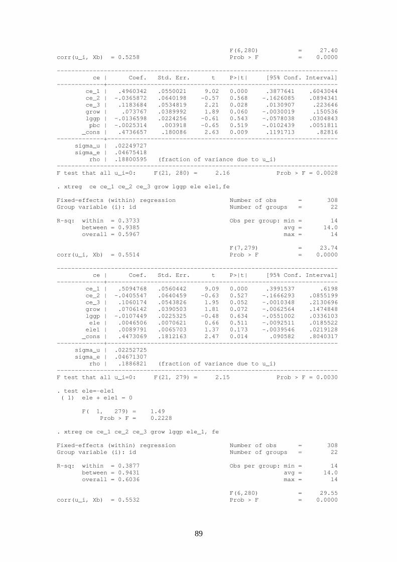
F(6,280) = 27.40 corr(u_i, Xb) = 0.5258 Prob > F = 0.0000 ------------------------------------------------------------------------------ ce | Coef. Std. Err. t P>|t| [95% Conf. Interval] -------------+---------------------------------------------------------------- ce_1 | .4960342 .0550021 9.02 0.000 .3877641 .6043044 ce_2 | -.0365872 .0640198 -0.57 0.568 -.1626085 .0894341 ce_3 | .1183684 .0534819 2.21 0.028 .0130907 .223646 grow | .073767 .0389992 1.89 0.060 -.0030019 .150536 lggp | -.0136598 .0224256 -0.61 0.543 -.0578038 .0304843 pbc | -.0025314 .003918 -0.65 0.519 -.0102439 .0051811 _cons | .4736657 .180086 2.63 0.009 .1191713 .82816 -------------+---------------------------------------------------------------- sigma_u | .02249727 sigma_e | .04675418 rho | .18800595 (fraction of variance due to u_i) ------------------------------------------------------------------------------ F test that all u_i=0: F(21, 280) = 2.16 Prob > F = 0.0028 . xtreg ce ce_1 ce_2 ce_3 grow lggp ele ele1,fe Fixed-effects (within) regression Number of obs = 308 Group variable (i): id Number of groups = 22 R-sq: within = 0.3733 Obs per group: min = 14 between = 0.9385 avg = 14.0 overall = 0.5967 max = 14 F(7,279) = 23.74 corr(u_i, Xb) = 0.5514 Prob > F = 0.0000 ------------------------------------------------------------------------------ ce | Coef. Std. Err. t P>|t| [95% Conf. Interval] -------------+---------------------------------------------------------------- ce_1 | .5094768 .0560442 9.09 0.000 .3991537 .6198 ce_2 | -.0405547 .0640459 -0.63 0.527 -.1666293 .0855199 ce_3 | .1060174 .0543826 1.95 0.052 -.0010348 .2130696 grow | .0706142 .0390503 1.81 0.072 -.0062564 .1474848 lggp | -.0107449 .0225325 -0.48 0.634 -.0551002 .0336103 ele | .0046506 .0070621 0.66 0.511 -.0092511 .0185522 ele1 | .0089791 .0065703 1.37 0.173 -.0039546 .0219128 _cons | .4473069 .1812163 2.47 0.014 .090582 .8040317 -------------+---------------------------------------------------------------- sigma_u | .02252725 sigma_e | .04671307 rho | .1886821 (fraction of variance due to u_i) ------------------------------------------------------------------------------ F test that all u_i=0: F(21, 279) = 2.15 Prob > F = 0.0030 . test ele=-ele1 ( 1) ele + ele1 = 0 F( 1, 279) = 1.49 Prob > F = 0.2228 . xtreg ce ce_1 ce_2 ce_3 grow lggp ele_1, fe Fixed-effects (within) regression Number of obs = 308 Group variable (i): id Number of groups = 22 R-sq: within = 0.3877 Obs per group: min = 14 between = 0.9431 avg = 14.0 overall = 0.6036 max = 14 F(6,280) = 29.55 corr(u_i, Xb) = 0.5532 Prob > F = 0.0000
89

------------------------------------------------------------------------------ ce | Coef. Std. Err. t P>|t| [95% Conf. Interval] -------------+---------------------------------------------------------------- ce_1 | .5064715 .0543087 9.33 0.000 .3995664 .6133766 ce_2 | -.0247478 .0624277 -0.40 0.692 -.1476349 .0981394 ce_3 | .0898578 .0534849 1.68 0.094 -.0154258 .1951415 grow | .0772384 .0378411 2.04 0.042 .0027493 .1517276 lggp | -.0101332 .0221414 -0.46 0.648 -.053718 .0334516 ele_1 | -.0194332 .0066483 -2.92 0.004 -.0325203 -.0063462 _cons | .4520359 .1776843 2.54 0.011 .1022692 .8018026 -------------+---------------------------------------------------------------- sigma_u | .02273794 sigma_e | .04609108 rho | .19573466 (fraction of variance due to u_i) ------------------------------------------------------------------------------ F test that all u_i=0: F(21, 280) = 2.23 Prob > F = 0.0019 . . *GMM . xtabond ce l(0).ele , lags(2) pre(grow, lag(1,.)) pre(lggp, lag(1,.)) Arellano-Bond dynamic panel-data estimation Number of obs = 308 Group variable (i): id Number of groups = 22 Wald chi2(7) = 142.57 Time variable (t): y Obs per group: min = 14 avg = 14 max = 14 One-step results ------------------------------------------------------------------------------ ce | Coef. Std. Err. z P>|z| [95% Conf. Interval] -------------+---------------------------------------------------------------- ce | LD | .5204356 .0568682 9.15 0.000 .4089759 .6318952 L2D | -.0343043 .0569018 -0.60 0.547 -.1458298 .0772211 grow | D1 | .0892711 .0950972 0.94 0.348 -.097116 .2756583 LD | -.069051 .0411043 -1.68 0.093 -.149614 .0115121 lggp | D1 | .0052189 .0929107 0.06 0.955 -.1768827 .1873206 LD | -.0666234 .0900221 -0.74 0.459 -.2430635 .1098168 ele | D1 | -.0057964 .0064121 -0.90 0.366 -.0183639 .006771 _cons | .0049174 .001014 4.85 0.000 .00293 .0069048 ------------------------------------------------------------------------------ Sargan test of over-identifying restrictions: chi2(365) = 244.93 Prob > chi2 = 1.0000 Arellano-Bond test that average autocovariance in residuals of order 1 is 0: H0: no autocorrelation z = -12.35 Pr > z = 0.0000 Arellano-Bond test that average autocovariance in residuals of order 2 is 0: H0: no autocorrelation z = -0.89 Pr > z = 0.3739 . xtabond ce l(0).pbc , lags(2) pre(grow, lag(1,.)) pre(lggp, lag(1,.)) Arellano-Bond dynamic panel-data estimation Number of obs = 308 Group variable (i): id Number of groups = 22 Wald chi2(7) = 145.08 Time variable (t): y Obs per group: min = 14 avg = 14 max = 14 One-step results ------------------------------------------------------------------------------
90

ce | Coef. Std. Err. z P>|z| [95% Conf. Interval] -------------+---------------------------------------------------------------- ce | LD | .5213213 .0559603 9.32 0.000 .4116411 .6310014 L2D | -.0292606 .0561441 -0.52 0.602 -.1393011 .0807799 grow | D1 | .0920027 .0947985 0.97 0.332 -.093799 .2778045 LD | -.0585332 .0416931 -1.40 0.160 -.1402502 .0231838 lggp | D1 | -.0067717 .0926874 -0.07 0.942 -.1884357 .1748924 LD | -.056363 .0897739 -0.63 0.530 -.2323166 .1195905 pbc | D1 | -.0065655 .0038776 -1.69 0.090 -.0141655 .0010344 _cons | .0048776 .001011 4.82 0.000 .0028961 .0068591 ------------------------------------------------------------------------------ Sargan test of over-identifying restrictions: chi2(365) = 243.05 Prob > chi2 = 1.0000 Arellano-Bond test that average autocovariance in residuals of order 1 is 0: H0: no autocorrelation z = -12.41 Pr > z = 0.0000 Arellano-Bond test that average autocovariance in residuals of order 2 is 0: H0: no autocorrelation z = -0.52 Pr > z = 0.6014 . xtabond ce l(0).ele ele1, lags(2) pre(grow, lag(1,.)) pre(lggp, lag(1,.)) Arellano-Bond dynamic panel-data estimation Number of obs = 308 Group variable (i): id Number of groups = 22 Wald chi2(8) = 145.53 Time variable (t): y Obs per group: min = 14 avg = 14 max = 14 One-step results ------------------------------------------------------------------------------ ce | Coef. Std. Err. z P>|z| [95% Conf. Interval] -------------+---------------------------------------------------------------- ce | LD | .5329169 .0572878 9.30 0.000 .4206349 .6451989 L2D | -.0366249 .057022 -0.64 0.521 -.148386 .0751362 grow | D1 | .0879901 .0952772 0.92 0.356 -.0987497 .27473 LD | -.0559375 .0419735 -1.33 0.183 -.138204 .026329 lggp | D1 | -.0017589 .0931851 -0.02 0.985 -.1843983 .1808805 LD | -.0604062 .0902535 -0.67 0.503 -.2372998 .1164874 ele | D1 | -.0015722 .0068145 -0.23 0.818 -.0149284 .0117839 ele1 | D1 | .0111912 .0066819 1.67 0.094 -.0019051 .0242874 _cons | .0048946 .0010158 4.82 0.000 .0029037 .0068854 ------------------------------------------------------------------------------ Sargan test of over-identifying restrictions: chi2(365) = 244.37 Prob > chi2 = 1.0000 Arellano-Bond test that average autocovariance in residuals of order 1 is 0: H0: no autocorrelation z = -12.55 Pr > z = 0.0000 Arellano-Bond test that average autocovariance in residuals of order 2 is 0: H0: no autocorrelation z = -0.36 Pr > z = 0.7182 . test D1.ele=-D1.ele1 ( 1) D.ele + D.ele1 = 0 chi2( 1) = 0.76 Prob > chi2 = 0.3831
91

. xtabond ce l(0).ele_1 , lags(2) pre(grow, lag(1,.)) pre(lggp, lag(1,.)) Arellano-Bond dynamic panel-data estimation Number of obs = 308 Group variable (i): id Number of groups = 22 Wald chi2(7) = 148.01 Time variable (t): y Obs per group: min = 14 avg = 14 max = 14 One-step results ------------------------------------------------------------------------------ ce | Coef. Std. Err. z P>|z| [95% Conf. Interval] -------------+---------------------------------------------------------------- ce | LD | .5460397 .0559632 9.76 0.000 .4363538 .6557256 L2D | -.0449919 .0550667 -0.82 0.414 -.1529206 .0629368 grow | D1 | .0807695 .0943044 0.86 0.392 -.1040637 .2656027 LD | -.0788889 .0406327 -1.94 0.052 -.1585274 .0007497 lggp | D1 | .0262696 .0910579 0.29 0.773 -.1522006 .2047398 LD | -.0790056 .0883866 -0.89 0.371 -.2522403 .094229 ele_1 | D1 | -.0148937 .0067283 -2.21 0.027 -.028081 -.0017064 _cons | .0046604 .0010169 4.58 0.000 .0026673 .0066536 ------------------------------------------------------------------------------ Sargan test of over-identifying restrictions: chi2(365) = 242.60 Prob > chi2 = 1.0000 Arellano-Bond test that average autocovariance in residuals of order 1 is 0: H0: no autocorrelation z = -12.32 Pr > z = 0.0000 Arellano-Bond test that average autocovariance in residuals of order 2 is 0: H0: no autocorrelation z = -0.50 Pr > z = 0.6165
92

TABLES 9 and 10 - Elections and Total Revenue . *OLS . regress tr tr_1 tr_2 tr_3 grow lggp ele, robust Regression with robust standard errors Number of obs = 308 F( 6, 301) = 72.19 Prob > F = 0.0000 R-squared = 0.8920 Root MSE = .0332 ------------------------------------------------------------------------------ | Robust tr| Coef. Std. Err. t P>|t| [95% Conf. Interval] -------------+---------------------------------------------------------------- tr_1 | 1.007357 .1669972 6.03 0.000 .678727 1.335987 tr_2 | -.280931 .2239186 -1.25 0.211 -.7215751 .1597131 tr_3 | .158464 .0864167 1.83 0.068 -.0115934 .3285214 grow | -.051079 .0274964 -1.86 0.064 -.1051884 .0030304 lggp | .0007143 .0031351 0.23 0.820 -.0054552 .0068839 ele | .0111455 .004261 2.62 0.009 .0027604 .0195306 _cons | .0141335 .0306862 0.46 0.645 -.0462533 .0745202 ------------------------------------------------------------------------------ . regress tr tr_1 tr_2 tr_3 grow lggp pbc, robust Regression with robust standard errors Number of obs = 308 F( 6, 301) = 65.81 Prob > F = 0.0000 R-squared = 0.8903 Root MSE = .03347 ------------------------------------------------------------------------------ | Robust tr| Coef. Std. Err. t P>|t| [95% Conf. Interval] -------------+---------------------------------------------------------------- tr_1 | 1.011438 .1685758 6.00 0.000 .679702 1.343175 tr_2 | -.299546 .2214875 -1.35 0.177 -.735406 .136314 tr_3 | .1719821 .0842619 2.04 0.042 .0061651 .3377991 grow | -.053444 .0276693 -1.93 0.054 -.1078938 .0010058 lggp | .0006089 .0031729 0.19 0.848 -.0056351 .0068528 pbc | .0024608 .002744 0.90 0.371 -.002939 .0078606 _cons | .0179009 .0312325 0.57 0.567 -.0435607 .0793626 ------------------------------------------------------------------------------ . regress tr_1 tr_2 tr_3 grow lggp ele ele1,robust Regression with robust standard errors Number of obs = 308 F( 7, 300) = 77.98 Prob > F = 0.0000 R-squared = 0.8930 Root MSE = .0331 ------------------------------------------------------------------------------ | Robust tr| Coef. Std. Err. t P>|t| [95% Conf. Interval] -------------+---------------------------------------------------------------- tr_1 | .9937757 .1704347 5.83 0.000 .6583768 1.329175 tr_2 | -.2660834 .2282896 -1.17 0.245 -.7153353 .1831684 tr_3 | .1580741 .0865007 1.83 0.069 -.0121509 .3282991 grow | -.0556565 .0270965 -2.05 0.041 -.1089799 -.0023332 lggp | .0008512 .003169 0.27 0.788 -.005385 .0070873 ele | .0137865 .0047429 2.91 0.004 .0044529 .0231202 ele1 | .0075717 .005269 1.44 0.152 -.0027971 .0179405 _cons | .0101636 .0305855 0.33 0.740 -.0500258 .070353 ------------------------------------------------------------------------------ . test ele=-ele1
93

( 1) ele + ele1 = 0 F( 1, 300) = 6.30 Prob > F = 0.0126 . regress trtr_1 tr_2 tr_3 grow lggp ele_1, robust Regression with robust standard errors Number of obs = 308 F( 6, 301) = 65.24 Prob > F = 0.0000 R-squared = 0.8901 Root MSE = .03349 ------------------------------------------------------------------------------ | Robust tr| Coef. Std. Err. t P>|t| [95% Conf. Interval] -------------+---------------------------------------------------------------- tr_1 | 1.001558 .1695455 5.91 0.000 .6679135 1.335203 tr_2 | -.2998994 .2223525 -1.35 0.178 -.7374615 .1376628 tr_3 | .1814686 .0844263 2.15 0.032 .0153281 .3476092 grow | -.05567 .0278415 -2.00 0.046 -.1104586 -.0008815 lggp | .0006317 .003206 0.20 0.844 -.0056773 .0069406 ele_1 | -.0029734 .0039099 -0.76 0.448 -.0106675 .0047207 _cons | .0183559 .0314147 0.58 0.559 -.0434643 .0801762 ------------------------------------------------------------------------------ . . . *FE . xtreg tr tr_1 tr_2 tr_3 grow lggp ele,fe Fixed-effects (within) regression Number of obs = 308 Group variable (i): id Number of groups = 22 R-sq: within = 0.4882 Obs per group: min = 14 between = 0.9475 avg = 14.0 overall = 0.5713 max = 14 F(6,280) = 44.51 corr(u_i, Xb) = 0.6137 Prob > F = 0.0000 ------------------------------------------------------------------------------ tr| Coef. Std. Err. t P>|t| [95% Conf. Interval] -------------+---------------------------------------------------------------- tr_1 | .5988355 .0416372 14.38 0.000 .5168737 .6807972 tr_2 | -.2727789 .0490768 -5.56 0.000 -.3693852 -.1761727 tr_3 | -.1350257 .0384525 -3.51 0.001 -.2107184 -.059333 grow | -.0559339 .0186706 -3.00 0.003 -.0926865 -.0191813 lggp | -.0076158 .0100646 -0.76 0.450 -.0274277 .0121962 ele | .0051387 .003222 1.59 0.112 -.0012036 .0114811 _cons | .2346181 .0887453 2.64 0.009 .0599255 .4093107 -------------+---------------------------------------------------------------- sigma_u | .07997137 sigma_e | .02275159 rho | .92512213 (fraction of variance due to u_i) ------------------------------------------------------------------------------ F test that all u_i=0: F(21, 280) = 17.19 Prob > F = 0.0000 . xtreg tr tr_1 tr_2 tr_3 grow lggp pbc,fe Fixed-effects (within) regression Number of obs = 308 Group variable (i): id Number of groups = 22 R-sq: within = 0.4836 Obs per group: min = 14 between = 0.9417 avg = 14.0 overall = 0.5554 max = 14
94

F(6,280) = 43.70 corr(u_i, Xb) = 0.6010 Prob > F = 0.0000 ------------------------------------------------------------------------------ tr| Coef. Std. Err. t P>|t| [95% Conf. Interval] -------------+---------------------------------------------------------------- tr_1 | .5962759 .0420166 14.19 0.000 .5135674 .6789843 tr_2 | -.2815121 .0489819 -5.75 0.000 -.3779317 -.1850926 tr_3 | -.129584 .0385897 -3.36 0.001 -.2055468 -.0536211 grow | -.0580038 .0188756 -3.07 0.002 -.0951599 -.0208476 lggp | -.0078138 .0101177 -0.77 0.441 -.0277301 .0121025 pbc | .0004041 .0019049 0.21 0.832 -.0033457 .0041539 _cons | .2387625 .0891719 2.68 0.008 .0632301 .4142948 -------------+---------------------------------------------------------------- sigma_u | .08059363 sigma_e | .02285287 rho | .92557934 (fraction of variance due to u_i) ------------------------------------------------------------------------------ F test that all u_i=0: F(21, 280) = 17.41 Prob > F = 0.0000 . xtreg trtr_1 tr_2 tr_3 grow lggp ele ele1,fe Fixed-effects (within) regression Number of obs = 308 Group variable (i): id Number of groups = 22 R-sq: within = 0.4938 Obs per group: min = 14 between = 0.9606 avg = 14.0 overall = 0.5816 max = 14 F(7,279) = 38.87 corr(u_i, Xb) = 0.6222 Prob > F = 0.0000 ------------------------------------------------------------------------------ tr| Coef. Std. Err. t P>|t| [95% Conf. Interval] -------------+---------------------------------------------------------------- tr_1 | .5906884 .0417431 14.15 0.000 .508517 .6728599 tr_2 | -.2623382 .0492571 -5.33 0.000 -.3593009 -.1653756 tr_3 | -.1337519 .0383177 -3.49 0.001 -.2091804 -.0583234 grow | -.0599213 .0187403 -3.20 0.002 -.0968115 -.023031 lggp | -.0062672 .010057 -0.62 0.534 -.0260644 .01353 ele | .0070712 .003394 2.08 0.038 .0003902 .0137522 ele1 | .0054775 .0031235 1.75 0.081 -.0006712 .0116262 _cons | .220364 .088791 2.48 0.014 .0455785 .3951494 -------------+---------------------------------------------------------------- sigma_u | .07961596 sigma_e | .02266774 rho | .92501649 (fraction of variance due to u_i) ------------------------------------------------------------------------------ F test that all u_i=0: F(21, 279) = 17.18 Prob > F = 0.0000 . test ele=-ele1 ( 1) ele + ele1 = 0 F( 1, 279) = 5.59 Prob > F = 0.0187 . xtregtrtr_1 tr_2 tr_3 grow lggp ele_1, fe Fixed-effects (within) regression Number of obs = 308 Group variable (i): id Number of groups = 22 R-sq: within = 0.4846 Obs per group: min = 14 between = 0.9470 avg = 14.0 overall = 0.5572 max = 14 F(6,280) = 43.87 corr(u_i, Xb) = 0.6028 Prob > F = 0.0000
95

------------------------------------------------------------------------------ it | Coef. Std. Err. t P>|t| [95% Conf. Interval] -------------+---------------------------------------------------------------- tr_1 | .5911466 .0420922 14.04 0.000 .5082893 .6740038 tr_2 | -.2812704 .048933 -5.75 0.000 -.3775937 -.1849472 tr_3 | -.1250099 .038729 -3.23 0.001 -.2012468 -.048773 grow | -.0579308 .0186826 -3.10 0.002 -.0947069 -.0211547 lggp | -.0073739 .0101109 -0.73 0.466 -.0272769 .0125291 ele_1 | -.0024626 .0032909 -0.75 0.455 -.0089406 .0040154 _cons | .235504 .0890983 2.64 0.009 .0601165 .4108916 -------------+---------------------------------------------------------------- sigma_u | .08055516 sigma_e | .02283188 rho | .92564008 (fraction of variance due to u_i) ------------------------------------------------------------------------------ F test that all u_i=0: F(21, 280) = 17.50 Prob > F = 0.0000 . . *GMM . xtabond it l(0).ele , lags(2) pre(grow, lag(1,.)) pre(lggp, lag(1,.)) Arellano-Bond dynamic panel-data estimation Number of obs = 308 Group variable (i): id Number of groups = 22 Wald chi2(7) = 268.76 Time variable (t): y Obs per group: min = 14 avg = 14 max = 14 One-step results ------------------------------------------------------------------------------ it | Coef. Std. Err. z P>|z| [95% Conf. Interval] -------------+---------------------------------------------------------------- it | LD | .7139933 .0506127 14.11 0.000 .6147942 .8131923 L2D | -.2993771 .0483703 -6.19 0.000 -.3941812 -.204573 grow | D1 | -.0576599 .0589354 -0.98 0.328 -.1731712 .0578514 LD | .111362 .025856 4.31 0.000 .0606853 .1620388 lggp | D1 | -.0320426 .0577771 -0.55 0.579 -.1452835 .0811984 LD | -.053781 .0558419 -0.96 0.336 -.163229 .0556671 ele | D1 | .0095186 .003906 2.44 0.015 .001863 .0171741 _cons | .002413 .0005494 4.39 0.000 .0013363 .0034898 ------------------------------------------------------------------------------ Sargan test of over-identifying restrictions: chi2(365) = 270.19 Prob > chi2 = 0.9999 Arellano-Bond test that average autocovariance in residuals of order 1 is 0: H0: no autocorrelation z = -8.33 Pr > z = 0.0000 Arellano-Bond test that average autocovariance in residuals of order 2 is 0: H0: no autocorrelation z = 1.25 Pr > z = 0.2096 . xtabond it l(0).pbc , lags(2) pre(grow, lag(1,.)) pre(lggp, lag(1,.)) Arellano-Bond dynamic panel-data estimation Number of obs = 308 Group variable (i): id Number of groups = 22 Wald chi2(7) = 261.15 Time variable (t): y Obs per group: min = 14 avg = 14 max = 14 One-step results
96

------------------------------------------------------------------------------ it | Coef. Std. Err. z P>|z| [95% Conf. Interval] -------------+---------------------------------------------------------------- it | LD | .7187746 .0508761 14.13 0.000 .6190594 .8184898 L2D | -.3142351 .0481481 -6.53 0.000 -.4086036 -.2198665 grow | D1 | -.0472061 .0590767 -0.80 0.424 -.1629943 .0685821 LD | .1147523 .0263393 4.36 0.000 .0631282 .1663765 lggp | D1 | -.0489422 .0579701 -0.84 0.399 -.1625614 .0646771 LD | -.0374842 .0559705 -0.67 0.503 -.1471844 .072216 pbc | D1 | .0019902 .0023928 0.83 0.406 -.0026996 .0066801 _cons | .0022855 .000549 4.16 0.000 .0012095 .0033615 ------------------------------------------------------------------------------ Sargan test of over-identifying restrictions: chi2(365) = 273.64 Prob > chi2 = 0.9999 Arellano-Bond test that average autocovariance in residuals of order 1 is 0: H0: no autocorrelation z = -8.24 Pr > z = 0.0000 Arellano-Bond test that average autocovariance in residuals of order 2 is 0: H0: no autocorrelation z = 0.98 Pr > z = 0.3289 . xtabond it l(0).ele ele1, lags(2) pre(grow, lag(1,.)) pre(lggp, lag(1,.)) Arellano-Bond dynamic panel-data estimation Number of obs = 308 Group variable (i): id Number of groups = 22 Wald chi2(8) = 280.15 Time variable (t): y Obs per group: min = 14 avg = 14 max = 14 One-step results ------------------------------------------------------------------------------ it | Coef. Std. Err. z P>|z| [95% Conf. Interval] -------------+---------------------------------------------------------------- it | LD | .7011586 .0502729 13.95 0.000 .6026256 .7996916 L2D | -.2851209 .0482156 -5.91 0.000 -.3796218 -.19062 grow | D1 | -.0580364 .0581288 -1.00 0.318 -.1719667 .0558939 LD | .1213578 .0259548 4.68 0.000 .0704874 .1722283 lggp | D1 | -.0375077 .0570538 -0.66 0.511 -.1493311 .0743158 LD | -.0497497 .0551136 -0.90 0.367 -.1577704 .058271 ele | D1 | .0124942 .0041004 3.05 0.002 .0044575 .0205308 ele1 | D1 | .0084908 .0040986 2.07 0.038 .0004578 .0165238 _cons | .0024929 .0005433 4.59 0.000 .001428 .0035578 ------------------------------------------------------------------------------ Sargan test of over-identifying restrictions: chi2(365) = 274.97 Prob > chi2 = 0.9999 Arellano-Bond test that average autocovariance in residuals of order 1 is 0: H0: no autocorrelation z = -8.22 Pr > z = 0.0000 Arellano-Bond test that average autocovariance in residuals of order 2 is 0: H0: no autocorrelation z = 1.00 Pr > z = 0.3194 . . test D1.ele=-D1.ele1 ( 1) D.ele + D.ele1 = 0 chi2( 1) = 9.76 Prob > chi2 = 0.0018
97

. xtabond it l(0).ele_1 , lags(2) pre(grow, lag(1,.)) pre(lggp, lag(1,.)) Arellano-Bond dynamic panel-data estimation Number of obs = 308 Group variable (i): id Number of groups = 22 Wald chi2(7) = 263.49 Time variable (t): y Obs per group: min = 14 avg = 14 max = 14 One-step results ------------------------------------------------------------------------------ it | Coef. Std. Err. z P>|z| [95% Conf. Interval] -------------+---------------------------------------------------------------- it | LD | .7136762 .0515131 13.85 0.000 .6127124 .81464 L2D | -.3121723 .0484659 -6.44 0.000 -.4071637 -.2171808 grow | D1 | -.043272 .0587091 -0.74 0.461 -.1583397 .0717957 LD | .1189453 .0257069 4.63 0.000 .0685607 .1693298 lggp | D1 | -.057316 .0569039 -1.01 0.314 -.1688457 .0542137 LD | -.0301892 .0550328 -0.55 0.583 -.1380515 .0776732 ele_1 | D1 | -.0017399 .0042163 -0.41 0.680 -.0100036 .0065239 _cons | .0022668 .0005479 4.14 0.000 .0011929 .0033408 ------------------------------------------------------------------------------ Sargan test of over-identifying restrictions: chi2(365) = 276.45 Prob > chi2 = 0.9998 Arellano-Bond test that average autocovariance in residuals of order 1 is 0: H0: no autocorrelation z = -8.13 Pr > z = 0.0000 Arellano-Bond test that average autocovariance in residuals of order 2 is 0: H0: no autocorrelation z = 0.88 Pr > z = 0.3768
98

TABLES 11 and 12 - Elections and Revenue from Federal Government . *OLS . regress fr fr_1 fr_2 fr_3 grow lggp ele, robust Regression with robust standard errors Number of obs = 308 F( 6, 301) = 131.61 Prob > F = 0.0000 R-squared = 0.9049 Root MSE = .03052 ------------------------------------------------------------------------------ | Robust fr | Coef. Std. Err. t P>|t| [95% Conf. Interval] -------------+---------------------------------------------------------------- fr_1 | 1.004842 .1443267 6.96 0.000 .7208247 1.288859 fr_2 | -.2122897 .1985607 -1.07 0.286 -.6030325 .1784532 fr_3 | .1084967 .0781301 1.39 0.166 -.0452537 .2622471 grow | -.0498083 .025191 -1.98 0.049 -.0993811 -.0002355 lggp | -.0004904 .003127 -0.16 0.875 -.006644 .0056632 ele | .0113934 .0039385 2.89 0.004 .0036429 .0191439 _cons | .0182307 .0305493 0.60 0.551 -.0418866 .0783479 ------------------------------------------------------------------------------ . regress fr fr_1 fr_2 fr_3 grow lggp pbc, robust Regression with robust standard errors Number of obs = 308 F( 6, 301) = 119.05 Prob > F = 0.0000 R-squared = 0.9030 Root MSE = .03081 ------------------------------------------------------------------------------ | Robust fr | Coef. Std. Err. t P>|t| [95% Conf. Interval] -------------+---------------------------------------------------------------- fr_1 | 1.008407 .1462416 6.90 0.000 .7206219 1.296193 fr_2 | -.2309958 .1985459 -1.16 0.246 -.6217095 .159718 fr_3 | .1225613 .0766267 1.60 0.111 -.0282305 .2733532 grow | -.0518731 .0256435 -2.02 0.044 -.1023363 -.0014098 lggp | -.0006274 .0031662 -0.20 0.843 -.0068581 .0056033 pbc | .0027726 .0025483 1.09 0.277 -.0022422 .0077874 _cons | .0223104 .0311374 0.72 0.474 -.0389641 .0835849 ------------------------------------------------------------------------------ . regress fr fr_1 fr_2 fr_3 grow lggp ele ele1,robust Regression with robust standard errors Number of obs = 308 F( 7, 300) = 122.71 Prob > F = 0.0000 R-squared = 0.9058 Root MSE = .03042 ------------------------------------------------------------------------------ | Robust fr | Coef. Std. Err. t P>|t| [95% Conf. Interval] -------------+---------------------------------------------------------------- fr_1 | .9891585 .1484102 6.67 0.000 .6971016 1.281215 fr_2 | -.1942327 .2037218 -0.95 0.341 -.5951374 .2066719 fr_3 | .1068462 .0783029 1.36 0.173 -.0472463 .2609387 grow | -.0543071 .0250902 -2.16 0.031 -.1036823 -.0049319 lggp | -.0003557 .0031491 -0.11 0.910 -.0065528 .0058414 ele | .0138578 .0042657 3.25 0.001 .0054633 .0222522 ele1 | .0071179 .0046235 1.54 0.125 -.0019807 .0162165 _cons | .0144918 .0303717 0.48 0.634 -.0452767 .0742604 ------------------------------------------------------------------------------ . test ele=-ele1
99

( 1) ele + ele1 = 0 F( 1, 300) = 8.03 Prob > F = 0.0049 . regress fr fr_1 fr_2 fr_3 grow lggp ele_1, robust Regression with robust standard errors Number of obs = 308 F( 6, 301) = 117.48 Prob > F = 0.0000 R-squared = 0.9029 Root MSE = .03083 ------------------------------------------------------------------------------ | Robust fr | Coef. Std. Err. t P>|t| [95% Conf. Interval] -------------+---------------------------------------------------------------- fr_1 | .9940371 .1472625 6.75 0.000 .7042428 1.283832 fr_2 | -.2296705 .2000504 -1.15 0.252 -.623345 .1640039 fr_3 | .1345786 .0779217 1.73 0.085 -.0187618 .287919 grow | -.054518 .0256805 -2.12 0.035 -.1050541 -.0039819 lggp | -.000635 .003203 -0.20 0.843 -.0069381 .0056681 ele_1 | -.0038346 .0037698 -1.02 0.310 -.011253 .0035838 _cons | .0232096 .0312747 0.74 0.459 -.0383351 .0847544 ------------------------------------------------------------------------------ . . . *FE . xtreg fr fr_1 fr_2 fr_3 grow lggp ele,fe Fixed-effects (within) regression Number of obs = 308 Group variable (i): id Number of groups = 22 R-sq: within = 0.4508 Obs per group: min = 14 between = 0.8928 avg = 14.0 overall = 0.6720 max = 14 F(6,280) = 38.30 corr(u_i, Xb) = 0.6993 Prob > F = 0.0000 ------------------------------------------------------------------------------ fr | Coef. Std. Err. t P>|t| [95% Conf. Interval] -------------+---------------------------------------------------------------- fr_1 | .5847009 .0443512 13.18 0.000 .4973967 .672005 fr_2 | -.2077448 .0521033 -3.99 0.000 -.3103086 -.105181 fr_3 | -.1474463 .039764 -3.71 0.000 -.2257207 -.0691719 grow | -.0452483 .0175997 -2.57 0.011 -.0798927 -.0106038 lggp | -.0154633 .0096178 -1.61 0.109 -.0343955 .003469 ele | .0052995 .0030445 1.74 0.083 -.0006936 .0112925 _cons | .2719578 .0849833 3.20 0.002 .1046705 .4392452 -------------+---------------------------------------------------------------- sigma_u | .07463975 sigma_e | .02151267 rho | .9233007 (fraction of variance due to u_i) ------------------------------------------------------------------------------ F test that all u_i=0: F(21, 280) = 15.51 Prob > F = 0.0000 . xtreg fr fr_1 fr_2 fr_3 grow lggp pbc,fe Fixed-effects (within) regression Number of obs = 308 Group variable (i): id Number of groups = 22 R-sq: within = 0.4449 Obs per group: min = 14 between = 0.8817 avg = 14.0 overall = 0.6561 max = 14
100

F(6,280) = 37.41 corr(u_i, Xb) = 0.6870 Prob > F = 0.0000 ------------------------------------------------------------------------------ fr | Coef. Std. Err. t P>|t| [95% Conf. Interval] -------------+---------------------------------------------------------------- fr_1 | .5799352 .0448884 12.92 0.000 .4915736 .6682968 fr_2 | -.2158632 .0521866 -4.14 0.000 -.3185911 -.1131353 fr_3 | -.1418172 .0399137 -3.55 0.000 -.2203862 -.0632482 grow | -.0472567 .0178163 -2.65 0.008 -.0823276 -.0121857 lggp | -.0158394 .0096719 -1.64 0.103 -.0348782 .0031995 pbc | .0004165 .0018057 0.23 0.818 -.003138 .003971 _cons | .2777569 .0854076 3.25 0.001 .1096343 .4458794 -------------+---------------------------------------------------------------- sigma_u | .0753887 sigma_e | .0216267 rho | .92396341 (fraction of variance due to u_i) ------------------------------------------------------------------------------ F test that all u_i=0: F(21, 280) = 15.76 Prob > F = 0.0000 . xtreg fr fr_1 fr_2 fr_3 grow lggp ele ele1,fe Fixed-effects (within) regression Number of obs = 308 Group variable (i): id Number of groups = 22 R-sq: within = 0.4579 Obs per group: min = 14 between = 0.9099 avg = 14.0 overall = 0.6823 max = 14 F(7,279) = 33.67 corr(u_i, Xb) = 0.7090 Prob > F = 0.0000 ------------------------------------------------------------------------------ fr | Coef. Std. Err. t P>|t| [95% Conf. Interval] -------------+---------------------------------------------------------------- fr_1 | .5738351 .0445019 12.89 0.000 .486233 .6614373 fr_2 | -.1935724 .0523787 -3.70 0.000 -.2966799 -.0904649 fr_3 | -.1474734 .0395749 -3.73 0.000 -.2253766 -.0695701 grow | -.0495832 .017661 -2.81 0.005 -.084349 -.0148175 lggp | -.0140664 .0095996 -1.47 0.144 -.0329633 .0048305 ele | .0072865 .0032021 2.28 0.024 .0009832 .0135897 ele1 | .0056745 .0029569 1.92 0.056 -.0001462 .0114953 _cons | .2573784 .0849196 3.03 0.003 .0902138 .4245429 -------------+---------------------------------------------------------------- sigma_u | .07433849 sigma_e | .02141034 rho | .9234031 (fraction of variance due to u_i) ------------------------------------------------------------------------------ F test that all u_i=0: F(21, 279) = 15.55 Prob > F = 0.0000 . test ele=-ele1 ( 1) ele + ele1 = 0 F( 1, 279) = 6.69 Prob > F = 0.0102 . xtreg fr fr_1 fr_2 fr_3 grow lggp ele_1, fe Fixed-effects (within) regression Number of obs = 308 Group variable (i): id Number of groups = 22 R-sq: within = 0.4474 Obs per group: min = 14 between = 0.8895 avg = 14.0 overall = 0.6592 max = 14 F(6,280) = 37.79 corr(u_i, Xb) = 0.6903 Prob > F = 0.0000
101

------------------------------------------------------------------------------ fr | Coef. Std. Err. t P>|t| [95% Conf. Interval] -------------+---------------------------------------------------------------- fr_1 | .5722638 .0446705 12.81 0.000 .4843313 .6601964 fr_2 | -.215896 .0520624 -4.15 0.000 -.3183795 -.1134126 fr_3 | -.1346562 .0401207 -3.36 0.001 -.2136326 -.0556798 grow | -.0471067 .0176013 -2.68 0.008 -.0817543 -.012459 lggp | -.0152872 .0096545 -1.58 0.114 -.0342919 .0037174 ele_1 | -.0035662 .0031072 -1.15 0.252 -.0096826 .0025502 _cons | .273778 .0852407 3.21 0.001 .105984 .441572 -------------+---------------------------------------------------------------- sigma_u | .07535224 sigma_e | .02157805 rho | .92421147 (fraction of variance due to u_i) ------------------------------------------------------------------------------ F test that all u_i=0: F(21, 280) = 15.93 Prob > F = 0.0000 . . *GMM . xtabond fr l(0).ele , lags(2) pre(grow, lag(1,.)) pre(lggp, lag(1,.)) Arellano-Bond dynamic panel-data estimation Number of obs = 308 Group variable (i): id Number of groups = 22 Wald chi2(7) = 267.16 Time variable (t): y Obs per group: min = 14 avg = 14 max = 14 One-step results ------------------------------------------------------------------------------ fr | Coef. Std. Err. z P>|z| [95% Conf. Interval] -------------+---------------------------------------------------------------- fr | LD | .7235389 .052213 13.86 0.000 .6212032 .8258746 L2D | -.2624027 .0488318 -5.37 0.000 -.3581113 -.1666942 grow | D1 | -.0632153 .0539575 -1.17 0.241 -.1689701 .0425394 LD | .085278 .0236323 3.61 0.000 .0389594 .1315965 lggp | D1 | -.0199589 .0528216 -0.38 0.706 -.1234874 .0835696 LD | -.0494736 .0511049 -0.97 0.333 -.1496373 .0506901 ele | D1 | .0097197 .0035651 2.73 0.006 .0027323 .0167071 _cons | .0017769 .0005019 3.54 0.000 .0007931 .0027607 ------------------------------------------------------------------------------ Sargan test of over-identifying restrictions: chi2(365) = 254.86 Prob > chi2 = 1.0000 Arellano-Bond test that average autocovariance in residuals of order 1 is 0: H0: no autocorrelation z = -9.18 Pr > z = 0.0000 Arellano-Bond test that average autocovariance in residuals of order 2 is 0: H0: no autocorrelation z = 1.49 Pr > z = 0.1355 . xtabond fr l(0).pbc , lags(2) pre(grow, lag(1,.)) pre(lggp, lag(1,.)) Arellano-Bond dynamic panel-data estimation Number of obs = 308 Group variable (i): id Number of groups = 22 Wald chi2(7) = 257.36 Time variable (t): y Obs per group: min = 14 avg = 14 max = 14 One-step results
102

------------------------------------------------------------------------------ fr | Coef. Std. Err. z P>|z| [95% Conf. Interval] -------------+---------------------------------------------------------------- fr | LD | .7270714 .0526907 13.80 0.000 .6237995 .8303434 L2D | -.2765132 .0488825 -5.66 0.000 -.3723211 -.1807053 grow | D1 | -.0532748 .0542056 -0.98 0.326 -.1595159 .0529662 LD | .0879425 .0241098 3.65 0.000 .0406882 .1351968 lggp | D1 | -.0355654 .0531379 -0.67 0.503 -.1397138 .0685829 LD | -.0345157 .0513627 -0.67 0.502 -.1351847 .0661534 pbc | D1 | .0023271 .0021952 1.06 0.289 -.0019755 .0066297 _cons | .001648 .0005025 3.28 0.001 .0006631 .0026329 ------------------------------------------------------------------------------ Sargan test of over-identifying restrictions: chi2(365) = 258.41 Prob > chi2 = 1.0000 Arellano-Bond test that average autocovariance in residuals of order 1 is 0: H0: no autocorrelation z = -9.14 Pr > z = 0.0000 Arellano-Bond test that average autocovariance in residuals of order 2 is 0: H0: no autocorrelation z = 1.25 Pr > z = 0.2115 . xtabond fr l(0).ele ele1, lags(2) pre(grow, lag(1,.)) pre(lggp, lag(1,.)) Arellano-Bond dynamic panel-data estimation Number of obs = 308 Group variable (i): id Number of groups = 22 Wald chi2(8) = 278.28 Time variable (t): y Obs per group: min = 14 avg = 14 max = 14 One-step results ------------------------------------------------------------------------------ fr | Coef. Std. Err. z P>|z| [95% Conf. Interval] -------------+---------------------------------------------------------------- fr | LD | .70871 .0519173 13.65 0.000 .6069539 .8104661 L2D | -.2466791 .0487802 -5.06 0.000 -.3422866 -.1510716 grow | D1 | -.0631314 .0532212 -1.19 0.236 -.167443 .0411801 LD | .0944206 .0237134 3.98 0.000 .0479431 .1408981 lggp | D1 | -.0255887 .052176 -0.49 0.624 -.1278518 .0766744 LD | -.0451149 .0504519 -0.89 0.371 -.1439988 .0537689 ele | D1 | .0124454 .0037407 3.33 0.001 .0051138 .0197769 ele1 | D1 | .007851 .0037595 2.09 0.037 .0004826 .0152195 _cons | .0018506 .0004965 3.73 0.000 .0008775 .0028237 ------------------------------------------------------------------------------ Sargan test of over-identifying restrictions: chi2(365) = 258.52 Prob > chi2 = 1.0000 Arellano-Bond test that average autocovariance in residuals of order 1 is 0: H0: no autocorrelation z = -9.13 Pr > z = 0.0000 Arellano-Bond test that average autocovariance in residuals of order 2 is 0: H0: no autocorrelation z = 1.30 Pr > z = 0.1944 . test D1.ele=-D1.ele1 ( 1) D.ele + D.ele1 = 0 chi2( 1) = 10.92 Prob > chi2 = 0.0010
103

. xtabond fr l(0).ele_1 , lags(2) pre(grow, lag(1,.)) pre(lggp, lag(1,.)) Arellano-Bond dynamic panel-data estimation Number of obs = 308 Group variable (i): id Number of groups = 22 Wald chi2(7) = 260.19 Time variable (t): y Obs per group: min = 14 avg = 14 max = 14 One-step results ------------------------------------------------------------------------------ fr | Coef. Std. Err. z P>|z| [95% Conf. Interval] -------------+---------------------------------------------------------------- fr | LD | .7153949 .0530404 13.49 0.000 .6114376 .8193522 L2D | -.2702834 .0490696 -5.51 0.000 -.3664579 -.1741088 grow | D1 | -.0482444 .0537563 -0.90 0.369 -.1536049 .0571161 LD | .0922413 .0235113 3.92 0.000 .04616 .1383226 lggp | D1 | -.044831 .0520502 -0.86 0.389 -.1468474 .0571855 LD | -.0255652 .0504065 -0.51 0.612 -.1243602 .0732298 ele_1 | D1 | -.0033428 .0038497 -0.87 0.385 -.0108879 .0042024 _cons | .0016022 .0005006 3.20 0.001 .000621 .0025833 ------------------------------------------------------------------------------ Sargan test of over-identifying restrictions: chi2(365) = 260.82 Prob > chi2 = 1.0000 Arellano-Bond test that average autocovariance in residuals of order 1 is 0: H0: no autocorrelation z = -9.00 Pr > z = 0.0000 Arellano-Bond test that average autocovariance in residuals of order 2 is 0: H0: no autocorrelation z = 1.16 Pr > z = 0.2458
104

TABLES 13 and 14 - Elections and Revenue from Provincial Taxes . *OLS . regress ptr ptr_1 ptr_2 ptr_3 grow lggp ele, robust Regression with robust standard errors Number of obs = 308 F( 6, 301) = 132.20 Prob > F = 0.0000 R-squared = 0.8422 Root MSE = .00561 ------------------------------------------------------------------------------ | Robust ptr | Coef. Std. Err. t P>|t| [95% Conf. Interval] -------------+---------------------------------------------------------------- ptr_1 | .942762 .144488 6.52 0.000 .6584275 1.227096 ptr_2 | -.3730599 .1568082 -2.38 0.018 -.6816391 -.0644808 ptr_3 | .2536957 .0794738 3.19 0.002 .0973011 .4100903 grow | -.0033285 .0048578 -0.69 0.494 -.012888 .006231 lggp | .0026659 .0009725 2.74 0.006 .0007522 .0045796 ele | .0001689 .0007483 0.23 0.822 -.0013037 .0016416 _cons | -.0178248 .0074551 -2.39 0.017 -.0324954 -.0031541 ------------------------------------------------------------------------------ . regress ptr ptr_1 ptr_2 ptr_3 grow lggp pbc, robust Regression with robust standard errors Number of obs = 308 F( 6, 301) = 128.07 Prob > F = 0.0000 R-squared = 0.8424 Root MSE = .00561 ------------------------------------------------------------------------------ | Robust ptr | Coef. Std. Err. t P>|t| [95% Conf. Interval] -------------+---------------------------------------------------------------- ptr_1 | .9453385 .144014 6.56 0.000 .6619368 1.22874 ptr_2 | -.3809934 .1547589 -2.46 0.014 -.6855398 -.076447 ptr_3 | .2592307 .0804054 3.22 0.001 .1010028 .4174587 grow | -.003823 .0047544 -0.80 0.422 -.0131792 .0055331 lggp | .0026665 .0009774 2.73 0.007 .000743 .0045899 pbc | -.0002816 .0005121 -0.55 0.583 -.0012894 .0007261 _cons | -.0177999 .007467 -2.38 0.018 -.0324942 -.0031057 ------------------------------------------------------------------------------ . regress ptr ptr_1 ptr_2 ptr_3 grow lggp ele ele1,robust Regression with robust standard errors Number of obs = 308 F( 7, 300) = 114.91 Prob > F = 0.0000 R-squared = 0.8430 Root MSE = .0056 ------------------------------------------------------------------------------ | Robust ptr | Coef. Std. Err. t P>|t| [95% Conf. Interval] -------------+---------------------------------------------------------------- ptr_1 | .9415359 .1426356 6.60 0.000 .6608429 1.222229 ptr_2 | -.3741504 .1539818 -2.43 0.016 -.6771716 -.0711292 ptr_3 | .2574332 .0800395 3.22 0.001 .0999233 .4149431 grow | -.0039038 .0047272 -0.83 0.410 -.0132066 .0053989 lggp | .0026621 .0009674 2.75 0.006 .0007583 .0045659 ele | .0004969 .0007576 0.66 0.512 -.0009939 .0019878 ele1 | .0009575 .0008671 1.10 0.270 -.0007489 .0026639 _cons | -.0181551 .0074988 -2.42 0.016 -.032912 -.0033983 ------------------------------------------------------------------------------ . test ele=-ele1
105
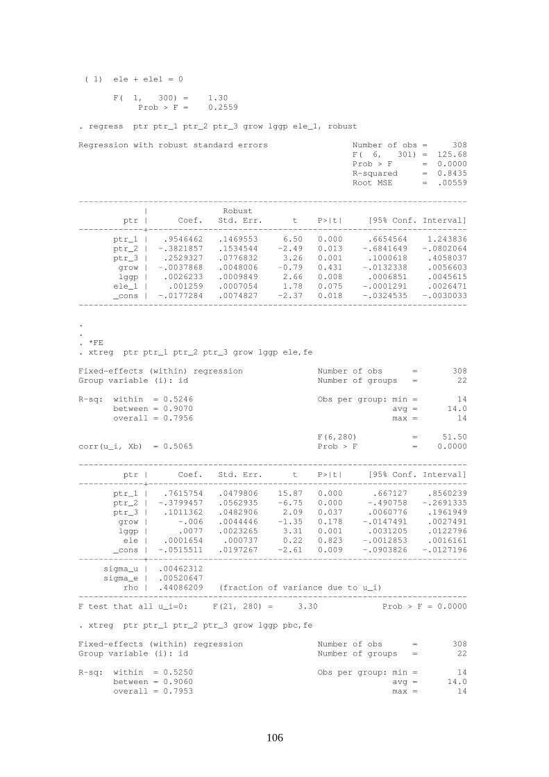
( 1) ele + ele1 = 0 F( 1, 300) = 1.30 Prob > F = 0.2559 . regress ptr ptr_1 ptr_2 ptr_3 grow lggp ele_1, robust Regression with robust standard errors Number of obs = 308 F( 6, 301) = 125.68 Prob > F = 0.0000 R-squared = 0.8435 Root MSE = .00559 ------------------------------------------------------------------------------ | Robust ptr | Coef. Std. Err. t P>|t| [95% Conf. Interval] -------------+---------------------------------------------------------------- ptr_1 | .9546462 .1469553 6.50 0.000 .6654564 1.243836 ptr_2 | -.3821857 .1534544 -2.49 0.013 -.6841649 -.0802064 ptr_3 | .2529327 .0776832 3.26 0.001 .1000618 .4058037 grow | -.0037868 .0048006 -0.79 0.431 -.0132338 .0056603 lggp | .0026233 .0009849 2.66 0.008 .0006851 .0045615 ele_1 | .001259 .0007054 1.78 0.075 -.0001291 .0026471 _cons | -.0177284 .0074827 -2.37 0.018 -.0324535 -.0030033 ------------------------------------------------------------------------------ . . . *FE . xtreg ptr ptr_1 ptr_2 ptr_3 grow lggp ele,fe Fixed-effects (within) regression Number of obs = 308 Group variable (i): id Number of groups = 22 R-sq: within = 0.5246 Obs per group: min = 14 between = 0.9070 avg = 14.0 overall = 0.7956 max = 14 F(6,280) = 51.50 corr(u_i, Xb) = 0.5065 Prob > F = 0.0000 ------------------------------------------------------------------------------ ptr | Coef. Std. Err. t P>|t| [95% Conf. Interval] -------------+---------------------------------------------------------------- ptr_1 | .7615754 .0479806 15.87 0.000 .667127 .8560239 ptr_2 | -.3799457 .0562935 -6.75 0.000 -.490758 -.2691335 ptr_3 | .1011362 .0482906 2.09 0.037 .0060776 .1961949 grow | -.006 .0044446 -1.35 0.178 -.0147491 .0027491 lggp | .0077 .0023265 3.31 0.001 .0031205 .0122796 ele | .0001654 .000737 0.22 0.823 -.0012853 .0016161 _cons | -.0515511 .0197267 -2.61 0.009 -.0903826 -.0127196 -------------+---------------------------------------------------------------- sigma_u | .00462312 sigma_e | .00520647 rho | .44086209 (fraction of variance due to u_i) ------------------------------------------------------------------------------ F test that all u_i=0: F(21, 280) = 3.30 Prob > F = 0.0000 . xtreg ptr ptr_1 ptr_2 ptr_3 grow lggp pbc,fe Fixed-effects (within) regression Number of obs = 308 Group variable (i): id Number of groups = 22 R-sq: within = 0.5250 Obs per group: min = 14 between = 0.9060 avg = 14.0 overall = 0.7953 max = 14
106

F(6,280) = 51.58 corr(u_i, Xb) = 0.5007 Prob > F = 0.0000 ------------------------------------------------------------------------------ ptr | Coef. Std. Err. t P>|t| [95% Conf. Interval] -------------+---------------------------------------------------------------- ptr_1 | .763964 .0478951 15.95 0.000 .6696838 .8582441 ptr_2 | -.3867665 .0560174 -6.90 0.000 -.4970352 -.2764978 ptr_3 | .1059282 .0484006 2.19 0.029 .010653 .2012035 grow | -.006467 .0044717 -1.45 0.149 -.0152695 .0023355 lggp | .0077662 .002328 3.34 0.001 .0031836 .0123488 pbc | -.0002204 .0004341 -0.51 0.612 -.0010749 .0006342 _cons | -.052095 .0197446 -2.64 0.009 -.0909617 -.0132284 -------------+---------------------------------------------------------------- sigma_u | .00461705 sigma_e | .00520454 rho | .44039739 (fraction of variance due to u_i) ------------------------------------------------------------------------------ F test that all u_i=0: F(21, 280) = 3.30 Prob > F = 0.0000 . xtreg ptr ptr_1 ptr_2 ptr_3 grow lggp ele ele1,fe Fixed-effects (within) regression Number of obs = 308 Group variable (i): id Number of groups = 22 R-sq: within = 0.5268 Obs per group: min = 14 between = 0.9050 avg = 14.0 overall = 0.7955 max = 14 F(7,279) = 44.36 corr(u_i, Xb) = 0.4922 Prob > F = 0.0000 ------------------------------------------------------------------------------ ptr | Coef. Std. Err. t P>|t| [95% Conf. Interval] -------------+---------------------------------------------------------------- ptr_1 | .7613549 .0479597 15.87 0.000 .6669461 .8557636 ptr_2 | -.3811856 .0562794 -6.77 0.000 -.4919719 -.2703994 ptr_3 | .1051559 .0484029 2.17 0.031 .0098746 .2004372 grow | -.006579 .0044727 -1.47 0.142 -.0153837 .0022256 lggp | .0078497 .0023293 3.37 0.001 .0032645 .0124349 ele | .0004351 .0007752 0.56 0.575 -.0010908 .001961 ele1 | .0007915 .0007082 1.12 0.265 -.0006026 .0021857 _cons | -.0531774 .0197716 -2.69 0.008 -.0920978 -.014257 -------------+---------------------------------------------------------------- sigma_u | .00459919 sigma_e | .00520415 rho | .4385246 (fraction of variance due to u_i) ------------------------------------------------------------------------------ F test that all u_i=0: F(21, 279) = 3.28 Prob > F = 0.0000 . test ele=-ele1 ( 1) ele + ele1 = 0 F( 1, 279) = 1.04 Prob > F = 0.3083 . xtreg ptr ptr_1 ptr_2 ptr_3 grow lggp ele_1, fe Fixed-effects (within) regression Number of obs = 308 Group variable (i): id Number of groups = 22 R-sq: within = 0.5281 Obs per group: min = 14 between = 0.9093 avg = 14.0 overall = 0.7978 max = 14 F(6,280) = 52.21 corr(u_i, Xb) = 0.5150 Prob > F = 0.0000
107
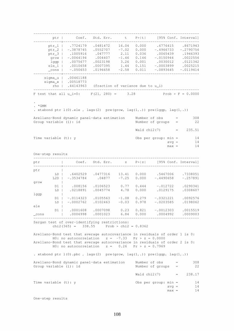
------------------------------------------------------------------------------ ptr | Coef. Std. Err. t P>|t| [95% Conf. Interval] -------------+---------------------------------------------------------------- ptr_1 | .7724179 .0481472 16.04 0.000 .6776415 .8671943 ptr_2 | -.3878745 .0552707 -7.02 0.000 -.4966733 -.2790756 ptr_3 | .1005916 .047777 2.11 0.036 .0065439 .1946393 grow | -.0064194 .004407 -1.46 0.146 -.0150944 .0022556 lggp | .0075677 .0023198 3.26 0.001 .0030012 .0121342 ele_1 | .0010658 .0007395 1.44 0.151 -.0003899 .0025215 _cons | -.050653 .0196658 -2.58 0.011 -.0893645 -.0119414 -------------+---------------------------------------------------------------- sigma_u | .00461188 sigma_e | .00518773 rho | .44143963 (fraction of variance due to u_i) ------------------------------------------------------------------------------ F test that all u_i=0: F(21, 280) = 3.28 Prob > F = 0.0000 . . *GMM . xtabond ptr l(0).ele , lags(2) pre(grow, lag(1,.)) pre(lggp, lag(1,.)) Arellano-Bond dynamic panel-data estimation Number of obs = 308 Group variable (i): id Number of groups = 22 Wald chi2(7) = 235.51 Time variable (t): y Obs per group: min = 14 avg = 14 max = 14 One-step results ------------------------------------------------------------------------------ ptr | Coef. Std. Err. z P>|z| [95% Conf. Interval] -------------+---------------------------------------------------------------- ptr | LD | .6402529 .0477316 13.41 0.000 .5467006 .7338051 L2D | -.3534784 .04877 -7.25 0.000 -.4490658 -.257891 grow | D1 | .008156 .0106523 0.77 0.444 -.012722 .0290341 LD | .0218891 .0045774 4.78 0.000 .0129175 .0308607 lggp | D1 | -.0114323 .0105563 -1.08 0.279 -.0321221 .0092576 LD | -.0002762 .0102463 -0.03 0.978 -.0203585 .0198062 ele | D1 | .0001608 .0007098 0.23 0.821 -.0012303 .0015519 _cons | .0006998 .0001023 6.84 0.000 .0004992 .0009003 ------------------------------------------------------------------------------ Sargan test of over-identifying restrictions: chi2(365) = 338.55 Prob > chi2 = 0.8362 Arellano-Bond test that average autocovariance in residuals of order 1 is 0: H0: no autocorrelation z = -7.33 Pr > z = 0.0000 Arellano-Bond test that average autocovariance in residuals of order 2 is 0: H0: no autocorrelation z = 0.26 Pr > z = 0.7969 . xtabond ptr l(0).pbc , lags(2) pre(grow, lag(1,.)) pre(lggp, lag(1,.)) Arellano-Bond dynamic panel-data estimation Number of obs = 308 Group variable (i): id Number of groups = 22 Wald chi2(7) = 238.17 Time variable (t): y Obs per group: min = 14 avg = 14 max = 14 One-step results
108
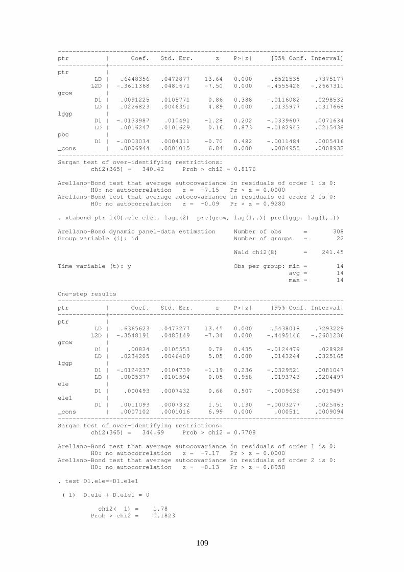
------------------------------------------------------------------------------ ptr | Coef. Std. Err. z P>|z| [95% Conf. Interval] -------------+---------------------------------------------------------------- ptr | LD | .6448356 .0472877 13.64 0.000 .5521535 .7375177 L2D | -.3611368 .0481671 -7.50 0.000 -.4555426 -.2667311 grow | D1 | .0091225 .0105771 0.86 0.388 -.0116082 .0298532 LD | .0226823 .0046351 4.89 0.000 .0135977 .0317668 lggp | D1 | -.0133987 .010491 -1.28 0.202 -.0339607 .0071634 LD | .0016247 .0101629 0.16 0.873 -.0182943 .0215438 pbc | D1 | -.0003034 .0004311 -0.70 0.482 -.0011484 .0005416 _cons | .0006944 .0001015 6.84 0.000 .0004955 .0008932 ------------------------------------------------------------------------------ Sargan test of over-identifying restrictions: chi2(365) = 340.42 Prob > chi2 = 0.8176 Arellano-Bond test that average autocovariance in residuals of order 1 is 0: H0: no autocorrelation z = -7.15 Pr > z = 0.0000 Arellano-Bond test that average autocovariance in residuals of order 2 is 0: H0: no autocorrelation z = -0.09 Pr > z = 0.9280 . xtabond ptr l(0).ele ele1, lags(2) pre(grow, lag(1,.)) pre(lggp, lag(1,.)) Arellano-Bond dynamic panel-data estimation Number of obs = 308 Group variable (i): id Number of groups = 22 Wald chi2(8) = 241.45 Time variable (t): y Obs per group: min = 14 avg = 14 max = 14 One-step results ------------------------------------------------------------------------------ ptr | Coef. Std. Err. z P>|z| [95% Conf. Interval] -------------+---------------------------------------------------------------- ptr | LD | .6365623 .0473277 13.45 0.000 .5438018 .7293229 L2D | -.3548191 .0483149 -7.34 0.000 -.4495146 -.2601236 grow | D1 | .00824 .0105553 0.78 0.435 -.0124479 .028928 LD | .0234205 .0046409 5.05 0.000 .0143244 .0325165 lggp | D1 | -.0124237 .0104739 -1.19 0.236 -.0329521 .0081047 LD | .0005377 .0101594 0.05 0.958 -.0193743 .0204497 ele | D1 | .000493 .0007432 0.66 0.507 -.0009636 .0019497 ele1 | D1 | .0011093 .0007332 1.51 0.130 -.0003277 .0025463 _cons | .0007102 .0001016 6.99 0.000 .000511 .0009094 ------------------------------------------------------------------------------ Sargan test of over-identifying restrictions: chi2(365) = 344.69 Prob > chi2 = 0.7708 Arellano-Bond test that average autocovariance in residuals of order 1 is 0: H0: no autocorrelation z = -7.17 Pr > z = 0.0000 Arellano-Bond test that average autocovariance in residuals of order 2 is 0: H0: no autocorrelation z = -0.13 Pr > z = 0.8958 . test D1.ele=-D1.ele1 ( 1) D.ele + D.ele1 = 0 chi2( 1) = 1.78 Prob > chi2 = 0.1823
109

. xtabond ptr l(0).ele_1 , lags(2) pre(grow, lag(1,.)) pre(lggp, lag(1,.)) Arellano-Bond dynamic panel-data estimation Number of obs = 308 Group variable (i): id Number of groups = 22 Wald chi2(7) = 240.63 Time variable (t): y Obs per group: min = 14 avg = 14 max = 14 One-step results ------------------------------------------------------------------------------ ptr | Coef. Std. Err. z P>|z| [95% Conf. Interval] -------------+---------------------------------------------------------------- ptr | LD | .654307 .0476871 13.72 0.000 .560842 .747772 L2D | -.3644378 .0477916 -7.63 0.000 -.4581075 -.2707681 grow | D1 | .0084525 .0105253 0.80 0.422 -.0121766 .0290816 LD | .0222522 .0045305 4.91 0.000 .0133725 .0311319 lggp | D1 | -.012632 .0102835 -1.23 0.219 -.0327874 .0075234 LD | .000438 .0099595 0.04 0.965 -.0190822 .0199582 ele_1 | D1 | .00121 .0007525 1.61 0.108 -.0002649 .002685 _cons | .0007078 .0001015 6.97 0.000 .0005087 .0009068 ------------------------------------------------------------------------------ Sargan test of over-identifying restrictions: chi2(365) = 338.54 Prob > chi2 = 0.8363 Arellano-Bond test that average autocovariance in residuals of order 1 is 0: H0: no autocorrelation z = -7.03 Pr > z = 0.0000 Arellano-Bond test that average autocovariance in residuals of order 2 is 0: H0: no autocorrelation z = -0.18 Pr > z = 0.8538
110
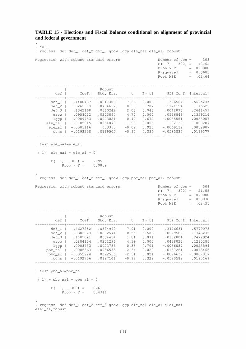
TABLE 15 - Elections and Fiscal Balance conditional on alignment of provincial and federal government . . *OLS . regress def def_1 def_2 def_3 grow lggp ele_nal ele_al, robust Regression with robust standard errors Number of obs = 308 F( 7, 300) = 18.62 Prob > F = 0.0000 R-squared = 0.3681 Root MSE = .02464 ------------------------------------------------------------------------------ | Robust def | Coef. Std. Err. t P>|t| [95% Conf. Interval] -------------+---------------------------------------------------------------- def_1 | .4480437 .0617306 7.26 0.000 .326564 .5695235 def_2 | .0265503 .0704657 0.38 0.707 -.1121194 .16522 def_3 | .1342168 .0660242 2.03 0.043 .0042876 .2641459 grow | .0958032 .0203864 4.70 0.000 .0556848 .1359216 lggp | .0009753 .0023021 0.42 0.672 -.0035551 .0055057 ele_nal | -.0105915 .0054873 -1.93 0.055 -.02139 .000207 ele_al | -.0003116 .003355 -0.09 0.926 -.0069139 .0062907 _cons | -.0193228 .0199505 -0.97 0.334 -.0585834 .0199377 ------------------------------------------------------------------------------ . test ele_nal=ele_al ( 1) ele_nal - ele_al = 0 F( 1, 300) = 2.95 Prob > F = 0.0869 . . regress def def_1 def_2 def_3 grow lggp pbc_nal pbc_al, robust Regression with robust standard errors Number of obs = 308 F( 7, 300) = 21.55 Prob > F = 0.0000 R-squared = 0.3830 Root MSE = .02435 ------------------------------------------------------------------------------ | Robust def | Coef. Std. Err. t P>|t| [95% Conf. Interval] -------------+---------------------------------------------------------------- def_1 | .4627852 .0584999 7.91 0.000 .3476631 .5779073 def_2 | .0383323 .0692571 0.55 0.580 -.0979589 .1746235 def_3 | .1185021 .0654454 1.81 0.071 -.0102881 .2472924 grow | .0884154 .0201296 4.39 0.000 .0488023 .1280285 lggp | .0008753 .0022786 0.38 0.701 -.0036087 .0053594 pbc_nal | -.0085363 .0036535 -2.34 0.020 -.0157261 -.0013465 pbc_al | -.0052224 .0022566 -2.31 0.021 -.0096632 -.0007817 _cons | -.0192706 .0197101 -0.98 0.329 -.0580582 .0195169 ------------------------------------------------------------------------------ . test pbc_al=pbc_nal ( 1) - pbc_nal + pbc_al = 0 F( 1, 300) = 0.61 Prob > F = 0.4344 . . regress def def_1 def_2 def_3 grow lggp ele_nal ele_al ele1_nal ele1_al,robust
111

Regression with robust standard errors Number of obs = 308 F( 9, 298) = 18.31 Prob > F = 0.0000 R-squared = 0.4024 Root MSE = .02405 ------------------------------------------------------------------------------ | Robust def | Coef. Std. Err. t P>|t| [95% Conf. Interval] -------------+---------------------------------------------------------------- def_1 | .4906409 .058432 8.40 0.000 .3756493 .6056326 def_2 | .0441476 .0669999 0.66 0.510 -.0877053 .1760005 def_3 | .0758215 .0661612 1.15 0.253 -.0543809 .2060238 grow | .0810632 .0194898 4.16 0.000 .0427081 .1194183 lggp | .0011404 .0022679 0.50 0.615 -.0033228 .0056036 ele_nal | -.0050489 .0054465 -0.93 0.355 -.0157674 .0056695 ele_al | .0053321 .0035467 1.50 0.134 -.0016477 .0123118 ele1_nal | .0126689 .0054326 2.33 0.020 .0019777 .0233601 ele1_al | .0149723 .0038884 3.85 0.000 .0073201 .0226245 _cons | -.0254291 .0198264 -1.28 0.201 -.0644465 .0135883 ------------------------------------------------------------------------------ . . . *FE . xtreg def def_1 def_2 def_3 grow lggp ele_nal ele_al,fe Fixed-effects (within) regression Number of obs = 308 Group variable (i): id Number of groups = 22 R-sq: within = 0.2217 Obs per group: min = 14 between = 0.1807 avg = 14.0 overall = 0.1970 max = 14 F(7,279) = 11.35 corr(u_i, Xb) = -0.2134 Prob > F = 0.0000 ------------------------------------------------------------------------------ def | Coef. Std. Err. t P>|t| [95% Conf. Interval] -------------+---------------------------------------------------------------- def_1 | .3167075 .0572156 5.54 0.000 .2040785 .4293366 def_2 | -.0525461 .0609854 -0.86 0.390 -.1725962 .0675039 def_3 | .0233805 .0574846 0.41 0.685 -.0897782 .1365391 grow | .081999 .0198999 4.12 0.000 .042826 .121172 lggp | .0241361 .0111286 2.17 0.031 .0022293 .0460428 ele_nal | -.0091026 .0056708 -1.61 0.110 -.0202657 .0020604 ele_al | -.0001709 .0040272 -0.04 0.966 -.0080984 .0077566 _cons | -.2259702 .0964533 -2.34 0.020 -.4158388 -.0361017 -------------+---------------------------------------------------------------- sigma_u | .01618276 sigma_e | .02380216 rho | .31612005 (fraction of variance due to u_i) ------------------------------------------------------------------------------ F test that all u_i=0: F(21, 279) = 2.03 Prob > F = 0.0056 . test ele_nal=ele_al ( 1) ele_nal - ele_al = 0 F( 1, 279) = 1.75 Prob > F = 0.1872 . . xtreg def def_1 def_2 def_3 grow lggp pbc_nal pbc_al,fe Fixed-effects (within) regression Number of obs = 308 Group variable (i): id Number of groups = 22
112

R-sq: within = 0.2419 Obs per group: min = 14 between = 0.1776 avg = 14.0 overall = 0.2087 max = 14 F(7,279) = 12.72 corr(u_i, Xb) = -0.2181 Prob > F = 0.0000 ------------------------------------------------------------------------------ def | Coef. Std. Err. t P>|t| [95% Conf. Interval] -------------+---------------------------------------------------------------- def_1 | .3298263 .0562128 5.87 0.000 .2191713 .4404813 def_2 | -.0418431 .0603655 -0.69 0.489 -.1606727 .0769866 def_3 | .0096215 .0564232 0.17 0.865 -.1014477 .1206908 grow | .0744957 .0198654 3.75 0.000 .0353906 .1136008 lggp | .0244439 .0109902 2.22 0.027 .0028096 .0460782 pbc_nal | -.0079502 .0031667 -2.51 0.013 -.014184 -.0017165 pbc_al | -.0047893 .0024372 -1.97 0.050 -.0095868 8.28e-06 _cons | -.2292877 .0952479 -2.41 0.017 -.4167835 -.0417919 -------------+---------------------------------------------------------------- sigma_u | .01627861 sigma_e | .02349101 rho | .32442006 (fraction of variance due to u_i) ------------------------------------------------------------------------------ F test that all u_i=0: F(21, 279) = 2.07 Prob > F = 0.0046 . test pbc_nal=pbc_al ( 1) pbc_nal - pbc_al = 0 F( 1, 279) = 0.63 Prob > F = 0.4279 . . xtreg def def_1 def_2 def_3 grow lggp ele_nal ele_al ele1_nal ele1_al,fe Fixed-effects (within) regression Number of obs = 308 Group variable (i): id Number of groups = 22 R-sq: within = 0.2661 Obs per group: min = 14 between = 0.1835 avg = 14.0 overall = 0.2266 max = 14 F(9,277) = 11.16 corr(u_i, Xb) = -0.2185 Prob > F = 0.0000 ------------------------------------------------------------------------------ def | Coef. Std. Err. t P>|t| [95% Conf. Interval] -------------+---------------------------------------------------------------- def_1 | .359114 .057382 6.26 0.000 .2461538 .4720742 def_2 | -.0344669 .0596956 -0.58 0.564 -.1519815 .0830478 def_3 | -.0320873 .0576502 -0.56 0.578 -.1455755 .0814008 grow | .0667094 .0197935 3.37 0.001 .0277446 .1056743 lggp | .0249521 .0108543 2.30 0.022 .0035848 .0463194 ele_nal | -.0041232 .0057258 -0.72 0.472 -.0153948 .0071483 ele_al | .0054027 .0041545 1.30 0.195 -.0027756 .0135811 ele1_nal | .0123814 .004699 2.63 0.009 .0031312 .0216316 ele1_al | .0142442 .0039573 3.60 0.000 .0064539 .0220345 _cons | -.2373958 .0941035 -2.52 0.012 -.4226447 -.0521468 -------------+---------------------------------------------------------------- sigma_u | .01625373 sigma_e | .02319634 rho | .32930193 (fraction of variance due to u_i) ------------------------------------------------------------------------------ F test that all u_i=0: F(21, 277) = 2.06 Prob > F = 0.0048 . . . *GMM
113

. xtabond def l(0).ele_nal ele_al , lags(2) pre(grow, lag(1,.)) pre(lggp, lag(1,.)) Arellano-Bond dynamic panel-data estimation Number of obs = 308 Group variable (i): id Number of groups = 22 Wald chi2(8) = 84.54 Time variable (t): y Obs per group: min = 14 avg = 14 max = 14 One-step results ------------------------------------------------------------------------------ def | Coef. Std. Err. z P>|z| [95% Conf. Interval] -------------+---------------------------------------------------------------- def | LD | .3408507 .0564977 6.03 0.000 .2301172 .4515842 L2D | -.0186403 .0556472 -0.33 0.738 -.1277068 .0904262 grow | D1 | .0517557 .046549 1.11 0.266 -.0394787 .14299 LD | .01787 .0204059 0.88 0.381 -.0221249 .0578649 lggp | D1 | .0419703 .0457179 0.92 0.359 -.0476351 .1315756 LD | -.0411702 .0442312 -0.93 0.352 -.1278618 .0455215 ele_nal | D1 | -.0083771 .0046536 -1.80 0.072 -.017498 .0007439 ele_al | D1 | .0003532 .0037823 0.09 0.926 -.00706 .0077664 _cons | .0006791 .0004395 1.55 0.122 -.0001823 .0015405 ------------------------------------------------------------------------------ Sargan test of over-identifying restrictions: chi2(365) = 283.40 Prob > chi2 = 0.9994 Arellano-Bond test that average autocovariance in residuals of order 1 is 0: H0: no autocorrelation z = -12.70 Pr > z = 0.0000 Arellano-Bond test that average autocovariance in residuals of order 2 is 0: H0: no autocorrelation z = -0.19 Pr > z = 0.8472 . test D1.ele_nal=D1.ele_al ( 1) D.ele_nal - D.ele_al = 0 chi2( 1) = 2.37 Prob > chi2 = 0.1238 . . xtabond def l(0).pbc_nal pbc_al , lags(2) pre(grow, lag(1,.)) pre(lggp, lag(1,.)) Arellano-Bond dynamic panel-data estimation Number of obs = 308 Group variable (i): id Number of groups = 22 Wald chi2(8) = 97.05 Time variable (t): y Obs per group: min = 14 avg = 14 max = 14 One-step results ------------------------------------------------------------------------------ def | Coef. Std. Err. z P>|z| [95% Conf. Interval] -------------+---------------------------------------------------------------- def | LD | .3503589 .0551863 6.35 0.000 .2421957 .4585221 L2D | -.007449 .0545239 -0.14 0.891 -.1143138 .0994158 grow | D1 | .0608424 .0457483 1.33 0.184 -.0288226 .1505074
114

LD | .0291702 .0203258 1.44 0.151 -.0106677 .0690081 lggp | D1 | .0237321 .0449345 0.53 0.597 -.064338 .1118021 LD | -.0261715 .0433608 -0.60 0.546 -.1111572 .0588142 pbc_nal | D1 | -.0090788 .0028501 -3.19 0.001 -.0146649 -.0034926 pbc_al | D1 | -.0042633 .0023424 -1.82 0.069 -.0088544 .0003277 _cons | .0007186 .0004287 1.68 0.094 -.0001216 .0015588 ------------------------------------------------------------------------------ Sargan test of over-identifying restrictions: chi2(365) = 284.92 Prob > chi2 = 0.9993 Arellano-Bond test that average autocovariance in residuals of order 1 is 0: H0: no autocorrelation z = -11.96 Pr > z = 0.0000 Arellano-Bond test that average autocovariance in residuals of order 2 is 0: H0: no autocorrelation z = 0.10 Pr > z = 0.9165 . test D1.pbc_nal=D1.pbc_al ( 1) D.pbc_nal - D.pbc_al = 0 chi2( 1) = 1.79 Prob > chi2 = 0.1810 . . xtabond def l(0).ele_nal ele_al ele1_nal ele1_al, lags(2) pre(grow, lag(1,.)) pre(lggp, lag(1,.)) Arellano-Bond dynamic panel-data estimation Number of obs = 308 Group variable (i): id Number of groups = 22 Wald chi2(10) = 106.17 Time variable (t): y Obs per group: min = 14 avg = 14 max = 14 One-step results ------------------------------------------------------------------------------ def | Coef. Std. Err. z P>|z| [95% Conf. Interval] -------------+---------------------------------------------------------------- def | LD | .3792731 .0566973 6.69 0.000 .2681484 .4903977 L2D | -.0182932 .0549103 -0.33 0.739 -.1259153 .0893289 grow | D1 | .0516656 .0459368 1.12 0.261 -.0383688 .1417 LD | .0337473 .0204248 1.65 0.098 -.0062846 .0737793 lggp | D1 | .0305162 .045106 0.68 0.499 -.0578899 .1189223 LD | -.0331017 .0435865 -0.76 0.448 -.1185297 .0523264 ele_nal | D1 | -.0034857 .0047616 -0.73 0.464 -.0128184 .0058469 ele_al | D1 | .0048919 .003899 1.25 0.210 -.00275 .0125339 ele1_nal | D1 | .0149939 .0047189 3.18 0.001 .0057451 .0242428 ele1_al | D1 | .0135665 .0039398 3.44 0.001 .0058446 .0212884 _cons | .0007661 .0004355 1.76 0.079 -.0000874 .0016196 ------------------------------------------------------------------------------ Sargan test of over-identifying restrictions: chi2(365) = 276.69 Prob > chi2 = 0.9998 Arellano-Bond test that average autocovariance in residuals of order 1 is 0: H0: no autocorrelation z = -12.24 Pr > z = 0.0000 Arellano-Bond test that average autocovariance in residuals of order 2 is 0: H0: no autocorrelation z = 1.08 Pr > z = 0.2792
115
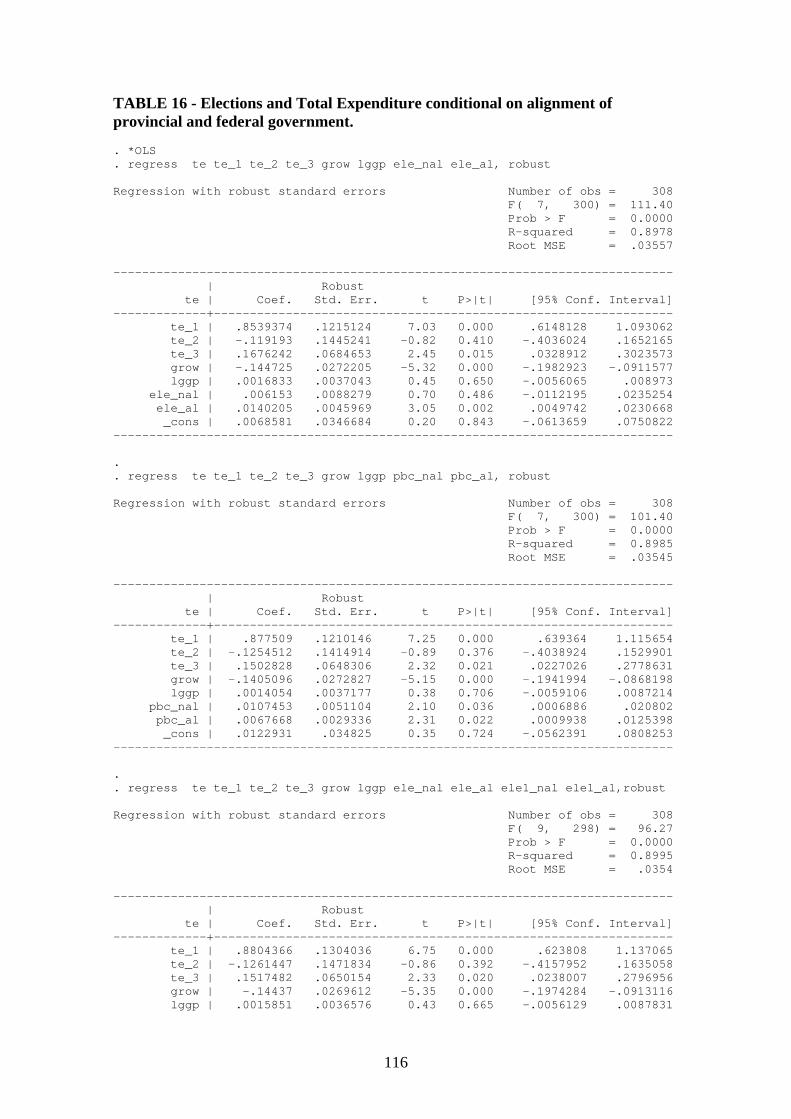
TABLE 16 - Elections and Total Expenditure conditional on alignment of provincial and federal government. . *OLS . regress te te_1 te_2 te_3 grow lggp ele_nal ele_al, robust Regression with robust standard errors Number of obs = 308 F( 7, 300) = 111.40 Prob > F = 0.0000 R-squared = 0.8978 Root MSE = .03557 ------------------------------------------------------------------------------ | Robust te | Coef. Std. Err. t P>|t| [95% Conf. Interval] -------------+---------------------------------------------------------------- te_1 | .8539374 .1215124 7.03 0.000 .6148128 1.093062 te_2 | -.119193 .1445241 -0.82 0.410 -.4036024 .1652165 te_3 | .1676242 .0684653 2.45 0.015 .0328912 .3023573 grow | -.144725 .0272205 -5.32 0.000 -.1982923 -.0911577 lggp | .0016833 .0037043 0.45 0.650 -.0056065 .008973 ele_nal | .006153 .0088279 0.70 0.486 -.0112195 .0235254 ele_al | .0140205 .0045969 3.05 0.002 .0049742 .0230668 _cons | .0068581 .0346684 0.20 0.843 -.0613659 .0750822 ------------------------------------------------------------------------------ . . regress te te_1 te_2 te_3 grow lggp pbc_nal pbc_al, robust Regression with robust standard errors Number of obs = 308 F( 7, 300) = 101.40 Prob > F = 0.0000 R-squared = 0.8985 Root MSE = .03545 ------------------------------------------------------------------------------ | Robust te | Coef. Std. Err. t P>|t| [95% Conf. Interval] -------------+---------------------------------------------------------------- te_1 | .877509 .1210146 7.25 0.000 .639364 1.115654 te_2 | -.1254512 .1414914 -0.89 0.376 -.4038924 .1529901 te_3 | .1502828 .0648306 2.32 0.021 .0227026 .2778631 grow | -.1405096 .0272827 -5.15 0.000 -.1941994 -.0868198 lggp | .0014054 .0037177 0.38 0.706 -.0059106 .0087214 pbc_nal | .0107453 .0051104 2.10 0.036 .0006886 .020802 pbc_al | .0067668 .0029336 2.31 0.022 .0009938 .0125398 _cons | .0122931 .034825 0.35 0.724 -.0562391 .0808253 ------------------------------------------------------------------------------ . . regress te te_1 te_2 te_3 grow lggp ele_nal ele_al ele1_nal ele1_al,robust Regression with robust standard errors Number of obs = 308 F( 9, 298) = 96.27 Prob > F = 0.0000 R-squared = 0.8995 Root MSE = .0354 ------------------------------------------------------------------------------ | Robust te | Coef. Std. Err. t P>|t| [95% Conf. Interval] -------------+---------------------------------------------------------------- te_1 | .8804366 .1304036 6.75 0.000 .623808 1.137065 te_2 | -.1261447 .1471834 -0.86 0.392 -.4157952 .1635058 te_3 | .1517482 .0650154 2.33 0.020 .0238007 .2796956 grow | -.14437 .0269612 -5.35 0.000 -.1974284 -.0913116 lggp | .0015851 .0036576 0.43 0.665 -.0056129 .0087831
116

ele_nal | .0033287 .0093622 0.36 0.722 -.0150957 .021753 ele_al | .0111605 .0052609 2.12 0.035 .0008072 .0215138 ele1_nal | -.0153207 .0079202 -1.93 0.054 -.0309073 .0002659 ele1_al | -.0027616 .0056323 -0.49 0.624 -.0138456 .0083225 _cons | .0097218 .0340566 0.29 0.775 -.0573001 .0767437 ------------------------------------------------------------------------------ . . . . *FE . xtreg te te_1 te_2 te_3 grow lggp ele_nal ele_al,fe Fixed-effects (within) regression Number of obs = 308 Group variable (i): id Number of groups = 22 R-sq: within = 0.3833 Obs per group: min = 14 between = 0.7705 avg = 14.0 overall = 0.6013 max = 14 F(7,279) = 24.77 corr(u_i, Xb) = 0.6281 Prob > F = 0.0000 ------------------------------------------------------------------------------ te | Coef. Std. Err. t P>|t| [95% Conf. Interval] -------------+---------------------------------------------------------------- te_1 | .4770493 .0472696 10.09 0.000 .3839988 .5700997 te_2 | -.1393148 .0525461 -2.65 0.008 -.2427519 -.0358777 te_3 | -.1056939 .041856 -2.53 0.012 -.1880876 -.0233002 grow | -.1187113 .022547 -5.27 0.000 -.1630951 -.0743274 lggp | -.0279396 .0127324 -2.19 0.029 -.0530034 -.0028758 ele_nal | .0004721 .0064768 0.07 0.942 -.0122776 .0132218 ele_al | .0082504 .0045688 1.81 0.072 -.0007434 .0172442 _cons | .4199735 .1145877 3.67 0.000 .1944072 .6455398 -------------+---------------------------------------------------------------- sigma_u | .08465536 sigma_e | .02712268 rho | .90690664 (fraction of variance due to u_i) ------------------------------------------------------------------------------ F test that all u_i=0: F(21, 279) = 11.29 Prob > F = 0.0000 . . xtreg te te_1 te_2 te_3 grow lggp pbc_nal pbc_al,fe Fixed-effects (within) regression Number of obs = 308 Group variable (i): id Number of groups = 22 R-sq: within = 0.3908 Obs per group: min = 14 between = 0.7483 avg = 14.0 overall = 0.5904 max = 14 F(7,279) = 25.57 corr(u_i, Xb) = 0.6123 Prob > F = 0.0000 ------------------------------------------------------------------------------ te | Coef. Std. Err. t P>|t| [95% Conf. Interval] -------------+---------------------------------------------------------------- te_1 | .4905815 .0472002 10.39 0.000 .3976677 .5834953 te_2 | -.1387299 .0517279 -2.68 0.008 -.2405564 -.0369033 te_3 | -.1196374 .0419784 -2.85 0.005 -.2022719 -.0370028 grow | -.1129704 .0225688 -5.01 0.000 -.1573971 -.0685437 lggp | -.0299444 .0126541 -2.37 0.019 -.054854 -.0050349 pbc_nal | .0073168 .0036847 1.99 0.048 .0000635 .0145702 pbc_al | .0048557 .0027983 1.74 0.084 -.0006527 .0103642 _cons | .4387467 .1137557 3.86 0.000 .2148183 .6626752 -------------+---------------------------------------------------------------- sigma_u | .08470989 sigma_e | .02695613
117

rho | .90804906 (fraction of variance due to u_i) ------------------------------------------------------------------------------ F test that all u_i=0: F(21, 279) = 11.42 Prob > F = 0.0000 . . xtreg te te_1 te_2 te_3 grow lggp ele_nal ele_al ele1_nal ele1_al,fe Fixed-effects (within) regression Number of obs = 308 Group variable (i): id Number of groups = 22 R-sq: within = 0.4004 Obs per group: min = 14 between = 0.7163 avg = 14.0 overall = 0.5684 max = 14 F(9,277) = 20.56 corr(u_i, Xb) = 0.5865 Prob > F = 0.0000 ------------------------------------------------------------------------------ te | Coef. Std. Err. t P>|t| [95% Conf. Interval] -------------+---------------------------------------------------------------- te_1 | .5054411 .0479296 10.55 0.000 .4110887 .5997936 te_2 | -.1485521 .0521958 -2.85 0.005 -.251303 -.0458013 te_3 | -.1251661 .0420609 -2.98 0.003 -.2079658 -.0423665 grow | -.1158163 .0225742 -5.13 0.000 -.160255 -.0713775 lggp | -.031298 .0126577 -2.47 0.014 -.0562155 -.0063804 ele_nal | -.0039277 .0065996 -0.60 0.552 -.0169194 .0090641 ele_al | .0055675 .0047452 1.17 0.242 -.0037738 .0149087 ele1_nal | -.015121 .0054274 -2.79 0.006 -.0258051 -.0044369 ele1_al | -.0044441 .0045695 -0.97 0.332 -.0134395 .0045513 _cons | .4521684 .1140153 3.97 0.000 .2277219 .6766149 -------------+---------------------------------------------------------------- sigma_u | .08531184 sigma_e | .02683879 rho | .90994223 (fraction of variance due to u_i) ------------------------------------------------------------------------------ F test that all u_i=0: F(21, 277) = 11.50 Prob > F = 0.0000 . . . *GMM . xtabond te l(0).ele_nal ele_al , lags(1) pre(grow, lag(2,.)) pre(lggp, lag(2,.)) Arellano-Bond dynamic panel-data estimation Number of obs = 286 Group variable (i): id Number of groups = 22 Wald chi2(9) = 218.00 Time variable (t): y Obs per group: min = 13 avg = 13 max = 13 One-step results ------------------------------------------------------------------------------ te | Coef. Std. Err. z P>|z| [95% Conf. Interval] -------------+---------------------------------------------------------------- te | LD | .3542436 .0342517 10.34 0.000 .2871114 .4213757 grow | D1 | -.0610862 .0510332 -1.20 0.231 -.1611095 .0389371 LD | -.0134358 .0516954 -0.26 0.795 -.114757 .0878853 L2D | .0458159 .0205939 2.22 0.026 .0054526 .0861792 lggp | D1 | -.0744527 .0501499 -1.48 0.138 -.1727447 .0238394 LD | .0327572 .052699 0.62 0.534 -.070531 .1360454 L2D | -.0438775 .04678 -0.94 0.348 -.1355646 .0478095 ele_nal | D1 | .0015802 .005632 0.28 0.779 -.0094584 .0126187
118

ele_al | D1 | .0101126 .0039015 2.59 0.010 .0024657 .0177595 _cons | .0032027 .000501 6.39 0.000 .0022207 .0041847 ------------------------------------------------------------------------------ Sargan test of over-identifying restrictions: chi2(357) = 354.41 Prob > chi2 = 0.5287 Arellano-Bond test that average autocovariance in residuals of order 1 is 0: H0: no autocorrelation z = -5.76 Pr > z = 0.0000 Arellano-Bond test that average autocovariance in residuals of order 2 is 0: H0: no autocorrelation z = -0.61 Pr > z = 0.5406 . . xtabond te l(0).pbc_nal pbc_al , lags(1) pre(grow, lag(2,.)) pre(lggp, lag(2,.)) Arellano-Bond dynamic panel-data estimation Number of obs = 286 Group variable (i): id Number of groups = 22 Wald chi2(9) = 213.11 Time variable (t): y Obs per group: min = 13 avg = 13 max = 13 One-step results ------------------------------------------------------------------------------ te | Coef. Std. Err. z P>|z| [95% Conf. Interval] -------------+---------------------------------------------------------------- te | LD | .3574712 .0346565 10.31 0.000 .2895457 .4253966 grow | D1 | -.058509 .0506359 -1.16 0.248 -.1577536 .0407356 LD | -.0090566 .0515688 -0.18 0.861 -.1101296 .0920164 L2D | .0446451 .0205946 2.17 0.030 .0042805 .0850097 lggp | D1 | -.0730087 .0496266 -1.47 0.141 -.1702751 .0242577 LD | .023525 .0532392 0.44 0.659 -.080822 .1278719 L2D | -.0334326 .0467877 -0.71 0.475 -.1251348 .0582695 pbc_nal | D1 | .003445 .0032815 1.05 0.294 -.0029866 .0098765 pbc_al | D1 | .0045548 .0024308 1.87 0.061 -.0002094 .009319 _cons | .0031332 .0005037 6.22 0.000 .002146 .0041205 ------------------------------------------------------------------------------ Sargan test of over-identifying restrictions: chi2(357) = 350.88 Prob > chi2 = 0.5813 Arellano-Bond test that average autocovariance in residuals of order 1 is 0: H0: no autocorrelation z = -5.66 Pr > z = 0.0000 Arellano-Bond test that average autocovariance in residuals of order 2 is 0: H0: no autocorrelation z = -0.59 Pr > z = 0.5567 . . xtabond te l(0).ele_nal ele_al ele1_nal ele1_al, lags(1) pre(grow, lag(2,.)) pre(lggp, lag(2,.)) Arellano-Bond dynamic panel-data estimation Number of obs = 286 Group variable (i): id Number of groups = 22 Wald chi2(11) = 219.12 Time variable (t): y Obs per group: min = 13 avg = 13 max = 13 One-step results ------------------------------------------------------------------------------
119

te | Coef. Std. Err. z P>|z| [95% Conf. Interval] -------------+---------------------------------------------------------------- te | LD | .3642079 .0349848 10.41 0.000 .2956389 .4327769 grow | D1 | -.0624094 .0513818 -1.21 0.225 -.1631159 .0382971 LD | -.007328 .0521566 -0.14 0.888 -.109553 .094897 L2D | .0470332 .0206934 2.27 0.023 .0064748 .0875916 lggp | D1 | -.0741531 .0503219 -1.47 0.141 -.1727822 .0244761 LD | .0255778 .0534345 0.48 0.632 -.0791519 .1303074 L2D | -.034831 .0478941 -0.73 0.467 -.1287016 .0590397 ele_nal | D1 | -.0000804 .0058109 -0.01 0.989 -.0114695 .0113087 ele_al | D1 | .010124 .0040844 2.48 0.013 .0021187 .0181294 ele1_nal | D1 | -.006566 .0048799 -1.35 0.178 -.0161304 .0029984 ele1_al | D1 | .0014815 .0039938 0.37 0.711 -.0063462 .0093092 _cons | .0031005 .0005069 6.12 0.000 .002107 .0040941 ------------------------------------------------------------------------------ Sargan test of over-identifying restrictions: chi2(357) = 352.06 Prob > chi2 = 0.5639 Arellano-Bond test that average autocovariance in residuals of order 1 is 0: H0: no autocorrelation z = -5.70 Pr > z = 0.0000 Arellano-Bond test that average autocovariance in residuals of order 2 is 0: H0: no autocorrelation z = -0.70 Pr > z = 0.4836 . .
120

TABLE 17 - Elections and Composition Effect conditional on alignment of provincial and federal government . . *OLS . regress ce ce_1 ce_2 ce_3 grow lggp ele_nal ele_al, robust Regression with robust standard errors Number of obs = 308 F( 7, 300) = 61.36 Prob > F = 0.0000 R-squared = 0.6031 Root MSE = .04835 ------------------------------------------------------------------------------ | Robust ce | Coef. Std. Err. t P>|t| [95% Conf. Interval] -------------+---------------------------------------------------------------- ce_1 | .5995961 .061782 9.71 0.000 .478015 .7211771 ce_2 | -.0213828 .0680687 -0.31 0.754 -.1553353 .1125698 ce_3 | .1608774 .0507902 3.17 0.002 .0609272 .2608277 grow | .0693663 .0414834 1.67 0.096 -.012269 .1510017 lggp | -.0080006 .0052204 -1.53 0.126 -.0182739 .0022727 ele_nal | .0190341 .0103003 1.85 0.066 -.0012359 .0393041 ele_al | -.0092474 .0079625 -1.16 0.246 -.0249168 .006422 _cons | .2947636 .0573407 5.14 0.000 .1819227 .4076045 ------------------------------------------------------------------------------ . . regress ce ce_1 ce_2 ce_3 grow lggp pbc_nal pbc_al, robust Regression with robust standard errors Number of obs = 308 F( 7, 300) = 59.98 Prob > F = 0.0000 R-squared = 0.5989 Root MSE = .0486 ------------------------------------------------------------------------------ | Robust ce | Coef. Std. Err. t P>|t| [95% Conf. Interval] -------------+---------------------------------------------------------------- ce_1 | .5976495 .0624706 9.57 0.000 .4747134 .7205857 ce_2 | -.0133118 .0690227 -0.19 0.847 -.1491417 .1225181 ce_3 | .1532459 .0522022 2.94 0.004 .0505171 .2559747 grow | .0601375 .0420054 1.43 0.153 -.0225249 .1428 lggp | -.0077647 .0052582 -1.48 0.141 -.0181124 .002583 pbc_nal | .001249 .0062511 0.20 0.842 -.0110525 .0135506 pbc_al | -.0068275 .0048365 -1.41 0.159 -.0163452 .0026903 _cons | .2940792 .0581322 5.06 0.000 .1796808 .4084777 ------------------------------------------------------------------------------ . regress ce ce_1 ce_2 ce_3 grow lggp ele_nal ele_al ele1_nal ele1_al, robust Regression with robust standard errors Number of obs = 308 F( 9, 298) = 46.85 Prob > F = 0.0000 R-squared = 0.6068 Root MSE = .04829 ------------------------------------------------------------------------------ | Robust ce | Coef. Std. Err. t P>|t| [95% Conf. Interval] -------------+---------------------------------------------------------------- ce_1 | .6113 .0640376 9.55 0.000 .4852768 .7373232 ce_2 | -.0117046 .0684177 -0.17 0.864 -.1463477 .1229385 ce_3 | .142987 .0521572 2.74 0.006 .0403439 .2456301 grow | .062752 .0411132 1.53 0.128 -.0181569 .1436609 lggp | -.0077523 .0051948 -1.49 0.137 -.0179754 .0024707 ele_nal | .0229098 .010766 2.13 0.034 .0017229 .0440968
121

ele_al | -.0054081 .0084171 -0.64 0.521 -.0219725 .0111564 ele1_nal | .0138903 .008527 1.63 0.104 -.0028904 .0306711 ele1_al | .0087037 .0078404 1.11 0.268 -.006726 .0241333 _cons | .285859 .0582352 4.91 0.000 .1712548 .4004633 ------------------------------------------------------------------------------ . . . regress ce ce_1 ce_2 ce_3 grow lggp ele_1_nal ele_1_al, robust Regression with robust standard errors Number of obs = 307 F( 7, 299) = 63.23 Prob > F = 0.0000 R-squared = 0.6059 Root MSE = .04819 ------------------------------------------------------------------------------ | Robust ce | Coef. Std. Err. t P>|t| [95% Conf. Interval] -------------+---------------------------------------------------------------- ce_1 | .6061938 .0635952 9.53 0.000 .4810429 .7313447 ce_2 | -.0017324 .0705638 -0.02 0.980 -.140597 .1371323 ce_3 | .1347668 .052169 2.58 0.010 .0321018 .2374317 grow | .0683599 .0405587 1.69 0.093 -.0114568 .1481766 lggp | -.0073873 .0050994 -1.45 0.148 -.0174227 .002648 ele_1_nal | -.0220308 .0109319 -2.02 0.045 -.043544 -.0005175 ele_1_al | -.017825 .007972 -2.24 0.026 -.0335135 -.0021366 _cons | .2932242 .0562071 5.22 0.000 .1826126 .4038359 ------------------------------------------------------------------------------ . . . *FE . xtreg ce ce_1 ce_2 ce_3 grow lggp ele_nal ele_al,fe Fixed-effects (within) regression Number of obs = 308 Group variable (i): id Number of groups = 22 R-sq: within = 0.3783 Obs per group: min = 14 between = 0.9245 avg = 14.0 overall = 0.5972 max = 14 F(7,279) = 24.25 corr(u_i, Xb) = 0.5238 Prob > F = 0.0000 ------------------------------------------------------------------------------ ce | Coef. Std. Err. t P>|t| [95% Conf. Interval] -------------+---------------------------------------------------------------- ce_1 | .5030042 .0552797 9.10 0.000 .3941859 .6118225 ce_2 | -.0473224 .0636497 -0.74 0.458 -.172617 .0779723 ce_3 | .1199319 .0527954 2.27 0.024 .016004 .2238597 grow | .0812057 .0384184 2.11 0.035 .005579 .1568324 lggp | -.0143168 .0223597 -0.64 0.523 -.058332 .0296984 ele_nal | .0195942 .0111393 1.76 0.080 -.0023335 .041522 ele_al | -.0072665 .0078704 -0.92 0.357 -.0227595 .0082264 _cons | .4806433 .179468 2.68 0.008 .1273599 .8339267 -------------+---------------------------------------------------------------- sigma_u | .02246686 sigma_e | .04652605 rho | .1890887 (fraction of variance due to u_i) ------------------------------------------------------------------------------ F test that all u_i=0: F(21, 279) = 2.14 Prob > F = 0.0030 . . xtreg ce ce_1 ce_2 ce_3 grow lggp pbc_nal pbc_al,fe Fixed-effects (within) regression Number of obs = 308 Group variable (i): id Number of groups = 22
122

R-sq: within = 0.3728 Obs per group: min = 14 between = 0.9206 avg = 14.0 overall = 0.5932 max = 14 F(7,279) = 23.69 corr(u_i, Xb) = 0.5188 Prob > F = 0.0000 ------------------------------------------------------------------------------ ce | Coef. Std. Err. t P>|t| [95% Conf. Interval] -------------+---------------------------------------------------------------- ce_1 | .4976502 .0549923 9.05 0.000 .3893977 .6059026 ce_2 | -.0399575 .0640558 -0.62 0.533 -.1660516 .0861366 ce_3 | .1173338 .0534622 2.19 0.029 .0120933 .2225743 grow | .0719694 .0390114 1.84 0.066 -.0048246 .1487634 lggp | -.0144201 .022424 -0.64 0.521 -.0585619 .0297217 pbc_nal | .0031389 .0063482 0.49 0.621 -.0093575 .0156353 pbc_al | -.0058203 .0048717 -1.19 0.233 -.0154103 .0037697 _cons | .4826527 .1801676 2.68 0.008 .1279922 .8373132 -------------+---------------------------------------------------------------- sigma_u | .02257763 sigma_e | .04673016 rho | .18925469 (fraction of variance due to u_i) ------------------------------------------------------------------------------ F test that all u_i=0: F(21, 279) = 2.17 Prob > F = 0.0026 . . xtreg ce ce_1 ce_2 ce_3 grow lggp ele_nal ele_al ele1_nal ele1_al,fe Fixed-effects (within) regression Number of obs = 308 Group variable (i): id Number of groups = 22 R-sq: within = 0.3827 Obs per group: min = 14 between = 0.9392 avg = 14.0 overall = 0.6028 max = 14 F(9,277) = 19.08 corr(u_i, Xb) = 0.5487 Prob > F = 0.0000 ------------------------------------------------------------------------------ ce | Coef. Std. Err. t P>|t| [95% Conf. Interval] -------------+---------------------------------------------------------------- ce_1 | .5139267 .0558756 9.20 0.000 .4039319 .6239214 ce_2 | -.0404036 .0639201 -0.63 0.528 -.1662344 .0854273 ce_3 | .1033572 .0541931 1.91 0.058 -.0033254 .2100397 grow | .0736409 .039063 1.89 0.060 -.003257 .1505389 lggp | -.0115245 .0224492 -0.51 0.608 -.0557172 .0326683 ele_nal | .0232328 .0114591 2.03 0.044 .0006748 .0457908 ele_al | -.004182 .0082449 -0.51 0.612 -.0204127 .0120487 ele1_nal | .0107419 .0091966 1.17 0.244 -.0073623 .028846 ele1_al | .007824 .0079533 0.98 0.326 -.0078327 .0234806 _cons | .4522695 .180622 2.50 0.013 .0967033 .8078357 -------------+---------------------------------------------------------------- sigma_u | .02229704 sigma_e | .04652836 rho | .1867579 (fraction of variance due to u_i) ------------------------------------------------------------------------------ F test that all u_i=0: F(21, 277) = 2.09 Prob > F = 0.0040 . . xtreg ce ce_1 ce_2 ce_3 grow lggp ele_1_nal ele_1_al,fe Fixed-effects (within) regression Number of obs = 307 Group variable (i): id Number of groups = 22 R-sq: within = 0.3874 Obs per group: min = 13 between = 0.9402 avg = 14.0 overall = 0.6023 max = 14
123

F(7,278) = 25.12 corr(u_i, Xb) = 0.5479 Prob > F = 0.0000 ------------------------------------------------------------------------------ ce | Coef. Std. Err. t P>|t| [95% Conf. Interval] -------------+---------------------------------------------------------------- ce_1 | .5036629 .0545102 9.24 0.000 .3963578 .610968 ce_2 | -.0270155 .0627164 -0.43 0.667 -.1504749 .0964439 ce_3 | .0968443 .0536343 1.81 0.072 -.0087365 .2024252 grow | .0764725 .0380743 2.01 0.046 .001522 .151423 lggp | -.0093118 .022347 -0.42 0.677 -.0533026 .0346789 ele_1_nal | -.0253947 .0111714 -2.27 0.024 -.047386 -.0034034 ele_1_al | -.0151406 .0078785 -1.92 0.056 -.0306498 .0003686 _cons | .4433675 .1794741 2.47 0.014 .0900666 .7966684 -------------+---------------------------------------------------------------- sigma_u | .02271984 sigma_e | .04624685 rho | .19442504 (fraction of variance due to u_i) ------------------------------------------------------------------------------ F test that all u_i=0: F(21, 278) = 2.22 Prob > F = 0.0019 . . *GMM . xtabond ce l(0).ele_nal ele_al , lags(1) pre(grow, lag(2,.)) pre(lggp, lag(2,.)) Arellano-Bond dynamic panel-data estimation Number of obs = 286 Group variable (i): id Number of groups = 22 Wald chi2(9) = 116.02 Time variable (t): y Obs per group: min = 13 avg = 13 max = 13 One-step results ------------------------------------------------------------------------------ ce | Coef. Std. Err. z P>|z| [95% Conf. Interval] -------------+---------------------------------------------------------------- ce | LD | .4244163 .0481967 8.81 0.000 .3299525 .5188802 grow | D1 | .0437274 .0978521 0.45 0.655 -.1480591 .2355139 LD | -.0248147 .0993933 -0.25 0.803 -.219622 .1699925 L2D | -.1247953 .0389633 -3.20 0.001 -.2011619 -.0484286 lggp | D1 | .0241884 .0960115 0.25 0.801 -.1639907 .2123675 LD | -.0579368 .1011588 -0.57 0.567 -.2562044 .1403308 L2D | -.0017364 .0898229 -0.02 0.985 -.177786 .1743132 ele_nal | D1 | .0198176 .010916 1.82 0.069 -.0015773 .0412126 ele_al | D1 | -.0084013 .0074824 -1.12 0.262 -.0230664 .0062639 _cons | .0035316 .0010719 3.29 0.001 .0014307 .0056326 ------------------------------------------------------------------------------ Sargan test of over-identifying restrictions: chi2(357) = 235.44 Prob > chi2 = 1.0000 Arellano-Bond test that average autocovariance in residuals of order 1 is 0: H0: no autocorrelation z = -8.11 Pr > z = 0.0000 Arellano-Bond test that average autocovariance in residuals of order 2 is 0: H0: no autocorrelation z = -0.09 Pr > z = 0.9250 . . xtabond ce l(0).pbc_nal pbc_al , lags(1) pre(grow, lag(2,.)) pre(lggp, lag(2,.))
124

Arellano-Bond dynamic panel-data estimation Number of obs = 286 Group variable (i): id Number of groups = 22 Wald chi2(9) = 112.68 Time variable (t): y Obs per group: min = 13 avg = 13 max = 13 One-step results ------------------------------------------------------------------------------ ce | Coef. Std. Err. z P>|z| [95% Conf. Interval] -------------+---------------------------------------------------------------- ce | LD | .41893 .0483384 8.67 0.000 .3241886 .5136715 grow | D1 | .0658286 .0973504 0.68 0.499 -.1249746 .2566318 LD | -.0115323 .0994981 -0.12 0.908 -.206545 .1834804 L2D | -.1214897 .0391498 -3.10 0.002 -.1982219 -.0447574 lggp | D1 | -.0120289 .0951552 -0.13 0.899 -.1985297 .1744719 LD | -.0310876 .1026825 -0.30 0.762 -.2323417 .1701664 L2D | .0020614 .0902111 0.02 0.982 -.1747491 .1788719 pbc_nal | D1 | .0012497 .0062639 0.20 0.842 -.0110272 .0135267 pbc_al | D1 | -.0073465 .0046828 -1.57 0.117 -.0165246 .0018316 _cons | .0036662 .0010789 3.40 0.001 .0015517 .0057808 ------------------------------------------------------------------------------ Sargan test of over-identifying restrictions: chi2(357) = 230.71 Prob > chi2 = 1.0000 Arellano-Bond test that average autocovariance in residuals of order 1 is 0: H0: no autocorrelation z = -8.15 Pr > z = 0.0000 Arellano-Bond test that average autocovariance in residuals of order 2 is 0: H0: no autocorrelation z = 0.01 Pr > z = 0.9897 . . . xtabond ce l(0).ele_1_nal ele_1_al , lags(1) pre(grow, lag(2,.)) pre(lggp, lag(2,.)) Arellano-Bond dynamic panel-data estimation Number of obs = 285 Group variable (i): id Number of groups = 22 Wald chi2(9) = 114.89 Time variable (t): y Obs per group: min = 12 avg = 12.95455 max = 13 One-step results ------------------------------------------------------------------------------ ce | Coef. Std. Err. z P>|z| [95% Conf. Interval] -------------+---------------------------------------------------------------- ce | LD | .428159 .0488848 8.76 0.000 .3323466 .5239713 grow | D1 | .0587193 .096841 0.61 0.544 -.1310856 .2485241 LD | -.0271393 .0998154 -0.27 0.786 -.2227739 .1684954 L2D | -.1077007 .0399224 -2.70 0.007 -.1859472 -.0294542 lggp | D1 | .0098829 .0941948 0.10 0.916 -.1747356 .1945015 LD | -.0340245 .1004902 -0.34 0.735 -.2309816 .1629326 L2D | -.0076788 .0901485 -0.09 0.932 -.1843667 .169009 ele_1_nal | D1 | -.0214231 .0109311 -1.96 0.050 -.0428476 1.45e-06 ele_1_al |
125

D1 | -.0089575 .0077136 -1.16 0.246 -.0240759 .0061609 _cons | .0034386 .0010808 3.18 0.001 .0013202 .005557 ------------------------------------------------------------------------------ Sargan test of over-identifying restrictions: chi2(357) = 233.23 Prob > chi2 = 1.0000 Arellano-Bond test that average autocovariance in residuals of order 1 is 0: H0: no autocorrelation z = -8.04 Pr > z = 0.0000 Arellano-Bond test that average autocovariance in residuals of order 2 is 0: H0: no autocorrelation z = -0.01 Pr > z = 0.9901 . .
126

TABLE 18 - Elections and Total Revenue conditional on alignment of provincial and federal government . . *OLS . regress tr tr_1 tr_2 tr_3 grow lggp ele_nal ele_al, robust Regression with robust standard errors Number of obs = 308 F( 7, 300) = 62.69 Prob > F = 0.0000 R-squared = 0.8932 Root MSE = .03307 ------------------------------------------------------------------------------ | Robust tr | Coef. Std. Err. t P>|t| [95% Conf. Interval] -------------+---------------------------------------------------------------- tr_1 | 1.009453 .1677577 6.02 0.000 .6793225 1.339584 tr_2 | -.2862726 .2245212 -1.28 0.203 -.7281084 .1555632 tr_3 | .1631853 .0863944 1.89 0.060 -.0068305 .3332011 grow | -.0519202 .0272518 -1.91 0.058 -.1055491 .0017087 lggp | .0008989 .0030511 0.29 0.768 -.0051053 .0069032 ele_nal | .0004781 .0063636 0.08 0.940 -.0120449 .0130011 ele_al | .0162604 .0048283 3.37 0.001 .0067587 .0257621 _cons | .0122643 .0301458 0.41 0.684 -.0470598 .0715883 ------------------------------------------------------------------------------ . . regress tr tr_1 tr_2 tr_3 grow lggp pbc_nal pbc_al, robust Regression with robust standard errors Number of obs = 308 F( 7, 300) = 58.50 Prob > F = 0.0000 R-squared = 0.8905 Root MSE = .0335 ------------------------------------------------------------------------------ | Robust tr | Coef. Std. Err. t P>|t| [95% Conf. Interval] -------------+---------------------------------------------------------------- tr_1 | 1.012568 .1688137 6.00 0.000 .6803589 1.344777 tr_2 | -.3035379 .2220007 -1.37 0.173 -.7404138 .1333379 tr_3 | .1742855 .0845343 2.06 0.040 .0079302 .3406408 grow | -.0524522 .0278074 -1.89 0.060 -.1071745 .0022701 lggp | .0006539 .0031627 0.21 0.836 -.00557 .0068779 pbc_nal | -.0000464 .0047776 -0.01 0.992 -.0094483 .0093554 pbc_al | .0039302 .0033777 1.16 0.246 -.0027167 .0105772 _cons | .0175292 .0311409 0.56 0.574 -.043753 .0788114 ------------------------------------------------------------------------------ . . regress tr tr_1 tr_2 tr_3 grow lggp ele_nal ele_al ele1_nal ele1_al,robust Regression with robust standard errors Number of obs = 308 F( 9, 298) = 62.76 Prob > F = 0.0000 R-squared = 0.8945 Root MSE = .03298 ------------------------------------------------------------------------------ | Robust tr | Coef. Std. Err. t P>|t| [95% Conf. Interval] -------------+---------------------------------------------------------------- tr_1 | .9943475 .1721787 5.78 0.000 .6555074 1.333188 tr_2 | -.2661339 .2315013 -1.15 0.251 -.7217184 .1894505 tr_3 | .1605942 .0873215 1.84 0.067 -.0112508 .3324392 grow | -.0585203 .0272922 -2.14 0.033 -.11223 -.0048105 lggp | .0010462 .0030872 0.34 0.735 -.0050293 .0071216
127

ele_nal | .0031448 .0068274 0.46 0.645 -.0102913 .0165809 ele_al | .0189662 .0052129 3.64 0.000 .0087075 .0292249 ele1_nal | .0038419 .0078429 0.49 0.625 -.0115927 .0192765 ele1_al | .0102612 .0058747 1.75 0.082 -.0012999 .0218224 _cons | .0078894 .0300726 0.26 0.793 -.0512923 .067071 ------------------------------------------------------------------------------ . . . *FE . xtreg tr tr_1 tr_2 tr_3 grow lggp ele_nal ele_al,fe Fixed-effects (within) regression Number of obs = 308 Group variable (i): id Number of groups = 22 R-sq: within = 0.5016 Obs per group: min = 14 between = 0.9384 avg = 14.0 overall = 0.5627 max = 14 F(7,279) = 40.12 corr(u_i, Xb) = 0.6027 Prob > F = 0.0000 ------------------------------------------------------------------------------ tr | Coef. Std. Err. t P>|t| [95% Conf. Interval] -------------+---------------------------------------------------------------- tr_1 | .6013849 .0411699 14.61 0.000 .5203418 .6824281 tr_2 | -.2775477 .0485447 -5.72 0.000 -.3731081 -.1819873 tr_3 | -.1328645 .0380194 -3.49 0.001 -.2077059 -.0580231 grow | -.0574305 .0184644 -3.11 0.002 -.0937778 -.0210832 lggp | -.0069166 .0099524 -0.69 0.488 -.0265079 .0126748 ele_nal | -.0067297 .0053694 -1.25 0.211 -.0172995 .00384 ele_al | .0108026 .0037947 2.85 0.005 .0033327 .0182725 _cons | .2286671 .0877537 2.61 0.010 .0559237 .4014106 -------------+---------------------------------------------------------------- sigma_u | .08015312 sigma_e | .02249053 rho | .92701321 (fraction of variance due to u_i) ------------------------------------------------------------------------------ F test that all u_i=0: F(21, 279) = 17.60 Prob > F = 0.0000 . . xtreg tr tr_1 tr_2 tr_3 grow lggp pbc_nal pbc_al,fe Fixed-effects (within) regression Number of obs = 308 Group variable (i): id Number of groups = 22 R-sq: within = 0.4847 Obs per group: min = 14 between = 0.9476 avg = 14.0 overall = 0.5585 max = 14 F(7,279) = 37.48 corr(u_i, Xb) = 0.6039 Prob > F = 0.0000 ------------------------------------------------------------------------------ tr | Coef. Std. Err. t P>|t| [95% Conf. Interval] -------------+---------------------------------------------------------------- tr_1 | .5974332 .0420769 14.20 0.000 .5146046 .6802617 tr_2 | -.2845449 .0491842 -5.79 0.000 -.3813642 -.1877256 tr_3 | -.1274304 .0387248 -3.29 0.001 -.2036604 -.0512004 grow | -.0575113 .0189014 -3.04 0.003 -.0947189 -.0203038 lggp | -.0072853 .0101497 -0.72 0.473 -.0272649 .0126944 pbc_nal | -.0014398 .0030999 -0.46 0.643 -.0075419 .0046623 pbc_al | .0014785 .0023797 0.62 0.535 -.0032059 .0061629 _cons | .2340775 .0894564 2.62 0.009 .0579824 .4101727 -------------+---------------------------------------------------------------- sigma_u | .08050632 sigma_e | .02287047 rho | .92532352 (fraction of variance due to u_i)
128

------------------------------------------------------------------------------ F test that all u_i=0: F(21, 279) = 17.36 Prob > F = 0.0000 . regress tr tr_1 tr_2 tr_3 grow lggp ele_nal ele_al ele1_nal ele1_al,robust Regression with robust standard errors Number of obs = 308 F( 9, 298) = 62.76 Prob > F = 0.0000 R-squared = 0.8945 Root MSE = .03298 ------------------------------------------------------------------------------ | Robust tr | Coef. Std. Err. t P>|t| [95% Conf. Interval] -------------+---------------------------------------------------------------- tr_1 | .9943475 .1721787 5.78 0.000 .6555074 1.333188 tr_2 | -.2661339 .2315013 -1.15 0.251 -.7217184 .1894505 tr_3 | .1605942 .0873215 1.84 0.067 -.0112508 .3324392 grow | -.0585203 .0272922 -2.14 0.033 -.11223 -.0048105 lggp | .0010462 .0030872 0.34 0.735 -.0050293 .0071216 ele_nal | .0031448 .0068274 0.46 0.645 -.0102913 .0165809 ele_al | .0189662 .0052129 3.64 0.000 .0087075 .0292249 ele1_nal | .0038419 .0078429 0.49 0.625 -.0115927 .0192765 ele1_al | .0102612 .0058747 1.75 0.082 -.0012999 .0218224 _cons | .0078894 .0300726 0.26 0.793 -.0512923 .067071 ------------------------------------------------------------------------------ . . . *GMM . xtabond tr l(0).ele_nal ele_al , lags(1) pre(grow, lag(2,.)) pre(lggp, lag(2,.)) Arellano-Bond dynamic panel-data estimation Number of obs = 286 Group variable (i): id Number of groups = 22 Wald chi2(9) = 183.08 Time variable (t): y Obs per group: min = 13 avg = 13 max = 13 One-step results ------------------------------------------------------------------------------ tr | Coef. Std. Err. z P>|z| [95% Conf. Interval] -------------+---------------------------------------------------------------- tr | LD | .3500565 .0315188 11.11 0.000 .2882808 .4118322 grow | D1 | .0255954 .0458895 0.56 0.577 -.0643463 .1155372 LD | .0594925 .0465128 1.28 0.201 -.0316708 .1506559 L2D | .0162432 .0187645 0.87 0.387 -.0205345 .0530209 lggp | D1 | -.056169 .0450179 -1.25 0.212 -.1444025 .0320646 LD | -.0451783 .0473647 -0.95 0.340 -.1380113 .0476548 L2D | .0365996 .0421273 0.87 0.385 -.0459684 .1191676 ele_nal | D1 | -.0061026 .0051061 -1.20 0.232 -.0161104 .0039052 ele_al | D1 | .0090788 .0035288 2.57 0.010 .0021624 .0159951 _cons | .0033951 .000453 7.49 0.000 .0025072 .004283 ------------------------------------------------------------------------------ Sargan test of over-identifying restrictions: chi2(357) = 364.10 Prob > chi2 = 0.3863 Arellano-Bond test that average autocovariance in residuals of order 1 is 0: H0: no autocorrelation z = -4.47 Pr > z = 0.0000 Arellano-Bond test that average autocovariance in residuals of order 2 is 0:
129

H0: no autocorrelation z = -0.75 Pr > z = 0.4523 . xtabond tr l(0).pbc_nal pbc_al , lags(1) pre(grow, lag(2,.)) pre(lggp, lag(2,.)) Arellano-Bond dynamic panel-data estimation Number of obs = 286 Group variable (i): id Number of groups = 22 Wald chi2(9) = 179.14 Time variable (t): y Obs per group: min = 13 avg = 13 max = 13 One-step results ------------------------------------------------------------------------------ tr | Coef. Std. Err. z P>|z| [95% Conf. Interval] -------------+---------------------------------------------------------------- tr | LD | .3357761 .0313136 10.72 0.000 .2744025 .3971497 grow | D1 | .032752 .045178 0.72 0.468 -.0557953 .1212992 LD | .0583417 .0461052 1.27 0.206 -.0320229 .1487062 L2D | .012797 .0186396 0.69 0.492 -.023736 .04933 lggp | D1 | -.0671218 .0441787 -1.52 0.129 -.1537104 .0194668 LD | -.0295629 .0476002 -0.62 0.535 -.1228577 .0637318 L2D | .0305214 .0419206 0.73 0.467 -.0516415 .1126843 pbc_nal | D1 | -.0057203 .002923 -1.96 0.050 -.0114493 8.76e-06 pbc_al | D1 | -.0003357 .0021771 -0.15 0.877 -.0046029 .0039314 _cons | .0034825 .0004526 7.69 0.000 .0025953 .0043696 ------------------------------------------------------------------------------ Sargan test of over-identifying restrictions: chi2(357) = 373.00 Prob > chi2 = 0.2693 Arellano-Bond test that average autocovariance in residuals of order 1 is 0: H0: no autocorrelation z = -4.21 Pr > z = 0.0000 Arellano-Bond test that average autocovariance in residuals of order 2 is 0: H0: no autocorrelation z = -1.09 Pr > z = 0.2770 . . xtabond tr l(0). ele_nal ele_al ele1_nal ele1_al, lags(1) pre(grow, lag(2,.)) pre(lggp, lag(2,.)) Arellano-Bond dynamic panel-data estimation Number of obs = 286 Group variable (i): id Number of groups = 22 Wald chi2(11) = 212.53 Time variable (t): y Obs per group: min = 13 avg = 13 max = 13 One-step results ------------------------------------------------------------------------------ tr | Coef. Std. Err. z P>|z| [95% Conf. Interval] -------------+---------------------------------------------------------------- tr | LD | .3475647 .0306374 11.34 0.000 .2875165 .4076128 grow | D1 | .009285 .0446843 0.21 0.835 -.0782947 .0968646 LD | .0445231 .0453884 0.98 0.327 -.0444364 .1334827 L2D | .0122236 .0182512 0.67 0.503 -.0235482 .0479954 lggp | D1 | -.0521419 .0436858 -1.19 0.233 -.1377644 .0334807 LD | -.0207505 .0464785 -0.45 0.655 -.1118467 .0703457
130

L2D | .0066651 .0417441 0.16 0.873 -.0751518 .088482 ele_nal | D1 | -.0024982 .0050867 -0.49 0.623 -.0124679 .0074715 ele_al | D1 | .01353 .0035753 3.78 0.000 .0065226 .0205374 ele1_nal | D1 | .0089831 .0041688 2.15 0.031 .0008125 .0171537 ele1_al | D1 | .013825 .0034746 3.98 0.000 .007015 .020635 _cons | .0034533 .0004423 7.81 0.000 .0025864 .0043202 ------------------------------------------------------------------------------ Sargan test of over-identifying restrictions: chi2(357) = 369.15 Prob > chi2 = 0.3175 Arellano-Bond test that average autocovariance in residuals of order 1 is 0: H0: no autocorrelation z = -4.46 Pr > z = 0.0000 Arellano-Bond test that average autocovariance in residuals of order 2 is 0: H0: no autocorrelation z = -0.58 Pr > z = 0.5640 . .
131

TABLE 19 - Elections and Revenue from Federal Government conditional on alignment of provincial and federal government . *OLS . regress fr fr_1 fr_2 fr_3 grow lggp ele_nal ele_al, robust Regression with robust standard errors Number of obs = 308 F( 7, 300) = 115.80 Prob > F = 0.0000 R-squared = 0.9061 Root MSE = .03036 ------------------------------------------------------------------------------ | Robust fr | Coef. Std. Err. t P>|t| [95% Conf. Interval] -------------+---------------------------------------------------------------- fr_1 | 1.00824 .1446013 6.97 0.000 .7236783 1.292801 fr_2 | -.2187173 .1986039 -1.10 0.272 -.6095505 .172116 fr_3 | .1128744 .0775378 1.46 0.147 -.0397124 .2654612 grow | -.0507363 .0249693 -2.03 0.043 -.0998733 -.0015992 lggp | -.0002838 .0030505 -0.09 0.926 -.0062868 .0057192 ele_nal | .0006585 .0058137 0.11 0.910 -.0107823 .0120993 ele_al | .0165713 .0045323 3.66 0.000 .0076522 .0254904 _cons | .016237 .0300383 0.54 0.589 -.0428754 .0753494 ------------------------------------------------------------------------------ . . regress fr fr_1 fr_2 fr_3 grow lggp pbc_nal pbc_al, robust Regression with robust standard errors Number of obs = 308 F( 7, 300) = 103.34 Prob > F = 0.0000 R-squared = 0.9032 Root MSE = .03083 ------------------------------------------------------------------------------ | Robust fr | Coef. Std. Err. t P>|t| [95% Conf. Interval] -------------+---------------------------------------------------------------- fr_1 | 1.010338 .1464464 6.90 0.000 .722146 1.298531 fr_2 | -.2361745 .1991115 -1.19 0.237 -.6280066 .1556575 fr_3 | .1252573 .0767807 1.63 0.104 -.0258397 .2763543 grow | -.0509198 .025696 -1.98 0.048 -.101487 -.0003526 lggp | -.0005945 .0031477 -0.19 0.850 -.0067889 .0055998 pbc_nal | .0003441 .0041343 0.08 0.934 -.0077919 .00848 pbc_al | .0042087 .0032478 1.30 0.196 -.0021827 .0106002 _cons | .0220303 .0309912 0.71 0.478 -.0389573 .083018 ------------------------------------------------------------------------------ . regress fr fr_1 fr_2 fr_3 grow lggp ele_nal ele_al ele1_nal ele1_al,robust Regression with robust standard errors Number of obs = 308 F( 9, 298) = 99.72 Prob > F = 0.0000 R-squared = 0.9074 Root MSE = .03027 ------------------------------------------------------------------------------ | Robust fr | Coef. Std. Err. t P>|t| [95% Conf. Interval] -------------+---------------------------------------------------------------- fr_1 | .9900392 .149949 6.60 0.000 .6949461 1.285132 fr_2 | -.1932028 .2066576 -0.93 0.351 -.5998959 .2134902 fr_3 | .1078675 .0783245 1.38 0.169 -.0462716 .2620066 grow | -.0573516 .0251816 -2.28 0.023 -.1069079 -.0077953 lggp | -.0001107 .0030843 -0.04 0.971 -.0061803 .005959 ele_nal | .0031823 .0061115 0.52 0.603 -.0088448 .0152094
132

ele_al | .0190761 .0048024 3.97 0.000 .0096253 .028527 ele1_nal | .0032 .0066132 0.48 0.629 -.0098146 .0162145 ele1_al | .009921 .00539 1.84 0.067 -.0006863 .0205283 _cons | .011899 .0300007 0.40 0.692 -.0471411 .0709391 ------------------------------------------------------------------------------ . . . . *FE . xtreg fr fr_1 fr_2 fr_3 grow lggp ele_nal ele_al,fe Fixed-effects (within) regression Number of obs = 308 Group variable (i): id Number of groups = 22 R-sq: within = 0.4671 Obs per group: min = 14 between = 0.8886 avg = 14.0 overall = 0.6649 max = 14 F(7,279) = 34.93 corr(u_i, Xb) = 0.6902 Prob > F = 0.0000 ------------------------------------------------------------------------------ fr | Coef. Std. Err. t P>|t| [95% Conf. Interval] -------------+---------------------------------------------------------------- fr_1 | .5892793 .043795 13.46 0.000 .5030687 .6754899 fr_2 | -.213446 .0514539 -4.15 0.000 -.3147332 -.1121589 fr_3 | -.1464361 .0392417 -3.73 0.000 -.2236835 -.0691887 grow | -.0468293 .0173763 -2.70 0.007 -.0810345 -.0126241 lggp | -.0148224 .0094936 -1.56 0.120 -.0335106 .0038657 ele_nal | -.0065903 .0050604 -1.30 0.194 -.0165518 .0033711 ele_al | .0110163 .003586 3.07 0.002 .0039571 .0180754 _cons | .26652 .0838845 3.18 0.002 .1013932 .4316469 -------------+---------------------------------------------------------------- sigma_u | .07481693 sigma_e | .02122926 rho | .92548566 (fraction of variance due to u_i) ------------------------------------------------------------------------------ F test that all u_i=0: F(21, 279) = 15.94 Prob > F = 0.0000 . . xtreg fr fr_1 fr_2 fr_3 grow lggp pbc_nal pbc_al,fe Fixed-effects (within) regression Number of obs = 308 Group variable (i): id Number of groups = 22 R-sq: within = 0.4463 Obs per group: min = 14 between = 0.8889 avg = 14.0 overall = 0.6600 max = 14 F(7,279) = 32.12 corr(u_i, Xb) = 0.6910 Prob > F = 0.0000 ------------------------------------------------------------------------------ fr | Coef. Std. Err. t P>|t| [95% Conf. Interval] -------------+---------------------------------------------------------------- fr_1 | .5818032 .0449729 12.94 0.000 .4932739 .6703324 fr_2 | -.2199583 .0524566 -4.19 0.000 -.3232193 -.1166973 fr_3 | -.1392907 .0400564 -3.48 0.001 -.2181419 -.0604395 grow | -.0467731 .0178366 -2.62 0.009 -.0818846 -.0116617 lggp | -.015308 .0096994 -1.58 0.116 -.0344012 .0037852 pbc_nal | -.001471 .0029299 -0.50 0.616 -.0072385 .0042964 pbc_al | .0015274 .0022599 0.68 0.500 -.0029212 .0059759 _cons | .2730504 .0856513 3.19 0.002 .1044455 .4416554 -------------+---------------------------------------------------------------- sigma_u | .07530624 sigma_e | .02163946 rho | .92372636 (fraction of variance due to u_i)
133

------------------------------------------------------------------------------ F test that all u_i=0: F(21, 279) = 15.72 Prob > F = 0.0000 . . xtreg tr tr_1 tr_2 tr_3 grow lggp ele_nal ele_al ele1_nal ele1_al,fe Fixed-effects (within) regression Number of obs = 308 Group variable (i): id Number of groups = 22 R-sq: within = 0.5132 Obs per group: min = 14 between = 0.9240 avg = 14.0 overall = 0.5583 max = 14 F(9,277) = 32.45 corr(u_i, Xb) = 0.5952 Prob > F = 0.0000 ------------------------------------------------------------------------------ tr | Coef. Std. Err. t P>|t| [95% Conf. Interval] -------------+---------------------------------------------------------------- tr_1 | .5905748 .0411159 14.36 0.000 .5096354 .6715142 tr_2 | -.2586676 .0487209 -5.31 0.000 -.3545778 -.1627575 tr_3 | -.1376176 .0378614 -3.63 0.000 -.2121502 -.063085 grow | -.0641876 .0185117 -3.47 0.001 -.1006291 -.0277461 lggp | -.0067447 .0099218 -0.68 0.497 -.0262765 .0127871 ele_nal | -.0058484 .0054614 -1.07 0.285 -.0165995 .0049027 ele_al | .0133248 .0039312 3.39 0.001 .005586 .0210636 ele1_nal | -.0001588 .0043569 -0.04 0.971 -.0087357 .008418 ele1_al | .0095074 .0037683 2.52 0.012 .0020894 .0169255 _cons | .2246446 .0875908 2.56 0.011 .0522164 .3970729 -------------+---------------------------------------------------------------- sigma_u | .08014266 sigma_e | .02230825 rho | .92808936 (fraction of variance due to u_i) ------------------------------------------------------------------------------ F test that all u_i=0: F(21, 277) = 17.83 Prob > F = 0.0000 . . *GMM . xtabond fr l(0).ele_nal ele_al, lags(1) pre(grow, lag(2,.)) pre(lggp, lag(2,.)) Arellano-Bond dynamic panel-data estimation Number of obs = 286 Group variable (i): id Number of groups = 22 Wald chi2(9) = 185.37 Time variable (t): y Obs per group: min = 13 avg = 13 max = 13 One-step results ------------------------------------------------------------------------------ fr | Coef. Std. Err. z P>|z| [95% Conf. Interval] -------------+---------------------------------------------------------------- fr | LD | .3738862 .0329054 11.36 0.000 .3093929 .4383795 grow | D1 | .0229733 .0429132 0.54 0.592 -.061135 .1070815 LD | .0590242 .0435073 1.36 0.175 -.0262485 .144297 L2D | .0055715 .0174559 0.32 0.750 -.0286414 .0397844 lggp | D1 | -.0627462 .0421046 -1.49 0.136 -.1452697 .0197773 LD | -.0372138 .0443214 -0.84 0.401 -.1240821 .0496545 L2D | .0462688 .0394034 1.17 0.240 -.0309605 .123498 ele_nal | D1 | -.0064311 .0047781 -1.35 0.178 -.015796 .0029338 ele_al | D1 | .0082487 .0033091 2.49 0.013 .001763 .0147344
134

_cons | .002559 .0004199 6.09 0.000 .001736 .0033819 ------------------------------------------------------------------------------ Sargan test of over-identifying restrictions: chi2(357) = 346.63 Prob > chi2 = 0.6431 Arellano-Bond test that average autocovariance in residuals of order 1 is 0: H0: no autocorrelation z = -5.19 Pr > z = 0.0000 Arellano-Bond test that average autocovariance in residuals of order 2 is 0: H0: no autocorrelation z = -0.36 Pr > z = 0.7156 . . . xtabond fr l(0).pbc_nal pbc_al, lags(1) pre(grow, lag(2,.)) pre(lggp, lag(2,.)) Arellano-Bond dynamic panel-data estimation Number of obs = 286 Group variable (i): id Number of groups = 22 Wald chi2(9) = 179.93 Time variable (t): y Obs per group: min = 13 avg = 13 max = 13 One-step results ------------------------------------------------------------------------------ fr | Coef. Std. Err. z P>|z| [95% Conf. Interval] -------------+---------------------------------------------------------------- fr | LD | .3576535 .0327499 10.92 0.000 .2934649 .4218421 grow | D1 | .0281981 .0423676 0.67 0.506 -.0548409 .1112371 LD | .0574934 .0432459 1.33 0.184 -.0272671 .1422538 L2D | .0023443 .0173902 0.13 0.893 -.0317399 .0364285 lggp | D1 | -.0715109 .0414332 -1.73 0.084 -.1527186 .0096967 LD | -.0241315 .0446573 -0.54 0.589 -.1116582 .0633951 L2D | .0403942 .0393127 1.03 0.304 -.0366572 .1174456 pbc_nal | D1 | -.0051577 .0027407 -1.88 0.060 -.0105293 .0002139 pbc_al | D1 | -.0004197 .0020449 -0.21 0.837 -.0044275 .0035881 _cons | .0026318 .0004205 6.26 0.000 .0018076 .003456 ------------------------------------------------------------------------------ Sargan test of over-identifying restrictions: chi2(357) = 353.74 Prob > chi2 = 0.5387 Arellano-Bond test that average autocovariance in residuals of order 1 is 0: H0: no autocorrelation z = -5.04 Pr > z = 0.0000 Arellano-Bond test that average autocovariance in residuals of order 2 is 0: H0: no autocorrelation z = -0.58 Pr > z = 0.5629 . . xtabond fr l(0).ele_nal ele_al ele1_nal ele1_al , lags(1) pre(grow, lag(2,.)) pre(lggp, lag(2,.)) Arellano-Bond dynamic panel-data estimation Number of obs = 286 Group variable (i): id Number of groups = 22 Wald chi2(11) = 211.37 Time variable (t): y Obs per group: min = 13 avg = 13 max = 13 One-step results ------------------------------------------------------------------------------ fr | Coef. Std. Err. z P>|z| [95% Conf. Interval]
135

-------------+---------------------------------------------------------------- fr | LD | .3721047 .0321465 11.58 0.000 .3090987 .4351108 grow | D1 | .0082227 .0420188 0.20 0.845 -.0741327 .090578 LD | .0460954 .042689 1.08 0.280 -.0375735 .1297644 L2D | .0019717 .0170738 0.12 0.908 -.0314923 .0354358 lggp | D1 | -.0592305 .0410833 -1.44 0.149 -.1397522 .0212912 LD | -.0157837 .0437323 -0.36 0.718 -.1014974 .0699301 L2D | .0202422 .039256 0.52 0.606 -.0566981 .0971825 ele_nal | D1 | -.0033791 .0047862 -0.71 0.480 -.0127598 .0060017 ele_al | D1 | .0122515 .0033712 3.63 0.000 .0056441 .0188589 ele1_nal | D1 | .007472 .0039281 1.90 0.057 -.0002269 .015171 ele1_al | D1 | .0126459 .0032706 3.87 0.000 .0062357 .0190561 _cons | .0025978 .0004122 6.30 0.000 .00179 .0034056 ------------------------------------------------------------------------------ Sargan test of over-identifying restrictions: chi2(357) = 347.76 Prob > chi2 = 0.6270 Arellano-Bond test that average autocovariance in residuals of order 1 is 0: H0: no autocorrelation z = -5.30 Pr > z = 0.0000 Arellano-Bond test that average autocovariance in residuals of order 2 is 0: H0: no autocorrelation z = -0.04 Pr > z = 0.9697
136

TABLE 20 - Elections and Revenue from Provincial Taxes conditional on alignment of provincial and federal government . . *OLS . regress ptr ptr_1 ptr_2 ptr_3 grow lggp ele_nal ele_al, robust Regression with robust standard errors Number of obs = 308 F( 7, 300) = 112.99 Prob > F = 0.0000 R-squared = 0.8422 Root MSE = .00562 ------------------------------------------------------------------------------ | Robust ptr | Coef. Std. Err. t P>|t| [95% Conf. Interval] -------------+---------------------------------------------------------------- ptr_1 | .9428694 .1447413 6.51 0.000 .6580326 1.227706 ptr_2 | -.3730106 .157066 -2.37 0.018 -.6821013 -.06392 ptr_3 | .2532924 .0795903 3.18 0.002 .0966665 .4099184 grow | -.0033364 .0048706 -0.69 0.494 -.0129213 .0062485 lggp | .002668 .0009754 2.74 0.007 .0007486 .0045874 ele_nal | .0002664 .0009324 0.29 0.775 -.0015684 .0021012 ele_al | .0001219 .0008605 0.14 0.887 -.0015715 .0018152 _cons | -.0178357 .0074739 -2.39 0.018 -.0325436 -.0031278 ------------------------------------------------------------------------------ . regress ptr ptr_1 ptr_2 ptr_3 grow lggp pbc_nal pbc_al, robust Regression with robust standard errors Number of obs = 308 F( 7, 300) = 113.08 Prob > F = 0.0000 R-squared = 0.8425 Root MSE = .00561 ------------------------------------------------------------------------------ | Robust ptr | Coef. Std. Err. t P>|t| [95% Conf. Interval] -------------+---------------------------------------------------------------- ptr_1 | .9464471 .1443851 6.56 0.000 .6623113 1.230583 ptr_2 | -.3815714 .1550447 -2.46 0.014 -.6866842 -.0764585 ptr_3 | .258749 .0803934 3.22 0.001 .1005425 .4169555 grow | -.0039578 .0048465 -0.82 0.415 -.0134952 .0055795 lggp | .0026596 .0009787 2.72 0.007 .0007337 .0045855 pbc_nal | -1.40e-06 .0010759 -0.00 0.999 -.0021186 .0021158 pbc_al | -.0004472 .0004581 -0.98 0.330 -.0013488 .0004544 _cons | -.0177302 .0074854 -2.37 0.018 -.0324607 -.0029997 ------------------------------------------------------------------------------ . . . . *FE . xtreg ptr ptr_1 ptr_2 ptr_3 grow lggp ele_nal ele_al,fe Fixed-effects (within) regression Number of obs = 308 Group variable (i): id Number of groups = 22 R-sq: within = 0.5246 Obs per group: min = 14 between = 0.9070 avg = 14.0 overall = 0.7956 max = 14 F(7,279) = 43.99 corr(u_i, Xb) = 0.5065 Prob > F = 0.0000 ------------------------------------------------------------------------------ ptr | Coef. Std. Err. t P>|t| [95% Conf. Interval] -------------+----------------------------------------------------------------
137

ptr_1 | .7615601 .0481035 15.83 0.000 .6668682 .8562519 ptr_2 | -.3799494 .0563961 -6.74 0.000 -.4909653 -.2689334 ptr_3 | .1011669 .0485239 2.08 0.038 .0056476 .1966863 grow | -.006 .0044526 -1.35 0.179 -.0147649 .002765 lggp | .0077006 .0023316 3.30 0.001 .0031108 .0122904 ele_nal | .0001572 .0012493 0.13 0.900 -.002302 .0026164 ele_al | .0001693 .0008805 0.19 0.848 -.001564 .0019026 _cons | -.0515562 .0197718 -2.61 0.010 -.090477 -.0126353 -------------+---------------------------------------------------------------- sigma_u | .0046232 sigma_e | .00521579 rho | .43998939 (fraction of variance due to u_i) ------------------------------------------------------------------------------ F test that all u_i=0: F(21, 279) = 3.29 Prob > F = 0.0000 . xtreg ptr ptr_1 ptr_2 ptr_3 grow lggp pbc_nal pbc_al,fe Fixed-effects (within) regression Number of obs = 308 Group variable (i): id Number of groups = 22 R-sq: within = 0.5253 Obs per group: min = 14 between = 0.9071 avg = 14.0 overall = 0.7959 max = 14 F(7,279) = 44.11 corr(u_i, Xb) = 0.5064 Prob > F = 0.0000 ------------------------------------------------------------------------------ ptr | Coef. Std. Err. t P>|t| [95% Conf. Interval] -------------+---------------------------------------------------------------- ptr_1 | .7649158 .0480094 15.93 0.000 .6704092 .8594224 ptr_2 | -.3871655 .0561041 -6.90 0.000 -.4976065 -.2767245 ptr_3 | .1051567 .0484995 2.17 0.031 .0096853 .2006281 grow | -.0065774 .0044847 -1.47 0.144 -.0154056 .0022508 lggp | .0076987 .0023361 3.30 0.001 .0031001 .0122973 pbc_nal | .0000305 .0007047 0.04 0.965 -.0013567 .0014178 pbc_al | -.0003677 .0005432 -0.68 0.499 -.0014369 .0007016 _cons | -.0514966 .0198169 -2.60 0.010 -.0905062 -.012487 -------------+---------------------------------------------------------------- sigma_u | .00462108 sigma_e | .00521195 rho | .44012564 (fraction of variance due to u_i) ------------------------------------------------------------------------------ F test that all u_i=0: F(21, 279) = 3.28 Prob > F = 0.0000 . . *GMM . . xtabond ptr l(0).ele_nal ele_al , lags(2) pre(grow, lag(1,.)) pre(lggp, lag(1,.)) Arellano-Bond dynamic panel-data estimation Number of obs = 308 Group variable (i): id Number of groups = 22 Wald chi2(8) = 235.98 Time variable (t): y Obs per group: min = 14 avg = 14 max = 14 One-step results ------------------------------------------------------------------------------ ptr | Coef. Std. Err. z P>|z| [95% Conf. Interval] -------------+---------------------------------------------------------------- ptr | LD | .6402771 .0477628 13.41 0.000 .5466637 .7338905 L2D | -.3542546 .0488073 -7.26 0.000 -.4499151 -.2585941 grow |
138

D1 | .0076223 .0106768 0.71 0.475 -.0133037 .0285484 LD | .02173 .0045843 4.74 0.000 .0127449 .0307151 lggp | D1 | -.0107819 .01059 -1.02 0.309 -.0315378 .0099741 LD | -.0010354 .0102877 -0.10 0.920 -.021199 .0191281 ele_nal | D1 | .0008757 .0010659 0.82 0.411 -.0012133 .0029648 ele_al | D1 | -.0002924 .0008692 -0.34 0.737 -.0019959 .0014111 _cons | .0007099 .0001029 6.90 0.000 .0005083 .0009115 ------------------------------------------------------------------------------ Sargan test of over-identifying restrictions: chi2(365) = 337.35 Prob > chi2 = 0.8475 Arellano-Bond test that average autocovariance in residuals of order 1 is 0: H0: no autocorrelation z = -7.37 Pr > z = 0.0000 Arellano-Bond test that average autocovariance in residuals of order 2 is 0: H0: no autocorrelation z = 0.33 Pr > z = 0.7379 . xtabond ptr l(0).pbc_nal pbc_al , lags(2) pre(grow, lag(1,.)) pre(lggp, lag(1,.)) Arellano-Bond dynamic panel-data estimation Number of obs = 308 Group variable (i): id Number of groups = 22 Wald chi2(8) = 237.61 Time variable (t): y Obs per group: min = 14 avg = 14 max = 14 One-step results ------------------------------------------------------------------------------ ptr | Coef. Std. Err. z P>|z| [95% Conf. Interval] -------------+---------------------------------------------------------------- ptr | LD | .6454538 .0474125 13.61 0.000 .552527 .7383806 L2D | -.3618317 .0482875 -7.49 0.000 -.4564735 -.2671898 grow | D1 | .0083689 .0106442 0.79 0.432 -.0124934 .0292311 LD | .0224597 .0046561 4.82 0.000 .0133338 .0315856 lggp | D1 | -.0128237 .0105429 -1.22 0.224 -.0334874 .00784 LD | .0010048 .0102152 0.10 0.922 -.0190166 .0210261 pbc_nal | D1 | .0000999 .0006629 0.15 0.880 -.0011993 .0013992 pbc_al | D1 | -.0005707 .0005444 -1.05 0.295 -.0016377 .0004963 _cons | .0006956 .0001017 6.84 0.000 .0004963 .0008948 ------------------------------------------------------------------------------ Sargan test of over-identifying restrictions: chi2(365) = 338.36 Prob > chi2 = 0.8380 Arellano-Bond test that average autocovariance in residuals of order 1 is 0: H0: no autocorrelation z = -7.19 Pr > z = 0.0000 Arellano-Bond test that average autocovariance in residuals of order 2 is 0: H0: no autocorrelation z = -0.02 Pr > z = 0.9852 .
139


