School of Economics and Business

Department of Applied Economics

PhD Program in Applied Economics

Three essays on the determinants of

labor market dynamics

PhD dissertation

Dario S. Judzik

Advisor

Hector Sala Lorda

Universitat Autònoma de Barcelona

March 2014

.

2

Acknowledgements

I am grateful to the Spanish Ministry of Education, Culture and Sports for financial

support through grant FPU code AP2008-02662. I would like to express my gratitude to

Hector Sala for his insightful supervision of the research activity presented in this doctoral

dissertation. He has been a remarkable teacher and guide during this vital era.

Special thanks are in order to my office and PhD program companions for their contri-

bution through advice during long coffee talks. Roberto Dopeso, Monica Oviedo, Natalia

Nollenberger, Paula Herrera, Paola Rocchi, Pedro Trivin, Alicia Gomez and Luciana

Mendez, amongst others, were important people throughout the process.

I am also thankful to the academic and administrative staff of the Applied Economics

Department (Universitat Autònoma de Barcelona). I would like to mention as well the

members of the School of Economics and Finance of Queen Mary University of London

that kindly hosted my research visit.

The most unconditional support during the production of this work has been provided

by my family without whom I could not have concluded this dissertation. To them, my

most sincere appreciation and recognition.

And to Natalia, for being next to me in crucial times, my endless gratitude.

3

Contents

Introduction and main results 5

Essay 1: Productivity, deunionization and trade: Wage effects 14

and labor share implications.

1. Introduction 15

2. Analytical framework 20

3. Econometric Analysis 25

4. Simulations 32

5. Conclusions 40

References 41

Appendix 46

Essay 2: The determinants of capital intensity in Japan 47

and the U.S.

1. Introduction 48

2. Analytical framework 50

3. Empirical issues 55

4. Results 60

5. Simulations 65

6. Concluding remarks 69

References 70

Appendix 73

Essay 3: Heterogeneous labor demand: sectoral elasticity and 76

trade effects in the U.S., Germany and Sweden.

1. Introduction 77

2. Stylized characterization of sectoral employment and trade 80

3. Analytical framework 83

4. Econometric analysis 87

5. Results 92

6. Concluding remarks 102

References 104

Appendix 108

4

Introduction and main results

This section provides an introduction to this PhD thesis in three parts: a general motiva-

tion for the study of labor market macroeconomics, a description of the scientific relevance

of the topics studied, an overview of the main results, and finally, some policy implications

of these results.

The rest of the dissertation is structured as follows. Three essays on the determinants

of labor market dynamics are presented as three main chapters. Each one of these essays

has a research paper structure: introduction and motivations, theoretical underpinnings,

empirical model and results, discussion or further exploration of the results, and conclud-

ing remarks. This introductory section also operates as a brief summary of the results

obtained and discussed throughout the dissertation.

1 Motivation

The labor market recovery from the massive economic recession unleashed in 2008 has

shown to be tricky. The U.S. is a good example, where the employment rate as of mid-

2013 had still not reached its pre-crisis level. Also Spain, where unemployment is still

scaling on sky-high levels of unemployment (26% in the third quarter of 20131). But this

is not the case everywhere. Some countries, like Germany, are experiencing growth in the

employment rate for a few years now, with a remarkable performance during the turmoil

of the Great Recession.

This dissertation brings some new insights into why we observe these highly different

paths in labor market outcomes across countries. In previous decades, there was an

“unemployment problem” in Europe. Analysts wondered what was different in the U.S.

than in Europe to explain such persistent gap on the time-paths of the unemployment

rate. Unemployment was steadily higher in Europe, in contrast to the U.S., apparently

because of the institutional set up. In other words, the European welfare state and its

employment protection mechanisms were keeping unemployment higher than it could be

at a given level of technology and productivity. Labor market institutions became the

usual suspects of Europe’s unemployment problem, and then the standard knowledge

became that the reduction in employment protection and benefits would provide better

incentives, allowing employment to rise.

The behavior of labor markets in the aftermath of the Great Recession is putting this

standard policy advice to trial. It looks like the paradigm may change. Recent work

by Freeman (2013) shows how the flexible job machine that the U.S. had been for more

1Source: INE (www.ine.es).

5

than a decade is being closely examined since it is not performing as it should. The

job-less recovery in the U.S. comes across as unexpected. The diagnostics get even worse

when comparing with the “German miracle” or other “less flexible” and more “institution-

oriented” economies and their noteworthy labor market performance in the last few years.

As stressed by Schettkat (2010), new questions are arising. Markets were supposed

to be fully efficient and the private sector to be wiser and outperform the public sector,

monetary policy was supposed to be neutral to the real economy, and expansive fiscal

policy was supposed to be ineffective because consumers’ rationale implies full transpar-

ent knowledge that public debt is followed by tax increases (i.e. what is known as the

Ricardian equivalence). However, we find ourselves with growing labor market problems

such as high and resistant unemployment rates.

This dissertation is motivated from the scientific urge to learn more about the dynamics

behind labor market outcomes. From this perspective we take into account some of the

questions in today’s economic debate and bring them to the analysis. We observe different

time-paths of unemployment. It is clear that among developed countries labor market

performances are heterogeneous. Then, what are the forces behind unemployment that

may help in explaining these differences? Should we also question some of the standard

assumptions in economic analysis? What can we learn from the experience? Maybe

economics should be based more on actual facts and less on beliefs. In words of Nobel

laureate Robert Solow: “It ain’t the things you don’t know that hurt you, it’s the things

you know that ain’t so” (Solow, 1997).

2 Relevance of this study

This PhD thesis presents empirical investigations and international comparison of la-

bor market performances. The scenario just described calls for the study of the forces

underlying unemployment dynamics. The unemployment rate is the final output of all

labor market kinematics where these forces take place. In a nutshell, the main objective

throughout the thesis is to learn more about how labor markets work.

To that end it is crucial to look into the evolution of employment. On one hand,

this dissertation studies the forces behind wage determination, a crucial variable to labor

demand since the real wage affects hiring and firing decisions. Also, sector-level employ-

ment is analyzed. We compute the sectoral elasticity of labor demand, and investigate

the employment effect of openness to international trade. Sector-level analysis is critical

for the study of aggregate results as stated by Young (2013). On the other hand, this

thesis studies the degree of substitutability between labor and capital and how technolog-

ical improvement affects the relative demand for production factors which is central for

6

unemployment determination in the long-run.

This dissertation is structured in three essays that focus on three main variables: the

real wage, capital per worker, and sector-level employment.

The wage level is important for the hiring decisions that determine employment, but

also for worker participation in the labor market. This is why the wage level receives much

attention: it defines the incentives to hire (labor demand) and to participate providing

work effort (labor supply). Wages, therefore, are one of the basic mechanisms behind the

observed level of unemployment.

Besides employment, the other main factor in aggregate production is the stock of

capital, which is the result of a series of investment decisions. Firms combine both factors

in the production of total output, where the state of technology and efficiency play an

important role. The time-path of capital intensity, i.e. the ratio of capital per worker,

is affected by the degree of substitutability between production factors (with a given

production target) and the effect that technological progress may have on the proportion

of factors used in aggregate production, a mechanism that directly affects the employment

level.

On a step further, it is important to look into the sectoral dynamics behind these

aggregate variables. The outcome of aggregate employment is the result of the sum of

employment dynamics in each industry or sector. Therefore, for a better understanding of

the determination of employment, one must look at sector-level mechanisms. For example,

a policy maker interested in raising employment will want to know in which sectors the

elasticity of labor demand is higher and where it is lower. Then, sector-targeted policy

may be more efficient than general reductions in labor costs because the employment-

response of wage variations is heterogeneous across economic sectors.

Thus, the three essays that constitute this PhD thesis have common denominators. In

all three essays we apply the analysis to more than one country. International comparison

of experiences provides insights on what should be the target of labor market policy. Also

in all three chapters we take the degree of openness to trade as an important determinant

of our focus variables. It is well-established knowledge in related literature that labor

market dynamics are affected by the exposure to international trade and globalization.

This is reflected in the fact that trade is present in the three chapters of this thesis. Fi-

nally, in all three there is a detailed study of long-run elasticities as a crucial feature of

labor market modeling. In the first essay we examine the one-to-one relationship between

labor productivity and the real wage, in the second essay we estimate the elasticity of sub-

stitution between labor and capital, and in the third essay we discuss the sector elasticity

of labor demand (with respect to the sector real wage). These elasticities measure the

sensitivity of the focus variables to changes in the exogenous variables and thus provide

7

very useful information for policy design.

The issues studied in this thesis are highly relevant. Proof of this can be found in

very recent scholarly publications. The core questions being asked are shared by other

authors and they take important part in the present academic debate. Other papers use

different approaches or methodological paths. But it is critical that the issues discussed

in this dissertation are central to learning more about labor market outcomes.

For example, the first essay studies the wage-effects of deunionization and interna-

tional trade and their consequent role in the decline of labor’s share of income. This same

issue is treated in a recent International Labour Organization (UN) discussion paper by

Stockhammer (2013). Also, Poilly and Wesselbaum (2013) show that a reform aimed

at improving labor market flexibility is not necessarily welfare-enhancing. On the other

hand, McAdam and Willman (2013) study the medium-run dynamics of economic growth

with emphasis on capital intensity and the factor-biased effect of technical progress, and

León-Ledesma et al. (2013) analyze the substitutability between labor and capital, the

process of productivity growth and how they associate to the modelization of aggregate

production. All these are subjects brought to discussion in the second essay. The labor-

saving nature of factor-biased technical change in the U.S., also discussed in the second

essay, is a result also surveyed in Klump et al. (2012). Finally, the third essay computes

the sector-level elasticity of labor demand in three countries. Young (2013) recently fo-

cused on the elasticity of factor substitution at the industry-level for the U.S. The third

essay also studies the employment effect of higher exposure to trade, an issue examined

by recent studies like Yanikkaya (2013) and Gozgor (2013). Finally, it argues that tech-

nological progress may have a negative effect on employment, at least in the short-run,

an issue also discussed by Feldmann (2013).

The research objectives of this thesis required the utilization of essential empirical

methodologies. Two paramount econometric methods have been applied, time-series and

panel data, and two levels of aggregation have been considered, aggregate national series

and sector-level data.

The first essay examines the effect of union density and trade on wage-setting dynam-

ics, which is dependant on the institutional and administrative structure of each economy,

and it is reasonable to focus on aggregate data. Furthermore, complete trade data is not

available for several sectors. Thus, we choose to run country-level time series estimations

for 8 countries, grouped in 3 categories according to their labor market structure, and

compare the results.

The second essay looks into the determination of capital intensity, with the inclusion of

demand-side pressures to a standard model. Capital intensity, the demand-side approx-

imation and controls like the openness to international trade, are also better analyzed

8

at the aggregate level. We compare two countries with different time-paths of capital

intensity and obtain contrasted results.

Finally, it is important to understand that labor market outcomes are also the re-

sult of sector-level dynamics. Factor markets associated to each sector are, for example,

exposed to different degrees of competition, which affects the employment sensitivity to

changes in wages. Hence, a sector-level analysis of labor demand must be included for

better understanding of labor market outcomes. In this case, we construct three two-

dimensional dynamic panels (i = sector, t = period) for three countries, representative of

the 3 aforementioned categories.

To sum up, this dissertation not only works on important research objectives, but to

do so, it develops relevant tools that are crucial for applied economic analysis.

3 Overview of main results

3.1 Essay 1: “Productivity, deunionization and trade: Wage

effects and labor share implications”

The first essay presents wage-setting analysis applied to 8 countries, according to the

labor-market classification in Daveri and Tabellini (2000): Anglo-Saxon (U.S. and U.K.),

Continental Europe (France, Italy and Spain), Nordic (Sweden and Finland), and Japan.

The results show that wage determination in recent decades has been conditioned

by three structural drivers, irrespective of the differences between these economic models.

That is, the results are robust to different institutional structures, e.g., if the labor market

is affected by a more or less strict employment protection legislation. The identification

of these main drivers of wage determination is crucial for unemployment policy design

since they shape labor market outcomes through their pressure on wages.

The first of these drivers is productivity growth, it reflects efficiency gains and is a

common factor across all economies. In the absence of productivity growth, real wages in

all economies would have displayed a downward trend, relatively flat in the Anglo-Saxon

and Nordic countries (the United States, the United Kingdom, Finland and Sweden), and

relatively steep in Japan and continental Europe (France, Italy and Spain).

The second structural driver is deunionization, which has a particularly strong effect

in Japan, followed by the continental European countries (except Spain). The weakening

of union power has had much less of an impact on wages in the Anglo-Saxon countries,

which represent the paradigm of deregulated markets, and no significant effect in the

Nordic countries. This confirms the well-known result that union power is fundamentally

innocuous to the labor market in these economies.

9

The third structural driver is trade. While the impact of trade on wage setting is

found to be simply irrelevant in the closed economies of the United States and Japan,

our counterfactual simulations show that trade has prevented wages from increasing in

all of the European economies (except Sweden, where its impact has been minor). The

strongest wage effects of trade were observed in Italy and Spain, suggesting that labor

costs have been critical to these countries’ adjustment to the new market conditions

brought about by the globalization process.

Lastly, we have also shown that, by preventing real wages from rising further and

thereby enhancing the wage—productivity gap, deunionization and trade are significant

contributors to the continuous fall in the labor income share.

A version of this essay has been published by the International Labour Organization’s

academic journal, the International Labour Review (2013, issue 2), coauthored with Hec-

tor Sala.

3.2 Essay 2: “The determinants of capital intensity in Japan

and the U.S.”

Capital intensity (i.e. the capital-per-worker ratio) is usually considered as an input in

growth accounting and the empirical assessment of its determinants has been a rather

neglected topic. This essay presents an analytical setting that includes demand-side con-

siderations to the single-equation capital intensity model of the type used in Antràs (2004)

and McAdam andWillman (2013). By including product demand uncertainty in a monop-

olistic competition framework we are able to include demand-side forces in the determi-

nation of the capital stock per worker. The resulting empirical model of capital intensity

includes relative factor cost (which is the key supply-side driver), relative factor utilization

(which is the demand-side driver), a time trend (as a proxy for constant-rate technological

change), and other relevant controls such as international trade and taxation. It is applied

to the cases of Japan and the U.S. with individual time-series analysis.

The estimation results confirm the relative cost of production factors as a key supply-

side driver of capital intensity yielding, also, plausible estimates of the elasticity of sub-

stitution between capital and labor. The two proxies we consider for the demand-side

pressures are also found relevant. This result calls for a wider approach than the usual

one when working with production factor demands and, as we have done, when examining

the determinants of capital intensity.

This essay also uncovers the possibility of a different nature of technological change in

Japan and the US. As argued, this very difference provides an explanation of the different

evolution of capital intensity in Japan and the US, and even of their contrasted growth

models; Japan having been, traditionally, one of the great world net exporters; and the

10

US having been, and being, one of the greatest net importing economies.

Policywise, our results warn about a simplistic design of policies exclusively based on

supply-side considerations. On the supply-side, our finding also calls for a careful design

of policies affecting firms’ decisions on investment and hiring. The reason is that these

policies crucially affect the procyclical behavior of the ratio between the rates of capacity

utilization and (the use of) employment, since in economic expansions the capacity uti-

lization rate tends to increase proportionally more than the employment rate, probably

because in the very short run it is less costly to use already installed capacity than to hire

new workers.

3.3 Essay 3: “Heterogeneous labor demand: sectoral elasticity

and trade effects in the U.S., Germany and Sweden.”

This essay analyzes the heterogeneity in labor demand from two empirical perspectives.

On the one hand, we compute the sector-level elasticity of labor demand and find that

these values vary significantly across economic activities. They are generally higher in

the U.S. and in Sweden than they are in Germany. According to our results, there is no

heterogeneous rule regarding whether services sectors or manufactures are more or less

flexible. In sum, a one-size-fits-all approach to labor market policy will probably have

very dissimilar results depending on economic activities.

On the other hand, we investigate the employment effects of higher exposure to inter-

national trade. We do this by augmenting a standard labor demand model with openness

to trade in the empirical employment equation, first in its aggregate version, and later dis-

aggregating openness to trade into four variables according to four types of merchandise:

manufactures, services, agriculture and fuel. Openness to trade presents a non-negative

effect on employment (neutral in Germany and positive in the U.S. and Sweden). But

new insights come along with the disaggregation of openness to trade in the aforemen-

tioned subcategories. Higher trade in manufactures has a positive effect on employment,

as expected, in the U.S. and Sweden. But, a larger degree of openness to trade in services

exerts a negative effect on employment in the U.S. and a positive effect in Sweden.

We believe that this last result may be associated to the growing importance of im-

ported services in the U.S. economy, and the important role that service industries already

play, in contrast to Sweden, where the services share of the economy is still not as large,

and there may be room to increase trade in services and boost domestic employment.

Lastly, this essay also verifies the presence of labor-saving technical change in the

three countries studied. This finding is a common result in related literature (Klump et

al. 2012, Feldmann 2013). In particular, in the U.S. and Sweden there is a similar rate

of labor efficiency growth. Since there is a decelerating employment effect of technical

11

change, this smaller rate of efficiency growth in Germany’s case may help in explaining

its differentiated employment performance over the last decade.

3.4 Policy implications

In all, this dissertation intends to enhance knowledge about labor market dynamics from

a macroeconomic perspective. Our intention has been to present strong arguments and

corresponding evidence on the determination of labor market dynamics. Consequently,

important policy implication arise.

We show how the simultaneous fall in union power and exposure to international trade

experienced in recent years has undermined the labor income share, which has important

distributive consequences. Hence, policy aimed at improving redistribution should take

the phenomenona of deunionization and trade exposure under careful consideration.

We also outline the close connection between economic growth drivers and labor mar-

ket outcomes. Moreover, we analyze the factors behind the evolution of one of those

drivers, capital intensity. In that analysis, we show that demand-side forces must be con-

sidered in policy making. Active labor market policy should be undertaken by the public

sector, taking into account that demand-side variables can positively shape labor market

outcomes. In other words, not only the reduction of labor costs and efficiency growth are

the remedies for aching labor markets. Our results show that demand-side variables may

provide with robust macroeconomic results.

Additionally, we call for policy strategies designed to address sectoral specificities.

Labor market outcomes depend strongly on particular dynamics of each economic sec-

tor. These specificities respond to industrial characteristics. For example, a particular

sector may produce tradable or non-tradable goods or services, it may use a higher or

lower proportion of imported inputs, its production chain may be more or less involved

with commodities (such as oil, metals, or grains), it may be more or less exposed to local

and foreign competition, among other factors. These sector-level dynamics are also in-

vestigated in this dissertation to conclude that policy addressed to improve labor market

outcomes must have sectoral-specific ramifications.

The remainder of the dissertation is structured in three main essays with the research

paper structure and content summarized above.

References

[1] Antràs, Pol (2004) “Is the U.S. aggregate production function Cobb-Douglas? New esti-

mates of the elasticity of substitution”, Berkeley Electronic Journals in Macroeconomics:

12

Contributions to Macroeconomics, 4 (1), article 4.

[2] Daveri, Francesco and Guido Tabellini (2000) “Unemployment, growth and taxation in

industrial countries”, Economic Policy, 15(30), 47-104.

[3] Feldmann, Horst (2013) “Technological unemployment in industrial countries”, Journal of

Evolutionary Economics, 23(5), 1099-1126.

[4] Freeman, Richard B. (2013) “Failing the test? The flexible U.S. job market in the Great

Recession”, The Annals of the American Academy of Political and Social Science, 650,

78-97.

[5] Gozgor, Giray (2013) “The impact of trade openness on the unemployment rate in G7

countries”, The Journal of International Trade & Economic Development, forthcoming.

[6] Klump, Rainer, Peter McAdam and AlpoWillman (2012) “The normalized CES production

function: theory and empirics”, Journal of Economic Surveys, 26(5), 769-799.

[7] León-Ledesma, Miguel, Peter McAdam and Alpo Willman (2013) “Production technol-

ogy estimates and balanced growth”, Oxford Bulletin of Economics and Statistics, DOI:

10.1111/obes.12049.

[8] McAdam, Peter and AlpoWillman (2013) “Medium run redux”,Macroeconomic Dynamics,

17(04), 695-727.

[9] Poilly, Céline and Dennis Wesselbaum (2013) “Evaluating labor mar-

ket reforms: a normative analysis”, Journal of Macroeconomics,

http://dx.doi.org/10.1016/j.jmacro.2013.10.004.

[10] Schettkat, Ronald (2010) “Will only an earthquake shake up economics?”, International

Labour Review, 149(2), 185—207.

[11] Solow, Robert M. (1997) “It ain’t the things you don’t know that hurt you, it’s the things

you know that ain’t so”, The American Economic Review, 87(2), 107-108.

[12] Stockhammer, Engelbert (2013) “Why have wage shares fallen? A panel analysis of the de-

terminants of functional income distribution”, ILO Working Papers, 470913, International

Labour Organization, Geneva.

[13] Yanıkkaya, Halit (2013) “Is trade liberalization a solution to the unemployment problem?”,

Portuguese Economic Journal, 12(1), 57-85.

[14] Young, Andrew T. (2013) “U.S. elasticities of substitution and factor augmentation at the

industry level”, Macroeconomic Dynamics, 17, 2013, 861-897.

13

Essay 1

Productivity, deunionization and trade: Wage effects

and labor share implications2

.

Abstract

A key feature of standard macroeconomic and labor market models is the one-to-one

relationship between wages and productivity. This taken for granted, empirical studies

have extensively focused on the wage and unemployment impacts of ‘unfriendly’ labor

market institutions, and have left aside other considerations. In contrast, in this paper

we look at the long-term implications for wages of productivity growth, deunionization,

and international trade. Once controlled for this productivity effect, we document an

underlying downward trend in wages that is relatively flat in the Anglo-Saxon and Nordic

countries (US, UK, Finland, and Sweden), and relatively steep in Japan and Continental

Europe (France, Italy, and Spain). This downward trend is mainly associated to changes in

the labor relations system of these countries —represented by the evolution of trade union

density— and their growing exposure to international trade —measured by the degree of

openness—. Our analysis is useful to interpret the fall in the labor income share experienced

by these economies in 1980-2010.

2A version of this Essay has been published by the International Labour Review (ILO, UN). The fullreference is: Judzik, Dario and Hector Sala (2013) “Productivity, deunionization and trade: wage effectsand labour share implications”, International Labour Review, 152(2), 205-236.

14

1 Introduction

Fully flexible wages ensure labor market clearing and leave unemployment as a voluntary

phenomenon. If unemployment is involuntary, as we perceive in the society, conventional

wisdom asserts that it is because wages stand above their market-clearing level. Con-

sequently, it has become standard to look at the causes that push wages above their

equilibrium level. The conclusion reached points to a set of “unfriendly” labor market

institutions (or regulations) that prevent labor demand and labor supply to meet at the

full-employment level.

This paper estimates wage equations for a selection of eight OECD economies repre-

sentative of the Anglo-Saxon, Nordic and Continental European countries (plus Japan).

These groups were defined by Daveri and Tabellini (2000) according to the characteristics

of their fiscal and welfare state systems. The literature focusing on the effects of insti-

tutional wage-push factors has since then tried to disentangle their impact by resorting

explicitly or implicitly to this classification. In this paper, in contrast, we take a fresh

look at the global forces driving employment compensation. We show that, irrespective

of this standard classification, pay determination in last decades has been conditioned by

three structural phenomena: (i) productivity growth, which denotes efficiency progress;

(ii) deunionization, as reflection of the labor market deregulation process; and (iii) the

growing exposure to international trade, resulting from globalization.

In the standard approach,3 the impact of the labor market institutions is generally

assessed by specifying a reduced form equation where unemployment depends on institu-

tions, shocks, and a demand-side control:

• Institutions. labor market institutions are normally classified in four sets con-

nected to the employment protection legislation (EPL), the unemployment pro-

tection legislation (UPL), trade union power, and the tax system. An important

characteristic of the variables related to the first three sets is that they typically

consist in indices capturing the relative intensity of EPL, UPL, and the degree of

coordination of collective bargaining.4 Because long annual time-series of these in-

dices are non-available, the estimation is usually conducted on five-year averages.

The resulting reduction in the time dimension of the sample period is compensated

3See, among others, Nickell (1997), Elmeskov et al. (1998), Blanchard and Wolfers (2000), Daveri andTabellini (2000), Nickell et al. (2005), and Bentolila and Jimeno (2006).

4In EPL we find indices measuring the strictness of employment protection, and regulations on labourstandards (working time, minimum wages, fixed-term contracts). In UPL we find expenditures in theprovision of public social security services, the benefit replacement rate, and the generosity and durationof unemployment benefits. Related to trade union power we have trade union density, union coverage,and the degree of centralisation of the bargaining process. The tax system may include direct taxes(payroll taxes), indirect taxes, and the tax wedge.

15

by the inclusion of enough cross-section units and, consequently, panel data has

become the standard estimation method in the field. Moreover, the fact that the

analysis is conducted on five-year averages is rationalized on the grounds of focusing

on equilibrium relationships making abstraction of business cycle considerations. No

attention is thus paid to dynamics and the role of adjustment costs.

• Shocks. Shocks in oil prices, the terms of trade, interest rates, and productivity

(or total factor productivity) are typically considered to complete the modeling of

the supply-side together with the institutions.

• Demand-side control. In mainstream analysis, demand-side considerations have

been relegated to a minimum. It has become standard to introduce a single demand-

side control, which varies with the dependant variable. If unemployment is ex-

plained, this control is the change in inflation. When the dependent variable is the

real wage, it is the unemployment rate what controls for demand-side pressures.

In contrast to the standard practice of estimating reduced form unemployment equa-

tions, Nunziata (2005) focuses on how these three sets of factors affect wage setting. His

main statement was that “labor market regulations explain a large part of the labor cost

rise in OECD countries in the last few decades once we control for productivity” (ibid,

p. 435). In turn, the second main statement was that his results are consistent with the

findings in Nickell et al. (2005), where most of the unemployment increase is associated to

these regulations. No surprise, therefore, on the conclusions reached, even if the explained

variable was not the unemployment rate, but directly the average real wage.

The problem with these results are diverse. First of all, the role played by productivity

is not appropriately captured because its business cycle component is ignored, only its

trend component (obtained by filtering the series using the Hodrik-Prescott filter) is con-

sidered in the regressor. Beyond that, the elasticity of wages with respect to productivity

is larger than one and thus contrary to theory (Blanchard and Katz, 1999). Empirically

this is also problematic because the omission of the business cycle component and the non-

validity of the long-run one-to-one relationship between wages and productivity may cause

biases in the estimation of the other variables’ coefficients. Second, apart from collapsing

available information into few time data points (thereby compressing data variability),

the use of five-year averages imply the underlying assumption of perfect business cycle

synchronization across the 20 economies considered. Existing evidence, however, is not

supportive of this perfect synchronization. Third, the use of panel data, and thus the im-

position of common slopes, is at odds with the acknowledged heterogeneity of the countries

considered (Nunziata, 2005, tests the poolability of his data and is a clear exception in

the standard literature). We should recall, on this account, Daveri and Tabellini’s (2000)

16

classification of countries which, presumably, should entail a careful analysis by groups of

economies (if not by countries themselves) according to their structural characteristics.

This is not done in most of the mainstream literature.

In contrast to Nunziata (2005), we endeavor to estimate country-specific dynamic wage

equations, where each of them may display a different lagged structure —reflecting different

adjustment costs—, and include a particular set of explanatory variables —due to the specific

productive and institutional environment in which wage setting takes place. Of course,

there are a number of common regressors, but all of them have different short- and long-

run effects on wages (except productivity in the long-run). Finally, rather than relying

on dummy variables so that “the empirical counterpart of each institutional dimension

is represented by an indicator” (ibid, p. 439), we consider variables with long enough

time-series availability. Since we conduct country-specific estimations, we are interested

in identifying common drivers so as to provide a comparative analysis based on common

grounds. Three driving forces, representative of major phenomena in last decades, are

found of paramount importance in wage determination:

• Productivity. Labor productivity is the central determinant of wages. In this

paper we ensure that all estimated equations satisfy the condition of a unit long-run

elasticity between wages and productivity. This is crucial to comply with standard

theories of wage determination —efficiency wage, insider-outsider, or union models—,

and undertake a new empirical exercise where we evaluate the medium-term impact

of productivity growth on wages.

• Deunionization. We interpret the evolution of trade union density as a global in-

dicator of the changes experienced by the labor market in the advanced economies.

Naturally, these changes have taken different forms and intensities, and have fol-

lowed different routes, but arguably they have also had a common reflection in the

weakening of the workers’ bargaining power.

We have searched for the most promising indicator summarizing the evolution of the

wage-push factors, and we find trade union density as our best candidate. Statis-

tically, it is the best-performing wage-push variable across country-regressions, but

our choice is not purely statistical. It is also judgemental on the grounds that the

sequence of never-ending labor market reforms witnessed in the OECD countries in

the last decades, and the weakening of the workers’ bargaining power, has resulted

either in the reduction of wage growth, in the emergence of irregular work, or in both,

to some extent.5 Our claim is thus that the steep decline in trade union density,

5Broadly speaking, labor market reforms have followed two routes. The first was the reduction ofEPL and UPL with a consequent a rise in labor turnover, and the second consisted of two-tier reforms

17

which is pictured in Figure A1 in the Appendix, reflects the global deunionization

process of the OECD economies, and is an appropriate indicator of the weakening

of the workers’ bargaining power. It is probably surprising to see that this choice

is consistent with Nickell and Layard’s (1999) claim that unions and social security

systems are more relevant in unemployment dynamics since “by comparison, time

spent worrying about strict labor market regulations, employment protection and

minimum wages is probably time largely wasted” (ibid, p. 3030). Furthermore,

Addison and Teixeira (2003) argue that there is a problem of subjectivity in the

construction of these indices, since the choice of weights and other criteria is quite

discretional. Note, finally, that in our specifications we also control for a set of tax

variables whenever they are found significant.

• Trade. A third major phenomenon is the growing exposure of all advanced economies

to international trade. This reflects the acceleration, in recent decades, of the in-

exorable globalization process. We follow the standard procedure (IMF, 2007) and

measure this phenomenon through the degree of economic openness (exports plus

imports of goods and services over GDP), which is also pictured in Figure A1. It

is worth pointing out that, despite their growing exposure to international trade,

US and Japan remain as closed economies in contrast to the rest. Interestingly,

these are also the two countries where we failed to find openness as a significant

determinant of wages.

Although the impact of trade on unemployment has been widely analyzed (see

Felbermayr et al., 2011, for a recent contribution), but not on wages at the aggregate

level. This paper shows that this impact is critical in the open economies considered.

Beyond controlling for the influence on wages of these three major phenomena, our

estimated equations contain unemployment and different fiscal variables as additional

controls. As standard, unemployment accounts for downward wage pressures stemming

from labor markets with excessive supply, while tax variables such as direct, indirect, or

payroll taxes are among the conventional set of wage-push factors driving employment

compensation upwards.

Once provisioned with empirical wage equations for US, UK, Finland, Sweden, France,

Italy, Spain, and Japan, we use them to conduct dynamic accounting simulations in

which we examine to what extent productivity, deunionization, and international trade

prompting a general use of temporary work that has also caused large increases in job flows. These reformshave centred on marginal flexibilizations of EPL that have generated dual labor markets featuring highand low levels of worker protection. Although the consequences of this two-sided strategy have beenwidely examined in terms of the resulting labour market volatility (Sala et al., 2012), another salientresult has been the fall in union power (Checchi and Lucifora, 2002; Arpaia and Mourre, 2012).

18

have contributed to shape the trajectories of wages in 1980-2010. Our findings are diverse

and challenge conventional accounts of the unemployment problem based on the excessive

range of unfriendly labor market institutions. The first salient result is that in the absence

of productivity growth real wages display a downward trend with cumulative falls close to

8% in the US, near 12% in the UK, 5.4% in Finland (by 13.6% since 1991), and around

12% in Sweden. This downward trend is steeper in Japan, with an overall fall of 18.4%,

and Continental Europe: 14.5% in France, 26.8% in Italy, and 17.0% in Spain if we exclude

the end years of the Spanish wild ride just before the crisis. The second main result is

that deunionization and trade (or globalization) are key drivers of this falling trend. On

one side, the deunionization process has prevented wages from increasing near 10% in

the Anglo-Saxon countries, between 10% and 20% in the Continental European ones, and

by more than 20% in Japan. No effects, though, are identified in Scandinavia on this

respect. On the other side, trade has prevented wages to increase by almost 5% in the

UK and France, by close to 10% in Finland, and by more than 25% in Spain and Italy.

These, of course, are not all driving forces at work, but they are, quantitatively, the most

relevant ones. The third outcome of our analysis is that deunionization and trade, as

key contributors to wage control, have played a fundamental role in widening the wage-

productivity gap. This result adds to a growing literature now exploring the causes of the

continuous fall in the labor income share (see Table 5).

These findings align our work with those skeptical of the conventional wisdom. Indeed,

although largely accepted, the mainstream view has also been target of criticism in recent

years. Baker et al. (2005) conclude that the results are not robust to variations in variable

specification, time period and estimation method; rather, “they seem dependent on the

particular measures of the institutions used and on the time period covered” (ibid, p. 40).

Baccaro and Rei (2007) stress that it is unclear whether there really is robust empirical

support for the view that unemployment is caused by labor market rigidities and should

be addressed through systematic institutional deregulation. Seemingly, Freeman (2005,

2008) questions the idea that, in the absence of institutions, labor markets would clear

and unemployment would be inexistent or very low. He states, moreover, that works

like Nickell (1997) and Nickell et al. (2005) were well received and widely cited but their

empirical results are not accurate (Freeman, 2008, p. 21). Arpaia and Moure (2012) refer

to the endogenous nature of the labor market institutions stressing that a one-size-fits-

all approach is unrealistic: labor market institutions should respond to each country’s

needs, structure and idiosyncrasy. Regarding wages specifically, Podrecca (2010) finds

that only some of the many usually cited labor market institutions do affect wage setting

significantly.

The remaining of the paper is structured as follows. Section 2 deals with the analytical

19

framework. Section 3 presents the estimated wage equations for the eight economies

considered. Section 4 shows dynamic simulations where, together with the incidence

of labor productivity, we evaluate the impact of the deunionization and globalization

processes on the evolution of wages and the labor share of income. Section 5 concludes.

2 Analytical framework

2.1 Theoretical underpinnings

There is a vast literature on microfounded wage setting models. On one side, they have

been extensively used to explain staggered nominal wages and prices: Taylor (1979),

Rotemberg (1982), and Calvo (1983). On the other side, they have rationalized the

existence of a wage setting curve (or positive relationship between real wages and em-

ployment) through efficiency wage models (Shapiro and Stiglitz, 1984) or insider-outsider

models (Lindbeck and Snower, 1989). Whatever is the modeling strategy, a common

feature is the unit long-run elasticity between wages and productivity.

One of the simplest ways to show this result is to assume the following Nash bar-

gaining process. In exchange of their work, employees receive an average compensation

W , while firms obtain Y/N −W , which is the workers’ average product Y/N lessened by

the average compensation they receive in exchange (in case of an individual negotiation,

the reference would be the marginal product rather than the average one). The solution

of this problem involves the maximisation of the following program:

Ω = (W )µY

N−W

1−µ,

where µ and (1− µ) are, respectively, the workers’ and the firms’ bargaining power.

Taking the first order condition with respect to wages, we have:

dΩ

dW= µ (W )µ−1

Y

N−W

1−µ+ (1− µ) (W )µ

Y

N−W

−µ

(−1) = 0,

which rearranged implies:

W = µ

Y

N

. (1)

This expression implies a one-to-one relationship between wages and productivity6.

6Note that in a more complex bargaining model, unemployment is the outcome of the chosen realwage and equation (1) becomes: W = µ

YN

+(1−µ)u, where u is the unemployment rate (for textbook

cases, see Cahuc and Zylberberg, 2004). See also the model developed in Walsh (2012), which yields thisequation with the inclusion of effort (equation 13 on page 641).

20

In applied work, this relationship is estimated in logarithms so that the estimated

coefficients can be interpreted as elasticities. Of course, the crucial estimated parameter

is the one capturing the relationship between wages and productivity. For example, in the

simple case of equation (1) we would have w = α0 + π, where w = log(W ), α0 = log(β),

and π = log (Y/N). This would imply the estimation of

wt = α0 + α1πt + εt, (2)

and testing the null hypothesis H0 : α1 ≃ 1. In practice, however, this simple empirical

equation is augmented at least in a twofold direction: (i) inclusion of dynamics to account

for costly adjustments; and (ii) inclusion of extra control variables such as unemployment

and a set of variables representative of wage-push factors.

Figure 1 represents the unit long-run relationship between wages and productivity (if

both variables in logs). The benchmark situation is the one depicted by the continuous

line departing from zero, while the parallel upper dotted line shows a situation with strong

wage-push factors. This parallel shift indicates that, under strong-wage push factors, the

same wage is achieved with a lower productivity level (as indicated by point b) or, given

the same efficiency, wage compensation is higher (as in point d). In turn, in a scenario

of weak wage-push factors, as the one depicted by the lower dotted line, the same wage

is achieved with a larger productivity level (point c) or, alternatively, wages are lower

(as in point e) at the same level of efficiency. This clarifies Nunziata’s (2005) claim that

“unemployment has to increase in order to balance the pressure on wages induced by

institutions. It follows that the change in unemployment tends to be bigger when the

institutional effects are bigger in the opposite direction.” (ibid, p. 459).

Consider, for example, a situation in which strong institutions place wages at point

d. Nunziata states that the difference between a and d needs to be compensated with

high enough unemployment. This line of reasoning creates a direct positive relationship

between strong wage-push factors and unemployment without further considerations.

21

Figure 1. Wages and productivity in the long-run.

d

wages

º45

a

typroductivi

cb

e

iprelationshbenchmark

factorspushwagestrong −

factorspush

wageweak −

The difference between the benchmark situation and the dotted lines is essentially

what the standard empirical approximations to wage setting try to measure.

2.2 Related literature

Blanchard and Katz (1999), Nunziata (2005), and Hatton (2007) are among the few

studies focusing on wage determination from an aggregate perspective.

Following Blanchard and Katz (1999, p. 70), “most efficiency-wage or bargaining mod-

els deliver a wage relation that can be represented (under some simplifying assumptions

about functional form and the appropriate indicator of labor-market tightness) as:

Wt − P et = µbt + (1− µ) yt − βut + εt,

where b is the log reservation wage and y is the log of labor productivity.” The value of

µ, 0 < µ < 1, indicates which of these two variables is more influential in wage setting.

The reservation wage depends on the generosity of any form of public income support on

the unemployed, notably the unemployment benefits. Given that they are institutionally

fixed as depending on past wages, and considering also the aspirations wage literature,

Blanchard and Katz (1999) assume a linear dependence between the reservation wage

and past wages. They also find reasonable to assume that nonlabour income also grows

with productivity. Because the reservation wage depends also on nonlabour income, they

postulate the following reservation wage equation:

22

bt = a+ λ (Wt−1 − Pt−1) + (1− λ) yt.

The reservation wage is homogeneous of degree 1 in real wages and productivity (in

the long-run) because this is consistent with the fact that technological change does not

lead to a persistent trend in the unemployment rate. Combination of these two equations

yield the benchmark encompassing wage-setting equation here reproduced as (3) which,

they claim, summarizes most wage-setting theoretical models:

Wt − P et = µa+ µλ (Wt−1 − Pt−1) + (1− µλ) yt − βut + εt, (3)

where W is the nominal wage, P e are expected prices, P actual prices, y is productivity,

and u is the unemployment rate; a, µ, and λ are parameters; and ε is a residual (ibid,

equation 5, p. 70). Blanchard and Katz (1999) make use of this expression to compare

the US and Europe on the basis of the different values taken by µ and λ in the two areas.

Our analysis, however, takes a different direction. For our purposes it is just interesting

to rewrite equation (3) as

wt = α0 + α1wt−1 + (1− α1)πt − α2ut + εt. (4)

Hence, with respect to the microfounded simple equation (2), we can see that equation

(4) incorporates dynamics and the unemployment rate term, and maintains the long-run

one-to-one relationship between wages and productivity. Although this expression is much

closer to our estimated empirical models, we still lack some additional variables.

To complete the picture, we turn our attention to the works by Nickell (1998) and

Nunziata (2005). The latter starts his analysis from the following wage equation (equation

3, p. 438):

W − P = −θ2 ln (u)− θ3∆ ln (u) + zw − θ1 (P − P e) , (5)

which in fact corresponds to equation 4 in Nickell (1998, p. 803), where zw captures

all exogenous factors influencing wages. Nunziata estimates an ad-hoc generalization of

this model that includes endogenous persistence (Wt−1 − Pt−1), trend productivity (π), a

vector of exogenous wage pressure factors (zwt), and a vector of nominal and real macro

23

shocks (st) that replaces (P − P e):7

Wt − Pt = β1 (Wt−1 − Pt−1)− β2 ln (ut)− β3∆ ln (ut) + β4πt + γ′zwt + υ

′st. (6)

This equation clearly reflects the conventional wisdom on wage determination. It pays

explicit attention to the role potentially played by a set of wage-push variables and a set of

macroeconomic nominal and real shocks. In the first set, Nunziata considers indicators for

the degree of employment protection, the unemployment benefit replacement rate, union

density, bargaining coordination, and the tax wedge. For the second set, he considers

terms of trade shocks, the acceleration in TFP, the acceleration in money supply, and

a home ownership variable proxying low labor mobility. One of the conclusions reached

is that “on average, the major labor cost changes are generated by taxation, the benefit

replacement ratio and employment protection” (Nunziata, 2005, p. 459).

In a similar vein, Hatton (2007) postulates the following real wage equation in error

correction form:

∆(W − P )t = β0 + β1∆π + β2[πt−1 − (W − P )t−1]− β3ut−1 + xt, (7)

where π is labor productivity (not its trend component as in Nunziata), and “x represents

a vector of wage pressure variables including a stochastic term” (ibid, p. 480). For our

purposes,8 it is interesting to write it as:

wt = α0 + α1wt−1 + (1− α1) πt + α3∆πt + α4ut−1 + xt. (8)

This is the equation we estimate next, although we express the rate of unemployment

in current terms, and we impose the one-to-one long-run relationship between wages and

productivity not ex-ante, but once we ensure that the restriction cannot be rejected by

the data.

7This generalisation, however, clearly differs from Nickell’s (1998) model whose equation 3 (p. 803)is P −W = zp − β2 (P − P

e), which rearranged gives (P − P e) = 1

β2

(zp +W − P ), and substituted

in equation (5) yields W − P = −θ2 ln (u) − θ3∆ln (u) + zw − θ11

β2

(zp +w − p). Rewritten, this is

equivalent to: W − P = −β2 ln (u) − β3∆ln (u) + β4zw − β5zp, where β2 =θ2

1+θ1/β2, β3 =

θ31+θ1/β2

,

β4 =1

1+θ1/β2, and β5 =

θ1/β21+θ1/β2

. Therefore, the real wage depends negatively on the log and on

the growth rate of the unemployment rate, positively on wage-pressure factors, and negatively on pricepressure factors. Note that, in contrast to Nunziata (2005), no role is given to labor productivity.

8Hatton presents this wage equation in conjunction with another one explaining unemployment.This system of equations is used to investigate the long-run effects of productivity growth on the non-accelerating inflation rate of unemployment (NAIRU).

24

3 Econometric analysis

3.1 Data

We use annual data for years 1960-2010 taken from the OECD Labor Market Indicators

and from the OECD Economic Outlook no. 90. The sample period starts in the early

1960s in all countries but Spain. This is due to lack of data on trade union density, given

that unions were legalized in 1977 and that the corresponding time-series start in 1981.

In turn, union time-series are available for all countries up to 2010, but for France (up

to 2008) and Spain (2009). Definitions of the variables used are provided in Table 1. It

is important to note that standard indicators representative of wage-push factors such as

employment or unemployment protection indicators were also considered. Some exam-

ples are the EPL indicator from the OECD Employment and Labor Market Statistics,

the benefit replacement rate from the CEP-LSE database (see Nickell, 2006), or the un-

employment benefit indicator from Allard (2005). However, in view that they sometimes

shortened the sample period substantially, did not provide the best fit, and/or they simply

were non-significant, these indicators were discarded from the pool of regressors. As a

consequence, they are not defined nor considered in the rest of the analysis.

Table 1. Definitions of variables.

w real compensation per employee

π labor productivity (= y − n) τh direct taxes on households, % GDP

y GDP (at market prices) τ i indirect taxes, % GDP

n employment τd total direct taxes, % GDP

ls labor share (= w − π) ss social security contributions, % GDP

u unemployment rate tud trade union density

tr trade=(exports + imports)/GDP d75 dummy (value 1 1975 onwards)

c constant ∆ difference operator

Note: All variables are expressed in logs, except the unemployment rate.

Sources: OECD labor Market Indicators and OECD Economic Outlook no. 90.

Although these variables are standard in the literature, two of them deserve a brief

comment. The first one is trade union density, which corresponds to the ratio of wage

and salary earners that are trade union members, divided by the total number of wage

and salary earners. The second one is the labor income share, which in our case (as in

Checci and García-Peñalosa, 2010) is not adjusted for self-employment rents.9 Finally,

9Nevertheless, we have compared our series with those provided by the European Commission (in theAmeco database) on adjusted wage shares. Level differences between the series are in the form of parallel

25

note that in the regressions all variables are treated in logs with the sole exception of the

unemployment rate.

3.2 Methodology

As noted in the introduction, following the influential works by Nickell (1997) and Blan-

chard and Wolfers (2000), among others, the labor market impact of institutions is gen-

erally assessed through the estimation of static regressions that use five-year averages

of stationary variables (for example, indices proxying the institutional setup). Here, on

the contrary, we focus on long-run relationships of non-stationary variables —wages, pro-

ductivity, and others, as documented in Table 3 below— in the context of the estimation

of dynamic models. Therefore, to produce asymptotically unbiased normally distributed

estimates of the long-run elasticities, we consider the cointegration analysis within the

autoregressive distributed lag (ARDL) framework. As shown by Pesaran and Shin (1999)

and Pesaran et al. (2001), a central advantage of the ARDL is that it yields consistent

estimates of long-run coefficients that are asymptotically normal irrespective of whether

the underlying regressors are I(1) or I(0). This approach is also known as a bounds

testing procedure for the analysis of level relationships, and is an alternative to the stan-

dard cointegration techniques of the Phillips-Hansen semi-parametric fully-modified OLS

procedure, and the Johansen maximum likelihood method.

It is important to note that the estimation of a cointegrating vector from an ARDL

specification is equivalent to that from an error-correction model. We thus report the

ARDL estimates in Table 2, whereas in Table 4 we show the implied cointegrating vec-

tors10.

In order to ensure that our ARDL estimated vectors conform with those that would

be obtained from the Johansen methodology, we also perform the standard Johansen

cointegration analysis. We thus use the maximal eigenvalue and trace statistics to confirm

that the variables involved in each equation are cointegrated. Then we estimate the

corresponding VAR models ensuring that they contain all the variables in our selected

wage equations, both the I(0) and I(1) variables, and the same lag ordering. From

the estimated VARs we obtain Johansen’s cointegrating vectors (which are presented

in the third column of Table 4). Then we restrict these vectors to take the values of

the cointegrating relationships obtained through the ARDL procedure. Finally, we run

shifts (outwards for some countries, inwards for some other countries). In terms of growth rates, however,there is an almost perfect fit between the two sources in all countries considered. Because our analysismakes use of the variation in these series and is based on estimated elasticities, it follows that our resultsin terms of the labour income share are not flawed.10The orders of the lags in the ARDL models are selected by the optimal lag-length algorithm of the

Schwarz information criterion.

26

a likelihood ratio test to check whether these restrictions hold, in which case we find

evidence that the results from both methodologies do not provide discrepant evidence.

Next subsection presents the estimated equations using the ARDLmethodology. In the

following one we report the results on the likelihood ratio tests, and validate the implied

long-run cointegrating relationships. Once our models are validated econometrically, we

use them to assess the driving forces of wages in last decades.

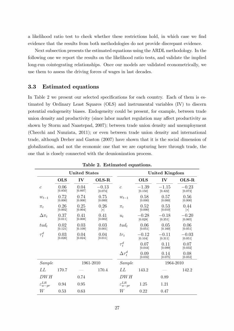
3.3 Estimated equations

In Table 2 we present our selected specifications for each country. Each of them is es-

timated by Ordinary Least Squares (OLS) and instrumental variables (IV) to discern

potential endogeneity biases. Endogeneity could be present, for example, between trade

union density and productivity (since labor market regulation may affect productivity as

shown by Storm and Naastepad, 2007); between trade union density and unemployment

(Checchi and Nunziata, 2011); or even between trade union density and international

trade, although Dreher and Gaston (2007) have shown that it is the social dimension of

globalization, and not the economic one that we are capturing here through trade, the

one that is closely connected with the deunionization process.

Table 2. Estimated equations.

United States United Kingdom

OLS IV OLS-R OLS IV OLS-R

c 0.06[0.850]

0.04[0.897]

−0.13[0.074]

c −1.39[0.150]

−1.15[0.422]

−0.23[0.072]

wt−1 0.72[0.000]

0.74[0.000]

0.75[0.000]

wt−1 0.58[0.000]

0.57[0.000]

0.56[0.000]

πt 0.26[0.002]

0.25[0.004]

0.26[∗]

πt 0.52[0.000]

0.53[0.010]

0.44[∗]

∆πt 0.37[0.011]

0.41[0.008]

0.41[0.002]

ut −0.28[0.028]

−0.18[0.351]

−0.20[0.065]

tudt 0.02[0.121]

0.03[0.109]

0.03[0.001]

tudt 0.06[0.051]

0.05[0.160]

0.06[0.051]

τdt 0.03[0.020]

0.04[0.024]

0.04[0.011]

trt −0.12[0.104]

−0.11[0.311]

−0.03[0.051]

τdt 0.07[0.044]

0.11[0.099]

0.07[0.032]

∆τdt 0.09[0.032]

0.14[0.075]

0.08[0.052]

Sample 1961-2010 Sample 1964-2010

LL 170.7 – 170.4 LL 143.2 – 142.2

DWH 0.74 DWH 0.89

εLRw−pr 0.94 0.95 εLRw−pr 1.25 1.21

W 0.53 0.63 W 0.22 0.47

27

... Continuation Table 2

Finland Sweden

OLS IV OLS-R OLS IV OLS-R

c −0.28[0.417]

−0.03[0.948]

−0.21[0.011]

c 1.32[0.290]

2.94[0.583]

−0.53[0.036]

wt−1 0.80[0.000]

0.81[0.000]

0.80[0.000]

wt−1 0.57[0.000]

0.60[0.000]

0.59[0.000]

πt 0.21[0.001]

0.17[0.069]

0.20[∗]

πt 0.29[0.003]

0.11[0.736]

0.41[∗]

ut −0.16[0.008]

−0.12[0.106]

−0.16[0.007]

ut −0.17[0.122]

−0.23[0.156]

−0.15[0.176]

∆ssrt 0.12[0.000]

0.16[0.017]

0.12[0.000]

∆ut 0.54[0.012]

0.76[0.461]

0.37[0.041]

tudt−1 0.16[0.048]

0.20[0.236]

0.16[0.041]

∆ssrt 0.18[0.000]

0.22[0.012]

0.18[0.000]

tudt−2 −0.13[0.088]

−0.17[0.289]

−0.13[0.086]

τdt 0.12[0.004]

0.07[0.578]

0.10[0.010]

trt −0.03[0.266]

−0.01[0.847]

−0.03[0.040]

τ it −0.08[0.002]

−0.08[0.279]

−0.09[0.001]

tudt 0.11[0.019]

0.17[0.106]

0.09[0.049]

trt 0.13[0.081]

0.25[0.480]

0.02[0.137]

Sample 1963-2010 Sample 1964-2010

LL 143.8 – 143.8 LL 155.0 – 153.6

DWH 0.55 DWH 0.76

εLRw−pr 1.04 0.90 εLRw−pr 0.67 0.28

W 0.85 0.72 W 0.11 0.42

28

... Continuation Table 2

France Italy

OLS IV OLS-R OLS IV OLS-R

c −0.82[0.054]

−1.15[0.039]

−0.21[0.001]

c −0.35[0.565]

−1.46[0.112]

−0.80[0.000]

wt−1 0.78[0.000]

0.83[0.000]

0.79[0.000]

wt−1 0.63[0.000]

0.61[0.000]

0.62[0.000]

πt 0.27[0.000]

0.26[0.002]

0.21[∗]

πt 0.33[0.001]

0.45[0.004]

0.38[∗]

ut −0.22[0.114]

−0.47[0.018]

−0.07[0.465]

ut −0.25[0.226]

−0.59[0.051]

−0.39[0.000]

tudt 0.04[0.001]

0.02[0.098]

0.04[0.000]

tudt 0.14[0.000]

0.11[0.021]

0.13[0.000]

trt −0.05[0.063]

−0.06[0.047]

−0.01[0.101]

trt −0.10[0.025]

−0.18[0.009]

−0.14[0.000]

Sample 1964-2008 Sample 1961-2010

LL 163.5 – 162.3 LL 147.7 – 147.4

DWH 0.08 DWH 0.17

εLRw−pr 1.25 1.54 εLRw−pr 0.89 1.16

W 0.14 0.07 W 0.45 0.45

... Continuation Table 2

Spain Japan

OLS IV OLS-R OLS IV OLS-R

c −0.06[0.942]

−0.54[0.596]

−0.23[0.000]

c −0.79[0.000]

−0.63[0.004]

−0.60[0.000]

wt−1 0.79[0.000]

0.82[0.000]

0.88[0.000]

wt−1 0.69[0.000]

0.72[0.000]

0.71[0.000]

πt 0.18[0.036]

0.20[0.037]

0.12[∗]

πt 0.32[0.000]

0.28[0.???]

0.29[∗]

∆sst 0.25[0.000]

0.29[0.001]

0.28[0.000]

tudt 0.17[0.000]

0.15[0.000]

0.15[0.000]

tudt 0.06[0.049]

0.04[0.176]

0.04[0.000]

d75 0.03[0.001]

0.03[0.002]

0.03[0.001]

trt −0.05[0.000]

−0.05[0.000]

−0.04[0.000]

Sample 1983-2009 Sample 1963-2010

LL 97.3 – 97.2 LL 161.5 – 160.8

DWH 0.81 DWH 0.09

εLRw−pr 0.88 1.14 εLRw−pr 1.03 1.01

W 0.53 0.81 W 0.30 0.81

Notes: Probabilities in brackets; ∗=Restricted coefficient.

LL=Log-likelihood; DWH=Durbin-Wu-Hausman Test;

εLRw−pr=Long-run elasticity of wages with respect to productivity; W=Wald test.

Instruments on the IV estimation are first lag of each regressor, plus wt−2.

29

We conduct the Durbin-Wu-Hausman test and we find that none of the estimated

equations are suspicious of endogeneity problems (the results of this test for each country

are presented in Table 2). The absence of significant endogeneity problems should come as

no surprise since two of the key driving forces, deunionization and trade, are independent

of one another (Dreher and Gaston, 2007), while the third one, productivity, is restricted

so that there is a one-to-one relationship with wages in the long-run. We thus use the

OLS estimator which in any case is more efficient than the IV one.

To test the validity of this long-run relationship we conduct a Wald test (whose results

are also presented in Table 2). In all cases we conclude that the null hypothesis of a long-

run unit elasticity between wages and productivity cannot be rejected. Consequently, we

estimate again all equations using OLS (given the results of the Durbin-Wu-Hausman

test) and restricting the long-run coefficient of productivity to be unity (given the results

of the Wald test). The corresponding estimates are displayed in the third column of

country results under the heading OLS-R (where R denotes Restricted). These are our

reference estimates and, of course, the ones used in the simulation analysis.

All models capture wage adjustment costs through a single persistence coefficient

ranging from around 0.55 to 0.90. UK, Sweden, and Italy have the lowest values around

0.60; the US and Japan come next, with persistence coefficients of at least 0.70; while

in Finland, France they get close to 0.80, and in Spain they reach 0.88. Unemployment

exerts the expected negative sign in all European countries but in Spain (where wages are

not sensitive to a rate of unemployment that has been extremely high and persistent in

all years of the sample period), and has no significant influence also in the US and Japan

(note that US is the paradigm of a deregulated labor market, whereas Japan is a very

specific case, with unemployment rates below 3% until the 1990s’ lost decade, and with a

very particular labor relations system).

Regarding the major driving forces we have, first of all, that the long-run coefficient

of productivity is restricted to unity in all equations. It is important to remark that this

restriction cannot be rejected in any equation (the results of the corresponding Wald test

are reported below the results for each economy). The second noteworthy result is the

presence of trade union density, with the expected positive sign, in all specifications. In

turn, international trade enters significantly in all open economies, which are the European

ones, but not in the closed ones —US and Japan in our sample of countries—, where trade

does not play any significant role in wage determination.

Different fiscal variables enter some of the equations as additional controls. These are

direct taxes in the US, UK, and Sweden; indirect taxes in Sweden; and social security

contributions in Finland, Sweden, and Spain.

30

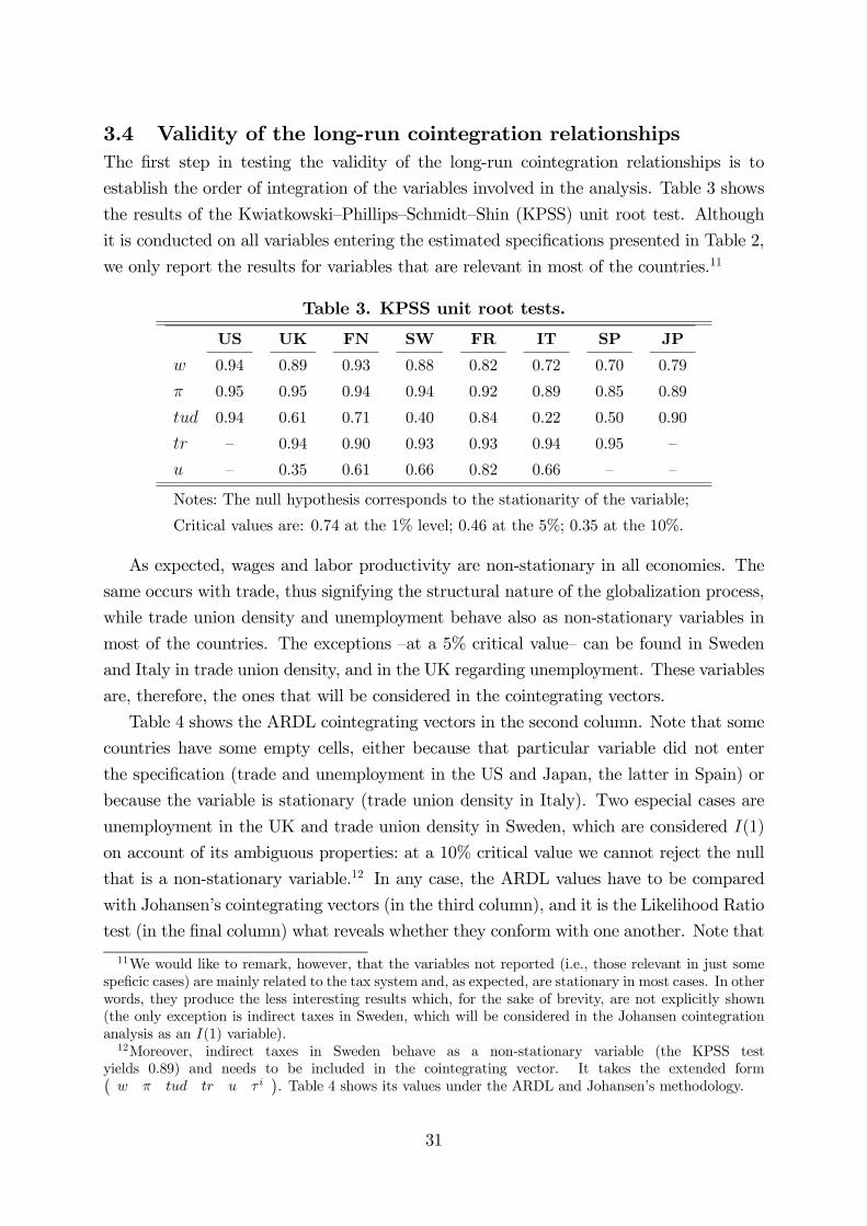
3.4 Validity of the long-run cointegration relationships

The first step in testing the validity of the long-run cointegration relationships is to

establish the order of integration of the variables involved in the analysis. Table 3 shows

the results of the Kwiatkowski—Phillips—Schmidt—Shin (KPSS) unit root test. Although

it is conducted on all variables entering the estimated specifications presented in Table 2,

we only report the results for variables that are relevant in most of the countries.11

Table 3. KPSS unit root tests.

US UK FN SW FR IT SP JP

w 0.94 0.89 0.93 0.88 0.82 0.72 0.70 0.79

π 0.95 0.95 0.94 0.94 0.92 0.89 0.85 0.89

tud 0.94 0.61 0.71 0.40 0.84 0.22 0.50 0.90

tr — 0.94 0.90 0.93 0.93 0.94 0.95 —

u — 0.35 0.61 0.66 0.82 0.66 — —

Notes: The null hypothesis corresponds to the stationarity of the variable;

Critical values are: 0.74 at the 1% level; 0.46 at the 5%; 0.35 at the 10%.

As expected, wages and labor productivity are non-stationary in all economies. The

same occurs with trade, thus signifying the structural nature of the globalization process,

while trade union density and unemployment behave also as non-stationary variables in

most of the countries. The exceptions —at a 5% critical value— can be found in Sweden

and Italy in trade union density, and in the UK regarding unemployment. These variables

are, therefore, the ones that will be considered in the cointegrating vectors.

Table 4 shows the ARDL cointegrating vectors in the second column. Note that some

countries have some empty cells, either because that particular variable did not enter

the specification (trade and unemployment in the US and Japan, the latter in Spain) or

because the variable is stationary (trade union density in Italy). Two especial cases are

unemployment in the UK and trade union density in Sweden, which are considered I(1)

on account of its ambiguous properties: at a 10% critical value we cannot reject the null

that is a non-stationary variable.12 In any case, the ARDL values have to be compared

with Johansen’s cointegrating vectors (in the third column), and it is the Likelihood Ratio

test (in the final column) what reveals whether they conform with one another. Note that

11We would like to remark, however, that the variables not reported (i.e., those relevant in just somespeficic cases) are mainly related to the tax system and, as expected, are stationary in most cases. In otherwords, they produce the less interesting results which, for the sake of brevity, are not explicitly shown(the only exception is indirect taxes in Sweden, which will be considered in the Johansen cointegrationanalysis as an I(1) variable).12Moreover, indirect taxes in Sweden behave as a non-stationary variable (the KPSS test

yields 0.89) and needs to be included in the cointegrating vector. It takes the extended formw π tud tr u τ i

. Table 4 shows its values under the ARDL and Johansen’s methodology.

31

the number of restrictions we impose varies depending on the number of variables entering

the cointegrating vector. It ranges from 2, in the US and Japan, to 5 in Sweden.

Table 4. Testing the long-run relationships in the Johansen framework.

ARDL Johansen LR testw π tud tr u

w π tud tr u

US-1 1 0.12 − −

-1 0.72 0.06 − −

χ2 (2)=4.64[0.098]

UK-1 1 0.14 -0.07 -0.45

-1 1.42 0.10 -0.44 -0.85

χ2 (4)=4.90[0.298]

FN-1 1 0.15 -0.15 -0.80

-1 0.93 0.12 -0.13 -0.17

χ2 (4)=4.77[0.312]

SW (*) (**) χ2 (5)=10.9[0.053]

FR-1 1 0.19 -0.05 -0.33

-1 1.21 0.15 -0.21 -1.46

χ2 (4)=6.16[0.188]

IT-1 1 − -0.37 -1.03

-1 0.97 − -0.38 -0.85

χ2 (3)=2.23[0.525]

SP-1 1 0.33 -0.33 −

-1 1.23 0.22 -0.32 −

χ2 (3)=0.92[0.819]

JP-1 1 0.52 − −

-1 0.96 0.53 − −

χ2 (2)=3.92[0.141]

Notes: p-values in square brackets; 5% critical values: χ2 (1)= 3.84; χ2 (2)= 5.99; χ2 (3)= 7.82;

χ2 (4)= 9.49; χ2 (5)= 11.07; (*) ARDL:−1 1 0.22 0.05 −0.37 −0.22

;

(**) Johansen:−1 0.78 0.21 0.09 0.14 −0.02

.

The results of the LR test allow us to conclude that the specification of the wage

equation for all economies yields cointegrated long-run relationships that are indeed robust

across methodologies.

4 Simulations

We use our estimated equations to conduct dynamic accounting simulations. We always

use the restricted estimates so that the condition of a unit long-run elasticity between

wages and productivity holds. We simulate our models in a twofold situation: a first

scenario in which all exogenous variables take their actual values, and a second scenario

where one of these variables is fixed at its 1980 value. The difference in the fitted values

obtained from the two scenarios accounts for the effect on wages of the variable that

has been fixed. Hence, our exercise provides answers to questions of the following type:

How would the evolution of the real wage have looked like if had, say productivity, not

grown since 1980? It is important to stress that we are not claiming that this would

have been the true evolution of wages in that case. We are just conducting counterfactual

experiments to learn on the driving forces that have shaped the real wage trajectory in

the last three decades.

32

As in Karanassou and Sala (2010), we choose 1980 as the reference year for a variety

of reasons: we are looking at structural phenomena and we are interested in a medium-

to long-term perspective; we favor country-comparability and the sample period in Spain

does not allow us to go further behind; finally, the 1980s are generally considered as an

inflection point in many economic dimensions: Keynesian ideas loose their prevalence,

most advanced economies undertake extensive and intensive deregulation processes, deu-

nionization becomes apparent, and the globalization course accelerates.

4.1 Productivity

The first simulation exercise corresponds to the example above where productivity is

fixed in all countries in 1980 (1982 in Spain due to sample period constraints). The

corresponding results are presented in Figure 2 for all countries (we take exponentials

to express real wages in absolute values rather than in logs). Solid lines are used for

actual values, dotted lines for simulated values. The difference between the two shows

the cumulative impact on wages since 1980 of a zero productivity growth rate.

In the Anglo-Saxon and Nordic countries we see a relatively flat downward trend. Real

wages would have decreased by close to 8% in the US (from 37,500 in 1980 to 33,600 USD

in 2010), and near 12% in the UK (from 20,600 to 18,400 GBP); by 5.4% in Finland

(from 22,100 to 20,900 euros), and by around 12% in Sweden (from 281,000 to 248,000

SEK). Finland shows the mildest decrease, overall, but it can be perceived that the fall

accelerated since 1991 in parallel with the liberalization process that took place after the

deep crisis of the early 1990s (see Honkapohja and Koskela, 1999). Taking the 1991-2010

period, the wage fall in the absence of productivity gains would have been 13.6%.

This downward trend is steeper in Continental Europe. Wages in France go down by

14.5% (from 29,600 to 25,300 euros), while Italy almost doubles this figure with 26.8%

(from 28,000 to 20,500 euros). Regarding Spain, if we exclude the end years of the Spanish

wild ride just before the crisis, in which wages grew fast, the wage fall in the absence of

productivity growth attains 17.0%. If these years are not excluded, this fall would still

surpass 11% and resemble that of France (in particular it would have been from 25,300

euros in 1982 to 22,500 euros in 2009). The simulation in Japan yields a similar picture,

where wages would have gone down by 18.4% (from 3,800,000 to 3,100,000 JPY).

Overall, although the intensity in the real wage downward trend is diverse, these results

provide an unanimous conclusion irrespective of the type of economy considered (Anglo-

Saxon, Nordic, Continental European, or Japanese): productivity gains have been the

key sustain of real wage progress. Viewed from the opposite side, the conclusion is that,

leaving aside productivity, the aggregate influence of the remaining wage determinants

has had a negative influence across countries and periods (with only two exceptions in the

33

1980s in Finland, and the late 1980s/early 1990s in Spain). This influence is quantified

next.

Figure 2. Real wage evolution in the absence of productivity growth.

32,000

36,000

40,000

44,000

48,000

52,000

56,000

80 82 84 86 88 90 92 94 96 98 00 02 04 06 08 10

Actual

Si mulated(pr oduc tivity kept constant

at i ts 1980 val ue)

37,465

53,391

33,631

a. United States (2005 USD).

16,000

18,000

20,000

22,000

24,000

26,000

28,000

30,000

32,000

80 82 84 86 88 90 92 94 96 98 00 02 04 06 08 10

b. United Kingdom (2008 GBP).

Actual

Simulated( productivity kept constant

at its 1980 value)

20,569

31,663

18,365

20,000

24,000

28,000

32,000

36,000

40,000

80 82 84 86 88 90 92 94 96 98 00 02 04 06 08 10

c. Finland (2000 EUR).

Actual

Simulated(produc tivi ty kept cons tant

at its 1980 value)22,052

38,080

20,938

240,000

280,000

320,000

360,000

400,000

440,000

480,000

80 82 84 86 88 90 92 94 96 98 00 02 04 06 08 10

d. Sweden (2010 SEK).

Actual

Simulated(producti vity kept constant

at its 1980 value)

281,361

428,243

247,669

24,000

26,000

28,000

30,000

32,000

34,000

36,000

38,000

40,000

80 82 84 86 88 90 92 94 96 98 00 02 04 06 08

e. France (2005 EUR).

Actual

Simulated( productivity kept constant

at its 1980 value)

29,594

38,142

25,33018,000

20,000

22,000

24,000

26,000

28,000

30,000

32,000

80 82 84 86 88 90 92 94 96 98 00 02 04 06 08 10

f. Ital y (2005 EUR ).

Actual

Simulated(productivity kept cons tant

at its 1980 value)

28,008

28,886

20,528

20,000

22,000

24,000

26,000

28,000

30,000

82 84 86 88 90 92 94 96 98 00 02 04 06 08

g. Spain (2008 EUR).

Actual

Simulated(productivity kept cons tant

at its 1982 value)

25,335

28,538

22,466

2,800,000

3,200,000

3,600,000

4,000,000

4,400,000

4,800,000

5,200,000

80 82 84 86 88 90 92 94 96 98 00 02 04 06 08 10

h. Japan (2000 JPY).

Actual

Si mul ated(pr oduct ivity kept constant

at its 1980 value)

3,778,056

5,072,015

3,072,428

34

4.2 Deunionization and growing exposure to international trade

In the next exercise, productivity series are restored to their actual values, whereas trade

union density and the degree of openness are kept at their 1980 values in each country.

In this way we can assess how deunionization and the growing exposure to international

trade have contributed to shape the real wage trajectory in the last decades. The results

are presented in Figure 3. The short-dotted line corresponds to the simulation where

trade union density is hold constant. The long-dotted line to the simulation where both

trade union density and international trade are fixed. The difference between the two

accounts for the wage impact of the increasing degree of economic openness (recall that,

following the econometric analysis, there is no such impact in the two closed economies

US and Japan).

Our estimates show that the deunionization process has contributed to reduce wages in

the Anglo-Saxon and Continental European economies (except Spain), and Japan. On the

contrary, there is no effect in the Nordic economies. The innocuous wage effect of unions

in Scandinavia is generally justified on the grounds of its high degree of centralization of

collective bargaining. Here we find this result as the natural consequence of the absence

of a secular deunionization process. Trade union density in Finland and Sweden increased

in the 1980s and early 1990s, and started going down along with the liberalization process

that followed the crisis of the early 1990s. Although the decrease in trade union density

has been notable in Sweden, it is still close to 70%, as in Finland.

As pictured in Figure A1, trade union density in the US, UK, France, Italy, and Japan

has unambiguously and severely trended down. Figures 3a, 3b, 3e, 3f, and 3h, respectively,

show that in the absence of this deunionization process, wages would have gone up to

57,800 USD in the US (instead of 53,400), to 34,200 GBP in the UK (instead of 31,700),

to 45,500 euros in France (instead of 38,100), to 32,700 euros in Italy (instead of remaining

roughly constant at 28,900), and to 6,600,000 JPY (instead of 5,100,000). This implies

extra wage increases of, respectively, 8.2%, 7.3%, 16.3%, 11.6%, and 22.7%. In other

words, the deunionization process in 1980-2010 has prevented wages from increasing near

10% in the Anglo-Saxon countries, between 10% and 20% in the Continental European

ones (but Spain), and by more than 20% in Japan.

Spain follows a different pattern due to the late legalization of unions in 1977. Trade

union density, which was initially low, more than doubled between the early 1980s and

1993, to stabilize afterwards. This union consolidation caused wages to go up by 12.2%

—from 25,400 to 28,500 euros. In other words, in the absence of this increase in trade

union density, wages in Spain would have been more than 10% lower. This effect is in the

range of the union impact found for the other Continental European countries.

35

Figure 3. Deunionization and openness effects on wages.

36,000

40,000

44,000

48,000

52,000

56,000

60,000

80 82 84 86 88 90 92 94 96 98 00 02 04 06 08 10

a. United States (2005 USD).

Actual

Si mulated(holding trade union

density constant)

37,465

57,753

53,391

20,000

22,000

24,000

26,000

28,000

30,000

32,000

34,000

36,000

80 82 84 86 88 90 92 94 96 98 00 02 04 06 08 10

Simulated (holding trade union density constant)

b. United Kingdom (2008 GBP).

Actual

Simulated(hol ding trade union density

and openness constant)

35,756

34,235

31,663

20,569

20,000

24,000

28,000

32,000

36,000

40,000

44,000

80 82 84 86 88 90 92 94 96 98 00 02 04 06 08 10

Simulated (holding trade union density constant)

c. Finland (2000 EUR).

Actual

Si mulated(holding trade union densi ty

and openness constant)

38,45538,080

42,068

22,052

250,000

275,000

300,000

325,000

350,000

375,000

400,000

425,000

450,000

80 82 84 86 88 90 92 94 96 98 00 02 04 06 08 10

Simulated (holding trade union density constant)

d. Sweden (2010 SEK).

Actual

Simul ated( hol ding tr ade uni on dens ity

and openness constant)

438,825

428,243422,784

281,361

28,000

32,000

36,000

40,000

44,000

48,000

80 82 84 86 88 90 92 94 96 98 00 02 04 06 08

Simulated (holding trade union density constant)

e. France (2005 EUR).

Actual

Simul ated( holdi ng tr ade uni on dens ity

and openness cons tant)

29,594

47,162

45,534

38,142

26,000

28,000

30,000

32,000

34,000

36,000

38,000

40,000

42,000

44,000

80 82 84 86 88 90 92 94 96 98 00 02 04 06 08 10

Simulated (holding trade union density constant)

f. Italy (2005 EUR).

Actual

Si mulated(hol ding tr ade uni on densi ty

and openness constant )

28,007

41,491

32,664

28,886

22,000

24,000

26,000

28,000

30,000

32,000

34,000

82 84 86 88 90 92 94 96 98 00 02 04 06 08

Simulated (holding trade union density constant)

g. Spain (2008 EUR).

Actual

Simul ated( holdi ng tr ade uni on dens ity

and openness constant)

25,335

32,448

28,538

25,413

3,500,000

4,000,000

4,500,000

5,000,000

5,500,000

6,000,000

6,500,000

7,000,000

80 82 84 86 88 90 92 94 96 98 00 02 04 06 08 10

h. Japan (2000 JPY).

Actual

Simul ated(holding tr ade union

dens ity constant)

3,778,056

6,623,131

5,072,015

The growing exposure to international trade is the third major driving force shaping

36

the trajectory of wages in all European economies, which are all open economies (Figure

A1). In the absence of such trend, wages would have been higher in all of them, but

Sweden (in Sweden, however, the impact of international trade only explains a 2.4%

growth in real wages). Globalization, therefore, appears as a key stopper of wage growth.

Interestingly, this is especially the case in the two countries that have suffered the most

the consequences of the recent Great Recession.

As it is also shown in Figure 3, in the UK trade prevented wages to increase by further

1,500 GBP (=35,800-34,200), in Finland by 3,600 euros (=42,100-38,500), in Italy by

8,800 euros (=41,500-32,700), and in Spain by 7,000 euros (=32,400-25,400). Although

these are all significant magnitudes in levels, there are substantial relative differences.

Trade prevented wages to increase by almost 5% in the UK and France, by close to 10%

in Finland, and by more than 25% in Spain and Italy. It seems clear that, in these two

Southern European economies, labor costs have been a critical adjustment mechanism to

the new productive and market conditions brought by the economic integration process.

4.3 Implications for the labor income share

Once examined the wage impact of three major structural phenomena such as produc-

tivity, deunionization, and international trade, our final step is to evaluate the resulting

consequences for the labor income share.

Regarding the productivity effect, let us go back to equation (1) and rewrite it as

β = W/YN

. In this simple setting, β represents a labor share that is constant and

is thus consistent with the standard Cobb-Douglas framework of analysis (Karanassou

and Sala, 2013). Taking a step further, and just for illustrative purposes, we can relax

this restriction and consider a time-varying labor share LSt consistent, for example, with

its downward trajectory in last decades (IMF, 2007). Substituting β by LSt, defining

PR = Y/N , adding time subscripts, and taking logs (denoted by lower case letters) we

have:

lst = wt − prt.

By taking first-differences, we can see that labor income changes are the outcome of

changes in wage and changes in productivity:

∆lst = ∆wt −∆prt.

This expression corresponds to the standard conceptualization of the labor share as the

wage-productivity gap. It implies that, controlling for productivity (recall that the long-

run one-to-one relationship between wages and productivity always holds), we can examine

how changes in wages, in response to changes in their driving forces, translate into the

37

labor share.

Figure 4. Deunionization and openness’ effects on the labor income share.

56

57

58

59

60

61

62

63

64

65

80 82 84 86 88 90 92 94 96 98 00 02 04 06 08 10

a. United States.

Actual

Simulated (hol ding tr ade union density constant)63.7%

61.4%

56.7%62

64

66

68

70

72

74

76

80 82 84 86 88 90 92 94 96 98 00 02 04 06 08 10

Simulated (holding trade union density constant)

b. United Kingdom.

Actual

Simul ated( holding trade union density and

openness cons tant)

73.9%

65.9%

71.2%

74.4%

52

54

56

58

60

62

64

66

68

80 82 84 86 88 90 92 94 96 98 00 02 04 06 08 10

Simulated (holding trade union density constant)

c. Finland.

Actual

Simul ated( holding trade union density and

openness cons tant)64.2%

58.4%58.9%

64.5%

56

58

60

62

64

66

68

70

80 82 84 86 88 90 92 94 96 98 00 02 04 06 08 10

Simulated (holding trade union density constant)

d. Sweden.

Actual

Si mulated( hol ding tr ade union density

and openness constant)

68.1%

59.0%58.2%

60.4%

52

54

56

58

60

62

64

66

68

70

80 82 84 86 88 90 92 94 96 98 00 02 04 06 08

Simulated (holding trade union density constant)

e. France.

Actual

Simulated(holding trade union dens ity and

openness constant)

65.8%

54.9%

65.6%

67.9%

44

48

52

56

60

64

68

80 82 84 86 88 90 92 94 96 98 00 02 04 06 08 10

Simulated (holding trade union density constant)

e. Italy.

Actual

Si mulated(hol ding trade union density and

openness constant)

63.2%

46.5%

52.6%

66.8%

44

46

48

50

52

54

56

58

60

82 84 86 88 90 92 94 96 98 00 02 04 06 08

Simulated (holding trade union density constant)

g. Spain.

Actual

Simulated(holding trade union density and

openness constant)

59.9%

45.8%

58.5%

51.5%

56

60

64

68

72

76

80

80 82 84 86 88 90 92 94 96 98 00 02 04 06 08 10

h. Japan.

Actual

Si mulated (holding trade uniondensity constant)

76.7%

58.7%

73.6%

38

We thus proceed as follows. We take our previously simulated wage trajectories (the

ones displayed in Figure 3). We compute a simulated labor income share which is the

outcome of these simulated wage trajectories minus the actual productivity series. We

compare it with the actual evolution of the labor income share, and we examine the

implications, for its trajectory, of the deunionization process and the rise in international

trade. The outcome of this exercise is presented in Figure 4.

By preventing real wages to rise further, and as a consequence by enhancing the wage-

productivity gap, the deunionization process in the US, UK, France, Italy and Japan has

contributed significantly to the labor share fall of these economies in last decades. In the

Anglo-Saxon countries by around 5 percentage points (pp henceforth), 4.7 pp. in the US

and 5.3 in the UK. In Italy by 6.7 pp, in France by near 11 pp, and in Japan by 18 pp.13

This is the cumulative impact along a time span of three decades. Note, in turn, that in

Finland and Sweden the union incidence is negligible since it amounts to less than 1 pp.

Table 5. Literature on union and trade effects on the labor income share.

LIS effects of:

Study Country Period Unions Trade

Conyon (1994) U.K. 1983-1986 +

Wallace et al. (1999) U.S. 1949-1992 +

Jayadev (2007) OECD countries 1972-1996 + -

Fichtenbaum (2009) U.S. 1949-2006 + -

Fichtenbaum (2011) U.S. 1997-2006 + -

Schneider (2011) Western Europe 1980-2005 -

Young and Zuleta (2011) U.S. 1983-2005 +

Karanassou and Sala (2013) U.S. 1962-2009 -

Hogrefe and Kappler (2013) 18 countries 1980-2008 -

Stockhammer (2013) 71 countries 1970-2007 + -

Note: LIS= Labor Income Share.

Regarding trade, the largest impacts are in Spain and Italy because these are the

economies where globalization has had more influence in restricting wage growth. In

particular, the growing exposure to international trade in Spain and Italy accounts, re-

spectively, for 12.5 pp and 14.2 fall in their labor income shares in the last three decades.

This is, by far, a much larger incidence than in France and the UK (2.3 and 3.2 pp), or

Finland (5.6 pp).

13This result is consistent with the findings in Agnese and Sala (2011) according to which the fall inthe labour share in Japan can be attributed to the changes that took place within the labour relationssystem, mainly the weakening of unions.

39

These results add to the growing literature on the effects of unions and international

trade on the fall of the labor income share, which is briefly summarized in Table 5 (the

positive sign of unions imply, as in our study, a positive connection between union power

and the labor income share).

5 Conclusions

Conventional wisdom asserts that unemployment is caused by labor market rigidities

and should be addressed through systematic institutional deregulation. This would al-

low wages to converge to their market-clearing level. In this paper, we divert from the

standard approach and take a fresh look at the drivers of employment compensation. We

estimate country-specific wage equations for a selection of eight OECD economies and

take a medium- to long-term perspective to evaluate the main factors conditioning pay

determination. Our selected economies are representative of the Anglo-Saxon, Nordic, and

Continental European economic models, as they were classified in Daveri and Tabellini

(2000), plus Japan.

We show that pay determination in last decades has been conditioned by three struc-

tural phenomena irrespective of the differences in these economic models.

The first one is productivity growth. It reflects efficiency progress and is a common

factor in all economies. Our analysis uncovers a relevant fact: in the absence of produc-

tivity growth, real wages in all economies display and downward trend. This trend is

relatively flat in the Anglo-Saxon and Nordic countries (US, UK, Finland, and Sweden),

and relatively steep in Japan and Continental Europe (France, Italy, and Spain).

The second phenomena is the deunionization process, which has had especial incidence

in Japan, followed by the Continental European countries (with the exception of Spain).

The weakening of union power has had a much lower incidence in the Anglo-Saxon coun-

tries —which are the paradigm of deregulated markets—, and no relevant influence in the

Nordic economies. This confirms the well-known result that union power is innocuous to

the labor market in Scandinavia.

The third phenomena is trade. We find the impact of trade on wage setting simply

irrelevant in closed economies such as the US and Japan. On the contrary, our counterfac-

tual simulations show that trade prevented wages to increase in all European economies

(with the exception of Sweden, where its impact is of minor magnitude). The effect of

trade reaches its maximum in Italy and Spain, and reveals that labor costs have been the

critical adjustment mechanism to the new economic conditions brought by the globaliza-

tion process.

We also show that, by preventing real wages to rise further and, as a consequence, by

40

enhancing the wage-productivity gap, deunionization and trade are significant contribu-

tors to the continuous fall in the labor income share

Our results align our work with those studies skeptical of the conventional wisdom, and

call for reappraisal of the policy measures so often recommended from standard accounts

of the unemployment problem.

References

[1] Addison, John T. and Paulino Teixeira (2003) “The economics of employment protection”,

Journal of Labor Research, 24(1), 85-129.

[2] Agnese, Pablo and Hector Sala (2011) “The driving forces behind the falling labour share

and persistent unemployment in Japan”, Pacific Economic Review, 16(5), 577-603.

[3] Allard, Gale (2005) “Measuring the changing generosity of unemployment benefits: beyond

existing indicators”, IE Working Paper, WP05-18.

[4] Arpaia, Alfonso and Gilles Mourre (2012) “Institutions and performance in european labour

markets: taking a fresh look at evidence”, Journal of Economic Surveys, 26(1), 1-41.

[5] Baccaro, Lucio and Diego Rei (2007) “Institutional determinants of unemployment in OECD

countries: does the deregulatory view hold water?”, International Organization, 61(3), 527-

569.

[6] Baker, Dean, Andrew Glyn, David R. Howell and John Schmitt (2005) “Labor market

institutions and unemployment: A critical assessment of the cross-country evidence”, in D.R.

Howell (ed.), Fighting unemployment: the limits of free market orthodoxy, Oxford University

Press.

[7] Bentolila, Samuel and Juan F. Jimeno (2006) “Spanish unemployment: The end of the Wild

Ride?”, in M. Werding (ed.), Structural Unemployment in Western Europe: Reasons and

Remedies, MIT Press.

[8] Blanchard, Olivier (2006) “European unemployment: the evolution of facts and ideas”,

Economic Policy, 21(45), 6-59.

[9] Blanchard, Olivier and Justin Wolfers (2000) “The role of shocks and institutions in the

rise of european unemployment: the aggregate evidence”, The Economic Journal, 110(462),

C1-C33.

41

[10] Blanchard, Olivier and Lawrence F. Katz (1999) “Wage dynamics: reconciling theory and

evidence”, the American Economic Review Papers and Proceedings, 89(2), 69-74.

[11] Cahuc, Pierre and André Zylberberg (2004) Labor Economics. Cambridge, MA, The MIT

Press.

[12] Calvo, Guillermo A. (1983) “Staggered prices in a utility-maximizing framework”, Journal

of Monetary Economics, 12(3), 383-398.

[13] Checchi, Daniele and Cecilia García-Peñalosa (2010) “Labour market institutions and the

personal distribution of income in the OECD”, Economica, 77, 413-450.

[14] Checchi, Daniele and Claudio Lucifora (2002) “Unions and labour market institutions in

Europe”, Economic Policy, 17(35), 361-408.

[15] Checchi, Daniele and Luca Nunziata (2011) “Models of unionism and unemployment”,

European Journal of Industrial Relations, 17(2), 141-152.

[16] Conyon, Martin J. (1994). “Labour’s share, market structure and trade unionism”, Inter-

national Journal of Industrial Organization, 12(1), 117-131.

[17] Daveri, Francesco and Guido Tabellini (2000) “Unemployment and taxes: do taxes affect

the rate of unemployment?”, Economic Policy, 15(30), 47-104.

[18] Dreher, Axel, and Noel Gaston (2007) “Has globalisation really had no effect on unions?”,

Kyklos, 60, 165-186.

[19] Elmeskov, Jørgen, John P. Martin and Stefano Scarpetta (1998) “Key lessons for labour

market reforms: evidence from OECD countries’ experiences”, Swedish Economic Policy Re-

view, 5, 205-252.

[20] Felbermayr, Gabriel J., Julien Prat and Hans-Jörg Schmerer (2011) “Trade and unemploy-

ment: what do the data say?”, European Economic Review, 55(6), 741-758.

[21] Fichtenbaum, Rudy (2009) “The impact of unions on labor’s share of income: a time-series

analysis”, Review of Political Economy, 21(4), 567-588.

[22] Fichtenbaum, Rudy (2011) “Do unions affect labor’s share of income: evidence using panel

data”, American Journal of Economics and Sociology, 70(3), 784-810.

[23] Freeman, Richard B. (2005) “Labour market institutions without blinders: the debate over

flexibility and labor market performance”, International Economic Journal, 19(2), 129-145.

42

[24] Freeman, Richard B. (2008) “Labour market institutions around the world”, CEP Discus-

sion Papers, DP0844, Centre for Economic Performance, LSE.

[25] Hogrefe, Jan and Marcus Kappler (2013) “The labour share of income: heterogeneous

causes for parallel movements?”, Journal of Economic Inequality, 11(3), 303-319.

[26] Hutchinson, John and Damiaan Persyn (2012) “Globalisation, concentration and footloose

firms: in search of the main cause of the declining labor share”, Review of World Economics,

148, 17-43.

[27] Jayadev, Arjun (2007) “Capital account openness and the labor share of income”, Cam-

bridge Journal of Economics, 31, 423-443.

[28] Hatton, Timothy J. (2007) “Can productivity growth explain the NAIRU? Long-run evi-

dence from Britain, 1871-1999”, Economica, 74, 475-491.

[29] Honkapohja, Seppo and Erkki Koskela (1999) “The economic Crisis of the 1990s in Fin-

land”, Economic Policy, 14, 399-436.

[30] IMF (2007) World economic outlook: globalization and inequality, Washington, DC.

[31] Karanassou, Marika and Hector Sala (2010) “The wage-productivity gap revisited: Is the

labor share neutral to employment?”, Discussion Paper, 5092, IZA, Bonn.

[32] Karanassou, Marika and Hector Sala (2013) “Distributional consequences of capital accu-

mulation, globalisation and financialisation in the US”, Discussion Paper, 7244, IZA, Bonn.

[33] Lindbeck, Assar and Dennis J. Snower (1989) The Insider-Outsider Theory of Employment

and Unemployment, MIT Press.

[34] Nickell, Stephen J. (1997) “Unemployment and labour market rigidities: Europe versus

North America”, The Journal of Economic Perspectives, 11(3), 55-74.

[35] Nickell, Stephen J. (1998) “Unemployment: questions and some answers”, The Economic

Journal, 108(448), 802-816.

[36] Nickell, Stephen J. and Richard Layard (1999) “Labor market institutions and economic

performance”, in O. C. Ashenfelter and D. Card (eds.) Handbook of labor economics, vol. 3,

3029-3084, Elsevier, Amsterdam.

[37] Nickell, Stephen J., Luca Nunziata and Wolfgang Ochel (2005) “Unemployment in the

OECD since the 1960s. What do we know?”, The Economic Journal, 115, 1-27.

43

[38] Nickell, William (2006) “The CEP-OECD institutions data set (1960-2004)”, CEP Discus-

sion Papers, CEPDP0759, Centre for Economic Performance, LSE.

[39] Nunziata, Luca (2005) “Institutions and wage determination: a multi-country approach”,

Oxford Bulletin of Economics and Statistics, 67(4), 435-464.

[40] OECD (2011), Economic Outlook. No. 90, Vol. 2011/2, Paris.

[41] Pesaran, M. Hashem and Yongcheol Shin (1999) “An autoregressive distributed-lag mod-

elling approach to cointegration analysis”, in S. Strom (ed.), Econometrics and economic

theory in the twentieth century: the ragnar frisch centennial symposium, Cambridge Univer-

sity Press: 371-413.

[42] Pesaran, M. Hashem, Yongcheol Shin and Richard J. Smith (2001) “Bounds testing ap-

proaches to the analysis of level relationships”, Journal of Applied Econometrics, 16, 289-326.

[43] Podrecca, Elena (2010) “labor market institutions and wage setting: evidence for OECD

countries”, Applied Econonomics, 43(25), 1-16.

[44] Rotemberg, Julio J. (1982) “Monopolistic price adjustment and aggregate output”, Review

of Economic Studies, 49(4), 517-531.

[45] Shapiro, Carl and Joseph E. Stiglitz (1984) “Equilibrium unemployment as a worker disci-

pline device”, The American Economic Review, 74(3), 433-444.

[46] Schneider, Dorothee (2011) “Bargaining, openness, and the labor share”, Discussion Paper,

SFB 649 DP 2011-068, Humboldt University, Berlin.

[47] Stockhammer, Engelbert and Erik Klär (2011) “Capital accumulation, labour market in-

stitutions and unemployment in the medium run”, Cambridge Journal of Economics, 35,

437-457.

[48] Stockhammer, Engelbert (2013) "Why have wage shares fallen? A panel analysis of the

determinants of functional income distribution", ILO Working Papers, 470913, International

Labour Organization, Geneva.

[49] Storm, Servaas and C.W.M. Nastepaad (2007) “Why labour market regulation may pay

off: worker motivation, co-ordination and productivity growth”, Economic and Labour Market

Papers, 2007/04, International Labour Organization (ILO).

[50] Wallace, Michael, Kevin T. Leicht and Lawrence E. Raffalovich (1999) “Unions, strikes,

and labour’s share of income: a quarterly analysis of the United States, 1949—1992”, Social

Science Research, 28(3), 265-288.

44

[51] Walsh, Frank (2012) “Efficiency wages and bargaining”, Oxford Economic Papers, 64(4),

635-654.

[52] Young, Andrew T. and Hernando Zuleta (2011) “Do unions increase labour’s shares? Evi-

dence from US industry-level data”, Working Paper 11-06, College of Business & Economics,

West Virginia University.

[53] Taylor, John B. (1979) “Staggered wage setting in a macro model”, The American Eco-

nomic Review, 69(2), 108-113.

45

Appendix

Figure A1. Unions and international trade. 1980-2010.

10.0

12.5

15.0

17.5

20.0

22.5

25.0

27.5

30.0

80 82 84 86 88 90 92 94 96 98 00 02 04 06 08 10

a. United States.

Tr ade union density

22.1%

28.6%

11.4%

Openness

11.9%25

30

35

40

45

50

55

60

65

80 82 84 86 88 90 92 94 96 98 00 02 04 06 08 10

b. United Kingdom.

Trade uni on density

49.7%

60.7%

26.5%

Openness

32.7%

40

50

60

70

80

90

100

80 82 84 86 88 90 92 94 96 98 00 02 04 06 08 10

c. Finland.

Trade union density

44.8%

88.6%

70.0%

Openness

69.4%

40

50

60

70

80

90

100

80 82 84 86 88 90 92 94 96 98 00 02 04 06 08 10

d. Sweden.

Trade uni on density

43.9%

93.7%

68.4%

Openness

78.0%

0

10

20

30

40

50

60

80 82 84 86 88 90 92 94 96 98 00 02 04 06 08 10

e. France.

Trade uni on density

18.3%

50.5%

7.6%

Openness

27.6%

25

30

35

40

45

50

55

60

80 82 84 86 88 90 92 94 96 98 00 02 04 06 08 10

f. Italy.

Trade uni on density

27.8%

55.2%

35.1%

Openness49.6%

0

10

20

30

40

50

60

70

80 82 84 86 88 90 92 94 96 98 00 02 04 06 08 10

g. Spa in.

Tr ade union densi ty

8.3%

58.3%

15.9%

Openness

18.5%

12

16

20

24

28

32

80 82 84 86 88 90 92 94 96 98 00 02 04 06 08 10

h. Japan.

Trade union dens ity

13.7%

26.1%

18.4%Openness

31.1%

Sources: OECD labor Market Indicators and OECD Economic Outlook no. 90.

46

Essay 2

The determinants of capital intensity in Japan and the

U.S.

Abstract

This paper develops a model of capital intensity determination that includes both supply

and demand-side drivers. This model is estimated for two economies with different time

paths of capital intensity, Japan and the United States, and both sets of determinants are

shown to be relevant. We provide new estimates of the elasticity of substitution between

production factors (around 0.30 for the U.S. and 0.85 for Japan). We also find a differenced

nature of biased technical change in both countries, i.e. capital-saving in Japan and labor-

saving in the U.S., which can help in explaining their diverse paths in the capital deepening

process. We conduct a counterfactual analysis with dynamic simulations that verifies the

role assignable to each determinant of capital intensity in the model. The results indicate

that without the fall in the relative factor cost (supply-side driver), capital intensity would

not have grown as much, in both countries, over the sample period (around 60% less in

Japan, 16% less in the U.S.). In turn, without the fall experienced in relative factor

utilization (demand-side driver), capital intensity would have grown much more in the

U.S. (a whole 177% instead of the actual 66% growth). This role of demand-side forces is

not detected in Japan’s case. The simulation of the model without a time-trend to proxy

technical change gives a higher trajectory of capital intensity in Japan and a lower one in

the U.S., reinforcing the opposite-sign biased effect of technical change in each case. These

results may help to enlighten the design of economic growth and labor market policies,

which should not be the by-product of economic analysis based exclusively on supply-side

considerations. Demand-side forces are, potentially, a crucial part of economic growth, as

shown for the U.S. case, and their inclusion in the policy-making frame of thought may

bring renewed answers for economic recovery.

47

1 Introduction

Although capital intensity, i.e. the ratio of capital stock over employment, plays a central

role in economic growth models, it is generally considered as an input variable. No effort

is devoted to the empirical assessment of its determinants in spite, for example, of the

contrasted trajectory of capital intensity across countries, or in spite of the limitation that

this imposes in growth accounting analysis.14

This paper intends to fill this void by providing evidence on the determinants of capital

intensity in two economies with different institutional settings: Japan and the United

States. As shown in Figure 1, the different time paths followed by the capital-per-worker

ratio is itself calling for an empirical analysis of its causes.

Figure 1. Capital intensity.

0

100

200

300

400

500

600

60 65 70 75 80 85 90 95 00 05 10

Japan

United States

Inde

x 10

0 =

196

0

a. Levels

-2

0

2

4

6

8

60 65 70 75 80 85 90 95 00 05 10

Japan

United States

Per

cent

age

b. Growth rates

Source: Ameco Database.

The process of capital intensity growth was specially intense in Japan, where the

amount of capital stock per employee grew almost sixfold between 1960 and 2011. In

contrast, it less than doubled in the US (Figure 1a). The origin of these differences lies

in the very dynamic process of capital deepening linked to the industrialization process

experienced by Japan in the 1960s and 1970s. After peaking in the first half of the 1970s,

however, the growth rate of capital intensity has evolved around a steady downward path

(Figure 1b). On the contrary, the process of capital deepening in the US accelerated from

the mid 1980s until 2009. The Great Recession has then caused a sudden fall similar to

those occurred in the aftermath of the oil prices shocks.

Departing from a standard analytical framework for the demand of production factors

(Antràs, 2004; McAdam and Willman, 2013), we take a step further and relax the perfect

competition assumption. When dealing with product demand uncertainty, firms adjust

14Madsen (2010), for example, points out that a problem associated with the traditional growth ac-counting framework is the lack of information about the factors responsible for the evolution of capitalintensity.

48

their degree of factor utilization ex post once investment decisions are already made.

In that context, capital intensity is driven by supply-side factors (i.e., factor costs and

technology) as well as by demand-side conditions. The result is a model of capital intensity

where the capital-per-worker ratio is explained by the relative factor cost, relative factor

utilization, a time trend proxying technical change, and further controls, such as taxation

and the degree of exposure to international trade (both shown relevant to this analysis

by related literature).

Capital intensity, jointly with technological progress, are the main factors of economic

growth, and so is acknowledged by the standard macroeconomic literature. In a recent

contribution, for example, Takahashi et al. (2012) show that capital intensity has been

crucial in Japan and other OECD economies’ postwar growth. Very few efforts, how-

ever, have been assigned to the assessment of the determination of an economy’s capital

intensity.

In a Hecksher-Ohlin analytical background, Hasan et al. (2013) argue that labor and

capital market regulations determine the industry-level capital stock per worker. They

claim that restrictive labor laws can curb firms’ ability to adjust their labor demand

to shocks in demand, technology and trade. This may be seen as an indirect way of

looking into capital intensity. In our model, we directly study the determinants of capital

intensity.

In this way, our paper contributes to the literature in three main dimensions. First

of all, in considering a model in which capital accumulation depends both on supply-side

and demand-side factors. Second, in providing an empirical account of the determinants

of capital intensity from a wider than usual perspective, with controls for demand-side

constraints, tax variables and the degree of exposure to international trade. Third, in

providing updated estimates of the elasticity of substitution between capital and labor

and identifying the nature of factor-biased technical change.

The results show that the estimated coefficients associated to relative factor costs are

statistically significant in all specifications in both countries. This is specially important,

since those coefficients allow for the estimation of the elasticity of substitution between

production factors. In turn, the significance of the proxies of demand-side channels is more

scatter but still cannot be dismissed. Further controls, as direct taxation and openness to

trade, also show a relevant role in decelerating capital intensity growth. The most striking

feature of our results, however, is the different nature of the factor-biased technological

change in Japan and the US. This provides a new explanation of the reasons why these

economies have followed such different paths in their capital deepening process.

A counterfactual exercise of dynamic simulations disentangles the participation of each

determinant in the evolution of capital intensity. The fall in relative factor costs over the

49

sample period impulses capital per worker growth in both countries. In turn, demand-

side forces are partly responsible for capital intensity growth only in the U.S., where

without the decline in relative factor utilization since the 1970s the growth in capital per

worker could have been steeper. When controlling for technical change, the path of capital

intensity evolution is higher than the actual one in Japan and lower than the actual one

in the U.S. This result points to technological progress as having a capital-saving effect

in Japan, and a labor-saving effect in the U.S. Regarding openness to international trade

and direct taxation, simulation results prove them responsible of a decelerating effect of

capital intensity.

The rest of this paper is structured as follows. Section 2 presents the analytical

framework. Section 3 deals with empirical issues related to the data and the estimated

models. Section 4 computes the elasticities of substitution between capital and labor, and

evaluates technological change in Japan and the US. Section 5 presents counterfactual

simulations. Finally, section 6 concludes.

2 Analytical framework

As Antràs (2004) and McAdam andWillman (2013), we depart from a Constant Elasticity

of Substitution (CES) production function from which the factor demand equations are

first derived, and then combined into a single expression that accounts for the supply-

side determinants of capital intensity. Then, along the lines of Andrés et al. (1990a,

1990b), Fagnart et al. (1999) and Bontempi et al. (2010), we consider the possibility

of product demand uncertainty. In that context, when expected demand is not met by

its actual value, firms are likely to react by adjusting their use of the production factors

either by hiring or firing workers, by changing the rate of capacity utilization, or by using

both mechanisms. In other words, the uncertainty on the actual level of product demand

creates a transmission channel by which the demand-side conditions affect the investment

and hiring/firing decisions of the firms. This explains why capital intensity is likely to

depend on demand-side factors (on top of the supply-side ones), and justifies the extended

model we present at the end of this Section.

2.1 Factor demands and capital intensity

Consider an economy with f identical firms that supply a homogeneous good. These firms

acquire inputs in competitive markets and face a cost per unit of labor W , and a cost of

capital use CC. Each firm has a CES production technology so that:

Yt =θ(ANt Nt)

−β + (1− θ) (AKt Kt)−β−1/β

, (1)

50

where Y is output, N is employment, K is capital stock, AN is an index of labor-

augmenting efficiency (proxying Harrod-neutral technological change), and AK is an index

of capital-augmenting efficiency (proxying Solow-neutral technological change); parameter

θ represents the factor share (0 < θ < 1); σ = 11+β

is the constant elasticity of substitu-

tion between capital and labor; and β denotes the degree of substitutability between both

factors.

As standard (Antràs, 2004; León-Ledesma et al., 2010), we assume that biased tech-

nological progress grows at constant rates denoted, respectively, by λN and λK. We thus

have ANt = AN0 eλN .t and AKt = AK0 e

λK .t, where AN0 and AK0 are the initial values of the

technological progress parameters, and t is a linear time trend. Note that λN = λK > 0

would imply Hicks-neutral technical progress, λK > 0 and λN = 0 implies Solow neutral-

ity, λN > 0 and λK = 0 yields Harrod neutrality, and λN , λK > 0 but λN = λK indicates

factor-biased technical change.

Profit maximization in a perfectly competitive environment yields expressions for the

factor demands (as a proportion of total output) that log-linearized can be written as

log(Kt/Yt) = αK − σ log(CCt/Pt)− (1− σ)λKt (2)

log(Nt/Yt) = αN − σ log(Wt/Pt)− (1− σ)λNt, (3)

where P is the aggregate product market price; αK = σ log(1 − θ) + (σ − 1) logAK0 and

αN = σ log θ+ (σ − 1) logAN0 are constant; and 1− σ = β1+β. Subtraction of equation (3)

from equation (2) yields the following specification for capital intensity:

log(Kt/Nt) = α− σ log(CCt/Wt) + (1− σ)(λN − λK)t. (4)

where α = αK − αN .

Equation (4) is standard; it corresponds, for example, to equation (3’) in Antràs (2004,

p. 19) and equation (5) in McAdam and Willman (2013, p. 704). It explains that capital

intensity depends on two supply-side factors: (i) the relative cost of labor and capital

(there is capital intensity growth if the real wage grows relatively to the user cost of

capital, making labor relatively more expensive); and (ii) the direction of factor-biased

technical change (given that labor and capital are gross complements, i.e. σ < 1, then

if labor-efficiency grows faster than capital-efficiency (λN > λK), there will be capital

intensity growth).

51

2.2 Product demand uncertainty

Next, we relax the assumption of perfect competition and perfect information in the prod-

uct market by assuming that firms hold some market power and are subject to random

unexpected shocks. This implies that firms will now maximize profits based on an ex-

pectation of the stochastic demand (Y E). Uncertainty about aggregate demand shapes

firms’ investment decisions (Fagnart et al., 1999; Bond and Jenkinson, 2000; Bontempi et

al., 2010) and allows for the inclusion of demand-side considerations.

The sequence of decisions is as follows. Firms maximize profits subject to their expec-

tation of demand in period t. In t+1, once the realization of the random (and unexpected)

shocks that determine the demand are known, the utilization rate of installed capacity

and the corresponding labor demand are adjusted accordingly.

Along the lines of Fagnart et al. (1999) firms use a putty-clay technology. Under a

fixed productive capacity in the short-run, firms adjust the degree of factor utilization,

and capital and labor are substitutes ex ante. Ex post, with capacity choices made and

idiosyncratic shocks known, firms face the actual demand by adjusting the utilization

intensity of the production factors, by hiring or firing workers, and by deciding on the

capacity utilization rate. At this stage, production factors may be thought as complements

to achieve a certain level of production. This model, therefore, allows for ex post rationing

of factor utilization in contrast to the standard maximization problem.

The realization of the demand faced by firms depends on two factors: the price level

(chosen by firms) and random shocks. The expected demand that firms consider in their

profit maximization problem is the expected value of this realization Y Et :

Y Et = Et−1 [Yt(Pt, ϕ)] , (5)

where E is the rational expectations operator, and ϕ is represents an idiosyncratic (sto-

chastic) shock with zero mean and a constant standard deviation greater than zero. In

other words, firms produce (and decide their factor demands) accordingly to their expec-

tation of product demand, which is a function of the the aggregate product market price

and the shocks.

Under these assumptions, the profit-maximization problem of the firm corresponds to

a standard monopolistic competition case:

max π (Kt, Nt, Pt) = PtYEt −WtNt − CCtKt

subject to :

Y Et = Et−1

θ(AN0 e

λN .tNt)−β + (1− θ) (AK0 e

λK .tKt)−β−1/β

52

where π stands for the firms’ profit function.

Operating from the first order conditions of this problem, the optimal levels of factor

utilization relative to output are obtained as an inverse relation with respect to each

factor’s cost:

Kt

Y Et

= (1− θ)σCCtPt

−σ

(AK0 eλK .t)

−β

1+β (6)

Nt

Y Et

= θσWt

Pt

−σ

(AN0 eλN .t)

−β1+β (7)

Note that log-linearization of equations (6) and (7) under perfect competition and perfect

information would yield equations (2) and (3).

Through aggregation of the f firms, the overall expected demand can be replaced by

the potential aggregate demand level (Y ). Further addition of the ratio YtYt(= 1) to the

left-hand side of both equations then yields:

Kt

Yt= (1− θ)σ

CCtPt

−σ

(AK0 eλK .t)

−β

1+β

YtYt

(8)

Nt

Yt= θσ

Wt

Pt

−σ

(AN0 eλN .t)

−β

1+β

YtYt

(9)

where the ratioYtYtexpresses the gap between potential aggregate demand (Y ) and the

actual level of aggregate production (Y ), once factor demands have been adjusted ex post.

2.3 Mind the gap

TheYtYtratio is the transmission channel for business cycle effects (Nakajima 2005, Fagnart

et al. 1999). As such, it is directly related to the gap between total installed production

capacity and the rate of capacity utilization of the production factors. Because the later

is observable (in contrast to Yt), we assume that the degree of factor utilization can beempirically used as a proxy for the ratio

YtYt. Although this is relatively standard in the

literature, we believe that equations (8) and (9) require a specific proxy accounting, as

close as possible, for the demand-pressures that capital and labor will experience.

The standard procedure, however, consists in looking at only one of the production

factors’ side (see, for example, Andrés et al. 1990a). The reasoning is the following. Firms

invest in capacity with an expectation of potential demand but, because they end up using

this capacity only with the intensity required by actual demand (which is called ex post

rationing), the degree of capacity utilization (or capacity utilization rate) is determined

accordingly. Because of the correspondence between the fact that production is responsive

to aggregate demand ex post, and installed capacity is rigid in the short run, we follow this

53

route regarding equation (8) and proxy the unobservable YtYtratio through the standard

capacity utilization rate (CUR) variable15.

With respect to the extent to which the other production factor, labor, is used relative

to its potential, we consider the employment rate, which reflects the actual use of the labor

factor (employment, N) over its total possible use (working-age population, Z). It follows

that, for equation (9), we account for the degree of labor usage through the employment

rate (NR = N/Z).

In other words, we re-write the factor demand equations as:

Kt

Yt= (1− θ)σ

CCtPt

−σ

(AK0 eλK .t)

−β

1+β .h(CURt) (10)

Nt

Yt= θσ

Wt

Pt

−σ

(AN0 eλN .t)

−β

1+β .h(NRt), (11)

where h(·) is a monotonically increasing function as in Andrés et al. (1990a, p. 88).

Log-linearization of equations (10) and (11), and substraction of the second one from

the first one yields an expression for capital intensity and its determinants:

log

Kt

Nt

= α− σ

log

CCtPt

− log

Wt

Pt

+ (1− σ) (λN − λK) t

(12)

+(γK − γN ) [log (CURt)− log (NRt)] .

Note that the only difference with respect to equation (4) is the last term, which results

from the assumption of an stochastic behavior of aggregate product demand allowing for

ex post rationing of factor utilization16.

2.4 Factor-biased technical change

Regarding the second term in the right-hand side of equation (12), we follow McAdam and

Willman (2013), León-Ledesma et al. (2010, 2013) and Antràs (2004), among others, in

applying empirical efforts to identify and measure biased technical change17. The evidence

15As already said above, this is relatively standard in the literature. For example, Graff and Sturm(2012) associate the degree of capacity utilisation directly to the output gap and Planas et al. (2013) tothe cycle of total factor productivity.16We assume that the log-linearization of h(·) yields a linear function of the logs of CUR and NR in

each case, as presented in (12).17To cite McAdam and Willman (2013, p.698): “... despite renewed interest in models of biased

technical change, the corresponding empirical effort to identify (i.e., measure) episodes from macro datahas been lacking.”

54

in this strand of the literature shows that making a priori assumptions about the form

of technical progress (e.g. assuming Hicks neutrality) is likely to misguide the insights on

the effect of technical progress on capital intensity.

The dominant assumption of a balanced growth path (BGP) in theoretical growth lit-

erature implies a framework where the main macro variables converge to a common growth

rate, the underlying ratios (factor income shares and factor-GDP ratios) remain constant

[as described by Kaldor (1961)], and technical change is solely labor augmenting (i.e. Har-

rod neutral). Acemoglu (2003) and McAdam and Willman (2013) suggest that although

technical progress is labor-augmenting along the BGP, it can be capital-augmenting in

medium-run transitions away from the BGP. With an elasticity of substitution between

labor and capital lower than one (gross complements), this pattern allows for long-run

asymptotic stability of factor shares, and also non-stationary evolution in the medium-run

(which we observe in reality).

Specifically, the model in this Section shows how given that labor and capital are gross

complements (i.e., the elasticity of substitution is lower than one18), a relatively higher

growth of labor-augmenting technical change favors capital intensity, as shown in terms

of equation (13)19.

∂(K/N)

∂(AN/AK)> 0 if σ < 1 (13)

In our model, along the lines of Acemoglu (2003), Antràs (2004) and McAdam and

Willman (2013), capital accumulation in the long-run implies that labor-efficiency has to

grow faster than capital-efficiency. Recall that in (4) and (12), with σ < 1, higher capital

intensity is reached when λN > λK .

3 Empirical issues

3.1 Estimated models

Consideration of demand-side drivers in factor demand equations is still an open issue.

This is the reason why, on top of the relative degree of factor utilization log (CURt) −

log (NRt), we follow Añón-Higón (2007), and consider the variation in worked hours per

employee as an alternative aggregate proxy of demand-side pressures (we take the growth

18There a several recent studies that find σ < 1. For example, Antràs (2004), Chirinko (2008), Chirinkoet al. (2011), León-Ledesma et al. (2010), Klump et al. (2012) and McAdam and Willman (2013).19McAdam and Willman (2013, p. 703).

55

rate because this proxies the business cycle in terms of varying demand-side pressures).

The reasoning behind this choice is that worked hours per employee reflect simultaneously

an increase in the usage intensity in capital stock and labor. Moreover, the average annual

amount of hours worked per employee is likely to avoid the endogeneity problems that

would entail considering variations in output (since the dependent variable is indeed made

of capital and labor), which is the natural alternative in the literature.

Two additional sets of control variables are related to capital intensity: the degree

of exposure to international trade and the fiscal system. Since capital intensity, the

degree of substitution between capital and labor, and globalization are deeply intertwined

(Hutchinson and Persyn, 2012), inclusion of the degree of trade openness (op) is a must.

Regarding the fiscal system, a key variable for firm’s decisions is direct taxes on business,

which is crucial in defining, for example, investment decisions. This has been studied in

Bond and Jenkinson (2000), Edgerton (2010) and Madsen (2010), where the decelerating

effect of corporate taxation on capital deepening is explained as a disincentive to firm-

level investment. Beyond that, because we have confronted the user cost of capital with

the labor cost, and the degree of capital stock utilization with the employment rate, we

confront direct taxes on businessτ bto direct taxes on households

τhto capture, if any,

the specific impact of taxes on each demand factor. Of course, payroll taxes is another

crucial element of the tax system, but its relevance is more related to the wage bargaining

process between firms and workers. Since this is implicitly taken into account through

the wage variable (total compensation, which includes social security contributions) we

do not need any further control.

Overall, we estimate two empirical versions of equation (12). Model 1 will be a straight-

forward augmented version of equation (12):

knt = β0 + β1(cct − wt) + β2(curt − nrt) + β3t+ β4opt + β5τb + β6τ

h + u1t, (14)

where knt = log(Kt/Nt), cct = log (CCt/Pt), wt = log (Wt/Pt), curt = log(CURt),

nrt = log(NRt) and u1t represents a standard error term with zero mean and constant

standard deviation. Detailed definitions of the additional controls, op, τ b,and τh (and also

of the rest of the variables) are given in Table 1.

Model 2 substitutes relative factor utilization, curt − nrt, by the change in worked

hours per employee (∆hr):

knt = γ0 + γ1(cct − wt) + γ2∆hrt−1 + γ3t+ γ4opt + γ5τb + γ6τ

h + u2t, (15)

where u2t represents a standard error term with zero mean and constant standard de-

viation. Note that the coefficient on hours is lagged once to help avoiding endogeneity

56

problems. In contrast, the term capturing demand-side pressures in equation (14) is not

lagged to maintain coherence with respect to the theoretical model. We have assumed

a putty-clay technology and argued that short-run capital stock adjustments take place

through changes in the degree of capacity utilization. This implies that demand changes

foreseen in t− 1 are accommodated through changes in investment, not through changes

cur which can only respond in period t.

A crucial remark is that these empirical models are estimated as dynamic equations to

take into account the adjustment costs potentially surrounding all variables involved in the

analysis (endogenous and exogenous). The lagged structure of the estimated relationships

is therefore a pure empirical matter.

The coefficients β1/γ1 are associated to the relative cost of production factors, and a

negative sign is expected. As the wedge between the cost of factors (cc − w) increases,

capital becomes relatively more costly than labor, and a deceleration of capital intensity

growth is expected.20 The crucial feature of this coefficient is its correspondence with the

constant elasticity of substitution between capital and labor (σ).

The coefficients β2/γ2 are associated to the role of demand-side pressures, and a

positive sign is expected. A rise in the wedge between the relative intensity in factor

utilization (cur− nr) implies that tightness in the capital side is larger than in the labor

side. Firms, therefore, are expected to react by investing more intensively than embarking

in new hirings. As a consequence, capital intensity is expected to accelerate.

Firm’s decisions to expand capacity through investment are based to a large extent

on their assessment of their future sales, which we assumed to be uncertain. Managers

are naturally cautious about overestimating future sales, as the penalty for doing so

tends to be much greater than for losing potential business by failing to expand (Smith,

1996). In our model, the capacity utilization rate is a proxy for the perception of the

firm of the economic reality, which reflects on its expectations on aggregate demand.

Since the expansion of capacity drives investment, we expect a positive effect on capital

intensity when the wedge between a higher degree of capacity utilization rate and a higher

employment rate widens.

Given the assumption of constant rates of technical progress, the coefficients β3/γ3 =

(1 − σ)(λN − λK) measure an asymmetric progress in the efficiency of each production

factor. If β3/γ3 > 0 and σ < 1, there is evidence that labor-augmenting efficiency grows

faster than capital-augmenting efficiency (the same holds in case of opposite signs in both

estimates). If, on the contrary, the β3/γ3 > 0 are positive and σ > 1, the conclusion is

20Decisions to invest in new capacity are influenced by the cost and availability of capital and thetarget rates of return sought by firms and financial institutions. The dependence on bank loans is animportant factor limiting expansion and the user cost of capital is a crucial factor in the expected netreturn to investment by firms.

57

that capital-augmenting efficiency grows faster than labor-augmenting efficiency. In both

cases, therefore, there is evidence of biased technological change, something that in the

standard Cobb-Douglas framework, where σ = 1, cannot be measured.

3.2 Data

We use annual data obtained from various sources. From the European Commission’s

Ameco database we take net long-time series on net capital stock21. Data on the capacity

utilitzation rate is obtained from Ministry of Economy, Trade and Industry for Japan,

and from the Board of Governors of the Federal Reserve System for the U.S. The rest of

the variables is gathered from the OECD Economic Outlook 91 (2012).

Table 1. Definitions of variables.

k real net capital stock p GDP deflator

n employment pi investment deflator

kn capital intensity (= k − n) δ depreciation rate

z working-age population i nominal interest rate

nr employment rate (= n− z) cc real user cost of capital

cur capacity utilization rate = pi

p(i+ δ −∆pi)

w real compensation per employee T direct taxes on business

hr hours of work per employee τ b direct taxes on business (TB) as % GDP

Y GDP = log (TB/Y )

X exports of goods and services τh direct taxes on households (TH) as % GDP

M imports of goods and services = log (TH/Y )

op trade openness t linear time trend

= log ([X +M ] /Y ) ∆ difference operator

c constant

Note: All variables used in the econometric analysis are expressed in logs.

Table 1 provides the concrete definitions of the empirical variables used. All of them

are standard and the only clarification refers to the definition of the user cost of capital,

which is constructed as in Andrés et al. (1990a) assuming a constant depreciation rate

equal to 0.1.McAdam and Willman (2013) argue that the observed government bond rate

21The net capital stock at constant prices, total economy (OKND), is calculated as OKNDt =OKNDt−1 + [OIGTt − (UKCTt : PIGTt) ∗ 100], where OIGT = Gross fixed capital formation atconstant prices; total economy, UKCT = Consumption of fixed capital at current prices; total economyand PIGT = Price deflator gross fixed capital formation; total economy.OIGT = Gross fixed capital formation at constant prices; construction + equipment + products of

agriculture, forestry, fisheries and aquaculture + other procucts.

58

does not correctly capture firms’ marginal financing costs in an imperfectly functioning

financial market. The real observed user cost of capital would have been above the

indicated. Along these lines, we follow the deifinition in Andrés et al. (1990a) detailed in

Table 1.Note, also, that all variables will be used in logs so as to allow an unambiguous

interpretation of the estimated coefficients as elasticities.

3.3 Estimation procedure

We deal with long time-series data and we need to ensure that the long-run estimated

relationships between capital intensity and its determinants are non-spurious. Of course,

if k, n, cc, w, cur, z, T , and Y behaved certainly as I(1) variables we could argue, since we

work with these variables by ratios (kn, cc−w, cur− nr, (X +M)/Y and T/Y ), that we

end up dealing with I(0) variables and cointegration issues are of no concern. Nonetheless,

we have indeed conducted the standard unit root tests and we are able to stress that, yes,

we are indeed dealing with I(1) variables (see Table A1 in the Appendix for test results)22.

Nevertheless, we proceed as if we were unsure of the degree of integration of our

variables. This is why our estimation is conducted following the bounds testing approach,

or ARDL (AutoRegressive Distributed Lag) approach, which yields consistent short- and

long-run estimates irrespective of whether the regressors are I(1) or I(0). This approach,

which was developed by Pesaran and Shin (1999) and Pesaran, Shin and Smith (2001),

provides an alternative econometric tool to the standard Johansen maximum likelihood,

and the Phillips-Hansen semi-parametric fully-modified Ordinary Least Squares (OLS)

procedures. The main advantage of the bounds testing approach is the possibility of

avoiding the pretesting problem implicit in the standard cointegration techniques. It also

yields consistent long-run estimates of the equation parameters even for small size samples

and under potential endogeneity of some of the regressors (see Harris and Sollis, 2003).

We first estimate our models by OLS. Then, to make sure that we have indeed obtained

non-spurious relationships between potential non-stationary variables, we verified that the

residuals resulting from our estimated models are indeed stationary (see Table 4 below).

Regarding the selection of the estimated models, we first select equations that are

dynamically stable and satisfy the conditions of linearity, structural stability, no serial

correlation, homoscedasticity, and normality of the residuals. Then, among the models

that meet these requirements, we select the dynamic specification of each equation by re-

lying on the optimal lag-length algorithm of the Schwartz information criterion (Table A2

in the Appendix shows that these standard diagnostic tests are all passed at conventional

significance levels).

22In the case of Model 2, ∆hrs is, as expected, stationary.

59

Finally, we estimate the selected specifications by Two Stages Least Squares (TSLS)

so as to control for potential endogeneity biases in the estimated effect of the relative

factor costs (cc−w), in relative factor utilization (cur−nr) or hours, and in direct taxes

on business. The instruments are statistically significant and we find the OLS and the

TSLS results to be relatively alike, thus supporting the robustness of the results (only

model 2 for Japan rejects by a short margin the Durbin-Wu-Hausman test of exogeneity).

4 Results

4.1 Estimated equations

We present the estimation results for equations (14) and (15) in Table 2, for Japan, and

in Table 3, for the US.

Japan’s estimation includes three dummy variables d9102, d83, and d97, which take

value one in the years indicated by the superscript. They account for the lost decade,

and specific events such as the East-Asian crisis. They do not have any special economic

relevance, but they help to achieve better results in terms of the misspecification tests

(see Table A1).

All estimated equations have a high estimated coefficient associated to the first lag of

capital intensity. This high persistence in the dynamic process is to be expected since pro-

ductive capacity is not easily changed in the short run. The results for Japan show that

relative factor costs present a highly statistically significant negative sign coefficient -as

expected- in both models. Moreover, the estimated short-run coefficient is quite homoge-

neous in value. Regarding the proxies for demand-side channels to capital deepening, the

cycle component of average hours worked (model 2) has greater statistical significance.

Both direct taxes on businesses and households show a decelerating effect on capital inten-

sity in the two models, as also does the degree of openness to international trade. Finally,

the estimated coefficient associated to the time trend is negative, which combined with a

lower-than-one elasticity of substitution would indicate that capital-associated efficiency

grows at a higher rate than labor-associated efficiency (see section 4.2).

As for the U.S., again the coefficients associated to relative factor cost are negative

and significant. In this case, now not only ∆ht−1 presents statistical significance, but

also the relative factor utilization. Direct taxes and openness are also detrimental for

capital intensity in the U.S., but the latter enters the equations as the variation between

two years, indicating that this is more a conjunctural downward pressure than a long-run

effect. The estimated coefficient associated to the time trend is positive, and considering

that the estimated elasticity of substitution for the U.S. is lower than the unity, that would

imply labor-saving biased technical change as labor-efficiency grows faster than capital-

60

efficiency (see section 4.2). Note that, according to these results, the U.S. and Japan would

have opposite-direction bias in technological change between both production factors.

Table 2. Japan, 1980-2011.

Model 1 Model 2∗

OLS TSLS OLS TSLS

c 0.005[0.983]

0.084[0.759]

c −0.020[0.907]

−0.008[0.969]

knt−1 0.964[0.000]

0.954[0.000]

knt−1 0.966[0.000]

0.960[0.000]

cct − wt −0.033[0.000]

−0.038[0.001]

cct − wt −0.034[0.000]

−0.036[0.062]

∆(cct − wt) 0.020[0.001]

0.019[0.003]

∆(cct − wt) 0.021[0.000]

0.031[0.030]

∆(cct−1 − wt−1) 0.015[0.002]

0.016[0.005]

∆(cct−1 − wt−1) 0.021[0.001]

0.025[0.004]

curt − nrt 0.005[0.625]

0.003[0.813]

∆hrt−1 0.076[0.106]

0.111[0.070]

∆(curt − nrt) 0.015[0.188]

0.019[0.175]

∆τ bt −0.015[0.001]

−0.014[0.012]

∆τ bt −0.014[0.001]

−0.007[0.573]

∆τht−1 −0.007[0.329]

−0.006[0.426]

∆τht−1 −0.009[0.149]

−0.010[0.200]

opt −0.030[0.003]

−0.035[0.008]

opt −0.035[0.001]

−0.056[0.002]

D9102 0.005[0.005]

0.005[0.024]

D9102 0.004[0.005]

0.003[0.039]

D83 −0.014[0.000]

−0.013[0.000]

D83 −0.014[0.000]

−0.014[0.000]

D97 −0.010[0.000]

−0.011[0.000]

D97 −0.010[0.000]

−0.009[0.034]

t −0.001[0.030]

−0.001[0.145]

t −0.001[0.016]

−0.0003[0.605]

LL 167.6 167.33

Obs 32 32 32 32

Notes: LL = Log-likelihood; p-values in brackets; Instruments: knt−1 cct−1 wt−1

∆cct−1 ∆wt−1 curt−1 nrt−1 opt−1 ∆τht−1 ∆τ bt ∆τ bt−1 D9102 D83 D97 t

∆hrt−1 ∆hrt−2.

Durbin-Wu-Hausman test [prob]: Model 1 [0.95]; Model 2 [0.04].

61

Table 3. US, 1970-2011.

Model 1 Model 2∗

OLS TSLS OLS TSLS

c 0.345[0.401]

0.327[0.516]

c 0.136[0.772]

0.286[0.582]

knt−1 0.951[0.000]

0.941[0.000]

knt−1 0.973[0.000]

0.965[0.000]

∆knt−1 0.292[0.015]

0.308[0.038]

∆knt−1 0.215[0.241]

0.288[0.176]

cct − wt −0.010[0.094]

−0.016[0.132]

cct − wt −0.013[0.058]

−0.011[0.443]

curt − nrt 0.083[0.139]

0.126[0.192]

∆hrt−1 −0.310[0.317]

−0.204[0.572]

∆(curt − nrt) −0.182[0.000]

−0.170[0.001]

∆hrt−2 0.526[0.027]

0.547[0.026]

τ bt −0.019[0.069]

−0.035[0.114]

τ bt −0.018[0.115]

−0.008[0.699]

τht −0.002[0.899]

0.003[0.862]

τht 0.014[0.366]

0.011[0.535]

∆opt −0.099[0.024]

−0.069[0.382]

∆opt −0.149[0.002]

−0.206[0.002]

t 0.001[0.079]

0.001[0.191]

t 0.0002[0.655]

0.0004[0.492]

LL 161.2 155.5

Obs. 42 42 42 42

Notes: LL = Log-likelihood; p-values in brackets; Instruments: knt−1 ∆knt−1

cct−1 wt−1 curt−1 nrt−1 ∆curt−1 ∆nrt−1 τ bt τbt−1 τht τht−1 ∆opt−1 t

∆hrt−1 ∆hrt−2

Durbin-Wu-Hausman test [prob]: Model 1 [0.92]; Model 2 [0.73].

Furthermore, regarding the validity of the long-run relationships between variables,

the Augmented Dickey-Fuller test (ADF, with null hypothesis of non-stationarity) and

the Kwiatkowski-Phillips-Schmidt-Shin test (KPSS, with null hypothesis of stationarity)

were performed on the residuals of the estimated equations presented above. The results

can be seen in Table 4. They largely reject in all cases the hypothesis of the existence

of a unit root in the ADF test, and also do not reject stationarity in the KPSS test,

reinforcing the stationarity of the residuals and therefore that we have obtained non-

spurious relationships23.

23At the 5% level, the residuals for Japan’s model 2 estimation by TSLS may not be strictly stationaryaccording to the KPSS. Nevertheless, the ADF test for those same residuals largely rejects the unit roothypothesis at the 1% level.

62

Table 4. Unit root tests on the residuals of equations (14) and (15)

ADF test KPSS test

Model 1 (u1t) Model 2 (u2t) Model 1 (u1t) Model 2 (u2t)

OLS TSLS OLS TSLS OLS TSLS OLS TSLS

Japan −5.84 −5.32 −5.47 −6.61 0.054 0.045 0.447 0.500

U.S. −4.17 −6.18 −6.41 −6.89 0.054 0.042 0.081 0.083

Note: ADF test critical value is -3.60 at the 1% level.

KPSS test critical values are 0.739 at the 1% level, and 0.463 at the 5% level.

4.2 Elasticities of substitution and technological change

Directed technical change is a consequence of a production factor becoming relatively

more scarce, more expensive, or both. Innovation is then directed towards technologies

that would save on the relatively more expensive factor. The bias in technical change

may have a saving effect on one factor and an augmenting effect on the other one. The

degree of substitutability between labor and capital is closely related to this phenomenon.

Then, the elasticity of substitution between labor and capital and the rate of factor-biased

technical change are key variables in economic growth models, specially in medium-run

dynamics (McAdam and Willman, 2013).

Table 5 shows the elasticity of substitution between factors implied by our empirical

models, together with the long-run impact on capital intensity of the constant rate of

technological progressεLRkn−trend

. Given that the estimated models are dynamic, the

elasticity of substitution is computed as the long-run elasticity of kn with respect to

(cc− w). Taking the example of Japan using Model 1, we have 0.038/(1−0.954) = 0.83 = σ.

In turn, εLRkn−trend = (−0.001/ (1− 0.954)) ∗ 100 = −2.2%. These two values are used to

compute the implied rate of biased technological change following equations (4) or (12).

More precisely, in case of Model’s 1 estimates for Japan, we use σ = 0.83 and εLRkn−trend =

−2.2% to compute the value of (λK − λN) using:

−2.2% = (1− 0.83)(λN − λK)

=⇒ (λK − λN ) = 12.5%

This result implies that there is factor-biased technical change in Japan (λK−λN > 0,

that is, λK = λN). In this case, the direction is capital saving.

63

Table 5 shows the calculations for both countries using the instrumental variables

estimation of Models 1 and 2.

Table 5. Elasticities of substitution and technological change.

Model 1 Model 2

Technical progress Technical progress

σ εLRkn−trend Type Rate σ εLRkn−trend Type Rate

Japan 0.83 -2.2% Capital 12.5% 0.90 -0.7% Capital 7.5%

saving saving

US 0.27 1.7% Labor 2.3% 0.31 1.1% Labor 1.7%

saving saving

Notes: εLRkd−trend denotes the long-run elasticity of capital deepening with respect to constant

technical change; technical change is capital saving whenever λK> λN and labor saving

whenever λN> λK .

As noted, we find the elasticity of substitution between capital and labor to be below

1 in Japan. This value is larger than in other studies, which place it between 0.2 and

0.4 (Rowthorn 1999, Klump et al. 2012). However, neither the sample period nor the

methodology is common to the one followed here.

We find the long-run impact of technological change to be between -0.7% and -2.2%.

This implies that a rise in the rate of technological progress is translated, in the long-run

and ceteris paribus, to a fall in capital intensity. In the context of our model, technological

change in Japan is a long-run decelerator of the evolution of capital per worker. This result

is critical to understand the deceleration in the process of capital deepening experienced

by Japan since the mid 1970s. Together with the estimated elasticity of substitution, it

provides evidence of a substantial bias in technological change, which is capital saving, and

evolves at a rate between 7.5% and 12.5%. The capital-saving effect comes from the fact

that a higher rate of capital related efficiency growth (i.e., λK > λN) reduces the pace of

capital stock growth. This is consistent with the path followed by the process of capital

deepening in Japan, with a huge increase in capital accumulation in the expansionary

decades of 1960 and 1970, and a steep and continuous decrease in the 1980s, 1990s and

2000s. On this account, let us recall that our sample period for Japan starts in 1980. Not

only this prevents us to have noise from the structural break occurred in the Japanese

64

economic growth model, but it also allows us to capture more precisely this extraordinary

long period of continuous deterioration in the ratio of capital stock to employment.

Regarding the US, our analysis yields an elasticity of substitution between capital and

labor around 0.3 in the US, a value in the lower range of the estimates provided by the

literature. In particular, although Chirinko (2008) finds a σ between 0.4 and 0.6, and

León-Ledesma et al. (2010) and Klump et al. (2007) present values in the 0.5-0.7 range,

it is important to emphasize Chirinko’s et al. (2011) indication that the use of time series

data at annual frequencies may lower the estimation of σ.24 Chirinko et al. (1999), for

example, provide an estimation of the elasticity of substitution rather low for the US of

around 0.25.

We also find a long-run impact of technological change on capital intensity between

1% and 2%. This implies that a rise of 1 percentage point in the rate of technological

progress is translated, in the long-run, in at least a 1% increase in capital intensity. In

terms of biased technological change, we find consistent evidence (since Models 1 and

2 yield similar results) of a labor-saving bias (i.e., labor-related efficiency grows at a

faster rate in the U.S., λK < λN). This may contribute to explain the secular process

of industrial firms’ delocalization of the US economy including the growing relevance of

phenomena such as offshoring and outsourcing. This is however, barely a novelty, since

our estimates of biased technological change in the US, between 1.7% and 2.5%, are fully

aligned with those supplied by the literature [see the survey of Klump et al. (2012), Table

1, where rage of values from many papers is placed between 0.27% and 2.2%, although

Antràs (2004) places it slightly above 3%].

5 Simulations

We now use our estimated Model 1 to perform dynamic accounting simulations. We

simulate the model under two scenarios: first, a baseline scenario in which all exogenous

variables take their actual values, and second, a scenario in which each one of the exoge-

nous variables is kept constant at its value in the beginning of the sample period (1980 for

Japan, 1970 for the U.S.). We call this a counterfactual simulation because the difference

between the fitted values of capital intensity obtained from each one of those scenarios

reveals how much of the actual capital intensity growth can be explained by the factor

kept constant in the simulation.

We do not claim that the fitted values from the second scenario are the true values

that capital intensity would have taken if one determinant was kept constant, they are

24Chirinko et al. (2011) argue that time series variations of investment spending largely reflect ad-justments to transitory shocks and, in turn, firms usually respond to permanent variation. Hence, anelasticity estimated with time series data will tend to be lower than the “true” long-run elasticity.

65

only auxiliary to this accounting exercise. Figure 2 plots the results. The scale in all

graphs is based on a 100 index for the first year of the sample period. To evaluate these

results it is important to take into account the evolution of the exogenous variables (see

Figures A1 and A2 in the Appendix).

t

Figure 2: Simulation results.

Japan U.S.

a. Relative factor cost (cc-w) kept constant

80

100

120

140

160

180

200

220

1980 1985 1990 1995 2000 2005 2010

198.9

138.4

90

100

110

120

130

140

150

160

170

1970 1975 1980 1985 1990 1995 2000 2005 2010

165.9

140.2

b. Relative factor utilization (cur-nr) kept constant

80

100

120

140

160

180

200

220

1980 1985 1990 1995 2000 2005 201080

120

160

200

240

280

1970 1975 1980 1985 1990 1995 2000 2005 2010

198.9

198.8

165.9

276.8

c. Without a proxy for constant-rate technical change (time trend)

80

120

160

200

240

280

1980 1985 1990 1995 2000 2005 2010

Actual Simulated

80

90

100

110

120

130

140

150

160

170

1970 1975 1980 1985 1990 1995 2000 2005 2010

198.9

262.3 165.9

96.9

66

Figure 2 (cont.)

Japan U.S.

d. Openness to trade (op) kept constant

80

100

120

140

160

180

200

220

240

260

1980 1985 1990 1995 2000 2005 201090

100

110

120

130

140

150

160

170

1970 1975 1980 1985 1990 1995 2000 2005 2010

198.9

247.9 165.9

141.9

e. Direct taxation kept constant

80

100

120

140

160

180

200

220

1980 1985 1990 1995 2000 2005 2010

Actual Simulated

90

100

110

120

130

140

150

160

170

1970 1975 1980 1985 1990 1995 2000 2005 2010

198.9

190.8

165.9

158.5

The actual path of capital intensity, represented by the baseline scenario (continuous

line), almost doubled in Japan between 1980 and 2011 (98.9% growth) and it grew a

65.9% in the U.S. over the 1970 to 2011 period. When the main supply-side determinant

of capital intensity (cc − w) is kept constant at the beginning of the sample, the fitted

values in this second scenario display a growth of only 38.4% in Japan and 40.2% in the

U.S. The relative cost of factors declined in both countries over the sample period. That

means that without this decline, keeping the value of cc−w constant at the beginning of

the sample, capital intensity could have had a lower evolution path. Hence, we verify the

negative effect of relative factor cost growth on capital intensity.

When turning to the analysis of the demand-side factor, we find that keeping the

relative factor utilization rate at its value in the beginning of the sample has a remarkable

effect on the simulated path of capital intensity in the U.S. However, the same cannot be

said in Japan’s case. The evolution of cur− nr in Japan over the 1980-2011 has different

faces: it fell during the 1990s and grew steeply over the 2000s. The value of cur − nr in

2011 is a 10% higher than in 1980. In the U.S. the evolution is more homogeneous: there

is a constant fall in cur − nr over the sample period (13% in total).

In the case of Japan, as can be seen in Figure 2 (panel b), the absence of that 10%

67

growth in the demand-side determinant does not seem to alter the evolution of capital

intensity. This is consistent with the fact that the significant variable in the case of

Japan is ∆(cur−nr), so when controlling for this growth the simulated scenario is almost

identical to the baseline scenario.

In turn, in the U.S. the fitted values of the second scenario (without the 10% fall in

cur−nr) grow up to a 176.8% in contrast to the 65.9% growth of the actual path of capital

intensity. That is, without the fall in relative factor utilization that the U.S. experienced,

the growth of capital per worker could have been steeper, proving the accelerating effect

on capital intensity of demand-side pressures, in this case, a higher capacity utilization

relative to the employment rate.

Panel c shows the fitted values of simulating Model 1 without the time trend that

proxies constant-rate factor-biased technical change. In Japan, when controlling for ef-

ficiency growth, the fitted values grow more than the actual capital intensity (162.3%

simulated growth vs. a 98.9% of actual growth). In the case of the U.S., the fitted values

of the second scenario have an almost flat evolution (a 3.1% decrease over the sample

period). This result again reinforces the idea that Japan’s factor-biased technical change

is capital saving and in the U.S. case it is labor saving. Moreover, in the case of the U.S.,

labor-saving technical change is so crucial that in absence of that determinant capital

intensity would not grow at all.

On the other hand, the degree of openness to trade doubled over the sample period in

Japan. The simulated values in the absence of this path represent a considerably steeper

growth of capital intensity (panel d). In the U.S., the average growth rate of openness

(2.8%) is lower than the initial value in 1970 (6.5%), and the simulated values with this

constant growth rate at 2.8% are slightly lower than the actual capital intensity growth.

Both results verify the negative effect of a higher exposure to international trade on capital

intensity.

Finally, direct taxation also proves to have a negative effect on the evolution of capital

per worker. The growth rate of direct taxes (on businesses and households) in Japan

is lower in 2011 than at the beginning of the sample (the average growth rate for the

sample period is negative). In the U.S., direct taxes on businesses (as a % of GDP) are

lower during most of the sample than they were in 1970 and direct taxes on households

grow in the second half of the 1990s but they fall again afterwards. In both countries

the simulated path of capital intensity is lower than the actual evolution, specially in

the U.S. Then, without the fall in direct taxation variables, there would be lower growth

of capital intensity, verifying the negative effect of direct taxation on the growth of the

capital-over-employment ratio.

68

6 Concluding remarks

This paper focuses on a generally unattended issue: the determination of capital intensity.

The capital-per-worker ratio is usually considered as an input in growth accounting and

the empirical assessment of its determinants has been a rather neglected topic.

We develop an analytical setting that includes demand-side considerations to the

single-equation capital intensity model of the type used in Antràs (2004) and McAdam

and Willman (2013). From this setting, we estimate an empirical model where the deter-

minants of capital intensity include supply- and demand-side determinants, technology,

and relevant controls related to international trade exposure and the tax system.

We confirm the relative cost of production factors as a main supply-side driver of

capital intensity yielding, also, plausible estimates of the elasticity of substitution between

capital and labor. The two proxies we consider for the demand-side pressures experienced

by firms are also found relevant in the U.S., and partly so in the case of Japan. In any case,

the effect of demand-side pressures is non-neglectable which calls for a wider approach

than the usual one when working with production factor demands and, as we have done,

when examining the determinants of capital intensity.

By following the factor-specific efficiency growth suggested by Acemoglu (2003), Klump

et al. (2012), McAdam and Willman (2013), and related papers, we have also uncovered

the possibility, at least according to our analytical setting, of a different nature of tech-

nological change in Japan and the US. As argued, this divergence between both countries

provides an explanation of their contrasted evolution of capital per worker, and even of

their diverse growth models; Japan having been, traditionally, one of the great world net

exporters and the US having been, and being, one of the greatest net importing economies.

Policywise, our results warn about a simplistic design of policies exclusively based on

supply-side considerations. On the supply-side, our finding also calls for a careful design

of policies affecting firms’ decisions on investment and hiring. The reason is that these

policies crucially affect the procyclical behavior of the ratio between the rates of capacity

utilization and (the use of) employment, since in economic expansions the capacity uti-

lization rate tends to increase proportionally more than the employment rate, probably

because in the very short run it is less costly to use already installed capacity than to hire

new workers. From this point of view, the design and implementation of labor market

reforms should be closely connected to investment policies, a conclusion already obtained

in Sala and Silva (2013) in their analysis of labor productivity.

Usually, demand-side forces are not included in the analysis of economic-growth mod-

eling. This paper joins a strand of the literature that calls for a review of this position.

Our results show the incidence of demand-side pressures on the evolution of capital in-

tensity. Furthermore, the simulation exercise indicates that the growth path of capital

69

intensity in the U.S. could have been much steeper without the fall in the relative factor

utilization rate. Considering capital intensity is a main growth driver, this result has

important policy implications in the fields of economic growth and development.

To conclude, there are three sources of potential improvements in this analysis. The

first one is the introduction of imperfect competition in factor markets. There is work

done regarding the labor market (Raurich et al. 2012), but financial markets, and the

associated mark-up over the marginal product of capital, should simultaneously be eval-

uated. The second one, as explained in León-Ledesma et al. (2010), is to block potential

identification problems by moving from single-equation estimates of the elasticity of sub-

stitution to multi-equation systems in which output and all factor demands are modeled.

The third avenue for improvement is to relax the assumptions on technological change

and devote further effort in modeling efficiency progress by explicitly considering R&D

and innovation. Future research will have to face these compelling challenges.

References

[1] Acemoglu, Daron (2003) “Labor- and capital-augmenting technical change”, Journal of the

European Economic Association, 1(1), 1-37.

[2] Andrés, Javier, Juan J. Dolado, Cesar Molinas, Miguel Sebastian and David Taguas (1990a)

La inversión en España, Instituto de Estudios Fiscales, Antoni Bosch Ed.

[3] Andrés Javier, Juan J. Dolado, Cesar Molinas, Miguel Sebastian and Antonio Zabalza

(1990b) “The influence of demand and capital constraints on spanish unemployment”, in

Europe’s Unemployment Problem, J. Drèze and C. Bean (eds), MIT Press, 1990.

[4] Antràs, Pol (2004) “Is the U.S. aggregate production function Cobb-Douglas? New es-

timates of the elasticity of substitution”, Berkeley Electronic Journals in Macroeconomics:

Contributions to Macroeconomics, 4 (1), article 4.

[5] Añón-Higón, Dolores (2007) “The impact of R&D spillovers on UK manufacturing TFP: A

dynamic panel approach”, Research Policy, 36, 964-979.

[6] Bond, Stephen and Tim Jenkinson (2000) “Investment performance and policy”, in Readings

in Macroeconomics, T. Jenkinson (ed.), Oxford University Press.

[7] Chirinko, Robert, Steven Fazzari and Andrew Meyer (2011) “A new approach to estimating

production function parameters: the elusive capital—labor substitution elasticity”, Journal of

Business & Economic Statistics, 29(4), 587-594.

70

[8] Chirinko, Robert, Steven Fazzari and Andrew Meyer (1999) “How responsive is business

capital formation to its user cost?: An exploration with micro data”, Journal of Public Eco-

nomics, 74(1), 53-80.

[9] Chirinko, Robert (2008) “σ: The long and short of it”, Journal of Macroeconomics, 30(2),

671-686.

[10] Edgerton, Jesse (2010) “Investment incentives and corporate tax asymmetries”, Journal of

Public Economics, 94, 936-952.

[11] Fagnart, Jean-François, Omar Licandro and Franck Portier (1999) “Firm heterogeneity,

capacity utilization and the business cycle”, Review of Economic Dynamics, 2, 433-455.

[12] Graff, Michael and Jan-Egbert Sturm (2012) “The information content of capacity utiliza-

tion rates for output gap estimates”, CESifo Economic Studies, 58(1), 220-251.

[13] Harris, Richard and Robert Sollis (2003) Applied time series modelling and forecasting,

Wiley, West Sussex.

[14] Hasan, Rana, Devashish Mitra and Asha Sundaram (2013) “The determinants of capital

intensity in manufacturing: the role of factor market imperfections”,World Development, 51,

91-103.

[15] Hutchinson, John and Damiaan Persyn (2012) “Globalisation, concentration and footloose

firms: in search of the main cause of the declining labor share”, Review of World Economics,

148, 17-43.

[16] Kaldor, Nicholas (1961) “Capital accumulation and economic growth”, in F.A. Lutz and

D.C. Hague (eds.), The theory of capital, 177-222, New York, St. Martin’s Press.

[17] Klump, Rainer, Peter McAdam and Alpo Willman (2007) “Factor substitution and factor-

augmenting technical progress in the United States: a normalized supply-side system ap-

proach”, Review of Economics and Statistics, 89(1), 183—192.

[18] Klump, Rainer, Peter McAdam and AlpoWillman (2012) “The normalized CES production

function: theory and empirics”, Journal of Economic Surveys, 26(5), 769-799.

[19] León-Ledesma, Miguel A., Peter McAdam and Alpo Willman (2010) “Identifying the elas-

ticity of substitution with biased technical change”, American Economic Review, 100(4),

1330—1357.

[20] León-Ledesma, Miguel A., Peter McAdam and Alpo Willman (2013) “Production tech-

nology estimates and balanced growth”, Oxford Bulletin of Economics and Statistics, DOI:

10.1111/obes.12049.

71

[21] McAdam, Peter and AlpoWillman (2013) “Medium run redux”,Macroeconomic Dynamics,

17(04), 695-727.

[22] Madsen, Jakob B., Vinod Mishra and Russell Smyth (2012) “Is the Output—Capital Ratio

Constant in the Very Long Run?”, The Manchester School, 80(2), 210-236.

[23] Nakajima, Tomoyuki (2005) “A business cycle model with variable capacity utilization and

demand disturbances”, European Economic Review, 49(5), 1331-1360.

[24] OECD (2012), Economic Outlook. No. 91, June 2012, OECD, Paris.

[25] Pesaran, M. Hashem and Yongcheol Shin (1999) “An autoregressive distributed-lag mod-

elling approach to cointegration analysis”, in S. Strom (ed.), Econometrics and economic

theory in the twentieth century: the Ragnar Frisch centennial symposium. Cambridge Univer-

sity Press: 371-413.

[26] Pesaran, M. Hashem, Yongcheol Shin and Richard J. Smith (2001) “Bounds testing ap-

proaches to the analysis of level relationships”, Journal of Applied Econometrics, 16, 289-326.

[27] Planas, Christophe, Werner Roeger and Alessandro Rossi (2012) “The information con-

tent of capacity utilization for detrending total factor productivity”, Journal of Economic

Dynamics and Control, in press.

[28] Raurich, Xavier, Hector Sala and Valeri Sorolla (2012) “Factor shares, the price markup,

and the elasticity of substitution between capital and labor”, Journal of Macroeconomics,

34(10), 181-198.

[29] Rowthorn, Robert (1999) “Unemployment, wage bargaining and capital-labor substitu-

tion”, Cambridge Journal of Economics, 23, 413-425.

[30] Sala, Hector and José I. Silva (2013) “Labor productivity and vocational training: evidence

from Europe”, Journal of Productivity Analysis, 40(1), 31-41.

[31] Schettkat, Ronald (2010) “Will only an earthquake shake up economics?”, International

Labour Review, 149(2), 185—207.

[32] Smith, John G. (1996) “Rebuilding industrial capacity” in Creating industrial capacity:

towards full employment, Michie J. and Smith J. G. (eds.), Oxford University Press.

[33] Takahashia, Harutaka, Koichi Mashiyamaa and Tomoya Sakagami (2012) "Does the capital

intensity matter? Evidence from the postwar japanese economy and other OECD countries",

Macroeconomic Dynamics, 16(S1), 103-116.

72

Appendix

Table A1. Unit root tests of main variables.

Japan US

kd cc.w cur.nr op ∆hrs kd cc.w cur.nr op ∆hrs

ADF 0.33I(1)

0.71I(1)

−1.11I(1)

0.03I(1)

−4.80I(0)

3.18I(1)

−0.94I(1)

−2.45I(1)

−0.25I(1)

−4.95I(0)

KPSS 0.72I(1)

0.70I(1)

0.20I(0)

0.61I(1)

0.13I(0)

0.78I(1)

0.54I(1)

0.75I(1)

0.81I(1)

0.23I(0)

Result I(1) I(1) – I(1) I(0) I(1) I(1) I(1) I(1) I(0)

ADF = Augmented Dickey-Fuller Test. Hypothesis of unit root.

1% and 5% critical values = -3.66 and -2.96 respectively.

KPSS = Kwiatkowski-Phillips-Schmidt-Shin Test. Hypothesis of stationarity.

1% and 5% critical values = 0.739 and 0.463 respectively.

Table A2. Misspecification tests.

Japan US

Model 1 Model 2 Model 1 Model 2

OLS TSLS OLS TSLS OLS TSLS OLS TSLS

SC [χ2(1)] 0.01[0.931]

0.08[0.772]

1.53[0.216]

0.64[0.425]

0.52[0.470]

0.003[0.960]

0.01[0.916]

2.17[0.141]

HET [χ2(a)] 9.83[0.364]

7.55[0.580]

8.05[0.529]

8.04[0.530]

10.9[0.615]

9.98[0.696]

10.2[0.602]

9.03[0.700]

ARCH [χ2(1)] 0.52[0.470]

1.88[0.170]

0.09[0.770]

0.04[0.853]

1.95[0.163]

1.61[0.204]

0.16[0.693]

0.06[0.801]

NOR [JB] 1.57[0.457]

1.87[0.392]

1.46[0.481]

0.93[0.627]

0.47[0.791]

1.62[0.445]

0.45[0.799]

1.25[0.534]

Notes: p-values in brackets.

SC = Lagrange multiplier test for serial correlation of residuals;

HET = White test for Heteroscedasticity; NOR = Jarque-Bera test for Normality

ARCH = Autoregressive Conditional Heteroscedasticity; a = number of coefficients

in estimated equation (intercept not included).

73

Figure A1: Evolution of main variables (Japan).

30

40

50

60

70

80

90

100

110

1980 1985 1990 1995 2000 2005 2010

Supply-side factor (cc-w )

85

90

95

100

105

110

115

1980 1985 1990 1995 2000 2005 2010

Demand-side factor (cur-nr)

80

100

120

140

160

180

200

1980 1985 1990 1995 2000 2005 2010

Openess to trade

50

60

70

80

90

100

110

120

1980 1985 1990 1995 2000 2005 2010

Direct taxation

DTB growth

DTH(-1) growth

Figure A2: Evolution of main variables (U.S.).

20

40

60

80

100

120

140

160

1970 1975 1980 1985 1990 1995 2000 2005 2010

Supply-side factor (cc-w )

75

80

85

90

95

100

105

110

1970 1975 1980 1985 1990 1995 2000 2005 2010

Demand-side factor (cur-nr)

-150

-100

-50

0

50

100

150

1970 1975 1980 1985 1990 1995 2000 2005 2010

Grow th in degree of openness to trade

50

60

70

80

90

100

110

120

130

1970 1975 1980 1985 1990 1995 2000 2005 2010

Direct taxation

DTH

DTB

74

.

Essay 3

Heterogeneous labor demand: sectoral elasticity and

trade effects in the U.S., Germany and Sweden.

Abstract

This paper analyzes labor demand at the sector level in the U.S., Germany and Sweden

in two ways: by providing new computations of the sector elasticity of labor demand, and

by evaluating the employment effects of trade in manufactures, services, agriculture and

fuel. We compute the elasticity through a standard fixed-effects model (i.e., under the

assumption of full coefficient homogeneity) and then by taking a semi-pooling sector-level

approach (i.e., by flexibilizing the homogeneity assumption). The results reveal that most

sector-level elasticities differ largely from the aggregate estimate in all three countries.

Also, the sector elasticity values are generally higher in the U.S. and Sweden than they

are in Germany. Among the most flexible sectors are manufacturing in Germany and

Sweden, the IT sector in the U.S. and Germany, as well as the mining and energy sectors

in the U.S. and Sweden. On the other hand, the employment effect of openness to trade

is generally positive, although it varies according to country-level differences. We also

measure employment effect of technical change and the growth rate of labor efficiency, to

find that the latter is similar in the U.S. and Sweden, and small or inexistent in Germany.

Since there is a decelerative employment effect of technical change, these results may help

in understanding Germany’s remarkable employment performance over the last decade.

75

1 Introduction

To what extent are labor markets flexible (or not)? Should they be further flexibilized?

The recent worldwide economic crisis caused high unemployment levels (10.2% in the Euro

area and 9.0% in the U.S. in 2011) and aroused the standard economic policy advice of

labor market flexibilization. This advice is based on the classical idea that wage rigidity

over the market clearing level does not let unemployment to cool down, and has been

used to argue, for example, that more flexible labor markets recover faster from financial

crises (Bernal-Verdugo et al., 2012). Another strand of the literature, however, dissents

from this mainstream view by stressing that recent data shows that the U.S. “flexible

jobs machine” may be failing relative to other “less flexible” economies like Germany

(Freeman, 2013).

Whatever the case, the achievement of a certain level of unemployment is the result of

the aggregation of employment dynamics (jobs creation and destruction) in each economic

sector. In this context, in case of sectoral heterogeneity, for a fine tuning of policy design

it is crucial to identify these differences.

In a recent contribution, Young (2013) provides new estimates of the elasticity of

substitution between labor and capital (σ) in the U.S. at the industry level. He argues

that σ differs significantly across industries which creates heterogeneous responses to

economic policy. For example, a tax policy that increases the user cost of capital will

affect disproportionately the demand for capital where σ is larger. Hence, the focus on

sector-level employment is vital for a better understanding of labor market outcomes.

This paper analyzes labor demand at the sector level in the U.S., Germany and Sweden

from two perspectives. First, we provide and contrast new computations of sector labor-

demand as well as the aggregate labor demand elasticities (ε). Second, we differentiate

the effect of trade on employment by four types of merchandises: manufactures, services,

agriculture and fuel.

We argue that sector-level mechanisms are essential to labor market outcomes and

usually concealed behind aggregate results. The heterogeneity in ε at the sector level is

a measure of the unbalanced effects on employment of any potential labor market policy

or shock. These diverse effects call for sector-level tailoring of labor market policy, at

least as a complement to economy-wide ways of action. The dependence of labor market

dynamics on the institutional setting is frequently mentioned in the literature and calls

for country-level study and comparability. Accordingly, the analysis in this paper takes a

step further than Young (2013) by providing international comparison between economies

76

representative of three different labor market types.

According to Slaughter (2001) the importance of measuring the elasticity of labor

demand relies on three main pillars. First, the higher the elasticity of labor demand,

then new labor costs (like higher payroll taxes) have a proportionally higher effect on

labor than it does on firms. Second, a higher elasticity implies a higher sensitivity of

employment to any exogenous shock to wages or labor demand. And third, with a higher

elasticity, labor has lower bargaining power over rent distribution, and thus a declining

labor income share is expected. Hence, policy addressed to increase the employment

elasticity, allegedly intended to lower unemployment, may have backfire effects for workers

and households. The decline of the labor income share over labor market deregulation

and trade liberalization are issues covered in Judzik and Sala (2013) and Stockhammer

(2013).

We also examine the employment effects of higher openness to trade in manufactures,

services, agriculture, and fuel. Both aspects, the elasticity of labor demand and trade,

relate closely. There is evidence that labor market flexibility has increased in recent

decades because of the higher exposure to international trade (e.g. Slaughter 2001, Hijzen

and Swaim 2010), although less efforts have been devoted to analyzing the influence of

international trade on the number of workers employed using sector level data.

We contribute to this literature by tackling the following question: how does further

openness to international trade affect employment? The relevance of this question relies

on the fact that the employment consequences of international trade are still an unresolved

issue (see, for example, Rueda-Cantuche et al., 2013; and Jansen and Lee, 2007). Jansen

and Lee (2007) stress that “the only general conclusion that may be justified is that

employment effects depend on a large number of country-specific factors” (ibid, p. 30),

which again calls for individual-country analysis. The same authors also argue that most

existing studies of trade and employment refer to manufacturing employment, which leaves

most of the economy unattended (manufactures represented in 2010 about 12% of total

value added in the U.S., 19% in Sweden and 22% in Germany). In this paper, we extend

the analysis to the whole economy.

In order to achieve our objective of identifying sector-level elasticities of labor demand,

our econometric analysis is performed on a semi-pooling approach (Nunziata, 2005; Heinz

and Rusinova, 2011). We estimate a pooled model under the usual assumption of full

coefficient homogeneity, and also by applying a semi-pooling approach conceived as an

intermediate stage of aggregation between full homogeneity and the other extreme (i.e.

individual time-series estimation for each cross-section). This intermediate level of aggre-

gation allows us to find labor-demand elasticities not only for the aggregate economy, but

also at the sector-level in each country, while also benefiting from the efficiency gains of

77

pooling control variables.

The analytical framework for our empirical analysis is based on two steps. First,

we present a standard formulation of a sectoral labor demand where employment in each

sector depends on standard factors such as sectoral average real wage, sectoral value added,

openness to trade and a time trend proxying technical change. Second, we compute the

output-constant labor-demand elasticity (Hamermesh, 1993) for nine sectors (as defined

by the ISIC Revision 4) in the U.S., Germany and Sweden.

The model includes the degree of openness to trade as a determinant of employment

following previous research. Its inclusion serves as a control variable aiming at a better

estimation of the wage-coefficient in the employment equation and, additionally, it allows

the analysis of the effect of trade openness on domestic employment. On a further step, we

disaggregate the effects of openness to international trade on sectoral employment in four

types of merchandise: manufactures, services, agriculture and fuel. This exercise provides

information on which types of trade are more beneficial or detrimental for the evolution of

employment in each country. Although we would have preferred to use individual-sector

data on international trade, or other variables related to international trade than the

degree of openness, data limitations operated as a true constraint.

Our results confirm that the heterogeneity in sector labor-demand elasticity is usually

disguised under the common-coefficient assumption imbedded in standard panel data

estimations. In other words, the estimated values of sector elasticity of labor demand

range in considerably wider intervals than the values found from an aggregate perspective

in all three countries. Sector elasticity values are generally higher in the U.S. and in

Sweden than they are in Germany.

If we rank sectors according to their estimated labor demand elasticity, some sectors

are repeatedly among the highest ranked values. For example, manufacturing in Germany

and Sweden, the IT sectors in the U.S. and Germany, and the mining and energy sectors

in the U.S. and Sweden. In contrast, the retail trade sector has the lowest elasticities in

the U.S. and Germany, together with the finance services sector in Germany and Sweden.

Notably, in our results we do not observe general criteria in terms of manufacturing having

lower or higher elasticity than services sectors at this level of disaggregation. In sum, a

one-size-fits-all approach to labor market policy will probably be inefficient since it will

have very dissimilar results depending on economic activities and country (or institutional

setting).

Regarding openness, a larger exposure to trade is associated with an impulse on em-

ployment in the U.S. and Sweden, but not in Germany. This is consistent with our finding

of higher sector labor-demand flexibility in the U.S. and Sweden than in Germany. Ex-

posure to international trade tends to increase labor market flexibility and, according to

78

this result, trade has a stronger effect on labor market dynamics in the U.S. and Sweden.

When looking into different types of merchandise, openness to trade in manufactures

has also an accelerating effect on employment in both the U.S. and Sweden, as expected.

However, a higher level of trade in services has a positive effect on employment in Sweden

and a negative impact in the U.S. We believe that the different role of services industries

in each of these countries, plus service offshoring and its skill-biased effect on domestic

employment may provide possible explanations.

In line with recent research, we identify and measure technological change. Our es-

timations assert that there is a relevant negative employment effect of technical change.

At first glance, this effect is similar in Sweden and Germany, and bigger in the U.S. But

when turning to the growth rate of labor efficiency, it results to be similar in Sweden

and the U.S., and small in Germany. As we explain below, this result contributes to the

understanding of the better employment performance in Germany over the last decade.

The rest of the paper is structured as follows. Section 2 presents a bird-eye view of

stylized facts regarding employment structure and openness to trade. Section 3 provides

the analytical framework. Section 4 stresses the econometric analysis, and section 5

presents and discusses the results. Finally, section 6 concludes.

2 Stylized characterization of sectoral employment

and trade exposure

The U.S., Germany and Sweden are industrialized economies with diverse labor market

structures and exposures to international trade. Regarding the institutional setting of the

labor market, these three countries represent examples of three frequently cited categories

of labor market structure according to their tax and welfare systems (e.g. Daveri and

Tabellini, 2000): the Anglo-Saxon (U.S.), the Continental Europe (Germany) and the

Nordic (Sweden) setting.

At the aggregate level, these three economies had different labor market performances

over the last few decades, specially after 2008. Germany introduced major labor market

reforms between 2003 and 2005 (so-called Hartz reforms) that included new strong em-

ployment policy and services, a reduction in long-term unemployment with new incentives

for job searching, and deregulation of fixed-term contracts to stimulate labor demand.

These reforms contributed to Germany’s resilience to the Great Recession (Rinne and

Zimmermann, 2013) and went further than mere flexibilization.

As put by Freeman et al. (2010), “the Swedish economic model is perhaps the most

ambitious and publicized effort by a capitalist market economy to develop a large and

active welfare state” (ibid, p. 1). Sweden suffered a strong economic crisis in the first part

79

of the 1990s from which recovered by curbing this ambitious welfare state; with strong

policy reforms concerning flexible exchange rates and inflation targeting for stronger cur-

rency and export-led growth, contraction of the public sector, reduced generosity in social

insurance systems, and deregulation in product markets (Freeman et al., 2010). The re-

cession that started in 2008 in the U.S. had similar causes than the 1990s crisis in Sweden

(deregulated financial markets and bubble burst in asset pricing transmitted from banks

to the whole economy). This time around, perhaps, Sweden was better prepared.

But when looking at sector-level behavior, sectors have evolved in different ways. The

U.S. and Sweden have become more service-oriented economies, whereas in Germany

manufactures and construction represent more important parts of the economy. Figure

1 presents the evolution of employment of selected sectors in the U.S., Germany and

Sweden.

Figure 1. Sectoral employment (% of total employment).

1

2

3

4

5

6

80 85 90 95 00 05 10

Agriculture

5

10

15

20

25

30

80 85 90 95 00 05 10

Manufactures

4

5

6

7

8

9

80 85 90 95 00 05 10

Construction

4

6

8

10

12

14

16

80 85 90 95 00 05 10

U.S. Germany Sweden

Real Estate and Business Services

The percentage of employment allocated in manufactures is higher in Germany than

in Sweden and the U.S., but it has declined in all three since the 1980s. In turn, the

real estate and business services sector employs an increasing proportion of workers. Note

that at the last available observation, in Germany there is still a higher percentage of

80

employment in manufactures than in real estate and business services (17.4% and 14.1%

respectively), in Sweden it is almost the same (13.4% and 13.2%), while in the U.S.

the proportion of employment in manufactures is now lower than that of the real estate

and business services sector (8.2% and 13.5%). This structural change in sector-level

employment has been the object of study in several works (e.g. Schettkat and Yocarini,

2006).

Structural change has not arrived everywhere. In all three countries the retail trade

and financial services sectors have not increased significantly the proportion of employ-

ment over the last decades. The U.S. has the highest proportion of sectoral employment

in both sectors, Sweden has the lowest, and Germany is an intermediate case. Retail

trade represents more than 20% of employment in all three countries, while finance and

insurance services still represent less than 5% of total employment.

Figure 2. Degree of openness to international trade (%).

0

20

40

60

80

100

1990 1995 2000 2005 2010

a. Total openness to trade

10

20

30

40

50

60

70

1990 1995 2000 2005 2010

b. Openness to trade in manufactures

1

2

3

4

5

6

7

1990 1995 2000 2005 2010

c. Openness to trade in agriculture

0

2

4

6

8

10

12

1990 1995 2000 2005 2010

d. Openness to trade in fuel

5

10

15

20

25

30

1990 1995 2000 2005 2010

U.S. Germany Sweden

e. Openness to trade in services

81

On the other hand, these three economies have different degrees of exposure to inter-

national trade. The rate of total trade (exports plus imports) over GDP is a frequently

used proxy of the degree of openness to international trade. It is of around 30% in the

U.S., 94% in Germany and 95% in Sweden (data of 2011). In this sense the former is a

lesser open economy and the two latter are much more open ones (Figure 2, plot a). The

degree of openness in the U.S. had a flat evolution since 1990, while it doubled (or nearly

doubled) in Germany and Sweden.

These aggregate values, however, do not tell the whole story. For example, Germany

and Sweden display a high degree of trade openness in manufactured goods, while trade

of manufactures over GDP is less than 20% in the U.S. (plot b). In contrast, the U.S. has

the highest level of trade in service industries, closely followed by Sweden, while Germany

has a lower third place (plot e).

We believe that these differentiated labor market structures and performance, com-

bined with diverse experiences in employment across sectors (Figure 1), plus also differ-

entiated trade exposures (Figure 2) call for a sector-level computation of the elasticity of

labor demand. Different industries have diverse hiring and firing dynamics and, hence,

sector labor demand elasticity computations may provide new information than the usual

aggregate labor demand elasticity. Moreover, individual-country analysis should be judged

appropriate considering that employment responsiveness is conditional on the institutional

structure of each economy and unique multifunctional policy cannot be properly tailored.

3 Analytical framework

3.1 A sector-level labor demand model

We follow Young (2013), who adopts industry subscripts to the CES production function

with factor-augmenting technological change à la Antràs (2004) and McAdam and Will-

man (2013), in order to incorporate sectors. This scheme represents the behavior of the

representative firm for each industry instead of the representative firm for the aggregate

economy.

Accordingly, consider a CES production function where the representative firm in

sector i in period t produces real output Q following:

Qit =θi(A

Nt Nit)

−βi + (1− θi) (AKt Kit)

−βi−1/βi , (1)

where K = capital stock and N = employment; ANt and AKt are time-varying coefficients

of technological change; ANt proxies labor-augmenting (Harrod-neutral) technical change

and AKt proxies capital-augmenting (Solow-neutral) technical change; σ =11+β

is sector

82

i constant elasticity of substitution between capital and labor and θi is sector i constant

coefficient of factor share (0 < θ < 1).

Note that ANt = AKt implies Hicks-neutral technical change. We apply no a priori

restrictions in this sense (see Section 3.2) and apply a flexible set-up with factor-specific

efficiency growth.

• The sectoral demand for labor

A profit-maximizing firm in a competitive environment will employ labor so that the

marginal productivity equals the real wage rate:

∂Qit

∂Nit

=MPLit = Wit (2)

where W = real wage rate andMPL = marginal productivity of labor. According to (2),

deriving from (1) we find that:

Wit = θi(ANt )

−βi(Qit)1+βi(Nit)

−(1+βi) (3)

Solving for N:

Nit = (θi)1

1+βi (Wit)−1

1+βi (ANt )−βi1+βiQit (4)

and log-linearizing we find an employment equation representation of a marginal produc-

tivity condition:

nit = σi log θi − σiwit + qit − (1− σi) logANt (5)

where n = log(N), w = log(W ) and q = log(Q).

Following the hypothesis in Antràs (2004) we assume that labor efficiency grows at a

constant rate and ANt is determined as follows:

ANt = AN0 eλN .t (6)

where t is a time trend, λN is the constant rate of labor-augmenting efficiency growth and

AN0 is the initial value of the efficiency coefficient.

Moreover, we include openness to trade for two reasons: as a control variable (since

there is evidence that trade liberalization affects the elasticity of labor demand) and to

83

analyze its effect on employment. Then further disaggregation in four types of merchan-

dise provides information on what sort of trade is more or less favorable to domestic

employment in the three economies studied.

Hence, (5) can be re-expressed as:

nit = αi − σiwit + qit − (1− σi)λNt+ λopopt (7)

where αi = σi log θi − (1 − σi)AN0 is a cross-section specific intercept. Equation (7) is

the baseline equation. It presents the time-evolution of employment in each sector as

determined by: a cross-section intercept, the average real wage in that sector, the sectoral

output or value added, a time trend as a proxy for technical change, and the degree of

openness to international trade. Note that the coefficient associated to the real wage is

the sector-level constant elasticity of substitution between labor and capital.

• The output-constant elasticity of labor demand

Following Hammermesh (1993) we compute the output-constant elasticity of labor

demand at the sector level using the estimated elasticity of substitution between labor

and capital (σi) from the model described above. The Hicks-Allen elasticity of substitution

was defined as changes in relative factor price on relative inputs of the two factors, holding

output constant. That is:

σ =d ln(K/N)

d ln(w/r)=

d ln(K/N)

d ln(FK/FN)=

FN .FKY.FNK

(8)

where F (K,N) is a generic production function, r is the user cost of capital and FN = w

and FK = r under the assumption of a competitive environment.

Then Hamermesh (1993) defined the own-wage elasticity of labor demand (with output

and cost of capital constant) as:

εi = −(1− si)σi (9)

where si is labor’s share in sectoral value added and subscript i represents each sector.

Note that in (9) output is kept constant but the capital-labor ratio is allowed to vary as

the relative price of production factors changes. Each εi is computed with the estimated

σi from our empirical model and the average si from the data . Thus, the computed sector

elasticity depends on the relative availability of capital in that sector and the elasticity of

substitution. The sectors where labor represents a lower share of income are associated

with a higher elasticity of labor demand. Likewise, a higher elasticity of substitution

makes labor more easily substitutable by capital, and this also implies a higher elasticity

of labor demand.

84

3.2 Discussion

Our functional form for aggregate production [equation (1)] is equivalent to equation (1)

in Young (2013). In this way, we follow a broad strand of the literature that deals with

the modeling of the aggregate production assuming a CES functional form along the lines

of Arrow et al. (1961). The employment equation obtained is a productivity condition

derived from the optimization of aggregate production.

First, it is important to stress that it is a mistake to interpret the coefficient of real

wage as an output-constant elasticity of demand, since by equation (7), it is actually

σ. According to Hamermesh (1993), the output-constant elasticity of labor demand is

the elasticity of substitution between labor and capital adjusted by the capital share of

total income. If a Cobb-Douglas technology of production is assumed, the elasticity of

substitution between labor and capital is one, the labor share of income around 0.66,

and the elasticity of labor demand around -0.33. But when flexibilizing the aggregate

production to take a CES form, the long-run coefficient associated to the real wage is

the elasticity of substitution between labor and capital. The crucial point is that this

elasticity can be estimated instead of assumed to be unity.

Hence, the substitutability between capital and labor is at the core of the elasticity of

labor demand with respect to the real wage. As stressed by Rowthorn (1999), economics

based on Cobb-Douglas production functions (with σ = 1) implies that an increase in real

wages generated by investment in new capital leads to a loss of employment on existing

equipment, which is enough to offset entirely the extra jobs created on new equipment,

and therefore capital investment cannot increase employment in the long run. There is

large evidence that the elasticity of substitution between capital and labor is significantly

lower than one, specially in the U.S. (e.g., McAdam and Willman, 2013; Klump et al.,

2012; Chirinko et al., 2011; León-Ledesma et al., 2010; and Chirinko, 2008).

Second, once an aggregate production is modeled as a CES production function, there

is a choice between Hicks-neutral or factor-augmenting technical change. On this account,

we follow Acemoglu (2003), Antràs (2004), León-Ledesma et al. (2010), and McAdam and

Willman (2013), among others, in adopting a factor-augmenting approach. This allows

for the identification of factor-biased technical change and the measure of its incidence,

instead of undertaking, for example, the a priori assumption of Hicks neutrality. This

literature is relatively new, and presents estimates that identify a significant labor-saving

effect of technological change in the U.S. (Klump et al., 2012).

Lastly, the functional form of the sector employment equation must reflect the fact

that exposure to trade affects labor market outcomes. Recent evidence points in the

direction that higher trade intensity affects employment (e.g., Felbermayr et al., 2011;

Gozgor, 2013; and Yanikkaya, 2013).

85

4 Econometric analysis

This section discusses the methodological aspects of our endeavor. The choices that de-

termine those aspects are made in correspondence to the type of data and empirical

objectives of this study. Also, we follow recent literature in dealing with the critical issues

faced by related research. The first part is standard: we select estimation methods appro-

priate for our database and empirical model. Second, regarding the issue of cross-section

heterogeneity, we argue in favor of a semi-pooling approach as our empirical strategy. We

understand as a semi-pooling approach as an intermediate stage between full parameter

homogeneity (that is, one constant coefficient for all cross-sections, the most common

approach to panel data) and the individual cross-section estimations for all variables in

time-series models. In this paper, a semi-pooled regression refers to the estimation of in-

dividual cross-section coefficients for key variables and homogenous coefficients associated

to control variables.

4.1 Estimation methodology

The choice of estimation methodology in panel-data macroeconomic models is not trivial.

Usually, panel data estimations are designed for a large cross-section dimension (i = 1...N)

and a few time periods (t = 1...T ). Moreover, some underlying assumptions are based on

the fact that many N homogeneous cross-sections are randomly selected out of a much

bigger population (e.g., individuals, households or firms). In this scenario, to model with

common coefficients for all cross sections is efficient and advisable.

In our case, we have three panels with N = 9 sectors that cover the whole economy,

and the maximum availability of time-periods (T differs from 19 to 40 annual observations,

depending the case). These are panels with T > N where the homogeneity assumption

does not hold. When the database is a pool of short time-series, where each one constitutes

a cross-section unit with a strong personality like countries or sectors, the standard panel

data models may not be the best fit.

A common practice is the inclusion of fixed-effects (FE, i.e. cross-section specific inter-

cepts) to control for some degree of baseline heterogeneity (that is, constant heterogeneity

through time). Not only this control for heterogeneity is not enough in our case, but also

the OLS with FE model presents a bias in dynamic specifications as shown in Nickell

(1981) and henceforth known as Nickell bias. This bias may be reduced when T is high,

which it is so in our panels.

Another issue comes along the inclusion of the lagged endogenous variable for the

explicit modeling of dynamics in sector employment: it introduces the impossibility to

hold the OLS assumption of strict exogeneity of the regressors. Regarding this issue, an

86

instrumental variable method should be considered to avoid the menace of endogeneity

bias.

Pooling time-series together introduces new problems related to the spherical errors

assumption. While cross-sectional errors may be homoscedastic and non auto-correlated,

the pool has new issues, because homoscedasticity is required across both dimension.

When having cross-section units with strong personality as in our case (economic sectors)

it is likely that cross-section residuals will have different variances and thus the panel will

be heteroscedatic across N . Also, since they are sectors of the same economy (and coun-

try) they have common unobservable variables, so that the disturbances are presumably

correlated.

The related literature deals with these issues by using the panel-corrected standard er-

rors (PCSE) suggested by Beck and Katz (1995) and Beck (2001), the feasible generalized

least squares estimator (FGLS) and instrumental variables (Gnagnon 2013; Zhu 2013).

The OLS estimation with PCSE, while still assuming same-unit homoscedasticity as

the usual time-series models, corrects for contemporaneous correlation of common un-

observables and inter-unit heteroscedasticity (the so-called “panel heteroscedasticity”)

caused by the pooling of several time-series (Beck and Katz, 1995). Therefore the PCSE

is a robust standard error approach for cross-unit dependence (Zhu, 2013).

Moreover, the standard FGLS is a highly used method among the studies with T > N

panels (e.g. Heinz and Rusinova, 2011). Instrumental variables are included to control

for the potential endogeneity of the dynamic modeling as well as for the fact that real

wage may not be exogenous to employment (Lewis and McDonald, 2002). Then, the

second method used is a two-stage FGLS with instrumental variables (TS-FGLS). Recent

contributions like Young (2013) also add instrumental variables to the GLS framework

for the same reason. In this FGLS context, cross-section weights provide residuals robust

to cross-sectional heteroscedasticity.

4.2 To pool or not to pool?

A standard modelization under full cross-section homogeneity would give biased estima-

tions. Many argue that this assumption rarely holds in non-randomized observational

studies (Zhu, 2013). The heterogeneity bias that arises from estimating constant coeffi-

cients for all cross-sections in a heterogeneous dynamic panel model persists regardless

the number of cross-section dimensions, time periods and choice of instrumental variables

(Pesaran and Smith, 1995). Moreover, cross-section units that respond to sectors or coun-

tries rather than individuals or firms are likely to be heterogeneous. It follows that an

effective control for heterogeneity must be examined.

The fixed-effects (FE) model controls for baseline unobserved heterogeneity with a

87

cross-section specific intercept. In a dynamic heterogeneous model the FE approximation,

which imposes coefficient homogeneity (i.e., identical slopes for all cross-section units),

may give inconsistent estimations (Steiner, 2011). A dynamic heterogeneous panel model

needs to take into account the different responses of sector employment to changes in the

main variables. But even if the FE model was not biased we would be estimating an

“average” slope. So we need to ask ourselves: is this useful to our empirical objective?

One can easily find, for example, a “not significant” slope (i.e. statistically zero) when

actually every cross-sectional slope is non-zero, but as they are “summed up” they cancel

out each other (Juhl and Lugovskyy, 2013).

At the opposite end, there is the random coefficient model where both intercept and all

estimated coefficients vary across economic sectors (i). This model entails the estimation

of numerous coefficients thus requires large panel dimensions (degrees of freedom). For

that reason this model may not be adequate for our database.

It is a main concern in panel data analysis how much to pool. For the reasons described

we must consider an intermediate degree of pooling between the full-homogeneity assump-

tion and the individual coefficient estimation for all intercepts and variables included in

the model. Juhl and Lugovskyy (2013) argue that the specification of a “partially hetero-

geneous” model where some variables share a common slope and others are allowed to be

heterogeneous is a viable solution for the pooling issue.

In our model of sector employment, cross-section units consist on nine sectors that

clearly present an heterogeneous behavior (see Figure 1), as studied by the structural

change literature. Nunziata (2005) faces a similar challenge in a wage-setting study where

cross-sections are countries with institutional heterogeneity. He argues that the pooled

model yields more efficient estimates than the country by country regression, but the

poolability test results are not robust enough to justify a pure coefficient homogeneity

framework. In his view, this situation calls for an intermediate degree of poolability that

allows for some degree of heterogeneity (at least in key variables), in a pooled data frame-

work that gains efficiency from a common estimation of control variables. This procedure

reduces the potential bias from assuming full homogeneity in actually heterogeneous mod-

els.

Ultimately, our objective is to find reliable estimates for the elasticity of substitution

between production factors at the sector level (σi). It would be our preference to perform

sector-level time-series estimations, but we come across the lack of large annual time

series in several sectors as an inexorable shortcoming. As in Nunziata’s case, we need to

explore an intermediate degree of pooling that improves the degrees of freedom from the

lack of large sector-level time series and at the same time, that allows for cross-section

specific estimations of the main coefficients. Zhu (2013) stresses that pooling different

88

time series together while accounting for cross-section heterogeneity can compensate the

lack of extended annual data.

As argued by Beck and Katz (2007), there are relatively few attempts like Nunziata

(2005) to go beyond the limited heterogeneity provided by the fixed-effects model. They

argue that the degree of pooling should be a scientific decision, and then intermediate

situations should be explored. Heinz and Rusinova (2011) also decide to pool together

the observations for all countries using panel estimation but allowing for differential slopes.

They argue that if there are reasons for expecting heterogeneous behavior, this technique

could substantially reduce the potential bias introduced by the homogeneity restriction.

This paper uses both methodologies and contrasts the full aggregation of the data

with a semi-pooling approach where individual cross-section coefficients are estimated for

the key variables (in particular, for those required for the estimation of the elasticity

of substitution between capital and labor). The other control variables included in the

model share common coefficients to all cross-sections. This system “borrows strength” by

estimating only one homogeneous coefficient for control variables and keeping cross-section

heterogeneity in the main interest variables: real wage and persistence coefficient (lagged

employment). Then we can compute the elasticity of labor demand (with respect to the

real wage) for each sector while also gaining efficiency by estimating common coefficients

associated to the control variables (value added, openness to trade, and time trend).

4.3 Data

Regarding the data, this paper employs OECD STAN sector-level data including nine

sectors following the two-digit ISIC Revision 4 classification: (1) agriculture, hunting,

forestry and fishing, (2) mining, energy and waste management, (3) manufacturing, (4)

construction, (5) wholesale and retail trade, transportation and storage, accommodation

and food service activities, (6) information and communication, (7) finance and insurance

activities, (8) real estate and business activities, and finally (9) community, social and

personal services. Table 1 defines the variables used in the empirical analysis.

The sample availability for the United States is 1978-2010 for five industries. For

the rest, 1988-2010 for community services, 1989-2010 for retail trade, 1998-2011 for

mining and energy, and 2000-2010 for information and communication. For Germany the

availability is a balanced sample for the 1993-2011 period. For Sweden, the availability

of data is 1970-2011 for agriculture, manufactures, mining and energy, and construction,

and 1993-2011 for all other sectors.

89

Table 1. Variable definitions and sources of data.

n Total employment (number engaged)25. OECD Stan

w Labor compensation of employees. OECD Stan

va Value added, volume. OECD Stan

op Openness to trade (Exports + Imports) / GDP. OECD Economic Outlook 91

opm Openness to trade, Manufactures. WTO and OECD

ops Openness to trade, Services. WTO and OECD

opa Openness to trade, Agriculture. WTO and OECD

opf Openness to trade, Fuel. WTO and OECD

s Labor income share (= W.NV A

).

t Time trend.

Note: all variables are in logs (except s and t).

Aggregate data of international trade (exports and imports) and GDP are national

series from the OECD Economic Outlook 91 (December 2012). Disaggregated data on

trade of manufactures, agriculture, fuel and services were extracted from the WTO official

database. The labor income share (s) for each sector is computed as the ratio of labor

compensation over value added.

4.4 Empirical strategy

We estimate equation (7) from different perspectives on the degree of pooling, alternating

both estimation methods discussed in the previous section: the panel-corrected standard

errors least squares (PCSE) and two-stage feasible generalized least squares with instru-

mental variables (TS-FGLS). It is crucial to stress that the empirical models are estimated

as dynamic equations to take into account the adjustment costs potentially surrounding

all variables involved in the analysis (endogenous and exogenous). Also, the signs of the

estimated coefficients will be determined empirically: ex ante all coefficients are presented

with a + sign behind them.

First we assume full homogeneity of the coefficients, only with fixed effects for each

cross-section in order to mitigate estimator bias. In this case, the estimated equation

takes the form represented by (10).

nit = β0i + β1nit−1 + β2wit + β3qit + β4t+ β5opt + υit (10)

where β0i = αi includes a cross-section fixed effect, β1 is the persistence coefficient, β2 = σ

25Includes full-time, part-time and self-employed.

90

is the aggregate elasticity of substitution, β3 = (1 − σ)λN , β4 = λop and υit is a well-

behaved error term.

On a second step, we estimate an augmented equation with a disaggregation in nine

sectors, as detailed above.

nit = γ0i + γ1init−1 + γ2iwit + γ3qit + γ4t+ γ5opt + νit (11)

The difference with equation (10) is that, in equation (11), the coefficients γ1i and γ2i =

σi, associated to the effect of the real wage on employment, are estimated individually

for each sector (for all i). The rest of estimated coefficients, γ3, γ4 and γ5, remain as

homogeneous coefficients (under the borrowing strength concept explained previously).

A third and last step includes the disaggregation of total openness to trade in four

variables according to the type of merchandise: openness to trade in manufactures (opm),

services (ops), agriculture (opa) and fuel (opf). This gives rise to our third empirical

model represented by equation (12).

nit = γ0i+ γ1init−1 + γ2iwit + γ3qit + γ4t+ γ5opmt + γ6opst + γ7opat + γ8opft + νit (12)

Combining the empirical models of sector-level employment represented in equations

(10), (11) and (12), and the estimation methods explained in the previous section (PCSE

and TS-FGLS), we compute the sectoral elasticity of labor demand in the nine industries

included in the sample and evaluate the effect of openness to trade on employment.

5 Results

This section presents the empirical results of our study in three subsections. First, we

present and discuss the estimated values of σi and computed values of εi for each one of

the three countries studied. Second, we discuss the employment effect of a higher exposure

to international trade. Third, we disclose the employment effect of technological change.

Note that in all tables in section 5.1. we abbreviate the sectors as follows: AG for

agriculture, hunting, forestry and fishing; ME for mining, energy and waste management;

MA for manufacturing; CO for construction; RT for wholesale and retail trade, trans-

portation and storage, accommodation and food service activities; IT for information

and communication; FI for finance and insurance activities; RE for real estate and busi-

ness activities; and SE for community, social and personal services. Additionally, all the

estimated equations are available in the Appendix.

91

5.1 Sector elasticity of labor demand

The results for the U.S. are generally consistent with the values found by Young (2013).

He estimates 35 industry-level elasticities of substitution between capital and labor (σ),

with three different specifications and three estimation methods. Table 2 compares our

results to those of Young (2013), in an adaptation of his industry-level classification to

the 9 sectors used in this paper, this is the reason why it is designed with 3 columns

presenting, each, a range of values for: the results in our study, Young’s preferred method

(GMM), and his alternative method that is similar to one of the used in this paper, that

he calls three-stage generalized instrumental variables (GIV).

The ranges of values of our estimated elasticities overlap to those of Young (2013).

Only the estimated elasticity for the IT sector is outside the range of values found by

Young (2013), although the adaptation from his disaggregation in 35 industries to our

sectors is not perfect. For example, finance, real estate and insurance services are com-

bined into one industry, whereas the ISIC Revision 4 classification considers two separate

sectors; finance and insurance services on the one hand, and real estate services and on

the other one.

Table 2. Estimated U.S. sectoral elasticity of substitution (σi).

This study Young (2013)

GMM GIV

Agriculture (AG) [0.35 0.52] [-0.39 0.68] [-0.09 0.84]

Energy (ME) [0.62 0.85] [0.62 0.87] [0.57 1.64]

Manufactures (MA) [0.91 1.30] [0.02 1.41]∗ [-0.34 1.26]

Construction (CO) [0.83 1.12] [0.32 0.50] [0.29 1.01]

Retail (RT) 0.49 [0.42 0.60] [0.11 1.12]

IT Services (IT) [1.06 1.22] [0.42 0.48] [0.57 1.11]

Finance (FI) [0.54 1.21] [0.99 1.00] [0.66 0.92]

Real Estate (RE) [1.14 3.68] ∗∗

Community (SER) < 0 0.39 [-0.02 1.32]

∗ [0.21 1.10] without leather industry.∗∗ included in finance and insurance.

The estimation of the sectoral elasticity of substitution between capital and labor (σi)

is an input in the overall analysis. It is used in the subsequent calculation of the sector

elasticity of labor demand (εi) which is the central variable of interest. Tables 3, 4 and 5

present the main results for the U.S., Germany and Sweden. In all tables the first column

presents the sector labor income share (si) computed with the OECD Stan data and used

92

in the calculation of εi. In turn, HC denotes homogeneous coefficients, corresponding to

the results under the assumption of full coefficient homogeneity [equation (10)].

Table 3. U.S. sectoral labor shares, elasticity of substitution and labor demand elasticity.

1 2 3 4 5

PCSE TS-FGLS PCSE TS-FGLS PCSE

s σ ε σ ε σ ε σ ε σ ε

AG 0.25 0.37 -0.28 0.49 -0.37 0.35 -0.26 0.52 -0.39 0.40 -0.30

ME 0.18 0.85 -0.70 0.62 -0.51

MA 0.64 0.95 -0.34 1.30 -0.47 0.87 -0.32 1.28 -0.46 0.91 -0.33

CO 0.68 0.98 -0.32 0.83 -0.27 1.12 -0.36 0.80b -0.26b 0.84 -0.27

RT 0.72 0.19b -0.05b 0.49 -0.14

IT 0.57 1.06 -0.45 1.22 -0.52

FI 0.56 0.95 -0.41 1.21 -0.53 0.95 -0.42 1.07 -0.47 0.54 -0.24

RE 0.35 1.81 -1.17 2.96 -1.91 1.59 -1.03 3.68 -2.38 1.14 -0.73

SE 0.81 -4.70 ∗ 0.33b -0.06b

HC 0.61 0.50a -0.19a 0.59 -0.23 0.44a -0.17a 0.33b -0.13b 0.52 -0.20

Sample 1978 2010 1978 2010 1978 2010 1978 2010 1980 2010

Obs 230 229 165 165 155

Note: PCSE = Panel-corrected standard errors. TSFGLS = two-stage feasible generalized

least squares. No superscript = wage-coefficient significance at 10% level.a = 0.10 < p-value < 0.15 b = p-value > 0.15 ∗ = εi > 0

In the case of the U.S., specifications 1 and 2 in Table 3 present the unbalanced estima-

tion with all available observations by PCSE and TS-FGLS respectively. Specifications 3

and 4 are performed with a balanced sample of the sectors for which a complete 1978-2010

sample is available. Specification 5 includes the disaggregation of openness to trade, it is

also estimated with a balanced sample, and by PCSE. One can see that the values of the

estimated sector elasticity of labor demand is broadly robust to a change in estimation

methodology, sample (sector selection), and control variables.

The aggregate elasticity of labor demand for the U.S. lies in the -0.23 to -0.17 interval

according to our results. Hence, it is likely that the actual value is significantly below the

standard Cobb-Douglas assumption of -0.33.

Furthermore, when relaxing this assumption and allowing for sector specific elastic-

ities of substitution, we find that the elasticity of labor demand varies heterogeneously

depending on the economic activity. Table 4 shows that 29 out of a total of 33 estimated

elasticities are statistically different than zero (at a 15% level).

93

Take for instance specification 2, which is a two-stage FGLS unbalanced estimation for

all sectors. The labor-demand elasticity we find for the real estate and business services

sector (RE) is -1.91, far away from the aggregate estimation. But this is the highest value.

If we consider manufacturing (MA) or the finance services sector (FI), the elasticities are

-0.47 and -0.53 respectively, which is more than twofold the upper-bound aggregate value

(-0.23). On the other hand, the estimated value for the retail trade, transportation and

accommodation services sector (RT) is -0.14, lower than the aggregate value. The wage

coefficient associated to community and social services sector (SE) is non-significant and

hence statistically zero.

If we would gather only the homogeneous coefficients (HC) result, we would conclude

that the elasticity of labor demand in the U.S. lies in the -0.23 to -0.17 range, and elaborate

labor market policy accordingly. This paper shows that this procedure could be a seriously

mistaken, since we would be missing out on the fact that the level of flexibility varies

significantly across sectors. Then, labor market policy meant to increase employment

could have very dissimilar outcomes. The bottom line is that sector-level analysis has to

be taken into account in order to design effective policies.

Table 4 presents the results for Germany. All specifications have balanced samples

(1993-2011). Specifications 3, 4 and 5 have a reduced sample of sectors based only on the

statistical performance in specifications 1 and 2.

Specifications 1 and 2 for Sweden (Table 5) are unbalanced samples for all sectors

(1972-2011). Then, specifications 3, 4 and 5 are balanced samples (1993-2011), with

again a restriction of two sectors based on statistical performance in specifications 1 and

2.

The estimation results for Germany and Sweden present similar patterns than those

of the U.S. The elasticity of labor demand at the sector level is in fact heterogeneous.

Moreover, the values obtained are generally robust to sample period, estimation method

and control variables. The same may be said about the ordinal ranking of sectors from

the highest to the lowest estimated elasticity. Hence, the findings associated to the results

for the U.S. are also robust to applying our empirical model to three different countries,

with diverse labor market structures, size and degree of exposure to international trade.

In Germany’s case, the HC estimated elasticity of labor demand ranges in the -0.72 to

-0.23 interval. In turn, when adopting sector-level computations of the elasticity of labor

demand, we find estimated values between -1.07 and -0.04. Taking again specification

2 as an example, the estimated elasticity under HC is -0.72, while the estimated sector

labor demand elasticity for the finance services sector (FI) is -0.08 and the one for the

retail trade sector (RT) is -0.09, both rather low. This low elasticity of labor demand

in the retail sector is also found in the U.S. The most sensitive sectoral labor demand

94

in Germany are agricultural activities (AG), where a 10% increase in the real wage may

have a 8% reduction in sectoral labor demand. In general, Germany clearly presents lower

εi than the U.S. (in absolute value) and in that sense it is, broadly, a less flexible labor

market.

Table 4. Germany sectoral labor shares, elasticity of substitution and labor demand elasticity.

1 2 3 4 5

PCSE TS-FGLS PCSE TS-FGLS PCSE

s σ ε σ ε σ ε σ ε σ ε

AG 0.29 0.88 -0.62 1.12 -0.80 0.96 -0.68 1.51 -1.07 1.03 -0.73

ME 0.45 1.05 -0.57 -0.10

MA 0.70 0.66 -0.20 0.89 -0.27 0.68 -0.20 1.06 -0.32 0.69 -0.21

CO 0.75 1.62 -0.40 0.73 -0.18 1.47 -0.36 0.51 -0.12 1.71 -0.42

RT 0.66 0.13b -0.04b 0.27 -0.09 0.06b -0.02b 0.24 -0.08 0.02b -0.01b

IT 0.57 0.25b -0.11b 0.55 -0.24 0.21b -0.09b 0.56 -0.24 0.17b -0.07b

FI 0.66 0.18 -0.06 0.23 -0.08 0.17 -0.06 0.31 -0.11 0.12 -0.04

RE 0.22 0.79b -0.62b 0.39b -0.30b

SE 0.74 0.68b -0.17b 0.21b -0.05b

HC 0.58 0.78 -0.32 1.73 -0.72 0.58 -0.24 0.66 -0.27 0.56 -0.23

Sample 1993 2011 1993 2011 1993 2011 1993 2011 1993 2011

Obs 171 171 114 114 114

Note: PCSE = Panel-corrected standard errors. TSFGLS = two-stage feasible generalized

least squares. No superscript = significance at 10% level. b = p-value > 0.10

In Table 5 we display the results for Sweden, where again we find heterogeneity of

sector elasticity values when dropping the HC assumption. The HC estimated values

range in the -0.31 to -0.19 interval, while sector-level values range from -1.06 to -0.04.

As in Germany’s case, the agriculture (AG) sector presents high labor-market flexibility.

Taking the attention towards specification 2, as in the previous cases, the elasticity of

labor demand in the manufacturing sector and the retail trade sector would be -0.49 and

-0.55 respectively. We also find positive values of labor demand elasticity in the personal

and community services sector (SE), as we did for one specification in the U.S. case, and

the same possible explanation applies.

95

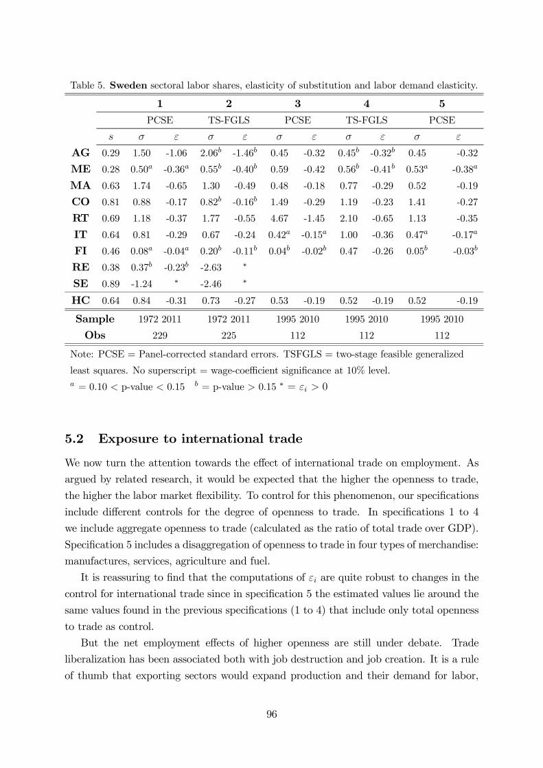
Table 5. Sweden sectoral labor shares, elasticity of substitution and labor demand elasticity.

1 2 3 4 5

PCSE TS-FGLS PCSE TS-FGLS PCSE

s σ ε σ ε σ ε σ ε σ ε

AG 0.29 1.50 -1.06 2.06b -1.46b 0.45 -0.32 0.45b -0.32b 0.45 -0.32

ME 0.28 0.50a -0.36a 0.55b -0.40b 0.59 -0.42 0.56b -0.41b 0.53a -0.38a

MA 0.63 1.74 -0.65 1.30 -0.49 0.48 -0.18 0.77 -0.29 0.52 -0.19

CO 0.81 0.88 -0.17 0.82b -0.16b 1.49 -0.29 1.19 -0.23 1.41 -0.27

RT 0.69 1.18 -0.37 1.77 -0.55 4.67 -1.45 2.10 -0.65 1.13 -0.35

IT 0.64 0.81 -0.29 0.67 -0.24 0.42a -0.15a 1.00 -0.36 0.47a -0.17a

FI 0.46 0.08a -0.04a 0.20b -0.11b 0.04b -0.02b 0.47 -0.26 0.05b -0.03b

RE 0.38 0.37b -0.23b -2.63 ∗

SE 0.89 -1.24 ∗ -2.46 ∗

HC 0.64 0.84 -0.31 0.73 -0.27 0.53 -0.19 0.52 -0.19 0.52 -0.19

Sample 1972 2011 1972 2011 1995 2010 1995 2010 1995 2010

Obs 229 225 112 112 112

Note: PCSE = Panel-corrected standard errors. TSFGLS = two-stage feasible generalized

least squares. No superscript = wage-coefficient significance at 10% level.a = 0.10 < p-value < 0.15 b = p-value > 0.15 ∗ = εi > 0

5.2 Exposure to international trade

We now turn the attention towards the effect of international trade on employment. As

argued by related research, it would be expected that the higher the openness to trade,

the higher the labor market flexibility. To control for this phenomenon, our specifications

include different controls for the degree of openness to trade. In specifications 1 to 4

we include aggregate openness to trade (calculated as the ratio of total trade over GDP).

Specification 5 includes a disaggregation of openness to trade in four types of merchandise:

manufactures, services, agriculture and fuel.

It is reassuring to find that the computations of εi are quite robust to changes in the

control for international trade since in specification 5 the estimated values lie around the

same values found in the previous specifications (1 to 4) that include only total openness

to trade as control.

But the net employment effects of higher openness are still under debate. Trade

liberalization has been associated both with job destruction and job creation. It is a rule

of thumb that exporting sectors would expand production and their demand for labor,

96

while sectors exposed to competition with imports would reduce production and hence

reduce the employment of labor (Jansen and Lee, 2007).

Associated to trade openness is international outsourcing, since the balance of pay-

ments includes the trade in services. As put by Amiti and Wei (2005), in the past, service

sectors were considered virtually unaffected by trade. For example, “accountants did

not fear that someone abroad would take their high-paying jobs”, but this scenario has

changed.

Tables 6 and 7 present the elasticity of the openness to trade variables in our spec-

ifications with respect to sector employment. The values in those tables are computed

with the homogeneous coefficients estimations (HC). The reason for the utilization of the

HC results is that the construction of the elasticity requires the openness coefficient (β5),

plus a global coefficient of persistence (β1). Table 6 shows in each column the elasticity

computed from specifications 1 to 4, and Table 7 refers to the results from specification 5

that disaggregates openness to trade.

Table 6. Long-run employment impact of international trade.

1 2 3 4

U.S. 1.86∗∗∗ -0.02 2.88∗∗∗ -0.26

Germany 0.15 -0.72∗ 0.06 0.08

Sweden 1.70∗∗∗ 1.40∗∗∗ 1.17∗∗∗ 0.90∗∗

Note: ∗∗∗,∗∗ and ∗ = significance at 1%, 5% and 10% level.

The degree of openness to international trade has a quite strong positive effect on

sectoral employment in Sweden in all specifications (1 to 4; Table 6). The value of the

long-run elasticity of this effect lies in the 0.90-1.70 range, thus the exposure to trade

in Sweden is likely to be elastic with respect to employment. This positive effect also

appears in the U.S., with even higher elasticities (1.86 and 2.88). In turn, the positive

employment effect of trade cannot be detected in Germany’s case. Not only that, but

one specification for the case of Germany (number 2) suggests a negative effect of further

openness to trade on employment.

The results for the U.S. and Sweden are consistent with recent evidence. Gozgor

(2013), for example, includes four different measures of trade liberalization and globaliza-

tion in a reduced-form unemployment equation and estimates the parameters for a panel

of G7 countries, and all four proxies present a negative and significant effect on equilib-

rium unemployment. Also, Felbermayr et al. (2011), in panel and cross-sectional data

specifications for several OECD countries, find a long-run reduction of unemployment

associated to a higher exposure to international trade. In this context, Germany is an

97

exception, where the exposure to trade has a non-positive effect on employment (that is,

a low negative effect, or altogether inexistent).

The disaggregation of the openness to trade variable on to four sectors of merchandise

brings further insights (Table 7). Germany still presents no significant effects of openness

to trade on employment. The U.S. and Sweden present a robust positive effect on em-

ployment of further openness to trade in manufactures, with a similar elasticity than the

aggregate case. The case of the degree of exposure to trade in services deserves particular

discussion: it has a negative effect on employment in the U.S. and a positive effect in the

case of Sweden.

Table 7. Disaggregated employment effect of openness to trade.

Manufactures Agriculture Fuel Services

U.S. 2.02∗∗∗ -0.51 0.02 -0.83∗∗

Germany 0.14 0.17 0.05 -0.44

Sweden 1.34∗∗∗ 0.09 -0.17 0.43∗

Note: ∗∗∗,∗∗ and ∗ = significance at 1%, 5% and 10% level.

In a recent paper, Yanikkaya (2013) finds that a higher total openness to international

trade has a negative effect on the growth rate of industrial employment and a positive

effect on the growth rate of service employment. It follows that higher trade intensity

may have diverse effects in different sectors.

In order to understand the opposite effect of higher trade intensity in services industries

on employment in the U.S. and in Sweden we must take a look at what is different between

these two countries. Figure 2 (panel e) shows that openness to trade in service industries

grew in both countries over the last decades. Nevertheless, it has been always higher in

the U.S., especially during the 1990s. Later, this difference has slightly declined (in 2011,

openness to trade in services was 30% in the U.S. and 24% in Sweden). Also, most service

sectors represented a higher proportion of employment in the U.S. than in Sweden over

the sample period, with the exception of the information and communications sector26.

As aforementioned, in recent years there has been a strong debate over the effect of off-

shoring (and international outsourcing) on domestic employment. Crinò (2009) presents

a complete review of empirical results: Amiti and Wei (2005) find a negative and signifi-

cant effect of offshoring on employment in an industry-level study for the UK (1992-2000

period), OECD (2007) finds a positive but non-significant effect on employment in 24

industries across 17 OECD countries, and Crinò (2010) estimates the elasticity of service

offshoring on domestic employment in 135 occupations in the U.S. over the 1997-2006

26Excluding the public sector (community services).

98

period and finds mostly negative effects on low and medium-skilled workers and a slim

positive effect on high-skilled worker. The results of Crinò (2010) are consistent with our

result for the U.S. The results in OECD’s report of 2007 for a panel of 17 countries agree

that there may be a positive effect in a given country.

So the answer must be in the role of trade in services in the U.S. and Sweden. Figure

3 presents the ratio of service imports over the industrial GDP (panel a) and the share

that services represent on total GDP (panel b). The ratio of U.S. imports of business

services over the industrial GDP has grown almost twofold over the 1993-2010 period. In

turn, in Sweden this ratio had a flatter evolution, with moderate growth starting only

after 2002. These contrasted evolutions combine with the fact that the dimension of the

so-called structural change is higher in the U.S. Over the 1990s there was a steep growth of

services fraction of GDP in the U.S. while it had a broadly constant evolution in Sweden.

Figure 3: Services in the U.S. and Sweden.

.01

.02

.03

.04

.05

.06

.07

1994 1996 1998 2000 2002 2004 2006 2008 2010

U.S.

Sweden

.68

.72

.76

.80

.84

.88

.92

1994 1996 1998 2000 2002 2004 2006 2008 2010

U.S.

Sweden

a. Imports of tradable services (over industrial GDP) b. Fraction of services over total GDP

In all, further openness to trade in services in the U.S. can threaten domestic employ-

ment, mainly because it could translate in strong growth of imports, continuing the trend

depicted over the last decade (Figure 3a). In Sweden, since domestic service industries

do not represent as much of total income, and imports of services do not display a strong

positive trend, higher levels of trade in services may favor employment.

It is important to recall that the effect of service offshoring is skill-biased and has dif-

ferent effects on high-skilled white-collar, low-skilled white-collar and blue-collar workers

(Crinò, 2010). In that sense, certain sectors are more sensitive to openness in services in-

dustries than others, bringing different results for different economies depending on their

economic structure.

99

5.3 Technical Change

Finally, we discuss the employment effect of technological progress. Recall that the time

trend included in the model is a standard proxy of a constant-rate technical change (e.g.

Antràs, 2004). The estimated coefficient associated to the time trend is (1 − σ)λN (by

equations 10, 11 and 12). In almost all specifications σ < 1. Hence, if the estimated

coefficient is negative, then technical change, in the context of the employment model in

this paper, would have a negative effect on employment.

Table 8 presents the calculation of the long-run elasticity of the time trend with respect

to employment (εLRn−t), which quantifies the employment effect of constant-rate technical

change, along with the annual growth rate of labor efficiency implied by our employment

equations (λN). It is based on the homogeneous coefficient (HC) estimations for long-run

computations as in the previous cases of trade effects. Cells left blank represent that the

trend coefficient is not statistically different from zero.

Take for example specification 1 in the U.S. The estimated elasticity of substitution

between factors is σ = 0.59, the long-run elasticity of the time trend is −6.8% [in the

context of equation (10), εLRn−t = β4/(1−β1)] and then λN = 17% [since λN = εLRn−t/(1−σ)].

Table 8. Employment effect of technical change.

1 2 3 4 5

εLRn−t λN εLRn−t λN εLRn−t λN εLRn−t λN εLRn−t λN

U.S. −6.8% 17% −12% 22% −3.2% 7%

Germany 2.8% 4%

Sweden −3.6% 22% −2.7% 10% −1.7% 4%

Notes: εLRn−t = long-run elasticity of time trend with respect to employment.

λN = growth rate of labor-related efficiency.

According to specification 5, a one percentage point increase in the rate of labor-related

technical change would imply a 3.2% fall in employment. This labor-saving technical

change grows at an annual constant rate of 7%. It follows that technological progress is

a detrimental force of employment.

In Germany’s case, specification 2 has a positive-sign long-run elasticity for the time

trend, but in that same specification σ = 1.7 > 1 (Table 4), and then the effect is also

labor-saving (McAdam and Willman, 2013). The employment effect of higher technical

change is 2.8%, and the growth rate of labor efficiency around 4%.

The long-run employment effect of technical change in Sweden is similar to that of

Germany, both considerably smaller than in the U.S. case. In Sweden, an additional

percentage point in the rate of technical change implies a fall in employment of between

100

a 1% and a 4%. The growth rate of labor efficiency, in turn, is similar to those of the

U.S.27

In this paper we estimate the growth rate of labor-related efficiency (λN), and not the

full bias in technical change (i.e., the gap in the growth rates of labor- and capital-related

efficiency). Nevertheless, labor-saving technical change was already identified for the U.S.

by several studies as surveyed by Klump et al. (2012), so the direction of the employment

effect of technological change may come as no surprise (see also Feldmann, 2013).

Note that technical change that presents a labor-saving effect in all three countries, is

either smaller in Germany than in the U.S. and Sweden, or almost inexistent. This result

may help in explaining the better performance of employment in Germany over the last

decade.

6 Concluding remarks

This paper analyzes the heterogeneity in labor demand from two empirical perspectives.

On the one hand, we provide calculations of the sector-level elasticities of labor demand

and find that these values vary significantly across economic activities. If we rank sectors

according to their estimated labor demand elasticity, some sectors are repeatedly among

the most sensitive sector-level labor markets. For example, the IT sector in the U.S. and

Germany, manufacturing in Germany and Sweden, and the mining and energy sectors in

the U.S. and Sweden have the most elastic employment effects to changes in labor costs.

In contrast, the retail trade sector has the lowest elasticities in the U.S. and Germany,

together with the finance services sector in Germany and Sweden. Notably, in our results

we do not observe general criteria in terms of manufacturing having lower or higher

elasticity than services sectors at this level of disaggregation. The standard economic

knowledge is that more competitive sectors (or with a more competitive labor market,

with less barriers like employment protection and benefits) are supposed to be more

flexible and thus exert a higher elasticity of labor demand.

Policywise, the main implication of these results is that a one—size-fits-all approach to

labor market policy will probably be inefficient. The reaction of employment to policy will

be quite different depending on economic activities. According to our results, different

economic sectors have different sensitivities in their demand for labor. Then, for a better

outcome, labor market policy should be properly conceived taking into account sectoral

27In Germany’s case, only one specification provides an statistically signicant time trend in the em-ployment equation (number 2). That same specification gives a high elasticity of substitution betweenlabor and capital, at least higher than those estimated in Sweden’s case. That is why although havingsimilar long-run elasticities of techinical change with respect to employment, Sweden has much higherefficieny growth rates than Germany.

101

particularities, in contrast to multifunctional recipes.

Also, Germany clearly presents lower sector-level elasticities of labor demand than the

U.S. (in absolute value) and in that sense it is, in general, a less flexible labor market.

Thus, looking at the performance that both labor markets had during the Great Reces-

sion, the following policy question arises: is flexibilization of European labor markets

the answer? We join those that call for a rethinking of labor market policy, trying to

go beyond labor market flexibilization and place more emphasis on investment, technol-

ogy, productivity, and related issues. The expansion of productive capacity, via targeted

investment and labor-enhancing innovation, is probably a better long-run solution than

social welfare deconstruction.

On the other hand, we investigate the employment effects of higher exposure to inter-

national trade. We do this by including the degree of openness to trade in the empirical

employment equation, first in its aggregate version, and later disaggregating openness to

trade into four variables according to four types of merchandise: manufactures, services,

agriculture and fuel. Openness to trade presents a non-negative effect on employment

(neutral in Germany and positive in the U.S. and Sweden). But new insights come along

disaggregating aggregate openness to trade. Higher trade in manufactures has a positive

effect on employment, as expected, in the U.S. and Sweden. Interestingly, a larger degree

of openness to trade in services has a negative effect on employment in the U.S. and a

positive effect in Sweden.

We believe that this result may be associated to the growing importance of imported

services in the U.S. economy and the important role that service industries already play,

in contrast to Sweden, where the services share of the economy is still not as large and

there may be room to increase trade in services and boost domestic employment. The

skill-biased effect of offshoring and international outsourcing is a phenomenon that should

be considered.

Lastly, this paper also verifies the presence of a negative employment effect of technical

change in the three countries studied. The long-run elasticity of constant-rate technical

change with respect to employment is between 3% and 12% in the U.S., less than 4% in

Sweden, and around a 3% in Germany. The annual growth rate of labor efficiency implied

by the model is 7% to 22% in the U.S., 4% to 22% in Sweden, and 0% to 4% in Germany.

The fact that this growth rate is small(er) in Germany may help in explaining its better

employment performance over the last decade. The main drivers of growth in economic

modeling are total factor productivity (or efficiency growth) and capital intensity. In

each economy, one of these drivers prevails over the other one, or they combine together.

This fact may contribute to explain the difference in the effect of efficiency growth on

employment that we observe in our results between the three countries, and should be

102

further investigated.

Future research should explore ways to estimate the elasticity of labor demand from

the empirical model directly instead of indirectly computing it via the estimated elasticity

of substitution. Also, disaggregated effects of openness to trade and technical change for

each one of the nine sectors in ISIC Revision 4 should be undertaken as a methodological

challenge. This paper uses a semi-pooling approach because it is the methodology that

suits best our sample. With higher T [or even higher N via disaggregation in industries

like, for example, Young (2013)], empirical methodology should be explored in order to

have nt−1i and wti for all i sectors (or industries). This should also allow to estimate the

employment effects of technical change and trade exposure at the sector level.

References

[1] Acemoglu, Daron (2003) “Labor- and capital-augmenting technical change”, Journal of the

European Economic Association, 1(1), 1-37.

[2] Amiti, Mary and Shang-Jin Wei (2005) “Fear of service outsourcing: is it justified?”, Eco-

nomic Policy, 307-347.

[3] Antràs, Pol (2004) “Is the U.S. aggregate production function Cobb-Douglas? New es-

timates of the elasticity of substitution”, Berkeley Electronic Journals in Macroeconomics:

Contributions to Macroeconomics, 4 (1), article 4.

[4] Arrow, Kenneth J., Hollis B. Chenery, Bagicha Singh Minhas and Robert M. Solow (1961)

“Capital-labor substitution and economic efficiency”, The Review of Economics and Statistics,

43(3), 225-250.

[5] Bernal-Verdugo, Lorenzo E., Davide Furceri, Dominique Guillaume (2012) “Labor market

flexibility and unemployment: new empirical evidence of static and dynamic effects”, Com-

parative Economic Studies, 54(2), 251-273.

[6] Beck, Nathaniel (2001) “Time-series cross-section data: what have we learned in the past

few years?”, Annual Review of Political Science, 4, 271-293.

[7] Beck, Nathaniel and Jonathan N. Katz (1995) “What to do (and not to do) with time-series

cross-section data”, American Political Science Review, 89, 634-647.

[8] Beck, Nathaniel and Jonathan N. Katz (2007) “Random coefficient models for time-series

cross-section data: Monte Carlo experiments”, Political Analysis, 15, 182-195.

103

[9] Chirinko, Robert (2008) “σ: The long and short of it”, Journal of Macroeconomics, 30(2),

671-686.

[10] Chirinko, Robert, Steven Fazzari and Andrew Meyer (2011) “A new approach to estimating

production function parameters: the elusive capital—labor substitution elasticity”, Journal of

Business & Economic Statistics, 29(4), 587-594.

[11] Crinò, Rosario (2010) “Service offshoring and white-collar employment”, Review of Eco-

nomic Studies, 77(2), 595-632.

[12] Crinò, Rosario (2009) “Offshoring, multinationals and labor market: a review of the em-

pirical literature”, Journal of Economic Surveys, 23, 197-249.

[13] Daveri, Francesco and Guido Tabellini (2000) “Unemployment, growth and taxation in

industrial countries”, Economic Policy, 15(30), 47-104.

[14] Felbermayr, Gabriel J., Julien Prat and Hans-Jörg Schmerer (2011) “Trade and unemploy-

ment: what do the data say?”, European Economic Review, 55(6), 741-758.

[15] Feldmann, Horst (2013) “Technological unemployment in industrial countries”, Journal of

Evolutionary Economics, 23(5), 1099-1126.

[16] Freeman, Richard B. (2013) “Failing the test? The flexible U.S. job market in the Great

Recession”, The Annals of the American Academy of Political and Social Science, 650, 78-97.

[17] Freeman, Richard B., Birgitta Swedenborg and Robert H. Topel (2010) “Introduction”, in

Freeman, Swedenborg and Topel (eds.) Reforming the welfare state: recovery and beyond in

Sweden, NBER, The University of Chicago Press.

[18] Gnangnon, Sena K. (2013) “The consequences of fiscal episodes in OECD DAC countries

for aid supply”, The Quarterly Review of Economics and Finance, 53, 302-313.

[19] Gozgor, Giray (2013) “The impact of trade openness on the unemployment rate in G7

countries”, The Journal of International Trade & Economic Development, forthcoming.

[20] Hamermesh, Daniel S. (1993) Labor Demand, Princeton University Press.

[21] Heinz, Frigyes Ferdinand and Desislava Rusinova (2011) “How flexible are real wages in

EU countries? A panel investigation”, Working Paper Series, 1360, European Central Bank.

[22] Hijzen, Alexander and Paul Swaim (2010) “Offshoring, labor market institutions and the

elasticity of labor demand”, European Economic Review, 54, 1016-1034.

104

[23] Jansen, Marion and Eddy Lee (2007) Trade and employment: challenges for policy research,

International Labour Organization (ILO) and World Trade Organization (WTO), Geneve.

[24] Judzik, Dario and Hector Sala (2013) “Productivity, deunionization and trade: wage effects

and labor share implications”, International Labour Review, 152(2), 205-236.

[25] Juhl, Ted and Oleksandr Lugovskyy (2013) “A test for slope heterogeneity in fixed effects

models”, Econometric Reviews, DOI: 10.1080/07474938.2013.806708.

[26] Klump, Rainer, Peter McAdam and Alpo Willman (2007) “Factor substitution and factor-

augmenting technical progress in the United States: a normalized supply-side system ap-

proach”, Review of Economics and Statistics, 89(1), 183—192.

[27] Klump, Rainer, Peter McAdam and AlpoWillman (2012) “The normalized CES production

function: theory and empirics”, Journal of Economic Surveys, 26(5), 769-799.

[28] Lewis, Philip E. T. and Garry MacDonald (2002) “The elasticity of demand for labor in

Australia”, The Economic Record, 78, pp. 18-30.

[29] León-Ledesma, Miguel, Peter McAdam and Alpo William (2010) “Identifying the elasticity

of substitution with biased technical change”, American Economic Review, 100(4), 1330-1357.

[30] McAdam, Peter and AlpoWillman (2013) “Medium run redux”,Macroeconomic Dynamics,

17(04), 695-727.

[31] Nickell, Stephen (1981) “Biases in dynamic models with fixed effects”, Econometrica, 49(6),

1417-1426.

[32] Nunziata, Luca (2005) “Institutions and wage determination: a multi-country approach”,

Oxford Bulletin of Economics and Statistics, 67(4), 435-464.

[33] OECD (2007), Employment Outlook, OECD: Paris.

[34] OECD (2012), Economic Outlook. No. 91, June 2012, OECD, Paris.

[35] Rinne, Ulf and Klaus F. Zimmermann (2013) “Is Germany the north star of labor market

policy?”, Discussion Paper, 7260, IZA, Bonn.

[36] Rowthorn, Robert (1999) “Unemployment, wage bargaining and capital-labour substitu-

tion”, Cambridge Journal of Economics, 23(4), 413-425.

[37] Rueda-Cantuche, José Manuel, Nuno Sousa, Valeria Andreoni and Iñaki Arto (2013) “The

single market as an engine for employment through external trade”, Journal of Common

Market Studies, 51(5), 931-947.

105

[38] Schettkat, Ronald and Lara Yocarini (2006) “The shift to services employment: a review

of the literature”, Structural Change and Economic Dynamics, 17, 127-147.

[39] Slaughter, Matthew J. (2001) “International trade and labor—demand elasticities”, Journal

of International Economics, 54, 27-56.

[40] Steiner, Andreas (2011) “Do dynamics and heterogeneity in panel data models matter?”,

Empirical Economics, 40, 165-176.

[41] Yanıkkaya, Halit (2013) “Is trade liberalization a solution to the unemployment problem?”,

Portuguese Economic Journal, 12(1), 57-85.

[42] Young, Andrew T. (2013) “U.S. elasticities of substitution and factor augmentation at the

industry level”, Macroeconomic Dynamics, 17, 2013, 861-897.

[43] Zhu, Ling (2013) “Panel data analysis in public administration: substantive and statistical

considerations”, Journal of Public Administration Research and Theory, 23(2), 395-428.

106

Appendix

Table A1. United States. Semi-pooled model.

[1] PCSE [2] TS-FGLS

c 0.636[0.290]

c 0.171[0.863]

∆nt−1 0.227[0.003]

∆nt−1 0.333[0.000]

∆nt−2 −0.184[0.027]

∆nt−2 −0.178[0.005]

vat 0.211[0.000]

vat 0.301[0.001]

t −0.007[0.000]

t −0.001[0.738]

opt 0.179[0.000]

opt 0.017[0.688]

nAGt−1 0.535[0.000]

wAGt −0.171[0.000]

nAGt−1 0.538[0.191]

wAGt −0.226[0.006]

nMEt−1 0.631[0.000]

wMEt −0.314[0.000]

nMEt−1 0.623[0.000]

wMEt −0.232[0.012]

nMAt−1 0.697[0.000]

wMAt −0.287[0.000]

nMAt−1 0.706[0.000]

wMAt −0.384[0.000]

nCOt−1 0.720[0.000]

wCOt −0.273[0.011]

nCOt−1 0.616[0.000]

wCOt −0.320[0.030]

nRTt−1 0.536[0.000]

wRTt −0.086[0.201]

nRTt−1 0.502[0.003]

wRTt −0.246[0.053]

nITt−1 0.860[0.000]

wITt −0.148[0.102]

nITt−1 0.730[0.031]

wITt −0.329[0.015]

nFIt−1 0.772[0.000]

wFIt −0.217[0.000]

nFIt−1 0.706[0.000]

wFIt −0.355[0.000]

nREt−1 0.857[0.000]

wREt −0.260[0.010]

nREt−1 0.830[0.000]

wREt −0.502[0.000]

nSEt−1 0.845[0.000]

wSEt 0.732[0.001]

nSEt−1 0.714[0.000]

wSEt −0.095[0.697]

Unbalanced Sample: 1978-2010 Unbalanced Sample: 1978-2010

Total obs: 230 Total obs: 229

Notes: p-values in brackets; Instruments: ∆nt−1 ∆nt−2 vat−1 opt−1 t

and nit−1 wit−1 ∀i. c = intercept.

107

Table A2. United States. Semi-pooled model.

[3] PCSE [4] TS-FGLS

c 1.017[0.085]

c 0.040[0.974]

∆nt−1 0.268[0.002]

∆nt−1 0.327[0.006]

∆nt−2 −0.218[0.016]

∆nt−2 −0.190[0.003]

vat 0.209[0.000]

vat 0.283[0.020]

t −0.008[0.001]

t 0.001[0.841]

opt 0.192[0.000]

opt −0.021[0.705]

nAGt−1 0.533[0.005]

wAGt −0.163[0.000]

nAGt−1 0.604[0.141]

wAGt −0.205[0.013]

nMAt−1 0.685[0.000]

wMAt −0.275[0.000]

nMAt−1 0.713[0.000]

wMAt −0.367[0.000]

nCOt−1 0.737[0.000]

wCOt −0.294[0.008]

nCOt−1 0.652[0.000]

wCOt −0.277[0.168]

nFIt−1 0.788[0.000]

wFIt −0.202[0.001]

nFIt−1 0.699[0.000]

wFIt −0.322[0.001]

nREt−1 0.862[0.000]

wREt −0.220[0.041]

nREt−1 0.854[0.000]

wREt −0.538[0.000]

Balanced Sample: 1978-2010 Balanced Sample: 1978-2010

Total obs: 165 Total obs: 165

Notes: p-values in brackets; Instruments: ∆nt−1 ∆nt−2 vat−1 opt−1 t

and nit−1 wit−1 ∀i. c = intercept.

108

Table A3. United States. FE model (HC).

[1] PCSE [2] TS-FGLS [3] PCSE [4] TS-FGLS

c 0.454[0.114]

c 0.416[0.083]

c 0.425[0.202]

c 0.130[0.731]

nt−1 0.912[0.000]

nt−1 0.939[0.000]

nt−1 0.935[0.000]

nt−1 0.957[0.000]

∆nt−1 0.330[0.000]

∆nt−1 0.520[0.000]

∆nt−1 0.353[0.000]

∆nt−1 0.522[0.000]

∆nt−2 −0.233[0.005]

∆nt−2 −0.275[0.000]

∆nt−2 −0.285[0.003]

∆nt−2 −0.258[0.004]

vat 0.072[0.007]

vat 0.019[0.469]

vat 0.057[0.060]

vat 0.023[0.538]

t −0.006[0.000]

t 0.0001[0.933]

t −0.008[0.000]

t −0.001[0.815]

opt 0.163[0.000]

opt −0.001[0.968]

opt 0.186[0.000]

opt −0.011[0.823]

wt −0.052[0.006]

wt −0.030[0.131]

wt −0.028[0.150]

wt −0.014[0.517]

Unbalanced Sample: 1978-2010 Balanced Sample: 1978-2010

Total obs: 230 Total obs: 229 Total obs: 165

Notes: p-values in brackets; Instruments in [2] and [4]: nit−1 ∆nt−1 ∆nt−2 vat−1 opt−1 t wit−1

c = intercept.

109

Table A4. United States. Specification [5]. PCSE.

[5] Semi-pooled. [5] HC

c 1.366[0.028]

c 0.191[0.618]

vat 0.209[0.000]

nt−1 0.905[0.000]

t −0.002[0.167]

vat 0.065[0.054]

opmt 0.217[0.000]

t −0.003[0.042]

opst −0.094[0.008]

opmt 0.192[0.000]

opat −0.095[0.006]

opst −0.079[0.046]

opft 0.008[0.557]

opat −0.048[0.147]

nAGt−1 0.471[0.022]

wAGt −0.212[0.000]

opft −0.002[0.898]

nMAt−1 0.595[0.000]

wMAt −0.368[0.000]

wt −0.049[0.031]

nCOt−1 0.624[0.000]

wCOt −0.315[0.006]

nFIt−1 0.621[0.000]

wFIt −0.205[0.002]

nREt−1 0.793[0.000]

wREt −0.236[0.089]

Balanced Sample: 1978-2010 Balanced Sample: 1978-2010

Total obs: 165 Total obs: 165

Notes: p-values in brackets. c = intercept.

110

Table A5. Germany. Semi-pooled model.

[1] PCSE [2] TS-FGLS

c 0.299[0.217]

c 0.170[0.541]

∆nt−1 0.328[0.000]

∆nt−1 0.352[0.000]

vat 0.145[0.000]

vat 0.206[0.000]

t −0.003[0.075]

t 0.010[0.581]

opt 0.036[0.191]

opt 0.010[0.743]

nAGt−1 0.909[0.000]

wAGt −0.080[0.017]

nAGt−1 0.838[0.000]

wAGt −0.182[0.000]

nMEt−1 0.918[0.000]

wMEt −0.086[0.027]

nMEt−1 0.908[0.000]

wMEt 0.009[0.850]

nMAt−1 0.677[0.000]

wMAt −0.213[0.008]

nMAt−1 0.593[0.000]

wMAt −0.364[0.000]

nCOt−1 0.863[0.000]

wCOt −0.222[0.013]

nCOt−1 0.801[0.000]

wCOt −0.146[0.020]

nRTt−1 0.646[0.000]

wRTt −0.044[0.522]

nRTt−1 0.483[0.000]

wRTt −0.140[0.020]

nITt−1 0.743[0.000]

wITt −0.064[0.248]

nITt−1 0.737[0.000]

wITt −0.146[0.020]

nFIt−1 0.658[0.000]

wFIt −0.063[0.018]

nFIt−1 0.577[0.000]

wFIt −0.098[0.026]

nREt−1 0.913[0.000]

wREt −0.069[0.679]

nREt−1 0.876[0.000]

wREt −0.048[0.803]

nSEt−1 0.868[0.000]

wSEt −0.091[0.287]

nSEt−1 0.777[0.000]

wSEt −0.048[0.523]

Balanced Sample: 1993-2011 Balanced Sample: 1993-2011

Total obs: 171 Total obs: 171

Notes: p-values in brackets; Instruments: ∆nt−1 vat−1 opt−1 t

and nit−1 wit−1 ∀i. c = intercept.

111

Table A6. Germany. Semi-pooled model.

[3] PCSE [4] TS-FGLS

c 0.813[0.016]

c 0.810[0.023]

∆nt−1 0.373[0.000]

∆nt−1 0.419[0.000]

vat 0.145[0.000]

vat 0.297[0.000]

t −0.003[0.087]

t −0.002[0.466]

opt 0.053[0.165]

opt 0.024[0.589]

nAGt−1 0.918[0.005]

wAGt −0.078[0.037]

nAGt−1 0.839[0.141]

wAGt −0.241[0.000]

nMAt−1 0.690[0.000]

wMAt −0.210[0.014]

nMAt−1 0.518[0.000]

wMAt −0.514[0.000]

nCOt−1 0.854[0.000]

wCOt −0.215[0.020]

nCOt−1 0.701[0.000]

wCOt −0.151[0.025]

nRTt−1 0.629[0.000]

wRTt −0.023[0.772]

nRTt−1 0.220[0.285]

wRTt −0.184[0.012]

nITt−1 0.731[0.000]

wITt −0.058[0.336]

nITt−1 0.628[0.000]

wITt −0.210[0.004]

nFIt−1 0.618[0.000]

wFIt −0.065[0.022]

nFIt−1 0.562[0.001]

wFIt −0.137[0.052]

Balanced Sample: 1993-2011 Balanced Sample: 1993-2011

Total obs: 114 Total obs: 114

Notes: p-values in brackets; Instruments: ∆nt−1 vat−1 opt−1 t

and nit−1 wit−1 ∀i. c = intercept.

112

Table A7. Germany. FE model (HC).

[1] PCSE [2] TS-FGLS [3] PCSE [4] TS-FGLS

c −0.236[0.130]

c −1.125[0.026]

c −0.022[0.903]

c 0.042[0.767]

nt−1 0.906[0.000]

nt−1 0.824[0.000]

nt−1 0.853[0.000]

nt−1 0.832[0.000]

∆nt−1 0.366[0.000]

∆nt−1 0.013[0.945]

∆nt−1 0.367[0.000]

∆nt−1 0.399[0.000]

vat 0.104[0.000]

vat 0.289[0.005]

vat 0.126[0.000]

vat 0.142[0.001]

t −0.001[0.410]

t 0.005[0.107]

t −0.001[0.422]

t −0.001[0.518]

opt 0.014[0.603]

opt −0.128[0.068]

opt 0.009[0.793]

opt 0.014[0.771]

wt −0.073[0.000]

wt −0.305[0.009]

wt −0.085[0.001]

wt −0.110[0.001]

∆wt 0.020[0.298]

∆wt −1.032[0.040]

Balanced Sample: 1993-2011 Balanced Sample: 1993-2011

Total obs: 171 Total obs: 114

Notes: p-values in brackets; Instruments in [2] and [4]: nit−1 ∆nt−1 vat−1 opt−1 t wit−1 wit−2

c = intercept.

113

Table A8. Germany. Specification [5]. PCSE.

[5] Semi-pooled. [5] HC

c 0.631[0.112]

c −0.034[0.903]

∆nt−1 0.397[0.000]

nt−1 0.857[0.000]

vat 0.145[0.000]

∆nt−1 0.379[0.000]

t 0.001[0.636]

vat 0.120[0.000]

opmt 0.048[0.176]

t −0.001[0.814]

opst −0.121[0.129]

opmt 0.020[0.542]

opat −0.036[0.333]

opst −0.062[0.417]

opft 0.017[0.178]

opat 0.025[0.437]

nAGt−1 0.927[0.000]

wAGt −0.075[0.057]

opft 0.007[0.559]

nMAt−1 0.658[0.000]

wMAt −0.238[0.015]

wt −0.080[0.002]

nCOt−1 0.862[0.000]

wCOt −0.235[0.016]

nRTt−1 0.602[0.001]

wRTt −0.009[0.925]

nITt−1 0.706[0.000]

wITt −0.050[0.400]

nFIt−1 0.559[0.001]

wFIt −0.055[0.069]

Balanced Sample: 1993-2011 Balanced Sample: 1993-2011

Total obs: 114 Total obs: 114

Notes: p-values in brackets. c = intercept.

114

Table A9. Sweden. Semi-pooled model.

[1] PCSE [2] TS-FGLS

c −0.398[0.270]

c −0.398[0.483]

∆nt−1 0.247[0.000]

∆nt−1 0.217[0.001]

vat 0.248[0.000]

vat 0.161[0.007]

t −0.003[0.002]

t −0.003[0.007]

opt 0.151[0.000]

opt 0.152[0.005]

nAGt−1 0.942[0.000]

wAGt −0.086[0.004]

nAGt−1 0.976[0.000]

wAGt −0.086[0.004]

nMEt−1 0.678[0.001]

wMEt −0.162[0.140]

nMEt−1 0.681[0.010]

wMEt −0.162[0.140]

nMAt−1 0.829[0.000]

wMAt −0.297[0.000]

nMAt−1 0.831[0.000]

wMAt −0.297[0.000]

nCOt−1 0.720[0.000]

wCOt −0.245[0.002]

nCOt−1 0.852[0.000]

wCOt −0.245[0.002]

nRTt−1 0.706[0.000]

wRTt −0.347[0.000]

nRTt−1 0.856[0.000]

wRTt −0.347[0.000]

nITt−1 0.671[0.000]

wITt −0.148[0.102]

nITt−1 0.731[0.000]

wITt −0.148[0.102]

nFIt−1 0.772[0.000]

wFIt −0.217[0.000]

nFIt−1 0.582[0.010]

wFIt −0.217[0.000]

nREt−1 0.857[0.000]

wREt −0.260[0.010]

nREt−1 0.552[0.125]

wREt −0.260[0.010]

nSEt−1 0.743[0.000]

wSEt 0.732[0.001]

nSEt−1 0.743[0.000]

wSEt 0.732[0.001]

Unbalanced Sample: 1972-2011 Unbalanced Sample: 1972-2011

Total obs: 229 Total obs: 225

Notes: p-values in brackets; Instruments: ∆nt−1 vat−1 opt−1 t

and nit−1 wit−1 ∀i. c = intercept.

115

Table A10. Sweden. Semi-pooled model.

[3] PCSE [4] TS-FGLS

c 1.639[0.021]

c 1.635[0.428]

∆nt−1 0.242[0.009]

∆nt−1 0.232[0.018]

vat 0.148[0.014]

vat 0.302[0.010]

t −0.007[0.005]

t −0.005[0.080]

opt 0.299[0.000]

opt 0.283[0.004]

nAGt−1 0.699[0.000]

wAGt −0.134[0.037]

nAGt−1 −0.136[0.938]

wAGt −0.517[0.458]

nMEt−1 0.633[0.004]

wMEt −0.215[0.052]

nMEt−1 0.153[0.805]

wMEt −0.478[0.224]

nMAt−1 0.505[0.000]

wMAt −0.236[0.000]

nMAt−1 0.505[0.000]

wMAt −0.381[0.000]

nCOt−1 0.660[0.000]

wCOt −0.506[0.002]

nCOt−1 0.499[0.004]

wCOt −0.594[0.007]

nRTt−1 0.938[0.000]

wRTt −0.289[0.002]

nRTt−1 0.740[0.010]

wRTt −0.545[0.001]

nITt−1 0.692[0.000]

wITt −0.130[0.148]

nITt−1 0.641[0.000]

wITt −0.357[0.011]

nFIt−1 0.342[0.094]

wFIt −0.024[0.676]

nFIt−1 0.558[0.082]

wFIt −0.209[0.059]

Balanced Sample: 1995-2010 Balanced Sample: 1995-2010

Total obs: 112 Total obs: 112

Notes: p-values in brackets; Instruments: ∆nt−1 vat−1 opt−1 t

and nit−1 wit−1 ∀i. c = intercept.

116

Table A11. Sweden. FE model (HC).

[1] PCSE [2] TS-FGLS [3] PCSE [4] TS-FGLS

c 0.568[0.002]

c 0.608[0.000]

c 1.359[0.001]

c 1.772[0.000]

nt−1 0.888[0.000]

nt−1 0.925[0.000]

nt−1 0.761[0.000]

nt−1 0.782[0.000]

∆nt−1 0.300[0.000]

∆nt−1 0.263[0.000]

∆nt−1 0.187[0.036]

∆nt−1 0.123[0.180]

vat 0.062[0.001]

vat 0.018[0.430]

vat 0.075[0.080]

vat 0.014[0.831]

t −0.004[0.000]

t −0.002[0.039]

t −0.004[0.011]

t −0.001[0.621]

opt 0.190[0.000]

opt 0.104[0.006]

opt 0.279[0.000]

opt 0.196[0.017]

wt −0.094[0.000]

wt −0.055[0.009]

wt −0.127[0.000]

wt −0.113[0.014]

Balanced Sample: 1995-2011 Balanced Sample: 1995-2011

Total obs: 112 Total obs: 112

Notes: p-values in brackets; Instruments in [2] and [4]: nit−1 ∆nt−1 vat−1 opt−1 t wit−1

c = intercept.

117

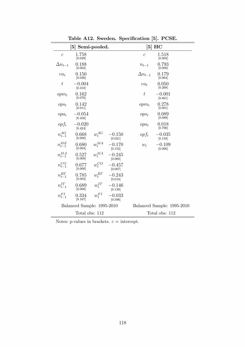
Table A12. Sweden. Specification [5]. PCSE.

[5] Semi-pooled. [5] HC

c 1.758[0.029]

c 1.518[0.002]

∆nt−1 0.188[0.062]

nt−1 0.793[0.000]

vat 0.150[0.036]

∆nt−1 0.179[0.064]

t −0.004[0.310]

vat 0.050[0.268]

opmt 0.162[0.076]

t −0.001[0.801]

opst 0.142[0.011]

opmt 0.278[0.001]

opat −0.054[0.456]

opst 0.089[0.089]

opft −0.020[0.424]

opat 0.018[0.790]

nAGt−1 0.668[0.000]

wAGt −0.150[0.021]

opft −0.035[0.158]

nMEt−1 0.680[0.004]

wMAt −0.170[0.152]

wt −0.109[0.000]

nMAt−1 0.527[0.000]

wMAt −0.245[0.000]

nCOt−1 0.677[0.000]

wCOt −0.457[0.007]

nRTt−1 0.785[0.002]

wRTt −0.243[0.018]

nITt−1 0.689[0.000]

wITt −0.146[0.130]

nFIt−1 0.334[0.167]

wFIt −0.033[0.596]

Balanced Sample: 1995-2010 Balanced Sample: 1995-2010

Total obs: 112 Total obs: 112

Notes: p-values in brackets. c = intercept.

118