Courant Research Centre ‘Poverty, Equity and Growth in Developing and Transition Countries: Statistical Methods and

Empirical Analysis’ Georg-August-Universität Göttingen

(founded in 1737)

No. 103

The estimation of threshold models in price

transmission analysis

Friederike Greb, Stephan von Cramon-Taubadel, Tatyana Krivobokova, Axel Munk

November 2011 (updated October 2012)

Discussion Papers

Wilhelm-Weber-Str. 2 ⋅ 37073 Goettingen ⋅ Germany Phone: +49-(0)551-3914066 ⋅ Fax: +49-(0)551-3914059

Email: crc-peg@uni-goettingen.de Web: http://www.uni-goettingen.de/crc-peg

The estimation of threshold models in pricetransmission analysis

Friederike Greb 1 Stephan von Cramon-Taubadel 2

Tatyana Krivobokova1, 3 Axel Munk3, 4

October 8, 2012

Abstract

The threshold vector error correction model is a popular tool for the analysis ofspatial price transmission and market integration. In the literature, the profile like-lihood estimator is the preferred choice for estimating this model. Yet, in certainsettings this estimator performs poorly. In particular, if the true thresholds are suchthat one or more regimes contain only a small number of observations, if unknownmodel parameters are numerous or if parameters differ little between regimes, theprofile likelihood estimator displays large bias and variance. Such settings are likelywhen studying price transmission. For simpler, but related threshold models Grebet al. (2011) have developed an alternative estimator, the regularized Bayesian esti-mator, which does not exhibit these weaknesses. We explore the properties of thisestimator for threshold vector error correction models. Simulation results show thatit outperforms the profile likelihood estimator, especially in situations in which theprofile likelihood estimator fails. Two empirical applications – a reassessment of thethe seminal paper by Goodwin and Piggott (2001), and an analysis of price trans-mission between German and Spanish markets for pork – demonstrate the relevanceof the new approach for spatial price transmission analysis.

Key words and phrases. Bayesian estimator, market integration, price transmission,

spatial arbitrage, TVECM.

1 Introduction

When assessing the integration of spatially separated markets, agricultural economists

typically analyze the transmission of price shocks between these markets (Fackler and

Goodwin 2001). The law of one price (LOP) states that prices for a homogeneous good

1Courant Research Centre ”Poverty, Equity and Growth in Developing Countries”, Georg-August-Universitat Gottingen, Wilhelm-Weber-Str. 2, 37073 Gottingen, Germany

2Department of Agricultural Economics and Rural Development, Georg-August-Universitat Gottin-gen, Platz der Gottinger Sieben 5, 37073 Gottingen, Germany

3Institute for Mathematical Stochastics, Georg-August-Universitat Gottingen, Goldschmidstrasse 7,37077 Gottingen, Germany

4Max Planck Institute for Biophysical Chemistry, Am Faßberg 11, 37077 Gottingen, Germany

1

at different locations should differ by no more than the transaction costs of trading the

good between these locations. Otherwise traders will engage in spatial arbitrage, which

increases the price at the low-price location and reduces the price at the high-price location

until the LOP is restored. In spatial equilibrium, the manner in which price shocks are

transmitted between two locations will therefore depend on the magnitude of the price

difference between these locations (Goodwin and Piggott 2001; Stephens et al. 2011).

Shocks that increase the price difference so that it exceeds the costs of trade between the

two locations will lead to arbitrage and price transmission. However, if the price difference

remains less than these transaction costs, arbitrage will not be profitable and there will

be no price transmission. The result is referred to in the literature as ”regime-dependent”

price transmission. Specifically, the spatial equilibrium model described above will lead

to three regimes delineated by two threshold values that equal the transaction costs of

trade in one and the other direction, respectively. In the outer regimes where the price

difference is greater than the transaction costs of trade in the one or the other direction,

arbitrage will lead to the transmission of price shocks. If the price difference lies within the

”band of inaction” between these transaction costs, prices can evolve independently of one

another. The costs of trade between two locations need not be symmetric; for example,

river transport might be more expensive going upstream than it is going downstream.

Hence, the thresholds that define the boundaries of the spatial price transmission regimes

will have opposite signs and possibly different magnitudes.

Threshold vector error correction models (TVECMs) are frequently used to model this

regime-dependent spatial price transmission process. TVECMs became popular with

Balke and Fomby’s (1997) article on threshold cointegration. Goodwin and Piggott’s

(2001) seminal paper established TVECMs in price transmission analysis, and dozens of

applications have followed. As an indication of the ongoing popularity of the TVECM, a

search of the AgEconSearch website (www.ageconsearch.umn.edu) on November 15, 2011

with the keywords ”price transmission” and ”threshold” produced 11 papers posted in

2

2010 and 2011.

Typically, and as we explain in greater detail below, thresholds in TVECMs are estimated

by maximizing the profile likelihood (Hansen and Seo 2002). However, in many settings,

this estimator is biased and has a high variance. Lo and Zivot (2001) as well as Balcombe

et al. (2007) acknowledge this problem. Profile likelihood estimates are especially prone

to be unreliable in situations characterized by large numbers of unknown model parame-

ters besides the thresholds, when there is little difference between adjoining regimes, and

when the location of the thresholds leaves only few observations in one of the regimes

(which is inevitable in small samples). These problems are generic and emerge in many

econometric settings, but they are particularly acute when profile likelihood is used to

estimate TVECMs. To cope with these shortcomings, several strategies are proposed in

the literature. Perhaps the most well-known of these is the modified profile likelihood

function introduced by Barndorff-Nielsen (1983). However, the proposed modifications

are usually based on regularity assumptions that do not hold for the TVECM. A further

weakness of the profile likelihood estimator is that it depends on an arbitrary trimming

parameter that ensures that each regime contains a minimum number of observations

and, thus, that estimation of the model parameters in that regime is possible. This can

be a problematic restriction when modeling spatial price transmission. If market integra-

tion is strong, differences in prices between two locations that exceed the transaction cost

thresholds – and therefore fall into one of the outer regimes – will be corrected quickly.

If this is the case, there will be few observations in the outer regimes, and a trimming

parameter which forces more observations into these regimes will inevitably lead to un-

reliable estimates of both the threshold values and the model parameters in each regime.

Estimation is not necessarily easier if the price data originate from markets that are poorly

integrated because in this case the weak price transmission displayed in the outer regimes

may be observationally quite similar to the independent price movements in the inner

”band of inaction”. Finally, the non-differentiability of the TVECM’s likelihood function

3

with respect to the thresholds exacerbates computation of its maximum, which can also

be a source of imprecise estimates.

These problems with the profile likelihood estimator suggest that there is a need to rethink

the estimation of TVECMs in price transmission analysis. In this article we investigate

the suitability of an alternative threshold estimator developed for generalized threshold

regression models (Greb et al. 2011). Among its advantages, this alternative estimator

does not require a trimming parameter. We demonstrate using Monte Carlo experiments

that this so-called regularized Bayesian estimator clearly outperforms the profile likelihood

estimator not only for generalized threshold regression models, but also specifically for

TVECMs, even in settings in which the profile likelihood estimator is highly biased and

variable. We also show that although employing the regularized Bayesian estimator is

technically easy, careful numerical implementation – even if it is computationally intensive

– can be decisive. Of course, it is important to go beyond the demonstration of the superior

statistical properties of the regularized Bayesian threshold estimator, and to consider as

well its implications for empirical price transmission analysis using TVECMs. Here, it is

crucial to interpret not only the estimated threshold parameters, but also the parameters

that describe the dynamics of price transmission within each regime. We draw on two

empirical applications to illustrate this.

The rest of this article is organized as follows. In the next section, we specify the TVECM,

discuss existing threshold estimators and their deficiencies, present the alternative esti-

mator, and comment on computational pitfalls in threshold estimation. Subsequently, we

illustrate the performance of the new estimator by means of a simulation study. As em-

pirical applications we first revisit the analysis of spatial market integration for four corn

and soybean markets in North Carolina detailed in the seminal contribution by Goodwin

and Piggott (2001), and second analyze spatial price transmission between German and

Spanish pork markets. The last section concludes.

4

2 Theory

2.1 The Model

Observations pt = (p1,t, p2,t)′, t = 1 . . . n, of a two-dimensional time series generated by a

TVECM with three different regimes, which are characterized by parameters ρk, θk ∈ R2

and Θkm ∈ R2×2 for k = 1, 2, 3 and m = 1, . . . ,M , can be written as

∆pt =

ρ1γ′pt−1 + θ1 +

M∑m=1

Θ1m∆pt−m + εt , γ′pt−1 ≤ ψ1 (Regime 1)

ρ2γ′pt−1 + θ2 +

M∑m=1

Θ2m∆pt−m + εt , ψ1 < γ′pt−1 ≤ ψ2 (Regime 2)

ρ3γ′pt−1 + θ3 +

M∑m=1

Θ3m∆pt−m + εt , ψ2 < γ′pt−1 (Regime 3).

(1)

We assume that pt forms an I(1) time series with cointegrating vector γ ∈ R2 and error-

correction term γ′pt. We further assume that the errors denoted by εt have expected

value E (εt) = 0 and covariance matrix Cov (εt) = σ2I2 ∈ (R+)2×2

; I2 ∈ R2×2 denotes

the identity matrix. We call ψ1, ψ2 the threshold parameters and define the threshold

parameter space Ψ to include all ψ = (ψ1, ψ2) such that min(γ′pt) < ψ1 < ψ2 < max(γ′pt).

Although all of the coefficients in equation (1) can vary across regimes, some of them can

remain constant.

In the spatial equilibrium setting, p1,t and p2,t are prices at different locations and γ is

often taken to equal (1,−1)′ so that the error correction term γ′pt measures the difference

between p1 and p2 at time t. The threshold ψ1 (ψ2) corresponds to the transaction costs

of trade from location 1 to location 2 (location 2 to location 1). Regimes 1 and 3 are

the outer regimes in which the violation of spatial equilibrium leads to arbitrage and

price transmission, and regime 2 represents the inner ”band of inaction”. For economic

interpretation, not only the estimates of the threshold parameters are of interest. The

estimates of ρk (k = 1, 2, 3) (often referred to as the ”adjustment parameter”) are also of

interest as they measure the speed with which violations of spatial equilibrium between

two locations are corrected in the respective regimes.

To express the model in matrix notation, we define vectors ∆pi and εi by stacking the

5

ith components of ∆pt and εt, respectively; and I (γ′p ≤ ψ1), I (ψ1 < γ′p ≤ ψ2), and

I (ψ2 < γ′p) by stacking I (γ′pt−1 ≤ ψ1), I (ψ1 < γ′pt−1 ≤ ψ2) and I (ψ2 < γ′pt−1), respec-

tively. I(·) denotes the indicator function. For observations at n time points, an n × d

matrix X is constructed by stacking rows x′t = (γ′pt−1, 1,∆p′t−1, . . . ,∆p

′t−M) of length

d = 2M + 2. βi,k is the ith column of the matrix (ρk, θk,Θk1, . . . ,ΘkM)′, i = 1, 2 and

k = 1, 2, 3. With diag {I(·)} defined as the diagonal matrix with entries I(·) in the

diagonal, we can write

∆pi = diag {I (γ′p ≤ ψ1)}Xβi,1 + diag {I (ψ1 < γ′p ≤ ψ2)}Xβi,2 (2)

+ diag {I (ψ1 < γ′p ≤ ψ2)}Xβi,3 + εi

= X1βi,1 +X2βi,2 +X3βi,3 + εi

for i = 1, 2. This leads to the a compact representation of model (1),

∆p =

(∆p1∆p2

)=(I2 ⊗X1)β1 + (I2 ⊗X2)β2 + (I2 ⊗X3)β3 + ε, (3)

where β′k =(β′1,k, β

′2,k

)for k = 1, 2, 3, and X = X1 +X2 +X3.

A variety of modifications and restrictions of the general TVECM (1) have been imple-

mented in price transmission studies. Lo and Zivot (2001) and Ihle (2010, table 2.1)

provide details on a number of important specifications. We limit attention to the general

TVECM. Restrictions of the model imply further information about the parameters (or

relations between them) and, hence, facilitate estimation. The most general case is thus

the most challenging. Although the TVECM can be generalized to include r thresholds

and r + 1 regimes, we focus on a TVECM with two thresholds and three regimes as this

is the version of the TVECM that is grounded in spatial equilibrium theory as outlined

above. Generalization is straightforward.

2.2 Commonly used threshold estimators

The most frequently used threshold estimator in the econometrics literature is the profile

likelihood estimator (Hansen and Seo 2002; Lo and Zivot 2001). According to this method,

6

for each possible pair of the threshold parameters ψ = (ψ1, ψ2) the remaining parameters

in the likelihood function corresponding to (1) are replaced by their maximum likelihood

estimates. The pair of thresholds that maximizes the resulting profile likelihood function

is selected as the estimate. More precisely, denoting the log-likelihood function of (1) by

` (ψ, β1, β2, β3, σ2), the profile likelihood estimator is defined as

ψpL = arg max `p(ψ) with `p(ψ) = `(ψ, β1, β2, β3, σ

2)

(4)

and βk and σ2 the maximum likelihood estimates of βk and σ2. Hence,

`p(ψ) ∝−{

∆p− (I2 ⊗X1)β1 − (I2 ⊗X2)β2 − (I2 ⊗X3)β3

}′{

∆p− (I2 ⊗X1)β1 − (I2 ⊗X2)β2 − (I2 ⊗X3)β3

} (5)

and βk = {(I2 ⊗Xk)′(I2 ⊗Xk)}−1 (I2 ⊗ Xk)

′∆p, k = 1, 2, 3. Since the profile likelihood

function is not differentiable with respect to the threshold parameters, the thresholds

that maximize the profile likelihood are determined by calculating (5) for each point on a

two-dimensional grid of possible threshold values, which is why the literature often refers

to the ”grid search” method.

The bias and high variance of the profile likelihood threshold estimator are mentioned

but not further pursued in the literature on TVECMs (see table 4 and figure 1 in Lo

and Zivot 2001). The simulation results we present below confirm the existence of these

weaknesses (see table 1 and figures 1 and 2). Greb et al. (2011) provide a detailed analysis

of the problems associated with the profile likelihood approach to threshold estimation.

In summary, there are two principal problems: i) the dependence on an arbitrary trim-

ming parameter; and ii) the uncertainty inherent in the βk which are estimated for each

combination of possible threshold values. The problems can be very pronounced in small

samples.

In spatial arbitrage modeling, the first issue can be decisive. ψ places each of the ob-

servations into one of three regimes. In order to compute βk, it is essential that at least

d = dim(βi,k) observations fall into the k-th regime. To ensure this, ψ1 must be greater

7

than or equal to γ′p(d), where γ′p(1), . . . , γ′p(n) is the ordered sequence of error correction

terms, and ψ2 must be correspondingly less than or equal to γ′p(n−d). The trimming

parameter restricts ψ accordingly. A variety of trimming parameters are suggested in the

literature. Goodwin and Piggott (2001) specify that each regime in the TVECM that

they estimate must include at least 25 observations. Balcombe et al. (2007) impose the

restriction that each regime must include at least 20% of the observations in their sample,

while Andrews (1993) proposes a minimum proportion of 15%. However, if markets are

well-integrated, then arbitrage will lead to rapid correction of any price differences that

exceed the thresholds, and the outer regimes will contain correspondingly few observa-

tions. Especially in small samples, this can lead to a situation in which the outer regimes

actually contain fewer observations than imposed by the chosen trimming parameter. In

this case, the resulting estimator cannot be consistent as the threshold parameter space Ψ

(and, hence, the grid that is searched) excludes the true thresholds. Despite its potential

impact on threshold estimation, the literature only offers a variety of arbitrary suggestions

for the trimming parameter.

The second problem naturally becomes more pronounced as the number of parameters in

the model (i.e. the dimension of βk) increases. Each additional lag included in a bivariate

TVECM with three regimes adds 12 coefficients. Hence, the number of coefficients to

be estimated can grow rapidly relative to the potentially few observations in the outer

regimes. If there is also little difference in coefficients between regimes, pinpointing the

location of the thresholds becomes increasingly difficult.

As an alternative to profile likelihood, Bayesian estimators have been employed in some

price transmission studies (Balcombe et al. 2007; Balcombe and Rapsomanikis 2008). As

explained in Greb et al. (2011), the performance of a Bayesian estimator in generalized

threshold regression models crucially depends on the selected priors. In the absence of

any prior knowledge of potential parameter values, so-called noninformative priors are the

natural choice. However, these can distort estimates. In particular, the posterior density

8

associated with noninformative priors for the βk inherits the dependence on a trimming

parameter from the profile likelihood. Due to an extra term in the likelihood function,

which grows rapidly as fewer observations are left in one of the regimes, the posterior

density takes its largest values exactly for those threshold values that are arbitrarily

included or excluded from the threshold parameter space Ψ when the trimming parameter

is varied. Consequently, the trimming parameter strongly affects the threshold estimate.

Nevertheless, Balcombe et al. (2007) and Balcombe and Rapsomanikis (2008) base their

Bayesian estimators on noninformative priors. Chen (1998) suggests a Bayesian estimator

based on a normal prior with known hyper-parameters for the βk and a uniform prior for

the threshold parameter. However, she designs the latter to assign zero probability to

threshold values that do not leave a minimum number of observations in each regime,

which is equivalent to assuming an arbitrary trimming parameter.

2.3 Regularized Bayesian estimator

Given the deficiencies of profile likelihood and Bayesian estimation with noninformative

priors, we explore the properties of an alternative threshold estimator (Greb et al. 2011)

in the context of TVCEMs. This regularized Bayesian estimator (RBE) was developed

for univariate generalized threshold regression models with one threshold. The idea of the

estimator is to penalize differences between regimes so as to keep these differences rea-

sonably small when the data contain little information. The strength of this regularizing

penalty is fundamental to the estimator. It is determined in a data-driven manner em-

ploying the so-called empirical Bayes paradigm. The estimator is developed in a Bayesian

framework and the penalization is a result of the choice of priors. As an important conse-

quence of the regularization, the posterior density is well-defined on the entire threshold

parameter space Ψ. Hence, there is no need to choose a trimming parameter and no risk

of excluding the true threshold from Ψ. In the setting of generalized threshold regression

models, the RBE outperforms commonly used estimators, especially when the threshold

9

leaves only few observations in one of the regimes or there is little difference in coefficients

between regimes.

Extension of the theory detailed in Greb et al. (2011) to the TVECM with two thresholds

in equation (1) is straightforward. It involves reparametrizing the model in equation (3),

∆p = (I2 ⊗X1)β1 + (I2 ⊗X2)β2 + (I2 ⊗X3)β3 + ε (6)

= (I2 ⊗X1)(β1 − β2) + {(I2 ⊗X1) + (I2 ⊗X2) + (I2 ⊗X3)} β2

+ (I2 ⊗X3)(β3 − β2) + ε

= (I2 ⊗X1)(β1 − β2) + (I2 ⊗X)β2 + (I2 ⊗X3)(β3 − β2) + ε

= (I2 ⊗X1)δ1 + (I2 ⊗X)β2 + (I2 ⊗X3)δ3 + ε,

and specifying a noninformative constant prior for β2 and normal priors for δi,

δi ∼ N (0, σ2δiI2d), i = 1, 3. The empirical Bayes strategy amounts to replacing σ2, σ2

δ1,

and σ2δ3

by their maximum likelihood estimates σ2, σ2δ1

, and σ2δ3

. As illustrated in the

appendix, this yields a log posterior density

p(ψ|∆p,X) ∝ −1

2

{(2n− 2d) log σ2 + log |V |+ log |Z ′V −1Z|

+1

σ2(∆p− Zβ2)′V −1(∆p− Zβ2)

} (7)

with β2 = (Z ′V −1Z)−1Z ′V −1∆p and V = I2n+ σ2δ1/σ2Z1Z

′1 + σ2

δ3/σ2Z3Z

′3 for Z = I2 ⊗X,

Z1 = I2 ⊗X1 and Z3 = I2 ⊗X3. A comparison of `p(ψ) in equation (5) with p(ψ|∆p,X)

in equation (7) shows that unlike the former, the latter does not depend on βk,

k = 1, 2, 3, which are not well-defined unless ψ leaves a minimum of d observations in

each regime. Accordingly, p(ψ|∆p,X) is defined on the entire threshold parameter space

Ψ = {(ψ1, ψ2) such that min(γ′pt) < ψ1 < ψ2 < max(γ′pt)}.

The regularized Bayesian threshold estimator ψrB =(ψ1rB, ψ2rB

)is computed as the

posterior median

ψirB∫min(γ′pt)

p(ψi|∆p,X)dψi = 0.5, i = 1, 2 (8)

10

assuming a prior p(ψ|X) ∝ I(ψ ∈ Ψ) for ψ. Here, p(ψi|∆p,X) denotes the i-th threshold’s

marginal posterior density. We choose the median of the posterior distribution because

it is more robust than the mode and yields more reliable results than the mean when

this density is skewed (which tends to be the case when the true threshold is close to the

boundary of the threshold parameter space Ψ).

2.4 Computational aspects

Any two threshold values which produce the same allocation of observations into regimes

produce identical values of the profile likelihood function Lp(ψ). Hence, Lp(ψ) is a step

function and not differentiable. The same holds for the posterior density p(ψ|∆p,X).

However, searching a grid that includes all of the observed error-correction terms yields

the exact maximum of Lp(ψ) and also makes it possible to calculate the precise value

of the integral of p(ψ|∆p,X). Obviously, this can be computationally intensive in large

samples. Hence, in practice, profile likelihood functions are often evaluated on a coarser

grid. For example, some authors (e.g. Goodwin and Piggott 2001) employ evenly spaced

grids that divide the threshold parameter space Ψ into a chosen number of equal steps and

that therefore do not necessarily include each of the observed error-correction terms. In

the absence of local maxima and large jumps between subsequent steps, such a simplified

grid will provide a reasonable approximation of the maximum/integral. However, when

the dimension of βk is high or the thresholds leave few observations in one of the regimes,

Lp(ψ) and p(ψ|∆p,X) tend to be jagged and display several local maxima. In such a case,

even a fairly dense grid can produce a poor approximation of the true maximum and,

consequently, poor estimates, if it does not include all function values. We demonstrate

this effect of an inappropriate grid choice in one of the empirical applications below.

Computation of the RBE is greatly simplified by taking advantage of functions for mixed

models available in statistical software packages. Again, we refer to Greb et al. (2011)

for details. R code for calculating RB estimates (for the general TVECM in equation (1)

11

and for restricted models such as the BAND-TVECM) is available from the authors.

3 Simulations

In a simulation study, we generate data using model (1) with the following

parameters: thresholds are set to ψ1 = −4 and ψ2 = 4; adjustment coefficients

ρ1 = ρ3 = (−0.25, 0)′ and ρ2 = (0, 0)′; intercepts θ1 = (−1, 0)′, θ2 = (0, 0)′, θ3 = (1, 0)′;

and Θ11 = Θ31 =(0.20

0.20

), Θ21 =

(00

00

). The cointegrating vector γ = (1,−1)′ is as-

sumed to be known; this implies an error correction term γ′pt = p1,t − p2,t that is simply

equal to the difference between p1 and p2. Errors are normally distributed, εt ∼ N (0, σ2I2)

with σ2 = 1. The length of the series is n = 200. We have selected the parameters to take

on values that are plausible in real data applications. They imply that in most simula-

tions about one half of the data belongs to the inner and one fourth to each of the outer

regimes.

We estimate thresholds by applying the profile likelihood and RB estimators to a Monte

Carlo sample of 300 replications of the data generating process defined above. We show

profile likelihood estimates for three different trimming parameters. These are, first, the

least restrictive trimming parameter possible (d = 2M+2, which ensures that each regime

contains at least exactly the minimum number of observations necessary to estimate

all model parameters), second, 15%, and third, 20% of the sample size. Results are

summarized in figures 1 and 2 together with table 1. The RBE clearly outperforms the

profile likelihood estimator. We observe a considerable reduction in both bias and variance

and, consequently, mean squared error. In contrast to the profile likelihood estimates, the

RB estimates are not drawn towards zero. The histograms show that the distribution of

the RB estimates is also less skewed. Further simulations (including restricted models)

confirm these findings. Altogether, the results indicate that the RBE is not only superior

for generalized threshold regression models, but also for TVECMs specifically.

12

Lower threshold Upper threshold

●

●

●

●

●

●

●

●●

●

●

●

●

●

●

●

●

●

−5

05

regBayes pL min pL 15% pL 20%

●

●●

●

●

●

●

●

●

●

−5

05

regBayes pL min pL 15% pL 20%

Figure 1: Simulation results – boxplots. Note: The horizontal dashed gray line indicatesthe true threshold. The dark lines in the shaded boxes are the respective sample means.”pL min”, ”pL 15%”, and ”pL 20%” denote profile likelihood estimates with trimmingparameters equal to the smallest possible value ( d = 2M + 2), 15% of the sample size,and 20% of the sample size, respectively.

Lower thresholdregBayes pL min pL 15% pL 20%

−10 −5 0 50.00

0.05

0.10

0.15

0.20

−10 −5 0 50.00

0.04

0.08

0.12

−10 −5 0 50.00

0.05

0.10

0.15

−10 −5 0 50.00

0.05

0.10

0.15

Upper thresholdregBayes pL min pL 15% pL 20%

−10 −5 0 50.00

0.10

0.20

−10 −5 0 50.00

0.04

0.08

0.12

−10 −5 0 50.00

0.05

0.10

0.15

−10 −5 0 50.00

0.05

0.10

0.15

Figure 2: Simulation results – histograms. Note: ”pL min”, ”pL 15%”, and ”pL 20%”denote profile likelihood estimates with trimming parameters equal to the smallest possiblevalue (d = 2M + 2), 15% of the sample size, and 20% of the sample size, respectively.

13

Regularized Bayesian estimator Profile likelihood estimator

lower threshold upper threshold lower threshold upper threshold

min 15% 20 % min 15% 20 %

true -4 4 -4 -4 -4 4 4 4

mean -3.63 3.72 -1.82 -1.22 -0.93 1.69 0.92 0.85

(2.23) (1.88) (3.40) (2.67) (2.45) (3.50) (2.79) (2.52)

MSE 5.10 3.62 16.31 14.86 15.40 17.57 17.21 16.24

Table 1: Simulation Results. Note: Standard errors are reported in parentheses belowthe mean. ”min”, ”15%”, and ”20%” denote trimming parameters equal to the small-est possible value (d = 2M + 2), 15% of the sample size, and 20% of the sample size,respectively.

4 Empirical Applications

4.1 Goodwin and Piggott (2001) revisited

In the first empirical application, we revisit Goodwin and Piggott’s (2001) seminal analysis

of spatial price transmission with TVECMs. We apply the RBE to their dataset and

compare the results with their profile likelihood estimates. Goodwin and Piggott (2001)

explore daily corn and soybean prices at important North Carolina terminal markets

(figure 3). These are Williamston, Candor, Cofield, and Kinston for corn, and Fayetteville,

Raleigh, Greenville, and Kinston for soybeans. Observations range from 2 January 1992

until 4 March 1999. For each commodity, Goodwin and Piggott (2001) evaluate pairs

consisting of a central market – Williamston for corn and Fayetteville for soybeans –

and each of the other markets in turn. They estimate the TVECM in equation (1)

with logarithmic prices by maximizing the profile likelihood function Lp(ψ) under the

assumption of Gaussian errors (or, equivalently, minimizing the sum of squared errors).

In accordance with spatial equilibrium theory they assume that ψ1 ≤ 0 and ψ2 ≥ 0 and

search for the maximum of Lp(ψ) among those ψ that meet this condition. To obtain

comparable results, we also incorporate this information in the RBE; we specify a prior

on ψ which is zero for any ψ such that ψ1 > 0 or ψ2 < 0, and uniform otherwise.

Goodwin and Piggott (2001) evaluate the estimating function at 100 equally spaced grid

14

(1) (2)0.

81.

01.

21.

41.

6

time

log(

pric

e)

WilliamstonCandorCofieldKinston

1992 1993 1994 1995 1996 1997 1998 1999 1.5

1.6

1.7

1.8

1.9

2.0

2.1

2.2

time

log(

pric

e)

FayettevilleRaleighGreenvilleKinston

1992 1993 1994 1995 1996 1997 1998 1999

Figure 3: Daily corn (1) and soybean (2) (log)prices at four North Carolina terminalmarkets. Source: Goodwin and Piggott (2001), who kindly made this data available.

points for each threshold. In contrast, we compute the RB estimates exactly, that is, the

posterior density is evaluated on a complete grid (that includes all observed values of the

error-correction term).

We report RB estimates together with Goodwin and Piggott’s (2001) original profile

likelihood estimates in table 2. It is evident that relative to the profile likelihood estimates,

the RB estimates for both thresholds tend to be of greater magnitude. This is confirmed

by the results reported in the last three columns of the same table, which show (in square

brackets) for each pair of markets the number of observations assigned to each of the

three regimes by the respective estimation method. Since the thresholds estimated by the

regularized Bayesian method are farther from zero, this method assigns correspondingly

less (more) observations to the outer (inner) regimes. The only exceptions are found in

regime 3 for Cofield – Williamston (corn) and Greenville – Fayetteville (soybeans).

In the last three columns of table 2 we also illustrate the effect of using a complete rather

than a uniform grid on the allocation of observations into regimes. For the profile likeli-

hood results, the first number in square brackets is the number of observations allocated

15

to the respective regime when Goodwin and Piggott’s uniform grid is employed, and the

second number is the corresponding number of observations when a complete grid is em-

ployed. If both grids lead to similar estimates of the thresholds ψ1 and ψ2, then they

will also lead to similar allocations of observations into regimes. While this is the case

for some market pairs, the cases of Raleigh – Fayetteville and Greenville – Fayetteville in

particular illustrate that a complete grid is necessary to ensure correct identification of

the global maximum of the likelihood function.

What are the economic implications of these results? Several points can be made. First,

the fact that the regularized Bayesian threshold estimates are father apart can be in-

terpreted as evidence of greater market integration. It implies that more observations

are in the inner ”band of inaction”, and correspondingly fewer are in the outer bands

where spatial equilibrium is violated, triggering trade and price adjustments.1 However,

if thresholds are estimates of the transaction costs of trade between two locations, then

the RBE suggests that these costs are higher than indicated by the profile likelihood

estimates (see O’Connell and Wei 2002). Hence, the regularized Bayesian threshold es-

timates suggest that the markets in question are more integrated in the sense that they

display fewer violations of spatial equilibrium, but also that they are separated by higher

transactions costs which must be overcome before arbitrage becomes profitable.

Second, market integration is reflected not only in how often violations of spatial equilib-

rium occur, but also in the speed with which such violations are corrected. According to

the two-market spatial equilibrium theory discussed above, the outer regimes should be

characterized by more rapid error correction than the inner regime, within which prices

can move independently and no error correction is expected. The profile likelihood and

regularized Bayesian estimates of the adjustment parameters presented in table 2 gener-

ally confirm this expectation. However, the profile likelihood estimates are surprising in

1The only major exception to this pattern is Fayetteville – Greenville, for which the inner regime ismore than twice as wide according to profile likelihood as it is according to the RBE. We discuss thisexception below.

16

two cases. First, for corn in Kinston – Williamston, the estimated adjustment parameters

in regime 1 are both greater than one in magnitude, which is implausible as it would

suggest that errors are amplified and not corrected. The total adjustment implied by

these two parameters (−0.166 in the third to last column of table 2) is negative, which

confirms that this regime is not consistent with error correction and cointegration. This

may be a reflection of the ”weaker” evidence for cointegration between corn prices in

Kinston and Williamston reported by Goodwin and Piggott (2001, p. 306). Second, total

adjustment in the inner regime (regime 2) in the case of corn in Candor and Williamston

(−0.015 in the second to last column of table 2) is also negative, which suggests that

price differences in this regime will also be amplified rather than corrected. This result is

incompatible with spatial equilibrium theory, which does not predict that prices will be

driven apart in the inner regime. However, it is not incompatible with market integration

between Candor and Williamston overall, because outer bands for this pair of markets are

characterized by error correction that will drive prices back towards equilibrium whenever

they leave the inner regime.

The regularized Bayesian estimates of the adjustment parameters presented in table 2

do not display any anomalies of this nature and therefore provide stronger evidence of

market integration. However, for many market pairs the adjustment coefficients in the

outer bands are smaller according to the RBE compared with profile likelihood. For corn

in Candor and Williamston, for example, total adjustment amounts to 0.130 in regime 1

and 0.120 in regime 3 according to profile likelihood, compared with 0.043 in both regimes

according to the RBE. Hence, while 13% (12%) of any difference between the two prices

is corrected per period in regime 1 (3) according to the profile likelihood results, only

4.3% is corrected in either regime according to the RBE.2 Hence, the RBE results point

to slower transmission of price shocks than the profile likelihood results.

2While most of the adjustment coefficients reported in table 2 are quite small, regardless of the methodused to estimate them, they are estimated using daily prices. Hence, in most cases the adjustment half-lifeis in the range of 1 – 2 weeks.

17

One other aspect of the results in table 2 deserves mention. For one of the corn market

pairs (Candor – Williamston) and all three of the soybean market pairs, the regularized

Bayesian estimates of the adjustment parameters are very similar or identical across all

three regimes. These results might indicate that the two-threshold, three-regime model

of price transmission is misspecified. As data on trade in corn and soybeans between the

markets in question are not available, it is not clear whether a model with two thresholds,

which includes a regime for trade from market 1 to market 2, but also a regime for trade

in the opposite direction, is correctly specified. If trade only flows in one direction, then

a model with one threshold and two regimes would be more appropriate. Sephton (2003),

who also revisits the Goodwin and Piggott (2001) data, finds that a one-threshold model is

indicated for four of the six pairs, and that the pairs Raleigh-Fayetteville and Greenville-

Fayetteville display little evidence of any threshold effects whatsoever. Our regularized

Bayesian estimates of very similar or identical adjustment coefficients across regimes for

some market pairs appear to corroborate Sephton’s finding.

18

Est. Dep.var. ρ1 σ (ρ1) ψ1 ρ2 σ (ρ2) ψ2 ρ3 σ (ρ3)Total(ρ1) Total(ρ2) Total(ρ3)

[#obs.] [#obs.] [#obs.]

Corn: Candor-Williamston

PL∆pCAN 0.003 (0.061)

-0.0250.006 (0.053)

0.003-0.030 (0.040) 0.130 -0.015 0.120

∆pWIL 0.133 (0.061) -0.009 (0.053) 0.090 (0.040) [295/298] [761/670] [716/797]

RBE∆pCAN 0.008 (0.019) -0.069 0.002 (0.013) 0.030 0.002 (0.013) 0.043 0.043 0.043

∆pWIL 0.051 (0.019) (0.011) 0.045 (0.013) (0.016) 0.045 (0.013) [12] [1545] [208]

Corn: Cofield-Williamston

PL∆pCOF -0.083 (0.063)

-0.0570.028 (0.012)

0.065-0.351 (0.558) 0.136 0.007 1.074

∆pWIL 0.053 (0.063) 0.035 (0.012) 0.723 (0.558) [69/68] [1669/1686] [35/11]

RBE∆pCOF 0.007 (0.011) -0.056 0.024 (0.013) 0.034 0.020 (0.012) 0.045 0.022 0.024

∆pWIL 0.052 (0.011) (0.026) 0.046 (0.013) (0.021) 0.044 (0.012) [73] [1409] [283]

Corn: Kinston-Williamston

PL∆pKIN -2.619 (0.773)

-0.0130.162 (0.053)

0.01900.954 (0.686) -0.166 0.028 0.204

∆pWIL -2.785 (0.773) 0.190 (0.053) 1.158 (0.686) [249/197] [1469/1558] [55/10]

RBE∆pKIN -0.011 (0.273) -0.020 0.092 (0.038) 0.0192 0.087 (0.041) 0.384 0.035 0.039

∆pWIL 0.373 (0.273) (0.004) 0.127 (0.038) (0.005) 0.126 (0.041) [7] [1753] [5]

Soybeans: Raleigh-Fayetteville

PL∆pRAL -0.352 (0.277)

-0.001-0.091 (0.108)

0.0100.257 (0.465) 0.417 -0.002 0.095

∆pFAY 0.065 (0.277) -0.093 (0.108) 0.352 (0.465) [166/492] [1559/1226] [47/47]

19

RBE∆pRAL -0.090 (0.063) -0.022 -0.090 (0.063) 0.014 -0.090 (0.063) 0.128 0.123 0.123

∆pFAY 0.038 (0.063) (0.002) 0.033 (0.063) (0.003) 0.033 (0.063) [11] [1714] [40]

Soybeans: Greenville-Fayetteville

PL∆pGRE -0.040 (0.048)

-0.0090.042 (0.047)

0.0120.083 (0.587) 0.064 0.029 0.370

∆pFAY 0.024 (0.048) 0.071 (0.047) 0.453 (0.587) [410/435] [1292/1026] [70/304]

RBE∆pGRE 0.014 (0.022) -0.008 0.014 (0.022) 0.006 0.015 (0.022) 0.053 0.053 0.053

∆pFAY 0.067 (0.022) (0.026) 0.067 (0.022) (0.011) 0.068 (0.022) [462] [558] [745]

Soybeans: Kinston-Fayetteville

PL∆pKIN -0.071 (0.043)

-0.0060.029 (0.182)

0.007-0.104 (0.093) 0.094 0.115 0.200

∆pFAY 0.023 (0.043) 0.144 (0.182) 0.096 (0.093) [544/550] [508/502] [721/713]

RBE∆pKIN -0.008 (0.021) -0.097 -0.003 (0.022) 0.021 -0.003 (0.022) 0.070 0.064 0.064

∆pFAY 0.062 (0.021) (0.029) 0.061 (0.022) (0.010) 0.061 (0.022) [9] [1691] [65]

Table 2: Estimates for the Data in Figure 3 – TVECM with three Regimes. Notes:- PL is the profile likelihood estimator; RBE is the regularized Bayesian estimator.- Standard errors of the estimated adjustment parameters (ρk) are provided in brackets. These must be interpreted with care becausethey are computed without accounting for the variability of the threshold estimate. Estimates that are significant at the 10% level arein bold. Standard errors for regularized Bayesian threshold estimates (in brackets below the estimate) are calculated in the customaryBayesian manner as their posterior standard deviation. To the best of our knowledge, it is an open question how to compute standarderrors for PL threshold estimates in TVECMs.- The error correction term is normalized so that the first adjustment parameter in each pair is expected to be negative, and the secondpositive. For example, for soybeans, the market pair Kinston – Fayetteville, and the profile likelihood (PL) estimator, the ρ1-values (-0.071and 0.023) have the expected signs.- Total(ρk) measures the total error-correction of price differences in regime k as the sum of the second adjustment parameter in each pairminus the first. For example, for soybeans, the market pair Kinston – Fayetteville, and the profile likelihood (PL) estimator, Total(ρ1) =0.094 = 0.023-(-0.071).- The number in square brackets below Total(ρk) is the estimated number of observations in regime k. For PL, the first number correspondsto Goodwin and Piggott’s estimates, the second to PL estimates based on a complete grid.

20

4.2 Price transmission between German and Spanish porkprices

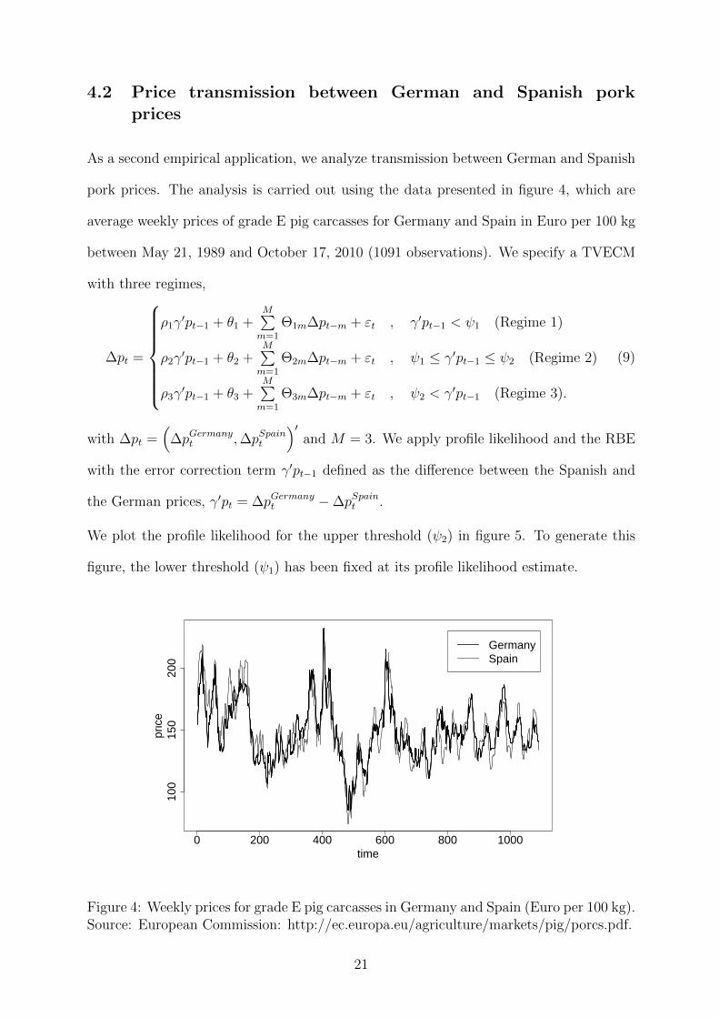
As a second empirical application, we analyze transmission between German and Spanish

pork prices. The analysis is carried out using the data presented in figure 4, which are

average weekly prices of grade E pig carcasses for Germany and Spain in Euro per 100 kg

between May 21, 1989 and October 17, 2010 (1091 observations). We specify a TVECM

with three regimes,

∆pt =

ρ1γ′pt−1 + θ1 +

M∑m=1

Θ1m∆pt−m + εt , γ′pt−1 < ψ1 (Regime 1)

ρ2γ′pt−1 + θ2 +

M∑m=1

Θ2m∆pt−m + εt , ψ1 ≤ γ′pt−1 ≤ ψ2 (Regime 2)

ρ3γ′pt−1 + θ3 +

M∑m=1

Θ3m∆pt−m + εt , ψ2 < γ′pt−1 (Regime 3).

(9)

with ∆pt =(

∆pGermanyt ,∆pSpaint

)′and M = 3. We apply profile likelihood and the RBE

with the error correction term γ′pt−1 defined as the difference between the Spanish and

the German prices, γ′pt = ∆pGermanyt −∆pSpaint .

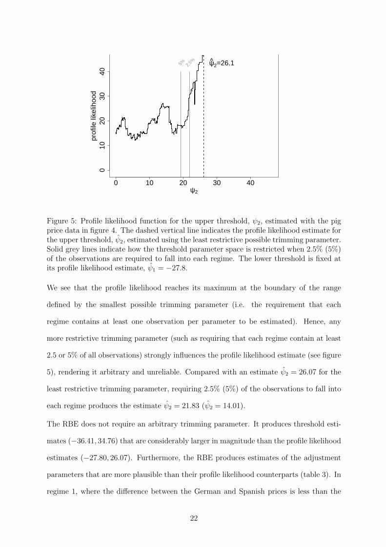
We plot the profile likelihood for the upper threshold (ψ2) in figure 5. To generate this

figure, the lower threshold (ψ1) has been fixed at its profile likelihood estimate.

0 200 400 600 800 1000

100

150

200

time

pric

e

GermanySpain

Figure 4: Weekly prices for grade E pig carcasses in Germany and Spain (Euro per 100 kg).Source: European Commission: http://ec.europa.eu/agriculture/markets/pig/porcs.pdf.

21

0 10 20 30 40

010

2030

40

ψ2

prof

ile li

kelih

ood

5% 2.5% ψ2=26.1

Figure 5: Profile likelihood function for the upper threshold, ψ2, estimated with the pigprice data in figure 4. The dashed vertical line indicates the profile likelihood estimate forthe upper threshold, ψ2, estimated using the least restrictive possible trimming parameter.Solid grey lines indicate how the threshold parameter space is restricted when 2.5% (5%)of the observations are required to fall into each regime. The lower threshold is fixed atits profile likelihood estimate, ψ1 = −27.8.

We see that the profile likelihood reaches its maximum at the boundary of the range

defined by the smallest possible trimming parameter (i.e. the requirement that each

regime contains at least one observation per parameter to be estimated). Hence, any

more restrictive trimming parameter (such as requiring that each regime contain at least

2.5 or 5% of all observations) strongly influences the profile likelihood estimate (see figure

5), rendering it arbitrary and unreliable. Compared with an estimate ψ2 = 26.07 for the

least restrictive trimming parameter, requiring 2.5% (5%) of the observations to fall into

each regime produces the estimate ψ2 = 21.83 (ψ2 = 14.01).

The RBE does not require an arbitrary trimming parameter. It produces threshold esti-

mates (−36.41, 34.76) that are considerably larger in magnitude than the profile likelihood

estimates (−27.80, 26.07). Furthermore, the RBE produces estimates of the adjustment

parameters that are more plausible than their profile likelihood counterparts (table 3). In

regime 1, where the difference between the German and Spanish prices is less than the

22

lower threshold value, the profile likelihood estimate of the adjustment parameter for the

Spanish price is significant and of relatively high magnitude (−0.665), but with an im-

plausible sign. Both magnitude and sign are implausible for the corresponding parameter

estimate in regime 3 (−1.193), where the difference between the German and the Spanish

prices exceeds the upper threshold. The corresponding estimated adjustment parameters

for the German price in regimes 1 and 3 (−0.198 and −0.334) have the expected negative

signs, but they are insignificant. Altogether, the total adjustments for regimes 1 and 3 are

negative according to the profile likelihood method (see the third-to-last and last colums

of table 3). Hence, the profile likelihood estimates suggest that there is no mechanism

that returns German and Spanish prices to their long run equilibrium when shocks drive

them apart. In comparison, the regularized Bayesian estimates of the adjustment param-

eters make considerably more sense. All of the regularized Bayesian estimates that are

significant, have the expected sign, and together they indicate that when the difference

between the German and the Spanish prices exceeds one of the thresholds, adjustments

are triggered that return these prices to their long run equilibrium (total adjustment

equals 0.318 in regime 1 and 0.348 in regime 3).

In summary, the empirical applications illustrate the advantages of the RBE in the con-

text of spatial price transmission analysis. The RBE does not depend on a trimming

parameter that arbitrarily influences the profile likelihood results in the application with

Spanish and German pork prices. Furthermore, in both applications the RB estimates

of the adjustment parameters are more plausible. In the application with the Goodwin

and Piggott (2001) data they appear to confirm Sephton’s (2003) finding that the two-

threshold TVECM is misspecified. In the application with Spanish and German pork

prices they are, unlike the profile likelihood estimates, consistent with spatial equilibrium

theory and price transmission between the markets in question.

23

Est. Dep.var. ρ1 σ (ρ1) ψ1 ρ2 σ (ρ2) ψ2 ρ3 σ (ρ3)Total(ρ1) Total(ρ2) Total(ρ3)

[#obs.] [#obs.] [#obs.]

PL∆pGermany -0.198 (0.354)

-27.8-0.028 (0.012)

26.1-0.334 (1.498) -0.467 0.080 -0.859

∆pSpain -0.665 (0.354) 0.052 (0.012) -1.193 (1.498) [21] [1058] [8]

RBE∆pGermany -0.286 (0.104) -36.4 -0.029 (0.011) 34.8 -0.355 (0.116) 0.318 0.092 0.348

∆pSpain 0.031 (0.104) (28.3) 0.063 (0.011) (149.9) -0.007 (0.116) [2] [1084] [1]

Table 3: Estimates for the Data in Figure 3 – TVECM with three Regimes. Note: The notes below table 2 apply.

24

5 Conclusions

We discuss the estimation of TVCEMs in spatial price transmission analysis. We point

out shortcomings of the common (profile likelihood) estimation procedure and emphasize

the relevance of these problems for applied price transmission studies. As an alternative,

we suggest employing a regularized Bayesian estimator (Greb et al. 2011), and we demon-

strate this estimator’s superior performance in a simulation study. Revisiting the empirical

analysis in Goodwin and Piggott’s influential paper on TVECMs in price transmission

analysis, we find that the RB estimates are free of several anomalies that characterise the

profile likelihood estimates, and appear to corroborate Sephton’s (2003) finding that the

two-threshold, three-regime TVECM is misspecified for the data in question. A second

application, with German and Spanish pork prices, confirms the advantages of the RBE

in spatial price transmission modeling, producing results that are more consistent with

the theory of spatial equilibrium than the corresponding profile likelihood results. Future

work could move beyond the pairwise consideration of markets to study multivariate sets

of prices and the more complex multiple-threshold relationships that exist between them.

Another extension would be to investigate time-varying thresholds, since especially for

longer time-series the assumption of constant transaction costs is questionable.

6 Acknowledgments

We acknowledge the support of the German Research Foundation (Deutsche Forschungs-

gemeinschaft) as part of the Institutional Strategy of the University of Gottingen. We

would like to thank Barry Goodwin and Nicholas Piggott for sharing their dataset with

us.

25

7 Appendix

Our aim is to compute the posterior density p (ψ|∆p,X) for the model

∆p = (I2 ⊗X1)δ1 + (I2 ⊗X)β2 + (I2 ⊗X3)δ3 + ε, ε ∼ N (0, σ2I2n)

with a normal prior δ1 ∼ N (0, σ2δ1I2d), where d = 2M + 2 with M the number of lags

included in the model; a uniform prior β2 ∼ U(R2d); a normal prior δ3 ∼ N (0, σ2

δ3I2d);

and a uniform prior ψ ∼ U(ψ ∈ Ψ).

To this end, we first calculate p (∆p|ψ,X), since

p (ψ|∆p,X) = p (∆p|ψ,X) p(ψ|X)/p(∆p|X) ∝ p (∆p|ψ,X)

given a constant prior p(ψ|X). Employing an empirical Bayes approach, it suffices to com-

pute p(∆p|ψ,X, σ2, σ2

δ1, σ2

δ3

): parameters σ2, σ2

δ1, and σ2

δ3are replaced by their maximum

likelihood estimates σ2, σ2δ1

, and σ2δ3

. Given our specification of priors,

p(∆p|ψ,X, σ2, σ2

δ1, σ2

δ3

)=

∫p(∆p, β2|ψ,X, σ2, σ2

δ1, σ2

δ3

)dβ2

=

∫p(∆p|β2, ψ,X, σ2, σ2

δ1, σ2

δ3

)p(β2|ψ,X, σ2, σ2

δ1, σ2

δ3

)dβ2

=

∫p(∆p|β2, ψ,X, σ2, σ2

δ1, σ2

δ3

)dβ2

and

∆p|β2, ψ,X, σ2,σ2δ1, σ2

δ3∼

N{

(I2 ⊗X)β2, σ2I2n + σ2

δ1(I2 ⊗X1)(I2 ⊗X1)

′ + σ2δ3

(I2 ⊗X3)(I2 ⊗X3)′} .

To simplify notation, define Z = I2 ⊗ X, Z1 = I2 ⊗ X1, Z3 = I2 ⊗ X3, and

V = I2n + σ2δ1/σ2Z1Z

′1 + σ2

δ3/σ2Z3Z

′3 and write

∆p|β2, ψ,X, σ2, σ2δ1, σ2

δ3∼ N

(Zβ2, σ

2V).

26

Consequently,

p(∆p|ψ,X, σ2, σ2

δ1, σ2

δ3

)=

∫ (1

2πσ2

)2n/21√|V |

exp

{− 1

2σ2(∆p− Zβ2)′V −1(∆p− Zβ2)

}dβ2

=

(1

2πσ2

)2n/21√|V |

exp

{− 1

2σ2(∆p− Zβ2)′V −1(∆p− Zβ2)

}·∫

exp

{− 1

2σ2(β2 − β2)′Z ′V −1Z(β2 − β2)

}dβ2

=

(1

2πσ2

)2n/21√|V |

exp

{− 1

2σ2(∆p− Zβ2)′V −1(∆p− Zβ2)

}(2πσ2)2d/2

1√|Z ′V −1Z|

=

(1

2πσ2

)2(n−d)/21√

|V ||Z ′V −1Z|exp

{− 1

2σ2(∆p− Zβ2)′V −1(∆p− Zβ2)

}with β2 = (Z ′V −1Z)−1Z ′V −1∆p. Substituting σ2, σ2

δ1, and σ2

δ3for σ2, σ2

δ1, and σ2

δ3respec-

tively yields a log posterior density

p(ψ|∆p,X) ∝ p (∆p|ψ,X) ∝ −1

2

{(2n− 2d) log σ2 + log |V |+ log |Z ′V −1Z|

+1

σ2(∆p− Zβ2)′V −1(∆p− Zβ2)

}

Note that for ease of notation we use the same letter V to denote the covariance matrix

based on σ2, σ2δ1

, and σ2δ3

or on σ2, σ2δ1

, and σ2δ3

. Here V = I2n + σ2δ1/σ2Z1Z

′1 + σ2

δ3/σ2Z3Z

′3.

27

References

Andrews, D. (1993). Tests for parameter instability and structural change with unknown

change point. Econometrica, 61(4):821–856.

Balcombe, K., Bailey, A., and Brooks, J. (2007). Threshold effects in price transmission:

the case of Brazilian wheat, maize, and soya prices. American Journal of Agricultural

Economics, 89(2):308–323.

Balcombe, K. and Rapsomanikis, G. (2008). Bayesian estimation and selection of non-

linear vector error correction models: the case of the sugar-ethanol-oil nexus in Brazil.

American Journal of Agricultural Economics, 90(3):658–668.

Balke, N. and Fomby, T. (1997). Threshold cointegration. International Economic Review,

38(3):627–645.

Barndorff-Nielsen, O. (1983). On a formula for the distribution of the maximum likelihood

estimator. Biometrika, 70(2):343.

Chen, C. (1998). A Bayesian analysis of generalized threshold autoregressive models.

Statistics & probability letters, 40(1):15–22.

Fackler, P. and Goodwin, B. (2001). Spatial price analysis. Handbook of agricultural

economics, 1:971–1024.

Goodwin, B. and Piggott, N. (2001). Spatial market integration in the presence of thresh-

old effects. American Journal of Agricultural Economics, 83(2):302–317.

Greb, F., Krivobokova, T., Munk, A., and von Cramon-Taubadel, S. (2011). Regularized

Bayesian estimation in generalized threshold regression models. CRC-PEG Discussion

Paper No.99, Courant Research Centre ”Poverty, Equity and Growth in Developing

Countries”, Georg-August-Universitat Gottingen.

28

Hansen, B. and Seo, B. (2002). Testing for two-regime threshold cointegration in vector

error-correction models. Journal of Econometrics, 110(2):293–318.

Ihle, R. (2010). Models for Analyzing Nonlinearities in Price Transmission. PhD thesis,

Niedersachsische Staats-und Universitatsbibliothek Gottingen.

Lo, M. and Zivot, E. (2001). Threshold cointegration and nonlinear adjustment to the

law of one price. Macroeconomic Dynamics, 5(04):533–576.

O’Connell, P. and Wei, S. (2002). ”The bigger they are, the harder they fall”: Retail

price differences across US cities. Journal of International Economics, 56(1):21–53.

Sephton, P. (2003). Spatial market arbitrage and threshold cointegration. American

Journal of Agricultural Economics, 85(4):1041–1046.

Stephens, E., Mabaya, E., Cramon-Taubadel, S., and Barrett, C. (2011). Spatial price

adjustment with and without trade. Oxford Bulletin of Economics and Statistics.

29