POPULATION AGING RESEARCH CENTER

Time Preference and Its Relationship with Age, Health, and Longevity Expectations

Li-Wei Chao, Helena Szrek, Nuno Sousa Pereira, Mark V. Pauly

PARC Working Paper Series

WPS 07-05

"The authors acknowledge the support of the National Institutes of Health - National Institute on Aging, Grant number P30 AG12836, B.J. Soldo, PI"

3718 Locust Walk Philadelphia, PA 19104-6298 Tel 215-898-6441 Fax 215-898-2124

1

Time Preference and Its Relationship with Age, Health, and Longevity Expectations

LI-WEI CHAOa, HELENA SZREKb,c, NUNO SOUSA PEREIRAb,c, MARK V. PAULYd*

WORKING PAPER PLEASE DO NOT CITE WITHOUT PERMISSION.

COMMENTS ARE WELCOME.

(Version Date: 15 April 2007)

a Population Studies Department, University of Pennsylvania, 3718 Locust Walk, Room 239, Philadelphia, Pennsylvania 19104-6298 U.S.A.

b Faculdade de Economia, Universidade do Porto, Rua Dr. Roberto Frias, 4200-464 Porto, Portugal

c CETE (Research Center in Industrial, Labour, and Managerial Economics, Universidade do Porto, Rua Dr. Roberto Frias, 4200-464 Porto, Portugal

d Health Care Systems Department, The Wharton School, University of Pennsylvania, 3641 Locust Walk, Room 204, Philadelphia, Pennsylvania 19104-6257 U.S.A. Email addresses: chao69@wharton.upenn.edu (L.W. Chao), hszrek@fep.up.pt hszrek@wharton.upenn.edu (H. Szrek), npereira@fep.up.pt (N. Sousa Pereira), pauly@wharton.upenn.edu (M.V. Pauly) Acknowledgement: We gratefully acknowledge financial support for the study provided by the National Institutes of Health National Institute on Ageing (P30AG12836, B.J. Soldo, P.I.) and the Fogarty International Center (R01TW005611, M.V. Pauly, P.I.; K01TW06658, L.W.Chao, P.I.). Nuno Sousa Pereira also gratefully acknowledges support from CETE, Research Center on Industrial, Labour and Managerial Economics, which is supported by the Fundacao para a Ciencia e a Tecnologia, Programa de Financiamento Plurianual, through the Programa Operacional Ciencia, Tecnologia e Inovacao (POCTI) of the Quadro Comunitario de Apoio III. All errors are our own.

2

ABSTRACT

Although theories in both evolutionary biology and economics predict that an individual’s health

should be associated with the individual’s time preference, no prior study has been done to

empirically support or refute such predictions. By collecting detailed measures of health, time

preference, and expected longevity on a sample of individuals in townships around Durban,

South Africa, this study breaks new ground by being the first to analyze in detail the relationship

between time preference and health, in an area of the world with high mortality and morbidity.

Interestingly, we find that both physical health and expectations of longevity have a U-shaped

relationship with the person’s subjective discount rate. This suggests that those in very poor

health have high discount rates, but those in very good health also have high discount rates.

Similarly those with longevity expectations on the extremes have high discount rates. The

research question addressed by this pilot project is policy relevant, as the study tries to determine

the importance of health in economic development, not from the commonly asserted

productivity-gain argument, but from a much broader investment-for-the-future argument.

3

INTRODUCTION

The utility from consumption in the future is, ceteris paribus, often “discounted” relative

to the utility from consuming the same commodity bundle in the current period. “Time

preference” is the term used to describe the phenomenon that people attach different values to

the same consumption bundle depending on when consumption of that commodity bundle

occurs. In this paper, we are concerned with the degree to which an individual discounts future

consumption relative to current consumption, which we call the subjective discount rate or level

of impatience. Where patience is the willingness to wait for something in the future, which

corresponds to forgoing current consumption and its associated utility in exchange for future

consumption and utility, impatience is the unwillingness to wait.

Although time preference is commonly assumed in models of intertemporal choice, the

literature does not fully explain why some people are more impatient than others. For example,

some individuals manage to save money for retirement, whereas others with otherwise similar

personal characteristics (like income, education, race, age, and sex) do not manage to save.

Understanding the determinants of a person’s subjective discount rate is important because

policies could be better tuned to induce more desirable results if they included an accurate

estimate of people’s intertemporal optimization decisions, while, at the same time, decision tools

and policy manipulable variables could be developed to shape people’s intrinsic subjective

discount rates. In other words, policy analysts should be concerned about impatience because

individuals underinvest in the future in many domains, including retirement savings and health.

Furthermore, individuals could be encouraged to counter this underinvestment behavior if pre-

commitment devices were more readily available. An example is a pre-commitment to save, such

as a retirement plan with savings rates tied to future salary increases (Thaler and Bernartzi, 2004)

4

or a fixed deposit account with large penalties for early withdrawal (Ashraf, Karlan, and Yin,

2006), or even a pre-commitment to fertility control such as an implantable contraceptive device

that lasts two or more years instead of the condom that often requires last minute decision-

making. The intrinsic interest in policies or strategies that entail pre-commitment arises in

situations where an individual would rather invest for the future but finds it difficult to resist the

temptations of consuming in the present period.

Recent advances in evolutionary biology, economics, psychology, and neuroscience have

provided some clues as to the potential determinants of subjective discount rates (for a succinct

review, see Read & Read 2004). Evolutionary biology assumes that subjective discount rates are

exogenously dictated by one’s genes and models a person’s subjective discount rate as a product

of natural selection to maximally propagate one’s genes (e.g., Rogers 1994; Sozou & Seymour

2003). These models predict a subjective discount rate that peaks at a time in life (as proxied by

age) when reproductive potential is high, so that resources can be expended on sexual

reproduction to propagate genes, rather than saved.

In contrast to the evolutionary biology approach, the field of economics models time

preference from a utility maximization framework and derives subjective discount rates as

outcomes of endogenous choice. Becker & Mulligan (1997) assume that each person is endowed

with an initial level of subjective discount rate, but that rate can be modified by the individual

investing time and resources to produce “future-oriented capital” to make the future more salient,

allowing one to appreciate the future more and to place more weight on future utility of

consumption -- leading to a lower subjective discount rate. Their model implies that an

exogenous increase in longevity will correspondingly give consumers incentives to invest in

“future-oriented capital” so that the extra life years gained can be better appreciated – resulting

5

in a lower subjective discount rate. In addition to longevity, subjective discount rate may also be

related to health. Trostel & Taylor (2001) show that the increasing rate of decline in one’s ability

to enjoy visceral pleasures, such as with natural ageing and declines in health over the lifecycle,

is associated with increasing decline of marginal utility of consumption over time, resulting in an

inverse relationship between subjective discount rate and age (as a proxy for health). Recently,

neuroimaging data provide a physiological explanation of impatience. Data derived from

participants’ choices between smaller sooner monetary rewards versus larger later monetary

rewards show that separate processes (limbic areas versus the lateral prefrontal areas,

respectively) regulate decisions regarding immediate rewards versus delayed rewards (McClure

et al. 2004) and that a quasi-hyperbolic discount function (e.g., Laibson 1997) approximates

neuroimaging and survey data better than alternative functional forms. Nevertheless, it is unclear

at this time what factors (such as ageing, illness, or experience), if any, might alter the activities

of these brain regions in making temporal decisions.

We build our hypotheses based on the above theories and relate them to existing

empirical findings. First, we expect the discount rate to be U-shaped when plotted against age,

based on the theory developed in evolutionary biology and described above. Read & Read

(2004) found evidence of a mostly U-shaped function using a survey of young, middle, and older

aged adults in the United Kingdom.

H1: The discount rate is high for young adults, low for middle-aged individuals, and

high for older individuals.

Second, the subjective discount rate may vary with health. We can expect this to be the

case for a few reasons. Those in poor health may have a high subjective discount rate because

they do not expect to live as long. Besides longevity reasons, those in poor health may expend

6

more resources to improve health (or prevent further health decline) than to build “future

oriented capital” as in Becker & Mulligan (1997), resulting in a higher subjective discount rate.

Although poor health may be associated with a high subjective discount rate, the theory by

Trostel and Taylor (2004) suggests that those in very good health may also have a high

subjective discount rate because they derive greater utility from consumption when healthy than

when sick. A few studies have also empirically examined the relationship between one’s health

and one’s subjective discount rate, but these studies used somewhat limited measures for health

and found mixed results. Kirby et al. (2002) used body mass index (BMI) and found no

relationship; Read & Read (2004) used two dichotomous variables for health (good vs. bad

health; existence of disease in last year vs. no existence of disease in last year) and found poor

health to be unrelated to the subjective discount rate for money but related to the subjective

discount rate for vacation; and Tu et al. (2004) found BMI and general health to be positively

associated with the subjective discount rate for money, linking obesity with impatience but also

good health with impatience. Based on these theories and empirical studies, we expect the

discount rate to be U-shaped when plotted against health.

H2: Those in very poor or very good health have a high subjective discount rate,

and those with average health have a lower discount rate.

Third, we expect the subjective discount rate to be inversely correlated with expected

longevity. Individuals that do not expect to live long will expend their resources in the current

period. Bloom et al. (2003), in a cross country panel study of national savings rates, found

evidence of a relationship between increased longevity and increased savings behavior. Picone et

al. (2004), using the U.S. Health and Retirement Study population, found that increased

longevity is associated with investments in health. Thornton (2007) found that people in Malawi

7

who learned they were HIV negative and were optimistic about their future infection risks had

higher subjective life expectancies and were more likely to invest in agricultural inputs than

those who tested positive or were pessimistic about their future risks.

H3: The subjective discount rate will be inversely correlated with expected

longevity.

In this paper, we try to add some insight into the determinants of subjective discount rates

by testing the above hypotheses. We continue by discussing the survey data that we collected,

and then we describe our results. Next, we explore potential explanations for our results, list the

weaknesses and strengths of our study, and conclude with policy implications.

METHOD

Participants and Procedures

This study is part of a larger study on the impact of poor health and HIV/AIDS on micro and

small enterprises (MSEs) around Durban, South Africa. The sample is described in detail in

Chao et. al. (2007). Surveys were conducted over a three year period in select townships around

Durban, South Africa, with information on health, business activity, and general demographics.

Time preference measures were collected during the third year of the survey, and this paper is

based on the results from the total of 175 individuals that had complete responses to questions on

time preference, health, and other related variables collected during the third-year survey.

Measures

Five parts of the questionnaire were used to measure the respondent’s subjective discount rate,

physical and mental health, subjective probabilities of one-, five-, and ten-year survival, planning

and savings behavior, expectations of future economic condition and income.

Subjective discount rate. The first set of questions adopts the time preference instrument

8

originally developed by Kirby and Marakovic (1996) and also used in Kirby et al. (1999). The

questionnaire presents participants with a set of 27 hypothetical choices between smaller sooner

rewards and larger later rewards. An example of one of the choices in this instrument is “Would

you prefer $34 today to $50 in 30 days?” From these choices, an overall subjective discount rate

can be calculated. The respondents in Kirby et al. (1999) had a one in six chance of actually

receiving real payoffs. In our experiment, all responses were hypothetical, and we used the South

African Rand (which had an exchange rate at the time of survey of about 6.7 rand to the dollar).

It is not obvious whether having a real payoff from the time preference questions would have

resulted in better measures of impatience. The literature provides conflicting evidence as to

whether answers to hypothetical time preference questions differed from those with real payoffs.

Coller and Williams (1999), using a between subject design, found the discount rates from

hypothetical questions to be larger than those from questions with real payoffs; however,

Johnson and Bickel (2002), using a within subject design, found no statistical difference in

discount rates derived from real and hypothetical questions.

In this study, we decided not to use real payoffs for two pressing issues. First, we were

unable to make a 100% guarantee of delivery of the future reward to our participants (due to

respondent trust, relocation, and other logistical issues). Without 100% certainty that a chosen

future reward would be delivered, the measured discount rates would reflect not only impatience,

but also the risk premium that the participants attach to the uncertainty of receiving the chosen

future reward. Although the direction of such a bias would likely be choice for the immediate

reward (i.e., a higher measured discount rate), the magnitude of such a bias would be unobserved

and would likely differ by participants. Eliciting time preference using real money, thus, would

more likely result in this kind of bias that could not be controlled for by our statistical procedures

9

in the analysis. We have shown elsewhere that health is related to trusting behavior (Chao &

Kohler 2007). Because health is a key explanatory variable in our regressions, we did not want to

create an omitted variable bias (i.e., “trust in the interviewer’s ability to deliver a future reward”)

that was correlated with both health and discount rates.

The second reason that we did not give real monetary rewards was that we did not want

the participants to “think too much” about the monetary tradeoffs. Real monetary rewards have

been purported to create incentives for participants to exert cognitive effort in answering survey

questions (Camerer & Hogarth 1999; Read 2005), but time preference questions of the type

asked in our survey have also been scrutinized and criticized for measuring outside lending and

borrowing opportunities rather than impatience in consumption (Coller & Williams 1999; Cubitt

& Read 2007). Because the goal of our study was to find determinants of impatience rather than

outside financial opportunities, we used monetary tradeoffs that were hypothetical, so as to

minimize the incentive for the participants to answer after careful calculations. In fact, our

interviewers were trained to instruct the respondents to answer these monetary tradeoff questions

quickly and based on “gut feeling” rather than careful introspective mathematical calculation.

Health Measures. We used the SF12 health status instrument, which consists of 12 questions

that assess symptoms, functioning, and quality of life among two dimensions: mental and

physical health. Examples of questions included in the SF12 are “Do you have any health

problems that limit you in carrying out moderate activities? (For example walking to transport or

helping at home. If so, how much?)” and “How much of the time during the past 4 weeks did

you have a lot of energy?” Also, one of the 12 questions is a self-assessed general health

question in which the respondent is asked to rate his/her health into five categories, ranging from

excellent to poor. Separate scores for physical health (PCS12) and for mental health (MCS12)

10

are obtained by weighting each question according to a formula (Ware et al. 1995). This

instrument was designed to be easily administered and answered even by individuals that cannot

read and has been validated in many developing countries in various languages.

Subjective Probabilities of Survival. The next set of questions asked individuals about their

subjective probabilities of survival from 0% to 100% to measure how certain the respondent is

that he/she will not die in the next 1, 5, or 10 years. (Although, we are not technically calculating

longevity, in the text we sometimes refer to longevity, so the reader should be aware that we are

calculating subjective survival probabilities.) A similar question is asked in the Health and

Retirement Study (HRS) in the U.S. Smith et al. (2001) `demonstrate that respondents not only

can answer these questions, but that their answers indeed predict how long they will live.

Planning and Savings Behavior. We asked two questions about the respondents’ planning

behavior and another two questions about the respondents’ savings behavior. For the planning

behavior, we asked whether the respondents classified themselves as planning ahead all the time

or living from day to day. Similarly, for savings behavior, we asked whether the respondents

classified themselves as preferring to spend money to enjoy life today or to save more for the

future. These questions were modeled after the US Panel Study of Income Dynamics.

Expectations of Economic and Business Situation in the Next Two Years. Because current

versus future marginal utility of consumption depends on the income level in the two time

periods, we asked all respondents whether they expected the economic situation of their

community to improve a lot, improve a little, remain the same, decline a little, or decline a lot in

the next two years. Among the owners of small businesses, we also asked an additional question

on their expectations of income growth from their own business for the following two years.

Data Analysis

11

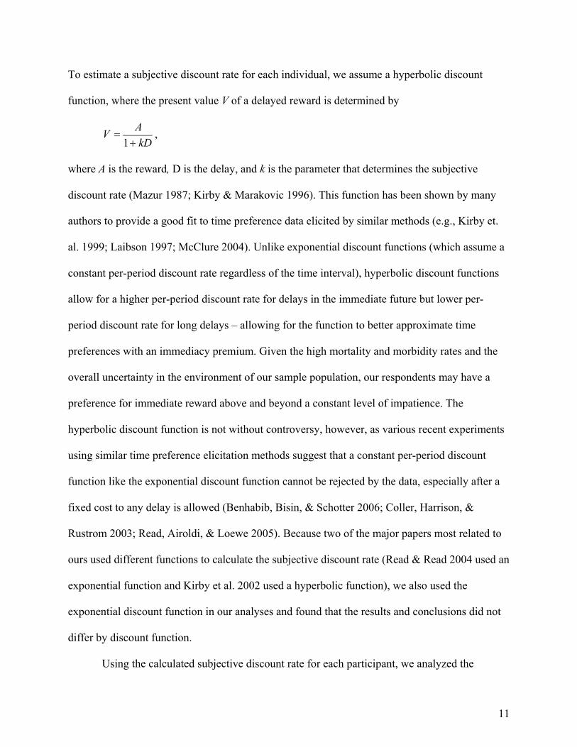
To estimate a subjective discount rate for each individual, we assume a hyperbolic discount

function, where the present value V of a delayed reward is determined by

kDAV+

=1

,

where A is the reward, D is the delay, and k is the parameter that determines the subjective

discount rate (Mazur 1987; Kirby & Marakovic 1996). This function has been shown by many

authors to provide a good fit to time preference data elicited by similar methods (e.g., Kirby et.

al. 1999; Laibson 1997; McClure 2004). Unlike exponential discount functions (which assume a

constant per-period discount rate regardless of the time interval), hyperbolic discount functions

allow for a higher per-period discount rate for delays in the immediate future but lower per-

period discount rate for long delays – allowing for the function to better approximate time

preferences with an immediacy premium. Given the high mortality and morbidity rates and the

overall uncertainty in the environment of our sample population, our respondents may have a

preference for immediate reward above and beyond a constant level of impatience. The

hyperbolic discount function is not without controversy, however, as various recent experiments

using similar time preference elicitation methods suggest that a constant per-period discount

function like the exponential discount function cannot be rejected by the data, especially after a

fixed cost to any delay is allowed (Benhabib, Bisin, & Schotter 2006; Coller, Harrison, &

Rustrom 2003; Read, Airoldi, & Loewe 2005). Because two of the major papers most related to

ours used different functions to calculate the subjective discount rate (Read & Read 2004 used an

exponential function and Kirby et al. 2002 used a hyperbolic function), we also used the

exponential discount function in our analyses and found that the results and conclusions did not

differ by discount function.

Using the calculated subjective discount rate for each participant, we analyzed the

12

bivariate relationships between the subjective discount rate and the respondents’ demographic

characteristics, as well as their age, health, and expectations of their own subjective survival

probability to live a certain number of years. We then performed multivariate regressions.

Because the subjective discount rates elicited by the hypothetical monetary tradeoffs are

constrained to be between 0.00016 and 0.25, we used two-sided tobit regressions to account for

the left- and right-side censoring of the calculated subjective discount rate.

RESULTS

Descriptive Statistics

We have 175 individuals in the sample, 73% are female, 46% are married or have a cohabiting

partner. The mean age of the sample is just above 46 years, ranging from 18 to 91. In terms of

education, 6% of respondents have no formal education, 20% have some primary, 13% have

finished primary school, 29% have some secondary, 21% have finished secondary school, 4%

have some tertiary school, and 7% have finished tertiary school. Of the 175 respondents in our

sample, 95 (55%) are either currently running a small business or ran a business that has recently

closed.

Health Status: The respondents’ mean physical and mental health scores for the SF12 are

42.4 and 51.8, respectively, with standard deviations of 12.1 and 10.9. The mean health score in

our population is lower than that in the United States (which has a normalized score of 50),

although the standard deviation is similar (at around 10) (Ware et al. 1995). Twenty-two percent

of respondents report their health to be excellent, 25% report their health to be very good, 28%

report their health to be good, 21% report their health to be fair, and 4% report their health to be

poor.

Subjective Probability of Survival: An analysis of the time horizon questions shows that

13

there is some variance in individuals’ expectations regarding how long they will live. Although

38% say they are 100% confident that they will “live to this time next year,” 21% state at least a

60% chance of not living until the next year. The mean response is an 82% confidence to live to

the next year. When we asked individuals their expectations to living to this time in five years,

25% expressed a 100% confidence that they would live to this time in 5 years, and 31% of

respondents expressed a 50-50 chance of living to the next 5 years. The mean response was just

above a 70% chance of living to the next 5 years. A similar pattern is found when we consider

individuals’ expectations to live 10 years. While 19% of respondents are 100% confident that

they will be alive, 48% of respondents expressed a 50-50 percent chance or lower of being alive

in 10 years.

//Table 1: Descriptive Statistics of the Sample//

Means Subjective discount rates: Subjective discount rates as calculated by the Kirby-

Marakovic method were relatively high in our sample, at 0.078, which is substantially higher

than the subjective discount rates of both heroin addicts (0.025) and controls (0.013) studied by

Kirby et al. (1999) in the U.S., but lower than the median subjective discount rates (0.12) found

by Kirby et al. (2002) among the Tsimane’ Amerindians in Bolivia. We found a skewed

distribution of subjective discount rates. Although a large number of individuals exhibit

subjective discount rates that are within the ranges found in other studies such as Kirby et al.

(1999), there is also a large number of individuals displaying the highest subjective discount rate

(31 in 175), and a significant number of individuals displaying the lowest subjective discount

rate (7 in 175), which reflects the censoring of the subjective discount rates due to the nature of

the monetary-choice tradeoffs in our questionnaire. The high proportion of right-censored

observations confirms the hypothesis that individuals suffer from a bias towards immediate

14

gratification in this subsample. Figures 1a and 1b show the frequency distributions of the

subjective discount rates and of the natural log of the subjective discount rates, with the lines

representing a kernel density estimation and the best-fitting normal distribution.

//Figure 1a and 1b; Frequency Diagram of dr and ln(dr)//

Subjective discount rate, Socioeconomics, Age, Health, Survival.

We also looked at the bivariate relationship between the subjective discount rate and the various

socioeconomic variables, age, health, and survival expectations, and these are presented in Table

2a. It is interesting to note that gender, marital status, business ownership, and income level of

the respondent’s area of residence were not statistically significantly related to subjective

discount rate.

//Table 2a: (need new revised table) Mean Subjective discount rate, by Sociodemographics//

We also examined the Spearman rank correlations between the individual subjective

discount rate and education, age, physical health, mental health, and subjective survival

probability. The results are shown in the bottom half of Table 2a. It is interesting to note that

none of these variables is rank-correlated with subjective discount rate. This could either be

because a relationship between these variables and the subjective discount rate does not exist, or

that the relationship is non-linear. Because the theoretical predictions (see Introduction above)

suggest that the relationship between age and subjective discount rate may be non-linear and

perhaps U-shaped, we also plotted the subjective discount rate against age, health, and subjective

survival probability. We do not find any relationship between subjective discount rate and age,

but the relationship between subjective discount rate and health and between subjective discount

rate and survival probability are both U-shaped.

//Figure 2a,b,c: Subjective discount rate vs. Age, PCS12, Survival//

15

We also examined the relationship between subjective discount rates and several

behavioral variables that are often linked with time preference, such as willingness to plan for the

future and to save money. We found that respondents that claimed that they “planned their life

ahead all the time” had lower subjective discount rates than those that claimed to “live more

from day to day” (0.066 compared to 0.106, p=0.0085, one-tailed). Also, those that preferred to

“spend money and enjoy life now” had higher subjective discount rates than those that preferred

to “save more for the future” (0.110 compared to 0.067, p=0.01, one-tailed). Because planning

and savings require a preference for waiting for a larger reward in the future, these behaviors are

good tests for the construct validity of our discount rate measure. Indeed, the results in Table 2b

suggest that the level of patience as measured by our subjective discount rate is consistent with

the planning and savings behaviors in our sample.

//Table 2b: Spearman Correlation: Subjective discount rate, by Selected Behavioral Variables//

Two-Sided Tobit Regressions

We performed a series of regressions using both ordinary least squares and two-sided

tobit, with both subjective discount rate and the natural log of the subjective discount rate as the

dependent variable. The results were similar but not identical, and our main conclusions remain

the same with the various specifications. Given that the subjective discount rate is censored from

the left and the right and that the subjective discount rate is highly skewed without the log

transformation, we present below the results obtained from two-sided tobit regressions with

ln(subjective discount rate) as the dependent variable.

In order to test Hypothesis 1 that the subjective discount rate should be related to age, we

first regressed ln(subjective discount rate) on age and age square. The results are shown in

column one. It is noteworthy that although the subjective discount rate appeared to have a U-

16

shape relationship with respect to age, the estimates were only marginally significant, while at

the same time, age and age-squared were not jointly significant. Gender and marital status were

insignificant. Those who had no education had a very significantly higher subjective discount

rate than those with at least some primary school education.

//Table 3: Two-Sided Tobit Regression of ln(subjective discount rate)//

We next examined Hypotheses 2 and 3 to test whether health and survival probability

were associated with subjective discount rates, and these results are presented in specifications

(2) through (5) in Table 3. Physical health, but not mental health, was highly significantly

associated with the subjective discount rate. The significance of the age variable disappeared

with the inclusion of the health variables; this suggests that rather than age, it may be the level of

physical health that explains the U-shaped pattern found in previous studies. Given that health

may be associated with the subjective discount rate through its effect on mortality risk, we next

added the one-year subjective probability of survival to the regression. (Because the questions to

elicit the subjective discount rates were all framed with a delay that is less than one year, we use

the 1-year survival probability in our analyses below; the results from using the 5- or 10-year

survival probability variable bear similar trends as the 1-year.) Interestingly, as shown in

specification (5) of Table 3, survival was not only highly significant, but inclusion of the survival

variables reduced both the magnitude and the significance level of the physical health variables –

suggesting that part of the effect of the health variable on subjective discount rate was via the

relationship between health and survival. In regressions not reported in Table 3, we also included

one-year survival without the health variables; the coefficient magnitude and significance level

of the survival variables were not reduced with the inclusion of the health variables. This

suggests that the effect of survival on discounting is not via health, but part of the effect of health

17

on discounting is via survival.

From specification (5) in Table 3, it is apparent that the relationship between the

subjective discount rate and both health and survival was U-shaped, supporting hypothesis 2 but

in contrast to hypothesis 3. This suggests that those in very poor health have high subjective

discount rates, but those in very good health also have high subjective discount rates. Similarly

those with both high and low survival probabilities (but not those in between), display high

subjective discount rates. In fact, the nadir of the U-relationship between subjective discount rate

and health occured when PCS12 was 37.8, or slightly below the mean physical health level of the

sample. The nadir for the U-shaped relationship between the subjective discount rate and the

one-year survival probability occured at around 75%, or slightly below the mean subjective

survival probability for the sample.

Expanding income or consumption opportunity in the future may reduce the marginal

utility of consumption in the future (and hence lead to greater discounting of the future). To

control for the potential confounding effects that this might have on our results, we included a

variable on the respondent’s subjective outlook for the overall economic environment in their

community in the next two years. (Ten respondents did not answer this question and were

excluded from subsequent analysis.) Although this variable is not the same as the respondents’

subjective outlook for their own future consumption opportunity, to the extent that the subjective

outlook for own future consumption is correlated with that for their community, our variable

may still proxy for the effect of expanding or declining consumption or income possibilities on

the subjective discount rate. The results, shown in specification (6), show that those who thought

the economy was going to worsen a lot in the next two years (the omitted dummy) had the lowest

subjective discount rate. We also find that people with good future income prospects have a

18

higher subjective discount rate, but also that the U-shaped relationship between the subjective

discount rate and health persists. Although the linear term is no longer significant at conventional

levels, the linear and quadratic terms combined are jointly significant in the model. Moreover,

because 6% of our sample did not respond to the question on prospects of future income, our

sample size was further reduced when we controlled for income expectations in the model.

Nevertheless, these results suggest that both health and longevity have a U-shaped relationship

with the subjective discount rate and that both are independent predictors of time preference.

DISCUSSION

Several of our main findings are surprising. Our first main finding is that age is not a

significant predictor of time preference, and is in contrast to the findings in Kirby et al. (2002)

and Read & Read (2004). In our sample, age was only significant in models where physical

health level was not included as a regressor. Our findings differ from those of these authors for at

least two reasons. One is that only 25% of our sample consists of people over the age of 55 and

that our sample may not contain enough older people to show an age effect, whereas Read &

Read (2004) concentrated their sample selection based on three age strata, with the oldest strata

around age 70. Notably, we are comparing different kinds of people in very different

environments. The other reason is that expected longevity, not age, may be a true underlying

determinant of people’s subjective discount rates. In populations where age does correlate well

with expected longevity, the effect of longevity on subjective discount rates can be well-

manifested by the effects from age. However, because causes of mortality in South Africa are not

necessarily related to age (e.g., mortality from HIV/AIDS affects more people less than age 40

than above), age is no longer a strong predictor of subjective discount rates.

Our second main finding is the U-shaped relationship between health and the subjective

19

discount rate. This is a very interesting and important finding, and although we predicted this

relationship, no one else has either tested for it or found evidence for it. The few studies that did

examine the relationship between health and the subjective discount rate use of crude measures

of health. Furthermore, a non-linear relationship between health and the subjective discount rate

could have also contributed to the lack of any significant (linear) relationship assumed in these

other studies. We give more detail here to better explain the U-shaped relationship between the

subjective discount rate and health; however, we cannot yet determine which of the explanations

is driving the real relationship that we find, and it is even very likely that they coexist and that it

is exactly the interaction that determined the observed pattern. Our finding that those with

average health have lower discount rate than those who are very healthy or very sick could be

due to several reasons. First, according to Trostel & Taylor (2002) and Olsho (2006), the ability

to enjoy consumption depends on an individual’s health, and the healthier an individual, the

greater the enjoyment of the same commodity bundle. Because health generally declines over the

life cycle, individuals should have a high subjective discount rate when healthy and, thus, enjoy

the consumption while they still can. Second, people who are not very healthy are likely those

who were once very healthy but have now experienced some health decline; these people may

long for their better health in the past, which motivates them to start examining the past and the

future in general, so that the future becomes more salient (as in Liu & Aaker 2006 and Becker &

Mulligan 1997), resulting in a lower subjective discount rate for the future. The foregoing

explains why people of average health may have lower subjective discount rates than those with

very good health. We also find a higher subjective discount rate among people with very poor

health, and this finding is robust to having controlled for longevity (and hence wanting to spend

resources before death cannot explain this finding). People with very poor health may have more

20

immediate need for cash to pay for medical care or for daily survival (perhaps because they are

too sick to work), hence the unwillingness to wait for the larger reward.

Our third main finding is the U-shaped relationship between the subjective discount rate

and survival probability after controlling for current physical and mental health status. It is

reasonable for people with low expected survival to have a high subjective discount rate, because

their future consumption may never come. This is what we expected to find (Hypothesis 3). It is

somewhat perplexing as to why those with a very high expected survival probability also highly

discount the future. We believe that saliency of time may explain this finding (as in the argument

for the saliency of health and its decline above). Liu & Aaker (2006) showed that personal

experience with someone who died of cancer is associated with decisions that favor long-term

future over the short-term present, and this effect seems to be related to the “salience and

concreteness regarding one’s future life course, shifting focus away from the present toward the

long run.” It is thus plausible that people who expect a very high probability of survival may not

have had cues from the environment to tell them otherwise; mortality to them is nonexistent.

However, as they experience deaths from social and family networks, death becomes more

salient. They not only start to revise downward their expected survival probability, but they also

start to think more about the future. As the future becomes more salient, they are more likely to

invest in “future oriented capital” and will discount the future less (as in Becker & Mulligan

1997).

LIMITATIONS & STRENGTHS

Our study provides seminal and thought provoking findings in terms of the relationship

between the individual subjective discount rate and age, health, survival, and future consumption

or income opportunities. While the study is subject to many limitations, our study also has

21

strengths that overcome many other studies´ weaknesses. We first discuss the limitations,

followed by the strengths, and we end with some policy implications of our results.

The first limitation to our study is that we had a small sample that consisted of a majority

of business operators. While this gave us confidence that the answers to questions involving

monetary tradeoffs were less likely to be subject to the problems of low mathematical literacy, it

is unclear whether our results from a mostly mathematically-literate population are fully

generalizable to the general population in the developing world.

The second limitation is that we did not have good measures of household assets and

income; we only have measures of business profit and the income strata where the respondents

resided. Relative to the highest income area, the fixed effects for low and middle income areas

were consistently negative and some statistically significantly negative, which indicates that

respondents in the lower income areas have lower subjective discount rates than those from the

highest income area. This finding is opposite to that found by Read & Read (2004), who also

included income strata for their time preference study among populations of the United Kingdom

and found that high income strata were associated with a lower subjective discount rate. This

seeming contradiction may be because all of our respondents are poor, just that some are less

poor than others. Even our “high income” strata would be considered the lowest income strata in

Read & Read’s study population.

The third limitation is that although most theoretical models of time preference assume

that ability to enjoy consumption now and ability to enjoy consumption in the future (and their

difference) would be important determinants of subjective discount rate, our study did not have a

measure for “ability to enjoy future consumption.” We also lack a variable on expected health in

the future, which might have been a good proxy for the felicity function as expounded by Trostel

22

& Taylor (2001) and as implicitly assumed in Becker & Mulligan (1997). Other studies also

suffer from this problem. To try and address this issue, we used data on the respondents´ current

and prior health, instead of future physical health, but these past health and past health change

variables were all insignificant determinants of subjective discount rates.

Despite the foregoing limitations, our study does have many strengths that improve on

others’ studies. First, our results are compelling because, despite a small sample size, our results

are robust to different specifications. We found that physical health, physical health squared,

survival probability, and survival probability squared were significant in most of the

specifications explained here as well as numerous others that we tried.

Second, we used comprehensive measures of health status that have been culturally

validated in Zulu speaking populations in South Africa (personal communication with Michelle

Koch of Qualitymetrics). The SF12 instrument combines multiple symptoms into one summary

scale each for physical health and for mental health, and is less subject to systematic

measurement error than single question health status measures (Dow et al. 1997). No other study

on time preference that we are aware of has incorporated the use of health status instruments;

most used only dichotomous categorization of good versus bad health or body mass index, which

may not be sensitive enough to capture the multiple dimensions of health and health differences

in the sample population. As suggested in the discussion, our use of a comprehensive measure of

health may be what contributed to our capturing the U-shaped relationship between health and

the subjective discount rate.

Third, our study is also the first to incorporate subjective probabilities of survival as a

determinant of time preference. Although most theories on why there is time preference make

use of mortality risk as one factor that reduces the utility of future consumption, most empirical

23

studies on time preference resort to the use of age as the variable of interest. However, age

proxies for a lot of factors in life, with mortality risk as only one such factor. In particular, many

studies confound the differential effects of age and expected length of life on discounting.

Although age is correlated with health and expected survival probability, in sub-Saharan Africa

where morbidity and mortality risks are very high and where disease profiles are not necessarily

related to ageing, age may not be a good proxy for morbidity and mortality. For instance, HIV

morbidity and mortality afflict people age 20-40 far more than those below 20 or above 40

(Shisana et al. 2005).

Fourth, our study is the first to simultaneously control for age, health, survival, and future

consumption opportunities as co-determinants of the subjective discount rate. We separately

measure age, health, and expected length of life – all of which are very distinct. This teases apart

the contributions of each of these variables to time preference. For example, up to 15% of all

mortality in South Africa is non-health related and non-age related (e.g., homicide, suicide,

accidents; Statistics South Africa 2005). This should be reflected in longevity expectations, not

in health or in age. Further, our use of two-sided tobit regression also allows for less bias in the

estimation of these relationships, especially in the face of both left and right censoring of the

calculated subjective discount rate.

Fifth, our study incorporates a subjective economic outlook variable that may proxy for

consumption and income opportunities in the near future. Although all economic theories of time

preference subsume future consumption opportunity as a determinant of subjective discount rate,

no empirical study has included such a variable.

Finally, despite the set of 27 questions used to measure time preference, the consistency

of the answers is above 90%, which suggests that the respondents were not answering randomly.

24

Moreover, based on the answers to the other questions in the survey about planning and savings

behavior, our time preference measure also shows strong construct validity in measuring

willingness to wait for the future.

In view of the strengths but also the limitations of our data, our results should be

interpreted with caution. Nevertheless, we find important and novel results regarding the

relationship between health and the subjective discount rate and longevity and the subjective

discount rate.

Our study has important policy implications. Our finding that subjective discount rates

differ by health levels implies that economic evaluation of healthcare programs that use results

from surveys of the public (who are likely to be healthier than those that are helped by the

potential health programs) may be inaccurately weighting future costs and benefits by not taking

into consideration that the subjective discount rate is a function of health status. Furthermore, the

provision of healthcare and health insurance (especially in countries with low health levels) may

improve health and survival, leading to more future-oriented thinking and investments for the

future; this positive externality should not be neglected in welfare analysis of these social

programs. Finally, there is the possibility that those who think they are extremely healthy or will

live forever discount the future more because of lack of information. This impedes their ability to

put the future into proper perspective, resulting in non-optimal inter-temporal trade-offs with

potential for regret later in life. Here, public health education to make the future more salient

may be an additional policy tool; alternatively, development and provision of pre-commitment

devices may also be welfare improving.

25

REFERENCES

Ashraf N, Karlan D, Yin W. Tying Odysseus to the mast: Evidence from a commitment savings

product in the Philippines. Quarterly Journal of Economics 121(2):635-672. 2006.

Becker GS, Mulligan CB. The endogenous determination of time preference. Quarterly Journal

of Economics 112:729-798. 1997.

Benhabib J, Bisin A, Schotter A. Present-bias, quasi-hyperbolic discounting, and fixed costs.

Working Paper. January 2006.

Bloom DE, Canning D, Graham B. Longevity and life-cycle savings. Scand J of Economics

105(3):319-338. 2003.

Camerer CF, Hogarth RM. The effects of financial incentives in experiments: a review and

capital-labor-production framework. Journal of Risk and Uncertainty 19:7-42. 1999.

Chao LW, Kohler HP. The behavioral economics of altruism, reciprocity and transfers within

families and rural communities: evidence from sub-Saharan Africa. Population Association

of America 2007 Annual Conference, New York City. March 30, 2007.

Chao LW, Pauly MV, Szrek H, Sousa Pereira N, Bundred F, Cross C, Gow J. Poor health kills

small business: Illness and microenterprises in South Africa. Health Affairs 26(2):474-482.

2007.

Coller M, Harrison GW, Rustrom EE. Are discount rates constant? Reconciling theory and

observation. University of South Carolina Moore School of Business Working Paper.

December 2003.

Coller M, Williams MB. Eliciting individual discount rates. Experimental Economics 2:1027-

127. 1999.

Cubitt RP, Read D. Can intertermporal choice experiments elicit time preferences for

26

consumption? Experimental Economics DOI 10.1007/s10683-006-9140-2, (February 1,

2007)

Domeij D, Johannesson M. Consumption and health. Department of Economics Working Paper,

Stockholm School of Economics. January 2006.

Dow WH, Gertler P, Schoeni RF, Strauss J, Thomas D. Health care prices, health and labor

outcomes: experimental evidence. RAND Labor and Population Program Working Paper 97-

01. 1997.

Johnson MW, Bickel WK. Within-subject comparison of real and hypothetical money rewards in

delay discounting. Journal of the Experimental Analysis of Behavior 77(2):129-146. 2002.

Kirby KN, Godoy R, Reyes-Garcia V, Byron E, Apaza L, Leonard W, Perez E, Vadez V, Wilkie

D. Correlates of delay-discount rates: Evidence from Tsimane’ Amerindians of the Bolivian

rain forest. Journal of Economic Psychology 23:291-316. 2002.

Kirby KN, Marakovic NN. Modeling myopic decisions: Evidence of hyperbolic delay-

discounting within subjects and amounts. Organizational Behavior and Human Decision

Processes 64:22-30. 1995.

Kirby KN, Petry NM, Bickel WK. Heroin addicts have higher discount rates for delayed rewards

than non-drug-using controls. Journal of Experimental Psychology: General 128(7):78-87.

1999.

Laibson D. Golden eggs and hyperbolic discounting. Quarterly Journal of Economics

112(2):443-477. 1997.

Liu W, Aaker J. Do you look to the future or focus on today? The impact of life experience on

intertemporal decisions. Organizational Behavior and Human Decision Processes.

(forthcoming in 2006).

27

Mazur JE. An adjusting procedure for studying delayed reinforcement. In M.L. Commons, J.E.

Mazur, J.A. Nevin, & H. Rachlin (Eds.), Quantitative analyses of behavior: Vol. 5. The effect

of delay and of intervening events on reinforcement value (Hillsdale, NJ: Erlbaum), pp. 55-

73. 1987.

McClure SM, Laibson DI, Loewenstein G, Cohen JD. Separate neural systems value immediate

and delayed monetary rewards. Science 306. 503-507. 15 October 2004.

Olsho L. Spend it while you can still enjoy it: Health, longevity, aging, and consumption in the

life cycle. Department of Economics Working Paper, University of Wisconsin-Madison.

August 2006.

Picone G, Sloan F, Taylor D. Jr. Effects of risk and time preference and expected longevity on

demand for medical tests. J of Risk and Uncertainty 28(1):39-53. 2004.

Read D. Monetary incentives, what are they good for? Journal of Economic Methodology

12(2):265-276. 2005.

Read D, Airoldi M, Loewe G. Intertemporal tradeoffs priced in interest rates and amounts: A

study of method variance. London School of Economics and Political Science Department of

Operational Research Working Paper. 2005.

Read D, Read NL. Time discounting over the lifespan. Organizational Behavior and Human

Decision Processes 94:22-32. 2004.

Rogers AR. Evolution of time preference by natural selection. American Economic Review

84(3):461-481. 1994.

Shisana O, Rehle T, Simbayi LC, Parker W, Zuma K, Bhana A, Connolly C, Jooste S, Pillay V,

et. al. 2005. South African National HIV Prevalence, HIV Incidence, Behaviour and

Communication Survey, 2005. South African Human Sciences Research Council

28

(HSRC),(http://www.hsrcpress.co.za/index.asp?id=2134 accessed on 25 January 2006)

Smith VK, Taylor DH, Sloan FA. Longevity expectations and death: can people predict their

own demise? American Economic Review 91(4):1126-1134. 2001.

Sozou PD, Seymour RM. Augmented discounting: interaction between ageing and time-

preference behaviour. Proc. R. Soc. Lond. B 270:1047-1053. 2003.

Statistics South Africa. Mortality and causes of death in South Africa, 1997-2003: Findings from

death notification. Statistical release P0309.3. 18 February 2005.

Thaler RH, Benartzi S. Save more tomorrow: Using behavioral economics to increase employee

saving. Journal of Political Economy 112(1 part 2):S164-S187. 2004.

Thornton RL. Hope for the future: How learning HIV status affects savings and expenditures.

Harvard University Kennedy School Working Paper. April 18, 2006.

Trostel PA, Taylor GA. A theory of time preference. Economic Inquiry 39(3):379-395. 2001.

Tu Q, Donkers B, Melenberg B, van Soest A. 2004. The time preference of gains and losses.

Working Paper, Tilburg University.

Ware JE, Kosinski M, Keller SD. How to Score the SF-12 Physical and Mental Health Summary

Scale, 2d ed. (Boston: Health Institute, New England Medical Center, 1995).

Table 1: Descriptive Statistics of the Sample

Mean(S.D.)

Female (%) 72.57Married or Cohabiting (%) 45.71Education (% with no education) 6.29Belief that the economy will worsen a lot (%) 6.10Belief that income will decrease a lot (%) 4.82

Age 46.52(15.09)

SF12 Scores PCS12 (physical health score) 47.48

(12.06)

MCS12 (mental health score) 51.90(10.86)

Subjective probability of survival Probability of being alive in 1 year (%) 81.83

(19.71)

Probability of being alive in 5 years (%) 70.23(26.04)

Probability of being alive in 10 years (%) 57.77(31.11)

Overall Discount Rates 0.078(0.084)

Number of observations 175

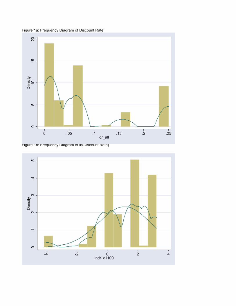
Figure 1a: Frequency Diagram of Discount Rate

Figure 1b: Frequency Diagram of ln(Discount Rate)

0.1

.2.3

.4.5

Den

sity

-4 -2 0 2 4lndr_all100

05

1015

20D

ensi

ty

0 .05 .1 .15 .2 .25dr_all

Table 2a: Mean Discount Rate, by Sociodemographic Variables

Significance of DifferenceMean Discount Rate Between Groups

Gender Male 0.071 Kruskal Wallace = 0.000; df = 1 Female 0.081 p = 0.992Marital Status Married or Cohabiting 0.089 Krukal Wallace = 0.244; df = 1 Single, Divorced, Widowed 0.069 p = 0.621Business Ownership Business Owner or Past Owner 0.083 Kruskal Wallace = 0.614; df = 1 Never Owner 0.077 p = 0.433Income High Income 0.083 Kruskal Wallace = 1.706; df = 2 Middle Income 0.067 p = 0.426 Low Income 0.087Education Lowest Quintile 0.099 Spearman Rank Correlation 2nd Quintile 0.063 rho = -0.040 3rd Quintile 0.057 p = 0.603 4th Quintile 0.070 Highest Quintile 0.073Age Lowest Quintile 0.080 Spearman Rank Correlation 2nd Quintile 0.065 rho = -0.042 3rd Quintile 0.071 p = 0.585 4th Quintile 0.072 Highest Quintile 0.079Physical Health (pcs12) Lowest Quintile 0.082 Spearman Rank Correlation 2nd Quintile 0.074 rho = 0.072 3rd Quintile 0.065 p = 0.344 4th Quintile 0.044 Highest Quintile 0.095Mental Health (mcs12) Lowest Quintile 0.077 Spearman Rank Correlation 2nd Quintile 0.051 rho = 0.028 3rd Quintile 0.080 p = 0.714 4th Quintile 0.067 Highest Quintile 0.0881-Year Survival Probability Lowest Quintile 0.114 Spearman Rank Correlation 2nd Quintile 0.075 rho = 0.108 3rd Quintile 0.050 p = 0.156 4th Quintile 0.065 Highest Quintile 0.075

Table 2b: Mean Discount Rate, by Selected Behavioral Variables

Planning Horizon Plan Ahead All the Time 0.066 one-tailed ttest Live from Day to Day 0.106 p = 0.009Savings Behavior Prefer Saving Money 0.067 one-tailed ttest Prefer Spending Money 0.110 p = 0.010

Figure 2a: Discount Rate vs. Age, Plot and Fitted Values

Figure 2b: Discount Rate vs. PCS12, Plot and Fitted Values

Figure 2c: Discount Rate vs. One-Year Survival Probability, Plot and Fitted Values

0.0

5.1

.15

.2.2

5

20 40 60 80 100age

dr_kirby Fitted values

0.0

5.1

.15

.2.2

5

20 40 60 80 100a1

dr_kirby Fitted values

0.0

5.1

.15

.2.2

5

10 20 30 40 50 60pcs12

dr_kirby Fitted values

Table 3: Double-Sided Tobit Regression: ln(dr_kirby*100) as the dependent variable

(1) (2) (3) (4) (5) (6)

Constant 3.855*** 7.292*** 2.619 6.988** 9.623*** 7.469**(1.291) (2.234) (2.754) (3.415) (3.577) (3.664)

Age -0.093* -0.080 -0.082 -0.067 -0.039 -0.030(0.055) (0.056) (0.058) (0.057) (0.058) (0.057)

Age*Age 0.001 0.001 0.001 0.001 0.000 0.000(0.000) (0.001) (0.001) (0.001) (0.001) (0.000)

Female 0.414 0.434 0.416 0.422 0.448 0.242(0.362) (0.360) (0.363) (0.361) (0.355) (0.344)

Married or Cohabiting 0.087 0.040 0.076 0.025 -0.046 0.175(0.351) (0.348) (0.352) (0.349) (0.343) (0.333)

Area Dummy = Ntuzuma C -0.911 -0.903 -0.866 -0.856 -0.792 -0.854(0.570) (0.563) (0.572) (0.566) (0.573) (0.562)

Area Dummy = Klaarwater -0.456 -0.457 -0.446 -0.462 -0.628 -0.314(0.513) (0.508) (0.516) (0.511) (0.504) (0.486)

Area Dummy = Umlazi J -0.881 -0.744 -0.825 -0.676 -0.761 -1.056**(0.543) (0.538) (0.547) (0.542) (0.474) (0.532)

Area Dummy = Kwa Mgaga -0.897 -0.962* -0.855 -0.911* -0.926* -0.667(0.560) (0.555) (0.562) (0.557) (0.550) (0.530)

Area Dummy = Clare Estates -1.313** -1.341** -1.281** -1.297** -1.444*** -1.322**(0.553) (0.545) (0.555) (0.548) (0.540) (0.508)

No education 2.330*** 2.171*** 2.391*** 2.163*** 2.322*** 3.003***(0.725) (0.730) (0.749) (0.754) (0.752) (0.770)

PCS12 -0.233** -0.240** -0.165* -0.131(0.096) (0.097) (0.099) (0.097)

PCS12 squared 0.003*** 0.003*** 0.002** 0.002*(0.001) (0.001) (0.001) (0.001)

MCS12 0.024 -0.015 0.001 -0.045(0.110) (0.109) (0.000) (0.112)

MCS12 squared -0.001 0.000 0.000 0.000(0.001) (0.001) (0.001) (0.001)

Longevity -0.156*** -0.118**(0.059) (0.059)

Longevity squared 0.001*** 0.001**(0.000) (0.000)

Economic Outlook for Next 2 Years Improve a lot 1.144

(0.875)

Improve a little 1.727***(0.679)

Remain the same 1.417**(0.666)

Worsen a little 1.642**(0.689)

Observations 164Mean of the Dependent Variable 1.134Pr > Chi-square 0.025 0.001 0.050 0.017 0.001 0.000Pseudo R-square 0.029 0.039 0.031 0.040 0.051 0.069

Note: Values in parentheses represent standard errors. *p < .10; **p < .05; ***p < .01

1751.117