Embed Size (px)
Citation preview
arX
iv:h
ep-p
h/93
1231
6v1
21
Dec
199
3
Top and Higgs Masses in Dynamical Symmetry Breaking1
David E. Kahana2
Center for Nuclear Research
Kent State University
Kent, OH 44242-0001
and
Sidney H. Kahana3
Physics Department
Brookhaven National Laboratory
Upton, NY 11973
ABSTRACT
A model for composite electroweak bosons is re-examined to establish approximate
ranges for the initial predictions of the top and Higgs masses. Higher order corrections to
this 4-fermion theory at a high mass scale where the theory is matched to the Standard
Model have little effect, as do wide variations in this scale. However, including all one loop
evolution and defining the masses self-consistently, at their respective poles, moves the top
mass upward by some 10 GeV to near 175 GeV and the Higgs mass down by a similar
amount to near 125 GeV.
1This manuscript has been authored under NSF supported research Contract No. PHY91-
13117 and DOE supported research Contract No. DE-AC02-76CH00016.2e-mail: [email protected]: [email protected]
1. Introduction
In this paper we refine predictions for the top and Higgs masses made in an earlier work
on dynamical symmetry breaking [1]. The specific 4-fermion model of dynamical symmetry
breaking presented in Reference 1 (see the Lagrangian in Eq.1 below) may perhaps be
ultimately viewed as the low mass limit of a gauge theory at some very high scale Λ,
with primordial boson masses, MB ∼ O(Λ). This scale then acts as an effective cutoff
for the 4-fermion theory. Certainly, no explanation is presented here for the number and
character of elementary fermions in the modeling nor for the large disparity in mass scales,
i.e. mf ≪ MB . Rather, a central point of our calculation is that new, composite, bosons
with masses near 2mf arise naturally in the theory. These are just fermion–antifermion
bound states produced by the 4-fermion interaction. This phenomenon is well described
in the papers of Nambu and Jona–Lasinio on the four fermion theories [2], and has been
exploited by many authors [3,4,5,6,7,8]. Since the scale Λ at which any new physics enters
is so high, the theory is in fact a weak coupling, albeit constrained, version of the Standard
Model for scales well below Λ.
Previously [1] we abstracted simple, asymptotic mass relationships from the 4-fermion
theory, and used these as boundary conditions on the standard model renormalisation
group (RG) equations. This was done at a matching scale µ ∼ MGUTS , where the elec-
troweak (EW) sector can still be treated as approximately independent of QCD (SU(3)c).
Values for the top and Higgs masses then followed from downward evolution of the top-
Higgs and Higgs-self couplings to scales near mW , assuming no intervening structure.
In the present work we show that modifications in these asymptotic relationships, due
to higher order corrections in the 4-fermion theory at the upper scale µ, have a consid-
erably diminished effect on mt and mH at their much lower scale. Also, large, several
orders of magnitude, changes in µ affect the top hardly at all and the Higgs only slightly.
However, a more consistent handling of the RG evolution moves the prediction for mt from
approximately 165 GeV to nearer 175 GeV, while that for mH moves from 140 GeV to
about 125 GeV.
2.The 4-Fermion Theory
In Ref.1, we indicated that a 4-fermion interaction including vector terms led to rather
low, well-determined masses for the top-quark and Higgs. The model is defined by the
1
Lagrangian:
L = ψ̄i(γ · ∂)ψ − 1
2[(ψ̄GSψ)2 − (ψ̄GSτγ5ψ)2]
− 1
2G2
B(ψ̄γµY ψ)2 − 1
2G2
W (ψ̄γµτPLψ)2
(1)
in which very specific vector interactions have been added to the usual scalar and pseu-
doscalar terms of NJL. The field operator is ψ = {fi}, and the index i runs over all
fermions, i = {(t, b, τ, ντ), (c, s, ...), ...}. The scalar-coupling matrix Gs is taken diagonal
and the dimensionful couplings are adjusted to produce the known fermion masses dynam-
ically; in practice only the top acquires an appreciable mass. The model admits bound
states corresponding to the Higgs as well as the gauge bosons of the standard electroweak
theory, and is essentially equivalent to the Standard Model below some high mass scale
µ. It is the vector terms in Eq.1 which ensure the existence of the Higgs, Z, and W as
composites with masses of the order of mt, thus naturally explaining why the Standard
Model bosons and the top appear to have about the same mass.
In re-examining the predictions for the top and Higgs we do not presume to seek
precise values for their masses, but rather attempt to determine the latitude in masses
present in the modeling. Such a study is especially timely in light of the search for the
top being carried out at FNAL [9]. The apparent paucity of top events in the latest
data suggests a high mass for the top, certainly it now seems mt is greater than 120 GeV
and possibly considerably higher. Present analyses of LEP data [10] with respect to EW
corrections, suggest mt = 166±30 GeV.
As usual in NJL the necessary fine tuning of the scalar coupling is accomplished by
solving the scalar gap equation, whence diagonalisation of the scalar action yields the Higgs
mass formula:
mH(µ) = 2mt(µ)(1 +O(g2t )) (2)
Fine tuning determinines the dimensionful scalar coupling in terms of the cutoff Λ,
G2t =
1
Λ2 −m2t ln
(
Λ2
m2
t
) (3)
Bound states also exist in the vector sector defined by Eq.1 corresponding to the W ,
Z, and the photon. A similar fine tuning of the vector coupling is required, but here with
the added physical interpretation that the photon mass should vanish [1]. This latter
2
constraint leads, at lowest order in the electroweak and Yukawa couplings, to the mass
relationship
m2W (µ) =
3
8m2
t (µ) (4)
To the same order in couplings, the required diagonalision of the neutral vector boson
action results in
sin2(θW ) = (∑
iQ2
i )−1 =
3
8, (5)
with the denominator on the right hand side of Eq.(5) being summed over the charges Qi
in one generation.
The dimensionful couplings of the 4-fermion theory are replaced, after fine-tuning
and wave function renormalisation, by the dimensionless couplings of the Standard Model
[11,1], and the gradient expansion of the effective action is in fact an expansion in these
dimensionless electroweak couplings. One has for the scalars
gS = GSZ−
1
2
S ,
ZS =1
2Tr
[
G2S
1
(∂2 +M2)2
]
,
(6)
where the fermion–scalar coupling matrix is for the present taken diagonal:
(GS)ij = Giδij . (7)
Similarly, for the vector couplings one has
g22
=GW√ZW
andg′
2=
GB√ZB
(9)
and the usual relationship between g2 and g′
g2 sin(θW ) = g′ cos(θW ). (10)
From equations {(2), (4), (5)}, valid presumably at a scale µ where the cross coupling
between the EW and strong sectors is small but still well below the cutoff Λ, we derived val-
ues for the top and Higgs masses at a scale near mW . The theory leading to these equations
is equivalent to the electroweak sector of the Standard Model below µ, and the framework
for connecting the scales µ and mW is provided by the Standard Model RG. Thus SU(3)c
influences on the top and Higgs masses are included through the renormalisation group,
below the matching scale µ.
3
3. Renormalisation Group Evolution
We turn now to the calculation of smaller effects, neglected in the initial work, due
to corrections in the 4-fermion theory of higher order in the electroweak couplings and
to a more consistent treatment of the evolution downward to experimental mass scales.
Our basic equations are: (1) the boundary condition relationships between the Higgs, top
and W masses including dependence on electroweak couplings and quark masses, and (2)
the RG evolution equations for the top-Higgs and Higgs-self couplings gt and λ. Defining
[12,13]
κt =g2
t
2π,
one hasdκt
dt=
9
4πκ2
t −4
πκtαS − 9
8πκtαW − 17
4πκtα1, (12)
with αS, αW , α1 taken equal to α3, α2, α1 respectively in reference [12,13], and t = ln( qm ).
We note that with these choices
mt = gtv,
mW =gW
2v,
(13)
where v is the standard EW vev.
Also taking m2H = 2λv2 the evolution equation for the Higgs self-coupling is, to the
same (one-loop) order [14]:
dλ
dt=
1
16π2
{
12λ2 + 6λg2t − 3g4
t − 3
2λ(
3g2W + g′
2)
+3
16
(
2g4W +
(
g2W + g′
2)2)}
. (14)
Redefining the standard choice of couplings [12]
α1 =5
3α′ with α1 =
g21
4π, α′ =
g′2
4π(15)
and setting
σ =λ
4π(16)
results in
dσ
dt=
1
2π
{
12σ2 + 6σκt − 3κ2t −
9
2σ
(
αW +1
5α1
)
+3
16
(
2α2W +
(
αW +3
5α1
)2)}
.
(17)
4
Equations (2) and (4) impose boundary conditions on equations (12) and (17) at the
scale µ. These are to lowest order
m2t =
8
3m2
W
and
m2H = 4m2
t =32
3m2
W , (18)
which can be restated to include higher orders:
κt
α2(µ) =
4
3+O(g2
i ) andσ
α2(µ) =
4
3+O(g2
i ). (19)
Such corrections can come from two sources, higher order 1/N , multi-loop, contributions
to the effective action, and more trivial 1/ln(Λ) terms within the lowest order. The latter
arise, for example, from the proper generalised form of Eq.4:
m2W =
1
2
∑
im2i
[
ln(
Λ2
m2
i
+ 1)
− 1]
∑
iri
6
[
ln(
Λ2
m2
i
+ 1)
− 116
] , (20)
where the sum is over all fermions and ri = α−2(
β4(y2Li + y2
Ri) − β2α2yLiτ3i + α4τ3
i τ3i
)
,
while yLi, yRi and τ3i are the fermion hypercharges and isospins. Equation (4) is obtained
from (20) by keeping only the top mass and ignoring terms of order (ln(Λ))−1. These
terms are of higher order in the electro weak couplings; for example the Higgs-top Yukawa
coupling is, from (6), proportional to (ln(Λ))−1.
We note parenthetically that the basic SU(5) symmetry evident in Eqs(4,5) results
from the 5̄ + 10 generational structure (u, d, eL,R, νR) built into the present model, and
follows from (20) in the limit of large Λ. We also note that the 38 appearing in the lowest
order (Eq(4)) for m2W is more properly written
m2W
m2t
=3
8
ng
nc, (21)
and so is not simply sin2(θW ) but instead depends on the number of colours as well as the
number of massive fermion generations. We find that the several percent change implied
in Eq(20) relative to Eq(4) produces a considerably smaller change in mt, less than one
percent. Thus, to the accuracy meaningful here, we can perhaps ignore these corrections
as well as other higher order 1/N effects arising from discarded, incoherent, summations
over fermions.
5
4. Solution of the RG Equations.
It is possible to obtain an explicit solution to Eq(12), and a perturbative solution for
Eq(17). For the top evolution one has, making a simple transformation of Eq(12)
d
dt
1
κt= − 9
4π+
1
κt
(
4
παS +
9
8παW +
17
40πα1
)
, (22)
with the one parameter family of solutions
1
κt=
[
(1 + αS0bSt)8/7(1 + αW0bW t)27/38
(1 − α10b1t)17/82
]
×[
D − 9
4π
∫ t
0
dt′(1 − α10b1t
′)17/82
(1 + αS0bSt′)8/7(1 + αW0bW t′)27/38
]
(23)
Here αS0, αW0, and α10 are the couplings at t = ln mW
mW= 0, and the constants bS = 7
2π ,
bW = 1912π and b1 = 41
20π determine the evolution of the SU(3), SU(2), and U(1) couplings
respectively. The constant D in Eq(23) is given by
D =1
κt(0), (24)
and directly yields the running top mass at the scale mW from
m2t (mW ) =
2κt(0)
αW (0)m2
W (mW ). (25)
To self-consistently determine the physical top mass as a pole in the top quark propagator,
one must run mt(mW ) back up to get mt(mt).
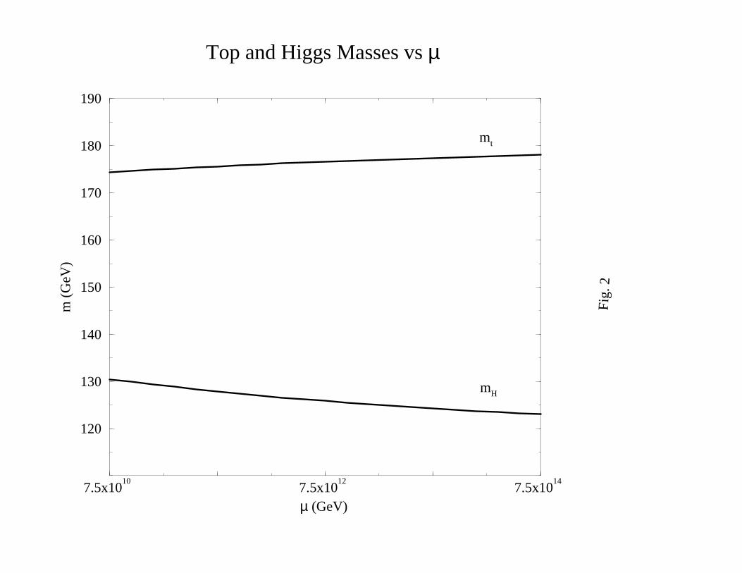
The cross coupling in Eq(17) complicates its solution. The pure scalar self-coupling
result
σ0(t) =σ0(0)
1 − 6πσ0(0)t
, (26)
may be improved perturbatively
σ(t) = σ0(t) + σ1(t). (27)
Linearising in the small correction σ1(t) produces
σ1(t) = e−v(t)
∫ t
tµ
dt′g(t′)ev(t′), (28)
6
with
v(t) = −∫ t
tµ
dt′f(t′), (29a)
f(t) =12
πσ0(t) +
3κt(t)
π− 9
4π
[
α2(t) +1
5α1(t)
]
, (29b)
and
g(t) =3
πσ0(t)κt(t) −
3κ2t
2π+
3
32π
[
2α22(t) +
(
α2(t) +3
5α1(t)
)2]
. (29c)
Boundary conditions are introduced at tµ = ln µmW
through
σ1(tµ) = 0, σ0(tµ) = κt(tµ) =4
3α2(tµ) +O(α2
i ). (30)
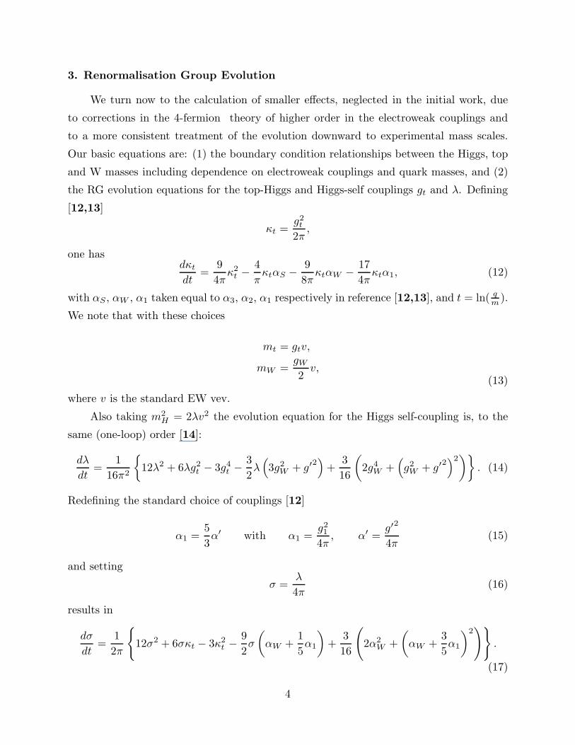
Since σ1(t) is small over the range mH to µ (see Fig.1) there is no need to include higher
orders.
Results from numerical integration of equations (23) and (28,29) are displayed in
Table 1, and Figs 1-4. We have varied the inputs to these calculations, the strong and
electroweak couplings αi0, i = 1,W, S over a reasonable range, somewhat wider than the
flexibility allowed by present experiments. The W mass is fixed at 80.1 GeV. There are no
free parameters in the theory, the couplings and mW being determined from experiment. A
possible exception is the cutoff Λ, which is surely well above µ and has essentially no effect
on mt and mH . Any dependence other than logarithmic on Λ has been eliminated by fine
tuning, while residual ln(Λ) presence is transmuted into dependence on the dimensionless
couplings.
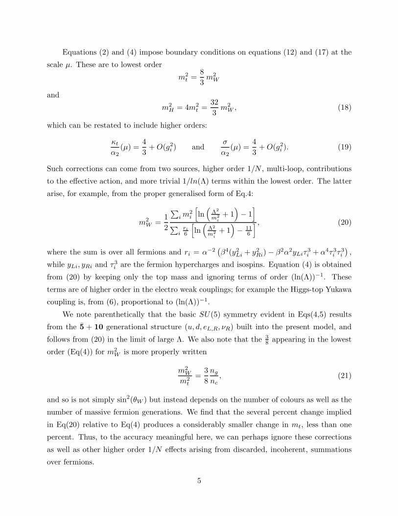
The effect of imposing boundary conditions sharply at a scale µ remains to be exam-
ined. As we noted above, µ is that point, when one is evolving downward in mass, at which
the gi become interdependent. For example, the top quark evolution is strongly influenced
by SU(3)c from µ ∼ 1014 downward, and the running of αW is also significant. Varying
µ over four orders of magnitude from µ = 1010 GeV to µ = 1014 GeV has practically
no effect on mt, and only a small effect on mH . This remarkable result is demonstrated
in Fig.(2) for central choices of the couplings, and lends credence to our use of a sharp
boundary condition.
The one physical parameter sensitive to µ is the weak mixing angle θW . We indicated
[1] that, for one loop evolution, sin2(θW ) achieves its experimental value ∼ 0.23 (at mW )
for µ ∼ 1013 GeV. Unlike GUTS, the present theory need not have a single scale at which
the gauge couplings are equal. The unification present in this model simply implies that
7
the Standard Model should evolve smoothly into the effective 4-fermion theory where the
couplings become weak. Table 1 displays the value of the couplings at scale µ; the αi are
the experimental values determined at mW evolved upward to µ at 1-loop and κt(µ) is
obtained from the boundary condition κt
α2
= 43 . It is clear that the couplings are indeed all
small at µ, again justifying the placing of the boundary conditions there.
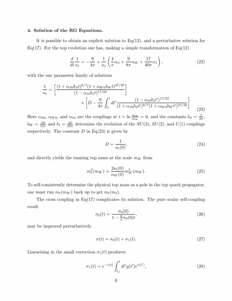
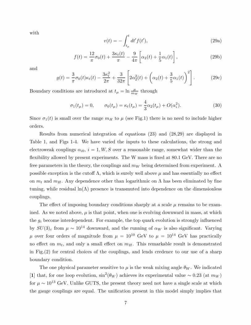
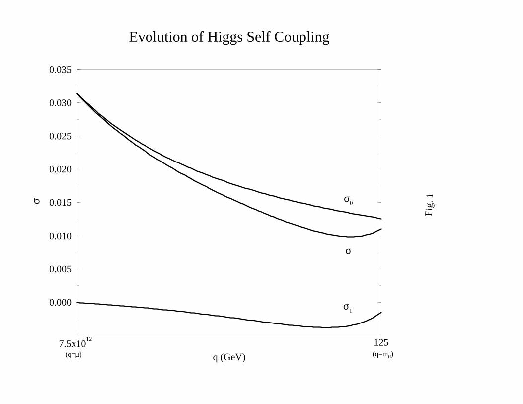
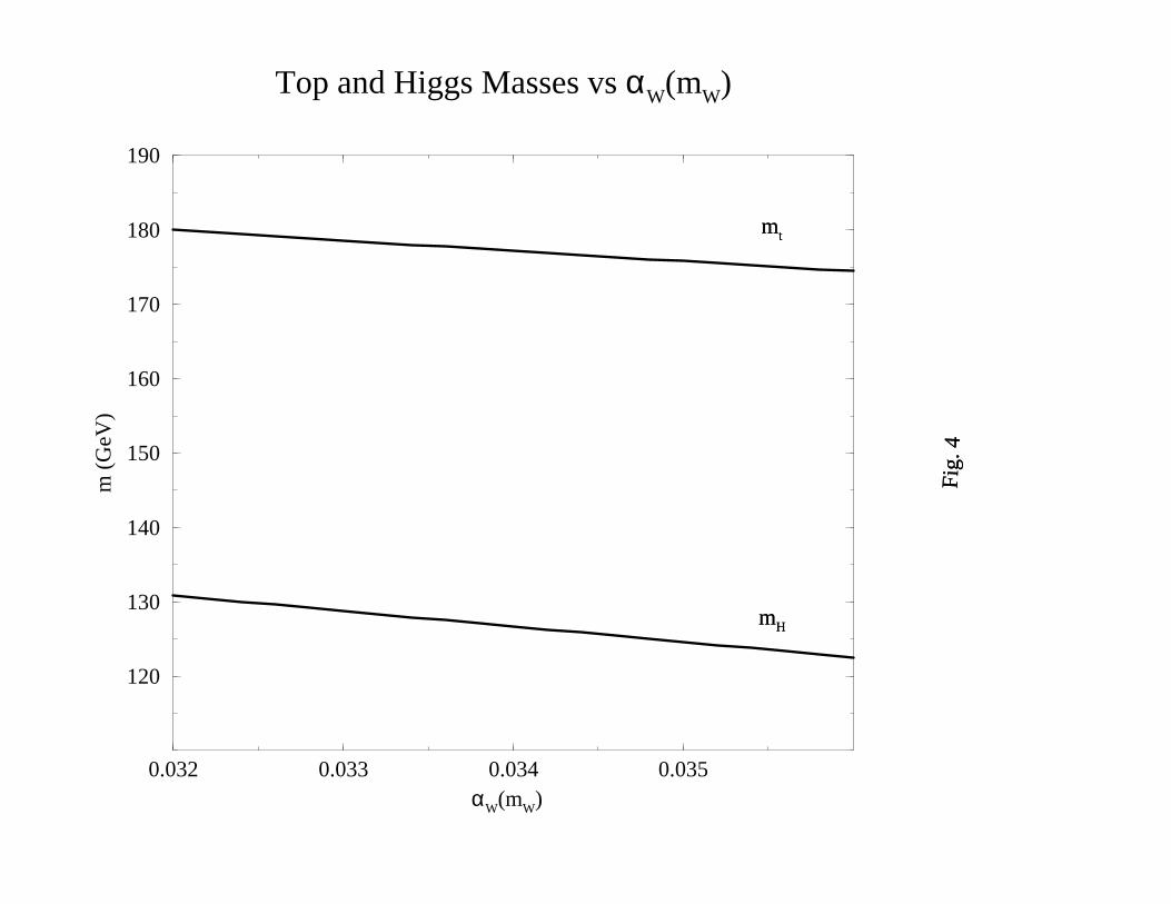
Figures (3) and (4) show the variations of mt and mH with the strong and electroweak
couplings, respectively. The strong coupling is less well known. Using as central values
αS0 = 0.107, αW0 = 0.0344, and α10 = 0.0169 [10,16], we get mt ≃ 175 GeV and
mH ≃ 125 GeV. Included in the 175 Gev is is a 6 Gev reduction from evolving the top
self-consistently to its proper mass at q = mt; for the Higgs this effect is much smaller.
Further small contributions to Eq(19), from non-leading log terms in defining the top pole
and from running the W mass, more or less cancel. It is clear from the figures that mH
is somewhat more sensitive to all these changes, and so the remaining uncertainty in the
mass 125 GeV is larger. This uncertainty nevertheless may be usefully bounded by noting
[1] that a rather large arbitrary variation in the boundary condition ratio mH/mt from
2 to√
8 produces ≤ 15 GeV change in mH . One must also keep in mind that the top is
confined and its mass therefore subject to some ambiguity in definition.
4. Conclusions.
In summary, one gets remarkably stable predictions for the top and Higgs masses and
in a parameter free fashion. The only inputs were the experimentally known couplings and
the W-mass. A characteristic prediction of this type of theory is mh < mt, so that the
Higgs, which is practically a tt̄ condensate, is deeply bound.
In view of the present dearth of events from the FNAL experiments with DØ and
CDF, the above prediction for the top (near 175 GeV) may not be wholly wild. In light
of the recent unfortunate developments at the SSC, the somewhat low prediction for the
Higgs mass, near 125 GeV, may take considerably longer to test.
Finally, there is the question of the number of generations. In Ref(1), we indicated
that a fourth generation, with massive quarks mt′ ∼ mb′ ∼ mt, implies a top mass near
115 GeV. Such a constraint arises from the sum rule (Eq(19)) for m2W . Present data at
FNAL appear to rule out this possibility.
8
Acknowledgements
One of the authors (SHK) would like to thank the Alexander von Humboldt Founda-
tion (Bonn, Germany) for partial support and Professor W. Greiner of the Johan Wolfgang
Goethe University, Frankfurt, Germany for his hospitality.
9
References
1. D.E. Kahana and S.H. Kahana, Phys. Rev. D43, 2361 (1991)
2. Y. Nambu and G. Jona–Lasinio, Phys. Rev. 122, 345 (1961)
3. J.D. Bjorken, Ann. Phys. (NY) 24, 174 (1963)
4. W. Bardeen, C.T. Hill, and M. Lindner, Phys. Rev. D41, 1647 (1990)
5. H. Terazawa, Y. Chikashige, and K. Akama, Phys. Rev. D15, 480 (1977)
6. T. Eguchi, Phys. Rev. D14, 2755 (1976)
7. M. Bando, T. Kugo, and K. Yanawaki, Phys. Rep. 164, 210 (1988)
M. Suzuki, Phys. Rev. D37, 210 (1988)
8. V.A. Miranski, M. Tanabashi, and K. Yamawaki, Mod. Phys. Lett. A4, 1043 (1989)
9. Avi Yagil, et al., CDF Collaboration, “Proceedings of the 7th Meeting of the American
Physical Society, Division of Particles and Fields, 10-14 November, 1992.”, Vol. 1.
Edited by Carl H. Albright, Peter H. Kasper, Rajendran Raja and John Yoh; World
Scientific (1993), (and other contributions therein).
Ronald J. Mahas, et al., DØ Collaboration, “Proceedings of the 7th Meeting of the
American Physical Society, Division of Particles and Fields, 10-14 November, 1992.”,
Vol. 1. Edited by Carl H. Albright, Peter H. Kasper, Rajendran Raja and John Yoh;
World Scientific (1993), (and other contributions therein).
DØ Collaboration, in the “Proceedings of the Lepton Photon Conference, August 4-7,
1993, Cornell University, Ithaca, N.Y.
10. Samuel Ting, Summary of LEP Results, “Proceedings of the 7th Meeting of the Amer-
ican Physical Society, Division of Particles and Fields, 10-14 November, 1992.”, Vol. 1.
Edited by Carl H. Albright, Peter H. Kasper, Rajendran Raja and John Yoh; World
Scientific (1993), (and other contributions therein).
LEP Summary, in the “Proceedings of the Lepton Photon Conference, August 4-7,
1993, Cornell University, Ithaca, N.Y.
11. G. S. Guralnik, K. Tamvakis, Nucl. Phys. B148, 283 (1979)
12. W. Marciano, Phys. Rev. Lett. 62, 2793 (1989)
13. W. Marciano, Phys. Rev. D41, 219 (1990)
W. Marciano and A. Sirlin, Phys. Rev. D22, 2695 (1980)
14. John F. Gunion, Howard E. Haber, Gordon Kane and Sally Dawson, “The Higgs
Hunter’s Guide”, Addison-Wesley, New York (1990)
15. H. Georgi and S. Glashow, Phys. Rev. Lett. 32, 438 (1974)
H. Georgi, H. Quinn and S. Weinberg, ibid. 33, 451 (1974)
16. U. Amaldi et al., Phys. Rev. D36, 1385 (1984)
and LEP in DPF92
17. S. Fanchiotti and A. Sirlin, Phys. Rev. D41, 319 (1990)
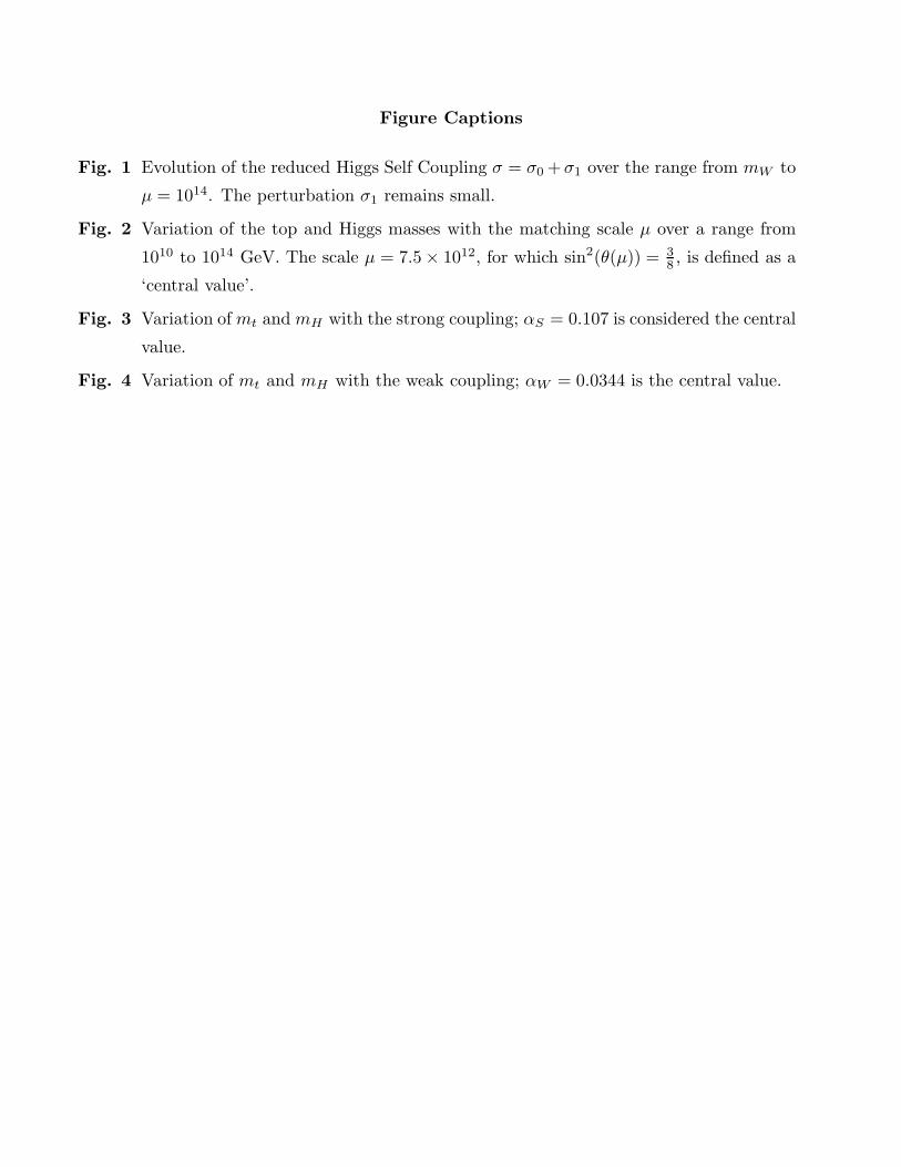
Figure Captions
Fig. 1 Evolution of the reduced Higgs Self Coupling σ = σ0 +σ1 over the range from mW to
µ = 1014. The perturbation σ1 remains small.
Fig. 2 Variation of the top and Higgs masses with the matching scale µ over a range from
1010 to 1014 GeV. The scale µ = 7.5 × 10¹², for which sin2(θ(µ)) = 38 , is defined as a
‘central value’.
Fig. 3 Variation of mt and mH with the strong coupling; αS = 0.107 is considered the central
value.
Fig. 4 Variation of mt and mH with the weak coupling; αW = 0.0344 is the central value.

This figure "fig1-1.png" is available in "png" format from:
http://arXiv.org/ps/hep-ph/9312316v1

This figure "fig2-1.png" is available in "png" format from:
http://arXiv.org/ps/hep-ph/9312316v1

This figure "fig2-2.png" is available in "png" format from:
http://arXiv.org/ps/hep-ph/9312316v1

This figure "fig2-3.png" is available in "png" format from:
http://arXiv.org/ps/hep-ph/9312316v1

This figure "fig2-4.png" is available in "png" format from:
http://arXiv.org/ps/hep-ph/9312316v1
7.5x10¹⁰
7.5x10¹²
7.5x10¹⁴
µ (GeV)
120
130
140
150
160
170
180
190
m (
GeV
)Top and Higgs Masses vs µ
mt
mH
Fig.
2
7.5x10¹² 125
q (GeV)
0.000
0.005
0.010
0.015
0.020
0.025
0.030
0.035
σEvolution of Higgs Self Coupling
σ0
σ
σ1
Fig.
1
(q=µ) (q=mH)
0.100 0.105 0.110 0.115αs (mW)
120
130
140
150
160
170
180
190
m (
GeV
)Top and Higgs Masses vs αs(mW)
mt
mH
Fig.
3
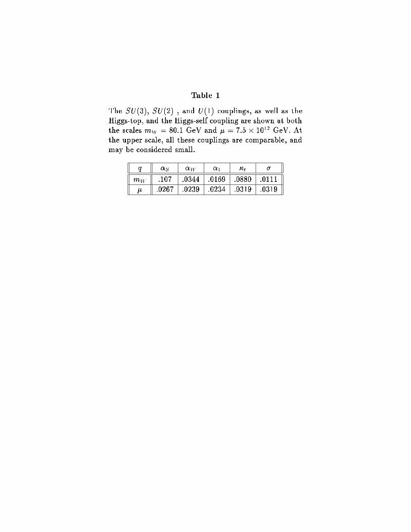
Table 1
The SU(3), SU(2) , and U(1) couplings, as well as the
Higgs-top, and the Higgs-self coupling are shown at both
the scales m
W
= 80:1 GeV and � = 7:5 � 10
12
GeV. At
the upper scale, all these couplings are comparable, and
may be considered small.
q �
S
�
W
�
1
�
t
�
m
W
:107 :0344 :0169 :0880 :0111
� :0267 :0239 :0234 :0319 :0319
0.032 0.033 0.034 0.035αW(mW)
120
130
140
150
160
170
180
190
m (
GeV
)Top and Higgs Masses vs αW(mW)
Fig.
4
mt
mH
Fig.
4
mt
mH


