Theory and applications of atomic and ionic polarizabilities

This article has been downloaded from IOPscience. Please scroll down to see the full text article.

2010 J. Phys. B: At. Mol. Opt. Phys. 43 202001

(http://iopscience.iop.org/0953-4075/43/20/202001)

Download details:

IP Address: 128.175.13.10

The article was downloaded on 30/10/2010 at 12:00

Please note that terms and conditions apply.

View the table of contents for this issue, or go to the journal homepage for more

Home Search Collections Journals About Contact us My IOPscience

IOP PUBLISHING JOURNAL OF PHYSICS B: ATOMIC, MOLECULAR AND OPTICAL PHYSICS

J. Phys. B: At. Mol. Opt. Phys. 43 (2010) 202001 (38pp) doi:10.1088/0953-4075/43/20/202001

TOPICAL REVIEW

Theory and applications of atomic andionic polarizabilities

J Mitroy1, M S Safronova2 and Charles W Clark3

1 School of Engineering, Charles Darwin University, Darwin NT 0909, Australia2 Department of Physics and Astronomy, University of Delaware, Newark, DE 19716, USA3 Joint Quantum Institute, National Institute of Standards and Technology and the University ofMaryland, Gaithersburg, MD 20899-8410, USA

E-mail: jxm107@rsphysse.anu.edu.au, msafrono@udel.edu and charles.clark@nist.gov

Received 21 April 2010Published 4 October 2010Online at stacks.iop.org/JPhysB/43/202001

Abstract

Atomic polarization phenomena impinge upon a number of areas and processes in physics.The dielectric constant and refractive index of any gas are examples of macroscopic propertiesthat are largely determined by the dipole polarizability. When it comes to microscopicphenomena, the existence of alkaline-earth anions and the recently discovered ability ofpositrons to bind to many atoms are predominantly due to the polarization interaction. Animperfect knowledge of atomic polarizabilities is presently looming as the largest source ofuncertainty in the new generation of optical frequency standards. Accurate polarizabilities forthe group I and II atoms and ions of the periodic table have recently become available by avariety of techniques. These include refined many-body perturbation theory andcoupled-cluster calculations sometimes combined with precise experimental data for selectedtransitions, microwave spectroscopy of Rydberg atoms and ions, refractive indexmeasurements in microwave cavities, ab initio calculations of atomic structures usingexplicitly correlated wavefunctions, interferometry with atom beams and velocity changes oflaser cooled atoms induced by an electric field. This review examines existing theoreticalmethods of determining atomic and ionic polarizabilities, and discusses their relevance tovarious applications with particular emphasis on cold-atom physics and the metrology ofatomic frequency standards.

1. Introduction

By the time Maxwell presented his article on a ‘dynamicaltheory of the electromagnetic field’ [1], it was understoodthat bulk matter had a composition of particles of oppositeelectrical charge, and that an applied electric field wouldrearrange the distribution of those charges in an ordinaryobject. This rearrangement could be described accuratelyeven without a detailed microscopic understanding of matter.For example, if a perfectly conducting sphere of radius r0 isplaced in a uniform electric field F, simple potential theoryshows that the resulting electric field at a position r outsidethe sphere must be F − ∇(

F · rr30

/r3

). This is equivalent to

replacing the sphere with a point electric dipole

d = αF, (1)

where α = r30 is the dipole polarizability of the sphere4.

An arbitrary applied electric field can be decomposed intomultipole fields of the form Fk

q(r) = −Fkq ∇(

rkCkq(r)

), where

Ckq(r) is a spherical tensor [2]. Each of these will induce

a multipole moment of Fkq r2k+1

0 in the conducting sphere,corresponding to a multipole polarizability of αk = r2k+1

0 .

Treatment of the electrical polarizabilities of macroscopicbodies is a standard topic of textbooks on electromagnetictheory, and the only material properties that it requires aredielectric constants and conductivities.

Quantum mechanics, on the other hand, offers afundamental description of matter, incorporating the effects

4 For notational convenience, we use the Gaussian system of electrical units,as discussed in subsection A. In the Gaussian system, electric polarizabilityhas the dimensions of volume.

0953-4075/10/202001+38$30.00 1 © 2010 IOP Publishing Ltd Printed in the UK & the USA

J. Phys. B: At. Mol. Opt. Phys. 43 (2010) 202001 Topical Review

of electric and magnetic fields on its elementary constituents,and thus enables polarizabilities to be calculated from firstprinciples. The standard framework for such calculations,perturbation theory, was first laid out by Schrodinger [3] in apaper that reported his calculations of the Stark effect in atomichydrogen. A system of particles with positions ri and electriccharges qi exposed to a uniform electric field, (F = F F), isdescribed by the Hamiltonian

H = H0 − F F · d, (2)

where H0 is the Hamiltonian in the absence of the field, and d

is the dipole moment operator

d =∑

i

qiri . (3)

Treating the field strength, F = |F|, as a perturbationparameter means that the energy and wavefunction can beexpanded as

|�〉 = |�0〉 + F |�1〉 + F 2|�2〉 + · · · (4)

E = E0 + FE1 + F 2E2 + · · · . (5)

The first-order energy E1 = 0 if |�0〉 is an eigenfunctionof the parity operator. In this case, |�1〉 satisfies the equation

(H0 − E0)|�1〉 = −F · d|�0〉. (6)

From the solution to equation (6), we can find the expectationvalue

〈�|d|�〉 = F(〈�0|d|�1〉 + 〈�1|d|�0〉)= αF, (7)

where α is a matrix. The second-order energy is given by

E2 = − 12 F · αF. (8)

Although equation (6) can be solved directly, and in somecases in closed form, it is often more practical to express thesolution in terms of the eigenfunctions and eigenvalues of H0,so that equation (8) takes the form

E2 = −∑

n

|〈�0|d · F|�n〉|2En − E0

. (9)

This sum over all stationary states shows that calculationof atomic polarizabilities is a demanding special case ofthe calculation of atomic structure. The sum extends inprinciple over the continuous spectrum, which sometimesmakes substantial contributions to the polarizability.

Interest in the subject of polarizabilities of atomic stateshas recently been elevated by the appreciation that the accuracyof next-generation atomic time and frequency standards, basedon optical transitions [4–9], is significantly limited by thedisplacement of atomic energy levels due to universal ambientthermal fluctuations of the electromagnetic field: blackbodyradiation (BBR) shifts [10–13]. This phenomenon brings themost promising approach to a more accurate definition of theunit of time, the second, into contact with deep understandingof the thermodynamics of the electromagnetic radiation field.

Description of the interplay between these twofundamental phenomena is a major focus of this review, whichin earlier times might have seemed a pedestrian discourse

on atomic polarizabilities. The precise calculation of atomicpolarizabilities also has implications for quantum informationprocessing and optical cooling and trapping schemes. Modernrequirements for precision and accuracy have elicited renewedattention to methods of accurate first-principles calculations ofatomic structure, which recently have been increased in scopeand precision by developments in methodology, algorithms,and raw computational power. It is expected that the futurewill lead to an increased reliance on theoretical treatmentsto describe the details of atomic polarization. Indeed, atthe present time, many of the best estimates of atomicpolarizabilities are derived from a composite analysis whichintegrates experimental measurements with first principlescalculations of atomic properties.

There have been a number of reviews and tabulationsof atomic and ionic polarizabilities [14–25]. Some of thesereviews, e.g. [16, 17, 22, 23], have largely focused onexperimental developments while others [19, 21, 25] havegiven theory more attention.

In this review, the strengths and limitations of differenttheoretical techniques are discussed in detail given theirexpected importance in the future. The discussion ofthe experimental work is mainly confined to presenting acompilation of existing results and very brief overviews of thevarious methods. The exception to this is the interpretationof resonance excitation Stark ionization spectroscopy [23]since issues pertaining to the convergence of the perturbationanalysis of the polarization interaction are important here. Thisreview is confined to discussing the polarizabilities of lowlying atomic and ionic states despite the existence of a body ofresearch on Rydberg states [26]. High-order polarizabilitiesare not considered except in those circumstances where theyare specifically relevant to ordinary polarization phenomenon.The influence of external electric fields on energy levelscomprises part of this review as does the nature of thepolarization interaction between charged particles with atomsand ions. The focus of this review is on developments relatedto contemporary topics such as the development of opticalfrequency standards, quantum computing and the study offundamental symmetries. Major emphasis of this review is toprovide critically evaluated data on atomic polarizabilities.Table 1 summarizes the data presented in this review tofacilitate the search for particular information.

1.1. Systems of units

Dipole polarizabilities are given in a variety of units,depending on the context in which they are determined. Themost widely used unit for theoretical atomic physics is atomicunits (au), in which, e, me, 4πε0 and the reduced Planckconstant h have the numerical value 1. The polarizability inau has the dimension of volume, and its numerical valuespresented here are thus expressed in units of a3

0 , wherea0 ≈ 0.052 918 nm is the Bohr radius. The preferred unitsystems for polarizabilities determined by experiment are A3,kHz (kV cm−1)−2, cm3 mol−1 or C m2 N−1 where C m2 N−1 isthe SI unit. In this review, almost all polarizabilities are givenin au with uncertainties in the last digits (if appropriate) given

2

J. Phys. B: At. Mol. Opt. Phys. 43 (2010) 202001 Topical Review

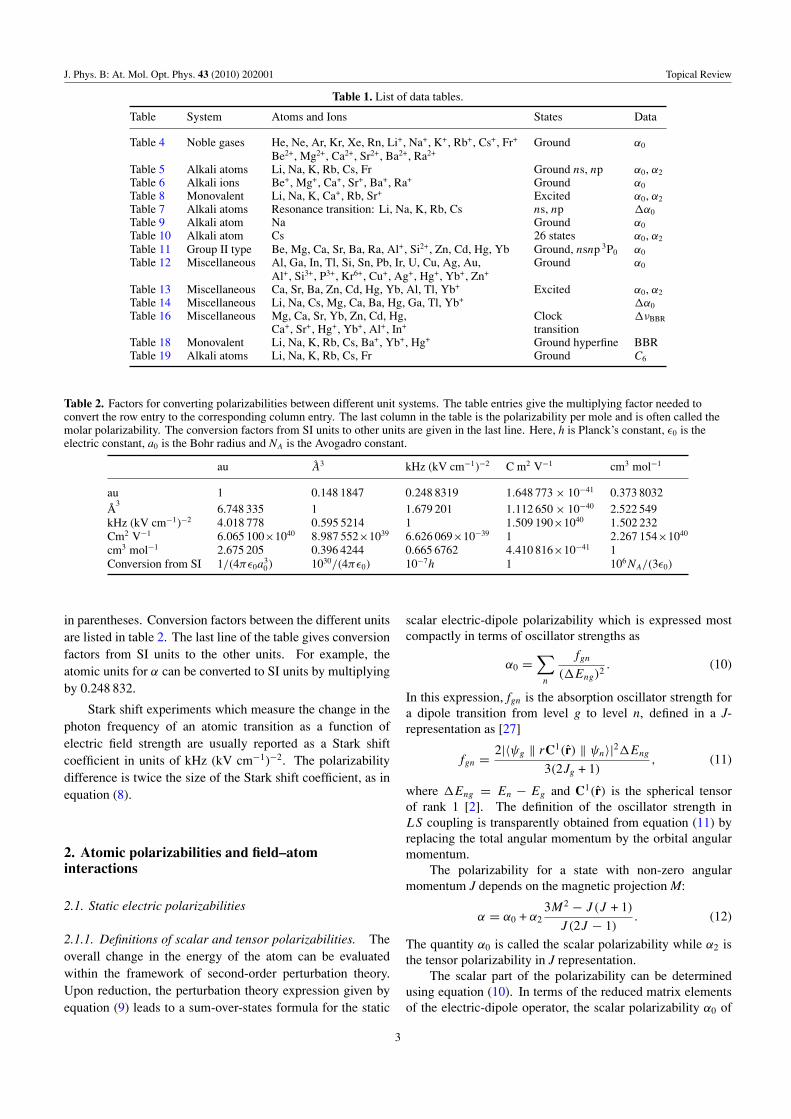
Table 1. List of data tables.

Table System Atoms and Ions States Data

Table 4 Noble gases He, Ne, Ar, Kr, Xe, Rn, Li+, Na+, K+, Rb+, Cs+, Fr+ Ground α0

Be2+, Mg2+, Ca2+, Sr2+, Ba2+, Ra2+

Table 5 Alkali atoms Li, Na, K, Rb, Cs, Fr Ground ns, np α0, α2

Table 6 Alkali ions Be+, Mg+, Ca+, Sr+, Ba+, Ra+ Ground α0

Table 8 Monovalent Li, Na, K, Ca+, Rb, Sr+ Excited α0, α2

Table 7 Alkali atoms Resonance transition: Li, Na, K, Rb, Cs ns, np �α0

Table 9 Alkali atom Na Ground α0

Table 10 Alkali atom Cs 26 states α0, α2

Table 11 Group II type Be, Mg, Ca, Sr, Ba, Ra, Al+, Si2+, Zn, Cd, Hg, Yb Ground, nsnp 3P0 α0

Table 12 Miscellaneous Al, Ga, In, Tl, Si, Sn, Pb, Ir, U, Cu, Ag, Au, Ground α0

Al+, Si3+, P3+, Kr6+, Cu+, Ag+, Hg+, Yb+, Zn+

Table 13 Miscellaneous Ca, Sr, Ba, Zn, Cd, Hg, Yb, Al, Tl, Yb+ Excited α0, α2

Table 14 Miscellaneous Li, Na, Cs, Mg, Ca, Ba, Hg, Ga, Tl, Yb+ �α0

Table 16 Miscellaneous Mg, Ca, Sr, Yb, Zn, Cd, Hg, Clock �νBBR

Ca+, Sr+, Hg+, Yb+, Al+, In+ transitionTable 18 Monovalent Li, Na, K, Rb, Cs, Ba+, Yb+, Hg+ Ground hyperfine BBRTable 19 Alkali atoms Li, Na, K, Rb, Cs, Fr Ground C6

Table 2. Factors for converting polarizabilities between different unit systems. The table entries give the multiplying factor needed toconvert the row entry to the corresponding column entry. The last column in the table is the polarizability per mole and is often called themolar polarizability. The conversion factors from SI units to other units are given in the last line. Here, h is Planck’s constant, ε0 is theelectric constant, a0 is the Bohr radius and NA is the Avogadro constant.

au A3 kHz (kV cm−1)−2 C m2 V−1 cm3 mol−1

au 1 0.148 1847 0.248 8319 1.648 773 × 10−41 0.373 8032A

36.748 335 1 1.679 201 1.112 650 × 10−40 2.522 549

kHz (kV cm−1)−2 4.018 778 0.595 5214 1 1.509 190×1040 1.502 232Cm2 V−1 6.065 100×1040 8.987 552×1039 6.626 069×10−39 1 2.267 154×1040

cm3 mol−1 2.675 205 0.396 4244 0.665 6762 4.410 816×10−41 1Conversion from SI 1/(4πε0a

30) 1030/(4πε0) 10−7h 1 106NA/(3ε0)

in parentheses. Conversion factors between the different unitsare listed in table 2. The last line of the table gives conversionfactors from SI units to the other units. For example, theatomic units for α can be converted to SI units by multiplyingby 0.248 832.

Stark shift experiments which measure the change in thephoton frequency of an atomic transition as a function ofelectric field strength are usually reported as a Stark shiftcoefficient in units of kHz (kV cm−1)−2. The polarizabilitydifference is twice the size of the Stark shift coefficient, as inequation (8).

2. Atomic polarizabilities and field–atominteractions

2.1. Static electric polarizabilities

2.1.1. Definitions of scalar and tensor polarizabilities. Theoverall change in the energy of the atom can be evaluatedwithin the framework of second-order perturbation theory.Upon reduction, the perturbation theory expression given byequation (9) leads to a sum-over-states formula for the static

scalar electric-dipole polarizability which is expressed mostcompactly in terms of oscillator strengths as

α0 =∑

n

fgn

(�Eng)2. (10)

In this expression, fgn is the absorption oscillator strength fora dipole transition from level g to level n, defined in a J-representation as [27]

fgn = 2|〈ψg ‖ rC1(r) ‖ ψn〉|2�Eng

3(2Jg + 1), (11)

where �Eng = En − Eg and C1(r) is the spherical tensorof rank 1 [2]. The definition of the oscillator strength inLS coupling is transparently obtained from equation (11) byreplacing the total angular momentum by the orbital angularmomentum.

The polarizability for a state with non-zero angularmomentum J depends on the magnetic projection M:

α = α0 + α23M2 − J (J + 1)

J (2J − 1). (12)

The quantity α0 is called the scalar polarizability while α2 isthe tensor polarizability in J representation.

The scalar part of the polarizability can be determinedusing equation (10). In terms of the reduced matrix elementsof the electric-dipole operator, the scalar polarizability α0 of

3

J. Phys. B: At. Mol. Opt. Phys. 43 (2010) 202001 Topical Review

an atom in a state ψ with total angular momentum J and energyE is also written as

α0 = 2

3(2J + 1)

∑n

|〈ψ‖rC1(r)‖ψn〉|2En − E

. (13)

The tensor polarizability α2 is defined as

α2 = 4

(5J (2J − 1)

6(J + 1)(2J + 1)(2J + 3)

)1/2

×∑

n

(−1)J+Jn

{J 1 Jn

1 J 2

} |〈ψ‖rC1(r)‖ψn|〉2

En − E. (14)

It is useful in some cases to calculate polarizabilities in strictLS coupling. In such cases [28], the tensor polarizability α2,L

for a state with orbital angular momentum L is given by

α2,L =∑

n

[(L 1 Ln

−L 0 L

)2 − 1

3(2L + 1)

]

×2|〈ψ ‖ rC1(r) ‖ ψn〉|2E − En

. (15)

The tensor polarizabilities α2 and α2,L in the J and Lrepresentations, respectively, are related by

α2 = α2,L(−1)S+L+J+2(2J + 1)

{S L J

2 J L

}×

(J 2 J

−J 0 J

) (L 2 L

−L 0 L

)−1

. (16)

For L = 1 and J = 3/2, equation (16) gives α2 = α2,L. ForL = 1, S = 1 and J = 1, equation (16) gives α2 = −α2,L/2.For L = 2, α2 = (7/10)α2,L for J = 3/2 and α2 =α2,L for J = 5/2. We use the shorter 〈ψ‖D‖ψn〉 designationfor the reduced electric-dipole matrix elements instead of〈ψ‖rC1(r)‖ψn〉 below.

Equation (14) indicates that spherically symmetric levels(such as the 6s1/2 and 6p1/2 levels of cesium) only have ascalar polarizability. However, the hyperfine states of theselevels can have polarizabilities that depend upon the hyperfinequantum numbers F and MF . The relationship between F andJ polarizabilities is discussed in [29]. This issue is discussedin more detail in the section on BBR shifts.

There are two distinctly different broad approaches to thecalculation of atomic polarizabilities. The ‘sum-over-states’approach uses a straightforward interpretation of equation (9)with the contribution from each state �n being determinedindividually, either from a first principles calculation or fromthe interpretation of experimental data. A second class ofapproaches solves inhomogeneous equation (6) directly. Werefer to this class of approaches as direct methods, but notethat there are many different implementations of this strategy.

2.1.2. The sum-over-states method. The sum-over-statesmethod utilizes the expression such as equations (10), (13)–(15) to determine the polarizability. This approach is widelyused for systems with one or two valence electrons since thepolarizability is often dominated by transitions to a few low-lying excited states. The sum-over-states approach can be usedwith oscillator strengths (or electric-dipole matrix elements)derived from experiment or atomic structure calculations. It

is also possible to insert high-precision experimental valuesof these quantities into an otherwise theoretical determinationof the total polarizability. For such monovalent or divalentsystems, it is computationally feasible to explicitly construct aset of intermediate states that is effectively complete. Such anapproach is computationally more difficult to apply for atomsnear the right-hand side of the periodic table since the largerdimensions involved would preclude an explicit computationof the entire set of intermediate state wavefunctions.

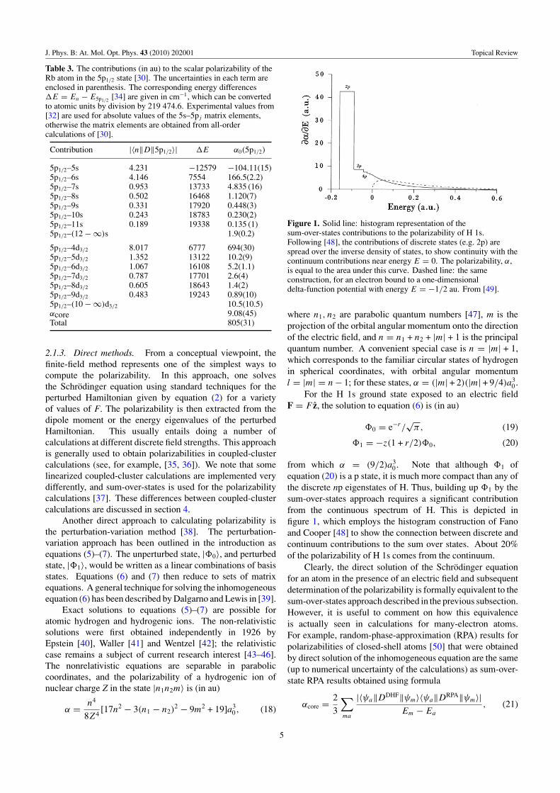
For monovalent atoms, it is convenient to separate thetotal polarizability of an atom into the core polarizabilityαcore and the valence part defined by equation (13). The corecontribution actually has two components, the polarizabilityof the ionic core and a small change due to the presence of thevalence electron [30]. For the alkali atoms, the valence partof the ground state polarizability is completely dominated bythe contribution from the lowest excited state. For example,the 5s–5p1/2 and 5s–5p3/2 transitions contribute more than99% of the Rb valence polarizability [31]. The Rb+ corepolarizability contributes about 3%. Therefore, precisionexperimental measurements of the transition rates for thedominant transitions can also be used to deduce accurate valuesof the ground state polarizability. However, this is not the casefor some excited states where several transitions may havelarge contributions and the continuum contribution may be notnegligible.

This issue is illustrated using the polarizability of the 5p1/2

state of the Rb atom [30], which is given by

α0(5p1/2) = 1

3

∑n

|〈ns‖D‖5p1/2〉|2Ens − E5p1/2

+1

3

∑n

|〈nd3/2‖D‖5p1/2〉|2End3/2 − E5p1/2

+ αcore. (17)

We present a solution to equation (17) that combinesfirst principles calculations with experimental data. Thestrategy to produce a high-quality recommended value withthis approach is to calculate as many terms as realistic orfeasible using the high-precision atomic structure methods.Where experimental high-precision data are available (forexample, for the 5s–5p transitions) they are used in placeof theory, assuming that the expected theory uncertainty ishigher than that of the experimental values. The remainderthat contains contributions from highly excited states isgenerally evaluated using (Dirac–Hartree–Fock) DHF orrandom-phase approximation (RPA) methods. In our example,the contribution from the very high discrete (n > 10) andcontinuum states is about 1.5% and cannot be omitted ina precision calculation. Table 3 lists the dipole matrixelements and energy differences required for evaluation ofequation (17) as well as the individual contributions to thepolarizability. Experimental values from [32] are used forthe 5s–5pj matrix elements, otherwise the matrix elementsare obtained from the all-order calculations of [30] describedin section 4.6. Absolute values of the matrix elementsare given. Experimental energies from [33, 34] are used.Several transitions give significant contributions. The finalpolarizability value agrees with the experimental measurementwithin the uncertainty. The comparison with experiment isdiscussed in section 5.

4

J. Phys. B: At. Mol. Opt. Phys. 43 (2010) 202001 Topical Review

Table 3. The contributions (in au) to the scalar polarizability of theRb atom in the 5p1/2 state [30]. The uncertainties in each term areenclosed in parenthesis. The corresponding energy differences�E = En − E5p1/2 [34] are given in cm−1, which can be convertedto atomic units by division by 219 474.6. Experimental values from[32] are used for absolute values of the 5s–5pj matrix elements,otherwise the matrix elements are obtained from all-ordercalculations of [30].

Contribution |〈n‖D‖5p1/2〉| �E α0(5p1/2)

5p1/2–5s 4.231 −12579 −104.11(15)5p1/2–6s 4.146 7554 166.5(2.2)5p1/2–7s 0.953 13733 4.835 (16)5p1/2–8s 0.502 16468 1.120(7)5p1/2–9s 0.331 17920 0.448(3)5p1/2–10s 0.243 18783 0.230(2)5p1/2–11s 0.189 19338 0.135 (1)5p1/2–(12 − ∞)s 1.9(0.2)

5p1/2–4d3/2 8.017 6777 694(30)5p1/2–5d3/2 1.352 13122 10.2(9)5p1/2–6d3/2 1.067 16108 5.2(1.1)5p1/2–7d3/2 0.787 17701 2.6(4)5p1/2–8d3/2 0.605 18643 1.4(2)5p1/2–9d3/2 0.483 19243 0.89(10)5p1/2–(10 − ∞)d3/2 10.5(10.5)αcore 9.08(45)Total 805(31)

2.1.3. Direct methods. From a conceptual viewpoint, thefinite-field method represents one of the simplest ways tocompute the polarizability. In this approach, one solvesthe Schrodinger equation using standard techniques for theperturbed Hamiltonian given by equation (2) for a varietyof values of F. The polarizability is then extracted from thedipole moment or the energy eigenvalues of the perturbedHamiltonian. This usually entails doing a number ofcalculations at different discrete field strengths. This approachis generally used to obtain polarizabilities in coupled-clustercalculations (see, for example, [35, 36]). We note that somelinearized coupled-cluster calculations are implemented verydifferently, and sum-over-states is used for the polarizabilitycalculations [37]. These differences between coupled-clustercalculations are discussed in section 4.

Another direct approach to calculating polarizability isthe perturbation-variation method [38]. The perturbation-variation approach has been outlined in the introduction asequations (5)–(7). The unperturbed state, |�0〉, and perturbedstate, |�1〉, would be written as a linear combinations of basisstates. Equations (6) and (7) then reduce to sets of matrixequations. A general technique for solving the inhomogeneousequation (6) has been described by Dalgarno and Lewis in [39].

Exact solutions to equations (5)–(7) are possible foratomic hydrogen and hydrogenic ions. The non-relativisticsolutions were first obtained independently in 1926 byEpstein [40], Waller [41] and Wentzel [42]; the relativisticcase remains a subject of current research interest [43–46].The nonrelativistic equations are separable in paraboliccoordinates, and the polarizability of a hydrogenic ion ofnuclear charge Z in the state |n1n2m〉 is (in au)

α = n4

8Z4[17n2 − 3(n1 − n2)

2 − 9m2 + 19]a30, (18)

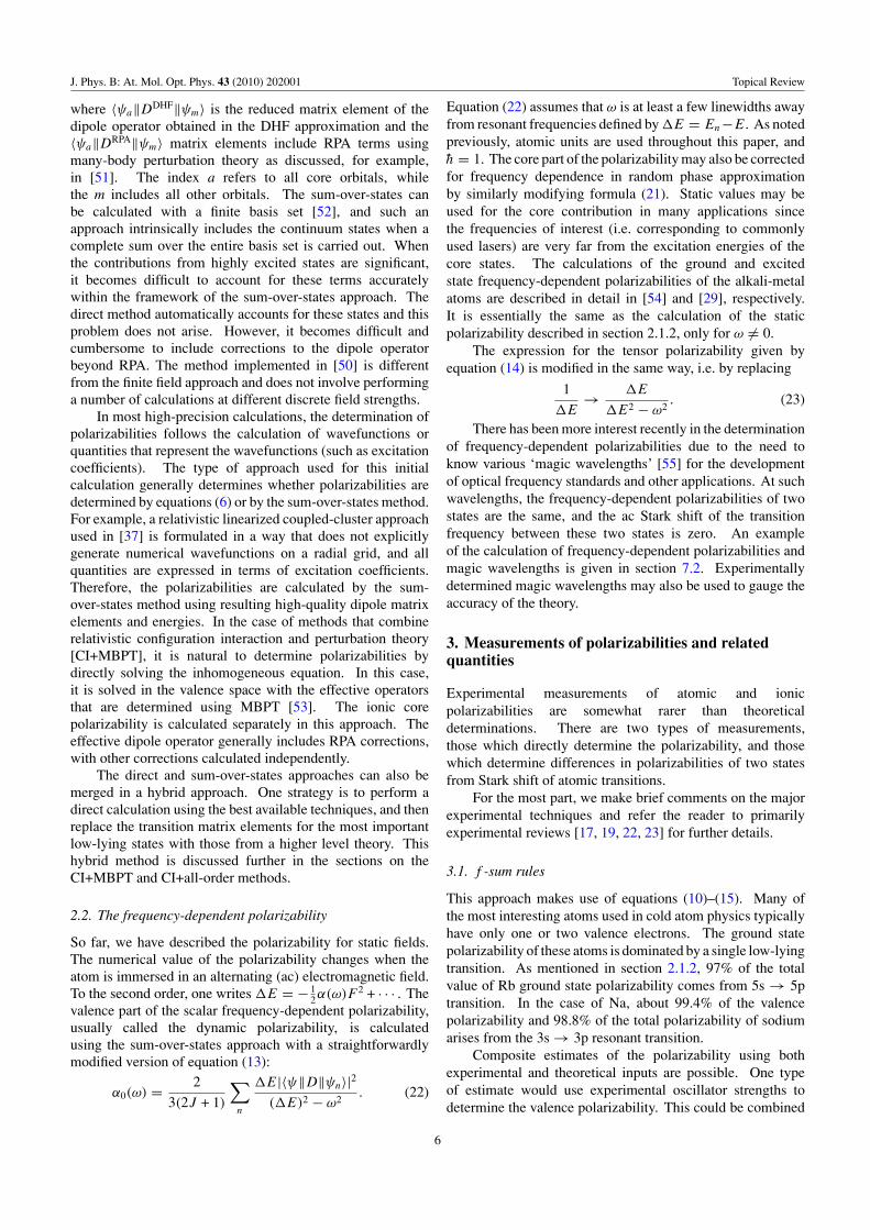
Figure 1. Solid line: histogram representation of thesum-over-states contributions to the polarizability of H 1s.Following [48], the contributions of discrete states (e.g. 2p) arespread over the inverse density of states, to show continuity with thecontinuum contributions near energy E = 0. The polarizability, α,is equal to the area under this curve. Dashed line: the sameconstruction, for an electron bound to a one-dimensionaldelta-function potential with energy E = −1/2 au. From [49].

where n1, n2 are parabolic quantum numbers [47], m is theprojection of the orbital angular momentum onto the directionof the electric field, and n = n1 + n2 + |m| + 1 is the principalquantum number. A convenient special case is n = |m| + 1,which corresponds to the familiar circular states of hydrogenin spherical coordinates, with orbital angular momentuml = |m| = n − 1; for these states, α = (|m| + 2)(|m| + 9/4)a3

0 .For the H 1s ground state exposed to an electric field

F = F z, the solution to equation (6) is (in au)

�0 = e−r/√

π, (19)

�1 = −z(1 + r/2)�0, (20)

from which α = (9/2)a30 . Note that although �1 of

equation (20) is a p state, it is much more compact than any ofthe discrete np eigenstates of H. Thus, building up �1 by thesum-over-states approach requires a significant contributionfrom the continuous spectrum of H. This is depicted infigure 1, which employs the histogram construction of Fanoand Cooper [48] to show the connection between discrete andcontinuum contributions to the sum over states. About 20%of the polarizability of H 1s comes from the continuum.

Clearly, the direct solution of the Schrodinger equationfor an atom in the presence of an electric field and subsequentdetermination of the polarizability is formally equivalent to thesum-over-states approach described in the previous subsection.However, it is useful to comment on how this equivalenceis actually seen in calculations for many-electron atoms.For example, random-phase-approximation (RPA) results forpolarizabilities of closed-shell atoms [50] that were obtainedby direct solution of the inhomogeneous equation are the same(up to numerical uncertainty of the calculations) as sum-over-state RPA results obtained using formula

αcore = 2

3

∑ma

|〈ψa‖DDHF‖ψm〉〈ψa‖DRPA‖ψm〉|Em − Ea

, (21)

5

J. Phys. B: At. Mol. Opt. Phys. 43 (2010) 202001 Topical Review

where 〈ψa‖DDHF‖ψm〉 is the reduced matrix element of thedipole operator obtained in the DHF approximation and the〈ψa‖DRPA‖ψm〉 matrix elements include RPA terms usingmany-body perturbation theory as discussed, for example,in [51]. The index a refers to all core orbitals, whilethe m includes all other orbitals. The sum-over-states canbe calculated with a finite basis set [52], and such anapproach intrinsically includes the continuum states when acomplete sum over the entire basis set is carried out. Whenthe contributions from highly excited states are significant,it becomes difficult to account for these terms accuratelywithin the framework of the sum-over-states approach. Thedirect method automatically accounts for these states and thisproblem does not arise. However, it becomes difficult andcumbersome to include corrections to the dipole operatorbeyond RPA. The method implemented in [50] is differentfrom the finite field approach and does not involve performinga number of calculations at different discrete field strengths.

In most high-precision calculations, the determination ofpolarizabilities follows the calculation of wavefunctions orquantities that represent the wavefunctions (such as excitationcoefficients). The type of approach used for this initialcalculation generally determines whether polarizabilities aredetermined by equations (6) or by the sum-over-states method.For example, a relativistic linearized coupled-cluster approachused in [37] is formulated in a way that does not explicitlygenerate numerical wavefunctions on a radial grid, and allquantities are expressed in terms of excitation coefficients.Therefore, the polarizabilities are calculated by the sum-over-states method using resulting high-quality dipole matrixelements and energies. In the case of methods that combinerelativistic configuration interaction and perturbation theory[CI+MBPT], it is natural to determine polarizabilities bydirectly solving the inhomogeneous equation. In this case,it is solved in the valence space with the effective operatorsthat are determined using MBPT [53]. The ionic corepolarizability is calculated separately in this approach. Theeffective dipole operator generally includes RPA corrections,with other corrections calculated independently.

The direct and sum-over-states approaches can also bemerged in a hybrid approach. One strategy is to perform adirect calculation using the best available techniques, and thenreplace the transition matrix elements for the most importantlow-lying states with those from a higher level theory. Thishybrid method is discussed further in the sections on theCI+MBPT and CI+all-order methods.

2.2. The frequency-dependent polarizability

So far, we have described the polarizability for static fields.The numerical value of the polarizability changes when theatom is immersed in an alternating (ac) electromagnetic field.To the second order, one writes �E = − 1

2α(ω)F 2 + · · · . Thevalence part of the scalar frequency-dependent polarizability,usually called the dynamic polarizability, is calculatedusing the sum-over-states approach with a straightforwardlymodified version of equation (13):

α0(ω) = 2

3(2J + 1)

∑n

�E|〈ψ‖D‖ψn〉|2(�E)2 − ω2

. (22)

Equation (22) assumes that ω is at least a few linewidths awayfrom resonant frequencies defined by �E = En−E. As notedpreviously, atomic units are used throughout this paper, andh = 1. The core part of the polarizability may also be correctedfor frequency dependence in random phase approximationby similarly modifying formula (21). Static values may beused for the core contribution in many applications sincethe frequencies of interest (i.e. corresponding to commonlyused lasers) are very far from the excitation energies of thecore states. The calculations of the ground and excitedstate frequency-dependent polarizabilities of the alkali-metalatoms are described in detail in [54] and [29], respectively.It is essentially the same as the calculation of the staticpolarizability described in section 2.1.2, only for ω = 0.

The expression for the tensor polarizability given byequation (14) is modified in the same way, i.e. by replacing

1

�E→ �E

�E2 − ω2. (23)

There has been more interest recently in the determinationof frequency-dependent polarizabilities due to the need toknow various ‘magic wavelengths’ [55] for the developmentof optical frequency standards and other applications. At suchwavelengths, the frequency-dependent polarizabilities of twostates are the same, and the ac Stark shift of the transitionfrequency between these two states is zero. An exampleof the calculation of frequency-dependent polarizabilities andmagic wavelengths is given in section 7.2. Experimentallydetermined magic wavelengths may also be used to gauge theaccuracy of the theory.

3. Measurements of polarizabilities and relatedquantities

Experimental measurements of atomic and ionicpolarizabilities are somewhat rarer than theoreticaldeterminations. There are two types of measurements,those which directly determine the polarizability, and thosewhich determine differences in polarizabilities of two statesfrom Stark shift of atomic transitions.

For the most part, we make brief comments on the majorexperimental techniques and refer the reader to primarilyexperimental reviews [17, 19, 22, 23] for further details.

3.1. f -sum rules

This approach makes use of equations (10)–(15). Many ofthe most interesting atoms used in cold atom physics typicallyhave only one or two valence electrons. The ground statepolarizability of these atoms is dominated by a single low-lyingtransition. As mentioned in section 2.1.2, 97% of the totalvalue of Rb ground state polarizability comes from 5s → 5ptransition. In the case of Na, about 99.4% of the valencepolarizability and 98.8% of the total polarizability of sodiumarises from the 3s → 3p resonant transition.

Composite estimates of the polarizability using bothexperimental and theoretical inputs are possible. One typeof estimate would use experimental oscillator strengths todetermine the valence polarizability. This could be combined

6

J. Phys. B: At. Mol. Opt. Phys. 43 (2010) 202001 Topical Review

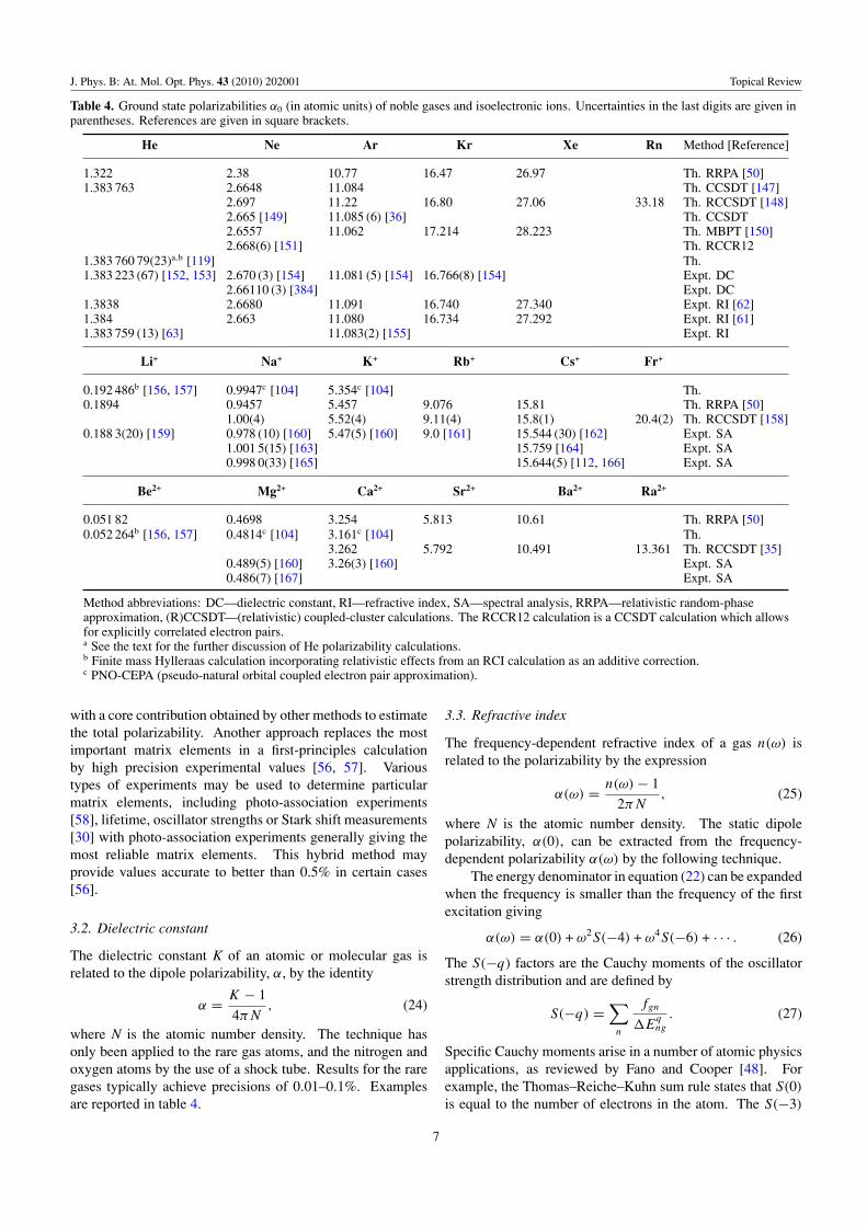
Table 4. Ground state polarizabilities α0 (in atomic units) of noble gases and isoelectronic ions. Uncertainties in the last digits are given inparentheses. References are given in square brackets.

He Ne Ar Kr Xe Rn Method [Reference]

1.322 2.38 10.77 16.47 26.97 Th. RRPA [50]1.383 763 2.6648 11.084 Th. CCSDT [147]

2.697 11.22 16.80 27.06 33.18 Th. RCCSDT [148]2.665 [149] 11.085 (6) [36] Th. CCSDT2.6557 11.062 17.214 28.223 Th. MBPT [150]2.668(6) [151] Th. RCCR12

1.383 760 79(23)a,b [119] Th.1.383 223 (67) [152, 153] 2.670 (3) [154] 11.081 (5) [154] 16.766(8) [154] Expt. DC

2.66110 (3) [384] Expt. DC1.3838 2.6680 11.091 16.740 27.340 Expt. RI [62]1.384 2.663 11.080 16.734 27.292 Expt. RI [61]1.383 759 (13) [63] 11.083(2) [155] Expt. RI

Li+ Na+ K+ Rb+ Cs+ Fr+

0.192 486b [156, 157] 0.9947c [104] 5.354c [104] Th.0.1894 0.9457 5.457 9.076 15.81 Th. RRPA [50]

1.00(4) 5.52(4) 9.11(4) 15.8(1) 20.4(2) Th. RCCSDT [158]0.188 3(20) [159] 0.978 (10) [160] 5.47(5) [160] 9.0 [161] 15.544 (30) [162] Expt. SA

1.001 5(15) [163] 15.759 [164] Expt. SA0.998 0(33) [165] 15.644(5) [112, 166] Expt. SA

Be2+ Mg2+ Ca2+ Sr2+ Ba2+ Ra2+

0.051 82 0.4698 3.254 5.813 10.61 Th. RRPA [50]0.052 264b [156, 157] 0.4814c [104] 3.161c [104] Th.

3.262 5.792 10.491 13.361 Th. RCCSDT [35]0.489(5) [160] 3.26(3) [160] Expt. SA0.486(7) [167] Expt. SA

Method abbreviations: DC—dielectric constant, RI—refractive index, SA—spectral analysis, RRPA—relativistic random-phaseapproximation, (R)CCSDT—(relativistic) coupled-cluster calculations. The RCCR12 calculation is a CCSDT calculation which allowsfor explicitly correlated electron pairs.a See the text for the further discussion of He polarizability calculations.b Finite mass Hylleraas calculation incorporating relativistic effects from an RCI calculation as an additive correction.c PNO-CEPA (pseudo-natural orbital coupled electron pair approximation).

with a core contribution obtained by other methods to estimatethe total polarizability. Another approach replaces the mostimportant matrix elements in a first-principles calculationby high precision experimental values [56, 57]. Varioustypes of experiments may be used to determine particularmatrix elements, including photo-association experiments[58], lifetime, oscillator strengths or Stark shift measurements[30] with photo-association experiments generally giving themost reliable matrix elements. This hybrid method mayprovide values accurate to better than 0.5% in certain cases[56].

3.2. Dielectric constant

The dielectric constant K of an atomic or molecular gas isrelated to the dipole polarizability, α, by the identity

α = K − 1

4πN, (24)

where N is the atomic number density. The technique hasonly been applied to the rare gas atoms, and the nitrogen andoxygen atoms by the use of a shock tube. Results for the raregases typically achieve precisions of 0.01–0.1%. Examplesare reported in table 4.

3.3. Refractive index

The frequency-dependent refractive index of a gas n(ω) isrelated to the polarizability by the expression

α(ω) = n(ω) − 1

2πN, (25)

where N is the atomic number density. The static dipolepolarizability, α(0), can be extracted from the frequency-dependent polarizability α(ω) by the following technique.

The energy denominator in equation (22) can be expandedwhen the frequency is smaller than the frequency of the firstexcitation giving

α(ω) = α(0) + ω2S(−4) + ω4S(−6) + · · · . (26)

The S(−q) factors are the Cauchy moments of the oscillatorstrength distribution and are defined by

S(−q) =∑

n

fgn

�Eqng

. (27)

Specific Cauchy moments arise in a number of atomic physicsapplications, as reviewed by Fano and Cooper [48]. Forexample, the Thomas–Reiche–Kuhn sum rule states that S(0)

is equal to the number of electrons in the atom. The S(−3)

7

J. Phys. B: At. Mol. Opt. Phys. 43 (2010) 202001 Topical Review

moment is related to the non-adiabatic dipole polarizability[59, 60].

The general functional dependence of the polarizabilityat low frequencies is given by equation (26) [61, 62]. Theachievable precision for the rare gases is 0.1% or better[62, 63]. Experiments on the vapours of Zn, Cd and Hggave polarizabilities with uncertainties of 1–10% [64, 65].

3.4. Deflection of an atom beam by electric fields

The beam deflection experiment is conceptually simple. Acollimated atomic beam is directed through an interactionregion containing an inhomogeneous electric field. While theatom is in the interaction region, the electric field F induces adipole moment on the atom. Since the field is not uniform, aforce proportional to the gradient of the electric field and theinduced dipole moment results in the deflection of the atomicbeam. The polarizability is deduced from the deflection of thebeam. The overall uncertainty in the derived polarizabilitiesis between 5 and 10% [66]. Therefore, this method is mainlyuseful at this time for polarizability measurements in atomsinaccessible by any other means.

3.5. The E–H balance method

In this approach, the E–H balance configuration applies aninhomogeneous electric field and an inhomogeneous magneticfield in the interaction region [67]. The magnetic field actson the magnetic moment of the atom giving a magneticdeflection force in addition to the electric deflection. Theexperiment is tuned so that the electric and magnetic forcesare in balance. The polarizability can be determined since themagnetic moments of many atoms are known. Uncertaintiesrange from 2% to 10% [67–69].

3.6. Atom interferometry

The interferometry approach splits the beam of atoms so thatone path sends a beam through a parallel plate capacitor whilethe other goes through a field-free region. An interferencepattern is then measured when the beams are subsequentlymerged and detected. The polarizability is deduced fromthe phase shift of the beam passing through the field-freeregion. So far, this approach has been used to measure thepolarizabilities of helium (see [70] for a discussion of thismeasurement), lithium [71], sodium [72, 73], potassium [73]and rubidium [73], achieving uncertainties of 0.35–0.8%.

It has been suggested that multi-species interferometerscould possibly determine the polarizability ratio R = αX/αY

to 10−4 relative accuracy [70]. Consequently, a measurementof R in conjunction with a known standard, say lithium, couldlead to a new level of precision in polarizability measurements.Already the Na:K and Na:Rb polarizability ratios have beenmeasured with a precision of 0.3% [73].

3.7. Cold atom velocity change

The experiment of Amini and Gould [74] measured the kineticenergy gained as cold cesium atoms were launched from

a magneto-optical trap into a region with a finite electricfield. The kinetic energy gained only depends on the finalvalue of the electric field. The experimental arrangementactually measures the time of return for cesium atoms tofall back after they are launched into a region between a setof parallel electric-field plates. The only such experimentreported so far gave a very precise estimate of the Cs groundstate polarizability, namely α0 = 401.0(6) au. This approachcan in principle be applied to measure the polarizability ofmany other atoms with a precision approaching 0.1% [22].

3.8. Other approaches

The deflection of an atomic beam by pulsed lasers has beenused to obtain the dynamic polarizabilities of rubidium anduranium [75, 76]. The dynamic polarizabilities of some metalatoms sourced from an exploding wire have been measuredinterferometrically [77, 78]. These approaches measurepolarizabilities to an accuracy of 5–20%.

3.9. Spectral analysis for ion polarizabilities

The polarizability of an ion can in principle be extracted fromthe energies of the non-penetrating Rydberg series of the parentsystem [41, 79, 80]. The polarizability of the ionic core leadsto a shift in the (n, L) energy levels away from their hydrogenicvalues.

Consider a charged particle interacting with an atom orion at large distances. To zeroth order, the interaction potentialbetween a highly excited electron and the residual ion is just

V (r) = Z − N

r, (28)

where Z is the nuclear charge and N is the number ofelectrons. However, the outer electron perturbs the atomiccharge distribution. This polarization of the electron chargecloud leads to an attractive polarization potential between theexternal electron and the atom. The Coulomb interaction in amultipole expansion with |r| > |x| is written as

1

|r − x| =∑

k

Ck(x) · Ck(r)xk

rk+1. (29)

Applying second-order perturbation theory leads to theadiabatic polarization potential between the charged particleand the atom, e.g.

Vpol(r) = −∞∑

k=1

αEk

2r2k+2. (30)

The quantities αEk are the multipole polarizabilities defined as

αEk =∑

n

f (k)gn

(�Egn)2. (31)

In this notation, the electric-dipole polarizability is writtenas αE1, and f (k)

gn is the absorption oscillator strength for amultipole transition from g −→ n. Equation (30), withits leading term involving the dipole polarizability is notabsolutely convergent in k [81]. At any finite r, continuedsummation of the series given by equation (30), with respect

8

J. Phys. B: At. Mol. Opt. Phys. 43 (2010) 202001 Topical Review

to k, will eventually result in a divergence in the value of thepolarization potential.

Equation (30) is modified by non-adiabatic corrections[59, 60]. The non-adiabatic dipole term is written as

Vnon-ad = 6β0

2r6, (32)

where the non-adiabatic dipole polarizability β0 is defined as

β0 =∑ f (1)

gn

2(�Egn)3. (33)

The non-adiabatic interaction is repulsive for atoms in theirground states. The polarization interaction includes furtheradiabatic, non-adiabatic and higher order terms that contributeat the r−7 and r−8, but there has been no systematic study ofwhat could be referred to as the non-adiabatic expansion ofthe polarization potential.

When the Rydberg electron is in a state that has negligibleoverlap with the core (this is best achieved with the electronin high angular momentum orbitals), then the polarizationinteraction usually provides the dominant contribution to thisenergy shift. Suppose the dominant perturbation to the long-range atomic interaction is

Vpol(r) = −C4

r4− C6

r6, (34)

where C4 = α0/2 and C6 = (α0 − 6β)/2. Equation (34)omits the C7/r7 and C8/r8 terms that are included in a morecomplete description [82–84]. The energy shift due to aninteraction of this type can be written as

�E

�〈r−4〉 = C4 + C6�〈r−6〉�〈r−4〉 , (35)

where �E is usually the energy difference between twoRydberg states. The expectation values �〈r−6〉 and �〈r−4〉are simply the differences in the radial expectations of thetwo states. These are easily evaluated using the identities ofBockasten [85]. Plotting �E

�〈r−4〉 versus �〈r−6〉�〈r−4〉 yields C4 as the

intercept and C6 as the gradient. Such a graph is sometimescalled a polarization plot.

Traditional spectroscopies such as discharges or laserexcitation find it difficult to excite atoms into Rydberg stateswith L > 6. Exciting atoms into states with L > 6 is bestdone with resonant excitation Stark ionization spectroscopy(RESIS) [23]. RESIS spectroscopy first excites an atomic orionic beam into a highly excited state, and then uses a laserto excite the system into a very highly excited state which isStark ionized.

While this approach to extracting polarizabilities fromRydberg series energy shifts is appealing, there are a numberof perturbations that act to complicate the analysis. Theseinclude relativistic effects �Erel, Stark shifts from ambientelectric fields �Ess, second-order effects due to relaxation ofthe Rydberg electron in the field of the polarization potential�Esec [86–88], and finally the corrections due to the C7/r7

and C8/r8 terms, �E7,�E8 and �E8L. Therefore, the energyshift between two neighbouring Rydberg states is

�E = �E4 + �E6 + �E7 + �E8 + �E8L

+ �Erel + �Esec + �Ess. (36)

One way to solve the problem is to simply subtract these termsfrom the observed energy shift, e.g.

�Ec

�〈r−4〉 = �Eobs

�〈r−4〉 −(

�Erel + �Esec + �Ess

�〈r−4〉)

−(

�E7 + �E8 + �E8L

�〈r−4〉)

(37)

and then deduce C4 and C6 from the polarization plot of thecorrected energy levels [84].

3.10. Stark shift measurements of polarizability differences

The Stark shift experiment predates the formulation ofquantum mechanics in its modern form [89]. An atom isimmersed in an electric field, and the shift in the wavelengthof one of its spectral lines is measured as a function of thefield strength. Stark shift experiments effectively measure thedifference between the polarizability of the two atomic statesinvolved in the transition. Stark shifts can be measured forboth static and dynamic electric fields. While there have beenmany Stark shift measurements, relatively few have achievedan overall precision of 1% or better.

While the polarizabilities can generally be extracted fromthe Stark shift measurement, it is useful to compare theexperimental values directly with theoretical predictions wherehigh precision is achieved for both theory and experiment. Inthis review, comparisons of the theoretical static polarizabilitydifferences for the resonance transitions involving the alkaliatoms with the corresponding Stark shifts are provided insection 5. Some of the alkali atom experiments listed in table 7report precisions between 0.01 and 0.1 au [90–93]. The manyStark shift experiments involving Rydberg atoms [94] are notdetailed here.

Selected Stark shifts for some non-alkali atoms that are ofinterest for applications described in this review are discussedin section 5 as well. The list is restricted to low-lying excitedstates for which high precision Stark shifts are available.When compared with the alkali atoms, there are not that manymeasurements and those that have been performed have largeruncertainties.

The tensor polarizability of an open shell atomcan be extracted from the difference in polarizabilitiesbetween the different magnetic sub-levels. Consequently,tensor polarizabilities do not rely on absolute polarizabilitymeasurements and can be extracted from Stark shiftmeasurements by tuning the polarization of a probe laser.Tensor polarizabilities for a number of states of selectedsystems are discussed in section 5.

One unusual experiment was a measurement of the acenergy shift ratio for the 6s and 5d3/2 states of Ba+ to anaccuracy of 0.11% [95]. This experiment does not givepolarizabilities. Its main purpose was to determine selectedE1 matrix elements [96].

3.11. AC Stark shift measurements

There are few experimental measurements of ac Stark shiftsat optical frequencies. Two recent examples would be thedetermination of the Stark shift for the Al+ clock transition [97]

9

J. Phys. B: At. Mol. Opt. Phys. 43 (2010) 202001 Topical Review

and the Li 2s–3s Stark shifts [98] at the frequencies of the pumpand probe laser of a two-photon resonance transition betweenthe two states. One difficulty in the interpretation of ac Starkshift experiments is the lack of precise knowledge about theoverlap of the laser beam with atoms in the interaction region.There are also complications in the analysis of experiments ondeflection of atomic beams by lasers [75, 76].

4. Practical calculation of atomic polarizabilities

There have been numerous theoretical studies of atomic andionic polarizabilities in the last several decades. Most methodsused to determine atomic wavefunctions and energy levelscan be adapted to generate polarizabilities. These have beendivided into a number of different classes that are listed below.We give a brief description of each approach. It should benoted that the list is not exhaustive, and the emphasis herehas been on those methods that have achieved the highestaccuracy or those methods that have been applied to a numberof different atoms and ions.

4.1. Configuration interaction

The configuration interaction (CI) method [99] and its variantsare widely used for atomic structure calculations owing togeneral applicability of the CI method. The CI wavefunction iswritten as a linear combination of configuration state functions

�CI =∑

i

ci�i, (38)

i.e. a linear combination of Slater determinants from amodel subspace [100]. Each configuration is constructedwith consideration given to anti-symmetrization, angularmomentum and parity requirements. There is a great dealof variety in how the CI approach is implemented. Forexample, sometimes the exact functional form of the orbitals inthe excitation space is generated iteratively during successivediagonalization of the excitation basis. Such a scheme iscalled the multi-configuration Hartree–Fock (MCHF) or multi-configuration self-consistent field (MCSCF) approach [101].The relativistic version of MCHF is referred to as the multi-configuration Dirac–Fock (MCDF) method [102].

The CI approach has a great deal of generality sincethere are no restrictions imposed upon the virtual orbitalspace and classes of excitations beyond those limited bythe computer resources. The method is particularly usefulfor open-shell systems which contain a number of stronglyinteracting configurations. On the other hand, there canbe a good deal of variation in quality between different CIcalculations for the same system, because of the flexibility ofintroducing additional configuration state functions.

The most straightforward way to evaluate polarizabilitieswithin the framework of the CI method it to use a directapproach by solving the inhomogeneous equation (6). RPAcorrections to the dipole operator can be incorporated usingthe effective operator technique described in section 4.7. It isalso possible to use CI-generated matrix elements and energiesto evaluate sums over states. The main drawback of the CImethod is its loss of accuracy for heavier systems. It becomes

difficult to include a sufficient number of configurations forheavier systems to produce accurate results even with moderncomputer facilities. One solution of this problem is to usea semi-empirical core potential (CICP method) described inthe next subsection. Another, ab initio solution involvesconstruction of the effective Hamiltonian using either many-body perturbation theory (CI+MBPT) or all-order linearizedcoupled-cluster method (CI+all-order) and carrying out CIcalculations in the valence sector. These approaches aredescribed in the last two sections of this chapter.

4.2. CI calculations with a semi-empirical core potential(CICP)

The ab initio treatment of core–valence correlations greatlyincreases the complexity of any structure calculation.Consequently, to include this physics in the calculation, usinga semi-empirical approach is an attractive alternative for anatom with a few valence electrons [103–105].

In this method, the active Hamiltonian for a system withtwo valence electrons is written as

H =2∑

i=1

(−1

2∇2

i + Vdir(ri) + Vexc(ri) + Vp1(ri)

)+

1

r12+ Vp2(r1, r2). (39)

The Vdir and Vexc represent the direct and exchangeinteractions with the core electrons. In some approaches,these terms are represented by model potentials, [106–108].More refined approaches evaluate Vdir and Vexc using corewavefunctions calculated with the Hartree–Fock (or Dirac–Fock) method [104, 105, 109]. The one-body polarizationinteraction Vpol(r) is semi-empirical in nature and can bewritten in its most general form as an �-dependent potential,e.g.

Vp1(r) = −∑�m

αg2� (r)

2r4|�m〉〈�m|, (40)

where α is the static dipole polarizability of the core and g2� (r)

is a cutoff function that eliminates the 1/r4 singularity at theorigin. The cutoff functions usually include an adjustableparameter that is tuned to reproduce the binding energies of thevalence states. The two-electron or di-electronic polarizationpotential is written as

Vp2(ri , rj ) = − α

r3i r3

j

(ri · rj )g(ri)g(rj ) . (41)

There is variation between expressions for the core polarizationpotential, but what is described above is fairly representative.One choice for the cutoff function is g2

� (r) = 1−exp(−r6/ρ6

�

)[105], but other choices exist.

A complete treatment of the core-polarization correctionsalso implies that corrections have to be made to the multipoleoperators [104, 105, 110, 111]. The modified transitionoperator is obtained from the mapping

rkCk(r) → g�(r)rkCk(r). (42)

10

J. Phys. B: At. Mol. Opt. Phys. 43 (2010) 202001 Topical Review

The usage of the modified operator is essential to the correctprediction of the oscillator strengths. For example, it reducesthe K(4s → 4p) oscillator strength by 8% [104].

One advantage of this configuration interaction pluscore-polarization (CICP) approach is in reducing the sizeof the calculation. The elimination of the core fromactive consideration permits very accurate solutions ofthe Schrodinger equation for the valence electrons. Theintroduction of the core-polarization potentials, Vp1 andVp2, presents an additional source of uncertainty into thecalculation. However, this additional small source ofuncertainty is justified by the almost complete eliminationof computational uncertainty in the solution of the resultingsimplified Schrodinger equation.

The CICP approach only gives the polarizability of thevalence electrons. Core polarizabilities are typically quitesmall for the group I and II atoms, e.g. the cesium atom hasa large core polarizability of about 15.6 a3

0 [112], but thisrepresents only 4% of the total ground state polarizability of401 a3

0 [74]. Hence, the usage of moderate accuracy corepolarizabilities sourced from theory or experiment will lead toonly small inaccuracies in the total polarizability.

Most implementation of the CICP approach to thecalculation of polarizabilities have been within a non-relativistic framework. A relativistic variant (RCICP) hasrecently been applied to zinc, cadmium and mercury [113].It should be noted that even non-relativistic calculationsincorporate relativistic effects to some extent. Tuning thecore polarization correction to reproduce the experimentalbinding energy partially incorporates relativistic effects on thewavefunction.

4.3. Density functional theory

Approaches based on density functional theory (DFT) arenot expected to give polarizabilities as accurate as thosecoming from the refined ab initio calculations described inthe following sections. Polarizabilities from DFT calculationsare most likely to be useful for systems for which large scaleab initio calculations are difficult, e.g. the transition metals.DFT calculations are often much less computationallyexpensive than ab initio calculations. There have been tworelatively extensive DFT compilations [114, 115] that havereported dipole polarizabilities for many atoms in the periodictable.

4.4. Correlated basis functions

The accuracy of atomic structure calculations can bedramatically improved by the use of basis functions whichexplicitly include the electron–electron coordinate. The mostaccurate calculations reported for atoms and ions with two orthree electrons have typically been performed with exponentialbasis functions including the inter-electronic coordinates as alinear factor. A typical Hylleraas basis function for lithiumwould be

χ = rj11 r

j22 r

j33 r

j1212 r

j1313 r

j2323 exp (−αr1 − βr2 − γ r3) . (43)

Difficulties with performing the multi-centre integrals haveeffectively precluded the use of such basis functions forsystems with more than three electrons. Within the frameworkof the non-relativistic Schrodinger equation, calculations withHylleraas basis sets achieve accuracies of 13 significant digits[116] for the polarizabilities of two-electron systems andsix significant digits for the polarizability of three-electronsystems [117, 118]. Inclusion of relativistic and quantumelectrodynamic (QED) corrections to the polarizability ofhelium has been carried out in [116, 119], and the resultingfinal value is accurate to seven significant digits.

Another correlated basis set that has recently foundincreasingly widespread use utilizes the explicitly correlatedGaussian (ECG). A typical spherically symmetric explicitlycorrelated Gaussian for a three-electron system is written as[120]

χ = exp

⎛⎝−3∑

i=1

αir2i −

∑i<j

βij r2ij

⎞⎠ . (44)

The multi-centre integrals that occur in the evaluation of theHamiltonian can be generally reduced to analytic expressionsthat are relatively easy to compute. Calculations usingcorrelated Gaussians do not achieve the same precision asHylleraas forms but are still capable of achieving muchhigher precision than orbital-based calculations provided theparameters αi and βij are well optimized [120, 121].

4.5. Many-body perturbation theory

The application of many-body perturbation theory (MBPT)is discussed in this section in the context of the Diracequation. While MBPT has been applied with the non-relativistic Schrodinger equation, many recent applicationsmost relevant to this review have been using a relativisticHamiltonian.

The point of departure for the discussions of relativisticmany-body perturbation theory (RMBPT) calculations is theno-pair Hamiltonian obtained from QED by Brown andRavenhall [122], where the contributions from negative-energy(positron) states are projected out. The no-pair Hamiltoniancan be written in the second-quantized form as H = H0 + V ,where

H0 =∑

i

εi

[a†i ai

], (45)

V = 1

2

∑ijkl

(gijkl + bijkl)[a†i a

†j alak

]+

∑ij

(VDHF + BDHF − U)ij[a†i aj

], (46)

and a c-number term that just provides an additive constant tothe energy of the atom has been omitted.

In equations (45)–(46), a†i and ai are creation and

annihilation operators for an electron state i, and thesummation indices range over electron bound and scatteringstates only. Products of operators enclosed in brackets, suchas

[a†i a

†j alak

], designate normal products with respect to a

11

J. Phys. B: At. Mol. Opt. Phys. 43 (2010) 202001 Topical Review

closed core. The core DHF potential is designated by VDHF

and its Breit counterpart is designated by BDHF. The quantityεi in equation (45) is the eigenvalue of the Dirac equation.The quantities gijkl and bijkl in equation (46) are two-electronCoulomb and Breit matrix elements, respectively:

gijkl =⟨ij

∣∣∣∣ 1

r12

∣∣∣∣ kl

⟩, (47)

bijkl = −⟨ij

∣∣∣∣α1 · α2 + (α1 · r12)(α2 · r12)

2r12

∣∣∣∣ kl

⟩, (48)

where α are Dirac matrices.For neutral atoms, the Breit interaction is often a small

perturbation that can be ignored compared to the Coulombinteraction. In such cases, it is particularly convenient tochoose the starting potential U(r) to be the core DHF potentialU = VDHF:

(VDHF)ij =∑

a

[giaja − giaaj ], (49)

since with this choice, the second term in equation (46)vanishes. The index a refers to all core orbitals. The Breit(BDHF)ij term is defined as

(BDHF)ij =∑

a

[biaja − biaaj ]. (50)

For monovalent atoms, the lowest-order wavefunction iswritten as ∣∣�(0)

v

⟩ = a†v|0c〉, (51)

where |0c〉 = a†aa

†b · · · a†

n|0〉 is the closed core wavefunction,|0〉 the vacuum wavefunction and a†

v a valence-state creationoperator. The indices a and b refer to core orbitals.

The perturbation expansion for the wavefunction leadsimmediately to a perturbation expansion for matrix elements.Thus, for the one-particle operator written in the second-quantized form as

Z =∑ij

zij a†i aj , (52)

perturbation theory leads to an order-by-order expansion forthe matrix element of Z between states v and w of an atomwith one valence electron:

〈�w|Z|�v〉 = Z(1)wv + Z(2)

wv + · · · . (53)

The first-order matrix element is given by the DHF value inthe present case

Z(1)wv = zwv. (54)

The second-order expression for the matrix element of aone-body operator Z in a Hartree–Fock potential is given by

Z(2)wv =

∑am

zamgwmva

εav − εmw

+∑am

zmagwavm

εwa − εmv

, (55)

where εwa = εw + εa and gwmva = gwmva − gwmav . Thesummation index a ranges over states in the closed core, andthe summation index m ranges over the excited states. Thecomplete third-order MBPT expression for the matrix elementsof monovalent systems was given in [51]. The monumentaltask of deriving and evaluating the complete expression for

the fourth-order matrix elements has been carried out for Nain [123].

The polarizabilities are obtained using a sum-over-stateapproach by combining the resulting matrix elements andeither experimental or theoretical energies. The calculationsare carried out with a finite basis set, resulting in a finite sumin the sum-over-state expression that it is equivalent to theinclusion of all bound states and the continuum. Third-orderMBPT calculation of polarizabilities is described in detail, forexample, in [124] for Yb+.

The relativistic third-order many-body perturbationtheory generally gives good results for electric-dipole (E1)matrix elements of lighter systems in the cases when thecorrelation corrections are not unusually large. For example,the third-order value of the Na 3s–3p1/2 matrix element agreeswith high-precision experiment to 0.6% [37]. However, thethird-order values for the 6s–6p1/2 matrix element in Cs and7s–7p1/2 matrix element in Fr differ from the experimental databy 1.3% and 2%, respectively [37]. For some small matrixelements, for example 6s–7p in Cs, third-order perturbationtheory gives much poorer values. As a result, variousmethods that are equivalent to summing dominant classes ofperturbation theory terms to all orders have to be used to obtainprecision values, in particular when sub-per cent accuracy isrequired.

The relativistic all-order correlation potential methodthat enables efficient treatment of dominant core–valencecorrelations was developed in [125]. It was used to studyfundamental symmetries in heavy atoms and to calculateatomic properties of alkali-metal atoms and isoelectronic ions(see, for example, [126, 127] and references therein). Inthe correlation potential method for monovalent systems, thecalculations generally start from the relativistic Hartree–Fockmethod in the V N−1 approximation. The correlations areincorporated by means of a correlation potential � definedin such a way that its expectation value over a valenceelectron wavefunction is equal to the RMBPT expressionfor the correlation correction to the energy of the electron.Two classes of higher-order corrections are generally includedin the correlation potential: the screening of the Coulombinteraction between a valence electron and a core electronby outer electrons, and hole–particle interactions. Ladderdiagrams were included to all orders in [128]. The correlationpotential is used to build a new set of single-electron statesfor subsequent evaluation of various matrix elements usingthe random-phase approximation. Structural radiation andthe normalization corrections to matrix elements are alsoincorporated. This approach was used to evaluate black-bodyradiation shifts in microwave frequency standards in [129, 130](see section 7.3.5).

Another class of the all-order approaches based on thecoupled-cluster method is discussed in the next subsection.

4.6. Coupled-cluster methods

In the coupled-cluster method, the exact many-bodywavefunction is represented in the form [131]

|�〉 = exp(S)|�(0)〉, (56)

12

J. Phys. B: At. Mol. Opt. Phys. 43 (2010) 202001 Topical Review

where |�(0)〉 is the lowest-order atomic wavefunction. Theoperator S for an N-electron atom consists of ‘cluster’contributions from one-electron, two-electron, . . ., N-electronexcitations of the lowest-order wavefunction |�(0)〉: S =S1 + S2 + · · · + SN . In the single-double approximation ofthe coupled-cluster (CCSD) method, only single and doubleexcitation terms with S1 and S2 are retained. Coupled-clustercalculations which use a relativistic Hamiltonian are identifiedby a prefix of R, e.g. RCCSD.

The exponential in equation (56), when expanded in termsof the n-body excitations Sn, becomes

|�〉 = {1 + S1 + S2 + S3 + 1

2S21 + S1S2 + · · · }|�(0)〉. (57)

Actual implementations of the coupled-cluster approachand subsequent determination of polarizability varysignificantly with the main source of variation being theinclusion of triple excitations or nonlinear terms and useof different basis sets. These differences account for somediscrepancies between different coupled-cluster calculationsfor the same system. It is common for triple excitations to beincluded perturbatively. In this review, all coupled-clustercalculations that include triples in some way are labelledas CCSDT (or RCCSDT, RLCCSDT) calculations with nofurther distinctions being made.

We can generally separate coupled-cluster calculationsof polarizabilities into two groups, but note that details ofcalculations vary between different works. Implementations ofthe CCSDT method in the form typically used for the quantumchemistry calculations use Gaussian type orbital basis sets.Care should be taken to explore the dependence of the finalresults on the choice and size of the basis set. The dependenceof the dipole polarizability values on the quality of the basisset used has been discussed, for example, in [35]. In thosecalculations, the polarizabilities are generally calculated usingthe finite-field approach [35, 36, 132]. Consequently, suchCC calculations are not restricted to monovalent systems, andRCC calculations of polarizabilities of divalent systems havebeen reported in [35, 133, 134].

The second type of relativistic coupled-clustercalculations is carried out using the linearized variant ofthe coupled-cluster method (referred to as the relativistic all-order method in most references), which was first developedfor atomic physics calculations and applied to He in [135].The extension of this method to monovalent systems wasintroduced in [136]. We refer to this approach as the RLCCSDor RLCCSDT method [37]. We note that the RLCCSDTmethod includes only valence triples using the perturbativeapproach. As noted above, all CC calculations that includetriples in some way are labelled as CCSDT. The RLCCSDTmethod uses a finite basis set of B-splines rather than Gaussianorbitals. The B-spline basis sets are effectively complete foreach partial wave, i.e. using a larger basis set will producenegligible changes in the results. The partial waves withl = 0–6 are generally used. Third-order perturbation theoryis used to account for higher partial waves where necessary.Very large basis sets are used, typically a total of 500–700orbitals are included for monovalent systems. Therefore,this method avoids the basis set issues generally associated

with other coupled-cluster calculations. The actual algorithmimplementation is distinct from standard quantum chemistrycodes as well.

In the linearized coupled-cluster approach, all nonlinearterms are omitted and the wavefunction takes the form

|�〉 = {1 + S1 + S2 + S3 + · · · + SN } |�(0)〉. (58)

The inclusion of the nonlinear terms within the frameworkof this method is described in [137]. Restricting the sum inequation (58) to single, double and valence triple excitationsyields the expansion for the wavefunction of a monovalentatom in state v:

|�v〉 =[

1 +∑ma

ρmaa†maa +

1

2

∑mnab

ρmnaba†ma†

nabaa

+∑m=v

ρmva†mav +

∑mna

ρmnvaa†ma†

naaav

+1

6

∑mnrab

ρmnrvaba†ma†

na†r abaaav

] ∣∣�(0)v

⟩, (59)

where the indices m, n and r range over all possiblevirtual states while indices a and b range over all occupiedcore states. The quantities ρma , ρmv are single-excitationcoefficients for core and valence electrons and ρmnab andρmnva are double-excitation coefficients for core and valenceelectrons, respectively, ρmnrvab are the triple valence excitationcoefficients. For the monovalent systems, U is generally takento be the frozen-core V N−1 potential, U = VDF.

We refer to results obtained with this approach asRLCCSDT, indicating inclusion of single, double and partialtriple excitations. The triple excitations are generally includedperturbatively. Strong cancellations between groups of smallerterms, for example nonlinear terms and certain triple excitationterms, have been found in [138]. As a result, an additionalinclusion of certain classes of terms may not necessarily leadto more accurate values.

The matrix elements for any one-body operator Z givenin the second-quantized form by equation (52) are obtainedwithin the framework of the linearized coupled-cluster methodas

Zwv = 〈�w|Z|�v〉√〈�v|�v〉〈�w|�w〉 , (60)

where |�v〉 and |�w〉 are given by the expansion (59).In the SD approximation, the resulting expression for thenumerator of equation (60) consists of the sum of the DHFmatrix element zwv and 20 other terms that are linear orquadratic functions of the excitation coefficients [136]. Themain advantage of this method is its general applicabilityto calculation of many atomic properties of ground andexcited states: energies, electric and magnetic multipolematrix elements and other transition properties such asoscillator strengths and lifetimes, A and B hyperfine constants,dipole and quadrupole polarizabilities, parity-nonconservingmatrix elements, electron electric-dipole-moment (EDM)enhancement factors, C3 and C6 coefficients, etc.

The all-order method yields results for the properties ofalkali atoms [31] in excellent agreement with the experiment.

13

J. Phys. B: At. Mol. Opt. Phys. 43 (2010) 202001 Topical Review

The application of this method to the calculation of alkalipolarizabilities (using a sum-over-state approach) is describedin detail in [29–31, 56].

In its present form described above, the RLCCSDTmethod is only applicable to the calculation of polarizabilitiesof monovalent systems. The work on combining theRLCCSDT approach with the CI method to create a methodthat is more general is currently in progress [139] and isdescribed in section 4.8.

4.7. Combined CI and many-body perturbation theory

Precise calculations for atoms with several valence electronsrequire an accurate treatment of valence–valence correlations.While finite-order MBPT is a powerful technique for atomicsystems with weakly interacting configurations, its accuracycan be limited when the wavefunction has a number ofstrongly interacting configurations. One example occursfor the alkaline-earth atoms where there is strong mixingbetween the ns2 and np2 configurations of 1S symmetry.For such systems, an approach combining both aspects hasbeen developed by Dzuba et al [100] and later applied tothe calculation of atomic properties of many other systems[53, 57, 140–143]. This composite approach to the calculationof atomic structure is often abbreviated as CI+MBPT (we useRCI+MBPT designations in this review to indicate that themethod is relativistic).

For many-electron systems, the precision of the CI methodis drastically limited by the sheer number of the configurationsthat should be included. As a result, the core–core and core–valence correlations might only receive a limited treatment,which can lead to a significant loss of accuracy. TheRCI+MBPT approach provides a complete treatment of corecorrelations to a limited order of perturbation theory. TheRCI+MBPT approach uses perturbation theory to construct aneffective Hamiltonian, and then a CI calculation is performedto generate the valence wavefunctions.

The no-pair Hamiltonian given by equations (45) and(46) separates into a sum of the one-body and two-bodyinteractions,

H = H1 + H2, (61)

where H2 contains the Coulomb (or Coulomb + Breit) matrixelements vijkl . In the RCI+MBPT approach, the one-body term H1 is modified to include a correlation potential�1 that accounts for part of the core–valence correlations,H1 → H1 + �1. Either the second-order expression for�

(2)1 or all-order chains of such terms can be used (see, for

example, [100]). The two-body Coulomb interaction termin H2 is modified by including the two-body part of core–valence interaction that represents screening of the Coulombinteraction by valence electrons: H2 → H2 +�2. The quantity�2 is calculated in second-order MBPT [100]. The CI methodis then used with the modified Heff to obtain improved energiesand wavefunctions.

The polarizabilities are determined using the directapproach (in the valence sector) by solving the inhomogeneousequation in the valence space, approximated from equation (6).

For the state v with total angular momentum J and projectionM, the corresponding equation is written as [53]

(Ev − Heff)|�(v,M ′)〉 = Deff|�0(v, J,M)〉. (62)

The wavefunction �(v,M ′) is composed of parts that haveangular momenta of J ′ = J, J ± 1. This then permits thescalar and tensor polarizability of the state |v, J,M〉 to bedetermined [53].

The construction of Heff was described in the precedingparagraphs. The effective dipole operator Deff includesrandom phase approximation (RPA) corrections and severalsmaller MBPT corrections described in [144]. Non-RPAcorrections may be neglected in some cases [53]. There areseveral variants of the RCI+MBPT method that differ by thecorrections included in the effective operators Heff and Deff , thefunctions used for the basis sets and versions of the CI code. Insome implementations of the RCI+MBPT, the strength of theeffective Hamiltonian is rescaled to improve agreement withbinding energies. However, this procedure may not necessarilyimprove the values of polarizabilities.

The contributions from the dominant transitions maybe separated and replaced by more accurate experimentalmatrix elements when appropriate. Such a procedure isdiscussed in detail in [141]. This hybrid RCI+MBPT approach[13, 57, 145] has been used to obtain present recommendedvalues for the polarizabilities of the ns2 and nsnp3P0 statesof Mg, Ca, Sr, Hg and Yb needed to evaluate the blackbodyradiation shifts of the relevant optical frequency standards.

4.8. Combined CI and all-order method

The RCI+MBPT approach described in the previous sectionincludes only a limited number of the core–valence excitationterms (mostly in second order) and deteriorates in accuracy forheavier, more complicated systems. The linearized coupled-cluster approach described in section 4.6 is designed to treatcore–core and core–valence correlations with high accuracy.As noted above, it is restricted in its present form to thecalculation of properties of monovalent systems. Directextension of this method to even divalent systems faces twomajor problems.

First, the use of the Rayleigh–Schrodinger RMBPT forheavy systems with more than one valence electron leads toa non-symmetric effective Hamiltonian and to the problemof ‘intruder states’ [146]. Second, the complexity of the all-order formalism for matrix elements increases rapidly with thenumber of valence electrons. The direct extensions of the all-order approach to more complicated systems is impractical.For example, the expression for all-order matrix elementsin divalent systems contains several hundred terms insteadof the 20 terms in the corresponding monovalent expression.However, combining the linearized coupled-cluster approach(also referred to as the all-order method) with CI methodeliminates many of these difficulties. This method (referredto as CI+all-order) was developed in [139] and tested on thecalculation of energy levels of Mg, Ca, Sr, Zn, Cd, Ba andHg. The prefix R is used to indicate the use of the relativisticHamiltonian.

14

J. Phys. B: At. Mol. Opt. Phys. 43 (2010) 202001 Topical Review

In the RCI+all-order approach, the effective Hamiltonianis constructed using fully converged all-order excitationscoefficients ρma , ρmnab, ρmv , ρmnva and ρmnvw (seesection 4.6 for designations). The ρmnvw coefficients donot arise in the monovalent all-order method, but arestraightforwardly obtained from the above core and core–valence coefficients. As a result, the core–core and core–valence sectors of the correlation corrections for systems withfew valence electrons are treated with the same accuracy asin the all-order approach for the monovalent systems. The CImethod is used to treat valence–valence correlations and toevaluate matrix elements and polarizabilities.

The RCI+all-order method employs a variant of theBrillouin–Wigner many-body perturbation theory, rather thanRayleigh–Schrodinger perturbation theory. In the Brillouin–Wigner variant of MBPT, the effective Hamiltonian issymmetric and accidentally small denominators do not arise[139]. Comparisons of the RCI+MBPT and RCI+all-orderbinding energies for the ground and excited states of a numberof two-electron systems reveal that the RCI+all-order energiesare usually more accurate by at least a factor of 3 [139].

The preliminary calculations of polarizabilities values inCa and Sr indicate better agreement of the RCI+all-orderab initio results with recommended values from [13] incomparison with the RCI+MBPT approach.

5. Benchmark comparisons of theory andexperiment

5.1. Noble gases and isoelectronic ions

Theoretical [36, 50, 104, 116, 117, 147, 148, 150, 151,158, 280] and experimental [61, 62, 112, 152–155, 159–167]values for the ground state polarizabilities of the noble gasesand isoelectronic ions are listed in table 4. References aregiven in square brackets. The reference is given at the endof the row when all data in this row come from the samework. Otherwise, the references are listed together with theparticular value. The following method abbreviations are usedin the table: DC—dielectric constant, RI—refractive index,SA—spectral analysis, RRPA—relativistic random phaseapproximation, MBPT—many-body perturbation theory,(R)CCSDT—(relativistic) coupled-cluster method. If anytriple excitations are included, CCSDT abbreviation is usedfor coupled-cluster calculations, single-double coupled-clustercalculations are labelled (R)CCSD. The RCCR12 calculation[151] is a CCSDT calculation which allows for explicitlycorrelated electron pairs. The pseudo-natural orbital coupledelectron pair approximation (PNO-CEPA) [104] can beregarded as a precursor of modern CCSD-type models. Wefirst discuss the general trends of values for the noble gases asa whole, and then consider He in more detail separately.

The most precise calculations of the noble gaspolarizabilities (apart from helium) have mostly been obtainedwith coupled-cluster-type calculations. As we noted in theprevious sections, particular care has to be taken to ensure thatthe basis set used in CC calculations is of sufficiently highquality to obtain accurate values. One curious aspect about

the noble gases is their insensitivity to relativistic effects. Therelativistic correction to α0 is less than 1% for Ne, Ar and Krand is only about 2% for Xe [148].

One notable feature of table 4 is the good agreement ofthe RRPA [50] with the much more elaborate coupled-clusterand Hylleraas basis function calculations and experimentaldata. The difference between RRPA values and othercalculations/experimental values for neutral systems rangesfrom 10% for Ne to 1.6% for Kr (4% for He). The RRPA values[50] improve significantly for the singly ionized systems anddiffer from other values by 5% for Na+ and only 0.4% forRb+. The discrepancies are reduced further for doubly ionizedsystems owing to the decrease in the relative contribution ofthe correlation corrections beyond RRPA. Core polarizabilitiesfor the alkali and alkaline-earth atoms are important forthe construction of CICP-type models of these atoms. Inaddition, the RRPA calculations of the core polarizabilitiesare embedded into many calculations of the polarizabilities ofalkali and alkaline-earth ions (see, for example, [13, 56, 57]).

5.1.1. Helium. The helium atom is of particular interestsince it allows for the most precise calculations and benchmarktests of theory and experiment. Within the framework ofthe non-relativistic Schrodinger equation with infinite-nuclear-mass Hamiltonian, the He polarizability value obtained usinga modified version of the generalized Hylleraas basis set [281]is 1.383 192 174 455(1) au [116], achieving accuracy of 13significant digits. This value is in agreement with the 1996calculation of [117].

The finite mass effects increase the polarizability by about0.000 62 au, with the mass polarization effect accounting for0.000 049 au resulting in the 4He nonrelativistic value of1.383 809 99 au [116, 119, 282]. The α2 relativistic correctionscontribute −0.000 080 35(2) au [116, 119, 282]. The α3 QEDcorrections with exception of the terms containing electric-field derivative of the Bethe logarithm were calculated in [116]to give 0.000 0305 au. These latter terms were calculated in[119], together with the estimates of the α4, α2me/MHe andα3me/MHe, yielding the final value of 4He polarizability of1.383 760 79(23) au listed in table 4.

A non-relativistic coupled-cluster calculation in theinfinite mass limit carried out in [147] provides a detailedstudy of the dependence of the CCSDT results on the choiceof the basis set and tests of basis set convergence. Thevalues obtained with different uncontracted, even-temperedbasis sets varied in the fifth significant digit. Their finalvalue of α(∞He) = 1.383 763 au differs from the exact non-relativistic Hylleraas value of 1.383 192 au [116, 117] at thesame level.

A microwave cavity was recently used to measurethe refractive index of helium giving a polarizability of1.383 759 (13) au [63]. The best experiment has an uncertaintyof about 10 ppm and is in accord with the most accuratetheory value [119]. Availability of such precise theoretical andexperimental values of He polarizability allows for accuratedeterminations of the thermodynamic temperature and maylead to a more accurate value of the Boltzmann constant [63].This application is discussed in more detail in section 7.5.

15

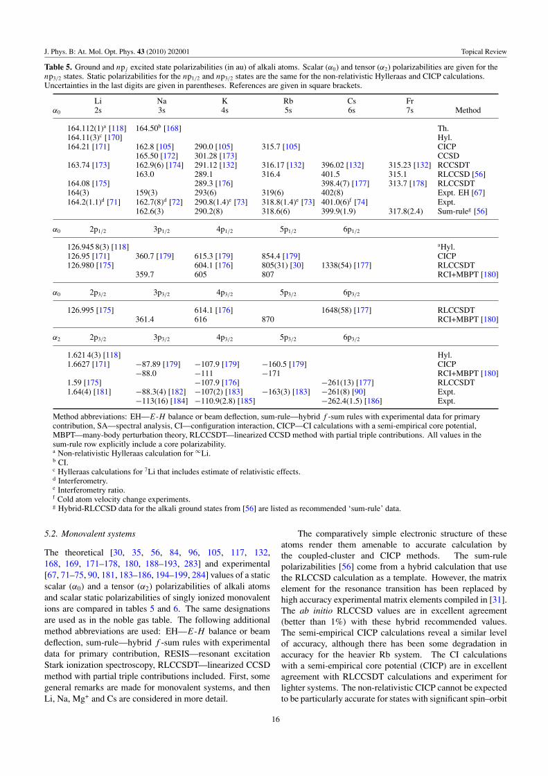
J. Phys. B: At. Mol. Opt. Phys. 43 (2010) 202001 Topical Review

Table 5. Ground and npj excited state polarizabilities (in au) of alkali atoms. Scalar (α0) and tensor (α2) polarizabilities are given for thenp3/2 states. Static polarizabilities for the np1/2 and np3/2 states are the same for the non-relativistic Hylleraas and CICP calculations.Uncertainties in the last digits are given in parentheses. References are given in square brackets.

Li Na K Rb Cs Frα0 2s 3s 4s 5s 6s 7s Method

164.112(1)a [118] 164.50b [168] Th.164.11(3)c [170] Hyl.164.21 [171] 162.8 [105] 290.0 [105] 315.7 [105] CICP

165.50 [172] 301.28 [173] CCSD163.74 [173] 162.9(6) [174] 291.12 [132] 316.17 [132] 396.02 [132] 315.23 [132] RCCSDT

163.0 289.1 316.4 401.5 315.1 RLCCSD [56]164.08 [175] 289.3 [176] 398.4(7) [177] 313.7 [178] RLCCSDT164(3) 159(3) 293(6) 319(6) 402(8) Expt. EH [67]164.2(1.1)d [71] 162.7(8)d [72] 290.8(1.4)e [73] 318.8(1.4)e [73] 401.0(6)f [74] Expt.

162.6(3) 290.2(8) 318.6(6) 399.9(1.9) 317.8(2.4) Sum-ruleg [56]

α0 2p1/2 3p1/2 4p1/2 5p1/2 6p1/2

126.945 8(3) [118] aHyl.126.95 [171] 360.7 [179] 615.3 [179] 854.4 [179] CICP126.980 [175] 604.1 [176] 805(31) [30] 1338(54) [177] RLCCSDT

359.7 605 807 RCI+MBPT [180]

α0 2p3/2 3p3/2 4p3/2 5p3/2 6p3/2

126.995 [175] 614.1 [176] 1648(58) [177] RLCCSDT361.4 616 870 RCI+MBPT [180]

α2 2p3/2 3p3/2 4p3/2 5p3/2 6p3/2

1.621 4(3) [118] Hyl.1.6627 [171] −87.89 [179] −107.9 [179] −160.5 [179] CICP

−88.0 −111 −171 RCI+MBPT [180]1.59 [175] −107.9 [176] −261(13) [177] RLCCSDT1.64(4) [181] −88.3(4) [182] −107(2) [183] −163(3) [183] −261(8) [90] Expt.

−113(16) [184] −110.9(2.8) [185] −262.4(1.5) [186] Expt.

Method abbreviations: EH—E-H balance or beam deflection, sum-rule—hybrid f -sum rules with experimental data for primarycontribution, SA—spectral analysis, CI—configuration interaction, CICP—CI calculations with a semi-empirical core potential,MBPT—many-body perturbation theory, RLCCSDT—linearized CCSD method with partial triple contributions. All values in thesum-rule row explicitly include a core polarizability.a Non-relativistic Hylleraas calculation for ∞Li.b CI.c Hylleraas calculations for 7Li that includes estimate of relativistic effects.d Interferometry.e Interferometry ratio.f Cold atom velocity change experiments.g Hybrid-RLCCSD data for the alkali ground states from [56] are listed as recommended ‘sum-rule’ data.

5.2. Monovalent systems

The theoretical [30, 35, 56, 84, 96, 105, 117, 132,168, 169, 171–178, 180, 188–193, 283] and experimental[67, 71–75, 90, 181, 183–186, 194–199, 284] values of a staticscalar (α0) and a tensor (α2) polarizabilities of alkali atomsand scalar static polarizabilities of singly ionized monovalentions are compared in tables 5 and 6. The same designationsare used as in the noble gas table. The following additionalmethod abbreviations are used: EH—E-H balance or beamdeflection, sum-rule—hybrid f -sum rules with experimentaldata for primary contribution, RESIS—resonant excitationStark ionization spectroscopy, RLCCSDT—linearized CCSDmethod with partial triple contributions included. First, somegeneral remarks are made for monovalent systems, and thenLi, Na, Mg+ and Cs are considered in more detail.

The comparatively simple electronic structure of theseatoms render them amenable to accurate calculation bythe coupled-cluster and CICP methods. The sum-rulepolarizabilities [56] come from a hybrid calculation that usethe RLCCSD calculation as a template. However, the matrixelement for the resonance transition has been replaced byhigh accuracy experimental matrix elements compiled in [31].The ab initio RLCCSD values are in excellent agreement(better than 1%) with these hybrid recommended values.The semi-empirical CICP calculations reveal a similar levelof accuracy, although there has been some degradation inaccuracy for the heavier Rb system. The CI calculationswith a semi-empirical core potential (CICP) are in excellentagreement with RLCCSDT calculations and experiment forlighter systems. The non-relativistic CICP cannot be expectedto be particularly accurate for states with significant spin–orbit

16

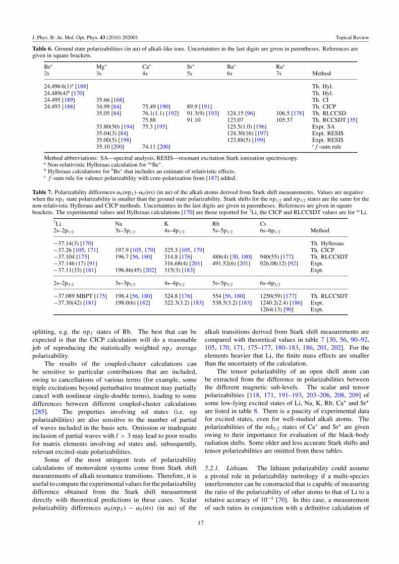
J. Phys. B: At. Mol. Opt. Phys. 43 (2010) 202001 Topical Review

Table 6. Ground state polarizabilities (in au) of alkali-like ions. Uncertainties in the last digits are given in parentheses. References aregiven in square brackets.

Be+ Mg+ Ca+ Sr+ Ba+ Ra+

2s 3s 4s 5s 6s 7s Method

24.496 6(1)a [188] Th. Hyl.24.489(4)b [170] Th. Hyl.24.495 [189] 35.66 [168] Th. CI24.493 [188] 34.99 [84] 75.49 [190] 89.9 [191] Th. CICP

35.05 [84] 76.1(1.1) [192] 91.3(9) [193] 124.15 [96] 106.5 [178] Th. RLCCSD75.88 91.10 123.07 105.37 Th. RCCSDT [35]

33.80(50) [194] 75.3 [195] 125.5(1.0) [196] Expt. SA35.04(3) [84] 124.30(16) [197] Expt. RESIS35.00(5) [198] 123.88(5) [199] Expt. RESIS35.10 [200] 74.11 [200] cf -sum rule

Method abbreviations: SA—spectral analysis, RESIS—resonant excitation Stark ionization spectroscopy.a Non-relativistic Hylleraas calculation for ∞Be+.b Hylleraas calculations for 9Be+ that includes an estimate of relativistic effects.c f -sum rule for valence polarizability with core-polarization from [187] added.

Table 7. Polarizability differences α0(npJ )–α0(ns) (in au) of the alkali atoms derived from Stark shift measurements. Values are negativewhen the npJ state polarizability is smaller than the ground state polarizability. Stark shifts for the np1/2 and np3/2 states are the same for thenon-relativistic Hylleraas and CICP methods. Uncertainties in the last digits are given in parentheses. References are given in squarebrackets. The experimental values and Hylleraas calculations [170] are those reported for 7Li, the CICP and RLCCSDT values are for ∞Li.

7Li Na K Rb Cs2s–2p1/2 3s–3p1/2 4s–4p1/2 5s–5p1/2 6s–6p1/2 Method

−37.14(3) [170] Th. Hylleraas−37.26 [105, 171] 197.9 [105, 179] 325.3 [105, 179] Th. CICP−37.104 [175] 196.7 [56, 180] 314.8 [176] 488(4) [30, 180] 940(55) [177] Th. RLCCSDT−37.146 (17) [91] 316.68(4) [201] 491.52(6) [201] 926.08(12) [92] Expt.−37.11(33) [181] 196.86(45) [202] 315(3) [183] Expt.

2s–2p3/2 3s–3p3/2 4s–4p3/2 5s–5p3/2 6s–6p3/2

−37.089 MBPT [175] 198.4 [56, 180] 324.8 [176] 554 [56, 180] 1250(59) [177] Th. RLCCSDT−37.30(42) [181] 198.0(6) [182] 322.3(3.2) [183] 538.5(3.2) [183] 1240.2(2.4) [186] Expt.

1264(13) [90] Expt.

splitting, e.g. the npJ states of Rb. The best that can beexpected is that the CICP calculation will do a reasonablejob of reproducing the statistically weighted npJ averagepolarizability.

The results of the coupled-cluster calculations canbe sensitive to particular contributions that are included,owing to cancellations of various terms (for example, sometriple excitations beyond perturbative treatment may partiallycancel with nonlinear single-double terms), leading to somedifferences between different coupled-cluster calculations[285]. The properties involving nd states (i.e. nppolarizabilities) are also sensitive to the number of partialof waves included in the basis sets. Omission or inadequateinclusion of partial waves with l > 3 may lead to poor resultsfor matrix elements involving nd states and, subsequently,relevant excited-state polarizabilities.

Some of the most stringent tests of polarizabilitycalculations of monovalent systems come from Stark shiftmeasurements of alkali resonance transitions. Therefore, it isuseful to compare the experimental values for the polarizabilitydifference obtained from the Stark shift measurementdirectly with theoretical predictions in these cases. Scalarpolarizability differences α0(npJ ) − α0(ns) (in au) of the

alkali transitions derived from Stark shift measurements arecompared with theoretical values in table 7 [30, 56, 90–92,105, 170, 171, 175–177, 180–183, 186, 201, 202]. For theelements heavier that Li, the finite mass effects are smallerthan the uncertainty of the calculation.

The tensor polarizability of an open shell atom canbe extracted from the difference in polarizabilities betweenthe different magnetic sub-levels. The scalar and tensorpolarizabilities [118, 171, 191–193, 203–206, 208, 209] ofsome low-lying excited states of Li, Na, K, Rb, Ca+ and Sr+

are listed in table 8. There is a paucity of experimental datafor excited states, even for well-studied alkali atoms. Thepolarizabilities of the nd5/2 states of Ca+ and Sr+ are givenowing to their importance for evaluation of the black-bodyradiation shifts. Some older and less accurate Stark shifts andtensor polarizabilities are omitted from these tables.

5.2.1. Lithium. The lithium polarizability could assumea pivotal role in polarizability metrology if a multi-speciesinterferometer can be constructed that is capable of measuringthe ratio of the polarizability of other atoms to that of Li to arelative accuracy of 10−4 [70]. In this case, a measurementof such ratios in conjunction with a definitive calculation of

17

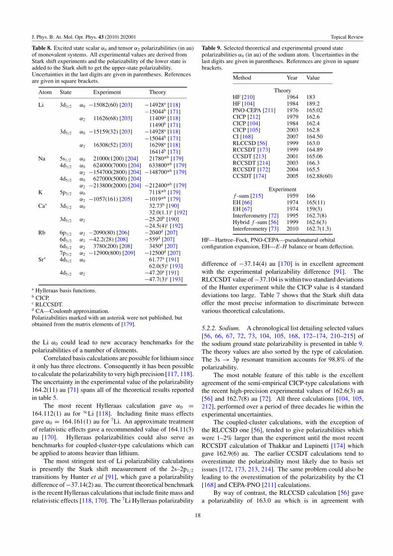
J. Phys. B: At. Mol. Opt. Phys. 43 (2010) 202001 Topical Review

Table 8. Excited state scalar α0 and tensor α2 polarizabilities (in au)of monovalent systems. All experimental values are derived fromStark shift experiments and the polarizability of the lower state isadded to the Stark shift to get the upper-state polarizability.Uncertainties in the last digits are given in parentheses. Referencesare given in square brackets.

Atom State Experiment Theory

Li 3d3/2 α0 −15082(60) [203] −14928a [118]−15044b [171]

α2 11626(68) [203] 11409a [118]11490b [171]

3d5/2 α0 −15159(32) [203] −14928a [118]−15044b [171]

α2 16308(52) [203] 16298a [118]16414b [171]

Na 5s1/2 α0 21000(1200) [204] 21780*b [179]4d3/2 α0 624000(7000) [204] 633800*b [179]

α2 −154700(2800) [204] −148700*b [179]4d5/2 α0 627000(5000) [204]

α2 −213800(2000) [204] −212400*b [179]K 5p3/2 α0 7118*b [179]

α2 −1057(161) [205] −1019*b [179]Ca+ 3d5/2 α0 32.73b [190]

32.0(1.1)c [192]3d5/2 α2 −25.20b [190]

−24.5(4)c [192]Rb 6p3/2 α2 −2090(80) [206] −2040d [207]

6d3/2 α2 −42.2(28) [208] −559d [207]6d5/2 α2 3780(200) [208] 3450d [207]7p3/2 α2 −12900(800) [209] −12500d [207]

Sr+ 4d5/2 α0 61.77a [191]62.0(5)c [193]

4d5/2 α2 −47.20a [191]−47.7(3)c [193]

a Hylleraas basis functions.b CICP.c RLCCSDT.d CA—Coulomb approximation.Polarizabilities marked with an asterisk were not published, butobtained from the matrix elements of [179].

the Li α0 could lead to new accuracy benchmarks for thepolarizabilities of a number of elements.

Correlated basis calculations are possible for lithium sinceit only has three electrons. Consequently it has been possibleto calculate the polarizability to very high precision [117, 118].The uncertainty in the experimental value of the polarizability164.2(11) au [71] spans all of the theoretical results reportedin table 5.

The most recent Hylleraas calculation gave α0 =164.112(1) au for ∞Li [118]. Including finite mass effectsgave α0 = 164.161(1) au for 7Li. An approximate treatmentof relativistic effects gave a recommended value of 164.11(3)au [170]. Hylleraas polarizabilities could also serve asbenchmarks for coupled-cluster-type calculations which canbe applied to atoms heavier than lithium.

The most stringent test of Li polarizability calculationsis presently the Stark shift measurement of the 2s–2p1/2

transitions by Hunter et al [91], which gave a polarizabilitydifference of −37.14(2) au. The current theoretical benchmarkis the recent Hylleraas calculations that include finite mass andrelativistic effects [118, 170]. The 7Li Hylleraas polarizability

Table 9. Selected theoretical and experimental ground statepolarizabilities α0 (in au) of the sodium atom. Uncertainties in thelast digits are given in parentheses. References are given in squarebrackets.

Method Year Value

TheoryHF [210] 1964 183HF [104] 1984 189.2PNO-CEPA [211] 1976 165.02CICP [212] 1979 162.6CICP [104] 1984 162.4CICP [105] 2003 162.8CI [168] 2007 164.50RLCCSD [56] 1999 163.0RCCSDT [173] 1999 164.89CCSDT [213] 2001 165.06RCCSDT [214] 2003 166.3RCCSDT [172] 2004 165.5CCSDT [174] 2005 162.88(60)

Experimentf -sum [215] 1959 166EH [66] 1974 165(11)EH [67] 1974 159(3)Interferometry [72] 1995 162.7(8)Hybrid f -sum [56] 1999 162.6(3)Interferometry [73] 2010 162.7(1.3)

HF—Hartree–Fock, PNO-CEPA—pseudonatural orbitalconfiguration expansion, EH—E-H balance or beam deflection.

difference of −37.14(4) au [170] is in excellent agreementwith the experimental polarizability difference [91]. TheRLCCSDT value of −37.104 is within two standard deviationsof the Hunter experiment while the CICP value is 4 standarddeviations too large. Table 7 shows that the Stark shift dataoffer the most precise information to discriminate betweenvarious theoretical calculations.

5.2.2. Sodium. A chronological list detailing selected values[56, 66, 67, 72, 73, 104, 105, 168, 172–174, 210–215] ofthe sodium ground state polarizability is presented in table 9.The theory values are also sorted by the type of calculation.The 3s → 3p resonant transition accounts for 98.8% of thepolarizability.

The most notable feature of this table is the excellentagreement of the semi-empirical CICP-type calculations withthe recent high-precision experimental values of 162.6(3) au[56] and 162.7(8) au [72]. All three calculations [104, 105,212], performed over a period of three decades lie within theexperimental uncertainties.

The coupled-cluster calculations, with the exception ofthe RLCCSD one [56], tended to give polarizabilities whichwere 1–2% larger than the experiment until the most recentRCCSDT calculation of Thakkar and Lupinetti [174] whichgave 162.9(6) au. The earlier CCSDT calculations tend tooverestimate the polarizability most likely due to basis setissues [172, 173, 213, 214]. The same problem could also beleading to the overestimation of the polarizability by the CI[168] and CEPA-PNO [211] calculations.

By way of contrast, the RLCCSD calculation [56] gavea polarizability of 163.0 au which is in agreement with

18

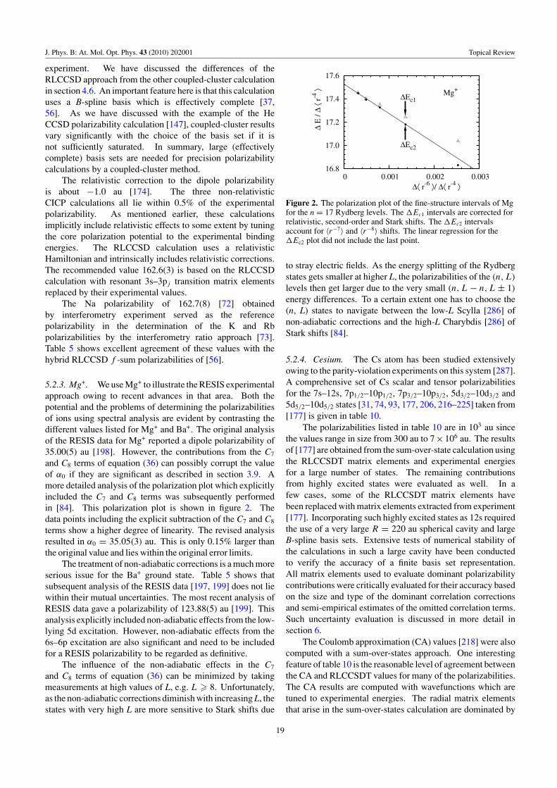
J. Phys. B: At. Mol. Opt. Phys. 43 (2010) 202001 Topical Review

experiment. We have discussed the differences of theRLCCSD approach from the other coupled-cluster calculationin section 4.6. An important feature here is that this calculationuses a B-spline basis which is effectively complete [37,56]. As we have discussed with the example of the HeCCSD polarizability calculation [147], coupled-cluster resultsvary significantly with the choice of the basis set if it isnot sufficiently saturated. In summary, large (effectivelycomplete) basis sets are needed for precision polarizabilitycalculations by a coupled-cluster method.

The relativistic correction to the dipole polarizabilityis about −1.0 au [174]. The three non-relativisticCICP calculations all lie within 0.5% of the experimentalpolarizability. As mentioned earlier, these calculationsimplicitly include relativistic effects to some extent by tuningthe core polarization potential to the experimental bindingenergies. The RLCCSD calculation uses a relativisticHamiltonian and intrinsically includes relativistic corrections.The recommended value 162.6(3) is based on the RLCCSDcalculation with resonant 3s–3pj transition matrix elementsreplaced by their experimental values.

The Na polarizability of 162.7(8) [72] obtainedby interferometry experiment served as the referencepolarizability in the determination of the K and Rbpolarizabilities by the interferometry ratio approach [73].Table 5 shows excellent agreement of these values with thehybrid RLCCSD f -sum polarizabilities of [56].

5.2.3. Mg+. We use Mg+ to illustrate the RESIS experimentalapproach owing to recent advances in that area. Both thepotential and the problems of determining the polarizabilitiesof ions using spectral analysis are evident by contrasting thedifferent values listed for Mg+ and Ba+. The original analysisof the RESIS data for Mg+ reported a dipole polarizability of35.00(5) au [198]. However, the contributions from the C7

and C8 terms of equation (36) can possibly corrupt the valueof α0 if they are significant as described in section 3.9. Amore detailed analysis of the polarization plot which explicitlyincluded the C7 and C8 terms was subsequently performedin [84]. This polarization plot is shown in figure 2. Thedata points including the explicit subtraction of the C7 and C8

terms show a higher degree of linearity. The revised analysisresulted in α0 = 35.05(3) au. This is only 0.15% larger thanthe original value and lies within the original error limits.

The treatment of non-adiabatic corrections is a much moreserious issue for the Ba+ ground state. Table 5 shows thatsubsequent analysis of the RESIS data [197, 199] does not liewithin their mutual uncertainties. The most recent analysis ofRESIS data gave a polarizability of 123.88(5) au [199]. Thisanalysis explicitly included non-adiabatic effects from the low-lying 5d excitation. However, non-adiabatic effects from the6s–6p excitation are also significant and need to be includedfor a RESIS polarizability to be regarded as definitive.

The influence of the non-adiabatic effects in the C7

and C8 terms of equation (36) can be minimized by takingmeasurements at high values of L, e.g. L � 8. Unfortunately,as the non-adiabatic corrections diminish with increasing L, thestates with very high L are more sensitive to Stark shifts due

16.8

17.0

17.2

17.4

17.6

0 0.001 0.002 0.003

Δ E

/ Δ

⟨ r-4

⟩

Δ⟨ r-6 ⟩/ Δ⟨ r-4 ⟩

ΔEc1

ΔEc2

Mg+

Figure 2. The polarization plot of the fine-structure intervals of Mgfor the n = 17 Rydberg levels. The �Ec1 intervals are corrected forrelativistic, second-order and Stark shifts. The �Ec2 intervalsaccount for 〈r−7〉 and 〈r−8〉 shifts. The linear regression for the�Ec2 plot did not include the last point.

to stray electric fields. As the energy splitting of the Rydbergstates gets smaller at higher L, the polarizabilities of the (n, L)

levels then get larger due to the very small (n, L − n,L ± 1)

energy differences. To a certain extent one has to choose the(n, L) states to navigate between the low-L Scylla [286] ofnon-adiabatic corrections and the high-L Charybdis [286] ofStark shifts [84].

5.2.4. Cesium. The Cs atom has been studied extensivelyowing to the parity-violation experiments on this system [287].A comprehensive set of Cs scalar and tensor polarizabilitiesfor the 7s–12s, 7p1/2–10p1/2, 7p3/2–10p3/2, 5d3/2–10d3/2 and5d5/2–10d5/2 states [31, 74, 93, 177, 206, 216–225] taken from[177] is given in table 10.

The polarizabilities listed in table 10 are in 103 au sincethe values range in size from 300 au to 7 × 106 au. The resultsof [177] are obtained from the sum-over-state calculation usingthe RLCCSDT matrix elements and experimental energiesfor a large number of states. The remaining contributionsfrom highly excited states were evaluated as well. In afew cases, some of the RLCCSDT matrix elements havebeen replaced with matrix elements extracted from experiment[177]. Incorporating such highly excited states as 12s requiredthe use of a very large R = 220 au spherical cavity and largeB-spline basis sets. Extensive tests of numerical stability ofthe calculations in such a large cavity have been conductedto verify the accuracy of a finite basis set representation.All matrix elements used to evaluate dominant polarizabilitycontributions were critically evaluated for their accuracy basedon the size and type of the dominant correlation correctionsand semi-empirical estimates of the omitted correlation terms.Such uncertainty evaluation is discussed in more detail insection 6.

The Coulomb approximation (CA) values [218] were alsocomputed with a sum-over-states approach. One interestingfeature of table 10 is the reasonable level of agreement betweenthe CA and RLCCSDT values for many of the polarizabilities.The CA results are computed with wavefunctions which aretuned to experimental energies. The radial matrix elementsthat arise in the sum-over-states calculation are dominated by

19

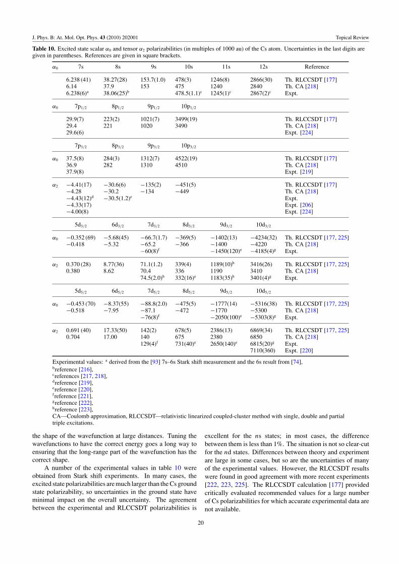
J. Phys. B: At. Mol. Opt. Phys. 43 (2010) 202001 Topical Review

Table 10. Excited state scalar α0 and tensor α2 polarizabilities (in multiples of 1000 au) of the Cs atom. Uncertainties in the last digits aregiven in parentheses. References are given in square brackets.

α0 7s 8s 9s 10s 11s 12s Reference

6.238 (41) 38.27(28) 153.7(1.0) 478(3) 1246(8) 2866(30) Th. RLCCSDT [177]6.14 37.9 153 475 1240 2840 Th. CA [218]6.238(6)a 38.06(25)b 478.5(1.1)c 1245(1)c 2867(2)c Expt.

α0 7p1/2 8p1/2 9p1/2 10p1/2

29.9(7) 223(2) 1021(7) 3499(19) Th. RLCCSDT [177]29.4 221 1020 3490 Th. CA [218]29.6(6) Expt. [224]

7p3/2 8p3/2 9p3/2 10p3/2

α0 37.5(8) 284(3) 1312(7) 4522(19) Th. RLCCSDT [177]36.9 282 1310 4510 Th. CA [218]37.9(8) Expt. [219]

α2 −4.41(17) −30.6(6) −135(2) −451(5) Th. RLCCSDT [177]−4.28 −30.2 −134 −449 Th. CA [218]−4.43(12)d −30.5(1.2)e Expt.−4.33(17) Expt. [206]−4.00(8) Expt. [224]

5d3/2 6d3/2 7d3/2 8d3/2 9d3/2 10d3/2

α0 −0.352 (69) −5.68(45) −66.7(1.7) −369(5) −1402(13) −4234(32) Th. RLCCSDT [177, 225]−0.418 −5.32 −65.2 −366 −1400 −4220 Th. CA [218]

−60(8)f −1450(120)e −4185(4)g Expt.

α2 0.370 (28) 8.77(36) 71.1(1.2) 339(4) 1189(10)h 3416(26) Th. RLCCSDT [177, 225]0.380 8.62 70.4 336 1190 3410 Th. CA [218]

74.5(2.0)h 332(16)e 1183(35)h 3401(4)g Expt.

5d5/2 6d5/2 7d5/2 8d5/2 9d5/2 10d5/2

α0 −0.453 (70) −8.37(55) −88.8(2.0) −475(5) −1777(14) −5316(38) Th. RLCCSDT [177, 225]−0.518 −7.95 −87.1 −472 −1770 −5300 Th. CA [218]

−76(8)f −2050(100)e −5303(8)g Expt.

α2 0.691 (40) 17.33(50) 142(2) 678(5) 2386(13) 6869(34) Th. RLCCSDT [177, 225]0.704 17.00 140 675 2380 6850 Th. CA [218]

129(4)f 731(40)e 2650(140)e 6815(20)g Expt.7110(360) Expt. [220]

Experimental values: a derived from the [93] 7s–6s Stark shift measurement and the 6s result from [74],breference [216],creferences [217, 218],dreference [219],ereference [220],freference [221],greference [222],hreference [223],CA—Coulomb approximation, RLCCSDT—relativistic linearized coupled-cluster method with single, double and partialtriple excitations.

the shape of the wavefunction at large distances. Tuning thewavefunctions to have the correct energy goes a long way toensuring that the long-range part of the wavefunction has thecorrect shape.

A number of the experimental values in table 10 wereobtained from Stark shift experiments. In many cases, theexcited state polarizabilities are much larger than the Cs groundstate polarizability, so uncertainties in the ground state haveminimal impact on the overall uncertainty. The agreementbetween the experimental and RLCCSDT polarizabilities is

excellent for the ns states; in most cases, the differencebetween them is less than 1%. The situation is not so clear-cutfor the nd states. Differences between theory and experimentare large in some cases, but so are the uncertainties of manyof the experimental values. However, the RLCCSDT resultswere found in good agreement with more recent experiments[222, 223, 225]. The RLCCSDT calculation [177] providedcritically evaluated recommended values for a large numberof Cs polarizabilities for which accurate experimental data arenot available.

20

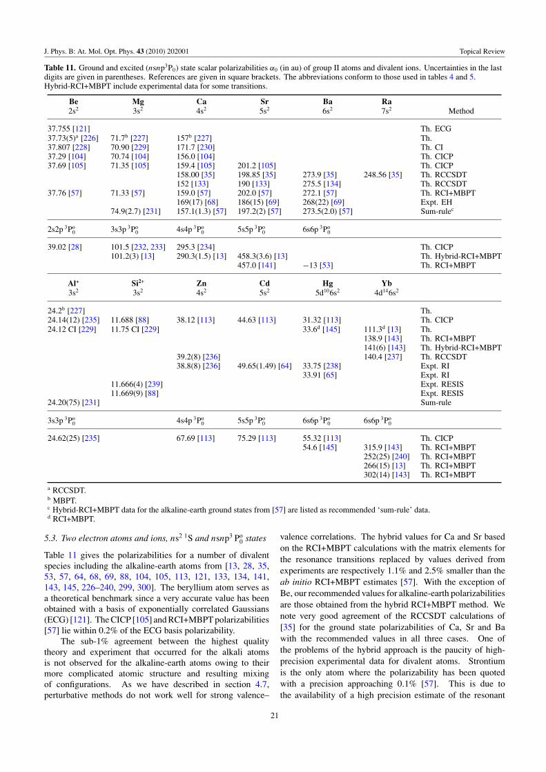
J. Phys. B: At. Mol. Opt. Phys. 43 (2010) 202001 Topical Review

Table 11. Ground and excited (nsnp3P0) state scalar polarizabilities α0 (in au) of group II atoms and divalent ions. Uncertainties in the lastdigits are given in parentheses. References are given in square brackets. The abbreviations conform to those used in tables 4 and 5.Hybrid-RCI+MBPT include experimental data for some transitions.

Be Mg Ca Sr Ba Ra

2s2 3s2 4s2 5s2 6s2 7s2 Method

37.755 [121] Th. ECG37.73(5)a [226] 71.7b [227] 157b [227] Th.37.807 [228] 70.90 [229] 171.7 [230] Th. CI37.29 [104] 70.74 [104] 156.0 [104] Th. CICP37.69 [105] 71.35 [105] 159.4 [105] 201.2 [105] Th. CICP

158.00 [35] 198.85 [35] 273.9 [35] 248.56 [35] Th. RCCSDT152 [133] 190 [133] 275.5 [134] Th. RCCSDT

37.76 [57] 71.33 [57] 159.0 [57] 202.0 [57] 272.1 [57] Th. RCI+MBPT169(17) [68] 186(15) [69] 268(22) [69] Expt. EH

74.9(2.7) [231] 157.1(1.3) [57] 197.2(2) [57] 273.5(2.0) [57] Sum-rulec

2s2p 3Po0 3s3p 3Po

0 4s4p 3Po0 5s5p 3Po

0 6s6p 3Po0

39.02 [28] 101.5 [232, 233] 295.3 [234] Th. CICP101.2(3) [13] 290.3(1.5) [13] 458.3(3.6) [13] Th. Hybrid-RCI+MBPT

457.0 [141] −13 [53] Th. RCI+MBPT

Al+ Si2+ Zn Cd Hg Yb

3s2 3s2 4s2 5s2 5d106s2 4d146s2

24.2b [227] Th.24.14(12) [235] 11.688 [88] 38.12 [113] 44.63 [113] 31.32 [113] Th. CICP24.12 CI [229] 11.75 CI [229] 33.6d [145] 111.3d [13] Th.

138.9 [143] Th. RCI+MBPT141(6) [143] Th. Hybrid-RCI+MBPT

39.2(8) [236] 140.4 [237] Th. RCCSDT38.8(8) [236] 49.65(1.49) [64] 33.75 [238] Expt. RI

33.91 [65] Expt. RI11.666(4) [239] Expt. RESIS11.669(9) [88] Expt. RESIS

24.20(75) [231] Sum-rule

3s3p 3Po0 4s4p 3Po

0 5s5p 3Po0 6s6p 3Po

0 6s6p 3Po0

24.62(25) [235] 67.69 [113] 75.29 [113] 55.32 [113] Th. CICP54.6 [145] 315.9 [143] Th. RCI+MBPT

252(25) [240] Th. RCI+MBPT266(15) [13] Th. RCI+MBPT302(14) [143] Th. RCI+MBPT

a RCCSDT.b MBPT.c Hybrid-RCI+MBPT data for the alkaline-earth ground states from [57] are listed as recommended ‘sum-rule’ data.d RCI+MBPT.

5.3. Two electron atoms and ions, ns2 1S and nsnp3 Po0 states

Table 11 gives the polarizabilities for a number of divalentspecies including the alkaline-earth atoms from [13, 28, 35,53, 57, 64, 68, 69, 88, 104, 105, 113, 121, 133, 134, 141,143, 145, 226–240, 299, 300]. The beryllium atom serves asa theoretical benchmark since a very accurate value has beenobtained with a basis of exponentially correlated Gaussians(ECG) [121]. The CICP [105] and RCI+MBPT polarizabilities[57] lie within 0.2% of the ECG basis polarizability.

The sub-1% agreement between the highest qualitytheory and experiment that occurred for the alkali atomsis not observed for the alkaline-earth atoms owing to theirmore complicated atomic structure and resulting mixingof configurations. As we have described in section 4.7,perturbative methods do not work well for strong valence–

valence correlations. The hybrid values for Ca and Sr basedon the RCI+MBPT calculations with the matrix elements forthe resonance transitions replaced by values derived fromexperiments are respectively 1.1% and 2.5% smaller than theab initio RCI+MBPT estimates [57]. With the exception ofBe, our recommended values for alkaline-earth polarizabilitiesare those obtained from the hybrid RCI+MBPT method. Wenote very good agreement of the RCCSDT calculations of[35] for the ground state polarizabilities of Ca, Sr and Bawith the recommended values in all three cases. One ofthe problems of the hybrid approach is the paucity of high-precision experimental data for divalent atoms. Strontiumis the only atom where the polarizability has been quotedwith a precision approaching 0.1% [57]. This is due tothe availability of a high precision estimate of the resonant

21

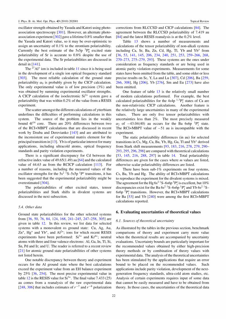
J. Phys. B: At. Mol. Opt. Phys. 43 (2010) 202001 Topical Review

oscillator strength obtained by Yasuda and Katori using photo-association spectroscopy [301]. However, an alternate photo-association experiment [302] gave a lifetime 0.8% smaller thanthe Yasuda and Katori value, so it may be over-optimistic toassign an uncertainty of 0.1% to the strontium polarizability.Currently the best estimate of the 5s5p 3Po

0 excited statepolarizability of Sr is accurate to 0.8% despite the use ofthe experimental data. The Sr polarizabilities are discussed indetail in [141].

The 27Al+ ion is included in table 11 since it is being usedin the development of a single ion optical frequency standard[303]. The most reliable calculation of the ground statepolarizability α0 is probably given by the CICP calculation.The only experimental value is of low precision (3%) andwas obtained by summing experimental oscillator strengths.A CICP calculation of the isoelectronic Si2+ system gave apolarizability that was within 0.2% of the value from a RESISexperiment.

The scatter amongst the different calculations of ytterbiumunderlines the difficulties of performing calculations in thissystem. The source of the problem lies in the weaklybound 4f14 core. There are 20% differences between twoof the RCI+MBPT calculations that are discussed in recentwork by Dzuba and Derevianko [143] and are attributed tothe inconsistent use of experimental matrix element for theprincipal transition in [13]. Yb is of particular interest for manyapplications, including ultracold atoms, optical frequencystandards and parity violation experiments.

There is a significant discrepancy for Cd between therefractive index value of 49.65(1.49) au [64] and the calculatedvalue of 44.63 au from the RCICP calculation [113]. Fora number of reasons, including the measured values of theoscillator strengths for the 5s2 1S–5s5p 1Po transitions, it hasbeen suggested that the experimental polarizability might beoverestimated [304].

The polarizabilities of other excited states, tensorpolarizabilities and Stark shifts in divalent systems arediscussed in the next subsection.

5.4. Other data

Ground state polarizabilities for the other selected systemsfrom [36, 50, 76, 84, 124, 168, 241–245, 247–258, 305] aregiven in table 12. In this review, we list data for selectedsystems with a monovalent ns ground state: Cu, Ag, Au,Zn+, Hg+ and Yb+, and Al2+; ions for which recent RESISexperiments have been performed: Si3+ and Kr6+; neutralatoms with three and four valence electrons: Al, Ga, In, Tl, Si,Sn, Pd and Ir; and U. The reader is referred to a recent review[21] for atomic ground state polarizabilities of other systemsnot listed herein.

One notable discrepancy between theory and experimentoccurs for the Al ground state where the best calculationsexceed the experiment value from an EH balance experimentby 25% [36, 254]. The most precise experimental value intable 12 is the RESIS value for Si3+. The final value 7.433 (25)au comes from a reanalysis of the raw experimental data[248, 306] that includes estimates of r−7 and r−8 polarization

corrections from RLCCSD and CICP calculations [84]. Theagreement between the RLCCSD polarizability of 7.419 au[84] and the latest RESIS reanalysis is at the 0.2% level.

Table 13 shows a number of measurements andcalculations of the tensor polarizability of non-alkali systemsincluding Ca, Sr, Ba, Zn, Cd, Hg, Tl, Yb and Yb+ from[36, 53, 141, 145, 206, 234, 240, 251, 253, 259–266, 268,270–273, 275–279, 293]. These systems are the ones underconsideration as frequency standards or are being used inatomic parity violation experiments. Measurements for somestates have been omitted from the table, and some older or lessprecise results on Sc, Y, La and Lu [307], Cd [206], Ba [259,266, 308], Hg [206], Yb [276], Sm and Eu [273] have alsobeen omitted.

One feature of table 13 is the relatively small numberof modern calculations performed. For example, the bestcalculated polarizabilities for the 4s4p 1,3Po

1 states of Ca arethe non-relativistic CICP calculations. Another feature isthe relatively large uncertainties in many of the experimentalvalues. There are only five tensor polarizabilities withuncertainties less than 2%. The most precisely measuredα2 of −43.04(40) au occurs for the Ba 6s6p 1Po

1 state.The RCI+MBPT value of −51 au is incompatible with theexperiment.

The static polarizability differences (in au) for selectedtransitions in Cs, Mg, Ca, Ba, Yb, Hg, Ga, Tl and Yb+ derivedfrom Stark shift measurements [93, 183, 216, 278, 279, 290–293, 295, 296, 298] are compared with theoretical calculations[53, 145, 216, 288, 297] in table 14. Total polarizabilitydifferences are given for the cases where m values are listed,otherwise scalar polarizability differences are listed.

There have been sub-1% experiments on four systems,Cs, Ba, Yb and Hg. The ability of RCI+MBPT calculationsto reproduce the experiment for the divalent systems is mixed.The agreement for the Hg 6s2 1S–6s6p 3Po

1 is excellent, but 10%discrepancies exist for the Ba 6s2 1S–6s6p 1Po

1 and Yb 6s2 1S–6s6p 3Po

1 transitions. However, the RCI+MBPT calculationsfor Ba [53] and Yb [240] were among the first RCI+MBPTcalculations reported.

6. Evaluating uncertainties of theoretical values

6.1. Sources of theoretical uncertainty

As illustrated by the tables in the previous section, benchmarkcomparisons of theory and experiment carry more valuewhen the theoretical results are accompanied by uncertaintyevaluations. Uncertainty bounds are particularly important forthe recommended values obtained by either high-precisiontheory methods or by combination of theory values withexperimental data. The analysis of the theoretical uncertaintieshas been stimulated by the applications that require an errorbound to be placed on the recommended values. Suchapplications include parity violation, development of the next-generation frequency standards, ultra-cold atom studies, etc.Analysis of certain experiments requires input of some datathat cannot be easily measured and have to be obtained fromtheory. In those cases, the uncertainties of the theoretical data

22

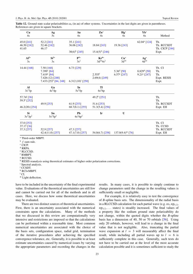
J. Phys. B: At. Mol. Opt. Phys. 43 (2010) 202001 Topical Review

Table 12. Ground state scalar polarizabilities α0 (in au) of other systems. Uncertainties in the last digits are given in parentheses.References are given in square brackets.

Cu Ag Au Zn+ Hg+ Yb+

4s 5s 6s 4s 6s 6s Method

45.0 [241] 52.2 [241] 35.1 [241] 62.04a [124] Th.46.50 [242] 52.46 [242] 36.06 [242] 18.84 [243] 19.36 [243] Th. RCCSDT41.65 46.17 Th. CICP [244]

30(4)b [245] 15.4(5)b [246] Expt.

Al2+ Si3+ P3+ Kr6+ Cu+ Ag+

3s 3s 3s2 3d104s2 3d10 4d10

14.44 [168] 7.50 [168] 6.73 [229] Th. CI7.399c [84] 5.36d [50] 8.829d [50] Th.7.419e [84] 2.555f 6.57g [247] 9.21g [247] Th.7.426 (12) [248] 2.69(4) [249] Expt. RESIS7.433 (25)h [84, 248] 6.312 (10)i [250] Expt.

Al Ga In Tl

3s23p 4s24p 5s25p 6s26p

57.74j [36] 49.2k [251] Th.59.5l [252] Th.

49.9 [253] 61.9 [253] 51.6 [253] Th. RCCSDT46.2(20) [254] 68.7(8.1) [255] 51.3(5.4) [256] Expt. EH

Si Sn Pb Ir U

3s23p2 5s25p2 6s26p2

37.0 [252] Th. CI37.17 [36] Th. CCSD37.3 [257] 52.9 [257] 47.3 [257] Th. RCCSDT

42.4(11.0) [257] 47.1(7.0) [257] 54.0(6.7) [258] 137.0(9.4)m [76] Expt. EH

a Third-order MBPT.b f -sum rule.c CICP.d RRPA.e RLCCSD.f RMBPT.g RCCSD.h RESIS reanalysis using theoretical estimates of higher order polarization corrections.i Spectral analysis.j CCSDT.k RCI+MBPT.l CI.m Light deflection.

have to be included in the uncertainty of the final experimentalvalue. Evaluations of the theoretical uncertainties are still fewand cannot be carried out for all of the methods and in allcases. Here, we discuss how some theoretical uncertaintiesmay be evaluated.

There are two distinct sources of theoretical uncertainties.First, there is an uncertainty associated with the numericalconstraints upon the calculations. Many of the methodsthat we discussed in this review are computationally veryintensive and restrictions are imposed so that the calculationscan be performed within a reasonable time. Most commonnumerical uncertainties are associated with the choice ofthe basis sets, configuration space, radial grid, terminationof the iterative procedures after achieving the specifiedconvergence tolerance, etc. Generally, it is possible to at leastestimate uncertainties caused by numerical issues by varyingthe appropriate parameters and recording the changes in the

results. In many cases, it is possible to simply continue tochange parameters until the change in the resulting values issufficiently small or negligible.

For example, it is relatively easy to test the convergenceof B-spline basis sets. The dimensionality of the radial basisin a RLCCSD calculation for each partial wave (e.g. ns, np1/2,np3/2, . . . states) is steadily increased. The final values ofa property like the sodium ground state polarizability donot change, within the quoted digits whether the B-splinebasis has a dimension of 40, 50 or 70 orbitals [56]. Usingonly 20 orbitals, however, will lead to a change in the finalvalue that is not negligible. Also, truncating the partialwave expansion at l = 3 will measurably affect the finalresult, while including all partial waves up to l = 6 issufficiently complete in this case. Generally, such tests donot have to be carried out at the level of the most accuratecalculation possible and it is sometimes sufficient to study the

23

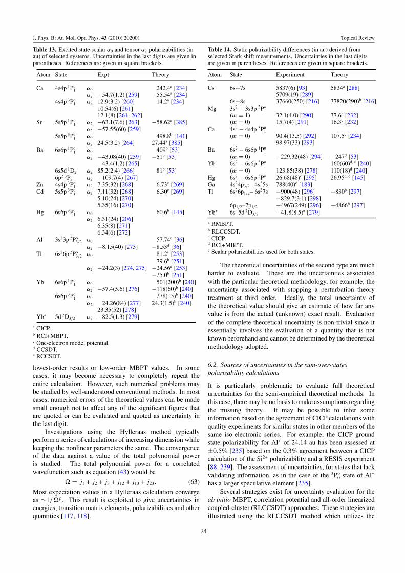
J. Phys. B: At. Mol. Opt. Phys. 43 (2010) 202001 Topical Review

Table 13. Excited state scalar α0 and tensor α2 polarizabilities (inau) of selected systems. Uncertainties in the last digits are given inparentheses. References are given in square brackets.

Atom State Expt. Theory

Ca 4s4p 1Po1 α0 242.4a [234]

α2 −54.7(1.2) [259] −55.54a [234]4s4p 3Po

1 α2 12.9(3.2) [260] 14.2a [234]10.54(6) [261]12.1(8) [261, 262]

Sr 5s5p 1Po1 α2 −63.1(7.6) [263] −58.62a [385]

α2 −57.55(60) [259]5s5p 3Po

1 α0 498.8b [141]α2 24.5(3.2) [264] 27.44a [385]

Ba 6s6p 1Po1 α0 409b [53]

α2 −43.08(40) [259] −51b [53]−43.4(1.2) [265]

6s5d 1D2 α2 85.2(2.4) [266] 81b [53]6p2 3P2 α2 −109.7(4) [267]

Zn 4s4p 3Po1 α2 7.35(32) [268] 6.73c [269]

Cd 5s5p 3Po1 α2 7.11(32) [268] 6.30c [269]

5.10(24) [270]5.35(16) [270]

Hg 6s6p 3Po1 α0 60.6b [145]

α2 6.31(24) [206]6.35(8) [271]6.34(6) [272]

Al 3s23p 2Po3/2 α0 57.74d [36]

α2 −8.15(40) [273] −8.53d [36]Tl 6s26p 2Po

3/2 α0 81.2e [253]79.6b [251]

α2 −24.2(3) [274, 275] −24.56e [253]−25.0b [251]

Yb 6s6p 1Po1 α0 501(200)b [240]

α2 −57.4(5.6) [276] −118(60)b [240]6s6p 3Po

1 α0 278(15)b [240]α2 24.26(84) [277] 24.3(1.5)b [240]

23.35(52) [278]Yb+ 5d 2D3/2 α2 −82.5(1.3) [279]

a CICP.b RCI+MBPT.c One-electron model potential.d CCSDT.e RCCSDT.

lowest-order results or low-order MBPT values. In somecases, it may become necessary to completely repeat theentire calculation. However, such numerical problems maybe studied by well-understood conventional methods. In mostcases, numerical errors of the theoretical values can be madesmall enough not to affect any of the significant figures thatare quoted or can be evaluated and quoted as uncertainty inthe last digit.

Investigations using the Hylleraas method typicallyperform a series of calculations of increasing dimension whilekeeping the nonlinear parameters the same. The convergenceof the data against a value of the total polynomial poweris studied. The total polynomial power for a correlatedwavefunction such as equation (43) would be

� = j1 + j2 + j3 + j12 + j13 + j23. (63)

Most expectation values in a Hylleraas calculation convergeas ∼1/�p. This result is exploited to give uncertainties inenergies, transition matrix elements, polarizabilities and otherquantities [117, 118].

Table 14. Static polarizability differences (in au) derived fromselected Stark shift measurements. Uncertainties in the last digitsare given in parentheses. References are given in square brackets.

Atom State Experiment Theory

Cs 6s−7s 5837(6) [93] 5834a [288]5709(19) [289]

6s−8s 37660(250) [216] 37820(290)b [216]Mg 3s2 − 3s3p 3Po

1(m = 1) 32.1(4.0) [290] 37.6c [232](m = 0) 15.7(4) [291] 16.3c [232]

Ca 4s2 − 4s4p 3Po1

(m = 0) 90.4(13.5) [292] 107.5c [234]98.97(33) [293]

Ba 6s2 − 6s6p 1Po1

(m = 0) −229.32(48) [294] −247d [53]Yb 6s2 − 6s6p 3Po

1 160(60)d, e [240](m = 0) 123.85(38) [278] 110(18)d [240]

Hg 6s2 − 6s6p 3Po1 26.68(48)e [295] 26.95d, e [145]

Ga 4s24p3/2– 4s25s 788(40)e [183]Tl 6s26p1/2– 6s27s −900(48) [296] −830b [297]

−829.7(3.1) [298]6p1/2–7p1/2 −4967(249) [296] −4866b [297]

Yb+ 6s–5d 2D3/2 −41.8(8.5)e [279]

a RMBPT.b RLCCSDT.c CICP.d RCI+MBPT.e Scalar polarizabilities used for both states.

The theoretical uncertainties of the second type are muchharder to evaluate. These are the uncertainties associatedwith the particular theoretical methodology, for example, theuncertainty associated with stopping a perturbation theorytreatment at third order. Ideally, the total uncertainty ofthe theoretical value should give an estimate of how far anyvalue is from the actual (unknown) exact result. Evaluationof the complete theoretical uncertainty is non-trivial since itessentially involves the evaluation of a quantity that is notknown beforehand and cannot be determined by the theoreticalmethodology adopted.

6.2. Sources of uncertainties in the sum-over-statespolarizability calculations

It is particularly problematic to evaluate full theoreticaluncertainties for the semi-empirical theoretical methods. Inthis case, there may be no basis to make assumptions regardingthe missing theory. It may be possible to infer someinformation based on the agreement of CICP calculations withquality experiments for similar states in other members of thesame iso-electronic series. For example, the CICP groundstate polarizability for Al+ of 24.14 au has been assessed at±0.5% [235] based on the 0.3% agreement between a CICPcalculation of the Si2+ polarizability and a RESIS experiment[88, 239]. The assessment of uncertainties, for states that lackvalidating information, as in the case of the 3Po

0 state of Al+

has a larger speculative element [235].Several strategies exist for uncertainty evaluation for the

ab initio MBPT, correlation potential and all-order linearizedcoupled-cluster (RLCCSDT) approaches. These strategies areillustrated using the RLCCSDT method which utilizes the

24

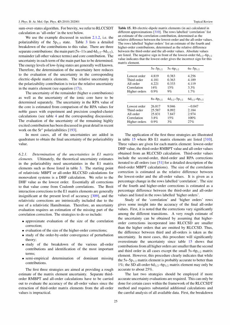
J. Phys. B: At. Mol. Opt. Phys. 43 (2010) 202001 Topical Review

sum-over-states algorithm. For brevity, we refer to RLCCSDTcalculation as ‘all-order’ in the text below.

We use the example discussed in section 2.1.2, i.e. thepolarizability of the 5p1/2 state. Table 3 lists a detailedbreakdown of the contributions to this value. There are threeseparate contributions: the main part (5s–11s and 4d3/2–9d3/2),remainder (all other valence terms) and core contribution. Theuncertainty in each term of the main part has to be determined.The energy levels of low-lying states are generally well known.Therefore, the determination of the uncertainty here reducesto the evaluation of the uncertainty in the correspondingelectric-dipole matrix elements. The relative uncertainty inthe polarizability contribution is twice the relative uncertaintyin the matrix element (see equation (17)).

The uncertainty of the remainder (higher n contributions)as well as the uncertainty of the ionic core have to bedetermined separately. The uncertainty in the RPA value ofthe core is estimated from comparison of the RPA values fornoble gases with experiment and precision coupled-clustercalculations (see table 4 and the corresponding discussion).The evaluation of the uncertainty of the remaining highlyexcited contribution has been discussed in great detail in recentwork on the Sr+ polarizabilities [193].

In most cases, all of the uncertainties are added inquadrature to obtain the final uncertainty of the polarizabilityvalue.

6.2.1. Determination of the uncertainties in E1 matrixelements. Ultimately, the theoretical uncertainty estimatesin the polarizability need uncertainties in the E1 matrixelements such as those listed in table 3. The starting pointof relativistic MBPT or all-order RLCCSD calculations formonovalent systems is a DHF calculation. We refer to theDHF value as the lowest order. Essentially all correctionsto that value come from Coulomb correlations. The Breitinteraction corrections to the E1 matrix elements are generallyinsignificant at the present level of accuracy [309], and therelativistic corrections are intrinsically included due to theuse of a relativistic Hamiltonian. Therefore, an uncertaintyevaluation requires an estimation of the missing part of thecorrelation correction. The strategies to do so include:

• approximate evaluation of the size of the correlationcorrection;

• evaluation of the size of the higher-order corrections;• study of the order-by-order convergence of perturbation

theory;• study of the breakdown of the various all-order

contributions and identification of the most importantterms;

• semi-empirical determination of dominant missingcontributions.

The first three strategies are aimed at providing a roughestimate of the matrix element uncertainty. Separate third-order RMBPT and all-order calculations have to be carriedout to evaluate the accuracy of the all-order values since theextraction of third-order matrix elements from the all-ordervalues is impractical.

Table 15. Rb electric-dipole matrix elements (in au) calculated indifferent approximations [310]. The rows labelled ‘correlation’ listan estimate of the correlation contribution, determined as therelative difference between the lowest-order and the all-order values.The rows labelled ‘higher orders’ list an estimate of the fourth andhigher-order contributions, determined as the relative differencebetween the third-order and the all-order values. Absolute valuesare listed. The negative sign in front of the lowest-order 6d3/2–6p1/2

value indicates that the lowest order gives the incorrect sign for thismatrix element.

5s–5p1/2 5s–6p1/2 6s–5p1/2

Lowest order 4.819 0.383 4.256Third order 4.181 0.363 4.189All order 4.221 0.333 4.119Correlation 14% 15% 3.3%Higher orders 0.9% 9% 1.7%

8s–8p1/2 4d3/2–5p1/2 6d3/2–6p1/2

Lowest order 26.817 9.046 −0.047Third order 25.587 8.092 2.184All order 25.831 7.847 2.974Correlation 3.8% 15% 100%Higher orders 0.9% 3% 27%

The application of the first three strategies are illustratedin table 15 where Rb E1 matrix elements are listed [310].Three values are given for each matrix element: lowest-orderDHF value, the third-order RMBPT value and all-order valuesobtained from an RLCCSD calculation. Third-order valuesinclude the second-order, third-order and RPA correctionsiterated to all orders (see [51] for a detailed description of thethird-order MBPT calculations). The size of the correlationcorrection is estimated as the relative difference betweenthe lowest-order and the all-order values. It is given as apercentage change in the rows labelled ‘correlation’. The sizeof the fourth and higher-order corrections is estimated as apercentage difference between the third-order and all-ordervalues and listed in the rows labelled ‘higher orders’.

Study of the ‘correlation’ and ‘higher orders’ rowsgives some insight into the accuracy of the final all-ordervalues. First, it is noted that the corrections vary significantlyamong the different transitions. A very rough estimate ofthe uncertainty can be obtained by assuming that higher-order corrections incorporated into RLCCSD are smallerthan the higher orders that are omitted by RLCCSD. Thus,the difference between third and all-orders is taken as theuncertainty. In most cases, this procedure will significantlyoverestimate the uncertainty since table 15 shows thatcontributions from all higher orders are smaller than the secondand third order in all cases except the small 5s–6p1/2 matrixelement. However, this procedure clearly indicates that whilethe 5s–5p1/2 matrix element is probably accurate to better than1%; the SD all-order 6d3/2–6p3/2 matrix element may only beaccurate to about 25%.

The last two strategies should be employed if moreaccurate uncertainty evaluations are required. This can only bedone for certain cases within the framework of the RLCCSDTmethod and requires substantial additional calculations andthe careful analysis of all available data. First, the breakdown

25

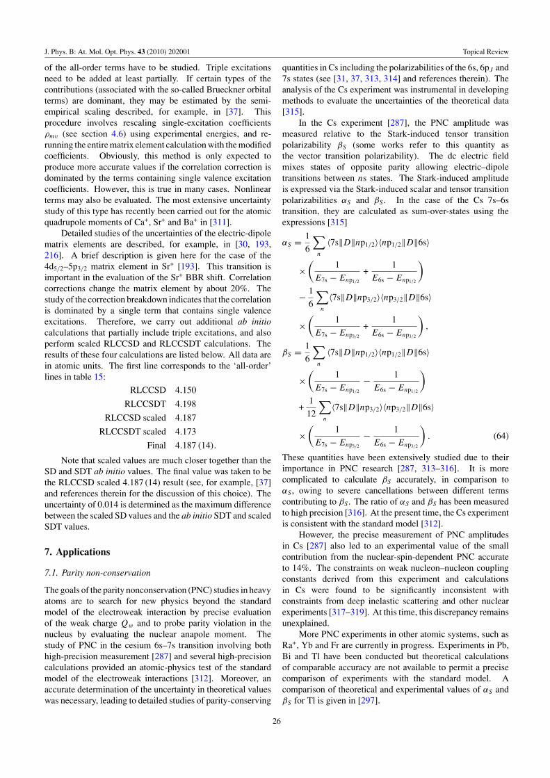
J. Phys. B: At. Mol. Opt. Phys. 43 (2010) 202001 Topical Review

of the all-order terms have to be studied. Triple excitationsneed to be added at least partially. If certain types of thecontributions (associated with the so-called Brueckner orbitalterms) are dominant, they may be estimated by the semi-empirical scaling described, for example, in [37]. Thisprocedure involves rescaling single-excitation coefficientsρmv (see section 4.6) using experimental energies, and re-running the entire matrix element calculation with the modifiedcoefficients. Obviously, this method is only expected toproduce more accurate values if the correlation correction isdominated by the terms containing single valence excitationcoefficients. However, this is true in many cases. Nonlinearterms may also be evaluated. The most extensive uncertaintystudy of this type has recently been carried out for the atomicquadrupole moments of Ca+, Sr+ and Ba+ in [311].

Detailed studies of the uncertainties of the electric-dipolematrix elements are described, for example, in [30, 193,216]. A brief description is given here for the case of the4d5/2–5p3/2 matrix element in Sr+ [193]. This transition isimportant in the evaluation of the Sr+ BBR shift. Correlationcorrections change the matrix element by about 20%. Thestudy of the correction breakdown indicates that the correlationis dominated by a single term that contains single valenceexcitations. Therefore, we carry out additional ab initiocalculations that partially include triple excitations, and alsoperform scaled RLCCSD and RLCCSDT calculations. Theresults of these four calculations are listed below. All data arein atomic units. The first line corresponds to the ‘all-order’lines in table 15:

RLCCSD 4.150

RLCCSDT 4.198

RLCCSD scaled 4.187

RLCCSDT scaled 4.173

Final 4.187 (14).

Note that scaled values are much closer together than theSD and SDT ab initio values. The final value was taken to bethe RLCCSD scaled 4.187 (14) result (see, for example, [37]and references therein for the discussion of this choice). Theuncertainty of 0.014 is determined as the maximum differencebetween the scaled SD values and the ab initio SDT and scaledSDT values.

7. Applications

7.1. Parity non-conservation

The goals of the parity nonconservation (PNC) studies in heavyatoms are to search for new physics beyond the standardmodel of the electroweak interaction by precise evaluationof the weak charge Qw and to probe parity violation in thenucleus by evaluating the nuclear anapole moment. Thestudy of PNC in the cesium 6s–7s transition involving bothhigh-precision measurement [287] and several high-precisioncalculations provided an atomic-physics test of the standardmodel of the electroweak interactions [312]. Moreover, anaccurate determination of the uncertainty in theoretical valueswas necessary, leading to detailed studies of parity-conserving

quantities in Cs including the polarizabilities of the 6s, 6pJ and7s states (see [31, 37, 313, 314] and references therein). Theanalysis of the Cs experiment was instrumental in developingmethods to evaluate the uncertainties of the theoretical data[315].

In the Cs experiment [287], the PNC amplitude wasmeasured relative to the Stark-induced tensor transitionpolarizability βS (some works refer to this quantity asthe vector transition polarizability). The dc electric fieldmixes states of opposite parity allowing electric–dipoletransitions between ns states. The Stark-induced amplitudeis expressed via the Stark-induced scalar and tensor transitionpolarizabilities αS and βS . In the case of the Cs 7s–6stransition, they are calculated as sum-over-states using theexpressions [315]

αS = 1

6

∑n

〈7s‖D‖np1/2〉〈np1/2‖D‖6s〉

×(

1

E7s − Enp1/2

+1

E6s − Enp1/2

)− 1

6

∑n

〈7s‖D‖np3/2〉〈np3/2‖D‖6s〉

×(

1

E7s − Enp3/2

+1

E6s − Enp3/2

),

βS = 1

6

∑n

〈7s‖D‖np1/2〉〈np1/2‖D‖6s〉

×(

1

E7s − Enp1/2

− 1

E6s − Enp1/2

)+

1

12

∑n

〈7s‖D‖np3/2〉〈np3/2‖D‖6s〉

×(

1

E7s − Enp3/2

− 1

E6s − Enp3/2

). (64)

These quantities have been extensively studied due to theirimportance in PNC research [287, 313–316]. It is morecomplicated to calculate βS accurately, in comparison toαS , owing to severe cancellations between different termscontributing to βS . The ratio of αS and βS has been measuredto high precision [316]. At the present time, the Cs experimentis consistent with the standard model [312].

However, the precise measurement of PNC amplitudesin Cs [287] also led to an experimental value of the smallcontribution from the nuclear-spin-dependent PNC accurateto 14%. The constraints on weak nucleon–nucleon couplingconstants derived from this experiment and calculationsin Cs were found to be significantly inconsistent withconstraints from deep inelastic scattering and other nuclearexperiments [317–319]. At this time, this discrepancy remainsunexplained.

More PNC experiments in other atomic systems, such asRa+, Yb and Fr are currently in progress. Experiments in Pb,Bi and Tl have been conducted but theoretical calculationsof comparable accuracy are not available to permit a precisecomparison of experiments with the standard model. Acomparison of theoretical and experimental values of αS andβS for Tl is given in [297].

26

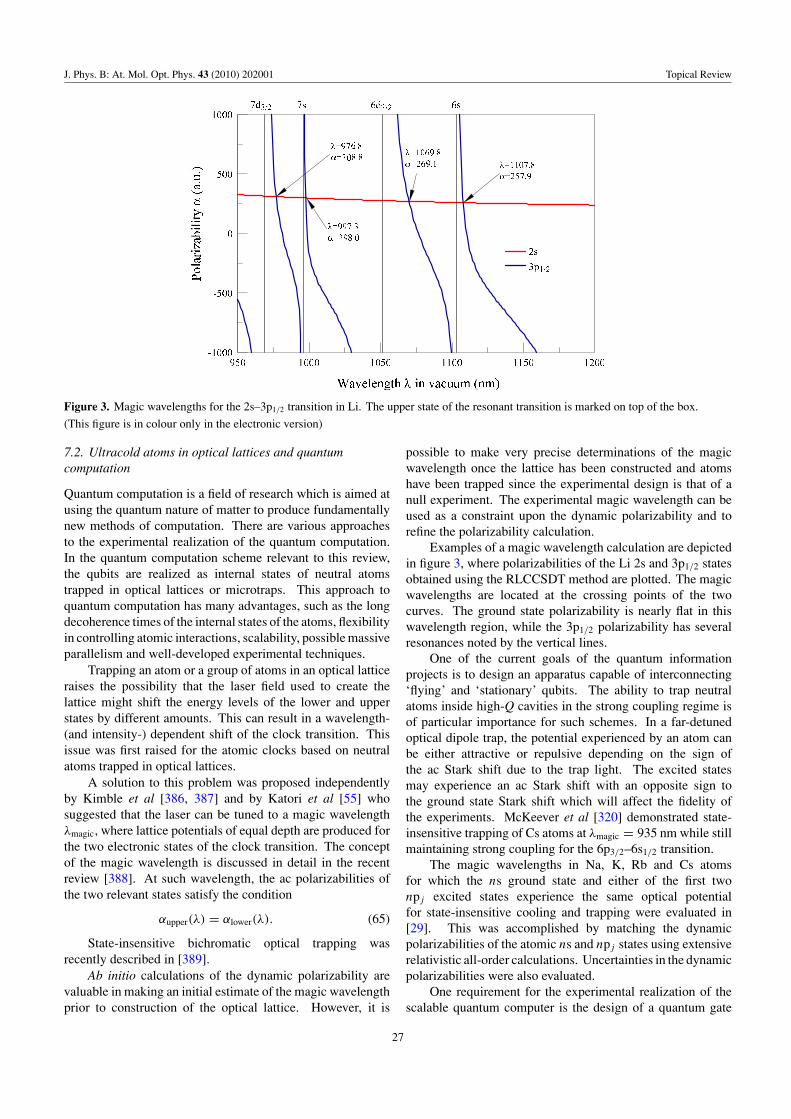
J. Phys. B: At. Mol. Opt. Phys. 43 (2010) 202001 Topical Review

Figure 3. Magic wavelengths for the 2s–3p1/2 transition in Li. The upper state of the resonant transition is marked on top of the box.

(This figure is in colour only in the electronic version)

7.2. Ultracold atoms in optical lattices and quantumcomputation

Quantum computation is a field of research which is aimed atusing the quantum nature of matter to produce fundamentallynew methods of computation. There are various approachesto the experimental realization of the quantum computation.In the quantum computation scheme relevant to this review,the qubits are realized as internal states of neutral atomstrapped in optical lattices or microtraps. This approach toquantum computation has many advantages, such as the longdecoherence times of the internal states of the atoms, flexibilityin controlling atomic interactions, scalability, possible massiveparallelism and well-developed experimental techniques.

Trapping an atom or a group of atoms in an optical latticeraises the possibility that the laser field used to create thelattice might shift the energy levels of the lower and upperstates by different amounts. This can result in a wavelength-(and intensity-) dependent shift of the clock transition. Thisissue was first raised for the atomic clocks based on neutralatoms trapped in optical lattices.

A solution to this problem was proposed independentlyby Kimble et al [386, 387] and by Katori et al [55] whosuggested that the laser can be tuned to a magic wavelengthλmagic, where lattice potentials of equal depth are produced forthe two electronic states of the clock transition. The conceptof the magic wavelength is discussed in detail in the recentreview [388]. At such wavelength, the ac polarizabilities ofthe two relevant states satisfy the condition

αupper(λ) = αlower(λ). (65)

State-insensitive bichromatic optical trapping wasrecently described in [389].

Ab initio calculations of the dynamic polarizability arevaluable in making an initial estimate of the magic wavelengthprior to construction of the optical lattice. However, it is

possible to make very precise determinations of the magicwavelength once the lattice has been constructed and atomshave been trapped since the experimental design is that of anull experiment. The experimental magic wavelength can beused as a constraint upon the dynamic polarizability and torefine the polarizability calculation.

Examples of a magic wavelength calculation are depictedin figure 3, where polarizabilities of the Li 2s and 3p1/2 statesobtained using the RLCCSDT method are plotted. The magicwavelengths are located at the crossing points of the twocurves. The ground state polarizability is nearly flat in thiswavelength region, while the 3p1/2 polarizability has severalresonances noted by the vertical lines.

One of the current goals of the quantum informationprojects is to design an apparatus capable of interconnecting‘flying’ and ‘stationary’ qubits. The ability to trap neutralatoms inside high-Q cavities in the strong coupling regime isof particular importance for such schemes. In a far-detunedoptical dipole trap, the potential experienced by an atom canbe either attractive or repulsive depending on the sign ofthe ac Stark shift due to the trap light. The excited statesmay experience an ac Stark shift with an opposite sign tothe ground state Stark shift which will affect the fidelity ofthe experiments. McKeever et al [320] demonstrated state-insensitive trapping of Cs atoms at λmagic = 935 nm while stillmaintaining strong coupling for the 6p3/2–6s1/2 transition.

The magic wavelengths in Na, K, Rb and Cs atomsfor which the ns ground state and either of the first twonpj excited states experience the same optical potentialfor state-insensitive cooling and trapping were evaluated in[29]. This was accomplished by matching the dynamicpolarizabilities of the atomic ns and npj states using extensiverelativistic all-order calculations. Uncertainties in the dynamicpolarizabilities were also evaluated.

One requirement for the experimental realization of thescalable quantum computer is the design of a quantum gate

27

J. Phys. B: At. Mol. Opt. Phys. 43 (2010) 202001 Topical Review

with low error rate which will allow for error correction.Therefore, it is important to study the various decoherencemechanisms and to search for ways to optimize gateperformance.

The issue of the mismatch of the polarizabilities of theground and excited states has also arisen in schemes to performquantum logical operations where it is a source of decoherence.In the Rydberg gate scheme [321], the qubit is based ontwo ground hyperfine states of neutral atoms confined inan optical lattice. A two-qubit phase gate may be realizedby conditionally exciting two atoms to relatively low-lyingRydberg states. The choice of this particular scheme resultsfrom its potential for fast (sub-microsecond) gate operations.Such a gate has been experimentally demonstrated recently[322]. An atom in a Rydberg state will, in general, move in adifferent optical lattice potential than that experienced by theground state. Therefore, the vibrational state of the atom inthe lattice may change after the gate operation is completed,leading to decoherence due to motional heating. The opticalpotential for a given state depends on its ac polarizability, sowe can seek to minimize this motional heating effect by thechoice of a particular Rydberg state or of the lattice photonfrequency ω. A method for accomplishing this by matchingthe frequency-dependent polarizabilities α(λ) of the atomicground state and Rydberg state is described in [323, 324].

In a recent work [325], a novel approach to quantuminformation processing, in which multiple qubits can beencoded and manipulated using electronic and nuclear degreesof freedom associated with individual alkaline-earth-metalatoms trapped in an optical lattice, was proposed and analysed.In this scheme, curves of dynamic polarizabilities are neededfor alkali and group II atom elements to locate the wavelengthswhere one of the species can escape or where ac Stark shiftscancel for a specific transition.

7.3. Atomic clocks

The current definition of the second in the International Systemof Units (SI) is based on the microwave transition betweenthe two hyperfine levels of the ground state of 133Cs [343].The present relative standard uncertainty of the Cs microwavefrequency standard is around 5×10−16. More accurate clocksare needed for a variety of applications. Significant recentprogress in optical spectroscopy and measurement techniqueshas led to the achievement of relative standard uncertaintiesin optical frequency standards that are comparable to the Csmicrowave benchmark. The frequencies of feasible opticalclock transitions are five orders of magnitude greater thanthe standard microwave transitions, and so smaller relativeuncertainties are potentially achievable. A list of opticaltransitions recommended for this purpose has recently beendisseminated by the International Committee for Weights andMeasures [344].

There are two types of optical atomic clocks under activeinvestigation at the moment. Both types of clocks are basedon optical frequency transitions with a narrow linewidth. Thenarrow linewidth mandates that the upper state of the clocktransition be a long-lived metastable state. One type of clock isimplemented using a group of cold atoms trapped in an optical

lattice. The second consists of a single laser-cooled ion. Withextremely low systematic perturbations and better stability andaccuracy, such optical frequency standards should exceed theperformance of the existing Cs standard. A commonly quotedtarget for the new generation of optical frequency standards isa fractional uncertainty of �ν/ν0 = 10−18 [5, 334, 345, 346].

There are two main interconnecting areas of theoreticalatomic clock research: prediction of atomic propertiesrequired for new clock proposals and determination ofquantities contributing to the uncertainty budget. New clockproposals require estimates of the atomic properties for detailsof the proposals (transition rates, lifetimes, branching ratios,magic wavelengths, scattering rates, etc) and evaluation ofthe systematic shifts (Zeeman shift, electric quadrupole shift,blackbody radiation shift, ac Stark shifts due to variouslaser fields, etc). While a large fraction of these quantitiesmay be eventually measured, lack of knowledge of some ofthese properties may delay experimental realization of newproposals. In the case of well-developed proposals, one of themain uncertainty issues is the blackbody radiation (BBR) shift.The operation of atomic clocks is generally carried out at roomtemperature, whereas the definition of the second refers to theclock transition in an atom at absolute zero. This implies thatthe clock transition frequency should be corrected for effectsof finite temperature, of which the leading contributor is theblackbody radiation shift. The BBR shift is looming as a majorcomponent in the uncertainty budget of the optical frequencystandards. Table 16 gives the BBR shifts in clock frequenciesof many proposed standards while table 17 gives the fractionaluncertainty budget for a 87Sr optical frequency standard [347].The BBR shift is by far the largest source of uncertainty inthe Sr uncertainty budget [347]. It is noteworthy that thesecond largest source of uncertainty is the ac stark shift causedby the optical lattice (this estimate did not take into accountpossible corrections due to M1 and E2 multipoles caused byspatial inhomogeneities of the lattice field). Experimentalmeasurements of BBR shifts are difficult and high-precisiontheoretical calculations are presently needed.

7.3.1. Blackbody radiation shifts. The BBR shift is the acStark shift resulting from the ambient blackbody radiation fieldsurrounding the atom. The BBR energy shift of an atomic statecan be approximately calculated as [57]

�E = − 215 (απ)3α0(0)T 4(1 + η), (66)

where α is the fine structure constant. The static scalarpolarizability α0(0) and energy shift �E in equation (66)are in atomic units. In this expression, the temperature inK is multiplied by 3.166 8153 × 10−6 and �E is convertedto Hz by multiplying by 6.579 684 × 1015. The factor η isa correction factor that allows for the frequency dependenceof the polarizability when the blackbody integral is performed[11, 13, 235]. The factor η, referred to as the dynamic shift, ismost conveniently written as [13, 235]

η ≈ −40π2T 2

21αd(0)S(−4). (67)

The dynamic shift is largest when the excitation energies of thestates that make the largest contribution to the polarizabilities

28

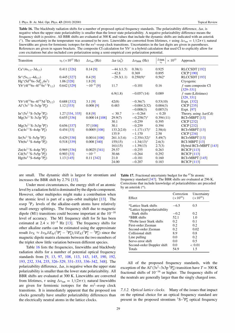
J. Phys. B: At. Mol. Opt. Phys. 43 (2010) 202001 Topical Review

Table 16. The blackbody radiation shifts for a number of proposed optical frequency standards. The polarizability difference, �α, isnegative when the upper state polarizability is smaller than the lower state polarizability. A negative polarizability difference means thefrequency shift is positive. All BBR shifts are evaluated at 300 K and values that include the dynamic shifts are indicated with an asterisk(∗). The uncertainty in the temperature was assumed to be zero. Linewidths are converted from lifetimes, τ using �νnat = 1/(2πτ); naturallinewidths are given for fermionic isotopes for the ns2–nsnp clock transitions. Uncertainties in the last digits are given in parentheses.References are given in square brackets. The composite CI calculation for Yb+ is a hybrid calculation that used CI to explicitly allow forcore excitations but also included core polarization using a semi-empirical core polarization potential.

Transition ν0 (×1015 Hz) �νnat (Hz) �α (a30 ) �νBBR (Hz)

∣∣∣�νBBRν0

∣∣∣ × 1015 Approach

Ca+(4s1/2–3d5/2) 0.411 [326] 0.14 [9] −44.1(1.5) 0.38(1) 0.925 RLCCSDT [192]−42.8 0.369 0.895 CICP [190]

Sr+(5s1/2–4d5/2) 0.445 [327] 0.4 [9] −29.3(1.1) 0.250(9)∗ 0.562∗ RLCCSDT [193]Hg+(5d106s–5d9

5/26s2) 1.06 [328] 1.8 [9] CryogenicYb+(4f146s–4f136s2 2F7/2) 0.642 [329] ∼10−9 [9] 11.7 −0.101 0.16 f -sum composite CI

[329–331]6.9(1.8) −0.057 (14) 0.089 f -sum (Lifetimes)

[329, 331]Yb+(4f146s–4f145d 2D3/2) 0.688 [332] 3.1 [9] 42(8) −0.36(7) 0.53(10) Expt. [332]Al+(3s2 1S–3s3p 3Po

0) 1.12 [333] 0.008 [9] 0.483 −0.004 2(32) 0.004(3) CICP [235]−0.008(3) 0.007(3) Expt. [97]

In+(5s2 1S–5s5p 3Po0) 1.27 [334, 335] 0.8 [9] < 30.7 >−0.264 < 0.20 Theory, using �α(Cd)

Mg(3s2 1S–3s3p 3Po0) 0.655 [336] 0.000 14 [108] 29.9(7) −0.258(7)∗ 0.394 (11) RCI+MBPT [13]

30.1 −0.259 0.395 CICP [232]Mg(3s2 1S–3s3p 3Po

1) 0.656 [337] 57 [108] 30.1 −0.259 0.394 CICP [232]Ca(4s2 1S–4s4p 3Po

0) 0.454 [33] 0.0005 [108] 133.2(2.0) −1.171 (17)∗ 2.58(4) RCI+MBPT [13]135.9 −1.170 2.58 CICP [234]

Sr(5s2 1S–5s5p 3Po0) 0.429 [338] 0.0014 [108] 261.1(3.6) −2.354 (32)∗ 5.49(7) RCI+MBPT [13]

Yb(6s2 1S–6s6p 3Po0) 0.518 [339] 0.008 [340] 155(15) −1.34(13)∗ 2.6(3) RCI-MBPT [13]

161(15) −1.39(13) 2.7(3) Hybrid RCI+MBPT [143]Zn(4s2 1S–4s4p 3Po

0) 0.969 [336] 0.0025 [341] 29.57 −0.255 0.263 RCICP [113]Cd(5s2 1S–5s5p 3Po

0) 0.903 [33] ∼10−2 30.66 −0.264 0.292 RCICP [113]Hg(6s2 1S–6s6p 3Po

0) 1.13 [145] 0.11 [342] 21.0 −0.181 0.160 RCI+MBPT [145]24.00 −0.207 0.183 RCICP [113]

are small. The dynamic shift is largest for strontium andincreases the BBR shift by 2.7% [13].

Under most circumstances, the energy shift of an atomiclevel by a radiation field is dominated by the dipole component.However, other multipoles might make a contribution whenthe atomic level is part of a spin–orbit multiplet [13]. Thensnp 3PJ levels of the alkaline-earth atoms have relativelysmall energy splittings. The frequency shift due to magneticdipole (M1) transitions could become important at the 10−18

level of accuracy. The M1 frequency shift for Sr has beenestimated at 2.4 × 10−5 Hz [13]. The frequency shifts forother alkaline earths can be estimated using the approximateresult δνX ≈ δνSrδESr(

3Po1 − 3Po

0)/δEX(3Po1 − 3Po

0) since themagnetic dipole matrix elements between the two members ofthe triplet show little variation between different species.

Table 16 lists the frequencies, linewidths and blackbodyradiation shifts for a number of potential optical frequencystandards from [9, 13, 97, 108, 113, 143, 145, 190, 192,193, 232, 334, 235, 326–329, 331–333, 336–342, 348]. Thepolarizability difference, �α, is negative when the upper statepolarizability is smaller than the lower state polarizability. AllBBR shifts are evaluated at 300 K. Linewidths are convertedfrom lifetimes, τ using �νnat = 1/(2πτ); natural linewidthsare given for fermionic isotopes for the ns2–nsnp clocktransitions. It is immediately apparent that the proposed ionclocks generally have smaller polarizability differences thanthe electrically neutral atoms in the lattice clocks.

Table 17. Fractional uncertainty budget for the 87Sr atomicfrequency standard [347]. The BBR shifts are evaluated at 296 K.Corrections that include knowledge of polarizabilities are precededby an asterisk (*).

Correction UncertaintyEffect (×1016) (×1016)

*Lattice Stark shifts −6.5 0.5*Lattice hyperpolarizability

Stark shifts −0.2 0.2*BBR shifts 52.1 1.0*Probe laser Stark shifts 0.2 0.1First-order Zeeman 0.2 0.2Second-order Zeeman 0.2 0.02Collisional shift 8.9 0.8Line pulling 0.0 0.2Servo error shift 0.0 0.5Second-order Doppler shift 0.0 < 0.01Totals 54.9 1.5

All of the proposed frequency standards, with theexception of the Al+(3s2–3s3p 3Po

0) transition have T = 300 Kfractional shifts of 10−16 or higher. The frequency shifts ofthe neutrals are generally larger than the singly charged ions.

7.3.2. Optical lattice clocks. Many of the issues that impacton the optimal choice for an optical frequency standard arepresent in the proposed strontium 1S–3Po

0 optical frequency

29

J. Phys. B: At. Mol. Opt. Phys. 43 (2010) 202001 Topical Review

standard [338, 349]. While Sr might be a desirable atom fromthe perspective of practical experimentation, it is the mostsusceptible to BBR shifts since the polarizability differencebetween the two states is 259.8 au, giving a BBR shift of2.35 Hz at T = 300 K [141].

Assuming that the polarizability difference can bedetermined to 0.2% accuracy, the resulting BBR uncertaintywould be 0.0047 Hz which corresponds to a fractionaluncertainty of 1 × 10−17. Achieving such a level of precisionrequires experimental determination of the five most importanttransitions in the oscillator strength sum-over-states to aprecision of 0.1% [141].

Another problem associated with large polarizabilitydifferences is the enhanced sensitivity with respect tovariations in temperature. A 1.0 K uncertainty in thetemperature at 300 K would of itself lead to a frequencyuncertainty of �ν = 0.031 Hz. The large BBR shift makesa Sr standard particularly sensitive to an imprecisely knowntemperature. These problems can be reduced by runningthe clock at lower temperatures. For example, the BBRuncertainties stated above can be reduced in size by a factorof more than 200 by maintaining the clock at liquid nitrogentemperatures.

Sensitivity to BBR fields has resulted in a proposalthat mercury would be a superior candidate for an opticalfrequency standard [145] despite the inconvenience of muchshorter optical lattice wavelengths. Cadmium and zinc havealso been identified as candidates with reduced BBR shifts[113, 341]. The drawback of the group IIB atomsare the greater uncertainties in the determination of thepolarizabilities. The underlying (nd)10 shell of the group IIBatoms implies large core polarizabilities, stronger valence–core correlations and valence expectation values that areslower to converge. In addition, the resonant oscillator strengthfor these atoms is about 1.4, as opposed to 1.7–1.8 for the groupII atoms. Consequently the use of a high precision resonanttransition matrix element from a photo-association experimentwould do less to minimize the uncertainty than in a group IIatom.

Ytterbium has also been the subject of increasedexperimental interest [339]. This system also suffers fromthe drawback that it has a large polarizability. Furthermore, afirst-principles calculation of the polarizability to a guaranteedaccuracy of even 1% is a very difficult proposition. Themost weakly bound core shell is the (4f)14 shell and the Yb2+

polarizability is ∼9 au [124].The atoms that have so far been used in most experiments

are those that are amenable to cooling and trapping. The lightergroup II atoms, Be and Mg, have the disadvantage that they aredifficult to cool, but have the advantage of much smaller BBRshifts [337]. Further, it would be easier to compensate for theeffect of the BBR shift in Be and Mg than in most other atoms.Besides having smaller shifts, these are relatively light atomswith small core polarizabilities, so the uncertainties associatedwith any calculation will be smaller than those of other latticeclocks. These considerations apply most strongly to beryllium.In this case, the polarizability difference of the states in theclock transition is only 1.3 au (table 11). Beryllium has only

four electrons, so calculations with ECGs are possible andshould ultimately be able to achieve a precision approaching0.01 au.

The dynamic correction to the BBR shift makes a finitecontribution when the precision reaches the 10−18 Hz level[57, 193] but should not lead to a significant increase in theBBR shift uncertainty. The sum rule for evaluation of S(−4)

is more strongly dominated by a few major transitions thanα0 and the relative uncertainty in S(−4) will not be any largerthan that of α0. Further, the dynamic contribution will be smallso the need for a precise evaluation is reduced.

One recent complication has been the realization thathigher order multipoles could have an impact upon themagic wavelength. The inhomogenous spatial distributionsof the electric and magnetic fields in the standing wavepatterns that define the lattice can lead to energy shifts in theatomic vibrational motion [350]. This requires the definitionof a motion insensitive magic wavelength which requiresknowledge of the frequency-dependent electric quadrupoleand magnetic dipole polarizabilities [351].

7.3.3. Ion clocks. Ion state polarizabilities are generallysmaller than those for neutral atoms because the electrons aremore tightly bound. None of the ion clocks have polarizabilitydifferences that exceed 50 au.

The Al+(3s2–3s3p 3Po0) transition has the smallest BBR

shift of any ion clock due to the fortuitous near equality ofpolarizabilities of the two states in the clock transition. TheCICP BBR shift is only −0.004 2(32) Hz [235] while theexperiment gave −0.008(3) Hz [97]. However, the technicalrequirements for construction of an Al+ clock are much moredemanding since the clock transition and cooling laser are inthe ultraviolet [333].

While the Ca+ system is monovalent, calculation of itspolarizabilities using the RLCCSDT method is a more difficultproposition than for the iso-electronic neutral potassium [192].The difficulties lie in the determination of the 3d statepolarizability. First, the 3d state is quite compact and itscharge distribution does perturb the charge distribution ofthe 3s23p6 core. This leads to a more slowly convergentperturbation theory or CI expansion. Second, about 30%of the polarizability comes from the 3d → nf excitations.The sum-over-states in this case is not dominated by asingle transition, so discrete excitations up to the 12f haveto be included. Furthermore, the continuum contribution issignificant. Including states up to 12f means a much largerB-spline basis needs to be used, which in turn makes thecalculation more exacting. Similar considerations impact theBBR shift calculation for Sr+ [193].

The relative uncertainties associated with the determina-tion of the BBR shifts for the two proposed Yb+ standardsare also large due to the underlying 4f14 core. This is partlymitigated by the small size of the BBR shifts. The BBR shiftfor In+ was determined by assuming that the polarizability dif-ference would be smaller than that of cadmium. This estimatewill be an overestimate since the In+ ion will have smallerpolarizabilities than cadmium.

30

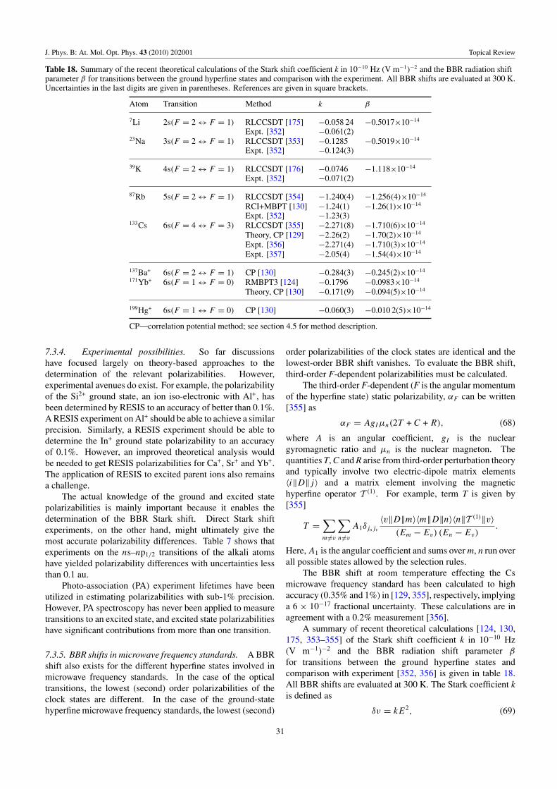
J. Phys. B: At. Mol. Opt. Phys. 43 (2010) 202001 Topical Review

Table 18. Summary of the recent theoretical calculations of the Stark shift coefficient k in 10−10 Hz (V m−1)−2 and the BBR radiation shiftparameter β for transitions between the ground hyperfine states and comparison with the experiment. All BBR shifts are evaluated at 300 K.Uncertainties in the last digits are given in parentheses. References are given in square brackets.

Atom Transition Method k β

7Li 2s(F = 2 ↔ F = 1) RLCCSDT [175] −0.058 24 −0.5017×10−14

Expt. [352] −0.061(2)23Na 3s(F = 2 ↔ F = 1) RLCCSDT [353] −0.1285 −0.5019×10−14

Expt. [352] −0.124(3)

39K 4s(F = 2 ↔ F = 1) RLCCSDT [176] −0.0746 −1.118×10−14

Expt. [352] −0.071(2)

87Rb 5s(F = 2 ↔ F = 1) RLCCSDT [354] −1.240(4) −1.256(4)×10−14

RCI+MBPT [130] −1.24(1) −1.26(1)×10−14

Expt. [352] −1.23(3)133Cs 6s(F = 4 ↔ F = 3) RLCCSDT [355] −2.271(8) −1.710(6)×10−14

Theory, CP [129] −2.26(2) −1.70(2)×10−14

Expt. [356] −2.271(4) −1.710(3)×10−14

Expt. [357] −2.05(4) −1.54(4)×10−14

137Ba+ 6s(F = 2 ↔ F = 1) CP [130] −0.284(3) −0.245(2)×10−14

171Yb+ 6s(F = 1 ↔ F = 0) RMBPT3 [124] −0.1796 −0.0983×10−14

Theory, CP [130] −0.171(9) −0.094(5)×10−14

199Hg+ 6s(F = 1 ↔ F = 0) CP [130] −0.060(3) −0.010 2(5)×10−14

CP—correlation potential method; see section 4.5 for method description.

7.3.4. Experimental possibilities. So far discussionshave focused largely on theory-based approaches to thedetermination of the relevant polarizabilities. However,experimental avenues do exist. For example, the polarizabilityof the Si2+ ground state, an ion iso-electronic with Al+, hasbeen determined by RESIS to an accuracy of better than 0.1%.A RESIS experiment on Al+ should be able to achieve a similarprecision. Similarly, a RESIS experiment should be able todetermine the In+ ground state polarizability to an accuracyof 0.1%. However, an improved theoretical analysis wouldbe needed to get RESIS polarizabilities for Ca+, Sr+ and Yb+.The application of RESIS to excited parent ions also remainsa challenge.

The actual knowledge of the ground and excited statepolarizabilities is mainly important because it enables thedetermination of the BBR Stark shift. Direct Stark shiftexperiments, on the other hand, might ultimately give themost accurate polarizability differences. Table 7 shows thatexperiments on the ns–np1/2 transitions of the alkali atomshave yielded polarizability differences with uncertainties lessthan 0.1 au.

Photo-association (PA) experiment lifetimes have beenutilized in estimating polarizabilities with sub-1% precision.However, PA spectroscopy has never been applied to measuretransitions to an excited state, and excited state polarizabilitieshave significant contributions from more than one transition.

7.3.5. BBR shifts in microwave frequency standards. A BBRshift also exists for the different hyperfine states involved inmicrowave frequency standards. In the case of the opticaltransitions, the lowest (second) order polarizabilities of theclock states are different. In the case of the ground-statehyperfine microwave frequency standards, the lowest (second)

order polarizabilities of the clock states are identical and thelowest-order BBR shift vanishes. To evaluate the BBR shift,third-order F-dependent polarizabilities must be calculated.

The third-order F-dependent (F is the angular momentumof the hyperfine state) static polarizability, αF can be written[355] as

αF = AgIμn(2T + C + R), (68)

where A is an angular coefficient, gI is the nucleargyromagnetic ratio and μn is the nuclear magneton. Thequantities T, C and R arise from third-order perturbation theoryand typically involve two electric-dipole matrix elements〈i‖D‖j 〉 and a matrix element involving the magnetichyperfine operator T (1). For example, term T is given by[355]

T =∑m=v

∑n=v

A1δjnjv

〈v‖D‖m〉〈m‖D‖n〉〈n‖T (1)‖v〉(Em − Ev) (En − Ev)

.

Here, A1 is the angular coefficient and sums over m, n run overall possible states allowed by the selection rules.

The BBR shift at room temperature effecting the Csmicrowave frequency standard has been calculated to highaccuracy (0.35% and 1%) in [129, 355], respectively, implyinga 6 × 10−17 fractional uncertainty. These calculations are inagreement with a 0.2% measurement [356].

A summary of recent theoretical calculations [124, 130,175, 353–355] of the Stark shift coefficient k in 10−10 Hz(V m−1)−2 and the BBR radiation shift parameter β

for transitions between the ground hyperfine states andcomparison with experiment [352, 356] is given in table 18.All BBR shifts are evaluated at 300 K. The Stark coefficient kis defined as

δν = kE2, (69)

31

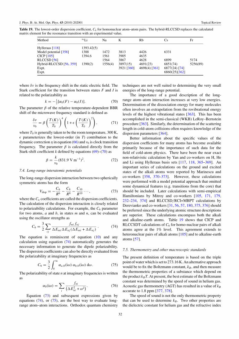
J. Phys. B: At. Mol. Opt. Phys. 43 (2010) 202001 Topical Review

Table 19. The lowest-order dispersion coefficient, C6 for homonuclear atom–atom pairs. The hybrid-RLCCSD replaces the calculatedmatrix element for the resonance transition with an experimental value.

Method ∞Li Na K Rb Cs Fr

Hylleraas [118] 1393.42(5)Model potential [358] 1388 1472 3813 4426 6331CICP [105] 1394.6 1561 3905 4635RLCCSD [56] 1564 3867 4628 6899 5174Hybrid-RLCCSD [56, 359] 1390(2) 1556(4) 3897(15) 4691(23) 6851(74) 5256(89)Expt. 3921 [360] 4698(4) [361] 6877(24) [74]Expt. 6860(25)[362]

where δν is the frequency shift in the static electric field. TheStark coefficient for the transition between states F and I isrelated to the polarizability as

k = − 12 [α0(F ) − α0(I )]. (70)

The parameter β of the relative temperature-dependent BBRshift of the microwave frequency standard is defined as

δν

ν0= β

(T (K)

T0

)4(

1 + ε

(T (K)

T0

)2)

, (71)

where T0 is generally taken to be the room temperature, 300 K,ε parameterizes the lowest-order (in T) contribution to thedynamic correction η in equation (66) and ν0 is clock transitionfrequency. The parameter β is calculated directly from theStark-shift coefficient k defined by equations (69)–(70) as

β = k

ν0(831.9 V m−1)2. (72)

7.4. Long-range interatomic potentials

The long-range dispersion interaction between two sphericallysymmetric atoms has the form

Vdisp = −C6

R6− C8

R8− C10

R10· · · , (73)

where the Cn coefficients are called the dispersion coefficients.The calculation of the dispersion interaction is closely relatedto polarizability calculations. For example, the C6 parameterfor two atoms, a and b, in states m and n, can be evaluatedusing the oscillator strengths as

C6 = 3

2

∑ij

fmifnj

�Emi�Enj (�Emi + �Enj ). (74)

The equation is reminiscent of equation (10) and anycalculation using equation (74) automatically generates thenecessary information to generate the dipole polarizability.The dispersion coefficients can also be directly evaluated fromthe polarizability at imaginary frequencies as

C6 = 3

2

∫ ∞

0αa,0(iω) αb,0(iω) dω. (75)

The polarizability of state n at imaginary frequencies is writtenas

α0(iω) =∑

i

fni(�E2

ni + ω2) . (76)

Equation (73) and subsequent expressions given byequations (74), or (75), are the best way to evaluate long-range atom–atom interactions. Orthodox quantum chemistry

techniques are not well suited to determining the very smallenergies of the long-range potential.

The importance of a good description of the long-range atom–atom interaction increases at very low energies.Determination of the dissociation energy for many moleculesoften involves an extrapolation from the rovibrational energylevels of the highest vibrational states [363]. This has beenaccomplished in the semi-classical (WKB) LeRoy–Bernsteinprocedure [363]. Similarly, the determination of the scatteringlength in cold-atom collisions often requires knowledge of thedispersion parameters [364].

Better information about the specific values of thedispersion coefficients for many atoms has become availableprimarily because of the importance of such data for thefield of cold-atom physics. There have been the near exactnon-relativistic calculation by Yan and co-workers on H, Heand Li using Hylleraas basis sets [117, 118, 365–369]. Animportant series of calculations on the ground and excitedstates of the alkali atoms were reported by Marinescu andco-workers [358, 370–373]. However, these calculationswere performed with a model potential approach that omittedsome dynamical features (e.g. transitions from the core) thatshould be included. Later calculations with semi-empiricalHamiltonians by Mitroy and co-workers [105, 171, 179,232–234, 374] and RLCCSD/RCI+MBPT calculations byDerevianko and co-workers [31, 56, 57, 180, 375, 376] shouldbe preferred since the underlying atomic structure descriptionsare superior. These calculations encompass both the alkaliand alkaline-earth atoms. Table 19 shows that CICP andRLCCSDT calculations of C6 for homo-nuclear pairs of alkaliatoms agree at the 1% level. This agreement extends toheteronuclear pairs of alkali atoms [105] and to alkaline-earthatoms [57].

7.5. Thermometry and other macroscopic standards

The present definition of temperature is based on the triplepoint of water which is set to 273.16 K. An alternative approachwould be to fix the Boltzmann constant, kB , and then measurethe thermometric properties of a substance which depend onthe product kBT. At present, the best estimate of the Boltzmannconstant was determined by the speed of sound in helium gas.Acoustic gas thermometry (AGT) has resulted in a value of kB

accurate to 1.8 ppm [377, 378].The speed of sound is not the only thermometric property

that can be used to determine kB . Two other properties arethe dielectric constant for helium gas and the refractive index

32

J. Phys. B: At. Mol. Opt. Phys. 43 (2010) 202001 Topical Review

for helium gas [63, 378, 379]. The most recent refractiveindex experiment using a microwave cavity [63] has given thedipole polarizability to an accuracy of 9.3 ppm. If the 4Hepolarizability is taken as a known quantity from theory, thenthe microwave cavity experiment admits other interpretations.Taking the polarizability and diamagnetic susceptibility asknown quantities, the refractive index experiment yields avalue for the universal gas constant, R = 8.314 487(76),which is not far removed in precision from the recommendedvalue of 8.314 472 (15) [377]. Boltzmann’s constant, thedefinition of the mol and the universal gas constant are allinter-related through the identity, R = kBNA.

7.6. Atomic transition rate determinations

The sum-over-states approach described in section 2.1.2 isgenerally used to determine the polarizabilities from calculatedor experimental oscillator strengths or E1 matrix elements. Itis possible to reverse the process for systems which have aprecisely known polarizability that is dominated by a singlestrong transition. A good example occurs for the cesium atom[380] where the dipole polarizability [74] and line strengthratio [381] have been measured to high accuracy.

The ground state static polarizability α0 can be written as

α0 = α6p + α′v + αcore, (77)

where α6p is the contribution of the resonance excitations tothe polarizability, i.e. from 6s–6p1/2 and 6s–6p3/2 transitions,and α′

v includes contributions from all other excited states.Rearranging and expressing α6p in terms of the 6s → 6p1/2

line strength gives

S6s−6p1/2 = α0 − α′v − αcore

1

3�E6s−6p1/2

+R

3�E6s−6p3/2

. (78)

The factor R is the ratio of the line strengths of the spin–orbitdoublet. Using α0 = 401.0(6) [74], R = 1.9809(9) [381],the ionic core polarizability of 15.644(4) [112] that needs tobe corrected for the presence of the valence electron by theterm αcv = −0.72, α′

v = 1.81 yields S6s−6p1/2 = 20.308 (42)

and S6s−6p3/2 = 40.227 (84). The corresponding values forthe reduced matrix elements in atomic units are 4.510(4)and 6.347(5) for the 6s–6p1/2 and 6s–6p3/2 transitions,respectively. The uncertainties of these values are dominatedby the uncertainty in the experimental value of α0.

A similar approach has been used to determine themultiplet strengths for the resonance transitions in Mg+, Si3+

[84] and Si2+ [88] from RESIS experimental data [198, 239].Stark shifts for the ns–np1/2 transition [201] have also

been used to derive estimates for the S(np1/2–(n− 1)d3/2)

line strengths with a precision of about 1% for potassium andrubidium [30]. This analysis relied on the result that 80–90%of the np1/2 polarizability comes from the excitation to the(n − 1)d3/2 state. These values were also used to determinethe magic wavelengths for the np–ns transitions in these alkaliatoms [29]. Such determination of matrix elements permittedbenchmark comparisons of theory and experiment [30].

The procedures described above also permit thecrosschecking of results from completely different types

of experiment. The domination of the 6p Cs scalarpolarizabilities by the 5d–6p dipole matrix elements facilitatedan exacting consistency check of the 5d lifetime with 6ppolarizability data [169]. In that work, 5d–6p matrixelements obtained from experimental Stark shift data werecompared with the values extracted from the 5d lifetimes.The experimental measurements of the 5d lifetime and 6pscalar polarizabilities were found to be inconsistent withinthe uncertainties quoted by the experimental groups [169].Theoretical RLCCSDT matrix elements [169] were found tobe in agreement with the Stark shift experiments but not withthe lifetime measurements.

8. Conclusions

The advent of cold-atom physics owes its existence to theability to manipulate groups of atoms with electromagneticfields. Consequently, many topics in the area of field–atominteractions have recently been the subject of considerableinterest and heightened importance. This applies to a quantitylike the dipole polarizability which governs the first-orderresponse of an atom to an applied electric field and thepreceding few years have seen many calculations of atomicpolarizabilities for a variety of systems.

The aim of this review has been to provide a reasonablycomprehensive treatment of polarizability-related issues asthey relate to topics of contemporary importance. However,our treatment is not exhaustive. The polarizabilities of manyatoms such as the halogens have been omitted. The readeris referred to the broader treatment in [21]. Similarly, thetreatment of dc and ac Stark shift data is better described asselective as opposed to exhaustive.

Part of the motivation for this review has been theimportance in developing new atom-based standards of time[344], and corresponding need for precise knowledge ofthe blackbody radiation shifts. The primary requirement forthe BBR application is for polarizabilities and Stark shifts tobe known with a precision of 0.1% or better. Much of theexisting body of experimental data is an order of magnitudeless precise. Precise measurements of clock transition Starkshifts would be helpful in reducing the BBR shift uncertainties.

One area where theory might be useful in this endeavourwould be in the development of atom-based polarizabilitystandards. Such a standard is already in existence forhelium where theoretical and experimental polarizabilitieshave uncertainties of 0.17 ppm and 9.1 ppm [63], respectively.These results are not relevant to atomic clock research andanother atom needs to serve as a standard. Hylleraascalculations on lithium could yet serve to provide a theoreticalreference point for Stark shift experiments. At the moment theuncertainties in the best calculation and best experiment are0.08% [170] and 0.05% [91]. A better treatment of relativisticeffects should result in the uncertainty in the Hylleraascalculation decreasing to the 0.01% level of precision.

One possible avenue for improvement could be in thedevelopment of hybrid theoretical approaches combining thebest features of different methods. For example, orbital-basedapproaches cannot match the extreme accuracies achievable

33

J. Phys. B: At. Mol. Opt. Phys. 43 (2010) 202001 Topical Review

with correlated basis sets. Direct incorporation of theDirac Hamiltonian into orbital-based calculations is nowrelatively routine, but this is not the case for calculations withcorrelated basis sets. Perhaps, comparisons of correlated basiscalculations with non-relativistic orbital-based calculationsand with relativistic orbital-based calculations could be usedto estimate relativistic corrections to Hylleraas calculations orcorrelation corrections to orbital-based calculations.

It is likely that the determination of polarizabilitieswill become increasingly important in the future. Asexperiments become capable of greater precision, it willbecome necessary to make more detailed corrections of theeffects of electromagnetic fields that are used for manipulationand investigation of atoms.

Acknowledgments

The authors express their appreciation to Dr U I Safronova foruseful discussions and comments on the manuscript, and inparticularly for her thorough check of most of the tables. Thiswork was partly supported by the National Science Foundationunder Physics Frontiers Center grant PHY-0822671 to theUniversity of Maryland. This research has made extensiveuse of NASA’s Astrophysics Data System. The work of MSSwas supported in part by the US National Science Foundationgrant no PHY-07-58088. The work of JM was supported inpart by the Australian Research Council Discovery ProjectDP-1092620. This research was performed in part under thesponsorship of the US Department of Commerce, NationalInstitute of Standards and Technology.

References

[1] Maxwell J C 1864 Phil. Trans. R. Soc. 155 459[2] Edmonds A R 1996 Angular Momentum in Quantum

Mechanics (Princeton, NJ: Princeton University Press)[3] Schrodinger E 1926 Ann. Phys. 385 437[4] Madej A A and Bernard J E 2001 Frequency Measurement

and Control (Topics in Applied Physics vol 79) ed A NLuiten pp 153–95

[5] Udem T, Holzwarth R and Hansch T W 2002 Nature 416 233[6] Diddams S A, Bergquist J C, Jefferts S R and Oates C W

2004 Science 306 1318[7] Gill P, Barwood G P, Klein H A, Huang G, Webster S A,

Blythe P J, Hosaka K, Lea S N and Margolis H S 2003Meas. Sci. Technol. 14 1174

[8] Gill P 2005 Metrologia 42 S125[9] Margolis H S 2009 J. Phys. B: At. Mol. Opt. Phys. 41 154017

[10] Gallagher T F and Cooke W E 1979 Phys. Rev. Lett. 42 835[11] Itano W M, Lewis L L and Wineland D J 1982 Phys. Rev. A

25 1233[12] Hollberg L and Hall J L 1984 Phys. Rev. Lett. 53 230[13] Porsev S G and Derevianko A 2006 Phys. Rev. A 74 020502[14] Dalgarno A 1962 Adv. Phys. 11 281[15] Teachout R R and Pack R T 1971 At. Data 3 195[16] Miller T M and Bederson B 1977 Adv. At. Mol. Phys. 13 1[17] Miller T M 1988 Adv. At. Mol. Phys. 25 37[18] van Wijngaarden W A 1996 Adv. At. Mol. Opt. Phys. 36 141[19] Bonin K D and Kresin V V 1997 Electric Dipole

Polarizabilities of Atoms, Molecules and Clusters(Singapore: World Scientific)

[20] Delone N B and Krainov V P 1999 Phys.—Usp. 42 669

[21] Schwerdtfeger P 2006 Atomic Static Dipole Polarizabilitieschapter 1, p 1, in [383]

[22] Gould H and Miller T M 2005 Adv. At. Mol. Opt. Phys. 51343

[23] Lundeen S R 2005 Adv. At. Mol. Opt. Phys. 52 161[24] Miller T M 2006 Atomic and Molecular Polarizabilities

chapter 10, pp 10–192 volume 87 of [382][25] Lupinetti C and Thakkar A J in [383], p 505[26] Gallagher T F 2005 Rydberg Atoms (Cambridge: Cambridge

University Press)[27] Sobelmann I I 1979 Atomic Spectra and Radiative

Transitions (Berlin: Springer)[28] Mitroy J and Bromley M W J 2004 Phys. Rev. A 70 052503[29] Arora B, Safronova M S and Clark C W 2007 Phys. Rev. A

76 052509[30] Arora B, Safronova M S and Clark C W 2007 Phys. Rev. A

76 052516[31] Safronova M S, Johnson W R and Derevianko A 1999 Phys.

Rev. A 60 4476[32] Volz U and Schmoranzer H 1996 Phys. Scr. T 65 48[33] Sansonetti J, Martin W and Young S 2005 Handbook of Basic

Atomic Spectroscopic Data (version 1.1.2) (Gaithersburg,MD: National Institute of Standards and Technology)available at http://physics.nist.gov/Handbook (29 August2007)

[34] Moore C E 1971 Atomic Energy Levels (Chromium–NiobiumNSRDS-NBS 35) vol 2 (Washington DC: US GPO)

[35] Lim I S and Schwerdtfeger P 2004 Phys. Rev. A 70 062501[36] Lupinetti C and Thakkar A J 2005 J. Chem. Phys. 122 044301[37] Safronova M S and Johnson W R 2008 Adv. At. Mol. Opt.

Phys. 55 191[38] Hibbert A, LeDourneuf M and Lan V K 1977 J. Phys. B: At.

Mol. Phys. 10 1015[39] Dalgarno A and Lewis J T 1955 Proc. R. Soc. A 233 70[40] Epstein P 1926 Phys. Rev. 28 695[41] Waller I 1926 Z. Phys. 38 635[42] Wentzel G 1926 Z. Phys. 38 527[43] Yakhontov V 2003 Phys. Rev. Lett. 91 093001[44] Szmytkowski R and Mielewczyk K 2004 J. Phys. B: At. Mol.

Opt. Phys. 37 3961[45] Szmytkowski R 2006 Chem. Phys. Lett. 419 537[46] Jentschura U D and Haas M 2008 Phys. Rev. A 78 042504[47] Bethe H A and Salpeter E E 1977 Quantum Mechanics of

One- and Two-Electron Atoms (New York: Plenum)[48] Fano U and Cooper J W 1968 Rev. Mod. Phys. 40 441[49] Clark C W 1990 J. Opt. Soc. Am. B 7 488[50] Johnson W R, Kolb D and Huang K 1983 At. Data Nucl.

Data Tables 28 333[51] Johnson W R, Liu Z W and Sapirstein J 1996 At. Data Nucl.

Data Tables 64 279[52] Johnson W R, Blundell S A and Sapirstein J 1988 Phys. Rev.

A 37 307[53] Kozlov M G and Porsev S G 1999 Eur. Phys. J. D 5 59[54] Safronova M S, Arora B and Clark C W 2006 Phys. Rev. A

73 022505[55] Katori H, Ido T and Kuwata-Gonokami M 1999 J. Phys. Soc.

Japan 68 2479[56] Derevianko A, Johnson W R, Safronova M S and Babb J F

1999 Phys. Rev. Lett. 82 3589[57] Porsev S G and Derevianko A 2006 JETP 102 195[58] Bouloufa N, Crubellier A and Dulieu O 2009 Phys. Scr.

T134 014014[59] Kleinman C J, Hahn Y and Spruch L 1968 Phys. Rev. 165 53[60] Dalgarno A D, Drake G W F and Victor G A 1968 Phys. Rev.

176 194[61] Dalgarno A and Kingston A E 1960 Proc. R. Soc. A 259 424[62] Langhoff P W and Karplus M 1969 J. Opt. Soc. Am. 59 863[63] Schmidt J W, Gavioso R M, May E F and Moldover M R

2007 Phys. Rev. Lett. 98 254504

34

J. Phys. B: At. Mol. Opt. Phys. 43 (2010) 202001 Topical Review

[64] Goebel D and Hohm U 1995 Phys. Rev. A 52 3691[65] Goebel D and Hohm U 1996 J. Phys. Chem. 100 7710[66] Hall W D and Zorn J C 1974 Phys. Rev. A 10 1141[67] Molof R W, Schwartz H L, Miller T M and Bederson B 1974

Phys. Rev. A 10 1131[68] Miller T M and Bederson B 1976 Phys. Rev. A 14 1572[69] Schwartz H L, Miller T M and Bederson B 1974 Phys. Rev. A

10 1924[70] Cronin A D, Schmiedmayer J and Pritchard D E 2009 Rev.

Mod. Phys. 81 1051[71] Miffre A, Jacquet M, Buchner M, Trenec G and Vigue J 2006

Eur. Phys. J. D 38 353[72] Ekstrom C R, Schmiedmayer J, Chapman M S, Hammond T

D and Pritchard D E 1995 Phys. Rev. A 51 3883[73] Holmgren W F, Revelle M C, Lonij V P A and Cronin A

2010 Phys. Rev. A 81 063607[74] Amini J M and Gould H 2003 Phys. Rev. Lett. 91 153001[75] Kadar-Kallen M A and Bonin K D 1992 Phys. Rev. Lett.

68 2015[76] Kadar-Kallen M A and Bonin K D 1994 Phys. Rev. Lett.

72 828[77] Hu M and Kusse B R 2002 Phys. Rev. A 66 062506[78] Sarkisov G S, Beigman I L, Shevelko V P and Struve K W

2006 Phys. Rev. A 73 042501[79] Born M and Heisenberg W 1924 Z. Phys. 23 388[80] Mayer J E and Mayer M G 1933 Phys. Rev. 43 605[81] Dalgarno A and Lewis J T 1956 Proc. Phys. Soc. A 69 57[82] Drachman R J 1982 Phys. Rev. A 26 1228[83] Drachman R J and Bhatia A K 1995 Phys. Rev. A 51 2926[84] Mitroy J and Safronova M S 2009 Phys. Rev. A 79 012513[85] Bockasten K 1974 Phys. Rev. A 9 1087[86] Drake G W F and Swainson R A 1991 Phys. Rev. A 44 5448[87] Swainson R A and Drake G W F 1992 Can. J. Phys. 70 187[88] Mitroy J 2008 Phys. Rev. A 78 052515[89] Stark J 1913 Ann. Phys. 43 965[90] Hunter L R, Krause D Jr, Murthy S and Sung T W 1988

Phys. Rev. A 37 3283[91] Hunter L R, Krause D, Berkeland D J and Boshier M G 1991

Phys. Rev. A 44 6140[92] Hunter L R, Krause D, Miller K E, Berkeland D J

and Boshier M G 1992 Opt. Commun. 94 210[93] Bennett S C, Roberts J L and Wieman C E 1999 Phys. Rev. A

59 R16[94] van Wijngaarden W A 1999 American Institute of Physics

Conference Series vol 477 ed W E Baylis and G W FDrake (New York: AIP) pp 305–21

[95] Sherman J A, Koerber T W, Markhotok A, Nagourney Wand Fortson E N 2005 Phys. Rev. Lett. 94 243001

[96] Iskrenova-Tchoukova E and Safronova M S 2008 Phys. Rev.A 78 012508

[97] Rosenband T, Itano W M, Schmidt P O, Hume D B,Koelemeij J C J, Bergquist J C and Wineland D J 2006Proc. 20th European Frequency and Time Forum (PTBBraunschweig, Germany, 2006) p 289

[98] Sanchez R et al 2009 New J. Phys. 11 073016[99] Hibbert A 1975 Rep. Prog. Phys. 38 1217

[100] Dzuba V A, Flambaum V V and Kozlov M G 1996 Phys.Rev. A 54 3948

[101] Froese Fischer C, Brage T and Jonsson P 1997Computational Atomic Structure: An MCHF Approach(Bristol: Institute of Physics Publishing)

[102] Grant I P 2007 Relativistic Quantum Theory of Atoms andMolecules Theory and Computation (New York: Springer)

[103] Laughlin C and Victor G A 1988 Adv. At. Mol. Phys. 25 163[104] Muller W, Flesch J and Meyer W 1984 J. Chem. Phys.

80 3297[105] Mitroy J and Bromley M W J 2003 Phys. Rev. A 68 052714[106] Victor G A, Stewart R F and Laughlin C 1976 Astrophys. J.

Suppl. Ser. 31 237

[107] Norcross D W and Seaton M J 1976 J. Phys. B: At. Mol.Phys. 9 2983

[108] Santra R, Christ K V and Greene C H 2004 Phys. Rev. A69 042510

[109] Migdalek J and Baylis W E 1978 J. Phys. B: At. Mol. Phys.11 L497

[110] Hameed S, Herzenberg A and James M G 1968 J. Phys. B:At. Mol. Phys. 1 822

[111] Hameed S 1972 J. Phys. B: At. Mol. Phys. 5 746[112] Zhou H L and Norcross D W 1989 Phys. Rev. A 40 5048[113] Ye A and Wang G 2008 Phys. Rev. A 78 014502[114] Doolen G D 1984 CRC Handbook of Chemistry and Physics

unpublished, referenced in [24][115] Chu X and Dalgarno A 2004 J. Chem. Phys. 121 4083[116] Pachucki K and Sapirstein J 2001 Phys. Rev. A 63 012504[117] Yan Z C, Babb J F, Dalgarno A and Drake G W F 1996 Phys.

Rev. A 54 2824[118] Tang L-Y, Yan Z-C, Shi T-Y and Babb J F 2009 Phys. Rev. A

79 062712[119] Łach G, Jeziorski B and Szalewicz K 2004 Phys. Rev. Lett.

92 233001[120] Suzuki Y and Varga K 1998 Stochastic Variational Approach

to Quantum-Mechanical Few-Body Problems vol 172(New York: Springer)

[121] Komasa J 2002 Phys. Rev. A 65 012506[122] Brown G E and Ravenhall D 1951 Proc. R. Soc. A 208 552[123] Cannon C and Derevianko A 2004 Phys. Rev. A 69 030502[124] Safronova U I and Safronova M S 2009 Phys. Rev. A

79 022512[125] Dzuba V A, Flambaum V V and Sushkov O P 1989 Phys.

Lett. A 140 493[126] Dzuba V A, Flambaum V V and Ginges J S M 2001 Phys.

Rev. A 63 062101[127] Dzuba V A, Flambaum V V and Ginges J S M 2002 Phys.

Rev. D 66 076013[128] Dzuba V A 2008 Phys. Rev. A 78 042502[129] Angstmann E J, Dzuba V A and Flambaum V V 2006 Phys.

Rev. Lett. 97 040802[130] Angstmann E J, Dzuba V A and Flambaum V V 2006 Phys.

Rev. A 74 023405[131] Coester F and Kummel H 1960 Nucl. Phys. 17 477[132] Lim I S, Schwerdtfeger P, Metz B and Stoll H 2005 J. Chem.

Phys. 122 104103[133] Sadlej A J, Urban M and Gropen O 1991 Phys. Rev. A

44 5547[134] Schafer S, Mehring M, Schafer R and Schwerdtfeger P 2007

Phys. Rev. A 76 052515[135] Blundell S A, Johnson W R, Liu Z W and Sapirstein J 1989

Phys. Rev. A 39 3768[136] Blundell S A, Johnson W R, Liu Z W and Sapirstein J 1989

Phys. Rev. A 40 2233[137] Pal R, Safronova M S, Johnson W R, Derevianko A

and Porsev S G 2007 Phys. Rev. A 75 042515[138] Porsev S G and Derevianko A 2006 Phys. Rev. A 73 012501[139] Safronova M S, Kozlov M G, Johnson W R and Jiang D 2009

Phys. Rev. A 80 012516[140] Porsev S G, Kozlov M G, Rakhlina Y G and Derevianko A

2001 Phys. Rev. A 64 012508[141] Porsev S G, Ludlow A D, Boyd M M and Ye J 2008 Phys.

Rev. A 78 032508[142] Dzuba V A and Ginges J S 2006 Phys. Rev. A 73 032503[143] Dzuba V A and Derevianko A 2010 J. Phys. B: At. Mol. Opt.

Phys. 43 074011[144] Dzuba V A, Kozlov M G, Porsev S G and Flambaum V V

1998 Zh. Eksp. Theor. Fiz. 114 1636 (Engl. transl. 1998JETP 87 885)

[145] Hachisu H, Miyagishi K, Porsev S G, Derevianko A,Ovsiannikov V D, Pal’Chikov V G, Takamoto Mand Katori H 2008 Phys. Rev. Lett. 100 053001

35

J. Phys. B: At. Mol. Opt. Phys. 43 (2010) 202001 Topical Review

[146] Nikolic D and Lindroth E 2004 J. Phys. B: At. Mol. Opt.Phys. 37 L285

[147] Soldan P, Lee E P F and Wright T G 2001 Phys. Chem.Chem. Phys. (Incorporating Faraday Transactions) 3 4661

[148] Nakajima T and Hirao K 2001 Chem. Lett. 30 706[149] Hald K, Pawłowski F, Jørgensen P and Hattig C 2003

J. Chem. Phys. 118 1292[150] Thakkar A J, Hettema H and Wormer P E S 1992 J. Chem.

Phys. 97 3252[151] Franke R, Muller H and Noga J 2001 J. Chem. Phys. 114 7746[152] Gugan D and Michel G W 1980 Mol. Phys. 39 783[153] Gugan D and Michel G W 1980 Metrologia 16 149[154] Orcutt R H and Cole R H 1967 J. Chem. Phys. 46 697[155] Newell A C and Baird R C 1965 J. Appl. Phys. 36 3751[156] Bhatia A K and Drachman R J 1997 Can. J. Phys. 75 11[157] Johnson W R and Cheng K T 1996 Phys. Rev. A 53 1375[158] Lim I S, Laerdahl J K and Schwerdtfeger P 2002 J. Chem.

Phys. 116 172[159] Cooke W E, Gallagher T F, Hill R M and Edelstein S A 1977

Phys. Rev. A 16 1141[160] Opik U 1967 Proc. Phys. Soc. 92 566[161] Johansson I 1961 Ark. Fys. 20 135[162] Safinya K A, Gallagher T F and Sandner W 1980 Phys. Rev.

A 22 2672[163] Freeman R R and Kleppner D 1976 Phys. Rev. A 14 1614[164] Curtis L J and Ramanujam P S 1981 J. Opt. Soc. Am. 71 1315[165] Gray L G, Sun X and MacAdam K B 1988 Phys. Rev. A

38 4985[166] Weber K-H and Sansonetti C J 1987 Phys. Rev. A 35 4650[167] Bockasten K 1956 Phys. Rev. 102 729[168] Hamonou L and Hibbert A 2007 J. Phys. B: At. Mol. Opt.

Phys. 40 3555[169] Safronova M S and Clark C W 2004 Phys. Rev. A 69 040501[170] Tang L-Y, Yan Z-C, Shi T-Y and Mitroy J 2010 Phys. Rev. A

81 042521[171] Zhang J Y, Mitroy J and Bromley M W J 2007 Phys. Rev. A

75 042509[172] Maroulis G 2004 J. Chem. Phys. 121 10519[173] Lim I S, Pernpointner M, Seth M, Laerdahl J K,

Schwerdtfeger P, Neogrady P and Urban M 1999 Phys.Rev. A 60 2822

[174] Thakkar A J and Lupinetti C 2005 Chem. Phys. Lett. 402 270[175] Johnson W R, Safronova U I, Derevianko A and

Safronova M S 2008 Phys. Rev. A 77 022510[176] Safronova U I and Safronova M S 2008 Phys. Rev. A

78 052504[177] Iskrenova-Tchoukova E, Safronova M S and Safronova U I

2007 J. Comput. Methods Sci. Eng. 7 521[178] Safronova U I, Johnson W R and Safronova M S 2007 Phys.

Rev. A 76 042504[179] Zhang J Y and Mitroy J 2007 Phys. Rev. A 76 022705[180] Zhu C, Dalgarno A, Porsev S G and Derevianko A 2004

Phys. Rev. A 70 032722[181] Windholz L, Musso M, Zerza G and Jager H 1992 Phys. Rev.

A 46 5812[182] Windholz L and Musso M 1989 Phys. Rev. A 39 2472[183] Krenn C, Scherf W, Khait O, Musso M and Windholz L 1997

Z. Phys. D 41 229[184] Hannaford P, MacGillivray W R and Standage M C 1979

J. Phys. B: At. Mol. Phys. 12 4033[185] Kawamura M, Jin W, Takahasi N and Minowi T 2009

J. Phys. Soc. Japan 78 034301[186] Tanner C E and Wieman C 1988 Phys. Rev. A 38 162[187] Werner H-J and Meyer W 1976 Phys. Rev. A 13 13[188] Tang L-Y, Zhang J-Y, Yan Z-C, Shi T-Y, Babb J F

and Mitroy J 2009 Phys. Rev. A 80 042511[189] Wang Z-W and Chung K T 1994 J. Phys. B: At. Mol. Opt.

Phys. 27 855[190] Mitroy J and Zhang J Y 2008 Eur. Phys. J. D 46 415

[191] Mitroy J, Zhang J Y and Bromley M W J 2008 Phys. Rev. A77 032512

[192] Arora B, Safronova M S and Clark C W 2007 Phys. Rev. A76 064501

[193] Jiang D, Arora B, Safronova M S and Clark C W 2009J. Phys. B: At. Mol. Opt. Phys. 42 154020

[194] Lyons B J and Gallagher T F 1998 Phys. Rev. A 57 2426[195] Chang E S 1983 J. Phys. B: At. Mol. Phys. 16 L539[196] Gallagher T F, Kachru R and Tran N H 1982 Phys. Rev. A

26 2611[197] Snow E L, Gearba M A, Komara R A, Lundeen S R

and Sturrus W G 2005 Phys. Rev. A 71 022510[198] Snow E L and Lundeen S R 2008 Phys. Rev. A 77 052501[199] Snow E L and Lundeen S R 2007 Phys. Rev. A 76 052505[200] Theodosiou C E, Curtis L J and Nicolaides C A 1995 Phys.

Rev. A 52 3677[201] Miller K E, Krause D Jr and Hunter L R 1994 Phys. Rev. A

49 5128[202] Windholz L and Neureiter C 1985 Phys. Lett. A 109 155[203] Ashby R, Clarke J J and van Wijngaarden W A 2003 Eur.

Phys. J. D 23 327[204] Harvey K C, Hawkins R T, Meisel G and Schawlow A L

1975 Phys. Rev. Lett. 34 1073[205] Schmieder R W, Lurio A and Happer W 1971 Phys. Rev. A

3 1209[206] Khadjavi A, Lurio A and Happer W 1968 Phys. Rev. 167 128[207] van Wijngaarden W 1997 J. Quant. Spectrosc. Radiat.

Transfer 57 275[208] Hogervorst W and Svanberg S 1975 Phys. Scr. 12 67[209] Svanberg S 1972 Phys. Scr. 5 132[210] Yoshimine M and Hurst R P 1964 Phys. Rev. 135 612[211] Reinsch E A and Meyer W 1976 Phys. Rev. A 14 915[212] Maeder F and Kutzelnigg W 1979 Chem. Phys. 42 95[213] Maroulis G 2001 Chem. Phys. Lett. 334 207[214] Soldan P, Cvitas M T and Hutson J M 2003 Phys. Rev. A

67 054702[215] Dalgarno A and Kingston A E 1959 Proc. Phys. Soc. 73 455[216] Gunawardena M, Elliott D S, Safronova M S and

Safronova U 2007 Phys. Rev. A 75 022507[217] van Wijngaarden W A, Hessels E A, Li J and Rothery N E

1994 Phys. Rev. A 49 2220[218] van Wijngaarden W and Li J 1994 J. Quant. Spectrosc.

Radiat. Transfer 52 555[219] Khvostenko G and Chaika M 1968 Opt. Spectrosk. 25 246[220] Fredriksson K and Svanberg S 1977 Z. Phys. A 281 189[221] Wessel J E and Cooper D E 1987 Phys. Rev. A 35 1621[222] Xia J, Clarke J, Li J and van Wijngaarden W 1997 Phys. Rev.

A 56 5176[223] Auzinsh M, Blushs K, Ferber R, Gahbauer F, Jarmola A

and Tamanis M 2006 Opt. Commun. 264 333[224] Domelunksen V 1983 Opt. Spectrosk. 54 565[225] Auzinsh M, Bluss K, Ferber R, Gahbauer F, Jarmola A,

Safronova M S, Safronova U I and Tamanis M 2007 Phys.Rev. A 75 022502

[226] Tunega D 1997 Chem. Phys. Lett. 269 435[227] Archibong E F and Thakkar A J 1991 Phys. Rev. A 44 5478[228] Bendazzoli G L and Monari A 2004 Chem. Phys. 306 153[229] Hamonou L and Hibbert A 2008 J. Phys. B: At. Mol. Opt.

Phys. 41 245004[230] Glass R 1987 J. Phys. B: At. Mol. Phys. 20 4649[231] Reshetnikov N, Curtis L J, Brown M S and Irving R E 2008

Phys. Scr. 77 015301[232] Mitroy J and Zhang J Y 2007 Phys. Rev. A 76 062703[233] Mitroy J and Zhang J Y 2008 Mol. Phys. 106 127[234] Mitroy J and Zhang J Y 2008 J. Chem. Phys. 128 134305[235] Mitroy J, Zhang J Y, Bromley M W J and Rollin K G 2009

Eur. Phys. J. D 53 15[236] Goebel D, Hohm U and Maroulis G 1996 Phys. Rev. A

54 1973

36

J. Phys. B: At. Mol. Opt. Phys. 43 (2010) 202001 Topical Review

[237] Thierfelder C and Schwerdtfeger P 2009 Phys. Rev. A79 032512

[238] Tang K T and Toennies J P 2008 Mol. Phys. 106 1645[239] Komara R A, Gearba M A, Fehrenbach C W and

Lundeen S R 2005 J. Phys. B: At. Mol. Opt. Phys. 38 S87[240] Porsev S G, Rakhlina Y G and Kozlov M G 1999 Phys. Rev.

A 60 2781[241] Schwerdtfeger P and Bowmaker G A 1994 J. Chem. Phys.

100 4487[242] Neogrady P, Kello V, Urban M and Sadlej A J 1997 Int. J.

Quantum Chem. 63 557[243] Ilias M and Neogrady P 1999 Chem. Phys. Lett. 309 441[244] Zhang J Y, Mitroy J, Sadeghpour H R and Bromley M W J

2008 Phys. Rev. A 78 062710[245] Henderson M, Curtis L J, Matulioniene R, Ellis D G

and Theodosiou C E 1997 Phys. Rev. A 56 1872[246] Curtis L J and Theodosiou C E 1995 J. Opt. Soc. Am. B

12 175[247] Neogrady P, Kello V, Urban M and Sadlej A J 1996 Theor.

Chim. Acta 93 101[248] Snow E L and Lundeen S R 2007 Phys. Rev. A 75 062512[249] Lundeen S R and Fehrenbach C W 2007 Phys. Rev. A

75 032523[250] Magnusson C E and Zetterberg P O 1977 Phys. Scr. 15 237[251] Kozlov M G, Porsev S G and Johnson W R 2001 Phys. Rev.

A 64 052107[252] Hibbert A 1980 J. Phys. B: At. Mol. Phys. 13 3725[253] Fleig T 2005 Phys. Rev. A 72 052506[254] Milani P, Moullet I and de Heer W A 1990 Phys. Rev. A

42 5150[255] Guella T P, Miller T M, Bederson B, Stockdale J A D

and Jaduszliwer B 1984 Phys. Rev. A 29 2977[256] Guella T P 1985 PhD Thesis New York University[257] Thierfelder C, Assadollahzadeh B, Schwerdtfeger P,

Schafer S and Schafer R 2008 Phys. Rev. A 78 052506[258] Bardon J and Audriffen M 1984 J. Physique C 9 245[259] Kreutztrager A and von Oppen G 1973 Z. Phys. 265 421[260] von Oppen G 1970 Z. Phys. 232 473[261] Yanagimachi S, Kajiro M, Machiya M and Morinaga A 2002

Phys. Rev. A 65 042104[262] Zeiske K, Zinner G, Riehle F and Helmcke J 1995 Appl.

Phys. B 60 205[263] von Oppen G 1971 Z. Phys. 248 41[264] von Oppen G 1969 Z. Phys. 227 207[265] Hese A, Renn A and Schweda H S 1977 Opt. Commun.

20 385[266] van Leeuwen K A H and Hogervorst W 1983 Z. Phys. A

310 37[267] Li C-H, Rochester S M, Kozlov M G and Budker D 2004

Phys. Rev. A 69 042507[268] Rinkleff R-H 1979 Z. Phys. A 291 23[269] Robinson E J 1969 J. Opt. Soc. Am. 59 782[270] Legowski S, Molhem A, Osinski G and Rudecki P 1995 Z.

Phys. D 35 101[271] Sandle W J, Standage M C and Warrington D M 1975

J. Phys. B: At. Mol. Phys. 8 1203[272] Kaul R D and Latshaw W S 1972 J. Opt. Soc. Am. 62 615[273] Martin N J, Sandars P G H and Woodgate G K 1968 Proc. R.

Soc. A 305 139[274] Petersen F R, Palmer H G and Shirley J H 1968 Bull. Am.

Phys. Soc. 13 1674[275] Gould H 1976 Phys. Rev. A 14 922[276] Rinkleff R-H 1980 Z. Phys. A 296 101[277] Kulina P and Rinkleff R-H 1982 Z. Phys. A 304 371[278] Li J and Van Wijngaarden W A 1995 J. Phys. B: At. Mol.

Opt. Phys. 28 2559[279] Schneider T, Peik E and Tamm C 2005 Phys. Rev. Lett.

94 230801[280] Bhatia A K and Drachman R J 1992 Phys. Rev. A 45 7752

[281] Korobov V I 2000 Phys. Rev. A 61 064503[282] Cencek W, Szalewicz K and Jeziorski B 2001 Phys. Rev. Lett.

86 5675[283] Pipin J and Bishop D M 1993 Phys. Rev. A 47 R4571[284] Vaidyanathan A G, Spencer W P, Rubbmark J R, Kuiper H,

Fabre C, Kleppner D and Ducas T W 1982 Phys. Rev. A26 3346

[285] Porsev S G and Derevianko A 2006 Phys. Rev. A 73 012501[286] Homer The Odyssey (circa 900BC)[287] Wood C S, Bennett S C, Cho D, Masterson B P, Roberts J L,

Tanner C E and Wieman C E 1997 Science 275 1759[288] Kozlov M G, Porsev S G and Tupitsyn I I 2001 Phys. Rev.

Lett. 86 3260[289] Watts R N, Gilbert S L and Wieman C E 1983 Phys. Rev. A

27 2769[290] Rieger V, Sengstock K, Sterr U, Muller J H and Ertmer W

1993 Opt. Commun. 99 172[291] Rieger V 1996 PhD Thesis Univerisitat Hannover[292] Morinaga A, Nakamura M, Kurosu T and Ito N 1996 Phys.

Rev. A 54 21[293] Li J and van Wijngaarden W A 1996 Phys. Rev. A 53 604[294] Li J and van Wijngaarden W A 1995 Phys. Rev. A 51 3560[295] Harber D M and Romalis M V 2001 Phys. Rev. A

63 013402[296] DeMille D, Budker D and Commins E D 1994 Phys. Rev. A

50 4657[297] Safronova M S, Johnson W R, Safronova U I and Cowan T E

2006 Phys. Rev. A 74 022504[298] Doret S C, Friedberg P D, Speck A J, Richardson D S

and Majumder P K 2002 Phys. Rev. A 66 052504[299] Mitroy J and Norcross D W 1989 Phys. Rev. A 39 537[300] Goebel D, Hohm U and Kerl K 1995 J. Mol. Struct.

349 253[301] Yasuda M, Kishimoto T, Takamoto M and Katori H 2006

Phys. Rev. A 73 011403[302] Nagel S B, Mickelson P G, Saenz A D, Martinez Y N,

Chen Y C, Killian T C, Pellegrini P and Cote R 2005 Phys.Rev. Lett. 94 083004

[303] Rosenband T et al 2008 Science 319 1808[304] Bromley M W J and Mitroy J 2002 Phys. Rev. A 65 062506[305] Topcu S, Nasser J, Daku L M L and Fritzsche S 2006 Phys.

Rev. A 73 042503[306] Komara R A, Gearba M A, Lundeen S R and

Fehrenbach C W 2003 Phys. Rev. A 67 062502[307] Rinkleff R-H and Thorn F 1994 Z. Phys. D 31 31[308] Schuh B, Neureiter C, Jager H and Windholz L 1996 Z. Phys.

D 37 149[309] Derevianko A 2002 Phys. Rev. A 65 012106[310] Safronova M S, Williams C J and Clark C W 2004 Phys. Rev.

A 69 022509[311] Jiang D, Arora B and Safronova M S 2008 Phys. Rev. A

78 022514[312] Porsev S G, Beloy K and Derevianko A 2009 Phys. Rev. Lett.

102 181601[313] Dzuba V A, Flambaum V V and Sushkov O P 1997 Phys.

Rev. A 56 R4357[314] Vasilyev A A, Savukov I M, Safronova M S and Berry H

2002 Phys. Rev. A 66 020101R[315] Blundell S A, Sapirstein J and Johnson W R 1992 Phys. Rev.

D 45 1602[316] Cho D, Wood C S, Bennett S C, Roberts J L and Wieman C E

1997 Phys. Rev. A 55 1007[317] Haxton W C and Wieman C E 2001 Annu. Rev. Nucl. Part.

Sci. 51 261[318] Haxton W C, Liu C-P and Ramsey-Musolf M J 2001 Phys.

Rev. Lett. 86 5247[319] Safronova M S, Pal R, Jiang D, Kozlov M, Johnson W

and Safronova U I 2009 Nucl. Phys. A 827 411c

37

J. Phys. B: At. Mol. Opt. Phys. 43 (2010) 202001 Topical Review

[320] McKeever J, Buck J R, Boozer A D, Kuzmich A, NagerlH-C, Stamper-Kurn D M and Kimble H J 2003 Phys. Rev.Lett. 90 133602

[321] Jaksch D, Briegel H-J, Cirac J I, Gardiner C W and Zoller P1999 Phys. Rev. Lett. 82 1975

[322] Isenhower L, Urban E, Zhang X L, Gill A T, Henage T,Johnson T A, Walker T G and Saffman M 2010 Phys. Rev.Lett. 104 010503

[323] Safronova M S, Williams C J and Clark C W 2003 Phys. Rev.A 67 040303

[324] Saffman M and Walker T G 2005 Phys. Rev. A 72 22347[325] Gorshkov A V, Rey A M, Daley A J, Boyd M M, Ye J,

Zoller P and Lukin M D 2009 Phys. Rev. Lett.102 110503

[326] Chwalla M et al 2009 Phys. Rev. Lett. 102 023002[327] Dube P, Madej A A, Bernard J E and Shiner A D 2007

Society of Photo-Optical Instrumentation Engineers(SPIE) Conference Series vol 6637 p 667305

[328] Oskay W H et al 2006 Phys. Rev. Lett. 97 020801[329] Hosaka K, Webster S A, Stannard A, Walton B R,

Margolis H S and Gill P 2009 Phys. Rev.A 79 033403

[330] Biemont E, Dutrieux J, Martin I and Quinet P 1998 J. Phys.B: At. Mol. Opt. Phys. 31 3321

[331] Lea S N, Webster S A and Barwood G P 2006 Proc. 20thEuropean Frequency and Time Form (PTB Braunschweig,Germany) vol 85 p 302

[332] Tamm C, Lipphardt B, Schnatz H, Wyands R, Weyers S,Schneider T and Peik E 2007 IEEE Trans. Instrum. Meas.56 601

[333] Rosenband T et al 2007 Phys. Rev. Lett. 98 220801[334] Becker T, Zanthier J V, Nevsky A Y, Schwedes C,

Skvortsov M N, Walther H and Peik E 2001 Phys. Rev. A63 051802

[335] Eichenseer M, Nevsky A Y, Schwedes C, von Zanthier Jand Walther H 2003 J. Phys. B: At. Mol. Opt. Phys.36 553

[336] Ralchenko Y, Kramida A and Reader J and NIST ASD Team2008 NIST Atomic Spectra Database Version 3.1.5http://physics.nist.gov/asd3

[337] Friebe J et al 2008 Phys. Rev. A 78 033830[338] Campbell G K et al 2008 Metrologia 45 539[339] Poli N et al 2008 Phys. Rev. A 77 050501[340] Porsev S G and Derevianko A 2004 Phys. Rev.

A 69 042506[341] Wang G and Ye A 2007 Phys. Rev. A 76 043409[342] Bigeon M C 1967 J. Phys. France 28 51[343] Taylor B N and Thompson A 2008 The International System

of Units (SI) (Special Publication 330) (Gaithersburg,MD: National Institute of Standards and Technology)http://physics.nist.gov/Pubs/SP330/sp330.pdf

[344] Wallard A 2006 Metrologia 43 175[345] Katori H, Takamoto M, Pal’chikov V G and

Ovsiannikov V D 2003 Phys. Rev. Lett. 91 173005[346] Takamoto M, Hong F-L, Higashi R and Katori H 2005

Nature 435 321[347] Ludlow A D et al 2008 Science 319 1805[348] Wilpers G et al 2007 Metrologia 44 146[349] Boyd M M, Ludlow A D, Blatt S, Foreman S M, Ito T,

Zelevinsky T and Ye J 2007 Phys. Rev. Lett. 98 083002[350] Taichenachev A V, Yudin V I, Ovsiannikov V D,

Pal’Chikov V G and Oates C W 2008 Phys. Rev. Lett.101 193601

[351] Katori H, Hashiguchi K, Il’inova E Y and Ovsiannikov V D2009 Phys. Rev. Lett. 103 153004

[352] Mowat J R 1972 Phys. Rev. A 5 1059[353] Safronova M S, Jiang D, Arora B, Clark C W, Kozlov M G,

Safronova U I and Johnson W R 2010 IEEE Trans.Ultrason. Ferroelectr. Freq. Control 57 94

[354] Safronova M S, Jiang D and Safronova U I 2010 Phys. Rev. A82 022510

[355] Beloy K, Safronova U I and Derevianko A 2006 Phys. Rev.Lett. 97 040801

[356] Simon E, Laurent P and Clairon A 1998 Phys. Rev. A 57 436[357] Godone A, Calonico D, Levi F, Micalizio S and Calosso C

2005 Phys. Rev. A 71 063401[358] Marinescu M, Sadeghpour H R and Dalgarno A 1994 Phys.

Rev. A 49 982[359] Derevianko A, Babb J F and Dalgarno A 2001 Phys. Rev. A

63 052704[360] Pashov A, Popov P, Knockel H and Tiemann E 2008 Eur.

Phys. J. D 46 241[361] van Kempen E G M, Kokkelmans S J J M F, Heinzen D J

and Verhaar B J 2002 Phys. Rev. Lett. 88 093201[362] Chin C, Vuletic V, Kerman A J, Chu S, Tiesinga E, Leo P J

and Williams C J 2004 Phys. Rev. A 70 032701[363] Le Roy R J and Bernstein R B 1971 J. Mol. Spectrosc. 37 109[364] Marte A, Volz T, Schuster J, Durr S, Rempe G,

van Kempen E G M and Verhaar B J 2002 Phys. Rev. Lett.89 283202

[365] Yan Z C, Zhu J M and Zhou B L 2000 Phys. Rev. A62 034501

[366] Zhang J Y, Yan Z C, Vrinceanu D and Sadeghpour H R 2005Phys. Rev. A 71 032712

[367] Zhang J Y, Yan Z C, Vrinceanu D, Babb J F andSadeghpour H R 2006 Phys. Rev. A 73 022710

[368] Zhang J Y, Yan Z C, Vrinceanu D, Babb J F andSadeghpour H R 2006 Phys. Rev. A 74 014704

[369] Zhang J Y, Yan Z C, Vrinceanu D, Babb J F andSadeghpour H R 2007 Phys. Rev. A 76 012723

[370] Marinescu M and Dalgarno A 1995 Phys. Rev. A 52 311[371] Marinescu M and Dalgarno A 1996 Z. Phys. D 36 239[372] Marinescu M 1997 Phys. Rev. A 56 4764[373] Marinescu M and Sadeghpour H R 1999 Phys. Rev. A 59 390[374] Mitroy J and Zhang J Y 2007 Phys. Rev. A 76 032706[375] Porsev S G and Derevianko A 2002 Phys. Rev. A 65 020701[376] Porsev S G and Derevianko A 2003 J. Chem. Phys. 119 844[377] Mohr P J and Taylor B N 2005 Rev. Mod. Phys. 77 1[378] Fellmuth B, Gaiser C and Fischer J 2006 Meas. Sci. Technol.

17 145[379] Stone J A and Stejskal A 2004 Metrologia 41 189[380] Derevianko A and Porsev S G 2002 Phys. Rev. A 65 053403[381] Rafac R J and Tanner C E 1998 Phys. Rev. A 58 1087[382] Lide D R and Frederikse H P R (eds) 2006 CRC Handbook of

Chemistry and Physics vol 87 (Boca Raton, FL: CRCPress)

[383] Maroulis G (ed) 2006 Atoms, Molecules and Clusters inElectric Fields: Theoretical Approaches to the Calculationof Electric Polarizability (London: World Scientific)

[384] Gaiser C and Fellmuth B 2010 Europhys. Lett. 90 63002[385] Mitroy J and Zhang J Y 2010 Mol. Phys. 109 1999[386] Kimble H J, Hood C J, Lynn T W, Mabuchi H, Vernooy D W

and Ye J 1999 Laser Spectroscopy, Proc. XIV InternationalConference (ICOLS99) ed R Blatt, J Eschner, D Leibfriedand F Schmidt-Kaler (Singapore: World Scientific) p 80

[387] Ye J, Vernooy D W and Kimble H J 1999 Phys. Rev. Lett.83 4987

[388] Ye J, Kimble H J and Katori H 2008 Science 320 1734[389] Arora B, Safronova M S and Clark C W 2010 Phys. Rev. A

82 022509

38