Tracer diffusion in colloidal suspensions under dilute and crowdedconditions with hydrodynamic interactionsA. Tomilov, A. Videcoq, T. Chartier, T. Ala-Nissilä, and I. Vattulainen Citation: J. Chem. Phys. 137, 014503 (2012); doi: 10.1063/1.4731661 View online: http://dx.doi.org/10.1063/1.4731661 View Table of Contents: http://jcp.aip.org/resource/1/JCPSA6/v137/i1 Published by the American Institute of Physics. Additional information on J. Chem. Phys.Journal Homepage: http://jcp.aip.org/ Journal Information: http://jcp.aip.org/about/about_the_journal Top downloads: http://jcp.aip.org/features/most_downloaded Information for Authors: http://jcp.aip.org/authors

Downloaded 16 Jul 2012 to 132.206.186.108. Redistribution subject to AIP license or copyright; see http://jcp.aip.org/about/rights_and_permissions

THE JOURNAL OF CHEMICAL PHYSICS 137, 014503 (2012)

Tracer diffusion in colloidal suspensions under dilute and crowdedconditions with hydrodynamic interactions

A. Tomilov,1 A. Videcoq,1,a) T. Chartier,1 T. Ala-Nissilä,2,3 and I. Vattulainen4,5

1SPCTS, UMR 7315, ENSCI, CNRS; Centre Européen de la Céramique, 12 rue Atlantis,87068 Limoges cedex, France2Department of Applied Physics and COMP CoE, Aalto University School of Science, P.O. Box 11100,FI-00076 Aalto, Espoo, Finland3Department of Physics, Brown University, Providence, Rhode Island 02912-8143, USA4Department of Physics, Tampere University of Technology, P.O. Box 692, FI-33101 Tampere, Finland5MEMPHYS – Center for Biomembrane Physics, Department of Physics, Chemistry and Pharmacy,University of Southern Denmark, DK-5230 Odense, Denmark

(Received 6 April 2012; accepted 13 June 2012; published online 3 July 2012)

We consider tracer diffusion in colloidal suspensions under solid loading conditions, where hydrody-namic interactions play an important role. To this end, we carry out computer simulations based onthe hybrid stochastic rotation dynamics-molecular dynamics (SRD-MD) technique. Many details ofthe simulation method are discussed in detail. In particular, our choices for the SRD-MD parametersand for the different scales are adapted to simulating colloidal suspensions under realistic conditions.Our simulation data are compared with published theoretical, experimental and numerical results andcompared to Brownian dynamics simulation data. We demonstrate that our SRD-MD simulations re-produce many features of the hydrodynamics in colloidal fluids under finite loading. In particular,finite-size effects and the diffusive behavior of colloids for a range of volume fractions of the sus-pension show that hydrodynamic interactions are correctly included within the SRD-MD technique.© 2012 American Institute of Physics. [http://dx.doi.org/10.1063/1.4731661]

I. INTRODUCTION

Understanding the behavior of colloidal suspensions isof great importance in various fields such as ceramic process-ing, coatings, paints, inks, drug delivery, and food processing.The applied field of ceramic processes is particularly excit-ing as the use of colloids in related applications is based onwidely used and standardized processes. In order to developnew, improved and at the same time reliable processes, it iscrucial that one has means to control the structural and rhe-ological properties of the suspensions. Indeed, the colloidalarrangement in a suspension will largely determine both thesuspension rheology that has to be rigorously controlled forthe shaping process and the final material microstructure andmaterial properties such as mechanical, optical, and electricalproperties.

The conditions for reliability are particularly strict, high-lighting the importance to have techniques that are able toaccurately and reliably predict the behavior of a colloidalsuspension. Numerical simulations comprising atomistic,molecular, and coarse-grained techniques are highly usefulmethods of choice to predict the properties of colloidal sus-pensions. However, being complex fluids, simulating the be-havior of suspensions is not a simple feat. Colloids are char-acterized by sizes that range from a few nanometers to severalmicrometers, and their dynamics is characterized in a similarmanner by a broad distribution of time scales up to seconds.Further, as there is a distinct separation of length and time

a)Author to whom correspondence should be addressed. E-mail:arnaud.videcoq@unilim.fr.

scales between the dynamics of colloidal and solvent parti-cles, the computational treatment of colloids under realistichydrodynamic conditions is a daunting task. In practice, withthe computational resources that are usually available the onlyappropriate way to consider colloidal dynamics is to coarse-grain the description of the solvent.

Perhaps the simplest technique developed for this pur-pose is Brownian dynamics (BD),1 where Newton’s equa-tions of motion (in terms of the Langevin equation) are solvedfor each colloid, including the effect of fluid on the col-loids in terms of dissipative and random thermal forces. Be-cause of its simplicity, this technique is widely used and hasquite often been able to make appropriate predictions con-cerning the behavior of suspensions, e.g., in heteroaggre-gation (suspension stability, aggregate structure, aggregationkinetics, porosity, and percolation threshold).2–5 Nevertheless,BD neglects the many-body hydrodynamic interactions (HIs)(i.e., momentum transport through the fluid) that are knownto play an important role especially in concentrated colloidalsuspensions.

Consequently, several other simulation techniques haveemerged in order to take the HIs into account. Stokesiandynamics6 uses higher-order terms in a multipole expansionof hydrodynamic interactions, so it is an improvement com-pared to BD, but the downside is that it is relatively slow.The Lattice-Boltzmann (LB) method, which is an efficientway to solve for the Navier-Stokes equations of hydrodynam-ics has been extended to include colloidal particles;7, 8 how-ever, artificial Langevin noise has to be added to the col-loidal particles to achieve thermal equilibrium.9, 10 Recently,a new fluctuating LB method has been presented, where this

0021-9606/2012/137(1)/014503/11/$30.00 © 2012 American Institute of Physics137, 014503-1

Downloaded 16 Jul 2012 to 132.206.186.108. Redistribution subject to AIP license or copyright; see http://jcp.aip.org/about/rights_and_permissions

014503-2 Tomilov et al. J. Chem. Phys. 137, 014503 (2012)

problem has been solved,11 making the method the first quan-titatively predictive multi-scale simulation method of its kindat present. Another coarse-grained method that naturally in-corporates thermal fluctuations, namely dissipative particledynamics (DPD) (Refs. 12, 13) has become standard molec-ular dynamics (MD) technique that is based on specificallychosen dissipative and thermal forces that are bridged to oneanother in a manner which conserves local momentum. Whileit is an appropriate method for many situations, its main chal-lenge in terms of computational effort is to deal with systemswith a large number of solvent particles, since they are explic-itly treated.

The technique that we will adopt in the present case isthe stochastic rotation dynamics (SRD) method (also calledmulti-particle collision dynamics) derived by Malevanets andKapral.14 In SRD, space is partitioned into cubic cells, andat discrete time intervals the coarse-grained fluid particles in-side each cell exchange momentum by rotating their veloci-ties relative to the center of mass velocity of all the particlesin the given cell. SRD is particularly adapted to the simulationof mesoscopic particles embedded in a fluid. Malevanets andKapral derived a hybrid SRD-MD algorithm that combines afull MD scheme for the colloid-colloid and colloid-fluid in-teractions, with a treatment of the fluid-fluid interactions viaSRD.15 SRD-MD has been found to be a good compromisebetween good precision of results and relatively low computa-tional cost.16 Nevertheless, even though SRD-MD has alreadybeen used to simulate colloidal suspensions,17–21 its use re-mains quite tricky and several different implementations havebeen developed.

In this paper, we use the hybrid SRD-MD technique tosimulate a realistic model of a colloidal, aqueous suspensionbased on spherical silica particles of diameter ≈600 nm. Sucha ceramic system has been previously studied both experi-mentally and by means of BD simulations, when two pop-ulations of colloids with different surface properties werepresent.4, 5 Here, we consider identical colloids, with a uni-modal size distribution interacting through soft repulsive po-tentials, and we study the colloids’ tracer diffusion coefficientDT(φc) as a function of the colloidal volume fraction φc. Thisconstitutes a good model system in order to test if our 3DSRD-MD simulations correctly describe the hydrodynamicsin the system, since hydrodynamic interactions play an in-creasing role when the colloid volume fraction increases.22

Second, after validation of the model, its implementation pro-vides an opportunity to make predictions for the complex dy-namics of colloids under both dilute and crowded conditions.

This paper is organized as follows. Section II summarizesthe description of our simulation methodology. The SRD-MDtechnique used in this paper is first described, along withour choice of the SRD parameters and interaction potentials.Then, we explain how the various physical scales have beenchosen in order to map the coarse-grained simulation to ourreal colloidal system. As we are interested in the dynamicalproperties of this system, we describe how the solvent viscos-ity and the tracer diffusion coefficient of both fluid and col-loidal particles are computed in the simulations. The resultsare presented and discussed in Sec. III. On the basis of thefluid properties, we first explain our choice of the fluid par-

ticle number as a function of the colloidal volume fraction.Effects of finite system size are also discussed. Then, resultsconcerning the colloidal tracer diffusion coefficient as a func-tion of the colloid volume fraction are presented. In particular,we discuss the nature of short and long-time diffusive behav-ior using the SRD-MD method. The results are also comparedwith new BD simulation data using the same interaction po-tentials as for the SRD-MD case.

II. SIMULATION METHODOLOGY

A. Pure fluid (SRD)

The fluid is represented by Nf point-like particles, eachhaving a mass mf. Their dynamics consists in a successionof streaming steps of duration �tSRD interrupted by multi-particle collisions, in which the fluid particles exchange mo-mentum. During streaming steps, the position of particle i, xi,is updated as follows:

xi(t + �tSRD) = xi(t) + vi(t)�tSRD, (1)

where vi denotes the velocity of the particle. For collisionsteps, space is partitioned into cubic cells (collision volumes)of linear size a0, and during a collision event the velocity ofeach fluid particle relative to the center of mass velocity of allthe particles in the given cell is rotated by an angle α aroundan axis chosen randomly for each cell:

vi(t + �tSRD) = vcm + R(vi(t) − vcm), (2)

where vcm is the center of mass velocity of all the particles inthe cell the particle i belongs to, and R is the rotation matrix.This procedure conserves energy and momentum locally andthus provides the correct hydrodynamics as described by thecontinuum Navier-Stokes equations.

In an SRD simulation, lengths are expressed in units ofthe linear size of collision cells a0, energies in units of kBT andmasses in units of the fluid particle mass mf. Time is expressedin units of t0 = a0

√mf /kBT . The fluid properties (such as

viscosity and the Schmidt number Sc) depend on the threefollowing independent SRD parameters:

� The dimensionless mean free path

λ = �tSRD

t0, (3)

which provides a measure of the average fraction ofcell size that a fluid particle travels between collisions.For the simulation of a liquid rather than a gas, it isimportant to keep the value of λ � 1. However, de-creasing λ increases the simulation time.

� The average number of fluid particles per collision cellγ that does not strongly influence fluid properties. Itis advisable to keep the value of γ relatively small(≤10) in order to maintain reasonable computationalefficiency.

� The rotation angle α, for which high values lead tohigh Schmidt numbers. Because of this values in therange of [90◦ ; 170◦] should be used.

The relative simplicity of the fluid particle dynamics inSRD has allowed the derivation of analytic expressions for

Downloaded 16 Jul 2012 to 132.206.186.108. Redistribution subject to AIP license or copyright; see http://jcp.aip.org/about/rights_and_permissions

014503-3 Tomilov et al. J. Chem. Phys. 137, 014503 (2012)

the fluid properties as functions of the three SRD parameters(λ, γ , and α).23, 24 The normalized diffusion coefficient of afluid particle is given by

Df

D0= λ

[3

2[1 − cos(α)]

(γ

γ − 1

)− 1

2

]. (4)

The kinematic viscosity of the fluid is the sum of a kineticcontribution that dominates for a gas and a collisional contri-bution, which is dominant for a liquid, ν = νkin + νcol, andthe two contributions are given by

νkin

ν0= λ

3

[15γ

(γ − 1 + e−γ )[4 − 2 cos(α)] − 2 cos(2α)− 3

2

],

(5)

νcol

ν0= 1

18λ[1 − cos(α)](1 − 1/γ + e−γ /γ ). (6)

The units of particle self diffusion and kinematic viscosityare D0 = ν0 = a2

0/t0, and the ratio of momentum diffusivityto mass diffusivity gives the Schmidt number as Sc = ν/Df.

As proposed by Padding and Louis16 for the simulationof a colloidal suspension, we have chosen the three SRD pa-rameters to be as follows: λ = 0.1, γ = 5, and α = π /2. Theseparameter values give a Schmidt number of the order of three.Even if this value is low compared to the Schmidt numberof a real solvent (water), the authors claim that this shouldbe enough to reproduce correctly the hydrodynamics of thesystem. This has also been earlier verified in the SRD-MDsimulations of Falck et al. for dense 2D colloidal systems.17

It is worth noticing that when the average distance that afluid particle travels between collisions is small compared tothe linear size of the cells (λ � 1), the fluid particles remain inthe same cell for several time steps and there are correlationsbetween the collision events that break Galilean invariance.One way to solve this problem has been proposed by Ihle andKroll.25 It consists of a translation of all fluid particles by avector, whose coordinates are randomly chosen in the range[− a0/2; a0/2], to be carried out just before the collision. Afterthe collision event, the fluid particles are moved back to theirprevious positions. This grid shifting procedure has been ap-plied in the present SRD simulations.

B. Colloids embedded in the fluid (hybrid SRD-MD)

1. Basic principles

Colloids are treated microscopically by MD, with mi-croscopically defined colloid-colloid and colloid-fluid inter-actions. The colloid-fluid interactions are also included intothe streaming steps of SRD. Hence, fluid and colloidal parti-cles obey Newton’s laws of motion:

dxi

dt= vi and mi

dvi

dt= Fi , (7)

where Fi is the external force applied to particle i.For fluid particles, the only contribution to this force

comes from moving boundary conditions constituted by thesurface of the colloids. In the present simulations this forceis assumed to come from a radial colloid-fluid interaction po-tential Vcf. The interaction potential between fluid particles

IP, n=12

IP, n=48

WCA, n=12

WCA, n=48

DLVO

0

5

10

15

20

25

0.8 0.9 1 1.1 1.2 1.3

r / (2ac)

FIG. 1. Colloid-colloid interaction potentials as a function of the dimension-less center-to-center separation distance (see text for details).

is assumed to be zero (Vff = 0). The exchange of momen-tum between fluid particles takes place in the collision eventsof SRD. On the other hand, the force applied to the colloidscontains two contributions: one coming from fluid particles(interaction potential Vcf) and one coming from the other col-loids (interaction potential Vcc). With all these interaction po-tentials defined, Eqs. (7) are solved using the velocity-Verletalgorithm, with a time step �tMD shorter than �tSRD.

2. Interaction potentials

a. Colloid-colloid interaction. For describing thecolloid-colloid interaction, we have employed inverse-power(IP) pair potentials that are commonly used for hard-spherecolloids (see for examples the 2D studies of Refs. 17, 26):

Vcc(r) ={εcc

(σcc

r

)n(r ≤ rc);

0 (r > rc),(8)

where r is the center-to-center separation distance. We usedtwo values for n, namely n = 12 with rc ≡ 2.5σ cc, andn = 48 with rc ≡ 1.26σ cc. We define an effective radius for thecolloids through the interaction parameter σ cc as ac = σ cc/2,and εcc = 2.5kBT. These two potentials are plotted in Fig. 1.

For comparison, we have also plotted in Fig. 1 the Weeks-Chandler-Andersen (WCA) potential:

Vcc(r) ={

4εcc

[(σcc

r

)n − (σcc

r

)n/2 + 14

](r ≤ rc ≡ 22/nσcc),

0 (r > rc),(9)

with n = 12 and n = 48. The WCA potential has been usedfor example in a previous study concerning the SRD-MDtechnique16 and in a study of 3D colloidal diffusion with theDPD technique.27

Downloaded 16 Jul 2012 to 132.206.186.108. Redistribution subject to AIP license or copyright; see http://jcp.aip.org/about/rights_and_permissions

014503-4 Tomilov et al. J. Chem. Phys. 137, 014503 (2012)

In Fig. 1, we also depict the Derjaguin Landau VerweyOverbeek (DLVO) potential that we have used in our previ-ous studies of ceramic suspensions to describe the interactionbetween charged silica particles.4 This potential is the sumof two contributions: attraction due to van der Waals forcesV vdW

cc and electrostatic double layer interaction V elcc due to the

surface charges of the colloids:

V DLVOcc = V vdW

cc + V elcc . (10)

The van der Waals contribution is28

V vdWcc (r) = −A

6

[2a2

c

r2 − 4a2c

+ 2a2c

r2+ ln

(r2 − 4a2

c

r2

)],

(11)where A = 4.6 × 10−21 J is the Hamaker constant for silicain water.29, 30 The electrostatic term (interaction at constantsurface potentials)31 is given by

V elcc (r) = πεacψ

2

[ln

(1 + e−κh

1 − e−κh

)+ ln (1 − e−2κh)

],

(12)where ε = ε0εr is the dielectric constant of the solvent (εr

= 81 for water), ψ is the surface potential of the particle, h= r − 2ac is the surface-to-surface separation distance, andκ is the inverse Debye screening length. The surface poten-tial and the inverse Debye screening length are deduced fromexperimental measurements: the value of the zeta potential isused for the surface potential (ψ = −52 mV, measured at pH= 5.5) and the value κ = 108 m−1 comes from conductivitymeasurements.4

In these conditions of pH and ionic strength, the DLVOpotential exhibits a strong, short-range repulsion that preventsfrom the particle aggregation, in accordance with sedimenta-tion tests, which have experimentally proven the suspensionstability.4 Thus, our aim is here to describe a system with noaggregation and we note that the DLVO potential, with theparameters used here, has a shape very close to the purely re-pulsive IP potential of Eq. (8), with n = 48, so that resultsprovided by those potentials should be very similar under arescaling of the colloid size.

b. Colloid-fluid interaction. The coupling between thedynamics of colloids solved by MD and the fluid solved bySRD is treated by radial interactions between the colloid andfluid particles that intervene into the MD steps. The potentialused here for this repulsion is an IP potential:

Vcf(r) ={

εcf

( σcf

r

)n(r ≤ rc ≡ 2.5σcf ),

0 (r > rc),(13)

with n = 12.As suggested by Padding and Louis,16 the colloid-fluid

interaction parameter σ cf has been taken to be smaller thanthe colloid radius (σ cf < ac). This lets the fluid particles pen-etrate in between two colloids, so that spurious depletion at-traction between colloids is avoided. This also mimics lubri-cation forces between the colloids. A value of σ cf = 0.8ac isused here, and εcf = εcc = 2.5kBT.

A WCA potential could also be used for the colloid-fluidrepulsion,16

Vcf(r) ={

4εcf

[( σcf

r

)n − ( σcf

r

)n/2 + 14

](r ≤ rc ≡ 22/nσcf );

0 (r > rc),(14)

with n = 12. For this potential we have found out that a valueof σ cf = 0.9ac is sufficient to avoid depletion attraction be-tween colloids.

According to this choice of the potentials, we have usedthe following MD time step: �tMD = �tSRD/8. This value hasbeen adjusted in order to conserve energy in the simulation(at constant temperature).

C. Length, mass, and time scales

Our aim is to simulate the behavior of a realistic colloidalsuspension. In order to choose the various scales, we haveapplied the mapping between the physical and coarse-grainedsystems as described in Ref. 16.

1. Length scale

The linear size of the collision cells is fixed to half thecolloid radius:

a0 = ac

2= 1.5 × 10−7m. (15)

This value should give a good compromise between resolu-tion and computational cost.16

2. Mass scale

The mass of the fluid particle mf is fixed in order to obtainthe correct physical value for the fluid mass density ρ f = 1000kg m−3 (as for water):

mf = a30ρf

γ= 6.75 × 10−19kg. (16)

The mass of a colloid corresponds to the mass of a silicasphere of radius ac:

Mc = 4

3πa3

c ρc = 2.49 × 10−16kg ≈ 369mf , (17)

with the silica mass density of ρc = 2200 kg m−3.

3. Time scale

As SRD-MD is compacting the large physical hierarchyof time scales, it is not possible to correctly reproduce all therelevant time scales. Here, we have chosen to map the largertime scales, i.e., the diffusion time,

τD = a2c

D0, (18)

which is the time for a colloid to diffuse over its radius andwhere D0 is the (tracer) diffusion coefficient of a colloid. In

Downloaded 16 Jul 2012 to 132.206.186.108. Redistribution subject to AIP license or copyright; see http://jcp.aip.org/about/rights_and_permissions

014503-5 Tomilov et al. J. Chem. Phys. 137, 014503 (2012)

order to evaluate τD, we use the standard Stokes-Einstein ex-pression of the colloid diffusion coefficient

D0 = kBT

ζ, (19)

where ζ is the hydrodynamic friction coefficient ζ = 6πηac,for the stick boundary conditions at the colloid surface, andη is the shear viscosity of the solvent. Using T = 293 K andη = 10−3 Pa s (for water), the evaluation of the real physicalvalues of the diffusion coefficient and of the diffusion timegives D0 = 7.15 × 10−13 m2 s−1 and τD = 0.126 s, respec-tively.

In the present simulations, as we have radial interactionsbetween colloids and fluid particles, which do not transfer an-gular momentum to a spherical colloid, effective slip bound-ary conditions are induced. We can evaluate the friction co-efficient generated by the simulated liquid. There are twosources of friction.16 The first comes from the local Browniancollisions with the small particles and can be calculated bya simplified Enskog-Boltzmann-type kinetic theory adaptedhere for slip boundary conditions:

ζE = 8

3

(2πkBT Mcmf

Mc + mf

)1/2

nf σ 2cf

= 8

3

(2π

Mc

Mc + mf

)1/2

γ

(σcf

a0

)2mf

t0= ξE

mf

t0, (20)

where nf = γ /a30 is the fluid particle number density. The

second contribution is the Stokes friction, ζ S, for which asubstantial system-size effect is expected, since it depends onlong-range hydrodynamic effects. These can be expressed interms of a correction factor f(σ cf/L):

ζS = 4πησcf

f (σcf /L). (21)

The correction factor should scale as

f (σcf /L) ≈ 1 − 2.837σcf

L. (22)

If we do not take this correction into account and useη = νρf = νγmf /a3

0 , we find

ζS = 4π

(νkin

ν0+ νcol

ν0

)γ

σcf

a0

mf

t0= ξS

mf

t0. (23)

These two contributions to the friction should be added in par-allel to obtain the total friction,

1

ζ= 1

ζS

+ 1

ζE

, (24)

such that

ζ =(

1

ξS

+ 1

ξE

)−1mf

t0= ξ

mf

t0. (25)

Thus, the colloid diffusion coefficient is given by

D0 = kBT

ζ= 1

ξ

a20

t0(26)

and the diffusion time is

τD = a2c

D0� σ 2

cf

D0= ξ

(σcf

a0

)2

t0. (27)

Equating this time to the real physical value of the diffusiontime fixes the time scale as t0 = 7.37 × 10−4 s.

4. Temperature scale

When the length, mass, and time scales are fixed, the tem-perature scale is also fixed as

T = a20mf

kBt20

= 2.02 × 10−3K. (28)

D. Calculation of dynamical properties

As we are interested in the dynamical properties of thecolloidal system, we compute in the simulations the viscosityassociated to the fluid particles and the tracer diffusion coef-ficients of both the fluid and colloidal particles.

1. Fluid viscosity

The shear viscosity of the fluid is calculated from thestress autocorrelation function15, 25, 32

η = m2f nf �tSRD

Nf kBT

(1

2

⟨σ 2

xy(0)⟩ + ∞∑

k=1

〈σxy(t)σxy(0)〉)

,

(29)where t = k�tSRD and

σxy(t) = − 1

�tSRD

Nf∑i=1

[vix(t)�ξiy(t) + �vix(t)�ξS

iy(t)],

(30)with �ξ iy(t) = ξ iy(t + �tSRD) − ξ iy(t), �ξS

iy(t) = ξiy(t +�tSRD) − ξS

iy(t + �tSRD), and �vix(t) = vix(t + �tSRD) −vix(t). The quantity ξ i(t) is the cell coordinate of particle iat time t and ξS

i (t) is its cell coordinate in the shifted frame(using the grid shifting procedure). The ratio nf = Nf /Vf isthe fluid number density, where Vf denotes the volume thatcan be occupied by the fluid particles.

2. Tracer diffusion coefficient

The tracer diffusion coefficient of either fluid particlesor colloids can be computed in the following three differentways:16, 17, 33

a. Velocity autocorrelation function. The time integral ofthe velocity autocorrelation function: ϕ(t) ≡ 〈vi(t) · vi(0)〉,where vi(t) is the velocity of particle i at time t, gives thetime-dependent transport coefficient as

DT (t) = 1

dN

N∑i=1

∫ t

0dt ′〈vi(t

′) · vi(0)〉. (31)

The average is taken over all the N identical particles andd = 3 is the dimensionality of the system. The tracer dif-fusion coefficient corresponds to the hydrodynamic limitDT = limt → ∞DT(t).

b. Displacement autocorrelation function. The displace-ment autocorrelation function is CT (t) ≡ 〈δri(t) · δri(0)〉,

Downloaded 16 Jul 2012 to 132.206.186.108. Redistribution subject to AIP license or copyright; see http://jcp.aip.org/about/rights_and_permissions

014503-6 Tomilov et al. J. Chem. Phys. 137, 014503 (2012)

where δri(tm) is the change in the position of particle i in be-tween two consecutive discrete time steps: tm = mτ 0 and tm−1

= (m − 1)τ 0. The tracer diffusion coefficient is then given by

DT = 1

dτ0N

N∑i=1

[1

2〈δri(0) · δri(0)〉+

∞∑k=1

〈δri(kτ0) · δri(0)〉]

.

(32)

c. Mean-square displacement. The tracer diffusion coef-ficient can also be computed from the mean-square displace-ment

DT = limt→∞

1

2dNt

N∑i=1

〈[ri(t) − ri(0)]2〉. (33)

III. RESULTS AND DISCUSSION

Most of the simulations were performed in a cubic boxwhose linear size is L = 32a0, after considering the finite-size effects (cf. Sec. III B). The number of colloidal parti-cles Nc was varied and the relevant parameter that we use isthe effective colloidal volume fraction, i.e., the ratio betweenthe volume occupied by the colloids and the total volume ofthe simulation box, defined as

φc =43πa3

cNc

(32a0)3. (34)

We note that the value of the particle radius ac is not uniquelydefined for particles, which interact through IP potentials asin the present case. Further, the hydrodynamic radius of theparticles is not well-defined in the SRD-MD method, either.11

Thus, the above definition of φc should be considered as aneffective volume fraction, which should be rescaled appro-priately to facilitate comparison with hard-core particles. Wewill discuss this issue further in Sec. III D.

The initial configurations were generated as follows.For φc ≤ 0.3, colloids are initially placed at random, non-overlapping positions in the simulation box, while above thisvolume fraction they are placed at regular lattice positions.The fluid particles are always placed at random positions, butat a distance larger than σ cf of the center of any colloid. Initialrandom velocities with a Maxwell distribution are attributedto all particles. Then, the system is equilibrated (possibly athigher temperature for high volume fractions, in order to min-imize the influence of the initial lattice positions). At the be-ginning of these steps the relaxation of the system makes thepotential energy decrease and, consequently, because of totalenergy conservation, the kinetic energy increases. A rescalingof all velocities is therefore also performed during the equi-libration steps. The real simulation starts afterward, and thequantities needed for the computation of dynamical proper-ties are stored.

A. Number of fluid particles

In a simulation without any colloids, the number of fluidparticles is Nf = 323γ = 163 840. As the coupling betweenthe MD of the colloids and the SRD of the fluid particles

1

2

3

4

5

6

7

0 0.1 0.2 0.3 0.4 0.5 0.6

φc

FIG. 2. Schmidt number as a function of the colloidal volume fraction in thecase where the number of fluid particles is decreased (disks) and when it iskept constant (squares).

is realized by colloid-fluid interactions, the fluid particlescan only slightly penetrate the surface of the colloids. Asa consequence, it seems logical to decrease the number offluid particles as φc is increased, taking into account that thefree volume for the fluid particles is actually Vf = (32a0)3

− Nc43πσ 3

cf , which decreases as Nc increases. Nevertheless,we tried both cases (a decreasing number of fluid particles anda constant one) and calculated the dynamical properties asso-ciated to the fluid particles (viscosity with Eq. (29), the self-diffusion coefficient with Eq. (32), and the Schmidt number)as a function of the colloidal volume fraction. The Schmidtnumber is shown in Fig. 2.

It can be seen that Sc only weakly depends on the volumefraction when the number of fluid particles remains constant.However, when fluid particles are removed with increasing φc

there is no change in Sc, and thus we have chosen this optionin the simulations. We have additionally checked that keepingNf constant has virtually no influence on the results shown inSecs. III B–III D. Table I summarizes the values of Nc and Nf

used for different colloid volume fractions.In the following, we concentrate on the colloidal tracer

diffusion coefficient computed by Eqs. (31)–(33). Averagesare taken over the different colloids and time steps. For eachsimulation run, the number of SRD time steps was chosen

TABLE I. Number of colloids and fluid particles as a function of the col-loidal volume fraction. The numbers are used within a simulation box of 32× 32 × 32 collision cells and with the colloid-fluid interaction potential givenby Eq. (13).

φc 0.001 0.1 0.2 0.3 0.4 0.5 0.6

Nc 1 98 196 293 391 489 587Nf 163754 155433 147026 138705 130298 121890 113483

Downloaded 16 Jul 2012 to 132.206.186.108. Redistribution subject to AIP license or copyright; see http://jcp.aip.org/about/rights_and_permissions

014503-7 Tomilov et al. J. Chem. Phys. 137, 014503 (2012)

3

4

5

6

7

8

9

10

0 0.05 0.1 0.15

ac / L

FIG. 3. Colloidal tracer diffusion coefficient under high dilution D0 as afunction of ac/L (ac = 2a0). The results compare well to the dashed linethat is a linear fit with the slope given by Eq. (36).

so that the product Nc × NSRD time steps is at least equal to,namely 106 for φc = 0.001, 5 × 106 for 0.008 ≤ φc ≤ 0.2and 107 for φc > 0.2. The average values and error bars arecomputed from at least three separate simulation runs in eachcase.

B. Finite size effects

In any numerical simulation with HIs, it is imperative totake into account the finite-size effects because of the long-range nature of the HIs. Let us first consider the highly dilutedcase. Simulations were performed for different box sizes,namely L = 16a0, 20a0, 24a0, 32a0, and 64a0, with a constantcolloidal volume fraction φc ≈ 0.008, which corresponds toone colloid in the smallest box, and the colloidal tracer diffu-sion coefficient DT ≈ D0 was computed. Results are shown inFig. 3.

As discussed in Sec. II C 3, the tracer diffusion coefficientfor a single colloid D0 can be expressed as

D0 = kBT

ζ= kBT

(1

ζS

+ 1

ζE

), (35)

with the box size dependence of the Stokes friction givenby Eqs. (21) and (22), because of the HIs. Consequently, D0

should behave as

D0 = kBT

ζ= kBT

(1

4πησcf

+ 1

ζE

)− 2.837

kBT

4πηac

ac

L.

(36)

As shown in Fig. 3, the slope −2.837kBT/(4πηac) pro-vides a very good fit to the system size dependence, tellingus that the long-range hydrodynamic effects are well repro-duced in the present simulations. For the shear viscosity, wehave used here the value given by Eqs. (5) and (6): η = 1.52× 10−8 Pa s, which is in agreement with the value com-

0

0.2

0.4

0.6

0.8

1

0 0.05 0.1 0.15ac / L

FIG. 4. Dimensionless colloidal tracer diffusion coefficient for a colloid vol-ume fraction equal to 0.2 as a function of ac/L. The dashed line that corre-sponds to a constant value is a guide to the eye.

puted in the simulations using Eq. (29). To check the con-sistency of the finite-size dependence for finite volume frac-tions, in Fig. 4 we show the normalized (dimensionless) tracerdiffusion coefficient DT(φc = 0.2)/D0. These data show thatwhen normalized with D0, the volume fraction dependenttracer diffusion coefficients should be independent of the sys-tem size within the statistical accuracy of the data. We notethat the same conclusion was also drawn for the 2D case inRef. 17.

C. Short and long time diffusion

To study the volume fraction dependence of colloidal dy-namics we performed extensive simulations for a wide rangeof values of φc, from the dilute case (φc = 0.001 correspond-ing to a single particle for L = 32) up to a highly concentratedsuspension with φc = 0.6. All data shown here are for the caseof an inverse power law colloid-colloid interaction potentialgiven by Eq. (8), with either n = 12 or n = 48. For eachcase, the colloid tracer diffusion coefficient has been com-puted using Eqs. (31)–(33). We first note that results fromthe velocity autocorrelation function and from the displace-ment autocorrelation function (Eqs. (31) and (32)) give ex-actly the same results, which is a good consistency check fordiffusion.

To begin with, from the simulation with only one colloid,which corresponds to the volume fraction of 0.001, one candeduce the colloid tracer diffusion coefficient in infinite dilu-tion. We find out the value D0 = (7.2 ± 0.2) × 10−13 m2 s−1,which is in very good agreement with the theoretical valueof the diffusion coefficient given by Eq. (19) (D0 = 7.15 ×10−13 m2 s−1). This means that the methodology explained inRef. 16 and employed in Sec. II C 3 to derive the time scaleworks well.

Downloaded 16 Jul 2012 to 132.206.186.108. Redistribution subject to AIP license or copyright; see http://jcp.aip.org/about/rights_and_permissions

014503-8 Tomilov et al. J. Chem. Phys. 137, 014503 (2012)

slope

= 1

φ = 0

.001

φ = 0

.2

φ = 0

.4

φ = 0

.5

φ = 0

.6φ =

0.5

8

slop

e =

2

10-16

10-15

10-14

10-13

10-12

0.0001 0.001 0.01 0.1 1 10

t (s)

FIG. 5. Log-log plot of the colloid mean-squared displacement for colloidvolume fractions of 0.001, 0.1, 0.2, 0.3, 0.4, 0.5, 0.58, and 0.6. Here, thepower of the IP colloid-colloid potential is n = 12.

Next, we discuss the mean-square displacements (MSD)of the colloidal particles. In Fig. 5, we show data for the casewhere the exponent n = 12 for the IP colloid-colloid potential.

From the data it can be clearly seen that at very earlytimes the MSD follows a power law behavior in time withan exponent of two, which characterizes pre-diffusive, ballis-tic behavior.27, 34, 35 For hard particles it is also theoreticallyexpected36 that for finite concentrations there is also a well-defined short-time diffusion coefficient DS

T , which is associ-ated with the time scale separation between local, short-timemotion of the colloidal particles and the asymptotic Brownianbehavior. The physical explanation for dense systems is thatthere is a finite amount of free space (unoccupied by othercolloids) around each colloid and thus the mobility of the col-loids within a short distance (fraction of the colloid radius)is faster than the asymptotic diffusion over a larger distance,which involves the coordinated displacement of several col-loids. Hydrodynamic effects are essentially included in theshort-time tracer diffusion coefficient, while the direct inter-actions are dominant at long times. Medina-Noyola37 has sug-gested as a first approximation for self-diffusion at high vol-ume fractions, to decouple the hydrodynamic effects from thedirect interactions as

DT /D0 = DST /D0 · DH

T /D0, (37)

where DHT is the asymptotic (long-time) self-diffusion coef-

ficient in the absence of hydrodynamic interactions. How-ever, as can be seen in Fig. 5, in the present case thereseems to be no well-defined DS

T , as the MSD curves do notshow a clear intermediate linear regime before crossing overto the asymptotic Brownian behavior. The same conclusionwas drawn from the DPD simulation data of Ref. 27, and at-tributed to the lack of clear time scale separation in coarse-grained simulation methods. The same conclusion applies toour MSD data presented here. Contrary to the short-time dif-

0

1

2

3

4

5

6

7

8

-0.1 0 0.1 0.2 0.3 0.4 0.5

t (s)

FIG. 6. DT(t) computed from the velocity autocorrelation function. From topto bottom the colloidal volume fraction is equal to 0.001, 0.1, 0.2, 0.3, 0.4,and 0.5. The red dashed lines correspond to the value of DT as obtained fromthe mean-square displacement. The blue lines at short times indicate the valueof D̃S

T (φc) (see text for details).

fusion, the asymptotic Brownian behavior is clearly exhibitedin the MSD data, and the values of DT(φc) thus obtained arereported in Table II.

Next, Fig. 6 shows data for the time-dependent quan-tity DT(t) from Eq. (31) using n = 12 in the inverse power-law potential (the same kind of behavior is obtained for n= 48). For each volume fraction, DT(t) reaches a plateau atlong times, which defines the asymptotic tracer diffusion co-efficient DT(φc). The values thus obtained are also reportedin Table II. It is interesting to note that as the volume frac-tion increases, the curve DT(t) exhibits a peak at short times.As noted above, the MSD data cannot be used to define ashort-time diffusion coefficient DS

T for the present simula-tions. However, using the short-time maximum in DT(t) wecan define an effective transport coefficient D̃S

T , which we willbelow compare with the actual values of DS

T as obtained frommore microscopic simulations or experiments. The values ofD̃S

T (φc) are also displayed in Table II.To further clarify the role of the HIs in the SRD-MD

simulations, we have carried out additional Brownian dynam-ics (BD) simulations with the same colloid size and colloid-colloid IP potential (given by Eq. (8), with n = 12). In thesesimulations, the Langevin equation, in which the inertia termis neglected, has been solved for each colloid, with a time step�tBD = 5 × 10−7 s (see Ref. 38 for more details concern-ing the BD algorithm). Figure 7 shows the log-log plot of theMSD data. As expected, the ballistic regime is virtually absentfor the current choice of parameters for the SRD-MD method.Overall, the behavior of the MSDs for BD simulations is verysimilar to those of SRD-MD, confirming the conclusion thatthe time scale separation is not present in SRD-MD data. Thevalues of DT(φc) from BD are also reported in Table II.

Downloaded 16 Jul 2012 to 132.206.186.108. Redistribution subject to AIP license or copyright; see http://jcp.aip.org/about/rights_and_permissions

014503-9 Tomilov et al. J. Chem. Phys. 137, 014503 (2012)

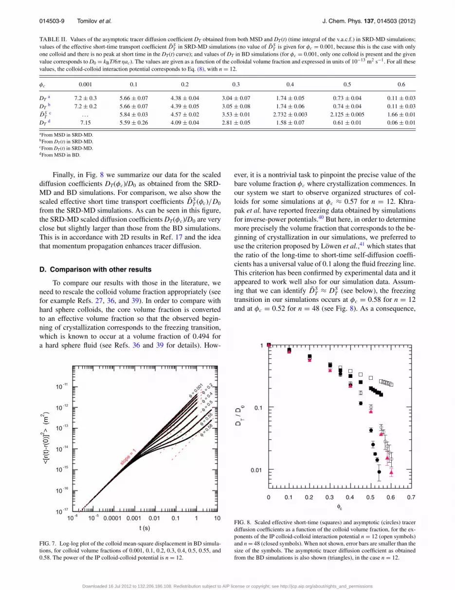
TABLE II. Values of the asymptotic tracer diffusion coefficient DT obtained from both MSD and DT(t) (time integral of the v.a.c.f.) in SRD-MD simulations;values of the effective short-time transport coefficient D̃S

T in SRD-MD simulations (no value of D̃ST is given for φc = 0.001, because this is the case with only

one colloid and there is no peak at short time in the DT(t) curve); and values of DT in BD simulations (for φc = 0.001, only one colloid is present and the givenvalue corresponds to D0 = kBT/6πηac). The values are given as a function of the colloidal volume fraction and expressed in units of 10−13 m2 s−1. For all thesevalues, the colloid-colloid interaction potential corresponds to Eq. (8), with n = 12.

φc 0.001 0.1 0.2 0.3 0.4 0.5 0.6

DTa 7.2 ± 0.3 5.66 ± 0.07 4.38 ± 0.04 3.04 ± 0.07 1.74 ± 0.05 0.73 ± 0.04 0.11 ± 0.03

DTb 7.2 ± 0.2 5.66 ± 0.07 4.39 ± 0.05 3.05 ± 0.08 1.74 ± 0.06 0.74 ± 0.04 0.11 ± 0.03

D̃ST

c . . . 5.84 ± 0.03 4.57 ± 0.02 3.53 ± 0.01 2.732 ± 0.003 2.125 ± 0.005 1.66 ± 0.01DT

d 7.15 5.59 ± 0.26 4.09 ± 0.04 2.81 ± 0.05 1.58 ± 0.07 0.61 ± 0.01 0.06 ± 0.01

aFrom MSD in SRD-MD.bFrom DT(t) in SRD-MD.cFrom DT(t) in SRD-MD.dFrom MSD in BD.

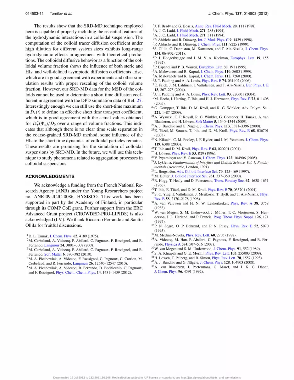
Finally, in Fig. 8 we summarize our data for the scaleddiffusion coefficients DT(φc)/D0 as obtained from the SRD-MD and BD simulations. For comparison, we also show thescaled effective short time transport coefficients D̃S

T (φc)/D0

from the SRD-MD simulations. As can be seen in this figure,the SRD-MD scaled diffusion coefficients DT(φc)/D0 are veryclose but slightly larger than those from the BD simulations.This is in accordance with 2D results in Ref. 17 and the ideathat momentum propagation enhances tracer diffusion.

D. Comparison with other results

To compare our results with those in the literature, weneed to rescale the colloid volume fraction appropriately (seefor example Refs. 27, 36, and 39). In order to compare withhard sphere colloids, the core volume fraction is convertedto an effective volume fraction so that the observed begin-ning of crystallization corresponds to the freezing transition,which is known to occur at a volume fraction of 0.494 fora hard sphere fluid (see Refs. 36 and 39 for details). How-

slope

= 1

φ = 0.0

01

φ = 0.2

φ = 0.4

φ = 0.5

8φ = 0.5

5φ =

0.5

10 -17

10 -16

10 -15

10 -14

10 -13

10 -12

10 -11

10 -6 10 -5 0.0001 0.001 0.01 0.1 1 10t (s)

FIG. 7. Log-log plot of the colloid mean-square displacement in BD simula-tions, for colloid volume fractions of 0.001, 0.1, 0.2, 0.3, 0.4, 0.5, 0.55, and0.58. The power of the IP colloid-colloid potential is n = 12.

ever, it is a nontrivial task to pinpoint the precise value of thebare volume fraction φc where crystallization commences. Inour system we start to observe organized structures of col-loids for some simulations at φc ≈ 0.57 for n = 12. Khra-pak et al. have reported freezing data obtained by simulationsfor inverse-power potentials.40 But here, in order to determinemore precisely the volume fraction that corresponds to the be-ginning of crystallization in our simulations, we preferred touse the criterion proposed by Löwen et al.,41 which states thatthe ratio of the long-time to short-time self-diffusion coeffi-cients has a universal value of 0.1 along the fluid freezing line.This criterion has been confirmed by experimental data and itappeared to work well also for our simulation data. Assum-ing that we can identify D̃S

T ≈ DST (see below), the freezing

transition in our simulations occurs at φc = 0.58 for n = 12and at φc = 0.52 for n = 48 (see Fig. 8). As a consequence,

0.01

0.1

1

0 0.1 0.2 0.3 0.4 0.5 0.6 0.7

φc

FIG. 8. Scaled effective short-time (squares) and asymptotic (circles) tracerdiffusion coefficients as a function of the colloid volume fraction, for the ex-ponents of the IP colloid-colloid interaction potential n = 12 (open symbols)and n = 48 (closed symbols). When not shown, error bars are smaller than thesize of the symbols. The asymptotic tracer diffusion coefficient as obtainedfrom the BD simulations is also shown (triangles), in the case n = 12.

Downloaded 16 Jul 2012 to 132.206.186.108. Redistribution subject to AIP license or copyright; see http://jcp.aip.org/about/rights_and_permissions

014503-10 Tomilov et al. J. Chem. Phys. 137, 014503 (2012)

0

0.2

0.4

0.6

0.8

1

0 0.1 0.2 0.3 0.4 0.5 0.6

Exp., Segrè et al. (1995)

Exp., van Megen et al. (1989)

SRD-MD, n=12

SRD-MD, n=48

LB, Segrè et al. (1995)

ASD, Banchio et al. (2008)

Φc

FIG. 9. Comparison of the effective quantity D̃ST /D0 from SRD-MD

results with the short-time diffusion coefficients as determined fromexperimental results36, 39 and other simulation results based on theLattice-Boltzmann (LB) (Ref. 36) and accelerated Stokesian dynamics(ASD).42 �c denotes the rescaled colloid volume fraction (see text fordetails).

in the following, we will use the rescaled volume fractions�c = 0.494

0.58 φc for n = 12, and �c = 0.4940.52 φc for n = 48.

Considering first the issue of the short-time diffusion co-efficient, Fig. 9 shows the comparison between our effectivevalues D̃S

T (�c)/D0, experimental results,36, 39 and simulationresults from Lattice-Boltzmann36 and accelerated Stokesiandynamics42 techniques. In all these other cases, a well-definedvalue of the short time diffusion coefficient DS

T was deter-mined. Our effective D̃S

T (especially for the case n = 48) turnout to be in good agreement with all the other results, despitethe fact that using the MSD it was not possible to determineany short time diffusive behavior. This agreement indicatesthat some features of the expected microscopic behavior atshort times are present in the SRD-MD simulations despitethe coarse-grained nature of the solvent.

In Fig. 10, we compare our data for the true (long time)diffusion coefficients with those obtained from experimen-tal results,35, 39, 43 and other simulation results from the DPD(Ref. 27) technique. The difference observed in our simula-tions between n = 12 and n = 48 after the rescaling of thevolume fraction shows that the long-time diffusion coefficientis affected by the colloid-colloid interaction potential. Quitea good agreement is obtained in between our simulation re-sults (especially with n = 12) and experimental data. Exceptfor the highest volume fractions, our SRD-MD simulation re-sults fit the experimental data better than the DPD simulationresults from Pryamitsyn et al.,27 where hydrodynamic interac-tions are included and where a 6-12 Lennard-Jones potentialis used for the colloid-colloid interaction. It is worth notingthat, in their study, they also rescale the colloid volume frac-tion but using a different criterion. They estimated from theirsimulation results that the large-scale particle diffusion is ar-

0.001

0.01

0.1

1

0 0.1 0.2 0.3 0.4 0.5 0.6

Φc

Exp., van Blaaderen et al. (1992)

Exp., van Megen et al. (1989, 1997)

SRD-MD, n=12

SRD-MD, n=48

DPD, Pryamitsyn et al. (2005)

FIG. 10. Asymptotic diffusion coefficient: comparison of our simulation re-sults with experimental results from Refs. 35, 39, and 43 and with other sim-ulation results using dissipative particle dynamics (DPD).27 �c denotes therescaled colloid volume fraction (see text for details).

rested at 0.68, while it is known to occur at the glass transitionvolume fraction of 0.58 in a hard sphere fluid, so that in theircase �c = 0.58

0.68φc. This rescaling is essentially the same as theone we used for n = 12. In their study, the colloid-colloidinteraction is treated by a 6-12 Lennard-Jones potential. Ac-cording to the shape of this potential, which is in between theIP potential with n = 12 and the one with n = 48 (see Fig. 1),it seems that the rescaling they used slightly overestimates thecorrection applied to the data.

IV. CONCLUSIONS

In this work, we have studied the colloid tracer diffusioncoefficients in a realistic model of a colloidal suspension bymeans of SRD-MD simulations. This technique has been cho-sen because of its efficiency to solve the hydrodynamics ofcolloids embedded in a liquid and subject to thermal fluctu-ations. SRD and MD have been used to simulate the dynam-ics of the solvent and of the colloids, respectively. These twoparts are coupled by the introduction of a colloid-fluid inter-action potential that intervenes in the MD steps. Special atten-tion has been paid in the choice of the SRD parameters andof the various scales in order to keep a balance between goodresolution and computational cost. The linear size of collisioncells has been chosen to be equal to half the colloid radius andthe mean free path of the fluid particles to one tenth of thissize. As a consequence, the grid shifting procedure has beenused in order to preserve Galilean invariance. The time scalehas been adjusted so that the simulation correctly reproducesthe colloid diffusion time. The colloid-fluid interaction poten-tial has been tuned such that the fluid particles can penetratein between two colloids in order to avoid spurious depletionattraction between the colloids.

Downloaded 16 Jul 2012 to 132.206.186.108. Redistribution subject to AIP license or copyright; see http://jcp.aip.org/about/rights_and_permissions

014503-11 Tomilov et al. J. Chem. Phys. 137, 014503 (2012)

The results show that the SRD-MD technique employedhere is capable of properly including the essential features ofthe hydrodynamic interactions in a colloidal suspension. Thecomputation of the colloid tracer diffusion coefficient underhigh dilution for different system sizes exhibits long-rangehydrodynamic effects in agreement with theoretical predic-tions. The colloidal diffusive behavior as a function of the col-loidal volume fraction shows the influence of both steric andHIs, and well-defined asymptotic diffusion coefficients arise,which are in good agreement with experiments and other sim-ulation results with proper rescaling of the colloid volumefraction. However, our SRD-MD data for the MSD of the col-loids cannot be used to determine a short time diffusion coef-ficient in agreement with the DPD simulation data of Ref. 27.Interestingly enough we can still use the short-time maximumin DT(t) to define an effective short time transport coefficient,which is in good agreement with the actual values obtainedfor DS

T (�c)/D0 over a range of volume fractions. This indi-cates that although there is no clear time scale separation inthe coarse-grained SRD-MD method, some influence of theHIs to the short time dynamics of colloidal particles remains.These results are promising for the simulation of colloidalsuspensions by SRD-MD. In the future, we will use this tech-nique to study phenomena related to aggregation processes incolloidal suspensions.

ACKNOWLEDGMENTS

We acknowledge a funding from the French National Re-search Agency (ANR) under the Young Researchers projectno. ANR-09-JCJC-0086, HYSISCO. This work has beensupported in part by the Academy of Finland, in particularthrough its COMP CoE grant. Further support from the ERCAdvanced Grant project (CROWDED-PRO-LIPIDS) is alsoacknowledged (I.V.). We thank Riccardo Ferrando and SanttuOllila for fruitful discussions.

1D. L. Ermak, J. Chem. Phys. 62, 4189 (1975).2M. Cerbelaud, A. Videcoq, P. Abélard, C. Pagnoux, F. Rossignol, and R.Ferrando, Langmuir 24, 3001–3008 (2008).

3M. Cerbelaud, A. Videcoq, P. Abélard, C. Pagnoux, F. Rossignol, and R.Ferrando, Soft Matter 6, 370–382 (2010).

4M. A. Piechowiak, A. Videcoq, F. Rossignol, C. Pagnoux, C. Carrion, M.Cerbelaud, and R. Ferrando, Langmuir 26, 12540–12547 (2010).

5M. A. Piechowiak, A. Videcoq, R. Ferrando, D. Bochicchio, C. Pagnoux,and F. Rossignol, Phys. Chem. Chem. Phys. 14, 1431–1439 (2012).

6J. F. Brady and G. Bossis, Annu. Rev. Fluid Mech. 20, 111 (1988).7A. J. C. Ladd, J. Fluid Mech. 271, 285 (1994).8A. J. C. Ladd, J. Fluid Mech. 271, 311 (1994).9P. Ahlrichs and B. Dünweg, Int. J. Mod. Phys. C 9, 1429 (1998).

10P. Ahlrichs and B. Dünweg, J. Chem. Phys. 111, 8225 (1999).11S. Ollila, C. Denniston, M. Karttunen, and T. Ala-Nissila, J. Chem. Phys.

134, 064902 (2011).12P. J. Hoogerbrugge and J. M. V. A. Koelman, Europhys. Lett. 19, 155

(1992).13P. Español and P. B. Warren, Europhys. Lett. 30, 191 (1995).14A. Malevanets and R. Kapral, J. Chem. Phys. 110, 8605 (1999).15A. Malevanets and R. Kapral, J. Chem. Phys. 112, 7260 (2000).16J. T. Padding and A. A. Louis, Phys. Rev. E 74, 031402 (2006).17E. Falck, J. M. Lahtinen, I. Vattulainen, and T. Ala-Nissila, Eur. Phys. J. E

13, 267–275 (2004).18J. T. Padding and A. A. Louis, Phys. Rev. Lett. 93, 220601 (2004).19M. Hecht, J. Harting, T. Ihle, and H. J. Herrmann, Phys. Rev. E 72, 011408

(2005).20G. Gompper, T. Ihle, D. M. Kroll, and R. G. Winkler, Adv. Polym. Sci.

221, 1–87 (2009).21A. Wysocki, C. P. Royall, R. G. Winkler, G. Gompper, H. Tanaka, A. van

Blaaderen, and H. Löwen, Soft Matter 5, 1340–1344 (2009).22A. J. Banchio and G. Nägele, J. Chem. Phys. 113, 3381–3396 (2000).23E. Tüzel, M. Strauss, T. Ihle, and D. M. Kroll, Phys. Rev. E 68, 036701

(2003).24N. Kikuchi, C. M. Pooley, J. F. Ryder, and J. M. Yeomans, J. Chem. Phys.

119, 6388 (2003).25T. Ihle and D. M. Kroll, Phys. Rev. E 63, 020201 (2001).26H. Löwen, Phys. Rev. E 53, R29 (1996).27V. Pryamitsyn and V. Ganesan, J. Chem. Phys. 122, 104906 (2005).28J. Lyklema, Fundamentals of Interface and Colloid Science, Vol. 1: Funda-

mentals (Academic, London, 1991).29L. Bergström, Adv. Colloid Interface Sci. 70, 125–169 (1997).30M. Hütter, J. Colloid Interface Sci. 231, 337–350 (2000).31R. Hogg, T. Healy, and D. Fuerstenau, Trans. Faraday Soc. 62, 1638–1651

(1966).32T. Ihle, E. Tüzel, and D. M. Kroll, Phys. Rev. E 70, 035701 (2004).33S. C. Ying, I. Vattulainen, J. Merikoski, T. Hjelt, and T. Ala-Nissila, Phys.

Rev. B 58, 2170–2178 (1998).34A. van Veluwen and H. N. W. Lekkerkerker, Phys. Rev. A 38, 3758

(1988).35W. van Megen, S. M. Underwood, J. Müller, T. C. Mortensen, S. Hen-

derson, J. L. Harland, and P. Francis, Prog. Theor. Phys. Suppl. 126, 171(1997).

36P. N. Segrè, O. P. Behrend, and P. N. Pusey, Phys. Rev. E 52, 5070(1995).

37M. Medina-Noyola, Phys. Rev. Lett. 60, 2705 (1988).38A. Videcoq, M. Han, P. Abélard, C. Pagnoux, F. Rossignol, and R. Fer-

rando, Physica A 374, 507–516 (2007).39W. van Megen and S. M. Underwood, J. Chem. Phys. 91, 552 (1989).40S. A. Khrapak and G. E. Morfill, Phys. Rev. Lett. 103, 255003 (2009).41H. Löwen, T. Palberg, and R. Simon, Phys. Rev. Lett. 70, 1557 (1993).42A. J. Banchio and G. Nägele, J. Chem. Phys. 128, 104903 (2008).43A. van Blaaderen, J. Peetermans, G. Maret, and J. K. G. Dhont,

J. Chem. Phys. 96, 4591 (1992).

Downloaded 16 Jul 2012 to 132.206.186.108. Redistribution subject to AIP license or copyright; see http://jcp.aip.org/about/rights_and_permissions