Embed Size (px)
Citation preview
Trade and Labor Market Institutions:
A Tale of Two Liberalizations
Alessandro Ruggieri∗
University of Nottingham
April 12, 2021
Abstract
How do labor market policies interact with trade reforms? Do minimum wage
regulation and employment protection legislation hamper the gains from trade? Are
these regulations effective in protecting workers from import competition? I answer
these questions by studying how labor market institutions at the time of a trade reform
determine the dynamic adjustment to trade. I first document that for a large group of
developing countries (1) unemployment increases following a trade reform, and (2) the
response is stronger when the firing costs are lower and the statutory minimum wage
is higher. I interpret this evidence through the lens of a model of international trade,
featuring heterogeneous firms, endogenous industry dynamics and search and matching
frictions in a dual labor market. I calibrate the model to match the pre-liberalization
firm and labor market dynamics in Colombia and Mexico, two countries that differed
by the labor regulations in place at the time of trade liberalization, and I solve the full
transition path towards the new steady state. I show that lower firing costs and higher
minimum wage enhance firm selection following a trade liberalization, fostering short-
and long-run gains from trade at the expense of higher job reallocation between and
within industries, and higher unemployment. Taken together, these two institutions
can explain around 30% of the short-run and up to 60% of the long-run cross-country
difference in unemployment response to a fall in trade costs. Finally, I find that a
strong efficiency-equity trade-off arises as an economy reduces employment rigidities
in favor of stronger downward wage rigidities.
Keywords: Trade reforms, labor market institutions, unemployment, transitional
dynamics, gains from trade, inequality
JEL Classification: E24, F12, F16, L11
∗Contact: School of Economics, Sir Clive Granger Building, University of Nottingham, University Park,NG7 2RD, Nottingham, [email protected]. I am indebted to Nezih Guner and Jim Tybout fortheir help and suggestions. I would also like to thank Chris Busch, Paula Bustos, Lorenzo Caliendo, Rus-sell Cooper, Rafael Dix-Carneiro, Swati Dhringa, Andres Erosa, Marcela Eslava, Giammario Impullitti,Omar Licandro, Tim Lee, Alejandro Riano, Raul Santaeulalia, Jaume Ventura, Neil Wallace and SteveYeaple for their comments along different stages of the paper, and the department of Economics at PennState University and CEMFI for the hospitality offered during the final stage of this project. The usualdisclaimers apply.
1
1 Introduction
Over the past 50 years, most developing countries have embarked on programs of trade
liberalization and become integrated into the global product market.1 Empirically, trade
reforms have been shown to trigger significant employment adjustments, sometimes with
adverse effects on labor markets, in most cases with a prolonged increase in unemployment
(Figure 1).2 While workers reallocation constitutes an important margin of labor market
adjustment in response to trade shocks,3 growing concerns is forming about the role of labor
market institutions in distorting the adjustments to trade, thus hampering the potential
gains from trade.4
In this paper I study how labor market regulations interact with the dynamics of labor
market adjustments to trade liberalization. Labor regulations in place at the eve of a trade
reform vary greatly among countries. Some countries adopted free-trade policies with flexible
labor market institutions, while others did so with more rigid ones.5 Nevertheless, at the
time of trade opening, most of the local labor markets were highly regulated but with limited
active labor market policies.6 Table 1 reproduces this evidence and reports the statutory
minimum wage, measures of firing restrictions (employment protection legislation, EPL) and
unemployment insurance (UI) for a sample of developing countries at the time of a trade
reform. The burden of regulation on employment protection was high in the majority of
the countries in the sample. The total firing costs per employee, which consists of costs
associated with advance notice (AN) and severance payments (SP), were about 6 months
of real average wage, a value more than twice higher than that observed for instance in
France between the ′80s and ′90s, and almost three times higher than that in place in Italy
during the same two decades.7 On the other hand, unemployment insurance was limited in
1See Rodrik (1993) for a comprehensive overview of the trade policy reforms in developing countries.2On the effect of trade openness on unemployment and inequality in developing countries, see, for in-
stance, Revenga (1997) and Airola and Juhn (2008) for the case of Mexico, Currie and Harrison (1997)for Morocco, Goldberg and Pavcnik (2004) for Colombia, Kpodar (2007) for Algeria, Peluffo (2013) forUruguay, Nicita (2008) for Madagascar, Balat and Porto (2007) for Zambia, Hasan et al. (2012) for Indiaand Menezes-Filho and Muendler (2011) and Dix-Carneiro and Kovak (2017) for Brazil. See Bellon (2016)for an cross-country study.3For a summary about the margins of adjustment to trade in developing countries, consequence of trade
reforms and policy recommendation, see Hoekman and Porto (2010) and Pavcnik (2017).4Concerns about the interaction between trade reforms and institutions have been manifested, among the
others, in Zagha et al. (2005) and in Rodrik (2008).5Freeman (2007) and Freeman (2010) document large cross-country differences in labor institutions for
a spectrum of developing countries, with particular focus on government regulations, as dismissal costs,social security and minimum wage policies. See Heckman and Pages (2004) for a description of the labormarket institutions in place in LAC countries, the nature of the reforms implemented, and the link withtrade liberalization.6In a report prepared by the World Bank for Latin America and the Caribbean, Burki and Perry (1997)
write that “labor market reform is the area of structural reform where the least progress has been madein the region”. In the same spirit, the IADB (1997) concludes: “labor code reforms have been few and notvery deep,” adding that “current labor legislation may have hindered the re-absorption of workers whowere displaced during the reform process”. See Forteza and Rama (2006) for a summary.7Source: FRdB Labor Institution v.1 database
2
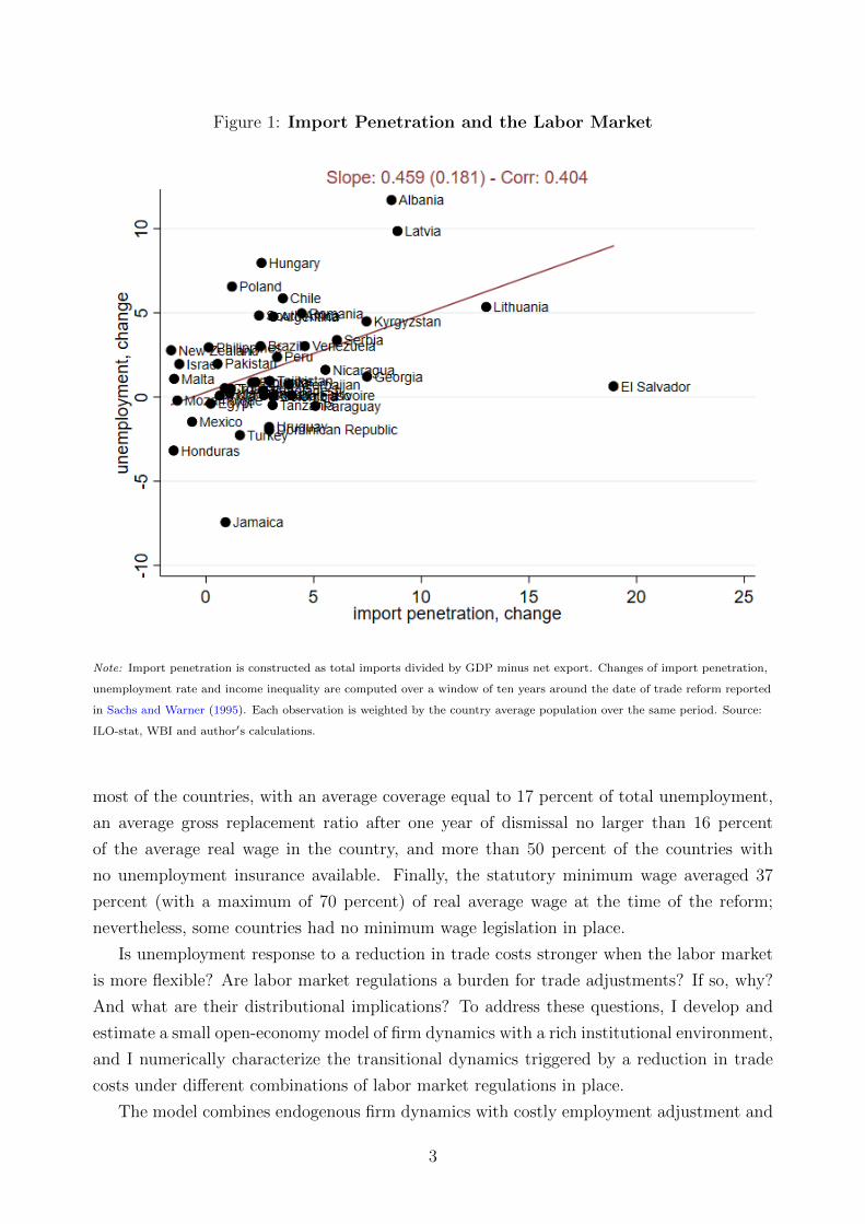
Figure 1: Import Penetration and the Labor Market
Note: Import penetration is constructed as total imports divided by GDP minus net export. Changes of import penetration,
unemployment rate and income inequality are computed over a window of ten years around the date of trade reform reported
in Sachs and Warner (1995). Each observation is weighted by the country average population over the same period. Source:
ILO-stat, WBI and author′s calculations.
most of the countries, with an average coverage equal to 17 percent of total unemployment,
an average gross replacement ratio after one year of dismissal no larger than 16 percent
of the average real wage in the country, and more than 50 percent of the countries with
no unemployment insurance available. Finally, the statutory minimum wage averaged 37
percent (with a maximum of 70 percent) of real average wage at the time of the reform;
nevertheless, some countries had no minimum wage legislation in place.
Is unemployment response to a reduction in trade costs stronger when the labor market
is more flexible? Are labor market regulations a burden for trade adjustments? If so, why?
And what are their distributional implications? To address these questions, I develop and
estimate a small open-economy model of firm dynamics with a rich institutional environment,
and I numerically characterize the transitional dynamics triggered by a reduction in trade
costs under different combinations of labor market regulations in place.
The model combines endogenous firm dynamics with costly employment adjustment and
3
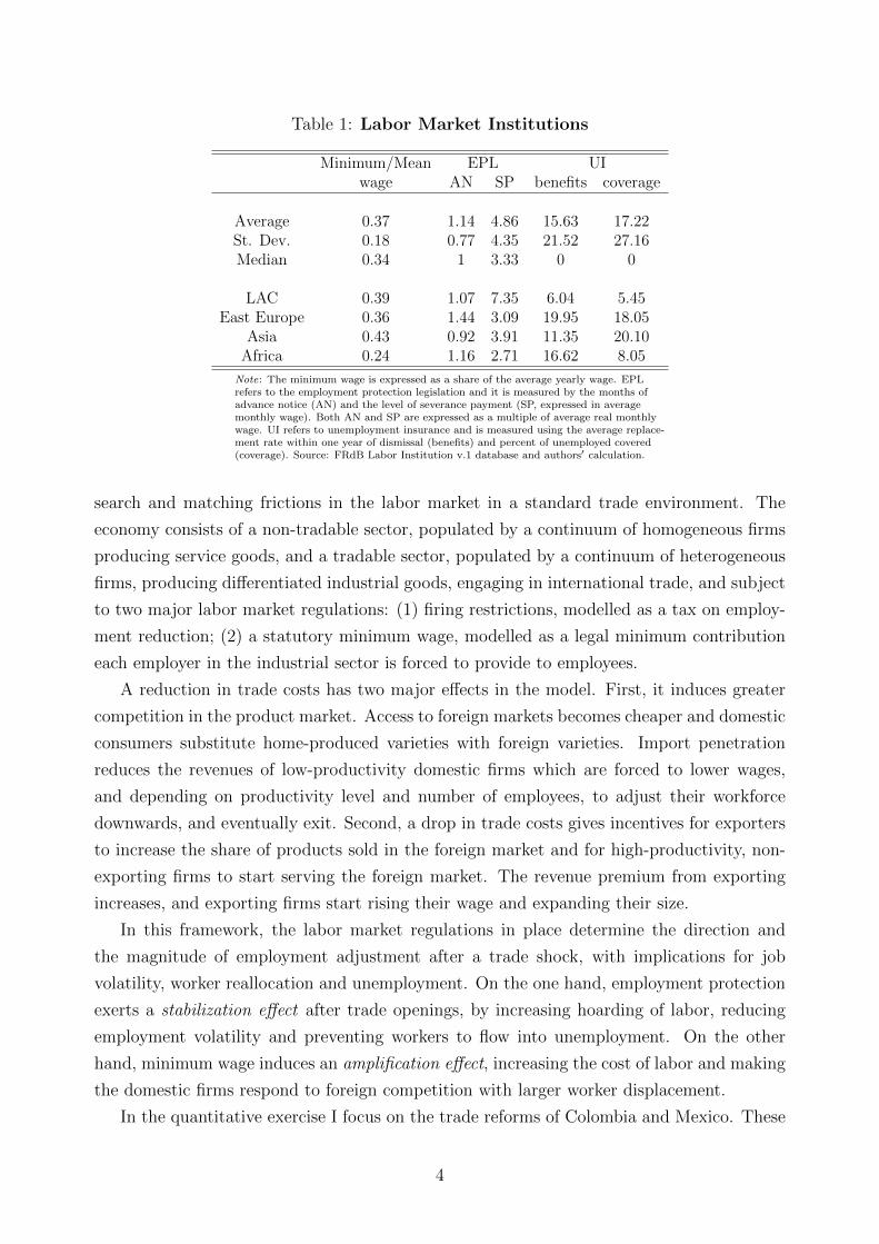
Table 1: Labor Market Institutions
Minimum/Mean EPL UIwage AN SP benefits coverage
Average 0.37 1.14 4.86 15.63 17.22St. Dev. 0.18 0.77 4.35 21.52 27.16Median 0.34 1 3.33 0 0
LAC 0.39 1.07 7.35 6.04 5.45East Europe 0.36 1.44 3.09 19.95 18.05
Asia 0.43 0.92 3.91 11.35 20.10Africa 0.24 1.16 2.71 16.62 8.05
Note: The minimum wage is expressed as a share of the average yearly wage. EPLrefers to the employment protection legislation and it is measured by the months ofadvance notice (AN) and the level of severance payment (SP, expressed in averagemonthly wage). Both AN and SP are expressed as a multiple of average real monthlywage. UI refers to unemployment insurance and is measured using the average replace-ment rate within one year of dismissal (benefits) and percent of unemployed covered(coverage). Source: FRdB Labor Institution v.1 database and authors′ calculation.
search and matching frictions in the labor market in a standard trade environment. The
economy consists of a non-tradable sector, populated by a continuum of homogeneous firms
producing service goods, and a tradable sector, populated by a continuum of heterogeneous
firms, producing differentiated industrial goods, engaging in international trade, and subject
to two major labor market regulations: (1) firing restrictions, modelled as a tax on employ-
ment reduction; (2) a statutory minimum wage, modelled as a legal minimum contribution
each employer in the industrial sector is forced to provide to employees.
A reduction in trade costs has two major effects in the model. First, it induces greater
competition in the product market. Access to foreign markets becomes cheaper and domestic
consumers substitute home-produced varieties with foreign varieties. Import penetration
reduces the revenues of low-productivity domestic firms which are forced to lower wages,
and depending on productivity level and number of employees, to adjust their workforce
downwards, and eventually exit. Second, a drop in trade costs gives incentives for exporters
to increase the share of products sold in the foreign market and for high-productivity, non-
exporting firms to start serving the foreign market. The revenue premium from exporting
increases, and exporting firms start rising their wage and expanding their size.
In this framework, the labor market regulations in place determine the direction and
the magnitude of employment adjustment after a trade shock, with implications for job
volatility, worker reallocation and unemployment. On the one hand, employment protection
exerts a stabilization effect after trade openings, by increasing hoarding of labor, reducing
employment volatility and preventing workers to flow into unemployment. On the other
hand, minimum wage induces an amplification effect, increasing the cost of labor and making
the domestic firms respond to foreign competition with larger worker displacement.
In the quantitative exercise I focus on the trade reforms of Colombia and Mexico. These
4
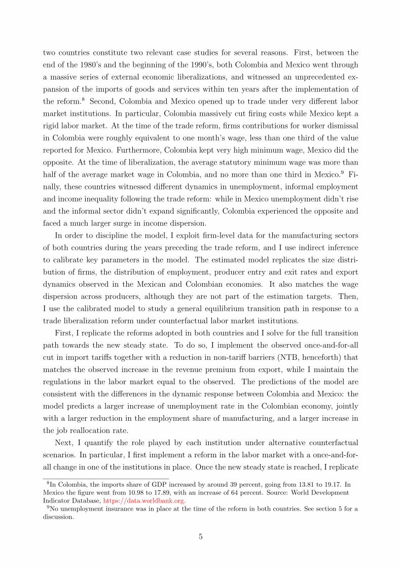
two countries constitute two relevant case studies for several reasons. First, between the
end of the 1980’s and the beginning of the 1990’s, both Colombia and Mexico went through
a massive series of external economic liberalizations, and witnessed an unprecedented ex-
pansion of the imports of goods and services within ten years after the implementation of
the reform.8 Second, Colombia and Mexico opened up to trade under very different labor
market institutions. In particular, Colombia massively cut firing costs while Mexico kept a
rigid labor market. At the time of the trade reform, firms contributions for worker dismissal
in Colombia were roughly equivalent to one month’s wage, less than one third of the value
reported for Mexico. Furthermore, Colombia kept very high minimum wage, Mexico did the
opposite. At the time of liberalization, the average statutory minimum wage was more than
half of the average market wage in Colombia, and no more than one third in Mexico.9 Fi-
nally, these countries witnessed different dynamics in unemployment, informal employment
and income inequality following the trade reform: while in Mexico unemployment didn’t rise
and the informal sector didn’t expand significantly, Colombia experienced the opposite and
faced a much larger surge in income dispersion.
In order to discipline the model, I exploit firm-level data for the manufacturing sectors
of both countries during the years preceding the trade reform, and I use indirect inference
to calibrate key parameters in the model. The estimated model replicates the size distri-
bution of firms, the distribution of employment, producer entry and exit rates and export
dynamics observed in the Mexican and Colombian economies. It also matches the wage
dispersion across producers, although they are not part of the estimation targets. Then,
I use the calibrated model to study a general equilibrium transition path in response to a
trade liberalization reform under counterfactual labor market institutions.
First, I replicate the reforms adopted in both countries and I solve for the full transition
path towards the new steady state. To do so, I implement the observed once-and-for-all
cut in import tariffs together with a reduction in non-tariff barriers (NTB, henceforth) that
matches the observed increase in the revenue premium from export, while I maintain the
regulations in the labor market equal to the observed. The predictions of the model are
consistent with the differences in the dynamic response between Colombia and Mexico: the
model predicts a larger increase of unemployment rate in the Colombian economy, jointly
with a larger reduction in the employment share of manufacturing, and a larger increase in
the job reallocation rate.
Next, I quantify the role played by each institution under alternative counterfactual
scenarios. In particular, I first implement a reform in the labor market with a once-and-for-
all change in one of the institutions in place. Once the new steady state is reached, I replicate
8In Colombia, the imports share of GDP increased by around 39 percent, going from 13.81 to 19.17. InMexico the figure went from 10.98 to 17.89, with an increase of 64 percent. Source: World DevelopmentIndicator Database, https://data.worldbank.org.9No unemployment insurance was in place at the time of the reform in both countries. See section 5 for a
discussion.
5
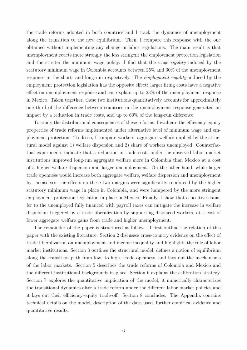
the trade reforms adopted in both countries and I track the dynamics of unemployment
along the transition to the new equilibrium. Then, I compare this response with the one
obtained without implementing any change in labor regulations. The main result is that
unemployment reacts more strongly the less stringent the employment protection legislation
and the stricter the minimum wage policy. I find that the wage rigidity induced by the
statutory minimum wage in Colombia accounts between 25% and 30% of the unemployment
response in the short- and long-run respectively. The employment rigidity induced by the
employment protection legislation has the opposite effect: larger firing costs have a negative
effect on unemployment response and can explain up to 23% of the unemployment response
in Mexico. Taken together, these two institutions quantitatively accounts for approximately
one third of the difference between countries in the unemployment response generated on
impact by a reduction in trade costs, and up to 60% of the long-run difference.
To study the distributional consequences of these reforms, I evaluate the efficiency-equity
properties of trade reforms implemented under alternative level of minimum wage and em-
ployment protection. To do so, I compare workers’ aggregate welfare implied by the struc-
tural model against 1) welfare dispersion and 2) share of workers unemployed. Counterfac-
tual experiments indicate that a reduction in trade costs under the observed labor market
institutions improved long-run aggregate welfare more in Colombia than Mexico at a cost
of a higher welfare dispersion and larger unemployment. On the other hand, while larger
trade openness would increase both aggregate welfare, welfare dispersion and unemployment
by themselves, the effects on these two margins were significantly reinforced by the higher
statutory minimum wage in place in Colombia, and were hampered by the more stringent
employment protection legislation in place in Mexico. Finally, I show that a positive trans-
fer to the unemployed fully financed with payroll taxes can mitigate the increase in welfare
dispersion triggered by a trade liberalization by supporting displaced workers, at a cost of
lower aggregate welfare gains from trade and higher unemployment.
The remainder of the paper is structured as follows. I first outline the relation of this
paper with the existing literature. Section 2 discusses cross-country evidence on the effect of
trade liberalization on unemployment and income inequality and highlights the role of labor
market institutions. Section 3 outlines the structural model, defines a notion of equilibrium
along the transition path from low- to high- trade openness, and lays out the mechanisms
of the labor markets. Section 5 describes the trade reforms of Colombia and Mexico and
the different institutional backgrounds in place. Section 6 explains the calibration strategy.
Section 7 explores the quantitative implication of the model, it numerically characterizes
the transitional dynamics after a trade reform under the different labor market policies and
it lays out their efficiency-equity trade-off. Section 8 concludes. The Appendix contains
technical details on the model, description of the data used, further empirical evidence and
quantitative results.
6
1.1 Review of related literature
This paper relates to a number of literatures. First, it contributes to the recent literature
that studies the joint effects of labor market frictions and trade reforms. To this extent,
this paper is close to Helpman and Itskhoki (2010), Helpman et al. (2010) and Felbermayr
et al. (2016) who focus on the long-run impact of globalization and labor market rigidities
on job volatility, unemployment rate and the distribution of wages.10 Within this literature,
Fajgelbaum (2016) embeds job-to-job transition into a trade environment to study how
search frictions impede exporting firms to grow in response to reduction in trade costs.
Cosar et al. (2016) estimate a structural steady-state model using Colombian firm-level data
to quantify the contribution of trade and labor market reforms on the observed increase
in wage inequality and job volatility. Unlike these papers, I focus on the consequences of
labor market institutions for transitional dynamics in a framework where firms costly adjust
employment and workers transit from employment to unemployment as a response to a
fall in trade costs. I quantitatively characterize the differential impact of trade reforms on
unemployment rate and income inequality along the entire transition path between different
steady states, through ongoing productivity shocks, endogenous firm entry and exit, and
endogenous job creation and destruction. More importantly, I study the complementarities
between labor-market policies and trade reforms, a margin the trade literature has largely
abstracted from (Atkin and Khandelwal, 2020).
Existing models with transitional dynamics have primarily focused on two main key
dimensions: the reallocation of workers with different levels of human capital across sectors,
and reallocation of heterogeneous jobs between firms within the same sector, in frameworks
with labor market frictions. Papers like Cosar (2013) and Dix-Carneiro (2014) belong to
the first group: they develop models where workers slowly accumulate sector-specific human
capital, and can costly switch between sectors, to study the distributional response to a trade
shock.11 This paper instead belongs to the literature that focuses on the role of employment
adjustments, preventing firms to instantaneously adjust to changes in the product market.
To this extent, it is close to Itskhoki and Helpman (2015) who use a two-country two-sector
model to study how jobs and workers reallocate along the entire transition path after a
change in trade costs, and to Bellon (2016) who develops a model of directed search in the
labor market and costly firms′ screening of workers to micro-found the dynamic response
of inequality to a trade liberalization. These papers also show that lower trade costs could
10Empirical papers on this subject include, among others, Amiti and Cameron (2012) and Helpman et al.(2017).11Empirical evidence has shown instead that most of the workers and job reallocation after a trade lib-eralization occurs within sectors. Wacziarg and Wallack (2004) use 25 episodes of trade liberalization toprovide evidence of weak intersectoral labor movements after a trade reform. Haltiwanger et al. (2004)document the association between job turnover and openness in Latin America.Bernanrd et al. (2003) es-timates substantial effect of a trade liberalization on inter-sectoral job turnover using the US Census ofManufacturing.
7
induce a short-run increase in unemployment and income inequality. Unlike these papers,
my model links the response of unemployment to the regulations in place at the time of
a trade reform, a feature they both abstract from, generating in comparison much richer
responses of firms to a trade liberalization.
Finally, this paper speaks about the effects of labor market institutions on unemploy-
ment, aggregate income and income inequality. To this regard, this paper follows Bentolila
and Bertola (1990), Hopenhayn and Rogerson (1993), and, among all, to Alvarez and Ve-
racierto (2000), who explore to which extent differences in labor market policies, such as
minimum wages, firing restrictions, unemployment insurance, and unions, can generate dif-
ferences in labor-market performance and aggregate efficiency. Kambourov (2009) uses a
general equilibrium model of international trade to study the effect of firing costs on the
speed of inter-sectoral reallocation of workers after a trade shock. Instead, I focus on the
intra-sectoral reallocation of labor triggered by a fall in trade costs, and the potential in-
crease in unemployment during transition. Dix-Carneiro and Kovak (2017) and McCaig
and Pavcnik (2014) document that shifts into or out of unemployment and non-employment
constitute important margins of labor market adjustment to trade. To this purpose, search
and matching frictions in the labor market allow me to study how a reduction in trade costs
links to worker displacement and unemployment in a setting where labor market institutions
induce rigidities on both quantities and wages.
2 Aggregate evidence
In this section, I document the dynamics of the unemployment rate around episodes of trade
liberalization. In particular, I focus on a subset of countries who embraced a trade reform
during the last 50 years. I track the labor marker dynamics in each country before and after
the trade reform and I relate it to the degree of employment protection, minimum wages
and unemployment insurance observed at the time of trade liberalization.
The event study I conduct mainly draws from four data sources. To identify periods of
trade openness, I use the liberalization dates reported by Wacziarg and Welch (2003), which
are based on those developed by Sachs and Warner (1995), and I construct a country-specific
dummy variable taking value one in each period after this date. To capture the strength of
different labor market institutions, I rely on the data provided by the Fondazione Rodolfo
de Benedetti (FRdb-IMF labor institutions database v.1).12 In particular, I use the ratio
between the statutory minimum wage in place and the average market wage as a proxy for
the minimum wage legislation, while I use the average number of months of advance notice in
case of dismissal plus the average compensation for dismissal over different seniority horizons
12The FRdb-IMF labor institutions database collects information on minimum wages, unemployment ben-efits and employment protection legislation around the world. It covers a set of 91 countries and a timespan from 1980 to 2005. Source: http://www.frdb.org/page/data/categoria/international-data
8
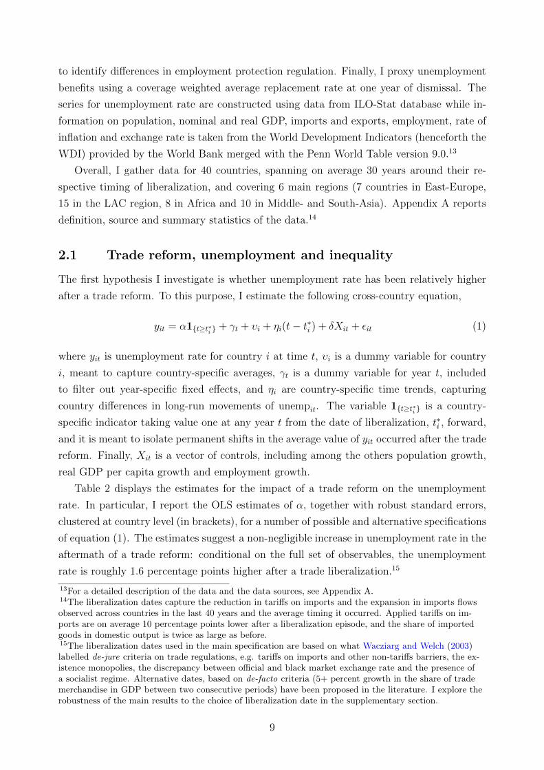
to identify differences in employment protection regulation. Finally, I proxy unemployment
benefits using a coverage weighted average replacement rate at one year of dismissal. The
series for unemployment rate are constructed using data from ILO-Stat database while in-
formation on population, nominal and real GDP, imports and exports, employment, rate of
inflation and exchange rate is taken from the World Development Indicators (henceforth the
WDI) provided by the World Bank merged with the Penn World Table version 9.0.13
Overall, I gather data for 40 countries, spanning on average 30 years around their re-
spective timing of liberalization, and covering 6 main regions (7 countries in East-Europe,
15 in the LAC region, 8 in Africa and 10 in Middle- and South-Asia). Appendix A reports
definition, source and summary statistics of the data.14
2.1 Trade reform, unemployment and inequality
The first hypothesis I investigate is whether unemployment rate has been relatively higher
after a trade reform. To this purpose, I estimate the following cross-country equation,
yit = α1t≥t∗i + γt + υi + ηi(t− t∗i ) + δXit + εit (1)
where yit is unemployment rate for country i at time t, υi is a dummy variable for country
i, meant to capture country-specific averages, γt is a dummy variable for year t, included
to filter out year-specific fixed effects, and ηi are country-specific time trends, capturing
country differences in long-run movements of unempit. The variable 1t≥t∗i is a country-
specific indicator taking value one at any year t from the date of liberalization, t∗i , forward,
and it is meant to isolate permanent shifts in the average value of yit occurred after the trade
reform. Finally, Xit is a vector of controls, including among the others population growth,
real GDP per capita growth and employment growth.
Table 2 displays the estimates for the impact of a trade reform on the unemployment
rate. In particular, I report the OLS estimates of α, together with robust standard errors,
clustered at country level (in brackets), for a number of possible and alternative specifications
of equation (1). The estimates suggest a non-negligible increase in unemployment rate in the
aftermath of a trade reform: conditional on the full set of observables, the unemployment
rate is roughly 1.6 percentage points higher after a trade liberalization.15
13For a detailed description of the data and the data sources, see Appendix A.14The liberalization dates capture the reduction in tariffs on imports and the expansion in imports flowsobserved across countries in the last 40 years and the average timing it occurred. Applied tariffs on im-ports are on average 10 percentage points lower after a liberalization episode, and the share of importedgoods in domestic output is twice as large as before.15The liberalization dates used in the main specification are based on what Wacziarg and Welch (2003)labelled de-jure criteria on trade regulations, e.g. tariffs on imports and other non-tariffs barriers, the ex-istence monopolies, the discrepancy between official and black market exchange rate and the presence ofa socialist regime. Alternative dates, based on de-facto criteria (5+ percent growth in the share of trademerchandise in GDP between two consecutive periods) have been proposed in the literature. I explore therobustness of the main results to the choice of liberalization date in the supplementary section.
9
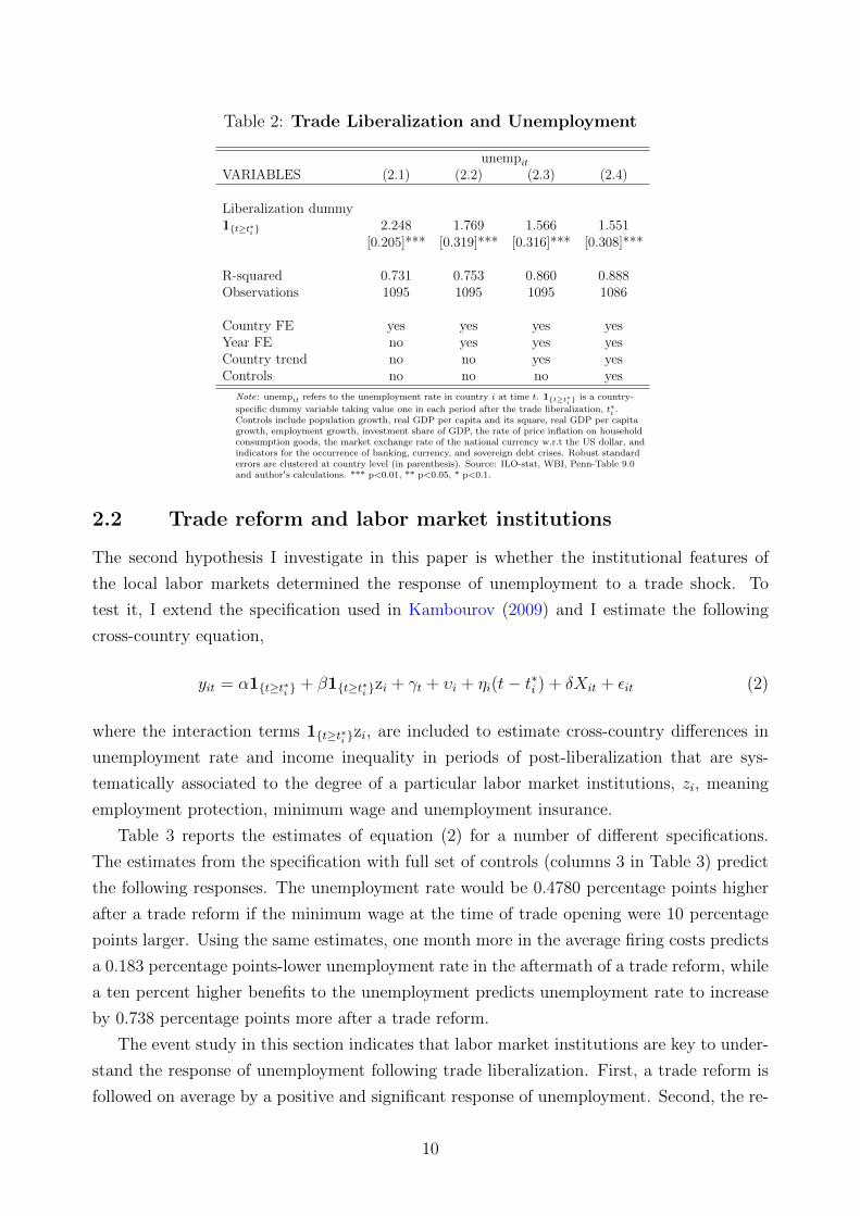
Table 2: Trade Liberalization and Unemployment
unempitVARIABLES (2.1) (2.2) (2.3) (2.4)
Liberalization dummy1t≥t∗i 2.248 1.769 1.566 1.551
[0.205]*** [0.319]*** [0.316]*** [0.308]***
R-squared 0.731 0.753 0.860 0.888Observations 1095 1095 1095 1086
Country FE yes yes yes yesYear FE no yes yes yesCountry trend no no yes yesControls no no no yes
Note: unempit refers to the unemployment rate in country i at time t. 1t≥t∗i is a country-
specific dummy variable taking value one in each period after the trade liberalization, t∗i .Controls include population growth, real GDP per capita and its square, real GDP per capitagrowth, employment growth, investment share of GDP, the rate of price inflation on householdconsumption goods, the market exchange rate of the national currency w.r.t the US dollar, andindicators for the occurrence of banking, currency, and sovereign debt crises. Robust standarderrors are clustered at country level (in parenthesis). Source: ILO-stat, WBI, Penn-Table 9.0and author′s calculations. *** p<0.01, ** p<0.05, * p<0.1.
2.2 Trade reform and labor market institutions
The second hypothesis I investigate in this paper is whether the institutional features of
the local labor markets determined the response of unemployment to a trade shock. To
test it, I extend the specification used in Kambourov (2009) and I estimate the following
cross-country equation,
yit = α1t≥t∗i + β1t≥t∗i zi + γt + υi + ηi(t− t∗i ) + δXit + εit (2)
where the interaction terms 1t≥t∗i zi, are included to estimate cross-country differences in
unemployment rate and income inequality in periods of post-liberalization that are sys-
tematically associated to the degree of a particular labor market institutions, zi, meaning
employment protection, minimum wage and unemployment insurance.
Table 3 reports the estimates of equation (2) for a number of different specifications.
The estimates from the specification with full set of controls (columns 3 in Table 3) predict
the following responses. The unemployment rate would be 0.4780 percentage points higher
after a trade reform if the minimum wage at the time of trade opening were 10 percentage
points larger. Using the same estimates, one month more in the average firing costs predicts
a 0.183 percentage points-lower unemployment rate in the aftermath of a trade reform, while
a ten percent higher benefits to the unemployment predicts unemployment rate to increase
by 0.738 percentage points more after a trade reform.
The event study in this section indicates that labor market institutions are key to under-
stand the response of unemployment following trade liberalization. First, a trade reform is
followed on average by a positive and significant response of unemployment. Second, the re-
10
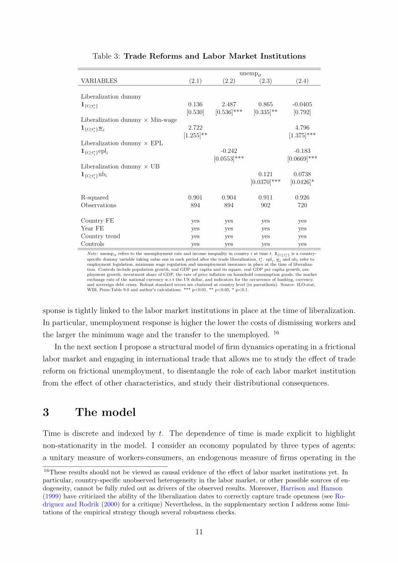
Table 3: Trade Reforms and Labor Market Institutions
unempitVARIABLES (2.1) (2.2) (2.3) (2.4)
Liberalization dummy1t≥t∗i 0.136 2.487 0.865 -0.0405
[0.530] [0.536]*** [0.335]** [0.792]Liberalization dummy × Min-wage1t≥t∗i wi 2.722 4.796
[1.255]** [1.375]***Liberalization dummy × EPL1t≥t∗i epli -0.242 -0.183
[0.0553]*** [0.0669]***Liberalization dummy × UB1t≥t∗i ubi 0.121 0.0738
[0.0370]*** [0.0426]*
R-squared 0.901 0.904 0.911 0.926Observations 894 894 902 720
Country FE yes yes yes yesYear FE yes yes yes yesCountry trend yes yes yes yesControls yes yes yes yes
Note: unempit refers to the unemployment rate and income inequality in country i at time t. 1t≥t∗i is a country-
specific dummy variable taking value one in each period after the trade liberalization, t∗i . epli, wi and ubi refer toemployment legislation, minimum wage regulation and unemployment insurance in place at the time of liberaliza-tion. Controls include population growth, real GDP per capita and its square, real GDP per capita growth, em-ployment growth, investment share of GDP, the rate of price inflation on household consumption goods, the marketexchange rate of the national currency w.r.t the US dollar, and indicators for the occurrence of banking, currency,and sovereign debt crises. Robust standard errors are clustered at country level (in parenthesis). Source: ILO-stat,WBI, Penn-Table 9.0 and author′s calculations. *** p<0.01, ** p<0.05, * p<0.1.
sponse is tightly linked to the labor market institutions in place at the time of liberalization.
In particular, unemployment response is higher the lower the costs of dismissing workers and
the larger the minimum wage and the transfer to the unemployed. 16
In the next section I propose a structural model of firm dynamics operating in a frictional
labor market and engaging in international trade that allows me to study the effect of trade
reform on frictional unemployment, to disentangle the role of each labor market institution
from the effect of other characteristics, and study their distributional consequences.
3 The model
Time is discrete and indexed by t. The dependence of time is made explicit to highlight
non-stationarity in the model. I consider an economy populated by three types of agents:
a unitary measure of workers-consumers, an endogenous measure of firms operating in the
16These results should not be viewed as causal evidence of the effect of labor market institutions yet. Inparticular, country-specific unobserved heterogeneity in the labor market, or other possible sources of en-dogeneity, cannot be fully ruled out as drivers of the observed results. Moreover, Harrison and Hanson(1999) have criticized the ability of the liberalization dates to correctly capture trade openness (see Ro-driguez and Rodrik (2000) for a critique) Nevertheless, in the supplementary section I address some limi-tations of the empirical strategy though several robustness checks.
11

industrial sector and a fixed measure of firms producing service goods. Workers are ex-ante
homogeneous and risk neutral. They can be employed in the industrial sector, employed in
the service sectors, or they can be unemployed. Firms in the service sector are homogeneous
and operate in a perfectly competitive market under constant return to scale in production.
Firms in the industrial sector are heterogeneous: they produce a differentiated industrial
variety and operate under monopolistic competition in the product market. The labor market
for service jobs is frictionless, whereas the labor market for industrial jobs is subject to search
and matching frictions and multiple labor market regulations are enforced. In particular,
industrial wages are subject to a statutory minimum wage level, industrial firms are subject
to linear firing costs in case of individual dismissal and workers who separate from industrial
firms and fail to form a new match are granted a lump-sum benefit. eventually financed
with payroll taxes on industrial firms. Finally, workers to live hand-to-mouth: no savings
technology is available to them, hence they cannot insure against firm-level productivity
shocks, unemployment shocks and eventual changes in trade costs.
3.1 Preferences
Workers derive utility from the consumption of a homogeneous, service good, st, and from
the consumption of a CES composite of industrial differentiated varieties, ct, defined as
ct =
(∫ Nt
0
ct(ω)σ−1σ dω
) σσ−1
(3)
where Nt denotes the measure of industrial varieties ω available at time t, while σ > 1
denotes the elasticity of substitution between these varieties. Services and industrial goods
are combined by means of a Cobb-Douglas function,
ut = cγt s1−γt , (4)
where γ ∈ (0, 1) is the fraction of expenditure on the composite industrial good. In each pe-
riod t, workers maximize their the expected discounted value of their utility stream, denoted
by Ut, and equal to
Ut =∞∑j=t
uj(1 + rj)j−t
(5)
where rj > 0 denotes the discount rate at time j ≥ t.
3.2 Labor market
Workers can obtain a job in the service sector with certainty: the service sector labor market
is frictionless. If they choose to get a job in the services, they earn a wage ws,t. In what
12
follows, without loss of generality, I choose the wage in the services to be the numeraire of
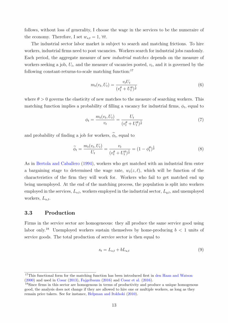
the economy. Therefore, I set ws,t = 1, ∀t.The industrial sector labor market is subject to search and matching frictions. To hire
workers, industrial firms need to post vacancies. Workers search for industrial jobs randomly.
Each period, the aggregate measure of new industrial matches depends on the measure of
workers seeking a job, Ut, and the measure of vacancies posted, vt, and it is governed by the
following constant-returns-to-scale matching function:17
mt(vt, Ut) =vtUt
(vθt + U θt )
1θ
(6)
where θ > 0 governs the elasticity of new matches to the measure of searching workers. This
matching function implies a probability of filling a vacancy for industrial firms, φt, equal to
φt =mt(vt, Ut)
vt=
Ut
(vθt + U θt )
1θ
(7)
and probability of finding a job for workers, φt, equal to
φt =mt(vt, Ut)
Ut=
vt
(vθt + U θt )
1θ
= (1− φθt )1θ (8)
As in Bertola and Caballero (1994), workers who get matched with an industrial firm enter
a bargaining stage to determined the wage rate, wt(z, `), which will be function of the
characteristics of the firm they will work for. Workers who fail to get matched end up
being unemployed. At the end of the matching process, the population is split into workers
employed in the services, Ls,t, workers employed in the industrial sector, Lq,t, and unemployed
workers, Lu,t.
3.3 Production
Firms in the service sector are homogeneous: they all produce the same service good using
labor only.18 Unemployed workers sustain themselves by home-producing b < 1 units of
service goods. The total production of service sector is then equal to
st = Ls,t + bLu,t (9)
17This functional form for the matching function has been introduced first in den Haan and Watson(2000) and used in Cosar (2013), Fajgelbaum (2016) and Cosar et al. (2016).18Since firms in this sector are homogenous in terms of productivity and produce a unique homogenousgood, the analysis does not change if they are allowed to hire one or multiple workers, as long as theyremain price takers. See for instance, Helpman and Itskhoki (2010).
13
Firms in the industrial sectors are heterogeneous. Each of them produces a unique product,
ω, and is subject to an idiosyncratic productivity shock, z, which follows an AR(1) process,
zt+1 = ρzzt + σzεz,t (10)
where ρz ∈ (0, 1), σz > 0 and εz,t ∼ N(0, 1), ∀t. Denote by Γ(z′|z) the the conditional
probability distribution induced by (10). To produce, firms combine labor, `t, and final
goods used as intermediates, mt, through a Cobb-Douglas production technology,
qt(ω) = zt`αtm
1−αt (11)
where α ∈ (0, 1] is the employment elasticity of output, whereas mt combines differentiated
varieties used as intermediates,
mt =
(∫ Nt
0
mt(ω)σ−1σ dω
) σσ−1
(12)
using the same elasticity, σ, as for final consumption.
3.4 Revenues and intermediates
Denote by ps,t the price of a unit of service sector good, by pt(ω) the home-price of an
industrial variety ω, and by Pt the ideal domestic price index for the aggregate industrial
good, defined as follows
Pt =
(∫ Nt
0
pt(ω)1−σdω
) 11−σ
(13)
Service goods are sold in a perfectly competitive market. Perfect competition and constant
return to scale in production makes the price charged for unit of service good be equal to
the marginal cost, implying, in equilibrium, zero profits and the equality between price and
wage, that is ps,t = ws,t, ∀t.The industrial sector is modelled following Melitz (2003). Differentiated industrial goods
are sold in monopolistically competitive markets and are purchased by consumers as final
consumption good and by firm as intermediate inputs. Standard optimization solution im-
plies the total demand for any variety ω at time t can be written as
qt(ω) = Dtpt(ω)−σ (14)
where Dt denotes the aggregate size of the market and it is constant across all varieties.
Given (14), the gross revenue function for a firm producing variety ω can be written as
Gt(ω) = pt(ω)qt(ω) = D1σt qt(ω)
σ−1σ (15)
14
Because of the CES structure of consumer preferences, monopolistic competition leads to
downward sloping demand and decreasing marginal revenue functions, since consumers′
marginal utility from a particular variety declines with firms′ supply.
Firms determine their output level q(ω) by choosing their intermediate input m given cur-
rent productivity z end employment `. Intermediate inputs are purchased to maximize (15)
net of material costs. Substituting equation (11) into (15) the net revenue function can be
expressed in terms of current period productivity, z, and employment values, `:
Rt(z, `) = maxm≥0
Gt(zm1−α`α)− Ptm (16)
The solution to this optimization problem yields the following expression for the net revenue
function,
Rt(z, `) = ∆t (z`α)σ−1
σ−(1−α)(σ−1) (17)
where ∆t is a revenue shifter, equal to Θ[D
1σt P−(1−α)σ−1
σt
] σσ−(1−α)(σ−1)
> 0, and
Θ = σ−(1−α)(σ−1)(1−α)(σ−1)
((1−α)(σ−1)
σ
) σσ−(1−α)(σ−1)
> 0 is a constant.
3.5 Industrial firms′ problem
At the beginning of a period t, incumbent firms decide whether to keep operating or not.
Conditional on operating, they observe a new productivity level, z′, and enter the interim
stage of the period with an inherited stock of employees, `. Conditional on the new realization
of the productivity shock, each incumbent firm decides how many workers to employ in
the current period, that is, whether to hire new employees, or to fire some of the existing
employees, or to keep the same payroll. The value of a firm entering the interim stage with
productivity z′ and employees ` is thus equal to
Vt(z′, `) = maxV h
t (z′, `), V it (z′, `), V f
t (z′, `) (18)
where V ht (z′, `) is the firm’s value of expanding, equal to
V ht (z′, `) = max
`′>`πt(z′, `′)− C(`, `′) + Vt+1(z′, `′) (19)
V it (z′, `) is the firm’s value of being inactive, equal to
V it (z′, `) = πt(z
′, `) + Vt+1(z′, `) (20)
15
and V ft (z′, `) is the firm’s value of downsizing, equal to
V ft (z′, `) = max
`′<`πt(z′, `′)− C(`, `′) + Vt+1(z′, `′) (21)
In equations (19)-(21), πt(z′, `) is the gross profit at time t, defined as
πt(z′, `′) = Rt(z
′, `′)−maxwt, wt(z′, `′)`′ (22)
where maxw,wt(z′, `′)`′ is the wage bill paid by the employer, while Vt+1(z′, `′) is the firm
continuation value at the beginning of time t+ 1. A solution to the problem of the firm is a
sequence of policy functions for hiring 1ht (z′, `), resting 1it(z
′, `), and firing 1ft (z′, `), defined
as
1s(z′, `) =
1 if V st (z′, `) = maxV h
t (z′, `), V it (z′, `), V f
t (z′, `)
0 otherwise
for s ∈ h, i, f and ∀t, and policy function for employment, Lt(z′, `), ∀t. The problem of
the industrial firms is characterized by three main features. First, the wage rate, wt(z′, `′),
depends on firms′ productivity and on the stocks of employees in firm′s hand. This is the
case because (1) search frictions create rents that are split between employers and employees
and (2) the marginal revenue is decreasing in labor.19 Second, the wage rate is subject to a
the legal constraint imposed by the statutory minimum wage in force, wt. Finally, changes
in employment are subject to adjustment costs, Ct(`, `′), and described by the following
function,
Ct(`, `′) =
Cht (`, `′) = ch
λ1
(vt(z′,`,`′)
`λ2
)λ1, if `′ > `
Cft (`, `′) = cf,t(`− `′), if `′ < `
0, otherwise
(23)
where vt(z′, `, `′) denotes the number of vacancies posted at time t by a hiring firm with
productivity z′ and initial stock of employed, `, and it is equal to
vt(z′, `, `′) =
`′ − `φt
(24)
The hiring cost profile is endogenously time-varying, as it depends on the job filling rate, φt
along the transition path, and it is function of three main parameters, i.e. the parameter
ch > 0 that governs the overall cost of adjustment, the parameter λ1 > 0 that governs
the convexity of the cost with respect to the size of employment adjustment, and λ2 > 0
19The wage rate is negotiated through the intra-firm bargaining protocol proposed by Stole and Zwiebel(1996). See section 3.8 for a description
16
governing the relative cost faced by small and large employers.20 On the other hand, the
firing costs are described by a single parameters, cf,t, which is assumed to be constant,
unless subject to an exogenous reform. Finally, I assume that firing costs are collected by
the government and are rebated back to consumers, while the adjustment costs of hiring are
incurred in terms of service good.
3.6 Firms′ entry and exit
At the beginning of period t, incumbent firms choose whether to keep operating or not: they
compare the expected value of entering the interim stage with ` workers in hand against the
outside option of closing down.21 The ex-ante value of a firm with initial productivity z and
employment, ` is thus equal to
Vt(z, `) = max
0,
1− δ1 + rt
∫z′∈Z
(Vt(z
′, `)− co)
Γ(z′|z)
(25)
where δ > 0 is a fixed exogenous probability of firm death, co denotes a fixed operating
cost, and Γ(z′|z) denotes the transition function for productivity shocks. A solution to the
problem of the firm is a sequence of policy functions for exit, 1ot (z, `) defined as
1ot (z, `) =
1 if Vt(z′, `) > co
0 otherwise
Each period, a large pool of potential firms decide whether to enter the industry and start
a new business: they compare the expected value of operating, evaluated at the ergodic
productivity distribution of the productivity shock, with the sunk cost of creating a new
firm, ceφ−λ1t , inclusive of capital fixed costs and initial hiring costs. With a positive measure
of entrant firms in equilibrium, Ne,t ≥ 0, a free entry condition must hold:
V et =
∫z∈Z
Vt(z, 1)Γe(z)dz ≤ ceφ−λ1t , with equality if Ne,t > 0 (26)
where Γe(z) is a time-invariant ergodic distribution of productivity shock derived from equa-
tion (10).
20Yashiv (2000) provides empirical evidence in favour of convex vacancy hiring costs. Other papers thatinclude convexity adjustment costs in net employment include Nilsen et al. (2007) and Cooper et al.(2007).21Notice that bankruptcy can be an attractive option for firms because (1) it allows to save on wage bills(plus taxes) of employees, (2) it allows to save on fixed costs of operation and (3) it allows to save on fir-ing costs in case of dismissal of employees.
17
3.7 Workers′ problem
In this section I turn to describe the problems of the workers. Consider a worker who enter
period t not employed in the industrial sector. At the beginning of period t, this worker has
two different options: to work in the service sector or to search for a job in the industrial
sector. Call Jot , Jst and Jut , the value of being not-employed in the industrial sector at the
beginning of period t, the value of working in the service sector and the value of searching for
a job in the industrial sector, respectively. The value of being not-employed in the industry
at the beginning of period t reads as follows:
Jot =1
1 + rtmaxJst , Jut (27)
where the value of being employed in the services, Jst , is equal to
Jst = maxcs,t
cs,t + Jot+1 s.t. Ptcs,t ≤ ws,t = 1
where Pt denotes the aggregate price index in the economy, while the value of searching for
a job in the industry, Jut is equal to
Jut = Ju,ht + φt
∫z′∈Z
∫`∈L
max0, Je,ht (z′, Lt(z′, `))− Ju,ht gt(z′, `)dz′d` (28)
where Ju,ht is the value of being unemployed at the interim stage of the period,
Ju,ht = maxcu,t
cu,t + Jot+1 s.t. Ptcu,t ≤ b+ but + Πt + Tt (29)
while Je,ht (z′, `′) is the value of being employed at the interim stage of the period,
Je,ht (z′, `′) = maxce,t
ce,t + Jet+1(z′, `′) s.t. Ptce,t ≤ maxwt, wt(z′, `′)+ Πt + Tt (30)
In equation (28), gt(z′, `) denotes the distribution of vacancies posted in the interim stage of
the period by hiring firms with productivity z′ and ` stock of employees, whereas the term
max0, Je,ht (z′, Lt(z′, `))−Ju,ht is the option value of accepting a job in the industrial sector.22
In equation (29), but denotes any lump-sum transfer from government to unemployed workers.
Finally, in equation (30), Jet+1(z′, `′) denotes the continuation value of being employed in firm
(z′, `′).
With no savings technology available, the supply of workers searching for a employment
in the industrial sector depends on their income outside the sector, i.e., their outside options.
Because workers are free to direct their search to any type of job, in any equilibrium with
22In equation (28) it is acknowledged that the optimal employment choice, Lt(z′, `) is functions of the
state variables (z′, `), over which the expectation is taken.
18
both sectors in operation and strictly positive measure of employees in the industrial sector,
workers must be indifferent between Jst and Jut , so that Jst = Jut , ∀t.23 Using condition (27),
it must be that Jst and Jut are all equal to
Jot =1
1 + rt
[cs,t + Jot+1
](31)
The equalization between value of searching for a job the industrial sector and the outside
values works through the adjustment in the matching rates, φt. Suppose Jut > Jst . If so,
all job seekers would direct their search towards industrial jobs. As more and more workers
apply, the contact rate with a hiring firm decreases up to the point where the value of
searching for an industrial jobs is as profitable as the values of the outside options. The
opposite, that is an increase in the workers′ contact rate, would happen if Jut < Jst .
Consider now the problem of a worker who is employed in the industrial sector at the
beginning of period t. This worker can separate from his job either because the firm decides
to exit the industry, or because, after observing the new productivity level, the firm wants
to contract her scale. In this case, the worker joins the pool of searchers and enjoy a value
equal to Jot . On the other hand, if a worker keeps her job in the industrial sector, she will
receive a new wage payment, wt(z′, `′) ≥ w, conditional on the realization of the productivity
shock and will start the next period employed. Industrial workers do not have the option
of searching on-the-job.24 Denote by pot (z, `) the probability for a worker of being dismissed
because of firm exit and by pft (z′, `) the probability for a worker of being fired by a contracting
firm. Therefore, the value of being employed at the beginning of period t is equal to
Jet (z, `) = pot (z, `)Jut + (1− pot (z, `))
∫z′∈Z
max Jut , J ct (z′, `)Γ(z′|z) (32)
where J ct (z′, `) is the value of continuing to work for the same employer, equal to
J ct (z′, `) = pft (z
′, `))Jut +(1− pft (z′, `))
1 + rtJe,ht (z′, Lt(z
′, `)) (33)
Notice that hiring and firing policies determine the probability of retaining a job in the
future, impacting value and the stability of being employed for a given employer.
23As in Helpman et al. (2010), this feature of the model makes the equilibrium job finding rate decreasingin workers′ income outside industrial jobs. This mechanism trace back at least to the Harris and Todaro(1970) model. See Cosar et al. (2016) for a discussion.24Workers could at any moment leave their job and join the pool of job seekers. However, since in themodel all the employers have to ensure at least the value of searching for a formal job to their employees,no workers have incentive to quit.
19
3.8 Wages
Wages for industrial employees are determined using the Binmore et al. (1986) bargaining
solution, generalized to a setting when marginal returns are diminishing.25 At the time of
bargaining the labor market is already closed and the costs of posting vacancies are sunk.
Upon matching, firms and workers meet and bargain simultaneously and on a one-to-one
basis. Failing to reach an agreement would imply a loss for firms (who cannot recover back
the costs of posting vacancies and cannot contact other workers in the current period to
replace the existing ones) and for workers (who would instead forgo wage payments in the
current period). The threats of a temporary disruption of production due to a breakdown
of negotiations generates a surplus to split between parties, which is equal to the marginal
flow surplus.26 At the time of determining wages, firms marginal flow surplus is equal to:
Πfirmt (z′, `′) =
∂Rt(z′, `′)
∂`′− ∂wt(z
′, `′)`′
∂`′(34)
while worker marginal flow surplus equals the difference between wages and home production:
Πworkert (z′, `′) = wit(z
′, `′)− b (35)
The bargaining problem consists of maximizing the joint marginal flow surplus subject to
the participation constraints, ensuring a non-negative surplus accruing to the worker,
maxwt(z′,`′)
Πfirmt (z′, `′)1−βΠworker
t (z′, `′)β
s.t. Je,ht (z′, `′) ≥ Ju,ht
where β ∈ (0, 1) is the worker bargaining power in the wage negotiation.
Consider a firm currently hiring workers. New workers generate positive rents at a hiring
firm, making the wage solution of the bargaining problem be implicitly determined by the
following Nash sharing rule:
βΠfirmt (z′, `′) = (1− β)Πworker
t (z′, `′) (36)
Denote by wht (z′, `′) the solution to this problem. Consider instead an incumbent firm
firing workers. In this case, the existing matches do not generate any more positive rents,
making the worker participation constraint of the problem be binding. To see this, notice
that, at the time of bargaining, firms has already chosen a level of employment up to the
25A similar strategy has been employed by Hall and Milgrom (2008) within a single-worker firm modeland more recently by Elsby and Gottfries (2019) in multi-worker firm model.26Hall and Milgrom (2008) argue that threat of a permanent suspension of negotiations is not credible inthis protocol. Regardless of a breakdown in the current period, the firm will rather prefer to resume nego-tiations with the same workers in the subsequent period instead of replacing him with a different worker.
20
point where optimality condition is re-established, i.e. up to a level where Πfirmt (z′, `′) =
−cf,t − ∂Vt+1(z′,`′)∂`′
< 0. The Nash splitting rule would then imply a negative total flow
surplus, invalidating the participation constraint. Therefore, the unique wage solution of the
bargaining problem between a worker and a firing firm is the one ensuring the participation
constraint is satisfied:
Je,ht (z′, `′) = Ju,ht (37)
which implies the following wage for workers at a firing firm,
wft(z′, `′) = Ju,ht − Jet+1(z′, `′) (38)
Notice that this bargaining protocol generated dispersion of wage of workers also across firing
firms, since workers who continue to be employed enjoy the continuation value Jet+1(z′, `′).
Finally, consider a resting firm. In this case, depending on stock of workers employed and
productivity level, the existing matches could generate positive rents - if revenues are large
but not enough to cover hiring costs and expand - making the wage solution be at the
interior, or negative rents, - if revenues are low but not enough to make job destruction a
viable option - driving the wage solution to the corner. Therefore, the wage for workers at
a resting firm is equal to the maximum of the previous two, i.e.
wit(z′, `′) = maxwh
t (z′, `′), wft(z′, `′) (39)
4 Open economy
I now turn to describe the open-economy version of this model. I consider two countries,
home h and foreign f , and I assume the home-economy to be small relative to the foreign
one: under this assumption foreign conditions do not react to changes in the home-policies.
I assume markets are internationally segmented and only industrial varieties can be traded
across borders. Service goods are assumed to be non-tradable. Denote by Nh,t the measure
of varieties produced in the home-country and by Nf,t = Nt −Nh,t the measure of varieties
produced abroad.
4.1 Prices and aggregates
Let pt(ω∗) be the free on board (FOB) price of a variety ω∗ produced in the foreign country,
denominated in foreign currency and exogenous to home-country conditions. Denote by Pf,t
the price index of imports,
Pf,t =
(∫ Nf,t
0
pt(ω∗)1−σdω∗
) 11−σ
(40)
21
and by Ph,t the be the price index of domestic varieties,
Ph,t =
(∫ Nt
Nf,t
pt(ω)1−σdω
) 11−σ
(41)
An ideal home price index for the aggregate industrial good, Pt, can written as
Pt =
(P 1−σh,t + (τc,tτa,tktPf,t)
1−σ) 1
1−σ
(42)
where τc,t ≥ 1 denotes iceberg cost trade, τa,t−1 ≥ 0 denotes ad-valorem tariff on imports and
kt is the equilibrium exchange rate. Since the exchange rate adjusts in general equilibrium to
clear the trade balance, and foreign economy is exogenous to changes in the home-country,
we can normalize the foreign price index and set Pf,t = 1. Finally, let the foreign price of
domestic good exported abroad be p∗t (ω), denominated in foreign currency. An ideal foreign
market price index for exported goods, denominated in foreign currency, is defined as
P ∗h,t =
(∫ Nt
Nf,t
1xt (ω)p∗t (ω)1−σdω
) 11−σ
(43)
where 1xt (ω) is an indicator function that equals one if variety ω is exported, zero otherwise.
Let Dh,t be the aggregate size of the domestic market and let Df,t denote the aggregate
size of the foreign market, expressed in units of foreign currency, and assumed to be exogenous
to the home-country.27 Given the domestic and the foreign price indexes, the total domestic
demand for any domestic variety ω ∈ (Nf,t, Nt] at time t can be written as
qt(ω) = Dh,tpt(ω)−σ (44)
Similarly, the total domestic demand for any imported variety ω∗ ∈ [0, Nf,t] reads as
qt(ω∗) = Dh,t[τa,tτc,tktpt(ω
∗)]−σ (45)
whereas the total foreign demand for any domestic variety ω ∈ (Nf,t, Nt] exported abroad is
equal to
qt(ω) = Df,tp∗t (ω)−σ (46)
Given the demand functions (44) and (46), the gross revenue function of non-exporting
domestic firms can be written as
Gh,t(ω) = D1σh,tq(ω)
σ−1σ (47)
27See the supplementary section for a full derivation of Dh,t.
22
whereas the gross revenues of an exporting domestic firms are equal to
Gf,t(ω) = [Dh,t + kσt τ−(σ−1)c,t Df,t]
1σ q(ω)
σ−1σ = Gh,t(ω)[1 + df,t]
1σ (48)
where df,t is the revenue premium from exporting, defined as the ratio between the foreign
market capacity and the domestic revenues,
df,t = kσt τ−(σ−1)c,t
Df,t
Dh,t
> 0 (49)
and capturing the extra revenue generated by exporting, conditional on output.
4.2 Export decision
Each period t, before taking input decisions, incumbent firms decide whether to sell their
product abroad or not. Participation in the export market is a static decision for the in-
dustrial producers, who bear a fixed cost of exporting cx. Given output levels q(ω), firms
choose to export so to maximize their current gross sales revenues, i.e.
Gt(q(ω)) = max Gh,t(q(ω)), Gf,t(q(ω))− cx (50)
where Gh,t(q(ω)) and Gf,t(q(ω)) are defined in equations (47) and (48).
A solution for policy export participation, 1xt is an indicator function defined as follows:
1xt =
1 if Gf,t(q(ω))− cx > Gh,t(q(ω))
0, otherwise(51)
Using equations (47) and (48) the total gross revenues can be written as a function of the
export participation policy, policy (51),
Gt(q(ω)) = D1σh,t[1 + 1xt df,t]
1σ q(ω)
σ−1σ − cx1xt (52)
4.3 Trade balance
Given the domestic demand for foreign variety ω∗ in equation (45), the value of aggregate
imports expressed in unit of local currency, and before tariffs on import are imposed, is equal
to ∫ Nf,t
0
Dh,t[τa,tτc,tktpt(ω∗)]1−σdω∗ = Dh,t(τc,tτa,tkt)
1−σ (53)
where the equivalence comes from the definition of price index for imported varieties, given
in equation (40). Taking tariffs into account, the domestic demand for foreign currency
23
equalsDh,t
τa,t(τc,tτa,tkt)
1−σ = Dh,tτ−σa,t (τc,tkt)
1−σ (54)
Given the foreign foreign demand for domestic variety ω in equation (46), the value of
aggregate exports, expressed in domestic currency, is equal to
ktτc,t
∫ Nt
Nf,t
1xt (ω)Df,tp∗t (ω)1−σdω =
ktτc,t
Df,tP∗1−σh,t (55)
where the equivalence comes from the definition of price index for domestic varieties exported
abroad, given in equation (43).
4.4 Government
Government revenues are collected from two different sources, namely tariffs on imports
Dh,tτ−σa,t (τc,tkt)
1−σ(τa,t − 1) (56)
and firing costs,
cf,t
∫z∈Z
∫`∈L
1ft (z′, `)(`− `′)ψt(z′, `)dz′d` (57)
Government revenues are returned to unemployed worker in form of unemployment benefit
(if positive) and, what left, to each worker in the form of lump-sum transfers.
4.5 Mechanisms
Trade openness, unemployment and inequality - The evolution of the unemployment rate
after a trade reform is tightly linked to the employment adjustments of firms and to the
reallocation of workers across employers. A reduction in trade costs boosts cross-border
flows of goods for intermediate and final consumption. Lowering trade barriers produces two
opposing forces. On the one hand, it increases import penetration of foreign varieties in the
domestic market and reduces revenues in small, low-productive, non-exporting firms, that
respond, on impact, by displacing workers or by adjusting wages downward. On the other
hand, trade liberalization magnifies the value of participating in the foreign market: large,
high-productive firms can benefit from higher foreign market revenues by starting exporting
or by increasing their export flows, and respond to lower trade costs by expanding their
size. However, because of search frictions in the labor market and convexity in the hiring
costs, exporting firms grow slowly, making reallocation of workers toward larger and higher
productive employers sluggish. Moreover, since the hiring costs per worker vary with size, the
rate at which industrial firms adjust employment and wages in response to shocks depends
upon their size. After the initial response, labor market dynamics is governed by larger
24
firms. Along the transition towards the new steady state, low-productivity firms become
less responsive to shocks, employment is reallocated towards larger and more-stable firms
and job turnover is triggered by the larger revenue steepness of exporting firms.
Polarization in the marginal revenue product of firms translates into higher wages paid by
exporting firms and lower wages paid by import competing firms. On impact, the distribution
of wages across firms becomes more dispersed and remains so along the transition towards
the new equilibrium. Dispersion of income will reflect dispersion of wage on one side, but will
also react to job reallocation from the industrial to the service sector and worker reallocation
out of employment on the other side.
Labor market institutions enter the picture by introducing price and quantity rigidity,
which distorts the adjustments in labor demand and wage payments after a trade shock,
with effects on employment volatility, workers turnover and, ultimately, unemployment rate
and income inequality.
Effect of firing costs - In partial equilibrium, higher firing costs make firms employment
less volatile by discouraging labor adjustments to fluctuations in revenues. To this extent,
employment protection legislation introduces a quantity rigidity : as in Bertola and Caballero
(1994), higher firing costs increase the cost of downsizing after a negative productivity shock,
hampering labor mobility and increasing labor hoarding, thus keeping alive unproductive
matches that would otherwise disappear. In general equilibrium, the opposite effect arises.
Stricter EPL increases the future costs of hiring, both directly, by rising the expected costs
of dismissing workers, as in Hopenhayn and Rogerson (1993), and indirectly, by modifying
the firms probability of filling vacancies. Firms react by posting less vacancies, generating a
positive pressure on unemployment. Accordingly, the effect of firing costs on unemployment
is ambiguous. The effect of firing costs on the dispersion of income after trade reform is
ambiguous too. Lower firing costs increase firms’ selection and shift the firm size distribution
rightward, inducing a less dispersed distribution for the marginal revenue product of labor,
thus reducing wage dispersion across firms. On the other hand, this increases the value of
employment in the industrial sector. In order for the no-arbitrage condition between sectors
to hold, this effect has to be offset by a further reduction in the job finding probability, which
contributes to increase income inequality through unemployment and workers reallocation
across sectors.
Effect of minimum wage - A binding statutory minimum wage introduces a price rigidity :
higher minimum wage prevents firms to cut wages in response to a negative productivity
shock. It rather magnifies the downward adjustment of employment, leading to larger job
displacement. In the aftermath of trade reform, a high minimum wage is likely to hurt small,
low-productivity firm relatively more, since the constraint on wage is relatively more likely to
be binding. On the other hand, a higher minimum wage induces a selection mechanism, by
shifting the productivity/size threshold for operating in the industry rightward, and reducing
the dispersion of wages across firms. As the economy approaches the new steady state,
25

only high-productivity firms survive, inducing a new distribution for the marginal revenue
product of labor which in turn feeds back into the distribution of wages, the distribution of
new vacancy for jobs and the job filling rate, confounding the net effect of a high minimum
wage on unemployment rate and inequality.
Non-tradable service sector - The consequence of a trade reform for the employment in
the non-tradable sector are ambiguous too. As in Melitz (2003), trade openness triggers con-
centration of industrial employment in the hands of a smaller measure of high-productivity,
exporting firms. As long the as the expansion of those firms does not compensate the
workforce displacement of low-productivity firms, workers are permanently forced out the
industrial employment, either into unemployment or into services. The extent to which the
service sector can operate as buffer for workers who are displaced depends on the no-arbitrage
condition between the values of searching for a job in the industrial sector and the value of
working in the services. Regulations in the labor market modify employment concentration
by inducing firm selection, with consequences for employment reallocation across sectors.
Finally, in the Appendix B, I discuss the notion of recursive competitive equilibrium for
this economy and provide the conditions that characterize it.
5 The cases of Colombia and Mexico
To explore the mechanisms proposed above, I compare the cases of Colombia and Mexico.
Between the end of the 1980′s and the beginning of the 1990′s, both Colombia and Mexico
went through a massive series of trade and investment reforms. As part of the Apertura
(opening) plan, from 1985 to 1994 Colombia gradually liberalized its trading regime by
reducing the tariff levels and virtually eliminating all the non-tariff barriers to trade, a process
that culminated in the drastic reductions of 1990-91. In this decade, the average tariff across
all industry declined from 21 to about 11 percent (Goldberg and Pavcnik, 2004), with a drop
from 50 to 13 in the only manufacturing sector. As for protection through non-tariff barriers,
the average coverage ratio went from 72.2 percent in 1986 to 10.3 percent in 1992 (Attanasio
et al., 2004a). Throughout the 1990s, further trade reforms were implemented, including
bilateral trade agreements with other Latin American countries in 1993-94.
During the second half of the ′80s, after more than a decades of pursuing an import-
substitution industrialization strategy, Mexico initiated a radical liberalization of its external
sector as well. In 1984, Mexico pursued a policy of privatization and liberalization in order
to attract foreign direct investment (Henry, 1999). In 1985, a program of stabilization and
structural adjustment was implemented, including trade liberalization. After signing the
General Agreement on Tariffs and Trade (GATT) in 1985, official prices for imports were
entirely abolished. Import licensing requirements were scaled back to about a quarter of
their previous levels - the domestic production value covered by import licensing went from
26
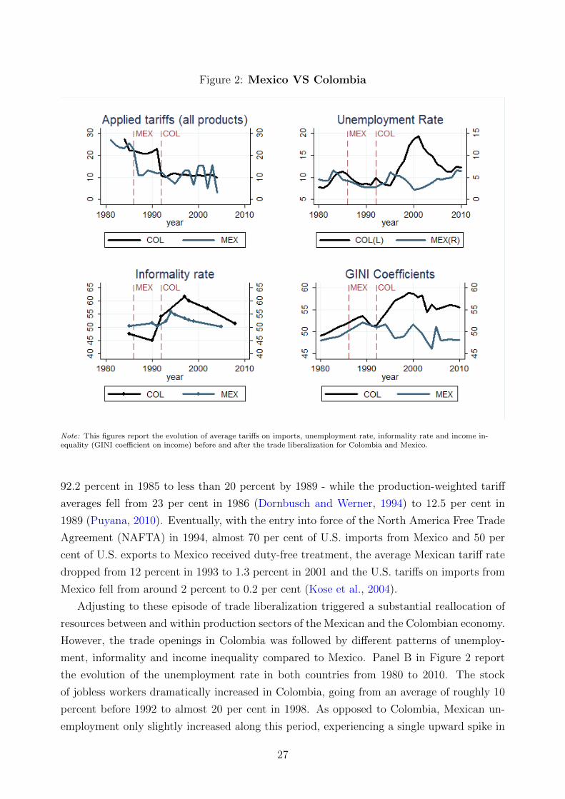
Figure 2: Mexico VS Colombia
Note: This figures report the evolution of average tariffs on imports, unemployment rate, informality rate and income in-equality (GINI coefficient on income) before and after the trade liberalization for Colombia and Mexico.
92.2 percent in 1985 to less than 20 percent by 1989 - while the production-weighted tariff
averages fell from 23 per cent in 1986 (Dornbusch and Werner, 1994) to 12.5 per cent in
1989 (Puyana, 2010). Eventually, with the entry into force of the North America Free Trade
Agreement (NAFTA) in 1994, almost 70 per cent of U.S. imports from Mexico and 50 per
cent of U.S. exports to Mexico received duty-free treatment, the average Mexican tariff rate
dropped from 12 percent in 1993 to 1.3 percent in 2001 and the U.S. tariffs on imports from
Mexico fell from around 2 percent to 0.2 per cent (Kose et al., 2004).
Adjusting to these episode of trade liberalization triggered a substantial reallocation of
resources between and within production sectors of the Mexican and the Colombian economy.
However, the trade openings in Colombia was followed by different patterns of unemploy-
ment, informality and income inequality compared to Mexico. Panel B in Figure 2 report
the evolution of the unemployment rate in both countries from 1980 to 2010. The stock
of jobless workers dramatically increased in Colombia, going from an average of roughly 10
percent before 1992 to almost 20 per cent in 1998. As opposed to Colombia, Mexican un-
employment only slightly increased along this period, experiencing a single upward spike in
27
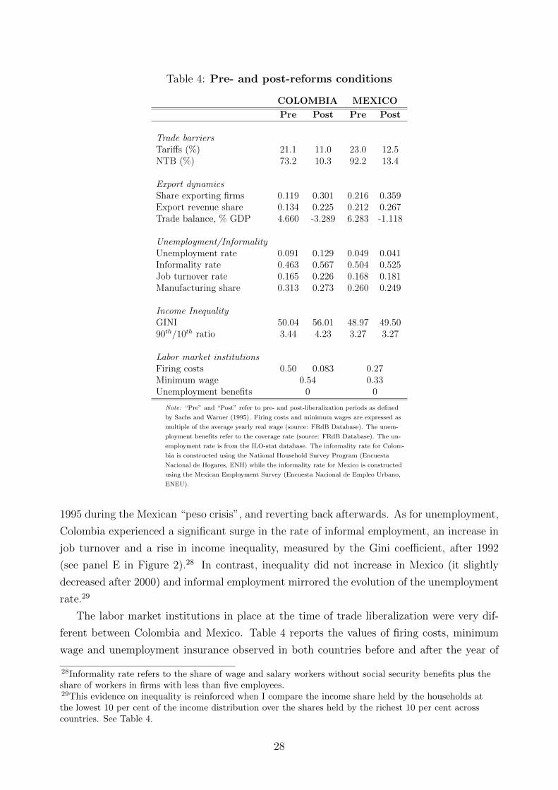
Table 4: Pre- and post-reforms conditions
COLOMBIA MEXICO
Pre Post Pre Post
Trade barriersTariffs (%) 21.1 11.0 23.0 12.5NTB (%) 73.2 10.3 92.2 13.4
Export dynamicsShare exporting firms 0.119 0.301 0.216 0.359Export revenue share 0.134 0.225 0.212 0.267Trade balance, % GDP 4.660 -3.289 6.283 -1.118
Unemployment/InformalityUnemployment rate 0.091 0.129 0.049 0.041Informality rate 0.463 0.567 0.504 0.525Job turnover rate 0.165 0.226 0.168 0.181Manufacturing share 0.313 0.273 0.260 0.249
Income InequalityGINI 50.04 56.01 48.97 49.5090th/10th ratio 3.44 4.23 3.27 3.27
Labor market institutionsFiring costs 0.50 0.083 0.27Minimum wage 0.54 0.33Unemployment benefits 0 0
Note: “Pre” and “Post” refer to pre- and post-liberalization periods as defined
by Sachs and Warner (1995). Firing costs and minimum wages are expressed as
multiple of the average yearly real wage (source: FRdB Database). The unem-
ployment benefits refer to the coverage rate (source: FRdB Database). The un-
employment rate is from the ILO-stat database. The informality rate for Colom-
bia is constructed using the National Household Survey Program (Encuesta
Nacional de Hogares, ENH) while the informality rate for Mexico is constructed
using the Mexican Employment Survey (Encuesta Nacional de Empleo Urbano,
ENEU).
1995 during the Mexican “peso crisis”, and reverting back afterwards. As for unemployment,
Colombia experienced a significant surge in the rate of informal employment, an increase in
job turnover and a rise in income inequality, measured by the Gini coefficient, after 1992
(see panel E in Figure 2).28 In contrast, inequality did not increase in Mexico (it slightly
decreased after 2000) and informal employment mirrored the evolution of the unemployment
rate.29
The labor market institutions in place at the time of trade liberalization were very dif-
ferent between Colombia and Mexico. Table 4 reports the values of firing costs, minimum
wage and unemployment insurance observed in both countries before and after the year of
28Informality rate refers to the share of wage and salary workers without social security benefits plus theshare of workers in firms with less than five employees.29This evidence on inequality is reinforced when I compare the income share held by the households atthe lowest 10 per cent of the income distribution over the shares held by the richest 10 per cent acrosscountries. See Table 4.
28
reform. On the one hand, Colombia massively cut dismissal costs at the beginning of the 90s,
while Mexico kept a rigid labor market. At the time of trade reform, Colombian employers
were required to deposit a contribution equal to 8 percent of the yearly real annual wage
(corresponding to roughly one month) into a savings fund, eventually accessible to workers
in the event of separation, whereas in Mexico the severance payment legislation, defined
under Labor Law Article 165, prescribed an obligation of 90 days (roughly three months) of
minimum daily salary for each year of service.30 Moreover, the advance notice for termina-
tion of indefinite contracts in Colombia was set to 15 days a year whereas in Mexico it was
kept to one month (Heckman and Pages, 2000), and the compensation for dismissal due to
economic reasons for one-year tenure workers was reduced to 45 days, one third than what
observed in Mexico.31 On the other hand, the minimum wage legislation in Colombia was
much stricter than Mexico. At the beginnings of the 1990s, the average statutory minimum
wage in Colombia amounted to roughly 50 percent of the average market wage, versus 34
percent in Mexico.32 For the same period, Bell (1997) reports values for the minimum wage
of white and blue collar workers in Mexican manufacturing sector, amounting, respectively,
to 22 and 42 percent of their average wage in 1984. The same figures reported for Colombia
amount to 39 percent for high-skill workers, 52 percent for low-skill workers, and 73 percent
for apprentice workers in 1987.33 Notice that, in both countries, at the time of trade openings
no unemployment insurance system was in place (FRdB-IMF, 2018).
6 Bringing the model to the data
Assuming that both economies were in steady state before the trade reform, I fit the model
respectively to the periods 1981-1990 for Colombia and 1984-1986 for Mexico, so to replicate
the pre-liberalization behavior of these two economies. The model is set to fit the distribution
of employment in the autarckic steady-state, together with the size distribution of plants,
export dynamics and plant turnover.
30Source: Kugler (1999) for Colombia and Grandolini and Cerda (1998) - based on information providedby the Instituto Mexicano de Seguridad Social (IMSS)- for Mexico.31Source: Kambourov (2009) and IADB Report (1997) based on information from Ministries of Labour.32Source: ILO-stat. When the figures are missing, I construct them converting the annual nominal min-imum wage reported by the ILO-stat into real minimum wage (at 2005 constant prices) using the PPPconversion factor, and then dividing them by the average real wage observed in the same year.33Bell (1997) documents a divergent trend in the real value of the legally imposed minimum wage in Mex-ico and Colombia in the 1980s, leading by 1990 to a level equal to just 13% of the average unskilled man-ufacturing wage in Mexico and roughly 53% of the average unskilled wage in Colombia. As explained inMaloney and Mendez (2004), the difference between these two patterns can be partly explained by thewage indexation to past inflation (salario minimo movil), imposed by the Constitution in Colombia andnot present in Mexico.
29
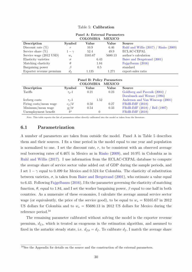
Table 5: Calibration
Panel A: External ParametersCOLOMBIA MEXICO
Description Symbol Value Value SourceDiscount rate (%) r 10.9 6.46 Ruhl and Willis (2017) / Riano (2009)Service share (%) 1− γ 52.4 49.9 ECLAC-CEPALService wage (2012 USD) ws 3165.67 5680.13 author’s calculationElasticity varieties σ 6.43 Baier and Bergstrand (2001)Matching elasticity θ 1.84 Fajgelbaum (2016)Bargaining power β 0.5 standardExporter revenue premium df 1.135 1.271 export-sales ratio
Panel B: Policy ParametersCOLOMBIA MEXICO
Description Symbol Value Value SourceTariffs τa-1 0.21 0.23 Goldberg and Pavcnik (2004) /
Dornbusch and Werner (1994)Iceberg costs τc-1 1.52 Anderson and Van Wincoop (2001)Firing costs/mean wage cf/w 0.50 0.27 FRdB-IMF (2018)Minimum/mean wage w/w 0.54 0.33 FRdB-IMF (2018) / Bell (1997)Unemployment benefit bu 0 FRdB-IMF (2018)
Note: This table reports the list of parameters either directly calibrated into the model or taken from the literature.
6.1 Parametrization
A number of parameters are taken from outside the model. Panel A in Table 5 describes
them and their sources. I fix a time period in the model equal to one year and population
is normalized to one. I set the discount rate, r, to be consistent with an observed average
real borrowing rates of 6.46% in Mexico as in Riano (2009), and 10.9% in Colombia as in
Ruhl and Willis (2017). I use information from the ECLAC-CEPAL database to compute
the average share of service sector value added out of GDP during the sample periods, and
I set 1− γ equal to 0.499 for Mexico and 0.524 for Colombia. The elasticity of substitution
between varieties, σ, is taken from Baier and Bergstrand (2001), who estimate a value equal
to 6.43. Following Fajgelbaum (2016), I fix the parameter governing the elasticity of matching
function, θ, equal to 1.84, and I set the worker bargaining power, β equal to one half in both
countries. As a numeraire of these economies, I calculate the average annual service sector
wage (or equivalently, the price of the service good), to be equal to ws = $3165.67 in 2012
US dollars for Colombia and to ws = $5680.13 in 2012 US dollars for Mexico during the
reference period.34
The remaining parameter calibrated without solving the model is the exporter revenue
premium, df,t, which is treated as exogenous in the estimation algorithm, and assumed to
fixed in the autarkic steady state, i.e. df,0 = df . To calibrate df , I match the average share
34See the Appendix for details on the source and the construction of the external parameters.
30
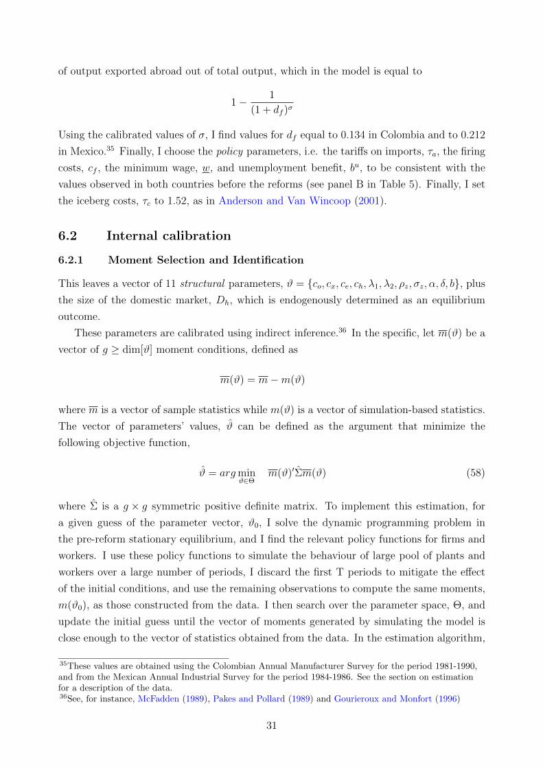
of output exported abroad out of total output, which in the model is equal to
1− 1
(1 + df )σ
Using the calibrated values of σ, I find values for df equal to 0.134 in Colombia and to 0.212
in Mexico.35 Finally, I choose the policy parameters, i.e. the tariffs on imports, τa, the firing
costs, cf , the minimum wage, w, and unemployment benefit, bu, to be consistent with the
values observed in both countries before the reforms (see panel B in Table 5). Finally, I set
the iceberg costs, τc to 1.52, as in Anderson and Van Wincoop (2001).
6.2 Internal calibration
6.2.1 Moment Selection and Identification
This leaves a vector of 11 structural parameters, ϑ = co, cx, ce, ch, λ1, λ2, ρz, σz, α, δ, b, plus
the size of the domestic market, Dh, which is endogenously determined as an equilibrium
outcome.
These parameters are calibrated using indirect inference.36 In the specific, let m(ϑ) be a
vector of g ≥ dim[ϑ] moment conditions, defined as
m(ϑ) = m−m(ϑ)
where m is a vector of sample statistics while m(ϑ) is a vector of simulation-based statistics.
The vector of parameters’ values, ϑ can be defined as the argument that minimize the
following objective function,
ϑ = argminϑ∈Θ
m(ϑ)′Σm(ϑ) (58)
where Σ is a g × g symmetric positive definite matrix. To implement this estimation, for
a given guess of the parameter vector, ϑ0, I solve the dynamic programming problem in
the pre-reform stationary equilibrium, and I find the relevant policy functions for firms and
workers. I use these policy functions to simulate the behaviour of large pool of plants and
workers over a large number of periods, I discard the first T periods to mitigate the effect
of the initial conditions, and use the remaining observations to compute the same moments,
m(ϑ0), as those constructed from the data. I then search over the parameter space, Θ, and
update the initial guess until the vector of moments generated by simulating the model is
close enough to the vector of statistics obtained from the data. In the estimation algorithm,
35These values are obtained using the Colombian Annual Manufacturer Survey for the period 1981-1990,and from the Mexican Annual Industrial Survey for the period 1984-1986. See the section on estimationfor a description of the data.36See, for instance, McFadden (1989), Pakes and Pollard (1989) and Gourieroux and Monfort (1996)
31
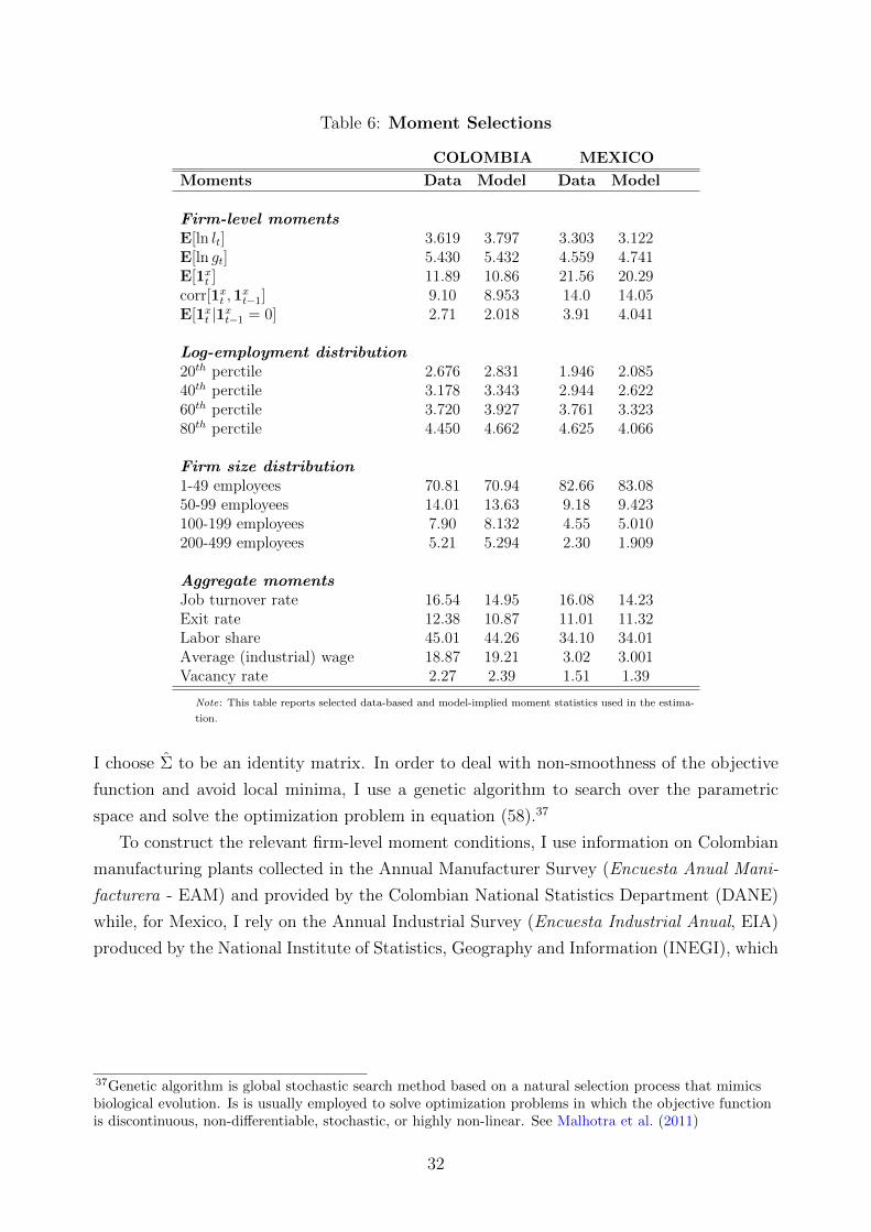
Table 6: Moment Selections
COLOMBIA MEXICO
Moments Data Model Data Model
Firm-level momentsE[ln lt] 3.619 3.797 3.303 3.122E[ln gt] 5.430 5.432 4.559 4.741E[1xt ] 11.89 10.86 21.56 20.29corr[1xt ,1
xt−1] 9.10 8.953 14.0 14.05
E[1xt |1xt−1 = 0] 2.71 2.018 3.91 4.041
Log-employment distribution20th perctile 2.676 2.831 1.946 2.08540th perctile 3.178 3.343 2.944 2.62260th perctile 3.720 3.927 3.761 3.32380th perctile 4.450 4.662 4.625 4.066
Firm size distribution1-49 employees 70.81 70.94 82.66 83.0850-99 employees 14.01 13.63 9.18 9.423100-199 employees 7.90 8.132 4.55 5.010200-499 employees 5.21 5.294 2.30 1.909
Aggregate momentsJob turnover rate 16.54 14.95 16.08 14.23Exit rate 12.38 10.87 11.01 11.32Labor share 45.01 44.26 34.10 34.01Average (industrial) wage 18.87 19.21 3.02 3.001Vacancy rate 2.27 2.39 1.51 1.39
Note: This table reports selected data-based and model-implied moment statistics used in the estima-
tion.
I choose Σ to be an identity matrix. In order to deal with non-smoothness of the objective
function and avoid local minima, I use a genetic algorithm to search over the parametric
space and solve the optimization problem in equation (58).37
To construct the relevant firm-level moment conditions, I use information on Colombian
manufacturing plants collected in the Annual Manufacturer Survey (Encuesta Anual Mani-
facturera - EAM) and provided by the Colombian National Statistics Department (DANE)
while, for Mexico, I rely on the Annual Industrial Survey (Encuesta Industrial Anual, EIA)
produced by the National Institute of Statistics, Geography and Information (INEGI), which
37Genetic algorithm is global stochastic search method based on a natural selection process that mimicsbiological evolution. Is is usually employed to solve optimization problems in which the objective functionis discontinuous, non-differentiable, stochastic, or highly non-linear. See Malhotra et al. (2011)
32
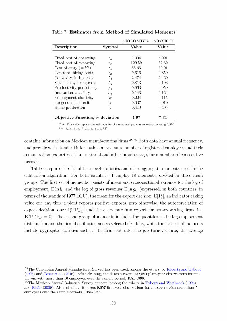
Table 7: Estimates from Method of Simulated Moments
COLOMBIA MEXICO
Description Symbol Value Value
Fixed cost of operating co 7.094 5.991Fixed cost of exporting cx 120.59 52.82Cost of entry (= V e) ce 55.63 69.01Constant, hiring costs ch 0.616 0.859Convexity, hiring costs λ1 2.474 2.469Scale effect, hiring costs λ2 0.813 0.103Productivity persistency ρz 0.963 0.959Innovation volatility σz 0.143 0.164Employment elasticity α 0.224 0.115Exogenous firm exit δ 0.037 0.010Home production b 0.419 0.405
Objective Function, % deviation 4.97 7.31
Note: This table reports the estimates for the structural parameters estimates using MSM,
ϑ = co, cx, ce, ch, λ1, λ2, ρz , σz , α, δ, b.
contains information on Mexican manufacturing firms.38,39 Both data have annual frequency,
and provide with standard information on revenues, number of registered employees and their
remuneration, export decision, material and other inputs usage, for a number of consecutive
periods.
Table 6 reports the list of firm-level statistics and other aggregate moments used in the
calibration algorithm. For both countries, I employ 18 moments, divided in three main
groups. The first set of moments consists of mean and cross-sectional variance for the log of
employment, E[ln lt] and the log of gross revenues E[ln gt] (expressed, in both countries, in
terms of thousands of 1977 LCU), the mean for the export decision, E[1xt ], an indicator taking
value one any time a plant reports positive exports, zero otherwise, the autocorrelation of
export decision, corr[1xt ,1xt−1], and the entry rate into export for non-exporting firms, i.e.
E[1xt |1xt−1 = 0]. The second group of moments includes the quantiles of the log employment
distribution and the firm distribution across selected size bins, while the last set of moments
include aggregate statistics such as the firm exit rate, the job turnover rate, the average
38The Colombian Annual Manufacturer Survey has been used, among the others, by Roberts and Tybout(1996) and Cosar et al. (2016). After cleaning, the dataset covers 152,580 plant-year observations for em-ployers with more than 10 employees over the sample period, 1981-1990.39The Mexican Annual Industrial Survey appears, among the others, in Tybout and Westbrook (1995)and Riano (2009). After cleaning, it covers 9,657 firm-year observations for employers with more than 5employees over the sample periods, 1984-1986.
33
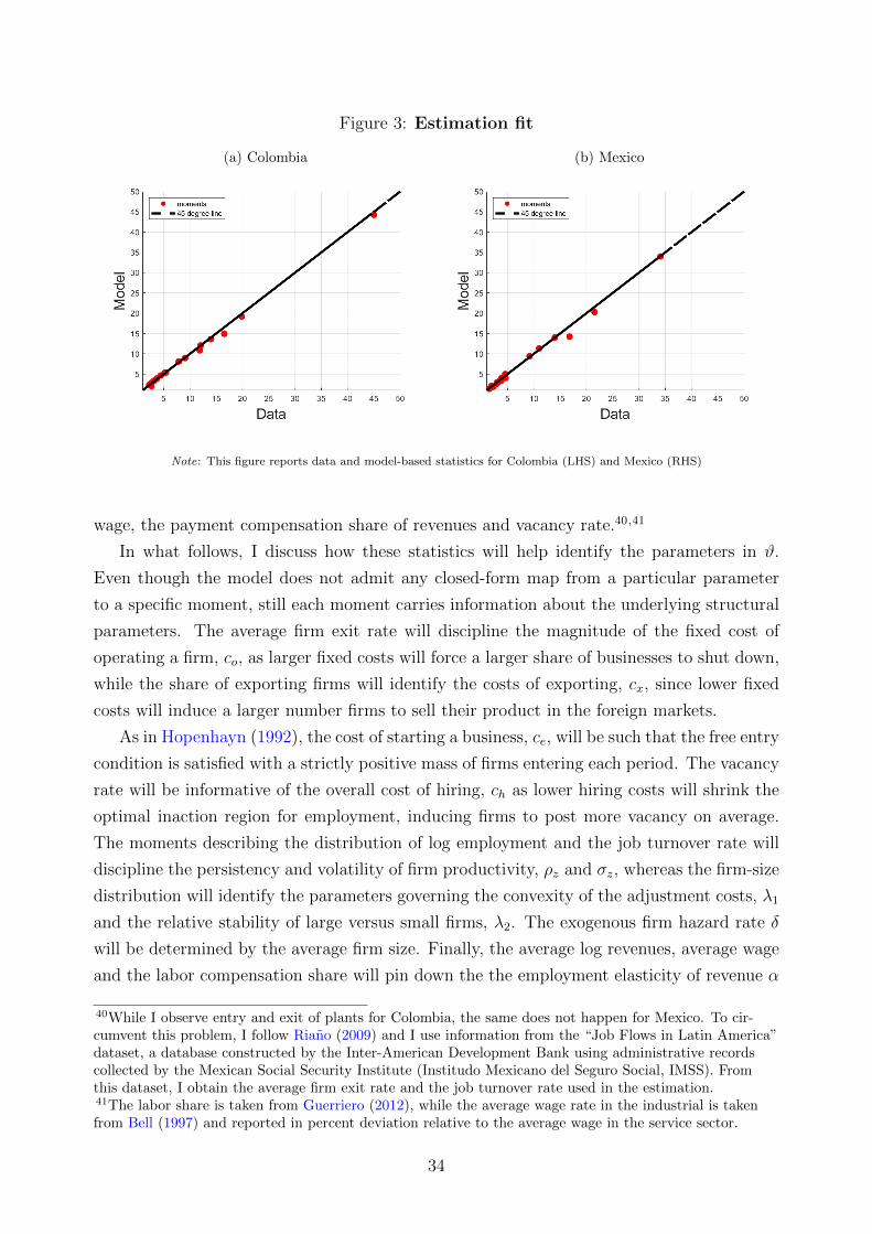
Figure 3: Estimation fit
(a) Colombia (b) Mexico
Note: This figure reports data and model-based statistics for Colombia (LHS) and Mexico (RHS)
wage, the payment compensation share of revenues and vacancy rate.40,41
In what follows, I discuss how these statistics will help identify the parameters in ϑ.
Even though the model does not admit any closed-form map from a particular parameter
to a specific moment, still each moment carries information about the underlying structural
parameters. The average firm exit rate will discipline the magnitude of the fixed cost of
operating a firm, co, as larger fixed costs will force a larger share of businesses to shut down,
while the share of exporting firms will identify the costs of exporting, cx, since lower fixed
costs will induce a larger number firms to sell their product in the foreign markets.
As in Hopenhayn (1992), the cost of starting a business, ce, will be such that the free entry
condition is satisfied with a strictly positive mass of firms entering each period. The vacancy
rate will be informative of the overall cost of hiring, ch as lower hiring costs will shrink the
optimal inaction region for employment, inducing firms to post more vacancy on average.
The moments describing the distribution of log employment and the job turnover rate will
discipline the persistency and volatility of firm productivity, ρz and σz, whereas the firm-size
distribution will identify the parameters governing the convexity of the adjustment costs, λ1
and the relative stability of large versus small firms, λ2. The exogenous firm hazard rate δ
will be determined by the average firm size. Finally, the average log revenues, average wage
and the labor compensation share will pin down the the employment elasticity of revenue α
40While I observe entry and exit of plants for Colombia, the same does not happen for Mexico. To cir-cumvent this problem, I follow Riano (2009) and I use information from the “Job Flows in Latin America”dataset, a database constructed by the Inter-American Development Bank using administrative recordscollected by the Mexican Social Security Institute (Institudo Mexicano del Seguro Social, IMSS). Fromthis dataset, I obtain the average firm exit rate and the job turnover rate used in the estimation.41The labor share is taken from Guerriero (2012), while the average wage rate in the industrial is takenfrom Bell (1997) and reported in percent deviation relative to the average wage in the service sector.
34
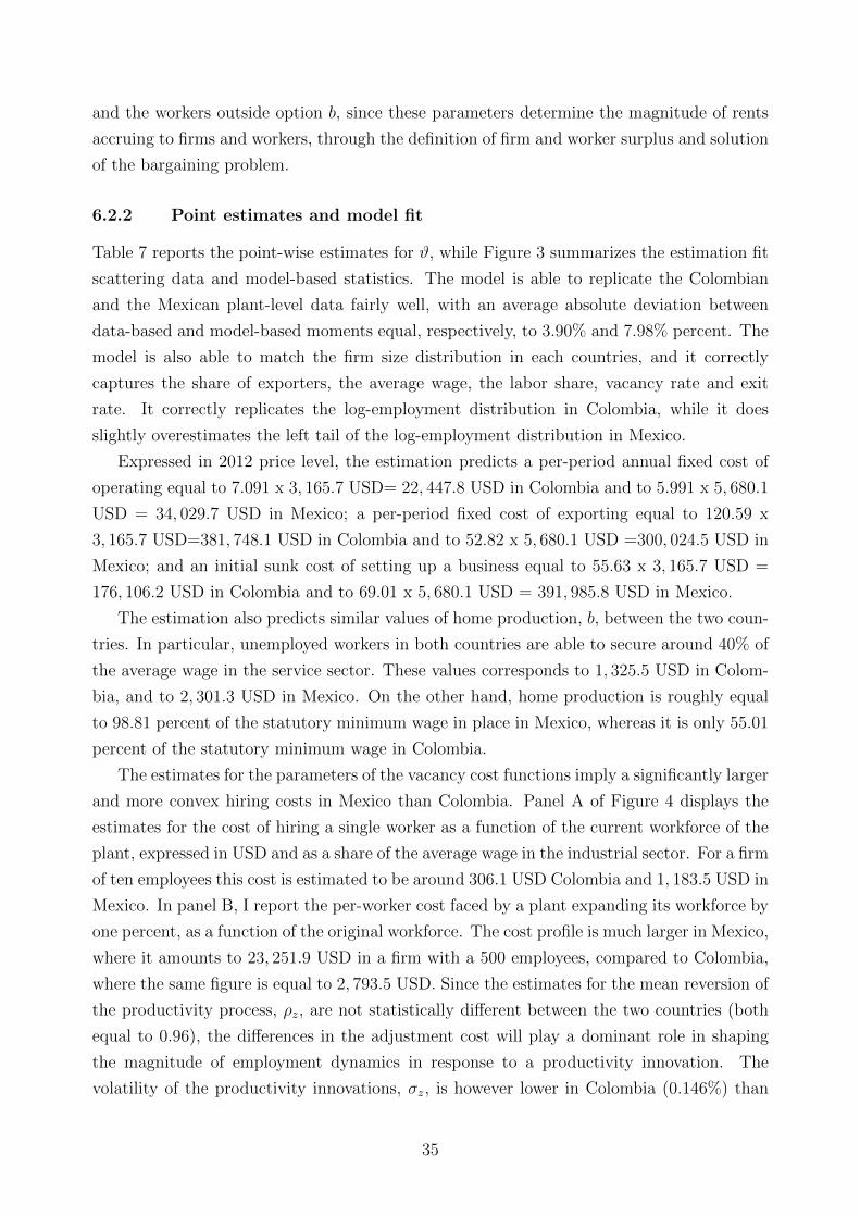
and the workers outside option b, since these parameters determine the magnitude of rents
accruing to firms and workers, through the definition of firm and worker surplus and solution
of the bargaining problem.
6.2.2 Point estimates and model fit
Table 7 reports the point-wise estimates for ϑ, while Figure 3 summarizes the estimation fit
scattering data and model-based statistics. The model is able to replicate the Colombian
and the Mexican plant-level data fairly well, with an average absolute deviation between
data-based and model-based moments equal, respectively, to 3.90% and 7.98% percent. The
model is also able to match the firm size distribution in each countries, and it correctly
captures the share of exporters, the average wage, the labor share, vacancy rate and exit
rate. It correctly replicates the log-employment distribution in Colombia, while it does
slightly overestimates the left tail of the log-employment distribution in Mexico.
Expressed in 2012 price level, the estimation predicts a per-period annual fixed cost of
operating equal to 7.091 x 3, 165.7 USD= 22, 447.8 USD in Colombia and to 5.991 x 5, 680.1
USD = 34, 029.7 USD in Mexico; a per-period fixed cost of exporting equal to 120.59 x
3, 165.7 USD=381, 748.1 USD in Colombia and to 52.82 x 5, 680.1 USD =300, 024.5 USD in
Mexico; and an initial sunk cost of setting up a business equal to 55.63 x 3, 165.7 USD =
176, 106.2 USD in Colombia and to 69.01 x 5, 680.1 USD = 391, 985.8 USD in Mexico.
The estimation also predicts similar values of home production, b, between the two coun-
tries. In particular, unemployed workers in both countries are able to secure around 40% of
the average wage in the service sector. These values corresponds to 1, 325.5 USD in Colom-
bia, and to 2, 301.3 USD in Mexico. On the other hand, home production is roughly equal
to 98.81 percent of the statutory minimum wage in place in Mexico, whereas it is only 55.01
percent of the statutory minimum wage in Colombia.
The estimates for the parameters of the vacancy cost functions imply a significantly larger
and more convex hiring costs in Mexico than Colombia. Panel A of Figure 4 displays the
estimates for the cost of hiring a single worker as a function of the current workforce of the
plant, expressed in USD and as a share of the average wage in the industrial sector. For a firm
of ten employees this cost is estimated to be around 306.1 USD Colombia and 1, 183.5 USD in
Mexico. In panel B, I report the per-worker cost faced by a plant expanding its workforce by
one percent, as a function of the original workforce. The cost profile is much larger in Mexico,
where it amounts to 23, 251.9 USD in a firm with a 500 employees, compared to Colombia,
where the same figure is equal to 2, 793.5 USD. Since the estimates for the mean reversion of
the productivity process, ρz, are not statistically different between the two countries (both
equal to 0.96), the differences in the adjustment cost will play a dominant role in shaping
the magnitude of employment dynamics in response to a productivity innovation. The
volatility of the productivity innovations, σz, is however lower in Colombia (0.146%) than
35
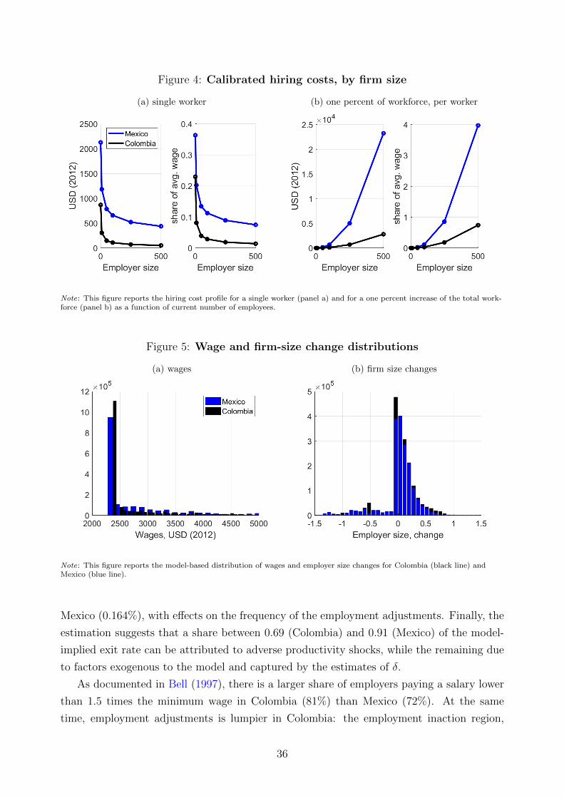
Figure 4: Calibrated hiring costs, by firm size
(a) single worker (b) one percent of workforce, per worker
Note: This figure reports the hiring cost profile for a single worker (panel a) and for a one percent increase of the total work-force (panel b) as a function of current number of employees.
Figure 5: Wage and firm-size change distributions
(a) wages (b) firm size changes
Note: This figure reports the model-based distribution of wages and employer size changes for Colombia (black line) andMexico (blue line).
Mexico (0.164%), with effects on the frequency of the employment adjustments. Finally, the
estimation suggests that a share between 0.69 (Colombia) and 0.91 (Mexico) of the model-
implied exit rate can be attributed to adverse productivity shocks, while the remaining due
to factors exogenous to the model and captured by the estimates of δ.
As documented in Bell (1997), there is a larger share of employers paying a salary lower
than 1.5 times the minimum wage in Colombia (81%) than Mexico (72%). At the same
time, employment adjustments is lumpier in Colombia: the employment inaction region,
36
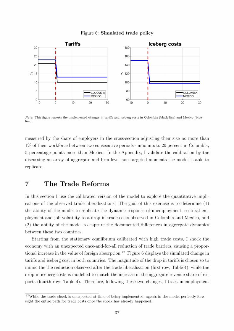
Figure 6: Simulated trade policy
Note: This figure reports the implemented changes in tariffs and iceberg costs in Colombia (black line) and Mexico (blueline).
measured by the share of employers in the cross-section adjusting their size no more than
1% of their workforce between two consecutive periods - amounts to 20 percent in Colombia,
5 percentage points more than Mexico. In the Appendix, I validate the calibration by the
discussing an array of aggregate and firm-level non-targeted moments the model is able to
replicate.
7 The Trade Reforms
In this section I use the calibrated version of the model to explore the quantitative impli-
cations of the observed trade liberalizations. The goal of this exercise is to determine (1)
the ability of the model to replicate the dynamic response of unemployment, sectoral em-
ployment and job volatility to a drop in trade costs observed in Colombia and Mexico, and
(2) the ability of the model to capture the documented differences in aggregate dynamics
between these two countries.
Starting from the stationary equilibrium calibrated with high trade costs, I shock the
economy with an unexpected once-and-for-all reduction of trade barriers, causing a propor-
tional increase in the value of foreign absorption.42 Figure 6 displays the simulated change in
tariffs and iceberg cost in both countries. The magnitude of the drop in tariffs is chosen so to
mimic the the reduction observed after the trade liberalization (first row, Table 4), while the
drop in iceberg costs is modelled to match the increase in the aggregate revenue share of ex-
ports (fourth row, Table 4). Therefore, following these two changes, I track unemployment
42While the trade shock is unexpected at time of being implemented, agents in the model perfectly fore-sight the entire path for trade costs once the shock has already happened.
37
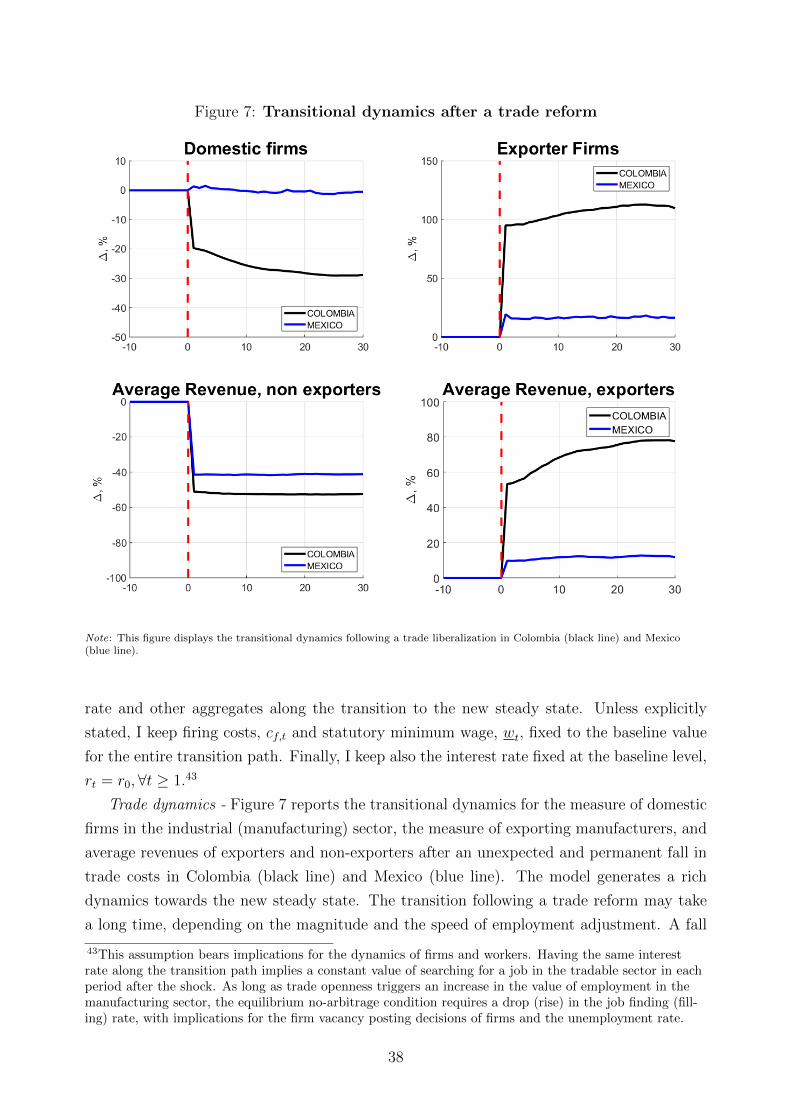
Figure 7: Transitional dynamics after a trade reform
Note: This figure displays the transitional dynamics following a trade liberalization in Colombia (black line) and Mexico(blue line).
rate and other aggregates along the transition to the new steady state. Unless explicitly
stated, I keep firing costs, cf,t and statutory minimum wage, wt, fixed to the baseline value
for the entire transition path. Finally, I keep also the interest rate fixed at the baseline level,
rt = r0,∀t ≥ 1.43
Trade dynamics - Figure 7 reports the transitional dynamics for the measure of domestic
firms in the industrial (manufacturing) sector, the measure of exporting manufacturers, and
average revenues of exporters and non-exporters after an unexpected and permanent fall in
trade costs in Colombia (black line) and Mexico (blue line). The model generates a rich
dynamics towards the new steady state. The transition following a trade reform may take
a long time, depending on the magnitude and the speed of employment adjustment. A fall
43This assumption bears implications for the dynamics of firms and workers. Having the same interestrate along the transition path implies a constant value of searching for a job in the tradable sector in eachperiod after the shock. As long as trade openness triggers an increase in the value of employment in themanufacturing sector, the equilibrium no-arbitrage condition requires a drop (rise) in the job finding (fill-ing) rate, with implications for the firm vacancy posting decisions of firms and the unemployment rate.
38
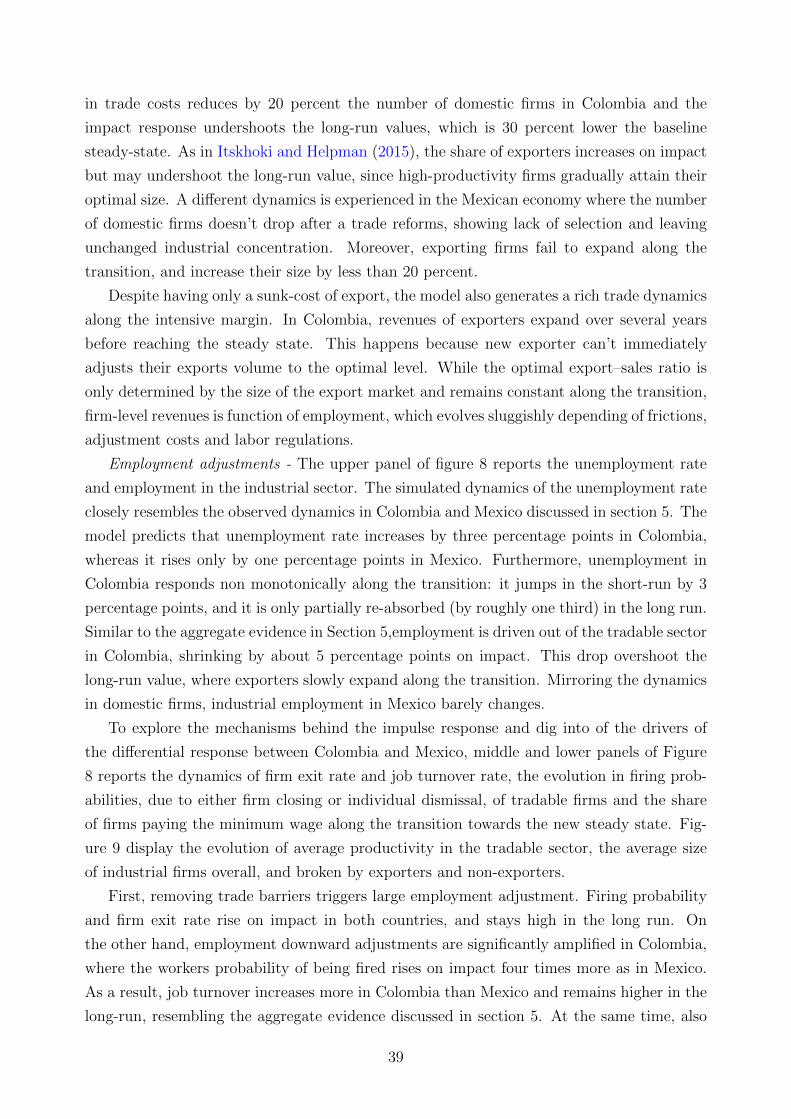
in trade costs reduces by 20 percent the number of domestic firms in Colombia and the
impact response undershoots the long-run values, which is 30 percent lower the baseline
steady-state. As in Itskhoki and Helpman (2015), the share of exporters increases on impact
but may undershoot the long-run value, since high-productivity firms gradually attain their
optimal size. A different dynamics is experienced in the Mexican economy where the number
of domestic firms doesn’t drop after a trade reforms, showing lack of selection and leaving
unchanged industrial concentration. Moreover, exporting firms fail to expand along the
transition, and increase their size by less than 20 percent.
Despite having only a sunk-cost of export, the model also generates a rich trade dynamics
along the intensive margin. In Colombia, revenues of exporters expand over several years
before reaching the steady state. This happens because new exporter can’t immediately
adjusts their exports volume to the optimal level. While the optimal export–sales ratio is
only determined by the size of the export market and remains constant along the transition,
firm-level revenues is function of employment, which evolves sluggishly depending of frictions,
adjustment costs and labor regulations.
Employment adjustments - The upper panel of figure 8 reports the unemployment rate
and employment in the industrial sector. The simulated dynamics of the unemployment rate
closely resembles the observed dynamics in Colombia and Mexico discussed in section 5. The
model predicts that unemployment rate increases by three percentage points in Colombia,
whereas it rises only by one percentage points in Mexico. Furthermore, unemployment in
Colombia responds non monotonically along the transition: it jumps in the short-run by 3
percentage points, and it is only partially re-absorbed (by roughly one third) in the long run.
Similar to the aggregate evidence in Section 5,employment is driven out of the tradable sector
in Colombia, shrinking by about 5 percentage points on impact. This drop overshoot the
long-run value, where exporters slowly expand along the transition. Mirroring the dynamics
in domestic firms, industrial employment in Mexico barely changes.
To explore the mechanisms behind the impulse response and dig into of the drivers of
the differential response between Colombia and Mexico, middle and lower panels of Figure
8 reports the dynamics of firm exit rate and job turnover rate, the evolution in firing prob-
abilities, due to either firm closing or individual dismissal, of tradable firms and the share
of firms paying the minimum wage along the transition towards the new steady state. Fig-
ure 9 display the evolution of average productivity in the tradable sector, the average size
of industrial firms overall, and broken by exporters and non-exporters.
First, removing trade barriers triggers large employment adjustment. Firing probability
and firm exit rate rise on impact in both countries, and stays high in the long run. On
the other hand, employment downward adjustments are significantly amplified in Colombia,
where the workers probability of being fired rises on impact four times more as in Mexico.
As a result, job turnover increases more in Colombia than Mexico and remains higher in the
long-run, resembling the aggregate evidence discussed in section 5. At the same time, also
39
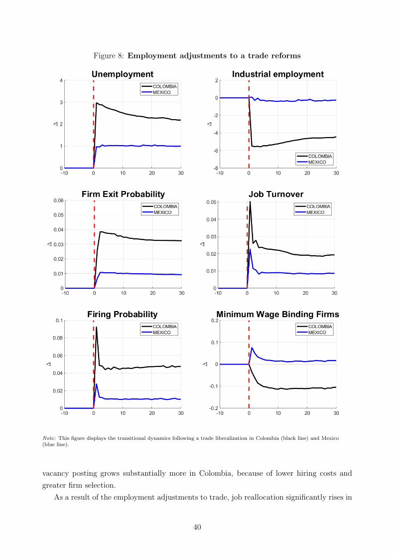
Figure 8: Employment adjustments to a trade reforms
Note: This figure displays the transitional dynamics following a trade liberalization in Colombia (black line) and Mexico(blue line).
vacancy posting grows substantially more in Colombia, because of lower hiring costs and
greater firm selection.
As a result of the employment adjustments to trade, job reallocation significantly rises in
40
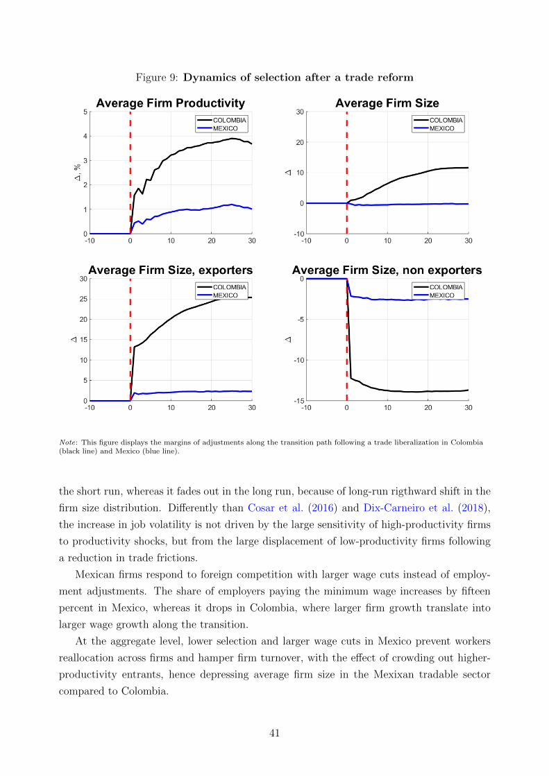
Figure 9: Dynamics of selection after a trade reform
Note: This figure displays the margins of adjustments along the transition path following a trade liberalization in Colombia(black line) and Mexico (blue line).
the short run, whereas it fades out in the long run, because of long-run rigthward shift in the
firm size distribution. Differently than Cosar et al. (2016) and Dix-Carneiro et al. (2018),
the increase in job volatility is not driven by the large sensitivity of high-productivity firms
to productivity shocks, but from the large displacement of low-productivity firms following
a reduction in trade frictions.
Mexican firms respond to foreign competition with larger wage cuts instead of employ-
ment adjustments. The share of employers paying the minimum wage increases by fifteen
percent in Mexico, whereas it drops in Colombia, where larger firm growth translate into
larger wage growth along the transition.
At the aggregate level, lower selection and larger wage cuts in Mexico prevent workers
reallocation across firms and hamper firm turnover, with the effect of crowding out higher-
productivity entrants, hence depressing average firm size in the Mexixan tradable sector
compared to Colombia.
41
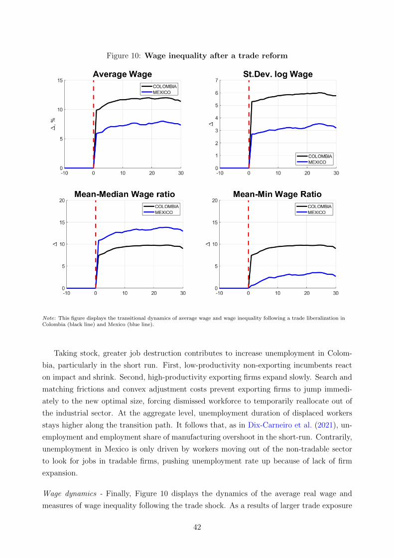
Figure 10: Wage inequality after a trade reform
Note: This figure displays the transitional dynamics of average wage and wage inequality following a trade liberalization inColombia (black line) and Mexico (blue line).
Taking stock, greater job destruction contributes to increase unemployment in Colom-
bia, particularly in the short run. First, low-productivity non-exporting incumbents react
on impact and shrink. Second, high-productivity exporting firms expand slowly. Search and
matching frictions and convex adjustment costs prevent exporting firms to jump immedi-
ately to the new optimal size, forcing dismissed workforce to temporarily reallocate out of
the industrial sector. At the aggregate level, unemployment duration of displaced workers
stays higher along the transition path. It follows that, as in Dix-Carneiro et al. (2021), un-
employment and employment share of manufacturing overshoot in the short-run. Contrarily,
unemployment in Mexico is only driven by workers moving out of the non-tradable sector
to look for jobs in tradable firms, pushing unemployment rate up because of lack of firm
expansion.
Wage dynamics - Finally, Figure 10 displays the dynamics of the average real wage and
measures of wage inequality following the trade shock. As a results of larger trade exposure
42

and lower aggregate domestic price, average real wage increases in both countries. Moreover,
higher revenues dispersion between exporters and non-exporting firms results into higher
wage dispersion after the trade reform. On the other hand, the source of wage inequality are
different between the two countries. Higher minimum wage in Colombia hampers the increase
in the mean to median wage ratio relative to Mexico, where the median wage falls relative to
the mean because of larger downward wage adjustment. Instead, larger selection and workers
reallocation in Colombia resulted into higher average wage relative to the minimum, with an
increase more than two times as in Mexico. Overall, the second effect dominates making the
standard deviation of log wages in Colombia increasing by more than 2 percentage points
compared to Mexico, a finding in lines with the aggregate evidence reported in Section 5.
7.1 The role of labor market institutions
To isolate the contribution of each labor market institutions, I conduct a series of counter-
factual exercises using the structure of the calibrated model. The goal of this exercise is to
determine to which extent the labor market institutions in place affects the labor market
adjustments to a trade liberalization.
In particular, I consider two alternative scenarios, one for each country. The first counter-
facual is a trade liberalization implemented in Colombia under the minimum wage regulation
observed in Mexico. The second countefactual is trade liberalization implemented in Mexico
under the employment protection legislation observed in Colombia. Within each country,
differences in the impulse response across simulation must have a causal interpretation: they
are only driven by differences in the initial regulations in place.
Figure 11 display the dynamics of unemployment rate, firing probability and share of firms
paying the minimum wage following a trade reform implemented under baseline and coun-
terfactual initial institutions at different horizons.44 As in Kambourov (2009), regulations in
the labor market are key determinants of the magnitude and the speed of employment ad-
justment after a trade reform. High firing costs hamper job destruction, low minimum wage
foster greater wage cuts. Greater job destruction contributes to increase unemployment,
particularly in the short run.
Consistent with the cross-country evidence documented in sections 2.1 and 2.2, the down-
ward price rigidity induced by a binding statutory minimum wage observed in Colombia is
cause of large unemployment rate as response to a trade shock. The quantity rigidity induced
by a stricter employment protection legislation in Mexico has the opposite effect. While part
of adjustments still happen through wage renegotiation, stricter minimum wage and lower
firing costs increase the probability of workers dismissal, both in the short and the long run.
Stricter minimum wage in Colombia pushes up unemployment rate following a trade
44Appendix D reports similar counterfactual dynamics for the number of producers, average firm size,average productivity and wages.
43
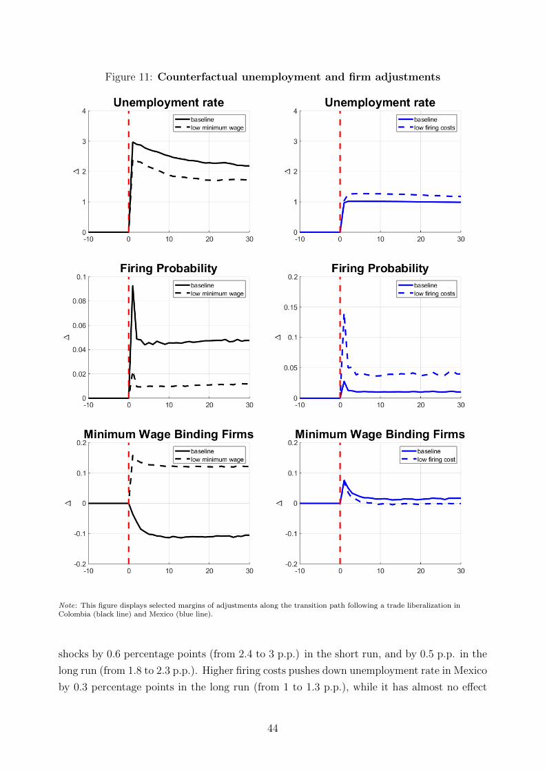
Figure 11: Counterfactual unemployment and firm adjustments
Note: This figure displays selected margins of adjustments along the transition path following a trade liberalization inColombia (black line) and Mexico (blue line).
shocks by 0.6 percentage points (from 2.4 to 3 p.p.) in the short run, and by 0.5 p.p. in the
long run (from 1.8 to 2.3 p.p.). Higher firing costs pushes down unemployment rate in Mexico
by 0.3 percentage points in the long run (from 1 to 1.3 p.p.), while it has almost no effect
44
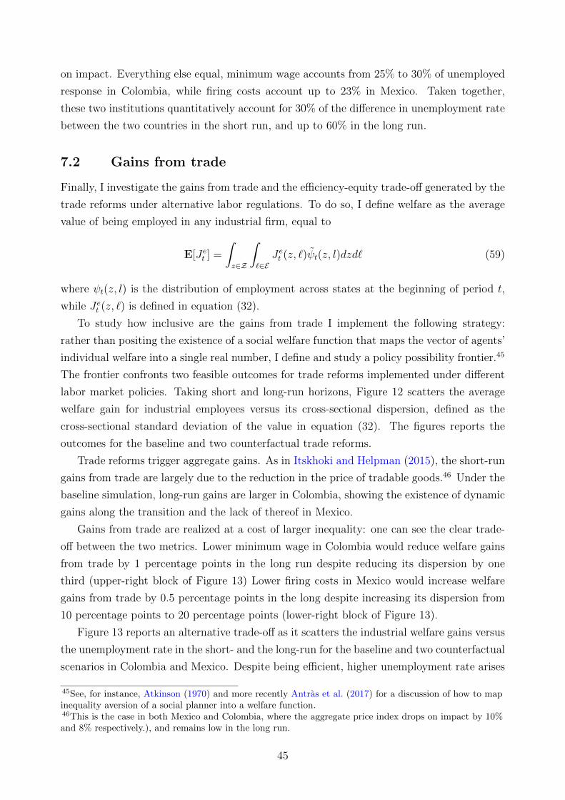
on impact. Everything else equal, minimum wage accounts from 25% to 30% of unemployed
response in Colombia, while firing costs account up to 23% in Mexico. Taken together,
these two institutions quantitatively account for 30% of the difference in unemployment rate
between the two countries in the short run, and up to 60% in the long run.
7.2 Gains from trade
Finally, I investigate the gains from trade and the efficiency-equity trade-off generated by the
trade reforms under alternative labor regulations. To do so, I define welfare as the average
value of being employed in any industrial firm, equal to
E[Jet ] =
∫z∈Z
∫`∈E
Jet (z, `)ψt(z, l)dzd` (59)
where ψt(z, l) is the distribution of employment across states at the beginning of period t,
while Jet (z, `) is defined in equation (32).
To study how inclusive are the gains from trade I implement the following strategy:
rather than positing the existence of a social welfare function that maps the vector of agents’
individual welfare into a single real number, I define and study a policy possibility frontier.45
The frontier confronts two feasible outcomes for trade reforms implemented under different
labor market policies. Taking short and long-run horizons, Figure 12 scatters the average
welfare gain for industrial employees versus its cross-sectional dispersion, defined as the
cross-sectional standard deviation of the value in equation (32). The figures reports the
outcomes for the baseline and two counterfactual trade reforms.
Trade reforms trigger aggregate gains. As in Itskhoki and Helpman (2015), the short-run
gains from trade are largely due to the reduction in the price of tradable goods.46 Under the
baseline simulation, long-run gains are larger in Colombia, showing the existence of dynamic
gains along the transition and the lack of thereof in Mexico.
Gains from trade are realized at a cost of larger inequality: one can see the clear trade-
off between the two metrics. Lower minimum wage in Colombia would reduce welfare gains
from trade by 1 percentage points in the long run despite reducing its dispersion by one
third (upper-right block of Figure 13) Lower firing costs in Mexico would increase welfare
gains from trade by 0.5 percentage points in the long despite increasing its dispersion from
10 percentage points to 20 percentage points (lower-right block of Figure 13).
Figure 13 reports an alternative trade-off as it scatters the industrial welfare gains versus
the unemployment rate in the short- and the long-run for the baseline and two counterfactual
scenarios in Colombia and Mexico. Despite being efficient, higher unemployment rate arises
45See, for instance, Atkinson (1970) and more recently Antras et al. (2017) for a discussion of how to mapinequality aversion of a social planner into a welfare function.46This is the case in both Mexico and Colombia, where the aggregate price index drops on impact by 10%and 8% respectively.), and remains low in the long run.
45
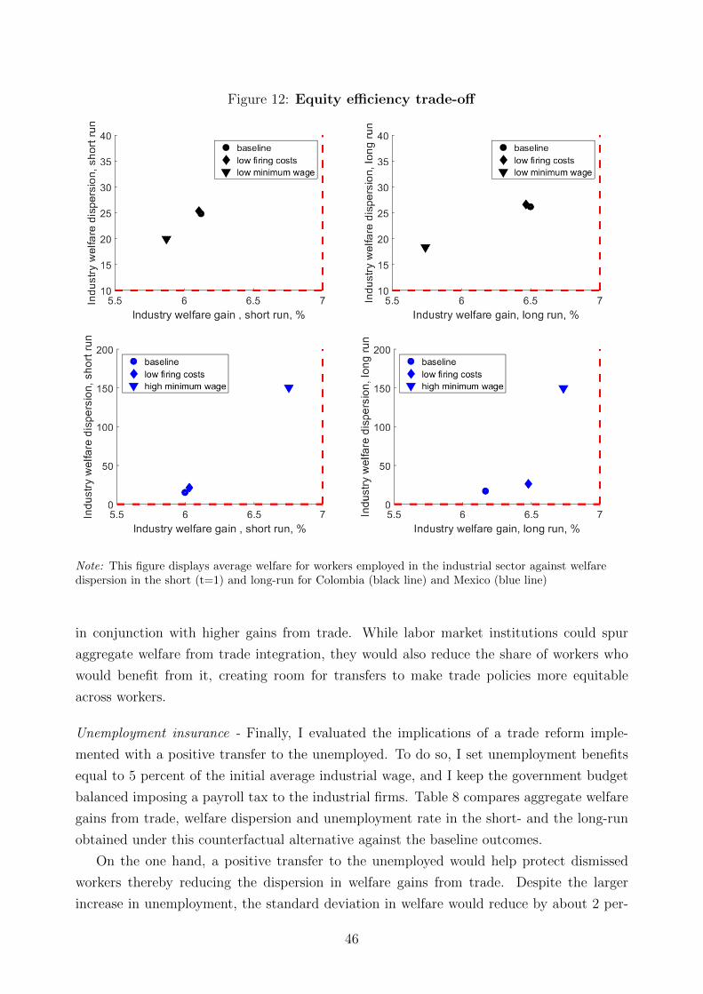
Figure 12: Equity efficiency trade-off
Note: This figure displays average welfare for workers employed in the industrial sector against welfaredispersion in the short (t=1) and long-run for Colombia (black line) and Mexico (blue line)
in conjunction with higher gains from trade. While labor market institutions could spur
aggregate welfare from trade integration, they would also reduce the share of workers who
would benefit from it, creating room for transfers to make trade policies more equitable
across workers.
Unemployment insurance - Finally, I evaluated the implications of a trade reform imple-
mented with a positive transfer to the unemployed. To do so, I set unemployment benefits
equal to 5 percent of the initial average industrial wage, and I keep the government budget
balanced imposing a payroll tax to the industrial firms. Table 8 compares aggregate welfare
gains from trade, welfare dispersion and unemployment rate in the short- and the long-run
obtained under this counterfactual alternative against the baseline outcomes.
On the one hand, a positive transfer to the unemployed would help protect dismissed
workers thereby reducing the dispersion in welfare gains from trade. Despite the larger
increase in unemployment, the standard deviation in welfare would reduce by about 2 per-
46
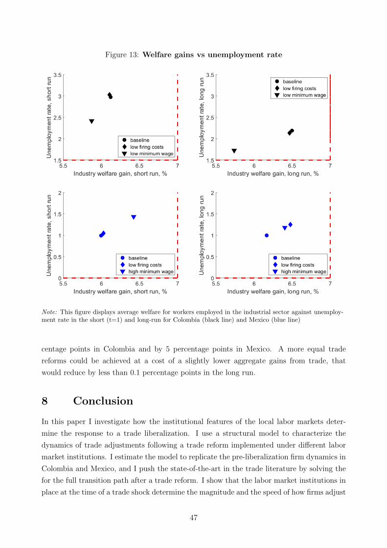
Figure 13: Welfare gains vs unemployment rate
Note: This figure displays average welfare for workers employed in the industrial sector against unemploy-ment rate in the short (t=1) and long-run for Colombia (black line) and Mexico (blue line)
centage points in Colombia and by 5 percentage points in Mexico. A more equal trade
reforms could be achieved at a cost of a slightly lower aggregate gains from trade, that
would reduce by less than 0.1 percentage points in the long run.
8 Conclusion
In this paper I investigate how the institutional features of the local labor markets deter-
mine the response to a trade liberalization. I use a structural model to characterize the
dynamics of trade adjustments following a trade reform implemented under different labor
market institutions. I estimate the model to replicate the pre-liberalization firm dynamics in
Colombia and Mexico, and I push the state-of-the-art in the trade literature by solving the
for the full transition path after a trade reform. I show that the labor market institutions in
place at the time of a trade shock determine the magnitude and the speed of how firms adjust
47
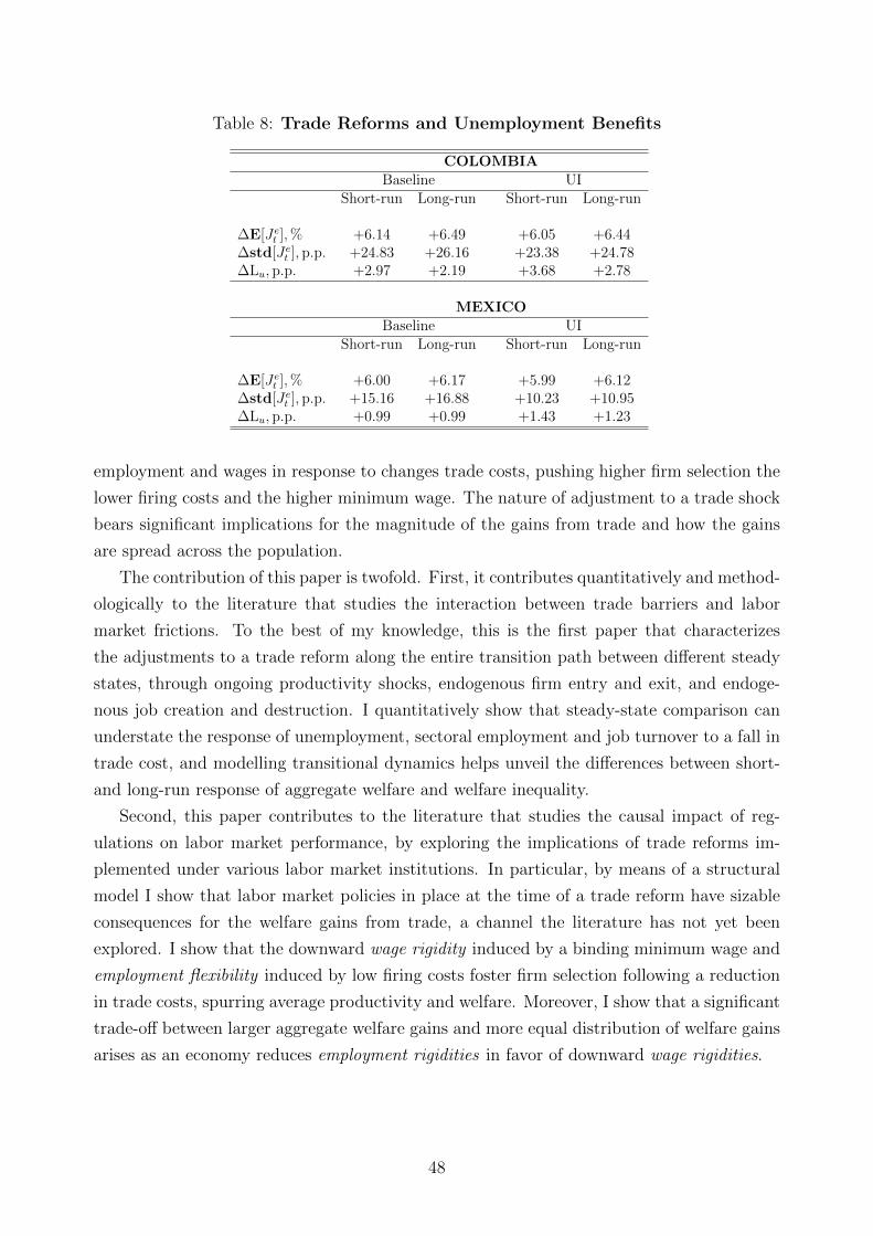
Table 8: Trade Reforms and Unemployment Benefits
COLOMBIABaseline UI
Short-run Long-run Short-run Long-run
∆E[Jet ],% +6.14 +6.49 +6.05 +6.44∆std[Jet ], p.p. +24.83 +26.16 +23.38 +24.78∆Lu, p.p. +2.97 +2.19 +3.68 +2.78
MEXICOBaseline UI
Short-run Long-run Short-run Long-run
∆E[Jet ],% +6.00 +6.17 +5.99 +6.12∆std[Jet ], p.p. +15.16 +16.88 +10.23 +10.95∆Lu, p.p. +0.99 +0.99 +1.43 +1.23
employment and wages in response to changes trade costs, pushing higher firm selection the
lower firing costs and the higher minimum wage. The nature of adjustment to a trade shock
bears significant implications for the magnitude of the gains from trade and how the gains
are spread across the population.
The contribution of this paper is twofold. First, it contributes quantitatively and method-
ologically to the literature that studies the interaction between trade barriers and labor
market frictions. To the best of my knowledge, this is the first paper that characterizes
the adjustments to a trade reform along the entire transition path between different steady
states, through ongoing productivity shocks, endogenous firm entry and exit, and endoge-
nous job creation and destruction. I quantitatively show that steady-state comparison can
understate the response of unemployment, sectoral employment and job turnover to a fall in
trade cost, and modelling transitional dynamics helps unveil the differences between short-
and long-run response of aggregate welfare and welfare inequality.
Second, this paper contributes to the literature that studies the causal impact of reg-
ulations on labor market performance, by exploring the implications of trade reforms im-
plemented under various labor market institutions. In particular, by means of a structural
model I show that labor market policies in place at the time of a trade reform have sizable
consequences for the welfare gains from trade, a channel the literature has not yet been
explored. I show that the downward wage rigidity induced by a binding minimum wage and
employment flexibility induced by low firing costs foster firm selection following a reduction
in trade costs, spurring average productivity and welfare. Moreover, I show that a significant
trade-off between larger aggregate welfare gains and more equal distribution of welfare gains
arises as an economy reduces employment rigidities in favor of downward wage rigidities.
48
References
Airola, J. and Juhn, C. (2008). Wage inequality in post-reform mexico. Journal of Income
Distribution, 17(1):110–134.
Alvarez, F. and Veracierto, M. (2000). Labor market policies in an equilibrium search model,
in nber macroeconomics annual. Cambridge and London: MIT Press, pages 265–304.
Amiti, M. and Cameron, L. (2012). Trade liberalization and the wage skill premium: Evi-
dence from indonesia. Journal of International Economics, 87(2):277–287.
Anderson, J. E. and Van Wincoop, E. (2001). Borders, trade and welfare. Technical report,
National Bureau of Economic Research.
Antras, P., De Gortari, A., and Itskhoki, O. (2017). Globalization, inequality and welfare.
Journal of International Economics, 108:387–412.
Atkin, D. and Khandelwal, A. K. (2020). How distortions alter the impacts of international
trade in developing countries. Annual Review of Economics, 12:213–238.
Atkinson, A. B. (1970). On the measurement of inequality. Journal of economic theory,
2(3):244–263.
Attanasio, O., Goldberg, P. K., and Pavcnik, N. (2004a). Trade reforms and wage inequality
in colombia. Journal of Development Economics, 74(2):331–366.
Attanasio, O., Goldberg, P. K., and Pavcnik, N. (2004b). Trade reforms and wage inequality
in colombia. Journal of development Economics, 74(2):331–366.
Baier, S. L. and Bergstrand, J. H. (2001). The growth of world trade: tariffs, transport
costs, and income similarity. Journal of International Economics, 53(1):1–27.
Balat, J. F. and Porto, G. G. (2007). Globalization and complementary policies: Poverty
impacts on rural zambia. In Globalization and Poverty, pages 373–416. University of
Chicago Press.
Bell, L. A. (1997). The impact of minimum wages in mexico and colombia. Journal of Labor
Economics, 15(3):102–135.
Bellon, M. (2016). Trade liberalization and inequality: a dynamic model with firm and
worker heterogeneity. Columbia University, unpublished manuscript.
Bentolila, S. and Bertola, G. (1990). Firing costs and labour demand: How bad is euroscle-
rosis?. The Review of Economic Studies, 57(3):381–402.
49
Bernanrd, A., Eaton, J., Jensen, J. B., and Kortum, S. (2003). Plants and productivity in
international trade. American Economic Review, 93(4):1268–1290.
Bernard, A. B., Jensen, J. B., and Lawrence, R. Z. (1995). Exporters, jobs, and wages in
us manufacturing: 1976-1987. Brookings papers on economic activity. Microeconomics,
1995:67–119.
Bertola, G. and Caballero, R. J. (1994). Cross-sectional efficiency and labour hoarding in a
matching model of unemployment. Review of Economic Studies, 61(3):435–456.
Binmore, K., Rubinstein, A., and Wolinsky, A. (1986). The nash bargaining solution in
economic modelling. The RAND Journal of Economics, pages 176–188.
Brown, C. and Medoff, J. (1989). The employer size-wage effect. Journal of political Econ-
omy, 97(5):1027–1059.
Burki, S. J. and Perry, G. E. (1997). The long march: a reform agenda for Latin America
and the Caribbean in the next decade. The World Bank.
Cooper, R., Haltiwanger, J., and Willis, J. L. (2007). Search frictions: Matching aggregate
and establishment observations. Journal of Monetary Economics, 54:56–78.
Cosar, K. (2013). Adjusting to trade liberalization: Reallocation and labor market policies.
University of Virginia, unpublished manuscript.
Cosar, K., Guner, N., and Tybout, J. (2016). Firm dynamics, job turnover, and wage
distributions in an open economy. American Economic Review, 106(3):625–663.
Currie, J. and Harrison, A. (1997). Sharing the costs: the impact of trade reform on capital
and labor in morocco. Journal of Labor Economics, 15(S3):S44–S71.
den Haan, Wouter J., G. R. and Watson, J. (2000). Job destruction and the propagation of
shocks. American Economic Review, 90(3):482–498.
Dix-Carneiro, R. (2014). Trade liberalization and labor market dynamics. Econometrica,
82(3):825–885.
Dix-Carneiro, R., Goldberg, P. K., Meghir, C., and Ulyssea, G. (2018). Trade and informality
in the presence of labor market frictions and regulations. (mimeo).
Dix-Carneiro, R. and Kovak, B. K. (2017). Margins of labor market adjustment to trade.
Technical report, National Bureau of Economic Research.
Dix-Carneiro, R., Pessoa, J. P., Reyes-Heroles, R. M., and Traiberman, S. (2021). Globaliza-
tion, trade imbalances and labor market adjustment. Technical report, National Bureau
of Economic Research.
50
Dornbusch, R. and Werner, A. (1994). Mexico: Stabilization, reform and no growth. Brooking
Papers on Economic Activity, 1.
Elsby, M. W. and Gottfries, A. (2019). Firm dynamics, on-the-job search, and labor market
fluctuations. Technical report, Working Paper.
Fajgelbaum, P. (2016). Labor market frictions, firm growth, and international trade. NBER
Working Paper, 19492.
Felbermayr, G., Impullitti, G., and Prat, J. (2016). Firm dynamics and residual inequality
in open economies. IZA Discussion Paper, 7960.
Forteza, A. and Rama, M. (2006). Labor market ‘rigidity’and the success of economic reforms
across more than 100 countries. The Journal of Policy Reform, 9(1):75–105.
FRdB-IMF (2018). Labour institutions database (1980-2005). available at
http://www.frdb.org.
Freeman, R. B. (2007). Labor market institutions around the world. Technical report,
National Bureau of Economic Research.
Freeman, R. B. (2010). Labor regulations, unions, and social protection in developing coun-
tries: market distortions or efficient institutions? In Handbook of development economics,
volume 5, pages 4657–4702. Elsevier.
Goldberg, P. K. and Pavcnik, N. (2004). Trade reforms and wage inequality in colombia.
Journal of Development Economics, 74(2):331–366.
Gourieroux and Monfort (1996). Simulation-based econometric methods. Oxford, UK: Ox-
ford University Press.
Grandolini, G. and Cerda, L. (1998). The 1997 mexican pension reform: genesis and design
features. Financial Markets and Pension Reform Project, Policy Research Working Paper,
1733.
Guerriero, M. (2012). The labour share of income around the world. evidence from a panel
dataset. Development Economics and Public Policy Working Paper Series, (32).
Hall, R. E. and Milgrom, P. R. (2008). The limited influence of unemployment on the wage
bargain. American economic review, 98(4):1653–74.
Haltiwanger, J., Kugler, A., Kugler, M., Micco, A., and Pages, C. (2004). Effects of tariffs
and real exchange rates on job reallocation: Evidence from latin america. Journal of
Policy Reform, 7(4):191–208.
51
Harris, J. R. and Todaro, M. P. (1970). Migration, unemployment, and development: A
two-sector analysis. American Economic Review, 60(1):126–142.
Harrison, A. and Hanson, G. (1999). Who gains from trade reform? some remaining puzzles1.
Journal of development Economics, 59(1):125–154.
Hasan, R., Mitra, D., Ranjan, P., and Ahsan, R. N. (2012). Trade liberalization and
unemployment: Theory and evidence from india. Journal of Development Economics,
97(2):269–280.
Heckman, J. and Pages, C. (2000). The cost of job security regulation: Evidence from latin
american labor markets. NBER working paper, 7773.
Heckman, J. and Pages, C. (2004). Law and employment: Lessons from latin america and
the caribbean. NBER working paper, 10129.
Helpman, E. and Itskhoki, O. (2010). Labor market rigidities, trade and unemployment.
Review of Economic Studies, 77(3):1100–1137.
Helpman, E., Itskhoki, O., Muendler, M.-A., and Redding, S. J. (2017). Trade and inequality:
From theory to estimation. The Review of Economic Studies, 84(1):357–405.
Helpman, E., Itskhoki, O., and Redding, S. (2010). Inequality and unemployment in a global
economy. Econometrica, 78(4):1239–1283.
Hoekman, B. and Porto, G. (2010). Trade adjustment costs in developing countries: Impacts,
determinants and policy responses. Trade Adjustment Costs in Developing Countries:
Impacts, Determinants and, page 1.
Hopenhayn, H. (1992). Entry, exit, and firm dynamics in long run equilibrium. Econometrica,
60(5):1127–1150.
Hopenhayn, H. and Rogerson, R. (1993). Job turnover and policy evaluation: A general
equilibrium analysis. Journal of Political Economy, 101(5):915–938.
IADB (1997). Latin America after a decade of reforms: economic and social progress: 1997
report. Inter-American Development Bank.
Itskhoki, O. and Helpman, E. (2015). Trade liberalization and labor market dynamics with
heterogeneous firms. Princeton Papers.
Kambourov, G. (2009). Labor market regulations and the sectoral reallocation of workers:
The case of trade reforms. Review of Economic Studies, 76(4):1321–1358.
Kose, A., Meredith, G. M., and Towe, C. M. (2004). How has nafta affected the mexican
economy? review and evidence. IMF working paper, 59.
52
Kpodar, K. (2007). Why has unemployment in Algeria been higher than in MENA and
transition countries. Number 7-210. International Monetary Fund.
Kugler, A. D. (1999). The impact of firing costs on turnover and unemployment: Evidence
from the colombian labour market reform. International Tax and Public Finance, 6(3):389–
410.
Laeven, L. and Valencia, F. (2013). Systemic banking crises database. IMF Economic
Review, 61(2):225–270.
Malhotra, R., Singh, N., and Singh, Y. (2011). Genetic algorithms: Concepts, design for
optimization of process controllers. Computer and Information Science, 4(2):39.
Maloney, W. and Mendez, J. (2004). Measuring the impact of minimum wages. evidence
from latin america. NBER working paper, 9800.
McCaig, B. and Pavcnik, N. (2014). Export markets and labor allocation in a low-income
country. Technical report, National Bureau of Economic Research.
McFadden, D. (1989). A method of simulated moments for estimation of discrete response
models without numerical integration. Econometrica, 57(5):995–1026.
Melitz, M. J. (2003). The impact of trade on intra-industry reallocations and aggregate
industry productivity. Econometrica, 71(6):1695–1725.
Menezes-Filho, N. A. and Muendler, M.-A. (2011). Labor reallocation in response to trade
reform. Technical report, National Bureau of Economic Research.
Nicita, A. (2008). Who benefits from export-led growth? evidence from madagascar’s textile
and apparel industry. Journal of African Economies, 17(3):465–489.
Nilsen, Ø. A., Salvanes, K. G., and Schiantarelli, F. (2007). Employment changes, the
structure of adjustment costs, and plant size. European Economic Review, 51(3):577–598.
Pakes, A. and Pollard, D. (1989). Simulation and the asymptotics of optimization estimators.
Econometrica, 57(5):1027–1057.
Pavcnik, N. (2017). The impact of trade on inequality in developing countries. Technical
report, National Bureau of Economic Research.
Peluffo, A. (2013). Assessing labor market impacts of trade opening in uruguay. SpringerPlus,
2(1):219.
Puyana, A. (2010). The impact of trade liberalization and the global economic crisis on the
productive sectors, employment and incomes in mexico. Issue Paper, 15.
53
Revenga, A. (1997). Employment and wage effects of trade liberalization: the case of mexican
manufacturing. Journal of labor Economics, 15(S3):S20–S43.
Riano, A. (2009). Trade, technology adoption and the rise of the skill premium in mexico.
University of Nottingham, unpublished manuscript.
Roberts, M. J. and Tybout, J. R. (1996). Industrial evolution in developing countries: Micro
patterns of turnover, productivity, and market structure.
Rodriguez, F. and Rodrik, D. (2000). Trade policy and economic growth: a skeptic’s guide
to the cross-national evidence. NBER macroeconomics annual, 15:261–325.
Rodrik, D. (1993). Trade and industrial policy reform in developing countries: a review of
recent theory and evidence. Technical report, National Bureau of Economic Research.
Rodrik, D. (2008). One economics, many recipes: globalization, institutions, and economic
growth. Princeton University Press.
Ruhl, K. J. and Willis, J. L. (2017). New exporter dynamics. International Economic Review,
58(3):703–726.
Sachs, J. D. and Warner, A. (1995). Economic reform and the process of global integration.
Brookings Papers on Economic Activity, 26(1):1–118.
Schaal, E. (2012). Uncertainty, productivity and unemployment in the great recession.
Federal Reserve Bank of Minneapolis, mimeo.
Stole, L. A. and Zwiebel, J. (1996). Intra-firm bargaining under non binding contracts. The
Review of Economic Studies, 63(3):375–410.
Tybout, J. R. and Westbrook, M. D. (1995). Trade liberalization and the dimensions of effi-
ciency change in mexican manufacturing industries. Journal of International Economics,
39(1-2):53–78.
Wacziarg, R. and Wallack, J. S. (2004). Trade liberalization and intersectoral labor move-
ments. Journal of International Economics, 64(2):411–439.
Wacziarg, R. and Welch, K. H. (2003). Trade liberalization and growth: New evidence.
NBER Working Paper, 10152.
Yashiv, E. (2000). The determinants of equilibrium unemployment. American Economic
Review, 90(5):1297–1322.
Zagha, R., Nankani, G. T., et al. (2005). Economic Growth in the 1990s: Learning from a
Decade of Reform. World Bank Publications.
54
Online Appendix to
“Trade and Labor Market Institutions:A Tale of Two Liberalizations”
Appendix A. Details on Aggregate Evidence
A.1. Data Source and Definitions
The cross-country empirical evidence is based on 40 countries, for a period spanning be-
tween 30 and 40 years around the respective date of trade liberalization. In the spe-
cific, the countries covered are Albania (1970-2010), Argentina (1970-2010), Azerbaijan
(1980-2010), Bangladesh (1980-2010), Republic of Bolivia (1970-2006), Brazil (1970-2010),
Burkina Faso (1980-2010), Chile (1960-1996), Colombia (1970-2010), Cote d′Ivoire (1980-
2010), Dominican Republic (1970-2010), Ecuador (1970-2010), Egypt (1980-2019), El Sal-
vador (1970-2009), Ethiopia (1980-2010), Georgia (1980-2010), Hungary (1980-2010), In-
dia (1980-2007), Israel (1970-2005), Jamaica (1973-2009), Kyrgyzstan (1980-2010), Latvia
(1990-2010), Lithuania (1980-2010), Madagascar (1980-2010), Mexico (1970-2006), Mozam-
bique (1980-2010), New Zealand (1970-2007), Nicaragua (1970-2010), Pakistan (1980-2010),
Paraguay (1970-2009), Peru′ (1970-2010), Philippines (1970-2008), Poland (1980-2010), Ro-
mania (1985-2010), South Africa (1970-2010), Republic of Tanzania: Mainland (1980-2009),
Tunisia (1970-2009), Turkey (1970-2009), Uruguay (1970-2010) and the Bolivarian Republic
of Venezuela (1974-2010). 47
Trade Liberalizations: The liberalization dates are taken from Wacziarg and Welch (2003)
and are based on Sachs and Warner (1995) criteria. Sachs and Warner classify an economy as
open starting from the first year from which the following five characteristics are continuously
met:
1. Average nominal tariff rates (TAR) below 40%;
2. Non-tariff barriers (NTB) covering less than 40% of trade;
3. A black market exchange rate (BMP) depreciated by less than 20% relative to the
official exchange rate;
4. Absence of monopoly (XMB) on major exports;
47Data on trade liberalization and unemployment is also available for Croatia (1984-2010), Honduras(1970-2010), Malta (1983-2010), Serbia (1990-2014) and Tajikistan (1990-2010). However, since I do nothave information on labor market institutions for these countries, I drop them from the sample. The inclu-sion of these observations in the first regression does not alter any of the results presented.
55
5. No socialist economic system (SOC), as defined by Kornai (1992), is in place.48
Sachs and Warner (1995) selected the these five criteria to cover various types of trade
restrictions. Tariffs and NTBs (like for instance, import quotas) increase directly or indirectly
(through import substitution) the effective FOB price paid for importing foreign goods. A
black market premium on the exchange rate can have effects equivalent to a formal trade
restriction: if exporters purchase foreign inputs using foreign currency obtained on the black
market, but remit their foreign exchange receipts from exports to the government at the
official exchange rate, the black market premium acts as a trade restriction. The state
monopoly on exports is included among the trade restriction, since it acts as an alternative
form of export subsidy and finally the socialist regime dummy variable accounts for the
trade-limiting aspects of centrally-planned economies. However, the threshold values set in
the first three criteria are arbitrary. They provide with liberalization dates for 141 countries
for which they have enough information. From 1960, the great majority of the countries
in the sample experienced a unique episode of trade liberalization and subsequent period
of prolonged openness. Within the sample of countries used in this paper, only Bolivia,
Ecuador and Jamaica went through a period of temporary liberalization, i.e. a period of full
trade opening followed by subsequent failure on one or more of the five criteria listed above.
For these countries, the date of reform is taken to be that at which the openness criteria are
met without subsequent reversal, thus ignoring the initial episode of openness.
Labor Market Institutions: Measures of labor market institutions are taken from the
Fondazione R. de Benedetti (FrdB) Labor Instituion v.1 database. In the paper, I focus on
three specific institutions, namely minimum wage and employment protection legislation.
• The minimum wage regulation is identified using the ratio of statutory minimum wage
to mean wage. Reported data correspond to the values in effect on July 1st of each year,
unless otherwise specified. In countries were several minimum wages were in place,
varying by sector or by location, a simple average minimum wage was constructed.
Non-statutory minimum wage arrangements in place, like wage grids, or minimum
wage determined by collective agreements are excluded.
• The employment protection legislation is measured by sum of the average advance
notice periods and the average severance payments, measured after 9 months, 4 and
20 years, and expressed in months. The data are collected and reported for workers
with regular contracts of unspecified duration after any trial period, for the case of fair
dismissals caused by personal grounds or individual redundancy (economic reason) at
the initiative of the employer, and averaged out across different types of workers (high
and low skilled, white and blue collars, when differently specified).
48A full description of these five variables is provided in the Sachs and Warner (1995).
56
• Unemployment benefits is constructed as the product of the average gross replacement
rate over 1 year after dismissal and the unemployment benefits coverage, so to capture
both extensive and intensive margin of the legislation. The gross replacement ratio is
defined as levels of statutory entitlements over the average wage, after the first year of
unemployment, while the unemployment benefit coverage is constructed as the ratio
of the number of UI benefit recipients to the number of unemployed.
Unemployment Rates: Series for unemployment rate are constructed using data from
ILO-Stat database, except for Chile, for which I used data from Caputo and Saravia (2014).
ILO-Stat defines unemployed a person of working age (from 15 to 64 y.o.) who was (i) without
work during the reference period, i.e. was not in paid employment or self-employment, (ii)
currently available for work, meaning available for paid employment or self-employment
during the reference period, and (iii) seeking work, i.e. had taken specific steps in a specified
recent period to seek paid employment or self-employment. For purposes of international
comparability, ILO-Stat defines the period of job search as the preceding four weeks, though
the definition might vary from country to country. Therefore, the unemployment rate is
calculated as the number of persons who are unemployed during the reference period given
as a percent of the total number of employed and unemployed persons (i.e., the labour force)
in the same reference period.
Controls: Series for GDP, GDP deflator, imports, exports and total population are taken
from the World Development Indicator (WDI) Database of the World Bank. For the case of
Poland and Paraguay, they are integrated with estimates from the International Financial
Statistics (IFS) Database. GDP series are nominal and expressed in current USD price
level. Nominal GDP measures the total output of goods and services for final use occurring
within the domestic territory of a given country, regardless of the allocation to domestic and
foreign claims. Total population refers to all residents regardless of legal status or citizenship.
Nominal measures are converted into real values using the associated GDP deflator and
expressed at constant 2005 USD price level. The import penetration is constructed by
dividing total imports by GDP minus of net exports. Series for employment, rate of inflation
and exchange rate are taken from the Penn Table Dataset v.9.0. Total employment refers
to the number of persons engaged in production. Inflation rate is constructed as the growth
rate of price level for household consumption goods (with price level of USA GDP in 2011
normalized to 1) whereas the exchange rate refers the market value of national currency
per USD. Finally, the dates for the occurrence of banking, currency, and sovereign debt
crises are taken from Laeven and Valencia (2013). In particular, they define (1) a banking
crisis as the first year with signs of financial distress in the banking system (as indicated by
significant bank runs, losses in the banking system, and/or bank liquidations) and banking
policy intervention measures in response to significant losses in the banking system; (2) a
currency crisis as a nominal depreciation of the currency vis-a-vis the U.S. dollar of at least
57
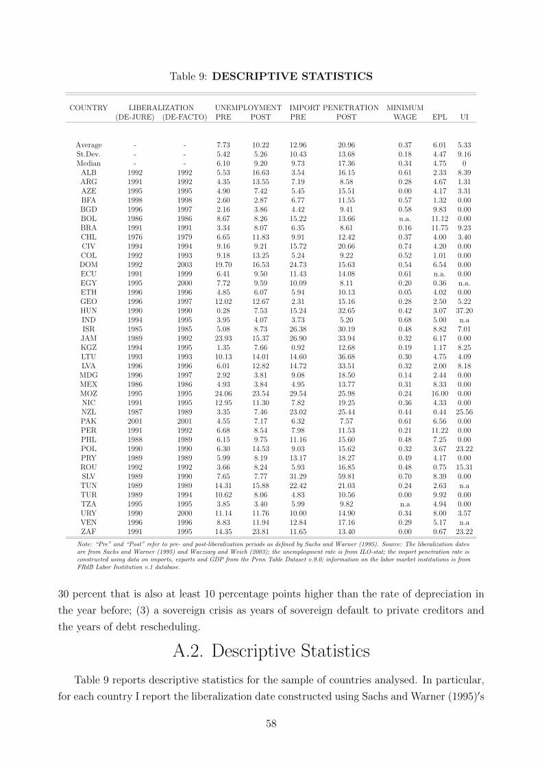
Table 9: DESCRIPTIVE STATISTICS
COUNTRY LIBERALIZATION UNEMPLOYMENT IMPORT PENETRATION MINIMUM(DE-JURE) (DE-FACTO) PRE POST PRE POST WAGE EPL UI
Average - - 7.73 10.22 12.96 20.96 0.37 6.01 5.33St.Dev. - - 5.42 5.26 10.43 13.68 0.18 4.47 9.16Median - - 6.10 9.20 9.73 17.36 0.34 4.75 0
ALB 1992 1992 5.53 16.63 3.54 16.15 0.61 2.33 8.39ARG 1991 1992 4.35 13.55 7.19 8.58 0.28 4.67 1.31AZE 1995 1995 4.90 7.42 5.45 15.51 0.00 4.17 3.31BFA 1998 1998 2.60 2.87 6.77 11.55 0.57 1.32 0.00BGD 1996 1997 2.16 3.86 4.42 9.41 0.58 9.83 0.00BOL 1986 1986 8.67 8.26 15.22 13.66 n.a. 11.12 0.00BRA 1991 1991 3.34 8.07 6.35 8.61 0.16 11.75 9.23CHL 1976 1979 6.65 11.83 9.91 12.42 0.37 4.00 3.40CIV 1994 1994 9.16 9.21 15.72 20.66 0.74 4.20 0.00COL 1992 1993 9.18 13.25 5.24 9.22 0.52 1.01 0.00DOM 1992 2003 19.70 16.53 24.73 15.63 0.54 6.54 0.00ECU 1991 1999 6.41 9.50 11.43 14.08 0.61 n.a. 0.00EGY 1995 2000 7.72 9.59 10.09 8.11 0.20 0.36 n.a.ETH 1996 1996 4.85 6.07 5.94 10.13 0.05 4.02 0.00GEO 1996 1997 12.02 12.67 2.31 15.16 0.28 2.50 5.22HUN 1990 1990 0.28 7.53 15.24 32.65 0.42 3.07 37.20IND 1994 1995 3.95 4.07 3.73 5.20 0.68 5.00 n.aISR 1985 1985 5.08 8.73 26.38 30.19 0.48 8.82 7.01JAM 1989 1992 23.93 15.37 26.90 33.94 0.32 6.17 0.00KGZ 1994 1995 1.35 7.66 0.92 12.68 0.19 1.17 8.25LTU 1993 1993 10.13 14.01 14.60 36.68 0.30 4.75 4.09LVA 1996 1996 6.01 12.82 14.72 33.51 0.32 2.00 8.18
MDG 1996 1997 2.92 3.81 9.08 18.50 0.14 2.44 0.00MEX 1986 1986 4.93 3.84 4.95 13.77 0.31 8.33 0.00MOZ 1995 1995 24.06 23.54 29.54 25.98 0.24 16.00 0.00NIC 1991 1995 12.95 11.30 7.82 19.25 0.36 4.33 0.00NZL 1987 1989 3.35 7.46 23.02 25.44 0.44 0.44 25.56PAK 2001 2001 4.55 7.17 6.32 7.57 0.61 6.56 0.00PER 1991 1992 6.68 8.54 7.98 11.53 0.21 11.22 0.00PHL 1988 1989 6.15 9.75 11.16 15.60 0.48 7.25 0.00POL 1990 1990 6.30 14.53 9.03 15.62 0.32 3.67 23.22PRY 1989 1989 5.99 8.19 13.17 18.27 0.49 4.17 0.00ROU 1992 1992 3.66 8.24 5.93 16.85 0.48 0.75 15.31SLV 1989 1990 7.65 7.77 31.29 59.81 0.70 8.39 0.00TUN 1989 1989 14.31 15.88 22.42 21.03 0.24 2.63 n.aTUR 1989 1994 10.62 8.06 4.83 10.56 0.00 9.92 0.00TZA 1995 1995 3.85 3.40 5.99 9.82 n.a 4.94 0.00URY 1990 2000 11.14 11.76 10.00 14.90 0.34 8.00 3.57VEN 1996 1996 8.83 11.94 12.84 17.16 0.29 5.17 n.aZAF 1991 1995 14.35 23.81 11.65 13.40 0.00 0.67 23.22
Note: “Pre” and “Post” refer to pre- and post-liberalization periods as defined by Sachs and Warner (1995). Source: The liberalization datesare from Sachs and Warner (1995) and Wacziarg and Weich (2003); the unemployment rate is from ILO-stat; the import penetration rate isconstructed using data on imports, exports and GDP from the Penn Table Dataset v.9.0; information on the labor market institutions is fromFRdB Labor Institution v.1 database.
30 percent that is also at least 10 percentage points higher than the rate of depreciation in
the year before; (3) a sovereign crisis as years of sovereign default to private creditors and
the years of debt rescheduling.
A.2. Descriptive Statistics
Table 9 reports descriptive statistics for the sample of countries analysed. In particular,
for each country I report the liberalization date constructed using Sachs and Warner (1995)′s
58
criteria, the average unemployment rate and the average import penetration rate before and
after the trade reform occurs, and the labor market institutions in place at the time of trade
reform. After a trade reform was implemented, the import penetration increase on average
by 8 percentage points (from 12.96 to 20.96) while the unemployment rate increased on
average by about 2.5 percentage points (from 7.73 to 10.22 percent). At the time of a trade
reforms, the cross-country average minimum wage in place wage slightly more than one third
(37%) of the average real monthly wage, the average firing costs was slightly less than the
equivalent of one year and half salary (16.2 real monthly wages), while slightly more than five
percent (5.33%) of the labor force without a job was covered by unemployment insurance.
Appendix B. Details on the Model
B.1. Recursive Competitive Equilibrium
Given aggregate foreign expenditure denominated in foreign currency, Df,t∞t=0, a se-
quence of iceberg costs and tariffs on imports, τc,t, τa,t∞t=0, a sequence of exogenous labor
market policies, cf,t, wt, but ∞t=0, a path for the interest rate rt∞t=0, a transition density
function of the Markov process for productivity shock and its ergodic distribution, Γ(z′|z)
and Γe(z), a Small Open Economy Recursive Competitive Equilibrium is characterized by
a list of value functions for incumbent and potential entrant firms, Vt(z, `), V et ∞t=0, a list
of value functions for workers, Jot , Jst , J it , Jut , Jet (z, `), J ct (z′, `)∞t=0, a list of policy functions
for incumbent firms, Lt(z′, `),1ot (z′, `),1ht (z′, `),1ft (z′, `),1xt (z
′, `)∞t=0, a list of measures for
incumbent and entrant firms Nh,t, Ne,t∞t=0, a list of aggregate domestic price indexes and
aggregate domestic demand for the industrial composite good Dh,t, Pt∞t=0, a stream of ag-
gregate income It∞t=0 and exchange rates kt∞t=0, a list of measures for workers employed
in the service sector, workers in the industrial sector, workers searching for jobs in the indus-
trial sector and unemployed workers, Ls,t, Lq,t, Ut, Lu,t∞t=0, a list of vacancy filling rates, job
finding rates and probabilities of being fired, φt, φt, pot (z, `), pft (z′, `)∞t=0, a stream of wage
schedules for industrial workers at hiring and firing firms, wht (z, `), wf
t(z, `)∞t=0, and a list
of probability distributions of firms over the state space (z, `) at the end and at the interim
states of the period, ψt(z′, `), ψt(z′, `′)∞t=0 such that the following conditions are met:
1. the policy functions Lt(z′, `),1ot (z′, `),1ht (z′, `),1ft (z′, `),1xt (z
′, `)∞t=0 solve the problem
of the incumbent firms in the industrial sector and Vt(z, `) and Vt(z, `) attain their
maximum ∀t = 0, 1, ...
2. there is a positive mass of entrant firms in the industrial sector, Ne,t > 0, in every
period t, and V et attains its maximum ∀t = 0, 1, ...
59

3. no-arbitrage conditions holds,
Jot = J it = Jut = Jst ∀t = 0, 1, ..., (60)
since workers are free to choose between working in the service sector, or searching for
formal job in the industrial sector;
4. the probabilities that an industrial worker is fired, pot (z, `) and pft (z′, `), are consistent
with firm exit policy function, employment policy function and optimal hiring and
firing decisions, i.e.
pot (z, `) = δ + (1− δ)(1− 1ot (z, `)) pft (z′, `) = 1ft (z
′, `)
(`− Lt(z′, `)
`
)(61)
5. the probability distributions of firms over the state space (z, `) at the end and the
interim stage of the period, ψt(z′, `′), ψt(z′, `)∞t=0, evolve according to the following
laws of motion:
ψt(z′, `) =
(1− δ)∫z∈Z Ω(z′|z)ψt−1(z, `)1ot (z, `)dz, if ` 6= 1
Ne,tNh,t−1
ψe(z′) + (1− δ)
∫z∈Z Ω(z′|z)ψt−1(z, `)1ot (z, `)dz, if ` = 1
(62)
where Ne,tNh,t−1
is the ratio of firms entering in period t over the total mass of firm active
at time t− 1, and
ψt(z′, `′) =
∫`∈L ψt(z
′, `)1Lt(z′,`)=`′d`∫`∈L
∫z′′∈Z ψt(z
′′, `)1Lt(z′′,`)=`′dz′′d`
(63)
where 1Lt(z′,`)=`′ = 1 if Lt(z′, `) = `′, 0 otherwise;
6. firms enter the economy up to the point where the free entry condition holds with
equality, V et = ceφ
−λ1t and the total mass of firms evolve according the following law of
motion:
Nh,t = (1− δ)(1− µexitt )Nh,t−1 +Ne,t (64)
where µexitt is the fraction of firms exiting at time t, determined by the end-of period
distribution at time t− 1 and the exit policy function at time t:
µexitt =
∫`∈L
∫z∈Z
[1− 1ot (z, `)]ψt−1(z, `)dzd` (65)
7. the wage of industrial employees, wt(z′, `′) is consistent with the bargaining protocols
given in equations (36) and (37) for hiring and firing firms;
8. the labor markets clear, i.e.
60

• the measure of industrial workers who are employed at time t in the industrial
sector, Lq,t, matches the measure of active jobs in industrial firms:
Lq,t = Nh,t
∫`∈L
∫z′∈Z
Lt(z′, `)ψt(z
′, `)dz′d` (66)
• the measure of workers who are unemployed at the end of the period, Lu,t, evolves
according to the following low of motion:
Lu,t = (1− φt)Ut (67)
where Ut = Ut + Lu,t−1 and
Ut = δNh,t−1
∫`∈L
∫z∈Z
`ψt−1(z, `)dzd`+
(1− δ)Nh,t−1
∫`∈L
∫z∈Z
(1− 1ot−1(z, `))`ψt−1(z, `)dzd`+
Nh,t
∫`∈L
∫z∈Z
1ft (z′, `)[`− Lt(z′, `)]ψt(z′, `)dz′d`
(68)
• workers who have jobs in one of the sectors and unsuccessful industrial job seekers
must sum up to total population, i.e. Lq,t + Ls,t + Lu,t = 1 ∀t = 0, 1, ...
• the vacancy filling rate, φt, and the job finding rate, φt, are consistently deter-
mined by the measures of worker searching for industrial jobs in the interim state,
Ut, and the measure of vacancy posted by firms,
vt = Nh,t
∫`∈L
∫z′∈Z
1ht (z′, `)
(Lt(z
′, `)− `φt
)ψt(z
′, `)dz′d` (69)
9. the market for service clears, i.e. total supply of services, equal to the sum of home
and market production, bLu,t +Ls,t, matches the total demand of services, which sums
intermediate and final demand,
bLu,t + Ls,t = Nh,t[c+ co + µxcx] +Ne,tce︸ ︷︷ ︸intermediate demand
+ (1− γ)It︸ ︷︷ ︸final demand
(70)
The intermediate demand combines firms′ demand for services used to pay fixed oper-
ating costs, exporting costs, initial costs of set-up for firms and labor adjustment costs
(hiring costs), defined as
c = Nh,t
∫z′∈Z
∫`∈L
1ht (z′, `)Ch
t (`, Lt(z′, `))ψt(z
′, `)dz′d` (71)
The final demand is equal to a share (1 − γ) of total income, It, which is composed
61
by total labor income (industrial and service sector wage payments plus value of home
production) aggregate profits in the industrial sector distributed to worker-consumers
who own the firms and government transfers
It = [b+ but ]Lu,t + Ls,t + wtNh,t︸ ︷︷ ︸labor income
+ Tt︸︷︷︸lump-sum transfer
+
Nh,t
∫z′∈Z
∫`∈L
[πt(z′, `, Lt(z
′, `))− co)]ψt(z′, `)dz′d`−Ne,tce︸ ︷︷ ︸aggregate profits
(72)
10. trade is balanced, i.e. every period t the exchange rate kt adjusts so that total domestic
expenditures on imported varieties (expressed in domestic currency) equals total export
revenues,
Dh,tτ−σa,t (τc,tkt)
1−σ = ktDf,tτ−1c,t (73)
11. government budget is balanced, i.e. unemployment benefits plus lump-sum rebates
matches revenues collected from firing costs, tariffs and payroll taxes
Tt + butLu,t =
cf,t
∫z∈Z
∫`∈L
1ft (z′, `)(`− Lt(z′, `))ψt(z′, `)dz′d`︸ ︷︷ ︸
firing cost revenues
+
Dh,tτ−σa,t (τc,tkt)
1−σ(τa,t − 1)︸ ︷︷ ︸tariff revenue
(74)
B.2. Stationary Recursive Competitive Equilibrium
A Stationary Recursive Competitive Equilibrium is a Recursive Competitive Equilibrium
where
1. value functions and policy functions are time-invariant;
2. the probability distributions of firms over the state space (z, `) at the end and the
interim stage of the period, ψ(z, `) and ψ(z, `) are time-invariant, i.e. they replicate
themselves through the Markov processes on z, the policy functions and the produc-
tivity draws upon entry;
3. the measure of active firms in the industrial sector is time-invariant, the exit rate is
constant and the measure of exiting firms resembles that of entrants,
Ne = µexitNh
62

4. the vacancy filling rate for firm and the probability of finding industrial jobs for workers
are time-invariant;
5. the number of workers flowing into industrial jobs matches the number of industrial
jobs that are destroyed,
φU = δNh
∫`∈L
∫z∈Z
`ψ(z, `)dzd`+
(1− δ)Nh
∫`∈L
∫z∈Z
(1− 1o(z, `))`ψ(z, `)dzd`+
Nh
∫`∈L
∫z′∈Z
1f (z′, `)[`− L(z′, `)]ψ(z′, `)dz′d`
6. the measures over workers over services and industrial employment are constant over
time
7. aggregate price indexes, aggregate income and profits, wages, interest rate and ex-
change rate are constant over time
B.3. Numerical Solution Algorithm
To characterize the dynamics of this economy outside the stationary equilibria, I assume
the following timing. At time t = 0 the economy is in a stationary equilibrium with limited
openness to trade. At t = 1 a trade reform is implemented. Workers cannot forecast the date
of the reform, which takes the form of unexpected shock. I assume by the time T > 1 the
transition towards the new steady state is complete. In the quantitative exercise (based on
yearly time periods) I will impose T = 100. From period T onward, the economy converges
to a new stationary equilibrium with a larger trade exposure. The trade shock consists of an
exogenous and unexpected once-and-for-all increase in the revenue premium from exporting,
df,t,∀t ≥ 1, led by either a drop in the iceberg costs, τc,t or by a drop the tariffs on imports,
τa,t, or both. Let cf,t, wt, but Tt=0 be an exogenous sequence of labor market policies. To solve
for the full transition I assume the interest rate is exogenous and does not react to changes
in home-policies, i.e. rt = r, ∀t = 0, 1, ...T . The numerical strategy I adopt is therefore the
following.
1. I first solve for the initial and the final stationary equilibria. (See Appendix 4 in Cosar,
Guner and Tybout (2016)). To do so, I discretize the state space using a log-spaced grid
of 300 points for employment of industrial firms, ` and a grid of 50 equally-distanced
points for productivity, z.49 Once solved, I store equilibrium allocations and prices. In
particular, I store:
49In steady state, workers value functions are homogeneous of degree one with respect to aggregate homeprice. This allows me to solve them in nominal terms and deflated them after convergence is achieved.
63
• the stationary probability distributions of firms over the state space (z, `) at the
end and the interim stage of the initial equilibrium, ψ0(z, `), ψ0(z, `), and the final
equilibrium ψT (z, `), ψT (z, `)
• the initial mass of operative firms, Nh,0
• the final steady-state value functions for the firms, VT (z, `) and VT (z, `), and the
final steady-state value of being employed in the industrial sector at the beginning
of period T for the workers, JeT (z, `)
• the final aggregate home price indexes, equal to γ−γ(1− γ)1−γP γT , where Pt is the
aggregate home price index for the bundle of industrial goods in the final steady
state.
2. I impose a path of foreign expenditure of domestic products, df,t,∀t = 1 : T − 1, so to
match the observed the revenue premium of exporters
3. I guess a path along the periods t = 1 : T − 1 for the following variables:
• probability of filling a vacancy, φtT−1t=1 , which determines a sequence of workers
probability of finding a job, φtT−1t=1 , through equation 8
• domestic sales, Dh,tT−1t=1
• wages of industrial workers at hiring, firing and inactive firms, wht (z, `), wf
t(z, `)T−1t=1
• measures of entrant firms, Ne,tT−1t=1
• aggregate home price index for industrial goods, PtT−1t=1
I will update these guesses until convergence so to be consistent with a number of
equilibrium conditions. In the specific, along the transition path:
• guesses for domestic sales, Dh,tT−1t=1 , are updated until convergence period by
period backward, so to ensure that the firm entry condition holds at any t
• guesses for industrial wages, wht (z, `), wf
t(z, `)T−1t=1 , are updated until convergence
period by period backward, using the closed form solutions available
• guesses for the measures of entrant firms, Ne,tT−1t=1 , are updated until convergence
period by period forward, so to ensure that supply and demand are equal in the
service sector at any period t
• guesses for the probability of filling a vacancy, φtT−1t=1 , are updated after simu-
lating forward, to ensure equilibrium in the labor market of the industrial sector
in any period t. New guesses are used to solve the problem backward again, until
convergence.
64

4. Given the steady state value function at time T for the firm and the guesses of the
above variables, I solve recursively the problem of the firm at time T − 1:
VT−1(z, `) = max
0,
1− δ1 + r
Ez′|z max`′
[πT−1(z′, `, `′)− co + VT (z′, `′)]
where:
πT−1(z′, `, `′) = RT−1(z′, `′)− whT−1(z′, `′)`′ − Ch
T−1(`, `′)
if `′ > `, or
RT−1(z′, `′)− wfT−1(z′, `′)`′ − cf,T−1(`− `′)
if `′ ≤ `. I store firms value function at time T −1, VT−1(z, `) and the associated policy
functions for optimal employment, `′ = L′T−1(z, `), the optimal exit decision, 1oT−1(z, `)
and exporting decision, 1xT−1(z′, `′).
5. Using the solution of the firm problem, I compute the expected value of entry at time
T − 1:
V eT−1 =
∫z∈Z
max`′
[πT−1(z, 1, `′)− co + VT (z, `′)]ψe(z)dz
where ψe(z) is the ergodic distribution of productivity z, constant over time. To obtain
domestic sales arising in equilibrium, I compare V eT−1 with the cost of entry, ceφ
−λ1t . If
V eT−1 > ceφ
−λ1t , I decrease domestic sales Dh,T−1, otherwise I increase them. Therefore,
I repeat this until convergence and I store the converged value, D∗h,T−1
6. Using the final steady state value of being employed, JeT (z′, `′), the final steady state
value of being unemployed JuT , and exploiting the equilibrium condition Jut = Jst =
Jot ∀t = 0, 1, ...T , I update the wages for firing firms in the industrial sector so to
ensure the participation constraint in the bargaining problem is not violated, i.e. such
the interim value of a match is equal to the outside option of being unemployed
wfT−1(z′, `′) = b+ but +
PT−1
PTJoT −
PT−1
PTJeT (z′, `′)
where we express the continuation value for workers in terms of current aggregate price.
Thus I repeat this until convergence and I store the converged value for the firing wage,
wf∗T−1(z′, `′).
7. Using the guesses for φT−1 and the converged values for D∗h,T−1 and wf∗T−1(z′, `′), I
update wages for hiring firms using the closed form solution of the bargaining problem:
wht (z′, `′) = (1− β)(b+ but ) +
β
1− β + αfβΛ
∂Rt(z′, `′)
∂`′
where Λ = α(σ−1)σ−(1−α)(σ−1)
. Thus I repeat until convergence and I store the converged value
65

for the hiring wage, wh∗t (z′, `′). I construct the wage rate for inactive industrial firms as
the maximum between the hiring and the firing wage, wit(z′, `′) = maxwh
t (z′, `′), wfT−1(z′, `′).
Finally, I construct the final wage rate imposing a legal statutory minimum wage, wt,
i.e.
wt(z′, `′) = maxwt, wh
t (z′, `′)1ht (z′, `)+wf
t(z′, `′)1ft (z
′, `)+wit(z′, `′)(1−1ht (z
′, `)−1ft (z′, `))
8. Given the final steady state value function for workers and guesses for the above vari-
ables, I solve recursively the problem of the workers. I use the final steady state value
of being employed for the worker, JeT (z′, `′) , and the converged value for wages of
hiring firms, wh∗T−1(z′, L′T−1(z, `)) to compute the interim value of being employed in a
hiring firms:
Je,hT−1(z′, `) = wh∗T−1(z′, L′T−1(z, `)) +
PT−1
PTJeT (z′, L′T−1(z, `))
9. Using the firms policy functions obtained above, and the wage scheduled constructed
above, I compute the workers value of being employed at the beginning of period T−1:
JeT−1(z, `) =1
1 + r
((δ + (1− δ)(1− 1oT−1(z, `))JoT−1 + ...
... (1− δ)1oT−1(z, `)Ez′|z max
JuT−1, J
cT−1(z′, `)
)where
J cT−1(z′, `) = pfT−1(z′, `))JoT−1 +(1− pfT−1(z′, `))
1 + rT−1
Je,hT−1(z′, `) (75)
and JoT−1 is computed using equation 31 in the main text. I store all the converged
values.
10. Therefore I solve backward for all the periods t = T −1, ..., 1 along the transition path,
e.g. I repeat steps 3-8 for all the periods backward. Using the policy functions obtained
before and the guesses for the mass of entrants, Ne,tT−1t=1 , I simulate the economy for
T periods forward, using ψ0(z, `), ψ0(z, `) as initial distributions for the end and the
interim states.
11. I update guesses for the mass of entrants, Ne,t as follow:
• given ψt−1(z, `), ψt−1(z, `), the policy function for exit, 1ot (z, `), the guessed mass
of entrants, Ne,t, and the total mass of firms at time t − 1, Nh,t−1, I compute
ψt(z, `), ψt(z, `), the probability distributions over (z, `) at the end and interim
stage in period t.
66
• I use the guess for φt to compute industrial vacancies at time t:
vt(z′, `) = 1ht (z
′, `)(Lt(z
′, `)− `)φt
• I use ψt(z, `) to compute the average number of vacancies vt and the average
industrial employment ¯t in period t:
vt =
∫`∈L
∫z′∈Z
vt(z′, `, Lt(z
′, `))ψt(z′, `)dz′d`
¯t =
∫`∈L
∫z′∈Z
Lt(z′, `)ψt(z
′, `)dz′d`
• Using ψt(z, `) and the exit policy function, 1ot (z, `), I compute the exit rate at
time t, µexitt , using equation (65).
• Given the initial guess for the measure of entrant firm, Ne,t, the exit rate, µexitt ,
and the previous period mass of firms, Nh,t−1, I compute the mass of operative
firms at time t using equation (64).
• Given the initial guess for the measure of entrant firm, Ne,t, the mass of operative
firms, Ne,t, and the guess for the job finding probability, ψt(z, `), I compute the
distribution of vacancies in the interim stage, gt(z′, `).
• Given gt(z′, `), I use Jeh,t(z
′, `) to compute the expected value of a match in the
interim stage, EtJeh,t(z
′, `).
• Given Nh,t, Ne,t, vt, the guess for φt and vet = 1/φt (equilibrium vacancies posted
by entrant firms), I compute the unique measure of workers searching for a job in
the industrial sector at time t, Ut from the following equation:
φt =Ut
[(Nh,tvt +Ne,tvet )θ + U θ
t ]1θ
• given Ut and φt, I compute the mass of unemployed workers who fail to find a job
in the industrial sector, Lu,t = (1− φt)Ut
• given ¯t, I compute the mass of workers who are employed in the service sector,
Ls,t = 1− Lu,t − Lq,t, where Lq,t = ¯tNh,t
• with Nh,t, Ne,t, Lu,t, Ls,t and Lq,t I compute aggregate income It at time t, and I
check if supply and demand are equal in the service sector. If not, I update the
initial guess for Ne,t.
• I iterate until convergence and I store the converged value for entry rate, N∗e,t.
67
• I compute Jut T−1t=1 through the following formula:
Jut = φtEJeh,t + (1− φt)
(b+ but +
PtPt+1
Jot+1
)If Jut > Jot , I assign a lower value to new guess of the probability of filling a
vacancy at time t, otherwise, I increase it. Thus I store the new path of guesses,
φtT−1t=1 .
12. I update the sequence of prices PtT−1t=1 using the definition in the main text and I use
the new path of guesses for φtT−1t=1 to solve again the recursive problem backward and
I iterate until convergence.
13. Once convergence is achieved, I compute the aggregate export revenues using the firm
policy functions and the equilibrium firm distribution and I use the equilibrium condi-
tion in the foreign market to back up the unique sequence of exchange rates, ktT−1t=1
that ensures trade balance (total exports equal to total imports), for an exogenous
values for the iceberg costs and the tariffs.
Appendix C. Details on Calibration
C.1. External Parameters
In the calibration exercise, a number of parameters are taken from external sources.
Among those, the discount rate, r, the service share in output, γ and the average wage in
the service sector used as numeraire, ws are constructed as follows.
Interest Rate. The interest rate for Mexico is taken from Riano (2011). It corresponds
to the average real interest rate for the period 1982-2006 based Certificados de la Tesoreria
de la Federazione a 28 dias, CETES bonds. The interest rate for Colombia is taken from
Ruhl and Willis (2017). The IFS dataset reports a similar value for real average lending rate
(10.63%) for the period 1986-2010.
Service Share. For both countries, the service share in output is taken from national
accounts information available at http://estadisticas.cepal.org/cepalstat.
Average Service Wage. The average wage in the service sector is constructed as follow.
I first construct an estimate for the average manufacturing wage of both countries in the
pre-liberalization period. For Colombia, I take the nominal weekly wage in the manufac-
turing sector for the period 1984-1990 reported in Attanasio, Goldberg and Pavcnik (2002)
and express it in annual term (assuming 48 working weeks a year). I convert this value from
68
national currency (pesos) into USD using the observed exchange rate (available at FRED
dataset), and express it in real terms (2012 constant price) using the producer price index
for all commodities (available at FRED). For Mexico, I take the nominal daily wage in the
manufacturing sector for 1982 reported in Boltvinik (2000), “Nada que festejar”, published in
Jornada, available at http://www.jornada.unam.mx/2000/05/05/boltvinik.html and express
it in annual term (assuming 264 working days a year). I convert this value from national
currency (pesos) into USD using the exchange rate reported in Tailor (1995), “Peso’s Plum-
meting Past”, available at
http://timothytaylor.net/1995/031695.htm and express it in real terms (2012 constant price)
using the producer price index for all commodities (available at FRED). Finally, I convert
the average real wage in the manufacturing sector into average real wage in the service sector
using a ratio between the two equal to 1.20:1 in Colombia (Cosar, Guner and Tybout, 2016)
and to 1.03:1 (Marcouiller, Ruiz de Castilla and Woodruff, 1997) in Mexico.
C.2. Data Description
The Colombian data is obtained from the Annual Manufactuer Survey (Encuesta Anual
Manufacturera, EAM) run by the National Administrative Department of Statistics (Depar-
tamento Administrativo Nacional de Estadistica, DANE) and covers the universe of manu-
facturing plants with more than 10 employees, along the period 1981-1991. The Mexican
data is obtained from the Annual Industrial Survey (Encuesta Industrial Anual, EIA) run by
the Mexican National Institute of Statistics, Geography and Information (Institudo Nacional
de Estadistica, Geografia e Informacion, INEGI), and covers a sample of 3200 firms for the
period 1984-1987. Although the Mexican data reports firm-level data, I use the term “plant”
to describe a unit of observation. In both data, firms are required to report the number of
formal employees, which is used as measure of size in the estimation. The data provide
with further information about annual domestic and foreign sales, employment compensa-
tion (inclusive of salaries and other benefits), and cost of material and other intermediate
inputs. Total sales is constructed by summing domestic and foreign sales plus the change in
inventories. Nominal variables are cleaned and deflated as in Roberts and Tybout (1996).50
Each firm-year observation is classified as exporter if the firm exports a positive share of
their output. For Mexico, information on exports is available starting from 1986, and entry
and exit of firms cannot be observed.
C.3. Calibration Algorithm
To calibrate the model, I assume the economy is in steady state. Thereafter, I can drop
the time index, t. During the estimation, I treat the aggregate domestic expenditure, Dh,
50See the section “Appendix: Data Preparation” in Clerides, Lach and Tybout (1998) for a comprehensivedescription of the data cleaning.
69

as a parameter to estimate. This is not the case when I compute the equilibrium of the
model (see section on solution algorithm), in which case Dh is endogenously determined by
the free entry condition. Moreover, since no unemployment benefits were available in either
countries during the ′80s, bu is set equal to zero (see Table 5 in the main text). Given these
assumptions, the estimation algorithm goes as follow.
1. I propose a guess for the following parameters: ϑ0 = c0o, c
0x, c
0h, λ
01, λ
02, ρ
0z, σ
0z , α
0, δ0, b0, D0h.
Notice that no guess for the entry cost, ce, is proposed.
2. Given the guess, I solve for the equilibrium. To do so,
2.1. I guess a value for job finding probability in the industrial labor market, φ.
i. I guess the wage schedule for industrial workers, w(z, `).
A. I solve the dynamic problem of the firms, given by equation (18) of the
main text. I store value functions and policy functions.
B. I compute the firm entry value, V e using equation (26) in the main text,
and I set the entry cost, ce = V e.
C. If ce < 0, I discard the initial parameter guess, and I go back to step 1.
ii. If ce > 0, I update the wage equation. To do so, I first solve the dynamic
problem of the workers, given by equation (32) in the main text and I store
the value functions and policy functions. Therefore, I use workers′ value
function, firms′ policy functions and the solution to the bargaining problem
to construct a new wage schedule. I go back to step 2.1.i till convergence. I
store the wage function.
2.2. If convergence is achieved, I update the job filling probability. To do so, I construct
the stationary probability distributions of firms over the state space (z, `) at the
end and the interim stage of the period, ψ(z′, `), and ψ(z′, `′). I use them to
construct the distribution of vacancies for industrial jobs at interim stage of the
period, g(z′, `), and, in turn, to compute the expected value of being employed
in the industrial sector, EJe,h (equation 30 in the main text) and the value of
searching for an industrial job, Ju (equation 28 in the main text). Therefore, I
use the no-arbitrage condition between sectors to obtain a new guess for φ, as in
step 11 of the solution algorithm. I go back to step 2.1 till convergence. I store
the job filling rate.
3. Once convergence is achieved and an equilibrium for the economy is found, I use the
equilibrium policy functions, wage schedule and job filling rate to simulate a large pool
of firms for a large number of periods. I discard the first T periods of the simulation to
remove the dependence from the initial conditions, and I use the remaining periods to
70
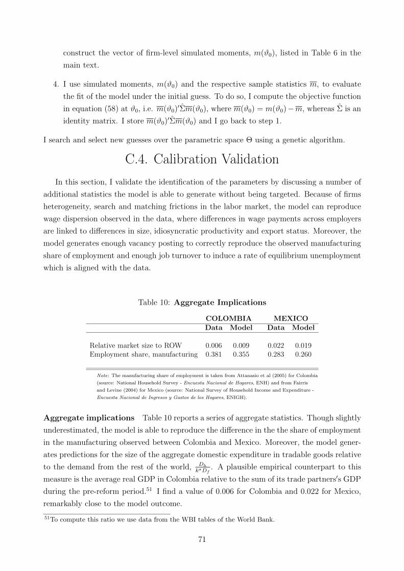
construct the vector of firm-level simulated moments, m(ϑ0), listed in Table 6 in the
main text.
4. I use simulated moments, m(ϑ0) and the respective sample statistics m, to evaluate
the fit of the model under the initial guess. To do so, I compute the objective function
in equation (58) at ϑ0, i.e. m(ϑ0)′Σm(ϑ0), where m(ϑ0) = m(ϑ0)−m, whereas Σ is an
identity matrix. I store m(ϑ0)′Σm(ϑ0) and I go back to step 1.
I search and select new guesses over the parametric space Θ using a genetic algorithm.
C.4. Calibration Validation
In this section, I validate the identification of the parameters by discussing a number of
additional statistics the model is able to generate without being targeted. Because of firms
heterogeneity, search and matching frictions in the labor market, the model can reproduce
wage dispersion observed in the data, where differences in wage payments across employers
are linked to differences in size, idiosyncratic productivity and export status. Moreover, the
model generates enough vacancy posting to correctly reproduce the observed manufacturing
share of employment and enough job turnover to induce a rate of equilibrium unemployment
which is aligned with the data.
Table 10: Aggregate Implications
COLOMBIA MEXICOData Model Data Model
Relative market size to ROW 0.006 0.009 0.022 0.019Employment share, manufacturing 0.381 0.355 0.283 0.260
Note: The manufacturing share of employment is taken from Attanasio et al (2005) for Colombia
(source: National Household Survey - Encuesta Nacional de Hogares, ENH) and from Fairris
and Levine (2004) for Mexico (source: National Survey of Household Income and Expenditure -
Encuesta Nacional de Ingresos y Gastos de los Hogares, ENIGH).
Aggregate implications Table 10 reports a series of aggregate statistics. Though slightly
underestimated, the model is able to reproduce the difference in the the share of employment
in the manufacturing observed between Colombia and Mexico. Moreover, the model gener-
ates predictions for the size of the aggregate domestic expenditure in tradable goods relative
to the demand from the rest of the world, DhkσDf
. A plausible empirical counterpart to this
measure is the average real GDP in Colombia relative to the sum of its trade partners′s GDP
during the pre-reform period.51 I find a value of 0.006 for Colombia and 0.022 for Mexico,
remarkably close to the model outcome.
51To compute this ratio we use data from the WBI tables of the World Bank.
71
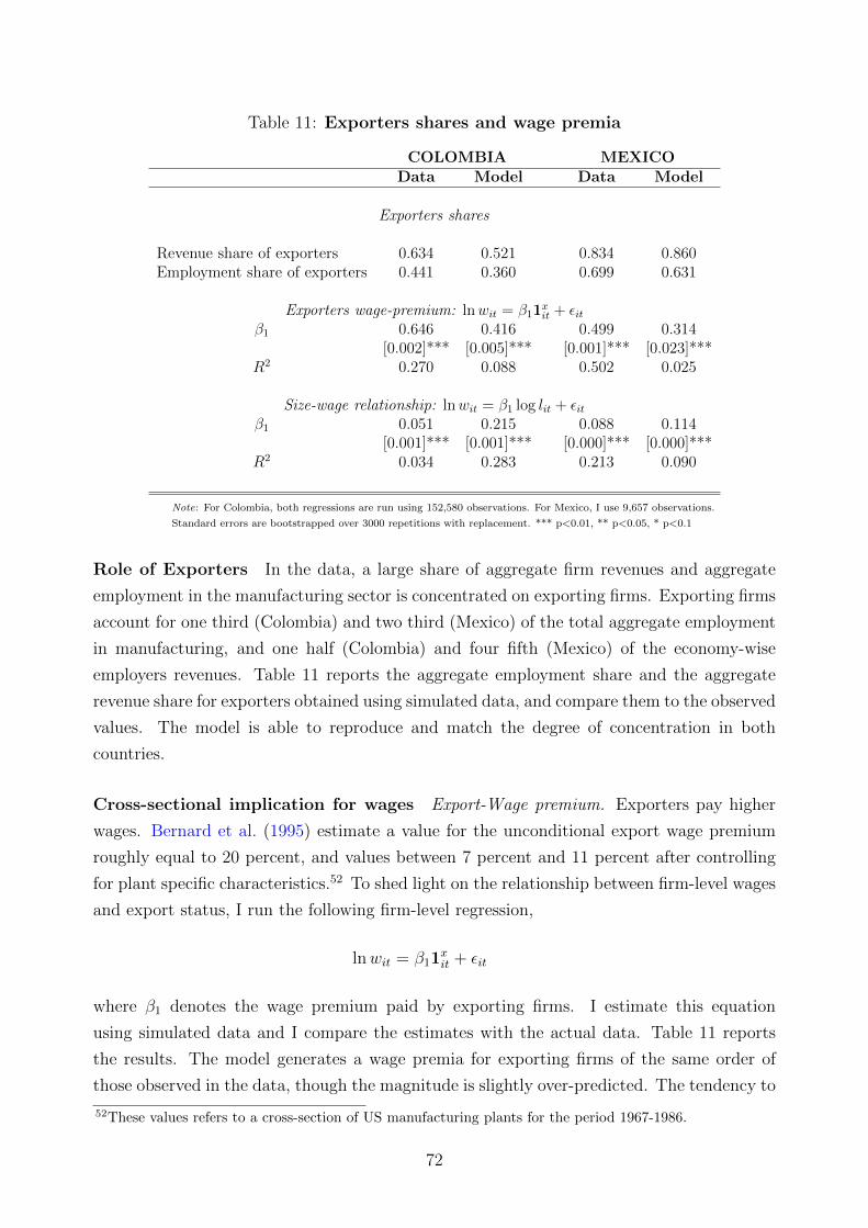
Table 11: Exporters shares and wage premia
COLOMBIA MEXICOData Model Data Model
Exporters shares
Revenue share of exporters 0.634 0.521 0.834 0.860Employment share of exporters 0.441 0.360 0.699 0.631
Exporters wage-premium: lnwit = β11xit + εit
β1 0.646 0.416 0.499 0.314[0.002]*** [0.005]*** [0.001]*** [0.023]***
R2 0.270 0.088 0.502 0.025
Size-wage relationship: lnwit = β1 log lit + εitβ1 0.051 0.215 0.088 0.114
[0.001]*** [0.001]*** [0.000]*** [0.000]***R2 0.034 0.283 0.213 0.090
Note: For Colombia, both regressions are run using 152,580 observations. For Mexico, I use 9,657 observations.
Standard errors are bootstrapped over 3000 repetitions with replacement. *** p<0.01, ** p<0.05, * p<0.1
Role of Exporters In the data, a large share of aggregate firm revenues and aggregate
employment in the manufacturing sector is concentrated on exporting firms. Exporting firms
account for one third (Colombia) and two third (Mexico) of the total aggregate employment
in manufacturing, and one half (Colombia) and four fifth (Mexico) of the economy-wise
employers revenues. Table 11 reports the aggregate employment share and the aggregate
revenue share for exporters obtained using simulated data, and compare them to the observed
values. The model is able to reproduce and match the degree of concentration in both
countries.
Cross-sectional implication for wages Export-Wage premium. Exporters pay higher
wages. Bernard et al. (1995) estimate a value for the unconditional export wage premium
roughly equal to 20 percent, and values between 7 percent and 11 percent after controlling
for plant specific characteristics.52 To shed light on the relationship between firm-level wages
and export status, I run the following firm-level regression,
lnwit = β11xit + εit
where β1 denotes the wage premium paid by exporting firms. I estimate this equation
using simulated data and I compare the estimates with the actual data. Table 11 reports
the results. The model generates a wage premia for exporting firms of the same order of
those observed in the data, though the magnitude is slightly over-predicted. The tendency to
52These values refers to a cross-section of US manufacturing plants for the period 1967-1986.
72
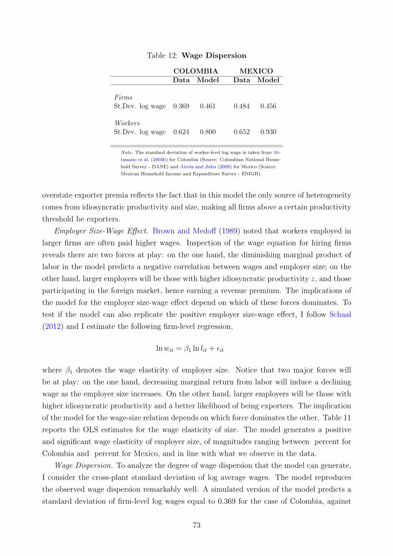
Table 12: Wage Dispersion
COLOMBIA MEXICOData Model Data Model
FirmsSt.Dev. log wage 0.369 0.461 0.484 0.456
WorkersSt.Dev. log wage 0.624 0.800 0.652 0.930
Note: The standard deviation of worker-level log wage is taken from At-
tanasio et al. (2004b) for Colombia (Source: Colombian National House-
hold Survey - DANE) and Airola and Juhn (2008) for Mexico (Source:
Mexican Household Income and Expenditure Survey - ENIGH).
overstate exporter premia reflects the fact that in this model the only source of heterogeneity
comes from idiosyncratic productivity and size, making all firms above a certain productivity
threshold be exporters.
Employer Size-Wage Effect. Brown and Medoff (1989) noted that workers employed in
larger firms are often paid higher wages. Inspection of the wage equation for hiring firms
reveals there are two forces at play: on the one hand, the diminishing marginal product of
labor in the model predicts a negative correlation between wages and employer size; on the
other hand, larger employers will be those with higher idiosyncratic productivity z, and those
participating in the foreign market, hence earning a revenue premium. The implications of
the model for the employer size-wage effect depend on which of these forces dominates. To
test if the model can also replicate the positive employer size-wage effect, I follow Schaal
(2012) and I estimate the following firm-level regression,
lnwit = β1 ln lit + εit
where β1 denotes the wage elasticity of employer size. Notice that two major forces will
be at play: on the one hand, decreasing marginal return from labor will induce a declining
wage as the employer size increases. On the other hand, larger employers will be those with
higher idiosyncratic productivity and a better likelihood of being exporters. The implication
of the model for the wage-size relation depends on which force dominates the other. Table 11
reports the OLS estimates for the wage elasticity of size. The model generates a positive
and significant wage elasticity of employer size, of magnitudes ranging between percent for
Colombia and percent for Mexico, and in line with what we observe in the data.
Wage Dispersion. To analyze the degree of wage dispersion that the model can generate,
I consider the cross-plant standard deviation of log average wages. The model reproduces
the observed wage dispersion remarkably well. A simulated version of the model predicts a
standard deviation of firm-level log wages equal to 0.369 for the case of Colombia, against
73
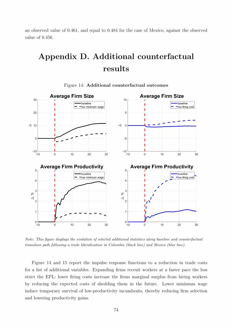
an observed value of 0.461, and equal to 0.484 for the case of Mexico, against the observed
value of 0.456.
Appendix D. Additional counterfactual
results
Figure 14: Additional counterfactual outcomes
Note: This figure displays the evolution of selected additional statistics along baseline and counterfactual
transition path following a trade liberalization in Colombia (black line) and Mexico (blue line).
Figure 14 and 15 report the impulse response functions to a reduction in trade costs
for a list of additional variables. Expanding firms recruit workers at a faster pace the less
strict the EPL: lower firing costs increase the firms marginal surplus from hiring workers
by reducing the expected costs of shedding them in the future. Lower minimum wage
induce temporary survival of low-productivity incumbents, thereby reducing firm selection
and lowering productivity gains.
74
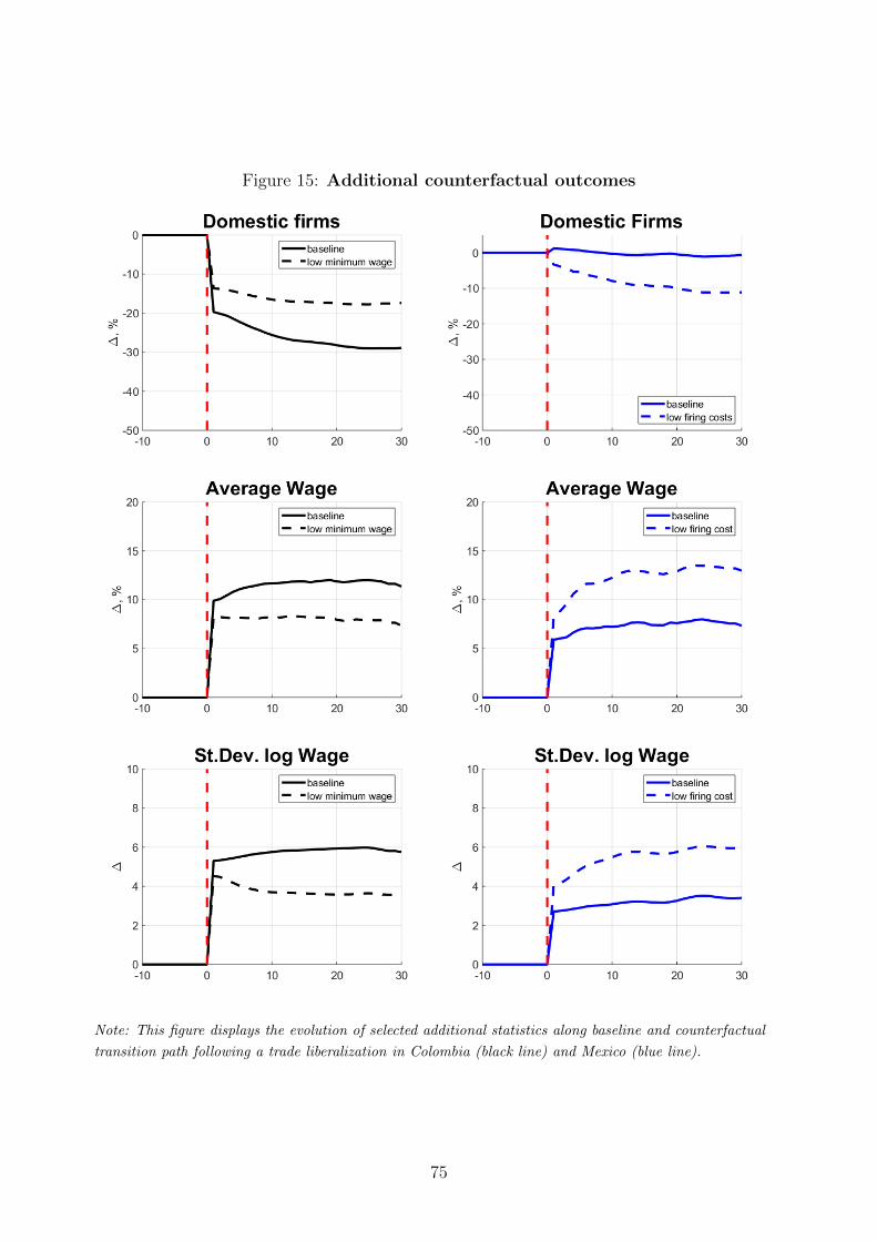
Figure 15: Additional counterfactual outcomes
Note: This figure displays the evolution of selected additional statistics along baseline and counterfactual
transition path following a trade liberalization in Colombia (black line) and Mexico (blue line).
75