Embed Size (px)
Citation preview

Seediscussions,stats,andauthorprofilesforthispublicationat:https://www.researchgate.net/publication/220222487
TransonicShockFormationinaRarefactionRiemannProblemforthe2DCompressibleEulerEquations
ARTICLEinSIAMJOURNALONAPPLIEDMATHEMATICS·JANUARY2008
ImpactFactor:1.43·DOI:10.1137/07070632X·Source:DBLP
CITATIONS
32
READS
71
7AUTHORS,INCLUDING:
JiequanLi
BeijingNormalUniversity
47PUBLICATIONS661CITATIONS
SEEPROFILE
XiaolinLi
StonyBrookUniversity
67PUBLICATIONS1,084CITATIONS
SEEPROFILE
TongZhang
22PUBLICATIONS542CITATIONS
SEEPROFILE
YuxiZheng
PennsylvaniaStateUniversity
33PUBLICATIONS1,001CITATIONS
SEEPROFILE
Availablefrom:JiequanLi
Retrievedon:05February2016

Transonic Shock Formation in a
Rarefaction Riemann Problem for the 2-D
Compressible Euler Equations
James Glimm12, Xiaomei Ji∗1, Jiequan Li3, Xiaolin Li1,
Peng Zhang3, Tong Zhang4 and Yuxi Zheng5
1 Department of Applied Mathematics and Statistics,Stony Brook University, NY 11794-3600
E-mail: [email protected]; [email protected]; [email protected]
2 Computational Science Center, Brookhaven National Laboratory, Upton, NY 11973-5000.
∗ Corresponding author.
3 Department of Mathematics, Capital Normal University, 100037, P.R.ChinaE-mail: [email protected]; [email protected]
4 Institute of Mathematics, Chinese Academy of Mathematics and System Sciences, 100080, P.R.ChinaE-mail: [email protected]
5 Department of Mathematics, Penn State University, PA 16802E-mail: [email protected]
August 7, 2008
Abstract
It is perhaps surprising for a shock wave to exist in the solution of a rarefactionRiemann problem for the compressible Euler equations in two space dimensions. Wepresent numerical evidence and generalized characteristic analysis to establish theexistence of a shock wave in such a 2D Riemann problem, defined by the interactionof four rarefaction waves. We consider both the customary configuration of wavesat the right angle and also an oblique configuration for the rarefaction waves. Twodistinct mechanisms for the formation of a shock wave are discovered as the anglebetween the waves is varied.
AMS subject classification (2000). Primary: 35L65, 35J70, 35R35; Secondary: 35J65.Keywords. 2-D Riemann problem, gas dynamics, shock waves, generalized characteristicanalysis, front tracking method.
1
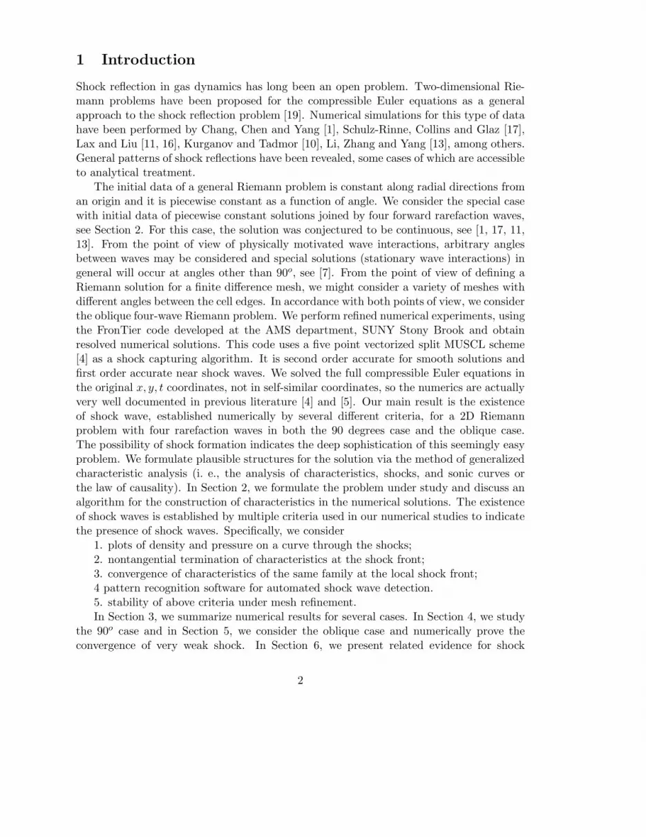
1 Introduction
Shock reflection in gas dynamics has long been an open problem. Two-dimensional Rie-mann problems have been proposed for the compressible Euler equations as a generalapproach to the shock reflection problem [19]. Numerical simulations for this type of datahave been performed by Chang, Chen and Yang [1], Schulz-Rinne, Collins and Glaz [17],Lax and Liu [11, 16], Kurganov and Tadmor [10], Li, Zhang and Yang [13], among others.General patterns of shock reflections have been revealed, some cases of which are accessibleto analytical treatment.
The initial data of a general Riemann problem is constant along radial directions froman origin and it is piecewise constant as a function of angle. We consider the special casewith initial data of piecewise constant solutions joined by four forward rarefaction waves,see Section 2. For this case, the solution was conjectured to be continuous, see [1, 17, 11,13]. From the point of view of physically motivated wave interactions, arbitrary anglesbetween waves may be considered and special solutions (stationary wave interactions) ingeneral will occur at angles other than 90o, see [7]. From the point of view of defining aRiemann solution for a finite difference mesh, we might consider a variety of meshes withdifferent angles between the cell edges. In accordance with both points of view, we considerthe oblique four-wave Riemann problem. We perform refined numerical experiments, usingthe FronTier code developed at the AMS department, SUNY Stony Brook and obtainresolved numerical solutions. This code uses a five point vectorized split MUSCL scheme[4] as a shock capturing algorithm. It is second order accurate for smooth solutions andfirst order accurate near shock waves. We solved the full compressible Euler equations inthe original x, y, t coordinates, not in self-similar coordinates, so the numerics are actuallyvery well documented in previous literature [4] and [5]. Our main result is the existenceof shock wave, established numerically by several different criteria, for a 2D Riemannproblem with four rarefaction waves in both the 90 degrees case and the oblique case.The possibility of shock formation indicates the deep sophistication of this seemingly easyproblem. We formulate plausible structures for the solution via the method of generalizedcharacteristic analysis (i. e., the analysis of characteristics, shocks, and sonic curves orthe law of causality). In Section 2, we formulate the problem under study and discuss analgorithm for the construction of characteristics in the numerical solutions. The existenceof shock waves is established by multiple criteria used in our numerical studies to indicatethe presence of shock waves. Specifically, we consider
1. plots of density and pressure on a curve through the shocks;2. nontangential termination of characteristics at the shock front;3. convergence of characteristics of the same family at the local shock front;4 pattern recognition software for automated shock wave detection.5. stability of above criteria under mesh refinement.In Section 3, we summarize numerical results for several cases. In Section 4, we study
the 90o case and in Section 5, we consider the oblique case and numerically prove theconvergence of very weak shock. In Section 6, we present related evidence for shock
2

formation in the case of two backward and two forward rarefaction waves. In Section7, we discuss the physical mechanism that leads to the shock formation in the presentproblem and summarize results testing the stability of the numerical solutions.
2 The Problem Formulation and Its Characteristic Curves
We consider the Euler equations
ρt + ∇ · (ρU) = 0 ,(ρU)t + ∇ · (ρU ⊗ U) + ∇p = 0 ,(ρE)t + ∇ · ((ρE + p)U) = 0
(2.1)
for the variables (ρ, U,E), where ρ is the density, U = (u, v) is the velocity, p is thepressure, E = 1
2 |U |2 + e is the specific total energy, and e is the specific internal energy.We consider a polytropic gas with pressure p defined by the equation
e =p
(γ − 1)ρ.
For more details, see the books by Li et. al. [13] or Zheng [20].We solve the full compressible flow equations (2.1) in the original x,y,t coordinates.
Our numerical studies are based on (2.1), using the MUSCL algorithm [4] as implementedin the FronTier code. This code uses a five point vectorized split MUSCL scheme [4] as ashock capturing algorithm. It is the second order accurate for smooth solutions and thefirst order accurate near shock waves. Both the MUSCL algorithm and FronTier codehave been extensively verified for shock capturing simulations, for example in [4] and [5].Shock jump conditions for (2.1) can be found in standard textbooks, for example, in [2].The numerical verification of these jump conditions is addressed in Section 5.
Because the equation (2.1) and the initial data are both self-similar, the solution isalso, and we introduce the self-similar coordinate system (ξ, η) = (x−x0
t , y−y0
t ) centered atthe point (x0, y0). In these coordinates, the system (2.1) takes the form
−ξρξ − ηρη + (ρu)ξ + (ρv)η = 0 ,−ξ(ρu)ξ − η(ρu)η + (ρu2 + p)ξ + (ρuv)η = 0 ,−ξ(ρv)ξ − η(ρv)η + (ρv2 + p)η + (ρuv)ξ = 0 ,−ξ(ρE)ξ − η(ρE)η + (ρu(E + p
ρ))ξ + (ρv(E + pρ))η = 0 .
(2.2)
Let η = η(ξ) be a smooth discontinuity with limit states (ρ1, u1, v1, p1) and (ρ0, u0, v0, p0)on both sides. The Rankine-Hugoniot relation for (2.2) is derived in [13, page 218-219]. Bydefinition, Riemann initial data is constant along radial directions from an origin (x0, y0)and piecewise constant as a function of angle. The initial data for (2.1) become boundarydata at infinity for (2.2). We use the self-similar formulation (2.2) for the analysis ofnumerical solutions of (2.1). We specialize to a four-rarefaction wave Riemann problem.
3

As a special case we consider first the case of four rectangularly oriented waves, repre-senting boundary conditions at infinity for the self-similar Euler equations (2.2) satisfyingconditions of four forward rarefaction waves, denoted configuration A in [13, page 237].We next consider the case of four constant states joined by forward rarefaction waves thatform angles different from 90o as in Fig. 2.1. Such a problem is called an oblique four-wave
Riemann problem, in contrast to the rectangular four-wave Riemann problem discussed in[19]. Our initial data is located as indicated in Fig. 2.1 in the initial plane.
(ρ, u, v, p) = (ρi, ui, vi, pi), i = 1, 2, 3, 4. (2.3)
x
y
0θ
θ
(ρ1, u1, v1, p1)
(ρ2, u2, v2, p2)
(ρ3, u3, v3, p3) (ρ4, u4, v4, p4)
Figure 2.1: The initial data for an oblique four-wave Riemann problem
Let Rij denote the forward rarefaction wave, which is a 1D rarefaction wave, con-necting contiguously constant states (ρi, ui, vi, pi) and (ρj , uj , vj , pj). R12 is parallel tothe positive y-axis, and R41 is parallel to the positive x-axis as before, but the angle be-tween R23 and the negative x-axis is allowed to be a variable θ in (0, π/4). To simplifythe analysis, we impose symmetry about the line x = y. We choose the angle betweenR34 and the negative y-axis be the same θ, so that the angle between R23 and R34 isequal to π
2 − 2θ. Let w represent the velocity component that is perpendicular to the lineof discontinuity, and w′ represent the velocity component parallel to it. At an interface(i, j) ∈ {(1, 2), (2, 3), (3, 4), (4, 1)}, a forward planar rarefaction wave Rij is described bythe formula in [11]
wi − wj =2γ
1
2
γ − 1
(
(
pi
ρi
)1
2
−
(
pj
ρj
)1
2
)
, w′
i = w′
j ,pi
pj=
(
ρi
ρj
)γ
. (2.4)
For each Rij, the compatibility conditions derived from (2.4), using the normal and tan-gential components of ui, vj , i, j = 1, 2, 3, 4 along Rij , are
(ρ(γ−1)/23 − ρ
(γ−1)/24 ) cos θ − (ρ
(γ−1)/22 − ρ
(γ−1)/23 ) sin θ + (ρ
(γ−1)/21 − ρ
(γ−1)/22 ) = 0 ; (2.5)
4

(ρ(γ−1)/22 − ρ
(γ−1)/23 ) cos θ − (ρ
(γ−1)/23 − ρ
(γ−1)/24 ) sin θ − (ρ
(γ−1)/21 − ρ
(γ−1)/24 ) = 0 . (2.6)
We limit ourselves to the initially symmetric case ρ2 = ρ4 and u1 = v1. Then the twocompatibility conditions merge to yield
ρ(γ−1)/22 (cos θ + sin θ + 1) = ρ
(γ−1)/21 + ρ
(γ−1)/23 (sin θ + cos θ) . (2.7)
For any fixed ρ1, p1, u1, v1, ρ3, and θ, we find ρ2 from the compatibility condition (2.7) andother initial values from (2.4) and symmetry. We consider a fixed polytropic index γ = 1.4.The computational domain is a square [0, 1] × [0, 1]. We perform numerical experimentswith varying Riemann initial data.
We draw both families of (pseudo) characteristic curves corresponding to λ± in [13],
dη
dξ= λ±(ξ, η) ≡
(u − ξ)(v − η) ± c[(u − ξ)2 + (v − η)2 − c2]1/2
(u − ξ)2 − c2, (2.8)
where c is the sonic speed, ξ = x−x0
T0, η = y−y0
T0, T0 is fixed, and x0 = y0 = 0.5 is the center
of the computational domain. By the definition in [13], the pseudo-Mach number is
M =[(u − ξ)2 + (v − η)2]1/2
c. (2.9)
The M = 1 contour, as understood here, indicates both sonic points and shock points,where M jumps from a value less than 1 to a value greater than 1. The sonic curve is thusa subset of the M = 1 contour line. We notice λ+ = λ− on the sonic curve.
We discuss the algorithm for characteristics. The characteristic curves starting at thetop boundary of the rectangular domain belong to the family λ+, while the characteristiccurves from the right boundary of the rectangular domain belong to λ−. To draw theλ± characteristics, we assume the numerical solution of the Euler equations is definedon a rectangular grid. We extend this solution to the entire computational domain fora discrete time t = T0, using linear interpolation. Thus λ± become globally definedfunctions. Starting at the the right boundary, we solve for λ− to obtain the pseudocharacteristic curves, using the Runge-Kutta scheme. The solution for λ− is continued upto the sonic curve. For the reflected characteristics λ±(ξ, η) at the sonic curve, we repeatthe above processes. Since these characteristics are reflections of the previously constructedfamily, we use bilinear interpolation to obtain initial states at the point on the M = 1contour where an incoming characteristic has terminated. We solved all singularities inthe characteristics equations (2.8) numerically. Since the main point of this paper is toestablish the existence of a shock wave, we list here criteria that we use for this purpose.
The most sensitive of our measures for existence of a shock wave is the fact thata shock will appear when the two families of λ± characteristics are not parallel at theM = 1 contour line. The existence of a point on the M = 1 contour line with λ+ notparallel to λ− contradicts (2.8) if the point is a sonic point, i.e. a point at which thesolution is continuous. We thus plot λ− − λ+ vs. the angle around M = 1 contour, where
5
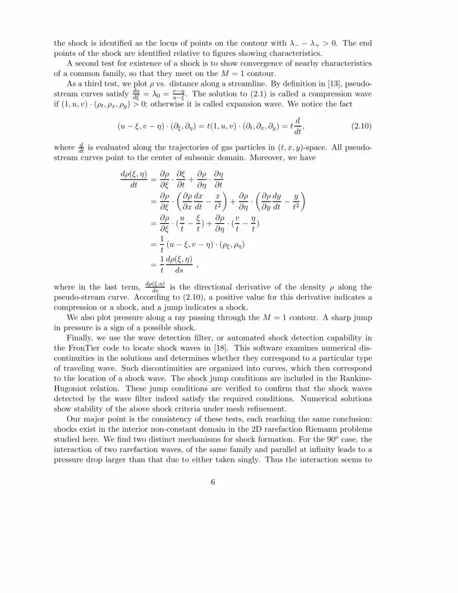
the shock is identified as the locus of points on the contour with λ− − λ+ > 0. The endpoints of the shock are identified relative to figures showing characteristics.
A second test for existence of a shock is to show convergence of nearby characteristicsof a common family, so that they meet on the M = 1 contour.
As a third test, we plot ρ vs. distance along a streamline. By definition in [13], pseudo-stream curves satisfy dη
dξ = λ0 = v−ηu−ξ . The solution to (2.1) is called a compression wave
if (1, u, v) · (ρt, ρx, ρy) > 0; otherwise it is called expansion wave. We notice the fact
(u − ξ, v − η) · (∂ξ , ∂η) = t(1, u, v) · (∂t, ∂x, ∂y) = td
dt, (2.10)
where ddt is evaluated along the trajectories of gas particles in (t, x, y)-space. All pseudo-
stream curves point to the center of subsonic domain. Moreover, we have
dρ(ξ, η)
dt=
∂ρ
∂ξ·∂ξ
∂t+
∂ρ
∂η·∂η
∂t
=∂ρ
∂ξ·
(
∂ρ
∂x
dx
dt−
x
t2
)
+∂ρ
∂η·
(
∂ρ
∂y
dy
dt−
y
t2
)
=∂ρ
∂ξ· (
u
t−
ξ
t) +
∂ρ
∂η· (
v
t−
η
t)
=1
t(u − ξ, v − η) · (ρξ, ρη)
=1
t
dρ(ξ, η)
ds,
where in the last term, dρ(ξ,η)ds is the directional derivative of the density ρ along the
pseudo-stream curve. According to (2.10), a positive value for this derivative indicates acompression or a shock, and a jump indicates a shock.
We also plot pressure along a ray passing through the M = 1 contour. A sharp jumpin pressure is a sign of a possible shock.
Finally, we use the wave detection filter, or automated shock detection capability inthe FronTier code to locate shock waves in [18]. This software examines numerical dis-continuities in the solutions and determines whether they correspond to a particular typeof traveling wave. Such discontinuities are organized into curves, which then correspondto the location of a shock wave. The shock jump conditions are included in the Rankine-Hugoniot relation. These jump conditions are verified to confirm that the shock wavesdetected by the wave filter indeed satisfy the required conditions. Numerical solutionsshow stability of the above shock criteria under mesh refinement.
Our major point is the consistency of these tests, each reaching the same conclusion:shocks exist in the interior non-constant domain in the 2D rarefaction Riemann problemsstudied here. We find two distinct mechanisms for shock formation. For the 90o case, theinteraction of two rarefaction waves, of the same family and parallel at infinity leads to apressure drop larger than that due to either taken singly. Thus the interaction seems to
6
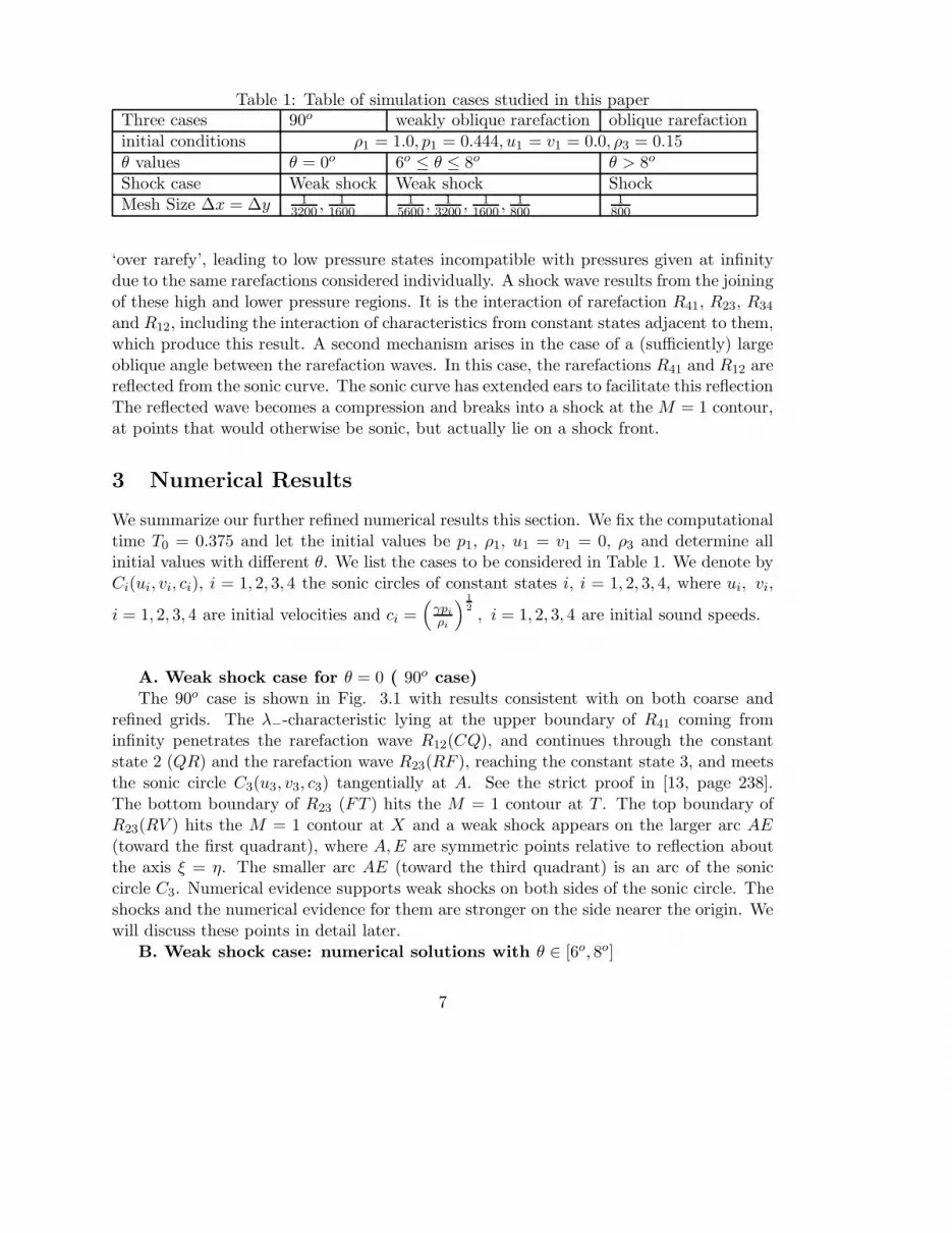
Table 1: Table of simulation cases studied in this paperThree cases 90o weakly oblique rarefaction oblique rarefactioninitial conditions ρ1 = 1.0, p1 = 0.444, u1 = v1 = 0.0, ρ3 = 0.15θ values θ = 0o 6o ≤ θ ≤ 8o θ > 8o
Shock case Weak shock Weak shock ShockMesh Size ∆x = ∆y 1
3200 , 11600
15600 , 1
3200 , 11600 , 1
8001
800
‘over rarefy’, leading to low pressure states incompatible with pressures given at infinitydue to the same rarefactions considered individually. A shock wave results from the joiningof these high and lower pressure regions. It is the interaction of rarefaction R41, R23, R34
and R12, including the interaction of characteristics from constant states adjacent to them,which produce this result. A second mechanism arises in the case of a (sufficiently) largeoblique angle between the rarefaction waves. In this case, the rarefactions R41 and R12 arereflected from the sonic curve. The sonic curve has extended ears to facilitate this reflectionThe reflected wave becomes a compression and breaks into a shock at the M = 1 contour,at points that would otherwise be sonic, but actually lie on a shock front.
3 Numerical Results
We summarize our further refined numerical results this section. We fix the computationaltime T0 = 0.375 and let the initial values be p1, ρ1, u1 = v1 = 0, ρ3 and determine allinitial values with different θ. We list the cases to be considered in Table 1. We denote byCi(ui, vi, ci), i = 1, 2, 3, 4 the sonic circles of constant states i, i = 1, 2, 3, 4, where ui, vi,
i = 1, 2, 3, 4 are initial velocities and ci =(
γpi
ρi
)1
2
, i = 1, 2, 3, 4 are initial sound speeds.
A. Weak shock case for θ = 0 ( 90o case)The 90o case is shown in Fig. 3.1 with results consistent with on both coarse and
refined grids. The λ−-characteristic lying at the upper boundary of R41 coming frominfinity penetrates the rarefaction wave R12(CQ), and continues through the constantstate 2 (QR) and the rarefaction wave R23(RF ), reaching the constant state 3, and meetsthe sonic circle C3(u3, v3, c3) tangentially at A. See the strict proof in [13, page 238].The bottom boundary of R23 (FT ) hits the M = 1 contour at T . The top boundary ofR23(RV ) hits the M = 1 contour at X and a weak shock appears on the larger arc AE(toward the first quadrant), where A,E are symmetric points relative to reflection aboutthe axis ξ = η. The smaller arc AE (toward the third quadrant) is an arc of the soniccircle C3. Numerical evidence supports weak shocks on both sides of the sonic circle. Theshocks and the numerical evidence for them are stronger on the side nearer the origin. Wewill discuss these points in detail later.
B. Weak shock case: numerical solutions with θ ∈ [6o, 8o]
7

0 0.2 0.4 0.6 0.8 10
0.1
0.2
0.3
0.4
0.5
0.6
0.7
0.8
0.9
112
34
R12
R41R
23
R34
CQ
D WL
V N
5
A
E
M=0.8
M=1.0
SP
TF K
P0
P2
P1
I’
N’K’
H’L’
G’X
R
B
Figure 3.1: Case A: Some pseudo-characteristic curves (light) and Mach number contours(bold) marked with M = 1.0 and M = 0.8 at θ = 0.
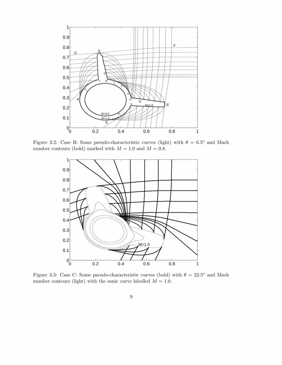
We obtain weak shock cases for θ ∈ [6o, 8o]. See Fig. 3.2 and Fig. 5.7 for the casesθ = 6.5o and θ = 8o. In Fig. 3.2, both the upper boundaries FS of R41 and GS of R23
are parallel, tangential to the sonic curve at S. SA is tangential to the sonic circle C3 atA, which is a reflection of the λ+-characteristic curve GS. SK, which is the reflection ofthe λ−-characteristic curve FS, terminates on a shock. The weak shock appears on thearc AT
⋃
BR⋃
UE, where A,E are symmetric points regarding the axis ξ = η, and thesmaller arc AE is the arc of sonic circle C3.
C. Strong shock case: numerical solutions with θ > 8o
We increase the value of θ, and we observe a shock wave which is sharply defined andwith little numerical oscillation. The shock wave lies in the interior, non-constant domainbetween R23 and R34 and constant states adjacent to them whose structure is similar tocase B. See Fig. 3.3. Furthermore, we find that the strength of the shock wave becomesstronger as we increase θ or decrease ρ3 while keeping the other parameters constant. Thenumerical oscillations between R23 and R34 attenuate, or even vanish as the strength ofthe shock wave intensifies. In summary, numerical solutions show the existence of shockwaves in the interaction of four rarefaction waves and constant states.
8
0 0.2 0.4 0.6 0.8 10
0.1
0.2
0.3
0.4
0.5
0.6
0.7
0.8
0.9
1
F
SG
A
E
P1
T BT
1
Q
P
K
R
U
P2
Q’S’M=1.0
M=0.8
M=1.0
Figure 3.2: Case B: Some pseudo-characteristic curves (light) with θ = 6.5o and Machnumber contours (bold) marked with M = 1.0 and M = 0.8.
0 0.2 0.4 0.6 0.8 10
0.1
0.2
0.3
0.4
0.5
0.6
0.7
0.8
0.9
1
M=1.0
Figure 3.3: Case C: Some pseudo-characteristic curves (bold) with θ = 22.5o and Machnumber contours (light) with the sonic curve labelled M = 1.0.
9

0 0.2 0.4 0.6 0.8 1−0.1
0
0.1
0.2
0.3
0.4
0.5
0.6
λ ±
X−coordinate
P
λ+
λ−
Figure 4.1: The characteristics λ+ = dηdξ along SP and λ− = dη
dξ along WP meet at P .Note that λ+ 6= λ− at the common point P .
4 Shock Formation in the 90o Case
A constructive analysis of some of the major ideas of this paper is found in [6], wherewe study the Riemann problem for the Hamilton-Jacobi equations as a simpler problem,developing a number of ideas needed here. These equations can be regarded as a general-ization of Burgers’ equation to high dimensions. The analysis there follows a constructivepoint of view, and thus emphasizes ideas such as generalized characteristics, the propaga-tion of the Riemann solution inward from data located at infinity, and a sonic curve asdiscussed in the present paper.We discuss in this section the shock formation in the 90o
case. We analyze the mechanism for shock formation assuming from the interaction of rar-efaction waves R12, R23, R34 and R41, including the interaction of R41 and characteristicsfrom constant state 3, 4, 5 adjacent to them. We use numerical methods and generalizedcharacteristic analysis.
4.1 A numerical study of the 90o case
In Fig. 3.1, the characteristic WP along bottom boundary of R41 meets the characteristicsSP from constant state 3 at P . The intersection point P is located on the M = 1contour. If P were a sonic point, then we would have λ+(P ) = λ−(P ). However, weshow numerically in Fig. 4.1 and Fig. 4.2 that P cannot be a sonic point because thecharacteristics are not parallel at P . The numerical results in Fig. 4.1, show that at the
10

0.1 0.15 0.2 0.25
0.3
0.32
0.34
0.36
0.38
0.4
0.42
0.44
0.46
0.48
A
P
K
TF
Figure 4.2: Enlarged view from Fig. 3.1 in the 90o case shows the non parallel terminationof characteristics on the M = 1.0 contour(outer curved arc) and shock existence at thepoint P . Lower curved arc is the M = 0.8 contour.
0.35 0.4 0.45 0.5 0.55 0.60.028
0.03
0.032
0.034
0.036
0.038
0.04
0.042
0.044
0.046
Distance R from origin
Pre
ssur
e p
P
Figure 4.3: Pressure vs. distance along OP for the 90o case. The downward jump at thepoint P is a shock front. The crosses mark cell center locations near the shock front.
11

−2 −1 0 1 2 3 40
0.1
0.2
0.3
0.4
0.5
0.6
0.7
0.8
0.9
φ
λ −−
λ +
AE
Figure 4.4: λ− − λ+ vs. the angle φ along the M = 1 contour in the 90o case. This plotshows the shock existence, the endpoints E and A of the shock wave shown in Fig. 3.1
common point P of the two characteristic curves, λ+(P ) < 0.4, λ−(P ) > 0.5, λ+(P ) 6=λ−(P ), indicating that P is not sonic. Thus the termination of the λ+ characteristicand the beginning of the λ− characteristic must lie on a shock curve. We have twocharacteristics N ′P0 and L′P0 meet at P0 on ξ = η, but they are not parallel. Similarly,G′P2 and I ′P2 meet at P2 nontangentially, H ′P1 and K ′P1 meet at P1 nontangentially.P0, P1, P2 are located on a shock front. An enlarged view of the non tangential, non paralleltermination of the characteristic curves at the shock front is shown in Fig. 4.2. We plotpressure vs. the distance R = (x2 + y2)
1
2 along the straight line OP in Fig. 4.3, whereO is the center of subsonic domain in [0, 1] × [0, 1]. The downward jump in the pressureis a shock front, and P is shown in Fig. 3.1. The curve indicates values at individualmesh points mean the shock. In Fig. 4.4, we represent shock strength by the differencein characteristics λ−(X)− λ+(X) vs. the angle plotted along the M = 1 contour to showshock existence. The angle between the ray from O and the positive x-axis is denoted byφ.
4.2 Generalized characteristic analysis in the 90o case
Let us recall [19]. We use the method of generalized characteristic analysis to indicate theplausible structure of the solution in the 90o case. The values imposed at infinity are givenby (2.1) for the self-similar system (2.2). We first construct the solution in the far field
12

(neighborhood of the infinity), which is comprised of four forward planar rarefaction wavesR12, R23, R34 and R41, besides the constant states (ρi, ui, vi, pi), i = 1, 2, 3, 4. We extendthe four forward rarefaction waves inward from the far field till they interact, denoted byregions in Fig. 3.1. We find the boundary of the interaction domain, which consists ofCQRFSAEBWC in Fig. 3.1, where the arc AE is an arc of sonic circle C3 and K is theintersection point of the bottom boundaries of R23 and R41.
Then we solve the first Goursat problem with characteristic segments CQ and CW ,employing the result in [12, 15], and obtain a continuous (pseudo-supersonic) solution in-side the domain enclosed by the characteristic segments CQ, QD, DW and WC. Secondly,we solve the Goursat problem with characteristic segments QR and QD. The solutionsare still continuous in the domain QRLD. We continue solve the third Gousat problemwith support DL and DN . In [14], they are straight support. Then we get the continuoussolutions in the domain DLV N . The wave R41 penetrates R12 and then R23 to emergeas a simple wave RFKL by [14], which is adjacent to the constant state 2 and constantstate 5 and located in the supsonic domain without shock wave.
We prove rigorously that two subcases possibly happen: either P3 is greater than P5
or P5 is greater than P3 in [15], where P3 and P5 are pressures in constant state 3 and5. This inverted pressure profile P3 > P5 is surprising, because one would expect thatpressure would be expansive in the interaction of four forward rarefaction waves. However,the inverted pressure profile is the direct result of the interaction of two waves R41 andR12. Why is the pressure drop in the interaction region larger than the combined dropacross each of the individual waves? Intuitively or based on physics, it is not easy to seewhether the pressure would go up along a characteristic curve to end on a sonic point,or go down to zero to end on a vacuum. In [15], it has been proven rigorously that thepressure in the interaction region approaches zero along any characteristics, which forma hyperbolic domain determined completely by the data on the characteristic boundaries.Once the participating rarefaction waves are relatively large, the binary interaction willproduce vacuum. The pressure satisfies P1 > P2 = P4 > P3 and continues to drop inthe simple wave interaction zone RFKL, which is proved in [13], to result in an evenlower pressure value at K, where K is shown in Figs. 3.1 and 4.2. From the numericalresults, we note that the sonic boundary AP is a free boundary, as the hyperbolic domainof determinacy of the Goursat problem AFT does not include AP , see Fig. 4.2. Thus theelliptic region influences the solution there. Numerical results show that a global minimumfor the pressure in the whole space [0, 1] × [0, 1] occurs in the domain KPT . The highpressure in the subsonic domain, adjacent to the low pressure in the neighboring domainKPT and FAT , forces the shock wave to occur.
Fig. 4.5 and Fig. 4.6 show the variation of density ρ along the pseudo-stream curveI, and the shock wave caused by compression waves with high pressure in the subsonicdomain pushing the expansion wave in the supsonic domain. In Fig. 4.6, s denotes thedistance along pseudo-stream curve.
13

0 0.2 0.4 0.6 0.8 10
0.1
0.2
0.3
0.4
0.5
0.6
0.7
0.8
0.9
1
M=0.8
M=1.0
I
O
Figure 4.5: Density contours (light), two Mach contours (light) with M = 1.0 and M = 0.8and pseudo-stream curve I (bold) which cuts through a shock wave in a neighborhood ofthe M = 1 contour. Arrows indicate the direction of particles motion along the streamline.
14

0 0.1 0.2 0.3 0.4 0.5 0.6 0.70.1
0.15
0.2
0.25
0.3
0.35
0.4
0.45
Den
sity
ρ(s
)
Distance s along the pseudo−stream curve
R23
Shock
Figure 4.6: Plot of ρ(s) vs. s, the position of a shock wave is visible as a small increasingbump with the distance along the pseudo-stream curve I in Fig. 4.5.
5 Shock Formation in the Oblique Rarefaction Case
5.1 Numerical results
In oblique wave interaction case at θ = 6.5o, two reflected characteristic curves QP,Q′Pin Fig. 5.1, meet at P |X=0.42 on the 45o diagonal line. The intersection point P is locatedon the M = 1 contour. If P were a sonic point, then we would have λ+(P ) = λ−(P ).However, we show numerically in Fig. 5.1 that P cannot be a sonic point because thecharacteristics are not parallel at P . At the common point P of the two plots, λ+(P ) <−1, λ−(P ) > −1, λ+(P ) 6= λ−(P ), indicating that P is not sonic. Thus the terminationof the λ+ characteristics and the beginning of the λ− characteristics must be on shock.The plots for two computations, showing level of mesh refinement, are indistinguishable.In Fig. 5.2, we show shock strength by the difference λ−(X) − λ+(X) in the direction ofcharacteristics vs. the angle around the M = 1 contour. See Fig. 3.2 for locations of thepoints A,T,B,R,U,E. The plot demonstrates shock existence. The angle between the rayfrom O (the center of subsonic domain) and the positive x-axis is denoted by φ. We showfurther details of the non tangential termination of the characteristic curves at the shockfront in Fig. 5.3. The characteristic curves terminate non tangentially and are not parallelto each other. We find numerically that the reflected simple wave is a compressive waveand forms a weak shock. See Fig. 5.4, where the characteristic distance denotes the ‘shockdistance’. The separation distance, i.e. the normal separation between two neighboring
15

0.25 0.3 0.35 0.4 0.45 0.5 0.55 0.6−9
−8
−7
−6
−5
−4
−3
−2
−1
0
X−coordinate
λ ±
1600x16001600x16003200x32003200x3200 P
λ+
λ−
Figure 5.1: Plot of λ+ = dηdξ along QP and λ− = dη
dξ along PQ′ show the shock existenceat P , since λ+(P ) 6= λ−(P ). The plots for two computations, showing one level of meshrefinement, are indistinguishable.
characteristics is plotted vs. the length along the reflected characteristics. The plot alsoshows the occurrence of the shock.
We plot pressure p vs. the distance from the origin R= (x2 + y2)1
2 along the 45o
diagonal line in Fig. 5.5 and as well as Fig. 5.6. Under refinement of the mesh, theoscillations are getting weaker and the shock becomes sharper. The circles and crosses arelocated at mesh block centers, for cells within the shock profile. The trend of convergenceof shocks in each plot in Fig. 5.5 is clear and sufficient: the shock wave here is very weakbut its strength is not decreasing as mesh is refined; the shock will be stable even withextremely fine meshes.
We use the wave filter embedded in the FronTier code. The wave filter is an automatedpattern recognition algorithm which locates shock waves, rarefaction waves and contactdiscontinuities in numerical solutions of the Euler equations for compressible fluids onthe basis of detecting a local jump in the solution which satisfies the Rankine-Hugoniotrelations. The shock wave as determined by this wave filter program is shown in Fig. 5.7by the curve AB. Note that the labeled Mach number contours M = 0.98 and M = 1.02in Fig. 5.7 and M = 0.96 and M = 1.02 in Fig. 5.8 coincide on the curve AB respectively,indicating that they are shock fronts. These curves match the pseudo-Mach numbercontours well.
16

−4 −3 −2 −1 0 1 2 3 40
0.5
1
1.5
2
2.5
3
3.5
φ
λ −−
λ +
E U R B T A
Figure 5.2: The difference λ−(X)−λ+(X) vs. angle along the M = 1 contour at θ = 6.5o.This plot shows existence of shocks both on the inward and the reverse sides of the M = 1contour, in the second and fourth quadrants.
5.2 Generalized characteristic analysis
We use the method of generalized characteristic analysis to indicate the plausible structureof the solution to our problem for θ > 8o based on numerical results in Section 5.1. Weretain the notation from [19]. We discuss causal relationships and decompose the boundaryvalue problem into three sub-problems based on the features of the characteristics. Theanalysis consists of the following steps. The first is a classical rarefaction Goursat problemwhich has been solved analytically in [12, 15]. The second is a degenerate Goursat problem,whose solution is proved to be a simple wave in [14]. The last is a pseudo-transonicboundary value problem with free boundaries consisting of interior sonic curves and shocks.The mathematical proof for the structure of this last sub-problem is open. The probleminvolves collisions of rarefaction waves with sonic curves which produce compressive wavesupon reflection, which may then form shocks. We outline the boundary of the domain ofinteraction for the initial four rarefaction waves in both cases above.
Step 5.2.1. The constant states and simple waves in the far field.As in [19], we transform problem (2.1) and (2.3) into a boundary value problem for
the self-similar system (2.2) with values imposed at infinity
limξ2+η2→∞
(ρ, u, v, p)(ξ, η) = (ρi, ui, vi, pi) , i = 1, 2, 3, 4, (5.1)
in which the limiting direction is consistent with the data sector in (2.3). We first con-
17

0.34 0.36 0.38 0.4 0.42 0.44 0.46 0.48 0.5 0.52 0.54
0.34
0.36
0.38
0.4
0.42
0.44
0.46
0.48
0.5
0.52
0.54
P
Figure 5.3: Enlarged view with details in Fig. 3.2 near the point P on the shock frontat 6.5o. Bold curves are λ± characteristics; light curves are Mach number contours. Notethat the characteristics terminate non tangentially on the shock.
0.1 0.15 0.2 0.25 0.3 0.350
0.005
0.01
0.015
0.02
0.025
0.03
0.035
Characteristic distance
Sep
arat
ion
dist
ance
Figure 5.4: Plot of separation between neighboring characteristics vs. distance alongcharacteristics with θ = 6.5o in case B. This plot shows shock formation.
18

0.45 0.5 0.55 0.6 0.65 0.70.0305
0.0306
0.0307
0.0308
0.0309
0.031
0.0311
0.0312
0.0313
Distance R from origin
Pre
ssur
e p
3200x32005600x5600
0.45 0.5 0.55 0.6 0.65 0.70.0305
0.0306
0.0307
0.0308
0.0309
0.031
0.0311
0.0312
0.0313
Distance R from origin
Pre
ssur
e p
3200x32005600x5600
0.45 0.5 0.55 0.6 0.65 0.70.03
0.0305
0.031
0.0315
Distance R from origin
Pre
ssur
e p
3200x32005600x5600
Figure 5.5: Left: pressure vs. distance along a 45o diagonal line at 6o. Right: pressure vs.distance along a 45o diagonal line at θ = 6.5o. The x and o indicate cell center solutionvalues moving through the shock, for the region of rapid solution transition.
0.45 0.5 0.55 0.6 0.65 0.70.0298
0.03
0.0302
0.0304
0.0306
0.0308
0.031
0.0312
0.0314
Distance R from origin
Pre
ssur
e p
3200x3200
0.45 0.5 0.55 0.6 0.650.022
0.024
0.026
0.028
0.03
0.032
0.034
0.036
Distance R from origin
Pre
ssur
e p
800x800
Figure 5.6: Pressure vs. distance along a 45o diagonal line. Left: θ = 7o. Right: θ = 22.5o
19

0 0.2 0.4 0.6 0.8 10
0.1
0.2
0.3
0.4
0.5
0.6
0.7
0.8
0.9
1
+1.0
+0.98B
A
+1.02
Figure 5.7: Comparison of wave filter shock location A,B and pseudo-Mach number con-tour plots at θ = 8o with 800 × 800 mesh.
0 0.2 0.4 0.6 0.8 10
0.1
0.2
0.3
0.4
0.5
0.6
0.7
0.8
0.9
1
B
+0.96
+1.02
A
+1.0
Figure 5.8: Comparison of wave filter shock location A,B and pseudo-Mach number con-tour plots at θ = 22.5o.
20

14
17
6
8
9
11
12
16
13
10
7
15
12
3
4
R12
R34
R14
R23
PQ
RS
P ′
Q′
R′
S′
λ+
λ+
λ+
λ+
λ−
λ−
λ−
λ−
SubsonicU
T
U ′
T ′
W
W ′
C2
C4
C3
R25
R455V
V ′
Z
Z ′
ShockX
Figure 5.9: Generalized characteristic analysis for the case of four forward rarefactions in a 2DRiemann problem.
struct the solution in the far field (neighborhood of the infinity), which is comprised offour forward planar rarefaction waves R12, R23, R34 and R41, besides the constant states(ρi, ui, vi, pi), i = 1, 2, 3, 4. We extend the four forward rarefaction waves inward from thefar field till they interact, denoted by regions as in Fig. 5.9. We find the boundary of theinteraction domain, as in [19], which consists of the characteristic segments PQ, QR, ST ,TU , U ′T ′, T ′S′, R′Q′, Q′P and arcs of sonic circles RS, UU ′, S′R′. See Fig.5.9.
Step 5.2.2 Simple wave solutions after interaction of planar rarefactionwaves.
The two rarefaction waves R12 and R41 start to interact at P . We use the resultin [12, 15] to solve the Goursat problem with the boundary values supported on thecharacteristic curves PQ and PQ′, and obtain a continuous (pseudo-supersonic) solutioninside the domain enclosed by the characteristic segments PQ, QP ′, P ′Q′ and Q′P .
Then we proceed to solve the Goursat problem with the boundary data supported onQR and QP ′. Since the state (ρ2, u2, v2, p2) is constant, we use the result in [14, Theorem7]: Adjacent to a constant state is a simple wave in which (ρ, u, v, p) are constant along a
21
0.2 0.25 0.3 0.35 0.40
0.005
0.01
0.015
0.02
0.025
0.03
Characteristic distance
Sep
arat
ion
dist
ance
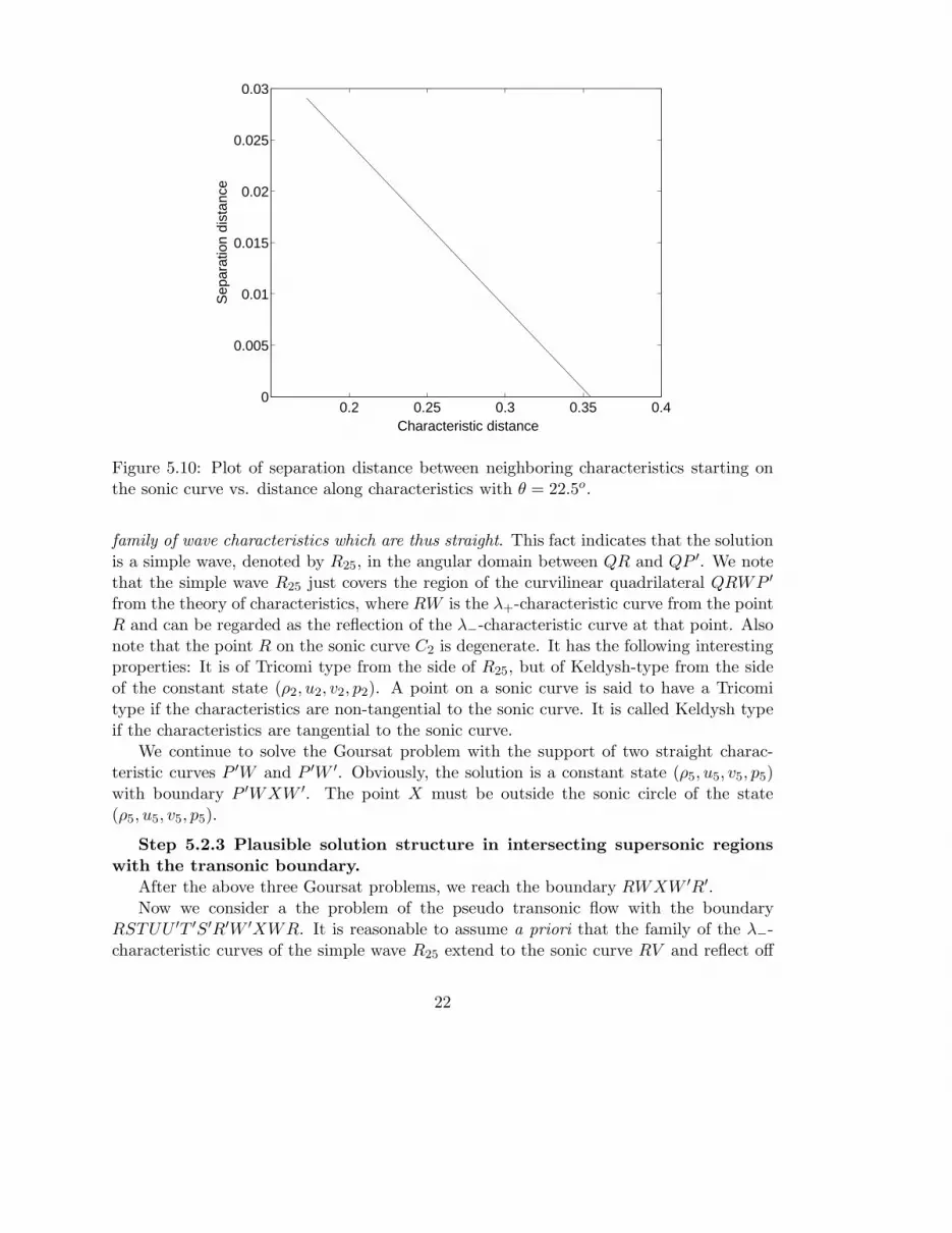
Figure 5.10: Plot of separation distance between neighboring characteristics starting onthe sonic curve vs. distance along characteristics with θ = 22.5o.
family of wave characteristics which are thus straight. This fact indicates that the solutionis a simple wave, denoted by R25, in the angular domain between QR and QP ′. We notethat the simple wave R25 just covers the region of the curvilinear quadrilateral QRWP ′
from the theory of characteristics, where RW is the λ+-characteristic curve from the pointR and can be regarded as the reflection of the λ−-characteristic curve at that point. Alsonote that the point R on the sonic curve C2 is degenerate. It has the following interestingproperties: It is of Tricomi type from the side of R25, but of Keldysh-type from the sideof the constant state (ρ2, u2, v2, p2). A point on a sonic curve is said to have a Tricomitype if the characteristics are non-tangential to the sonic curve. It is called Keldysh typeif the characteristics are tangential to the sonic curve.
We continue to solve the Goursat problem with the support of two straight charac-teristic curves P ′W and P ′W ′. Obviously, the solution is a constant state (ρ5, u5, v5, p5)with boundary P ′WXW ′. The point X must be outside the sonic circle of the state(ρ5, u5, v5, p5).
Step 5.2.3 Plausible solution structure in intersecting supersonic regionswith the transonic boundary.
After the above three Goursat problems, we reach the boundary RWXW ′R′.Now we consider a the problem of the pseudo transonic flow with the boundary
RSTUU ′T ′S′R′W ′XWR. It is reasonable to assume a priori that the family of the λ−-characteristic curves of the simple wave R25 extend to the sonic curve RV and reflect off
22

Shock
Expansion wave
Sonic line Reflected compressive wave
ξ
η
Figure 5.11: Shock formation from the reflection of rarefaction wave on a sonic curve
0 0.2 0.4 0.6 0.8 10
0.1
0.2
0.3
0.4
0.5
0.6
0.7
0.8
0.9
1
O
M=0.92
M=1.0
III
Figure 5.12: Density contours (light), two Mach contours (light) with M = 1, M = 0.92and two pseudo-stream curves I, II (bold) which cut through the weak shock waves andshock waves in the neighborhood of the M = 1 contour shown at θ = 22.5o.
23

0 0.2 0.4 0.6 0.8 10.1
0.2
0.3
0.4
0.5
0.6
0.7
0.8
0.9
1
Distance s along the pseudo−stream curve
Den
sity
ρ(s
)
R12
R12
+R41
R25
I
ShockWeak shock
Constant
II
Figure 5.13: The increasing positions of (weak shock wave and shock wave) in the plotof ρ(s) vs s plots are visible as bumps along two pseudo-stream curves I (above) and II(below) in Fig. 5.12.
24

it as a family of λ+-characteristic curves. Here the extension of R25 is not a simple wavebecause the solution must vary along both λ− and λ+ characteristics. The solution isjointly determined by the subsonic domain and the supersonic domain. These reflectedλ+-characteristic curves reach a curved boundary WV , which forms another degenerateGoursat problem with the support of a straight λ+-characteristic line WXand a curvedλ−-characteristic line WV . This degenerate Goursat problem has a simple wave solutionwhose data are on the left boundary QP ′ since adjacent to the WX side is the constantstate (ρ5, u5, v5, p5). The numerical results indicate that this reflected simple wave is acompressive wave and forms a shock with starting point V . See Fig. 5.10, where character-istic distance denotes the ‘shock distance’, i.e. the length of the reflected characteristics,and separation distance is the normal separation between two neighboring characteristics.This plot shows the occurrence of the shock. The shock borders the constant domain(ρ5, u5, v5, p5). By symmetry, this structure is repeated accross the symmetric axis withstarting point V ′ of another shock in the primed variables W ′V ′X.
We analyze the numerical results in Fig. 5.12 and Fig. 5.13, which show the variationof density ρ along pseudo-stream curves I and II, presenting regions corresponding toexpansion and compression waves. The arrows on the stream curves indicate the directionof particle motions. In Fig. 5.13, the distance s denotes the distance along pseudo-streamcurves, standing at the data beginning and ending on the pseudo-stream curves I and II.
The structure of the solution for the reflected characteristic curves R23 in Fig. 5.9is clarified, where the family of λ+-characteristic curves coming from R23 collide with aTricomi type pseudo sonic curve SZ and are reflected to form a weak shock wave ZU ,which resembles 90o case.
6 Shock Formation for Two Backward and Two Forward
Rarefaction Waves
For the case of two backward and two forward rarefaction waves, there are two symmetrictransonic shocks in the solution as shown in [1, 17, 11, 13] and see Fig. 6.1. The mechanismof shock formation is the same as was discussed for the case of four forward rarefactionwaves in Fig. 5.9 because the part of Fig. 6.1 upper-right to ξ + η = u2 + v2 has the samestructure as that of the corresponding part in Fig. 5.9.
7 Conclusion
We discuss numerical simulations showing two distict mechanisms for shock formation andsupporting theoretical conjectures based on generalized characteristic analysis regardingmathematical mechanism in the 90o case and the oblique rarefaction case. We also discoverthat the same mathematical mechanism as in the oblique rarefaction case occurs for theshock formation for two forward and two backward rarefaction waves.
25

0 0.2 0.4 0.6 0.8 10
0.1
0.2
0.3
0.4
0.5
0.6
0.7
0.8
0.9
1
+1.0
Figure 6.1: The case of two forward and two backward rarefactions oriented at 90o withp1 = 0.444, ρ1 = 1.0, u1 = v1 = 0.00, ρ2 = 0.5197, T = 0.25 ; characteristics (bold) andcontour curves of pseudo-Mach number (light) are plotted.
26

For the 90o case, the interaction of two rarefaction waves of the same family andparallel at infinity leads to a pressure drop larger than that due to enter taken singly.Thus the interaction seems to ‘over rarefy’, leading to low pressure states incompatiblewith pressures given at infinity due to the same rarefactions considered individually. Ashock wave results from the joining of these high and lower pressure regions. It is theinteraction of rarefaction R41 and R23 and R34 and R12, including the interaction of R41
and characteristics from constant state 3 below R23, which produce this result.The shock formation for the oblique case has a possible physical mechanism similar
to one found in stationary flow, which is illustrated schematically in Fig. 5.11, associatedwith the numerical result in Fig. 3.3. Basically, a rarefaction reflection reflects at a sonicboundary; the reflected wave is a compression, which may in time break and become ashock. For the steady transonic small disturbance equation, shock reflection on a soniccurve is illustrated in Cole and Cook [3], see the shock formation over an airfoil in pp.314, Fig. 5.4.13. The structure of shock formation from the reflection of rarefactionwaves on a sonic curve was suggested by Guderly [8], for the two-dimensional steadyirrotational isentropic flow, they put forward a concept of shock formation from reflectionof characteristics on a sonic curve. When a supersonic bubble appears on the top of anairfoil in an ambient subsonic domain, a family of characteristics are generated in thebubble from the surface of the airfoil, and they hit the rear portion of the sonic curve,and are reflected downstream to form a compressive wave which then forms a shock wavewithin the bubble. The subsonic region plays the role of a permeable obstacle whichdeclines streamlines towards the airfoil and causes compressive waves in the same way asa concave wall does in the classical problem of supersonic flow over a smooth rigid wall. Wepoint out the bump on the wall of the flow channel causes the shock formation naturallyin Cole and Cook [3], where it has an important application in the study of a flow overan airplane wing. Furthermore, this formation of shocks seems to be the fundamentalmechanism for the Guderly reflection pattern in Hunter and Tesdall [9].
For waves interacting with a sufficiently large oblique angle in the third quadrant, thesonic curve has an exaggerated non convex shape (rabbit ears). The curve extends into therarefaction waves and interacts with them. The rarefactions are reflected as compressionwaves along these rabbit ears, in the sense that along this part of the sonic curve, thereare impinging λ+ and λ− characteristics. The characteristics coming from infinity arepart of the rarefaction wave, while the reflected ones, as stated, are compressions. On theside facing the first quadrant, these compressions have sufficient travel distance to breakand form a shock wave, centered at the 45o line, where it crosses the M = 1 contour.On the side facing the third quadrant, due to the angle between the waves at infinity,there is a very weak shock on this side of the M = 1 contour, which can be analogouslyinterpreted in Fig. 11 in [2, page 390], where stationary flow is in nozzles and jets. Verylikely these characteristics would have an envelope if they were not intercepted by a shockfront. To prevent the envelope singularity, an “intercepting” shock is therefore necessary.The reason for the reflected wave to be a compression is illustrated by similarity to arelated problem in aerodynamics, as discussed in the literature, and explained in [3] and
27

[8].The Riemann problem is typically unstable in that it is a locus of bifurcation for the
Riemann data. Even in 1D, the isolated jump discontinuity holds only at time zero and(for gas dynamics) the solution at all positive times has three traveling waves.
However, it is stable in the sense of preservation of structure upon variation of initial(Riemann) conditions. In this sense, our analysis deals with representative variation of theinitial conditions, but does not explore the complete seven dimensional space of nearbyinitial conditions numerically. This numerical stability analysis was conducted for the fullEuler equations (2.1) rather than for the self-similar equations (2.2). No non-self-similarsolutions were observed in the variations of initial data. We have studied systematicallya variation of the angle between two of the four initial rarefaction waves. As this angle ismodified sufficiently, we find a jump to a new solution branch, with a distinct mechanism(in a detailed sense) for the shock formation. Although it is conceptually possible to allowan arbitrary number of waves, at arbitrary angles in the 2D Riemann problem formulation,the case of four waves is the case most commonly considered.
Acknowledgment: Discussions with John Hunter, Wancheng Sheng are very help-ful. James Glimm’s research has been partially supported by DOE and ARO with IDDEFG5206NA26208 and ID W911NF0510413. Tong Zhang’s research has been par-tially supported by The Project-sponsored by SRF for ROCS, SEM with No.2004176,the Key Programm from Beijing Educational Committee with no. KZ200510028018 andNSFC 10671120. Xiaolin Li’s research has been partially supported by DOE with IDDEFC0206ER25770. Xiaomei Ji’s research has been partially supported by The Project-sponsored by SRF for ROCS, SEM with No.2004176 when she worked in Beijing Uni-versity of Technology, China before 8/2005 and supported by AMS Dpartment, StonyBrook University. Jiequan Li’s research has been partially supported by the Key Pro-gram from Beijing Educational Commission with no.KZ200510028018, Program for NewCentury Excellent Talents in University (NCET) and Funding Project for Academic Hu-man Resources Development in Institutions of Higher Learning Under the Jurisdictionof Beijing Municipality (PHR-IHLB). Peng Zhang’s research has been supported by KeyProgramm of Natural Science Foundation from Beijing Municipality with No.4051002.Yuxi Zheng’s research has been partially supported by NSF-DMS-0305497, 0305114, and0603859. Computations were performed on the Galaxy computer and seawulf computer atStony Brook and the Stony Brook-Brookhaven New York Blue computer. This researchutilized resources from the Galaxy computer at Stony Brook and the New York Centerfor Computational Sciences at Stony Brook University/Brookhaven National Laboratorywhich is supported by the U.S. Department of Energy under Contract No. DE-AC02-98CH10886 and by the State of New York.
28

References
[1] Chang, T.; Chen, G.; Yang, S.: On the 2-D Riemann problem for the compressibleEuler equations, I. Interaction of shocks and rarefaction waves, Discrete and Contin-
uous Dynamical Systems, 1(1995), 555–584; II. Interaction of contact discontinuities,Discrete and Continuous Dynamical Systems, 6(2000), 419-430.
[2] Courant, R.; Friedrichs, K.O.: Supersonic flow and shock waves, Springer-Verlag,New York Inc., 1948.
[3] Cole, J. D.; Cook, L. P.: Transonic Aerodynamics, North-Holland, Amsterdam, 1986.
[4] Colella, P.; A direct Eulerian MUSCL scheme for gas dynamics, SIAM J. Sci. Stat.
Comput., 6(1985), 104-117.
[5] Glimm, J.; Grove, J. W.; Kang, Y.; Lee, T., Li, X.; Sharp, D.; Yu, Y.; Ye, K.; Zhao,M.: Statistical Riemann Problems and a Composition Law for Errors in NumericalSolutions of Shock Physics Problems, SIAM J. Sci. Comp., 26(2005), 666–697.
[6] Glimm, J.; Kranzer, H. C.; Tan, D.; Tangerman, F. M.: Wave Fronts for Hamilton-Jacobi Equations: The General Theory for Riemann Solutions in Rn, Commun. Math.
Phys., 187(1997), 647-677.
[7] Glimm, J.; Sharp, D.: An S-matrix Theory for Classical Nonlinear Physics, Founda-
tions of Physics, 16 (1986), 125-141.
[8] Guderly, K. G.: The theory of transonic flow, Pergamon Press, London, 1962.
[9] Hunter, J. K.; Tesdall, A. M.: Self-similar solutions for weak shock reflection, SIAM
J. Appl. Math., 63 (2002), 42–61.
[10] Kurganov, A.; Tadmor, E.: Solution of two-dimensional Riemann problems for gasdynamics without Riemann problem solvers, Numerical Methods for Partial Differ-
ential Equations, 18(2002), 548-608.
[11] Lax, P. D.; Liu, X.: Solution of two-dimensional Riemann problems of gas dynamicsby positive schemes, SIAM J. Sci. Comp., 19(1998), 319–340.
[12] Li, J.: On the two-dimensional gas expansion for the compressible Euler equations,SIAM J. Appl. Math., 62(2002), 831–852.
[13] Li, J.; Zhang, T.; Yang, S.: The Two-Dimensional Riemann Problem in Gas Dynam-
ics, Pitman Monographs 98, Longman, 1998.
[14] Li, J.; Zhang, T.; Zheng, Y.: Simple waves and a characteristic decomposition of thetwo dimensional compressible Euler equations, Commun. Math. Phys, 267(2006),1-12.
29

[15] Li, J.; Zheng, Y.: Interaction of rarefaction waves of the two-dimensional self-similarEuler equations, Arch. Rat. Mech. Anal., (in press).
[16] Liu, X.; Lax, P. D.: Positive schemes for solving multi-dimensional hyperbolic systemsof conservation laws, J. Comp. Fluid Dynam., 5(1996), 133–156.
[17] Schulz-Rinne, C. W.; Collins, J. P.; Glaz, H. M.: Numerical solution of the Riemannproblem for two-dimensional gas dynamics, SIAM J. Sci. Comp., 4(1993), 1394–1414.
[18] Yu, Y., Zhao, M., Lee, T., Pestieau, N., Bo, W., Glimm, J., Grove, J. W.: Uncer-tainty Quantification for Chaotic Computational Fluid Dynamics, J. Comp. Phys.,217(2006), 200-216.
[19] Zhang, T.; Zheng, Y.: Conjecture on the structure of solutions of the Riemann prob-lem for two-dimensional gas dynamics systems, SIAM J. Math. Anal., 21(1990), 593-630.
[20] Zheng, Y.; Systems of Conservation Laws: Two-Dimensional Riemann Problems, 38PNLDE, Birkhauser, Boston, 2001.
30