Embed Size (px)
Citation preview

Heft 215 Cjestmir Volkert de Boer
Transport of Nano Sized Zero ValentIron Colloids during Injection into theSubsurface

Transport of Nano Sized Zero Valent Iron Colloids during Injection into the Subsurface
Von der Fakultät Bau- und Umweltingenieurwissenschaften der Universität Stuttgart zur Erlangung der Würde eines Doktor-Ingenieurs (Dr.-Ing.) genehmigte Abhandlung
Vorgelegt von Cjestmir Volkert de Boer
aus Langedijke, Königreich der Niederlande
Hauptberichter: Prof. Dr.-Ing. Rainer Helmig Mitberichter: Prof. Dr. Ruud Schotting Prof. Dr. Rajandrea Sethi Tag der mündlichen Prüfung: 19. Juli 2012
Institut für Wasser- und Umweltsystemmodellierung der Universität Stuttgart
2012

Heft 215 Transport of Nano Sized Zero Valent Iron Colloids during Injection into the Subsurface
von Dr.-Ing. Cjestmir Volkert de Boer
Eigenverlag des Instituts für Wasser- und Umweltsystemmodellierung der Universität Stuttgart
D93 Transport of Nano Sized Zero Valent Iron Colloids during Injection into the Subsurface
Bibliografische Information der Deutschen Nationalbibliothek Die Deutsche Nationalbibliothek verzeichnet diese Publikation in der Deutschen Nationalbibliografie; detaillierte bibliografische Daten sind im Internet über http://www.d-nb.de abrufbar
de Boer, Cjestmir Volkert: Transport of Nano Sized Zero Valent Iron Colloids during Injection into the
Subsurface von Cjestmir Volkert de Boer. Institut für Wasser- und Umweltsystemmodellierung, Universität Stuttgart. - Stuttgart: Institut für Wasser- und Umweltsystemmodellierung, 2012
(Mitteilungen Institut für Wasser- und Umweltsystemmodellierung, Universität
Stuttgart: H. 215) Zugl.: Stuttgart, Univ., Diss., 2012 ISBN 978-3-942036-19-1 NE: Institut für Wasser- und Umweltsystemmodellierung <Stuttgart>: Mitteilungen
Gegen Vervielfältigung und Übersetzung bestehen keine Einwände, es wird lediglich um Quellenangabe gebeten. Herausgegeben 2012 vom Eigenverlag des Instituts für Wasser- und Umwelt-systemmodellierung Druck: Document Center S. Kästl, Ostfildern


“Muad’Dib could indeed see the Future, but you must understand the limits
of this power. Think of sight. You have eyes, yet cannot see without light. If
you are on the floor of a valley, you cannot see beyond your valley. Just so,
Muad’Dib could not always choose to look across the mysterious terrain. He
tells us that a single obscure decision of prophecy, perhaps the choice of one
word over another, could change the entire aspect of the future. He tells us,
‘The vision of time is broad, but when you pass through it, time becomes a
narrow door.’
And always, he fought the temptation to choose a clear, safe course,
warning, ‘That path leads ever down into stagnation.’
-from ‘Arrakis Awakening’ by the Princess Irulan”
Frank Herbert - Dune - 1965

Acknowledgments
I sincerely thank professors Rainer Helmig, Ruud Schotting and Rajandrea Sethi for their
continuous support, constructive feedback and above all their patience. I enjoyed the nu-
merous discussions I had in the beginning with Ruud and Rainer about how to extract
a dissertation from the results of my work at VEGAS and later the in-detail discussions
about my work with Rajandrea. Beside that, during several visits to Utrecht there was
often time to join the great group activities and while staying in Torino Rajandrea even
introduced me to the local cuisine and wine tasting traditions. More than once I had
serious doubts about finishing this dissertation, but each time I found support and mo-
tivation from the talks I had with each one of you, which motivated me to continue and
finish this work.
I thank all the colleagues from VEGAS for these wonderful years and great working
experience. Special thanks go out to my supervisors Jurgen Braun and Norbert Klaas,
and also Oliver, Steffen, Ralf, Bojan, Hubert, Henning and Tanja for their great help in
working out experimental ideas. I learned a lot from you all and I am confident that this
knowledge will continue to help me in my future work.
During the two projects after finishing my Masters, I had the chance to supervise
several Diplom, Masters and Bachelors students, which helped to keep the fundamental
research going while I was working on the more applied side to reach the project goals.
The dynamic interaction with Stefan, Weining, Willem-Bart, Rein and Dave has helped
me keeping hold of my motivation for being a researcher at the university. It is to a large
extent due to them that I decided to choose for a career in science.
I would like to thank my parents Joke and Gerrit for their unconditional confidence in
me and their support in keeping me on the job of finishing this work. Throughout my
research and especially in the final phase of writing, I have loved the mental support from
Flora, who at the same time was writing her dissertation in Geneva. Thank you for being
such a great friend throughout all these years!
I am very grateful to Tobias for his help with the German summary and being such a
supportive and good friend.
Special picture credits go out to Andre Buchau (2.4, 2.5, 2.8), Bojan Skodic (4.6),
David Estrella (4.23), Flora Boekhout (4.1a), Hua Li (2.12-2.15, 2.19, 2.23) and Stefan
Steiert (2.24, 3.9)
The presented research was performed within three projects at the Research Facility
for Subsurface Remediation (VEGAS ), University of Stuttgart, Germany. I gratefully
I

thank Jurgen Braun for letting me work on these projects and all the effort he has put
into getting these grants. Two projects were funded by the State of Baden-Wurttemberg,
Germany, the first through BW-PLUS under the project number BWR25001, the sec-
ond under the project number 111-047588.6 / 973.049977.9, BUT 013. And one by
the European Commission through the 7th Research Framework Programme: FP7 ENV
2008.3.1.1.1., AQUAREHAB.
Finally, I know I would not have finished my dissertation without the mental support
from my friends and family, “Thank You All!”
Cjestmir de BoerOctober 2012, London (ON), Canada
II
Contents
Acknowledgments I
List of Figures VI
List of Tables IX
Notation IX
Abstract XVI
Kurzfassung XVII
1 Introduction 11.1 Background . . . . . . . . . . . . . . . . . . . . . . . . . . . . . . . . . . . 1
1.2 Remediation Technologies . . . . . . . . . . . . . . . . . . . . . . . . . . . 2
1.2.1 Ex-Situ . . . . . . . . . . . . . . . . . . . . . . . . . . . . . . . . . 2
1.2.2 In-Situ . . . . . . . . . . . . . . . . . . . . . . . . . . . . . . . . . . 3
1.2.3 Nanotechnology for Groundwater Remediation . . . . . . . . . . . . 3
1.2.4 Chemical Reactions and the Chemical Composition of nZVI . . . . 6
1.2.5 Field Application of nZVI . . . . . . . . . . . . . . . . . . . . . . . 8
1.2.6 Detection and Concentration Measurement of nZVI in the Subsurface 10
1.3 Research Questions . . . . . . . . . . . . . . . . . . . . . . . . . . . . . . . 11
1.4 Structure of the Dissertation . . . . . . . . . . . . . . . . . . . . . . . . . . 11
2 Detection and Concentration Measurement of nZVI in the Subsurface 132.1 Motivation . . . . . . . . . . . . . . . . . . . . . . . . . . . . . . . . . . . . 13
2.2 Susceptibility . . . . . . . . . . . . . . . . . . . . . . . . . . . . . . . . . . 14
2.3 Measurement of nZVI Concentration Profiles in a Column . . . . . . . . . 15
2.3.1 Experimental Set Up . . . . . . . . . . . . . . . . . . . . . . . . . . 16
2.3.2 Concentration Profiles and Calibration . . . . . . . . . . . . . . . . 16
2.3.3 About the Metal Detector . . . . . . . . . . . . . . . . . . . . . . . 19
2.4 Measuring Iron Break Through Curves in the Container Experiment . . . . 20
2.4.1 Data Analysis and Post Processing Algorithms . . . . . . . . . . . . 22
2.4.2 Sensor Design and Data Acquisition . . . . . . . . . . . . . . . . . . 24
III
2.4.3 Experimental Verification . . . . . . . . . . . . . . . . . . . . . . . 28
2.5 Measuring Iron Break Through Curves in the Field . . . . . . . . . . . . . 30
2.5.1 Sensor Design and Data Acquisition . . . . . . . . . . . . . . . . . . 31
2.5.2 Measuring Device . . . . . . . . . . . . . . . . . . . . . . . . . . . . 35
2.5.3 Post-Processing Algorithms . . . . . . . . . . . . . . . . . . . . . . 35
2.5.4 Sensor Calibration . . . . . . . . . . . . . . . . . . . . . . . . . . . 39
2.5.5 Sensor Test . . . . . . . . . . . . . . . . . . . . . . . . . . . . . . . 40
2.6 Chemical Measurement of nZVI in Soil & Suspension . . . . . . . . . . . . 43
2.6.1 Materials & Methods . . . . . . . . . . . . . . . . . . . . . . . . . . 44
3 Fundamentals of Transport of Nano Sized Zero Valent Iron Colloids 473.1 Motivation . . . . . . . . . . . . . . . . . . . . . . . . . . . . . . . . . . . . 47
3.2 Colloid Transport & Filtration in Porous Media . . . . . . . . . . . . . . . 47
3.2.1 Colloid Filtration Theory . . . . . . . . . . . . . . . . . . . . . . . . 48
3.2.2 Attachment Efficiency . . . . . . . . . . . . . . . . . . . . . . . . . 49
3.2.3 Sensitivity of Colloid Filtration Theory Parameters . . . . . . . . . 50
3.3 Characteristics of the nZVI Suspension . . . . . . . . . . . . . . . . . . . . 54
3.3.1 nZVI Suspension . . . . . . . . . . . . . . . . . . . . . . . . . . . . 54
3.3.2 Aging of nZVI During Storage . . . . . . . . . . . . . . . . . . . . . 55
3.3.3 Aging of nZVI after Dilution . . . . . . . . . . . . . . . . . . . . . . 57
3.3.4 Size of nZVI in Suspension using Stokes’ Law . . . . . . . . . . . . 57
3.3.5 Size of nZVI in Suspension using a Laser Detector . . . . . . . . . . 60
3.4 Conceptual Model for Transport of nZVI . . . . . . . . . . . . . . . . . . . 61
3.5 Mathematical Model for Transport of nZVI . . . . . . . . . . . . . . . . . . 64
3.5.1 Groundwater Flow and Transport . . . . . . . . . . . . . . . . . . . 64
3.5.2 Transport and Kinetic Removal . . . . . . . . . . . . . . . . . . . . 65
3.5.3 nZVI Removal in Porous Media . . . . . . . . . . . . . . . . . . . . 65
3.6 Transport Experiments (1D) . . . . . . . . . . . . . . . . . . . . . . . . . . 67
3.6.1 Materials and Methods . . . . . . . . . . . . . . . . . . . . . . . . . 68
3.6.2 Conditions . . . . . . . . . . . . . . . . . . . . . . . . . . . . . . . . 72
3.6.3 Results & Discussion . . . . . . . . . . . . . . . . . . . . . . . . . . 73
3.7 Numerical Model . . . . . . . . . . . . . . . . . . . . . . . . . . . . . . . . 80
3.7.1 Numerical Simulation with Fitting on Transient Column Data . . . 80
3.8 Summarizing the Findings . . . . . . . . . . . . . . . . . . . . . . . . . . . 83
4 Colloid Transport in a Radial Flow Field 854.1 Motivation . . . . . . . . . . . . . . . . . . . . . . . . . . . . . . . . . . . . 85
4.2 Flow and Transport in Radial Systems . . . . . . . . . . . . . . . . . . . . 86
4.2.1 Concept . . . . . . . . . . . . . . . . . . . . . . . . . . . . . . . . . 86
4.2.2 Mathematical Description . . . . . . . . . . . . . . . . . . . . . . . 86
IV
4.3 Container Experiments with a Radial Flow Field . . . . . . . . . . . . . . . 88
4.3.1 Motivation . . . . . . . . . . . . . . . . . . . . . . . . . . . . . . . . 88
4.3.2 Material & Methods . . . . . . . . . . . . . . . . . . . . . . . . . . 89
4.3.3 Conditions . . . . . . . . . . . . . . . . . . . . . . . . . . . . . . . . 95
4.3.4 Results and Discussion . . . . . . . . . . . . . . . . . . . . . . . . . 97
4.4 Discretized Radial Flow Field Reproduced with Columns . . . . . . . . . . 106
4.4.1 Motivation . . . . . . . . . . . . . . . . . . . . . . . . . . . . . . . . 106
4.4.2 Concept . . . . . . . . . . . . . . . . . . . . . . . . . . . . . . . . . 106
4.4.3 Methods . . . . . . . . . . . . . . . . . . . . . . . . . . . . . . . . . 112
4.4.4 Conditions . . . . . . . . . . . . . . . . . . . . . . . . . . . . . . . . 113
4.4.5 Results & Discussion . . . . . . . . . . . . . . . . . . . . . . . . . . 115
4.5 Numerical Simulations . . . . . . . . . . . . . . . . . . . . . . . . . . . . . 119
4.5.1 Motivation . . . . . . . . . . . . . . . . . . . . . . . . . . . . . . . . 119
4.5.2 Solver . . . . . . . . . . . . . . . . . . . . . . . . . . . . . . . . . . 120
4.5.3 FEniCS vs. Matlab . . . . . . . . . . . . . . . . . . . . . . . . . . . 124
4.5.4 Results . . . . . . . . . . . . . . . . . . . . . . . . . . . . . . . . . . 125
4.5.5 Discussion . . . . . . . . . . . . . . . . . . . . . . . . . . . . . . . . 130
4.6 Comparison of Radial Flow Simulations Methods . . . . . . . . . . . . . . 131
5 Feasibility of Injecting nZVI into the Subsurface 1335.1 Motivation . . . . . . . . . . . . . . . . . . . . . . . . . . . . . . . . . . . . 133
5.2 Prerequisites for Success . . . . . . . . . . . . . . . . . . . . . . . . . . . . 133
5.3 Determination of Necessary Amount of nZVI . . . . . . . . . . . . . . . . . 137
5.4 Application of Feasibility Test Methods . . . . . . . . . . . . . . . . . . . . 138
5.5 Application of Methods in the Field . . . . . . . . . . . . . . . . . . . . . . 141
Conclusion 143
Outlook 145
Bibliography 147
V

List of Figures
1.1 NAPL Distributions in the Subsurface . . . . . . . . . . . . . . . . . . . . 2
1.2 From Meter to Nanometer . . . . . . . . . . . . . . . . . . . . . . . . . . . 4
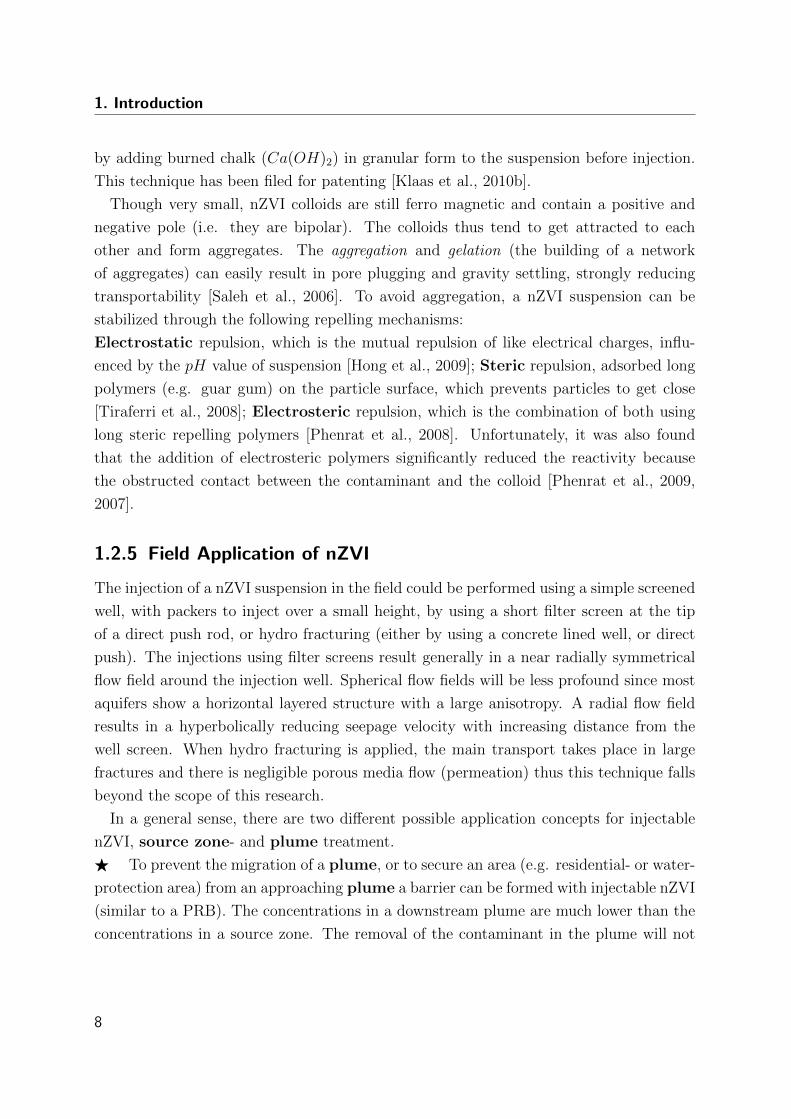
1.3 Conceptual Injection Field . . . . . . . . . . . . . . . . . . . . . . . . . . . 9
1.4 Dissertation Structure . . . . . . . . . . . . . . . . . . . . . . . . . . . . . 12
2.1 Photo of the Metal Detector used for Column Experiments . . . . . . . . . 18
2.2 Calibration Set Up and Data from the Metal Detector . . . . . . . . . . . . 19
2.3 Calibration Curve of the Metal Detector . . . . . . . . . . . . . . . . . . . 20
2.4 Magnetic Field Strength of a Cylindrical Coil . . . . . . . . . . . . . . . . 21
2.5 Equivalent Network of the Container Sensor . . . . . . . . . . . . . . . . . 23
2.6 Coil winding machine . . . . . . . . . . . . . . . . . . . . . . . . . . . . . . 25
2.7 Container Sensor Development . . . . . . . . . . . . . . . . . . . . . . . . . 26
2.8 Iso Surface of the Magnetic Field Strength of the Primary Coil . . . . . . . 27
2.9 Container nZVI Detection Electronics . . . . . . . . . . . . . . . . . . . . . 28
2.10 Influence of Fluid Chemistry on Dual Coil Sensor . . . . . . . . . . . . . . 29
2.11 Schematic Overview of an In-Situ Application of nZVI . . . . . . . . . . . 30
2.12 nZVI Field Sensor . . . . . . . . . . . . . . . . . . . . . . . . . . . . . . . . 31
2.13 Equivalent Network of the Field Sensor . . . . . . . . . . . . . . . . . . . . 32
2.14 Cross Section of the Field Sensor . . . . . . . . . . . . . . . . . . . . . . . 33
2.15 Response of the Field Sensor on nZVI at Increasing Distance . . . . . . . . 33
2.16 Field Sensor Development . . . . . . . . . . . . . . . . . . . . . . . . . . . 34
2.17 Field nZVI Measurement System Overview . . . . . . . . . . . . . . . . . . 36
2.18 Calibration Set Up for the Field Sensor . . . . . . . . . . . . . . . . . . . . 40
2.19 Susceptibility of nZVI at Different Concentrations . . . . . . . . . . . . . . 40
2.20 Field Sensor Test Set Up . . . . . . . . . . . . . . . . . . . . . . . . . . . . 41
2.21 Field Measuring Electronics . . . . . . . . . . . . . . . . . . . . . . . . . . 42
2.22 Propagation of nZVI Inside a Small Container . . . . . . . . . . . . . . . . 42
2.23 Concentration and Temperature During the Injection . . . . . . . . . . . . 43
2.24 Measuring Set Up for Analytical ZVI Measurement . . . . . . . . . . . . . 45
3.1 Transport Mechanisms of Particle Filtration . . . . . . . . . . . . . . . . . 48
3.2 Contact Efficiencies as a Function of Different Parameters . . . . . . . . . 52
3.3 Fe0 Reduction of Stored nZVI . . . . . . . . . . . . . . . . . . . . . . . . . 56
VI
3.4 Oxidation of nZVI Suspensions after Dilution . . . . . . . . . . . . . . . . 57
3.5 Sedimentation Curves of nZVI Suspensions . . . . . . . . . . . . . . . . . . 59
3.6 Size of Nano-Fraction of nZVI in Suspension . . . . . . . . . . . . . . . . . 61
3.7 Conceptual Model for nZVI Transport . . . . . . . . . . . . . . . . . . . . 63
3.8 Set Up of the Column Experiment . . . . . . . . . . . . . . . . . . . . . . . 67
3.9 Column Tracer Experiment . . . . . . . . . . . . . . . . . . . . . . . . . . 70
3.10 Mixer and Disperser . . . . . . . . . . . . . . . . . . . . . . . . . . . . . . 71
3.11 Schematic Overview of the 1-D Experiments . . . . . . . . . . . . . . . . . 72
3.12 Photos of the Propagation of nZVI in a Column Experiment . . . . . . . . 74
3.13 Transient Concentration Profiles of Column Experiments . . . . . . . . . . 75
3.14 Pressure Gradient Development . . . . . . . . . . . . . . . . . . . . . . . . 76
3.15 Water Flushing After Injection . . . . . . . . . . . . . . . . . . . . . . . . 77
3.16 nZVI Breakthrough at 50 cm from Column Inlet . . . . . . . . . . . . . . . 78
3.17 Normalized Transport Distance . . . . . . . . . . . . . . . . . . . . . . . . 79
3.18 Numerically Fitted Model on Column Data . . . . . . . . . . . . . . . . . . 81
3.19 Fitting Parameter S0max in Relation to C0 . . . . . . . . . . . . . . . . . . . 83
4.1 Hyperbolically Decreasing Seepage Velocity Around a Well . . . . . . . . . 86
4.2 Photo of the Container Experiment . . . . . . . . . . . . . . . . . . . . . . 89
4.3 Schematic Overview of the Container Experiment Set Up . . . . . . . . . . 90
4.4 Filter Screens of the Container Experiment . . . . . . . . . . . . . . . . . . 91
4.5 Two Different Types of Pumps Used . . . . . . . . . . . . . . . . . . . . . 92
4.6 3-D Graphical Overview of the Container Experiment . . . . . . . . . . . . 93
4.7 View into the Container During Filling . . . . . . . . . . . . . . . . . . . . 94
4.8 Samples Taken for Chemical Analysis . . . . . . . . . . . . . . . . . . . . . 95
4.9 Reynolds Number in the Container Experiments . . . . . . . . . . . . . . . 98
4.10 nZVI Propagation in the Container . . . . . . . . . . . . . . . . . . . . . . 99
4.11 Magnetic Susceptibility Measured During Container Exp. 1 . . . . . . . . . 100
4.12 Photos of Container Experiment Results at 1000 l/h . . . . . . . . . . . . 102
4.13 Chemically Analyzed nZVI from Container Exp. 1 & 4 . . . . . . . . . . . 102
4.14 Photos of Container Experiment Results at 500 & 1000 l/h . . . . . . . . . 104
4.15 Chemically Analyzed nZVI from Container Exp. 3 & 4 . . . . . . . . . . . 104
4.16 Photos of Container Experiment Results with Different Pumps . . . . . . . 105
4.17 Chemically Analyzed nZVI from Container Exp. 2 & 3 . . . . . . . . . . . 105
4.18 Graphical Overview of all Notation for Radial Flow Discretization . . . . . 108
4.19 Discretization of a Radial Flow Field into Three Sections . . . . . . . . . . 112
4.20 Results of Column Set 1 for Container Exp. 1 . . . . . . . . . . . . . . . . 116
4.21 Results of Column Set 3 for Container Exp. 3 . . . . . . . . . . . . . . . . 116
4.22 Manual Correction of Recorded Data . . . . . . . . . . . . . . . . . . . . . 119
4.23 Example Mesh for Radial Flow Simulation . . . . . . . . . . . . . . . . . . 123
VII
4.24 Comparison of the Matlab and FEniCS models . . . . . . . . . . . . . . . 124
4.25 Hydraulic Head Distribution for Container Exp. 1 & 4 Simulation . . . . . 125
4.26 nZVI Distribution from Simulation of Container Exp. 1 . . . . . . . . . . . 126
4.27 Simulation and Container Exp. 1 Data . . . . . . . . . . . . . . . . . . . . 126
4.28 Hydraulic Head Distribution for Container Exp. 3 Simulation . . . . . . . 127
4.29 nZVI Distribution from Simulation of Container Exp. 3 . . . . . . . . . . . 128
4.30 Simulation and Container Exp. 3 Data . . . . . . . . . . . . . . . . . . . . 128
4.31 nZVI Distribution from Simulation of Container Exp. 4 . . . . . . . . . . . 129
4.32 Simulation and Container Exp. 4 Data . . . . . . . . . . . . . . . . . . . . 129
5.1 Injection Wells and Sensor Locations . . . . . . . . . . . . . . . . . . . . . 136
5.2 Differently Possible Distributions of nZVI . . . . . . . . . . . . . . . . . . . 138
5.3 Decision Chart for Using nZVI . . . . . . . . . . . . . . . . . . . . . . . . . 140
5.4 Drawing of Funnel Shaped nZVI Reservoir . . . . . . . . . . . . . . . . . . 141
VIII
List of Tables
1.1 Pollutants that can be Remediated by nZVI . . . . . . . . . . . . . . . . . 6
2.1 Susceptibilities Measured and Calculated . . . . . . . . . . . . . . . . . . . 39
3.1 Filtration Sensitivity Analysis Constants . . . . . . . . . . . . . . . . . . . 50
3.2 Filtration Sensitivity Analysis Variables . . . . . . . . . . . . . . . . . . . . 51
3.3 nZVI Aging of Different Lots . . . . . . . . . . . . . . . . . . . . . . . . . . 55
3.4 Conditions Used for the Column Experiments . . . . . . . . . . . . . . . . 72
3.5 Normalized Transport Distances of the Column Experiments . . . . . . . . 79
3.6 Parameters of the Column Experiment Simulations . . . . . . . . . . . . . 82
4.1 Conditions of the Container Experiments . . . . . . . . . . . . . . . . . . . 92
4.2 Parameters of the Container Experiments . . . . . . . . . . . . . . . . . . . 96
4.3 Parameters for Column Set 1 . . . . . . . . . . . . . . . . . . . . . . . . . 114
4.4 Parameters for Column Set 3 . . . . . . . . . . . . . . . . . . . . . . . . . 114
4.5 Measured Input and Effluent Concentrations . . . . . . . . . . . . . . . . . 115
4.6 Mass Balance Calculations . . . . . . . . . . . . . . . . . . . . . . . . . . . 118
4.7 Parameters Used for Model Comparison . . . . . . . . . . . . . . . . . . . 124
IX
Notation
Abbreviation Definition
1-D one dimensional
2-D two dimensional
3-D three dimensional
A/D analog digital
AC alternating current
ADC analog to digital converter
CHC chlorinated hydrocarbons
DNAPL dense non aqueous phase liquid
GSM global system for mobile communications
ID inner diameter
L, W, H length, width, height
L, T , M dimensions: Length, Time, Mass
LNAPL light non aqueous phase liquid
MTBE Methyl-tert-butyl-ether
PCE Tetrachloroethylene
PDE differential equation
Pe Peclet number
PEN project on emerging nanotechnologies
PP Polypropylene
PRB permeable reactive barrier
PTFE Polytetrafluoroethylene (Teflon)
PV pore volume
Re Reynolds number
RMS root mean square
RMSE root mean square error
RNIP reactive nano iron particle
TCE Trichloroethylene
TTL transistor-transistor logic
UV ultra violet
X
Abbreviation Definition
ZVI zero valent iron
modem modulator-demodulator
nZVI nano sized zero valent iron
µZVI micro sized zero valent iron
nr. number
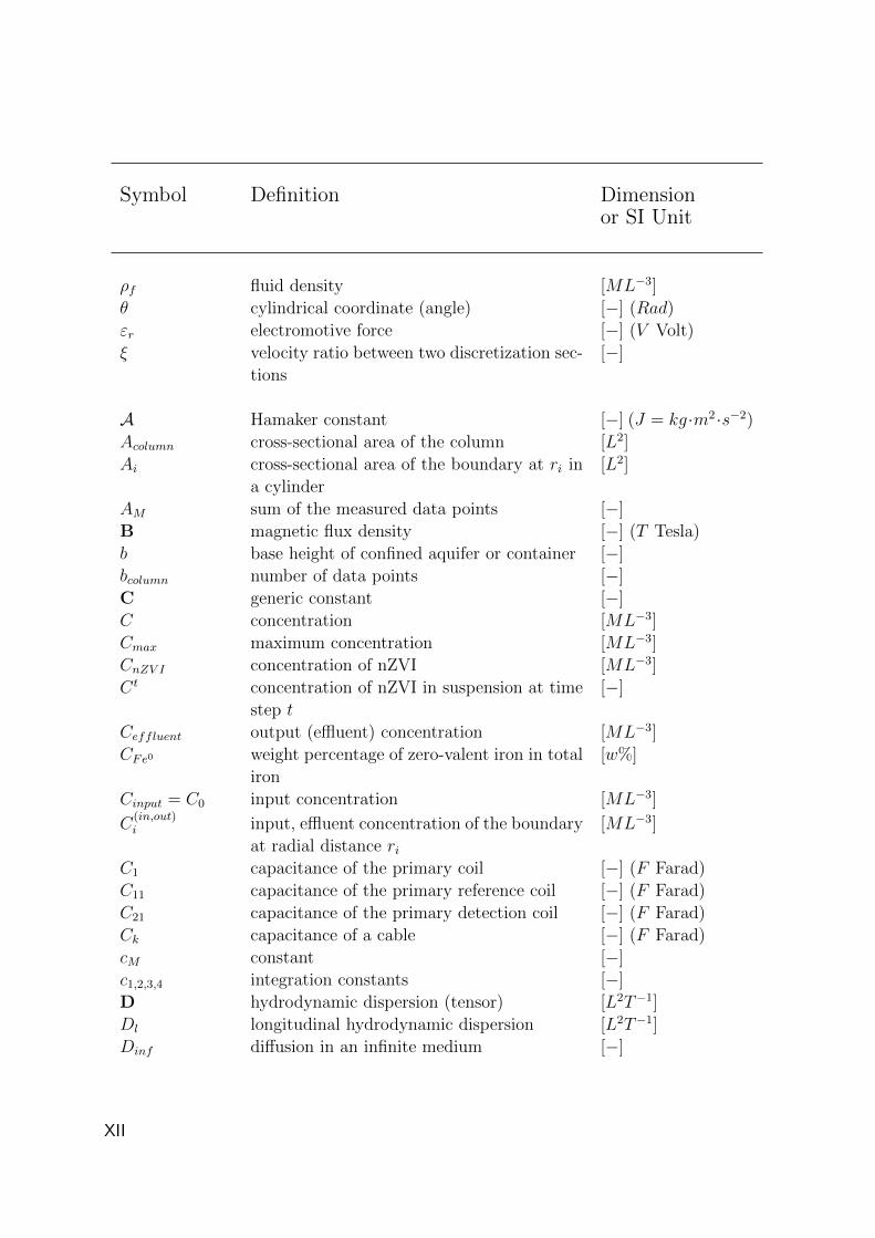
Symbol Definition Dimensionor SI Unit
α empirical attachment efficiency [−]
αagg empirical attachment efficiency of aggregates [−]
αk fitting coefficient for the geometry factor [−]
αl dispersion length [L]
χD average susceptibility measured [−]
χ observed susceptibility [−]
χm susceptibility in accessible domain [−]
χnZV I susceptibility of nZVI [−]
η effective single-collector contact efficiency [−]
ηD single-collector contact efficiency for Brown-
ian diffusion
[−]
ηD single-collector contact efficiency for gravita-
tional effects
[−]
ηI single-collector contact efficiency for inter-
ception
[−]
ηagg0 summed single-collector contact efficiency of
aggregates
[−]
η0 summed single-collector contact efficiency of
colloids
[−]
µ absolute fluid viscosity [ML−1T−1]
µ0 permeability of vacuum [−] (TmA−1)
Ω domain [−]
Φ magnetic flux [−] (Tm2)
ρsand sand density [ML−3]
ρbulk = ρb sand bulk density (porosity included) [ML−3]
XI
Symbol Definition Dimensionor SI Unit
ρf fluid density [ML−3]
θ cylindrical coordinate (angle) [−] (Rad)
εr electromotive force [−] (V Volt)
ξ velocity ratio between two discretization sec-
tions
[−]
A Hamaker constant [−] (J = kg·m2·s−2)
Acolumn cross-sectional area of the column [L2]
Ai cross-sectional area of the boundary at ri in
a cylinder
[L2]
AM sum of the measured data points [−]
B magnetic flux density [−] (T Tesla)
b base height of confined aquifer or container [−]
bcolumn number of data points [−]
C generic constant [−]
C concentration [ML−3]
Cmax maximum concentration [ML−3]
CnZV I concentration of nZVI [ML−3]
Ct concentration of nZVI in suspension at time
step t
[−]
Ceffluent output (effluent) concentration [ML−3]
CFe0 weight percentage of zero-valent iron in total
iron
[w%]
Cinput = C0 input concentration [ML−3]
C(in,out)i input, effluent concentration of the boundary
at radial distance ri
[ML−3]
C1 capacitance of the primary coil [−] (F Farad)
C11 capacitance of the primary reference coil [−] (F Farad)
C21 capacitance of the primary detection coil [−] (F Farad)
Ck capacitance of a cable [−] (F Farad)
cM constant [−]
c1,2,3,4 integration constants [−]
D hydrodynamic dispersion (tensor) [L2T−1]
Dl longitudinal hydrodynamic dispersion [L2T−1]
Dinf diffusion in an infinite medium [−]
XII
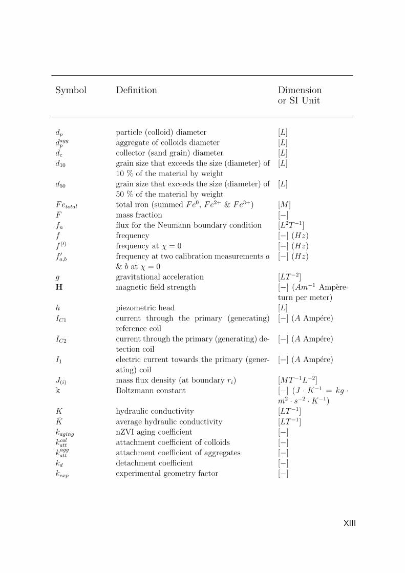
Symbol Definition Dimensionor SI Unit
dp particle (colloid) diameter [L]
daggp aggregate of colloids diameter [L]
dc collector (sand grain) diameter [L]
d10 grain size that exceeds the size (diameter) of
10 % of the material by weight
[L]
d50 grain size that exceeds the size (diameter) of
50 % of the material by weight
[L]
Fetotal total iron (summed Fe0, Fe2+ & Fe3+) [M ]
F mass fraction [−]
fn flux for the Neumann boundary condition [L2T−1]
f frequency [−] (Hz)
f (′) frequency at χ = 0 [−] (Hz)
f ′a,b frequency at two calibration measurements a
& b at χ = 0
[−] (Hz)
g gravitational acceleration [LT−2]
H magnetic field strength [−] (Am−1 Ampere-
turn per meter)
h piezometric head [L]
IC1 current through the primary (generating)
reference coil
[−] (A Ampere)
IC2 current through the primary (generating) de-
tection coil
[−] (A Ampere)
I1 electric current towards the primary (gener-
ating) coil
[−] (A Ampere)
J(i) mass flux density (at boundary ri) [MT−1L−2]
k Boltzmann constant [−] (J · K−1 = kg ·m2 · s−2 ·K−1)
K hydraulic conductivity [LT−1]
K average hydraulic conductivity [LT−1]
kaging nZVI aging coefficient [−]
kcolatt attachment coefficient of colloids [−]
kaggatt attachment coefficient of aggregates [−]
kd detachment coefficient [−]
kexp experimental geometry factor [−]
XIII
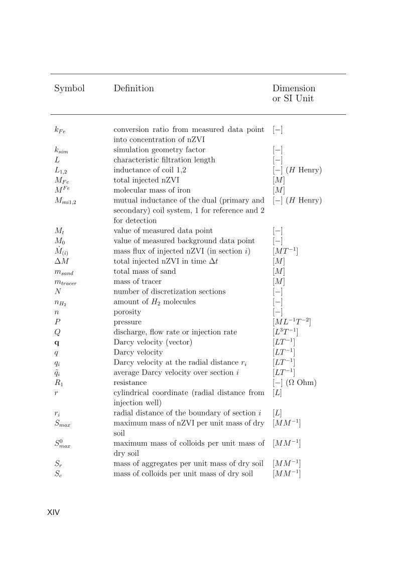
Symbol Definition Dimensionor SI Unit
kFe conversion ratio from measured data point
into concentration of nZVI
[−]
ksim simulation geometry factor [−]
L characteristic filtration length [−]
L1,2 inductance of coil 1,2 [−] (H Henry)
MFe total injected nZVI [M ]
MFe molecular mass of iron [M ]
Mmi1,2 mutual inductance of the dual (primary and
secondary) coil system, 1 for reference and 2
for detection
[−] (H Henry)
Mt value of measured data point [−]
M0 value of measured background data point [−]
M(i) mass flux of injected nZVI (in section i) [MT−1]
∆M total injected nZVI in time ∆t [M ]
msand total mass of sand [M ]
mtracer mass of tracer [M ]
N number of discretization sections [−]
nH2 amount of H2 molecules [−]
n porosity [−]
P pressure [ML−1T−2]
Q discharge, flow rate or injection rate [L3T−1]
q Darcy velocity (vector) [LT−1]
q Darcy velocity [LT−1]
qi Darcy velocity at the radial distance ri [LT−1]
qi average Darcy velocity over section i [LT−1]
R1 resistance [−] (Ω Ohm)
r cylindrical coordinate (radial distance from
injection well)
[L]
ri radial distance of the boundary of section i [L]
Smax maximum mass of nZVI per unit mass of dry
soil
[MM−1]
S0max maximum mass of colloids per unit mass of
dry soil
[MM−1]
Sr mass of aggregates per unit mass of dry soil [MM−1]
Sc mass of colloids per unit mass of dry soil [MM−1]
XIV
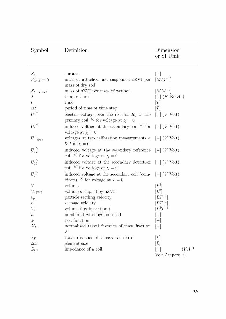
Symbol Definition Dimensionor SI Unit
Sb surface [−]
Stotal = S mass of attached and suspended nZVI per
mass of dry soil
[MM−1]
Stotal|wet mass of nZVI per mass of wet soil [MM−1]
T temperature [−] (K Kelvin)
t time [T ]
∆t period of time or time step [T ]
U(′)1 electric voltage over the resistor R1 at the
primary coil, (′) for voltage at χ = 0
[−] (V Volt)
U(′)2 induced voltage at the secondary coil, (′) for
voltage at χ = 0
[−] (V Volt)
U ′1,2|a,b voltages at two calibration measurements a
& b at χ = 0
[−] (V Volt)
U(′)12 induced voltage at the secondary reference
coil, (′) for voltage at χ = 0
[−] (V Volt)
U(′)22 induced voltage at the secondary detection
coil, (′) for voltage at χ = 0
[−] (V Volt)
U(′)3 induced voltage at the secondary coil (com-
bined), (′) for voltage at χ = 0
[−] (V Volt)
V volume [L3]
VnZV I volume occupied by nZVI [L3]
vp particle settling velocity [LT−1]
v seepage velocity [LT−1]
Vi volume flux in section i [L3T−1]
w number of windings on a coil [−]
ω test function [−]
XF normalized travel distance of mass fraction
F
[−]
xF travel distance of a mass fraction F [L]
∆x element size [L]
ZC1 impedance of a coil [−] (V A−1
Volt Ampere−1)
XV
Abstract
One of the recent In-Situ groundwater remediation techniques under development uses
reactive zero valent iron (ZVI) to turn highly toxic chlorinated hydrocarbons (CHCs) into
harmless compounds. CHCs are non miscible and characterized by a low solubility which
determines their slow dissolution (over decades or centuries) into groundwater, forming
plumes that can target drinking water wells, rivers and lakes. Injection of nano sized zero
valent iron (nZVI) suspension into the subsurface could target the contaminants directly
in the source zone. The high reactivity of nZVI together with the injection into the source
fastens the depletion of the contaminant and interrupts the plume generation.
The presented work focused on the transport of nZVI during the injection. To make
quantitative descriptions of transport possible, an effective detection technique was de-
veloped. Exact concentrations of nZVI inside the porous medium was measured through
changes in susceptibility detected with electromagnetic induction sensors. Mobility tests
with different suspension concentrations were performed in a 1-D horizontally orientated
two meter long column. Continuous concentration measurements were performed over
the whole length of the column. In a near field scale container experiment a confined
aquifer with a radial flow field over a radius of almost two meters was simulated. Differ-
ent injection rates and pumping techniques were tested inside this experimental set up.
A discretization method to represent all effects of a radial flow field using sets of columns
was developed. The method could be verified successfully by comparing the concentration
profiles to the results obtained from the container experiments. A mathematical model,
developed by starting from the classic colloid filtration theory and by considering the
transport of primary colloids and aggregates separately, was able to be fitted on the 1-D
results. After implementation in a numerical solver, the model was furthermore capa-
ble of providing a very good fit on the results of the radial geometry tests while using
exclusively the fitted parameters obtained from the 1-D tests.
Throughout the work a better understanding of the transport of nZVI during the in-
jection was developed. It was demonstrated that transport of nZVI without modification
was possible over a distance of two meters in both 1-D and radial geometry flow fields.
An extrapolation of the work for field application was furthermore described. By ap-
plying the methods developed in this work the necessary suspension concentration, the
volume of suspension and the injection rate could be determined in advance. The pre-
sented work showed promising results and could be a sound scientific basis for further
investigations and case studies on nZVI based remediation.
XVI
Kurzfassung
Einleitung
Hintergrund
Die Wahrnahme der Gefahren, die von verunreinigten Standorten ausgehen, hat in den
letzten paar Jahrzehnten stark zugenommen. Viele dieser Standorte wurden kontaminiert
mit chlorierten Kohlenwasserstoffen (CKW’s), welche bereits in niedrigsten Konzentratio-
nen außerst toxisch und umweltschadlich sind und von denen einige sogar krebserregend
fur den Menschen sind. Flussige CKW’s haben eine hohere Dichte als Wasser, wodurch
Sie bis auf große Tiefen im Untergrund versickern konnen. Ihre Loslichkeit im vorbeistro-
menden Grundwasser ist sehr gering, weshalb die CKW’s den Aquifer im unterstromigen
Bereich fur mehrere Jahrhunderte verunreinigen konnen.
In den letzten Jahrzehnten wurden die unterschiedlichsten Methoden entwickelt, um
diese Verunreinigungen zu beseitigen. Eine von den neuesten und vielversprechendsten
Methoden ist die Sanierung mittels nullwertigem Eisen in nanoskaliger, kolloidaler Form.
Diese sogenannten Nano-Eisen-Kolloide haben durch ihre geringe Große eine sehr große
Oberflache und damit eine sehr hohe Reaktivitat. Neben CKW’s kann ein ganzes Spek-
trum von Schadstoffen mit ihrer Hilfe abgebaut und somit unschadlich gemacht werden.
Bis vor Kurzem wurde hauptsachlich die Reaktivitat von Nano-Eisen erforscht. Durch
die geringe Partikelgroße wurde angenommen, dass sich die Kolloide einwandfrei in den
Untergrund einbringen ließen. Leider musste jedoch bei mehreren Pilotanwendungen
[Muller et al., 2006a,b] und Vorversuchen im Labor [de Boer, 2007; Koch, 2007] festgestellt
werden, dass sich die Kolloide deutlich schlechter im Untergrund verteilen als erwartet.
Forschungsfragen
Um ein besseres Verstandnis vom Transport nanoskaliger Eisenkolloide im Untergrund
zu bekommen und deren Anwendbarkeit fur die Sanierung von Schadensfallen besser
abschatzen zu konnen, wurden im Rahmen dieser Arbeit die folgenden Forschungsfragen
aufgestellt.
(a) Ist es moglich, Nano-Eisen direkt im Untergrund zu messen?
(b) Welche Faktoren bedingen die niedrige Transportfahigkeit im porosen Medium und
wie kann der Transport optimiert werden?
XVII
(c) Welche Reichweite kann in einem radialen Stromungsfeld erreicht werden?
(d) Wie lasst sich die Machbarkeit der Injektion an einem Standort feststellen?
Detektion von Nano-Eisen und Konzentrationsmessung
im Untergrund
Die Messung von Nano-Eisen im Untergrund ist mit den gangigen Messtechniken nicht
ohne weiteres moglich, weshalb im Rahmen dieser Arbeit ein neues Messverfahren speziell
fur die Messung von Nano-Eisen entwickelt wurde. Das Messverfahren wurde sukzessive
fur drei verschiedene Skalen angepasst. Zunachst wurde die Messung von Konzentra-
tionsprofilen entlang einer Saule realisiert. Danach folgte die Aufnahme von Durchbruch-
skurven in einem großskaligen Containerversuch mittels stationarer, durchstromter Son-
den. Schlussendlich wurde die Technik dann bis zur Feldtauglichkeit weiterentwickelt.
Messprinzip
Das neue Messverfahren basiert auf den ferromagnetischen Eigenschaften von nullwer-
tigem Eisen. Durch den Ferromagnetismus haben die Kolloide eine messbare Suszeptibil-
itat. Die Suszeptibilitat ist das Verhaltnis aus der Magnetisierung in einer Substanz und
der daraus resultierenden magnetischen Kraft. Die Auswahl eines Messverfahrens, das
die Anderung der magnetischen Suszeptibilitat im Boden erfassen kann, liegt also nahe.
Die Anderung der Suszeptibilitat im Boden ist direkt proportional zur Suszeptibilitat
von Nano-Eisen und damit dessen Konzentration am Ort der Messung.
Messtechnik fur Saulenversuchen
Zur Bestimmung der Transporteigenschaften von Nano-Eisen wurde ein Saulenversuchs-
stand aufgebaut. Um Konzentrationsprofile entlang der Saule messen zu konnen, wurde
zunachst eine modifizierte Version eines kommerzielles verfugbaren Minensuchdetek-
tor (FX2FD, Minex, Reutlingen) genutzt. Der Detektor wurde an einen Rechner
angeschlossen, sodass die Rohdaten ausgelesen werden konnten. Zur Aufnahme von
Konzentrationsprofilen wurde das Minensuchgerat auf einem fahrbaren Wagen montiert,
der mittels eines Schrittmotors entlang der Saule verfahren werden konnte.
Vor der Injektion wurde eine Hintergrundmessung durchgefuhrt. Dann wurde wahrend
der Injektion alle zehn Minuten ein Profil gemessen und die Hintergrunddaten abgezogen.
Um die Rohdaten in reale Konzentrationen umzusetzen, wurde die Gesammtmasse an in-
jiziertem Nano-Eisen zum Zeitpunkt der Messung bestimmt und mit der Integralsumme
der gemessenen Masse uber alle Messpunkte gleichgesetzt. Somit wurde ein Faktor fur
XVIII

jeden Messpunkt ermittelt , der zur Umrechung aller Rohdaten eines Versuchs in Konzen-
trationsprofile herangezogen wurde.
Messtechnik fur die großskaligen Containerversuche
Das bei den Saulenversuchen verwendete Messgerat war nicht fur den Einsatz im großskali-
gen Containerversuch geeignet. Die Messtechnik musste direkt im Boden eingegraben
werden. Die dafur notigen Messsensoren sowie die dazu gehorige Messelektronik wurden
eigens entwickelt.
Es wurde eine lange, zylinderformige Spule gewickelt, um ein elektromagnetisches Feld
aufzubauen (Erregerspule). Um diese Spule wurde eine kurze Spule gewickelt, in der
durch Induktion eine Spannung erzeugt wurde (Messspule). Die Messsensoren wurde
wahrend des Einbaus in den Container mit Bodenmaterial gefullt und so angeordnet,
dass die Grundwasser-Stromungslinien genau mittig durch die Spule verliefen. Wenn nun
die Nano-Eisen Suspension durch die Spulen stromt, andert sich die Suszeptibilitat im
Inneren der Spule, die Spannung der Messspule steigt in der Folge an und der Strom in
der Erregerspule sinkt ab.
Die Anderung der induzierten Spannung und der durch die Erregerspule fließende Strom
wurden mittels einer elektronischen Schaltung erfasst und die Daten auf einem Rechner
gespeichert.
Zur Umrechnung der Daten in reale Konzentrationen, wurden nach Ablauf des Ver-
suches Bodenproben aus den Spulen entnommen und mittels chemischer Analyse die
Konzentration an Nano-Eisen bestimmt. Diese Konzentration wurde dann mit dem let-
zten gemessenen Wert des Sensors gleichgesetzt und die wahrend der gesamten Injek-
tionsdauer gemessenen Konzentrationen entsprechend korrigiert.
Messtechnik furs Feld
Im nachsten Schritt wurde die Messtechnik fur den Feldeinsatz angepasst. Im Feld sollen
die Sensoren in einen Brunnen oder mittels anderer Sondierungsverfahren in der Tiefe
angebracht werden. Dabei ist die parallele Ausrichtung der Sensoren zu den Stromungslin-
ien nicht immer gewahrleistet und die Spulen werden unter Umstanden nicht immer gleich
durchstromt.
Aus diesem Grund wurde ein Spulenpaar entwickelt, bei dem das elektromagnetische
Feld nach außen gerichtet ist. Die Sensitivitat der Messung wurde aber hierdurch deutlich
reduziert, was eine Neuentwicklung der Elektronik erforderlich machte. Die Elektronik
wurde außerdem um die Moglichkeit erweitert, die Daten direkt im Messgerat zu speichern
und uber ein Master-Slave-Verfahren abzurufen. Fur jede Messlanze mit mehreren uber
die Tiefe verteilten Sensoren wurde ein Slave eingesetzt und zentral uber einen Master
abgerufen.
XIX
Da uber chemische Verfahren keine genaue Konzentration im Untergrund zu bestim-
men ist, wurde außerdem eine Methode entwickelt, die Sensoren bereits im Vorfeld zu
kalibrieren.
Diese Methode wurde vor dem Einsatz im Feld mittels eines kleinen Containerversuchs
uberpruft.
Messung von nullwertigem Eisen in Boden- und Flussigproben
Um die Bodenproben vom großskaligen Containerversuch aber auch den Anteil an nullw-
ertigem Eisen in den Nano-Eisen-Partikeln bestimmen zu konnen, wurde ein Messstand
aufgebaut wie z.B. in Elion and Elion [1933] beschrieben. Die Messung beruht darauf,
dass bei einer Reaktion von nullwertigem Eisen mit Salzsaure ein genau definiertes Volu-
men an Wasserstoff freigesetzt wird. Der gebildete Wasserstoff kann somit sehr genau in
die Masse an nullwertigem Eisen umgerechnet werden, die zum Zeitpunkt der Messung
in der Probe enthalten war.
Grundlagen zum Transport von Nano-Eisen-Kolloiden
Hintergrund
Das Hauptziel der Arbeit ist ein besseres Verstandis des Transports kolloidaler Nano-
Eisen-Partikel wahrend der Injektion in den Untergrund. Hierzu wurden zuerst beste-
hende Theorien zur Filtration von Kolloiden im Detail betrachtet. Anschließend wurde
die zu verwendende Nano-Eisen Suspension charakteriziert und ein konzeptionelles Modell
entwickelt. Auf Basis dieses Modells konnte dann ein mathematisches Modell hergeleitet
werden welche dann mittels eines numerischen Modells und eindimensionaler Saulenver-
suche uberpruft wurde.
Kolloidfiltrationstheorie
In porosen Medien wird der Transport von Kolloiden gehemmt durch Filtrationseffekte.
Die Filtration fuhrt dazu, dass die Kolloide aus der Suspension entfernt werden. Die am
haufigste eingesetzte Filtrationstheorie ist die Theorie von Tufenkji and Elimelech [2004].
Der Theorie beschreibt die Filtration auf Basis von drei verschiedenen Filtrationsmech-
anismen: Festsetzung am porosen Medium durch Interzeption, Gravitationseffekte und
Brownsche Diffusion. Das Zusammenspiel der drei Mechanismen ergibt die Kontaktef-
fizienz.
Da mit der Theorie nicht alle Effekte vollstandig beschrieben werden konnen, wird ein
Kontaktseffizienz Koeffizient eingesetzt, welche experimentell zu bestimmen ist. Uber
XX
eine Sensitivitatsanalyse wurde festgestellt, dass die Kolloidgroße den großten Einfluss
auf die Kontakteffizienz hat.
Charakterisierung der Nano-Eisen Suspension
Die ausgewahlte Suspension war RNIP 10-E von Toda Kogyo, Japan. Die Suspension
wird vom Hersteller als sehr hoch konzentrierter Schlamm geliefert, der vor der Verwen-
dung verdunnt werden muss. Uber Vorversuche [de Boer, 2007] wurde festgestellt, dass
die Kolloide im Schlamm stark aggregiert sind, jedoch mittels hoher Scherkrafte von einen
Dispergiergerat wieder aufgebrochen werden konnen. Ein weiteres Ergebnis der Vorun-
tersuchungen war, dass sich eine Suspensionskonzentration von etwa 10 g/l am besten im
porosen Medium transportieren lasst.
Es stellte sich heraus, dass der Schlamm wahrend der Lagerung altert und der Anteil an
nullwertigem Eisen mit der Zeit abnimmt. Hierzu wurden Langzeitmessungen uber mehr
als funf Jahre durchgefuhrt, woraus Alterungsgleichungen hergeleitet werden konnten.
Aus der in Sedimentationsversuchen bestimmten Absatzkurve konnte festgestellt wer-
den, dass auch nach der Dispergierung noch Aggregate mit einem mittleren Durchmesser
von 4, 4 µm vorlagen. Mit Hilfe von Messungen mit einem Partikelgroßenmessgerat, das
auf der Streuung von einem Helium-Laser basiert, konnten jedoch auch die primaren
Nano-Eisen-Kolloide mit einer Große zwischen 60nm und 120nm nachgewiesen werden.
Konzeptionelles Transportmodell
Auf Basis der Charakterisierung und der Filtrationstheorie konnte ein konzeptionelles
Modell aufgesetzt werden. Das Modell lasst sich zusammenfassen in vier Punkte:
Die Suspension besteht aus nanoskaligen Kolloiden und mikroskaligen, kolloidalen Ag-
gregaten.
Die Kolloide binding an der Kornoberflache, wobei die verfugbaren Bindungsplatze
begrenzt sind.
Aggregate werden durch Gravitationseffekte und auf Basis ihrer Große aus der Suspen-
sion entfernt. Hierzu gibt es kein Maximum außer dem verfugbaren Porenvolumen, was
aber hier vernachlassigt wird.
Die Filtrationstheorie von Tufenkji and Elimelech [2004] kann sowohl die Entfernung
der Kolloide als Aggregate beschreiben, gegeben Sie werden getrennt betrachtet.
1-D Transport Modell
Fur das konzeptionelle Modell wurde eine mathematische Beziehung hergeleitet. Diese
Transportgleichung wurde dann in ein numerisches Modell (in Matlab) integriert, mit
Hilfe dessen der Transport berechnet werden konnte. Anschließend wurden Saulenver-
suche durchgefuhrt. Da in der Filtrationstheorie die Suspensionskonzentration nicht
XXI
berucksichtigt wird, musste zunachst festgestellt werden, ob die Transportgleichung fur
unterschiedliche Eingangskonzentrationen gleichermaßen gilt oder ob dazu zusatzliche
Konstitutivbeziehungen notig sind.
Die Saulenversuche wurden sodann mit verschiedenen Eingangskonzentrationen
durchgefuhrt und dabei jeweils Konzentrationsprofile zu verschiedenen Zeitpunkten
aufgezeichnet.
Das numerische Modell wurde dann mit drei Parametern iterativ an die Daten
angepasst. Die Parameter waren die Kontaktseffizienz Koeffizient fur die Kolloide und
die Aggregate, und die Maximalkonzentration der gebundene Kolloide. Mit Hilfe der
Experimente konnte festgestellt werden, dass die Filtrationstheorie fur die Kolloide eine
sehr gute Vorhersage lieferte. Einzig der Kontaktseffizienz Koeffizient fur die Aggregate
musste recht niedrig eingestellt werden, um eine gute Ubereinstimmung mit den experi-
mentellen Daten zu erreichen. Beide Koeffizienten wiesen keine erkennbare Abhangigkeit
von der Kolloidkonzentration auf. Die Maximalkonzentration der Kolloide war jedoch
konzentrationsabhangig, wozu eine lineare Beziehung aufgestellt werden konnte.
Transport von Nano-Eisen-Kolloiden im radialen
Stromungsfeld
Hintergrund
Saulenversuche konnen nur bedingt die Transportfahigkeit von Nano-Eisen darstellen,
da Sie nur ein sehr einfaches, eindimensionales Stromungsfeld besitzen. Um das Trans-
portverhalten von Nano-Eisen wahrend der Injektion im Untergrund richtig beschreiben
zu konnen, muß das Stromungsfeld mindest radialsymmetrisch gewahlt werden. In einem
radialsymmetrischen Stromungsfeld weist unter anderem die Fließgeschwindigkeit eine hy-
perbolische Abnahme mit zunehmender Entfernung von der Injektionsstelle auf. Dieser
Effekt lasst sich mittels standard Saulenversuchen nicht darstellen.
Im Rahmen dieser Arbeit wurden drei verschiedene Methoden entwickelt, um den
Transport in einem radialsymmetrischen Stromungsfeld nachbilden bzw. vorhersagen zu
konnen.
Großskalige Containerversuche
Zur Erstellung eines hyperbolisch abnehmenden Fließgeschwindigkeitsprofils wurde ein
Container in Form eines gleichseitigen Dreiecks zur Annaherung an ein Zylindersegment
aufgebaut (Lange = 2 m, Hohe = 60 cm, Winkel = 60). Ein Dreieck wurde ausgewahlt,
da dies annahernd die gleichen Stromungseffekte wie ein kompletter Zylinder nachweist
aber nur ein Sechstel an Bodenmaterial und Suspension benotigt. Ein Dreiecksschenkel
XXII
wurde mit einer Glasscheibe versehen, um die Ausbreitung der Kolloide auch visuell
beobachten zu konnen. In der Spitze wurde ein Injektionsbrunnen eingebracht und ent-
lang des gegenuberliegenden Dreiecksschenkels wurden Drainagerohre installiert, die an
einen Auslaufbehalter mit Festpotential angeschlossen wurden. Der Behalter wurde ho-
mogen mit Sand befullt und mit einem festen Deckel verschlossen, sodass ein gespannter
Aquifer gebildet war. Im Container wurden verschiedene Versuche durchgefuhrt. So kon-
nte gezeigt werden, dass eine kontinuierliche Pumprate bei der Injektion besser ist als eine
pulsierende. Auch wurde festgestellt, dass eine Halbierung der Injektionsrate nur einen
geringen Effekt auf den Ausbreitungsradius hatte.
Bei den Versuchen war es moglich, das Nano-Eisen uber eine Distanz von etwa zwei
Metern zu transportieren, wenn etwa drei Porenvolumina uber eine Injektionsdauer von
einer Stunde injiziert wurden.
Abbildung eines radialen Stromungsfeldes mittels Saulenversuchen
Da die großskaligen Containerversuche sehr arbeitsintensiv waren, viel Vorbereitungszeit
brauchten und sehr große Mengen an Suspension benotigten, wurde nach einer einfacheren
und schnelleren Methode gesucht, um den Transport in einem radialen Stromungsfeld
darzustellen.
Hierzu wurde zunachst mathematisch das Stromungsfeld aufgeteilt in kleinere Kreis-
segmente. Dann wurde die Fließrate in jedem Segment auf eine Saule gleicher Lange
ubertragen. Bei der Injektion der Suspension in eine der jeweils ein Segment represen-
tierenden Saulen wurde der Auslauf gesammelt, sodass er als Eingangssuspension fur die
nachste Saule genutzt werden konnte. Somit wurde eine Versuchsmethode entwickelt, um
das radiale Stromungsfeld diskretisiert darzustellen.
Es wurden zwei Versuche mit jeweils drei Segmenten durchgefuhrt. Die Ergebnisse
wurden sodann mit denen von zwei großskaligen Containerversuchen verglichen. Hierzu
wurde von jeder einzelnen Saule das Konzentrationsprofil aufgezeichnet. In der graphis-
chen Darstellung wurden sodann die einzelnen Profile entsprechend der Position der Saule
im Gesamtablauf aneinandergehangt. Es konnte somit nachgewiesen werden, dass die
Methode in der Lage ist, die Realitat akzeptabel bis gut zu reprasentieren.
Ein Hauptproblem bei der Durchfuhrung war die genaue Einstellung der Ein-
gangskonzentration durch Verdunnung aus dem Nano-Eisen-Schlamm. Da die Trans-
porteigenschaften der Suspension stark von deren Einganskonzentration abhangig sind,
ist es schwierig, verschiedene Falle zu vergleichen oder Vorhersagen bezuglich des Trans-
portverhaltens in einem bestimmten System zu treffen, wenn auch nur geringfugig veran-
derte Eingangskonzentrationen vorliegen.
XXIII
Numerische Simulation
Als dritte Methode wurde die hergeleitete Transportgleichung in ein numerisches Model
mit mehrere Dimensionen umgesetzt. Um die Robustheit vom Modell zu steigern und
die Moglichkeiten der Anwendbarkeit zu vergroßern, wurde der Finite-Elemente-Solver
FEniCS [Logg et al., 2011] gewahlt. Auch hier wurde das Modell getestet gegen die Resul-
tate der großskaligen Containerversuche, wobei die Eingangsparameter entsprechend dem
großskaligen Containerversuche gewahlt wurden. Dazu wurden die Kontaktseffizienz Ko-
effizienten fur die Kolloide und die Aggregate und die Gleichung fur die Maximalkonzen-
tration der Kolloide eingesetzt, die aus den Saulenversuchen bestimmt wurden. Das Re-
sultat wurde dann vergleichend mit den Endresultaten vom großskaligen Containerversuch
graphisch dargestellt. Auffallig war, dass die Ergebnisse der numerischen Simulation fast
genau durch die Mittelwerte der gemessenen Konzentrationen gingen.
Durch den Einsatz der Transportgleichung in einer numerischen Simulation konnte also
eine sehr gute Vorhersage des Transports im radialen Stromungsfeld getroffen werden.
Machbarkeitsanalyse zum Einsatz von Nano-Eisen im
Feld
Hintergrund
Die bisher in dieser Arbeit prasentierten Erkenntnisse sind weitgehend als Grundlagen-
forschung anzusehen und stellen die Basis fur ein vertieftes Prozessverstandnis zum
Transport von injizierten Nano-Eisen-Partikeln im Untergrund. Uber die rein wis-
senschaftlichen Aspekte hinaus konnen die entwickelten Methoden und hergeleiteten
Beziehungen auch zur Einschatzung der Machbarkeit einer Injektion im Feld herange-
zogen werden.
Einschrankend lasst sich nochmals darauf hinweisen, dass alle hier beschriebenen Meth-
oden auf der Annahme basieren, dass Stromung und Transport im Untergrund nur mittels
Permeation im porosen Medium stattfinden und nicht durch hydraulisch erzeugte Klufte.
Außerdem wurden fur die Beweisfuhrung nur dispergierte, verdunnte Nano-Eisen Suspen-
sionen eingesetzt. Die Ubertragbarkeit auf Suspensionen mit anderen Eigenschaften ist
daher vorher im Einzelfall zu uberprufen.
Voraussetzungen fur einen erfolgreichen Einsatz
Bevor Nano-Eisen zur Grundwassersanierung eingesetzt werden kann, muss bekannt sein,
ob ein Einsatz mit einer hinreichend hohen Wahrscheinlichkeit zum Erfolg fuhrt. Hierzu
sollten bereits in einem fruhen Stadium der Planung einige grundlegende Fragen beant-
wortet werden, um die grundsatzliche Machbarkeit einer Injektion einschatzen zu konnen.
XXIV

Befindet sich zum Beispiel der Schadensherd hauptsachlich in der ungesattigten Zone, ist
der Einsatz von Nano-Eisen nicht sinnvoll, da es sofort durch den hohen Sauerstoffge-
halt oxidieren wurde. Ein weiteres Ausschlusskriterium ist die hydraulische Leitfahigkeit
des Untergrundes. Ist diese zu niedrig, kann hochstwahrscheinlich kein Transport uber
Permeation stattfinden. Falls alle sonstigen Kriterien aber fur den Einsatz von Nano-
Eisen sprechen, sollten Laborversuche durchgefuhrt werden, um die Machbarkeit naher
zu untersuchen.
Zunachst sollte festgestellt werden, wie im Einzellfall ein Erfolg definiert ist und wie
dieser nachzuweisen ist. Hauptsachlich sollte bewiesen werden, dass die erforderliche Aus-
breitung der Partikel wahrend der Injektion erreicht wurde. Dazu kann beispielsweise die
im Rahmen dieser Arbeit entwickelte Feldmesstechnik eingesetzt werden. Die Sensoren
werden dazu idealerweise direkt zwischen zwei Injektionspunkten installiert. Des Weit-
eren sollte die Reduktion der unterstromigen Schadstofffracht nachgewiesen werden. Zu
beachten ist dabei, dass bei der Injektion von Nano-Eisen-Suspension zumeist auch viel
sauberes Wasser injiziert wird. Bevor aus der Abnahme der Schadstofffracht Schlussfol-
gerungen gezogen werden konnen, muss gewahrleistet werden, dass diese Injektionsflus-
sigkeit vor der Beprobung komplett ausgespult wurde. Des Weiteren konnen vor und
nach der Injektion durchgefuhrte Tracerversuche dabei helfen, die in die Frachtberech-
nung eingehende Grundwasserfließgeschwindigkeit moglichst genau zu bestimmen
Anwendung von Entwickelte Machbarkeitstests
Die in dieser Arbeit beschriebenen Methoden zur Vorhersage der Ausbreitung von Nano-
Eisen-Suspension im radialen Stromungsfeld konnen dazu eingesetzt werden, sowohl die
Eingangskonzentration als auch die Injektionsrate fur einen Feldeinsatz zu bemessen.
Gegebenenfalls kann zusatzlich noch die Distanz zwischen den Injektionsbrunnen op-
timiert werden, wobei fur deren Lage jedoch haufig andere Faktoren (z.B. Bebauung)
ausschlaggebend sind.
Ziel einer Auslegung sollte es sein, eine Kombination von Eingangskonzentration und
Injektionsrate zu finden, mit der eine zuvor bestimmte Mindestkonzentration an Nano-
Eisen in moglichst großen Bereichen des zu sanierenden Untergrundes erreicht werden
kann. Die benotigte Menge an Nano-Eisen kann somit minimiert werden.
Schlußfolgerungen
Der Einsatz von Nano-Eisen ist ein vielversprechendes Verfahren zur Sanierung von verun-
reinigten Aquiferen. Das Ziel eines solchen Einsatzes ist die Entfernung des Schaden-
sherdes in-situ, also direkt im Untergrund. Das Transportverhalten von Nano-Eisen
wahrend der Injektion wurde in dieser Arbeit im Detail untersucht und es konnte ein
deutlicher Fortschritt im Verstandnis des Transportverhaltens verzeichnet werden. Die
XXV
chemische Machbarkeit einer Sanierung mit Nano-Eisen wurde in dieser Arbeit nicht be-
trachtet. Abschließend soll nun auf die eingangs gestellten vier Forschungsfragen einge-
gangen werden, welche alle vier eindeutig beantwortet werden konnten:
(a) Ist es moglich Nano-Eisen direkt im Untergrund zu messen?
Es gab bis zum Anfang der Arbeit noch keinen verfugbaren Messtechnik. Deshalb
wurde im Rahmen der Arbeit eine neue Messtechnik entwickelt mit Hilfe derer die
Nano-Eisen-Konzentration zerstorungsfrei gemessen werden kann.
(b) Welche Faktoren bedingen die niedrige Transportfahigkeit im porosen Medium und
wie kann der Transport optimiert werden?
Die Große der Kolloide wurde als Hauptfaktor fur den Transport bestimmt. Beim be-
trachteten Nano-Eisen-Material (RNIP 10-E, Toda Kogyo, Japan) wurde festgestellt,
dass die Kolloide zur Bildung von Aggregaten neigen und der angelieferte Schlamm fur
eine direkte Einbringung in den Untergrund zu hoch konzentriert ist. Ein vorrangiges
Ziel dieser Arbeit war es, die minimal notige Vorbehandlung der Suspension fur eine
erfolgreiche Injektion zu ermitteln. Die kolloidalen Aggregate konnen unter Einsatz
hoher Scherkrafte mittels eines Dispergiergerates in kleinere Aggregate aufgebrochen
werden. Die Primarkolloide konnen aber selbst damit nur bedingt wiederhergestellt
werden. Zusatzlich muss der angelieferte Schlamm runterverdunnt werden, um den
Transport im Untergrund moglich zu machen.
(c) Welche Reichweite kann in einem radialen Stromungsfeld erreicht werden?
In dieser Arbeit wurde erstmalig ein Transport von fast zwei Metern in einem radialen
Stromungsfeld nachgewiesen.
(d) Wie lasst sich die Machbarkeit der Injektion an einem Standort feststellen?
Es wurde ein Fließschema erstellt, um bei der Einschatzung der Machbarkeit einer
Injektion zu helfen. Es wurden zwei alternative Methoden entwickelt, um den Trans-
port im radialen Stromungsfeld vorhersagen zu konnen. Der Einsatz einer dieser
Methoden kann in der Planungsphase helfen, die richtigen Entscheidungen zu treffen
und die benotigten Ablaufbedingungen festzulegen.
Die Ergebnisse dieser Arbeit sind vielversprechend und stellen eine gute Basis fur
weitere Forschung bezuglich des Einsatzes von Nano-Eisen bei der Sanierung von kon-
taminierten Aquiferen dar. Des Weiteren konnen die hier vorgestellten Ergebnisse bei der
Beurteilung von entsprechend gelagerten Fallbeispielen helfen.
XXVI
1 Introduction
1.1 Background
The awareness of the dangers of contaminated sites and the resulting contamination in
groundwater has been increasing over the last decades. The number of sites that have
been recognized for the need to be treated is large, in the European Union there are over
three million sites contaminated [Swartjes, 2011]. In Germany 350 000 sites are potentially
contaminated and are a danger for the environment and the groundwater [Hahn, 2006].
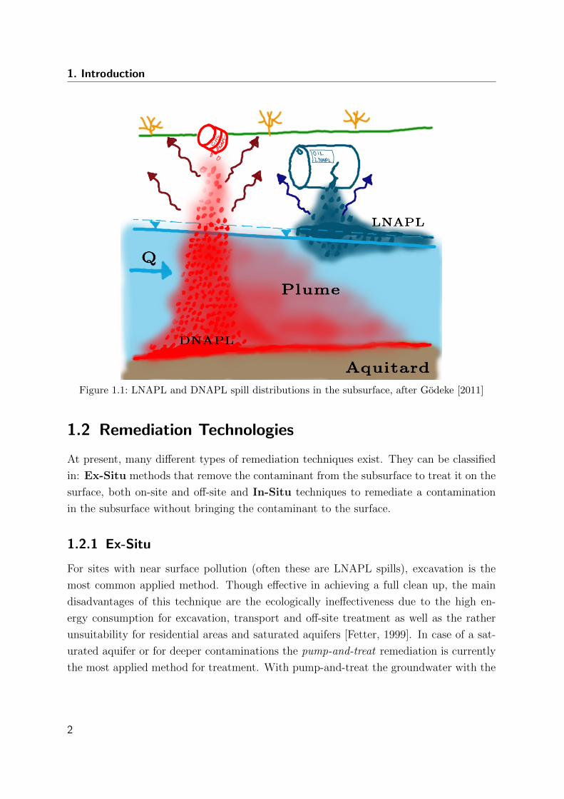
A major separation of contaminant types is made based on their density (Figure 1.1).
Contaminants that have a higher density than water are called dense nonaqueous phase
liquids (DNAPL), if their density is lower than water they are light nonaqueous phase
liquids (LNAPL). Among the sites in Germany, 35% are contaminated by chlorinated
hydrocarbons (CHCs), these are very toxic and many of them are carcinogenic. CHCs like
Tetrachloroethylene (PCE) and Trichloroethylene (TCE) are non flammable solvents for
organic materials and were thus used in many industrial areas, mainly to degrease metal
parts. Furthermore, PCE was also applied in many dry-cleaning facilities, which were
often situated in urban areas. Liquid CHCs like PCE and TCE are DNAPLs. If spilled
in large volumes, due to their high density, they can penetrate deep into the subsurface,
moving through the unsaturated zone and pass the groundwater table into the saturated
zone, leaving a trail of residual NAPL (ganglia) behind, until a less permeable layer like
a clay layer or an aquitard (typically the bedrock formation), holds them from moving
further downward, where a highly saturated pool forms. DNAPLs like PCE and TCE
dissolve (albeit, very slowly) into the groundwater passing through the zone of ganglias
and pool (source zone), the formed contaminated groundwater plume in turn often ends
up in drinking water wells, rivers and lakes. Due to the high toxicity of these CHCs, even
very low concentrations in the groundwater can form a risk for human health and the
environment. Furthermore, because CHC phase is so persistent, downstream groundwater
can end up to be polluted for several centuries.
1
1. Introduction
Figure 1.1: LNAPL and DNAPL spill distributions in the subsurface, after Godeke [2011]
1.2 Remediation Technologies
At present, many different types of remediation techniques exist. They can be classified
in: Ex-Situ methods that remove the contaminant from the subsurface to treat it on the
surface, both on-site and off-site and In-Situ techniques to remediate a contamination
in the subsurface without bringing the contaminant to the surface.
1.2.1 Ex-Situ
For sites with near surface pollution (often these are LNAPL spills), excavation is the
most common applied method. Though effective in achieving a full clean up, the main
disadvantages of this technique are the ecologically ineffectiveness due to the high en-
ergy consumption for excavation, transport and off-site treatment as well as the rather
unsuitability for residential areas and saturated aquifers [Fetter, 1999]. In case of a sat-
urated aquifer or for deeper contaminations the pump-and-treat remediation is currently
the most applied method for treatment. With pump-and-treat the groundwater with the
2
1.2. Remediation Technologies
dissolved contaminant is pumped out of the ground and treated on the surface, for ex-
ample by using activated-carbon filters. With this technique it often takes many years or
even decades to remediate a site if NAPL phase or sorbed contaminants is present [Fetter,
1999].
1.2.2 In-Situ
Different In-Situ techniques have been developed to remove CHCs from the groundwater
and source zone. Some methods involve only a single action after which chemical reactions
or biology removes the contaminants or when the natural conditions are suitable to remove
the contaminants it might even involve no action beside close observation and monitoring
of the contaminants in the downstream groundwater.
Contaminant plumes downstream of the source zone can be cut off by placing permeable
reactive barriers (PRBs) or they can be treated by enhanced natural attenuation (ENA).
ENA is mainly the controlled and enhanced biodegradation by bacteria or plants (e.g.
Ferguson and Pietari [2000]; Yang et al. [2009]).
The PRB method was proposed by Gillham and O’Hannesin [1992], these barriers are in
principle trenches where the aquifer material has been replaced by reactive material, the
exactly chosen chemical substance can differ for each pollution origin. Once the polluted
groundwater flows through the PRB, the reactive components of the PRB transform the
pollutants into harmless or immobile end products.
One of the materials often used (e.g. Vogan et al. [1999] or VanStone et al. [2005]) in
PRBs is zero valent iron (also denoted as “elementary iron” or “Fe0”). Zero valent iron is
capable of remediating several types of pollutants, the most common target pollutions of
PRBs are chlorinated hydrocarbons. Most of them can be dechlorinated by zero-valent
iron.
1.2.3 Nanotechnology for Groundwater Remediation
In an interview in The Progressive [Higgs, 2009], David Rejiski of the Project on Emerging
Nanotechnologies (PEN) states that products that include nano-sized particles are boom-
ing with 212 different products in March 2006 up to 1015 products in August 2009. This
organization also notes a 50% increase in the number of organizations that are involved
in nanotechnology between 2006 and 2008.
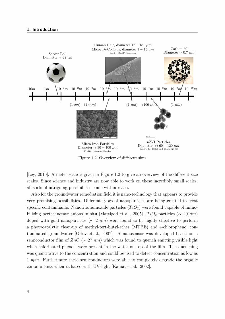
Nanotechnology takes place at a scale of one to several billionths of a meter. For
comparison, the diameter of a human hair varies between 17 000 and 181 000 nanometer
3
1. Introduction
1m 10−1m 10−2m 10−3m 10−4m 10−5m 10−6m 10−7m 10−8m 10−9m 10−10m
(1 cm) (1 mm) (1 µm) (100 nm) (1 nm)
Soccer BallDiameter ≈ 22 cm
Human Hair, diameter 17− 181 µmMicro Fe-Colloids, diameter 1− 15 µm
Credit: BASF, Germany
nZVI ParticlesDiameter: ≈ 60− 120 nmCredit: Li, Elliot and Zhang [2006]
Carbon 60Diameter ≈ 0.7 nm
10m
Micro Iron ParticlesDiameter ≈ 30− 100 µm
Credit: Hoganas, Sweden
1
Figure 1.2: Overview of different sizes
[Ley, 2010]. A meter scale is given in Figure 1.2 to give an overview of the different size
scales. Since science and industry are now able to work on these incredibly small scales,
all sorts of intriguing possibilities come within reach.
Also for the groundwater remediation field it is nano-technology that appears to provide
very promising possibilities. Different types of nanoparticles are being created to treat
specific contaminants. Nanotitaniumoxide particles (TiO2) were found capable of immo-
bilizing pertechnetate anions in situ [Mattigod et al., 2005]. TiO2 particles (∼ 20 nm)
doped with gold nanoparticles (∼ 2 nm) were found to be highly effective to perform
a photocatalytic clean-up of methyl-tert-butyl-ether (MTBE) and 4-chlorophenol con-
taminated groundwater [Orlov et al., 2007]. A nanosensor was developed based on a
semiconductor film of ZnO (∼ 27 nm) which was found to quench emitting visible light
when chlorinated phenols were present in the water on top of the film. The quenching
was quantitative to the concentration and could be used to detect concentration as low as
1 ppm. Furthermore these semiconductors were able to completely degrade the organic
contaminants when radiated with UV-light [Kamat et al., 2002].
4
1.2. Remediation Technologies
Based on the success of zero valent iron used in PRBs, an In-Situ method was proposed
by Cantrell and Kaplan [1997]. Instead of an excavated trench filled with ZVI filings, they
proposed the injection of a zero valent iron colloid suspension into the subsurface using
wells. This method forms a reactive permeable zone which is no longer bound to limited
depths and plume treatment, but can also be used directly in the contaminant source zone.
By treating the source directly, the contaminant removal time is significantly reduced. The
ZVI removes the contaminant from the water in the direct vicinity of the contaminant
phase, thus increasing the dissolution rate. Furthermore, the contaminant plume is cut off
and no new plume can develop. In the first tests, Cantrell and Kaplan [1997] used iron of
micrometer scale. These particles were rather heavy and gravitational settling occurred
during injection, limiting the transport and feasibility of this method. Due to the recent
developments in the nano technology branche, it has become possible to create zero-
valent iron particles at the nanometer scale. Some of the currently commercially available
nano-sized zero-valent iron (nZVI) colloids are between 10 and 100 nm in diameter (e.g.
RNIP, Toda Kogyo, Japan or NANOFER 25, NanoIron, Czech Republic). These are
provided suspended in water (with additives like surfactants and/or polymers) as a highly
concentrated slurry.
Common aquifer pore diameters range from 200 nm for a silty aquifer to 100 000 nm in
a gravel aquifer. Thus nZVI colloids are small enough to be transported through the finer
pore spaces of the porous media where micro sized particles would be filtered out [Elliott
and Zhang, 2001]. Considering the small size of nZVI, filtration effects and the chance of
clogging the aquifer are reduced and also they will have a lower settling velocity, which
should make it possible to transport them farther away from the injection well. Still
though, Tratnyek and Johnson [2006] describe that the transport distance in an aquifer
is expected to be limited based on the deep-bed filtration theory. Transport of larger
colloids is reduced mainly due to gravitational forces and straining effects (trapping in
pore throats that are too small to allow passage), whereas smaller colloids will filter out
of suspension mainly due to Van der Waals forces and Brownian diffusion [Tufenkji and
Elimelech, 2004].
While several field tests have been performed with nZVI, the delivery of the particles
to the desired location often was unsuccessful or at least disputable [Schrick et al., 2004]
or the transported distance was very small resulting in a very narrow grid of boreholes
needed for the injection (e.g. Muller et al. [2006b]).
5
1. Introduction
1.2.4 Chemical Reactions and the Chemical Composition of nZVI
The reactivity of nZVI colloids is mainly controlled by their specific surface, a higher
specific surface resulting in a higher reactivity [Bradford and Torkzaban, 2008]. The
specific surface of nZVI colloids is approximately 33.5 m2/g [Elliott and Zhang, 2001], in
comparison, for micro iron particles 0.1 − 1 m2/g [Nurmi et al., 2005] and for granular
iron filings approximately 0.004 m2/g [Huang et al., 2003], although the latter can due to
surface roughness and angularity reach a specific surface of approximately 0.5 m2/g. The
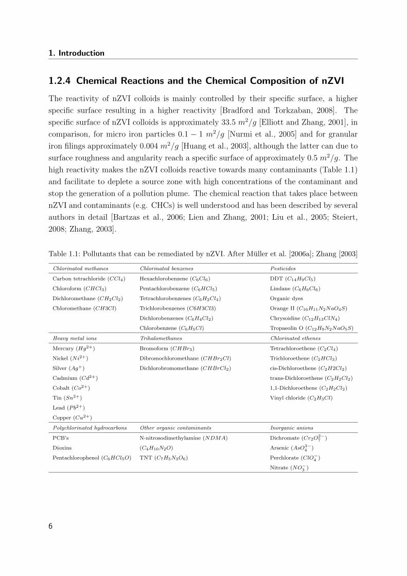
high reactivity makes the nZVI colloids reactive towards many contaminants (Table 1.1)
and facilitate to deplete a source zone with high concentrations of the contaminant and
stop the generation of a pollution plume. The chemical reaction that takes place between
nZVI and contaminants (e.g. CHCs) is well understood and has been described by several
authors in detail [Bartzas et al., 2006; Lien and Zhang, 2001; Liu et al., 2005; Steiert,
2008; Zhang, 2003].
Table 1.1: Pollutants that can be remediated by nZVI. After Muller et al. [2006a]; Zhang [2003]
Chlorinated methanes Chlorinated benzenes Pesticides
Carbon tetrachloride (CCl4) Hexachlorobenzene (C6Cl6) DDT (C14H9Cl5)
Chloroform (CHCl3) Pentachlorobenzene (C6HCl5) Lindane (C6H6Cl6)
Dichloromethane (CH2Cl2) Tetrachlorobenzenes (C6H2Cl4) Organic dyes
Chloromethane (CH3Cl) Trichlorobenzenes (C6H3Cl3) Orange II (C16H11N2NaO4S)
Dichlorobenzenes (C6H4Cl2) Chrysoidine (C12H13ClN4)
Chlorobenzene (C6H5Cl) Tropaeolin O (C12H9N2NaO5S)
Heavy metal ions Trihalomethanes Chlorinated ethenes
Mercury (Hg2+) Bromoform (CHBr3) Tetrachloroethene (C2Cl4)
Nickel (Ni2+) Dibromochloromethane (CHBr2Cl) Trichloroethene (C2HCl3)
Silver (Ag+) Dichlorobromomethane (CHBrCl2) cis-Dichloroethene (C2H2Cl2)
Cadmium (Cd2+) trans-Dichloroethene (C2H2Cl2)
Cobalt (Co2+) 1,1-Dichloroethene (C2H2Cl2)
Tin (Sn2+) Vinyl chloride (C2H3Cl)
Lead (Pb2+)
Copper (Cu2+)
Polychlorinated hydrocarbons Other organic contaminants Inorganic anions
PCB’s N-nitrosodimethylamine (NDMA) Dichromate (Cr2O2−7 )
Dioxins (C4H10N2O) Arsenic (AsO3−4 )
Pentachlorophenol (C6HCl5O) TNT (C7H5N3O6) Perchlorate (ClO−4 )
Nitrate (NO−3 )
6
1.2. Remediation Technologies
Though, the colloids are not only more reactive towards the contaminants, they are also
strongly affected by undesired side reactions. The main side reaction is the tendency
to quickly corrode. Dry nZVI colloids would even self ignite due to the reaction with
oxygen in the air. Aerobic corrosion also occurs in suspension with the dissolved oxygen
(Equation 1.1). Hence, the colloids are unsuitable for the remediation of pollutants in
the unsaturated zone, whereas fully saturated aquifers are in general completely anaerobe
and thus provide a suitable environment.
2Fe0(s) + 4H+
(aq) +O2(aq) → 2Fe2+(aq) + 2H2O(l) (1.1)
An other side reaction is anaerobic corrosion (Equation 1.2), this reaction though is much
slower and strongly pH dependent [Bartzas et al., 2006]. During storage the colloids are in
an anaerobic environment, in which, even tough no free oxygen is present, they can thus
still corrode. The anaerobe corrosion is in a closed environment self inhibiting because
the corrosion sets hydrogen and hydroxide free which increases the pH and consequently
reduces the corrosion rate.
Fe0(s) + 2H2O(aq) → Fe2+
(aq) +H2(g) + 2OH−(aq) (1.2)
The amount of zero valent iron inside a colloid therefore reduces with residence time in
water. Anaerobe corrosion sets hydrogen gas free (Equation 1.2) which could clog the
porous media.
To minimize the corrosion problem, nZVI colloids are often covered with a thin
shell that shields the zero valent iron from direct contact with water. The nZVI col-
loids as presented by Wang and Zhang [1997] were produced with a palladium acetate
([Pd](C2H3O2)2]3) that reacts with a small outer part of the zero-valent iron colloid, cre-
ating a small shield against corrosion and will function as a catalyst. Towards several
contaminants additional metals like the palladium acetate can function as a catalyst as
well, other metals that can be used with the same purposes are for example platinum
(Fe/Pt), silver (Fe/Ag), nickel (Fe/Ni), cobalt (Fe/Co) and copper (Fe/Cu). The
particles of Toda Kogyo (Japan) and Nano Iron (Czech republic) are shielded with crys-
talline magnetite (Fe3O4) (Fe/Fe) [Wang and Zhang, 1997]. So far only the last type
has shown to be producible in larger amounts for a fairly acceptable price.
The chemical feasibility of the remediation technique has been worked out in detail with
Steiert [2008]. Within his research it was furthermore discovered that the production of
hydrogen gas and with that the clogging of the porous media can be significantly reduced
7
1. Introduction
by adding burned chalk (Ca(OH)2) in granular form to the suspension before injection.
This technique has been filed for patenting [Klaas et al., 2010b].
Though very small, nZVI colloids are still ferro magnetic and contain a positive and
negative pole (i.e. they are bipolar). The colloids thus tend to get attracted to each
other and form aggregates. The aggregation and gelation (the building of a network
of aggregates) can easily result in pore plugging and gravity settling, strongly reducing
transportability [Saleh et al., 2006]. To avoid aggregation, a nZVI suspension can be
stabilized through the following repelling mechanisms:
Electrostatic repulsion, which is the mutual repulsion of like electrical charges, influ-
enced by the pH value of suspension [Hong et al., 2009]; Steric repulsion, adsorbed long
polymers (e.g. guar gum) on the particle surface, which prevents particles to get close
[Tiraferri et al., 2008]; Electrosteric repulsion, which is the combination of both using
long steric repelling polymers [Phenrat et al., 2008]. Unfortunately, it was also found
that the addition of electrosteric polymers significantly reduced the reactivity because
the obstructed contact between the contaminant and the colloid [Phenrat et al., 2009,
2007].
1.2.5 Field Application of nZVI
The injection of a nZVI suspension in the field could be performed using a simple screened
well, with packers to inject over a small height, by using a short filter screen at the tip
of a direct push rod, or hydro fracturing (either by using a concrete lined well, or direct
push). The injections using filter screens result generally in a near radially symmetrical
flow field around the injection well. Spherical flow fields will be less profound since most
aquifers show a horizontal layered structure with a large anisotropy. A radial flow field
results in a hyperbolically reducing seepage velocity with increasing distance from the
well screen. When hydro fracturing is applied, the main transport takes place in large
fractures and there is negligible porous media flow (permeation) thus this technique falls
beyond the scope of this research.
In a general sense, there are two different possible application concepts for injectable
nZVI, source zone- and plume treatment.
F To prevent the migration of a plume, or to secure an area (e.g. residential- or water-
protection area) from an approaching plume a barrier can be formed with injectable nZVI
(similar to a PRB). The concentrations in a downstream plume are much lower than the
concentrations in a source zone. The removal of the contaminant in the plume will not
8
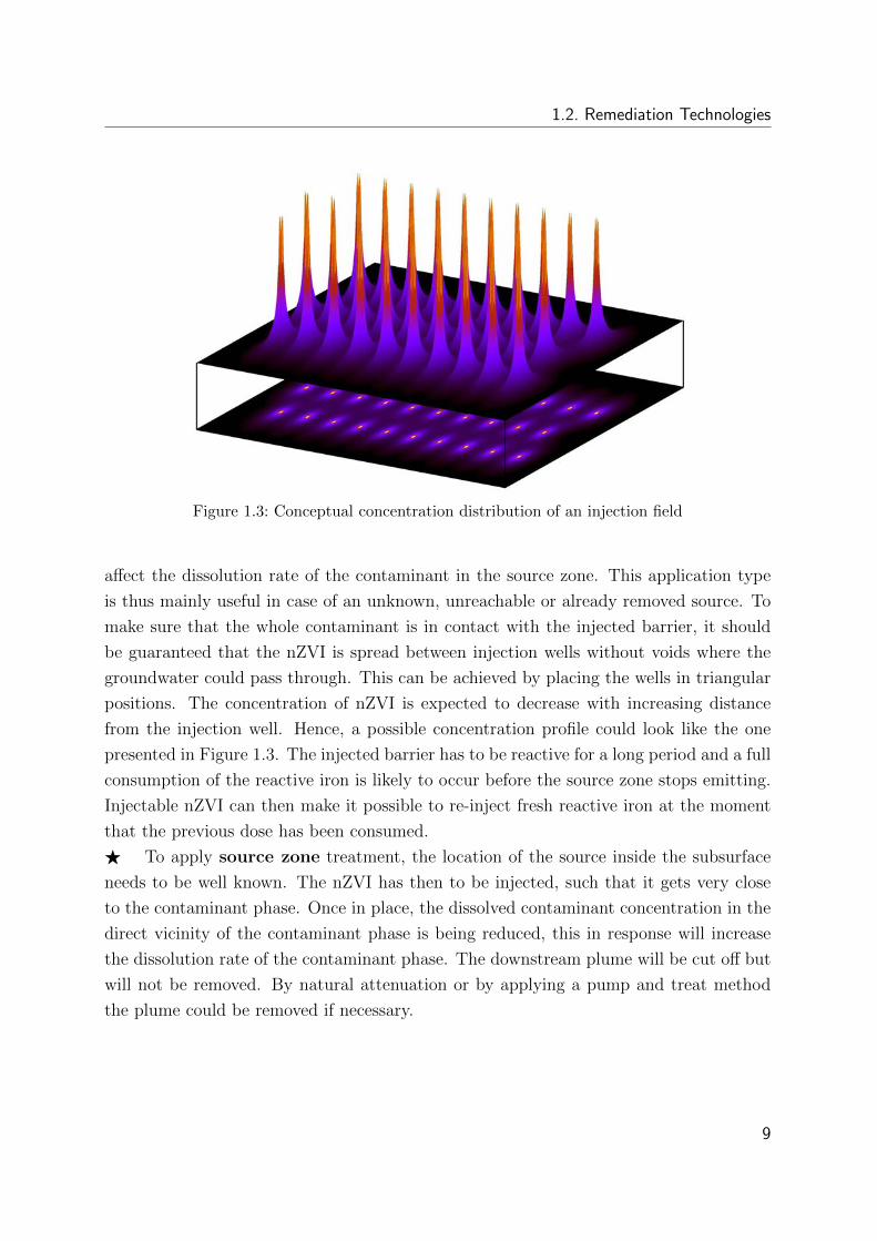
1.2. Remediation Technologies
Figure 1.3: Conceptual concentration distribution of an injection field
affect the dissolution rate of the contaminant in the source zone. This application type
is thus mainly useful in case of an unknown, unreachable or already removed source. To
make sure that the whole contaminant is in contact with the injected barrier, it should
be guaranteed that the nZVI is spread between injection wells without voids where the
groundwater could pass through. This can be achieved by placing the wells in triangular
positions. The concentration of nZVI is expected to decrease with increasing distance
from the injection well. Hence, a possible concentration profile could look like the one
presented in Figure 1.3. The injected barrier has to be reactive for a long period and a full
consumption of the reactive iron is likely to occur before the source zone stops emitting.
Injectable nZVI can then make it possible to re-inject fresh reactive iron at the moment
that the previous dose has been consumed.
F To apply source zone treatment, the location of the source inside the subsurface
needs to be well known. The nZVI has then to be injected, such that it gets very close
to the contaminant phase. Once in place, the dissolved contaminant concentration in the
direct vicinity of the contaminant phase is being reduced, this in response will increase
the dissolution rate of the contaminant phase. The downstream plume will be cut off but
will not be removed. By natural attenuation or by applying a pump and treat method
the plume could be removed if necessary.
9
1. Introduction
1.2.6 Detection and Concentration Measurement of nZVI in the
Subsurface
To do a source zone treatment, as for most methods targeting the source zone, it is
essential that the exact location of the source is well known. This is far from trivial and
puts a high demand on the measuring techniques used for the field characterization. Once
the site has been characterized and the contaminant source localized, the nZVI has to
be transported to these locations. Hence, an accurate detection technique is necessary
to determine the location of nZVI during and after the injection. Since the reaction in
this active zone is expected to be fast, nZVI will be consumed rapidly as the reaction
proceeds. An accurate monitoring technique would thus be preferable to determine when
the nZVI has been consumed and a renewal is needed.
So far several measuring techniques have been applied during pilot tests to proof the
effectiveness of injected nZVI. Muller et al. [2006b] used geophysical measurements, like
ground penetrating radar, geomagnetic and geoelectric mapping. Glazier et al. [2003]
and Zhang [2003] used in their field test measurements of flow rate, water level, oxidation
reduction potential (ORP), dissolved oxygen (DO), pH, specific conductance, tempera-
ture and the contaminant concentration reduction to show the radius of influence of the
injection and the location of nZVI during and after the injection. Elliott and Zhang [2001]
monitored the total iron and dissolved iron concentrations in combination with the pH
and ORP values at monitoring wells throughout the injection to determine the migration
of nZVI. Quinn et al. [2005] used soil samples from cores taken at different times after the
injection of emulsified zero valent iron and compared the TCE content in the samples to
samples from cores taken prior to the injection. They also measured the TCE concentra-
tions in ground water samples at different times after the injection and compared them
with samples taken prior to the injection.
The aforementioned measuring techniques all share some common problems. The meth-
ods based on ground water sampling are not conclusive since during the injection a large
amount of clean water (used as carrier fluid for nZVI) was injected, pushing away the
dissolved contaminants. It takes time before the contaminants again dissolve into the
fresh water up to the old concentration and also the groundwater flow velocity through
the contaminated zone might be reduced due to the presence of the nZVI and possibly
hydrogen gas. Using cores from different locations to compare samples after the injection
with samples taken prior to the injection will likely be inconclusive even if the cores are
taken close to each other since the subsurface is heterogeneous. Therefore, geogenic iron
10
1.3. Research Questions
background values are likely to differ more than the additional iron added due to injection
of nZVI from one location to another.
To quantitatively and conclusively measure the nZVI presence in the subsurface during
and after the injection, a new technique able to monitor directly iron concentrations
without background interference is desirable.
1.3 Research Questions
In the previous sections it has been emphasized that the treatment of contaminations in
the groundwater with injectable nZVI is promising. Nevertheless, there are still questions
to be answered and technical problems to be overcome before the method can be applied.
The goal of this doctoral research is to get a better description and understanding of
the transport behavior of nZVI during the injection into the subsurface which led to the
following research questions:
(a) Is it possible to detect In-Situ the concentration of iron and determine the transport
distance?
(b) Which conditions have the largest effect on mobility and how can they be opti-
mized?
(c) What is the transport distance in a radial flow field?
(d) Which method can test the feasibility of injection into the subsurface?
1.4 Structure of the Dissertation
To obtain a better description and understanding of the transport behavior of nZVI in
porous media the research started at the fundamental of colloid filtration and worked
this out through 1-D and 2-D experiments and numerical simulations to recommenda-
tions for the field, covering a wide range of scales. For this need, it was found that no
non-destructive and direct measuring technique was available and thus first had to be
developed to describe and understand the transport behavior (Figure 1.4).
This work distinguishes four main chapters after this introduction. Chapter 2 presents
the developed quantitative non-destructive measuring and detection techniques based on
the ferro magnetic property of nZVI to measure the nZVI concentration in the porous
medium at the column, container and field scale. A chemical (destructive) analysis
method was furthermore developed to provide a chemical verification method of the non-
destructive measurements as well as to characterize nZVI suspensions. Chapter ??
11
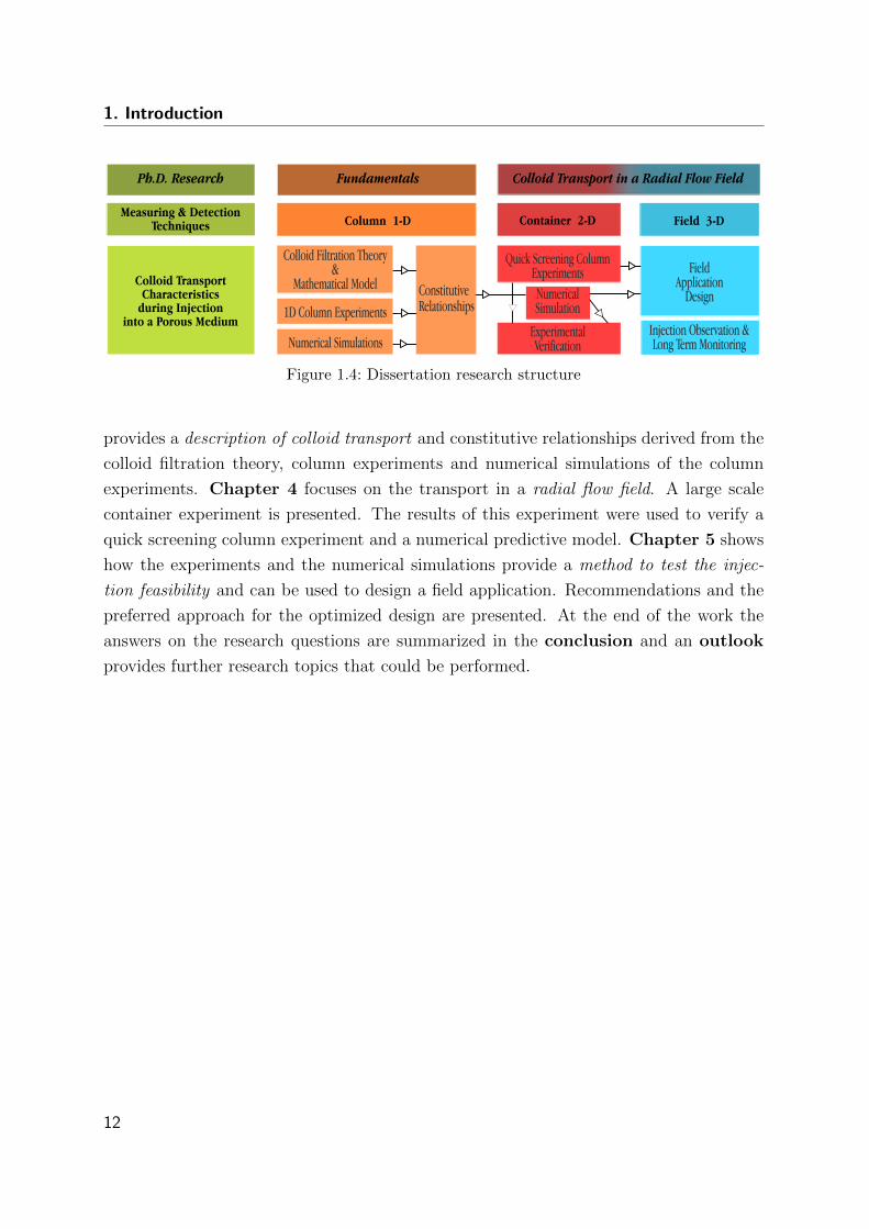
1. Introduction
Figure 1.4: Dissertation research structure
provides a description of colloid transport and constitutive relationships derived from the
colloid filtration theory, column experiments and numerical simulations of the column
experiments. Chapter 4 focuses on the transport in a radial flow field. A large scale
container experiment is presented. The results of this experiment were used to verify a
quick screening column experiment and a numerical predictive model. Chapter 5 shows
how the experiments and the numerical simulations provide a method to test the injec-
tion feasibility and can be used to design a field application. Recommendations and the
preferred approach for the optimized design are presented. At the end of the work the
answers on the research questions are summarized in the conclusion and an outlook
provides further research topics that could be performed.
12
2 Detection and Concentration
Measurement of nZVI in the
Subsurface
2.1 Motivation
Research on the transport of nZVI is only possible with accurate methods to determine
the concentration inside porous media. So far most research was based on break through
curves of columns (e.g. Baumann and Werth [2005]; Bradford and Bettahar [2006]), some-
times supported by a destructive chemical analysis of the column contents after the exper-
iments were finished (e.g. Tufenkji and Elimelech [2005b]). Break through curves can be
useful and through a combination with numerical simulations [Tosco et al., 2009], many
transport parameters can be determined by fitting. The exact distribution inside the
porous medium though is far from sure to be realistic, many different scenarios can lead
to the same break through curve. Visual observation can not provide quantitative con-
centrations, since the iron already colors the sand black at very low concentrations, only
the front of the iron can be determined and further no separation between low and high
concentrations is possible. In a chemical determination the natural presence (geogenic)
of iron in the sand will create a large unknown factor in the determination. Because even
the geogenic iron content of sand packed in a column or container is not homogeneously
spread, it is not possible to make a fully reliable difference measurement based on chem-
ical iron detection. Furthermore, a chemical analysis can first be performed after the
experiment is finished because sand samples have to be taken.
To facilitate a quantitative measurement of the nano sized zero valent iron (nZVI)
concentration during and after the injection into a column, a container or an aquifer,
a new measuring technique has been developed. The method has been produced in
different stages for different uses. The first stage was the adaptation of existing hardware
to measure concentrations inside a column. The second phase was the development of a
13
2. Detection and Concentration Measurement of nZVI in the Subsurface
sensor and the accompanying electronics to measure break through curves within a large
container experiment. The final stage was the development of sensors and electronics to
measure concentrations in an aquifer for a field application. All three different types of
sensors and accompanying electronics have been tested in the lab. The following sections
separately describe the measuring techniques for all three uses.
Collaborations
The container and field sensor development was performed in collaboration with Andre
Buchau and Hua Li of the Institute of Theoretic Electrical Engineering (ITE), Univer-
sity of Stuttgart. They performed numerical simulations of the electromagnetic fields
of different types of sensors to optimize the sensors for the container and the field and
developed post processing algorithms. The coordination, design of the sensor production
techniques, production and experimental testing of all the sensors and implementation of
the post processing algorithms into data analysis software were performed by the author.
The electronics for the container and field sensors was developed in collaboration with
Hubert Hermes from Hermes Messtechnik, Stuttgart, Germany. The building and testing
of all the electronics based on the electrical layouts were performed by the author.
2.2 Susceptibility
Susceptibility is the ratio of the magnetization in a substance to the corresponding mag-
netizing force, iron has a significant susceptibility [Getzlaff, 2008]. Simple experiments
on nZVI showed that this material property is still observable [de Boer, 2007]. Hence, a
measurement system that detects changes in susceptibility of the monitored subsurface
is possible. The system should be designed in a way that the magnetic field strength
is small enough to neglect the non-linear behavior of susceptibility of iron. Then, the
magnetic flux density B is simply connected to the magnetic field strength H by
B = µ0(1 + χnZV I)H (2.1)
where χnZV I is the susceptibility of nZVI and µ0 is the permeability of vacuum [Getzlaff,
2008]. The volume of nZVI (VnZV I), which is injected into an aquifer, is very small.
Furthermore, it is assumed that the nZVI near the sensor is approximately homogeneously
distributed in the aquifer. Then, the observed susceptibility χ is expected to be in the
14
2.3. Measurement of nZVI Concentration Profiles in a Column
range of:
χ ' VnZV IχnZV I (2.2)
The measured susceptibility in Equation 2.2 depends both on the concentration of nZVI
and on its susceptibility [Bregar and Pavlin, 2004]. If the susceptibility of nZVI is con-
stant, the resulting susceptibility depends only on the concentration of nZVI. Non-linear
behaviour of nZVI is excluded by small magnetic fields to ensure the recommended con-
stant susceptibility of nZVI. By using an alternating magnetic field (e.g. between 1 kHz
and 20 kHz), there is no chance of polarizing the nZVI nor is there any magnetic attrac-
tion or repelling. Starting from the statement in Equation 2.2, the concentration of nZVI
in the porous medium (CnZV I) can be related to the total susceptibility
CnZV I = s (χ) (2.3)
The function s (χ) can be obtained from posteriori chemical analysis (e.g. using the
method described in Elion and Elion [1933] or Liu and Lowry [2006]), or a priori cal-
ibration of the sensor. The calibration of the column experiments was performed by
calculating the total injected mass of iron present inside the column at the moment the
susceptibility was measured along the column. The posteriori chemical analysis method
has been used for the container experiments and is described in more detail in Section 2.6,
for the field measurement a method to calibrate the sensors before installation has been
developed and is presented in Section 2.5.4. Since the total susceptibility χ is very small, a
high sensitivity and precision of the electronics was necessary for a reliable measurement.
In the following three sections the measurement of the susceptibility at three different
scales is presented.
2.3 Measurement of nZVI Concentration Profiles in a
Column
A column experiment was set up to investigate the transportability of nZVI. To measure
the particle concentration and determine transport characteristics in porous media, a
commercially available metal detector was adopted. Institute Dr. Foerster (Reutlingen,
Germany) provided one of their research and development devices (Minex FX2FD) which
could be connected to a computer to store all the raw data internally produced by the
15
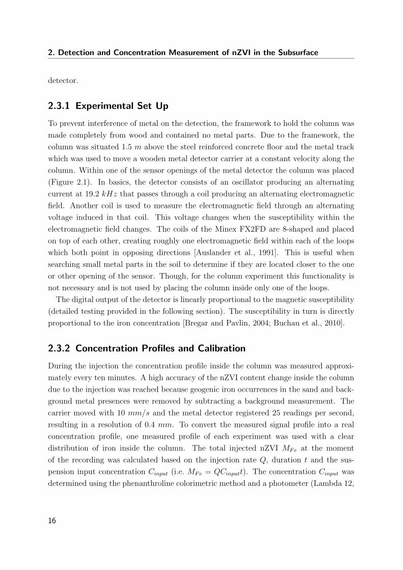
2. Detection and Concentration Measurement of nZVI in the Subsurface
detector.
2.3.1 Experimental Set Up
To prevent interference of metal on the detection, the framework to hold the column was
made completely from wood and contained no metal parts. Due to the framework, the
column was situated 1.5 m above the steel reinforced concrete floor and the metal track
which was used to move a wooden metal detector carrier at a constant velocity along the
column. Within one of the sensor openings of the metal detector the column was placed
(Figure 2.1). In basics, the detector consists of an oscillator producing an alternating
current at 19.2 kHz that passes through a coil producing an alternating electromagnetic
field. Another coil is used to measure the electromagnetic field through an alternating
voltage induced in that coil. This voltage changes when the susceptibility within the
electromagnetic field changes. The coils of the Minex FX2FD are 8-shaped and placed
on top of each other, creating roughly one electromagnetic field within each of the loops
which both point in opposing directions [Auslander et al., 1991]. This is useful when
searching small metal parts in the soil to determine if they are located closer to the one
or other opening of the sensor. Though, for the column experiment this functionality is
not necessary and is not used by placing the column inside only one of the loops.
The digital output of the detector is linearly proportional to the magnetic susceptibility
(detailed testing provided in the following section). The susceptibility in turn is directly
proportional to the iron concentration [Bregar and Pavlin, 2004; Buchau et al., 2010].
2.3.2 Concentration Profiles and Calibration
During the injection the concentration profile inside the column was measured approxi-
mately every ten minutes. A high accuracy of the nZVI content change inside the column
due to the injection was reached because geogenic iron occurrences in the sand and back-
ground metal presences were removed by subtracting a background measurement. The
carrier moved with 10 mm/s and the metal detector registered 25 readings per second,
resulting in a resolution of 0.4 mm. To convert the measured signal profile into a real
concentration profile, one measured profile of each experiment was used with a clear
distribution of iron inside the column. The total injected nZVI MFe at the moment
of the recording was calculated based on the injection rate Q, duration t and the sus-
pension input concentration Cinput (i.e. MFe = QCinputt). The concentration Cinput was
determined using the phenanthroline colorimetric method and a photometer (Lambda 12,
16
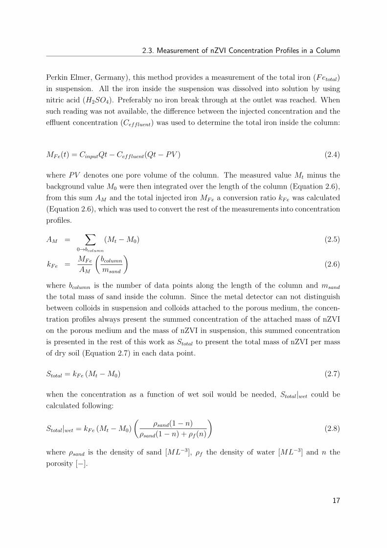
2.3. Measurement of nZVI Concentration Profiles in a Column
Perkin Elmer, Germany), this method provides a measurement of the total iron (Fetotal)
in suspension. All the iron inside the suspension was dissolved into solution by using
nitric acid (H2SO4). Preferably no iron break through at the outlet was reached. When
such reading was not available, the difference between the injected concentration and the
effluent concentration (Ceffluent) was used to determine the total iron inside the column:
MFe(t) = CinputQt− Ceffluent(Qt− PV ) (2.4)
where PV denotes one pore volume of the column. The measured value Mt minus the
background value M0 were then integrated over the length of the column (Equation 2.6),
from this sum AM and the total injected iron MFe a conversion ratio kFe was calculated
(Equation 2.6), which was used to convert the rest of the measurements into concentration
profiles.
AM =∑
0→bcolumn
(Mt −M0) (2.5)
kFe =MFe
AM
(bcolumnmsand
)(2.6)
where bcolumn is the number of data points along the length of the column and msand
the total mass of sand inside the column. Since the metal detector can not distinguish
between colloids in suspension and colloids attached to the porous medium, the concen-
tration profiles always present the summed concentration of the attached mass of nZVI
on the porous medium and the mass of nZVI in suspension, this summed concentration
is presented in the rest of this work as Stotal to present the total mass of nZVI per mass
of dry soil (Equation 2.7) in each data point.
Stotal = kFe (Mt −M0) (2.7)
when the concentration as a function of wet soil would be needed, Stotal|wet could be
calculated following:
Stotal|wet = kFe (Mt −M0)
(ρsand(1− n)
ρsand(1− n) + ρf (n)
)(2.8)
where ρsand is the density of sand [ML−3], ρf the density of water [ML−3] and n the
porosity [−].
17
2. Detection and Concentration Measurement of nZVI in the Subsurface
Figure 2.1: Setup of the metal detector to non-destructively measure concentration profilesalong the column. The metal detector was placed on a wooden frame which could move over a
rails. The column was placed inside the lower opening of the metal detector ring
2.3.2.1 Linearity of the Detector
To show the linear response of the metal detector to the concentration of iron, different
amounts of dry iron powder were mixed with sand. The iron powder was each time
completely mixed with 140 g sand, this filled a section of 10 cm in the column. In the
column the iron sand mixtures were separated by a section with 10 cm clean sand for the
low concentrations and a section with 15 cm clean sand for the higher concentrations (see
top of Figure 2.2). The whole column was measured by moving the detector at a rate of
10 mm/s along the column.
The signal of the metal detector responded to the iron content in the vicinity of the
location of the measuring coil (Figure 2.2). Thus the signal was already changing in the
clean sand area when it got close to the section containing iron. In the middle of each
iron filled section, the signal was at a maximum because on both sides of the measuring
coil an equal amount of metal was present.
To determine the maximum value for each metal containing section, over a length of
10 mm around the maximum value (12 data points in each direction plus the center point,
giving 25 data points in total), the sum of the response frequency was taken. This integral
value was divided by the amount of data point in 10 mm to get an average response for
1 mm of column length. Figure 2.3 shows the determined values for each integrated
section.
18
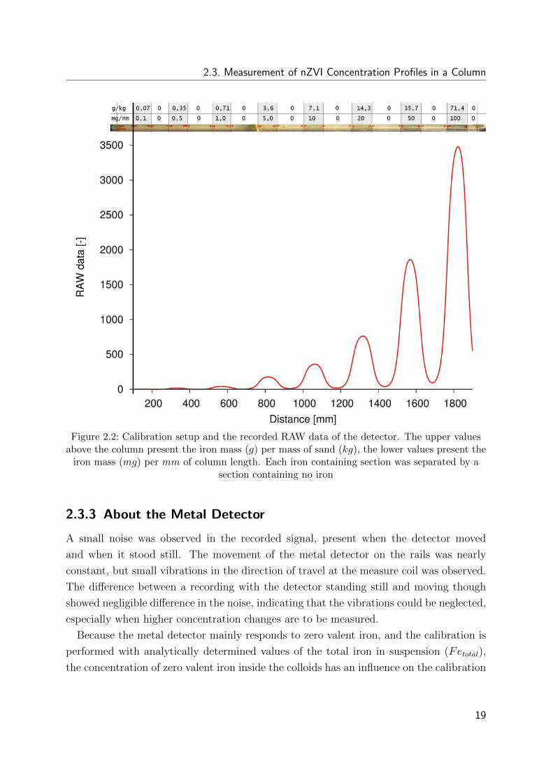
2.3. Measurement of nZVI Concentration Profiles in a Column
Figure 2.2: Calibration setup and the recorded RAW data of the detector. The upper valuesabove the column present the iron mass (g) per mass of sand (kg), the lower values present the
iron mass (mg) per mm of column length. Each iron containing section was separated by asection containing no iron
2.3.3 About the Metal Detector
A small noise was observed in the recorded signal, present when the detector moved
and when it stood still. The movement of the metal detector on the rails was nearly
constant, but small vibrations in the direction of travel at the measure coil was observed.
The difference between a recording with the detector standing still and moving though
showed negligible difference in the noise, indicating that the vibrations could be neglected,
especially when higher concentration changes are to be measured.
Because the metal detector mainly responds to zero valent iron, and the calibration is
performed with analytically determined values of the total iron in suspension (Fetotal),
the concentration of zero valent iron inside the colloids has an influence on the calibration
19
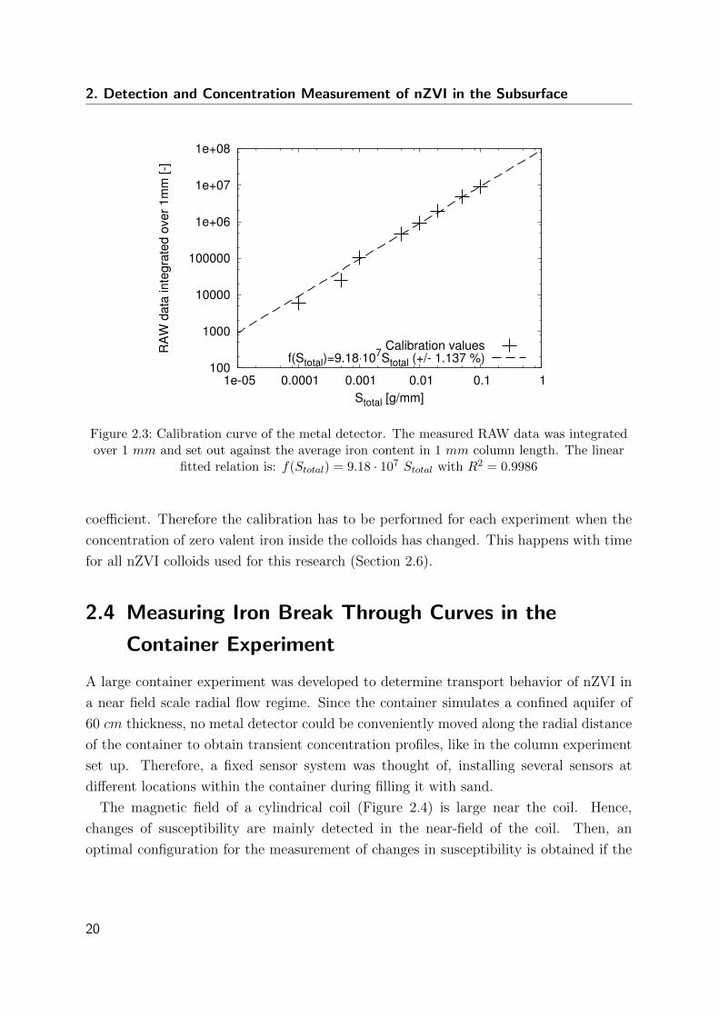
2. Detection and Concentration Measurement of nZVI in the Subsurface
100
1000
10000
100000
1e+06
1e+07
1e+08
1e-05 0.0001 0.001 0.01 0.1 1
RA
W d
ata
in
teg
rate
d o
ve
r 1
mm
[-]
Stotal [g/mm]
Calibration valuesf(Stotal)=9.18⋅10
7Stotal (+/- 1.137 %)
Figure 2.3: Calibration curve of the metal detector. The measured RAW data was integratedover 1 mm and set out against the average iron content in 1 mm column length. The linear
fitted relation is: f(Stotal) = 9.18 · 107 Stotal with R2 = 0.9986
coefficient. Therefore the calibration has to be performed for each experiment when the
concentration of zero valent iron inside the colloids has changed. This happens with time
for all nZVI colloids used for this research (Section 2.6).
2.4 Measuring Iron Break Through Curves in the
Container Experiment
A large container experiment was developed to determine transport behavior of nZVI in
a near field scale radial flow regime. Since the container simulates a confined aquifer of
60 cm thickness, no metal detector could be conveniently moved along the radial distance
of the container to obtain transient concentration profiles, like in the column experiment
set up. Therefore, a fixed sensor system was thought of, installing several sensors at
different locations within the container during filling it with sand.
The magnetic field of a cylindrical coil (Figure 2.4) is large near the coil. Hence,
changes of susceptibility are mainly detected in the near-field of the coil. Then, an
optimal configuration for the measurement of changes in susceptibility is obtained if the
20
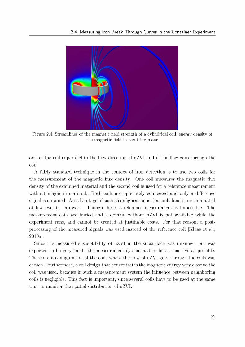
2.4. Measuring Iron Break Through Curves in the Container Experiment
Figure 2.4: Streamlines of the magnetic field strength of a cylindrical coil; energy density ofthe magnetic field in a cutting plane
axis of the coil is parallel to the flow direction of nZVI and if this flow goes through the
coil.
A fairly standard technique in the context of iron detection is to use two coils for
the measurement of the magnetic flux density. One coil measures the magnetic flux
density of the examined material and the second coil is used for a reference measurement
without magnetic material. Both coils are oppositely connected and only a difference
signal is obtained. An advantage of such a configuration is that unbalances are eliminated
at low-level in hardware. Though, here, a reference measurement is impossible. The
measurement coils are buried and a domain without nZVI is not available while the
experiment runs, and cannot be created at justifiable costs. For that reason, a post-
processing of the measured signals was used instead of the reference coil [Klaas et al.,
2010a].
Since the measured susceptibility of nZVI in the subsurface was unknown but was
expected to be very small, the measurement system had to be as sensitive as possible.
Therefore a configuration of the coils where the flow of nZVI goes through the coils was
chosen. Furthermore, a coil design that concentrates the magnetic energy very close to the
coil was used, because in such a measurement system the influence between neighboring
coils is negligible. This fact is important, since several coils have to be used at the same
time to monitor the spatial distribution of nZVI.
21
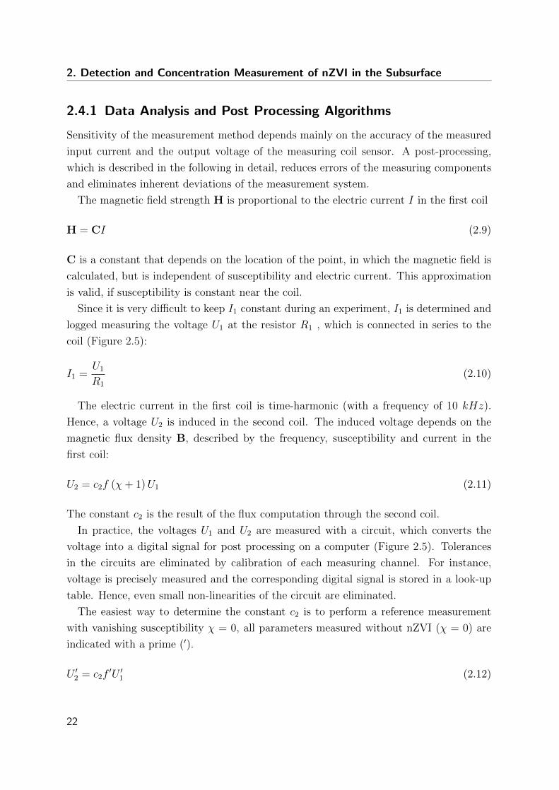
2. Detection and Concentration Measurement of nZVI in the Subsurface
2.4.1 Data Analysis and Post Processing Algorithms
Sensitivity of the measurement method depends mainly on the accuracy of the measured
input current and the output voltage of the measuring coil sensor. A post-processing,
which is described in the following in detail, reduces errors of the measuring components
and eliminates inherent deviations of the measurement system.
The magnetic field strength H is proportional to the electric current I in the first coil
H = CI (2.9)
C is a constant that depends on the location of the point, in which the magnetic field is
calculated, but is independent of susceptibility and electric current. This approximation
is valid, if susceptibility is constant near the coil.
Since it is very difficult to keep I1 constant during an experiment, I1 is determined and
logged measuring the voltage U1 at the resistor R1 , which is connected in series to the
coil (Figure 2.5):
I1 =U1
R1
(2.10)
The electric current in the first coil is time-harmonic (with a frequency of 10 kHz).
Hence, a voltage U2 is induced in the second coil. The induced voltage depends on the
magnetic flux density B, described by the frequency, susceptibility and current in the
first coil:
U2 = c2f (χ+ 1)U1 (2.11)
The constant c2 is the result of the flux computation through the second coil.
In practice, the voltages U1 and U2 are measured with a circuit, which converts the
voltage into a digital signal for post processing on a computer (Figure 2.5). Tolerances
in the circuits are eliminated by calibration of each measuring channel. For instance,
voltage is precisely measured and the corresponding digital signal is stored in a look-up
table. Hence, even small non-linearities of the circuit are eliminated.
The easiest way to determine the constant c2 is to perform a reference measurement
with vanishing susceptibility χ = 0, all parameters measured without nZVI (χ = 0) are
indicated with a prime (′).
U ′2 = c2f′U ′1 (2.12)
22
2.4. Measuring Iron Break Through Curves in the Container Experiment
Figure 2.5: Equivalent network of the first coil, which is used to determine the electric currentin the coil IC1 from the measured current I1; measured signals are sent to a PC
where the prime denotes the measurement at χ = 0. Note, the voltage U2 in Equation 2.11
and U ′2 in Equation 2.12 depend directly on the frequencies f and f ′. Since the frequency
produced by a signal generator is generally not stable enough for the desired accuracy,
f is recorded during the measurement by performing a TTL-conversion of the sine wave.
Finally, susceptibility is obtained from:
χ =U2f
′U ′1U ′2fU1
− 1 (2.13)
Experimental data showed, however, that an analysis purely based on Equation 2.13 is
not accurate enough in practice. The voltage U2 changed when water was injected into
the container, even though water with a zero nZVI concentration has no susceptibility.
An important quantity is the capacitance of the coil, which is caused by the electric
field between the windings of the coil. The capacitance of a coil is proportional to the
permittivity, which can be influenced by salts and surfactants in the water. Surfactants
are necessary for the transport of nZVI and the injected water was a degassed tap water,
without further treatment to remove salts. The flow of water could thus cause a change
in the permittivity and with that influence U2 due to salts and surfactants in the water.
The equivalent network of the first coil is depicted in Figure 2.5, the electric current I1,
which is measured with help of the voltage U1, it is not equal to the current IC1 through
the first coil, though preferred, it is impossible to measure IC1 directly. A solution to
avoid this problem, would be to decrease the frequency of the system. Though, that
23
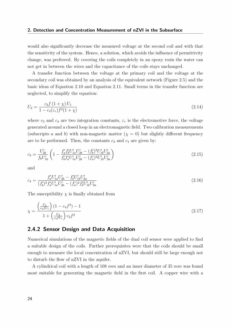
2. Detection and Concentration Measurement of nZVI in the Subsurface
would also significantly decrease the measured voltage at the second coil and with that
the sensitivity of the system. Hence, a solution, which avoids the influence of permittivity
change, was preferred. By covering the coils completely in an epoxy resin the water can
not get in between the wires and the capacitance of the coils stays unchanged.
A transfer function between the voltage at the primary coil and the voltage at the
secondary coil was obtained by an analysis of the equivalent network (Figure 2.5) and the
basic ideas of Equation 2.10 and Equation 2.11. Small terms in the transfer function are
neglected, to simplify the equation:
U2 =c3f (1 + χ)U1
1− c4(εr)f 2(1 + χ)(2.14)
where c3 and c4 are two integration constants, εr is the electromotive force, the voltage
generated around a closed loop in an electromagnetic field. Two calibration measurements
(subscripts a and b) with non-magnetic matter (χ = 0) but slightly different frequency
are to be performed. Then, the constants c3 and c4 are given by:
c3 =U ′2bfbU ′1b
(1− f ′af
′bU′1aU
′2b − (f ′b)
2U ′1bU′2a
f ′bf′aU′1aU
′2b − (f ′a)
2U ′1bU′2a
)(2.15)
and
c4 =f ′aU
′1aU
′2b − f ′bU ′1bU ′2a
(f ′b)2f ′aU
′1aU
′2b − (f ′a)
2f ′bU′1bU
′2a
(2.16)
The susceptibility χ is finally obtained from
χ =
(U2
c3fU1
)(1− c4f
2)− 1
1 +(
U2
c4fU1
)c2f 2
(2.17)
2.4.2 Sensor Design and Data Acquisition
Numerical simulations of the magnetic fields of the dual coil sensor were applied to find
a suitable design of the coils. Further prerequisites were that the coils should be small
enough to measure the local concentration of nZVI, but should still be large enough not
to disturb the flow of nZVI in the aquifer.
A cylindrical coil with a length of 108 mm and an inner diameter of 35 mm was found
most suitable for generating the magnetic field in the first coil. A copper wire with a
24
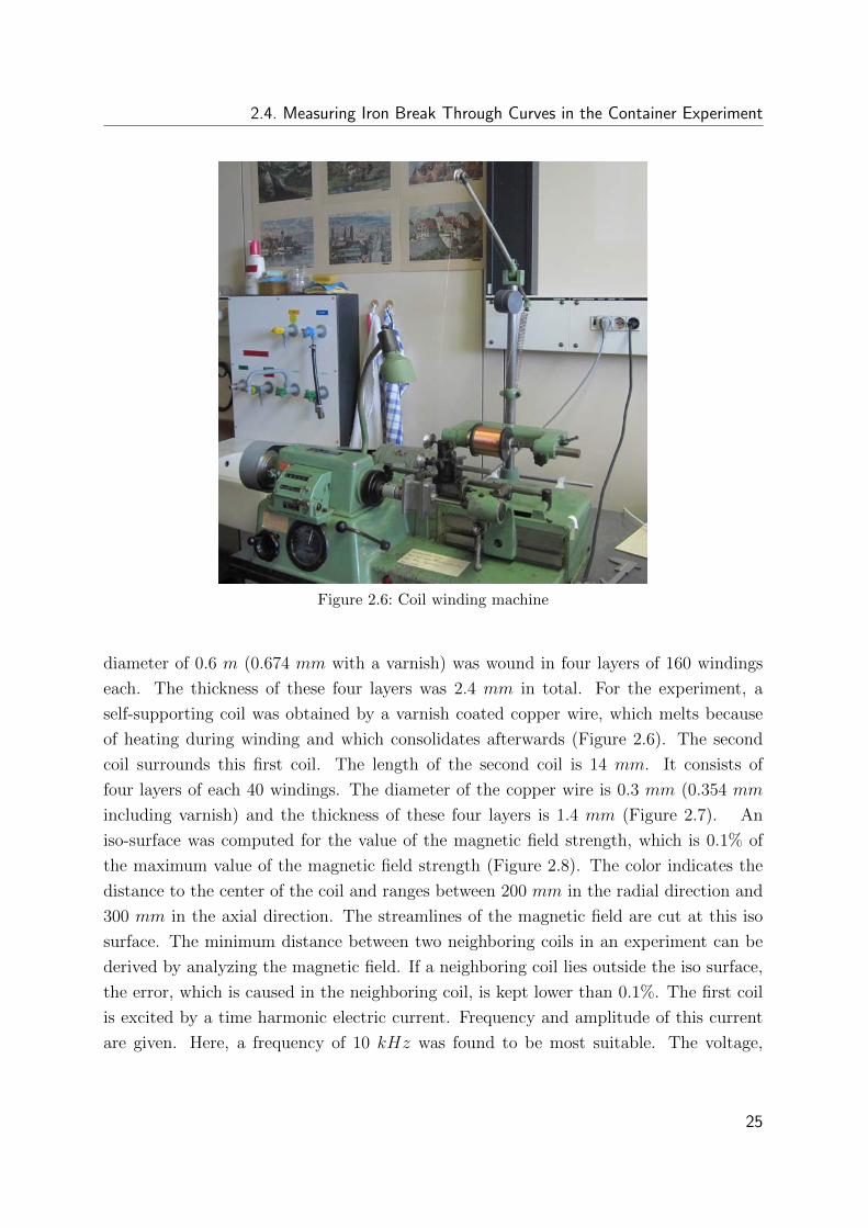
2.4. Measuring Iron Break Through Curves in the Container Experiment
Figure 2.6: Coil winding machine
diameter of 0.6 m (0.674 mm with a varnish) was wound in four layers of 160 windings
each. The thickness of these four layers was 2.4 mm in total. For the experiment, a
self-supporting coil was obtained by a varnish coated copper wire, which melts because
of heating during winding and which consolidates afterwards (Figure 2.6). The second
coil surrounds this first coil. The length of the second coil is 14 mm. It consists of
four layers of each 40 windings. The diameter of the copper wire is 0.3 mm (0.354 mm
including varnish) and the thickness of these four layers is 1.4 mm (Figure 2.7). An
iso-surface was computed for the value of the magnetic field strength, which is 0.1% of
the maximum value of the magnetic field strength (Figure 2.8). The color indicates the
distance to the center of the coil and ranges between 200 mm in the radial direction and
300 mm in the axial direction. The streamlines of the magnetic field are cut at this iso
surface. The minimum distance between two neighboring coils in an experiment can be
derived by analyzing the magnetic field. If a neighboring coil lies outside the iso surface,
the error, which is caused in the neighboring coil, is kept lower than 0.1%. The first coil
is excited by a time harmonic electric current. Frequency and amplitude of this current
are given. Here, a frequency of 10 kHz was found to be most suitable. The voltage,
25
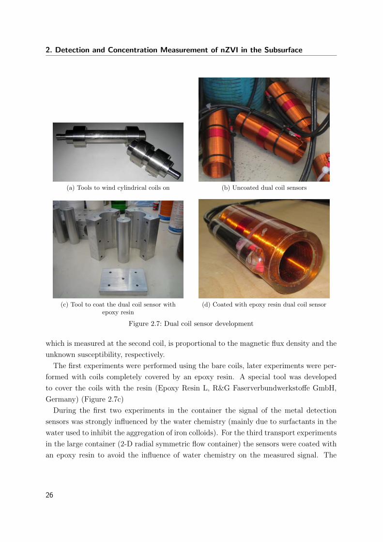
2. Detection and Concentration Measurement of nZVI in the Subsurface
(a) Tools to wind cylindrical coils on (b) Uncoated dual coil sensors
(c) Tool to coat the dual coil sensor withepoxy resin
(d) Coated with epoxy resin dual coil sensor
Figure 2.7: Dual coil sensor development
which is measured at the second coil, is proportional to the magnetic flux density and the
unknown susceptibility, respectively.
The first experiments were performed using the bare coils, later experiments were per-
formed with coils completely covered by an epoxy resin. A special tool was developed
to cover the coils with the resin (Epoxy Resin L, R&G Faserverbundwerkstoffe GmbH,
Germany) (Figure 2.7c)
During the first two experiments in the container the signal of the metal detection
sensors was strongly influenced by the water chemistry (mainly due to surfactants in the
water used to inhibit the aggregation of iron colloids). For the third transport experiments
in the large container (2-D radial symmetric flow container) the sensors were coated with
an epoxy resin to avoid the influence of water chemistry on the measured signal. The
26
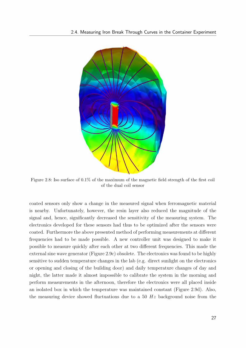
2.4. Measuring Iron Break Through Curves in the Container Experiment
Figure 2.8: Iso surface of 0.1% of the maximum of the magnetic field strength of the first coilof the dual coil sensor
coated sensors only show a change in the measured signal when ferromagnetic material
is nearby. Unfortunately, however, the resin layer also reduced the magnitude of the
signal and, hence, significantly decreased the sensitivity of the measuring system. The
electronics developed for these sensors had thus to be optimized after the sensors were
coated. Furthermore the above presented method of performing measurements at different
frequencies had to be made possible. A new controller unit was designed to make it
possible to measure quickly after each other at two different frequencies. This made the
external sine wave generator (Figure 2.9c) obsolete. The electronics was found to be highly
sensitive to sudden temperature changes in the lab (e.g. direct sunlight on the electronics
or opening and closing of the building door) and daily temperature changes of day and
night, the latter made it almost impossible to calibrate the system in the morning and
perform measurements in the afternoon, therefore the electronics were all placed inside
an isolated box in which the temperature was maintained constant (Figure 2.9d). Also,
the measuring device showed fluctuations due to a 50 Hz background noise from the
27
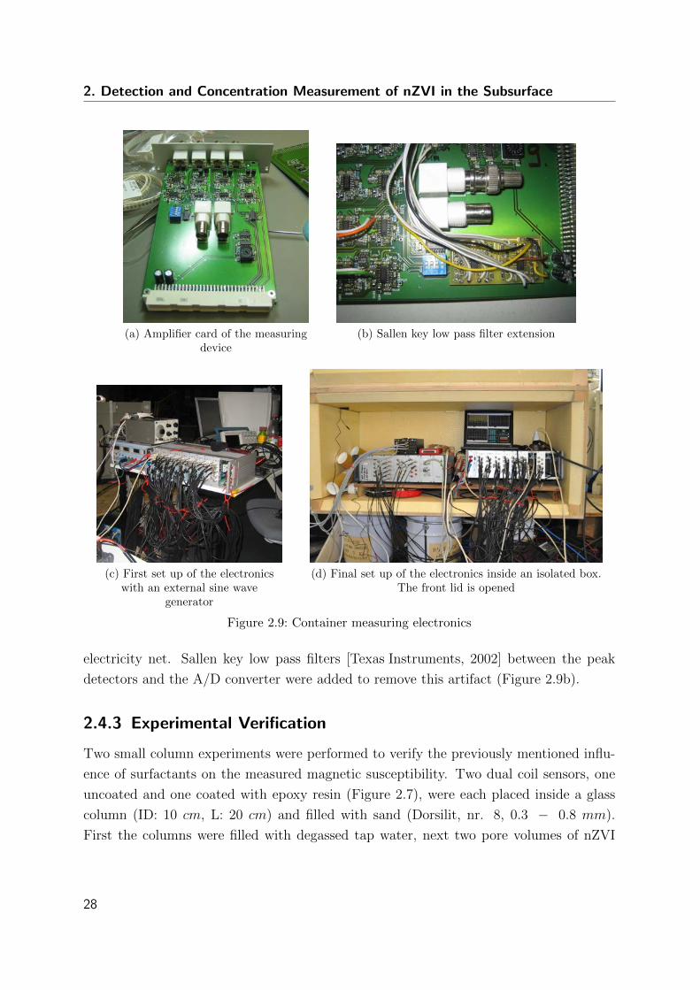
2. Detection and Concentration Measurement of nZVI in the Subsurface
(a) Amplifier card of the measuringdevice
(b) Sallen key low pass filter extension
(c) First set up of the electronicswith an external sine wave
generator
(d) Final set up of the electronics inside an isolated box.The front lid is opened
Figure 2.9: Container measuring electronics
electricity net. Sallen key low pass filters [Texas Instruments, 2002] between the peak
detectors and the A/D converter were added to remove this artifact (Figure 2.9b).
2.4.3 Experimental Verification
Two small column experiments were performed to verify the previously mentioned influ-
ence of surfactants on the measured magnetic susceptibility. Two dual coil sensors, one
uncoated and one coated with epoxy resin (Figure 2.7), were each placed inside a glass
column (ID: 10 cm, L: 20 cm) and filled with sand (Dorsilit, nr. 8, 0.3 − 0.8 mm).
First the columns were filled with degassed tap water, next two pore volumes of nZVI
28
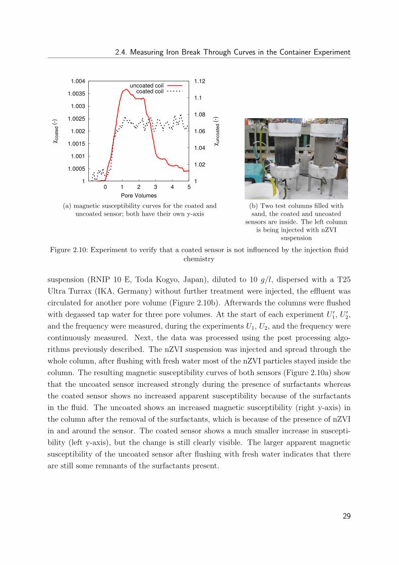
2.4. Measuring Iron Break Through Curves in the Container Experiment
1
1.0005
1.001
1.0015
1.002
1.0025
1.003
1.0035
1.004
0 1 2 3 4 5 1
1.02
1.04
1.06
1.08
1.1
1.12
χco
ated
(-)
χun
coat
ed (-
)
Pore Volumes
uncoated coilcoated coil
(a) magnetic susceptibility curves for the coated anduncoated sensor; both have their own y-axis
(b) Two test columns filled withsand, the coated and uncoated
sensors are inside. The left columnis being injected with nZVI
suspension
Figure 2.10: Experiment to verify that a coated sensor is not influenced by the injection fluidchemistry
suspension (RNIP 10 E, Toda Kogyo, Japan), diluted to 10 g/l, dispersed with a T25
Ultra Turrax (IKA, Germany) without further treatment were injected, the effluent was
circulated for another pore volume (Figure 2.10b). Afterwards the columns were flushed
with degassed tap water for three pore volumes. At the start of each experiment U ′1, U ′2,
and the frequency were measured, during the experiments U1, U2, and the frequency were
continuously measured. Next, the data was processed using the post processing algo-
rithms previously described. The nZVI suspension was injected and spread through the
whole column, after flushing with fresh water most of the nZVI particles stayed inside the
column. The resulting magnetic susceptibility curves of both sensors (Figure 2.10a) show
that the uncoated sensor increased strongly during the presence of surfactants whereas
the coated sensor shows no increased apparent susceptibility because of the surfactants
in the fluid. The uncoated shows an increased magnetic susceptibility (right y-axis) in
the column after the removal of the surfactants, which is because of the presence of nZVI
in and around the sensor. The coated sensor shows a much smaller increase in suscepti-
bility (left y-axis), but the change is still clearly visible. The larger apparent magnetic
susceptibility of the uncoated sensor after flushing with fresh water indicates that there
are still some remnants of the surfactants present.
29
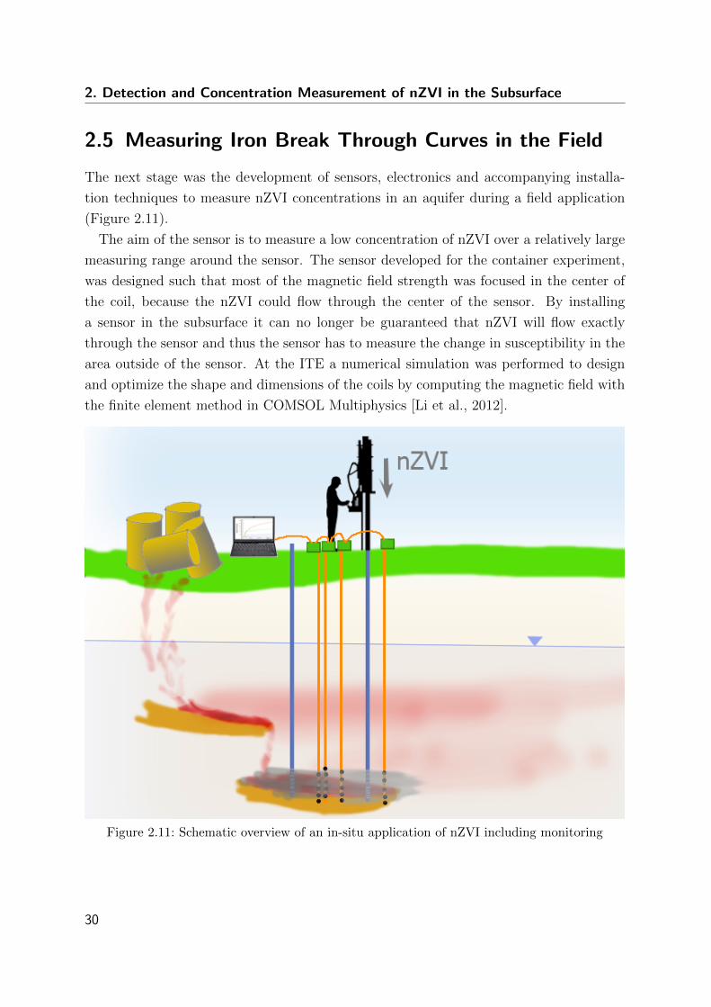
2. Detection and Concentration Measurement of nZVI in the Subsurface
2.5 Measuring Iron Break Through Curves in the Field
The next stage was the development of sensors, electronics and accompanying installa-
tion techniques to measure nZVI concentrations in an aquifer during a field application
(Figure 2.11).
The aim of the sensor is to measure a low concentration of nZVI over a relatively large
measuring range around the sensor. The sensor developed for the container experiment,
was designed such that most of the magnetic field strength was focused in the center of
the coil, because the nZVI could flow through the center of the sensor. By installing
a sensor in the subsurface it can no longer be guaranteed that nZVI will flow exactly
through the sensor and thus the sensor has to measure the change in susceptibility in the
area outside of the sensor. At the ITE a numerical simulation was performed to design
and optimize the shape and dimensions of the coils by computing the magnetic field with
the finite element method in COMSOL Multiphysics [Li et al., 2012].
Figure 2.11: Schematic overview of an in-situ application of nZVI including monitoring
30
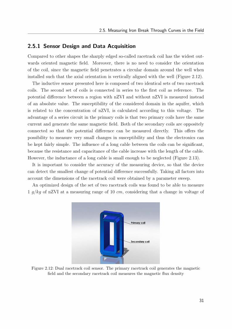
2.5. Measuring Iron Break Through Curves in the Field
2.5.1 Sensor Design and Data Acquisition
Compared to other shapes the sharply edged so-called racetrack coil has the widest out-
wards oriented magnetic field. Moreover, there is no need to consider the orientation
of the coil, since the magnetic field penetrates a circular domain around the well when
installed such that the axial orientation is vertically aligned with the well (Figure 2.12).
The inductive sensor presented here is composed of two identical sets of two racetrack
coils. The second set of coils is connected in series to the first coil as reference. The
potential difference between a region with nZVI and without nZVI is measured instead
of an absolute value. The susceptibility of the considered domain in the aquifer, which
is related to the concentration of nZVI, is calculated according to this voltage. The
advantage of a series circuit in the primary coils is that two primary coils have the same
current and generate the same magnetic field. Both of the secondary coils are oppositely
connected so that the potential difference can be measured directly. This offers the
possibility to measure very small changes in susceptibility and thus the electronics can
be kept fairly simple. The influence of a long cable between the coils can be significant,
because the resistance and capacitance of the cable increase with the length of the cable.
However, the inductance of a long cable is small enough to be neglected (Figure 2.13).
It is important to consider the accuracy of the measuring device, so that the device
can detect the smallest change of potential difference successfully. Taking all factors into
account the dimensions of the racetrack coil were obtained by a parameter sweep.
An optimized design of the set of two racetrack coils was found to be able to measure
1 g/kg of nZVI at a measuring range of 10 cm, considering that a change in voltage of
Figure 2.12: Dual racetrack coil sensor. The primary racetrack coil generates the magneticfield and the secondary racetrack coil measures the magnetic flux density
31
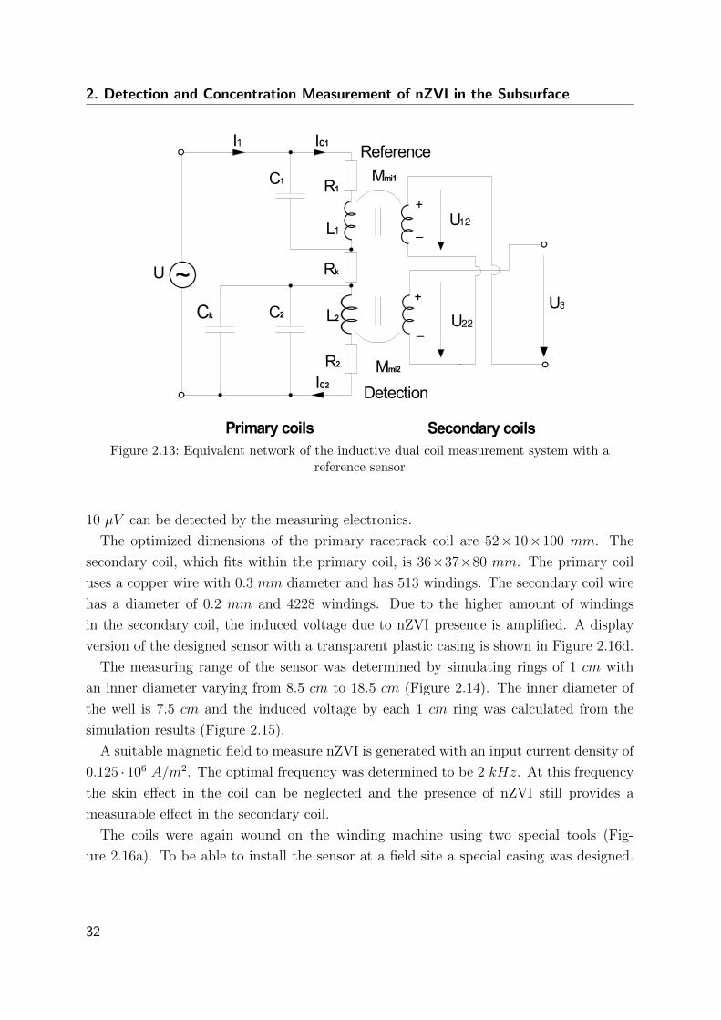
2. Detection and Concentration Measurement of nZVI in the Subsurface
12
22
3
Figure 2.13: Equivalent network of the inductive dual coil measurement system with areference sensor
10 µV can be detected by the measuring electronics.
The optimized dimensions of the primary racetrack coil are 52×10×100 mm. The
secondary coil, which fits within the primary coil, is 36×37×80 mm. The primary coil
uses a copper wire with 0.3 mm diameter and has 513 windings. The secondary coil wire
has a diameter of 0.2 mm and 4228 windings. Due to the higher amount of windings
in the secondary coil, the induced voltage due to nZVI presence is amplified. A display
version of the designed sensor with a transparent plastic casing is shown in Figure 2.16d.
The measuring range of the sensor was determined by simulating rings of 1 cm with
an inner diameter varying from 8.5 cm to 18.5 cm (Figure 2.14). The inner diameter of
the well is 7.5 cm and the induced voltage by each 1 cm ring was calculated from the
simulation results (Figure 2.15).
A suitable magnetic field to measure nZVI is generated with an input current density of
0.125 · 106 A/m2. The optimal frequency was determined to be 2 kHz. At this frequency
the skin effect in the coil can be neglected and the presence of nZVI still provides a
measurable effect in the secondary coil.
The coils were again wound on the winding machine using two special tools (Fig-
ure 2.16a). To be able to install the sensor at a field site a special casing was designed.
32
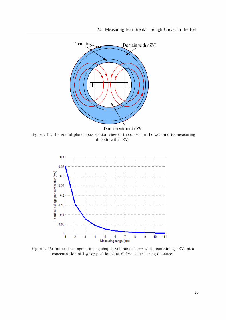
2.5. Measuring Iron Break Through Curves in the Field
Figure 2.14: Horizontal plane cross section view of the sensor in the well and its measuringdomain with nZVI
Figure 2.15: Induced voltage of a ring-shaped volume of 1 cm width containing nZVI at aconcentration of 1 g/kg positioned at different measuring distances
33
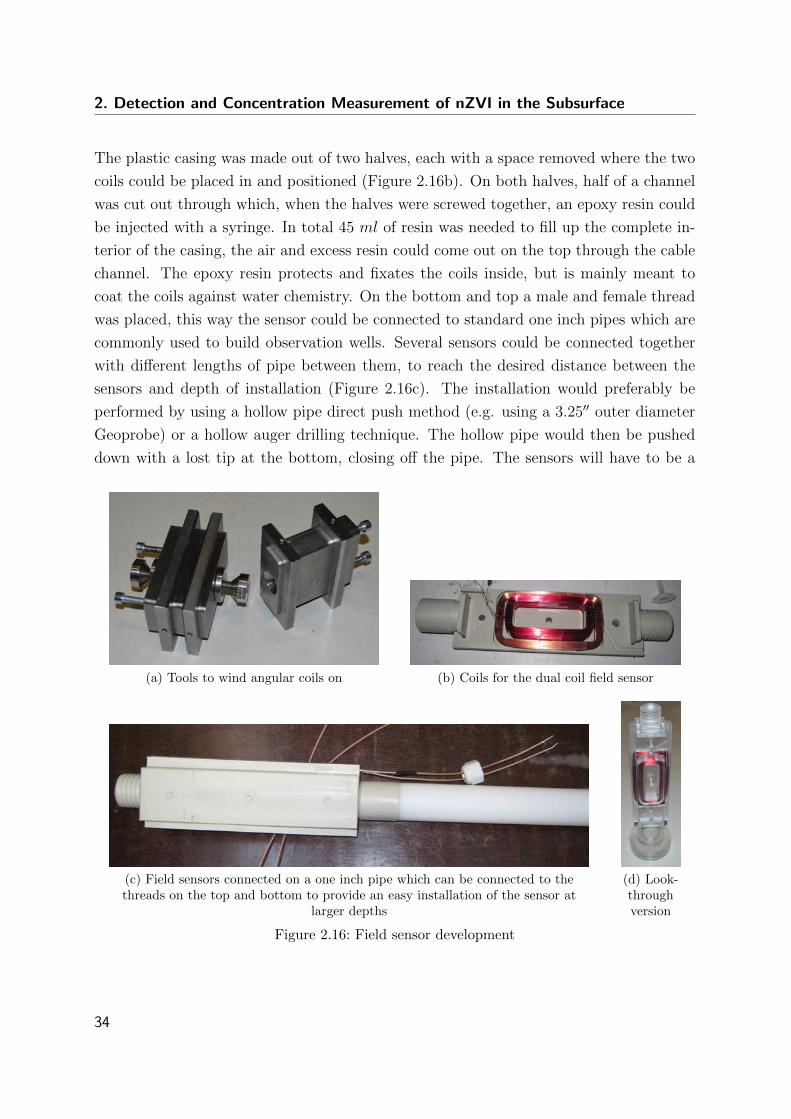
2. Detection and Concentration Measurement of nZVI in the Subsurface
The plastic casing was made out of two halves, each with a space removed where the two
coils could be placed in and positioned (Figure 2.16b). On both halves, half of a channel
was cut out through which, when the halves were screwed together, an epoxy resin could
be injected with a syringe. In total 45 ml of resin was needed to fill up the complete in-
terior of the casing, the air and excess resin could come out on the top through the cable
channel. The epoxy resin protects and fixates the coils inside, but is mainly meant to
coat the coils against water chemistry. On the bottom and top a male and female thread
was placed, this way the sensor could be connected to standard one inch pipes which are
commonly used to build observation wells. Several sensors could be connected together
with different lengths of pipe between them, to reach the desired distance between the
sensors and depth of installation (Figure 2.16c). The installation would preferably be
performed by using a hollow pipe direct push method (e.g. using a 3.25′′ outer diameter
Geoprobe) or a hollow auger drilling technique. The hollow pipe would then be pushed
down with a lost tip at the bottom, closing off the pipe. The sensors will have to be a
(a) Tools to wind angular coils on (b) Coils for the dual coil field sensor
(c) Field sensors connected on a one inch pipe which can be connected to thethreads on the top and bottom to provide an easy installation of the sensor at
larger depths
(d) Look-throughversion
Figure 2.16: Field sensor development
34
2.5. Measuring Iron Break Through Curves in the Field
certain distance away from this metal tip, preferably a blind pipe of one meter would be
connected to the bottom of the deepest sensors. Once down, the sensors connected to
the pipe with all cables bound to the pipe, could be inserted. Afterwards the hollow pipe
would be removed with the tip left below and the aquifer material falls back towards the
sensors and pipe. By placing bentonite plugs or a socking filled with bentonite pellets,
cross connections and preferential flow paths along the installation could be avoided. Be-
side the sensor other measuring techniques could be installed as well together on the same
pipe, creating a multi functional observation well. These could be temperature sensors,
fluorescence sensors (glass fiber cables) and small liquid sampling ports.
2.5.2 Measuring Device
Since the detection of nZVI is needed at different wells and depths, the measurement
system is set up modular, and can thus consist of several amplifier cards. Each amplifier
card holds a sine generator with an audio power amplifier. This generates the excitation
AC voltage of approximately 14 V RMS at a frequency of 2 kHz. This voltage is sent
through both primary coils of the detection and reference system, which are intercon-
nected as described above. The current through the excitation coils is measured by a
shunt resistor with an adjacent RMS detector and 24 bit analog digital converter (ADC).
An operational amplifier is used to amplify the few µV RMS (root mean square) differ-
ence of the voltages induced in the secondary coils. The signal then is also led to an RMS
voltage amplitude detector and an ADC. In this way a small change can be measured.
Due to geometrical and electrical differences of the coils, there is a signal offset to be
expected, even without the presence of iron. The more similar the two sets of coils are,
the lower this offset will be. With the produced coils used here, this difference was around
100 mV .
The data should be collected at a central point to access all the data at once and make
remote control through a GSM modem possible. Therefore, the whole system is set up
as a master-slave system (Figure 2.17). The slaves, on request, will start measuring and
send their data to the central master. Each slave is positioned at a well and can have up
to 16 amplifier cards for sensors at 16 different depths.
2.5.3 Post-Processing Algorithms
The equivalent circuit diagram of two windings of primary coil is composed of the dis-
tributed capacitance between these windings, which is parallel to resistance and induc-
35
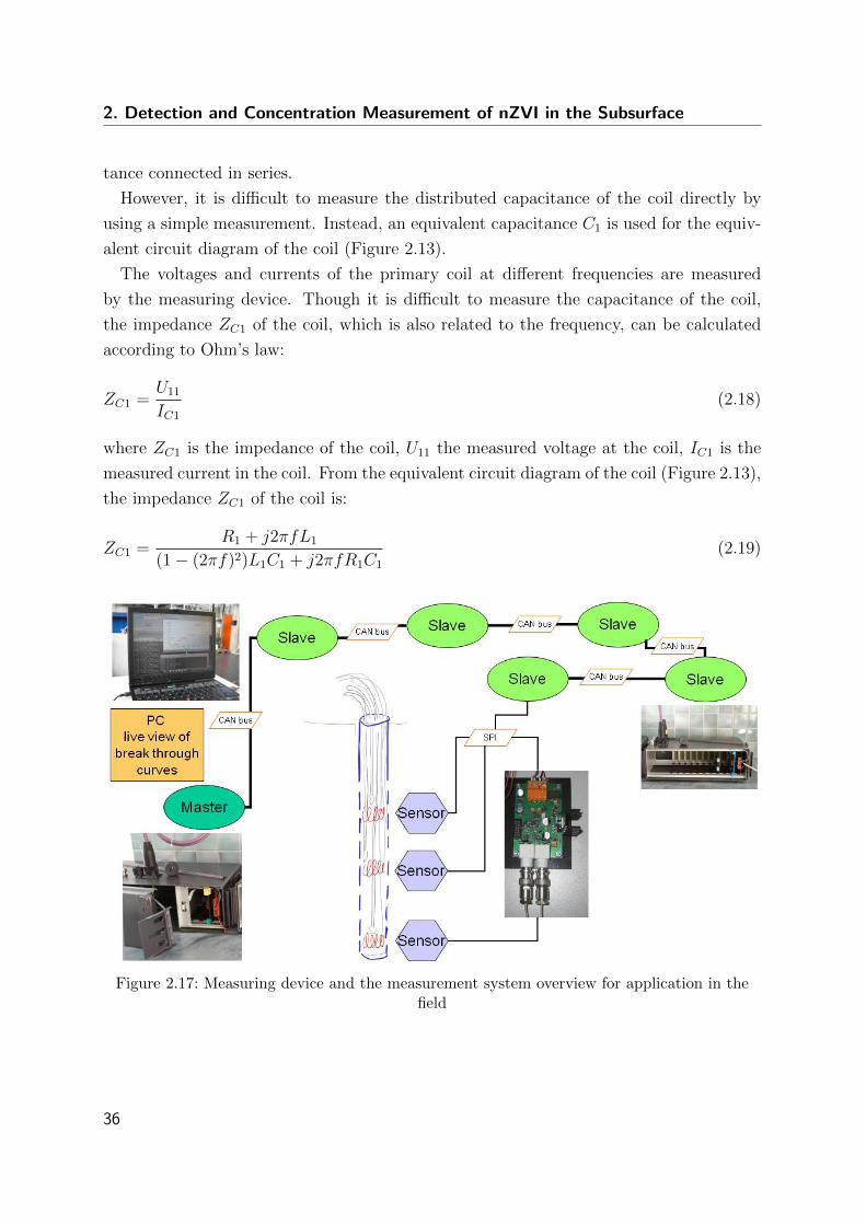
2. Detection and Concentration Measurement of nZVI in the Subsurface
tance connected in series.
However, it is difficult to measure the distributed capacitance of the coil directly by
using a simple measurement. Instead, an equivalent capacitance C1 is used for the equiv-
alent circuit diagram of the coil (Figure 2.13).
The voltages and currents of the primary coil at different frequencies are measured
by the measuring device. Though it is difficult to measure the capacitance of the coil,
the impedance ZC1 of the coil, which is also related to the frequency, can be calculated
according to Ohm’s law:
ZC1 =U11
IC1
(2.18)
where ZC1 is the impedance of the coil, U11 the measured voltage at the coil, IC1 is the
measured current in the coil. From the equivalent circuit diagram of the coil (Figure 2.13),
the impedance ZC1 of the coil is:
ZC1 =R1 + j2πfL1
(1− (2πf)2)L1C1 + j2πfR1C1
(2.19)
Figure 2.17: Measuring device and the measurement system overview for application in thefield
36
2.5. Measuring Iron Break Through Curves in the Field
where j indicates the imaginary part, R1 the resistance, L1 the inductance and C1 the
capacitance of the first reference coil.
The values of R1, L1 and C1, were determined by performing a measurement where
the frequency f was varied from 100 Hz to 3 kHz. The lower and upper bounds of
R1, L1 were estimated by a measuring device, the bounds of C1 were computed by the
simulation. The measured impedance ZC1 was imported and plotted in the curve fitting
tool of MATLAB, to fit Equation 2.19 to the measured data by varying C1.
The current in the primary coil decreases because of the increased inductance, when
nZVI is in the measuring domain of the sensor. The symbols of I ′1, I ′C1, I ′C2 and U ′12, U ′22,
U ′3 in Figure 2.13 are the currents and voltages without nZVI (χ = 0). The following
symbols of I1, IC1, IC2 and U11, U12, U22 are the currents and voltages with nZVI χ 6= 0.
The currents I1, I ′1 and the voltages U12, U ′12, U22, U ′22 can be measured by the measuring
device. The currents in the primary coils are
IC1, (I′C1) =
∣∣((1− (2πf)2L1C1) + j2πfR1C1
)−1∣∣I1, (I′1) (2.20)
IC2, (I′C2) =
∣∣((1− (2πf)2L2(C2 + Ck)) + j2πfR2(C2 + Ck))−1∣∣I1, (I
′1) (2.21)
where C1 is the capacitance and L1 the inductance and I(′)1 the current of the primary
reference coil, and Ck is the capacitance of the cable, C2 the capacitance and L2 the
inductance of the primary detection coil. Hence, if there is no nZVI around the coil, the
induced voltages U ′12 und U ′22 in each secondary coil are
U ′12, (U′22) = j2πfMmi1I
′C1, (j2πfMmi2I
′C2) (2.22)
where Mmi1 and Mmi2 are the mutual inductances of the dual coil system (reference and
detection respectively). Which can be calculated according to the induced voltage U12,22
and the current IC1,C2, which are measured in the circuit by the measuring device. If
there is nZVI around the sensor, the induced voltages U12 and U22 are
U12 = j2πfMmi1IC1 (2.23)
U22 = j2πf
(1 +
χmkexp
)Mmi2IC2 (2.24)
where kexp is the measured geometry factor as defined in Equation 2.34), and χm the
measured susceptibility. Since the two dual coil systems are connected in series, the
37
2. Detection and Concentration Measurement of nZVI in the Subsurface
potential difference of the secondary coils from the reference and detection sensor is:
U ′3 = U ′22 − U ′12 (2.25)
U ′3 = j2πf(Mmi2I
′C2 −Mmi1I
′C1
)(2.26)
U3 = U22 − U12 (2.27)
U3 = j2πf
((1 +
χmkexp
)Mmi2I
′C2 −Mmi1I
′C1
)(2.28)
Finally, the susceptibility is obtained from
χm = kexp
∣∣U3
∣∣−∣∣U ′3∣∣2πf
−Mmi1(I ′C1 − IC1)
Mmi2IC2
+I ′C2
IC2
− 1
(2.29)
where U3(′) is the potential difference of the reference and detection sensors’ secondary
coils. The plastic casing of the sensor obstructs the nZVI from getting too close or within
the coil center. The average susceptibility measured χD thus consists of two domains,
one where nZVI can enter χm and one where it cannot (Figure 2.14). To calculate only
the susceptibility in the area around the sensor where nZVI can be present, a geometry
factor ksim has to be calculated. It is obtained through the following equations:
Φ = wMmiI1 (2.30)
Mmi = (1 + χD)cM (2.31)
χD =Φ
wI1
cM − 1 (2.32)
ksim =χmχD
(2.33)
kexp = αkksim (2.34)
where Φ is the magnetic flux in the secondary coil, w is the windings, Mmi is the mutual
inductance between two coils and cM is the constant term of it. The average susceptibility
χD in the measuring domain can be calculated according to the above equations and the
susceptibility of nZVI χm can be obtained from the simulation. Therefore, the geometry
factor ksim is 4.5. The calibration coefficient αk is determined experimentally.
38
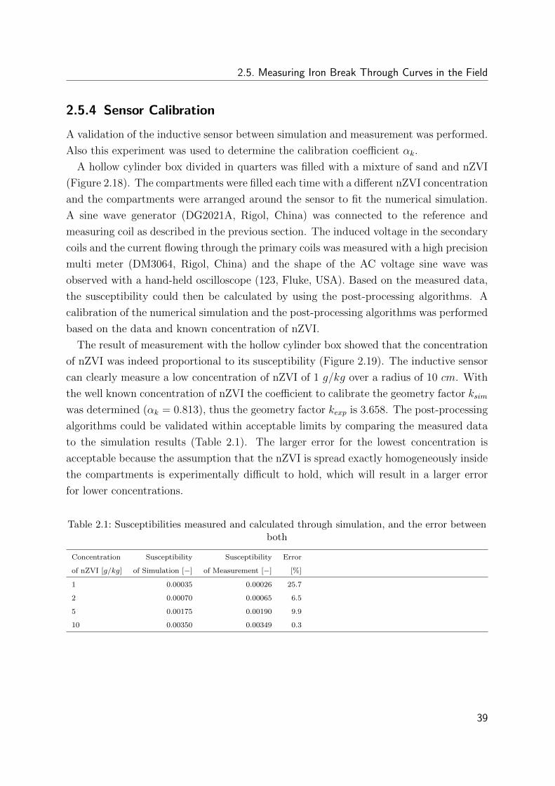
2.5. Measuring Iron Break Through Curves in the Field
2.5.4 Sensor Calibration
A validation of the inductive sensor between simulation and measurement was performed.
Also this experiment was used to determine the calibration coefficient αk.
A hollow cylinder box divided in quarters was filled with a mixture of sand and nZVI
(Figure 2.18). The compartments were filled each time with a different nZVI concentration
and the compartments were arranged around the sensor to fit the numerical simulation.
A sine wave generator (DG2021A, Rigol, China) was connected to the reference and
measuring coil as described in the previous section. The induced voltage in the secondary
coils and the current flowing through the primary coils was measured with a high precision
multi meter (DM3064, Rigol, China) and the shape of the AC voltage sine wave was
observed with a hand-held oscilloscope (123, Fluke, USA). Based on the measured data,
the susceptibility could then be calculated by using the post-processing algorithms. A
calibration of the numerical simulation and the post-processing algorithms was performed
based on the data and known concentration of nZVI.
The result of measurement with the hollow cylinder box showed that the concentration
of nZVI was indeed proportional to its susceptibility (Figure 2.19). The inductive sensor
can clearly measure a low concentration of nZVI of 1 g/kg over a radius of 10 cm. With
the well known concentration of nZVI the coefficient to calibrate the geometry factor ksim
was determined (αk = 0.813), thus the geometry factor kexp is 3.658. The post-processing
algorithms could be validated within acceptable limits by comparing the measured data
to the simulation results (Table 2.1). The larger error for the lowest concentration is
acceptable because the assumption that the nZVI is spread exactly homogeneously inside
the compartments is experimentally difficult to hold, which will result in a larger error
for lower concentrations.
Table 2.1: Susceptibilities measured and calculated through simulation, and the error betweenboth
Concentration Susceptibility Susceptibility Error
of nZVI [g/kg] of Simulation [−] of Measurement [−] [%]
1 0.00035 0.00026 25.7
2 0.00070 0.00065 6.5
5 0.00175 0.00190 9.9
10 0.00350 0.00349 0.3
39
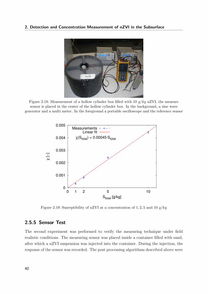
2. Detection and Concentration Measurement of nZVI in the Subsurface
Figure 2.18: Measurement of a hollow cylinder box filled with 10 g/kg nZVI, the measuresensor is placed in the center of the hollow cylinder box. In the background, a sine wave
generator and a multi meter. In the foreground a portable oscilloscope and the reference sensor
0
0.001
0.002
0.003
0.004
0.005
0 1 2 5 10
χ [−
]
Stotal [g/kg]
χ(Stotal) = 0.00045·Stotal
MeasurementsLinear fit
Figure 2.19: Susceptibility of nZVI at a concentration of 1, 2, 5 and 10 g/kg
2.5.5 Sensor Test
The second experiment was performed to verify the measuring technique under field
realistic conditions. The measuring sensor was placed inside a container filled with sand,
after which a nZVI suspension was injected into the container. During the injection, the
response of the sensor was recorded. The post processing algorithms described above were
40
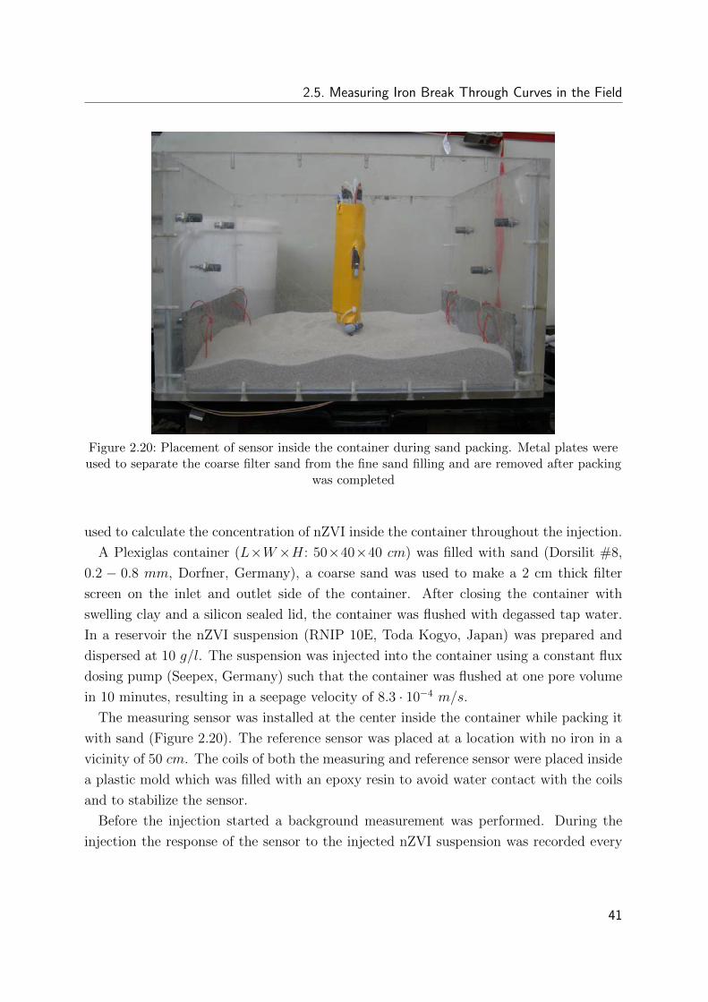
2.5. Measuring Iron Break Through Curves in the Field
Figure 2.20: Placement of sensor inside the container during sand packing. Metal plates wereused to separate the coarse filter sand from the fine sand filling and are removed after packing
was completed
used to calculate the concentration of nZVI inside the container throughout the injection.
A Plexiglas container (L×W×H: 50×40×40 cm) was filled with sand (Dorsilit #8,
0.2 − 0.8 mm, Dorfner, Germany), a coarse sand was used to make a 2 cm thick filter
screen on the inlet and outlet side of the container. After closing the container with
swelling clay and a silicon sealed lid, the container was flushed with degassed tap water.
In a reservoir the nZVI suspension (RNIP 10E, Toda Kogyo, Japan) was prepared and
dispersed at 10 g/l. The suspension was injected into the container using a constant flux
dosing pump (Seepex, Germany) such that the container was flushed at one pore volume
in 10 minutes, resulting in a seepage velocity of 8.3 · 10−4 m/s.
The measuring sensor was installed at the center inside the container while packing it
with sand (Figure 2.20). The reference sensor was placed at a location with no iron in a
vicinity of 50 cm. The coils of both the measuring and reference sensor were placed inside
a plastic mold which was filled with an epoxy resin to avoid water contact with the coils
and to stabilize the sensor.
Before the injection started a background measurement was performed. During the
injection the response of the sensor to the injected nZVI suspension was recorded every
41
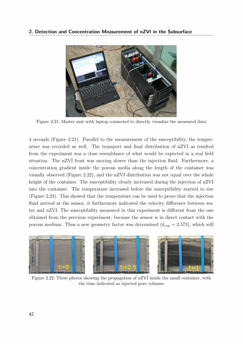
2. Detection and Concentration Measurement of nZVI in the Subsurface
Figure 2.21: Master unit with laptop connected to directly visualize the measured data
4 seconds (Figure 2.21). Parallel to the measurement of the susceptibility, the temper-
ature was recorded as well. The transport and final distribution of nZVI as resulted
from the experiment was a close resemblance of what would be expected in a real field
situation. The nZVI front was moving slower than the injection fluid. Furthermore, a
concentration gradient inside the porous media along the length of the container was
visually observed (Figure 2.22), and the nZVI distribution was not equal over the whole
height of the container. The susceptibility clearly increased during the injection of nZVI
into the container. The temperature increased before the susceptibility started to rise
(Figure 2.23). This showed that the temperature can be used to prove that the injection
fluid arrived at the sensor, it furthermore indicated the velocity difference between wa-
ter and nZVI. The susceptibility measured in this experiment is different from the one
obtained from the previous experiment, because the sensor is in direct contact with the
porous medium. Thus a new geometry factor was determined (kexp = 2.573), which will
Figure 2.22: Three photos showing the propagation of nZVI inside the small container, withthe time indicated as injected pore volumes
42
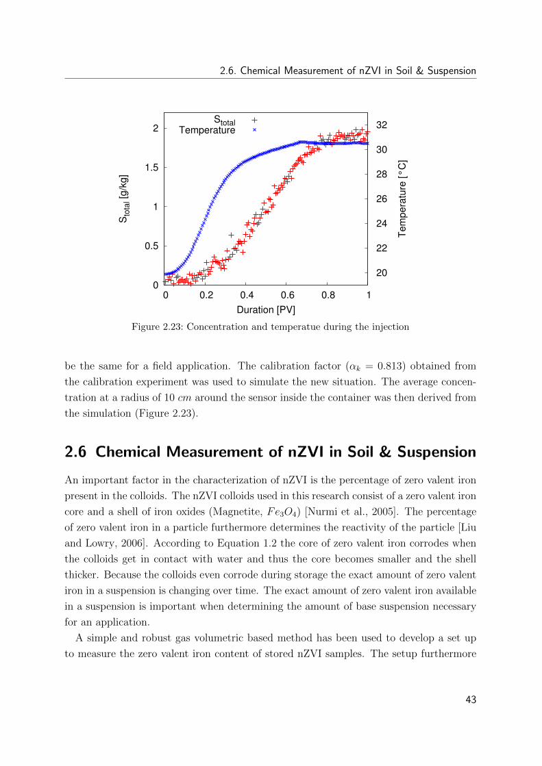
2.6. Chemical Measurement of nZVI in Soil & Suspension
0
0.5
1
1.5
2
0 0.2 0.4 0.6 0.8 1
20
22
24
26
28
30
32S
tota
l [g/
kg]
Tem
pera
ture
[°C
]
Duration [PV]
StotalTemperature
Figure 2.23: Concentration and temperatue during the injection
be the same for a field application. The calibration factor (αk = 0.813) obtained from
the calibration experiment was used to simulate the new situation. The average concen-
tration at a radius of 10 cm around the sensor inside the container was then derived from
the simulation (Figure 2.23).
2.6 Chemical Measurement of nZVI in Soil & Suspension
An important factor in the characterization of nZVI is the percentage of zero valent iron
present in the colloids. The nZVI colloids used in this research consist of a zero valent iron
core and a shell of iron oxides (Magnetite, Fe3O4) [Nurmi et al., 2005]. The percentage
of zero valent iron in a particle furthermore determines the reactivity of the particle [Liu
and Lowry, 2006]. According to Equation 1.2 the core of zero valent iron corrodes when
the colloids get in contact with water and thus the core becomes smaller and the shell
thicker. Because the colloids even corrode during storage the exact amount of zero valent
iron in a suspension is changing over time. The exact amount of zero valent iron available
in a suspension is important when determining the amount of base suspension necessary
for an application.
A simple and robust gas volumetric based method has been used to develop a set up
to measure the zero valent iron content of stored nZVI samples. The setup furthermore
43
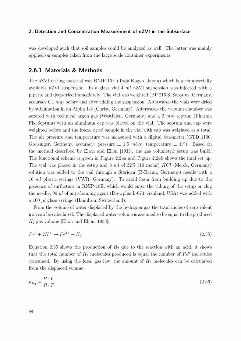
2. Detection and Concentration Measurement of nZVI in the Subsurface
was developed such that soil samples could be analyzed as well. The latter was mainly
applied on samples taken from the large scale container experiments.
2.6.1 Materials & Methods
The nZVI testing material was RNIP-10E (Toda Kogyo, Japan) which is a commercially
available nZVI suspension. In a glass vial 4 ml nZVI suspension was injected with a
pipette and deep-fried immediately. The vial was weighted (BP 210 S, Satorius, Germany,
accuracy 0.1 mg) before and after adding the suspension. Afterwards the vials were dried
by sublimation in an Alpha 1-2 (Christ, Germany). Afterwards the vacuum chamber was
aerated with technical argon gas (Westfalen, Germany) and a 3 mm septum (Pharma
Fix Septum) with an aluminum cap was placed on the vial. The septum and cap were
weighted before and the freeze dried sample in the vial with cap was weighted as a total.
The air pressure and temperature was measured with a digital barometer (GTD 1100,
Greisinger, Germany, accuracy: pressure ± 1.5 mbar, temperature ± 1%). Based on
the method described by Elion and Elion [1933], the gas volumetric setup was build.
The functional scheme is given in Figure 2.24a and Figure 2.24b shows the final set up.
The vial was placed in the setup and 3 ml of 32% (10 molar) HCl (Merck, Germany)
solution was added to the vial through a Sterican (B-Braun, Germany) needle with a
10 ml plastic syringe (VWR, Germany). To avoid foam from building up due to the
presence of surfactant in RNIP-10E, which would enter the tubing of the setup or clog
the needle, 90 µl of anti-foaming agent (Drewplus L-674, Ashland, USA) was added with
a 100 µl glass syringe (Hamilton, Switzerland).
From the volume of water displaced by the hydrogen gas the total moles of zero valent
iron can be calculated. The displaced water volume is assumed to be equal to the produced
H2 gas volume [Elion and Elion, 1933].
Fe0 + 2H+ → Fe2+ +H2 (2.35)
Equation 2.35 shows the production of H2 due to the reaction with an acid, it shows
that the total number of H2 molecules produced is equal the number of Fe0 molecules
consumed. By using the ideal gas law, the amount of H2 molecules can be calculated
from the displaced volume:
nH2 =P · VR · T (2.36)
44
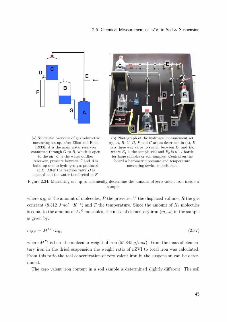
2.6. Chemical Measurement of nZVI in Soil & Suspension
(a) Schematic overview of gas volumetricmeasuring set up, after Elion and Elion
[1933]. A is the main water reservoirconnected through G to B, which is open
to the air. C is the water outflowreservoir, pressure between C and A isbuild up due to hydrogen gas produced
at E. After the reaction valve D isopened and the water is collected in F
(b) Photograph of the hydrogen measurement setup. A, B, C, D, F and G are as described in (a), Eis a three way valve to switch between E1 and E2,where E1 is the sample vial and E2 is a 1 l bottlefor large samples or soil samples. Central on the
board a barometric pressure and temperaturemeasuring device is positioned
Figure 2.24: Measuring set up to chemically determine the amount of zero valent iron inside asample
where nH2 is the amount of molecules, P the pressure, V the displaced volume, R the gas
constant (8.312 Jmol−1K−1) and T the temperature. Since the amount of H2 molecules
is equal to the amount of Fe0 molecules, the mass of elementary iron (mFe0) in the sample
is given by:
mFe0 = MFe · nH2 (2.37)
where MFe is here the molecular weight of iron (55.845 g/mol). From the mass of elemen-
tary iron in the dried suspension the weight ratio of nZVI to total iron was calculated.
From this ratio the real concentration of zero valent iron in the suspension can be deter-
mined.
The zero valent iron content in a soil sample is determined slightly different. The soil
45
2. Detection and Concentration Measurement of nZVI in the Subsurface
sample is filled into a 1 l glass bottle (Duran, Germany), which is weighted before and
after filling. To prevent oxidation of Fe0 to air, the head space is flushed with Argon
gas. This allows the sample to be stored for a short period. The bottle is placed in the
measuring set up (location E2 in Figure 2.24b), through the three-way valve above the
bottle acid (HCl, 32 %) is added with a syringe and a stainless steel needle. The three-
way valve is turned such that the bottle is open towards E, and the bottle is shaken by
hand to get a good mixing of the acid and the soil sample. If the content in the bottle are
still black from the iron, new acid is added. This is repeated until the water level in A no
longer moves down. The produced gas volume is again used to calculate the content of
Fe0 in the sample using Equations 2.35-2.37. When the Fe0 content of the colloids of the
injected suspension was determined prior to the injection, the determined concentration
of Fe0 in the soil sample can also be converted into a Fetotal concentration
46
3 Fundamentals of Transport of Nano
Sized Zero Valent Iron Colloids
3.1 Motivation
The main goal of this work is to get a better understanding and description of the trans-
port of nZVI colloids during the injection into the subsurface. This chapter presents a
conceptual transport model based on ideas obtained from the filtration theory and the
characterization of the nZVI suspension. Furthermore a method is presented to obtain
quantitative measures of transport from column experiments by combining transient con-
centration profiles, transport equations, an adapted application of the classical filtration
theory and numerical modeling. Constitutive relations were sought by looking at the
filtration theory, transient concentration profiles of the column experiments and fitting
parameters for a numerical model of these experiments.
3.2 Colloid Transport & Filtration in Porous Media
In a porous medium, transport of particles is limited due to filtration effects. Filtration
causes particles to be removed from the liquid phase.
In this section the filtration theory as described by Tufenkji and Elimelech [2004] is
presented. It is based upon Happel’s sphere-in-cell model [Happel, 1958] to describe the
fluid flow in a porous media and Prieve & Ruckenstein’s theory [Prieve and Ruckenstein,
1974] which concludes that all individual contributions from transport mechanisms can
be summed to calculate the total deposition rate. Many scientist have used this filtration
theory (e.g. [Long and Hilpert, 2009; Schrick et al., 2004; Wang et al., 2008; Zhan et al.,
2008]).
47
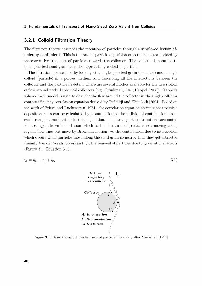
3. Fundamentals of Transport of Nano Sized Zero Valent Iron Colloids
3.2.1 Colloid Filtration Theory
The filtration theory describes the retention of particles through a single-collector ef-
ficiency coefficient. This is the rate of particle deposition onto the collector divided by
the convective transport of particles towards the collector. The collector is assumed to
be a spherical sand grain as is the approaching colloid or particle.
The filtration is described by looking at a single spherical grain (collector) and a single
colloid (particle) in a porous medium and describing all the interactions between the
collector and the particle in detail. There are several models available for the description
of flow around packed spherical collectors (e.g. [Brinkman, 1947; Happel, 1958]). Happel’s
sphere-in-cell model is used to describe the flow around the collector in the single-collector
contact efficiency correlation equation derived by Tufenkji and Elimelech [2004]. Based on
the work of Prieve and Ruckenstein [1974], the correlation equation assumes that particle
deposition rates can be calculated by a summation of the individual contributions from
each transport mechanism to this deposition. The transport contributions accounted
for are: ηD, Brownian diffusion which is the filtration of particles not moving along
regular flow lines but move by Brownian motion; ηI , the contribution due to interception
which occurs when particles move along the sand grain so nearby that they get attracted
(mainly Van der Waals forces) and ηG, the removal of particles due to gravitational effects
(Figure 3.1, Equation 3.1).
η0 = ηD + ηI + ηG (3.1)
Figure 3.1: Basic transport mechanisms of particle filtration, after Yao et al. [1971]
48
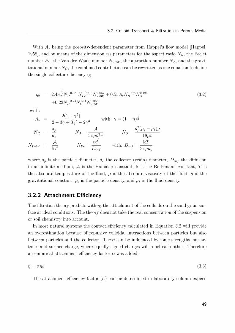
3.2. Colloid Transport & Filtration in Porous Media
With As being the porosity-dependent parameter from Happel’s flow model [Happel,
1958], and by means of the dimensionless parameters for the aspect ratio NR, the Peclet
number Pe, the Van der Waals number NV dW , the attraction number NA, and the gravi-
tational number NG, the combined contribution can be rewritten as one equation to define
the single collector efficiency η0:
η0 = 2.4A13sN
−0.081R N−0.715
Pe N0.052V dW + 0.55AsN
1.675R N0.125
A (3.2)
+0.22N−0.24R N1.11
G N0.053V dW
with:
As =2(1− γ5)
2− 3γ + 3γ5 − 2γ6with: γ = (1− n)
13
NR =dpdc
NA =A
3πµd2pv
NG =d2p(ρp − ρf )g
18µv
NV dW =AkT
NPe =vdcDinf
with: Dinf =kT
3πµdp
where dp is the particle diameter, dc the collector (grain) diameter, Dinf the diffusion
in an infinite medium, A is the Hamaker constant, k is the Boltzmann constant, T is
the absolute temperature of the fluid, µ is the absolute viscosity of the fluid, g is the
gravitational constant, ρp is the particle density, and ρf is the fluid density.
3.2.2 Attachment Efficiency
The filtration theory predicts with η0 the attachment of the colloids on the sand grain sur-
face at ideal conditions. The theory does not take the real concentration of the suspension
or soil chemistry into account.
In most natural systems the contact efficiency calculated in Equation 3.2 will provide
an overestimation because of repulsive colloidal interactions between particles but also
between particles and the collector. These can be influenced by ionic strengths, surfac-
tants and surface charge, where equally signed charges will repel each other. Therefore
an empirical attachment efficiency factor α was added:
η = αη0 (3.3)
The attachment efficiency factor (α) can be determined in laboratory column experi-
49
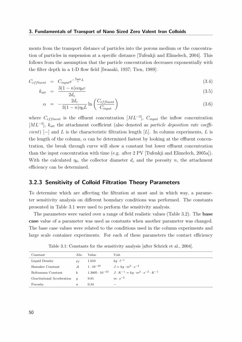
3. Fundamentals of Transport of Nano Sized Zero Valent Iron Colloids
ments from the transport distance of particles into the porous medium or the concentra-
tion of particles in suspension at a specific distance [Tufenkji and Elimelech, 2004]. This
follows from the assumption that the particle concentration decreases exponentially with
the filter depth in a 1-D flow field [Iwasaki, 1937; Tien, 1989]:
Ceffluent = Cinpute− katt
vL (3.4)
katt =3(1− n)αη0v
2dc(3.5)
α = − 2dc3(1− n)η0L
ln
(CeffluentCinput
)(3.6)
where Ceffluent is the effluent concentration [ML−3], Cinput the inflow concentration
[ML−3], katt the attachment coefficient (also denoted as particle deposition rate coeffi-
cient) [−] and L is the characteristic filtration length [L]. In column experiments, L is
the length of the column, α can be determined fastest by looking at the effluent concen-
tration, the break through curve will show a constant but lower effluent concentration
than the input concentration with time (e.g. after 2 PV [Tufenkji and Elimelech, 2005a]).
With the calculated η0, the collector diameter dc and the porosity n, the attachment
efficiency can be determined.
3.2.3 Sensitivity of Colloid Filtration Theory Parameters
To determine which are affecting the filtration at most and in which way, a parame-
ter sensitivity analysis on different boundary conditions was performed. The constants
presented in Table 3.1 were used to perform the sensitivity analysis.
The parameters were varied over a range of field realistic values (Table 3.2). The base
case value of a parameter was used as constants when another parameter was changed.
The base case values were related to the conditions used in the column experiments and
large scale container experiments. For each of these parameters the contact efficiency
Table 3.1: Constants for the sensitivity analysis [after Schrick et al., 2004].
Constant Abr. Value Unit
Liquid Density ρf 1.010 kg · l−1
Hamaker Constant A 1 · 10−20 J = kg ·m2 · s−2
Boltzmann Constant k 1.3805 · 10−23 J ·K−1 = kg ·m2 · s−2 ·K−1
Gravitational Acceleration g 9.81 m · s−2
Porosity n 0.34 −
50
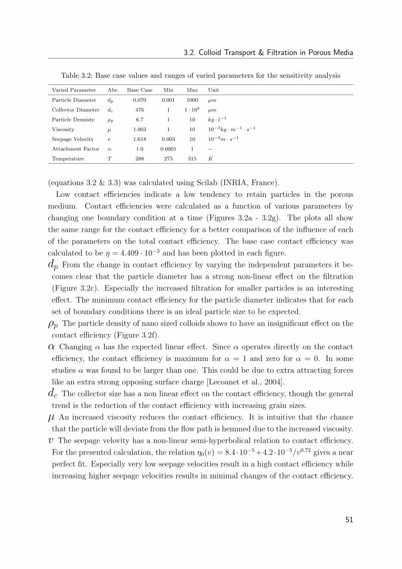
3.2. Colloid Transport & Filtration in Porous Media
Table 3.2: Base case values and ranges of varied parameters for the sensitivity analysis
Varied Parameter Abr. Base Case Min Max Unit
Particle Diameter dp 0.070 0.001 1000 µm
Collector Diameter dc 476 1 1 · 105 µm
Particle Densisty ρp 6.7 1 10 kg · l−1
Viscosity µ 1.003 1 10 10−3kg ·m−1 · s−1
Seepage Velocity v 1.618 0.003 10 10−3m · s−1
Attachment Factor α 1.0 0.0001 1 −
Temperature T 288 275 315 K
(equations 3.2 & 3.3) was calculated using Scilab (INRIA, France).
Low contact efficiencies indicate a low tendency to retain particles in the porous
medium. Contact efficiencies were calculated as a function of various parameters by
changing one boundary condition at a time (Figures 3.2a - 3.2g). The plots all show
the same range for the contact efficiency for a better comparison of the influence of each
of the parameters on the total contact efficiency. The base case contact efficiency was
calculated to be η = 4.409 · 10−3 and has been plotted in each figure.
dp From the change in contact efficiency by varying the independent parameters it be-
comes clear that the particle diameter has a strong non-linear effect on the filtration
(Figure 3.2c). Especially the increased filtration for smaller particles is an interesting
effect. The minimum contact efficiency for the particle diameter indicates that for each
set of boundary conditions there is an ideal particle size to be expected.
ρp The particle density of nano sized colloids shows to have an insignificant effect on the
contact efficiency (Figure 3.2f).
α Changing α has the expected linear effect. Since α operates directly on the contact
efficiency, the contact efficiency is maximum for α = 1 and zero for α = 0. In some
studies α was found to be larger than one. This could be due to extra attracting forces
like an extra strong opposing surface charge [Lecoanet et al., 2004].
dc The collector size has a non linear effect on the contact efficiency, though the general
trend is the reduction of the contact efficiency with increasing grain sizes.
µ An increased viscosity reduces the contact efficiency. It is intuitive that the chance
that the particle will deviate from the flow path is hemmed due to the increased viscosity.
v The seepage velovity has a non-linear semi-hyperbolical relation to contact efficiency.
For the presented calculation, the relation η0(v) = 8.4 ·10−5 +4.2 ·10−5/v0.72 gives a near
perfect fit. Especially very low seepage velocities result in a high contact efficiency while
increasing higher seepage velocities results in minimal changes of the contact efficiency.
51
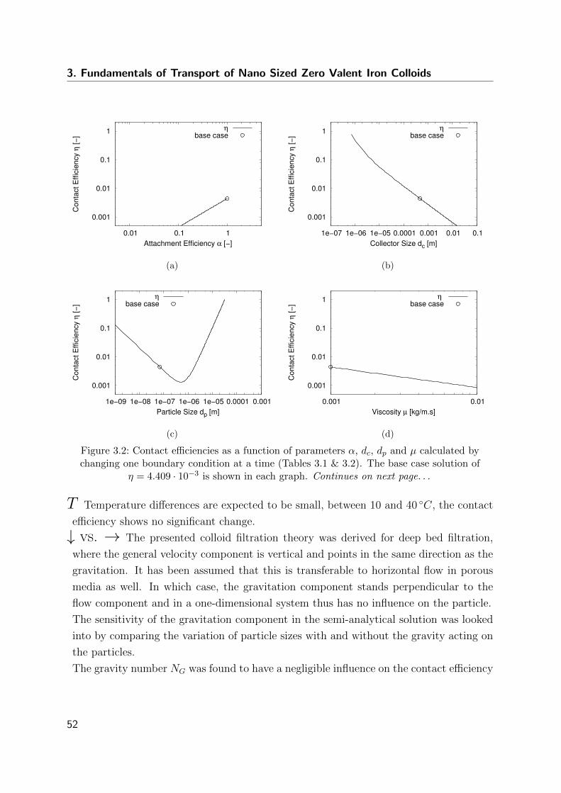
3. Fundamentals of Transport of Nano Sized Zero Valent Iron Colloids
0.001
0.01
0.1
1
0.01 0.1 1
Con
tact
Effi
cien
cy η
[−]
Attachment Efficiency α [−]
η
base case
(a)
0.001
0.01
0.1
1
1e−07 1e−06 1e−05 0.0001 0.001 0.01 0.1
Con
tact
Effi
cien
cy η
[−]
Collector Size dc [m]
η
base case
(b)
0.001
0.01
0.1
1
1e−09 1e−08 1e−07 1e−06 1e−05 0.0001 0.001
Con
tact
Effi
cien
cy η
[−]
Particle Size dp [m]
η
base case
(c)
0.001
0.01
0.1
1
0.001 0.01
Con
tact
Effi
cien
cy η
[−]
Viscosity µ [kg/m.s]
η base case
(d)
Figure 3.2: Contact efficiencies as a function of parameters α, dc, dp and µ calculated bychanging one boundary condition at a time (Tables 3.1 & 3.2). The base case solution of
η = 4.409 · 10−3 is shown in each graph. Continues on next page. . .
T Temperature differences are expected to be small, between 10 and 40 C, the contact
efficiency shows no significant change.
↓ vs. → The presented colloid filtration theory was derived for deep bed filtration,
where the general velocity component is vertical and points in the same direction as the
gravitation. It has been assumed that this is transferable to horizontal flow in porous
media as well. In which case, the gravitation component stands perpendicular to the
flow component and in a one-dimensional system thus has no influence on the particle.
The sensitivity of the gravitation component in the semi-analytical solution was looked
into by comparing the variation of particle sizes with and without the gravity acting on
the particles.
The gravity number NG was found to have a negligible influence on the contact efficiency
52
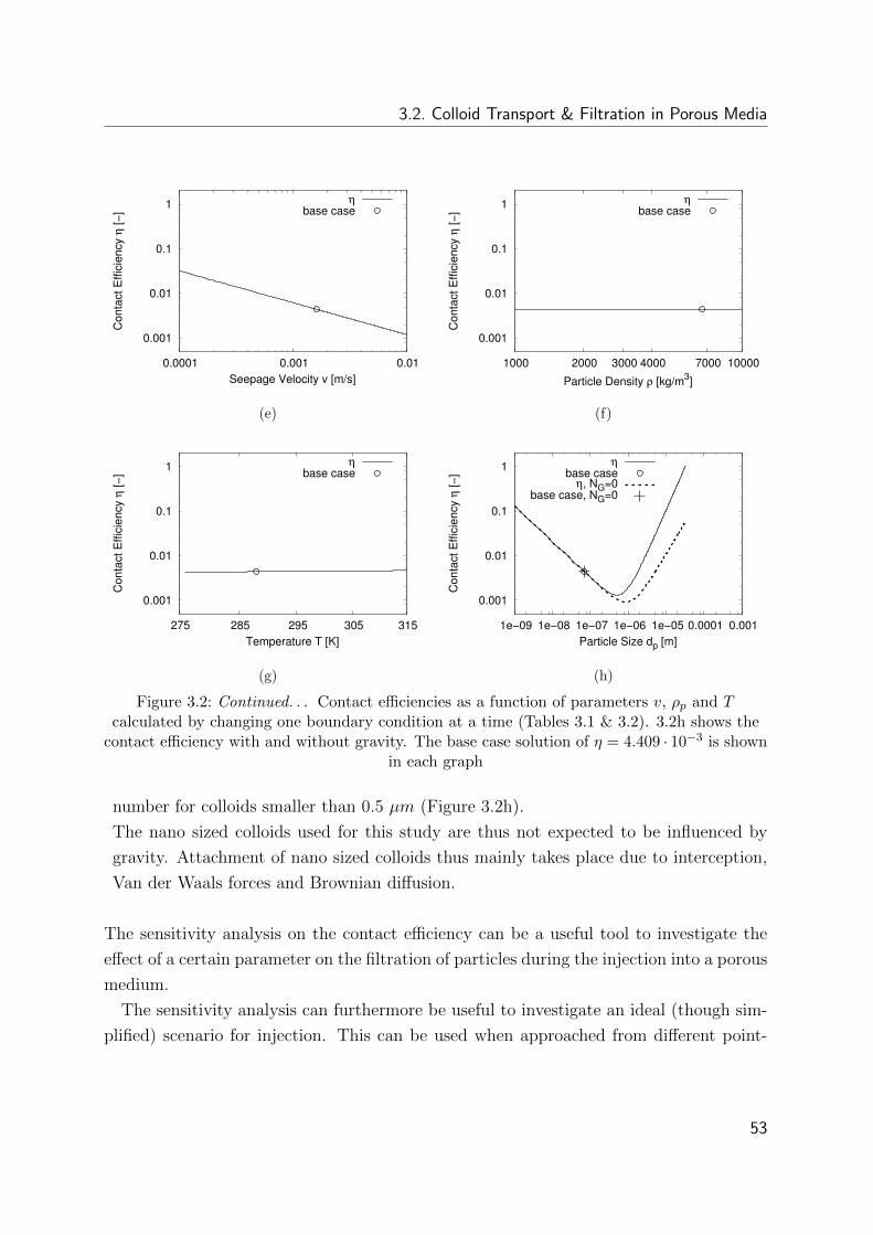
3.2. Colloid Transport & Filtration in Porous Media
0.001
0.01
0.1
1
0.0001 0.001 0.01
Con
tact
Effi
cien
cy η
[−]
Seepage Velocity v [m/s]
η
base case
(e)
0.001
0.01
0.1
1
1000 2000 3000 4000 7000 10000
Con
tact
Effi
cien
cy η
[−]
Particle Density ρ [kg/m3]
η
base case
(f)
0.001
0.01
0.1
1
275 285 295 305 315
Con
tact
Effi
cien
cy η
[−]
Temperature T [K]
η
base case
(g)
0.001
0.01
0.1
1
1e−09 1e−08 1e−07 1e−06 1e−05 0.0001 0.001
Con
tact
Effi
cien
cy η
[−]
Particle Size dp [m]
η
base caseη, NG=0
base case, NG=0
(h)
Figure 3.2: Continued. . . Contact efficiencies as a function of parameters v, ρp and Tcalculated by changing one boundary condition at a time (Tables 3.1 & 3.2). 3.2h shows the
contact efficiency with and without gravity. The base case solution of η = 4.409 · 10−3 is shownin each graph
number for colloids smaller than 0.5 µm (Figure 3.2h).
The nano sized colloids used for this study are thus not expected to be influenced by
gravity. Attachment of nano sized colloids thus mainly takes place due to interception,
Van der Waals forces and Brownian diffusion.
The sensitivity analysis on the contact efficiency can be a useful tool to investigate the
effect of a certain parameter on the filtration of particles during the injection into a porous
medium.
The sensitivity analysis can furthermore be useful to investigate an ideal (though sim-
plified) scenario for injection. This can be used when approached from different point-
53
3. Fundamentals of Transport of Nano Sized Zero Valent Iron Colloids
of-views. (I) One approach would be to find out which particle size would be most
suitable for a given aquifer. This is a valuable tool that can be taken into account
while designing a field application. (II) To indicate the range of porous media types
or injection conditions that are most suitable for a given particle. This for example is
useful when the chemical behavior of a certain given particle is preferred but it is not
possible to change the size of that particle.
To be able to predict the transport distance of particles during an injection in the
field a non-linear numerical transport model should be used to be able to account for the
suspension concentration and non-constant seepage velocity around the injection well.
3.3 Characteristics of the nZVI Suspension
Classic filtration theories and most classic research on colloid transport focuses on other
colloids than nZVI. Bacteriophages [Schijven et al., 2002], viruses [Schijven and Has-
sanizadeh, 2002], latex particles [Tosco et al., 2009] and many more have all been reason-
ably described using the classic filtration theory by approaching them as single colloids in
suspension. Furthermore, most descriptions focus on suspensions with very low particle
concentrations. The colloids used here are very dense (approximately seven times the
density of water), are ferromagnetic and are applied in very high concentrations. During
preliminary research [de Boer, 2007], it was also found that a freshly received suspension
behaves different from an older one, which can be approached as an aging effect. There-
fore, it was necessary to focus also on characterizing the colloidal suspension itself when
looking for a good description of the transport behavior. This helps to understand the
behavior of the colloids in suspension, and could lead to verification or extension of the
available theories to account for the behavior observed.
3.3.1 nZVI Suspension
For this research the nano sized zero valent iron colloids (nZVI, RNIP 10E) were obtained
from Toda Kogyo Corp., Japan. It was delivered as slurry with a concentration of 214 g/l.
The colloids contained according to the data sheet 60% zero valent iron (Fe0) and 40%
Magnetite (Fe3O4). For the experiments the slurry was diluted with degassed tap water
(dissolved O2 . 1 mg/l, Total Organic Carbon: 0.4 g/l, pH: 8.0, Electrical Conductivity:
∼ 8.9 S/m) to the desired suspension concentration. To break up aggregated colloids after
the suspension was taken from storage, a disperser with a flow through chamber (UTL25
54
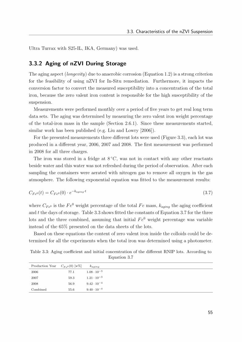
3.3. Characteristics of the nZVI Suspension
Ultra Turrax with S25-IL, IKA, Germany) was used.
3.3.2 Aging of nZVI During Storage
The aging aspect (longevity) due to anaerobic corrosion (Equation 1.2) is a strong criterion
for the feasibility of using nZVI for In-Situ remediation. Furthermore, it impacts the
conversion factor to convert the measured susceptibility into a concentration of the total
iron, because the zero valent iron content is responsible for the high susceptibility of the
suspension.
Measurements were performed monthly over a period of five years to get real long term
data sets. The aging was determined by measuring the zero valent iron weight percentage
of the total-iron mass in the sample (Section 2.6.1). Since these measurements started,
similar work has been published (e.g. Liu and Lowry [2006]).
For the presented measurements three different lots were used (Figure 3.3), each lot was
produced in a different year, 2006, 2007 and 2008. The first measurement was performed
in 2008 for all three charges.
The iron was stored in a fridge at 8 C, was not in contact with any other reactants
beside water and this water was not refreshed during the period of observation. After each
sampling the containers were aerated with nitrogen gas to remove all oxygen in the gas
atmosphere. The following exponential equation was fitted to the measurement results:
CFe0(t) = CFe0(0) · e−kaging ·t (3.7)
where CFe0 is the Fe0 weight percentage of the total Fe mass, kaging the aging coefficient
and t the days of storage. Table 3.3 shows fitted the constants of Equation 3.7 for the three
lots and the three combined, assuming that initial Fe0 weight percentage was variable
instead of the 65% presented on the data sheets of the lots.
Based on these equations the content of zero valent iron inside the colloids could be de-
termined for all the experiments when the total iron was determined using a photometer.
Table 3.3: Aging coefficient and initial concentration of the different RNIP lots. According toEquation 3.7
Production Year CFe0 (0) [w%] kaging
2006 77.1 1.08 · 10−3
2007 59.3 1.21 · 10−3
2008 56.9 9.42 · 10−4
Combined 55.6 9.40 · 10−4
55
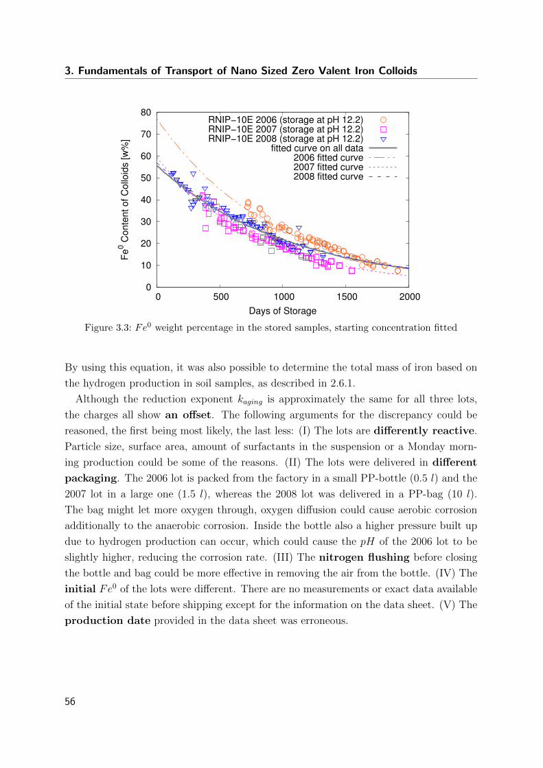
3. Fundamentals of Transport of Nano Sized Zero Valent Iron Colloids
0
10
20
30
40
50
60
70
80
0 500 1000 1500 2000
Fe0 C
onte
nt o
f Col
loid
s [w
%]
Days of Storage
RNIP−10E 2006 (storage at pH 12.2)RNIP−10E 2007 (storage at pH 12.2)RNIP−10E 2008 (storage at pH 12.2)
fitted curve on all data2006 fitted curve2007 fitted curve2008 fitted curve
Figure 3.3: Fe0 weight percentage in the stored samples, starting concentration fitted
By using this equation, it was also possible to determine the total mass of iron based on
the hydrogen production in soil samples, as described in 2.6.1.
Although the reduction exponent kaging is approximately the same for all three lots,
the charges all show an offset. The following arguments for the discrepancy could be
reasoned, the first being most likely, the last less: (I) The lots are differently reactive.
Particle size, surface area, amount of surfactants in the suspension or a Monday morn-
ing production could be some of the reasons. (II) The lots were delivered in different
packaging. The 2006 lot is packed from the factory in a small PP-bottle (0.5 l) and the
2007 lot in a large one (1.5 l), whereas the 2008 lot was delivered in a PP-bag (10 l).
The bag might let more oxygen through, oxygen diffusion could cause aerobic corrosion
additionally to the anaerobic corrosion. Inside the bottle also a higher pressure built up
due to hydrogen production can occur, which could cause the pH of the 2006 lot to be
slightly higher, reducing the corrosion rate. (III) The nitrogen flushing before closing
the bottle and bag could be more effective in removing the air from the bottle. (IV) The
initial Fe0 of the lots were different. There are no measurements or exact data available
of the initial state before shipping except for the information on the data sheet. (V) The
production date provided in the data sheet was erroneous.
56
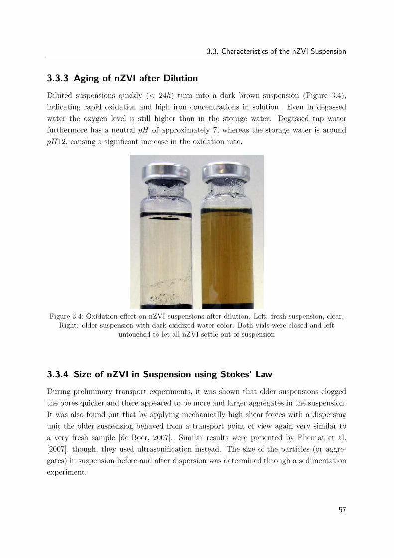
3.3. Characteristics of the nZVI Suspension
3.3.3 Aging of nZVI after Dilution
Diluted suspensions quickly (< 24h) turn into a dark brown suspension (Figure 3.4),
indicating rapid oxidation and high iron concentrations in solution. Even in degassed
water the oxygen level is still higher than in the storage water. Degassed tap water
furthermore has a neutral pH of approximately 7, whereas the storage water is around
pH12, causing a significant increase in the oxidation rate.
Figure 3.4: Oxidation effect on nZVI suspensions after dilution. Left: fresh suspension, clear,Right: older suspension with dark oxidized water color. Both vials were closed and left
untouched to let all nZVI settle out of suspension
3.3.4 Size of nZVI in Suspension using Stokes’ Law
During preliminary transport experiments, it was shown that older suspensions clogged
the pores quicker and there appeared to be more and larger aggregates in the suspension.
It was also found out that by applying mechanically high shear forces with a dispersing
unit the older suspension behaved from a transport point of view again very similar to
a very fresh sample [de Boer, 2007]. Similar results were presented by Phenrat et al.
[2007], though, they used ultrasonification instead. The size of the particles (or aggre-
gates) in suspension before and after dispersion was determined through a sedimentation
experiment.
57
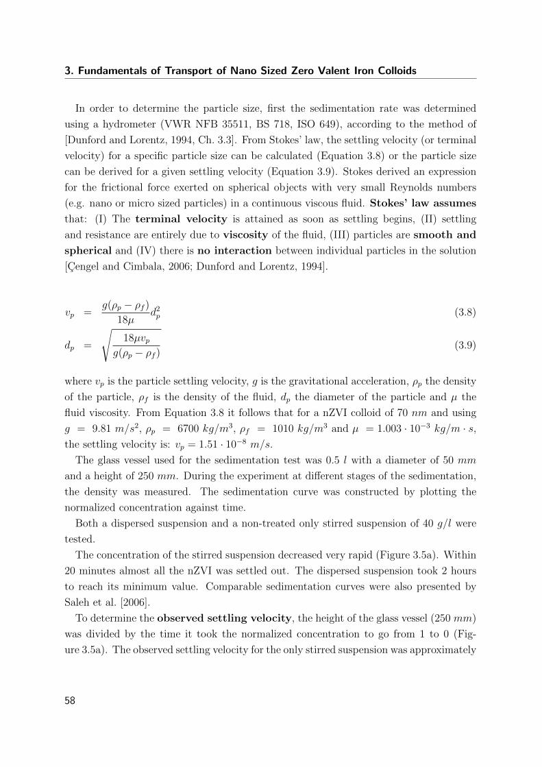
3. Fundamentals of Transport of Nano Sized Zero Valent Iron Colloids
In order to determine the particle size, first the sedimentation rate was determined
using a hydrometer (VWR NFB 35511, BS 718, ISO 649), according to the method of
[Dunford and Lorentz, 1994, Ch. 3.3]. From Stokes’ law, the settling velocity (or terminal
velocity) for a specific particle size can be calculated (Equation 3.8) or the particle size
can be derived for a given settling velocity (Equation 3.9). Stokes derived an expression
for the frictional force exerted on spherical objects with very small Reynolds numbers
(e.g. nano or micro sized particles) in a continuous viscous fluid. Stokes’ law assumes
that: (I) The terminal velocity is attained as soon as settling begins, (II) settling
and resistance are entirely due to viscosity of the fluid, (III) particles are smooth and
spherical and (IV) there is no interaction between individual particles in the solution
[Cengel and Cimbala, 2006; Dunford and Lorentz, 1994].
vp =g(ρp − ρf )
18µd2p (3.8)
dp =
√18µvp
g(ρp − ρf )(3.9)
where vp is the particle settling velocity, g is the gravitational acceleration, ρp the density
of the particle, ρf is the density of the fluid, dp the diameter of the particle and µ the
fluid viscosity. From Equation 3.8 it follows that for a nZVI colloid of 70 nm and using
g = 9.81 m/s2, ρp = 6700 kg/m3, ρf = 1010 kg/m3 and µ = 1.003 · 10−3 kg/m · s,the settling velocity is: vp = 1.51 · 10−8 m/s.
The glass vessel used for the sedimentation test was 0.5 l with a diameter of 50 mm
and a height of 250 mm. During the experiment at different stages of the sedimentation,
the density was measured. The sedimentation curve was constructed by plotting the
normalized concentration against time.
Both a dispersed suspension and a non-treated only stirred suspension of 40 g/l were
tested.
The concentration of the stirred suspension decreased very rapid (Figure 3.5a). Within
20 minutes almost all the nZVI was settled out. The dispersed suspension took 2 hours
to reach its minimum value. Comparable sedimentation curves were also presented by
Saleh et al. [2006].
To determine the observed settling velocity, the height of the glass vessel (250 mm)
was divided by the time it took the normalized concentration to go from 1 to 0 (Fig-
ure 3.5a). The observed settling velocity for the only stirred suspension was approximately
58
3.3. Characteristics of the nZVI Suspension
0
0.2
0.4
0.6
0.8
1
0 0.25 0.5 0.75 1 1.25 1.5 1.75 2 2.25 2.5
C/C
0 [-]
Time [h]
Stirred: f(x) = -3.3 x + 1Dispersed: g(x) = -0.49 x + 1
Stirred: vp = 2.32e-04 m/sDispersed: vp = 3.39e-05 m/s
Stirred: dp = 8.7 µmDispersed: dp = 3.3 µm
Stirred: ∆t = 0.2994 hDispersed: ∆t = 2.05 h
Stirred nZVIDispersed nZVI
Stirred fitDispersed fit
(a)
0
0.2
0.4
0.6
0.8
1
0 2 4 6
C/C
0 [-]
Time [h]
I: f(x) = -0.0092 x + 1II: g(x) = -0.86 x + 1.3
III: h(x) = -0.26 x + 0.61I: vp = 6.42e-07 m/s
II: vp = 5.96e-05 m/sIII: vp = 1.78e-05 m/s
I: ∆t = 108.2 hII: ∆t = 1.165 h
III: ∆t = 3.901 h
I: dp = 0.46 µmII: dp = 4.4 µmIII: dp = 2.4 µm
Dispersed nZVIIII
III
(b)
Figure 3.5: Concentration change due to sedimentation of nZVI. Both suspensions had aninitial concentration of 40 g/l
vstirredobs = 2.32 · 10−4 m/s and for the dispersed suspension vdispobs = 3.39 · 10−5 m/s.
These observed fall velocities are not even close to the calculated one. The assumption
that the colloids fall as single colloids has thus to be declined. With the assumption
that the colloids attach to each other while in suspension and colloid-colloid interaction
thus results in the formation of aggregates [Phenrat et al., 2007], an approximation
of the aggregate size can be made based on the observed fall velocity.
The determined velocities were used as the settling velocity in Stokes’ Law, to es-
timate the diameter of the aggregates (Equation 3.9). For the non-dispersed suspen-
sion this is: dstirredp = 8.7 · 10−6 m = 8.7 µm, and for the dispersed suspension:
ddispp = 3.3 · 10−6 m = 3.3 µm. This would mean that mean diameter of the aggre-
gates is approximately 50− 100 times the diameter of the primary colloids.
The above calculated diameters were based on the average sedimentation time. The
sedimentation curve of the dispersed suspension though shows three phases (Fig-
ure 3.5a) of sedimentation. (I) The first half hour shows almost no change in the
concentration, (II) then a rapid change occurs for about 40 minutes, (III) followed by
a slower change.
It can be reasoned that the differences are caused by aggregation effects and this aggre-
59
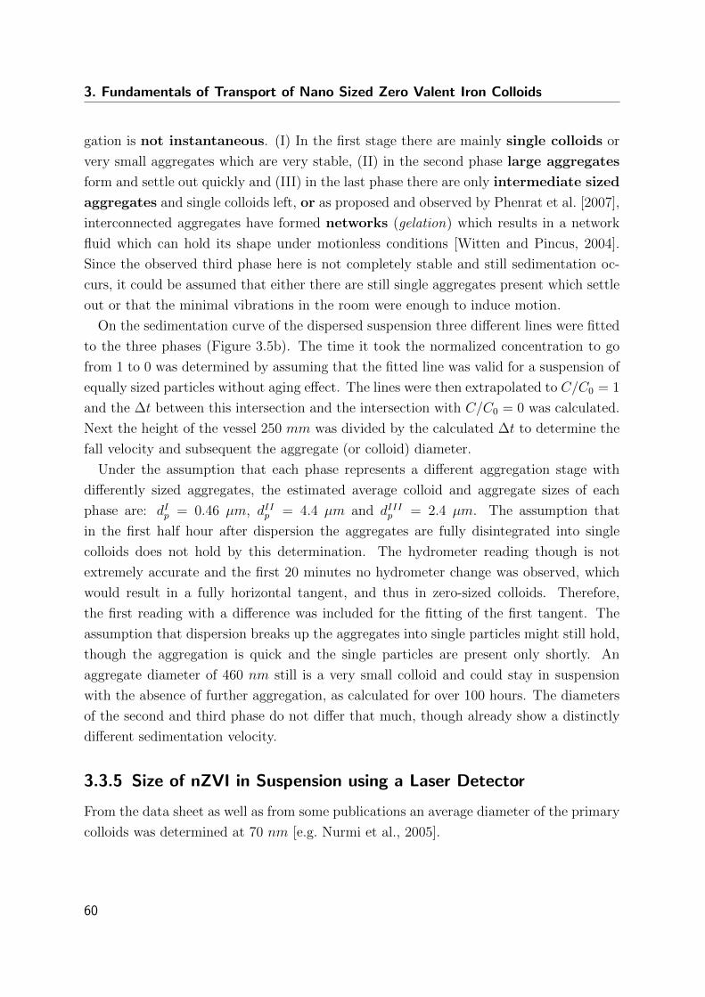
3. Fundamentals of Transport of Nano Sized Zero Valent Iron Colloids
gation is not instantaneous. (I) In the first stage there are mainly single colloids or
very small aggregates which are very stable, (II) in the second phase large aggregates
form and settle out quickly and (III) in the last phase there are only intermediate sized
aggregates and single colloids left, or as proposed and observed by Phenrat et al. [2007],
interconnected aggregates have formed networks (gelation) which results in a network
fluid which can hold its shape under motionless conditions [Witten and Pincus, 2004].
Since the observed third phase here is not completely stable and still sedimentation oc-
curs, it could be assumed that either there are still single aggregates present which settle
out or that the minimal vibrations in the room were enough to induce motion.
On the sedimentation curve of the dispersed suspension three different lines were fitted
to the three phases (Figure 3.5b). The time it took the normalized concentration to go
from 1 to 0 was determined by assuming that the fitted line was valid for a suspension of
equally sized particles without aging effect. The lines were then extrapolated to C/C0 = 1
and the ∆t between this intersection and the intersection with C/C0 = 0 was calculated.
Next the height of the vessel 250 mm was divided by the calculated ∆t to determine the
fall velocity and subsequent the aggregate (or colloid) diameter.
Under the assumption that each phase represents a different aggregation stage with
differently sized aggregates, the estimated average colloid and aggregate sizes of each
phase are: dIp = 0.46 µm, dIIp = 4.4 µm and dIIIp = 2.4 µm. The assumption that
in the first half hour after dispersion the aggregates are fully disintegrated into single
colloids does not hold by this determination. The hydrometer reading though is not
extremely accurate and the first 20 minutes no hydrometer change was observed, which
would result in a fully horizontal tangent, and thus in zero-sized colloids. Therefore,
the first reading with a difference was included for the fitting of the first tangent. The
assumption that dispersion breaks up the aggregates into single particles might still hold,
though the aggregation is quick and the single particles are present only shortly. An
aggregate diameter of 460 nm still is a very small colloid and could stay in suspension
with the absence of further aggregation, as calculated for over 100 hours. The diameters
of the second and third phase do not differ that much, though already show a distinctly
different sedimentation velocity.
3.3.5 Size of nZVI in Suspension using a Laser Detector
From the data sheet as well as from some publications an average diameter of the primary
colloids was determined at 70 nm [e.g. Nurmi et al., 2005].
60
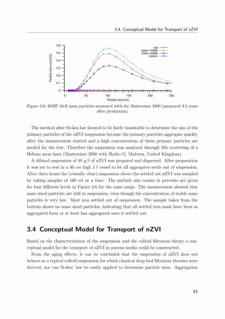
3.4. Conceptual Model for Transport of nZVI
0
0.1
0.2
0.3
0.4
0.5
0.6
0 50 100 150 200 250
Par
ticle
siz
e co
unt [
%]
Particle size [nm]
topupper middlelower middle
bottom
Figure 3.6: RNIP 10-E nano particles measured with the Mastersizer 2000 (measured 3.5 yearsafter production)
The method after Stokes law showed to be fairly unsuitable to determine the size of the
primary particles of the nZVI suspension because the primary particles aggregate quickly
after the measurement started and a high concentration of these primary particles are
needed for the test. Therefore the suspension was analyzed through Mie scattering of a
Helium neon laser (Mastersizer 2000 with Hydro G, Malvern, United Kingdom).
A diluted suspension of 40 g/l of nZVI was prepared and dispersed. After preparation
it was set to rest in a 40 cm high 1 l vessel to let all aggregates settle out of suspension.
After three hours the (visually clear) suspension above the settled out nZVI was sampled
by taking samples of 160 ml at a time. The particle size counts in percents are given
for four different levels in Figure 3.6 for the nano range. The measurement showed that
nano sized particles are still in suspension, even though the concentration of stable nano
particles is very low. Most iron settled out of suspension. The sample taken from the
bottom shows no nano sized particles, indicating that all settled iron must have been in
aggregated form or at least has aggregated once it settled out.
3.4 Conceptual Model for Transport of nZVI
Based on the characterization of the suspension and the colloid filtration theory a con-
ceptual model for the transport of nZVI in porous media could be constructed.
From the aging effects, it can be concluded that the suspension of nZVI does not
behave as a typical colloid suspension for which classical deep bed filtration theories were
derived, nor can Stokes’ law be easily applied to determine particle sizes. Aggregation
61
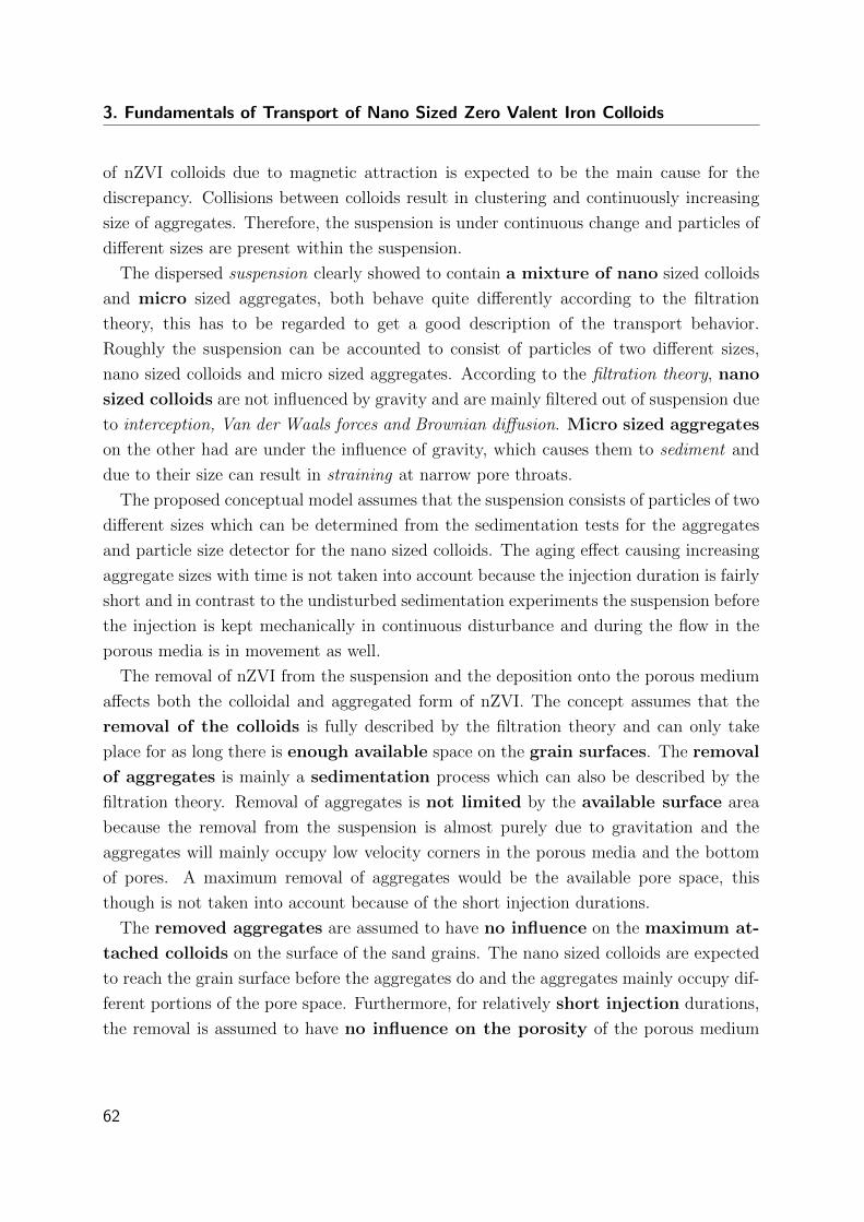
3. Fundamentals of Transport of Nano Sized Zero Valent Iron Colloids
of nZVI colloids due to magnetic attraction is expected to be the main cause for the
discrepancy. Collisions between colloids result in clustering and continuously increasing
size of aggregates. Therefore, the suspension is under continuous change and particles of
different sizes are present within the suspension.
The dispersed suspension clearly showed to contain a mixture of nano sized colloids
and micro sized aggregates, both behave quite differently according to the filtration
theory, this has to be regarded to get a good description of the transport behavior.
Roughly the suspension can be accounted to consist of particles of two different sizes,
nano sized colloids and micro sized aggregates. According to the filtration theory, nano
sized colloids are not influenced by gravity and are mainly filtered out of suspension due
to interception, Van der Waals forces and Brownian diffusion. Micro sized aggregates
on the other had are under the influence of gravity, which causes them to sediment and
due to their size can result in straining at narrow pore throats.
The proposed conceptual model assumes that the suspension consists of particles of two
different sizes which can be determined from the sedimentation tests for the aggregates
and particle size detector for the nano sized colloids. The aging effect causing increasing
aggregate sizes with time is not taken into account because the injection duration is fairly
short and in contrast to the undisturbed sedimentation experiments the suspension before
the injection is kept mechanically in continuous disturbance and during the flow in the
porous media is in movement as well.
The removal of nZVI from the suspension and the deposition onto the porous medium
affects both the colloidal and aggregated form of nZVI. The concept assumes that the
removal of the colloids is fully described by the filtration theory and can only take
place for as long there is enough available space on the grain surfaces. The removal
of aggregates is mainly a sedimentation process which can also be described by the
filtration theory. Removal of aggregates is not limited by the available surface area
because the removal from the suspension is almost purely due to gravitation and the
aggregates will mainly occupy low velocity corners in the porous media and the bottom
of pores. A maximum removal of aggregates would be the available pore space, this
though is not taken into account because of the short injection durations.
The removed aggregates are assumed to have no influence on the maximum at-
tached colloids on the surface of the sand grains. The nano sized colloids are expected
to reach the grain surface before the aggregates do and the aggregates mainly occupy dif-
ferent portions of the pore space. Furthermore, for relatively short injection durations,
the removal is assumed to have no influence on the porosity of the porous medium
62
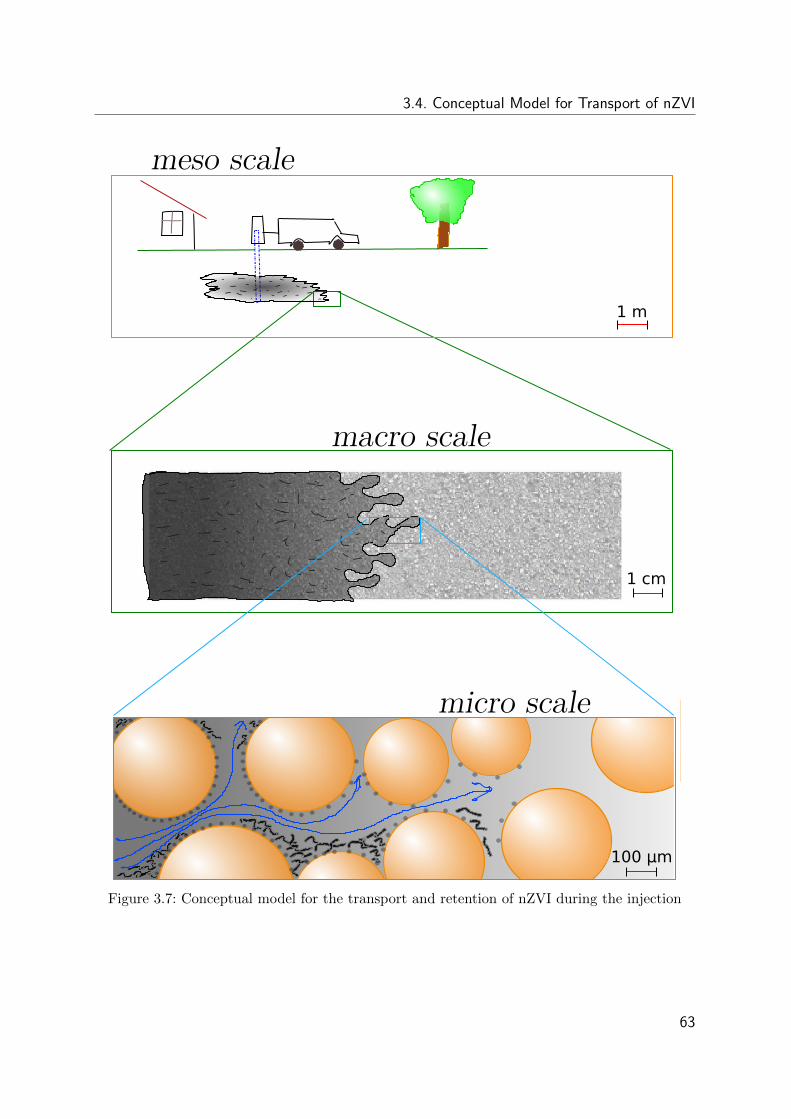
3.4. Conceptual Model for Transport of nZVI
1 cm
meso scale
macro scale
1 m
micro scale
100 µm
Figure 3.7: Conceptual model for the transport and retention of nZVI during the injection
63
3. Fundamentals of Transport of Nano Sized Zero Valent Iron Colloids
and the associated seepage velocity.
The conceptual model is graphically depicted in Figure 3.7, the model can be summa-
rized following:⊙Two sizes of particles: nano colloids, micro aggregates⊙Grain surface attachment of nano colloids, with a maximum due to availability of
surface area⊙Sedimentation and straining of micro aggregates, no maximum amount of ag-
gregates retained in porous media⊙The filtration theory of Tufenkji and Elimelech [2004] can describe the removal of
both the colloids and aggregates if regarded separately
3.5 Mathematical Model for Transport of nZVI
In the search for a good description of the transport of nZVI in porous media a robust
mathematical description of the transport is preferred. A robust mathematical description
in 1-D can easily be verified and fitted to column data and could provide the basis for
the prediction of nZVI transport in more dimensions and larger scales.
The presented mathematical model here describes the removal of nZVI from the sus-
pension in colloidal and aggregated form and its deposition onto the porous medium. The
approach assumes that the concentration of removed aggregates is a continuous addition
to the total concentration of nZVI removed from the suspension. The removed aggregates
are assumed to have no influence on the maximum attached colloids on the surface of the
sand grains. Therefore, the removed aggregates are added to the maximum attachable
colloid concentration, and thus, there is no maximum of nZVI in the porous media. This
limits the applicability of the model to relatively short injection durations (or respectively
small removal rates) since a prolonged injection (or high removal rate) would induce so
much solid phase to the system that the alteration of the porous medium would no longer
be negligible.
3.5.1 Groundwater Flow and Transport
The conservative transport of mass in a porous medium can be described by the governing
equation of mass transport combined with a continuity equation including hydrodynamic
64
3.5. Mathematical Model for Transport of nZVI
dispersion and advection:
n∂C
∂t+ C∇ · q + q∇C −∇ · (nD∇C) = 0 (3.10)
where C is the concentration of nZVI in suspension [ML−3], q the Darcy velocity vector
[LT−1], t time [T ], n porosity [−] and D the hydrodynamic dispersion tensor [L2T−1].
Taking into account only the component in the x-direction the conservative advection
dispersion equation becomes:
∂C
∂t+ v
∂C
∂x−Dl
∂2C
∂x2= 0 (3.11)
where v is the seepage velocity [LT−1] and Dl the longitudinal hydrodynamic dispersion
coefficient [L2T−1].
3.5.2 Transport and Kinetic Removal
Non-conservative transport of mass in a porous medium can be described by the mass
balance equation for the liquid phase (including hydrodynamic dispersion, advection and
a sink term) combined with the mass balance equation for the solid phase, that describes
the sink term of the first one. Assuming that the porosity is constant and the transport
only occurs in the direction of flow, the equation becomes:
∂C
∂t+ v
∂C
∂x−Dl
∂2C
∂x2= −ρb
n
∂S
∂t(3.12)
where S is the mass of nZVI per dry unit weight of sand [MM−1] and ρb the bulk density
(ρb = (1− n)ρs, with n the porosity and ρs the density of the sand).
3.5.3 nZVI Removal in Porous Media
The removal of colloids from the suspension, and with that the associated concentration
of colloids at the solid phase S, is here treated to be not only caused by the attachment on
the grain surface but also by the gravitational settling and straining effects of the colloids
and aggregates in the porous medium during transport.
It is here proposed to build up the removal of nZVI from the liquid phase in two parts,
kcolatt for the attachment on the grain surface due to colloid filtration of single colloids and
kaggatt to account for the removal of aggregates from the suspension. The sink term from
65
3. Fundamentals of Transport of Nano Sized Zero Valent Iron Colloids
Equation 3.12) is described by a kinetic version of the Langmuir sorption isotherm for the
removal of colloids due to filtration and a term to account for the continuous filtration of
the aggregates. This results in the following definition of the sink term:
∂S
∂t=
n
ρbkcolatt
(1− S
Smax
)C +
n
ρbkaggatt C − kdS (3.13)
where kcolatt and kaggatt represent the attachment- and kd the detachment coefficients [−] and
Smax the maximum amount of nZVI that can be attached at the solid phase [MM−1]. The
aggregates removed from the suspension are assumed to have no effect on the maximum
of colloids that can be attached on the grain surface, thus they were chosen to be added
to Smax, which was therefore defined by:
Smax = S0max + Sr (3.14)
where Sr represents the removed aggregates from the suspension (i.e. Sr = nρb−1kaggatt C).
Once these equations are substituted into Equation 3.13, it becomes clear that the total
mass of removed colloids will show an asymptotic behavior. Concentrations taking in
more space than available by the pore space are in theory possible. Though, it is assumed
that the injection duration is relatively short or the removal rates are respectively small,
avoiding the system to ever reach concentrations which could significantly fill up the pore
space. The removal of aggregates is proposed to also be described by using the contact
efficiency coefficient:
kaggatt =3(1− n)αaggηagg0 v
2dc(3.15)
where, ηagg0 is the contact efficiency coefficient calculated for the aggregates and αagg is
the aggregate removal efficiency. Since the aggregates are much bigger, the removal will
be mainly caused by sedimentation and straining and thus the available surface area of
the sand grains is less of importance, hence, a Langmuir isotherm is not expected to be
necessary for the removal of the aggregates.
It is assumed that furthermore for the transport of nZVI colloids, the desorption is
negligibly small and thus further has not to be taken into account. Together these
equations form the following flow, transport and kinetic removal equation:
66
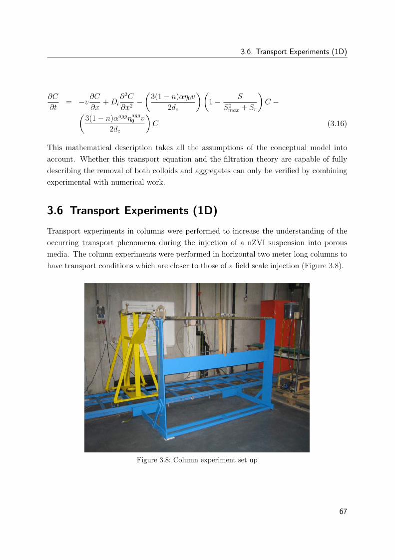
3.6. Transport Experiments (1D)
∂C
∂t= −v∂C
∂x+Dl
∂2C
∂x2−(
3(1− n)αη0v
2dc
)(1− S
S0max + Sr
)C −(
3(1− n)αaggηagg0 v
2dc
)C (3.16)
This mathematical description takes all the assumptions of the conceptual model into
account. Whether this transport equation and the filtration theory are capable of fully
describing the removal of both colloids and aggregates can only be verified by combining
experimental with numerical work.
3.6 Transport Experiments (1D)
Transport experiments in columns were performed to increase the understanding of the
occurring transport phenomena during the injection of a nZVI suspension into porous
media. The column experiments were performed in horizontal two meter long columns to
have transport conditions which are closer to those of a field scale injection (Figure 3.8).
Figure 3.8: Column experiment set up
67
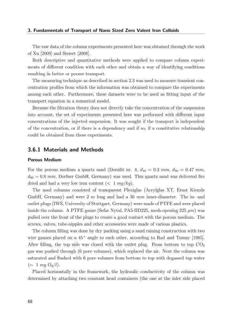
3. Fundamentals of Transport of Nano Sized Zero Valent Iron Colloids
The raw data of the column experiments presented here was obtained through the work
of Xu [2009] and Steiert [2008].
Both descriptive and quantitative methods were applied to compare column experi-
ments of different condition with each other and obtain a way of identifying conditions
resulting in better or poorer transport.
The measuring technique as described in section 2.3 was used to measure transient con-
centration profiles from which the information was obtained to compare the experiments
among each other. Furthermore, these datasets were to be used as fitting input of the
transport equation in a numerical model.
Because the filtration theory does not directly take the concentration of the suspension
into account, the set of experiments presented here was performed with different input
concentrations of the injected suspension. It was sought if the transport is independent
of the concentration, or if there is a dependency and if so, if a constitutive relationship
could be obtained from these experiments.
3.6.1 Materials and Methods
Porous Medium
For the porous medium a quartz sand (Dorsilit nr. 8, d10 = 0.3 mm, d50 = 0.47 mm,
d90 = 0.8 mm, Dorfner GmbH, Germany) was used. This quartz sand was delivered fire
dried and had a very low iron content (< 1 mg/kg).
The used columns consisted of transparent Plexiglas (Acrylglas XT, Ernst Kienzle
GmbH, Germany) and were 2 m long and had a 36 mm inner-diameter. The in- and
outlet plugs (IWS, University of Stuttgart, Germany) were made of PTFE and were placed
inside the column. A PTFE gauze (Sefar Nytal, PA5-HD225, mesh-opening 225 µm) was
pulled over the front of the plugs to create a good contact with the porous medium. The
screws, valves, tube-nipples and other accessories were made of various plastics.
The column filling was done by dry packing using a sand raining construction with two
wire gauzes placed on a 45 angle to each other, according to Rad and Tumay [1985].
After filling, the top side was closed with the outlet plug. From bottom to top CO2
gas was pushed through (6 pore volumes), which replaced the air. Next the column was
saturated and flushed with 6 pore volumes from bottom to top with degassed tap water
(∼ 1 mg O2/l).
Placed horizontally in the framework, the hydraulic conductivity of the column was
determined by attaching two constant head containers (the one at the inlet side placed
68
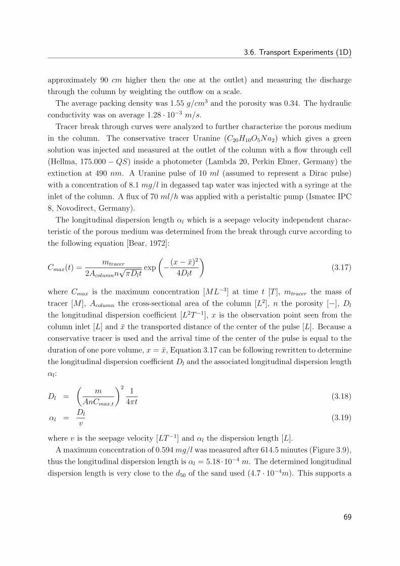
3.6. Transport Experiments (1D)
approximately 90 cm higher then the one at the outlet) and measuring the discharge
through the column by weighting the outflow on a scale.
The average packing density was 1.55 g/cm3 and the porosity was 0.34. The hydraulic
conductivity was on average 1.28 · 10−3 m/s.
Tracer break through curves were analyzed to further characterize the porous medium
in the column. The conservative tracer Uranine (C20H10O5Na2) which gives a green
solution was injected and measured at the outlet of the column with a flow through cell
(Hellma, 175.000 − QS) inside a photometer (Lambda 20, Perkin Elmer, Germany) the
extinction at 490 nm. A Uranine pulse of 10 ml (assumed to represent a Dirac pulse)
with a concentration of 8.1 mg/l in degassed tap water was injected with a syringe at the
inlet of the column. A flux of 70 ml/h was applied with a peristaltic pump (Ismatec IPC
8, Novodirect, Germany).
The longitudinal dispersion length αl which is a seepage velocity independent charac-
teristic of the porous medium was determined from the break through curve according to
the following equation [Bear, 1972]:
Cmax(t) =mtracer
2Acolumnn√πDlt
exp
(−(x− x)2
4Dlt
)(3.17)
where Cmax is the maximum concentration [ML−3] at time t [T ], mtracer the mass of
tracer [M ], Acolumn the cross-sectional area of the column [L2], n the porosity [−], Dl
the longitudinal dispersion coefficient [L2T−1], x is the observation point seen from the
column inlet [L] and x the transported distance of the center of the pulse [L]. Because a
conservative tracer is used and the arrival time of the center of the pulse is equal to the
duration of one pore volume, x = x, Equation 3.17 can be following rewritten to determine
the longitudinal dispersion coefficient Dl and the associated longitudinal dispersion length
αl:
Dl =
(m
AnCmax,t
)21
4πt(3.18)
αl =Dl
v(3.19)
where v is the seepage velocity [LT−1] and αl the dispersion length [L].
A maximum concentration of 0.594mg/l was measured after 614.5 minutes (Figure 3.9),
thus the longitudinal dispersion length is αl = 5.18 ·10−4 m. The determined longitudinal
dispersion length is very close to the d50 of the sand used (4.7 · 10−4m). This supports a
69
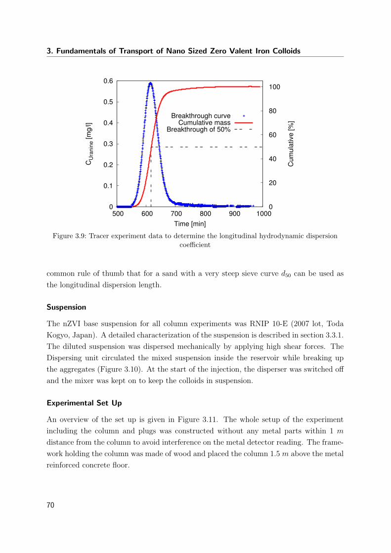
3. Fundamentals of Transport of Nano Sized Zero Valent Iron Colloids
0
0.1
0.2
0.3
0.4
0.5
0.6
500 600 700 800 900 1000 0
20
40
60
80
100C
Ura
nine
[mg/
l]
Cum
ulat
ive
[%]
Time [min]
Breakthrough curveCumulative mass
Breakthrough of 50%
Figure 3.9: Tracer experiment data to determine the longitudinal hydrodynamic dispersioncoefficient
common rule of thumb that for a sand with a very steep sieve curve d50 can be used as
the longitudinal dispersion length.
Suspension
The nZVI base suspension for all column experiments was RNIP 10-E (2007 lot, Toda
Kogyo, Japan). A detailed characterization of the suspension is described in section 3.3.1.
The diluted suspension was dispersed mechanically by applying high shear forces. The
Dispersing unit circulated the mixed suspension inside the reservoir while breaking up
the aggregates (Figure 3.10). At the start of the injection, the disperser was switched off
and the mixer was kept on to keep the colloids in suspension.
Experimental Set Up
An overview of the set up is given in Figure 3.11. The whole setup of the experiment
including the column and plugs was constructed without any metal parts within 1 m
distance from the column to avoid interference on the metal detector reading. The frame-
work holding the column was made of wood and placed the column 1.5 m above the metal
reinforced concrete floor.
70
3.6. Transport Experiments (1D)
Figure 3.10: Disperser connected to the nZVI reservoir with mixer
The constant head container at the outflow side was kept connected during the trans-
port experiment, the constant head at the inlet side was disconnected to connect a peri-
staltic pump (Watson Marlow 323, pump heads 318MC and 314X) for the injection of
the nZVI suspension. This pump could deliver a constant flux until a pressure of approx-
imately 0.2 bar (i.e. a gradient of 1 in this system). At higher pressures the discharge
reduces and eventually stops. To know the exact discharge throughout the experiment
the outflow was collected and weighted on a scale. The pressure was measured at the
inlet and outlet side with pressure sensors (DRTR 0−1.6 bar, HYGROSENS, Germany).
The hydraulic conductivity of the column could be measured by selecting the constant
head instead of the pump at the inlet using the 3-way valve. To inject the suspension
from the nZVI reservoir the 3-way valve was turned towards the pump. The water at
the outlet was collected and continuously weighed using a balance (DE 12K1A, Kern,
Germany) to know the exact discharge during the hydraulic conductivity measurement
and the injection.
The pressure sensors (PS1 and PS2) were connected in the vicinity of the in- and outlet
plugs.
71
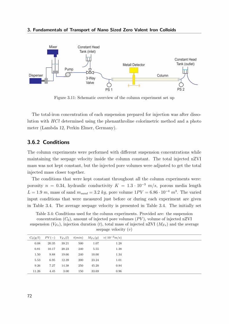
3. Fundamentals of Transport of Nano Sized Zero Valent Iron Colloids
Constant Head Tank (outlet)Metall Detector
Column
PumpDisperser
Mixer
PS 1
Constant Head Tank (inlet)
3-WayValve
PS 2
Figure 3.11: Schematic overview of the column experiment set up
The total-iron concentration of each suspension prepared for injection was after disso-
lution with HCl determined using the phenanthroline colorimetric method and a photo
meter (Lambda 12, Perkin Elmer, Germany).
3.6.2 Conditions
The column experiments were performed with different suspension concentrations while
maintaining the seepage velocity inside the column constant. The total injected nZVI
mass was not kept constant, but the injected pore volumes were adjusted to get the total
injected mass closer together.
The conditions that were kept constant throughout all the column experiments were:
porosity n = 0.34, hydraulic conductivity K = 1.3 · 10−3 m/s, porous media length
L = 1.9 m, mass of sand msand = 3.2 kg, pore volume 1PV = 6.86 · 10−4 m3. The varied
input conditions that were measured just before or during each experiment are given
in Table 3.4. The average seepage velocity is presented in Table 3.4. The initially set
Table 3.4: Conditions used for the column experiments. Provided are: the suspensionconcentration (C0), amount of injected pore volumes (PV ), volume of injected nZVI
suspension (VFe), injection duration (t), total mass of injected nZVI (MFe) and the averageseepage velocity (v)
C0(g/l) PV (−) VFe(l) t(min) MFe(g) v(·10−3m/s)
0.08 20.35 39.21 500 1.07 1.28
0.81 10.17 20.23 240 5.55 1.38
1.50 9.88 19.66 240 10.00 1.34
5.53 6.95 12.39 200 23.24 1.01
9.26 7.27 14.38 250 45.20 0.94
11.26 4.45 3.00 150 33.69 0.96
72
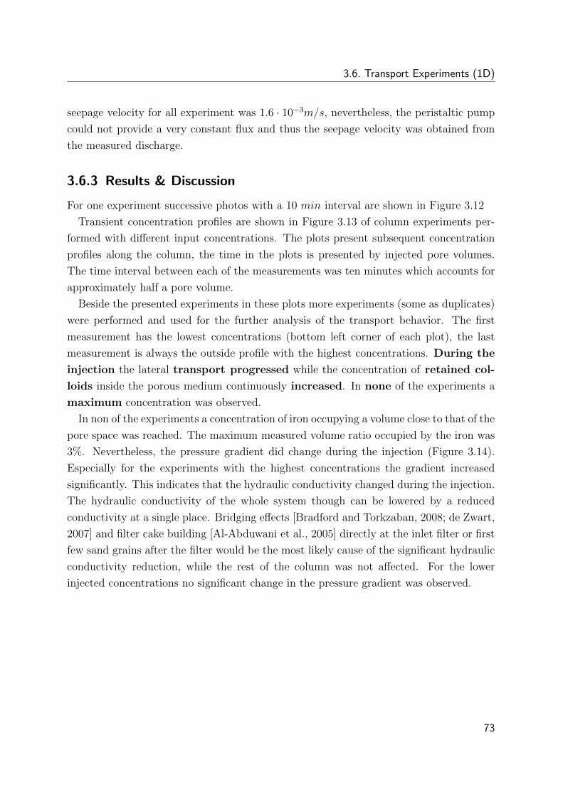
3.6. Transport Experiments (1D)
seepage velocity for all experiment was 1.6 · 10−3m/s, nevertheless, the peristaltic pump
could not provide a very constant flux and thus the seepage velocity was obtained from
the measured discharge.
3.6.3 Results & Discussion
For one experiment successive photos with a 10 min interval are shown in Figure 3.12
Transient concentration profiles are shown in Figure 3.13 of column experiments per-
formed with different input concentrations. The plots present subsequent concentration
profiles along the column, the time in the plots is presented by injected pore volumes.
The time interval between each of the measurements was ten minutes which accounts for
approximately half a pore volume.
Beside the presented experiments in these plots more experiments (some as duplicates)
were performed and used for the further analysis of the transport behavior. The first
measurement has the lowest concentrations (bottom left corner of each plot), the last
measurement is always the outside profile with the highest concentrations. During the
injection the lateral transport progressed while the concentration of retained col-
loids inside the porous medium continuously increased. In none of the experiments a
maximum concentration was observed.
In non of the experiments a concentration of iron occupying a volume close to that of the
pore space was reached. The maximum measured volume ratio occupied by the iron was
3%. Nevertheless, the pressure gradient did change during the injection (Figure 3.14).
Especially for the experiments with the highest concentrations the gradient increased
significantly. This indicates that the hydraulic conductivity changed during the injection.
The hydraulic conductivity of the whole system though can be lowered by a reduced
conductivity at a single place. Bridging effects [Bradford and Torkzaban, 2008; de Zwart,
2007] and filter cake building [Al-Abduwani et al., 2005] directly at the inlet filter or first
few sand grains after the filter would be the most likely cause of the significant hydraulic
conductivity reduction, while the rest of the column was not affected. For the lower
injected concentrations no significant change in the pressure gradient was observed.
73
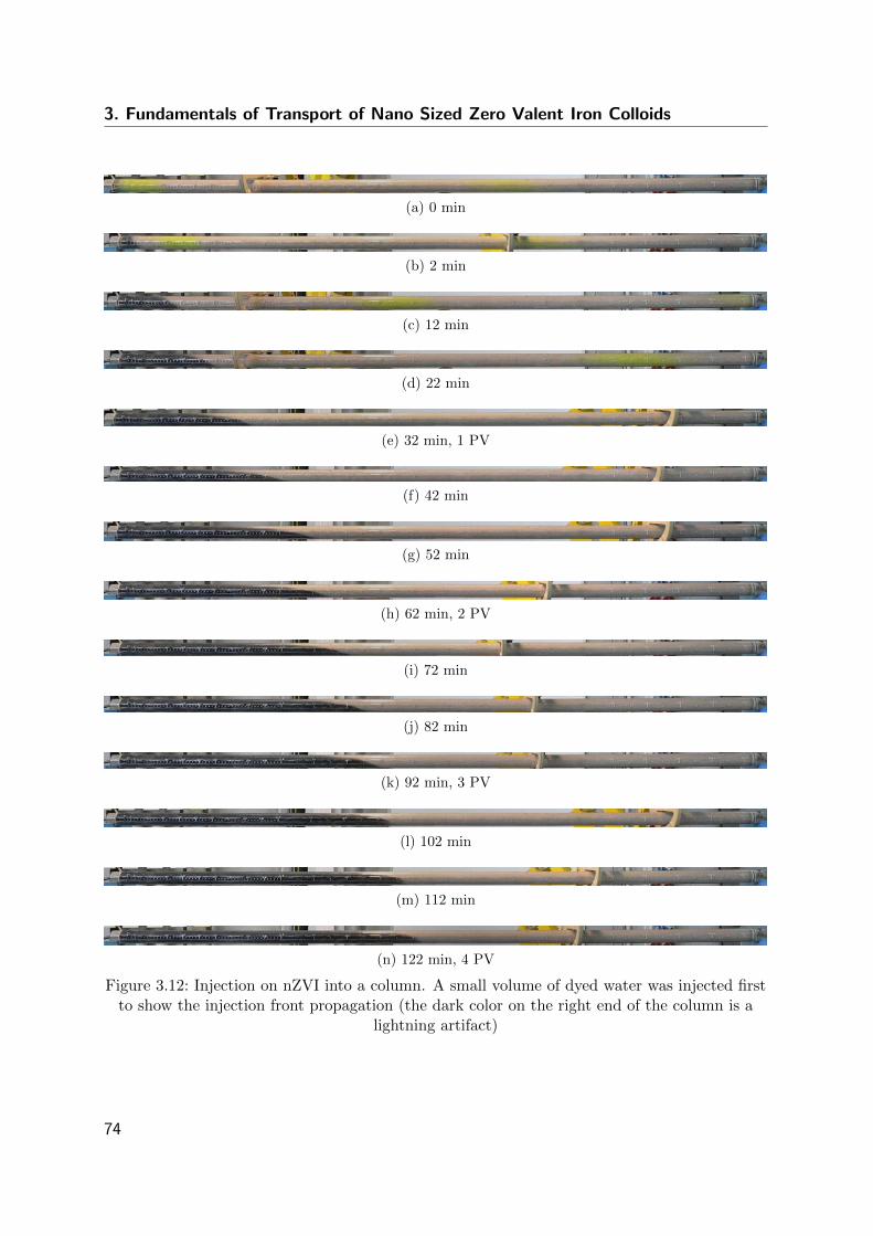
3. Fundamentals of Transport of Nano Sized Zero Valent Iron Colloids
(a) 0 min
(b) 2 min
(c) 12 min
(d) 22 min
(e) 32 min, 1 PV
(f) 42 min
(g) 52 min
(h) 62 min, 2 PV
(i) 72 min
(j) 82 min
(k) 92 min, 3 PV
(l) 102 min
(m) 112 min
(n) 122 min, 4 PV
Figure 3.12: Injection on nZVI into a column. A small volume of dyed water was injected firstto show the injection front propagation (the dark color on the right end of the column is a
lightning artifact)
74
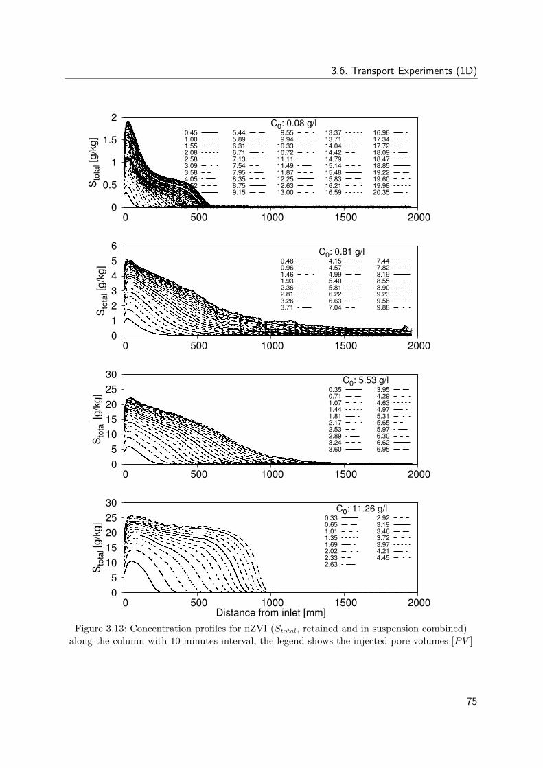
3.6. Transport Experiments (1D)
0
0.5
1
1.5
2
0 500 1000 1500 2000
Sto
tal [
g/kg
]
C0: 0.08 g/l0.451.001.552.082.583.093.584.054.524.98
5.445.896.316.717.137.547.958.358.759.15
9.559.94
10.3310.7211.1111.4911.8712.2512.6313.00
13.3713.7114.0414.4214.7915.1415.4815.8316.2116.59
16.9617.3417.7218.0918.4718.8519.2219.6019.9820.35
0 1 2 3 4 5 6
0 500 1000 1500 2000
Sto
tal [
g/kg
]
C0: 0.81 g/l0.480.961.461.932.362.813.263.71
4.154.574.995.405.816.226.637.04
7.447.828.198.558.909.239.569.88
0 5
10 15 20 25 30
0 500 1000 1500 2000
Sto
tal [
g/kg
]
C0: 5.53 g/l0.350.711.071.441.812.172.532.893.243.60
3.954.294.634.975.315.655.976.306.626.95
0 5
10 15 20 25 30
0 500 1000 1500 2000
Sto
tal [
g/kg
]
Distance from inlet [mm]
C0: 11.26 g/l0.330.651.011.351.692.022.332.63
2.923.193.463.723.974.214.45
Figure 3.13: Concentration profiles for nZVI (Stotal, retained and in suspension combined)along the column with 10 minutes interval, the legend shows the injected pore volumes [PV ]
75
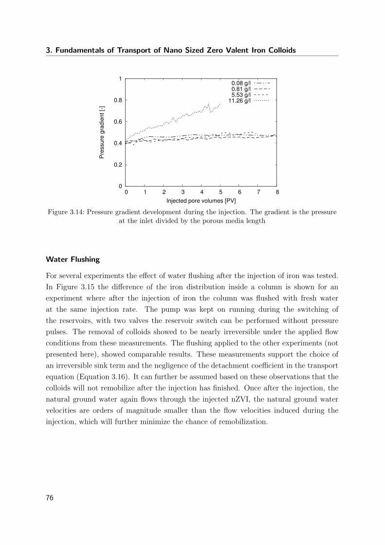
3. Fundamentals of Transport of Nano Sized Zero Valent Iron Colloids
0
0.2
0.4
0.6
0.8
1
0 1 2 3 4 5 6 7 8
Pre
ssur
e gr
adie
nt [-
]
Injected pore volumes [PV]
0.08 g/l0.81 g/l5.53 g/l
11.26 g/l
Figure 3.14: Pressure gradient development during the injection. The gradient is the pressureat the inlet divided by the porous media length
Water Flushing
For several experiments the effect of water flushing after the injection of iron was tested.
In Figure 3.15 the difference of the iron distribution inside a column is shown for an
experiment where after the injection of iron the column was flushed with fresh water
at the same injection rate. The pump was kept on running during the switching of
the reservoirs, with two valves the reservoir switch can be performed without pressure
pulses. The removal of colloids showed to be nearly irreversible under the applied flow
conditions from these measurements. The flushing applied to the other experiments (not
presented here), showed comparable results. These measurements support the choice of
an irreversible sink term and the negligence of the detachment coefficient in the transport
equation (Equation 3.16). It can further be assumed based on these observations that the
colloids will not remobilize after the injection has finished. Once after the injection, the
natural ground water again flows through the injected nZVI, the natural ground water
velocities are orders of magnitude smaller than the flow velocities induced during the
injection, which will further minimize the chance of remobilization.
76
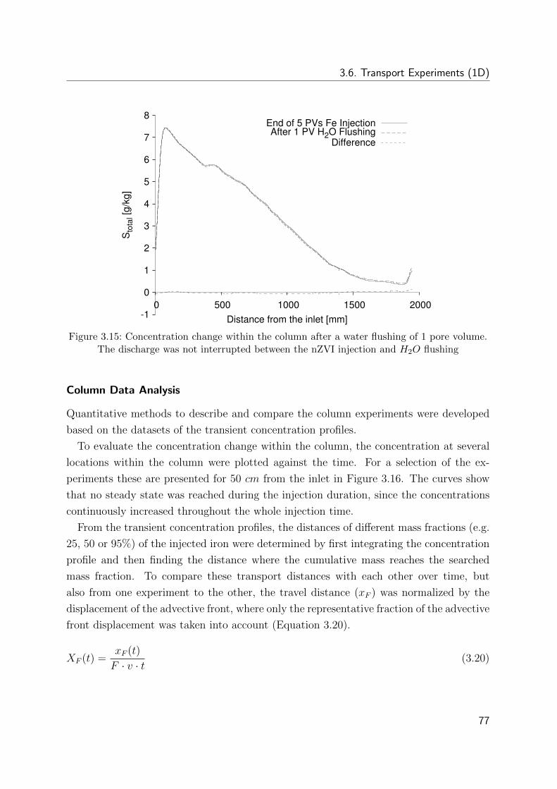
3.6. Transport Experiments (1D)
-1
0
1
2
3
4
5
6
7
8
0 500 1000 1500 2000
Sto
tal [
g/kg
]
Distance from the inlet [mm]
End of 5 PVs Fe InjectionAfter 1 PV H2O Flushing
Difference
Figure 3.15: Concentration change within the column after a water flushing of 1 pore volume.The discharge was not interrupted between the nZVI injection and H2O flushing
Column Data Analysis
Quantitative methods to describe and compare the column experiments were developed
based on the datasets of the transient concentration profiles.
To evaluate the concentration change within the column, the concentration at several
locations within the column were plotted against the time. For a selection of the ex-
periments these are presented for 50 cm from the inlet in Figure 3.16. The curves show
that no steady state was reached during the injection duration, since the concentrations
continuously increased throughout the whole injection time.
From the transient concentration profiles, the distances of different mass fractions (e.g.
25, 50 or 95%) of the injected iron were determined by first integrating the concentration
profile and then finding the distance where the cumulative mass reaches the searched
mass fraction. To compare these transport distances with each other over time, but
also from one experiment to the other, the travel distance (xF ) was normalized by the
displacement of the advective front, where only the representative fraction of the advective
front displacement was taken into account (Equation 3.20).
XF (t) =xF (t)
F · v · t (3.20)
77
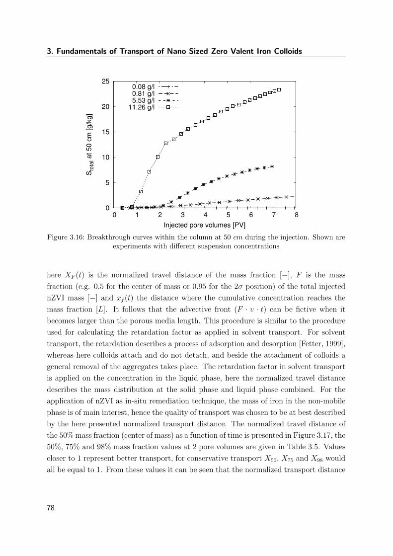
3. Fundamentals of Transport of Nano Sized Zero Valent Iron Colloids
0
5
10
15
20
25
0 1 2 3 4 5 6 7 8
Sto
tal a
t 50
cm [g
/kg]
Injected pore volumes [PV]
0.08 g/l0.81 g/l5.53 g/l
11.26 g/l
Figure 3.16: Breakthrough curves within the column at 50 cm during the injection. Shown areexperiments with different suspension concentrations
here XF (t) is the normalized travel distance of the mass fraction [−], F is the mass
fraction (e.g. 0.5 for the center of mass or 0.95 for the 2σ position) of the total injected
nZVI mass [−] and xf (t) the distance where the cumulative concentration reaches the
mass fraction [L]. It follows that the advective front (F · v · t) can be fictive when it
becomes larger than the porous media length. This procedure is similar to the procedure
used for calculating the retardation factor as applied in solvent transport. For solvent
transport, the retardation describes a process of adsorption and desorption [Fetter, 1999],
whereas here colloids attach and do not detach, and beside the attachment of colloids a
general removal of the aggregates takes place. The retardation factor in solvent transport
is applied on the concentration in the liquid phase, here the normalized travel distance
describes the mass distribution at the solid phase and liquid phase combined. For the
application of nZVI as in-situ remediation technique, the mass of iron in the non-mobile
phase is of main interest, hence the quality of transport was chosen to be at best described
by the here presented normalized transport distance. The normalized travel distance of
the 50% mass fraction (center of mass) as a function of time is presented in Figure 3.17, the
50%, 75% and 98% mass fraction values at 2 pore volumes are given in Table 3.5. Values
closer to 1 represent better transport, for conservative transport X50, X75 and X98 would
all be equal to 1. From these values it can be seen that the normalized transport distance
78
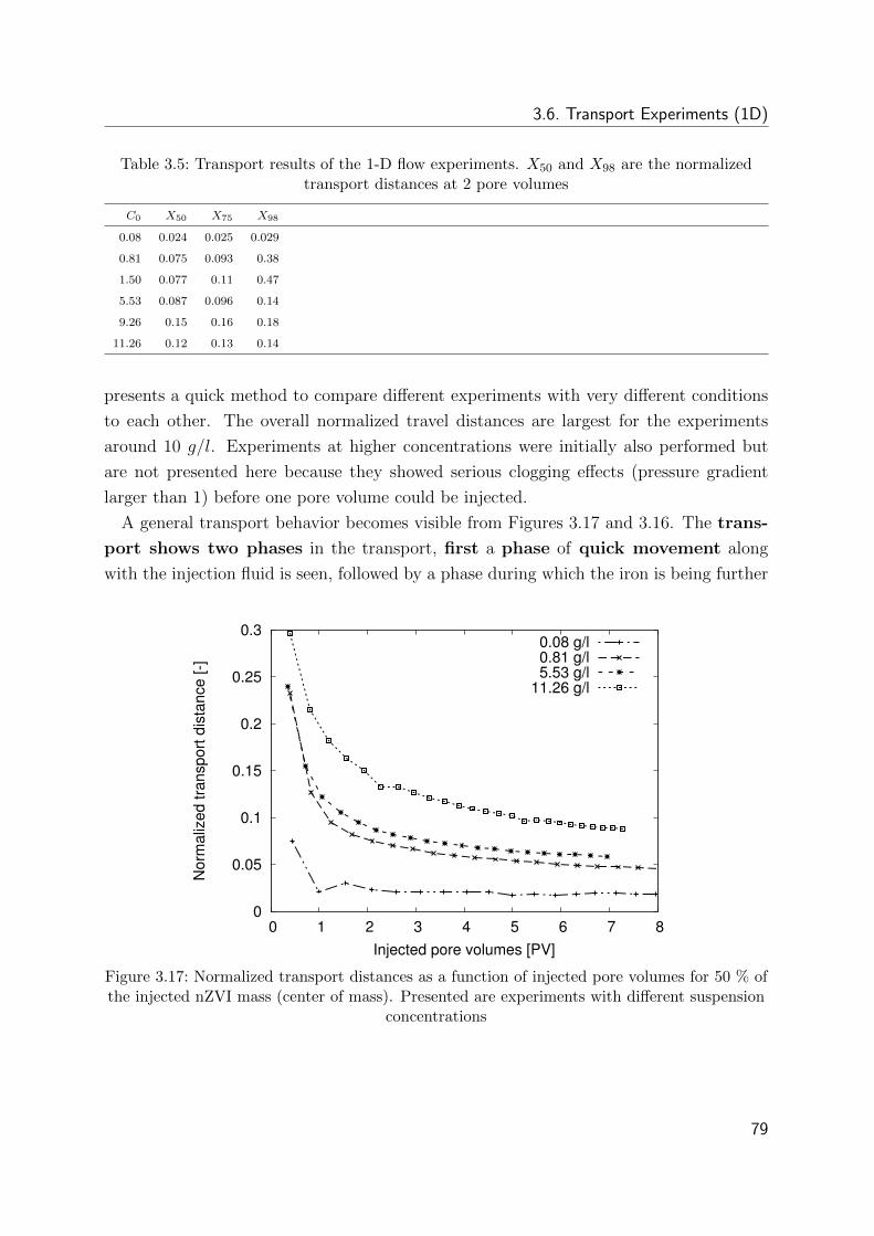
3.6. Transport Experiments (1D)
Table 3.5: Transport results of the 1-D flow experiments. X50 and X98 are the normalizedtransport distances at 2 pore volumes
C0 X50 X75 X98
0.08 0.024 0.025 0.029
0.81 0.075 0.093 0.38
1.50 0.077 0.11 0.47
5.53 0.087 0.096 0.14
9.26 0.15 0.16 0.18
11.26 0.12 0.13 0.14
presents a quick method to compare different experiments with very different conditions
to each other. The overall normalized travel distances are largest for the experiments
around 10 g/l. Experiments at higher concentrations were initially also performed but
are not presented here because they showed serious clogging effects (pressure gradient
larger than 1) before one pore volume could be injected.
A general transport behavior becomes visible from Figures 3.17 and 3.16. The trans-
port shows two phases in the transport, first a phase of quick movement along
with the injection fluid is seen, followed by a phase during which the iron is being further
0
0.05
0.1
0.15
0.2
0.25
0.3
0 1 2 3 4 5 6 7 8
Nor
mal
ized
tran
spor
t dis
tanc
e [-]
Injected pore volumes [PV]
0.08 g/l0.81 g/l5.53 g/l
11.26 g/l
Figure 3.17: Normalized transport distances as a function of injected pore volumes for 50 % ofthe injected nZVI mass (center of mass). Presented are experiments with different suspension
concentrations
79
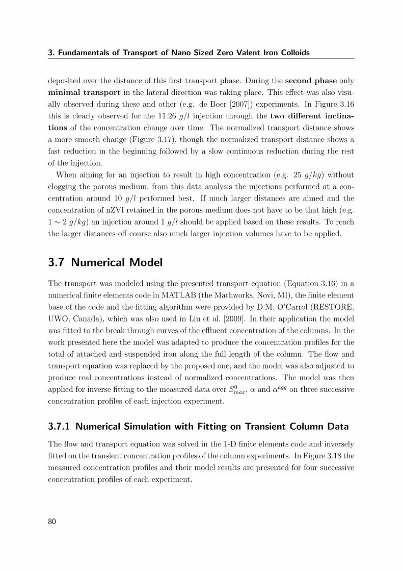
3. Fundamentals of Transport of Nano Sized Zero Valent Iron Colloids
deposited over the distance of this first transport phase. During the second phase only
minimal transport in the lateral direction was taking place. This effect was also visu-
ally observed during these and other (e.g. de Boer [2007]) experiments. In Figure 3.16
this is clearly observed for the 11.26 g/l injection through the two different inclina-
tions of the concentration change over time. The normalized transport distance shows
a more smooth change (Figure 3.17), though the normalized transport distance shows a
fast reduction in the beginning followed by a slow continuous reduction during the rest
of the injection.
When aiming for an injection to result in high concentration (e.g. 25 g/kg) without
clogging the porous medium, from this data analysis the injections performed at a con-
centration around 10 g/l performed best. If much larger distances are aimed and the
concentration of nZVI retained in the porous medium does not have to be that high (e.g.
1 ∼ 2 g/kg) an injection around 1 g/l should be applied based on these results. To reach
the larger distances off course also much larger injection volumes have to be applied.
3.7 Numerical Model
The transport was modeled using the presented transport equation (Equation 3.16) in a
numerical finite elements code in MATLAB (the Mathworks, Novi, MI), the finite element
base of the code and the fitting algorithm were provided by D.M. O’Carrol (RESTORE,
UWO, Canada), which was also used in Liu et al. [2009]. In their application the model
was fitted to the break through curves of the effluent concentration of the columns. In the
work presented here the model was adapted to produce the concentration profiles for the
total of attached and suspended iron along the full length of the column. The flow and
transport equation was replaced by the proposed one, and the model was also adjusted to
produce real concentrations instead of normalized concentrations. The model was then
applied for inverse fitting to the measured data over S0max, α and αagg on three successive
concentration profiles of each injection experiment.
3.7.1 Numerical Simulation with Fitting on Transient Column Data
The flow and transport equation was solved in the 1-D finite elements code and inversely
fitted on the transient concentration profiles of the column experiments. In Figure 3.18 the
measured concentration profiles and their model results are presented for four successive
concentration profiles of each experiment.
80
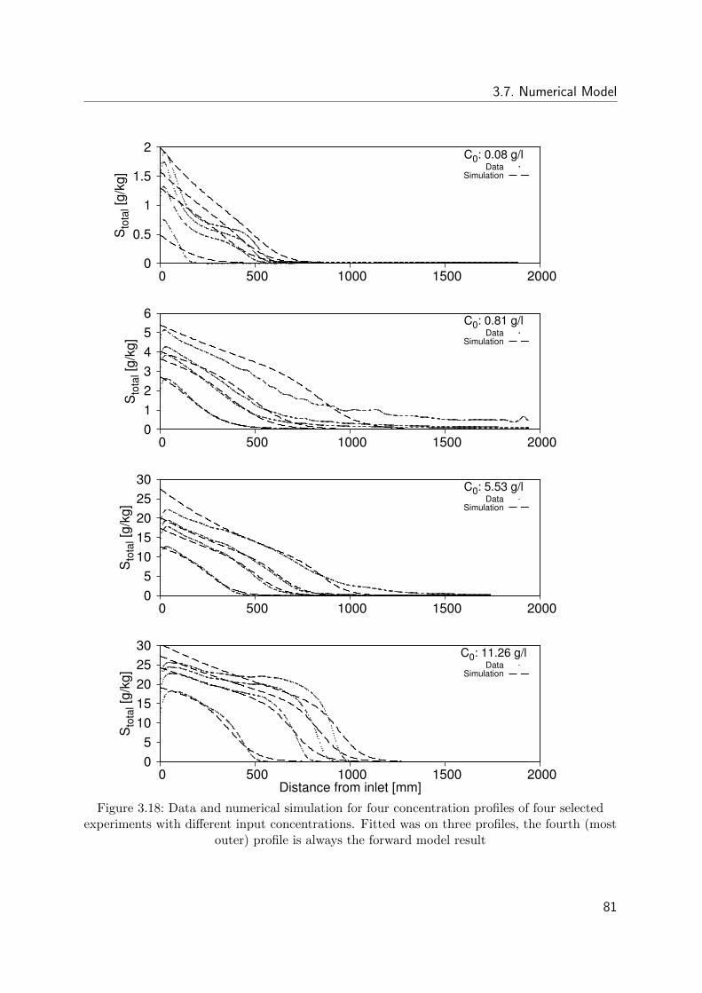
3.7. Numerical Model
0
0.5
1
1.5
2
0 500 1000 1500 2000
Sto
tal [
g/kg
]
C0: 0.08 g/lData
Simulation
0 1 2 3 4 5 6
0 500 1000 1500 2000
Sto
tal [
g/kg
]
C0: 0.81 g/lData
Simulation
0 5
10 15 20 25 30
0 500 1000 1500 2000
Sto
tal [
g/kg
]
C0: 5.53 g/lData
Simulation
0 5
10 15 20 25 30
0 500 1000 1500 2000
Sto
tal [
g/kg
]
Distance from inlet [mm]
C0: 11.26 g/lData
Simulation
Figure 3.18: Data and numerical simulation for four concentration profiles of four selectedexperiments with different input concentrations. Fitted was on three profiles, the fourth (most
outer) profile is always the forward model result
81
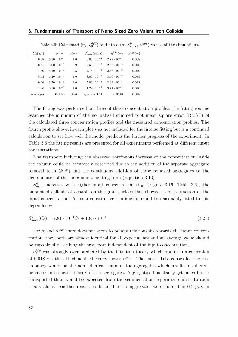
3. Fundamentals of Transport of Nano Sized Zero Valent Iron Colloids
Table 3.6: Calculated (η0, ηagg0 ) and fitted (α, S0max, αagg) values of the simulations.
C0(g/l) η0(−) α(−) S0max(g/kg) ηagg0 (−) αagg(−)
0.08 5.30 · 10−3 1.0 6.08 · 10−4 2.77 · 10−2 0.038
0.81 5.00 · 10−3 0.9 2.53 · 10−3 2.56 · 10−2 0.016
1.50 5.10 · 10−3 0.3 4.13 · 10−3 2.66 · 10−2 0.010
5.53 6.20 · 10−3 1.0 8.00 · 10−3 3.46 · 10−2 0.019
9.26 6.70 · 10−3 1.0 5.00 · 10−3 3.92 · 10−2 0.018
11.26 6.50 · 10−3 1.0 1.29 · 10−2 3.71 · 10−2 0.010
Averages 0.0058 0.86 Equation 3.21 0.0318 0.018
The fitting was performed on three of these concentration profiles, the fitting routine
searches the minimum of the normalized summed root mean square error (RMSE) of
the calculated three concentration profiles and the measured concentration profiles. The
fourth profile shown in each plot was not included for the inverse fitting but is a continued
calculation to see how well the model predicts the further progress of the experiment. In
Table 3.6 the fitting results are presented for all experiments performed at different input
concentrations.
The transport including the observed continuous increase of the concentration inside
the column could be accurately described due to the addition of the separate aggregate
removal term (kaggatt ) and the continuous addition of these removed aggregates to the
denominator of the Langmuir weighting term (Equation 3.16).
S0max increases with higher input concentration (C0) (Figure 3.19, Table 3.6), the
amount of colloids attachable on the grain surface thus showed to be a function of the
input concentration. A linear constitutive relationship could be reasonably fitted to this
dependency:
S0max(C0) = 7.81 · 10−4C0 + 1.83 · 10−3 (3.21)
For α and αagg there does not seem to be any relationship towards the input concen-
tration, they both are almost identical for all experiments and an average value should
be capable of describing the transport independent of the input concentration.
ηagg0 was strongly over predicted by the filtration theory which results in a correction
of 0.018 via the attachment efficiency factor αagg. The most likely causes for the dis-
crepancy would be the non-spherical shape of the aggregates which results in different
behavior and a lower density of the aggregates. Aggregates thus clearly get much better
transported than would be expected from the sedimentation experiments and filtration
theory alone. Another reason could be that the aggregates were more than 0.5 µm, in
82
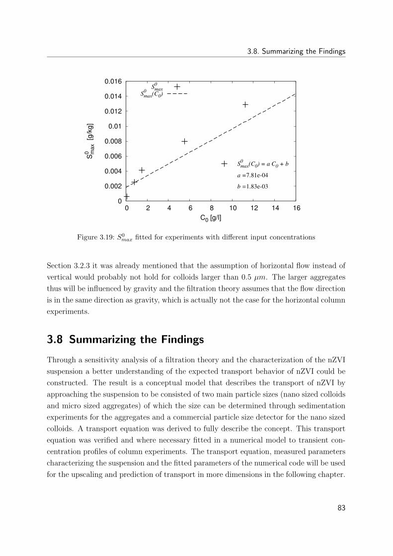
3.8. Summarizing the Findings
0
0.002
0.004
0.006
0.008
0.01
0.012
0.014
0.016
0 2 4 6 8 10 12 14 16
S0 m
ax [
g/kg
]
C0 [g/l]
S0max(C0) = a C0 + b
a =7.81e-04
b =1.83e-03
S0max
S0max(C0)
Figure 3.19: S0max fitted for experiments with different input concentrations
Section 3.2.3 it was already mentioned that the assumption of horizontal flow instead of
vertical would probably not hold for colloids larger than 0.5 µm. The larger aggregates
thus will be influenced by gravity and the filtration theory assumes that the flow direction
is in the same direction as gravity, which is actually not the case for the horizontal column
experiments.
3.8 Summarizing the Findings
Through a sensitivity analysis of a filtration theory and the characterization of the nZVI
suspension a better understanding of the expected transport behavior of nZVI could be
constructed. The result is a conceptual model that describes the transport of nZVI by
approaching the suspension to be consisted of two main particle sizes (nano sized colloids
and micro sized aggregates) of which the size can be determined through sedimentation
experiments for the aggregates and a commercial particle size detector for the nano sized
colloids. A transport equation was derived to fully describe the concept. This transport
equation was verified and where necessary fitted in a numerical model to transient con-
centration profiles of column experiments. The transport equation, measured parameters
characterizing the suspension and the fitted parameters of the numerical code will be used
for the upscaling and prediction of transport in more dimensions in the following chapter.
83

3. Fundamentals of Transport of Nano Sized Zero Valent Iron Colloids
84
4 Colloid Transport in a Radial Flow
Field
4.1 Motivation
Column experiments as described in Section 3.6 give an indication on how nZVI is being
transported in a 1-D geometry. They cannot be directly used to predict field conditions
or to design a pilot or full remediation. Therefore, research of two and three dimensional
transport behavior at a near field scale would be preferable.
So far, in the literature, most of the research, has been done on column experiments,
and transport was characterized in only one dimension. Less research has been done
into the two and three dimensional description of transport of nZVI. Most of the studies
involving two or three dimensions, use small scale flume experiments [Kanel et al., 2008;
Phenrat et al., 2010, 2011]. Although the basic transport mechanisms of nZVI transport
in porous media must be understood before accurate predictions of transport can be made,
one dimensional models and experiments are insufficient to describe the rapid decrease
of the seepage velocity in a radial flow field around an injection well. Furthermore,
flume experiments at small scales do not sufficiently reproduce the results of field scale
injections.
Here, three different methods were developed to get a better description and prediction
possibility of nZVI transport in radial full scale flow fields. (I) Large near field scale con-
tainer experiments, (II) experiments using multiple columns and boundary conditions to
experimentally discretize a radial flow field, and (III) the transfer of calibrated parameters
from the 1-D model (Section 3.7) to run forward simulations of radial flow.
85
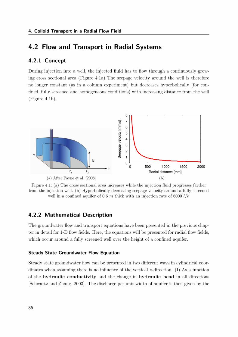
4. Colloid Transport in a Radial Flow Field
4.2 Flow and Transport in Radial Systems
4.2.1 Concept
During injection into a well, the injected fluid has to flow through a continuously grow-
ing cross sectional area (Figure 4.1a) The seepage velocity around the well is therefore
no longer constant (as in a column experiment) but decreases hyperbolically (for con-
fined, fully screened and homogeneous conditions) with increasing distance from the well
(Figure 4.1b).
(a) After Payne et al. [2008]
0
1
2
3
4
5
6
7
8
0 500 1000 1500 2000
See
page
vel
ocity
[mm
/s]
Radial distance [mm]
(b)
Figure 4.1: (a) The cross sectional area increases while the injection fluid progresses fartherfrom the injection well. (b) Hyperbolically decreasing seepage velocity around a fully screened
well in a confined aquifer of 0.6 m thick with an injection rate of 6000 l/h
4.2.2 Mathematical Description
The groundwater flow and transport equations have been presented in the previous chap-
ter in detail for 1-D flow fields. Here, the equations will be presented for radial flow fields,
which occur around a fully screened well over the height of a confined aquifer.
Steady State Groundwater Flow Equation
Steady state groundwater flow can be presented in two different ways in cylindrical coor-
dinates when assuming there is no influence of the vertical z-direction. (I) As a function
of the hydraulic conductivity and the change in hydraulic head in all directions
[Schwartz and Zhang, 2003]. The discharge per unit width of aquifer is then given by the
86
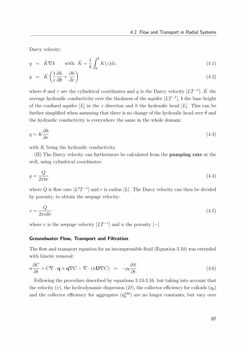
4.2. Flow and Transport in Radial Systems
Darcy velocity:
q = K∇h with: K =1
b
∫ b
0
K(z)dz (4.1)
q = K
(1
r
∂h
∂θ+∂h
∂r
)(4.2)
where θ and r are the cylindrical coordinates and q is the Darcy velocity [LT−1], K the
average hydraulic conductivity over the thickness of the aquifer [LT−1], b the base height
of the confined aquifer [L] in the z direction and h the hydraulic head [L]. This can be
further simplified when assuming that there is no change of the hydraulic head over θ and
the hydraulic conductivity is everywhere the same in the whole domain:
q = K∂h
∂r(4.3)
with K being the hydraulic conductivity.
(II) The Darcy velocity can furthermore be calculated from the pumping rate at the
well, using cylindrical coordinates:
q =Q
2πbr(4.4)
where Q is flow rate [L3T−1] and r is radius [L]. The Darcy velocity can then be divided
by porosity, to obtain the seepage velocity:
v =Q
2πnbr(4.5)
where v is the seepage velocity [LT−1] and n the porosity [−].
Groundwater Flow, Transport and Filtration
The flow and transport equation for an incompressible fluid (Equation 3.10) was extended
with kinetic removal:
n∂C
∂t+ C∇ · q + q∇C −∇ · (nD∇C) = −ρb
∂S
∂t(4.6)
Following the procedure described by equations 3.13-3.16, but taking into account that
the velocity (v), the hydrodynamic dispersion (D), the collector efficiency for colloids (η0)
and the collector efficiency for aggregates (ηagg0 ) are no longer constants, but vary over
87
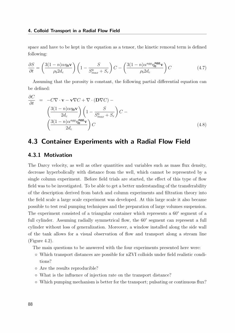
4. Colloid Transport in a Radial Flow Field
space and have to be kept in the equation as a tensor, the kinetic removal term is defined
following:
∂S
∂t=
(3(1− n)αη0v
ρb2dc
)(1− S
S0max + Sr
)C −
(3(1− n)αaggηagg0 v
ρb2dc
)C (4.7)
Assuming that the porosity is constant, the following partial differential equation can
be defined:
∂C
∂t= −C∇ · v − v∇C +∇ · (D∇C)−(
3(1− n)αη0v
2dc
)(1− S
S0max + Sr
)C −(
3(1− n)αaggηagg0 v
2dc
)C (4.8)
4.3 Container Experiments with a Radial Flow Field
4.3.1 Motivation
The Darcy velocity, as well as other quantities and variables such as mass flux density,
decrease hyperbolically with distance from the well, which cannot be represented by a
single column experiment. Before field trials are started, the effect of this type of flow
field was to be investigated. To be able to get a better understanding of the transferability
of the description derived from batch and column experiments and filtration theory into
the field scale a large scale experiment was developed. At this large scale it also became
possible to test real pumping techniques and the preparation of large volumes suspension.
The experiment consisted of a triangular container which represents a 60° segment of a
full cylinder. Assuming radially symmetrical flow, the 60° segment can represent a full
cylinder without loss of generalization. Moreover, a window installed along the side wall
of the tank allows for a visual observation of flow and transport along a stream line
(Figure 4.2).
The main questions to be answered with the four experiments presented here were:
Which transport distances are possible for nZVI colloids under field realistic condi-
tions?
Are the results reproducible?
What is the influence of injection rate on the transport distance?
Which pumping mechanism is better for the transport; pulsating or continuous flux?
88
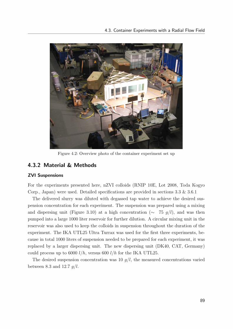
4.3. Container Experiments with a Radial Flow Field
Figure 4.2: Overview photo of the container experiment set up
4.3.2 Material & Methods
ZVI Suspensions
For the experiments presented here, nZVI colloids (RNIP 10E, Lot 2008, Toda Kogyo
Corp., Japan) were used. Detailed specifications are provided in sections 3.3 & 3.6.1
The delivered slurry was diluted with degassed tap water to achieve the desired sus-
pension concentration for each experiment. The suspension was prepared using a mixing
and dispersing unit (Figure 3.10) at a high concentration (∼ 75 g/l), and was then
pumped into a large 1000 liter reservoir for further dilution. A circular mixing unit in the
reservoir was also used to keep the colloids in suspension throughout the duration of the
experiment. The IKA UTL25 Ultra Turrax was used for the first three experiments, be-
cause in total 1000 liters of suspension needed to be prepared for each experiment, it was
replaced by a larger dispersing unit. The new dispersing unit (DK40, CAT, Germany)
could process up to 6000 l/h, versus 600 l/h for the IKA UTL25.
The desired suspension concentration was 10 g/l, the measured concentrations varied
between 8.3 and 12.7 g/l.
89
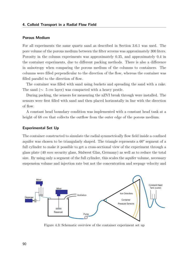
4. Colloid Transport in a Radial Flow Field
Porous Medium
For all experiments the same quartz sand as described in Section 3.6.1 was used. The
pore volume of the porous medium between the filter screens was approximately 300 liters.
Porosity in the column experiments was approximately 0.35, and approximately 0.4 in
the container experiments, due to different packing methods. There is also a difference
in anisotropy when comparing the porous medium of the columns to containers. The
columns were filled perpendicular to the direction of the flow, whereas the container was
filled parallel to the direction of flow.
The container was filled with sand using buckets and spreading the sand with a rake.
The sand (∼ 5 cm layer) was compacted with a heavy pestle.
During packing, the sensors for measuring the nZVI break through were installed. The
sensors were first filled with sand and then placed horizontally in line with the direction
of flow.
A constant head boundary condition was implemented with a constant head tank at a
height of 68 cm that collects the outflow from the outer edge of the porous medium.
Experimental Set Up
The container constructed to simulate the radial symmetrically flow field inside a confined
aquifer was chosen to be triangularly shaped. The triangle represents a 60° segment of a
full cylinder to make it possible to get a cross-sectional view of the experiment through a
glass plate (40 mm security glass, Sudwest Glas, Germany) as well as to reduce the total
size. By using only a segment of the full cylinder, this scales the aquifer volume, necessary
suspension volume and injection rate but not the concentration and seepage velocity and
Figure 4.3: Schematic overview of the container experiment set up
90
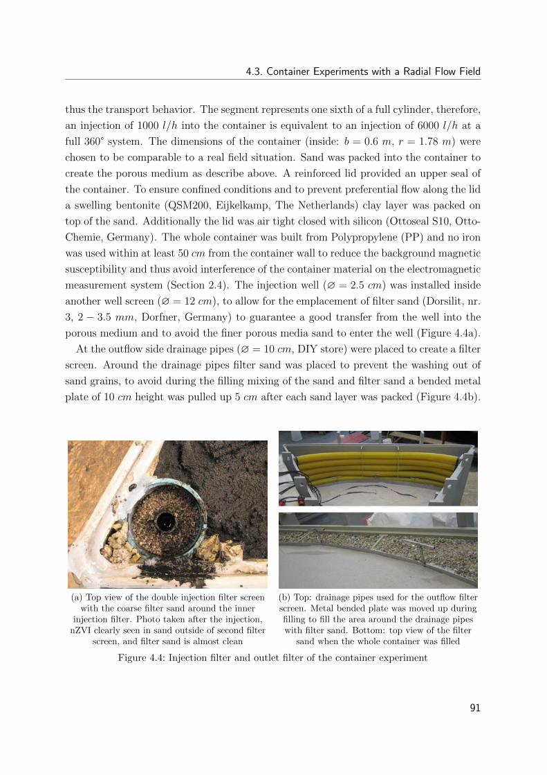
4.3. Container Experiments with a Radial Flow Field
thus the transport behavior. The segment represents one sixth of a full cylinder, therefore,
an injection of 1000 l/h into the container is equivalent to an injection of 6000 l/h at a
full 360° system. The dimensions of the container (inside: b = 0.6 m, r = 1.78 m) were
chosen to be comparable to a real field situation. Sand was packed into the container to
create the porous medium as describe above. A reinforced lid provided an upper seal of
the container. To ensure confined conditions and to prevent preferential flow along the lid
a swelling bentonite (QSM200, Eijkelkamp, The Netherlands) clay layer was packed on
top of the sand. Additionally the lid was air tight closed with silicon (Ottoseal S10, Otto-
Chemie, Germany). The whole container was built from Polypropylene (PP) and no iron
was used within at least 50 cm from the container wall to reduce the background magnetic
susceptibility and thus avoid interference of the container material on the electromagnetic
measurement system (Section 2.4). The injection well (∅ = 2.5 cm) was installed inside
another well screen (∅ = 12 cm), to allow for the emplacement of filter sand (Dorsilit, nr.
3, 2 − 3.5 mm, Dorfner, Germany) to guarantee a good transfer from the well into the
porous medium and to avoid the finer porous media sand to enter the well (Figure 4.4a).
At the outflow side drainage pipes (∅ = 10 cm, DIY store) were placed to create a filter
screen. Around the drainage pipes filter sand was placed to prevent the washing out of
sand grains, to avoid during the filling mixing of the sand and filter sand a bended metal
plate of 10 cm height was pulled up 5 cm after each sand layer was packed (Figure 4.4b).
(a) Top view of the double injection filter screenwith the coarse filter sand around the inner
injection filter. Photo taken after the injection,nZVI clearly seen in sand outside of second filter
screen, and filter sand is almost clean
(b) Top: drainage pipes used for the outflow filterscreen. Metal bended plate was moved up duringfilling to fill the area around the drainage pipeswith filter sand. Bottom: top view of the filter
sand when the whole container was filled
Figure 4.4: Injection filter and outlet filter of the container experiment
91
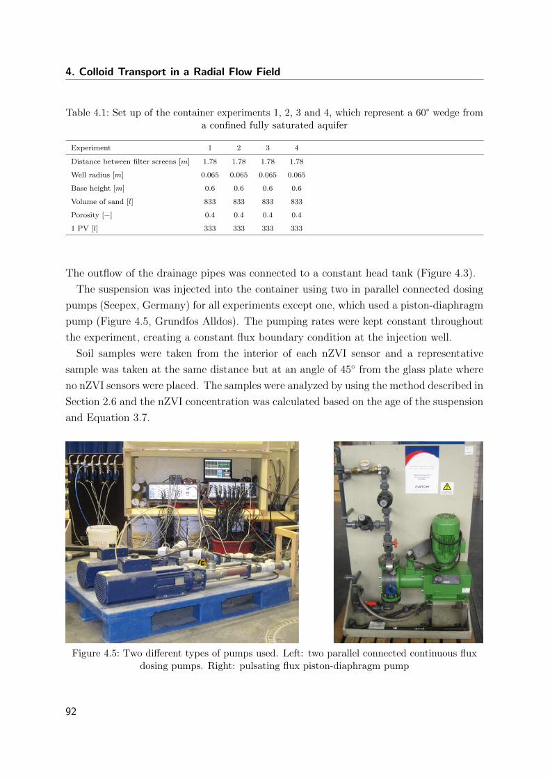
4. Colloid Transport in a Radial Flow Field
Table 4.1: Set up of the container experiments 1, 2, 3 and 4, which represent a 60° wedge froma confined fully saturated aquifer
Experiment 1 2 3 4
Distance between filter screens [m] 1.78 1.78 1.78 1.78
Well radius [m] 0.065 0.065 0.065 0.065
Base height [m] 0.6 0.6 0.6 0.6
Volume of sand [l] 833 833 833 833
Porosity [−] 0.4 0.4 0.4 0.4
1 PV [l] 333 333 333 333
The outflow of the drainage pipes was connected to a constant head tank (Figure 4.3).
The suspension was injected into the container using two in parallel connected dosing
pumps (Seepex, Germany) for all experiments except one, which used a piston-diaphragm
pump (Figure 4.5, Grundfos Alldos). The pumping rates were kept constant throughout
the experiment, creating a constant flux boundary condition at the injection well.
Soil samples were taken from the interior of each nZVI sensor and a representative
sample was taken at the same distance but at an angle of 45 from the glass plate where
no nZVI sensors were placed. The samples were analyzed by using the method described in
Section 2.6 and the nZVI concentration was calculated based on the age of the suspension
and Equation 3.7.
Figure 4.5: Two different types of pumps used. Left: two parallel connected continuous fluxdosing pumps. Right: pulsating flux piston-diaphragm pump
92
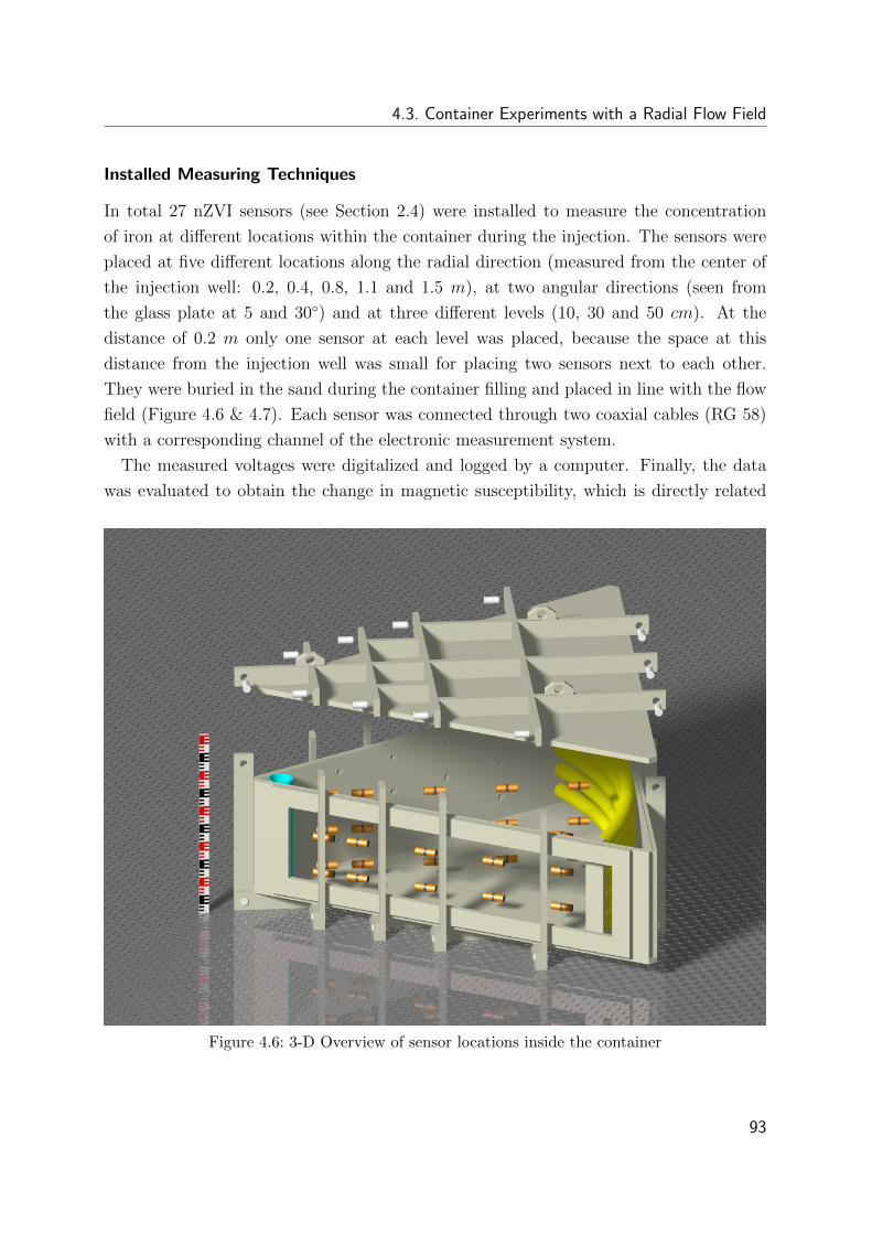
4.3. Container Experiments with a Radial Flow Field
Installed Measuring Techniques
In total 27 nZVI sensors (see Section 2.4) were installed to measure the concentration
of iron at different locations within the container during the injection. The sensors were
placed at five different locations along the radial direction (measured from the center of
the injection well: 0.2, 0.4, 0.8, 1.1 and 1.5 m), at two angular directions (seen from
the glass plate at 5 and 30) and at three different levels (10, 30 and 50 cm). At the
distance of 0.2 m only one sensor at each level was placed, because the space at this
distance from the injection well was small for placing two sensors next to each other.
They were buried in the sand during the container filling and placed in line with the flow
field (Figure 4.6 & 4.7). Each sensor was connected through two coaxial cables (RG 58)
with a corresponding channel of the electronic measurement system.
The measured voltages were digitalized and logged by a computer. Finally, the data
was evaluated to obtain the change in magnetic susceptibility, which is directly related
Figure 4.6: 3-D Overview of sensor locations inside the container
93
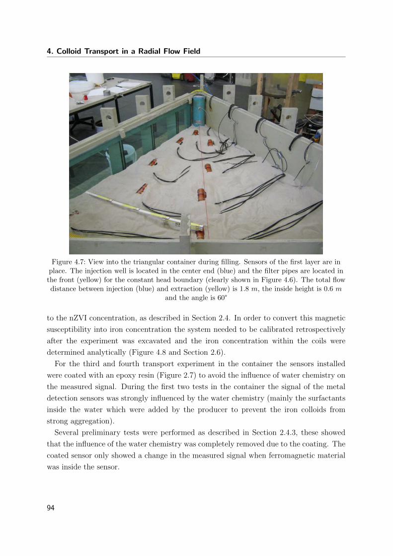
4. Colloid Transport in a Radial Flow Field
Figure 4.7: View into the triangular container during filling. Sensors of the first layer are inplace. The injection well is located in the center end (blue) and the filter pipes are located in
the front (yellow) for the constant head boundary (clearly shown in Figure 4.6). The total flowdistance between injection (blue) and extraction (yellow) is 1.8 m, the inside height is 0.6 m
and the angle is 60°
to the nZVI concentration, as described in Section 2.4. In order to convert this magnetic
susceptibility into iron concentration the system needed to be calibrated retrospectively
after the experiment was excavated and the iron concentration within the coils were
determined analytically (Figure 4.8 and Section 2.6).
For the third and fourth transport experiment in the container the sensors installed
were coated with an epoxy resin (Figure 2.7) to avoid the influence of water chemistry on
the measured signal. During the first two tests in the container the signal of the metal
detection sensors was strongly influenced by the water chemistry (mainly the surfactants
inside the water which were added by the producer to prevent the iron colloids from
strong aggregation).
Several preliminary tests were performed as described in Section 2.4.3, these showed
that the influence of the water chemistry was completely removed due to the coating. The
coated sensor only showed a change in the measured signal when ferromagnetic material
was inside the sensor.
94
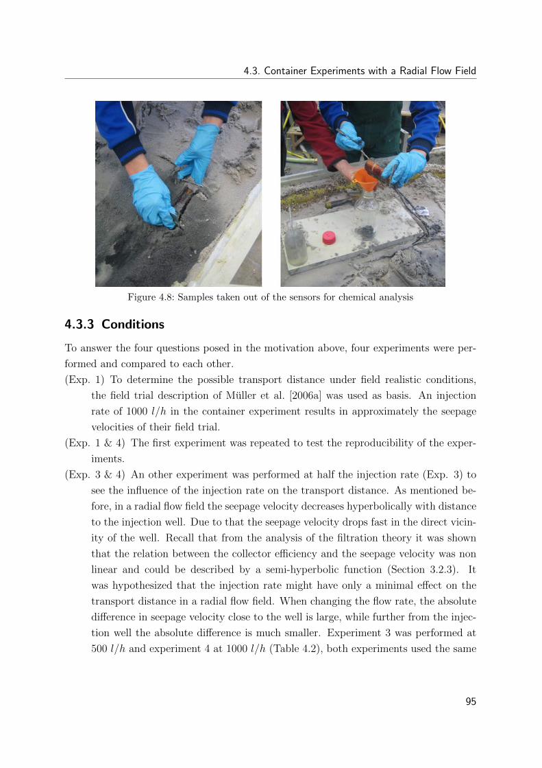
4.3. Container Experiments with a Radial Flow Field
Figure 4.8: Samples taken out of the sensors for chemical analysis
4.3.3 Conditions
To answer the four questions posed in the motivation above, four experiments were per-
formed and compared to each other.
(Exp. 1) To determine the possible transport distance under field realistic conditions,
the field trial description of Muller et al. [2006a] was used as basis. An injection
rate of 1000 l/h in the container experiment results in approximately the seepage
velocities of their field trial.
(Exp. 1 & 4) The first experiment was repeated to test the reproducibility of the exper-
iments.
(Exp. 3 & 4) An other experiment was performed at half the injection rate (Exp. 3) to
see the influence of the injection rate on the transport distance. As mentioned be-
fore, in a radial flow field the seepage velocity decreases hyperbolically with distance
to the injection well. Due to that the seepage velocity drops fast in the direct vicin-
ity of the well. Recall that from the analysis of the filtration theory it was shown
that the relation between the collector efficiency and the seepage velocity was non
linear and could be described by a semi-hyperbolic function (Section 3.2.3). It
was hypothesized that the injection rate might have only a minimal effect on the
transport distance in a radial flow field. When changing the flow rate, the absolute
difference in seepage velocity close to the well is large, while further from the injec-
tion well the absolute difference is much smaller. Experiment 3 was performed at
500 l/h and experiment 4 at 1000 l/h (Table 4.2), both experiments used the same
95
4. Colloid Transport in a Radial Flow Field
continuous flux dosing pump and the total amount of nZVI suspension injected was
the same for both experiments.
(Exp. 2 & 3) For a field application different types of pumps can be used. Two extremes
were compared here, a pump providing a very stable and continuous flux (Exp. 3)
through a rotor stator technique and one that provides a pulsating discontinuous
flux (Exp. 2) through a large single diaphragm (Table 4.2). Both pumps are shown
in Figure 4.5. Both experiments were performed at 500 l/h. The comparison of the
two pumping techniques should give an indication if the pulsating effect provides
a better or worse transport. The fluctuations in shear rate as a result of pulsation
could improve the transport of the colloids since colloids that attach to a sand grain
can potentially be remobilized by the high shear rates exited by the high flow rate
at the beginning of each pulse. It would though be worse if the increased flow rate
at the beginning of each pulse is not high enough to remobilize the colloids and
the lower flow rates (down to zero-flux) would result in a stronger removal of colloids.
Each of the experiments consisted of three injection phases. (I) Five liters of tracer
solution (Uranine, 0.5 g/l) were injected followed by (II) 900 liters of nZVI suspension.
The aimed suspension concentration was for all four experiments 10 g/l. (III) An in-
jection of 900 liters of degassed tap water (DO: ∼ 1 mg/l, pH: 7.0).The conditions of
the four experiments are presented in Table 4.2. Experiments 1 and 4 were performed
as duplicates, experiments 2 and 3 were performed at half the injection rate, and 2 was
performed with a different pump.
Table 4.2: The parameters used in the container experiments 1, 2, 3 and 4, which represent a60° wedge from a confined fully saturated aquifer
Experiment 1 2 3 4
Experiment Injection Rate [l/h] 1000 500 500 1000
Pump type Continuous Pulsating Continuous Continuous
Number of PVs injected [−] 2.7 2.7 2.7 2.7
Duration of injection [min] 55 110 110 55
nZVI age [days] 184 338 556 921
Cinput set [g/l] 10 10 10 10
Cinput measured [g/l] 8.3 9.9 10.5 12.7
96
4.3. Container Experiments with a Radial Flow Field
4.3.4 Results and Discussion
In total four experiments were carried out to test the transport of nZVI colloids in a
confined aquifer using the container setup. Only the results of the nZVI sensors from
experiment 1 are shown, the strong influence of the water chemistry on the measurement
resulted the measurements of experiment 2 to go off scale. For experiments 3 and 4 the
coated nZVI sensors were installed, unfortunately, due to the resin around the sensors the
total signal was also reduced and during experiment 3 the sensitivity of the measuring
system was not enough anymore to get representative iron break through curves, this was
solved for experiment 4 but there the datafile unfortunately got corrupted during saving.
Each of the injections of nZVI was followed by an equal volume of fresh water, visually
no change in the distribution could be observed (compare Figures 4.10d and 4.10e), also
in the measurements with the nZVI sensors during the water flushing no change was
observed (Figure 4.11a). The presence of the surfactants in the suspension (although the
concentration of surfactants is low in the strongly diluted suspension) could enhance the
transport during the suspension injection and the lack of these surfactants during the
water flushing would then stop the transport.
For the container experiments the Reynolds number (Re) was calculated to test the
validity of assuming laminar flow throughout the whole container and thus the applica-
bility of Darcy’s Law to describe the flow field in the container. Reynolds Number is a
dimensionless indicator for the type of flow, the exact boundaries of the flow types laminar
and turbulent are case specific and also depend on the exact choice of the characteristic
length, Bear [1972] describes four different characteristic lengths and states that all of
them result in an upper limit for laminar flow at a value of Re between 1 and 10. Thus,
for Re values below 1−10 there correlation between pressure and Darcy velocity is linear
and for Re values between 1 − 10 and 100 a transition from laminar to turbulent flow
takes place because inertial forces start to predominate the flow. Reynolds number is
calculated by:
Re =ρfqL
µ(4.9)
where ρf is the fluid density [ML−3], q the Darcy velocity (or specific discharge) [LT−1],
L the characteristic length (often taken to be the representative grain diameter for the
porous medium, d50) [L] and µ the viscosity [ML−1T−1] [Bear, 1972]. Figure 4.9 shows
the resulting function for L = d50 = 0.6 mm. In the experiment the filter screens were
positioned at 6.5 cm and 184.4 cm from the center of the injection well which are indicated
97

4. Colloid Transport in a Radial Flow Field
0.1
1
10
0 0.5 1 1.5 2
Rey
nold
s nu
mbe
r [-]
Distance from injection well center [m]
6 m3/h3 m3/h
Figure 4.9: Dependency of Reynolds number on r between the two filter screens of thecontainer. Used parameters were:
d50 = 6 · 10−4 m, b = 0.6 m,n = 0.4, ρf = 1 kg/l, µ = 1.003 g/m · s,Q1 = 6 m3/h,Q2 = 3 m3/h,which represent container experiments 1 and 4 for Q1, and 2 and 3 for Q2
by the blue and yellow vertical lines in Figure 4.9. The graph shows that for both injection
rates the Reynolds number is below 10 in the whole domain, although close to the well
the injection rate of 1000 l/h is only just below 10. 60 cm from the injection well screen
it is below 1 for the injection at 1000 l/h and for the injection rate of 500 l/h this is
already after 27 cm.
Injection at 1000 l/h (Exp. 1)
During experiment 1 (Table 4.2) it was possible to get the iron colloids transported over
the full length of the container (Figure 4.10). While visually the window was black
throughout, the sensors showed a large gradient in concentration along the flow path. Vi-
sual observation through the glass plate showed significant retention of nZVI compared to
the injection front which was highlighted by a conservative tracer (Uranine, Figure 4.10b).
The iron front visibly arrived at the outlet side after three pore volumes of suspension
were injected.
98
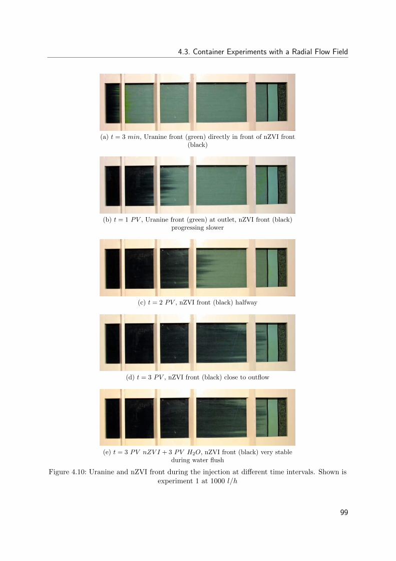
4.3. Container Experiments with a Radial Flow Field
(a) t = 3 min, Uranine front (green) directly in front of nZVI front(black)
(b) t = 1 PV , Uranine front (green) at outlet, nZVI front (black)progressing slower
(c) t = 2 PV , nZVI front (black) halfway
(d) t = 3 PV , nZVI front (black) close to outflow
(e) t = 3 PV nZV I + 3 PV H2O, nZVI front (black) very stableduring water flush
Figure 4.10: Uranine and nZVI front during the injection at different time intervals. Shown isexperiment 1 at 1000 l/h
99
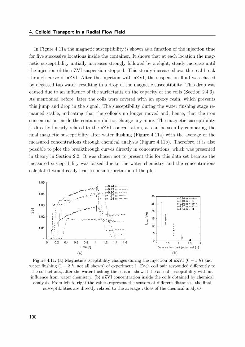
4. Colloid Transport in a Radial Flow Field
In Figure 4.11a the magnetic susceptibility is shown as a function of the injection time
for five successive locations inside the container. It shows that at each location the mag-
netic susceptibility initially increases strongly followed by a slight, steady increase until
the injection of the nZVI suspension stopped. This steady increase shows the real break
through curve of nZVI. After the injection with nZVI, the suspension fluid was chased
by degassed tap water, resulting in a drop of the magnetic susceptibility. This drop was
caused due to an influence of the surfactants on the capacity of the coils (Section 2.4.3).
As mentioned before, later the coils were covered with an epoxy resin, which prevents
this jump and drop in the signal. The susceptibility during the water flushing stage re-
mained stable, indicating that the colloids no longer moved and, hence, that the iron
concentration inside the container did not change any more. The magnetic susceptibility
is directly linearly related to the nZVI concentration, as can be seen by comparing the
final magnetic susceptibility after water flushing (Figure 4.11a) with the average of the
measured concentrations through chemical analysis (Figure 4.11b). Therefore, it is also
possible to plot the breakthrough curves directly in concentrations, which was presented
in theory in Section 2.2. It was chosen not to present this for this data set because the
measured susceptibility was biased due to the water chemistry and the concentrations
calculated would easily lead to misinterpretation of the plot.
1
1.01
1.02
1.03
1.04
1.05
0 0.2 0.4 0.6 0.8 1 1.2 1.4 1.6
χ [-
]
Time [h]
r=0.24 mr=0.43 mr=0.80 mr=1.17 mr=1.54 m
(a)
0
5
10
15
20
25
30
0 0.5 1 1.5 2
Sto
tal,
[g/k
g]
Distance from the injection well [m]
r=0.24 mr=0.43 mr=0.80 mr=1.17 mr=1.54 m
(b)
Figure 4.11: (a) Magnetic susceptibility changes during the injection of nZVI (0− 1 h) andwater flushing (1− 2 h, not all shown) of experiment 1. Each coil pair responded differently tothe surfactants, after the water flushing the sensors showed the actual susceptibility withoutinfluence from water chemistry. (b) nZVI concentration inside the coils obtained by chemicalanalysis. From left to right the values represent the sensors at different distances; the final
susceptibilities are directly related to the average values of the chemical analysis
100
4.3. Container Experiments with a Radial Flow Field
Reproducibility of the container experiments (Exp. 1 & 4)
The conditions of experiment 4 were chosen identical to the conditions of experiment 1
to test the reproducibility of the experiments. The boundary conditions of both experi-
ments were not exactly the same, it is with experimental investigations nearly impossible
to perform an experiment twice with exactly the same boundary conditions. The main
deviations determined for these experiments were the dispersing unit and the input con-
centration of the nZVI suspension.
In a visual comparison (Figure 4.12), the transport distances of both experiments are
similar but not identical, experiment 4 shows higher concentrations and a sharper front.
Unfortunately, a comparison of the break through curves of the inductive iron detectors
could not be performed because the datasets were corrupted during saving.
A comparison of the concentrations obtained in the chemical analysis of the soil sam-
ples taken during excavation is shown in Figure 4.13. Looking at the average of these
measurements, it can be seen that the transport of experiment 4 to a large extend repli-
cated the results of experiment 1. The measured values all are on average a little higher,
this is mainly due to the higher concentration of nZVI injected. During experiment 1, the
dispersing was done using the much smaller IKA machine as compared to the large CAT
machine used in experiment 4. In experiment 4 the concentration at three different levels
inside the filter sand of the injection well was measured additionally. Even though some
iron is located inside the filter sand, the concentration is low compared to the concen-
trations at 20 cm from the injection well. A risk of well clogging is based on these data
minimal for this material, and the filter sand worked well to provide a good connection
between the injection well and the porous medium.
It can be seen that the measuring technique to analytically determine the nZVI con-
centrations inside the soil samples (Figure 4.13) has been improved significantly since
the first experiment, the measured concentrations for each location have a much smaller
deviation. During the first experiment this measuring set up was still in a testing state,
whereas from experiment 2 on the set up was replaced by the one described in Section 2.6.
Influence of Different Injection Rates (Exp. 3 & 4)
Experiments 3 and 4 are here compared to discuss the influence of the injection rate on
the transport in a radial flow field. In Figure 4.14 the final iron distribution can be seen
for both experiments. In experiment 4 (1000 l/h) the iron is transported slightly further.
101
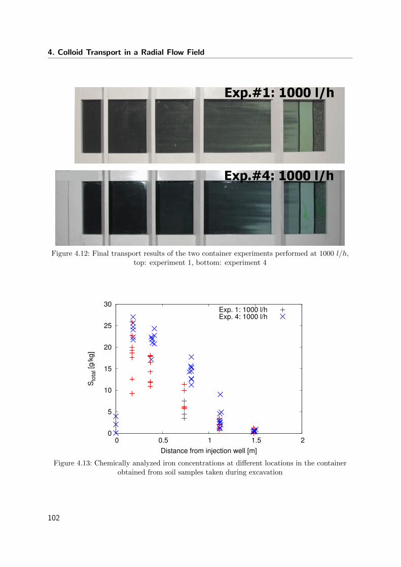
4. Colloid Transport in a Radial Flow Field
Figure 4.12: Final transport results of the two container experiments performed at 1000 l/h,top: experiment 1, bottom: experiment 4
0
5
10
15
20
25
30
0 0.5 1 1.5 2
Sto
tal [
g/kg
]
Distance from injection well [m]
Exp. 1: 1000 l/hExp. 4: 1000 l/h
Figure 4.13: Chemically analyzed iron concentrations at different locations in the containerobtained from soil samples taken during excavation
102
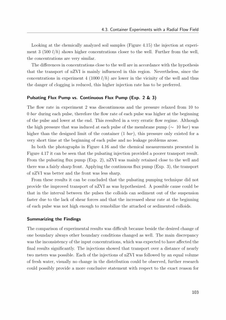
4.3. Container Experiments with a Radial Flow Field
Looking at the chemically analyzed soil samples (Figure 4.15) the injection at experi-
ment 3 (500 l/h) shows higher concentrations closer to the well. Further from the well,
the concentrations are very similar.
The differences in concentrations close to the well are in accordance with the hypothesis
that the transport of nZVI is mainly influenced in this region. Nevertheless, since the
concentrations in experiment 4 (1000 l/h) are lower in the vicinity of the well and thus
the danger of clogging is reduced, this higher injection rate has to be preferred.
Pulsating Flux Pump vs. Continuous Flux Pump (Exp. 2 & 3)
The flow rate in experiment 2 was discontinuous and the pressure relaxed from 10 to
0 bar during each pulse, therefore the flow rate of each pulse was higher at the beginning
of the pulse and lower at the end. This resulted in a very erratic flow regime. Although
the high pressure that was induced at each pulse of the membrane pump (∼ 10 bar) was
higher than the designed limit of the container (1 bar), this pressure only existed for a
very short time at the beginning of each pulse and no leakage problems arose.
In both the photographs in Figure 4.16 and the chemical measurements presented in
Figure 4.17 it can be seen that the pulsating injection provided a poorer transport result.
From the pulsating flux pump (Exp. 2), nZVI was mainly retained close to the well and
there was a fairly sharp front. Applying the continuous flux pump (Exp. 3), the transport
of nZVI was better and the front was less sharp.
From these results it can be concluded that the pulsating pumping technique did not
provide the improved transport of nZVI as was hypothesized. A possible cause could be
that in the interval between the pulses the colloids can sediment out of the suspension
faster due to the lack of shear forces and that the increased shear rate at the beginning
of each pulse was not high enough to remobilize the attached or sedimented colloids.
Summarizing the Findings
The comparison of experimental results was difficult because beside the desired change of
one boundary always other boundary conditions changed as well. The main discrepancy
was the inconsistency of the input concentrations, which was expected to have affected the
final results significantly. The injections showed that transport over a distance of nearly
two meters was possible. Each of the injections of nZVI was followed by an equal volume
of fresh water, visually no change in the distribution could be observed, further research
could possibly provide a more conclusive statement with respect to the exact reason for
103
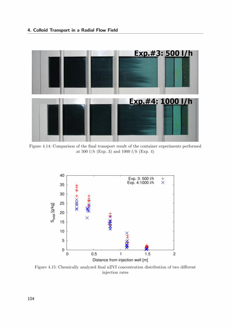
4. Colloid Transport in a Radial Flow Field
Figure 4.14: Comparison of the final transport result of the container experiments performedat 500 l/h (Exp. 3) and 1000 l/h (Exp. 4)
0
5
10
15
20
25
30
35
40
0 0.5 1 1.5 2
Sto
tal [
g/k
g]
Distance from injection well [m]
Exp. 3: 500 l/hExp. 4:1000 l/h
Figure 4.15: Chemically analyzed final nZVI concentration distribution of two differentinjection rates
104
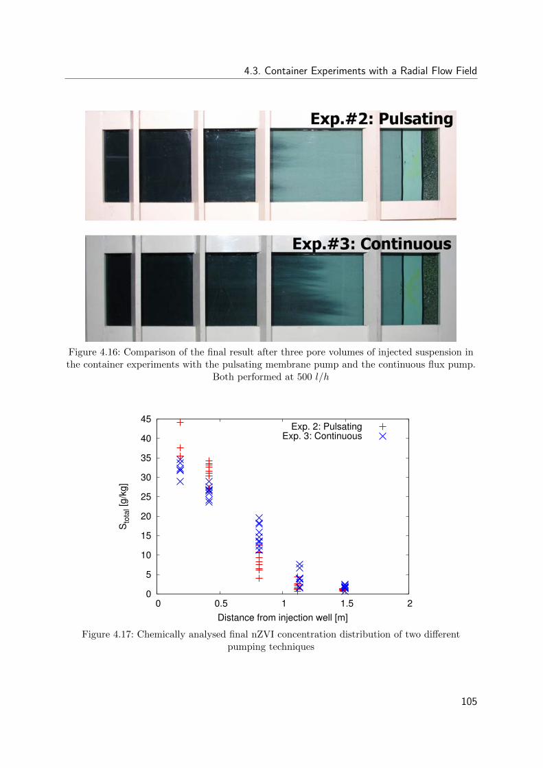
4.3. Container Experiments with a Radial Flow Field
Figure 4.16: Comparison of the final result after three pore volumes of injected suspension inthe container experiments with the pulsating membrane pump and the continuous flux pump.
Both performed at 500 l/h
0
5
10
15
20
25
30
35
40
45
0 0.5 1 1.5 2
Sto
tal [
g/kg
]
Distance from injection well [m]
Exp. 2: PulsatingExp. 3: Continuous
Figure 4.17: Chemically analysed final nZVI concentration distribution of two differentpumping techniques
105
4. Colloid Transport in a Radial Flow Field
the immobilization of nZVI during water flushing. It was also shown that a continuous
flux is preferable over a pulsating flux for injection. The influence of the injection rate is
less pronounced in the large scale experiments than in the column experiments due to the
hyperbolically decreasing seepage velocity in a radial flow field. Nevertheless the injection
at the higher injection rate performed slightly better. Especially the concentrations close
to the well were lower, avoiding the risk of clogging.
4.4 Discretized Radial Flow Field Reproduced with
Columns
4.4.1 Motivation
The container experiment is a very useful tool to provide insight into the impact of real
field scale methods like pumps used and large suspension volumes preparation on the
transport of nZVI. The experiments on the other hand are also very labor intense and
costly. For a quick screening of applicability of a certain nZVI, porous medium or injection
rate, the container experiment would simply take too much time and effort. Therefore
simplified quick screening methods were developed.
The first to be developed was an experimental method to approximate the results
of full scale radial nZVI injections by discretizing the full radial flow field into hollow
cylinder segments and representing each of these with 1-D column experiments using sets
of multiple subsequent column experiments with the appropriate boundary conditions
[de Boer et al., 2008; Estrella, 2011a]. The measured concentration profile from each
column was assumed to represent the concentration profile of that section of the radial
flow field. This would allow for the quick approximation of a nZVI injection using only
column experiments. The method was tested and validated against the results of two
of the near field scale container experiments performed with the continuous flux dosing
pump described before (experiments 1 and 3).
4.4.2 Concept
Equations were derived to discretize a two dimensional radial flow field into a series of
sections (as presented in Figure 4.18). These equations were derived so that the boundary
conditions from a full scale radial flow system could be applied to a discretization with
any number of columns.
106
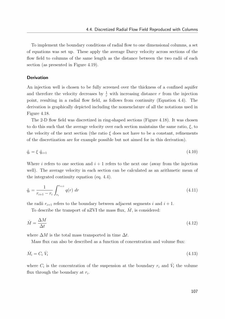
4.4. Discretized Radial Flow Field Reproduced with Columns
To implement the boundary conditions of radial flow to one dimensional columns, a set
of equations was set up. These apply the average Darcy velocity across sections of the
flow field to columns of the same length as the distance between the two radii of each
section (as presented in Figure 4.19).
Derivation
An injection well is chosen to be fully screened over the thickness of a confined aquifer
and therefore the velocity decreases by 1r
with increasing distance r from the injection
point, resulting in a radial flow field, as follows from continuity (Equation 4.4). The
derivation is graphically depicted including the nomenclature of all the notations used in
Figure 4.18.
The 2-D flow field was discretized in ring-shaped sections (Figure 4.18). It was chosen
to do this such that the average velocity over each section maintains the same ratio, ξ, to
the velocity of the next section (the ratio ξ does not have to be a constant, refinements
of the discretization are for example possible but not aimed for in this derivation).
qi = ξ qi+1 (4.10)
Where i refers to one section and i + 1 refers to the next one (away from the injection
well). The average velocity in each section can be calculated as an arithmetic mean of
the integrated continuity equation (eq. 4.4).
qi =1
ri+1 − ri
∫ ri+1
ri
q(r) dr (4.11)
the radii ri+1 refers to the boundary between adjacent segments i and i+ 1.
To describe the transport of nZVI the mass flux, M , is considered:
M =∆M
∆t(4.12)
where ∆M is the total mass transported in time ∆t.
Mass flux can also be described as a function of concentration and volume flux:
Mi = Ci Vi (4.13)
where Ci is the concentration of the suspension at the boundary ri and Vi the volume
flux through the boundary at ri.
107
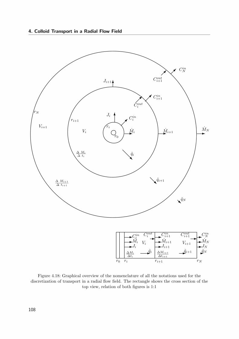
4. Colloid Transport in a Radial Flow Field
µ
µ
µ
- - -
µ
µ
R
R
R
Vi+1
Vi
Cini
Couti
Cini+1
Couti+1
CinN
qi
qi+1
qN
Mi Mi+1MN
ri
ri+1
rN
∆ Mi
∆ ti
∆ Mi+1
∆ ti+1
-
- --
-
- -
--
Cini
Cini+1 Cin
N
Mi Mi+1 MN
qi qi+1 qN
Couti+1Cout
i
Vi Vi+1
∆Mi
∆ti
∆Mi+1
∆ti+1
ri ri+1 rN
r0
6
6
Ji
Ji+1
r0
--
- - -JNJi+1Ji
1
Figure 4.18: Graphical overview of the nomenclature of all the notations used for thediscretization of transport in a radial flow field. The rectangle shows the cross section of the
top view, relation of both figures is 1:1
108
4.4. Discretized Radial Flow Field Reproduced with Columns
The volume flux can also be rewritten in terms of the Darcy velocity due to continuity:
Mi = Ci Q (4.14)
Mi = Ci qi Ai (4.15)
where Ai is the cross-sectional area of the boundary at ri.
Although the mass flux is a constant throughout the system, the mass flux density (J)
is not. Mass flux density can be described as follows:
J =M
A(4.16)
The ratio of the mass flux density from one radius to the next can be derived as follows:
Mi = Mi+1 (4.17)
JiAi = Ji+1Ai+1 (4.18)
Ji+1 =AiAi+1
Ji (4.19)
Ji+1 =2πbri
2πbri+1
Ji (4.20)
Ji+1 =riri+1
Ji (4.21)
Because the mass flux density (Equation 4.16) can also be described by the Darcy velocity:
J =CQ
A= Cq (4.22)
Equation 4.21 can be rewritten as (for this derivation it was assumed that the mass flux
is conservative, otherwise sink terms would have to be added to this set of equations):
Ji+1 =riri+1
Ji (4.23)
Cqi+1 =riri+1
Cqi (4.24)
qi+1 =riri+1
qi (4.25)
qi =ri+1
riqi+1 (4.26)
109
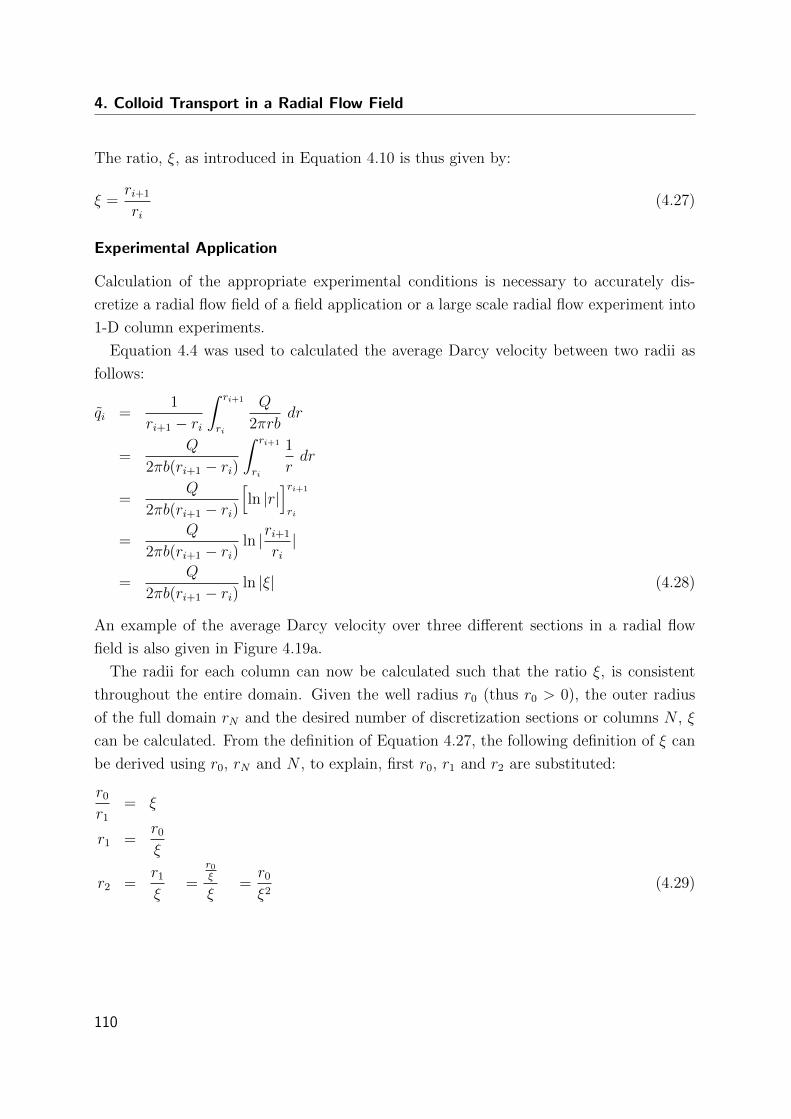
4. Colloid Transport in a Radial Flow Field
The ratio, ξ, as introduced in Equation 4.10 is thus given by:
ξ =ri+1
ri(4.27)
Experimental Application
Calculation of the appropriate experimental conditions is necessary to accurately dis-
cretize a radial flow field of a field application or a large scale radial flow experiment into
1-D column experiments.
Equation 4.4 was used to calculated the average Darcy velocity between two radii as
follows:
qi =1
ri+1 − ri
∫ ri+1
ri
Q
2πrbdr
=Q
2πb(ri+1 − ri)
∫ ri+1
ri
1
rdr
=Q
2πb(ri+1 − ri)[ln |r|
]ri+1
ri
=Q
2πb(ri+1 − ri)ln |ri+1
ri|
=Q
2πb(ri+1 − ri)ln |ξ| (4.28)
An example of the average Darcy velocity over three different sections in a radial flow
field is also given in Figure 4.19a.
The radii for each column can now be calculated such that the ratio ξ, is consistent
throughout the entire domain. Given the well radius r0 (thus r0 > 0), the outer radius
of the full domain rN and the desired number of discretization sections or columns N , ξ
can be calculated. From the definition of Equation 4.27, the following definition of ξ can
be derived using r0, rN and N , to explain, first r0, r1 and r2 are substituted:
r0
r1
= ξ
r1 =r0
ξ
r2 =r1
ξ=
r0ξ
ξ=r0
ξ2(4.29)
110
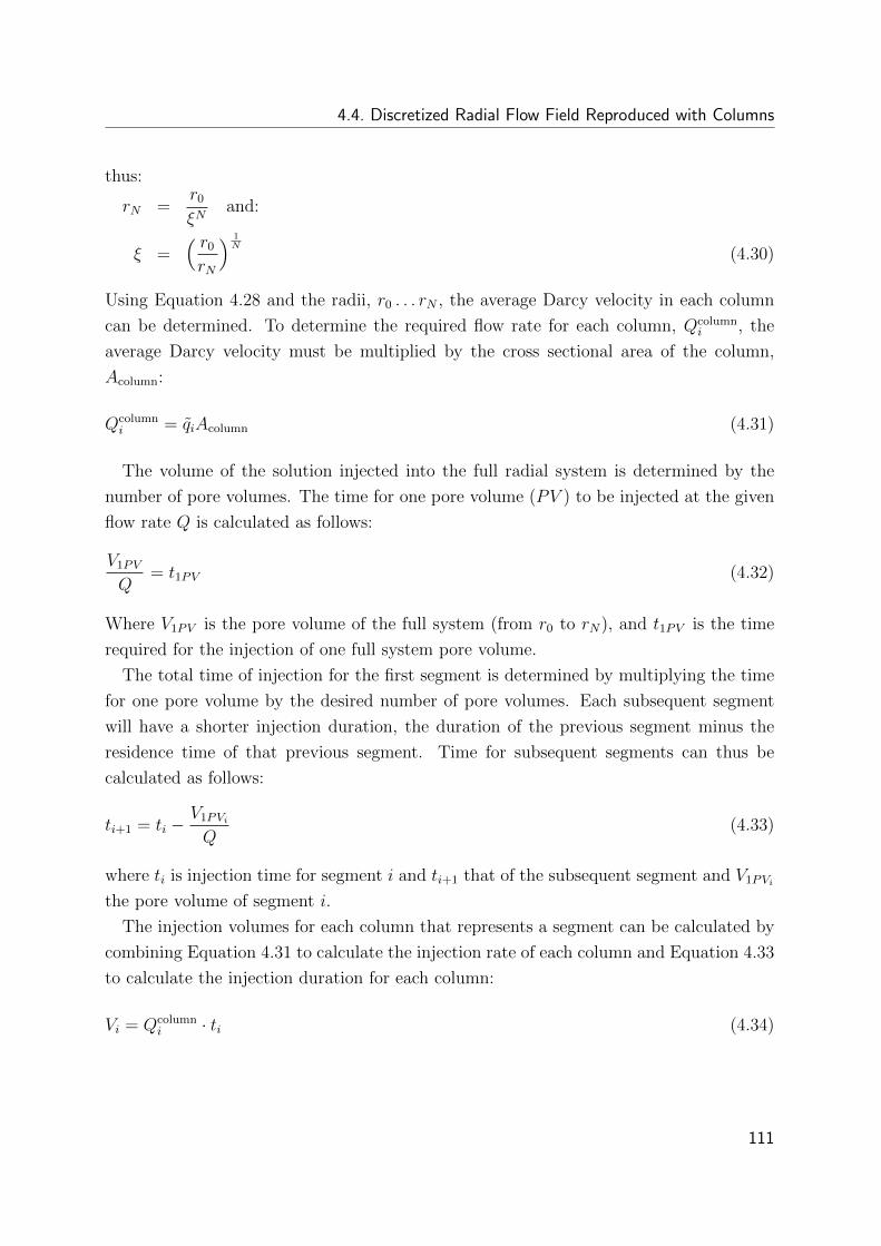
4.4. Discretized Radial Flow Field Reproduced with Columns
thus:
rN =r0
ξNand:
ξ =( r0
rN
) 1N
(4.30)
Using Equation 4.28 and the radii, r0 . . . rN , the average Darcy velocity in each column
can be determined. To determine the required flow rate for each column, Qcolumni , the
average Darcy velocity must be multiplied by the cross sectional area of the column,
Acolumn:
Qcolumni = qiAcolumn (4.31)
The volume of the solution injected into the full radial system is determined by the
number of pore volumes. The time for one pore volume (PV ) to be injected at the given
flow rate Q is calculated as follows:
V1PV
Q= t1PV (4.32)
Where V1PV is the pore volume of the full system (from r0 to rN), and t1PV is the time
required for the injection of one full system pore volume.
The total time of injection for the first segment is determined by multiplying the time
for one pore volume by the desired number of pore volumes. Each subsequent segment
will have a shorter injection duration, the duration of the previous segment minus the
residence time of that previous segment. Time for subsequent segments can thus be
calculated as follows:
ti+1 = ti −V1PVi
Q(4.33)
where ti is injection time for segment i and ti+1 that of the subsequent segment and V1PVi
the pore volume of segment i.
The injection volumes for each column that represents a segment can be calculated by
combining Equation 4.31 to calculate the injection rate of each column and Equation 4.33
to calculate the injection duration for each column:
Vi = Qcolumni · ti (4.34)
111
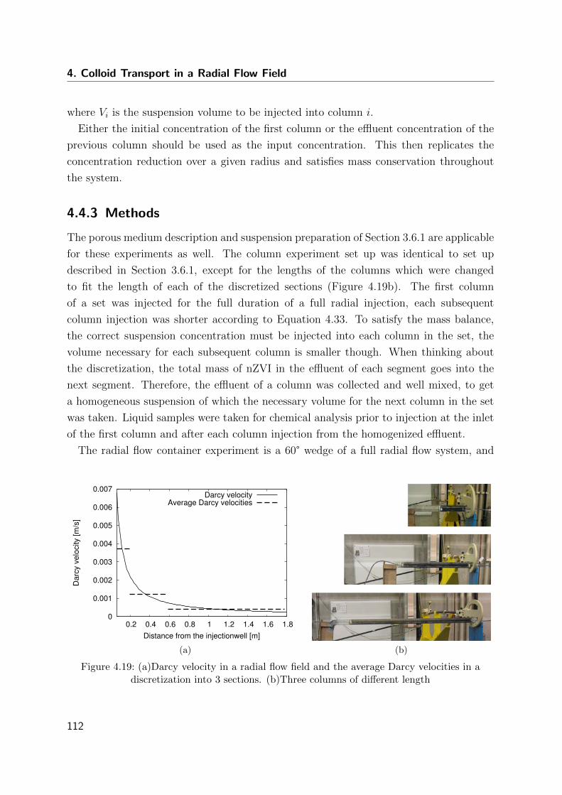
4. Colloid Transport in a Radial Flow Field
where Vi is the suspension volume to be injected into column i.
Either the initial concentration of the first column or the effluent concentration of the
previous column should be used as the input concentration. This then replicates the
concentration reduction over a given radius and satisfies mass conservation throughout
the system.
4.4.3 Methods
The porous medium description and suspension preparation of Section 3.6.1 are applicable
for these experiments as well. The column experiment set up was identical to set up
described in Section 3.6.1, except for the lengths of the columns which were changed
to fit the length of each of the discretized sections (Figure 4.19b). The first column
of a set was injected for the full duration of a full radial injection, each subsequent
column injection was shorter according to Equation 4.33. To satisfy the mass balance,
the correct suspension concentration must be injected into each column in the set, the
volume necessary for each subsequent column is smaller though. When thinking about
the discretization, the total mass of nZVI in the effluent of each segment goes into the
next segment. Therefore, the effluent of a column was collected and well mixed, to get
a homogeneous suspension of which the necessary volume for the next column in the set
was taken. Liquid samples were taken for chemical analysis prior to injection at the inlet
of the first column and after each column injection from the homogenized effluent.
The radial flow container experiment is a 60° wedge of a full radial flow system, and
0
0.001
0.002
0.003
0.004
0.005
0.006
0.007
0.2 0.4 0.6 0.8 1 1.2 1.4 1.6 1.8
Dar
cy v
eloc
ity [m
/s]
Distance from the injectionwell [m]
Darcy velocityAverage Darcy velocities
(a) (b)
Figure 4.19: (a)Darcy velocity in a radial flow field and the average Darcy velocities in adiscretization into 3 sections. (b)Three columns of different length
112
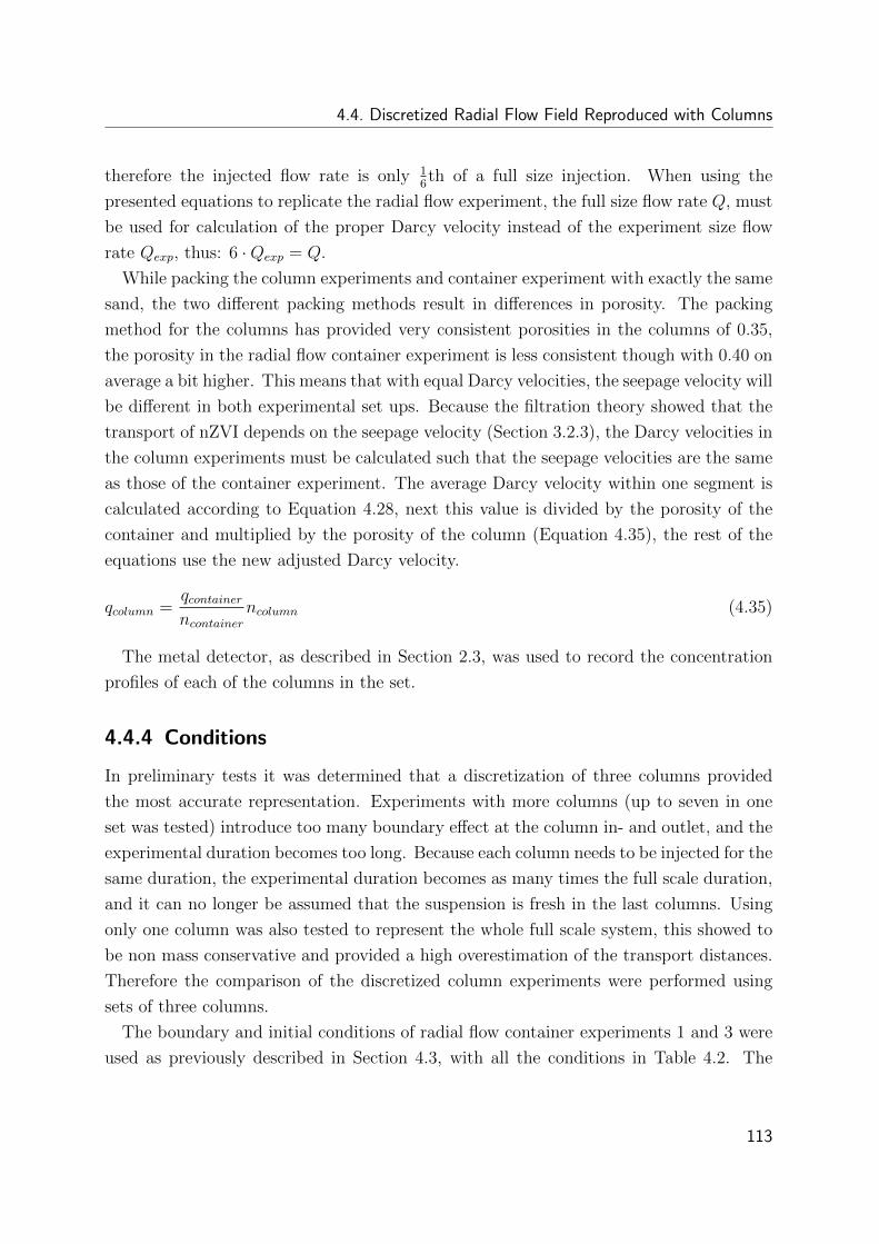
4.4. Discretized Radial Flow Field Reproduced with Columns
therefore the injected flow rate is only 16th of a full size injection. When using the
presented equations to replicate the radial flow experiment, the full size flow rate Q, must
be used for calculation of the proper Darcy velocity instead of the experiment size flow
rate Qexp, thus: 6 ·Qexp = Q.
While packing the column experiments and container experiment with exactly the same
sand, the two different packing methods result in differences in porosity. The packing
method for the columns has provided very consistent porosities in the columns of 0.35,
the porosity in the radial flow container experiment is less consistent though with 0.40 on
average a bit higher. This means that with equal Darcy velocities, the seepage velocity will
be different in both experimental set ups. Because the filtration theory showed that the
transport of nZVI depends on the seepage velocity (Section 3.2.3), the Darcy velocities in
the column experiments must be calculated such that the seepage velocities are the same
as those of the container experiment. The average Darcy velocity within one segment is
calculated according to Equation 4.28, next this value is divided by the porosity of the
container and multiplied by the porosity of the column (Equation 4.35), the rest of the
equations use the new adjusted Darcy velocity.
qcolumn =qcontainerncontainer
ncolumn (4.35)
The metal detector, as described in Section 2.3, was used to record the concentration
profiles of each of the columns in the set.
4.4.4 Conditions
In preliminary tests it was determined that a discretization of three columns provided
the most accurate representation. Experiments with more columns (up to seven in one
set was tested) introduce too many boundary effect at the column in- and outlet, and the
experimental duration becomes too long. Because each column needs to be injected for the
same duration, the experimental duration becomes as many times the full scale duration,
and it can no longer be assumed that the suspension is fresh in the last columns. Using
only one column was also tested to represent the whole full scale system, this showed to
be non mass conservative and provided a high overestimation of the transport distances.
Therefore the comparison of the discretized column experiments were performed using
sets of three columns.
The boundary and initial conditions of radial flow container experiments 1 and 3 were
used as previously described in Section 4.3, with all the conditions in Table 4.2. The
113
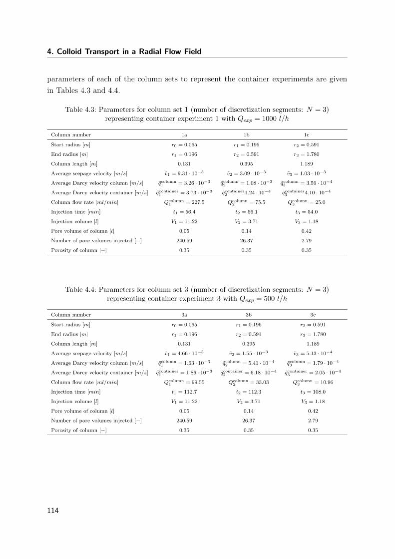
4. Colloid Transport in a Radial Flow Field
parameters of each of the column sets to represent the container experiments are given
in Tables 4.3 and 4.4.
Table 4.3: Parameters for column set 1 (number of discretization segments: N = 3)representing container experiment 1 with Qexp = 1000 l/h
Column number 1a 1b 1c
Start radius [m] r0 = 0.065 r1 = 0.196 r2 = 0.591
End radius [m] r1 = 0.196 r2 = 0.591 r3 = 1.780
Column length [m] 0.131 0.395 1.189
Average seepage velocity [m/s] v1 = 9.31 · 10−3 v2 = 3.09 · 10−3 v3 = 1.03 · 10−3
Average Darcy velocity column [m/s] qcolumn1 = 3.26 · 10−3 qcolumn
2 = 1.08 · 10−3 qcolumn3 = 3.59 · 10−4
Average Darcy velocity container [m/s] qcontainer1 = 3.73 · 10−3 qcontainer2 1.24 · 10−4 qcontainer3 4.10 · 10−4
Column flow rate [ml/min] Qcolumn1 = 227.5 Qcolumn
2 = 75.5 Qcolumn3 = 25.0
Injection time [min] t1 = 56.4 t2 = 56.1 t3 = 54.0
Injection volume [l] V1 = 11.22 V2 = 3.71 V3 = 1.18
Pore volume of column [l] 0.05 0.14 0.42
Number of pore volumes injected [−] 240.59 26.37 2.79
Porosity of column [−] 0.35 0.35 0.35
Table 4.4: Parameters for column set 3 (number of discretization segments: N = 3)representing container experiment 3 with Qexp = 500 l/h
Column number 3a 3b 3c
Start radius [m] r0 = 0.065 r1 = 0.196 r2 = 0.591
End radius [m] r1 = 0.196 r2 = 0.591 r3 = 1.780
Column length [m] 0.131 0.395 1.189
Average seepage velocity [m/s] v1 = 4.66 · 10−3 v2 = 1.55 · 10−3 v3 = 5.13 · 10−4
Average Darcy velocity column [m/s] qcolumn1 = 1.63 · 10−3 qcolumn
2 = 5.41 · 10−4 qcolumn3 = 1.79 · 10−4
Average Darcy velocity container [m/s] qcontainer1 = 1.86 · 10−3 qcontainer2 = 6.18 · 10−4 qcontainer3 = 2.05 · 10−4
Column flow rate [ml/min] Qcolumn1 = 99.55 Qcolumn
2 = 33.03 Qcolumn3 = 10.96
Injection time [min] t1 = 112.7 t2 = 112.3 t3 = 108.0
Injection volume [l] V1 = 11.22 V2 = 3.71 V3 = 1.18
Pore volume of column [l] 0.05 0.14 0.42
Number of pore volumes injected [−] 240.59 26.37 2.79
Porosity of column [−] 0.35 0.35 0.35
114
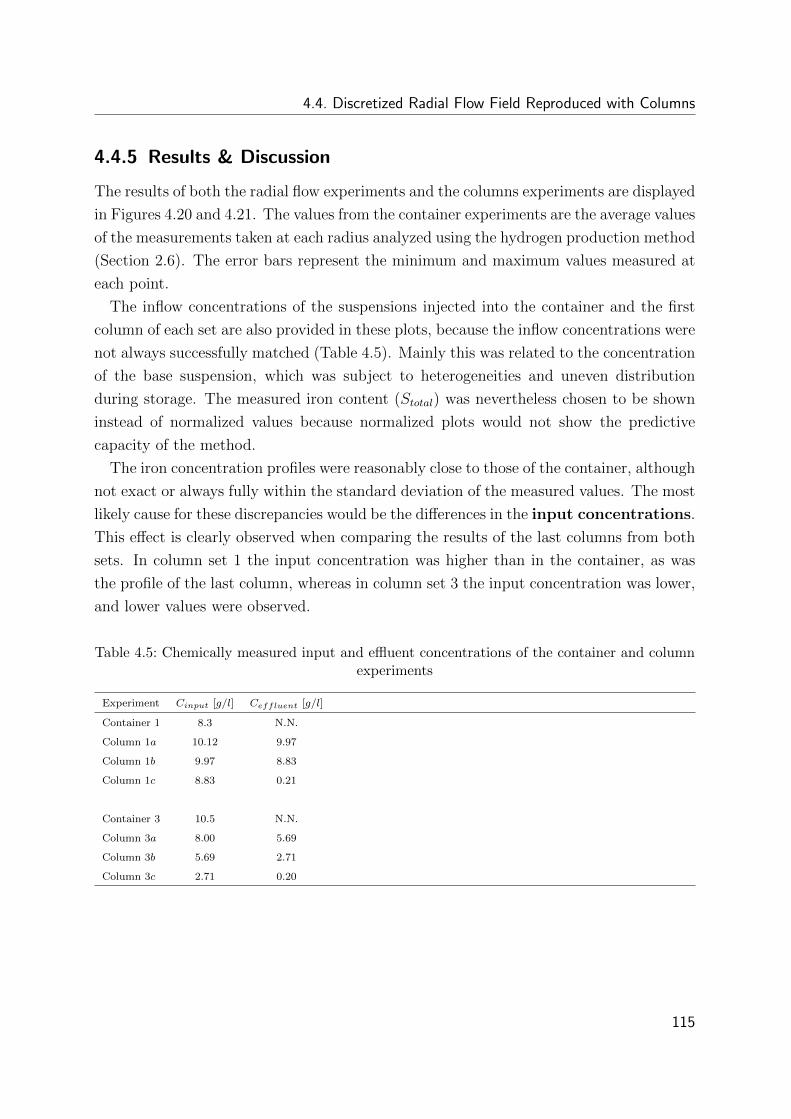
4.4. Discretized Radial Flow Field Reproduced with Columns
4.4.5 Results & Discussion
The results of both the radial flow experiments and the columns experiments are displayed
in Figures 4.20 and 4.21. The values from the container experiments are the average values
of the measurements taken at each radius analyzed using the hydrogen production method
(Section 2.6). The error bars represent the minimum and maximum values measured at
each point.
The inflow concentrations of the suspensions injected into the container and the first
column of each set are also provided in these plots, because the inflow concentrations were
not always successfully matched (Table 4.5). Mainly this was related to the concentration
of the base suspension, which was subject to heterogeneities and uneven distribution
during storage. The measured iron content (Stotal) was nevertheless chosen to be shown
instead of normalized values because normalized plots would not show the predictive
capacity of the method.
The iron concentration profiles were reasonably close to those of the container, although
not exact or always fully within the standard deviation of the measured values. The most
likely cause for these discrepancies would be the differences in the input concentrations.
This effect is clearly observed when comparing the results of the last columns from both
sets. In column set 1 the input concentration was higher than in the container, as was
the profile of the last column, whereas in column set 3 the input concentration was lower,
and lower values were observed.
Table 4.5: Chemically measured input and effluent concentrations of the container and columnexperiments
Experiment Cinput [g/l] Ceffluent [g/l]
Container 1 8.3 N.N.
Column 1a 10.12 9.97
Column 1b 9.97 8.83
Column 1c 8.83 0.21
Container 3 10.5 N.N.
Column 3a 8.00 5.69
Column 3b 5.69 2.71
Column 3c 2.71 0.20
115
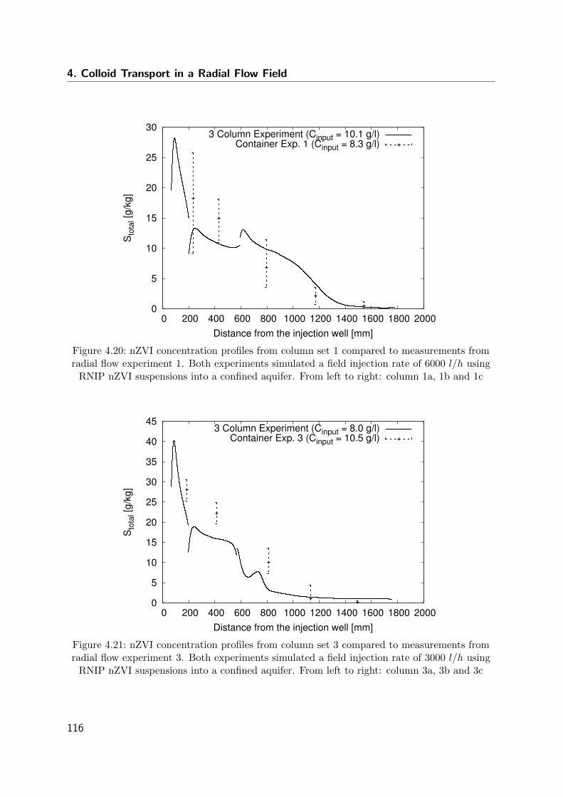
4. Colloid Transport in a Radial Flow Field
0
5
10
15
20
25
30
0 200 400 600 800 1000 1200 1400 1600 1800 2000
Sto
tal [
g/kg
]
Distance from the injection well [mm]
3 Column Experiment (Cinput = 10.1 g/l)Container Exp. 1 (Cinput = 8.3 g/l)
Figure 4.20: nZVI concentration profiles from column set 1 compared to measurements fromradial flow experiment 1. Both experiments simulated a field injection rate of 6000 l/h using
RNIP nZVI suspensions into a confined aquifer. From left to right: column 1a, 1b and 1c
0
5
10
15
20
25
30
35
40
45
0 200 400 600 800 1000 1200 1400 1600 1800 2000
Sto
tal [
g/kg
]
Distance from the injection well [mm]
3 Column Experiment (Cinput = 8.0 g/l)Container Exp. 3 (Cinput = 10.5 g/l)
Figure 4.21: nZVI concentration profiles from column set 3 compared to measurements fromradial flow experiment 3. Both experiments simulated a field injection rate of 3000 l/h using
RNIP nZVI suspensions into a confined aquifer. From left to right: column 3a, 3b and 3c
116
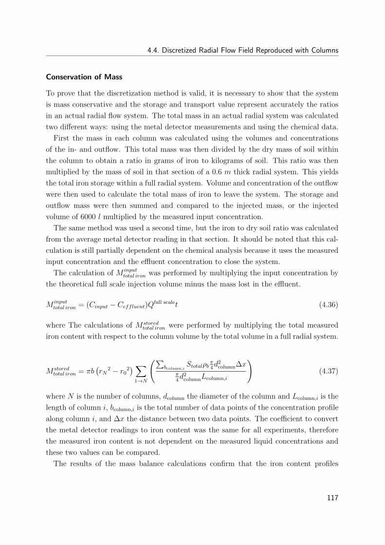
4.4. Discretized Radial Flow Field Reproduced with Columns
Conservation of Mass
To prove that the discretization method is valid, it is necessary to show that the system
is mass conservative and the storage and transport value represent accurately the ratios
in an actual radial flow system. The total mass in an actual radial system was calculated
two different ways: using the metal detector measurements and using the chemical data.
First the mass in each column was calculated using the volumes and concentrations
of the in- and outflow. This total mass was then divided by the dry mass of soil within
the column to obtain a ratio in grams of iron to kilograms of soil. This ratio was then
multiplied by the mass of soil in that section of a 0.6 m thick radial system. This yields
the total iron storage within a full radial system. Volume and concentration of the outflow
were then used to calculate the total mass of iron to leave the system. The storage and
outflow mass were then summed and compared to the injected mass, or the injected
volume of 6000 l multiplied by the measured input concentration.
The same method was used a second time, but the iron to dry soil ratio was calculated
from the average metal detector reading in that section. It should be noted that this cal-
culation is still partially dependent on the chemical analysis because it uses the measured
input concentration and the effluent concentration to close the system.
The calculation of M inputtotal iron was performed by multiplying the input concentration by
the theoretical full scale injection volume minus the mass lost in the effluent.
M inputtotal iron = (Cinput − Ceffluent)Qfull scalet (4.36)
where The calculations of M storedtotal iron were performed by multiplying the total measured
iron content with respect to the column volume by the total volume in a full radial system.
M storedtotal iron = πb
(rN
2 − r02) ∑
1→N
(∑bcolumn,i
Stotalρbπ4d2
column∆xπ4d2
columnLcolumn,i
)(4.37)
where N is the number of columns, dcolumn the diameter of the column and Lcolumn,i is the
length of column i, bcolumn,i is the total number of data points of the concentration profile
along column i, and ∆x the distance between two data points. The coefficient to convert
the metal detector readings to iron content was the same for all experiments, therefore
the measured iron content is not dependent on the measured liquid concentrations and
these two values can be compared.
The results of the mass balance calculations confirm that the iron content profiles
117
4. Colloid Transport in a Radial Flow Field
satisfy mass balance when converted to a full radial system (Table 4.6).
Table 4.6: Mass balance calculations compared the calculated mass storage in a full radialsystem from both the liquid concentrations of the in and outflow, and the metal detector
readings
Column Set M inputtotal iron [g] Mstored
total iron [g] Percent Error
from inflow - outflow from Stotal
1 53526 53606 0.10%
3 42186 41838 -0.80%
Errors in the Concentration Profiles
Measurements of the iron concentration profiles with the metal detector result in some
errors, especially associated with the boundaries of columns, which for short columns
are much more prominent and can unfortunately dominate the measurement. The most
prominent error is (I) the peak in nZVI concentration in the direct vicinity of the
inlet, as opposed to directly at the inlet, where the peak concentration would be expected.
As the metal detector moves from the filter to the porous media, it detects nZVI only
on one side, therefore the reading will be lower than when it is one or two centimeters
farther and is completely surrounded by sand that contains iron. This is most prominent
with very short columns where the first two centimeters accord to a significant portion of
the column, in columns of one meter or more this effect is negligible. So far no reliable
methods were found to automatically and scientifically acceptable convert the recordings
in the vicinity of the inlet and outlet. Therefore it was chosen to keep the data as it was
recorded. For long columns the induced error is negligible, only with very short column
this measuring artefact can induce a significant error. For short columns it could be
discussed if manual adjustment of the recordings as shown in Figure 4.22 is justifiable.
The metal detector reading was (II) transformed using data from the chemical anal-
yses for each experiment, errors in the chemical analysis thus directly transfer into the
concentration profiles and mass balances. The transformation factor was calculated from
the input and effluent concentration of the second column of each set and this factor was
then applied to all columns of the set, which for these two experiments was identical.
The chemical analysis using the photometer is highly accurate, though, the method
as a whole does have some error associated with it. The photometer itself (given it is
correctly calibrated) has negligible error, but the method has some error associated with
118
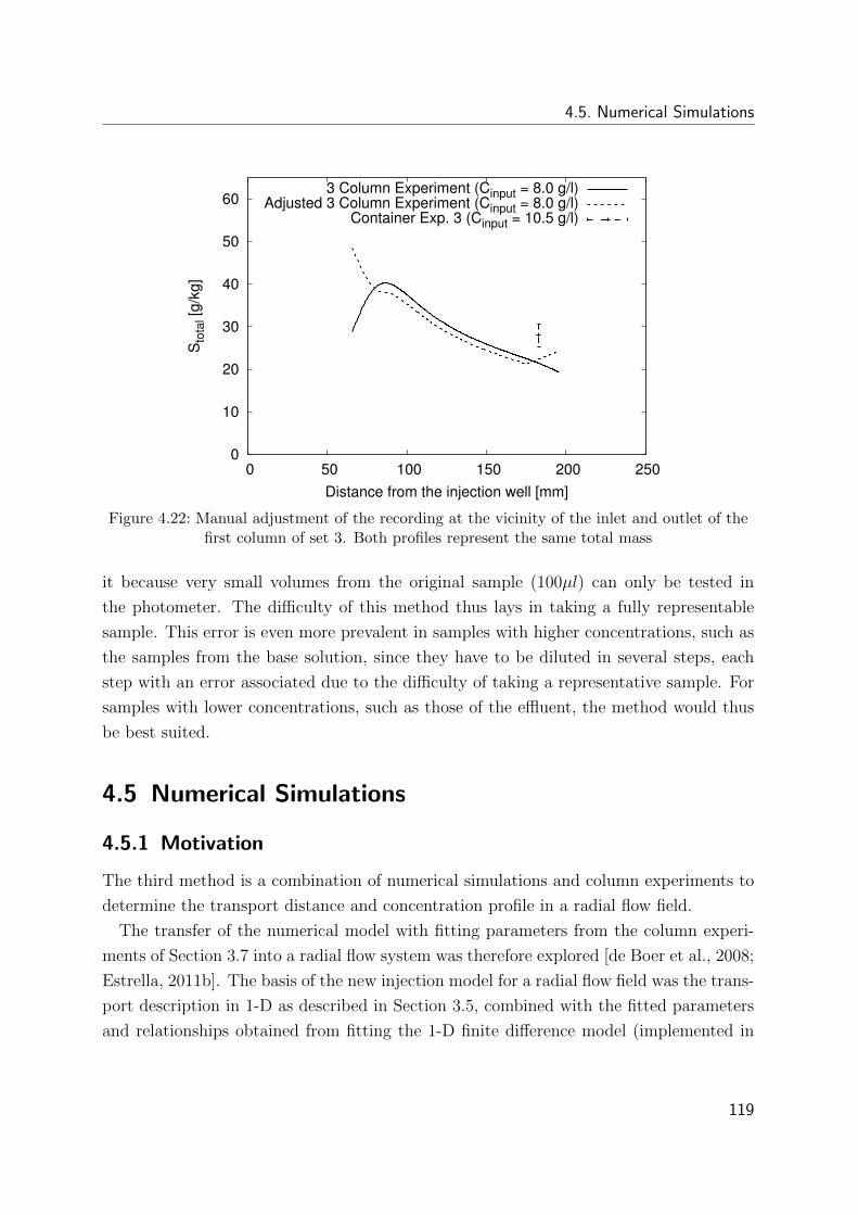
4.5. Numerical Simulations
0
10
20
30
40
50
60
0 50 100 150 200 250
Sto
tal [
g/kg
]
Distance from the injection well [mm]
3 Column Experiment (Cinput = 8.0 g/l)Adjusted 3 Column Experiment (Cinput = 8.0 g/l)
Container Exp. 3 (Cinput = 10.5 g/l)
Figure 4.22: Manual adjustment of the recording at the vicinity of the inlet and outlet of thefirst column of set 3. Both profiles represent the same total mass
it because very small volumes from the original sample (100µl) can only be tested in
the photometer. The difficulty of this method thus lays in taking a fully representable
sample. This error is even more prevalent in samples with higher concentrations, such as
the samples from the base solution, since they have to be diluted in several steps, each
step with an error associated due to the difficulty of taking a representative sample. For
samples with lower concentrations, such as those of the effluent, the method would thus
be best suited.
4.5 Numerical Simulations
4.5.1 Motivation
The third method is a combination of numerical simulations and column experiments to
determine the transport distance and concentration profile in a radial flow field.
The transfer of the numerical model with fitting parameters from the column experi-
ments of Section 3.7 into a radial flow system was therefore explored [de Boer et al., 2008;
Estrella, 2011b]. The basis of the new injection model for a radial flow field was the trans-
port description in 1-D as described in Section 3.5, combined with the fitted parameters
and relationships obtained from fitting the 1-D finite difference model (implemented in
119
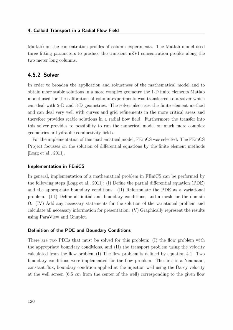
4. Colloid Transport in a Radial Flow Field
Matlab) on the concentration profiles of column experiments. The Matlab model used
three fitting parameters to produce the transient nZVI concentration profiles along the
two meter long columns.
4.5.2 Solver
In order to broaden the application and robustness of the mathematical model and to
obtain more stable solutions in a more complex geometry the 1-D finite elements Matlab
model used for the calibration of column experiments was transferred to a solver which
can deal with 2-D and 3-D geometries. The solver also uses the finite element method
and can deal very well with curves and grid refinements in the more critical areas and
therefore provides stable solutions in a radial flow field. Furthermore the transfer into
this solver provides to possibility to run the numerical model on much more complex
geometries or hydraulic conductivity fields.
For the implementation of this mathematical model, FEniCS was selected. The FEniCS
Project focusses on the solution of differential equations by the finite element methods
[Logg et al., 2011].
Implementation in FEniCS
In general, implementation of a mathematical problem in FEniCS can be performed by
the following steps [Logg et al., 2011]: (I) Define the partial differential equation (PDE)
and the appropriate boundary conditions. (II) Reformulate the PDE as a variational
problem. (III) Define all initial and boundary conditions, and a mesh for the domain
Ω. (IV) Add any necessary statements for the solution of the variational problem and
calculate all necessary information for presentation. (V) Graphically represent the results
using ParaView and Gnuplot.
Definition of the PDE and Boundary Conditions
There are two PDEs that must be solved for this problem: (I) the flow problem with
the appropriate boundary conditions, and (II) the transport problem using the velocity
calculated from the flow problem.(I) The flow problem is defined by equation 4.1. Two
boundary conditions were implemented for the flow problem. The first is a Neumann,
constant flux, boundary condition applied at the injection well using the Darcy velocity
at the well screen (6.5 cm from the center of the well) corresponding to the given flow
120
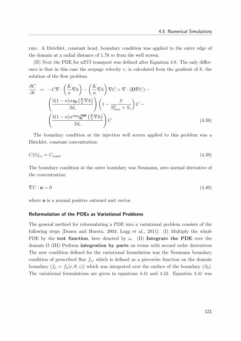
4.5. Numerical Simulations
rate. A Dirichlet, constant head, boundary condition was applied to the outer edge of
the domain at a radial distance of 1.78 m from the well screen.
(II) Next the PDE for nZVI transport was defined after Equation 4.8. The only differ-
ence is that in this case the seepage velocity v, is calculated from the gradient of h, the
solution of the flow problem.
∂C
∂t= −C∇ ·
(K
n∇h)−(K
n∇h)∇C +∇ · (D∇C)−(
3(1− n)αη0(Kn∇h)
2dc
)(1− S
S0max + Sr
)C −(
3(1− n)αaggηagg0
(Kn∇h)
2dc
)C (4.38)
The boundary condition at the injection well screen applied to this problem was a
Dirichlet, constant concentration:
C(t)|r0 = Cinput (4.39)
The boundary condition at the outer boundary was Neumann, zero normal derivative of
the concentration:
∇C · n = 0 (4.40)
where n is a normal positive outward unit vector.
Reformulation of the PDEs as Variational Problems
The general method for reformulating a PDE into a variational problem consists of the
following steps [Donea and Huerta, 2003; Logg et al., 2011]: (I) Multiply the whole
PDE by the test function, here denoted by ω. (II) Integrate the PDE over the
domain Ω (III) Perform integration by parts on terms with second order derivatives
The new condition defined for the variational formulation was the Neumann boundary
condition of prescribed flux fn, which is defined as a piecewise function on the domain
boundary (fn = fn(r, θ, z)) which was integrated over the surface of the boundary (Sb).
The variational formulations are given in equations 4.41 and 4.42. Equation 4.41 was
121
4. Colloid Transport in a Radial Flow Field
solved as a steady state problem, so there is no time dependency.∫Ω
ωK∇h dΩ =
∫Sb
ωfn dSb (4.41)
Equation 4.42 is time dependent, therefore the solution of C is defined for both the
current and previous time steps as Ct and Ct−1
∫Ω
ωCt−1dΩ =
∫Ω
ωCt dΩ +
∫Ω
ω
(K
n∇h)· ∇Ct dΩ
−∫
Ω
∇ω · (D∇Ct) dΩ
+
∫Ω
ω3(1− n)αη0
(Kn∇h)
2dc
(1− St−1
S0max + St−1
r
)Ct dΩ
+
∫Ω
ω3(1− n)αaggηagg0
(Kn∇h)
2dcCt dΩ (4.42)
Additional Equations and Statements
Several additional calculations are made within the model, both for the solving of the
PDE, as well as presentation of the results. At each time step and location within the
domain, the values of S and Sr are calculated based on the removal of nZVI during the
previous time step. Sr is now calculated following:
Sr =n
ρbkaggatt C
t−1dt+ St−1r (4.43)
where ρb is the bulk density of the soil [ML−3], and kaggatt is the removal coefficients of the
aggregates [−] as presented in Equation 3.15. The calculation of S is calculated similarly
such that the removal of iron due to the constant removal and colloid terms are combined,
yielding equation 4.44.
S = Sc + Sr (4.44)
where
Sc = St−1c +
n
ρb
(3(1− n)αη0v
2dc
)(1− St−1
c + St−1r
S0max + St−1
r
)Ct−1dt (4.45)
122
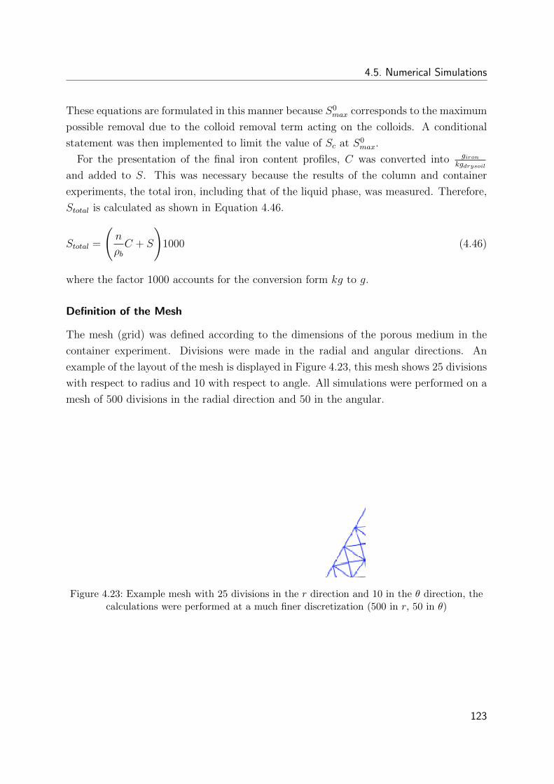
4.5. Numerical Simulations
These equations are formulated in this manner because S0max corresponds to the maximum
possible removal due to the colloid removal term acting on the colloids. A conditional
statement was then implemented to limit the value of Sc at S0max.
For the presentation of the final iron content profiles, C was converted into gironkgdrysoil
and added to S. This was necessary because the results of the column and container
experiments, the total iron, including that of the liquid phase, was measured. Therefore,
Stotal is calculated as shown in Equation 4.46.
Stotal =
(n
ρbC + S
)1000 (4.46)
where the factor 1000 accounts for the conversion form kg to g.
Definition of the Mesh
The mesh (grid) was defined according to the dimensions of the porous medium in the
container experiment. Divisions were made in the radial and angular directions. An
example of the layout of the mesh is displayed in Figure 4.23, this mesh shows 25 divisions
with respect to radius and 10 with respect to angle. All simulations were performed on a
mesh of 500 divisions in the radial direction and 50 in the angular.
Figure 4.23: Example mesh with 25 divisions in the r direction and 10 in the θ direction, thecalculations were performed at a much finer discretization (500 in r, 50 in θ)
123
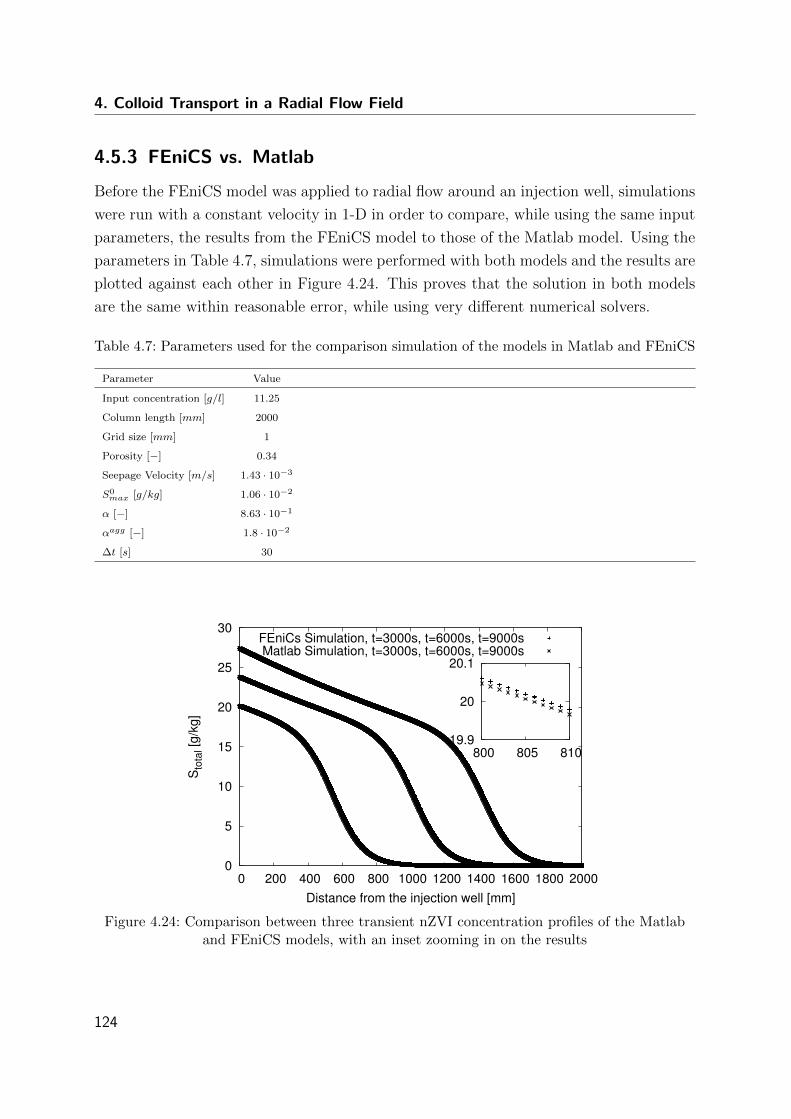
4. Colloid Transport in a Radial Flow Field
4.5.3 FEniCS vs. Matlab
Before the FEniCS model was applied to radial flow around an injection well, simulations
were run with a constant velocity in 1-D in order to compare, while using the same input
parameters, the results from the FEniCS model to those of the Matlab model. Using the
parameters in Table 4.7, simulations were performed with both models and the results are
plotted against each other in Figure 4.24. This proves that the solution in both models
are the same within reasonable error, while using very different numerical solvers.
Table 4.7: Parameters used for the comparison simulation of the models in Matlab and FEniCS
Parameter Value
Input concentration [g/l] 11.25
Column length [mm] 2000
Grid size [mm] 1
Porosity [−] 0.34
Seepage Velocity [m/s] 1.43 · 10−3
S0max [g/kg] 1.06 · 10−2
α [−] 8.63 · 10−1
αagg [−] 1.8 · 10−2
∆t [s] 30
0
5
10
15
20
25
30
0 200 400 600 800 1000 1200 1400 1600 1800 2000
Sto
tal [
g/kg
]
Distance from the injection well [mm]
FEniCs Simulation, t=3000s, t=6000s, t=9000sMatlab Simulation, t=3000s, t=6000s, t=9000s
19.9
20
20.1
800 805 810
Figure 4.24: Comparison between three transient nZVI concentration profiles of the Matlaband FEniCS models, with an inset zooming in on the results
124
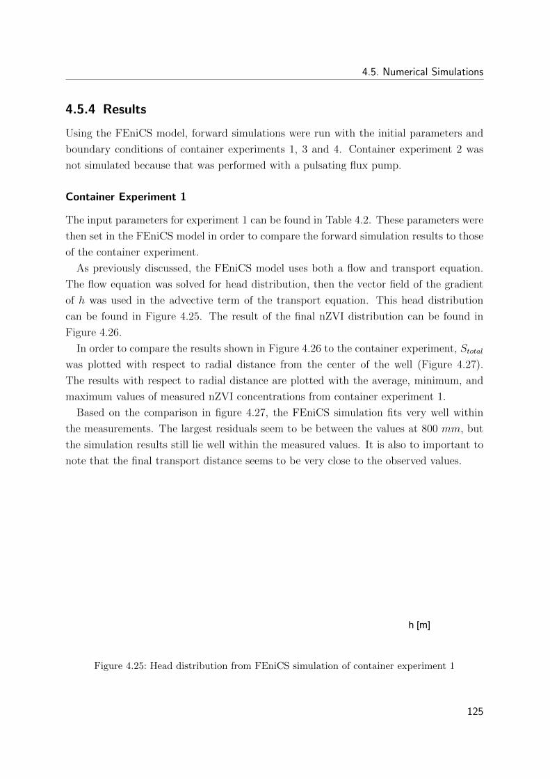
4.5. Numerical Simulations
4.5.4 Results
Using the FEniCS model, forward simulations were run with the initial parameters and
boundary conditions of container experiments 1, 3 and 4. Container experiment 2 was
not simulated because that was performed with a pulsating flux pump.
Container Experiment 1
The input parameters for experiment 1 can be found in Table 4.2. These parameters were
then set in the FEniCS model in order to compare the forward simulation results to those
of the container experiment.
As previously discussed, the FEniCS model uses both a flow and transport equation.
The flow equation was solved for head distribution, then the vector field of the gradient
of h was used in the advective term of the transport equation. This head distribution
can be found in Figure 4.25. The result of the final nZVI distribution can be found in
Figure 4.26.
In order to compare the results shown in Figure 4.26 to the container experiment, Stotal
was plotted with respect to radial distance from the center of the well (Figure 4.27).
The results with respect to radial distance are plotted with the average, minimum, and
maximum values of measured nZVI concentrations from container experiment 1.
Based on the comparison in figure 4.27, the FEniCS simulation fits very well within
the measurements. The largest residuals seem to be between the values at 800 mm, but
the simulation results still lie well within the measured values. It is also to important to
note that the final transport distance seems to be very close to the observed values.
Figure 4.25: Head distribution from FEniCS simulation of container experiment 1
125
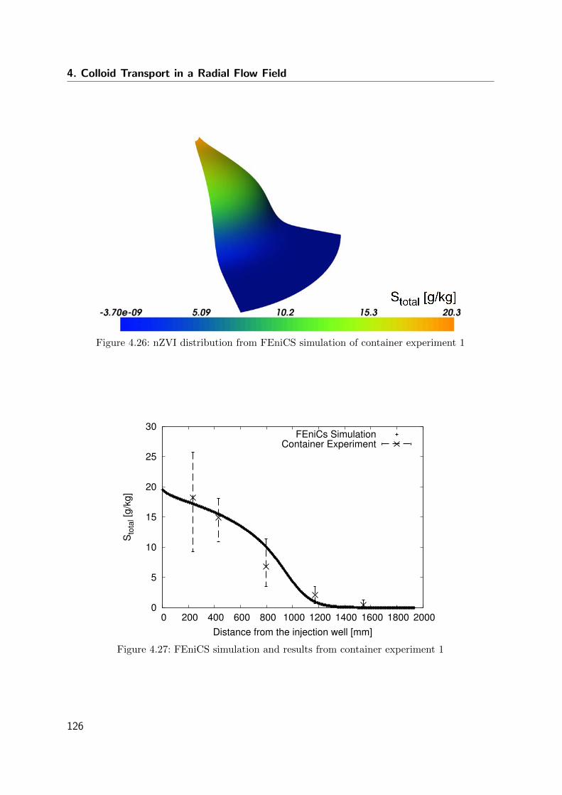
4. Colloid Transport in a Radial Flow Field
Figure 4.26: nZVI distribution from FEniCS simulation of container experiment 1
0
5
10
15
20
25
30
0 200 400 600 800 1000 1200 1400 1600 1800 2000
Sto
tal [
g/kg
]
Distance from the injection well [mm]
FEniCs SimulationContainer Experiment
Figure 4.27: FEniCS simulation and results from container experiment 1
126
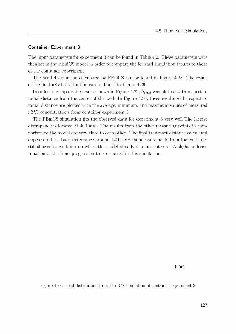
4.5. Numerical Simulations
Container Experiment 3
The input parameters for experiment 3 can be found in Table 4.2. These parameters were
then set in the FEniCS model in order to compare the forward simulation results to those
of the container experiment.
The head distribution calculated by FEniCS can be found in Figure 4.28. The result
of the final nZVI distribution can be found in Figure 4.29.
In order to compare the results shown in Figure 4.29, Stotal was plotted with respect to
radial distance from the center of the well. In Figure 4.30, these results with respect to
radial distance are plotted with the average, minimum, and maximum values of measured
nZVI concentrations from container experiment 3.
The FEniCS simulation fits the observed data for experiment 3 very well The largest
discrepancy is located at 400 mm. The results from the other measuring points in com-
parison to the model are very close to each other. The final transport distance calculated
appears to be a bit shorter since around 1200 mm the measurements from the container
still showed to contain iron where the model already is almost at zero. A slight underes-
timation of the front progression thus occurred in this simulation.
Figure 4.28: Head distribution from FEniCS simulation of container experiment 3
127
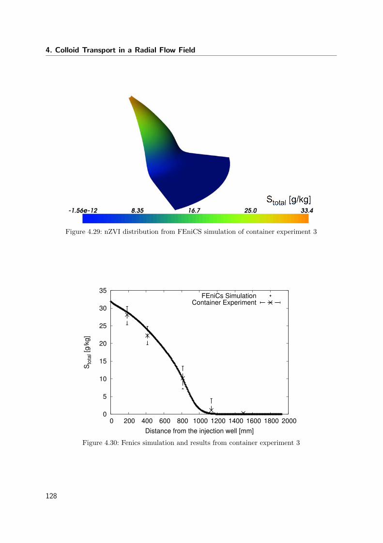
4. Colloid Transport in a Radial Flow Field
Figure 4.29: nZVI distribution from FEniCS simulation of container experiment 3
0
5
10
15
20
25
30
35
0 200 400 600 800 1000 1200 1400 1600 1800 2000
Sto
tal [
g/kg
]
Distance from the injection well [mm]
FEniCs SimulationContainer Experiment
Figure 4.30: Fenics simulation and results from container experiment 3
128
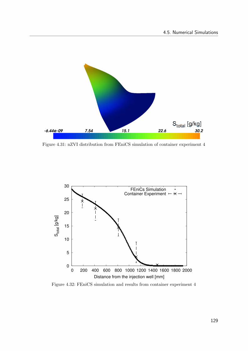
4.5. Numerical Simulations
Figure 4.31: nZVI distribution from FEniCS simulation of container experiment 4
0
5
10
15
20
25
30
0 200 400 600 800 1000 1200 1400 1600 1800 2000
Sto
tal [
g/kg
]
Distance from the injection well [mm]
FEniCs SimulationContainer Experiment
Figure 4.32: FEniCS simulation and results from container experiment 4
129
4. Colloid Transport in a Radial Flow Field
Container Experiment 4
The input parameters for experiment 4 can again be found in Table 4.2.
The head distribution calculated by FEniCS was identical to the head distribution of
container experiment 1, and can thus be found in Figure 4.25. The result of the final
nZVI distribution can be found in Figure 4.31.
The results from the simulation of experiment 4 are very close to the observed values.
The largest residuals are located at around 200 mm and 400 mm, but they are still within
the error limits of the chemical measurements. At all other points of the simulation
data not only fit within the maximum and minimum values, but intersect the average
measurement values.
4.5.5 Discussion
The implementation of the governing nZVI transport equation into FEniCS was success-
ful, and the comparison of the results to the calculations from the Matlab model clearly
demonstrated that the solution calculated by both solvers was identical. The subsequent
transfer of the FEniCS model to two dimensions assumes that the calibrated parameters
hold true as the flow properties change. This assumption is also supported by the lack
of any clear correlations between the fitting parameters and seepage velocity. This indi-
cated that changes in velocity are accurately accounted for by the function for collector
efficiency, η0 and ηagg. Based on the good correlations between the forward FEniCS sim-
ulations and the measured data from the container experiments, it can be stated that
these calibrated parameters are indeed transferable to different conditions.
Another important point of discussion is the further application of these calibration
parameters to other materials. These calibrations were performed only with one combi-
nation of sand and iron particles. Some of the soil and iron suspension properties, such
as particle size, density, and viscosity, are accounted for in the equation for single particle
collector efficiency, η0 and ηagg, but the effects of these changes on the calibration param-
eters is not known. Future research with different nZVI suspensions and soils would have
to determine the dependence of these fitting parameters on the nZVI-soil combinations.
This does not mean that this model cannot be used for other materials; it means only
that these parameters may need to be derived from a set of column experiments, where
parameter correlations can be investigated. Information for a specific soil-nZVI combina-
tion can be obtained by 3−6 two meter column experiments with concentrations ranging
from 1− 30 g/l.
130
4.6. Comparison of Radial Flow Simulations Methods
4.6 Comparison of Radial Flow Simulations Methods
All three techniques presented in this chapter have their pros and cons.
The final transport distance is one of the most important pieces of information because,
in application of nZVI as a remediation technique, it determines the required distance to
the next well while maintaining a minimum nZVI concentration in the soil. The apparent
accuracy of the transport distance of all methods is promising for the application of such
techniques for a field application design.
Radial Flow Field Container
The simulation of a full scale radial system using the large scale container experiments is
an exclusive and useful method. Real field scale techniques like the pumps and volume
of suspension used can be tested with this method, which is otherwise only possible in
a field pilot test. The big advantage of the container experiment is in the possibility to
emplace sensors for direct measurement of different parameters. The sensors developed in
this work could be used to get In-Situ live break trough curves of nZVI. Sensors for tracer
detection could aid in characterizing the hydraulic conductivity of the system and pressure
sensors could be used to show whether clogging occurs at specific locations. Sample points
could be installed to measure nZVI concentrations or colloid and aggregate sizes in liquid
samples. Furthermore, the container experiments showed to be a perfect tool to provide
near field scale data to compare the other simulation techniques to.
Sets of Columns Representing Radial Flow
The experimental approximation method for injected nZVI transport showed adequate
accuracy in comparison to the measured data from the radial flow container experiments,
but it does not quantify transport properties. Mass balance conditions for experiments
of three columns were satisfied within reasonable error in all cases.
Simulations using column experiments showed to be difficult because the aimed input
concentration was never without error. Comparison of the results from columns between
each other is difficult due to the differences in input concentration, but also the prediction
of a full radial system based on column experiments is only valid when the same input
concentration in the full system is matched. Comparison of column experiments between
each other with differences in other conditions like the injection rate is furthermore diffi-
cult because in most cases not only the injection rate will be changed but also the input
concentration.
131
4. Colloid Transport in a Radial Flow Field
Nevertheless, the discretization using column experiments to represent the radial flow
field can be a useful and quick tool to do qualitative screening of differences in several
conditions (e.g. porous medium material, suspension chemistry, nZVI pretreatment or
ZVI type), given that more care is taken into getting the aimed input concentration
to make the experiments comparable. This could be done by chemically analyzing the
suspension before the injection is started, the chemical analysis is not very quick so the
suspension would age already a bit before the experiment is started. When nZVI would be
dried (e.g. through sublimation) and exact masses could be weighted under an anaerobic
environment (glove box) or when µZVI would be used which is air stable, the exact aimed
input concentration could be accurately set. Furthermore, this technique can be used to
test the transport behavior of other nano materials in a radial flow field. The metal
detector might then not be usable (e.g. when not using ferro-magnetic materials), but
still the outflow concentrations of each of the columns in a set will be able to show the
transport distance.
Numerical Simulations of Transport in Radial Flow Fields
Numerical aided predictions proved to work best when compared to the observed ex-
perimental data. Though, it is the most elaborate method and knowledge of both the
experimental work as well as numerics is needed. The big advantage is that there is no
problem with the input concentration and discharge in the column experiments performed
to find the fitting parameters. A range of different input concentrations are needed, but
the exact concentration of the individual column experiments is of no importance. Fur-
thermore the boundary effects that occur with the short columns are insignificant with the
two meter long columns used for the model fitting. Given the relationships determined
with the column experiments many different injection scenarios could be simulated.
This method could further reduce the amount of experimental work when investigating
injection parameters, and broaden the application of these parameters to a wider range
of systems and boundary conditions. The total amount of resources used for injection
optimization would be greatly reduced.
132
5 Feasibility of Injecting nZVI into the
Subsurface
5.1 Motivation
The results presented in the previous chapters provide a better scientific understanding
of the transport of nano sized zero valent iron (nZVI) during the injection into the sub-
surface. It was shown that the transport of nZVI is limited by filtration of primary and
aggregated particles, therefore the progression of the nZVI front is much slower than the
injection front. The study is not just theoretical but the developed relationships and
models can also be used in order to understand the fate of nZVI in the field. It was
shown that given the right conditions, nZVI can be transported in a radial flow field over
a distance of almost two meters. Long term measurements showed that after five years in
storage the material still contains the reactive zero valent iron (ZVI), though significantly
less than in the beginning. In the field, dilution and continuous contact with fresh water
will further reduce the longevity.
The main impact will be the methods developed in this work which can be used for test-
ing the feasibility and expected success of using nZVI for the remediation of contaminated
aquifers.
In the following the assumption was again made that transport of nZVI has to be
due to permeation and the carrier liquid is a near newtonian fluid. Other techniques like
fracturing the subsurface, addition of chemical colloid stabilizing compounds or using non-
newtonian carrier fluids were not taken into account in this work, and thus no predictions
can be made for those techniques.
5.2 Prerequisites for Success
Before starting to use nZVI for the remediation of a contaminated aquifer, it should be
know if the application is likely to lead to a successful remediation. In order to decide if
133
5. Feasibility of Injecting nZVI into the Subsurface
the remediation using nZVI will be successful, several questions will have to be answered
first. The questions of main importance are listed and discussed below.
(a) At which depth is the source located, and is it located in the saturated or unsaturated
zone?
(b) Is the source of contamination concentrated in one point, is the source smeared over
a large area and/or depth or is generally little known about the exact location, shape
and dimension of the source?
(c) Which type of aquifer material is present. Porous or fractured aquifer; consolidated
or unconsolidated sediments; coarse or fine material; heterogeneous or homogeneous;
lenses of fine or coarse material present?
(d) Is nZVI capable of remediating the contaminant under consideration?
(e) What is the average hydraulic conductivity of the aquifer and what is the average
seepage velocity of the groundwater through the contaminated area (hydraulic head
gradient)?
(f) What is the aim of remediation and how will this result be tested?
(g) Which amount of injection points is possible or affordable?
(h) Which concentrations in the subsurface (in suspension and attached to the aquifer
material, i.e. Stotal) are required to emplace the necessary total mass of nZVI. Is this
technically possible to reach with a single injection?
Already based on these questions a decision on using nZVI or not can be made. The
following discussion points with respect to the open questions will have to be taken into
account for that decision.
(a) The application of nZVI in the unsaturated zone is not possible, nZVI corrodes rapidly
when in contact with free oxygen. The depth will provide an indication of the injection
pressures that can be build up before fracturing or daylighting is expected to occur.
(b) With a contamination spread of a very large aquifer volume at a fairly low concen-
tration, the use of nZVI is likely to become very costly because many injection points
and especially at many levels will be needed, furthermore, the consumption on nZVI
due to the reaction with other compounds will be too abundant.
(c) If the aquifer material is consolidated, very fine, or the contaminants are mainly
located inside fine sand lenses, the injection of nZVI is unlikely to be successful.
Injection into consolidated or very fine material will likely results in fracturing and
when lenses with fine material are present, nZVI will be transported around these
lenses. In these situations, nZVI won’t be able to reach the contaminant source.
134
5.2. Prerequisites for Success
(d) Many contaminants can be remediated by nZVI, though some better than others,
preliminary batch experiments might therefore be necessary.
(e) With an unconsolidated fairly coarse sand with good hydraulic conductivity
(K > ∼ 1 · 10−4 m/s) the injection of nZVI is possible. Lower hydraulic con-
ductivities could be feasible but experimental proof first has to be obtained. Other
stabilizing agents are likely to be necessary for lower hydraulic conductivities, which
was not investigated in this study. The average groundwater seepage velocity through
the source zone will indicate if the contact time is long enough for the nZVI to fully
reduce the contaminant. Also, at too high flow rates the side reactions (e.g. anaerobic
corrosion) are likely to become too abundant resulting in significant reduction of the
longevity of nZVI.
(f) Required fast remediation (e.g. less than two years) in combination with the right
subsurface conditions would make nZVI a suitable technique. Caution must be taken
when testing the success, the techniques used should suitable for testing the success of
the remediation due to nZVI. Consumption of nZVI could for example be monitored
by measuring the susceptibility change throughout the whole remediation process. A
mass flux calculation based on a large cross section down stream can also be used
to show that the contaminant flux reduces, this measuring net should then be set
up abundantly long early before the injection of nZVI takes place and operated long
enough afterwards to make sure all dilution effects due to the injection of the carrier
fluid are gone. The seepage velocity through the source zone is likely to be lower
once nZVI has been injected because the hydraulic conductivity is slightly reduced.
Therefore, tracer tests before and after the injection are necessary to determine the
dilution effect caused by more groundwater flowing around the source zone than
through it.
(g) The minimum or maximum distance between the injection points is needed, these
might be restricted due to on-site building constructions or infrastructure (above-
and underground). The necessary transport distance of nZVI will be bounded by the
size of the treatment volume and distances between injection wells.
(h) The minimal concentration of nZVI necessary in the subsurface (Stotal|minimal) can
be calculated based on stoichiometric mass balance, but an extra amount of nZVI
is needed to cover the loss of nZVI due to side reactions. With high groundwater
flow rates, side reactions are likely to become more abundant. It might be necessary
to perform multiple injections if the concentration can not be reached with a single
injection or the longevity of nZVI is not enough for the expected remediation duration.
135
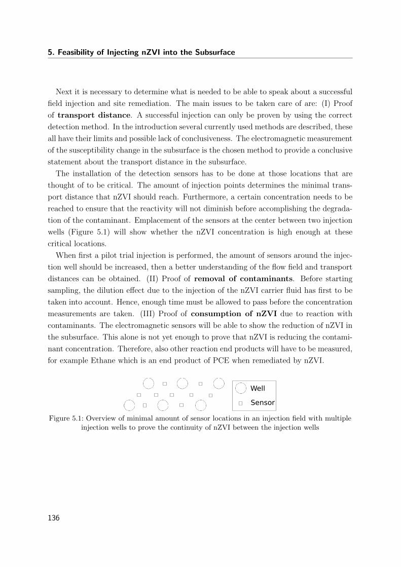
5. Feasibility of Injecting nZVI into the Subsurface
Next it is necessary to determine what is needed to be able to speak about a successful
field injection and site remediation. The main issues to be taken care of are: (I) Proof
of transport distance. A successful injection can only be proven by using the correct
detection method. In the introduction several currently used methods are described, these
all have their limits and possible lack of conclusiveness. The electromagnetic measurement
of the susceptibility change in the subsurface is the chosen method to provide a conclusive
statement about the transport distance in the subsurface.
The installation of the detection sensors has to be done at those locations that are
thought of to be critical. The amount of injection points determines the minimal trans-
port distance that nZVI should reach. Furthermore, a certain concentration needs to be
reached to ensure that the reactivity will not diminish before accomplishing the degrada-
tion of the contaminant. Emplacement of the sensors at the center between two injection
wells (Figure 5.1) will show whether the nZVI concentration is high enough at these
critical locations.
When first a pilot trial injection is performed, the amount of sensors around the injec-
tion well should be increased, then a better understanding of the flow field and transport
distances can be obtained. (II) Proof of removal of contaminants. Before starting
sampling, the dilution effect due to the injection of the nZVI carrier fluid has first to be
taken into account. Hence, enough time must be allowed to pass before the concentration
measurements are taken. (III) Proof of consumption of nZVI due to reaction with
contaminants. The electromagnetic sensors will be able to show the reduction of nZVI in
the subsurface. This alone is not yet enough to prove that nZVI is reducing the contami-
nant concentration. Therefore, also other reaction end products will have to be measured,
for example Ethane which is an end product of PCE when remediated by nZVI.
Sensor
Well
Figure 5.1: Overview of minimal amount of sensor locations in an injection field with multipleinjection wells to prove the continuity of nZVI between the injection wells
136
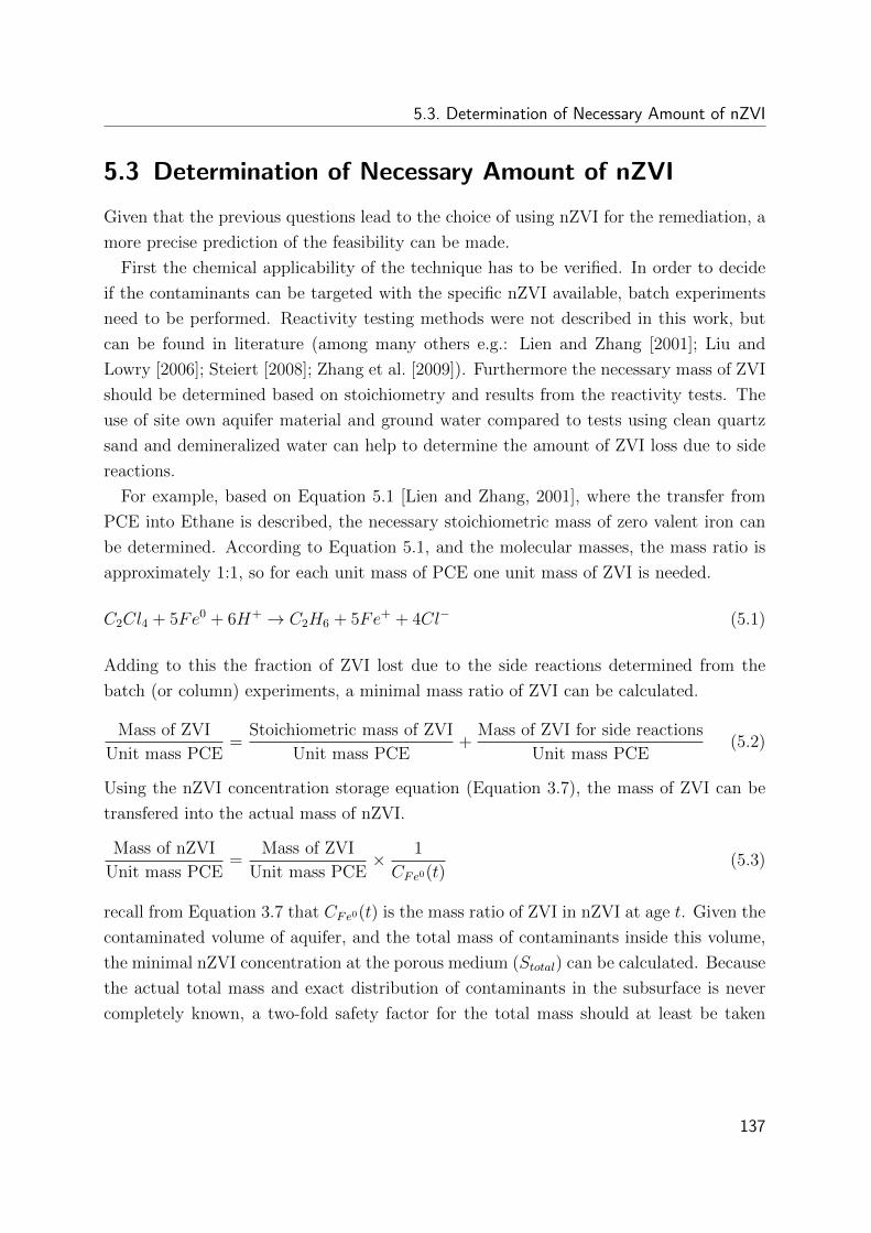
5.3. Determination of Necessary Amount of nZVI
5.3 Determination of Necessary Amount of nZVI
Given that the previous questions lead to the choice of using nZVI for the remediation, a
more precise prediction of the feasibility can be made.
First the chemical applicability of the technique has to be verified. In order to decide
if the contaminants can be targeted with the specific nZVI available, batch experiments
need to be performed. Reactivity testing methods were not described in this work, but
can be found in literature (among many others e.g.: Lien and Zhang [2001]; Liu and
Lowry [2006]; Steiert [2008]; Zhang et al. [2009]). Furthermore the necessary mass of ZVI
should be determined based on stoichiometry and results from the reactivity tests. The
use of site own aquifer material and ground water compared to tests using clean quartz
sand and demineralized water can help to determine the amount of ZVI loss due to side
reactions.
For example, based on Equation 5.1 [Lien and Zhang, 2001], where the transfer from
PCE into Ethane is described, the necessary stoichiometric mass of zero valent iron can
be determined. According to Equation 5.1, and the molecular masses, the mass ratio is
approximately 1:1, so for each unit mass of PCE one unit mass of ZVI is needed.
C2Cl4 + 5Fe0 + 6H+ → C2H6 + 5Fe+ + 4Cl− (5.1)
Adding to this the fraction of ZVI lost due to the side reactions determined from the
batch (or column) experiments, a minimal mass ratio of ZVI can be calculated.
Mass of ZVI
Unit mass PCE=
Stoichiometric mass of ZVI
Unit mass PCE+
Mass of ZVI for side reactions
Unit mass PCE(5.2)
Using the nZVI concentration storage equation (Equation 3.7), the mass of ZVI can be
transfered into the actual mass of nZVI.
Mass of nZVI
Unit mass PCE=
Mass of ZVI
Unit mass PCE× 1
CFe0(t)(5.3)
recall from Equation 3.7 that CFe0(t) is the mass ratio of ZVI in nZVI at age t. Given the
contaminated volume of aquifer, and the total mass of contaminants inside this volume,
the minimal nZVI concentration at the porous medium (Stotal) can be calculated. Because
the actual total mass and exact distribution of contaminants in the subsurface is never
completely known, a two-fold safety factor for the total mass should at least be taken
137
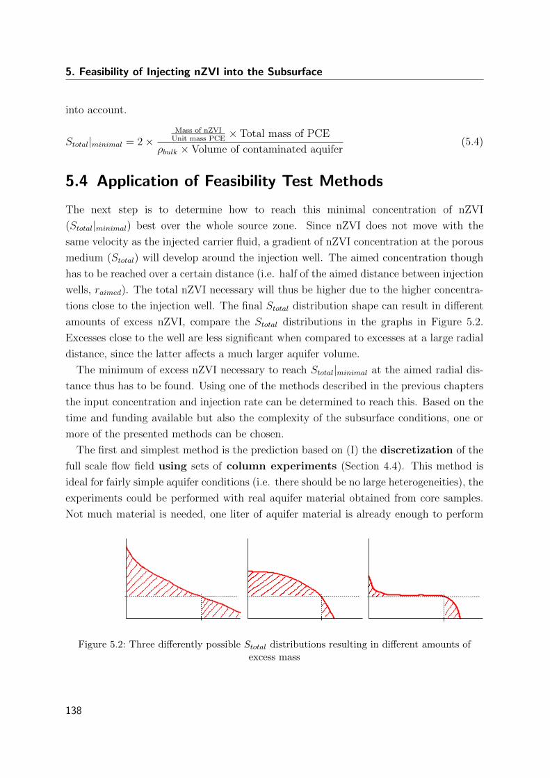
5. Feasibility of Injecting nZVI into the Subsurface
into account.
Stotal|minimal = 2×Mass of nZVI
Unit mass PCE× Total mass of PCE
ρbulk × Volume of contaminated aquifer(5.4)
5.4 Application of Feasibility Test Methods
The next step is to determine how to reach this minimal concentration of nZVI
(Stotal|minimal) best over the whole source zone. Since nZVI does not move with the
same velocity as the injected carrier fluid, a gradient of nZVI concentration at the porous
medium (Stotal) will develop around the injection well. The aimed concentration though
has to be reached over a certain distance (i.e. half of the aimed distance between injection
wells, raimed). The total nZVI necessary will thus be higher due to the higher concentra-
tions close to the injection well. The final Stotal distribution shape can result in different
amounts of excess nZVI, compare the Stotal distributions in the graphs in Figure 5.2.
Excesses close to the well are less significant when compared to excesses at a large radial
distance, since the latter affects a much larger aquifer volume.
The minimum of excess nZVI necessary to reach Stotal|minimal at the aimed radial dis-
tance thus has to be found. Using one of the methods described in the previous chapters
the input concentration and injection rate can be determined to reach this. Based on the
time and funding available but also the complexity of the subsurface conditions, one or
more of the presented methods can be chosen.
The first and simplest method is the prediction based on (I) the discretization of the
full scale flow field using sets of column experiments (Section 4.4). This method is
ideal for fairly simple aquifer conditions (i.e. there should be no large heterogeneities), the
experiments could be performed with real aquifer material obtained from core samples.
Not much material is needed, one liter of aquifer material is already enough to perform
Figure 5.2: Three differently possible Stotal distributions resulting in different amounts ofexcess mass
138
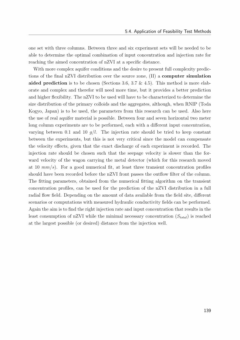
5.4. Application of Feasibility Test Methods
one set with three columns. Between three and six experiment sets will be needed to be
able to determine the optimal combination of input concentration and injection rate for
reaching the aimed concentration of nZVI at a specific distance.
With more complex aquifer conditions and the desire to present full complexity predic-
tions of the final nZVI distribution over the source zone, (II) a computer simulation
aided prediction is to be chosen (Sections 3.6, 3.7 & 4.5). This method is more elab-
orate and complex and therefor will need more time, but it provides a better prediction
and higher flexibility. The nZVI to be used will have to be characterized to determine the
size distribution of the primary colloids and the aggregates, although, when RNIP (Toda
Kogyo, Japan) is to be used, the parameters from this research can be used. Also here
the use of real aquifer material is possible. Between four and seven horizontal two meter
long column experiments are to be performed, each with a different input concentration,
varying between 0.1 and 10 g/l. The injection rate should be tried to keep constant
between the experiments, but this is not very critical since the model can compensate
the velocity effects, given that the exact discharge of each experiment is recorded. The
injection rate should be chosen such that the seepage velocity is slower than the for-
ward velocity of the wagon carrying the metal detector (which for this research moved
at 10 mm/s). For a good numerical fit, at least three transient concentration profiles
should have been recorded before the nZVI front passes the outflow filter of the column.
The fitting parameters, obtained from the numerical fitting algorithm on the transient
concentration profiles, can be used for the prediction of the nZVI distribution in a full
radial flow field. Depending on the amount of data available from the field site, different
scenarios or computations with measured hydraulic conductivity fields can be performed.
Again the aim is to find the right injection rate and input concentration that results in the
least consumption of nZVI while the minimal necessary concentration (Stotal) is reached
at the largest possible (or desired) distance from the injection well.
139
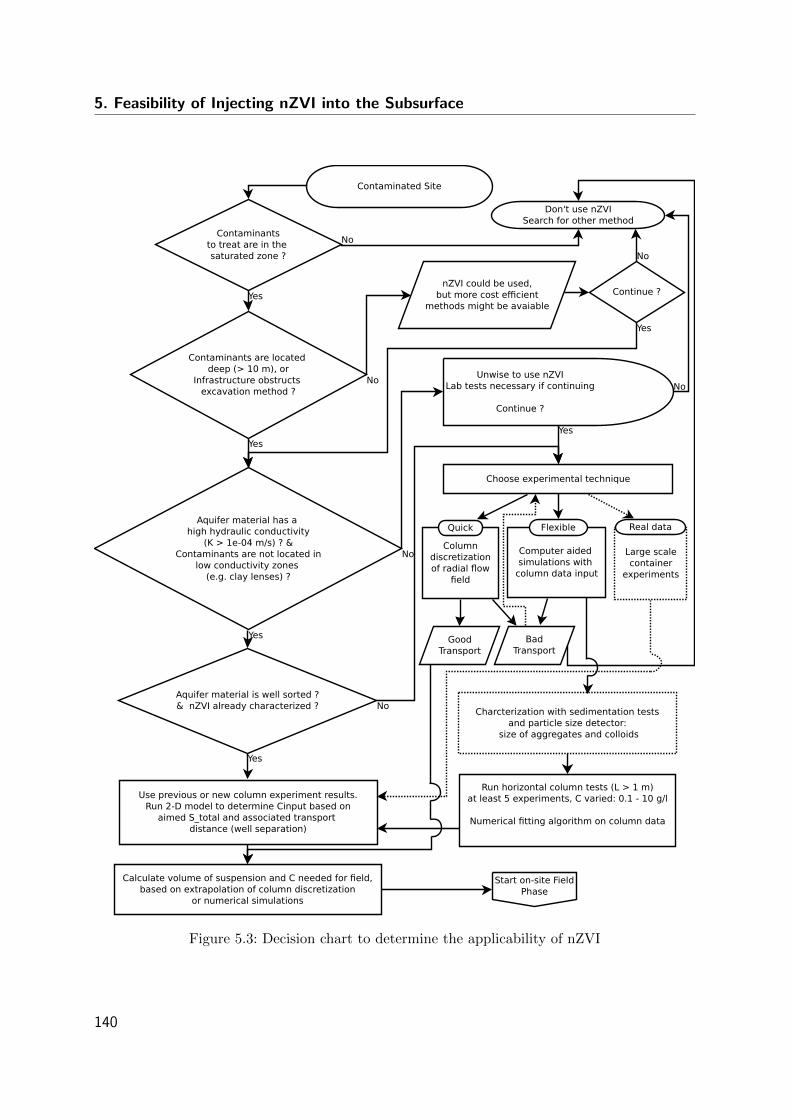
5. Feasibility of Injecting nZVI into the Subsurface
Contaminated Site
Contaminantsto treat are in the saturated zone ?
Don't use nZVISearch for other method
No
Contaminants are located deep (> 10 m), or
Infrastructure obstructs excavation method ?
nZVI could be used,but more cost efficient
methods might be avaiable
No
Continue ?
Aquifer material has a high hydraulic conductivity
(K > 1e-04 m/s) ? &Contaminants are not located in
low conductivity zones (e.g. clay lenses) ?
Yes
Yes
Yes
No
No
Yes
Unwise to use nZVILab tests necessary if continuing
Continue ?
No
Aquifer material is well sorted ?& nZVI already characterized ?
Yes
No
Columndiscretizationof radial flow
field
Quick
Computer aided simulations with
column data input
Flexible
Large scalecontainer
experiments
Real data
Choose experimental technique
GoodTransport
BadTransport
Charcterization with sedimentation testsand particle size detector:
size of aggregates and colloids
Run horizontal column tests (L > 1 m)at least 5 experiments, C varied: 0.1 - 10 g/l
Numerical fitting algorithm on column data
Use previous or new column experiment results.Run 2-D model to determine Cinput based on
aimed S_total and associated transport distance (well separation)
Calculate volume of suspension and C needed for field,based on extrapolation of column discretization
or numerical simulations
Start on-site FieldPhase
Yes
Figure 5.3: Decision chart to determine the applicability of nZVI
140
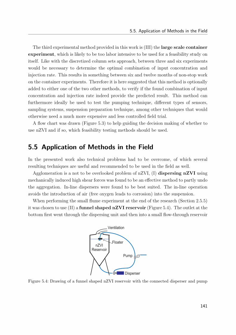
5.5. Application of Methods in the Field
The third experimental method provided in this work is (III) the large scale container
experiment, which is likely to be too labor intensive to be used for a feasibility study on
itself. Like with the discretized column sets approach, between three and six experiments
would be necessary to determine the optimal combination of input concentration and
injection rate. This results in something between six and twelve months of non-stop work
on the container experiments. Therefore it is here suggested that this method is optionally
added to either one of the two other methods, to verify if the found combination of input
concentration and injection rate indeed provide the predicted result. This method can
furthermore ideally be used to test the pumping technique, different types of sensors,
sampling systems, suspension preparation technique, among other techniques that would
otherwise need a much more expensive and less controlled field trial.
A flow chart was drawn (Figure 5.3) to help guiding the decision making of whether to
use nZVI and if so, which feasibility testing methods should be used.
5.5 Application of Methods in the Field
In the presented work also technical problems had to be overcome, of which several
resulting techniques are useful and recommended to be used in the field as well.
Agglomeration is a not to be overlooked problem of nZVI, (I) dispersing nZVI using
mechanically induced high shear forces was found to be an effective method to partly undo
the aggregation. In-line dispersers were found to be best suited. The in-line operation
avoids the introduction of air (free oxygen leads to corrosion) into the suspension.
When performing the small flume experiment at the end of the research (Section 2.5.5)
it was chosen to use (II) a funnel shaped nZVI reservoir (Figure 5.4). The outlet at the
bottom first went through the dispersing unit and then into a small flow-through reservoir
Pump
Disperser
nZVIReservoir
Floater
Ventilation
Figure 5.4: Drawing of a funnel shaped nZVI reservoir with the connected disperser and pump
141
5. Feasibility of Injecting nZVI into the Subsurface
from which the dosing pump took the suspension, all surplus suspension automatically
went back into the top op the funnel shaped reservoir. By using a floater, the well
dispersed suspension was injected just under the water table, providing a very good and
homogeneous suspension inside the reservoir. It is highly recommended that a similar set
up be used for field applications.
One of the tests performed in the container experiments was to determine which type of
pump performed better for an injection. (III) The continuous flux dosing pump was
found to be best suitable. This type of pump can provide a very continuous flux and can
build up high pressures while maintaining the same flux. Also for the column experiments
a small version of such a dosing pump could be used to maintain a continuous flux, also
at higher injection pressures.
(IV) The susceptibility based monitoring technique to observe the transport
during injection should be installed to make sure that nZVI arrived at the calculated
concentration at the desired distance from the injection well. For long term observation
of the consumption of nZVI it is advisable to keep the sensors and electronics installed.
While installing the electro magnetic sensors, this can easily be (V) combined with
the installation of a whole range of other sensors and sampling ports to support the
monitoring during and after the injection.
142
Conclusion
Application of nano sized zero valent iron (nZVI) to remediate contaminated aquifers is a
promising method. By applying nZVI in the source zone and reduce the concentration of
contaminants directly in-situ, the remediation duration and expenses are expected to be
significantly reduced. The main goal of this work was to get a better understanding and
description of the transport of nZVI during the injection into the subsurface. Chemical
feasibility was in the context of this work assumed to be granted and was not further
investigated. Four research questions were set up which could all be answered throughout
this work.
(a) Is it possible to detect In-Situ the concentration of iron and determine the transport
distance?
The first problem faced was the lack of available measuring techniques to determine
non-destructively the concentration of nZVI inside the porous medium. A measuring
technique based on the magnetic susceptibility of zero valent iron inside nZVI col-
loids was developed. The technique was at first worked out for column experiments,
making it possible to measure transient concentration profiles along the full length of
a column. Next the technique was further developed to make in-situ measurements of
nZVI breakthrough possible in a large scale container experiment. This technique was
then further upscaled to a field ready technique, which could be installed in boreholes
at a pilot test or full scale field application.
(b) Which conditions have the largest effect on mobility and how can they be optimized?
By looking into a classic filtration theory in detail, it was determined that the colloid
size is the main factor affecting the transport of nZVI. Through characterization of
the chosen nZVI material in this study (RNIP 10-E, Toda Kogyo, Japan), it was
found out that colloidal aggregation is very abundant, which following the filtration
theory significantly reduces the transport. In order to undo the aggregation, mechan-
ically induced high shear forces were applied by using an in-line dispersing unit, the
aggregation was found not be fully undone, and smaller aggregates maintained.
Column experiments with different input suspension concentrations were performed
143
Conclusion
because the colloid filtration theory does not take the suspension concentration into
account. It was found out that the suspension concentration was a further factor that
significantly influences the transport of nZVI.
Based on these finding, the minimal alterations that had to be applied to the sup-
plied nZVI suspension were dilution and dispersion. Further methods of optimizing
the suspension were not investigated because the aim was to use the commercially
available material with as little changes as possible.
(c) What is the transport distance in a radial flow field?
The transport in a radial flow field was investigated first by performing transport
experiments in a large triangular shaped container, representing a wedge out of a full
cylinder. nZVI was transported over a distance of almost two meters (distance of
one pore volume) after injecting three pore volumes of suspension at 10 g/l, at an
injection duration of one hour. A transport distance of two meters is a very reasonable
distance for field applications.
(d) Which method can test the feasibility of injection into the subsurface?
Two methods were developed to predict the transport of nZVI in a radial flow field
with a high accuracy. A computer simulation aided prediction based on input from
column experiments, and a discretization of the radial flow field into segments that
could be represented by a set of column experiments of various length. An extended
transport and filtration equation was derived and used in the numerical simulations,
both for the column and container experiments. The results of both predictive meth-
ods were compared to the results obtained from the container experiment.
An overview on how to decide in favor of using nZVI and how the predictive methods
can help to design a field application has finally been presented.
The results of this work are very promising and are a sound scientific basis for further
investigations and case studies on nZVI based remediation of contaminated aquifers.
144
Outlook
Already the methods developed here showed to be very useful and the understanding of
the transport of nZVI was significantly improved. Nevertheless, more research could be
performed to further improve the methods and to make the extrapolation to real field
situations solid. The following research items could be taken into account:
Further improve the field sensor to make measurements without reference sensor pos-
sible, as was the case with the sensor developed for the container.
Record breakthrough curves during the container experiments with the container sen-
sors but using the much more sensitive electronics that were developed for the field
sensors. The breakthrough curves could then be used to verify the transient results of
the numerical simulations.
Transient concentration profiles in the container based on photo series from the con-
tainer experiments calibrated on the final measured nZVI distribution might be possi-
ble. This could then also be used to test the transient results of the numerical simula-
tions instead of just the final results.
Identify the mechanisms responsible for the fairly low attachment efficiency of the
aggregates when predicted by the filtration theory.
Improve the filtration theory, which is based on deep bed filtration, because the flow
direction is not only equal to the vertical gravity force component during an injection
in the subsurface.
Perform simulations in a radial flow field by using hydraulic conductivity fields obtained
from tracer breakthrough curves of the container experiments.
Test the simulation with other hydraulic conductivities, include lenses with a lower
or higher hydraulic conductivity, extend the model to full 3-D, include variation in
hydraulic conductivity in the z-direction and simulate multiple injection wells.
Run the numerical simulation for different flow fields, e.g. using an injection-extraction
configuration of wells (e.g. 2-spot or 5-spot).
Testing of characterization and prediction methods on other nZVI products and other
soil material.
145

Outlook
Use a real field site as a case study to determine the input concentration and injection
rate by using the methods developed in this work.
146
Bibliography
Al-Abduwani, F., Bedrikovetsky, P., Farajzadeh, R., van den Broek, W., and Currie, P.
(2005). External filter cake erosion: Mathematical model and experimental study. In
SPE 6th European Formation Damage Conference, SPE 94635. Society of Petroleum
Engineers Inc.
Auslander, K., Fabris, H.-J., Mock, K.-H., Patwald, W., and Seichter, H. (1991). Elec-
tromagnetic shield for an inductive search coil assembly. Patent: US5068612.
Bartzas, G., Komnitsas, K., and Paspaliaris, I. (2006). Laboratory evaluation of Fe0
barriers to treat acidic leachates. Minerals Engineering, 19:505–514.
Baumann, T. and Werth, C. (2005). Visualization of colloid transport through hetero-
geneous porous media using magnetic resonance imaging. Colloids and Surfaces A:
Physicochemical and Engineering Aspects, 265(1-3):2–10.
Bear, J. (1972). Dynamics of Fluids in Porous Media. Elsevier (New York).
Bradford, S. and Bettahar, M. (2006). Concentration dependent transport of colloids in
saturated porous media. Journa of Contaminant Hydrology, 82(1-2):99–117.
Bradford, S. and Torkzaban, S. (2008). Colloid transport and retention in unsaturated
porous media: A review of interface-, collector-, and pore-scale processes and models.
Vadose Zone Journal, 7(2):667–681.
Bregar, V. B. and Pavlin, M. (2004). Effective-susceptibility tensor for a composite
with ferromagnetic inclusions: Enhancement of effective-media theory and alternative
ferromagnetic approach. Journal of Applied Physics, 95(11):6289 –6293.
Brinkman, H. (1947). A calculation of the viscous force exerted by a flowing fluid on a
dense swarm of particles. Applied Scientific Research, A1:27.
147
Bibliography
Buchau, A., Rucker, W., de Boer, C., and Klaas, N. (2010). Inductive detection and con-
centration measurement of nano sized zero valent iron in the subsurface. IET Science,
Measurement & Technology, 4(6):289–297.
Cantrell, K. and Kaplan, D. (1997). Zero-valent iron colloid emplacement in sand columns.
Journal of Environmental Engineering, May:499–505.
Cengel, Y. and Cimbala, J. (2006). Fluid Mechanics, Fundamentals and Applications.
Graw-Hill, New York.
de Boer, C. V. (2007). Characteristics and mobility of zero-valent nano-iron in porous
media. Master’s thesis, Utrecht University.
de Boer, C. V., Braun, J., Klaas, N., and Steiert, S. (2008). Injection of nano-scale iron
for the in-situ remediation of chlorinated hydrocarbons in soil and groundwater. In
Flow & Transport in Permeable Media, Gordon Research Conferences, 13 - 18 July,
Magdalan College, Oxford, United Kingdom.
de Zwart, B.-R. (2007). Investigation of clogging processes in unconsolidated aquifers near
water supply wells. PhD thesis, Delft University of Technology.
Donea, J. and Huerta, A. (2003). Finite Element Methods for Flow Problems. Wiley.
Dunford, D. and Lorentz, S. (1994). Tests of hydraulic and leaching properties of the
vadose zone and groundwater. Department of Agricultural and Chemical Engineering,
Fort Collins, CO 80523.
Elion, E. and Elion, L. (1933). Eine einfache gasvolumetrische methode. Laboratorium
fur Garungstechnik und Angewandte Chemie.
Elliott, D. and Zhang, W.-X. (2001). Field assessment of nanoscale bimetallic particles
for groundwater treatment. Environmental Science & Technology, 35:4922–4926.
Estrella, D. (2011a). Transport of nano-sized zero-valent iron in porous media: Transfor-
mation of 2D container experiments into 1D column experiments. Independent study,
Institut fur Wasserbau, Universitat Stuttgart.
Estrella, D. (2011b). Experimental and numerical approximation methods for zero-valent
iron transport around injection wells. Master’s thesis, Institut fur Wasserbau, Univer-
sitat Stuttgart.
148
Ferguson, J. F. and Pietari, J. M. H. (2000). Anaerobic transformations and bioremedi-
ation of chlorinated solvents. Environmental Pollution, 107(2):209 – 215.
Fetter, C. (1999). Contaminant Hydrogeology, Second Edition. Prentice Hall, NJ.
Getzlaff, M. (2008). Introduction. In Fundamentals of Magnetism, pages 1–6. Springer
Berlin Heidelberg.
Gillham, R. and O’Hannesin, F. (1992). Metal-catelysed abiotic degradation of halo-
genated organic compounds. In IAH Conference Modern trends in Hydrogeology.
Glazier, R., Venkatakrishnan, R., Gheorghiu, F., Walata, L., Nash, R., and Zhang, W.-X.
(2003). Nanotechnology takes root. Civil Engineering, 73(5):64–67.
Godeke, S. (2011). Contaminant hydrogeology. Online. http://www.eugris.info.
Hahn, R. (2006). Personal Communication. Landesanstalt fur Umwelt, Messungen und
Naturschutz Baden-Wurttemberg (LUBW).
Happel, J. (1958). Viscous flow in multiparticle systems. slow motion of fluids relative to
beds of spherical particles. AIChE Journal, 4:197.
Higgs, S. (2009). Mama, Dada, and Nano? Subparticles may be toxic for kids. The
Progressive, 74:18–20.
Hong, Y., Honda, R. J., Myung, N. V., and Walker, S. L. (2009). Transport of iron-
based nanoparticles: Role of magnetic properties. Environmental Science & Technology,
43(23):8834–8839.
Huang, Y., Zhang, T., Shea, P., and Comfort, S. (2003). Effects of oxide coating and
selected cations on nitrate reduction by iron metal. Journal of Environmental Quality,
32:1306–1315.
Iwasaki, T. (1937). Some notes on sand filtration. Journal of the American Water Works
Association, 29:1591–1602.
Kamat, P. V., Huehn, R., and Nicolaescu, R. (2002). A sense and shoot approach for
photocatalytic degradation of organic contaminants in water. The Journal of Physical
Chemistry B, 106(4):788–794.
149
Bibliography
Kanel, S. R., Goswami, R. R., Clement, T. P., Barnett, M. O., and Zhao, D. (2008). Two
dimensional transport characteristics of surface stabilized zero-valent iron nanoparticles
in porous media. Environmental Science & Technology, 42(3):896–900.
Klaas, N. C., Buchau, A., and de Boer, C. V. (2010a). Induktive in-situ-Messtechnik fur
elementare Metalle bei der Sanierung von Grundwasserkontaminationen mit Metallkol-
loiden. Patent: DE102009047858A1.
Klaas, N. C., Steiert, S., de Boer, C. V., and Ruck, W. (2010b). Stabilisierung des ph-
Werts bei wassrigen Suspensionen von Metallpartikeln. Patent: DE102009012834A1.
Koch, D. (2007). Untersuchungen zu den Transporteigenschaften von nullwertigen Fe-
Nanopartikeln in Saulenversuchen. Master’s thesis, Fachbereich Geowissenschaften,
Universitat Bremen.
Lecoanet, H., Bottero, J.-Y., and Wiesner, M. (2004). Laboratory assessment of the mo-
bility of nanomaterials in porous media. Environmental Science & Technology, 38:5164–
5169.
Ley, B. (2010). Diameter of a human hair. Online.
http://hypertextbook.com/facts/1999/BrianLey.shtml.
Li, H., de Boer, C. V., Buchau, A., Klaas, N. C., Rucker, W. M., and Hermes, H. (2012).
Development of an inductive concentration measurement sensor of nano sized zero
valent iron. In Conference of 9th International Multi-Conference on Systems, Signals
and Devices, SSD 2012.
Lien, H.-L. and Zhang, W.-X. (2001). Nanoscale iron particles for complete reduction of
chlorinated ethenes. Colloids and Surfaces, 191:97–105.
Liu, X., O’Carroll, D. M., Petersen, E. J., Huang, Q., and Anderson, C. L. (2009).
Mobility of multiwalled carbon nanotubes in porous media. Environmental Science &
Technology, 43(21):8153–8158.
Liu, Y. and Lowry, G. V. (2006). Effect of particle age (Fe-0 content) and solution pH
on NZVI reactivity: H-2 evolution and TCE dechlorination. Environmental Science &
Technology, 40(19):6085–6090.
150
Liu, Y., Majetich, S., Tilton, R., Sholl, D., and Lowry, G. (2005). TCE Dechlorination
Rates, Pathways, and Efficiency of Nanoscale Iron Particles with Different Properties.
Environmental Science & Technology, 39:1338–1345.
Logg, A., Mardal, K.-A., and Wells, G. (2011). Automated Solution of Differential Equa-
tions by the Finite Element Method. Free Software Foundation.
Long, W. and Hilpert, M. (2009). A correlation for the collector efficiency of Brownian
particles in clean-bed filtration in sphere packings by a Lattice-Boltzmann method.
Environmental Science & Technology, 43(12):4419–4424.
Mattigod, S. V., Fryxell, G. E., Alford, K., Gilmore, T., Parker, K., Serne, J., and
Engelhard, M. (2005). Functionalized TiO2 nanoparticles for use for in situ anion
immobilization. Environmental Science & Technology, 39(18):7306–7310.
Muller, C., Lobel, E., and Rissing, P. (2006a). Sanierung mit Nano-Eisen - Stand der
Technik. Altlasten Spektrum, 2:75–83.
Muller, C., Rissing, P., Widmayer, F., and Wischott, M. (2006b). Nano-Eisen Feldversuch:
Strategie, Durchfuhrung, Ergebnisse und Auswertung. Altlasten Spektrum, 3:137–147.
Nurmi, J., Tratnyek, P., Srathy, V., Baer, D., Amonette, J., Pecher, K., Wang, C.,
Linehan, J., Matson, D., Penn, R., and Driessen, M. (2005). Characterization and
properties of metallic iron nanoparticles: spectroscopy, electrochemistry, and kinetics.
Environmental Science & Technology, 39:1221–1230.
Orlov, A., Jefferson, D. A., Tikhov, M., and Lambert, R. M. (2007). Enhancement of
MTBE photocatalytic degradation by modification of TiO2 with gold nanoparticles.
Catalysis Communications, 8(5):821 – 824.
Payne, F., Quinnan, J., and Potter, S. (2008). Remediation Hydraulics. Boca Raton:
CRC Press.
Phenrat, T., Cihan, A., Kim, H.-J., Mital, M., Illangasekare, T., and Lowry, G. V. (2010).
Transport and deposition of polymer-modified Fe0 nanoparticles in 2-D heterogeneous
porous media: Effects of particle concentration, Fe0 content, and coatings. Environ-
mental Science & Technology, 44(23):9086–9093.
Phenrat, T., Fagerlund, F., Illangasekare, T., Lowry, G. V., and Tilton, R. D. (2011).
Polymer-modified Fe0 nanoparticles target entrapped NAPL in two dimensional porous
151
Bibliography
media: Effect of particle concentration, NAPL saturation, and injection strategy. En-
vironmental Science & Technology, 45(14):6102–6109.
Phenrat, T., Liu, Y., Tilton, R., and Lowry, G. (2009). Adsorbed polyelectrolyte coat-
ings decrease Fe0 nanoparticle reactivity with TCE in water: Conceptual model and
mechanisms. Environmental Science & Technology, 43(5):1507–1514.
Phenrat, T., Saleh, N., Sirk, K., Kim, H.-J., Tilton, R., and Lowry, G. (2008). Stabi-
lization of aqueous nanoscale zerovalent iron dispersions by anionic polyelectrolytes:
adsorbed anionic polyelectrolyte layer properties and their effect on aggregation and
sedimentation. Journal of Nanoparticle Research, 10(5):795–814.
Phenrat, T., Saleh, N., Sirk, K., Tilton, R., and Lowry, G. (2007). Aggregation and
sedimentation of aqueous nanoscale zerovalent iron dispersions. Environmental Science
& Technology, 41(1):284–290.
Prieve, D. C. and Ruckenstein, E. (1974). Effect of london forces upon the rate of depo-
sition of brownian particles. AIChE Journal, 20(6):1178–1187.
Quinn, J., Geiger, C., Clausen, C., et al. (2005). Field demonstration of DNAPL de-
halogenation using emulsified zero-valent iron. Environmental Science & Technology,
March 1(39):1309–1318.
Rad, N. S. and Tumay, M. T. (1985). Factors affecting sand specimen preparation by
raining. Technical report, American Society for Testing and Materials.
Saleh, N., Sirk, K., Liu, Y., Phenrat, T., Dufour, B., Matyjaszewski, K., Tilton, R.,
and Lowry, G. V. (2006). Surface modifications enhance nanoiron transport and dnapl
targeting in saturated porous media. Environmental Engineering Science, in press.
Schijven, J. and Hassanizadeh, S. (2002). Virus removal by soil passage at field scale and
ground-water protection of sandy aquifers. Water Science & Technology, 46(3):123–129.
Schijven, J. F., Hassanizadeh, S., and de Bruin, R. H. (2002). Two-site kinetic model-
ing of bacteriophages transport through columns of saturated dune sand. Journal of
Contaminant Hydrology, 57(34):259–279.
Schrick, B., Hydutsky, B., Blough, J., and Mallouk, T. (2004). Delivery vehicles for ze-
rovalent metal nanoparticles in soil and groundwater. Chemistry of Materials, 16:2187–
2193.
152
Schwartz, F. and Zhang, H. (2003). Fundamentals of Ground Water. John Wiley & Sons,
Inc., New York.
Steiert, S. (2008). Reaktivitat und Langzeitstabilitat von nullwertigem Nano-Eisen bei
der Sanierung von CKW-Schadensfallen in Grundwasserleitern. Diplomarbeit, Versuch-
seinrichtung zur Grundwasser- und Altlastensanierung VEGAS, Institut fur Wasserbau,
Universitat Stuttgart.
Swartjes, F. A. (2011). Introduction to contaminated site management. In Swartjes,
F. A., editor, Dealing with Contaminated Sites, pages 3–89. Springer Netherlands.
Texas Instruments (2002). Analysis of the Sallen-Key Architecture, Application Report.
Texas Instruments, Dallas, Texas 75265, SLOA024B edition.
Tien, C. (1989). Granular Filtration of Aerosols and Hydrosols. Butterworth, Stoneham,
MA.
Tiraferri, A., Chen, K. L., Sethi, R., and Elimelech, M. (2008). Reduced aggregation and
sedimentation of zero-valent iron nanoparticles in the presence of guar gum. Journal
Of Colloid And Interface Science, 324(1-2):71–79.
Tosco, T., Tiraferri, A., and Sethi, R. (2009). Ionic strength dependent transport of
microparticles in saturated porous media: Modeling mobilization and immobilization
phenomena under transient chemical conditions. Environmental Science & Technology,
43(12):4425–4431.
Tratnyek, P. and Johnson, R. (2006). Nanotechnologies for environmental cleanup. nan-
otoday, 1(2):44–48.
Tufenkji, N. and Elimelech, M. (2004). Correlation equation for predicting single-collector
efficiency in physicochemical filtration in saturated porous media. Environmental Sci-
ence & Technology, 38(2):529–536.
Tufenkji, N. and Elimelech, M. (2005a). Breakdown of colloid filtration theory: Role of the
secondary energy minimum and surface charge heterogeneities. Langmuir, 21(3):841–
852.
Tufenkji, N. and Elimelech, M. (2005b). Response to comment on correlation equation for
predicting single-collector efficiency in physicochemical filtration in saturated porous
media. Environmental Science & Technology, 39(14):5496–5497.
153
Bibliography
VanStone, N., Przepiora, A., Vogan, J., Lacrampe-Couloume, G., Powers, B., Perez,
E., Mabury, S., and Lollar, B. S. (2005). Monitoring trichloroethene remediation at
an iron permeable reactive barrier using stable carbon isotopic analysis. Journal Of
Contaminant Hydrology, 78(4):313–325.
Vogan, J. L., Focht, R. M., Clark, D. K., and Graham, S. L. (1999). Performance evalu-
ation of a permeable reactive barrier for remediation of dissolved chlorinated solvents
in groundwater. Journal of Hazardous Materials, 68(1-2):97–108.
Wang, C. B. and Zhang, W. X. (1997). Synthesizing nanoscale iron particles for rapid
and complete dechlorination of TCE and PCBs. Environmental Science & Technology,
31(7):2154–2156.
Wang, Y., Li, Y., Fortner, J. D., Hughes, J. B., Abriola, L. M., and Pennell, K. D. (2008).
Transport and retention of nanoscale C60 aggregates in water-saturated porous media.
Environmental Science & Technology, 42(10):3588–3594.
Witten, T. and Pincus, P. (2004). Structured Fluids. Polymers, Colloids, Surfactants.
Oxford.
Xu, W. (2009). Ermittlung der Transporteigenschaften von reaktiven Nano-Eisen-
Partikel mittels horizontaler Saulenversuche. Diplomarbeit, Versuchseinrichtung zur
Grundwasser- und Altlastensanierung VEGAS, Institut fur Wasserbau, Universitat
Stuttgart.
Yang, S.-Z., Jin, H.-J., Wei, Z., He, R.-X., Ji, Y.-J., Li, X.-M., and Yu, S.-P. (2009).
Bioremediation of oil spills in cold environments: A review. Pedosphere, 19(3):371 –
381.
Yao, K.-M., Habibian, M. T., and O’Melia, C. R. (1971). Water and waste water filtration.
concepts and applications. Environmental Science & Technology, 5(11):1105–1112.
Zhan, J., Zheng, T., Piringer, G., Day, C., McPherson, G. L., Lu, Y., Papadopoulos,
K., and John, V. T. (2008). Transport characteristics of nanoscale functional zerova-
lent iron/silica composites for in situ remediation of trichloroethylene. Environmental
Science & Technology, 42(23):8871–8876.
Zhang, W. (2003). Nanoscale iron particles for environmental remediation: An overview.
Journal of Nanoparticle Research, 5:323–332.
154

Zhang, X., Lin, Y.-M., and Chen, Z.-l. (2009). 2,4,6-Trinitrotoluene reduction kinetics
in aqueous solution using nanoscale zero-valent iron. Journal of Hazardous Materials,
165(1-3):923–927.
155

Curriculum Vitae
Cjestmir Volkert de Boer, M.Sc.
Personal Details
Gender: Male
Date of birth: 27th of July, 1980
Place of birth: Langedijke, Ooststellingwerf, The Netherlands
Citizenship: Dutch
Email: [email protected]
Language Knowledge
Dutch: native English: fluent German: fluent
Education
09/2000–06/2007 Bachelor-/ Master study in Earth Sciences with specialization in En-
vironmental Hydrogeology at the department of Geo Sciences of the
Utrecht University, The Netherlands
09/1992–07/1999 High-school (Atheneum) at Stellingwerf College in Oosterwolde, Fries-
land, The Netherlands
Working Experience
04/2007–03/2012 Research assistant at VEGAS research facility, department of Hy-
draulic Engineering, Stuttgart University, Germany (full-time)
09/2003–08/2004 Help desk assistance at the Faculty ICT Service, Earth Sciences,
Utrecht University (part-time)
04/2003–09/2009 First-line help desk Technical Supporter for YourName Webhosting,
Nijmegen, The Netherlands (part-time)
05/2000–09/2000 Lock-keeper in Friesland, Provinsje Fryslan, The Netherlands (full-
time)
02/2000–05/2000 Assemblage worker at Aludon, Donkerbroek, The Netherlands (full-
time)
Research Projects
05/2009–03/2012 Development of rehabilitation technologies and approaches for multi-
pressured degraded waters and the integration of their impact on river
basin management. Funded by the European Commission through
the 7th Research Framework Programme: FP7 ENV 2008.3.1.1.1,
AQUAREHAB
08/2007–12/2008 Injection of Nano-Scale Iron for the In-Situ Remediation of Chlo-
rinated Hydrocarbons in Soil and Groundwater (Investigations on
Transport in large-scale Experiments and in Field Applications).
Funded by the State of Baden-Wurttemberg, Germany under the
project number 111-047588.6 / 973.049977.9, BUT 013
05/2007–08/2007 Surfactant Flushing in Column and Flume Experiments for the Re-
moval of Residual Chloronaphthaline.
10/2005–05/2007 Feasibility Study on the In-Situ Application of Reactive Nano-Sized
Iron Particles to Remediate CHC-Contaminations. Funded by the
State of Baden-Wurttemberg, Germany through BW-PLUS under the
project number BWR25001

Institut für Wasser- und Umweltsystemmodellierung Universität Stuttgart
Pfaffenwaldring 61 70569 Stuttgart (Vaihingen) Telefon (0711) 685 - 64717/64749/64752/64679 Telefax (0711) 685 - 67020 o. 64746 o. 64681 E-Mail: [email protected] http://www.iws.uni-stuttgart.de
Direktoren Prof. Dr. rer. nat. Dr.-Ing. András Bárdossy Prof. Dr.-Ing. Rainer Helmig Prof. Dr.-Ing. Silke Wieprecht Vorstand (Stand 01.04.2009) Prof. Dr. rer. nat. Dr.-Ing. A. Bárdossy Prof. Dr.-Ing. R. Helmig Prof. Dr.-Ing. S. Wieprecht Jürgen Braun, PhD Dr.-Ing. H. Class Dr.-Ing. S. Hartmann Dr.-Ing. H.-P. Koschitzky PD Dr.-Ing. W. Marx Dr. rer. nat. J. Seidel Emeriti Prof. Dr.-Ing. habil. Dr.-Ing. E.h. Jürgen Giesecke Prof. Dr.h.c. Dr.-Ing. E.h. Helmut Kobus, PhD
Lehrstuhl für Wasserbau und Wassermengenwirtschaft Leiter: Prof. Dr.-Ing. Silke Wieprecht Stellv.: PD Dr.-Ing. Walter Marx, AOR Versuchsanstalt für Wasserbau Leiter: Dr.-Ing. Sven Hartmann, AOR Lehrstuhl für Hydromechanik und Hydrosystemmodellierung Leiter: Prof. Dr.-Ing. Rainer Helmig Stellv.: Dr.-Ing. Holger Class, AOR Lehrstuhl für Hydrologie und Geohydrologie Leiter: Prof. Dr. rer. nat. Dr.-Ing. András Bárdossy Stellv.: Dr. rer. nat. Jochen Seidel VEGAS, Versuchseinrichtung zur Grundwasser- und Altlastensanierung Leitung: Jürgen Braun, PhD Dr.-Ing. Hans-Peter Koschitzky, AD
Verzeichnis der Mitteilungshefte
1 Röhnisch, Arthur: Die Bemühungen um eine Wasserbauliche Versuchsanstalt an
der Technischen Hochschule Stuttgart, und Fattah Abouleid, Abdel: Beitrag zur Berechnung einer in lockeren Sand geramm-ten, zweifach verankerten Spundwand, 1963
2 Marotz, Günter: Beitrag zur Frage der Standfestigkeit von dichten Asphaltbelägen
im Großwasserbau, 1964 3 Gurr, Siegfried: Beitrag zur Berechnung zusammengesetzter ebener Flächen-
tragwerke unter besonderer Berücksichtigung ebener Stauwände, mit Hilfe von Randwert- und Lastwertmatrizen, 1965
4 Plica, Peter: Ein Beitrag zur Anwendung von Schalenkonstruktionen im Stahlwas-
serbau, und Petrikat, Kurt: Möglichkeiten und Grenzen des wasserbaulichen Ver-suchswesens, 1966

2 Institut für Wasser- und Umweltsystemmodellierung * Universität Stuttgart * IWS 5 Plate, Erich: Beitrag zur Bestimmung der Windgeschwindigkeitsverteilung in der
durch eine Wand gestörten bodennahen Luftschicht, und Röhnisch, Arthur; Marotz, Günter: Neue Baustoffe und Bauausführungen für den Schutz der Böschungen und der Sohle von Kanälen, Flüssen und Häfen; Geste-hungskosten und jeweilige Vorteile, sowie Unny, T.E.: Schwingungs-untersuchungen am Kegelstrahlschieber, 1967
6 Seiler, Erich: Die Ermittlung des Anlagenwertes der bundeseigenen Bin-
nenschiffahrtsstraßen und Talsperren und des Anteils der Binnenschiffahrt an die-sem Wert, 1967
7 Sonderheft anläßlich des 65. Geburtstages von Prof. Arthur Röhnisch mit Beiträ-
gen von Benk, Dieter; Breitling, J.; Gurr, Siegfried; Haberhauer, Robert; Hone-kamp, Hermann; Kuz, Klaus Dieter; Marotz, Günter; Mayer-Vorfelder, Hans-Jörg; Miller, Rudolf; Plate, Erich J.; Radomski, Helge; Schwarz, Helmut; Vollmer, Ernst; Wildenhahn, Eberhard; 1967
8 Jumikis, Alfred: Beitrag zur experimentellen Untersuchung des Wassernachschubs
in einem gefrierenden Boden und die Beurteilung der Ergebnisse, 1968 9 Marotz, Günter: Technische Grundlagen einer Wasserspeicherung im natürlichen
Untergrund, 1968 10 Radomski, Helge: Untersuchungen über den Einfluß der Querschnittsform wellen-
förmiger Spundwände auf die statischen und rammtechnischen Eigenschaften, 1968
11 Schwarz, Helmut: Die Grenztragfähigkeit des Baugrundes bei Einwirkung vertikal
gezogener Ankerplatten als zweidimensionales Bruchproblem, 1969 12 Erbel, Klaus: Ein Beitrag zur Untersuchung der Metamorphose von Mittelgebirgs-
schneedecken unter besonderer Berücksichtigung eines Verfahrens zur Bestim-mung der thermischen Schneequalität, 1969
13 Westhaus, Karl-Heinz: Der Strukturwandel in der Binnenschiffahrt und sein Einfluß
auf den Ausbau der Binnenschiffskanäle, 1969 14 Mayer-Vorfelder, Hans-Jörg: Ein Beitrag zur Berechnung des Erdwiderstandes un-
ter Ansatz der logarithmischen Spirale als Gleitflächenfunktion, 1970 15 Schulz, Manfred: Berechnung des räumlichen Erddruckes auf die Wandung kreis-
zylindrischer Körper, 1970 16 Mobasseri, Manoutschehr: Die Rippenstützmauer. Konstruktion und Grenzen ihrer
Standsicherheit, 1970 17 Benk, Dieter: Ein Beitrag zum Betrieb und zur Bemessung von Hochwasser-
rückhaltebecken, 1970

Verzeichnis der Mitteilungshefte 3 18 Gàl, Attila: Bestimmung der mitschwingenden Wassermasse bei überströmten
Fischbauchklappen mit kreiszylindrischem Staublech, 1971, 19 Kuz, Klaus Dieter: Ein Beitrag zur Frage des Einsetzens von Kavitationserschei-
nungen in einer Düsenströmung bei Berücksichtigung der im Wasser gelösten Ga-se, 1971,
20 Schaak, Hartmut: Verteilleitungen von Wasserkraftanlagen, 1971 21 Sonderheft zur Eröffnung der neuen Versuchsanstalt des Instituts für Wasserbau
der Universität Stuttgart mit Beiträgen von Brombach, Hansjörg; Dirksen, Wolfram; Gàl, Attila; Gerlach, Reinhard; Giesecke, Jürgen; Holthoff, Franz-Josef; Kuz, Klaus Dieter; Marotz, Günter; Minor, Hans-Erwin; Petrikat, Kurt; Röhnisch, Arthur; Rueff, Helge; Schwarz, Helmut; Vollmer, Ernst; Wildenhahn, Eberhard; 1972
22 Wang, Chung-su: Ein Beitrag zur Berechnung der Schwingungen an Kegelstrahl-
schiebern, 1972 23 Mayer-Vorfelder, Hans-Jörg: Erdwiderstandsbeiwerte nach dem Ohde-
Variationsverfahren, 1972 24 Minor, Hans-Erwin: Beitrag zur Bestimmung der Schwingungsanfachungs-
funktionen überströmter Stauklappen, 1972, 25 Brombach, Hansjörg: Untersuchung strömungsmechanischer Elemente (Fluidik)
und die Möglichkeit der Anwendung von Wirbelkammerelementen im Wasserbau, 1972,
26 Wildenhahn, Eberhard: Beitrag zur Berechnung von Horizontalfilterbrunnen, 1972 27 Steinlein, Helmut: Die Eliminierung der Schwebstoffe aus Flußwasser zum Zweck
der unterirdischen Wasserspeicherung, gezeigt am Beispiel der Iller, 1972 28 Holthoff, Franz Josef: Die Überwindung großer Hubhöhen in der Binnenschiffahrt
durch Schwimmerhebewerke, 1973 29 Röder, Karl: Einwirkungen aus Baugrundbewegungen auf trog- und kastenförmige
Konstruktionen des Wasser- und Tunnelbaues, 1973 30 Kretschmer, Heinz: Die Bemessung von Bogenstaumauern in Abhängigkeit von
der Talform, 1973 31 Honekamp, Hermann: Beitrag zur Berechnung der Montage von Unterwasserpipe-
lines, 1973 32 Giesecke, Jürgen: Die Wirbelkammertriode als neuartiges Steuerorgan im Was-
serbau, und Brombach, Hansjörg: Entwicklung, Bauformen, Wirkungsweise und Steuereigenschaften von Wirbelkammerverstärkern, 1974
4 Institut für Wasser- und Umweltsystemmodellierung * Universität Stuttgart * IWS 33 Rueff, Helge: Untersuchung der schwingungserregenden Kräfte an zwei hinterein-
ander angeordneten Tiefschützen unter besonderer Berücksichtigung von Kavita-tion, 1974
34 Röhnisch, Arthur: Einpreßversuche mit Zementmörtel für Spannbeton - Vergleich
der Ergebnisse von Modellversuchen mit Ausführungen in Hüllwellrohren, 1975 35 Sonderheft anläßlich des 65. Geburtstages von Prof. Dr.-Ing. Kurt Petrikat mit Bei-
trägen von: Brombach, Hansjörg; Erbel, Klaus; Flinspach, Dieter; Fischer jr., Ri-chard; Gàl, Attila; Gerlach, Reinhard; Giesecke, Jürgen; Haberhauer, Robert; Haf-ner Edzard; Hausenblas, Bernhard; Horlacher, Hans-Burkhard; Hutarew, Andreas; Knoll, Manfred; Krummet, Ralph; Marotz, Günter; Merkle, Theodor; Miller, Chris-toph; Minor, Hans-Erwin; Neumayer, Hans; Rao, Syamala; Rath, Paul; Rueff, Hel-ge; Ruppert, Jürgen; Schwarz, Wolfgang; Topal-Gökceli, Mehmet; Vollmer, Ernst; Wang, Chung-su; Weber, Hans-Georg; 1975
36 Berger, Jochum: Beitrag zur Berechnung des Spannungszustandes in rotations-
symmetrisch belasteten Kugelschalen veränderlicher Wandstärke unter Gas- und Flüssigkeitsdruck durch Integration schwach singulärer Differentialgleichungen, 1975
37 Dirksen, Wolfram: Berechnung instationärer Abflußvorgänge in gestauten Gerin-
nen mittels Differenzenverfahren und die Anwendung auf Hochwasserrückhalte-becken, 1976
38 Horlacher, Hans-Burkhard: Berechnung instationärer Temperatur- und Wärme-
spannungsfelder in langen mehrschichtigen Hohlzylindern, 1976 39 Hafner, Edzard: Untersuchung der hydrodynamischen Kräfte auf Baukörper im
Tiefwasserbereich des Meeres, 1977, ISBN 3-921694-39-6 40 Ruppert, Jürgen: Über den Axialwirbelkammerverstärker für den Einsatz im Was-
serbau, 1977, ISBN 3-921694-40-X 41 Hutarew, Andreas: Beitrag zur Beeinflußbarkeit des Sauerstoffgehalts in Fließge-
wässern an Abstürzen und Wehren, 1977, ISBN 3-921694-41-8, 42 Miller, Christoph: Ein Beitrag zur Bestimmung der schwingungserregenden Kräfte
an unterströmten Wehren, 1977, ISBN 3-921694-42-6 43 Schwarz, Wolfgang: Druckstoßberechnung unter Berücksichtigung der Radial- und
Längsverschiebungen der Rohrwandung, 1978, ISBN 3-921694-43-4 44 Kinzelbach, Wolfgang: Numerische Untersuchungen über den optimalen Einsatz
variabler Kühlsysteme einer Kraftwerkskette am Beispiel Oberrhein, 1978, ISBN 3-921694-44-2
45 Barczewski, Baldur: Neue Meßmethoden für Wasser-Luftgemische und deren An-
wendung auf zweiphasige Auftriebsstrahlen, 1979, ISBN 3-921694-45-0
Verzeichnis der Mitteilungshefte 5 46 Neumayer, Hans: Untersuchung der Strömungsvorgänge in radialen Wirbelkam-
merverstärkern, 1979, ISBN 3-921694-46-9 47 Elalfy, Youssef-Elhassan: Untersuchung der Strömungsvorgänge in Wirbelkam-
merdioden und -drosseln, 1979, ISBN 3-921694-47-7 48 Brombach, Hansjörg: Automatisierung der Bewirtschaftung von Wasserspeichern,
1981, ISBN 3-921694-48-5 49 Geldner, Peter: Deterministische und stochastische Methoden zur Bestimmung der
Selbstdichtung von Gewässern, 1981, ISBN 3-921694-49-3, 50 Mehlhorn, Hans: Temperaturveränderungen im Grundwasser durch Brauchwas-
sereinleitungen, 1982, ISBN 3-921694-50-7, 51 Hafner, Edzard: Rohrleitungen und Behälter im Meer, 1983, ISBN 3-921694-51-5 52 Rinnert, Bernd: Hydrodynamische Dispersion in porösen Medien: Einfluß von Dich-
teunterschieden auf die Vertikalvermischung in horizontaler Strömung, 1983, ISBN 3-921694-52-3,
53 Lindner, Wulf: Steuerung von Grundwasserentnahmen unter Einhaltung ökologi-
scher Kriterien, 1983, ISBN 3-921694-53-1, 54 Herr, Michael; Herzer, Jörg; Kinzelbach, Wolfgang; Kobus, Helmut; Rinnert, Bernd:
Methoden zur rechnerischen Erfassung und hydraulischen Sanierung von Grund-wasserkontaminationen, 1983, ISBN 3-921694-54-X
55 Schmitt, Paul: Wege zur Automatisierung der Niederschlagsermittlung, 1984, ISBN
3-921694-55-8, 56 Müller, Peter: Transport und selektive Sedimentation von Schwebstoffen bei ge-
stautem Abfluß, 1985, ISBN 3-921694-56-6 57 El-Qawasmeh, Fuad: Möglichkeiten und Grenzen der Tropfbewässerung unter be-
sonderer Berücksichtigung der Verstopfungsanfälligkeit der Tropfelemente, 1985, ISBN 3-921694-57-4,
58 Kirchenbaur, Klaus: Mikroprozessorgesteuerte Erfassung instationärer Druckfelder
am Beispiel seegangsbelasteter Baukörper, 1985, ISBN 3-921694-58-2 59 Kobus, Helmut (Hrsg.): Modellierung des großräumigen Wärme- und Schadstoff-
transports im Grundwasser, Tätigkeitsbericht 1984/85 (DFG-Forschergruppe an den Universitäten Hohenheim, Karlsruhe und Stuttgart), 1985, ISBN 3-921694-59-0,
60 Spitz, Karlheinz: Dispersion in porösen Medien: Einfluß von Inhomogenitäten und
Dichteunterschieden, 1985, ISBN 3-921694-60-4, 61 Kobus, Helmut: An Introduction to Air-Water Flows in Hydraulics, 1985,
ISBN 3-921694-61-2
6 Institut für Wasser- und Umweltsystemmodellierung * Universität Stuttgart * IWS 62 Kaleris, Vassilios: Erfassung des Austausches von Oberflächen- und Grundwasser
in horizontalebenen Grundwassermodellen, 1986, ISBN 3-921694-62-0 63 Herr, Michael: Grundlagen der hydraulischen Sanierung verunreinigter Poren-
grundwasserleiter, 1987, ISBN 3-921694-63-9 64 Marx, Walter: Berechnung von Temperatur und Spannung in Massenbeton infolge
Hydratation, 1987, ISBN 3-921694-64-7 65 Koschitzky, Hans-Peter: Dimensionierungskonzept für Sohlbelüfter in Schußrinnen
zur Vermeidung von Kavitationsschäden, 1987, ISBN 3-921694-65-5 66 Kobus, Helmut (Hrsg.): Modellierung des großräumigen Wärme- und Schadstoff-
transports im Grundwasser, Tätigkeitsbericht 1986/87 (DFG-Forschergruppe an den Universitäten Hohenheim, Karlsruhe und Stuttgart) 1987, ISBN 3-921694-66-3
67 Söll, Thomas: Berechnungsverfahren zur Abschätzung anthropogener Tempera-
turanomalien im Grundwasser, 1988, ISBN 3-921694-67-1 68 Dittrich, Andreas; Westrich, Bernd: Bodenseeufererosion, Bestandsaufnahme und
Bewertung, 1988, ISBN 3-921694-68-X, 69 Huwe, Bernd; van der Ploeg, Rienk R.: Modelle zur Simulation des Stickstoffhaus-
haltes von Standorten mit unterschiedlicher landwirtschaftlicher Nutzung, 1988, ISBN 3-921694-69-8,
70 Stephan, Karl: Integration elliptischer Funktionen, 1988, ISBN 3-921694-70-1 71 Kobus, Helmut; Zilliox, Lothaire (Hrsg.): Nitratbelastung des Grundwassers, Aus-
wirkungen der Landwirtschaft auf die Grundwasser- und Rohwasserbeschaffenheit und Maßnahmen zum Schutz des Grundwassers. Vorträge des deutsch-franzö-sischen Kolloquiums am 6. Oktober 1988, Universitäten Stuttgart und Louis Pas-teur Strasbourg (Vorträge in deutsch oder französisch, Kurzfassungen zwei-sprachig), 1988, ISBN 3-921694-71-X
72 Soyeaux, Renald: Unterströmung von Stauanlagen auf klüftigem Untergrund unter
Berücksichtigung laminarer und turbulenter Fließzustände,1991, ISBN 3-921694-72-8
73 Kohane, Roberto: Berechnungsmethoden für Hochwasserabfluß in Fließgewäs-
sern mit überströmten Vorländern, 1991, ISBN 3-921694-73-6 74 Hassinger, Reinhard: Beitrag zur Hydraulik und Bemessung von Blocksteinrampen
in flexibler Bauweise, 1991, ISBN 3-921694-74-4, 75 Schäfer, Gerhard: Einfluß von Schichtenstrukturen und lokalen Einlagerungen auf
die Längsdispersion in Porengrundwasserleitern, 1991, ISBN 3-921694-75-2 76 Giesecke, Jürgen: Vorträge, Wasserwirtschaft in stark besiedelten Regionen; Um-
weltforschung mit Schwerpunkt Wasserwirtschaft, 1991, ISBN 3-921694-76-0
Verzeichnis der Mitteilungshefte 7 77 Huwe, Bernd: Deterministische und stochastische Ansätze zur Modellierung des
Stickstoffhaushalts landwirtschaftlich genutzter Flächen auf unterschiedlichem Skalenniveau, 1992, ISBN 3-921694-77-9,
78 Rommel, Michael: Verwendung von Kluftdaten zur realitätsnahen Generierung von
Kluftnetzen mit anschließender laminar-turbulenter Strömungsberechnung, 1993, ISBN 3-92 1694-78-7
79 Marschall, Paul: Die Ermittlung lokaler Stofffrachten im Grundwasser mit Hilfe von
Einbohrloch-Meßverfahren, 1993, ISBN 3-921694-79-5, 80 Ptak, Thomas: Stofftransport in heterogenen Porenaquiferen: Felduntersuchungen
und stochastische Modellierung, 1993, ISBN 3-921694-80-9, 81 Haakh, Frieder: Transientes Strömungsverhalten in Wirbelkammern, 1993,
ISBN 3-921694-81-7 82 Kobus, Helmut; Cirpka, Olaf; Barczewski, Baldur; Koschitzky, Hans-Peter: Ver-
sucheinrichtung zur Grundwasser und Altlastensanierung VEGAS, Konzeption und Programmrahmen, 1993, ISBN 3-921694-82-5
83 Zang, Weidong: Optimaler Echtzeit-Betrieb eines Speichers mit aktueller Abflußre-
generierung, 1994, ISBN 3-921694-83-3, 84 Franke, Hans-Jörg: Stochastische Modellierung eines flächenhaften Stoffeintrages
und Transports in Grundwasser am Beispiel der Pflanzenschutzmittelproblematik, 1995, ISBN 3-921694-84-1
85 Lang, Ulrich: Simulation regionaler Strömungs- und Transportvorgänge in Karst-
aquiferen mit Hilfe des Doppelkontinuum-Ansatzes: Methodenentwicklung und Pa-rameteridentifikation, 1995, ISBN 3-921694-85-X,
86 Helmig, Rainer: Einführung in die Numerischen Methoden der Hydromechanik,
1996, ISBN 3-921694-86-8, 87 Cirpka, Olaf: CONTRACT: A Numerical Tool for Contaminant Transport and
Chemical Transformations - Theory and Program Documentation -, 1996, ISBN 3-921694-87-6
88 Haberlandt, Uwe: Stochastische Synthese und Regionalisierung des Niederschla-
ges für Schmutzfrachtberechnungen, 1996, ISBN 3-921694-88-4 89 Croisé, Jean: Extraktion von flüchtigen Chemikalien aus natürlichen Lockergestei-
nen mittels erzwungener Luftströmung, 1996, ISBN 3-921694-89-2, 90 Jorde, Klaus: Ökologisch begründete, dynamische Mindestwasserregelungen bei
Ausleitungskraftwerken, 1997, ISBN 3-921694-90-6, 91 Helmig, Rainer: Gekoppelte Strömungs- und Transportprozesse im Untergrund -
Ein Beitrag zur Hydrosystemmodellierung-, 1998, ISBN 3-921694-91-4,
8 Institut für Wasser- und Umweltsystemmodellierung * Universität Stuttgart * IWS 92 Emmert, Martin: Numerische Modellierung nichtisothermer Gas-Wasser Systeme
in porösen Medien, 1997, ISBN 3-921694-92-2 93 Kern, Ulrich: Transport von Schweb- und Schadstoffen in staugeregelten Fließge-
wässern am Beispiel des Neckars, 1997, ISBN 3-921694-93-0, 94 Förster, Georg: Druckstoßdämpfung durch große Luftblasen in Hochpunkten von
Rohrleitungen 1997, ISBN 3-921694-94-9 95 Cirpka, Olaf: Numerische Methoden zur Simulation des reaktiven Mehrkomponen-
tentransports im Grundwasser, 1997, ISBN 3-921694-95-7, 96 Färber, Arne: Wärmetransport in der ungesättigten Bodenzone: Entwicklung einer
thermischen In-situ-Sanierungstechnologie, 1997, ISBN 3-921694-96-5 97 Betz, Christoph: Wasserdampfdestillation von Schadstoffen im porösen Medium:
Entwicklung einer thermischen In-situ-Sanierungstechnologie, 1998, ISBN 3-921694-97-3
98 Xu, Yichun: Numerical Modeling of Suspended Sediment Transport in Rivers,
1998, ISBN 3-921694-98-1, 99 Wüst, Wolfgang: Geochemische Untersuchungen zur Sanierung CKW-
kontaminierter Aquifere mit Fe(0)-Reaktionswänden, 2000, ISBN 3-933761-02-2 100 Sheta, Hussam: Simulation von Mehrphasenvorgängen in porösen Medien unter
Einbeziehung von Hysterese-Effekten, 2000, ISBN 3-933761-03-4 101 Ayros, Edwin: Regionalisierung extremer Abflüsse auf der Grundlage statistischer
Verfahren, 2000, ISBN 3-933761-04-2, 102 Huber, Ralf: Compositional Multiphase Flow and Transport in Heterogeneous Po-
rous Media, 2000, ISBN 3-933761-05-0 103 Braun, Christopherus: Ein Upscaling-Verfahren für Mehrphasenströmungen in po-
rösen Medien, 2000, ISBN 3-933761-06-9 104 Hofmann, Bernd: Entwicklung eines rechnergestützten Managementsystems zur
Beurteilung von Grundwasserschadensfällen, 2000, ISBN 3-933761-07-7 105 Class, Holger: Theorie und numerische Modellierung nichtisothermer Mehrphasen-
prozesse in NAPL-kontaminierten porösen Medien, 2001, ISBN 3-933761-08-5
106 Schmidt, Reinhard: Wasserdampf- und Heißluftinjektion zur thermischen Sanie-
rung kontaminierter Standorte, 2001, ISBN 3-933761-09-3 107 Josef, Reinhold:, Schadstoffextraktion mit hydraulischen Sanierungsverfahren un-
ter Anwendung von grenzflächenaktiven Stoffen, 2001, ISBN 3-933761-10-7
Verzeichnis der Mitteilungshefte 9 108 Schneider, Matthias: Habitat- und Abflussmodellierung für Fließgewässer mit un-
scharfen Berechnungsansätzen, 2001, ISBN 3-933761-11-5 109 Rathgeb, Andreas: Hydrodynamische Bemessungsgrundlagen für Lockerdeckwer-
ke an überströmbaren Erddämmen, 2001, ISBN 3-933761-12-3 110 Lang, Stefan: Parallele numerische Simulation instätionärer Probleme mit adapti-
ven Methoden auf unstrukturierten Gittern, 2001, ISBN 3-933761-13-1 111 Appt, Jochen; Stumpp Simone: Die Bodensee-Messkampagne 2001, IWS/CWR
Lake Constance Measurement Program 2001, 2002, ISBN 3-933761-14-X 112 Heimerl, Stephan: Systematische Beurteilung von Wasserkraftprojekten, 2002,
ISBN 3-933761-15-8, 113 Iqbal, Amin: On the Management and Salinity Control of Drip Irrigation, 2002, ISBN
3-933761-16-6 114 Silberhorn-Hemminger, Annette: Modellierung von Kluftaquifersystemen: Geosta-
tistische Analyse und deterministisch-stochastische Kluftgenerierung, 2002, ISBN 3-933761-17-4
115 Winkler, Angela: Prozesse des Wärme- und Stofftransports bei der In-situ-
Sanierung mit festen Wärmequellen, 2003, ISBN 3-933761-18-2 116 Marx, Walter: Wasserkraft, Bewässerung, Umwelt - Planungs- und Bewertungs-
schwerpunkte der Wasserbewirtschaftung, 2003, ISBN 3-933761-19-0 117 Hinkelmann, Reinhard: Efficient Numerical Methods and Information-Processing
Techniques in Environment Water, 2003, ISBN 3-933761-20-4 118 Samaniego-Eguiguren, Luis Eduardo: Hydrological Consequences of Land Use /
Land Cover and Climatic Changes in Mesoscale Catchments, 2003, ISBN 3-933761-21-2
119 Neunhäuserer, Lina: Diskretisierungsansätze zur Modellierung von Strömungs-
und Transportprozessen in geklüftet-porösen Medien, 2003, ISBN 3-933761-22-0 120 Paul, Maren: Simulation of Two-Phase Flow in Heterogeneous Poros Media with
Adaptive Methods, 2003, ISBN 3-933761-23-9 121 Ehret, Uwe: Rainfall and Flood Nowcasting in Small Catchments using Weather
Radar, 2003, ISBN 3-933761-24-7 122 Haag, Ingo: Der Sauerstoffhaushalt staugeregelter Flüsse am Beispiel des Ne-
ckars - Analysen, Experimente, Simulationen -, 2003, ISBN 3-933761-25-5 123 Appt, Jochen: Analysis of Basin-Scale Internal Waves in Upper Lake Constance,
2003, ISBN 3-933761-26-3
10 Institut für Wasser- und Umweltsystemmodellierung * Universität Stuttgart * IWS 124 Hrsg.: Schrenk, Volker; Batereau, Katrin; Barczewski, Baldur; Weber, Karolin und
Koschitzky, Hans-Peter: Symposium Ressource Fläche und VEGAS - Statuskol-loquium 2003, 30. September und 1. Oktober 2003, 2003, ISBN 3-933761-27-1
125 Omar Khalil Ouda: Optimisation of Agricultural Water Use: A Decision Support
System for the Gaza Strip, 2003, ISBN 3-933761-28-0 126 Batereau, Katrin: Sensorbasierte Bodenluftmessung zur Vor-Ort-Erkundung von
Schadensherden im Untergrund, 2004, ISBN 3-933761-29-8 127 Witt, Oliver: Erosionsstabilität von Gewässersedimenten mit Auswirkung auf den
Stofftransport bei Hochwasser am Beispiel ausgewählter Stauhaltungen des Ober-rheins, 2004, ISBN 3-933761-30-1
128 Jakobs, Hartmut: Simulation nicht-isothermer Gas-Wasser-Prozesse in komplexen
Kluft-Matrix-Systemen, 2004, ISBN 3-933761-31-X 129 Li, Chen-Chien: Deterministisch-stochastisches Berechnungskonzept zur Beurtei-
lung der Auswirkungen erosiver Hochwasserereignisse in Flussstauhaltungen, 2004, ISBN 3-933761-32-8
130 Reichenberger, Volker; Helmig, Rainer; Jakobs, Hartmut; Bastian, Peter; Niessner,
Jennifer: Complex Gas-Water Processes in Discrete Fracture-Matrix Systems: Up-scaling, Mass-Conservative Discretization and Efficient Multilevel Solution, 2004, ISBN 3-933761-33-6
131 Hrsg.: Barczewski, Baldur; Koschitzky, Hans-Peter; Weber, Karolin; Wege, Ralf:
VEGAS - Statuskolloquium 2004, Tagungsband zur Veranstaltung am 05. Oktober 2004 an der Universität Stuttgart, Campus Stuttgart-Vaihingen, 2004, ISBN 3-933761-34-4
132 Asie, Kemal Jabir: Finite Volume Models for Multiphase Multicomponent Flow
through Porous Media. 2005, ISBN 3-933761-35-2 133 Jacoub, George: Development of a 2-D Numerical Module for Particulate Con-
taminant Transport in Flood Retention Reservoirs and Impounded Rivers, 2004, ISBN 3-933761-36-0
134 Nowak, Wolfgang: Geostatistical Methods for the Identification of Flow and Trans-
port Parameters in the Subsurface, 2005, ISBN 3-933761-37-9 135 Süß, Mia: Analysis of the influence of structures and boundaries on flow and
transport processes in fractured porous media, 2005, ISBN 3-933761-38-7 136 Jose, Surabhin Chackiath: Experimental Investigations on Longitudinal Dispersive
Mixing in Heterogeneous Aquifers, 2005, ISBN: 3-933761-39-5 137 Filiz, Fulya: Linking Large-Scale Meteorological Conditions to Floods in Mesoscale
Catchments, 2005, ISBN 3-933761-40-9
Verzeichnis der Mitteilungshefte 11 138 Qin, Minghao: Wirklichkeitsnahe und recheneffiziente Ermittlung von Temperatur
und Spannungen bei großen RCC-Staumauern, 2005, ISBN 3-933761-41-7 139 Kobayashi, Kenichiro: Optimization Methods for Multiphase Systems in the Sub-
surface - Application to Methane Migration in Coal Mining Areas, 2005, ISBN 3-933761-42-5
140 Rahman, Md. Arifur: Experimental Investigations on Transverse Dispersive Mixing
in Heterogeneous Porous Media, 2005, ISBN 3-933761-43-3 141 Schrenk, Volker: Ökobilanzen zur Bewertung von Altlastensanierungsmaßnahmen,
2005, ISBN 3-933761-44-1 142 Hundecha, Hirpa Yeshewatesfa: Regionalization of Parameters of a Conceptual
Rainfall-Runoff Model, 2005, ISBN: 3-933761-45-X 143 Wege, Ralf: Untersuchungs- und Überwachungsmethoden für die Beurteilung na-
türlicher Selbstreinigungsprozesse im Grundwasser, 2005, ISBN 3-933761-46-8 144 Breiting, Thomas: Techniken und Methoden der Hydroinformatik - Modellierung
von komplexen Hydrosystemen im Untergrund, 2006, 3-933761-47-6 145 Hrsg.: Braun, Jürgen; Koschitzky, Hans-Peter; Müller, Martin: Ressource Unter-
grund: 10 Jahre VEGAS: Forschung und Technologieentwicklung zum Schutz von Grundwasser und Boden, Tagungsband zur Veranstaltung am 28. und 29. Sep-tember 2005 an der Universität Stuttgart, Campus Stuttgart-Vaihingen, 2005, ISBN 3-933761-48-4
146 Rojanschi, Vlad: Abflusskonzentration in mesoskaligen Einzugsgebieten unter
Berücksichtigung des Sickerraumes, 2006, ISBN 3-933761-49-2 147 Winkler, Nina Simone: Optimierung der Steuerung von Hochwasserrückhaltebe-
cken-systemen, 2006, ISBN 3-933761-50-6 148 Wolf, Jens: Räumlich differenzierte Modellierung der Grundwasserströmung allu-
vialer Aquifere für mesoskalige Einzugsgebiete, 2006, ISBN: 3-933761-51-4 149 Kohler, Beate: Externe Effekte der Laufwasserkraftnutzung, 2006,
ISBN 3-933761-52-2 150 Hrsg.: Braun, Jürgen; Koschitzky, Hans-Peter; Stuhrmann, Matthias: VEGAS-
Statuskolloquium 2006, Tagungsband zur Veranstaltung am 28. September 2006 an der Universität Stuttgart, Campus Stuttgart-Vaihingen, 2006, ISBN 3-933761-53-0
151 Niessner, Jennifer: Multi-Scale Modeling of Multi-Phase - Multi-Component Pro-
cesses in Heterogeneous Porous Media, 2006, ISBN 3-933761-54-9 152 Fischer, Markus: Beanspruchung eingeerdeter Rohrleitungen infolge Austrocknung
bindiger Böden, 2006, ISBN 3-933761-55-7

12 Institut für Wasser- und Umweltsystemmodellierung * Universität Stuttgart * IWS 153 Schneck, Alexander: Optimierung der Grundwasserbewirtschaftung unter Berück-
sichtigung der Belange der Wasserversorgung, der Landwirtschaft und des Natur-schutzes, 2006, ISBN 3-933761-56-5
154 Das, Tapash: The Impact of Spatial Variability of Precipitation on the Predictive
Uncertainty of Hydrological Models, 2006, ISBN 3-933761-57-3 155 Bielinski, Andreas: Numerical Simulation of CO2 sequestration in geological forma-
tions, 2007, ISBN 3-933761-58-1 156 Mödinger, Jens: Entwicklung eines Bewertungs- und Entscheidungsunterstüt-
zungssystems für eine nachhaltige regionale Grundwasserbewirtschaftung, 2006, ISBN 3-933761-60-3
157 Manthey, Sabine: Two-phase flow processes with dynamic effects in porous
media - parameter estimation and simulation, 2007, ISBN 3-933761-61-1 158 Pozos Estrada, Oscar: Investigation on the Effects of Entrained Air in Pipelines,
2007, ISBN 3-933761-62-X 159 Ochs, Steffen Oliver: Steam injection into saturated porous media – process
analysis including experimental and numerical investigations, 2007, ISBN 3-933761-63-8
160 Marx, Andreas: Einsatz gekoppelter Modelle und Wetterradar zur Abschätzung
von Niederschlagsintensitäten und zur Abflussvorhersage, 2007, ISBN 3-933761-64-6
161 Hartmann, Gabriele Maria: Investigation of Evapotranspiration Concepts in Hydro-
logical Modelling for Climate Change Impact Assessment, 2007, ISBN 3-933761-65-4
162 Kebede Gurmessa, Tesfaye: Numerical Investigation on Flow and Transport Char-
acteristics to Improve Long-Term Simulation of Reservoir Sedimentation, 2007, ISBN 3-933761-66-2
163 Trifković, Aleksandar: Multi-objective and Risk-based Modelling Methodology for
Planning, Design and Operation of Water Supply Systems, 2007, ISBN 3-933761-67-0
164 Götzinger, Jens: Distributed Conceptual Hydrological Modelling - Simulation of
Climate, Land Use Change Impact and Uncertainty Analysis, 2007, ISBN 3-933761-68-9
165 Hrsg.: Braun, Jürgen; Koschitzky, Hans-Peter; Stuhrmann, Matthias: VEGAS –
Kolloquium 2007, Tagungsband zur Veranstaltung am 26. September 2007 an der Universität Stuttgart, Campus Stuttgart-Vaihingen, 2007, ISBN 3-933761-69-7
166 Freeman, Beau: Modernization Criteria Assessment for Water Resources Plan-
ning; Klamath Irrigation Project, U.S., 2008, ISBN 3-933761-70-0
Verzeichnis der Mitteilungshefte 13 167 Dreher, Thomas: Selektive Sedimentation von Feinstschwebstoffen in Wechselwir-
kung mit wandnahen turbulenten Strömungsbedingungen, 2008, ISBN 3-933761-71-9
168 Yang, Wei: Discrete-Continuous Downscaling Model for Generating Daily Precipi-
tation Time Series, 2008, ISBN 3-933761-72-7 169 Kopecki, Ianina: Calculational Approach to FST-Hemispheres for Multiparametrical
Benthos Habitat Modelling, 2008, ISBN 3-933761-73-5 170 Brommundt, Jürgen: Stochastische Generierung räumlich zusammenhängender
Niederschlagszeitreihen, 2008, ISBN 3-933761-74-3 171 Papafotiou, Alexandros: Numerical Investigations of the Role of Hysteresis in Het-
erogeneous Two-Phase Flow Systems, 2008, ISBN 3-933761-75-1 172 He, Yi: Application of a Non-Parametric Classification Scheme to Catchment Hy-
drology, 2008, ISBN 978-3-933761-76-7 173 Wagner, Sven: Water Balance in a Poorly Gauged Basin in West Africa Using At-
mospheric Modelling and Remote Sensing Information, 2008, ISBN 978-3-933761-77-4
174 Hrsg.: Braun, Jürgen; Koschitzky, Hans-Peter; Stuhrmann, Matthias; Schrenk, Vol-
ker: VEGAS-Kolloquium 2008 Ressource Fläche III, Tagungsband zur Veranstal-tung am 01. Oktober 2008 an der Universität Stuttgart, Campus Stuttgart-Vaihingen, 2008, ISBN 978-3-933761-78-1
175 Patil, Sachin: Regionalization of an Event Based Nash Cascade Model for Flood
Predictions in Ungauged Basins, 2008, ISBN 978-3-933761-79-8 176 Assteerawatt, Anongnart: Flow and Transport Modelling of Fractured Aquifers
based on a Geostatistical Approach, 2008, ISBN 978-3-933761-80-4 177 Karnahl, Joachim Alexander: 2D numerische Modellierung von multifraktionalem
Schwebstoff- und Schadstofftransport in Flüssen, 2008, ISBN 978-3-933761-81-1 178 Hiester, Uwe: Technologieentwicklung zur In-situ-Sanierung der ungesättigten Bo-
denzone mit festen Wärmequellen, 2009, ISBN 978-3-933761-82-8 179 Laux, Patrick: Statistical Modeling of Precipitation for Agricultural Planning in the
Volta Basin of West Africa, 2009, ISBN 978-3-933761-83-5 180 Ehsan, Saqib: Evaluation of Life Safety Risks Related to Severe Flooding, 2009,
ISBN 978-3-933761-84-2 181 Prohaska, Sandra: Development and Application of a 1D Multi-Strip Fine Sedi-
ment Transport Model for Regulated Rivers, 2009, ISBN 978-3-933761-85-9
14 Institut für Wasser- und Umweltsystemmodellierung * Universität Stuttgart * IWS 182 Kopp, Andreas: Evaluation of CO2 Injection Processes in Geological Formations
for Site Screening, 2009, ISBN 978-3-933761-86-6 183 Ebigbo, Anozie: Modelling of biofilm growth and its influence on CO2 and water
(two-phase) flow in porous media, 2009, ISBN 978-3-933761-87-3 184 Freiboth, Sandra: A phenomenological model for the numerical simulation of
multiphase multicomponent processes considering structural alterations of po-rous media, 2009, ISBN 978-3-933761-88-0
185 Zöllner, Frank: Implementierung und Anwendung netzfreier Methoden im Kon-
struktiven Wasserbau und in der Hydromechanik, 2009, ISBN 978-3-933761-89-7
186 Vasin, Milos: Influence of the soil structure and property contrast on flow and
transport in the unsaturated zone, 2010, ISBN 978-3-933761-90-3 187 Li, Jing: Application of Copulas as a New Geostatistical Tool, 2010, ISBN 978-3-
933761-91-0 188 AghaKouchak, Amir: Simulation of Remotely Sensed Rainfall Fields Using Copu-
las, 2010, ISBN 978-3-933761-92-7 189 Thapa, Pawan Kumar: Physically-based spatially distributed rainfall runoff model-
ling for soil erosion estimation, 2010, ISBN 978-3-933761-93-4 190 Wurms, Sven: Numerische Modellierung der Sedimentationsprozesse in Retenti-
onsanlagen zur Steuerung von Stoffströmen bei extremen Hochwasserabflusser-eignissen, 2011, ISBN 978-3-933761-94-1
191 Merkel, Uwe: Unsicherheitsanalyse hydraulischer Einwirkungen auf Hochwasser-
schutzdeiche und Steigerung der Leistungsfähigkeit durch adaptive Strömungs-modellierung, 2011, ISBN 978-3-933761-95-8
192 Fritz, Jochen: A Decoupled Model for Compositional Non-Isothermal Multiphase
Flow in Porous Media and Multiphysics Approaches for Two-Phase Flow, 2010, ISBN 978-3-933761-96-5
193 Weber, Karolin (Hrsg.): 12. Treffen junger WissenschaftlerInnen an Wasserbauin-
stituten, 2010, ISBN 978-3-933761-97-2 194 Bliefernicht, Jan-Geert: Probability Forecasts of Daily Areal Precipitation for Small
River Basins, 2011, ISBN 978-3-933761-98-9 195 Hrsg.: Koschitzky, Hans-Peter; Braun, Jürgen: VEGAS-Kolloquium 2010 In-situ-
Sanierung - Stand und Entwicklung Nano und ISCO -, Tagungsband zur Veran-staltung am 07. Oktober 2010 an der Universität Stuttgart, Campus Stuttgart-Vaihingen, 2010, ISBN 978-3-933761-99-6
Verzeichnis der Mitteilungshefte 15 196 Gafurov, Abror: Water Balance Modeling Using Remote Sensing Information - Fo-
cus on Central Asia, 2010, ISBN 978-3-942036-00-9 197 Mackenberg, Sylvia: Die Quellstärke in der Sickerwasserprognose:
Möglichkeiten und Grenzen von Labor- und Freilanduntersuchungen, 2010, ISBN 978-3-942036-01-6
198 Singh, Shailesh Kumar: Robust Parameter Estimation in Gauged and Ungauged
Basins, 2010, ISBN 978-3-942036-02-3 199 Doğan, Mehmet Onur: Coupling of porous media flow with pipe flow, 2011,
ISBN 978-3-942036-03-0 200 Liu, Min: Study of Topographic Effects on Hydrological Patterns and the Implica-
tion on Hydrological Modeling and Data Interpolation, 2011, ISBN 978-3-942036-04-7
201 Geleta, Habtamu Itefa: Watershed Sediment Yield Modeling for Data Scarce Ar-
eas, 2011, ISBN 978-3-942036-05-4 202 Franke, Jörg: Einfluss der Überwachung auf die Versagenswahrscheinlichkeit von
Staustufen, 2011, ISBN 978-3-942036-06-1 203 Bakimchandra, Oinam: Integrated Fuzzy-GIS approach for assessing regional soil
erosion risks, 2011, ISBN 978-3-942036-07-8 204 Alam, Muhammad Mahboob: Statistical Downscaling of Extremes of Precipita-
tion in Mesoscale Catchments from Different RCMs and Their Effects on Local Hydrology, 2011, ISBN 978-3-942036-08-5
205 Hrsg.: Koschitzky, Hans-Peter; Braun, Jürgen: VEGAS-Kolloquium 2011 Flache
Geothermie - Perspektiven und Risiken, Tagungsband zur Veranstaltung am 06. Oktober 2011 an der Universität Stuttgart, Campus Stuttgart-Vaihingen, 2011, ISBN 978-3-933761-09-2
206 Haslauer, Claus: Analysis of Real-World Spatial Dependence of Subsurface
Hydraulic Properties Using Copulas with a Focus on Solute Transport Behav-iour, 2011, ISBN 978-3-942036-10-8
207 Dung, Nguyen Viet: Multi-objective automatic calibration of hydrodynamic mod-
els – development of the concept and an application in the Mekong Delta, 2011, ISBN 978-3-942036-11-5
208 Hung, Nguyen Nghia: Sediment dynamics in the floodplain of the
Mekong Delta, Vietnam, 2011, ISBN 978-3-942036-12-2 209 Kuhlmann, Anna: Influence of soil structure and root water uptake on flow in the
unsaturated zone, 2012, ISBN 978-3-942036-13-9
16 Institut für Wasser- und Umweltsystemmodellierung * Universität Stuttgart * IWS 210 Tuhtan, Jeffrey Andrew: Including the Second Law Inequality in Aquatic Ecody-
namics: A Modeling Approach for Alpine Rivers Impacted by Hydropeaking, 2012, ISBN 978-3-942036-14-6
211 Tolossa, Habtamu: Sediment Transport Computation Using a Data-Driven Adap-
tive Neuro-Fuzzy Modelling Approach, 2012, ISBN 978-3-942036-15-3 212 Tatomir, Alexandru-Bodgan: From Discrete to Continuum Concepts of Flow in
Fractured Porous Media, 2012, ISBN 978-3-942036-16-0 213 Erbertseder, Karin: A Multi-Scale Model for Describing Cancer-Therapeutic Trans-
port in the Human Lung, 2012, ISBN 978-3-942036-17-7 214 Noack, Markus: Modelling Approach for Interstitial Sediment Dynamics and Repro-
duction of Gravel Spawning Fish, 2012, ISBN 978-3-942036-18-4 215 De Boer, Cjestmir Volkert: Transport of Nano Sized Zero Valent Iron Colloids dur-
ing Injection into the Subsurface, 2012, ISBN 978-3-942036-19-1 Die Mitteilungshefte ab der Nr. 134 (Jg. 2005) stehen als pdf-Datei über die Homepage des Instituts: www.iws.uni-stuttgart.de zur Verfügung.