Embed Size (px)
Citation preview

econstorMake Your Publications Visible.
A Service of
zbwLeibniz-InformationszentrumWirtschaftLeibniz Information Centrefor Economics
Nguyen, Duc Khuong (Ed.); Goutte, Stéphane (Ed.)
Book — Published Version
Trends in emerging markets finance, institutions andmoney
Provided in Cooperation with:MDPI – Multidisciplinary Digital Publishing Institute, Basel
Suggested Citation: Nguyen, Duc Khuong (Ed.); Goutte, Stéphane (Ed.) (2020) : Trends inemerging markets finance, institutions and money, ISBN 978-3-03936-486-2, MDPI, Basel,http://dx.doi.org/10.3390/books978-3-03936-486-2
This Version is available at:http://hdl.handle.net/10419/230559
Standard-Nutzungsbedingungen:
Die Dokumente auf EconStor dürfen zu eigenen wissenschaftlichenZwecken und zum Privatgebrauch gespeichert und kopiert werden.
Sie dürfen die Dokumente nicht für öffentliche oder kommerzielleZwecke vervielfältigen, öffentlich ausstellen, öffentlich zugänglichmachen, vertreiben oder anderweitig nutzen.
Sofern die Verfasser die Dokumente unter Open-Content-Lizenzen(insbesondere CC-Lizenzen) zur Verfügung gestellt haben sollten,gelten abweichend von diesen Nutzungsbedingungen die in der dortgenannten Lizenz gewährten Nutzungsrechte.
Terms of use:
Documents in EconStor may be saved and copied for yourpersonal and scholarly purposes.
You are not to copy documents for public or commercialpurposes, to exhibit the documents publicly, to make thempublicly available on the internet, or to distribute or otherwiseuse the documents in public.
If the documents have been made available under an OpenContent Licence (especially Creative Commons Licences), youmay exercise further usage rights as specified in the indicatedlicence.
https://creativecommons.org/licenses/by/4.0/
www.econstor.eu
Trends in Emerging M
arkets Finance, Institutions and Money • Duc Khuong N
guyen and Stéhane Goutte
Trends in Emerging Markets Finance, Institutions and Money
Printed Edition of the Special Issue Published in Journal of Risk and Financial Management
www.mdpi.com/journal/jrfm
Duc Khuong Nguyen and Stéhane GoutteEdited by

Trends in Emerging Markets Finance,Institutions and Money

Trends in Emerging Markets Finance,Institutions and Money
Special Issue Editors
Duc Khuong Nguyen
Stephane Goutte
MDPI • Basel • Beijing • Wuhan • Barcelona • Belgrade
Special Issue Editors
Duc Khuong Nguyen
IPAG Business School
France
Stephane Goutte
Universite Paris-Saclay, CEMOTEV France
Editorial Office
MDPI
St. Alban-Anlage 66
4052 Basel, Switzerland
This is a reprint of articles from the Special Issue published online in the open access journal
Journal of Risk and Financial Management (ISSN 1911-8074) from 2018 to 2020 (available at: https://
www.mdpi.com/journal/jrfm/special issues/EMF).
For citation purposes, cite each article independently as indicated on the article page online and as
indicated below:
LastName, A.A.; LastName, B.B.; LastName, C.C. Article Title. Journal Name Year, Article Number,
Page Range.
ISBN 978-3-03936-485-5 (Pbk)
ISBN 978-3-03936-486-2 (PDF)
c© 2020 by the authors. Articles in this book are Open Access and distributed under the Creative
Commons Attribution (CC BY) license, which allows users to download, copy and build upon
published articles, as long as the author and publisher are properly credited, which ensures maximum
dissemination and a wider impact of our publications.
The book as a whole is distributed by MDPI under the terms and conditions of the Creative Commons
license CC BY-NC-ND.
Contents
About the Special Issue Editors . . . . . . . . . . . . . . . . . . . . . . . . . . . . . . . . . . . . . vii
Preface to ”Trends in Emerging Markets Finance, Institutions and Money” . . . . . . . . . . . ix
Maria Elisabete Duarte Neves, Maria Do Castelo Gouveia and Catarina Alexandra Neves
Proenca
European Bank’s Performance and EfficiencyReprinted from: J. Risk Financial Manag. 2020, 13, 67, doi:10.3390/jrfm13040067 . . . . . . . . . . 1
Mpho Bosupeng, Janet Dzator and Andrew Nadolny
Exchange Rate Misalignment and Capital Flight from Botswana: A Cointegration Approachwith Risk ThresholdsReprinted from: J. Risk Financial Manag. 2019, 12, 101, doi:10.3390/jrfm12020101 . . . . . . . . . . 18
Rashid Mehmood, Ahmed Imran Hunjra and Muhammad Irfan Chani
The Impact of Corporate Diversification and Financial Structure on Firm Performance:Evidence from South Asian CountriesReprinted from: J. Risk Financial Manag. 2019, 12, 49, doi:10.3390/jrfm12010049 . . . . . . . . . . 44
Peter J. Morgan and Long Q. Trinh
Determinants and Impacts of Financial Literacy in Cambodia and Viet NamReprinted from: J. Risk Financial Manag. 2019, 12, 19, doi:10.3390/jrfm12010019 . . . . . . . . . . 61
Duc Hong Vo, Anh The Vo and Zhaoyong Zhang
Exchange Rate Volatility and Disaggregated Manufacturing Exports: Evidence from anEmerging CountryReprinted from: J. Risk Financial Manag. 2019, 12, 12, doi:10.3390/jrfm12010012 . . . . . . . . . . 85
Bertrand Guillotin
Using Unconventional Wisdom to Re-Assess and Rebuild the BRICSReprinted from: J. Risk Financial Manag. 2019, 12, 8, doi:10.3390/jrfm12010008 . . . . . . . . . . . 110
Thi Bich Ngoc TRAN
Contagion Risks in Emerging Stock Markets: New Evidence from Asia and Latin AmericaReprinted from: J. Risk Financial Manag. 2019, 11, 89, doi:10.3390/jrfm11040089 . . . . . . . . . . 123
Wint Thiri Swe and Nnaemeka Vincent Emodi
Assessment of Upstream Petroleum Fiscal Regimes in MyanmarReprinted from: J. Risk Financial Manag. 2018, 11, 85, doi:10.3390/jrfm11040085 . . . . . . . . . . 143
Abdul Qayyum and Khalid Riaz
Incorporating Credit Quality in Bank Efficiency Measurements: A Directional DistanceFunction ApproachReprinted from: J. Risk Financial Manag. 2018, 11, 78, doi:10.3390/jrfm11040078 . . . . . . . . . . 167
Maria Sochi and Steve Swidler
A Test of Market Efficiency When Short Selling Is Prohibited: A Case of the DhakaStock ExchangeReprinted from: J. Risk Financial Manag. 2018, 11, 59, doi:10.3390/jrfm11040059 . . . . . . . . . . 186
v

Ripon Kumar Dey, Syed Zabid Hossain and Zabihollah Rezaee
Financial Risk Disclosure and Financial Attributes among Publicly Traded ManufacturingCompanies: Evidence from BangladeshReprinted from: J. Risk Financial Manag. 2018, 11, 50, doi:10.3390/jrfm11030050 . . . . . . . . . . 203
Paul Bui Quang, Tony Klein, Nam H. Nguyen and Thomas Walther
Value-at-Risk for South-East Asian Stock Markets: Stochastic Volatility vs. GARCHReprinted from: J. Risk Financial Manag. 2018, 11, 18, doi:10.3390/jrfm11020018 . . . . . . . . . . 219
vi
About the Special Issue Editors
Duc Khuong Nguyen is Professor of Finance and Deputy Director for Research at IPAG Business
School (France). He holds a Ph.D. in Finance from the University of Grenoble Alpes (France)
and an HDR (Habilitation for Supervising Scientific Research) degree in Management Science
from University of Cergy-Pontoise (France), and he completed an executive education program in
“Leadership in Development” at Harvard Kennedy School (United States). He is also President
of the Association of Vietnamese Scientists and Experts (AVSE Global) and a Visiting Professor of
Finance at International School, Vietnam National University. His research articles are published
in various refereed journals, such as European Journal of Operational Research, Journal of Banking
and Finance, Journal of Economic Dynamics and Control, Journal of Empirical Finance, Journal
of International Money and Finance, Journal of Macroeconomics, Macroeconomic Dynamics,
and Review of International Economics. Dr. Nguyen has edited many books on corporate finance
and financial market issues and serves as a subject editor and associate editor of several finance
journals. He is the co-founder (with Sabri Boubaker) of the Paris Financial Management Conference
(2013–) and Vietnam Symposium in Banking and Finance (2016–).
Stephane Goutte has two Ph.D. degrees: one in Mathematics and one in Economics. He received
his Habilitation for Supervising Scientific Research (HDR) in 2017 at University Paris Dauphine.
He is Full Professor at CEMOTEV, Universite Paris-Saclay, France. He is a Senior Editor of Finance
Research Letters; an Associate Editor of Energy Policy (JEPO); International Review of Financial
Analysis (IRFA) and Research in International Business and Finance (RIBAF); a Subject Editor of
Journal of International Financial Markets, Institutions and Money (JIFMIM). His interests lie in the
area of mathematical finance and econometrics applied to energy, commodities and environmental
economics. He has published more than 50 research papers in international review. He has also
been a Guest Editor of various Special Issues of international peer-reviewed journals and Editor of
many handbooks.
vii

Preface to ”Trends in Emerging Markets Finance,
Institutions and Money”
During a speech at the University of Maryland in her role as Managing Director of the
International Monetary Fund, on 4 February 2016, Christine Lagarde pointed out the increasing
importance of emerging market countries as a locomotive of global growth (80% since the global
financial crisis of 2008), job creation, poverty reduction and international trade activities. Together
with other developing economies, they have contributed up to 60% of global GDP. However,
emerging markets are still found to be vulnerable to external shocks; this vulnerability is essentially
due to their ongoing maturing institutions and increased financial tights with their developed
counterparts. High exposure to decreases in capital outflows following a more-rapid-than-expected
tightening of the US monetary policy is another challenge that could hinder the economic growth and
financial development of emerging markets. The recent geopolitical competition and trade war have
also put emerging markets at risk, particularly those that continue to rely on international trade.
This Special Issue dedicates special attention to the current dynamics of emerging financial
markets, as well as their perspectives on development as a key driver for sustainable firms and
economies. Accordingly, the focus is particularly placed on market integration and interdependence,
valuations and risk management practices, and the financing means for inclusive growth.
This book highlights a large panel of contributions in different sectors and cases using various
methodologies and approaches. These include but are not restricted to the following:
• A study whose aim is to understand and identify the main factors that can influence the
performance and efficiency of 94 commercial listed banks from Eurozone countries through a
dynamic evaluation;
• An investigation of the impact of corporate diversification and financial structure on the firms’
financial performance;
• An examination on the extent that this link has been attracting attention from policymakers,
academics, and practitioners for some time, particularly for emerging countries;
• An exploration of the relationship between the degree of financial risk disclosure and a firm’s
financial attributes;
• An analysis of the impact of a short-selling ban on market efficiency for the Dhaka Stock
Exchange (DSE) through the consideration of runs in daily stock returns and then the formation
of a distribution of return clusters according to their duration;
• A comparison of the performance of several methods to calculate the value-at-risk of the six
main ASEAN stock markets.
Duc Khuong Nguyen, Stephane Goutte
Special Issue Editors
ix

Journal of
Risk and FinancialManagement
Article
European Bank’s Performance and Efficiency
Maria Elisabete Duarte Neves 1,2,*, Maria Do Castelo Gouveia 1,3 and
Catarina Alexandra Neves Proença 1
1 Coimbra Business School ISCAC, Polytechnic Institute of Coimbra, Quinta Agrícola—Bencanta,3040-316 Coimbra, Portugal; [email protected] (M.D.C.G.); [email protected] (C.A.N.P.)
2 Centre for Transdisciplinary Development Studies (CETRAD), University of Trás-os-Montes and AltoDouro-CETRAD, Quinta de Prados, 5000-801 Vila Real, Portugal
3 INESC Coimbra, DEEC, University of Coimbra, Polo 2, 3030-290 Coimbra, Portugal* Correspondence: [email protected]; Tel.: +351-239-802000 or +351-963-368147
Received: 3 March 2020; Accepted: 1 April 2020; Published: 5 April 2020
Abstract: The research interest in bank profitability and efficiency is linked to the economic situationand an important issue for policymakers is to ensure economic stability. Nevertheless, managerialdecisions and the environment could play a critical role in ensuring proper and efficient allocation ofthe resources. The purpose of this study is to understand which are the main factors that can influencethe performance and efficiency of 94 commercial listed banks from Eurozone countries through adynamic evaluation, in the period between 2011 and 2016. To achieve this aim, the generalizedmethod of moments estimator technique is used to analyze the influence of some bank-specificcharacteristics, controlled by management, on the profitability as a measure of bank performance.After that, through the value-based data envelopment analysis (DEA) methodology, those factors areconsidered in determining the efficient banks. The results show that banking efficiency depends onset bank-specific characteristics and that the effect of determinants on efficiency differs, consideringthe macroeconomic conditions.
Keywords: determinants of bank performance; generalized method of moments; value-based DEA;multi-criteria decision aiding
JEL Classification: G21; G15; C33; C44; C61
1. Introduction
The research interest in bank efficiency has been recognized for a long time since banks play acentral role in the economic development and growth of a country. The presence of an increasinglycompetitive market reinforces the great importance of assessing banks’ performance to continuouslyimprove their financial condition (Beck et al. 2000; Rajan and Zingales 1998). However, an efficient andprofitable banking system is even more important for countries characterized as belonging to the civillaw model, more oriented to the banking system, and less to the capital market system1.
Due to liberalization and internationalization, competition in the financial sector has increasedand, consequently, the pressure to obtain higher levels of profitability and efficiency increased as well(Meles et al. 2016). Moreover, the world banking sector, with the recent global financial crisis, haddifficulty accessing financing, causing problems in terms of financial autonomy. This event has givengreater importance to the banking sector concerning the global economy.
1 For an interesting seminal paper which attempts to combine insights from the theory of corporate finance, institutionaleconomics, and different legal and economic systems, see La Porta et al. (1998). See also Levine (2002) for a summary of thetheoretical views on bank-based and market-based systems.
J. Risk Financial Manag. 2020, 13, 67; doi:10.3390/jrfm13040067 www.mdpi.com/journal/jrfm1
J. Risk Financial Manag. 2020, 13, 67
Therefore, Athanasoglou et al. (2008) displayed that profitability is also important for the survivalof banks, since the higher their profitability, the greater their economic capacity to cope with unfavorablesituations. Besides this, efficiency is also a perception that guarantees the survival of the banks andthat should be explained. This concept is often used as a synonym for productivity, however, it is arelative concept. It compares what was produced, given the resources available, with what could havebeen produced considering the same resources.
In this context, it is necessary to understand better which factors are determinants for bank efficiency,i.e., which variables could be more relevant for the manager´s decisions to improve bank performance.
Thus, the purpose of this study is to investigate how intrinsic characteristics of banks in Eurozonecountries, have an impact on bank efficiency for a period covering six consecutive years, 2011–2016.Member countries should have similar levels of economic performance, especially in the bankingsystem, as European Union regulatory changes are designed to push the industry into the direction ofa single market, especially in countries with a common currency.
In this view, the present work offers several relevant contributions to the existing literature. Firstly,the paper focuses on the banking sector, which plays a central role in the economic development andgrowth of a country. A profitable and efficient sector leads to more economic development. Secondly,it studies Eurozone banking, which since the financial crisis has faced major changes in terms ofperformance and restructuring (e.g., new capital requirements, new demands on the adequacy ofdirectors, incentive system). Moreover, several studies have already been carried out with the aim ofcomparing the various economic cycles (e.g., Tsionas et al. 2015), and others helped us to identify thevarious moments of crisis, speculative period and deep crisis (for example, Neves et al. 2019). To thatextent, we believe that our work can be considered original because it emphasizes a period not of adeep and global financial crisis, but of a sovereign debt crisis, called the eurozone crisis.
Thirdly, dual analysis is proposed, and to the best of the literature knowledge, this topic has notbeen studied jointly: (1) the dynamic evaluation of bank profitability uses the generalized method ofmoments (GMM) method (Arellano and Bond 1991; Arellano and Bover 1995; Blundell and Bond 1998),where past performance impacts present performance; (2) and the value-based data envelopmentanalysis (DEA) method is also used to measure banking efficiency (Gouveia et al. 2008). The GMMsystem provides new evidence about which bank-specific variables are important to explain banks´profitability. After that, the value-based DEA method, considering these specifics variables, identifieswhich banks in the dataset are the best performers. DEA is a technique for measuring the relativeefficiency of peer decision making units (DMUs) doing business under the same operating conditionsand allows the consideration of multiple inputs and multiple outputs in global performance evaluation.As an efficiency measure for a given DMU, the DEA uses the maximum of weighted outputs toweighted inputs.
The information that results from this type of dual analysis can be used to help the managers toidentify the gaps of inefficiency, i.e., the factors in which further improvements are needed, to set futuredevelopment strategies and to identify the best targets for the inefficient DMUs. Without dischargeof the importance of the traditional ratio measures, it is known that each of the ratios examines onlypart of the activities of the DMU under analysis, leading to insufficient information on the globalperformance. Several authors confirm that DEA is one of the most successful operational researchtechniques used in evaluating banks’ performance (Fethi and Pasiouras 2010; Paradi and Zhu 2013).
Finally, the results show that management decisions, reflected in the specific characteristics ofthe bank, are important factors explaining profitability. Moreover, the findings highlight that if bankmanagers want to protect their performance, they will have to improve cost management efficiency.This study can be considered as an extension to the existing literature because it focuses on the earlyyears after the crisis (e.g., Christopoulos et al. 2019; Wild 2016). Such exposure can be relevant formanagers, regulators and potential investors. The relative comparison of bank performance acrossEurozone countries enables us to identify the best practices in a way that could allow policies to beestablished to improve the efficiency of less efficient banks, facilitate an understanding of the impacts
2
J. Risk Financial Manag. 2020, 13, 67
of constant regulatory changes on banking operations and investigate the ability of banks to realigntheir business with banking operations.
The remainder of the paper is organized as follows: Section 2 surveys the relevant literatureon banking profitability and reviews the hypotheses to test. Section 3 is dedicated to the data andmethodological framework. The results for the dynamic evaluation are presented in Sections 4 and 5provides some final considerations.
2. Literature Review and Hypothesis
According to Varmaz (2007) the factors that most influence the profitability of banks are marketconditions regarding competition as well as service production capability. Therefore, profitabilitycorresponds to how the company is managing its resources to create value. To measure the profitabilityof banks, the return on average equity (ROAE) and return on average assets (ROAA) ratios aretraditionally used, because they are connected with some advantages. The ROAE provides a directassessment of the financial return for shareholder’s investment (Lee and Kim 2013) and the ROAAshows the bank’s ability to generate revenue through better asset utilization (Ongore and Kusa 2013).Trujillo-Ponce (2013) argues that ROAA is perhaps the most important measure for comparing theefficiency and the operational performance of banking institutions. This is because the ROAA explainsthe success of the management in obtaining results with the assets that the bank holds.
The ROAE considers the contribution of all equity and off-balance sheet events, while the ROAAdisregards off-balance sheet activities (Athanasoglou et al. 2008), as commitments assumed by the bank,which generate income but are not recorded in the accounts of the bank. The new challenge for bankersis focused on balance sheet management in their loan pricing discipline with strong control of operatingexpenses. Thus, this suggests that ROAA could be the best measure to capture bank performance.
According to extensive previous studies, the importance of factors determining the banks’performance is not new and was strengthened in the last two decades due to the fall in bankingearnings, accelerated by the global financial crisis (Ghosh 2016).
These earlier studies have focused their analyses on individual country-specific studies likeAthanasoglou et al. (2008); Dietrich and Wanzenried (2011); García-Herrero et al. (2009); Rumler andWaschiczek (2016), among others. Further authors already consider cross country data, for instance,Bitar et al. (2018); Dietrich and Wanzenried (2014); Nguyen (2018); Pasiouras and Kosmidou (2007);Staikouras and Wood (2004).
According to Trujillo-Ponce (2013), the determinants of bank performance could be dichotomized.First, there is a group of bank-specific determinants, resulting directly from managerial decisions, suchas asset composition, capitalization, operational efficiency or size. The second group of determinantsincludes factors relating to the macroeconomic environment or industry specificities, such as industryconcentration, economic growth, inflation, and interest rates.
In this paper, on the one hand, a model with specific characteristics of the bank, to understandwhich are determinant in the achievement of profitability will be considered. From there, usingthe value-based DEA method, it will be possible to observe how important these variables are inthe definition of an efficient bank, using a cross-country comparison. Therefore, this article startswith a set of variables widely debated in the literature to estimate the bank’s profitability and endswith the efficiency evaluation of banks via value-based DEA, which confirms the importance of theeconomic environment.
2.1. Bank-Specific Characteristic’s to Determine Profitability
2.1.1. Asset Composition
The bank asset structure is an interesting bank-specific factor and the relationship with profitabilityis far from conclusive.
3
J. Risk Financial Manag. 2020, 13, 67
Also referred to as asset diversification, the ratio of total loans to total assets have a positiverelationship in the literature, since asset diversification, e.g., hedge funds or other assets, is consideredto increase profitability (Saona 2016). So, in general, loans have a positive influence on profitability,because as a bank’s core business, they are a major generator of interest income (Bikker and Hu 2002).
Based on this assumption, authors, like Bourke (1989); García-Herrero et al. (2009); Saona (2016);Trujillo-Ponce (2013) refer to a positive relationship between the relative percentage of loans in theassets of a bank and its profitability.
However, other authors pointed out that ambiguous effects depending on the profitability measureare considered (Valverde and Fernández 2007; Tan et al. 2017; Trabelsi and Trad 2017), while a negativerelationship between the asset structure of banks and its profitability was obtained by Bikker andHu (2002) or Rumler and Waschiczek (2016). A large set of loans implies higher operating costs andprobably the premium put on long-term interest rates (as included in the credit rate), insufficient coverfor processing costs, credit losses and the cost of required capital reserves.
Consistent with this empirical evidence, the first hypothesis is stated:
Hypothesis 1. There is a relationship between the asset bank’s composition and its performance.
2.1.2. Equity
There are reasons to believe that a better-capitalized bank should be more profitable becausebanks with higher capital to assets ratios are considered relatively safer to financial institutions withlower capital ratios. A bank with higher capital will have more flexibility to absorb negative shocks,so this positive impact on bank performance can be because capital acts as a safety net in the case ofadverse developments (Athanasoglou et al. 2008; Beltratti and Stulz 2012). Also, a high level of capitalcan lead to a lower cost of debt, as to finance their assets, banks will not need as many interest-bearingfunds. In other words, this relation would help the bank to finance its assets at the more favorableinterest rates, increasing expected profitability and offsetting the cost of equity, considering the mostexpensive bank liability in terms of expected return (Garcia and Guerreiro 2016; Tran et al. 2016).García-Herrero et al. (2009) also argue that more capitalized banks have a high value, so they haveincentives to remain well-capitalized and to engage in prudent lending. Following these arguments, itseems that banks with higher capital-to-assets ratios usually have a reduced need for external funding,which again has a positive effect on their profitability (Kosmidou 2008; Pasiouras and Kosmidou 2007).Thus, the empirical evidence indicates that the best performing banks are those who maintain a highlevel of equity concerning their assets. Consistent with these influences, a direct association betweencapital and profitability is expected, and the following hypothesis is established:
Hypothesis 2. There is a positive relationship between the equity ratio of a bank and its performance.
2.1.3. Operational Efficiency
Traditionally, the operational efficiency for the bank sector is measured by using the cost-to-incomeratio (CIR), and a higher CIR reflects more cost inefficiency. To increase profitability, it is necessaryto increase the efficiency of the financial institution management (Athanasoglou et al. 2008; Dietrichand Wanzenried 2011), that is, the reduction of operational costs (administrative expenses, salaries ofemployees, property costs) and, at the same time, to increase revenues, that could lead to a high levelof bank profitability. Therefore, this ratio is usually negatively related to profitability, see, for example,Azam and Siddiqui (2012); Dietrich and Wanzenried (2011); García-Herrero et al. (2009); Garcia andGuerreiro (2016); Guru et al. (2002); Pasiouras and Kosmidou (2007), among others.
Based on this assumption, the following hypothesis is considered:
Hypothesis 3. There is a positive association between the operational efficiency of a bank and its performance.
4
J. Risk Financial Manag. 2020, 13, 67
2.1.4. Size
There are a wide range of studies that associate bank dimension with profitability. The economiesof scale are often cited as the reason why bank size may have a positive effect on bank profits(e.g., Diamond 1984), that is, the larger a bank, the more easily it can achieve economies of scale because,having a large dimension can increase its services with the same fixed costs, thus reducing expenses(Boyd and Runkle 1993). However, a too large bank may also incur diseconomies of scale as it willhave an increase in costs, such as operational, bureaucratic and marketing expenses or inertia, thusnegatively affecting the bank profitability (see, for example, Athanasoglou et al. 2008; Dietrich andWanzenried 2011; Djalilov and Piesse 2016; Kosmidou 2008). According to García-Herrero et al. (2009),the increase in the size of the bank can also make bank management difficult due to the occurrence ofaggressive competitive strategies.
Therefore, empirical research on the existence of economies of scale in banking does not come to aclear conclusion. In this context, some studies reveal a positive relationship between profitability andsize (Ahamed 2017; Albertazzi and Gambacorta 2009; Altunbas et al. 2001; Dietrich and Wanzenried2014; Kosmidou 20082; Petria et al. 2015), and others reveal a negative relationship (Berger et al. 1987;Pasiouras and Kosmidou 2007). Additionally, some authors like Athanasoglou et al. (2008); Bikkerand Vervliet (2017) and Goddard et al. (2004), among others, found that bank size had no statisticallysignificant influence on bank performance.
Since the literature is unclear regarding the sign of the relationship between bank size andprofitability, the overall effect needs to be investigated empirically. Therefore, the following hypothesisis proposed:
Hypothesis 4. There is a relationship between the bank size and its performance.
3. Data and Methodological Framework
3.1. Data
The sample comprises 94 active banks listed on the main stock exchange from 19 EurozoneCountries for the period between 2011 and 2016. An unbalanced panel was constructed with the94 European banks whose information was available for at least five consecutive years. Thus, thissample was chosen for two reasons: (i) all active banks, listed on the main stock exchange from19 Eurozone Countries, were included as they were considered the banks with the highest volumeof total assets; (ii) a necessary condition was that banks must have complete information on thevariables under study, for at least five consecutive years; this condition was fundamental for theuse of panel data methodology and specifically the GMM system method. We emphasize that thesebanks correspond to about 20% of the total assets of eurozone banks in 2016. This is important totest for second-order serial correlation, as Arellano and Bond (1991); Arellano and Bover (1995) andBlundell and Bond (1998) stated. The test for second-order serial correlation was realized becausethe estimation method GMM is based on this assumption (Neves 2018). The data were collectedfrom the Bankscope database (Bureau Van Dijk’s company) and it was used to test the hypothesesestablished in the previous section. Regarding the variables used in the model (1), since there is noconsensus about which variables best explain the bank profitability, the ROAA will be considered asthe dependent variable, following, for instance, Trujillo-Ponce (2013). The banks with high competitionand high operating costs from increasing regulation, and fewer opportunities to raise fees to offsetthese costs, include an intense balance sheet management. So, in the author’s opinion, ROAA could bethe best way to explain bank performance, because it is a measure which depends in a large way on the
2 This author shows positive effects of size on Greek bank’s performance only when the macroeconomic and financial structurevariables are introduced in the model.
5
J. Risk Financial Manag. 2020, 13, 67
management decisions. The explanatory variables selected in this study are related to factors that arespecific to banks. These variables are controlled by management and reflect the different policies andmanagerial decisions; consequently, they command the bank´s performance (Dietrich and Wanzenried2014, 2011; Djalilov and Piesse 2016; Guru et al. 2002). Table 1 displays more details about the selectedexplanatory variables.
Table 1. Description of the explanatory variables. Bank-specific characteristics as determinants of bankreturn on average assets (ROAA).
AssetComposition
The ratio of net loans to total assets (NLTA) measures asset composition between bothloans and asset portfolios. The bank asset composition measure follows, for instance,Guru et al. (2002) or Trujillo-Ponce (2013).
Equity
The equity to assets ratio (ETA) is included to control for the degree of financial leverage.This is a measure of capital adequacy. The higher the ratio, the lower the risk of the bank.Capital adequacy was considered, for example, by Bourke (1989);Athanasoglou et al. (2008), or Kosmidou (2008).
Cost-to IncomeThe cost-to income ratio (CIR) represents the total expenses over total generated revenuesas a measure of operational efficiency (%). The model includes CIR following, for instance,Kosmidou (2008); Garcia and Guerreiro (2016)
Bank Size The bank size (SIZE) is the logarithm of the number of employees; (see, for example,Sabatier 2015 or Dang et al. 2018)
3.2. Methodological Framework Using GMM System
Considering the ROAA as the dependent variable, and the independent variables defined before,the model (1) is established:
ROAAit = β0 + β1ROAAit-1 + β2NLTAit + β3ETAit + β4CIRit + β5SIZEit + εit (1)
where εit is the random disturbance.The model was estimated by using the GMM panel data methodology which has two important
advantages regarding cross-section analysis. Firstly, it controls individual heterogeneity, and thisfact is very important because the ROAA depends on management decisions, and this circumstancecould be very closely related to the specificity of each bank. Secondly, the methodology resolves theendogeneity problem between the dependent variable and some of the explanatory variables, usinglagged values of the dependent variable in levels and in differences as instruments. Thus, with thismethodology, there is no correlation between endogenous variables and the error term, obtainingconsistent estimates (Dietrich and Wanzenried 2014).
Therefore, the model was estimated using certain instruments, following Blundell and Bond’s(1998) suggestion, when deriving the system estimator used in this paper. Note that the system GMMestimator also controls for unobserved heterogeneity and the persistence of the dependent variable.The regression was performed by using a two-step dynamic panel with equations at levels, as suggestedby the same authors. García-Herrero et al. (2009) also say that the GMM system for an unbalancedpanel model employs all possible instruments, and thus non-significant independent variables will besuppressed in a way that results are more effective.
3.3. Methodological Framework Using Value-Based DEA Method
There are different ways to evaluate efficiency; the parametric methods assume a pre-definedfunctional relationship between the resources and the products. Usually, they use averages to determinewhat could have been produced. The non-parametric methods, among which is the data envelopmentanalysis (DEA) method, do not make any functional assumptions and considers that the maximumthat could have been produced is obtained by observing the most productive units. The underlyingidea is to compare a set of similar units and then identify those that show best practices. Although
6
J. Risk Financial Manag. 2020, 13, 67
the efficiency concept is not always accurate, in most of the cases the Pareto–Koopmans definitionis usually followed. The formal definition stated by Charnes et al. (1978) says that “A unit is fullefficient if and only if it is not possible to improve any input or output without worsening some ofother input or output.” This definition avoids the need for explicitly specifying the formal relationsthat are assumed to exist between inputs and outputs and there is no need to have prices or otherassumptions of weights, which are supposed to reflect the relative importance of the different inputsor outputs.
It is acknowledged and confirmed by several studies that multiple criteria decision aiding (MCDA)approaches are widely used in finance (for a comprehensive review, see Zopounidis et al. 2015).The value-based DEA method developed by Gouveia et al. (2008) is a variant of the additive DEAmodel (Charnes et al. 1985) with oriented projections (Ali et al. 1995), in order to overcome some ofits drawbacks by applying concepts from multi-attribute utility theory (MAUT). MAUT is one of themost popular analytic tools associated with the field of decision analysis (Keeney and Raiffa 1976).In the spirit of MAUT, the inputs (factors to be minimized) and outputs (factors to be maximized) arefirstly converted into value functions. This transformation allows dealing with negative data, which isa difficulty in classical DEA models (Charnes, Cooper and Rhodes – CCR model and Banker, Charnes,and Cooper - BCC model).
The set of n DMUs to be evaluated is:{DMUj : j = 1, . . . , n
}. Each DMUj is evaluated on m factors
to be minimized xij (i = 1, . . . , m) and p factors to be maximized yrj (r = 1, . . . , p).The measure of performance on criterion c is:
{vc(DMUj), c = 1, . . . , q, with q = m+ p, j = 1, . . . , n
}based on a value function (or utility function) vc(.).
Considering that pcj is the performance of DMU j in factor c, the value functions must be definedsuch that, for each factor c the worst pcj, j = 1, . . . , n, has the value 0 and the best pcj, j = 1, . . . , n, hasthe value 1, resulting in a maximization of all factors. Therefore, the value functions are defined in therange [0, 1], which overcomes the scale-dependence problem of the additive DEA model.
A preliminary phase of the value-based DEA method comprises the assessment of marginal(partial) value functions on each criterion to establish a global value function. According to the
additive MAUT model, the value obtained is V(DMUj
)=
q∑c=1
wcvc(DMUj
), where wc ≥ 0, ∀c = 1, . . . ,q
andq∑
c=1wc = 1 (by convention). The weights w1, . . . , wq considered in the aggregation are the scale
coefficients of the value functions and are established such that each alternative minimizes the valuedifference to the best alternative (bank), according to the “min-max regret” rule.
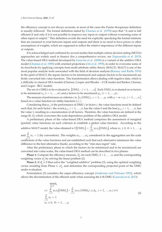
After the preliminary phase in which the factors (to be minimized and to be maximized) areconverted into value scales, the value-based DEA method can be described in two phases:
Phase 1: Compute the efficiency measure, d∗k, for each DMU, k = 1, . . . ,n, and the correspondingweighting vector w∗
k by solving the linear problem (2).Phase 2: If d∗k ≥ 0 then solve the “weighted additive” problem (3), using the optimal weighting
vector resulting from Phase 1, w∗k, and determine the corresponding projected point of the DMU
under evaluation.Formulation (2) considers the super-efficiency concept (Andersen and Petersen 1993), which
allows the discrimination of the efficient units when assessing the k-th DMU (Gouveia et al. 2013):
mindk,w
dk
s.t.q∑
c=1wcvc(DMUj
)−
q∑c=1
wcvc(DMUk) ≤ dk, j = 1, . . . , n; j � kq∑
c=1wc = 1
wc ≥ 0, ∀c = 1, . . . , q
(2)
7
J. Risk Financial Manag. 2020, 13, 67
The efficiency measure, d∗k, for each DMU k (k = 1, . . . ,n) and the corresponding weighting vectorare calculated by solving the linear problem (2). The optimal value of the objective function d∗k providesthe distance in terms of the difference in value for the best of all DMUs (note that the best DMU willalso depend on w), excluding this from the reference set. If the score obtained in (2), d∗k, is not positive,then the DMU k under evaluation is efficient, otherwise, it is inefficient.
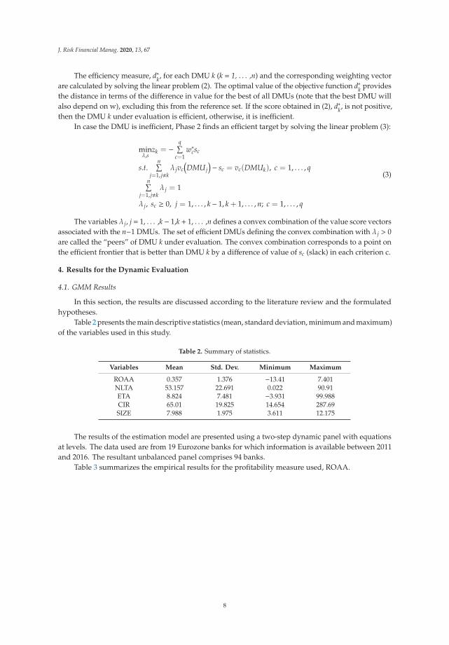
In case the DMU is inefficient, Phase 2 finds an efficient target by solving the linear problem (3):
minλ,s
zk = −q∑
c=1w∗
csc
s.t.n∑
j=1, j�kλ jvc(DMUj
)− sc = vc(DMUk), c = 1, . . . , q
n∑j=1, j�k
λ j = 1
λ j, sc ≥ 0, j = 1, . . . , k− 1, k + 1, . . . , n; c = 1, . . . , q
(3)
The variables λ j, j = 1, . . . ,k − 1,k + 1, . . . ,n defines a convex combination of the value score vectorsassociated with the n−1 DMUs. The set of efficient DMUs defining the convex combination with λ j > 0are called the “peers” of DMU k under evaluation. The convex combination corresponds to a point onthe efficient frontier that is better than DMU k by a difference of value of sc (slack) in each criterion c.
4. Results for the Dynamic Evaluation
4.1. GMM Results
In this section, the results are discussed according to the literature review and the formulatedhypotheses.
Table 2 presents the main descriptive statistics (mean, standard deviation, minimum and maximum)of the variables used in this study.
Table 2. Summary of statistics.
Variables Mean Std. Dev. Minimum Maximum
ROAA 0.357 1.376 −13.41 7.401NLTA 53.157 22.691 0.022 90.91ETA 8.824 7.481 −3.931 99.988CIR 65.01 19.825 14.654 287.69SIZE 7.988 1.975 3.611 12.175
The results of the estimation model are presented using a two-step dynamic panel with equationsat levels. The data used are from 19 Eurozone banks for which information is available between 2011and 2016. The resultant unbalanced panel comprises 94 banks.
Table 3 summarizes the empirical results for the profitability measure used, ROAA.
8
J. Risk Financial Manag. 2020, 13, 67
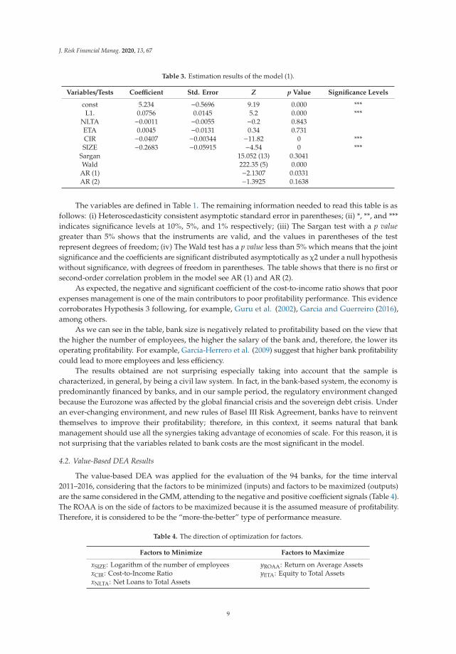
Table 3. Estimation results of the model (1).
Variables/Tests Coefficient Std. Error Z p Value Significance Levels
const 5.234 −0.5696 9.19 0.000 ***L1. 0.0756 0.0145 5.2 0.000 ***
NLTA −0.0011 −0.0055 −0.2 0.843ETA 0.0045 −0.0131 0.34 0.731CIR −0.0407 −0.00344 −11.82 0 ***SIZE −0.2683 −0.05915 −4.54 0 ***
Sargan 15.052 (13) 0.3041Wald 222.35 (5) 0.000
AR (1) −2.1307 0.0331AR (2) −1.3925 0.1638
The variables are defined in Table 1. The remaining information needed to read this table is asfollows: (i) Heteroscedasticity consistent asymptotic standard error in parentheses; (ii) *, **, and ***indicates significance levels at 10%, 5%, and 1% respectively; (iii) The Sargan test with a p valuegreater than 5% shows that the instruments are valid, and the values in parentheses of the testrepresent degrees of freedom; (iv) The Wald test has a p value less than 5% which means that the jointsignificance and the coefficients are significant distributed asymptotically as χ2 under a null hypothesiswithout significance, with degrees of freedom in parentheses. The table shows that there is no first orsecond-order correlation problem in the model see AR (1) and AR (2).
As expected, the negative and significant coefficient of the cost-to-income ratio shows that poorexpenses management is one of the main contributors to poor profitability performance. This evidencecorroborates Hypothesis 3 following, for example, Guru et al. (2002), Garcia and Guerreiro (2016),among others.
As we can see in the table, bank size is negatively related to profitability based on the view thatthe higher the number of employees, the higher the salary of the bank and, therefore, the lower itsoperating profitability. For example, García-Herrero et al. (2009) suggest that higher bank profitabilitycould lead to more employees and less efficiency.
The results obtained are not surprising especially taking into account that the sample ischaracterized, in general, by being a civil law system. In fact, in the bank-based system, the economy ispredominantly financed by banks, and in our sample period, the regulatory environment changedbecause the Eurozone was affected by the global financial crisis and the sovereign debt crisis. Underan ever-changing environment, and new rules of Basel III Risk Agreement, banks have to reinventthemselves to improve their profitability; therefore, in this context, it seems natural that bankmanagement should use all the synergies taking advantage of economies of scale. For this reason, it isnot surprising that the variables related to bank costs are the most significant in the model.
4.2. Value-Based DEA Results
The value-based DEA was applied for the evaluation of the 94 banks, for the time interval2011–2016, considering that the factors to be minimized (inputs) and factors to be maximized (outputs)are the same considered in the GMM, attending to the negative and positive coefficient signals (Table 4).The ROAA is on the side of factors to be maximized because it is the assumed measure of profitability.Therefore, it is considered to be the “more-the-better” type of performance measure.
Table 4. The direction of optimization for factors.
Factors to Minimize Factors to Maximize
xSIZE: Logarithm of the number of employees yROAA: Return on Average AssetsxCIR: Cost-to-Income Ratio yETA: Equity to Total AssetsxNLTA: Net Loans to Total Assets
9
J. Risk Financial Manag. 2020, 13, 67
Let DMUj, j = 1, . . . ,94 be observed in t = 1, . . . ,6 consecutive years. Then the sampleused has 6 × 94 DMUs (DMUt
j). The matrices of inputs and outputs of the 564 DMUs
in evaluation are X = (x11, x1
2, . . . , x194, x2
1, x22, . . . , x2
94, . . . , x61, x6
2, . . . , x694) and Y = (y1
1, y12, . . . , y1
94,y2
1, y22, . . . , y2
80, . . . , y61, y6
2, . . . , y694), respectively.
Considering that the value ptcj is the performance of DMU j in factor c, for the year t, the factors
performances are linearly converted into values following the procedure: Firstly, two limits, MLc
and MUc , are defined for each factor, such that ML
c < min{pt
cj , j = 1, . . . , 94; t = 1, . . . , 6}
and MUc >
max{pt
cj , j = 1, . . . , 94; t = 1, . . . , 6}, for each c = 1, . . . , 5. Secondly, the values for each DMU are
computed using:
vtc
(DMUj
)=
⎧⎪⎪⎪⎪⎨⎪⎪⎪⎪⎩
ptcj−ML
c
MUc −ML
c, i f the f actor c is to maximize
MUc −pt
cj
MUc −ML
c, i f the f actor c is to minimize
, j = 1, . . . , 94; t = 1, . . . , 6; c = 1, . . . , 5 (4)
The MLc and MU
c values of the factors to minimize and the factor to maximize that were consideredfor all DMUs and for the interval 2011–2016 are displayed in Table 2.
The different DEA models have been widely used for performance evaluation in different practicalapplications, however, it is very common to find factors that have negative or zero values. For radialmeasures of efficiency, as the classical models (CCR and BCC), the presence of negative data is aproblematical matter. The valued-based DEA overcomes this drawback by converting the performanceson each factor into a value scale. Hence after being converted into value functions, all factors are tobe maximized.
Value functions could also be obtained from the DMs’ preferences and this may lead to piecewiseand nonlinear value functions (see, for instance, Almeida and Dias 2012; Gouveia et al. 2015, 2016; andGouveia and Clímaco 2018).
For this study, a unifying reference set for the whole period was considered, and then the optimalvalue difference d∗k was computed for each bank k, in each year, making it possible to compare all ofthem across years.
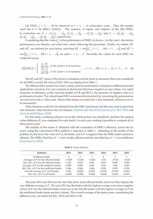
The statistic of the scores d∗ obtained with the evaluation of DMU’s efficiency across the sixyears, using the value-based DEA method is depicted in Table 5. Attending to the results of theproblem (2), the lower the value of d∗ is, the better, and if d∗ is negative then the DMU under analysis isefficient. The DMUs that have d∗ = 0 are weakly efficient and the ones that have d∗ > 0 are inefficient(Gouveia et al. 2013).
Table 5. Score statistics.
Statistics 2011 2012 2013 2014 2015 2016
# efficient banks 4 3 3 4 3 3Average of d* for the efficient banks −0.069 −0.024 −0.026 −0.01 −0.014 −0.010Std. Dev. of d* for the efficient banks 0.123 0.033 0.041 0.011 0.007 0.008Average of d* for the inefficient banks 0.089 0.086 0.081 0.08 0.08 0.085Std. Dev. of d* for the inefficient banks 0.046 0.046 0.044 0.036 0.039 0.038
Overall Average of d* of all banks 0.081 0.0823 0.0774 0.0754 0.0765 0.0814Std. Dev. of d* of all banks 0.0609 0.0496 0.0486 0.0406 0.0421 0.0415
The years 2011 and 2014 are the ones that show more efficient banks, however they display thevery different average of d∗. The year 2011 has the banks with the highest average score (more negativevalues of d∗) for the efficient banks, however, it also has the banks with the highest average of d∗ forthe inefficient banks (more positive values). The overall average of the bank scores, considering thedifferent years, are better for 2011, 2012 and 2016 (>0.8).
10
J. Risk Financial Manag. 2020, 13, 67
There are three efficient banks for the remaining years, but the scores of the efficient banks are onaverage better for 2012 and 2013.
Probably these results are reflective of the financial help that banks were getting, gradually, afterthe global financial crisis (Gulati and Kumar 2016), and that impact the different Eurozone countries atdifferent times (Wild 2016). Faced with serious economic difficulties in Greece, the European Union hasadopted an aid plan, including loans and supervision of the European Central Bank. Our results are inline with Christopoulos et al. (2019) since they show that the PIIGS countries (Portugal, Ireland, Italy,Greece, and Spain) have a high degree of inefficiency, which is aggravated after the sovereign debtcrisis since these countries pursued a fragile economic policy for the macroeconomic characteristics ofthese countries
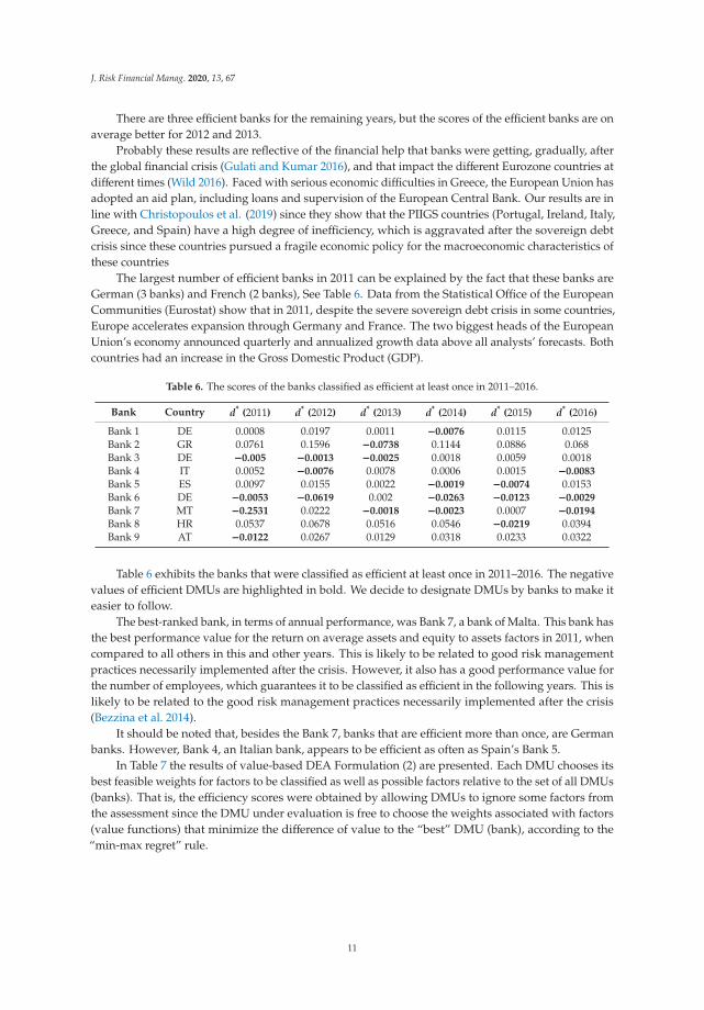
The largest number of efficient banks in 2011 can be explained by the fact that these banks areGerman (3 banks) and French (2 banks), See Table 6. Data from the Statistical Office of the EuropeanCommunities (Eurostat) show that in 2011, despite the severe sovereign debt crisis in some countries,Europe accelerates expansion through Germany and France. The two biggest heads of the EuropeanUnion’s economy announced quarterly and annualized growth data above all analysts’ forecasts. Bothcountries had an increase in the Gross Domestic Product (GDP).
Table 6. The scores of the banks classified as efficient at least once in 2011–2016.
Bank Country d* (2011) d* (2012) d* (2013) d* (2014) d* (2015) d* (2016)
Bank 1 DE 0.0008 0.0197 0.0011 −0.0076 0.0115 0.0125Bank 2 GR 0.0761 0.1596 −0.0738 0.1144 0.0886 0.068Bank 3 DE −0.005 −0.0013 −0.0025 0.0018 0.0059 0.0018Bank 4 IT 0.0052 −0.0076 0.0078 0.0006 0.0015 −0.0083
Bank 5 ES 0.0097 0.0155 0.0022 −0.0019 −0.0074 0.0153Bank 6 DE −0.0053 −0.0619 0.002 −0.0263 −0.0123 −0.0029
Bank 7 MT −0.2531 0.0222 −0.0018 −0.0023 0.0007 −0.0194
Bank 8 HR 0.0537 0.0678 0.0516 0.0546 −0.0219 0.0394Bank 9 AT −0.0122 0.0267 0.0129 0.0318 0.0233 0.0322
Table 6 exhibits the banks that were classified as efficient at least once in 2011–2016. The negativevalues of efficient DMUs are highlighted in bold. We decide to designate DMUs by banks to make iteasier to follow.
The best-ranked bank, in terms of annual performance, was Bank 7, a bank of Malta. This bank hasthe best performance value for the return on average assets and equity to assets factors in 2011, whencompared to all others in this and other years. This is likely to be related to good risk managementpractices necessarily implemented after the crisis. However, it also has a good performance value forthe number of employees, which guarantees it to be classified as efficient in the following years. This islikely to be related to the good risk management practices necessarily implemented after the crisis(Bezzina et al. 2014).
It should be noted that, besides the Bank 7, banks that are efficient more than once, are Germanbanks. However, Bank 4, an Italian bank, appears to be efficient as often as Spain’s Bank 5.
In Table 7 the results of value-based DEA Formulation (2) are presented. Each DMU chooses itsbest feasible weights for factors to be classified as well as possible factors relative to the set of all DMUs(banks). That is, the efficiency scores were obtained by allowing DMUs to ignore some factors fromthe assessment since the DMU under evaluation is free to choose the weights associated with factors(value functions) that minimize the difference of value to the “best” DMU (bank), according to the“min-max regret” rule.
11
J. Risk Financial Manag. 2020, 13, 67
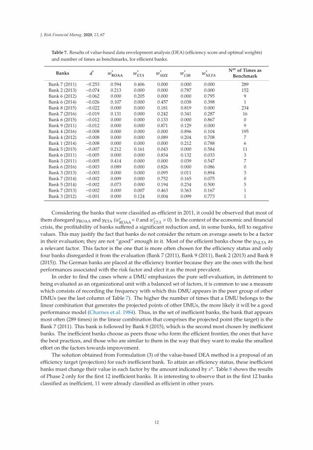
Table 7. Results of value-based data envelopment analysis (DEA) (efficiency score and optimal weights)and number of times as benchmarks, for efficient banks.
Banks d* w*ROAA
w*ETA w*
SIZE w*CIR w*
NLTANer of Times as
Benchmark
Bank 7 (2011) −0.253 0.594 0.406 0.000 0.000 0.000 289Bank 2 (2013) −0.074 0.213 0.000 0.000 0.787 0.000 152Bank 6 (2012) −0.062 0.000 0.205 0.000 0.000 0.795 9Bank 6 (2014) −0.026 0.107 0.000 0.457 0.038 0.398 1Bank 8 (2015) −0.022 0.000 0.000 0.181 0.819 0.000 234Bank 7 (2016) −0.019 0.131 0.000 0.242 0.341 0.287 16Bank 6 (2015) −0.012 0.000 0.000 0.133 0.000 0.867 0Bank 9 (2011) −0.012 0.000 0.000 0.871 0.129 0.000 9Bank 4 (2016) −0.008 0.000 0.000 0.000 0.896 0.104 195Bank 4 (2012) −0.008 0.000 0.000 0.089 0.204 0.708 7Bank 1 (2014) −0.008 0.000 0.000 0.000 0.212 0.788 6Bank 5 (2015) −0.007 0.212 0.161 0.043 0.000 0.584 11Bank 6 (2011) −0.005 0.000 0.000 0.834 0.132 0.033 3Bank 3 (2011) −0.005 0.414 0.000 0.000 0.039 0.547 7Bank 6 (2016) −0.003 0.089 0.000 0.826 0.000 0.086 0Bank 3 (2013) −0.003 0.000 0.000 0.095 0.011 0.894 3Bank 7 (2014) −0.002 0.009 0.000 0.752 0.165 0.075 0Bank 5 (2014) −0.002 0.073 0.000 0.194 0.234 0.500 5Bank 7 (2013) −0.002 0.000 0.007 0.463 0.363 0.167 1Bank 3 (2012) −0.001 0.000 0.124 0.004 0.099 0.773 1
Considering the banks that were classified as efficient in 2011, it could be observed that most ofthem disregard yROAA and yETA (w∗
ROAA= 0 and w∗ETA = 0). In the context of the economic and financial
crisis, the profitability of banks suffered a significant reduction and, in some banks, fell to negativevalues. This may justify the fact that banks do not consider the return on average assets to be a factorin their evaluation; they are not “good” enough in it. Most of the efficient banks chose the yNLTA asa relevant factor. This factor is the one that is more often chosen for the efficiency status and onlyfour banks disregarded it from the evaluation (Bank 7 (2011), Bank 9 (2011), Bank 2 (2013) and Bank 8(2015)). The German banks are placed at the efficiency frontier because they are the ones with the bestperformances associated with the risk factor and elect it as the most prevalent.
In order to find the cases where a DMU emphasizes the pure self-evaluation, in detriment tobeing evaluated as an organizational unit with a balanced set of factors, it is common to use a measurewhich consists of recording the frequency with which this DMU appears in the peer group of otherDMUs (see the last column of Table 7). The higher the number of times that a DMU belongs to thelinear combination that generates the projected points of other DMUs, the more likely it will be a goodperformance model (Charnes et al. 1984). Thus, in the set of inefficient banks, the bank that appearsmost often (289 times) in the linear combination that comprises the projected point (the target) is theBank 7 (2011). This bank is followed by Bank 8 (2015), which is the second most chosen by inefficientbanks. The inefficient banks choose as peers those who form the efficient frontier, the ones that havethe best practices, and those who are similar to them in the way that they want to make the smallesteffort on the factors towards improvement.
The solution obtained from Formulation (3) of the value-based DEA method is a proposal of anefficiency target (projection) for each inefficient bank. To attain an efficiency status, these inefficientbanks must change their value in each factor by the amount indicated by s*. Table 8 shows the resultsof Phase 2 only for the first 12 inefficient banks. It is interesting to observe that in the first 12 banksclassified as inefficient, 11 were already classified as efficient in other years.
12
J. Risk Financial Manag. 2020, 13, 67
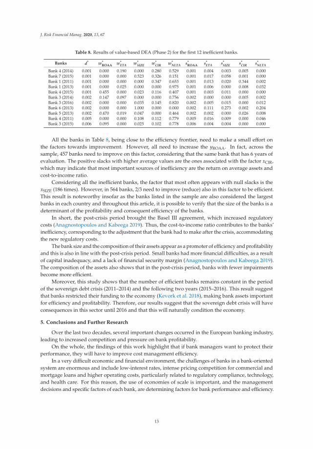
Table 8. Results of value-based DEA (Phase 2) for the first 12 inefficient banks.
Banks d* w*ROAA
w*ETA w*
SIZE w*CIR w*
NLTA s*ROAA
s*ETA s*
SIZE s*CIR s*
NLTA
Bank 4 (2014) 0.001 0.000 0.190 0.000 0.280 0.529 0.001 0.004 0.003 0.005 0.000Bank 7 (2015) 0.001 0.000 0.000 0.523 0.326 0.151 0.001 0.017 0.058 0.001 0.000Bank 1 (2011) 0.001 0.000 0.000 0.000 0.347 0.653 0.001 0.013 0.020 0.344 0.002Bank 1 (2013) 0.001 0.000 0.025 0.000 0.000 0.975 0.001 0.006 0.000 0.008 0.032Bank 4 (2015) 0.001 0.455 0.000 0.023 0.116 0.407 0.001 0.003 0.011 0.000 0.000Bank 3 (2014) 0.002 0.147 0.097 0.000 0.000 0.756 0.002 0.000 0.000 0.005 0.002Bank 3 (2016) 0.002 0.000 0.000 0.035 0.145 0.820 0.002 0.005 0.015 0.000 0.012Bank 6 (2013) 0.002 0.000 0.000 1.000 0.000 0.000 0.002 0.111 0.273 0.002 0.204Bank 5 (2013) 0.002 0.470 0.019 0.047 0.000 0.464 0.002 0.002 0.000 0.026 0.008Bank 4 (2011) 0.005 0.000 0.000 0.108 0.112 0.779 0.005 0.016 0.009 0.000 0.046Bank 3 (2015) 0.006 0.095 0.000 0.025 0.102 0.778 0.006 0.004 0.004 0.000 0.000
All the banks in Table 8, being close to the efficiency frontier, need to make a small effort onthe factors towards improvement. However, all need to increase the yROAA. In fact, across thesample, 457 banks need to improve on this factor, considering that the same bank that has 6 years ofevaluation. The positive slacks with higher average values are the ones associated with the factor xCIR,which may indicate that most important sources of inefficiency are the return on average assets andcost-to-income ratio.
Considering all the inefficient banks, the factor that most often appears with null slacks is thexSIZE (186 times). However, in 564 banks, 2/3 need to improve (reduce) also in this factor to be efficient.This result is noteworthy insofar as the banks listed in the sample are also considered the largestbanks in each country and throughout this article, it is possible to verify that the size of the banks is adeterminant of the profitability and consequent efficiency of the banks.
In short, the post-crisis period brought the Basel III agreement, which increased regulatorycosts (Anagnostopoulos and Kabeega 2019). Thus, the cost-to-income ratio contributes to the banks’inefficiency, corresponding to the adjustment that the bank had to make after the crisis, accommodatingthe new regulatory costs.
The bank size and the composition of their assets appear as a promoter of efficiency and profitabilityand this is also in line with the post-crisis period. Small banks had more financial difficulties, as a resultof capital inadequacy, and a lack of financial security margin (Anagnostopoulos and Kabeega 2019).The composition of the assets also shows that in the post-crisis period, banks with fewer impairmentsbecome more efficient.
Moreover, this study shows that the number of efficient banks remains constant in the periodof the sovereign debt crisis (2011–2014) and the following two years (2015–2016). This result suggestthat banks restricted their funding to the economy (Kevork et al. 2018), making bank assets importantfor efficiency and profitability. Therefore, our results suggest that the sovereign debt crisis will haveconsequences in this sector until 2016 and that this will naturally condition the economy.
5. Conclusions and Further Research
Over the last two decades, several important changes occurred in the European banking industry,leading to increased competition and pressure on bank profitability.
On the whole, the findings of this work highlight that if bank managers want to protect theirperformance, they will have to improve cost management efficiency.
In a very difficult economic and financial environment, the challenges of banks in a bank-orientedsystem are enormous and include low-interest rates, intense pricing competition for commercial andmortgage loans and higher operating costs, particularly related to regulatory compliance, technology,and health care. For this reason, the use of economies of scale is important, and the managementdecisions and specific factors of each bank, are determining factors for bank performance and efficiency.
13
J. Risk Financial Manag. 2020, 13, 67
This work points out the factors that lead to a bank being classified as efficient change, whichconfirms the importance of the economic environment in a way that could affect the bank performances,aside from the bank level features.
The new European regulation has been important, but the fact that in a universe of 564 DMUs(94 banks used in the value-based DEA method observed in six consecutive years) only 20 have beenconsidered efficient shows that there is still a long way to go.
The main limitation of this study is related to the number of banks listed by country. So, for futureresearch it would be interesting to analyze other markets and integrate institutional and ownershipfactors, with very different characteristics in civil law and common law countries; to compare thedeterminants of efficiency in the bull and bear periods also considering different external factors suchcultural and market sentiment factors.
The results obtained could help managers, investors or governments to know how to improve theefficiency of their banking sector, which is the engine of the economy for civil law countries.
Author Contributions: Conceptualization, M.E.D.N. and M.D.C.G.; methodology, M.E.D.N. and M.D.C.G.;software, M.D.C.G. and M.E.D.N.; validation, M.E.D.N., M.D.C.G. and C.A.N.P.; formal analysis, C.A.N.P.;investigation, M.E.D.N., M.D.C.G. and C.A.N.P.; resources, M.E.D.N.; data curation, C.A.N.P.; writing—originaldraft preparation, M.E.D.N., M.D.C.G. and C.A.N.P.; writing—review and editing, M.E.D.N., M.D.C.G. andC.A.N.P.; visualization, M.D.C.G.; supervision, M.E.D.N.; project administration, M.E.D.N. All authors have readand agreed to the published version of the manuscript.
Funding: This work is supported by: European Structural and Investment Funds in the FEDER component,through the Operational Competitiveness and Internationalization Programme (COMPETE 2020) [ProjectNo. 006971 (UID/SOC/04011); Funding Reference: POCI-01- 0145-FEDER-006971]; and national funds, throughthe FCT—Portuguese Foundation for Science and Technology under the projects, UIDB/04011/2020 andUIDB/00308/2020.
Conflicts of Interest: The authors declare no conflict of interest.
References
Ahamed, M. Mostak. 2017. Asset quality, non-interest income, and bank profitability: Evidence from Indian banks.Economic Modelling 63: 1–14. [CrossRef]
Albertazzi, Ugo, and Leonardo Gambacorta. 2009. Bank profitability and the business cycle. Journal of FinancialStability 5: 393–409. [CrossRef]
Ali, Agha. Iqbal, Catherine S. Lerme, and Lawrence M. Seiford. 1995. Components of efficiency evaluation in dataenvelopment analysis. Euro Journal of Operational Research 80: 462–73. [CrossRef]
Almeida, Pedro Nuno, and Luis Cândido Dias. 2012. Value-based DEA models: application-driven developments.Journal of the Operational Research Society 63: 16–27. [CrossRef]
Altunbas, Yener, Edward P.M. Gardener, Philip Molyneux, and Basil Moore. 2001. Efficiency in European banking.European Economic Review 45: 1931–55. [CrossRef]
Anagnostopoulos, Yiannis, and Jackie Kabeega. 2019. Insider perspectives on European banking challenges in thepost-crisis regulation environment. Journal of Bank Regulation 20: 136–58. [CrossRef]
Andersen, Per, and Niels Christian Petersen. 1993. A Procedure for Ranking Efficient Units in Data EnvelopmentAnalysis. Management Science 39: 1261–64. [CrossRef]
Arellano, Manuel, and Stephen Bond. 1991. Some Tests of Specification for Panel Data: Monte Carlo Evidence andan Application to Employment Equations. The Review of Economic Studies 58: 277. [CrossRef]
Arellano, Manuel, and Olympia Bover. 1995. Another look at the instrumental variable estimation of error-components models. Journal of Econometrics 68: 29–51. [CrossRef]
Athanasoglou, Panayiotis P., Sophocles N. Brissimis, and Matthaios D. Delis. 2008. Bank-specific, industry-specificand macroeconomic determinants of bank profitability. Journal of International Finance Markets, Institutionsand Money 18: 121–36. [CrossRef]
Azam, Muhammad, and Sana Siddiqui. 2012. Domestic and Foreign Banks’ Profitability: Differences and TheirDeterminants. International Journal of Economics and Financial Issues 2: 33–40.
Beck, Thorsten, Ross Levine, and Norman Loayza. 2000. Finance and the sources of growth. Journal FinancialEconomics 58: 261–300. [CrossRef]
14
J. Risk Financial Manag. 2020, 13, 67
Beltratti, Andrea, and Rene M. Stulz. 2012. The credit crisis around the globe: Why did some banks performbetter? Journal Financial Economics 105: 1–17. [CrossRef]
Berger, Allen N., Gerald A. Hanweck, and David B. Humphrey. 1987. Competitive viability in banking.Journal Monetary Economics 20: 501–20. [CrossRef]
Bezzina, Frank, Simon Grima, and Josephine Mamo. 2014. Risk management practices adopted by financial firmsin Malta. Managerial Finance 40: 587–612. [CrossRef]
Bikker, Jacob A., and Haixia Hu. 2002. Cyclical patterns in profits, provisioning and lending of banks andprocyclicality of the new Basel capital requirements. Banca Nazionale del Lavoro Quarterly Review 55: 143–75.
Bikker, Jacob A., and Tobias M. Vervliet. 2017. Bank profitability and risk-taking under low interest rates.International Journal of Finance and Economics 23: 1–16. [CrossRef]
Bitar, Mohammad, Kuntara Pukthuanthong, and Thomas Walker. 2018. The effect of capital ratios on the risk,efficiency and profitability of bankss: Evidence from OECD countries. Journal International Financial Markets,Institutions and Money 53: 227–62. [CrossRef]
Blundell, Richard, and Stephen Bond. 1998. Initial conditions and moment restrictions in dynamic panel datamodels. Journal of Econometrics 87: 115–43. [CrossRef]
Bourke, Philip. 1989. Concentration and other determinants of bank profitability in Europe, North America andAustralia. Journal of Banking & Finance 13: 65–79. [CrossRef]
Boyd, John H., and David E. Runkle. 1993. Size and performance of banking firms. Journal of Monetary Economics31: 47–67. [CrossRef]
Charnes, Abraham, William W. Cooper, and Eduard L. Rhodes. 1978. Measuring the efficiency of decision makingunits. European Journal Operational Research 2: 429–44. [CrossRef]
Charnes, Abraham, Clain T. Clark, William W. Cooper, and Boaz Golany. 1984. A developmental study of dataenvelopment analysis in measuring the efficiency of maintenance units in the U.S. air forces. Annals ofOperations Research 2: 95–112. [CrossRef]
Charnes, Abraham, William W. Cooper, Boaz Golany, Lawrence M. Seiford, and Joel Stutz. 1985. Foundationsof Data Envelopment Analysis for Pareto-Koopmans efficient empirical production functions. Journal ofEconometrics 30: 91–107. [CrossRef]
Christopoulos, Apostolos G., Ioannis G. Dokas, Sofia Katsimardou, and Eleftherios Spyromitros. 2019. AssessingBanking Sectors’ Efficiency of Financially Troubled Eurozone Countries. Research in International Business andFinance 52: 101121. [CrossRef]
Dang, Chongyu, Zhichuan Frank Li, and Chen Yang. 2018. Measuring firm size in empirical corporate finance.Journal of Banking & Finance 86: 159–76.
Diamond, Douglas W. 1984. Financial Intermediation and Delegated Monitoring. The Review of Economic Studies51: 393. [CrossRef]
Dietrich, Andreas, and Gabrielle Wanzenried. 2011. Determinants of bank profitability before and during thecrisis: Evidence from Switzerland. Journal of International Financial Markets, Institutions and Money 21: 307–27.[CrossRef]
Dietrich, Andreas, and Gabrielle Wanzenried. 2014. The determinants of commercial banking profitability in low-,middle-, and high-income countries. The Quarterly Review Economics and Finance 54: 337–54. [CrossRef]
Djalilov, Khurshid, and Jenifer Piesse. 2016. Determinants of bank profitability in transition countries: Whatmatters most? Research International Business and Finance 38: 69–82. [CrossRef]
Fethi, Meryem Duygun, and Fotios Pasiouras. 2010. Assessing bank efficiency and performance with operationalresearch and artificial intelligence techniques: A survey. European Journal of Operational Research 204: 189–98.[CrossRef]
Garcia, Maria Teresa Medeiros, and João Pedro Silva Martins Guerreiro. 2016. Internal and external determinantsof banks’ profitability. Journal of Economic Studies 43: 90–107. [CrossRef]
García-Herrero, Alicia, Sergio Gavilá, and Daniel Santabárbara. 2009. What explains the low profitability ofChinese banks? Journal of Banking & Finance 33: 2080–92. [CrossRef]
Ghosh, Amit. 2016. Banking sector globalization and bank performance: A comparative analysis of low incomecountries with emerging markets and advanced economies. Review of Development Finance 6: 58–70. [CrossRef]
Goddard, John, Philip Molyneux, and John Wilson. 2004. The profitability of european banks: a cross-sectionaland dynamic panel analysis. Manchester School 72: 363–81. [CrossRef]
15
J. Risk Financial Manag. 2020, 13, 67
Gouveia, Maria do Castelo, and Isabel Clímaco. 2018. Assessment of Fuel Tax Policies to Tackle Carbon Emissionsfrom Road Transport—An Application of the Value-Based DEA Method Including Robustness Analysis.In Energy Management—Collective and Computational Intelligence with Theory and Applications. Edited byCengiz Kahraman and Gülgün Kayakutlu. Cham: Springer, pp. 167–91.
Gouveia, Maria Castelo, Luís Cândido Dias, and Carlos Henggler Antunes. 2008. Additive DEA based on MCDAwith imprecise information. Journal of the Operational Research Society 59: 54–63. [CrossRef]
Gouveia, Maria Castelo, Luís Cândido Dias, and Carlos Henggler Antunes. 2013. Super-efficiency and stabilityintervals in additive DEA. Journal of the Operational Research Society 64: 86–96. [CrossRef]
Gouveia, Maria Castelo, Luís Cândido Dias, Carlos Henggler Antunes, Júlia Boucinha, and Catarina Feteira Inácio.2015. Benchmarking of maintenance and outage repair in an electricity distribution company using thevalue-based DEA method. Omega 53: 104–14. [CrossRef]
Gouveia, M.C., L.C. Dias, C.H. Antunes, Maria Augusta Mota, Eduardo Duarte, and Eduardo Tenreiro. 2016.An application of value-based DEA to identify the best practices in primary health care. OR Spectrum.38: 743–67. [CrossRef]
Gulati, R., and S. Kumar. 2016. Assessing the impact of the global financial crisis on the profit efficiency of Indianbanks. Economic Modelling 58: 167–81. [CrossRef]
Guru, Balachandher K., John Staunton, and Bala Shanmugam. 2002. Determinants of commercial bank profitabilityin Malaysia. Journal of Money, Credit, and Banking 17: 69–82.
Keeney, Ralph L., and Howard Raiffa. 1976. Decisions with Multiple Objectives: Preferences and Value Tradeoffs.In Proceedings of the ICML-06 Workshop on Kernel Methods in Reinforcement Learning. New York: John Wiley & Sons.
Kevork, Ilias S., Christos Kollias, Panayiotis Tzeremes, and Nickolaos G. Tzeremes. 2018. European financial crisisand bank productivity: evidence from Eastern European Countries. Applied Economics Letters 25: 283–89.[CrossRef]
Kosmidou, Kyriaki. 2008. The determinants of banks´ profits in Greece during the period of EU financialintegration. Managerial Finance 34: 146–59. [CrossRef]
La Porta, Rafael, Florencio Lopez-de-SIlanes, Andrei Shleifer, and Robert W. Vishny. 1998. Law and Finance RafaelLa Porta, Florencio Lopez-de-Silanes. Journal of Political Economy 106: 11131–55. [CrossRef]
Lee, Jeong Yeon, and Doyeon Kim. 2013. Bank performance and its determinants in Korea. Japan and the WorldEconomy 27: 83–94. [CrossRef]
Levine, Ross. 2002. Bank-based or market-based financial systems: Which is better? Journal of FinancialIntermediation 11: 398–428. [CrossRef]
Meles, Antoino, Claudio Porzio, Gabriele Sampagnaro, and Vincenzo Verdoliva. 2016. The impact of intellectualcapital efficiency on commercial bank performance: Evidence from the US. Journal of Multinatinal FinancialManagement 36: 64–74. [CrossRef]
Neves, Maria Elisabete Duarte. 2018. Payout and firm’s catering. International Journal of Managerial Finance 14: 2–22.[CrossRef]
Neves, Maria Elisabete Duarte, Carla Manuela Fernandes, and Pedro Coimbra Martins. 2019. Are ETFs goodvehicles for diversification? New evidence for critical investment periods. Borsa Istanbul Review 19: 149–57.[CrossRef]
Nguyen, Thi Lam Anh. 2018. Diversification and bank efficiency in six ASEAN countries. Global Finance Journal37: 57–78. [CrossRef]
Ongore, Vincent Okoth, and Gemechu Berhanu Kusa. 2013. Determinants of Financial Performance of CommercialBanks in Kenya. International Journal of Economics and Financial Issues 3: 237–52.
Paradi, Joseph C., and Haiyan Zhu. 2013. A survey on bank branch efficiency and performance research with dataenvelopment analysis. Omega 41: 61–79. [CrossRef]
Pasiouras, Fotios, and Kyriaki Kosmidou. 2007. Factors influencing the profitability of domestic and foreigncommercial banks in the European Union. Research in International Business and Finance 21: 222–37. [CrossRef]
Petria, Nicolae, Bogdan Capraru, and Iulian Ihnatov. 2015. Determinants of Banks’ Profitability: Evidence fromEU 27 Banking Systems. Procedia Economics and Finance 20: 518–24. [CrossRef]
Rajan, Raghuram, and Luigi Zingales. 1998. Financial Dependence and Growth. American Economic Review88: 559–86.
Rumler, Fabio, and Walter Waschiczek. 2016. Have changes in the financial structure affected bank profitability?Evidence for Austria. The European Journal of Finance 22: 803–24. [CrossRef]
16
J. Risk Financial Manag. 2020, 13, 67
Sabatier, Mareva. 2015. A women’s boom in the boardroom: effects on performance? Applied Economics 47: 2717–27.[CrossRef]
Saona, Paolo. 2016. Intra- and extra-bank determinants of Latin American Banks’ profitability. International Reviewof Economics and Finance 45: 197–214. [CrossRef]
Staikouras, Christos, and Geoffrey Wood. 2004. The determinants of bank profitability in Europe. InternationalJournal of Economics and Business Research 3: 57–68. [CrossRef]
Tan, Yong, Christos Floros, and John Anchor. 2017. The profitability of Chinese banks: impacts of risk, competitionand efficiency. Review of Accounting and Finance 16: 86–105. [CrossRef]
Trabelsi, Mohamed Ali, and Naama Trad. 2017. Profitability and risk in interest-free banking industries: a dynamicpanel data analysis. International Journal of Islamic and Middle Eastern Finance and Management 10: 454–69.[CrossRef]
Tran, Vuong Thao, Chien-Ting Lin, and Hoa Nguyen. 2016. Liquidity creation, regulatory capital, and bankprofitability. International Review of Financial Analysis 48: 98–109. [CrossRef]
Trujillo-Ponce, Antonio. 2013. What determines the profitability of banks? Evidence from Spain. Accounting &Finance 53: 561–86. [CrossRef]
Tsionas, Efthymios G., A. George Assaf, and Roman Matousek. 2015. Dynamic technical and allocative efficienciesin European banking. Journal of Banking & Finance 52: 130–39.
Valverde, Carbó Santiago, and Francisco Rodríguez Fernández. 2007. The determinants of bank margins inEuropean banking. Journal of Banking & Finance 31: 2043–63. [CrossRef]
Varmaz, Armin. 2007. Rentabilität im Bankensektor. Deutscher: Deutscher Universitäts-Verlag GWV Fachverlage.[CrossRef]
Wild, Joerg. 2016. Efficiency and risk convergence of Eurozone financial markets. Research in International Businessand Finance. [CrossRef]
Zopounidis, Constantin, Emilios Galariotis, Michael Doumpos, Stavroula Sarri, and Kostas Andriosopoulos. 2015.Multiple criteria decision aiding for finance: An updated bibliographic survey. European Journal of OperationalResearch 247: 339–48. [CrossRef]
© 2020 by the authors. Licensee MDPI, Basel, Switzerland. This article is an open accessarticle distributed under the terms and conditions of the Creative Commons Attribution(CC BY) license (http://creativecommons.org/licenses/by/4.0/).
17
Journal of
Risk and FinancialManagement
Article
Exchange Rate Misalignment and Capital Flightfrom Botswana: A Cointegration Approach withRisk Thresholds
Mpho Bosupeng *, Janet Dzator and Andrew Nadolny
Newcastle Business School, The University of Newcastle, Callaghan, NSW 2308, Australia;[email protected] (J.D.); [email protected] (A.N.)* Correspondence: [email protected]; Tel.: +61-2-043-216-2486
Received: 30 May 2019; Accepted: 15 June 2019; Published: 17 June 2019
Abstract: This study investigates the impact of exchange rate misalignment on outward capitalflight in Botswana over the period 1980–2015. The study uses the autoregressive distributed lag(ARDL) approach to cointegration and the Toda and Yamamoto (1995) approach to Granger causality.Botswana’s currency misalignment was caused by current account imbalances. The most importantdeterminant of capital flight from Botswana is trade openness, which indicates that exportablecommodities are misinvoiced leading to net capital outflows. Our main findings show that in thelong-run, when the currency is overvalued, the volume of capital flight through trade misinvoicingdeclines and increasing foreign reserves does not reduce outward capital flight. However, whenthe currency is undervalued, the volume of capital flight through trade misinvoicing increases andforeign reserves reduce outward capital flight. Investors respond more to prospects of devaluationthan to inflation. Botswana should tolerate overvaluation of the pula of only up to 5%. When the pulais overvalued beyond 5%, capital flight increases substantially. The government has to formulatetrade regulations and monitor imported and exported commodities. Botswana should also implementcapital controls to limit capital smuggling and maintain monetary autonomy.
Keywords: real exchange rate; exchange rate misalignment; overvaluation; undervaluation; capitalflight
1. Introduction
Botswana is a small, upper middle-income economy in sub-Saharan Africa, dependent on itsmining sector. Its principal export commodity is diamonds and prudent natural resource managementpolicies have propelled its economy to grow significantly compared to other resource-rich countries.In addition, political stability is one of Botswana’s key features. Nonetheless, the country facesmajor economic problems. First, the capital-intensive mining sector has not reduced the persistentunemployment in Botswana. Second, the country has the third highest HIV prevalence in world,which increases fiscal pressures (Deléchat and Gaertner 2008; Hillboom 2008; Limi 2006; Matlho et al.2019). In addition, previous studies indicate an important structural problem, namely, that Botswana’scurrency (the pula) is overvalued (Iyke and Odhiambo 2016; Limi 2006; Pegg 2010; Taye 2012). Limi(2006) and Pegg (2010) indicate that the substantial mining revenue plays a role in this overvaluation.Lindgren and Wicklund (2018) posit that diamond prices and business confidence in Botswana have anegative correlation with the domestic exchange rate. Hence, the important issue considered in thisstudy is the effects of exchange rate misalignment on the economy.
The extant literature shows that exchange rate overvaluation can increase capital flight, misallocateresources, abate economic efficiency and induce unfavourable downward spirals of trade and exchangerate controls (Cuddington 1986; Dornbusch 1984; Edwards 1989; Pfeffermann 1985; World Bank 1984).
J. Risk Financial Manag. 2019, 12, 101; doi:10.3390/jrfm13040067 www.mdpi.com/journal/jrfm18
J. Risk Financial Manag. 2019, 12, 101
This study evaluates the impact of exchange rate misalignment on capital flight from Botswana overthe period 1980–2015. The country aims to attract capital inflows to develop economic sectors otherthan mining. Botswana is unique because unlike other developing economies, it used only the fixedexchange rate regime since 1976. There has been no exchange rate regime change and the country hasexperienced significant undervaluation and overvaluation of the currency. It is conceivable that suchmisalignment has an impact on outward capital flight in Botswana. Botswana needs capital inflows foreconomic diversification, therefore, it is imperative to determine the impact of misalignment on capitalflight from Botswana.
This study empirically investigates the impact of exchange rate misalignment on capital flightfrom Botswana. The examination contributes to the literature in two important ways. First, previousstudies posit that the pula is overvalued but there is no study that evaluates the impact of exchangerate misalignment on capital flight from Botswana. The present study aims to fill this gap. Theresults of this study are important for implementing macroeconomic policies that support capitalinflows for economic diversification in Botswana. Further, the World Bank (2019) indicates thatBotswana’s diamond mines will be depleted by 2030. In the absence of diamonds, Botswana’s economicgrowth will decline drastically. Correcting exchange rate misalignment is necessary for early economicdiversification and sustainable economic growth without diamonds.
Second, this investigation extends Gouider and Nouira (2014) methodological approach tomisalignment. Gouider and Nouira (2014) defined overvaluation and undervaluation as either positiveor negative misalignment without any thresholds. The lack of thresholds in Gouider and Nouira (2014)study implies that insignificant real effective exchange rate (REER) misalignments were included inthe estimations. This study uses thresholds to capture only significant REER misalignment. Thisapproach is important for determining which level of misalignment initiates high capital flight as anearly warning indicator. This will curb substantial capital outflows, which are needed desperatelyfor economic diversification in Botswana. The use of thresholds in this study allows policymakers totake informed actions in correcting misalignment, for example devaluing the currency. The resultsshow that Botswana should tolerate overvaluation of the pula of only up to 5%. The present studyuses the autoregressive distributed lag (ARDL) bounds testing approach to cointegration and theToda and Yamamoto (1995) approach to Granger causality to determine the relationship betweeneconomic variables. This paper is organised as follows. Section 2 reviews the literature on exchangerate misalignment and capital flight. Section 3 presents the methodology used to achieve researchobjectives. Section 4 presents the results of the empirical models and discussions. Section 5 summarizesthe results, reviews the objectives and provides policy implications. It also identifies areas for furtherinvestigation and study limitations.
2. Literature Review
The Smithsonian Agreement formulated in 1971 necessitated that developed nations should pegtheir currencies to the US dollar. The Nixon Shock caused the collapse of the Bretton Woods systemof fixed exchange rates among developed nations. To stimulate economic growth by stabilising thereal exchange rate (RER), developing economies subsequently adopted crawling pegs and managedfloating regimes. In this regard, a major concern for economies engaged in trade is RER misalignment,which has economic growth implications. Misalignment is a common occurrence by which the RERdeviates from the ideal or the equilibrium exchange rate. Fixed exchange rate regimes like Botswanaare generally associated with exchange rate misalignment (Chowdhury and Wheeler 2015; Dubas2009; Ghosh et al. 2015). Pesaran et al. (2001) define exchange rate misalignment as the percentagegap between the observed exchange rate and the equilibrium real exchange rate (ERER). Deviationsof the RER from the equilibrium instigated major currency crises in developing nations, such as the1994 Mexican currency crisis, the 1997 Asian currency crises and the 1999 Brazilian financial crisis.Currencies of Asian economies were significantly misaligned before the currency crisis (Chinn 2000;Coudert et al. 2013; El-Shagi et al. 2016; Jeong et al. 2010; Kinkyo 2008).
19
J. Risk Financial Manag. 2019, 12, 101
The literature posits that overvaluation of the RER was the cause of capital flight in Latin America(Cuddington 1986). The Latin American debt crisis was a financial crisis accompanied by significantcapital flight. The debate as to whether capital flight initiated the debt crisis or foreign debt causedcapital flight in Latin America is ongoing. Capital flight occurs when monetary assets flow out ofa country rapidly as a response to economic and political changes. It leads to loss of wealth anddepreciation of the local currency. Erbe (1985) defines capital flight as total private capital outflowsfrom developing nations. Dooley (1986) and Lessard and Williamson (1987) suggest that capital flightshould be distinguished by its motivations rather than economic consequences. A challenge facingresearch on capital flight is its measurements, which do not capture the actual value of capital flightbecause capital flight can occur illegally. Illegal capital outflow is large in developing economiessince they have ineffective, or no capital controls to stimulate foreign direct investment (FDI) inflows.Capital flight has significant adverse effects on economic growth, particularly in developing economies,because it reduces private and public investment. As capital leaves the domestic economy, governmenttax revenue declines, which reduces funding for public investments. Therefore, the governmentmust borrow from foreign bodies at high costs. The interest rate for an investor taking assets abroadis fixed. However, the loan interest incurred by the government increases with the magnitude ofthe loan. Hence, capital flight creates major debt obligations, particularly in developing economies(Cuddington 1986).
According to Hermes et al. (2004), capital flight occurs owing to macroeconomic instability andmanifests in multiple ways, such as budget deficits, current account deficits, overvaluation of thecurrency and high inflation. Overvaluation of the domestic currency is an important underlyingdeterminant of capital flight. Expectations of depreciation are high when the currency is overvalued.Since investors aim to maximize returns and avoid welfare losses, domestic investors would beinclined to send their monetary assets abroad. The literature on exchange rate misalignment arguesthe Botswana pula is overvalued because of mining revenue (Limi 2006; Pegg 2010). Hence, thisstudy aims to identify the impact of exchange rate misalignment on capital flight from Botswana as anattempt to promote FDI inflows, economic diversification and sustainable growth.
Few studies investigate the effects of exchange rate misalignment on capital flight. To determinethese effects, we have to reflect on the exchange rate expectations theory developed by Hermes et al.(2004). The theory posits that an overvalued currency leads to increasing expectations of depreciation inthe future. As a result, economic agents will demand more foreign goods than domestic goods, leadingto inflationary pressures and loss of real income. Under such circumstances, economic agents willprefer to hold their assets abroad to avoid welfare losses, leading to capital flight. Gouider and Nouira(2014) examine the role of exchange rate misalignment on capital flight for a sample of 52 developingeconomies using data on the 1980–2010 period. Their results show that strong undervaluation of thedomestic currency restricts capital flight, while strong overvaluation stimulates it (Gouider and Nouira2014). Further, Sohrabji (2011) examines the link between capital flows and REER overvaluation. Theauthor uses Edwards’ (1989) model, cointegration tests and an error-correction model. The resultsshow that capital inflows significantly contribute to exchange rate misalignment.
Botswana has no exchange rate restrictions, since it aims to boost domestic business efficiencyand FDI inflows. The country attracted significant capital flows in the mining sector with moderateportfolio investments (Bank of Botswana 2016). FDI in Botswana is required for investment capital,economic diversification and promotion of inclusive growth. In 2017, Botswana experienced loss offoreign exchange reserves due to appreciation of the pula, which increases its exposure to a financialcrisis (Agénor et al. 1992; Coudert et al. 2013; El-Shagi et al. 2016; Jeong et al. 2010; Kaminsky et al. 1998;Kinkyo 2008; Krugman 1979). Following Hermes et al. (2004) and Cuddington (1986), overvaluation ofthe pula may create expectations of depreciation thereby increasing capital outflows. The central bankconducted portfolio-rebalancing operations in 2017 to counter persistent capital outflows. As regardsthe literature on this issue, although capital inflow is vital to Botswana’s economy, previous studieshave not evaluated the impact of exchange rate misalignment on capital flight from Botswana.
20
J. Risk Financial Manag. 2019, 12, 101
3. Methodology
This section explains the methodology used to determine the relationship between exchangerate misalignment and capital flight from Botswana. It provides research hypotheses and estimationapproaches as well as diagnostic measures. According to Edwards (1989), exchange rate misalignmentcauses severe welfare and efficiency costs owing to exchange rate and trade controls that accompanyovervaluation. There is supporting evidence that REER misalignment reduces exports and deterioratesthe agricultural sector (Pfeffermann 1985; World Bank 1984). A financial risk associated with exchangerate misalignment is that it generates massive capital flight, which increases social welfare costs(Cuddington 1986). Anticipations of macroeconomic instability cause high capital outflows, inducinglarge, rapid adjustments in interest rates and exchange rates. Further, capital flight reduces the taxbase and this reduction increases budget deficits and costs of foreign borrowing (Cuddington 1986;Dornbusch 1984; Edwards 1989).
Previous studies posit that overvalued currencies generate capital flight (Cuddington 1986;Edwards 1989; Gouider and Nouira 2014; Pastor 1990). As Hermes et al. (2004) describe, overvaluationof the REER creates expectations of depreciation of the domestic currency, thereby increasing capitaloutflows. Currency devaluation diminishes the value of domestic assets relative to foreign assets,which encourages residents to switch to foreign assets (Cuddington 1986; Dornbusch 1984; Lessardand Williamson 1987). However, an increase in foreign exchange reserves allows the government toprevent balance of payments crises and macroeconomic crisis (Alam and Quazi 2003). As a result,investor confidence in the economy is boosted, which reduces capital outflows (Boyce 1992). Thus,the literature shows that exchange rate misalignment and capital flight affect a country’s economicstability and growth. Hence, to examine these effects in relation to Botswana, this study proposes thefollowing hypotheses:
H1. Overvaluation of the pula increases capital flight in the long-run.
H2. Undervaluation of the pula decreases capital flight in the long-run.
To determine the impact of exchange rate misalignment on capital flight, Botswana’s exchange ratefundamentals should be identified first. Exchange rate fundamentals are variables that determine theREER and thus the internal and external equilibrium of the economy (Edwards 1989). Edwards (1988)proposes that exchange rate fundamentals in developing economies are terms of trade, governmentconsumption, technological progress and capital inflows. However, further research on exchange ratemisalignment shows that other macroeconomic factors, such as external debt, trade openness andcapital formation are important determinants of the REER (Gouider and Nouira 2014; Hossain 2011;Pham and Delpachitra 2015; Salim and Shi 2019). Following Edwards (1988) and Hossain (2011), therelative impact of the exchange rate fundamentals for Botswana is specified as follows:
LNREERt = α0 + δ1LNTOTt + δ2LNGOVt + δ3GDPt + δ4FDIt + δ5AIDt
+δ6LNOPENNESSt + δ7LNDEBTt + δ8LNCAPITALt + εt(1)
The definition of terms is as follows. LNREER (dependent variable) is the natural log of the REERindex. LNTOT is the natural log of the terms of trade index. LNGOV is the natural log of governmentfinal consumption expenditure. GDP is the rate of GDP growth to measure domestic technologicalprogress. FDI is FDI net capital inflows. AID is the real official foreign aid inflow received by Botswana.LNOPENNESS is the natural log of trade openness. LNDEBT is the natural log of Botswana’s stock ofexternal debt. LNCAPITAL is the natural log of the domestic gross capital formation. The epsilon εt
represents the error term (Table S1).To evaluate the degree of misalignment, first, the long-run exchange rate fundamentals for the
Botswana economy are determined using Equation (1). Next, the Hodrick–Prescott (HP) filter is usedto separate permanent and temporary components of the exchange rate fundamentals to obtain thelong-run values (HP trend). Hodrick and Prescott (1997) used this technique to analyse post-war
21
J. Risk Financial Manag. 2019, 12, 101
business cycles. The filter computes the smoothed series, s of y by minimising the variance of y arounds. The filter uses s to minimise the equation:
T∑t=1
(yt − st)2 + λ
T−1∑t=2
((st+1 − st) − (st − st−1))2 (2)
Consequently, the long-run exchange rate fundamentals are used to estimate the long-run LNREER.The fitted LNREER is filtered to obtain the equilibrium REER (LNEREER). The smoothness of theseries is determined using the parameter λ. Since this study uses annual data, the optimal value1 for λis 100. The next step is to calculate the degree of misalignment as follows:
MISREERt = LNREERt − LNEREERt (3)
The next phase is to evaluate whether misalignment of the pula was caused by unsustainable fiscaland monetary policies following Hossain (2011). The Toda and Yamamoto (1995) approach to Grangercausality is applied to determine causation between the REER misalignment (MISREER), cyclicalcomponents of the current account (LNCAC), external debt (LNDEBTC) and real GDP (LNRGDPC).Excess broad money supply is captured by the variable EMS. The cyclical component LNRGDPC willbe derived from the filtered series LNRGDP. LNRGDP is the natural log of real GDP. The cyclicalcomponent LNDEBTC will be obtained from the filtered natural log of (100 + DEBT) where DEBT isthe total stock of external debt as a percentage of GDP. EMS is excess broad money supply defined asthe difference between actual broad money supply and the predicted broad money supply. Owing todata limitations, the broad money determinants used are Botswana’s real GDP (LNRGDP) and theannual yield on the US government medium-term bond
(LNiUS
). The cyclical component LNCAC will
be obtained from the filtered natural log of (100 + CA) where CA is the current account balance as apercentage of GDP.
Following Gouider and Nouira (2014), this study decomposes misalignment into overvaluation(OVER) and undervaluation (UNDER). OVER will take the positive values of the misalignment,while UNDER will be negative misalignment. As a contribution to the literature, a 5% threshold2 formisalignment is set to capture only significant deviations from the equilibrium real effective exchangerate (EREER). Therefore, from Equation (3), OVER and UNDER are defined as:
OVERt =
⎧⎪⎪⎨⎪⎪⎩1 i f MISREERt > 5%
0 otherwise(4)
UNDERt =
⎧⎪⎪⎨⎪⎪⎩1 i f −MISREERt < −5%
0 otherwise(5)
To determine the impact of exchange rate misalignment on capital flight from Botswana, thisstudy will adopt the exchange rate expectations theory developed by Hermes et al. (2004). Thetheory posits that an overvalued currency leads to increasing expectations of depreciation in the future.Hence, economic agents will demand more foreign goods than domestic goods, leading to inflationary
1 Estimated using EViews version 10.2 Zhang et al. (2019) used 25% and 50% thresholds for their early warning system while Kaminsky et al. (1998) used a 10%
threshold for the signal extraction early warning system. However, these thresholds are too high to capture misalignmentin this study. The 5% threshold is selected because it is optimal for detecting significant REER misalignment. When thethreshold was set to 3%, 4% and 5% the results were similar with minimum disparities between the coefficients. However, anincrease in overvaluation beyond the 5% threshold causes high outward capital flight. Therefore, the 5% percent threshold isalso an early warning indicator for high capital flight from Botswana. The maximum threshold value accommodated byMISREER observations was 8%.
22
J. Risk Financial Manag. 2019, 12, 101
pressures and loss of real income. Under such circumstances, economic agents will prefer to hold theirassets abroad, leading to capital flight. The principal methods used for measuring capital flight in theextant literature are the residual method, the Dooley method and the hot money approach. Hermes etal. (2004) argue that the Dooley and hot money methods provide inaccurate estimates of capital flight.This study adopts the residual method to estimate the volume of capital flight3 from Botswana. Thismethod evaluates capital flight by comparing sources of capital flows and their use in the economy.An advantage of this approach is that it measures all private capital outflows as capital flight (Hermeset al. 2004). Following Hermes et al. (2004), capital flight from Botswana will be estimated as follows:
VKFt = ΔEDt + FIt −CADt − ΔFRt (6)
VKF is Botswana’s current volume of outward capital flight (monetary value) not scaled to GDP.ΔED is the first difference of Botswana’s stock of gross external debt. FI is the net foreign investmentinflows in Botswana. CAD is Botswana’s current account deficit and ΔFR is the first difference of thestock of official foreign reserves. Following Alam and Quazi (2003), Ndikumana and Boyce (2003)and Cheung and Qian (2010) an econometric model for capital flight based on the determinants isspecified as:
KFt = α0 + δ1RESERVESt + δ2GDPt + δ3INFt + δ4IRDt + δ5AIDt
+δ6LNOPENNESSt + δ7LNDEBTt + δ8LNREERt + εt(7)
The definition of the variables is as follows. KF (dependent variable) is the volume of Botswana’soutward capital flight4 as a percentage of GDP. Note that this variable is different from VKF, which isthe monetary value of Botswana’s outward capital flight. The variable KF is better than VKF because itfacilitates tracking of the dynamics of capital flight from the Botswana economy. The regressors aredefined as follows. RESERVES is the volume of reserves per GDP. GDP is the real GDP growth rate.INF is the domestic inflation rate. IRD is the real interest rate differential5 between Botswana andSouth Africa due to proximity and economic linkages between the two countries (Kganetsano 2007).6
AID is the real foreign aid inflow. LNOPENNESS is the natural log of trade openness. LNDEBT is thenatural log of external debt. LNREER is natural log of the REER index for Botswana. The epsilon εt
represents the error term.Equation (7) does not directly assess the impact of REER misalignment, which is the focus of this
investigation. To determine the effects of misalignment on capital flight, LNREER in Equation (7) issubstituted with overvaluation (OVER) and undervaluation (UNDER) dummies as follows:
KFt = α0 + δ1RESERVESt + δ2GDPt + δ3INFt + δ4IRDt + δ5AIDt
+δ6LNOPENNESSt + δ7LNDEBTt + δ8OVERt + εt(8)
KFt = α0 + δ1RESERVESt + δ2GDPt + δ3INFt + δ4IRDt + δ5AIDt
+δ6LNOPENNESSt + δ7LNDEBTt + δ8UNDERt + εt(9)
3 Capital flight can be either massive capital leaving a particular country to other nations (outward capital flight) or massivecapital from other nations entering the domestic economy (inward capital flight). This study evaluates the magnitude ofcapital flight from Botswana to other economies.
4 KF was calculated as(
VKFtGDPt
)% where VKF is the volume of capital flight measured using the residual method and GDP is
Botswana’s total GDP.5 In this study, IRD is the difference between Botswana and South Africa’s real interest rate. An increase in IRD is expected to
reduce capital flight (δ4 < 0). However, if IRD is taken as the difference between South Africa and Botswana’s real interestrate, an increase in IRD will encourage capital flight (δ4 > 0).
6 Kganetsano (2007) argue that macroeconomic changes in South Africa are likely to affect Botswana, given the large size ofthe South African economy and the volume of its exports to Botswana.
23
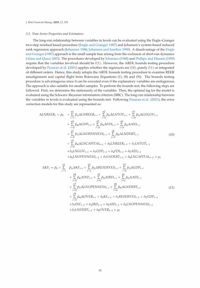
J. Risk Financial Manag. 2019, 12, 101
3.1. Time Series Properties and Estimators
The long-run relationship between variables in levels can be evaluated using the Engle–Grangertwo-step residual based procedure (Engle and Granger 1987) and Johansen’s system-based reducedrank regression approach (Johansen 1988; Johansen and Juselius 1990). A disadvantage of the Engleand Granger (1987) approach is the small sample bias arising from the exclusion of short-run dynamics(Alam and Quazi 2003). The procedures developed by Johansen (1988) and Phillips and Hansen (1990)require that the variables involved should be I(1). However, the ARDL bounds testing proceduredeveloped by Pesaran et al. (2001) applies whether the regressors are I(0), purely I(1) or integratedof different orders. Hence, this study adopts the ARDL bounds testing procedure to examine REERmisalignment and capital flight from Botswana (Equations (1), (8) and (9)). The bounds testingprocedure is advantageous since it can be executed even if the explanatory variables are endogenous.The approach is also suitable for smaller samples. To perform the bounds test, the following steps arefollowed. First, we determine the stationarity of the variables. Then, the optimal lag for the model isevaluated using the Schwarz–Bayesian information criterion (SBIC). The long-run relationship betweenthe variables in levels is evaluated using the bounds test. Following Pesaran et al. (2001), the errorcorrection models for this study are represented as:
ΔLNREERt = β0 +n1∑
i=1β1iΔLNREERt−i +
n2∑i=0β2iΔLNTOTt−i +
n3∑i=0β3iΔLNGOVt−i
+n4∑
i=0β4iΔGDPt−i +
n5∑i=0β5iΔFDIt−i +
n6∑i=0β6iΔAIDt−i
+n7∑
i=0β7iΔLNOPENNESSt−i +
n8∑i=0β8iΔLNDEBTt−i
+n9∑
i=0β9iΔLNCAPITALt−i + δ0LNREERt−1 + δ1LNTOTt−1
+δ2LNGOVt−1 + δ3GDPt−1 + δ4FDIt−1 + δ5AIDt−1
+δ6LNOPENNESSt−1 + δ7LNDEBTt−1 + δ8LNCAPITALt−1 + μt
(10)
ΔKFt = β0 +n1∑
i=1β1iΔKFt−i +
n2∑i=1β2iΔRESERVESt−i +
n3∑i=0β3iΔGDPt−i
+n4∑
i=0β4iΔINFt−i +
n5∑i=0β5iΔIRDt−i +
n6∑i=0β6iΔAIDt−i
+n7∑
i=0β7iΔLNOPENNESSt−i +
n8∑i=0β8iΔLNDEBTt−i
+n9∑
i=0β9iΔOVERt−i + δ0KFt−1 + δ1RESERVESt−1 + δ2GDPt−1
+δ3INFt−1 + δ4IRDt−1 + δ5AIDt−1 + δ6LNOPENNESSt−1
+δ7LNDEBTt−1 + δ8OVERt−1 + μt
(11)
24
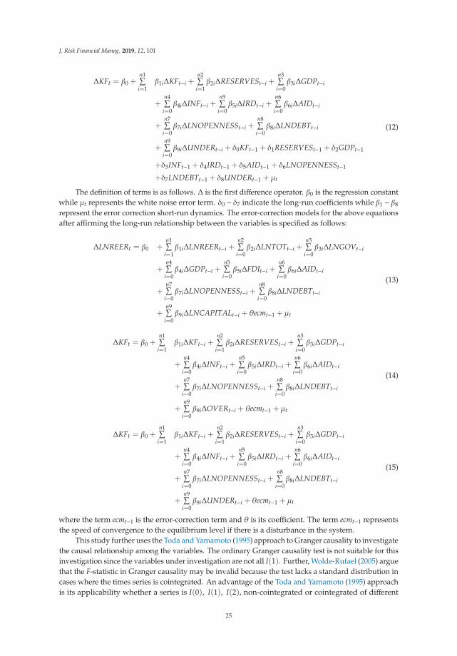
J. Risk Financial Manag. 2019, 12, 101
ΔKFt = β0 +n1∑
i=1β1iΔKFt−i +
n2∑i=1β2iΔRESERVESt−i +
n3∑i=0β3iΔGDPt−i
+n4∑
i=0β4iΔINFt−i +
n5∑i=0β5iΔIRDt−i +
n6∑i=0β6iΔAIDt−i
+n7∑
i=0β7iΔLNOPENNESSt−i +
n8∑i=0β8iΔLNDEBTt−i
+n9∑
i=0β9iΔUNDERt−i + δ0KFt−1 + δ1RESERVESt−1 + δ2GDPt−1
+δ3INFt−1 + δ4IRDt−1 + δ5AIDt−1 + δ6LNOPENNESSt−1
+δ7LNDEBTt−1 + δ8UNDERt−1 + μt
(12)
The definition of terms is as follows. Δ is the first difference operator. β0 is the regression constantwhile μt represents the white noise error term. δ0 − δ7 indicate the long-run coefficients while β1 − β8
represent the error correction short-run dynamics. The error-correction models for the above equationsafter affirming the long-run relationship between the variables is specified as follows:
ΔLNREERt = β0 +n1∑
i=1β1iΔLNREERt−i +
n2∑i=0β2iΔLNTOTt−i +
n3∑i=0β3iΔLNGOVt−i
+n4∑
i=0β4iΔGDPt−i +
n5∑i=0β5iΔFDIt−i +
n6∑i=0β6iΔAIDt−i
+n7∑
i=0β7iΔLNOPENNESSt−i +
n8∑i=0β8iΔLNDEBTt−i
+n9∑
i=0β9iΔLNCAPITALt−i + θecmt−1 + μt
(13)
ΔKFt = β0 +n1∑
i=1β1iΔKFt−i +
n2∑i=1β2iΔRESERVESt−i +
n3∑i=0β3iΔGDPt−i
+n4∑
i=0β4iΔINFt−i +
n5∑i=0β5iΔIRDt−i +
n6∑i=0β6iΔAIDt−i
+n7∑
i=0β7iΔLNOPENNESSt−i +
n8∑i=0β8iΔLNDEBTt−i
+n9∑
i=0β9iΔOVERt−i + θecmt−1 + μt
(14)
ΔKFt = β0 +n1∑
i=1β1iΔKFt−i +
n2∑i=1β2iΔRESERVESt−i +
n3∑i=0β3iΔGDPt−i
+n4∑
i=0β4iΔINFt−i +
n5∑i=0β5iΔIRDt−i +
n6∑i=0β6iΔAIDt−i
+n7∑
i=0β7iΔLNOPENNESSt−i +
n8∑i=0β8iΔLNDEBTt−i
+n9∑
i=0β9iΔUNDERt−i + θecmt−1 + μt
(15)
where the term ecmt−1 is the error-correction term and θ is its coefficient. The term ecmt−1 representsthe speed of convergence to the equilibrium level if there is a disturbance in the system.
This study further uses the Toda and Yamamoto (1995) approach to Granger causality to investigatethe causal relationship among the variables. The ordinary Granger causality test is not suitable for thisinvestigation since the variables under investigation are not all I(1). Further, Wolde-Rufael (2005) arguethat the F-statistic in Granger causality may be invalid because the test lacks a standard distribution incases where the times series is cointegrated. An advantage of the Toda and Yamamoto (1995) approachis its applicability whether a series is I(0), I(1), I(2), non-cointegrated or cointegrated of different
25
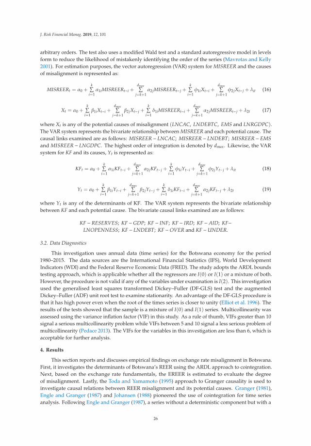
J. Risk Financial Manag. 2019, 12, 101
arbitrary orders. The test also uses a modified Wald test and a standard autoregressive model in levelsform to reduce the likelihood of mistakenly identifying the order of the series (Mavrotas and Kelly2001). For estimation purposes, the vector autoregression (VAR) system for MISREER and the causesof misalignment is represented as:
MISREERt = α0 +k∑
i=1α1iMISREERt−i +
dmax∑j=k+1
α2 jMISREERt− j +k∑
i=1φ1iXt−i +
dmax∑j=k+1
φ2 jXt− j + λit (16)
Xt = α0 +k∑
i=1β1iXt−i +
dmax∑j=k+1
β2 jXt− j +k∑
i=1δ1iMISREERt−i +
dmax∑j=k+1
α2 jMISREERt− j + λ2t (17)
where Xt is any of the potential causes of misalignment (LNCAC, LNDEBTC, EMS and LNRGDPC).The VAR system represents the bivariate relationship between MISREER and each potential cause. Thecausal links examined are as follows: MISREER− LNCAC; MISREER− LNDEBT; MISREER− EMSand MISREER − LNGDPC. The highest order of integration is denoted by dmax. Likewise, the VARsystem for KF and its causes, Yt is represented as:
KFt = α0 +k∑
i=1α1iKFt−i +
dmax∑j=k+1
α2 jKFt− j +k∑
i=1φ1iYt−i +
dmax∑j=k+1
φ2 jYt− j + λit (18)
Yt = α0 +k∑
i=1β1iYt−i +
dmax∑j=k+1
β2 jYt− j +k∑
i=1δ1iKFt−i +
dmax∑j=k+1
α2 jKFt− j + λ2t (19)
where Yt is any of the determinants of KF. The VAR system represents the bivariate relationshipbetween KF and each potential cause. The bivariate causal links examined are as follows:
KF−RESERVES; KF−GDP; KF− INF; KF− IRD; KF−AID; KF−LNOPENNESS; KF− LNDEBT; KF−OVER and KF−UNDER.
3.2. Data Diagnostics
This investigation uses annual data (time series) for the Botswana economy for the period1980–2015. The data sources are the International Financial Statistics (IFS), World DevelopmentIndicators (WDI) and the Federal Reserve Economic Data (FRED). The study adopts the ARDL boundstesting approach, which is applicable whether all the regressors are I(0) or I(1) or a mixture of both.However, the procedure is not valid if any of the variables under examination is I(2). This investigationused the generalised least squares transformed Dickey–Fuller (DF-GLS) test and the augmentedDickey–Fuller (ADF) unit root test to examine stationarity. An advantage of the DF-GLS procedure isthat it has high power even when the root of the times series is closer to unity (Elliot et al. 1996). Theresults of the tests showed that the sample is a mixture of I(0) and I(1) series. Multicollinearity wasassessed using the variance inflation factor (VIF) in this study. As a rule of thumb, VIFs greater than 10signal a serious multicollinearity problem while VIFs between 5 and 10 signal a less serious problem ofmulticollinearity (Pedace 2013). The VIFs for the variables in this investigation are less than 6, which isacceptable for further analysis.
4. Results
This section reports and discusses empirical findings on exchange rate misalignment in Botswana.First, it investigates the determinants of Botswana’s REER using the ARDL approach to cointegration.Next, based on the exchange rate fundamentals, the EREER is estimated to evaluate the degreeof misalignment. Lastly, the Toda and Yamamoto (1995) approach to Granger causality is used toinvestigate causal relations between REER misalignment and its potential causes. Granger (1981),Engle and Granger (1987) and Johansen (1988) pioneered the use of cointegration for time seriesanalysis. Following Engle and Granger (1987), a series without a deterministic component but with a
26
J. Risk Financial Manag. 2019, 12, 101
stationary autoregressive moving average after differencing d times is integrated of order d, [xt ∼ I(d)].The properties of I(0) and I(1) series differ based on their responsiveness to innovations. If xt ∼ I(0),its variance is finite and innovations have a short-term effect on the magnitude of xt. In contrast,an innovation has a long-term effect on the value of an I(1) series (Engle and Granger 1987). Theprocedure followed for the ARDL bounds cointegration approach is as follows. First, the variableswere subjected to stationarity tests. The results show that only GDP is I(0) while other variables(LNREER, LNTOT, LNGOV, FDI, AID, LNOPENNESS, LNDEBT and LNCAPITAL) are I(1). Next,the optimal lag length of the specifications is determined using the SBIC. The SBIC is used to determinethe optimal lag length since it is more reliable for optimal model selection than the Akaike informationcriterion (AIC) (Pesaran and Shin 1999). The long-run levels relationships for different specificationsare evaluated using the F-test. Subsequently, the coefficients of the variables are estimated withdiagnostic tests.
The benchmark for determining a long-run relationship between the dependent variable andindependent variables is the F-test. The optimal lag established for the ARDL model using theSBIC is zero when LNREER is the dependent variable. The null hypothesis of no cointegration isH0 : δ1 = δ2 = · · · δP = 0 against the alternative H1 : δ1 � δ2 � · · · δP � 0. The criterion for the long-runequilibrium relationship is based on the lower and upper bound critical values proposed by Pesaran etal. (2001). Following Pesaran et al. (2001), we reject the null of no long-run equilibrium relationship ifthe computed F-statistic is higher than the upper bound critical values. However, if the F-statistic isless than the lower bounds, we fail to reject the null of no long-run equilibrium relationship. The test isinconclusive if the F-statistic falls between the lower and upper bounds.
Banerjee et al. (1998) suggest that a negative and significant error-correction term signals along-run relationship. The F-test for the parameter that δ1 = δ2 = · · · δP = 0 in the specificationwith LNREER as the dependent variable is expressed as F(LNREER|X1, X2, · · ·XP) where X1 toXP are the determinants of the REER. The procedure is repeated by interchanging the dependentvariable with the regressors. The order of the variables when LNREER is an independent variableis F(X1|LNREER, X2, · · ·XP). Following Pesaran et al. (2001) we determine the F-test by including arestricted constant (RC); unrestricted constant (UC) and unrestricted constant with unrestricted trend(UC + UT) in the specifications. This is important because it helps to determine the sensitivity ofthe long-run equilibrium relationship to a deterministic trend. When a specification includes RC, itindicates the dynamics of the long-run equilibrium relationship when the intercept is restricted withno linear trend. When a specification includes UC it shows the dynamics of the relationship when anunrestricted constant with no trend is included in the specification. Consequently, when a specificationincludes UC + UT it reveals the relationship between the variables when there is an unrestrictedconstant with unrestricted trend in the model specification. Since F(LNREER|X1, X2, · · ·XP) withtrend and intercept (Table 1) is greater than the upper limit of the critical bound (3.23 > 3.14), the nullhypothesis of no long-run equilibrium relationship7 is rejected at the 10% level. In addition, whenthe test is conducted with restricted and unrestricted constants, the null of no long-run equilibriumrelationship is rejected at the 5% level. Further, when LNREER is switched to a regressor position, thecomputed F-statistic for the majority of the determinants of the REER is greater than the upper boundcritical values indicating a long-run equilibrium relationship. The presence of a long-run equilibriumrelationship indicates that the regressors are not long-run forcing variables8 (Pesaran et al. 2001).Table 1 presents the results of the F-test.
7 For the exchange rate fundamentals, the value of the regressors k was greater than 7, therefore only Pesaran et al. (2001)critical values were followed.
8 A variable xt is long-run forcing if there is no feedback from the long-run equilibrium relationship on the change of xt.Consequently, there will be no information on the marginal process for xt about the parameters of the relationship (Pesaranet al. 2001).
27
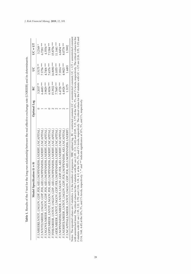
J. Risk Financial Manag. 2019, 12, 101
Ta
ble
1.
Res
ults
ofth
eF-
test
for
the
long
-run
rela
tion
ship
betw
een
the
real
effec
tive
exch
ange
rate
(LN
REE
R)a
ndit
sde
term
inan
ts.
Mo
de
lS
pe
cifi
cati
on
(k=
8)
Op
tim
al
La
gR
CU
CU
C+
UT
F(LN
REE
R|LN
TOT
,LN
GO
V,G
DP,
FDI,
AID
,LN
OPE
NN
ESS,
LND
EBT,
LNC
API
TAL)
03.
2037
**3.
5175
**3.
2349
*F(
LNTO
T |LN
REE
R,L
NG
OV
,GD
P,FD
I,A
ID,L
NO
PEN
NES
S,LN
DEB
T,LN
CA
PITA
L)
16.
4683
***
7.17
56**
*6.
7281
***
F(LN
GO
V|LN
REE
R,L
NTO
T,G
DP,
FDI,
AID
,LN
OPE
NN
ESS,
LND
EBT,
LNC
API
TAL)
13.
9829
***
4.74
06**
*4.
3554
**F(
GD
P |LN
REE
R,L
NTO
T,LN
GO
V,F
DI,
AID
,LN
OPE
NN
ESS,
LND
EBT,
LNC
API
TAL)
06.
9034
***
7.63
76**
*7.
1384
***
F(FD
I |LN
REE
R,L
NTO
T,LN
GO
V,G
DP,
AID
,LN
OPE
NN
ESS,
LND
EBT,
LNC
API
TAL)
215
.392
2**
*16
.809
0**
*15
.875
6**
*F(
AID|LN
REE
R,L
NTO
T,LN
GO
V,G
DP,
FDI,
LNO
PEN
NES
S,LN
DEB
T,LN
CA
PITA
L)
27.
7685
***
8.10
55**
*11
.144
1**
*F(
LNO
PEN
NES
S |LN
REE
R,L
NTO
T,LN
GO
V,G
DP,
FDI,
AID
,LN
DEB
T,LN
CA
PITA
L)
16.
4728
***
7.18
14**
*6.
8454
***
F(LN
DEB
T |LN
REE
R,L
NTO
T,LN
GO
V,G
DP,
FDI,
LNO
PEN
NES
S,A
ID,L
NC
API
TAL)
24.
4928
***
4.98
25**
*8.
0778
***
F(LN
CA
PITA
L |LN
REE
R,L
NTO
T,LN
GO
V,G
DP,
FDI,
AID
,LN
OPE
NN
ESS,
LND
EBT)
11.
3175
1.44
931.
5992
Not
es:T
here
port
edva
lues
are
F-st
atis
tics
.kis
the
num
ber
ofre
gres
sors
.SB
ICop
tim
alla
g.R
C=
rest
rict
edco
nsta
nt;U
C=
unr
estr
icte
dco
nsta
nt;U
C+
UT=
unr
estr
icte
dco
nsta
ntw
ith
unre
stri
cted
tren
d.T
hecr
itic
alva
lues
for
the
F-st
atis
tic
wit
hR
Car
e{1.
85,
2.11
,2.
62}a
nd{2.
85,
3.15
,3.
77}a
tthe
10%
,5%
,and
1%le
vels
,res
pect
ivel
y.T
hecr
itic
alva
lues
for
the
F-st
atis
tic
wit
hU
Car
e{1
.95,
2.22
,2.
79}a
nd{3
.06,
3.39
,4.
1 }at
the
10%
,5%
,and
1%le
vels
,res
pect
ivel
y.T
hecr
itic
alva
lues
for
the
F-st
atis
tic
wit
hU
C+
UT
are{2.
26,
2.55
,3.
15}a
nd{3.
14,
3.68
,4.
43}a
tthe
10%
,5%
,and
1%le
vels
,res
pect
ivel
y.*,
**an
d**
*in
dica
tesi
gnifi
canc
eat
10%
,5%
,and
1%,r
espe
ctiv
ely.
28
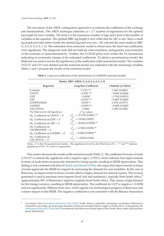
J. Risk Financial Manag. 2019, 12, 101
The next phase of the ARDL cointegration approach is to estimate the coefficients of the exchangerate fundamentals. The ARDL technique estimates (p + 1)k number of regressions for the optimallag length for each variable. The term p is the maximum number of lags and k here is the number ofvariables in the equation. The optimal SBIC lag length is zero while that for AIC is one. Since a smalllag length provides better results, the optimal lag used was zero. AIC selected the same model as SBIC(1, 0, 0, 0, 0, 0, 0, 1, 0). The estimated error-correction model is robust since the short-run coefficientswere significant. The diagnostic tests did not indicate autocorrelation, endogeneity, non-normalityof the residuals or heteroskedasticity. Further, the CUSUM plots were within the 5% boundaries,indicating no systematic change of the estimated coefficients. To obtain a parsimonious model, theWald test was used to test for the significance of the coefficients of the unrestricted model. The variablesLNGOV and FDI were deleted and the restricted model was estimated with the remaining variables.Tables 2 and 3 presents the results of the restricted model.
Table 2. Long-run coefficients of the determinants of LNREER (restricted model).
Model: SBIC-ARDL (1, 0, 0, 0, 0, 0, 0, 1, 0)
Regressor Long-Run Coefficient t-Statistic (p-Value)
Constant 5.1731 *** 7.1801 (0.0000)LNTOT −0.3551 *** −3.9642 (0.0004)GDP −0.0038 * −1.7363 (0.0931)AID −0.0193 *** −5.4407 (0.0000)LNOPENNESS 0.2374 ** 2.1781 (0.0377)LNDEBT −0.0553 *** −2.8405 (0.0082)LNCAPITAL 0.0462 1.1897 (0.2438)The Wald test for the hypothesis: χ2 (p-value)H0: Coefficient on LNTOT = 0 χ2
(1)= 15.7152 (0.0001) **
H0: Coefficient on GDP = 0 χ2(1)
= 3.0146 (0.0825)
H0: Coefficient on AID = 0 χ2(1)
= 29.6016 (0.0000) **
H0: Coefficient onLNOPENNESS = 0
χ2(1)
= 4.7440 (0.0294) **
H0: Coefficient on LNDEBT = 0 χ2(1)
= 8.0683 (0.0045) **
H0: Coefficient onLNCAPITAL = 0
χ2(1)
= 1.4154 (0.2342)
Notes: χ2 is the Chi-squared test statistic. The significance level for the Wald test is 5%. *, ** and *** indicatesignificance at 10%, 5%, and 1%, respectively.
This section discusses the results of the restricted model (Table 2). The coefficient for terms of trade(LNTOT) is statistically significant with a negative sign (−0.3551), which indicates that improvementsin terms of trade terms increases the demand for foreign goods, resulting in REER depreciation. Thisfinding is not consistent with that of Hinkle and Montiel (1999), who argue that improvements in termsof trade appreciate the REER for imports by increasing the demand for non-tradables. In the case ofBotswana, an improvement in terms of trade reflects a higher demand for mineral exports. The revenuegenerated is used to purchase more imports (food, fuel and machinery), typically from South Africa.9
Approximately 80% of Botswana’s imports originate from South Africa. This causes a high demandfor the foreign currency, resulting in REER depreciation. The coefficient for GDP is negative (−0.0038)and not significantly different from zero, which signals low technological progress in Botswana anda minor impact on the REER. The negative coefficient is not consistent with the Balassa–Samuelson
9 According to the International Monetary Fund (2007), South Africa’s competitive advantage overshadows Botswana’scompetitive advantage, given the large domestic market and abundant labour supply in South Africa. Consequently, theInternational Monetary Fund (2007) recommends that Botswana should import from South Africa rather than producegoods domestically.
29
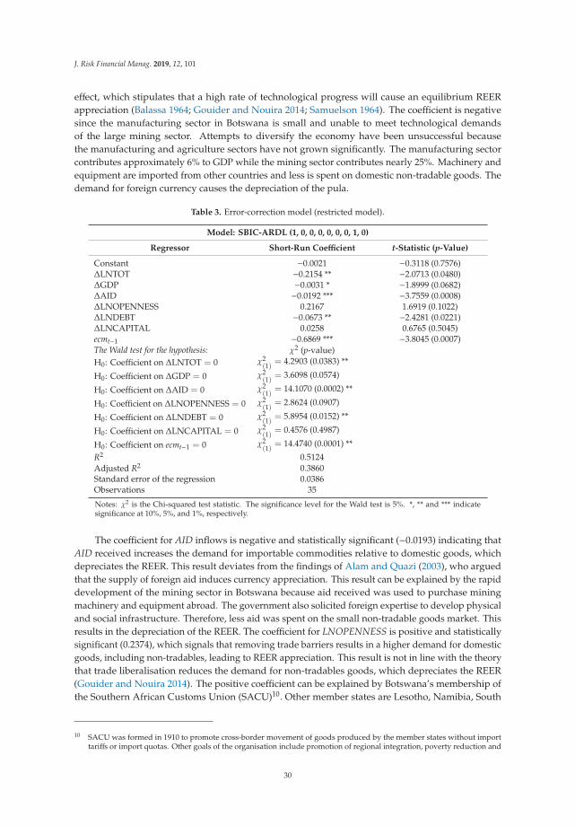
J. Risk Financial Manag. 2019, 12, 101
effect, which stipulates that a high rate of technological progress will cause an equilibrium REERappreciation (Balassa 1964; Gouider and Nouira 2014; Samuelson 1964). The coefficient is negativesince the manufacturing sector in Botswana is small and unable to meet technological demandsof the large mining sector. Attempts to diversify the economy have been unsuccessful becausethe manufacturing and agriculture sectors have not grown significantly. The manufacturing sectorcontributes approximately 6% to GDP while the mining sector contributes nearly 25%. Machinery andequipment are imported from other countries and less is spent on domestic non-tradable goods. Thedemand for foreign currency causes the depreciation of the pula.
Table 3. Error-correction model (restricted model).
Model: SBIC-ARDL (1, 0, 0, 0, 0, 0, 0, 1, 0)
Regressor Short-Run Coefficient t-Statistic (p-Value)
Constant −0.0021 −0.3118 (0.7576)ΔLNTOT −0.2154 ** −2.0713 (0.0480)ΔGDP −0.0031 * −1.8999 (0.0682)ΔAID −0.0192 *** −3.7559 (0.0008)ΔLNOPENNESS 0.2167 1.6919 (0.1022)ΔLNDEBT −0.0673 ** −2.4281 (0.0221)ΔLNCAPITAL 0.0258 0.6765 (0.5045)ecmt−1 −0.6869 *** −3.8045 (0.0007)The Wald test for the hypothesis: χ2 (p-value)H0: Coefficient on ΔLNTOT = 0 χ2
(1)= 4.2903 (0.0383) **
H0: Coefficient on ΔGDP = 0 χ2(1)
= 3.6098 (0.0574)
H0: Coefficient on ΔAID = 0 χ2(1)
= 14.1070 (0.0002) **
H0: Coefficient on ΔLNOPENNESS = 0 χ2(1)
= 2.8624 (0.0907)
H0: Coefficient on ΔLNDEBT = 0 χ2(1)
= 5.8954 (0.0152) **
H0: Coefficient on ΔLNCAPITAL = 0 χ2(1)
= 0.4576 (0.4987)
H0: Coefficient on ecmt−1 = 0 χ2(1)
= 14.4740 (0.0001) **
R2 0.5124Adjusted R2 0.3860Standard error of the regression 0.0386Observations 35
Notes: χ2 is the Chi-squared test statistic. The significance level for the Wald test is 5%. *, ** and *** indicatesignificance at 10%, 5%, and 1%, respectively.
The coefficient for AID inflows is negative and statistically significant (−0.0193) indicating thatAID received increases the demand for importable commodities relative to domestic goods, whichdepreciates the REER. This result deviates from the findings of Alam and Quazi (2003), who arguedthat the supply of foreign aid induces currency appreciation. This result can be explained by the rapiddevelopment of the mining sector in Botswana because aid received was used to purchase miningmachinery and equipment abroad. The government also solicited foreign expertise to develop physicaland social infrastructure. Therefore, less aid was spent on the small non-tradable goods market. Thisresults in the depreciation of the REER. The coefficient for LNOPENNESS is positive and statisticallysignificant (0.2374), which signals that removing trade barriers results in a higher demand for domesticgoods, including non-tradables, leading to REER appreciation. This result is not in line with the theorythat trade liberalisation reduces the demand for non-tradables goods, which depreciates the REER(Gouider and Nouira 2014). The positive coefficient can be explained by Botswana’s membership ofthe Southern African Customs Union (SACU)10. Other member states are Lesotho, Namibia, South
10 SACU was formed in 1910 to promote cross-border movement of goods produced by the member states without importtariffs or import quotas. Other goals of the organisation include promotion of regional integration, poverty reduction and
30
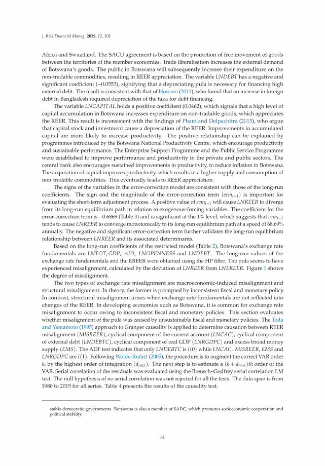
J. Risk Financial Manag. 2019, 12, 101
Africa and Swaziland. The SACU agreement is based on the promotion of free movement of goodsbetween the territories of the member economies. Trade liberalisation increases the external demandof Botswana’s goods. The public in Botswana will subsequently increase their expenditure on thenon-tradable commodities, resulting in REER appreciation. The variable LNDEBT has a negative andsignificant coefficient (−0.0553), signifying that a depreciating pula is necessary for financing highexternal debt. The result is consistent with that of Hossain (2011), who found that an increase in foreigndebt in Bangladesh required depreciation of the taka for debt financing.
The variable LNCAPITAL holds a positive coefficient (0.0462), which signals that a high level ofcapital accumulation in Botswana increases expenditure on non-tradable goods, which appreciatesthe REER. This result is inconsistent with the findings of Pham and Delpachitra (2015), who arguethat capital stock and investment cause a depreciation of the REER. Improvements in accumulatedcapital are more likely to increase productivity. The positive relationship can be explained byprogrammes introduced by the Botswana National Productivity Centre, which encourage productivityand sustainable performance. The Enterprise Support Programme and the Public Service Programmewere established to improve performance and productivity in the private and public sectors. Thecentral bank also encourages sustained improvements in productivity, to reduce inflation in Botswana.The acquisition of capital improves productivity, which results in a higher supply and consumption ofnon-tradable commodities. This eventually leads to REER appreciation.
The signs of the variables in the error-correction model are consistent with those of the long-runcoefficients. The sign and the magnitude of the error-correction term (ecmt−1) is important forevaluating the short-term adjustment process. A positive value of ecmt−1 will cause LNREER to divergefrom its long-run equilibrium path in relation to exogenous-forcing variables. The coefficient for theerror-correction term is −0.6869 (Table 3) and is significant at the 1% level, which suggests that ecmt−1
tends to cause LNREER to converge monotonically to its long-run equilibrium path at a speed of 68.69%annually. The negative and significant error-correction term further validates the long-run equilibriumrelationship between LNREER and its associated determinants.
Based on the long-run coefficients of the restricted model (Table 2), Botswana’s exchange ratefundamentals are LNTOT, GDP, AID, LNOPENNESS and LNDEBT. The long-run values of theexchange rate fundamentals and the EREER were obtained using the HP filter. The pula seems to haveexperienced misalignment, calculated by the deviation of LNREER from LNEREER. Figure 1 showsthe degree of misalignment.
The two types of exchange rate misalignment are macroeconomic-induced misalignment andstructural misalignment. In theory, the former is prompted by inconsistent fiscal and monetary policy.In contrast, structural misalignment arises when exchange rate fundamentals are not reflected intochanges of the REER. In developing economies such as Botswana, it is common for exchange ratemisalignment to occur owing to inconsistent fiscal and monetary policies. This section evaluateswhether misalignment of the pula was caused by unsustainable fiscal and monetary policies. The Todaand Yamamoto (1995) approach to Granger causality is applied to determine causation between REERmisalignment (MISREER), cyclical component of the current account (LNCAC), cyclical componentof external debt (LNDEBTC), cyclical component of real GDP (LNRGDPC) and excess broad moneysupply (EMS). The ADF test indicates that only LNDEBTC is I(0) while LNCAC, MISREER, EMS andLNRGDPC are I(1). Following Wolde-Rufael (2005), the procedure is to augment the correct VAR orderk, by the highest order of integration (dmax). The next step is to estimate a (k + dmax)th order of theVAR. Serial correlation of the residuals was evaluated using the Breusch–Godfrey serial correlation LMtest. The null hypothesis of no serial correlation was not rejected for all the tests. The data span is from1980 to 2015 for all series. Table 4 presents the results of the causality test.
stable democratic governments. Botswana is also a member of SADC, which promotes socioeconomic cooperation andpolitical stability.
31
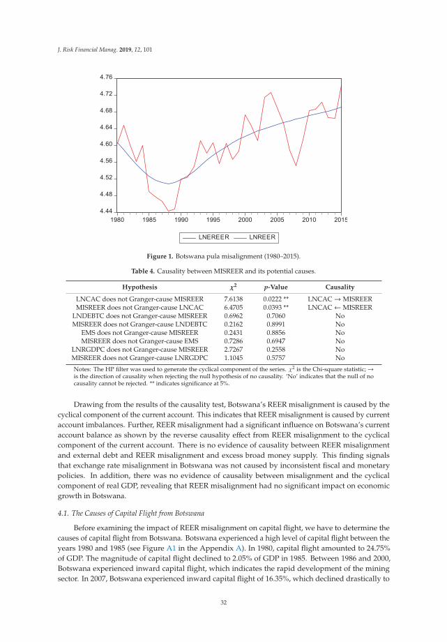
J. Risk Financial Manag. 2019, 12, 101
Figure 1. Botswana pula misalignment (1980–2015).
Table 4. Causality between MISREER and its potential causes.
Hypothesis χ2 p-Value Causality
LNCAC does not Granger-cause MISREER 7.6138 0.0222 ** LNCAC → MISREERMISREER does not Granger-cause LNCAC 6.4705 0.0393 ** LNCAC ← MISREER
LNDEBTC does not Granger-cause MISREER 0.6962 0.7060 NoMISREER does not Granger-cause LNDEBTC 0.2162 0.8991 No
EMS does not Granger-cause MISREER 0.2431 0.8856 NoMISREER does not Granger-cause EMS 0.7286 0.6947 No
LNRGDPC does not Granger-cause MISREER 2.7267 0.2558 NoMISREER does not Granger-cause LNRGDPC 1.1045 0.5757 No
Notes: The HP filter was used to generate the cyclical component of the series. χ2 is the Chi-square statistic; →is the direction of causality when rejecting the null hypothesis of no causality. ‘No’ indicates that the null of nocausality cannot be rejected. ** indicates significance at 5%.
Drawing from the results of the causality test, Botswana’s REER misalignment is caused by thecyclical component of the current account. This indicates that REER misalignment is caused by currentaccount imbalances. Further, REER misalignment had a significant influence on Botswana’s currentaccount balance as shown by the reverse causality effect from REER misalignment to the cyclicalcomponent of the current account. There is no evidence of causality between REER misalignmentand external debt and REER misalignment and excess broad money supply. This finding signalsthat exchange rate misalignment in Botswana was not caused by inconsistent fiscal and monetarypolicies. In addition, there was no evidence of causality between misalignment and the cyclicalcomponent of real GDP, revealing that REER misalignment had no significant impact on economicgrowth in Botswana.
4.1. The Causes of Capital Flight from Botswana
Before examining the impact of REER misalignment on capital flight, we have to determine thecauses of capital flight from Botswana. Botswana experienced a high level of capital flight between theyears 1980 and 1985 (see Figure A1 in the Appendix A). In 1980, capital flight amounted to 24.75%of GDP. The magnitude of capital flight declined to 2.05% of GDP in 1985. Between 1986 and 2000,Botswana experienced inward capital flight, which indicates the rapid development of the miningsector. In 2007, Botswana experienced inward capital flight of 16.35%, which declined drastically to
32
J. Risk Financial Manag. 2019, 12, 101
0.89% as outward capital flight in 2008. This marks the period of the 2007−2008 Global Financial Crisisas investors were seeking higher returns for their monetary assets in other economies. The generaltrend is that from 2012 to 2015, Botswana experienced increasing inward capital flight amounting to6.34% of GDP in 2015. This may be attributed to the Sectoral Development and Business LinkagesUnit developed in 2011, which was designed to attract FDI and promote skills transfer as part of theEconomic Diversification Drive. On average, Botswana experienced inward capital flight over theperiod 1980−2015.
The general to specific approach is used to identify determinants of capital flight. Trade openness(LNOPENNESS) and the level of foreign reserves (RESERVES) are found to be the determinants ofBotswana’s capital flight. The other variables (GDP, INF, IRD, AID and LNDEBT) are redundantand have no explanatory power on capital flight from Botswana. The results of the stationaritytests show that the variable RESERVES is I(0) while KF and LNOPENNESS are I(1). The F-test asdescribed by Pesaran et al. (2001) is used for determining a long-run relationship for the variablesKF, LNOPENNESS and RESERVES. The optimal lag established for the ARDL model using the SBIC iszero when KF is the dependent variable. The null hypothesis of no long-run equilibrium relationship isH0 : δ1 = δ2 = δ3 = 0 whereas the alternative is H1 : δ1 � δ2 � δ3 � 0. The F-test for the restriction thatδ1 = δ2 = δ3 = 0 when KF is the dependent variable is expressed as F(KF|LNOPENNESS, RESERVES).The process is repeated by interchanging the dependent variable with the regressors. The F-statisticfor F(KF|LNOPENNESS, RESERVES) with trend and intercept is greater than the upper limit of thecritical bound (22.23 > 7.52). Consequently, the null hypothesis of no long-run equilibrium relationshipis rejected at the 1% significance level. The test is also executed with constants only and the null ofno long-run equilibrium relationship is still rejected at the 1% significance level. The null hypothesisof no long-run equilibrium relationship is rejected at the 5% level when RESERVES is a dependentvariable in all regressions. However, the variable LNOPENNESS indicated no evidence of a long-runequilibrium relationship with other variables when it is a dependent variable.
The next procedure is to estimate the short-run and long-run coefficients for KF, LNOPENNESSand RESERVES. The optimal lag length for SBIC and AIC is zero when KF is the dependent variable.AIC selected the same model as SBIC (1, 0, 1). Table 5 presents the results of the estimated coefficients.
The estimated error-correction model is robust since the short-run coefficients are significant.The diagnostic tests do not signal autocorrelation, endogeneity, non-normality of the residuals orheteroskedasticity. The estimated model is stable because the CUSUM plots suggested no systematicchanges in the estimated coefficients. The coefficient for LNOPENNESS is positive and significant(62.3474), which signals that trade liberalisation increases the volume of outward capital flight. Thecoefficient suggests that the reported value of Botswana’s exports is understated, leading to net capitaloutflows through trade. According to Global Financial Integrity (Global Financial Integrity 2015),Botswana lost approximately 13 billion US dollars through trade misinvoicing in 2004–2013. Theestimated value of Botswana’s under-invoiced exports is approximately 9 billion US dollars against4 billion US dollars for over-invoiced exports during 2004–2013 (Global Financial Integrity 2015).In the case of imports, the disparity was small, which indicates that the economy experiences netcapital outflows through trade. Ajayi and Ndikumana (2015) posit that trade misinvoicing occursby understating the quantity of goods or prices. The seller sends the difference between the actualearnings and the understated values to foreign accounts. The results are consistent with those ofCheung and Qian (2010), who argue that increasing trade openness allows economic agents to falsifytrade prices in China, resulting in a rise in capital flight.
33
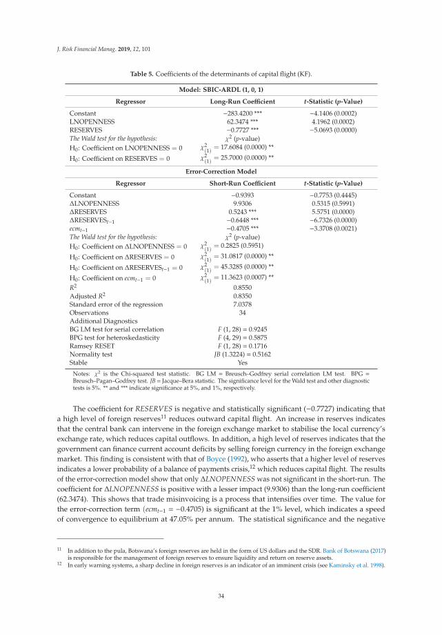
J. Risk Financial Manag. 2019, 12, 101
Table 5. Coefficients of the determinants of capital flight (KF).
Model: SBIC-ARDL (1, 0, 1)
Regressor Long-Run Coefficient t-Statistic (p-Value)
Constant −283.4200 *** −4.1406 (0.0002)LNOPENNESS 62.3474 *** 4.1962 (0.0002)RESERVES −0.7727 *** −5.0693 (0.0000)The Wald test for the hypothesis: χ2 (p-value)H0: Coefficient on LNOPENNESS = 0 χ2
(1)= 17.6084 (0.0000) **
H0: Coefficient on RESERVES = 0 χ2(1)
= 25.7000 (0.0000) **
Error-Correction Model
Regressor Short-Run Coefficient t-Statistic (p-Value)
Constant −0.9393 −0.7753 (0.4445)ΔLNOPENNESS 9.9306 0.5315 (0.5991)ΔRESERVES 0.5243 *** 5.5751 (0.0000)ΔRESERVESt−1 −0.6448 *** −6.7326 (0.0000)ecmt−1 −0.4705 *** −3.3708 (0.0021)The Wald test for the hypothesis: χ2 (p-value)H0: Coefficient on ΔLNOPENNESS = 0 χ2
(1)= 0.2825 (0.5951)
H0: Coefficient on ΔRESERVES = 0 χ2(1)
= 31.0817 (0.0000) **
H0: Coefficient on ΔRESERVESt−1 = 0 χ2(1)
= 45.3285 (0.0000) **
H0: Coefficient on ecmt−1 = 0 χ2(1)
= 11.3623 (0.0007) **
R2 0.8550Adjusted R2 0.8350Standard error of the regression 7.0378Observations 34Additional DiagnosticsBG LM test for serial correlation F (1, 28) = 0.9245BPG test for heteroskedasticity F (4, 29) = 0.5875Ramsey RESET F (1, 28) = 0.1716Normality test JB (1.3224) = 0.5162Stable Yes
Notes: χ2 is the Chi-squared test statistic. BG LM = Breusch–Godfrey serial correlation LM test. BPG =Breusch–Pagan–Godfrey test. JB = Jacque–Bera statistic. The significance level for the Wald test and other diagnostictests is 5%. ** and *** indicate significance at 5%, and 1%, respectively.
The coefficient for RESERVES is negative and statistically significant (−0.7727) indicating thata high level of foreign reserves11 reduces outward capital flight. An increase in reserves indicatesthat the central bank can intervene in the foreign exchange market to stabilise the local currency’sexchange rate, which reduces capital outflows. In addition, a high level of reserves indicates that thegovernment can finance current account deficits by selling foreign currency in the foreign exchangemarket. This finding is consistent with that of Boyce (1992), who asserts that a higher level of reservesindicates a lower probability of a balance of payments crisis,12 which reduces capital flight. The resultsof the error-correction model show that only ΔLNOPENNESS was not significant in the short-run. Thecoefficient for ΔLNOPENNESS is positive with a lesser impact (9.9306) than the long-run coefficient(62.3474). This shows that trade misinvoicing is a process that intensifies over time. The value forthe error-correction term (ecmt−1 = −0.4705) is significant at the 1% level, which indicates a speedof convergence to equilibrium at 47.05% per annum. The statistical significance and the negative
11 In addition to the pula, Botswana’s foreign reserves are held in the form of US dollars and the SDR. Bank of Botswana (2017)is responsible for the management of foreign reserves to ensure liquidity and return on reserve assets.
12 In early warning systems, a sharp decline in foreign reserves is an indicator of an imminent crisis (see Kaminsky et al. 1998).
34
J. Risk Financial Manag. 2019, 12, 101
sign of the error-correction term confirm the presence of a long-run equilibrium relationship betweenKF, LNOPENNESS and RESERVES.
The previous section indicated that trade openness and the level of foreign reserves are thedeterminants of capital flight from Botswana. The aim of the following sections is to examine the effectsof exchange rate misalignment on capital flight by including dummy variables for overvaluation andundervaluation in the specification.
4.1.1. The Impact of Overvaluation on Capital Flight
The null of the first hypothesis (H1) proposed that overvaluation of the Botswana pula increasescapital flight in the long-run. In this study, a 5% threshold for positive misalignment was used tocreate the overvaluation dummy variable (OVER). The variable is included in the regression todetermine its effect on capital flight and other regressors. The F-test is used to determine a long-runrelationship between KF, OVER, LNOPENNESS and RESERVES. The optimal lag established for theARDL model using the SBIC is zero when KF is the dependent variable. The computed F-statistic whenKF is the dependent variable with trend and intercept is greater than the upper limit of the criticalbound (16.10 > 6.36). The null hypothesis of no long-run equilibrium relationship is rejected at the1% significance level. The test is performed again with constants only and the null of no long-runequilibrium relationship is still rejected at the 1% significance level. The null hypothesis of no long-runequilibrium relationship is rejected at the 1% significance level when OVER is a dependent variable inall cases. However, when the variables LNOPENNESS and RESERVES are dependent variables, thenull hypothesis of no long-run equilibrium relationship is not rejected in all cases. The optimal laglength for SBIC and AIC is zero when KF is the dependent variable. AIC selected the same model asSBIC (1, 0, 0, 1). Table 6 presents the results of the estimated regression coefficients.
The estimated error-correction model above shows no challenges of endogeneity, non-normalityof the residuals or heteroskedasticity. The estimated coefficients for the model are systematically stable.The coefficient for OVER is positive (8.0067), indicating that an overvalued currency leads to increasingexpectations of depreciation in the future resulting in substantial capital outflows13. Consequently,we fail to reject the null of H1. The results are consistent with those of Cuddington (1986), whoshows that overvaluation of the Argentine Peso increased the probability of a major devaluationand was the cause of capital flight in 1980–1982. The coefficient for LNOPENNESS is positive andsignificant (49.3755) at the 5% significance level. This signals that when the currency is overvalued,trade liberalisation increases the volume of outward capital flight through exportable commodities.This finding is consistent with that of Cheung and Qian (2010).
The coefficient for RESERVES is positive (0.2439), indicating that increasing the level of foreignreserves when the currency is overvalued does not reduce outward capital flight. This result is notconsistent with that of Boyce (1992), who argues that a higher level of reserves reduces capital flight.This finding can be explained by Botswana’s history of devaluation of the pula for competitiveness ofexports. The pula was devalued seven times between 1980 and 2005. The highest devaluation was 15%in 1985 and 12% in 2005. Investors may expect a larger depreciation of the pula, leading to high capitaloutflows. The fear of welfare losses from devaluation may be too high such that increasing foreignreserves does not deter investors from sending their assets abroad.
13 At the 3% threshold, the coefficient for OVER is 8.7746. The coefficient for OVER is 8.0067 at the 4% and 5% thresholds.When the threshold is 6%, 7%, and 8% the coefficient for OVER is three times greater (24.0354, 24.0354, and 24.2009) than thecoefficient at the 5% threshold. This shows that the higher the overvaluation, the higher the expectations of devaluationresulting in large capital flight. Policymakers should tolerate overvaluation only up to 5%. The coefficient for LNOPENNESSincreases from 49.4755 at the 5% level to 57.5182 at the 6% and 7% thresholds. There was less variation in the coefficients ofRESERVES when the threshold was altered.
35
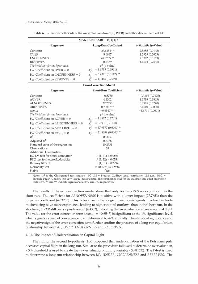
J. Risk Financial Manag. 2019, 12, 101
Table 6. Estimated coefficients of the overvaluation dummy (OVER) and other determinants of KF.
Model: SBIC-ARDL (1, 0, 0, 1)
Regressor Long-Run Coefficient t-Statistic (p-Value)
Constant −232.1514 ** 2.5855 (0.0145)OVER 8.0067 1.2929 (0.2053)LNOPENNESS 49.3755 ** 2.5362 (0.0163)RESERVES 0.2439 1.1604 (0.2545)The Wald test for the hypothesis: χ2 (p-value)H0: Coefficient on OVER = 0 χ2
(1)= 1.6715 (0.1961)
H0: Coefficient on LNOPENNESS = 0 χ2(1)
= 6.4321 (0.0112) **
H0: Coefficient on RESERVES = 0 χ2(1)
= 1.3465 (0.2549)
Error-Correction Model
Regressor Short-Run Coefficient t-Statistic (p-Value)
Constant −0.5780 −0.3316 (0.7425)ΔOVER 4.4302 1.3719 (0.1803)ΔLNOPENNESS 27.7653 0.9965 (0.3270)ΔRESERVES 0.7909 *** 6.1610 (0.0000)ecmt−1 −0.6547 *** −4.6701 (0.0001)The Wald test for the hypothesis: χ2 (p-value)H0: Coefficient on ΔOVER = 0 χ2
(1)= 1.8822 (0.1701)
H0: Coefficient on ΔLNOPENNESS = 0 χ2(1)
= 0.9931 (0.3190)
H0: Coefficient on ΔRESERVES = 0 χ2(1)
= 37.9577 (0.0000) **
H0: Coefficient on ecmt−1 = 0 χ2(1)
= 21.8099 (0.0000) **
R2 0.6804Adjusted R2 0.6378Standard error of the regression 10.2731Observations 35Additional DiagnosticsBG LM test for serial correlation F (1, 31) = 0.0896BPG test for heteroskedasticity F (3, 32) = 0.0534Ramsey RESET F (1, 31) = 0.2794Normality test JB (0.0224) = 0.9889Stable Yes
Notes: χ2 is the Chi-squared test statistic. BG LM = Breusch–Godfrey serial correlation LM test. BPG =Breusch–Pagan–Godfrey test. JB = Jacque–Bera statistic. The significance level for the Wald test and other diagnostictests is 5%. ** and *** indicate significance at 5%, and 1%, respectively.
The results of the error-correction model show that only ΔRESERVES was significant in theshort-run. The coefficient for ΔLNOPENNESS is positive with a lower impact (27.7653) than thelong-run coefficient (49.3755). This is because in the long-run, economic agents involved in trademisinvoicing have more experience, leading to higher capital outflows than in the short-run. In theshort-run, OVER still bears a positive sign (4.4302), indicating that overvaluation increases capital flight.The value for the error-correction term (ecmt−1 = −0.6547) is significant at the 1% significance level,which signals a speed of convergence to equilibrium at 65.47% annually. The statistical significance andthe negative sign of the error-correction term further confirm the presence of a long-run equilibriumrelationship between KF, OVER, LNOPENNESS and RESERVES.
4.1.2. The Impact of Undervaluation on Capital Flight
The null of the second hypothesis (H2) proposed that undervaluation of the Botswana puladecreases capital flight in the long-run. Similar to the procedure followed to determine overvaluation,a 5% threshold is used to create the undervaluation dummy variable (UNDER). The F-test is usedto determine a long-run relationship between KF, UNDER, LNOPENNESS and RESERVES. The
36
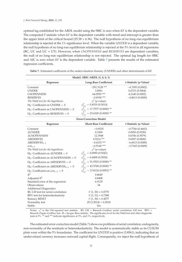
J. Risk Financial Manag. 2019, 12, 101
optimal lag established for the ARDL model using the SBIC is zero when KF is the dependent variable.The computed F-statistic when KF is the dependent variable with trend and intercept is greater thanthe upper limit of the critical bound (25.38 > 6.36). The null hypothesis of no long-run equilibriumrelationship is rejected at the 1% significance level. When the variable UNDER is a dependent variable,the null hypothesis of no long-run equilibrium relationship is rejected at the 5% level in all regressions(RC, UC and UC + UT). However, when LNOPENNESS and RESERVES are dependent variables,the null of no long-run equilibrium relationship is not rejected. The optimal lag length for SBICand AIC is zero when KF is the dependent variable. Table 7 presents the results of the estimatedregression coefficients.
Table 7. Estimated coefficients of the undervaluation dummy (UNDER) and other determinants of KF.
Model: SBIC-ARDL (1, 0, 0, 1)
Regressor Long-Run Coefficient t-Statistic (p-Value)
Constant −291.5128 *** −4.1595 (0.0002)UNDER 3.8561 0.6723 (0.5064)LNOPENNESS 64.0550 *** 4.2140 (0.0002)RESERVES −0.8190 *** −4.8613 (0.0000)The Wald test for the hypothesis: χ2 (p-value)H0: Coefficient on UNDER = 0 χ2
(1)= 0.4519 (0.5014)
H0: Coefficient on LNOPENNESS = 0 χ2(1)
= 17.7577 (0.0000) **
H0: Coefficient on RESERVES = 0 χ2(1)
= 23.6320 (0.0000) **
Error-Correction Model
Regressor Short-Run Coefficient t-Statistic (p-Value)
Constant −0.9235 −0.7760 (0.4443)ΔUNDER 0.3369 0.0950 (0.9250)ΔLNOPENNESS 12.3948 0.6706 (0.5079)ΔRESERVES 0.5214 *** 5.6507 (0.0000)ΔRESERVESt−1 −0.6333 *** −6.6013 (0.0000)ecmt−1 −0.5149 *** −3.7165 (0.0009)The Wald test for the hypothesis: χ2 (p-value)H0: Coefficient on ΔUNDER = 0 χ2
(1)= 0.0090 (0.9243)
H0: Coefficient on ΔLNOPENNESS = 0 χ2(1)
= 0.4498 (0.5024)
H0: Coefficient on ΔRESERVES = 0 χ2(1)
= 31.9303 (0.0000) **
H0: Coefficient on ΔRESERVESt−1 = 0 χ2(1)
= 43.5768 (0.0000) **
H0: Coefficient on ecmt−1 = 0 χ2(1)
= 13.8124 (0.0003) **
R2 0.8649Adjusted R2 0.8408Standard error of the regression 6.9135Observations 34Additional DiagnosticsBG LM test for serial correlation F (1, 30) = 0.0770BPG test for heteroskedasticity F (3, 31) = 0.7388Ramsey RESET F (1, 30) = 0.4577Normality test JB (3.2014) = 0.2018Stable Yes
Notes: χ2 is the Chi-squared test statistic. BG LM = Breusch–Godfrey serial correlation LM test. BPG =Breusch–Pagan–Godfrey test. JB = Jacque–Bera statistic. The significance level for the Wald test and other diagnostictests is 5%. ** and *** indicate significance at 5%, and 1%, respectively.
The estimated error-correction model (Table 7) shows no problems of serial correlation, endogeneity,non-normality of the residuals or heteroskedasticity. The model is systematically stable as its CUSUMplots were within the 5% boundaries. The coefficient for UNDER is positive (3.8561), indicating that anundervalued currency increases outward capital flight. Consequently, we reject the null hypothesis of
37
J. Risk Financial Manag. 2019, 12, 101
H2. The results are not consistent with the findings of Gouider and Nouira (2014), who argue thatundervaluation has no effect on capital flight. This disparity can be explained by the methodologyGouider and Nouira (2014) used. The duo did not use any threshold for determining undervaluation.Undervaluation was assumed as cases where the calculated value for misalignment was negative.Therefore, the study included redundant observations in the analysis that may not qualify to beundervaluation. In the present study, a 5% threshold is used to capture only significant cases ofundervaluation14. The results agree partially with those of Gouider and Nouira (2014) because theChi-square statistic p-value (p = 0.5014) for the variable UNDER indicates that undervaluation isa minor determinant of capital flight. Therefore, for a restricted model, the variable UNDER canbe deleted.
The coefficient for LNOPENNESS is positive and significant (64.0550) at the 5% significance level.This signals that when the currency is undervalued, removing trade barriers increases the volume ofoutward capital flight through exportable commodities. The coefficient for LNOPENNESS when thecurrency is undervalued is greater than when the currency is overvalued (64.0550 > 49.3755). This canbe explained by an increase in the volume of exports when the currency is undervalued (Vo et al. 2019;Thuy and Thuy 2019). An undervalued currency raises competitiveness of exports, which allows moregoods to be misinvoiced and results in high capital flight. However, when the currency is overvalued,the demand for exports is low. Consequently, there will be less trade misinvoicing and low capitalflight. The coefficient for RESERVES is negative (−0.8190), which indicates that an increase in the levelof foreign reserves when the currency is undervalued reduces outward capital flight. This finding isconsistent with economic theory that a higher level of reserves reduces capital flight (Boyce 1992).
The results of the error-correction model show that only ΔRESERVES and its lag were significantin the short-run. The coefficient for ΔLNOPENNESS is positive with a lower impact (12.3948) than thelong-run coefficient (64.0550). In the short-run, the coefficient for UNDER still bears a positive sign(0.3369), indicating that undervaluation induces capital flight. The value for the error-correction term(ecmt−1 = −0.5149) is significant at the 1% level, which signals a speed of convergence to equilibrium at51.49% annually. The significant and negative error-correction term confirms a long-run equilibriumrelationship between the variables KF, UNDER, LNOPENNESS and RESERVES. The results of theF-test indicated a long-run relationship15 when KF is a dependent variable. The Gregory–Hansencointegration test was used to account for structural breaks in the relationship between the variables.The results of the Gregory–Hansen cointegration test reject the null hypothesis of no cointegrationwhen KF is the dependent variable which confirms the long-run relation between KF and the regressors.
The results of the ARDL bounds test show that a long-run equilibrium relationship existsbetween capital flight and its determinants. The estimated coefficients of the ARDL models do notindicate causality between the variables. Therefore, the Toda and Yamamoto (1995) approach toGranger causality is applied to determine causation between KF, OVER, UNDER, LNOPENNESSand RESERVES. Table 8 presents the results of the causality test.
14 At the 3% threshold, the coefficient for UNDER is 3.3463. The coefficient is 4.0487 at the 4% threshold. The coefficientincreases to 12.4325 at the 8% threshold level. There was less variation in the coefficients of LNOPENNESS and RESERVESwhen the threshold was altered.
15 Narayan (2005) critical values were further used to determine the long-run equilibrium relationship between KF and theregressors (unrestricted constant without the time trend). The computed F-statistic for F(KF|LNOPENNESS, RESERVES) is5.1459 which is significant at the 5% level. The computed F-statistic for F(KF|OVER, LNOPENNESS, RESERVES) is 14.0664which is significant at the 1% level. The computed F-statistic for F(KF|UNDER, LNOPENNESS, RESERVES) is 5.9052 whichis significant at the 5% level.
38
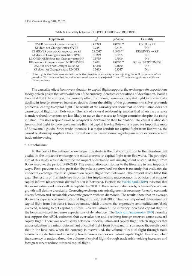
J. Risk Financial Manag. 2019, 12, 101
Table 8. Causality between KF, OVER, UNDER and RESERVES.
Hypothesis χ2 p-Value Causality
OVER does not Granger-cause KF 4.2343 0.0396 ** OVER → KFKF does not Granger-cause OVER 0.2481 0.6184 No
RESERVES does not Granger-cause KF 28.5347 0.0000 *** RESERVES → KFKF does not Granger-cause RESERVES 0.3219 0.5705 No
LNOPENNESS does not Granger-cause KF 0.5755 0.7500 NoKF does not Granger-cause LNOPENNESS 6.4861 0.0390 ** KF → LNOPENNESS
UNDER does not Granger-cause KF 1.4348 0.4880 NoKF does not Granger-cause UNDER 0.3613 0.8347 No
Notes: χ2 is the Chi-square statistic; → is the direction of causality when rejecting the null hypothesis of nocausality. ‘No’ indicates that the null of no causality cannot be rejected. ** and *** indicate significance at 5%, and1%, respectively.
The causality effect from overvaluation to capital flight supports the exchange rate expectationstheory, which posits that overvaluation of the currency increases expectations of devaluation, leadingto capital flight. In addition, the causality effect from foreign reserves to capital flight indicates that adecline in foreign reserves increases doubts about the ability of the government to solve economicproblems, leading to capital flight. The results of the causality test show that undervaluation does notcause capital flight from Botswana. The lack of a causal relationship implies that when the currencyis undervalued, investors are less likely to move their assets to foreign countries despite the risinginflation. Investors respond more to prospects of devaluation than to inflation. The causal relationshipfrom capital flight to trade openness implies that capital leaving Botswana is used for importing moreof Botswana’s goods. Since trade openness is a major conduit for capital flight from Botswana, thecausal relationship implies a habit formation effect as economic agents gain more experience withtrade misinvoicing.
5. Conclusions
To the best of the authors’ knowledge, this study is the first contribution to the literature thatevaluates the impact of exchange rate misalignment on capital flight from Botswana. The principalaim of this study was to determine the impact of exchange rate misalignment on capital flight fromBotswana over the period 1980–2015. The examination contributes to the literature in two importantways. First, previous studies posit that the pula is overvalued but there is no study that evaluates theimpact of exchange rate misalignment on capital flight from Botswana. The present study filled thisgap. The results of this study are important for implementing macroeconomic policies that supportcapital inflows for economic diversification in Botswana. Further, the World Bank (2019) indicates thatBotswana’s diamond mines will be depleted by 2030. In the absence of diamonds, Botswana’s economicgrowth will decline drastically. Correcting exchange rate misalignment is necessary for early economicdiversification and sustainable economic growth without diamonds. The results show that on average,Botswana experienced inward capital flight during 1980–2015. The most important determinant ofcapital flight from Botswana is trade openness, which indicates that exportable commodities are falselyinvoiced, leading to net capital outflows. Overvaluation of the currency increased capital flight inthe long-run since it increases expectations of devaluation. The Toda and Yamamoto (1995) causalitytest support the ARDL estimates that overvaluation and declining foreign reserves cause outwardcapital flight. There was no causality between undervaluation and capital flight, which suggests thatundervaluation is a minor determinant of capital flight from Botswana. In summary, the results positthat in the long-run, when the currency is overvalued, the volume of capital flight through trademisinvoicing declines and increasing foreign reserves does not reduce capital flight. However, whenthe currency is undervalued, the volume of capital flight through trade misinvoicing increases andforeign reserves reduce outward capital flight.
39
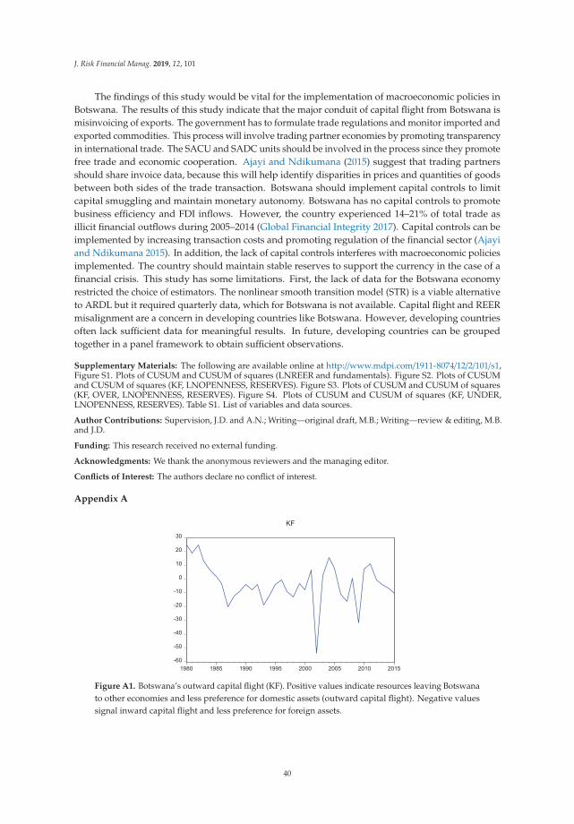
J. Risk Financial Manag. 2019, 12, 101
The findings of this study would be vital for the implementation of macroeconomic policies inBotswana. The results of this study indicate that the major conduit of capital flight from Botswana ismisinvoicing of exports. The government has to formulate trade regulations and monitor imported andexported commodities. This process will involve trading partner economies by promoting transparencyin international trade. The SACU and SADC units should be involved in the process since they promotefree trade and economic cooperation. Ajayi and Ndikumana (2015) suggest that trading partnersshould share invoice data, because this will help identify disparities in prices and quantities of goodsbetween both sides of the trade transaction. Botswana should implement capital controls to limitcapital smuggling and maintain monetary autonomy. Botswana has no capital controls to promotebusiness efficiency and FDI inflows. However, the country experienced 14–21% of total trade asillicit financial outflows during 2005–2014 (Global Financial Integrity 2017). Capital controls can beimplemented by increasing transaction costs and promoting regulation of the financial sector (Ajayiand Ndikumana 2015). In addition, the lack of capital controls interferes with macroeconomic policiesimplemented. The country should maintain stable reserves to support the currency in the case of afinancial crisis. This study has some limitations. First, the lack of data for the Botswana economyrestricted the choice of estimators. The nonlinear smooth transition model (STR) is a viable alternativeto ARDL but it required quarterly data, which for Botswana is not available. Capital flight and REERmisalignment are a concern in developing countries like Botswana. However, developing countriesoften lack sufficient data for meaningful results. In future, developing countries can be groupedtogether in a panel framework to obtain sufficient observations.
Supplementary Materials: The following are available online at http://www.mdpi.com/1911-8074/12/2/101/s1,Figure S1. Plots of CUSUM and CUSUM of squares (LNREER and fundamentals). Figure S2. Plots of CUSUMand CUSUM of squares (KF, LNOPENNESS, RESERVES). Figure S3. Plots of CUSUM and CUSUM of squares(KF, OVER, LNOPENNESS, RESERVES). Figure S4. Plots of CUSUM and CUSUM of squares (KF, UNDER,LNOPENNESS, RESERVES). Table S1. List of variables and data sources.
Author Contributions: Supervision, J.D. and A.N.; Writing—original draft, M.B.; Writing—review & editing, M.B.and J.D.
Funding: This research received no external funding.
Acknowledgments: We thank the anonymous reviewers and the managing editor.
Conflicts of Interest: The authors declare no conflict of interest.
Appendix A
Figure A1. Botswana’s outward capital flight (KF). Positive values indicate resources leaving Botswanato other economies and less preference for domestic assets (outward capital flight). Negative valuessignal inward capital flight and less preference for foreign assets.
40
J. Risk Financial Manag. 2019, 12, 101
References
Agénor, Pierre-Richard, Jagdeep S. Bhandari, and Robert P. Flood. 1992. Speculative attacks and models of balanceof payments crises. IMF Staff Papers 39: 357–94. [CrossRef]
Ajayi, S. Ibi, and Leonce Ndikumana. 2015. Capital Flight from Africa: Causes, Effects, and Policy Issues. Oxford:Oxford University Press.
Alam, Imam, and Rahim Quazi. 2003. Determinants of capital flight: An econometric case study of Bangladesh.International Review of Applied Economics 17: 85–103. [CrossRef]
Balassa, Bela. 1964. The purchasing-power parity doctrine: A reappraisal. Journal of Political Economy 72: 584–96.[CrossRef]
Banerjee, Anindya, Juan Dolado, and Ricardo Mestre. 1998. Error-correction mechanism tests for cointegration ina single-equation framework. Journal of Time Series Analysis 19: 267–83. [CrossRef]
Bank of Botswana. 2016. Bank of Botswana Annual Report. Available online: http://www.bankofbotswana.bw/assets/uploaded/AR%202016%20Final%20PDF%20-Text%20Only.pdf (accessed on 15 April 2019).
Bank of Botswana. 2017. Bank of Botswana Annual Report. Available online: http://www.bankofbotswana.bw/assets/uploaded/ANNUAL%20REPORT.pdf (accessed on 15 April 2019).
Boyce, James K. 1992. The revolving door? External debt and capital flight: A Philippine case study. WorldDevelopment 20: 335–49. [CrossRef]
Cheung, Ying-Wong, and XingWang Qian. 2010. Capital flight: China’s experience. Review of DevelopmentEconomics 14: 227–47. [CrossRef]
Chinn, Menzie D. 2000. Before the fall: Were East Asian currencies overvalued? Emerging Markets Review 1: 101–26.[CrossRef]
Chowdhury, Abdur R., and Mark Wheeler. 2015. The impact of output and exchange rate volatility on fixedprivate investment: Evidence from selected G7 countries. Applied Economics 47: 2628–41. [CrossRef]
Coudert, Virginie, Cécil Couharde, and Valerie Mignon. 2013. On currency misalignments within the Euro Area.Review of International Economics 21: 35–48. [CrossRef]
Cuddington, John T. 1986. Capital flight: Estimates, issues and explanations. Princeton Studies in InternationalFinance 58: 1–39.
Deléchat, Corrinne, and Matthew Gaertner. 2008. Exchange Rate Assessment in a Resource-RichDependent Economy: The Case of Botswana. IMF Working Paper, No. 08/83.Available online: https://www.imf.org/en/Publications/WP/Issues/2016/12/31/Exchange-Rate-Assessment-in-a-Resource-Dependent-Economy-The-Case-of-Botswana-21833 (accessed on 15 January 2019).
Dooley, Michael P. 1986. Country-Specific Risk Premiums, Capital Flight and Net Investment Income Payments in SelectedDeveloping Countries. Washington: International Monetary Fund.
Dornbusch, Rudiger. 1984. External Debt, Budget Deficits and Disequilibrium Exchange Rates (Working PaperNo. 1336). Available online: https://www.nber.org/papers/w1336.pdf (accessed on 15 April 2019).
Dubas, Justin M. 2009. The importance of the exchange rate regime in limiting misalignment. World Development37: 1612–22. [CrossRef]
Edwards, Sebastian. 1988. Real and monetary determinants of real exchange rate behaviour: Theory and evidencefrom developing countries. Journal of Development Economics 29: 311–41. [CrossRef]
Edwards, Sebastian. 1989. Exchange rate misalignment in developing countries. The World Bank Research Observer4: 3–21. [CrossRef]
Elliot, Graham, Thomas J. Rothenberg, and James H. Stock. 1996. Efficient tests for an autoregressive unit root.Econometrica 64: 813–836. [CrossRef]
El-Shagi, Makram, Alex Linder, and Gregor Von Schweinitz. 2016. Real effective exchange rate misalignment inthe Euro area: A counterfactual analysis. Review of International Economics 24: 37–66. [CrossRef]
Engle, Robert F., and Clive W. J. Granger. 1987. Cointegration and error correction: Representation, estimationand testing. Econometrica 55: 251–76. [CrossRef]
Erbe, Susanne. 1985. The flight of capital from developing countries. Intereconomics 20: 268–75. [CrossRef]Ghosh, Atish R., Jonathan David Ostry, and Mahvash S. Qureshi. 2015. Exchange rate management and crisis
susceptibility: A reassessment. IMF Economic Review 63: 238–76. [CrossRef]
41
J. Risk Financial Manag. 2019, 12, 101
Global Financial Integrity. 2015. Illicit Financial Flows to and from Developing Countries: 2004–2013. Availableonline: https://www.gfintegrity.org/wp-content/uploads/2015/12/IFF-Update_2015-Final-1.pdf (accessed on15 April 2019).
Global Financial Integrity. 2017. Illicit Financial Flows to and from Developing Countries: 2005–2014. Availableonline: https://www.gfintegrity.org/wp-content/uploads/2017/05/GFI-IFF-Report-2017_final.pdf (accessedon 15 April 2019).
Gouider, Abdessalem, and Ridha Nouira. 2014. Relationship between the misalignment of the real exchange rateand capital flight in developing countries. Theoretical and Applied Economics 11: 121–40.
Granger, Clive W. J. 1981. Some properties of time series data and their use in econometric model specification.Journal of Econometrics 16: 121–30. [CrossRef]
Hermes, Niels, Robert Lensink, and Victor Murinde. 2004. Flight capital and its reversal for developmentfinancing. In External Finance for Private Sector Development. Edited by Matthew Odedokun. London:Palgrave Macmillan, pp. 207–33.
Hillboom, Ellen. 2008. Diamonds or development? A structural assessment of Botswana’s forty years of success.The Journal of Modern African Studies 46: 191–214. [CrossRef]
Hinkle, Lawrence, and Peter J. Montiel. 1999. Exchange Rate Misalignment: Concepts and Measurement for DevelopingCountries: A World Bank Research Publication. Oxford: Oxford University Press.
Hodrick, Robert J., and Edward C. Prescott. 1997. Post-war U.S business cycles: An empirical investigation.Journal of Money, Credit and Banking 29: 1–16. [CrossRef]
Hossain, Akhand Akhtar. 2011. Exchange rate policy and real exchange rate behaviour in Bangladesh: 1972–2008.Indian Economic Review 46: 191–216.
International Monetary Fund. 2007. Botswana: Selected Issues and Statistical Appendix. IMF Country Report,No. 07/228. Available online: https://www.imf.org/external/pubs/ft/scr/2007/cr07228.pdf (accessed on 10January 2019).
Iyke, Bernard Njindan, and Nicholas M. Odhiambo. 2016. Modelling long-run equilibrium exchange rate inBotswana. Macroeconomics and Finance in Emerging Market 10: 268–85. [CrossRef]
Jeong, Se-Eun, Jacques Mazier, and Jamel Saadaoui. 2010. Exchange rate misalignments at world and Europeanlevels: A FEER approach. International Economics 121: 25–57. [CrossRef]
Johansen, S∅ren. 1988. Statistical analysis of cointegration vectors. Journal of Economic Dynamics and Control 12:231–54. [CrossRef]
Johansen, S∅ren, and Katarina Juselius. 1990. Maximum likelihood estimation and inference on cointegration withapplications to the demand for money. Oxford Bulletin of Economics and Statistics 52: 169–210. [CrossRef]
Kaminsky, Graciela, Sauk Lizondo, and Carmen M. Reinhart. 1998. Leading indicators of currency crises. IMFStaff Papers 45: 1–48. [CrossRef]
Kganetsano, Tshokologo Alex. 2007. The Transmission Mechanism of Monetary Policy in Botswana. Availableonline: https://dspace.lboro.ac.uk/dspace-jspui/bitstream/2134/7988/3/17628.pdf (accessed on 15 April 2019).
Kinkyo, Takuji. 2008. Disorderly adjustments to the misalignments in the Korean Won. Cambridge Journal ofEconomics 32: 111–24. [CrossRef]
Krugman, Paul. 1979. A model of balance of payments crises. Journal of Money, Credit and Banking 11: 311–25.[CrossRef]
Lessard, Donald, and John Williamson. 1987. Capital Flight and Third World Debt. Washington: Institute forInternational Economics.
Limi, Atsutshi. 2006. Exchange Rate Misalignment: An Application of the Behavioral EquilibriumExchange Rate (BEER) to Botswana. IMF Working Paper, No. 06/140. Available online:https://www.imf.org/en/Publications/WP/Issues/2016/12/31/Exchange-Rate-Misalignment-An-Application-of-the-Behavioral-Equilibrium-Exchange-Rate-BEER-19208 (accessed on 15 March 2019).
Lindgren, Philip, and Rasmus Wicklund. 2018. Determining Factors That Influence the Botswanian Pulaand Their Respective Significance. Available online: http://www.diva-portal.org/smash/get/diva2:1213813/FULLTEXT01.pdf (accessed on 15 April 2019).
Matlho, Kabo, Randell Madeleine, Refelwetswe Lebelonyane, Joseph Kefas, Tim Driscoll, and Joel Negin. 2019.HIV prevalence and related behaviours of older people in Botswana—Secondary analysis of the BotswanaAIDS impact survey (BAIS) IV. The African Journal of AIDS Research 18: 18–26. [CrossRef] [PubMed]
42
J. Risk Financial Manag. 2019, 12, 101
Mavrotas, George, and Roger Kelly. 2001. Old wine in new bottle: Testing causality between savings and growth.Manchester School Supplement 69: 97–105. [CrossRef]
Narayan, Paresh Kumar. 2005. The saving and investment nexus for China: Evidence from cointegration tests.Applied Economies 37: 1979–90. [CrossRef]
Ndikumana, Leonce, and James K. Boyce. 2003. Public debts and private assets: Explaining capital flight fromSub-Saharan African countries. World Development 31: 107–30. [CrossRef]
Pastor, Manuel, Jr. 1990. Capital flight from Latin America. World Development 18: 1–18. [CrossRef]Pedace, Roberto. 2013. Econometrics for Dummies. Hoboken: Wiley.Pegg, Scott. 2010. Is there a Dutch disease in Botswana? Resources Policy 35: 14–19. [CrossRef]Pesaran, M. Hashem, and Yongcheoi Shin. 1999. An autoregressive distributed lag modelling approach to
cointegration analysis. In Econometrics and Economic Theory in the 20th Century: The Ragnar Frisch CentennialSymposium. Edited by Steinar Str∅m. Cambridge: Cambridge University Press, pp. 371–413. [CrossRef]
Pesaran, M. Hashem, Yongcheoi Shin, and Richard J. Smith. 2001. Bounds testing approaches to the analysis oflevel relationships. Journal of Applied Econometrics 16: 289–326. [CrossRef]
Pfeffermann, Guy. 1985. Overvalued exchange rates and development. Finance and Development 22: 17–19.Pham, Dai van, and Sarath Delpachitra. 2015. Does real exchange rate depreciation boost capital accumulation?
An intertemporal analysis. Australian Economic Papers 53: 230–44. [CrossRef]Phillips, Peter C. B., and Bruce E. Hansen. 1990. Statistical inference in instrumental variables regression with I(1)
processes. Review of Economics Studies 57: 99–125. [CrossRef]Salim, Agus, and Kai Shi. 2019. A cointegration of the exchange rate and macroeconomic fundamentals: The
case of the Indonesian Rupiah vis-á-vis currencies of primary trade partners. Journal of Risk and FinancialManagement 12: 87. [CrossRef]
Samuelson, Paul A. 1964. Theoretical notes on trade problems. Review of Economics and Statistics 46: 145–54.[CrossRef]
Sohrabji, Niloufer. 2011. Capital inflows and real exchange rate misalignment: The Indian experience. IndianJournal of Economics and Business 10: 407–23.
Taye, Haile Kebret. 2012. Is the Botswana Pula misaligned? BIDPA Working Paper No. 33, 1–20. Availableonline: https://www.africaportal.org/documents/9274/Is_the_Botswana_Pula_Misaligned.pdf (accessed on11 January 2019).
Thuy, Vinh Nguyen Thi, and Duong Trinh Thi Thuy. 2019. The impact of exchange rate volatility on exports inVietnam: A bounds testing approach. Journal of Risk and Financial Management 12: 6. [CrossRef]
Toda, Hiro Y., and Taku Yamamoto. 1995. Statistical inference in vector autoregressions with possibly integratedprocess. Journal of Econometrics 66: 225–50. [CrossRef]
Vo, Duc Hong, Anh The Vo, and Zhaoyong Zhang. 2019. Exchange rate volatility and disaggregated manufacturingexports: Evidence from an emerging country. Journal of Risk and Financial Management 12: 12. [CrossRef]
Wolde-Rufael, Yemane. 2005. Energy demand and economic growth: The African experience. Journal of PolicyModeling 27: 891–903. [CrossRef]
World Bank. 1984. Toward Sustained Development in Sub-Saharan Africa. Washington: World Bank.World Bank. 2019. Botswana: Country Brief. Available online: http://web.worldbank.org/archive/website01321/
WEB/0__CONTE.HTM (accessed on 15 January 2019).Zhang, Rengui, Xueshen Xian, and Haowen Fang. 2019. The early warning system of stock market crises with
investor sentiment: Evidence from China. International Journal of Finance and Economics 24: 361–69. [CrossRef]
© 2019 by the authors. Licensee MDPI, Basel, Switzerland. This article is an open accessarticle distributed under the terms and conditions of the Creative Commons Attribution(CC BY) license (http://creativecommons.org/licenses/by/4.0/).
43
Journal of
Risk and FinancialManagement
Article
The Impact of Corporate Diversification and FinancialStructure on Firm Performance: Evidence from SouthAsian Countries
Rashid Mehmood 1, Ahmed Imran Hunjra 1,* and Muhammad Irfan Chani 2
1 University Institute of Management Sciences, PMAS-Arid Agriculture University Rawalpindi, Punjab 46000,Pakistan; [email protected]
2 COMSATS University Islamabad, Vehari Campus, Islamabad 45550, Pakistan; [email protected]* Correspondence: [email protected]
Received: 29 January 2019; Accepted: 21 March 2019; Published: 25 March 2019
Abstract: We examined the impact of corporate diversification and financial structure on the firms’financial performance. We collected data from 520 manufacturing firms from Pakistan, India, SriLanka, and Bangladesh. We used panel data of 14 years from 2004–2017 to analyze the results.We applied a two-step dynamic panel approach to analyze the hypotheses. We found that productdiversification and geographic diversification significantly affected the firms’ financial performance.We further found that dividend policy and capital structure had a significant impact on the firm’sfinancial performance.
Keywords: corporate diversification; financial structure; corporate governance; audit quality; firmfinancial performance
1. Introduction
Managers tend to diversify their business to get more benefits from the current market withminimum risk. Globalization provides an opportunity to expand their business across the border forprofit maximization. Thus, corporate diversification strategy becomes important for the expansion andgrowth of firms in competitive and dynamic environments. The objective of corporate diversification isto increase profitability, market share, debt capacity, growth opportunity, risk reduction, and the needto use human and financial resources efficiently (Afza et al. 2008). Changes in economic or industrialconditions force management to diversify their business (Phung and Mishra 2016). Diversification alsohelps firms to explore different markets (Gomes and Livdan 2004).
When firms go for diversification, they need extra capital. According to Lewellen (1971),diversified firms need more debt financing than non-diversified firms. The effective financial structuremaximizes the value for shareholders. There are three types of financial structure in finance theory:investing, financing, and dividend policies (Zulkafli et al. 2015). Corporate governance plays animportant role to improve the firms’ financial performance (Yermack 1996; Erickson et al. 2005). We takecorporate governance into consideration and how corporate governance affects the firms’ financialperformance. Claessens and Yurtoglu (2013) explain that a good governance system is beneficial forthe firms through better access to finance, good financial performance, and more desirable treatmentof stakeholders.
In this complex world, survival of the manufacturing industry becomes more challenging.Given the complex, globalized, and challenging environment, there is a need for survival andbetter financial performance of the manufacturing sector. Therefore, this sector has to diversifyits businesses into different products and different markets. However, the corporate diversification,financial structure (investment, financing, and dividend policies), and corporate governance are the
J. Risk Financial Manag. 2019, 12, 49; doi:10.3390/jrfm12010049 www.mdpi.com/journal/jrfm44
J. Risk Financial Manag. 2019, 12, 49
important factors to enhance the firms’ financial performance. We find that product diversification,geographic diversification, and financial structure significantly affect the firms’ financial performance.The outputs of our study suggest that financial policies are important determinants of firms’ financialperformance. In addition, our findings are beneficial for firms in emerging markets engaging indiversification operations.
There are five sections of the study. We discuss the introduction in Section 1 followed by literaturein Section 2. The methodology is explained in Section 3. Section 4 deals with the empirical analysisand we conclude our study in Section 5.
2. Review of Literature
A corporate diversification strategy deals with business expansion and profit maximization of afirm. The modern portfolio theory of Markowitz (1952) states that diversification in various investmentprojects leads to minimize risk and maximize expected return. In agency theory, the literature showsthat managers work for their personal benefits at the expense of shareholders by using diversificationstrategies (Jensen and Meckling 1976; Denis et al. 1997). Lins and Servaes (2002) explain that theutilization of internal capital is an attraction for diversification due to imperfection in the externalcapital market. The concept explains a positive relationship between corporate diversification andfirms’ value because a firm has informational advantages in raising capital and it can avoid the costsof external financing, which is greater than the cost of internal financing.
To meet challenges and survive in the markets, firms make diversification decisions. Managementof the firms decide whether to go for related or unrelated diversification. If firms opt for relateddiversification, that provides good output and reduces total risk. However, if management goes forunrelated diversification, it may have a negative impact on firm value. Corporate diversificationstrategy helps firms to expand business activities and get maximum profit (Phung and Mishra2016). According to Pandya and Rao (1998), diversified firms perform better on risk and returnbasis. According to Phung and Mishra (2016), there is a negative impact of diversification on financialperformance. This negative impact is due to a weak and inefficient corporate governance system,which motivates firms to diversify and ultimately negatively affects the firms’ financial performance.Furthermore, inefficient diversification strategy negatively affects the firms’ financial performance(Berger and Ofek 1995). The literature states that diversification is important and has the potentialto increase the firms’ financial performance. Therefore, the impact of diversification on the firms’financial performance depends on its effective management.
Hypothesis 1 (H1). Corporate diversification positively affects the firm’s financial performance.
When firms make diversification decisions, financial structure is an important factor which affectsthe firms’ financial performance. Zulkafli et al. (2015) consider financing, investment, and dividendpolicies as corporate financial structure. Proper management of financial decisions (investment,financing, working capital, and dividend policy) is essential for the firms’ financial performance (Buttet al. 2010). However, we investigate the impact of capital structure on the firms’ financial performance.Based on some assumptions, Modigliani and Miller (1958) state that capital structure does not affect thefirm’s value. Later, Modigliani and Miller (1963) suggest that with an increase in taxes and deductibleinterest expenses, a firm prefers debt financing instead of equity financing. It shows that they have adifferent opinion when they consider the effects of tax shield and capital market imperfection. Theyrevise their arguments and explain that capital structure affects the value of the firm due to the costof debt. Myers and Majluf (1984); Myers (1984) explain Pecking Order Theory when a firm opts forinternal rather than external sources of financing. Equity and debt financing bear the capital cost;therefore, it is not a cheap source of financing. A firm opts debt financing as it bears less cost ascompared to equity financing. Dividend payments also give information to shareholders about firms’financial performance. This is among the major financial decisions that top management takes (Baker
45
J. Risk Financial Manag. 2019, 12, 49
et al. 2001). The business activities and growth depend on the financial structure of a firm. Firms needto make an investment decision with great care as this demands the estimation of the value of certainprojects based on timing, size, and estimation of the cash flow of the future.
Butt et al. (2010) suggest that capital structure and dividend payments are important elements offirm growth and they find the positive impact of capital structure on the firms’ financial performance.Safieddine and Titman (1999) state a positive impact of debt financing on the firms’ financialperformance. According to Gleason et al. (2000), capital structure and firms’ financial performance havea negative relationship. Yat Hung et al. (2002); Salim and Yadav (2012) find a negative impact of capitalstructure on the firms’ financial performance because the increase in leverage enhances the chancesof bankruptcy cost which in turn decreases financial performance. Firms face financing obstacles,which slow down the firms’ growth (Beck and Demirguc-Kunt 2006). The negative impact of capitalstructure on the firms’ financial performance confirms the Pecking Order Theory of Myers and Majluf(1984) which explains that when firms go for more debt financing, they earn less profit. Literatureleads us to think that the relationship between capital structure and firms’ financial performance andshareholders’ wealth is still present. The firms should generate optimal capital structure in order tomaximize wealth for shareholders.
Hypothesis 2 (H2). Capital structure negatively affects the firm’s financial performance.
Does the dividend payment policy affect the value of a firm? There are different views in theliterature about dividend policy and the value of a firm. Literature states that when firms buy backtheir stock, it gives a signal about undervaluation of stock prices of firms. This ultimately positivelyinfluences the firms’ return because it creates wealth for stockholders along with an increase in shareprices. The bird in hand theory of Gordon (1963) and the dividend growth model of Walter (1963)explain the relevance of dividend payment and further explain that dividend payment affects thevalue of the firms. Butt et al. (2010); Ali et al. (2015) find that dividend policy positively affects thefirm’s financial performance. Hunjra (2018) proves a significant role of dividend payments towardsthe firm’s financial performance and support the relevancy school of thought. The concepts describethat dividend is less risky as compared to capital gain. Therefore, investors prefer dividend insteadof receiving capital gain. This means that dividend payments increase the value of the firm. Titmanet al. (2004); Cooper et al. (2008) state that dividend payment has a negative impact on firms’financial performance.
Hypothesis 3 (H3). Dividend policy positively affects the firm’s financial performance.
Investment decision-making is another important component of the financial structure of thefirm. The purpose of every investment is to earn the profit. Thus, investment decision-makingdirectly affects the firms’ financial performance. Miller and Modigliani (1961) present irrelevanceproposition of dividend and explain that dividend payment does not affect the value of the firms ratherinvestment decision affects the firm’s value. Chen and Ho (1997); Chung et al. (1998); Jiang et al. (2006)show a positive impact of investment plans on the firm’s financial performance. Titman et al. (2004)and Cooper et al. (2008) state investment decision has a negative impact on financial performance.The firms having an investment in fixed assets are less likely to have liquid assets. Therefore, firmshaving more liquid assets are likely to capitalize on long-term investment opportunities.
Hypothesis 4 (H4). Investment policy positively affects the firm’s financial performance.
We have incorporated a set of control variables in our study (i.e., corporate governance, firmage, and firm size and growth). Firms can generate more capital for investment and improve theirfinancial performance by applying good corporate governance practices. In a competitive environment,effective corporate governance is important for economic development (Boubaker and Nguyen 2015).
46
J. Risk Financial Manag. 2019, 12, 49
Jensen and Meckling (1976) present agency theory which explains that in a corporate governancesystem, managers work for their self-interest instead of owners’ interest which results in inefficientallocation of resources and a decrease in financial performance. Due to availing personal benefits,management makes a decision like diversification. The theory supports the fact that agency conflictsnegatively affects the firms’ financial performance. Corporate governance minimizes the agencyproblem as individual and institutional investors prefer firms which are well governed. On thecontrary, Stewardship theory explains that managers focus only on the collective wellbeing of thefirms regardless of the self-interest of the managers (Donaldson and Davis 1991). Therefore, this theorysuggests that firms can increase their financial performance if the top-level management possessesmore power and they develop trust in running business affairs.
The literature explains the impact of corporate governance on firm’s financial performance.Board of directors is a fundamental element of a firm’s corporate governance structure (Black etal. 2009). Yermack (1996) finds a negative impact of board size on the financial performance oflarge firms in USA. Mak and Kusnadi (2005) find a negative impact of board size on firms’ financialperformance. Kiel and Nicholson (2003); Dar et al. (2011) find a positive impact of board size onthe firm’s financial performance. The literature states that board size is an important element of agood corporate governance practice. Bhagat and Bolton (2008); Ehikioya (2009) reveal a negativeand significant relationship between CEO duality and firm’s financial performance. The positiverelationships between corporate governance mechanisms and financial performance show efficientmanagement of corporate governance system. The negative relationship validates Agency Theory andindicates the situations where management performs for their own best interest with the investmentof owners.
The auditor’s full independent opinion after audit leads to audit quality (DeAngelo 1981). Anaudit committee performs an important and monitoring part to ensure the quality of the firm’saccountability and financial statements (Carcello and Neal 2003). Resource dependence theory suggeststhat the large size of the audit committee can bring good resources into the firm like experience andskills. This shows the effectiveness of audit work while monitoring the operations of management thatimproves the firms’ financial performance (Pearce and Zahra 1992). External audit quality in terms ofbig audit firms is also an important element of the audit committee. DeAngelo (1981) argues that thebig four firms provide better audit quality which enhances the firms’ financial performance. Baueret al. (2009) find a positive impact of large audit committee size on the firms’ financial performance.The frequency of audit committee meetings ensures the activeness of the audit committee, whichimproves the financial performance of the firms. Vafeas (1999); Xie et al. (2003) find the frequency ofaudit committee meetings has a positive impact on firms’ financial performance. Considering the abovestudies, we take an audit committee and audit quality in our study to check their impact on the firms’financial performance as they enhance the quality of financial reporting and financial performance.
Large board size enhances the utilization of the firm’s useful resources (Boubaker and Nguyen2012). Hence, large firms have more opportunities to gain economies of scale and economies of scope.Firm size has a positive impact on the firm’s financial performance (Titman and Wessels 1988; Frankand Goyal 2003; Hunjra et al. 2014). It is argued that firms with large size faceless financial distressand generate more profit (Titman and Wessels 1988). The firms’ financial performance also dependson growth opportunities and the firms’ age. Firm age is important in a way that it explains about theexperience of the firm in its operations. Muritala (2012); Hunjra et al. (2014); Lazar (2016) find thatfirm growth and firm age have a positive impact on firms’ financial performance. The positive impactof growth indicates the opportunities for the firms to expand business and earn more profit. Pervan etal. (2017) present a theoretical discussion about the positive and negative impact of age on financialperformance. Firms with old age have more abilities, experience, good technology, skilled labor, andlearning environment, which help them to increase financial performance. On the contrary, older firmsface the situation where there is a reduction in flexibility and ability to make immediate changes andtake quick decisions. With the increase in age, firms also avoid taking the risk.
47
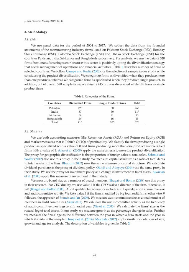
J. Risk Financial Manag. 2019, 12, 49
3. Methodology
3.1. Data
We use panel data for the period of 2004 to 2017. We collect the data from the financialstatements of the manufacturing industry firms listed on Pakistan Stock Exchange (PSX), BombayStock Exchange (BSE), Colombo Stock Exchange (CSE) and Dhaka Stock Exchange (DSE) for thecountries Pakistan, India, Sri-Lanka and Bangladesh respectively. For analysis, we use the data of 520firms from manufacturing sector because this sector is positively opting the diversification strategythat needs management of operations and financial activities. Table 1 describes number of firms ofselected countries. We follow Campa and Kedia (2002) for the selection of sample in our study whileconsidering the product diversification. We categorize firms as diversified when they produce morethan one products, whereas we categorize firms as specialized when they produce single product. Inaddition, out of overall 520 sample firms, we classify 415 firms as diversified while 105 firms as singleproduct firms.
Table 1. Categories of the Firms.
Countries Diversified Firms Single Product Firms Total
Pakistan 225 38 263India 87 30 117
Sri Lanka 74 21 95Bangladesh 29 16 45
Total 415 105 520
3.2. Statistics
We use both accounting measures like Return on Assets (ROA) and Return on Equity (ROE)and market measures that is Tobin’s Q (TQ) of profitability. We classify the firms producing a singleproduct as specialized with a value of 0 and firms producing more than one product as diversifiedfirms with a value of 1. Afza et al. (2008) apply the same criteria to measure product diversification.The proxy for geographic diversification is the proportion of foreign sales to total sales. Schmid andWalter (2012) also use this proxy in their study. We measure capital structure as a ratio of total debtsto total assets of the firm. Bhaduri (2002) uses the same measure of capital structure. We calculatedividend per share as the proxy of dividend policy. Oloidi and Adeyeye (2014) use the same proxy intheir study. We use the proxy for investment policy as a change in investment in fixed assets. Aivazianet al. (2005) apply this measure of investment in their study.
We measure board size as a number of board members. Bhagat and Bolton (2008) use this proxyin their research. For CEO duality, we use value 1 if the CEO is also a director of the firm, otherwise, itis 0 (Bhagat and Bolton 2008). Audit quality characteristics include audit quality, audit committee sizeand audit committee activity. We take value 1 if the firm is audited by big four audit firms, otherwise, 0followed the approach of Francis and Yu (2009). We measure audit committee size as a total number ofmembers in audit committee (Azim 2012). We calculate the audit committee activity as the frequencyof audit committee meetings in a financial year (Xie et al. 2003). We calculate the firms’ size as thenatural log of total assets. In our study, we measure growth as the percentage change in sales. Further,we measure the firms’ age as the difference between the year in which a firm starts and the year inwhich it exists in the sample. Hunjra et al. (2014); Muritala (2012) apply similar calculations of size,growth and age for analysis. The description of variables is given in Table 2.
48
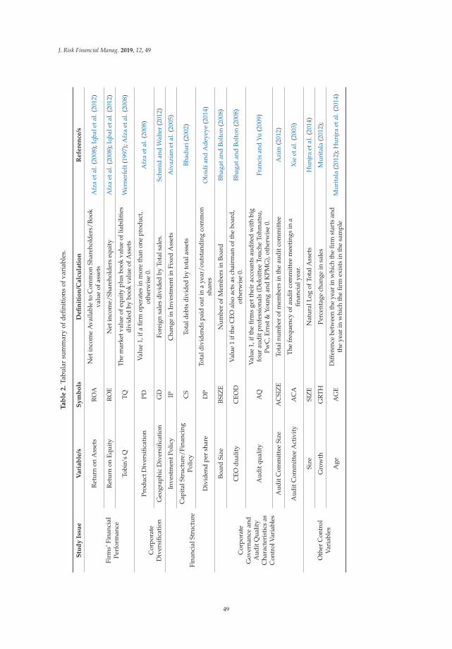
J. Risk Financial Manag. 2019, 12, 49
Ta
ble
2.
Tabu
lar
sum
mar
yof
defin
itio
nsof
vari
able
s.
Stu
dy
Issu
eV
ari
ab
le/s
Sy
mb
ols
De
fin
itio
n/C
alc
ula
tio
nR
efe
ren
ce/s
Firm
s’Fi
nanc
ial
Perf
orm
ance
Ret
urn
onA
sset
sR
OA
Net
inco
me
Ava
ilabl
eto
Com
mon
Shar
ehol
ders
/Boo
kva
lue
ofas
sets
Afz
aet
al.(
2008
);Iq
bale
tal.
(201
2)
Ret
urn
onEq
uity
RO
EN
etin
com
e/Sh
areh
olde
rseq
uity
Afz
aet
al.(
2008
);Iq
bale
tal.
(201
2)
Tobi
n’s
QTQ
The
mar
ketv
alue
ofeq
uity
plus
book
valu
eof
liabi
litie
sdi
vide
dby
book
valu
eof
Ass
ets
Wer
nerf
elt(
1997
);A
fza
etal
.(20
08)
Cor
pora
teD
iver
sific
atio
n
Prod
uctD
iver
sific
atio
nPD
Val
ue1,
ifa
firm
oper
ates
inm
ore
than
one
prod
uct,
othe
rwis
e0.
Afz
aet
al.(
2008
)
Geo
grap
hic
Div
ersi
ficat
ion
GD
Fore
ign
sale
sdi
vide
dby
Tota
lsal
es.
Schm
idan
dW
alte
r(2
012)
Fina
ncia
lStr
uctu
re
Inve
stm
entP
olic
yIP
Cha
nge
inIn
vest
men
tin
Fixe
dA
sset
sA
ivaz
ian
etal
.(20
05)
Cap
ital
Stru
ctur
e/Fi
nanc
ing
Polic
yC
STo
tald
ebts
divi
ded
byto
tala
sset
sBh
adur
i(20
02)
Div
iden
dpe
rsh
are
DP
Tota
ldiv
iden
dspa
idou
tin
aye
ar/o
utst
andi
ngco
mm
onsh
ares
Olo
idia
ndA
deye
ye(2
014)
Cor
pora
teG
over
nanc
ean
dA
udit
Qua
lity
Cha
ract
eris
tics
asC
ontr
olV
aria
bles
Boar
dSi
zeBS
IZE
Num
ber
ofM
embe
rsin
Boar
dBh
agat
and
Bolt
on(2
008)
CEO
dual
ity
CEO
DV
alue
1if
the
CEO
also
acts
asch
airm
anof
the
boar
d,ot
herw
ise
0.Bh
agat
and
Bolt
on(2
008)
Aud
itqu
alit
yA
QV
alue
1,if
the
firm
sge
tthe
irac
coun
tsau
dite
dw
ith
big
four
audi
tpro
fess
iona
ls(D
eloi
ttee
Touc
heTo
hmat
su,
PwC
,Ern
st&
Youn
gan
dK
PMG
),ot
herw
ise
0.Fr
anci
san
dYu
(200
9)
Aud
itC
omm
itte
eSi
zeA
CSI
ZE
Tota
lnum
ber
ofm
embe
rsin
the
audi
tcom
mit
tee
Azi
m(2
012)
Aud
itC
omm
itte
eA
ctiv
ity
AC
ATh
efr
eque
ncy
ofau
ditc
omm
itte
em
eeti
ngs
ina
finan
cial
year
.X
ieet
al.(
2003
)
Oth
erC
ontr
olV
aria
bles
Size
SIZ
EN
atur
alLo
gof
Tota
lAss
ets
Hun
jra
etal
.(20
14)
Gro
wth
GR
THPe
rcen
tage
chan
gein
sale
sM
urit
ala
(201
2);
Age
AG
ED
iffer
ence
betw
een
the
year
inw
hich
the
firm
star
tsan
dth
eye
arin
whi
chth
efir
mex
ists
inth
esa
mpl
eM
urit
ala
(201
2);H
unjr
aet
al.(
2014
)
49
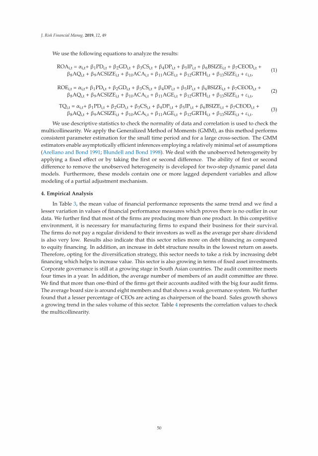
J. Risk Financial Manag. 2019, 12, 49
We use the following equations to analyze the results:
ROAi,t = αi,t+ β1PDi,t + β2GDi,t + β3CSi,t + β4DPi,t + β5IPi,t + β6BSIZEi,t + β7CEODi,t +β8AQi,t + β9ACSIZEi,t + β10ACAi,t + β11AGEi,t + β12GRTHi,t + β13SIZEi,t + εi,t,
(1)
ROEi,t = αi,t+ β1PDi,t + β2GDi,t + β3CSi,t + β4DPi,t + β5IPi,t + β6BSIZEi,t + β7CEODi,t +β8AQi,t + β9ACSIZEi,t + β10ACAi,t + β11AGEi,t + β12GRTHi,t + β13SIZEi,t + εi,t,
(2)
TQi,t = αi,t+ β1PDi,t + β2GDi,t + β3CSi,t + β4DPi,t + β5IPi,t + β6BSIZEi,t + β7CEODi,t +β8AQi,t + β9ACSIZEi,t + β10ACAi,t + β11AGEi,t + β12GRTHi,t + β13SIZEi,t + εi,t.
(3)
We use descriptive statistics to check the normality of data and correlation is used to check themulticollinearity. We apply the Generalized Method of Moments (GMM), as this method performsconsistent parameter estimation for the small time period and for a large cross-section. The GMMestimators enable asymptotically efficient inferences employing a relatively minimal set of assumptions(Arellano and Bond 1991; Blundell and Bond 1998). We deal with the unobserved heterogeneity byapplying a fixed effect or by taking the first or second difference. The ability of first or seconddifference to remove the unobserved heterogeneity is developed for two-step dynamic panel datamodels. Furthermore, these models contain one or more lagged dependent variables and allowmodeling of a partial adjustment mechanism.
4. Empirical Analysis
In Table 3, the mean value of financial performance represents the same trend and we find alesser variation in values of financial performance measures which proves there is no outlier in ourdata. We further find that most of the firms are producing more than one product. In this competitiveenvironment, it is necessary for manufacturing firms to expand their business for their survival.The firms do not pay a regular dividend to their investors as well as the average per share dividendis also very low. Results also indicate that this sector relies more on debt financing as comparedto equity financing. In addition, an increase in debt structure results in the lowest return on assets.Therefore, opting for the diversification strategy, this sector needs to take a risk by increasing debtfinancing which helps to increase value. This sector is also growing in terms of fixed asset investments.Corporate governance is still at a growing stage in South Asian countries. The audit committee meetsfour times in a year. In addition, the average number of members of an audit committee are three.We find that more than one-third of the firms get their accounts audited with the big four audit firms.The average board size is around eight members and that shows a weak governance system. We furtherfound that a lesser percentage of CEOs are acting as chairperson of the board. Sales growth showsa growing trend in the sales volume of this sector. Table 4 represents the correlation values to checkthe multicollinearity.
50
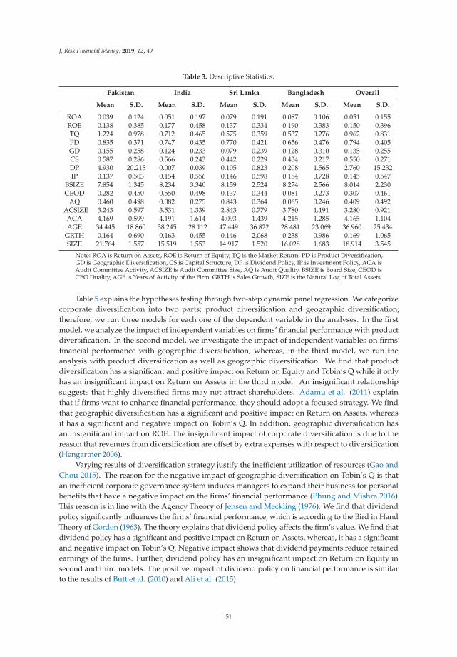
J. Risk Financial Manag. 2019, 12, 49
Table 3. Descriptive Statistics.
Pakistan India Sri Lanka Bangladesh Overall
Mean S.D. Mean S.D. Mean S.D. Mean S.D. Mean S.D.
ROA 0.039 0.124 0.051 0.197 0.079 0.191 0.087 0.106 0.051 0.155ROE 0.138 0.385 0.177 0.458 0.137 0.334 0.190 0.383 0.150 0.396TQ 1.224 0.978 0.712 0.465 0.575 0.359 0.537 0.276 0.962 0.831PD 0.835 0.371 0.747 0.435 0.770 0.421 0.656 0.476 0.794 0.405GD 0.155 0.258 0.124 0.233 0.079 0.239 0.128 0.310 0.135 0.255CS 0.587 0.286 0.566 0.243 0.442 0.229 0.434 0.217 0.550 0.271DP 4.930 20.215 0.007 0.039 0.105 0.823 0.208 1.565 2.760 15.232IP 0.137 0.503 0.154 0.556 0.146 0.598 0.184 0.728 0.145 0.547
BSIZE 7.854 1.345 8.234 3.340 8.159 2.524 8.274 2.566 8.014 2.230CEOD 0.282 0.450 0.550 0.498 0.137 0.344 0.081 0.273 0.307 0.461
AQ 0.460 0.498 0.082 0.275 0.843 0.364 0.065 0.246 0.409 0.492ACSIZE 3.243 0.597 3.531 1.339 2.843 0.779 3.780 1.191 3.280 0.921ACA 4.169 0.599 4.191 1.614 4.093 1.439 4.215 1.285 4.165 1.104AGE 34.445 18.860 38.245 28.112 47.449 36.822 28.481 23.069 36.960 25.434
GRTH 0.164 0.690 0.163 0.455 0.146 2.068 0.238 0.986 0.169 1.065SIZE 21.764 1.557 15.519 1.553 14.917 1.520 16.028 1.683 18.914 3.545
Note: ROA is Return on Assets, ROE is Return of Equity, TQ is the Market Return, PD is Product Diversification,GD is Geographic Diversification, CS is Capital Structure, DP is Dividend Policy, IP is Investment Policy, ACA isAudit Committee Activity, ACSIZE is Audit Committee Size, AQ is Audit Quality, BSIZE is Board Size, CEOD isCEO Duality, AGE is Years of Activity of the Firm, GRTH is Sales Growth, SIZE is the Natural Log of Total Assets.
Table 5 explains the hypotheses testing through two-step dynamic panel regression. We categorizecorporate diversification into two parts; product diversification and geographic diversification;therefore, we run three models for each one of the dependent variable in the analyses. In the firstmodel, we analyze the impact of independent variables on firms’ financial performance with productdiversification. In the second model, we investigate the impact of independent variables on firms’financial performance with geographic diversification, whereas, in the third model, we run theanalysis with product diversification as well as geographic diversification. We find that productdiversification has a significant and positive impact on Return on Equity and Tobin’s Q while it onlyhas an insignificant impact on Return on Assets in the third model. An insignificant relationshipsuggests that highly diversified firms may not attract shareholders. Adamu et al. (2011) explainthat if firms want to enhance financial performance, they should adopt a focused strategy. We findthat geographic diversification has a significant and positive impact on Return on Assets, whereasit has a significant and negative impact on Tobin’s Q. In addition, geographic diversification hasan insignificant impact on ROE. The insignificant impact of corporate diversification is due to thereason that revenues from diversification are offset by extra expenses with respect to diversification(Hengartner 2006).
Varying results of diversification strategy justify the inefficient utilization of resources (Gao andChou 2015). The reason for the negative impact of geographic diversification on Tobin’s Q is thatan inefficient corporate governance system induces managers to expand their business for personalbenefits that have a negative impact on the firms’ financial performance (Phung and Mishra 2016).This reason is in line with the Agency Theory of Jensen and Meckling (1976). We find that dividendpolicy significantly influences the firms’ financial performance, which is according to the Bird in HandTheory of Gordon (1963). The theory explains that dividend policy affects the firm’s value. We find thatdividend policy has a significant and positive impact on Return on Assets, whereas, it has a significantand negative impact on Tobin’s Q. Negative impact shows that dividend payments reduce retainedearnings of the firms. Further, dividend policy has an insignificant impact on Return on Equity insecond and third models. The positive impact of dividend policy on financial performance is similarto the results of Butt et al. (2010) and Ali et al. (2015).
51
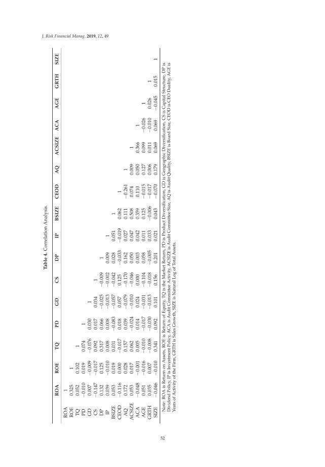
J. Risk Financial Manag. 2019, 12, 49
Ta
ble
4.
Cor
rela
tion
Ana
lysi
s.
RO
AR
OE
TQ
PD
GD
CS
DP
IPB
SIZ
EC
EO
DA
QA
CS
IZE
AC
AA
GE
GR
TH
SIZ
E
RO
A1
RO
E0.
325
1TQ
0.05
20.
102
1PD
−0.0
100.
019
0.07
41
GD
0.00
7−0
.009
−0.0
760.
030
1C
S−0
.147
−0.0
170.
092
0.01
70.
034
1D
P0.
132
0.12
50.
317
0.06
6−0
.025
−0.0
091
IP0.
039
−0.0
100.
008
0.00
8−0
.013
−0.0
020.
009
1BS
IZE
0.05
30.
019
0.03
1−0
.083
−0.0
57−0
.042
0.02
80.
051
1C
EOD
−0.1
160.
000
−0.0
170.
018
0.05
70.
125
−0.0
33−0
.019
0.06
21
AQ
0.17
20.
028
0.15
70.
039
−0.0
79−0
.170
0.16
20.
027
0.11
1−0
.261
1A
CSI
ZE
0.05
30.
017
0.06
2−0
.024
−0.0
10−0
.046
0.05
00.
047
0.50
80.
074
0.00
91
AC
A−0
.048
−0.0
010.
005
0.01
40.
024
0.00
00.
003
0.04
20.
359
0.11
00.
050
0.36
61
AG
E0.
051
−0.0
16−0
.010
−0.0
17−0
.031
−0.1
040.
058
0.01
10.
125
−0.0
150.
127
0.09
9−0
.026
1G
RTH
0.03
50.
007
−0.0
08−0
.030
−0.0
13−0
.018
−0.0
050.
033
−0.0
06−0
.017
0.00
60.
011
−0.0
100.
026
1SI
ZE
−0.0
46−0
.010
0.34
10.
092
0.10
10.
156
0.20
10.
021
0.04
3−0
.070
0.17
90.
069
0.06
9−0
.045
0.01
51
Not
e:R
OA
isR
etu
rnon
Ass
ets,
RO
Eis
Ret
urn
ofE
quit
y,T
Qis
the
Mar
ketR
etu
rn,P
Dis
Pro
du
ctD
iver
sifi
cati
on,G
Dis
Geo
grap
hic
Div
ersi
fica
tion
,CS
isC
apit
alSt
ruct
ure
,DP
isD
ivid
end
Polic
y,IP
isIn
vest
men
tPol
icy,
AC
Ais
Aud
itC
omm
itte
eA
ctiv
ity,
AC
SIZ
Eis
Aud
itC
omm
itte
eSi
ze,A
Qis
Aud
itQ
ualit
y,BS
IZE
isBo
ard
Size
,CEO
Dis
CEO
Dua
lity,
AG
Eis
Year
sof
Act
ivit
yof
the
Firm
,GR
THis
Sale
sG
row
th,S
IZE
isN
atur
alLo
gof
Tota
lAss
ets.
52
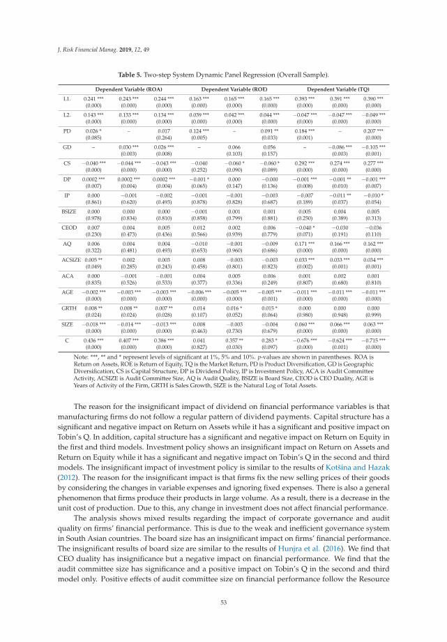
J. Risk Financial Manag. 2019, 12, 49
Table 5. Two-step System Dynamic Panel Regression (Overall Sample).
Dependent Variable (ROA) Dependent Variable (ROE) Dependent Variable (TQ)
L1. 0.241 *** 0.243 *** 0.244 *** 0.163 *** 0.165 *** 0.165 *** 0.393 *** 0.391 *** 0.390 ***(0.000) (0.000) (0.000) (0.000) (0.000) (0.000) (0.000) (0.000) (0.000)
L2. 0.143 *** 0.133 *** 0.134 *** 0.039 *** 0.042 *** 0.044 *** −0.047 *** −0.047 *** −0.049 ***(0.000) (0.000) (0.000) (0.000) (0.000) (0.000) (0.000) (0.000) (0.000)
PD 0.026 * – 0.017 0.124 *** – 0.091 ** 0.184 *** – 0.207 ***(0.085) (0.264) (0.005) (0.033) (0.001) (0.000)
GD – 0.030 *** 0.026 *** – 0.066 0.056 – −0.086 *** −0.103 ***(0.003) (0.008) (0.103) (0.157) (0.003) (0.001)
CS −0.040 *** −0.044 *** −0.043 *** −0.040 −0.060 * −0.060 * 0.292 *** 0.274 *** 0.277 ***(0.000) (0.000) (0.000) (0.252) (0.090) (0.089) (0.000) (0.000) (0.000)
DP 0.0002 *** 0.0002 *** 0.0002 *** −0.001 * 0.000 −0.000 −0.001 *** −0.001 ** −0.001 ***(0.007) (0.004) (0.004) (0.065) (0.147) (0.136) (0.008) (0.010) (0.007)
IP 0.000 −0.001 −0.002 −0.001 −0.001 −0.003 −0.007 −0.011 ** −0.010 *(0.861) (0.620) (0.493) (0.878) (0.828) (0.687) (0.189) (0.037) (0.054)
BSIZE 0.000 0.000 0.000 −0.001 0.001 0.001 0.005 0.004 0.005(0.978) (0.834) (0.810) (0.858) (0.799) (0.881) (0.250) (0.389) (0.313)
CEOD 0.007 0.004 0.005 0.012 0.002 0.006 −0.040 * −0.030 −0.036(0.230) (0.473) (0.436) (0.566) (0.939) (0.779) (0.071) (0.191) (0.110)
AQ 0.006 0.004 0.004 −0.010 −0.001 −0.009 0.171 *** 0.166 *** 0.162 ***(0.322) (0.481) (0.493) (0.653) (0.960) (0.686) (0.000) (0.000) (0.000)
ACSIZE 0.005 ** 0.002 0.003 0.008 −0.003 −0.003 0.033 *** 0.033 *** 0.034 ***(0.049) (0.285) (0.243) (0.458) (0.801) (0.823) (0.002) (0.001) (0.001)
ACA 0.000 −0.001 −0.001 0.004 0.005 0.006 0.001 0.002 0.001(0.835) (0.526) (0.533) (0.377) (0.336) (0.249) (0.807) (0.680) (0.810)
AGE −0.002 *** −0.003 *** −0.003 *** −0.006 *** −0.005 *** −0.005 *** −0.011 *** −0.011 *** −0.011 ***(0.000) (0.000) (0.000) (0.000) (0.000) (0.001) (0.000) (0.000) (0.000)
GRTH 0.008 ** 0.008 ** 0.007 ** 0.014 0.016 * 0.015 * 0.000 0.000 0.000(0.024) (0.024) (0.028) (0.107) (0.052) (0.064) (0.980) (0.948) (0.999)
SIZE −0.018 *** −0.014 *** −0.013 *** 0.008 −0.003 −0.004 0.060 *** 0.066 *** 0.063 ***(0.000) (0.000) (0.000) (0.463) (0.730) (0.679) (0.000) (0.000) (0.000)
C 0.436 *** 0.407 *** 0.386 *** 0.041 0.357 ** 0.283 * −0.676 *** −0.624 *** −0.715 ***(0.000) (0.000) (0.000) (0.827) (0.030) (0.097) (0.000) (0.001) (0.000)
Note: ***, ** and * represent levels of significant at 1%, 5% and 10%. p-values are shown in parentheses. ROA isReturn on Assets, ROE is Return of Equity, TQ is the Market Return, PD is Product Diversification, GD is GeographicDiversification, CS is Capital Structure, DP is Dividend Policy, IP is Investment Policy, ACA is Audit CommitteeActivity, ACSIZE is Audit Committee Size, AQ is Audit Quality, BSIZE is Board Size, CEOD is CEO Duality, AGE isYears of Activity of the Firm, GRTH is Sales Growth, SIZE is the Natural Log of Total Assets.
The reason for the insignificant impact of dividend on financial performance variables is thatmanufacturing firms do not follow a regular pattern of dividend payments. Capital structure has asignificant and negative impact on Return on Assets while it has a significant and positive impact onTobin’s Q. In addition, capital structure has a significant and negative impact on Return on Equity inthe first and third models. Investment policy shows an insignificant impact on Return on Assets andReturn on Equity while it has a significant and negative impact on Tobin’s Q in the second and thirdmodels. The insignificant impact of investment policy is similar to the results of Kotšina and Hazak(2012). The reason for the insignificant impact is that firms fix the new selling prices of their goodsby considering the changes in variable expenses and ignoring fixed expenses. There is also a generalphenomenon that firms produce their products in large volume. As a result, there is a decrease in theunit cost of production. Due to this, any change in investment does not affect financial performance.
The analysis shows mixed results regarding the impact of corporate governance and auditquality on firms’ financial performance. This is due to the weak and inefficient governance systemin South Asian countries. The board size has an insignificant impact on firms’ financial performance.The insignificant results of board size are similar to the results of Hunjra et al. (2016). We find thatCEO duality has insignificance but a negative impact on financial performance. We find that theaudit committee size has significance and a positive impact on Tobin’s Q in the second and thirdmodel only. Positive effects of audit committee size on financial performance follow the Resource
53
J. Risk Financial Manag. 2019, 12, 49
Dependence Theory that states a positive relationship between audit committee size and the firms’financial performance (Pearce and Zahra 1992). Audit committee activity has an insignificant impacton the firms’ financial performance. Reasons for the inconsistent and insignificant impact of auditcommittee activity and audit committee size are the very small variation in audit committee activityand audit committee size of the firms that do not affect financial performance. We find that auditquality has significance and positive impact on Tobin’s Q only. For the other two measures of financialperformance, audit quality has an insignificant impact. The reason for varying results is that each oneof the selected countries has a different quality of audit professionals.
Tables 6 and 7 deal with the analysis of an individual country. It states that product diversificationhas a significant and positive impact on all measures of financial performance for Pakistan and thatshows improvement in product development of firms in Pakistan. The positive effects also followMarkowitz (1952) portfolio theory which explains that firms can reduce risk and increase output ifthey diversify their resources. In addition, product diversification significantly but negatively affectsthe financial performance of the firms in India which shows agency issues are more prevailing in firmsas well as underutilization of assets of the firms. For Sri Lanka and Bangladesh, product diversificationshows mixed and inconsistent outputs but the general trend shows that product diversification hasa significant impact on financial performance. Geographic diversification has a significant impacton financial performance for the firms of all individual countries of our study. Generally, the impactis positive which shows improvement in product quality and more acceptability in foreign markets.Furthermore, the impact is negative when we measure financial performance as Return on Equity.The reason for the negative impact of geographic diversification on financial performance is thatmultinational firms have inefficient innovation as compared to domestic firms and this low level ofinnovation explains adverse effect of geographic diversification on financial performance (Gao andChou 2015).
There are inconsistent results with respect to dividend policy and capital structure for all selectedcountries. This is because the stock market is not efficient and the debt market is also in developingphase in these countries. There is inconsistent pattern of paying the dividend as well as generatinglong-term loans. Firms mostly rely on bank loans. Therefore, the capital structure of firms in Pakistaniand Sri Lanka shows significant impact on the firms’ financial performance, but the impact is negative.The negative impact of capital structure on the firms’ financial performance is in line with the resultsof Vatavu (2015). The capital structure of Indian firms has a significant impact on all measures offinancial performance. The results show that firms in India implement capital structure decisionsproperly. For Bangladesh, the impact of capital structure on firm’s financial performance is significantand positive that shows a development of the loan market in Bangladesh.
Investment policy shows mixed results in all selected countries. For Pakistani firms, investmentpolicy has a significant and negative impact on Return on Assets, but the impact is significant andpositive on Tobin’s Q. For Indian firms, investment policy has a significant and positive impact onReturn on Assets, while it has a significant and negative impact on Tobin’s Q. The investment decisionis a significant determinant of financial performance for Sri Lanka, but the impact is negative onReturn on Equity. For firms in Bangladesh, investment policy has a significant and positive impact onTobin’s Q. For the other two measures of financial performance, investment policy has varying outputsfor each one of the models of the analysis. The negative impact of CEO duality follows ResourceDependence Theory, which explains the lack of concentration. In general, corporate governance andaudit quality mechanisms show mixed findings. We can link these findings with Institutional Theory,which argues that firms might follow regulations or practices of corporate governance in order toincrease financial performance. The insignificant effects of corporate governance variables are similarto the results of Chen et al. (2008) and Dar et al. (2011).
54

J. Risk Financial Manag. 2019, 12, 49
Ta
ble
6.
Two-
step
Syst
emD
ynam
icPa
nelR
egre
ssio
n(P
akis
tan
and
Indi
a).
Pa
kis
tan
Ind
ia
De
pe
nd
en
tV
ari
ab
le(R
OA
)D
ep
en
de
nt
Va
ria
ble
(RO
E)
De
pe
nd
en
tV
ari
ab
le(T
Q)
De
pe
nd
en
tV
ari
ab
le(R
OA
)D
ep
en
de
nt
Va
ria
ble
(RO
E)
De
pe
nd
en
tV
ari
ab
le(T
Q)
L1.
0.22
3**
*0.
224
***
0.22
3**
*0.
098
***
0.10
3**
*0.
099
***
0.34
0**
*0.
338
***
0.33
8**
*0.
293
***
0.29
0**
*0.
291
***
0.14
5**
*0.
143
***
0.14
4**
*0.
616
***
0.61
7**
*0.
616
***
(0.0
00)
(0.0
00)
(0.0
00)
(0.0
00)
(0.0
00)
(0.0
00)
(0.0
00)
(0.0
00)
(0.0
00)
(0.0
00)
(0.0
00)
(0.0
00)
(0.0
00)
(0.0
00)
(0.0
00)
(0.0
00)
(0.0
00)
(0.0
00)
L2.
0.11
9**
*0.
118
***
0.11
9**
*0.
050
***
0.05
6**
*0.
049
***
−0.0
74**
*−0
.073
***
−0.0
76**
*0.
229
***
0.22
9**
*0.
229
***
0.05
7**
*0.
057
***
0.05
8**
*−0
.159
***
−0.1
64**
*−0
.163
***
(0.0
00)
(0.0
00)
(0.0
00)
(0.0
00)
(0.0
00)
(0.0
00)
(0.0
00)
(0.0
00)
(0.0
00)
(0.0
00)
(0.0
00)
(0.0
00)
(0.0
00)
(0.0
00)
(0.0
00)
(0.0
00)
(0.0
00)
(0.0
00)
PD0.
026
**–
0.02
2*
0.14
4**
*–
0.12
1**
*0.
318
***
–0.
384
***
−0.0
31**
*–
−0.0
32**
*−0
.086
***
–−0
.078
***
−0.0
09–
−0.0
11*
(0.0
20)
(0.0
53)
(0.0
00)
(0.0
01)
(0.0
01)
(0.0
00)
(0.0
00)
(0.0
00)
(0.0
03)
(0.0
04)
(0.1
81)
(0.0
86)
GD
–0.
027
***
0.02
4**
*–
0.16
8**
*0.
151
***
–−0
.185
***
−0.2
46**
*–
0.00
6**
*0.
008
***
–−0
.017
***
−0.0
19**
*–
−0.0
25**
*−0
.027
***
(0.0
03)
(0.0
07)
(0.0
00)
(0.0
00)
(0.0
00)
(0.0
00)
(0.0
03)
(0.0
00)
(0.0
00)
(0.0
00)
(0.0
06)
(0.0
04)
CS
−0.0
87**
*−0
.089
***
−0.0
89**
*−0
.079
***
−0.0
73**
*−0
.074
***
−0.0
71*
−0.0
96**
−0.0
86**
0.02
0**
*0.
020
***
0.02
1**
*−0
.343
***
−0.3
53**
*−0
.350
***
0.52
2**
*0.
518
***
0.52
0**
*(0
.000
)(0
.000
)(0
.000
)(0
.003
)(0
.007
)(0
.006
)(0
.069
)(0
.010
)(0
.027
)(0
.000
)(0
.000
)(0
.000
)(0
.000
)(0
.000
)(0
.000
)(0
.000
)(0
.000
)(0
.000
)
DP
0.00
04**
*0.
0004
***
0.00
04**
*0.
000
0.00
00.
000
0.00
00.
000
0.00
00.
319
***
0.32
0**
*0.
321
***
0.56
4**
*0.
541
***
0.55
0**
*0.
408
***
0.43
2**
*0.
447
***
(0.0
00)
(0.0
00)
(0.0
00)
(0.2
72)
(0.2
94)
(0.3
62)
(0.2
12)
(0.1
40)
(0.3
53)
(0.0
00)
(0.0
00)
(0.0
00)
(0.0
00)
(0.0
00)
(0.0
00)
(0.0
00)
(0.0
00)
(0.0
00)
IP−0
.005
***
−0.0
05**
*−0
.005
***
−0.0
12*
−0.0
07−0
.009
0.03
7**
*0.
030
***
0.03
4**
*0.
020
***
0.02
1**
*0.
021
***
0.00
40.
001
0.00
1−0
.041
***
−0.0
40**
*−0
.041
***
(0.0
08)
(0.0
02)
(0.0
02)
(0.0
70)
(0.3
47)
(0.1
94)
(0.0
00)
(0.0
01)
(0.0
00)
(0.0
00)
(0.0
00)
(0.0
00)
(0.1
19)
(0.6
93)
(0.5
84)
(0.0
00)
(0.0
00)
(0.0
00)
BSIZ
E−0
.002
−0.0
02−0
.002
0.00
40.
005
0.00
60.
026
*0.
024
*0.
025
*0.
003
***
0.00
3**
*0.
003
***
0.00
3**
0.00
2*
0.00
3*
0.02
5**
*0.
024
***
0.02
5**
*(0
.186
)(0
.124
)(0
.175
)(0
.542
)(0
.426
)(0
.329
)(0
.071
)(0
.089
)(0
.080
)(0
.000
)(0
.000
)(0
.000
)(0
.020
)(0
.070
)(0
.050
)(0
.000
)(0
.000
)(0
.000
)
CEO
D−0
.004
−0.0
05−0
.005
−0.0
12−0
.009
−0.0
15−0
.188
***
−0.1
83**
*−0
.177
***
−0.0
59**
*−0
.061
***
−0.0
63**
*0.
042
***
0.05
2**
*0.
048
***
−0.1
53**
*−0
.159
***
−0.1
60**
*(0
.456
)(0
.441
)(0
.412
)(0
.491
)(0
.616
)(0
.446
)(0
.000
)(0
.000
)(0
.000
)(0
.000
)(0
.000
)(0
.000
)(0
.000
)(0
.000
)(0
.000
)(0
.000
)(0
.000
)(0
.000
)
AQ
−0.0
02−0
.001
−0.0
02−0
.137
***
−0.1
30**
*−0
.131
***
0.56
6**
*0.
561
***
0.54
5**
*−0
.006
***
−0.0
09−0
.008
−0.0
27*
−0.0
25*
−0.0
230.
661
***
0.65
4**
*0.
667
***
(0.7
06)
(0.8
45)
(0.7
42)
(0.0
00)
(0.0
00)
(0.0
00)
(0.0
00)
(0.0
00)
(0.0
00)
(0.0
00)
(0.2
44)
(0.2
54)
(0.0
57)
(0.0
67)
(0.1
12)
(0.0
00)
(0.0
00)
(0.0
00)
AC
SIZ
E0.
012
***
0.01
2**
*0.
012
***
0.03
5**
0.02
9**
0.03
2**
0.20
9**
*0.
204
***
0.20
8**
*0.
014
***
0.01
3**
*0.
013
***
−0.0
15**
*−0
.015
***
−0.0
15**
*−0
.007
*−0
.006
*−0
.006
(0.0
00)
(0.0
00)
(0.0
00)
(0.0
18)
(0.0
49)
(0.0
35)
(0.0
00)
(0.0
00)
(0.0
00)
(0.0
00)
(0.0
00)
(0.0
00)
(0.0
00)
(0.0
00)
(0.0
00)
(0.0
57)
(0.0
97)
(0.1
14)
AC
A−0
.00
*−0
.005
*−0
.005
*0.
004
0.00
10.
001
−0.0
010.
004
0.00
2−0
.011
***
−0.0
11**
*−0
.011
***
0.00
9**
*0.
010
***
0.00
9**
*0.
023
***
0.02
4**
*0.
024
***
(0.0
73)
(0.0
54)
(0.0
62)
(0.4
82)
(0.8
35)
(0.8
84)
(0.9
26)
(0.7
80)
(0.8
76)
(0.0
00)
(0.0
00)
(0.0
00)
(0.0
00)
(0.0
00)
(0.0
00)
(0.0
00)
(0.0
00)
(0.0
00)
AG
E−0
.003
***
−0.0
03**
*−0
.003
***
−0.0
02*
0.00
0−0
.001
0.02
2**
*0.
020
***
0.02
2**
*−0
.001
***
−0.0
01**
*−0
.001
***
−0.0
07**
*−0
.008
***
−0.0
07**
*−0
.012
***
−0.0
12**
*−0
.012
***
(0.0
00)
(0.0
00)
(0.0
00)
(0.0
51)
(0.8
79)
(0.4
22)
(0.0
00)
(0.0
00)
(0.0
00)
(0.0
00)
(0.0
00)
(0.0
00)
(0.0
00)
(0.0
00)
(0.0
00)
(0.0
00)
(0.0
00)
(0.0
00)
GR
TH0.
019
***
0.01
9**
*0.
019
***
0.02
8**
*0.
030
***
0.02
9**
*0.
014
**0.
015
***
0.01
6**
*0.
022
***
0.02
1**
*0.
022
***
0.07
5**
*0.
072
***
0.07
3**
*−0
.043
***
−0.0
43**
*−0
.042
***
(0.0
00)
(0.0
00)
(0.0
00)
(0.0
00)
(0.0
00)
(0.0
00)
(0.0
22)
(0.0
06)
(0.0
09)
(0.0
00)
(0.0
00)
(0.0
00)
(0.0
00)
(0.0
00)
(0.0
00)
(0.0
00)
(0.0
00)
(0.0
00)
SIZ
E0.
019
***
0.01
8**
*0.
017
***
−0.0
03−0
.008
−0.0
07−0
.450
***
−0.4
30**
*−0
.444
***
−0.0
51**
*−0
.050
***
−0.0
51**
*−0
.090
***
−0.0
86**
*−0
.087
***
0.18
4**
*0.
184
***
0.18
4**
*(0
.000
)(0
.000
)(0
.000
)(0
.808
)(0
.548
)(0
.624
)(0
.000
)(0
.000
)(0
.000
)(0
.000
)(0
.000
)(0
.000
)(0
.000
)(0
.000
)(0
.000
)(0
.000
)(0
.000
)(0
.000
)
C−0
.255
***
−0.2
23**
*−0
.234
***
0.07
00.
230
0.12
08.
561
***
8.51
5**
*8.
410
***
0.87
1**
*0.
848
***
0.87
5**
*2.
025
***
1.92
2**
*1.
989
***
−2.5
69**
*−2
.592
***
−2.5
83**
*(0
.000
)(0
.000
)(0
.000
)(0
.781
)(0
.380
)(0
.656
)(0
.000
)(0
.000
)(0
.000
)(0
.000
)(0
.000
)(0
.000
)(0
.000
)(0
.000
)(0
.000
)(0
.000
)(0
.000
)(0
.000
)
Not
e:**
*,**
,and
*re
pres
ents
leve
lsof
sign
ifica
ntat
1%,5
%,a
nd10
%.p
-val
ues
are
show
nin
pare
nthe
ses.
55

J. Risk Financial Manag. 2019, 12, 49
Ta
ble
7.
Two-
step
Syst
emD
ynam
icPa
nelR
egre
ssio
n(S
riLa
nka
and
Bang
lade
sh).
Sri
La
nk
aB
an
gla
de
sh
De
pe
nd
en
tV
ari
ab
le(R
OA
)D
ep
en
de
nt
Va
ria
ble
(RO
E)
De
pe
nd
en
tV
ari
ab
le(T
Q)
De
pe
nd
en
tV
ari
ab
le(R
OA
)D
ep
en
de
nt
Va
ria
ble
(RO
E)
De
pe
nd
en
tV
ari
ab
le(T
Q)
L1.
0.43
0**
*0.
400
***
0.39
3**
*0.
084
***
0.10
6**
*0.
112
***
0.39
0**
*0.
391
***
0.40
2**
*0.
122
***
0.10
3**
*0.
094
**0.
124
***
0.07
3**
*0.
088
***
0.46
6**
*0.
507
***
0.47
9**
*(0
.000
)(0
.000
)(0
.000
)(0
.000
)(0
.000
)(0
.000
)(0
.000
)(0
.000
)(0
.000
)(0
.000
)(0
.000
)(0
.021
)(0
.000
)(0
.000
)(0
.000
)(0
.000
)(0
.000
)(0
.000
)
L2.
0.37
0**
*0.
277
***
0.27
4**
*0.
056
***
0.00
10.
011
***
−0.1
44**
*−0
.122
***
−0.1
46**
*0.
170
***
0.13
2**
*0.
163
***
−0.2
29**
*−0
.203
***
−0.1
89**
*−0
.134
***
−0.1
47**
*−0
.102
***
(0.0
00)
(0.0
00)
(0.0
00)
(0.0
00)
(0.3
17)
(0.0
00)
(0.0
00)
(0.0
00)
(0.0
00)
(0.0
00)
(0.0
00)
(0.0
00)
(0.0
00)
(0.0
00)
(0.0
00)
(0.0
00)
(0.0
00)
(0.0
04)
PD−0
.006
–−0
.073
***
0.59
9**
*–
0.22
4**
*−0
.292
***
–−0
.312
***
0.20
4**
*–
0.20
9**
*1.
505
***
–1.
471
***
0.06
3–
−0.1
57(0
.362
)(0
.000
)(0
.000
)(0
.000
)(0
.000
)(0
.000
)(0
.000
)(0
.000
)(0
.000
)(0
.000
)(0
.482
)(0
.130
)
GD
–0.
217
***
0.20
1**
*–
−0.5
75**
*−0
.508
***
–0.
018
*−0
.005
–0.
018
***
0.01
7**
*–
−0.1
87**
*−0
.152
***
–0.
035
***
0.03
1**
(0.0
00)
(0.0
00)
(0.0
00)
(0.0
00)
(0.0
61)
(0.4
98)
(0.0
03)
(0.0
07)
(0.0
00)
(0.0
00)
(0.0
06)
(0.0
11)
CS
−0.2
01**
*−0
.201
***
−0.1
96**
*−0
.493
***
−0.4
77**
*−0
.473
***
0.98
9**
*0.
972
***
0.98
9**
*0.
027
**0.
005
0.03
0**
1.02
1**
*0.
599
***
0.51
9**
*0.
492
***
0.47
9**
*0.
508
***
(0.0
00)
(0.0
00)
(0.0
00)
(0.0
00)
(0.0
00)
(0.0
00)
(0.0
00)
(0.0
00)
(0.0
00)
(0.0
19)
(0.5
44)
(0.0
25)
(0.0
00)
(0.0
00)
(0.0
00)
(0.0
00)
(0.0
00)
(0.0
00)
DP
−0.0
03**
*−0
.003
***
−0.0
03**
*0.
029
***
0.02
0**
*0.
019
***
−0.0
07**
*−0
.001
***
−0.0
07**
*−0
.001
0.00
10.
000
−0.0
18**
*−0
.023
***
−0.0
19**
*−0
.021
***
−0.0
17**
*−0
.016
***
(0.0
00)
(0.0
00)
(0.0
01)
(0.0
00)
(0.0
00)
(0.0
00)
(0.0
00)
(0.0
00)
(0.0
00)
(0.2
20)
(0.2
81)
(0.9
35)
(0.0
00)
(0.0
00)
(0.0
00)
(0.0
00)
(0.0
00)
(0.0
00)
IP0.
049
***
0.05
3**
*0.
053
***
−0.0
66**
*−0
.075
***
−0.0
75**
*−0
.004
***
0.00
4**
*−0
.006
***
−0.0
02−0
.004
*−0
.002
0.00
9−0
.027
***
−0.0
18**
0.03
0**
*0.
035
***
0.02
9**
*(0
.000
)(0
.000
)(0
.000
)(0
.000
)(0
.000
)(0
.000
)(0
.000
)(0
.000
)(0
.000
)(0
.498
)(0
.070
)(0
.234
)(0
.111
)(0
.000
)(0
.026
)(0
.000
)(0
.000
)(0
.000
)
BSIZ
E0.
001
0.00
5**
*0.
004
***
−0.0
28**
*−0
.021
***
−0.0
20**
*0.
008
***
0.01
0**
*0.
007
***
0.00
2*
0.00
40.
005
***
0.04
6**
*−0
.030
***
0.01
1**
−0.0
010.
005
−0.0
07(0
.161
)(0
.000
)(0
.000
)(0
.000
)(0
.000
)(0
.000
)(0
.000
)(0
.000
)(0
.000
)(0
.099
)(0
.008
)(0
.002
)(0
.000
)(0
.000
)(0
.031
)(0
.832
)(0
.436
)(0
.242
)
CEO
D−0
.001
0.05
0**
*0.
051
***
−0.0
64**
*−0
.068
***
−0.0
64**
*0.
101
***
0.10
3**
*0.
094
***
−0.0
34**
−0.0
14−0
.030
**−0
.192
***
−0.1
90**
*−0
.192
***
0.02
90.
175
**0.
126
(0.8
48)
(0.0
00)
(0.0
00)
(0.0
00)
(0.0
00)
(0.0
00)
(0.0
00)
(0.0
00)
(0.0
00)
(0.0
14)
(0.2
69)
(0.0
48)
(0.0
00)
(0.0
00)
(0.0
00)
(0.4
90)
(0.0
24)
(0.1
30)
AQ
0.03
6**
*−0
.173
***
−0.1
77**
*0.
483
***
0.42
9**
*0.
366
***
−0.1
93**
*−0
.270
***
−0.1
78**
*0.
047
***
0.04
0**
*0.
044
***
−0.0
24−0
.003
0.04
7−0
.033
−0.0
180.
001
(0.0
01)
(0.0
00)
(0.0
00)
(0.0
00)
(0.0
00)
(0.0
00)
(0.0
00)
(0.0
00)
(0.0
00)
(0.0
00)
(0.0
00)
(0.0
00)
(0.6
61)
(0.9
18)
(0.3
76)
(0.5
69)
(0.1
88)
(0.9
43)
AC
SIZ
E0.
013
***
0.02
9**
*0.
033
***
−0.1
34**
*−0
.130
***
−0.1
34**
*0.
004
−0.0
16**
*0.
003
0.01
9**
*0.
020
***
0.02
2**
*0.
084
***
0.03
6**
*0.
072
***
−0.0
09−0
.004
−0.0
17**
(0.0
00)
(0.0
00)
(0.0
00)
(0.0
00)
(0.0
00)
(0.0
00)
(0.4
81)
(0.0
00)
(0.6
24)
(0.0
00)
(0.0
00)
(0.0
00)
(0.0
00)
(0.0
00)
(0.0
00)
(0.3
31)
(0.5
26)
(0.0
21)
AC
A−0
.004
***
−0.0
06**
*−0
.005
***
0.01
7**
*0.
001
0.00
5**
0.00
10.
001
0.00
0−0
.006
***
−0.0
05**
*−0
.005
*−0
.012
0.06
6**
*0.
033
**−0
.022
***
−0.0
30**
*−0
.028
***
(0.0
00)
(0.0
00)
(0.0
00)
(0.0
00)
(0.6
75)
(0.0
18)
(0.2
21)
(0.3
24)
(0.8
37)
(0.0
08)
(0.0
06)
(0.0
93)
(0.4
71)
(0.0
00)
(0.0
22)
(0.0
00)
(0.0
00)
(0.0
00)
AG
E−0
.013
***
−0.0
10**
*−0
.009
***
0.00
6**
*0.
005
***
0.00
6**
*0.
011
***
0.01
2**
*0.
011
***
−0.0
03**
*−0
.000
5*
−0.0
02**
*−0
.032
***
−0.0
23**
*−0
.039
***
0.00
00.
004
***
0.00
4**
(0.0
00)
(0.0
00)
(0.0
00)
(0.0
00)
(0.0
00)
(0.0
00)
(0.0
00)
(0.0
00)
(0.0
00)
(0.0
00)
(0.0
74)
(0.0
02)
(0.0
00)
(0.0
00)
(0.0
00)
(0.9
25)
(0.0
00)
(0.0
17)
GR
TH0.
003
***
0.00
4**
*0.
004
***
0.00
2**
*0.
004
0.00
50.
004
***
0.00
3**
*0.
003
***
0.01
2**
*0.
009
***
0.02
0**
*0.
047
***
−0.0
37**
*0.
021
***
0.00
3−0
.003
−0.0
07(0
.000
)(0
.003
)(0
.006
)(0
.628
)(0
.226
)(0
.220
)(0
.000
)(0
.002
)(0
.000
)(0
.000
)(0
.000
)(0
.000
)(0
.000
)(0
.000
)(0
.004
)(0
.519
)(0
.276
)(0
.106
)
SIZ
E0.
019
***
−0.0
25**
*−0
.026
***
−0.1
40**
*−0
.161
***
−0.1
60**
*−0
.019
***
−0.0
35**
*−0
.016
***
0.00
4−0
.022
***
−0.0
080.
139
***
0.13
0**
*0.
094
***
−0.0
19**
−0.0
18**
−0.0
26**
*(0
.000
)(0
.000
)(0
.000
)(0
.000
)(0
.000
)(0
.000
)(0
.000
)(0
.000
)(0
.000
)(0
.475
)(0
.000
)(0
.189
)(0
.000
)(0
.000
)(0
.001
)(0
.044
)(0
.047
)(0
.001
)
C0.
386
***
0.96
6**
*1.
027
***
1.83
4**
*2.
726
***
2.53
6**
*0.
025
0.12
4**
*0.
030
−0.1
49*
0.32
5**
*−0
.030
−3.2
31**
*−1
.610
***
−1.7
82**
*0.
528
***
0.39
8**
0.73
4**
*(0
.000
)(0
.000
)(0
.000
)(0
.000
)(0
.000
)(0
.000
)(0
.533
)(0
.000
)(0
.553
)(0
.071
)(0
.000
)(0
.747
)(0
.000
)(0
.000
)(0
.000
)(0
.004
)(0
.037
)(0
.000
)
Not
e:**
*,**
,and
*re
pres
ents
leve
lsof
sign
ifica
ntat
1%,5
%,a
nd10
%.p
-val
ues
are
show
nin
pare
nthe
ses.
56
J. Risk Financial Manag. 2019, 12, 49
Control variables show that firm age has a significant and negative effect on firms’ financialperformance. It shows that when firms get older, they start losing concentration of managing theirassets, hence they start devastating their financial performance. Results show that in general, firmgrowth has a significant and positive impact on financial performance. Firm size has a negative andsignificant and negative relationship with Return on Assets but it has a significant and positive impacton Tobin’s Q. Further, size has an insignificant impact on Return on Equity. Negative and insignificantimpact of size shows that manufacturing firms of South Asian countries fail to utilize economies ofscale, and they do not meet market requirements of economic efficiency. In a separate analysis ofeach country, control variables show varying findings but in the majority of the analyses, it showssignificant outputs. However, the use of different measures of financial performance and three modelsfor each one of the financial performance measure in our study reconciles the varying outputs.
5. Conclusions
The manufacturing sector plays a substantial role in the economic development of a country.This sector is opting for diversification strategies for growth and survival in a competitive businessenvironment. The objective of our study is to analyze the impact of corporate diversificationand financial structure on the financial performance of the manufacturing firms of South AsianCountries. Financial structure describes financing, dividend, and investment policies. We categorizedcorporate diversification as product and geographic diversification. Therefore, we ran three modelsfor each one of the independent variable; two separate models for product diversification andgeographic diversification and one overall model for both. Although some results relating toproduct diversification and geographic diversification follow Agency Theory, where managers preferdiversification strategy for their personal benefits, which adversely affects financial performancebut still we found mixed output. The varying results are the reasons of different circumstance andeconomic condition of the respective countries. We found dividend policy is a determinant of financialperformance of the firms. Investment plans show a general trend of insignificant impact on the firms’financial performance. Corporate governance and audit quality characteristics on the firm’s financialperformance revealed varying outputs in our study.
Based on the results, we drew several policy implications including that the manufacturingsector needs to apply efficient financial structure to improve its financial performance. In general, ourresults suggest that diversification improves firms’ financial performance but still there is a need ofproper management of diversification decisions as excessive diversification can lead to a decreasein firms’ financial performance. There is a need to efficiently utilize the firms’ resources to applyproper diversification strategies. The capital structure showed significant impact on firms’ financialperformance which suggests that there is need for an efficient mix of debt and equity in order todecrease the capital cost, which can increase the profitability, and value of the firms. We suggestedfirms follow a proper dividend policy to attract investors. In addition, effective management ofcorporate diversification with good corporate governance and proper implication of financial structurecan improve the financial performance of manufacturing firms.
Author Contributions: R.M. worked on conceptualization, writing—original draft preparation, resources, datacuration and formal analysis. A.I.H. contributes in writing—review and editing, supervision whereas M.I.C.handles the methodology, software and formal Analysis.
Funding: We received no funding for this project.
Conflicts of Interest: We declare there is no conflict of interest.
References
Adamu, Nasiru, Ibrahim Khalil Zubairu, Yahya Makarfi Ibrahim, and Aliyu Makarfi Ibrahim. 2011. Evaluatingthe Impact of Product Diversification on Financial Performance of Selected Nigerian Construction Firms.Journal of Construction in Developing Countries 16: 91–114.
57
J. Risk Financial Manag. 2019, 12, 49
Afza, Talat, Choudhary Slahudin, and Mian Sajid Nazir. 2008. Diversification and Corporate Performance:An Evaluation of Pakistani Firms. South Asian Journal of Management 15: 7–18.
Aivazian, Varouj A., Ying Ge, and Jiaping Qiu. 2005. The Impact of Leverage on Firm Investment: CanadianEvidence. Journal of Corporate Finance 11: 277–91. [CrossRef]
Ali, Adnan, Farzand Ali Jan, and Maryam Atta. 2015. The Impact of Dividend Policy on Firm Performance underHigh or Low Leverage; Evidence from Pakistan. Journal of Management Information 8: 50–83. [CrossRef]
Arellano, Manuel, and Stephen Bond. 1991. Some tests of specification for panel data: Monte Carlo evidence andan application to employment equations. The Review of Economic Studies 58: 277–97. [CrossRef]
Azim, Mohammad I. 2012. Corporate Governance Mechanisms and their Impact on Company Performance:A Structural Equation Model Analysis. Australian Journal of Management 37: 481–505. [CrossRef]
Baker, H. Kent, E. Theodore Veit, and Gary E. Powell. 2001. Factors influencing Dividend Policy Decisions ofNasdaq Firms. The Financial Review 36: 19–37. [CrossRef]
Bauer, Rob, Piet Eichholtz, and Nils Kok. 2009. Corporate Governance and Performance: The Reit Effect. Real EstateEconomics 38: 1–29. [CrossRef]
Beck, Thorsten, and Asli Demirguc-Kunt. 2006. Small and Medium-Size Enterprises: Access to Finance as aGrowth Constraint. Journal of Banking and Finance 30: 2931–43. [CrossRef]
Berger, Philip G., and Eli Ofek. 1995. Diversification’s Effect on Firm Value. Journal of Financial Economics 37: 39–65.[CrossRef]
Bhaduri, Saumitra N. 2002. Determinants of Corporate Borrowing: Some Evidence from the Indian CorporateStructure Corporate Structure. Journal of Economics and Finance 26: 200–15. [CrossRef]
Bhagat, Sanjai, and Brian Bolton. 2008. Corporate Governance and Firm Performance. Journal of Corporate Finance14: 257–73. [CrossRef]
Black, Bernard, Antonio Gledson de Carvalho, and Erica Gorga. 2009. The Corporate Governance of PrivatelyControlled Brazilian Firms. Revista Brasileira de Finanças 7: 358–428.
Blundell, Richard, and Stephen Bond. 1998. Initial conditions and moment restrictions in dynamic panel datamodels. Journal of Econometrics 87: 115–43. [CrossRef]
Boubaker, Sabri, and Duc Khuong Nguyen. 2012. Board Directors and Corporate Social Responsibility. Houndmills:Palgrave Macmillan.
Boubaker, Sabri, and Duc Khuong Nguyen. 2015. Corporate Governance and Corporate Social Responsibility: EmergingMarkets Focus. Hackensack: World Scientific.
Butt, Babar Zaheer, Ahmed Imran Hunjra, and Kashif-Ur Rehman. 2010. Financial Management Practices andtheir Impact on Organizational Performance. World Applied Sciences Journal 9: 997–1002.
Campa, Jose Manuel, and Simi Kedia. 2002. Explaining the diversification discount. The Journal of Finance 57:1731–62. [CrossRef]
Carcello, Joseph V., and Terry L. Neal. 2003. Audit Committee Independence and Disclosure: Choice for FinanciallyDistressed Firms. Corporate Governance 11: 289–99. [CrossRef]
Chen, Sheng-Syan, and Kim Wai Ho. 1997. Market Response to Product-Strategy and Capital ExpenditureAnnouncements in Singapore: Investment Opportunities and Free Cash Flow. Financial Management 26: 82–88.[CrossRef]
Chen, Chia-Wei, J. Barry Lin, and Bingsheng Yi. 2008. CEO Duality and Firm Performance—An EndogenousIssue. Corporate Ownership & Control 6: 58–65.
Chung, Kee H., Peter Wright, and Charlie Charoenwong. 1998. Investment Opportunities and Market Reaction toCapital Expenditure Decisions. Journal of Banking and Finance 22: 41–60. [CrossRef]
Claessens, Stijn, and B. Burcin Yurtoglu. 2013. Corporate governance in emerging markets: A survey. EmergingMarkets Review 15: 1–33. [CrossRef]
Cooper, Michael J., Huseyin Gulen, and Michael J. Schill. 2008. Asset Growth and the Cross Section of StockReturns. Journal of Finance 63: 1609–51. [CrossRef]
Dar, Laiba, Muhammad Akram Naseem, Ghulam Shabbir Khan Niazi, and Ramiz Ur Rehman. 2011. CorporateGovernance and Firm Performance: A Case Study of Pakistan Oil and Gas Companies Listed in KarachiStock Exchange. Global Journal of Management and Business Research 11: 1–10.
DeAngelo, Linda Elizabeth. 1981. Auditor Size and Audit Quality. Journal of Accounting and Economics 3: 183–99.[CrossRef]
58
J. Risk Financial Manag. 2019, 12, 49
Denis, David J., Diane K. Denis, and Atulya Sarin. 1997. Agency Problems, Equity Ownership and CorporateDiversification. Journal of Finance 52: 135–60. [CrossRef]
Donaldson, Lex, and James H. Davis. 1991. Stewardship Theory or Agency Theory: CEO Governance andShareholder Returns. Australian Journal of Management 16: 49–64. [CrossRef]
Ehikioya, Benjamin I. 2009. Corporate Governance Structure and Firm Performance in Developing Economies:Evidence from Nigeria. Corporate Governance 9: 231–43. [CrossRef]
Erickson, John, Yun W. Park, Joe Reising, and Hyun-Han Shin. 2005. Board Composition and Firm Value underConcentrated Ownership: The Canadian Evidence. Pacific-Basin Finance Journal 13: 387–410. [CrossRef]
Francis, Jere R., and Michael D. Yu. 2009. Big 4 Office Size and Audit Quality. The Accounting Review 84: 1521–52.[CrossRef]
Frank, Murray Z., and Vidhan K. Goyal. 2003. Testing the Pecking Order Theory of Capital Structure. Journal ofFinancial Economics 67: 217–48. [CrossRef]
Gao, Wenlian, and Julia Chou. 2015. Innovation Efficiency, Global Diversification, and Firm Value. Journal ofCorporate Finance 30: 278–98. [CrossRef]
Gleason, Kimberly C., Lynette Knowles Mathur, and Ike Mathur. 2000. The Interrelationship between Culture,Capital Structure, and Performance: Evidence from European Retailers. Journal of Business Research 50: 185–91.[CrossRef]
Gomes, Joao, and Dmitry Livdan. 2004. Optimal Diversification: Reconciling Theory and Evidence. The Journal ofFinance 59: 507–35. [CrossRef]
Gordon, Myron J. 1963. Optimal Investment and Financing Policy. The Journal of Finance 18: 264–72.Hengartner, Lukas. 2006. Explaining Executive Pay: The Roles of Managerial Power and Complexity.
Ph.D. dissertation, University of St Gallen, Sankt Gallen, Switzerland.Hunjra, Ahmed Imran. 2018. Mediating role of dividend policy among its determinants and organizational
financial performance. Cogent Economics and Finance 6: 1–16. [CrossRef]Hunjra, Ahmed Imran, Muhammad Irfan Chani, Sehrish Javed, Sana Naeem, and Muhammad Shahzad Ijaz. 2014.
Impact of Micro Economic Variables on Firms Performance. International Journal of Economics and EmpiricalResearch 2: 65–73.
Hunjra, Ahmed Imran, Hadia Naeem, Ayesha Noor, and Amna Saleem. 2016. Does Corporate Governance PlayRole In Firms’ Performance? A Comparative Study of Pakistan, India and Bangladesh. International Journalof Economics and Empirical Research 4: 450–64.
Iqbal, Athar, Irfan Hameed, and Majid Qadeer. 2012. Impact of Diversification on Firms’ Performance. AmericanJournal of Scientific Research 80: 42–53.
Jensen, Michael C., and William H. Meckling. 1976. Theory of the Firm: Managerial Behavior, Agency Costs andOwnership Structure. Journal of Financial Economics 3: 305–60. [CrossRef]
Jiang, Ching-Hai, Hsiang-Lan Chen, and Yen-Sheng Huang. 2006. Capital Expenditures and Corporate Earnings:Evidence from the Taiwan Stock Exchange. Managerial Finance 32: 853–61. [CrossRef]
Kiel, Geoffrey C., and Gavin J. Nicholson. 2003. Board Composition and Corporate Performance: Howthe Australian Experience Inform Contrasting Theories of Corporate Governance. Corporate Governance11: 189–205. [CrossRef]
Kotšina, Svetlana, and Aaro Hazak. 2012. Does Investment Intensity Impact Company Profitability? ACross-Country Empirical Study. Paper presented at the 2nd International Conference on Economics, Tradeand Development, Bangkok, Thailand, April 7–8; pp. 157–161.
Lazar, Sebastian. 2016. Determinants of Firm Performance: Evidence from Romanian Listed Companies. Review ofEconomic and Business Studies 9: 53–69. [CrossRef]
Lewellen, Wilbur G. 1971. A pure Financial Rationale for the Conglomerate Merger. The Journal of Finance26: 521–37. [CrossRef]
Lins, Karl V., and Henri Servaes. 2002. Is Corporate Diversification Beneficial in Emerging Markets? FinancialManagement 31: 5–31. [CrossRef]
Mak, Yuen Teen, and Yuanto Kusnadi. 2005. Size really matters: Further evidence on the negative relationshipbetween board size and firm value. Pacific-Basin Finance Journal 13: 301–18. [CrossRef]
Markowitz, Harry. 1952. Portfolio selection. The Journal of Finance 7: 77–91.Miller, Merton H., and Franco Modigliani. 1961. Dividend policy, Growth, and the Valuation of Shares. The Journal
of Business 34: 411–33. [CrossRef]
59
J. Risk Financial Manag. 2019, 12, 49
Modigliani, Franco, and Merton H. Miller. 1958. The cost of capital, corporation finance and the theory ofinvestment. The American Economic Review 48: 261–97.
Modigliani, Franco, and Merton H. Miller. 1963. Corporate Income Taxes and the Cost of Capital: A Correction.The American Economic Review 53: 433–43.
Muritala, Taiwo Adewale. 2012. An Empirical Analysis of Capital Structure on Firms’ Performance in Nigeria.International Journal of Advances in Management and Economics 1: 116–24.
Myers, Stewart C. 1984. The Capital Structure Puzzle. Journal of Finance 39: 575–92. [CrossRef]Myers, Stewart C., and Nicholas S. Majluf. 1984. Corporate Financing and Investment Decisions when firms have
Information that Investors do not have. Journal of Financial Economics 13: 187–221. [CrossRef]Oloidi, Adebayo G., and Patrick O. Adeyeye. 2014. Determinants of Dividend per Share: Evidence from the
Nigerian Stock Exchange. International Journal of Economics and Empirical Research 2: 496–501.Pandya, Anil M., and Narendar V. Rao. 1998. Diversification and Firm Performance: An Empirical Evaluation.
Journal of Financial and Strategic Decisions 11: 67–81.Pearce, John A., and Shaker A. Zahra. 1992. Board Composition from a Strategic Contingency Perspective.
Journal of Management Studies 29: 411–38. [CrossRef]Pervan, Maja, Ivica Pervan, and Marijana Curak. 2017. The Influence of Age on Firm Performance: Evidence from
the Croatian Food Industry. Journal of Eastern Europe Research in Business and Economics 2017: 1–9. [CrossRef]Phung, Duc Nam, and Anil V. Mishra. 2016. Corporation Diversification and Firm Performance: Evidence from
Vietnamese Listed Firms. Australian Economic Papers 55: 386–408. [CrossRef]Safieddine, Assem, and Sheridan Titman. 1999. Leverage and Corporate Performance: Evidence from Unsuccessful
Takeovers. Journal of Finance 54: 547–80. [CrossRef]Salim, Mahfuzah, and Raj Yadav. 2012. Capital Structure and Firm Performance: Evidence from Malaysian Listed
Companies. Procedia-Social and Behavioral Sciences 65: 156–66. [CrossRef]Schmid, Markus M., and Ingo Walter. 2012. Geographic Diversification and Firm Value in the Financial Services
Industry. Journal of Empirical Finance 19: 109–22. [CrossRef]Titman, Sheridan, and Roberto Wessels. 1988. The determinants of capital structure choice. Journal of Finance
43: 1–19. [CrossRef]Titman, Sheridan, Kuo-Chiang John Wei, and Feixue Xie. 2004. Capital Investments and Stock Returns. Journal of
Financial and Quantitative Analysis 39: 677–700. [CrossRef]Vafeas, Nikos. 1999. Board Meeting Frequency and Firm Performance. Journal of Financial Economics 53: 113–42.
[CrossRef]Vatavu, Sorana. 2015. The Impact of Capital Structure on Financial Performance in Romanian Listed Companies.
Procedia Economics and Finance 32: 1314–1322. [CrossRef]Walter, James E. 1963. Dividend policy: Its influence on the value of the enterprise. The Journal of Finance 18: 280–91.
[CrossRef]Wernerfelt, Birger. 1997. On the Nature and Scope of the Firm: An Adjustment-Cost Theory. The Journal of Business
70: 489–514. [CrossRef]Xie, Biao, Wallace N. Davidson III, and Peter J. DaDalt. 2003. Earnings Management and Corporate Governance:
The Role of the Board and the Audit Committee. Journal of Corporate Finance 9: 295–316. [CrossRef]Yat Hung, Chiang, Chan Ping Chuen Albert, and Hui Chi Man Eddie. 2002. Capital Structure and Profitability of
the Property and Construction Sectors in Hong Kong. Journal of Property Investment and Finance 20: 434–53.[CrossRef]
Yermack, David. 1996. Higher Market Valuation of Companies with a Small Board of Directors. Journal of FinancialEconomics 40: 185–213. [CrossRef]
Zulkafli, Abdul Hadi, Ahmad Husni Hamzah, and Norhidayah Abu Bakar. 2015. Board Governance and FinancingPolicy: Evidence Form Public Listed Company in Malaysia. Advanced Science Letters 21: 961–65. [CrossRef]
© 2019 by the authors. Licensee MDPI, Basel, Switzerland. This article is an open accessarticle distributed under the terms and conditions of the Creative Commons Attribution(CC BY) license (http://creativecommons.org/licenses/by/4.0/).
60
Journal of
Risk and FinancialManagement
Article
Determinants and Impacts of Financial Literacy inCambodia and Viet Nam
Peter J. Morgan * and Long Q. Trinh
Asian Development Bank Institute, Tokyo 100-6008, Japan; [email protected]* Correspondence: [email protected]; Tel.: +81-3-3593-5514
Received: 1 December 2018; Accepted: 21 January 2019; Published: 24 January 2019
Abstract: Our paper extends the literature on the determinants and impacts of financial literacy byconducting the OECD/INFE survey in two relatively low-income Asian economies—Cambodia andViet Nam—and analyzing the determinants of financial literacy and the effects of financial literacy onsavings and financial inclusion. Generally, our study corroborates the findings of studies of othercountries, but uncovers some differences as well. The main determinants of financial literacy arefound to be educational level, income, age, and occupational status. Both financial literacy andgeneral education levels are found to be positively and significantly related to savings behavior andfinancial inclusion, and these results generally hold even when correcting for possible endogeneity offinancial literacy.
Keywords: financial literacy; financial inclusion; household saving; Cambodia; Viet Nam
1. Introduction
Financial literacy is becoming increasingly recognized as an important policy objective in manycountries (OECD/INFE 2015b). This reflects the increasing need for individuals to manage their ownretirement savings and pensions, resulting mainly from the trend of switching to defined-contributionfrom defined-benefit pension plans, as well as developments in financial technology (fintech) whichrequire greater sophistication on the part of users. However, surveys consistently show that the level offinancial literacy is relatively low even in advanced economies (OECD/INFE 2016). This points to theneed to develop strategies for financial education to improve financial literacy. At their summit in LosCabos in 2012, G20 leaders endorsed the High-Level Principles on National Strategies for FinancialEducation developed by the Organization for Economic Cooperation and Development InternationalNetwork on Financial Education (OECD/INFE), thereby acknowledging the importance of coordinatedpolicy approaches to financial education (Group of Twenty (G20) (2012)).
Survey data on financial literacy can provide information on the levels of financial literacy ofvarious groups within a country, and thereby indicate which groups have the greatest needs forfinancial education. Ideally, the survey should be carried out repeatedly to identify where policieshave led to improvement of what more needs to be done. Use of a standardized survey instrumentalso makes it possible to make cross-country comparisons of key measures of financial literacy andrelated variables.
In order to accomplish this, the OECD/INFE developed a standard survey for gatheringinformation on financial literacy and financial inclusion, the latest version of which is described inOECD/INFE (2015c). OECD/INFE (2016) and OECD/INFE (2017) provides summaries of the results ofthese surveys for over 30 countries. However, this list includes only five Asian economies—HongKong, China; India, the Republic of Korea; Malaysia; and Thailand—and most of these have relativelyhigh incomes. Our study of adult financial literacy in Cambodia and Viet Nam breaks new groundin two ways: (i) It marks the first implementation of the OECD/INFE survey in the so-called CLMV
J. Risk Financial Manag. 2019, 12, 19; doi:10.3390/jrfm12010019 www.mdpi.com/journal/jrfm61
J. Risk Financial Manag. 2019, 12, 19
countries (Cambodia, Lao PDR, Myanmar, and Viet Nam); and (ii) Cambodia and Viet Nam haveconsiderably lower levels of per capita income than do most of the other countries previously surveyed.In 2015, nominal per capita GDP in Cambodia was $1144, while in Viet Nam it was $2088, compared to$3754 for Georgia and $3954 for Albania, the lowest among countries previously sampled (IMF WorldEconomic Outlook database).
In the survey form, financial literacy is divided into three related aspects: financial knowledge,financial behavior, and attitudes toward longer-term financial planning. This is consistent withOECD/INFE (2016, p. 47), which defines financial literacy as “ . . . [a] combination of awareness,knowledge, skill, attitude, and behavior necessary to make sound financial decisions and ultimatelyachieve individual financial well-being.” In other words, the OECD/INFE concept of financial literacyis multidimensional, reflecting not only knowledge, but also skills, attitudes, and actual behavior.
Financial knowledge is information and concepts which help individuals to compare financialproducts and services and make appropriate, well-informed financial decisions. A basic knowledge offinancial concepts, and the ability to apply numerical skills to financial issues enable consumers tomanage their financial affairs and respond appropriately to news and events that may have implicationsfor their financial situation. Financial knowledge can be measured either objectively (through surveyquestions) or subjectively; i.e., by asking respondents to rate their own knowledge compared withthat of their peers.
Financial behavior (or financial “savvy”) refers to financial decisions and actions. Some types ofbehavior, such as delaying bill payments, not planning for future expenditures, or choosing financialproducts without researching the market, may adversely effect on an individual’s financial situationand well-being. Financial behavior may thus differ from financial knowledge, and it is important tohow financial knowledge can affect financial behavior.
Financial attitudes regarding longer-term financial planning include aspects such as individuals’time preference and willingness to make planned savings. For example, one survey question asksabout preferences for the short term through “living for today” and spending money. Such preferencesare likely to promote behaviors that could lead to reduced financial resilience and well-being.
This paper is organized as follows. Section 2 briefly discusses the literature on determinants offinancial literacy and its effects. The data collection and empirical approach is presented in Section 3.Sections 4 and 5 present the descriptive analyses and empirical results, followed by conclusions andpolicy implications in Section 6.
2. Literature Survey
The literature on financial literacy focuses on two main areas: (i) the determinants of financialliteracy, including age, gender, level of education, and occupation; and (ii) the effects of financialliteracy on financial behavior, including saving, use of credit, and preparation for retirement.
One of the earliest to develop quantifiable measures of financial literacy was that of the Jump$tartCoalition for Personal Financial Literacy program for high school and college students in the US in1997 described in Mandell (2009). Lusardi and Mitchell (2006) added a set of financial literacy questionsto the 2004 Health and Retirement Study (HRS), a survey of US households aged 50 and older, whichhave served as a model for later surveys. The three core questions in the original survey were aimedat identifying respondents’ understanding of some key financial concepts: compound interest, realrates of return, and risk diversification. Later surveys, including the OECD/INFE survey, extended thefinancial knowledge questions but also added questions about financial attitudes, financial behavior,and financial experience. The methodology for calculating scores from the OECD/INFE surveyresponses is described below in Section 3.2.
Lusardi and Mitchell (2014) provide an extensive review of the literature on factors related tofinancial literacy. Financial literacy scores tend to follow a hump-shaped pattern with respect to age,first rising and then declining in old age. However, elderly persons’ confidence in their financialliteracy shows no similar decline, suggesting a perceptual gap. Women generally score lower than
62
J. Risk Financial Manag. 2019, 12, 19
men in financial literacy, although this seems to vary a lot by country and culture. On the other hand,women tend to be more willing to admit not knowing an answer than men are. Higher levels ofeducation and parents’ education are positively correlated with financial literacy. These findings weregenerally confirmed in the analysis of the results of the OECD/INFE survey in the above-mentionedsample of 30 countries in OECD/INFE (2016).
A key question for policy is whether financial education programs can improve financial literacy.A large number of studies have been conducted, but the results are inconclusive. The results depend onmany specific aspects of the programs, including course content, knowledge of the teachers, etc.Fernandes et al. (2014) perform a meta-analysis of 188 studies and find that financial education has asignificant but very small effect of only 0.1% on related economic behaviors. Lusardi and Mitchell (2014)cite Walstad et al. (2010) as an example of a careful study that found significant impacts from a financialliteracy study program. In their survey, Hastings et al. (2013, p. 359) argue that the evidence on theeffectiveness of financial education programs on financial literacy is “ . . . at best contradictory.”
Many papers attempt to link measures of financial literacy with other economic and financialbehaviors, going back to Bernheim (1995, 1998) in the US. Hilgert et al. (2003) found astrong correlation between financial literacy and daily financial management skills, while otherstudies found that the more numerate and financially literate are more likely to participatein financial markets, invest in stocks, and make precautionary savings (Christelis et al. 2010;van Rooij et al. 2011; de Bassa Scheresberg 2013). The more financially savvy are also more likely toundertake retirement planning, and those who make financial plans also tend to accumulate morewealth (Lusardi and Mitchell 2011). Mahdzan and Tabiani (2013) find similar evidence in Malaysia.
In terms of household borrowing, Moore (2003) found that those with lower financial literacy aremore likely to have more expensive mortgages. Campbell (2006) showed that those with lower incomeand less education were less likely to refinance their mortgages during periods of falling interest rates.Stango and Zinman (2009) found that those who could not correctly calculate interest rates generallyborrowed more and accumulated less wealth.
3. Data and Methodology
3.1. Data Collection
We used the harmonized OECD/INFE questionnaire of adult financial literacy(OECD/INFE 2015c) to ensure comparability with studies of other countries. The questionnaireincludes questions about individual information (such as gender, age, income, occupation, and othersociodemographic information) and questions about financial literacy and financial inclusion. ADBItranslated the OECD/INFE questionnaire into Khmer and Vietnamese and conducted cross-checkswith Cambodian and Vietnamese teams from Indochina Research Ltd. to ensure the correctness ofthe translation.
The surveys were conducted by Indochina Research Ltd. under the direction of the AsianDevelopment Bank Institute. Data collection was conducted in October and November 2016. Multilevelstratification was used. Cambodia was divided into five geographical regions (including Phnom Penh,Coastal, Plain, Mountain, Plateau and Mountain, and Tonle Sap) and Viet Nam into six geographicalregions (including Northern Highland and Midland, Red River Delta, Northern and Coastal Central,Central Highland, South East, and Mekong River Delta). For Cambodia, we selected Phnom Penhplus two randomly chosen provinces from each of the other four regions. For Viet Nam, we selectedHa Noi (the capital city) and Ho Chi Minh City (the economic hub), plus two provinces each inthe Red River Delta and South East areas, and three provinces in other regions. In each province,the provincial city was selected to represent the urban population while we randomly selected onerural district (in Cambodia) or one or two rural districts (in Viet Nam) for the rural sample. In eachdistrict, we randomly selected the communes and individual households based on simple samplingprocedures. In Cambodia, there were 1035 respondents from nine cities/provinces, and in Viet Nam,there were 1000 respondents from 18 cities/provinces. Details of the sample distribution are given inAppendix A.
63
J. Risk Financial Manag. 2019, 12, 19
3.2. Construction of Financial Literacy Scores
In this paper, we follow the methodology in OECD/INFE (2015a) to calculate scores for thevarious indicators of financial literacy and financial inclusion. The score for financial knowledge iscalculated from responses to seven questions reflecting the subject’s understanding of basic knowledge(or awareness) of finance such as calculation of interest rates and compound interest rates, risk andreturn evaluation, the effect of inflation, and the benefits of financial diversification. This indicatorranges between 0 and 7 based on the number of correct answers. The financial behavior scoreis calculated from nine questions relating to household budgeting, saving, considered purchases,bill payments, care about financial affairs, long-term financial goals, and borrowing, and rangesbetween 0 and 9. The score for financial attitude measures the respondent’s responses to five questionsabout about money, saving, and spending, and ranges from 1 to 5. A higher score represents moreconservative and considered behavior. The overall score for financial literacy is the sum of three scores,and hence takes values between 1 and 21. The score for financial inclusion is calculated from sevenindicators, including holdings of payment products, savings, insurance, credit products, productchoice, and family financial support in case of emergency, and ranges from 0 to 7.
For ease of interpretation, we converted all indicator scores into z-score values:
scorez =(score − score)
scoresd
where scorez is the converted z-score, score is the mean score, and scoresd is the standard deviation ofthe score.
3.3. Methodology
In this paper, we estimate the following equations for indices related to financial literacy:
FLi = α0 + α1 Incomei + Xiα2 + εi (1)
where FLi alternatively indicates the financial literacy, financial knowledge, financial behavior, andfinancial attitude score of individual i; Incomei is the natural logarithm of individual i’s householdincome; Xi is a vector of control variables; and εi is the identically and independently distributed(i.i.d.) error term. The control variables include individual age, education level, gender, occupation,rural versus urban residence, and province. With regards to age, we divide the sample into threeage groups: those under 30 years old, those over 30 years old but under 60 years old, and those over60 years old. We use the group of over-60-years-old individuals as the base group. For educationallevel, we combine the categories into three groups: (i) those with some primary education or whohave completed primary school (called the “some primary education” group)1; (ii) those with somesecondary education or who have completed secondary school (called the “some secondary education”group); and (iii) those with at least some technical education or university-level education (called the“tertiary education” group). The last group is used as the base group. With regards to occupations,we combine those who are apprentices, unemployed workers (including voluntarily unemployedpeople), retired and disabled people, and students into one group of nonworking people and use thisas the base group in this study. The remaining groups are self-employed people, salaried employees,and housewives.2
1 None of the respondents has no primary education in either country.2 Housewives may also be viewed as nonworking people, but we still keep them as a separate group because they may play
an important role in managing household finance.
64
J. Risk Financial Manag. 2019, 12, 19
3.3.1. Effects of Financial Literacy on Saving Behavior
To quantify the effect of financial literacy on saving behavior, the following equation is estimated:
Savei = β0 + β1FLi + β2 Incomei + Xiβ3 + ηi (2)
where Savei is a dummy variable, taking the value of one if the individual has any types of savingproducts and zero otherwise.3 FLi is the financial literacy score, and β1 measures the effects of financialliteracy on saving behavior. Other variables are defined the same as in Equation (1) and ηi is the i.i.d.error term.
3.3.2. Effect of Financial Literacy on Financial Inclusion
To quantify the effect of financial literacy on financial inclusion, the following equationis estimated:
FIi = γ0 + γ1FLi + γ2 Incomei + Xiγ3 + ωi (3)
where FIi is the financial inclusion score, FLi is the financial literacy score, and γ1 measures theeffects of financial literacy on saving behavior. Other variables are defined the same as in Equation (1)and ωi is the i.i.d. error term.
4. Descriptive Statistics4
Table 1 presents the average values of the scores of financial literacy and financial inclusion inCambodia and Viet Nam, including breakdowns by various categories. In both countries, the level offinancial literacy is rather low, with that of Cambodia being the lower of the two. The financial literacyscores are only 11.8 and 12.5 in Cambodia and Viet Nam, respectively, out of a total possible score of21. These scores are much lower than the 30-country average score of 13.3 and those of some otherdeveloping Asian economies such as Thailand (12.8) and Malaysia (12.3) (OECD/INFE 2016).
Of greater concern, perhaps, is the fact that the share of respondents who answered correctlyfive out of seven financial knowledge questions, which is considered to be the minimum target level,was very low. Based on our samples, only 17.0% of people in Cambodia and 36% of people in VietNam answered correctly five or more questions. On average, this figure is 62% for the OECD countriessurveyed, and 56% for the full sample of 30 countries surveyed (OECD/INFE 2016). Again, however,this gap can be attributed to the low level of income in these two countries.
These average financial literacy scores are quite consistent with individuals’ self-assessment ofoverall knowledge about financial matters compared with other adults in each country (Figure 1).Only about 12–14% of Cambodian and Vietnamese respondents considered themselves to have a betterunderstanding of overall knowledge about financial matters than other adults. This is consistent withthe results for other countries with relatively low financial literacy scores. About 63% in Cambodiaand 59% in Viet Nam self-assessed that they have the same level as other adults.
3 The score for savings behavior in this section is identified through questions on whether the respondents hold any types ofsaving accounts or participate in saving clubs or not (the so-called “formal way to save”). Savings, however, could takemany other forms, such as holding cash at home, or in a wallet, building up a balance in a bank account, giving money toa family member to save, buying gold, property, or livestock, etc. We also present the estimation results using a broaderdefinition of savings (i.e., it takes the value of one if an individual either saves in formal ways or informal ways, and zerootherwise) in Appendix D.
4 In this section and the empirical results section, we use a weighted sample. In Viet Nam, weights are calculated based onthe rural-urban population distribution and economic conditions (measured by income per capita) to correct for theunderrepresentation of the top 40% income groups and slight underrepresentation of the urban population in our sample(especially in the South East region). In Cambodia, weights are calculated based on economic conditions (measured byincome per capita). Please refer to Appendix B for details.
65
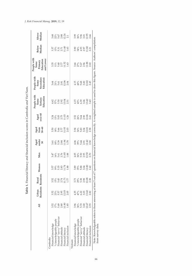
J. Risk Financial Manag. 2019, 12, 19
Ta
ble
1.
Fina
ncia
llit
erac
yan
dfin
anci
alin
clus
ion
scor
esin
Cam
bodi
aan
dV
ietN
am.
All
Urb
an
Re
sid
en
tsR
ura
lR
esi
de
nts
Wo
me
nM
en
Ag
ed
un
de
r3
0
Ag
ed
fro
m3
0–
60
Ag
ed
ov
er
60
Pe
op
lew
ith
So
me
Te
rtia
ryE
du
cati
on
Pe
op
lew
ith
So
me
Se
con
da
ryE
du
cati
on
Pe
op
lew
ith
So
me
Pri
ma
ryE
du
cati
on
an
dL
ow
er
Be
low
Me
dia
nA
bo
ve
Me
dia
n
Cam
bodi
aFi
nanc
ialk
now
ledg
e3.
523.
523.
523.
573.
473.
613.
503.
244.
623.
643.
353.
373.
68%
know
ledg
eabl
epe
ople
17%
23%
15%
19%
16%
18%
18%
13%
57%
21%
11%
13%
22%
Fina
ncia
l“sa
vvy”
beha
vior
5.49
5.57
5.45
5.35
5.61
5.39
5.66
5.05
5.50
5.61
5.40
5.31
5.67
Fina
ncia
latt
itud
e2.
802.
952.
742.
832.
762.
842.
772.
752.
922.
812.
772.
712.
88Fi
nanc
iall
iter
acy
11.8
012
.03
11.7
111
.74
11.8
511
.84
11.9
311
.03
13.0
412
.06
11.5
211
.40
12.2
4Fi
nanc
iali
nclu
sion
1.85
2.05
1.77
1.88
1.88
1.78
2.03
1.26
2.51
2.04
1.63
1.63
2.1
Vie
tnam
Fina
ncia
lkno
wle
dge
3.96
4.35
3.73
3.89
4.05
4.06
3.94
3.52
4.15
4.15
3.66
3.90
3.99
%kn
owle
dgea
ble
peop
le36
%47
%29
%35
%36
%39
%34
%26
%43
%40
%27
%34
%36
%Fi
nanc
ial“
savv
y”be
havi
or5.
706.
225.
385.
885.
505.
445.
835.
646.
395.
685.
274.
935.
96Fi
nanc
iala
ttit
ude
3.00
3.03
2.98
3.04
2.95
2.91
3.04
2.90
3.06
3.00
2.96
2.97
3.01
Fina
ncia
llit
erac
y12
.67
13.6
012
.08
12.8
012
.50
12.4
212
.81
12.0
613
.60
12.8
211
.88
11.8
012
.95
Fina
ncia
linc
lusi
on2.
552.
822.
382.
422.
702.
502.
582.
413.
432.
452.
022.
212.
66
Not
e:K
now
ledg
eabl
ere
fers
toth
ose
answ
erin
gat
leas
t5ou
tof7
ques
tions
onfin
anci
alkn
owle
dge
corr
ectly
.Aw
eigh
ted
sam
ple
isus
edto
draw
this
figur
e.So
urce
:Aut
hors
’com
pila
tion
from
surv
eyda
ta.
66
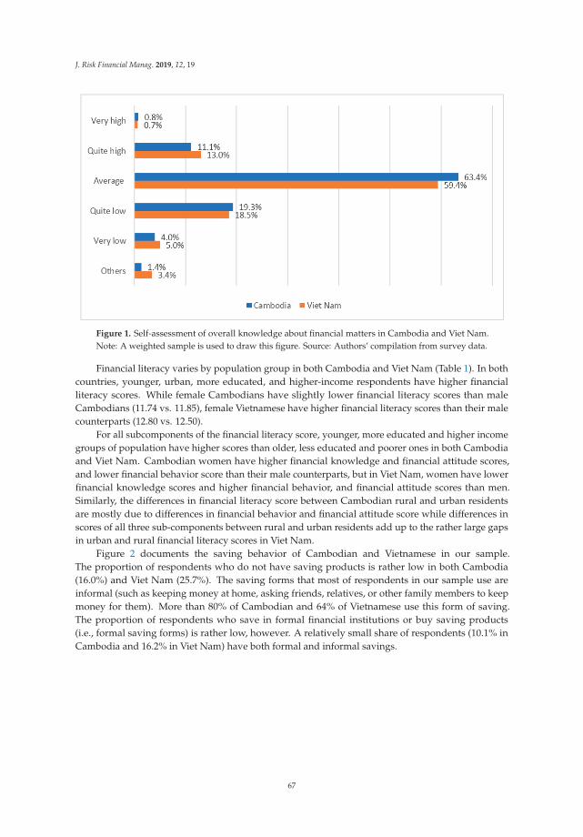
J. Risk Financial Manag. 2019, 12, 19
Figure 1. Self-assessment of overall knowledge about financial matters in Cambodia and Viet Nam.Note: A weighted sample is used to draw this figure. Source: Authors’ compilation from survey data.
Financial literacy varies by population group in both Cambodia and Viet Nam (Table 1). In bothcountries, younger, urban, more educated, and higher-income respondents have higher financialliteracy scores. While female Cambodians have slightly lower financial literacy scores than maleCambodians (11.74 vs. 11.85), female Vietnamese have higher financial literacy scores than their malecounterparts (12.80 vs. 12.50).
For all subcomponents of the financial literacy score, younger, more educated and higher incomegroups of population have higher scores than older, less educated and poorer ones in both Cambodiaand Viet Nam. Cambodian women have higher financial knowledge and financial attitude scores,and lower financial behavior score than their male counterparts, but in Viet Nam, women have lowerfinancial knowledge scores and higher financial behavior, and financial attitude scores than men.Similarly, the differences in financial literacy score between Cambodian rural and urban residentsare mostly due to differences in financial behavior and financial attitude score while differences inscores of all three sub-components between rural and urban residents add up to the rather large gapsin urban and rural financial literacy scores in Viet Nam.
Figure 2 documents the saving behavior of Cambodian and Vietnamese in our sample.The proportion of respondents who do not have saving products is rather low in both Cambodia(16.0%) and Viet Nam (25.7%). The saving forms that most of respondents in our sample use areinformal (such as keeping money at home, asking friends, relatives, or other family members to keepmoney for them). More than 80% of Cambodian and 64% of Vietnamese use this form of saving.The proportion of respondents who save in formal financial institutions or buy saving products(i.e., formal saving forms) is rather low, however. A relatively small share of respondents (10.1% inCambodia and 16.2% in Viet Nam) have both formal and informal savings.
67
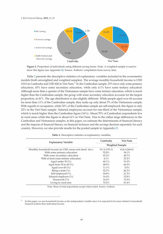
J. Risk Financial Manag. 2019, 12, 19
Figure 2. Proportion of individuals using different saving forms. Note: A weighted sample is used todraw this figure (see Appendix B). Source: Authors’ compilation from survey data.
Table 2 presents the descriptive statistics of explanatory variables included in the econometricmodels (both unweighted and weighted samples). The average monthly household income is USD310.0 in Cambodia and USD 420 in Viet Nam.5 In the Cambodian sample, 53% have only some primaryeducation, 43% have some secondary education, while only 4.1% have some tertiary education.Although more than a quarter of the Vietnamese sample have some tertiary education, which is muchhigher than the Cambodian sample, the group with some secondary education accounts for the largestproportion, at 41%. The age distribution is also slightly different. While people aged over 60 accountfor more than 11% of the Cambodian sample, they make up only about 3% of the Vietnamese sample.With regards to occupation, while 52% of the Cambodian sample are self-employed, this figure is only22% in the Viet Nam sample. Salaried employees account for one-third of the Vietnamese sample,which is much higher than the Cambodian figure (16%). About 70% of Cambodian respondents livein rural areas while this figure is about 61% in Viet Nam. Due to the rather large differences in theCambodian and Vietnamese samples, in this paper, we estimate the determinants of financial literacyand the impacts of financial literacy on financial inclusion and the savings decision separately for eachcountry. However, we also provide results for the pooled sample in Appendix D.
Table 2. Descriptive statistics of explanatory variables.
Explanatory VariableCambodia Viet Nam
Weighted Sample
Monthly household income (in USD, mean and stand. dev.) 311.0 (193.1) 414.4 (264.0)With some primary education 52.8% 34.1%
With some secondary education 43.2% 40.7%With at least some tertiary education 4.1% 25.2%
Aged under 30 (%) 40.1% 31.0%Aged from 30 to 60 (%) 48.9% 66.0%
Aged over 60 (%) 11.1% 3.0%Being a male (%) 52.3% 46.3%
Self-employed (%) 54.8% 21.5%Salaried employee (%) 16.4% 32.8%
Housewife (%) 16.0% 15.0%Living in rural area 72.0% 61.4%
Note: Share of total respondents except where noted. Source: Authors.
5 In this paper, we use household income as the independent variable since it is expected to be more related to householdfinancial matters than individual income.
68
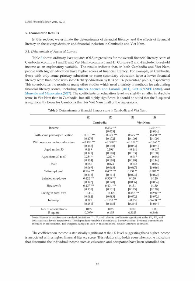
J. Risk Financial Manag. 2019, 12, 19
5. Econometric Results
In this section, we estimate the determinants of financial literacy, and the effects of financialliteracy on the savings decision and financial inclusion in Cambodia and Viet Nam.
5.1. Determinants of Financial Literacy
Table 3 shows ordinary least squares (OLS) regressions for the overall financial literacy score ofCambodia (columns 1 and 2) and Viet Nam (columns 3 and 4). Columns 2 and 4 include householdincome as an explanatory variable. The results indicate that, in both Cambodia and Viet Nam,people with higher education have higher scores of financial literacy. For example, in Cambodia,those with only some primary education or some secondary education have a lower financialliteracy score than those with some tertiary education by 0.63 or 0.37 percentage points, respectively.This corroborates the results of many other studies which used a variety of methods for calculatingfinancial literacy scores, including Bucher-Koenen and Lusardi (2011), OECD/INFE (2016), andMurendo and Mutsonziwa (2017). The coefficients on education level are slightly smaller in absoluteterms in Viet Nam than in Cambodia, but still highly significant. It should be noted that the R-squaredis significantly lower for Cambodia than for Viet Nam in all of the regressions.
Table 3. Determinants of financial literacy score in Cambodia and Viet Nam.
(1) (2) (3) (4)
Cambodia Viet Nam
Income 0.333 *** 0.224 ***[0.055] [0.064]
With some primary education −0.810 *** −0.629 *** −0.525 *** −0.460 ***[0.179] [0.172] [0.100] [0.100]
With some secondary education −0.496 *** −0.370 ** −0.202 ** −0.166 **[0.168] [0.160] [0.083] [0.084]
Aged under 30 0.189 0.196* −0.141 −0.147[0.121] [0.118] [0.153] [0.150]
Aged from 30 to 60 0.254 ** 0.269 ** −0.017 −0.068[0.114] [0.110] [0.148] [0.144]
Male 0.085 0.074 −0.043 −0.046[0.069] [0.068] [0.067] [0.066]
Self-employed 0.526 *** 0.457 *** 0.231 ** 0.202 **[0.112] [0.111] [0.093] [0.092]
Salaried employee 0.452 *** 0.358 *** 0.120 0.120[0.122] [0.120] [0.086] [0.084]
Housewife 0.407 *** 0.401 *** 0.151 0.130[0.135] [0.131] [0.125] [0.120]
Living in rural area −0.110 −0.120 −0.367 *** −0.288 ***[0.084] [0.083] [0.072] [0.072]
Intercept 0.375 −1.553 *** −0.056 −3.608 ***[0.281] [0.418] [0.344] [1.014]
No. of observations 1035 1035 1000 1000R square 0.0979 0.135 0.3325 0.3466
Note: Figures in brackets are standard deviations. ***, **, and * denote coefficients significant at the 1%, 5%, and10% statistical levels, respectively. The dependent variable is the financial literacy z-score. Province dummies areincluded in all estimates. The weighted sample is used in all estimations. Source: Authors’ estimates.
The coefficient on income is statistically significant at the 1% level, suggesting that a higher incomeis associated with a higher financial literacy score. This relationship holds even when some indicatorsthat determine the individual income such as education and occupation have been controlled for.
69

J. Risk Financial Manag. 2019, 12, 19
It is surprising that the coefficients of the two age categories are not statistically significant forViet Nam, suggesting that the individual age is not correlated with financial literacy, although the30–60 age group shows a significantly higher level in Cambodia.6 This result is different from someprevious literature such as Jappelli and Padula (2013) and OECD/INFE (2016). The correlation betweenage and financial literacy may be captured by the education variables. This could be due to the factthat both Viet Nam and Cambodia are developing economies, and thus the older generation haslower education levels than the younger generation. The coefficient for males is not significant, whichshows that there is not much difference in financial literacy between women and men in Cambodiaand Viet Nam. This is also different from results in other studies, where men typically score higher(Lusardi and Mitchell 2014).
The results also indicate that occupational status correlates with financial literacy. In Cambodia,the self-employed, salaried workers, and housewives have significantly higher financial literacy scoresthan the base group (the unemployed, retired people, students). In Viet Nam, the self-employedworkers have higher financial literacy scores than the base group, while the salaried workers’ andhousewives’ scores are not statistically, significantly different from the base group. Rural residentsin Viet Nam have lower financial literacy scores than their urban counterparts, as expected, but nodifference in financial literacy scores between rural and urban areas is observed in Cambodia.
Table 4 presents the regression results for the determinants of the three subcomponents of thefinancial literacy score: financial knowledge (columns 1 and 2), financial behavior (columns 3 and 4),and financial attitude (columns 5 and 6). We find that correlations between the covariates and each ofthe financial literacy subcomponents vary. For the Cambodian sample, only education level and incomeare significantly associated with financial knowledge. For the case of Viet Nam, income, educationlevel, and occupation are not significantly correlated with financial knowledge. Unlike the case ofCambodia, in Viet Nam men have significantly higher financial knowledge scores than do women.7
Rural residents also have lower financial knowledge scores than urban residents. With regards to thedeterminants of financial behavior, the estimation results for both Cambodian and Vietnamese samplessuggest that higher financial knowledge is positively associated with savvier financial behavior, andthis relationship is statistically significant at the 1% level. In both countries, individuals with a higherhousehold income show savvier behavior than those with a lower income. Higher education is onlysignificantly correlated with higher financial behavior scores in the Vietnamese sample. Cambodianrespondents who are from 30 to 60 years old and male are likely to have higher financial behaviorscores, but at only the 10% level of significance. Meanwhile, in Viet Nam, the respondents agedunder 30 are less savvy than those aged over 60, and those aged from 30 to 60 are not significantlydifferent from those aged over 60 in terms of “savvy” financial behavior. Unlike the Cambodiansample, male respondents in the Vietnamese sample are less savvy than female respondents at the1% level. In Cambodia, those who are either self-employed, salaried employees, or housewives aresavvier than those in the base groups (i.e., the unemployed, retired people, and students). But amongthe Vietnamese, only the self-employed are more likely to be savvy in their financial behavior thanindividuals in other occupations.
6 In Viet Nam, those who are aged 30 or over but under 60 tend to save slightly more than the other two age groups whenthose two groups are combined into the base group in our estimation. But this relationship is significant only at the 10%level (results upon request).
7 However, the magnitude is only about half of that of the average coefficient for males (0.32) in the OECD’s 30-countrysample (OECD/INFE 2016).
70
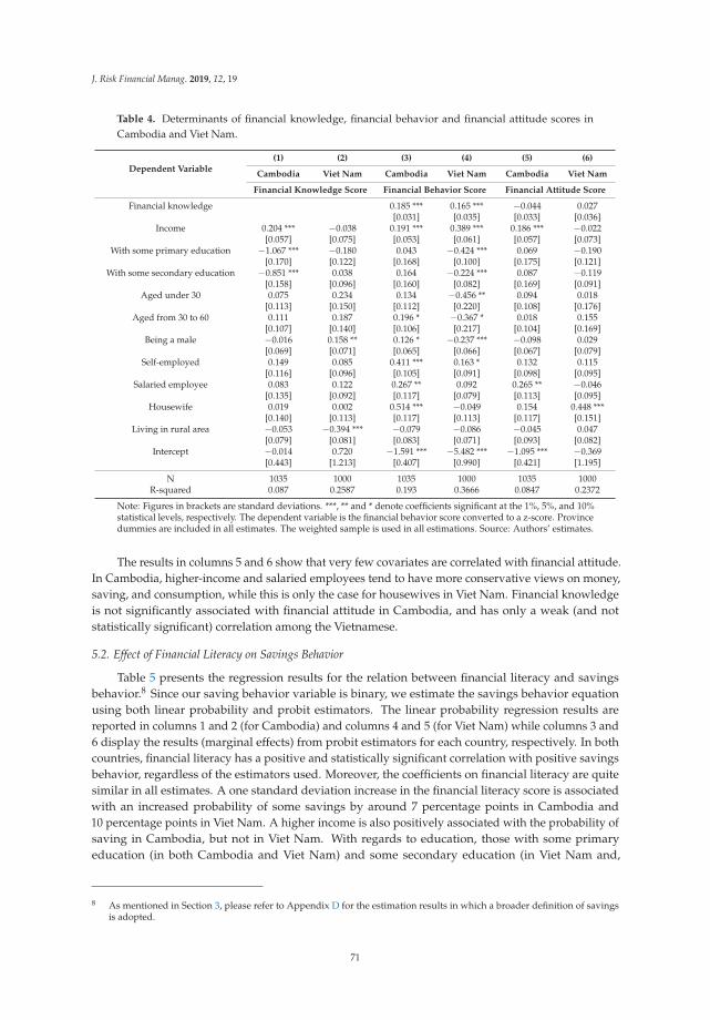
J. Risk Financial Manag. 2019, 12, 19
Table 4. Determinants of financial knowledge, financial behavior and financial attitude scores inCambodia and Viet Nam.
Dependent Variable(1) (2) (3) (4) (5) (6)
Cambodia Viet Nam Cambodia Viet Nam Cambodia Viet Nam
Financial Knowledge Score Financial Behavior Score Financial Attitude Score
Financial knowledge 0.185 *** 0.165 *** −0.044 0.027[0.031] [0.035] [0.033] [0.036]
Income 0.204 *** −0.038 0.191 *** 0.389 *** 0.186 *** −0.022[0.057] [0.075] [0.053] [0.061] [0.057] [0.073]
With some primary education −1.067 *** −0.180 0.043 −0.424 *** 0.069 −0.190[0.170] [0.122] [0.168] [0.100] [0.175] [0.121]
With some secondary education −0.851 *** 0.038 0.164 −0.224 *** 0.087 −0.119[0.158] [0.096] [0.160] [0.082] [0.169] [0.091]
Aged under 30 0.075 0.234 0.134 −0.456 ** 0.094 0.018[0.113] [0.150] [0.112] [0.220] [0.108] [0.176]
Aged from 30 to 60 0.111 0.187 0.196 * −0.367 * 0.018 0.155[0.107] [0.140] [0.106] [0.217] [0.104] [0.169]
Being a male −0.016 0.158 ** 0.126 * −0.237 *** −0.098 0.029[0.069] [0.071] [0.065] [0.066] [0.067] [0.079]
Self-employed 0.149 0.085 0.411 *** 0.163 * 0.132 0.115[0.116] [0.096] [0.105] [0.091] [0.098] [0.095]
Salaried employee 0.083 0.122 0.267 ** 0.092 0.265 ** −0.046[0.135] [0.092] [0.117] [0.079] [0.113] [0.095]
Housewife 0.019 0.002 0.514 *** −0.049 0.154 0.448 ***[0.140] [0.113] [0.117] [0.113] [0.117] [0.151]
Living in rural area −0.053 −0.394 *** −0.079 −0.086 −0.045 0.047[0.079] [0.081] [0.083] [0.071] [0.093] [0.082]
Intercept −0.014 0.720 −1.591 *** −5.482 *** −1.095 *** −0.369[0.443] [1.213] [0.407] [0.990] [0.421] [1.195]
N 1035 1000 1035 1000 1035 1000R-squared 0.087 0.2587 0.193 0.3666 0.0847 0.2372
Note: Figures in brackets are standard deviations. ***, ** and * denote coefficients significant at the 1%, 5%, and 10%statistical levels, respectively. The dependent variable is the financial behavior score converted to a z-score. Provincedummies are included in all estimates. The weighted sample is used in all estimations. Source: Authors’ estimates.
The results in columns 5 and 6 show that very few covariates are correlated with financial attitude.In Cambodia, higher-income and salaried employees tend to have more conservative views on money,saving, and consumption, while this is only the case for housewives in Viet Nam. Financial knowledgeis not significantly associated with financial attitude in Cambodia, and has only a weak (and notstatistically significant) correlation among the Vietnamese.
5.2. Effect of Financial Literacy on Savings Behavior
Table 5 presents the regression results for the relation between financial literacy and savingsbehavior.8 Since our saving behavior variable is binary, we estimate the savings behavior equationusing both linear probability and probit estimators. The linear probability regression results arereported in columns 1 and 2 (for Cambodia) and columns 4 and 5 (for Viet Nam) while columns 3 and6 display the results (marginal effects) from probit estimators for each country, respectively. In bothcountries, financial literacy has a positive and statistically significant correlation with positive savingsbehavior, regardless of the estimators used. Moreover, the coefficients on financial literacy are quitesimilar in all estimates. A one standard deviation increase in the financial literacy score is associatedwith an increased probability of some savings by around 7 percentage points in Cambodia and10 percentage points in Viet Nam. A higher income is also positively associated with the probability ofsaving in Cambodia, but not in Viet Nam. With regards to education, those with some primaryeducation (in both Cambodia and Viet Nam) and some secondary education (in Viet Nam and,
8 As mentioned in Section 3, please refer to Appendix D for the estimation results in which a broader definition of savingsis adopted.
71
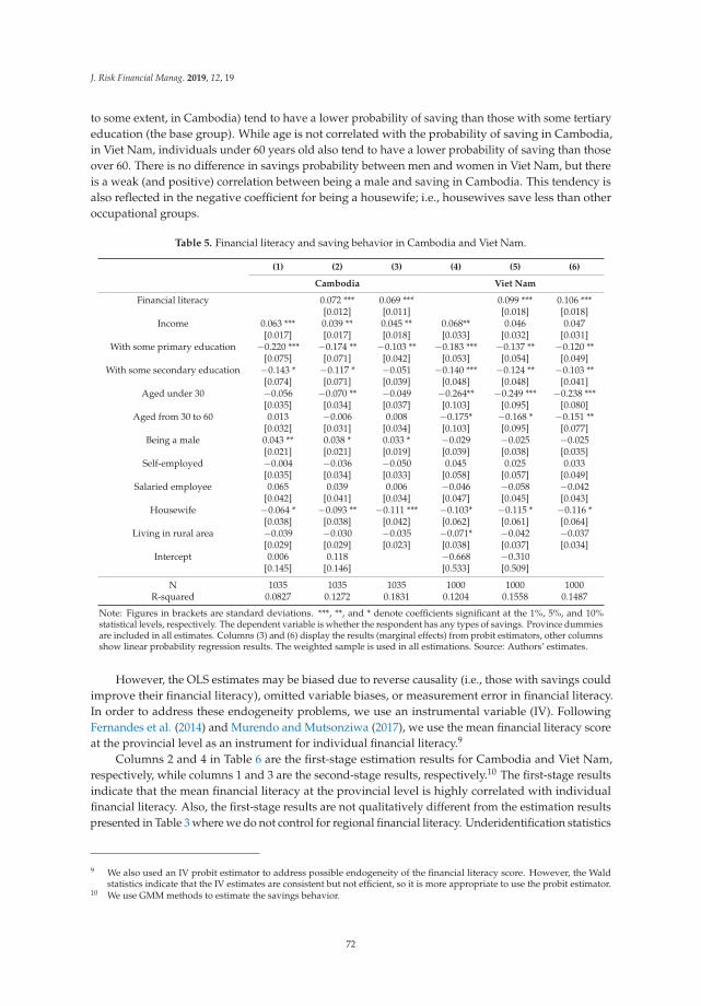
J. Risk Financial Manag. 2019, 12, 19
to some extent, in Cambodia) tend to have a lower probability of saving than those with some tertiaryeducation (the base group). While age is not correlated with the probability of saving in Cambodia,in Viet Nam, individuals under 60 years old also tend to have a lower probability of saving than thoseover 60. There is no difference in savings probability between men and women in Viet Nam, but thereis a weak (and positive) correlation between being a male and saving in Cambodia. This tendency isalso reflected in the negative coefficient for being a housewife; i.e., housewives save less than otheroccupational groups.
Table 5. Financial literacy and saving behavior in Cambodia and Viet Nam.
(1) (2) (3) (4) (5) (6)
Cambodia Viet Nam
Financial literacy 0.072 *** 0.069 *** 0.099 *** 0.106 ***[0.012] [0.011] [0.018] [0.018]
Income 0.063 *** 0.039 ** 0.045 ** 0.068** 0.046 0.047[0.017] [0.017] [0.018] [0.033] [0.032] [0.031]
With some primary education −0.220 *** −0.174 ** −0.103 ** −0.183 *** −0.137 ** −0.120 **[0.075] [0.071] [0.042] [0.053] [0.054] [0.049]
With some secondary education −0.143 * −0.117 * −0.051 −0.140 *** −0.124 ** −0.103 **[0.074] [0.071] [0.039] [0.048] [0.048] [0.041]
Aged under 30 −0.056 −0.070 ** −0.049 −0.264** −0.249 *** −0.238 ***[0.035] [0.034] [0.037] [0.103] [0.095] [0.080]
Aged from 30 to 60 0.013 −0.006 0.008 −0.175* −0.168 * −0.151 **[0.032] [0.031] [0.034] [0.103] [0.095] [0.077]
Being a male 0.043 ** 0.038 * 0.033 * −0.029 −0.025 −0.025[0.021] [0.021] [0.019] [0.039] [0.038] [0.035]
Self-employed −0.004 −0.036 −0.050 0.045 0.025 0.033[0.035] [0.034] [0.033] [0.058] [0.057] [0.049]
Salaried employee 0.065 0.039 0.006 −0.046 −0.058 −0.042[0.042] [0.041] [0.034] [0.047] [0.045] [0.043]
Housewife −0.064 * −0.093 ** −0.111 *** −0.103* −0.115 * −0.116 *[0.038] [0.038] [0.042] [0.062] [0.061] [0.064]
Living in rural area −0.039 −0.030 −0.035 −0.071* −0.042 −0.037[0.029] [0.029] [0.023] [0.038] [0.037] [0.034]
Intercept 0.006 0.118 −0.668 −0.310[0.145] [0.146] [0.533] [0.509]
N 1035 1035 1035 1000 1000 1000R-squared 0.0827 0.1272 0.1831 0.1204 0.1558 0.1487
Note: Figures in brackets are standard deviations. ***, **, and * denote coefficients significant at the 1%, 5%, and 10%statistical levels, respectively. The dependent variable is whether the respondent has any types of savings. Province dummiesare included in all estimates. Columns (3) and (6) display the results (marginal effects) from probit estimators, other columnsshow linear probability regression results. The weighted sample is used in all estimations. Source: Authors’ estimates.
However, the OLS estimates may be biased due to reverse causality (i.e., those with savings couldimprove their financial literacy), omitted variable biases, or measurement error in financial literacy.In order to address these endogeneity problems, we use an instrumental variable (IV). FollowingFernandes et al. (2014) and Murendo and Mutsonziwa (2017), we use the mean financial literacy scoreat the provincial level as an instrument for individual financial literacy.9
Columns 2 and 4 in Table 6 are the first-stage estimation results for Cambodia and Viet Nam,respectively, while columns 1 and 3 are the second-stage results, respectively.10 The first-stage resultsindicate that the mean financial literacy at the provincial level is highly correlated with individualfinancial literacy. Also, the first-stage results are not qualitatively different from the estimation resultspresented in Table 3 where we do not control for regional financial literacy. Underidentification statistics
9 We also used an IV probit estimator to address possible endogeneity of the financial literacy score. However, the Waldstatistics indicate that the IV estimates are consistent but not efficient, so it is more appropriate to use the probit estimator.
10 We use GMM methods to estimate the savings behavior.
72
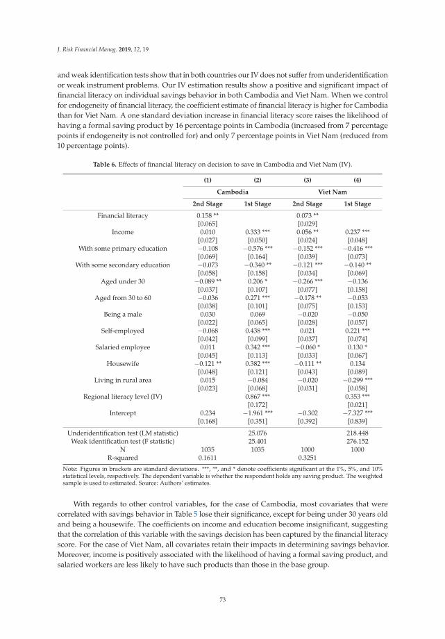
J. Risk Financial Manag. 2019, 12, 19
and weak identification tests show that in both countries our IV does not suffer from underidentificationor weak instrument problems. Our IV estimation results show a positive and significant impact offinancial literacy on individual savings behavior in both Cambodia and Viet Nam. When we controlfor endogeneity of financial literacy, the coefficient estimate of financial literacy is higher for Cambodiathan for Viet Nam. A one standard deviation increase in financial literacy score raises the likelihood ofhaving a formal saving product by 16 percentage points in Cambodia (increased from 7 percentagepoints if endogeneity is not controlled for) and only 7 percentage points in Viet Nam (reduced from10 percentage points).
Table 6. Effects of financial literacy on decision to save in Cambodia and Viet Nam (IV).
(1) (2) (3) (4)
Cambodia Viet Nam
2nd Stage 1st Stage 2nd Stage 1st Stage
Financial literacy 0.158 ** 0.073 **[0.065] [0.029]
Income 0.010 0.333 *** 0.056 ** 0.237 ***[0.027] [0.050] [0.024] [0.048]
With some primary education −0.108 −0.576 *** −0.152 *** −0.416 ***[0.069] [0.164] [0.039] [0.073]
With some secondary education −0.073 −0.340 ** −0.121 *** −0.140 **[0.058] [0.158] [0.034] [0.069]
Aged under 30 −0.089 ** 0.206 * −0.266 *** −0.136[0.037] [0.107] [0.077] [0.158]
Aged from 30 to 60 −0.036 0.271 *** −0.178 ** −0.053[0.038] [0.101] [0.075] [0.153]
Being a male 0.030 0.069 −0.020 −0.050[0.022] [0.065] [0.028] [0.057]
Self-employed −0.068 0.438 *** 0.021 0.221 ***[0.042] [0.099] [0.037] [0.074]
Salaried employee 0.011 0.342 *** −0.060 * 0.130 *[0.045] [0.113] [0.033] [0.067]
Housewife −0.121 ** 0.382 *** −0.111 ** 0.134[0.048] [0.121] [0.043] [0.089]
Living in rural area 0.015 −0.084 −0.020 −0.299 ***[0.023] [0.068] [0.031] [0.058]
Regional literacy level (IV) 0.867 *** 0.353 ***[0.172] [0.021]
Intercept 0.234 −1.961 *** −0.302 −7.327 ***[0.168] [0.351] [0.392] [0.839]
Underidentification test (LM statistic) 25.076 218.448Weak identification test (F statistic) 25.401 276.152
N 1035 1035 1000 1000R-squared 0.1611 0.3251
Note: Figures in brackets are standard deviations. ***, **, and * denote coefficients significant at the 1%, 5%, and 10%statistical levels, respectively. The dependent variable is whether the respondent holds any saving product. The weightedsample is used to estimated. Source: Authors’ estimates.
With regards to other control variables, for the case of Cambodia, most covariates that werecorrelated with savings behavior in Table 5 lose their significance, except for being under 30 years oldand being a housewife. The coefficients on income and education become insignificant, suggestingthat the correlation of this variable with the savings decision has been captured by the financial literacyscore. For the case of Viet Nam, all covariates retain their impacts in determining savings behavior.Moreover, income is positively associated with the likelihood of having a formal saving product, andsalaried workers are less likely to have such products than those in the base group.
73
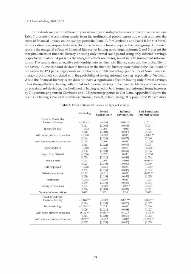
J. Risk Financial Manag. 2019, 12, 19
Individuals may adopt different types of savings to mitigate the risks or maximize the returns.Table 7 presents the estimation results from the multinomial probit regression, which estimates theeffect of financial literacy on the savings portfolio (Panel A for Cambodia and Panel B for Viet Nam).In this estimation, respondents who do not save in any form comprise the base group. Column 1reports the marginal effects of financial literacy on having no savings; columns 2 and 3 present themarginal effects of financial literacy on using only formal savings and using only informal savings,respectively. Column 4 presents the marginal effects on having saved in both formal and informalforms. The results show a negative relationship between financial literacy score and the probability ofnot saving. A one standard deviation increase in the financial literacy score reduces the likelihood ofnot saving by 12.4 percentage points in Cambodia and 16.8 percentage points in Viet Nam. Financialliteracy is positively correlated with the probability of having informal savings, especially in Viet Nam.While the financial literacy score does not have a significant effect on having only formal savings,it has strong effects on having both formal and informal savings. If the financial literacy score increasesby one standard deviation, the likelihood of having saved in both formal and informal forms increasesby 7.1 percentage points in Cambodia and 10.5 percentage points in Viet Nam. Appendix C shows theresults for having some form of savings (informal, formal, or both) using OLS, probit, and IV estimators.
Table 7. Effect of financial literacy on types of savings.
No SavingFormal
Savings OnlyInformal
Savings OnlyBoth Formal andInformal Savings
Panel A: CambodiaFinancial literacy −0.124 *** −0.004 0.056 *** 0.071 ***
[0.011] [0.004] [0.015] [0.011]Income (in log) −0.002 0.004 −0.029 0.027
[0.018] [0.008] [0.025] [0.017]With some primary education −0.000 −0.007 0.096 −0.089 **
[0.064] [0.024] [0.077] [0.040]With some secondary education −0.011 0.009 0.031 −0.030
[0.063] [0.022] [0.073] [0.037]Aged under 30 −0.010 0.025 0.053 −0.068 *
[0.036] [0.023] [0.051] [0.036]Aged from 30 to 60 −0.026 0.027 0.030 −0.030
[0.033] [0.022] [0.048] [0.034]Being a male −0.031 0.003 −0.015 0.044 **
[0.023] [0.010] [0.030] [0.019]Self-employed −0.028 −0.021 0.056 −0.007
[0.032] [0.014] [0.046] [0.034]Salaried employee −0.061 −0.011 0.001 0.072 **
[0.039] [0.015] [0.052] [0.035]Housewife −0.003 −0.009 0.043 −0.031
[0.039] [0.018] [0.056] [0.043]Living in rural area 0.034 −0.009 −0.061 * 0.035 *
[0.026] [0.009] [0.032] [0.021]Number of observations 1035 1035 1035 1035
Panel B: Viet NamFinancial literacy −0.168 *** −0.003 0.065 *** 0.105 ***
[0.014] [0.010] [0.020] [0.017]Income (in log) −0.092 *** 0.025 0.061 0.006
[0.026] [0.021] [0.038] [0.027]With some primary education 0.102 ** −0.109 *** 0.107 * −0.100 **
[0.044] [0.030] [0.058] [0.042]With some secondary education 0.119 *** −0.022 −0.006 −0.091 ***
[0.037] [0.029] [0.050] [0.035]
74
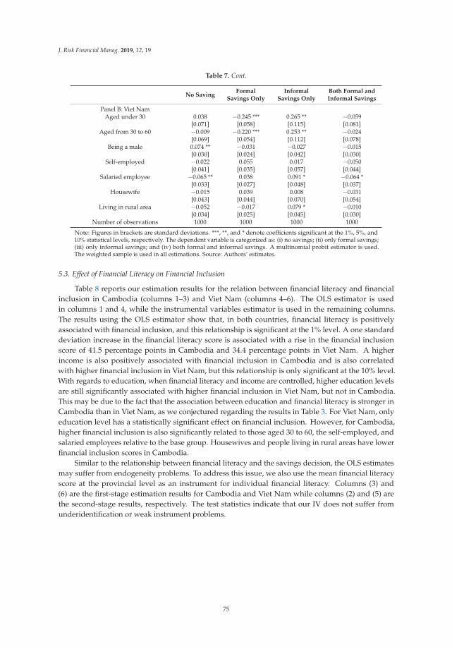
J. Risk Financial Manag. 2019, 12, 19
Table 7. Cont.
No SavingFormal
Savings OnlyInformal
Savings OnlyBoth Formal andInformal Savings
Panel B: Viet NamAged under 30 0.038 −0.245 *** 0.265 ** −0.059
[0.071] [0.058] [0.115] [0.081]Aged from 30 to 60 −0.009 −0.220 *** 0.253 ** −0.024
[0.069] [0.054] [0.112] [0.078]Being a male 0.074 ** −0.031 −0.027 −0.015
[0.030] [0.024] [0.042] [0.030]Self-employed −0.022 0.055 0.017 −0.050
[0.041] [0.035] [0.057] [0.044]Salaried employee −0.065 ** 0.038 0.091 * −0.064 *
[0.033] [0.027] [0.048] [0.037]Housewife −0.015 0.039 0.008 −0.031
[0.043] [0.044] [0.070] [0.054]Living in rural area −0.052 −0.017 0.079 * −0.010
[0.034] [0.025] [0.045] [0.030]Number of observations 1000 1000 1000 1000
Note: Figures in brackets are standard deviations. ***, **, and * denote coefficients significant at the 1%, 5%, and10% statistical levels, respectively. The dependent variable is categorized as: (i) no savings; (ii) only formal savings;(iii) only informal savings; and (iv) both formal and informal savings. A multinomial probit estimator is used.The weighted sample is used in all estimations. Source: Authors’ estimates.
5.3. Effect of Financial Literacy on Financial Inclusion
Table 8 reports our estimation results for the relation between financial literacy and financialinclusion in Cambodia (columns 1–3) and Viet Nam (columns 4–6). The OLS estimator is usedin columns 1 and 4, while the instrumental variables estimator is used in the remaining columns.The results using the OLS estimator show that, in both countries, financial literacy is positivelyassociated with financial inclusion, and this relationship is significant at the 1% level. A one standarddeviation increase in the financial literacy score is associated with a rise in the financial inclusionscore of 41.5 percentage points in Cambodia and 34.4 percentage points in Viet Nam. A higherincome is also positively associated with financial inclusion in Cambodia and is also correlatedwith higher financial inclusion in Viet Nam, but this relationship is only significant at the 10% level.With regards to education, when financial literacy and income are controlled, higher education levelsare still significantly associated with higher financial inclusion in Viet Nam, but not in Cambodia.This may be due to the fact that the association between education and financial literacy is stronger inCambodia than in Viet Nam, as we conjectured regarding the results in Table 3. For Viet Nam, onlyeducation level has a statistically significant effect on financial inclusion. However, for Cambodia,higher financial inclusion is also significantly related to those aged 30 to 60, the self-employed, andsalaried employees relative to the base group. Housewives and people living in rural areas have lowerfinancial inclusion scores in Cambodia.
Similar to the relationship between financial literacy and the savings decision, the OLS estimatesmay suffer from endogeneity problems. To address this issue, we also use the mean financial literacyscore at the provincial level as an instrument for individual financial literacy. Columns (3) and(6) are the first-stage estimation results for Cambodia and Viet Nam while columns (2) and (5) arethe second-stage results, respectively. The test statistics indicate that our IV does not suffer fromunderidentification or weak instrument problems.
75
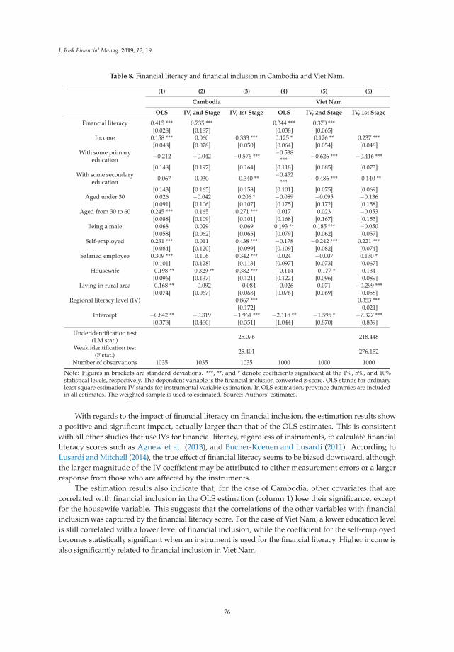
J. Risk Financial Manag. 2019, 12, 19
Table 8. Financial literacy and financial inclusion in Cambodia and Viet Nam.
(1) (2) (3) (4) (5) (6)
Cambodia Viet Nam
OLS IV, 2nd Stage IV, 1st Stage OLS IV, 2nd Stage IV, 1st Stage
Financial literacy 0.415 *** 0.735 *** 0.344 *** 0.370 ***[0.028] [0.187] [0.038] [0.065]
Income 0.158 *** 0.060 0.333 *** 0.125 * 0.126 ** 0.237 ***[0.048] [0.078] [0.050] [0.064] [0.054] [0.048]
With some primaryeducation −0.212 −0.042 −0.576 *** −0.538
*** −0.626 *** −0.416 ***
[0.148] [0.197] [0.164] [0.118] [0.085] [0.073]With some secondary
education −0.067 0.030 −0.340 ** −0.452*** −0.486 *** −0.140 **
[0.143] [0.165] [0.158] [0.101] [0.075] [0.069]Aged under 30 0.026 −0.042 0.206 * −0.089 −0.095 −0.136
[0.091] [0.106] [0.107] [0.175] [0.172] [0.158]Aged from 30 to 60 0.245 *** 0.165 0.271 *** 0.017 0.023 −0.053
[0.088] [0.109] [0.101] [0.168] [0.167] [0.153]Being a male 0.068 0.029 0.069 0.193 ** 0.185 *** −0.050
[0.058] [0.062] [0.065] [0.079] [0.062] [0.057]Self-employed 0.231 *** 0.011 0.438 *** −0.178 −0.242 *** 0.221 ***
[0.084] [0.120] [0.099] [0.109] [0.082] [0.074]Salaried employee 0.309 *** 0.106 0.342 *** 0.024 −0.007 0.130 *
[0.101] [0.128] [0.113] [0.097] [0.073] [0.067]Housewife −0.198 ** −0.329 ** 0.382 *** −0.114 −0.177 * 0.134
[0.096] [0.137] [0.121] [0.122] [0.096] [0.089]Living in rural area −0.168 ** −0.092 −0.084 −0.026 0.071 −0.299 ***
[0.074] [0.067] [0.068] [0.076] [0.069] [0.058]Regional literacy level (IV) 0.867 *** 0.353 ***
[0.172] [0.021]Intercept −0.842 ** −0.319 −1.961 *** −2.118 ** −1.595 * −7.327 ***
[0.378] [0.480] [0.351] [1.044] [0.870] [0.839]
Underidentification test(LM stat.) 25.076 218.448
Weak identification test(F stat.) 25.401 276.152
Number of observations 1035 1035 1035 1000 1000 1000
Note: Figures in brackets are standard deviations. ***, **, and * denote coefficients significant at the 1%, 5%, and 10%statistical levels, respectively. The dependent variable is the financial inclusion converted z-score. OLS stands for ordinaryleast square estimation; IV stands for instrumental variable estimation. In OLS estimation, province dummies are includedin all estimates. The weighted sample is used to estimated. Source: Authors’ estimates.
With regards to the impact of financial literacy on financial inclusion, the estimation results showa positive and significant impact, actually larger than that of the OLS estimates. This is consistentwith all other studies that use IVs for financial literacy, regardless of instruments, to calculate financialliteracy scores such as Agnew et al. (2013), and Bucher-Koenen and Lusardi (2011). According toLusardi and Mitchell (2014), the true effect of financial literacy seems to be biased downward, althoughthe larger magnitude of the IV coefficient may be attributed to either measurement errors or a largerresponse from those who are affected by the instruments.
The estimation results also indicate that, for the case of Cambodia, other covariates that arecorrelated with financial inclusion in the OLS estimation (column 1) lose their significance, exceptfor the housewife variable. This suggests that the correlations of the other variables with financialinclusion was captured by the financial literacy score. For the case of Viet Nam, a lower education levelis still correlated with a lower level of financial inclusion, while the coefficient for the self-employedbecomes statistically significant when an instrument is used for the financial literacy. Higher income isalso significantly related to financial inclusion in Viet Nam.
76
J. Risk Financial Manag. 2019, 12, 19
6. Discussion
Our study of adult financial literacy in Cambodia and Viet Nam breaks new ground in two ways:(i) It marks the first implementation of the OECD/INFE survey in the so-called CLMV countries(Cambodia, Lao PDR, Myanmar, and Viet Nam); and (ii) Cambodia and Viet Nam have considerablylower levels of per capita income than the other 30 countries in OECD/INFE (2016). Generally,our study corroborates the findings of studies of other countries but uncovers some differences as well.The overall scores of financial literacy in Cambodia (11.8) and Viet Nam (12.7) are at the low end ofthe range seen in the other 30 countries that have implemented the OECD/INFE survey, and nearthose for Poland and Belarus. However, these results are relatively good when taking into account thelevels of per capita income in those two countries.
Our analysis shows that that the level of education generally is highly significant and positivelycorrelated with financial literacy in both Cambodia and Viet Nam. This holds for both the overallmeasure of financial literacy and the subscores for financial knowledge, financial behavior, and forsavings. However, the education level was not significant for financial attitudes. These results wereconsistent with the findings for the other 30 countries reported in OECD/INFE (2016). These resultsalso consistent with those of Bucher-Koenen and Lusardi (2011), and Murendo and Mutsonziwa (2017),which use different measures of financial literacy.
Respondents aged 30–60 had significantly higher overall financial literacy scores than other agegroups, but the effects of age on individual subscores were less consistent or significant. In particular,there was no significant effect of age on financial attitude. This generally is consistent with the findingsfor the other 30 countries where age groups 30–60 generally had higher scores for both financialknowledge and financial behavior.
Interestingly, gender was not very significant for overall financial literacy in either country.The gender coefficient was not significant for Cambodia, while for Viet Nam it was significant, butonly about half the average magnitude of the other 30 countries (0.18 vs. 0.32) (OECD/INFE 2016).This result differs from some other studies. For example, Lusardi and Mitchell (2014) find that mentypically have higher financial literacy scores than women. While we do not have an explanation forthis difference, and cultural factors are probably significant, we conjecture that differences in educationlevels between men and women in Cambodia and Vietnam may capture most of the gender differencesin financial literacy. This issue merits further study.
The results generally showed that self-employed workers and salaried workers had higherlevels of financial literacy than other employment categories in both countries, and housewives hadhigher levels of financial literacy in Cambodia. These results were less strong for the various subscores,but generally pointed in the same direction, especially for financial behavior.
The finding with the most important macroeconomic implications is that both financial literacyand general education levels are positively and significantly related to formal and informal savingsactivity, and financial literacy has an independent effect even when the general education level iscorrected for. Similar to Fernandes et al. (2014) and Murendo and Mutsonziwa (2017), our resultstill holds when the possible endogeneity of financial literacy is corrected for by using the regionalaverage financial literacy level as an instrumental variable. This implies that improving generaleducation levels is important, but additional gains can be obtained by developing policies such asfinancial education programs that directly raise financial literacy. Such programs could have importantpotential impacts in terms of increasing savings in those countries.
Similarly, both financial literacy and general education levels are found to be positively andsignificantly related to the measure of financial inclusion. This holds in most cases even when thepossible endogeneity of financial literacy is corrected by using regional average financial literacy as aninstrumental variable. Increased financial inclusion means that increased savings can be made morereadily available for investment activity in those countries. Again, this underlines the importance ofdeveloping policies to raise both general education and financial literacy.
77
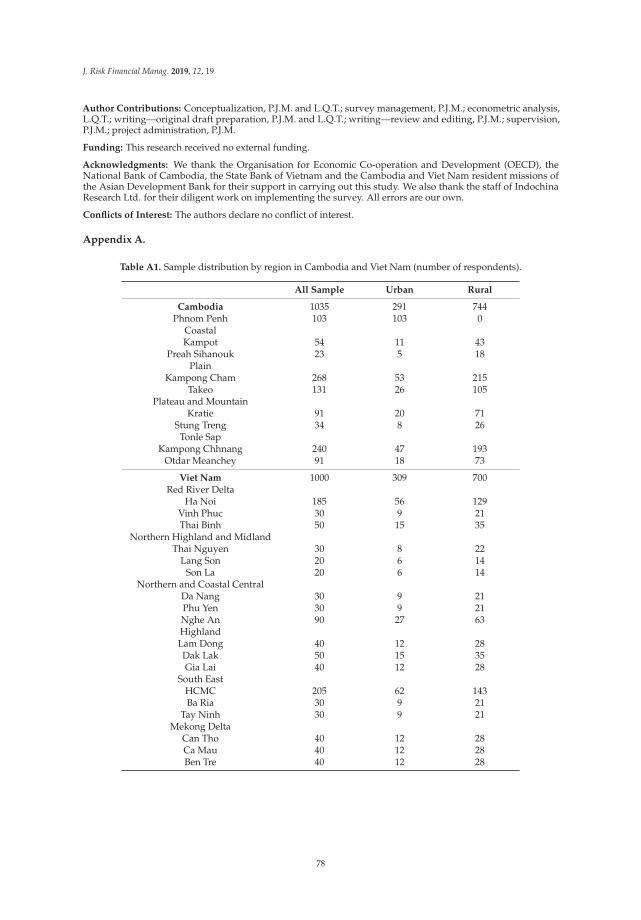
J. Risk Financial Manag. 2019, 12, 19
Author Contributions: Conceptualization, P.J.M. and L.Q.T.; survey management, P.J.M.; econometric analysis,L.Q.T.; writing—original draft preparation, P.J.M. and L.Q.T.; writing—review and editing, P.J.M.; supervision,P.J.M.; project administration, P.J.M.
Funding: This research received no external funding.
Acknowledgments: We thank the Organisation for Economic Co-operation and Development (OECD), theNational Bank of Cambodia, the State Bank of Vietnam and the Cambodia and Viet Nam resident missions ofthe Asian Development Bank for their support in carrying out this study. We also thank the staff of IndochinaResearch Ltd. for their diligent work on implementing the survey. All errors are our own.
Conflicts of Interest: The authors declare no conflict of interest.
Appendix A.
Table A1. Sample distribution by region in Cambodia and Viet Nam (number of respondents).
All Sample Urban Rural
Cambodia 1035 291 744Phnom Penh 103 103 0
CoastalKampot 54 11 43
Preah Sihanouk 23 5 18Plain
Kampong Cham 268 53 215Takeo 131 26 105
Plateau and MountainKratie 91 20 71
Stung Treng 34 8 26Tonle Sap
Kampong Chhnang 240 47 193Otdar Meanchey 91 18 73
Viet Nam 1000 309 700Red River Delta
Ha Noi 185 56 129Vinh Phuc 30 9 21Thai Binh 50 15 35
Northern Highland and MidlandThai Nguyen 30 8 22
Lang Son 20 6 14Son La 20 6 14
Northern and Coastal CentralDa Nang 30 9 21Phu Yen 30 9 21Nghe An 90 27 63HighlandLam Dong 40 12 28Dak Lak 50 15 35Gia Lai 40 12 28
South EastHCMC 205 62 143Ba Ria 30 9 21
Tay Ninh 30 9 21Mekong Delta
Can Tho 40 12 28Ca Mau 40 12 28Ben Tre 40 12 28
78
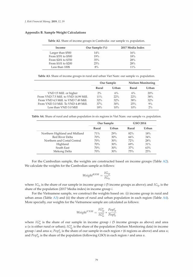
J. Risk Financial Manag. 2019, 12, 19
Appendix B. Sample Weight Calculations
Table A2. Share of income groups in Cambodia: our sample vs. population.
Income Our Sample (%) 2017 Media Index
Larger than $500 14% 16%From $351 to $500 19% 18%From $201 to $350 35% 28%From $101 to $200 25% 28%
Less than 100$ 8% 11%
Table A3. Share of income groups in rural and urban Viet Nam: our sample vs. population.
Our Sample Nielsen Monitoring
Rural Urban Rural Urban
VND 15 Mill. or higher 2% 6% 6% 20%From VND 7.5 Mill. to VND 14.99 Mill. 11% 22% 22% 38%From VND 4.5 Mill. to VND 7.49 Mill. 32% 32% 38% 32%From VND 3.0 Mill. To VND 4.49 Mill. 37% 30% 25% 9%
Less than VND 3.0 Mill 18% 10% 10% 2%
Table A4. Share of rural and urban population in six regions in Viet Nam: our sample vs. population.
Our Sample GSO 2014
Rural Urban Rural Urban
Northern Highland and Midland 71% 29% 82% 18%Red River Delta 70% 30% 66% 34%
Northern and Costal Central 70% 30% 72% 28%Highland 70% 30% 69% 31%South East 70% 30% 37% 63%
Mekong Delta 70% 30% 75% 25%
For the Cambodian sample, the weights are constructed based on income groups (Table A2).We calculate the weights for the Cambodian sample as follows:
WeightKHM =IGip
IGis
where IGis is the share of our sample in income group i (5 income groups as above); and IGip is theshare of the population (2017 Media index) in income group i.
For the Vietnamese sample, we construct the weights based on: (i) income group in rural andurban areas (Table A3) and (ii) the share of rural and urban population in each region (Table A4).More specially, our weights for the Vietnamese sample are calculated as follows:
WeightVNM =IGu
ip
IGuis∗ Popu
rp
Popurs
where IGuis is the share of our sample in income group i (5 income groups as above) and area
u (u is either rural or urban); IGuip is the share of the population (Nielsen Monitoring data) in income
group i and area u; Popurs is the share of our sample in each region r (6 regions as above) and area u;
and Popurp is the share of the population (following GSO) in each region r and area u.
79
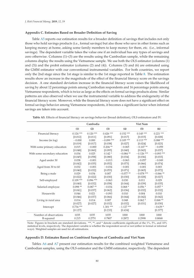
J. Risk Financial Manag. 2019, 12, 19
Appendix C. Estimates Based on Broader Definition of Saving
Table A5 reports our estimation results for a broader definition of savings that includes not onlythose who hold savings products (i.e., formal savings) but also those who save in other forms such askeeping money at home, asking some family members to keep money for them, etc. (i.e., informalsavings). The dependent variable takes the value one if an individual has any types of savings andzero otherwise. Columns (1)–(3) are the results using the Cambodian sample, while the remainingcolumns display the results using the Vietnamese sample. We use both the OLS estimator (columns (1)and (3)) and the probit estimator (columns (2) and (4)). Columns (3) and (6) are estimated usingthe GMM estimator with our conventional instrumental variables. For both countries, we reportonly the 2nd stage since the 1st stage is similar to the 1st stage reported in Table 8. The estimationresults show an increase in the magnitude of the effect of the financial literacy score on the savingsdecision. A one standard deviation increase in the financial literacy score raises the likelihood ofsaving by about 12 percentage points among Cambodian respondents and 16 percentage points amongVietnamese respondents, which is twice as large as the effects on formal savings products alone. Similarpatterns are also observed when we use the instrumental variable to address the endogeneity of thefinancial literacy score. Moreover, while the financial literacy score does not have a significant effect onformal savings behavior among Vietnamese respondents, it becomes a significant factor when informalsavings are taken into account.
Table A5. Effects of financial literacy on savings behavior (broad definition), OLS estimators and IV.
Cambodia Viet Nam
(1) (2) (3) (4) (5) (6)
Financial literacy 0.124 *** 0.120 *** 0.426 *** 0.152 *** 0.145 *** 0.221 ***[0.012] [0.011] [0.091] [0.017] [0.015] [0.028]
Income (in log) −0.000 0.000 −0.099 *** 0.105 *** 0.113 *** 0.088 ***[0.019] [0.017] [0.038] [0.027] [0.024] [0.023]
With some primary education 0.015 −0.000 0.204 ** −0.065 −0.107 ** −0.059[0.048] [0.060] [0.095] [0.040] [0.043] [0.037]
With some secondary education 0.034 0.025 0.142 * −0.084 ** −0.126 *** −0.093 ***[0.045] [0.058] [0.080] [0.034] [0.036] [0.033]
Aged under 30 0.038 −0.001 −0.013 −0.063 −0.057 −0.049[0.042] [0.035] [0.052] [0.073] [0.066] [0.074]
Aged from 30 to 60 0.032 −0.001 −0.034 −0.001 −0.001 0.003[0.040] [0.032] [0.053] [0.071] [0.065] [0.072]
Being a male 0.029 0.034 0.007 −0.077 ** −0.078 *** −0.066 **[0.022] [0.022] [0.030] [0.030] [0.028] [0.027]
Self-employed 0.109 *** 0.096 *** −0.063 0.030 0.011 0.029[0.040] [0.032] [0.058] [0.044] [0.039] [0.035]
Salaried employee 0.098 ** 0.087 ** −0.034 0.068 * 0.056 * 0.057 *[0.041] [0.037] [0.062] [0.036] [0.032] [0.032]
Housewife 0.044 0.021 −0.093 0.010 0.004 0.010[0.046] [0.037] [0.066] [0.044] [0.042] [0.042]
Living in rural area 0.014 0.014 0.007 0.048 0.062 * 0.068 **[0.027] [0.027] [0.032] [0.032] [0.031] [0.030]
Intercept 0.734 *** 1.301 *** −1.127 *** −0.639 *[0.127] [0.233] [0.434] [0.377]
Number of observations 1035 1035 1035 1000 1000 1000R-squared 0.215 0.2751 0.7807 0.2872 0.2998 0.8068
Note: Figures in brackets are standard deviations. ***, **, and * denote coefficients significant at the 1%, 5%, and 10%statistical levels, respectively. The dependent variable is whether the respondent saved or not (either in formal or informalways). Weighted samples are used for all estimations.
Appendix D. Estimates Based on Combined Samples of Cambodia and Viet Nam
Tables A6 and A7 present our estimation results for the combined weighted Vietnamese andCambodian samples, using the OLS estimator and the GMM estimator, respectively. The dependent
80
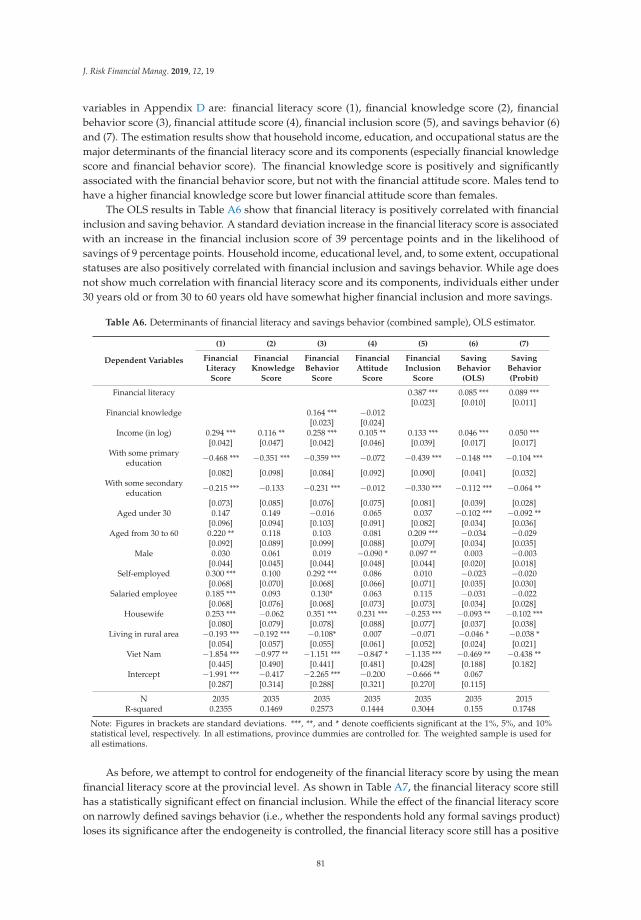
J. Risk Financial Manag. 2019, 12, 19
variables in Appendix D are: financial literacy score (1), financial knowledge score (2), financialbehavior score (3), financial attitude score (4), financial inclusion score (5), and savings behavior (6)and (7). The estimation results show that household income, education, and occupational status are themajor determinants of the financial literacy score and its components (especially financial knowledgescore and financial behavior score). The financial knowledge score is positively and significantlyassociated with the financial behavior score, but not with the financial attitude score. Males tend tohave a higher financial knowledge score but lower financial attitude score than females.
The OLS results in Table A6 show that financial literacy is positively correlated with financialinclusion and saving behavior. A standard deviation increase in the financial literacy score is associatedwith an increase in the financial inclusion score of 39 percentage points and in the likelihood ofsavings of 9 percentage points. Household income, educational level, and, to some extent, occupationalstatuses are also positively correlated with financial inclusion and savings behavior. While age doesnot show much correlation with financial literacy score and its components, individuals either under30 years old or from 30 to 60 years old have somewhat higher financial inclusion and more savings.
Table A6. Determinants of financial literacy and savings behavior (combined sample), OLS estimator.
Dependent Variables
(1) (2) (3) (4) (5) (6) (7)
FinancialLiteracy
Score
FinancialKnowledge
Score
FinancialBehavior
Score
FinancialAttitude
Score
FinancialInclusion
Score
SavingBehavior
(OLS)
SavingBehavior(Probit)
Financial literacy 0.387 *** 0.085 *** 0.089 ***[0.023] [0.010] [0.011]
Financial knowledge 0.164 *** −0.012[0.023] [0.024]
Income (in log) 0.294 *** 0.116 ** 0.258 *** 0.105 ** 0.133 *** 0.046 *** 0.050 ***[0.042] [0.047] [0.042] [0.046] [0.039] [0.017] [0.017]
With some primaryeducation −0.468 *** −0.351 *** −0.359 *** −0.072 −0.439 *** −0.148 *** −0.104 ***
[0.082] [0.098] [0.084] [0.092] [0.090] [0.041] [0.032]With some secondary
education −0.215 *** −0.133 −0.231 *** −0.012 −0.330 *** −0.112 *** −0.064 **
[0.073] [0.085] [0.076] [0.075] [0.081] [0.039] [0.028]Aged under 30 0.147 0.149 −0.016 0.065 0.037 −0.102 *** −0.092 **
[0.096] [0.094] [0.103] [0.091] [0.082] [0.034] [0.036]Aged from 30 to 60 0.220 ** 0.118 0.103 0.081 0.209 *** −0.034 −0.029
[0.092] [0.089] [0.099] [0.088] [0.079] [0.034] [0.035]Male 0.030 0.061 0.019 −0.090 * 0.097 ** 0.003 −0.003
[0.044] [0.045] [0.044] [0.048] [0.044] [0.020] [0.018]Self-employed 0.300 *** 0.100 0.292 *** 0.086 0.010 −0.023 −0.020
[0.068] [0.070] [0.068] [0.066] [0.071] [0.035] [0.030]Salaried employee 0.185 *** 0.093 0.130* 0.063 0.115 −0.031 −0.022
[0.068] [0.076] [0.068] [0.073] [0.073] [0.034] [0.028]Housewife 0.253 *** −0.062 0.351 *** 0.231 *** −0.253 *** −0.093 ** −0.102 ***
[0.080] [0.079] [0.078] [0.088] [0.077] [0.037] [0.038]Living in rural area −0.193 *** −0.192 *** −0.108* 0.007 −0.071 −0.046 * −0.038 *
[0.054] [0.057] [0.055] [0.061] [0.052] [0.024] [0.021]Viet Nam −1.854 *** −0.977 ** −1.151 *** −0.847 * −1.135 *** −0.469 ** −0.438 **
[0.445] [0.490] [0.441] [0.481] [0.428] [0.188] [0.182]Intercept −1.991 *** −0.417 −2.265 *** −0.200 −0.666 ** 0.067
[0.287] [0.314] [0.288] [0.321] [0.270] [0.115]
N 2035 2035 2035 2035 2035 2035 2015R-squared 0.2355 0.1469 0.2573 0.1444 0.3044 0.155 0.1748
Note: Figures in brackets are standard deviations. ***, **, and * denote coefficients significant at the 1%, 5%, and 10%statistical level, respectively. In all estimations, province dummies are controlled for. The weighted sample is used forall estimations.
As before, we attempt to control for endogeneity of the financial literacy score by using the meanfinancial literacy score at the provincial level. As shown in Table A7, the financial literacy score stillhas a statistically significant effect on financial inclusion. While the effect of the financial literacy scoreon narrowly defined savings behavior (i.e., whether the respondents hold any formal savings product)loses its significance after the endogeneity is controlled, the financial literacy score still has a positive
81
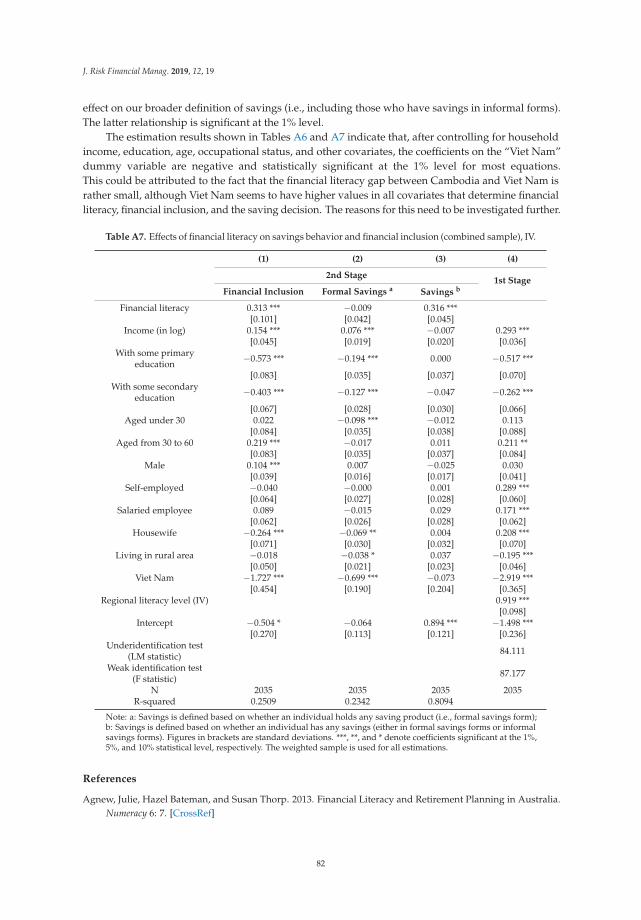
J. Risk Financial Manag. 2019, 12, 19
effect on our broader definition of savings (i.e., including those who have savings in informal forms).The latter relationship is significant at the 1% level.
The estimation results shown in Tables A6 and A7 indicate that, after controlling for householdincome, education, age, occupational status, and other covariates, the coefficients on the “Viet Nam”dummy variable are negative and statistically significant at the 1% level for most equations.This could be attributed to the fact that the financial literacy gap between Cambodia and Viet Nam israther small, although Viet Nam seems to have higher values in all covariates that determine financialliteracy, financial inclusion, and the saving decision. The reasons for this need to be investigated further.
Table A7. Effects of financial literacy on savings behavior and financial inclusion (combined sample), IV.
(1) (2) (3) (4)
2nd Stage1st Stage
Financial Inclusion Formal Savings a Savings b
Financial literacy 0.313 *** −0.009 0.316 ***[0.101] [0.042] [0.045]
Income (in log) 0.154 *** 0.076 *** −0.007 0.293 ***[0.045] [0.019] [0.020] [0.036]
With some primaryeducation −0.573 *** −0.194 *** 0.000 −0.517 ***
[0.083] [0.035] [0.037] [0.070]With some secondary
education −0.403 *** −0.127 *** −0.047 −0.262 ***
[0.067] [0.028] [0.030] [0.066]Aged under 30 0.022 −0.098 *** −0.012 0.113
[0.084] [0.035] [0.038] [0.088]Aged from 30 to 60 0.219 *** −0.017 0.011 0.211 **
[0.083] [0.035] [0.037] [0.084]Male 0.104 *** 0.007 −0.025 0.030
[0.039] [0.016] [0.017] [0.041]Self-employed −0.040 −0.000 0.001 0.289 ***
[0.064] [0.027] [0.028] [0.060]Salaried employee 0.089 −0.015 0.029 0.171 ***
[0.062] [0.026] [0.028] [0.062]Housewife −0.264 *** −0.069 ** 0.004 0.208 ***
[0.071] [0.030] [0.032] [0.070]Living in rural area −0.018 −0.038 * 0.037 −0.195 ***
[0.050] [0.021] [0.023] [0.046]Viet Nam −1.727 *** −0.699 *** −0.073 −2.919 ***
[0.454] [0.190] [0.204] [0.365]Regional literacy level (IV) 0.919 ***
[0.098]Intercept −0.504 * −0.064 0.894 *** −1.498 ***
[0.270] [0.113] [0.121] [0.236]Underidentification test
(LM statistic) 84.111
Weak identification test(F statistic) 87.177
N 2035 2035 2035 2035R-squared 0.2509 0.2342 0.8094
Note: a: Savings is defined based on whether an individual holds any saving product (i.e., formal savings form);b: Savings is defined based on whether an individual has any savings (either in formal savings forms or informalsavings forms). Figures in brackets are standard deviations. ***, **, and * denote coefficients significant at the 1%,5%, and 10% statistical level, respectively. The weighted sample is used for all estimations.
References
Agnew, Julie, Hazel Bateman, and Susan Thorp. 2013. Financial Literacy and Retirement Planning in Australia.Numeracy 6: 7. [CrossRef]
82
J. Risk Financial Manag. 2019, 12, 19
Bernheim, Douglas. 1995. Do Households Appreciate Their Financial Vulnerabilities? An Analysis of Actions,Perceptions, and Public Policy. In Tax Policy and Economic Growth. Washington: American Council for CapitalFormation, pp. 1–30.
Bernheim, Douglas. 1998. Financial Literacy, Education, and Retirement Saving. In Living with Defined ContributionPensions: Remaking Responsibility for Retirement. Edited by Olivia S. Mitchell and Sylvester J. Schieber.Philadelphia: University of Pennsylvania Press, pp. 38–68.
Bucher-Koenen, Tabea, and Annamaria Lusardi. 2011. Financial Literacy and Retirement Planning in Germany.Journal of Pension Economics & Finance 10: 565–84.
Campbell, John. 2006. Household Finance. Journal of Finance 61: 1553–604. [CrossRef]Christelis, Dimitris, Tullio Jappelli, and Mario Padula. 2010. Cognitive Abilities and Portfolio Choice. European
Economic Review 54: 18–38. [CrossRef]de Bassa Scheresberg, Carlo. 2013. Financial Literacy and Financial Behavior among Young Adults: Evidence and
Implications. Numeracy 6: 5. [CrossRef]Fernandes, Daniel, John G. Lynch Jr., and Richard G. Netemeyer. 2014. The Effect of Financial Literacy and
Financial Education on Downstream Financial Behaviors. Management Science 60: 1861–83. [CrossRef]Group of Twenty (G20). 2012. G20 Leaders Declaration. Los Cabos, Mexico. June 19. Available online:
http://www.g20.utoronto.ca/2012/2012-0619-loscabos.html (accessed on 4 October 2017).Hastings, Justine S., Brigitte C. Madrian, and William L. Skimmyhorn. 2013. Financial Literacy, Financial
Education, and Economic Outcomes. Annual Review of Economics 2013: 347–73. [CrossRef] [PubMed]Hilgert, Marianne A., Jeanne M. Hogarth, and Sondra G. Beverly. 2003. Household financial management:
The connection between knowledge and behavior. Federal Research Bulletin 89: 309.Jappelli, Tullio, and Mario Padula. 2013. Investment in Financial Literacy and Saving Decisions. Journal of
Banking & Finance 37: 2779–92.Lusardi, Annamaria, and Olivia S. Mitchell. 2006. Financial Literacy and Planning: Implications for Retirement
Wellbeing. Working Paper. Philadelphia, PA, USA: Pension Research Council, University of Pennsylvania.Lusardi, Annamaria, and Olivia S. Mitchell. 2011. Financial Literacy and Planning: Implications for Retirement
Well-Being. In Financial Literacy: Implications for Retirement Security and the Financial Marketplace. Edited byOlivia S. Mitchell and Annamaria Lusardi. Oxford and New York: Oxford University Press, pp. 17–39.
Lusardi, Annamaria, and Olivia S. Mitchell. 2014. The Economic Importance of Financial Literacy: Theory andEvidence. Journal of Economic Literature 52: 5–44. [CrossRef] [PubMed]
Mahdzan, Nurul Shahnaz, and Saleh Tabiani. 2013. The Impact of Financial Literacy on Individual Saving:An Exploratory Study in the Malaysian Context. Transformations in Business and Economics 12: 41–55.
Mandell, Lewis. 2009. The Financial Literacy of Young American Adults: Results of the 2008 National Jump$tart CoalitionSurvey of High School Seniors and College Students. Washington: Jump$tart Coalition.
Moore, Danna. 2003. Survey of Financial Literacy in Washington State: Knowledge, Behavior, Attitudes, and Experiences.Washington State University Social and Economic Sciences Research Center Technical Report 03-39. Pullman:Washington State University Social and Economic Sciences Research Center.
Murendo, Conrad, and Kingstone Mutsonziwa. 2017. Financial Literacy and Savings Decisions by Adult FinancialConsumers in Zimbabwe. International Journal of Consumer Studies 41: 95–103. [CrossRef]
OECD/INFE. 2015a. Guide to Creating Financial Literacy Scores and Financial Inclusion Indicators Using Data from theOECD/INFE 2015 Financial Literacy Survey. Paris: OECD.
OECD/INFE. 2015b. Policy Handbook on National Strategies for Financial Education. Paris: OECD, Availableonline: http://www.oecd.org/g20/topics/employment-and-social-policy/National-Strategies-Financial-Education-Policy-Handbook.pdf (accessed on 4 October 2017).
OECD/INFE. 2015c. 2015 OECD/INFE Toolkit for Measuring Financial Literacy and Financial Inclusion. Paris: OECD.OECD/INFE. 2016. OECD/INFE International Survey of Adult Financial Literacy Competencies. Paris: OECD.OECD/INFE. 2017. G20/OECD INFE Report on Adult Financial Literacy in G20 Countries. Paris: OECD,
Available online: http://www.oecd.org/daf/fin/financial-education/G20-OECD-INFE-report-adult-financial-literacy-in-G20-countries.pdf (accessed on 13 February 2018).
Stango, Victor, and Jonathan Zinman. 2009. Exponential Growth Bias and Household Finance. Journal of Finance64: 2807–49. [CrossRef]
83

J. Risk Financial Manag. 2019, 12, 19
van Rooij, Maarten, Annamaria Lusardi, and Rob Alessie. 2011. Financial Literacy and Stock Market Participation.Journal of Financial Economics 101: 449–72. [CrossRef]
Walstad, William B., Ken Rebeck, and Richard A. MacDonald. 2010. The Effects of Financial Education on theFinancial Knowledge of High School Students. Journal of Consumer Affairs 44: 336–57. [CrossRef]
© 2019 by the authors. Licensee MDPI, Basel, Switzerland. This article is an open accessarticle distributed under the terms and conditions of the Creative Commons Attribution(CC BY) license (http://creativecommons.org/licenses/by/4.0/).
84
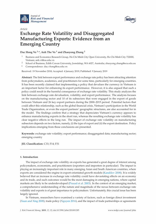
Journal of
Risk and FinancialManagement
Article
Exchange Rate Volatility and DisaggregatedManufacturing Exports: Evidence from anEmerging Country
Duc Hong Vo 1,*, Anh The Vo 1 and Zhaoyong Zhang 2
1 Business and Economics Research Group, Ho Chi Minh City Open University, Ho Chi Minh City 722000,Vietnam; [email protected]
2 School of Business, Edith Cowan University, Joondalup, WA 6027, Australia; [email protected]* Correspondence: [email protected]
Received: 19 November 2018; Accepted: 4 January 2019; Published: 9 January 2019
Abstract: The link between export performance and exchange rate policy has been attracting attentionfrom policymakers, academics, and practitioners for some time, particularly for emerging countries.It has been recently claimed that implementing a policy that devalues the currency in Vietnam isan important factor for enhancing its export performance. However, it is also argued that such apolicy could result in the harmful consequence of exchange rate volatility. This study analyzes thelink between exchange rate devaluation, volatility, and export performance. The analysis focuseson the manufacturing sector and 10 of its subsectors that were engaged in the export of goodsbetween Vietnam and 26 key export partners during the 2000–2015 period. Potential factors thatcould affect this relationship, such as the global financial crisis, Vietnam’s participation in the WorldTrade Organization, or even the export partners’ geographic structures, are also accounted for inthe model. The findings confirm that a strategy that depreciates Vietnam’s currency appears toenhance manufacturing exports in the short run, whereas the resulting exchange rate volatility hasclear negative effects in the long run. The impact of exchange rate volatility on manufacturingsubsectors depends on two factors, namely, (i) the type of export and (ii) the export destination. Policyimplications emerging from these conclusions are presented.
Keywords: exchange rate volatility; export performance; disaggregated data; manufacturing sector;emerging country
JEL Classification: C33; F14; F31
1. Introduction
The impact of exchange rate volatility on exports has generated a great degree of interest amongpolicymakers, economists, and practitioners (exporters and importers in particular). The impact isplaying an increasingly important role in many emerging Asian and South American countries, whereexports are considered the engine in export-orientated growth models (Kandilov 2008). It is widelybelieved that an increase in exchange rate volatility could have devastating effects on an economyand its trade, and such outcomes would be the most damaging in emerging nations, where capitalmarkets are likely to be underdeveloped (Prasad et al. 2003). In the context of an emerging market,a comprehensive understanding of the nature and magnitude of the nexus between exchange ratevolatility and exports is of great importance to policymakers. Unfortunately, this crucial issue has beenlargely ignored.
In Vietnam, researchers have examined a variety of factors, such as foreign direct investment(Xuan and Xing 2008), trade policy (Nguyen 2016), and the impact of trade partnerships or agreements
J. Risk Financial Manag. 2019, 12, 12; doi:10.3390/jrfm12010012 www.mdpi.com/journal/jrfm85
J. Risk Financial Manag. 2019, 12, 12
(Xiong 2017), that have affected aggregated exports. Nguyen (2016) examined the trade liberalizationpolicy in Vietnam and its link to the level of export sophistication. The study’s findings reveal that tradeliberalization has had a stronger effect on the non-manufacturing sector than the manufacturing sectorand that being a World Trade Organization (WTO) member does not have any impact on the level ofexport sophistication in Vietnam. In their analysis, Narayan and Nguyen (2016) used Vietnam as a casestudy to demonstrate how the variables in the gravity model are dependent on trading partners. Theirresults indicate that the country’s trading activities are more sensitive to exchanges with rich nationsthan low-income ones. Also, the issue of Vietnam’s currency depreciation (or devaluation, to use themore accurate term) has been the subject of debate in recent years. Some believe that although thisstrategy would enhance export performance, it would have the side effect of making exchange ratesvolatile, which, in turn, may be harmful to exports.
On balance, there are conflicting views in the literature on the relationship between exchange ratevolatility and exports: empirical studies have produced mixed results due to differing methodologies,volatility measurements, and the types of data used. To the best of our knowledge, few of thesestudies have been conducted in the context of Vietnam, so policies may lack evidentiary support fromacademic studies. Our efforts here are an attempt to fill this gap. This paper aims to provide empiricalevidence of the link between exchange rate devaluation, volatility, and export performance in Vietnamat disaggregated levels over a period of 16 years, from 2000 to 2015.
The contributions of this paper are as follows. First, a panel model was used to analyze therelationship between the two main variables of interest—the exchange rate volatility and exports,with a special focus on the manufacturing industry and its 10 subsectors. Details of the 10 subsectors,as well as 26 of Vietnam’s key export partners, are shown in Tables A1 and A2 in the Appendix. Thesepartners make up a significant share of Vietnam’s export transactions compared with the rest of theworld, and the manufacturing sector plays a substantial role in Vietnam’s export structure. We arguethat, in recent years, Vietnam has become a preferred destination for supply chain production formany multinational corporations (MNCs) due to the rise of China (Hooy et al. 2015). Also, the countryhas become deeply involved in further international economic integration by joining multilateralfree-trade agreements, such as the Regional Comprehensive Economic Partnership (RCEP). Second,we reexamined the effect of exchange rate volatility on exports in three different regions (Asia, Europe,and America). We are of the view that the manufacturing exports between Vietnam and its partnersin different regions may be influenced by regional factors such as geographic distances, political andeconomic relationships, and others. This may alter the export structure and the target destination,especially for the manufacturing sector. Therefore, we separated all of the data into three subsamplesbased on geographical characteristics, which enabled the exploration of whether location contributesto the impact on the nexus between exchange rate volatility and manufacturing exports in Vietnam.
The structure of this paper is as follows. Following this Introduction, information onmanufacturing exports and the trend of exchange rate volatility in Vietnam are briefly discussedin Section 2. Section 3 summarizes relevant theories and empirical studies related to exchange ratevolatility and exports. Model specifications are presented in Section 4. Section 5 describes the data andpresents the empirical results. A concluding remark follows in the remaining section of the paper.
2. Overview of Vietnam’s Exports and Exchange Rate
This section provides some background to provide insight into how the exchange rate market inVietnam operates, as well as the state of manufacturing exports in Vietnam during the 2000–2015 period.In Vietnam, the exchange rate market is controlled by the State Bank of Vietnam (SBV). In early 1999,it was announced that the exchange rate system would follow a managed floating regime, in whichthe SBV would publish a daily interbank exchange rate, the average of the exchange rate based on theprevious day, and a fluctuation band. The SBV predetermines the fluctuation band for exchange ratesto adjust to the market forces of demand and supply, and market participants are expected to tradewithin the setting band. Table 1 provides a summary of fluctuation bands specified by the SBV from
86
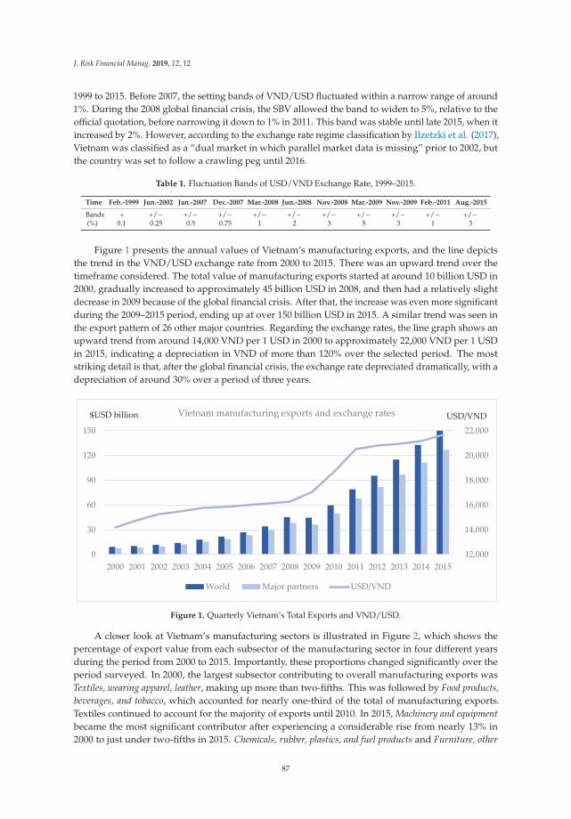
J. Risk Financial Manag. 2019, 12, 12
1999 to 2015. Before 2007, the setting bands of VND/USD fluctuated within a narrow range of around1%. During the 2008 global financial crisis, the SBV allowed the band to widen to 5%, relative to theofficial quotation, before narrowing it down to 1% in 2011. This band was stable until late 2015, when itincreased by 2%. However, according to the exchange rate regime classification by Ilzetzki et al. (2017),Vietnam was classified as a “dual market in which parallel market data is missing” prior to 2002, butthe country was set to follow a crawling peg until 2016.
Table 1. Fluctuation Bands of USD/VND Exchange Rate, 1999–2015.
Time Feb.-1999 Jun.-2002 Jan.-2007 Dec.-2007 Mar.-2008 Jun.-2008 Nov.-2008 Mar.-2009 Nov.-2009 Feb.-2011 Aug.-2015
Bands(%)
+0.1
+/−0.25
+/−0.5
+/−0.75
+/−1
+/−2
+/−3
+/−5
+/−3
+/−1
+/−3
Figure 1 presents the annual values of Vietnam’s manufacturing exports, and the line depictsthe trend in the VND/USD exchange rate from 2000 to 2015. There was an upward trend over thetimeframe considered. The total value of manufacturing exports started at around 10 billion USD in2000, gradually increased to approximately 45 billion USD in 2008, and then had a relatively slightdecrease in 2009 because of the global financial crisis. After that, the increase was even more significantduring the 2009–2015 period, ending up at over 150 billion USD in 2015. A similar trend was seen inthe export pattern of 26 other major countries. Regarding the exchange rates, the line graph shows anupward trend from around 14,000 VND per 1 USD in 2000 to approximately 22,000 VND per 1 USDin 2015, indicating a depreciation in VND of more than 120% over the selected period. The moststriking detail is that, after the global financial crisis, the exchange rate depreciated dramatically, with adepreciation of around 30% over a period of three years.
12,000
14,000
16,000
18,000
20,000
22,000
0
30
60
90
120
150
2000 2001 2002 2003 2004 2005 2006 2007 2008 2009 2010 2011 2012 2013 2014 2015
Vietnam manufacturing exports and exchange rates
World Major partners USD/VND
$USD billion USD/VND
Figure 1. Quarterly Vietnam’s Total Exports and VND/USD.
A closer look at Vietnam’s manufacturing sectors is illustrated in Figure 2, which shows thepercentage of export value from each subsector of the manufacturing sector in four different yearsduring the period from 2000 to 2015. Importantly, these proportions changed significantly over theperiod surveyed. In 2000, the largest subsector contributing to overall manufacturing exports wasTextiles, wearing apparel, leather, making up more than two-fifths. This was followed by Food products,beverages, and tobacco, which accounted for nearly one-third of the total of manufacturing exports.Textiles continued to account for the majority of exports until 2010. In 2015, Machinery and equipmentbecame the most significant contributor after experiencing a considerable rise from nearly 13% in2000 to just under two-fifths in 2015. Chemicals, rubber, plastics, and fuel products and Furniture, other
87
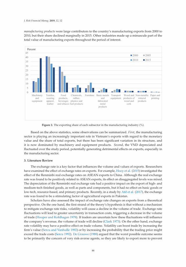
J. Risk Financial Manag. 2019, 12, 12
manufacturing products were large contributors to the country’s manufacturing exports from 2000 to2010, but their share declined marginally in 2015. Other industries made up a minuscule part of thetotal value of manufacturing exports throughout the period of interest.
Figure 2. The exporting share of each subsector in the manufacturing industry (%).
Based on the above statistics, some observations can be summarized. First, the manufacturingsector is playing an increasingly important role in Vietnam’s exports with regard to the monetaryvalue and the share of total exports, but there has been significant variation in its structure, andit is now dominated by machinery and equipment products. Second, the VND depreciated andfluctuated over the study period, potentially generating detrimental effects on exports, especially inthe manufacturing sector.
3. Literature Review
The exchange rate is a key factor that influences the volume and values of exports. Researchershave examined the effect of exchange rates on exports. For example, Hooy et al. (2015) investigated theeffect of the Renminbi real exchange rates on ASEAN exports to China. Although the real exchangerate was found to be positively related to ASEAN exports, its effect on disaggregated levels was mixed.The depreciation of the Renminbi real exchange rate had a positive impact on the export of high- andmedium-tech finished goods, as well as parts and components, but it had no effect on basic goods orlow-tech, resource-based, and primary products. Recently, in a study by Atif et al. (2017), the exchangerate was found to be a stimulating factor of agricultural exports in Pakistan.
Scholars have also assessed the impact of exchange rate changes on exports from a theoreticalperspective. On the one hand, the first strand of the theory’s hypothesis is that without a mechanismto mitigate exchange rate risks, volatility will cause a decline in the volume of trade. Exchange ratefluctuations will lead to greater uncertainty in transaction costs, triggering a decrease in the volumeof trade (Hooper and Kohlhagen 1978). If traders are uncertain how these fluctuations will influencethe company’s revenue, the volume of trade will decline (Clark 1973). On the other hand, exchangerate volatility may have a positive effect on trade volume. Volatility can boost trade by increasing thefirm’s value (Sercu and Vanhulle 1992) or by increasing the probability that the trading price mightexceed the trade costs (Sercu 1992). De Grauwe (1988) argued that the worst possible outcome seemsto be primarily the concern of very risk-averse agents, so they are likely to export more to prevent
88
J. Risk Financial Manag. 2019, 12, 12
a drastic decrease in their revenue. It is the extent of risk aversion among agents which determinesthe effect of volatility. Producers exhibiting even a slight degree of risk aversion will export less astheir marginal utility for export revenue declines. Some studies have concluded that the introductionof a capital market would not change the impact of volatility. Viaene and Vries (1992) conceded thatwithout hedging instruments, an increase in exchange rate risks leads to the deterioration of bothexports and imports. With the appearance of a forward market, the effects of exchange rate volatilityon importers and exporters are on opposite ends of the spectrum, because their roles are reversed.
Empirical studies have investigated the link between exchange rate volatility and exports usingaggregated trade data. For example, Asteriou et al. (2016) examined the relationship betweenexchange rate volatility and trade volume of four different nations—Mexico, Indonesia, Nigeria,and Turkey—with the rest of the world. These authors adopted the autoregressive distributed lag(ARDL) bound testing method to address the long-run association and the Granger causality test todetect the short-run relationship. In the long run, there was a marginally negative association betweenexchange rate volatility and trade volumes in Turkey, while, in the short run, Indonesia and Mexicoexperienced a causal relationship between these two variables. In their study, Hsu and Chiang (2011)found a negative effect of exchange rate volatility on trade between the US and 13 of its major tradingpartners, and this finding was unchanged when the sample size was expanded to 30 countries.
Studies have also focused on disaggregated data at commodity or sector levels. Choudhry andHassan (2015) reported the importance of exchange rate fluctuations for the UK’s imports from Brazil,China, and South Africa using an asymmetric ARDL model. The impact of the global financial crisison the link between volatility and imports was also taken into consideration. Thus, policymakersshould be cautious when making decisions, as any policy actions or trade adjustment programs mayhave unpredicted outcomes if the exchange rate becomes volatile. Bahmani-Oskooee et al. (2013)investigated the impact of exchange rate volatility on the bilateral imports and exports between Braziland the US between 1971 and 2010 for more than 100 industries. There were several interestingfindings. First, a vast number of the selected industries were not affected by exchange rate fluctuations,and the positive links significantly dominated the negative effects. Second, volatility had a moresignificant impact on small industries, which account for a smaller share of the total export value.Third, each industry reacted differently in response to volatility: for example, agricultural exportsin Brazil were found to be negatively related, while there were no recorded impacts on importingmachinery products in the US. Nishimura and Hirayama (2013) provided empirical evidence of theeffect of exchange rate volatility on Japan–China trade. The findings illustrate that although theexchange rate variation did not affect Japan’s exports to China, it had a negative influence on thereverse direction of trade—exporting from China to Japan—during the reform stage.
Authors have also attempted to investigate the long-run and short-run relationship betweenexchange rate volatility and trade at industry levels between two countries based on the cointegrationanalysis and bound testing approach. Typical pairs of countries used in these studies includeMalaysia and Thailand (Aftab et al. 2017), Malaysia and Japan (Aftab et al. 2015), Malaysia andChina (Soleymani and Chua 2014), Canada and Mexico (Bahmani-Oskooee et al. 2012), and the USand China (Bahmani-Oskooee and Wang 2007). These studies, taken together, support both positiveand negative impacts of exchange rate volatility on commodity trade between a country and one of itspartners. However, the impact may vary across the partners selected in the analysis. This suggests thatthe impact of exchange rate volatility on exports should be tested case by case; thus, studies on thisissue are always valuable.
It is important to consider impacts at the aggregated level so that policymakers have a generalenough picture of the effect of the exchange rate on exports. Nevertheless, using aggregated datacan lead to aggregated bias problems: the insignificant price elasticity of one industry could overlapwith that of another industry, potentially yielding an insignificant elasticity at the aggregated level(Bahmani-Oskooee et al. 2012). Investigating the issue at the disaggregated level provides moredetail on the effect of volatility on exports. Without considering the disaggregated level, it is likely
89
J. Risk Financial Manag. 2019, 12, 12
to be difficult for policymakers to ascertain which sectors actually suffer adverse effects of volatility.In this regard, the analysis presented in this paper included both forms of data, rather than a singlesource. Not only were the aggregated data of the manufacturing sector adopted in the analysis,but the disaggregated data of the manufacturing subsectors were also employed. We aim to add tothe literature by investigating a case study of a small open dynamic economy. The aggregated anddisaggregated outcomes are expected to supplement one another so that policymakers will have abalanced perspective on this complex effect.
An issue that lacks consistency among researchers is the measure of exchange rate volatility, asthere is no universal consensus on the proxy to use in empirical studies. As such, multiple measureshave been employed to represent volatility, three of which are widely adopted in empirical studies.The first is the standard deviation of the percentage change in the exchange rate (Chit 2008; Hayakawaand Kimura 2009). The second measure of volatility is the moving average standard deviation (MASD)of the real exchange rate in logarithmic terms (Chit et al. 2010; De Vita and Abbott 2004). The thirdmeasure is based on the conditional variance of exchange rates using the generalized autoregressiveconditional heteroscedasticity (GARCH) model. While some scholars adopt just one proxy, others haveused multiple alternatives as a robustness check. De Vita and Abbott (2004) compared three measuresof exchange rate volatility in their study, which examined the effect of volatility on the UK’s exports to14 other European nations. The results indicate that the MASD is likely the optimal volatility measureof total exports and subsector exports from the UK to the whole group of nations studied, while a mixof different alternatives are appropriate for analyzing exports from the UK to each individual country.
4. Model Specifications
Following previous studies (Aristotelous 2001; Chit et al. 2010), the model used for estimating theeffects of exchange rate volatility and exports is specified as follows:
lnEXmit = αct + β1lnGDPit + β2lnREXRit + β3lnVOLit + εit (1)
where EXmit denotes the real export value in thousands of US dollars of the manufacturing sector as
well as its 10 subsectors m at time t from Vietnam to its export partners i. GDPit represents the realGross Domestic Product (GDP) in a foreign partner country i of Vietnam, deflated by the GDP deflator.The real bilateral exchange rates (REXRit) between Vietnam and its counterparts are measured bymultiplying the relative price and the bilateral exchange rates, which are indirectly derived fromUS-based currency. The relative price is the ratio of the consumer price index (CPI) of export partnersto the CPI of Vietnam.1 Therefore, an increase in the value of the real exchange rate indicates adepreciation of Vietnam’s currency. Finally, our variable of interest is the volatility of the bilateralexchange rate (VOLit), measured by the GARCH model.
The first step is to check whether all variables of interest are stationary. We used three panel unitroot tests, including those of IPS (Im et al. 2003), Maddala and Wu (1999), and Choi (2001). Unlike othertypes of panel stationary tests, these tests allow data to be unbalanced. Next, the long-run relationshipamong these variables was checked using the cointegration tests introduced by Pedroni (1999, 2001),together with long-run estimations based on Panel Dynamic Ordinary Least Squares (DOLS). We usedDOLS because it is asymptotically unbiased, normally distributed, and controls for the problem ofendogeneity. Finally, to investigate the influence of the exchange rate on the growth of exports duringthe surveyed period, the equation was transformed in terms of an error correction model (ECM):
1 We would like to thank an anonymous referee for his/her suggestion to use the real bilateral exchange rate. Many of thecountries in the sample had varying inflation rates relative to Vietnam.
90
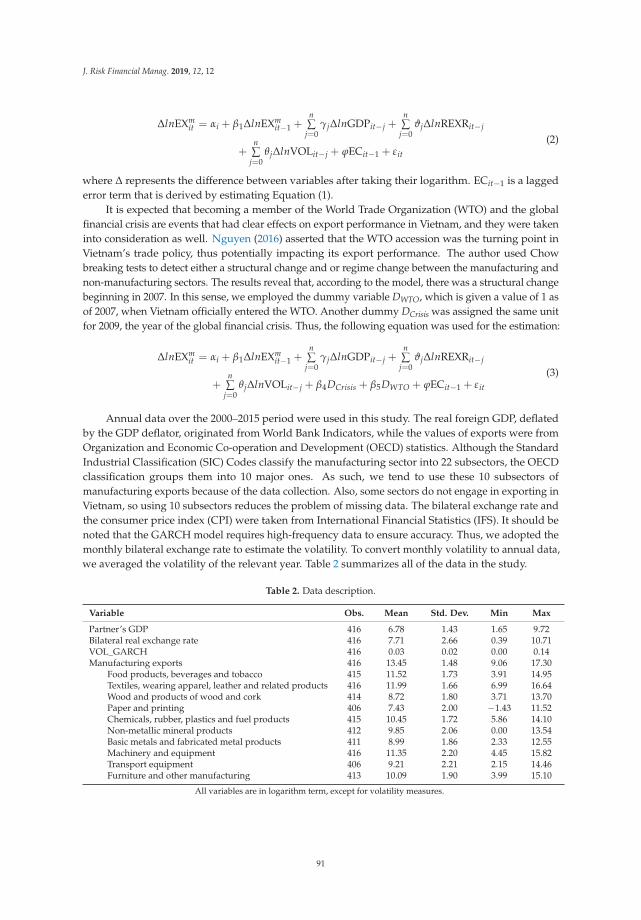
J. Risk Financial Manag. 2019, 12, 12
ΔlnEXmit = αi + β1ΔlnEXm
it−1 +n∑
j=0γjΔlnGDPit−j +
n∑
j=0ϑjΔlnREXRit−j
+n∑
j=0θjΔlnVOLit−j + ϕECit−1 + εit
(2)
where Δ represents the difference between variables after taking their logarithm. ECit−1 is a laggederror term that is derived by estimating Equation (1).
It is expected that becoming a member of the World Trade Organization (WTO) and the globalfinancial crisis are events that had clear effects on export performance in Vietnam, and they were takeninto consideration as well. Nguyen (2016) asserted that the WTO accession was the turning point inVietnam’s trade policy, thus potentially impacting its export performance. The author used Chowbreaking tests to detect either a structural change and or regime change between the manufacturing andnon-manufacturing sectors. The results reveal that, according to the model, there was a structural changebeginning in 2007. In this sense, we employed the dummy variable DWTO, which is given a value of 1 asof 2007, when Vietnam officially entered the WTO. Another dummy DCrisis was assigned the same unitfor 2009, the year of the global financial crisis. Thus, the following equation was used for the estimation:
ΔlnEXmit = αi + β1ΔlnEXm
it−1 +n∑
j=0γjΔlnGDPit−j +
n∑
j=0ϑjΔlnREXRit−j
+n∑
j=0θjΔlnVOLit−j + β4DCrisis + β5DWTO + ϕECit−1 + εit
(3)
Annual data over the 2000–2015 period were used in this study. The real foreign GDP, deflatedby the GDP deflator, originated from World Bank Indicators, while the values of exports were fromOrganization and Economic Co-operation and Development (OECD) statistics. Although the StandardIndustrial Classification (SIC) Codes classify the manufacturing sector into 22 subsectors, the OECDclassification groups them into 10 major ones. As such, we tend to use these 10 subsectors ofmanufacturing exports because of the data collection. Also, some sectors do not engage in exporting inVietnam, so using 10 subsectors reduces the problem of missing data. The bilateral exchange rate andthe consumer price index (CPI) were taken from International Financial Statistics (IFS). It should benoted that the GARCH model requires high-frequency data to ensure accuracy. Thus, we adopted themonthly bilateral exchange rate to estimate the volatility. To convert monthly volatility to annual data,we averaged the volatility of the relevant year. Table 2 summarizes all of the data in the study.
Table 2. Data description.
Variable Obs. Mean Std. Dev. Min Max
Partner’s GDP 416 6.78 1.43 1.65 9.72Bilateral real exchange rate 416 7.71 2.66 0.39 10.71VOL_GARCH 416 0.03 0.02 0.00 0.14Manufacturing exports 416 13.45 1.48 9.06 17.30
Food products, beverages and tobacco 415 11.52 1.73 3.91 14.95Textiles, wearing apparel, leather and related products 416 11.99 1.66 6.99 16.64Wood and products of wood and cork 414 8.72 1.80 3.71 13.70Paper and printing 406 7.43 2.00 −1.43 11.52Chemicals, rubber, plastics and fuel products 415 10.45 1.72 5.86 14.10Non-metallic mineral products 412 9.85 2.06 0.00 13.54Basic metals and fabricated metal products 411 8.99 1.86 2.33 12.55Machinery and equipment 416 11.35 2.20 4.45 15.82Transport equipment 406 9.21 2.21 2.15 14.46Furniture and other manufacturing 413 10.09 1.90 3.99 15.10
All variables are in logarithm term, except for volatility measures.
91
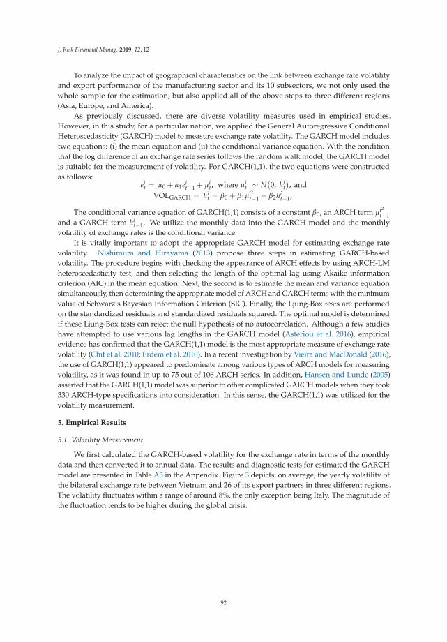
J. Risk Financial Manag. 2019, 12, 12
To analyze the impact of geographical characteristics on the link between exchange rate volatilityand export performance of the manufacturing sector and its 10 subsectors, we not only used thewhole sample for the estimation, but also applied all of the above steps to three different regions(Asia, Europe, and America).
As previously discussed, there are diverse volatility measures used in empirical studies.However, in this study, for a particular nation, we applied the General Autoregressive ConditionalHeteroscedasticity (GARCH) model to measure exchange rate volatility. The GARCH model includestwo equations: (i) the mean equation and (ii) the conditional variance equation. With the conditionthat the log difference of an exchange rate series follows the random walk model, the GARCH modelis suitable for the measurement of volatility. For GARCH(1,1), the two equations were constructedas follows:
eit = α0 + α1ei
t−1 + μit, where μi
t ∼ N(0, hi
t), and
VOLGARCH = hit = β0 + β1μi2
t−1 + β2hit−1,
The conditional variance equation of GARCH(1,1) consists of a constant β0, an ARCH term μi2t−1
and a GARCH term hit−1. We utilize the monthly data into the GARCH model and the monthly
volatility of exchange rates is the conditional variance.It is vitally important to adopt the appropriate GARCH model for estimating exchange rate
volatility. Nishimura and Hirayama (2013) propose three steps in estimating GARCH-basedvolatility. The procedure begins with checking the appearance of ARCH effects by using ARCH-LMheteroscedasticity test, and then selecting the length of the optimal lag using Akaike informationcriterion (AIC) in the mean equation. Next, the second is to estimate the mean and variance equationsimultaneously, then determining the appropriate model of ARCH and GARCH terms with the minimumvalue of Schwarz’s Bayesian Information Criterion (SIC). Finally, the Ljung-Box tests are performedon the standardized residuals and standardized residuals squared. The optimal model is determinedif these Ljung-Box tests can reject the null hypothesis of no autocorrelation. Although a few studieshave attempted to use various lag lengths in the GARCH model (Asteriou et al. 2016), empiricalevidence has confirmed that the GARCH(1,1) model is the most appropriate measure of exchange ratevolatility (Chit et al. 2010; Erdem et al. 2010). In a recent investigation by Vieira and MacDonald (2016),the use of GARCH(1,1) appeared to predominate among various types of ARCH models for measuringvolatility, as it was found in up to 75 out of 106 ARCH series. In addition, Hansen and Lunde (2005)asserted that the GARCH(1,1) model was superior to other complicated GARCH models when they took330 ARCH-type specifications into consideration. In this sense, the GARCH(1,1) was utilized for thevolatility measurement.
5. Empirical Results
5.1. Volatility Measurement
We first calculated the GARCH-based volatility for the exchange rate in terms of the monthlydata and then converted it to annual data. The results and diagnostic tests for estimated the GARCHmodel are presented in Table A3 in the Appendix. Figure 3 depicts, on average, the yearly volatility ofthe bilateral exchange rate between Vietnam and 26 of its export partners in three different regions.The volatility fluctuates within a range of around 8%, the only exception being Italy. The magnitude ofthe fluctuation tends to be higher during the global crisis.
92

J. Risk Financial Manag. 2019, 12, 12
Exchange rate volality in AsiaAustraliaCambodiaChinaHong KongIndiaIndonesiaJapanKoreaMalaysiaPhilippinesRussiaSingaporeThailand
Exchange rate volatility in Europe
Belgium
France
Germany
Italy
Netherlands
Exchange rate volatility in AmericaBrazil
Canada
Mexico
SouthAfrica
UnitedStates
Figure 3. Exchange rate volatility over the 2000–2015 period.
5.2. Effects of Exchange Rate Volatility on Exports
This section presents the estimation results pertaining to the effects of exchange rate volatilityon manufacturing exports for the whole sample and in three regions—Asia, Europe, and America.We first show the result for the manufacturing sector, followed by its 10 subsectors.
Regarding the manufacturing sector, Tables 3 and 4 show the results of three kinds of panel unitroot tests—IPS (Im et al. 2003), Maddala and Wu (1999), and Choi (2001)—for the whole sample and inthree regions, respectively. At the manufacturing sector level, strong evidence of unit roots is found forthe foreign GDP and real bilateral exchange rate, while, for the difference, the hypothesis that unit
93
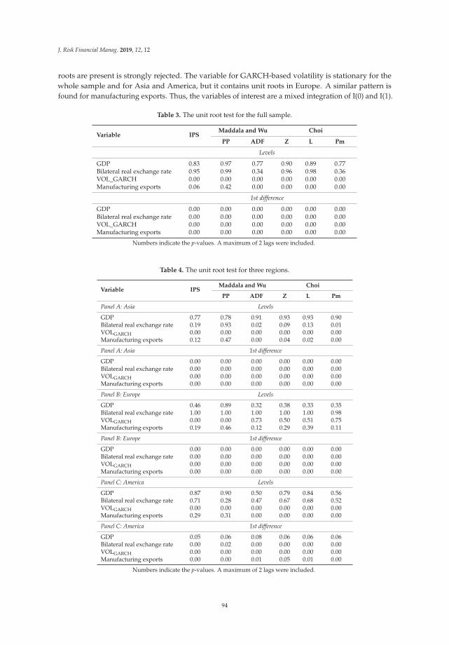
J. Risk Financial Manag. 2019, 12, 12
roots are present is strongly rejected. The variable for GARCH-based volatility is stationary for thewhole sample and for Asia and America, but it contains unit roots in Europe. A similar pattern isfound for manufacturing exports. Thus, the variables of interest are a mixed integration of I(0) and I(1).
Table 3. The unit root test for the full sample.
Variable IPSMaddala and Wu Choi
PP ADF Z L Pm
Levels
GDP 0.83 0.97 0.77 0.90 0.89 0.77Bilateral real exchange rate 0.95 0.99 0.34 0.96 0.98 0.36VOL_GARCH 0.00 0.00 0.00 0.00 0.00 0.00Manufacturing exports 0.06 0.42 0.00 0.00 0.00 0.00
1st difference
GDP 0.00 0.00 0.00 0.00 0.00 0.00Bilateral real exchange rate 0.00 0.00 0.00 0.00 0.00 0.00VOL_GARCH 0.00 0.00 0.00 0.00 0.00 0.00Manufacturing exports 0.00 0.00 0.00 0.00 0.00 0.00
Numbers indicate the p-values. A maximum of 2 lags were included.
Table 4. The unit root test for three regions.
Variable IPSMaddala and Wu Choi
PP ADF Z L Pm
Panel A: Asia Levels
GDP 0.77 0.78 0.91 0.93 0.93 0.90Bilateral real exchange rate 0.19 0.93 0.02 0.09 0.13 0.01VOLGARCH 0.00 0.00 0.00 0.00 0.00 0.00Manufacturing exports 0.12 0.47 0.00 0.04 0.02 0.00
Panel A: Asia 1st difference
GDP 0.00 0.00 0.00 0.00 0.00 0.00Bilateral real exchange rate 0.00 0.00 0.00 0.00 0.00 0.00VOLGARCH 0.00 0.00 0.00 0.00 0.00 0.00Manufacturing exports 0.00 0.00 0.00 0.00 0.00 0.00
Panel B: Europe Levels
GDP 0.46 0.89 0.32 0.38 0.33 0.35Bilateral real exchange rate 1.00 1.00 1.00 1.00 1.00 0.98VOLGARCH 0.00 0.00 0.73 0.50 0.51 0.75Manufacturing exports 0.19 0.46 0.12 0.29 0.39 0.11
Panel B: Europe 1st difference
GDP 0.00 0.00 0.00 0.00 0.00 0.00Bilateral real exchange rate 0.00 0.00 0.00 0.00 0.00 0.00VOLGARCH 0.00 0.00 0.00 0.00 0.00 0.00Manufacturing exports 0.00 0.00 0.00 0.00 0.00 0.00
Panel C: America Levels
GDP 0.87 0.90 0.50 0.79 0.84 0.56Bilateral real exchange rate 0.71 0.28 0.47 0.67 0.68 0.52VOLGARCH 0.00 0.00 0.00 0.00 0.00 0.00Manufacturing exports 0.29 0.31 0.00 0.00 0.00 0.00
Panel C: America 1st difference
GDP 0.05 0.06 0.08 0.06 0.06 0.06Bilateral real exchange rate 0.00 0.02 0.00 0.00 0.00 0.00VOLGARCH 0.00 0.00 0.00 0.00 0.00 0.00Manufacturing exports 0.00 0.00 0.01 0.05 0.01 0.00
Numbers indicate the p-values. A maximum of 2 lags were included.
94
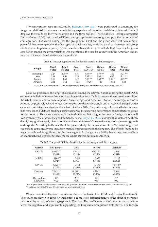
J. Risk Financial Manag. 2019, 12, 12
The cointegration tests introduced by Pedroni (1999, 2001) were performed to determine thelong-run relationship between manufacturing exports and the other variables of interest. Table 5displays the results for the whole sample and the three regions. Three statistics—group augmentedDickey-Fuller (ADF) test, panel ADF test, and group rho test—strongly support the hypothesis ofcointegration. It is worth noting that the group small t-test and the group ADF test have a morepowerful feature compared with other types of panel statistics, while the panel variance test and grouprho test seem to perform poorly. Thus, based on this feature, we conclude that there is a long-runassociation among the given variables. An exception is the case for countries in the American region,as none of the calculated statistics are significant.
Table 5. The cointegration test for the full sample and three regions.
SamplePanelv-stat
Panelrho-stat
Panelt-stat
PanelADF-stat
Grouprho-stat
Groupt-stat
GroupADF-stat
Full sample 0.29 2.26 ** 0.53 4.55 *** 4.35 *** 1.43 6.21 ***Asia 0.04 1.53 0.14 3.35 *** 3.05 *** 0.87 5.11 ***
Europe 0.16 1.60 1.49 3.87 *** 2.63 *** 2.19 ** 4.02 ***America 0.42 0.64 −1.24 −0.26 1.67 −0.91 0.84
**, *** indicate the hypothesis of no cointegration is rejected at significance levels of 5%, and 1%.
Next, we performed the long-run estimation among the relevant variables using the panel DOLSestimation in light of the confirmation by cointegration tests. Table 6 presents the estimation result forthe whole sample and in three regions—Asia, Europe, and America. Overall, the foreign income isfound to be positively related to Vietnam’s exports for the whole sample and in Asia and Europe, as theestimated coefficients are significant at a level of at least 10%. The positive sign illustrates that an increasein income among Vietnam’ trading partners enhances the exporting performance of manufactured goodsfor the country. This is consistent with the trade theory that a higher income in foreign nations willlead to an increase in domestic good demands. Also, Hooy et al. (2015) asserted that Vietnam has beendeeply engaged in supply chain production due to the rise of China, enhancing both economic growthand exports. According to the results of the present study, the depreciation of the Vietnam Dong is notexpected to cause an adverse impact on manufacturing exports in the long run. The effect is found to benegative, although insignificant, for the three regions. Exchange rate volatility has strong reverse effectson manufacturing exports, not only for the whole sample but also in America.
Table 6. The panel DOLS estimation for the full sample and three regions.
Variable Full Sample Asia Europe America
LnGDP 0.415 *** 0.222 * 0.831 *** 0.598(0.054) (0.119) (0.296) (0.441)
LnREXR −0.065 ** −0.045 −0.305 −0.163(0.029) (0.066) (0.551) (0.354)
LnVOL −0.829 *** −0.312 −0.476 −1.854 **(0.127) (0.463) (0.350) (0.805)
Constant 7.961 *** 11.236 *** 8.779 * 2.916(0.658) (2.203) (5.079) (2.435)
Observations 413 205 125 77R-squared 0.23 0.16 0.41 0.62
“Ln” represents variables defined in terms of logarithm. Standard errors are numbers in the parentheses. *, **, and*** indicate the 10%, 5% and 1% significance level, respectively.
We also examined the short-run relationship on the basis of the ECM model using Equation (3).The results are shown in Table 7, which paint a completely different picture of the effect of exchangerate volatility on manufacturing exports in Vietnam. The coefficients of the lagged error correctionterms are negative and significant, supporting the long-run cointegration tests above. The foreign
95
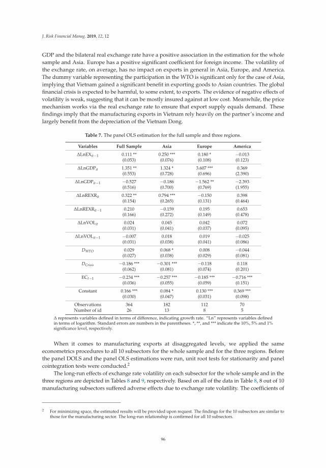
J. Risk Financial Manag. 2019, 12, 12
GDP and the bilateral real exchange rate have a positive association in the estimation for the wholesample and Asia. Europe has a positive significant coefficient for foreign income. The volatility ofthe exchange rate, on average, has no impact on exports in general in Asia, Europe, and America.The dummy variable representing the participation in the WTO is significant only for the case of Asia,implying that Vietnam gained a significant benefit in exporting goods to Asian countries. The globalfinancial crisis is expected to be harmful, to some extent, to exports. The evidence of negative effects ofvolatility is weak, suggesting that it can be mostly insured against at low cost. Meanwhile, the pricemechanism works via the real exchange rate to ensure that export supply equals demand. Thesefindings imply that the manufacturing exports in Vietnam rely heavily on the partner’s income andlargely benefit from the depreciation of the Vietnam Dong.
Table 7. The panel OLS estimation for the full sample and three regions.
Variables Full Sample Asia Europe America
ΔLnEXit−1 0.111 ** 0.250 *** 0.180 * −0.013(0.053) (0.076) (0.108) (0.123)
ΔLnGDPit 1.351 ** 1.324 * 3.607 *** 0.369(0.553) (0.728) (0.696) (2.390)
ΔLnGDPit−1 −0.527 −0.186 −1.562 ** −2.393(0.516) (0.700) (0.769) (1.955)
ΔLnREXRit 0.322 ** 0.794 *** −0.150 0.398(0.154) (0.265) (0.131) (0.464)
ΔLnREXRit−1 0.210 −0.159 0.195 0.653(0.166) (0.272) (0.149) (0.478)
ΔLnVOLit 0.024 0.045 0.042 0.072(0.031) (0.041) (0.037) (0.095)
ΔLnVOLit−1 −0.007 0.018 0.019 −0.025(0.031) (0.038) (0.041) (0.086)
DWTO 0.029 0.068 * 0.008 −0.044(0.027) (0.038) (0.029) (0.081)
DCrisis −0.186 *** −0.301 *** −0.118 0.118(0.062) (0.081) (0.074) (0.201)
ECt−1 −0.234 *** −0.257 *** −0.185 *** −0.716 ***(0.036) (0.055) (0.059) (0.151)
Constant 0.166 *** 0.084 * 0.130 *** 0.369 ***(0.030) (0.047) (0.031) (0.098)
Observations 364 182 112 70Number of id 26 13 8 5
Δ represents variables defined in terms of difference, indicating growth rate. “Ln” represents variables definedin terms of logarithm. Standard errors are numbers in the parentheses. *, **, and *** indicate the 10%, 5% and 1%significance level, respectively.
When it comes to manufacturing exports at disaggregated levels, we applied the sameeconometrics procedures to all 10 subsectors for the whole sample and for the three regions. Beforethe panel DOLS and the panel OLS estimations were run, unit root tests for stationarity and panelcointegration tests were conducted.2
The long-run effects of exchange rate volatility on each subsector for the whole sample and in thethree regions are depicted in Tables 8 and 9, respectively. Based on all of the data in Table 8, 8 out of 10manufacturing subsectors suffered adverse effects due to exchange rate volatility. The coefficients of
2 For minimizing space, the estimated results will be provided upon request. The findings for the 10 subsectors are similar tothose for the manufacturing sector. The long-run relationship is confirmed for all 10 subsectors.
96
J. Risk Financial Manag. 2019, 12, 12
two subsectors, namely, textiles, wearing apparel, leather, and related products and chemicals, rubber, plastics,and fuel products, are statistically insignificant although negative. The effect of the bilateral real exchangerate is also found to be negative in five subsectors in the long run. Thus, a depreciation policy in Vietnamwould lead to a decline in export value in the long term as it generates volatility in the exchange rate.
When the geographical factor is taken into consideration, we observe a completely differentpicture of the relationship between exchange rate devaluation, exchange rate volatility, and exportperformance at the subsector level. As can be seen from Table 9, exchange rate volatility has almost noeffect on exports in Asia and Europe, but America has five subsectors that are negatively related tothe exchange rate volatility.3 It is only the subsector of non-metallic mineral products in the Americanregion that enjoys a favorable gain from exchange rate depreciation without being influenced by theexchange rate fluctuation.
Using Equation (3), the short-run effects of exchange rate volatility on export performance atdisaggregated levels were regressed and are provided in the next four tables with the application ofpanel estimation. Table 10 presents the result for the whole sample. The bilateral real exchange ratehas a favorable impact on exports in such subsectors as (i) textiles, wearing apparel, leather, and relatedproducts and (ii) furniture and other manufacturing products. This implies that depreciation boosts exportsin the short run rather than in the long run in some subsectors. Similarly, exchange rate volatilityis found to be positively associated with exports for the subsector of transport equipment. Exportersin this subsector may pursue a strategy of exporting more in order to maintain its trading value, ashypothesized by De Grauwe (1988). The subsector of chemicals, rubber, plastics, and fuel products is foundto be quite sensitive to exchange rate volatility in the short run, given that its estimated coefficient ispositive in the current period but becomes negative in the first lag. We find no statistically significanteffect of exchange rate depreciation and volatility on export values for the eight remaining subsectors.
A significantly different pattern is seen in Asia, Europe, and America, as indicated in Tables 11–13,respectively. The short-run effects of exchange rate volatility vary considerably across the subsectors, aswell as in the given regions. Asia has three subsectors that are positively associated with exchange ratevolatility, together with one that reacts negatively. In Europe, the number of subsectors experiencingfavorable and harmful effects is three and two, respectively. In America, 3 out of 10 subsectors are foundto be positively related to exchange rate fluctuations. Interesting to note is that the export performancein the subsector of Transport equipment is observed to benefit from the exchange rate fluctuations,as its estimated coefficients are statistically positive in all three regions. There is an increase in theexport performance of textiles, wearing apparel, leather, and related products to countries in Europe andAmerica when the exchange rate is volatile. The Paper and printing subsector is negatively related tothe exchange rate fluctuations in Asia but positively associated in Europe. Other subsectors, such as(i) wood and products of wood and cork, (ii) Chemicals, rubber, plastics, and fuel products, (iii) Non-metallicmineral products, and (iv) Furniture and other manufacturing products are influenced by exchange ratevolatility, either positively or negatively.
In the short run, the impact of the bilateral exchange rate on the export performance atdisaggregated levels is considerably different across the regions. When the real bilateral exchangedevaluates, it raises Vietnam’s export value in three subsectors—textiles, wearing apparel, leather,and related products; wood and products of wood and cork; and paper and printing—to countries in Europeand America, and it has no effect on the remaining subsectors. In Europe, the estimated resultsindicate that two subsectors are positively influenced by exchange rate fluctuations, another two reactnegatively, and results for the rest of the subsectors are inconclusive. All results prove that the impactof the exchange rate on exports at the manufacturing disaggregated level depends on two factors:(i) the type of export and (ii) the exporting destination.
3 Table A4 presented in indicates the percent change in exports for the manufacturing subsectors resulting from a 1% increasein exchange rate volatility.
97
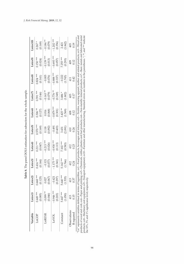
J. Risk Financial Manag. 2019, 12, 12
Ta
ble
8.
The
pane
lDO
LSes
tim
atio
nfo
rsu
bsec
tors
for
the
who
lesa
mpl
e.
Va
ria
ble
Ln
(ex
1)
Ln
(ex
2)
Ln
(ex
3)
Ln
(ex
4)
Ln
(ex
5)
Ln
(ex
6)
Ln
(ex
7)
Ln
(ex
8)
Ln
(ex
9)
Ln
(ex
10
)
LnG
DP
0.44
9**
*0.
668
***
0.41
6**
*0.
211
***
0.57
0**
*0.
306
**0.
591
***
0.82
4**
*0.
150
***
0.26
7*
(0.0
85)
(0.1
25)
(0.1
44)
(0.0
47)
(0.1
69)
(0.1
27)
(0.1
46)
(0.1
41)
(0.0
24)
(0.1
49)
LnR
EXR
−0.0
99**
0.02
7−0
.121
−0.2
13**
*0.
118
0.01
6−0
.163
**−0
.005
−0.1
39**
*−0
.184
**(0
.046
)(0
.067
)(0
.077
)(0
.026
)(0
.092
)(0
.068
)(0
.079
)(0
.076
)(0
.013
)(0
.079
)
LnV
OL
−0.9
46**
*−0
.421
−1.1
75**
*−0
.930
***
−0.4
91−0
.879
***
−0.7
76**
−0.8
88**
*−0
.693
***
−1.2
02**
*(0
.203
)(0
.297
)(0
.341
)(0
.113
)(0
.403
)(0
.301
)(0
.349
)(0
.337
)(0
.057
)(0
.356
)
Con
stan
t5.
447
***
5.64
0**
*5.
142
***
7.10
2**
*3.
431
3.42
5**
3.48
6*
−0.2
227.
255
***
2.42
1(1
.050
)(1
.535
)(1
.766
)(0
.583
)(2
.091
)(1
.569
)(1
.802
)(1
.745
)(0
.293
)(1
.842
)
Obs
erva
tion
s41
341
341
241
241
040
840
341
140
940
3R
-squ
ared
0.15
0.37
0.24
0.23
0.26
0.12
0.17
0.42
0.12
0.19
“Ln”
repr
esen
tsva
riab
les
defi
ned
inte
rms
oflo
gari
thm
.ex1
—Fo
odpr
oduc
ts,b
ever
ages
and
toba
cco;
ex2—
Text
iles,
wea
ring
appa
rel,
leat
her
and
rela
ted
prod
ucts
;ex3
—W
ood
and
prod
ucts
ofw
ood
and
cork
;ex4
—Pa
per
and
prin
ting
;ex5
—C
hem
ical
s,ru
bber
,pla
stic
san
dfu
elpr
oduc
ts;e
x6—
Non
-met
allic
min
eral
prod
ucts
;ex7
—Ba
sic
met
als
and
fabr
icat
edm
etal
prod
ucts
;ex8
—M
achi
nery
and
equi
pmen
t;ex
9—Tr
ansp
orte
quip
men
t;ex
10—
Furn
iture
and
othe
rm
anuf
actu
ring
.Sta
ndar
der
rors
are
num
bers
inth
epa
rent
hese
s.*,
**,a
nd**
*in
dica
teth
e10
%,5
%an
d1%
sign
ifica
nce
leve
l,re
spec
tive
ly.
98
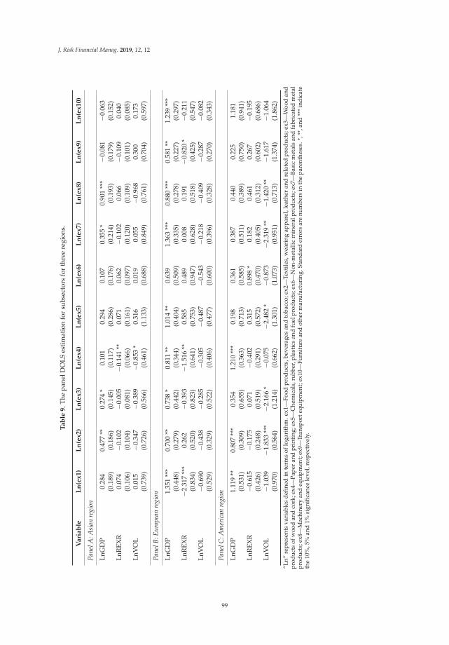
J. Risk Financial Manag. 2019, 12, 12
Ta
ble
9.
The
pane
lDO
LSes
tim
atio
nfo
rsu
bsec
tors
for
thre
ere
gion
s.
Va
ria
ble
Ln
(ex
1)
Ln
(ex
2)
Ln
(ex
3)
Ln
(ex
4)
Ln
(ex
5)
Ln
(ex
6)
Ln
(ex
7)
Ln
(ex
8)
Ln
(ex
9)
Ln
(ex
10
)
Pane
lA:A
sian
regi
on
LnG
DP
0.28
40.
477
**0.
274
*0.
101
0.29
40.
107
0.35
5*
0.90
1**
*−0
.081
−0.0
63(0
.189
)(0
.186
)(0
.145
)(0
.117
)(0
.286
)(0
.176
)(0
.214
)(0
.193
)(0
.179
)(0
.152
)Ln
REX
R0.
074
−0.1
02−0
.005
−0.1
41**
0.07
10.
062
−0.1
020.
066
−0.1
090.
040
(0.1
06)
(0.1
04)
(0.0
81)
(0.0
66)
(0.1
61)
(0.0
97)
(0.1
20)
(0.1
09)
(0.1
01)
(0.0
85)
LnV
OL
0.01
5−0
.347
−0.3
89−0
.853
*0.
316
0.01
90.
055
−0.9
680.
300
0.17
3(0
.739
)(0
.726
)(0
.566
)(0
.461
)(1
.133
)(0
.688
)(0
.849
)(0
.761
)(0
.704
)(0
.597
)
Pane
lB:E
urop
ean
regi
on
LnG
DP
1.35
1**
*0.
700
**0.
738
*0.
811
**1.
014
**0.
639
1.36
3**
*0.
880
***
0.58
1**
1.23
9**
*(0
.448
)(0
.279
)(0
.442
)(0
.344
)(0
.404
)(0
.509
)(0
.335
)(0
.278
)(0
.227
)(0
.297
)Ln
REX
R−2
.317
***
0.26
2−0
.393
−1.5
16**
0.58
50.
489
0.00
80.
191
−0.8
20*
−0.2
11(0
.834
)(0
.520
)(0
.823
)(0
.641
)(0
.753
)(0
.947
)(0
.628
)(0
.518
)(0
.425
)(0
.547
)Ln
VO
L−0
.690
−0.4
38−0
.285
−0.3
05−0
.487
−0.5
43−0
.218
−0.4
09−0
.287
−0.0
82(0
.529
)(0
.329
)(0
.522
)(0
.406
)(0
.477
)(0
.600
)(0
.396
)(0
.328
)(0
.270
)(0
.343
)
Pane
lC:A
mer
ican
regi
on
LnG
DP
1.11
9**
0.80
7**
*0.
354
1.21
0**
*0.
198
0.36
10.
387
0.44
00.
225
1.18
1(0
.531
)(0
.309
)(0
.655
)(0
.363
)(0
.713
)(0
.585
)(0
.511
)(0
.389
)(0
.750
)(0
.941
)Ln
REX
R−0
.615
−0.1
750.
071
−0.4
020.
315
0.89
8*
0.18
20.
461
0.26
7−0
.195
(0.4
26)
(0.2
48)
(0.5
19)
(0.2
91)
(0.5
72)
(0.4
70)
(0.4
05)
(0.3
12)
(0.6
02)
(0.6
86)
LnV
OL
−1.0
39−1
.833
***
−2.1
66*
−0.0
75−2
.482
*−0
.873
−2.3
19**
−1.4
20**
−1.6
17−1
.064
(0.9
70)
(0.5
64)
(1.2
14)
(0.6
62)
(1.3
01)
(1.0
73)
(0.9
51)
(0.7
13)
(1.3
74)
(1.8
62)
“Ln”
repr
esen
tsva
riab
les
defi
ned
inte
rms
oflo
gari
thm
.ex1
—Fo
odpr
oduc
ts,b
ever
ages
and
toba
cco;
ex2—
Text
iles,
wea
ring
appa
rel,
leat
her
and
rela
ted
prod
ucts
;ex3
—W
ood
and
prod
ucts
ofw
ood
and
cork
;ex4
—Pa
per
and
prin
ting
;ex5
—C
hem
ical
s,ru
bber
,pla
stic
san
dfu
elpr
oduc
ts;e
x6—
Non
-met
allic
min
eral
prod
ucts
;ex7
—Ba
sic
met
als
and
fabr
icat
edm
etal
prod
ucts
;ex8
—M
achi
nery
and
equi
pmen
t;ex
9—Tr
ansp
orte
quip
men
t;ex
10—
Furn
iture
and
othe
rm
anuf
actu
ring
.Sta
ndar
der
rors
are
num
bers
inth
epa
rent
hese
s.*,
**,a
nd**
*in
dica
teth
e10
%,5
%an
d1%
sign
ifica
nce
leve
l,re
spec
tive
ly.
99
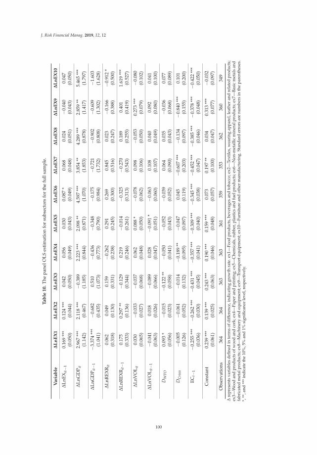
J. Risk Financial Manag. 2019, 12, 12
Ta
ble
10
.Th
epa
nelO
LSes
tim
atio
nfo
rsu
bsec
tors
for
the
full
sam
ple.
Va
ria
ble
ΔL
nE
X1
ΔL
nE
X2
ΔL
nE
X3
ΔL
nE
X4
ΔL
nE
X5
ΔL
nE
X6
ΔL
nE
X7
ΔL
nE
X8
ΔL
nE
X9
ΔL
nE
X1
0
ΔLn
EXit−1
0.16
9**
*0.
124
***
0.04
20.
056
0.03
00.
087
*0.
068
0.02
4−0
.040
0.04
7(0
.050
)(0
.044
)(0
.050
)(0
.049
)(0
.043
)(0
.049
)(0
.048
)(0
.051
)(0
.043
)(0
.050
)
ΔLn
GD
P it
2.96
7**
*2.
118
***
−0.3
892.
223
***
2.09
8**
4.59
7**
*3.
854
**4.
289
***
2.85
9**
5.46
5**
*(1
.142
)(0
.467
)(1
.185
)(0
.844
)(0
.871
)(1
.070
)(1
.853
)(0
.878
)(1
.417
)(1
.797
)
ΔLn
GD
P it−
1−3
.374
***
−0.6
820.
510
−0.4
36−0
.348
−0.1
75−0
.721
−0.9
02−0
.609
−1.6
03(1
.041
)(0
.435
)(1
.073
)(0
.773
)(0
.790
)(0
.984
)(1
.732
)(0
.808
)(1
.302
)(1
.628
)
ΔLn
REX
Rit
0.06
20.
049
0.15
9−0
.262
0.29
10.
269
0.84
50.
023
−0.1
66−0
.912
*(0
.318
)(0
.130
)(0
.331
)(0
.238
)(0
.245
)(0
.300
)(0
.516
)(0
.247
)(0
.388
)(0
.500
)
ΔLn
REX
Rit−1
0.17
50.
297
**−0
.129
0.21
9−0
.014
−0.3
25−0
.270
0.18
90.
401
1.61
9**
*(0
.333
)(0
.136
)(0
.344
)(0
.246
)(0
.261
)(0
.313
)(0
.543
)(0
.255
)(0
.419
)(0
.527
)
ΔLn
VO
L it
0.03
0−0
.033
−0.0
370.
062
0.08
8*
−0.0
780.
098
−0.0
530.
273
***
−0.0
80(0
.065
)(0
.027
)(0
.068
)(0
.048
)(0
.050
)(0
.062
)(0
.106
)(0
.050
)(0
.079
)(0
.102
)
ΔLn
VO
L it−
1−0
.041
0.01
8−0
.089
0.02
8−0
.091
*−0
.063
0.10
80.
040
0.09
20.
041
(0.0
63)
(0.0
26)
(0.0
66)
(0.0
47)
(0.0
51)
(0.0
60)
(0.1
07)
(0.0
49)
(0.0
80)
(0.1
00)
DW
TO0.
093
*−0
.015
−0.1
22**
−0.0
50−0
.052
−0.0
390.
064
0.03
5−0
.036
0.07
7(0
.056
)(0
.023
)(0
.058
)(0
.041
)(0
.043
)(0
.052
)(0
.090
)(0
.043
)(0
.068
)(0
.089
)
DC
risi
s−0
.005
−0.0
61−0
.014
−0.1
89**
−0.0
470.
045
−0.6
07**
*−0
.134
−0.8
40**
*0.
101
(0.1
26)
(0.0
52)
(0.1
32)
(0.0
95)
(0.0
97)
(0.1
19)
(0.2
03)
(0.0
97)
(0.1
55)
(0.2
00)
ECt −
1−0
.255
***
−0.2
62**
*−0
.431
***
−0.3
57**
*−0
.309
***
−0.3
45**
*−0
.452
***
−0.3
85**
*−0
.378
***
−0.4
22**
*(0
.036
)(0
.030
)(0
.045
)(0
.041
)(0
.040
)(0
.038
)(0
.047
)(0
.046
)(0
.048
)(0
.050
)
Con
stan
t0.
239
***
0.13
9**
*0.
243
***
0.19
0**
*0.
159
***
0.07
30.
197
**0.
034
0.31
3**
*−0
.032
(0.0
61)
(0.0
25)
(0.0
63)
(0.0
46)
(0.0
48)
(0.0
57)
(0.1
00)
(0.0
47)
(0.0
77)
(0.0
97)
Obs
erva
tion
s36
436
436
336
336
135
935
336
236
034
9
Δre
pres
ents
vari
able
sde
fined
inte
rms
ofdi
ffer
ence
,ind
icat
ing
grow
thra
te.e
x1—
Food
prod
ucts
,bev
erag
esan
dto
bacc
o;ex
2—Te
xtile
s,w
eari
ngap
pare
l,le
athe
ran
dre
late
dpr
oduc
ts;
ex3—
Woo
dan
dpr
oduc
tsof
woo
dan
dco
rk;e
x4—
Pape
ran
dpr
inti
ng;e
x5—
Che
mic
als,
rubb
er,p
last
ics
and
fuel
prod
ucts
;ex6
—N
on-m
etal
licm
iner
alpr
oduc
ts;e
x7—
Basi
cm
etal
san
dfa
bric
ated
met
alpr
oduc
ts;e
x8—
Mac
hine
ryan
deq
uipm
ent;
ex9—
Tran
spor
tequ
ipm
ent;
ex10
—Fu
rnit
ure
and
othe
rm
anuf
actu
ring
.Sta
ndar
der
rors
are
num
bers
inth
epa
rent
hese
s.*,
**,a
nd**
*in
dica
teth
e10
%,5
%an
d1%
sign
ifica
nce
leve
l,re
spec
tive
ly.
100
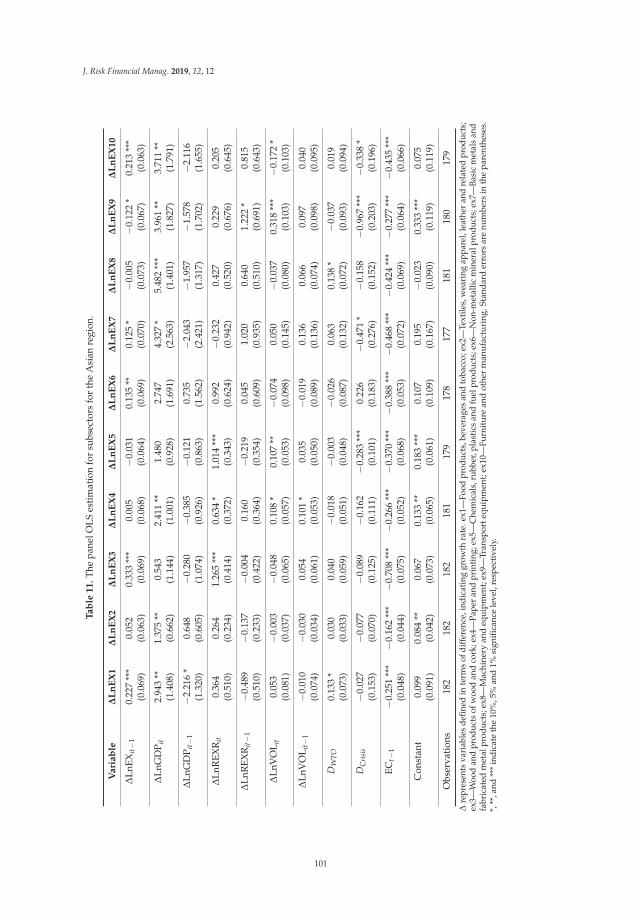
J. Risk Financial Manag. 2019, 12, 12
Ta
ble
11
.Th
epa
nelO
LSes
tim
atio
nfo
rsu
bsec
tors
for
the
Asi
anre
gion
.
Va
ria
ble
ΔL
nE
X1
ΔL
nE
X2
ΔL
nE
X3
ΔL
nE
X4
ΔL
nE
X5
ΔL
nE
X6
ΔL
nE
X7
ΔL
nE
X8
ΔL
nE
X9
ΔL
nE
X1
0
ΔLn
EXit−1
0.22
7**
*0.
052
0.33
3**
*0.
005
−0.0
310.
135
**0.
125
*−0
.005
−0.1
22*
0.21
3**
*(0
.069
)(0
.063
)(0
.069
)(0
.068
)(0
.064
)(0
.069
)(0
.070
)(0
.073
)(0
.067
)(0
.063
)
ΔLn
GD
P it
2.94
3**
1.37
5**
0.54
32.
411
**1.
480
2.74
74.
327
*5.
482
***
3.96
1**
3.71
1**
(1.4
08)
(0.6
62)
(1.1
44)
(1.0
01)
(0.9
28)
(1.6
91)
(2.5
63)
(1.4
01)
(1.8
27)
(1.7
91)
ΔLn
GD
P it−
1−2
.216
*0.
648
−0.2
80−0
.385
−0.1
210.
735
−2.0
43−1
.957
−1.5
78−2
.116
(1.3
20)
(0.6
05)
(1.0
74)
(0.9
26)
(0.8
63)
(1.5
62)
(2.4
21)
(1.3
17)
(1.7
02)
(1.6
55)
ΔLn
REX
Rit
0.36
40.
264
1.26
5**
*0.
634
*1.
014
***
0.99
2−0
.232
0.42
70.
229
0.20
5(0
.510
)(0
.234
)(0
.414
)(0
.372
)(0
.343
)(0
.624
)(0
.942
)(0
.520
)(0
.676
)(0
.645
)
ΔLn
REX
Rit−1
−0.4
89−0
.137
−0.0
040.
160
−0.2
190.
045
1.02
00.
640
1.22
2*
0.81
5(0
.510
)(0
.233
)(0
.422
)(0
.364
)(0
.354
)(0
.609
)(0
.935
)(0
.510
)(0
.691
)(0
.643
)
ΔLn
VO
L it
0.05
3−0
.003
−0.0
480.
108
*0.
107
**−0
.074
0.05
0−0
.037
0.31
8**
*−0
.172
*(0
.081
)(0
.037
)(0
.065
)(0
.057
)(0
.053
)(0
.098
)(0
.145
)(0
.080
)(0
.103
)(0
.103
)
ΔLn
VO
L it−
1−0
.010
−0.0
300.
054
0.10
1*
0.03
5−0
.019
0.13
60.
066
0.09
70.
040
(0.0
74)
(0.0
34)
(0.0
61)
(0.0
53)
(0.0
50)
(0.0
89)
(0.1
36)
(0.0
74)
(0.0
98)
(0.0
95)
DW
TO0.
133
*0.
030
0.04
0−0
.018
−0.0
03−0
.026
0.06
30.
138
*−0
.037
0.01
9(0
.073
)(0
.033
)(0
.059
)(0
.051
)(0
.048
)(0
.087
)(0
.132
)(0
.072
)(0
.093
)(0
.094
)
DC
risi
s−0
.027
−0.0
77−0
.089
−0.1
62−0
.283
***
0.22
6−0
.471
*−0
.158
−0.9
67**
*−0
.338
*(0
.153
)(0
.070
)(0
.125
)(0
.111
)(0
.101
)(0
.183
)(0
.276
)(0
.152
)(0
.203
)(0
.196
)
ECt −
1−0
.251
***
−0.1
62**
*−0
.708
***
−0.2
66**
*−0
.370
***
−0.3
88**
*−0
.468
***
−0.4
24**
*−0
.277
***
−0.4
35**
*(0
.048
)(0
.044
)(0
.075
)(0
.052
)(0
.068
)(0
.053
)(0
.072
)(0
.069
)(0
.064
)(0
.066
)
Con
stan
t0.
099
0.08
4**
0.06
70.
133
**0.
183
***
0.10
70.
195
−0.0
230.
333
***
0.07
5(0
.091
)(0
.042
)(0
.073
)(0
.065
)(0
.061
)(0
.109
)(0
.167
)(0
.090
)(0
.119
)(0
.119
)
Obs
erva
tion
s18
218
218
218
117
917
817
718
118
017
9
Δre
pres
ents
vari
able
sde
fined
inte
rms
ofdi
ffer
ence
,ind
icat
ing
grow
thra
te.e
x1—
Food
prod
ucts
,bev
erag
esan
dto
bacc
o;ex
2—Te
xtile
s,w
eari
ngap
pare
l,le
athe
ran
dre
late
dpr
oduc
ts;
ex3—
Woo
dan
dpr
oduc
tsof
woo
dan
dco
rk;e
x4—
Pape
ran
dpr
inti
ng;e
x5—
Che
mic
als,
rubb
er,p
last
ics
and
fuel
prod
ucts
;ex6
—N
on-m
etal
licm
iner
alpr
oduc
ts;e
x7—
Basi
cm
etal
san
dfa
bric
ated
met
alpr
oduc
ts;e
x8—
Mac
hine
ryan
deq
uipm
ent;
ex9—
Tran
spor
tequ
ipm
ent;
ex10
—Fu
rnit
ure
and
othe
rm
anuf
actu
ring
.Sta
ndar
der
rors
are
num
bers
inth
epa
rent
hese
s.*,
**,a
nd**
*in
dica
teth
e10
%,5
%an
d1%
sign
ifica
nce
leve
l,re
spec
tive
ly.
101
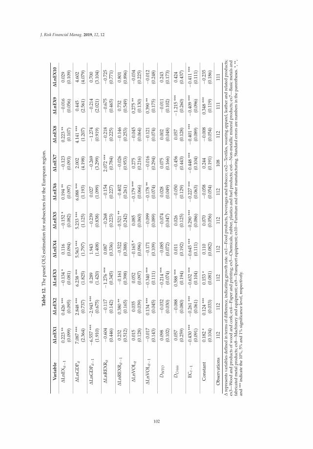
J. Risk Financial Manag. 2019, 12, 12
Ta
ble
12
.Th
epa
nelO
LSes
tim
atio
nfo
rsu
bsec
tors
for
the
Euro
pean
regi
on.
Va
ria
ble
ΔL
nE
X1
ΔL
nE
X2
ΔL
nE
X3
ΔL
nE
X4
ΔL
nE
X5
ΔL
nE
X6
ΔL
nE
X7
ΔL
nE
X8
ΔL
nE
X9
ΔL
nE
X1
0
ΔLn
EXit−1
0.22
3**
0.42
6**
*−0
.134
*0.
116
−0.1
52*
0.19
4**
−0.1
230.
223
**−0
.016
0.02
9(0
.099
)(0
.095
)(0
.081
)(0
.094
)(0
.082
)(0
.097
)(0
.093
)(0
.107
)(0
.056
)(0
.109
)
ΔLn
GD
P it
7.08
7**
*2.
848
***
6.23
8**
*5.
563
***
5.23
3**
*6.
088
***
2.00
24.
141
***
0.44
54.
602
(2.3
64)
(0.7
37)
(1.8
25)
(1.7
97)
(1.1
25)
(1.1
93)
(4.1
98)
(1.2
07)
(2.5
61)
(4.0
79)
ΔLn
GD
P it−
1−6
.557
***
−2.9
43**
*0.
289
1.94
3−0
.239
0.02
7−0
.269
−1.2
74−0
.214
0.70
0(1
.910
)(0
.675
)(1
.420
)(1
.408
)(0
.838
)(1
.099
)(3
.299
)(0
.919
)(2
.021
)(3
.104
)
ΔLn
REX
Rit
−0.6
04−0
.117
−1.2
76**
*0.
087
−0.2
68−0
.154
2.07
2**
*−0
.218
−0.6
75−0
.725
(0.4
46)
(0.1
42)
(0.3
45)
(0.3
36)
(0.2
23)
(0.2
27)
(0.7
84)
(0.2
25)
(0.4
65)
(0.7
71)
ΔLn
REX
Rit−1
0.23
20.
380
**−0
.161
−0.5
22−0
.521
**−0
.402
−0.0
26−0
.146
0.73
20.
801
(0.5
12)
(0.1
65)
(0.3
98)
(0.3
88)
(0.2
42)
(0.2
61)
(0.9
53)
(0.2
53)
(0.5
49)
(0.8
96)
ΔLn
VO
L it
0.01
50.
035
0.05
2−0
.165
*0.
085
−0.1
79**
*0.
275
−0.0
450.
275
**−0
.034
(0.1
28)
(0.0
39)
(0.0
97)
(0.0
96)
(0.0
60)
(0.0
66)
(0.2
16)
(0.0
64)
(0.1
30)
(0.2
25)
ΔLn
VO
L it−
1−0
.017
0.13
4**
*−0
.340
***
−0.1
71−0
.099
−0.1
78**
−0.0
16−0
.121
0.39
0**
−0.0
12(0
.143
)(0
.045
)(0
.111
)(0
.109
)(0
.089
)(0
.074
)(0
.294
)(0
.074
)(0
.175
)(0
.248
)
DW
TO0.
098
−0.0
32−0
.214
***
−0.0
85−0
.074
0.02
80.
075
0.00
2−0
.011
0.24
3(0
.102
)(0
.030
)(0
.074
)(0
.072
)(0
.047
)(0
.049
)(0
.166
)(0
.048
)(0
.102
)(0
.173
)
DC
risi
s0.
057
−0.0
880.
588
***
0.01
10.
026
−0.0
50−0
.456
0.05
7−1
.215
***
0.42
4(0
.259
)(0
.080
)(0
.194
)(0
.192
)(0
.125
)(0
.129
)(0
.443
)(0
.128
)(0
.260
)(0
.437
)
ECt −
1−0
.430
***
−0.2
61**
*−0
.632
***
−0.6
45**
*−0
.290
***
−0.2
27**
*−0
.448
***
−0.4
01**
*−0
.409
***
−0.4
11**
*(0
.091
)(0
.061
)(0
.104
)(0
.111
)(0
.086
)(0
.063
)(0
.104
)(0
.089
)(0
.096
)(0
.111
)
Con
stan
t0.
182
*0.
124
***
0.15
3*
0.11
00.
070
−0.0
580.
244
−0.0
080.
348
***
−0.2
35(0
.104
)(0
.033
)(0
.081
)(0
.082
)(0
.056
)(0
.054
)(0
.191
)(0
.054
)(0
.119
)(0
.186
)
Obs
erva
tion
s11
211
211
211
211
211
210
811
211
111
1
Δre
pres
ents
vari
able
sde
fined
inte
rms
ofdi
ffer
ence
,ind
icat
ing
grow
thra
te.e
x1—
Food
prod
ucts
,bev
erag
esan
dto
bacc
o;ex
2—Te
xtile
s,w
eari
ngap
pare
l,le
athe
ran
dre
late
dpr
oduc
ts;
ex3—
Woo
dan
dpr
oduc
tsof
woo
dan
dco
rk;e
x4—
Pape
ran
dpr
inti
ng;e
x5—
Che
mic
als,
rubb
er,p
last
ics
and
fuel
prod
ucts
;ex6
—N
on-m
etal
licm
iner
alpr
oduc
ts;e
x7—
Basi
cm
etal
san
dfa
bric
ated
met
alpr
oduc
ts;e
x8—
Mac
hine
ryan
deq
uipm
ent;
ex9—
Tran
spor
tequ
ipm
ent;
ex10
—Fu
rnitu
rean
dot
her
man
ufac
turi
ng.S
tand
ard
erro
rsar
enu
mbe
rsin
the
pare
nthe
ses.
*,**
,an
d**
*in
dica
teth
e10
%,5
%an
d1%
sign
ifica
nce
leve
l,re
spec
tive
ly.
102
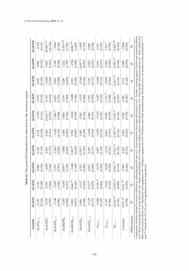
J. Risk Financial Manag. 2019, 12, 12
Ta
ble
13
.Th
epa
nelO
LSes
tim
atio
nfo
rsu
bsec
tors
for
the
Am
eric
anre
gion
.
Va
ria
ble
ΔL
nE
X1
ΔL
nE
X2
ΔL
nE
X3
ΔL
nE
X4
ΔL
nE
X5
ΔL
nE
X6
ΔL
nE
X7
ΔL
nE
X8
ΔL
nE
X9
ΔL
nE
X1
0
ΔLn
EXit−1
0.13
00.
134
0.08
80.
102
0.13
4−0
.076
0.17
40.
020
0.00
6−0
.152
(0.1
24)
(0.1
00)
(0.1
34)
(0.1
19)
(0.1
04)
(0.1
16)
(0.1
18)
(0.1
20)
(0.1
32)
(0.1
18)
ΔLn
GD
P it
−0.7
372.
376
−4.0
554.
259
0.16
810
.412
**6.
723
−0.0
859.
043
26.9
03**
*(4
.799
)(1
.818
)(7
.342
)(3
.717
)(5
.163
)(4
.251
)(6
.912
)(3
.239
)(6
.431
)(1
0.12
4)
ΔLn
GD
P it−
1−3
.140
−2.4
375.
179
−5.2
42*
−1.0
20−7
.540
**0.
025
3.90
51.
298
−3.8
96(3
.990
)(1
.540
)(5
.591
)(3
.022
)(4
.120
)(3
.458
)(5
.721
)(2
.558
)(5
.168
)(8
.156
)
ΔLn
REX
Rit
−0.3
57−0
.053
2.85
9**
−0.8
801.
308
0.90
00.
139
0.20
91.
222
−5.3
76**
*(0
.960
)(0
.351
)(1
.336
)(0
.692
)(0
.947
)(0
.782
)(1
.289
)(0
.600
)(1
.197
)(1
.792
)
ΔLn
REX
Rit−1
0.30
20.
666
**−1
.484
1.38
3**
0.79
4−0
.830
−0.4
980.
593
−0.5
264.
882
***
(0.8
77)
(0.3
25)
(1.1
69)
(0.6
18)
(0.9
02)
(0.7
38)
(1.1
58)
(0.5
39)
(1.0
98)
(1.6
20)
ΔLn
VO
L it
0.00
6−0
.117
0.32
30.
339
**0.
285
0.24
2−0
.157
−0.1
690.
637
**−0
.007
(0.1
89)
(0.0
74)
(0.2
62)
(0.1
45)
(0.1
98)
(0.1
64)
(0.2
68)
(0.1
26)
(0.2
53)
(0.3
53)
ΔLn
VO
L it−
1−0
.178
0.13
7*
0.01
30.
099
−0.2
940.
089
0.35
50.
120
0.22
30.
098
(0.1
73)
(0.0
75)
(0.2
46)
(0.1
31)
(0.1
94)
(0.1
51)
(0.2
59)
(0.1
17)
(0.2
31)
(0.3
38)
DW
TO−0
.086
−0.1
26**
−0.1
700.
067
−0.0
70−0
.123
−0.0
87−0
.049
0.01
60.
231
(0.1
65)
(0.0
64)
(0.2
26)
(0.1
22)
(0.1
70)
(0.1
41)
(0.2
29)
(0.1
12)
(0.2
12)
(0.3
31)
DC
risi
s0.
118
−0.1
26−0
.000
−0.1
190.
661
0.05
4−1
.191
**−0
.293
0.39
01.
513
*(0
.396
)(0
.152
)(0
.550
)(0
.311
)(0
.413
)(0
.339
)(0
.548
)(0
.256
)(0
.522
)(0
.799
)
ECt −
1−0
.618
***
−0.5
20**
*−0
.516
***
−0.5
14**
*−0
.393
***
−0.3
15**
−0.5
96**
*−0
.411
***
−0.6
56**
*−0
.605
***
(0.1
41)
(0.0
89)
(0.1
15)
(0.1
26)
(0.1
12)
(0.1
30)
(0.1
27)
(0.1
16)
(0.1
64)
(0.1
63)
Con
stan
t0.
531
***
0.31
2**
*0.
389
0.23
50.
265
0.25
80.
301
0.11
30.
089
−0.5
46(0
.198
)(0
.076
)(0
.266
)(0
.151
)(0
.210
)(0
.179
)(0
.287
)(0
.140
)(0
.270
)(0
.399
)
Obs
erva
tion
s70
7069
7070
6968
6969
59
Δre
pres
ents
vari
able
sde
fined
inte
rms
ofdi
ffer
ence
,ind
icat
ing
grow
thra
te.e
x1—
Food
prod
ucts
,bev
erag
esan
dto
bacc
o;ex
2—Te
xtile
s,w
eari
ngap
pare
l,le
athe
ran
dre
late
dpr
oduc
ts;
ex3—
Woo
dan
dpr
oduc
tsof
woo
dan
dco
rk;e
x4—
Pape
ran
dpr
inti
ng;e
x5—
Che
mic
als,
rubb
er,p
last
ics
and
fuel
prod
ucts
;ex6
—N
on-m
etal
licm
iner
alpr
oduc
ts;e
x7—
Basi
cm
etal
san
dfa
bric
ated
met
alpr
oduc
ts;e
x8—
Mac
hine
ryan
deq
uipm
ent;
ex9—
Tran
spor
tequ
ipm
ent;
ex10
—Fu
rnitu
rean
dot
her
man
ufac
turi
ng.S
tand
ard
erro
rsar
enu
mbe
rsin
the
pare
nthe
ses.
*,**
,an
d**
*in
dica
teth
e10
%,5
%an
d1%
sign
ifica
nce
leve
l,re
spec
tive
ly.
103
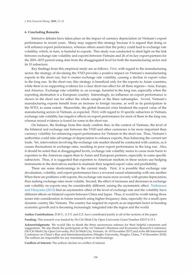
J. Risk Financial Manag. 2019, 12, 12
6. Concluding Remarks
Intensive debates have taken place on the impact of currency depreciation on Vietnam’s exportperformance in recent years. Many may support this strategy because it is argued that doing sowill enhance export performance, whereas others assert that the policy could lead to exchange ratevolatility, which, in turn, is harmful to exports. This study was conducted to shed light on the linkbetween exchange rate volatility and exports between Vietnam and 26 of its key export partners forthe 2001–2015 period using data from the disaggregated level for both the manufacturing sector andits 10 subsectors.
Key findings from this empirical study are as follows. First, with regard to the manufacturingsector, the strategy of devaluing the VND provides a positive impact on Vietnam’s manufacturingexports in the short run, but it creates exchange rate volatility, causing a decline in export valuein the long run. In the short run, this strategy is beneficial only for the exports to Asian countries,while there is no supporting evidence for a clear short-run effect for all three regions—Asia, Europe,and America. Exchange rate volatility is, on average, harmful in the long run, especially when theexporting destination is a European country. Interestingly, no influence on export performance isshown in the short run for either the whole sample or the three subsamples. Second, Vietnam’smanufacturing exports benefit from an increase in foreign income, as well as its participation inthe WTO, to some extent. Meanwhile, the global financial crisis hindered the export value of themanufacturing sectors in Vietnam, as expected. Third, with regard to 10 specific subsectors in Vietnam,exchange rate volatility has negative effects on export performance for most of them in the long run,whereas mixed evidence is found for some in the short run.
On balance, the findings from this study confirm that, in the context of Vietnam, the level ofthe bilateral real exchange rate between the VND and other currencies is far more important thancurrency volatility for enhancing export performance for Vietnam in the short run. Thus, Vietnam’sauthorities could take advantage of depreciation to enhance exports, thus balancing the current nettrade. Yet, intervention involving the exchange rate market should be conducted with caution, as itcauses fluctuations in exchange rates, resulting in poor export performance in the long run. Also,it should be noted that at disaggregated levels, exchange rate volatility seems to cause more harm toexporters to the American region than to Asian and European partners, especially in some specificsubsectors. Thus, it is suggested that exporters to American markets in these sectors use hedginginstruments in the derivatives market to maintain their targeted export value and profitability.
There are some shortcomings in the current study. First, it is possible that exchange ratedevaluation, volatility, and export performance have a reversed causal relationship with one another.When there are problems with exports, the exchange rate reacts more severely with greater depreciation,thus making exchange rates more volatile. Second, the effect of increases and decreases in exchangerate volatility on exports may be considerably different, raising the asymmetric effect. Nishimuraand Hirayama (2013) find an asymmetric effect of the level of exchange rate and the volatility havedifferent effects on bilateral exports between China and Japan. Thus, it would be worth taking thoseissues into consideration in future research using higher-frequency data, especially for a small opendynamic country like Vietnam. The country has targeted its exports as an important factor in boostingeconomic growth and is becoming increasingly integrated into the region and the world.
Author Contributions: D.H.V., A.T.V. and Z.Z. have contributed jointly to all of the sections of the paper.
Funding: This research was funded by Ho Chi Minh City Open University Grant Number E2017.6.15.1.
Acknowledgments: We would like to thank the three anonymous referees for their helpful comments andsuggestions. We also thank the participants at the 1st Vietnam’s Business and Economics Research Conference(Ho Chi Minh City Open University, Ho Chi Minh City, Vietnam, 16–18 November 2017) and at the 4th InternationalConference on China’s Rise and Internationalization (Ningbo University, Ningbo, China, 7–8 December 2018).The authors are responsible for any remaining errors or shortcomings.
Conflicts of Interest: The authors declare no conflict of interest.
104
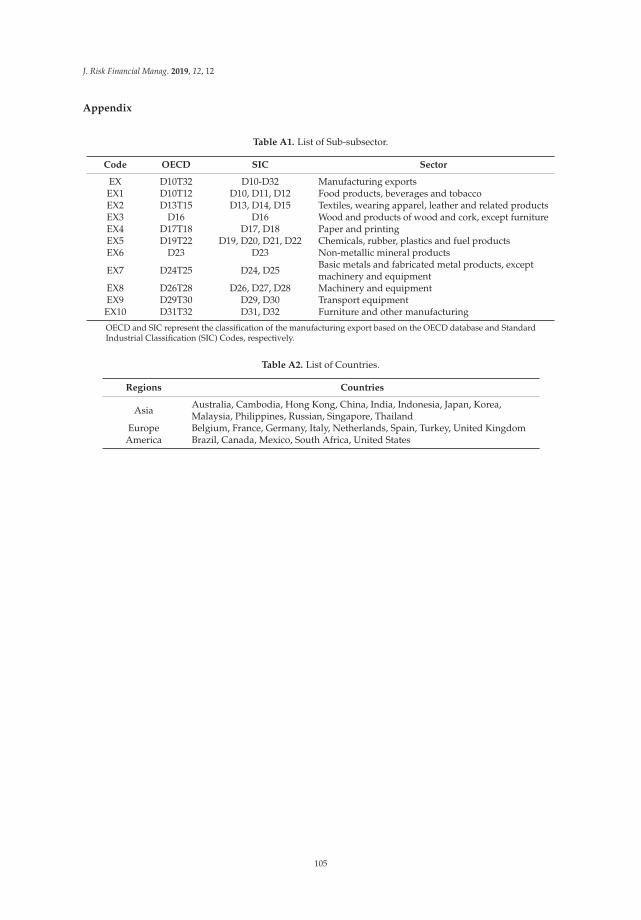
J. Risk Financial Manag. 2019, 12, 12
Appendix
Table A1. List of Sub-subsector.
Code OECD SIC Sector
EX D10T32 D10-D32 Manufacturing exportsEX1 D10T12 D10, D11, D12 Food products, beverages and tobaccoEX2 D13T15 D13, D14, D15 Textiles, wearing apparel, leather and related productsEX3 D16 D16 Wood and products of wood and cork, except furnitureEX4 D17T18 D17, D18 Paper and printingEX5 D19T22 D19, D20, D21, D22 Chemicals, rubber, plastics and fuel productsEX6 D23 D23 Non-metallic mineral products
EX7 D24T25 D24, D25 Basic metals and fabricated metal products, exceptmachinery and equipment
EX8 D26T28 D26, D27, D28 Machinery and equipmentEX9 D29T30 D29, D30 Transport equipmentEX10 D31T32 D31, D32 Furniture and other manufacturing
OECD and SIC represent the classification of the manufacturing export based on the OECD database and StandardIndustrial Classification (SIC) Codes, respectively.
Table A2. List of Countries.
Regions Countries
Asia Australia, Cambodia, Hong Kong, China, India, Indonesia, Japan, Korea,Malaysia, Philippines, Russian, Singapore, Thailand
Europe Belgium, France, Germany, Italy, Netherlands, Spain, Turkey, United KingdomAmerica Brazil, Canada, Mexico, South Africa, United States
105
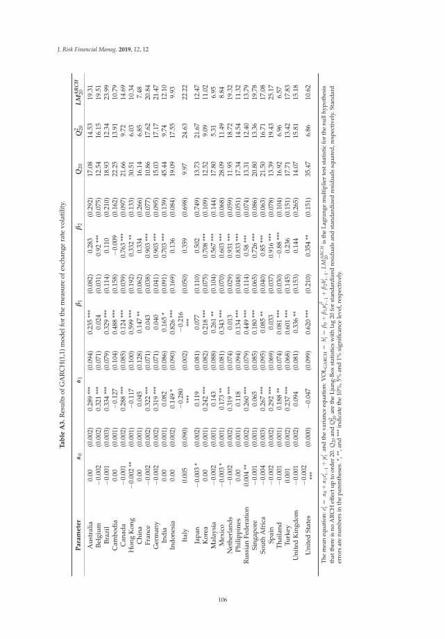
J. Risk Financial Manag. 2019, 12, 12
Ta
ble
A3
.R
esul
tsof
GA
RC
H(1
,1)m
odel
for
the
mea
sure
ofex
chan
gera
tevo
lati
lity.
Pa
ram
ete
rα
0α
1β
1β
2Q
20Q
2 20LM
AR
CH
20
Aus
tral
ia0.
00(0
.002
)0.
289
***
(0.0
94)
0.23
5**
*(0
.082
)0.
283
(0.2
92)
17.0
814
.53
19.3
1Be
lgiu
m−0
.002
(0.0
02)
0.32
1**
*(0
.071
)0.
024
(0.0
31)
0.92
***
(0.0
75)
12.5
416
.15
19.5
1Br
azil
−0.0
01(0
.003
)0.
334
***
(0.0
79)
0.32
9**
*(0
.114
)0.
110
(0.2
10)
18.9
312
.34
23.9
9C
ambo
dia
0.00
(0.0
01)
−0.1
27(0
.104
)0.
488
***
(0.1
58)
−0.0
09(0
.162
)22
.25
13.9
110
.79
Can
ada
−0.0
01(0
.002
)0.
288
***
(0.0
85)
0.12
4**
*(0
.039
)0.
763
***
(0.0
97)
21.6
69.
7214
.69
Hon
gK
ong
−0.0
02**
(0.0
01)
−0.1
17(0
.100
)0.
599
***
(0.1
92)
0.33
2**
(0.1
33)
30.5
16.
0310
.34
Chi
na0.
00(0
.001
)0.
045
(0.1
28)
0.14
7**
(0.0
62)
0.33
4(0
.266
)16
.14
6.85
7.48
Fran
ce−0
.002
(0.0
02)
0.32
2**
*(0
.071
)0.
043
(0.0
38)
0.90
3**
*(0
.077
)10
.86
17.6
220
.84
Ger
man
y−0
.002
(0.0
02)
0.31
9**
*(0
.071
)0.
040
(0.0
41)
0.90
3**
*(0
.095
)15
.03
17.1
721
.47
Indi
a0.
00(0
.001
)0.
082
(0.0
86)
0.16
5*
(0.0
91)
0.70
3**
*(0
.139
)45
.44
9.74
12.1
0In
done
sia
0.00
(0.0
02)
0.14
9*
(0.0
90)
0.82
6**
*(0
.169
)0.
136
(0.0
84)
19.0
917
.55
9.93
Ital
y0.
005
(0.0
90)
−0.2
80**
*(0
.002
)−0
.216
***
(0.0
50)
0.35
9(0
.698
)9.
9724
.63
22.2
2
Japa
n−0
.003
*(0
.002
)0.
119
(0.0
81)
0.07
7(0
.110
)0.
502
(0.7
49)
13.7
321
.67
12.4
7K
orea
0.00
(0.0
01)
0.24
2**
*(0
.082
)0.
218
***
(0.0
75)
0.70
8**
*(0
.109
)12
.52
9.09
11.0
2M
alay
sia
−0.0
02(0
.001
)0.
143
(0.0
88)
0.26
1**
(0.1
04)
0.56
7**
*(0
.144
)17
.80
5.31
6.95
Mex
ico
−0.0
03*
(0.0
01)
0.17
3**
(0.0
81)
0.34
3**
*(0
.070
)0.
603
***
(0.0
68)
28.0
911
.49
8.84
Net
herl
ands
−0.0
02(0
.002
)0.
319
***
(0.0
74)
0.01
3(0
.029
)0.
931
***
(0.0
59)
11.9
518
.72
19.3
2Ph
ilipp
ines
0.00
(0.0
01)
0.11
8(0
.094
)0.
134
***
(0.0
48)
0.83
3**
*(0
.051
)17
.34
14.5
411
.32
Rus
sian
Fede
rati
on0.
004
**(0
.002
)0.
260
***
(0.0
79)
0.44
9**
*(0
.114
)0.
58**
*(0
.074
)13
.31
12.4
013
.79
Sing
apor
e−0
.001
(0.0
01)
0.06
5(0
.085
)0.
180
***
(0.0
65)
0.72
6**
*(0
.086
)20
.80
13.3
619
.78
Sout
hA
fric
a−0
.004
(0.0
03)
0.26
7**
*(0
.095
)0.
085
**(0
.040
)0.
85**
*(0
.063
)21
.50
16.7
117
.08
Spai
n−0
.002
(0.0
02)
0.29
2**
*(0
.069
)0.
033
(0.0
37)
0.91
6**
*(0
.078
)13
.39
19.4
325
.17
Thai
land
−0.0
01(0
.001
)0.
188
**(0
.074
)0.
081
***
(0.0
30)
−0.8
8**
*(0
.104
)16
.92
6.96
6.57
Turk
ey0.
001
(0.0
02)
0.23
7**
*(0
.068
)0.
601
***
(0.1
45)
0.23
6(0
.151
)17
.71
13.4
217
.83
Uni
ted
Kin
gdom
−0.0
01(0
.002
)0.
094
(0.0
81)
0.33
6**
(0.1
53)
0.14
4(0
.265
)14
.07
15.8
115
.18
Uni
ted
Stat
es−0
.002
***
(0.0
00)
−0.0
47(0
.099
)0.
620
***
(0.2
10)
0.35
4**
(0.1
51)
35.4
76.
8610
.62
The
mea
neq
uatio
n:ei t=
α0+
α1e
i t −1+
μi t
and
the
vari
ance
equa
tion:
VO
L GA
RC
H=
hi t=
β0+
β1μ
i2 t−1+
β2h
i t −1.
LM
AR
CH
20is
the
Lagr
ange
mul
tiplie
rte
stst
atis
ticfo
rth
enu
llhy
poth
esis
that
ther
eis
noA
RC
Hef
fect
upto
orde
r20
.Q20
and
Q2 20
are
the
Ljun
g-Bo
xst
atis
tics
wit
hla
g20
for
stan
dard
ized
resi
dual
san
dst
anda
rdiz
edre
sidu
als
squa
red,
resp
ecti
vely
.Sta
ndar
der
rors
are
num
bers
inth
epa
rent
hese
s.*,
**,a
nd**
*in
dica
teth
e10
%,5
%an
d1%
sign
ifica
nce
leve
l,re
spec
tive
ly.
106
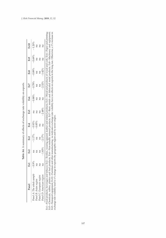
J. Risk Financial Manag. 2019, 12, 12
Ta
ble
A4
.A
sum
mar
yof
effe
cts
ofex
chan
gera
tevo
lati
lity
onex
port
s.
Pa
ne
lE
x1
Ex
2E
x3
Ex
4E
x5
Ex
6E
x7
Ex
8E
x9
Ex
10
Pane
lA:T
hew
hole
sam
ple
−0.9
%na
−1.1
7%−0
.93%
na−0
.88%
−0.7
8%−0
.89%
−0.6
9%−1
.20%
Pane
lB:A
sian
regi
onna
nana
−0.8
5%na
nana
nana
naPa
nelC
:Eur
opea
nre
gion
nana
nana
nana
nana
nana
Pane
lD:A
mer
ican
regi
onna
−1.8
3%−2
.17%
na−2
.48%
na−2
.32%
−1.4
2%na
na
Ex1
—Fo
odp
rod
uct
s,be
vera
ges
and
toba
cco;
Ex2
—Te
xtile
s,w
eari
ngap
par
el,l
eath
eran
dre
late
dp
rod
uct
s;E
x3—
Woo
dan
dp
rod
uct
sof
woo
dan
dco
rk;E
x4—
Pap
eran
dpr
inti
ng;
Ex5
—C
hem
ical
s,ru
bber
,p
last
ics
and
fuel
pro
du
cts;
Ex6
—N
on-m
etal
licm
iner
alp
rod
uct
s;E
x7—
Bas
icm
etal
san
dfa
bric
ated
met
alp
rod
uct
s;E
x8—
Mac
hine
ryan
deq
uip
men
t;E
x9—
Tran
spor
tequ
ipm
ent;
Ex1
0—Fu
rnit
ure
and
othe
rm
anu
fact
uri
ng.n
ain
dic
ates
exch
ange
rate
vola
tilit
yha
veno
effe
cts
onex
port
sin
the
long
run.
Oth
erw
ise,
a1%
incr
ease
inex
chan
gera
tevo
lati
lity
lead
tox%
chan
gein
expo
rts
(by
geog
raph
icre
gion
and
byse
ctor
orig
in).
107
J. Risk Financial Manag. 2019, 12, 12
References
Aftab, Muhammad, Karim Bux Shah Syed, Rubi Ahmad, and Izlin Ismail. 2015. Exchange-rate variability andindustry trade flows between Malaysia and Japan. The Journal of International Trade & Economic Development25: 453–78.
Aftab, Muhammad, Karim Bux Shah Syed, and Naveed Akhter Katper. 2017. Exchange-rate volatility andMalaysian-Thai bilateral industry trade flows. Journal of Economic Studies 44: 99–114. [CrossRef]
Aristotelous, Kyriacos. 2001. Exchange-rate volatility, exchange-rate regime, and trade volume: Evidence from theUK–US export function (1889–1999). Economics Letters 72: 87–94. [CrossRef]
Asteriou, Dimitrios, Kaan Masatci, and Keith Pılbeam. 2016. Exchange rate volatility and international trade:International evidence from the MINT countries. Economic Modelling 58: 133–40. [CrossRef]
Atif, Rao Muhammad, Liu Haiyun, and Haider Mahmood. 2017. Pakistan’s agricultural exports, determinantsand its potential: An application of stochastic frontier gravity model. The Journal of International Trade &Economic Development 26: 257–76.
Bahmani-Oskooee, Mohsen, and Yongqing Wang. 2007. United States-China trade at the commodity level and theYuan-Dollar exchange rate. Contemporary Economic Policy 25: 341–61. [CrossRef]
Bahmani-Oskooee, Mohsen, Marzieh Bolhassani, and Scott Hegerty. 2012. Exchange-rate volatility and industrytrade between Canada and Mexico. The Journal of International Trade & Economic Development 21: 389–408.
Bahmani-Oskooee, Mohsen, Hanafiah Harvey, and Scott W. Hegerty. 2013. The effects of exchange-rate volatilityon commodity trade between the US and Brazil. The North American Journal of Economics and Finance 25: 70–93.[CrossRef]
Chit, Myint Moe. 2008. Exchange rate volatility and exports: Evidence from the ASEAN-China Free Trade Area.Journal of Chinese Economic and Business Studies 6: 261–77. [CrossRef]
Chit, Myint Moe, Marian Rizov, and Dirk Willenbockel. 2010. Exchange rate volatility and exports: New empiricalevidence from the emerging East Asian economies. The World Economy 33: 239–63. [CrossRef]
Choi, In. 2001. Unit Root Tests for Panel Data. Journal of International Money and Finance 20: 249–72. [CrossRef]Choudhry, Taufiq, and Syed S. Hassan. 2015. Exchange rate volatility and UK imports from developing countries:
The effect of the global financial crisis. Journal of International Financial Markets, Institutions and Money39: 89–101. [CrossRef]
Clark, Peter B. 1973. Uncertainty, exchange risk, and the level of international trade. Western Economic Journal6: 302–13. [CrossRef]
De Grauwe, Paul. 1988. Exchange rate variability and the slowdown in growth of international trade. IMF StaffPapers 35: 63–84. [CrossRef]
De Vita, Glauco, and Andrew Abbott. 2004. The impact of exchange rate volatility on UK exports to EU countries.Scottish Journal of Political Economy 51: 62–81. [CrossRef]
Erdem, Ekrem, Saban Nazlioglu, and Cumhur Erdem. 2010. Exchange rate uncertainty and agricultural trade:Panel cointegration analysis for Turkey. Agricultural Economics 41: 537–43. [CrossRef]
Hansen, Peter R., and Asger Lunde. 2005. A forecast comparison of volatility models: Does anything beat aGARCH(1,1)? Journal of Applied Econometrics 20: 873–89. [CrossRef]
Hayakawa, Kazunobu, and Fukunari Kimura. 2009. The effect of exchange rate volatility on international trade inEast Asia. Journal of the Japanese and International Economies 23: 395–406. [CrossRef]
Hooper, Peter, and Steven W. Kohlhagen. 1978. The effect of exchange rate uncertainty on the prices and volumeof international trade. Journal of International Economics 8: 483–511. [CrossRef]
Hooy, Chee-Wooi, Law Siong-Hook, and Chan Tze-Haw. 2015. The impact of the Renminbi real exchange rate onASEAN disaggregated exports to China. Economic Modelling 47: 253–59. [CrossRef]
Hsu, Kuang-Chung, and Hui-Chu Chiang. 2011. The threshold effects of exchange rate volatility on exports:Evidence from US bilateral exports. The Journal of International Trade & Economic Development 20: 113–28.
Ilzetzki, Ethan, Carmen M. Reinhart, and Kenneth S. Rogoff. 2017. Exchange arrangements entering the 21stcentury: Which anchor will hold? National Bureau of Economic Research. [CrossRef]
Im, Kyung So, M. Hashem Pesaran, and Yongcheol Shin. 2003. Testing for unit roots in heterogeneous panels.Journal of Econometrics 115: 53–74. [CrossRef]
Kandilov, Ivan T. 2008. The effects of exchange rate volatility on agricultural trade. American Journal of AgriculturalEconomics 90: 1028–43. [CrossRef]
108
J. Risk Financial Manag. 2019, 12, 12
Maddala, Gangadharrao S., and Shaowen Wu. 1999. A comparative study of unit root tests with panel data and anew simple test. Oxford Bulletin of Economics and Statistics 61: 631–52. [CrossRef]
Narayan, Seema, and Tri Tung Nguyen. 2016. Does the trade gravity model depend on trading partners? Someevidence from Vietnam and her 54 trading partners. International Review of Economics & Finance 41: 220–37.
Nguyen, Dong Xuan. 2016. Trade liberalization and export sophistication in Vietnam. The Journal of InternationalTrade & Economic Development 25: 1071–89.
Nishimura, Yusaku, and Kenjiro Hirayama. 2013. Does exchange rate volatility deter Japan-China trade? Evidencefrom Pre-and Post-exchange rate reform in China. Japan and the World Economy 25: 90–101. [CrossRef]
Pedroni, Peter. 1999. Critical values for cointegration tests in heterogeneous panels with multiple regressors.Oxford Bulletin of Economics and Statistics 61: 653–70. [CrossRef]
Pedroni, Peter. 2001. Purchasing power parity tests in cointegrated panels. The Review of Economics and Statistics83: 727–31. [CrossRef]
Prasad, Eswar, Kenneth Rogoff, Shang-Jin Wei, and M. Ayhan Kose. 2003. Effects of financial globalization ondeveloping countries: Some empirical evidence. IMF Occasional Paper 220: 201–28.
Sercu, Piet. 1992. Exchange risk, exposure, and the option to trade. Journal of International Money and Finance11: 579–93.
Sercu, Piet, and Cynthia Vanhulle. 1992. Exchange rate volatility, international trade, and the value of exportingfirms. Journal of Banking and Finance 16: 155–82. [CrossRef]
Soleymani, Abdorreza, and Soo Y. Chua. 2014. Effect of exchange rate volatility on industry trade flows betweenMalaysia and China. The Journal of International Trade & Economic Development 23: 626–55.
Viaene, Jean-Marie, and Casper De Vries. 1992. International trade and exchange rate volatility. European EconomicReview 36: 1311–21. [CrossRef]
Vieira, Flavio Vilela, and Ronald MacDonald. 2016. Exchange rate volatility and exports: A panel data analysis.Journal of Economic Studies 43: 203–21. [CrossRef]
Xiong, Bo. 2017. The Impact of TPP and RCEP on tea exports from Vietnam: The case of Tariff elimination andpesticide policy cooperation. Agricultural Economics 8: 413–24. [CrossRef]
Xuan, Nguyen Thanh, and Yuqing Xing. 2008. Foreign Direct Investment and exports: The experiences of Vietnam.Economics of Transition 16: 183–97. [CrossRef]
© 2019 by the authors. Licensee MDPI, Basel, Switzerland. This article is an open accessarticle distributed under the terms and conditions of the Creative Commons Attribution(CC BY) license (http://creativecommons.org/licenses/by/4.0/).
109
Journal of
Risk and FinancialManagement
Article
Using Unconventional Wisdom to Re-Assess andRebuild the BRICS
Bertrand Guillotin
Fox School of Business, Temple University, Philadelphia, PA 19122, USA; [email protected];Tel.: +1-215-204-4201
Received: 21 November 2018; Accepted: 2 January 2019; Published: 7 January 2019
Abstract: In 2015, Goldman Sachs closed its BRIC (Brazil, Russia, India, China) fund after yearsof losses and plummeting assets. Emerging markets had, once again, turned into submergingmarkets. Their dependence on “developed” markets and established institutions had failed them ina post-Global Financial Crisis (GFC) era, anchored in protectionism, risks, volatility, and uncertainty.The once commonly-accepted wisdom that called for US housing prices to always increase was partof the problem and contagion. Rebuilding the BRICS (S for South Africa) using conventional wisdomwould probably not work. A new approach is necessary, especially since the last key contributions toshow the inadequacy of a conventional wisdom-based strategy in emerging markets are more thanten years old. To help fill this gap, this paper proposes a holistic analytical framework for strategiststo re-assess risks and opportunities in the BRICS. We illustrate how five basic assumptions can beproven wrong and lead to the creation of unconventional wisdom that can help derive some strategicinsights. We find that rebuilding the BRICS for them to be more resilient is possible, if not vital,for the health of the global economy.
Keywords: emerging markets; globalization; protectionism
1. Introduction
In 2001, an economist at Goldman Sachs by the name of Jim O’Neill coined the BRIC term basedon a paper that would change the world of investing and how we perceive risks in emerging markets(O’Neill 2001). Through his analysis, O’Neill, now Baron O’Neill of Gatley, convinced millions ofinvestors that the opportunities outweighed the risks. The analysis was so timely that it became a typeof conventional wisdom, expected to “show the path” for emerging markets through 2050 (Wilson andPurushothaman 2003). However, the path came to a dead-end in 2015 when Goldman Sachs closedthe BRIC fund after years of losses and plummeting assets1, about a year after O’Neill’s retirement.2
Whereas other acronyms have been invented (e.g., Next Eleven), none of them have managed to be asconvincing and widely used.
In 2001 as well, Khanna and Rivkin’s quantitative study of 12 emerging markets (3 out 5 BRICSwere represented) confirms the inadequacy of conventional wisdom in advanced economies that“unrelated diversification depresses profitability” (Khanna and Rivkin 2001, p. 45). More specifically,these Harvard Business School scholars demonstrate statistically that “business group3 affiliates earnhigher accounting profits than do otherwise comparable unaffiliated firms” in several of the markets
1 https://www.ft.com/content/89f59acc-8679-11e5-8a12-b0ce506400af.2 https://www.reuters.com/article/us-goldman-oneill/goldman-sachs-oneill-aka-mr-bric-to-retire-
idUSBRE91411320130205.3 Definition: “a business group is a set of firms which, though legally independent, are bound together by a constellation of
formal and informal ties and are accustomed to taking coordinated action” (Khanna and Rivkin 2001, pp. 47–48).
J. Risk Financial Manag. 2019, 12, 8; doi:10.3390/jrfm12010008 www.mdpi.com/journal/jrfm110
J. Risk Financial Manag. 2019, 12, 8
examined (Khanna and Rivkin 2001, p. 68). This important study, published in the Strategic ManagementJournal, led to more contributions on emerging markets and was followed by two instrumental studies(Wright et al. 2005; London and Hart 2004).
In “Strategy Research in Emerging Economies: Challenging the Conventional Wisdom,”Wright et al. point out the rising prominence of emerging economies in the world economy andexplain the limitations of theoretical contributions based on institutional theory alone. By combiningfour strategies4 in emerging economies with four theoretical perspectives5, they give strategistsa multidimensional lens for them to better understand emerging markets while challengingconventional wisdom. Their study builds on London and Hart (2004), whose exploratory analysisbased on interviews of MNC managers, 24 original case studies, and archival materials, challenges thetransnational model by suggesting that “Western-style patterns of economic development may notoccur in low-income [emerging] markets” (London and Hart 2004, p. 350). Furthermore, they findthat that “successful strategies suggest the importance of MNCs developing a global capacity in socialembeddedness” through relationships with non-traditional partners (London and Hart 2004, p. 350).
Since 2005, no major contributions have been published to show strategists how to navigatea new normal where conventional wisdom no longer holds true. In our new normal, uncertainty,volatility, protectionism, and risks abound in the aftermath of the Brexit vote and the surprise electionof Donald Trump that created the BRUMP effect (Ghemawat 2018). Therefore, a closer look at practiceand a combination of theory and practice might be a source of greater insights.
In fact, whereas the 2008 GFC erased trillions of dollars in wealth, John Paulson made billionswith his bet against the conventional wisdom on subprime loans and housing (Zuckerman 2010).The GFC, not only taught just about everyone the limitations of that wisdom, but also put institutionsin the hot seat for having failed to protect investors and for being associated with the root cause of themain issue: greed (Pandit 2018). Specifically, one of the oldest institutions in the world received muchcriticism: the university and its business school (Giacalone and Wargo 2009; Howard and Cornuel 2012;Currie et al. 2010), the main source of talent on Wall Street. Therefore, in the post GFC era, it might beexpected to marginalize business schools after this devastating crisis, in the same way that a comebackto protectionism—supposed to make things better at home—appears to be the most appropriatereaction against globalization and its risks. We think otherwise and challenge conventional wisdom onemerging and “developed” markets by using a holistic framework and five typical assumptions as ourbasis for illustration. We then carry out a comparative analysis of events and patterns across countries,institutions, and industries, in order to see if those assumptions are substantiated or invalidated ina broader and more complex context between 2000 and 2018, basing our inductive approach on a fewtheoretical framework and scholarly contributions.
This paper provides a simple framework to generate strategic insights to strategists and leaderswho seek to re-assess the risks and opportunities in emerging markets and increase their resilience,essentially rebuilding the BRICS. Using the resulting unconventional wisdom, this rebuildingis, not only vital for the economic health of these emerging countries, but also for that of theglobal economy.
2. Materials and Methods
In this section, we discuss our inductive research approach and seek to answer how to deriveany strategic insights going beyond the often-misleading conventional wisdom. Five assumptionsassociated with conventional wisdom have been formulating, as illustration, by the author who relieson his research and 25 years of international experience, including 10 years in corporate positions and
4 (1) Firms from developed economies entering emerging economies, (2) domestic firms competing within emergingeconomies, (3) firms from emerging economies entering other emerging economies, (4) firms from emerging economiesentering developed economies” (Wright et al. 2005, p. 1).
5 Institutional theory, transaction cost theory, resource-based theory, and agency theory (Wright et al. 2005, p. 1).
111
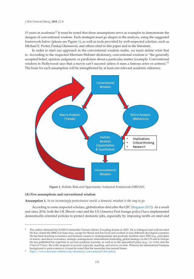
J. Risk Financial Manag. 2019, 12, 8
15 years in academia.6 It must be noted that these assumptions serve as examples to demonstrate thedangers of conventional wisdom. Each strategist must go deeper in the analysis, using the suggestedframework below (please see Figure 1), as well as tools provided by well-respected scholars, such asMichael E. Porter, Pankaj Ghemawat, and others cited in this paper and in the literature.
In order to start our approach in the conventional wisdom realm, we must define what thatis. According to the respected Merriam-Webster dictionary, conventional wisdom is “the generallyaccepted belief, opinion, judgment, or prediction about a particular matter (example: Conventionalwisdom in Hollywood says that a movie can’t succeed unless it stars a famous actor or actress).”7
The basis for each assumption will be strengthened by at least one relevant academic reference.
Figure 1. Holistic Risk and Opportunity Analytical Framework (HROAF).
(A) Five assumptions and conventional wisdom
Assumption 1. In an increasingly protectionist world, a domestic mindset is the way to go.
According to some respected scholars, globalization died after the GFC (Rugman 2012). As a resultand since 2016, both the UK (Brexit vote) and the US (America First foreign policy) have implementeddomestically-oriented policies to protect domestic jobs, especially by imposing tariffs on steel and
6 The author obtained his NASD Commodity Futures (Series 3) trading license in 2003. He is trilingual and well-traveled.He has visited the BRICS at least once, except for Brazil and has lived and worked in four different developed countries.He has been teaching economics and business courses to undergraduate and graduate students since 2002 (e.g., principlesof macro- and micro economics, strategic management, international marketing, global strategy) in the US and in Europe.He has published his expertise in several academic journals, as well as in the specialized press (e.g., Les Echos and theFinancial Times). He is the recipient of several corporate, teaching, and service awards. Whereas his international businessbackground is quite extensive, it must be noted that the researcher has natural biases.
7 https://www.merriam-webster.com/dictionary/conventional%20wisdom.
112
J. Risk Financial Manag. 2019, 12, 8
aluminum for the latter (Galbraith 2018). Other protectionist measures have included anti-immigrationrhetoric and a re-focus on nationalism and patriotism in these countries and in others (e.g., Hungary,Italy, and Austria). In essence, globalization, once the notion that called for integration andcollaboration in business and lifted hundreds of millions of people out of poverty (Ahlstrom 2010),has now become defunct for some and the enemy for others, even if the latter do not fully grasp thebenefits that they have been deriving from it (Betts 2016).
Assumption 2. Developed countries will always lead the global economy, others should follow theirbest practices.
Since the end of WWII, industrialized nations have developed a new industrial order (Drucker2017) and lowered trade barriers in order to boost global trade and foster peace among nations.This proven model for more than 70 years has propelled the US multinationals to unrivaled dominance.Therefore, all other countries tend to imitate the US (industrialized) model, especially developing oremerging countries.
Assumption 3. Developed countries have better institutions. Therefore, people who lead them know better.
Among modern institutions, universities are considered as some of the oldest ones. They dateback as far as the Middle Ages and were established in Europe (Altbach 1998) and used Latin as thecommon language (e.g., Bologna University, est. 1088 in Italy) to create and disseminate knowledge.This century-old process has attracted millions of students from the BRICS to Western Europe or toother developed countries that, over time, replaced Latin with English, as the lingua franca amongscholars. Nonetheless, it took centuries for universities to create the concept of a business school.
The world’s first collegiate business school was created in Philadelphia, Pennsylvania in 1881with a gift from entrepreneur and industrialist Joseph Wharton to produce graduates who wouldbecome “pillars of the state, whether in private or in public life.”8 Based on this intellectual legacy inindustrialized or developed countries, the assumption has been that people who lead institutions inthese countries know better.
Assumption 4. Emerging markets cannot produce world-class companies.
For decades, the concentration of power in US firms has been accumulated in systematic andstrategic fashion (White 2002). This dominance has been the source of much admiration around theworld thanks to the Forbes and Fortune 500 lists that have now become a ranking mechanism ofreputation (Bermiss et al. 2013) and prestige. Most of the firms in those list are American companies.Therefore, it is easy to assume that emerging markets cannot produce companies that could come closeto rival with a world-class American company.
Assumption 5. Among institutions, universities and their business schools do not play a major role in societysince business has been criticizing and ignoring business schools for decades.
In the 1950s and as a result of in-depth reports (Gordon and Howell 1959; Pierson 1959),the American business schools’ community was described as resembling trade schools which lackedacademic rigor. These reports also recommended that business education leverages the model ofmedical and law school for business to become a profession so that business can find its place insociety. Whereas the latter recommendation fell on deaf ears, the first one led to an (over)emphasison analytical skills and theories. This produced more criticisms about business education lackingrelevance (Pfeffer and Fong 2002) and the speculation as to whether the MBA will still exist in 2020(Schlegelmilch and Howard 2011). In any case, the disconnect between business schools and the
8 https://www.wharton.upenn.edu/about-wharton/.
113
J. Risk Financial Manag. 2019, 12, 8
business community has been clear and widely publicized (Skapinker 2011, 2008). Based on this, it canbe assumed that business schools do not play a major role in society.
As reasonable as these assumptions may appear to be, they need to be checked against thechronology of multiple events and patterns across countries, institutions, and industries.
(B) Chronology: from the dream of the BRICS to the nightmare of the GFC
In 2001 and in the developed world, many dreamed about the BRICs, not suspecting that a fewyears later, the 2008 GFC would become their worst nightmare. Trillions of dollars and millions ofjobs lost, due to greed and miscalculated risks in the developed world gave way to the BRICS andtheir emerging multinationals to rise. Unbeknownst to most in the developed world, the GFC alsocreated some deep cracks in society (increased income inequality, financial bankruptcies), whereasthe BRICS started collaborating with one another like never before. A closer look at the chronologyof these events and the trends that materialized informs us about the “big picture” that has affectedthe global economy by taking into account what happened in both developed and emerging marketswith a special look at the automotive industry, among other industries between 2000 and 2018 andas follows:
• 2000: The MSCI (Emerging Markets) index doubles within two years to reach 500 for the time.The shift from developed to emerging markets is starting. After two drops to 230 and 250 in 2001and 2002, respectively, this closely-watched index will climb above 1300 in October 2007 withoutsuffering any major setbacks.9
• 2000: Tata Tea buys Tetley Tea (UK).10
• 2000: John (Jack) C. Bogle, legendary investor and founder of the Vanguard Group ($5 trillion ofassets under management, as of 2018), warns investors about the dangers of a “sound premise”and provides timeless advice against conventional wisdom (Bogle 2000).
• 2001: Jim O’Neill coins the term BRIC.• 2001: China joins the WTO.• 2002: UN Secretary General, K. Annan, introduces the idea of inclusive globalization in a speech
at Yale University (Gemmill et al. 2002).• 2005: Lenovo buys IBM’s PC division.• 2007: against conventional wisdom on subprime loans and housing prices, John Paulson,
hedge fund manager, places his bet and executes the best trade ever, being rewarded withbillions of dollars and fame (Zuckerman 2010).
• 2008: The GFC starts with the collapse of Lehman Brothers (Mensi et al. 2016). The largestbankruptcy in US history; i.e., more than $600 bn, went against the conventional wisdom thatLehman was too big to fail and was going to be rescued by the US government like other financialinstitutions. It wasn’t and its collapse had many consequences in the financial markets, acrossindustries and countries. It bankrupted two out of three of the American BIG THREE. It leftFord moribund with record losses of $14.6 billion and fueled the growth of EMNCs, such as TataMotors and Geely. Except for Russia, which goes into isolation, the BRICS’ financial marketsrecouple with that of the US with increased linkages (Mensi et al. 2016) and later demonstrate theimportance of stocks from developed countries in optimal portfolios (Mensi et al. 2017). High riskstypically call for high rewards that will be delivered by the US stock market in a subsequentlong-term bull market.
9 https://seekingalpha.com/article/211305-the-shift-from-developed-to-emerging-markets-what-does-it-mean-for-investors.
10 https://www.indiatoday.in/magazine/cover-story/story/20091228-2000-tata-tea-tetley-merger-the-cup-that-cheered-741660-2009-12-25.
114
J. Risk Financial Manag. 2019, 12, 8
• 2008: Tata Motors buys Jaguar-Land Rover from Ford for $2.3 bn in cash.11
• 2008: China becomes a vital market for Ford since it passed the US as the largest market in theworld for all automakers in 2010 and became their largest foreign market.
• 2008: According to McKinsey, the number of connected devices equals the world’s population.12
• 2008: Lenovo becomes the sponsor of the Beijing Olympics.• 2009: Bernie Madoff is convicted and sentenced to 150 years in prison for the largest Ponzi scheme
in history.• 2009: GM files for bankruptcy after more than 100 years in business.• 2009: from an all-time high of 1337 in 2007, the MSCI (Emerging Markets) index plummets to 499
in February 2009.13
• 2010: Geely acquires Volvo cars from Ford and could have been seen as a partner. However,additional moves by the EMNC indicate that it is becoming a competitor to reckon with, both inChina and at home, not to mention in Europe.
• 2010: Grupo Bimbo (Mexico) acquires the North American fresh bakery business of Sara Lee.• 2011: MSCI (Emerging Markets) index recovers from the 2009 crash and reaches 1204 (see
footnote 13).• 2012: the MOOC revolution starts: greater access to business education at a fraction of the cost.
MOOC courses are offered to millions by Wharton, Harvard, MIT, etc.• 2012: The end of globalization? (Rugman 2012). The conventional wisdom about the benefits of
globalization starts to change. Globalization becomes the enemy of many. Populism (Mudambi2018) and protectionism grow in the UK, US, Spain, Italy, Russia, China, and Brazil.
• 2012: Dalian Wanda Group (China) acquires AMC Theaters for $2.6 bn.• 2013: Jim O’Neill retires from Goldman Sachs as Chairman of the Asset Management Division.• 2015: Goldman Sachs closes its BRIC fund after years of losses and assets under management
free-falling from $800 to $100 million.• 2015: LinkedIn reaches 500 million users and is increasingly used by scholars to socialize
their research.• 2016: Brexit vote takes place. It catches financial markets and political science experts by surprise.
Unaware of the consequences of leaving Europe, millions of British turn to google to betterunderstand the EU that they just rejected in a historic vote.
• 2016: Haier buys GE’s appliances division for $5.4 billion.• 2016: Donald Trump is elected President of the US.• 2016: the MSCI (Emerging Markets) index plummets again to 742 (see footnote 13).• 2017: President Trump announces his America First policy and exits the Transpacific Partnership
Agreement which was going to reduce tariffs, create jobs, and boost trade.• 2017: ChemChina completes the largest foreign takeover by a Chinese firm by acquiring Syngenta
for $43 billion.14
• 2017: Geely buys Lotus (UK).• 2018: the MSCI (Emerging Markets) index climbs to 1254 in January and loses 23.84% of its value
by 2 January 2019, trading at the level of 955 (see footnote 13).• 2018: amidst a trade war between the US and China ((Trump administration decision to impose
25 per cent tariffs on steel and 10 per cent aluminum imported from China, retaliation from China,
11 http://shares.telegraph.co.uk/news/article.php?id=2799469&archive=1&epic=500570.12 https://www.slideshare.net/AhmedALBilal/2017-q2-mckinsey-quarterly-global-forces.13 https://www.investing.com/indices/msci-emerging-markets-historical-data.14 https://www.reuters.com/article/us-syngenta-ag-m-a-chemchina/chemchina-clinches-landmark-43-billion-takeover-
of-syngenta-idUSKBN1810CU.
115
J. Risk Financial Manag. 2019, 12, 8
and escalation with other tariffs between the two countries), the conventional wisdom on thepermanence of free trade agreements and free-trade policies started after WWII is rocked to itscore. Major financial markets enter correction territory.
• 2018: Geely buys a stake in the truckmaker AB Volvo and took a 10% stake in Daimler (parentcompany of Mercedes-Benz). All of these brands are sold in the US.
• Late August 2018: Geely announces the building of a new plant to produce bigger vehicles (trucks,SUVs, and cross-overs) and expected 90% of its cars to be electric by 2020. This confirms thegrowth of Geely both as an automaker but also as a threatening competitor to Ford.
If we compare and contrast the assumptions with the events and patterns above, we might beable to uncover some unconventional wisdom, also known as strategic insights.
3. Results
Finding Some Unconventional Wisdom to Derive Strategic Insights
In this section, we aim to find new strategic insights by reviewing the five assumptions based onthe above chronology.
Assumption 1. In an increasingly protectionist world, a domestic mindset is the way to go.
Based on decades of research, the IMF re-affirmed in 2001, the year that China joined theWTO, that:
“Policies that make an economy open to trade and investment with the rest of the world areneeded for sustained economic growth. The evidence on this is clear. No country in recentdecades has achieved economic success, in terms of substantial increases in living standardsfor its people, without being open to the rest of the world.”15
Between 2001 and 2016, even with globalization suffering an identity crisis, the world remainedmore global-minded than protectionist and a global mindset was proven to be a predictor of success inglobal leadership positions (Javidan and Teagarden 2011; Beechler and Javidan 2007; Lane et al. 2009).
A research update as to whether tariffs are protecting American jobs also confirms that this is notthe case since Ford prepared mass layoffs at the end of 2018 in order to off-set some $1 billion lost dueto tariffs imposed by China in retaliation to US tariffs.16 Other industries and more than 200 companieswere also suffering from the tariffs in the US, cutting costs through layoffs and fore-going expansion.17
With the Smoot-Haley Tariff Act of 1930 in the US (Kennedy 2003) and the Imports Duties Act of1932 in the UK, history has also shown that protectionism can be destructive rather than protective.In 2010, Oxford University Press published a great analysis which explained that “Hoover refused tolisten to the pleas of 1,038 American economists who, in 1930, urged him to veto the Smoot–Hawleytariff bill. When it became law, this legislation raised US import duties and ultimately led to retaliatoryaction throughout the world. Not surprisingly, US foreign trade declined once the depression began tobite” (Crafts and Fearon 2010).
Clearly, this assumption is invalidated. It is a myth based on fear (Kennedy 2003). By definition,the 21st global economy cannot function based on a protectionist mindset. Globalization may bechanging. However, the world remains inter-dependent and semi-globalized, where global traderepresents at least 30% of the global economy (Ghemawat 2018).
Assumption 2. Developed countries will always lead the global economy, others should follow theirbest practices.
15 https://www.imf.org/external/np/exr/ib/2001/110801.htm.16 http://fortune.com/2018/10/09/ford-stock-today-layoffs-trump-trade-tariffs/.17 https://www.cato.org/publications/commentary/here-are-202-companies-hurt-trumps-tariffs.
116
J. Risk Financial Manag. 2019, 12, 8
This assumption is based on the current context, a view that suffers from myopia. When takinga much broader look at business and economic history, we should remember that China and Indiawere dominant countries during previous centuries and that Russia was a mighty empire led bystrategic tsars.
By focusing on China alone, it must be noted that the Han Dynasty established as a major powermore than 2000 years ago.18
In all fairness, China’s current economic development, growing faster than developed nations (e.g.,Japan) for decades since the 1980s (Kang 2007) but still considered “developing” due to institutionalvoids (Khanna and Palepu 2010, 2005), cannot be the only period used to assess this 5000 year oldcivilization that goes back much farther in history than most developed countries. For example, it mustbe noted that China developed fast when Europe was experiencing turmoil during the Middle-Agesafter the fall of the Roman Empire. According to a highly-cited book, published by the OECD,an important development was the “Chinese settlement of the relatively empty and swampy landssouth of the Yangtse, and introduction of new quick–ripening strains of rice from Vietnam suitable formulticropping” between the eighth and thirteenth centuries (Maddison 2007, p. 18). During these fivecenturies, “population growth accelerated, per capita income rose by a third, and the distribution ofpopulation and economic activity were transformed. In the eighth century only a quarter of the Chinesepopulation lived south of the Yangtse; in the thirteenth, more than three quarters. The new technologyinvolved higher labour inputs, so productivity rose less than per capita income” (Maddison 2007).Today, China and other countries are considered developing countries or emerging economies whereasthey once dominated, similarly to the Roman Empire. Dominance is not permanent. No developedcountry can aspire to always lead the global economy. Last but not least, adopting policies from theWest or the “developed” nations, also referred as the “Washington Consensus,” with the premise thatthey would be successful elsewhere, can result in economic disaster in developing nations (Chang2002). Therefore, this assumption is also invalidated.
Assumption 3. Developed countries have better institutions. Therefore, people who lead them know better.
Institutions, such as universities and business schools, can create and hire scholars who cancome from any country in the world and many have come from the BRICS. Scholars can also beborn out of institutions, even if it remains an exception rather than the norm. Indeed, one ofthe foremost mathematicians who was born in India, Srinivasa Ramanujan, solved very complexproblems and advanced theories through a series of breakthroughs in his youth without having muchformal education (Singh 2017). Other scholars from Russia include many Nobel Laureates in severaldisciplines, especially physics (Dardo 2004). For all these reasons, the assumption on the “superiority”of institutions in developed countries and of the knowledge accumulated by the people who lead themis invalidated.
Assumption 4. Emerging markets cannot produce world-class companies.
This assumption is also based on the perception that emerging markets are “not there yet” (Khannaand Palepu 2000; Khanna and Palepu 2010) and therefore cannot compete with industrialized countries’giants, such as IBM, Boeing, Ford, Apple, etc. The reality is much different: Lenovo, once a regionalplayer has become the largest PC vendor in the world after acquiring the PC division of IBM. Embraer(Brazil) is another success story, and so is Tata Motors which acquired Jaguar and Land Rover fromFord in 2008, or even Huawei overtaking Apple in global smartphones sales in 2018.19 These arejust a few examples among many. A closer look at the largest companies in the world, measured by
18 https://www.bbc.com/news/world-asia-pacific-13017882.19 https://qz.com/1345496/apple-was-just-overtaken-by-huawei-in-global-smartphone-sales/.
117
J. Risk Financial Manag. 2019, 12, 8
revenues, also indicates that 3 out of the first 5 largest are Chinese.20 This assumption is a myth that iseasily busted once researched.
Assumption 5. Among institutions, universities and their business schools do not play a major role in societysince business has been criticizing and ignoring business schools for decades.
This assumption is often based on the misunderstanding associated with the value andcontributions of education to society. According to a 2017 UNESCO report, the total number ofhigher-education students has doubled between 2000 and 201421 and represents a healthy 5% increaseon an annual basis. Business education is the most popular choice among all disciplines; it attractsabout a quarter of all university students. This assumption is often based on a quantitative analysiswhich does not account for qualitative contributions, such as launching new businesses, findingsolutions to societal problems, etc. Business education has even transformed an emerging marketlike China by going from Marx to a hybrid capitalistic model (Tsinghua)22 or profoundly boostingthe country’s competitiveness: India (Indian Institutes of Management), FGV (Brazil, and Skolkovo(Russia). Therefore, this assumption is also invalidated.
Many of the higher education students earn an MBA, the passport to management and especiallyto careers in Finance or Consulting. Business actually touches all disciplines and vice versa (e.g.,medicine). To better assess the role of business schools in society, we must wonder how the worldeconomy would perform without them and without business education in general. Clearly, if the BRICShave made so much economic progress, a large part of that can be attributed to education, the socialelevator, and one of the best ways to help a country navigate the global economy competitively.Education provides the tools to make better decisions, solve problems, and redistribute wealth. In bothemerging and developed countries, what is needed is not less education but more. We will discuss thisin greater details below.
4. Discussion
Invalidating assumptions that seemed reasonable at first can lead to a state of confusion.What should we believe now? This is where higher-education and business schools, in particular,have a particularly important role to play and can make a positive and global impact on society.Business schools teach the hard skills (e.g., research, analytics, problem-solving, and reasoning) andthe soft skills (communication, cross-cultural literacy, and conflict resolution). In addition, businessschools socialize their students with the rest of the university and the business community throughgeneral education courses on ethics or other matters, such as political science, computer science,and foreign languages. Students, not only acquire knowledge that is crucially important in the 21stcentury economy that is more internationally interdependent than ever, but also learn appropriatebehaviors and perspectives unlike their own. These skills and behaviors applied to the problems facedby today’s society can advance all of us toward a resolution that is acceptable to all (e.g., sharing valuesand reducing income inequality). In short, business education can help us coexist and reduce conflictswithin each country and between countries. To achieve this collaborative approach and avoid divisiveissues, an inter-disciplinary education is very important. However, all too often, students focus on onediscipline whereas problems call on several disciplines to be solved. These and our society are morecomplex than ever. Therefore, we must get both the small and the big pictures right.
By combining the reasonable assumptions above which were based on a narrow perspective witha bigger picture approach, this paper aims to provide a better understanding of key issues that havebeen plaguing emerging markets. That big picture approach reminds us that the largest two of them
20 http://fortune.com/global500/.21 http://unesdoc.unesco.org/images/0024/002478/247862E.pdf.22 https://money.cnn.com/magazines/fortune/fortune_archive/2005/05/16/8260218/index.htm.
118
J. Risk Financial Manag. 2019, 12, 8
by population (China and India) represent 40% of the world’s population. We also need to think inhuman terms, not just in numbers terms. Qualitative analysis must supplement quantitative analysisto better understand progress to date, as well as the risks and opportunities that lie ahead.
For example, the pattern of world-class companies coming out of emerging markets has surprisedmany executives and investors in developed markets. In some cases, some of them misunderstood theircompetition and the threat associated with those emerging multinationals. Some scholars spotted thetrend early on (Khanna and Palepu 2010; Guillén and García-Canal 2009; Ramamurti 2012; Holtbrüggeand Kreppel 2012). However, due to the focus of most business executives on the small pictureand short-term results, many of them did not benefit from these important research contributions.They were blindsided by the risks. It is, therefore, necessary to conceptualize a new and holisticframework [Figure 1] to challenge conventional wisdom in order to improve our assessment of risksand opportunities. This framework combines the quantitative and qualitative analyses of macro trends,micro behaviors (of institutions, firms, customers, especially if they become movements, such aspopulism), implications, critical thinking, and research. It should result in strategic insights that wecall unconventional wisdom, as it challenges pre-conceived ideas and contributes to new conventionalwisdom through a feedback loop of continuous improvement.
Education is a choice. We can choose to identify problems, prioritize them, and look for solutionsthat are acceptable to all and will avoid the worst catastrophic risks from materializing. An inclusiveglobalization based on shared values (Porter and Kramer 2011) would be advisable since we are allinter-dependent and “all in it together.” To put this important concept in practice, business schoolsplay a vital role in the economy and society, in regards to, not only create prosperity but also helpre-distribute it, while staying relevant. They must train their students about that role and increasinglyabout disruptions that affect countries, people –their future and the future of work in the context ofartificial intelligence (AI) advances, unparalleled until now—institutions, industries, and markets.Thankfully, business schools are not alone in this daunting tasks. Organized among peers by theAssociation for the Advancement of Colleges and Schools of Business (AACSB) International since 1916,world’s largest business education alliance, they clearly benefit from valuable resources.23 The newAACSB Chair as of 31 January 2018 shared the organization’s new vision and the key success factors forbusiness schools: (1) cultivate a position at the intersection of academe and practice, (2) be a driver ofinnovation in higher education, and (3) connect with other disciplines (Beck-Dudley 2018). Disruptionsand change in general, provide challenges and opportunities. Business schools, as well as the graduatesand scholars that they produce, have the unique capacity to address challenges and capitalize onopportunities. It will fascinating to watch how they evolve in society and what positive contributionsthey will continue to make.
5. Conclusions
Conventional wisdom, used knowingly or unknowingly, has not always been the friend ofthe strategist, especially in an emerging market environment where institutional voids, rampantcorruption, and other dangers loom large and can be found next to unparalleled opportunities. Due tothe scarcity of strategic frameworks to assess the BRICS since the GFC, this paper aims to help fillthis gap by providing a simple but holistic and analytical framework that we call the Holistic Riskand Opportunity Analytical Framework (HROAF). It relies on both qualitative and quantitate data,as well as macro (trends) and micro (behaviors) analyses. It can provide the strategist with a differentlens to manage a new normal of uncertainty, volatility, risks, and opportunities, thereby creating someunconventional wisdom and a sustainable competitive advantage for him or her. Whereas the HROAFshould allow strategists to generate some initial insights, each strategist is expected to dive deeper ineach portion of our multi-dimensional framework, as needed. We believe that, when used regularly,
23 https://www.aacsb.edu/newsroom/2018/2/new-leadership-named-to-aacsb-board-of-directors.
119
J. Risk Financial Manag. 2019, 12, 8
this framework could become a useful tool to unleash the potential of a new strategic and globalmindset that will help reduce the biases and dangers that come from conventional wisdom.
Limitations: as useful as this approach may be, it has limitations. It is based on only one researcher,his experience, his research, and his natural biases. Only five assumptions were tested as a basisfor illustration. It is possible that additional assumptions would unleash more insights. In addition,mixing methods can be challenging and require a large team supporting each strategist. Not everyonecan expect to have such support to implement this framework.
More research, a deeper dive, and more triangulation are needed, especially on how deeply-rootedin conventional wisdom any assumptions are. In an era of fake news, scholars have the societalresponsibility to redirect assumptions and bust myths that have been misleading investors,policymakers, and voters. Uninformed decisions can have catastrophic economic and humanconsequences for any given country and the world economy.
Using our Holistic Risk and Opportunity Analytical Framework to discover some much-neededunconventional wisdom and setting inclusive globalization as a priority could be a way to rebuild theBRICS and allow everyone to prosper in peace.
Funding: This research received no external funding.
Conflicts of Interest: The author declares no conflict of interest.
References
Ahlstrom, David. 2010. Innovation and growth: How business contributes to society. Academy of ManagementPerspectives 24: 11–24.
Altbach, Philip G. 1998. Comparative Higher Education: Knowledge, the University, and Development. Santa Barbara:Greenwood Publishing Group.
Beck-Dudley, Caryn L. 2018. The Future of Work, Business Education, and the Role of AACSB: Keynote Address tothe Academy of Legal Studies in Business, Annual Meeting, Savannah, Georgia, September 8, 2017. Journalof Legal Studies Education 35: 165–70. [CrossRef]
Beechler, Schon, and Mansour Javidan. 2007. Leading with a global mindset. In The Global Mindset. Bingley:Emerald Group Publishing Limited, pp. 131–69.
Bermiss, Y. Sekou, Edward J. Zajac, and Brayden G. King. 2013. Under construction: How commensuration andmanagement fashion affect corporate reputation rankings. Organization Science 25: 591–608. [CrossRef]
Betts, Alexander. 2016. Why Brexit happened–and what to do next. Ted Talk, June.Bogle, John C. 2000. Common Sense on Mutual Funds: New Imperatives for the Intelligent Investor. Hoboken: John Wiley
& Sons.Chang, Ha-Joon. 2002. Kicking away the Ladder: Development Strategy in Historical Perspective. London: Anthem
Press.Crafts, Nicholas, and Peter Fearon. 2010. Lessons from the 1930s Great Depression. Oxford Review of Economic
Policy 26: 285–317. [CrossRef]Currie, Graeme, David Knights, and Ken Starkey. 2010. Introduction: A post-crisis critical reflection on business
schools. British Journal of Management 21: s1–s5. [CrossRef]Dardo, Mauro. 2004. Nobel Laureates and Twentieth-Century Physics. Cambridge: Cambridge University Press.Drucker, Peter F. 2017. The New Society: The Anatomy of Industrial Order. Abingdon: Routledge.Galbraith, Jean. 2018. US tariffs on steel and aluminum imports go into effect, leading to trade disputes. American
Journal of International Law 112: 499–504.Gemmill, Barbara, Maria Ivanova, and Chee Yoke Ling. 2002. Designing a new architecture for global
environmental governance. In World Summit for Sustainable Development Briefing Papers. Johannesburg:United Nations.
Ghemawat, Pankaj. 2018. The New Global Road Map: Enduring Strategies for Turbulent Times. Brighton: HarvardBusiness Press.
Giacalone, Robert A., and Donald T. Wargo. 2009. The roots of the global financial crisis are in our businessschools. Journal of Business Ethics Education 6: 147–68.
120
J. Risk Financial Manag. 2019, 12, 8
Gordon, Robert Aaron, and James Edwin Howell. 1959. Higher education for business. The Journal of BusinessEducation 35: 115–17. [CrossRef]
Guillén, Mauro F., and Esteban García-Canal. 2009. The American model of the multinational firm and the newmultinationals from emerging economies. Academy of Management Perspectives 23: 23–35. [CrossRef]
Holtbrügge, Dirk, and Heidi Kreppel. 2012. Determinants of outward foreign direct investment from BRICcountries: an explorative study. International Journal of Emerging Markets 7: 4–30. [CrossRef]
Howard, Thomas, and Eric Cornuel. 2012. Business schools in transition? Issues of impact, legitimacy, capabilitiesand re-invention. The Journal of Management Development 31: 329–35. [CrossRef]
Javidan, Mansour, and Mary B. Teagarden. 2011. Conceptualizing and measuring global mindset. In Advances inGlobal Leadership. Bingley: Emerald Group Publishing Limited, pp. 13–39.
Kang, David Chan-oong. 2007. China Rising: Peace, Power, and Order in East Asia. New York: Columbia UniversityPress.
Kennedy, David M. 2003. The American People in the Great Depression: Freedom from Fear, Part One. Oxford: OxfordUniversity Press.
Khanna, Tarun, and Krishna Palepu. 2000. The future of business groups in emerging markets: Long-run evidencefrom Chile. Academy of Management Journal 43: 268–85.
Khanna, Tarun, and Krishna G. Palepu. 2005. Spotting Institutional Voids in Emerging Markets. Boston: HarvardBusiness School.
Khanna, Tarun, and Krishna G. Palepu. 2010. Winning in Emerging Markets: A Road Map for Strategy and Execution.Brighton: Harvard Business Press.
Khanna, Tarun, and Jan W. Rivkin. 2001. Estimating the performance effects of business groups in emergingmarkets. Strategic Management Journal 22: 45–74. [CrossRef]
Lane, Henry W., Martha Maznevski, Joerg Deetz, and Joseph DiStefano. 2009. International Management Behavior:Leading with a Global Mindset. Hoboken: John Wiley & Sons.
London, Ted, and Stuart L. Hart. 2004. Reinventing strategies for emerging markets: Beyond the transnationalmodel. Journal of International Business Studies 35: 350–70. [CrossRef]
Maddison, Angus. 2007. The World Economy Volume 1: A Millennial Perspective Volume 2: Historical Statistics.New Delhi: Academic Foundation.
Mensi, Walid, Shawkat Hammoudeh, Duc Khuong Nguyen, and Sang Hoon Kang. 2016. Global financial crisisand spillover effects among the US and BRICS stock markets. International Review of Economics & Finance 42:257–76.
Mensi, Walid, Shawkat Hammoudeh, and Sang Hoon Kang. 2017. Dynamic linkages between developed andBRICS stock markets: Portfolio risk analysis. Finance Research Letters 21: 26–33. [CrossRef]
Mudambi, Ram. 2018. Knowledge-intensive intangibles, spatial transaction costs, and the rise of populism. Journalof International Business Policy 1: 44–52. [CrossRef]
O’Neill, Jim. 2001. Building Better Global Economic BRICs. New York: Goldman Sachs.Pandit, Vishwanath. 2018. Global Economic Crisis 2008: A Contemporary Reappraisal with an Ethical Perspective.
New York: Goldman Sachs.Pfeffer, Jeffrey, and Christina T. Fong. 2002. The End of Business Schools? Less Success Than Meets the Eye.
Academy of Management Learning & Education 1: 78–95. [CrossRef]Pierson, Frank C. 1959. The education of American businessmen. The Journal of Business Education 35: 114–17.
[CrossRef]Porter, Michael E., and Mark R. Kramer. 2011. The Big Idea: Creating Shared Value. Boston: Harvard Business
Review.Ramamurti, Ravi. 2012. What is really different about emerging market multinationals? Global Strategy Journal 2:
41–47. [CrossRef]Rugman, Alan. 2012. The End of Globalization. New York: Random House.Schlegelmilch, Bodo B., and Thomas Howard. 2011. The MBA in 2020: Will there still be one? The Journal of
Management Development 30: 474–82. [CrossRef]Singh, Simon. 2017. Fermat’s Enigma: The Epic Quest to Solve the World’s Greatest Mathematical Problem. New York:
Anchor.Skapinker, Michael. 2008. Why business ignores the business schools. Financial Times, June 8.Skapinker, Michael. 2011. Why business still ignores business schools. Financial Times, January 24.
121

J. Risk Financial Manag. 2019, 12, 8
White, Lawrence J. 2002. Trends in aggregate concentration in the United States. Journal of Economic Perspectives 16:137–60. [CrossRef]
Wilson, Dominic, and Roopa Purushothaman. 2003. Dreaming with BRICs: The path to 2050. Global EconomicsPaper, October 1.
Wright, Mike, Igor Filatotchev, Robert E. Hoskisson, and Mike W. Peng. 2005. Strategy research in emergingeconomies: Challenging the conventional wisdom. Journal of Management Studies 42: 1–33. [CrossRef]
Zuckerman, Gregory. 2010. The Greatest Trade Ever: The Behind-the-Scenes Story of How John Paulson Defied WallStreet and Made Financial History. New York: Crown Pub.
© 2019 by the author. Licensee MDPI, Basel, Switzerland. This article is an open accessarticle distributed under the terms and conditions of the Creative Commons Attribution(CC BY) license (http://creativecommons.org/licenses/by/4.0/).
122
Journal of
Risk and FinancialManagement
Article
Contagion Risks in Emerging Stock Markets:New Evidence from Asia and Latin America
Thi Bich Ngoc TRAN
College of Economics, Hue University, Hue City 49127, Vietnam; [email protected]
Received: 26 September 2018; Accepted: 3 December 2018; Published: 14 December 2018
Abstract: The purpose of this study is to investigate whether contagion actually occurred duringthree well-known financial crises in 1990s and 2000s: Mexican “Tequila” crisis in 1994, Asian“flu” crisis in 1997 and US subprime crisis in 2007. We apply dynamic conditional correlationmodels (DCC-GARCH(1,1)) to daily stock-index returns of eight Asian stock markets, six LatinAmerican stock markets and US stock market. Defining contagion as a significant increase of dynamicconditional correlations, we test for contagion by using a difference test for DCC means. The resultsobtained shows that there is a pure contagion from crisis-originating markets to other emerging stockmarkets during these three crisis. However, the contagion effects are different from one crisis to theother. Firstly, during the Mexican crisis, contagion is detected in only the Latin American region.Secondly, during the Asian crisis, we find evidence of contagion in some markets in both the Asianand Latin American regions. Finally, contagion is proved to be present in all stock markets with theonly exception for Brazil during US subprime crisis.
Keywords: international financial contagion; shift contagion; emerging stock markets; Asian crisis;Mexican crisis; US subprime crisis; DCC-GARCH
JEL Classification: F30; G10; G15
1. Introduction
Since the 1990s, many widespread financial crises have been witnessed such as the ExchangeRate Mechanism (ERM) attacks in 1992, Mexican “Tequila” crisis in 1994, Asian “flu” crisis in 1997,the Russian collapse in 1998, the Brazilian devaluation in 1999, the US subprime crisis in 2007 andmore recently, the Greek and European sovereign debt crisis in 2011. One common feature of thesecrises is that they have provoked economic depressions not only for the crisis-originating market butalso for the others. This phenomenon is usually described as “contagion”. The question about howan initial shock of one market could be transmitted to the others have attracted as much attentionof policy makers as academic researchers, especially after Asian crisis in 1997. The latter have so farinvestigated the transmission mechanisms of the crises and the existence of contagion phenomenonacross financial markets.
Understanding contagion effect of financial crisis, especially the channels through which crisis istransmitted, would provide important implications for policy makers. It will help to adopt appropriatepolicy measures in order to reduce the vulnerability of a country to an external shock. Policyimplications differ depending on shock propagation through fundamentals or shock propagationunrelated to fundamentals (Forbes and Rigobon (2002)). If the crises are channeled through short-runlinkages which only exist after the crisis occurs (i.e., investors’ behavior) then temporary measure likeliquidity assistance can be a helpful response. Otherwise, if the crises are transmitted through permanentlinkages, such as trade or financial linkages, liquidity support might only delay the transmission of acrisis from one country to another but cannot be effective in reducing a country’s vulnerability to a crisis.In this case, policy measures improving the fundamentals are necessary (Moser (2003)).
J. Risk Financial Manag. 2019, 11, 1–20; doi:10.3390/jrfm11040089 www.mdpi.com/journal/jrfm123
J. Risk Financial Manag. 2019, 11
Up to now, there are many studies investigating the existence of contagion during financialcrises. However, their results are not all compatible with one another. It depends how “contagion” isdefined and empirical method used to detect for contagion. All of these issues will be discussed inSection 2. The results of King and Wadhwani (1990) support for contagion effects during the stockmarket crash in 1987. Calvo and Reinhart (1996) find evidence of contagion during the Mexicancrisis. Baig and Goldfajn (1999) also find the presence of contagion during the Asian crisis in 1997.However, Forbes and Rigobon (2002) reexamine contagion effects during these three crises withtests corrected for heteroskedasticity biases and find no contagion, only interdependence 1. On theother hand, Corsetti et al. (2005) reconsider the international transmission of shocks from the HongKong stock market crisis in October 1997 during the Asian crisis and find some contagion, someindependence. They find evidence for contagion for 5 countries in the sample of 17 including Singapore,the Philippines (among the emerging markets) and France, Italy and the UK (among the industrialcountries). Concerning the US subprime crisis, Horta et al. (2008) find evidence for effects of financialcontagion from the US subprime crisis in G7 markets. Naoui et al. (2010) also find contagion effectsfrom US toward some emerging (India, Malaysia, Singapore, China, Hong Kong and Tunisia) anddeveloped markets (France, Germany, Italy, Netherlands and United States).
In this paper, we investigate again the presence of contagion effects in Asian and Latin Americanstock markets during three major crises: the Mexican “Tequila” crisis in 1994, the Asian “flu” crisis in1997, and the US subprime crisis in 2007. We consider the contagion as the significant increase of assets’price co-movements after a shock in a country, as labeled “shift contagion” by Forbes and Rigobon(2000). In the first step, we employ multivariate DCC-GARCH models proposed by Engle (2002) toexamine how dynamic conditional correlations across markets vary in time. We apply this kind ofmodel in order to capture the dynamics of conditional correlation. In the second step, we use t-tests tocompare the correlations between markets’ returns in stable period and turmoil period. If there is anincrease of these correlations after a shock then contagion occurs.
The contribution of this paper is that we study the contagion risks among some selected emergingcountries in Asia and Latin America during three major crises: one occurred in Latin America, onein Asia, and one in US after their financial liberalisation. The results will show us how the financialcontagion spills over to these countries during the crises and help us to compare the contagion effectsof the three crisis. In fact, most of emerging countries began their financial liberalization in late 1980sand early 1990s. Theoretically, financial markets become more integrated as a result of the liberalizationprocess and hence, they may suffer greater contagion from external shocks. As a consequence, marketliberalization, accompanied by market integration, may lead to increased contagion risks. The resultsof this paper will show us somehow the effects of financial liberalization in emerging markets which isnecessary for policy makers. The paper is structured as follows. Section 2 presents a brief review of theliterature. Section 3 offers the methodology employed. Section 4 presents the data and statistics ofstock returns. Section 5 discusses empirical results. Section 6 draws conclusions.
2. Review of Studies
Contagion has been the subject of extensive academic literature. There exist several definitionsfor this concept2. In general, contagion is usually used to refer to the spread of market turbulencesfrom one country to the others. It needs to be distinguished from a common shock that affect manycountry simultaneously. Masson (1998) proposes the term “monsoonal effects” rather than contagionfor a such phenomenon.
1 The interdependence term here refers to a high level of market comovement in all periods.2 See Pericoli and Sbracia (2003) for a review of contagion definition.
124
J. Risk Financial Manag. 2019, 11
Contagion can be divided into two categories3: The first category is “fundamental-basedcontagion”, which refers to spillovers resulting from interdependence among markets. In thiscase, a shock to a market can be transmitted to the others through the linkages (trade, financiallinkages) between these markets. Forbes and Rigobon (2001) show that trade linkages are important intransmitting a crisis internationally during the currency crisis in 1990s. Kaminsky and Reinhart (2000)find that beside trade links, financial links are powerful channels of fundamental-based contagion.However, there are several authors who do not consider cross-country propagation of shocks throughfundamentals as contagion (See Masson (1998), Forbes and Rigobon (2002)) because it reflects normalinterdependence but in crisis period. Hence, another category of contagion labeled “pure contagion”or “non-fundamental based contagion” is considered. This form of contagion cannot be explainedby the fundamentals, but rather by the behaviors of investors. When a crisis occurs in one country,investors can withdraw their investments from many markets. “Pure contagion” is hence a panicmovement which cannot be justified by economic linkages between markets (See Moser (2003)). In thepaper of Kumar and Persaud (2001), the authors show that investors’ appetite for risk can conduct topure contagion.
Based on these two categories of contagion, theories on shock transmission are also dividedinto two groups: non crisis-contingent theories and crisis-contingent theories. On the one hand,the non crisis-contingent theories, which refer to the “fundamental-based contagion” category, assumethat transmission mechanisms do not change after a shock. On the other hand, the crisis-contingenttheories, which refer to the “pure contagion” category, propose that there is a significant differencein transmission mechanisms between stable and crisis periods and therefore cross-market linkagesincrease after a shock4.
In this paper, we follow the second group of theories mentioned above. More specifically,we use the definition of contagion established by Forbes and Rigobon (2001) and Forbes and Rigobon(2002). These authors label “shift-contagion” instead of simply “contagion”. They define contagion as“a significant increase in cross-market linkages after a shock to an individual country (or group of countries)”.If two markets always show high correlations in all states of the world, this situation should be referredto “interdependence” and not “contagion”. Although this definition is clearly narrow and restrictive,it exhibits two important advantages. First, it gives a simple empirical method to test for the existenceof contagion. We can simply compare the linkages between two markets during stable periods withthose during crisis periods. If there is a shift in linkages between markets during crisis period then weconclude that contagion occurs during the crisis under investigation. Second, by defining contagion asa significant increase in cross-market linkages, we can differentiate the mechanisms of transmission ofshocks. The evidence of “shift-contagion” would support for crisis-contingent theories.
One of the statistics used to measure cross-market linkages is cross-market correlation coefficients.The cross-markets linkages can also be measured by probability of a speculative attack, transmissionof shocks or volatility. In summary, there are four kinds of tests that are usually used: tests onthe correlation coefficients, tests estimating the variance-covariance transmission mechanism acrosscountries, tests for co-integration and tests measuring changes in the propagation by identifyinga model with simple assumptions and exogenous events (Forbes and Rigobon (2002)). The testsfor contagion based on this statistics will test for an increase in the correlation coefficients betweentwo markets after a shock. Due to its simplicity, this methodology is used in many papers suchas King and Wadhwani (1990), Calvo and Reinhart (1996). They all find a significant increase incross-market correlation during crisis period which gives evidence for the existence of contagion.However, as demonstrated by Forbes and Rigobon (2002), the results of this kind of tests are biasedin the presence of heteroskedasticity in market returns. They show that even though the linkages
3 See Dornbusch et al. (2001).4 See Forbes and Rigobon (2001).
125
J. Risk Financial Manag. 2019, 11
between two markets do not change after a shock, these tests do show an increase in cross-marketcorrelation coefficients because of an increase in market volatility. Hence, these tests of contagionneed to be corrected for this bias. In their paper, by using tests for contagion based on cross-marketcorrelation coefficient corrected for heteroskedasticiy, Forbes and Rigobon (2002) found no contagion,only interdependence during the 1994 Mexican Peso Crisis, the 1997 Asian Crisis and the 1987 US crisis.
Nevertheless, Billio and Pelizzon (2003) raises an issue with the methodology proposed by Forbesand Rigobon (2002) mentioned above. They show that even if correlation coefficients are adjusted forheteroskedasticity, the traditional tests for contagion are highly affected by the source of crisis and thewindows used. Moreover, splitting a sample according to realized or observed values (i.e., high andlow volatility) may provide misleading results due to the selection bias (See Boyer et al. (1999)).
Since this test for contagion based on simple correlation coefficients presents obvious limitations,another econometric technique is developed in the literature to study financial contagion: They aredynamic conditional correlation models (DCC-GARCH models). This method has four advantages.First, these models capture the dynamics of correlation coefficients. Many studies prove thatcross-market correlations are not constant but vary over time (See Longin (1995), Ramchand andSusmel (1998)). Second, the DCC-GARCH models estimate correlation coefficients of standardizedresiduals and thus account for heteroskedasticity directly5. Third, the DCC-GARCH models can be usedto examine multiple asset returns without adding too many parameters. Finally, this method allows toexamine all possible pair-wise correlations for all markets in only a single model (Chiang et al. (2007)).
Recently, this methodology has been usually used in examining financial contagion.Chiang et al. (2007) found evidence of contagion effects during the Asian financial crisis withheteroskedasticity-adjusted simple correlation analysis as well as dynamic correlation analysis.Cho and Parhizgari (2008) otherwise studied contagion during the Asian financial crisis in 1997 byusing dynamic conditional correlation (DCC) means and medians difference tests. They consideredtwo sources of contagion, Thailand and Hong Kong, and found the presence of contagion in equitymarkets across all markets studied: Korea, Malaysia, Philippines, Singapore, Taiwan, Indonesia.Naoui et al. (2010) investigated contagion during the 2007 US subprime crisis in using DCC-GARCHmodels and adjusting correlation coefficients to control for heteroscedasticity. They found contagioneffects from US toward Argentina, Brazil, Korea, Hong Kong, Malaysia, Mexico and Singapore.
3. Methodology
3.1. Dynamic Conditional Correlation Model
As mentioned in the previous section, we use the DCC-GARCH model developed by Engleand Sheppard (2001), Engle (2002) to examine the time-varying correlation coefficients in thisstudy. Generally, the DCC(1,1)-GARCH(1,1) specification is enough to capture the characteristicsof heteroscedasticity of stock and financial variables (See Bollerslev et al. (1992)). This model isestimated by applying log likelihood estimation procedures.
The estimation of dynamic correlation coefficients between the returns of two markets consistsof three steps. Firstly, we have to filter the returns in order to obtain residual returns (See Engle andSheppard (2001)). We employ the model specification proposed by Chiang et al. (2007) as follows:
rt = γ0 + γ1rt−1 + γ2rUSt−1 + εt (1)
An AR(1) process is used to account for the autocorrelation of stock returns. rUS is the U.S. stockindex returns, used as the global factor.
5 Problem raised by Forbes and Rigobon (2002) as discussed above.
126
J. Risk Financial Manag. 2019, 11
Secondly, the parameters in the variance models are estimated using the residual returns (εt) fromthe first step.
εt = Dtυt ∼ N(0, Ht) (2)
υt ∼ N(0, Rt) (3)
andHt = DtRtDt (4)
where:
• εt is a k.1 column vector of residual returns of rt.• Dt is a k.k diagonal matrix of the time varying standard deviations of residual returns.• υt is a column vector of standardized residual returns.• Ht is a k.k matrix of time-varying covariance.• Rt is a k.k matrix of time-varying conditional correlations.
The elements in Dt are obtained from the univariate GARCH(1,1) models with√
hi,t on theith diagonal.
hi,t = ωi + αiε2i,t−1 + βihi,t−1 (5)
for i = 1,...,k.The correlation coefficients are then estimated. The correlation between stock index returns i and
j at time t is defined as:
ρij,t =Et−1(εi,tε j,t)√
Et−1(ε2i,t)Et−1(ε
2j,t)
(6)
Substituting εi,t =√
hi,tυi,t and ε j,t =√
hj,tυj,t to the Equation (6), we will have:
ρij,t =Et−1(
√hi,tυi,t
√hj,tυj,t)√
Et−1(hi,tυ2i,t)Et−1(hj,tυ
2j,t)
=Et−1(υi,tυi,t)√
Et−1(υ2i,t)Et−1(υ
2j,t)
= Et−1(υi,tυj,t) (7)
with Et−1(υ2i,t) = Et−1(h−1
i,t ε2i,t) = h−1
i,t Et−1(ε2i,t) = 1 and Et−1(υ
2j,t) = Et−1(h−1
j,t ε2j,t) = h−1
j,t Et−1(ε2j,t) = 1.
The conditional correlation is hence the covariance of standardized disturbances. Let Qt thetime-varying covariance matrix of υt (Qt = Et−1(υtυ
′t)) then we have:
Rt = (diagQt)−1/2Qt(diagQt)
−1/2 (8)
Qt in this equation is a nxn positive symmetric matrix. It is defined by:
Qt = (1 − θ1 − θ2)Q + θ1νt−1ν′t−1 + θ2Qt−1 (9)
where:
• Q is the unconditional covariance of the standardized residuals resulting from the univariateGARCH(1,1) equation.
• θ1 and θ2 are positive parameters which satisfy θ1 + θ2 < 1.
The conditional correlation coefficient, also the element of matrix Rt, is then:
ρij,t =qij,t√qii,tqjj,t
(10)
ρij =(1 − θ1 − θ2)qij + θ1υi,t−1υj,t−1 + θ2qij,t−1√[
(1 − θ1 − θ2)qii + θ1υ2i,t−1 + θ2qii,t−1
]√[(1 − θ1 − θ2)qjj + θ1ν2
j,t−1 + θ2qjj,t−1
] (11)
127
J. Risk Financial Manag. 2019, 11
As proposed by Engle (2002), the DCC model can be estimated by using a two-stage approach tomaximize the log-likelihood. Let θ and φ be denoted the parameters respectively in matrices D and R,the log-likelihood function to determine the parameters in the Equations (1) and (5) can be writtenas follows:
L(θ, φ) = −12
T
∑t=1
(nlog(2π) + log |Ht|+ ε′tH−1t εt)
= −12
T
∑t=1
(nlog(2π) + log |DtRtDt|+ ε′tD−1t R−1
t D−1t εt) (12)
= −12
T
∑t=1
(nlog(2π) + 2log |Dt|+ log |Rt|+ υ′tR−1t υt)
where υt ∼ N(0,Rt) are the residuals standardized on the basis of their conditional standard deviations.Rewriting (12) gives:
L(θ, φ) = −12
T
∑t=1
(nlog(2π) + 2log |Dt|+ ε′tD−2t εt
+− 12
T
∑t=1
(log |Rt|+ υ′tR−1tυt − υ′tυt) (13)
= L1(θ) + L2(φ)
where:
L1(θ) = −12
T
∑t=1
(nlog(2π) + 2log |Dt|+ ε′tD−2t εt) (14)
L2(φ) = −12
T
∑t=1
(log |Rt|+ υ′tR−1tυt − υ′tυt) (15)
L1(θ) is log-likelihood function of variances and L2(φ) is that of correlations. In the first stage,the parameters of variances in L1 are determined by maximizing L1(θ). In the second stage, giventhe estimated parameters in the first stage, the likelihood function L2(φ) is maximized to estimate thecorrelation parameters in L2(φ).
3.2. Contagion Tests
Contagion occurs when there is a significant increase in correlations during the turmoil periodcompared with those during the tranquil period. However, the estimates of correlation coefficient canbe biased by market volatility heteroscedasticity, as pointed out by Forbes and Rigobon (2002). In fact,market volatility tends to increase after a shock or a crisis, which makes the correlation coefficientsincrease even though the underlying cross-market relationship is the same as during more stableperiods. In this paper, the correlation coefficients of stock returns are estimated by the DCC GARCHmodels, and hence vary with market variances through time. Thus, the conventional contagion effecttest that ignores the adjustment for heteroscedasticity can be improved.
To test for the existence of contagion, we use a one-sided t-test for the difference between averageconditional correlation coefficients of stable and turmoil periods. The test is as follows:
• H0: ρ2 = ρ1• H1: ρ2 > ρ1
where ρ1 and ρ2 are respectively average conditional correlation coefficients of stable and turmoilperiods. Rejecting the null hypothesis supports for the contagion.
This t-test of the equality of means is preceded by the preliminary test of the equality of variances.
128
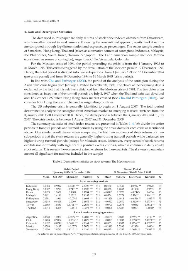
J. Risk Financial Manag. 2019, 11
4. Data and Descriptive Statistics
The data used in this paper are daily returns of stock price indexes obtained from Datastream,which are all expressed in local currency. Following the conventional approach, equity market returnsare computed through log-differentiation and expressed as percentages. The Asian sample consistsof 8 markets: Hong Kong, Thailand (taken as alternative sources of contagion), Indonesia, Malaysia,the Philippines, South Korea, Taiwan, Singapore. The Latin American sample includes Mexico(considered as source of contagion), Argentina, Chile, Venezuela, Colombia.
For the Mexican crisis of 1994, the period preceding the crisis is from the 1 January 1993 to31 March 1995. This crisis is triggered by the devaluation of the Mexican peso in 19 December 1994.Hence, the total period is divided into two sub-periods: from 1 January 1993 to 16 December 1994(pre-crisis period) and from 19 December 1994 to 31 March 1995 (crisis period).
In line with Cho and Parhizgari (2008), the period of the analysis of the contagion during theAsian “flu” crisis begins from January 1, 1996 to December 30, 1998. The choice of the beginning date isexplained by the fact that it is relatively distanced from the Mexican crisis of 1994. The two dates oftenconsidered as inception of the turmoil periods are July 2, 1997 when the Thailand baht was devaluedand 17 October 1997 when Hong Kong stock market crashed (See Cho and Parhizgari (2008)). Weconsider both Hong Kong and Thailand as originating countries.
The US subprime crisis is generally identified to begin on 1 August 2007. The total perioddetermined to analyze the contagion from American market to emerging markets stretches from the3 January 2006 to 31 December 2008. Hence, the stable period is between the 3 January 2006 and 31 July2007. The crisis period is between 1 August 2007 and 31 December 2008.
The summary statistics of stock-index returns are presented in Tables 1–4. We divide the entireperiods in tranquil periods and turmoil periods by using the break dates for each crisis as mentionedabove. One similar result drawn when comparing the first two moments of stock returns for twosub-periods is that the stock returns are generally higher during tranquil periods while variances arehigher during turmoil periods (except for Mexican crisis). Moreover, every series of stock returnsexhibits non-normality with significantly positive excess kurtosis, which is common to daily equitystock returns. This reveals the existence of extreme returns for these markets. The skewness parametersare not all significant for markets included in the sample.
Table 1. Descriptive statistics on stock returns: The Mexican crisis.
Stable Period Turnoil Period1 January 1993–16 December 1994 19 December 1994–31 March 1995
Mean Std Dev Skewness Kurtosis N Mean Std Dev Skewness Kurtosis N
Asian emerging markets
Indonesia 0.1004 0.9222 −0.4486 *** 2.6498 *** 511 0.0150 1.0549 −0.6917 ** 0.9270 75Hong Kong 0.0802 1.5790 −0.2401 ** 1.7596 *** 511 0.0528 1.7043 0.1988 0.9235 75Korea 0.0929 1.2632 0.1009 1.1744 *** 511 −0.0995 1.3775 −0.2445 0.6534 75Malaysia 0.0811 1.4140 0.0312 7.9182 *** 511 0.0554 1.5279 0.5262 * 1.9441 *** 75Philippines 0.1901 1.1940 −0.0740 1.4608 *** 511 −0.1428 1.4014 −0.6524 ** 1.1863 ** 75Singapore 0.0548 0.8429 0.0260 3.6975 *** 511 −0.0522 1.0070 −1.3139 *** 5.2778 *** 75Taiwan 0.1695 1.8683 0.3141 *** 2.2656 *** 511 −0.0700 1.2675 0.0863 1.9812 *** 75Thailand 0.1344 1.6338 −0.1610 3.3274 *** 511 −0.0396 1.5237 0.0994 1.1044* 75
Latin American emerging markets
Argentina 0.0628 1.7080 −0.4579 *** 1.7082 *** 511 −0.3181 3.4888 0.5977 ** 1.2190 ** 75Chile 0.1474 0.9804 −0.1968 * 1.4879 *** 511 −0.0893 1.9833 0.8658 *** 2.1619 *** 75Colombia 0.1092 0.8248 0.6607 *** 4.2164 *** 511 0.0963 0.7902 1.8254 *** 4.5397 *** 75Mexico 0.0588 1.3187 −0.0576 2.2076 *** 511 −0.2413 2.5392 0.2928 0.6904 75Venezuela 0.1356 2.8743 0.8210 *** 8.0160 *** 511 0.0285 1.4287 1.3654 ** 7.0395 ** 75
The returns are in percentages. *, **, *** represent statistical significance at the 1%, 5%, 10% levels of risk.
129
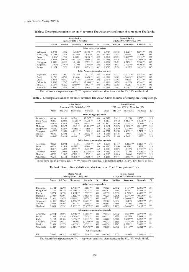
J. Risk Financial Manag. 2019, 11
Table 2. Descriptive statistics on stock returns: The Asian crisis (Source of contagion: Thailand).
Stable Period Turmoil Period1 January 1996–1 July 1997 2 July 1997–31 December 1998
Mean Std Dev Skewness Kurtosis N Mean Std Dev Skewness Kurtosis N
Asian emerging markets
Indonesia 0.0782 1.0492 −0.3121 ** 2.3480 *** 392 −0.0727 3.1918 0.2923 ** 3.2094 *** 392Hong Kong 0.1164 1.0426 −1.2222 8.9774 392 −0.1301 2.7824 0.4175 5.8187 392Korea −0.0467 1.3586 0.1910 0.7480 *** 392 −0.0060 3.3631 0.3847 *** 1.1348 *** 392Malaysia 0.0225 0.8135 −0.4775 *** 2.6060 *** 392 −0.1452 3.3526 0.6484 *** 12.4451 *** 392Philippines 0.0406 0.9691 −0.1981 2.5731 *** 392 −0.0839 2.2471 0.2459 ** 2.1380 *** 392Singapore −0.0264 0.80150 −0.1321 0.6031 ** 392 −0.0665 1.8973 0.3777 *** 3.6296 *** 392Taiwan 0.1674 1.3831 −0.0006 3.6794 *** 392 −0.0752 1.7950 −0.0360 1.4828 *** 392
Latin American emerging markets
Argentina 0.0976 1.2867 −0.1673 1.9277 *** 392 −0.0763 2.3432 −0.5134 *** 6.2535 *** 392Brazil 0.1766 0.9540 0.14830 3.4620 *** 392 −0.1811 2.4182 −0.6825 *** 3.1787 *** 392Chile 0.0252 0.6937 0.4481 *** 0.5236 ** 392 −0.1179 1.1195 0.1355 3.4237 *** 392Colombia 0.0587 1.0545 −0.7724 *** 47.0383 *** 392 −0.0800 1.0778 −0.0039 9.7246 *** 392Mexico 0.1178 0.9133 0.5029 *** 1.6971 *** 392 −0.0380 1.7365 0.0213 7.6136 *** 392Venezuela 0.3457 1.6706 1.0121 *** 3.7608 *** 392 −0.1866 2.7841 1.1492 *** 12.5781 *** 392
The returns are in percentages. **, *** represent statistical significance at the 5%, 10% levels of risk.
Table 3. Descriptive statistics on stock returns: The Asian Crisis (Source of contagion: Hong Kong).
Stable Period Turnoil Period1 January 1996–16 October 1997 17 October 1997–31 December 1998
Mean Std Dev Skewness Kurtosis N Mean Std Dev Skewness Kurtosis N
Asian emerging markets
Indonesia 0.0166 1.4280 0.6768 *** 12.7077 *** 469 −0.0178 3.3212 0.1758 2.8525 *** 315Hong Kong 0.0663 1.2338 −0.7219 *** 7.0780 *** 469 −0.1157 2.9568 0.4178 *** 5.3991 *** 315Korea −0.1033 1.3825 0.0313 0.9223 *** 469 0.0882 3.6760 0.3107 ** 0.5446 * 315Malaysia −0.0367 1.2673 1.5841 *** 25.3818 *** 469 −0.0981 3.5274 0.5284 *** 12.0150 *** 315Philippines −0.0352 1.2483 −0.3863 *** 7.4819 *** 469 −0.0015 2.2680 0.2740 ** 1.9341 *** 315Singapore −0.0393 0.9059 −0.2921 ** 1.8088 *** 469 −0.0572 2.0150 0.4080 *** 3.3187 *** 315Taiwan 0.1163 1.4502 −0.1110 2.5102 *** 469 −0.0584 1.8105 0.0031 1.9019 *** 315Thailand −0.1493 2.0219 0.6848 *** 3.3557 *** 469 −0.1054 3.2393 0.7468 *** 2.1230 *** 315
Latin American emerging markets
Argentina 0.1020 1.2704 −0.1831 1.7405 *** 469 −0.1255 2.5457 −0.4468 *** 5.2178 *** 315Brazil 0.1530 1.1524 −0.3935 *** 6.2960 *** 469 −0.2335 2.5350 −0.6586 *** 2.9229 *** 315Chile 0.0041 0.6880 0.4351 *** 0.5212 ** 469 −0.1215 1.2074 0.1294 2.8595 *** 315Colombia 0.0850 0.9906 −0.8211 *** 50.7480 *** 469 −0.1530 1.1604 0.1292 8.7253 *** 315Mexico 0.1322 0.9512 0.3708 *** 1.2385 *** 469 −0.0975 1.8516 0.0865 7.1560 *** 315Venezuela 0.3240 1.6112 0.9646 *** 3.8058 *** 469 −0.2844 3.0353 1.1840 *** 10.8894 *** 315
The returns are in percentages. *, **, *** represent statistical significance at the 1%, 5%, 10% levels of risk.
Table 4. Descriptive statistics on stock returns: The US subprime Crisis.
Stable Period Turnoil Period1 January 2006–31 July 2007 1 July 2007–31 December 2008
Mean Std Dev Skewness Kurtosis N Mean Std Dev Skewness Kurtosis N
Asian emerging markets
Indonesia 0.1522 1.2398 −0.7613 *** 4.3101 *** 411 −0.1525 2.3802 −0.4674 *** 4.1386 *** 371Hong Kong 0.1202 0.9329 −0.7289 *** 2.4423 *** 411 −0.1491 2.5215 0.0562 3.1464 *** 371Korea 0.0724 1.0974 −0.4801 *** 1.3515 *** 411 −0.1397 2.2650 −0.2754 ** 4.6030 *** 371Malaysia 0.1043 0.7091 −1.2220 *** 7.4879 *** 411 −0.1226 1.2308 −1.3304 *** 10.6139 *** 371Philippines 0.1311 1.1670 −0.863 *** 5.8259 *** 411 −0.1711 1.7675 −0.6680 *** 5.8814 *** 371Singapore 0.1081 0.8867 −0.9309 *** 2.9231 *** 411 −0.1902 1.8069 −0.1860 3.0287 *** 371Taiwan 0.0665 1.0303 −0.8786 3.1950 *** 411 −0.1804 1.9659 −0.0510 0.8381 *** 371Thailand 0.0488 1.5232 −2.8566 *** 53.3222 *** 411 −0.1798 2.1168 −0.6096 *** 5.6193 *** 371
Latin American emerging markets
Argentina 0.0882 1.0504 −0.9743 *** 5.9111 *** 411 −0.1113 1.3972 −0.0210 *** 3.3975 *** 371Brazil 0.1365 1.2836 −0.3056 ** 1.5830 *** 411 −0.1121 2.4737 −0.0278 2.9948 *** 371Chile 0.1152 0.7406 −1.1789 *** 5.9941 *** 411 −0.0788 1.3721 0.5007 *** 7.4257 *** 371Colombia 0.0333 1.6017 −0.0702 12.4863 *** 411 −0.0312 1.4454 −0.4301 *** 6.7485 *** 371Mexico 0.1359 1.1573 −0.1752 3.0393 *** 411 −0.0828 1.7243 0.3276 ** 3.6350 *** 371Venezuela 0.1247 1.5929 −3.0199 *** 33.0170 *** 411 −0.0758 0.6730 0.5511 *** 3.1822 *** 371
US stock market
US 0.0397 0.6747 −0.5250 *** 2.5716 *** 411 −0.1268 2.2007 −0.1491 5.2257 *** 371
The returns are in percentages. **, *** represent statistical significance at the 5%, 10% levels of risk.
130
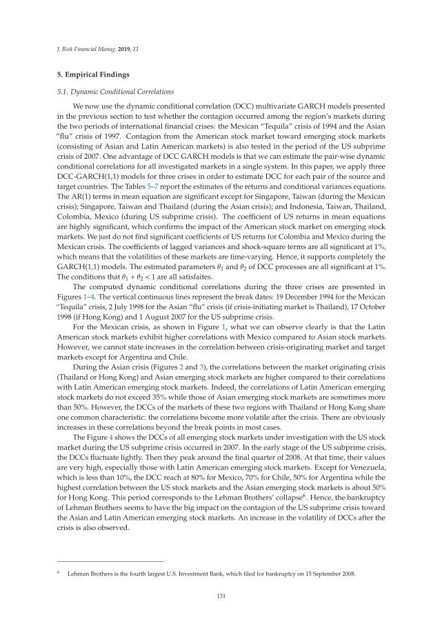
J. Risk Financial Manag. 2019, 11
5. Empirical Findings
5.1. Dynamic Conditional Correlations
We now use the dynamic conditional correlation (DCC) multivariate GARCH models presentedin the previous section to test whether the contagion occurred among the region’s markets duringthe two periods of international financial crises: the Mexican “Tequila” crisis of 1994 and the Asian“flu” crisis of 1997. Contagion from the American stock market toward emerging stock markets(consisting of Asian and Latin American markets) is also tested in the period of the US subprimecrisis of 2007. One advantage of DCC GARCH models is that we can estimate the pair-wise dynamicconditional correlations for all investigated markets in a single system. In this paper, we apply threeDCC-GARCH(1,1) models for three crises in order to estimate DCC for each pair of the source andtarget countries. The Tables 5–7 report the estimates of the returns and conditional variances equations.The AR(1) terms in mean equation are significant except for Singapore, Taiwan (during the Mexicancrisis); Singapore, Taiwan and Thailand (during the Asian crisis); and Indonesia, Taiwan, Thailand,Colombia, Mexico (during US subprime crisis). The coefficient of US returns in mean equationsare highly significant, which confirms the impact of the American stock market on emerging stockmarkets. We just do not find significant coefficients of US returns for Colombia and Mexico during theMexican crisis. The coefficients of lagged variances and shock-square terms are all significant at 1%,which means that the volatilities of these markets are time-varying. Hence, it supports completely theGARCH(1,1) models. The estimated parameters θ1 and θ2 of DCC processes are all significant at 1%.The conditions that θ1 + θ2 < 1 are all satisfaites.
The computed dynamic conditional correlations during the three crises are presented inFigures 1–4. The vertical continuous lines represent the break dates: 19 December 1994 for the Mexican“Tequila” crisis, 2 July 1998 for the Asian “flu” crisis (if crisis-initiating market is Thailand), 17 October1998 (if Hong Kong) and 1 August 2007 for the US subprime crisis.
For the Mexican crisis, as shown in Figure 1, what we can observe clearly is that the LatinAmerican stock markets exhibit higher correlations with Mexico compared to Asian stock markets.However, we cannot state increases in the correlation between crisis-originating market and targetmarkets except for Argentina and Chile.
During the Asian crisis (Figures 2 and 3), the correlations between the market originating crisis(Thailand or Hong Kong) and Asian emerging stock markets are higher compared to their correlationswith Latin American emerging stock markets. Indeed, the correlations of Latin American emergingstock markets do not exceed 35% while those of Asian emerging stock markets are sometimes morethan 50%. However, the DCCs of the markets of these two regions with Thailand or Hong Kong shareone common characteristic: the correlations become more volatile after the crisis. There are obviouslyincreases in these correlations beyond the break points in most cases.
The Figure 4 shows the DCCs of all emerging stock markets under investigation with the US stockmarket during the US subprime crisis occurred in 2007. In the early stage of the US subprime crisis,the DCCs fluctuate lightly. Then they peak around the final quarter of 2008. At that time, their valuesare very high, especially those with Latin American emerging stock markets. Except for Venezuela,which is less than 10%, the DCC reach at 80% for Mexico, 70% for Chile, 50% for Argentina while thehighest correlation between the US stock markets and the Asian emerging stock markets is about 50%for Hong Kong. This period corresponds to the Lehman Brothers’ collapse6. Hence, the bankruptcyof Lehman Brothers seems to have the big impact on the contagion of the US subprime crisis towardthe Asian and Latin American emerging stock markets. An increase in the volatility of DCCs after thecrisis is also observed.
6 Lehman Brothers is the fourth largest U.S. Investment Bank, which filed for bankruptcy on 15 September 2008.
131
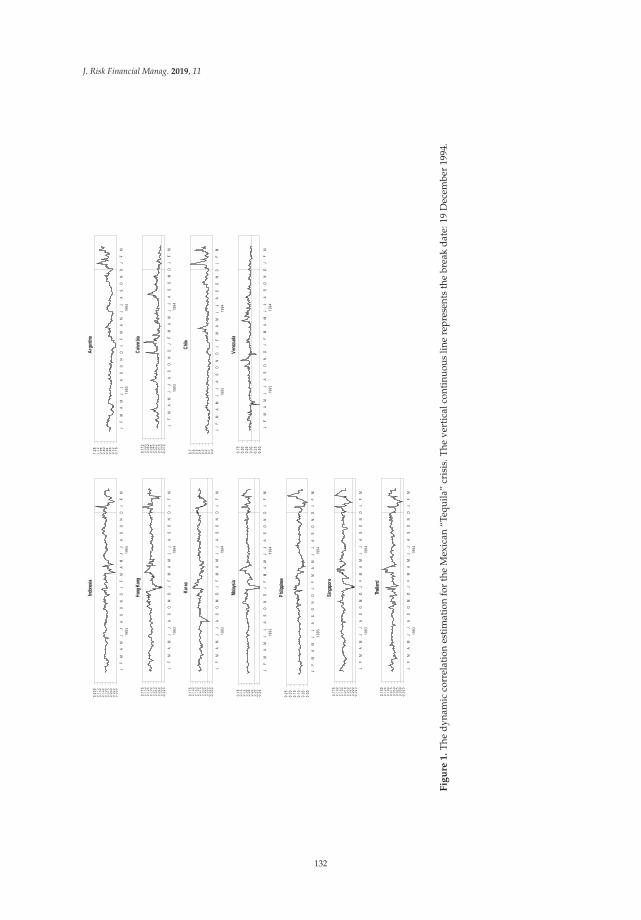
J. Risk Financial Manag. 2019, 11
Fig
ure
1.
The
dyna
mic
corr
elat
ion
esti
mat
ion
for
the
Mex
ican
“Teq
uila
”cr
isis
.The
vert
ical
cont
inuo
uslin
ere
pres
ents
the
brea
kda
te:1
9D
ecem
ber
1994
.
132
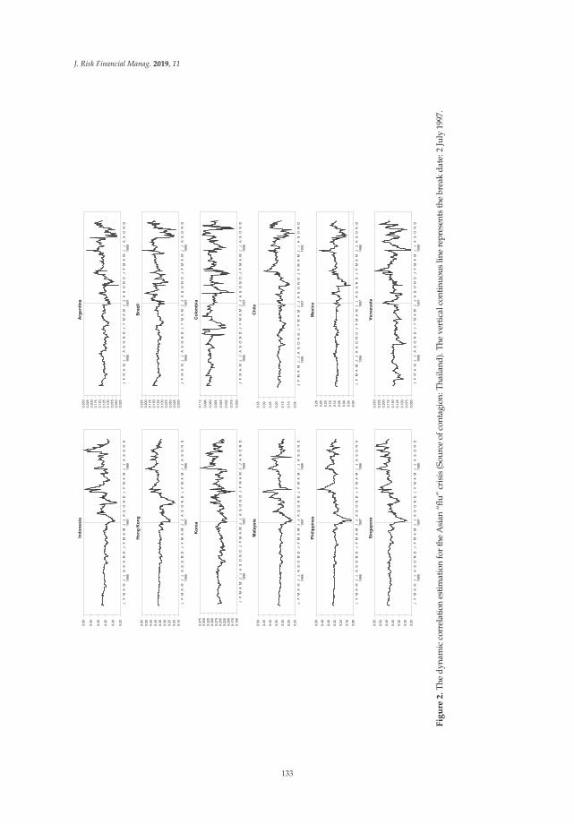
J. Risk Financial Manag. 2019, 11
Fig
ure
2.
The
dyna
mic
corr
elat
ion
estim
atio
nfo
rthe
Asi
an“f
lu”
cris
is(S
ourc
eof
cont
agio
n:Th
aila
nd).
The
vert
ical
cont
inuo
uslin
ere
pres
ents
the
brea
kda
te:2
July
1997
.
133
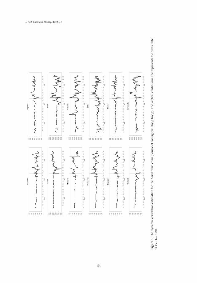
J. Risk Financial Manag. 2019, 11
Fig
ure
3.
The
dyn
amic
corr
elat
ion
esti
mat
ion
for
the
Asi
an“fl
u”cr
isis
(Sou
rce
ofco
ntag
ion:
Hon
gK
ong)
.The
vert
ical
cont
inuo
uslin
ere
pres
ents
the
brea
kd
ate:
17O
ctob
er19
97.
134
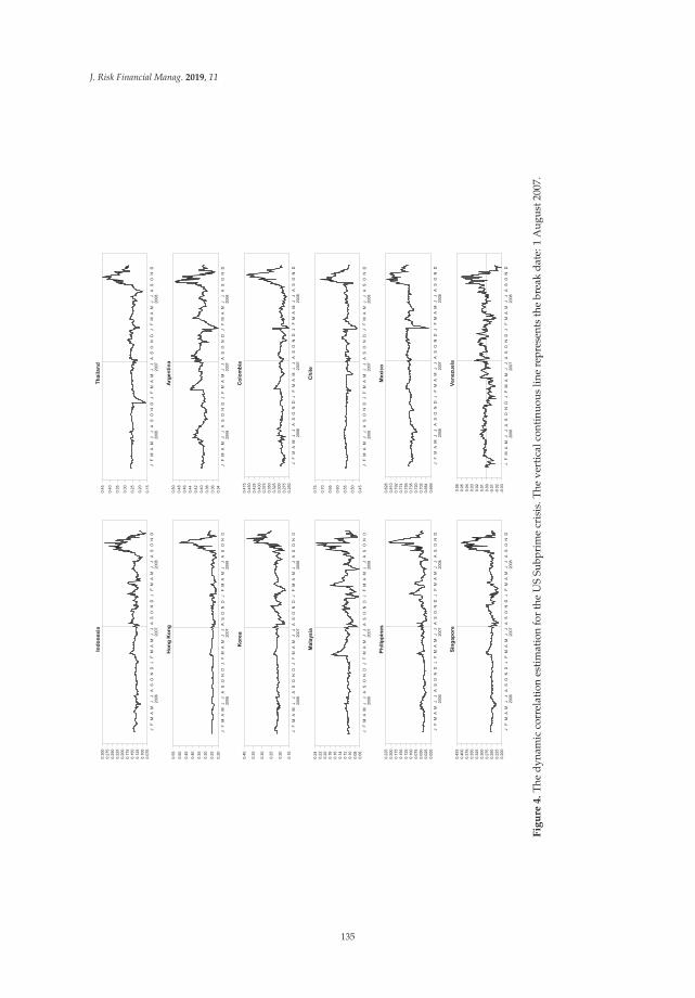
J. Risk Financial Manag. 2019, 11
Fig
ure
4.
The
dyna
mic
corr
elat
ion
esti
mat
ion
for
the
US
Subp
rim
ecr
isis
.The
vert
ical
cont
inuo
uslin
ere
pres
ents
the
brea
kda
te:1
Aug
ust2
007.
135
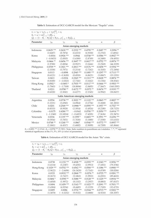
J. Risk Financial Manag. 2019, 11
Table 5. Estimation of DCC-GARCH model for the Mexican “Tequila” crisis.
rt = γ0 + γ1rt−1 + γ2rUSt−1 + εt
ht = ω + αε2t−1 + βht−1
Qt = (1 − θ1 − θ2)Q + θ1νt−1ν′t−1 + θ2Qt−1
Parameter γ0 γ1 γ2 ω α β
Asian emerging markets
Indonesia 0.0629 *** 0.2630 *** 0.2332 *** 0.4799 *** 0.2687 *** 0.2094 **(2.6687) (8.7874) (6.6515) (6.9350) (5.2765) (2.4816)
Korea −0.0016 0.0926 *** 0.0944 0.0748 *** 0.0586 *** 0.8927 ***(−0.0453) (2.8503) (1.6300) (2.8749) (4.2400) (34.4931)
Malaysia 0.0466 ** 0.0656 *** 0.3697 *** 0.0417 *** 0.0752 *** 0.8974 ***(1.9780) (2.8854) (8.9527) (3.1666) (5.2569) (44.3229)
Philippines 0.0709 ** 0.1821 *** 0.2813 *** 0.0176 *** 0.0458 *** 0.9394 ***(2.3330) (5.7971) (5.2114) (2.7262) (4.3183) (72.2894)
Singapore 0.0113 −0.0098 0.2945 *** 0.1085 *** 0.1297 *** 0.7113 ***(0.6121) (−0.3630) (8.4910) (4.8621) (5.0067) (15.1351)
Taiwan 0.0413 −0.0324 0.2365 *** 0.1313 *** 0.0628 *** 0.8874 ***(0.8180) (−1.0263) (2.7341) (3.1662) (5.1356) (38.8341)
Hong Kong 0.0502 * −0.0493 * 0.7935 *** 0.0117 *** 0.0444 *** 0.9503 ***(1.7065) (−1.7108) (18.8004) (2.8495) (7.5667) (168.3592)
Thailand 0.0211 0.0780 ** 0.4172 *** 0.0372 ** 0.0674 *** 0.9193 ***(0.6028) (2.5041) (6.6277) (2.1545) (4.9942) (50.8437)
Latin American emerging markets
Argentina 0.0554 0.0738 *** 0.3022 *** 0.1122 *** 0.0865 *** 0.8827 ***(1.2221) (2.6945) (4.0964) (3.1756) (5.2608) (41.3832)
Chile 0.0201 0.2549 *** 0.0988 ** 0.0595 *** 0.1957 *** 0.7527 ***(0.8533) (8.9928) (2.3914) (5.4924) (8.2280) (28.7125)
Colombia −0.0175 0.4280 *** −0.0162 0.0700 *** 0.2050 *** 0.6914 ***(−1.1340) (11.8014) (−0.6823) (7.4205) (7.5636) (21.9471)
Venezuela 0.0334 0.1197 *** 0.1559 * 0.4403 *** 0.3591 *** 0.6256 ***(0.5934) (3.7851) (1.7650) (5.1880) (7.3100) (15.6333)
Mexico 0.0748 ** 0.1240 *** 0.0867 0.0540 *** 0.0772 *** 0.8957 ***(2.1861) (4.4517) (1.4082) (2.9099) (4.7209) (41.8666)
θ1 = 0.0091 *** (2.5764) ; θ2 = 0.8750 *** (9.7801). Note: Italic numbers in parentheses are t-statistics. *, **, *** representstatistical significance at the 1%, 5%, 10% (p value) of parameters.
Table 6. Estimation of DCC-GARCH model for the Asian “flu” crisis.
rt = γ0 + γ1rt−1 + γ2rUSt−1 + εt
ht = ω + αε2t−1 + βht−1
Qt = (1 − θ1 − θ2)Q + θ1νt−1ν′t−1 + θ2Qt−1
Parameter γ0 γ1 γ2 ω α β
Asian emerging markets
Indonesia 0.0738 0.1152 *** 0.4308 *** 0.0355 *** 0.1043 *** 0.9056 ***(1.6114) (5.2387) (9.4292) (2.9913) (7.1851) (79.3786)
Hong Kong 0.1029 *** 0.0702 *** 0.6562 *** 0.0500 *** 0.1086 *** 0.8900 ***(2.9622) (−2.6696) (16.3620) (3.7141) (6.8789) (58.8206)
Korea 0.0153 0.0932 *** 0.2868 *** 0.0276 ** 0.0725 *** 0.9281 ***(0.2672) (2.7627) (5.1863) (1.9922) (6.8351) (89.4653)
Malaysia 0.0484 * 0.0590 ** 0.3088 *** 0.0128 *** 0.1229 *** 0.8934 ***(1.6858) (1.9972) (8.1332) (3.2957) (8.8803) (97.8157)
Philippines 0.0494 0.1459 *** 0.3143 *** 0.1023 *** 0.2091 *** 0.7831 ***(1.4304) (4.9254) (8.4482) (5.1229) (7.7183) (32.4725)
Singapore 0.0495 0.0086 0.3732 *** 0.0344 *** 0.0715 *** 0.9202 ***(1.5878) (−0.3252) (9.9155) (3.0880) (4.9210) (58.3597)
136
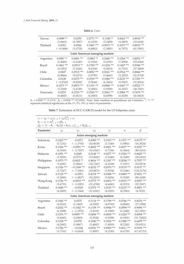
J. Risk Financial Manag. 2019, 11
Table 6. Cont.
Taiwan 0.0989 ** 0.0259 0.2771 *** 0.1180 ** 0.0662 *** 0.8918 ***(2.0661) (0.7897) (6.2478) (2.5499) (4.3803) (33.6636)
Thailand 0.0321 0.0344 0.3467 *** 0.0913 *** 0.1073 *** 0.8932 ***(−0.5486) (1.0719) (4.8863) (2.5801) (6.7971) (61.1801)
Latin American emerging markets
Argentina 0.0967 ** 0.0681 *** 0.0867 ** 0.2440 *** 0.1284 *** 0.8076 ***(2.4066) (2.6343) (2.1024) (5.6291) (7.4994) (35.4268)
Brazil 0.1461 *** 0.0513 ** 0.1783 *** 0.1234 *** 0.1427 *** 0.8349 ***(4.1852) (2.1644) (4.6334) (4.8453) (6.7531) (37.5869)
Chile 0.0207 0.2515 *** 0.0852 *** 0.0241 *** 0.0764 *** 0.8968 ***(0.8866) (9.0373) (3.8795) (3.4661) (5.2825) (51.0718)
Colombia 0.0128 0.2275 *** 0.0769 *** 0.1084 *** 0.2233 *** 0.7303 ***(−0.8760) (9.8500) (3.9644) (6.2665) (5.9507) (21.8016)
Mexico 0.1073 *** 0.0873 *** 0.1191 *** 0.0968 *** 0.1067 *** 0.8522 ***(3.2568) (3.4749) (3.4945) (3.9108) (6.5547) (38.7641)
Venezuela 0.0253 0.2219 *** 0.2545 *** 0.2062 *** 0.2084 *** 0.7679 ***(0.4845) (6.6611) (4.5883) (4.6099) (6.4188) (26.0453)
θ1 = 0.0100 *** (5.1374) ; θ2 = 0.9204 *** (52.0098). Note: Italic numbers in parentheses are t-statistics. *, **, ***represent statistical significance at the 1%, 5%, 10% (p value) of parameters.
Table 7. Estimation of DCC-GARCH model for the US Subprime crisis.
rt = γ0 + γ1rt−1 + γ2rUSt−1 + εt
ht = ω + αε2t−1 + βht−1
Qt = (1 − θ1 − θ2)Q + θ1νt−1ν′t−1 + θ2Qt−1
Parameter γ0 γ1 γ2 ω α β
Asian emerging markets
Indonesia 0.2265 *** −0.0371 0.4390 *** 0.1915 *** 0.1371 *** 0.8175 ***(5.7232) (−1.3703) (14.8630) (2.7140) (3.9892) (16.3024)
Korea 0.1426 *** −0.0591 *** 0.4602 *** 0.0451 *** 0.0677 *** 0.9227 ***(4.2410) (−2.7507) (16.6541) (3.7266) (6.3664) (80.1653)
Malaysia 0.1051 *** 0.0245 0.2148 *** 0.0277 *** 0.1524 *** 0.8425 ***(5.5955) (0.9712) (15.0682) (3.1640) (6.1689) (30.6932)
Philippines 0.1073 *** 0.0432 ** 0.4816 *** 0.1307 *** 0.2038 *** 0.7557 ***(3.6841) (2.0841) (24.7262) (4.1638) (7.1927) (24.0974)
Singapore 0.1526 *** −0.1309 *** 0.4332 *** 0.0370 *** 0.0719 *** 0.9157 ***(5.7167) (−7.1061) (19.0871) (5.9154) (9.3246) (110.2176)
Taiwan 0.1129 *** −0.0351 0.4178 *** 0.0308 *** 0.0490 *** 0.9431 ***(3.2060) (−1.4837) (16.4201) (3.0436) (5.1028) (80.4188)
Hong Kong 0.1726 *** −0.0933 *** 0.5775 *** 0.0474 *** 0.0915 *** 0.9057 ***(5.4715) (−5.1091) (21.4708) (4.6845) (8.9123) (92.2507)
Thailand 0.1680 *** −0.0329 0.3372 *** 1.0153 *** 0.2215 *** 0.4901 ***(4.2402) (−1.2364) (11.6561) (4.5281) (4.2943) (4.7025)
Latin American emerging markets
Argentina 0.1442 *** 0.0375 0.1114 *** 0.1799 *** 0.0746 *** 0.8276 ***(4.0163) (1.1469) (4.2305) (4.9710) (4.8060) (27.1994)
Brazil 0.2432 *** −0.1042 *** 0.1159 *** 0.0944 *** 0.0599 *** 0.9090 ***(6.2098) (−5.2976) (3.4103) (4.1900) (6.3348) (62.2301)
Chile 0.1276 *** 0.0995 *** 0.0496 *** 0.0650 *** 0.1224 *** 0.8094 ***(5.6065) (3.8369) (2.9036) (5.0398) (6.9301) (31.73603)
Colombia 0.1238 *** 0.0370 0.1040 *** 0.1820 *** 0.2388 *** 0.6475 ***(4.2682) (1.0867) (5.4842) (7.4010) (8.2245) (20.6911)
Mexico 0.1784 *** −0.0144 0.0521 *** 0.0569 *** 0.0611 *** 0.9105 ***(5.7761) (−0.6505) (1.8097) (4.2185) (6.6728) (67.41723)
137
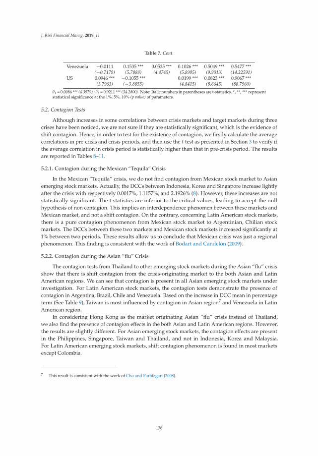
J. Risk Financial Manag. 2019, 11
Table 7. Cont.
Venezuela −0.0111 0.1535 *** 0.0535 *** 0.1026 *** 0.5049 *** 0.5477 ***(−0.7179) (5.7888) (4.4745) (5.8995) (9.9013) (14.22591)
US 0.0946 *** −0.1055 *** 0.0199 *** 0.0823 *** 0.9067 ***(3.7963) (−3.8855) (4.8415) (8.6645) (88.7960)
θ1 = 0.0086 *** (4.3979) ; θ2 = 0.9211 *** (34.2800). Note: Italic numbers in parentheses are t-statistics. *, **, *** representstatistical significance at the 1%, 5%, 10% (p value) of parameters.
5.2. Contagion Tests
Although increases in some correlations between crisis markets and target markets during threecrises have been noticed, we are not sure if they are statistically significant, which is the evidence ofshift contagion. Hence, in order to test for the existence of contagion, we firstly calculate the averagecorrelations in pre-crisis and crisis periods, and then use the t-test as presented in Section 3 to verify ifthe average correlation in crisis period is statistically higher than that in pre-crisis period. The resultsare reported in Tables 8–11.
5.2.1. Contagion during the Mexican “Tequila” Crisis
In the Mexican “Tequila” crisis, we do not find contagion from Mexican stock market to Asianemerging stock markets. Actually, the DCCs between Indonesia, Korea and Singapore increase lightlyafter the crisis with respectively 0.0017%, 1.1157%, and 2.1926% (8). However, these increases are notstatistically significant. The t-statistics are inferior to the critical values, leading to accept the nullhypothesis of non contagion. This implies an interdependence phenomen between these markets andMexican market, and not a shift contagion. On the contrary, concerning Latin American stock markets,there is a pure contagion phenomenon from Mexican stock market to Argentinian, Chilian stockmarkets. The DCCs between these two markets and Mexican stock markets increased significantly at1% between two periods. These results allow us to conclude that Mexican crisis was just a regionalphenomenon. This finding is consistent with the work of Bodart and Candelon (2009).
5.2.2. Contagion during the Asian “flu” Crisis
The contagion tests from Thailand to other emerging stock markets during the Asian “flu” crisisshow that there is shift contagion from the crisis-originating market to the both Asian and LatinAmerican regions. We can see that contagion is present in all Asian emerging stock markets underinvestigation. For Latin American stock markets, the contagion tests demonstrate the presence ofcontagion in Argentina, Brazil, Chile and Venezuela. Based on the increase in DCC mean in percentageterm (See Table 9), Taiwan is most influenced by contagion in Asian region7 and Venezuela in LatinAmerican region.
In considering Hong Kong as the market originating Asian “flu” crisis instead of Thailand,we also find the presence of contagion effects in the both Asian and Latin American regions. However,the results are slightly different. For Asian emerging stock markets, the contagion effects are presentin the Philippines, Singapore, Taiwan and Thailand, and not in Indonesia, Korea and Malaysia.For Latin American emerging stock markets, shift contagion phenomenon is found in most marketsexcept Colombia.
7 This result is consistent with the work of Cho and Parhizgari (2008).
138
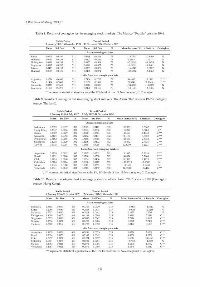
J. Risk Financial Manag. 2019, 11
Table 8. Results of contagion test in emerging stock markets: The Mexico “Tequila” crisis in 1994.
Stable Period Turnoil Period1 January 1993–16 December 1994 19 December 1994–31 March 1995
Mean Std Dev N Mean Std Dev N Mean Increase (%) t Statictis Contagion
Asian emerging markets
Korea 0.0775 0.0197 511 0.0668 0.0316 75 −13.7570 −2.8409 NMalaysia 0.0762 0.0235 511 0.0802 0.0261 75 5.2683 1.2577 NPhilippines 0.0989 0.0198 511 0.0933 0.0509 75 −5.6818 −0.9455 NSingapore 0.0897 0.0202 511 0.0891 0.0377 75 −0.6939 −0.1401 NTaiwan 0.0425 0.0153 511 0.0355 0.0370 75 −16.4346 −1.6127 NThailand 0.0659 0.0156 511 0.0491 0.0274 75 −25.5032 −5.1963 N
Latin American emerging markets
Argentina 0.4734 0.6880 511 0.7406 0.1717 75 56.4643 13.1390 C ***Chile 0.1494 0.3865 511 0.2638 0.1381 75 76.5546 7.1045 C ***Colombia 0.0279 0.1669 511 0.0126 0.0056 75 −54.8510 −18.0838 NVenezuela 0.1070 0.3271 511 0.0490 0.0456 75 −54.1615 −8.6066 N
*** represents statistical significance at the 10% level of risk. N: No contagion; C: Contagion.
Table 9. Results of contagion test in emerging stock markets: The Asian “flu” crisis in 1997 (Contagionsource: Thailand).
Stable Period Turnoil Period1 January 1996–1 July 1997 2 July 1997–31 December 1998
Mean Std Dev N Mean Std Dev N Mean Increase (%) t Statictis Contagion
Asian emerging markets
Indonesia 0.3559 0.0097 392 0.3673 0.0411 392 3.2073 5.3562 C ***Hong Kong 0.3547 0.0116 392 0.3593 0.0586 392 1.2997 1.5284 C *Korea 0.2529 0.0129 392 0.2640 0.0314 392 4.3660 6.4443 C ***Malaysia 0.3175 0.0092 392 0.3252 0.0404 392 2.4180 3.6650 C ***Philippines 0.3182 0.0166 392 0.3266 0.0615 392 2.6663 2.6372 C ***Singapore 0.4230 0.0120 392 0.4298 0.0472 392 1.6002 2.7536 C ***Taiwan 0.1475 0.0001 392 0.1665 0.0015 392 12.8759 9.2121 C ***
Latin American emerging markets
Argentina 0.1228 0.0112 392 0.1267 0.0302 392 3.1683 2.3918 C ***Brazil 0.1231 0.0108 392 0.1290 0.0338 392 4.8054 3.2968 C ***Chile 0.1714 0.0140 392 0.1854 0.0406 392 8.1982 6.4719 C ***Colombia 0.0784 0.0126 392 0.0688 0.0172 392 −12.2519 −8.9302 NMexico 0.1045 0.0088 392 0.1012 0.0365 392 −3.1670 −1.7448 NVenezuela 0.1341 0.0142 392 0.1513 0.0287 392 12.8308 10.6444 C ***
*, *** represent statistical significance at the 1%, 10% levels of risk. N: No contagion; C: Contagion.
Table 10. Results of contagion test in emerging stock markets: Asian “flu” crisis in 1997 (Contagionsource: Hong Kong).
Stable Period Turnoil Period1 January 1996–16 October 1997 17 October 1997–31 December1998
Mean Std Dev N Mean Std Dev N Mean Increase (%) t Statictis Contagion
Asian emerging markets
Indonesia 0.3802 0.0094 469 0.3766 0.0379 315 −0.9470 −1.6517 NKorea 0.2086 0.0089 469 0.2023 0.0518 315 −3.0045 −2.1265 NMalaysia 0.3517 0.0090 469 0.3524 0.0442 315 0.1975 0.2748 NPhilippines 0.4080 0.0105 469 0.4199 0.0390 315 2.8981 5.2614 C ***Singapore 0.5599 0.0118 469 0.5807 0.0362 315 3.7174 9.8697 C ***Taiwan 0.2336 0.0157 469 0.2499 0.0486 315 6.9547 5.7406 C ***Thailand 0.3468 0.0252 469 0.3723 0.0558 315 7.3427 7.5909 C ***
Latin American emerging markets
Argentina 0.1939 0.0136 469 0.2056 0.0353 315 6.0226 5.6008 C ***Brazil 0.2016 0.0153 469 0.2102 0.0342 315 4.3050 4.2230 C ***Chile 0.2297 0.0131 469 0.2494 0.0237 315 8.5714 13.4455 C ***Colombia 0.0811 0.0175 469 0.0781 0.0251 315 −3.7808 −1.8855 NMexico 0.1983 0.0111 469 0.2071 0.0306 315 4.4270 4.8752 C ***Venezuela 0.1983 0.0111 469 0.2071 0.0306 315 4.4270 5.1917 C ***
*** represents statistical significance at the 10% level of risk. N: No contagion; C: Contagion.
139

J. Risk Financial Manag. 2019, 11
Table 11. Results of contagion test in emerging stock markets: The US subprime crisis in 2007.
Stable Period Turnoil Period1 January 2006–31 July 2007 1 August 2007–31 December 2008
Mean Std Dev N Mean Std Dev N Mean Increase (%) t Statictis Contagion
Asian emerging markets
Indonesia 0.1337 0.0073 411 0.1468 0.0324 371 9.8224 7.6402 C ***Hong Kong 0.2451 0.0053 411 0.2555 0.0494 371 4.2302 4.0262 C ***Korea 0.2159 0.0058 411 0.2255 0.0350 371 4.4430 5.2203 C ***Malaysia 0.1119 0.0116 411 0.1147 0.0283 371 2.4937 1.7711 C **Philippines 0.0378 0.0067 411 0.0548 0.0332 371 45.0331 9.6879 C ***Singapore 0.2502 0.0069 411 0.2617 0.0371 371 4.6221 5.9123 C ***Taiwan 0.1233 0.0056 411 0.1326 0.0274 371 7.4918 6.3644 C ***Thailand 0.2485 0.0143 411 0.2651 0.0443 371 6.6707 6.8943 C ***
Latin American emerging markets
Argentina 0.3998 0.6323 411 0.4016 0.0237 371 0.4424 1.2989 C *Brazil 0.7134 0.8447 411 0.7146 0.0350 371 0.1562 0.6085 NChile 0.5401 0.7349 411 0.5463 0.0350 371 1.1536 3.3411 C ***Colombia 0.2901 0.5386 411 0.2997 0.0386 371 3.3137 4.6816 C ***Mexico 0.7391 0.8597 411 0.7523 0.0212 371 1.7914 11.5450 C ***Venezuela 0.0008 0.0290 411 0.0048 0.0125 371 472.0685 5.4992 C ***
*, **, *** represent statistical significance at the 1%, 5%, 10% levels of risk. N: No contagion; C: Contagion.
5.2.3. Contagion during the US Subprime Crisis
As presented in Table 11, the DCCs between US and Asian emerging stock markets are generallysmaller than those between US and Latin American emerging stock markets. Exceptionally, the DCCsfor Philippines and Venezuela are very small compared to other markets, respectively about 5% and1%. The highest DCC for Asian region is about 27% (for Singapore) while the highest DCC for LatinAmerican region is more than 75% (for Mexico). However, they all show an increase after the crisisoccurs. The t tests for the significant increases of DCCs between tranquil and turmoil periods leadto the rejection of non contagion for most of the markets, except Brazil. In fact, the DCCs betweenU.S. and Brazil increase after the crisis but it is not statistically significant. However, they are veryhigh, respectively 71.34% and 71.46% in tranquil and crisis periods. This indicates an interdependencephenomenon between Brazil and US and not a shift contagion.
6. Conclusions
Since the international financial crises that occurred in the last two decades, there have been avariety of papers that investigate whether contagion risk is present in financial markets during thecrisis periods. In fact, as observed in reality, financial shocks in one country have important impacts inother countries. This raises the question about the role of contagion in the literature. However, how todefine and measure contagion is still a contentious problem.
In this paper, we use a traditional definition of contagion which indicates it as a significantincrease in cross-market linkages after a shock to one country. Hence, the method applied to test forthe existence of contagion in stock markets under investigation is to test if the correlations increasesignificantly after the crisis. The increase of cross-market correlations is the evidence of contagion risk.This approach is used in many works that deals with the problem of financial contagion risk as it israther simple compared to other methods like including dummy variables.
We study contagion effects in emerging stock markets during the 1994 Mexican crisis, the 1997Asian crisis and the 2007 US crisis. The sample consists of eight emerging stock markets in Asia(Indonesia, Hong Kong, Korea, Malaysia, Philippines, Singapore, Taiwan and Thailand), and sixmarkets in Latin America (Argentina, Brazil, Chile, Colombia, Mexico, Venezuela) and the US stockmarket. To compute conditional correlations across markets, we apply DCC-GARCH(1,1) to dailystock index returns of all the markets in the sample for three crises. We then test for a significant
140
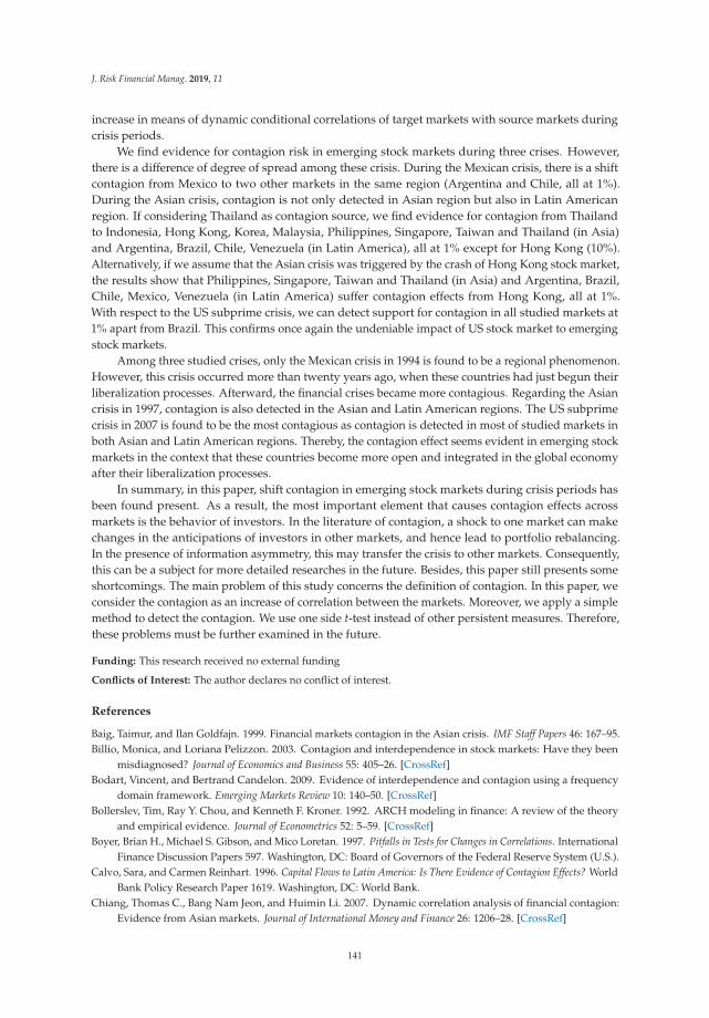
J. Risk Financial Manag. 2019, 11
increase in means of dynamic conditional correlations of target markets with source markets duringcrisis periods.
We find evidence for contagion risk in emerging stock markets during three crises. However,there is a difference of degree of spread among these crisis. During the Mexican crisis, there is a shiftcontagion from Mexico to two other markets in the same region (Argentina and Chile, all at 1%).During the Asian crisis, contagion is not only detected in Asian region but also in Latin Americanregion. If considering Thailand as contagion source, we find evidence for contagion from Thailandto Indonesia, Hong Kong, Korea, Malaysia, Philippines, Singapore, Taiwan and Thailand (in Asia)and Argentina, Brazil, Chile, Venezuela (in Latin America), all at 1% except for Hong Kong (10%).Alternatively, if we assume that the Asian crisis was triggered by the crash of Hong Kong stock market,the results show that Philippines, Singapore, Taiwan and Thailand (in Asia) and Argentina, Brazil,Chile, Mexico, Venezuela (in Latin America) suffer contagion effects from Hong Kong, all at 1%.With respect to the US subprime crisis, we can detect support for contagion in all studied markets at1% apart from Brazil. This confirms once again the undeniable impact of US stock market to emergingstock markets.
Among three studied crises, only the Mexican crisis in 1994 is found to be a regional phenomenon.However, this crisis occurred more than twenty years ago, when these countries had just begun theirliberalization processes. Afterward, the financial crises became more contagious. Regarding the Asiancrisis in 1997, contagion is also detected in the Asian and Latin American regions. The US subprimecrisis in 2007 is found to be the most contagious as contagion is detected in most of studied markets inboth Asian and Latin American regions. Thereby, the contagion effect seems evident in emerging stockmarkets in the context that these countries become more open and integrated in the global economyafter their liberalization processes.
In summary, in this paper, shift contagion in emerging stock markets during crisis periods hasbeen found present. As a result, the most important element that causes contagion effects acrossmarkets is the behavior of investors. In the literature of contagion, a shock to one market can makechanges in the anticipations of investors in other markets, and hence lead to portfolio rebalancing.In the presence of information asymmetry, this may transfer the crisis to other markets. Consequently,this can be a subject for more detailed researches in the future. Besides, this paper still presents someshortcomings. The main problem of this study concerns the definition of contagion. In this paper, weconsider the contagion as an increase of correlation between the markets. Moreover, we apply a simplemethod to detect the contagion. We use one side t-test instead of other persistent measures. Therefore,these problems must be further examined in the future.
Funding: This research received no external funding
Conflicts of Interest: The author declares no conflict of interest.
References
Baig, Taimur, and Ilan Goldfajn. 1999. Financial markets contagion in the Asian crisis. IMF Staff Papers 46: 167–95.Billio, Monica, and Loriana Pelizzon. 2003. Contagion and interdependence in stock markets: Have they been
misdiagnosed? Journal of Economics and Business 55: 405–26. [CrossRef]Bodart, Vincent, and Bertrand Candelon. 2009. Evidence of interdependence and contagion using a frequency
domain framework. Emerging Markets Review 10: 140–50. [CrossRef]Bollerslev, Tim, Ray Y. Chou, and Kenneth F. Kroner. 1992. ARCH modeling in finance: A review of the theory
and empirical evidence. Journal of Econometrics 52: 5–59. [CrossRef]Boyer, Brian H., Michael S. Gibson, and Mico Loretan. 1997. Pitfalls in Tests for Changes in Correlations. International
Finance Discussion Papers 597. Washington, DC: Board of Governors of the Federal Reserve System (U.S.).Calvo, Sara, and Carmen Reinhart. 1996. Capital Flows to Latin America: Is There Evidence of Contagion Effects? World
Bank Policy Research Paper 1619. Washington, DC: World Bank.Chiang, Thomas C., Bang Nam Jeon, and Huimin Li. 2007. Dynamic correlation analysis of financial contagion:
Evidence from Asian markets. Journal of International Money and Finance 26: 1206–28. [CrossRef]
141
J. Risk Financial Manag. 2019, 11
Cho, Jang Hyung, and Ali M. Parhizgari. 2008. East Asian financial contagion under DCC-GARCH. InternationalJournal of Banking and Finance 6: 17–30.
Corsetti, Giancarlo, Marcello Pericoli, and Massimo Sbracia. 2005. ‘Some contagion, some interdependence’: Morepitfalls in tests of financial contagion. Journal of International Money and Finance 24: 1177–99. [CrossRef]
Dornbusch, Rudiger, Yung Chul Park, and Stijn Claessens. 2001. Contagion: How it spreads and how it can bestopped? In International Cinancial Contagion. Boston: Klwer Academic Publishers.
Engle, Robert F. 2002. Dynamic conditional correlation: A simple class of multivariate generalized autoregressiveconditional heteroskedasticity models. Journal of Business and Economics Statistics 20: 339–50. [CrossRef]
Engle, Robert F., and Kevin Sheppard. 2001. Theoretical and Empirical Properties of Dynamic Conditional CorrelationMultivariate GARCH. NBER Working Paper No. 8554. Cambridge: National Bureau of Economic Research.
Forbes, Kristin J., and Roberto Rigobon. 2002. No contagion, only interdependence: Measuring stock marketcomovements. Journal of Finance 57: 2223–61. [CrossRef]
Forbes, Kristin, and Roberto Rigobon. 2000. Contagion in Latin America: Definitions, Measurements and Policy Implications.NBER Working Paper, No. 7885. Cambridge: National Bureau of Economic Research, September.
Forbes, Kristin, and Roberto Rigobon. 2001. Measuring contagion: Conceptual and empirical. In InternationalFiancial Contagion. Boston: Klwer Academic Publishers.
Horta, Paulo, Carlos Mendes, and Isabel Vieira. 2008. Contagion Effects of the U.S. Subprime Crisis on DeveloppedCountries. CEFAGE-UE Working Paper No. 2008/08. Évora: University of Evora.
Kaminsky, Graciela L., and Carmen Reinhart. 2000. On crises, contagion, and confusion. Journal of InternationalEconomics 51: 145–68. [CrossRef]
King, Mervyn A., and Sushil Wadhwani. 1990. Transmission of volatility between stock markets. Review ofFinancial Studies 3: 5–33. [CrossRef]
Kumar, Manmohan S., and Avinash Persaud. 2001. Pure contagion and investors’ shifting risk appetite: Analyticalissues and empirical evidence. International Finance 5: 401–36. [CrossRef]
Longin, Francois, and Bruno Solnik. 1995. Is the correlation in international equity returns constant: 1960–1990?Journal of International Money and Finance 14: 3–26. [CrossRef]
Masson, Paul. 1998. Contagion: Monsoonal Effects, Spillovers, and Jumps between Multiple Equilibra. IMF WorkingPaper 98/142. Washington, DC: International Monetary Fund.
Moser, Thomas. 2003. What is international financial contagion? International Finance 6: 157–78. [CrossRef]Naoui, Kamel, Naoufel Liouane, and Salem Brahim. 2010a. A dynamic conditional correlation analysis of financial
contagion: The case of the subprime credit crisis. International Journal of Economics and Finance 2: 85–96.[CrossRef]
Pericoli, Marcello, and Massimo Sbracia. 2003. A primer on financial contagion. Journal of Economic Surveys 17:571–608. [CrossRef]
Ramchand, Latha, and Raul Susmel. 1998. Volatility and cross correlation across major stock markets. Journal ofEmpirical Finance 5: 397–416. [CrossRef]
c© 2019 by the author. Licensee MDPI, Basel, Switzerland. This article is an open accessarticle distributed under the terms and conditions of the Creative Commons Attribution(CC BY) license (http://creativecommons.org/licenses/by/4.0/).
142
Journal of
Risk and FinancialManagement
Article
Assessment of Upstream Petroleum Fiscal Regimesin Myanmar
Wint Thiri Swe 1 and Nnaemeka Vincent Emodi 2,*
1 Oil and Gas Planning Department, Ministry of Electricity and Energy, Building number 6,Nay Pyi Taw 15011, Myanmar; [email protected]
2 Economics and Marketing Academic Group, College of Business, Law and Governance,James Cook University, P. O. Box 6811, Cairns Qld 4870, Australia
* Correspondence: [email protected]; Tel.: +61-421-793-682
Received: 28 October 2018; Accepted: 28 November 2018; Published: 1 December 2018
Abstract: This study aims to assess Myanmar’s upstream petroleum fiscal regimes by applyingcomprehensive indicators to rank the level of attractiveness of Myanmar. The indicators includegovernment take (GT), front loading index (FLI), and composite score (CS). The decision maker’sattitude for GT and FLI were considered in CS linear weighting method in ranking the fiscal termsattractiveness. The results showed that Myanmar’s upstream petroleum fiscal regime has lowattraction compared to its competing countries from the investor’s point of view, both in terms ofthe risk to the investor in the earlier part of the project and in terms of evaluation with or withoutthe time value of money. Also, royalty and cost recovery were identified to have an impact on theattractiveness rank of petroleum fiscal regime in Myanmar. Therefore, Myanmar should considerimproving its fiscal regimes that are not neutral—particularly, royalty, tax, profit split, and costrecovery—for a favorable investment climate.
Keywords: Myanmar; petroleum fiscal regimes; upstream oil and gas; fast and intuitive method;discounted cash flow model
1. Introduction
The petroleum industries in oil and gas producing nations play an important role in economicgrowth through revenue generation for the government (Odularu 2008). However, oil prices havebeen relatively low due to the increase in global petroleum supply which has outweighed demand(Sieminski 2014). The fall in oil prices may affect petroleum investors in the oil and gas sector dueto the large amount of capital invested in exploration activities during the period of high oil prices(Evans-Pritchard 2015). The investors now tend to focus on the country’s fiscal regimes with regard tothe valuation of oil and gas exploration and production (Nakhle 2015).
Petroleum fiscal regimes are set of laws, regulations, and agreements in a country whichgoverns the benefits derived from petroleum exploration and production (Gudmestad et al. 2010).This links the host government as the political entity and the international oil company asthe legal entity in the transaction. Also, the petroleum fiscal regime sets a standard forthe production of oil and gas as well as the income allocation between these two entities(Bindemann 1999; Sunley et al. 2003; Løvås and Osmundsen 2009). The petroleum fiscal regime isimportant to the government because it ensures the appropriate management of the country’snatural resources (Natural Resource Governace Institute (NRGI) 2015). To the petroleum investors,petroleum fiscal regimes influence their investment decisions in any country of interest(Hvozdyk and Mercer-Blackman 2010).
Ensuring an effective and attractive petroleum fiscal regime is vital and challenging in somedeveloping counties (Sunley et al. 2003; Cottarelli 2012). Myanmar is a resource rich developing country
J. Risk Financial Manag. 2018, 11, 85; doi:10.3390/jrfm11040085 www.mdpi.com/journal/jrfm143
J. Risk Financial Manag. 2018, 11, 85
with an estimated proven natural gas and oil reserves of 10 trillion cubic feet and 50 million barrelsrespectively. Myanmar exports about 12.7 billion cubic meters (2014 estimates), making Myanmarthe 17th largest natural gas exporting country in the world1. The petroleum sector is important forMyanmar’s economic growth as natural gas contributes about 25% of its foreign earnings. As adeveloping country, petroleum exploration in Myanmar is mainly carried out by overseas investors(Khine 2008; Asian Development Bank (ADB) 2014). Therefore, it is vital to ensure that the petroleumfiscal regime becomes attractive to petroleum investors through reforms that will lead to economicgrowth (McLaughlin 2012; Robinson 2012).
This study aims to analyze Myanmar’s upstream petroleum regimes, to ascertain whetherits current regimes are attractive when compared to its competing countries, from the investor’sperspective. In conducting an in-depth analysis of the fiscal regimes, it is necessary to usecomprehensive indicators to rank the attractiveness level of Myanmar, as different indicators are usedby different investors depending on their experience, in deciding the overseas selection. The researchalso intends to consider the attitude of investors in real situation, especially those in Korean energyinstitutions. Moreover, there are potentially over 14 countries competing with Myanmar oil and gasexports. This research regarding the assessment of Myanmar upstream petroleum fiscal regimes istimely and of significance to both the Myanmar government and investors for a wide range of reasons.
Firstly, the Myanmar government needs to know the exact level of attractiveness of its oil and gasexploration and production investment climate, as the government takes measures and policy reformin various sectors for the time being. Secondly, the findings from this research can help international oilcompanies (IOC) in making overseas investment decisions, because the evaluation and comparison ofpetroleum fiscal terms have practical significance. Thirdly, this study can also contribute to basicinsights into the Myanmar petroleum fiscal regimes package as it thoroughly analyses the whole fiscalpackage in the Myanmar petroleum industry. Fourthly, the major contribution of this research is toprovide policy recommendations for a more favorable investment climate in the Myanmar petroleumExploration & Production (E&P) industry. Finally, research focusing on the combination of decisionmaker’s attitudes and quantitative analysis regarding petroleum fiscal regimes are scarce. Therefore,this study intends to fill in the gap in the literature.
The rest of this study is arranged as follows. Section 2 presents the theoretical framework based onconcept of economic rent. Section 3 the literature survey followed by the quantitative analysis for theanalysis of upstream petroleum fiscal regimes in Section 4. The results are presented in Section 5, whileSection 6 summarizes the study with some major findings and policy recommendations.
2. Theoretical Framework: Concept of Economic Rent
Economic rent is defined as “the true value of natural resource which is the difference between therevenues generated from resource extraction and the costs of extraction” (Dickson 1999; Nakhle 2007).Most IOCs use cash flow models which are based on the concept of economic rent to evaluate petroleumresource projects. This is due to the model’s simplicity as its equations can project cash flow for thewhole project’s lifespan and reveal the profitability of the project. Moreover, it is also defined as“the surplus return above the value of the capital, labor and other factors of production employed toexploit the resource. It is the surplus revenue of the resource after accounting for the costs of capitaland labor inputs” (Banfi et al. 2005).
Significant economic rent can be generated from the exploitation and utilization of exhaustiblenatural resources, especially oil and gas resources which are exhaustible resources as well as a strategiccommodity with no perfect substitute. This implies that the extraction of oil and gas can earn hugeeconomic rent. Rowland and Hann (1987) asserted that “the economic worth of a license to produce oilfrom a tract may be measured by the present value of the flow of the future revenues from that tract’s
1 https://www.cia.gov/library/publications/the-world-factbook/geos/bm.html.
144
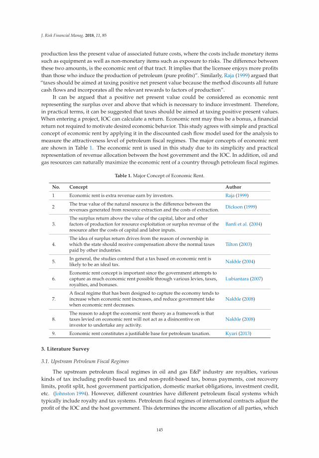
J. Risk Financial Manag. 2018, 11, 85
production less the present value of associated future costs, where the costs include monetary itemssuch as equipment as well as non-monetary items such as exposure to risks. The difference betweenthese two amounts, is the economic rent of that tract. It implies that the licensee enjoys more profitsthan those who induce the production of petroleum (pure profits)”. Similarly, Raja (1999) argued that“taxes should be aimed at taxing positive net present value because the method discounts all futurecash flows and incorporates all the relevant rewards to factors of production”.
It can be argued that a positive net present value could be considered as economic rentrepresenting the surplus over and above that which is necessary to induce investment. Therefore,in practical terms, it can be suggested that taxes should be aimed at taxing positive present values.When entering a project, IOC can calculate a return. Economic rent may thus be a bonus, a financialreturn not required to motivate desired economic behavior. This study agrees with simple and practicalconcept of economic rent by applying it in the discounted cash flow model used for the analysis tomeasure the attractiveness level of petroleum fiscal regimes. The major concepts of economic rentare shown in Table 1. The economic rent is used in this study due to its simplicity and practicalrepresentation of revenue allocation between the host government and the IOC. In addition, oil andgas resources can naturally maximize the economic rent of a country through petroleum fiscal regimes.
Table 1. Major Concept of Economic Rent.
No. Concept Author
1 Economic rent is extra revenue earn by investors. Raja (1999)
2 The true value of the natural resource is the difference between therevenues generated from resource extraction and the costs of extraction. Dickson (1999)
3.The surplus return above the value of the capital, labor and otherfactors of production for resource exploitation or surplus revenue of theresource after the costs of capital and labor inputs.
Banfi et al. (2004)
4.The idea of surplus return drives from the reason of ownership inwhich the state should receive compensation above the normal taxespaid by other industries.
Tilton (2003)
5. In general, the studies contend that a tax based on economic rent islikely to be an ideal tax. Nakhle (2004)
6.Economic rent concept is important since the government attempts tocapture as much economic rent possible through various levies, taxes,royalties, and bonuses.
Lubiantara (2007)
7.A fiscal regime that has been designed to capture the economy tends toincrease when economic rent increases, and reduce government takewhen economic rent decreases.
Nakhle (2008)
8.The reason to adopt the economic rent theory as a framework is thattaxes levied on economic rent will not act as a disincentive oninvestor to undertake any activity.
Nakhle (2008)
9. Economic rent constitutes a justifiable base for petroleum taxation. Kyari (2013)
3. Literature Survey
3.1. Upstream Petroleum Fiscal Regimes
The upstream petroleum fiscal regimes in oil and gas E&P industry are royalties, variouskinds of tax including profit-based tax and non-profit-based tax, bonus payments, cost recoverylimits, profit split, host government participation, domestic market obligations, investment credit,etc. (Johnston 1994). However, different countries have different petroleum fiscal systems whichtypically include royalty and tax systems. Petroleum fiscal regimes of international contracts adjust theprofit of the IOC and the host government. This determines the income allocation of all parties, which
145
J. Risk Financial Manag. 2018, 11, 85
contract fiscal terms with a distinctive petroleum feature and the core of the contract (Cameron 2006;Cottarelli 2012).
Petroleum fiscal regimes depend on resource facts the IOC has to consider if they would like toenter a country. Its attractiveness has a major impact on the feasibility of the project and the project ofthe IOC. Hence, they are significant when judging a country’s oil and gas resource investment climate.Moreover, evaluation and comparison of fiscal terms are crucial and will provide basis for the IOC’soverseas investment decision, and contribute to the most active implementation of upstream oil andgas E&P business (Boykett et al. 2012). Due to the importance of upstream fiscal terms in investment,there are several studies regarding the upstream fiscal regimes for oil-producing countries, in OECDcountries (Zhao and Dahl 2014); Indonesia (Abidin 2015); Malaysia (Manaf et al. 2014); Pakistanand Thailand (Zahidi 2010); Nigeria, Ghana, and Cameroon (Ghebremusse 2015); and Australia(Hunter 2008). However, there has still been a scarcity of studies for some developing countriesincluding Myanmar
3.2. Quantitative Method for Petroleum Fiscal Regimes Assessment
There are different types of petroleum co-operation in different regions, depending on nationalpetroleum legislation, international relations and the stage of oil and gas development. However,the major difference is only resource ownership transfer (Johnston et al. 2008). From the petroleumfiscal point of view, there are four steps: firstly, investment for oil and gas production; secondly,allocation of royalties or similar expenses attributable to the host government; thirdly, cost recovery,tax deduction and other compensation for IOC; and finally, profit split (Mabadi 2008; Serova 2015).
In the previous studies of Mommer (2001), Baunsgaard (2001), and Mommer (2002), the upstreamfiscal regimes are analyzed based on the concept of economic rent through tax instruments such asroyalties, bonuses, fixed fees, etc. Baunsgaard (2001) ascertained the equivalent fiscal regimes indifferent fiscal designs. For instance, the cost recovery concept in PSC is similar to the royalty ofconcessionary, and profit split in PSC is also similar to the initial tax rate in concessionary. It supportsthe concept that “fiscal regimes differences between contract types can be ignored when evaluating theattractiveness of the fiscal terms” (Luo and Yan 2010). As the number of types of fiscal contract designsis more than the number of countries (Johnston 1994), such findings for equivalent regimes has theadvantage for comparative analysis of different fiscal contract types in different countries. This studyagrees with those findings since the concessionary system uses only royalty and tax while PSC fiscaldesign uses various fiscal components.
3.3. Host Government Take (GT)
Government take (GT) is one of the most important criteria in making comparative analysisamong worldwide petroleum fiscal systems and calculated in various ways in the petroleum industry(Boodoo 2012). GT puts the impacts of several fiscal regimes such as bonus, royalties, profit split,and taxation of all levels, government equity participation and other factors into one indicator.In other words, GT is defined as the proportion of the host nation’s income from investment projectto the total project revenue within the valid period of the contract (Luo and Yan 2010). GT measureshow much the government takes through upstream petroleum fiscal terms as analyzed in previousstudies by Kaiser and Pulsipher (2004), Iledare and Kaiser (2006), Adenikinju and Oderinde (2009),Hao and Kaiser (2010), Kemp and Stephen (2011, 2012), Manaf et al. (2014), and Sen (2014). In theaforementioned studies, GT is calculated through a cash flow model based on historical data orreasonable assumptions combined with the given parameters in the fiscal system.
3.4. Non-Discounted Cash Flow Method (NDCF) and Discounted Cash Flow Method (DCF)
Without taking time value of money into consideration, cash inflows and outflows of the contractperiod are simulated at a certain level of oil price and output. Consequently, the appropriate deductionsand allocations of the contract are made in line with the fiscal terms of the contractual system, and the
146
J. Risk Financial Manag. 2018, 11, 85
proportion of the host nation’s return to the total project revenue within the whole project period is thenon-discounted GT (Johnston 1994). The formulae necessary for the computation of NDCF as well asDCF cash flows in the whole project life are based on the economic rent concept. The results of cashflow model can be used by an investor to assess the profitability of a project and establish how muchGT for the host country.
According to Wenrui et al. (1999), the discounted cash flow (DCF) method for the consideration oftime value of money is considered for the calculation of GT, as the project life cycle of the oil andgas E&P projects lasts generally more than 20 years. The best way to calculate GT requires detailedeconomic modelling using cash flow analysis (Johnston 2008).
The DCF method is calculated for the discounted host nation take based on a certain discountedrate. Cash inflow/outflow time of the host nation during the project life is simulated at a certainlevel of oil price and output. Moreover, the present value of the host nation’s income during the entirelife of the oil and gas project is calculated as per a certain discount rate (Luo and Yan 2010). DCF can beused to show how the tax take is calculated (Nakhle 2004). Furthermore, DCF method has been mostlyapplied in previous studies and is currently used by IOCs (Emhjellen and Alaouze 2001). According toSiew (2001), it has been found that 99% of IOCs used this DCF technique. In addition, the mostcommon technique widely used for project evaluation in energy industry has been the DCF for severaldecades (Laughton et al. 2000).
Wenrui et al. (1999) measured the profitability of upstream oil and gas projects by two systemsmeasures: NPV2 and IRR3 through a cash flow model. However, building a cash flow model takessome time and needs several data inputs. Moreover, a constantly discounted factor in DCF canoverestimate the project profitability. Kaiser and Pulsipher (2004) developed an analysis of upstreamfiscal regime by the real options theory to overcome the weakness of DCF. However, since this researchconsiders the combination effect with the opinions of decision makers for the evaluation method,it is necessary to use the most commonly applied method. Thus, about 99% of DCF is widely used byIOCs and was applied in this study.
3.5. Prompt and Intuitive Method
The prompt and intuitive method is the easiest and fastest way for an investor to make a decisionas soon as they know some fiscal regimes of the specific country (Luo and Yan 2010). As a matter of fact,forecasting the cash flow requires large amount of data, complex calculations, and multidisciplinarycollaborations. In addition, cash flow calculation is difficult to complete in a short time. Therefore,a fast estimation method or the fast and intuitive method is recommended.
In the fast estimation method, the total income of the project is assumed as 100%, and thecalculation is made in accordance with the order and proportion of the contractual system. Its strengthis that the IOCs can evaluate the attractiveness of the fiscal terms of the resource country in a simpleway. If IOCs are not aware of the detailed fiscal regimes of a specific country, it can also be used.However, the assumption of 100% total income for the entire project life cannot provide further insights.
According to Jiuliang and Fenglan (2001), there is no widely-accepted method for evaluatingand comparing different types of petroleum fiscal regimes used in the upstream oil and gas contractsworldwide. Therefore, it is difficult to choose the indicators that can reflect the combined effects ofdifferent fiscal systems. This research develops the evaluation method applied by Luo and Yan (2010).Different indicators—namely, government take (GT), front loading index (FLI), and composite score(CS)—are included in this evaluation method. Luo and Yan (2010) ascertained that these indicatorsare selected based on qualifications such as comprehensiveness, reflection of income allocation ratiobetween the IOC and resource-based country under the combined effects of fiscal regimes, considering
2 Net Present Value.3 Internal Rate of Return.
147
J. Risk Financial Manag. 2018, 11, 85
the impact of the allocation order due to time value of money and time sequence of allocation obtainedby different parties. Hence, the method using these indicators can affect the final benefit of the IOC.
3.6. Front Loading Index (FLI)
The FLI of IOCs are applied in this study to reflect the impact of time sequence differences of thehost nation on the project and IOC’s profit, with the intention of making up the weakness of the gapbetween GT and GTi indicators. FLI can reflect the combination level of a contract’s fiscal term. In theinternational oil and gas E&P industry, the time sequence of incomes gained by the host country is acrucial issue that an IOC should consider. This is because the IOC can recover costs as soon as possiblefor a higher return for an E&P project by delaying payment to the host country. Consider a case wherethe host resource country maximizes its government take (GT) based on the profit gained by the IOC.There would be no front-loading for the IOC and discounted GTi, while non-discounted GT would bethe same.
However, most of the host nations do not receive income, depending on profit from the project.There are some factors contributing to the difference of host nation’s proportion with discounted GTiand non-discounted GT. The fiscal regimes in the early project life are signature bonus and productionbonus. In addition to these early fiscal terms, other fiscal regimes4 in the construction period andregimes in the production phase5 may cause revenue of the host government to grow faster thanthe projected profit. This can cause front-loading to the IOC. The definition of FLI of an IOC is theratio of the difference between non-discounted GT and the discounted GTi to GT. The interpretationby Luo and Yan (2010) for the FLI relating to attractiveness is that the smaller the FLI is, the less risk theIOC will face in the earlier stage of the project life. Also, the less risk in the earlier phase of the project,the more attractive the petroleum fiscal regimes used in the E&P project.
3.7. Composite Score (CS)
Composite score (CS) is selected because it is a comprehensive evaluation indicator to evaluate thefiscal regimes of oil and gas projects. The linear weighting method is used to evaluate the indicators ofGT and FLI. Thus, the linear weighting function of the composite score is built as CS = W1 × GT +W2 × FLI, where W1 and W2 reflect the attitude of the investor relating to the contribution of GT andFLI to the attractiveness of the fiscal regimes. This is determined by the decision-maker in accordancewith their own experience. As the composite score is a comprehensive indicator that reflects theattractiveness of fiscal regimes, the interpretation for the CS is that the smaller the CS, the greaterthe attractiveness of the fiscal terms in the petroleum contract. The DCF and ROT could show theimpact of fiscal terms and identify fiscal regimes of oil production countries.
Moreover, it is the most common method used by the IOC (Siew 2001). However, it does notconsider the impact of different time sequences on the attractiveness of the fiscal terms. The modelwhich combines DCF, NDCF, FLI, and CS by Luo and Yan (2010) overcame this weakness andreflected the combination level of the contract’s fiscal terms more comprehensively. This is due to theconsideration of time different impact. However, the attitudes of the decision-maker were assumedfor the linear weighting method in the Luo and Yan (2010) study. Hence, it can limit the insight intothe attractiveness level of fiscal terms. With the intention of filling the gap in the literature, this studydevelops a comprehensive model of DCF, NDCF, FLI, and CS. The model considers the attitudes ofdecision-makers in the Korean energy industry for the combined effects of fiscal terms to impactmore realistically.
4 For example, business tax, value-added tax, import tax levied on the investment.5 For example, royalty, profit split, host government participation, bonus based on income and profit levels.
148
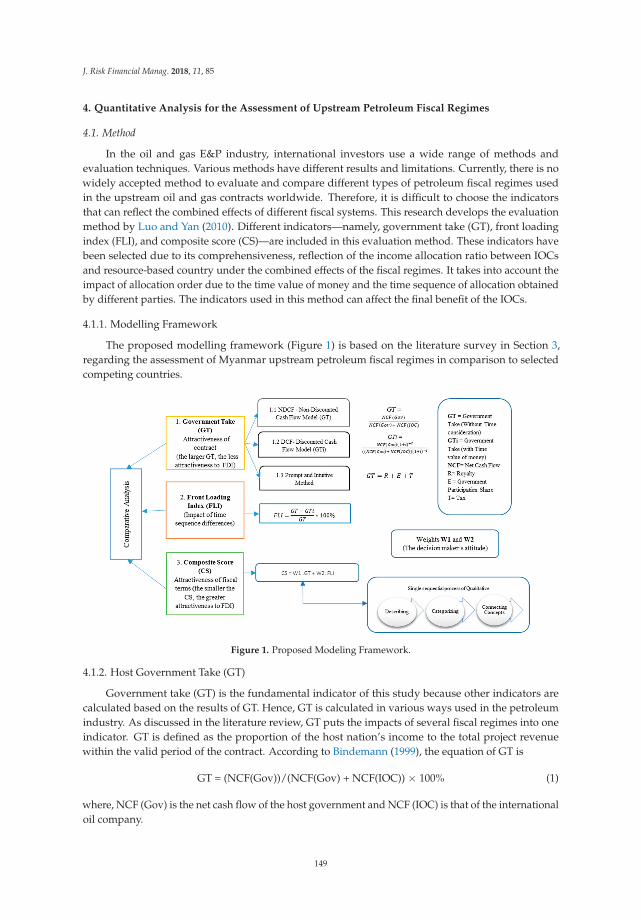
J. Risk Financial Manag. 2018, 11, 85
4. Quantitative Analysis for the Assessment of Upstream Petroleum Fiscal Regimes
4.1. Method
In the oil and gas E&P industry, international investors use a wide range of methods andevaluation techniques. Various methods have different results and limitations. Currently, there is nowidely accepted method to evaluate and compare different types of petroleum fiscal regimes usedin the upstream oil and gas contracts worldwide. Therefore, it is difficult to choose the indicatorsthat can reflect the combined effects of different fiscal systems. This research develops the evaluationmethod by Luo and Yan (2010). Different indicators—namely, government take (GT), front loadingindex (FLI), and composite score (CS)—are included in this evaluation method. These indicators havebeen selected due to its comprehensiveness, reflection of the income allocation ratio between IOCsand resource-based country under the combined effects of the fiscal regimes. It takes into account theimpact of allocation order due to the time value of money and the time sequence of allocation obtainedby different parties. The indicators used in this method can affect the final benefit of the IOCs.
4.1.1. Modelling Framework
The proposed modelling framework (Figure 1) is based on the literature survey in Section 3,regarding the assessment of Myanmar upstream petroleum fiscal regimes in comparison to selectedcompeting countries.
Figure 1. Proposed Modeling Framework.
4.1.2. Host Government Take (GT)
Government take (GT) is the fundamental indicator of this study because other indicators arecalculated based on the results of GT. Hence, GT is calculated in various ways used in the petroleumindustry. As discussed in the literature review, GT puts the impacts of several fiscal regimes into oneindicator. GT is defined as the proportion of the host nation’s income to the total project revenuewithin the valid period of the contract. According to Bindemann (1999), the equation of GT is
GT = (NCF(Gov))/(NCF(Gov) + NCF(IOC)) × 100% (1)
where, NCF (Gov) is the net cash flow of the host government and NCF (IOC) is that of the internationaloil company.
149
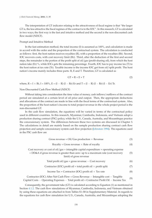
J. Risk Financial Manag. 2018, 11, 85
The interpretation of GT indicator relating to the attractiveness of fiscal regime is that “the largerGT is, the less attractive the fiscal regimes of the contract is to the IOC”. In this research, GT is calculatedin two ways; the first way is the fast and intuitive method and the second is the non-discounted cashflow model (NDCF).
Prompt and Intuitive Method
In the fast estimation method, the total income (I) is assumed as 100%, and calculation is madein accord with the order and the proportion of the contractual system. The calculation is conductedas follows: first, the host nation receives royalties (R), with a proportion of the royalties (Rt). Second,IOC recovers costs, with cost recovery limit (Rr). Third, after the deduction of the first and secondsteps, the remainder is the portion of the profit split of oil/gas (profit-sharing oil), from which the hostnation take (Er) %, while IOCs gets the remaining percentage. Fourth, IOC has to pay income tax (T) tothe host nation at tax rate (Tr). Taxable income is the income IOC get from oil/split profit. The hostnation’s income mainly includes three parts: R, E and T. Therefore, GT is calculated as
GT = R + E + T (2)
where, R = I × Rt, I = 100%, E = (I − R) (I − Rr) Er and T = (I − R) (I − Rr) (I − Er) Tr.
Non-Discounted Cash Flow Method (NDCF)
Without taking into consideration the time value of money, cash inflows/outflows of the contractperiod are simulated at a certain level of oil price and output. Then, the appropriate deductionsand allocations of the contract are made in line with the fiscal terms of the contractual system. Also,the proportion of the host nation’s income to total project revenue in the whole project period is thenon-discounted GT.
In the cash flow simulation, the equations will be varied in terms of the contractual policyused in different countries. In this research, Myanmar, Cambodia, Indonesia, and Vietnam adopt aproduction sharing contract (PSC) policy, while the U.S., Canada, Australia, and Mozambique practicethe concessionary system. The differences between these two systems are discussed in Chapter 3.The calculations in detail are mainly based on the sample production sharing contract cash flowprojection and sample concessionary system cash flow projection (Johnston 1994). The equations usedin the PSC cash flow are
Gross revenue = Oil/Gas production × Revenue (3)
Royalty = Gross revenue × Rate of royalty (4)
Cost recovery or cost of oil/gas = intangible capital expenditure + operating expense+ DD&A if gross revenue is greater than zero: up to a maximum rate (cost recovery
limit) of gross revenue(5)
Total profit oil/gas = gross revenue − Cost recovery (6)
Contractor (IOC) profit oil = total profit oil × profit split (7)
Income Tax = Contractor (IOC) profit oil × Tax rate (8)
Contractor (IOC) After Net Cash Flow = Gross Revenue − Intangible cost − TangibleCapital Costs − Operating Expenses − Total profit oil + Contractor Profit Oil − Income Tax
(9)
Consequently, the government take (GT) is calculated according to Equation (1) as mentioned inSection 4.1.2. The cash flow simulations of Myanmar, Cambodia, Indonesia, and Vietnam obtainedby using these equations are attached in from Tables S1–S8 in Supplementary Material. In regards tothe equations for cash flow simulation for U.S., Canada, Australia, and Mozambique adopting the
150
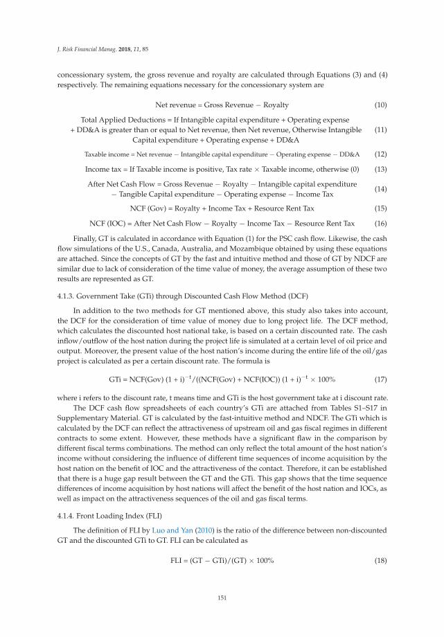
J. Risk Financial Manag. 2018, 11, 85
concessionary system, the gross revenue and royalty are calculated through Equations (3) and (4)respectively. The remaining equations necessary for the concessionary system are
Net revenue = Gross Revenue − Royalty (10)
Total Applied Deductions = If Intangible capital expenditure + Operating expense+ DD&A is greater than or equal to Net revenue, then Net revenue, Otherwise Intangible
Capital expenditure + Operating expense + DD&A(11)
Taxable income = Net revenue − Intangible capital expenditure − Operating expense − DD&A (12)
Income tax = If Taxable income is positive, Tax rate × Taxable income, otherwise (0) (13)
After Net Cash Flow = Gross Revenue − Royalty − Intangible capital expenditure− Tangible Capital expenditure − Operating expense − Income Tax
(14)
NCF (Gov) = Royalty + Income Tax + Resource Rent Tax (15)
NCF (IOC) = After Net Cash Flow − Royalty − Income Tax − Resource Rent Tax (16)
Finally, GT is calculated in accordance with Equation (1) for the PSC cash flow. Likewise, the cashflow simulations of the U.S., Canada, Australia, and Mozambique obtained by using these equationsare attached. Since the concepts of GT by the fast and intuitive method and those of GT by NDCF aresimilar due to lack of consideration of the time value of money, the average assumption of these tworesults are represented as GT.
4.1.3. Government Take (GTi) through Discounted Cash Flow Method (DCF)
In addition to the two methods for GT mentioned above, this study also takes into account,the DCF for the consideration of time value of money due to long project life. The DCF method,which calculates the discounted host national take, is based on a certain discounted rate. The cashinflow/outflow of the host nation during the project life is simulated at a certain level of oil price andoutput. Moreover, the present value of the host nation’s income during the entire life of the oil/gasproject is calculated as per a certain discount rate. The formula is
GTi = NCF(Gov) (1 + i)−t/((NCF(Gov) + NCF(IOC)) (1 + i)−t × 100% (17)
where i refers to the discount rate, t means time and GTi is the host government take at i discount rate.The DCF cash flow spreadsheets of each country’s GTi are attached from Tables S1–S17 in
Supplementary Material. GT is calculated by the fast-intuitive method and NDCF. The GTi which iscalculated by the DCF can reflect the attractiveness of upstream oil and gas fiscal regimes in differentcontracts to some extent. However, these methods have a significant flaw in the comparison bydifferent fiscal terms combinations. The method can only reflect the total amount of the host nation’sincome without considering the influence of different time sequences of income acquisition by thehost nation on the benefit of IOC and the attractiveness of the contact. Therefore, it can be establishedthat there is a huge gap result between the GT and the GTi. This gap shows that the time sequencedifferences of income acquisition by host nations will affect the benefit of the host nation and IOCs, aswell as impact on the attractiveness sequences of the oil and gas fiscal terms.
4.1.4. Front Loading Index (FLI)
The definition of FLI by Luo and Yan (2010) is the ratio of the difference between non-discountedGT and the discounted GTi to GT. FLI can be calculated as
FLI = (GT − GTi)/(GT) × 100% (18)
151
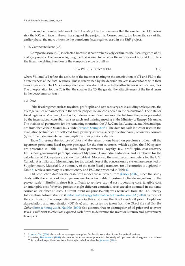
J. Risk Financial Manag. 2018, 11, 85
Luo and Yan’s interpretation of the FLI relating to attractiveness is that the smaller the FLI, the lessrisk the IOC will face in the earlier stage of the project life. Consequently, the lower the risk of theearlier phase, the more attractive the petroleum fiscal regimes used in the E&P project.
4.1.5. Composite Score (CS)
Composite score (CS) is selected because it comprehensively evaluates the fiscal regimes of oiland gas projects. The linear weighting method is used to consider the indicators of GT and FLI. Thus,the linear weighting function of the composite score is built as
CS = W1 × GT + W2 × FLI, (19)
where W1 and W2 reflect the attitude of the investor relating to the contribution of GT and FLI to theattractiveness of the fiscal regimes. This is determined by the decision-makers in accordance with theirown experience. The CS is a comprehensive indicator that reflects the attractiveness of fiscal regimes.The interpretation for the CS is that the smaller the CS, the greater the attractiveness of the fiscal termsin the petroleum contract.
4.2. Data
If the fiscal regimes such as royalties, profit split, and cost recovery are in a sliding scale system, theaverage values of parameters in the whole project life are considered in the calculation6. The data forfiscal regimes of Myanmar, Cambodia, Indonesia, and Vietnam are collected from the paper presentedby the international consultant at a research and training meeting at the Ministry of Energy, Myanmar.The main fiscal parameters for the remaining countries: the U.S., Canada, Australia, and Mozambiqueare from the Global Oil and Tax Guide (Ernst & Young 2015). The data for each indicator used in theevaluation techniques are collected from primary sources (survey questionnaire), secondary sources(government documents) and assumptions from previous studies.
Table 2 presents the sources of data and the assumptions based on previous studies. All theupstream petroleum fiscal regime packages for the four countries which applies the PSC systemare presented in Table 3. The main fiscal parameters—royalty, tax, profit split, cost recoverylimits, host government participations—of Myanmar, Cambodia, Indonesia, and Cambodia for thecalculation of PSC system are shown in Table 4. Moreover, the main fiscal parameters for the U.S.,Canada, Australia, and Mozambique for the calculation of the concessionary system are presented inSupplementary Material 9. A summary of the main fiscal parameters for all countries is depicted inTable 5, while a summary of concessionary and PSC are presented in Table 6.
Oil production data for the cash flow model are retrieved from Kaiser (2007), since the studydeals with the effects of fiscal parameters for a favorable investment climate regardless of theproject scale7. Similarly, since it is difficult to retrieve capital cost, operating cost, tangible cost,an intangible cost for every project in eight different countries, costs are also assumed in the samesource as for other studies. Current Brent oil price ($/bbl) was retrieved from the U.S. EnergyInformation Administration (United States Energy Information Administration (EIA ) 2014) as most ofthe countries in the comparative analysis in this study use the Brent crude oil price. Depletion,depreciation, and amortization (DD & A) and tax losses are taken from the Global Oil and Gas TaxGuide (Ernst & Young 2015). Nakhle (2004) also asserted that an assumption of oil price and relevanttaxes is sufficient to calculate expected cash flows to determine the investor’s return and governmenttake (GT).
6 Luo and Yan (2010) also made an average assumption for the sliding scales of petroleum fiscal regimes.7 Likewise, Bindemann (1999) also made the same assumptions for the study of upstream fiscal regime comparison.
This production profile came from the sample cash flow sheet by Johnston (1994).
152

J. Risk Financial Manag. 2018, 11, 85
Ta
ble
2.
Dat
aSo
urce
sfo
rea
chIn
dica
tor.
Ind
ica
tor
Ne
cess
ary
Pa
ram
ete
rsD
ata
So
urc
eP
rev
iou
sS
tud
ies
GT
(ND
CF)
Prod
ucti
onpr
ofile
,CA
PEX
,OPE
X,
DD
&Pr
ice
Fisc
alTe
rmV
aria
bles
(Roy
alty
,Bo
nus,
Cos
tRec
over
y,Pr
ofitS
plit
,Ta
x)
Kai
ser
(200
7)U
SEn
ergy
Info
rmat
ion
Adm
inis
trat
ion
1.Er
nst&
Youn
g(2
015)
.Glo
balO
il&
Gas
Tax
Gui
de2.
PSC
Feat
ures
for
Off
shor
ePe
trol
eum
Expl
orat
ion:
Min
istr
yof
Ener
gy,
Mya
nmar
Sam
eA
ssum
ptio
ns1.
(Kai
ser
(200
7)2.
Bind
eman
n(1
999)
3.Jo
hnst
on(1
994)
Ass
umpt
ion
ofoi
lpri
cean
dre
leva
ntta
xes
issu
ffici
ent:
-to
calc
ulat
eex
pect
edca
shflo
ws
tode
term
ine
the
inve
stor
’sre
turn
and
gove
rnm
entt
ake
(GT)
(Nak
hle
2004
)
GT
(DC
F)D
isco
untR
ate
(10%
)N
akhl
e(2
004)
.Pet
role
umta
xati
on.
Ass
umpt
ion
10pe
rce
ntin
real
term
s,-a
sw
asap
plie
din
the
maj
orit
yof
publ
ishe
dst
udie
s,-t
om
irro
rto
indu
stry
’sdi
scou
ntra
te.
CS
Wei
ghts
(Att
itud
eof
Dec
isio
nM
aker
s)
Prim
ary
sour
ceof
data
bysu
rvey
ques
tion
nair
eto
subj
ectm
atte
rex
pert
sof
Kor
ean
com
pani
es.
Scor
esan
dW
eigh
tings
shou
ldbe
dete
rmin
edus
ing
ate
chni
que
such
asD
elph
inor
Peer
revi
ewor
aqu
esti
onna
ire
(Hen
riks
enan
dTr
ayno
r19
99).
Com
para
tive
Ana
lysi
sC
ount
rySe
lect
ion
Prim
ary
sour
ceby
surv
eyqu
estio
nnai
re
153
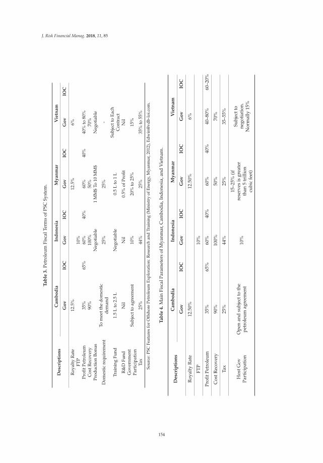
J. Risk Financial Manag. 2018, 11, 85
Ta
ble
3.
Petr
oleu
mFi
scal
Term
sof
PSC
Syst
em.
De
scri
pti
on
sC
am
bo
dia
Ind
on
esi
aM
ya
nm
ar
Vie
tna
m
Go
vIO
CG
ov
IOC
Go
vIO
CG
ov
IOC
Roy
alty
Rat
e12
.5%
12.5
%6%
FTP
10%
Profi
tPet
role
um35
%65
%60
%40
%60
%40
%40
%to
80%
Cos
tRec
over
y90
%10
0%50
%70
%Pr
oduc
tion
Bonu
sN
egot
iabl
e1
MM
$To
10M
M$
Neg
otia
ble
Dom
estic
requ
irem
ent
Tom
eett
hedo
mes
tic
dem
and
25%
25%
-
Trai
ning
Fund
1.5
Lto
2.5
LN
egot
iabl
e0.
5L
to1
LSu
bjec
tto
Each
Con
trac
tR
&D
Fund
Nil
Nil
0.5%
ofPr
ofit
Nil
Gov
ernm
ent
Part
icip
atio
nSu
bjec
tto
agre
emen
t10
%20
%to
25%
15%
Tax
25%
44%
25%
35%
to55
%
Sour
ce:P
SCFe
atur
esfo
rO
ffsh
ore
Petr
oleu
mEx
plor
atio
n:R
esea
rch
and
Trai
ning
(Min
istr
yof
Ener
gy,M
yanm
ar,2
012)
,Edw
in@
vdb-
loi.c
om.
Ta
ble
4.
Mai
nFi
scal
Para
met
ers
ofM
yanm
ar,C
ambo
dia,
Indo
nesi
a,an
dV
ietn
am.
De
scri
pti
on
sC
am
bo
dia
Ind
on
esi
aM
ya
nm
ar
Vie
tna
m
Go
vIO
CG
ov
IOC
Go
vIO
CG
ov
IOC
Roy
alty
Rat
e12
.50%
12.5
0%6%
FTP
10%
Profi
tPet
role
um35
%65
%60
%40
%60
%40
%40
–80%
60–2
0%
Cos
tRec
over
y90
%10
0%50
%70
%
Tax
25%
44%
25%
35–5
5%
Hos
tGov
Part
icip
atio
nO
pen
and
subj
ectt
oth
epe
trol
eum
agre
emen
t10
%
15–2
5%(i
fre
serv
esis
grea
ter
than
5tr
illio
ncu
bic
feet
)
Subj
ectt
one
goti
atio
n.N
orm
ally
15%
154
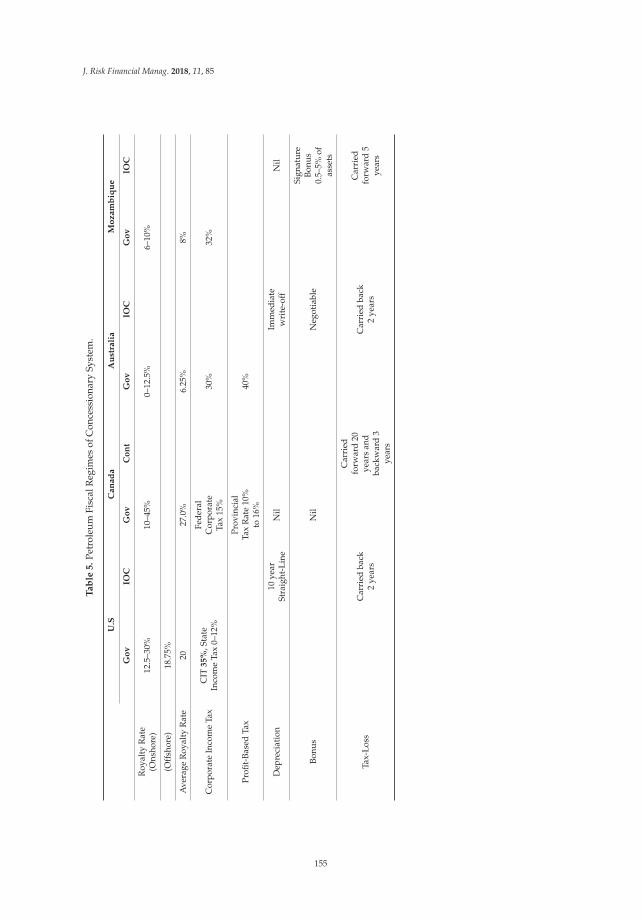
J. Risk Financial Manag. 2018, 11, 85
Ta
ble
5.
Petr
oleu
mFi
scal
Reg
imes
ofC
once
ssio
nary
Syst
em.
U.S
Can
ad
aA
ust
rali
aM
ozam
biq
ue
Go
vIO
CG
ov
Co
nt
Go
vIO
CG
ov
IOC
Roy
alty
Rat
e(O
nsho
re)
12.5
–30%
10–4
5%0–
12.5
%6–
10%
(Off
shor
e)18
.75%
Ave
rage
Roy
alty
Rat
e20
27.0
%6.
25%
8%
Cor
pora
teIn
com
eTa
xC
IT35%
,Sta
teIn
com
eTa
x0–
12%
Fede
ral
Cor
pora
teTa
x15
%30
%32
%
Profi
t-Ba
sed
Tax
Prov
inci
alTa
xR
ate
10%
to16
%40
%
Dep
reci
atio
n10
year
Stra
ight
-Lin
eN
ilIm
med
iate
wri
te-o
ffN
il
Bonu
sN
ilN
egot
iabl
e
Sign
atur
eBo
nus
0.5–
5%of
asse
ts
Tax-
Loss
Car
ried
back
2ye
ars
Car
ried
forw
ard
20ye
ars
and
back
war
d3
year
s
Car
ried
back
2ye
ars
Car
ried
forw
ard
5ye
ars
155
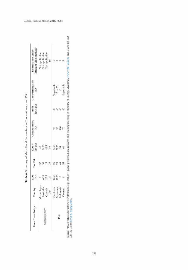
J. Risk Financial Manag. 2018, 11, 85
Ta
ble
6.
Sum
mar
yof
Mai
nFi
scal
Para
met
ers
inC
once
ssio
nary
and
PSC
.
Fis
cal
Term
Po
licy
Co
un
try
RO
Y(%
)T
ax
(%)
RO
Y+
Tax
(%)
Co
stR
eco
very
(%)
Pro
fit
Sp
lit
(%)
Go
v-P
art
icip
ati
on
(%)
Dep
reci
ati
on
(Year)
(Str
aig
ht
Lin
eM
eth
od
)
Con
cess
iona
ry
Moz
ambq
ue8
3240
Not
appl
icab
leA
ustr
alia
6.25
3036
.25
Not
appl
icab
leC
anad
a27
.515
42.5
Not
appl
icab
leU
.S20
3555
10
PSC
Cam
bodi
a12
.25
2537
.25
9035
Neg
otia
ble
5M
yanm
ar12
.25
2537
.25
5060
15to
255
Indo
nesi
a10
4454
100
6010
5V
ietn
am6
5561
7040
Neg
otia
ble
5
Sour
ce:“
PSC
Feat
ures
for
Off
shor
ePe
trol
eum
Expl
orat
ion”
,pap
erpr
esen
ted
ata
rese
arch
and
trai
ning
mee
ting
inM
inis
try
ofEn
ergy
,Mya
nmar
.ww
w.v
db-l
oi.c
om,a
ndG
loba
lOil
and
Gas
Tax
Gui
de(E
rnst
&Yo
ung
2015
).
156
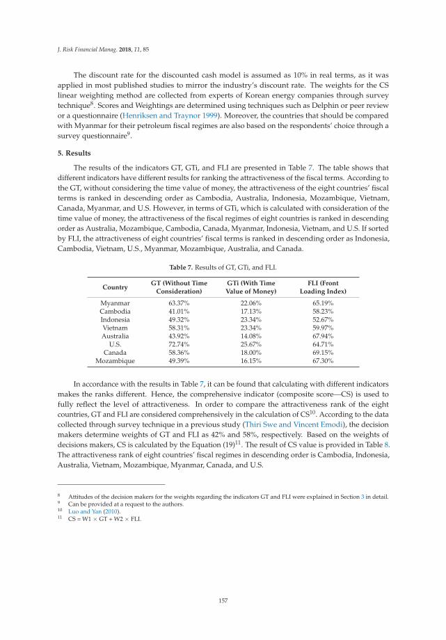
J. Risk Financial Manag. 2018, 11, 85
The discount rate for the discounted cash model is assumed as 10% in real terms, as it wasapplied in most published studies to mirror the industry’s discount rate. The weights for the CSlinear weighting method are collected from experts of Korean energy companies through surveytechnique8. Scores and Weightings are determined using techniques such as Delphin or peer reviewor a questionnaire (Henriksen and Traynor 1999). Moreover, the countries that should be comparedwith Myanmar for their petroleum fiscal regimes are also based on the respondents’ choice through asurvey questionnaire9.
5. Results
The results of the indicators GT, GTi, and FLI are presented in Table 7. The table shows thatdifferent indicators have different results for ranking the attractiveness of the fiscal terms. According tothe GT, without considering the time value of money, the attractiveness of the eight countries’ fiscalterms is ranked in descending order as Cambodia, Australia, Indonesia, Mozambique, Vietnam,Canada, Myanmar, and U.S. However, in terms of GTi, which is calculated with consideration of thetime value of money, the attractiveness of the fiscal regimes of eight countries is ranked in descendingorder as Australia, Mozambique, Cambodia, Canada, Myanmar, Indonesia, Vietnam, and U.S. If sortedby FLI, the attractiveness of eight countries’ fiscal terms is ranked in descending order as Indonesia,Cambodia, Vietnam, U.S., Myanmar, Mozambique, Australia, and Canada.
Table 7. Results of GT, GTi, and FLI.
CountryGT (Without Time
Consideration)GTi (With TimeValue of Money)
FLI (FrontLoading Index)
Myanmar 63.37% 22.06% 65.19%Cambodia 41.01% 17.13% 58.23%Indonesia 49.32% 23.34% 52.67%Vietnam 58.31% 23.34% 59.97%Australia 43.92% 14.08% 67.94%
U.S. 72.74% 25.67% 64.71%Canada 58.36% 18.00% 69.15%
Mozambique 49.39% 16.15% 67.30%
In accordance with the results in Table 7, it can be found that calculating with different indicatorsmakes the ranks different. Hence, the comprehensive indicator (composite score—CS) is used tofully reflect the level of attractiveness. In order to compare the attractiveness rank of the eightcountries, GT and FLI are considered comprehensively in the calculation of CS10. According to the datacollected through survey technique in a previous study (Thiri Swe and Vincent Emodi), the decisionmakers determine weights of GT and FLI as 42% and 58%, respectively. Based on the weights ofdecisions makers, CS is calculated by the Equation (19)11. The result of CS value is provided in Table 8.The attractiveness rank of eight countries’ fiscal regimes in descending order is Cambodia, Indonesia,Australia, Vietnam, Mozambique, Myanmar, Canada, and U.S.
8 Attitudes of the decision makers for the weights regarding the indicators GT and FLI were explained in Section 3 in detail.9 Can be provided at a request to the authors.10 Luo and Yan (2010).11 CS = W1 × GT + W2 × FLI.
157
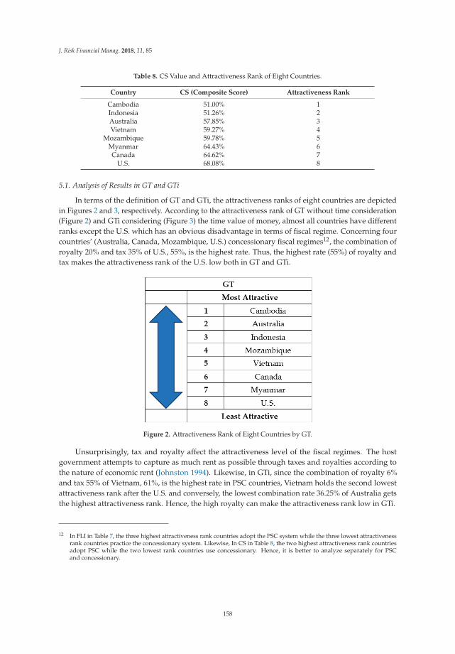
J. Risk Financial Manag. 2018, 11, 85
Table 8. CS Value and Attractiveness Rank of Eight Countries.
Country CS (Composite Score) Attractiveness Rank
Cambodia 51.00% 1Indonesia 51.26% 2Australia 57.85% 3Vietnam 59.27% 4
Mozambique 59.78% 5Myanmar 64.43% 6Canada 64.62% 7
U.S. 68.08% 8
5.1. Analysis of Results in GT and GTi
In terms of the definition of GT and GTi, the attractiveness ranks of eight countries are depictedin Figures 2 and 3, respectively. According to the attractiveness rank of GT without time consideration(Figure 2) and GTi considering (Figure 3) the time value of money, almost all countries have differentranks except the U.S. which has an obvious disadvantage in terms of fiscal regime. Concerning fourcountries’ (Australia, Canada, Mozambique, U.S.) concessionary fiscal regimes12, the combination ofroyalty 20% and tax 35% of U.S., 55%, is the highest rate. Thus, the highest rate (55%) of royalty andtax makes the attractiveness rank of the U.S. low both in GT and GTi.
Figure 2. Attractiveness Rank of Eight Countries by GT.
Unsurprisingly, tax and royalty affect the attractiveness level of the fiscal regimes. The hostgovernment attempts to capture as much rent as possible through taxes and royalties according tothe nature of economic rent (Johnston 1994). Likewise, in GTi, since the combination of royalty 6%and tax 55% of Vietnam, 61%, is the highest rate in PSC countries, Vietnam holds the second lowestattractiveness rank after the U.S. and conversely, the lowest combination rate 36.25% of Australia getsthe highest attractiveness rank. Hence, the high royalty can make the attractiveness rank low in GTi.
12 In FLI in Table 7, the three highest attractiveness rank countries adopt the PSC system while the three lowest attractivenessrank countries practice the concessionary system. Likewise, In CS in Table 8, the two highest attractiveness rank countriesadopt PSC while the two lowest rank countries use concessionary. Hence, it is better to analyze separately for PSCand concessionary.
158
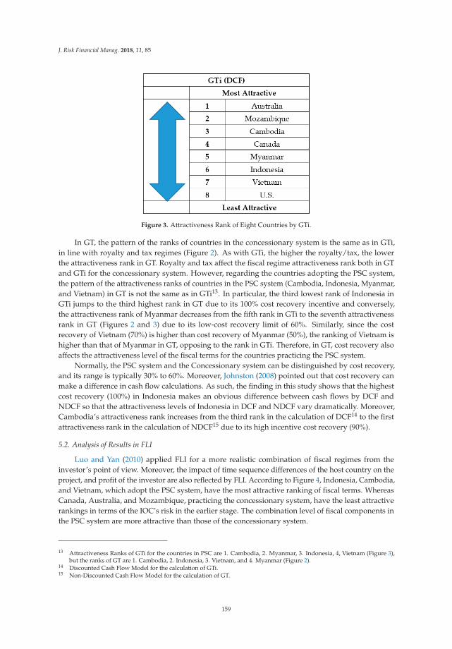
J. Risk Financial Manag. 2018, 11, 85
Figure 3. Attractiveness Rank of Eight Countries by GTi.
In GT, the pattern of the ranks of countries in the concessionary system is the same as in GTi,in line with royalty and tax regimes (Figure 2). As with GTi, the higher the royalty/tax, the lowerthe attractiveness rank in GT. Royalty and tax affect the fiscal regime attractiveness rank both in GTand GTi for the concessionary system. However, regarding the countries adopting the PSC system,the pattern of the attractiveness ranks of countries in the PSC system (Cambodia, Indonesia, Myanmar,and Vietnam) in GT is not the same as in GTi13. In particular, the third lowest rank of Indonesia inGTi jumps to the third highest rank in GT due to its 100% cost recovery incentive and conversely,the attractiveness rank of Myanmar decreases from the fifth rank in GTi to the seventh attractivenessrank in GT (Figures 2 and 3) due to its low-cost recovery limit of 60%. Similarly, since the costrecovery of Vietnam (70%) is higher than cost recovery of Myanmar (50%), the ranking of Vietnam ishigher than that of Myanmar in GT, opposing to the rank in GTi. Therefore, in GT, cost recovery alsoaffects the attractiveness level of the fiscal terms for the countries practicing the PSC system.
Normally, the PSC system and the Concessionary system can be distinguished by cost recovery,and its range is typically 30% to 60%. Moreover, Johnston (2008) pointed out that cost recovery canmake a difference in cash flow calculations. As such, the finding in this study shows that the highestcost recovery (100%) in Indonesia makes an obvious difference between cash flows by DCF andNDCF so that the attractiveness levels of Indonesia in DCF and NDCF vary dramatically. Moreover,Cambodia’s attractiveness rank increases from the third rank in the calculation of DCF14 to the firstattractiveness rank in the calculation of NDCF15 due to its high incentive cost recovery (90%).
5.2. Analysis of Results in FLI
Luo and Yan (2010) applied FLI for a more realistic combination of fiscal regimes from theinvestor’s point of view. Moreover, the impact of time sequence differences of the host country on theproject, and profit of the investor are also reflected by FLI. According to Figure 4, Indonesia, Cambodia,and Vietnam, which adopt the PSC system, have the most attractive ranking of fiscal terms. WhereasCanada, Australia, and Mozambique, practicing the concessionary system, have the least attractiverankings in terms of the IOC’s risk in the earlier stage. The combination level of fiscal components inthe PSC system are more attractive than those of the concessionary system.
13 Attractiveness Ranks of GTi for the countries in PSC are 1. Cambodia, 2. Myanmar, 3. Indonesia, 4, Vietnam (Figure 3),but the ranks of GT are 1. Cambodia, 2. Indonesia, 3. Vietnam, and 4. Myanmar (Figure 2).
14 Discounted Cash Flow Model for the calculation of GTi.15 Non-Discounted Cash Flow Model for the calculation of GT.
159
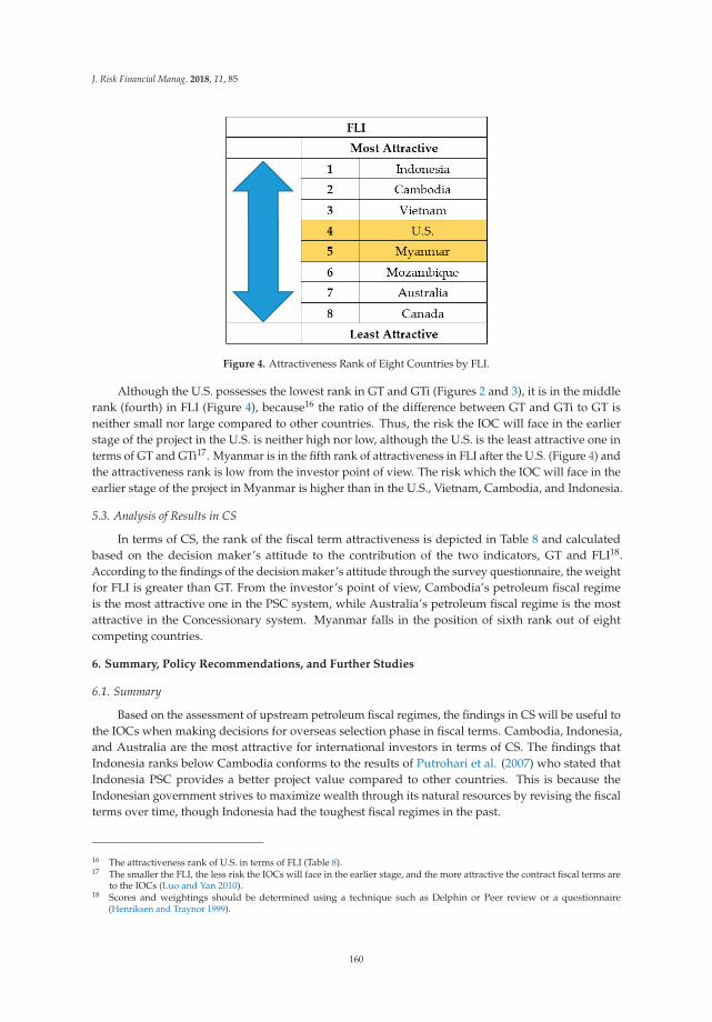
J. Risk Financial Manag. 2018, 11, 85
Figure 4. Attractiveness Rank of Eight Countries by FLI.
Although the U.S. possesses the lowest rank in GT and GTi (Figures 2 and 3), it is in the middlerank (fourth) in FLI (Figure 4), because16 the ratio of the difference between GT and GTi to GT isneither small nor large compared to other countries. Thus, the risk the IOC will face in the earlierstage of the project in the U.S. is neither high nor low, although the U.S. is the least attractive one interms of GT and GTi17. Myanmar is in the fifth rank of attractiveness in FLI after the U.S. (Figure 4) andthe attractiveness rank is low from the investor point of view. The risk which the IOC will face in theearlier stage of the project in Myanmar is higher than in the U.S., Vietnam, Cambodia, and Indonesia.
5.3. Analysis of Results in CS
In terms of CS, the rank of the fiscal term attractiveness is depicted in Table 8 and calculatedbased on the decision maker’s attitude to the contribution of the two indicators, GT and FLI18.According to the findings of the decision maker’s attitude through the survey questionnaire, the weightfor FLI is greater than GT. From the investor’s point of view, Cambodia’s petroleum fiscal regimeis the most attractive one in the PSC system, while Australia’s petroleum fiscal regime is the mostattractive in the Concessionary system. Myanmar falls in the position of sixth rank out of eightcompeting countries.
6. Summary, Policy Recommendations, and Further Studies
6.1. Summary
Based on the assessment of upstream petroleum fiscal regimes, the findings in CS will be useful tothe IOCs when making decisions for overseas selection phase in fiscal terms. Cambodia, Indonesia,and Australia are the most attractive for international investors in terms of CS. The findings thatIndonesia ranks below Cambodia conforms to the results of Putrohari et al. (2007) who stated thatIndonesia PSC provides a better project value compared to other countries. This is because theIndonesian government strives to maximize wealth through its natural resources by revising the fiscalterms over time, though Indonesia had the toughest fiscal regimes in the past.
16 The attractiveness rank of U.S. in terms of FLI (Table 8).17 The smaller the FLI, the less risk the IOCs will face in the earlier stage, and the more attractive the contract fiscal terms are
to the IOCs (Luo and Yan 2010).18 Scores and weightings should be determined using a technique such as Delphin or Peer review or a questionnaire
(Henriksen and Traynor 1999).
160
J. Risk Financial Manag. 2018, 11, 85
From the result for FLI, the highest ranks belong to the countries practicing the PSC systemsuch as Indonesia, Cambodia, and Vietnam. The lowest ranks belong to the countries adopting aconcessionary system such as Canada, Australia, and Mozambique. This implies that PSC fiscal policyis more attractive than the concessionary policy. This supports previous finding from Kyari (2013)and Iledare (2004) where the PSC system was more favorable than other systems. Due to differencesbetween PSC and concessionary, it is better to separately analyze the effects of each fiscal regime in thePSC system and those in a concessionary system.
The main findings of GT and GTi suggests that there are three main issues in this study. Firstly,royalty and tax affect the attractiveness rank of fiscal regimes in the evaluation of petroleum resourcedevelopment projects, with or without consideration of the time value of money, especially forcountries which use a concessionary policy. Secondly, in the PSC system, royalty and tax also affect theattractiveness rank of a fiscal regime, but only in an evaluation that considers the time value of money.Thirdly, cost recovery19 affects the attractiveness of fiscal regimes in the evaluation of projects withoutconsideration of the time value of money.
The findings about royalty and tax effect on upstream petroleum fiscal terms in this research areconsistent with the previous results by Nakhle (2004) and Kyari (2013). Likewise, the findings aboutcost recovery effect on the fiscal regimes’ attractiveness rank, the cost recovery rate in Myanmar alsosupports the concept that the low-cost recovery limit has a big impact (Johnston 2008).
Myanmar ranks sixth out of eight competing countries. With this low rank, it is not so attractivefor investors, especially in comparison with regional countries such as Indonesia, Cambodia, andVietnam. Disregarding the U.S., Australia, Mozambique, and Canada, which adopt a concessionarysystem, Myanmar is the least attractive country among those countries which practice a PSC policyin terms of both FLI and CS. In summary, the Myanmar upstream petroleum fiscal regime has a lowattraction compared to its competing countries from the investor’s point of view, both in terms of therisk to the investor in the earlier part of the project and in terms of evaluation with or without the timevalue of money.
6.2. Policy Recommendations
The main motivation for this study came from the necessity to assess the attractiveness rank ofMyanmar upstream petroleum fiscal regimes in the E&P investment climate, since Myanmar needs todevelop its oil and gas resources to fulfil increasing domestic demand without harming its existingnatural gas exports20. As the Myanmar upstream oil and gas investment climate is not favorable, thisstudy suggests some fiscal regime policy recommendations.
First, analysis of findings in GTi by DCF, considering the time value of money, suggests that,in order to encourage investors in the development of Myanmar’s oil and gas E&P industry, the lowerthe royalty and tax are dropped, the more attractive it will be for the investor. Similarly, the findingfor the qualitative analysis of the effects of Myanmar fiscal regimes shows that the Myanmar royaltyrate (12.5%), as a non-neutral regime, impacts on the investment decision. To reduce the distortionscaused by the imposition of royalty, a sliding scale royalty may be applied. Such a royalty is based oncharging different rates of tax, depending on the level of production or oil price. Therefore, the existingroyalty regime of Myanmar should be a sliding scale depending on production level or oil price orwater depth in offshore oil and gas blocks.
Second, the finding in the analysis of GT, without time consideration, by NDCF suggests that thehigher cost recovery incentives are, the more favorable the investment climate. Currently, Myanmar’scost recovery regime (50%) is the lowest among its competing countries. Although it is between thetypical cost recovery range 30–60%, its attractiveness level is low compared to competing countries
19 Cost recovery regime is used only in PSC fiscal system.20 25% of foreign earnings comes from natural gas export in Myanmar.
161
J. Risk Financial Manag. 2018, 11, 85
in this study. All competing countries’ cost recovery regimes are higher than Myanmar’s21. Such alow-cost recovery regime will hinder the attractiveness of its petroleum fiscal regimes. The FLI indicatorshows that the countries with the highest attractiveness rank (Indonesia, Cambodia, and Vietnam)adopt the PSC fiscal contractual system. Hence, it suggests that the PSC contractual system, which iscurrently used in Myanmar, will provide a more favorable investment climate than another system.
Third, the design of an efficient fiscal system must consider the political and geological risksas well as the potential rewards. Even though some countries have the toughest petroleum fiscalregimes, they are still attractive to the investors due to high geological prosperity which significantlyreduces exploration costs. Thus, it is recommended that 92% of such factors as geological condition,location, political stability, and investment opportunity should be taken into account before changingMyanmar’s existing petroleum fiscal regimes22. Moreover, Myanmar should consider improvingits fiscal regimes that are not neutral—royalty, tax, profit split, and cost recovery—for a favorableinvestment climate from the Korean investors’ perspective. This is because the current Myanmar fiscalregimes package, composed of four non-neutral regimes, can create high uncertainty for investors.
Finally, the indicator CS for the decisions of investors shows that Myanmar is in the position ofsixth attractiveness rank, while Cambodia, Indonesia, and Australia hold the first three ranks23. Hence,in terms of upstream petroleum fiscal regimes, this research suggests that Cambodia, Indonesia,and Australia will be the most attractive countries among eight competing nations where Koreaninvestors want to invest in the oil and gas E&P industry. Selecting the most attractive countries for E&Pinvestment will help them achieve greater operational efficiency, as well as securing and increasing thevalue of assets by adjusting their business strategy according to their own conditions.
6.3. Further Studies
Based on the discounted cash flow model, it would be interesting to extend the study to analysesother economic indicators—such as NPV, internal rate of return, etc.—with a view to assisting theproject selection phase for the investor. Furthermore, this research shows that the PSC system is moreattractive than the concessionary system solely in terms of fiscal regimes. However, according toprevious studies, there are lots of advantages in the concessionary system such as simplicity and nogovernment intervention, which are beyond the scope of this study. Therefore, it would be interesting tomake a comparative analysis of contract systems in the oil and gas E&P industry. This study showsthat there are several factors in addition to fiscal regimes which affect the investment decision. Hence,future study can explore the attractiveness rank of petroleum investment, considering the effects ofall competing factors on the IOC’s investment decision such as political stability, resource potential,location, project scale, and impact of oil price.
Supplementary Materials: The following are available online at http://www.mdpi.com/1911-8074/11/4/85/s1,Table S1: PSC Myanmar Cash Flow Projection of Petroleum Exploration & Production, Table S2: PSC MyanmarCash Flow Projection of Petroleum Exploration & Production (Cont.), Table S3: PSC Cambodia Cash FlowProjection of Petroleum Exploration & Production, Table S4: PSC Cambodia Cash Flow Projection of PetroleumExploration & Production (Cont.), Table S5: PSC Indonesia Cash Flow Projection of Petroleum Exploration &Production, Table S6: PSC Indonesia Cash Flow Projection of Petroleum Exploration & Production (Cont.), Table S7:PSC Vietnam Cash Flow Projection of Petroleum Exploration & Production, Table S8: PSC Vietnam Cash FlowProjection of Petroleum Exploration & Production (Cont.), Table S9: Concessionary U.S Cash Flow Projection ofPetroleum Exploration & Production, Table S10: Concessionary U.S Cash Flow Projection of Petroleum Exploration& Production (Cont.), Table S11: Concessionary Mozambique Cash Flow Projection of Petroleum Exploration &Production, Table S12: Concessionary Mozambique Cash Flow Projection of Petroleum Exploration & Production
21 Cost Recovery—50% in Myanmar, 100% in Indonesia, 90% in Cambodia, 70% in Vietnam (Table 7). Cost recovery regime isused only in the PSC system.
22 The stability of the fiscal regime is also considered to maintain the investor’s confidence.23 Assessment and comparison of fiscal terms in different countries can help the IOC in selection of investment areas and
adjust its business strategy according to its own situation, to achieve greater operational efficiency and secure and increasethe value of assets.
162
J. Risk Financial Manag. 2018, 11, 85
(Cont.), Table S13: Concessionary Australia Cash Flow Projection of Petroleum Exploration & Production,Table S14: Concessionary Australia Cash Flow Projection of Petroleum Exploration & Production (Cont.), Table S15:Concessionary Canada Cash Flow Projection of Petroleum Exploration & Production, Table S16: ConcessionaryCanada Cash Flow Projection of Petroleum Exploration & Production (Cont.), Table S17: Petroleum FiscalRegimes of Concessionary System.
Author Contributions: Conceptualization, methodology, formal analysis, writing—original draft preparation,W.T.S.; Writing—review and editing, N.V.E.
Funding: This research received no external funding.
Acknowledgments: The authors would like to acknowledge the support and supervision of Eunnyeong Heoand Kyungjin Boo of the Department of Technology Management Economics and Policy Program, College ofEngineering, Seoul National University, Seoul, Republic of Korea, as well as U Win Maw and U Tin Zaw Myint ofthe Department of Oil and Gas Planning Department, Ministry of Electricity and Energy, Myanmar.
Conflicts of Interest: The authors declare no conflict of interest.
References
Abidin, Faris Anwar Zainal. 2015. At an Investment Crossroads: Malaysia versus Indonesia. Paper presented atSPE/IATMI Asia Pacific Oil & Gas Conference and Exhibition, Society of Petroleum Engineers, Nusa Dua,Indonesia, October 20–22.
Adenikinju, Adeola, and Oladele Oderinde. 2009. Economics of Offshore Oil Investment Projects and ProductionSharing Contracts: A Meta Modeling Analysis. Paper presented at the 14th Annual Conference of AfricanEconometric Society, Abuja, Nigeria, July 8–10.
Asian Development Bank (ADB). 2014. Myanmar Unlocking the Potential: Country DiagnosticStudy. Available online: http://adb.org/sites/default/files/pub/2014/myanmar-unlocking-potential.pdf(accessed on 22 June 2016).
Banfi, Silvia, Massimo Filippini, and Cornelia Luchsinger. 2004. Resource Rent Taxation—A New Perspectivefor the (Swiss) Hydropower Sector. Politiche Pubbliche, Sviluppo E Crescita, side pubblica, Editor.p. 21. Available online: https://www.ethz.ch/content/dam/ethz/special-interest/mtec/cepe/cepe-dam/documents/research/cepe-wp/CEPE_WP34.pdf (accessed on 20 July 2016).
Banfi, Silvia, Massimo Filippini, and Adrian Mueller. 2005. An estimation of the Swiss hydropower rent.Energy Policy 33: 927–37. [CrossRef]
Baunsgaard, Thomas. 2001. A Primer on Mineral Taxation. No. 1–139. Washington, DC: International MonetaryFund.
Bindemann, Kirsten. 1999. Production-Sharing Agreements: An Economic Analysis. Oxford: Oxford Institute forEnergy Studies.
Boodoo, Craig. 2012. Trinidad and Tobago’s Measures to Enhance Its Competitiveness in the Upstream Deep-WaterPetroleum Industry Post 2006: Have They Been Successful? Available online: www.dundee.ac.uk/cepmlp/gateway/files.php?file=cepmlp_car16 (accessed on 13 June 2016).
Boykett, Tim, Marta Peirano, Simone Boria, Heather Kelley, Elisabeth Schimana, Andreas Dekrout, andRachel OReily. 2012. Oil Contracts: How to Read and Understand a Petroleum Contract. Version 1.1.Available online: http://www.eisourcebook.org/cms/January%202016/Oil%20Contratcs,%20How%20to%20Read%20and%20Understand%20them%202011.pdf (accessed on 15 June 2016).
Cameron, Peter. 2006. Stabilisation in Investment Contracts and Changes of Rules in Host Countries: Tools for Oil & GasInvestors. Houston: Association of International Petroleum Negotiators.
Cottarelli, Carlo. 2012. Fiscal Regimes for Extractive Industries: Design and Implementation. Washington, DC:International Monetary Fund, p. 67.
Dickson, Timothy. 1999. Taxing Our Resources for the Future. Paper Posted at Economic Research and Analysis(ERA). Available online: http://www.eraweb.net (accessed on 13 March 2016).
Emhjellen, Magne, and Chris Alaouze. 2001. Discounted Net Cashflow and Modern Asset Pricing Method: ProjectSelection and Policy Implications. Working Paper No. 35/02. Available online: https://brage.bibsys.no/xmlui/bitstream/handle/11250/165814/A35_02.pdf?sequence=1 (accessed on 24 June 2016).
Ernst & Young. 2015. Global Oil and Gas Tax Guide. Available online: http://www.ey.com/Publication/vwLUAssets/EY-2015-Global-oil-and-gas-tax-guide/$FILE/EY-2015-Global-oil-and-gas-tax-guide.pdf(accessed on 25 June 2016).
163
J. Risk Financial Manag. 2018, 11, 85
Evans-Pritchard, Ambrose. 2015. Saudi Arabia May Go Broke before the US Oil Industry Buckles. The Telegraph.Available online: http://www.telegraph.co.uk/finance/oilprices/11768136/Saudi-Arabia-may-go-broke-before-the-US-oil-industry-buckles.html (accessed on 1 July 2016).
Ghebremusse, Sara. 2015. Conceptualizing the Developmental State in Resource-Rich Sub-Saharan Africa. Law andDevelopment Review 8: 467–502. [CrossRef]
Gudmestad, Ove. T., Anatoly. B. Zolotukhin, and Erik. T. Jarlsby. 2010. Petroleum Resources with Emphasis onOffshore Fields. Southampton: WIT Press.
Hao, Hong, and Mark J. Kaiser. 2010. Modeling China’s offshore production sharing contracts using meta-analysis.Petroleum Science 7: 283–88. [CrossRef]
Henriksen, Anne De Piante, and Ann Jensen Traynor. 1999. A practical R&D project-selection scoring tool.IEEE Transactions on Engineering Management 46: 158–70.
Hunter, Tina. 2008. Review of the Australian Upstream Petroleum Sector: Submission to the AustralianProductivity Commission. Research Report. Available online: https://www.pc.gov.au/inquiries/completed/upstream-petroleum/submissions/sub009.pdf (accessed on 11 June 2016).
Hvozdyk, Lyudmyla, and Valerie Mercer-Blackman. 2010. What Determines Investment in the Oil Sector?: A New Erafor National and International Oil Companies. Washington, DC: Inter-American Development Bank.
Iledare, Omowumi O. 2004. Analyzing the Impact of Petroleum Fiscal Arrangements and Contract Termson Petroleum E&P Economics and the Host Government Take. Paper presented at the Nigeria AnnualInternational Conference and Exhibition, Abuja, Nigeria, August 2–4.
Iledare, Omowumi, and Mark Kaiser. 2006. Physical and Economic Performance Measures in Petroleum LeaseSales & Development: A Case Study of the US Gulf of Mexico Region, 1983–1999. Paper presented at theNigeria Annual International Conference and Exhibition, Abuja, Nigeria, July 31–August 2; January.
Jiuliang, Xue, and Jin Fenglan. 2001. An Economic Evaluation Study of Sharing Mode in International PetroleumCooperation. Techno-Economics in Petrochemicals 17: 20–27.
Johnston, Daniel. 1994. International Petroleum Fiscal Systems and Production Sharing Contracts. Houston: PennWellBooks.
Johnston, Daniel. 2008. Changing fiscal landscape. The Journal of World Energy Law & Business 1: 31–54.Johnston, David, Daniel Johnston, and Tony Rogers. 2008. International Petroleum Taxation for the Independent
Petroleum Association of America. Washington, DC: IPAA.Kaiser, Mark J. 2007. Fiscal system analysis—Concessionary systems. Energy 32: 2135–47. [CrossRef]Kaiser, Mark J., and Allan G. Pulsipher. 2004. Fiscal System Analysis: Concessionary and Contractual Systems Used in
Offshore Petroleum Arrangements; New Orleans: US Department of the Interior, Minerals Management Service,Gulf of Mexico OCS Region, OCS Study MMS. Available online: https://www.boem.gov/ESPIS/2/2977.pdf(accessed on 15 July 2016).
Kemp, Alexander George, and Linda Stephen. 2011. The Short and Long Term Prospects for Activity in the UKContinental Shelf: The 2011 Perspective. North Sea Study Occasional Paper No. 122. Aberdeen: AberdeenCentre for Research in Energy Economics and Finance.
Kemp, Alexander George, and Linda Stephen. 2012. A Comparative Study of Tax Reliefs for New Developments inthe UK Continental Shelf after Budget 2012. North Sea Study Occasional Paper No. 124. Aberdeen: AberdeenCentre for Research in Energy Economics and Finance.
Khine, Thandar. 2008. Foreign Direct Investment Relations between Myanmar and ASEAN. IDE Discussion Paper 149.Mihama-ku: Institute of Developing Economies.
Kyari, Adam Konto. 2013. A Theoretical and Empirical Investigation into the Design and Implementation ofan Appropriate Tax Regime: An Evaluation of Nigeria’s Petroleum Taxation Arrangements. Ph.D. thesis,Robert Gordon University, Aberdeen, UK.
Laughton, David Graham, Jacob. Shimon Sagi, and Michael Robert Samis. 2000. Modern asset pricing and projectevaluation in the energy industry. Journal of Energy Literature 6: 3–46.
Løvås, Kjell, and Petter Osmundsen. 2009. Petroleum taxation: Experience and issues. UiS Working Paper inEconomics and Finance 2009/8. Available online: http://www1.uis.no/ansatt/odegaard/uis_wps_econ_fin/uis_wps_2009_8_lovas_osmundsen.pdf (accessed on 15 July 2016).
Lubiantara, Benny. 2007. The Analysis of the Marginal Field Incentive—Indonesian Case. Oil, Gas & EnergyLaw Journal (OGEL). 5, no. 2. Available online: https://www.ogel.org/article.asp?key=2432 (accessed on18 July 2016).
164
J. Risk Financial Manag. 2018, 11, 85
Luo, Dongkun, and Na Yan. 2010. Assessment of fiscal terms of international petroleum contracts. PetroleumExploration and Development 37: 756–62. [CrossRef]
Mabadi, Amir. Hossein. 2008. Legal Strategies in Upstream Oil and Gas Contracts to Attract Foreign Investment:Iran’s Case. Available online: https://papers.ssrn.com/sol3/papers.cfm?abstract_id=1745427 (accessed on19 July 2016).
Manaf, Nor Aziah Abd, Natrah Saad, Zuaini Ishak, and Abdulsalam Mas’ud. 2014. Effects of Fiscal RegimeChanges on Investment Climate of Malaysia’s Marginal Oil Fields: Proposed Model. Procedia-Social andBehavioral Sciences 164: 55–61. [CrossRef]
McLaughlin, Tim. 2012. Myanmar reforms to lead growth: IMF. Myanmar Times 26 November 2012.Available online: https://www.mmtimes.com/business/3358-myanmar-reforms-to-lead-growth-imf.html(accessed on 21 July 2016).
Mommer, Bernard. 2001. Fiscal Regimes and Oil Revenues in the UK, Alaska and Venezuela. OIES WorkingPapers WPM, Oxford Institute for Energy Studies, Oxford, UK.
Mommer, Bernard. 2002. Global Oil and the Nation State. Oxford: Oxford University Press.Nakhle, Carole. 2004. Petroleum Taxation: A Critical Evaluation with Special Application to the UK Continental
Shelf. Ph.D. dissertation, University of Surrey, Guildford, UK.Nakhle, Carole. 2007. Do high oil prices justify an increase in taxation in a mature oil province? The case of the
UK continental shelf. Energy Policy 35: 4305–18. [CrossRef]Nakhle, Carole. 2008. Petroleum Taxation. London: Routledge.Nakhle, Carole. 2015. Licensing and Upstream Petroleum Fiscal Regimes: Assessing Lebanon’s Choices. Beirut:
The Lebanese Centre for Policy Studies.Natural Resource Governace Institute (NRGI). 2015. Oil, Gas, and Mining Fiscal Terms. Available online: http://
www.resourcegovernance.org/training/resource_center/backgrounders/oil-gas-and-mining-fiscal-terms(accessed on 22 July 2016).
Odularu, Gbadebo Olusegun. 2008. Crude oil and the Nigerian economic performance. Oil and Gas Business.1–29. Available online: https://s3.amazonaws.com/academia.edu.documents/5921722/odularo_1.pdf?AWSAccessKeyId=AKIAIWOWYYGZ2Y53UL3A&Expires=1543583443&Signature=l9llq1FWiEYvOOEX%2BN4mgOM9sOM%3D&response-content-disposition=inline%3B%20filename%3DCrude_Oil_and_the_Nigerian_Economic_Perf.pdf (accessed on 22 July 2016).
Putrohari, Rovicky Dwi, Anggoro Kasyanto, Heri Suryanto, and Ida Marianna Abdul Rashid. 2007. PSC Term andCondition and Its Implementation in South East Asia Region. Paper presented at the Indonesian PetroleumAssociation 31st Annual Convention and Exhibition May 2007; Available online: http://archives.datapages.com/data/ipa_pdf/078/078001/pdfs/IPA07-BC-127.htm (accessed on 23 July 2016).
Raja, Atif. 1999. Should Neutrality be the Major Objective in the Decision-Making Process of the Governmentand the Firm? CEPMLP Annual Review. 3. Available online: www.dundee.ac.uk/cepmlp/main/html/car_article2.htm (accessed on 13 June 2016).
Robinson, Gwen. 2012. Myanmar: Opening up. Financial Times, April 19, 18.Rowland, Chris, and Danny Hann. 1987. Economics of North Sea Oil Taxation. Berlin: Springer.Sen, Anupama. 2014. Out of Gas: An Empirical Analysis of the Fiscal Regime for Exploration in
India, 1999–2010. Available online: http://www.usaee.org/usaee2014/submissions/OnlineProceedings/ANUPAMA%20SEN%20Online%20Proceedings%20Paper%20%20IAEE%202014%20NY.pdf (accessed on24 July 2016).
Serova, Dina. 2015. Petroleum Fiscal System Design and Cost-Related Incentives in Oil and Gas Projects.Master’s thesis, Norwegian School of Economics, Bergen, Norway.
Sieminski, Adam. 2014. International Energy Outlook. Available online: http://www.eia.gov/forecasts/ieo/pdf/0484%282014%29.pdf (accessed on 29 July 2016).
Siew, Wei-Hun. 2001. Financial Evaluation Techniques Used to Evaluate Risk and Appraise Projects in the OilIndustry. Unpublished Ph.D. thesis, University of Dundee, Dundee, UK.
Sunley, Emil M., Thomas Baunsgaard, and Dominique Simard. 2003. Revenue from the oil and gas sector:Issues and country experience. In Fiscal Policy Formulation and Implementation in Oil-Producing Countries.Washington, DC: International Monetary Fund, pp. 153–83.
Thiri Swe, Wint, and Nnaemeka Vincent Emodi. Unpublished. Analysis of Myanmar Upstream Petroleum FiscalRegimes: The Investors’ perspective.
165
J. Risk Financial Manag. 2018, 11, 85
Tilton, John E. 2003. Assessing the threat of mineral depletion. Minerals and Energy-Raw Materials Report 18: 33–42.[CrossRef]
United States Energy Information Administration (EIA). 2014. Available online: https://www.eia.gov/(accessed on 27 July 2016).
Wenrui, Jia, Xu Qing, Wang Yanling, and Yang Xueyan. 1999. The Development Strategy for China’s Oil Industry,1996–2010. Beijing: Petroleum Industry Press.
Zahidi, Sara. 2010. Comparative analysis of upstream petroleum fiscal systems of Pakistan, Thailand and othercountries with medium ranked oil reserves. Paper presented at the International Conference on Energy andSustainable Development: Issues and Strategies (ESD), Chiang Mai, Thailand, June 2–4; pp. 1–14.
Zhao, Xu, and Carol Dahl. 2014. How OECD Countries Subsidizes Oil and Natural Gas Producers and Modelingthe Consequences. Paper presented at the 37th IAEE International Conference on Energy & the Economy,New York, NY, USA, June 15–18.
© 2018 by the authors. Licensee MDPI, Basel, Switzerland. This article is an open accessarticle distributed under the terms and conditions of the Creative Commons Attribution(CC BY) license (http://creativecommons.org/licenses/by/4.0/).
166
Journal of
Risk and FinancialManagement
Article
Incorporating Credit Quality in Bank EfficiencyMeasurements: A Directional DistanceFunction Approach
Abdul Qayyum and Khalid Riaz *
Department of Management Sciences, COMSATS University Islamabad, 44000 Islamabad, Pakistan;[email protected]* Correspondence: [email protected] or [email protected]
Received: 20 August 2018; Accepted: 6 November 2018; Published: 9 November 2018
Abstract: The objective of the study was to measure the risk-adjusted efficiency of banks in24 emerging economies for the period of 1999–2013. A two-stage network data envelopmentanalysis (DEA), with separate deposit mobilization and loan financing stages was used. Efficiencywas measured using directional distance functions with DEA, featuring non-performing loans asundesirable outputs. The distributions of efficiency scores were different when credit quality wastaken into account. The distribution of efficiency scores varied systematically with accumulation ofnon-performing loans across regions. The financial crisis of 2007–2008 impacted more adversely theregions that had higher proportions of non-performing loans in banks’ portfolios. The results of afollow-on non-parametric regression showed that smaller, better capitalized, and private banks weremore efficient. The conditions conducive for high levels of technical efficiency by banks were foundto be characterized by economic growth and low inflation.
Keywords: emerging economies; banks; directional distance functions; network DEA;non-parametric regression
1. Introduction
The financial system plays a vital role in the economic development of an economy. Financialintermediaries, particularly the banks, mobilize funds from a diverse set of savers to investors (Drigăand Dura 2014). Efficient intermediation contributes to growth (Saini and Sindhu 2014) and economicstability. On the other hand, crisis in the banking sector could lead to broader macroeconomicinstability (Baily and Elliott 2009) and adversely impact growth (Moyo et al. 2014). Despite their crucialimportance to the economy, banks are prone to agency problems that may induce some managers totake excessive risks (Acharya and Naqvi 2012), and potentially jeopardize bank solvency. Accordingto one study, 73% of the 171 failed banks in the United States for the period of 1979–1987 engaged inaggressive risk-taking (Office of the Comptroller of the Currency 1988).
There is a voluminous body of literature on the efficiency of banks (Kumar and Gulati 2014). With afew exceptions, this literature did not take into account the excessive risk-taking, often manifestedin the form of non-performing loans. Moreover, almost all previous studies employed a single-stage,black-box, conceptualization of banking operations (Färe and Grosskopf 2000).1 From a risk-modelingperspective, this is an inadequate representation of the actual banking operations, which have twostylized stages—a deposit mobilization stage and a loan financing stage—with excessive risk-takingrelevant to the latter stage only. The technologies used for converting productive inputs into outputs
1 Most previous studies used either the production or the intermediation approach to model bank efficiency.
J. Risk Financial Manag. 2018, 11, 78; doi:10.3390/jrfm11040078 www.mdpi.com/journal/jrfm167
J. Risk Financial Manag. 2018, 11, 78
may vary across different stages of bank operations; therefore, single-stage efficiency measurementapproaches may lead to serious misspecification of the efficient technological frontier, and the resultingefficiency measurements may be misleading. To the best of our knowledge, there are only two studiesthat incorporated risk-taking or credit quality into efficiency measurements, following Chung et al.(1997), while using a sufficiently flexible representation of the banking operations (Akther et al. 2013;Fukuyama and Weber 2010). These studies, however, considered banks in single countries. There is aneed for applying these more robust measurement approaches for investigating bank efficiency in amulti-country, emerging economy setting over time. This would allow the efficiency patterns to becompared across countries and regions and also make it possible to investigate the impacts on bankefficiency of macroeconomic shocks such as the 2007–2008 financial crisis.
The present study attempted to fill this gap. It used a two-stage network data envelopmentanalysis (DEA), with separate specification of technologies for the deposit mobilization and the loanfinancing stages using a directional distance function. In line with the stylized banking operations, theloan financing stage in the study was modeled with an undesirable output (non-performing loans)along with a good output. The risk-adjusted efficiency scores were found to be markedly different fromscores obtained without accounting for bad loans, and these differences were more pronounced in theloan financing stage, thus underscoring the restrictive nature of the common technology assumptionacross banking operations that was extensively used in the extant literature. A second contribution ofthe study is that it investigated the determinant of bank efficiency using non-parametric regressionthat does not rely on ad hoc assumptions. Finally, the significant differences in measured efficiencyscores across regions and countries served to highlight the importance of a studying bank efficiency ina cross-country setting in the emerging economies. The regional and cross-country comparisons areimportant as they help answer the question how global economic shocks, such as the Asian financialcrisis of 1997 and the global financial crisis of 2007–2008, impacted bank efficiency in individualcountries and regions.
2. Review of Literature
Charnes et al. (1978) invented the term data envelopment analysis and proposed an input-orientated DEA that measured efficiency in terms of radial contraction of input vectors necessary toreach the efficient frontier while assuming constant returns to scale. Banker et al. (1984) extended theDEA analysis to variable returns to scale (see (Emrouznejad and Yang 2017; Liu et al. 2013)).
Efficiency studies mostly model a single-stage decision-making process. However, manyorganizational operations, including banks, have multiple stages that offer possibilities for separatemeasurements of efficiency for each stage. The pioneering paper of Charnes et al. (1988) introducedthe notion of network DEA structures for the measurement of efficiency in multi-stage operations.
The network DEA was used for measuring the efficiency of US banks across profitability andmarketing stages (Seiford and Zhu 1999), Taiwanese banks for deposit mobilization and loan financingstages (Yang and Liu 2012), and Brazilian banks for cost efficiency and productive efficiency stages(Wanke and Barros 2014).
A separate strand of literature attempted to measure bank efficiency in the context of non-performingloans by employing single-stage directional distance functions (Chung et al. 1997), seeking to reduceinputs and undesirable outputs while increasing desirable outputs (Fukuyama and Weber 2008).
As mentioned earlier, credit risk arises in the second (loan financing) stage of banking operations.Given the considerable interest of the researchers in investigating efficiency measurements in thepresence of non-performing loans, network DEA—with non-performing loans at the financing stagemodeled as an undesirable output—is a natural direction for extending this literature. However, veryfew studies modeled bank efficiency in the presence of bad loans using the network DEA framework.
Wang et al. (2014) measured the efficiency of Chinese banks through hyperbolic Farrell-typeefficiency measures proposed by Färe et al. (1989). The study divided the overall efficiency into twosub-processes, i.e., deposit producing and profit earning. Huang et al. (2014) examined the super
168
J. Risk Financial Manag. 2018, 11, 78
efficiency of Chinese banks using a two-stage network model with bad outputs by extending thenetwork slack-based measure model (NSBM) of Tone and Tsutsui (2009). The non-performing loanswere modeled as a second-stage undesirable output.
Fukuyama and Weber (2010) proposed two-stage directional distance functions for measuring theefficiency of Japanese banks with non-performing loans as bad output in the second stage. Aktheret al. (2013) estimated the efficiency of banks in Bangladesh through two-stage directional distancefunctions, which modeled bad loans as an undesirable output in the second stage. While these studiesemployed two-stage DEA and modeled undesirable outputs following Chung et al. (1997), they allfocused on single countries. This is a serious limitation as it does not permit cross-country and regionalcomparisons of bank efficiency measurements, which, as noted above, could shed light on differentialimpacts on countries of common macroeconomic shocks such as global financial crises.
The selected countries were operated under different banking regulations and supervision.This was an important consideration investigated for cross-country comparison. Barth et al. (2013)conducted a survey to collect data and measures of bank regulatory and supervisory policies for theperiod of 1999–2011 in 180 countries. The authors collected the data based on several bank relatedquestions. The study concluded that the supervision and regulation of banks differ in many dimensionsacross selected countries. Moreover, the study found divergence in bank regulatory regimes over thepast decade despite the worst global financial crisis since the Great Depression.
Most DEA efficiency studies in the existing literature conducted a follow-on analysis to investigatethe determinants of efficiency, using a Tobit model (Tobin 1985) that produced point estimates ofcontributions of different variables. This approach relies on ad hoc distributional assumptions.An alternative is non-parametric regression based on Kernel density estimation (Rosenblatt 1956), whichdoes not suffer from ad hoc assumptions. For example, Illueca et al. (2009) examined the productivityof Spanish savings banks by employing kernel density estimations and non-parametric regression.However, the study did not consider non-performing loans within a multi-stage network DEA.
The present study makes the following contributions: (i) incorporation of credit risk in efficiencymeasurements of banks; (ii) use of a sufficiently flexible multi-stage network DEA framework, whichbetter captures stylized banking operations where credit risk arises at the loan financing stageand manifests in the form of non-performing loans; (iii) extension of efficiency measurements to amulti-country setting making possible comparisons across countries; and application of non-parametricregression, avoiding ad hoc assumptions in estimating the impact of bank characteristics and otherrelevant variables on efficiency.
3. Methodology
3.1. Directional Distance Functions with Undesirable Outputs
Consider a technology T with inputs x ε RN+ , desirable outputs y ε RM
+ , and undesirable outputs(such as bad loans) b ε RJ
+. The directional distance function introduced by Chung et al. (1997), whichseeks to directionally increase desirable outputs, while decreasing inputs and undesirable outputs, canbe defined as follows:
⇀DT (x, y, b; g) = Sup {β : (x − βgx, y + βgy, b − βgb) ∈ T}, (1)
where the nonzero vector g = (−gx, gy,−gb) determines the directions in which the inputs, desirableoutputs, and undesirable outputs are scaled. The reference technology set T = {(y, b): x can produce(y, b)} and is assumed to satisfy the assumptions of constant returns to scale, strong disposability ofdesirable outputs and inputs, and weak disposability of undesirable outputs.
Supposed there were k = 1, 2, . . . K decision-making units (DMUs). Then, according to Chung etal. (1997), the directional distance function can be obtained by solving the following DEA problem:
Maxβ =⇀DT(x, y, b; gx, gy, gb),
169
J. Risk Financial Manag. 2018, 11, 78
subject to
∑Kk=1 zkykm ≥ ykm + βykm, m = 1, 2, . . . , M; (2)
∑Kk=1 zkykj = ykj − βykj, j = 1, 2, . . . , J; (3)
∑Kk=1 zkxkn ≤ xkn − βxkn, n = 1, 2, . . . , N; (4)
∑Kk=1 zk = 1, (5)
zk ≥ 0, k = 1, 2, . . . , K;
where ∑Kk=1 zkykm is the efficient frontier formed as a linear combination of outputs of the other firms.
Equation (2) states that the actual output (ykm) produced by the firm, plus the possible expansion (βykm),should be at most as large as the output represented by the efficient frontier. Likewise, Equation (3)requires that the input use (xkn), minus the possible input contraction (βxkn), should be at least as largeas ∑K
k=1 zkxkn, the linear combination of inputs used by the other firms. The undesirable output, i.e.,the bad loans are represented by ykj, while βykj is the possible reduction in the undesirable output.The weights zk are the intensity variables for expanding or shrinking the individual observed activitiesof DMUs to construct convex combinations of the observed inputs and outputs.
Given the network DEA, the efficiency scores were obtained separately for the depositmobilization stage and the loan financing stages. The overall efficiency score for the bank wasobtained by multiplying the two sores.
3.2. Non-Parametric Regression
Most previous studies that measured efficiency also attempted to model the determinants ofefficiency in a second-stage follow-on regression, often employing the Tobit specification (McDonald2009), which relies on ad hoc parametric assumptions. Ashraf et al. (2017) measured bank risk-takingbehavior with three alternative proxies considered as dependent variables, while taking into accountthe non-performing loans as measures of risk in the efficiency measurement of banks. In contrast,the present study modeled the determinant of efficiency using non-parametric regression (Hayfieldand Racine 2008), which does not rely on arbitrary assumptions. Moreover, it dealt differently withcontinuous and discrete variables.
Yit = m(Zit) + εi, i = 1, 2, . . . , N; (6)
where Yit is the dependent variable, i.e., the efficiency score of the bank. Since regressors may be eithercontinuous or discrete, the study defined Zit = (Zc
it, Zdit), where Zc
it refers to the vector of continuousregressors and Zd
it refers to the vector of discrete regressors, t is the time in years, I is the bank inemerging economies, and N is the total sample observations (5685).
This non-parametric regression technique yields partial derivatives that are permitted to varyover the domain for the variable in question, in contrast with parametric multivariate linear regressiontechniques, in which the partial derivative is typically assumed to be constant over its domain (Racine1997). The np package was used to estimate non-parametric regressions that suggested more robustinterpretations (Hayfield and Racine 2008). The kernel bandwidths were selected via least-squarescross-validation and calculated as 3.45σn− 1
5 (Racine 2008). For hypothesis testing in non-parametricregression, the study employed the bootstrapping procedures for continuous variables proposed byRacine (1997) and Racine et al. (2006) for categorical variables.
4. Data
This study employed annual data of the banking sector from the BankScope database. The samplecovered the study period of 1999–2013. The study analyzed the performance of 918 banks in 24Emerging Economies from six regions of the world. The study included the following regions (number
170
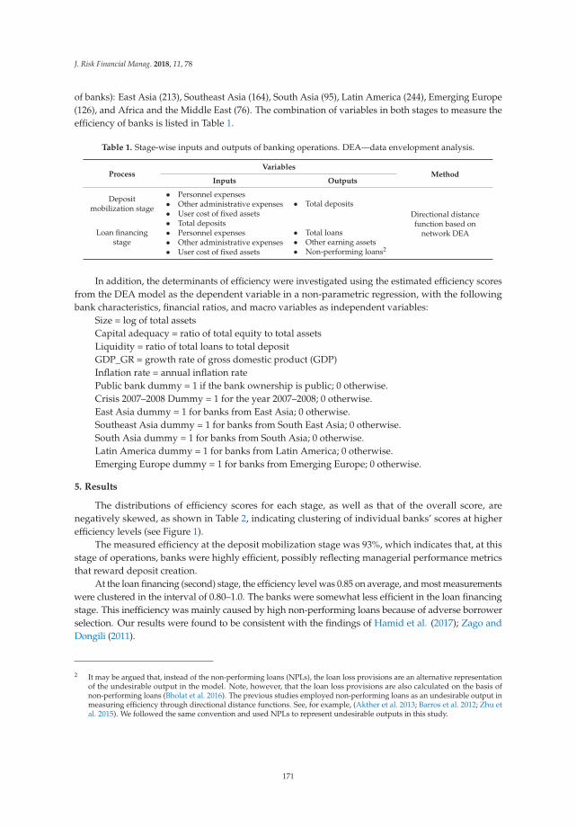
J. Risk Financial Manag. 2018, 11, 78
of banks): East Asia (213), Southeast Asia (164), South Asia (95), Latin America (244), Emerging Europe(126), and Africa and the Middle East (76). The combination of variables in both stages to measure theefficiency of banks is listed in Table 1.
Table 1. Stage-wise inputs and outputs of banking operations. DEA—data envelopment analysis.
ProcessVariables
MethodInputs Outputs
Depositmobilization stage
• Personnel expenses• Total deposits
Directional distancefunction based on
network DEA
• Other administrative expenses• User cost of fixed assets
Loan financingstage
• Total deposits• Personnel expenses • Total loans
• Other earning assets• Non-performing loans2
• Other administrative expenses• User cost of fixed assets
In addition, the determinants of efficiency were investigated using the estimated efficiency scoresfrom the DEA model as the dependent variable in a non-parametric regression, with the followingbank characteristics, financial ratios, and macro variables as independent variables:
Size = log of total assetsCapital adequacy = ratio of total equity to total assetsLiquidity = ratio of total loans to total depositGDP_GR = growth rate of gross domestic product (GDP)Inflation rate = annual inflation ratePublic bank dummy = 1 if the bank ownership is public; 0 otherwise.Crisis 2007–2008 Dummy = 1 for the year 2007–2008; 0 otherwise.East Asia dummy = 1 for banks from East Asia; 0 otherwise.Southeast Asia dummy = 1 for banks from South East Asia; 0 otherwise.South Asia dummy = 1 for banks from South Asia; 0 otherwise.Latin America dummy = 1 for banks from Latin America; 0 otherwise.Emerging Europe dummy = 1 for banks from Emerging Europe; 0 otherwise.
5. Results
The distributions of efficiency scores for each stage, as well as that of the overall score, arenegatively skewed, as shown in Table 2, indicating clustering of individual banks’ scores at higherefficiency levels (see Figure 1).
The measured efficiency at the deposit mobilization stage was 93%, which indicates that, at thisstage of operations, banks were highly efficient, possibly reflecting managerial performance metricsthat reward deposit creation.
At the loan financing (second) stage, the efficiency level was 0.85 on average, and most measurementswere clustered in the interval of 0.80–1.0. The banks were somewhat less efficient in the loan financingstage. This inefficiency was mainly caused by high non-performing loans because of adverse borrowerselection. Our results were found to be consistent with the findings of Hamid et al. (2017); Zago andDongili (2011).
2 It may be argued that, instead of the non-performing loans (NPLs), the loan loss provisions are an alternative representationof the undesirable output in the model. Note, however, that the loan loss provisions are also calculated on the basis ofnon-performing loans (Bholat et al. 2016). The previous studies employed non-performing loans as an undesirable output inmeasuring efficiency through directional distance functions. See, for example, (Akther et al. 2013; Barros et al. 2012; Zhu etal. 2015). We followed the same convention and used NPLs to represent undesirable outputs in this study.
171
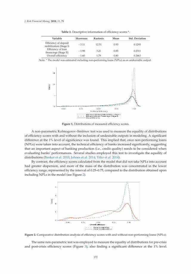
J. Risk Financial Manag. 2018, 11, 78
Table 2. Descriptive information of efficiency scores *.
Variable Skewness Kurtosis Mean Std. Deviation
Efficiency of depositmobilization (Stage I) −3.11 12.51 0.93 0.1293
Efficiency of loanfinancings (Stage II) −1.98 3.21 0.85 0.2311
Overall efficiency −1.60 1.79 0.80 0.2463
Note: * The model was estimated including non-performing loans (NPLs) as an undesirable output.
Figure 1. Distributions of measured efficiency scores.
A non-parametric Kolmogorov–Smirnov test was used to measure the equality of distributionsof efficiency scores with and without the inclusion of undesirable outputs in modeling. A significantdifference at the 1% level of significance was found. This implied that, once non-performing loans(NPLs) were taken into account, the technical efficiency of banks increased significantly, suggestingthat an important aspect of banking production (i.e., credit quality) needs to be considered whenevaluating banks’ performances. Several studies employed this test to investigate the equality ofdistributions (Banker et al. 2010; Johnes et al. 2014; Titko et al. 2014).
By contrast, the efficiency scores calculated from the model that did not take NPLs into accounthad greater dispersion, and more of the mass of the distribution was concentrated in the lowerefficiency range, represented by the interval of 0.25–0.75, compared to the distribution obtained uponincluding NPLs in the model (see Figure 2).
Figure 2. Comparative distribution analysis of efficiency scores with and without non-performing loans (NPLs).
The same non-parametric test was employed to measure the equality of distributions for pre-crisisand post-crisis efficiency scores (Figure 3), also finding a significant difference at the 1% level.
172
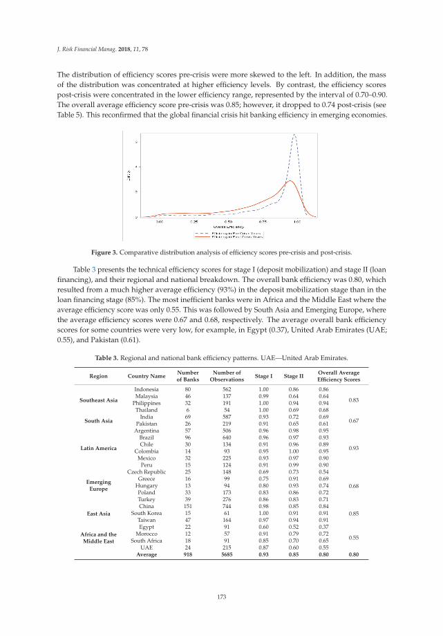
J. Risk Financial Manag. 2018, 11, 78
The distribution of efficiency scores pre-crisis were more skewed to the left. In addition, the massof the distribution was concentrated at higher efficiency levels. By contrast, the efficiency scorespost-crisis were concentrated in the lower efficiency range, represented by the interval of 0.70–0.90.The overall average efficiency score pre-crisis was 0.85; however, it dropped to 0.74 post-crisis (seeTable 5). This reconfirmed that the global financial crisis hit banking efficiency in emerging economies.
Figure 3. Comparative distribution analysis of efficiency scores pre-crisis and post-crisis.
Table 3 presents the technical efficiency scores for stage I (deposit mobilization) and stage II (loanfinancing), and their regional and national breakdown. The overall bank efficiency was 0.80, whichresulted from a much higher average efficiency (93%) in the deposit mobilization stage than in theloan financing stage (85%). The most inefficient banks were in Africa and the Middle East where theaverage efficiency score was only 0.55. This was followed by South Asia and Emerging Europe, wherethe average efficiency scores were 0.67 and 0.68, respectively. The average overall bank efficiencyscores for some countries were very low, for example, in Egypt (0.37), United Arab Emirates (UAE;0.55), and Pakistan (0.61).
Table 3. Regional and national bank efficiency patterns. UAE—United Arab Emirates.
Region Country NameNumberof Banks
Number ofObservations
Stage I Stage IIOverall AverageEfficiency Scores
Southeast Asia
Indonesia 80 562 1.00 0.86 0.86
0.83Malaysia 46 137 0.99 0.64 0.64
Philippines 32 191 1.00 0.94 0.94Thailand 6 54 1.00 0.69 0.68
South AsiaIndia 69 587 0.93 0.72 0.69
0.67Pakistan 26 219 0.91 0.65 0.61
Latin America
Argentina 57 506 0.96 0.98 0.95
0.93
Brazil 96 640 0.96 0.97 0.93Chile 30 134 0.91 0.96 0.89
Colombia 14 93 0.95 1.00 0.95Mexico 32 225 0.93 0.97 0.90
Peru 15 124 0.91 0.99 0.90
EmergingEurope
Czech Republic 25 148 0.69 0.73 0.54
0.68Greece 16 99 0.75 0.91 0.69
Hungary 13 94 0.80 0.93 0.74Poland 33 173 0.83 0.86 0.72Turkey 39 276 0.86 0.83 0.71
East Asia
China 151 744 0.98 0.85 0.840.85South Korea 15 61 1.00 0.91 0.91
Taiwan 47 164 0.97 0.94 0.91
Africa and theMiddle East
Egypt 22 91 0.60 0.52 0.37
0.55Morocco 12 57 0.91 0.79 0.72
South Africa 18 91 0.85 0.70 0.65UAE 24 215 0.87 0.60 0.55
Average 918 5685 0.93 0.85 0.80 0.80
173
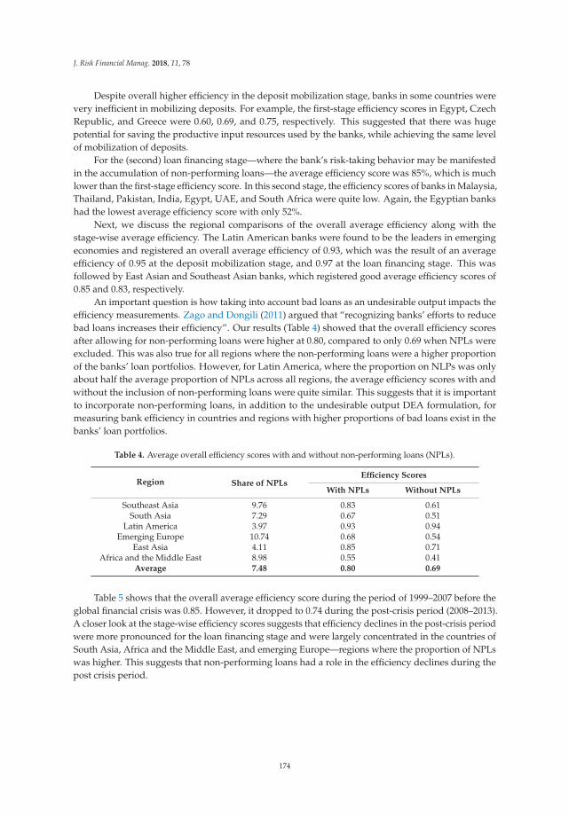
J. Risk Financial Manag. 2018, 11, 78
Despite overall higher efficiency in the deposit mobilization stage, banks in some countries werevery inefficient in mobilizing deposits. For example, the first-stage efficiency scores in Egypt, CzechRepublic, and Greece were 0.60, 0.69, and 0.75, respectively. This suggested that there was hugepotential for saving the productive input resources used by the banks, while achieving the same levelof mobilization of deposits.
For the (second) loan financing stage—where the bank’s risk-taking behavior may be manifestedin the accumulation of non-performing loans—the average efficiency score was 85%, which is muchlower than the first-stage efficiency score. In this second stage, the efficiency scores of banks in Malaysia,Thailand, Pakistan, India, Egypt, UAE, and South Africa were quite low. Again, the Egyptian bankshad the lowest average efficiency score with only 52%.
Next, we discuss the regional comparisons of the overall average efficiency along with thestage-wise average efficiency. The Latin American banks were found to be the leaders in emergingeconomies and registered an overall average efficiency of 0.93, which was the result of an averageefficiency of 0.95 at the deposit mobilization stage, and 0.97 at the loan financing stage. This wasfollowed by East Asian and Southeast Asian banks, which registered good average efficiency scores of0.85 and 0.83, respectively.
An important question is how taking into account bad loans as an undesirable output impacts theefficiency measurements. Zago and Dongili (2011) argued that “recognizing banks’ efforts to reducebad loans increases their efficiency”. Our results (Table 4) showed that the overall efficiency scoresafter allowing for non-performing loans were higher at 0.80, compared to only 0.69 when NPLs wereexcluded. This was also true for all regions where the non-performing loans were a higher proportionof the banks’ loan portfolios. However, for Latin America, where the proportion on NLPs was onlyabout half the average proportion of NPLs across all regions, the average efficiency scores with andwithout the inclusion of non-performing loans were quite similar. This suggests that it is importantto incorporate non-performing loans, in addition to the undesirable output DEA formulation, formeasuring bank efficiency in countries and regions with higher proportions of bad loans exist in thebanks’ loan portfolios.
Table 4. Average overall efficiency scores with and without non-performing loans (NPLs).
Region Share of NPLsEfficiency Scores
With NPLs Without NPLs
Southeast Asia 9.76 0.83 0.61South Asia 7.29 0.67 0.51
Latin America 3.97 0.93 0.94Emerging Europe 10.74 0.68 0.54
East Asia 4.11 0.85 0.71Africa and the Middle East 8.98 0.55 0.41
Average 7.48 0.80 0.69
Table 5 shows that the overall average efficiency score during the period of 1999–2007 before theglobal financial crisis was 0.85. However, it dropped to 0.74 during the post-crisis period (2008–2013).A closer look at the stage-wise efficiency scores suggests that efficiency declines in the post-crisis periodwere more pronounced for the loan financing stage and were largely concentrated in the countries ofSouth Asia, Africa and the Middle East, and emerging Europe—regions where the proportion of NPLswas higher. This suggests that non-performing loans had a role in the efficiency declines during thepost crisis period.
174
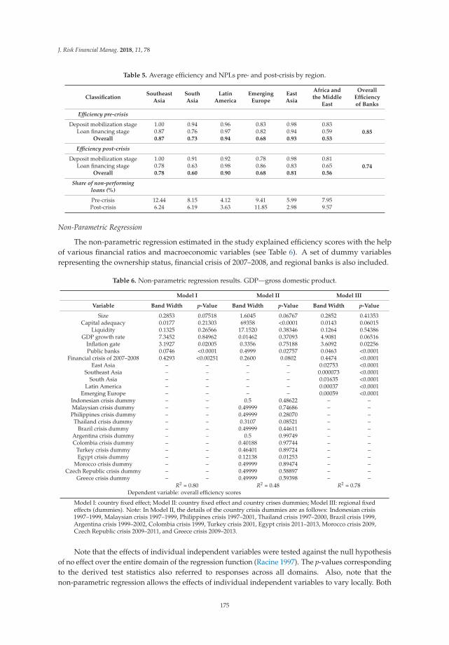
J. Risk Financial Manag. 2018, 11, 78
Table 5. Average efficiency and NPLs pre- and post-crisis by region.
ClassificationSoutheast
AsiaSouthAsia
LatinAmerica
EmergingEurope
EastAsia
Africa andthe Middle
East
OverallEfficiencyof Banks
Efficiency pre-crisis
Deposit mobilization stage 1.00 0.94 0.96 0.83 0.98 0.830.85Loan financing stage 0.87 0.76 0.97 0.82 0.94 0.59
Overall 0.87 0.73 0.94 0.68 0.93 0.53
Efficiency post-crisis
Deposit mobilization stage 1.00 0.91 0.92 0.78 0.98 0.810.74Loan financing stage 0.78 0.63 0.98 0.86 0.83 0.65
Overall 0.78 0.60 0.90 0.68 0.81 0.56
Share of non-performingloans (%)
Pre-crisis 12.44 8.15 4.12 9.41 5.99 7.95Post-crisis 6.24 6.19 3.63 11.85 2.98 9.57
Non-Parametric Regression
The non-parametric regression estimated in the study explained efficiency scores with the helpof various financial ratios and macroeconomic variables (see Table 6). A set of dummy variablesrepresenting the ownership status, financial crisis of 2007–2008, and regional banks is also included.
Table 6. Non-parametric regression results. GDP—gross domestic product.
Model I Model II Model III
Variable Band Width p-Value Band Width p-Value Band Width p-Value
Size 0.2853 0.07518 1.6045 0.06767 0.2852 0.41353Capital adequacy 0.0177 0.21303 69358 <0.0001 0.0143 0.06015
Liquidity 0.1325 0.26566 17.1520 0.38346 0.1264 0.54386GDP growth rate 7.3452 0.84962 0.01462 0.37093 4.9081 0.06516
Inflation gate 3.1927 0.02005 0.3356 0.75188 3.6092 0.02256Public banks 0.0746 <0.0001 0.4999 0.02757 0.0463 <0.0001
Financial crisis of 2007–2008 0.4293 <0.00251 0.2600 0.0802 0.4474 <0.0001East Asia – – – – 0.02753 <0.0001
Southeast Asia – – – – 0.000073 <0.0001South Asia – – – – 0.01635 <0.0001
Latin America – – – – 0.00037 <0.0001Emerging Europe – – – – 0.00059 <0.0001
Indonesian crisis dummy – – 0.5 0.48622 – –Malaysian crisis dummy – – 0.49999 0.74686 – –Philippines crisis dummy – – 0.49999 0.28070 – –
Thailand crisis dummy – – 0.3107 0.08521 – –Brazil crisis dummy – – 0.49999 0.44611 – –
Argentina crisis dummy – – 0.5 0.99749 – –Colombia crisis dummy – – 0.40188 0.97744 – –
Turkey crisis dummy – – 0.46401 0.89724 – –Egypt crisis dummy – – 0.12138 0.01253 – –
Morocco crisis dummy – – 0.49999 0.89474 – –Czech Republic crisis dummy – – 0.49999 0.58897 – –
Greece crisis dummy – – 0.49999 0.59398 – –R2 = 0.80 R2 = 0.48 R2 = 0.78
Dependent variable: overall efficiency scores
Model I: country fixed effect; Model II: country fixed effect and country crises dummies; Model III: regional fixedeffects (dummies). Note: In Model II, the details of the country crisis dummies are as follows: Indonesian crisis1997–1999, Malaysian crisis 1997–1999, Philippines crisis 1997–2001, Thailand crisis 1997–2000, Brazil crisis 1999,Argentina crisis 1999–2002, Colombia crisis 1999, Turkey crisis 2001, Egypt crisis 2011–2013, Morocco crisis 2009,Czech Republic crisis 2009–2011, and Greece crisis 2009–2013.
Note that the effects of individual independent variables were tested against the null hypothesisof no effect over the entire domain of the regression function (Racine 1997). The p-values correspondingto the derived test statistics also referred to responses across all domains. Also, note that thenon-parametric regression allows the effects of individual independent variables to vary locally. Both
175
J. Risk Financial Manag. 2018, 11, 78
these considerations have to be borne in the mind when interpreting the non-parametric regressionresults presented in Table 6 (and in Figure 4). Table 6 reports the band width and the p-values forindividual independent variables.
The efficiency of banks may also depend on the regulatory regime, which could vary from countryto country (Barth et al. 2008).3 There are some very detailed World Bank surveys that provide a richset of indicators of the bank regulatory environments for a large number of countries. These surveyscapture the various features of the regulatory regimes as they existed at specific points in time, i.e.,1999, 2002, and 2006 (ibid. p. 5). This study used a research design based on a panel of annualbank-level data from 24 emerging economies from 1999 to 2013. The integration of both datasetsfor use in model estimation, where the other bank characteristics were observed annually, is not atrivial matter.4 However, failing to control for the regulatory regime in some way may bias the results.We tried to control for the country-specific regulatory environment by introducing country fixed effectsin Model I and Model II (see Table 6).
The Model I results suggest that bank size significantly affected efficiency with a p-value of 0.075,which was somewhat above the conventional threshold of 5%. The ownership status (public bank)was also highly significant. No other bank characteristic had a statistically significant effect. Amongthe two indicators of macroeconomic environment, inflation had a significant effect on bank efficiencyand the GDP growth rate variable was insignificant. The impact of the 2007–2008 financial crisis onefficiency was highly significant.
While the financial crisis of 2007–2008 had global effects, individual countries also had financialcrises whose effects were less contagious. Model II included country financial crisis dummies. For thecountry in question, these dummy variables took the value of 1 during the crisis period, and 0 otherwise.Model II was also estimated with country fixed effects. The results presented in Table 6 suggest that, inaddition to size and ownership status, capital adequacy was a highly significant determinant of bankefficiency. None of the macroeconomic variables had statistical significance, and the dummy variablefor the 2007–2008 financial crisis had a p-value of 0.08, making it significant at the 10% level. Amongthe country financial dummies, only the dummy variables for Egypt and Thailand were statisticallysignificant, with the latter only marginally so. The model R2 value was only 0.48 compared to the R2 of0.80 for Model I.
In contrast to Models I and II, Model III did not specify country fixed effects, and insteadincluded dummy variables for regions to capture the regional heterogeneity of efficiency scores.All regional dummies were statistically highly significant. The model R2 was 0.78, which wascomparable to that of Model I. The bank characteristics that had statistically significant effect onefficiency were found to be capital adequacy and ownership status, with p-values of 0.06 and <0.0001,respectively. Both variables reflecting macroeconomic conditions were statistically highly significant.The dummy variable representing the impact on bank efficiency of the global financial crisis was alsohighly significant.
We present the partial regression plots for Model I in Figure 4. The plots for Models II and III canbe found in the Appendix A. The graphs from all plots show a high degree of similarity.
Increases in the capital adequacy ratio raised technical efficiency across the entire domain (topright panel of Figure 4). However, the imprecision of this effect increased, especially for capitaladequacy ratios higher than 0.3. Several other studies found a positive relationship between capitaladequacy and bank efficiency, for example, see (Gropp and Heider 2010; Kleff and Weber 2008).
3 We would like to thank an anonymous referee for this point.4 The surveys contain a wealth of information that, when suitably combined with other sources of bank-level data, could offer
rich possibilities for further research. We hope to explore some of these possibilities in our own future research. Models Iand II that incorporated country fixed effects in an attempt to capture the individual country regulatory environment, whilenot fully capturing the dynamics of the regulatory regimes, were motivated by Barth et al. (2008).
176
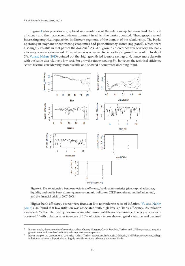
J. Risk Financial Manag. 2018, 11, 78
Figure 4 also provides a graphical representation of the relationship between bank technicalefficiency and the macroeconomic environment in which the banks operated. These graphs revealinteresting empirical regularities in different segments of the domain of the relationship. The banksoperating in stagnant or contracting economies had poor efficiency scores (top panel), which werealso highly volatile in that part of the domain.5 As GDP growth entered positive territory, the bankefficiency score also increased. This pattern was observed to be positive at growth rates of up to about5%. Vu and Nahm (2013) pointed out that high growth led to more savings and, hence, more depositswith the banks at a relatively low cost. For growth rates exceeding 5%, however, the technical efficiencyscores became considerably more volatile and showed a somewhat declining trend.
Figure 4. The relationship between technical efficiency, bank characteristics (size, capital adequacy,liquidity and public bank dummy), macroeconomic indicators (GDP growth rate and inflation rate),and the financial crisis of 2007–2008.
Higher bank efficiency scores were found at low to moderate rates of inflation. Vu and Nahm(2013) also found that low inflation was associated with high levels of bank efficiency. As inflationexceeded 6%, the relationship became somewhat more volatile and declining efficiency scores wereobserved.6 With inflation rates in excess of 10%, efficiency scores showed great variation and declined
5 In our sample, the economies of countries such as Greece, Hungary, Czech Republic, Turkey, and UAE experienced negativegrowth rates and poor bank efficiency during various sub-periods.
6 In our sample, the economies of countries such as Turkey, Argentina, Indonesia, Malaysia, and Pakistan experienced highinflation at various sub-periods and highly volatile technical efficiency scores for banks.
177
J. Risk Financial Manag. 2018, 11, 78
sharply. This finding is consistent with that of Batir et al. (2017) who pointed out that high inflationcaused the efficiency of banks to decline.
The ownership status of banks indicates that public banks performed significantly poor at the1% level of significance as compared to private banks. Several other studies pointed out the poorperformance of public banks; for example, private banks were more efficient than public banks in CzechRepublic and Poland (Weill 2003); public banks were less efficient compared to private banks in 15 EastEuropean transition countries (Fries and Taci 2005); joint-stock banks which were not owned by thegovernment were found to be more efficient than state-owned banks in China (Xiaoqing Maggie andHeffernan 2007).
The results of Model III suggested that the financial crisis of 2007–2008 caused efficiency scores todecline in emerging economies. The regional banks in East Asia, Southeast Asia, and Latin Americaperformed significantly better with p-values < 0.01. The banks in these regions had a lower proportionof non-performing loans in their portfolios. In contrast, banks in the regions of South Asia andEmerging Europe performed significantly poorly with p-values < 0.01.7 The banks in these regionshad a high proportion of non-performing loans (see Table 4). This suggests that the negative impact ofthe crisis on bank efficiency was associated with the accumulation of non-performing loans.
6. Concluding Remarks
The present study modeled banking operations as consisting of two stylized stages—the depositmobilization stage, and the loan financing stage—and separately estimated technical efficiency at eachstage. An important feature of the study was the use of a cross-country panel dataset for efficiencymeasurement. To the best of our knowledge, no other study estimated technical efficiency for a panelor emerging economy banks using network DEA and directional distance functions featuring NPLs.This research design made it possible to perform regional comparisons of bank efficiency and also toinvestigate the impact of global macroeconomic shocks. Our results indicated that lower efficiencyscores were concentrated in regions where the proportions of non-performing loans in banks’ loanportfolios were higher.
The results obtained allowed not only profiling the efficient banks, but also a meaningfulcharacterization of the macroeconomic environment conducive for achieving higher levels of bankefficiency. The efficient banks were smaller, better capitalized, and privately owned. The macroeconomicconditions conducive for bank efficiency were a growing economy, and low to moderate inflation rates(below ~5%). The financial crisis of 2007–2008 negatively impacted the technical efficiency of banks.The analysis of regional patterns of efficiency scores suggested that the most vulnerable banks werelocated in regions (South Asia and emerging Europe) where the proportion of non-performing loanswas high.
Policy Implications
The study provides several policy implications. Our results indicated that banks need to besufficiently capitalized. This may require regulations setting capital adequacy requirements that thebank could achieve by attracting capital from shareholders and investors, or acquired through mergersand acquisitions. Our results also support regulatory authorities forcing the less capitalized banksto merge.8
7 The negative impact on efficiency of banks was due to generating higher NPLs and administrative expenses faced by banksas a result of crises in the regions of South Asia and emerging Europe.
8 For example, if a small bank is merged with a large bank, then it is an empirical question whether or not the effect ofthe larger size on efficiency would outweigh the effect of improved capital adequacy. This study helps answer suchempirical questions.
178
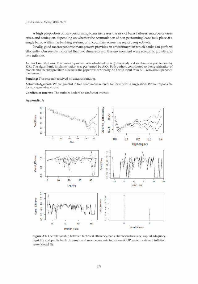
J. Risk Financial Manag. 2018, 11, 78
A high proportion of non-performing loans increases the risk of bank failures, macroeconomiccrisis, and contagion, depending on whether the accumulation of non-performing loans took place at asingle bank, within the banking system, or in countries across the region, respectively.
Finally, good macroeconomic management provides an environment in which banks can performefficiently. Our results indicated that two dimensions of this environment were economic growth andlow inflation.
Author Contributions: The research problem was identified by A.Q.; the analytical solution was pointed out byK.R.; The algorithmic implementation was performed by A.Q.; Both authors contributed to the specification ofmodels and the interpretation of results; the paper was written by A.Q. with input from K.R. who also supervisedthe research.
Funding: This research received no external funding.
Acknowledgments: We are grateful to two anonymous referees for their helpful suggestion. We are responsiblefor any remaining errors.
Conflicts of Interest: The authors declare no conflict of interest.
Appendix A
Figure A1. The relationship between technical efficiency, bank characteristics (size, capital adequacy,liquidity and public bank dummy), and macroeconomic indicators (GDP growth rate and inflationrate) (Model II).
179
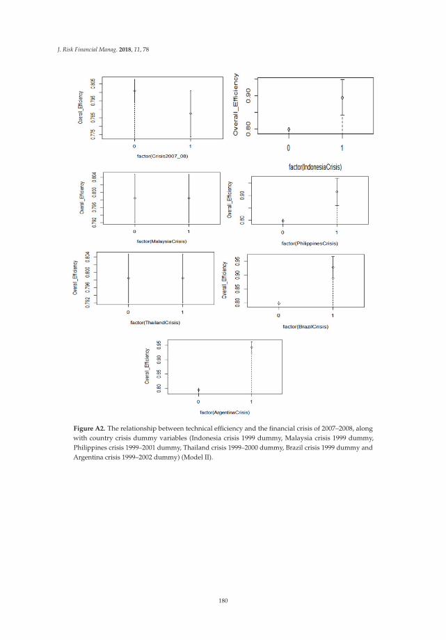
J. Risk Financial Manag. 2018, 11, 78
Figure A2. The relationship between technical efficiency and the financial crisis of 2007–2008, alongwith country crisis dummy variables (Indonesia crisis 1999 dummy, Malaysia crisis 1999 dummy,Philippines crisis 1999–2001 dummy, Thailand crisis 1999–2000 dummy, Brazil crisis 1999 dummy andArgentina crisis 1999–2002 dummy) (Model II).
180
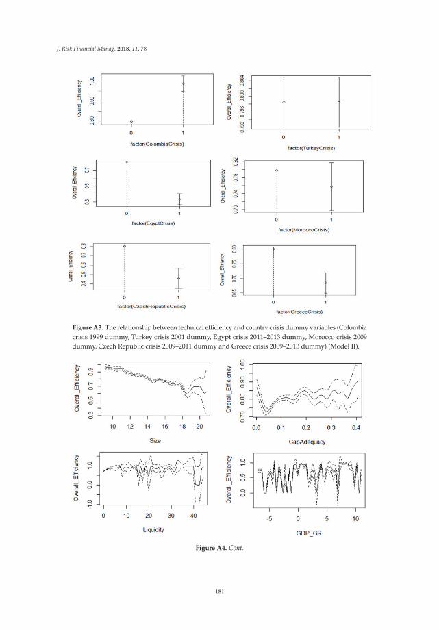
J. Risk Financial Manag. 2018, 11, 78
Figure A3. The relationship between technical efficiency and country crisis dummy variables (Colombiacrisis 1999 dummy, Turkey crisis 2001 dummy, Egypt crisis 2011–2013 dummy, Morocco crisis 2009dummy, Czech Republic crisis 2009–2011 dummy and Greece crisis 2009–2013 dummy) (Model II).
Figure A4. Cont.
181
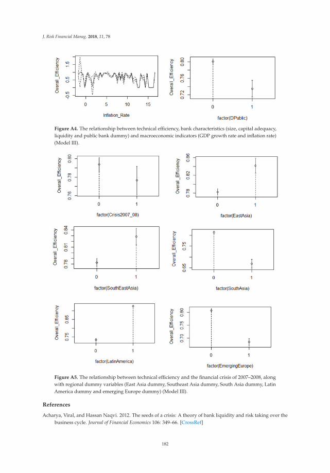
J. Risk Financial Manag. 2018, 11, 78
Figure A4. The relationship between technical efficiency, bank characteristics (size, capital adequacy,liquidity and public bank dummy) and macroeconomic indicators (GDP growth rate and inflation rate)(Model III).
Figure A5. The relationship between technical efficiency and the financial crisis of 2007–2008, alongwith regional dummy variables (East Asia dummy, Southeast Asia dummy, South Asia dummy, LatinAmerica dummy and emerging Europe dummy) (Model III).
References
Acharya, Viral, and Hassan Naqvi. 2012. The seeds of a crisis: A theory of bank liquidity and risk taking over thebusiness cycle. Journal of Financial Economics 106: 349–66. [CrossRef]
182
J. Risk Financial Manag. 2018, 11, 78
Akther, Syed, Hirofumi Fukuyama, and William L. Weber. 2013. Estimating two-stage network slacks-basedinefficiency: An application to Bangladesh banking. Omega 41: 88–96. [CrossRef]
Ashraf, Badar Nadeem, Sidra Arshad, and Liang Yan. 2017. Trade openness and bank risk-taking behavior:Evidence from emerging economies. Journal of Risk and Financial Management 10: 15. [CrossRef]
Baily, Martin Neil, and Douglas J. Elliott. 2009. The US Financial and Economic Crisis: Where Does It Stand andWhere Do We Go from Here. Brookings Institution, Jun. Available online: https://www.brookings.edu/wp-content/.../0615_economic_crisis_baily_elliott.pdf (accessed on 20 July 2018).
Banker, Rajiv D., Abraham Charnes, and William Wager Cooper. 1984. Some models for estimating technical andscale inefficiencies in data envelopment analysis. Management Science 30: 1078–92. [CrossRef]
Banker, Rajiv D., Zhiqiang Eric Zheng, and Ram Natarajan. 2010. DEA-based hypothesis tests for comparing twogroups of decision making units. European Journal of Operational Research 206: 231–38. [CrossRef]
Barros, Carlos Pestana, Shunsuke Managi, and Roman Matousek. 2012. The technical efficiency of the Japanesebanks: non-radial directional performance measurement with undesirable output. Omega 40: 1–8. [CrossRef]
Barth, James R., Gerard Caprio Jr., and Ross Levine. 2008. Bank Regulations Are Changing: For Better or Worse?The World Bank. Available online: https://openknowledge.worldbank.org/handle/10986/6664 (accessedon 8 September 2018).
Barth, James R., Gerard Caprio Jr., and Ross Levine. 2013. Bank Regulation and Supervision in 180 Countries from1999 to 2011. Journal of Financial Economic Policy 5: 111–219. [CrossRef]
Batir, Tugba Eyceyurt, David A. Volkman, and Bener Gungor. 2017. Determinants of bank efficiency in Turkey:Participation banks versus conventional banks. Borsa Istanbul Review 17: 86–96. [CrossRef]
Bholat, David M., Rosa M. Lastra, Sheri M. Markose, Andrea Miglionico, and Kallol Sen. 2016. Non-PerformingLoans: Regulatory and Accounting Treatments of Assets. Available online: https://papers.ssrn.com/abstract=2768865 (accessed on 15 July 2018).
Charnes, Abraham, William W. Cooper, and Edwardo Rhodes. 1978. Measuring the efficiency of decision makingunits. European Journal of Operational Research 2: 429–44. [CrossRef]
Charnes, A., W. W. Cooper, B. Golany, B. Kirby, J. McGahan, and D. Semple. 1988. Measuring the Impact ofNational Advertising on Recruiting by Data Envelopment Analysis Methods (No. CCS-595). Texas Univat Austin Center for Cybernetic Studies. Available online: www.dtic.mil/dtic/tr/fulltext/u2/a191591.pdf(accessed on 7 November 2018).
Chung, Yangho H., Rolf Färe, and Shawna Grosskopf. 1997. Productivity and undesirable outputs: A directionaldistance function approach. Journal of Environmental Management 51: 229–40. [CrossRef]
Drigă, Imola, and Codruta Dura. 2014. The Financial Sector and the Role of Banks in Economic Development.Paper presented at the 6th International Multidisciplinary Symposium “Universitaria SIMPRO”, Universityof Petrosani, Petros, ani, Romania, October 10–11.
Emrouznejad, Ali, and Guo-liang Yang. 2017. A survey and analysis of the first 40 years of scholarly literature inDEA: 1978–2016. Socio-Economic Planning Sciences 61: 4–8. [CrossRef]
Färe, Rolf, and Shawna Grosskopf. 2000. Network dea. Socio-Economic Planning Sciences 34: 35–49. [CrossRef]Färe, Rolf, Shawna Grosskopf, C. A. Knox Lovell, and Carl Pasurka. 1989. Multilateral productivity comparisons
when some outputs are undesirable: a nonparametric approach. The Review of Economics and Statistics 71:90–98. [CrossRef]
Fries, Steven, and Anita Taci. 2005. Cost efficiency of banks in transition: Evidence from 289 banks in 15post-communist countries. Journal of Banking & Finance 29: 55–81.
Fukuyama, Hirofumi, and William L. Weber. 2008. Japanese banking inefficiency and shadow pricing. Mathematicaland Computer Modelling 48: 1854–67. [CrossRef]
Fukuyama, Hirofumi, and William L. Weber. 2010. A slacks-based inefficiency measure for a two-stage systemwith bad outputs. Omega 38: 398–409. [CrossRef]
Gropp, Reint, and Florian Heider. 2010. The determinants of bank capital structure. Review of Finance 14: 587–622.[CrossRef]
Hamid, Nurhayati, Noor Asiah Ramli, and Siti Aida Sheikh Hussin. 2017. Efficiency measurement of the bankingsector in the presence of non-performing loan. In AIP Conference Proceedings. Melville: AIP Publishing,vol. 1795, no. 1. p. 020001.
Hayfield, Tristen, and Jeffrey S. Racine. 2008. Nonparametric econometrics: The np package. Journal of StatisticalSoftware 27: 1–32. [CrossRef]
183
J. Risk Financial Manag. 2018, 11, 78
Huang, Jianhuan, Juanjuan Chen, and Zhujia Yin. 2014. A network DEA model with super efficiency andundesirable outputs: An application to bank efficiency in China. Mathematical Problems in Engineering 2014:14. [CrossRef]
Illueca, Manuel, José M. Pastor, and Emili Tortosa-Ausina. 2009. The effects of geographic expansion on theproductivity of Spanish savings banks. Journal of Productivity Analysis 32: 119–43. [CrossRef]
Johnes, Jill, Marwan Izzeldin, and Vasileios Pappas. 2014. A comparison of performance of Islamic andconventional banks 2004–2009. Journal of Economic Behavior & Organization 103: 93–107.
Kleff, Volker, and Martin Weber. 2008. How do banks determine capital? Evidence from Germany. GermanEconomic Review 9: 354–72. [CrossRef]
Kumar, Sunil, and Rachita Gulati. 2014. A Survey of Empirical Literature on Bank Efficiency Deregulation and Efficiencyof Indian Banks. New Delhi: Springer, pp. 119–65.
Liu, John S., Louis Y. Y. Lu, Wen-Min Lu, and Bruce J. Y. Lin. 2013. A survey of DEA applications. Omega 41:893–902. [CrossRef]
McDonald, John. 2009. Using least squares and tobit in second stage DEA efficiency analyses. European Journal ofOperational Research 197: 792–98. [CrossRef]
Moyo, Jennifer, Boaz Nandwa, Dubai Economic Council, Jacob Oduor, and Anthony Simpasa. 2014. FinancialSector Reforms, Competition and Banking System Stability in Sub-Saharan Africa. Available online: https://www.imf.org/external/np/seminars/eng/2014/lic/pdf/Moyo.pdf (accessed on 3 August 2018).
Office of the Comptroller of the Currency, United States. 1988. Bank failure: An Evaluation of the FactorsContributing to the Failure of National Banks: Office of the Comptroller of the Currency. Availableonline: https://www.occ.treas.gov/publications/publications-by-type/other-publications-reports/pub-other-bank-failure.pdf (accessed on 5 August 2018).
Racine, Jeff. 1997. Consistent significance testing for nonparametric regression. Journal of Business & EconomicStatistics 15: 369–78.
Racine, Jeffrey S. 2008. Nonparametric econometrics: A primer. Foundations and Trends®in Econometrics 3: 1–88.[CrossRef]
Racine, Jeffery S., Jeffrey Hart, and Qi Li. 2006. Testing the significance of categorical predictor variables innonparametric regression models. Econometric Reviews 25: 523–44. [CrossRef]
Rosenblatt, Murray. 1956. Remarks on some nonparametric estimates of a density function. The Annals ofMathematical Statistics 1: 832–37. [CrossRef]
Saini, Priyanka, and Jyoti Sindhu. 2014. Role of Commercial Bank in the Economic Development of India.International Journal of Engineering and Management Research 4: 27–31.
Seiford, Lawrence M., and Joe Zhu. 1999. Profitability and marketability of the top 55 US commercial banks.Management science 45: 1270–88. [CrossRef]
Titko, Jelena, Jelena Stankeviciene, and Natal, ja Lace. 2014. Measuring bank efficiency: DEA application.Technological and Economic Development of Economy 20: 739–57. [CrossRef]
Tobin, James. 1985. Estimation of relationships for limited dependent variables. Econometrica: Journal of theEconometric Society, 24–36. [CrossRef]
Tone, Kaoru, and Miki Tsutsui. 2009. Network DEA: A slacks-based measure approach. European Journal ofOperational Research 197: 243–52. [CrossRef]
Vu, Ha, and Daehoon Nahm. 2013. The determinants of profit efficiency of banks in Vietnam. Journal of the AsiaPacific Economy 18: 615–31. [CrossRef]
Wang, Ke, Wei Huang, Jie Wu, and Ying-Nan Liu. 2014. Efficiency measures of the Chinese commercial bankingsystem using an additive two-stage DEA. Omega 44: 5–20. [CrossRef]
Wanke, Peter, and Carlos Barros. 2014. Two-stage DEA: An application to major Brazilian banks. Expert Systemswith Applications 41: 2337–44. [CrossRef]
Weill, Laurent. 2003. Banking efficiency in transition economies: The role of foreign ownership. Economics ofTransition 11: 569–92. [CrossRef]
Xiaoqing Maggie, F. U., and Shelagh Heffernan. 2007. Cost X-efficiency in China’s banking sector. China EconomicReview 18: 35–53.
Yang, Chyan, and Hsian-Ming Liu. 2012. Managerial efficiency in Taiwan bank branches: A network DEA.Economic Modelling 29: 450–61. [CrossRef]
184

J. Risk Financial Manag. 2018, 11, 78
Zago, Angelo, and Paola Dongili. 2011. Credit quality and technical efficiency in banking. Empirical Economics 40:537–38. [CrossRef]
Zhu, Ning, Bing Wang, and Yanrui Wu. 2015. Productivity, efficiency, and non-performing loans in the Chinesebanking industry. The Social Science Journal 52: 468–80. [CrossRef]
© 2018 by the authors. Licensee MDPI, Basel, Switzerland. This article is an open accessarticle distributed under the terms and conditions of the Creative Commons Attribution(CC BY) license (http://creativecommons.org/licenses/by/4.0/).
185
Journal of
Risk and FinancialManagement
Article
A Test of Market Efficiency When Short Selling IsProhibited: A Case of the Dhaka Stock Exchange
Maria Sochi 1 and Steve Swidler 2,3,*
1 Department of Finance, Texas Tech University, Lubbock, TX 79409, USA; [email protected] Department of Finance, Auburn University, Auburn, AL 36849, USA3 Department of Economics, Lafayette College, Easton, PA 18042, USA* Correspondence: [email protected]
Received: 9 August 2018; Accepted: 28 September 2018; Published: 2 October 2018
Abstract: A ban on short selling exists on several exchanges, especially in emerging markets. In mostcases, short selling has always been prohibited, thus making it difficult to examine the ban’s effecton price discovery. In this paper, we consider data from the Dhaka Stock Exchange (DSE) to testfor a short selling ban on market efficiency. The analysis examines runs in daily stock returnsand then forms a distribution of return clusters according to their duration. Using Monte Carlosimulation, we find that runs of longer duration appear more frequently in the DSE data than wewould expect in efficient markets. We compare these results to stocks in the Dow Jones IndustrialAverage (DJIA). We find that the same runs tests accord with market efficiency for liquid and easilyshorted DJIA stocks.
Keywords: emerging market exchange; market efficiency; non-parametric tests of efficiency; MonteCarlo simulation
1. Introduction
The practice of short selling and profiting from a fall in share price has been around for at least fourcenturies. In 1609, Isaac Le Maire formed a secret company to short shares in the East India Companyin anticipation of a new French firm that would offer stiff competition (Bris et al. 2007). As eventsplayed out, the creation of the French rival never occurred, and the ensuing litigation provided yetanother argument to ban short selling practices in the marketplace.
Potential abuse has led regulators to ban short selling in a number of national exchanges.Restrictions on short selling are especially commonplace in emerging markets, and exist becauseof an outright ban or lack of institutional mechanisms to borrow stock.1 Moreover, in many of thesemarkets there are no parallel option markets to effect a short sale through the buying of puts or writingof calls. As short selling restrictions inhibit information flow, market prices may be slow to adjustto news.
While potential abuse has led to a ban on short selling in a number of exchanges, a strain ofresearch suggests that short sale restrictions may inhibit the price discovery process. For example,Miller (1977) argues that with divergence of opinion, a short sales ban results in the overvaluation of asecurity. Diamond and Verrecchia (1987) develop a formal model to discuss the importance of shortselling in the asset price adjustment process. They show that constraints do not bias prices upward,although they do reduce the adjustment speed of prices to private information.
One way to test for the effect of a short selling ban is to investigate any differences in pricediscovery across regime shifts. For example, Beber and Pagano (2013) examine how temporary bans
1 For a list of global short selling regulations, see Jain et al. (2013).
J. Risk Financial Manag. 2018, 11, 59; doi:10.3390/jrfm11040059 www.mdpi.com/journal/jrfm186
J. Risk Financial Manag. 2018, 11, 59
in short selling around the world following the financial crisis of 2007–2009 led to a deterioration inmarket liquidity.
This was especially true for stocks with small market capitalization and no listed options.2
They displayed slower price discovery, especially in bear markets.3
A short selling ban may hinder price discovery even when news is positive. This can occur ifinvestors overreact to information, leading to a reversal of prices (see, De Bondt and Thaler 1985).Atkins and Dyl (1990) first find evidence of market overreaction using daily returns. To the extentthat market corrections require a decrease in returns, a ban on short sales may further inhibit the pricediscovery process.
In the following analysis, we examine the effect of short sale restrictions on market efficiencyfor the Dhaka Stock Exchange (DSE). The DSE has always had a ban on short selling of securities,so performing any type of test that depends upon a regime change is not possible. Instead, we rely ona battery of runs tests to examine market efficiency and the ability of prices to adjust rapidly to newinformation. In particular, we test for statistical independence, and employ a standard non- parametricruns test that looks at clusters of price changes in the same direction.
To further test for the effect of short selling restrictions, we also consider the distribution of dailyprice runs. Any evidence of an asymmetric distribution with an unusual number of long, negativereturn runs would suggest that a ban on short selling inhibits rapid price adjustment to adverseinformation. On the other hand, if investors overreact to positive news, a short sale ban may delayany market correction. In this situation, the distribution of daily price runs would display an unusualnumber of longer runs with positive price changes.
Previous work on the Dhaka Stock Exchange provides conflicting evidence regarding marketefficiency on the Dhaka Stock Exchange. Islam and Khaled (2005) consider DSE index returns for theperiod 1990–2001. They suggest that structural changes put in place after the market crash of 1996 ledto market efficiency. Their statistical tests show short term predictability of share prices prior to thecrash, but not subsequently.
Mollik and Bepari (2009) use the runs test to investigate the weak form market efficiency of theDSE. They examine two stock indices from 2002–2007 to see whether there was an unusual numberof runs. In contrast to Islam and Khaled (2005), they find that returns do not follow a random walk,and reject weak form efficiency of the DSE in the post-crash period.
In addition to DSE index returns, Mobarek et al. (2008) examine individual stock returns from1988–2000 provided by a data vendor. Even allowing for structural changes following the 1996 crash,they find that there is significant auto correlation over the sample period. They reject weak formmarket efficiency and call for additional studies using market price information.
Our analysis updates the sample time period, and following the suggestion of Mobarek et al. (2008),examines the dynamics of individual stock price data obtained directly from the exchange. This allowsus to also adjust for dividends, share splits, and other corporate events. Additionally, we introduceruns tests that specifically investigate for the effect of short sale restrictions on price adjustment;for robustness, we compare our results to evidence from the U.S. and Australian stock markets.
The runs test analysis suggests that DSE stock returns are not independent. Moreover, DSE stockprices appear to incorporate information more slowly than one would expect, with the daily runs
2 Swidler (1988) provides one early empirical study of the effect of short shale restrictions on stock prices and the furthereffect when there is option trading. He shows that with heterogeneous expectations, estimation risk is more important thanshort selling restrictions in explaining asset returns. Moreover, for stocks with listed options, investors can synthetically sellshort via long puts or short calls. The evidence finds that for stocks with listed options, only estimation risk is important indetermining asset returns.
3 Still another study that looks across regime changes is Wang (2014). He finds that when Chinese regulators lifted the shortselling ban on 90 stocks in 2010, they experienced a significant price decline. Moreover, the price declines were positivelyrelated to the amount of short selling and is consistent with the notion that short selling can be used as a mechanism tocorrect for overvaluation.
187
J. Risk Financial Manag. 2018, 11, 59
distributions exhibiting fatter tails for DSE stocks than for US stocks. In other words, for both goodand bad news, the DSE ban on short selling causes prices to adjust more slowly to a new equilibrium,resulting in a disproportionate number of lengthy return runs. For emerging market exchanges thathave never experienced short selling, this novel application of the runs test provides a valuable tool toanalyze the effect of short sale restrictions on asset price dynamics.
2. Data and Methodology
2.1. Data
The analysis focuses on the 21 most liquid stocks on the Dhaka Stock Exchange (DSE). We usedaily stock prices from January 1999 through December 2014. This yielded roughly 4000 stock pricesfor each of the 21 different stocks.
In addition to looking at individual stock price changes, we also consider stock indicesrepresenting the DSE market as a whole. As no single broad index exists for the entire sample period,we rely on two of the more popular indices. The DSE Broad Index, referred to as DSEX, represents97% of market capitalization. This free-float broad index became effective in 2013. The previous broadindex, the DSE General Index or DGEN, existed from December 2002 until July 2013. We thus usethe DGEN index from December 2002 through July 2013, and continue with the DSEX index fromAugust 2013 through the end of 2014. Hereafter, we will refer to the broad market index as the DSEX,recognizing that it represents both the DGEN and DSEX in their respective sample periods.
The Dhaka Stock Exchange library provided daily stock prices and data for the Dhaka Stock.We adjust all prices for cash and stock dividends, splits, bonus and right shares. It is important toremember that the 21 individual stocks chosen are the most liquid stocks, have trading on virtuallyevery business day; therefore, they are likely among the most efficiently-priced stocks on the DhakaStock Exchange.
For matters of robustness, we compare the DSE results to similar tests using US data. Specifically,we consider the Dow Jones Industrial Average and the component stocks. The analysis covers thesimilar 1999–2014 period for individual stocks and 2002–2014 for the DJIA index. Because Visa wasonly a constituent stock of the index for part of the time, we exclude it from the analysis. Thus,we examine price dynamics for the DJIA index and the remaining 29 stocks.
2.2. Methodology—Calculating Runs and Testing for Statistical Independence
The runs test is a non-parametric test that can be used to examine randomness in stock returns.Let returns be defined as (Pt+1 − Pt)/Pt, where Pt is the adjusted stock price on day t. We then definea run as a string of daily returns all of the same sign. If the data follows a binomial distribution, weassume that a 0 return continues the run. Thus, the end of a run and beginning of a new run is whenthe sign changes from either positive to negative, or vice versa. Put another way, the end of a run onlyoccurs when there is a sign change.
To illustrate how runs are calculated, let P denote a positive return, N a negative return, and 0denote no change in daily prices. Suppose that the price data yields the following string of returns:
PPPP N0N PP N PPP0P NNNNN PPP NN
This string of 25 daily returns includes 8 separate runs, the shortest being a 1 day run with anegative return, and the longest a 5 day run for both positive and negative returns.
Suppose, for the moment, we believe that 50% of returns are positive and 50% are negative.Given this binomial distribution, we can calculate the number of runs and see if it is more or less thanthe number we expect. If the number of runs differs significantly from what we expect, we reject thenull hypothesis that the data was randomly generated and accept the alternative that the sequencewas not produced in a random manner.
188
J. Risk Financial Manag. 2018, 11, 59
Comparing the number of runs to the expected value is a test of statistical independence. If,for example, we find significantly fewer runs than expected, that would suggest that the data is highlyclustered. Thus, positive returns likely follow positive returns, and negative returns likely follownegative returns, a result that implies a positive serial correlation of returns. On the other hand, if thereis little clustering and signs change frequently, such a pattern would indicate negative autocorrelation.
From the above discussion, we compare observed runs patterns to what we expect. In turn,expectations depend upon the true probability of success, for example, the probability of observing apositive return and the number of trials or observations in the sample. In our samples, the number ofobservations is approximately 4000 for stocks and 3200 returns for each index. With large samples,it is reasonable to assume as a first approximation that the observed frequency of positive outcomesis equal to the true probability of “success.” Mollik and Bepari (2009) implicitly follow this line ofreasoning and make this assumption in their runs tests.
Table 1 presents the percentage of positive returns and negative returns for each asset class.For both the DSEX and Dow Jones indexes, the observed frequency of positive returns is close to 53%.For stocks, however, the Dhaka and U.S. stocks diverge in the proportion of positive returns. For DSEstocks, the average frequency of positive returns is 46.33%, whereas for stocks in the Dow, the averagepercentage of positive returns is 51.13%.
Table 1. Proportion of Positive and Negative Returns (DSE vs. DJIA).
Indices/Sample Stocks PeriodAverage Proportionof Positive Returns
Average Proportionof Negative Returns
DSEX January 2002–December 2014 52.70% 47.30%DJIA January 2002–December 2014 53.06% 46.94%
21 DSE Stocks January 1999–December 2014 46.33% 53.67%29 Dow Jones Stocks January 1999–December 2014 51.13% 48.87%
2.3. Methodology—Monte Carlo Simulation and Forming Expectations
To form expectations on the number of runs to expect in a sample, we rely on a Monte Carlosimulation. Consider the case of the DSEX that has 3119 returns. If we observe positive returns 53% ofthe time, we generate 3119 returns from the binomial distribution, with a success rate of 53%. We thencount the number of runs found in our trial. The simulation then repeats this process 10,000 times toform a distribution of runs generated from all the trials.
Figure 1 illustrates the results of our 10,000 trial simulation given 3119 returns. Based on a successrate of 53%, 95% of the time we find that the number of runs is between 1497 and 1609. Thus, if thenumber of runs observed for the DSE Index is outside the 95% confidence interval, we reject the nullhypothesis of statistical independence. If the number of runs exceeds 1609, that suggests negativeserial correlation, whereas runs fewer than 1497 implies positive serial correlation.
189
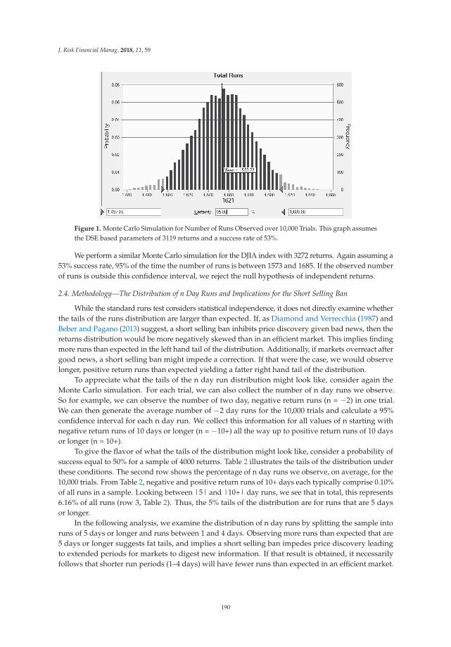
J. Risk Financial Manag. 2018, 11, 59
Figure 1. Monte Carlo Simulation for Number of Runs Observed over 10,000 Trials. This graph assumesthe DSE based parameters of 3119 returns and a success rate of 53%.
We perform a similar Monte Carlo simulation for the DJIA index with 3272 returns. Again assuming a53% success rate, 95% of the time the number of runs is between 1573 and 1685. If the observed numberof runs is outside this confidence interval, we reject the null hypothesis of independent returns.
2.4. Methodology—The Distribution of n Day Runs and Implications for the Short Selling Ban
While the standard runs test considers statistical independence, it does not directly examine whetherthe tails of the runs distribution are larger than expected. If, as Diamond and Verrecchia (1987) andBeber and Pagano (2013) suggest, a short selling ban inhibits price discovery given bad news, then thereturns distribution would be more negatively skewed than in an efficient market. This implies findingmore runs than expected in the left hand tail of the distribution. Additionally, if markets overreact aftergood news, a short selling ban might impede a correction. If that were the case, we would observelonger, positive return runs than expected yielding a fatter right hand tail of the distribution.
To appreciate what the tails of the n day run distribution might look like, consider again theMonte Carlo simulation. For each trial, we can also collect the number of n day runs we observe.So for example, we can observe the number of two day, negative return runs (n = −2) in one trial.We can then generate the average number of −2 day runs for the 10,000 trials and calculate a 95%confidence interval for each n day run. We collect this information for all values of n starting withnegative return runs of 10 days or longer (n = −10+) all the way up to positive return runs of 10 daysor longer (n = 10+).
To give the flavor of what the tails of the distribution might look like, consider a probability ofsuccess equal to 50% for a sample of 4000 returns. Table 2 illustrates the tails of the distribution underthese conditions. The second row shows the percentage of n day runs we observe, on average, for the10,000 trials. From Table 2, negative and positive return runs of 10+ days each typically comprise 0.10%of all runs in a sample. Looking between |5| and |10+| day runs, we see that in total, this represents6.16% of all runs (row 3, Table 2). Thus, the 5% tails of the distribution are for runs that are 5 daysor longer.
In the following analysis, we examine the distribution of n day runs by splitting the sample intoruns of 5 days or longer and runs between 1 and 4 days. Observing more runs than expected that are5 days or longer suggests fat tails, and implies a short selling ban impedes price discovery leadingto extended periods for markets to digest new information. If that result is obtained, it necessarilyfollows that shorter run periods (1–4 days) will have fewer runs than expected in an efficient market.
190
J. Risk Financial Manag. 2018, 11, 59
Table 2. Tails of the n day distribution (probability of success assumed equal to 50%).
−5 5 −6 6 −7 7 −8 8 −9 9 −10+ 10+
3.14% 3.13% 1.56% 1.56% 0.78% 0.78% 0.39% 0.39% 0.20% 0.20% 0.10% 0.10%
3.13% * 4.69% 5.47% 5.86% 6.06% 6.16%
* Cumulates percentages from day |5| to day n.
3. Empirical Results
3.1. Results for Statistical Independence of Index Returns
The first test is to see whether index returns are statistically independent. Consider the returnsto the DSE index. In Table 3, we observe that the total number of runs based on DSEX returnsequals 1334, below the lower bound of the 95% confidence interval. We reject the null hypothesisof statistical independence, and the fact that there are fewer runs than expected suggests a positive,serial correlation. For returns on the DSE index, similar sign returns follow each other more thanexpected, a result that indicates that the markets are slow to adjust to new information.
Table 3. Statistical Independence of Index Returns.
Indices Actual Number of Runs Lower Tail, 95% CI Upper Tail, 95% CI
DSEX 1334 1497 1609DJIA 1727 1573 1685
For returns on the Dow Jones Industrial Average, the number of runs equals 1727, which is slightlyhigher than the upper bound of the 95% confidence interval, 1685. This result also rejects statisticalindependence, instead implying a negative serial correlation of returns. A finding of slight negativeserial correlation is in line with earlier studies of U.S. markets. Fama (1965), for instance, finds that 8 ofthe 30 stocks listed in the Dow had negative serial correlations, but that most of the serial correlationsare less than 0.05. French and Roll (1986) repeat Fama’s tests for NYSE and AMEX stocks during1963–1982 period. They report a small but significant negative serial correlation of daily returns. To geta better idea of the runs distribution for both indexes, Figure 2A,B plots the number of n day runsand the 95% confidence intervals. From Figure 2A, the number of runs observed from −2 to +2 iswell below the lower bound of each confidence interval. Conversely, the number of obtained longerruns tend to be higher than expected. In comparison, Figure 2B illustrates the runs distribution forthe Dow Jones index. Short runs (−2 to +2) occur slightly more often than expected, while longer nday runs happen within expected boundaries. These results further confirm our previous findings.For the DSE index, information is more slowly digested in the market, thus yielding positive, serialcorrelation. On the other hand, for the U.S. index, runs accord nearly as anticipated, with only slightlymore short-term runs than one might expect in an efficient market. In the next section, we considerthe runs pattern for the individual stocks in both the DSE and DJ indexes and see if similar resultsare obtained.
3.2. Run Results for Individual Stock Returns
In order to examine runs for individual stocks, we must first investigate the success rate of apositive return occurring for each firm in our sample. Figure 3A,B graph the percentage of positiveand negative returns for the 21 DSE and 29 DJ stocks in our sample. As reported earlier, the averagesuccess rate for DSE stocks is 46.33% and equals 51.13% for DJ stocks. The figures reveal that thesuccess rate for each individual stock is near the relevant average; therefore, we base our confidenceintervals for DSE and DJ stocks on the 46.33% and 51.13% success rates, respectively.
191
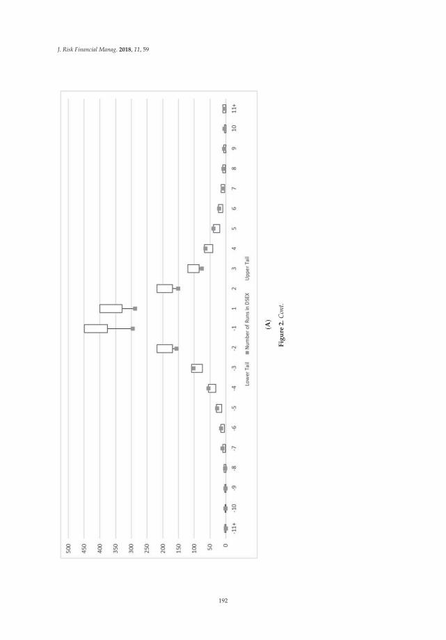
J. Risk Financial Manag. 2018, 11, 59
Fig
ure
2.
Con
t.
192
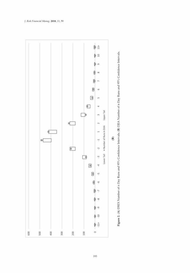
J. Risk Financial Manag. 2018, 11, 59
Fig
ure
2.
(A)D
SEX
Num
ber
ofn
Day
Run
san
d95
%C
onfid
ence
Inte
rval
s;(B
)DJI
AN
umbe
rof
nD
ayR
uns
and
95%
Con
fiden
ceIn
terv
als.
193
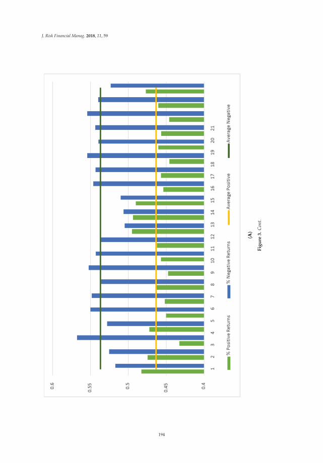
J. Risk Financial Manag. 2018, 11, 59
Fig
ure
3.
Con
t.
194
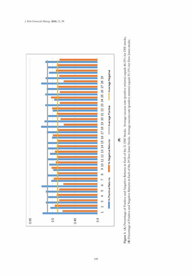
J. Risk Financial Manag. 2018, 11, 59
Fig
ure
3.
(A)
Per
cent
age
ofP
osit
ive
and
Neg
ativ
eR
etu
rns
inE
ach
ofth
e21
DSE
Stoc
ks.
Ave
rage
succ
ess
rate
(pos
itiv
ere
turn
s)eq
ual
s46
.33%
for
DSE
stoc
ks;
(B)P
erce
ntag
eof
Posi
tive
and
Neg
ativ
eR
etur
nsin
Each
ofth
e29
Dow
Jone
sSt
ocks
.Ave
rage
succ
ess
rate
(pos
itiv
ere
turn
s)eq
uals
51.1
3%fo
rD
owJo
nes
stoc
ks.
195
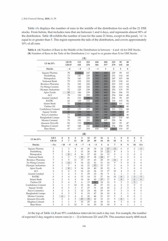
J. Risk Financial Manag. 2018, 11, 59
Table 4A displays the number of runs in the middle of the distribution for each of the 21 DSEstocks. From before, that includes runs that are between 1 and 4 days, and represents almost 90% ofthe distribution. Table 4B exhibits the number of runs for the same 21 firms, except in this panel, |n| isequal to or greater than 5. This region represents the tails of the distribution, and covers approximately10% of all runs.
Table 4. (A) Number of Runs in the Middle of the Distribution (n between −4 and +4) for DSE Stocks.(B) Number of Runs in the Tails of the Distribution (|n| equal to or greater than 5) for DSE Stocks.
(A)
CI 46.33%LB 55UB 87
113155
221278
426501
494577
223279
95135
4068
Stocks −4 −3 −2 −1 1 2 3 4
Square Pharma 78 112 247 367 430 229 95 63Heidelberg 73 141 235 399 467 231 114 60Shinepukur 78 143 235 312 429 247 107 44
National Bank 75 133 222 348 390 235 118 61Beximco Pharama 76 142 244 299 401 223 119 64Fu-Wang Ceramic 71 144 226 356 430 246 113 54
Olympic Industries 72 125 238 401 464 252 115 55Apex Foods 90 146 239 368 466 264 106 53
ACI 78 130 255 378 469 254 106 49Aramit Limited 81 132 208 356 412 236 95 65
BATBC 62 138 232 400 427 236 115 56Islami Bank 70 100 212 382 390 221 101 62Padma Oil 38 79 180 320 330 188 56 46
Confidence Cement 82 139 209 391 463 231 114 68Square Textile 49 108 180 305 346 155 80 45
Keya Cosmetics 71 109 186 310 346 185 87 46Bangladesh Lamps 79 149 260 381 480 250 116 60
Monno Ceramic 79 130 253 399 495 250 98Quasem Drycells 83 115 208 325 399 243 95 47Meghna Cement 87 148 242 362 450 256 104 59
Bata Shoes 67 137 253 430 509 217 119 57
(B)
CI 46.33%LB 0
UB 1005
07
211
518
1229
2749
1634
619
110
06
04
02
04
Stocks −11+ −10 −9 −8 −7 −6 −5 5 6 7 8 9 10 11+
Square Pharma 2 1 3 8 16 20 39 24 27 12 6 0 2 5Heidelberg 0 2 4 3 13 26 38 25 21 8 4 3 1 1Shinepukur 7 1 8 8 16 27 42 24 13 9 1 2 0 0
National Bank 3 2 2 7 19 27 38 38 17 7 6 2 2 0Beximco Pharama 7 3 5 11 15 19 43 28 15 11 0 0 1 2Fu-Wang Ceramic 5 2 11 5 14 22 41 31 10 9 5 0 0 0
Olympic Industries 0 1 5 4 14 22 57 25 17 3 6 2 0 0Apex Foods 0 1 8 9 14 18 40 20 12 6 5 1 0 0
ACI 4 2 4 9 14 22 36 19 17 10 4 3 0 1Aramit Limited 1 1 4 3 8 29 33 30 9 6 1 1 0 0
BATBC 0 3 4 6 15 14 31 27 16 10 8 2 3 5Islami Bank 6 2 4 4 14 26 40 37 17 8 8 3 6 6Padma Oil 3 0 4 5 6 15 24 18 12 9 3 3 3 1
Confidence Cement 2 1 3 10 12 26 48 27 12 4 2 2 0 0Square Textile 2 0 3 3 8 27 31 24 10 2 2 3 2 0
Keya Cosmetics 4 2 6 2 12 24 44 29 10 7 3 3 0 0Bangladesh Lamps 3 0 3 5 8 19 47 24 10 8 3 1 0 1
Monno Ceramic 2 6 2 4 8 20 46 31 15 5 3 0 0 1Quasem Drycells 5 2 6 5 25 35 42 33 13 9 8 1 0 2Meghna Cement 0 1 1 5 10 25 43 30 13 8 3 0 0 0
Bata Shoes 3 0 3 10 9 16 29 20 18 9 6 1 1 1
At the top of Table 4A,B are 95% confidence intervals for each n day run. For example, the numberof expected 2-day, negative return runs (n = −2) is between 221 and 278. This assumes nearly 4000 stock
196
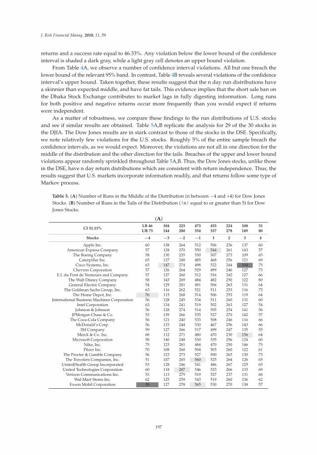
J. Risk Financial Manag. 2018, 11, 59
returns and a success rate equal to 46.33%. Any violation below the lower bound of the confidenceinterval is shaded a dark gray, while a light gray cell denotes an upper bound violation.
From Table 4A, we observe a number of confidence interval violations. All but one breach thelower bound of the relevant 95% band. In contrast, Table 4B reveals several violations of the confidenceinterval’s upper bound. Taken together, these results suggest that the n day run distributions havea skinnier than expected middle, and have fat tails. This evidence implies that the short sale ban onthe Dhaka Stock Exchange contributes to market lags in fully digesting information. Long runsfor both positive and negative returns occur more frequently than you would expect if returnswere independent.
As a matter of robustness, we compare these findings to the run distributions of U.S. stocksand see if similar results are obtained. Table 5A,B replicate the analysis for 29 of the 30 stocks inthe DJIA. The Dow Jones results are in stark contrast to those of the stocks in the DSE. Specifically,we note relatively few violations for the U.S. stocks. Roughly 5% of the entire sample breach theconfidence intervals, as we would expect. Moreover, the violations are not all in one direction for themiddle of the distribution and the other direction for the tails. Breaches of the upper and lower boundviolations appear randomly sprinkled throughout Table 5A,B. Thus, the Dow Jones stocks, unlike thosein the DSE, have n day return distributions which are consistent with return independence. Thus, theresults suggest that U.S. markets incorporate information readily, and that returns follow some type ofMarkov process.
Table 5. (A) Number of Runs in the Middle of the Distribution (n between −4 and +4) for Dow JonesStocks. (B) Number of Runs in the Tails of the Distribution (|n| equal to or greater than 5) for DowJones Stocks.
(A)
CI 51.13%LB 46UB 75
104144
225280
473554
453537
224278
108149
5180
Stocks −4 −3 −2 −1 1 2 3 4
Apple Inc. 60 138 264 512 506 236 137 60American Express Company 57 128 270 550 544 261 143 57
The Boeing Company 58 130 235 550 507 273 109 65Caterpillar Inc. 65 127 248 485 468 256 121 69
Cisco Systems, Inc. 63 147 274 498 522 244 104 75Chevron Corporation 57 126 264 529 499 246 127 73
E.I. du Pont de Nemours and Company 57 127 260 512 516 242 127 66The Walt Disney Company 58 143 269 484 482 250 122 80General Electric Company 54 129 281 491 506 263 131 64
The Goldman Sachs Group, Inc. 63 116 262 521 511 253 116 73The Home Depot, Inc. 76 115 268 514 506 253 119 64
International Business Machines Corporation 56 128 245 534 511 260 131 60Intel Corporation 63 134 241 519 502 263 127 54
Johnson & Johnson 56 128 274 514 505 254 141 56JPMorgan Chase & Co. 53 139 266 535 527 270 142 57
The Coca-Cola Company 56 121 240 533 508 246 116 66McDonald’s Corp. 56 133 244 530 467 256 143 66
3M Company 59 127 266 517 499 247 135 55Merck & Co. Inc. 68 112 271 480 470 230 156 64
Microsoft Corporation 58 140 248 530 535 256 124 60Nike, Inc. 75 123 281 484 470 250 146 75Pfizer Inc. 70 108 260 504 503 260 122 61
The Procter & Gamble Company 56 123 273 527 500 263 130 73The Travelers Companies, Inc. 51 107 265 560 525 264 126 65
UnitedHealth Group Incorporated 53 128 246 541 486 267 125 65United Technologies Corporation 60 118 287 546 523 266 133 69
Verizon Communications Inc. 53 113 279 519 527 237 131 68Wal-Mart Stores Inc. 62 125 259 543 519 260 136 62
Exxon Mobil Corporation 39 127 278 565 530 270 138 57
197
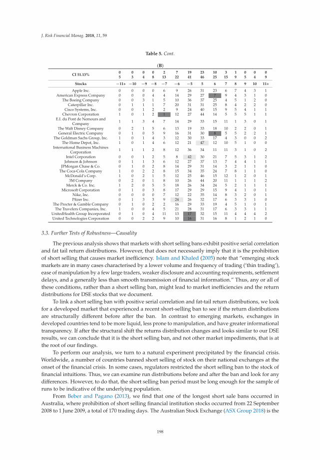
J. Risk Financial Manag. 2018, 11, 59
Table 5. Cont.
(B)
CI 51.13%05
03
04
08
213
722
1941
2346
1025
315
19
05
04
09
Stocks −11+ −10 −9 −8 −7 −6 −5 5 6 7 8 9 10 11+
Apple Inc. 0 0 0 0 6 9 26 31 23 6 7 4 3 1American Express Company 0 0 0 4 4 14 29 27 7 9 4 3 1 0
The Boeing Company 0 0 3 1 5 10 36 37 25 4 5 1 2 0Caterpillar Inc. 0 1 1 1 7 20 31 31 25 8 4 2 2 0
Cisco Systems, Inc. 0 0 1 2 2 9 24 40 15 9 5 4 1 1Chevron Corporation 1 0 1 2 1 12 27 44 14 5 5 5 1 1
E.I. du Pont de Nemours andCompany 1 1 3 4 7 14 29 33 15 11 1 3 0 1
The Walt Disney Company 0 2 1 5 6 13 19 33 18 10 2 2 0 1General Electric Company 0 1 0 5 9 16 31 30 8 5 5 2 2 1
The Goldman Sachs Group, Inc. 1 0 1 4 3 12 30 33 17 4 3 0 0 2The Home Depot, Inc. 1 0 1 4 6 12 21 47 12 10 5 1 0 0
International Business MachinesCorporation 1 1 1 2 8 12 36 34 11 11 3 1 0 2
Intel Corporation 0 0 1 2 5 8 42 30 21 7 5 3 1 2Johnson & Johnson 0 1 1 3 6 12 27 37 13 7 4 4 1 1
JPMorgan Chase & Co. 0 1 0 2 8 14 29 31 14 3 2 1 1 0The Coca-Cola Company 1 0 2 2 8 15 34 35 24 7 8 1 1 0
McDonald’s Corp. 1 0 2 1 5 12 25 46 15 12 1 2 0 13M Company 0 2 0 1 8 10 26 44 20 11 1 1 1 2
Merck & Co. Inc. 1 2 0 5 5 18 26 34 24 5 2 1 1 1Microsoft Corporation 0 1 0 3 8 17 29 29 15 9 4 1 0 1
Nike, Inc. 0 0 0 0 7 12 22 35 14 8 3 2 0 1Pfizer Inc. 0 1 3 3 9 24 26 32 17 6 3 3 1 0
The Procter & Gamble Company 0 1 0 2 2 16 29 33 19 4 5 1 0 1The Travelers Companies, Inc. 1 0 0 4 5 21 28 31 17 6 3 3 1 1
UnitedHealth Group Incorporated 0 1 0 4 11 13 17 32 15 11 4 4 4 2United Technologies Corporation 0 0 2 2 9 10 16 31 16 8 1 2 1 0
3.3. Further Tests of Robustness—Causality
The previous analysis shows that markets with short selling bans exhibit positive serial correlationand fat tail return distributions. However, that does not necessarily imply that it is the prohibitionof short selling that causes market inefficiency. Islam and Khaled (2005) note that “emerging stockmarkets are in many cases characterised by a lower volume and frequency of trading (‘thin trading’),ease of manipulation by a few large traders, weaker disclosure and accounting requirements, settlementdelays, and a generally less than smooth transmission of financial information.” Thus, any or all ofthese conditions, rather than a short selling ban, might lead to market inefficiencies and the returndistributions for DSE stocks that we document.
To link a short selling ban with positive serial correlation and fat-tail return distributions, we lookfor a developed market that experienced a recent short-selling ban to see if the return distributionsare structurally different before after the ban. In contrast to emerging markets, exchanges indeveloped countries tend to be more liquid, less prone to manipulation, and have greater informationaltransparency. If after the structural shift the returns distribution changes and looks similar to our DSEresults, we can conclude that it is the short selling ban, and not other market impediments, that is atthe root of our findings.
To perform our analysis, we turn to a natural experiment precipitated by the financial crisis.Worldwide, a number of countries banned short selling of stock on their national exchanges at theonset of the financial crisis. In some cases, regulators restricted the short selling ban to the stock offinancial intuitions. Thus, we can examine run distributions before and after the ban and look for anydifferences. However, to do that, the short selling ban period must be long enough for the sample ofruns to be indicative of the underlying population.
From Beber and Pagano (2013), we find that one of the longest short sale bans occurred inAustralia, where prohibition of short selling financial institution stocks occurred from 22 September2008 to 1 June 2009, a total of 170 trading days. The Australian Stock Exchange (ASX Group 2018) is the
198
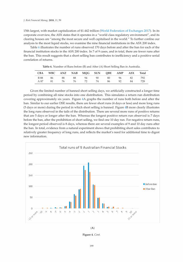
J. Risk Financial Manag. 2018, 11, 59
15th largest, with market capitalization of $1.442 trillion (World Federation of Exchanges 2017). In itscorporate overview, the ASX states that it operates in a “world class regulatory environment”, and itsclearing houses are “among the most secure and well capitalised in the world.” To further confine ouranalysis to the most liquid stocks, we examine the nine financial institutions in the ASX 200 index.
Table 6 illustrates the number of runs observed 170 days before and after the ban for each of thefinancial institution stocks in the ASX 200 index. In 7 of 9 cases, and in total, there are fewer runs afterthe ban. This result suggests that a short selling ban contributes to inefficiency and a positive serialcorrelation of returns.
Table 6. Number of Runs before (B) and After (A) Short Selling Ban in Australia.
CBA WBC ANZ NAB MQG SUN QBE AMP ASX Total
B 88 86 88 88 94 90 80 96 82 792A 87 81 76 76 72 74 86 92 84 728
Given the limited number of banned short selling days, we artificially constructed a longer timeperiod by combining all nine stocks into one distribution. This simulates a return run distributioncovering approximately six years. Figure 4A graphs the number of runs both before and after theban. Similar to our earlier DSE results, there are fewer short runs (4 days or less) and more long runs(5 days or more) during the period in which short selling is banned. Figure 4B more clearly illustratesthe long runs observed in the tails of the distribution. There are several more runs of positive returnsthat are 5 days or longer after the ban. Whereas the longest positive return run observed is 7 daysbefore the ban, after the prohibition of short selling, we find one 10 day run. For negative return runs,the longest period observed is 8 days, whereas there are several examples of 9 and 10 day runs afterthe ban. In total, evidence from a natural experiment shows that prohibiting short sales contributes torelatively greater frequency of long runs, and reflects the market’s need for additional time to digestnew information.
(A)
Figure 4. Cont.
199
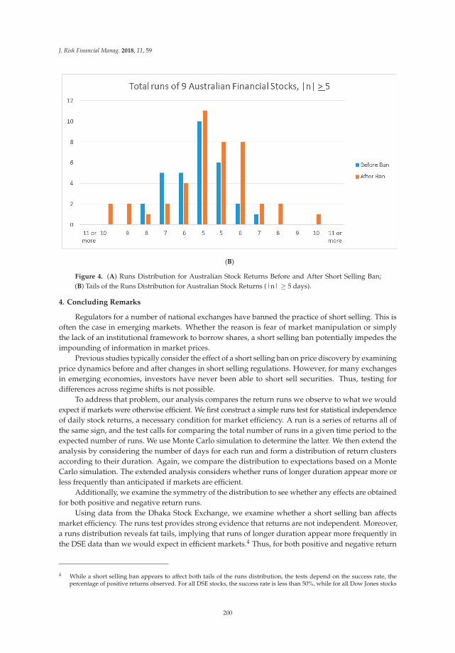
J. Risk Financial Manag. 2018, 11, 59
(B)
Figure 4. (A) Runs Distribution for Australian Stock Returns Before and After Short Selling Ban;(B) Tails of the Runs Distribution for Australian Stock Returns (|n| ≥ 5 days).
4. Concluding Remarks
Regulators for a number of national exchanges have banned the practice of short selling. This isoften the case in emerging markets. Whether the reason is fear of market manipulation or simplythe lack of an institutional framework to borrow shares, a short selling ban potentially impedes theimpounding of information in market prices.
Previous studies typically consider the effect of a short selling ban on price discovery by examiningprice dynamics before and after changes in short selling regulations. However, for many exchangesin emerging economies, investors have never been able to short sell securities. Thus, testing fordifferences across regime shifts is not possible.
To address that problem, our analysis compares the return runs we observe to what we wouldexpect if markets were otherwise efficient. We first construct a simple runs test for statistical independenceof daily stock returns, a necessary condition for market efficiency. A run is a series of returns all ofthe same sign, and the test calls for comparing the total number of runs in a given time period to theexpected number of runs. We use Monte Carlo simulation to determine the latter. We then extend theanalysis by considering the number of days for each run and form a distribution of return clustersaccording to their duration. Again, we compare the distribution to expectations based on a MonteCarlo simulation. The extended analysis considers whether runs of longer duration appear more orless frequently than anticipated if markets are efficient.
Additionally, we examine the symmetry of the distribution to see whether any effects are obtainedfor both positive and negative return runs.
Using data from the Dhaka Stock Exchange, we examine whether a short selling ban affectsmarket efficiency. The runs test provides strong evidence that returns are not independent. Moreover,a runs distribution reveals fat tails, implying that runs of longer duration appear more frequently inthe DSE data than we would expect in efficient markets.4 Thus, for both positive and negative return
4 While a short selling ban appears to affect both tails of the runs distribution, the tests depend on the success rate, thepercentage of positive returns observed. For all DSE stocks, the success rate is less than 50%, while for all Dow Jones stocks
200
J. Risk Financial Manag. 2018, 11, 59
runs, we observe a relatively large number of runs that are 5 days or longer. We next consider similartests for the DJIA and stocks within the index. This list includes extremely liquid stocks that are easilyshorted. In contrast to the DSE results, the runs tests generally accord with market efficiency. Finally,to further show causality, we examine Australian stock return runs before and after a ban on shortselling. After the prohibition, the findings are similar to the DSE results and reproduce the longer timenecessary for markets to reach a new equilibrium. The evidence taken as a whole suggests that a shortselling ban delays the market’s digestion of information. This is true for both positive and negativenews. In light of these results, regulators may want to rethink the prohibition of short selling securities.
Author Contributions: The authors contributed equally to the research and writing of the manuscript.
Funding: This research received no external funding.
Acknowledgments: We would like to thank our discussant at the 2017 Paris Financial Management Conference,Suk-Joong Kim, the University of Sydney, Australia and two anonymous reviewers. We also appreciate the helpof Assistant Editor, Eliza Dou, and the encouragement and editorial guidance of Duc Khuong Nguyen.
Conflicts of Interest: The authors declare no conflict of interest.
References
Atkins, Allen B., and Edward A. Dyl. 1990. Price Reversals, Bid-Ask Spreads, and Market Efficiency. Journal ofFinancial and Quantitative Analysis 25: 535–47. [CrossRef]
ASX Group. 2018. Australian Securities Exchange, LTD, Corporate Overview. Available online: https://www.asx.com.au/about/corporate-overview.htm (accessed on 26 September 2018).
Beber, Alessandro, and Marco Pagano. 2013. Short-Selling Bans around the World: Evidence from the 2007–2009Crisis. Journal of Finance 68: 343–81. [CrossRef]
Bris, Arturo, William N. Goetzmann, and Ning Zhu. 2007. Efficiency and the Bear: Short Sales Markets aroundthe World. Journal of Finance 62: 1029–79. [CrossRef]
De Bondt, Werner F.M., and Richard Thaler. 1985. Does the Stock Market Overreact? Journal of Finance 40: 793–805.[CrossRef]
Diamond, Douglas W., and Robert E. Verrecchia. 1987. Constraints on short-selling and asset price adjustment toprivate information. Journal of Financial Economics 18: 277–311. [CrossRef]
Fama, Eugene F. 1965. The Behavior of Stock Market Prices. Journal of Business 38: 34–105. [CrossRef]French, Kenneth R., and Richard Roll. 1986. Stock Return Variances: The Arrival of Information and Reaction of
Traders. Journal of Financial Economics 17: 5–26. [CrossRef]Islam, Ainul, and Mohammed Khaled. 2005. Tests of Weak-Form Efficiency of the Dhaka Stock Exchange. Journal of
Business Finance and Accounting 32: 1613–24. [CrossRef]Jain, Archana, Pankaj K. Jain, Thomas H. McInish, and Michael McKenzie. 2013. Worldwide Reach of Short Selling
Regulations. Journal of Financial Economics 109: 177–97. [CrossRef]Miller, Edward M. 1977. Risk, Uncertainty, and Divergence of Opinion. Journal of Finance 32: 1151–68. [CrossRef]Mobarek, Asma, A. Sabur Mollah, and Rafiqul Bhuyan. 2008. Market Efficiency in Emerging Stock Market:
Evidence from Bangladesh. Journal of Emerging Market Finance 7: 17–41. [CrossRef]Mollik, A., and Md Bepari. 2009. Weak-Form Market Efficiency of Dhaka Stock Exchange (DSE), Bangladesh.
Paper presented at 22nd Australasian Finance and Banking Conference (Abstracted in SSRN), Sydney,Australia, December 16–18.
Swidler, Steve. 1988. An Empirical Investigation of Heterogeneous Expectations, Analysts’ Earnings Forecastsand the Capital Asset Pricing Model. Quarterly Journal of Business and Economics 27: 20–41.
the success rate is greater than 50%. Thus, it may be that a short selling ban affects the success rate itself causing thesemarkets to exhibit negative returns more frequently. It should be noted that theory does not give any guidance to whatthe success rate must be if markets are efficient and follow some type of Markov process. Indeed, it can be shown that ifstock prices follow some type of geometric Brownian motion, the success rate increases with the stock returns drift term anddecreases with idiosyncratic risk and can theoretically be greater or less than 50%.
201

J. Risk Financial Manag. 2018, 11, 59
Wang, Song. 2014. Does idiosyncratic risk deter short-sellers? Evidence from a First- time Introduction ofShort-Selling. Paper presented at European Financial Management Association Meetings, Rome, Italy,June 25–28.
World Federation of Exchanges. 2017. Annual Statistics Guide. London: World Federation of Exchanges.
© 2018 by the authors. Licensee MDPI, Basel, Switzerland. This article is an open accessarticle distributed under the terms and conditions of the Creative Commons Attribution(CC BY) license (http://creativecommons.org/licenses/by/4.0/).
202
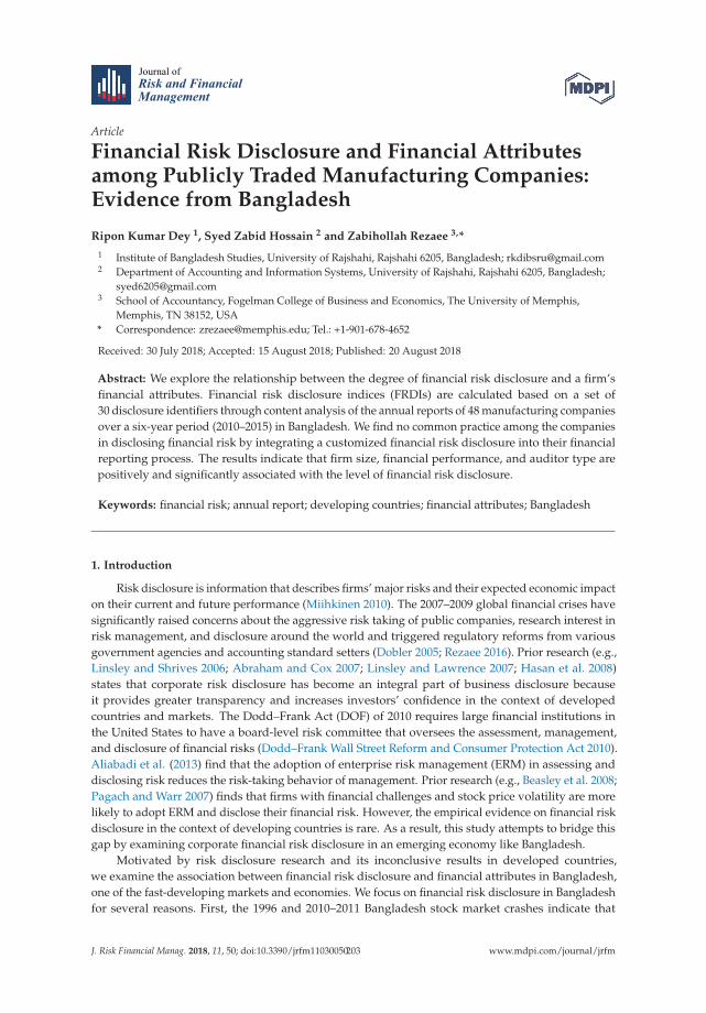
Journal of
Risk and FinancialManagement
Article
Financial Risk Disclosure and Financial Attributesamong Publicly Traded Manufacturing Companies:Evidence from Bangladesh
Ripon Kumar Dey 1, Syed Zabid Hossain 2 and Zabihollah Rezaee 3,*
1 Institute of Bangladesh Studies, University of Rajshahi, Rajshahi 6205, Bangladesh; [email protected] Department of Accounting and Information Systems, University of Rajshahi, Rajshahi 6205, Bangladesh;
[email protected] School of Accountancy, Fogelman College of Business and Economics, The University of Memphis,
Memphis, TN 38152, USA* Correspondence: [email protected]; Tel.: +1-901-678-4652
Received: 30 July 2018; Accepted: 15 August 2018; Published: 20 August 2018
Abstract: We explore the relationship between the degree of financial risk disclosure and a firm’sfinancial attributes. Financial risk disclosure indices (FRDIs) are calculated based on a set of30 disclosure identifiers through content analysis of the annual reports of 48 manufacturing companiesover a six-year period (2010–2015) in Bangladesh. We find no common practice among the companiesin disclosing financial risk by integrating a customized financial risk disclosure into their financialreporting process. The results indicate that firm size, financial performance, and auditor type arepositively and significantly associated with the level of financial risk disclosure.
Keywords: financial risk; annual report; developing countries; financial attributes; Bangladesh
1. Introduction
Risk disclosure is information that describes firms’ major risks and their expected economic impacton their current and future performance (Miihkinen 2010). The 2007–2009 global financial crises havesignificantly raised concerns about the aggressive risk taking of public companies, research interest inrisk management, and disclosure around the world and triggered regulatory reforms from variousgovernment agencies and accounting standard setters (Dobler 2005; Rezaee 2016). Prior research (e.g.,Linsley and Shrives 2006; Abraham and Cox 2007; Linsley and Lawrence 2007; Hasan et al. 2008)states that corporate risk disclosure has become an integral part of business disclosure becauseit provides greater transparency and increases investors’ confidence in the context of developedcountries and markets. The Dodd–Frank Act (DOF) of 2010 requires large financial institutions inthe United States to have a board-level risk committee that oversees the assessment, management,and disclosure of financial risks (Dodd–Frank Wall Street Reform and Consumer Protection Act 2010).Aliabadi et al. (2013) find that the adoption of enterprise risk management (ERM) in assessing anddisclosing risk reduces the risk-taking behavior of management. Prior research (e.g., Beasley et al. 2008;Pagach and Warr 2007) finds that firms with financial challenges and stock price volatility are morelikely to adopt ERM and disclose their financial risk. However, the empirical evidence on financial riskdisclosure in the context of developing countries is rare. As a result, this study attempts to bridge thisgap by examining corporate financial risk disclosure in an emerging economy like Bangladesh.
Motivated by risk disclosure research and its inconclusive results in developed countries,we examine the association between financial risk disclosure and financial attributes in Bangladesh,one of the fast-developing markets and economies. We focus on financial risk disclosure in Bangladeshfor several reasons. First, the 1996 and 2010–2011 Bangladesh stock market crashes indicate that
J. Risk Financial Manag. 2018, 11, 50; doi:10.3390/jrfm11030050 www.mdpi.com/journal/jrfm203
J. Risk Financial Manag. 2018, 11, 50
the traditional reporting culture fails to provide enough information to investors in making soundinvestment decisions (Das et al. 2015). Second, the Institute of Chartered Accountants of Bangladesh(ICAB) adopted the International Financial Reporting Standard No. 7 (IFRS-7) as Bangladesh FinancialReporting Standard (BFRS)-7 in 2010. BFRS No. 7 requires the disclosure of information relating toboth recognized and unrecognized financial instruments, their significance, performance, accountingpolicies, terms, conditions, net fair value, and risk information, as well as company policies forcontrolling risk and exposure.
Third, the Bangladesh National Parliament enacted the Financial Reporting Act of 2015 (FRA) on6 September 2015 (FRA 2015). The FRA requires the establishment of a new oversight body, referred toas the Financial Reporting Council (FRC). The main purpose of the FRC is to regulate the financialreporting procedure followed by the reporting entities. The FRA recognizes the major functions of theFRC and monitoring of financial reporting including risk assessment and management. The FRC isintended to bring a level of discipline into corporate financial reporting, and thus strengthen the safetyand soundness of capital markets. From that perspective, this study could provide evidence pertainingto the efficacy of the FRA. Finally, the type and extent of risk disclosure vary and are influenced by thefactors related to a given company in Bangladesh (Al-Mulhem 1997).
We posit that the degree of financial risk disclosure is positively associated with financial attributes.Our rationale for such an association is the following: (1) risk disclosure provides greater transparencyand enhances investors’ confidence that may lead to higher firm value; (2) leveraged firms are obligedto disclose more risk information to satisfy the needs of investors and creditors; (3) large firmsare more exposed to public scrutiny than small firms, and hence they are more likely to disclosemore information; (4) higher financial performance could persuade management to provide moreinformation to demonstrate its ability to create shareholder value; and (5) liquidity risk might encouragereporting entities to enhance the extent of risk disclosure to notify shareholders that management isconsidering such a risk.
The theoretical intuition for our prediction of the relationship between risk disclosure andfinancial attributes is based on signaling theory and the institutional settings in Bangladesh. Signalingtheory explains management’s incentives for disclosing financial risk to differentiate its firm’s risktolerance and appetite from other firms with higher financial risk to avoid adverse selection problems(Verrecchia 1983; Ng and Rezaee 2015). The institutional settings are relevant to our study as manyprovisions of regulatory measures in Bangladesh specifically address management risk assessmentand disclosure. For example, provisions of Section 184 of the Companies Act of 1994, Rule 12 of theBangladesh Securities and Exchange Rules of 1987, Bangladesh Securities and Exchange Commission(BSEC), and Accounting Standards as adopted by the ICAB require that listed companies report theirtrue and fair position to shareholders. After the adoption of IFRS-7 as BFRS-7, financial risk disclosurehas been reinforced.
We use financial risk disclosure indices (FRDIs) calculated based on a set of 30 disclosure identifiersthrough content analysis to assess the level of financial risk disclosure in the annual reports of48 manufacturing companies in Bangladesh over a period of six years (2010–2015). The associationbetween the level of financial risk disclosure and firm specific characteristics has been examinedusing regression analyses. The content analysis of individual FRDIs shows that there is no commonpractice among the companies in disclosing financial risk and they treat financial risk disclosure ina heterogeneous way. However, the regression model reveals that firm size, financial performance,and auditor type are positively and significantly associated with the level of financial risk disclosure.
This study contributes to the accounting and business literature in several ways. First, this papercontributes to corporate risk disclosure literature in the Anglo-Saxon countries by using the setting ofBangladesh as a highly speculative and volatile capital market of an emerging economy. Second, thismanuscript adds to relatively limited literature relating to risk disclosure in emerging economies andmarkets. Another contribution is the development of a risk disclosure index based on financial riskdisclosure identifiers in the light of reporting standards, professional requirements, prior research, and
204
J. Risk Financial Manag. 2018, 11, 50
the regulatory framework of Bangladesh. The examination of the relationship between firm specificcharacteristics and the extent of financial risk disclosure not only enhances our understanding of thereasons behind the variation of the disclosure, but also assists policy makers in adopting the appropriatetools to alleviate inconsistencies. Third, this study provides policy and practical implications by findingan association between financial leverage and liquidity and the level of financial risk disclosure, whichmay stimulate the regulatory bodies of the country to consider it and act accordingly. Undoubtedly, theInstitute of Chartered Accountants of Bangladesh (ICAB) has adopted IFRS 7 as Bangladesh FinancialReporting Standard 7 (BFRS 7) to ensure understandable, comparable, reliable, and transparentfinancial risk reporting for a sound, organized, and stable capital market in Bangladesh. However,empirical results document a compliance gap and suggest for full compliance of BFRS 7 without anydeviation to achieve comparability and reliability in disclosing financial risk. An analysis of the linkbetween the level of financial risk disclosure and the firm’s attributes has not previously been done inthe context of Bangladesh.
Fourth, we measure the level of aggregate disclosure (both mandatory and voluntary) on financialrisk in the annual reports of Dhaka Stock Exchange (DSE) listed manufacturing companies in termsof financial risk indices for a period of six years from 2010 to 2015 in response to BFRS-7. Thus,this manuscript enables regulators, policy makers, and corporate managers to understand the financialrisk disclosure pattern of publicly traded manufacturing companies in Bangladesh and to set anappropriate risk disclosure policy with guidelines to minimize the heterogeneous problem relating tocorporate financial risk disclosure. Finally, prior related research does not directly address financialrisk disclosure in emerging markets and economies.
The remainder of the paper is organized as follows: Section 2 presents the legal framework fordisclosure in Bangladesh. The literature review is provided in Section 3. The theoretical frameworkand hypothesis development are presented in Section 4. Methodology, description of our sample, anddescriptive analysis are provided in Section 5. The results and their interpretations are presented inSection 6 and the last section concludes the paper.
2. Legal Framework for Risk Disclosure in Bangladesh
Generally, each country has its own regulatory framework that governs corporate disclosurewithin the country. The corporate reports, in general, include information in accordance withreporting and disclosure requirements of the regulatory body, and as such, the reporting entityneeds to provide at least the required amount of information to facilitate the evaluation of securities(Akhtaruddin 2005). In Bangladesh, the Companies Act of 1994, Securities and Exchange Rules1987, and accounting standards adopted by ICAB provide the framework for corporate disclosure.The disclosure best practices can affect the extent of risk disclosure by listing regulations of stockexchanges (DSE and CSE—Chittagong Stock Exchange) and Income Tax Ordinance 1984. Besides,BSEC issues notifications and guidelines from time to time on different issues, which increases thelevel of corporate disclosure.
The Companies Act of 1994 provides the basic requirements for corporate disclosure and reportingin Bangladesh. The Act requires that the corporate financial statements must reflect the true and fairview of the reporting entity. Concomitantly, BSEC plays the leading role in monitoring and enforcingmandatory disclosure compliance of publicly traded companies. Moreover, Accounting Standardsadopted by the ICAB, in addition to its own disclosure provisions, gain mandatory status through thedirectives of the BSEC.
3. Literature Review
Risk has different notions and researchers have defined risk disclosure in different waysand contexts. Basically, risk disclosure is the communication of information concerning a firm’sstrategies, characteristics, operations, and other external factors that have the potential to affectexpected results (Beretta and Bozzolan 2004). Firms incur different types of risks to attain their
205
J. Risk Financial Manag. 2018, 11, 50
mission and aims throughout their life-cycle and management, and financial risks are among these(Lombardi et al. 2016). For our study, we have considered five categories of risks (i.e., capital structurerisk, credit risk, liquidity risk, interest rate risk, and exchange risk) and the disclosure of these risks inannual reports. Several studies examine risk disclosure in developed countries including the UnitedKingdom (Linsley and Shrives 2006; Abraham and Cox 2007), Italy (Beretta and Bozzolan 2004),Canada (Lajili and Zéghal 2005), and Australia (Poskitt 2005). These studies address corporate overallrisk with less emphasis on financial risk. Lombardi et al. (2016) examine financial risk disclosure in thesetting of Italy by addressing the commodity price risk category.
In the context of Bangladesh, there are a few studies on corporate disclosure, includingAkhtaruddin (2005); Hasan et al. (2008); Hasan et al. (2013); Das et al. (2015). Specifically,Akhtaruddin (2005); Hasan et al. (2008); and Das et al. (2015) investigate corporate mandatorydisclosure, whereas Hasan et al. (2013) examine financial disclosure. These studies, while findinga positive association between corporate disclosure and financial attributes for firms in Bangladesh,do not directly address financial risk disclosure. Basically, financial risk disclosure practice started inBangladesh after the adoption of IFRS-7 by the ICAB in 2010, hence its implementation is at an earlystage. We contribute to the literature by providing an initial understanding and a portrait of financialrisk disclosure practice in developing countries.
4. Theoretical Framework
Several theories are suggested in the accounting and finance literature in providing an explanationof the voluntary disclosure practices of business entities. The most common theories that are relevantto our research issues are the following: agency theory, signaling theory, political cost theory, capitalneed theory, and legitimacy theory. We briefly discussed these theories and their implications forour research because there is no specific theory perceived to explain the motivation for voluntarydisclosure (Khlifi and Bouri 2010).
Agency theory can explain voluntary disclosure phenomena in many countries with a differentsocial, political, and economic context (Ferguson et al. 2002; Akhtaruddin and Hossain 2008;Hossain and Taylor 2007). Disclosure is seen as a monitoring mechanism in agency theory.Healy and Palepu (2001) argue that demand for financial reporting and disclosure arises frominformation asymmetry along with agency conflicts between managers and outside investors. Priorresearch (Oliveira et al. 2011a, 2011b; Konishi and Ali 2007) uses firm size as a proxy for agency costsand assumes a positive association between disclosure and firm size and argues that leverage representsthe agency cost between debt-holders and managers, and is thus reflected in disclosure practices.
Signaling theory also explains why companies voluntarily disclose information in their annualreports (Haniffa and Cooke 2002; Akhtaruddin and Hossain 2008). In accordance with this theory,a firm’s information disclosure can be considered a signal to capital markets, directed to reduceinformation asymmetry that often exists between management and stakeholders, as well as to increasethe firm’s value (Connelly et al. 2011; Rezaee 2016).
Under political cost theory, firms with high political visibility in the market place tend to increasedisclosure as a means of mitigating potential political costs. The political cost theory is usually discussedin relation to the corporate size hypothesis, in which the manager of a big corporation is more likely toselect accounting procedures that defer reported earnings from current to future periods. (Milne 2002).The capital needs theory also helps explain the reasons behind companies’ disclosure of voluntaryinformation by suggesting that companies disclose more information to raise capital at the lowest cost(Core 2001). The capital needs theory predicts that increased voluntary disclosure is likely to lowerthe cost of capital because of the reduced uncertainty from an investor’s perspective (Schuster andO’Connell 2006).
The legitimacy theory assumes that a company has no right to exist unless its values are perceivedas being matched with those of the society at large in which it operates (Magness 2006). Companiesmay disclose information voluntarily for improving communication with society that helps societal
206
J. Risk Financial Manag. 2018, 11, 50
people to believe that the entities are operating within the social value system. In summary, the abovetheories have implications for financial risk disclosure in the sense that firms should assess, manage,and disclose risk to shareholders in compliance with agency theory, disclosing management riskappetite, and risk-taking under the signaling theory, focusing on financial risk disclosure as a meansof mitigating political costs and government intervention in accordance with political cost theory,and communicating risk tolerance under legitimacy theory. Although all these theories are relevantto our study, the two prevailing theories that provide the foundations for our research hypotheses,as described in the next section, are the signaling and political cost theories. The signaling theorysuggests that firms have incentives to disclose their good information to the capital markets and thepolitical cost theory explains the institutional setting in Bangladesh.
5. Hypothesis Development
Dodd Frank Act of 2010 (DOF) was the United States Congress’ response to the 2007–2009global financial crisis primarily caused by a lack of proper risk assessment and management(Dodd–Frank Wall Street Reform and Consumer Protection Act 2010). The DOF Act requires banks in nestablishing either a risk and compliance board committee or a risk and compliance executive position.Prior research (e.g., Beasley et al. 2008; Aliabadi et al. 2013) argues that firms with financial challengesand high stock price volatility are more likely to adopt ERM in managing and disclosing their risks.Earlier empirical studies (e.g., Oliveira et al. 2011a, 2011b; Alsaeed 2006; Kamal Hassan 2009) thatexamined the relationship between the extent of disclosure and firm-specific attributes have shownthat there are several firm characteristics that may influence the extent of disclosure in annual reports.Based upon theoretical discussion and previous empirical research on disclosure, we have selected sixcharacteristics (firm size, financial performance, corporate financial leverage, liquidity, industry type,and auditor type) for this study to test their relationship with the extent of financial risk disclosureexclusively in the context of a developing country as there is hardly any empirical evidence on thesame in literature.
5.1. Firm Size and Level of Financial Risk Disclosure
Prior research (Linsley and Shrives 2006; Abraham and Cox 2007; Beretta and Bozzolan 2004;Hasan et al. 2008; Das et al. 2015) suggests that firm size is an important determinant of the level ofdisclosure and presents mixed results regarding the link between size and the extent of disclosure.Brammer and Pavelin (2008) argue that larger firms tend to be more visible to stakeholders as theytend to be more complex, and thus are subject to more inherent risk. Agency theory also suggests thatlarger companies have higher information asymmetry between managers and owners, and as such,higher agency costs arise. To reduce these agency costs, larger companies disclose more informationthan smaller companies. Political cost theory also supports this notion. We posit that larger firmsprovide more financial risk disclosure and formulate the following hypothesis:
H1. There is a positive association between the level of financial risk disclosure and firm size.
5.2. Firm Performance and Level of Financial Risk Disclosure
Prior research (Inchausti 1997) supports the existence of a relationship between companyperformance and risk disclosure in light of signaling theory. However, empirical results are mixed.Some studies (Wang et al. 2008; Nandi and Ghosh 2013) find a positive association, whereas otherstudies (Reverte 2009; Bujaki and McConomy 2002) report an insignificant relationship between firmperformance and the extent of risk disclosure. However, studies (Hasan et al. 2008) in the context ofBangladesh find insignificant association between profitability and comprehensiveness of disclosure.Thus, we formulate the following hypothesis:
H2. There is a positive association between the financial performance level of a company and financial riskdisclosure level.
207
J. Risk Financial Manag. 2018, 11, 50
5.3. Corporate Financial Leverage and Level of Financial Risk Disclosure
The corporate financial leverage, as measured by total debt to total assets, may affect thelevel of financial risk disclosure. Companies with high levels of debt tend to be highly leveraged,more speculative, and riskier. Debt-holders have greater power over the financial structure of suchcompanies. From an agency theory perspective, creditors of highly leveraged companies have strongincentives to encourage management to disclose more information. Linsley and Shrives (2006) arguethat firms with higher levels of risk disclosure provide greater amounts of risk-related information asmanagers are willing to explain the causes of high risk. Thus, we formulate the following hypothesis:
H3. There is a positive association between corporate financial leverage and financial risk disclosure.
5.4. Liquidity and Level of Financial Risk Disclosure
Wallace and Naser (1995) argue that liquidity is an essential factor to disclose more informationabout a company’s ability to meet its obligation, as well as to testify that the company is a goingconcern to dispel the fears of investors and creditors. According to signaling theory, a firm with a highliquidity ratio tends to disclose more information in order to be differentiated from other firms witha lower liquidity ratio. Conversely, agency theory proposes that firms with lower liquidity disclosemore information to reduce conflict between shareholders and creditors. Findings of prior studiesare mixed. For example, Naser et al. (2002) support this reasoning of agency theory, whereas otherstudies (Alsaeed 2006; Barako et al. 2006) do not support either of these two theories by reporting noassociation between liquidity and financial disclosure. These contradictory results provide an incentiveto test this association between liquidity and disclosure. Thus, we formulate the following hypothesis:
H4. The level of liquidity is associated with the extent of financial risk disclosure.
5.5. Industry Type and Level of Financial Risk Disclosure
The financial literacy level of capital market investors and participants is relatively low inBangladesh, and thus in most cases, their source of information is only the audited annual reports ofpublic companies, unlike in the United States with voluntary financial and non-financial informationdisseminated to the capital markets (e.g., management discussion and analysis, short sellers, financialanalysts, institutional investors). As stated earlier, high volatility and market manipulation is a commonphenomenon in Bangladesh capital markets. Thus, a standardized risk reporting format is an urgentrequirement to achieve greater financial transparency and to make investors aware of the financial risksin this highly unpredictable environment. Homogeneous disclosure practices could be very helpful inthis regard. Thus, the heterogeneous/varied financial risk disclosure practices of companies impedesobtaining an efficient capital market and informed assessment of the investors.
The industry type has been identified as a significant factor that influences the disclosure practices(Amran and Haniffa 2011). The signaling theory suggests a positive association between industrytype and the level of risk disclosure. However, the prior empirical studies indicate mixed results,with some studies suggesting the association to be significant (Haniffa and Cooke 2002), whereasNaser et al. (2002) find an insignificant association between industry type and risk disclosure. Firms inthe financial and chemical industries have more incentives to provide financial risk disclosure. Thus,we state the following hypothesis:
H5. The industry type is associated with the extent of financial risk disclosure.
5.6. Auditor Type and Level of Financial Risk Disclosure
It is reported that financial statements of firms that are audited by the Big 4 audit firms areperceived to be more credible than those audited by non-Big 4 firms (Das et al. 2015). These largerand well-known audit firms tend to encourage firms to disclose more information to safeguard theaudit firms’ reputation and avoid reputational costs to them (Chalmers and Godfrey 2004). Lopes and
208
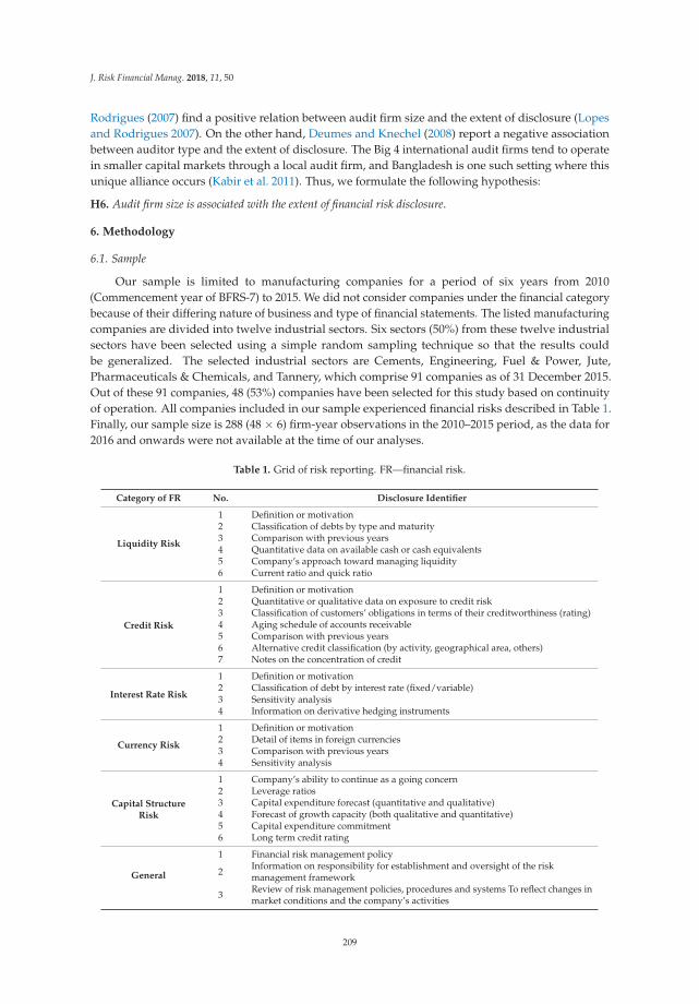
J. Risk Financial Manag. 2018, 11, 50
Rodrigues (2007) find a positive relation between audit firm size and the extent of disclosure (Lopesand Rodrigues 2007). On the other hand, Deumes and Knechel (2008) report a negative associationbetween auditor type and the extent of disclosure. The Big 4 international audit firms tend to operatein smaller capital markets through a local audit firm, and Bangladesh is one such setting where thisunique alliance occurs (Kabir et al. 2011). Thus, we formulate the following hypothesis:
H6. Audit firm size is associated with the extent of financial risk disclosure.
6. Methodology
6.1. Sample
Our sample is limited to manufacturing companies for a period of six years from 2010(Commencement year of BFRS-7) to 2015. We did not consider companies under the financial categorybecause of their differing nature of business and type of financial statements. The listed manufacturingcompanies are divided into twelve industrial sectors. Six sectors (50%) from these twelve industrialsectors have been selected using a simple random sampling technique so that the results couldbe generalized. The selected industrial sectors are Cements, Engineering, Fuel & Power, Jute,Pharmaceuticals & Chemicals, and Tannery, which comprise 91 companies as of 31 December 2015.Out of these 91 companies, 48 (53%) companies have been selected for this study based on continuityof operation. All companies included in our sample experienced financial risks described in Table 1.Finally, our sample size is 288 (48 × 6) firm-year observations in the 2010–2015 period, as the data for2016 and onwards were not available at the time of our analyses.
Table 1. Grid of risk reporting. FR—financial risk.
Category of FR No. Disclosure Identifier
Liquidity Risk
1 Definition or motivation2 Classification of debts by type and maturity3 Comparison with previous years4 Quantitative data on available cash or cash equivalents5 Company’s approach toward managing liquidity6 Current ratio and quick ratio
Credit Risk
1 Definition or motivation2 Quantitative or qualitative data on exposure to credit risk3 Classification of customers’ obligations in terms of their creditworthiness (rating)4 Aging schedule of accounts receivable5 Comparison with previous years6 Alternative credit classification (by activity, geographical area, others)7 Notes on the concentration of credit
Interest Rate Risk
1 Definition or motivation2 Classification of debt by interest rate (fixed/variable)3 Sensitivity analysis4 Information on derivative hedging instruments
Currency Risk
1 Definition or motivation2 Detail of items in foreign currencies3 Comparison with previous years4 Sensitivity analysis
Capital StructureRisk
1 Company’s ability to continue as a going concern2 Leverage ratios3 Capital expenditure forecast (quantitative and qualitative)4 Forecast of growth capacity (both qualitative and quantitative)5 Capital expenditure commitment6 Long term credit rating
General
1 Financial risk management policy
2 Information on responsibility for establishment and oversight of the riskmanagement framework
3 Review of risk management policies, procedures and systems To reflect changes inmarket conditions and the company’s activities
209
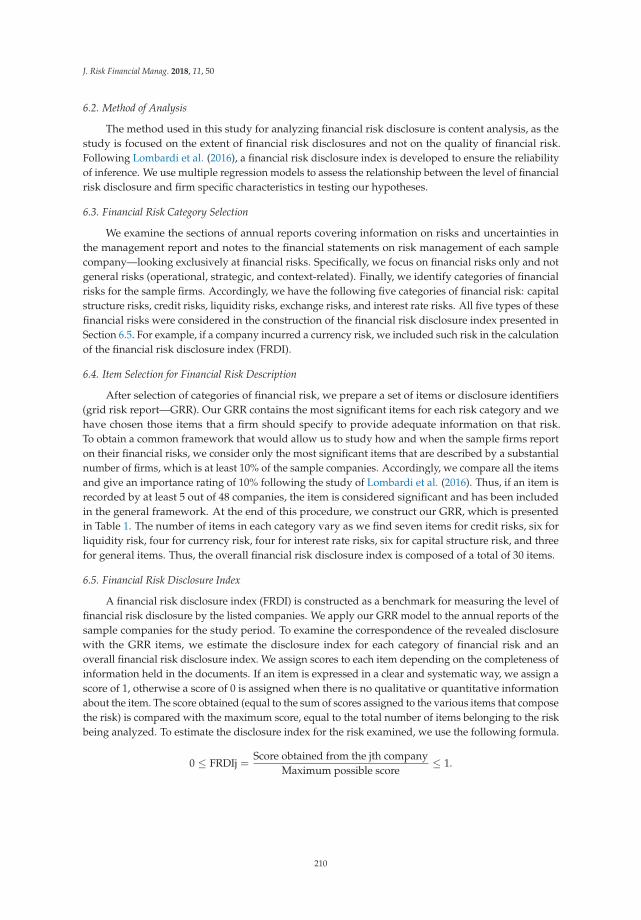
J. Risk Financial Manag. 2018, 11, 50
6.2. Method of Analysis
The method used in this study for analyzing financial risk disclosure is content analysis, as thestudy is focused on the extent of financial risk disclosures and not on the quality of financial risk.Following Lombardi et al. (2016), a financial risk disclosure index is developed to ensure the reliabilityof inference. We use multiple regression models to assess the relationship between the level of financialrisk disclosure and firm specific characteristics in testing our hypotheses.
6.3. Financial Risk Category Selection
We examine the sections of annual reports covering information on risks and uncertainties inthe management report and notes to the financial statements on risk management of each samplecompany—looking exclusively at financial risks. Specifically, we focus on financial risks only and notgeneral risks (operational, strategic, and context-related). Finally, we identify categories of financialrisks for the sample firms. Accordingly, we have the following five categories of financial risk: capitalstructure risks, credit risks, liquidity risks, exchange risks, and interest rate risks. All five types of thesefinancial risks were considered in the construction of the financial risk disclosure index presented inSection 6.5. For example, if a company incurred a currency risk, we included such risk in the calculationof the financial risk disclosure index (FRDI).
6.4. Item Selection for Financial Risk Description
After selection of categories of financial risk, we prepare a set of items or disclosure identifiers(grid risk report—GRR). Our GRR contains the most significant items for each risk category and wehave chosen those items that a firm should specify to provide adequate information on that risk.To obtain a common framework that would allow us to study how and when the sample firms reporton their financial risks, we consider only the most significant items that are described by a substantialnumber of firms, which is at least 10% of the sample companies. Accordingly, we compare all the itemsand give an importance rating of 10% following the study of Lombardi et al. (2016). Thus, if an item isrecorded by at least 5 out of 48 companies, the item is considered significant and has been includedin the general framework. At the end of this procedure, we construct our GRR, which is presentedin Table 1. The number of items in each category vary as we find seven items for credit risks, six forliquidity risk, four for currency risk, four for interest rate risks, six for capital structure risk, and threefor general items. Thus, the overall financial risk disclosure index is composed of a total of 30 items.
6.5. Financial Risk Disclosure Index
A financial risk disclosure index (FRDI) is constructed as a benchmark for measuring the level offinancial risk disclosure by the listed companies. We apply our GRR model to the annual reports of thesample companies for the study period. To examine the correspondence of the revealed disclosurewith the GRR items, we estimate the disclosure index for each category of financial risk and anoverall financial risk disclosure index. We assign scores to each item depending on the completeness ofinformation held in the documents. If an item is expressed in a clear and systematic way, we assign ascore of 1, otherwise a score of 0 is assigned when there is no qualitative or quantitative informationabout the item. The score obtained (equal to the sum of scores assigned to the various items that composethe risk) is compared with the maximum score, equal to the total number of items belonging to the riskbeing analyzed. To estimate the disclosure index for the risk examined, we use the following formula.
0 ≤ FRDIj =Score obtained from the jth company
Maximum possible score≤ 1.
210
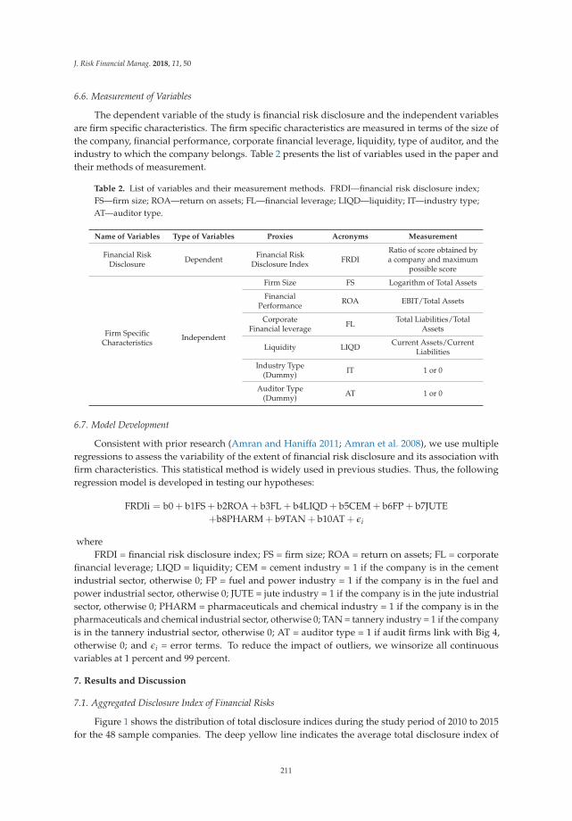
J. Risk Financial Manag. 2018, 11, 50
6.6. Measurement of Variables
The dependent variable of the study is financial risk disclosure and the independent variablesare firm specific characteristics. The firm specific characteristics are measured in terms of the size ofthe company, financial performance, corporate financial leverage, liquidity, type of auditor, and theindustry to which the company belongs. Table 2 presents the list of variables used in the paper andtheir methods of measurement.
Table 2. List of variables and their measurement methods. FRDI—financial risk disclosure index;FS—firm size; ROA—return on assets; FL—financial leverage; LIQD—liquidity; IT—industry type;AT—auditor type.
Name of Variables Type of Variables Proxies Acronyms Measurement
Financial RiskDisclosure Dependent Financial Risk
Disclosure Index FRDIRatio of score obtained bya company and maximum
possible score
Firm SpecificCharacteristics
Independent
Firm Size FS Logarithm of Total Assets
FinancialPerformance ROA EBIT/Total Assets
CorporateFinancial leverage FL Total Liabilities/Total
Assets
Liquidity LIQD Current Assets/CurrentLiabilities
Industry Type(Dummy) IT 1 or 0
Auditor Type(Dummy) AT 1 or 0
6.7. Model Development
Consistent with prior research (Amran and Haniffa 2011; Amran et al. 2008), we use multipleregressions to assess the variability of the extent of financial risk disclosure and its association withfirm characteristics. This statistical method is widely used in previous studies. Thus, the followingregression model is developed in testing our hypotheses:
FRDIi = b0 + b1FS + b2ROA + b3FL + b4LIQD + b5CEM + b6FP + b7JUTE+b8PHARM + b9TAN + b10AT + εi
whereFRDI = financial risk disclosure index; FS = firm size; ROA = return on assets; FL = corporate
financial leverage; LIQD = liquidity; CEM = cement industry = 1 if the company is in the cementindustrial sector, otherwise 0; FP = fuel and power industry = 1 if the company is in the fuel andpower industrial sector, otherwise 0; JUTE = jute industry = 1 if the company is in the jute industrialsector, otherwise 0; PHARM = pharmaceuticals and chemical industry = 1 if the company is in thepharmaceuticals and chemical industrial sector, otherwise 0; TAN = tannery industry = 1 if the companyis in the tannery industrial sector, otherwise 0; AT = auditor type = 1 if audit firms link with Big 4,otherwise 0; and εi = error terms. To reduce the impact of outliers, we winsorize all continuousvariables at 1 percent and 99 percent.
7. Results and Discussion
7.1. Aggregated Disclosure Index of Financial Risks
Figure 1 shows the distribution of total disclosure indices during the study period of 2010 to 2015for the 48 sample companies. The deep yellow line indicates the average total disclosure index of
211
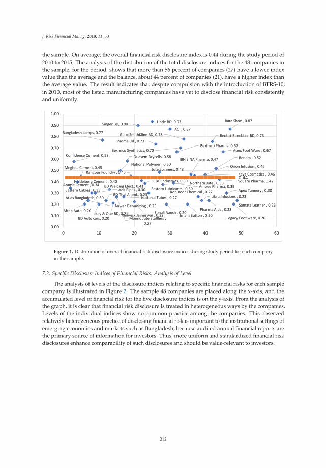
J. Risk Financial Manag. 2018, 11, 50
the sample. On average, the overall financial risk disclosure index is 0.44 during the study period of2010 to 2015. The analysis of the distribution of the total disclosure indices for the 48 companies inthe sample, for the period, shows that more than 56 percent of companies (27) have a lower indexvalue than the average and the balance, about 44 percent of companies (21), have a higher index thanthe average value. The result indicates that despite compulsion with the introduction of BFRS-10,in 2010, most of the listed manufacturing companies have yet to disclose financial risk consistentlyand uniformly.
Aramit Cement , 0.34
Confidence Cement, 0.58
Heidelberg Cement , 0.40
Meghna Cement, 0.45
Aftab Auto, 0.20Anwer Galvanizing , 0.23
Atlas Bangladesh, 0.30
Aziz Pipes , 0.30
BD Auto cars, 0.20
Bangladesh Lamps, 0.77
BD Thai Alumi., 0.23Eastern Cables , 0.33
Kay & Que BD, 0.21Monno Jute Stafllers ,
0.27
National Polymer , 0.50
National Tubes , 0.27
Quasem Drycells, 0.58
Rangpur Foundry , 0.45
Renwick Jajneswar , 0.22
Singer BD, 0.90
BD Welding Elect., 0.41CBO Industries, 0.39
Eastern Lubricants , 0.30
Linde BD, 0.93
Padma Oil , 0.73
Jute Spinners, 0.48
Northern Jute , 0.38
Sonali Aansh , 0.20
ACI , 0.87
Ambee Pharma, 0.39
Beximco Pharma, 0.67Beximco Synthetics, 0.70
GlaxoSmithKline BD, 0.78
Imam Button , 0.20
IBN SINA Pharma, 0.47
Keya Cosmetics , 0.46
Kohinoor Chemical , 0.27Libra Infusions , 0.23
Orion Infusion , 0.46
Pharma Aids , 0.23
Reckitt Benckiser BD, 0.76
Renata , 0.52
Square Pharma, 0.42
Apex Foot Ware , 0.67
Apex Tannery , 0.30
Bata Shoe , 0.87
Legacy Foot ware, 0.20
Samata Leather , 0.23
0.44
0.00
0.10
0.20
0.30
0.40
0.50
0.60
0.70
0.80
0.90
1.00
0 10 20 30 40 50 60
Figure 1. Distribution of overall financial risk disclosure indices during study period for each companyin the sample.
7.2. Specific Disclosure Indices of Financial Risks: Analysis of Level
The analysis of levels of the disclosure indices relating to specific financial risks for each samplecompany is illustrated in Figure 2. The sample 48 companies are placed along the x-axis, and theaccumulated level of financial risk for the five disclosure indices is on the y-axis. From the analysis ofthe graph, it is clear that financial risk disclosure is treated in heterogeneous ways by the companies.Levels of the individual indices show no common practice among the companies. This observedrelatively heterogeneous practice of disclosing financial risk is important to the institutional settings ofemerging economies and markets such as Bangladesh, because audited annual financial reports arethe primary source of information for investors. Thus, more uniform and standardized financial riskdisclosures enhance comparability of such disclosures and should be value-relevant to investors.
212
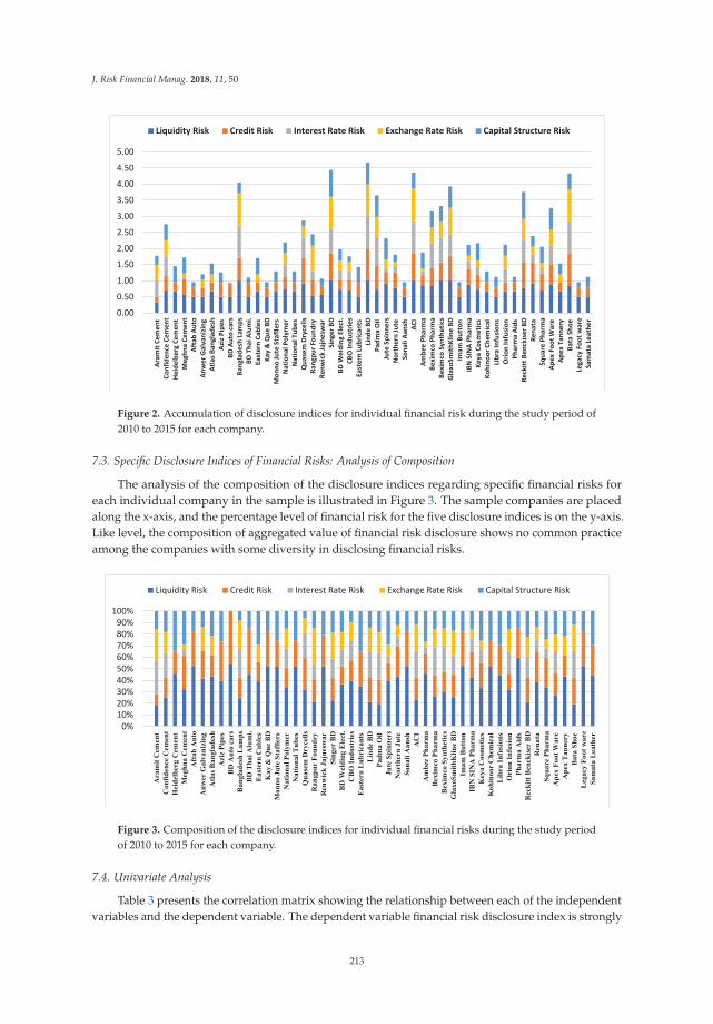
J. Risk Financial Manag. 2018, 11, 50
0.00
0.50
1.00
1.50
2.00
2.50
3.00
3.50
4.00
4.50
5.00Ar
amit
Cem
ent
Conf
iden
ce C
emen
tHe
idel
berg
Cem
ent
Meg
hna
Cem
ent
Afta
b Au
toAn
wer
Gal
vani
zing
Atla
s Ban
glad
esh
Aziz
Pip
esBD
Aut
o ca
rsBa
ngla
desh
Lam
psBD
Tha
i Alu
mi.
East
ern
Cabl
esKa
y &
Que
BD
Mon
no Ju
te S
tafll
ers
Nat
iona
l Pol
ymer
Nat
iona
l Tub
esQ
uase
m D
ryce
llsRa
ngpu
r Fou
ndry
Renw
ick
Jajn
esw
arSi
nger
BD
BD W
eldi
ng E
lect
.CB
O In
dust
ries
East
ern
Lubr
ican
tsLi
nde
BDPa
dma
Oil
Jute
Spi
nner
sN
orth
ern
Jute
Sona
li Aa
nsh
ACI
Ambe
e Ph
arm
aBe
xim
co P
harm
aBe
xim
co S
ynth
etic
sGl
axoS
mith
Klin
e BD
Imam
But
ton
IBN
SIN
A Ph
arm
aKe
ya C
osm
etic
sKo
hino
or C
hem
ical
Libr
a In
fusio
nsO
rion
Infu
sion
Phar
ma
Aids
Reck
itt B
enck
iser
BD
Rena
taSq
uare
Pha
rma
Apex
Foo
t War
eAp
ex T
anne
ryBa
ta S
hoe
Lega
cy F
oot w
are
Sam
ata
Leat
her
Liquidity Risk Credit Risk Interest Rate Risk Exchange Rate Risk Capital Structure Risk
Figure 2. Accumulation of disclosure indices for individual financial risk during the study period of2010 to 2015 for each company.
7.3. Specific Disclosure Indices of Financial Risks: Analysis of Composition
The analysis of the composition of the disclosure indices regarding specific financial risks foreach individual company in the sample is illustrated in Figure 3. The sample companies are placedalong the x-axis, and the percentage level of financial risk for the five disclosure indices is on the y-axis.Like level, the composition of aggregated value of financial risk disclosure shows no common practiceamong the companies with some diversity in disclosing financial risks.
0%10%20%30%40%50%60%70%80%90%
100%
Ara
mit
Cem
ent
Con
fiden
ce C
emen
tH
eide
lber
g C
emen
tM
eghn
a C
emen
tA
ftab
Aut
oA
nwer
Gal
vani
zing
Atla
s Ban
glad
esh
Azi
z Pi
pes
BD
Aut
o ca
rsB
angl
ades
h L
amps
BD
Tha
i Alu
mi.
Eas
tern
Cab
les
Kay
& Q
ue B
DM
onno
Jut
e St
aflle
rsN
atio
nal P
olym
erN
atio
nal T
ubes
Qua
sem
Dry
cells
Ran
gpur
Fou
ndry
Ren
wic
k Ja
jnes
war
Sing
er B
DB
D W
eldi
ng E
lect
.C
BO
Indu
stri
esE
aste
rn L
ubri
cant
sL
inde
BD
Padm
a O
ilJu
te S
pinn
ers
Nor
ther
n Ju
teSo
nali
Aan
shA
CI
Am
bee
Phar
ma
Bex
imco
Pha
rma
Bex
imco
Syn
thet
ics
Gla
xoSm
ithK
line
BD
Imam
But
ton
IBN
SIN
A P
harm
aK
eya
Cos
met
ics
Koh
inoo
r C
hem
ical
Lib
ra In
fusi
ons
Ori
on In
fusi
onPh
arm
a A
ids
Rec
kitt
Ben
ckise
r B
DR
enat
aSq
uare
Pha
rma
Ape
x Fo
ot W
are
Ape
x T
anne
ryB
ata
Shoe
Leg
acy
Foot
war
eSa
mat
a Le
athe
rLiquidity Risk Credit Risk Interest Rate Risk Exchange Rate Risk Capital Structure Risk
Figure 3. Composition of the disclosure indices for individual financial risks during the study periodof 2010 to 2015 for each company.
7.4. Univariate Analysis
Table 3 presents the correlation matrix showing the relationship between each of the independentvariables and the dependent variable. The dependent variable financial risk disclosure index is strongly
213
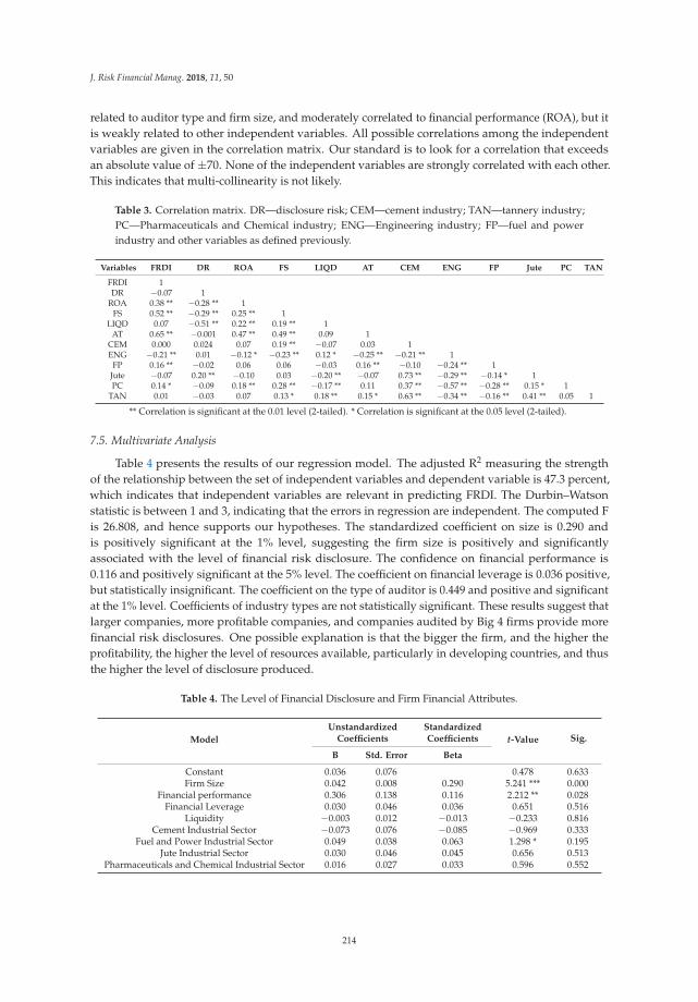
J. Risk Financial Manag. 2018, 11, 50
related to auditor type and firm size, and moderately correlated to financial performance (ROA), but itis weakly related to other independent variables. All possible correlations among the independentvariables are given in the correlation matrix. Our standard is to look for a correlation that exceedsan absolute value of ±70. None of the independent variables are strongly correlated with each other.This indicates that multi-collinearity is not likely.
Table 3. Correlation matrix. DR—disclosure risk; CEM—cement industry; TAN—tannery industry;PC—Pharmaceuticals and Chemical industry; ENG—Engineering industry; FP—fuel and powerindustry and other variables as defined previously.
Variables FRDI DR ROA FS LIQD AT CEM ENG FP Jute PC TAN
FRDI 1DR −0.07 1
ROA 0.38 ** −0.28 ** 1FS 0.52 ** −0.29 ** 0.25 ** 1
LIQD 0.07 −0.51 ** 0.22 ** 0.19 ** 1AT 0.65 ** −0.001 0.47 ** 0.49 ** 0.09 1
CEM 0.000 0.024 0.07 0.19 ** −0.07 0.03 1ENG −0.21 ** 0.01 −0.12 * −0.23 ** 0.12 * −0.25 ** −0.21 ** 1
FP 0.16 ** −0.02 0.06 0.06 −0.03 0.16 ** −0.10 −0.24 ** 1Jute −0.07 0.20 ** −0.10 0.03 −0.20 ** −0.07 0.73 ** −0.29 ** −0.14 * 1PC 0.14 * −0.09 0.18 ** 0.28 ** −0.17 ** 0.11 0.37 ** −0.57 ** −0.28 ** 0.15 * 1
TAN 0.01 −0.03 0.07 0.13 * 0.18 ** 0.15 * 0.63 ** −0.34 ** −0.16 ** 0.41 ** 0.05 1
** Correlation is significant at the 0.01 level (2-tailed). * Correlation is significant at the 0.05 level (2-tailed).
7.5. Multivariate Analysis
Table 4 presents the results of our regression model. The adjusted R2 measuring the strengthof the relationship between the set of independent variables and dependent variable is 47.3 percent,which indicates that independent variables are relevant in predicting FRDI. The Durbin–Watsonstatistic is between 1 and 3, indicating that the errors in regression are independent. The computed Fis 26.808, and hence supports our hypotheses. The standardized coefficient on size is 0.290 andis positively significant at the 1% level, suggesting the firm size is positively and significantlyassociated with the level of financial risk disclosure. The confidence on financial performance is0.116 and positively significant at the 5% level. The coefficient on financial leverage is 0.036 positive,but statistically insignificant. The coefficient on the type of auditor is 0.449 and positive and significantat the 1% level. Coefficients of industry types are not statistically significant. These results suggest thatlarger companies, more profitable companies, and companies audited by Big 4 firms provide morefinancial risk disclosures. One possible explanation is that the bigger the firm, and the higher theprofitability, the higher the level of resources available, particularly in developing countries, and thusthe higher the level of disclosure produced.
Table 4. The Level of Financial Disclosure and Firm Financial Attributes.
Model
UnstandardizedCoefficients
StandardizedCoefficients t-Value Sig.
B Std. Error Beta
Constant 0.036 0.076 0.478 0.633Firm Size 0.042 0.008 0.290 5.241 *** 0.000
Financial performance 0.306 0.138 0.116 2.212 ** 0.028Financial Leverage 0.030 0.046 0.036 0.651 0.516
Liquidity −0.003 0.012 −0.013 −0.233 0.816Cement Industrial Sector −0.073 0.076 −0.085 −0.969 0.333
Fuel and Power Industrial Sector 0.049 0.038 0.063 1.298 * 0.195Jute Industrial Sector 0.030 0.046 0.045 0.656 0.513
Pharmaceuticals and Chemical Industrial Sector 0.016 0.027 0.033 0.596 0.552
214
J. Risk Financial Manag. 2018, 11, 50
Table 4. Cont.
Model
UnstandardizedCoefficients
StandardizedCoefficients t-Value Sig.
B Std. Error Beta
Tannery Industrial Sector −0.033 0.038 −0.054 −0.855 0.393Type of Audit Firm 0.263 0.035 0.449 7.590 *** 0.000
Adj. R2 0.473
This table presents the results from a regression of the level of financial risk disclosure and firms financial attributes.The dependent variable is the level of financial risk disclosure (FRDI). The independent variables are firm size,financial performance, leverage, liquidity, and industry classifications. This table presents results from OLS(Ordinary Least Squares) regression of the level of FRDI on financial attributes. The definitions of all other variablesare reported in Table 1. Standard errors are clustered at the firm level, and t-statistics are reported in the relatedcolumn. Significance at the 10%, 5%, and 1% levels are denoted by *, **, and ***, respectively.
8. Conclusions and Limitations
This study examines the level of financial risk disclosure of publicly traded manufacturingcompanies by investigating the association between the level of financial risk disclosure and firmspecific characteristics. The results of the content analysis show that the sample companies treatfinancial risk disclosure in heterogeneous and less standardized manners. Although compliance withBFRS-7 requires that public companies uniformly disclose financial risk, our results show that there isno common practice in this regard. Thus, a more uniform and standardized financial risk disclosurecan improve corporate disclosure in compliance with BFRS-7 and enhance comparability of financialrisk disclosure. The results also confirm that the companies tend to provide more information onliquidity risk and less information about interest rate risk and currency risk.
The regression results show that firm size, financial performance, and auditor type are positivelyand significantly associated with the level of financial risk disclosure in annual reports. These resultsare consistent with those of various previous empirical studies worldwide (Amran et al. 2008;Das et al. 2015; Linsley and Shrives 2006). The results suggest that firm size, performance, and auditortype are the main determinants of risk disclosure and are the driving factors for the selected companiesto increase the level of financial risk disclosure. The results reveal that financial leverage, liquidity,and industry type have no association with the level of financial risk disclosure, which are consistentwith findings of prior studies (e.g., Alsaeed 2006). As a result, these characteristics have no relevance todisclosing financial risk of the publicly traded manufacturing companies. Our results contribute to thebusiness and accounting literature by providing an initial understanding of financial risk disclosurepractices in Bangladesh, where the risk disclosure practice is still in an early stage.
There are, however, several limitations of this study. First, the study focuses on 30 selecteddisclosure items. Moreover, the choice of the items does not reflect their level of importance asperceived by financial information users and the coding approach is subject to coder bias. Second,the un-weighted or binary approach is used to measure the level of financial risk disclosure, which maynot reflect the quality of financial risk disclosure. Third, the study is confined to one country inemerging markets and economies. Fourth, the information regarding risk can be provided in sourcesother than annual reports. Finally, a potential endogenous concern may exist in our analysis giventhe sample size in relation with the estimated coefficients. Thus, the results and their policy, practical,and research implications should be interpreted with caution, considering these potential limitations.Future research should address financial risk disclosure in other developing countries and investigateboth the quality and quantity of financial risk disclosure.
Author Contributions: Authors have equally contributed to the paper. Research questions and hypothesis andresearch method were developed by S.Z.H., R.K.D. performed the analyses and Z.R. prepared the manuscript.
Funding: This research received no external funding.
Conflicts of Interest: The authors declare no conflicts of interest.
215
J. Risk Financial Manag. 2018, 11, 50
References
Abraham, Santhosh, and Paul Cox. 2007. Analyzing the determinants of narrative risk information in UK FTSE100 annual reports. British Accounting Review 39: 227–48. [CrossRef]
Akhtaruddin, Md. 2005. Corporate mandatory disclosure practices in Bangladesh. International Journal Accounting40: 399–422. [CrossRef]
Akhtaruddin, Mohamed, and Mahmud Hossain. 2008. Investment opportunity set, ownership control andvoluntary disclosures in Malaysia. JOAAG 3: 25–39.
Aliabadi, Sara, Alireza Dorestani, and Zabihollah Rezaee. 2013. Integration of Enterprise Risk management intoCorporate Governance. International Journal of Management Accounting Research 3: 31–46.
Al-Mulhem, Adnan Abdullah. 1997. An Empirical Investigation of the Level of Financial Disclosure by SaudiArabian Corporations. Doctoral dissertation, University of Hull, Hull, UK.
Alsaeed, Khalid. 2006. The association between firm-specific characteristics and disclosure: The case of SaudiArabia. Managerial Auditing Journal 21: 476–96. [CrossRef]
Amran, Azlan, and Roszaini Haniffa. 2011. Evidence in development of sustainability reporting: A case of adeveloping country. Business Strategy and the Environment 3: 141–56. [CrossRef]
Amran, Azlan, Abdul Manaf Rosli Bin, and Bin Che Haat Mohd Hassan. 2008. Risk reporting: An exploratorystudy on risk management disclosure in Malaysian annual reports. Managerial Auditing Journal 24: 39–57.[CrossRef]
Barako, Dulacha G., Phil Hancock, and H. Y. Izan. 2006. Factors influencing voluntary corporate disclosure byKenyan companies. Corporate Governance: An International Review 14: 107–25. [CrossRef]
Beasley, Mark, Don Pagach, and Richard Warr. 2008. Information conveyed in hiring announcement of seniorexecutives overseeing enterprise-wide risk management process. Journal of Accounting, Auditing and Finance23: 311–32. [CrossRef]
Beretta, Sergio, and Saverio Bozzolan. 2004. A framework for the analysis of firm risk communication.The International Journal of Accounting 39: 265–88. [CrossRef]
Brammer, Stephen, and Stephen Pavelin. 2008. Factors influencing the quality of corporate environmentaldisclosure. Business Strategy and the Environment 17: 120–36. [CrossRef]
Bujaki, Merridee, and Bruce J. McConomy. 2002. Corporate governance: Factors influencing voluntary disclosureby publicly traded Canadian firms. Accounting Perspectives 1: 105–39. [CrossRef]
Chalmers, Keryn, and Jayne M. Godfrey. 2004. Reputation costs: The impetus for voluntary derivative financialinstrument reporting. Accounting Organizations and Society 29: 95–125. [CrossRef]
Connelly, Brian L., S. Trevis Certo, R. Duane Ireland, and Christopher R. Reutzel. 2011. Signaling theory: A reviewand assessment. Journal of Management 37: 39–67. [CrossRef]
Core, John E. 2001. A review of the empirical disclosure literature: Discussion. Journal of Accounting and Economics31: 441–56. [CrossRef]
Das, Sumon, Rob Dixon, and Amir Michael. 2015. Corporate mandatory reporting: A longitudinal investigationof listed companies in Bangladesh. Global Review of Accounting and Finance 6: 64–85. [CrossRef]
Deumes, Rogier, and W. Robert Knechel. 2008. Economic incentives for voluntary reporting on internal riskmanagement and control systems. Auditing: A Journal of Practice & Theory 27: 35–66.
Dobler, Michael. 2005. National and international developments in risk reporting: May the German AccountingStandard 5 lead the way internationally. German Law Journal 6: 1191–200.
(DOF) Dodd–Frank Wall Street Reform and Consumer Protection Act. 2010. 111th Congress Public Law 203;Washington, DC: Government Printing Office. Available online: http://www.gpo.gov/fdsys/pkg/PLAW-111publ203/html/PLAW-111publ203.htm (accessed on 16 June 2018).
Ferguson, Michael J., Kevin C. K. Lam, and Grace Meina Lee. 2002. Voluntary disclosure by state-ownedenterprises listed on the stock exchange of Hong Kong. Journal of International Financial Management &Accounting 13: 125–52.
Financial Reporting Act (FRA). 2015. The Bangladesh National Parliament. Available online: http://www.icmab.org.bd/images/stories/journal/2015/Nov-Dec/6.Opinions%20%20Comments.pdf (accessed on 16 June 2018).
Haniffa, Ros M., and Terry E. Cooke. 2002. Culture, corporate governance and disclosure in Malaysiancorporations. Abacus 38: 317–49. [CrossRef]
216
J. Risk Financial Manag. 2018, 11, 50
Hasan, Tanweer, Waresul Karim, and Shakil Quayes. 2008. Regulatory change and the quality of complianceto mandatory disclosure requirements: Evidence from Bangladesh. Research in Accounting Regulation 20:193–203. [CrossRef]
Hasan, Md. Shamimul, Syed Zabid Hossain, and Robert J. Swieringa. 2013. Corporate governance and financialdisclosures: Bangladesh perspective. Corporate Governance 4: 109–19.
Healy, Paul M., and Krishna G. Palepu. 2001. Information asymmetry, corporate disclosure, and the capitalmarkets: A review of the empirical disclosure literature. Journal of Accounting and Economics 31: 405–40.[CrossRef]
Hossain, Mohammed, and Peter J. Taylor. 2007. The empirical evidence of the voluntary information disclosure inthe annual reports of banking companies: The case of Bangladesh. Corporate Ownership and Control 4: 111–25.[CrossRef]
Inchausti, Begoña Giner. 1997. The influence of company characteristics and accounting regulation on informationdisclosed by Spanish firms. European Accounting Review 6: 45–68. [CrossRef]
Kabir, M. Humayun, Divesh Sharma, Md Ainul Islam, and Amirus Salat. 2011. Big 4 auditor affiliation andaccruals quality in Bangladesh. Managerial Auditing Journal 26: 161–81. [CrossRef]
Kamal Hassan, Mostafa. 2009. UAE corporations-specific characteristics and level of risk disclosure. ManagerialAuditing Journal 24: 668–87. [CrossRef]
Khlifi, Foued, and Abdelfettah Bouri. 2010. Corporate Disclosure and Firm Characteristics: A PuzzlingRelationship. Journal of Accounting, Business & Management 17: 62–89.
Konishi, Noriyuki, and Md Mohobbot Ali. 2007. Risk reporting of Japanese companies and its association withcorporate characteristics. International Journal of Accounting, Auditing and Performance Evaluation 4: 263–85.[CrossRef]
Lajili, Kaouthar, and Daniel Zéghal. 2005. A content analysis of risk management disclosures in Canada annualreports. Canada Journal of Administrative Science 22: 125–42. [CrossRef]
Linsley, Philip M., and Michael J. Lawrence. 2007. Risk reporting by the largest UK companies: Readability andlack of obfuscation. Accounting, Auditing & Accountability Journal 20: 620–27.
Linsley, Philip M., and Philip J. Shrives. 2006. Risk reporting: A study of risk disclosures in the annual reports ofUK companies. The British Accounting Review 38: 387–404. [CrossRef]
Lombardi, Rosa, Daniela Coluccia, Giuseppe Russo, and Silvia Solimene. 2016. Exploring financial risks fromcorporate disclosure: Evidence from Italian listed companies. Journal of the Knowledge Economy 7: 309–27.[CrossRef]
Lopes, Patrícia Teixeira, and Lúcia Lima Rodrigues. 2007. Accounting for financial instruments: An analysis ofthe determinants of disclosure in the Portuguese stock exchange. The International Journal of Accounting 42:25–56. [CrossRef]
Magness, Vanessa. 2006. Strategic posture, financial performance and environmental disclosure: An empirical testof legitimacy theory. Accounting, Auditing & Accountability Journal 19: 540–63.
Miihkinen, Antti. 2010. What drives quality of firm risk disclosure? The impact of a national disclosure standardand reporting incentives under IFRS. The International Journal of Accounting 47: 437–68. [CrossRef]
Milne, Markus J. 2002. Positive accounting theory, political costs and social disclosure analyses: A critical look.Critical Perspectives on Accounting 13: 369–95. [CrossRef]
Nandi, Sunil, and Santanu Kumar Ghosh. 2013. Corporate governance attributes, firm characteristics and the levelof corporate disclosure: Evidence from the Indian listed firms. Decision Science Letters 2: 45–58. [CrossRef]
Naser, Kamal, Khalid Al-Khatib, and Yusuf Karbhari. 2002. Empirical evidence on the depth of corporateinformation disclosure in developing countries: The case of Jordan. International Journal of Commerce andManagement 12: 122–55. [CrossRef]
Ng, Anthony C., and Zabihollah Rezaee. 2015. Business sustainability performance and cost of equity capital.Journal of Corporate Finance 34: 128–49. [CrossRef]
Oliveira, Jonas, Lúcia Lima Rodrigues, and Russell Craig. 2011a. Risk-related disclosures by non-financecompanies: Portuguese practices and disclosure characteristics. Managerial Auditing Journal 26: 817–39.[CrossRef]
Oliveira, Jonas, Lúcia Lima Rodrigues, and Russell Craig. 2011b. Voluntary risk reporting to enhance institutionaland organizational legitimacy: Evidence from Portuguese banks. Journal of Financial Regulation and Compliance19: 271–89. [CrossRef]
217
J. Risk Financial Manag. 2018, 11, 50
Pagach, Donald, and Richard Warr. 2007. An Empirical Investigation of the Characteristics of Firms AdoptingEnterprise Risk Management. Working Paper, College of Management, North Carolina State University,Raleigh, NC, USA.
Poskitt, Russell. 2005. Disclosure regulation and information risk. Accounting and Finance 45: 457–77. [CrossRef]Reverte, Carmelo. 2009. Determinants of corporate social responsibility disclosure ratings by Spanish listed firms.
Journal of Business Ethics 88: 351–66. [CrossRef]Rezaee, Zabihollah. 2016. Business sustainability research: A theoretical and integrated perspective. Journal of
Accounting Literature 36: 48–64. [CrossRef]Schuster, Peter, and Vincent O’Connell. 2006. The trend toward voluntary corporate disclosures. Management
Accounting Quarterly 7: 1–9.Verrecchia, Robert E. 1983. Discretionary disclosure. Journal of Accounting and Economics 5: 179–94. [CrossRef]Wallace, R. S. Olusegun, and Kamal Naser. 1995. Firm-specific determinants of the comprehensiveness of
mandatory disclosure in the corporate annual reports of firms listed on the stock exchange of Hong Kong.Journal of Accounting and Public Policy 14: 311–68. [CrossRef]
Wang, Kun, O. Sewon, and M. Cathy Claiborne. 2008. Determinants and consequences of voluntary disclosurein an emerging market: Evidence from China. Journal of International Accounting, Auditing and Taxation 17:14–30. [CrossRef]
© 2018 by the authors. Licensee MDPI, Basel, Switzerland. This article is an open accessarticle distributed under the terms and conditions of the Creative Commons Attribution(CC BY) license (http://creativecommons.org/licenses/by/4.0/).
218
Article
Value-at-Risk for South-East Asian Stock Markets:Stochastic Volatility vs. GARCH
Paul Bui Quang 1, Tony Klein 2,3, Nam H. Nguyen 1 and Thomas Walther 3,4,*
1 John von Neumann Institute, Vietnam National University, Ho Chi Minh City, Vietnam;[email protected] (P.B.Q.); [email protected] (N.H.N.)
2 Queen’s Management School, Queen’s University Belfast, Belfast BT7 1NN, UK; [email protected] Faculty of Business and Economics, Technische Universität Dresden, 01062 Dresden, Germany4 Institute for Operations Research and Computational Finance, University of St. Gallen,
9000 St. Gallen, Switzerland* Correspondence: [email protected]; Tel.: +41-71-224-2088
Received: 16 March 2018; Accepted: 3 April 2018; Published: 5 April 2018
Abstract: This study compares the performance of several methods to calculate the Value-at-Riskof the six main ASEAN stock markets. We use filtered historical simulations, GARCH models,and stochastic volatility models. The out-of-sample performance is analyzed by various backtestingprocedures. We find that simpler models fail to produce sufficient Value-at-Risk forecasts, whichappears to stem from several econometric properties of the return distributions. With stochasticvolatility models, we obtain better Value-at-Risk forecasts compared to GARCH. The quality variesover forecasting horizons and across markets. This indicates that, despite a regional proximity andhomogeneity of the markets, index volatilities are driven by different factors.
Keywords: ASEAN; GARCH; stochastic volatility; Value-at-Risk
JEL Classification: C58; F37; G15; G17
1. Introduction
The members of the Association of Southeast Asian Nations (ASEAN)1 already produce 3.43% ofthe worldwide Gross Domestic Product (GDP) in 2016 and even the economically smaller countriessuch as Vietnam are on the rise. The ASEAN-62 have an annual GDP growth from 2016 to 2017 of4.91% and share 4.48% of the world’s average annual GDP growth of 3.6%.3
However, the crisis of Asian markets in 1997 shows that investors have to accept other risks thanthose in industrialized and developed western economies. The Asian crisis is characterized by anunparalleled contagion throughout the markets and extreme market and currency movements. Whilethis crisis has almost only regional macroeconomic effects, consequences and lessons from it are drawnglobally (Hunter et al. 1999). Another example for very high contagion in these markets are disruptionsin the wake of the global financial crisis beginning in 2007, as Asian emerging markets do not offerdiversification potential (Kenourgios and Dimitriou 2015).
During times of crises as well as during more moderate times of daily business, investors andportfolio managers face the challenge to properly estimate and model dispersion in market prices,
1 The ASEAN consists of ten countries: Brunei, Cambodia, Indonesia, Laos, Malaysia, Myanmar, Philippines, Singapore,Thailand, and Vietnam.
2 ASEAN-6 are the six biggest contributor to GDP of the ASEAN region, i.e., Indonesia, Thailand, Philippines, Singapore,Malaysia, and Vietnam.
3 Own calculations based on data.worldbank.org and www.imf.org.
J. Risk Financial Manag. 2018, 11, 18; doi:10.3390/jrfm11020018 www.mdpi.com/journal/jrfm219
J. Risk Financial Manag. 2018, 11, 18
formalized in its volatility or variance. Depending on the trading position, financial risk has to bedetermined for the long and short position. While the long trading position (e.g., having bought anasset to sell it at a later point) is concerned with falling prices or negative returns, the short tradingposition (e.g., short-selling an asset, i.e., borrow an asset and directly sell, to re-buy it at a later pointto give it back to the owner) faces rising prices or positive returns (Giot and Laurent 2003). This isof particular importance if asymmetric distributions, such as the Skewed Student’s-t distribution,are found to provide a better resemblance of the empirical price return distribution than symmetricdistributions like the Normal or Student’s-t distribution. In this work, we use the Value-at-Risk (VaR)as a measure for financial risk, which is determined by the volatility of an investment. Albeit thefact that VaR has been replaced by Expected Shortfall as the main tool to determine the minimumcapital requirements for banks under the Basel framework, VaR is still in place for backtesting theinternally used risk models (Basel Committee on Banking Supervision 2016). Here, we incorporatetwo competing classes of volatility models. Within the framework of Generalized AutoregressiveConditional Heteroskedasticity (GARCH) models (Bollerslev 1986; Engle 1982), we model volatilityconditional on its past. This allows for including volatility clusters with periods of high and low marketmovements. In the next step, the Asymmetric Power ARCH (Ding et al. 1993) is applied to account toasymmetric news impact on volatility. Another so-called stylized fact is the long lasting dependenceof shocks in a time series known as long memory. The Fractionally Integrated GARCH (FIGARCH,(Baillie et al. 1996)) model is able to depict this pattern. The Fractionally Integrated Asymmetric PowerARCH (FIAPARCH) of Tse (1998) combines both long memory and asymmetry. The second classof models is based on the stochastic volatility (SV) model introduced by Taylor (1986). In additionto the standard SV model, we implement specifications that are able to depict the leverage effectas well as heavy tails. We use both classes to forecast the volatility over specific horizons based onestimates of a training window. With these variance forecasts, we then predict the VaR. These VaRpredictions are evaluated and compared over different markets against standard approaches such asthe non-parametric Historical Simulation (HS).
In this work, we focus on six major ASEAN stock market indices. Given the regional proximityand general similarity of these markets, we aim to understand if this also yields comparable varianceproperties. This would imply that methods of modeling and forecasting volatility as well as theVaR have comparable performances across the markets and that these markets could be grouped.While there is a plethora of literature on variance modeling for commodities, stock markets, andexchange rates of developed countries, academic advances on Asian stock indices and their comparisonis relatively sparse. Walther (2017) identifies a sufficient performance of GARCH with a symmetricStudent’s-t distribution as well as FIAPARCH with a skewed Student’s-t distribution in terms ofvariance and VaR forecasting for Vietnamese stock indices. Brooks and Persand (2003) show thatasymmetric approaches work well to forecast the VaR for the Singapore and Thailand equity indices.So and Yu (2006) use different GARCH models to estimate the VaR in twelve different stock marketsincluding Indonesia, Malaysia, Thailand, and Singapore. Su and Knowles (2006) perform a VaRanalysis of Mixture Normal models on stock indices including Malaysia, Singapore, and Thailand.Lastly, McMillan and Kambouroudis (2009) and Sharma and Vipul (2015) provide large studies ofdifferent equity indices (including many ASEAN countries) for VaR forecasting.
Our results suggest that the volatility structures in the ASEAN markets is heterogeneous andinclude various so-called stylized facts. Hence, we observe that more sophisticated models providebetter forecasts than standard approaches. However, given the different dynamics in the markets,we cannot conclude with one explicit model choice over all ASEAN equity markets.
The remainder of the paper is structured as follows: Section 2 presents methods of estimationof the volatility and forecasting and assessing the VaR. Section 3 provides the data basis. Section 4presents the results and their discussion. Section 5 provides the conclusions.
220
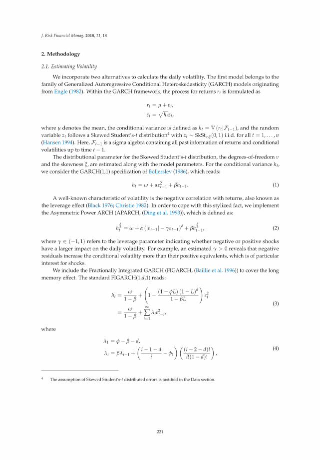
J. Risk Financial Manag. 2018, 11, 18
2. Methodology
2.1. Estimating Volatility
We incorporate two alternatives to calculate the daily volatility. The first model belongs to thefamily of Generalized Autoregressive Conditional Heteroskedasticity (GARCH) models originatingfrom Engle (1982). Within the GARCH framework, the process for returns rt is formulated as
rt = μ + εt,
εt =√
htzt,
where μ denotes the mean, the conditional variance is defined as ht = V (rt|Ft−1), and the randomvariable zt follows a Skewed Student’s-t distribution4 with zt ∼ SkStν,ξ(0, 1) i.i.d. for all t = 1, . . . , n(Hansen 1994). Here, Ft−1 is a sigma algebra containing all past information of returns and conditionalvolatilities up to time t − 1.
The distributional parameter for the Skewed Student’s-t distribution, the degrees-of-freedom ν
and the skewness ξ, are estimated along with the model parameters. For the conditional variance ht,we consider the GARCH(1,1) specification of Bollerslev (1986), which reads:
ht = ω + αε2t−1 + βht−1. (1)
A well-known characteristic of volatility is the negative correlation with returns, also known asthe leverage effect (Black 1976; Christie 1982). In order to cope with this stylized fact, we implementthe Asymmetric Power ARCH (APARCH, (Ding et al. 1993)), which is defined as:
hδ2t = ω + α (|εt−1| − γεt−1)
δ + βhδ2t−1, (2)
where γ ∈ (−1, 1) refers to the leverage parameter indicating whether negative or positive shockshave a larger impact on the daily volatility. For example, an estimated γ > 0 reveals that negativeresiduals increase the conditional volatility more than their positive equivalents, which is of particularinterest for shocks.
We include the Fractionally Integrated GARCH (FIGARCH, (Baillie et al. 1996)) to cover the longmemory effect. The standard FIGARCH(1,d,1) reads:
ht =ω
1 − β+
(1 − (1 − φL) (1 − L)d
1 − βL
)ε2
t
=ω
1 − β+
∞
∑i=1
λiε2t−i,
(3)
where
λ1 = φ − β − d,
λi = βλi−1 +
(i − 1 − d
i− φ1
)((i − 2 − d)!i!(1 − d)!
),
(4)
4 The assumption of Skewed Student’s-t distributed errors is justified in the Data section.
221
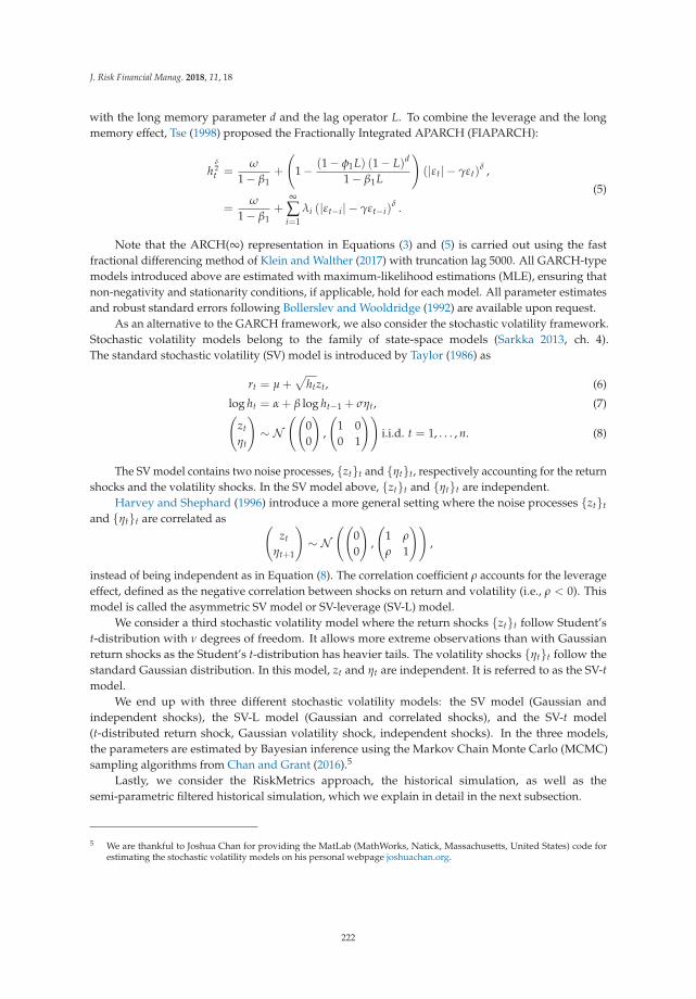
J. Risk Financial Manag. 2018, 11, 18
with the long memory parameter d and the lag operator L. To combine the leverage and the longmemory effect, Tse (1998) proposed the Fractionally Integrated APARCH (FIAPARCH):
hδ2t =
ω
1 − β1+
(1 − (1 − φ1L) (1 − L)d
1 − β1L
)(|εt| − γεt)
δ ,
=ω
1 − β1+
∞
∑i=1
λi (|εt−i| − γεt−i)δ .
(5)
Note that the ARCH(∞) representation in Equations (3) and (5) is carried out using the fastfractional differencing method of Klein and Walther (2017) with truncation lag 5000. All GARCH-typemodels introduced above are estimated with maximum-likelihood estimations (MLE), ensuring thatnon-negativity and stationarity conditions, if applicable, hold for each model. All parameter estimatesand robust standard errors following Bollerslev and Wooldridge (1992) are available upon request.
As an alternative to the GARCH framework, we also consider the stochastic volatility framework.Stochastic volatility models belong to the family of state-space models (Sarkka 2013, ch. 4).The standard stochastic volatility (SV) model is introduced by Taylor (1986) as
rt = μ +√
htzt, (6)
log ht = α + β log ht−1 + σηt, (7)(zt
ηt
)∼ N
((00
),
(1 00 1
))i.i.d. t = 1, . . . , n. (8)
The SV model contains two noise processes, {zt}t and {ηt}t, respectively accounting for the returnshocks and the volatility shocks. In the SV model above, {zt}t and {ηt}t are independent.
Harvey and Shephard (1996) introduce a more general setting where the noise processes {zt}t
and {ηt}t are correlated as (zt
ηt+1
)∼ N
((00
),
(1 ρ
ρ 1
)),
instead of being independent as in Equation (8). The correlation coefficient ρ accounts for the leverageeffect, defined as the negative correlation between shocks on return and volatility (i.e., ρ < 0). Thismodel is called the asymmetric SV model or SV-leverage (SV-L) model.
We consider a third stochastic volatility model where the return shocks {zt}t follow Student’st-distribution with ν degrees of freedom. It allows more extreme observations than with Gaussianreturn shocks as the Student’s t-distribution has heavier tails. The volatility shocks {ηt}t follow thestandard Gaussian distribution. In this model, zt and ηt are independent. It is referred to as the SV-tmodel.
We end up with three different stochastic volatility models: the SV model (Gaussian andindependent shocks), the SV-L model (Gaussian and correlated shocks), and the SV-t model(t-distributed return shock, Gaussian volatility shock, independent shocks). In the three models,the parameters are estimated by Bayesian inference using the Markov Chain Monte Carlo (MCMC)sampling algorithms from Chan and Grant (2016).5
Lastly, we consider the RiskMetrics approach, the historical simulation, as well as thesemi-parametric filtered historical simulation, which we explain in detail in the next subsection.
5 We are thankful to Joshua Chan for providing the MatLab (MathWorks, Natick, Massachusetts, United States) code forestimating the stochastic volatility models on his personal webpage joshuachan.org.
222
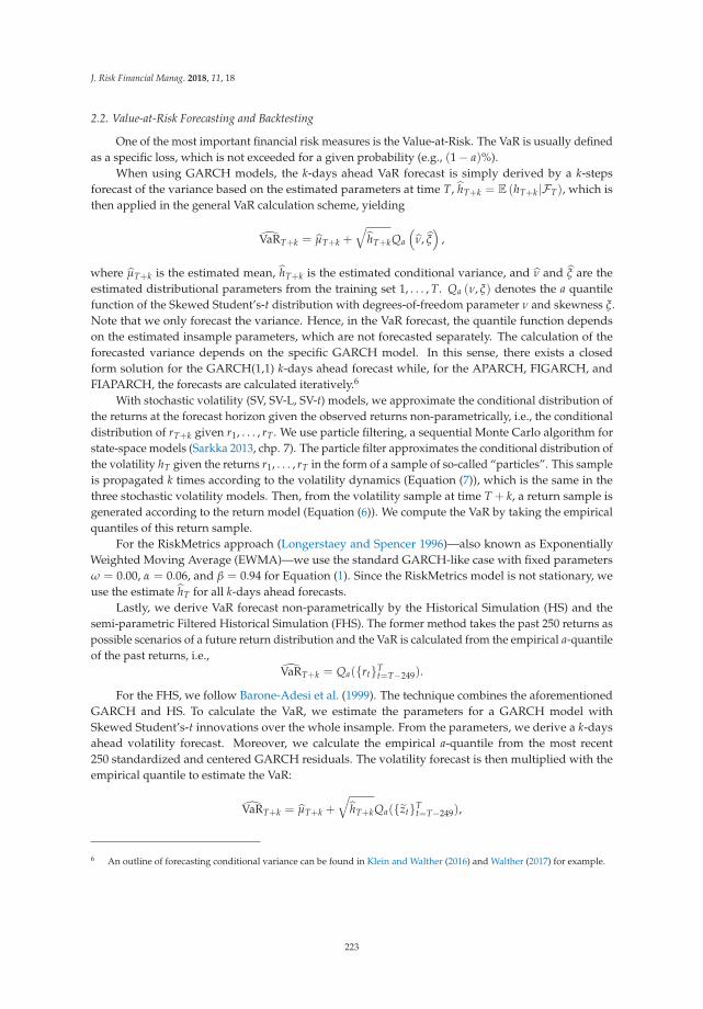
J. Risk Financial Manag. 2018, 11, 18
2.2. Value-at-Risk Forecasting and Backtesting
One of the most important financial risk measures is the Value-at-Risk. The VaR is usually definedas a specific loss, which is not exceeded for a given probability (e.g., (1 − a)%).
When using GARCH models, the k-days ahead VaR forecast is simply derived by a k-stepsforecast of the variance based on the estimated parameters at time T, hT+k = E (hT+k|FT), which isthen applied in the general VaR calculation scheme, yielding
VaRT+k = μT+k +
√hT+kQa
(ν, ξ
),
where μT+k is the estimated mean, hT+k is the estimated conditional variance, and ν and ξ are theestimated distributional parameters from the training set 1, . . . , T. Qa (ν, ξ) denotes the a quantilefunction of the Skewed Student’s-t distribution with degrees-of-freedom parameter ν and skewness ξ.Note that we only forecast the variance. Hence, in the VaR forecast, the quantile function dependson the estimated insample parameters, which are not forecasted separately. The calculation of theforecasted variance depends on the specific GARCH model. In this sense, there exists a closedform solution for the GARCH(1,1) k-days ahead forecast while, for the APARCH, FIGARCH, andFIAPARCH, the forecasts are calculated iteratively.6
With stochastic volatility (SV, SV-L, SV-t) models, we approximate the conditional distribution ofthe returns at the forecast horizon given the observed returns non-parametrically, i.e., the conditionaldistribution of rT+k given r1, . . . , rT . We use particle filtering, a sequential Monte Carlo algorithm forstate-space models (Sarkka 2013, chp. 7). The particle filter approximates the conditional distribution ofthe volatility hT given the returns r1, . . . , rT in the form of a sample of so-called “particles”. This sampleis propagated k times according to the volatility dynamics (Equation (7)), which is the same in thethree stochastic volatility models. Then, from the volatility sample at time T + k, a return sample isgenerated according to the return model (Equation (6)). We compute the VaR by taking the empiricalquantiles of this return sample.
For the RiskMetrics approach (Longerstaey and Spencer 1996)—also known as ExponentiallyWeighted Moving Average (EWMA)—we use the standard GARCH-like case with fixed parametersω = 0.00, α = 0.06, and β = 0.94 for Equation (1). Since the RiskMetrics model is not stationary, weuse the estimate hT for all k-days ahead forecasts.
Lastly, we derive VaR forecast non-parametrically by the Historical Simulation (HS) and thesemi-parametric Filtered Historical Simulation (FHS). The former method takes the past 250 returns aspossible scenarios of a future return distribution and the VaR is calculated from the empirical a-quantileof the past returns, i.e.,
VaRT+k = Qa({rt}Tt=T−249).
For the FHS, we follow Barone-Adesi et al. (1999). The technique combines the aforementionedGARCH and HS. To calculate the VaR, we estimate the parameters for a GARCH model withSkewed Student’s-t innovations over the whole insample. From the parameters, we derive a k-daysahead volatility forecast. Moreover, we calculate the empirical a-quantile from the most recent250 standardized and centered GARCH residuals. The volatility forecast is then multiplied with theempirical quantile to estimate the VaR:
VaRT+k = μT+k +
√hT+kQa({zt}T
t=T−249),
6 An outline of forecasting conditional variance can be found in Klein and Walther (2016) and Walther (2017) for example.
223
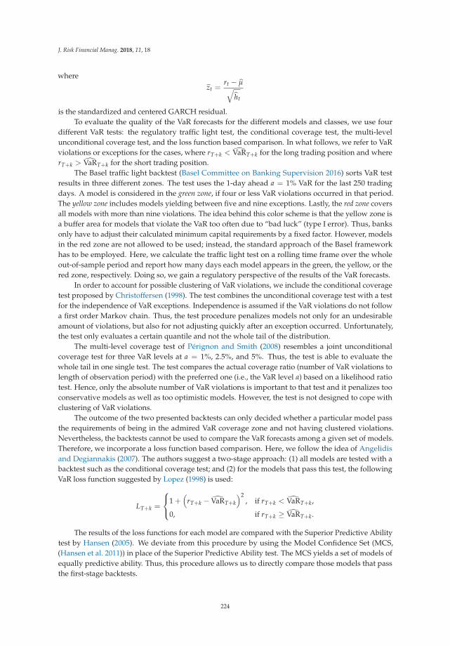
J. Risk Financial Manag. 2018, 11, 18
where
zt =rt − μ√
ht
is the standardized and centered GARCH residual.To evaluate the quality of the VaR forecasts for the different models and classes, we use four
different VaR tests: the regulatory traffic light test, the conditional coverage test, the multi-levelunconditional coverage test, and the loss function based comparison. In what follows, we refer to VaRviolations or exceptions for the cases, where rT+k < VaRT+k for the long trading position and whererT+k > VaRT+k for the short trading position.
The Basel traffic light backtest (Basel Committee on Banking Supervision 2016) sorts VaR testresults in three different zones. The test uses the 1-day ahead a = 1% VaR for the last 250 tradingdays. A model is considered in the green zone, if four or less VaR violations occurred in that period.The yellow zone includes models yielding between five and nine exceptions. Lastly, the red zone coversall models with more than nine violations. The idea behind this color scheme is that the yellow zone isa buffer area for models that violate the VaR too often due to “bad luck” (type I error). Thus, banksonly have to adjust their calculated minimum capital requirements by a fixed factor. However, modelsin the red zone are not allowed to be used; instead, the standard approach of the Basel frameworkhas to be employed. Here, we calculate the traffic light test on a rolling time frame over the wholeout-of-sample period and report how many days each model appears in the green, the yellow, or thered zone, respectively. Doing so, we gain a regulatory perspective of the results of the VaR forecasts.
In order to account for possible clustering of VaR violations, we include the conditional coveragetest proposed by Christoffersen (1998). The test combines the unconditional coverage test with a testfor the independence of VaR exceptions. Independence is assumed if the VaR violations do not followa first order Markov chain. Thus, the test procedure penalizes models not only for an undesirableamount of violations, but also for not adjusting quickly after an exception occurred. Unfortunately,the test only evaluates a certain quantile and not the whole tail of the distribution.
The multi-level coverage test of Pérignon and Smith (2008) resembles a joint unconditionalcoverage test for three VaR levels at a = 1%, 2.5%, and 5%. Thus, the test is able to evaluate thewhole tail in one single test. The test compares the actual coverage ratio (number of VaR violations tolength of observation period) with the preferred one (i.e., the VaR level a) based on a likelihood ratiotest. Hence, only the absolute number of VaR violations is important to that test and it penalizes tooconservative models as well as too optimistic models. However, the test is not designed to cope withclustering of VaR violations.
The outcome of the two presented backtests can only decided whether a particular model passthe requirements of being in the admired VaR coverage zone and not having clustered violations.Nevertheless, the backtests cannot be used to compare the VaR forecasts among a given set of models.Therefore, we incorporate a loss function based comparison. Here, we follow the idea of Angelidisand Degiannakis (2007). The authors suggest a two-stage approach: (1) all models are tested with abacktest such as the conditional coverage test; and (2) for the models that pass this test, the followingVaR loss function suggested by Lopez (1998) is used:
LT+k =
⎧⎨⎩1 +(
rT+k − VaRT+k
)2, if rT+k < VaRT+k,
0, if rT+k ≥ VaRT+k.
The results of the loss functions for each model are compared with the Superior Predictive Abilitytest by Hansen (2005). We deviate from this procedure by using the Model Confidence Set (MCS,(Hansen et al. 2011)) in place of the Superior Predictive Ability test. The MCS yields a set of models ofequally predictive ability. Thus, this procedure allows us to directly compare those models that passthe first-stage backtests.
224
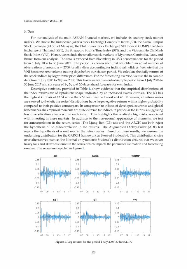
J. Risk Financial Manag. 2018, 11, 18
3. Data
For our analysis of the main ASEAN financial markets, we include six country stock marketindices. We choose the Indonesian Jakarta Stock Exchange Composite Index (JCI), the Kuala LumpurStock Exchange (KLSE) of Malaysia, the Philippines Stock Exchange PSEI Index (PCOMP), the StockExchange of Thailand (SET), the Singapore Strait’s Time Index (STI), and the Vietnam Ho Chi MinhStock Index (VNI). Hence, we exclude the smaller stock markets of Myanmar, Cambodia, Laos, andBrunei from our analysis. The data is retrieved from Bloomberg in USD denominations for the periodfrom 1 July 2006 to 30 June 2017. The period is chosen such that we obtain an equal number ofobservations of around n = 2700 for all indices accounting for individual holidays. We note that theVNI has some zero volume trading days before our chosen period. We calculate the daily returns ofthe stock indices by logarithmic price differences. For the forecasting exercise, we use the in-sampledata from 1 July 2006 to 30 June 2017. This leaves us with an out-of-sample period from 1 July 2006 to30 June 2017 and six years of 1-, 5-, and 20-days ahead forecasts for each index.
Descriptive statistics, provided in Table 1, show evidence that the empirical distributions ofthe index returns are of leptokurtic shape, indicated by an increased excess kurtosis. The JCI hasthe highest kurtosis of 12.54 while the VNI features the lowest at 4.46. Moreover, all return seriesare skewed to the left; the series’ distributions have large negative returns with a higher probabilitycompared to their positive counterpart. In comparison to indices of developed countries and globalbenchmarks, the empirical moments are quite extreme for indices, in particular the kurtosis, suggestingless diversification effects within each index. This highlights the relatively high risks associatedwith investing in these markets. In addition to the non-normal appearance of moments, we testfor autocorrelation in the return series. The Ljung–Box (LB) test and the ARCH test both rejectthe hypothesis of no autocorrelation in the returns. The Augmented Dickey-Fuller (ADF) testrejects the hypothesis of a unit root in the return series. Based on these results, we assume theunderlying distribution for the GARCH framework as Skewed Student’s-t. This distribution choiceover alternatives such as the Normal or symmetric Student’s-t distribution ensures that we coverheavy tails and skewness found in the series, which impacts the parameter estimation and forecastingexercise. The series are depicted in Figure 1.
07 09 11 13 15 17
-0.15
-0.1
-0.05
0
0.05
0.1
0.15
JCI
07 09 11 13 15 17
-0.15
-0.1
-0.05
0
0.05
0.1
0.15
KLSE
07 09 11 13 15 17
-0.15
-0.1
-0.05
0
0.05
0.1
0.15
PCOMP
07 09 11 13 15 17
-0.15
-0.1
-0.05
0
0.05
0.1
0.15
SET
07 09 11 13 15 17
-0.15
-0.1
-0.05
0
0.05
0.1
0.15
STI
07 09 11 13 15 17
-0.15
-0.1
-0.05
0
0.05
0.1
0.15
VNI
Figure 1. Log-returns for the period 1 July 2006–30 June 2017.
225
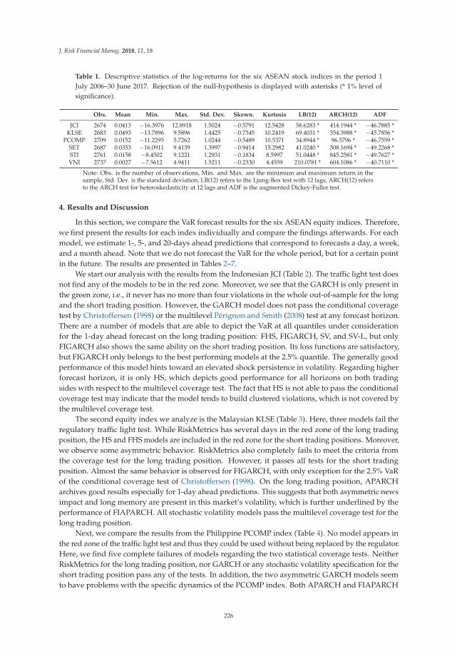
J. Risk Financial Manag. 2018, 11, 18
Table 1. Descriptive statistics of the log-returns for the six ASEAN stock indices in the period 1July 2006–30 June 2017. Rejection of the null-hypothesis is displayed with asterisks (* 1% level ofsignificance).
Obs. Mean Min. Max. Std. Dev. Skewn. Kurtosis LB(12) ARCH(12) ADF
JCI 2674 0.0413 −16.3976 12.8918 1.5024 −0.5791 12.5428 58.6283 * 414.1944 * −46.7885 *KLSE 2683 0.0493 −13.7896 9.5896 1.4425 −0.7345 10.2419 69.4031 * 354.3988 * −45.7856 *
PCOMP 2709 0.0152 −11.2295 5.7262 1.0244 −0.5489 10.5371 34.8944 * 96.5796 * −46.7559 *SET 2687 0.0353 −16.0911 9.4139 1.3997 −0.9414 15.2982 41.0240 * 308.1694 * −49.2268 *STI 2761 0.0158 −8.4502 9.1221 1.2931 −0.1834 8.5997 51.0448 * 845.2581 * −49.7627 *VNI 2737 0.0027 −7.5612 4.9411 1.5211 −0.2330 4.4559 210.0781 * 604.1086 * −40.7110 *
Note: Obs. is the number of observations, Min. and Max. are the minimum and maximum return in thesample, Std. Dev. is the standard deviation, LB(12) refers to the Ljung-Box test with 12 lags, ARCH(12) refersto the ARCH test for heteroskedasticity at 12 lags and ADF is the augmented Dickey-Fuller test.
4. Results and Discussion
In this section, we compare the VaR forecast results for the six ASEAN equity indices. Therefore,we first present the results for each index individually and compare the findings afterwards. For eachmodel, we estimate 1-, 5-, and 20-days ahead predictions that correspond to forecasts a day, a week,and a month ahead. Note that we do not forecast the VaR for the whole period, but for a certain pointin the future. The results are presented in Tables 2–7.
We start our analysis with the results from the Indonesian JCI (Table 2). The traffic light test doesnot find any of the models to be in the red zone. Moreover, we see that the GARCH is only present inthe green zone, i.e., it never has no more than four violations in the whole out-of-sample for the longand the short trading position. However, the GARCH model does not pass the conditional coveragetest by Christoffersen (1998) or the multilevel Pérignon and Smith (2008) test at any forecast horizon.There are a number of models that are able to depict the VaR at all quantiles under considerationfor the 1-day ahead forecast on the long trading position: FHS, FIGARCH, SV, and SV-L, but onlyFIGARCH also shows the same ability on the short trading position. Its loss functions are satisfactory,but FIGARCH only belongs to the best performing models at the 2.5% quantile. The generally goodperformance of this model hints toward an elevated shock persistence in volatility. Regarding higherforecast horizon, it is only HS, which depicts good performance for all horizons on both tradingsides with respect to the multilevel coverage test. The fact that HS is not able to pass the conditionalcoverage test may indicate that the model tends to build clustered violations, which is not covered bythe multilevel coverage test.
The second equity index we analyze is the Malaysian KLSE (Table 3). Here, three models fail theregulatory traffic light test. While RiskMetrics has several days in the red zone of the long tradingposition, the HS and FHS models are included in the red zone for the short trading positions. Moreover,we observe some asymmetric behavior. RiskMetrics also completely fails to meet the criteria fromthe coverage test for the long trading position. However, it passes all tests for the short tradingposition. Almost the same behavior is observed for FIGARCH, with only exception for the 2.5% VaRof the conditional coverage test of Christoffersen (1998). On the long trading position, APARCHarchives good results especially for 1-day ahead predictions. This suggests that both asymmetric newsimpact and long memory are present in this market’s volatility, which is further underlined by theperformance of FIAPARCH. All stochastic volatility models pass the multilevel coverage test for thelong trading position.
Next, we compare the results from the Philippine PCOMP index (Table 4). No model appears inthe red zone of the traffic light test and thus they could be used without being replaced by the regulator.Here, we find five complete failures of models regarding the two statistical coverage tests. NeitherRiskMetrics for the long trading position, nor GARCH or any stochastic volatility specification for theshort trading position pass any of the tests. In addition, the two asymmetric GARCH models seemto have problems with the specific dynamics of the PCOMP index. Both APARCH and FIAPARCH
226

J. Risk Financial Manag. 2018, 11, 18
perform very poorly with only a few passed tests. Generally, our model set does not include a clearcandidate to be preferred in terms of VaR prediction performance. However, the HS and the FHSdeliver the most promising results with respect to the multilevel test and the corresponding lossfunction results.
227
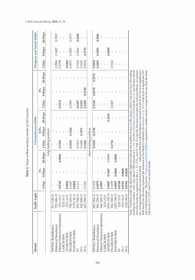
J. Risk Financial Manag. 2018, 11, 18
Ta
ble
2.
Val
ue-a
t-R
isk
back
test
resu
lts
for
JCIr
etur
ns.
Mo
de
lT
raffi
cL
igh
tC
hri
sto
ffe
rse
n(1
99
8)
Pé
rig
no
na
nd
Sm
ith
(20
08
)
1%
2.5
%5
%1
-Da
y5
-Da
ys
20
-Da
ys
1-D
ay
5-D
ay
s2
0-D
ay
s1
-Da
y5
-Da
ys
20
-Da
ys
1-D
ay
5-D
ay
s2
0-D
ay
s
long
trad
ing
posi
tion
EWM
A/R
iskM
etri
cs91
/112
0/0
−−
−−
−−
−−
−−
−−
His
tori
calS
imul
atio
n75
5/45
6/0
−−
−−
−−
−−
−0.
2996
0.30
070.
3053
Filt
ered
His
tori
calS
imul
atio
n12
11/0
/00
.07
40
−0
.08
68
0.1
52
6−
−0
.21
74
−−
0.27
58−
−G
AR
CH
-SkS
t12
11/0
/0−
−−
−−
−−
−−
−−
−A
PAR
CH
-SkS
t12
11/0
/00
.08
28
−−
−−
−−
−−
0.2
46
9−
−FI
GA
RC
H-S
kSt
758/
453/
00.
1047
−−
0.1
63
50
.15
26
−0.
2385
−−
0.30
750.
3007
0.31
73FI
APA
RC
H-S
kSt
1173
/38/
00
.08
28
−−
−−
−−
−−
−−
−SV
653/
558/
00.
1111
−−
0.18
13−
−0
.22
97
−−
0.31
300.
2961
0.2
69
5SV
-t36
2/84
9/0
−−
−0.
1696
0.1
57
1−
0.2
31
2−
−0.
3141
−−
SV-L
627/
584/
00.
1141
−−
0.1
52
6−
−0
.22
05
0.2
11
0−
0.29
140
.27
33
−sh
ortt
radi
ngpo
siti
on
EWM
A/R
iskM
etri
cs84
7/36
4/0
0.11
10−
−0
.16
55
0.1
73
6−
0.2
12
60
.21
74
0.2
17
40
.29
14
−−
His
tori
calS
imul
atio
n96
1/25
0/0
0.0
97
9−
−−
−−
−−
−0
.28
91
0.2
89
10
.29
26
Filt
ered
His
tori
calS
imul
atio
n94
6/26
5/0
0.0
90
7−
−−
−−
−−
−−
−−
GA
RC
H-S
kSt
1211
/0/0
−−
−−
−−
−−
−−
−−
APA
RC
H-S
kSt
1019
/192
/00
.09
07
0.1
04
70.
0944
−−
0.1
43
4−
−−
−0
.26
69
−FI
GA
RC
H-S
kSt
926/
285/
00.
1079
−−
0.1
71
6−
−0.
2427
−−
0.31
62−
−FI
APA
RC
H-S
kSt
1025
/186
/00
.09
07
0.0
86
80
.08
28
−−
−−
−−
−−
−SV
1211
/0/0
0.0
74
0−
−−
−−
−−
−−
−−
SV-t
1211
/0/0
0.0
78
50
.08
68
−−
−−
−−
−−
−−
SV-L
1152
/59/
00
.07
85
0.0
82
8−
−−
−−
−−
−−
−N
ote:
Nu
mbe
rsu
nder
the
Bas
eltr
affi
clig
htte
stin
dic
ate
the
num
ber
ofd
ays
inth
egr
een/
yello
w/
red
zone
for
a25
0ro
lling
trad
ing
day
win
dow
wit
h1-
day
ahea
dV
aRfo
reca
sts
ata=
1%.F
orth
eC
hris
toff
erse
n(1
998)
test
the
1-,5
-,an
d20
-day
sah
ead
fore
cast
sre
sult
sar
ere
port
edfo
rth
ea=
1%,2
.5%
,and
5%V
aR.I
fasp
ecifi
cte
stdo
esno
trej
ectt
henu
llhy
poth
esis
,we
pres
ent
the
corr
espo
ndin
gV
aRlo
ssfu
ncti
onre
sult
.−in
dic
ates
that
the
null
hypo
thes
isis
reje
cted
atle
asta
t10%
leve
lofs
igni
fican
ce.
Bold
face
dlo
ssfu
ncti
ons
repr
esen
tthe
incl
usio
nin
the
Mod
elC
onfid
ence
Set(
Han
sen
etal
.201
1)w
ith
leve
lofs
igni
fican
t10%
and
10,0
00bo
otst
raps
.The
test
byPé
rign
onan
dSm
ith
(200
8)is
repo
rted
ina
sim
ilar
man
ner,
exce
ptfo
rth
efa
ctth
atth
eth
ree
VaR
leve
ls(1
%,2
.5%
,and
5%)a
rete
sted
join
tly.
228
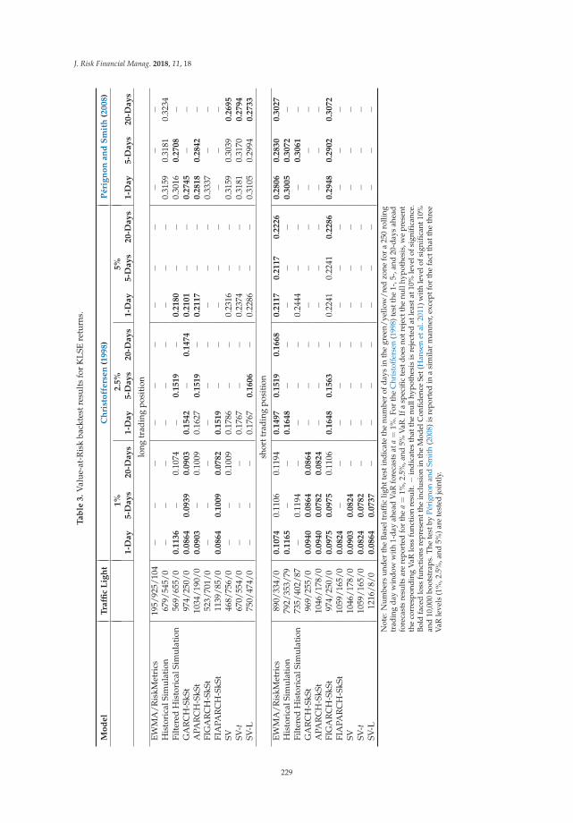
J. Risk Financial Manag. 2018, 11, 18
Ta
ble
3.
Val
ue-a
t-R
isk
back
test
resu
lts
for
KLS
Ere
turn
s.
Mo
de
lT
raffi
cL
igh
tC
hri
sto
ffe
rse
n(1
99
8)
Pé
rig
no
na
nd
Sm
ith
(20
08
)
1%
2.5
%5
%1
-Da
y5
-Da
ys
20
-Da
ys
1-D
ay
5-D
ay
s2
0-D
ay
s1
-Da
y5
-Da
ys
20
-Da
ys
1-D
ay
5-D
ay
s2
0-D
ay
s
long
trad
ing
posi
tion
EWM
A/R
iskM
etri
cs19
5/92
5/10
4−
−−
−−
−−
−−
−−
−H
isto
rica
lSim
ulat
ion
679/
545/
0−
−−
−−
−−
−−
0.31
590.
3181
0.32
34Fi
lter
edH
isto
rica
lSim
ulat
ion
569/
655/
00
.11
36
−0.
1074
−0
.15
19
−0
.21
80
−−
0.30
160
.27
08
−G
AR
CH
-SkS
t97
4/25
0/0
0.0
86
40
.09
39
0.0
90
30
.15
42
−0
.14
74
0.2
10
1−
−0
.27
45
−−
APA
RC
H-S
kSt
1034
/190
/00
.09
03
−0.
1009
0.16
270
.15
19
−0
.21
17
−−
0.2
81
80
.28
42
−FI
GA
RC
H-S
kSt
523/
701/
0−
−−
−−
−−
−−
0.33
37−
−FI
APA
RC
H-S
kSt
1139
/85/
00
.08
64
0.1
00
90
.07
82
0.1
51
9−
−−
−−
−−
−SV
468/
756/
0−
−0.
1009
0.17
86−
−0.
2316
−−
0.31
590.
3039
0.2
69
5SV
-t67
0/55
4/0
−−
−0.
1767
−−
0.23
74−
−0.
3181
0.31
700
.27
94
SV-L
750/
474/
0−
−−
0.17
670
.16
06
−0.
2286
−−
0.31
050.
2994
0.2
73
3
shor
ttra
ding
posi
tion
EWM
A/R
iskM
etri
cs89
0/33
4/0
0.1
07
40.
1106
0.11
940
.14
97
0.1
51
90
.16
68
0.2
11
70
.21
17
0.2
22
60
.28
06
0.2
83
00
.30
27
His
tori
calS
imul
atio
n79
2/35
3/79
0.1
16
5−
−0
.16
48
−−
−−
−0
.30
05
0.3
07
2−
Filt
ered
His
tori
calS
imul
atio
n73
5/40
2/87
−0.
1194
−−
−−
0.24
44−
−−
0.3
06
1−
GA
RC
H-S
kSt
969/
255/
00
.09
40
0.0
86
40
.08
64
−−
−−
−−
−−
−A
PAR
CH
-SkS
t10
46/1
78/0
0.0
94
00
.07
82
0.0
82
4−
−−
−−
−−
−−
FIG
AR
CH
-SkS
t97
4/25
0/0
0.0
97
50
.09
75
0.11
060
.16
48
0.1
56
3−
0.22
410.
2241
0.2
28
60
.29
48
0.2
90
20
.30
72
FIA
PAR
CH
-SkS
t10
59/1
65/0
0.0
82
4−
−−
−−
−−
−−
−−
SV10
46/1
78/0
0.0
90
30
.08
24
−−
−−
−−
−−
−−
SV-t
1059
/165
/00
.08
24
0.0
78
2−
−−
−−
−−
−−
−SV
-L12
16/8
/00
.08
64
0.0
73
7−
−−
−−
−−
−−
−N
ote:
Nu
mbe
rsu
nder
the
Bas
eltr
affi
clig
htte
stin
dic
ate
the
num
ber
ofd
ays
inth
egr
een/
yello
w/
red
zone
for
a25
0ro
lling
trad
ing
day
win
dow
wit
h1-
day
ahea
dV
aRfo
reca
sts
ata=
1%.F
orth
eC
hris
toff
erse
n(1
998)
test
the
1-,5
-,an
d20
-day
sah
ead
fore
cast
sre
sult
sar
ere
port
edfo
rth
ea=
1%,2
.5%
,and
5%V
aR.I
fasp
ecifi
cte
stdo
esno
trej
ectt
henu
llhy
poth
esis
,we
pres
ent
the
corr
espo
ndin
gV
aRlo
ssfu
ncti
onre
sult
.−in
dic
ates
that
the
null
hypo
thes
isis
reje
cted
atle
asta
t10%
leve
lofs
igni
fican
ce.
Bold
face
dlo
ssfu
ncti
ons
repr
esen
tthe
incl
usio
nin
the
Mod
elC
onfid
ence
Set(
Han
sen
etal
.201
1)w
ith
leve
lofs
igni
fican
t10%
and
10,0
00bo
otst
raps
.The
test
byPé
rign
onan
dSm
ith
(200
8)is
repo
rted
ina
sim
ilar
man
ner,
exce
ptfo
rth
efa
ctth
atth
eth
ree
VaR
leve
ls(1
%,2
.5%
,and
5%)a
rete
sted
join
tly.
229
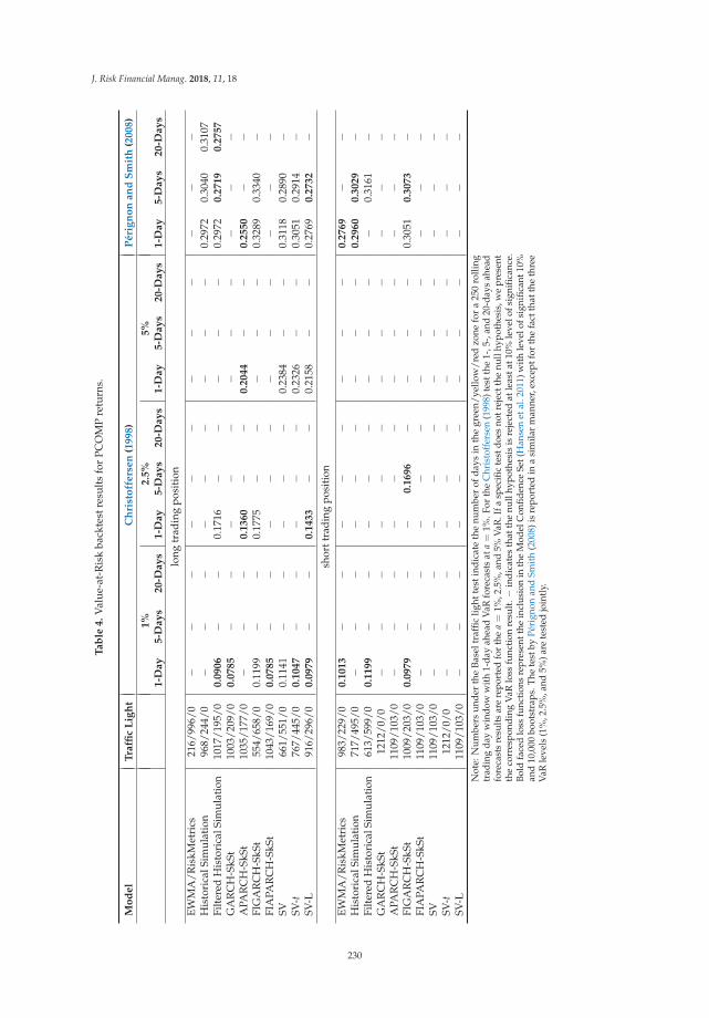
J. Risk Financial Manag. 2018, 11, 18
Ta
ble
4.
Val
ue-a
t-R
isk
back
test
resu
lts
for
PCO
MP
retu
rns.
Mo
de
lT
raffi
cL
igh
tC
hri
sto
ffe
rse
n(1
99
8)
Pé
rig
no
na
nd
Sm
ith
(20
08
)
1%
2.5
%5
%1
-Da
y5
-Da
ys
20
-Da
ys
1-D
ay
5-D
ay
s2
0-D
ay
s1
-Da
y5
-Da
ys
20
-Da
ys
1-D
ay
5-D
ay
s2
0-D
ay
s
long
trad
ing
posi
tion
EWM
A/R
iskM
etri
cs21
6/99
6/0
−−
−−
−−
−−
−−
−−
His
tori
calS
imul
atio
n96
8/24
4/0
−−
−−
−−
−−
−0.
2972
0.30
400.
3107
Filt
ered
His
tori
calS
imul
atio
n10
17/1
95/0
0.0
90
6−
−0.
1716
−−
−−
−0.
2972
0.2
71
90
.27
57
GA
RC
H-S
kSt
1003
/209
/00
.07
85
−−
−−
−−
−−
−−
−A
PAR
CH
-SkS
t10
35/1
77/0
−−
−0
.13
60
−−
0.2
04
4−
−0
.25
50
−−
FIG
AR
CH
-SkS
t55
4/65
8/0
0.11
99−
−0.
1775
−−
−−
−0.
3289
0.33
40−
FIA
PAR
CH
-SkS
t10
43/1
69/0
0.0
78
5−
−−
−−
−−
−−
−−
SV66
1/55
1/0
0.11
41−
−−
−−
0.23
84−
−0.
3118
0.28
90−
SV-t
767/
445/
00
.10
47
−−
−−
−0.
2326
−−
0.30
510.
2914
−SV
-L91
6/29
6/0
0.0
97
9−
−0
.14
33
−−
0.21
58−
−0.
2769
0.2
73
2−
shor
ttra
ding
posi
tion
EWM
A/R
iskM
etri
cs98
3/22
9/0
0.1
01
3−
−−
−−
−−
−0
.27
69
−−
His
tori
calS
imul
atio
n71
7/49
5/0
−−
−−
−−
−−
−0
.29
60
0.3
02
9−
Filt
ered
His
tori
calS
imul
atio
n61
3/59
9/0
0.1
19
9−
−−
−−
−−
−−
0.31
61−
GA
RC
H-S
kSt
1212
/0/0
−−
−−
−−
−−
−−
−−
APA
RC
H-S
kSt
1109
/103
/0−
−−
−−
−−
−−
−−
−FI
GA
RC
H-S
kSt
1009
/203
/00
.09
79
−−
−0
.16
96
−−
−−
0.30
510
.30
73
−FI
APA
RC
H-S
kSt
1109
/103
/0−
−−
−−
−−
−−
−−
−SV
1109
/103
/0−
−−
−−
−−
−−
−−
−SV
-t12
12/0
/0−
−−
−−
−−
−−
−−
−SV
-L11
09/1
03/0
−−
−−
−−
−−
−−
−−
Not
e:N
um
bers
und
erth
eB
asel
traf
fic
light
test
ind
icat
eth
enu
mbe
rof
day
sin
the
gree
n/ye
llow
/re
dzo
nefo
ra
250
rolli
ngtr
adin
gda
yw
indo
ww
ith
1-da
yah
ead
VaR
fore
cast
sat
a=
1%.F
orth
eC
hris
toff
erse
n(1
998)
test
the
1-,5
-,an
d20
-day
sah
ead
fore
cast
sre
sult
sar
ere
port
edfo
rth
ea=
1%,2
.5%
,and
5%V
aR.I
fasp
ecifi
cte
stdo
esno
trej
ectt
henu
llhy
poth
esis
,we
pres
ent
the
corr
espo
ndin
gV
aRlo
ssfu
ncti
onre
sult
.−in
dic
ates
that
the
null
hypo
thes
isis
reje
cted
atle
asta
t10%
leve
lofs
igni
fican
ce.
Bold
face
dlo
ssfu
ncti
ons
repr
esen
tthe
incl
usio
nin
the
Mod
elC
onfid
ence
Set(
Han
sen
etal
.201
1)w
ith
leve
lofs
igni
fican
t10%
and
10,0
00bo
otst
raps
.The
test
byPé
rign
onan
dSm
ith
(200
8)is
repo
rted
ina
sim
ilar
man
ner,
exce
ptfo
rth
efa
ctth
atth
eth
ree
VaR
leve
ls(1
%,2
.5%
,and
5%)a
rete
sted
join
tly.
230
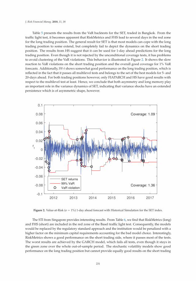
J. Risk Financial Manag. 2018, 11, 18
Table 5 presents the results from the VaR backtests for the SET, traded in Bangkok. From thetraffic light test, it becomes apparent that RiskMetrics and FHS lead to several days in the red zonefor the long trading position. The general result for SET is that most models can cope with the longtrading position to some extend, but completely fail to depict the dynamics on the short tradingposition. The results from HS suggest that it can be used for 1-day ahead predictions for the longtrading position. Even though it is not rejected by the unconditional coverage tests, it has problemsto avoid clustering of the VaR violations. This behavior is illustrated in Figure 2. It shows the slowreaction to VaR violations on the short trading position and the overall good coverage for 1% VaRforecasts. Additionally, SV-t shows somewhat good performance on the long trading position, which isreflected in the fact that it passes all multilevel tests and belongs to the set of the best models for 5- and20-days ahead. For both trading positions however, only FIAPARCH and HS have good results withrespect to the multilevel test at least. Hence, we conclude that both asymmetry and long memory playan important role in the variance dynamics of SET, indicating that variance shocks have an extendedpersistence which is of asymmetric shape, however.
2012 2013 2014 2015 2016 2017
rt
-0.1
-0.08
-0.06
-0.04
-0.02
0
0.02
0.04
0.06
0.08
0.1
Coverage: 1.36
Coverage: 1.09
SET returns99% VaRVaR violation
Figure 2. Value-at-Risk (a = 1%) 1-day ahead forecast with Historical Simulation for the SET index.
The STI from Singapore provides interesting results. From Table 6, we find that RiskMetrics (long)and FHS (short) are included in the red zone of the Basel traffic light test. Consequently, the modelswould be replaced by the regulatory standard approach and the institution would be penalized with ahigher factor on the minimum capital requirements accounting for the bad model choice. Interestingly,RiskMetrics shows a good performance on the short trading side, where it passes most of the tests.The worst results are achieved by the GARCH model, which fails all tests, even though it stays inthe green zone over the whole out-of-sample period. The stochastic volatility models show goodperformance on the long trading position but cannot provide equally good results on the short trading
231
J. Risk Financial Manag. 2018, 11, 18
position. APARCH provides very good results for both trading positions regarding 1-day aheadforecasts, which indicates that asymmetries play an important role in the STI return structure.
Lastly, we compare the forecasting results for the Vietnamese equity index VNI (Table 7).Within our model set, which includes very widely used VaR estimation procedures, only the SV modelprovides an average to good performance. All other models are either in the red zone (RiskMetrics, FHS,FIGARCH) or fail most of the statistical coverage tests (GARCH, APARCH, FIAPARCH). The models inthe red zone, however, are only included for one trading side. For the long trading position, FIGARCHand FHS provide good results from the coverage tests. The stochastic volatility models show verygood performance for 1- and 5-days ahead predictions on the long trading position and belong to themodel confidence set at every test they pass.
Finally, we compare all results from the six different equity indices of Indonesia, Malaysia,Philippines, Singapore, Thailand, and Vietnam. GARCH seems to be regulator’s darling with respectto the traffic light characterization. Although popular, it fails almost all statistical coverage tests, while,for most indices, it is 100% of the time in the green zone of the traffic light test. This indicates that themodel yields too conservative VaR forecast, which would result in particularly high minimum capitalrequirements. In addition, the very popular RiskMetrics model shows poor performance. McMillanand Kambouroudis (2009) concludes that the model only performs well in small markets and highVaR quantiles. Our findings suggest that the selected six markets in this paper may already be too bigfor the RiskMetrics approach. Interestingly, the HS is rarely rejected by the multilevel coverage test,i.e., regardless of the specific forecast horizon, it provides sufficient coverage ratios. However, it is notable to provide satisfying results for the conditional coverage test in all indices. This might be due tothe slow adaption of shocks resulting in clustering of violations. The SV model specifications providea framework with a good overall performance at all markets, but only on the long trading position.However, especially for shorter forecast horizons, the SV models belong to the model confidence sets.
Comparing the model performance for each index, we find evidence that the markets in ouranalyzed group are heterogeneous with respect to their volatility properties. For example, STI isdominated by asymmetric effects and long memory models are rejected by our coverage tests while,for the VNI, long memory models show a good forecasting performance and asymmetric modelsare rejected.
232
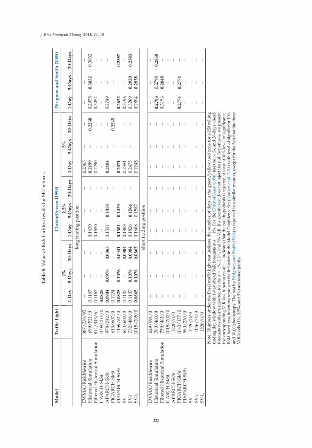
J. Risk Financial Manag. 2018, 11, 18
Ta
ble
5.
Val
ue-a
t-R
isk
back
test
resu
lts
for
SET
retu
rns.
Mo
de
lT
raffi
cL
igh
tC
hri
sto
ffe
rse
n(1
99
8)
Pé
rig
no
na
nd
Sm
ith
(20
08
)
1%
2.5
%5
%1
-Da
y5
-Da
ys
20
-Da
ys
1-D
ay
5-D
ay
s2
0-D
ay
s1
-Da
y5
-Da
ys
20
-Da
ys
1-D
ay
5-D
ay
s2
0-D
ay
s
long
trad
ing
posi
tion
EWM
A/R
iskM
etri
cs38
7/73
8/95
−−
−−
−−
0.23
63−
−−
−−
His
tori
calS
imul
atio
n69
9/52
1/0
0.11
67−
−0.
1630
−−
0.2
19
9−
0.2
26
00.
2975
0.3
03
20.
3032
Filt
ered
His
tori
calS
imul
atio
n81
4/34
5/61
0.11
67−
−0.
1650
−−
0.22
90−
−0.
3054
−−
GA
RC
H-S
kSt
1009
/211
/00
.08
25
−−
−−
−−
−−
−−
−A
PAR
CH
-SkS
t97
8/24
2/0
0.0
90
40
.09
76
0.0
86
50.
1521
0.1
45
3−
0.2
10
4−
−0.
2749
−−
FIG
AR
CH
-SkS
t61
3/60
7/0
0.12
24−
−−
−−
−−
0.2
24
5−
−−
FIA
PAR
CH
-SkS
t11
59/6
1/0
0.0
82
50
.10
76
0.0
94
10
.13
81
0.1
42
9−
0.2
07
1−
−0
.26
22
−0
.25
57
SV62
0/60
0/0
0.11
07−
0.0
90
40.
1808
−−
0.23
91−
−0.
3196
−−
SV-t
732/
488/
00.
1107
0.1
07
60
.09
04
0.18
260
.15
66
−0.
2475
−−
0.32
690
.29
29
0.2
58
3SV
-L10
15/2
05/0
0.0
86
50
.10
76
0.0
86
50.
1608
0.15
87−
0.22
45−
−0.
2894
0.2
85
8−
shor
ttra
ding
posi
tion
EWM
A/R
iskM
etri
cs62
9/59
1/0
−−
−−
−−
−−
−−
−−
His
tori
calS
imul
atio
n76
0/46
0/0
−−
−−
−−
−−
−0
.27
98
0.27
980
.28
58
Filt
ered
His
tori
calS
imul
atio
n75
9/46
1/0
−−
−−
−−
−−
−0.
3196
0.2
64
8−
GA
RC
H-S
kSt
1018
/202
/0−
−−
−−
−−
−−
−−
−A
PAR
CH
-SkS
t12
20/0
/0−
−−
−−
−−
−−
−−
−FI
GA
RC
H-S
kSt
1043
/177
/0−
−−
−−
−−
−−
0.2
77
40
.27
74
−FI
APA
RC
H-S
kSt
990/
230/
0−
−−
−−
−−
−−
−−
−SV
1220
/0/0
−−
−−
−−
−−
−−
−−
SV-t
1146
/74/
0−
−−
−−
−−
−−
−−
−SV
-L12
20/0
/0−
−−
−−
−−
−−
−−
−N
ote:
Nu
mbe
rsu
nder
the
Bas
eltr
affi
clig
htte
stin
dic
ate
the
num
ber
ofd
ays
inth
egr
een/
yello
w/
red
zone
for
a25
0ro
lling
trad
ing
day
win
dow
wit
h1-
day
ahea
dV
aRfo
reca
sts
ata=
1%.F
orth
eC
hris
toff
erse
n(1
998)
test
the
1-,5
-,an
d20
-day
sah
ead
fore
cast
sre
sult
sar
ere
port
edfo
rth
ea=
1%,2
.5%
,and
5%V
aR.I
fasp
ecifi
cte
stdo
esno
trej
ectt
henu
llhy
poth
esis
,we
pres
ent
the
corr
espo
ndin
gV
aRlo
ssfu
ncti
onre
sult
.−in
dic
ates
that
the
null
hypo
thes
isis
reje
cted
atle
asta
t10%
leve
lofs
igni
fican
ce.
Bold
face
dlo
ssfu
ncti
ons
repr
esen
tthe
incl
usio
nin
the
Mod
elC
onfid
ence
Set(
Han
sen
etal
.201
1)w
ith
leve
lofs
igni
fican
t10%
and
10,0
00bo
otst
raps
.The
test
byPé
rign
onan
dSm
ith
(200
8)is
repo
rted
ina
sim
ilar
man
ner,
exce
ptfo
rth
efa
ctth
atth
eth
ree
VaR
leve
ls(1
%,2
.5%
,and
5%)a
rete
sted
join
tly.
233
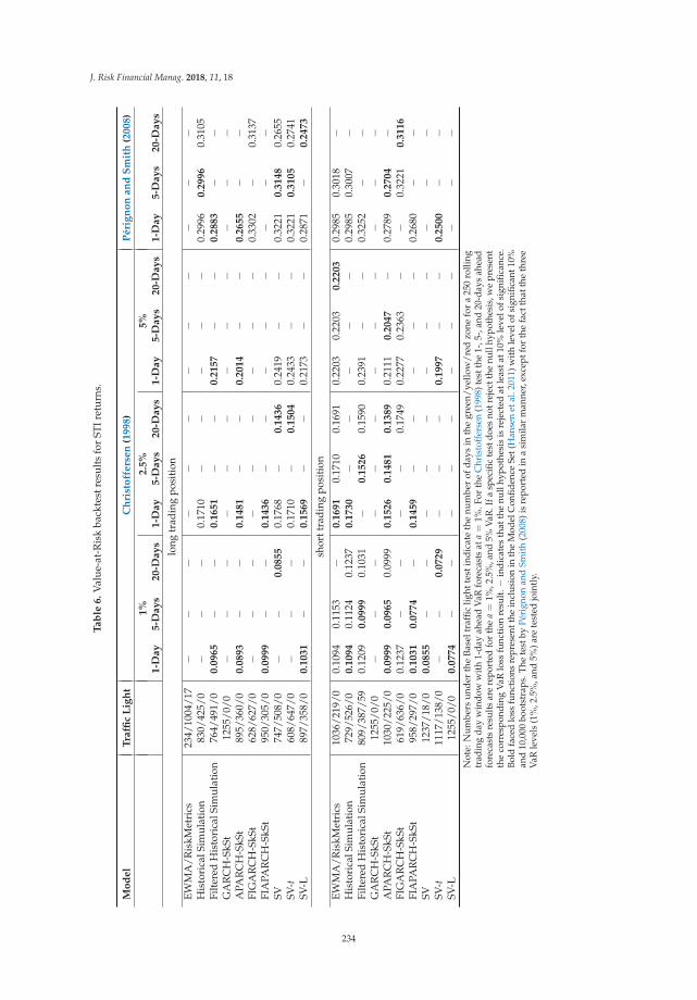
J. Risk Financial Manag. 2018, 11, 18
Ta
ble
6.
Val
ue-a
t-R
isk
back
test
resu
lts
for
STIr
etur
ns.
Mo
de
lT
raffi
cL
igh
tC
hri
sto
ffe
rse
n(1
99
8)
Pé
rig
no
na
nd
Sm
ith
(20
08
)
1%
2.5
%5
%1
-Da
y5
-Da
ys
20
-Da
ys
1-D
ay
5-D
ay
s2
0-D
ay
s1
-Da
y5
-Da
ys
20
-Da
ys
1-D
ay
5-D
ay
s2
0-D
ay
s
long
trad
ing
posi
tion
EWM
A/R
iskM
etri
cs23
4/10
04/1
7−
−−
−−
−−
−−
−−
−H
isto
rica
lSim
ulat
ion
830/
425/
0−
−−
0.17
10−
−−
−−
0.29
960
.29
96
0.31
05Fi
lter
edH
isto
rica
lSim
ulat
ion
764/
491/
00
.09
65
−−
0.1
65
1−
−0
.21
57
−−
0.2
88
3−
−G
AR
CH
-SkS
t12
55/0
/0−
−−
−−
−−
−−
−−
−A
PAR
CH
-SkS
t89
5/36
0/0
0.0
89
3−
−0
.14
81
−−
0.2
01
4−
−0
.26
55
−−
FIG
AR
CH
-SkS
t62
8/62
7/0
−−
−−
−−
−−
−0.
3302
−0.
3137
FIA
PAR
CH
-SkS
t95
0/30
5/0
0.0
99
9−
−0
.14
36
−−
−−
−−
−−
SV74
7/50
8/0
−−
0.0
85
50.
1768
−0
.14
36
0.24
19−
−0.
3221
0.3
14
80.
2655
SV-t
608/
647/
0−
−−
0.17
10−
0.1
50
40.
2433
−−
0.32
210
.31
05
0.27
41SV
-L89
7/35
8/0
0.1
03
1−
−0
.15
69
−−
0.21
73−
−0.
2871
−0
.24
73
shor
ttra
ding
posi
tion
EWM
A/R
iskM
etri
cs10
36/2
19/0
0.10
940.
1153
−0
.16
91
0.17
100.
1691
0.22
030.
2203
0.2
20
30.
2985
0.30
18−
His
tori
calS
imul
atio
n72
9/52
6/0
0.1
09
40.
1124
0.12
370
.17
30
−−
−−
−0.
2985
0.30
07−
Filt
ered
His
tori
calS
imul
atio
n80
9/38
7/59
0.12
090
.09
99
0.10
31−
0.1
52
60.
1590
0.23
91−
−0.
3252
−−
GA
RC
H-S
kSt
1255
/0/0
−−
−−
−−
−−
−−
−−
APA
RC
H-S
kSt
1030
/225
/00
.09
99
0.0
96
50.
0999
0.1
52
60
.14
81
0.1
38
90.
2111
0.2
04
7−
0.27
890
.27
04
−FI
GA
RC
H-S
kSt
619/
636/
00.
1237
−−
−−
0.17
490.
2277
0.23
63−
−0.
3221
0.3
11
6FI
APA
RC
H-S
kSt
958/
297/
00
.10
31
0.0
77
4−
0.1
45
9−
−−
−−
0.26
80−
−SV
1237
/18/
00
.08
55
−−
−−
−−
−−
−−
−SV
-t11
17/1
38/0
−−
0.0
72
9−
−−
0.1
99
7−
−0
.25
00
−−
SV-L
1255
/0/0
0.0
77
4−
−−
−−
−−
−−
−−
Not
e:N
um
bers
und
erth
eB
asel
traf
fic
light
test
ind
icat
eth
enu
mbe
rof
day
sin
the
gree
n/ye
llow
/re
dzo
nefo
ra
250
rolli
ngtr
adin
gda
yw
indo
ww
ith
1-da
yah
ead
VaR
fore
cast
sat
a=
1%.F
orth
eC
hris
toff
erse
n(1
998)
test
the
1-,5
-,an
d20
-day
sah
ead
fore
cast
sre
sult
sar
ere
port
edfo
rth
ea=
1%,2
.5%
,and
5%V
aR.I
fasp
ecifi
cte
stdo
esno
trej
ectt
henu
llhy
poth
esis
,we
pres
ent
the
corr
espo
ndin
gV
aRlo
ssfu
ncti
onre
sult
.−in
dic
ates
that
the
null
hypo
thes
isis
reje
cted
atle
asta
t10%
leve
lofs
igni
fican
ce.
Bold
face
dlo
ssfu
ncti
ons
repr
esen
tthe
incl
usio
nin
the
Mod
elC
onfid
ence
Set(
Han
sen
etal
.201
1)w
ith
leve
lofs
igni
fican
t10%
and
10,0
00bo
otst
raps
.The
test
byPé
rign
onan
dSm
ith
(200
8)is
repo
rted
ina
sim
ilar
man
ner,
exce
ptfo
rth
efa
ctth
atth
eth
ree
VaR
leve
ls(1
%,2
.5%
,and
5%)a
rete
sted
join
tly.
234
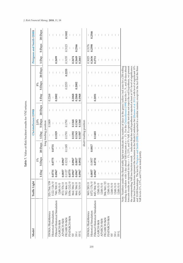
J. Risk Financial Manag. 2018, 11, 18
Ta
ble
7.
Val
ue-a
t-R
isk
back
test
resu
lts
for
VN
Iret
urns
.
Mo
de
lT
raffi
cL
igh
tC
hri
sto
ffe
rse
n(1
99
8)
Pé
rig
no
na
nd
Sm
ith
(20
08
)
1%
2.5
%5
%1
-Da
y5
-Da
ys
20
-Da
ys
1-D
ay
5-D
ay
s2
0-D
ay
s1
-Da
y5
-Da
ys
20
-Da
ys
1-D
ay
5-D
ay
s2
0-D
ay
s
long
trad
ing
posi
tion
EWM
A/R
iskM
etri
cs32
5/76
4/15
9−
−−
−0.
1809
−0.
2268
−−
−−
−H
isto
rica
lSim
ulat
ion
1122
/126
/00
.07
31
0.0
77
50
.07
31
−−
−−
−−
−−
−Fi
lter
edH
isto
rica
lSim
ulat
ion
748/
500/
00
.09
67
−−
0.1
52
9−
−0
.20
02
−−
0.2
69
9−
−G
AR
CH
-SkS
t12
48/0
/0−
−−
−−
−−
−−
−−
−A
PAR
CH
-SkS
t87
2/37
6/0
0.0
85
70
.09
67
−−
−−
−−
−−
−−
FIG
AR
CH
-SkS
t78
2/46
6/0
0.11
270.
1212
0.11
850.
1791
0.17
91−
−0.
2253
0.2
25
30.
3155
0.31
230
.31
02
FIA
PAR
CH
-SkS
t10
36/2
12/0
0.0
77
5−
−−
−−
−−
−−
−−
SV86
4/38
4/0
0.0
96
70
.09
67
−0
.13
92
0.1
36
8−
0.2
06
8−
−0
.26
74
−−
SV-t
864/
384/
00
.09
67
0.0
81
7−
0.1
34
30
.13
43
−0
.20
68
0.2
00
2−
0.2
64
90
.25
46
−SV
-L92
9/31
9/0
0.0
96
70
.09
32
−0
.15
07
0.1
36
8−
0.1
96
8−
−0
.26
61
−−
shor
ttra
ding
posi
tion
EWM
A/R
iskM
etri
cs96
5/28
3/0
−−
−−
−−
−−
−0.
3025
0.31
76−
His
tori
calS
imul
atio
n10
72/1
76/0
0.0
85
70.
0857
0.0
81
7−
−−
−−
−0
.26
36
0.2
59
80
.25
46
Filt
ered
His
tori
calS
imul
atio
n84
5/38
4/19
0.0
96
70
.07
31
−0
.14
85
−−
0.2
05
1−
−0
.27
11
−−
GA
RC
H-S
kSt
1248
/0/0
−−
−−
−−
−−
−−
−−
APA
RC
H-S
kSt
1248
/0/0
−−
−−
−−
−−
−−
−−
FIG
AR
CH
-SkS
t38
4/84
1/23
−−
−−
−−
−−
−−
−−
FIA
PAR
CH
-SkS
t12
48/0
/0−
−−
−−
−−
−−
−−
−SV
1248
/0/0
−−
−−
−−
−−
−−
−−
SV-t
1248
/0/0
−−
−−
−−
−−
−−
−−
SV-L
1248
/0/0
−−
−−
−−
−−
−−
−−
Not
e:N
um
bers
und
erth
eB
asel
traf
fic
light
test
ind
icat
eth
enu
mbe
rof
day
sin
the
gree
n/ye
llow
/re
dzo
nefo
ra
250
rolli
ngtr
adin
gda
yw
indo
ww
ith
1-da
yah
ead
VaR
fore
cast
sat
a=
1%.F
orth
eC
hris
toff
erse
n(1
998)
test
the
1-,5
-,an
d20
-day
sah
ead
fore
cast
sre
sult
sar
ere
port
edfo
rth
ea=
1%,2
.5%
,and
5%V
aR.I
fasp
ecifi
cte
stdo
esno
trej
ectt
henu
llhy
poth
esis
,we
pres
ent
the
corr
espo
ndin
gV
aRlo
ssfu
ncti
onre
sult
.−in
dic
ates
that
the
null
hypo
thes
isis
reje
cted
atle
asta
t10%
leve
lofs
igni
fican
ce.
Bold
face
dlo
ssfu
ncti
ons
repr
esen
tthe
incl
usio
nin
the
Mod
elC
onfid
ence
Set(
Han
sen
etal
.201
1)w
ith
leve
lofs
igni
fican
t10%
and
10,0
00bo
otst
raps
.The
test
byPé
rign
onan
dSm
ith
(200
8)is
repo
rted
ina
sim
ilar
man
ner,
exce
ptfo
rth
efa
ctth
atth
eth
ree
VaR
leve
ls(1
%,2
.5%
,and
5%)a
rete
sted
join
tly.
235
J. Risk Financial Manag. 2018, 11, 18
5. Conclusions
We compare the forecasting performance of different GARCH-type and Stochastic Volatilitymodels as well as non- and semi-parametric approaches in terms of the widely-used Value-at-Riskmeasure. We obtain results that are not consistent across markets as well as trading positions.The results imply that, for the long and short trading positions, different forecasting methods shouldbe implemented. Adding to this inconsistency, we find that, for different ASEAN stock indices,the model performances vary, indicating that the markets volatility might be driven by different factors.The simple GARCH and the RiskMetrics framework provide insufficient forecasts in terms of coverageand clustering. With only a few exceptions, the two models fail for all forecasting horizons and for allmarkets. This is a clear indication that the index volatilities should not be modeled by short memoryand symmetric processes. Long memory models with or without asymmetric news impact, such as theFIGARCH, APARCH, or FIAPARCH, are potent alternatives.
Given the significant skewness in the empirical returns, skewed distributions driving the volatilityprocesses are suggested. The Historical Simulation appears to be superior over its filtered extensionand provides reasonably good results for the multilevel unconditional coverage test. With StochasticVolatility models, we improve the quality of some forecasts. In general, we obtain better results forshorter horizons. In addition, there is no clear pattern in the failure rate of the unconditional andconditional coverage tests. Interestingly, for the stochastic volatility framework, we achieve a goodoverall VaR coverage, which is, however, clustered for most markets across the forecasting horizons.The clustering might be caused by periods of extreme market movements paired with only a minorreaction of the volatility models.
In summary, the results show that simple volatility models do not provide VaR forecasts ofpractical value and that more sophisticated models, which cover different stylized facts, are needed toproperly quantify financial risk on the long and short side for ASEAN stock market indices. Moreover,we conclude that, despite their regional proximity and homogeneity of the markets, the stock indexvolatilities of the biggest ASEAN markets are driven by different factors. This needs to be addressed infurther research.
Acknowledgments: We are thankful to three anonymous reviewers, whose valuable suggestions helped toimprove an earlier version of this paper. We thank Hermann Locarek-Junge and Duc Khuong Nguyen forsupport, and Stanislas Augier for his excellent student assistance during his stay at John von Neumann Institute.Moreover, we are thankful to the participants of the 2nd Vietnam Symposium in Banking and Finance in HoChi Minh City (2017), especially to Maximilian Adelmann for his discussion. Parts of the paper were writtenwhile Thomas Walther was a visiting researcher at the John von Neumann Institute, Ho Chi Minh City, Vietnam.Thomas Walther is grateful for the funding received from Innosuisse (Swiss Innovation Agency, Bern, Switzerland)for conducting this research.
Author Contributions: Nam H. Nguyen and Paul Bui Quang implemented the Stochastic Volatility models andthe corresponding Value-at-Risk estimation. Tony Klein and Thomas Walther jointly implemented and analyzedthe GARCH models, carried out the backtests, and wrote the article.
Conflicts of Interest: The authors declare no conflict of interest.
Abbreviations
The following abbreviations are used in this manuscript:
ASEAN Association of Southeast Asian NationsAPARCH Asymmetric Power Autoregressive HeteroskedasticityGARCH Generalized Autoregressive HeteroskedasticityEWMA Exponentially Weighted Moving AverageFHS Filtered Historical SimulationFIAPARCH Fractionally Integrated Asymmetric Power Autoregressive HeteroskedasticityFIGARCH Fractionally Integrated Generalized Autoregressive HeteroskedasticityHS Historical SimulationJCI Jakarta Stock Exchange Composite Index
236
J. Risk Financial Manag. 2018, 11, 18
KLSE Kuala Lumpur Stock ExchangeMCS Model Confidence SetPCOMP Philippines Stock Exchange IndexSET Stock Exchange of ThailandSTI Singapore Strait’s Time IndexSV Stochastic VolatilityVaR Value-at-RiskVNI Vietnam Ho Chi Minh Stock Index
References
Angelidis, Timotheos, and Stavros Degiannakis. 2007. Backtesting VaR models: A two-stage procedure. The Journalof Risk Model Validation 1: 27–48.
Baillie, Richard T., Tim Bollerslev, and Hans Ole Mikkelsen. 1996. Fractionally integrated generalizedautoregressive conditional heteroskedasticity. Journal of Econometrics 74: 3–30.
Baillie, Richard T., Ching-Fan Chung, and Margie A. Tieslau. 1996. Analysing Inflation by the FractionallyIntegrated ARFIMA-GARCH Model. Journal of Applied Econometrics 11: 23–40.
Barone-Adesi, Giovanni, Kostas Giannopoulos, and Les Vosper. 1999. VaR without correlations for portfolios ofderivative securities. Journal of Futures Markets 19: 583–602.
Basel Committee on Banking Supervision. 2016. Minimum Capital Requirements for Market Risk. Technical ReportJanuary 2016. Basel: Basel Committee on Banking Supervision.
Black, Fisher. 1976. Studies of Stock Price Volatility Changes. In Business and Economics Section. Washington:American Statistical Association, pp. 177–81.
Bollerslev, Tim. 1986. Generalized autoregressive conditional heteroskedasticity. Journal of Econometrics 31:307–27.
Bollerslev, Tim, and Jeffrey M. Wooldridge. 1992. Quasi-Maximum Likelihood Estimation and Inference inDynamic Models with Time-Varying Covariances. Econometric Reviews 11: 143–72.
Brooks, Chris, and Gita Persand. 2003. The Effect of Asymmetries on Stock Index Return Value-at-Risk Estimates.The Journal of Risk Finance 4: 29–42.
Chan, Joshua C., and Angelia L. Grant. 2016. Modeling energy price dynamics: GARCH versus stochasticvolatility. Energy Economics 54: 182–89.
Christie, Andrew A. 1982. The stochastic behavior of common stock variances. Value, leverage and interest rateeffects. Journal of Financial Economics 10: 407–32.
Christoffersen, Peter F. 1998. Evaluating Interval Forecasts. International Economic Review 39: 841–62.Ding, Zhuanxin, Clive W. J. Granger, and Robert F. Engle. 1993. A long memory property of stock market returns
and a new model. Journal of Empirical Finance 1: 83–106.Engle, Robert F. 1982. Autoregressive Conditional Heteroscedasticity with Estimates of the Variance of United
Kingdom Inflation. Econometrica 50: 987–1007.Giot, Pierre, and Sébastien Laurent. 2003. Value-at-Risk for long and short trading positions. Journal of Applied
Econometrics 18: 641–64.Hansen, Bruce E. 1994. Autoregressive Conditional Density Estimation. International Economic Review 35: 705–30.Hansen, Peter Reinhard. 2005. A Test for Superior Predictive Ability. Journal of Business & Economic Statistics 23:
365–80.Hansen, Peter R., Asger Lunde, and James M. Nason. 2011. The Model Confidence Set. Econometrica 79: 453–97.Harvey, Andrew C., and Neil Shephard. 1996. Estimation of an asymmetric stochastic volatility model for asset
returns. Journal of Business and Economic Statistics 14: 429–34.Hunter, William C., George G. Kaufman, and Thomas H. Krueger, eds. 1999. The Asian Financial Crisis: Origins,
Implications, and Solutions. New York: Springer.Longerstaey, Jacques, and Martin Spencer. 1996. RiskMetrics—Technical Document. Technical Report. New York:
Morgan Guaranty Trust Company.Kenourgios, Dimitris, and Dimitrios Dimitriou. 2015. Contagion of the Global Financial Crisis and the real
economy: A regional analysis. Economic Modelling 44: 283–93.
237
J. Risk Financial Manag. 2018, 11, 18
Klein, Tony, and Thomas Walther. 2016. Oil price volatility forecast with mixture memory GARCH. Energy Economics 58:46–58.
Klein, Tony, and Thomas Walther. 2017. Fast fractional differencing in modeling long memory of conditionalvariance for high-frequency data. Finance Research Letters 22: 274–79.
Lopez, Jose A. 1998. Methods for evaluating value-at-risk estimates. Economic Policy Review 2: 119–24.McMillan, David G., and Dimos Kambouroudis. 2009. Are RiskMetrics forecasts good enough? Evidence from 31
stock markets. International Review of Financial Analysis 18: 117–24.Pérignon, Christophe, and Daniel R. Smith. 2008. A New Approach to Comparing VaR Estimation Methods.
The Journal of Derivatives 16: 54–66.Sarkka, Simo. 2013. Bayesian Filtering and Smoothing. Cambridge: Cambridge University Press.Sharma, Prateek, and Vipul. 2015. Forecasting stock index volatility with GARCH models: International evidence.
Studies in Economics and Finance 32: 445–63.So, Mike K. P., and Philip L. H. Yu. 2006. Empirical analysis of GARCH models in value at risk estimation. Journal
of International Financial Markets, Institutions and Money 16: 180–97.Su, Ender, and Thomas W. Knowles. 2006. Asian Pacific Stock Market Volatility Modeling and Value at Risk
Analysis. Emerging Markets Finance and Trade 42: 18–62.Taylor, John B. 1986. New Econometric Approaches to Stabilization Policy in Stochastic Models of Macroeconomic
Fluctuations. In Handbook of Econometrics. New York: Elsevier, vol. 3.Tse, Yiu Kuen. 1998. The conditional heteroscedasticity of the yen-dollar exchange rate. Journal of Applied
Econometrics 13: 49–55.Walther, Thomas. 2017. Expected Shortfall in the Presence of Asymmetry and Long Memory: An Application to
Vietnamese Stock Markets. Pacific Accounting Review 29: 132–51.
c© 2018 by the authors. Licensee MDPI, Basel, Switzerland. This article is an open accessarticle distributed under the terms and conditions of the Creative Commons Attribution(CC BY) license (http://creativecommons.org/licenses/by/4.0/).
238

MDPISt. Alban-Anlage 66
4052 BaselSwitzerland
Tel. +41 61 683 77 34Fax +41 61 302 89 18
www.mdpi.com
Journal of Risk and Financial Management Editorial OfficeE-mail: [email protected]
www.mdpi.com/journal/jrfm


MDPI St. Alban-Anlage 66 4052 Basel Switzerland
Tel: +41 61 683 77 34 Fax: +41 61 302 89 18
www.mdpi.com ISBN 978-3-03936-486-2


