Tropical Intraseasonal Variability in the MRI-20km60L AGCM*

Tropical Intraseasonal Variability in the MRI-20km60L AGCM*

PING LIU,1 YOSHIYUKI KAJIKAWA,1 BIN WANG,1 AKIO KITOH,# TETSUZO YASUNARI,@

TIM LI,1 H. ANNAMALAI,1 XIOUHUA FU,1 KAZUYOSHI KIKUCHI,1 RYO MIZUTA,&

KAVIRAJAN RAJENDRAN,** DUANE E. WALISER,11 AND DAEHYUN KIM##

1 International Pacific Research Center, SOEST, University of Hawaii at Manoa, Honolulu, Hawaii# Meteorological Research Institute, Tsukuba, Japan

@ Frontier Research Center for Global Change, Japan Agency for Marine-Earth Science and Technology, Kanagawa, Japan& Advanced Earth Science and Technology Organization, Meteorological Research Institute, Tsukuba, Japan

** Centre for Mathematical Modelling and Computer Simulation, National Aerospace Laboratories, Bangalore, India11 Jet Propulsion Laboratory, California Institute of Technology, Pasadena, California

## School of Earth and Environmental Science, Seoul National University, Seoul, South Korea

(Manuscript received 4 January 2008, in final form 22 October 2008)

ABSTRACT

This study documents the detailed characteristics of the tropical intraseasonal variability (TISV) in the

MRI-20km60L AGCM that uses a variant of the Arakawa–Schubert cumulus parameterization. Mean states,

power spectra, propagation features, leading EOF modes, horizontal and vertical structures, and seasonality

associated with the TISV are analyzed. Results show that the model reproduces the mean states in winds

realistically and in convection comparable to that of the observations. However, the simulated TISV is less

realistic. It shows low amplitudes in convection and low-level winds in the 30–60-day band. Filtered anom-

alies have standing structures. Power spectra and lag correlation of the signals do not propagate dominantly

either in the eastward direction during boreal winter or in the northward direction during boreal summer. A

combined EOF (CEOF) analysis shows that winds and convection have a loose coupling that cannot sustain

the simulated TISV as realistically as that observed. In the composited mature phase of the simulated MJO,

the low-level convergence does not lead convection clearly so that the moisture anomalies do not tilt westward

in the vertical, indicating that the low-level convergence does not favor the eastward propagation. The less

realistic TISV suggests that the representation of cumulus convection needs to be improved in this model.

1. Introduction

Tropical intraseasonal variability (TISV) exhibits the

following two dominant modes: the boreal winter

Madden–Julian oscillation (MJO; Madden and Julian

1971, 1972) and the boreal summer intraseasonal oscil-

lations (ISOs; Yasunari 1979; Wang and Rui 1990).

These two modes have both distinct and similar char-

acteristics. The MJO exhibits eastward propagation at

zonal wavenumbers 1–3 and in a 30–60-day period.

Zonal wind anomalies are out of phase in the lower and

higher troposphere; they are closely coupled with con-

vection. The coupled pattern initiates in the western In-

dian Ocean then slowly propagates eastward at a speed

of 5 m s21 in the Eastern Hemisphere. Wind anomalies

in the atmospheric boundary layer lead in the eastward

propagation, building up the moist static energy that

fosters deep convection. In contrast, the ISOs have a

complex structure exhibiting both eastward and north-

ward propagations (Wang and Rui 1990; Annamalai and

Slingo 2001; Lawrence and Webster 2002). The north-

ward migration prevails over the Indian Ocean and in the

west Pacific from near the equator to 208–308N so as to

modulate the Asian summer monsoon at a 30–40-day time

scale. Winds and convection associated with the ISO are

also closely coupled, moving northward coherently. The

MJO–ISO distinction characterizes the TISV season-

ality that is attributed to the changes in the background

basic state of the atmosphere (Wang 2005).

* School of Ocean and Earth Science and Technology Contri-

bution Number 7574 and International Pacific Research Center

Contribution Number 556.

Corresponding author address: Ping Liu, 1680 East-West Road,

International Pacific Research Center, University of Hawaii at

Manoa, Honolulu, HI 96822.

E-mail: [email protected]

2006 J O U R N A L O F C L I M A T E VOLUME 22

DOI: 10.1175/2008JCLI2406.1

� 2009 American Meteorological Society

General circulation models (GCMs) have great diffi-

culties in simulating the TISV realistically. Early prim-

itive models that had coarse resolution and simple phys-

ical processes produced eastward-propagating MJO-like

signals that are much faster than those observed (Hayashi

and Golder 1986; Lau and Lau 1986). Even the state-of-

the-art GCMs with increased resolution and improved

physical processes show large deficiencies in capturing

the MJO features (Park et al. 1990; Slingo et al. 1996;

Wu et al. 2002; Lin et al. 2006). Some models simulated

an MJO with a standing structure. Others produced the

eastward propagation while the amplitude is too low,

the period is too short, or the phase speed is too fast.

The modeled coupling between convection and winds is

generally weak (Zhang 2005). The simulated ISOs are

even less realistic because of their increasing complexity

consisting of both northward- and eastward-propagating

components (Waliser et al. 2003).

Cumulus convection, which produces latent heat as a

primary driving force to the TISV, is represented by

parameterization schemes in the GCMs. Because the

cumulus has a small spatial scale and short lifetime, in-

cloud processes are modeled only crudely because of

insufficient observations. As a result, the schemes have

a large number of uncertainties, which contributes

greatly to the difficulties of the GCMs in simulating the

TISV. For example, closure conditions of the schemes

contribute differently to the simulated TISV. Slingo

et al. (1996) reported that the signal tends to be rela-

tively more realistic in some of the 15 AGCMs that use

a closure based on buoyancy than in others that have a

closure associated with moisture convergence. How-

ever, Lin et al. (2006) suggested that only schemes

having a closure linked to moisture convergence could

produce relatively better MJO. Using a similar buoyancy-

based closure, Zhang and Mu (2005) showed that the

simulated MJO is more sensitive to the buoyancy ten-

dency in the free atmosphere than to that in the whole

column. In contrast, Sperber and Annamalai (2008) did

not find any sensitivity of the simulate ISO to any par-

ticular closure.

Cloud-resolving models, which represent the cumulus

explicitly, can overcome some fundamental uncertainties

in the parameterization schemes. These models thus

simulated the TISV more realistically. Ziemianski et al.

(2004) embedded a cloud system–revolving model in a

300-km AGCM over the tropical western Pacific. The

simulated MJO-like disturbances are much more

prominent than in the default model that uses the cu-

mulus scheme only. Miura et al. (2007) reported that an

MJO event was realistically simulated by a 7-km global

cloud-resolving model using the observed initial condi-

tions. Nonetheless, the cloud-resolving models have such

an extraordinarily high resolution that present computing

power can afford a simulation of less than 2 months, which

is too short to disclose the periodicity and seasonality of

the TISV. Conventional AGCMs with increased resolu-

tions and improved cumulus schemes are still necessary

for simulating the long-term climate variability associated

with the TISV.

The success of the cloud-resolving models suggests

that the mesoscale circulations associated with the cu-

mulus convection may be important to the simulated

TISV. Gustafson and Weare (2004) supported the im-

portance by showing that a regional model at a 60-km

horizontal resolution can improve the simulated MJO,

even without intraseasonal perturbations prescribed by the

lateral boundary conditions. However, cumulus parame-

terizations (e.g., Arakawa and Schubert 1974) generally

neglect the effect of the mesoscale circulations; this ef-

fect can be included by increasing model resolution. A

GCM with finer vertical resolution improved the simu-

lated TISV (Inness et al. 2001), but the dependence

of the simulated TISV on increasing horizontal reso-

lution is inconsistent. Some models show improvement

(Hayashi and Golder 1986), while one reported no ef-

fect (Martin 1999) and others even deteriorated the

signal (Gualdi et al. 1997; Liess and Bengtsson 2004).

Because the horizontal resolution of these models is

typically larger than 200 km, a resolution of tens of ki-

lometers is probably necessary to resolve the mesoscale

circulations, as in Gustafson and Weare (2004).

In spite of the overall nonsuccess, some GCMs at a

300-km resolution can improve the simulated TISV

by using alternative cumulus schemes. Maloney and

Hartmann (2001) demonstrated that the relaxed Arakawa

and Schubert (1974) scheme improved the variance,

periodicity, and eastward propagation of the TISV in the

National Center for Atmospheric Research (NCAR)

Community Climate Model version 3 (Kiehl et al. 1998).

Liu et al. (2005) reported that the Tiedtke (1989)

scheme enhanced the MJO disturbances in the NCAR

Community Atmospheric Model version 2. The im-

provements in these two schemes were probably ach-

ieved by including more sophisticated cloud processes.

For example, a cloud ensemble and different water phases

in clouds, rather than a bulk model, are described by the

relaxed Arakawa–Schubert scheme. Turbulent effect and

vertically variable entrainment are included in the Tiedtke

scheme. When these relatively successful schemes are

used in a GCM that has a resolution that is high enough

to resolve the mesoscale circulations, whether and why

the simulated TISV can be improved are the objectives

of this study.

An AGCM at a horizontal resolution of T956 (approx-

imately 20 km) and with 60 vertical levels using a variant of

15 APRIL 2009 L I U E T A L . 2007

the Arakawa–Schubert scheme has been developed with

joint efforts of the Japan Meteorological Agency (JMA)

and Meteorological Research Institute (MRI) of Japan;

this model is termed the MRI-20km60L AGCM. Ear-

lier, a 10-yr run was carried out using the climatological

SST as external forcing. Rajendran et al. (2008) exam-

ined the TISV partially in power spectra and eastward

propagation in this particular run. They reported that

the simulated TISV exhibits eastward propagation in

200-hPa velocity potential, while the power spectra

concentrate on periods longer than 90 days. This study

continues to investigate the simulated TISV in detail

and understand why the simulated TISV is less realistic

in a 27-yr Atmospheric Model Intercomparison Project

(AMIP; Gates 1992) run using the monthly evolving

SST as external forcing. Variance, power spectra, and

lag correlation are diagnosed to disclose the modeled

TISV features. Following Wheeler and Hendon (2004,

hereafter WH04), a composited phase 3 of the MJO

is constructed to investigate the simulated convection–

circulation interaction. This MJO phase has a convection

maximum along the equator near 908E and a minimum to

the west of the date line. Section 2 briefly introduces the

model and methodology. Section 3 presents the TISV

characteristics and the horizontal and vertical structures

of the constructed MJO in phase 3. Section 4 discusses

possible causes of the nonsuccess.

2. Model and methodology

a. Model

The MRI-20km60L AGCM is developed for both

climate simulation and weather prediction. It is based

upon the global numerical weather prediction (NWP)

model of the JMA, version JMA-GSM0103, with modi-

fications and improvements. A detailed description of

the model can be found in Mizuta et al. (2006); a sum-

mary is presented here.

This model uses a spectral transform on the sphere

triangularly truncated at 959 waves on 1920 3 960 grid

cells (approximately 20 3 20 km2) and a sigma-pressure

hybrid coordinate with 60 vertical levels. The 20-km

horizontal resolution is able to resolve the mesoscale cir-

culations associated with the cumulus convection, which is

represented by the Arakawa–Schubert scheme with some

revisions. The cloud-base mass flux is determined by

solving a prognostic equation (Pan and Randall 1998).

The upward mass flux has a profile linearly related to

height (Moorthi and Suarez 1992). Effects of entrainment

and detrainment in downdraft are included between the

cloud base and cloud top (Nakagawa and Shimpo 2004),

which reduces the cooling bias in the tropical lower tro-

posphere. In addition, clouds are formed prognostically

(Smith 1990); cloud amount and cloud water content are

statistically estimated (Sommeria and Deardorff 1977).

Cloud water is in liquid state above 08C and in ice state

below 2158C; between 2158 and 08C the fraction changes

linearly with temperature. A quasi-conservative semi-

Lagrangian scheme (Yoshimura and Matsumura 2003)

is implemented for stable and efficient time integrations

so that the model is able to use a 6-min time step.

The model is forced with monthly SST evolving from

1979 to 2005. Six-hourly outputs are archived, from

which daily mean is derived. A two-step box-mean linear

interpolation is used to convert the high-resolution data

to 18 3 18 then 2.58 3 2.58 for analysis. The December–

February (DJF) and June–August (JJA) climatology is

derived from the daily output.

b. Methodology

The U.S. Climate Variability and Predictability (CLI-

VAR) MJO Working Group has developed a standard

software package for evaluating both the MJO and ISO

in GCMs. The variables in the package include obser-

vational datasets of the National Oceanic and Atmo-

spheric Administration (NOAA)-interpolated outgoing

longwave radiation (OLR) and the National Centers for

Environmental Prediction (NCEP)–NCAR reanalysis

(Kalnay et al. 1996) products of 850- and 200-hPa zonal

winds at a 2.58 3 2.58 resolution for the period of 1979–

2005. Daily anomalies are derived by subtracting the

long-term mean. A 20–100-day bandpass filter is then

applied to the daily anomalies. Standard metrics, in-

cluding estimation of variance, power spectra, lag cor-

relation, EOF analysis, and combined EOF (CEOF)

analysis, are applied to the filtered series. Apart from

these metrics, by incorporating the methods outlined in

WH04, modeled anomalies of 200-hPa zonal wind are

projected onto the observed first two CEOFs to select

events for constructing the horizontal and vertical

structure of the MJO in phase 3. Section 3d describes

the procedure in detail.

3. Results

a. Mean states

A necessary, but perhaps not a sufficient, condition

for GCMs to represent the TISV is the capture of the

time-mean climatology in precipitation and zonal wind

(Slingo et al. 1996; Wang and Xie 1997; Inness et al.

2003; Jiang et al. 2004). The MRI-20km60L AGCM has

simulated realistic mean states in equatorial zonal winds

during both the DJF and JJA seasons (Fig. 1). The

westerly winds at 850 hPa during DJF (Fig. 1a) over


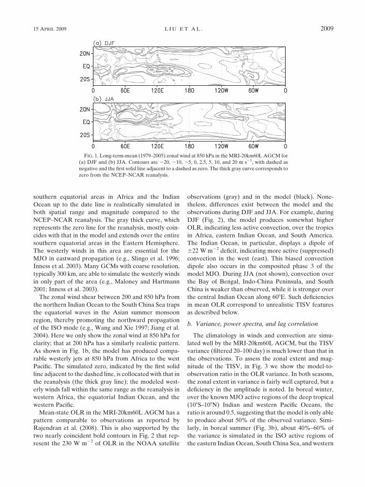
southern equatorial areas in Africa and the Indian

Ocean up to the date line is realistically simulated in

both spatial range and magnitude compared to the

NCEP–NCAR reanalysis. The gray thick curve, which

represents the zero line for the reanalysis, mostly coin-

cides with that in the model and extends over the entire

southern equatorial areas in the Eastern Hemisphere.

The westerly winds in this area are essential for the

MJO in eastward propagation (e.g., Slingo et al. 1996;

Inness et al. 2003). Many GCMs with coarse resolution,

typically 300 km, are able to simulate the westerly winds

in only part of the area (e.g., Maloney and Hartmann

2001; Inness et al. 2003).

The zonal wind shear between 200 and 850 hPa from

the northern Indian Ocean to the South China Sea traps

the equatorial waves in the Asian summer monsoon

region, thereby promoting the northward propagation

of the ISO mode (e.g., Wang and Xie 1997; Jiang et al.

2004). Here we only show the zonal wind at 850 hPa for

clarity; that at 200 hPa has a similarly realistic pattern.

As shown in Fig. 1b, the model has produced compa-

rable westerly jets at 850 hPa from Africa to the west

Pacific. The simulated zero, indicated by the first solid

line adjacent to the dashed line, is collocated with that in

the reanalysis (the thick gray line); the modeled west-

erly winds fall within the same range as the reanalysis in

western Africa, the equatorial Indian Ocean, and the

western Pacific.

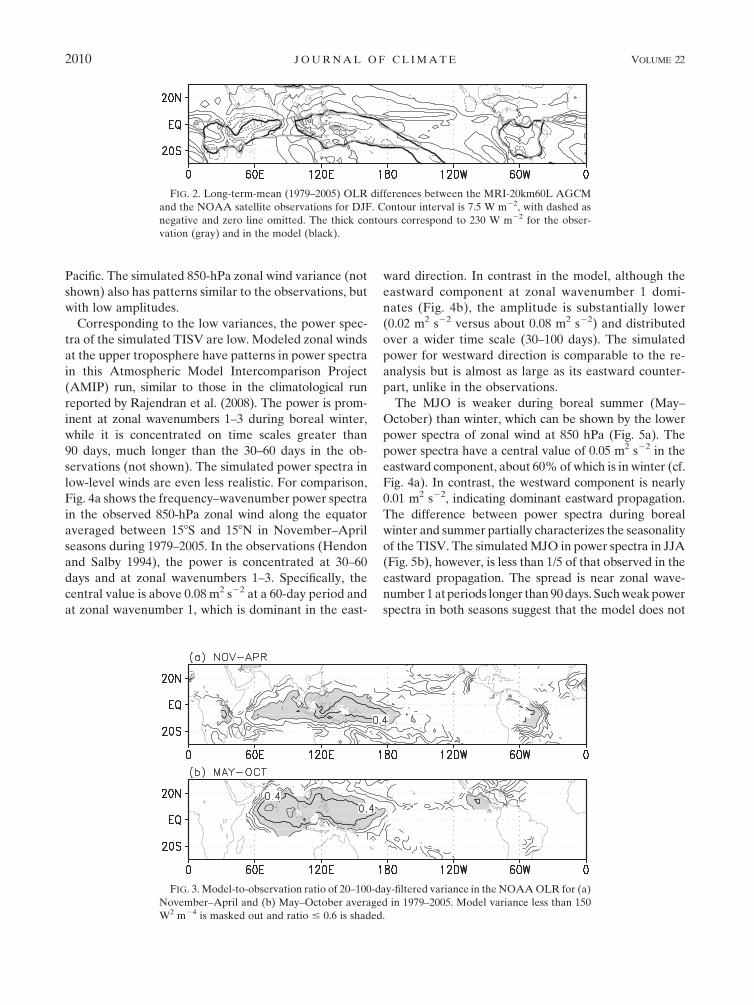
Mean-state OLR in the MRI-20km60L AGCM has a

pattern comparable to observations as reported by

Rajendran et al. (2008). This is also supported by the

two nearly coincident bold contours in Fig. 2 that rep-

resent the 230 W m22 of OLR in the NOAA satellite

observations (gray) and in the model (black). None-

theless, differences exist between the model and the

observations during DJF and JJA. For example, during

DJF (Fig. 2), the model produces somewhat higher

OLR, indicating less active convection, over the tropics

in Africa, eastern Indian Ocean, and South America.

The Indian Ocean, in particular, displays a dipole of

622 W m22 deficit, indicating more active (suppressed)

convection in the west (east). This biased convection

dipole also occurs in the composited phase 3 of the

model MJO. During JJA (not shown), convection over

the Bay of Bengal, Indo-China Peninsula, and South

China is weaker than observed, while it is stronger over

the central Indian Ocean along 608E. Such deficiencies

in mean OLR correspond to unrealistic TISV features

as described below.

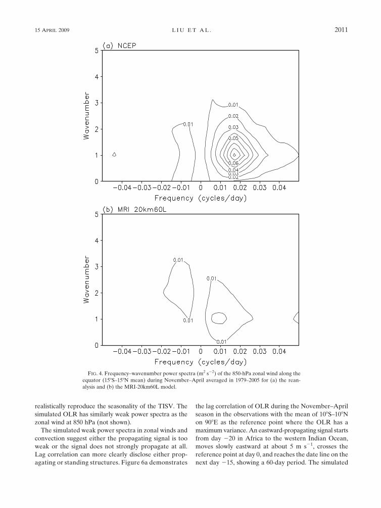
b. Variance, power spectra, and lag correlation

The climatology in winds and convection are simu-

lated well by the MRI-20km60L AGCM, but the TISV

variance (filtered 20–100 day) is much lower than that in

the observations. To assess the zonal extent and mag-

nitude of the TISV, in Fig. 3 we show the model-to-

observation ratio in the OLR variance. In both seasons,

the zonal extent in variance is fairly well captured, but a

deficiency in the amplitude is noted. In boreal winter,

over the known MJO active regions of the deep tropical

(108S–108N) Indian and western Pacific Oceans, the

ratio is around 0.5, suggesting that the model is only able

to produce about 50% of the observed variance. Simi-

larly, in boreal summer (Fig. 3b), about 40%–60% of

the variance is simulated in the ISO active regions of

the eastern Indian Ocean, South China Sea, and western

FIG. 1. Long-term-mean (1979–2005) zonal wind at 850 hPa in the MRI-20km60L AGCM for

(a) DJF and (b) JJA. Contours are 220, 210, 25, 0, 2.5, 5, 10, and 20 m s21, with dashed as

negative and the first solid line adjacent to a dashed as zero. The thick gray curve corresponds to

zero from the NCEP–NCAR reanalysis.

15 APRIL 2009 L I U E T A L . 2009

Pacific. The simulated 850-hPa zonal wind variance (not

shown) also has patterns similar to the observations, but

with low amplitudes.

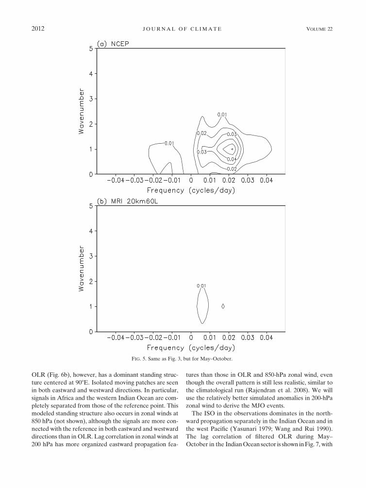
Corresponding to the low variances, the power spec-

tra of the simulated TISV are low. Modeled zonal winds

at the upper troposphere have patterns in power spectra

in this Atmospheric Model Intercomparison Project

(AMIP) run, similar to those in the climatological run

reported by Rajendran et al. (2008). The power is prom-

inent at zonal wavenumbers 1–3 during boreal winter,

while it is concentrated on time scales greater than

90 days, much longer than the 30–60 days in the ob-

servations (not shown). The simulated power spectra in

low-level winds are even less realistic. For comparison,

Fig. 4a shows the frequency–wavenumber power spectra

in the observed 850-hPa zonal wind along the equator

averaged between 158S and 158N in November–April

seasons during 1979–2005. In the observations (Hendon

and Salby 1994), the power is concentrated at 30–60

days and at zonal wavenumbers 1–3. Specifically, the

central value is above 0.08 m2 s22 at a 60-day period and

at zonal wavenumber 1, which is dominant in the east-

ward direction. In contrast in the model, although the

eastward component at zonal wavenumber 1 domi-

nates (Fig. 4b), the amplitude is substantially lower

(0.02 m2 s22 versus about 0.08 m2 s22) and distributed

over a wider time scale (30–100 days). The simulated

power for westward direction is comparable to the re-

analysis but is almost as large as its eastward counter-

part, unlike in the observations.

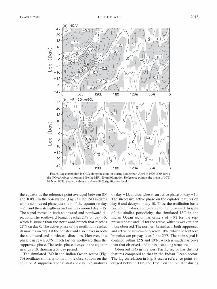
The MJO is weaker during boreal summer (May–

October) than winter, which can be shown by the lower

power spectra of zonal wind at 850 hPa (Fig. 5a). The

power spectra have a central value of 0.05 m2 s22 in the

eastward component, about 60% of which is in winter (cf.

Fig. 4a). In contrast, the westward component is nearly

0.01 m2 s22, indicating dominant eastward propagation.

The difference between power spectra during boreal

winter and summer partially characterizes the seasonality

of the TISV. The simulated MJO in power spectra in JJA

(Fig. 5b), however, is less than 1/5 of that observed in the

eastward propagation. The spread is near zonal wave-

number 1 at periods longer than 90 days. Such weak power

spectra in both seasons suggest that the model does not

FIG. 2. Long-term-mean (1979–2005) OLR differences between the MRI-20km60L AGCM

and the NOAA satellite observations for DJF. Contour interval is 7.5 W m22, with dashed as

negative and zero line omitted. The thick contours correspond to 230 W m22 for the obser-

vation (gray) and in the model (black).

FIG. 3. Model-to-observation ratio of 20–100-day-filtered variance in the NOAA OLR for (a)

November–April and (b) May–October averaged in 1979–2005. Model variance less than 150

W2 m24 is masked out and ratio # 0.6 is shaded.


realistically reproduce the seasonality of the TISV. The

simulated OLR has similarly weak power spectra as the

zonal wind at 850 hPa (not shown).

The simulated weak power spectra in zonal winds and

convection suggest either the propagating signal is too

weak or the signal does not strongly propagate at all.

Lag correlation can more clearly disclose either prop-

agating or standing structures. Figure 6a demonstrates

the lag correlation of OLR during the November–April

season in the observations with the mean of 108S–108N

on 908E as the reference point where the OLR has a

maximum variance. An eastward-propagating signal starts

from day 220 in Africa to the western Indian Ocean,

moves slowly eastward at about 5 m s21, crosses the

reference point at day 0, and reaches the date line on the

next day 215, showing a 60-day period. The simulated

FIG. 4. Frequency–wavenumber power spectra (m2 s22) of the 850-hPa zonal wind along the

equator (158S–158N mean) during November–April averaged in 1979–2005 for (a) the rean-

alysis and (b) the MRI-20km60L model.

15 APRIL 2009 L I U E T A L . 2011

OLR (Fig. 6b), however, has a dominant standing struc-

ture centered at 908E. Isolated moving patches are seen

in both eastward and westward directions. In particular,

signals in Africa and the western Indian Ocean are com-

pletely separated from those of the reference point. This

modeled standing structure also occurs in zonal winds at

850 hPa (not shown), although the signals are more con-

nected with the reference in both eastward and westward

directions than in OLR. Lag correlation in zonal winds at

200 hPa has more organized eastward propagation fea-

tures than those in OLR and 850-hPa zonal wind, even

though the overall pattern is still less realistic, similar to

the climatological run (Rajendran et al. 2008). We will

use the relatively better simulated anomalies in 200-hPa

zonal wind to derive the MJO events.

The ISO in the observations dominates in the north-

ward propagation separately in the Indian Ocean and in

the west Pacific (Yasunari 1979; Wang and Rui 1990).

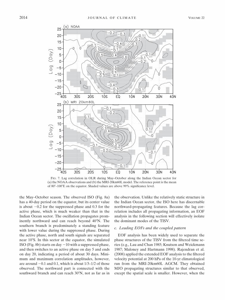
The lag correlation of filtered OLR during May–

October in the Indian Ocean sector is shown in Fig. 7, with

FIG. 5. Same as Fig. 3, but for May–October.


the equator as the reference point averaged between 808

and 1008E. In the observation (Fig. 7a), the ISO initiates

with a suppressed phase just south of the equator on day

225, and then strengthens and matures around day 215.

The signal moves in both southward and northward di-

rections. The southward branch reaches 208S on day 25,

which is sooner than the northward branch that reaches

228N on day 0. The active phase of the oscillation reaches

its maxima on day 0 at the equator and also moves in both

the southward and northward directions. However, this

phase can reach 308N, much farther northward than the

suppressed phase. The active phase decays on the equator

near day 10, showing a 35-day period.

The simulated ISO in the Indian Ocean sector (Fig.

7b) oscillates similarly to that in the observations on the

equator. A suppressed phase starts on day 225, matures

on day 215, and switches to an active phase on day 210.

The successive active phase on the equator matures on

day 0 and decays on day 10. Thus, the oscillation has a

period of 35 days, comparable to that observed. In spite

of the similar periodicity, the simulated ISO in the

Indian Ocean sector has centers of 20.2 for the sup-

pressed phase and 0.5 for the active, which is weaker than

those observed. The northern branches in both suppressed

and active phases can only reach 108N, while the southern

branches can propagate as far as 308S. The main signal is

confined within 128S and 108N, which is much narrower

than that observed, and it has a standing structure.

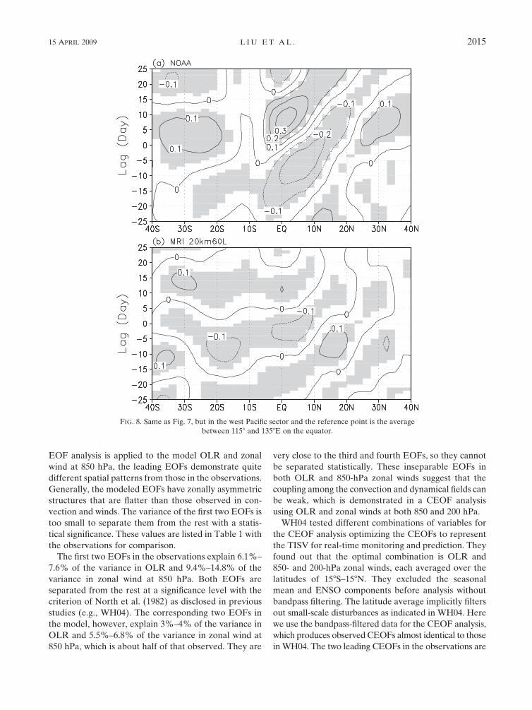
Observed ISO in the west Pacific sector has distinct

features compared to that in the Indian Ocean sector.

The lag correlation in Fig. 8 uses a reference point av-

eraged between 1158 and 1358E on the equator during

FIG. 6. Lag correlation in OLR along the equator during November–April in 1979–2005 for (a)

the NOAA observations and (b) the MRI-20km60L model. Reference point is the mean of 108S–

108N on 908E. Shaded values are above 99% significance level.

15 APRIL 2009 L I U E T A L . 2013

the May–October season. The observed ISO (Fig. 8a)

has a 40-day period on the equator, but its center value

is about 20.2 for the suppressed phase and 0.3 for the

active phase, which is much weaker than that in the

Indian Ocean sector. The oscillation propagates prom-

inently northward and can reach beyond 408N. The

southern branch is predominately a standing feature

with lower value during the suppressed phase. During

the active phase, north and south signals are separated

near 108S. In this sector at the equator, the simulated

ISO (Fig. 8b) starts on day 210 with a suppressed phase,

and then switches to an active phase on day 5 and ends

on day 20, indicating a period of about 30 days. Mini-

mum and maximum correlation amplitudes, however,

are around 20.1 and 0.1, which is about 1/3–1/2 of those

observed. The northward part is connected with the

southward branch and can reach 308N, not as far as in

the observation. Unlike the relatively static structure in

the Indian Ocean sector, the ISO here has discernable

northward-propagating features. Because the lag cor-

relation includes all propagating information, an EOF

analysis in the following section will effectively isolate

the dominant modes of the TISV.

c. Leading EOFs and the coupled pattern

EOF analysis has been widely used to separate the

phase structures of the TISV from the filtered time se-

ries (e.g., Lau and Chan 1985; Knutson and Weickmann

1987; Maloney and Hartmann 1998). Rajendran et al.

(2008) applied the extended EOF analysis to the filtered

velocity potential at 200 hPa of the 10-yr climatological

run from the MRI-20km60L AGCM. They obtained

MJO propagating structures similar to that observed,

except the spatial scale is smaller. However, when the

FIG. 7. Lag correlation in OLR during May–October along the Indian Ocean sector for

(a) the NOAA observations and (b) the MRI-20km60L model. The reference point is the mean

of 808–1008E on the equator. Shaded values are above 99% significance level.


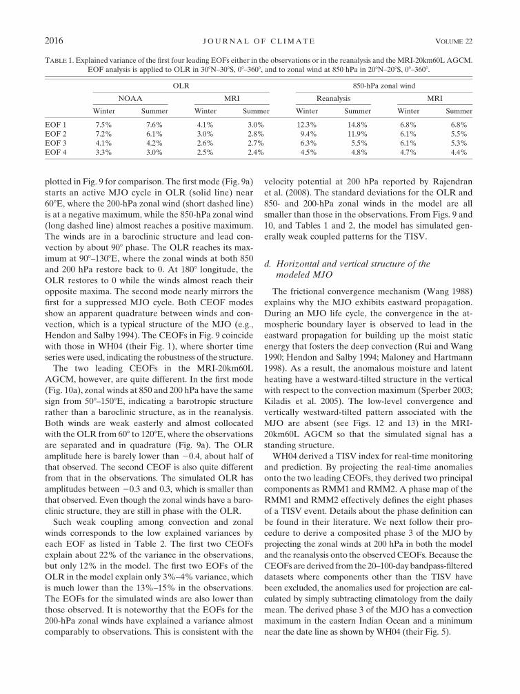
EOF analysis is applied to the model OLR and zonal

wind at 850 hPa, the leading EOFs demonstrate quite

different spatial patterns from those in the observations.

Generally, the modeled EOFs have zonally asymmetric

structures that are flatter than those observed in con-

vection and winds. The variance of the first two EOFs is

too small to separate them from the rest with a statis-

tical significance. These values are listed in Table 1 with

the observations for comparison.

The first two EOFs in the observations explain 6.1%–

7.6% of the variance in OLR and 9.4%–14.8% of the

variance in zonal wind at 850 hPa. Both EOFs are

separated from the rest at a significance level with the

criterion of North et al. (1982) as disclosed in previous

studies (e.g., WH04). The corresponding two EOFs in

the model, however, explain 3%–4% of the variance in

OLR and 5.5%–6.8% of the variance in zonal wind at

850 hPa, which is about half of that observed. They are

very close to the third and fourth EOFs, so they cannot

be separated statistically. These inseparable EOFs in

both OLR and 850-hPa zonal winds suggest that the

coupling among the convection and dynamical fields can

be weak, which is demonstrated in a CEOF analysis

using OLR and zonal winds at both 850 and 200 hPa.

WH04 tested different combinations of variables for

the CEOF analysis optimizing the CEOFs to represent

the TISV for real-time monitoring and prediction. They

found out that the optimal combination is OLR and

850- and 200-hPa zonal winds, each averaged over the

latitudes of 158S–158N. They excluded the seasonal

mean and ENSO components before analysis without

bandpass filtering. The latitude average implicitly filters

out small-scale disturbances as indicated in WH04. Here

we use the bandpass-filtered data for the CEOF analysis,

which produces observed CEOFs almost identical to those

in WH04. The two leading CEOFs in the observations are

FIG. 8. Same as Fig. 7, but in the west Pacific sector and the reference point is the average

between 1158 and 1358E on the equator.

15 APRIL 2009 L I U E T A L . 2015

plotted in Fig. 9 for comparison. The first mode (Fig. 9a)

starts an active MJO cycle in OLR (solid line) near

608E, where the 200-hPa zonal wind (short dashed line)

is at a negative maximum, while the 850-hPa zonal wind

(long dashed line) almost reaches a positive maximum.

The winds are in a baroclinic structure and lead con-

vection by about 908 phase. The OLR reaches its max-

imum at 908–1308E, where the zonal winds at both 850

and 200 hPa restore back to 0. At 1808 longitude, the

OLR restores to 0 while the winds almost reach their

opposite maxima. The second mode nearly mirrors the

first for a suppressed MJO cycle. Both CEOF modes

show an apparent quadrature between winds and con-

vection, which is a typical structure of the MJO (e.g.,

Hendon and Salby 1994). The CEOFs in Fig. 9 coincide

with those in WH04 (their Fig. 1), where shorter time

series were used, indicating the robustness of the structure.

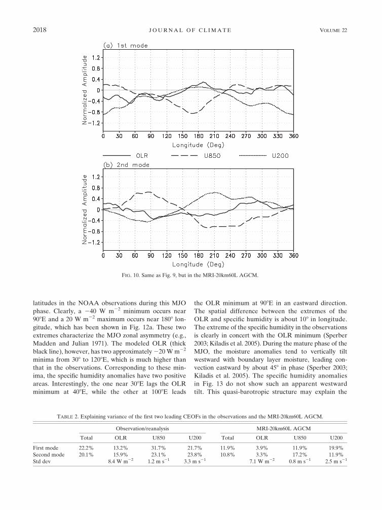
The two leading CEOFs in the MRI-20km60L

AGCM, however, are quite different. In the first mode

(Fig. 10a), zonal winds at 850 and 200 hPa have the same

sign from 508–1508E, indicating a barotropic structure

rather than a baroclinic structure, as in the reanalysis.

Both winds are weak easterly and almost collocated

with the OLR from 608 to 1208E, where the observations

are separated and in quadrature (Fig. 9a). The OLR

amplitude here is barely lower than 20.4, about half of

that observed. The second CEOF is also quite different

from that in the observations. The simulated OLR has

amplitudes between 20.3 and 0.3, which is smaller than

that observed. Even though the zonal winds have a baro-

clinic structure, they are still in phase with the OLR.

Such weak coupling among convection and zonal

winds corresponds to the low explained variances by

each EOF as listed in Table 2. The first two CEOFs

explain about 22% of the variance in the observations,

but only 12% in the model. The first two EOFs of the

OLR in the model explain only 3%–4% variance, which

is much lower than the 13%–15% in the observations.

The EOFs for the simulated winds are also lower than

those observed. It is noteworthy that the EOFs for the

200-hPa zonal winds have explained a variance almost

comparably to observations. This is consistent with the

velocity potential at 200 hPa reported by Rajendran

et al. (2008). The standard deviations for the OLR and

850- and 200-hPa zonal winds in the model are all

smaller than those in the observations. From Figs. 9 and

10, and Tables 1 and 2, the model has simulated gen-

erally weak coupled patterns for the TISV.

d. Horizontal and vertical structure of themodeled MJO

The frictional convergence mechanism (Wang 1988)

explains why the MJO exhibits eastward propagation.

During an MJO life cycle, the convergence in the at-

mospheric boundary layer is observed to lead in the

eastward propagation for building up the moist static

energy that fosters the deep convection (Rui and Wang

1990; Hendon and Salby 1994; Maloney and Hartmann

1998). As a result, the anomalous moisture and latent

heating have a westward-tilted structure in the vertical

with respect to the convection maximum (Sperber 2003;

Kiladis et al. 2005). The low-level convergence and

vertically westward-tilted pattern associated with the

MJO are absent (see Figs. 12 and 13) in the MRI-

20km60L AGCM so that the simulated signal has a

standing structure.

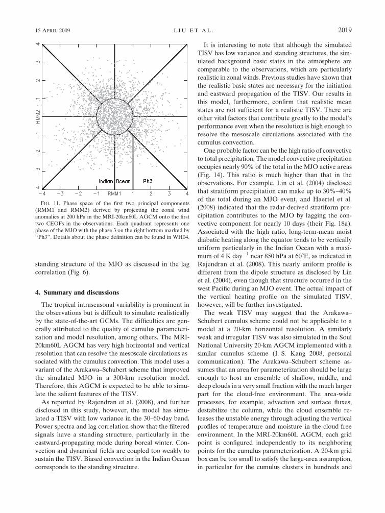
WH04 derived a TISV index for real-time monitoring

and prediction. By projecting the real-time anomalies

onto the two leading CEOFs, they derived two principal

components as RMM1 and RMM2. A phase map of the

RMM1 and RMM2 effectively defines the eight phases

of a TISV event. Details about the phase definition can

be found in their literature. We next follow their pro-

cedure to derive a composited phase 3 of the MJO by

projecting the zonal winds at 200 hPa in both the model

and the reanalysis onto the observed CEOFs. Because the

CEOFs are derived from the 20–100-day bandpass-filtered

datasets where components other than the TISV have

been excluded, the anomalies used for projection are cal-

culated by simply subtracting climatology from the daily

mean. The derived phase 3 of the MJO has a convection

maximum in the eastern Indian Ocean and a minimum

near the date line as shown by WH04 (their Fig. 5).

TABLE 1. Explained variance of the first four leading EOFs either in the observations or in the reanalysis and the MRI-20km60L AGCM.

EOF analysis is applied to OLR in 308N–308S, 08–3608, and to zonal wind at 850 hPa in 208N–208S, 08–3608.

OLR 850-hPa zonal wind

NOAA MRI Reanalysis MRI

Winter Summer Winter Summer Winter Summer Winter Summer

EOF 1 7.5% 7.6% 4.1% 3.0% 12.3% 14.8% 6.8% 6.8%

EOF 2 7.2% 6.1% 3.0% 2.8% 9.4% 11.9% 6.1% 5.5%

EOF 3 4.1% 4.2% 2.6% 2.7% 6.3% 5.5% 6.1% 5.3%

EOF 4 3.3% 3.0% 2.5% 2.4% 4.5% 4.8% 4.7% 4.4%


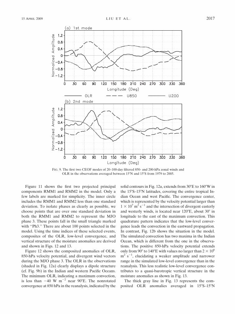
Figure 11 shows the first two projected principal

components RMM1 and RMM2 in the model. Only a

few labels are marked for simplicity. The inner circle

includes the RMM1 and RMM2 less than one standard

deviation. To isolate phases as clearly as possible, we

choose points that are over one standard deviation in

both the RMM1 and RMM2 to represent the MJO

phase 3. These points fall in the small triangle marked

with ‘‘Ph3.’’ There are about 100 points selected in the

model. Using the time indices of these selected events,

composites of the OLR, low-level convergence, and

vertical structure of the moisture anomalies are derived

and shown in Figs. 12 and 13.

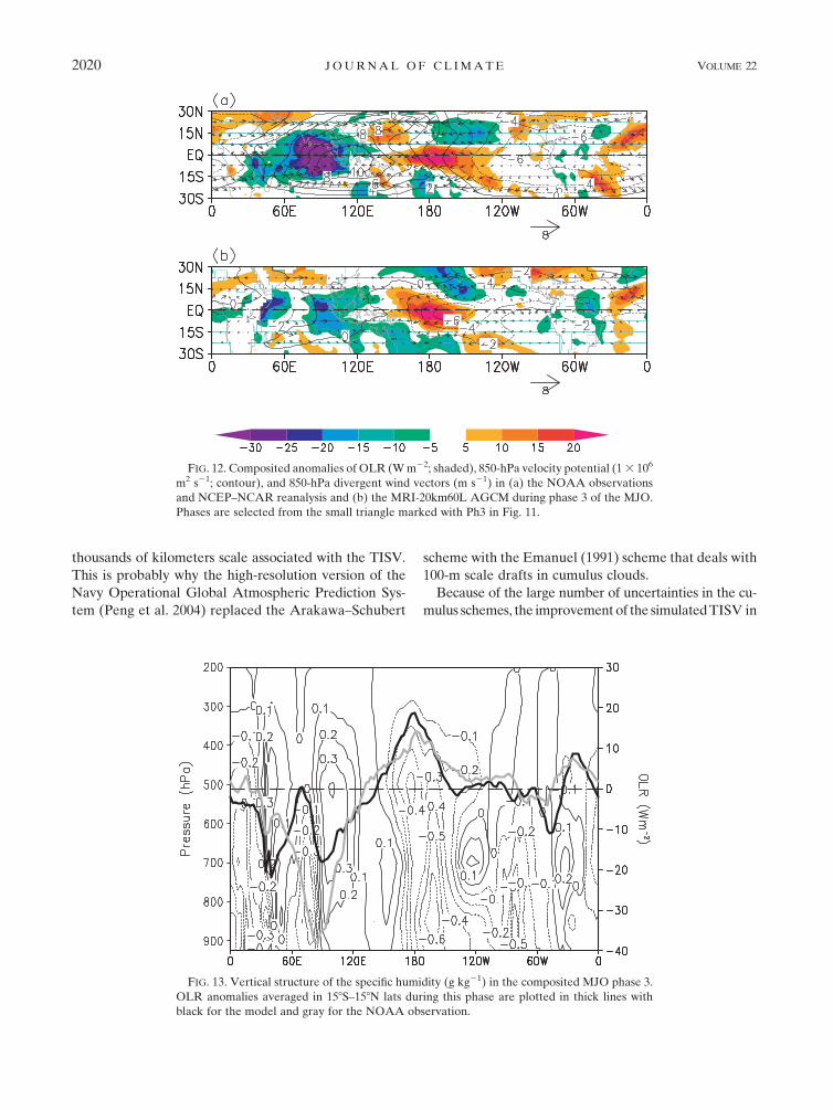
Figure 12 shows the composited anomalies of OLR,

850-hPa velocity potential, and divergent wind vectors

during the MJO phase 3. The OLR in the observations

(shaded in Fig. 12a) clearly displays a dipole structure

(cf. Fig. 9b) in the Indian and western Pacific Oceans.

The minimum OLR, indicating a maximum convection,

is less than 240 W m22 near 908E. The nonrotated

convergence at 850 hPa in the reanalysis, indicated by the

solid contours in Fig. 12a, extends from 308E to 1608W in

the 158S–158N latitudes, covering the entire tropical In-

dian Ocean and west Pacific. The convergence center,

which is represented by the velocity potential larger than

1 3 107 m2 s21 and the intersection of divergent easterly

and westerly winds, is located near 1208E, about 308 in

longitude to the east of the maximum convection. This

quadrature pattern indicates that the low-level conver-

gence leads the convection in the eastward propagation.

In contrast, Fig. 12b shows the situation in the model.

The simulated convection has two maxima in the Indian

Ocean, which is different from the one in the observa-

tions. The positive 850-hPa velocity potential extends

only from 908 to 1408E with values no larger than 2 3 106

m2 s21, elucidating a weaker amplitude and narrower

range in the simulated low-level convergence than in the

reanalysis. This less realistic low-level convergence con-

tributes to a quasi-barotropic vertical structure in the

moisture anomalies as shown in Fig. 13.

The thick gray line in Fig. 13 represents the com-

posited OLR anomalies averaged in 158S–158N

FIG. 9. The first two CEOF modes of 20–100-day filtered 850- and 200-hPa zonal winds and

OLR in the observations averaged between 158N and 158S from 1979 to 2005.

15 APRIL 2009 L I U E T A L . 2017

latitudes in the NOAA observations during this MJO

phase. Clearly, a 240 W m22 minimum occurs near

908E and a 20 W m22 maximum occurs near 1808 lon-

gitude, which has been shown in Fig. 12a. These two

extremes characterize the MJO zonal asymmetry (e.g.,

Madden and Julian 1971). The modeled OLR (thick

black line), however, has two approximately 220 W m22

minima from 308 to 1208E, which is much higher than

that in the observations. Corresponding to these min-

ima, the specific humidity anomalies have two positive

areas. Interestingly, the one near 308E lags the OLR

minimum at 408E, while the other at 1008E leads

the OLR minimum at 908E in an eastward direction.

The spatial difference between the extremes of the

OLR and specific humidity is about 108 in longitude.

The extreme of the specific humidity in the observations

is clearly in concert with the OLR minimum (Sperber

2003; Kiladis et al. 2005). During the mature phase of the

MJO, the moisture anomalies tend to vertically tilt

westward with boundary layer moisture, leading con-

vection eastward by about 458 in phase (Sperber 2003;

Kiladis et al. 2005). The specific humidity anomalies

in Fig. 13 do not show such an apparent westward

tilt. This quasi-barotropic structure may explain the

FIG. 10. Same as Fig. 9, but in the MRI-20km60L AGCM.

TABLE 2. Explaining variance of the first two leading CEOFs in the observations and the MRI-20km60L AGCM.

Observation/reanalysis MRI-20km60L AGCM

Total OLR U850 U200 Total OLR U850 U200

First mode 22.2% 13.2% 31.7% 21.7% 11.9% 3.9% 11.9% 19.9%

Second mode 20.1% 15.9% 23.1% 23.8% 10.8% 3.3% 17.2% 11.9%

Std dev 8.4 W m22 1.2 m s21 3.3 m s21 7.1 W m22 0.8 m s21 2.5 m s21


standing structure of the MJO as discussed in the lag

correlation (Fig. 6).

4. Summary and discussions

The tropical intraseasonal variability is prominent in

the observations but is difficult to simulate realistically

by the state-of-the-art GCMs. The difficulties are gen-

erally attributed to the quality of cumulus parameteri-

zation and model resolution, among others. The MRI-

20km60L AGCM has very high horizontal and vertical

resolution that can resolve the mesoscale circulations as-

sociated with the cumulus convection. This model uses a

variant of the Arakawa–Schubert scheme that improved

the simulated MJO in a 300-km resolution model.

Therefore, this AGCM is expected to be able to simu-

late the salient features of the TISV.

As reported by Rajendran et al. (2008), and further

disclosed in this study, however, the model has simu-

lated a TISV with low variance in the 30–60-day band.

Power spectra and lag correlation show that the filtered

signals have a standing structure, particularly in the

eastward-propagating mode during boreal winter. Con-

vection and dynamical fields are coupled too weakly to

sustain the TISV. Biased convection in the Indian Ocean

corresponds to the standing structure.

It is interesting to note that although the simulated

TISV has low variance and standing structures, the sim-

ulated background basic states in the atmosphere are

comparable to the observations, which are particularly

realistic in zonal winds. Previous studies have shown that

the realistic basic states are necessary for the initiation

and eastward propagation of the TISV. Our results in

this model, furthermore, confirm that realistic mean

states are not sufficient for a realistic TISV. There are

other vital factors that contribute greatly to the model’s

performance even when the resolution is high enough to

resolve the mesoscale circulations associated with the

cumulus convection.

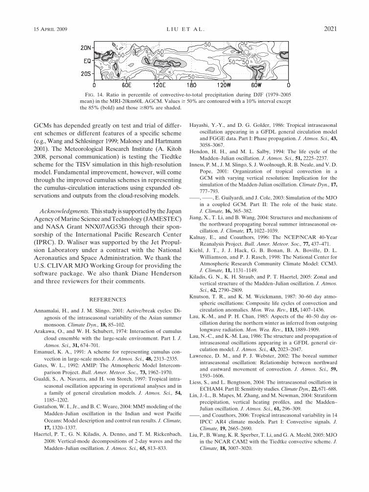
One probable factor can be the high ratio of convective

to total precipitation. The model convective precipitation

occupies nearly 90% of the total in the MJO active areas

(Fig. 14). This ratio is much higher than that in the

observations. For example, Lin et al. (2004) disclosed

that stratiform precipitation can make up to 30%–40%

of the total during an MJO event, and Haertel et al.

(2008) indicated that the radar-derived stratiform pre-

cipitation contributes to the MJO by lagging the con-

vective component for nearly 10 days (their Fig. 18a).

Associated with the high ratio, long-term-mean moist

diabatic heating along the equator tends to be vertically

uniform particularly in the Indian Ocean with a maxi-

mum of 4 K day21 near 850 hPa at 608E, as indicated in

Rajendran et al. (2008). This nearly uniform profile is

different from the dipole structure as disclosed by Lin

et al. (2004), even though that structure occurred in the

west Pacific during an MJO event. The actual impact of

the vertical heating profile on the simulated TISV,

however, will be further investigated.

The weak TISV may suggest that the Arakawa–

Schubert cumulus scheme could not be applicable to a

model at a 20-km horizontal resolution. A similarly

weak and irregular TISV was also simulated in the Soul

National University 20-km AGCM implemented with a

similar cumulus scheme (I.-S. Kang 2008, personal

communication). The Arakawa–Schubert scheme as-

sumes that an area for parameterization should be large

enough to host an ensemble of shallow, middle, and

deep clouds in a very small fraction with the much larger

part for the cloud-free environment. The area-wide

processes, for example, advection and surface fluxes,

destabilize the column, while the cloud ensemble re-

leases the unstable energy through adjusting the vertical

profiles of temperature and moisture in the cloud-free

environment. In the MRI-20km60L AGCM, each grid

point is configured independently to its neighboring

points for the cumulus parameterization. A 20-km grid

box can be too small to satisfy the large-area assumption,

in particular for the cumulus clusters in hundreds and

FIG. 11. Phase space of the first two principal components

(RMM1 and RMM2) derived by projecting the zonal wind

anomalies at 200 hPa in the MRI-20km60L AGCM onto the first

two CEOFs in the observations. Each quadrant represents one

phase of the MJO with the phase 3 on the right bottom marked by

‘‘Ph3’’. Details about the phase definition can be found in WH04.

15 APRIL 2009 L I U E T A L . 2019

thousands of kilometers scale associated with the TISV.

This is probably why the high-resolution version of the

Navy Operational Global Atmospheric Prediction Sys-

tem (Peng et al. 2004) replaced the Arakawa–Schubert

scheme with the Emanuel (1991) scheme that deals with

100-m scale drafts in cumulus clouds.

Because of the large number of uncertainties in the cu-

mulus schemes, the improvement of the simulated TISV in

FIG. 12. Composited anomalies of OLR (W m22; shaded), 850-hPa velocity potential (1 3 106

m2 s21; contour), and 850-hPa divergent wind vectors (m s21) in (a) the NOAA observations

and NCEP–NCAR reanalysis and (b) the MRI-20km60L AGCM during phase 3 of the MJO.

Phases are selected from the small triangle marked with Ph3 in Fig. 11.

FIG. 13. Vertical structure of the specific humidity (g kg21) in the composited MJO phase 3.

OLR anomalies averaged in 158S–158N lats during this phase are plotted in thick lines with

black for the model and gray for the NOAA observation.


GCMs has depended greatly on test and trial of differ-

ent schemes or different features of a specific scheme

(e.g., Wang and Schlesinger 1999; Maloney and Hartmann

2001). The Meteorological Research Institute (A. Kitoh

2008, personal communication) is testing the Tiedtke

scheme for the TISV simulation in this high-resolution

model. Fundamental improvement, however, will come

through the improved cumulus schemes in representing

the cumulus–circulation interactions using expanded ob-

servations and outputs from the cloud-resolving models.

Acknowledgments. This study is supported by the Japan

Agency of Marine Science and Technology (JAMESTEC)

and NASA Grant NNX07AG53G through their spon-

sorship of the International Pacific Research Center

(IPRC). D. Waliser was supported by the Jet Propul-

sion Laboratory under a contract with the National

Aeronautics and Space Administration. We thank the

U.S. CLIVAR MJO Working Group for providing the

software package. We also thank Diane Henderson

and three reviewers for their comments.

REFERENCES

Annamalai, H., and J. M. Slingo, 2001: Active/break cycles: Di-

agnosis of the intraseasonal variability of the Asian summer

monsoon. Climate Dyn., 18, 85–102.

Arakawa, O., and W. H. Schubert, 1974: Interaction of cumulus

cloud ensemble with the large-scale environment. Part I. J.

Atmos. Sci., 31, 674–701.

Emanuel, K. A., 1991: A scheme for representing cumulus con-

vection in large-scale models. J. Atmos. Sci., 48, 2313–2335.

Gates, W. L., 1992: AMIP: The Atmospheric Model Intercom-

parison Project. Bull. Amer. Meteor. Soc., 73, 1962–1970.

Gualdi, S., A. Navarra, and H. von Storch, 1997: Tropical intra-

seasonal oscillation appearing in operational analyses and in

a family of general circulation models. J. Atmos. Sci., 54,

1185–1202.

Gustafson, W. I., Jr., and B. C. Weare, 2004: MM5 modeling of the

Madden–Julian oscillation in the Indian and west Pacific

Oceans: Model description and control run results. J. Climate,

17, 1320–1337.

Haertel, P. T., G. N. Kiladis, A. Denno, and T. M. Rickenbach,

2008: Vertical-mode decompositions of 2-day waves and the

Madden–Julian oscillation. J. Atmos. Sci., 65, 813–833.

Hayashi, Y.-Y., and D. G. Golder, 1986: Tropical intraseasonal

oscillation appearing in a GFDL general circulation model

and FGGE data. Part I: Phase propagation. J. Atmos. Sci., 43,

3058–3067.

Hendon, H. H., and M. L. Salby, 1994: The life cycle of the

Madden–Julian oscillation. J. Atmos. Sci., 51, 2225–2237.

Inness, P. M., J. M. Slingo, S. J. Woolnough, R. B. Neale, and V. D.

Pope, 2001: Organization of tropical convection in a

GCM with varying vertical resolution: Implication for the

simulation of the Madden-Julian oscillation. Climate Dyn., 17,

777–793.

——, ——, E. Guilyardi, and J. Cole, 2003: Simulation of the MJO

in a coupled GCM. Part II: The role of the basic state.

J. Climate, 16, 365–382.

Jiang, X., T. Li, and B. Wang, 2004: Structures and mechanisms of

the northward propagating boreal summer intraseasonal os-

cillation. J. Climate, 17, 1022–1039.

Kalnay, E., and Coauthors, 1996: The NCEP/NCAR 40-Year

Reanalysis Project. Bull. Amer. Meteor. Soc., 77, 437–471.

Kiehl, J. T., J. J. Hack, G. B. Bonan, B. A. Boville, D. L.

Williamson, and P. J. Rasch, 1998: The National Center for

Atmospheric Research Community Climate Model: CCM3.

J. Climate, 11, 1131–1149.

Kiladis, G. N., K. H. Straub, and P. T. Haertel, 2005: Zonal and

vertical structure of the Madden–Julian oscillation. J. Atmos.

Sci., 62, 2790–2809.

Knutson, T. R., and K. M. Weickmann, 1987: 30–60 day atmo-

spheric oscillations: Composite life cycles of convection and

circulation anomalies. Mon. Wea. Rev., 115, 1407–1436.

Lau, K.-M., and P. H. Chan, 1985: Aspects of the 40–50 day os-

cillation during the northern winter as inferred from outgoing

longwave radiation. Mon. Wea. Rev., 113, 1889–1909.

Lau, N.-C., and K.-M. Lau, 1986: The structure and propagation of

intraseasonal oscillations appearing in a GFDL general cir-

culation model. J. Atmos. Sci., 43, 2023–2047.

Lawrence, D. M., and P. J. Webster, 2002: The boreal summer

intraseasonal oscillation: Relationship between northward

and eastward movement of convection. J. Atmos. Sci., 59,

1593–1606.

Liess, S., and L. Bengtsson, 2004: The intraseasonal oscillation in

ECHAM4. Part II: Sensitivity studies. Climate Dyn., 22, 671–688.

Lin, J.-L., B. Mapes, M. Zhang, and M. Newman, 2004: Stratiform

precipitation, vertical heating profiles, and the Madden–

Julian oscillation. J. Atmos. Sci., 61, 296–309.

——, and Coauthors, 2006: Tropical intraseasonal variability in 14

IPCC AR4 climate models. Part I: Convective signals. J.

Climate, 19, 2665–2690.

Liu, P., B. Wang, K. R. Sperber, T. Li, and G. A. Meehl, 2005: MJO

in the NCAR CAM2 with the Tiedtke convective scheme. J.

Climate, 18, 3007–3020.

FIG. 14. Ratio in percentile of convective-to-total precipitation during DJF (1979–2005

mean) in the MRI-20km60L AGCM. Values $ 50% are contoured with a 10% interval except

the 85% (bold) and those $80% are shaded.

15 APRIL 2009 L I U E T A L . 2021

Madden, R. A., and P. R. Julian, 1971: Detection of a 40–50 day

oscillation in the zonal wind in the tropical Pacific. J. Atmos.

Sci., 28, 702–708.

——, and ——, 1972: Description of global-scale circulation

cells in the tropics with a 40–50 day period. J. Atmos. Sci., 29,

1109–1123.

Maloney, E. D., and D. L. Hartmann, 1998: Frictional moisture

convergence in a composite life cycle of the Madden–Julian

oscillation. J. Climate, 11, 2387–2403.

——, and ——, 2001: The sensitivity of intraseasonal variability in

the NCAR CCM3 to changes in convective parameterization.

J. Climate, 14, 2015–2034.

Martin, G. M., 1999: The simulation of the Asian summer mon-

soon, and its sensitivity to horizontal resolution, in the UK

Meteorological Office Unified Model. Quart. J. Roy. Meteor.

Soc., 125, 1499–1525.

Miura, H., M. Satoh, T. Nasuno, A. T. Noda, and K. Oouchi, 2007:

A Madden-Julian oscillation event realistically simulated by a

global cloud-resolving model. Science, 318, 1763–1765.

Mizuta, R., and Coauthors, 2006: 20-km-mesh global climate

simulations using JMA-GSM model–—Mean climate states.

J. Meteor. Soc. Japan, 84, 165–185.

Moorthi, S., and M. J. Suarez, 1992: Relaxed Arakawa-Schubert: A

parameterization of moist convection for general circulation

models. Mon. Wea. Rev., 120, 978–1002.

Nakagawa, M., and A. Shimpo, 2004: Development of a cumulus

parameterization scheme for the operational global model at

JMA. RSMC Tokyo-Typhoon Center Technical Review, No.

7, Japanese Meteorological Agency, 10–15.

North, G. R., T. L. Bell, R. F. Cahalan, and F. J. Moeng, 1982:

Sampling errors in the estimation of empirical orthogonal

functions. Mon. Wea. Rev., 110, 699–706.

Pan, D.-M., and D. Randall, 1998: A cumulus parameterization

with a prognostic closure. Quart. J. Roy. Meteor. Soc., 124,949–981.

Park, C. K., D. M. Straus, and K. M. Lau, 1990: An evaluation of

the structure of tropical intraseasonal oscillation in 3 general

circulation models. J. Meteor. Soc. Japan, 68, 403–417.

Peng, M. S., J. A. Ridout, and T. F. Hogan, 2004: Recent modifi-

cations of the Emanuel convective scheme in the Navy Op-

erational Global Atmospheric Prediction System. Mon. Wea.

Rev., 132, 1254–1268.

Rajendran, K., A. Kitoh, R. Mizuta, S. Sajani, and T. Nakazawa,

2008: High-resolution simulation of mean convection and its

intraseasonal variability over the tropics in MRI/JMA 20-km

mesh AGCM. J. Climate, 21, 3722–3739.

Rui, H., and B. Wang, 1990: Development characteristics and

dynamic structure of tropical intraseasonal convection

anomalies. J. Atmos. Sci., 47, 357–379.

Slingo, J. M., and Coauthors, 1996: Intraseasonal oscillations in 15

atmospheric general circulation models: Results from an

AMIP diagnostic subproject. Climate Dyn., 12, 325–357.

Smith, R. N. B., 1990: A scheme for predicting layer clouds and

their water content in a general circulation model. Quart. J.

Roy. Meteor. Soc., 116, 435–460.

Sommeria, G., and J. W. Deardorff, 1977: Subgrid-scale conden-

sation in models of nonprecipitating clouds. J. Atmos. Sci., 34,

344–355.

Sperber, K. R., 2003: Propagation and the vertical structure of the

Madden–Julian oscillation. Mon. Wea. Rev., 131, 3018–3037.

——, and H. Annamalai, 2008: Coupled model simulations of

boreal summer intraseasonal (30–50 day) variability, Part 1:

Systematic errors and caution on use of metrics. Climate Dyn.,

31, 345–372, doi:10.1007/s00382-008-0367-9.

Tiedtke, M., 1989: A comprehensive mass flux scheme for cumulus

parameterization in large-scale models. Mon. Wea. Rev., 117,

1779–1800.

Waliser, D. E., and Coauthors, 2003: AGCM simulations of in-

traseasonal variability associated with the Asian summer

monsoon. Climate Dyn., 21, 423–446.

Wang, B., 1988: Dynamics of tropical low-frequency waves: An

analysis of the moist Kelvin wave. J. Atmos. Sci., 45, 2051–2065.

——, 2005: Theory. Intraseasonal Variability in the Atmosphere-

Ocean Climate System, W. K. M. Lau and D. E. Waliser, Eds.,

Praxis, 307–360.

——, and H. Rui, 1990: Synoptic climatology of transient tropical

intraseasonal convection anomalies: 1975-1985. Meteor. At-

mos. Phys., 44, 43–61.

——, and X. Xie, 1997: A model for the boreal summer intra-

seasonal oscillation. J. Atmos. Sci., 54, 72–86.

Wang, W. Q., and M. E. Schlesinger, 1999: The dependence on

convective parameterization of the tropical intraseasonal os-

cillation simulated by the UIUC 11-layer atmospheric GCM.

J. Climate, 12, 1423–1457.

Wheeler, M. C., and H. H. Hendon, 2004: An all-season real-time

multivariate MJO index: Development of an index for mon-

itoring and prediction. Mon. Wea. Rev., 132, 1917–1932.

Wu, M. L. C., S. Schubert, I.-S. Kang, and D. Waliser, 2002: Forced

and free intraseasonal variability over the South Asian

monsoon region simulated by 10 AGCMs. J. Climate, 15,

2862–2880.

Yasunari, T., 1979: Cloudiness fluctuation associated with the

Northern Hemisphere summer monsoon. J. Meteor. Soc. Ja-

pan, 57, 227–242.

Yoshimura, H., and T. Matsumura, 2003: A semi-Lagrangian ad-

vection scheme conservative in the vertical direction. Ex-

tended Abstracts, Fifth Int. Workshop on Next Generation

Climate Models for Advanced High Performance Computing

Facilities,Rome, Italy, RIST Tokyo, 3.19–3.20. [Available

online at http://www.tokyo.rist.or.jp/rist/workshop/rome/

abstract/yoshimura.pdf.]

Zhang, C., 2005: Madden-Julian oscillation. Rev. Geophys., 43,

RG2003, doi:10.1029/2004RG000158.

Zhang, G. J., and M. Mu, 2005: Simulation of the Madden–Julian

oscillation in the NCAR CCM3 using a revised Zhang–

McFarlane convection parameterization scheme. J. Climate,

18, 4046–4064.

Ziemianski, M. Z., W. W. Grabowski, and M. W. Moncrieff, 2004:

Explicit convection over the western Pacific warm pool in the

Community Atmospheric Model. J. Climate, 18, 1482–1502.


Documents

Tropical Intraseasonal Variability in the MRI-20km60L AGCM*