f4

juli 1996

,~iTU DelftTechnische Universiteit Delft

255

Introduction to bed, bank and shareproteetion

Faculteit der Civiele TechniekVakgroep WaterbouwkundeSectie Waterbouwkunde

/4

SHORE PROTECTION--- B7INTRaDUCTlaN Ta BED

Engineering the interface of soil and water

August 1995

G.J.Schiereck

F4 650255 fl.20.00

VOORWOORD VERGEET DIT NIET TE LEZEN!

Het dictaat f4 wordt verbouwd. Deze verbouwing heeft tot doel tegemoet te komen aan een aantalwensen en opmerkingen uit responsiegroepjes. De volgorde en indeling van de eerste 11hoofdstukken (oud, eerste 9 nieuw) is volledig omgegooid en herschreven om tot een leesbaarderen beter verteerbaar geheel te komen. Daarnaast zijn de lay-out en figuren veranderd, eveneensom de leesbaarheid te vergroten. Omdat tijdens de verbouwing het onderwijs gewoon doorgaat,betekent dit dat het tweede deel, vanaf hoofdstuk 9 in de nieuwe opzet, nog oud is. Deonvolkomenheden die dat met zich meebrengt, zijn van ondergeschikte aard. Het is wel debedoeling ook de latere hoofdstukken geheel te herzien.

Bij een breed vak als f4, waarbij ook nog de link gelegd moet worden tussen basistheorie enuitvoeringspraktijk, met alles wat daar tussen zit, kan niet alles even belangrijk zijn. Ter herhalingvan en in aanvulling op het op college gezegde het volgende:

Formules zijn nodig om ontwerpberekeningen te maken. Niemand kent die allemaal uit het hoofden dat is maar goed ook, dus dat wordt ook niet op het tentamen gevraagd. Wel is het nodig omzo'n formule met verstand te hanteren en te weten wat er ongeveer in zit en waarom. In deveelheid van empirische relaties, geldt dat vooral voor die formules die in de samenvattingen aanhet eind van ieder hoofdstuk nog eens genoemd worden. Van groot belang daarbij isvoorstellingsvermogen om in te schatten wat er in het water gebeurt. Het blijkt dat studenten daarde meeste moeite mee te hebben. Voor een ingenieur is een stromingsprobleem iets anders dan hetmaken van een algebra som!

Verder is datgene dat niet nodig is voor de hoofdlijn van het verhaal in appendices aan het eindvan sommige hoofdstukken geplaatst. Dat wil niet zeggen dat wat daarin staat niet belangrijk is.Vaak gaat het om kennis uit eerdere colleges, zoals bijv. de eerste appendix in hoofdstuk 7 overlineaire golftheorie, waarbij er van uit gegaan wordt dat je die reeds tot geestelijk eigendomgemaakt hebt. Als dat niet het geval is, zul je zelf moeten nagaan waarin je tekort schiet. Inandere gevallen, zoals de tweede appendix in hoofdstuk 7 over onregelmatige golven, gaat het omkennis uit parallel- of vervolgvakken die deels nodig is bij het gebruik van formules in f4. Het isdus niet zo dat appendixen overgeslagen kunnen worden, het is wel zo dat de hoofdlijn bij hettentamen ook ongeveer de hoofdlijn van het dictaat is.

Hetzelfde geldt voor de bijlagen A t/m C achterin. In A komen bijvoorbeeld zeefkrommen ensteengewichten aan de orde. Voor f4 wordt er van uit gegaan dat een student daar mee om weet tegaan. Appendix C is nuttig omdat daar het gebruik van de veelheid aan empirische relatiesgedemonstreerd wordt, hetgeen kan helpen bij het verkrijgen van inzicht in de toepassing van detheorie. In de tekst komen ook een aantal stukjes voor met een kleinere letter (niet dehoofdstukken 9 t/m 12, dat is de oude lay-out). Die zijn opgenomen, hetzij als illustratie, hetzijvoor de volledigheid om bij gebruik in voorkomende gevallen niet meteen naar een handboek tehoeven grijpen.

Tenslotte wordt gewezen op ACSIDO, het ondersteunende computerprogramma om het gebruikvan een aantal formules te oefenen en te helpen het dictaat kritischer, en dus beter, te kunnenlezen. ACSIDO is te vinden en vrij te copiëren (incl. "manuai" in WP5.1) op het netwerk vanzaal 3.14, inloggen onder f4 en bestanden copiëren of ter plaatse oefenen.

Kritiek in iedere vorm is welkom. Delft - 15 april 1996G.J .Schiereek

******** T.o.v. de versie van augustus 1995 zijn alleen enkele typefouten verbeterd. De verdereaanpassing zal plaatsvinden in het kader van de algehele curriculum herziening ********

CONTENTS

CHAPTER/Section page

CONTENTS

REFERENCES v

SYMBOLS x

DICTIONARY xiii

1 INTRODUCTION . . . . . . . . . . . . . . . . . . . . . . . . . . . . . . . . . . . . . .. 11.1 General 11.2 Phenomena. . . . . . . . . . • . . . . . . . . . . . . . . . . . . . . . . . . . . . . . .. 41.3 Design aspects . . . . . . . . . . . . . . . . . . . . . . . . . . . . . . . . . . . . . . .. 9

2 FLOW - I..oads . . . . . . . . . . . . . . . . . . . . . . . . . . . . . . . . . . .. 112.1 Introduetion . . . . . . . . . . . . . . . . . . . . . . . . . . . . . . . . . . . . . . . . .. 112.2 Turbulence. . . . . . . . . . . . . . . . . . . . . . . . . . . . . . . . . . . . . . . . .. 122.3 Flow situations . . . . . . . . . . . . . . . . . . . . . . . . . . . . . . . . . . . . . . .. 15

2.3.1 Wall flow . . . . . . . . . . . . . . . . . . . . . . . . . . . . . . . . . . . . .. 152.3.2 Free flow .... . . . . . . . . . . . . . . . . . . . . . . . . . . . . . . . . .. 182.3.3 Flow around detached bodies . . . . . . . . . . . . . . . . . . . . . . . . .. 212.3.4 Flow around attached bodies and in constrictions . . . . . . . . . . . . .. 23

2.4 Load reduction . . . . . . . . . . . . . . . . . . . . . . . . . . . . . . . . . . . . . . .. 272.5 Summary. . . . . . . . . . . . . . . . . . . . . . . . . . . . . . . . . . . . . . . . . .. 282.6 APPENDICES. . . . . . . . . . . . . . . . . . . . . . . . . . . . . . . . . . . . . . .. 29

2.6.1 Basic equations . . . . . . . . . . . . . . . . . . . . . . . . . . . . . . . . . .. 292.6.2 Why turbulence? . . . . . . . . . . . . . . . . . . . . . . . . . . . . . . . . .. 31

3 FLOW - Stability 353.1 Basic Equations 35

3.1.1 General 353.1.2 'lr - Threshold of motion 383.1.3 C - Roughness and waterdepth 39

3.2 Slope factor. . . . . . . . . . . . . . . . . . . . . . . . . . . . . . . . . . . . . . . . .. 413.3 Velocity factor . . . . . . . . . . . . . . . . . . . . . . . . . . . . . . . . . . . . . . .. 42

3.3.1 Acceleration 433.3.2 Deceleration 463.3.3 Values for velocity factor 48

3.4 Coherent material .... . . . . . . . . . . . . . . . . . . . . . . . . . . . . . . . . .. 503.5 Summary. . . . . . . . . . . . . . . . . . . . . . . . . . . . . . . . . . . . . . . . . .. 52

4 FLOW - Erosion . . . . . . . . . . . . . . . . . . . . . . . . . . . . . . . . . . . . . . . . . .. 534.1 Introduetion . . . . . . . . . . . . . . . . . . . . . . . . . . . . . . . . . . . . . . . . .. 534.2 Scour without proteetion . . . . . . . . . . . . . . . . . . . . . . . . . . . . . . . . .. 56

4.2.1 Scour in jets 564.2.2 Scour around detached bodies . . . . . . . . . . . . . . . . . . . . . . . . .. 584.2.3 Scour around attached bodies and in constrictions 60

4.3 Scour with proteetion " 634.3.1 Scour development in time 634.3.2 Equilibrium scour . . . . . . . . . . . . . . . . . . . . . . . . . . . . . . . .. 684.3.3 Stability of proteetion . . . . . . . . . . . . . . . . . . . . . . . . . . . . . .. 70

4.4 Summary. . . . . . . . . . . . . . . . . . . . . . . . . . . . . . . . . . . . . . . . . .. 72

5 POROUS FLOW - General . . . . . . . . . . . . . . . . . . . . . . . . . . . . . . . . . . .. 735.1 Introduetion . . . . . . . . . . . . . . . . . . . . . . . . . . . . . . . . . . . . . . . . .. 735.2 Basic equations . . . . . . . . . . . . . . . . . . . . . . . . . . . . . . . . . . . . . . .. 74

5.2.1 General 745.2.2 Solutions for laminar flow " 76

5.3 Load reduction . . . . . . . . . . . . . . . . . . . . . . . . . . . . . . . . . . . . . . .. 795.4 Stability of closed boundaries . . . . . . . . . . . . . . . . . . . . . . . . . . . . . .. 81

5.4.1 Impervious bottom protections 815.4.2 Impervious slope protections 82

5.5 Stability of open boundaries . . . . . . . . . . . . . . . . . . . . . . . . . . . . . . .. 845.5.1 Piping........................................ 845.5.2 Micro-stability of slopes . . . . . . . . . . . . . . . . . . . . . . . . . . . .. 86

5.6 Macro stability of slopes. . . . . . . . . . . . . . . . . . . . . . . . . . . . . . . . .. 875.7 Summary. . . . . . . . . . . . . . . . . . . . . . . . . . . . . . . . . . . . . . . . . .. 90

6 POROUS FLOW - Filters . . . . . . . . . . . . . . . . . . . . . . . . . . . . . . . . . . . .. 916.1 General 916.2 Granular filters. . . . . . . . . . . . . . . . . . . . . . . . . . . . . . . . . . . . . . .. 93

6.2.1 Introduction..................................... 936.2.2 Geometrically closed filters .. . . . . . . . . . . . . . . . . . . . . . . . .. 946.2.3 Geometrically open filters . . . . . . . . . . . . . . . . . . . . . . . . . . .. 95

6.3 Geotextiles. . . . . . . . . . . . . . . . . . . . . . . . . . . . . . . . . . . . . . . . .. 986.3.1 Introduction..................................... 986.3.2 Filter stability 996.3.3 Permeability 1006.3.4 Overall stability 102

6.4 Summary. . . . . . . . . . . . . . . . . . . . . . . . . . . . . . . . . . . . . . . . .. 103

ii

7 WAVES - Leads .7.1 Introduetion . . . . . . . . . . . . . . . . . . . . . . . . . . . . . . . . . . . . . . . . .7.2 Non breaking waves .

7.2.1 General .7.2.2 Shear stress .

7.3 Breaking waves .7.3.1 General .7.3.2 Energy absorption and turbulence .7.3.3 Wave impacts .7.3.4 Run-up and run-down .

7.4 Load reduction .7.5 Summary .7.6 APPENDICES. . . . . . . . . . . . . . . . . . . . . . . . . . . . . . . . . . . . . . .

7.6.1 Linear wave theory .7.6.2 Irregular waves .

8 WAVES - Erosion and stability .8.1 Introduetion .8.2 Erosion .

8.2.1 Erosion of slopes .8.2.2 Bottom erosion .

8.3 Stability of loose grains .8.3.1 Stability in non-break.ing waves .8.3.2 Stability in breaking waves .8.3.3 Stability for specific cases .8.3.4 Filters .

8.4 Stability of coherent material .8.4.1 Placed block revetments .8.4.2 Impervious layers .

8.5 Summary .

9 Ships .9.1 General .9.2 Primary waves . . . . . . . . . . . . . . . . . . . . . . . . . . . . . . . .9.3 Secundary waves .9.4 Propeller races .

iii

105105106106109111111113115116118120121121124

127127128128129130130131136138139139145147

149149151155158

10 Protections . . . . . . . . . . . . . . . . . . . . . . . . . . . . . . . . . . . . . . . . . . . . .. 16110.1 Shore protections 161

10.1.1 Shape of protections 16210.1.2 Revetment choice 16310.1.3 Transitions 16410.1.4 Toes 16610.1.5 Groynes . . . . . . . . . . . . . . . . . . . . . . . . . . . . . . . . . . . . .. 16710.1.6 Breakwaters . . . . . . . . . . . . . . . . . . . . . . . . . . . . . . . . . . .. 168

10.2 Bank protections . . . . . . . . . . . . . . . . . . . . . . . . . . . . . . . . . . . . .. 16910.2.1 Bank proteetion types. . . . . . . . . . . . . . . . . . . . . . . . . . . . .. 16910.2.2 Limits of protections . . . . . . . . . . . . . . . . . . . . . . .. 17010.2.3 Groynes . . . . . . . . . . . . . . . . . . . . . . . . . . . . . . . . . . . . .. 17110.2.4 FaIIing aprons 172

10.3 Bed protections 17310.3.1 Outlet structures . . . . . . . . . . . . . . . . . . . . . . . . . . . . . . . .. 17410.3.2 Bridge piers . . . . . . . . . . . . . . . . . . . . . . . . . . . . . . . . . . .. 17610.3.3 SeawaIls . . . . . . . . . . . . . . . . . . . . . . . . . . . . . . . . . . . . .. 176

11 Construction and maintenance . . . . . . . . . . . . . . . . . . . . . . . . . . . . . . . .. 17711.1 GeneraI........................................... 177

11.1.1 QuaIity assurance 17811.2 Construction 179

11.2.1 Waterborne - loose materiaI . . . . . . . . . . . . . . . . . . . . . . . . .. 17911.2.2 Waterborne - coherent materiaI . . . . . . . . . . . . . . . . . . . . . . .. 18211.2.3 Land based - loose materiaI . . . . . . . . . . . . . . . . . . . . . . . . .. 18311.2.4 Land based - coherent materiaI . . . . . . . . . . . . . . . . . . . . . . .. 18411.2.5 Construction costs . . . . . . . . . . . . . . . . . . . . . . . . . . . . . . .. 185

11.3 Maintenance........................................ 18611.3.1 GeneraI 18611.3.2 Theory . . . . . . . . . . . . . . . . . . . . . . . . . . . . . . . . . . . . . .. 18711.3.3 Practice 189

12 Design. . . . . . . . . . . . . . . . . . . . . . . . . . . . . . . . . . . . . . . . . . . . . . . .. 19112.1 Design process . . . . . . . . . . . . . . . . . . . . . . . . . . . . . . . . . . . . . .. 191

12.1.1 Introduction. . . . . . . . . . . . . . . . . . . . . . . . . . . . . . . . . . .. 19112.1.2 Influencing factors. . . . . . . . . . . . . . . . . . . . . . . . . . . . . . .. 19312.1.3 Design phases 195

12.2 ConceptuaI design. . . . . . . . . . . . . . . . . . . . . . . . . . . . . . . . . . . .. 19712.2.1 Generation of aIternatives 19712.2.2 Selection of aIternatives 198

12.3 StructuraI design. . . . . . . . . . . . . . . . . . . . . . . . . . . . . . . . . . . . .. 19912.3.1 Failure . . . . . . . . . . . . . . . . . . . . . . . . . . . . . . . . . . . . . .. 19912.3.2 Safety 203

Annex A: MATERlALS

Annex B: ENVIRONMENT AL ASPECTS

Annex C: CASES

iv

Akkerman1985

Akkerman1986

Ariëns1993

AshidaIBayazit1973

Battjes1974

Bear1972

REFERENCESHydraulic design criteria for rockfill closure oftidal gaps - Vertical closure method,Delft Hydraulics Laboratory report M1741 part IV

Hydraulic design criteria for rockfill closure of tidal gaps - Horizontal closuremethod, Delft Hydraulics Laboratory report S 861

Relatie tussen ontgrondingen en steenstabiliteit van de toplaag (in Dutch), MScthesis, Delft University of Technology

Initiation of motion and roughness of flows in steep channels, Papers IAHR­congress Istanbul, page 475-484

Computation of set-up, longshore currents, run-up and overtopping due to wind­generated waves, Dissertation Delft University of Technology

Dynamics of fluids in porous media, American Elsevier

BezuyenlBurger Taludbekledingen van gezette steen, samenvatting van/Klein Breteler onderzoeksresultaten 1980-1988M1795/H195 deel XXIV (in Dutch)1990 RWS-Dienst Weg- en Waterbouwkunde

Blom1991

Blom1993

Booij1986

Bouter1991

Turbulent flow over a sill, IAHR-congress Madrid

On the shallow water equations for turbulent flow over sillsDelft University of Technology, 1993

Turbulentie in de waterloopkunde (in Dutch), lecture notes b82, Delft Universityof Technology

Wave damping by reed- An investigation in environment friendly bank protections,PIANC bulletin, no 75

Breusers/Raudkivi Scouring, Balkema1991

Bruun/Gunbak1977

CIRIA1990

CUR/CIRIA1991

CURITAW1992

Stability of sloping structures in relation to ~ = tanaWHILCoastal Engineering 1, page 287-322

Use of vegetation in civil engineering, Coppin/Richards editorsCIRIA/Butterworths

Manual on the use of rock in coastal and shoreline engineering,CUR Report 154/CIRIA Special Publication 83, Balkema

Handboek voor dimensionering van gezette taludbekledingen (in Dutch),Rapport 155, Centrum Uitvoering researchITechnische Adviescommissie voor deWaterkeringen

v

Cohen de Lara1955

Co effi eient de perte de charge en milieu poreux basé sur I'équilibrehydrodynamique d'un massif (in French), La Houille Blanche No 2, page 167-176

Delft Hydraulics Stroombestendigheid los materiaal in wervelstraat (in Dutch)1960 report M 598 - VI

Fredsee/Deigaard Mechanics of coastal sediment transport, Advanced series in Ocean Engineering,1992 Volume 3, World Scientific

van Gent1992

Formulae to describe porous flow, Report no 92-2, DUT Civil Engineering

de Graauw/vdMeulen Design criteria for granular filters, Delft Hydraulics publication 287/vdDoes de Bye1983

GroenlDorrestein Zeegolven (in Dutch), Koninklijk Nederlands Meteorologisch Instituut1976

GrunelKohlhase Wave transmission through vertical slotted wall, Proceedings 14th International1974 Conference on Coastal Engineering, Vol lIl, page 1906-1923

Hedar1986

Hewlett1985

Hoffmans1992

Hoffmans1993a

Hoffmans1993b

Hudson1953

IzbashlKhaldre1970

Jansen1979

Jonsson1966

Armor layer stability of rubble-mound breakwaters, ASCE Journal of Waterway,port, coastal and ocean engineering, Vol 112, No 3, page 343-350

Reinforcement of steep grassed waterways, CIRIA

Two-dimensional mathematical modelling of local-scour holes, DissertationDelft University of Technology

A study concerning the influence of the relative turbulence intensity on local scourholes, Report W-DWW-93-251, Rijkswaterstaat, Road and Hydraulic EngineeringDivision

A hydraulic and morphological criterion for upstream slopes in local scour holes,Report W-DWW-93-255, Rijkswaterstaat, Road and Hydraulic EngineeringDivision

Wave forces on breakwaters, Proceedings-Separate ASCE, No 113, page 653-685

Hydraulics of river channel closure, Butterworth

Principles of river engineering, The non-tidal alluvial river, Pitman

Wave boundary layers and friction factors, Coastal Engineering Conference,Chapter 10, page 127-148

vi

JorissenNrijling Local scour downstream hydraulic constructions, IAHR-congress Ottawa1989

JorissenlKonter1991

van der Knaap1986

Kuijper1992

LeMéhauté1957/1958

LeMéhauté1976

van Mierlolde Ruijter1988

van der Linden1985

van der Meer1989

Prediction of time development of local scour, New Orleans

Design criteria for geotextiles beyond the sandtightness requirement,Delft Hydraulics, publication 358

Onderhoud in de waterbouw (in Dutch), Master thesis, Delft University ofTechnology, Civil Engineering

Permeabilité des digues en enrochements aux ondes de gravité périodiques (inFrench), La Houille Blanche, dec. 1957 - june 1958

Hydrodynamics and waterwaves. Springer

Turbulence measurements above dunes, Report Q789, Volume 1 and 2, DelftHydraulics Laboratory

Golfdempende constructies (in Dutch), Master thesis, Delft University ofTechnology, Civil Engineering

Rock slopes and gravel beaches under wave attack, Dissertation, Delft Universityof Technology

van der Meer Wave transmission at low-crested structures, Conference on Coastal Structures,Id'Angremond 1991 Telford

OumeracilPartenscky Wave-induced pore pressure in rubble mound breakwaters, Int. Conf. on1990 Coastal Engineering, Delft

Paintal1971

Pilarczyk1990

Concept of critical shear stress in loose boundary open channels, Journal ofhydraulic research, 9-1, page 91-113

Coastal protection, Proceedings of short course on coastal protection, DUT,Balkema

Pilarczyk/den Boer Stability and profile development of coarse materiaIs and their application in1983 coastal engineering, Delft Hydraulics, publication 293

Rajaratnam1976

Turbulent jets, Elsevier

RajaratnamlBerry Erosion by circular turbulent wall jets, Journal of Hydraulic Research 15(3)1977

Rajaratnam1981

Erosion by plane turbulent jets, Journal of Hydraulic Research 19(4), page 339-358

vii

Rajaratnam Erosion by plane wall jets with minimum tail water, ASCE Journal of Hydraulic/McDougall,1983 Engineering 109(7)

RWS1985

RWS1987a

RWS1987b

RWS1990

RWS1991

RWS1992

RWS/DHL1988

RWS/DHL1986

RWS/DHL1985

Schlichting1968

Sieath1978

Sorensen1973

SPM1984

van der Veer1979

Veldhuijzen v.Zanten, 1986

The use of asphalt in hydraulic engineering, Rijkswaterstaat communicationsno 37

Kwaliteit en kosten van rijksvaarwegen (in Dutch), Rijkswaterstaat, Dienst Weg­en Waterbouwkunde, Delft

The closure of tidal basins, Delft University Press

Waterbouw, Rekenregels voor waterbouwkundig ontwerpen (in Dutch), BouwdienstRijkswaterstaat

Handboek uitvoering bodemverdedigingsconstructies van losgestorte granulairematerialen (in Dutch), Bouwdienst Rijkswaterstaat

Transportmodel voor filters, Eindrapportage filteronderzoek (in Dutch),Rijkswaterstaat Dienst Weg- en Waterbouwkunde/Grondmechanica Delft/DelftHydraulics

Aantasting van dwarsprofielen in vaarwegen (in Dutch), Report M1115 XIX

Sekundaire scheepsgolven en hun effect op de stabiliteit van taludbekledingen (inDuteh), Report M1115 VI

Schroefstralen en de stabiliteit van bodem en oevers onder invloed van destroomsnelheden in de schroefstraal (in Dutch), Report M1115 VII

Boundary layer theory, McGraw-HiII(First German edition 1951)

Measurements of bed load in oscillatory flow, ASCE Journal of the waterway portcoastal and ocean division, Vol 104, NoWW4, page 291-307

Water waves produced by ships, ASCE Journal ofWaterways, harbors and coastalengineering division

Shore proteetion ManuaI, US Army Coastal Engineering Center

Grondwaterbeweging onder oeverconstructies (in Dutch), in: Kust- en oeverwerkenin praktijk en theorie

Geotextiles and geomembranes in civil engineering, Balkema

viii

Vellinga1986

Ven te Chow1959

van Vledder1990

de Vries1992

van der Weide1989

Xie Shi-Leng1981

Beach and dune erosion during storm surges, Dissertation, Delft University ofTechnology

Open-Channel hydraulies, McGraw-Hill

Literature survey to wave impacts on dike slopes, Delft Hydraulics,Report H976

River Engineering, Lecture notes flû, Delft University of Technology

General introduetion and hydraulic aspects, Short course on design of coastalstructures, AlT Bangkok

Scouring patterns in front of vertical breakwaters and their influences on thestability of the foundations of the breakwaters, Delft University of Technology

ix

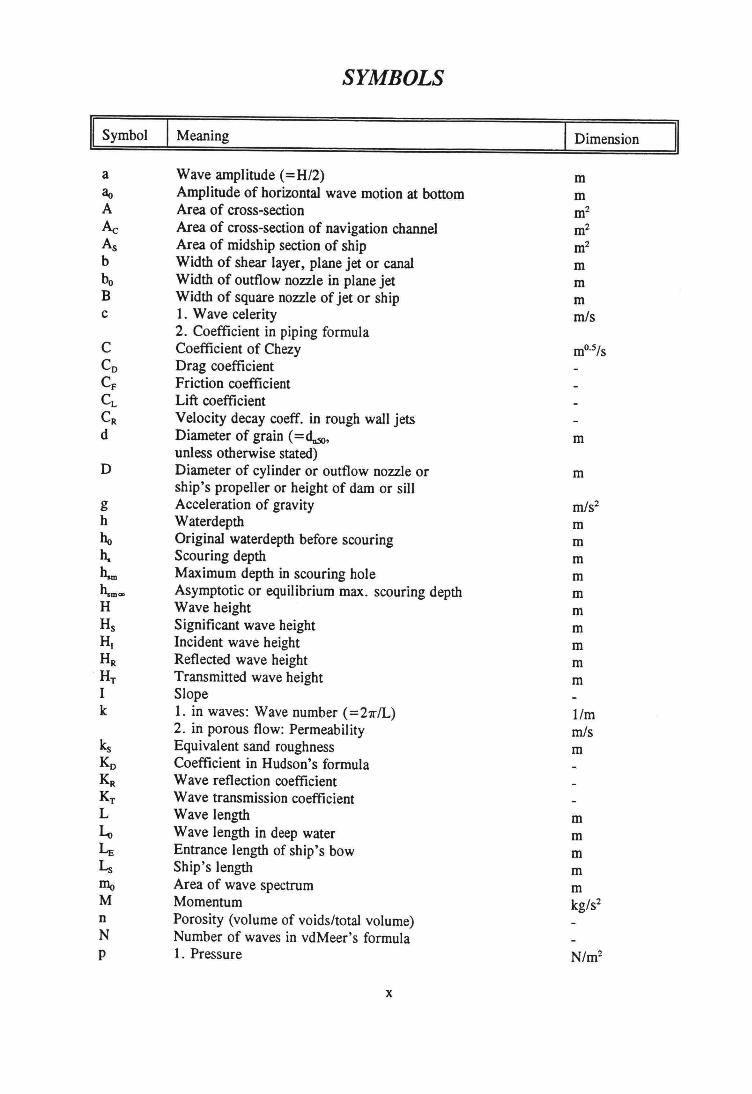
SYMBOLS

11 SymbolI1

Meaning Dimension

a Wave amplitude (=H/2) mao Amplitude of horizontal wave motion at bottom mA Area of cross-section m2

Ac Area of cross-section of navigation channel m2

As Area of midship section of ship m2

b Width of shear layer, plane jet or canal mbo Width of outflow nozzle in plane jet mB Width of square nozzle of jet or ship mc 1. Wave celerity mIs

2. Coefficient in piping formulaC Coefficient of Chezy mo.slsCo Drag coefficientCF Friction coefficientCL Lift coefficientCR Velocity decay coeff. in rough wall jetsd Diameter of grain (= duso, m

unless otherwise stated)D Diameter of cylinder or outtlow nozzle or m

ship's propeller or height of dam or sillg Acceleration of gravity m/s2h Waterdepth mho Original waterdepth before scouring m11. Scouring depth m11.m Maximum depth in scouring hole m11.moo Asymptotic or equilibrium max. scouring depth mH Wave height mHs Significant wave height mHl Incident wave height mHR Retlected wave height mHT Transmitted wave height mI Slopek 1. in waves: Wave number (=27r/L) lIm

2. in porous tlow: Permeability mIsks Equivalent sand roughness mKo Coefficient in Hudson's formulaKR Wave reflection coefficientKT Wave transmission coefficientL Wave length m1..0 Wave length in deep water m~ Entrance length of ship's bow mt, Ship's length mma Area of wave spectrum mM Momentum kg/s"n Porosity (volume of voids/total volume)N Number of waves in vdMeer's formulap 1. Pressure N/m2

x

2. Coefficient in parabolic beach profile mO.22

P Power WQ Discharge m3/sr 1. Relative turbulence

2. Radial distance from center of jet mR Hydraulic radius mRu Wave run-up mRo Wave run-down ms Distance from ship's saiIing line mS Sediment transport misS" Damage level in vdMeer's formulat Time sT Wave period or averaging period in turbulence sTM Meao wave period sTp Wave period with maximum wave energy sTs Significant wave period su Velocity in x-direction mIs11c Critical velocity mIsu, Filter velocity mIsu. Shear velocity (=VTIp) mIsu, Outtlow velocity in jets; verticaly averaged velocity mIsu", Maximum velocity mIsÜ Average velocity (in time) mIsu' Turbulent velocity fluctuation mIsû, Amplitude of wave velocity at bottom mIsUR Return current along ship mIsv Velocity in y-direction mIsVL Limit speed of ship mIsVs Ship's speed mIsw Velocity in z-direction mIsW Weight kg.m/s? =Nx Distance along horizontal axis m

parallel to main flow directiony Distance along horizontal axis m

perpendicular to main flow directionz Distance along vertical axis mZR Waterlevel depression in primo ship wave m

1. Slope angle degrees2. Coefficient in scour formula3. Coefficient in piping formula

(3 Slope of scour hole degrees'Yb Breaker depth ratio (H/h)Ö Boundary layer thickness m.:.\ Relative density (Ps - Pw)lpwE Turbulent (eddy) viscosity m2/sEs Eddy diffusivity of sediment m2/s11 Dimensionless distance in jets111 Waterlevel in waves mr Bow-geometry coefficient in ship's waves

xi

K von Karman constant ::::0.4À Leakage height mA Leakage length mP- l. Dynamic viscosity kg/m.s

2. Discharge coefficientv Kinematic viscosity m2/s~ Breaker parameterPs Density of sediment kg/m"Pw Density of water kg/m"CT Standard deviationT Shear stress N/m2 = PaTc Critical shear stress N/m2 = PaTo Wall shear stress N/m2 = Pa4> 1. Angle of repose degrees

2. Potential in porous flow m1/1 Stream function m2/sw Angular frequency in waves (211"1T) 1/s

THE GREEK ALPHABET

I Lower case I Capital I Name I1 Lower case I Capital I Name Iex A Alpha JI N Nu(3 B Beta ~ "::? Xi-'Y r Gamma 0 0 Omicron0 ~ Delta 11" II Pi€ E Epsilon P P Rbot Z Zeta CT E Sigma11 H Eta T T Tau(J e Theta v y UpsilonL I Iota 4> ~ PhiK K Kappa X X ChiÀ A Lambda 1/1 'lr PsiP- M Mu w 0 Omega

SPECIAL SIGNS

ex Proportional to

xii

DICTIONARY

abutmentantinodeapron

landhoofdbuik (van trilling)stortebed, bodembescherming (lett. beschermlap,voorschoot)beschermen, pantserenterugstroming (in golfoploop )oever(zand)bankbodemboegdichtslibbensamenhangendcohesiefin elkaar stortenbotsenbetonvernauwingbouw, uitvoering, constructiekernkruinduiker(sluis)interferentie piekrommel, afvalterugstromen (in golfoploop )slepen, trekken ,stromingsweerstandneer, wervelevenwichttakkeboszinkstukzettingsvloeiinggrindkribromp (van schip)niet poreus, ondoorlatendondoordringbaar, ondoorlatendtreffen, botsenbegin van bewegingbuigengrensvlak, overgangstraaluitlogenlekverwekingimpulsknoop (van trilling)tuit(uitstroom)openingpijler, pier

armouringbackwashbankbarbedbowcloggingcoherentcohesivecollapsecollideconcreteconstrictionconstructioncorecrestculvertcuspdebrisdownrushdrageddyequilibriumfaggotfascine mattressflow slidegravelgroynehuIlimpermeabieimperviousimpingeincipient motioninflectioninterfacejetleachleakageliquefactionmomentumnodenozzleorificepier

xiii

pitchplungepropeller raceprotrudequicksandquarryrectifierrevetmentripraprubblerun-downrun-upsaturatedscourseepagesegregationsettlementshallowshear stresssheet pilesillslagsslidespillsplit-bargespur-dikestemsurfsurgetailwaterthresholdtuguprushvoidsvortexwakewater-borne

plaveien, zettenduikenschroefstraaluitstekendrijfzandsteengroevegelijkrichteroeverbescherming, bekledingbreuksteen, stortsteenpuin, stortsteen(golt)terugloop(golt)oploopverzadigdontgronding, uitschuringkwelontmengingzettingondiepschuifspanningdamwanddrempelslakkenafschuivingmorsensplijtbakkrib, schermhek, achterstevenbrandingdeinenbenedenwaterdrempelsleepbootomhoog stromen in golfoploopporieënwervelzog (van schip)vanaf het water (Iett. door het water gedragen)

xiv

1 INTRODUCTION

1.1 General

The interface of land and water has always played an important role in human activities.Settlements are often located at coasts, river-banks or deltas. Harbours, waterways, dikes,dunes and beaches, structures for water-control and water-resources management etc. areexamples of hydraulic engineering on a macro-sca1e. In these lectures, the interface isstudied on a micro-sca1e. The occurring phenomena are important in all branches ofhydraulic engineering.

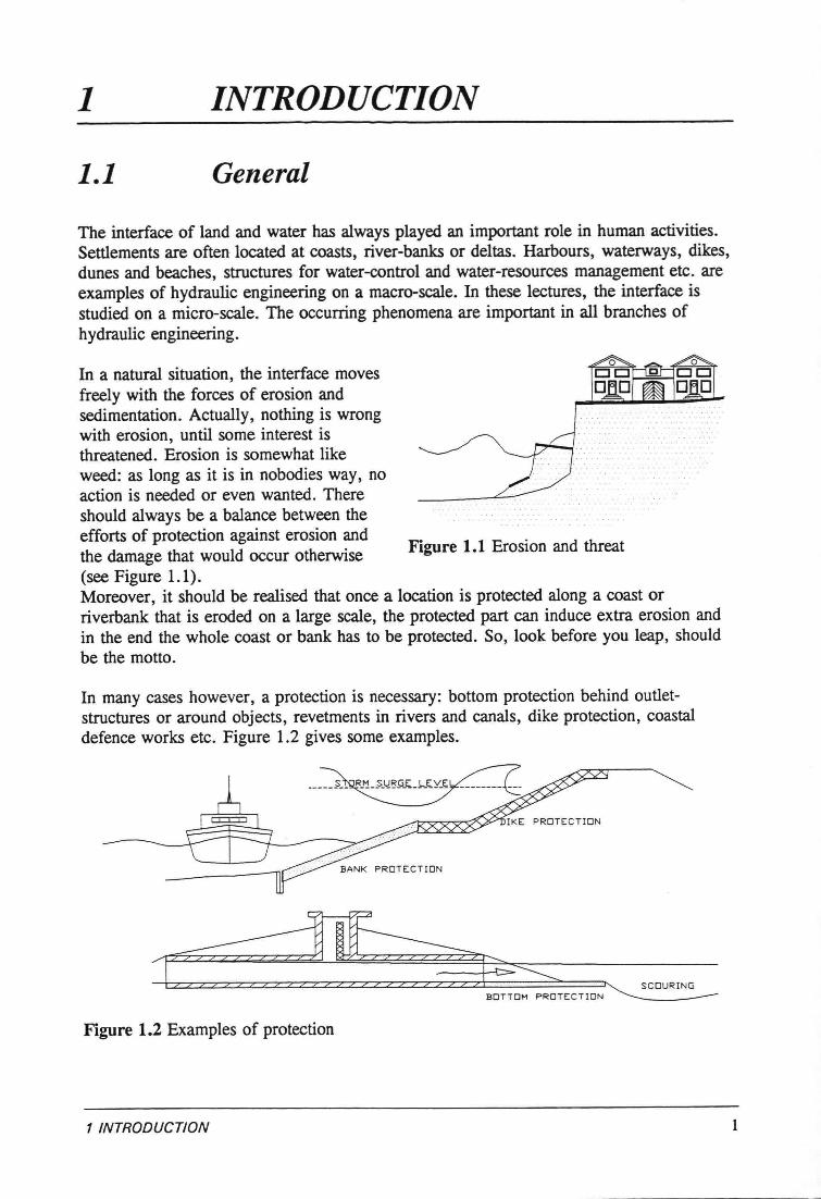
In a natura! situation, the interface movesfreely with the forces of erosion andsedimentation. Actually, nothing is wrongwith erosion, until some interest isthreatened. Erosion is somewhat likeweed: as long as it is in nobodies way, noaction is needed or even wanted. Thereshould always be a balance between theefforts of proteetion against erosion andthe damage that would occur otherwise(see Figure 1.1).Moreover , it should be rea1ised that once a location is protected along a coast orriverbank that is eroded on a large scale, the protected part can induce extra erosion andin the end the whole coast or bank has to be protected. So, look before you leap, shouldbe the motto.

Figure 1.1 Erosion and threat

In many cases however, a proteetion is necessary: bottom proteetion behind outlet­structures or around objects, revetments in rivers and canals, dike protection, coastaldefence works etc. Figure 1.2 gives some examples.

Figure 1.2 Examples of proteetion

BOTTOM PROTECTION

1 INTRODUCTION 1

A bare, erodable interface on one side and an interface that is proteeted with buildingmaterials like concrete, asphalt or rock on the other side, are two extremes. Nature itselfoffers a lot of possibilities in between, with vegetation as a major proteetion material.Mangrove trees along coasts and estuaries and reed along river banks are just twoexamples of a natural and low-cost proteetion. An important cause of erosion can be theremoval of this vegetation, disturbing an equilibrium that has existed for many ages. So, afirst measure in fighting erosion, will be the conservation of vegetation at the interface.

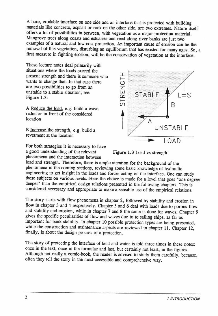
These leeture notes deal primarily withsituations where the loads exceed thepresent strength and there is someone whowants to change that. In that case thereare two possibilities to go from anunstable to a stable situation, seeFigure 1.3:

A Reduce the load, e.g. build a wavereductor in front of the consideredlocation

B Increase the strength, e.g. build arevetment at the location

B

UNSTABLE

----1 ...~ L0 ADFor both strategies it is necessary to havea good understanding of the relevant Figure 1.3 Load vs strengthphenomena and the interaction betweenload and strength. Therefore, there is ample attention for the background of thephenomena in the coming seetions, reviewing some basic knowledge of hydraulicengineering to get insight in the loads and forces acting on the interface. One can studythese subjeets on various levels. Here the choice is made for a level that goes "one degreedeeper" than the empirical design relations presented in the following chapters. This isconsidered neeessary and appropriate to make a sensible use of the empirical relations.

The story starts with flow phenomena in chapter 2, followed by stability and erosion inflow in chapter 3 and 4 respeetively. Chapter 5 and 6 deal with loads due to porous flowand stability and erosion, while in chapter 7 and 8 the same is done for waves. Chapter 9gives the speeific peeuliarities of flow and waves due to to sailing ships, as far asimportant for bank stability. In chapter 10 possible proteetion types are being presented,while the construction and maintenance aspeets are reviewed in chapter 11. Chapter 12,finally, is about the design process of a proteetion.

The story of proteeting the interface of land and water is told three times in these notes:once in the text, once in the formulae and last, but certainly not least, in the figures.Although not really a comic-book, the reader is advised to study them carefully, because,often they tell the story in the most accessible and comprehensive way.

2 1 INTRODUCTION

DEVELOPMENTS

Although protections of the interface of land and water are being made for more than1000 years (at least in the Netherlands), that does not meao there is nothing new. On thecontrary, like in architecture there are always new materials, creating new possibilitiesand changing demands from society, creating new challenges. Relatively new materials,like geo-textiles, give new opportunities to meet the contradicting demands in design as.There is not yet one ideal material combining the right strength, flexibility andpermeability but there are a lot more possibilities. The same goes for constructionmethods: new equipment makes application feasible of hitherto impossible structures.Major contributions to the design practice in the last decades, have been made possible bynew research facilities, like (large scale) wind wave flumes, (turbulent) flow measurementdevices etc.

In general there is a tendency to use a more scientific approach in the research and designof hydraulic structures. Much knowledge is fragmented and it would be a step forward toget an overall picture. Moreover most knowledge is of an empirical nature, leading tosometimes dubious relations. Dimensional homogenity is not always present while the useof the same variabie in two dimensionless parameters cao lead to spurious correlations,see de Vries, 1992. One of the challenges of the coming years is the combination of theuse of more scientific methods with experience which will always remain an importantfactor in hydraulic engineering.

An everlasting pressure on the designer is to create cheap solutions. "Cheap" has to beconsidered in a broad sense: low investment cao meao high maintenance costs and viceversa. The optimal solution should be found. An important cost factor in westerncountries is the construction; mechanisation replaces more and more the old labour­intensive handwork, while in developing countries material and equipment is veryexpensive and labour relatively cheap. This cao lead to a completely different design.

An important development in hydraulic engineering is the increasing relevanee ofenvironmental aspects. Itwas already mentioned that vegetation cao act as proteetion inmany cases and in situations where vegetation is present, it should be preserved as muchas possible. There are several examples in the world where problems with erosion onlystarted after the natural vegetation was removed (often to use plants or wood of trees orto make mooring facilities for ships). In the Netherlands, more and more use is made ofvegetation as proteetion where possible. This has to do with the importance of theinterface of soil and water in the ecosystem as a whoie. It is of crucial importance for alot of species of plants and animals. Not only the base of the food-chain, like worms andinsects, lives there; river banks for example are vital for many kinds of fish, looking forquiet places with low velocity to lay eggs. Mammals, like deer, have difficulties inclimbing out of the water at artificial river banks. Other mammals, like the readers ofthese notes have their demands when it comes to attractiveness of the landscape etc. Inthe design of a proteetion work, one should be aware of the fact that the interface of landand water is an essential part of the eco-system. More in general, especially in densilypopulated areas, there is a growing pressure on the use of the interface with manydifferent interests. This leads to a growing awareness of the multi-functionality of ashore, a bank or a dike. These (usually conflicting) interests, have to be incorporated intothe design.

1 INTRODUCTION 3

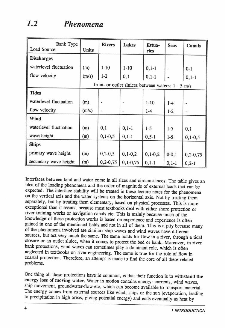
1.2 Phenomena

Bank Type Rivers Lakes Estua- Seas CanalsLoad Souree Units riesDischarges

waterlevel fluctuation (m) I-IQ 1-10 0,1-1 - 0-1flow velocity (mis) 1-2 0,1 0,1-1 - 0,1-1

In in- or outlet sluices between waters: 1 - 5 misTides

waterlevel fluctuation (m) - - 1-10 1-4 -flow velocity (mis) - - 1-4 1-2 -Wind

waterlevel fluctuation (m) 0,1 0,1-1 1-5 1-5 0,1wave height (m) 0,1-0,5 0,1-1 0,5-1 1-5 0,1-0,5Ships

primary wave height (m) 0,2-0,5 0,1-0,2 0,1-0,2 0-0,1 0,2-0,75seeundary wave height (m) 0,2-0,75 0,1-0,75 0,1-1 0,1-1 0,2-1

Interfaces between land and water come in all sizes and circumstances. The table gives anidea of the loading phenomena and the order of magnitude of extemalloads that can beexpeeted. The interface stability will be treated in these leeture notes for the phenomenaon the vertical axis and the water systems on the horizontal axis. Not by treating themseparately, but by treating them elementary, based on physica1processes. This is moreexceptional than it seems, because most textbooks deal with either shore proteetion orriver training works or navigation canals etc. This is mainly beeause much of theknowledge of these proteetion works is based on experience and experience is oftengained in one of the mentioned fields and not in all of them. This is a pity beeause manyof the phenomena involved are similar: ship waves and wind waves have differentsources, but act very much the same. The same holds for flow in a river, through a tidalclosure or an outlet sluice, when it comes to proteet the bed or bank. Moreover , in riverbank protections, wind waves can sometimes play a dominant role, which is oftennegleeted in textbooks on river engineering. The same is true for the role of flow incoastal proteetion. Therefore, an attempt is made to find the core of all these relatedproblems.

One thing all these protections have in common, is that their function is to withstand theenergy loss of moving water. Water in motion contains energy: currents, wind waves,ship movement, groundwater-flow etc, which can beeome available to transport material.The energy comes from external sourees like wind, ships or the sun (evaporation, leadingto preeipitation in high areas, giving potential energy) and ends eventually as heat by

4 1 INTRODUCTION

means of viscous friction. The expression "energy loss" is actually not correct. It is anenergy transfer, from kinetic energy via turbulence to heat. Turbulence plays an importantrole and will be discussed more in detail in the next chapter. Here it is sufficient to saythat turbulence is related to the transfer of kinetic energy into heat. During this transfer,much of the energy is available for attacking an interface.

Much research in hydraulic engineering is empirical and fragmented. This leads to anavalanche of relations for each subject, while the connections often remain in the dark.This is a pity and there is still a lot of work to do to establish genera! applicable relations.For a better understanding of the phenomena it is advised to keep the genera! picture inmind as much as possible, In many textbooks, hydrodynamic phenomena are treated anddescribed in all detail. The problem for many students in hydraulic engineering, however,is to recognize the phenomena in practical situations and translate them into basichydraulic problems. It will be shown, that most situations contain elements of threephenomena: wan flow, mixing layer and oscillating flow (wave). This will bedemonstrated with the following, hypothetical, situations. Another aim of these examplesis to show the large degree of analogy between many situations in hydraulics, which isalso useful to rea1ize in order to be able to recognize basic phenomena.

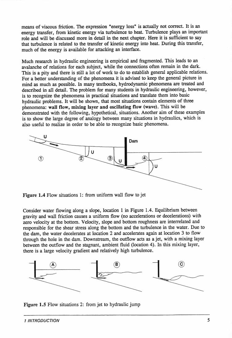
Figure 1.4 Flow situations I: from uniform wall flow to jet

Consider water flowing along a slope, location I in Figure 1.4. Equilibrium betweengravity and wall friction causes a uniform flow (no accelerations or decelerations) withzero velocity at the bottom. Velocity, slope and bottom roughness are interrelated andresponsible for the shear stress along the bottom and the turbulence in the water. Due tothe dam, the water decelerates at location 2 and accelerates again at location 3 to flowthrough the hole in the dam. Downstream, the outflow acts as a jet, with a mixing layerbetween the outflow and the stagnant, ambient fluid (location 4). In this mixing layer,there is a large velocity gradient and relatively high turbulence.

i ®L-----

Figure 1.5 Flow situations 2: from jet to hydraulic jump

1 INTRODUCTION 5

Situation A in Figure 1.5 is equivalent to location 4 in Figure 1.4: a jet flows into a largebody of stagnant water. In situation B, the downstream waterlevel is lowered and an eddyoccurs on top of the jet. This situation can be seen as a submerged hydraulic jump. Withan even lower waterlevel, a hydraulic jump occurs downstream of the outflow , situationC. Further lowering of the waterlevel will cause the hydraulic jump to move to the right.For certain combinations of discharge and outlet height, waves will origin from thehydraulic jump (undular jump). A mixing layer is present in all three situations.

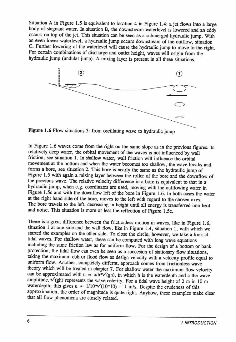
Figure 1.6Flow situations 3: from oscillating wave to hydraulic jump

In Figure 1.6 waves come from the right on the same slope as in the previous figures. Inrelatively deep water, the orbital movement of the waves is not influenced by wallfriction, see situation 1. In shallow water, wall friction will influence the orbitalmovement at the bottom and when the water becomes too shallow, the wave breaks andforms a bore, see situation 2. This bore is nearly the same as the hydraulic jump ofFigure 1.5 with again a mixing layer between the roller of the bore and the downflow ofthe previous wave. The relative velocity difference in a bore is equivalent to that in ahydraulic jump, when e.g. coordinates are used, moving with the outflowing water inFigure 1.5c and with the downflow left of the bore in Figure 1.6. In both cases the waterat the right hand side of the bore, moves to the left with regard to the chosen axes.The bore travels to the left, decreasing in height until all energy is transferred into heatand noise. This situation is more or less the reflection of Figure 1.5c.

There is agreat difference between the frictionless motion in waves, like in Figure 1.6,situation 1 at one side and the wall flow, like in Figure 1.4, situation 1, with which westarted the examples on the other side. To close the circle, however, we take a look attidal waves. For shallow water, these can be computed with long wave equationsincluding the same friction law as for uniform flow. For the design of a bottom or bankprotection, the tidal flow can even be seen as a succesion of stationary flow situations,taking the maximum ebb or flood flow as design velocity with a velocity profile equal touniform flow. Another, completely diffemt, approach comes from frictionless wavetheory which will be treated in chapter 7. For shallow water the maximum flow velocitycan be approximated with u =:: alh"V'(gh), in which h is the waterdepth and a the waveamplitude. v'(gh) represents the wave celerity. For a tidal wave height of 2 m in 10 mwaterdepth, this gives u =:: 1I1O"V'(1O*1O)= 1 mIs. Despite the crudeness of thisapproximation, the order of magnitude is quite right. Anyhow, these examples make clearthat all flow phenomena are closely related.

6 1/NTRODUCT/ON

With this in mind, one would suspect that all these features of water in motion obey thesame ground rules, and of course they do. The Navier-Stokes equations describe everytype of fluid motion in three dimensions as a function of time. Sinee, however, acomplete solution of these equations is not yet feasible for an area of practicaldimensions, still many simplifications have to be used to reach different solutions fordifferent cases of fluid motion. But the family ties between all these different flowfeatures are something to keep in mind constantly.

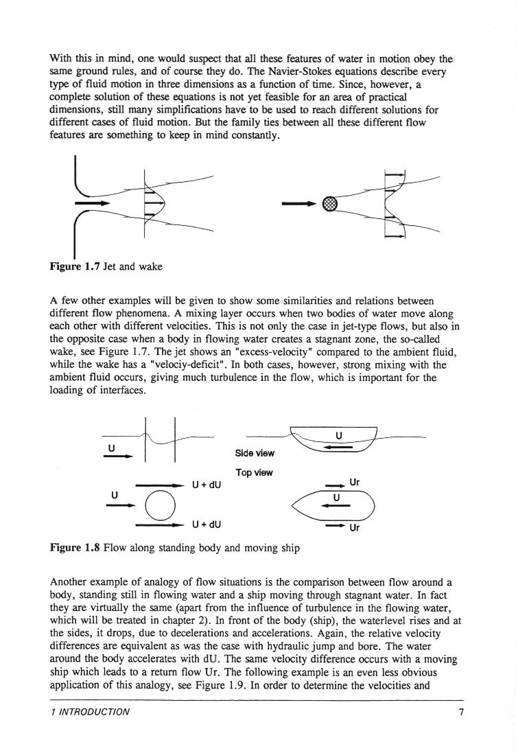
Figure 1.7 Jet and wake

A few other examples will be given to show some similarities and relations betweendifferent flow phenomena. A mixing layer occurs when two bodies of water move alongeach other with different velocities. This is not only the case in jet-type flows, but also inthe opposite case when a body in flowing water creates a stagnant zone, the so-calledwake, see Figure 1.7. The jet shows an "excess-velocity" compared to the ambient fluid,while the wake has a "velociy-deficit". In both cases, however, strong mixing with theambient fluid occurs, giving much turbulence in the flow, which is important for theloading of interfaces.

u Sideview

Top viewU+dU _Ur

<=)u oU+dU -Ur

Figure 1.8 Flow along standing body and moving ship

Another example of analogy of flow situations is the comparison between flow around abody, standing still in flowing water and a ship moving through stagnant water. In factthey are virtually the same (apart from the influence of turbulence in the flowing water,which will be treated in chapter 2). In front of the body (ship), the waterlevel rises and atthe sides, it drops, due to decelerations and accelerations. Again, the relative velocitydifferences are equivalent as was the case with hydraulic jump and bore. The wateraround the body accelerates with dU. The same velocity difference occurs with a movingship which leads to a return flow Ur. The following example is an even less obviousapplication of this analogy, see Figure 1.9. In order to determine the veloeities and

1 INTRODUCTION 7

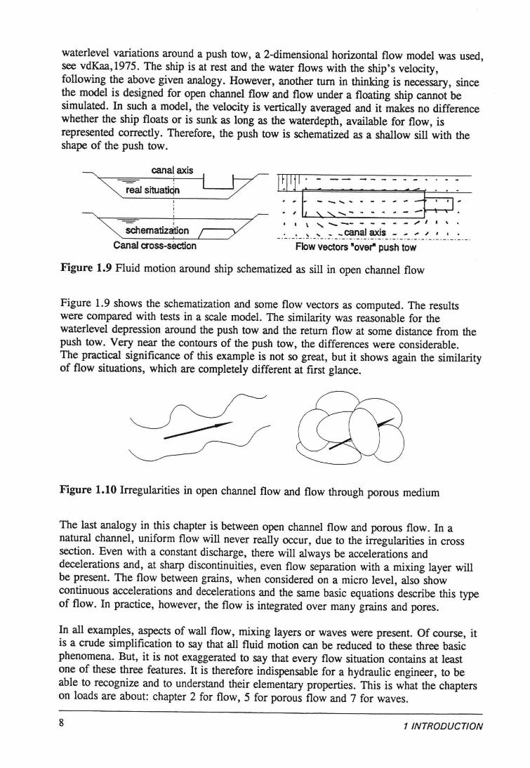
waterlevel variations around a push tow, a 2-dimensional horizontal flow model was used,see vdKaa,1975. The ship is at rest and the water flows with the ship's velocity,following the above given analogy. However, another turn in thinking is necessary, sincethe model is designed for open channel flow and flow under a floating ship cannot besimulated. In such a model, the velocity is vertically averaged and it makes no differencewhether the ship floats or is sunk as long as the waterdepth, available for flow, isrepresented correctly. Therefore, the push tow is schematized as a shallow sill with theshape of the push tow.

canalaxis-real situatiqn

~~--==~----~----------~~""( Sëhematiz~on / )//

Canal crcss-sèeton

., \ , .......... - _;,1.'"

_.._._~_.~._~_.:-._:-_~~~.~s_.~._-:-_.~._~_.~._~_.~._.Flowvectors ·ove'" push tow

Figure 1.9 Fluid motion around ship schematized as sill in open channel flow

Figure 1.9 shows the schematization and some flow veetors as computed. The resultswere compared with tests in a scale model. The similarity was reasonable for thewaterlevel depression around the push tow and the return flow at some distance from thepush tow. Very near the contours of the push tow, the differences were considerable.The practical significanee of this example is not so great, but it shows again the similarityof flow situations, which are completely different at first glance.

Figure 1.10 Irregularities in open channel flow and flow through porous medium

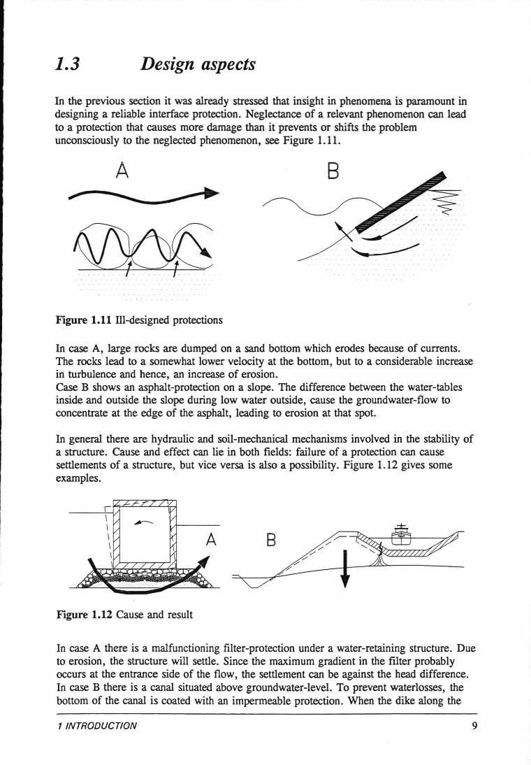
The last analogy in this chapter is between open channel flow and porous flow. In anatura! channel, uniform flow will never really occur, due to the irregularities in crosssection. Even with a constant discharge, there will always be accelerations anddecelerations and, at sharp discontinuities, even flow separation with a mixing layer willbe present. The flow between grains, when considered on a micro level, also showcontinuous accelerations and decelerations and the same basic equations describe this typeof flow. In practice, however, the flow is integrated over many grains and pores.

In all examples, aspects of wall flow, mixing layers or waves were present. Of course, itis a crude simplification to say that all fluid motion can be reduced to these three basicphenomena. But, it is not exaggerated to say that every flow situation contains at leastone of these three features. It is therefore indispensable for a hydraulic engineer, to beable to recognize and to understand their elementary properties. This is what the chapterson loads are about: chapter 2 for flow, 5 for porous flow and 7 for waves.

8 1 INTRODUCTION

1.3 Design aspects

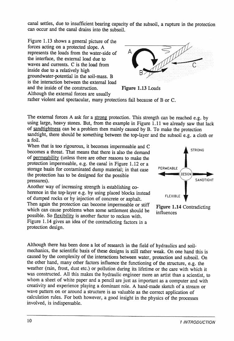
In the previous section it was already stressed that insight in phenomena is paramount indesigning a reliable interface protection. Neglectance of a relevant phenomenon can leadto a proteetion that causes more damage than it prevents or shifts the problemunconsciously to the neglected phenomenon, see Figure 1.11.

A

Figure 1.11 Ill-designed protections

In case A, large rocks are dumped on a sand bottom which erodes because of currents.The rocks lead to a somewhat lower velocity at the bottom, but to a considerable increasein turbulence and hence, an increase of erosion.Case B shows an asphalt-protection on a slope. The difference between the water-tablesinside and outside the slope during low water outside, cause the groundwater-flow toconcentrate at the edge of the asphalt, leading to erosion at that spot.

In genera! there are hydraulic and soil-mechanical mechanisms involved in the stability ofa structure. Cause and effect can lie in both fields: failure of a proteetion can causesettlements of a structure, but vice versa is also a possibility. Figure 1.12 gives someexamples.

~r /r v\ / ;-... V\/

~A\

\

\_\ l--(

t(//L'//A' "'*' ~

~ ......,-.. .............. ...it1' .Ó: ~

Figure 1.12 Cause and result

In case A there is a malfunctioning filter-proteetion under a water-retaining structure. Dueto erosion, the structure will settle. Since the maximum gradient in the filter probablyoccurs at the entrance side of the flow, the settlement can be against the head difference.In case B there is a canal situated above groundwater-level. To prevent waterlosses, thebottom of the canal is coated with an impermeable protection. When the dike along the

1 INTRODUCTION 9

canal settles, due to insufficient bearing capacity of the subsoil, a rupture in the proteetioncan occur and the canal drains into the subsoil.

Figure 1.13 shows a general picture of theforces acting on a protected slope. Arepresents the loads from the water-side ofthe interface, the extemalload due towaves and currents. C is the load frominside due to a relatively high B'~""''''_'''''groundwater-potential in the soil-mass. Bis the interaction between the extemal loadand the inside of the construction. Figure 1.13 LoadsAlthough the extemal forces are usuallyrather violent and spectacuIar, many protections fail because of B or C.

The extemal forces A ask for a strong protection. This strength can be reached e.g. byusing large, heavy stones. But, from the example in Figure 1.11 we already saw that Iackof sandtightness can be a problem then mainly caused by B. To make the proteetionsandtight, there should be something between the top-layer and the subsoil e.g. a cloth ora foil.When that is too rigourous, it becomes impermeable and Cbecomes a threat. That means that there is also the demandof permeability (unless there are other reasons to make theproteetion impermeabIe, e.g. the canal in Figure 1.12 or astorage basin for contaminated dump material; in that casethe proteetion has to be designed for the possiblepressures).Another way of increasing strength is establishing co­herenee in the top-layer e.g. by using placed blocks insteadof dumped rocks or by injection of concrete or asphalt.Then again the proteetion can become impermeabIe or stiffwhich can cause problems when some settlement should bepossible. So flexibility is another factor to reekon with.Figure 1.14 gives an idea of the contradicting factors in aproteetion design.

STRONG

.. • DESIGN ..

SANDTIGHT

fLEXIBLE lFigure 1.14 Contradictinginfluences

Although there has been done a lot of research in the field of hydraulics and soil­mechanics, the scientific basis of these designs is still rather weak. On one hand this iscaused by the complexity of the interactions between water, proteetion and subsoil. Onthe other hand, many other factors influence the functioning of the structure, e.g. theweather (rain, frost, dust etc.) or pollution during its lifetime or the care with which itwas constructed. All this makes the hydraulic engineer more an artist than a scientist, towhom a sheet of white paper and a pencil are just as important as a computer and withcreativity and experience playing a dominant role. A hand-made sketch of a stream orwave pattem on or around a structure is as valuable as the correct application ofcalculation rules, For both however, a good insight in the physics of the processesinvolved, is indispensabIe.

10 1 INTRODUCTION

2 FLOW - Loads

2.1 Introduetion

®u

® velocity head

=~~--27-t?i2~QJA

Figure 2.1 Velocity field in various situations

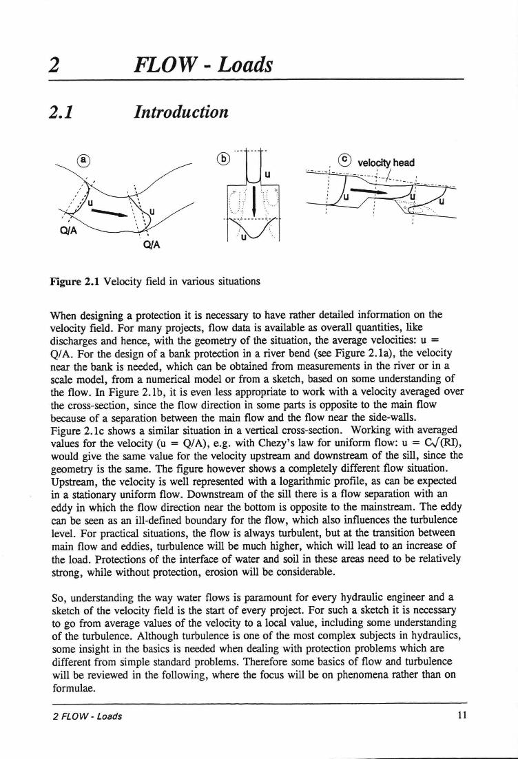
When designing a proteetion it is necessary to have rather detailed information on thevelocity field. For many projects, flow data is available as overall quantities, likedischarges and hence, with the geometry of the situation, the average velocities: u =Q/A. For the design of a bank proteetion in a river bend (see Figure 2.1a), the velocitynear the bank is needed, which can be obtained from measurements in the river or in ascale model, from a numerical model or from a sketch, based on some understanding ofthe flow. In Figure 2.lb, it is even less appropriate to work with a velocity averaged overthe cross-section, since the flow direction in some parts is opposite to the main flowbecause of aseparation between the main flow and the flow near the side-walls.Figure 2.1c shows a similar situation in avertical cross-section. Working with averagedvalues for the velocity (u = Q/A), e.g. with Chezy's law for uniform flow: u = C.J"(RI),would give the same value for the velocity upstream and downstream of the sill, since thegeometry is the same. The figure however shows a completely different flow situation.Upstream, the velocity is well represented with a logarithmic profile, as can be expectedin a stationary uniform flow. Downstream of the sill there is a flow separation with aneddy in which the flow direction near the bottom is opposite to the mainstream. The eddycan be seen as an ill-defined boundary for the flow, which also influences the turbulencelevel. For practical situations, the flow is always turbulent, but at the transition betweenmain flow and eddies, turbulence will be much higher, which williead to an increase ofthe load. Protections of the interface of water and soil in these areas need to be relativelystrong, while without protection, erosion will be considerabie.

So, understanding the way water flows is paramount for every hydraulic engineer and asketch of the velocity field is the start of every project. For such a sketch it is necessaryto go from average values of the velocity to a local value, including some understandingof the turbulence. Although turbulence is one of the most complex subjects in hydraulics,some insight in the basics is needed when dea1ingwith proteetion problems which aredifferent from simple standard problems. Therefore some basics of flow and turbulencewill be reviewed in the following, where the focus will be on phenomena rather than onformulae.

2 FLOW - Loads 11

2.2 Turbulence

® 1.5

tu1.0

® 1.5

tÜ

u1

t_ t_0.50.5.j...._----------

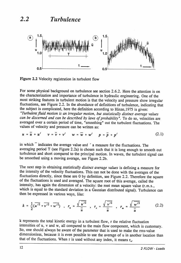
Figure 2.2 Velocity registration in turbulent flow

For some physical background on turbulence see section 2.6.2. Here the attention is onthe characterization and importance of turbulence in hydraulic engineering. One of themost striking features in turbulent motion is that the velocity and pressure show irregularfluctuations, see Figure 2.2. In the abundance of definitions of turbulence, indicating thatthe subject is complicated, here the definition according to Hinze, 1975 is given:"Turbulentfluid motion is an irregular motion, but statistically distinct average valuescan be discemed and can be described by laws of probability ti. To do so, veloeities areaveraged over a certain period of time, "smoothing" out the turbulent fluctuations. Thevalues of velocity and pressure cao be written as:

u = u + UI v = v + VI W = W + wl P = ; + pI (2.1)

in which indicates the average value and ' a measure for the fluctuations. Theaveraging period T (see Figure 2.2a) is chosen such that it is long enough to smooth outturbulence and short compared to the principal motion. In waves, the turbulent signal caobe smoothed using a moving average, see Figure 2.2b.

The next step in obtaining statisticaliy distinct average values is defining a measure forthe intensity of the velocity fluctuations. This cao not be done with the averages of thefluctuations directly, since these are 0 by definition, see Figure 2.2. Therefore the squareof the fluctuations is used and averaged. The square root of this average, called theintensity, has again the dimension of a velocity: the root meao square value (r.m.s.,which is equal to the standard deviation in a Gaussian distributed signal). Turbulence caothen be expressed in various ways, like:

1- -­k = -(u 12 +v'2 + w'2)2

J Ul2r = __11 -

U

J v/2r = __v -

U

(2.2)u

k represents the total kinetic energy in a turbulent flow, r the relative fluctuationintensities of u, v and w, all compared to the main flow component, which is customary.So, one should always be aware of the parameter that is used to make the rms-valuedimensionless, because it is even possible to use the average of u in another location thanthat of the fluctuations. When r is used without any index, it means ru.

12 2 FLOW - Loads

Reynolds stresses

In the appendix on basic equations (section 2.6.1) it is shown that due to the averaging ofthe velocity , extra normal and shear stresses appear in the momentum equation:

( OU - au - au) ap éPu (OUI2 aulw/)p - + u- + w- = -- + Il- - P-- + --at ox oz ox az2 ox ozinertia press. me. Reynolds-stresses

I---------------------------~ 1------------1by mean values by turbo fluet.

(2.3)

These extra terms come from the non-linear convective inertia terms and have thedimension of stresses, but how logic is it to consider them as stresses? The following is aqualitative analogy with elementary mechanics (adapted from LeMéhauté,1976).

Veloáty curve In flow

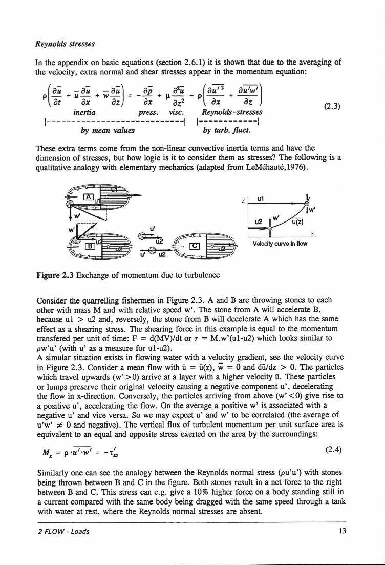
Figure 2.3 Exchange of momentum due to turbulence

Consider the quarrelling fishennen in Figure 2.3. A and B are throwing stones to eachother with mass M and with relative speed w'. The stone from A will accelerate B,because ul > u2 and, reversely, the stone from B will decelerate A which has the sameeffect as a shearing stress. The shearing force in this example is equal to the momentumtransfered per unit of time: F = d(MV)/dt or T = M.w'(uI-u2) which looks similar topw'u' (with u' as a measure for ul-u2).A simular situation exists in flowing water with a velocity gradient, see the velocity curvein Figure 2.3. Consider a mean flow with û = ü(z), W = 0 and dü/dz > O. The particleswhich travel upwards (w' >0) arrive at a layer with a higher velocity ü, These particlesor lumps preserve their original velocity causing a negative component u', deceleratingthe flow in x-direction. Conversely, the particles arriving from above (w' < 0) give rise toa positive u', accelerating the flow. On the average a positive w' is associated with anegative u' and vice versa. So we may expect u' and w' to be correlated (the average ofu'w' ~ 0 and negative). The vertical flux of turbulent momentum per unit surface area isequivalent to an equal and opposite stress exerted on the area by the surroundings:

-- IM = P -u'rw' = -'tz ~(2.4)

Similarly one can see the analogy between the Reynolds normal stress (pu'u') with stonesbeing thrown between B and C in the figure. Both stones result in a net force to the rightbetween B and C. This stress can e.g. give a 10% higher force on a body standing still ina current compared with the same body being dragged with the same speed through a tankwith water at rest, where the Reynolds normal stresses are absent.

2 FLOW - Loads 13

Eddy viscosity

The analogy between the motion of molecules and the turbulent movement of fluid ballshas led to the idea of a mixing length, I, which is the free path of a fluid ball. Assumingthe fluctuations u' and w' to be proportional to the velocity difference dû, which is equalto: dü = (dü/dz)dz = I(dü/dz). The same analogy leads to: r :: au/az (gradient-typetransport of momentum). The proportionality is expressed as the turbulent viscosity oreddy viscosity Vt. The total shear stress then becomes:

au 2 au au't' = p(u+u)- =p(u+1 1-1)-

t az az az (2.5)

There is, however, agreat difference between the two viscosity coefficients: themolecular viscosity is a property of the fluid, while the eddy viscosity is governed by theflow geometry. The purpose of many turbulence theories is to estimate Vu either via themixing length or with a sophisticated turbulence model and there is still a long way to goon that road. For a flow along a wall with I increasing linearly from 0 with the distancefrom the wall, this leads to a logarithmic velocity distribution. For more detail, the readeris referred to e.g Schlichting, 1968.Note: The association of turbulence with a velocity gradient is logical, since a differencein velocity is the cause of turbulence. However, when the velocity gradient is 0, there canstill be turbulent fluctuations, because turbulence is also transferred to other regions.

Flow resistance

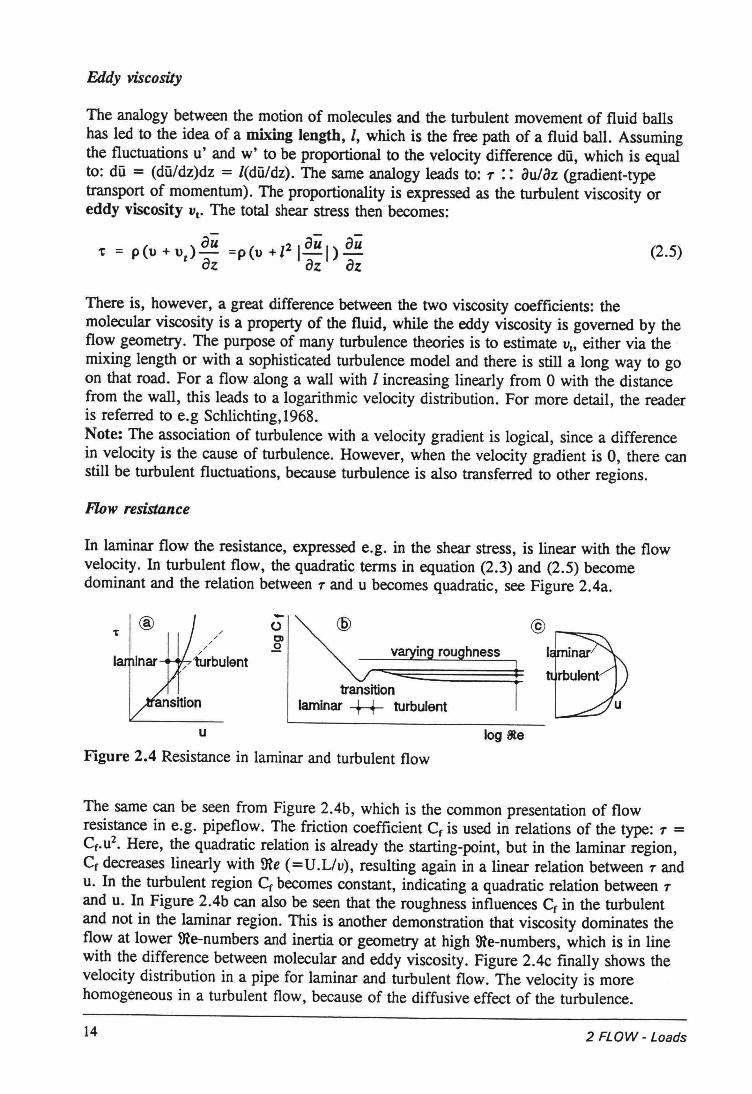
In laminar flow the resistance, expressed e.g. in the shear stress, is linear with the flowvelocity . In turbulent flow, the quadratic terms in equation (2.3) and (2.5) becomedominant and the relation between r and u becomes quadratic, see Figure 2.4a.

oOl..Q

@

transitionlamlnar ++- turbulent

u log meFigure 2.4 Resistance in laminar and turbulent flow

The same can be seen from Figure 2.4b, which is the common presentation of flowresistance in e.g. pipeflow. The friction coefficient Cf is used in relations of the type: r =Cf·U2• Here, the quadratic relation is already the starting-point, but in the laminar region,Cf decreases linearly with me (=U.L/v), resulting again in a linear relation between r andu. In the turbulent region Cf becomes constant, indicating aquadratic relation between rand u. In Figure 2.4b can also be seen that the roughness influences Cf in the turbulentand not in the laminar region. This is another demonstration that viscosity dominates theflow at lower me-numbers and inertia or geometry at high 9le-numbers, which is in linewith the difference between molecular and eddy viscosity. Figure 2.4c finally shows thevelocity distribution in a pipe for laminar and turbulent flow. The velocity is morehomogeneous in a turbulent flow, because of the diffusive effect of the turbulence.

14 2 FLOW - Loads

2.3 Flow situations

2.3.1 Wallflow

h-._-_.-._

_._~-- --

o 0.05 0.1 0.15

:,\ _2I u'w'!ü: ,: I: I: I

o -0,004

Figure 2.5 Uniform flow

Uniform flow

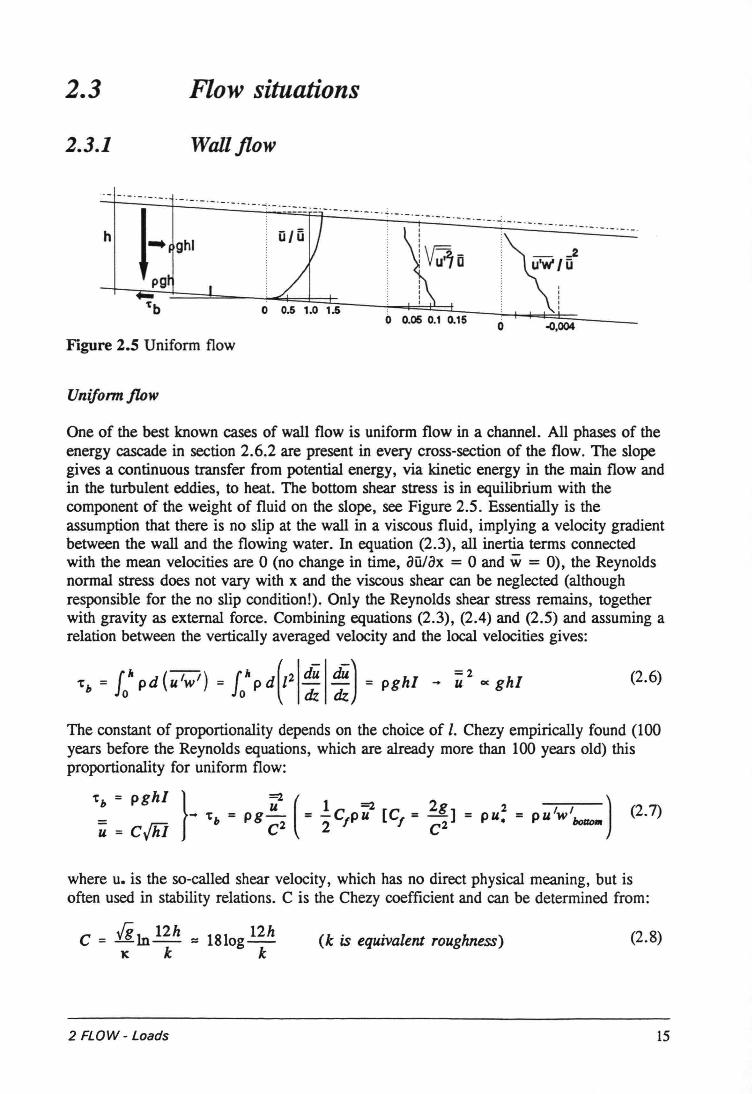
One of the best known cases of wall flow is uniform flow in a channel. All phases of theenergy cascade in section 2.6.2 are present in every cross-section of the flow. The slopegives a continuous transfer from potential energy, via kinetic energy in the main flow andin the turbulent eddies, to heat. The bottom shear stress is in equilibrium with thecomponent of the weight of fluid on the slope, see Figure 2.5. Essentially is theassumption that there is no slip at the wall in a viscous fluid, implying a velocity gradientbetween the wall and the flowing water. In equation (2.3), all inertia terrns connectedwith the mean veloeities are 0 (no change in time, éJü/éJx= 0 and w = 0), the Reynoldsnormal stress does not vary with x and the viscous shear can be neglected (althoughresponsible for the no slip condition!). Only the Reynolds shear stress remains, togetherwith gravity as extemal force. Combining equations (2.3), (2.4) and (2.5) and assuming arelation between the vertically averaged velocity and the local veloeities gives:

ril (- ) ril ( dü dÜ) - 2'tb = Jo pd u'w' = Jo pd 12 dz dz = pghI .. Ü oe ghI (2.6)

The constant of proportionality depends on the choice of I. Chezy empirically found (100years before the Reynolds equations, which are already more than 100 years old) thisproportionality for uniform flow:

'tb = pghI } =2 ( 1 =2 2 )_ .. 't = Pg ~ = - C pÜ [C = __K] = p U

2 = PU IW I- Iï:i b C2 2 I I C2 • bottolltU = CyhI

(2.7)

where u. is the so-called shear velocity, which has no direct physical meaning, but isoften used in stability relations. C is the Chezy coefficient and can be determined from:

C = .fi]n 12h ::::1810g 12hK k k

(k is equivalent roughness) (2.8)

2 FLOW - Loads 15

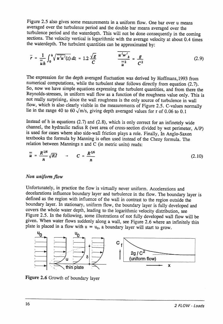
Figure 2.5 also gives some measurements in a uniform flow. One bar over u meansaveraged over the turbulence period and the double bar means averaged over theturbulence period and the waterdepth. This will not be done consequently in the comingsections. The velocity vertical is logarithmic with the average velocity at about 0.4 timesthe waterdepth. The turbulent quantities can be approximated by:

u'w'b = ..L

=2 C2U

(2.9)r = _1 J."J u'u'(z) dz = 1.2 {ëuh 0 C

The expression for the depth averaged fluctuation was derived by Hoffmans,1993 fromnumerical computations, while the turbulent shear follows directly from equation (2.7).So, now we have simple equations expressing the turbulent quantities, and from there theReynolds-stresses, in uniform wall flow as a function of the roughness value only. This isnot really surprising, since the wall roughness is the only souree of turbulence in wallflow, which is also c1early visible in the measurements of Figure 2.5. C-values normallylie in the range 40 to 60..Jm/s, giving depth averaged values for r of 0.06 to 0.1

Instead of h in equations (2.7) and (2.8), which is only correct for an infinetely widechannel, the hydraulic radius R (wet area of cross-section divided by wet perimeter, AlP)is used for cases where also side-wall friction plays a role. Finally, In Anglo-Saxontextbooks the formula by Manning is often used instead of the Chezy formula. Therelation between Mannings n and C (in metric units) reads:

= R1/6U = -[Ri

nR1/6c=­n

(2.10)

Non uniform flow

Unfortunately, in practice the flow is virtually never uniform. Accelerations anddecelarations influence boundary layer and turbulence in the flow. The boundary layer isdefined as the region with influence of the wall in contrast to the region outside theboundary layer. In stationary, uniform flow, the boundary layer is fully developed andcovers the whole water depth, leading to the logarithmic velocity distribution, seeFigure 2.5. In the following, some illustrations of not fully developed wall flow will begiven. When water flows suddenly along a wall, see Figure 2.6 where an infinitely thinplate is placed in a flow with u = uo, a boundary layer will start to grow.

uo ~ uo

2g I C2 ------------(uniform flow)

x

Figure 2.6 Growth of boundary layer

16 2 FLOW - Loads

At the start, o(x) = 0, leading to a theoretically infmite shear stress. This shear stresswill brake the flow and the boundary layer grows because of the exchange of momentum.This growth can roughly be estimated with o(x) = 0.02x to 0.03x, indicating that after 30- 50 times the waterdepth, the flow will be developed and the boundary layer will equalthe waterdepth. With the growth of 0, the shear stress decreases and eventually, Crreaches the value of equation (2.7).

Acceleration is due to a pressure gradient in the flow direction and an opposite gradientleads to deceleration, both causing a change in the boundary layer thickness. When thisconvective inertia is considerable, the change in 0 is roughly given by, see Booij,1988:

dl> = -(4 to 5) ö duodx Uo dx

(2.11)

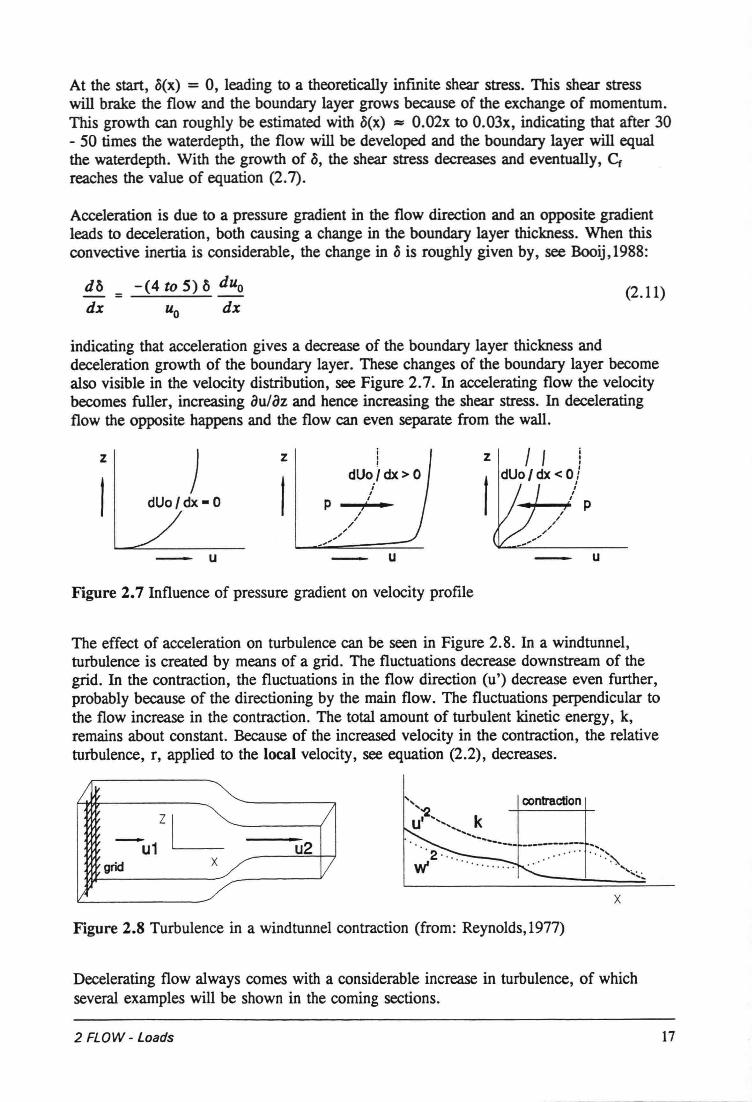
indicating that acceleration gives a decrease of the boundary layer thickness anddeceleration growth of the boundary layer. These changes of the boundary layer becomealso visible in the velocity distribution, see Figure 2.7. In accelerating flow the velocitybecomes fuller, increasing oulBz and hence increasing the shear stress. In deceleratingflow the opposite happens and the flow can even separate from the wall.

z )dUo/dx- 0

z

II/

'",/~,'

- u u u

Figure 2.7 Influence of pressure gradient on velocity profile

The effect of acceleration on turbulence can be seen in Figure 2.8. In a windtunnel,turbulence is created by means of a grid. The fluctuations decrease downstream of thegrid. In the contraction, the fluctuations in the flow direction (u') decrease even further,probably because of the directioning by the main flow. The fluctuations perpendicular tothe flow increase in the contraction. The total amount of turbulent kinetic energy, k,remains about constant. Because of the increased velocity in the contraction, the relativeturbulence, r, applied to the local velocity, see equation (2.2), decreases.

I~ -u1ZL /

u2griel x/ V

V

contraction

xFigure 2.8 Turbulence in a windtunnel contraction (from: Reynolds, 1977)

Decelerating flow always comes with a considerable increase in turbulence, of whichseveral examples will be shown in the coming sections.

2 FLOW - Loads 17

2.3.2 Freeflow

Mixing layers

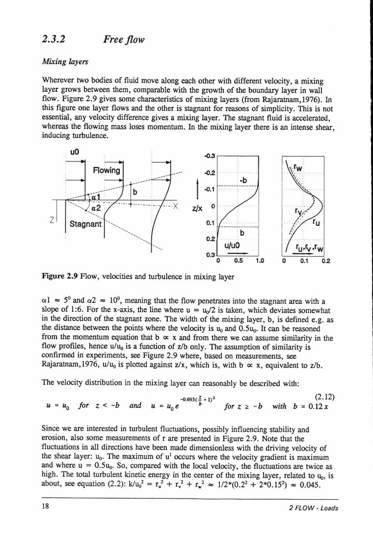
Wherever two bodies of fluid move along each other with different velocity , a mixinglayer grows between them, comparabie with the growth of the boundary layer in wallflow. Figure 2.9 gives some characteristics of mixing layers (from Rajaratnam,1976). Inthis figure one layer flows and the other is stagnant for reasons of simplicity . This is notessential, any velocity difference gives a mixing layer. The stagnant fluid is accelerated,whereas the flowing mass loses momentum. In the mixing layer there is an intense shear,inducing turbulence.

uO "().3~---~

z

-b"().2 .

0.1

0.2 ..u/uO

0.5 1.0

Figure 2.9 Flow, veloeities and turbulence in mixing layer

o 0.1

al := 5° and a2 := 10°, meaning that the flow penetrates into the stagnant area with aslope of 1:6. For the x-axis, the line where u = uJ2 is taken, which deviates somewhatin the direction of the stagnant zone. The width of the mixing layer, b, is defined e.g. asthe distance between the points where the velocity is Uoand 0.5Uo.It can be reasonedfrom the momentum equation that b ex x and from there we can assume similarity in theflow profiles, hence u/u, is a function of z/b only. The assumption of similarity isconfirmed in experiments, see Figure 2.9 where, based on measurements, seeRajaratnam,1976, u/u, is plotted against z/x, which is, with b ex x, equivalent to z/b.

The velocity distribution in the mixing layer cao reasonably be described with:

-0.693( ~ + 1)2U = Uo lor z < -b and u = Uoe b lor z ~ - b

(2.12)with b ~ 0.12x

Since we are interested in turbulent fluctuations, possibly influencing stability anderosion, also some measurements of rare presented in Figure 2.9. Note that thefluctuations in all directions have been made dimensionless with the driving velocity ofthe shear layer: Uo. The maximum of UI occurs where the velocity gradient is maximumand where u = 0.5uo. So, compared with the local velocity, the fluctuations are twice ashigh. The total turbulent kinetic energy in the center of the mixing layer, related to Uo, isabout, see equation (2.2): k/u02 = ru2+ r/ + r.,,z := 1/2*(0.22 + 2*0.152) = 0.045.

18 2 FLOW - Loads

Jets

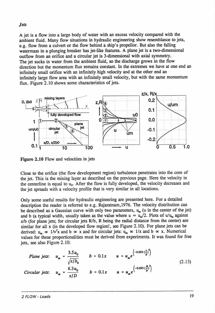
A jet is a flow into a large body of water with an excess velocity compared with theambient fluid. Many flow situations in hydraulic engineering show resemblance to jets,e.g. flow from a culvert or the flow bebind a ship's propellor. But also the fallingwatermass in a plunging breaker has jet-like features. A plane jet is a two-dimensionaloutflow from an orifice and a circular jet is 3-dimensional with axial symmetry.The jet sucks in water from the ambient fluid, so the discharge grows in the flowdirection but the momentum flux remains constant. In the extremes we have at one end aninfinitely small orifice with an infinitely high velocity and at the other end aninfinitely large flow area with an infmitely small velocity , but with the same momentumflux. Figure 2.10 shows some characteristics of jets.

urn/uO .

txJD. xJ2bO

0.11 10 100

Figure 2.10 Flow and veloeities in jets

,-- ----,zb; R/xl-- --,0.2

0.1

0.0

-0.1

-0.2 .o- U 0.5 1.0

Close to the orifice (the flow development region) turbulence penetrates into the core ofthe jet. This is the mixing layer as described on the previous page. Here the velocity inthe centerline is equal to uo. After the flow is fully developed, the velocity decreases andthe jet spreads with a velocity profile that is very similar in all locations.

Only some useful results for hydraulic engineering are presented here. For a detaileddescription the reader is referred to e.g. Rajaratnam,1976. The velocity distribution canbe described as a Gaussian curve with only two parameters, llm (u in the center of the jet)and b (a typical width, usually taken as the value where u = llm/2. Plots of u/llm againstz/b (for plane jets; for circular jets RIb, R being the radial distance from the center) aresimilar for all x (in the developed flow region!, see Figure 2.10). For plane jets can bederived: llm ex lIv'x and b oe x and for circular jets: u.n oe lIx and b oe x. Numericalvalues for these proportionalities must be derived from experiments. Itwas found for freejets, see also Figure 2.10:

Plane jets:3.5uo

u =--IJl JX/bo

6.3uou =--

IJl xl DCircular jets:

b = O.lx (-0.693 (~)2)U = U e b

IR

(2.13)

2 FLOW - Loads 19

b = O.lx

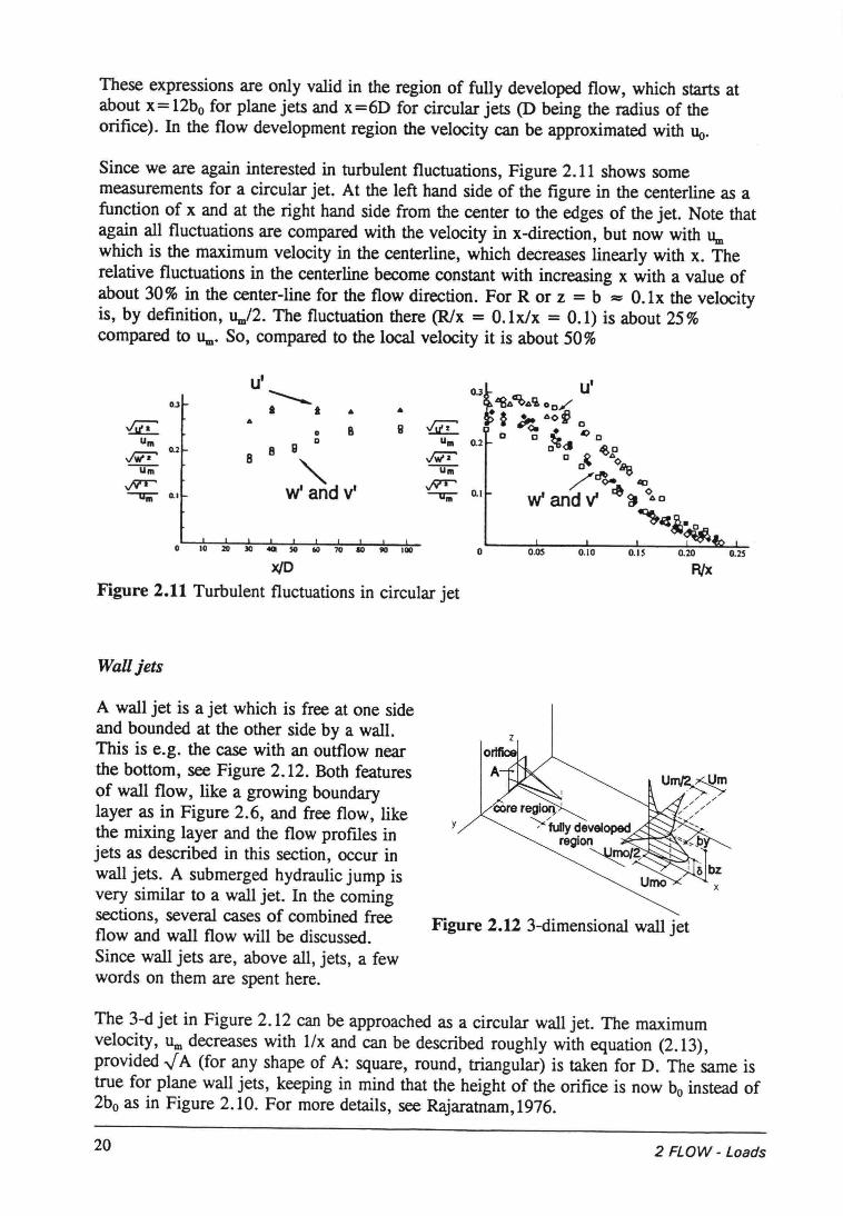
These expressions are only valid in the region of fully developed flow, which starts atabout x= 12bo for plane jets and x=6D for circular jets (D being the radius of theorifice). In the flow development region the velocity can be approximated with Uo.

Since we are again interested in turbulent fluctuations, Figure 2.11 shows somemeasurements for a circular jet. At the left hand side of the figure in the centerline as afunction of x and at the right hand side from the center to the edges of the jet. Note thatagain all fluctuations are compared with the velocity in x-direction, but now with llmwhich is the maximum velocity in the centerline, which decreases linearly with x. Therelative fluctuations in the centerline become constant with increasing x with a value ofabout 30% in the center-line for the flow direction. For R or z = b =:: O.lx the velocityis, by definition, llm12.The fluctuation there (R/x = O.Ix/x = 0.1) is about 25%compared to llm.So, compared to the local velocity it is about 50%

Ui+--;* a •0.3

..Jg.Um

../YjO' 0.2

-u;;;­.jY'T""--um- 0.1

oD

6 9

8 9

8 '"w' and v'

o JO 20 se 4CII so 60 70 10 90 100

X/DFigure 2.11 Turbulent fluctuations in circular jet

WaIljets

A wall jet is a jet which is free at one sideand bounded at the other side by a wall.This is e.g. the case with an outflow nearthe bottom, see Figure 2.12. Both featuresof wall flow, like a growing boundarylayer as in Figure 2.6, and free flow, likethe mixing layer and the flow profiles injets as described in this section, occur inwall jets. A submerged hydraulic jump isvery similar to a wall jet. In the comingsections, several cases of combined freeflow and wall flow will be discussed.Since wall jets are, above all, jets, a fewwords on them are spent here.

o 0.05 0.10 O.IS 0.20 0.25

Rlx

y

Figure 2.12 3-dimensional wall jet

The 3-d jet in Figure 2.12 can be approached as a circular wall jet. The maximumvelocity , llmdecreases with l/x and can be described roughly with equation (2.13),provided .JA (for any shape of A: square, round, triangular) is taken for D. The same istrue for plane wall jets, keeping in mind that the height of the orifice is now bo instead of2bo as in Figure 2.10. For more details, see Rajaratnam,1976.

20 2 FLOW - Loads

2.3.3 Flow around detached bodies

Figure 2.13 Flow separation around b1unt and round body

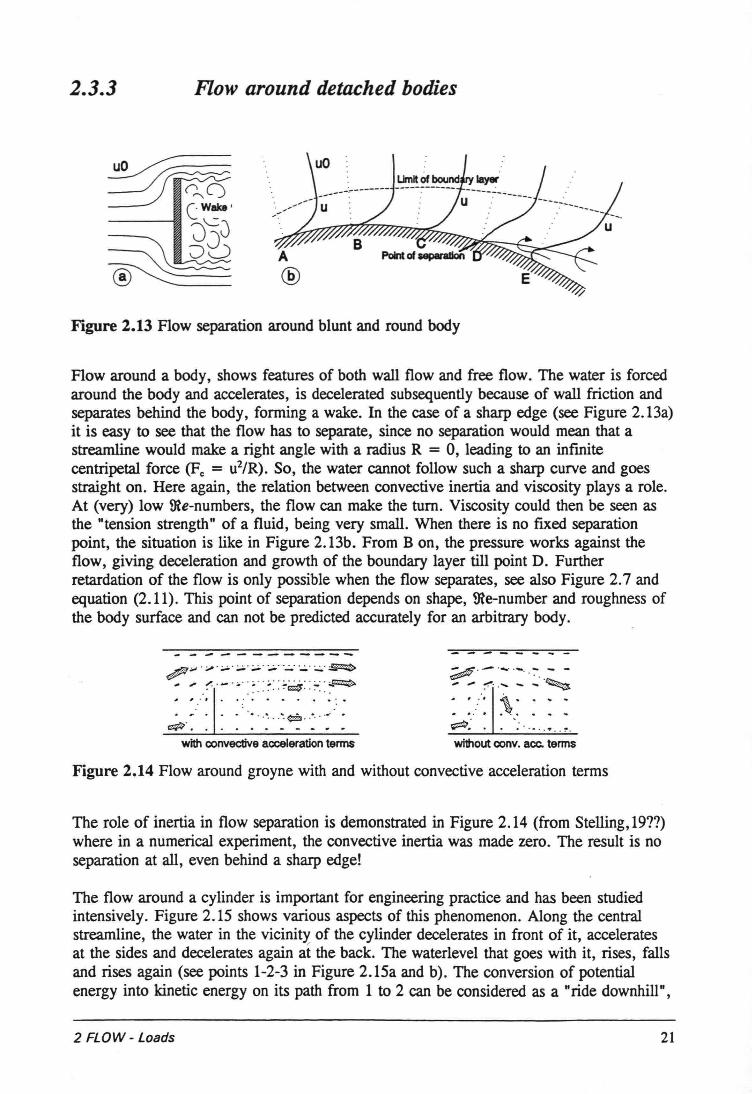
Flow around a body, shows features of both wall flow and free flow. The water is forcedaround the body and accelerates, is decelerated subsequently because of wall friction andseparates behind the body, fonning a wake. In the case of a sharp edge (see Figure 2. 13a)it is easy to see that the flow has to separate, since no separation wou1dmean that astreamline would make a right angle with a radius R = 0, leading to an infinitecentripetal force (F, = u2/R). So, the water cannot follow such a sharp curve and goesstraight on. Here again, the relation between convective inertia and viscosity p1aysa role.At (very) low 9le-numbers, the flow can make the turn. Viscosity could then be seen asthe "tension strength" of a fluid, being very small. When there is no fixed separationpoint, the situation is like in Figure 2.13b. From Bon, the pressure works against theflow, giving dece1eration and growth of the boundary layer till point D. Furtherretardation of the flow is only possible when the flow separates, see aIso Figure 2.7 andequation (2.11). This point of separation depends on shape, 9le-number and roughness ofthe body surface and can not be predicted accurately for an arbitrary body.

~.;.::..:..:..~. '·:'1i' .~.~... ': ' ..:... . .~, '.' .....•..•.without conv. ace. terms

Figure 2.14 Flow around groyne with and without convective acceleration tenns

The role of inertia in flow separation is demonstrated in Figure 2.14 (from Stelling, 1911)where in a numerical experiment, the convective inertia was made zero. The result is noseparation at all, even behind a sharp edge!

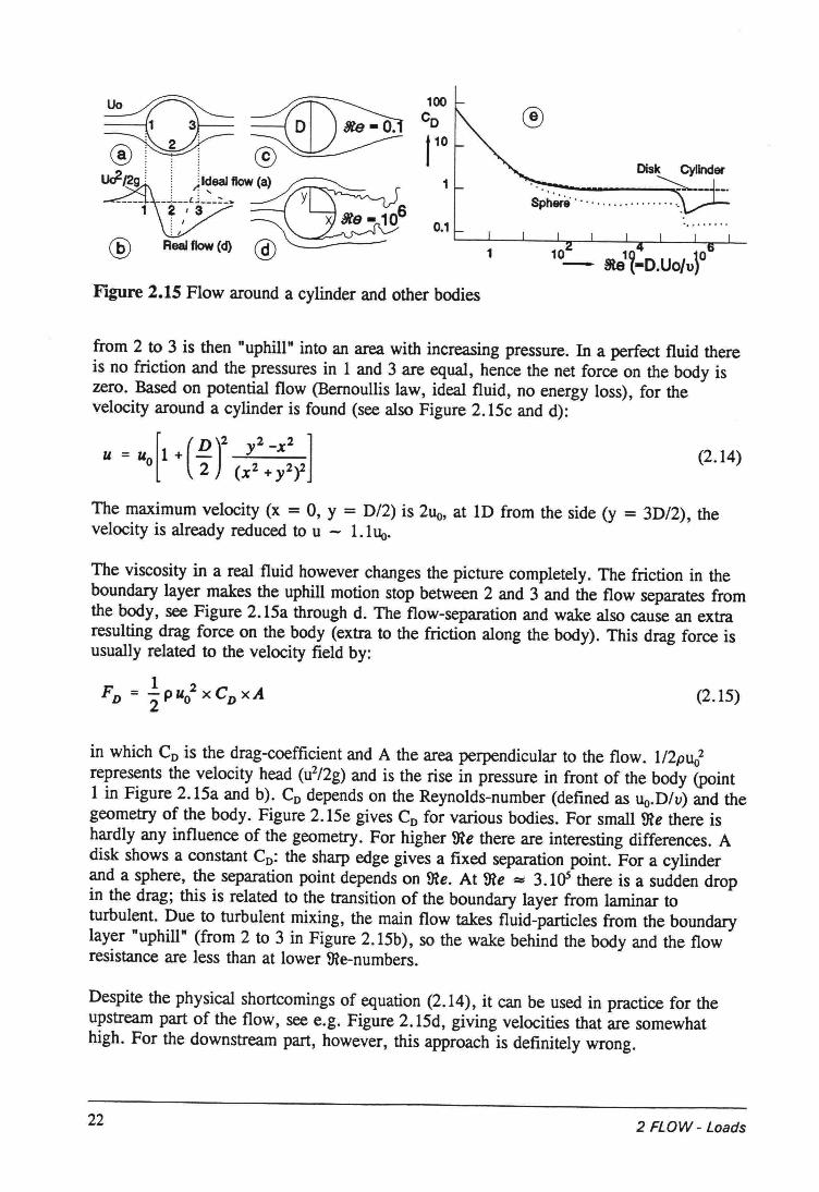
The flow around a cylinder is important for engineering practice and has been studiedintensive1y. Figure 2.15 shows various aspects of this phenomenon. Along the centra!streamline, the water in the vicinity of the cylinder decelerates in front of it, acceleratesat the sides and decelerates again at the back. The waterlevel that goes with it, rises, faIlsand rises again (see points 1-2-3 in Figure 2.15a and b). The conversion of potentiaIenergy into kinetic energy on its path from 1 to 2 can be considered as a "ride downhill" ,

2 FLOW - Loads 21

~~

~~Ucf./2g : : jldeal floW~a). . ....

~ y lIte-l06@ R~flow(d) ~

®

1SPh~e···· .

0.1

Figure 2.15 Flow around a cylinder and other bodies

from 2 to 3 is then "uphili" into an area with increasing pressure. In a perfect fluid thereis no friction and the pressures in 1 and 3 are equal, hence the net force on the body iszero. Based on potential flow (Bernoullis law, ideal fluid, no energy loss), for thevelocity around a cylinder is found (see also Figure 2.15c and d):

[ (D)2 y2 -x2 1u=uol+ -2 (x2 + y2)2

The maximum velocity (x = 0, y = D/2) is 2uo, at lD from the side (y = 3D/2), thevelocity is already reduced to u - 1.1Uo.

(2.14)

The viscosity in a real fluid however changes the picture completely. The friction in theboundary layer makes the uphill motion stop between 2 and 3 and the flow separates fromthe body, see Figure 2.15a through d. The flow-separation and wake also cause an extraresulting drag force on the body (extra to the friction along the body). This drag force isusually related to the velocity field by:

(2.15)

in which Co is the drag-coefficient and A the area perpendicular to the flow. 1/2puo2represents the velocity head (u2/2g) and is the rise in pressure in front of the body (point1 in Figure 2.15a and b). CD depends on the Reynolds-number (defined as Uo.D/v)and thegeometry of the body. Figure 2.15e gives CD for various bodies. For small me there ishardly any influence of the geometry. For higher me there are interesting differences. Adisk shows a constant CD: the sharp edge gives a fixed separation point. For a cylinderand a sphere, the separation point depends on me. At me := s.io' there is a sudden dropin the drag; this is related to the transition of the boundary layer from laminar toturbulent. Due to turbulent mixing, the main flow takes fluid-particles from the boundarylayer "uphill" (from 2 to 3 in Figure 2.15b), so the wake behind the body and the flowresistance are less than at lower me-numbers.

Despite the physical shortcomings of equation (2.14), it can be used in practice for theupstrearn part of the flow, see e.g. Figure 2.15d, giving veloeities that are somewhathigh. For the downstrearn part, however, this approach is definitely wrong.

22 2 FLOW - Loads

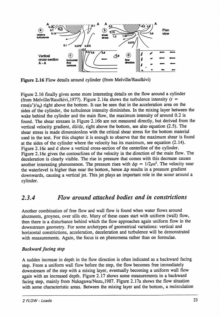
A

Planview

Vertlcalcross-sedionA-A

@ I " - -<1.tlIow

, ",. - -chdIon - -I p

~ • - -Figure 2.16 Flow details around cylinder (from Melville/Raudkivi)

Figure 2.16 finally gives some more interesting details on the flow around a cylinder(from Melville/Raudkivi,1977). Figure 2.16a shows the turbulence intensity (r =rms(u')/llo) right above the bottom. It can be seen that in the acceleration area on thesides of the cylinder, the turbulence intensity diminishes. In the mixing layer between thewake behind the cylinder and the main flow, the maximum intensity of around 0.2 isfound. The shear stresses in Figure 2.16b are not measured directly, but derived from thevertical velocity gradient, dü/dz, right above the bottom, see also equation (2.5). Theshear stress is made dimensionless with the critical shear stress for the bottom materialused in the test. For this chapter it is enough to observe that the maximum shear is foundat the sides of the cylinder where the velocity has its maximum, see equation (2.14).Figure 2.16c and d show avertical cross-section of the centerline of the cylinder.Figure 2.16c gives the contourlines of the velocity in the direction of the main flow. Thedeceleration is clearly visible. The rise in pressure that comes with this decrease causesanother interesting phenomenon. The pressure rises with .6.p= 1/2pu2• The velocity nearthe waterlevel is higher than near the bottom, hence .6.presults in a pressure gradientdownwards, causing a vertical jet. This jet plays an important role in the scour around acylinder.

2.3.4 Flow around attached bodies and in constrictions

Another combination of free flow and wall flow is found when water flows aroundabutments, groynes, over sills etc. Many of these cases start with uniform (wall) flow,then there is a disturbance behind which the flow approaches again uniform flow in thedownstream geometry. For some archetypes of geometrical variations: vertical andhorizontal constrictions, acceleration, deceleration and turbulence will be demonstratedwith measurements. Again, the focus is on phenomena rather than on formulae.

Backward facing step

A sudden increase in depth in the flow direction is often indicated as a backward facingstep. From a uniform wall flow before the step, the flow becomes free immediatelydownstream of the step with a mixing layer, eventually becoming a uniform wall flowagain with an increased depth. Figure 2.17 shows some measurements in a backwardfacing step, mainly from NakagawalNezu,1987. Figure 2.17a shows the flow situationwith some characteristic areas. Between the mixing layer and the bottom, a recirculation

2 FLOW - Loads 23

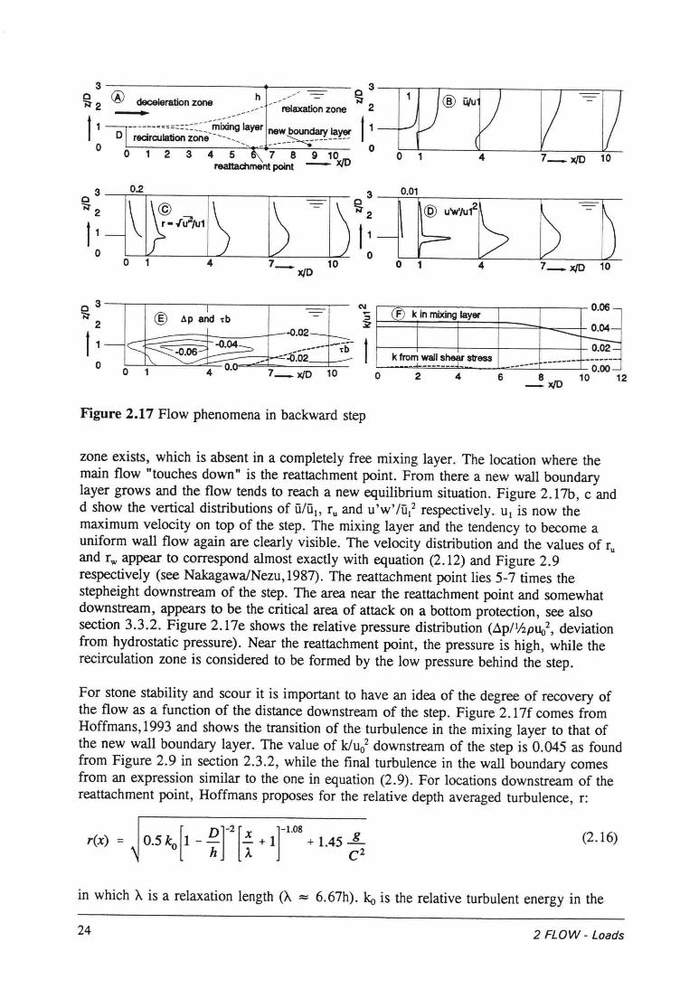
03 ® h __.> - ~3-W~®Ü/uy V -=-vtl 2 deceleration zone ~~_--- ~ relaxation zone 2

t 1 -::;'--_:~=:::::==:~~nglayer new boundary layer lo rearallation zone --_' _:::-------------o -, - --- -----. 0o 1 2 3 4 5 7 8 ~0xJD 0 1 4 7_ X/D 10

reattachrnent point

o 3 --,-----r-----,------r-----,-tl 2 ® .1p and 'tb -

t ' r--.b~=:::t::O:Ci4::=_r ~~~-----;1)-----I__",.<~.02

o

® ;-k in mixing layer

I I -- 0.04-t---0.02-

k fro_m~~~~ stress ------- -------------- 0.00-

006

o7_xJD 10 o 2 4 6 10 12

Figure 2.17 Flow phenomena in backward step

zone exists, which is absent in a completely free mixing layer. The location where themain flow "touches down" is the reattachment point. From there a new wall boundarylayer grows and the flow tends to reach a new equilibrium situation. Figure 2.17b, c andd show the vertical distributions of u/Ut, r, and u'w'/üt2 respectively. Ut is now themaximum velocity on top of the step. The mixing layer and the tendency to become auniform wall flow again are clearly visible. The velocity distribution and the values of r,and r; appear to correspond almost exactly with equation (2.12) and Figure 2.9respectively (see Nakagawa/Nezu, 1987). The reattachment point lies 5-7 times thestepheight downstream of the step. The area near the reattachment point and somewhatdownstream, appears to be the critica1 area of attack on a bottom protection, see alsosection 3.3.2. Figure 2.17e shows the relative pressure distribution (.~p/t/2P1lo2,deviationfrom hydrostatic pressure). Near the reattachment point, the pressure is high, while therecirculation zone is considered to be formed by the low pressure behind the step.

For stone stability and scour it is important to have an idea of the degree of recovery ofthe flow as a function of the distance downstream of the step. Figure 2.17f comes fromHoffmans,1993 and shows the transition of the turbulence in the mixing layer to that ofthe new wall boundary layer. The value of k/uo2 downstream of the step is 0.045 as foundfrom Figure 2.9 in section 2.3.2, while the final turbulence in the wall boundary comesfrom an expression similar to the one in equation (2.9). For locations downstream of thereattachment point, Hoffmans proposes for the relative depth averaged turbulence, r:

[ Dj-2 [ j-l08r(x) = 0.5 ko 1 - h ~+ 1 . + 1.45 ~2 (2.16)

in which À is a relaxation length (À :::::6.67h). ko is the relative turbulent energy in the

24 2 FLOW - Loads

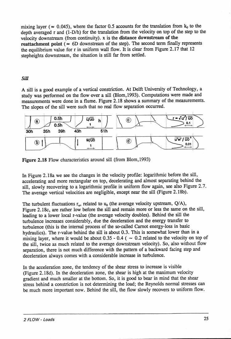
mixing layer (= 0.045), where the factor 0.5 accounts for the translation from ko to thedepth averaged r and (I-D/h) for the translation from the velocity on top of the step to thevelocity downstrearn (from continuity). x is the distance downstream of thereattachment point (= 6D downstrearn of the step). The second term finally representsthe equilibrium value for r in uniform wall flow. It is clear from Figure 2.17 that 12stepheights downstrearn, the situation is still far from settled.

Sill

A sill is a good example of avertical constriction. At Delft University of Technology, astudy was performed on the flow over a sill (Blom,1993). Computations were made andmeasurements were done in a flume. Figure 2.18 shows a summary of the measurements.The slopes of the sill were such that no real flow separation occurred.

. . .' _. .

IJ ®IJ ~::,<) ~ hi) 1\©}:-";43i1;__---==t:..--S'-1!....h-

.' ::. .

!--I - i}/_...!:..-_I ~---+-II_____::;~~1~--!---- ~-@j/-i--i =-l-~----T-~----=u'w'=--:IL=....-'t-~:5-

.. .

i\ c:s:u,,).~. 0.1.• .j....--..4... .

30h 35h 39h

Figure 2.18 Flow characteristics around sill (from Blom, 1993)

In Figure 2.18a we see the changes in the velocity profile: logarithmic before the sill,accelerating and more rectangular on top, decelerating and almost separating behind thesill, slowly recovering to a logarithmic profile in uniform flow again, see also Figure 2.7.The average vertical veloeities are negligible, except near the sill (Figure 2. 18b).

The turbulent fluctuations ru, related to llo (the average velocity upstrearn, Q/A),Figure 2.18c, are rather low before the sill and remain more or less the same on the sill,leading to a lower local r-value (the average velocity doubles). Behind the sill theturbulence increases considerably, due the deceleration and the energy transfer toturbulence (this is the intemal process of the so-called Camot energy-loss in basichydraulics). The r-value behind the sill is about 0.3. This is somewhat lower than in amixing layer, where it would be about 0.35 - 0.4 ( - 0.2 related to the velocity on top ofthe sill, twice as much related to the average downstream velocity). So, also without flowseparation, there is not much difference with the pattem of a backward facing step anddeceleration always comes with a considerabie increase in turbulence.

In the acceleration zone, the tendency of the shear stress to increase is visible(Figure 2.18d). In the deceleration zone, the shear is high at the maximum velocitygradient and much smaller at the bottom. So, it is good to bear in mind that the shearstress behind a constriction is not determining the load; the Reynolds normal stresses canbe much more important now. Behind the sill, the flow slowly reeovers to uniform flow.

2 FLOW - Loads 25

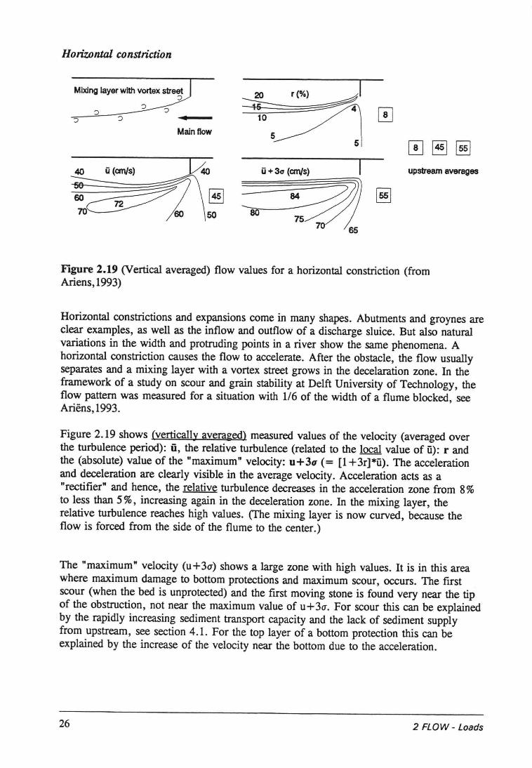
Horizontal constriction

Mixing Iayer wlth vortex streetJ r(%}

Main flow 55

ü +3(7 (an/s) I

=iO~~65

upstream averages

Figure 2.19 (Vertical averaged) flow values for a horizontal constriction (fromAriens, 1993)

Horizontal constrictions and expansions come in many shapes. Abutments and groynes areclear examples, as weU as the inflow and outflow of a discharge sluice. But also naturalvariations in the width and protruding points in a river show the same phenomena. Ahorizontal constriction causes the flow to accelerate. After the obstacle, the flow usuallyseparates and a mixing layer with a vortex street grows in the decelaration zone. In theframework of a study on scour and grain stability at Delft University of Technology, theflow pattem was measured for a situation with 1/6 of the width of a flume blocked, seeAriëns, 1993.

Figure 2.19 shows (vertically averaged) measured values of the velocity (averaged overthe turbulence period): û, the relative turbulence (related to the local value of ü): randthe (absolute) value of the "maximum" velocity: u+30' (= [1+3r]*ü). The accelerationand deceleration are clearly visible in the average velocity. Acceleration acts as a"rectifier" and hence, the relative turbulence decreases in the acceleration zone from 8%to less than 5%, increasing again in the deceleration zone. In the mixing layer, therelative turbulence reaches high values. (The mixing layer is now curved, because theflow is forced from the side of the flume to the center.)

The "maximum" velocity (u+30") shows a large zone with high values. It is in this areawhere maximum damage to bottom protections and maximum scour, occurs. The firstscour (when the bed is unprotected) and the first moving stone is found very near the tipof the obstruction, not near the maximum value of u+30". For scour this can be explainedby the rapidly increasing sediment transport capacity and the lack of sediment supplyfrom upstream, see section 4.1. For the top layer of a bottom proteetion this can beexplained by the increase of the velocity near the bottom due to the acceleration.

26 2 FLOW - Loads

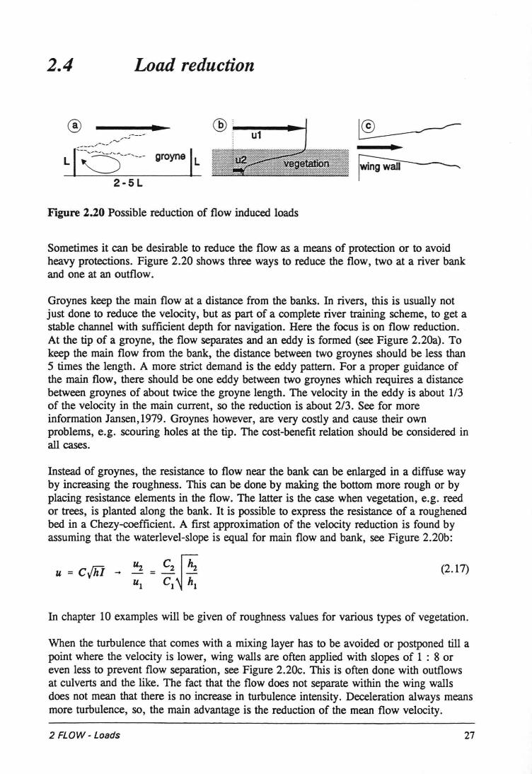
2.4 Load reduction

,---­,._..."

,'"

L 1'6------- groynel L

2-5 L

Figure 2.20 Possible reduction of flow induced loads

Sometimes it can be desirabie to reduce the flow as a means of proteetion or to avoidheavy protections. Figure 2.20 shows three ways to reduce the flow, two at a river bankand one at an outflow .

Groynes keep the main flow at a distance from the banks. In rivers, this is usually notjust done to reduce the velocity, but as part of a complete river training scheme, to get astabie channel with sufficient depth for navigation. Here the focus is on flow reduction.At the tip of a groyne, the flow separates and an eddy is formed (see Figure 2.20a). Tokeep the main flow from the bank, the distance between two groynes should be less than5 times the length. A more strict demand is the eddy pattem. For a proper guidance ofthe main flow, there should be one eddy between two groynes which requires a distancebetween groynes of about twice the groyne length. The velocity in the eddy is about 1/3of the velocity in the main current, so the reduction is about 2/3. See for moreinformation Jansen, 1979. Groynes however, are very costly and cause their ownproblems, e.g. scouring holes at the tip. The cost-benefit relation should be considered inall cases.

Instead of groynes, the resistance to flow near the bank can he enlarged in a diffuse wayby increasing the roughness. This can be done by making the bottom more rough or byplacing resistance elements in the flow. The latter is the case when vegetation, e.g. reedor trees, is planted along the bank. It is possible to express the resistance of a roughenedbed in a Chezy-coefficient. A first approximation of the velocity reduction is found byassuming that the waterlevel-slope is equal for main flow and bank, see Figure 2.20b:

(2.17)

In chapter 10 examples will be given of roughness values for various types of vegetation.

When the turbulence that comes with a mixing layer has to be avoided or postponed till apoint where the velocity is lower, wing walls are often applied with slopes of 1 : 8 oreven less to prevent flow separation, see Figure 2.2Oc. This is often done with outflowsat culverts and the like. The fact that the flow does not separate within the wing wallsdoes not mean that there is no increase in turbulence intensity. Deceleration always meansmore turbulence, so, the main advantage is the reduction of the mean flow velocity .

2 FLOW - Loads 27

2.5 Summary

For the design of a protection, or for the judgement whether a proteetion is necessary,detailed irformaiion on the velocity-field is needed to determine the loads. This con comefrom measurements, a flow model or a sketch, based on overall discharge data andinsight in the flow phenomena. In fact, every preliminary design should start with asimple sketch on a sheet of paper.

The same is true for turbulence in the velocity-field, albeit that the determination ofturbulence from a model is much more difficult and uncertain. The turbulent velocityfluctuaiions are a result of velocity differences, eisher between flow and a wall (wallturbulence) or between two fluid bodies (free turbulence). Turbulence is always coupledwith loss of kinetic energy. A typical value for wall turbulence is r (= r.m.s. u' /ü) = 0.1and for free turbulence rmax= 0.2-0.3, also depending on where û is defined. Inaccelerating flow the relative turbulence is less, although the shear stress can becomehigher. The turbulent fluctuations cause so-called Reynolds stresses: a normal stress duethe velocity fluctuations in one direction and a shear stress due to the correlation betweenthe fluctuations in two direcuons.

For uniform (wall)flow, relatively simple, panly empirical relations are available, likeChezy's law and the accompanying expressions for wall roughness and turbulentquantities. Mixing layers are on essensial pan in free turbulence and occur in manysituations in hydraulic engineering. Another example of free turbulence is found in jetflow, which is also frequently encountered in flow situaiions near hydraulic structures. Ajet stans with mixing layers at the edges and a non-turbulent core. After this core hasvanished, the flow in jets can be described wuh relatively simple expressions.

Flow situaüons around bodies, like (bridge) piers, through vertical constrictions, like sillsand through horizontal constrictions, like abutments and groynes, all showaccelerationfollowed by deceleration witn the accompanying turbulence. The acceleration leads tohigher veloeities than in uniform flow, giving a higher load on any interface in theneighbourhood. The same is true for the deceleration zone with the increase of theReynolds stresses caused by the increase of the turbulent fluctuations.

Wall flow, mixing layers, jets, flow around bodies, accelerations and decelerations atconstriaions are archetypes of elements in all kinds of flow situations. Uniformflow isone of the best described phenomena in hydraulics , but it is an exception rather than therule. Section 2.3 gives several examples of turbulent wall and free flow and combinasionsof these two. You are advised to study these thoroughly and, above all, to imagine what ishappening. This will be fruitful all the more when coupled to observations of flowphenomena everywhere around you in rivers, ditches or in your sink.

Load reduction is sometimes possible. The velocity along river or canal banks can bereduced, either with groynes or with extra roughness, e.g. by vegetasion. Yelocuies at anoutflow can be reduced with a diffuser consisting of wing walls. In all cases, the designershould weigb the extra costs of these reduction measures against the costs of proteaionmeasures without these reductions.

28 2 FLOW - Loads

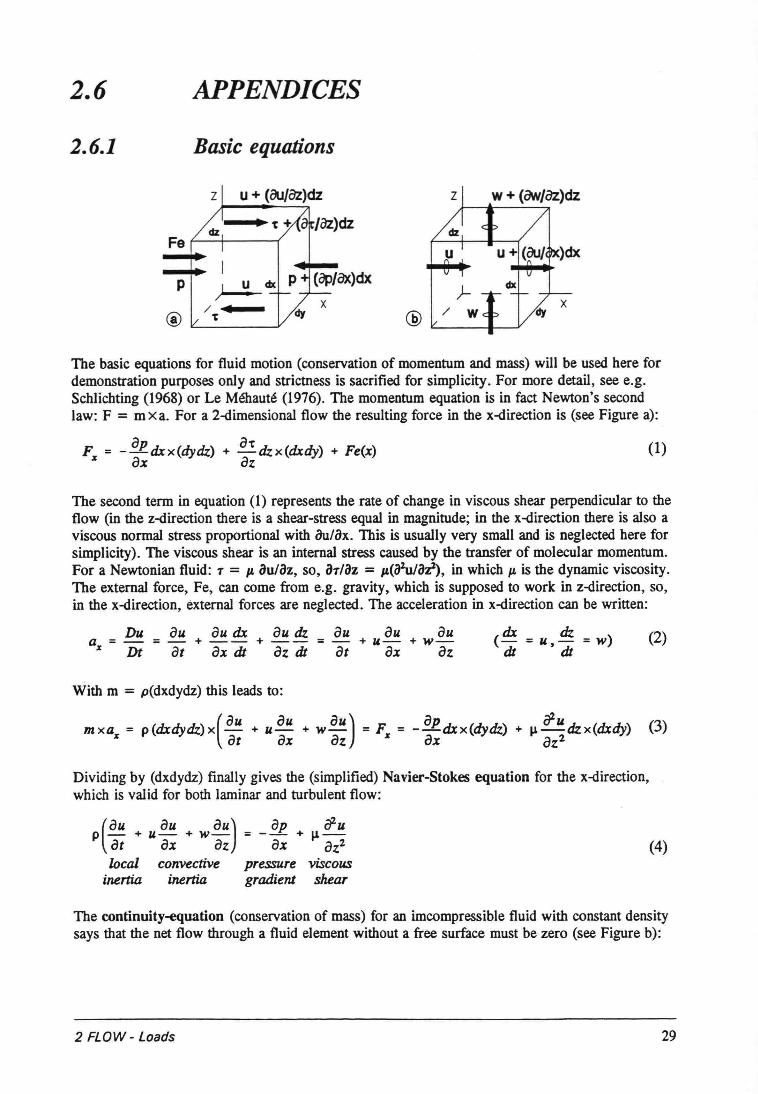
2.6 APPENDICES

2.6.1 Basic equations

z u+ (oulàz)dz z

Fe

p I/

/@ 't @

The basic equations for tluid motion (conservation of momentum and mass) will be used here fordemonstration purposes only and strictness is sacrified for simplicity . For more detail, see e.g.Schlichting (1968) or Le Méhauté (1976). The momentum equation is in fact Newton's secondlaw: F = m xa. For a 2-dimensional tlow the resulting force in the x-direction is (see Figure a):

ap a-rF = --dxx(dytk) + -tkx(dxdy) + Fe(x)% ax az

(1)

The second term in equation (1) represents the rate of change in viscous shear perpendicular to thetlow (in the z-direction there is a shear-stress equal in magnitude; in the x-direction there is also aviscous normal stress proportional with iJu/ox. This is usually very smalI and is neglected here forsimplicity). The viscous shear is an internal stress caused by the transfer of molecular momentum.For a Newtonian tluid: t = p. ou/az, so, ar/az = p.(a1ula7!), in which p. is the dynamic viscosity.The external force, Fe, can come from e.g. gravity, which is supposed to work in z-direction, so,in the x-direction, external forces are neglected. The acceleration in x-direction can be written:

a = Du = au + au dx + au dz = au + u au + w au% Dt at ax dl az dl at Bx az

(2)

With m = p(dxdydz) this leads to:

mxa = P(dxdytk)x(au + uau + wau) = F = _apdxx(dytk) + I.L alutkx(dxdy)x at ax êz % ax az2

(3)

Dividing by (dxdydz) finally gives the (simplified) Navier-Stokes equation for the x-direction,which is valid for both laminar and turbulent tlow:

p(au + u au + w au) = _ ap + 11 aluat ax az ax az2local convective pressure viscousinertia inertia gradient shear

(4)

The continuity-equation (conservation of mass) for an imcompressible tluid with constant densitysays that the net tlow through a tluid element without a free surface must be zero (see Figure b):

2 FLOW - Loads 29

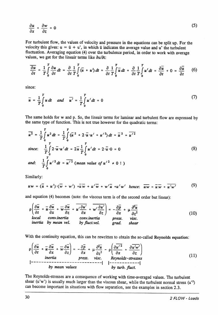
au + aw = 0ax az

(5)

For turbulent flow, the values of velocity and pressure in the equations cao be split up. For thevelocity this gives: u = Ü + u', in which ü indicates the average value and u' the turbulentfluctuation. Averaging equation (4) over the turbulence period, in order to work with averagevalues, we get for the lineair terms like au/Ol:

- T T T T __

au =! iz- =~! J(u + u~dt =~! Judt +~! Ju'dt = au + 0 = au (6)at T 0 at at T 0 at T 0 at T 0 at at

since:

T- IJu = - udtTo

andT- IJu' = - u' dt = 0

To(7)

The same holds for w and p. So, the lineair terms for laminar and turbulent flow are expressed bythe same type of function. This is not true however for the quadratic terms:

(8)

Similarly:

uw = (u + u') ·(w + w/) =uw + u' w + w'u +u'w' hence: uw = uw + u'w' (9)

and equation (4) becomes (note: the viscous term is of the second order but linear):

( au - au - au / au/ , au'] aiP at + u ax + w az + u ax + w al. = - ax +

local conv.inertia conv.inertia press.inertia by mean vel. by fluct. vel. grad.

(10)

With the continuity equation, this can be rewritten to obtain the so-called Reynolds equation:

( au - au - au] ai s: (au'2 au/w']P- + u- + w- = -- + Il- - P-- + --at àx al. ax al.2 ax al.inertia press. visc. Reynolds-stresses

1----------------------------1 1------------1by mean values by turbo fluct.

(11)

The Reynolds-stresses are a consequence of working with time-averaged values. The turbulentshear (u'w') is usually much larger than the viscous shear, while the turbulent normal stress (u")can become important in situations with flow separation, see the examples in section 2.3.

30 2 FLOW - Loads

------- - - - -

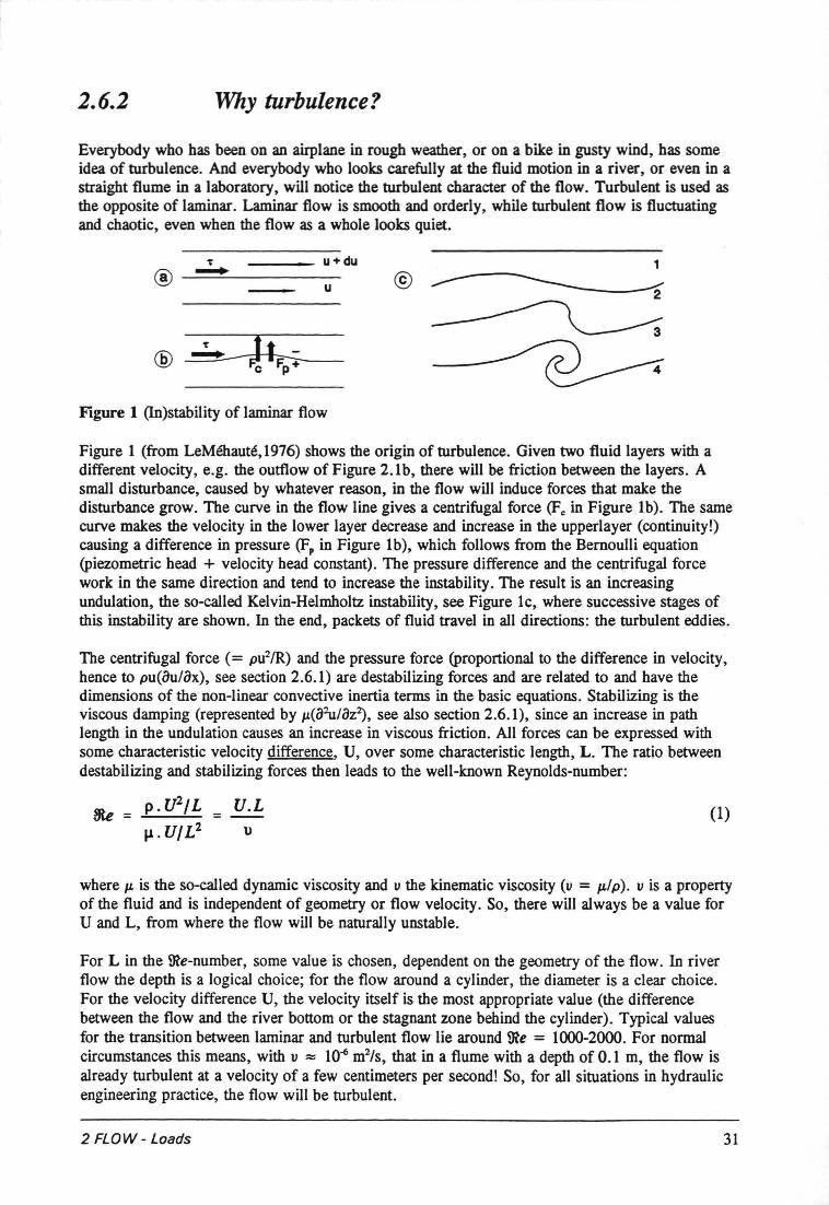
2.6.2 Why turbulence?

Everybody who has been on an airplane in rough weather, or on a bike in gusty wind, has someidea of turbulence. And everybody who looks carefully at the fluid motion in a river, or even in astraight flume in a laboratory , will notice the turbulent character of the flow. Turbulent is used asthe opposite of laminar . Laminar flow is smooth and orderly, while turbulent flow is fluctuatingand chaotic, even when the flow as a whole looks quiet.

~ u+du

~ --~-----------u1

@

Figure 1(In)stability of laminar flow

Figure 1 (from LeMéhauté,1976) shows the origin of turbulence. Given two fluid layers with adifferent velocity, e.g. the outflow of Figure 2.1b, there will be friction between the layers. Asmall disturbance, caused by whatever reason, in the flow will induce forces that make thedisturbance grow. The curve in the flow line gives a centrifugal force (Fe: in Figure lb). The samecurve makes the velocity in the lower layer decrease and increase in the upperlayer (continuity!)causing a difference in pressure (F, in Figure lb), which follows from the Bemoulli equation(piezometric head + velocity head constant). The pressure difference and the centrifugal forcework in the same direction and tend to increase the instability. The result is an increasingundulation, the so-called Kelvin-Helmholtz instability, see Figure lc, where successive stages ofthis instability are shown. In the end, packets of fluid travel in all directions: the turbulent eddies.

The centrifugal force (= pu2fR) and the pressure force (proportional to the difference in velocity,hence to pu(8u/8x), see section 2.6.1) are destabilizing forces and are related to and have thedimensions of the non-linear convective inertia terms in the basic equations. Stabilizing is theviscous damping (represented by p.(82u/8z~, see also section 2.6.1), since an iocrease in pathlength in the undulation causes an increase in viscous friction. All forces can be expressed withsome characteristic velocity difference, U, over some characteristic length, L. The ratio betweendestabilizing and stabilizing forces then leads to the well-known Reynolds-number:

me = p.U2/L = U.L1l.U/L2 u

(1)

wbere p. is the so-called dynamic viscosity and v the kinematic viscosity (u = p./p). u is a propertyof the fluid and is independent of geometry or flow velocity. So, there will always be a value forU and L, from where the flow will be naturally unstable.

For L in the ~e-number, some value is cbosen, dependent on the geometry of the flow. In riverflow the depth is a logical choice; for the flow around a cylinder, the diameter is a clear choice.For the velocity difference U, the velocity itself is the most appropriate value (the differencebetween the flow and the river bottom or the stagnant zone bebind the cylinder). Typical valuesfor the transition between laminar and turbulent flow lie around ~e = 1000-2000. For normalcircumstances this means, with v ~ 10-6m2/s, that in a flume with a depth of 0.1 m, the flow isalready turbulent at a velocity of a few centimeters per second! So, for all situations in hydraulicengineering practice, the flow will be turbulent.

2 FLOW - Loads 31

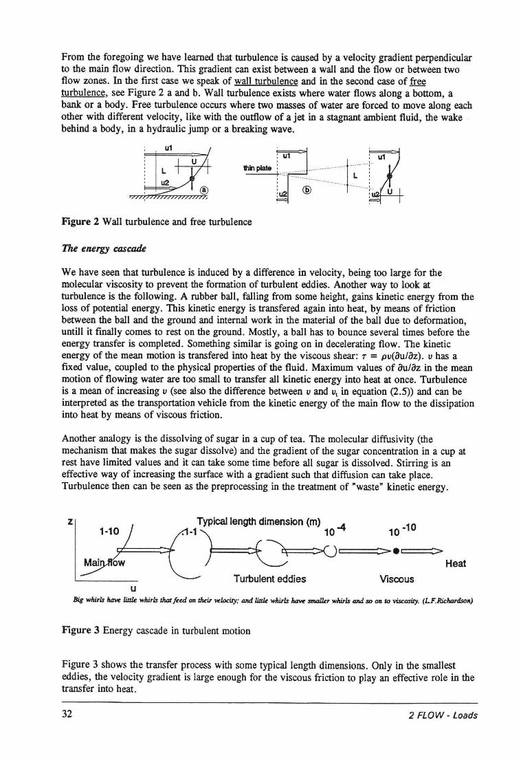
From the foregoing we have learned that turbulence is caused by a velocity gradient perpendicularto the main flow direction. This gradient cao exist between a wall and the flow or between twoflow zones. In the first case we speak:of wall turbulence and in the second case of freeturbulence, see Figure 2 a and b. Wall turbulence exists where water flows along a bottom, abank:or a body. Free turbulence occurs where two masses of water are forced to move along eachother with different velocity , like with the outflow of a jet in a stagnant ambient fluid, the wakebehind a body, in a hydraulic jump or a break:ingwave.

Figure 2 Wall turbulence and free turbulence

The energy cascade

We have seen that turbulence is induced by a difference in velocity, being too large for themolecular viscosity to prevent the formation of turbulent eddies. Another way to look atturbulence is the following. A rubber bali, falling from some height, gains kinetic energy from theloss of potential energy. This kinetic energy is transfered again into heat, by means of frictionbetween the bali and the ground and internal work in the material of the ball due to deformation,untill it finally comes to rest on the ground. Mostly, a bali has to bounce several times before theenergy transfer is completed. Something similar is going on in decelerating flow. The kineticenergy of the meao motion is transfered into heat by the viscous shear: T = pu(ou/oz). u has afixed value, coupled to the physical properties of the fluid. Maximum values of ou/oz in the meaomotion of flowing water are too small to transfer all kinetic energy into heat at once. Turbulenceis a meao of increasing u (see also the difference between u and Ut in equation (2.5)) and can beinterpreted as the transportation vehicle from the kinetic energy of the main flow to the dissipationinto heat by means of viscous friction.

Another analogy is the dissolving of sugar in a cup of tea. The molecular diffusivity (themechanism that makes the sugar dissolve) and the gradient of the sugar concentration in a cup atrest have limited values and it can take some time before all sugar is dissolved. Stirring is aneffective way of increasing the surface with a gradient such that diffusion can take place.Turbulence then can be seen as the preprocessing in the treatment of "waste" kinetic energy.

1-10Typicallength dimension (m) -4

~ 10

F===:* ~'C::===::::>.I >Heat

10 -10z

Turbulent eddies Viscousu

Big whirls have little whirls that leed 011 their velocity; and ÜIlle whirls have smalkr whirls and SD on 10 viscosily. (I-F.Richordsoll)

Figure 3 Energy cascade in turbulent motion

Figure 3 shows the transfer process with some typicallength dimensions. Only in the smal1esteddies, the velocity gradient is large enough for the viscous friction to play an effective role in thetransfer into heat.

32 2 FLOW - Loads

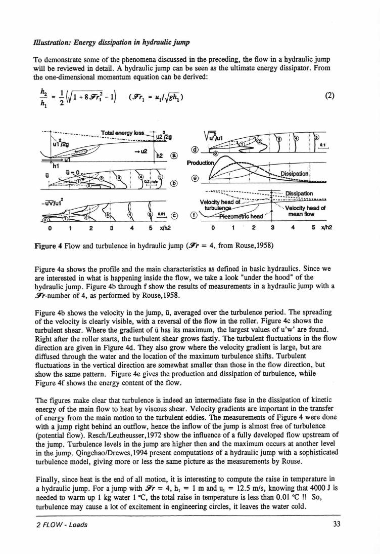
Illustration: Energy dissipation in hydraulic jump

To demonstrate some of the phenomena discussed in the preceding, the flow in a hydraulic jumpwill be reviewed in detail. A hydraulic jump cao be seen as tbe ultimate energy dissipator. Fromtbe one-dimensional momentum equation cao be derived:

(2)

o 1 . 2 5 X/t(}.3 4

Figure 4 Flow and turbulence in hydraulic jump (:Tr = 4, from Rouse,1958)

Figure 4a shows the profile and the main characteristics as defined in basic hydraulics. Since weare interested in what is happening inside the flow, we take a look "under the hood" of thehydraulic jump. Figure 4b through f show the results of measurements in a hydraulic jump with a:Tr-number of 4, as performed by Rouse, 1958.

Figure 4b shows the velocity in the jump, ü, averaged over the turbulence period. Tbe spreadingof the velocity is clearly visible, with a reversal of tbe flow in the roller. Figure 4c shows theturbulent shear. Wbere the gradient of ü has its maximum, the largest values of u'w' are found.Right after the roller starts, the turbulent shear grows fastly. Tbe turbulent fluctuations in tbe flowdirection are given in Figure 4d. Tbey also grow where the velocity gradient is large, but arediffused through the water and the location of the maximum turbulence shifts. Turbulentfluctuations in the vertical direction are somewhat smaller than those in the flow direction, butshow tbe same pattern. Figure 4e gives the production and dissipation of turbulence, whileFigure 4f shows the energy content of the flow.

Tbe figures make clear that turbulence is indeed an intermediate fase in the dissipation of kineticenergy of the main flow to heat by viscous shear. Velocity gradients are important in the transferof energy from the main motion to the turbulent eddies. Tbe measurements of Figure 4 were donewith a jump right behind an outflow, hence the inflow of the jump is almost free of turbulence(potential flow). Resch/Leutheusser, 1972 show the influence of a fully developed flow upstream ofthe jump. Turbulence levels in the jump are higher then and tbe maximum occurs at another levelin the jump. QingchaolDrewes, 1994 present computations of a hydraulic jump with a sophisticatedturbulence model, giving more or less the same picture as the measurements by Rouse.

Finally, since heat is tbe end of all motion, it is interesting to compute the raise in temperature ina hydraulic jump. For a jump with :Tr = 4, hl = 1 m and UI = 12.5 mis, knowing that 4000 J isneeded to warm up 1 kg water 1oe, the total raise in temperature is less than 0.01 Oe!! So,turbulence may cause a lot of excitement in engineering circles, it leaves the water cold.

2 FLOW - Loads 33

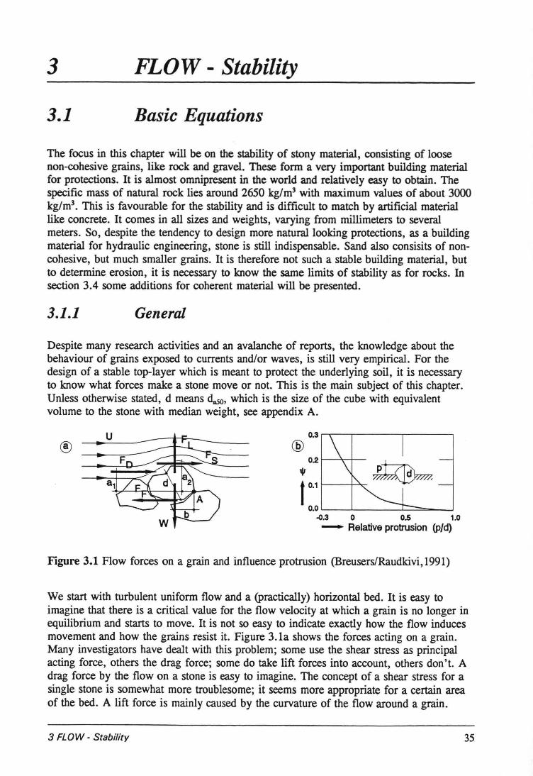
3 FLOW - Stability

3.1 Basic Equations

The focus in this chapter will be on the stability of stony material, consisting of loosenon-cohesive grains, like rock and gravel. These form a very important building materialfor protections. It is almost omnipresent in the world and relatively easy to obtain. Thespecific mass of natural rock lies around 2650 kg/m' with maximum values of about 3000kg/m", This is favourable for the stability and is difficuit to match by artificial materiallike concrete. It comes in all sizes and weights, varying from millimeters to severalmeters. So, despite the tendency to design more naturallooking protections, as a buildingmaterial for hydraulic engineering, stone is still indispensabie. Sand also consisits of non­cohesive, but much smaller grains. It is therefore not such a stable building material, butto determine erosion, it is necessary to know the same limits of stability as for rocks. Insection 3.4 some additions for coherent material will be presented.

3.1.1 General

Despite many research activities and an avalanche of reports, the knowledge about thebehaviour of grains exposed to currents and/or waves, is still very empirical. For thedesign of a stable top-layer which is meant to proteet the underlying soil, it is necessaryto know what forces make a stone move or not. This is the main subject of this chapter.Unless otherwise stated, d means <Înso, which is the size of the cube with equivalentvolume to the stone with median weight, see appendix A.

®0.3 ,...,...--,----..,-------,

@0.2 t-----r-t_

Vt 0.1

O.O'----'-----'---=--.J-0.3 0 0.5 1.0- Relative protrusion (P/d)

Figure 3.1 Flow forces on a grain and influence protrusion (Breusers/Raudkivi, 1991)

We start with turbulent uniform flow and a (practically) horizontal bed. It is easy toimagine that there is a critical value for the flow velocity at which a grain is no longer inequilibrium and starts to move. It is not so easy to indicate exactly how the flow inducesmovement and how the grains resist it. Figure 3.1a shows the forces acting on a grain.Many investigators have dealt with this problem; some use the shear stress as principalacting force, others the drag force; some do take lift forces into account, others don't. Adrag force by the flow on a stone is easy to imagine. The concept of a shear stress for asingle stone is somewhat more troublesome; it seems more appropriate for a certain areaof the bed. A lift force is mainly caused by the curvature of the flow around a grain.

3 FLOW - Stability 35

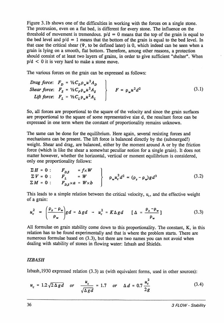
Figure 3.1b shows one of the difficulties in working with the forces on a single stone.The protrusion, even on a flat bed, is different for every stone. The influence on thethreshold of movement is tremendous. pi d = 0 means that the top of the grain is equal tothe bed level and p/d = 1 means that the bottom of the grain is equal to the bed level. Inthat case the critica! shear ('Ir, to be defined later) is 0, which indeed can be seen when agrain is lying on a smooth, flat bottom. Therefore, among other reasons, a proteetionshould consist of at least two layers of grains, in order to give sufficient "shelter". Whenpid < 0 it is very hard to make a stone move.

The various forces on the grain can be expressed as follows:

Drag force: FD = Y2CDPwu2AD }

Shear force: Fs = Y2CFPwu2AsLift force: FL = Y2CLPwu2AL

(3.1)

So, all forces are proportional to the square of the velocity and since the grain surfacesare proportional to the square of some representative size d, the resultant force can beexpressed in one term where the constant of proportionality remains unknown.

The same can be done for the equilibrium. Here again, several resisting forces andmechanisms can be present. The lift force is balanced directly by the (submerged!)weight. Shear and drag, are balanced, either by the moment around A or by the frictionforce (which is like the shear a somewhat peculiar notion for a single grain). It does notmatter however, whether the horizontal, vertica! or moment equilibrium is considered,only one proportionality follows:

lJH = 0 :lJV=O:lJM = 0 :

(3.2)

This leads to a simple relation between the critica! velocity, u., and the effective weightof a grain:

2 (Ps - pw) d 2Uc oe Pw g = !lgd - Uc = K!lgd (3.3)

All formulae on grain stability come down to this proportionality. The constant, K, in thisrelation has to be found experimentally and that is where the problem starts. There arenumerous formulae based on (3.3), but there are two names you can not avoid whendealing with stability of stones in flowing water: Izbash and Shields.

IZBASH

Izbash, 1930 expressed relation (3.3) as (with equivalent forms, used in other sources):

or = 1.7 or2

Uc!ld = 0.7-

2g(3.4)

36 3 FLOW - Stability

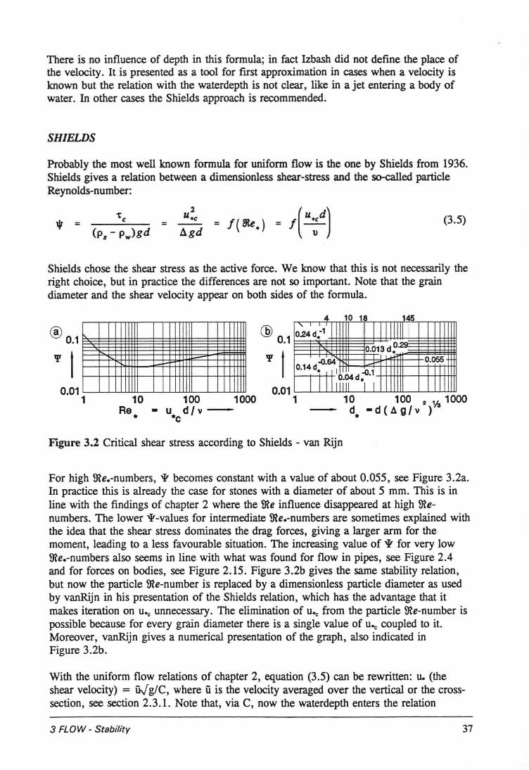
There is no influence of depth in this formula; in fact Izbash did not define the place ofthe velocity . It is presented as a tooI for fust approximation in cases when a velocity isknown but the relation with the waterdepth is not ciear, like in a jet entering a body ofwater. In other cases the Shields approach is recommended.

SHIELDS

Probably the most weil known formula for uniform flow is the one by Shields from 1936.Shields gives a relation between a dimensionless shear-stress and the so-called partieleReynolds-number:

(3.5)

Shields chose the shear stress as the active force. We know that this is not necessarily theright choice, but in practice the differences are not so important. Note that the graindiameter and the shear velocity appear on both sides of the formula.

® 0.1....-

I-

4 10 18 145

@ 0.1"' I 1111110.24d-1•

• 00.013d.

o d-O·64 ' -'""'" 0.055.14. 110 -0.1

I I 11" i~d·1 I

~t0.01

1 10Re•

100 1000- u dJv-·c

0.011 10 100 2 1131000

d. - d (4 g J v )

Figure 3.2 Critical shear stress according to Shields - van Rijn

For high 9te.-numbers, "IJrbecomes constant with a value of about 0.055, see Figure 3.2a.In practice this is already the case for stones with a diameter of about 5 mm. This is inline with the findings of chapter 2 where the 9te influence disappeared at high 9te­numbers. The lower "IJr-valuesfor intermediate 9te.-numbers are sometimes explained withthe idea that the shear stress dominates the drag forces, giving a larger arm for themoment, leading to a less favourable situation. The increasing value of v for very low9te.-numbers also seems in line with what was found for flow in pipes, see Figure 2.4and for forces on bodies, see Figure 2.15. Figure 3.2b gives the same stability relation,but now the partiele 9te-number is replaced by a dimensionless partiele diameter as usedby vanRijn in his presentation of the Shields relation, which has the advantage that itmakes iteration on u., unnecessary. The elimination of u., from the partiele 9te-number ispossibie because for every grain diameter there is a single value of u., coupled to it.Moreover, vanRijn gives a numerical presentation of the graph, also indicated inFigure 3.2b.

With the uniform flow relations of chapter 2, equation (3.5) cao be rewritten: u. (theshear velocity) = üJg/C, where û is the velocity averaged over the vertical or the cross­section, see section 2.3.1. Note that, via C, now the waterdepth enters the relation

3 FLOW - Stability 37

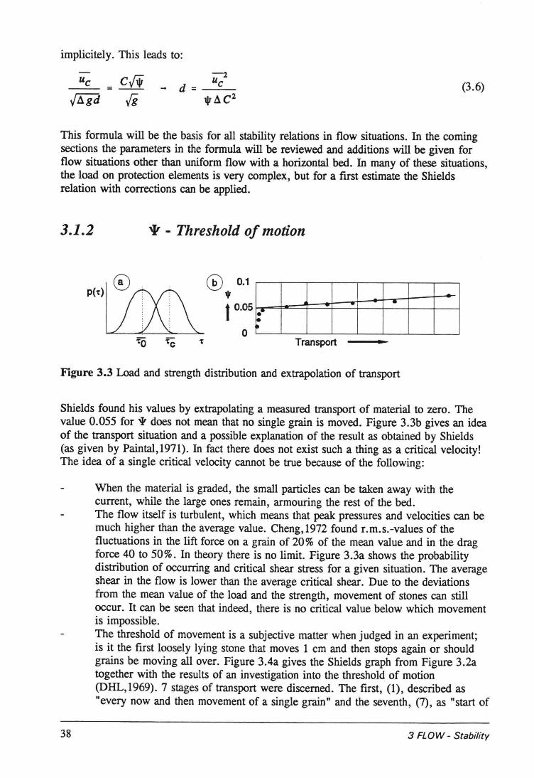
implicitely. This leads to:

U2.... d= __ c_lIr ä C2

(3.6)

This formula will be the basis for all stability relations in flow situations. In the comingsections the parameters in the formula will be reviewed and additions will be given forflow situations other than uniform flow with a horizontal bed. In many of these situations,the load on proteetion elements is very complex, but for a fust estimate the Shieldsrelation with corrections can be applied.

3.1.2 'Ir - Threshold of motion

Transport

Figure 3.3 Load and strength distribution and extrapolation of transport

Shields found his values by extrapolating a measured transport of material to zero. Thevalue 0.055 for ir does not mean that no single grain is moved. Figure 3.3b gives an ideaof the transport situation and a possible explanation of the result as obtained by Shields(as given by Paintal,1971). In fact there does not exist such a thing as a critical velocity!The idea of a single critical velocity cannot be true because of the following:

When the material is graded, the small particles can be taken away with thecurrent, while the large ones remain, armouring the rest of the bed.The flow itself is turbulent, which means that peak pressures and veloeities can bemuch higher than the average value. Cheng,1972 found r.m.s.-values of thefluctuations in the lift force on a grain of 20% of the mean value and in the dragforce 40 to 50%. In theory there is no limit. Figure 3.3a shows the probabilitydistribution of occurring and critical shear stress for a given situation. The averageshear in the flow is lower than the average critical shear. Due to the deviationsfrom the mean value of the load and the strength, movement of stones can stilloccur. It can be seen that indeed, there is no critical value below which movementis impossible.The threshold of movement is a subjective matter when judged in an experiment;is it the first loosely lying stone that moves 1 cm and then stops again or shouldgrains be moving all over. Figure 3.4a gives the Shields graph from Figure 3.2atogether with the results of an investigation into the threshold of motion(DHL,1969). 7 stages of transport were discemed. The first, (1), described as"every now and then movement of a single grain" and the seventh, (7), as "start of

38 3 FLOW - Stability

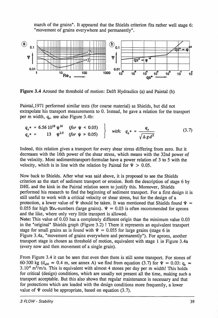
march of the grains". It appeared that the Shields criterion fits rather well stage 6:"movement of grains everywhere and permanently".

7-- --- ::.:!-- ~... -~...---

®O.1 L/

~LIl ~CC_11r

./ . .- qs* ...."

® 0.1

0.011 10R

e*100 10-6 ·1

10

Figure 3.4 Around the threshold of motion: Delft Hydraulics (a) and Paintal (b)

Paintal,1971 performed similar tests (for coarse material) as Shields, but did notextrapolate his transport measurements to O. Instead, he gave a relation for the transportper m width, CIs, see also Figure 3.4b:

qs* = 6.56 1018 '" 16

qs* = 13 ",2.5

(jor '" < 0.05)(jor '" > 0.05) } (3.7)

Indeed, this relation gives a transport for every shear stress differing from zero. But itdecreases with the 16th power of the shear stress, which means with the 32nd power ofthe velocity. Most sedimenttransport-formulae have a power relation of 3 to 5 with thevelocity, which is in line with the relation by Paintal for 'Ir > 0.05.

Now back to Shields. After what was said above, it is proposed to see the Shieldscriterion as the start of sediment transport or erosion. Both the description of stage 6 byDHL and the kink in the Paintal relation seem to justify this. Moreover, Shieldsperformed his research to find the beginning of sediment transport. For a first design it isstill useful to work with a critical velocity or shear stress, but for the design of aproteetion. a lower value of 'Ir should be taken. It was mentioned that Shields found 'Ir =0.055 for high me.-numbers (large grains). 'Ir = 0.03 is often recommended for apronsand the like, where only very little transport is allowed.Note: This value of 0.03 has a completely different origin than the minimum value 0.03in the "original" Shields graph (Figure 3.2) ! There it represents an equivalent transportstage for small grains as is found with 'Ir = 0.055 for large grains (stage 6 inFigure 3.4a, "movement of grains everywhere and permanently"). For aprons, anothertransport stage is chosen as threshold of motion, equivalent with stage 1 in Figure 3.4a(every now and then movement of a single grain).

From Figure 3.4 it can be seen that even then there is still some transport. For stones of60-300 kg (dnSo = 0.4 m, see annex A) we find from equation (3.7) for 'Ir = 0.03: CIs =3.10-6m3/m/s. This is equivalent with almost 4 stones per day per m width! This holdsfor critical (design) conditions, which are usually not present all the time, making such atransport acceptable. But this also shows that regular maintenance is necessary and thatfor protections which are loaded with the design conditions more frequently, a lowervalue of 'Ir could be appropriate, based on equation (3.7).

3 FLOW- Stability 39

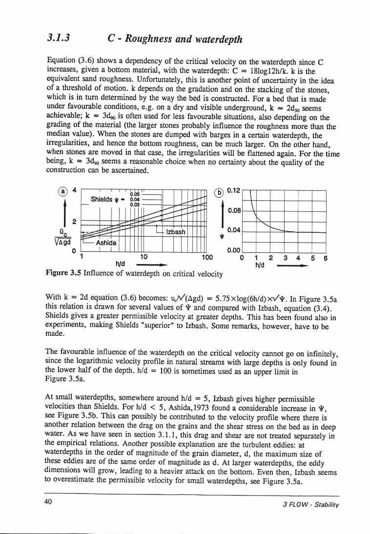
3.1.3 C - Roughness and waterdepth

Equation (3.6) shows a dependency of the critical velocity on the waterdepth since Cincreases, given a bottom material, with the waterdepth: C = l8log12h/k. kis theequivalent sand roughness. Unfortunately, this is another point of uncertainty in the ideaof a threshold of motion. k depends on the gradation and on the stacking of the stones,which is in turn determined by the way the bed is constructed. For a bed that is madeunder favourable conditions, e.g. on a dry and visible underground, k =: 2dso seemsachievable; k = 3<40is often used for less favourable situations, also depending on thegrading of the material (the larger stones probably influence the roughness more than themedian value). When the stones are dumped with barges in a certain waterdepth, theirregularities, and hence the bottom roughness, can be much larger. On the other hand,when stones are moved in that case, the irregularities will be flattened again. For the timebeing, k = 3d90 seems a reasonable choice when no certainty about the quality of theconstruction can be ascertained.

04

LI

0.05Shields 1jr - 0.04 L-~I---- 0.03

e::::: I-~I---~ -,__-I------- L- - I-:::::.T. --- --- - -

~ §~ I-~ Izbashre::Ashida

I I

@ 0.12

t O.~

0.041jJ

1\,

r-....

"r-_10

0.00100 0 1 2 3 4 5 6

h/dh/dFigure 3.5 Influence of waterdepth on critical velocity

With k = 2d equation (3.6) becomes: u/V(~gd) = 5.75Xlog(6h/d) xvi'. In Figure 3.5athis relation is drawn for several values of i' and compared with Izbash, equation (3.4).Shields gives a greater permissible velocity at greater depths. This has been found also inexperiments, making Shields "superior" to Izbash. Some remarks, however, have to bemade.

The favourable influence of the waterdepth on the critical velocity cannot go on infinitely,since the logarithmic velocity profile in natural streams with large depths is only found inthe lower half of the depth. h/d = 100 is sometimes used as an upper limit inFigure 3.5a.

At small waterdepths, somewhere around h/d = 5, Izbash gives higher permissibleveloeities than Shields. For hld < 5, Ashida,1973 found a considerable increase in i',see Figure 3.5b. This can possibly be contributed to the velocity profile where there isanother relation between the drag on the grains and the shear stress on the bed as in deepwater. As we have seen in section 3.1.1, this drag and shear are not treated separately inthe empirical relations. Another possible explanation are the turbulent eddies: atwaterdepths in the order of magnitude of the grain diameter, d, the maximum size ofthese eddies are of the same order of magnitude as d. At larger waterdepths, the eddydimensions will grow, leading to a heavier attack on the bottom. Even then, Izbash seemsto overestimate the permissible velocity for small waterdepths, see Figure 3.5a.

40 3 FLOW - Stebility

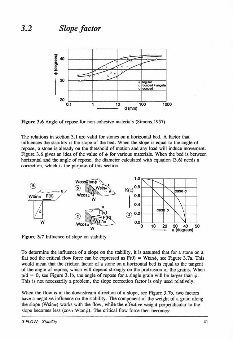
3.2 Slope factor

i40eClCl)

~-&

13020

0.1 1 10 100 1000---- d(mm)

Figure 3.6 Angle of repose for non-cohesive materials (Simons, 1957)

The relations in section 3.1 are valid for stones on a horizontal bed. A factor thatinfluences the stability is the slope of the bed. When the slope is equal to the angle ofrepose, a stone is already on the threshold of motion and any load will induce movement.Figure 3.6 gives an idea of the value of cP for various materials. When the bed is betweenhorizontal and the angle of repose, the diameter ca!culated with equation (3.6) needs acorrection, which is the purpose of this section.

u

~co~W

Figure 3.7 Influence of slope on stability

w

1.0 ~=->"---r----r---'---'

K(ex) 0.8

I 0.6

0.4 f---t--+-~-+--+--+---l

@) 0.2t----t--t----t-"._........-tt-----i0.0 l...----L_---L-_---L....-_.1,.___J

o 10 20 30 40 50ex (degrees)

To determine the influence of a slope on the stability, it is assumed that for a stone on aflat bed the critica! flow force can be expressed as F(O) = Wtané, see Figure 3.7a. Thiswould mean that the friction factor of a stone on a horlzontal bed is equal to the tangentof the angle of repose, which will depend strongly on the protrusion of the grains. Whenp/d = 0, see Figure 3.1b, the angle of repose for a single grain will be larger than cP.This is not necessarily a problem, the slope correction factor is only used relatively.

When the flow is in the downstream direction of a slope, see Figure 3.7b, two factorshave a negative influence on the stability. The component of the weight of a grain alongthe slope (Wsino) works with the flow, while the effective weight perpendicular to theslope becomes less (cosc.Wtanë). The critica! flow force then becomes:

3 FL0 W - Stability 41

F(a) = Wcosotané - Wsino. (Note: when the flow is reverse, the grain gets more stabIeand F(a) = Wcosotané + Wsino). The relation between F(a) and F(O) now gives thereduction to be applied on the shear stress:

K(ex) = F(ex)F(O)

= Wcos extan <I> - Wsin ex =Wtan<l>

sin(<I> - ex)sin<I>

(3.8)

For a side slope with angle ex, the same procedure can be followed, see Figure 3.7c:F(a)2 = F(R)2 - (Wsina)2 = (Wcosatan<l»2 - (Wsina)2, leading to:

K(ex) = F(ex) =F(O)

(3.9)

In Figure 3.7d, both the reduction factors K(a), for a slope in flow direction and for aslope perpendicular to the flow, are drawn for the case that <I> = 400• It is clear that aslope in the flow direction is much more unfavourable.

Both equations have been checked in laboratory experiments. Chiew/Parker, 1994 give theresults for a slope in flow direction, equation (3.8). The results are quite satisfactory forslopes not too close to the angle of repose. Also slopes with the flow in upward direction,when the stones become more stable were investigated with the same result. DHL,1970gives some results for gravel on slopes 1:3 and 1:4. Here too, the results weresatisfactory .

Note: K(a) is a correction factor for the diameter and has to be applied in thedenominator of equation (3.6). K(a) represents a reduction of the strength, henceK(a) < 1.

3.3 Velocity/turbulence factor

Relations like the one given by Shields are valid for stationary, uniform flow. When theflow is not uniform, the load will be locally higher. This cao be expressed in a factor forthe velocity, Kv, in stability relations (Kv is a load amplification factor, hence> 1):

Uc uniform flowK =-........:.------vUe with load increase (3.10)

Note: The use of the critical velocity in the denominator comes from experiments where,with some obstacle, a lower critical velocity is measured at which stones start to move.This does not mean that the critical velocity of the bed is lower: the strength of the beddoes not change, but the load increases.

In accelerating flow we have seen an increase in shear stress and a decrease of (relative)turbulence and in decelerating flow the other way around (section 2.3.1). For thesephenomena in vertical and horizontal constrictions, only results of empirical research areavailable. These results will be discussed here, with the knowledge of fluid motion fromchapter 2 as background.

42 3 FLOW - Stability

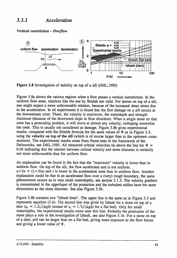
3.3.1 Acceleration

Vertical constriction - Overflow

----~~---

®4

L®

unifonnflowacceleration deceleration

h1/d

Figure 3.8 Investigation of stability on top of a sill (DHL,1985)

Figure 3.8a shows the various regions when a flow passes a vertica1 constriction. In theuniform flow zone, relations like the one by Shields are valid. For stones on top of a sill,one might expect a more unfavourable relation, because of the increased shear stress dueto the acceleration. In all experiments it is found that the first damage on a sill occurs atthe downstream crest. There, the velocity is maximum, the waterdepth and strengthminimum (because of the downward slope in flow direction). When a single stone on thatcrest has a protruding position, it will move at almost any velocity, reshaping somewhatthe crest. This is usua1lynot considered as damage. Figure 3.8b gives experimentalresults, compared with the Shields formula for the same values of v as in Figure 3.5,using the velocity on top of the sill (which is of course larger than in the upstream cross­sections). The experimental results come from flume tests in the framework of theDeltaworks, see DHL, 1985. All measured critica1 veloeities lie above the line for v =0.04 indicating that the relation between critica1 velocity and stone diameter is certainlynot more unfavourable than for uniform flow.

An explanation can be found in the fact that the "maximum" velocity is lower than inuniform flow. On top of the sill, the flow accelerates and is not uniform.u+30" = (1+3r)u and r is lower in the acceleration zone than in uniform flow. Anotherexplanation could be that in an accelerated flow over a (very) rough boundary, the samephenomenon occurs as in very small waterdepths, see section 3.1.3. The velocity gradientis concentrated in the upperlayer of the proteetion and the turbulent eddies have the samedimensions as the stone diameter. See also Figure 3.5b.

Figure 3.8b contains two "Izbash lines". The upper line is the same as in Figure 3.5 andrepresents equation (3.4). The second line was given by Izbash for a stone on top of adam (u, = 1.2·/(L\.gd)instead of u, = 1.7.J(L\.gd) for a flat bed). Only for smallwaterdepths, the experimental results come near this line. Probably the protrusion of thestone plays a role in the investigation of Izbash, see also Figure 3.1b. For a stone on topof a dam, p/d can be larger than on a flat bed, giving more exposure to the flow forcesand giving a lower value of v.

3 FL0W - Stability 43

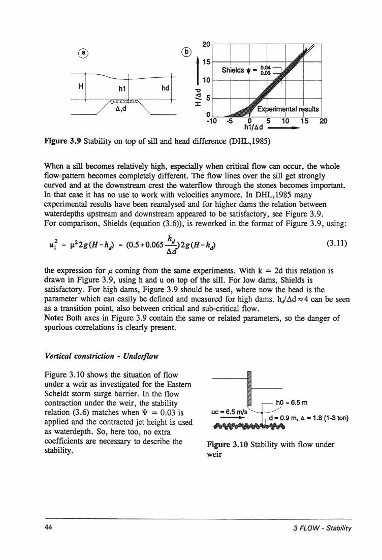
H h1 hd--------7::p:J:;~~------------ -

à,d

Figure 3.9 Stability on top of sill and head difference (DHL,1985)

When a sill becomes relatively high, especially when critical flow cao occur, the wholeflow-pattem becomes completely different. The flow lines over the sill get stronglycurved and at the downstream crest the waterflow through the stones becomes important.In that case it has no use to work with veloeities anymore. InDHL,1985 manyexperimental results have been reanalysed and for higher dams the relation betweenwaterdepths upstream and downstream appeared to be satisfactory, see Figure 3.9.For comparison, Shields (equation (3.6», is reworked in the format of Figure 3.9, using:

(3.11)

the expression for IJ. coming from the same experiments. With k = 2d this relation isdrawn in Figure 3.9, using h and u on top of the sill. For low dams, Shields issatisfactory. For high dams, Figure 3.9 should be used, where now the head is theparameter which cao easily be defined and measured for high dams. ~/ Ad:::4 cao be seenas a transition point, also between critical and sub-critical flow.Note: Both axes in Figure 3.9 contain the same or related parameters, so the danger ofspurious correlations is clearly present.

Vertical constriction - Underflow

Figure 3.10 shows the situation of flowunder a weir as investigated for the EastemScheldt storm surge barrier. In the flowcontraction under the weir, the stabilityrelation (3.6) matches when 'Ir = 0.03 isapplied and the contracted jet height is usedas waterdepth. So, here too, no extracoefficients are necessary to describe thestability.

Figure 3.10 Stability with flow underweir

44 3 FLOW - Stability

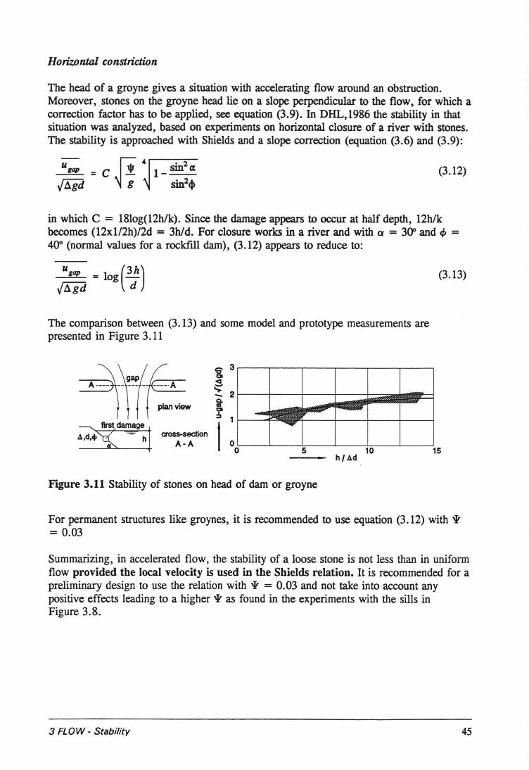
Horizontal constriction

The head of a groyne gives a situation with accelerating flow around an obstruction.Moreover , stones on the groyne head lie on a slope perpendicular to the flow, for which acorrection factor has to be applied, see equation (3.9). InDHL,1986 the stability in thatsituation was analyzed, based on experiments on horizontal closure of a river with stones.The stability is approached with Shields and a slope correction (equation (3.6) and (3.9):

(3.12)

in which C = 1810g(12h/k). Since the damage appears to occur at half depth, 12h/kbecomes (12x1l2h)/2d = 3h/d. For closure works in a river and with cr = 300and <I> =400 (normal values for a rockfill dam), (3.12) appears to reduce to:

u (3h)J:;d = log d (3.13)

The comparison between (3.13) and some model and prototype measurements arepresented in Figure 3.11

=91~f~i 3

<I;::;2-i

~ 1

-- flrst damage I1

cross-sectlon.c1.d•• "{: hA-A 0

0 10 15

Figure 3.11 Stability of stones on head of dam or groyne

For permanent structures like groynes, it is recommended to use equation (3.12) with ir= 0.03

Summarizing, in accelerated flow, the stability of a loose stone is not less than in uniformflow provided the local velocity is used in the Shields relation. It is recommended for apreliminary design to use the relation with ir = 0.03 and not take into account anypositive effects leading to a higher ir as found in the experiments with the sills inFigure 3.8.

3 FLOW - Stability 45

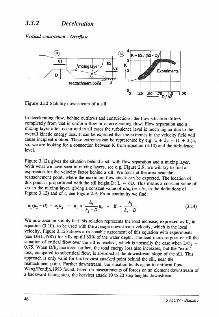
3.3.2 Deceleration

Vertical constriction - Overflow

II

mixing I~yer~---+-~_.,,-: I

---------~--:----I -- __...o

h2u2

®u1

reattachment pOint d

.25 .50 .750I ~ 1.25

Figure 3.12 Stability downstream of a sill

In decelerating flow, behind outflows and constrictions, the flow situation differscompletely from that in uniform flow or in accelerating flow. Flow separation and amixing layer often occur and in all cases the turbulence level is much higher due to theoverall kinetic energy loss. It can be expected that the extremes in the velocity field willcause incipient motion. These extremes can be represented by e.g. û + 3u = (l + 3r)ü,50, we are looking for a conneetion between K from equation (3.10) and the turbulencelevel.

Figure 3.12a gives the situation behind a sill with flow separation and a mixing layer.With what we have seen in mixing layers, see e.g. Figure 2.9, we will try to find anexpression for the velocity factor behind a sill. We focus at the area near thereattachement point, where the maximum flow attack can be expected. The location ofthis point is proportional with the sill height D: L ::= 6D. This means a constant value ofz/x in the mixing layer, giving a constant value of u/u, (= U/UI in the definitions ofFigure 3.12) and of r, see Figure 2.9. From continuity we find:

~ hzu1(hz -D) = uzhz .... UI = Uz .... Koe--h2-D ~-D

(3.14)

We now assume simply that this relation represents the load increase, expressed as Kv inequation (3.10), to be used with the average downstream velocity, which is the localvelocity. Figure 3.12b shows a reasonable agreement of this equation with experiments(see DHL,1985) for sills up till 60% of the water depth. The load increase goes on ti11 thesituation of critical flow over the sill is reached, which is normally the case when D/h2 ::=

0.75. When D/h2 increases further , the total energy loss also increases, but the "extra"loss, compared to subcritical flow, is absorbed at the downstream slope of the sill. Thisapproach is only valid for the heaviest attacked point behind the sill, near thereattachment point. Further downstream, the situation tends again to uniform flow.Wang/Fontijn, 1993 found, based on measurements of forces on an element downstream ofa backward facing step, the heaviest attack 10 to 20 step heights downstream.

46 3 FL0W - Stability

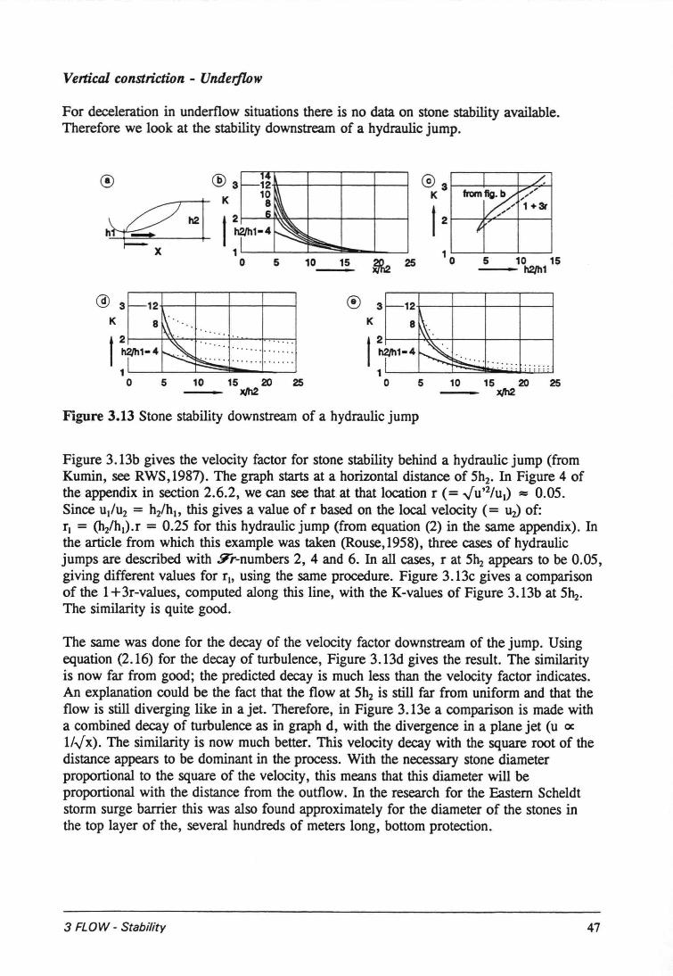
Vertical constriction - Underflow

For deceleration in underflow situations there is no data on stone stability available.Therefore we look at the stability downstream of a hydraulic jump.

LWnw v............

...... 1+31'...I-

10 15-- h2Jh15

@ 3~12+--+--+--t--1

K 8~· ...

t ~1-41\\. :::::::: :::::::T ~~ .1o 5 10 15 20 2S

xJh2

® 3~12+--+--+---+--___,

K 8~.

I:r'-4 ~ ;;.,; .... :: :::: ::::::

o 5 10 15 20 25xJh2

Figure 3.13 Stone stability downstream of a hydraulic jump

Figure 3.13b gives the velocity factor for stone stability bebind a hydraulic jump (fromKumin, see RWS,1987). The graph starts at a horizontal distance of 5h2• In Figure 4 ofthe appendix in section 2.6.2, we can see that at that location r (= ...{U'2/UI) =: 0.05.Since UI/U2 = h2/hl, this gives a value of r based on the local velocity (= uJ of:r, = (h/hl).r = 0.25 for this hydraulic jump (from equation (2) in the same appendix). Inthe artiele from which this example was taken (Rouse, 1958), three cases of hydraulicjumps are described with .9""r-numbers2, 4 and 6. In all cases, r at 5~ appears to be 0.05,giving different values for riousing the same procedure. Figure 3.13c gives a comparisonof the 1+3r-values, computed along this line, with the K-values of Figure 3.13b at 5~.The similarity is quite good.

The same was done for the decay of the velocity factor downstream of the jump. Usingequation (2.16) for the decay of turbulence, Figure 3.13d gives the result. The similarityis now far from good; the predicted decay is much less than the velocity factor indicates.An explanation could be the fact that the flow at 5h2 is still far from uniform and that theflow is still diverging like in a jet. Therefore, in Figure 3.13e a comparison is made witha combined decay of turbulence as in graph d, with the divergence in a plane jet (u exlI...{x).The similarity is now much better. This velocity decay with the square root of thedistance appears to be dominant in the process. With the necessary stone diameterproportional to the square of the velocity, this means that this diameter will beproportional with the distance from the outflow. In the research for the Eastem Scheldtstorm surge barrier this was also found approximately for the diameter of the stones inthe top layer of the, several hundreds of meters long, bottom protection.

3 FLOW - Stability 47

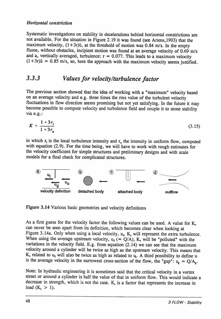
Horizontal constriction

Systematic investigations on stability in decelerations behind horizontal constrictions arenot available. For the situation in Figure 2.19 it was found (see Ariens,1993) that themaximum velocity, (1+3r)ü, at the threshold of motion was 0.84 mis. In the emptyflume, without obstacles, incipient motion was found at an average velocity of 0.69 misand a, vertically averaged, turbulence: r = 0.077. This leads to a maximum velocity(l+3r)ü = 0.85 mis, so, here the approach with the maximum velocity seems justified.

3.3.3 Values for velocityIturbulence factor

The previous section showed that the idea of working with a "maximum" velocity basedon an average velocity and e.g. three times the rms value of the turbulent velocityfluctuations in flow direction seems promising but not yet satisfying. In the future it maybecome possible to compute velocity and turbulence field and couple it to stone stabilityvia e.g.:

1+ 3r1K=---

1 + 37,. (3.15)

in which rl is the local turbulence intensity and ru the intensity in uniform flow, computedwith equation (2.9). For the time being, we will have to work with rough estimates forthe velocity coefficient for simple structures and preliminary designs and with scalemodels for a final check for complicated structures.

®uI I @ @

W @ ---------___-/e....... ....... .............. Uo - .......---------~ug

velocity definition detached body attached body outflow

Figure 3.14 Various basic geometries and velocity definitions

As a first guess for the velocity factor the following values can be used. A value for Kvcan never be seen apart from its definition, which becomes clear when looking atFigure 3.14a. Only when using a local velocity, UI' Kv will represent the extra turbulence.When using the average upstream velocity, Uo (= Q/A), Kv will be "polluted" with thevariations in the velocity field. E.g. from equation (2.14) we can see that the maximumvelocity around a cylinder will be twice as high as the upstream velocity . This means thatKv related to llo will also be twice as high as related to Ut. A third possibility to define uis the average velocity in the narrowest cross-section of the flow, the "gap": l.lg = Q/Ag.

Note: In hydraulic engineering it is sometimes said that the critical velocity in a vortexstreet or around a cylinder is half the value of that in uniform flow. This would indicate adecrease in strength, which is not the case. Kv is a factor that represents the increase inload CKv > 1).

48 3 FLOW - Stability

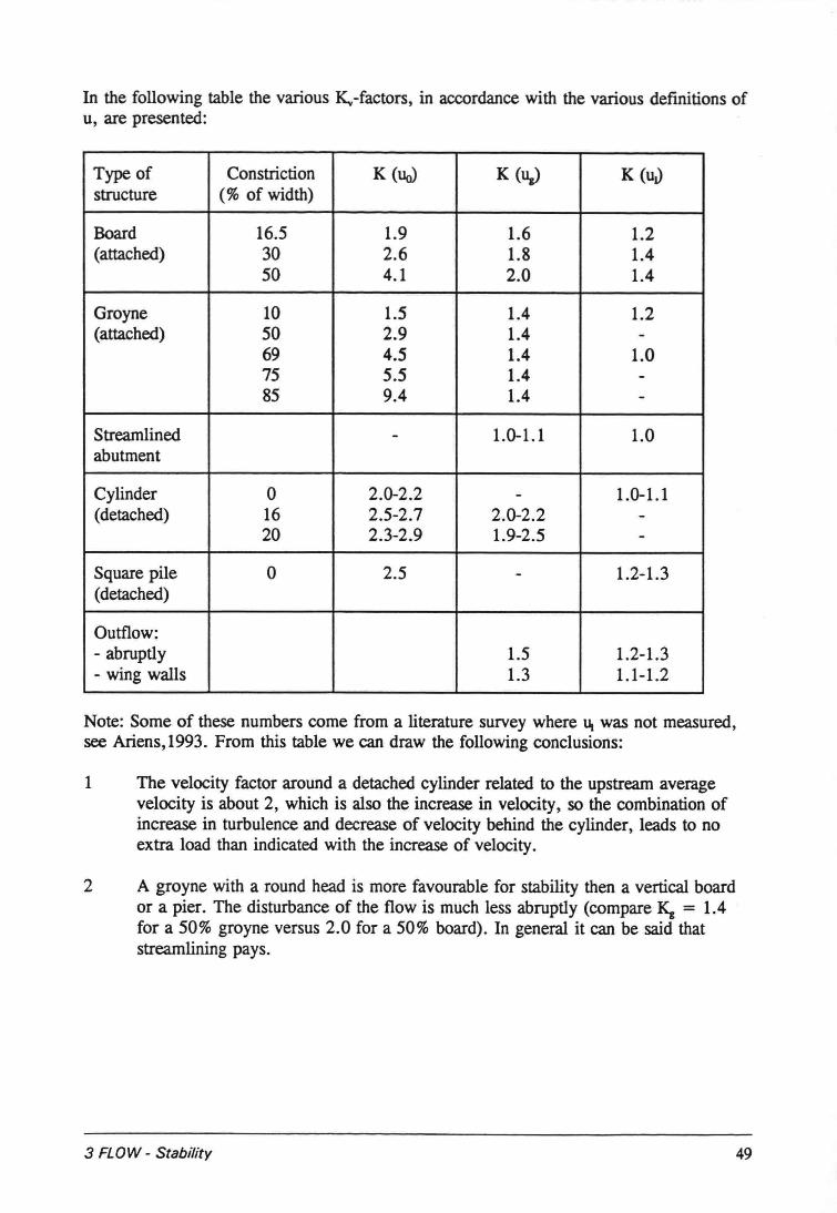
In the following table the various K.,.-factors, in accordance with the various defmitions ofu, are presented:

Type of Constriction K (Ua) K (lIJ K (uJstructure (% of width)

Board 16.5 1.9 1.6 1.2(attached) 30 2.6 1.8 1.4

50 4.1 2.0 1.4

Groyne 10 1.5 1.4 1.2(attached) 50 2.9 1.4 -

69 4.5 1.4 1.075 5.5 1.4 -85 9.4 1.4 -

Streamlined - 1.0-1.1 1.0abutment

Cylinder 0 2.0-2.2 - 1.0-1.1(detached) 16 2.5-2.7 2.0-2.2 -

20 2.3-2.9 1.9-2.5 -Square pile 0 2.5 - 1.2-1.3(detached)

Outflow:- abruptly 1.5 1.2-1.3- wing walls 1.3 1.1-1.2

Note: Some of these numbers come from a literature survey where U. was not measured,see Ariens,1993. From this table we cao draw the following conclusions:

1 The velocity factor around a detached cylinder related to the upstream averagevelocity is about 2, which is also the increase in velocity, so the combination ofincrease in turbulence and decrease of velocity behind the cylinder, leads to noextra load than indicated with the increase of velocity.

2 A groyne with a round head is more favourable for stability then a vertical boardor a pier. The disturbance of the flow is much less abruptly (compare K, = 1.4for a 50% groyne versus 2.0 for a 50% board). In general it cao be said thatstreamlining pays.

3 FLOW - Stability 49

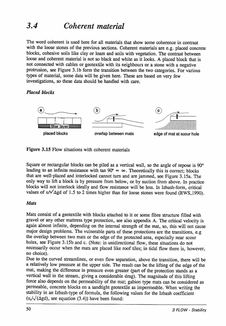
3.4 Coherent material

The word coherent is used here for all materials that show some coherence in contrastwith the loose stones of the previous sections. Coherent materials are e.g. placed concreteblocks, cohesive soils like clay or loam and soils with vegetation. The contrast betweenloose and coherent material is not so black and white as it looks. A placed block that isnot connected with cables or geotextile with its neighbours or a stone with a negativeprotrusion, see Figure 3.1b form the transition between the two categories. For varioustypes of material, some data will be given here. These are based on very fewinvestigations, so these data should be handled with care.

Placed blocks

0______

~I.fitt~: laledlJrnlllMllJplaced blocks overtap between mats edge of mat at scour hole

Figure 3.15 Flow situations with coherent materials

Square or rectangular blocks can be piled as avertical wall, so the angle of repose is 90°leading to an infinite resistance with tan 900 = 00. Theoretically this is correct; blocksthat are well-placed and interlocked cannot turn and are jammed, see Figure 3.15a. Theonly way to lift a block is by pressure from below, or by suction from above. In practiceblocks will not interlock ideally and flow resistance will be less. In Izbash-form, critica!values of utv'.~gd of 1.5 to 2 times higher than for loose stones were found (RWS, 1990).

Mats

Mats consist of a geotextile with blocks attached to it or some fibre structure filled withgravel or any other mattress type protection, see also appendix A. The critical velocity isagain almost infinite, depending on the internal strength of the mat, so, this will not causemajor design problems. The vulnerable parts of these protections are the transitions, e.gthe overlap between two mats or the edge of the protected area, especially near scourholes, see Figure 3.15b and c. (Note: in unidirectional flow, these situations do notnecessarily occur when the mats are placed like roof tiles; in tidal flow there is, however,no choice).Due to the curved streamlines, or even flow separation, above the transition, there will bea relatively low pressure at the upper side. The result can be the lifting of the edge of themat, making the difference in pressure even greater (part of the proteetion stands as avertical wall in the stream, giving a considerabie drag). The magnitude of this liftingforce also depends on the permeability of the mat; gabion type mats can be considered aspermeabie, concrete blocks on a sandtight geotextile as impermeabie. When writing thestability in an Izbash-type of formula, the following values for the Izbash coefficient(u/J(~gd), see equation (3.4» have been found:

50 3 FLOW - Stability

Overlap hetween matsEdge of scour holeLoose stones on flat bed

Permeable21.41.7

Impermeable1.41.1

The reversed flow in a scour hole is the most unfavourable situation, while with apermeable mattress, at an overlap, the value is still higher than the Izbash value for astone on a bed.

Gabions

Gabions consist of loose stones, packed together with some thread into larger elements,see appendix A. This can he useful when available elements are not large enough for theflow. Base of placing can also be the reason to apply gabions. The relative density is lessthan for a solid rock, because of the pores between the stones in the gabion:

ll. = (l-n)(ps-pw) (3.16)Pw

The porosity, n, lies usually around 40%. The stability is better than for a single stone,since the porosity also makes the load of the flow less effeetive. The coefficient for asingle gabion in the Izbash approach is about 2 times higher than for loose stones, so thefinal gain in stability coefficient is about 2 x .J(l-n) := 1.5.

Clay soils

Ven te Chow,1959 gives some data on the critical velocity for various clay types withoutvegetation. The results can be presented as follows:

Porosity: 20%1.5 - 1.8

40%1.0 - 1.2

60%0.1 - 0.4Critical velocity (mis)

Vegetation

Grass leaves and roots proteet an underlying (clay) soil. Grass leaves will flatten in theflow, acting as a kind of filter mattress. Time appears to become an important factor; infact the transition between stability and erosion becomes even more vague than in the caseof loose grains. CIRIA,1990 gives some information for grass. Based on this informationit is recommended that a grass cover can withstand in permanent flow:

Quality of grass cover: poor good

4 -53 -42.5 - 32

Critical velocity (mis):1 - 2 hours2 - 10 hours10 hours - 1 day1 - 2 days

2 -31.5 - 21 - 1.51

3 FL0 W - Stability 51

3.5 Summary

In this chapter the stability in flow is treated. The base relation for non-cohesive materiallike rock is the Shields rekuion wub correction factors for non-horizontal bottoms andflow situaiions that deviate from uniformflow:

(3.17)

The parameters in this formula are:

Uc the cntical, depth averaged, velocity in uniform flow for incipient motion.

i' the threshold of motion parameter, indicaiing the degree of transpon nearincipietu motion. i' = 0.06 could be seen as the start of sediment transpon andcan be used in compuuuions on erosion. For bed proteatons. where only minorlosses of material are accepted, a much lower value, e.g. i' = 0.03 isrecommended. Even then, periodic mainienance will be necessary. Equation (3.7)should be the basis when "carefree" protections have to be designed.

~ the relative density of the material. see appendix A

C the Chezy-coefficient, indicaiing the roughness. k = 3d90 can serve as a firstestimate of the equivalent roughness in equaiion (2.8).

K, is a strength reduction parameter for stones on a slope, see equations (3.8) and(3.9).

Kv the velocity/turbulence factor, indicating a load deviaiing from uniform flow. Inacceleraiing flow, Kv = 1,provided the local velocity is used in equaiion (3.17).For various flow situations, the table on page 49 gives valuesfor Ky. This factorshould be applied as a correction after the diameter in uniform flow is determined.Otherwise Kv will influence the iteratlon of d and C (which also comains d via kj.This would be conflicting wub the definltion of Kv (equation (3.10).

Finally, some data are presented for coherent material like mats, gabions, clay andvegetated soil. These are given in the shape of the Izbasn formula (equation (3.4).

52 3 FLOW - Stability

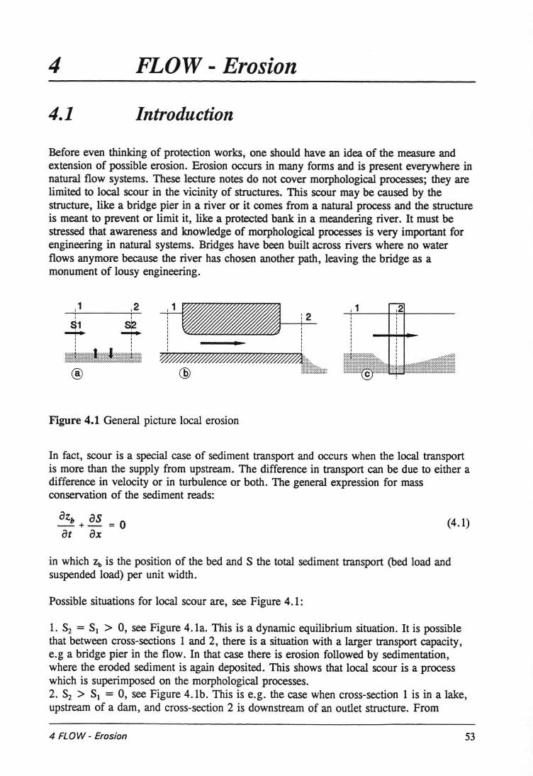
4 FLOW - Erosion

4.1 Introduetion

Before even thinking of proteetion works, one should have an idea of the measure andextension of possible erosion. Erosion occurs in many forms and is present everywhere innatural flow systems. These leeture notes do not cover morphological processes; they arelimited to local scour in the vicinity of structures. This scour may be caused by thestructure, like a bridge pier in a river or it comes from a natural process and the structureis meant to prevent or limit it, like a protected bank in a meandering river. Itmust bestressed that awareness and knowledge of morphological processes is very important forengineering in natural systems. Bridges have been built across rivers where no waterflows anymore because the river has chosen another path, leaving the bridge as amonument of lousy engineering.

®

i1IIIIIIIIII

:liil!i:···li·iil·.i:::::::::t~: :r::~f::::::::m:::ill:i::i::i:i::i::i:.:..:

Figure 4.1 General picture local erosion

In fact, scour is a special case of sediment transport and occurs when the local transportis more than the supply from upstream. The difference in transport can be due to either adifference in velocity or in turbulence or both. The general expression for massconservation of the sediment reads:

(4.1)

in which z, is the position of the bed and S the total sediment transport (bed load andsuspended load) per unit width.

Possible situations for local scour are, see Figure 4.1:

1. S2 = SI > 0, see Figure 4.1a. This is a dynamic equilibrium situation. It is possiblethat between cross-sections 1 and 2, there is a situation with a larger transport capacity ,e.g a bridge pier in the flow. In that case there is erosion followed by sedimentation,where the eroded sediment is again deposited. This shows that local scour is a processwhich is superimposed on the morphological processes.2. S2 > SI = 0, see Figure 4.1b. This is e.g. the case when cross-section 1 is in a lake,upstream of a dam, and cross-section 2 is downstream of an outlet structure. From

4 FLOW - Erosion 53

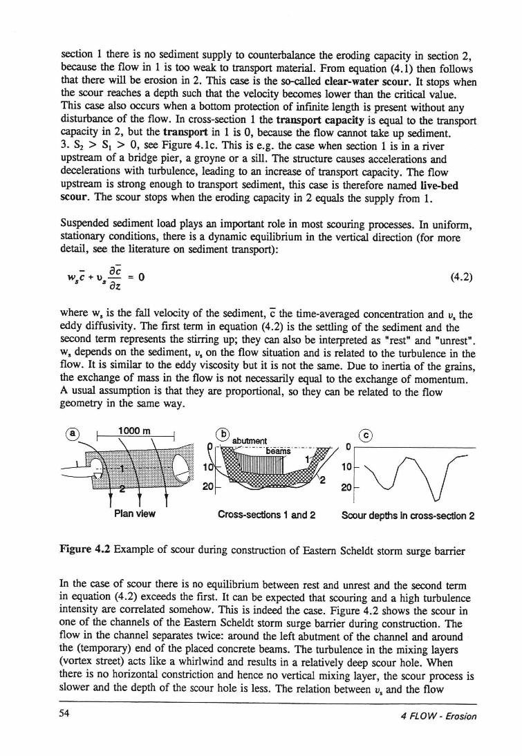
section 1 there is no sediment supply to counterbalance the eroding capacity in section 2,because the flow in 1 is too weak to transport material. From equation (4.1) then followsthat there will be erosion in 2. This case is the so-called clear-water scour. It stops whenthe scour reaches a depth such that the velocity becomes lower than the critical value.This case also occurs when a bottom proteetion of infmite length is present without anydisturbance of the flow. In cross-section 1 the transport capacity is equal to the transportcapacity in 2, but the transport in 1 is 0, because the flow cannot take up sediment.3. S2 > SI > 0, see Figure 4.1c. This is e.g. the case when section 1 is in a riverupstream of a bridge pier, a groyne or a sill. The structure causes accelerations anddecelerations with turbulence, leading to an increase of transport capacity. The flowupstream is strong enough to transport sediment, this case is therefore named live-bedscour. The scour stops when the eroding capacity in 2 equals the supply from 1.

Suspended sediment load plays an important role in most scouring processes. In uniform,stationary conditions, there is a dynamic equilibrium in the vertical direction (for moredetail, see the literature on sediment transport):

acwc+u- =011 11 az (4.2)

where w. is the fall velocity of the sediment, ë the time-averaged concentration and u, theeddy diffusivity. The first term in equation (4.2) is the settling of the sediment and thesecond term represents the stirring up; they can also be interpreted as "rest" and "unrest".w. depends on the sediment, v. on the flow situation and is related to the turbulence in theflow. It is similar to the eddy viscosity but it is not the same. Due to inertia of the grains,the exchange of mass in the flow is not necessarily equal to the exchange of momentum.A usual assumption is that they are proportional, so they can be related to the flowgeometry in the same way.

0.------------------

10

20

Plan view Cross-sectlons 1 and 2 Scour depths In cross-sectlon 2

Figure 4.2 Example of scour during construction of Eastern Scheldt storm surge barrier

In the case of scour there is no equilibrium between rest and unrest and the second termin equation (4.2) exceeds the first. It can be expected that scouring and a high turbulenceintensity are correlated somehow. This is indeed the case. Figure 4.2 shows the scour inone of the channels of the Eastern Scheldt storm surge barrier during construction. Theflow in the channel separates twice: around the left abutment of the channel and aroundthe (temporary) end of the placed concrete beams. The turbulence in the mixing layers(vortex street) acts like a whirlwind and results in a relatively deep scour hole. Whenthere is no horizontal constriction and hence no vertical mixing layer, the scour process isslower and the depth of the seour hole is less. The relation between Vs and the flow

54 4 FLOW - Erosion

geometry is not yet fully understood. A first attempt to approach the scouringphenomenon along this line is given by Hoffmans,1992. For engineering practice, thisapproach does not yet give useful results and empirical relations have to be used. In thecoming paragraphs some of those will be presented for different cases.

-0 equilibriumu --~ho - scourdepths:-C) IV.2

hs

log t

Figure 4.3 General definition scour hole and development in time

The development of a scour hole in time can be described in 4 phases (see Figure 4.3):

Phase I: the initial phase. The bottom is still flat, the velocity-profile is not yet influencedby the scour hole and the flow is still nearly uniform. Sediment goes into suspension, seeequation (4.2) and is convected with the main flow. The upstream slope is being formedand {3 increases.

Phase D: the development phase. The upstream slope of the scour hole, {3, becomesconstant. Sediment is picked up from the lower parts of the slope. Because of this slope,the flow separates, giving a mixing layer in the scour hole and a recirculation zone inwhich the flow is against the main flow direction . This also indicates that the scouringprocess is influenced by the scour hole itself, which is a complication compared to thestability phenomena as discussed in chapter 3. The influence of the scour hole has to beadded to the influence of the flow geometry on the veloeities and turbulence.

Phase ill: the stabilization phase. The velocity in the scour hole reaches values which arenear the critical value and the process slows down. Material is no longer moved from theupstream slope. The slope angle {3 remains constant.

Phase IV: the equilibrium phase. The final scour depth is reached (asymptotically). Thebed particles at the upstream slope are only moving to and fro and the net transport fromthe scour hole becomes zero.

For practical purposes phase 11and phase IV are the most important. When the erosionprocess goes fast, only the equilibrium depth of phase IV is of interest. When the processis slower, the development in time can be important, separately from the equilibriumdepth, which is always of interest. The importance of the development in time can lie ine.g. a maintenance policy in which the scour hole is covered when the depth becomesdangerously high. Another situation where the development in time will be important, iswhen scour develops during construction and different construction phases give differentscour intensities.

4 FLOW - Erosion 55

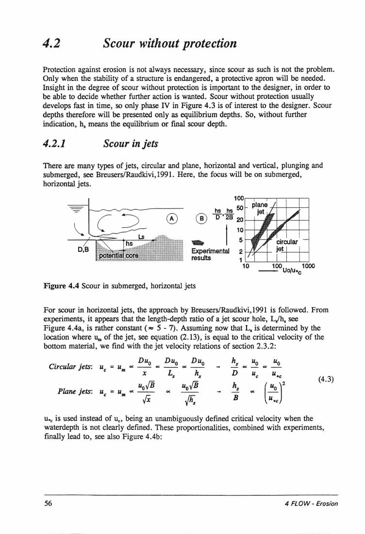
4.2 Scour without proteetion

Proteetion against erosion is not always necessary, since scour as such is not the problem.Only when the stability of a structure is endangered, a protective apron will be needed.Insight in the degree of scour without proteetion is important to the designer, in order tohe able to decide whether further action is wanted. Scour without proteetion usuallydevelops fast in time, so only phase IV in Figure 4.3 is of interest to the designer. Scourdepths therefore will be presented only as equilibrium depths. So, without furtherindication, hameans the equilibrium or final scour depth.

4.2.1 SCOUT in jets

There are many types of jets, circular and plane, horizontal and vertical, plunging andsubmerged, see Breusers/Raudkivi, 1991. Here, the focus will be on submerged,horizontal jets.

- hs hs 50

0 ® 0'28 20

I 10... 5

Experimental 2results

Figure 4.4 Scour in submerged, horizontal jets

For scour in horizontal jets, the approach by Breusers/Raudkivi,1991 is followed. Fromexperiments, it appears that the length-depth ratio of a jet scour hole, L/h. seeFigure 4.4a, is rather constant (= 5 - 7). Assuming now that La is determined by thelocation where 11m of the jet, see equation (2.13), is equal to the critical velocity of thebottom material, we find with the jet velocity relations of section 2.3.2:

Circular jets: Uc = uIIIDuo Duo Duo hs Uo Uo0( __ 0( __ 0( __

_0(_0(_

X Ls hs D Uc u.cuofB uofB hs (:~J (4.3)

Plane jets: Uc = uIII 0( __0( -- - 0(

{X Ihs B

u., is used instead of u., being an unambiguously defined critical velocity when thewaterdepth is not c1early defined. These proportionalities, combined with experiments,finally lead to, see also Figure 4.4b:

56 4 FLOW - Erosion

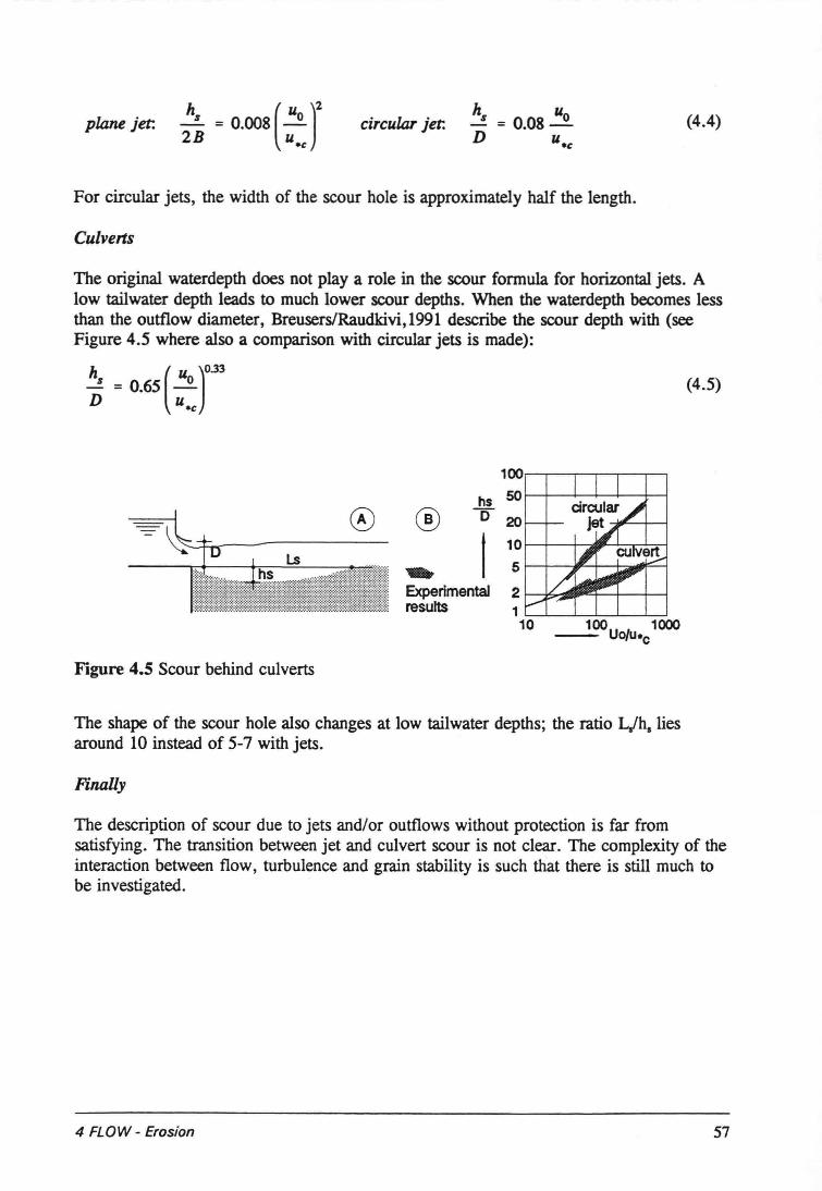
plane jet: circular jet: (4.4)

For circular jets, the width of the scour hole is approximately half the length.

Culvens

The original waterdepth does not play a role in the scour formula for horizontal jets. Alow tailwater depth leads to much lower scour depths. When the waterdepth becomes lessthan the outflow diameter, BreusersiRaudkivi,1991 describe the scour depth with (seeFigure 4.5 where also a comparison with circular jets is made):

h ( U )0.33.2. = 0.65 ~D »;

(4.5)

100.--r---r--,----r---,--,hs 50 I---t----I---+-+--+-_io®

~ExperimentaJresults

Figure 4.5 Scour behind culverts

The shape of the scour hole also changes at low tailwater depths; the ratio L,lh. liesaround 10 instead of 5-7 with jets.

Finally

The description of scour due to jets and/or outflows without proteetion is far fromsatisfying. The transition between jet and culvert scour is not clear. The complexity of theinteraction between flow, turbulence and grain stability is such that there is still much tobe investigated.

4 FLOW - Erosion 57

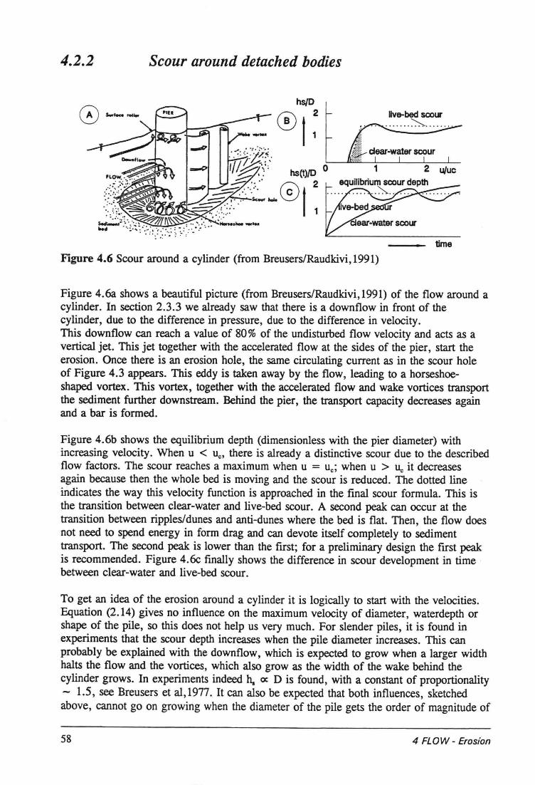
4.2.2 Scour around detached bodies

o s.o._ ......

timeFigure 4.6 Scour around a cylinder (from Breusers/Raudkivi, 1991)

Figure 4.6a shows a beautiful picture (from Breusers/Raudkivi,1991) of the flow around acylinder. In section 2.3.3 we already saw that there is a downflow in front of thecylinder, due to the difference in pressure, due to the difference in velocity.This downflow can reach a value of 80% of the undisturbed flow velocity and acts as avertical jet. This jet together with the accelerated flow at the sides of the pier, start theerosion. Once there is an erosion hole, the same circulating current as in the scour holeof Figure 4.3 appears. This eddy is taken away by the flow, leading to a horseshoe­shaped vortex. This vortex, together with the accelerated flow and wake vortices transportthe sediment further downstream. Behind the pier, the transport capacity decreases againand a bar is formed.

Figure 4.6b shows the equilibrium depth (dimensionless with the pier diameter) withincreasing velocity . When u < u., there is already a distinctive scour due to the describedflow factors. The scour reaches a maximum when u = u.; when u > u, it decreasesagain because then the whole bed is moving and the scour is reduced. The dotted lineindicates the way this velocity function is approached in the final scour formula. This isthe transition between clear-water and live-bed scour. A second peak can occur at thetransition between ripples/dunes and anti-dunes where the bed is flat. Then, the flow doesnot need to spend energy in form drag and can devote itself completely to sedimenttransport. The second peak is lower than the first; for a preliminary design the first peakis recommended. Figure 4.6c finally shows the difference in scour development in timebetween clear-water and live-bed scour.

To get an idea of the erosion around a cylinder it is logically to start with the velocities.Equation (2.14) gives no influence on the maximum velocity of diameter, waterdepth orshape of the pile, so this does not help us very much. For slender piles, it is found inexperiments that the scour depth increases when the pile diameter increases. This canprobably be explained with the downflow, which is expected to grow when a larger widthhalts the flow and the vortices, which also grow as the width of the wake behind thecylinder grows. In experiments indeed h, ex D is found, with a constant of proportionality- 1.5, see Breusers et al,1977. It can also be expected that both influences, sketchedabove, cannot go on growing when the diameter of the pile gets the order of magnitude of

58 4 FLOW - Erosion

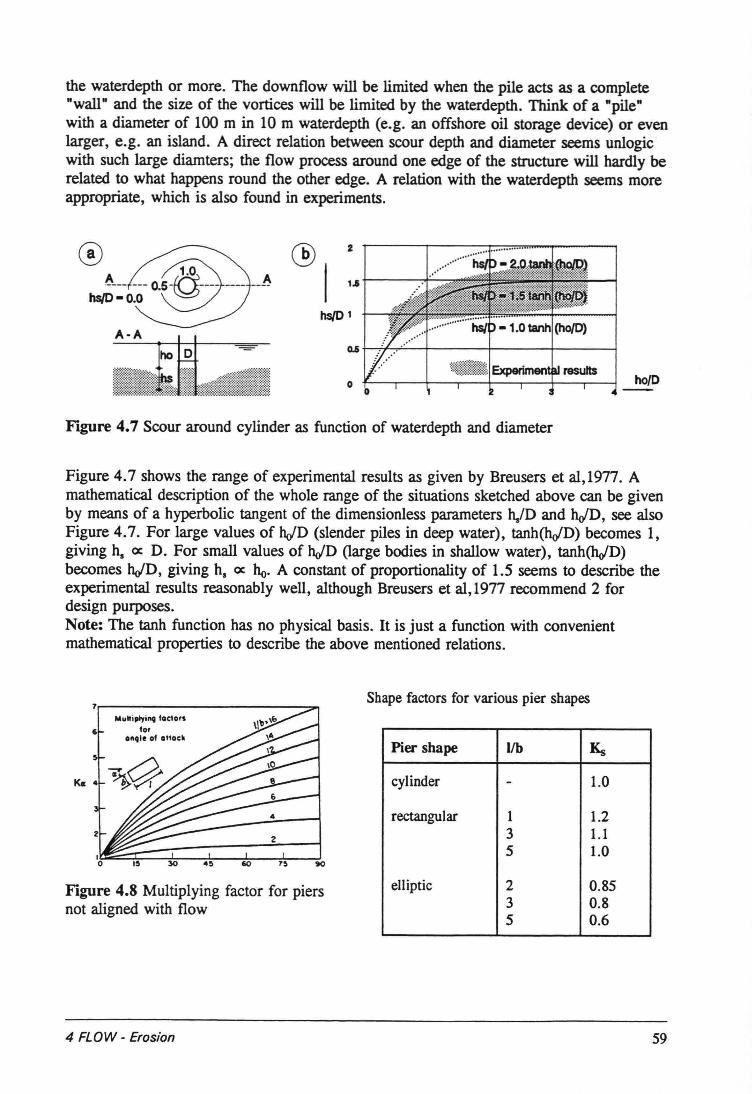
the waterdepth or more. The downflow will be limited when the pile acts as a complete"wall" and the size of the vortices will be limited by the waterdepth. Think of a "pile"with a diameter of 100 m in 10 m waterdepth (e.g. an offshore oil storage device) or evenlarger, e.g. an island. A direct relation between scour depth and diameter seems unlogicwith such large diamters; the flow process around one edge of the structure will hardly berelated to what happens round the other edge. A relation with the waterdepth seems moreappropriate, which is also found in experiments.

@I

ho/D

Figure 4.7 Scour around cylinder as function of waterdepth and diameter

Figure 4.7 shows the range of experimental results as given by Breusers et al,1977. Amathematical description of the whole range of the situations sketched above can be givenby means of a hyperbolic tangent of the dimensionless parameters h/D and hJD, see alsoFigure 4.7. For large values of hJD (slender piles in deep water), tanh(holD) becomes 1,giving hl <X D. For small values of hJD (large bodies in shallow water), tanh(holD)becomes hJD, giving hl <X ho. A constant of proportionality of 1.5 seems to describe theexperimental results reasonably weIl, although Breusers et al,1977 recommend 2 fordesign purposes.Note: The tanh function has no physical basis. It is just a function with convenientmathematical properties to describe the above mentioned relations.

Muhiplyill9 laclo"10'

Oft91e ol Ol,ock6

90

Figure 4.8 Multiplying factor for piersnot aligned with flow

Shape factors for various pier shapes

Pier shape I/b Kt;

cylinder - 1.0

rectangular 1 1.23 1.15 1.0

elliptic 2 0.853 0.85 0.6

4 FLOW - Erosion 59

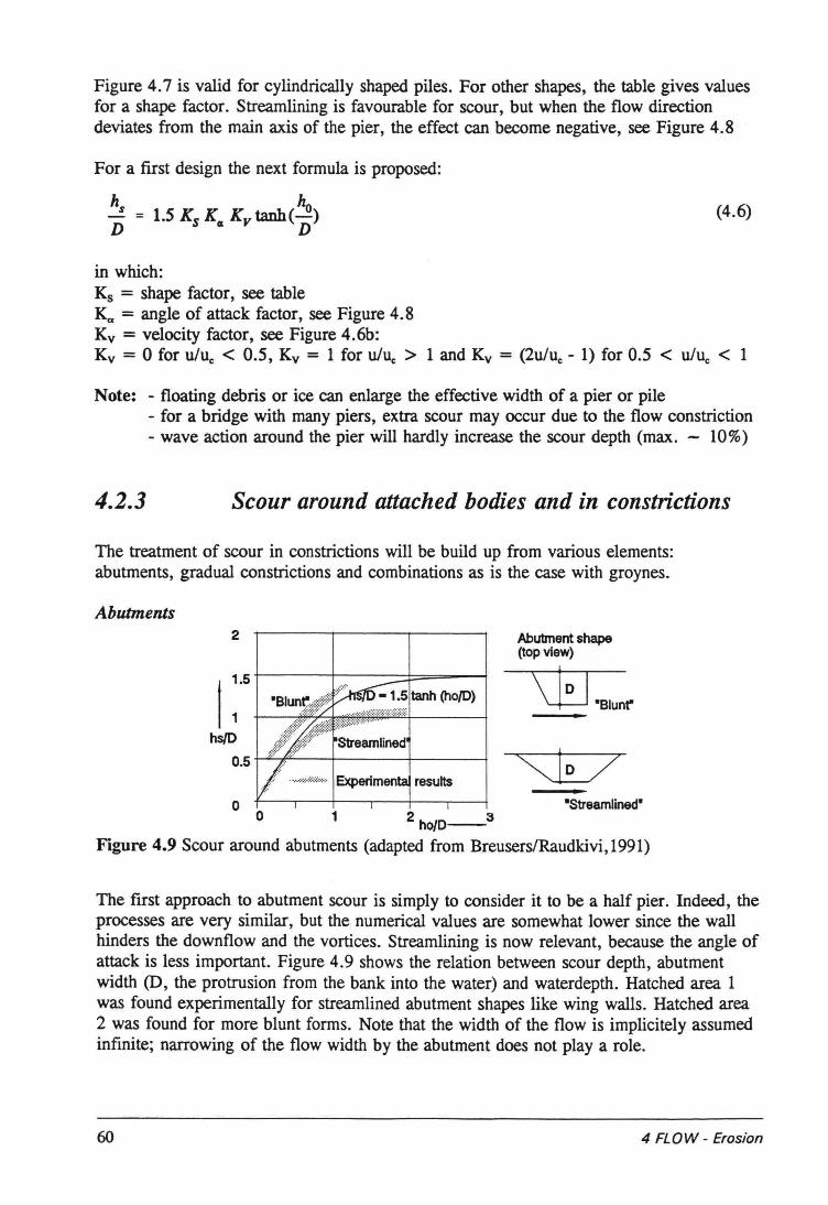
Figure 4.7 is valid for cylindrica1ly shaped piles. For other shapes, the table gives valuesfor a shape factor. Streamlining is favourable for scour, but when the flow directiondeviates from the main axis of the pier, the effect can become negative, see Figure 4.8

For a fust design the next formula is proposed:

ha hoD = 1.S x,x, s; tanh( D)

in which:K, = shape factor, see tableKa = angle of attack factor, see Figure 4.8Kv = velocity factor, see Figure 4.6b:Kv = 0 for u/u, < 0.5, Kv = 1 for u/u, >

(4.6)

1 and Kv = (2u/uc - 1) for 0.5 < u/u, < 1

Note: - floating debris or ice can enlarge the effective width of a pier or pile- for a bridge with many piers, extra scour may occur due to the flow constriction- wave action around the pier will hardly increase the scour depth (max. - 10%)

4.2.3 Scour around attached bodies and in constrictions

The treatment of scour in constrictions will be build up from various elements:abutments, gradual constrictions and combinations as is the case with groynes.

Abutments2

1hs/O

0.5+-"'---r---+----+-------I

o 0

Abutment shape(top view)

1 2hO/O_3

Figure 4.9 Scour around abutments (adapted from Breusers/Raudkivi,1991)

The first approach to abutment scour is simply to consider it to be a half pier. Indeed, theprocesses are very similar, but the numerical values are somewhat lower since the wallbinders the downflow and the vortices. Streamlining is now relevant, because the angle ofattack is less important. Figure 4.9 shows the relation between scour depth, abutmentwidth (D, the protrusion from the bank into the water) and waterdepth. Hatched area 1was found experimentally for streamlined abutment shapes like wing walls, Hatched area2 was found for more blunt forms. Note that the width of the flow is implicitely assumedinfinite; narrowing of the flow width by the abutment does not play a role.

60 4 FLOW - Erosion

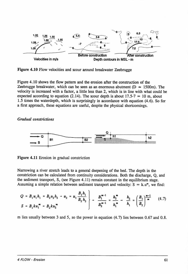
Velocities in mts

~-'--.s--:; r-. :~:;>c>\ ~§1 6.3 c'I " ~I 8 ----,- -~ <: .- "10' '" -e,

-7 .' '(':~':~:-'-8'ë"-' ~__-",~)· '7.5 .:.:::~>/--'6 •. :!..& r: 72. (---------&------.

'----:~'------------_:~ /'

Bëforeconstruction erconstructIonDepthcontoursin MSL- m

It--,\ --------_,----~~i'1:!1Q. ~ 1.55

188- 1.651_08/t=::=::::::- .......---..../ '- "1.05 I ./

----~------------

Figure 4.10 Flow veloeities and scour around breakwater Zeebrugge

Figure 4.10 shows the flow pattem and the erosion after the construction of theZeebrugge breakwater, which can be seen as an enormous abutment (D ::= 1500m). Thevelocity is increased with a factor, a little less than 2, which is in line with what could beexpected according to equation (2.14). The scour depth is about 17.5-7 = 10 m, about1.5 times the waterdepth, which is surprisingly in accordance with equation (4.6). So fora fust approach, these equations are useful, despite the physical shortcomings.

Gradual constrictions

Figure 4.11 Erosion in gradual constriction

Narrowing a river stretch leads to a general deepening of the bed. The depth in theconstriction can be calculated from continuity considerations. Both the discharge, Q, andthe sediment transport, S, (see Figure 4.11) remain constant in the equilibrium stage.Assuming a simple relation between sediment transport and velocity: S = k.u", we find:

(4.7)

m lies usually between 3 and 5, so the power in equation (4.7) lies between 0.67 and 0.8.

4 FLOW - Erosion 61

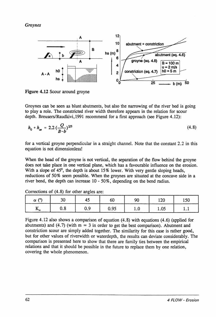
Groynes

,A 12

__ bern) 50

A

8hs (m)

6

4

2A-A : I

Figure 4.12 Scour around groyne

Groynes can be seen as blunt abutments, but also the narrowing of the river bed is goingto play a role. The constricted river width therefore appears in the relation for scourdepth. Breusers/Raudkivi,1991 recommend for a first approach (see Figure 4.12):

ho + h.. = 2.2 (_g_)2/3B-b

(4.8)

for avertical groyne perpendicular in a straight channel. Note that the constant 2.2 in thisequation is not dimensionless!

When the head of the groyne is not vertical, the separation of the flow behind the groynedoes not take place in one vertical plane, which has a favourable influence on the erosion.With a slope of 45°, the depth is about 15% lower. With very gentle sloping heads,reductions of 50% seem possible. When the groynes are situated at the concave side in ariver bend, the depth can increase 10 - 50%, depending on the bend radius.

Corrections of (4.8) for other angles are:

ex e) 30 45 60 90 120 150

Ka 0.8 0.9 0.95 1.0 1.05 1.1

Figure 4.12 also shows a comparison of equation (4.8) with equations (4.6) (applied forabutments) and (4.7) (with m = 3 in order to get the best comparison). Abutment andconstriction scour are simply added together. The similarity for this case is rather good,but for other values of riverwidth or waterdepth, the results can deviate considerably. Thecomparison is presented here to show that there are family ties between the empiricalrelations and that it should be possible in the future to replace them by one relation,covering the whole phenomenon.

62 4 FLOW - Erosion

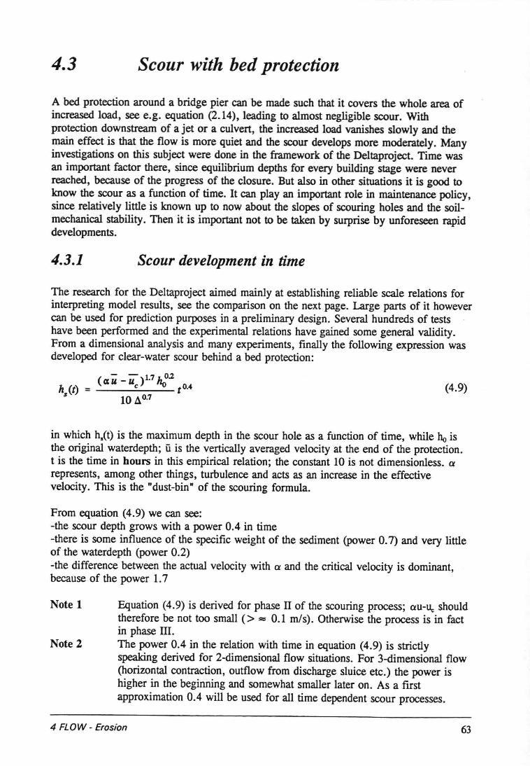
4.3 Scour with bed proteetion

A bed proteetion around a bridge pier can be made such that it covers the whole area ofincreased load, see e.g. equation (2.14), leading to almost negligible scour. Withproteetion downstream of a jet or a culvert, the increased load vanishes slowly and themain effect is that the flow is more quiet and the scour develops more moderately. Manyinvestigations on this subject were done in the framework of the Deltaproject. Time wasan important factor there, since equilibrium depths for every building stage were neverreached, because of the progress of the closure. But also in other situations it is good toknow the scour as a function of time. It can play an important role in maintenance policy,since relatively little is known up to now about the slopes of scouring holes and the soil­mechanical stability. Then it is important not to be taken by surprise by unforeseen rapiddevelopments.

4.3.1 Scour development in time

The research for the Deltaproject aimed mainly at establishing reliable scale relations forinterpreting model results, see the comparison on the next page. Large parts of it howevercan be used for prediction purposes in a preliminary design. Several hundreds of testshave been performed and the experimental relations have gained some general validity.From a dimensional analysis and many experiments, finally the following expression wasdeveloped for clear-water scour behind a bed protection:

(4.9)

in which hs(t) is the maximum depth in the scour hole as a function of time, while ho isthe original waterdepth; ti is the vertica1ly averaged velocity at the end of the protection.t is the time in hours in this empirica1 relation; the constant 10 is not dimensionless. arepresents, among other things, turbulence and acts as an increase in the effectivevelocity. This is the "dust-bin" of the scouring formula.

From equation (4.9) we can see:-the scour depth grows with a power 0.4 in time-there is some influence of the specific weight of the sediment (power 0.7) and very littleof the waterdepth (power 0.2)-the difference between the actual velocity with a and the critica1velocity is dominant,because of the power 1.7

Note 1 Equation (4.9) is derived for phase 11of the scouring process; ou-u, shouldtherefore be not too small (> := 0.1 mis). Otherwise the process is in factin phase Ill.The power 0.4 in the relation with time in equation (4.9) is strictlyspeaking derived for 2-dimensional flow situations. For 3-dimensional flow(horizontal contraction, outflow from discharge sluice etc.) the power ishigher in the beginning and somewhat smaller later on. As a firstapproximation 0.4 will be used for all time dependent scour processes.

Note 2

4 FLOW - Erosion 63

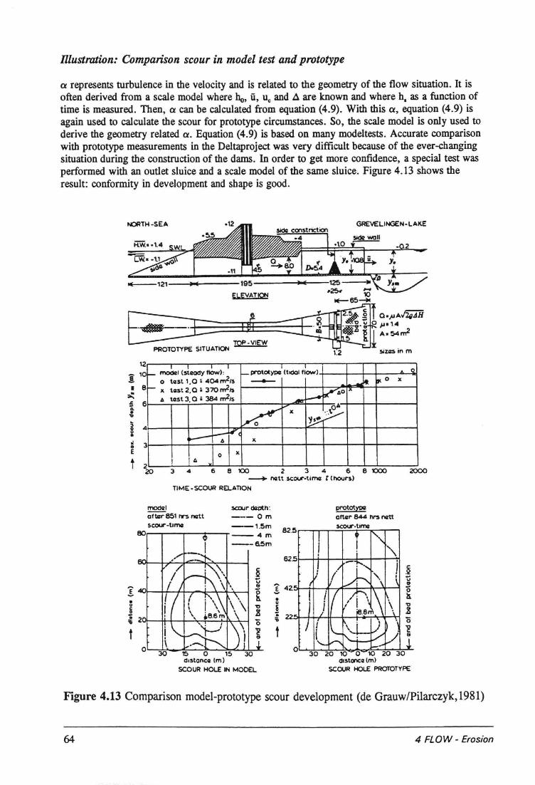
Illustration: Comparison scour in model test and prototype

a represents turbulence in the velocity and is related to the geometry of the flow situation. It isoften derived from a scale model where ho, ü, u, and .:1 are known and where h, as a function oftime is measured. Then, a can be calculated from equation (4.9). With this a, equation (4.9) isagain used to calculate the scour for prototype circumstances. So, the scale model is only used toderive the geometry related a. Equation (4.9) is based on many modeltests. Accurate comparisonwith prototype measurements in the Deltaproject was very difficult because of the ever-changingsituation during the construction of the dams. In order to get more confidence, a special test wasperformed with an outlet sluice and a scale model of the same sluice. Figure 4.13 shows theresult: conformity in development and shape is good.

NQRTH-SEA

ELEyAT!QN

TOP-VIEWPROTOTYPE SITUATION siZlZ$ in m

12

i 10

I e;.::5 6...•...§ 4•:: 3E

t 220 34 68100 2 34 681000 2000

~ rlQtt sçour-timcl t (hour1~)TIME· SCOUR RELATION

r- ~'(~aodY 'IOW):T I

0~ j)l"DtotYPll (tldO' 'IOW)o tut 1,0 i 404m2/s - ~~ ",0 x

~ .JI tast 2,0 ~370m21$ ~oiX11 tl2st 3,a ~384 m2/s ~ ,_..,

.r: OAx y'1p~ -:'11 X

0 xI t.

modql sccur~h:~es1trsrlQtt -- 0 mscour-tlmcl -- 1.Sm

80,.---.--.....--_ ........-_ ..m--~m

t

!~I~~-+~~~~~~•VCQi 201~_tt_t-+_.:.rr-_H\--l!:_l

Figure 4.13 Comparison model-prototype scour development (de Grauw/Pilarczyk,1981)

64 4 FLOW - Erosion

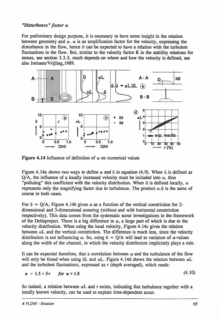
"Disturbance" factor Ol

For preliminary design purpose, it is necessary to have some insight in the relationbetween geometry and a. a is an amplification factor for the velocity, expressing thedisturbance in the flow, hence it can be expected to have a relation with the turbulentfluctuations in the flow. But, similar to the velocity factor K in the stability relations forstones, see section 3.3.3, much depends on where and how the velocity is defined, seealso Iorissen/Vrijling, 1989.

A-A

@

B-B

t 5

oo 0.5 1.0- D/hO

• 2d.. 3d

@ 5exL4~+--t--+---+--=1

t : 1---::;~-t--+---+---1

10.. @..

....j,. •• ••••

10 ,..----,-----,@

ClL

••• ••••

i

o '--_--':-::----"o 0.5 1.0- D/hO - r(%)

Figure 4.14 Influence of definition of a on numerical values

Figure 4.14a shows two ways to define a and ü in equation (4.9). When û is defined asQ/A, the influence of a locally increased velocity must be included into a, thus"polluting" this coefficient with the velocity distribution. When ü is defined locally, arepresents only the magnifying factor due to turbulence. The product o.ü is the same ofcourse in both cases.

For ü = Q/A, Figure 4.14b gives a as a function of the vertical constriction for 2-dimensional and 3-dimensional scouring (without and with horizontal constrictionrespectively). This data comes from the systematic scour investigations in the frameworkof the Deltaproject. There is a big difference in a, a large part of which is due to thevelocity distribution. When using the local velocity, Figure 4.14c gives the relationbetween aL and the vertical constriction. The difference is much less, since the velocitydistribution is not influencing a. So, using ü = Q/A will lead to variation of o-valuesalong the width of the channel, in which the velocity distribution implicitely plays a role.

It can be expected therefore, that a correlation between a and the turbulence of the flowwill only be found when using üL and aL. Figure 4.14d shows the relation between aLand the turbulent fluctuations, expressed as r (depth averaged), which reads:

(t ;:: 1.5 + 5 r for (t > 1.8 (4.10)

So indeed, a relation between aL and r exists, indicating that turbulence together with alocally known velocity, can be used to explain time-dependent scour.

4 FLOW - Erosion 65

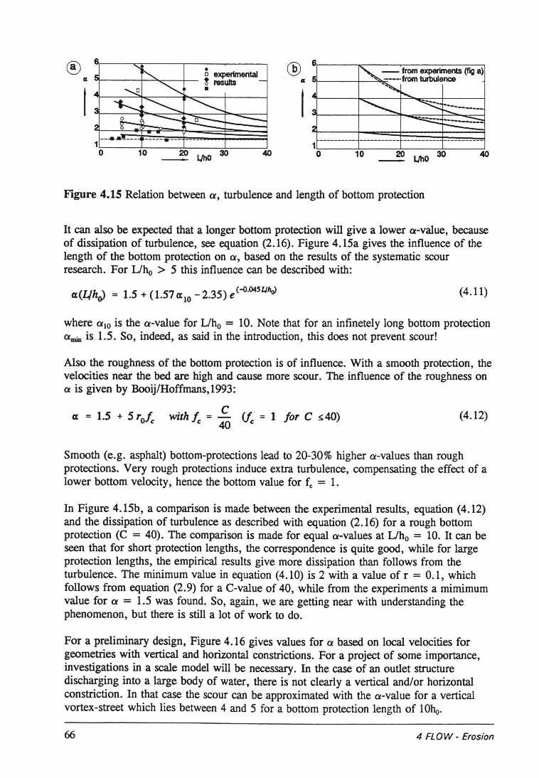
at

@6at

1'- from experiments (fig a)5 .----. from turbulence

jij "~

a ~ ~ ~--------~

~ ;::--=---------- ----------- ---------- ---------1o 10 20 WhO 30 40

®

~ WhO 30 40

Figure 4.15 Relation between a, turbulence and length of bottom proteetion

It can also be expected that a longer bottom proteetion will give a lower o-value, becauseof dissipation of turbulence, see equation (2.16). Figure 4.15a gives the influence of thelength of the bottom proteetion on a, based on the results of the systematic scourresearch. For L/ho > 5 this influence cao be described with:

a(L/hJ = 1.5 + (1.57 alO - 2.35) e(-{)·04SLl~ (4.11)

where alO is the o-value for L/ho = 10. Note that for an infinetely long bottom proteetiona1lÛD is 1.5. So, indeed, as said in the introduction, this does not prevent scour!

Also the roughness of the bottom proteetion is of influence. With a smooth protection, theveloeities near the bed are high and cause more scour. The influence of the roughness ona is given by Booij/Hoffmans,1993:

a = 1.5 + 5 Tofc with f. = ~ (Je = 1 fOT C ~40)e 40

(4.12)

Smooth (e.g. asphalt) bottom-protections lead to 20-30% higher o-values than roughprotections. Very rough protections induce extra turbulence, compensating the effect of alower bottom velocity , hence the bottom value for f, = 1.

In Figure 4.15b, a comparison is made between the experimental results, equation (4.12)and the dissipation of turbulence as described with equation (2.16) for a rough bottomproteetion (C = 40). The comparison is made for equal o-values at L/ho = 10. It can beseen that for short proteetion lengths, the correspondence is quite good, while for largeproteetion lengths, the empirical results give more dissipation than follows from theturbulence. The minimum value in equation (4.10) is 2 with a value of r = 0.1, whichfollows from equation (2.9) for a C-value of 40, while from the experiments a mimimumvalue for a = 1.5 was found. So, again, we are getting near with understanding thephenomenon, but there is still a lot of work to do.

For a preliminary design, Figure 4.16 gives values for a based on local veloeities forgeometries with vertical and horizontal constrictions. For a project of some importance,investigations in a scale model will be necessary. In the case of an outlet structuredischarging into a large body of water, there is not clearly avertical and/or horizontalconstriction. In that case the scour cao be approximated with the o-value for averticalvortex-street which lies between 4 and 5 for a bottom proteetion length of 10ho.

66 4 FLOW - Erosion

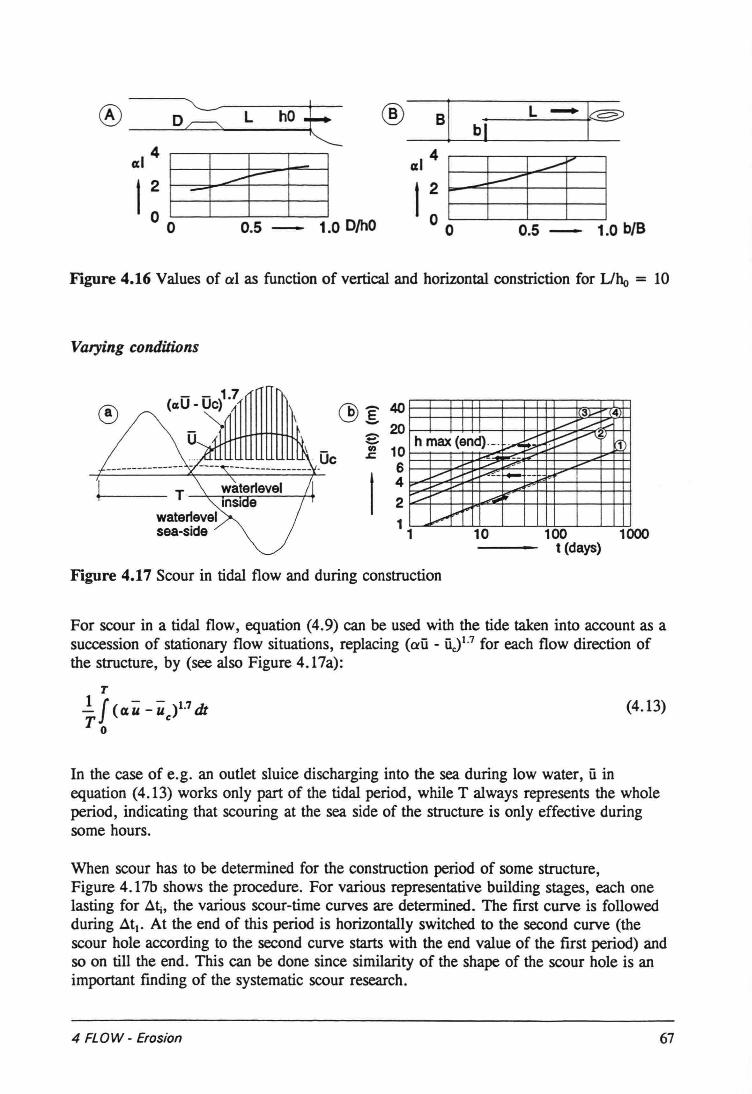
L .... I~0:;;: L hO~

î:14ittl-1o 0 0.5 - 1.0D/hO

®®

Figure 4.16 Values of al as function of vertical and horizontal constriction for Vbo = 10

Varying conditions

(cxO _Oe)1.7@ê 40- 20~-

Oe0) 10s:

642

3Y1" 411 ..........

~h max (end).-. ~ ;;..... e= 1....c.... ...,:- ,.,-- ~- .....

..........~ f"'" ~: _. -- ",,"'"-: ,..... -:,......- ..... ~rr

~ I--'f'"10 100 1000

t (days)

Figure 4.17 Scour in tidal flow and during construction

For scour in a tidal flow, equation (4.9) can be used with the tide taken into account as asuccession of stationary flow situations, replacing (oû - ÜJI.7 for each flow direction ofthe structure, by (see also Figure 4.17a):

T

.!.f (au - u )1.7dtT Co(4.13)

In the case of e.g. an outlet sluice discharging into the sea during low water, û inequation (4.13) works only part of the tidal period, while T always represents the wholeperiod, indicating that scouring at the sea side of the structure is only effective duringsome hours.

When scour has to be determined for the construction period of some structure,Figure 4.17b shows the procedure. For various representative building stages, each onelasting for ~~, the various scour-time curves are determined. The first curve is followedduring ~tl' At the end of this period is horizontally switched to the second curve (thescour hole according to the second curve starts with the end value of the first period) andso on till the end. This can be done since similarity of the shape of the scour hole is animportant finding of the systematic scour research.

4 FLOW - Erosion 67

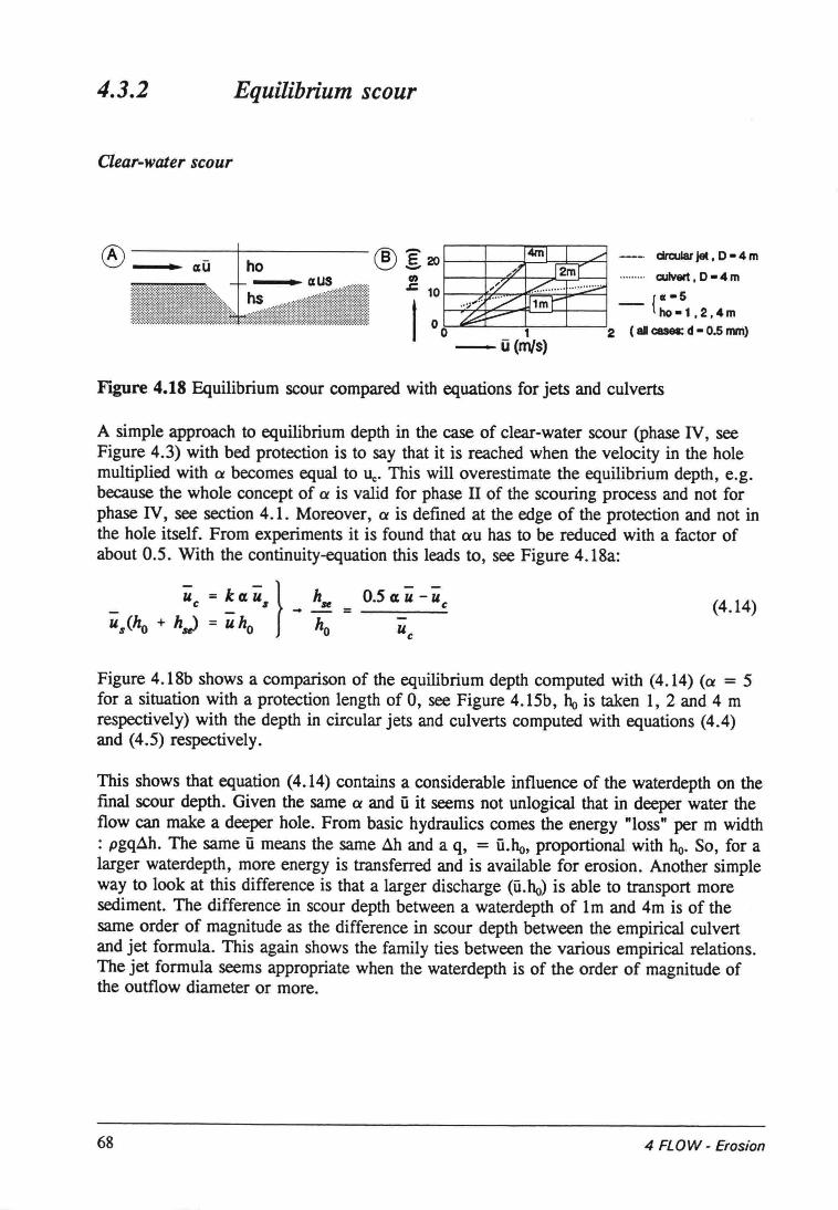
4.3.2 Equilibrium scour

Clear-water scour

,dj ho----, circular jet • 0 • 4m.........culvert.O-4m

{Cl-Sho-t.2.4m

2 ( aD cases: d - 0.5 mm)

Figure 4.18 Equilibrium scour compared with equations for jets and culverts

A simple approach to equilibrium depth in the case of clear-water scour (phase IV, seeFigure 4.3) with bed proteetion is to say that it is reached when the velocity in the holemultiplied with tx becomes equal to u.. This will overestimate the equilibrium depth, e.g.because the whole concept of tx is valid for phase TIof the scouring process and not forphase IV, see section 4.1. Moreover, a is defined at the edge of the proteetion and not inthe hole itself. From experiments it is found that OlU has to be reduced with a factor ofabout 0.5. With the continuity-equation this leads to, see Figure 4.18a:

_ Üc : ~ ClÜs } ... h:Je = 0.5 Cl! - ücus(ho + h~ - uho ho u

c

(4.14)

Figure 4.18b shows a comparison of the equilibrium depth computed with (4.14) (Ol = 5for a situation with a proteetion length of 0, see Figure 4.15b, ho is taken 1, 2 and 4 mrespectively) with the depth in circular jets and culverts computed with equations (4.4)and (4.5) respectively.

This shows that equation (4.14) contains a considerabie influence of the waterdepth on thefinal scour depth. Given the same Ol and ü it seems not unlogical that in deeper water theflow can make a deeper hole. From basic hydraulics comes the energy "loss" per m width: pgq~h. The same û means the same ~h and a q, = ü.ho, proportional with ho. So, for alarger waterdepth, more energy is transferred and is available for erosion. Another simpleway to look at this difference is that a larger discharge (ü.ho) is able to transport moresediment. The difference in scour depth between a waterdepth of lm and 4m is of thesame order of magnitude as the difference in scour depth between the empirical culvertand jet formula. This again shows the family ties between the various empirical relations.The jet formula seems appropriate when the waterdepth is of the order of magnitude ofthe outflow diameter or more.

68 4 FLOW - Erosion

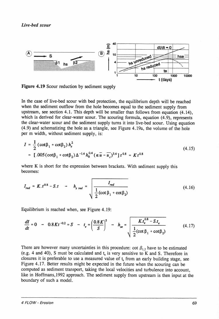
live-bed scour

_ 40

.5.@ ~ 10

4

dl/dt- 0 ........k f--"'"

~\l~ >--" _ -__ L _ _t!~~~" ...~,,~~;d , ",--- ~\l ' ,-- ,..,......;:::._- -- "5 ,- te:1

1 10 100 1000 10000t (days)

Figure 4.19 Scour reduction by sediment supply

In the case of live-bed scour with bed protection, the equilibrium depth will be reachedwhen the sediment outflow from the hole becomes equal to the sediment supply fromupstream, see section 4.1. This depth will be smaller than follows from equation (4.14),which is derived for c1ear-water scour. The scouring formula, equation (4.9), representsthe c1ear-water scour and the sediment supply tums it into live-bed scour. Using equation(4.9) and schematizing the hole as a triangle, see Figure 4.19a, the volume of the holeper m width, without sediment supply, is:

1 2I :::;- (cotû, + cotP2) hs2

:::;[.005 (cotf 1 + cotP2) II -}.4. hg·4 (Ct U - Uc)3.4 ] t 0.8 :::;K tO.8

(4.15)

where K is short for the expression between brackets. With sediment supply thisbecomes:

Ired :::;K.tO.8 -s.i (4.16)

Equilibrium is reached when, see Figure 4.19:

(4.17)

There are however many uncertainties in this procedure: cot (31,2 have to be estimated(e.g. 4 and 40), S must be calculated and te is very sensitive to K and S. Therefore inclosures it is preferabie to use a measured value of t, from an early building stage, seeFigure 4.17. Better results might be expected in the future when the scouring can becomputed as sediment transport, taking the local veloeities and turbulence into account,like in Hoffmans,1992 approach. The sediment supply from upstream is then input at theboundary of such a model.

4 FLOW - Erosion 69

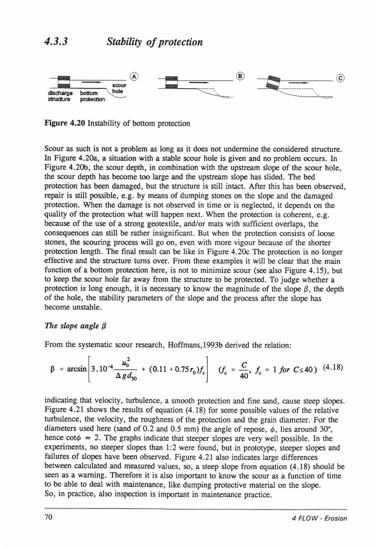
4.3.3 Stability of proteetion

---iII~-==-_®dlschargestructure

bottomprotection

scourhole

~:I'IIIII~iIIIIII_'___----:__=__=__=__=-__-\-, - ©---'

Figure 4.20 Instability of bottom proteetion

Scour as such is not a problem as long as it does not undermine the considered structure.In Figure 4.20a, a situation with a stable scour hole is given and no problem occurs. InFigure 4.20b, the scour depth, in combination with the upstream slope of the scour hole,the scour depth has become too large and the upstream slope has slided. The bedproteetion has been damaged, but the structure is still intact. After this has been observed,repair is still possible, e.g. by means of dumping stones on the slope and the damagedprotection. When the damage is not observed in time or is neglected, it depends on thequality of the proteetion what will happen next. When the proteetion is coherent, e.g.because of the use of a strong geotextile, and/or mats with sufficient overlaps, theconsequences can still be rather insignificant. But when the proteetion consists of loosestones, the scouring process will go on, even with more vigour because of the shorterproteetion length. The final result can be like in Figure 4.20c The proteetion is no longereffective and the structure tums over. From these examples it will be clear that the mainfunction of a bottom proteetion here, is not to minimize scour (see also Figure 4.15), butto keep the scour hole far away from the structure to be protected. To judge whether aproteetion is long enough, it is necessary to know the magnitude of the slope {3, the depthof the hole, the stability parameters of the slope and the process after the slope hasbecome unstable.

The slope angle {3

From the systematic scour research, Hoffmans, 1993b derived the relation:

P = arCSin[3010-4 u; + (0.11 + 0.75TO)fc] (je = 4OC,Ic = 1 fOT C~;40) (4.18)l1gdso

indicating that velocity , turbulence, a srnooth proteetion and fine sand, cause steep slopes.Figure 4.21 shows the results of equation (4.18) for some possible values of the relativeturbulence, the velocity , the roughness of the proteetion and the grain diameter. For thediameters used here (sand of 0.2 and 0.5 rnrn) the angle of repose, </>,lies around 30°,hence cot</>"""2. The graphs indicate that steeper slopes are very weIl possible. In theexperiments, no steeper slopes than 1:2 were found, but in prototype, steeper slopes andfailures of slopes have been observed. Figure 4.21 also indicates large differencesbetween calculated and rneasured values, so, asteep slope from equation (4.18) should beseen as a waming. Therefore it is also important to know the scour as a function of timeto be able to deal with maintenance, like dumping protective material on the slope.So, in practice, also inspeetion is important in maintenance practice.

70 4 FLOW - Erosion

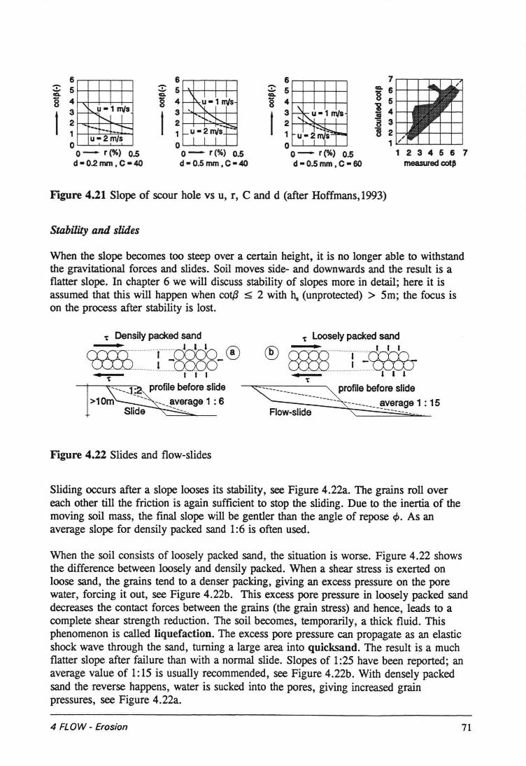
6 .-----.---r---r--.,....-,:::::5 f--+-I--+-+-IIA8 4 f-rt--I--+-+-I

t : j--.,;t-l-.,......±-I

1 u-2m/so '--'---'--'-""'---'0- r(%) 0.5d - 02 I'M'I , C - 40

6 ,...........,.-,---.-..,--,.....* 5 I--\t-t--+-+--l8 4

t ; I-""k-~-+---i

o L...-.I.__'__'___'___'

0- r(%) 0.5d-O.5mm,C-4O

6 r--r-,--.--,..--,:::::51-+-+--+-+---1IA8 4 1-+-+--+-+---1

t ; I-f~:+-+--lo L......J..__'___'___'___'

0- r(%) 0.5d-0.5mm,C-60

234567rneasurec:l cot"

Figure 4.21 Slope of scour hole vs u, r, C and d (after Hoffmans,1993)

Stabüity and slide«

When the slope becomes too steep over a certain height, it is no longer able to withstandthe gravitational forces and slides. Soil moves side- and downwards and the result is aflatter slope. In chapter 6 we will discuss stability of slopes more in detail; here it isassumed that this will happen when cot{3 < 2 with ha (unprotected) > 5m; the focus ison the process after stability is lost.

't Densily packed sand

C'f:'1:Yl . T dot)o ®UJJ,_J ...J..~OOOo-

I I I

profile before slide

Figure 4.22 Slides and flow-slides

't Loosely packed sand

® ffil3:: f:Wr..................I I I

profile before slide----------------- ------ !lverage 1 : 15

Flow-slide ---------

Sliding occurs after a slope looses its stability, see Figure 4.22a. The grains roil overeach other till the friction is again sufficient to stop the sliding. Due to the inertia of themoving soil mass, the final slope will be gentler than the angle of repose t/>. As anaverage slope for densily packed sand 1:6 is often used.

When the soil consists of loosely packed sand, the situation is worse. Figure 4.22 showsthe difference between loosely and densily packed. When a shear stress is exerted onloose sand, the grains tend to adenser packing, giving an excess pressure on the porewater, forcing it out, see Figure 4.22b. This excess pore pressure in loosely packed sanddecreases the contact forces between the grains (the grain stress) and hence, leads to acomplete shear strength reduction. The soil becomes, temporarily, a thick fluid. Thisphenomenon is called liquefaction. The excess pore pressure can propagate as an elasticshock wave through the sand, tuming a large area into quicksand. The result is a muchflatter slope after failure than with anormal slide. Slopes of 1:25 have been reported; anaverage value of 1:15 is usually recommended, see Figure 4.22b. With densely packedsand the reverse happens, water is sucked into the pores, giving increased grainpressures, see Figure 4.22a.

4 FLOW - Erosion 71

4.4 Summary

In general, local scour can be seen as a special case of sediment transport. The localvelocity anti turbulence pattem determines the local erosion. When this erosion takesplace in a flow in which sediment is transported, also without the local disturbance, wespeak of live-bed scour. When the only sediment transpon is due to the local disturbance,we speak of clear-water scour. Scour develops in time, reaching an equilibrium deptbwhen the flow forces can no longer take away sediment (clear-water scour) or when theoutflow of sediment becomes equal to the injlow (live-bed scour).

Two main streams of scour treatment are found in literature: one that studies the finalequilibrium scour anti one that studies the development in time. The choice depends onthe interest of the designer anti the process itself. When the equilibrium is reached veryfast, it has no use to know the development in time anti the design is based on the finalscour depth. When the process is slower, it can be economical to study the development intime anti to tune the design on some maintenance policy. Also when scour duringconstruction is important, it can be necessary to know the scour as a function of time,since the geometry of the flow, anti hence the scour, will change continuously.

In these lecture notes these !Woapproaches are coupled to the presence of a bottomproteetion. Without proteetion. the scour will reach equilibrium faster than withprotection. Empirical relations for scour in jets anti around bodies are presented whichcan be used for preliminary design purposes. Attempts are being made to give maximumphysical reasoning behind the empirical relations, although the physical basis of some ofthese equations is meager or virtualiy non-existent. Also comparisons are made betweensome of these equations to get the picture as complete as possible. lmportant relations aree.g. (4.4), (4.6) anti (4.7).

The scour as a function of time in cases with protection, is coupled as much as possible toturbulent flow phenomena. Although there are definite anti clear connections, here too itis still necessary to work with very empirical relations. Equation (4.9) is the basis of thisapproach, in whicn a paramount role is played by the coefficient a, which can be seen asa magnifying factor for the velocity. a is related to the relative turbulence of the flow,provided the local velocity is used. The estimate of equilibrium scour in the case witbproteetion anti the comparison with some formula without proteetion. make the storycomplete as far as possible.

Finally, some considerations are being given for the stability of scour holes anti bottomprotections in which the soil properties like angle of repose anti packing of the grains playa role. It is stressed that scour as such is not the problem, but the stability of somestructure that can be threatened by the scour. Proteetion anti maintenance policy shouldalways be focussed at the prevention of that to happen. The main function of protectionsbehind outflows is to keep the scour hole as far away as possible from the structure to beprotected. Decreasing turbulence is only a secundary funciion, since it takes 30 - 40 timesthe waterdepth, starting from a situation with high turbulence due to a vertical orhorizontal consmetion. to establish uniform flow conditions anti even then there will bescour. Only in a strongly varying flow field, like round a pile, it is possible to cover thearea with increased flow load, resulting in relatively small scour depths.

72 4 FLOW - Erosion

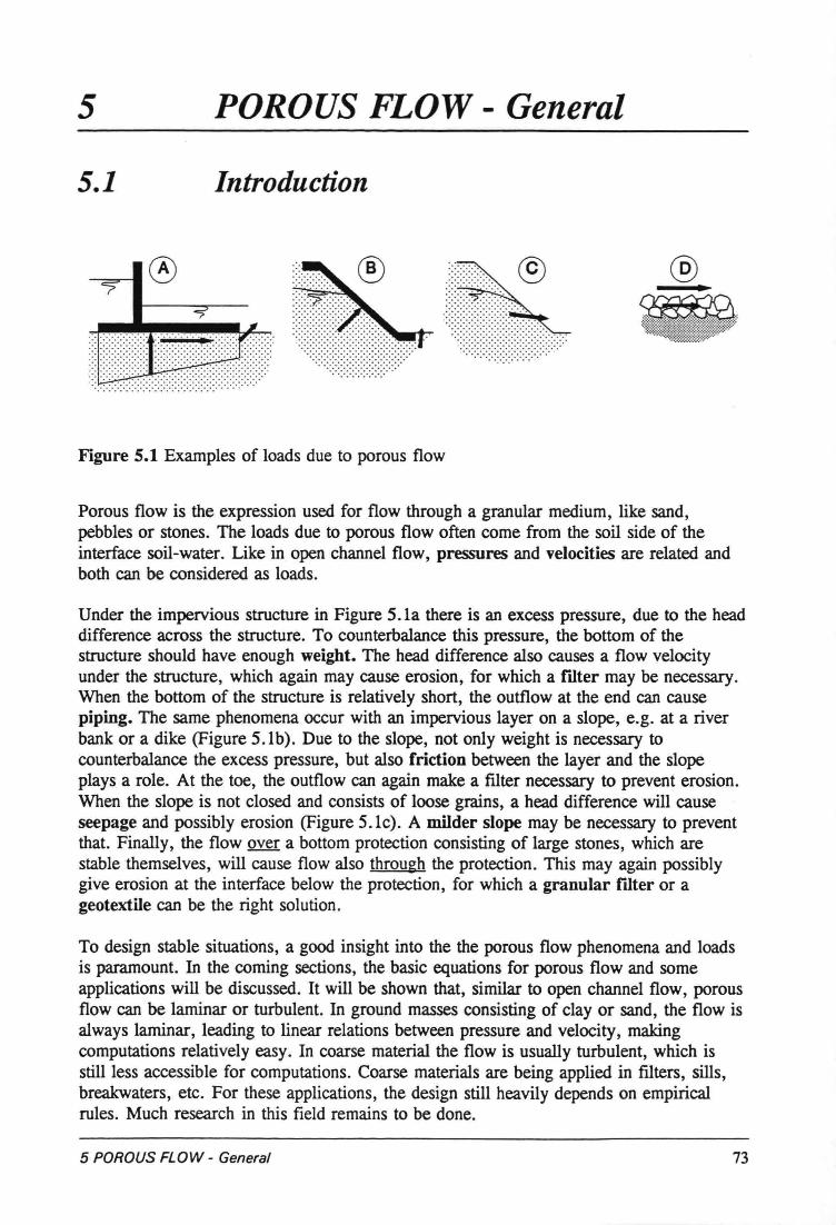
5 POROUS FLOW - General

5.1 Introduetion

........ ........ .... .................... ...... ..... .... .... .

...................................................... .. . . . . . . . . . . . . . . . . . . .. . . . . . . . . . . . . . . . . . .. . . . . . . . . . . . . . . . . .................... .. .

@

-. .. . . . . . . . . . . . . . . . . . . . . . . ....... .

Figure 5.1 Examples of loads due to porous flow

Porous flow is the expression used for flow through a granular medium, like sand,pebbles or stones. The loads due to porous flow often come from the soil side of theinterface soil-water. Like in open channel flow, pressures and velocities are related andboth can be considered as loads.

Under the impervious structure in Figure 5.1a there is an excess pressure, due to the headdifference across the structure. To counterbalance this pressure, the bottom of thestructure should have enough weight. The head difference also causes a flow velocityunder the structure, which again may cause erosion, for which a filter may be necessary.When the bottom of the structure is relatively short, the outflow at the end can causepiping. The same phenomena occur with an impervious layer on a slope, e.g. at a riverbank or a dike (Figure 5.1b). Due to the slope, not only weight is necessary tocounterbalance the excess pressure, but also friction between the layer and the slopeplays a role. At the toe, the outflow can again make a filter necessary to prevent erosion.When the slope is not closed and consists of loose grains, a head difference will causeseepage and possibly erosion (Figure 5.1c). A milder sIope may be necessary to preventthat. Finally, the flow over a bottom proteetion consisting of large stones, which arestabie themselves, will cause flow also through the protection. This may again possiblygive erosion at the interface below the protection, for which a granular filter or ageotextile can be the right solution.

To design stabie situations, a good insight into the the porous flow phenomena and loadsis paramount. In the coming sections, the basic equations for porous flow and someapplications will be discussed. It will be shown that, similar to open channel flow, porousflow can be laminar or turbulent. In ground masses consisting of clay or sand, the flow isalways laminar, leading to linear relations between pressure and velocity, makingcomputations relatively easy. In coarse material the flow is usually turbulent, which isstill less accessible for computations. Coarse materials are being applied in filters, sills,breakwaters, etc. For these applications, the design still heavily depends on empiricalrules. Much research in this field remains to be done.

5 POROUSFLOW - General 73

5.2 Basic equations

5.2.1 General

Starting point is again the Navier Stokes equation, written in the Reynolds-form for the x­direction (see chapter 2):

au au au-+u-+w-at ax aZ.1 ap êPu au'2 àu'w'

= ---+\)-------P ax az'2 ax aZ.

(5.1)

With this equation the flow in a porous medium can be calculated, provided that everystone and every pore is taken into account, which is practically impossible and notnecessary. An averaging procedure will be followed to reach practical solutions. The firststep in this procedure is to define an average velocity , the so-ca1led filter-velocity:

u,=.!. f f udA = n.uA A

(5.2)

in which n is the porosity and u the real velocity in the pores. The porosity, n, is usuallydefmed as the pore-volume, Vp, divided by the total volume, VT, although this is notnecessarily a measure for the permeability (compare Emmenthal cheese: many pores butpermeability zero). For anormal grain-structure this is however no objection.Note: The averaging has to cover enough pores to be able to speak of an average flow ina process which is of a random nature in detail. On the other hand the area dA must besmall compared to the mean motion (LeMehaute,1976). This may be physically translatedas: a large flow pattern through relatively small grains. Wave action (with a characteristiclength order of 1m) in the cover layer of a breakwater with elements of the same order ofmagnitude, cannot be described by porous flow formulae.

The next step is to combine terms in equation (5.1). The term au/az has a physicalmeaning in a particular pore, where there is a velocity-gradient from the centre of thepore to the grain (no slip at the boundary), but with an average of many pores it loses itsmeaning. Common practice is to combine all square inertia and turbulence terms to onequadratic friction term and to replace the (linear) viscous gradient with a linear frictionterm. The result is (see also van Gent,1992 and van Gent,1993):

with: (1 -n)2 ua=(X --

3 2n gdnSob = ~ (l-n) _1_

n3 gdn5()

(5.3)

For stationary flow au/at = 0, this is the classical Forchheimer equation. The influenceof the third term is usually small and can be neglected in most cases. In non-stationary,oscillatory flow, the coefficient b in the second term has to be corrected with a factordepending on the wave cyc1e, see van Gent,1993. The expressions for the dimensional

74 5 POROUSFLOW - Genera!

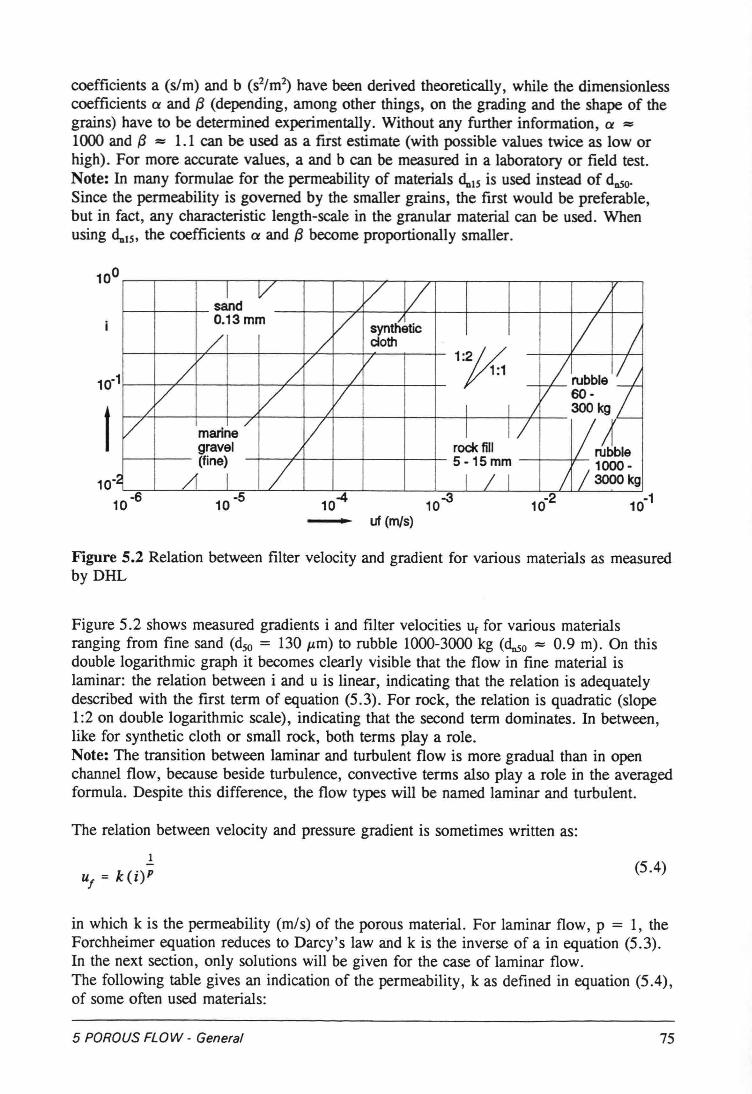
coefficients a (slm) and b (s2/m2) have been derived theoretically, while the dimensionlesscoefficients ex and {3 (depending, among other things, on the grading and the shape of thegrains) have to be determined experimentally. Without any further information, ex =1000 and {3 = 1.1 can he used as a first estimate (with possible values twice as low orhigh). For more accurate values, a and b can be measured in a laboratory or field test.Note: In many formulae for the permeability of materials <luIS is used instead of dnSo•

Since the permeability is govemed by the smaller grains, the first would be preferabie,but in fact, any characteristic length-scale in the granular material can be used. Whenusing <luIS, the coefficients ex and {3 become proportionally smaller.

I

~d V V 1/ L0.13 mm V synthetie V/ / cloth j_

v V V 1:;tG/ Nbbl. ,l_/ / _j_ 1:11

V V V V 60-/ I I I 300 kg

V . / V I 1/ I/J_mannegravel / rock till(fine) / 5 -15 mm 1000-

2 /f I 1 L J _L L 3000 kg

10-

10-3uf (mis)

Figure 5.2 Relation between filter velocity and gradient for various materials as measuredbyDHL

Figure 5.2 shows measured gradients i and filter veloeities u, for various materialsranging from fine sand (dso = 130 f'm) to rubble 1000-3000 kg (~o = 0.9 m). On thisdouble logarithmic graph it becomes clearly visible that the flow in fine material islaminar: the relation between i and u is linear, indicating that the relation is adequatelydescribed with the first term of equation (5.3). For rock, the relation is quadratic (slope1:2 on double logarithmic scale), indicating that the second term dominates. In between,like for synthetic cloth or small rock, both terms play a role.Note: The transition between laminar and turbulent flow is more gradual than in openchannel flow, because beside turbulence, convective terms also play a role in the averagedformula. Despite this difference, the flow types will be named laminar and turbulent.

The relation between velocity and pressure gradient is sometimes written as:

(5.4)

in which kis the permeability (mIs) of the porous material. For laminar flow, p = 1, theForchheimer equation reduces to Darcy's law and k is the inverse of a in equation (5.3).In the next section, only solutions will be given for the case of laminar flow.The following table gives an indication of the permeability, k as defined in equation (5.4),of some often used materials:

5 POROUSFLOW - General 75

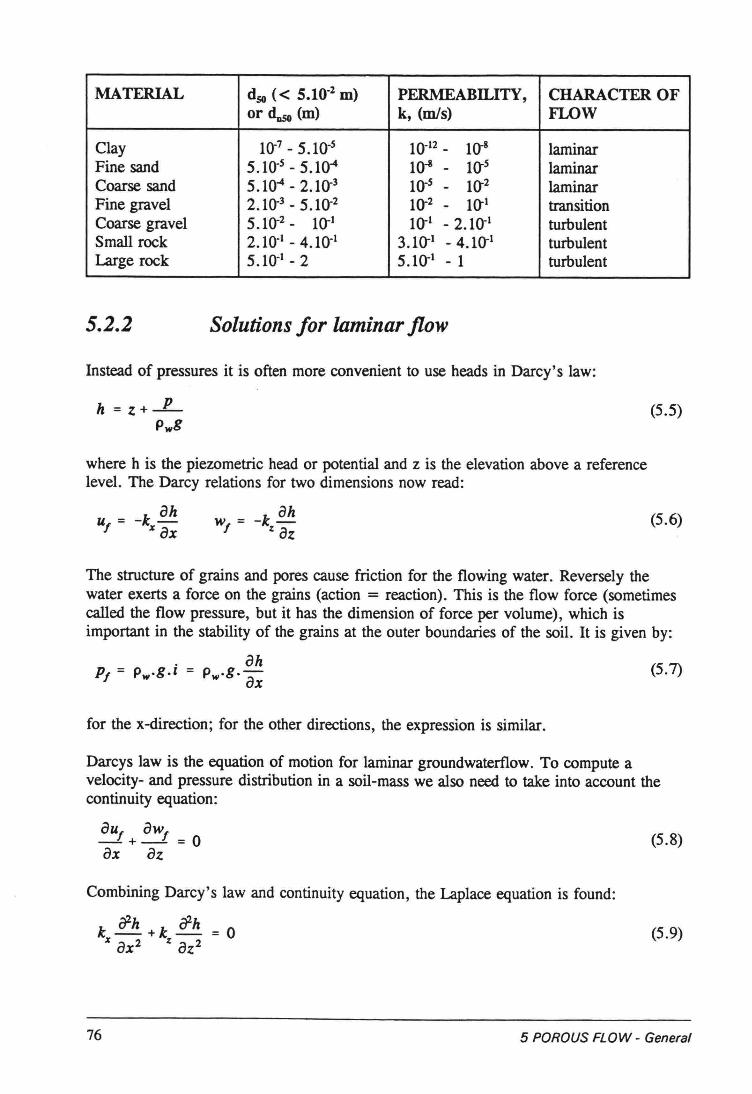
MATERIAL dso « 5.10-2 m) PERMEABILITY , CHARACTER OFor~ (m) k, (mis) FLOW

Clay 10-7 - 5.10-5 10-12- lO-S laminarFine sand 5.10-5 - 5.10-4 lO-S - 10"5 laminarCoarse sand 5.10-4 - 2.10"3 10-5 - 10"2 laminarFine gravel 2.10-3 - 5.10"2 10"2 - 10"1 transitionCoarse gravel 5.10"2 - 10"1 10"1 - 2.10"1 turbulentSmall rock 2.10-1 - 4.10-1 3.10-1 - 4.10-1 turbulentLarge rock 5.10-1 - 2 5.10-1 - 1 turbulent

5.2.2 Solutions for laminar flow

Instead of pressures it is often more convenient to use heads in Darcy's law:

(5.5)

where h is the piezometric head or potential and z is the elevation above a referencelevel. The Darcy relations for two dimensions now read:

w = -k oh, z êz (5.6)

The structure of grains and pores cause friction for the flowing water. Reversely thewater exerts a force on the grains (action = reaction). This is the flow force (sometimescalled the flow pressure, but it has the dimension of force per volume), which isimportant in the stability of the grains at the outer boundaries of the soil. It is given by:

(5.7)

for the x-direction; for the other directions, the expression is similar.

Darcys law is the equation of motion for laminar groundwaterflow. To compute avelocity- and pressure distribution in a soil-mass we also need to take into account thecontinuity equation:

ou, aWf-+- =0aX aZ

(5.8)

Combining Darcy's law and continuity equation, the Laplace equation is found:

k éPh + k éPh = 0Z ax2 z az2 (5.9)

76 5 POROUSFLOW - General

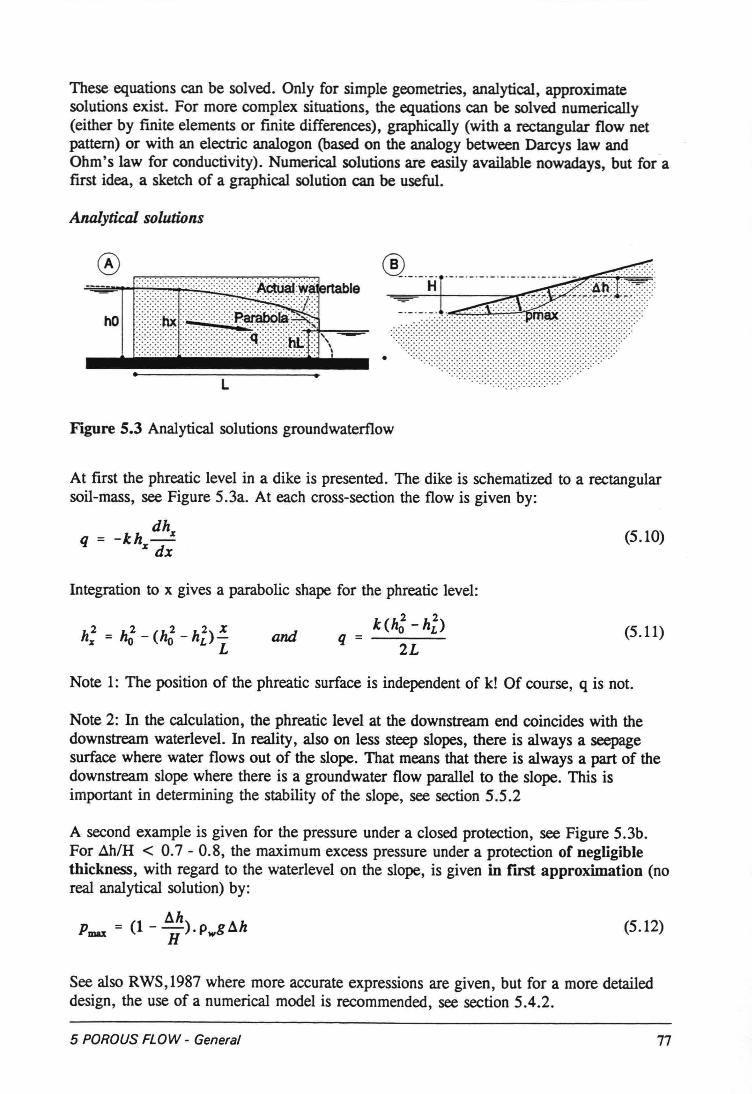
These equations can be solved. Only for simple geometries, analytica!, approximatesolutions exist. For more complex situations, the equations can be solved numerically(either by finite elements or finite differences), graphically (with a rectangular flow netpattern) or with an electric analogon (based on the analogy between Darcys lawandOhm's law for conductivity). Numerica! solutions are easily available nowadays, but for afust idea, a sketch of a graphica! solution can be useful.

Analytical solutions

® . . . . .~:::~:~:~:~:::::::::::::::::::~:~:::::::::::~::A~~~~a:~rtable..............~

hO ~m tt.~h-L

....................................... .....:.:-:-:.:.:-:.:-:-:.:.:.:.:-:.:.:-:.:.:-:-: .............................................

Figure 5.3 Analytica! solutions groundwaterflow

At first the phreatic level in a dike is presented. The dike is schematized to a rectangularsoil-mass, see Figure 5.3a. At each cross-section the flow is given by:

dh%q = -kh­

% dx(5.10)

Integration to x gives a parabolic shape for the phreatic level:

k(h; - hi)2L

and q = (5.11)

Notel: The position of the phreatic surface is independent of k! Of course, q is not.

Note 2: In the ca!culation, the phreatic level at the downstream end coincides with thedownstream waterlevel. In reality, also on less steep slopes, there is always a seepagesurface where water flows out of the slope. That means that there is always a part of thedownstream slope where there is a groundwater flow parallel to the slope. This isimportant in determining the stability of the slope, see section 5.5.2

A second example is given for the pressure under a closed protection, see Figure 5.3b.For .t:ih/H < 0.7 - 0.8, the maximum excess pressure under a proteetion of negligiblethickness, with regard to the waterlevel on the slope, is given in first approximation (noreal analytica! solution) by:

AhPmax = (1 - -)·PwgAhH

(5.12)

See also RWS,1987 where more accurate expressions are given, but for a more detaileddesign, the use of a numerical model is recommended, see section 5.4.2.

5 POROUSFLOW - General 77

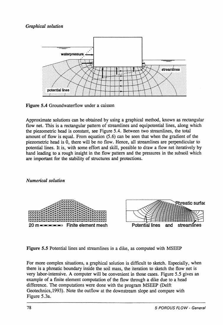
Graphical solution

Figure S.4 Groundwaterflow under a caisson

Approximate solutions can be obtained by using a graphical method, known as rectangularflow net. This is a rectangular pattem of streamlines and equipotential lines, along whichthe piezometric head is constant, see Figure 5.4. Between two streamlines, the totalamount of flow is equal. From equation (5.6) can be seen that when the gradient of thepiezometric head is 0, there will be no flow. Hence, all streamlines are perpendicular topotentiallines. It is, with some effort and skill, possible to draw a flow net iteratively byhand leading to a rough insight in the flow pattem and the pressures in the subsoil whichare important for the stability of structures and protections.

Numerical solution

Figure S.S Potentiallines and streamlines in a dike, as computed with MSEEP

For more complex situations, a graphical solution is difficult to sketch. Especially, whenthere is a phreatic boundary inside the soil mass, the iteration to sketch the flow net isvery labor-intensive. A computer will be convenient in those cases. Figure 5.5 gives anexample of a finite element computation of the flow through a dike due to a headdifference. The computations were done with the program MSEEP (DelftGeotechnics,1993). Note the outflow at the downstream slope and compare withFigure 5.3a.

78 5 POROUSFLOW - General

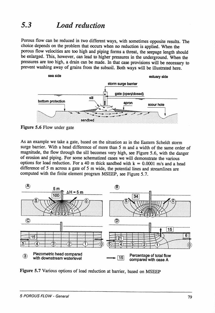
5.3 Load reduction

Porous flow can be reduced in two different ways, with sometimes opposite results. Thechoice depends on the problem that occurs when no reduction is applied. When theporous flow veloeities are too high and piping forms a threat, the seepage length shouldhe enlarged. This, however, can lead to higher pressures in the underground. When thepressures are too high, a drain can he made. In that case provisions will he necessary toprevent washing away of grains from the subsoil. Both ways will be illustrated here.

seaside estuary side

storm surge barrler

...............................................................................................

Figure 5.6 Flow under gate

As an example we take a gate, based on the situation as in the Eastem Scheldt stormsurge barrier. With a head difference of more than 5 m and a width of the same order ofmagnitude, the flow through the sill becomes very high, see Figure 5.6, with the dangerof erosion and piping. For some schematized cases we will demonstrate the variousoptions for load reduction. For a 40 m thick sandbed with k = 0.0001 mis and a headdifference of 5 m across a gate of 5 m wide, the potentiallines and streamlines arecomputed with the finite element program MSEEP, see Figure 5.7.

® Piezometric head comparedwith downstream waterlevel -[}§] Percentage of total flow

compared with case A

Figure 5.7 Various options of load reduction at barrier, based on MSEEP

5 POROUSFLOW - General 79

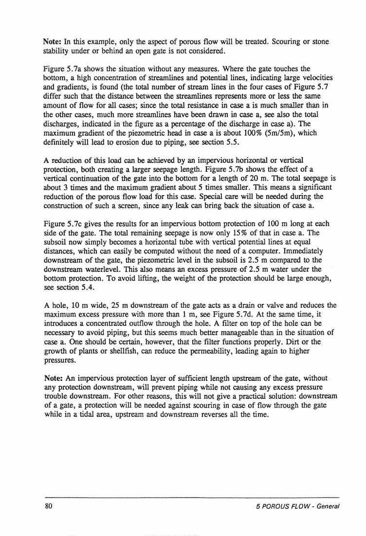
Note: In this example, only the aspect of porous flow will be treated. Scouring or stonestability under or behind an open gate is not considered.

Figure 5.7a shows the situation without any measures. Where the gate touches thebottom, a high concentration of streamlines and potentiallines, indicating large veloeitiesand gradients, is found (the total number of stream lines in the four cases of Figure 5.7differ such that the distance between the streamlines represents more or less the sameamount of flow for all cases; since the total resistance in case a is much smaller than inthe other cases, much more streamlines have been drawn in case a, see also the totaldischarges, indicated in the figure as a percentage of the discharge in case a). Themaximum gradient of the piezometric head in case a is about 100% (5m/5m), whichdefinitely will lead to erosion due to piping, see section 5.5.

A reduction of this load can be achieved by an impervious horizontal or verticalprotection, both creating a larger seepage length. Figure 5.7b shows the effect of avertical continuation of the gate into the bottom for a length of 20 m. The total seepage isabout 3 times and the maximum gradient about 5 times smaller. This means a significantreduction of the porous flow load for this case. Special care will be needed during theconstruction of such a screen, since any leak can bring back the situation of case a.

Figure 5.7c gives the results for an impervious bottom proteetion of 100 m long at eachside of the gate. The total remaining seepage is now only 15% of that in case a. Thesubsoil now simply becomes a horizontal tube with vertical potentiallines at equaldistances, which can easily be computed without the need of a computer. Immediatelydownstream of the gate, the piezometric level in the subsoil is 2.5 m compared to thedownstream waterlevel. This also means an excess pressure of 2.5 m water under thebottom protection. To avoid lifting, the weight of the proteetion should be large enough,see section 5.4.

A hole, 10 m wide, 25 m downstream of the gate acts as a drain or valve and reduces themaximum excess pressure with more than 1 m, see Figure 5.7d. At the same time, itintroduces a concentrated outflow through the hole. A filter on top of the hole can benecessary to avoid piping, but this seems much better manageable than in the situation ofcase a. One should be certain, however, that the filter functions properly. Dirt or thegrowth of plants or shellfish, can reduce the permeability, leading again to higherpressures.

Note: An impervious proteetion layer of sufficient length upstream of the gate, withoutany proteetion downstream, will prevent piping while not causing any excess pressuretrouble downstream. For other reasons, this will not give a practical solution: downstreamof a gate, a proteetion will be needed against scouring in case of flow through the gatewhile in a tidal area, upstream and downstream reverses all the time.

80 5 POROUSFLOW - General

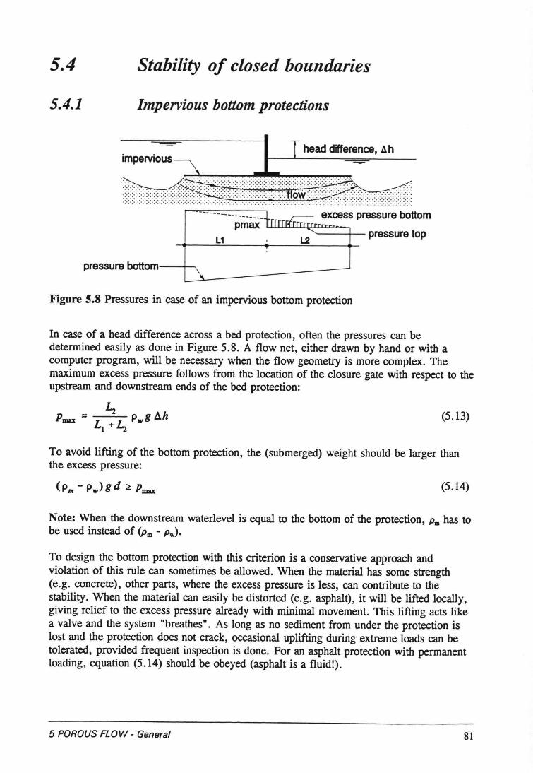
5.4 Stability of closed boundaries

5.4.1 Impervious bottom protections

imperviousheaddifference,.l1h

------------------.1 excesspressurebottompmax1IlDIIrnI,Lm:~~~~~

L1 L2 pressuretop

pressurebottoml---+L=\~-----------

Figure 5.8 Pressures in case of an impervious bottom proteetion

In case of a head difference across a bed protection, often the pressures cao bedetermined easily as done in Figure 5.8. A flow net, either drawn by hand or with acomputer program, will be necessary when the flow geometry is more complex. Themaximum excess pressure follows from the location of the closure gate with respect to theupstream and downstream ends of the bed protection:

(5.13)

To avoid lifting of the bottom protection, the (submerged) weight should be larger thanthe excess pressure:

(5.14)

Note: When the downstream waterlevel is equal to the bottom of the protection, Pm has tobe used instead of (Pm - Pw).

To design the bottom proteetion with this criterion is a conservative approach andviolation of this rule cao sometimes be allowed. When the material has some strength(e.g. concrete), other parts, where the excess pressure is less, cao contribute to thestability. When the material cao easily be distorted (e.g. asphalt), it will be lifted locally,giving relief to the excess pressure already with minimal movement. This lifting acts likea valve and the system "breathes". As long as no sediment from under the proteetion islost and the proteetion does not crack, occasional uplifting during extreme loads cao betolerated, provided frequent inspeetion is done. For an asphalt proteetion with permanentloading, equation (5.14) should be obeyed (asphalt is a fluid!).

5 POROUSFLOW - General 81

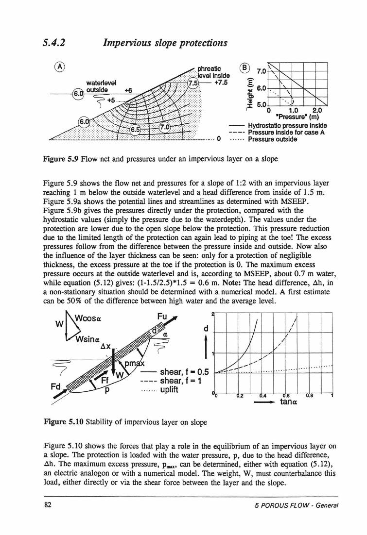
5.4.2 Impervious slope protections

® ® 7.0 ~'\.~

-\. r-,\. r-,' ..~ <,

î1: 6.0Q~J: 5.0I 0 1.0 2.0

·Pressure· (m)-- Hydrostatic pressure inside---- Pressure inside for case A.. . . .. Pressure outslde

Figure 5.9 Flow net and pressures under an impervious layer on a slope

Figure 5.9 shows the flow net and pressures for a slope of 1:2 with an impervious layerreaching 1 m below the outside waterlevel and a head difference from inside of 1.5 m.Figure 5.9a shows the potential lines and streamlines as determined with MSEEP.Figure 5.9b gives the pressures directly under the protection, compared with thehydrostatic values (simply the pressure due 10 the waterdepth). The values under theproteetion are lower due to the open slope below the protection. This pressure reductiondue to the limited length of the proteetion can again lead to piping at the toe! The excesspressures follow from the difference between the pressure inside and outside. Now alsothe influence of the layer thickness can be seen: only for a proteetion of negligiblethickness, the excess pressure at the toe if the proteetion is O. The maximum excesspressure occurs at the outside waterlevel and is, according to MSEEP, about 0.7 m water,while equation (5.12) gives: (1-1.5/2.5)*1.5 = 0.6 m. Note: The head difference, ~h, ina non-stationary situation should be determined with a numerical model. A first estimatecan be 50% of the difference between high water and the average level.

Wt\wcosa. d

t/wSin« tAx

Ir:

/ ///

/ v,/

I v/ ",--: ,'"........ .... .....

...:::-:. .... .... ...... , ....

0 .2 1.4 (.6 0.8

- shear, f - 0.5---- shear, f = 1....... uplift

tan«

Figure 5.10 Stability of impervious layer on slope

Figure 5.10 shows the forces that play a role in the equilibrium of an impervious layer ona slope. The proteetion is loaded with the water pressure, p, due to the head difference,~h. The maximum excess pressure, Pmax, can be determined, either with equation (5.12),an electric analogon or with a numerical model. The weight, W, must counterbalance thisload, either directly or via the shear force between the layer and the slope.

82 5 POROUSFLOW - General

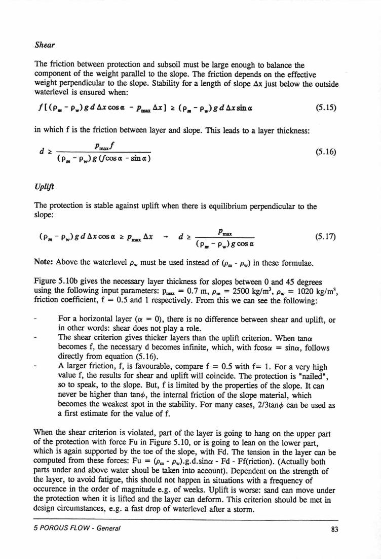
Shear

The friction between proteetion and subsoil must be large enough to balance thecomponent of the weight parallel to the slope. The friction depends on the effectiveweight perpendicular to the slope. Stability for a length of slope Ax just below the outsidewaterlevel is ensured when:

(5.15)

in which f is the friction between layer and slope. This leads to a layer thickness:

d pmaxl~ --------~~-------

( P", - pw) g (Jcos a. - sin a. )(5.16)

Uplift

The proteetion is stabie against uplift when there is equilibrium perpendicular to theslope:

(5.17)

Note: Above the waterlevel Pwmust be used instead of (Pm- Pw)in these formulae.

Figure 5. !Ob gives the necessary layer thickness for slopes between 0 and 45 degreesusing the following input parameters: Pmax = 0.7 m, Pm= 2500 kg/m", Pw= 1020 kg/rrr',friction coefficient, f = 0.5 and 1 respectively. From this we can see the following:

For a horizontallayer (a = 0), there is no difference between shear and uplift, orin other words: shear does not play a role.The shear criterion gives thicker layers than the uplift criterion. When tanobecomes f, the necessary d becomes infinite, which, with fcoso = sino, followsdirectly from equation (5.16).A larger friction, f, is favourable, compare f = 0.5 with f= 1. For a very highvalue f, the results for shear and uplift will coincide. The proteetion is "nailed" ,so to speak, to the slope. But, f is limited by the properties of the slope. It cannever be higher than tané, the internal friction of the slope material, whichbecomes the weakest spot in the stability. For many cases, 2/3tancj>can be used asa fust estimate for the value of f.

When the shear criterion is violated, part of the layer is going to hang on the upper partof the proteetion with force Fu in Figure 5.10, or is going to lean on the lower part,which is again supported by the toe of the slope, with Fd. The tension in the layer can becomputed from these forces: Fu = (Pm- pw).g.d.sina - Fd - Ff(riction). (Actually bothparts under and above water shoul be taken into account). Dependent on the strength ofthe layer, to avoid fatigue, this should not happen in situations with a frequency ofoccurence in the order of magnitude e.g. of weeks. Uplift is worse: sand can move underthe proteetion when it is lifted and the layer can deform. This criterion should be met indesign circumstances, e.g. a fast drop of waterlevel after a storm.

5 POROUSFLOW - General 83

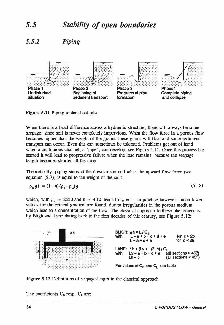
5.5 Stability of open boundaries

5.5.1 Piping

. , ..... . .... .... . ...................................................... . . . . .. . . . . . . . . . . . . . . . . . . . . .. . . . . . . . . . . . . . . . . . . . . . . . . ."Phasè" 1""""""""""""""""" "piiasè" 2 """""""""""""""" "phäSe" 3 """""""""""""""" PhäSë4" """""""""""""""""Undisturbed Beginningof Progressof pipe Complete pipingsituation sedimenttransport formation and collapse

Figure 5.11 Piping under sheet pile

When there is a head difference across a hydraulic structure, there will always be someseepage, since soil is never completely impervious. When the flow force in a porous flowbecomes higher than the weight of the grains, these grains will float and some sedimenttransport can occur. Even this can sometimes be tolerated. Problems get out of handwhen a continuous channel, a "pipe", can develop, see Figure 5.11. Once this process hasstarted it will lead to progressive failure when the load remains, because the seepagelength becomes shorter all the time.

Theoretically, piping starts at the downstream end when the upward flow force (seeequation (5.7») is equal to the weight of the soil:

(5.18)

which, with Ps = 2650 and n = 40% leads to ie == 1. In practice however, much lowervalues for the critical gradient are found, due to irregularities in the porous mediumwhich lead to a concentration of the flow. The classical approach to these phenomena isby Bligh and Lane dating back to the first decades of this century, see Figure 5.12:

BUGH: .ó.h< L/ CBwith: L-a+b+c+d+e

L-a+c+efor c> 2bfor c < 2b

LANE: .ó.h< (Lv + 1/3lh) / CLwith: Lv - a + b + d + e (all sactions > ~,..g)

Lh - c (all sections < 40-)

Forvaluas of CB and CL see tabla

Figure 5.12 Definitions of seepage-length in the classical approach

The coefficients CB resp. CL are:

84 5 POROUSFLOW - General

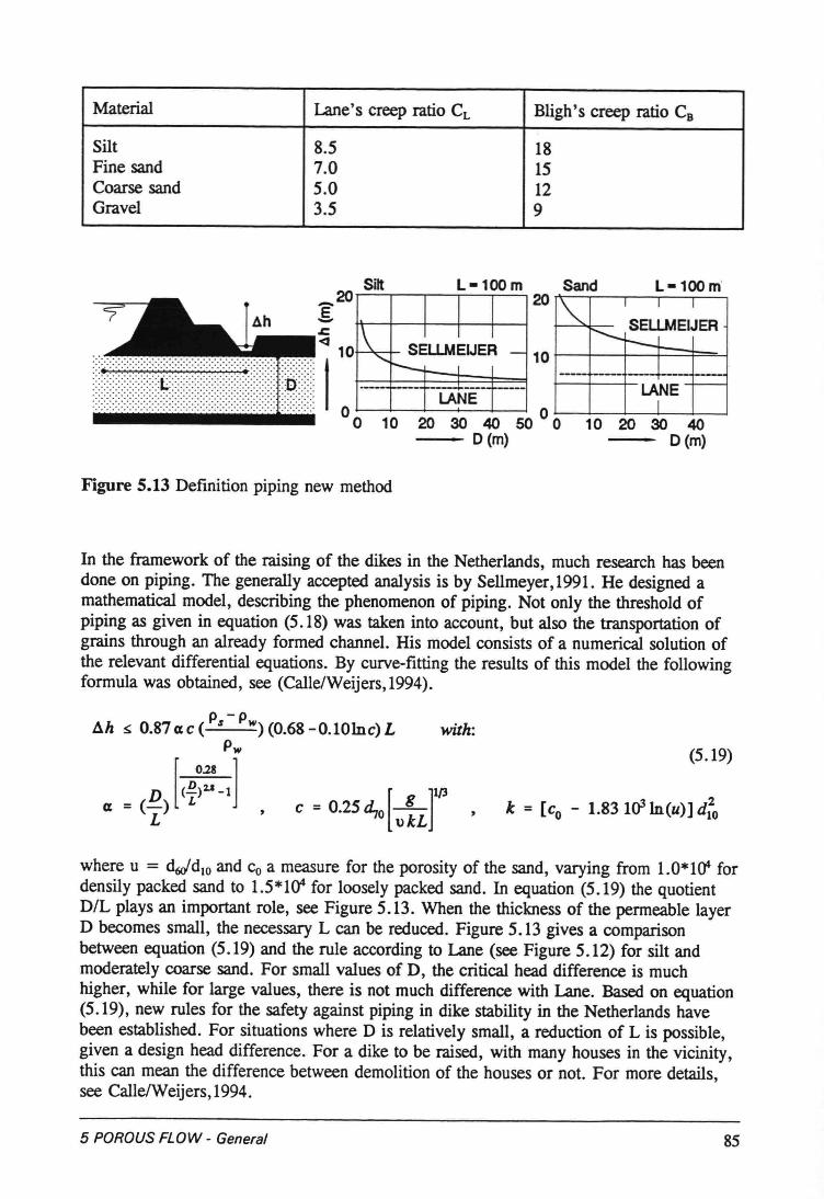
Material Lane' screep ratio CL Bligh' s creep ratio CB

Silt 8.5 18Fine sand 7.0 15Coarse sand 5.0 12Gravel 3.5 9

L-100 m Sand L-100m'

11\ I

SELLMEIJER -<,t-- _I

---- -- --:.~:---- ----LANE10 20 30 40 50 00

-- D(m)10 20 30 40

D(m)

Figure 5.13 Definition piping new method

In the framework of the raising of the dikes in the Netherlands, much research has beendone on piping. The generally accepted analysis is by Sellmeyer, 1991. He designed amathematical model, describing the phenomenon of piping. Not only the threshold ofpiping as given in equation (5.18)was taken into account, but also the transportation ofgrains through an already formed channel. Ris model consists of a numerical solution ofthe relevant differential equations. By curve-fitting the results of this model the followingformula was obtained, see (Calle/Weijers, 1994).

p -p~h ~ 0.87 ec (s w)(O.68-O.lOlne) L

Pw

D [(~:::-llex = (_) LL

with:(5.19)

e = 0.25 ti., [-L]113o 'UkL

where u = dtJdlO and Co a measure for the porosity of the sand, varying from 1.0*10' fordensily packed sand to 1.5*1Q4for loosely packed sand. In equation (5.19) the quotientDIL plays an important role, see Figure 5.13. When the thickness of the permeable layerD becomes small, the necessary L can be reduced. Figure 5.13 gives a comparisonbetween equation (5.19) and the rule according to Lane (see Figure 5.12) for silt andmoderately coarse sand. For small values of D, the critical head difference is muchhigher, while for large values, there is not much difference with Lane. Based on equation(5.19),new rules for the safety against piping in dike stability in the Netherlands havebeen established. For situations where D is relatively small, a reduction of Lis possible,given a design head difference. For a dike to be raised, with many houses in the vicinity,this can mean the difference between demolition of the houses or not. For more details,see Calle/Weijers, 1994.

5 POROUSFLOW - General 85

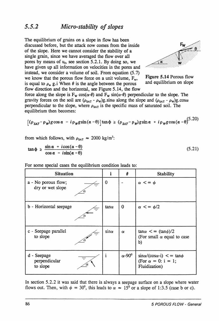
5.5.2 Micro-stability of slopes

The equilibrium of grains on a slope in flow has beendiscussed before, but the attack now comes from the insideof the slope. Here we cannot consider the stability of asingle grain, since we have averaged the flow over allpores by means of Uf, see section 5.2.1. By doing so, wehave given up all information on veloeities in the pores andinstead, we consider a volume of soil. From equation (5.7)we know that the porous flow force on a unit volume, Fw, Figure 5.14 Porous flowis equal to Pwg.i When 8 is the angle between the porous and equilibrium on slopeflow direction and the horizontal, see Figure 5.14, the flowforce along the slope is Fw cos(a-8) and Fw sin(a-8) perpendicular to the slope. Thegravity forces on the soil are (pSAT - pw)g.sina along the slope and (pSAT - pw)g.cosaperpendicular to the slope, where PSAT is the specitic mass of saturated soil. Theequilibrium then becomes:

from which follows, with PSAT = 2000 kg/m':

tan4> ~ sincx + icos(cx -6)coscx - isin(cx -6)

(5.21)

For some special cases the equilibrium condition leads to:

Situation i (J Stability

a - No porous flow; / 0 - a < = <I>dry or wet slope

b - Horizontal seepage/ tana 0 a < = <1>/2

c - Seepage parallel / sin« a tano <= (tané )/2to slope (For small a equal to case

b)

d - Seepage /;?\/ i a-900 sino/tcose-i) <= tanéperpendicular (For a = 0: i = 1;to slope Fluidization)

In section 5.2.2 it was said that there is always a seepage surface on a slope where waterflows out. Then, with <I> = 30°, this leads to a = 15° or a slope of 1:3.5 (case b or cl.

86 5 POROUSFLOW - General

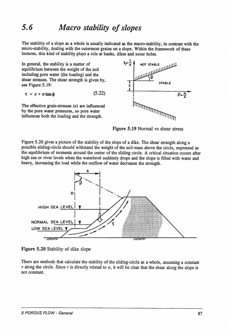
5.6 Macro stability of slopes

The stability of a slope as a whole is usually indicated as the macro-stability, in contrast with themicro-stability, dealing with the outermost grains on a slope. Within the framewerk of theselectures, this kind of stability plays a role at banks, dikes and scour holes.

In general, the stability is a matter ofequilibrium between the weight of the soilincluding pore water (the loading) and theshear stresses. The shear strength is given by,see Figure 5.19:

't == C + atan~ (5.22)

The effective grain-stresses (a) are influencedby the pore water pressures, so pore waterinfluences both the loading and the strength.

ç:-.!:!.A

Figure 5.19 Normal vs shea.r stress

Figure 5.20 gives a picture of the stability of the slope of a dike. The shear strength along apossible sliding-eirele should withstand the weight of the soil-mass above the circle, expressed asthe equilibrium of moments around the center of the sliding circle. A critical situation occurs afterhigh sea or river levels when the waterlevel suddenly drops and the slope is filled with water andheavy, increasing the load while the outflow of water decreases the strength.

~RI ,-,-I

HIGH SEA ..::L:E..:..V=E.::.L.;..I--L. +--/

Figure S.20 Stability of dike slope

There are methods that calculate the stability of the sliding-eirele as a whoie, assuming a constantT along the circle. Since T is directly related to a, it will be clear that the shear along the slope isnot constant.

5 POROUSFLOW - General 87

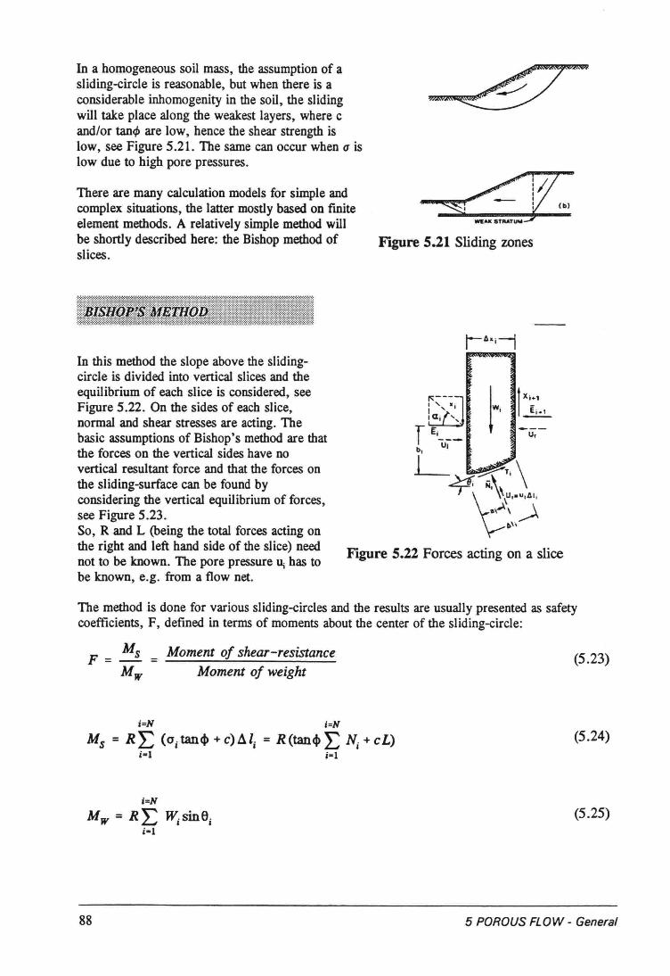
In a homogeneous soil mass, the assumption of asliding-eirele is reasonable, but when there is aconsiderabie inhomogenity in the soil, the slidingwill take place along the weak:estlayers, where cand/or tanë are low, hence the shear strength islow, see Figure 5.21. The same can occur when a islow due to high pore pressures.

There are many calculation models for simple andcomplex situations, the latter mostly based on finiteelement methods. A relatively simple method willbe shortly described here: the Bishop method ofslices.

-~"WE" STRATUW

Figure 5.21 Sliding zones

In this method the slope above the sliding­circle is divided into vertical slices and theequilibrium of each slice is considered, seeFigure 5.22. On the sides of each slice,normal and shear stresses are acting. Thebasic assumptions of Bishop's method are thatthe forces on the vertical sides have novertical resultant force and that the forces onthe sliding-surface can be found byconsidering the vertical equilibrium of forces,see Figure 5.23.So, R and L (being the total forces acting onthe right and left hand side of the slice) neednot to be known. The pore pressure U; has tobe known, e.g. from a flow net.

Figure 5.22 Forces acting on a slice

The method is done for various sliding-circles and the results are usually presented as safetycoefficients, F, defined in terms of moments about the center of the sliding-circle:

Moment of shear-resistanceMoment of weight

(5.23)

i=N i=N

u, = RE (Ojtan<l>+c)äli = R(tan<l>E Nj+cL) (5.24)j=1

i=N

Mw = RE ~sineij-1

(5.25)

88 5 POROUSFLOW - General

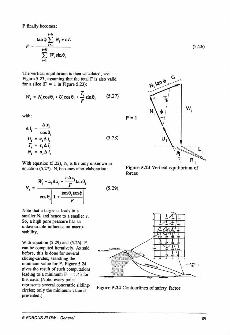
The vertical equilibrium is then calculated, seeFigure 5.23, assuming that the totaI F is also validfor a slice (F = 1 in Figure 5.23):

T,.~ = Nicos6i + Uicos6i + F sm6;

With equation (5.22), Ni is the only unknown inequation (5.27). Ni becomes after elaboration:

cSx.~ - uil\.Xi -Tt3nBi

00&6.[ 1 + tan6~tancf>1

F finally becomes:

i~N

tan4>L Ni + cLF i=1=------

i=N

L ~sinBii-I

with:

cosê,Ui = Uil\. li

Ti = 'ti l\. liNi = Gil\. li

Note that a larger Uileads to asmaller Ni and hence to a smaller T.So, a high pore pressure has anunfavourable influence on macro­stability.

With equation (5.29) and (5.26), Fcao be computed iteratively. As saidbefore, this is done for severalsliding-circles, searching theminimum value for F. Figure 5.24gives the result of such computationsleading to a minimum F = 1.43 forthis case. (Note: every pointrepresents several concentric sliding­circles; only the minimum value ispresented. )

(5.26)

(5.27)~

I

li!I

4>! Wj

III

F-1

(5.28)

RIFigure 5.23 Vertical equilibrium offorces

(5.29)

Figure 5.24 Contourlines of safety factor

5 POROUSFLOW - General 89

5.7 Summary

Porous flow, the flow through pores, follows the same laws as open channel flow, but canonly be described adequately, when averaged over many pores. The basic equation is the(extended) Forchheimer equation:

1 ~ . a~-- = , = au,+bu,lu,1+c­pg ax at

in which a laminar pan and a turbulent pan can be discemed, like in open channel flow.Theflow through fine material, like clay or sand, is laminar for which the Forchheimerrelation reduces to Datey's law, which can be solved together with the coniinuityequation, either graphical or numerical, inio potetuial lines and streamlines. With thisinfornuuion about loads (pressures and velocities), the stabiltry of various porous flowsituations can be judged. For turbulent porous flow, like in rock, often the knowledge isstill insufftcietu and empirical relastons have to be used in design computations.

Impervious protections have to withstand occurring pressures. Pressures can be computedby subtracting local haights from potetuials. Weight and friction are the parameters thatdetermine stability of protections without intemal strength. When weight and friction of aproteetion on a slope are insufficiem, tension forces in the proteetion will occur, forwhich the material has to be sufficienilly strong. The intemal strengtb of e.g. concreteslabs against pressures perpendicular to the slab, is outside the scope of these notes.

Open boundaries have to withstand the flow forces in the soil, for which the equilibrium isgiven by:

v.s! = (l-n)(p" -pJg

Piping is the phenomenon when this equilibrium is violared and there is an ongoingerosion downstream of a relaiively impervious structure. To avoid piping, the seepagelength has to be sufficienily long, in order to keep the gradients in the subsoil low. On aslope, seepage can cause micro-instability when the slope is too steep. To avoid this, theslope angle should be about half the value of the angle of repose of the slope material, q,.

Macro instability occurs when the sliding forces in a slope exceed the friction forces,determined by the soil propenies, like cohesion, c and angle of repose, q,. Highwaterpressures inside have an unfavourable influence on the stability. The same is true fora layer in the subsoil with low values of c and q,.

90 5 POROUSFLOW - General

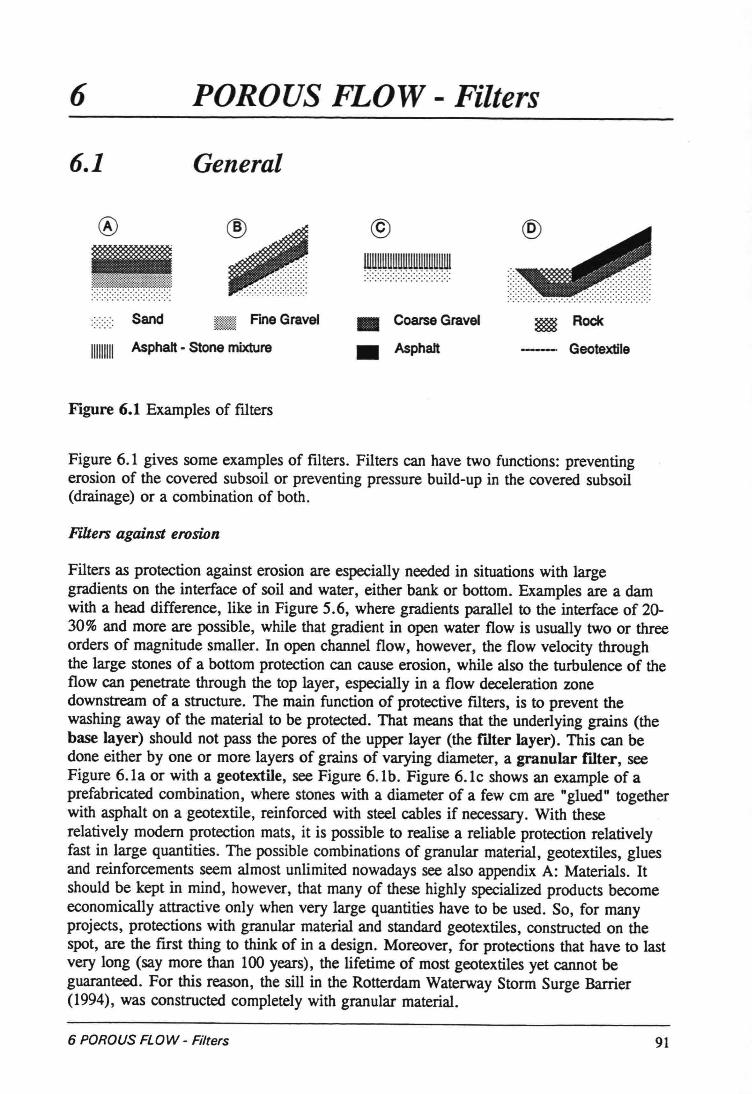
6 POROUS FLOW - Filters

6.1 General

® @

W~ij~~~~~~~~~................... ..................

Sand imme Fine Gravel

111111111 Asphalt - Stone mixture

• Coarse Gravel

• Asphalt

~ Rock

Geotextile

Figure 6.1 Examples of filters

Figure 6.1 gives some examples of filters. Filters can have two functions: preventingerosion of the covered subsoil or preventing pressure build-up in the covered subsoil(drainage) or a combination of both.

Filters against erosion

Filters as proteetion against erosion are especially needed in situations with largegradients on the interface of soil and water, either bank or bottom. Examples are a damwith a head difference, like in Figure 5.6, where gradients parallel to the interface of 20-30% and more are possible, while that gradient in open water flow is usually two or threeorders of magnitude smaller. In open channel flow, however, the flow velocity throughthe large stones of a bottom proteetion can cause erosion, while also the turbulence of theflow can penetrate through the top layer, especially in a flow deceleration zonedownstream of a structure. The main function of protective filters, is to prevent thewashing away of the material to be protected. That means that the underlying grains (thebase layer) should not pass the pores of the upper layer (the fiher layer). This can bedone either by one or more layers of grains of varying diameter, a granular filter; seeFigure 6.1a or with a geotextile, see Figure 6.1b. Figure 6.1c shows an example of aprefabricated combination, where stones with a diameter of a few cm are "glued" togetherwith asphalt on a geotextile, reinforeed with steel cables if necessary. With theserelatively modern proteetion mats, it is possible to realise a reliable proteetion relativelyfast in large quantities. The possible combinations of granular material, geotextiles, gluesand reinforcements seem almost unlimited nowadays see also appendix A: Materials. Itshould be kept in mind, however, that many of these highly specialized products becomeeconomically attractive only when very large quantities have to be used. So, for manyprojects, protections with granular material and standard geotextiles, constructed on thespot, are the fust thing to think of in a design. Moreover, for protections that have to lastvery long (say more than 100 years), the lifetime of most geotextiles yet cannot beguaranteed. For this reason, the sill in the Rotterdam Waterway Storm Surge Barrier(1994), was constructed completely with granular material.

6 POROUSFLOW - Filters 91

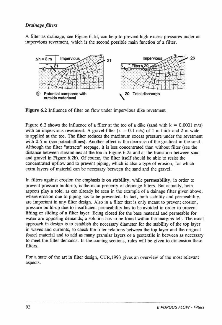
Drainage filters

A filter as drainage, see Figure 6.1d, can help to prevent high excess pressures under animpervious revetment, which is the second possible main function of a filter.

21 26

® Potential compared withoutside water1evel

Total discharge

Figure 6.2 Influence of filter on flow under impervious dike revetment

Figure 6.2 shows the influence of a filter at the toe of a dike (sand with k = 0.0001 mis)with an impervious revetment. A gravel-filter (k = 0.1 mis) of 1 m thick and 2 m wideis applied at the toe. The filter reduces the maximum excess pressure under the revetmentwith 0.5 m (see potentiallines). Another effect is the decrease of the gradient in the sand.Although the filter "attracts" seepage, it is less concentrated than without filter (see thedistance between streamlines at the toe in Figure 6.2a and at the transition between sandand gravel in Figure 6.2b). Of course, the filter itself should be able to resist theconcentrated upflow and to prevent piping, which is also a type of erosion, for whichextra layers of material can be necessary between the sand and the gravel.

In filters against erosion the emphasis is on stability, while penneability, in order toprevent pressure build-up, is the main property of drainage filters. But actually, bothaspects play a role, as can already be seen in the example of a dainage filter given above,where erosion due to piping has to be prevented. In fact, both stability and permeability,are important in any filter design. Also in a filter that is only meant to prevent erosion,pressure build-up due to insufficient permeability has to be avoided in order to preventlifting or sliding of a filter layer. Being closed for the base material and permeable forwater are opposing demands; a solution has to be found within the margins left. The usualapproach in design is to establish the necessary diameter for the stability of the top layerin waves and currents, to check the filter relations between the top layer and the original(base) material and to add as many granular layers or a geotextile in between as necessaryto meet the filter demands. In the coming sections, rules will be given to dimension thesefilters.

For a state of the art in filter design, CDR,1993 gives an overview of the most relevantaspects.

92 6 POROUSFLOW - Filters

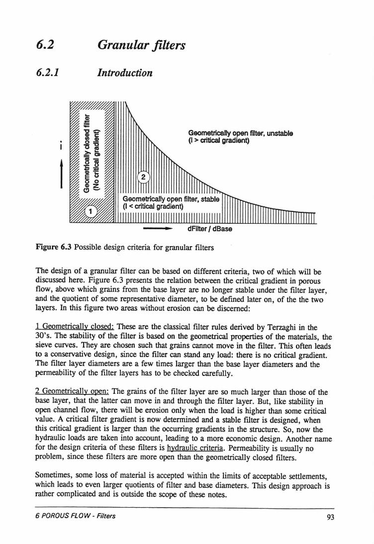
6.2 Granularfilters

6.2.1 Introduetion

t

GeometricaJly open filter, unstable(I > aiticaJ gradient)

dFllter I dBase

Figure 6.3 Possible design criteria for granular filters

The design of a granular filter can be based on different criteria, two of which will bediscussed here. Figure 6.3 presents the relation between the critica1 gradient in porousflow, above which grains from the base layer are no longer stabie under the filter layer,and the quotient of some representative diameter, to be defined later on, of the the twolayers. In this figure two areas without erosion can be discemed:

1 Geometrically closed: These are the classical filter rules derived by Terzaghi in the30's. The stability of the filter is based on the geometrica1 properties of the materials, thesieve curves. They are chosen such that grains cannot move in the filter. This often leadsto a conservative design, since the filter can stand any load: there is no critica1gradient.The filter layer diameters are a few times larger than the base layer diameters and thepermeability of the filter layers has to be checked carefully.

2 Geometrically open: The grains of the filter layer are so much larger than those of thebase layer, that the latter can move in and through the filter layer. But, like stability inopen channel flow, there will be erosion only when the load is higher than some critica1value. A critica1 filter gradient is now determined and a stabie filter is designed, whenthis critica1 gradient is larger than the occurring gradients in the structure. So, now thehydraulic loads are taken into account, leading to a more economie design. Another namefor the design criteria of these filters is hydraulic criteria. Permeability is usua11ynoproblem, since these filters are more open than the geometrically closed filters,

Sometimes, some loss of material is accepted within the limits of acceptable settlements,which leads to even larger quotients of filter and base diameters. This design approach israther complicated and is outside the scope of these notes.

6 POROUSFLOW - Filters 93

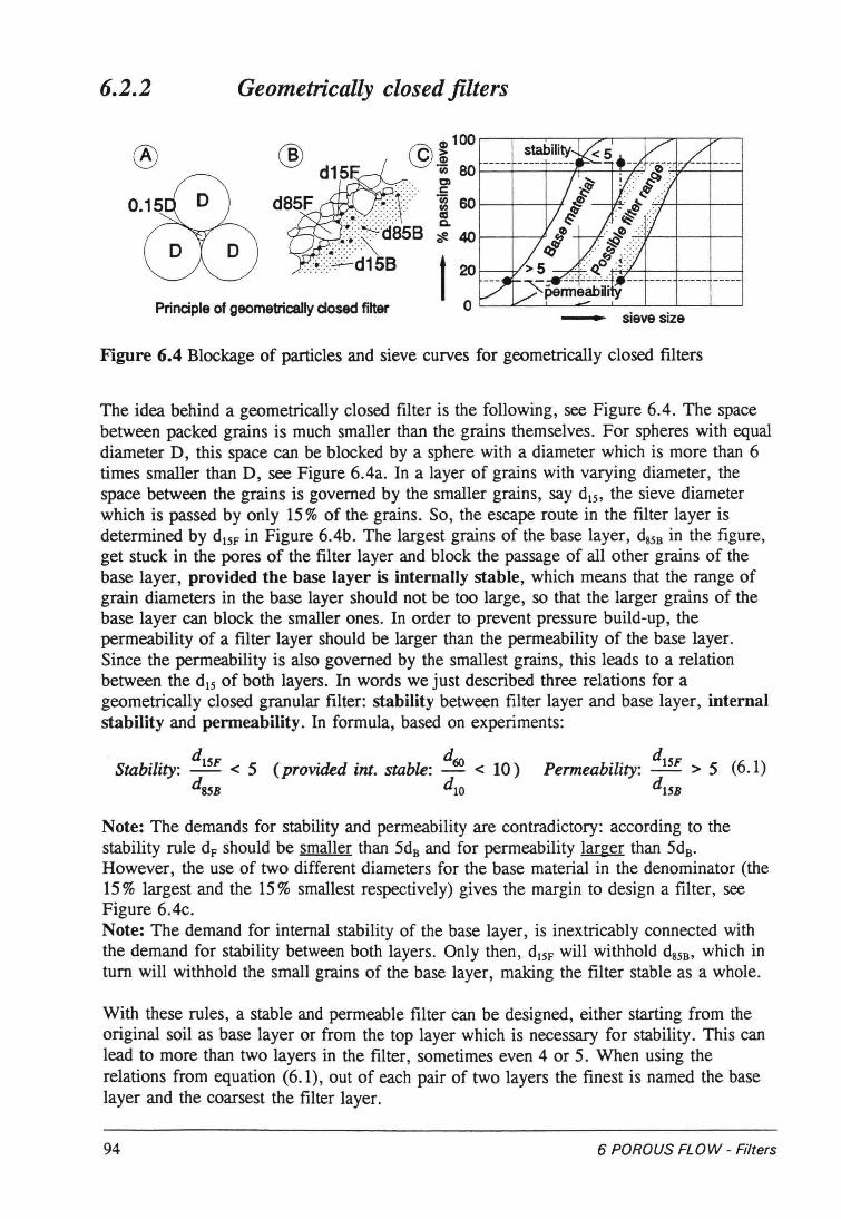
6.2.2 Geometrically closed filters

Principleof geometricallyclosed filter

®

- sievesize

Figure 6.4 Blockage of particles and sieve curves for geometrically closed filters

The idea behind a geometrically closed filter is the following, see Figure 6.4. The spacebetween packed grains is much smaller than the grains themselves. For spheres with equaldiameter D, this space can be blocked by a sphere with a diameter which is more than 6times smaller than D, see Figure 6.4a. In a layer of grains with varying diameter, thespace between the grains is govemed by the smaller grains, say d15, the sieve diameterwhich is passed by only 15% of the grains. So, the escape route in the filter layer isdetermined by dl5F in Figure 6.4b. The largest grains of the base layer, d85B in the figure,get stuck in the pores of the filter layer and block the passage of all other grains of thebase layer, provided the base layer is internally stabie, which means that the range ofgrain diameters in the base layer should not be too large, so that the larger grains of thebase layer can block the smaller ones. In order to prevent pressure build-up, thepermeability of a filter layer should be larger than the permeability of the base layer.Since the permeability is also governed by the smallest grains, this leads to a relationbetween the dl5 of both layers. In words we just described three relations for ageometrically closed granular filter: stability between filter layer and base layer, internalstability and penneability. In formula, based on experiments:

d dStability: lSF < 5 (provided int. stable: ~ < 10)

dSSB dlO

dPermeability: lSF > 5 (6.1)

d1SB

Note: The demands for stability and permeability are contradictory: according to thestability rule d, should be smaller than 5dB and for permeability larger than 5dB•

However, the use of two different diameters for the base material in the denominator (the15% largest and the 15% smallest respectively) gives the margin to design a filter, seeFigure 6.4c.Note: The demand for intemal stability of the base layer, is inextricably connected withthe demand for stability between both layers. Only then, dl5F will withhold d85B, which inturn will withhold the small grains of the base layer, making the filter stabIe as a whoIe.

With these rules, a stabIe and permeabIe filter can be designed, either starting from theoriginal soil as base layer or from the top layer which is necessary for stability. This canlead to more than two layers in the filter, sometimes even 4 or 5. When using therelations from equation (6.1), out of each pair of two layers the finest is named the baselayer and the coarsest the filter layer.

94 6 POROUSFLOW - Filters

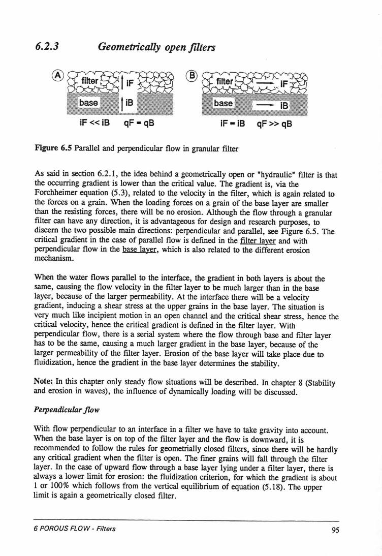
6.2.3 Geometrically open filters

®

iF« iB qF - qB iF - iB qF» qB

Figure 6.5 Parallel and perpendicular flow in granular filter

As said in section 6.2.1, the idea behind a geometrica1ly open or "hydraulic" filter is thatthe occurring gradient is lower than the critica1value. The gradient is, via theForchheimer equation (5.3), related to the velocity in the filter, which is again related tothe forces on a grain. When the loading forces on a grain of the base layer are smallerthan the resisting forces, there will be no erosion. Although the flow through a granularfilter can have any direction, it is advantageous for design and research purposes, todiscem the two possible main directions: perpendicular and parallel, see Figure 6.5. Thecritica1 gradient in the case of parallel flow is defined in the filter layer and withperpendicular flow in the base layer, which is also related to the different erosionmechanism.

When the water flows parallel to the interface, the gradient in both layers is about thesame, causing the flow velocity in the filter layer to be much larger than in the baselayer, because of the larger permeability. At the interface there will be a velocitygradient, inducing a shear stress at the upper grains in the base layer. The situation isvery much like incipient motion in an open channel and the critica1 shear stress, hence thecritica1 velocity, hence the critical gradient is defined in the filter layer. Withperpendicular flow, there is aserial system where the flow through base and filter layerhas to be the same, causing a much larger gradient in the base layer, because of thelarger permeability of the filter layer. Erosion of the base layer will take place due tofluidization, hence the gradient in the base layer determines the stability.

Note: In this chapter only steady flow situations will be described. In chapter 8 (Stabilityand erosion in waves), the influence of dynamically loading will be discussed.

Perpendicular flow

With flow perpendicular to an interface in a filter we have to take gravity into account.When the base layer is on top of the filter layer and the flow is downward, it isrecommended to follow the rules for geometrially closed filters, since there will be hardlyany critical gradient when the filter is open. The finer grains will fall through the filterlayer. In the case of upward flow through a base layer lying under a filter layer, there isalways a lower limit for erosion: the fluidization criterion, for which the gradient is about1 or 100% which follows from the vertical equilibrium of equation (5.18). The upperlimit is again a geometrically closed filter.

6 POROUSFLOW - Filters 95

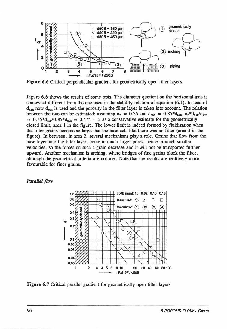
6o d50B -150 urn\l d50B - 220 jlmo d50B - 460 um

r:f\ geometricaJly\V closed

-Figure 6.6 Critical perpendicular gradient for geometrically open filter layers

Figure 6.6 shows the results of some tests. The diameter quotient on the horizontal axis issomewhat different from the one used in the stability relation of equation (6.1). Instead ofdSSBnow dSOBis used and the porosity in the filter layer is taken into account. The relationbetween the two can be estimated: assuming nF :::= 0.35 and dSOB=:: 0.85*dsSB'nF*d1Sp/dsoB=:: 0.35*d15F/0.85*ds5B:::= 0.4*5 = 2 as a conservative estimate for the geometricallyclosed limit, area 1 in the figure. The lower limit is indeed formed by fluidization whenthe filter grains become so large that the base acts like there was no filter (area 3 in thefigure). In between, in area 2, several mechanisms play a role. Grains that flow from thebase layer into the filter layer, come in much larger pores, hence in much smallervelocities, so the forces on such a grain decrease and it will not be transported furtherupward. Another mechanism is arching, where bridges of fine grains block the filter,although the geometrical criteria are not met. Note that the results are realtively morefavourable for finer grains.

Parallel flow

I

1.0 w/////.....::; ( dSOB(nvn):15 0.82 0.15 0.130... '//////h Measul'8d: <) L':I 0 00.6 v/u///./- r-.

~ .~.'l- "-'J I\. Calculated: CD

-=0.4 f...I01l .:c. \.0.3 i \ \ ~~,,~~ !J0.2 "I:a; -, J~~

E~

IL':I~~2

Ct

0.1 'l, h A..'l/h

0.08 <,'//////h -, ~

0.06 Wh0"h "' '\.~ <,W~ -, ) IY"' <,

0.04 ~ I\. '\. !J. c"" r-,

nn'.l~ -, -, c ~2 3 4 5 6 8 10 20 30 40 60 80 100

nF.d15F I dSOB

Figure 6.7 Critical parallel gradient for geometrically open filter layers

96 6 POROUSFLOW ..Filters

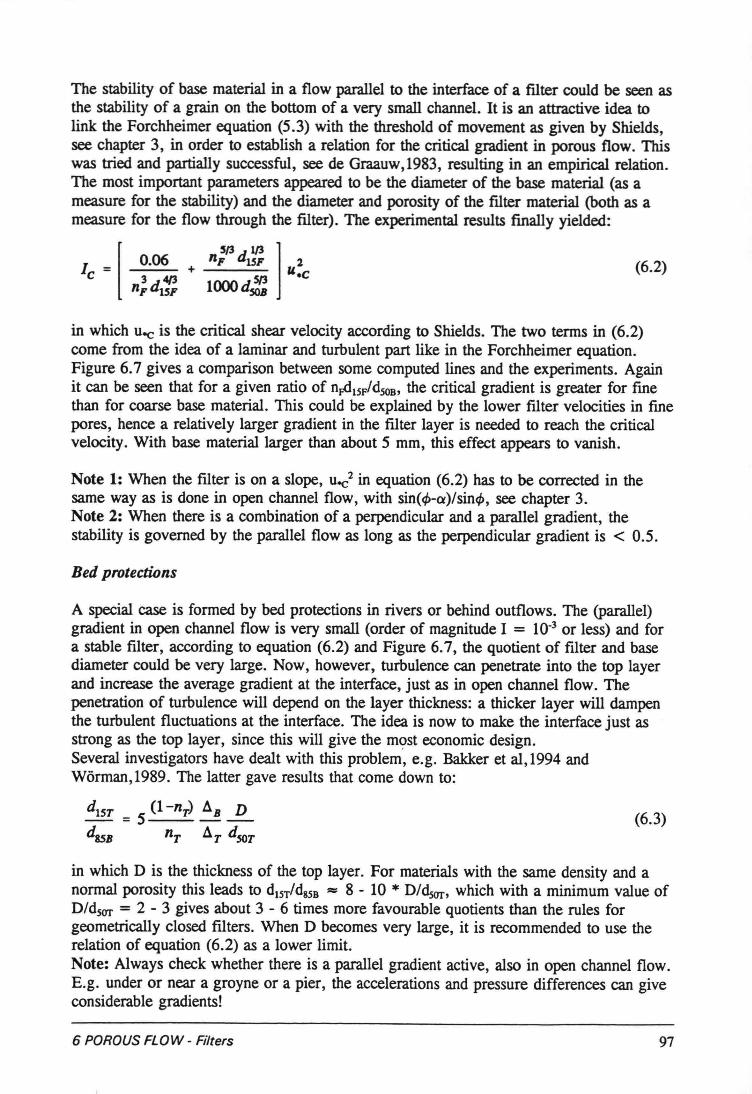
The stability of base material in a flow parallel to the interface of a filter could be seen asthe stability of a grain on the bottom of a very small channel. It is an attractive idea tolink the Forchheimer equation (5.3) with the threshold of movement as given by Shields,see chapter 3, in order to establish a relation for the critical gradient in porous flow. Thiswas tried and partially successful, see de Graauw,1983, resulting in an empirical relation.The most important parameters appeared to be the diameter of the base material (as ameasure for the stability) and the diameter and porosity of the filter material (both as ameasure for the flow through the filter). The experimental results finally yielded:

[5/3 1/3]0.06 nF dlSF 2Ic = + U.c

3 4f3 S{3nF dlSF 1000dSOB

(6.2)

in which U-cis the critical shear velocity according to Shields. The two terms in (6.2)come from the idea of a laminar and turbulent part like in the Forchheimer equation.Figure 6.7 gives a comparison between some computed lines and the experiments. Againit can be seen that for a given ratio of n~lSF/dsOB, the critical gradient is greater for finethan for coarse base material. This could be explained by the lower filter veloeities in finepores, hence a relatively larger gradient in the filter layer is needed to reach the criticalvelocity. With base materiallarger than about 5 mm, this effect appears to vanish.

Notel: When the filter is on a slope, u-c2 in equation (6.2) has to be corrected in thesame wayas is done in open channel flow, with sin(</>-a)/sin</>, see chapter 3.Note 2: When there is a combination of a perpendicular and a parallel gradient, thestability is governed by the parallel flow as long as the perpendicular gradient is < 0.5.

Bed protections

A special case is formed by bed protections in rivers or behind outflows. The (parallel)gradient in open channel flow is very small (order of magnitude I = 10-3or less) and fora stabIe filter, according to equation (6.2) and Figure 6.7, the quotient of filter and basediameter could be very large. Now, however, turbulence can penetrate into the top layerand increase the average gradient at the interface, just as in open channel flow. Thepenetration of turbulence will depend on the layer thickness: a thicker layer will dampenthe turbulent fluctuations at the interface. The idea is now to make the interface just asstrong as the top layer, since this will give the most economie design.Several investigators have dealt with this problem, e.g. Bakker et al,1994 andWörman,1989. The latter gave results that come down to:

d1ST (l-nT) IlB D- =s ---dSSB nT IlT dSOT

(6.3)

in which D is the thickness of the top layer. For materials with the same density and anormal porosity this leads to dlST/dsSB = 8 - 10 * D/dsar, which with a minimum value ofD/dsOT = 2 - 3 gives about 3 - 6 times more favourable quotients than the rules forgeometrically closed filters. When D becomes very large, it is recommended to use therelation of equation (6.2) as a lower limit.Note: Always check whether there is a parallel gradient active, also in open channel flow.E.g. under or near a groyne or a pier, the accelerations and pressure differences can giveconsiderabIe gradients!

6 POROUSFLOW - Filters 97

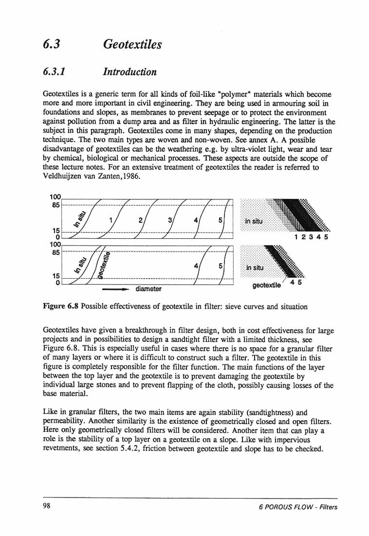
6.3 Geotextiles

6.3.1 Introduetion

Geotextiles is a generic term for all kinds of foil-like "polymer" materials which becomemore and more important in civil engineering. They are being used in armouring soil infoundations and slopes, as membranes to prevent seepage or to proteet the environmentagainst pollution from a dump area and as filter in hydraulic engineering. The latter is thesubject in this paragraph. Geotextiles come in many shapes, depending on the productiontechnique. The two main types are woven and non-woven. See annex A. A possibledisadvantage of geotextiles can be the weathering e.g. by ultra-violet light, wear and tearby chemical, biologica! or meehanica! processes. These aspects are outside the scope ofthese leeture notes. For an extensive treatment of geotextiles the reader is referred toVeldhuijzen van Zanten,1986.

1 234 5

diameter

.........~:-:-:-:-:-:':-:':':',:;:;:;:::;:;:;:;:;::::.\1:.:-:.:-:.:.:.:.:-:.:.:.:.,.,•.•......................•. 'Il

(:@Mi())>~................................? .geotextile 4 5

Figure 6.8 Possible effectiveness of geotextile in filter: sieve curves and situation

Geotextiles have given a breakthrough in filter design, both in cost effeetiveness for largeprojects and in possibilities to design a sandtight filter with a limited thickness, seeFigure 6.8. This is especially useful in cases where there is no space for a granular filterof many layers or where it is difficult to construct such a filter. The geotextile in thisfigure is completely responsible for the filter function. The main functions of the layerbetween the top layer and the geotextile is to prevent damaging the geotextile byindividuallarge stones and to prevent flapping of the cloth, possibly causing losses of thebase material.

Like in granular filters, the two main items are again stability (sandtightness) andpermeability. Another similarity is the existence of geometrica!ly closed and open filters.Here only geometrica!ly closed filters will be considered. Another item that can play arole is the stability of a top layer on a geotextile on a slope. Like with imperviousrevetments, see section 5.4.2, friction between geotextile and slope has to be cheeked.

98 6 POROUSFLOW - Filters

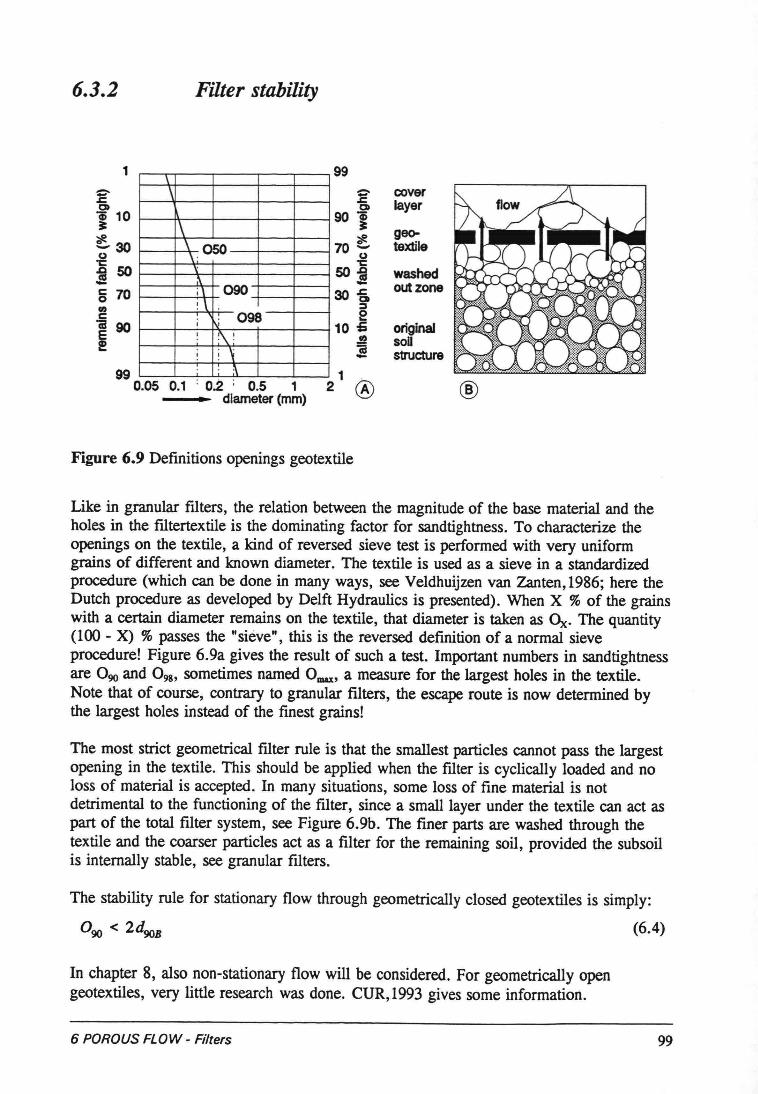
6.3.2 Filter stability

1\\

1\\ oso\ .\:\

090i\~\ ;

i i 098~ :\~I i \

~

=­s:I:IDäi 10:r:~30.gjSO5 70(#)c"äi90E!

990.05 0.1 . 0.2 '0.5 1

diameter (mm)

99

=- covers: layerCl>901

geo-::ot70 ~ textile()"t:SOi washed- out zone30á:s2

10 -5 originaI.!Q solI! structure

1®2 ®

Figure 6.9 Definitions openings geotextile

Like in granular filters, the relation between the magnitude of the base material and theholes in the filtertextile is the dominating factor for sandtightness. To characterize theopenings on the textile, a kind of reversed sieve test is performed with very uniformgrains of different and known diameter. The textile is used as a sieve in a standardizedprocedure (which can be done in many ways, see Veldhuijzen van Zanten,1986; here theDutch procedure as developed by Delft Hydraulics is presented). When X % of the grainswith a certain diameter remains on the textile, that diameter is taken as Üx. The quantity(100 - X) % passes the "sieve", this is the reversed definition of anormal sieveprocedure! Figure 6.9a gives the result of such a test. Important numbers in sandtightnessare 090 and 098, sometimes named 0max,a measure for the largest holes in the textile.Note that of course, contrary to granular filters, the escape route is now determined bythe largest holes instead of the finest grains!

The most strict geometrical filter rule is that the smallest partic1es cannot pass the largestopening in the textile. This should be applied when the filter is cyc1ically loaded and noloss of material is accepted. In many situations, some loss of fine material is notdetrimental to the functioning of the filter, since a smalllayer under the textile can act aspart of the total filter system, see Figure 6.9b. The finer parts are washed through thetextile and the coarser partic1es act as a filter for the remaining soil, provided the subsoilis internally stable, see granular filters.

The stability rule for stationary flow through geometrically closed geotextiles is simply:

(6.4)

In chapter 8, also non-stationary flow will be considered. For geometrically opengeotextiles, very little research was done. CUR,1993 gives some information.

6 POROUSFLOW - Filters 99

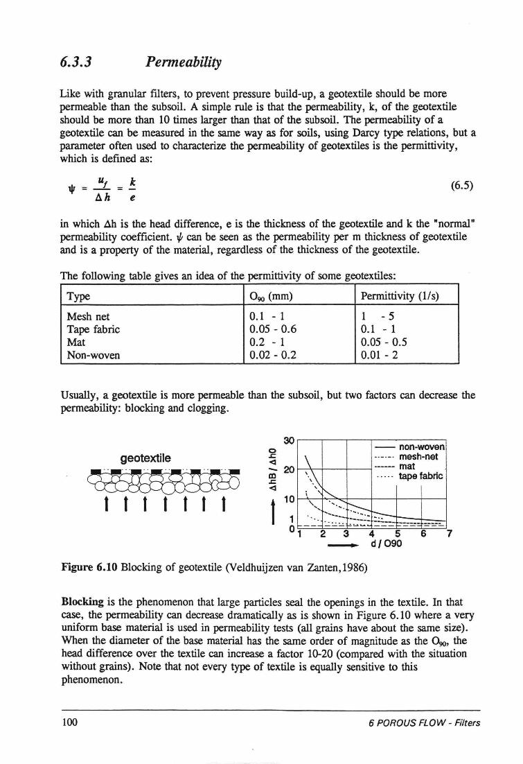
6.3.3 Permeability

Like with granular filters, to prevent pressure build-up, a geotextile should be morepermeable than the subsoil. A simple rule is that the permeability, k, of the geotextileshould be more than 10 times larger than that of the subsoil. The permeability of ageotextile can be measured in the same way as for soils, using Darcy type relations, but aparameter often used to characterize the permeability of geotextiles is the permittivity,which is defmed as:

u, k1IJ=-=­Ah e

(6.5)

in which .1.h is the head difference, e is the thickness of the geotextile and k the "normal "permeability coefficient. 1/1 can be seen as the permeability per m thickness of geotextileand is a property of the material, regardless of the thickness of the geotextile.

The following table gives an idea of the permittivity of some geotextiles:

Type 090 (mm) Permittivity (lis)

Mesh net 0.1 - 1 1 -5Tape fabric 0.05 - 0.6 0.1 - 1Mat 0.2 - 1 0.05 - 0.5Non-woven 0.02 - 0.2 0.01 - 2

Usually, a geotextile is more permeable than the subsoil, but two factors can decrease thepermeability: blocking and clogging.

300

geotextile .c<I- 20m.c<I

tt tt tt t

-- non-woven

\ .._--- mesh-net..._---- mat\\ ..... tape fabrIc

i\ r-,'''.. ...........

~.......... t::-". ......-.... ------ ------f----

...... !-=-~ .......... ~==----456d/090

7

Figure 6.10 Blocking of geotextile (Veldhuijzen van Zanten, 1986)

Blocking is the phenomenon that large particles seal the openings in the textile. In thatcase, the permeability can decrease dramatically as is shown in Figure 6.10 where a veryuniform base material is used in permeability tests (all grains have about the same size).When the diameter of the base material has the same order of magnitude as the Ow, thehead difference over the textile can increase a factor 10-20 (compared with the situationwithout grains). Note that not every type of textile is equally sensitive to thisphenomenon.

100 6 POROUS FLOW - Filters

Clogging is the trapping of (very) fine particles in the openings of the textile, leading alsoto a decrease of permeability. This can happen in water contaminated with chemicals, e.g.iron. In contrast with bloeking, clogging is a time dependent process. The idea is that itstabilizes at a certain level after a certain time, but not much experimental evidence isavailable to support this thesis. It should be realized that clogging is not special forgeotextiles; it also occurs in granular filters.

When the permeability of the textile is 10 times greater than that of the subsoil, there isusually no problem with pressure build-up, not even with bloeking or clogging. However,when used in very contaminated groundwater, one should examine the possibility ofsevere clogging. When the danger of bloeking or clogging can be excluded, apermeability factor of 2 or 3, is sufficient.

A better demand would be to link the permeability or permittivity directly to the absolutepressure build-up under the geotextile in order to prevent sliding along a slope, see nextsection.

6 POROUSFLOW - Filters 101

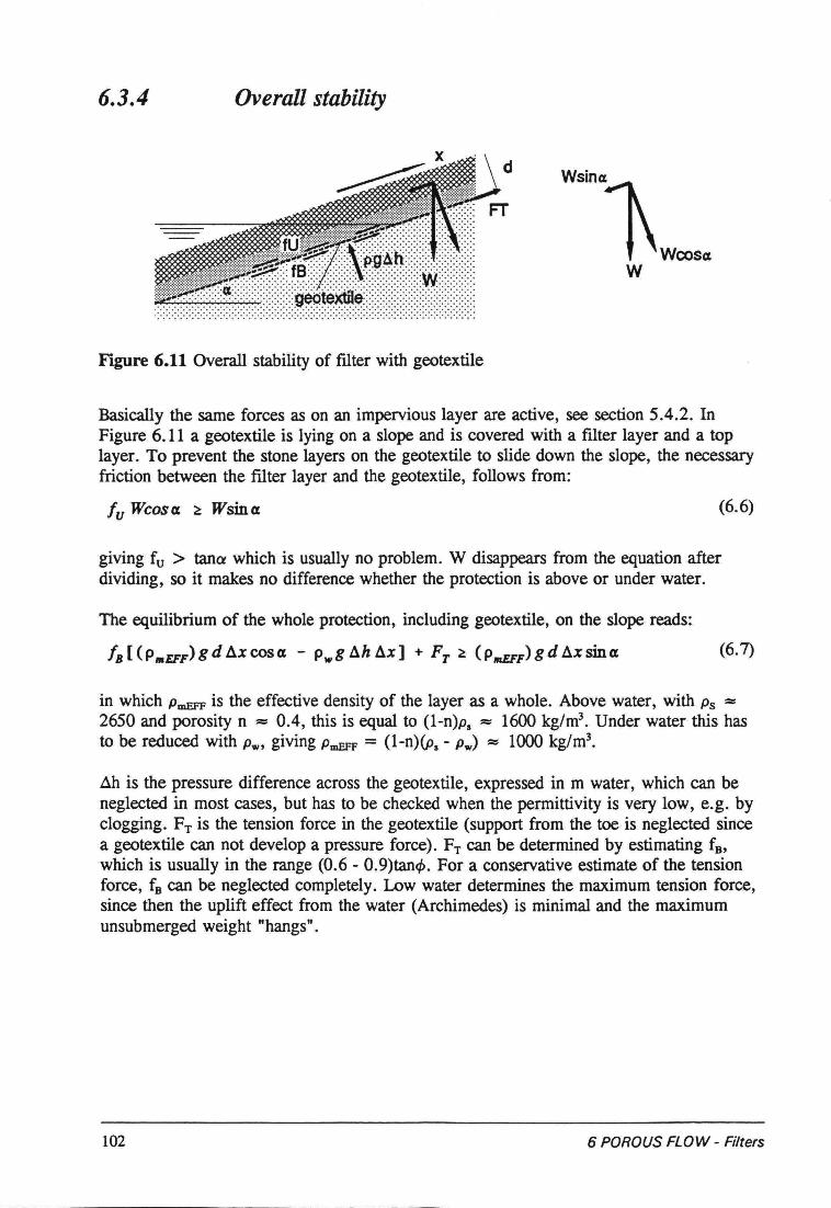
6.3.4 Overall stability

WSin,,~

, \wcos«w

Figure 6.11 Overall stability of filter with geotextile

Basically the same forces as on an impervious layer are active, see section 5.4.2. InFigure 6.11 a geotextile is lying on a slope and is covered with a filter layer and a toplayer. To prevent the stone layers on the geotextile to slide down the slope, the necessaryfriction between the filter layer and the geotextile, follows from:

to Wcoscx ~ Wsincx (6.6)

giving fu > tano which is usually no problem. W disappears from the equation afterdividing, so it makes no difference whether the proteetion is above or under water.

The equilibrium of the whole protection, including geotextile, on the slope reads:

IB [(PIIIEFF)gd ~xcoscx - pwg ~h ~x] + FT ~ (PlrIEFF)gd ~xsincx (6.7)

in which PmEFF is the effective density of the layer as a whoie. Above water, with Ps =2650 and porosity n -= 0.4, this is equal to (l-n}ps = 1600 kg/rn'. Under water this hasto be reduced with Pw, giving PmEFF = (l-n)(ps - Pw) = 1000 kg/rn'.

~h is the pressure difference across the geotextile, expressed in m water, which can beneglected in most cases, but has to be checked when the permittivity is very low, e.g. byclogging. FT is the tension force in the geotextile (support from the toe is neglected sincea geotextile can not develop a pressure force). FT can be determined by estimating fB,which is usually in the range (0.6 - 0.9}tan4>.For a conservative estimate of the tensionforce, fB can be neglected completely. Low water determines the maximum tension force,since then the uplift effect from the water (Archimedes) is minimal and the maximumunsubmerged weight "hangs".

102 6 POROUSFLOW - Filters

-- - ---

6.4 Summary

Filters can have two functions: preventing erosion under a coarse top layer or drainage toprevent pressure build-up. In both cases filter stability and permeability play a role.Stability concerns the grains that should be stable in the filter, while the permeability isimportara to avoid pressure build-up, which can cause instability of a layer as a whole.The two main types of filters are granular filters and geotextiles.

Granular filters can be designed along two lines: geometrically closed and geometricallyopen. Geometrically closed filters are stable, regardless of the porous flow through thefilter. In fact there is no critical gradient because the relation between the diameters inthe filter is such that the finer grains cannot move through the pores of the coarsergrains. Geometrically closed filters have to be designed within the margins of stability andpermeability. The design rules are simply:

d dStability: lSF < 5 (provided int. stable: ~ < 10)

dSSB -;

dPermeability: lSF > 5 (6.8)d1SB

Stable, geometrically open filters have a critical gradieni, above whicn the base materialis no longer stable. This is no problem as long as the occuring gradient is below thecritical value, just as in open channel flow. This means that botb these gradients have tobe known. Section 6.2.3 gives information on the critical gradients for flow perpendicularand parallel to the interface of the layers. The occuring gradient has to be derived frommeasurements or calculations inside the filter. In bottom protections witb low gradietu,but high turbulence, the thickness of the layers becomes important, for which equation(6.3) gives an estimate.

Geotextiles can replace several filter layers, giving a thinner filter as a whoie. A simplerule for stationary flow is:

090 < 2d90B

The permeability of a geotextile is usually expressed as the permittivity, which is definedas the permeability per m thickness of geotextile. The permeability of a geotextile can bereduced by blocking or clogging, which is a sudden or a gradual closure of the holes inthe textile respectively. With a permeability 10 times larger than that of the subsoil, thepermeability is usually enough to prevent pressure build-up. On slopes it can be necessaryta check the stability of filter layers with geotextile as a whoie. Thefriction betweengeotextile and the top layers or subsoil has to be sufficient and/or the geotextile has to bestrong enough to withstand any possible tension forces.

6 POROUSFLOW - Filters 103

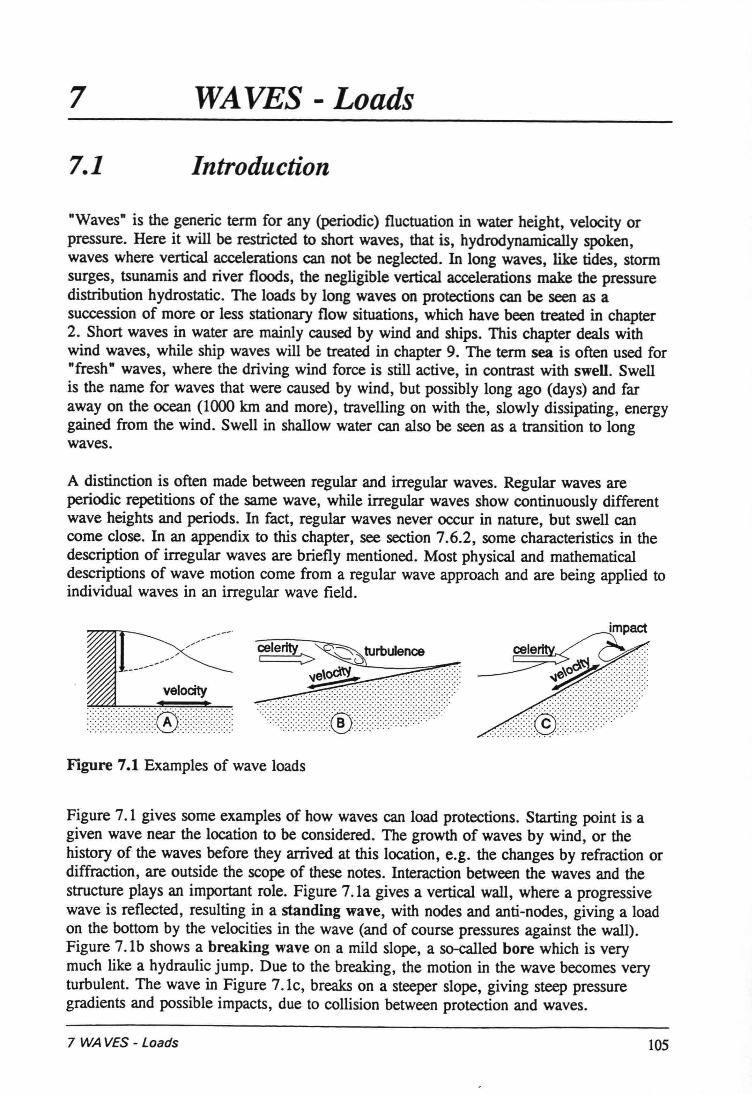
7 WAYES - Loads

7.1 Introduetion

"Waves" is the generic term for any (periodic) fluctuation in water height, velocity orpressure. Here it will be restricted to short waves, that is, hydrodynamically spoken,waves where vertical accelerations cao not be neglected. In long waves, like tides, stormsurges, tsunamis and river floods, the negligible vertical accelerations make the pressuredistribution hydrostatic. The loads by long waves on protections cao he seen as asuccession of more or less stationary flow situations, which have been treated in chapter2. Short waves in water are mainly caused by wind and ships. This chapter deals withwind waves, while ship waves will be treated in chapter 9. The term sea is often used for"fresh" waves, where the driving wind force is still active, in contrast with swell. Swellis the name for waves that were caused by wind, but possibly long ago (days) and faraway on the ocean (1000 km and more), travelling on with the, slowly dissipating, energygained from the wind. Swell in shallow water cao also be seen as a transition to longwaves.

A distinction is often made between regular and irregular waves. Regular waves areperiodic repetitions of the same wave, while irregular waves show continuously differentwave heights and periods. In fact, regular waves never occur in nature, but swell caocome close. In an appendix to this chapter, see section 7.6.2, some characteristics in thedescription of irregular waves are briefly mentioned. Most physical and mathematicaldescriptions of wave motion come from a regular wave approach and are being applied toindividual waves in an irregular wave field.

_' ..::::~:~~::~:~:::~:~::~~~::~:®:~::::::~::j:::: ~~~~;~:~:~:::::::::: ....:::::::::::::@::::::::::::::::::::::::.: ............... ..

Figure 7.1 Examples of wave loads

Figure 7.1 gives some examples of how waves cao load protections. Starting point is agiven wave near the location to be considered. The growth of waves by wind, or thehistory of the waves before they arrived at this location, e.g. the changes by refraction ordiffraction, are outside the scope of these notes. Interaction between the waves and thestructure plays an important role. Figure 7.la gives avertical wall, where a progressivewave is reflected, resulting in a standing wave, with nodes and anti-nodes, giving a loadon the bottom by the veloeities in the wave (and of course pressures against the wali).Figure 7.lb shows a breaking wave on a mild slope, a so-called bore which is verymuch like a hydraulic jump. Due to the brea.k:ing,the motion in the wave becomes veryturbulent. The wave in Figure 7.lc, breaks on asteeper slope, giving steep pressuregradients and possible impacts, due to collision between proteetion and waves.

7 WAYES - Loads 105

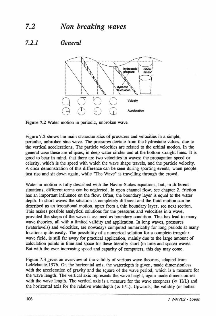
7.2 Non breaking waves

7.2.1 General

aG00C) E)

DG)

Velocity

Acceleration

Figure 7.2 Water motion in periodic, unbroken wave

Figure 7.2 shows the main characteristics of pressures and veloeities in a simple,periodic, unbroken sine wave. The pressures deviate from the hydrostatic values, due tothe vertical accelerations. The partiele veloeities are related to the orbital motion. In thegenera! case these are ellipses, in deep water circles and at the bottom straight lines. 1t isgood to bear in mind, that there are two veloeities in waves: the propagation speed orcelerity, which is the speed with which the wave shape travels, and the partiele velocity .A clear demonstration of this difference can be seen during sporting events, when peoplejust rise and sit down again, while "The Wave" is travelling through the crowd.

Water in motion is fully described with the Navier-Stokes equations, but, in differentsituations, different terms can be neglected. In open channel flow, see chapter 2, frictionhas an important influence on the flow. Often, the boundary layer is equal to the waterdepth. In short waves the situation is completely different and the fluid motion can bedescribed as an irrotational motion, apart from a thin boundary layer, see next section.This makes possible analytical solutions for the pressures and veloeities in a wave,provided the shape of the wave is assumed as boundary condition. This has lead to manywave theories, all with a limited validity and application. In long waves, pressures(waterlevels) and velocities, are nowadays computed numerically for long periods at manylocations quite easily. The possibility of a numerical solution for a complete irregularwave field, is still far away for practical application, mainly due to the large amount ofcalculation points in time and space for these literally short (in time and space) waves.But with the ever increasing speed and capacity of computers, this day may come.

Figure 7.3 gives an overview of the validity of various wave theories, adapted fromLeMehaute,1976. On the horizontal axis, the waterdepth is given, made dimensionlesswith the acceleration of gravity and the square of the wave period, which is a measure forthe wave length. The vertical axis represents the wave height, again made dimensionlesswith the wave length. The vertical axis is a measure for the wave steepness (oe RIL) andthe horizontal axis for the relative waterdepth (oe h/L). Upwards, the validity (or better:

106 7 WA VES - Loads

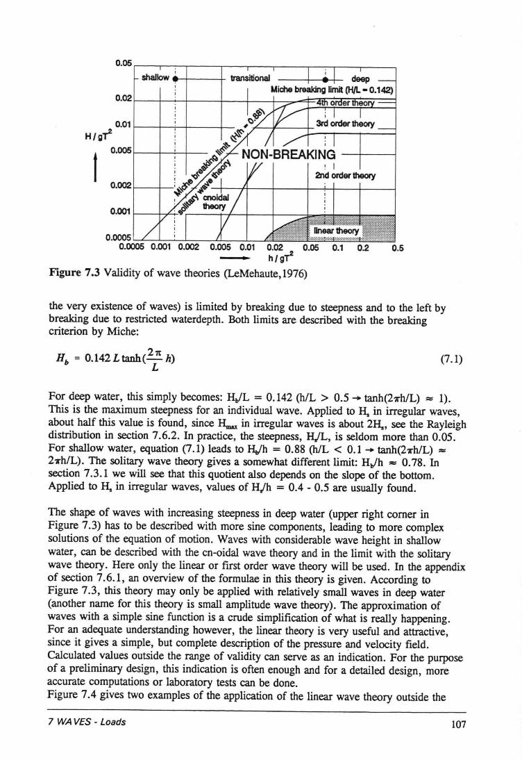
I0.0051--_1--":--1--_

shallow +-----t- transitional deepMichebreakingfimit (HJL - 0.142)

0.011--_1--+--1--_--+-_H/gr

! I2nd order theory

0.002~---1_'

0.0005 L..L--l_..____,___ LL--_-'----L:i::.

0.0005 0.001 0.002 0.005 0.01 0.02 0.05 0.1 0.2 0.5h/gr

Figure 7.3 Validity of wave theories (LeMehaute,1976)

the very existence of waves) is limited by breaking due to steepness and to the left bybreaking due to restricted waterdepth. Both limits are described with the breakingcriterion by Miche:

u, = 0.142 L tanh(21t h)L

(7.1)

For deep water, this simply becomes: HJL = 0.142 (h/L > 0.5 - tanh(27rh/L) :::: 1).This is the maximum steepness for an individual wave. Applied to H. in irregular waves,about half this value is found, since Hmax in irregular waves is about 2H., see the Rayleighdistribution in section 7.6.2. In practice, the steepness, H.lL, is seldom more than 0.05.For shallow water, equation (7.1) leads to HJh = 0.88 (h/L < 0.1 - tanh(2Th/L) ::::2'l'h/L). The solitary wave theory gives a somewhat different limit: HJh = 0.78. Insection 7.3.1 we will see that this quotient also depends on the slope of the bottom.Applied to H. in irregular waves, values of Hjh = 0.4 - 0.5 are usually found.

The shape of waves with increasing steepness in deep water (upper right corner inFigure 7.3) has to be described with more sine components, leading to more complexsolutions of the equation of motion. Waves with considerabie wave height in shallowwater, can be described with the cn-oidal wave theory and in the limit with the solitarywave theory. Here only the linear or first order wave theory will be used. In the appendixof section 7.6.1, an overview of the formulae in this theory is given. According toFigure 7.3, this theory may only be applied with relatively small waves in deep water(another name for this theory is small amplitude wave theory). The approximation ofwaves with a simple sine function is a crude simplification of what is really happening.For an adequate understanding however, the linear theory is very useful and attractive,since it gives a simpie, but complete description of the pressure and velocity field.Calculated values outside the range of validity can serve as an indication. For the purposeof a preliminary design, this indication is often enough and for a detailed design, moreaccurate computations or laboratory tests can be done.Figure 7.4 gives two examples of the application of the linear wave theory outside the

7 WAVES - Loads 107

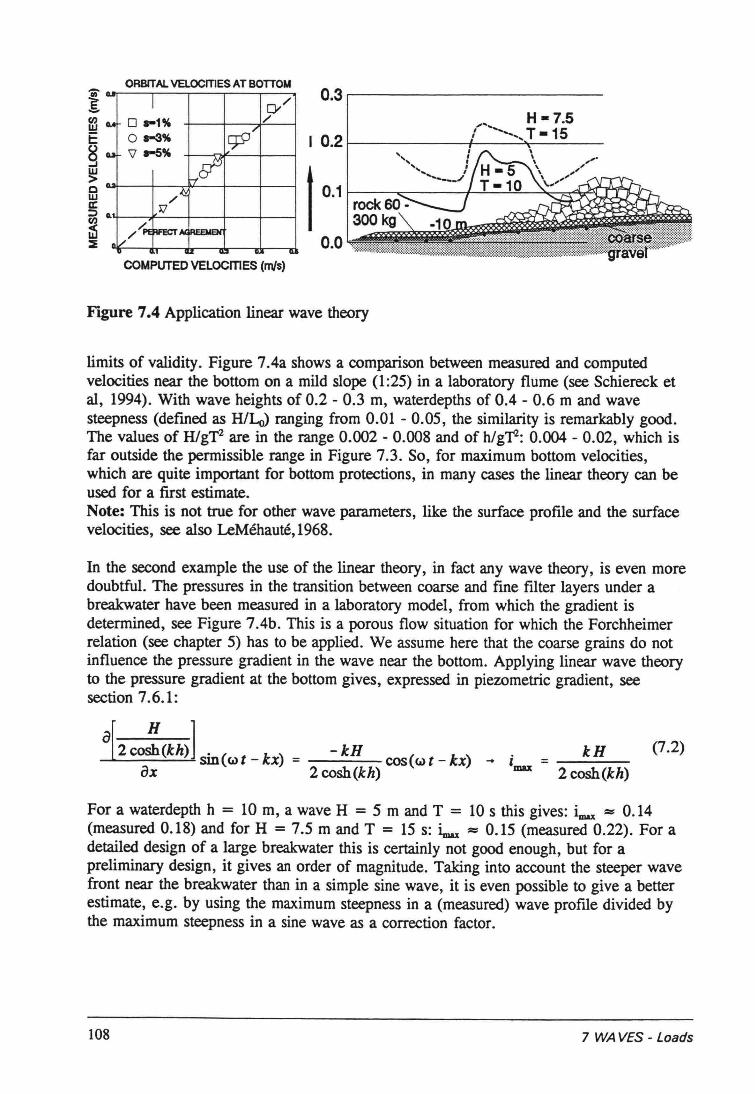
ORBITAL VELOCmeS AT BOTTOU- I 0-/CIA 0 .. 1% /

01-3% g9/u \] .-5%

7/.1::,

Cl.rJ

[///PE RFECT

.. ..

t 0.1

COMPUTeovnocrnes (mis)

Figure 7.4 Application linear wave theory

limits of validity. Figure 7.4a shows a comparison between measured and computedveloeities near the bottom on a mild slope (1:25) in a laboratory flume (see Schiereek etal, 1994). With wave heights of 0.2 - 0.3 m, waterdepths of 0.4 - 0.6 m and wavesteepness (defined as H/Lo) ranging from 0.01 - 0.05, the similarity is remarkably good.The values of H/gT2 are in the range 0.002 - 0.008 and of h/g'I": 0.004 - 0.02, which isfar outside the permissible range in Figure 7.3. So, for maximum bottom velocities,which are quite important for bottom protections, in many cases the linear theory can beused for a fust estimate.Note: This is not true for other wave parameters, like the surface profile and the surfacevelocities, see also LeMéhauté, 1968.

In the second example the use of the linear theory, in fact any wave theory, is even moredoubtful. The pressures in the transition between coarse and fine filter layers under abreakwater have been measured in a laboratory model, from which the gradient isdetermined, see Figure 7.4b. This is a porous flow situation for which the Forchheimerrelation (see chapter 5) has to be applied. We assume here that the coarse grains do notinfluence the pressure gradient in the wave near the bottom. Applying linear wave theoryto the pressure gradient at the bottom gives, expressed in piezometric gradient, seesection 7.6.1:

a[2co.!(kh)]sin(",t_kx) = -kH cos("'t-kx) _ i = kH (7.2)ax 2 cosh{kh) lIWt 2 cosh(kh)

For a waterdepth h = 10 m, a wave H = 5 m and T = 10 s this gives: imax= 0.14(measured 0.18) and for H = 7.5 m and T = 15 s: Îmax = 0.15 (measured 0.22). For adetailed design of a large breakwater this is certainly not good enough, but for apreliminary design, it gives an order of magnitude. Taking into account the steeper wavefront near the breakwater than in a simple sine wave, it is even possible to give a betterestimate, e.g. by using the maximum steepness in a (measured) wave profile divided bythe maximum steepness in a sine wave as a correction factor.

108 7 WAVES - Loads

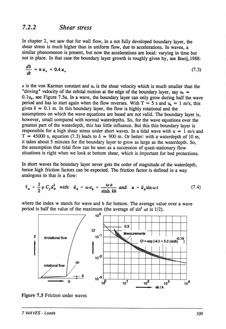
7.2.2 Shear stress

In chapter 2, we saw that for wall flow, in a not fully developed boundary layer, theshear stress is much higher than in uniform flow, due to accelerations. In waves, asimilar phenomenon is present, but now the accelerations are local: varying in time butnot in place. In that case the boundary layer growth is roughly given by, see Booij,1988:

df>- = Jeu. = 0.4u.dt

(7.3)

« is the von Karman constant and u. is the shear velocity which is much smaller than the"driving" velocity of the orbital motion at the edge of the boundary layer, say u. =0.1Ub' see Figure 7.5a. In a wave, the boundary layer can only grow during half the waveperiod and has to start again when the flow reverses. With T = 5 s and u, = 1 mIs, thisgives ó = 0.1 m. In this boundary layer, the flow is highly rotational and theassumptions on which the wave equations are based are not valid. The boundary layer is,however, small compared with normal waterdepths. So, for the wave equations over thegreatest part of the waterdepth, this has little influence. But this thin boundary layer isresponsible for a high shear stress under short waves. In a tidal wave with u = 1 mIs andT = 45000 s, equation (7.3) leads to ó = 900 m. Or better: with a waterdepth of 10 m,it takes about 5 minutes for the boundary layer to grow as large as the waterdepth. So,the assumption that tidal flow can be seen as a succession of quasi-stationary flowsituations is right when we look at bottom shear, which is important for bed protections.

In short waves the boundary layer never gets the order of magnitude of the waterdepth,hence high friction factors can be expected. The friction factor is defined in a wayanalogous to that in a flow:

(7.4)

where the index w stands for wave and b for bottom. The average value over a waveperiod is half the value of the maximum (the average of sin' wt is 1/2).

100

\. 0.3<, "- ,~ Measurements

~~ -0.19Cf - exp [-6.0+ 5.2 (ab/k) I

~ ...l'4QIIIIIl~ Oö:::

~ r=-;--

CfZ lrrotationaJ flow 10.1

I I10.2

ub

u 10-31cP

Figure 7.S Friction under waves

7 WAVES • Loads 109

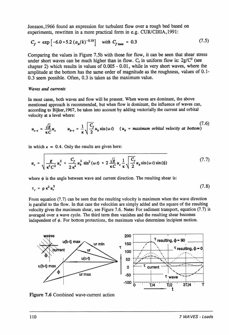
Jonsson,1966 found an expression for turbulent flow over a rough bed based onexperiments, rewritten in a more practical form in e.g. CURICIRIA,1991:

C, = exp [-6.0+5.2 (a"lkro.19] with C,mu.= 0.3 (7.5)

Comparing the values in Figure 7.5b with those for flow, it can be seen that shear stressunder short waves can be much higher than in flow. Cf in uniform flow is: 2g/C2 (seechapter 2) which resu1ts in values of 0.005 - 0.01, while in very short waves, where theamplitude at the bottom has the same order of magnitude as the roughness, values of 0.1-0.3 seem possible. Often, 0.3 is taken as the maximum value.

Waves and currents

Inmost cases, both waves and flow will be present. When waves are dominant, the abovementioned approach is recommended, but when flow is dominant, the influence of waves can,according to Bijker,1967, be taken into account by adding vectorially the current and orbitaIvelocity at a level where:

u = fi Uc-t 'KC c

(7.6)(ub = maximum orbital velocity at bottom)

in which IC ::= 0.4. Qnly the results are given here:

u =T

(7.7)

where <P is the angle between wave and current direction. The resulting shear is:

'tT = P Klu; (7.8)

From equation (7.7) can be seen that the resulting velocity is maximum when the wave directionis parallel to the flow. In that case the veloeities are simply added and the square of the resultingvelocity gives the maximum shear, see Figure 7.6. Note: For sediment transport, equation (7.7) isaveraged over a wave cycle. The third term then vanishes and the resulting shear becomesindependent of <p. For bottom protections, the maximum value determines incipient motion.

200

150

100

50

o-50

-100

1

't resulting, 4> - 90" I. ,, -. 't resultlng,4> - 0,- " , ",- .:,...-f-"':" • ,

.', ,1" " ,,L_ 't current " '. -.-' .-.... '", /7' .... ""'t wave ~- -

I0 4 iJ2 3 4

.,I

---- tJ I

Figure 7.6 Combined wave-current action

110 7 WAYES - Loads

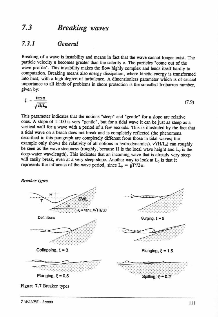
7.3 Breaking waves

7.3.1 General

Breaking of a wave is instability and means in fact that the wave cannot longer exist. Thepartiele velocity u becomes greater than the celerity c. The particles "come out of thewave profile". This instability makes the flow highly complex and lends itself hardly tocomputation. Breaking means also energy dissipation, where kinetic energy is transformedinto heat, with a high degree of turbulence. A dimensionless parameter which is of crucialimportance to all kinds of problems in shore proteetion is the so-called Irribarren number,given by:

tana~=--JHILo (7.9)

This parameter indicates that the notions "steep" and "gentle" for a slope are relativeones. A slope of 1:100 is very "gentle", but for a tidal wave it can he just as steep as avertical wall for a wave with a period of a few seconds. This is illustrated by the fact thata tidal wave on a beach does not break and is completely reflected (the phenomenadescribed in this paragraph are completely different from those in tidal waves; theexample only shows the relativity of all notions in hydrodynamics). v'(H/~) can roughlybe seen as the wave steepness (roughly, because H is the local wave height and L, is thedeep-water wavelength). This indicates that an incoming wave that is already very steepwill easily break, even at a very steep slope. Another way to look at Lo is that itrepresents the influence of the wave period, since Lo = gT2/2T.

Breaker types

Definitions Surging, ~ - 5

...................

......... .... " .....:.:::::::::::::::::::::::::::: ~:~:~::::::::::::.,

COllapsing, ( - 3 Plunging, ~ - 1.5

-~ .A.."'! .~ .':.:.::::::::::::::::::::::::::::::::::::::::::::...............................

. .. ............. .. .... .. ' .0.:.:::::::::::::::::::::::::::::::::::::::::::::::::::::::::::::::::.'

.... ... .. ....... '"

Plunging, ~ - 0.5

Figure 7.7 Breaker types

7 WAVES - Loads 111

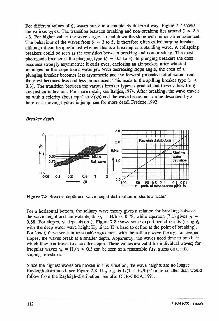
For different values of ~, waves break in a completely different way. Figure 7.7 showsthe various types. The transition between breaking and non-breaking lies around ~ =:.< 2.5- 3. For higher values the wave surges up and down the slope with minor air entrainment.The behaviour of the waves from ~ ::= 3 to 5, is therefore often called surging breakeralthough it can be questioned whether this is a breaking or a standing wave. A collapsingbreakers could be seen as the transition between breaking and non-breaking. The mostphotogenic breaker is the plunging type (~ =:.< 0.5 to 3). In plunging breakers the erestbecomes strongly asymmetrie; it eurls over, enclosing an air pocket, after whieh itimpinges on the slope like a water jet. With decreasing slope angle, the erest of aplunging breaker becomes less asymmetrie and the forward projected jet of water fromthe erest becomes less and less pronounced. This leads to the spilling breaker type (~ <0.3). The transition between the various breaker types is gradual and these values for ~are just an indication. For more detail, see Battjes,1974. After breaking, the wave travelson with a celerity about equal tovi(gh) and the wave behaviour can be described by abore or a moving hydraulie jump, see for more detail FredSIêJe , 1992.

Breaker depth

2.62

yb

t 1

0.50.05 0.5 1

~O

2.0

II I I I I I I l.;

Raylelgh distributIon v~

7' ,,~ Shallow1/ water/" deviationv

/'/'

.//'

H/Hs

0.0100 50 20 105 2 1 0.1 0.01--- prob. of exceedance p(H) %

Figure 7.8 Breaker depth and wave-height distribution in shallow water

For a horizon tal bottom, the solitary wave theory gives a relation for breaking betweenthe wave height and the waterdepth: 'Yb = Hlh =:.< 0.78, while equation (7.1) gives 'Yb =0.88. For slopes, 'Yb depends on ~. Figure 7.8 shows some experimental results (using ~owith the deep water wave height Ho, sinee H is hard to define at the point of breaking).For low ~ these seem in reasonable agreement with the solitary wave theory; for steeperslopes, the waves break at a smaller depth. Apparently, the waves need time to break, inwhieh they can travel to a smaller depth. These values are valid for individual waves; forirregular waves 'Yb = Hs/h =:.< 0.5 can be seen as a reasonable first guess on a mildsloping foreshore.

Since the highest waves are broken in this situation, the wave heights are no longerRayleigh distributed, see Figure 7.8. Hl~e.g. is 1/(1 + Hs/h)ll3 times smaller than wouldfollow from the Rayleigh-distribution, see also CUR/CIRIA, 1991.

112 7 WAVES - Loads

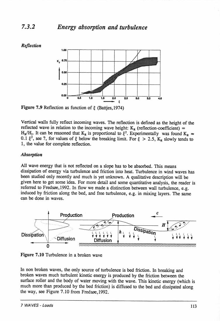
7.3.2 Energy absorption and turbulence

Reflection

I~- ~

Figure 7.9 Reflection as function of ~ (Battjes, 1974)

Vertical walls fully reflect incoming waves. The reflection is defined as the height of thereflected wave in relation to the incoming wave height: KR (reflection-coefficient) =HR/H1• It can be reasoned that KR is proportional to e. Experimenta1ly was found KR ::=

0.1 e, see 1, for values of ~ below the breaking limit. For ~ > 2.5, KR slowly tends to1, the value for complete reflection.

Absorption

All wave energy that is not reflected on a slope has to be absorbed. This meansdissipation of energy via turbulence and friction into heat. Turbulence in wind waves hasbeen studied only recently and much is yet unknown. A qualitative description will begiven here to get some idea. For more detail and some quantitative analysis, the reader isreferred to Freds0e,1992. In flow we made a distinction between wall turbulence, e.g.induced by friction along the bed, and free turbulence, e.g. in mixing layers. The samecan be done in waves.

a:~~~~~~Diffusion

/

III\

O· ·/t>"issipa rorr.\\\

. <...Diffusion

Production c-o

Figure 7.10 Turbulence in a broken wave

In non broken waves, the only souree of turbulence is bed friction. In breaking andbroken waves much turbulent kinetic energy is produced by the friction between thesurface roller and the body of water moving with the wave. This kinetic energy (which ismuch more than produced by the bed friction) is diffused to the bed and dissipated alongthe way, see Figure 7.10 from Freds0e,1992.

7 WAVES - Loads 113

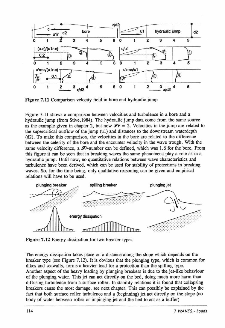
l~lrfd2 ~zJd~ hydraUOC~mp Id2

0 1 2 3 4 5 6 0 1 2 3 4 5t!~~-~~~+--~~ ------...~~ I )

0 1 2 3 4 5 6 0 1 2 3 4 5

r;S/~Ul~~) ~~ 1~ Vlf I~0 1 !..__ 3 xJd24 5 6 0 1 2_3xJd2 4 5

Figure 7.11 Comparison velocity field in bore and hydraulic jump

Figure 7.11 shows a comparison between veloeities and turbulence in a bore and ahydraulic jump (from Stive,1984). The hydraulic jump data come from the same soureeas the example given in chapter 2, but now !Fr = 2. Veloeities in the jump are related tothe supercritica1 outflow of the jump (ul) and distances to the downstream waterdepth(d2). To make this comparison, the veloeities in the bore are related to the differencebetween the celerity of the bore and the encounter velocity in the wave trough. With thesame velocity difference, a !Fr-number can be defined, which was 1.6 for the bore. Fromthis figure it can be seen that in breaking waves the same phenomena play a role as in ahydraulic jump. Until now, no quantitative relations between wave characteristics andturbulence have been derived, which can be used for stability of protections in breakingwaves. So, for the time being, only qualitative reasoning can be given and empirica1relations will have to be used.

plungingbreaker.-::/<>.~_._._._._.--?2 ..-~ .~4 .

. .-:-:,:.:-:-:.:-:-'

spillingbreaker plungingjet

energydissipation

. .. .. . . . . . . . ... , .. .. , ......... .... .. , ........ ...... .. . . . . . . . . . .. .... .....

....................... . " .. . . . . . . . . . . . . . . . .......... ....... .

Figure 7.12 Energy dissipation for two breaker types

The energy dissipation takes place on a distance along the slope which depends on thebreaker type (see Figure 7.12). It is obvious that the plunging type, which is common fordikes and seawalls, forms a heavier load for a proteetion than the spilling type.Another aspect of the heavy loading by plunging breakers is due to the jet-like behaviourof the plunging water. This jet can act directly on the bed, doing much more harm thandiffusing turbulence from a surface roller. In stability relations it is found that collapsingbreakers cause the most damage, see next chapter. This cao possibly be explained by thefact that both surface roller turbulence and a (beginning) jet act directly on the slope (nobody of water between roller or impinging jet and the bed to act as a buffer)

114 7 WAVES - Loads

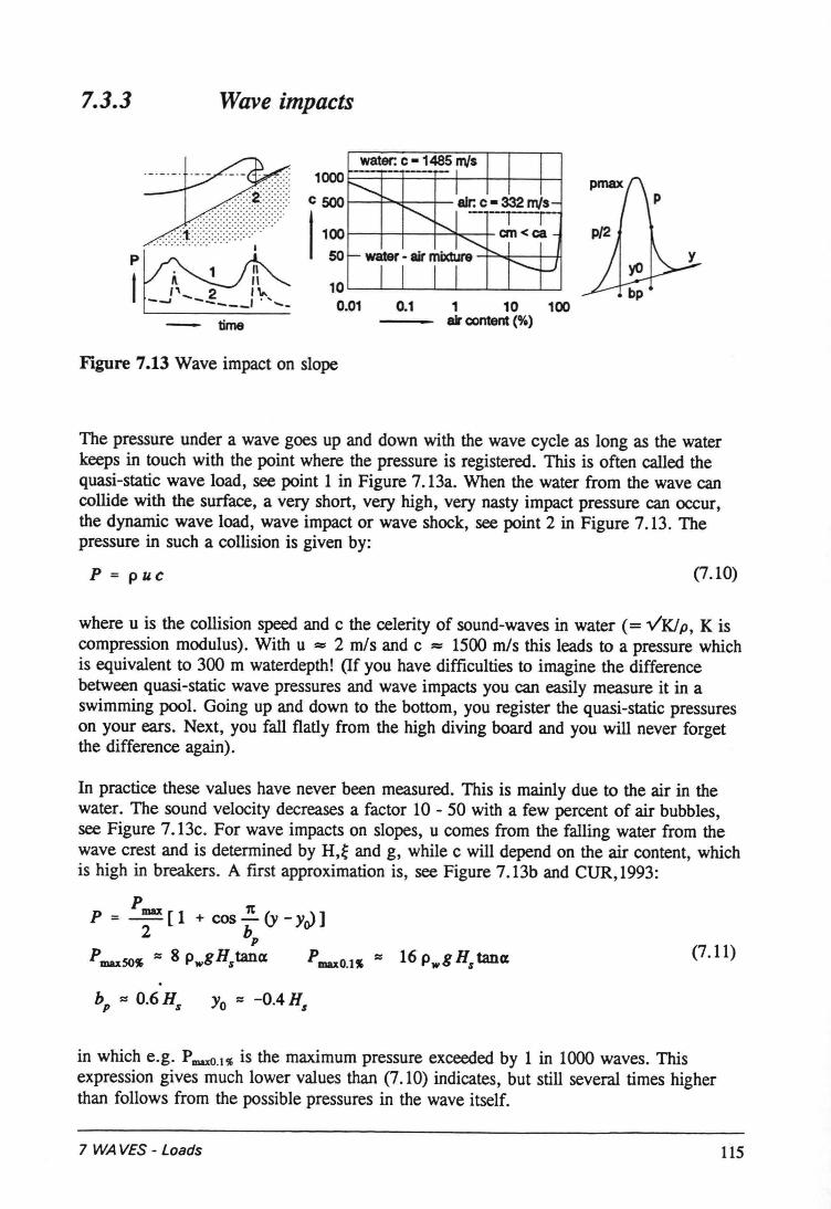
7.3.3 Wave impacts

p

I 10L--L~--~~~~ __~~0.01 0.1 1 10 100

air content (%)- time

Figure 7.13 Wave impact on slope

The pressure under a wave goes up and down with the wave cyc1eas long as the waterkeeps in touch with the point where the pressure is registered. This is often called thequasi-static wave load, see point 1 in Figure 7.13a. When the water from the wave cancollide with the surface, a very short, very high, very nasty impact pressure can occur,the dynamic wave load, wave impact or wave shock, see point 2 in Figure 7.13. Thepressure in such a collision is given by:

P = puc (7.10)

where u is the collision speed and c the celerity of sound-waves in water (= vKJp, K iscompression modulus). With u=::2 mIs and c =:: 1500 mIs this leads to a pressure whichis equivalent to 300 m waterdepth! (If you have difficulties to imagine the differencebetween quasi-static wave pressures and wave impacts you can easily measure it in aswimming pool. Going up and down to the bottom, you register the quasi-static pressureson your ears. Next, you fall flatly from the high diving board and you will never forgetthe difference again).

In practice these values have never been measured. This is mainly due to the air in thewater. The sound velocity decreases a factor 10 - 50 with a few percent of air bubbles,see Figure 7.13c. For wave impacts on slopes, u comes from the falling water from thewave crest and is determined by H,~ and g, while c will depend on the air content, whichis high in breakers. A first approximation is, see Figure 7.13b and CUR,1993:

Pmax 1tP = - [1 + cos - (y - yo> ]

2 bpPmaxSOS == 8PwgHstan« pmaxO.1S == 16PwgHstan« (7.11)

in which e.g. PmaxO.l% is the maximum pressure exceeded by 1 in 1000 waves. Thisexpression gives much lower values than (7.10) indicates, but still several times higherthan follows from the possible pressures in the wave itself.

7 WAVES - Loads 115

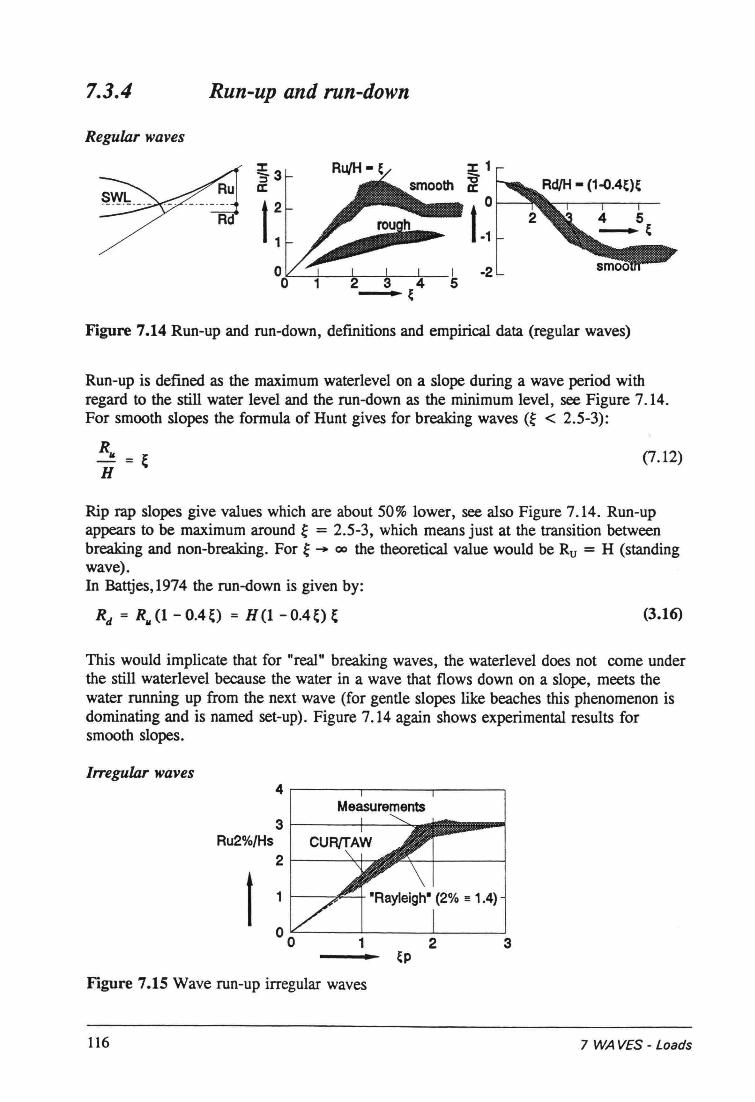
7.3.4 Run-up and run-down

Regular waves

% 1:g-a:

o

L1

Figure 7.14 Run-up and run-down, defmitions and empirical data (regular waves)

Run-up is defined as the maximum waterlevel on a slope during a wave period withregard to the still water level and the run-down as the minimum level, see Figure 7.14.For smooth slopes the formula of Hunt gives for breaking waves (~ < 2.5-3):

Ril- = ~H

(7.12)

Rip rap slopes give values which are about 50% lower, see also Figure 7.14. Run-upappears to be maximum around ~ = 2.5-3, which means just at the transition betweenbreaking and non-breaking. For ~ - 00 the theoretica1 value would be Ru = H (standingwave).In Battjes,1974 the run-down is given by:

Rd = R" (1 - 0.4~) = H (1 - 0.4~)~ (3.16)

This would implicate that for "real" breaking waves, the waterlevel does not come underthe still waterlevel because the water in a wave that flows down on a slope, meets thewater running up from the next wave (for gentle slopes like beaches this phenomenon isdominating and is named set-up). Figure 7.14 again shows experimental results forsmooth slopes.

Irregular waves

3 t-----+----'::.,.Ru2%/Hs

2 r----"tt-:

Measurements

1 2 3

Figure 7.15 Wave run-up irregular waves

116 7 WAVES - Loads

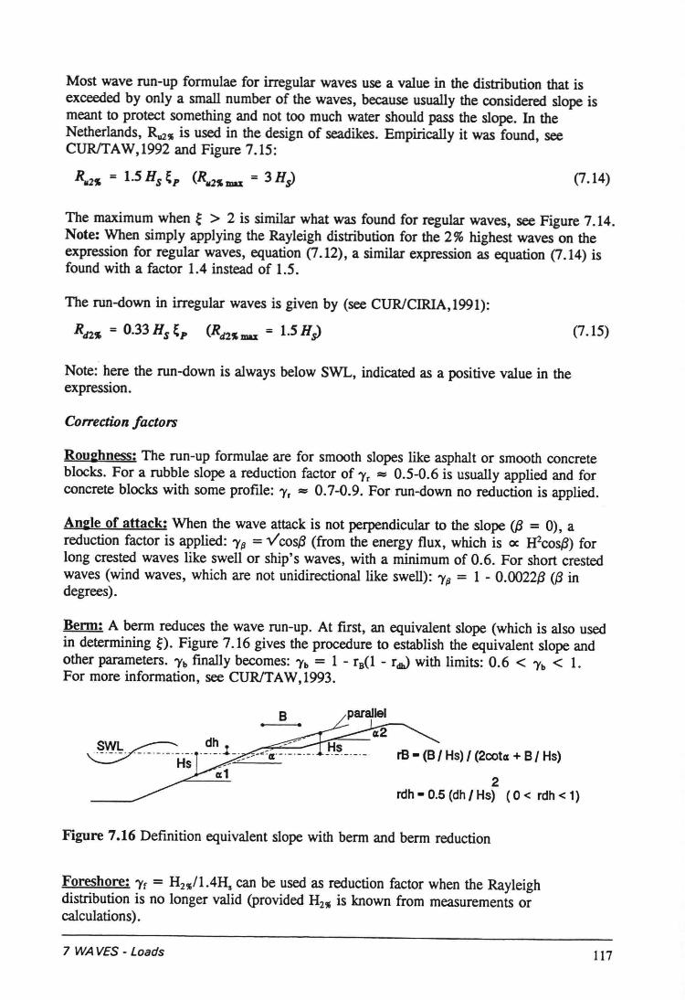
Most wave run-up formulae for irregular waves use a value in the distribution that isexceeded by only a small number of the waves, because usually the considered slope ismeant to proteet something and not too much water should pass the slope. In theNetherlands, Rul" is used in the design of seadikes. Empirically it was found, seeCURlTAW,1992 and Figure 7.15:

R.aJ. = I.S s,~p (R.,2J.mu = 3HJ (7.14)

The maximum when ~ > 2 is similar what was found for regular waves, see Figure 7.14.Note: When simply applying the Rayleigh distribution for the 2% highest waves on theexpression for regular waves, equation (7.12), a similar expression as equation (7.14) isfound with a factor 1.4 instead of 1.5.

The run-down in irregular waves is given by (see CURlCIRIA,1991):

Rd2~ = 0.33n,~p (Rd2J.mu = 1.SHs) (7.15)

Note: here the run-down is always below SWL, indicated as a positive value in theexpression.

Correction factors

Rouehness: The run-up formulae are for smooth slopes like asphalt or smooth concreteblocks. For a rubble slope a reduction factor of 'Yr = 0.5-0.6 is usually applied and forconcrete blocks with some profile: 'Yr = 0.7-0.9. For run-down no reduction is applied.

Ane1e of attack: When the wave attack is not perpendicular to the slope @ = 0), areduction factor is applied: 'YP =vcos{3(from the energy flux, which is oe H2cos(3)forlong crested waves like swell or ship's waves, with a minimum of 0.6. For short crestedwaves (wind waves, which are not unidirectionallike swell): 'Yp = 1 - 0.OO22{3({3indegrees).

Benn: A berm reduces the wave run-up. At first, an equivalent slope (which is also usedin determining ~). Figure 7.16 gives the procedure to establish the equivalent slope andother parameters. 'Yb finally becomes: 'Yb = 1 - rs(l - rcnJwith limits: 0.6 < 'Yb < 1.For more information, see CURlTAW,1993.

B

2rdh - 0.5 (dh IHs) (0 < rdh < 1)

Figure 7.16 Definition equivalent slope with berm and berm reduction

Foreshore: 'Yf = Hall.4Hs can be used as reduction factor when the Rayleighdistribution is no longer valid (provided Ha is known from measurements orcalculations).

7 WAVES - Loads 117

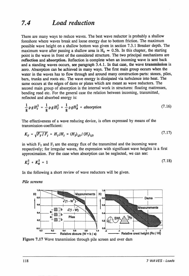
7.4 Load reduction

There are many ways to reduce waves. The best wave reductor is probably a shallowforeshore where waves break and loose energy due to bottom friction. The maximumpossible wave height on a shallow bottom was given in section 7.3.1 Breaker depth. Themaximum wave after passing a shallow area is H, := O.5h. In this chapter, the startingpoint is the wave in front of the considered structure. The two principal mechanisms arereflection and absorption. Reflection is complete when an incoming wave is sent backand a standing waves occurs, see paragraph 3.4.1. In that case, the wave transmission iszero. Absorption can be achieved in many ways. The fust main group occurs when thewater in the waves has to flow through and around many construction-parts: stones, piles,bars, trunks and roots etc. The wave energy is dissipated via turbulence into heat. Thesame occurs at the edges of dams or plates which are meant as wave reductors. Thesecond main group of absorption is the intemal work in structures: floating mattresses,bending reed etc. For the general case the relation between incoming, transmitted,reflected and absorbed energy is:

1 H2 1 H2 1 H2 bs ."8 p g 1 = "8 p g T + "8 pg R + a orptton (7.16)

The effectiveness of a wave reducing device, is often expressed by means of thetransmission-coefficient:

(7.17)

in which FT and FI are the energy flux of the transmitted and the incoming waverespectively; for irregular waves, the expression with significant wave heights is a firstapproximation. For the case when absorption can be neglected, we can see:

(7.18)

In the following a short review of wave reductors will be given.

Pile sereens

Kt Kt

O.O~--=-=-~--:---:l-:---~_---10.0 0.04 o.e 0..8 1.0 -2 .1 0 1 2

RelativaclosurerN - b I a) Relativecresthelght(ReI HijFigure 7.17 Wave transmission through pile screen and over dam

118 7 WA VES - Loads

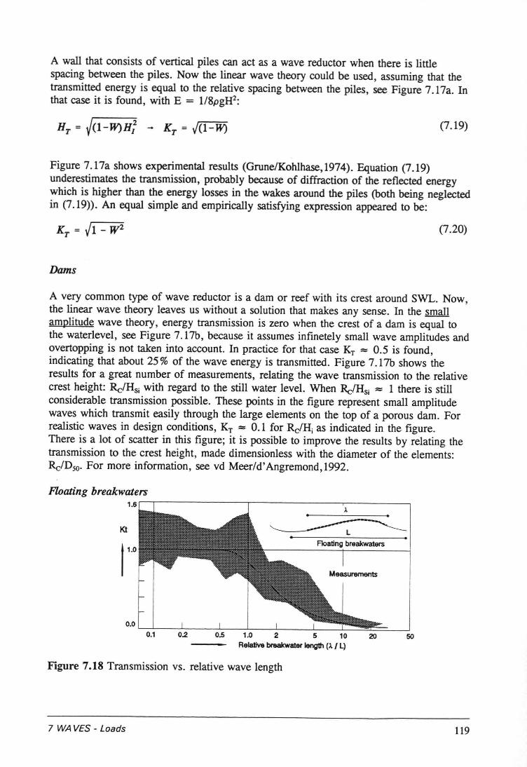
A wall that consists of vertical piles can act as a wave reductor when there is littlespacing between the piles. Now the linear wave theory could be used, assuming that thetransmitted energy is equal to the relative spacing between the piles, see Figure 7.17a. Inthat case it is found, with E = 1/8pgH2:

(7.19)

Figure 7.17a shows experimental results (Grune/Kohlhase,1974). Equation (7.19)underestimates the transmission, probably because of diffraction of the reflected energywhich is higher than the energy losses in the wakes around the piles (both being neglectedin (7.19». An equal simple and empirically satisfying expression appeared to be:

(7.20)

Dams

A very common type of wave reductor is a dam or reef with its crest around SWL. Now,the linear wave theory leaves us without a solution that makes any sense. In the smallamplitude wave theory, energy transmission is zero when the crest of a dam is equal tothe waterlevel, see Figure 7.17b, because it assumes infinetely small wave amplitudes andovertopping is not taken into account. In practice for that case KT = 0.5 is found,indicating that about 25% of the wave energy is transmitted. Figure 7.17b shows theresults for agreat number of measurements, relating the wave transmission to the relativecrest height: Rç/HSi with regard to the still water level. When Rc/Hsi = 1 there is stillconsiderable transmission possible. These points in the figure represent small amplitudewaves which transmit easily through the large elements on the top of a porous dam. Forrealistic waves in design conditions, KT = 0.1 for Rc/Hi as indicated in the figure.There is a lot of scatter in this figure; it is possible to improve the results by relating thetransmission to the crest height, made dimensionless with the diameter of the elements:Rç/D50• For more information, see vd Meer/d' Angremond, 1992.

Floating breakwaters

KlFloating breakwaters

0.1 0.2 0.5 1.0 2 5 10Relativa br'eakwater Iength ('./ L)

20 50

Figure 7.18 Transmission vs. relative wave length

7 WAVES - Loads 119

There are many types of floating breakwaters: rigid, flexible, porous etc. They have incommon that they are only effective when the length in the wave direction becomes morethan the order of magnitude of the wave length. An extra problem is formed by themooring forees on the anchors; they can become prohibitive, see vd Linden, 1985.Floating breakwaters are probably only of practical importance to reduee wavestemporarily, like during construction. Figure 7.18 gives a theoretica1 curve comparedwith measurements for a floating slab. À is the length of the protection, L the wavelength.

7.5 Summary

For the pressures and veloeities in non-breaking. shon waves, the linear wave theory, seeappendix 7.6.1, is a valuable and comprehensive tooi to get an idea of orders ofmagnitude and of the influence of parameters like wave height, period, waterdepth etc.For the description of an irregular wave field, H, and T, can best be used when workingwith single parameters instead of a whole spectrum.

To determine the shear stress under non-breaking waves, section 7.2.2 gives information,also for a combination of current and waves. Possible wave heights are limited due to .breaking. A general limit for individual waves is given by Miche:

tt, = 0.142 L tanh(21t h)L

For irregular waves, the limits are about HlLo = 0.05 - 0.06 in deep water and H/h =0.4 - 0.5 in shallow water.

In breaking waves, the character of the flow changes completely and becomes highiyturbulent. Unfottunaieiy, until now little quantative information on turbulence in the surfzone is available, so, most relations are based on empirical data. In many of theseempirical relations, the surf similarity parameter, ~, plays an importani role:

~ = tana

JH1Lo

Parameters like breaking type, breaker depth, reflection, wave run-up and run-down arerelated to ~.

Wave load reduction is possible with various devices like dams, screens, floatingbreakwaters etc. For an effective wave reduction, these structures must have largedimensions compared to waterdepin or wavelength. Their costs always should balancetheir effectiveness, otherwise dimensioning of the proteetion for the Juli load can be morecost effective.

120 7 WAVES - Loads

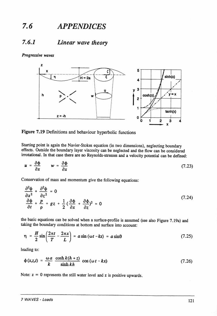
7.6 APPENDICES

7.6.1 Linear wave theory

Progressive waves

z

h

IIIIIII

I II U I

w~1'-------1I II II II II II II II II II II I

4 ./

".'

5

tanh(x)z--h O~--I!---+----I---io 1 2 3 4

-_- x

Figure 7.19 Definitions and behaviour hyperbolic functions

Starting point is again the Navier-Stokes equation (in two dimensions), neglecting boundaryeffects. Outside the boundary layer viscosity can be neglected and the flow can be consideredirrotational. In that case there are no Reynolds-stresses and a velocity potential can be defined:

u = a<l>ax

w = a<l>ax (7.23)

Conservation of mass and momentum give the following equations:

(7.24)

the basic equations can be solved when a surface-profile is assumed (see also Figure 7.19a) andtaking the boundary conditions at bottom and surface into account:

Tl = H sin (21tt - 21tX) = asin(<&>t -kt) = asin62 T L

(7.25)

leading to:

(I.) a cosh k(h + z)<I> (x,z,t) = - cos (<&> t - kx)

k sinhkh (7.26)

Note: z = 0 represents the still water level and z is positive upwards.

7 WAVES - Loads 121

From this expression for the potential q, as a function of x, z and t, allother quantities in thewave can be derived. In the following table (Table 7.1), a summary of the various parameters ispresented. The extremes for deep and shallow water in the table follow from the values fortransitional water, since for deep water: kb -+ co, so: tanh = 1, sinh = co and cosh = co and forshallow water: kb -+ 0, so: tanh = kb, sinh = kb and cosh = 1, see Figure 7.19b.

Standing waves

Progressive waves travel on without being halted. Walis, dikes and beaches do stop the waves,either by reflecting or absorbing them. VerticaI walls act like a mirror: the incoming waves aresent back and the result is superposition of two progressive waves with celerity +c and -Co Thisleads to a stand-still of the resulting wave, hence the name standing wave. The height is twice ofthat of the incoming wave.

Antlnode Node An1Inode

Figure 7.20 Standing wave

Figure 7.20 gives the pattern of a standing wave (or "clapotis"). Note that the orbits oftheparticIe movement have degenerated into straight lines. At the antinodes there is only averticaland at the nodes a horizontaI movement. The wave profile for a standing wave in firstapproximation according to linear theory is given by:

11 ::;: as coskx sin or ::;: 2aj coskx sin or

(7.27)

in which H, is the height of the incoming wave. Other characteristic expressions for standingwaves are:

u ::;: <a>a cosh k(h +z) sinla cos <a>ts sinh /ehsinh k(h +z) .w ::;:<a>as cosla sin <a>tcosh /eh

cosh k(h -z) coskx sin I.'tp = -pgz + pgas --~--=- ""cosh /eh

(7.28)

When the wall tilts backwards, the vertical motion of the water at the interface increases: themaximum waterlevel becomes higher than H, as is the case in Figure 7.20. But the standing wavepattem remains till the waves break (depending on the slope and the wave steepness).

122 7 WAVES - Loads

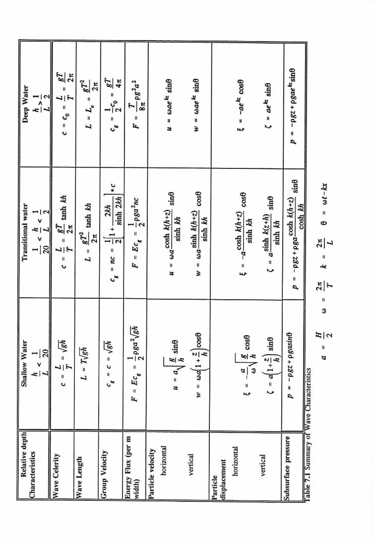
~.Sf...1 ~ (Ijf...1 ~ ~ ~ ~ ~ Jt

QoN ~I~ ('of

.S .S~ .S \)

Qo~ (;S(Ij

~"'" 11 QoN ('of (Ij

(Ij~

11 QoJt Jt Jt Jt Q.

- Q.= -IN ....:11 f...~~ 11

UOf...1: ~ ~ ~ +

A11 Cl

-IN 3 3 I ~=- ..c:I --.l --.l

11 Q.~ UO 11 11 11 11 11 11

IVQ

11 --.l u" koe :::t ~ ....,.11U

Q,

~.SU(Ij* ~ ~ ~ ~ 'N'

.....--...S (Ij (Ij

.S~ ~ u 0 8 + ~I:: (Ij t,)

(Ij ..c:"'" ~ ~ N ('of

'N' ~~ 1 ~ 'N' 'N' - ..d- -IN N

~ + + ~ +~

..c:

1(Ij

= 1 Q.

~~ s

~+ ~ 0

~~ u

V (Ij -IN-; f...1 ~ +~

oIlt ] :; oIlt ] t,)c ..c:1--.l QoN ~I~ - 11 1 :; 1 ~ ~e

(Ij (Ij (Ij (Ij.- V 11 QoN -IN U"

Q.- (Ij t,) (Ij

'r;]~ (;S (;S (;S +-I~ --.llf... 11 (;S

C11

3 3 I~

=11

11"'" 11 --.l u11 Q.

E- I:: koe 11 11V I

U 11:::t ~ ....,.

11u"Q,

~ ~~ ~ ~ .S8 (Ij('of ~ 0 .S s"'" ~ ~ ~ .S U (Ij-~

~(Ij -NI..c: I QoI; .- Q.

- Q.= -I~NI..c: +

~ 11 11 -IN I QoI; ++

~~ - 1:S13 - en~ V --.llf... ~ 11

~ ~ Q. ~11 (;S ....~I I en

..c:1--.l 11 ..C

11 --.l ~ 1111

= ~ 11 11 Q)..

11t)

.c ~ ::l~ ~v

'"11

~ ....,.Q, ...koe

~Q)

~~

~ 0.c

"'" >.e = ...-en '"

=-"'" -ca -ca !S E

~~ >. --= .... e -ca "'" E

>. =- - e -ca'0 0 (.) =-~ ~ .... .... - 0 (.) .... .t:!

~

.... - .... .c '0 >< e N 'E e 'E ~.- .... .t: .... e = Q;j 'C ~ ... ~- r:Il etJ

e 0 Q)~ Q;j ri: 0 Q)

:>- ..:: ....ca ._

e ... :>- .c .- "'" Q;j~ > .c

.!! ~"'" e-

~ ~~~êj U ...._~ ~ ca = .!!

=- etJ.c .- - en= ~ ~ = ""'- .... -=- .Q .Q"'" ... ... ~ ~-= "'" "'" r:Il uZ 11'=ca i = "'" ~j_ __f __f:s.c

~ e"U

~I-311

11

11

11

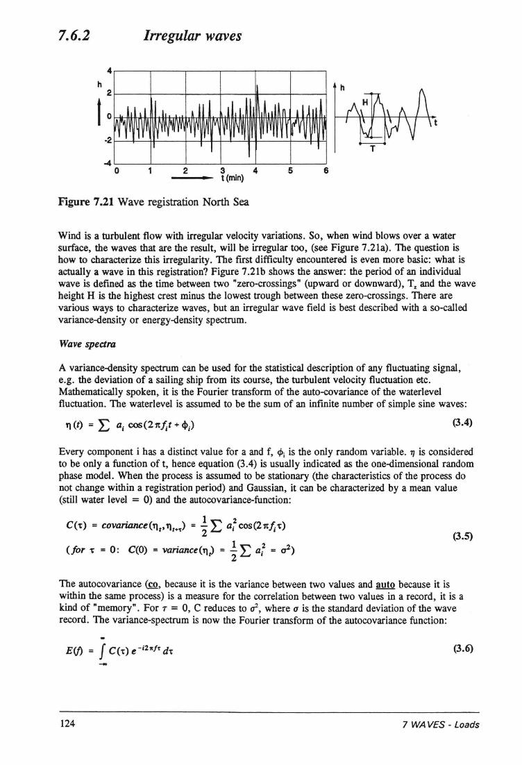
7.6.2 Irregular waves

4h

2

I0-2

-40 1 2 3 4 5 6

t (mln)

t

T

Figure 7.21 Wave registration North Sea

Wind is a turbulent tlow with irregular velocity variations. So, when wind blows over a watersurface, the waves that are the result, will be irregular too, (see Figure 7.21a). The question ishow to characterize this irregularity. The first difficulty encountered is even more basic: what isactually a wave in this registration? Figure 7.21b shows the answer: the period of an individualwave is defined as the time between two "zero-crossings" (upward or downward), T, and the waveheight H is the highest crest minus the lowest trough between these zero-crossings. There arevarious ways to characterize waves, but an irregular wave field is best described with a so-calledvariance-density or energy-density spectrum.

Wave spectra

A variance-density spectrum can be used for the statistical description of any tluctuating signal,e.g. the deviation of a sailing ship from its course, the turbulent velocity tluctuation etc.Mathematically spoken, it is the Fourier transform of the auto-covarianee of the waterleveltluctuation. The waterlevel is assumed to be the sum of an infinite number of simple sine waves:

(3.4)

Every component i has a distinct value for a and f, <Pi is the only random variabIe. 1] is consideredto be only a function of t, hence equation (3.4) is usually indicated as the one-dimensional randomphase model. When the process is assumed to be stationary (the characteristics of the process donot change within a registration period) and Gaussian, it can be characterized by a meao value(still water level = 0) and the autocovariance-function:

C('t) = covariance(l1,. 'l'+'f) = !L aj2 COS(21tf; r)2

(for 't = 0: C(O)= variance('l,) = !L a; = al)2

(3.5)

The autocovariance @, because it is the varianee between two values and auto because it iswithin the same process) is a measure for the correlation between two values in a record, it is akind of "memory". For T = 0, C reduces to dl, where u is the standard deviation of the waverecord. The varianee-spectrum is now the Fourier transform of the autocovariance function:

E(j) ;::;f C('t) e -j2K/'f d't (3.6)-.

124 7 WAVES - Loads

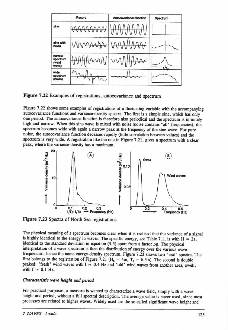
AuIocoYarianc:e fundion

sine

Record Speclrum

'OOoool\oor \ A A (\ A A n A {VVOVvOvvo \f\fV\fVVVV

'ifO.10

i"Q

Bi o.>

I Isine wiIhnoIse

\1\f\(\!\AI11\f\. \A{\OA"{\(\fUV v~vrvll\J \Tv VVVV v v

t

nanowspectrum(windwave)

wldespectrum(noise)

Figure 7.22 Examples of registrations, autocovariance and spectrum

Figure 7.22 shows some examples of registrations of a tluctuating variabie with the accompanyingautocovariance functions and variance-density spectra. The fust is a simple sine, which has onlyone period. The autocovariance function is therefore also periodical and the spectrum is infinitelyhigh and narrow. When this sine wave is mixed with noise (noise contains "all" frequencies), thespectrum becomes wide with again a narrow peak at the frequency of the sine wave. For purenoise, the autocovariance function deceases rapidly (little correlation between values) and thespectrum is very wide. A registration like the one in Figure 7.21, gives a spectrum with a clearpeak, where the variance-density has a maximum.

20'N%

t oL-~~+-~~~~o 0.1' 0.2 0.31ITp 1ITs - Frequency (Hz)

Figure 7.23 Spectra of North Sea registrations

Swell ®

o

The physical meaning of a spectrum becomes clear when it is realised that the varianee of a signalis highly identical to the energy in waves. The specific energy, see Table 7.1, is with H = 2a,identical to the standard deviation in equation (3.5) apart from a factor pg. The physicalinterpretation of a wave spectrum is then the distribution of energy over the various wavefrequencies, hence the name energy-density spectrum. Figure 7.23 shows two "real" spectra. Thefirst belongs to the registration of Figure 7.21 (H, = 4m, T, = 6.5 s). The second is doublepeaked: "fresh" wind waves with f """0.4 Hz and "old" wind waves from another area, swell,with f """0.1 Hz.

Characteristic wave height and period

For practical purposes, a measure is wanted to characterize a wave field, simply with a waveheight and period, without a full speetral description. The average value is never used, since mostprocesses are related to higher waves. Widely used are the so-called significant wave height and

7 WAYES - Loads 125

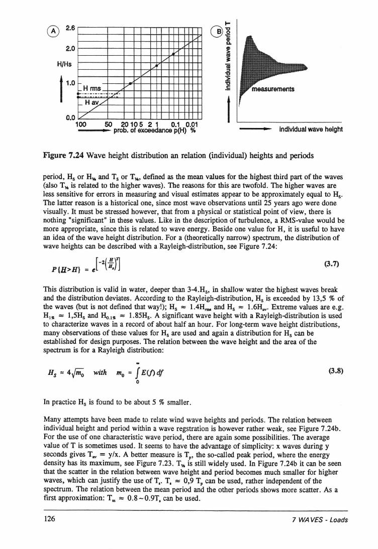
o 2.6i--"

,,;

t'"/

.//'

,/'~ V~H rms~._._._._. :z--_._._._.f- Hav/

/""L

2.0

H/Hs

0.0100 50 20105 2 1 0.1 0.01---- prob. of exceedancep(H) % IndMduai wave helght

Figure 7.24 Wave height distribution an relation (individual) heights and periods

period, H, or H~ and T, or T~, defined as the mean values for the highest third part of the waves(also T~ is related to the higher waves). The reasons for this are twofold. The higher waves areless sensitive for errors in measuring and visual estimates appear to be approximately equal to Hs.The latter reason is a historical one, since most wave observations until 25 years ago were donevisually. It must be stressed however, that from a physical or statistical point of view, there isnothing "significant" in these values. Like in the description of turbulence, a RMS-value would bemore appropriate, since this is related to wave energy. Beside one value for H, it is useful to havean idea of the wave height distribution. For a (theoretically narrow) spectrum, the distribution ofwave heights can be described with a Rayleigh-distribution, see Figure 7.24:

P{H>H} = J-2(~)1 (3.7)

This distribution is valid in water, deeper than 3-4.Hs, in shallow water the highest waves breakand the distribution deviates. According to the Rayleigh-distribution, H, is exceeded by 13,5 % ofthe waves (but is not defined that way!); H, ::::I.4HI'IIIIand H, :::: 1.6H..v.Extreme values are e.g.Hl" :::: 1,5Hs and Ho.l" :::: 1.85Hs' A significant wave height with a Rayleigh-distribution is usedto characterize waves in a record of about half an hour. For long-term wave height distributions,many observations of these values for H, are used and again a distribution for H, can beestablished for design purposes. The relation between the wave height and the area of thespectrum is for a Rayleigh distribution:

s, ::4..fiiïo with mo = J E(j) djo

In practice H, is found to be about 5 % smaller.

(3.8)

Many attempts have been made to relate wind wave heights and periods. The relation betweenindividual height and period within a wave regstration is however rather weak, see Figure 7.24b.For the use of one characteristic wave period, there are again some possibilities. The averagevalue of T is sometimes used. It seems to have the advantage of simplicity: x waves during yseconds gives Tav = y/x. A better measure is Tp, the so-called peak period, where the energydensity has its maximum, see Figure 7.23. T~ is still widely used. In Figure 7.24b it can be seenthat the scatter in the relation between wave height and period becomes much smaller for higherwaves, which can justify the use of T,. T, ::::0,9 T, can be used, rather independent of thespectrum. The relation between the mean period and the other periods shows more scatter. As afirst approximation: Tm ::::0.8-0.9T, can be used.

126 7 WAVES - Loads

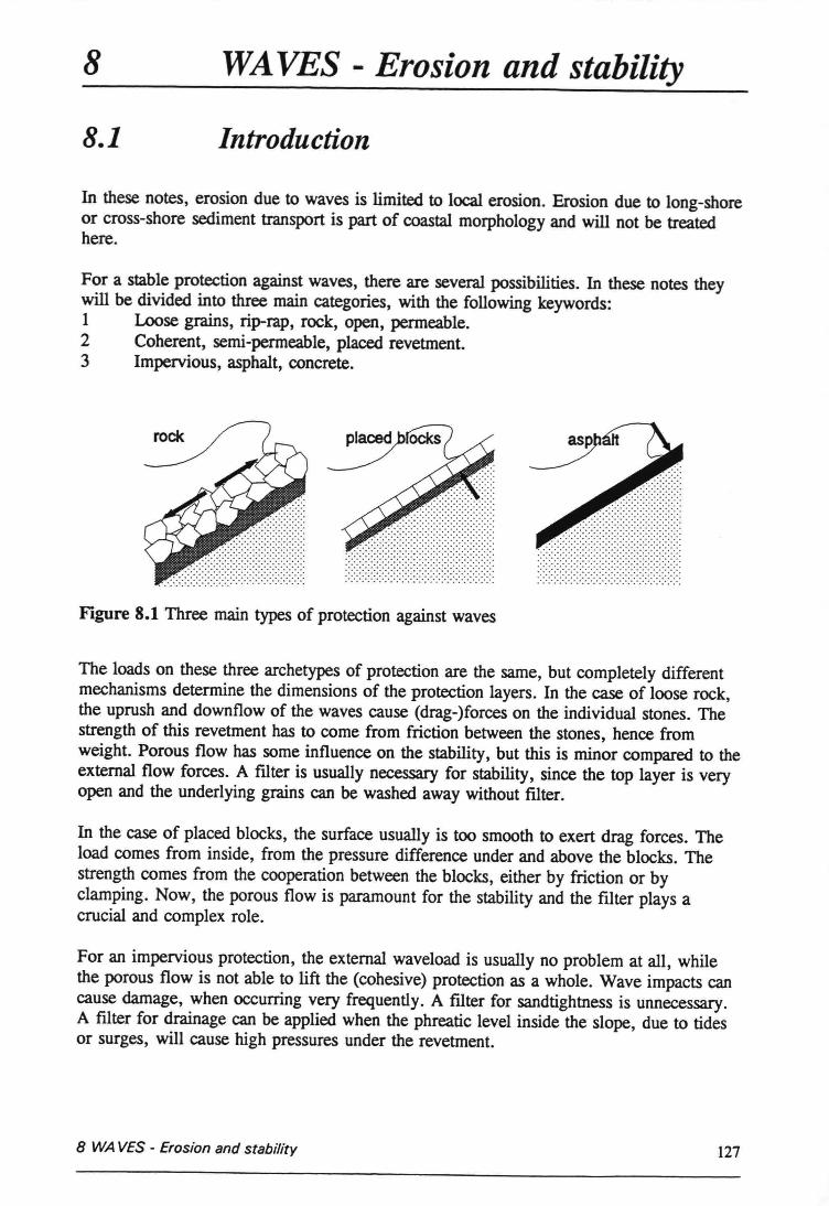
8 WAYES - Erosion and stability

8.1 Introduetion

In these notes, erosion due to waves is limited to local erosion. Erosion due to long-shoreor cross-shore sediment transport is part of coastal morphology and will not be treatedhere.

For a stabie proteetion against waves, there are several possibilities. In these notes theywill he divided into three main categories, with the following keywords:1 Loose grains, rip-rap, rock, open, permeabie.2 Coherent, semi-permeabie, placed revetment.3 Impervious, asphalt, concrete.

:::::::::::::::::::::::::::::::::::::::::::::::::::::........................ - .:.:.:.:-:.:.:.:.:.:.:.:.:.:.:.:.:.:.:.:.:.:.:.:.:.:-:.....................................................

Figure 8.1Three main types of proteetion against waves

. ..................................................... -.-:-:':-:-:':':-:-:':':':':-:<':':-:-:':':':':'~:~:~:~:~:~:~:~:~:~:~:~:~:~:~:~:~:~:~:~:~:~:~:~:~:~

The loads on these three archetypes of proteetion are the same, but completely differentmechanisms determine the dimensions of the proteetion layers. In the case of loose rock,the uprush and downflow of the waves cause (drag-)forces on the individual stones. Thestrength of this revetment has to come from friction between the stones, hence fromweight. Porous flow has some influence on the stability, but this is minor compared to theextemal flow forces. A filter is usually necessary for stability, since the top layer is veryopen and the underlying grains can be washed away without filter.

In the case of placed blocks, the surface usually is too smooth to exert drag forces. Theload comes from inside, from the pressure difference under and above the blocks. Thestrength comes from the cooperation between the blocks, either by friction or byclamping. Now, the porous flow is paramount for the stability and the filter plays acrucial and complex role.

For an impervious protection, the extemal waveload is usually no problem at all, whilethe porous flow is not able to lift the (cohesive) proteetion as a whoie. Wave impacts cancause damage, when occurring very frequently. A filter for sandtightness is unnecessary.A filter for drainage can be applied when the phreatic level inside the slope, due to tidesor surges, will cause high pressures under the revetment.

8 WAVES - Erosion and stability 127

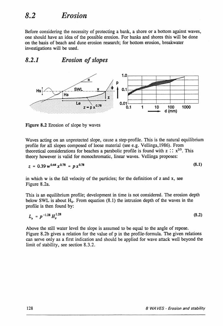
8.2 Erosion

Before considering the necessity of protecting a bank, a shore or a bottom against waves,one should have an idea of the possible erosion. For banks and shores this will be doneon the basis of beach and dune erosion research; for bottom erosion, breakwaterinvestigations will be used.

8.2.1 Erosion of slopes

1.0

~ ---F'

...............LJI'"

1 10 100 1000-- d(mm)....................................................... .

0 •••••• ···,·· ••••••••••••••••••••••••

Figure 8.2 Erosion of slope by waves

Waves acting on an unprotected slope, cause a step-profile. This is the natura! equilibriumprofile for all slopes composed of loose material (see e.g. Vellinga,1986). Fromtheoretica1 considerations for beaches a parabolic profile is found with z :: x2l3• Thistheory however is valid for monochromatic, linear waves. Veilinga proposes:

z = 0.39 wO.44 XO.78 = P X 0.78 (8.1)

in which w is the fall velocity of the partic1es; for the defmition of z and x, seeFigure 8.2a.

This is an equilibrium profile; development in time is not considered. The erosion depthbelow SWL is about Hs. From equation (8.1) the intrusion depth of the waves in theprofile is then found by:

L = -1.28H1.28e P s

(8.2)

Above the still water level the slope is assumed to be equal to the angle of repose.Figure 8.2b gives a relation for the value of p in the profile-formula. The given relationscan serve only as a first indication and should be applied for wave attack weil beyond thelimit of stability, see section 8.3.2.

128 8 WAVES - Erosion and stability

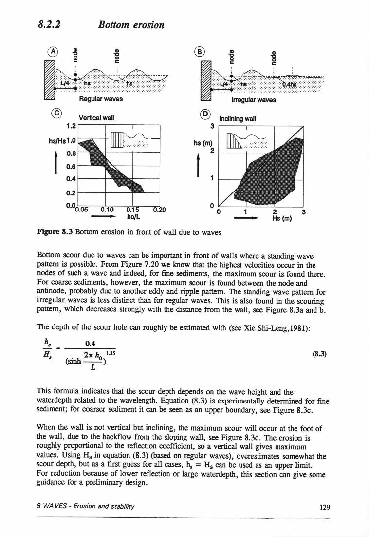
8.2.2 Bottom erosion

®

Irregular waves

@ VertIcaI wall @ Incllnlng wall1.2 3

hs (m)

t2

t 1

1 2 3Hs (m)

Figure 8.3 Bottom erosion in front of wall due to waves

Bottom scour due to waves can be important in front of walls where a standing wavepattern is possible. From Figure 7.20 we know that the highest veloeities occur in thenodes of such a wave and indeed, for fine sediments, the maximum scour is found there,For coarse sediments, however, the maximum scour is found between the node andantinode, probably due to another eddy and ripple pattern. The standing wave pattern forirregular waves is less distinct than for regular waves. This is also found in the scouringpattern, which decreases strongly with the distance from the wall, see Figure 8.3a and b.

The depth of the scour hole can roughly be estimated with (see Xie Shi-Leng, 1981):

hs 0.4=------21t h 1.35

(sinh-_O)L

(8.3)

This formula indicates that the scour depth depends on the wave height and thewaterdepth related to the wavelength. Equation (8.3) is experimentally determined for finesediment; for coarser sediment it can be seen as an upper boundary, see Figure 8.3c.

When the wall is not vertical but inclining, the maximum scour will occur at the foot ofthe wall, due to the backflow from the sloping wall, see Figure 8.3d. The erosion isroughly proportional to the reflection coefficient, so avertical wall gives maximumvalues. Using H, in equation (8.3) (based on regular waves), overestimates somewhat thescour depth, but as a first guess for all cases, h, = H, can be used as an upper limit.For reduction because of lower reflection or large waterdepth, this section can give someguidance for a preliminary design.

8 WAVES - Erosion and stability 129

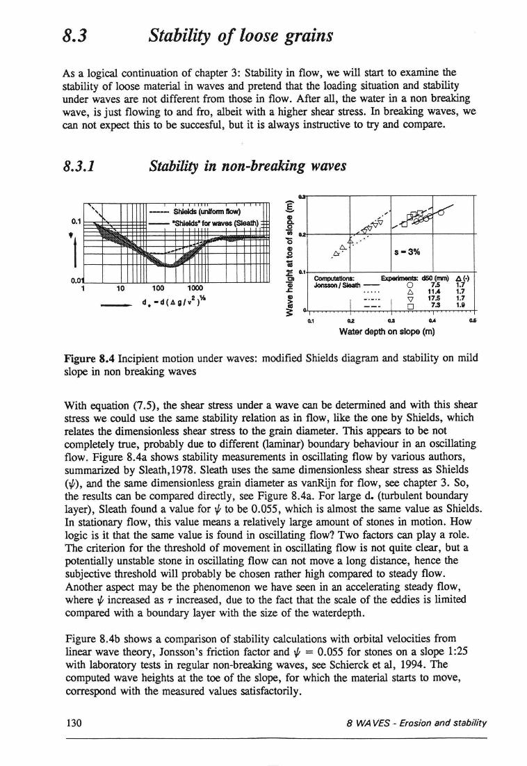
8.3 Stability of loose grains

As a logical continuation of chapter 3: Stability in flow, we will start to examine thestability of loose material in waves and pretend that the loading situation and stabilityunder waves are not different from those in flow. After all, the water in a non breakingwave, is just flowing to and fro, albeit with a higher shear stress. In breaking waves, wecan not expect this to be succesful, but it is always instructive to try and compare.

8.3.1 Stability in non-breaking waves

--- ShIeIds (uniform lIow)Ê-a0'i)-0CDSäi- 0.1.s=ClGis:CD~~

0.1

~..~. s-3%

Computa1ions: Experiments: cI50 (mm) ~ (.)Jonsson I SIeath - 0 7.5 1.1

6 11A 1.7"V 17.5 1.7o 7.3 1.8

Water depth on slope (m)

Figure 8.4 Incipient motion under waves: modified Shields diagram and stability on mildslope in non breaking waves

With equation (7.5), the shear stress under a wave can be determined and with this shearstress we could use the same stability relation as in flow, like the one by Shields, whichrelates the dimensionless shear stress to the grain diameter. This appears to be notcompletely true, probably due to different (laminar) boundary behaviour in an oscillatingflow. Figure 8.4a shows stability measurements in oscillating flow by various authors,summarized by Sleath,1978. Sleath uses the same dimensionless shear stress as Shields(1/1), and the same dimensionless grain diameter as vanRijn for flow, see chapter 3. So,the results can be compared directly, see Figure 8.4a. For large d, (turbulent boundarylayer), Sleath found a value for 1/1 to be 0.055, which is almost the same value as Shields.In stationary flow, this value means a relatively large amount of stones in motion. Howlogic is it that the same value is found in oscillating flow? Two factors can play a role.The criterion for the threshold of movement in oscillating flow is not quite c1ear, but apotentially unstable stone in oscillating flow can not move a long distance, hence thesubjective threshold will probably be chosen rather high compared to steady flow.Another aspect may be the phenomenon we have seen in an accelerating steady flow,where 1/1 increased as T increased, due to the fact that the scale of the eddies is limitedcompared with a boundary layer with the size of the waterdepth.

Figure 8.4b shows a comparison of stability calculations with orbital veloeities fromlinear wave theory, Jonsson's friction factor and 1/1 = 0.055 for stones on a slope 1:25with laboratory tests in regular non-breaking waves, see Schierck et al, 1994. Thecomputed wave heights at the toe of the slope, for which the material starts to move,correspond with the measured values satisfactorily.

130 8 WAYES - Erosion and stability

8.3.2 Stability in breaking waves

Most research on the stability of stones on a slope was done in the field of breakwaters,which is very much related to slope protections and revetments, but it is not the same. Animportant difference in the stability is the porosity of the structure as a whoie.Breakwaters usually have aporous core, while in dike revetments the core is made ofclay or sand. This has a significant influence on the stability of the protecting armourlayer as we will see later on in this section. We will start, however, with simple basicprinciples and will discuss shortcomings and extensions later on.

Encouraged by the succesful results of the modified Shields curve for waves, the next stepwould he the use of a slope correction factor and to take the breaking of the waves intoaccount. We use the same slope factor as for flow in the slope direction (for the 1:25slope in the previous section, this factor == 1). For the velocity in a breaking wave, noreliable expression is available. As a first guess, we will assume that the velocity in abreaking or broken wave on a slope is proportional to the celerity in shallow water withthe wave height as a representative measure for the waterdepth: u oe vigH. Following thesame reasoning as with stability in flow, see chapter 3, we find:

oe (p" -p,)gd3 (tanècose ±sin«)resisting force slope correction

(8.4)

Note: + and - in the slope correction are for uprush and backwash respectively. Raisingall terms to the third power and working with the mass of the stone (M oe p.d3) we find:

PsH3Moe---__;;_ _A3(tancllcos« ± sine)?

(8.5)

This is Irribarren's formula for stability of rock on slopes in waves, dating back to 1938.After the second world war, many tests were performed (particularly by Hudson,1953) tofind the constants of proportionality in equation (7.9), (8.5). Hudson finally proposed, forpractical reasons, another formula:

PsH3M = --=---­

KDA3cotex(or. (8.6)

Note: the use of HlAd as a stability parameter is convenient and is similar to flow, whereu2/.1d is used. The slope correction in Irribarren's formula is now reduced to cota. Thismeans that the validity of Hudson's formula is limited, because coto is insufficient todescribe friction and equilibrium on a slope: for a = 0, W = 0 and for a > tb, W hasstill a finite value, both of which are nonsense. The range of a for which Hudson is validis about 1.5 < coto < 4. The Hudson-formula is tested for waves that did not break atthe toe of the slope and did not overtop it. For cases where this is not true, extracorrections for Kn are sometimes applied. Hudson's formula is simple and is usedworldwide. Kn is again a dustbin-factor in which implicitely the accepted degree ofdamage. KD has different values for different kinds of elements (3-4 for natura! rock to 8-10 for artificial elements like tetrapods and tribars). The Shore Proteetion Manual(SPM,1984) gives values for Kn for various circumstances.

8 WAVES - Erosion and stability 131

The simplicity of the Hudson formula has its price. Some limitations of the presentedformulae have already been mentioned. The most important are:

Wave periodAlready in the Irribarren-formula this parameter is absent. There are two ways in whichthe period can have influence on stability. The period is related to the wave-length, henceto the wave-steepness and hence to the breaking pattern on the slope, which will defmitelyplay a role. The other one is the possible role of inertia-forces on a grain which dependon duldt, hence on the wave-period.

PermeabilityThe permeability of the structure must play an important role. In the assumptions onwhich Irribarren's formula is based, only a kind of drag force on the slope is included.The forces under and behind a grain will certainly be co-responsible for the equilibrium.It is easy to imagine that a homogeneous mass of stones will react different from a coverlayer of stones on an impermeable core. In the first case, a lot of wave energy isdissipated in the core, while in the latter the pressure build-up under the cover-layer canbe considerable.

Number of wavesAll modeltests in the 50's and 6O's were done with regular, monochromatic waves. Itappeared in those tests that the equilibrium damage profile was reached in, say, one halfhour. The wave height in the tests was then usually declared equivalent to Hs. It appearedfrom tests with wave spectra that the number of waves is not unimportant, which is logic,since more waves mean a greater chance for a large one.

Damage levelLike stones in flow, the threshold of motion is not always clear. The KD-valuesin theHudson formula are supposed to be valid for 5% damage, but the definition of damage isnot very c1ear.

All these objections led to new research activities, especially after some failures ofbreakwaters. In a period of about ten years the recommended coefficients in the ShoreProteetion Manual for breakwater design with the Hudson formula led to an increase inweight of about 200%. In the Netherlands, extensive modeltests were done to overcomethe limitations of and objections against the Hudson-formula. The results of curve-fittingof these large and small scale tests with irregular waves, finally led to the followingequations, see van der Meer,1988 summarized in CURICIRIA,1991:

H (s )0.2___!_ = 6.2 P 0.18 ~ ~ ~5àd .jN 111

H (s ]0.2zs. = l.Op~·13 ~ ~p Jcotf1.àd .jN m

(plunging breakersï(8.7)

(surging breakers)

The transition between the two expressions is found by equating them, giving:

~transitioll = [6.2P 0.31Jtm Cl] (p+105)(8.8)

when ~ > ~t the equation for surging breakers has to be used, for ~ < ~u the equation

132 8 WAVES - Erosion and stability

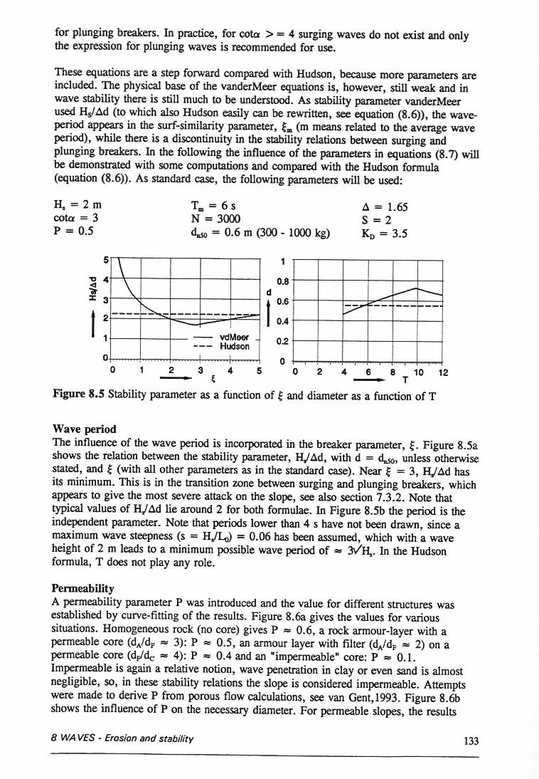
for plunging breakers. In practice, for coto >= 4 surging waves do not exist and onlythe expression for plunging waves is recommended for use.

These equations are a step forward compared with Hudson, because more parameters areincluded. The physical base of the vanderMeer equations is, however, still weak and inwave stability there is still much to be understood. As stability parameter vanderMeerused Hs/A.d (to which also Hudson easily can be rewritten, see equation (8.6», the wave­period appears in the surf-similarity parameter, ~m (m means related to the average waveperiod), while there is a discontinuity in the stability relations between surging andplunging breakers. In the following the influence of the parameters in equations (8.7) willbe demonstrated with some computations and compared with the Hudson formula(equation (8.6». As standard case, the following parameters will be used:

H, = 2 mcoto = 3P = 0.5

Tm = 6 sN = 3000<luso = 0.6 m (300 - 1000 kg)

A.= 1.65S=2KD = 3.5

5 \\

----~ ....---~--- -.==-

- vdMeer--- HudsonI I

1

~ ,..--......__;7 Fo-- ---....--

"C 4~:E: 3

oo 1 2 3 4

0.8d

t0.6

0.4

0.2

o5 0 2 4 6 8 10 12

T

Figure 8.5 Stability parameter as a function of ~ and diameter as a function of T

Wave periodThe influence of the wave period is incorporated in the breaker parameter, ~. Figure 8.5ashows the relation between the stability parameter, H/A.d, with d = <Ïuso, unless otherwisestated, and ç (with allother parameters as in the standard case). Near ç = 3, H/ A.dhasits minimum. This is in the transition zone between surging and plunging breakers, whichappears to give the most severe attack on the slope, see also section 7.3.2. Note thattypical values of H/A.d lie around 2 for both formulae. In Figure 8.5b the period is theindependent parameter. Note that periods lower than 4 s have not been drawn, since amaximum wave steepness (s = H/!.o) = 0.06 has been assumed, which with a waveheight of 2 m leads to a minimum possible wave period of =::: 3VH,. In the Hudsonformula, T does not play any role.

PermeabilityA permeability parameter P was introduced and the value for different structures wasestablished by curve-fitting of the results. Figure 8.6a gives the values for varioussituations. Homogeneous rock (no core) gives P :::::0.6, a rock armour-layer with apermeable core (dA/dF =::: 3): P :::::0.5, an armour layer with filter (dA/dF ::::: 2) on apermeable core (dF/dc =::: 4): P :::::0.4 and an "impermeable" core: P :::::0.1.ImpermeabIe is again a relative notion, wave penetration in clay or even sand is almostnegligible, so, in these stability relations the slope is considered impermeabIe. Attemptswere made to derive P from porous flow calculations, see van Gent,1993. Figure 8.6bshows the influence of Pon the necessary diameter. For permeable slopes, the results

8 WAVES - Erosion and stability 133

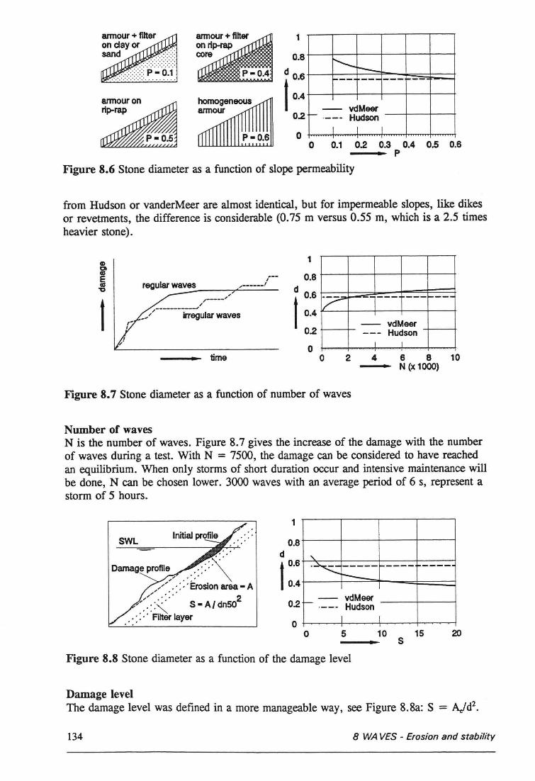
annouronrip-rap

1

0.8 i'-r--~----- -~--- vdMeer

I- ._-- HudsonI I I

dl 0.60.4

0.2

o o 0.1 0.2 0.3 0.4 0.5 0.6p

Figure 8.6 Stone diameter as a function of slope permeability

from Hudson or vanderMeer are almost identica1, but for impermeable slopes, like dikesor revetments, the difference is considerable (0.75 m versus 0.55 m, which is a 2.5 timesheavier stone).

r:regular W.:8V.:..;8S::-__ --r,,:;_-_--_--_-'_

1

0.8

I?-,- --~ .-

-_ vdMeer--- Hudson

I I

"/-----",;,,----------",./ irregular wavesI I

d 0.6

0.4

0.2

otime o 6 8 10

N (x 1000)2 4

Figure 8.7 Stone diameter as a function of number of waves

Number of wavesN is the number of waves. Figure 8.7 gives the increase of the damage with the numberof waves during a test. With N = 7500, the damage can be considered to have reachedan equilibrium. When only storms of short duration occur and intensive maintenance willbe done, N can be chosen lower. 3000 waves with an average period of 6 s, represent astorm of 5 hours.

SWL

Damage profile .r ,:" './<.::.ErosIon area - A~,," _- _-" '. 2"".-::< S - AI dn50

.: : : .: Filter layer

1

'\.

.~ ----- I----- ----t----

-- vdMeer~ Hudson._--I I

0.8d

t0.6

0.4

0.2

oo 5 15 2010

Figure 8.8 Stone diameter as a function of the damage levelS

Damage levelThe damage level was defined in a more manageable way, see Figure 8.8a: S = Ajd2•

134 8 WAVES - Erosion and stability

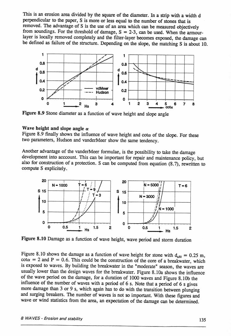
This is an erosion area divided by the square of the diameter. In a strip with a width dperpendicular to the paper, S is more or less equal to the number of stones that isremoved. The advantage of S is the use of an area which can be measured objectivelyfrom soundings. For the threshold of damage, S = 2-3, can be used. When the armour­layer is loca11yremoved completely and the filter-layer becomes exposed, the damage canbe defined as failure of the structure. Depending on the slope, the matching S is about 10.

1 ->//

~~/

- vdMeer/~ ._-- HudsonI

0.8

dl 0.6

0.4

0.2

oo 1 2 Hs 3

Figure 8.9 Stone diameter as a function of wave height and slope angle

1

~ r-,",~

~ ~ ;:.:::.- -- -0.8

d

I0.60.4

0.2

o4 1 2 3 4 5 678__ ~OOt4

Wave height and slope angle aFigure 8.9 finally shows the influence of wave height and coto of the slope. For thesetwo parameters, Hudson and vanderMeer show the same tendency.

Another advantage of the vanderMeer formulae, is the possibility to take the damagedevelopment into acccount. This can be important for repair and maintenance policy, butalso for construction of a protection. S can be computed from equation (8.7), rewritten tocompute S explicitely.

20 I +-6 j I /N -1000: T-9I

. ,I T-3I )I :/I

/V~.

S 15

t:o

o 0.5__ 1_ Hs 1.5

20N-5000:'1 T-6I II :

UN-3000 ::1:1 IJ'1:iIN-1000

!I.z-'I

S 15

o2 o 0.5 1 1.5- __ Hs 2

Figure 8.10 Damage as a function of wave height, wave period and storm duration

Figure 8.10 shows the damage as a function of wave height for stone with duso = 0.25 m,coto = 2 and P = 0.6. This could be the construction of the core of a breakwater, whichis exposed to waves. By building the breakwater in the "moderate" season, the waves areusually lower than the design waves for the breakwater. Figure 8.10a shows the influenceof the wave period on the damage, for a duration of 1000 waves and Figure 8. !Ob theinfluence of the number of waves with a period of 6 s. Note that a period of 6 s givesmore damage than 3 or 9 s, which again has to do with the transition between plungingand surging breakers. The number of waves is not so important. With these figures andwave or wind statistics from the area, an expectation of the damage can be determined.

8 WAVES - Erosion and stability 135

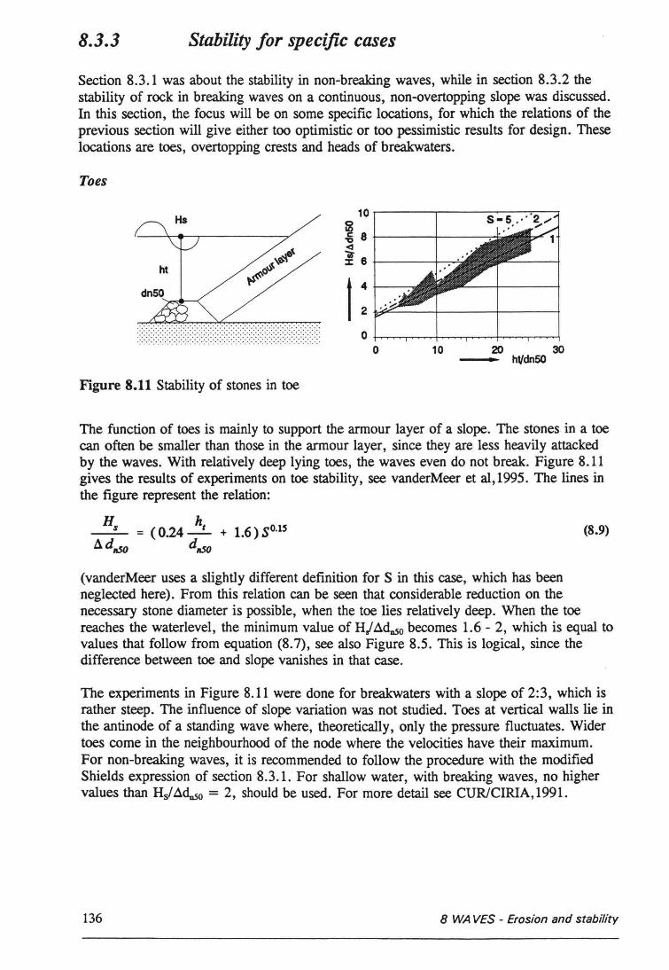
8.3.3 Stability lor specijic cases

Section 8.3.1 was about the stability in non-breaking waves, while in section 8.3.2 thestability of rock in breaking waves on a continuous, non-overtopping slope was discussed.In this section, the focus will be on some specific locations, for whieh the relations of theprevious section will give either too optimistie or too pessimistie results for design. Theselocations are toes, overtopping erests and heads of breakwaters.

Toes

10.---------~------------~----~~

!8 i-----+-----;-o:<I

! 6 +-----------+.......,.......

........................................... .... . .... , ..:.:.:.:-:.:.:.:::::::::::::::::::::::;:.:.:.:::::::::::::::::::::::::::::::::::

o 10 20 30-- ht/dn50

Figure 8.11 Stability of stones in toe

The funetion of toes is mainly to support the armour layer of a slope. The stones in a toecan often be smaller than those in the armour layer, since they are less heavily attaekedby the waves. With relatively deep lying toes, the waves even do not break. Figure 8.11gives the results of experiments on toe stability, see vanderMeer et al,1995. The lines inthe figure represent the relation:

Hs = (0.24 .s. + 1.6) SO.ISAdn50 dn50

(8.9)

(vanderMeer uses a slightly different definition for S in this case, whieh has beenneglected here). From this relation can be seen that considerable reduetion on thenecessary stone diameter is possible, when the toe lies relatively deep. When the toereaehes the waterlevel, the minimum value of Hi .ä.doSobecomes 1.6 - 2, whieh is equal tovalues that follow from equation (8.7), see also Figure 8.5. This is logical, sinee thedifference between toe and slope vanishes in that case.

The experiments in Figure 8.11 were done for breakwaters with a slope of 2:3, whieh israther steep. The influence of slope variation was not studied. Toes at vertical walls lie inthe antinode of a standing wave where, theoretically, only the pressure fluetuates. Widertoes come in the neighbourhood of the node where the veloeities have their maximum.For non-breaking waves, it is recommended to follow the procedure with the modifiedShields expression of section 8.3.1. For shallow water, with breaking waves, no highervalues than Hs/.ä.~o = 2, should be used. For more detail see CURICIRIA, 1991.

136 8 WAVES - Erosion and stability

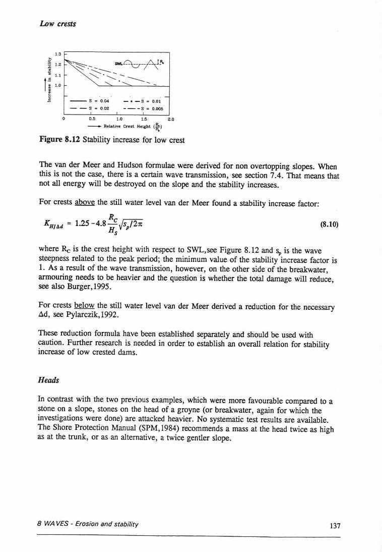
Low crests

1.3

-- 5 = 0.04

- - 5 = 0.02

-. -5 = 0.01

---5 = 0.005

~~ 1.2

"-;; 1.1

1i1.0

ec.5

o 0.5 1.0 1.5 2.0

- Relative Crest Height (fr>Figure 8.12 Stability increase for low crest

The van der Meer and Hudson formulae were derived for non overtopping slopes. Whenthis is not the case, there is a certain wave transmission, see section 7.4. That means thatnot all energy will be destroyed on the slope and the stability increases.

For crests above the still water level van der Meer found a stability increase factor:

(8.10)

where Re is the crest height with respect to SWL,see Figure 8.12 and Sp is the wavesteepness related to the peak period; the minimum value of the stability increase factor is1. As a result of the wave transmission, however, on the other side of the breakwater,armouring needs to be heavier and the question is whether the total damage will reduce,see also Burger, 1995.

For crests below the still water level van der Meer derived a reduction for the necessary~d, see Pylarczik, 1992.

These reduction formula have been established separately and should be used withcaution. Further research is needed in order to establish an overall relation for stabilityincrease of low crested dams.

Heads

In contrast with the two previous examples, which were more favourable compared to astone on a slope, stones on the head of a groyne (or breakwater, again for which theinvestigations were done) are attacked heavier. No systematic test results are available.The Shore Proteetion Manual (SPM,1984) recommends a mass at the head twice as highas at the trunk, or as an alternative, a twice gentler slope.

8 WAVES - Erosion and stebîlitv 137

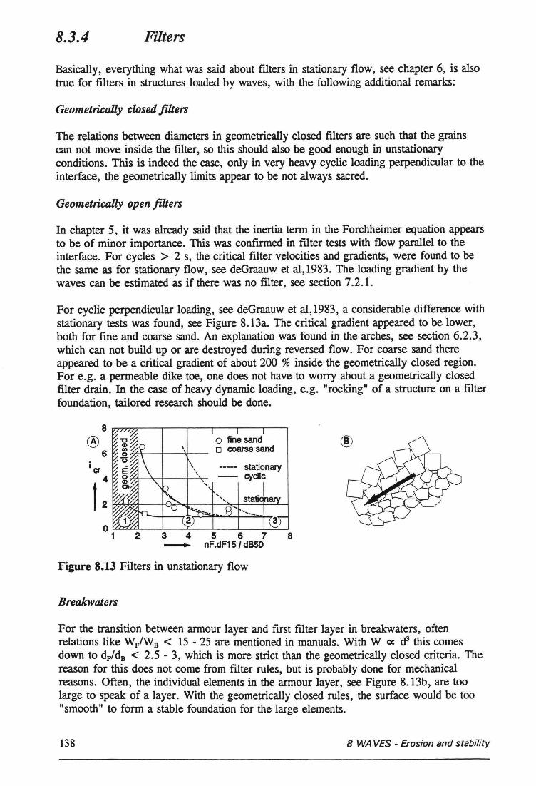
8.3.4 Filters

Basica1ly, everything what was said about filters in stationary flow, see chapter 6, is alsotrue for filters in structures loaded by waves, with the following additional remarks:

Geometrically closed .filters

The relations between diameters in geometrically closed filters are such that the grainscan not move inside the filter, so this should also be good enough in unstationaryconditions. This is indeed the case, only in very heavy cyclic loading perpendicular to theinterface, the geometrically limits appear to be not always sacred.

Geometrically open .filters

In chapter 5, it was already said that the inertia term in the Forchheimer equation appearsto be of minor importance. This was confirmed in filter tests with flow parallel to theinterface. For cycles > 2 s, the critical filter veloeities and gradients, were found to bethe same as for stationary flow, see deGraauw et al,1983. The loading gradient by thewaves can be estimated as if there was no filter, see section 7.2.1.

For cyclic perpendicular loading, see deGraauw et al,1983, a considerable difference withstationary tests was found, see Figure 8.13a. The critical gradient appeared to be lower,both for fine and coarse sand. An explanation was found in the arches, see section 6.2.3,which can not build up or are destroyed during reversed flow. For coarse sand thereappeared to be a critica1 gradient of about 200 % inside the geometrically closed region.For e.g. a permeable dike toe, one does not have to worry about a geometrically closedfilter drain. In the case of heavy dynamic loading, e.g. "rocking" of a structure on a filterfoundation, tailored research should be done.

8 ~~--~--~--~--~--~~

®6

ia ~oo~

t : ~~_--+<~..d- __ -+-~~~....:.CY.:.::cII=+C=.L~

o fine sando coarsesand

Figure 8.13 Filters in unstationary flow

Breakwaters

For the transition between armour layer and first filter layer in breakwaters, oftenrelations like WF/WB < 15 - 25 are mentioned in manuals. With W oe d3 this comesdown to dF/dB < 2.5 - 3, which is more strict than the geometrically closed criteria. Thereason for this does not come from filter rules, but is probably done for mechanicalreasons. Often, the individual elements in the armour layer, see Figure 8.13b, are toolarge to speak of a layer. With the geometrically closed rules, the surface would be too"smooth" to form a stabie foundation for the large elements.

138 8 WAVES - Erosion and stability

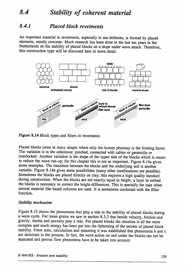
8.4 Stability of coherent material

8.4.1 Placed block revetments

An important material in revetments, especially in sea defences, is formed by placedelements, mostly concrete. Much research has been done in the last ten years in theNetherlands on the stability of placed blocks on a slope under wave attack. Therefore,this construction type will be discussed here in more detail.

cabIe

columns bIocksembedded stones mat of blocka

g80textDe

........ ,.. . . . . . . . .day11111

Figure 8.14 Block types and filters in revetments

Placed blocks come in many shapes where only the human phantasy is the limiting factor.The variation is in the coherence: pinched, connected with cables or geotextile orinterlocked. Another variation is the shape of the upper side of the blocks which is meantto reduce the wave run-up; for this chapter this is not so important. Figure 8.14a givessome examples. The transition between the blocks and the underlying soil is anothervariabIe. Figure 8.14b gives some possibilities (many other combinations are possible).Sometimes the blocks are placed directly on clay; this requires a high quality standardduring construction. When the blocks are not exactly equal in height, a layer to embedthe blocks is necessary to correct the height-differences. This is specially the case whennatural materiallike basalt columns are used. It is sometimes combined with the filterfunction.

Stahility meehanism

Figure 8.15 shows the phenomena that play a role in the stability of placed blocks duringa wave cycle. For loose grains we saw in section 8.3.2 that beside velocity, friction andgravity, inertia and porosity play a role. For placed blocks the situation is all the morecomplex and much energy has been put into the fathoming of the secrets of placed blockstability. From tests, calculations and reasoning it was established that phenomena b and care dominant in the process. In fact, the wave action on and under the blocks can not beseparated and porous flow phenomena have to be taken into account.

8 WAVES - Erosion and stability 139

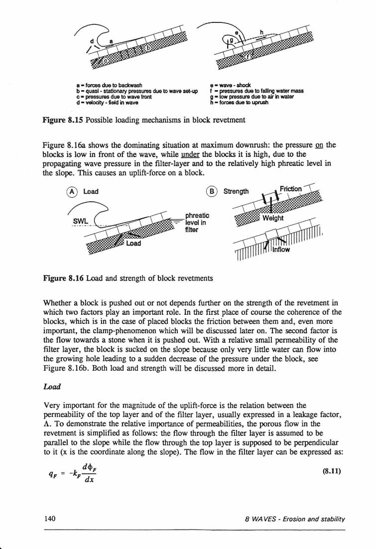
8- forces due to backwashb - quasi - stationary pressures due to wave set-upc - pressures due to wave frontd - velocity - field inwave

e - wave - shockf - pressures due to faIDng water massg - low pressure due 10 air In waterh - forces due 10 uprush

Figure 8.15 Possible loading mechanisms in bloek revetment

Figure 8.16a shows the dominating situation at maximum downrush: the pressure on thebloeks is low in front of the wave, while under the bloeks it is high, due to thepropagating wave pressure in the filter-layer and to the relatively high phreatic level inthe slope. This causes an uplift-force on a bloek.

® Lead ® Strength

Figure 8.16 Load and strength of bloek revetments

Whether a bloek is pushed out or not depends further on the strength of the revetment inwhich two factors play an important role. In the fust place of course the coherence of thebloeks, which is in the case of placed bloeks the friction between them and, even moreimportant, the c1amp-phenomenonwhich will be discussed later on. The second factor isthe flow towards a stone when it is pushed out. With a relative small permeability of thefilter layer, the bloek is sucked on the slope because only very little water can flow intothe growing hole leading to a sudden decrease of the pressure under the bloek, seeFigure 8.16b. Both load and strength will be discussed more in detail.

Load

Very important for the magnitude of the uplift-force is the relation between thepermeability of the top layer and of the filter layer, usually expressed in a leakage factor,A. To demonstrate the relative importance of permeabilities, the porous flow in therevetment is simplified as follows: the flow through the filter layer is assumed to beparallel to the slope while the flow through the top layer is supposed to be perpendicularto it (x is the coordinate along the slope). The flow in the filter layer can be expressed as:

d<hqF = -k -

F dx(8.11)

140 8 WAVES - Erosion and stability

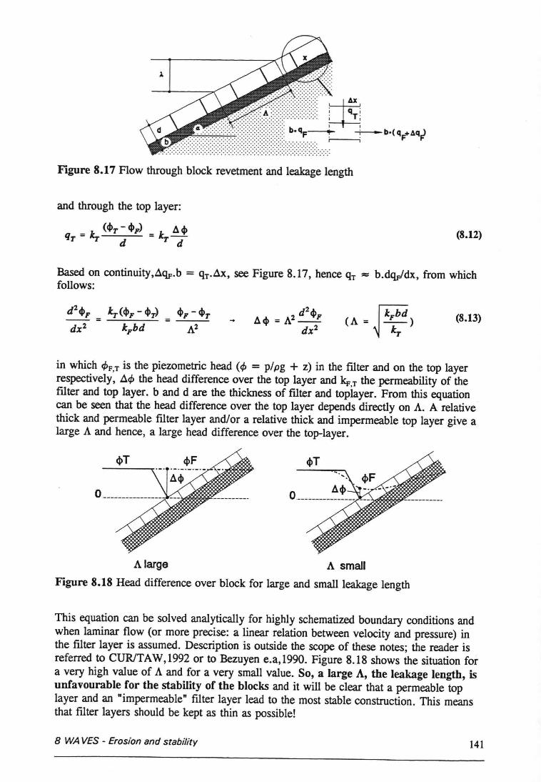
Figure 8.17 Flow through block revetment and leakage length

and through the top layer:

k: ($T - $p) = kT ä$qT = T d d (8.12)

Based on continuity.áqs.b = QT•.1X, see Figure 8.17, hence qT = b.dqj/dx, from whichfollows:

= (8.13)

in which cl>F.T is the piezometric head (cl> = p/pg + z) in the filter and on the top layerrespectively, .1c1> the head difference over the top layer and kto.T the permeability of thefilter and top layer. b and d are the thickness of filter and toplayer. From this equationcan be seen that the head difference over the top layer depends directly on A. A relativethick and permeable filter layer and/or a relative thick and impermeabie top layer give alarge A and hence, a large head difference over the top-Iayer.

A large

Figure 8.18 Head difference over block for large and small leakage lengthA small

This equation can be solved analytically for highly schematized boundary conditions andwhen laminar flow (or more precise: a linear relation between velocity and pressure) inthe filter layer is assumed. Description is outside the scope of these notes; the reader isreferred to CURlTAW,1992 or to Bezuyen e.a,1990. Figure 8.18 shows the situation fora very high value of A and for a very small value. So, a large A, the leakage length, isunfavourable for the stability of the blocks and it will be clear that a permeable toplayer and an "impermeable" filter layer lead to the most stabie construction. This meansthat filter layers should be kept as thin as possible!

8 WAVES - Erosion and stability 141

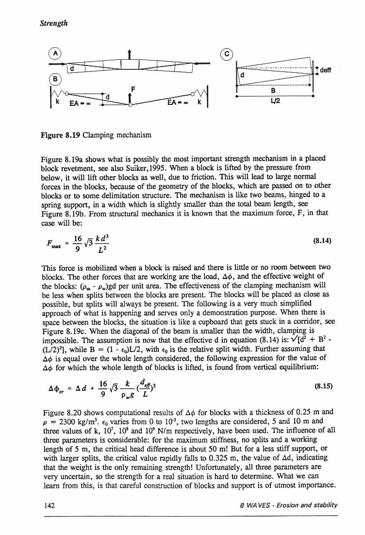
Strength

®@)

~l~

LJ2

Figure 8.19 Clamping mechanism

Figure 8.19a shows what is possibly the most important strength mechanism in a placedblock revetment, see also Suiker, 1995. When a block is lifted by the pressure frombelow, it will lift other blocks as well, due to friction. This will lead to large normalforces in the blocks, because of the geometry of the blocks, which are passed on to otherblocks or to some delimitation structure. The mechanism is like two beams, hinged to aspring support, in a width which is slightly smaller than the total beam length, seeFigure 8.19b. From structural mechanics it is known that the maximum force, F, in thatcase will be:

(8.14)

This force is mobilized when a block is raised and there is little or no room between twoblocks. The other farces that are working are the load, àcJ>, and the effective weight ofthe blocks: {Pm - Pw)gdper unit area. The effectiveness of the clamping mechanism willbe less when splits between the blocks are present. The blocks will be placed as close aspossible, but splits will always be present. The following is a very much simplifiedapproach of what is happening and serves only a demonstration purpose. When there isspace between the blocks, the situation is like a cupboard that gets stuck in a corridor, seeFigure 8. 19c. When the diagonal of the beam is smaller than the width, clamping isimpossible. The assumption is now that the effective d in equation (8.14) is: v[d2 + B2-(L/2)2], while B = (1 - Eo)U2, with Eo is the relative split width. Further assuming thatàcJ> is equal over the whole length considered, the following expression for the value offlcJ> for which the whole length of blocks is lifted, is found from vertical equilibrium:

,6,<1> =,6,d + ~ 13.s: (def/)3er 9 Pwg L

(8.15)

Figure 8.20 shows computational results of àcJ> for blocks with a thickness of 0.25 m andp = 2300 kg/m'. Eo varies from 0 to 10-3, two lengths are considered, 5 and 10 m andthree values of k, 107, 108 and 109N/m respectively, have been used. The influence of allthree parameters is considerabie: for the maximum stiffness, no splits and a workinglength of 5 m, the critica1 head difference is about 50 m! But for a less stiff support, orwith larger splits, the critical value rapidly falls to 0.325 m, the value of àd, indicatingthat the weight is the only remaining strength! Unfortunately, all three parameters arevery uncertain, so the strength for a real situation is hard to determine. What we canleam from this, is that careful construction of blocks and support is of utmost importance.

142 8 WAVES - Erosion and stability

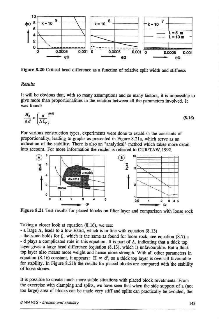
10

cl>c 8

t :oo

9 \r- k - 10 \1\. \" ,

-,....._- -------

-k-10 8

~

....._----- -===-=0.0005eO

0.001 0 0.0005

~k-10 7

-- L-5 mI--- ---- L-10m -

I- --- -0.001 0

eo0.0005 0.001

eo

Figure 8.20 Critica1 head difference as a function of relative split width and stiffness

Results

It will he obvious that, with so many assumptions and so many factors, it is impossible togive more than proportionalities in the relation between all the parameters involved. Itwas found:

(8.16)

For various construction types, experiments were done to establish the constants ofproportionality, leading to graphs as presented in Figure 8.21a, which serve as anindication of the stability. There is also an "analytica1" method which takes more detailinto account. For more information the reader is referred to CURITAW, 1992.

08 ® 10

6 'V'V <3<3 :f 5:f4

tt 22

~- -- r- -- ;--

<,<,

r-.....................

<,r-." I'" ",

", -- !--O,--_,--_,--__ji___ji___j 1

o 2 3 4 5 0.5 2 345(p (p

Figure 8.21 Test results for placed blocks on filter layer and comparison with loose rock

Taking a closer look at equation (8.16), we see:- a large A, leads to a low H/~d, which is in line with equation (8.13)- the same holds for ~, which is the same as found for loose rock, see equation (8.7).a- d plays a complicated role in this equation. It is part of A, indicating that a thick toplayer gives a large head difference (equation (8.13), which is unfavourable. But a thicktop layer also means more weight and hence more strength. With allother parameters inequation (8.16) constant, it appears: H <X d2, so a thick top layer is over-all favourablefor stability. In Figure 8.21b the results for placed blocks are compared with the stabilityof loose stones.

It is possible to create much more stable situations with placed block revetments. Fromthe excercise with c1amping and splits, we have seen that when the side support of a (nottoo large) area of blocks can be made very stiff and splits can practica1ly be avoided, the

8 WAVES - Erosion and stability 143

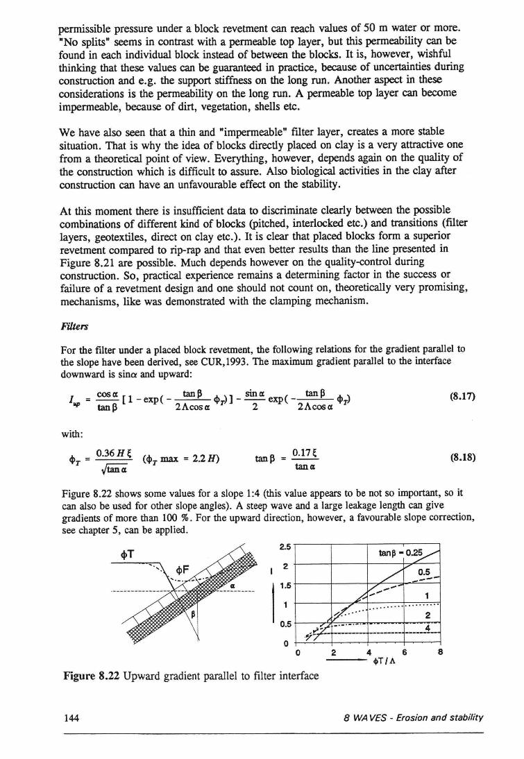
permissible pressure under a block revetment can reach values of 50 m water or more."No splits" seems in contrast with a permeable top layer, but this permeability can befound in each individual block instead of between the blocks. It is, however, wishfulthinking that these values can be guaranteed in practice, because of uncertainties duringconstruction and e.g. the support stiffness on the long run. Another aspect in theseconsiderations is the permeability on the long run. A permeable top layer can becomeimpermeable, because of dirt, vegetation, shells etc.

We have also seen that a thin and "impermeable" filter layer, creates a more stabiesituation. That is why the idea of blocks directly placed on clay is a very attractive onefrom a theoretical point of view. Everything, however, depends again on the quality ofthe construction which is difficult to assure. Also biological activities in the clay afterconstruction can have an unfavourable effect on the stability.

At this moment there is insufticient data to discriminate clearly between the possiblecombinations of different kind of blocks (pitched, interlocked etc.) and transitions (filterlayers, geotextiles, direct on clay etc.). It is clear that placed blocks form a superiorrevetment compared to rip-rap and that even better results than the line presented inFigure 8.21 are possible. Much depends however on the quality-control duringconstruction. So, practical experience remains a determining factor in the success orfailure of a revetment design and one should not count on, theoretically very promising,mechanisms, like was demonstrated with the clamping mechanism.

Filters

For the filter under a placed block revetment, the following relations for the gradient parallel tothe slope have been derived, see CUR,1993. The maximum gradient parallel to the interfacedownward is sinceaod upward:

cos 0: tan P sin 0: tan PI :::-- [1- exp( - <I> H- - exp( - <I> )up tanp 2Acos 0: T- 2 2Acos 0: T-

(8.17)

with:

(8.l8)

Figure 8.22 shows some values for a slope 1:4 (this value appears to be not so important, so itcao also be used for other slope aogles). A steep wave aod a large leakage length cao givegradients of more thao 100 %. For the upward direction, however, a favourable slope correction,see chapter 5, can be applied.

2tan~-O.2~

-:v ~~--/' _-....R ....- 1'"

V····....................2

.~~_ .....- . _____4__--------- ---------

2.5

1.5

0.5

oo 4 6

--- +T/A2 8

Figure 8.22 Upward gradient parallel to filter interface

144 8 WAVES - Erosion and stability

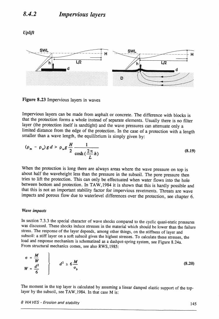
8.4.2 Impervious layers

Uplift

~-~H~ d L/2

. ,... . .. . . . . . . . . . . . . . . . . . . . . . . . . ..........................................................................................................................

Figure 8.23 Impervious layers in waves

Impervious layers can be made from asphalt or concrete. The difference with blocks isthat the proteetion forms a whole instead of separate elements. Usually there is no filterlayer (the proteetion itself is sandtight) and the wave pressures can attenuate only alimited distance from the edge of the protection. In the case of a proteetion with a lengthsmaller than a wave length, the equilibrium is simply given by:

H 1pg-MI 2 cosh( 21t h)

L(8.19)

When the proteetion is long there are always areas where the wave pressure on top isabout half the waveheight less than the pressure in the subsoil. The pore pressure thentries to lift the protection. This can only be effectuated when water flows into the holebetween bottom and protection. In TAW,1984 it is shown that this is hardly possible andthat this is not an important stability factor for impervious revetments. Threats are waveimpacts and porous flow due to waterlevel differences over the protection, see chapter 6.

Wave impacts

In section 7.3.3 the special character of wave shocks compared to the cyclic quasi-statie pressureswas discussed. These shocks induce stresses in the material which should be lower than the failurestress. The response of the layer depends, among other things, on the stiffness of layer andsubsoil: a stiff layer on a soft subsoil gives the highest stresses. To calculate these stresses, theload and response mechanism is schematized as a dashpot-spring system, see Figure 8.24a.From structural mechanics comes, see also RWS, 1985:

M0=-

Wd2w= -6

} (8.20)

The moment in the top layer is calculated by assuming a linear damped elastic support of the top­layer by the subsoil, see TAW, 1984. In that case Mis:

8 WAVES - Erosion and stability 145

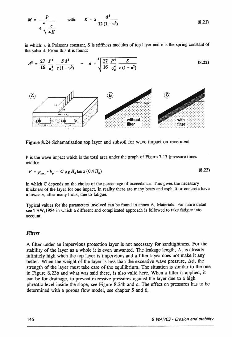
pM=--- with: K = S d3

12(1 - u~ (8.21)44ic~4K

in which: v is Poissons constant, S is stiffness modulus of top-Iayer and c is the spring constant ofthe subsoil. From this it is found:

dl = 27 p4 Sd316 0: c(1-u2)

5 ,.-----:-----d = _27 s: S (8.22)

16 a: c(1 - u~

® ®

Figure 8.24 Schematisation top layer and subsoil for wave impact on revetment

P is the wave impact which is the total area under the graph of Figure 7.13 (pressure timeswidth):

(8.23)

in which C depends on the choice of the percentage of exceedance. This gives the necessarythickness of the layer for one impact. In reality there are many beats and asphalt or concrete havea lower ab after many beats, due to fatigue.

Typical values for the parameters involved can be found in annex A, Materials. For more detailsee TAW, 1984 in which a different and complicated approach is followed to take fatigue intoaccount.

Filters

A filter under an impervious proteetion layer is not necessary for sandtightness. For thestability of the layer as a whole it is even unwanted. The leakage length, A, is alreadyinfmitely high when the top layer is impervious and a filter layer does not make it anybetter. When the weight of the layer is less than the excessive wave pressure, ~<P, thestrength of the layer must take care of the equilibrium. The situation is similar to the onein Figure 8.23b and what was said there, is also valid here. When a filter is applied, itcan be for drainage, to prevent excessive pressures against the layer due to a highphreatic level inside the slope, see Figure 8.24b and c. The effect on pressures has to bedetermined with a porous flow model, see chapter 5 and 6.

146 8 WAVES - Erosion and stability

8.5 Summary

At first some simple relations for erosion of unprotected slopes and bottoms infront ofwalls are given.

In this chapter the main item is stability in waves. In non breaking waves it appears thatlargely the same relations as in flow can be used, taking the increased shear stress underwaves into account. In breaking waves, only empirical relaiions can be used like the oneby Hudson:

PSH3M = --=---­

KD~3cot«x(or:

or vanderMeer:

Hs = ~.2P OOIS( Sd]O.2 ~-O5~d IN In

(S ]002

Hs = 1.0p-0013 ___.!!_ (.jcot«x~d IN In

(plunging breakers)(8.25)

(surging breakers)

The latter is to be preferred, since more parameters are included. The permeability of aslope gives one of the most importani differences between the two formulae. WithvanderMeer it is also possible to calculate the damage as a function of wave parameters.

Typical values of the stability parameter in breaking waves, H/MnSo, Ziearound 2 forconiinuous slopes. For toes, this value can be higher, depending on the relative depth ofthe toe. Low crests can give an increase of the stability parameter, while at the head of adam or breakwater twice the mass as computed for the trunk wil be needed.

For filters, roughly the same expressions as for flow are valid, witn two exceptions. Forlarge gradients perpendicular to the filter interface, the criticaI gradients are much less,because arching is impossible in a dynamic flow situation and for the first layer undervery coarse elements in the armour layer of a breakwater, also mechanical aspects play arole.

For placed block revetments, the mechanisms are explained and an empirical stabilityrelation is presented. From theoretical considerations it can be concluded that blockrevetments of good quality, can stand wave loads, larger than ever encountered in nature.From the same considerations, however, it appears that the quality is extremely sensitivefor deviations, so, for practical applications, these revetments are superior to a rip-raprevetment only to a certain extent. Typical values of the stability parameter, H/ MnSo, areabout 1.5 - 2 times the values for loose rock.

Waves will usually not be able to lift impervious layer revetments of some size. Waveimpacts can influence the thickness of the layer. A filter is not necessary, except possiblyfor the drainage of excessive pressures due to tides or surges.

8 WAVES - Erosion and stebititv 147

148 8 WAVES - Erosion and stability

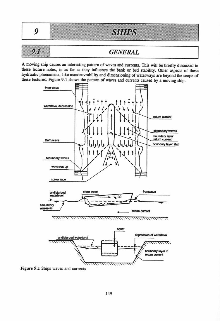
9

GENERAL

A moving ship causes an interesting pattem of waves and currents. This will be briefly discussed inthese lecture notes, in as far as they influence the bank or bed stability. Other aspects of thesehydraulic phenomena, like manoeuvrability and dimensioning of waterways are beyond the scope ofthese lectures. Figure 9.1 shows the pattem of waves and currents caused by a moving ship.

return current

frontwáve

stem wave

secu

waverun-up

sc:rew race

undisturbedwaterlevelt _....

secundary !wawaves

stem wave frontwave

~~~~-----w--

+-- retum current

Figure 9.1 Ships waves and currents

149

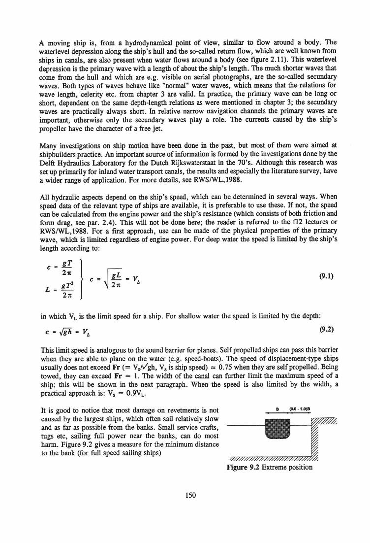
A moving ship is, from a hydrodynamicaI point of view, similar to flow around a body. Thewaterlevel depression along the ship's huil and the so-called return flow, which are weil known fromships in canaIs, are also present when water flows around a body (see figure 2.11). This waterleveldepression is the primary wave with a length of about the ship's length. The much shorter waves thatcome from the huil and which are e.g. visible on aerial photographs, are the so-called secundarywaves. Both types of waves behave like "normaI" water waves, which means that the relations forwave length, celerity etc. from chapter 3 are valid. In practice, the primary wave can be long orshort, dependent on the same depth-length relations as were mentioned in chapter 3; the secundarywaves are practically always short. In relative narrow navigation channels the primary waves areimportant, otherwise only the secundary waves play a role. The currents caused by the ship'spropeller have the character of a free jet.

Many investigations on ship motion have been done in the past, but most of them were aimed atshipbuilders practice. An important souree of information is formed by the investigations done by theDelft Hydraulics Laboratory for the Dutch Rijkswaterstaat in the 70's. Although this research wasset up primarily for inland water transport canaIs, the results and especially the literature survey, havea wider range of application. For more details, see RWSIWL,1988.

All hydraulic aspects depend on the ship's speed, which can be determined in several ways. Whenspeed data of the relevant type of ships are available, it is preferabie to use these. If not, the speedcan be calculated from the engine power and the ship's resistance (which consists ofboth friction andform drag, see par. 2.4). This will not be done here; the reader is referred to the f12 lectures orRWSIWL,1988. For a first approach, use can be made of the physical properties of the primarywave, which is limited regardless of engine power. For deep water the speed is limited by the ship'slength according to:

c = gT21t

gT2L=-21t

c = ~ gL = V21t L(9.1)

in which VL is the limit speed for a ship. For shallow water the speed is limited by the depth:

(9.2)

This limit speed is analogous to the sound barrier for planes. Self propelled ships can pass this barrierwhen they are able to plane on the water (e.g. speed-boats). The speed of displacement-type shipsusually does not exceed Fr (= Vsf../gh, Vs is ship speed) ::::0.75 when they are selfpropelled. Beingtowed, they can exceed Fr = 1. The width of the canal can further limit the maximum speed of aship; this will be shown in the next paragraph. When the speed is also limited by the width, apractical approach is: Vs = 0.9VL•

It is good to notice that most damage on revetments is notcaused by the largest ships, which often sail relatively slowand as far as possible from the banks. Small service crafts,tugs etc, sailing full power near the banks, can do mosthaem. Figure 9.2 gives a measure for the minimum distanceto the bank (for full speed sailing ships)

Figure 9.2 Extreme position

150

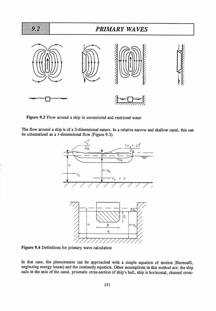
PRIMARY WA YES

-- --==[3= -- -

Figure 9.3 Flow around a ship in unrestricted and restricted water

The flow around a ship is of a 3-dimensional nature. In a relative narrow and shallow canal, this canbe schematized as a l-dimensional flow (Figure 9.3).

v2s29

h

---+--vs + u

/

Figure 9.4 Definitions for primary wave calculation

In that case, the phenomenon can be approached with a simple equation of motion (Bemoulli,neglecting energy losses) and the continuity equation. Other assumptions in this method are: the shipsails in the axis of the canal, prismatic cross-section of ship's hull, ship is horizontal, channel cross-

151

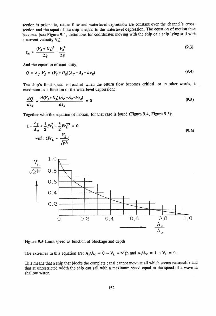
section is prismatic, return flow and waterlevel depression are constant over the channel's cross­section and the squat of the ship is equal to the waterlevel depression. The equation of motion thenbecomes (see Figure 9.4, definitions for coordinates moving with the ship or a ship lying still witha current velocity Vs):

~2S

2g

(9.3)

And the equation of continuity:

Q = Ac· Vs = (Vs + UR)(A.c -As - bz~ (9.4)

The ship's limit speed is reached when the return flow becomes critical, or in other words, ismaximum as a function of the waterlevel depression:

dQ = _d_(V.-=S~+_U....::.:R~)(_A.;;;_c_-A_s=--_b_z..:.:...R)= 0dZR

(9.5)

Together with the equation of motion, for that case is found (Figure 9.4, Figure 9.5):

As 1 2 3 2/31- - + -FrL - -FrL = 0Ac 2 2

Vwith: (Fr = _L )

L.fiïi

(9.6)

VL1.0

Jgh 0.8

r0.6

0.4

0.2

F-"-,

<,r-,

I'--.... ---- ----- I Ir-----+-_

o 0,2 0,4 0,6 1,0

Figure 9.5 Limit speed as function of blockage and depth

The extremes in this equation are: Asl Ac = 0 ....VL = vigh and AslAc = 1 ....VL = O.

This means that a ship that blocks the complete canal cannot move at all which seems reasonable andthat at unrestricted width the ship can sail with a maximum speed equal to the speed of a wave inshallow water.

152

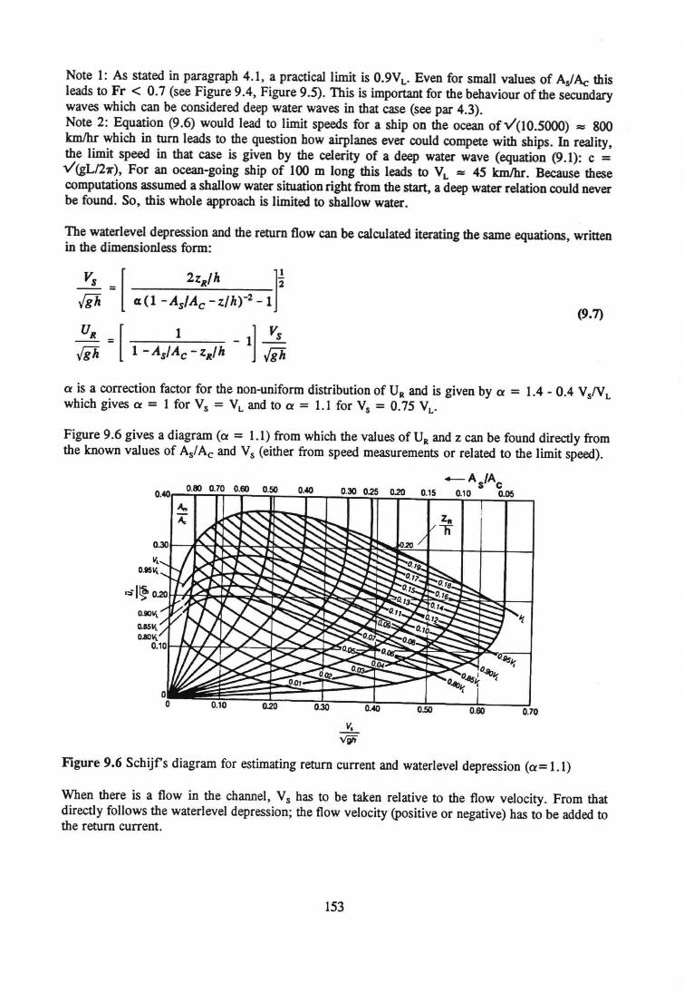
Notel: As stated in paragraph 4.1, a practical limit is 0.9VL• Even for small values of As/Ac thisleads to Fr < 0.7 (see Figure 9.4, Figure 9.5). This is important for the behaviour ofthe secundarywaves which can be considered deep water waves in that case (see par 4.3).Note 2: Equation (9.6) would lead to limit speeds for a ship on the ocean ofv(1O.5000) """800km/hr which in turn leads to the question how airplanes ever could compete with ships. In reality,the limit speed in that case is given by the celerity of a deep water wave (equation (9.1): c =v(gL/27r), For an ocean-going ship of 100 m long this leads to VL """ 45 kmIhr. Because thesecomputations assumed a shallow water situation right from the start, a deep water relation could neverbe found. So, this whole approach is limited to shallow water.

The waterlevel depression and the return flow can be calculated iterating the same equations, writtenin the dimensionless form:

(9.7)

a is a correction factor for the non-uniform distribution of UR and is given by a = 1.4 - 0.4 VSNL

which gives a = 1 for Vs = VL and to a = 1.1 for Vs = 0.75 VL'

Figure 9.6 gives a diagram (a = 1.1) from which the values of'U, and z can be found directIy fromthe known values of As/Ac and Vs (either from speed measurements or related to the limit speed).

-As/AcO.~'r--.;;,;.O.80r-~O.7n°__.:;0.60r-....;O~.50rr-_::0:;:.~:...._,-0::;;.30:::.....:0::;.2;.5_:::0.20;::...._:::0..;.:15~....!0~.1O~_~O'05~--.

O.~ 0.50 0.60 0.70v,

...;gïI

Figure 9.6 Schijfs diagram for estimating return current and waterlevel depression (a= 1.1)

When there is a flow in the channel, Vs has to be taken relative to the flow velocity. From thatdirectly follows the waterlevel depression; the flow velocity (positive or negative) has to be added tothe return current.

153

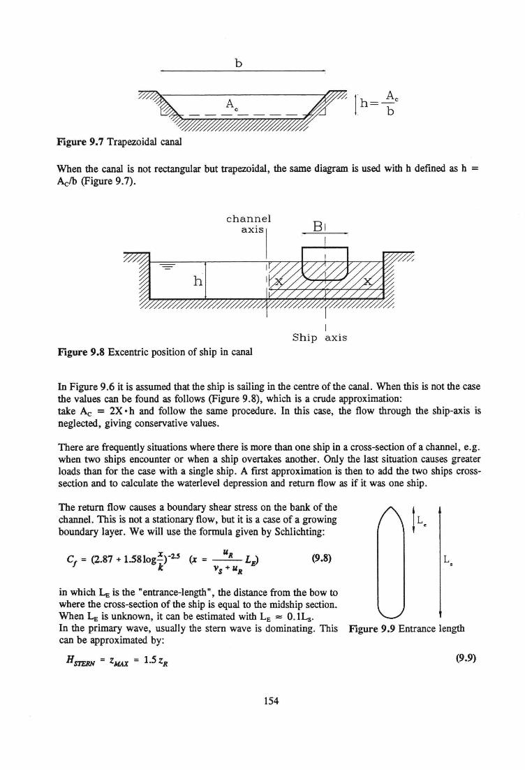
b

,~-~lh=~'~;_jFigure 9.7 Trapezoidal canal

Wben the canal is not rectangular but trapezoidal, the same diagram is used with h defined as h =Aclb (Figure 9.7).

channel

Ship axisFigure 9.8 Excentric position of ship in canal

In Figure 9.6 it is assumed that the ship is sailing in the centre ofthe canal. Wben this is not the casethe values can be found as follows (Figure 9.8), which is a crude approximation:take Ac = 2X· h and follow the same procedure. In this case, the flow through the ship-axis isneglected, giving conservative values.

There are frequently situations where there is more than one ship in a cross-section of a channel, e.g.when two ships encounter or when a ship overtakes another. Qnly the last situation causes greaterloads than for the case with a single ship. A first approximation is then to add the two ships cross­section and to calculate the waterlevel depression and return flow as if it was one ship.

in which ~ is the "entrance-length", the distance from the bow towhere the cross-section of the ship is equal to the midship section.Wben LE is unknown, it can be estimated with LE :::::O.ILs.In the primary wave, usually the stern wave is dominating. This Figure 9.9 Entrance lengthcan be approximated by:

HSTERJ{ = ZMAX = 1.5ZR (9.9)

The return flow causes a boundary shear stress on the bank of thechannel. This is not a stationary flow, but it is a case of a growingboundary layer. We will use the formula given by Schlichting:

Cf = (2.87 + 1.581og~kr2..S (x = uR LJVs +uR

(9.8)

154

L•

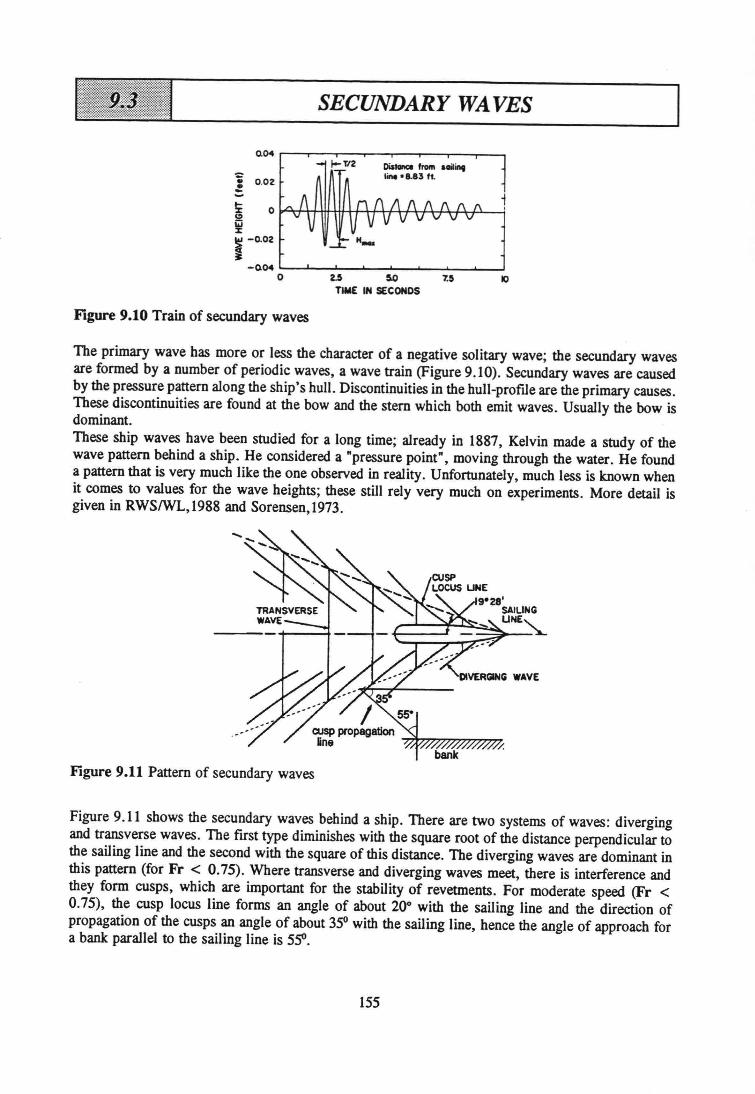
SECUNDARY WAYES

~ 0.02~-

Figure 9.10 Train of secundary waves

The primary wave has more or less the character of a negative solitary wave; the secundary wavesare formed by a number of periodic waves, a wave train (Figure 9.10). Secundary waves are causedby the pressure pattem along the ship's huil. Discontinuities in the huil-profile are the primary causes.These discontinuities are found at the bow and the stem which both emit waves. Usually the bow isdominant.These ship waves have been studied for a long time; already in 1887, Kelvin made a study of thewave pattem behind a ship. He considered a "pressure point", moving through the water. He foundapattem that is very much like the one observed in reality. Unfortunately, much less is known whenit comes to values for the wave heights; these still rely very much on experiments. More detail isgiven in RWS/WL,1988 and Sorensen,1973.

9·28'SAIUNG

_"____''F-J._.;::;~o:.:.....~ UNE~

Figure 9.11 Pattem of secundary waves

Figure 9.11 shows the secundary waves behind a ship. There are two systems of waves: divergingand transverse waves. The first type diminishes with the square root of the distance perpendicular tothe sailing line and the second with the square of this distance. The diverging waves are dominant inthis pattem (for Fr < 0.75). Where transverse and diverging waves meet, there is interference andthey form cusps, which are important for the stability of revetments. For moderate speed (Fr <0.75), the cusp locus line forms an angle of about 20° with the sailing line and the direction ofpropagation of the cusps an angle of about 35" with the sailing line, hence the angle of approach fora bank parallel to the sailing line is 55".

155

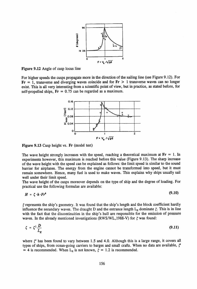
90..••...,.!...

1928

0 1 2F- V,IW

Figure 9.12 Angle of cusp locus line

For higher speeds the cusps propagate more in the direction ofthe sailing line (see Figure 9.12). ForFr = 1, transverse aod diverging waves coincide aod for Fr > 1 transverse waves cao no longerexist. This is all very interesting from a scientific point of view, but in practice, as stated before, forself-propelled ships, Fr = 0.75 cao be regarded as a maximum.

0.16c~

b.o

0~

00 0

J v

I

:: 0.12ClCl-_. 0.08•oex 0.04

oo I

F- V,/.JQd2

Figure 9.13 Cusp height vs. Fr (model test)

The wave height strongly increases with the speed, reaching a theoretical maximum at Fr = 1. Inexperiments however, this maximum is reached before this value (Figure 9.13). The sharp increaseof the wave height with the speed cao be explained as follows: the limit speed is similar to the soundbarrier for airplaoes. The energy from the engine cannot be transformed into speed, but it mustremain somewhere. Hence, maoy fuel is used to make waves. This explains why ships usually sailweIl under their limit speed.The wave height of the cusps moreover depends on the type of ship aod the degree of loading. Forpractical use the following formulae are available:

H = ,·h·Fr' (9.10)

r represents the ship's geometry. It was found that the ship's length aod the block coefficient hardlyinfluence the secundary waves. The draught D aod the entrance length 4, dominate r. This is in linewith the fact that the discontinuities in the ship's huIl are responsibie for the emission of pressurewaves. In the already mentioned investigations (RWS/WL,1988-V) for t was found:

{ = {1E..LE

(9.11)

where f has been found to vary between 1.5 and 4.0. Although this is a large range, it covers alltypes of ships, from ocean-going carriers to barges and smal1crafts. When no data are available, f= 4 is recommended. When 4, is not known, r = 1.2 is recommended.

156

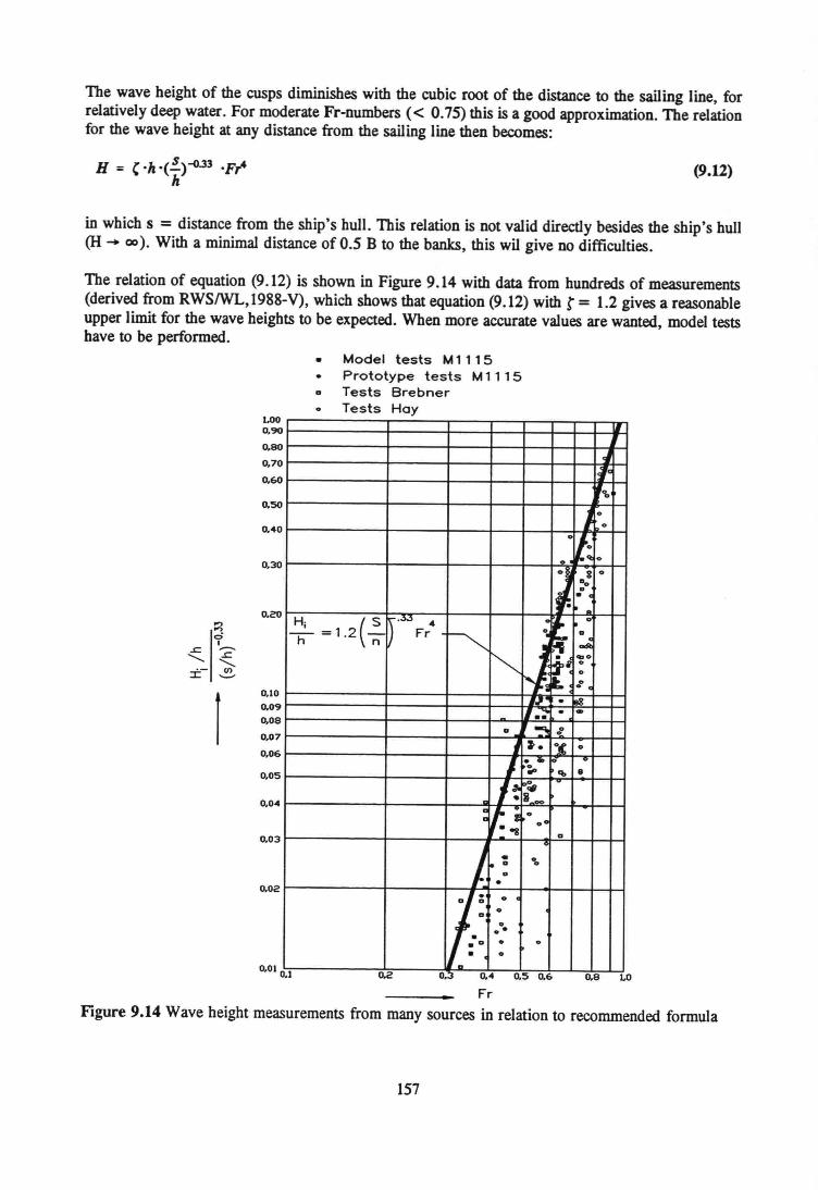
The wave height of the cusps diminishes with the cubic root of the distance to the sailing line, forrelatively deep water. For moderate Fr-numbers « 0.75) this is a good approximation. The relationfor the wave height at any distance from the sailing line then becomes:

H = "'h .(!)-O.33 'F~h (9.12)

in which s = distance from the ship's huil. This relation is not valid directly besides the ship's huil(H - (0). With a minimal distance of 0.5 B to the banks, this wil give no difficulties.

The relation of equation (9.12) is shown in Figure 9.14 with data from hundreds of measurements(derived from RWSIWL,1988-V), which shows that equation (9.12) with t = 1.2 gives a reasonableupper limit for the wave heights to be expected. When more accurate values are wanted, model testshave to be perfonned.

• Model tests M1115Prototype tests M1115Tests 8rebnerTests Hoy

D

1.000.90

0.800,70

0.60

0.50

0.40

0.30

0.20..,..,ei

.s: '...........<, s:

<,Ï- en_..

I 0.100.090,08

0.07

0.06

0,05

0.04

0.03

0.02

11

J!l'f....

10

0

0

t:o0

J.8 0

DOD•.H (SIr~4

-; J: 0-i- =1.2 n Fr r-. 'Ir; D~

NI,...sir-. ,",0

~60

0

J',~ .l8l!11•• . -

D ~ J'11• O( 0

I .- jó 0

:.. Ob •I! ,,;,11_

: If;_ g o 0'.eg

D

) • ....t- DD.,j 0

0

0o·D 0 0

• 0

D0.1 0.2 0.3 0.4 O.S 0.6 0.8 Lo0.01

FrFigure 9.14 Wave height measurements from many sourees in relation to recommended fonnula

157

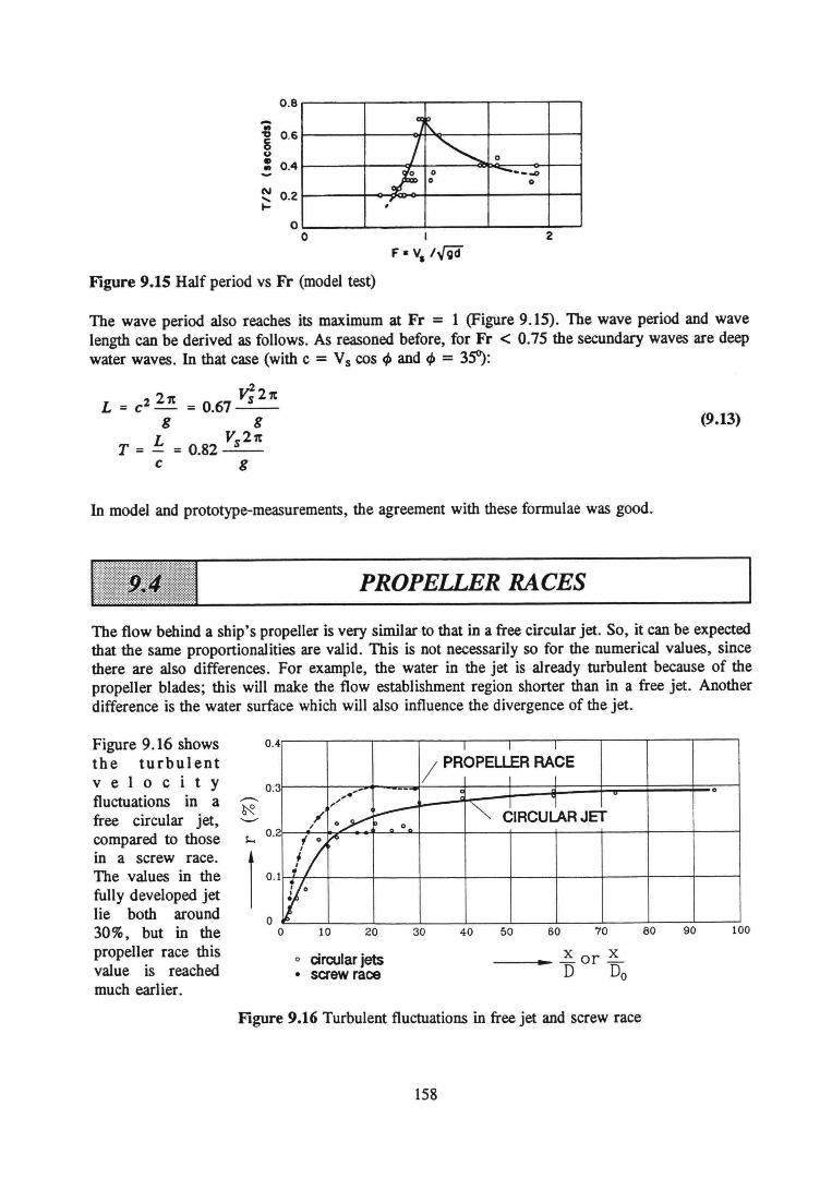
0.8<Ij~

] <, 0

~0 ----0 0

"

-..,i 0.6u: 0.4

~ 0.2I-

oo I

F· VI l..[id2

Figure 9.15 Half period vs Fr (model test)

The wave period also reaches its maximum at Fr = 1 (Figure 9.15). The wave period and wavelength can be derived as follows. As reasoned before, for Fr < 0.75 the secundary waves are deepwater waves. In that case (with c = Vs cos 4> and 4> = 3SO):

2

L - 221t 7 Vs 21t-c - =0.6--g g

L Vs21tT = - = 0.82--

c g

(9.13)

In model and prototype-measurements, the agreement with these formulae was good.

PROPELLER RACES

The flow behind a ship's propeller is very similar to that in a free circular jet. So, it can be expectedthat the same proportionalities are valid. This is not necessarily so for the numerical values, sincethere are also differences. For example, the water in the jet is already turbulent because of thepropeller blades; this will make the flow establishment region shorter than in a free jet. Anotherdifference is the water surface which will also influence the divergence of the jet.

Figure 9.16 showsthe turbul entvelocityfluctuations in afree circular jet,compared to thosein a screw race.The values in thefully developed jetlie both around30%, but in thepropeller race thisvalue is reachedmuch earlier.

0.4 I I I/ PROPELlER RACE

I I" -- c 0,.

1" ~I

/ -.»:" CIRCULAR JET/ 0

li ~

'y: 0•

0.3

s... 0.2

oo

o circular jets• screw race

60 70

____ ~or ~D Do

80 90 10040 5010 20 30

Figure 9.16 Turbulent fluctuations in free jet and screw race

158

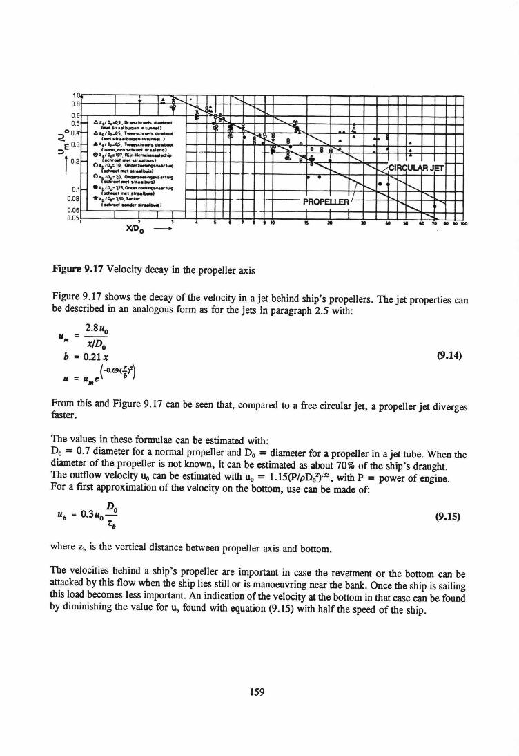
o0.00.00.0 1

.8 I ... I.. 1'--. .........I 1 I ,. ......~ .. t"'-~.6 ~ r--, _4.5 ~zs/o.~).Orle5ChrOlfl, ~ , "'i ~ .e.,_. Io" •• tlUIH'ft .. ,t..wwt)

'"6"/~:QS. fWft __ clu_ , • Ï'"'r-- r-, .. •..... strUfbYia"""' ..1"Wtel ) B .. ...3 .>.'''o=QS. _ .. _- ,.....,. o 8 I~ ..(,*",.H'ft actweef dr .. ien" r- -r r' -r'.zf~'::=:.~Mt\ÎP ~~ ~ I r---..... !.

.2 r--0'.10.: '.D. _......,._,,,,, .............t--.. <,~,CIRCULAR JET._..........-, r-- r-- .. r-',_O·f~:!:~~.,'.., • r- ',.....• r-,··.'Do=U5.- ...... _tuót t--...1 •_,_." ... ~I

PROP~/'........ ........8 ••• '~\SO.f ...... -t-- . r-.__ ..._,

r-,6 I ,5JD .. KI 10 ,. 10 10 1•

X/Do -4 S • 7' tlO DO

Figure 9.17 Velocity decay in the propeller axis

Figure 9.17 shows the decay of the velocity in a jet behind ship's propellers. The jet properties canbe described in an analogous forrn as for the jets in paragraph 2.5 with:

2.8uou =--• X/Dob = 0.21 x (9.14)

(-o.69(.!r)u = u e b•From this and Figure 9.17 can be seen that, compared to a free circular jet, a propeller jet divergesfaster.

The values in these forrnulae can be estimated with:Do = 0.7 diameter for a normal propeller and Do = diameter for a propeller in a jet tube. When thediameter of the propeller is not known, it CaD be estimated as about 70% of the ship's draught.The outflow velocity Uo can be estimated with u, = 1.15(p/pDl)·33, with P = power of engine.For a fust approximation of the velocity on the bottom, use CaD be made of:

DoUh = 0.3uo-

Zb(9.15)

where z, is the vertical distanee between propeller axis and bottom.

The veloeities behind a ship's propeller are important in case the revetment or the bottom can beattacked by this flow when the ship lies still or is manoeuvring near the bank. Once the ship is sailingthis load becomes less important. An indication of the velocity at the bottom in that case CaD be foundby diminishing the value for Ut, found with equation (9.15) with half the speed of the ship.

159

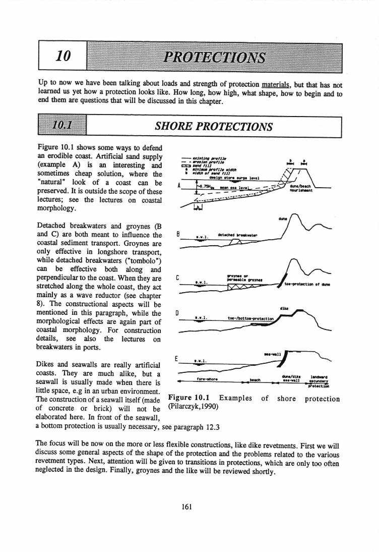
10

Up to now we have been talking about loads and strength of proteetion materials, but that has notlearned us yet how a proteetion looks like. How long, how high, what shape, how to begin and toend them are questions that will be discussed in this chapter.

SHORE PROTECTIONS

Dikes and seawalls are really artificialcoasts. They are much alike, but aseawall is usually made when there islittle space, e.g in an urban environment.The construction of a seawall itself (made Figure 10.1 Exam pIesof concrete or brick) will not be (pilarczyk, 1990)elaborated here. In front of the seawall,a bottom proteetion is usually necessary, see paragraph 12.3

Figure 10.1 shows some ways to defendan erodible coast. Artificial sand supply(example A) is an interesting andsometimes cheap solution, where the"natural" look of a coast can bepreserved. It is outside the scope of theselectures; see the lectures on coastaImorphology .

Detached breakwaters and groynes (Band C) are both meant to influence thecoastal sediment transport. Groynes areonly effective in longshore transport,while detached breakwaters ("tombolo")can be effective both along andperpendicular to the coast. When they arestretched along the whole coast, they actmainly as a wave reductor (see chapter8). The constructional aspects will bementioned in this paragraph, while themorphological effects are again part ofcoastal morphology. For constructiondetails, see also the lectures onbreakwaters in ports.

- UI."",_'u,- - -I." _'IJ.C3 und 'JJl• MnI__ 'IJ. ttJtItII, .ltIUI., _ '111

_I.., .t...........level

B ••W.l.

E

• ,....-.... oIIIne/dJ.l<.• ...... 11...•• Heeft

of shore proteetion

The focus will be now on the more or less flexible constructions, like dike revetments. First we willdiscuss some general aspects of the shape of the proteetion and the problems related to the variousrevetment types. Next, attention will be given to transitions in protections, which are only too oftenneglected in the design. Finally, groynes and the like will be reviewed shortly.

161

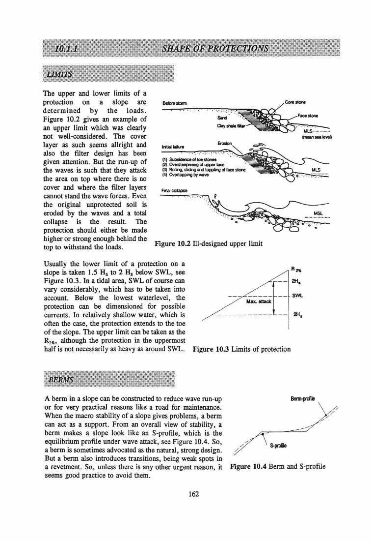
Usually the lower limit of a proteetion on aslope is taken 1.5 H, to 2 H, below SWL, seeFigure 10.3. In a tidal area, SWL of course caovary considerably, which has to be taken intoaccount. Below the lowest waterlevel, theproteetion cao be dimensioned for possiblecurrents. In relatively shallow water, which isoften the case, the proteetion extends to the toeof the slope. The upper limit cao be taken as theR2~' although the proteetion in the uppermosthalf is not necessarily as heavy as around SWL.

The upper aod lower limits of aproteetion on a slope aredetermined by the loads.Figure 10.2 gives an example ofan upper limit which was clearlynot well-considered. The coverlayer as such seems allright andalso the filter design has beengiven attention. But the run-up ofthe waves is such that they attackthe area on top where there is nocover aod where the filter layerscannot stand the wave forces. Eventhe original unprotected soil iseroded by the waves aod a totalcollapse is the result. Theproteetion should either be madehigher or strong enough bebind thetop to withstand the loads.

Before storm

IRtiailailure

(1) Subsidenc:e of toe stones(2) Ovemeepening of uppet face(3) Rolling. sróng lWld toppling ol face stone(4) Overlapping by WIM!

Final coIapse

Figure 10.2 Ill-designed upper limit

2H.

f--

----- --Malt. attack

----------- --

SWl

Figure 10.3 Limits of proteetion

A berm in a slope cao be constructed to reduce wave run-upor for very practical reasons like a road for maintenaoce.When the macro stability of a slope gives problems, a bermcao act as a support. From ao overall view of stability, aberm makes a slope look like an S-profile, which is theequilibrium profile under wave attack, see Figure 10.4. So,a berm is sometimes advocated as the naturaI, strong design.But a berm also introduces transitions, being weak spots ina revetment. So, unIess there is aoy other urgent reason, itseems good practice to avoid them.

__ -

Figure 10.4 Berm and S-profile

162

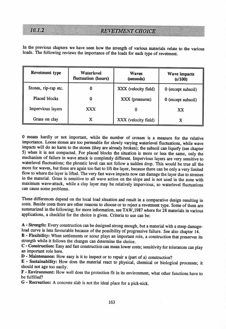
In the previous chapters we have seen how the strength of various materials relate to the variousloads. The foIIowing reviews the importance of the loads for each type of revetment.

Revetment type Waterlevel Waves Wave impactsnuctuation (hours) (seconcls) (s/l00)

Stones, rip-rap etc. 0 XXX (velocity field) o (except subsoil)

Placed bleeks 0 XXX (pressures) o (except subsoil)

Impervious layers XXX 0 XX

Grass on clay X XXX (velocity field) X

o means hardly or not important, while the number of crosses is a measure for the relativeimportance. Loose stones are too permeabie for slowly varying waterlevel fluctuations, while waveimpacts will do no harm to the stones (they are already breken); the subsoil cao liquefy (see chapter5) when it is not compacted. For placed blocks the situation is more or less the same, only themechanism of failure in wave attack is completely different. Impervious layers are very sensitive towaterlevel fluctuations; the phreatic level can not follow a sudden drop. This would be true all themore for waves, but these are again too fast to lift the layer, because there can be only a very Iimitedflow to where the layer is lifted. The very fast wave impacts now can damage the layer due to stressesin the material. Grass is sensitive to all wave action on the slope and is not used in the zone withmaximum wave-attack, while a cIay layer may be relatively impervious, so waterlevel fluctuationscan cause some problems.

These differences depend on the local load situation and result in a comparative design resulting incosts. Beside costs there are other reasons to choose or to reject a revetment type. Some of them aresummarized in the following; for more information, see TAW,1987 where for 28 materials in variousapplications, a checklist for the choice is given. Criteria to use can be:

A - Strength: Every construction can be designed strong enough, but a material with asteep damage­load curve is less favourable because of the possibility of progressive failure. See also chapter 14.B - Flexibility: When settlements or scour plays an important role, a construction that preserves itsstrength while it follows the changes can determine the choice.C - Construction: Easy and fast construction can meao lower costs; sensitivity for tolerances can playan important role here.D-Maintenance: How easy is it to inspeet or to repair a (part of a) construction?E - Sustainability: How does the material react to physical, chemical or biological processes; itshould not age too easily.F - Environment: How weIl does the proteetion fit in its environment, what other functions have tobe fulfilled?G - Recreation: A concrete slab is not the ideal place for a pick-nick.

163

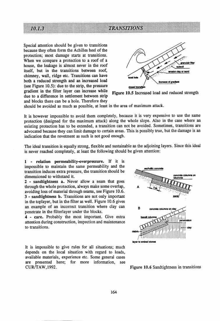
Special attention should be given to transitionsbecause they often form the Achilles heel of theprotection; most damage starts at transitions.When we compare a proteetion to a roof of ahouse, the leakage is almost never in the roofitself, but in the transitions between roof,chimney, wall, ridge etc. Transitions can haveboth a reduced strength and an increased load(see Figure 10.5): due to the strip, the pressuregradient in the filter layer can increase while Figure 10.5 Increased load and reduced strengthdue to a difference in settlement between stripand blocks there can be a hole. Therefore theyshould be avoided as much as possible, at least in the area of maximum attack.

It is however impossible to avoid them completely, because it is very expensive to use the sameproteetion (designed for the maximum attack) along the whole slope. Also in the case where anexisting proteetion has to be extended, a transition can not be avoided. Sometimes, transitions areadvocated because they can limit damage to certain areas. This is possibly true, but the damage is anindication that the revetment as such is not good enough.

The ideal transition is equally strong, flexible and sustainable as the adjoining layers. Since this idealis never reached completely, at least the following should be given attention:

1 - relation permeability-overpressure. If it isimpossible to maintain the same permeability and thetransition induces extra pressure, the transition should bedimensioned to withstand it.2 - sandtightness a. Never allowaseam that goesthrough the whole protection, always make some overlap,avoiding loss of material through seams, see Figure 10.6.3 - sandtightness b. Transitions are not only importantin the toplayer, but in the filter as weIl. Figure 10.6 givesan example of an incorrect transition where clay canpenetrate in the filterlayer under the blocks.4 - care. Probably the most important. Give extraattention during construction, inspeetion and maintenanceto transitions.

It is impossible to give rules for all situations; muchdepends on the local situation with regard to loads,available materials, experience etc. Some general casesare presented here; for more information, seeCURlTAW, 1992. Figure 10.6 Sandtightness in transitions

164

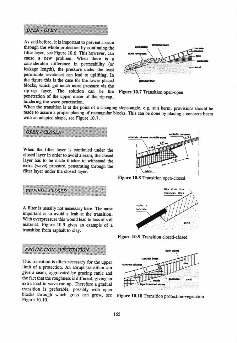
As said before, it is important to prevent a seamthrough the whole proteetion by continuing thefilter layer, see Figure 10.6. This however, cancause a new problem. When tbere is aconsiderabIe difference in permeability (orleakage length), the pressure under the leastpermeabie revetment can lead to uplifting. Inthe figure this is tbe case for the lower placedblocks, which get much more pressure via tberip-rap layer. The solution can be the Figure 10.7 Transition open-openpenetration of the upper meter of the rip-rap,hindering the wave penetration.Wben the transition is at the point of a changing slope-angle, e.g. at a berm, provisions should bemade to assure a proper placing of rectangular blocks. This can be done by placing a concrete beamwitb an adapted shape, see Figure 10.7.

When tbe filter layer is continued under tbeclosed layer in order to avoid a seam, the closedlayer has to be made thicker to witbstand tbeextra (wave) pressure, penetrating tbrough thefilter layer under tbe closed layer.

A filter is usually not necessary here. The mostimportant is to avoid a leak at the transition.Witb overpressure tbis would lead to loss of soilmaterial. Figure 10.9 gives an example of atransition from asphalt to clay.

This transition is often necessary for the upperlimit of a protection. An abrupt transition cangive a seam, aggravated by grazing cattle andthe fact tbat tbe roughness is different, giving anextra load in wave run-up. Therefore a gradualtransition is preferabIe, possibly witb openblocks tbrough which grass can grow, seeFigure 10.10.

..........

Figure 10.8 Transition open-closed

Figure 10.9 Transition closed-closed

.... . ......., ...:.: ..: .:.':

........, .............. ..

Figure 10.10 Transition protection-vegetation

165

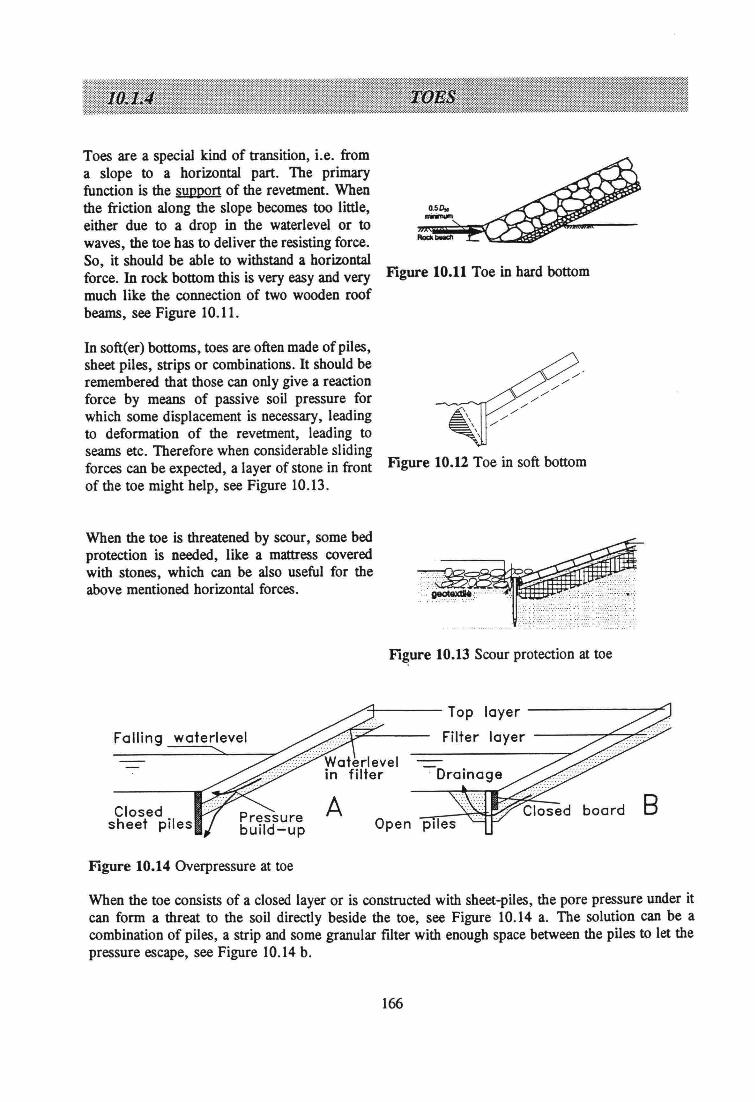
Toes are a special kind of transition. i.e. froma slope to a horizontaI part. The primaryfunction is the support of the revetment. Whenthe friction along the slope becomes too little,either due to a drop in the waterlevel or towaves, the toe has to deliver the resisting force.So, it should be able to withstand a horizontaIforce. In rock bottom this is very easy and verymuch like the conneetion of two wooden roofbeams, see Figure 10.11.

In soft(er) bottoms, toes are often made of piles,sheet piles, strips or combinations. It should beremembered that those can only give a reactionforce by means of passive soil pressure forwhich some displacement is necessary, leadingto deformation of the revetment, leading toseams etc. Therefore when considerable slidingforces can be expected, a layer of stone in frontof the toe might help, see Figure 10.13.

When the toe is threatened by scour, some bedproteetion is needed, like a mattress coveredwith stones, which can be also useful for theabove mentioned horizontaI forces.

Figure 10.11 Toe in hard bottom

Figure 10.12 Toe in soft bottom

Fi~ure 10.13 Scour proteetion at toe

/...,---- Top layer

Filter layer

Closedsheet piles

A

Figure 10.14 Overpressure at toe

BOpen piles

When the toe consists of a closed layer or is constructed with sheet-piles, the pore pressure under itcan form a threat to the soil directly beside the toe, see Figure 10.14 a. The solution can be acombination of piles, a strip and some granular filter with enough space between the piles to let thepressure escape, see Figure 10.14 b.

166

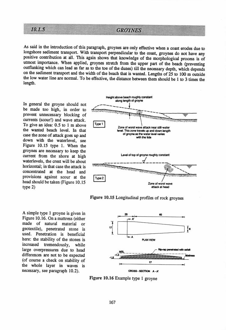
As said in the introduetion of this paragraph, groynes are only effective when a coast erodes due tolongshore sediment transport. With transport perpendicular to the coast, groynes do not have anypositive contribution at all. This again shows that knowledge of the morphological process is ofutmost importanee. When applied, groynes stretch from the upper part of the beach (preventingoutflanking which can lead as far as to the toe of the dunes) till the necessary depth, which dependson the sediment transport and the width of the beach that is wanted. Lengths of 25 to 100 m outsidethe low water line are normal. To be effective, the distance between them should be 1 to 3 times thelength.

In general the groyne should notbe made too high, in order toprevent unnecessary blocking ofcurrents (scour!) and wave attack.To give an idea: 0.5 to 1 m abovethe wanted beach level. In thatcase the zone of attack goes up anddown with the waterlevel. seeFigure 10.15 type 1. When thegroynes are necessary to keep thecurrent from the shore at highwaterlevels, the crest wiJl be abouthorizontal; in that case the attack isconcentrated at the head andprovisions against scour at thehead should be taken (Figure 10.15type 2)

A simple type 1 groyne is given inFigure 10.16. On a mattress (eithermade of natural material orgeotextile), penetrated stone isused. Penetration is beneficialhere: the stabiIity of the stones isincreased tremendously, whilelarge overpressures due to headdifferences are not to be expected(of course a check on stability ofthe whole layer in waves isnecessary, see paragraph 10.2).

Heiglt above beach roughly constantaIong Iength of grayne

,,----------J---

Level of top of groyne roughly constant____________.f ""_--==__

·;'·"""'·:;;.(··<:;;"","--r-'l.:'~.'·""i;~"",C_;;':'\1(::"':;,~••.,.,:i;:~'-;'S';~;''-'r.'';~'''i~<.j.).,,,~•.."'<':';:':~:;:::;;;':~i;i':>:~.,IType 2 I

Zone of worst waveattack at head

Figure 10.15 Longitudinal profiles of rock groynes

PLAN VIEW

17

CROSS· SECnON A· A'

Figure 10.16 Example type 1 groyne

167

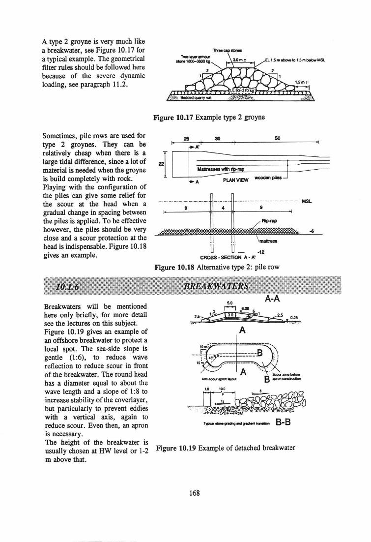
A type 2 groyne is very much likea breakwater, see Figure 10.17 fora typical example. The geometricalfilter rules should be followed herebecause of the severe dynamicloading, see paragraph 11.2.

Sometimes, pile rows are used fortype 2 groynes. They can berelatively cheap when there is alarge tidal difference, since a lot ofmaterial is needed when the groyneis build completely with rock.Playing with the configuration ofthe piles can give some relief forthe scour at the head when agradual change in spacing betweenthe piles is applied. To be effectivehowever , the piles should be veryclose and a scour proteetion at thehead is indispensabie. Figure 10.18gives an example.

'.5 m lIbowt 101.5mbeIow MSl

Figure 10.17 Example type 2 groyne

25 30 50

====t

MSL4 t

LRip-rap

u u_ ·12CROSS· SECTlONA· A'

Figure 10.18 Altemative type 2: pile row

Breakwaters will be mentionedhere only briefly, for more detailsee the lectures on this subject.Figure 10.19 gives an example ofan offshore breakwater to proteet alocal spot. The sea-side slope isgentle (1:6), to reduce wavereflection to reduce scour in frontof the breakwater . The round headhas a diameter equal to about thewave length and a slope of 1:8 toincrease stability ofthe coverlayer,but particularly to prevent eddieswith avertical axis, again toreduce scour. Even then, an apronis necessary.The height of the breakwater isusually chosen at HW level or 1-2m above that.

A-A

Figure 10.19 Example of detached breakwater

168

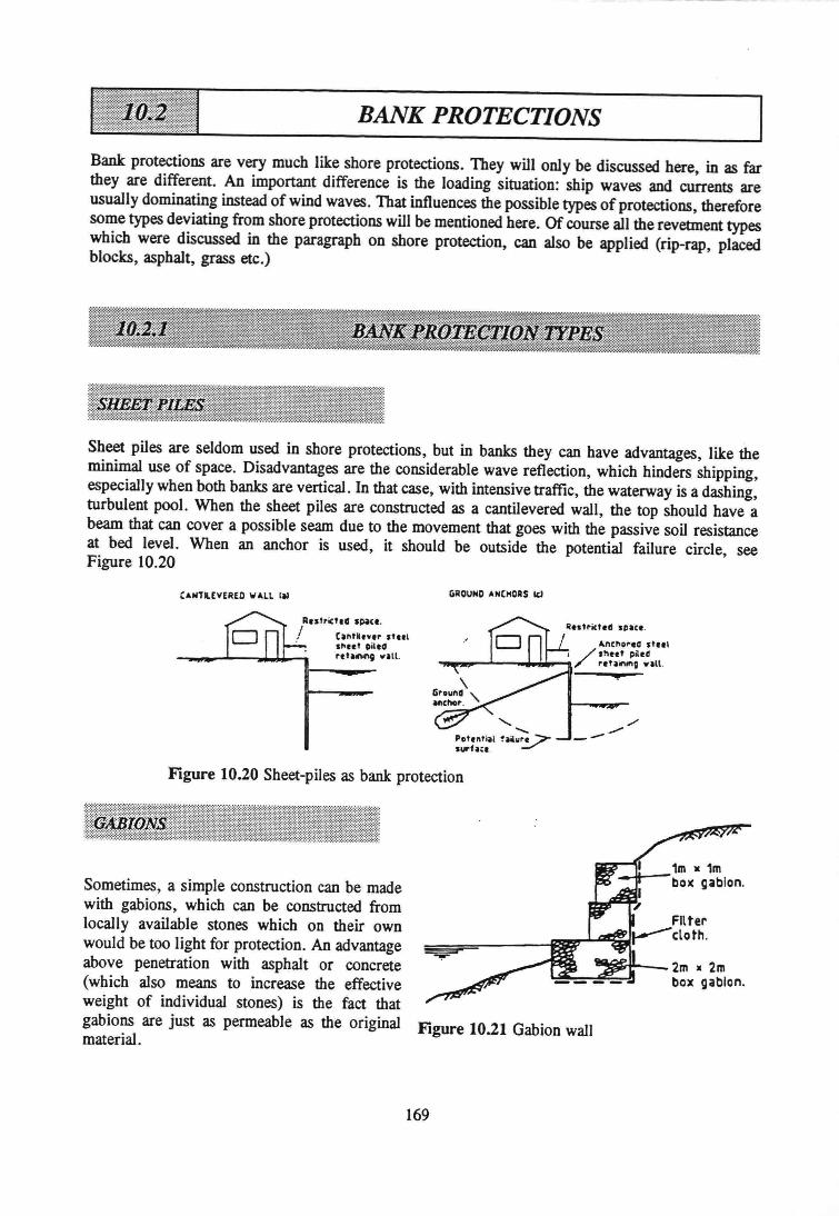
BANK PROTECTIONS

Bank protections are very much like shore protections. They will only be discussed here, in as farthey are different. An important difference is the loading situation: ship waves and currents areusually dominating instead of wind waves. That influences the possible types of protections, thereforesome types deviating from shore protections will be mentioned here. Of course all the revetment typeswhich were discussed in the paragraph on shore protection, can also be applied (rip-rap, placedblocks, asphalt, grass etc.)

Sheet piles are seldom used in shore protections, but in banks they can have advantages, like theminimal use of space. Disadvantages are the considerable wave reflection, which hinders shipping,especially when both banks are vertical. In that case, with intensive traffic, the waterway is a dashing,turbulent pool. When the sheet piles are constructed as a cantilevered wall, the top should have abeam that can cover a possible seam due to the movement that goes with the passive soil resistanceat bed level. When an anchor is used, it should be outside the potential failure circle, seeFigure 10.20

'ANTILEVERED W4LL lal

RutriCtlCl spat•..I tantRt'lr still

s~ .. t piltCir.tairWlg .,all.

GIIOUNDAN(HOAS Id

.'

./_-Figure 10.20 Sheet-piles as bank proteetion

Sometimes, a simple construction can be madewith gabions, which can be constructed fromlocally available stones which on their ownwould be too light for protection. An advantageabove penetration with asphalt or concrete(which also means to increase the effectiveweight of individual stones) is the fact thatgabions are just as permeable as the originalmateriaI.

~~'--2m .2mbox gabion.

Figure 10.21 Gabion wall

169

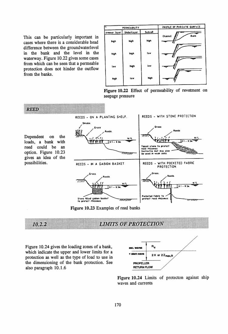
This can be particularly important incases where there is a considerable headdifference between the groundwaterlevelin the bank and the level in thewaterway. Figure 10.22 gives some casesfrom which can be seen that a permeableproteetion does not hinder the outflowfrom the banks.

,PERKEUIl"Y PROFLE OF PMREATC SURF.t.CE

at...... hur Und~~hrtr Subsol '_'v-:=_lIigh 1Iit" lIigII -

f....

IIigh 1Ii9~ 10.. ..."""'!i"

I." lIiQI'I I... ...I -'"9" 1o" 111'" ..

Figure 10.22 Effect of permeability of revetment onseepage pressure

REEDS. ON A PLANTING SHELF. REEDS. WITH STDNE PR07tCTION

SlIrllD•.

I

Dependent on theloads, a bank withreed could be anoption. Figure 10.23gives an idea of thepossibilities. REEDS • WITH POCKETED FABRE

PROTECTIONREEDS. IN A GABION BASKET

Figure 10.23 Examples of reed banks

Figure 10.24 gives the loading zones of a bank,which indicate the upper and lower limits for aproteetion as weIl as the type of load to use inthe dimensioning of the bank protection. Seealso paragraph 10.1.6

~~~~ .._---------- ---------+RIm"';;~ 2ZI'IIIIX.R

PROPELLERREl\JRN FlOW

Figure 10.24 Limits of proteeton against shipwaves and currents

170

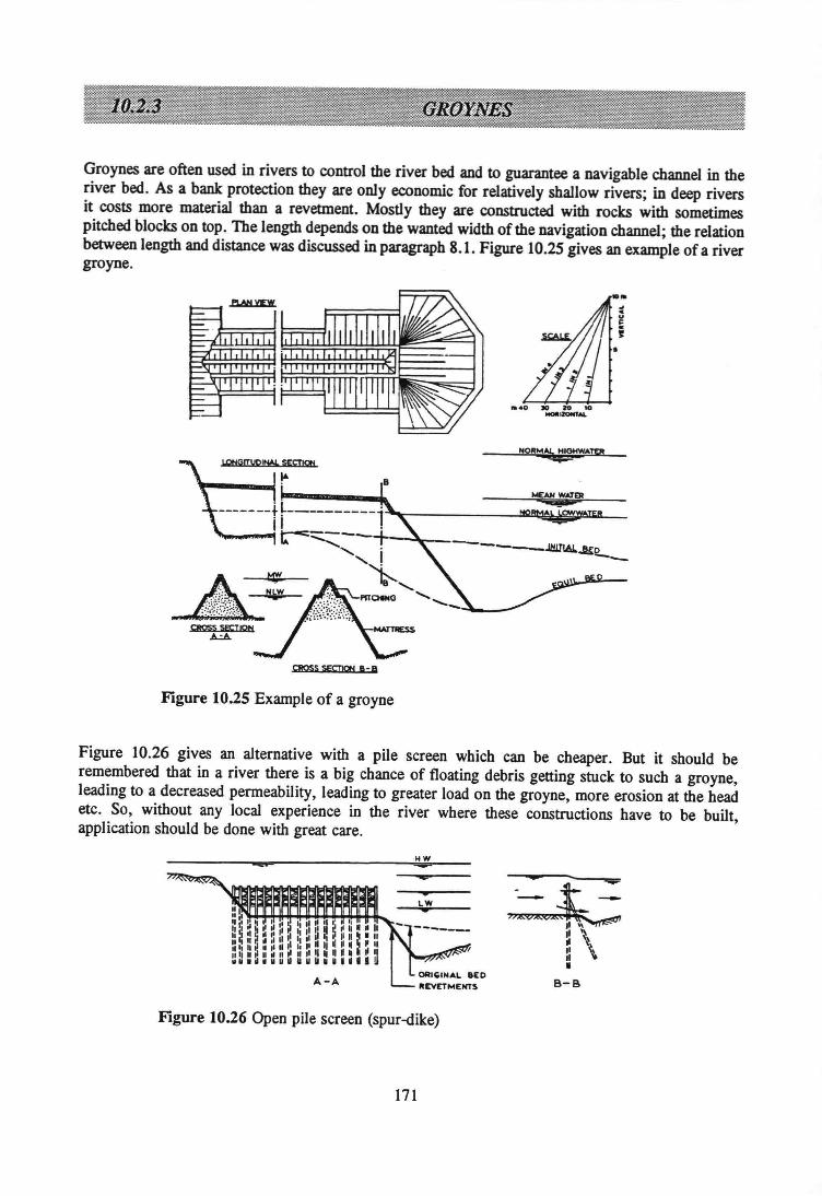
Groynes are often used in rivers to control the river bed and to guarantee a navigable channel in theriver bed. As a bank proteetion they are only economie for relatively shallow rivers; in deep riversit costs more material than a revetment. Mostly they are constructed with rocks with sometimespitched blocks on top. The length depends on the wanted width of the navigation channel; the relationbetween length and distance was discussed inparagraph 8.1. Figure 10.25 gives an example of a rivergroyne.

ID.

JCU;,

NOR"1:k. HIGHWATEI!

----JW1l~~o -_CROss sg;I1PN

A..:.A.

Figure 10.25 Exarnple of a groyne

Figure 10.26 gives an altemative with a pile screen which can be cheaper. But it should beremembered that in a river there is a big chance of floating debris getting stuck to such a groyne,leading to a decreased permeability, leading to greater load on the groyne, more erosion at the headetc. So, without any local experience in the river where these constructions have to be built,application should be done with great care.

Figure 10.26 Open pile screen (spur-dike)

171

~t_;11 ~.. ~II ~\11 ..•

8-8

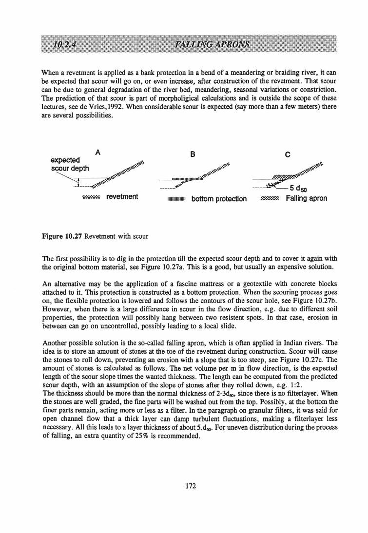
When a revetment is applied as a bank proteetion in a bend of a meandering or braiding river, it caobe expected that scour will go on, or even increase, after construction of the revetment. That scourcao be due to general degradation of the river bed, meandering, seasonal variations or constriction.The prediction of that scour is part of morpholigical calculations and is outside the scope of theselectures, see de Vries, 1992. When considerablescour is expected (say more than a few meters) thereare several possibilities.

A B c

~ revetment 111111111111111 bottom protection5d50

~ Falling apron

Figure 10.27 Revetment with scour

The first possibility is to dig in the proteetion till the expected scour depth and to cover it again withthe original bottom material, see Figure 10.27a. This is a good, but usually an expensive solution.

An altemative may be the application of a fascine mattress or a geotextile with concrete blodesattached to it. This proteetion is constructed as a bottom protection. When the scouring process goeson, the flexible proteetion is lowered and follows the contours of the scour hole, see Figure lO.27b.However, when there is a large difference in scour in the flow direction, e.g. due to different soilproperties, the proteetion will possibly hang between two resistent spots. In that case, erosion inbetween can go on uncontrolled, possibly leading to alocal slide.

Another possible solution is the so-called falling apron, which is often applied in Indian rivers. Theidea is to store an amount of stones at the toe of the revetment during construction. Scour will causethe stones to roll down, preventing an erosion with a slope that is too steep, see Figure 1O.27c.Theamount of stones is calculated as follows. The net volume per m in flow direction, is the expectedlength of the scour slope times the wanted thickness. The length cao be computed from the predictedscour depth, with an assumption of the slope of stones after they rolled down, e.g. 1:2.The thickness should be more than the normal thickness of2-3d~" since there is no filterlayer. Whenthe stones are weil graded, the fine parts will be washed out from the top. Possibly, at the bottom theflner parts remain, acting more or less as a filter. In the paragraph on granular filters, it was said foropen channel flow that a thick layer can damp turbulent fluctuations, making a filterlayer lessnecessary. All this leads to a layer thickness of about 5.dso• For uneven distribution during the processof falling, an extra quantity of 25% is recommended.

172

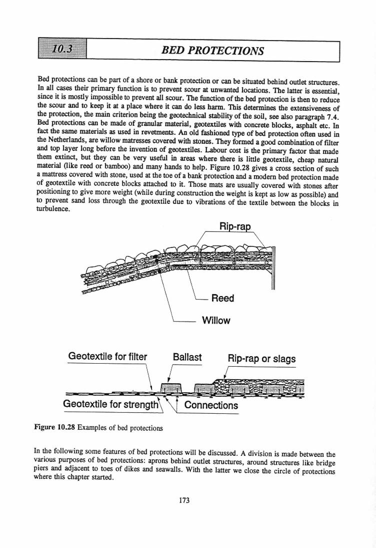
BED PROTECTIONS

Bed protections can be part of a shore or bank proteetion or can be situated behind outlet structures.In all cases their primary function is to prevent scour at unwanted locations. The latter is essential,since it is mostly impossible to prevent all SCOuf. The function ofthe bed proteetion is then to reducethe scour and to keep it at a piace where it can do less harm. This determines the extensiveness ofthe protection, the main criterion being the geotechnical stability of the soil, see also paragraph 7.4.Bed protections can be made of granular material, geotextiles with concrete blocks, asphalt etc. Infact the same materials as used in revetments. An old fashioned type of bed proteetion often used inthe Netherlands, are willow matresses covered with stones. They formed a good combination of filterand top layer long before the invention of geotextiles. Labour cost is the primary factor that madethem extinct, but they can be very useful in areas where there is little geotextile, cheap naturalmaterial (like reed or bamboo) and many hands to help. Figure 10.28 gives a cross section of sucha mattress covered with stone, used at the toe of a bank proteetion and a modem bed proteetion madeof geotextile with concrete blocks attached to it. Those mats are usually covered with stones afterpositioning to give more weight (whiIe during construction the weight is kept as low as possible) andto prevent sand loss througb the geotextile due to vibrations of the textile between the blocks inturbulence.

Reed

Willow

Geotextile tor strength\ \1 Co~nectio;s -

Flgure 10.28 Examples of bed protections

In the following some features of bed protections will be discussed. A division is made between thevarious purposes of bed protections: aprons bebind outlet structures, around structures like bridgepiers and adjacent to toes of dikes and seawalls. With the latter we close the circle of protectionswhere this chapter started.

173

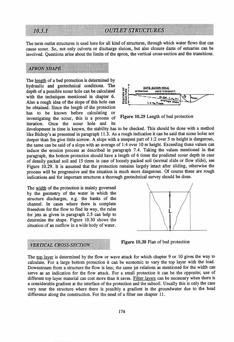
The term outlet structures is used here for all kind of structures, through which water flows that cancause scour. So, not only culverts or discharge sluices, but also closure dams of estuaries can beinvolved. Questions arise about the limits of the apron, the verticaI cross-section and the transitions.

The lim.gth of a bed proteetion is determined byhydraulic and geotechnical conditions. Thedepth of a possible scour hole can be calculatedwith the techniques mentioned in chapter 6.Also a rough idea of the slope of this hole canbe obtained. Since the length of the proteetionhas to be known before calculating orinvestigating the scour, this is a process of Figure 10.29 Length of bed proteetioniteration. Once the scour hole and itsdevelopment in time is known, the stability has to be checked. This should be done with a methodlike Bishop's as presented in paragraph 11.3. As a rough indication it can be said that scour holes notdeeper than 5m give little sorrow. A slope with a steepest part of 1:2 over 5 m height is dangerous,the same cao be said of a slope with an average of 1:4 over 10 m height. Exceeding these values caninduce the erosion process as described in paragraph 7.4. Taking the values mentioned in thatparagraph, the bottom proteetion should have a length of 6 times the predicted scour depth in caseof densily packed soil and 15 times in case of loosely packed soil (normal slide or flow slide), seeFigure 10.29. It is assumed that the proteetion remains largely intact after sliding, otherwise theprocess will be progressive and the situation is much more dangerous. Of course these are rougbindications and for important structures a thorougb geotechnical survey should be done.

The width of the proteetion is mainly governedby the geometry of the water in whicb thestructure discharges, e.g. the banks of thechannel. In cases where there is completefreeedom for the flow to find its way, the rulesfor jets as given in paragraph 2.5 can help todetermine the shape. Figure 10.30 shows thesituation of an outflow in a wide body of water.

L

Figure 10.30 Plan of bed proteetion

The top layer is determined by the flow or wave attack for whicb chapter 9 or 10 gives the way tocalculate. For a large bottom proteetion it can be economie to vary the top layer with the load.Downstream from a structure the flow is less; the same jet relations as mentioned for the width canserve as an indication for the flow attack. For a small proteetion it can be the opposite; use ofdifferent top layer material can cost more than it saves. Filter layers can be necessary when there isa considerable gradient at the interface of the proteetion and the subsoil. Usually this is only the casevery near the structure where there is possibly a gradient in the groundwater due to the headdifference along the construction. For the need of a filter see chapter 11.

174

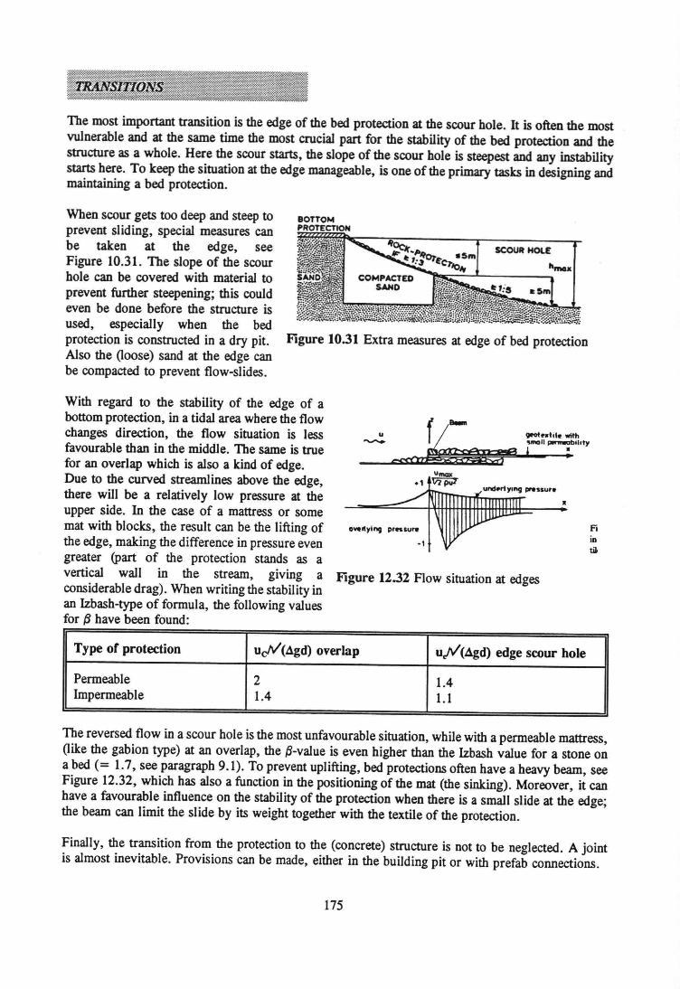
The most important transition is the edge of the bed protection at the scour hole. It is often the mostvulnerable and at the same time the most crucial part for the stability of the bed proteetion and thestructure as a whoie. Here the scour starts, the slope of the scour hole is steepest and any instabilitystarts here. To keep the situation at the edge manageable, is one of the primary tasks in designing andmaintaining a bed protection.

When scour gets too deep and steep to BOTTOM

prevent sliding, special measures caobe taken at the edge, see $COUR HOlE

Figure 10.31. The slope of the scourhole cao be covered with material toprevent further steepening; this couldeven be done before the structure isused, especially when the bedproteetion is constructed in a dry pit. Figure 10.31 Extra measures at edge of bed proteetionAlso the (loose) sand at the edge canbe compacted to prevent flow-slides.

With regard to the stability of the edge of abottom protection, in a tidal area where the flowchanges direction, the flow situation is lessfavourable than in the middle. The same is truefor an overlap which is also a kind of edge.Due to the curved stream1ines above the edge,there will be a relatively low pressure at theupper side. In the case of a mattress or somemat with blocks, the result can be the lifting ofthe edge, making the difference in pressure evengreater (part of the proteetion stands as avertical wall in the stream, grving aconsiderable drag). When writing the stability inan Izbash-type of formula, the following valuesfor (J have been found:

f a.-u ~ •• tol. wilh

~ ~ -'-""- @ , :c«rJl

FiintiJ.

•o... lIying p,ftsu,.

-I

Figure 12.32 Flow situation at edges

Type of protection uc/V'(.4gd) overlap u;V(..1gd) edge scour hole

Permeable 2 1.4ImpermeabIe 1.4 1.1

The reversed flow in a scour hole is the most unfavourable situation, while with a permeable mattress,(like the gabion type) at an overlap, the {J-valueis even higher than the Izbash value for a stone ona bed (= 1.7, see paragraph 9.1). To prevent uplifting, bed protections often have a heavy beam, seeFigure 12.32, which has also a function in the positioning of the mat (the sinking). Moreover, it caohave a favourable influence on the stability of the proteetion when there is a small slide at the edge;the beam cao limit the slide by its weight together with the textile of the protection.

Finally, the transition from the proteetion to the (concrete) structure is not to be neglected. A jointis almost inevitabIe. Provisions can be made, either in the building pit or with prefab connections.

175

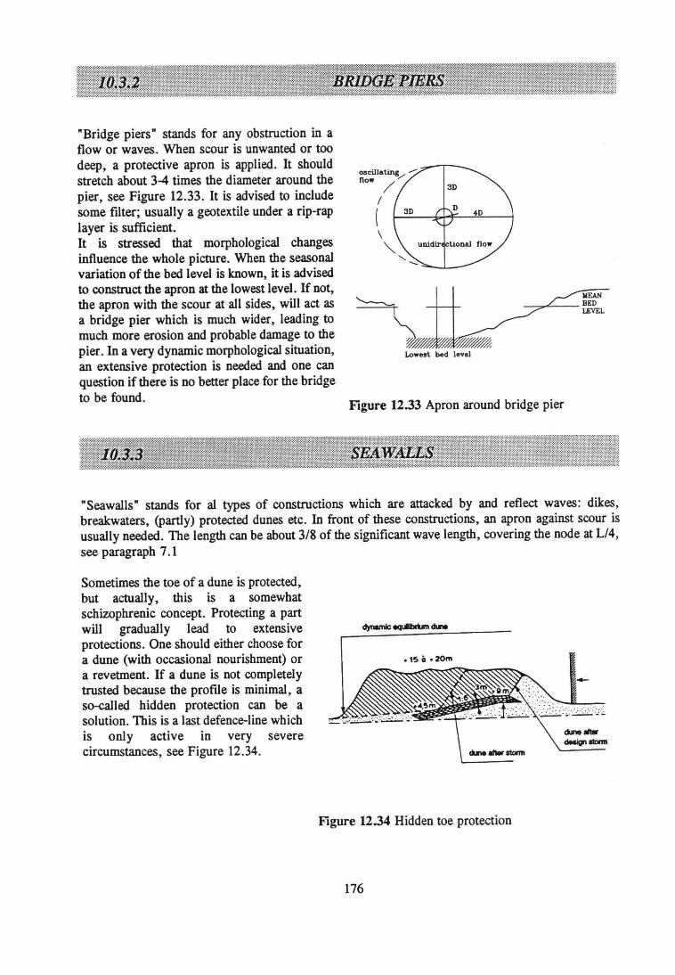
"Bridge piers" stands for any obstruction in aflow or waves. When scour is unwanted or toodeep, a protective apron is applied. It shouldstretch about 3-4 times the diameter around thepier, see Figure 12.33. It is advised to includesome filter; usually a geotextile under a rip-raplayer is sufficient.It is stressed that morphological changesinfluence the whole picture. When the seasonalvariation of the bed level is known, it is advisedto construct the apron at the lowest level. If not,the apron with the scour at all sides, will act asa bridge pier which is much wider, leading tomuch more erosion and probable damage to thepier. In a very dynamic morphological situation,an extensive proteetion is needed and one canquestion if there is no better place for the bridgeto be found.

oscülating/ --­now /

I(

Lowest bed level

Figure 12.33 Apron around bridge pier

"Seawalls" stands for al types of constructions which are attacked by and reflect waves: dikes,breakwaters, (partly) protected dunes etc. In front of these constructions, an apron against scour isusually needed. The length can be about 3/8 of the significant wave length, covering the node at L/4,see paragraph 7.1

Sometimes the toe of a dune is protected,but actually, this is a somewhatschizophrenic concept. Protecting a partwill gradually lead to extensiveprotections. One should either choose fora dune (with occasional nourishment) ora revetment. If a dune is not completelytrusted because the profile is minimal, aso-called hidden proteetion can be asolution. This is a last defence-line whichis only active in very severecircumstances, see Figure 12.34.

.1S 0 .20m

Figure 12.34 Hidden toe proteetion

176

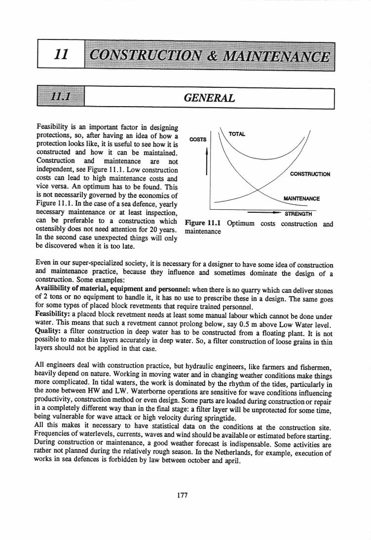
11

GENERAL

Feasibility is an important factor in designingprotections, 80, after having an idea of how aproteetion looks like, it is useful to see how it isconstructed and how it can be maintained.Construction and maintenance are notindependent, see Figure 11.1. Low constructioncosts can lead to high maintenance costs andvice versa. An optimum has to be found. Thisis not necessarily govemed by the economics ofFigure 11.1. In the case of a sea defence, yearlynecessary maintenance or at least inspection,can be preferabIe to a construction whichostensibly does not need attention for 20 years.In the second case unexpected things will onlybe discovered when it is too late.

COSTS

I CONSTRUCTION

STRENGTH

Figure 11.1 Optimum costs construction andmaintenance

Even in our super-specialized society, it is necessary for a designer to have some idea of constructionand maintenance practice, because they influence and sometimes dominate the design of aconstruction. Some examples:Availibility of material, equipment and personnel: when there is no quarry which can deliver stonesof 2 tons or no equipment to handle it, it has no use to prescribe these in a design. The same goesfor some types of placed block revetments that require trained personnel.Feasibility: a placed block revetment needs at least some manuallabour which cannot be done underwater. This means that such arevetment cannot prolong below, say 0.5 m above Low Water level.Quality: a filter construction in deep water has to be constructed from a floating plant. It is notpossible to make thin layers accurately in deep water. So, a filter construction of loose grains in thinlayers should not be applied in that case.

All engineers deal with construction practice, but hydraulic engineers, like farmers and fishermen,heavily depend on nature. Working in moving water and in changing weather conditions make thingsmore complicated. In tidal waters, the work is dominated by the rhythm of the tides, particularly inthe zone between HW and LW. Waterborne operations are sensitive for wave conditions influencingproductivity, construction method or even design. Some parts are loaded during construction or repairin a completely different way than in the final stage: a filter layer will be unprotected for some time,being vulnerable for wave attack or high velocity during springtide.All this makes it necessary to have statistical data on the conditions at the construction site.Frequencies of waterlevels, currents, waves and wind should be available or estimated before starting.During construction or maintenance, a good weather forecast is indispensabIe. Some activities arerather not planned during the relatively rough season. In the Netherlands, for example, execution ofworks in sea defences is forbidden by law between october and april.

177

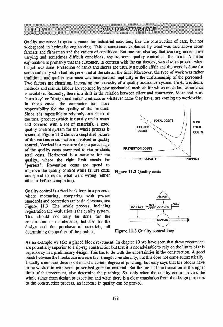
Quality assurance is quite common for industrial activities, like the construction of cars, but notwidespread in hydraulic engineering. This is sometimes explained by what was said above aboutfarmers and fishermen and the variety of conditions. But one cao also say that working under thesevarying and sometimes difficult conditions, require some quality control all the more. A betterexplanation is probably that the customer, in contrast with the car factory, was always present whenhis job was done. Proteetion of banks and shores are usually a public affair and the work is done forsome authority who had his personnel at the site all the time. Moreover , the type of work was rathertraditional and quality assurance was incorporated implicitly in the craftsmanship of the personnel.Two factors are changing, increasing the necessity of a quality assurance system. First, traditionalmethods and manuallabour are replaced by new mechanical methods for which much less experienceis available. Secondly, there is a shift in the relation between elient and contractor. More and more"turn-key" or "design and build" contracts or whatever name they have, are coming up worldwide.In those cases, the contractor has moreresponsibility for the quality of the product.Since it is impossible to rely only on a check ofthe final product (which is usually under waterand covered with a lot of material), a goodquality control system for the whole process isessential. Figure 11.2 shows a simplified pictureof the various costs that are involved in qualitycontrol. Vertical is a measure for the percentageof the quality costs compared to the productstotal costs. Horizontal is a measure for thequality, where the right limit stands for"perfect". Prevention costs are spend toimprove the quality control while failure costs Figure 11.2 Quality costsare spend to repair what went wrong (eitherafter or before completion).

%OFTOTALCOSTS

PREVENTION COSTS

- QUAUTY "PERFEC'r

Quality control is a feed-back loop in a process,where measuring, comparing with pre-setstandards and correction are basic elements, seeFigure 11.3. The whole process, includingregistration and evaluation is the quality system.This should not only be done for theconstruction or maintenance, but also for thedesign and the purchase of materials, alldetermining the quality of the product. Figure 11.3 Quality control loop

As an example we take a placed block revetment. In chapter 10 we have seen that these revetmentsare potentially superior to a rip-rap construction but that it is not advisable to rely on the limits ofthissuperiority in a preliminary design. This has to do with the uncertainties in the construction. A goodpinch between the blocks can increase the strength considerably, but this does not come automatically.Usually a contract does not demand a certain degree of pinching, but only says that the blocks haveto be washed-in with some prescribed granular material. But the toe and the transition at the upperlimit of the revetment, also determine the pinching. So, only when the quality control covers thewhole range from design to execution and when there is a clear translation from the design purposesto the construction process, an increase in quality can be proved.

178

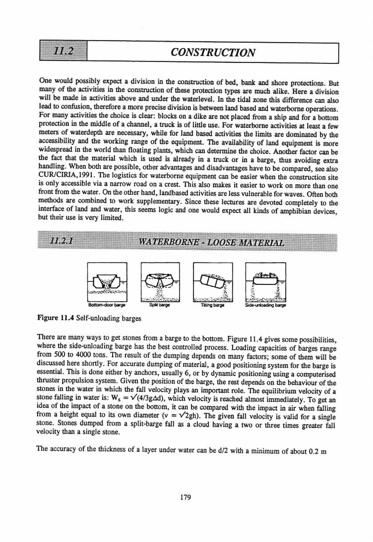
CONSTRUCT/ON

One would possibly expect a division in the construction of bed, bank and shore protections. Butmany of the activities in the construction of these proteetion types are much alike. Here a divisionwill be made in activities above and under tbe waterlevel. In tbe tidal zone tbis difference CaD alsolead to confusion, tberefore a more precise division is between land based and waterbome operations.For many activities the choice is clear: bleeks on a dike are not placed from a ship and for a bottomproteetion in the middle of a channel, a truck is of little use. For waterbome activities at least a fewmeters of waterdeptb are necessary, while for land based activities tbe limits are dominated by tbe

, accessibility and the working range of the equipment. The availability of land equipment is morewidespread in tbe world than floating plants, which CaD determine the choice. Another factor CaD bethe fact tbat the material which is used is already in a truck or in a barge, thus avoiding extrahandling. When both are possible, other advantages and disadvantages have to be compared, see alsoCURICIRIA,1991. The logistics for waterborne equipment can be easier when the construction siteis only accessible via a narrow road on acrest. This also makes it easier to work on more than onefront from tbe water. On the other hand,landbased activities are less vulnerable for waves. Often bothmetbods are combined to work supplementary. Since these lectures are devoted completely to theinterface of land and water, this seems logic and one would expect all kinds of amphibian devices,but their use is very limited.

~~..:.,~~I,...~_-..c'.~~".•. ;i~h:J

Figure 11.4 Self-unloading barges

There are many ways to get stones from a barge to the bottom. Figure 11.4 gives some possibilities,where the side-unloading barge has the best controlled process. Loading capacities of barges rangefrom 500 to 4000 tons. The result of the dumping depends on many factors; some of tbem will bediscussed here shortly. For accurate dumping of material, a good positioning system for the barge isessential. This is done either by anchors, usually 6, or by dynamic positioning using a computerisedthruster propulsion system. Given the position of the barge, the rest depends on the behaviour of thestones in the water in which the fall velocity plays an important role. The equilibrium velocity of astone falling in water is: Ws = V(4/3gAd), which velocity is reached almost immediately. To get anidea of the impact of a stone on the bottom, it can be compared with the impact in air when fallingfrom a height equal to its own diameter (v = V2gh). The given fall velocity is valid for a singlestone. Stones dumped from a split-barge fall as a cloud having a two or three times greater fallvelocity than a single stone.

The accuracy of the thickness of a layer under water can be d/2 with a minimum of about 0.2 m

179

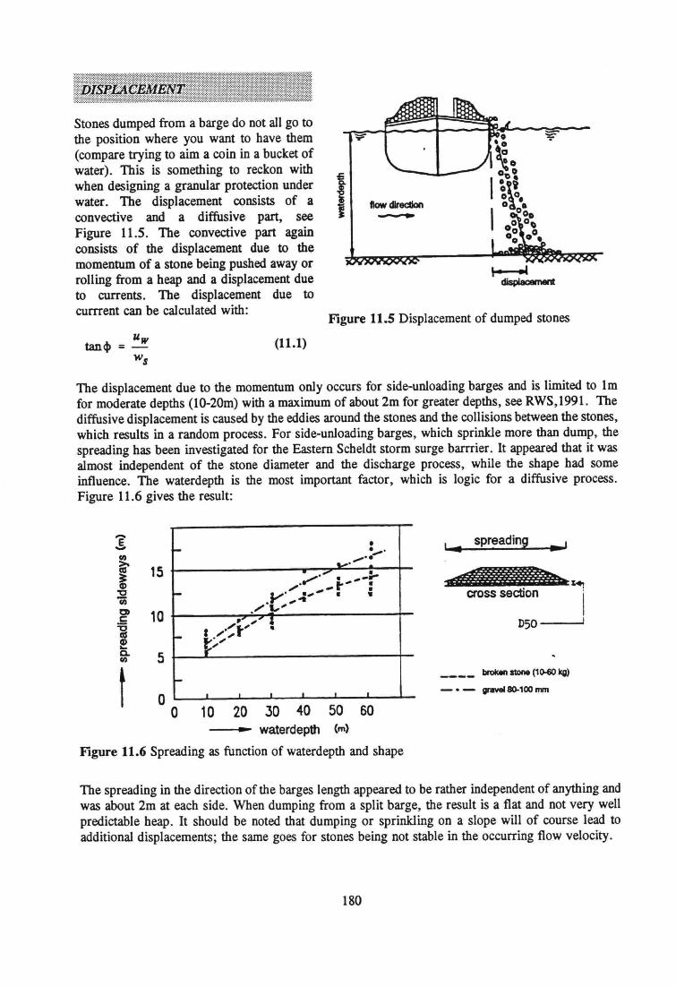
Stones dumped from a barge do not all go tothe position where you want to have them(compare trying to aim a coin in a bucket ofwater). This is something to reekon withwhen designing agranular proteetion underwater. The displacement consists of aconvective and a diffusive part, seeFigure 11.5. The convective part againconsists of the displacement due to themomentum of a stone being pushed away orrolling from a heap and a displacement dueto currents. The displacement due tocurrrent cao be calculated with:

(11.1)

flow dIredIon

---

Flgure 11.5 Displacement of dumped stones

The displacement due to the momentum only occurs for side-unloading barges and is limited to 1mfor moderate depths (10-20m) with a maximum of about 2m for greater depths, see RWS, 1991. Thediffusive displacement is caused by the eddies around the stones and the collisions between the stones,which results in a random process. For side-unloading barges, which sprinkle more than dump, thespreading has been investigated for the Eastern Scheldt storm surge barrrier. It appeared that it wasalmost independent of the stone diameter and the discharge process, while the shape had someinfluence. The waterdepth is the most important factor, which is logic for a diffusive process.Figure 11.6 gives the result:

- •._.~.-..~'''. ,-=-- ,,' _t' :V' .....""'. ,.• ,1./ .......'" !- I ...../t... •

t'''''1"

I-I •

15

10

5

,~ spreading ......

t o o

D50--...J

broken storMt (10-60 kg)

- • - gravel1JG.100 nvn

10 20 30 40 50 60---- waterdepth (m)

Figure 11.6 Spreading as function of waterdepth and shape

The spreading in the direction of the barges length appeared to be rather independent of anything andwas about 2m at each side. When dumping from a split barge, the result is a flat and not very wellpredictable heap. It should be noted that dumping or sprinlding on a slope will of course lead toadditional displacements; the same goes for stones being not stabie in the occurring flow velocity .

180

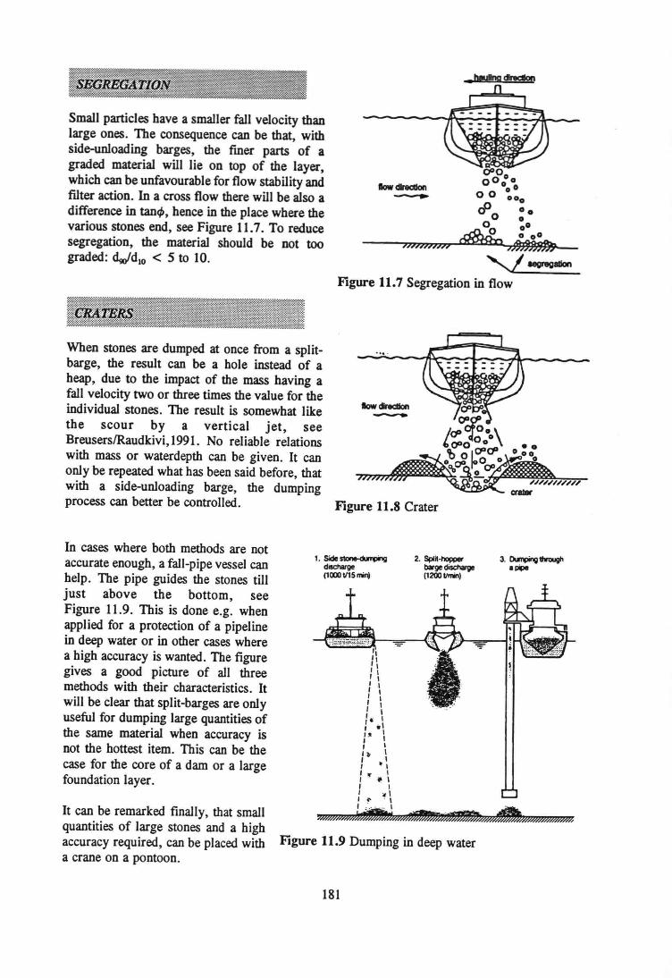
Small particles have a smaller fall velocity thanlarge ones. The consequence can be that, withside-unloading barges, the tiner parts of agraded material will lie on top of the layer,which can be unfavourable for flow stability andfilter action. In a cross flow there will be also adifference in tané hence in the place where thevarious stones end, see Figure 11.7. To reducesegregation, the material should be not toograded: dgo!d1o< 5 to 10.

When stones are dumped at once from a split­barge, the result can be a hole instead of aheap, due to the impact of the mass having afall velocity two or three times the value for theindividual stones. The result is somewhat likethe scour by a vertical jet, seeBreuserslRaudkivi,1991. No reliable relationswith mass or waterdepth can be given. It canonly be repeated what has been said before, thatwith a side-unloading barge, the dumpingprocess can better be controlled.

In cases where both methods are notaccurate enough, a fall-pipe vessel canhelp. The pipe guides the stones tilljust above the bottom, seeFigure 11.9. This is done e.g. whenapplied for a proteetion of a pipelinein deep water or in other cases wherea high accuracy is waoted. The figuregives a good picture of all threemethods with their characteristics. Itwill be clear that split-barges are onlyuseful for dumping large quantities ofthe same material when accuracy isnot the hottest item. This can be thecase for the core of a dam or a largefoundation layer.

It cao be remarked finally, that smalIquantities of large stones and a highaccuracy required, cao be placed witha crane on a pontoon.

V ugregllion

Figure 11.7 Segregation in flow

Iow dlredlon-

Figure 11.8 Crater

1.Side~discharge(1000tllS min)

2. SPHlOIlP8'barge discharge(1200 1Imin)

Figure 11.9 Dumping in deep water

181

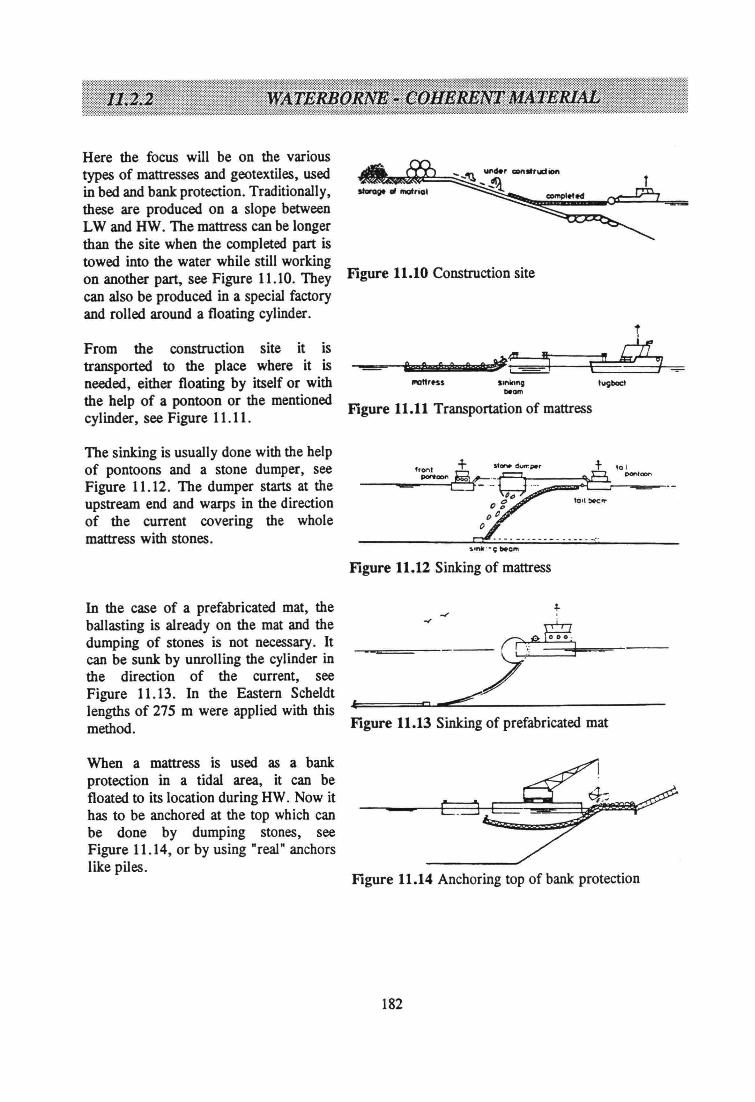
Here the focus will be on the varioustypes of mattresses and geotextiles, usedin bed and bank protection. Traditionally,these are produced on a slope betweenLW and HW. The mattress can be longerthan the site when the completed part istowed into the water while still workingon another part, see Figure 11.10. Theycan also be produced in a special factoryand rolled around a floating cylinder.

From the construction site it istransported to the place where it isneeded, either floating by itself or withthe help of a pontoon or the mentionedcylinder, see Figure 11.11.

The sinking is usually done with the helpof pontoons and a stone dumper, seeFigure 11.12. The dumper starts at theupstream end and warps in the directionof the current covering the wholemattress with stones.

In the case of a prefabricated mat, theballasting is already on the mat and thedumping of stones is not necessary. Itcan be sunk by unrolling the cylinder inthe direction of the current, seeFigure 11.13. In the Eastem Scheldtlengths of 275 m were applied with thismethod.

When a mattress is used as a bankproteetion in a tidal area, it can befloated to its location during HW. Now ithas to be anchored at the top which canbe done by dumping stones, seeFigure 11.14, or by using "real" anchorslike piles.

Figure 11.10 Construction site

~ Be ft ?? r 3~: I

t

"~\ -SIIIII1119... am

Figure 11.11 Transportation of mattress

Figure 11.12 Sinking of mattress

Figure 11.13 Sinking of prefabricated mat

Figure 11.14 Anchoring top of bank.proteetion

182

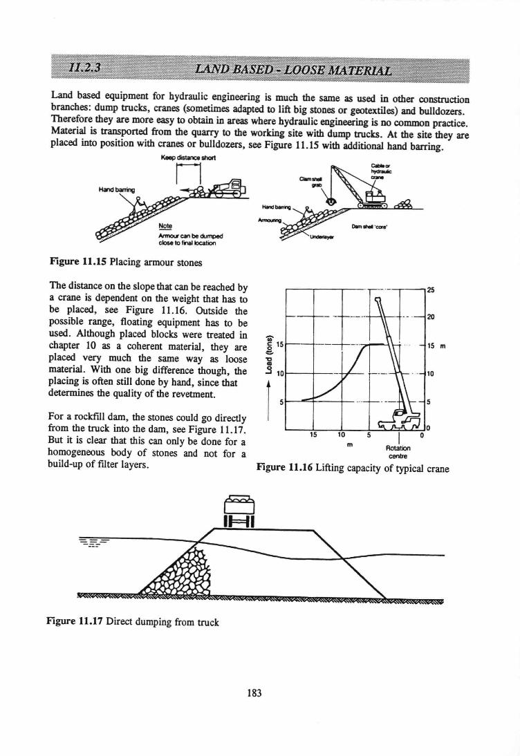
Land based equipment for hydraulic engineering is much the same as used in other constructionbranches: dump trucks, eranes (sometimes adapted to lift big stones or geotextiles) and bulldozers.Therefore they are more easy to obtain in areas where hydraulic engineering is no common practice.Material is transported from the quarry to the working site with dump trucks. At the site they areplaced lnto position with eranes or bulldozers, see Figure 11.15 with additional hand barring.

Keep distance&hortnNmIxIearlbe du~eIo&e tg fll'lallOeation

Figure 11.15 Placing annour stones

The distance on the slope that can be reached bya crane is dependent on the weight that has tobe placed, see Figure 11.16. Outside thepossible range, floating equipment has to beused. Although placed blocks were treated inchapter 10 as a coherent material, they areplaced very much the same way as loosematerial. With one big difference though, theplacing is often still done by hand, since thatdetermines the quality of the revetment.

For a rockfill dam, the stones could go directlyfrom the truck into the dam, see Figure 11.17.But it is cIear that this can only be done for ahomogeneous body of stones and not for abuild-up of filter layers.

aII=fI

f 15 15 m0~"caoS 10 10

r 5 5

15 10 IAotationcentre

Figure 11.16 Lifting capacity of typical crane

m

Figure 11.17 Direct dumping from truck

183

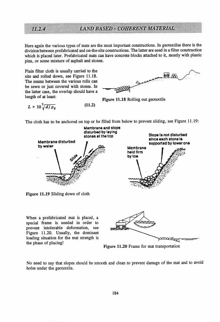
Here again the various types of mats are the most important constructions. In geotextiles there is thedivision between prefabricated and on-the-site constructions. The latter are used in a filter constructionwhich is placed later. Prefabricated mats cao have concrete blocks attached to it, mostly with plasticpins, or some mixture of asphalt and stones.

Plain filter cloth is usually carried to thesite and roUed down, see Figure 11.18.The seams between the various roUs caobe sewn or just covered with stones. Inthe latter case, the overlap should have alength of at least:

3L > 10 V dl Ps (11.2)

Figure 11.18 Rolling out geotextile

The cloth has to be aochored on top or be filled from below to prevent sliding, see Figure 11.19:Membrane and s!opedlsturbed by laylngstones at the top

Membrane dlsturbedby water

Figure 11.19 Sliding down of cloth

When a prefabricated mat is placed, aspecial frame is needed in order toprevent intolerable deformation, seeFigure 11.20. Usually, the dominantloading situation for the mat strength isthe phase of placing!

Slop. I. noldlsturbedIince aach slonll.aupportld by lowlron.

Figure 11.20 Frame for mat transportation

No need to say that slopes should be smooth and clean to prevent damage of the mat and to avoidholes under the geotextile.

184

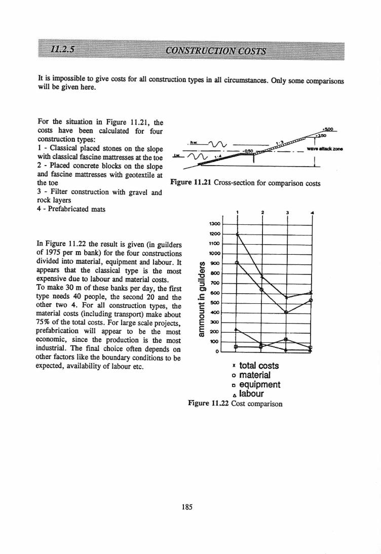
It is impossible to give costs for all construction types in all circumstances. OnIy some comparisonswill be given here.

For the situation in Figure 11.21, thecosts have been calculated for fourconstruction types:1 - ClassicaI placed stones on the slopewith classicaI fascine mattresses at the toe2 - Placed concrete blocks on the slopeand fascine mattresses with geotextile atthe toe3 - Filter construction with gravel androck layers4 - Prefabricated mats

.~'\/"'V-_. __ • - - !IC

.J.lL_ ~ "A

Figure 11.21 Cross-sectien for comparison costs

InFigure 11.22 the result is given (in guildersof 1975 per m bank) for the four constructionsdivided into materiaI, equipment and labour. Itappears that the classical type is the mostexpensive due to labour and material costs.To make 30 m of these banks per day, the fusttype needs 40 people, the second 20 and theother two 4. For all construction types, thematerial costs (including transport) make about75% of the totaI costs. For large scale projects,prefabrication will appear to be the mosteconomie, since the production is the mostindustriaI. The final choice often depends onother factors Iike the boundary conditions to beexpected, availability of labour etc.

2 3

1300

1200

1100

1000

e 900

CD 80032-5 7000)600.E:- 500c:~ .000E 300

E 200ca100

0

r\\\

L'\. ~~ ~

"I <,-, t- ...)

'\V

<, ~ ~t><:._ ~

x tataJcastso materiaJe equipment6 labour

Figure 11.22 Cost comparison

185

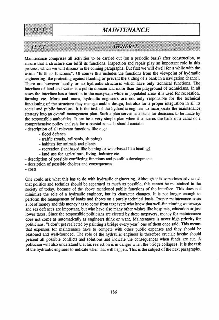
MAINTENANCE

Maintenance comprises all activities to be carried out (on a periodic basis) after construction, toensure that a structure can fulfil its functions. Inspeetion and repair play an important role in thisprocess, which we will discuss in the coming paragraphs. But fust we will dweil for a while with thewords "fulfil its functions". Of course this includes the functions from the viewpoint of hydraulicengineering like protecting against flooding or prevent the sliding of a bank in a navigation channel.There are however hardly or no hydraulic structures which have only technical functions. Theinterface of land and water is a public domain and more than the playground of technicians. In allcases the interface has a function in the ecosystem while in populated areas it is used for recreation,farming etc. More and more, hydraulic engineers are not only responsibie for the technicalfunctioning of the structure they manage and/or design, but also for a proper integration in all itssocial and public functions. It is the task of the hydraulic engineer to incorporate the maintenancestrategy into an overall management plan. Such a plan serves as a basis for decisions to be made bythe responsibie authorities. It can be a very simple plan when it concerns the bank of a canal or acomprehensive policy analysis for a coastal zone. It should contain:- description of all relevant functions like e.g.:

- flood defence- traftic (roads, railroads, shipping)- habitats for animals and plants- recreation (landbased like bathing or waterbased like boating)- land use for agriculture, living, industry etc.

- description of possible conflicting functions and possible developments- decription of possible choices and consequences- costs

One could ask what this has to do with hydraulic engineering. Although it is sometimes advocatedthat polities and technics should be separated as much as possible, this cannot be maintained in thesociety of today, because of the above mentioned public functions of the interface. This does notminimize the role of a hydraulic engineer, but its character changes. It is not longer enough toperform the management of banks and shores on a purely technical basis. Proper maintenance costsa lot of money and this money has to come from taxpayers who know that well-functioning waterwaysand sea defences are important, but who have also many other wishes like hospitals, education or justlower taxes. Since the responsibie politicians are elected by these taxpayers, money for maintenancedoes not come as automatically as engineers think or want. Maintenance is never high priority forpoliticians. "I don't get reelected by painting a bridge every year" one ofthem once said. This meansthat expenses for maintenance have to compete with other public expenses and they should bereasoned and well-founded. The role of the hydraulic engineer is therefore crucial: he/she shouldpresent all possible conflicts and solutions and indicate the consequences when funds are cut. Apolitician will also understand that his reeleetion is in danger when the bridge collapses. It is the taskof the hydraulic engineer to indicate when that will happen. This is the subject of the next paragraphs.

186

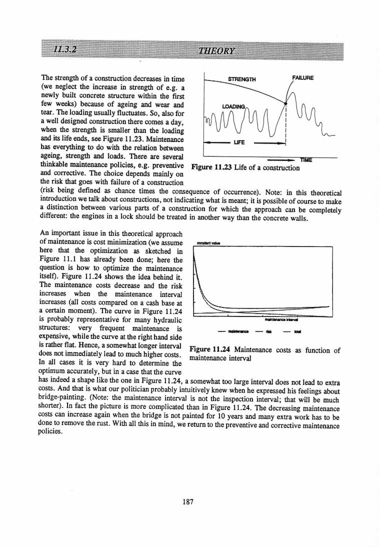
The strength of a construction decreases in time(we neglect the increase in strength of e.g. anewly built concrete structure within the fustfew weeks) because of ageing and wear andtear. The loading usually fluctuates. So, also fora weUdesigned construction there comes a day,wben the strength is smaller than the loadingand its life ends, see Figure 11.23. Maintenance UFEbas everything to do with the relation betweenageing, strength and loads. There are severalthinkable maintenance policies, e.g. preventive Figure 11.23 Life of a constructionand corrective. The cboice depends mainly onthe risk that goes with failure of a construction(risk being defined as chance times the consequence of occurrence). Note: in this theoreticalintroduetion we talk about constructions, not indicating what is meant; it is possible of course to makea distinction between various parts of a construction for which the approach can be completelydifferent: the engines in a loek should be treated in another way than the concrete walis.

An important issue in this theoretical approachof maintenance is cost minimization (we assumehere that the optimization as sketched inFigure 11.1 has already been done; here thequestion is how to optimize the maintenanceitselt). Figure 11.24 shows the idea behind it.The maintenance costs decrease and the riskincreases when the maintenance intervalincreases (all costs compared on a cash base ata certain moment). The curve in Figure 11.24is probably representative for many hydraulicstructures: very frequent maintenance isexpensive, while the curve at the right hand sideis rather flat. Hence, a somewhat longer interval Figure 11.24 Maintenance costs as function ofdoes not immediately lead to much higher costs. maintenance intervalIn all cases it is very hard to determine theoptimum accurately, but in a case that the curvebas indeed a shape like the one in Figure 11.24, a somewhat too large interval does not lead to extracosts. And that is what our politician probably intuitively knew when he expressed his feelings aboutbridge-palnting. (Note: the maintenance interval is not the inspeetion interval; that will be muchshorter). In fact the picture is more complicated than in Figure 11.24. The decreasing maintenanceCOStscan increase again when the bridge is not painted for 10 years and many extra work has to bedone to remove the rust. With all this in mind, we return to the preventive and corrective maintenancepolicies.

-- __ - flik

187

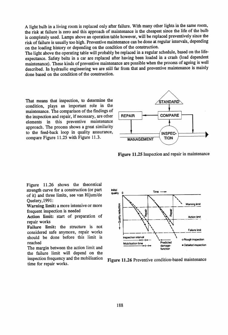
A light buib in a living room is replaced only after failure. With many other lights in the same room,the risk at failure is zero and this approach of maintenance is the cheapest since the life of the buibis compietely used. Lamps above an operation tabie however, will be replaced preventively since therisk of failure is usually too high. Preventive maintenance can be done at regular intervals, dependingon the Ioading history or depending on the condition of the construction.The light above the operating tabie will probably be replaced in a regular scheduIe, based on the life­expectance. Safety beIts in a car are replaced after having been Ioaded in a crash (load dependentmaintenance). These kinds of preventive maintenance are possibie when the process of ageing is welldescribed. In hydraulic engineering we are still far from that and preventive maintenance is mainlydone based on the condition of the construction.

That means that inspection, to determine thecondition, plays an important role in themaintenance. The comparison of the findings ofthe inspeetion and repair , if necessary, are otherelements in this preventive maintenanceapproach. The process shows agreat similarityto the feed-back loop in quality asssurance,compare Figure 11.25 with Figure 11.3.

Figure 11.26 shows the theoreticalstrength curve for a construction (or partof it) and three Iimits, see van HijumldeQuelery, 1991:Warning limit: a more intensive or morefrequent inspeetion is neededAction limit: start of preparation ofrepair worksFailure limit: the structure is notconsidered safe anymore, repair worksshouid be done before this limit isreachedThe margin between the action limit andthe failure limit will depend on theinspeetion frequency and the mobilisationtime for repair works.

REPAIR

MANAGEMENT

Figure 11.25lnspection and repair in maintenance

InspectlOn interval

Mobilisation timeoRough inspection

• OeIaiIed inspection

Figure 11.26 Preventive condition-based maintenance

188

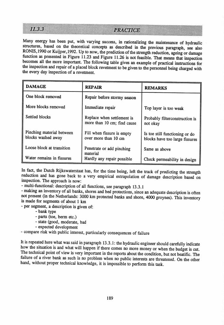
Many energy has been put, with varying success, in rationalizing the maintenance of hydraulicstructures, based on the theoretical concepts as described in the previous paragraph, see alsoRONIS,1990 or Kuijper,1992. Up to now, the prediction ofthe strength reduction, ageing or damagefunction as presented in Figure 11.23 and Figure 11.26 is not feasible. That means that inspeetionbecomes all the more important. The following table gives an example of practical instructions forthe inspeetion and repair of a placed block revetment to be given to the personnel being charged withthe every day inspeedon of a revetment.

DAMAGE REPAIR REMARKS

One block removed Repair before stormy season

More blocks removed Immediate repair Top layer is too weak

Settled blocks Replace when settlement is Probably filterconstruction ismore than 10 cm; find cause not okay

Pinching material between Fill when fissure is empty Is toe still functioning or doblocks washed away over more than 10 cm blocks have too large fissures

Loose block at transition Penetrate or add pinching Same as abovematerial

Water remains in fissures Hardly any repair possible Check permeabiIity in design

In fact, the Dutch Rijkswaterstaat has, for the time being, left the track of predicting the strengthreduction and has gone back to a very empirical extrapolation of damage description based oninspection. The approach is now:- multi-functional: description of all functions, see paragraph 13.3.1- making an inventory of all banks, shores and bed protections, since an adequate description is oftennot present (in the Netherlands: 3000 km protected banks and shore, 4000 groynes). This inventoryis made for segments of about 1 km- per segment, a description is given of:

- bank type- parts (toe, berm etc.)- state (good, moderate, bad- expected development

- compare risk with public interest, particularly consequences of failure

It is repeated here what was said in paragraph 13.3.1: the hydraulic engineer should carefully indicatehow the situation is and what will happen if there comes no more money or when the budget is cut.The technical point of view is very important in the reports about the condition, but not beatific. Thefailure of a river bank as such is no problem when no public interests are threatened. On the otherhand, without proper technical knowiedge, it is impossible to perform this task,

189

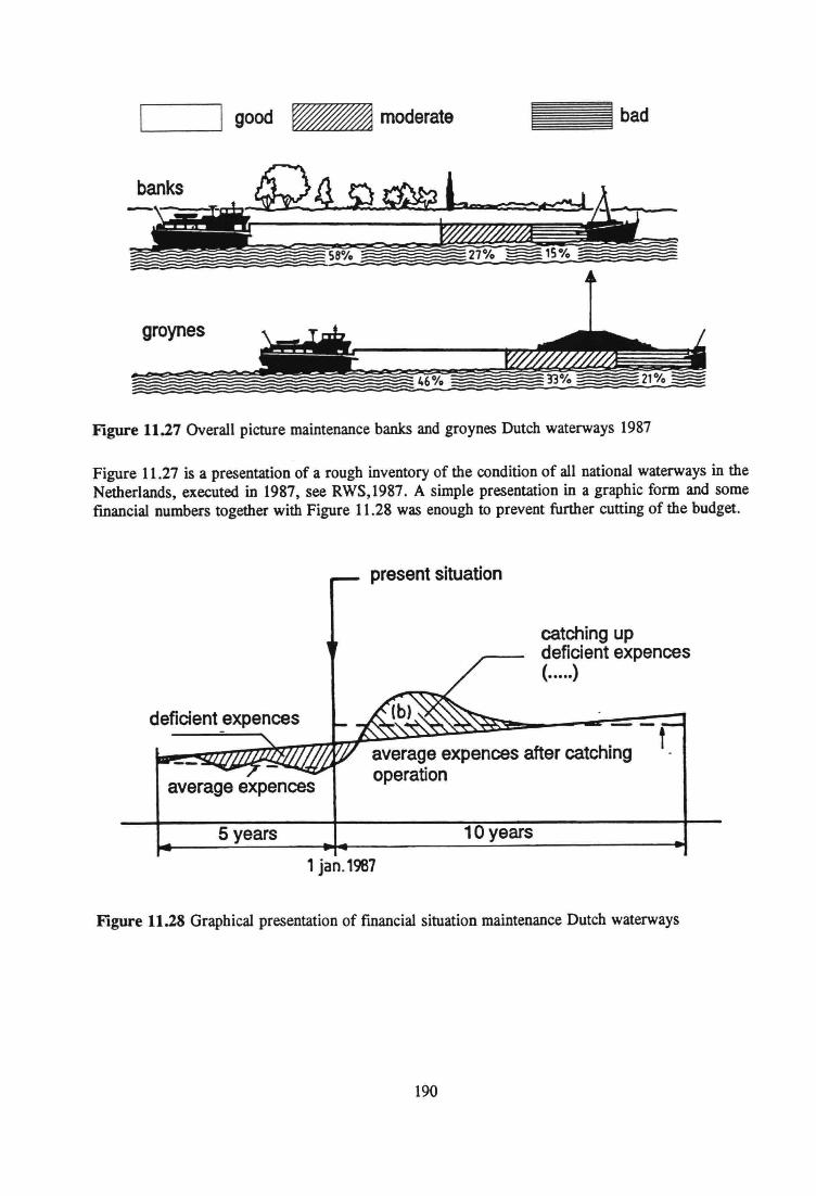
bad

groynes

Figure 11.27Overall picture maintenance banks and groynes Dutch waterways 1987

Figure 11.27 is a presentation of a rough inventory of the condition of all national waterways in theNetherlands, executed in 1987, see RWS,1987. A simple presentation in a graphic form and somefmancial numbers together with Figure 11.28 was enough to prevent further cutting of the budget.

present situation

catching updeficient expences(.....)

average expences

average expences after catchingoperation

f

5 years 10 years

1 jan.19B7

Figure 11.28Graphical presentation of fmancial situation maintenance Dutch waterways

190

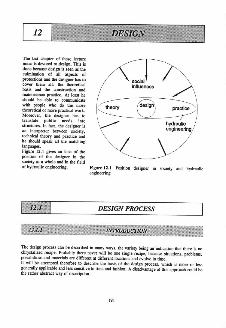
12

The last chapter of these lecturenotes is devoted to design. This isdone because design is seen as theculmination of all aspects ofprotections and the designer has tocover them all: the theoreticalbasis and the construction andmaintenance practice. At least heshould be able to communicatewith people who do the moretheoretical or more practical work.Moreover , the designer has totranslate public needs intostructures. In fact, the designer isan interpreter between society,technical theory and practice aodhe should speak all the matchinglanguages.Figure 12.1 gives an idea of theposition of the designer in thesociety as a whole aod in the fieldof hydraulic engineering.

/socialinfluences

Figure 12.1 Position designer in society and hydraulicengineering

DESIGN PROCESS

The design process cao be described in maoy ways, the variety being an indication that there is nochrystalized recipe. Probably there never will be one single recipe, because situations, problems,possibilities and materials are different at different locations and evolve in time.It will be attempted therefore to describe the basis of the design process, which is more or lessgenerally applicable and less sensitive to time and fashion. A disadvantage of this approach could bethe rather abstract way of description.

191

DETAILEDDESIGN

~NFLUENC~NG

FACTORS

Figure 12.2 Design process in time and surroundings

The design process can possibly best be described in two dimensions: time and influencing factors,see Figure 12.2. The time dimension (the various phases of the design) will be discussed in paragraph14.1.3 and the surroundings (the influencing factors) in paragraph 14.1.2. During the design process,the relative importance of the influencing factors will vary, so the course of the process inFigure 12.2 will certainly not be a straight line but will be pushed and pulled by forces in society.

Design of an interface-proteetion is usually part of a more comprehensive construction like a dam,a canal or an outlet-sluice. This again can be part of a larger plan: the development of an irrigationproject, a town renewal etc. These larger frameworks will certainly influence the choices to be madein the design process.

With many factors involved, the design process has an iterative nature, which can even go on afterconstruction. This may seem strange, since only one altemative will be actually executed, but theexperiences gathered from a construction can be a guideline for future designs or other parts of thesame project e.g. the revetment of a long dike which is constructed over a long period. In fact, thisforms the basis of many hydraulic engineering practice, where experience plays an important role.Science made its entrance in this field only the last few decades and experienee will remain crucial.The Deltaworks in the Netherlands were designed with the best available research techniques, but theplanning was such that the experience gathered with one dam, could be used in the next, going fromsmall to large.

192

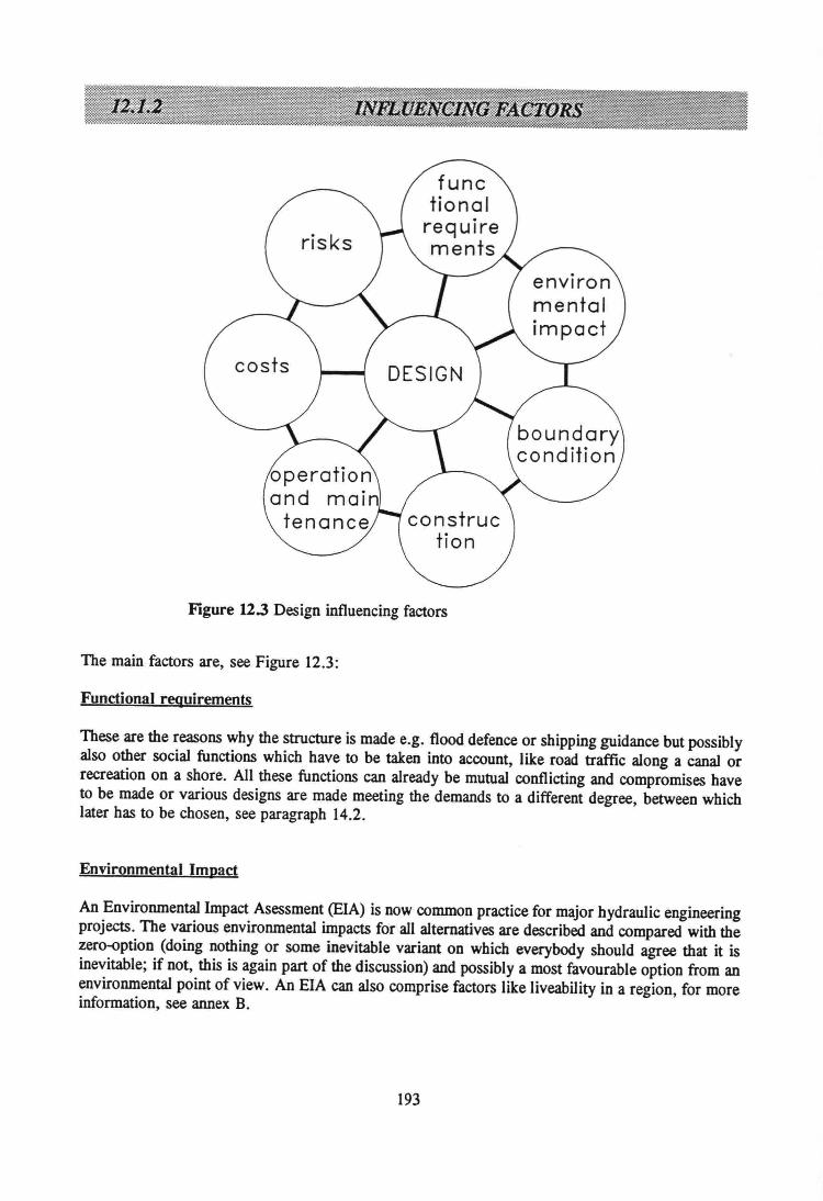
risks

environmentolimpact

operotionand maintenonce

Figure 12.3Design influencing factors

The main factors are, see Figure 12.3:

Functional reguirements

These are the reasons why the structure is made e.g. flood defence or shipping guidance but possiblyalso other social functions which have to be taken into account, like road traffic along a canal orrecreation on a shore. All these functions can already be mutual conflicting and compromises haveto be made or various designs are made meeting the demands to a different degree, between whichlater has to be chosen, see paragraph 14.2.

Environmental Impact

An Environmental Impact Asessment (EIA) is now common practice for major hydraulic engineeringprojects. The various environmental impacts for all alternatives are described and compared with thezero-option (doing nothing or some inevitabie variant on which everybody should agree that it isinevitabie; if not, this is again part of the discussion) and possibly a most favourable option from anenvironmental point of view. An EIA can also comprise factors like liveability in a region, for moreinformation, see annex B.

193

Boundary conditions

These include waterlevels, currents, wave conditions, sediment characteristics, soil shear stress,cohesion etc. Usually there is not very much to choose here and the data are just collected bysurveying.

Construction

As already stated in the previous chapter, the construction can have a large influence on the design.The availibility of materials, equipment and (skilled) personnel can be of crucial importance. Forlarge scale projects it is not unusual to design special equipment for the construction. In that case itcan open the way to other options in the design. Construction time can also play a role, either inrelation to boundary conditions (e.g. stormy season) or to the need of the project being executed.

Operation and maintenance

Here the same holds as for construction. Already in the design, the possibilities for maintenanceshould be taken into account. Factors like the accessibility of the structure for inspeetion and repair ,the repairability and the maintenance costs should be considered.

This factor needs no clarification.

Although all options will be designed with a same risk in the fmal stage, there can be differences.This can be because of unknown long-term behaviour of some new material or construction type. Forthe construction period there cao be differences in risks, either resulting in delay, accidents or damagedue to temporary lack of protection.

Not all factors will have the same importance; sometimes other factors are important as weIl. Theirrelative importance varies during the design process. In the conceptual phase, the functionalrequirements and the boundary conditions will probably be dominant above the possibilities ofmaintenance, which gets more important in the details of the structural phase. Neglecting howeverany one of them in any stage of the design process, will lead to extra iterations or worse, to anunsatisfying product. At least in every phase of the design process the designer should ask himselfthe question for every relevant factor: how does this influence my design and if Ineglect it now ormake an assumption, can I solve possible problems in the next phase?

194

Figure 12.4 Steps in the design process

Figure 12.4 shows the most important steps in the design process:

Problem identification

An essential step is the problem identification, because it happens that different people working onthe same project, have a different idea about the problem they are working at. Or the designing teamas a whole has a different idea than the responsibIe authorities or the comrnunity. The most tragicmistake a designer can make is coming with the right answer to the wrong question.

Project reguirements

The fust step to the solution of the identified problem is to formulate the requirements. There isalways the danger to jump into existing solutions, based on experience, while the problem maypossibly ask for completely different solutions. This may show that experience is not only essential,but cao also be a handicap! In fact the designer should have some "meta-experience" which tells himthat he should not only use his "historical" experience.

Conceptual desien

Again an essential step. With the project requirements and some basic boundary conditions, differentalternatives are generated. Brainstorm sessions can be useful and alternatives should not be rejectedtoo soon. Here the designer combines phantasy and experience, looking for opportunities andfavourable solutions, fit for local circumstances.

Preliminary desi2n

With some variants from the conceptual phase, the design is elaborated further before a final choiceis made. In this phase designs are detailed to a degree that a comparison cao be made in costs,feasibility and functionality.

195

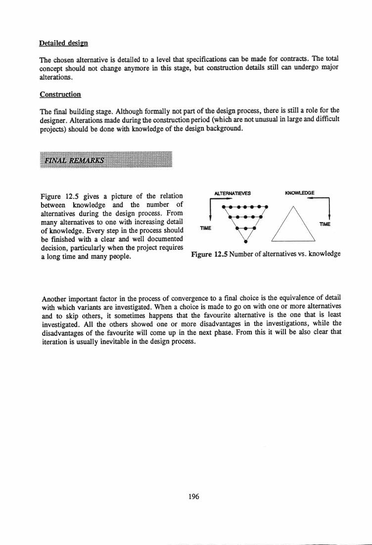
Detailed desiW

The chosen alternative is detailed to a level that specifications cao be made for contracts. The totalconcept should not change anymore in this stage, but construction details still cao undergo majoralterations.

Construction

The final building stage. Although formally not part of the design process, there is still a role for thedesigner. Alterations made during the construction period (which are not unusual in large and difficultprojects) should be done with knowledge of the design background.

Figure 12.5 gives a picture of the relationbetween knowledge and the number ofalternatives during the design process. Frommany alternatives to one with increasing detailof knowiedge. Every step in the process shouldbe finished with a clear and weil documenteddecision, particularly when the project requiresa long time and many people. Figure 12.5 Number of alternatives vs. knowledge

Another important factor in the process of convergence to a final choice is the equivalence of detailwith which variants are investigated. When a choice is made to go on with one or more alternativesand to skip others, it sometimes happens that the favourite alternative is the one that is leastinvestigated. All the others showed one or more disadvantages in the investigations, while thedisadvantages of the favourite will come up in the next phase. From this it will be also clear thatiteration is usually inevitabie in the design process.

196

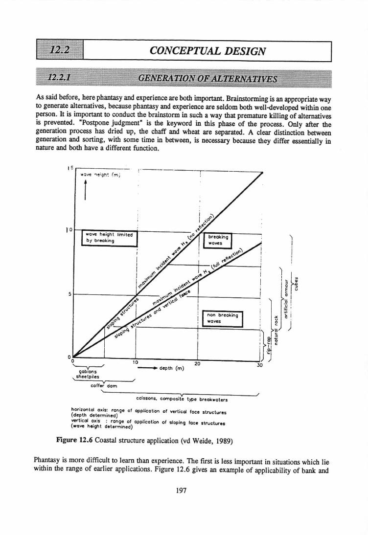
CONCEPTUAL DESIGN

As said before, bere pbantasy and experience are both important. Brainstorming is an appropriate wayto generate altematives, because pbantasy and experience are seldom both well-developed within oneperson. It is important to conduct the brainstorm in sucb a way that premature killing of alternativesis prevented. "Postpone judgment" is the keyword in this pbase of the process. Only after thegeneration process bas dried up, the chaff and wbeat are separated. A clear distinction betweengeneration and sorting, with some time in between, is necessary because they differ essentially innature and both bave a different function.

1=..-------

1

IO~----------~--------_wave height limitedb)' breoking

non breokingwaves

'} ë

; ..I :::0

j 0 ö: '~c

°o~------~------7.10~------------~2~O~------------_J30'-y----" ---. depth Cm)

goblQns, sheetpiles" r------'/

coff.1 dom

cclsscns, composite type breakwaters

horizontol oxis: range of application of vertical face structures(depth determined)verticol oxis : range of application of sloping face Structures(wave height determined)

Figure 12.6 Coastal structure application (vd Weide, 1989)

')!iI

!

Phantasy is more difficult to leam than experienee. The first is less important in situations wbicb liewithin the range of earlier applications. Figure 12.6 gives an example of applicability of bank and

197

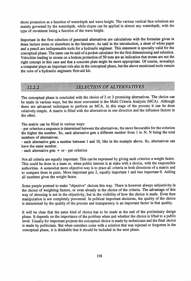
shore proteetion as a function of waterdepth and wave height. The various vertical face solutions aremainly governed by the waterdepth, while slopes can be applied in almost any waterdepth, with thetype of revetment being a function of the wave height.

Important in the first selection of generated alternatives are calculatioos with the formulae given inthese lecture notes or elsewhere in the literature. As said in the introduction, a sheet of white paperand a pencil are indispeosable tools for a hydraulic engineer. This statement is specially valid for theconceptual phase. The same can be said of a pocket calculator for the fust dimeosioning and selection.Velocities leading to stones on a bottom proteetion of 50 toos are an indication that stones are not theright concept in this case and that a concrete plate might be more appropriate. Of course, nowadaysa computer plays an important role also in the conceptual phase, but the above mentioned tools remainthe core of a hydraulic engineers first-aid kit.

The conceptual phase is concluded with the choice of 2 or 3 promising alternatives. The choice canbe made in various ways, but the most convenient is the Multi Criteria Analysis (MCA). Althoughthere are advanced techniques to perform an MCA, in this stage of the process it can be donerelatively simpie. A matrix is filled with the alternatives in one direction and the influence factors inthe other.

The matrix can be filled in various ways:- per criterion a sequence is determined between the alternatives, the more favourable for the criterionthe higher the number. So, each alternative gets a different number from 1 to N, N being the totalnumbers of alternatives.- each alternative gets a number between 1 and 10, like in the example above. So, alternatives canhave the same number.- each alternative gets + or - per criterion

Not all criteria are equally important. This can be expressed by giving each criterion a weight factor.This could be done in a team or, when public interest is at stake with a choice, with the responsibieauthorities. A somewhat more objective way is to place all criteria in both directions of a matrix andto compare them in pairs. More important gets 2, equally important 1 and less important O. Addingall numbers gives the weight factor.

Some people pretend to make "objective" choices this way. There is however always subjectivity inthe choice of weighting factors, or even already in the choice of the criteria. The advantage of thisway of choosing is not in the objectivity, but in the visibility of how the choice is made. Even thenmanipulation is not completely prevented. In political important decisions, the quality of the choiceis determined by the quality of the process and transparency is an important factor in that quality.

It will be clear that the same kind of choice has to be made at the end of the preliminary designphase. It depends on the importance of the problem when and whether the choice is lifted to a publiclevel. Usually for important projects the conceptual choice is made by technicians and the final choiceis made by politicians. But when outsiders come with a solution that was rejected or forgotten in theconceptual phase, it is thinkable that it should be included in the next phase.

198

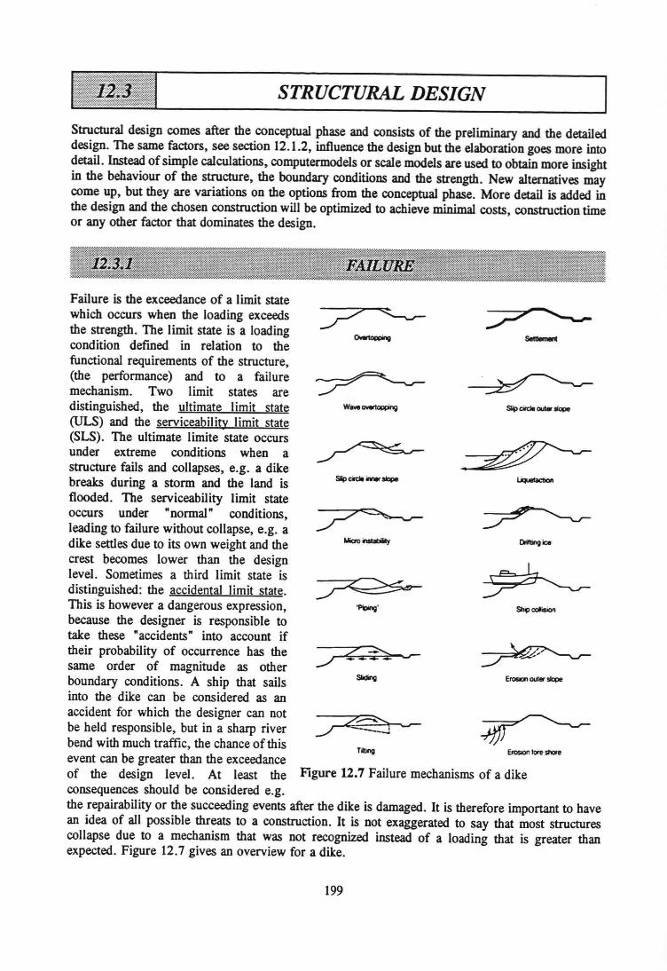
STRUCTURAL DESIGN

Structural design comes after the conceptual phase and consists of the preliminary and the detaileddesign. The same factors, see section 12.1.2, influence the design but the elaboration goes more intodetail. Instead of simple calculations, computermodels or scale models are used to obtain more insightin the bebaviour of the structure, the boundary conditions and the strength. New alternatives maycome up, but they are variations on the options from the conceptual phase. More detail is added inthe design and the chosen construction will be optimized to achieve minimal costs, construction timeor any other factor that dominates the design.

Failure is the exceedance of a limit statewhich occurs when the loading exceedsthe strength. The limit state is a loadingcondition defined in relation to thefunctional requirements of the structure,(the performance) and to a failuremechanism. Two limit states aredistinguished, the ultimate limit state(ULS) and the serviceability limit state(SLS). The ultimate limite state occursunder extreme conditions when astructure fails and collapses, e.g. a dikebreaks during a storm and the land istlooded. The serviceability limit stateoccurs under "normal" conditions,leading to failure without collapse, e.g. adike settles due to its own weight and thecrest becomes lower than the designlevel. Sometimes a third limit state isdistinguished: the accidental limit state.This is however a dangerous expression,because the designer is responsibie totake these "accidents" into account iftheir probability of occurrence has thesame order of magnitude as otherboundary conditions. A ship that sailsinto the dike can be considered as anaccident for which the designer can notbe held responsibie, but in a sharp riverbend with much traffic, the chance of thisevent can be greater than the exceedanceof the design level. At least the Flgure 12.7 Failure mechanisms of a dikeconsequences should be considered e.g.the repairability or the succeeding events after the dike is damaged. It is therefore important to havean idea of all possible threats to a construction. It is not exaggerated to say that most structurescollapse due to a mechanism that was not recognized instead of a loading that is greater thanexpected. Figure 12.7 gives an overview for a dike.

'Piping' SlIjp colision

Erosionout.. $lepe

199

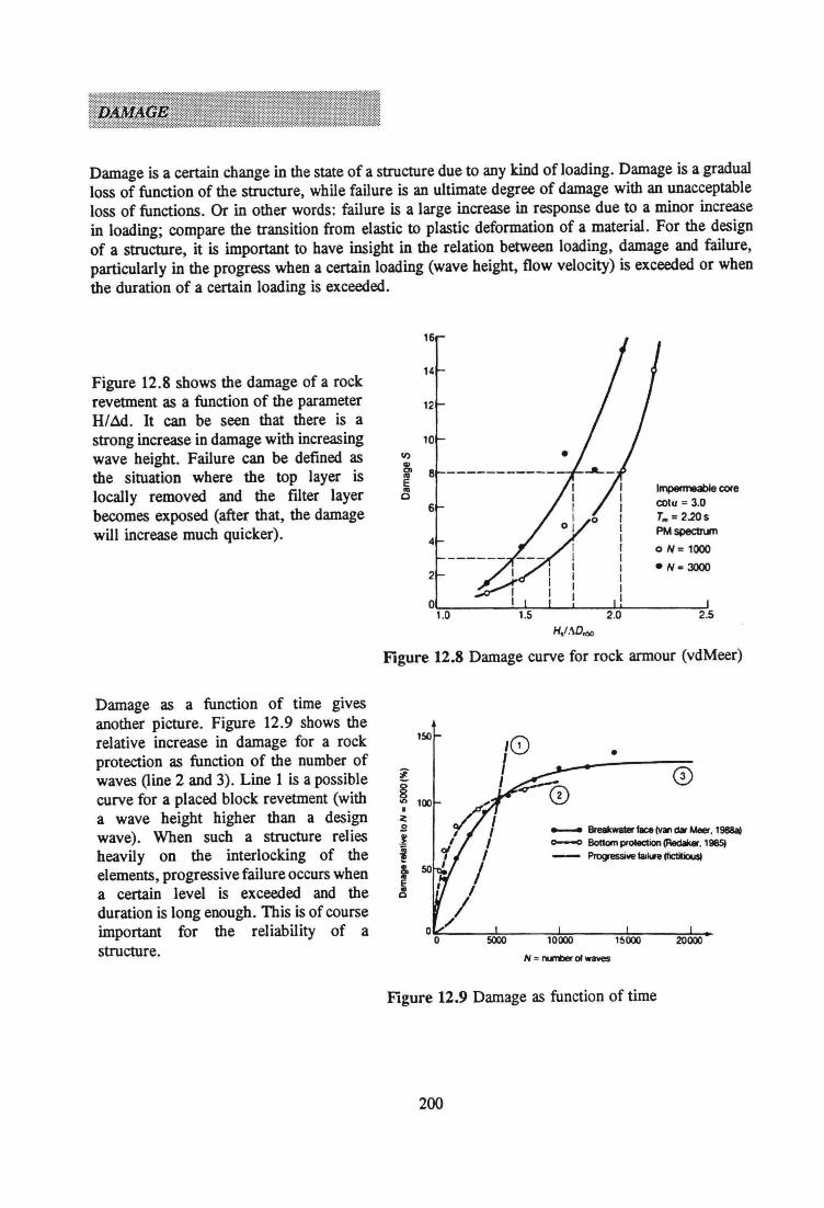
Damage is a certain change in the state of a structure due to any kind of loading. Damage is a gradualloss of function of the structure, while failure is an ultimate degree of damage with an unacceptableloss of functions. Or in other words: failure is a large increase in response due to a minor increasein loading; compare the transition from elastic to plastic deformation of a material. For the designof a structure, it is important to have insight in the relation between loading, damage and failure,particularly in the progress when a certain loading (wave height, flow velocity) is exceeded or whenthe duration of a certain loading is exceeded.

Figure 12.8 shows the damage of a rockrevetment as a function of the parameterH/~. It can be seen that there is astrong increase in damage with increasingwave height. Failure can be defined asthe situation where the top layer islocally removed and the filter layerbecomes exposed (after that, the damagewill increase much quicker).

Damage as a function of time givesanother picture. Figure 12.9 shows therelative increase in damage for a rockproteetion as function of the number ofwaves (line 2 and 3). Line 1 is a possiblecurve for apiaeed block revetment (witha wave height higher than a designwave). When such a structure reliesheavily on the interlocking of theelements, progressive failure occurs whena certain level is exceeded and theduration is long enough. This is of courseimportant for the reliability of astructure.

11)

8.~...o Impenneable care

cotu = 3.0Tm = 2.20sPMspectrum

o N= 1000·N .. 3000

Figure 12.8 Damage curve for rock armour (vdMeer)

10)II ~0

•

- Breakwaterf8ce(YanàarMeer. 1988a)--- Bottom prOlec:lion 1Redaka'. 19851- p~ lallure lfictitiousI

10000

N = l"IUITUr olwaves

Figure 12.9 Damage as function of time

200

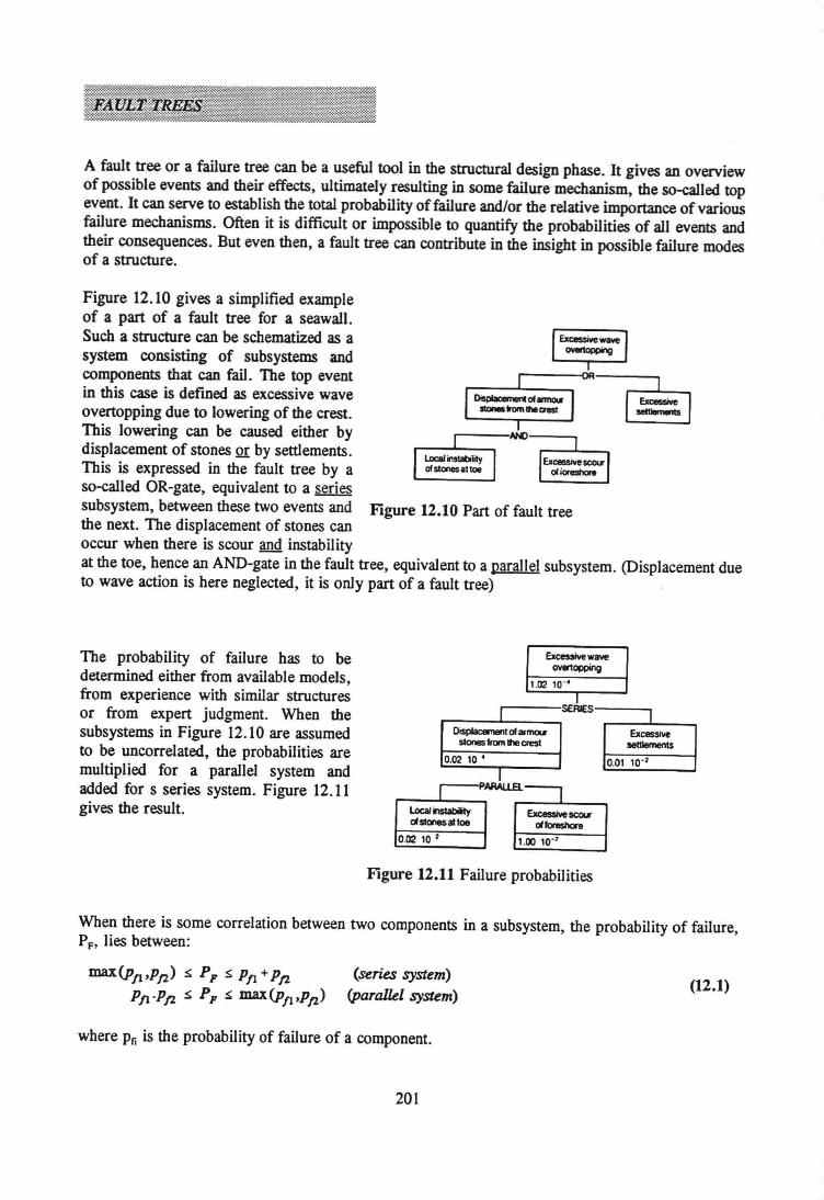
A fauIt tree or a fallure tree can be a useful tooi in tbe structural design phase. It gives an overviewof possible events and tbeir effects, ultimately resulting in some fallure mechanism, tbe so-called topevent. It can serve to establish the total probability of fallure and/or the relative importance of variousfailure mechanisms. Often it is difficult or impossible to quantify the probabilities of all events andtheir consequences. But even tben, a fault tree can contribute in tbe insight in possible fallure modesof a structure.

Figure 12.10 gives a simplified exampleof a part of a fault tree for a seawall.Such a structure can be schematized as asystem consisting of subsystems andcomponents tbat can fail, The top eventin tbis case is defined as excessive waveovertopping due to lowering of the crest.This lowering can be caused either bydisplacement of stones or by settlements.This is expressed in the fault tree by aso-called OR-gate, equivalent to a seriessubsystem, between these two events and Figure 12.10 Part of fault treethe next. The displacement of stones caooccur when tbere is scour and instabilityat the toe, hence an AND-gate in the fault tree, equivalent to a parallel subsystem. (Displacement dueto wave action is here neglected, it is only part of a fault tree)

The probability of failure has to bedetermined either from available modeis,from experience with similar structuresor from expert judgment. When thesubsystems in Figure 12.10 are assumedto be uncorrelated, the probabilities aremultiplied for a parallel system andadded for s series system. Figure 12.11gives the result.

1.02 10"I,.....---saues-----.,

OispIacement of armcuslonestrom !hecrest

Excessiveset1Iements

0.02 10 • ,PARAllB.

Loc:al WIstabiIi1yalstones altoe

0.02 10 '

ExeessiYe scouralfonIshare

1.00 10"

Figure 12.11 Failure probabilities

When there is some correlation between two components in a subsystem, the probability of failure,PF, lies between:

max(Pfl,Pf2) s PF s Pfl +PftPfl'Pft s PF s max(Pfl,P/l)

(series system)(parallel system)

(12.1)

where Pn is the probability of failure of a component.

201

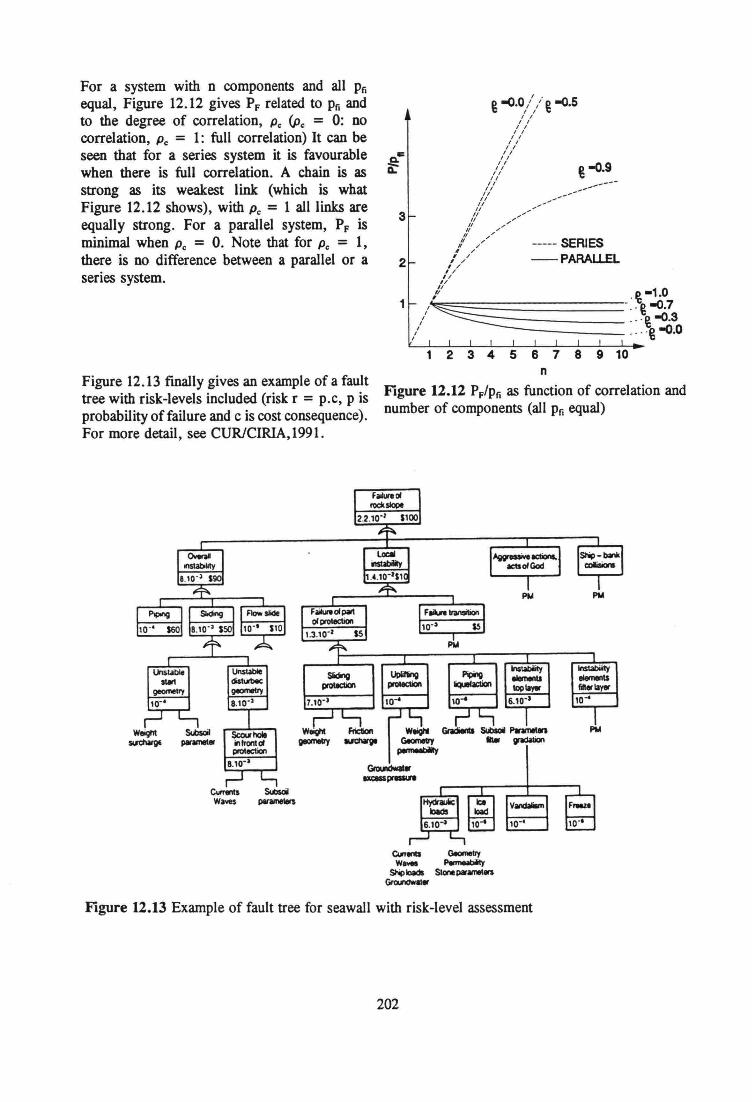
For a system with n oomponents and all Pfiequal, Figure 12.12 gives PF related to Pfiandto the degree of oorrelation, Pc (Pc = 0: nooorrelation, Pc = 1: full oorrelation) It can beseen that for a series system it is favourablewhen there is full oorrelation. A chain is asstrong as its weakest link: (which is whatFigure 12.12 shows), with Pc = 1 all links areequally strong. For a parallel system, PF isminimal when Pc = O. Note that for Pc = 1,there is no difference between a parallel or aseries system.

Figure 12.13 finally gives an example of a faulttree with risk-levels included (risk r = p.c, P isprobability offailure and c is oost oonsequence).For more detail, see CURlCIRIA,1991.

@-o.9

----- SERIES-PARALLEL

1 2 3 4 5 6 7 8 9 10n

Figure 12.12 PF/pfias function of oorrelation andnumber of oomponents (all Pfiequal)

WeighI Fnction WeigIII GIadiInIa SUbICIiI F'IramItngeomeuy NCIIarge GeomeIry ... pSaIion

~GIoundwaI.-~

Curr_ GeomeIryw_ PermeabiiIy

$NpIoads SION! l*amel8ISGroIIIOwaI.

Figure 12.13 Example of fault tree for seawall with risk-level assessment

202

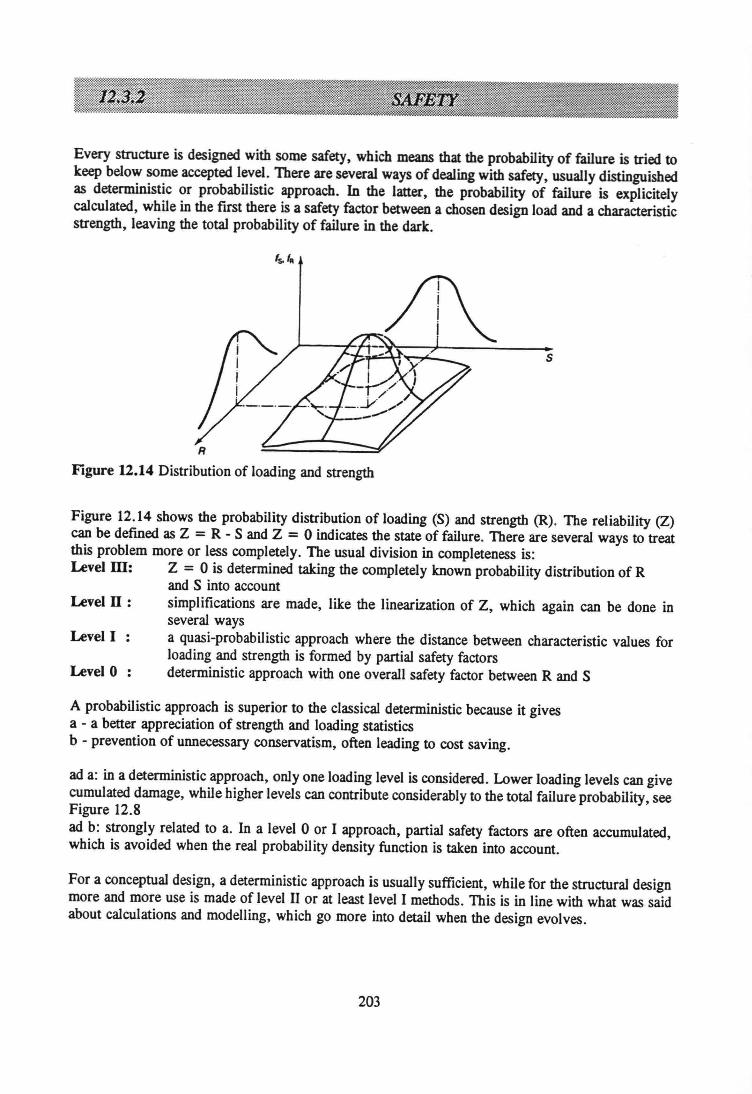
Every structure is designed with some safety, which means that the probability of failure is tried tokeep below some accepted level. There are several ways of dealing with safety, usually distinguishedas deterministic or probabilistic approach. In the latter, the probability of failure is explicitelycalculated, while in the fust there is a safety factor between a chosen design load and a characteristicstrength, leaving the total probability of failure in the dark.

•s

Figure U.14 Distribution of loading and strength

Figure 12.14 shows the probability distribution of loading (S) and strength (R). The reliability (Z)cao be defined as Z = R - S and Z = 0 indicates the state of failure. There are several ways to treatthis problem more or less completely. The usual division in completeness is:Level ill: Z = 0 is determined taking the completely known probability distribution of R

and S into accountLevelIl: simplifications are made, like the linearization of Z, which again can be done in

several waysLevel I a quasi-probabilistic approach where the distance between characteristic values for

loading and strength is formed by partial safety factorsLevel 0 deterministic approach with one overall safety factor between R and S

A probabilistic approach is superior to the classical deterministic because it givesa - a better appreciation of strength and loading statisticsb - prevention of unnecessary conservatism, often leading to cost saving.

ad a: in a deterministic approach, only one loading level is considered. Lower loading levels cao givecumulated damage, while higher levels cao contribute considerably to the total failure probability, seeFigure 12.8ad b: strongly related to a. In a levelOor 1approach, partial safety factors are often accumulated,which is avoided when the real probability density function is taken into account.

For a conceptual design, a deterministic approach is usually sufficient, while for the structural designmore and more use is made of level 11or at least level I methods. This is in line with what was saidabout calculations and modelling, which go more into detail when the design evolves.

203

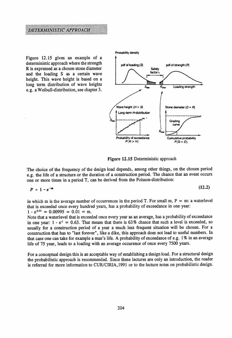
Probability density

Figure 12.15 gives an example of adeterministic approach where the strengthR is expressed as a chosen stone diameterand the loading S as a certain waveheight. This wave height is based on along term distribution of wave heightse.g. aWeibull-distribution, see chapter 3.

pdt ~ Ioaáng(S)

Long-term H-distributionS-7i---• IIIII

Probability of exceedanceP{H>H}

pdt of strength (R)

Stone diameter {D = R')

Cumulative probabilityP(D<D}

Figure 12.15 Deterministic approach

The choice of the frequency of the design load depends, among other things, on the chosen periode.g. the life of a structure or the duration of a construction period. The chance that an event occursone or more times in a period T, can be derived from the Poisson-distribution:

(12.2)

in which mis the average number of occurrences in the period T. For smal1m, P ::::m: a waterlevelthat is exceeded once every hundred years, has a probability of exceedance in one year:1 - e~·Ot= 0.00995 ::::0.01 = m.Note that a waterlevel that is exceeded once every year as an average, has a probability of exceedancein one year: 1 - e-t = 0.63. That means that there is 63% chance that such a level is exceeded, sousually for a construction period of a year a much less frequent situation will be chosen. For aconstruction that has to "last forever", like a dike, this approach does not lead to useful numbers. Inthat case one can take for example a man's life. A probability of exceedance of e.g. 1% in an averagelife of 75 year, leads to a loading with an average occurence of once every 7500 years.

For a conceptual design this is an acceptable way of establishing a design load. For a structural designthe probabilistic approach is recommended. Since these leetures are only an introduction, the readeris referred for more information to CURlCIRlA,1991 or to the lecture notes on probabilistic design.

204

ANNEX

A

It is impossible, within the framework of these lecture-notes, to describe all properties of all materiaIsthat can be used in hydraulic engineering. In this appendix some reprints of relevant texts from thereference list are presented for the most important materiaIs:

STONE:Dimensions, weights, gradations. Source: CUR/CIRIA, 1991

CONCRETE BLOCKS:Examples of shape. Source: Pilarczyk, 1990

ASPHALT:Types and use of mixtures. Source: RWS, 1985

GEOTEXTILES:Types and properties. Source: CUR/CIRIA, 1991Other references:

COMPOSITE MATERIALS:Principle and examples. Source: CUR/CIRIA, 1991

CLAY AND VEGETATION:Gradations, properties and fitness of soil-types for vegetation. Source: CIRIA, 1990

A.I

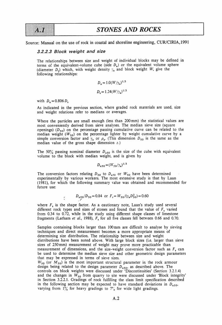
STONES AND ROCKS

Souree: Manual on the use of rock in eoastal and shoreline engineering, CUR/CIRIA,1991

3.2.2.3 8/oek weight and size

The relationships between size and weight of individual bloeks may be defined interms of the equivalent-volume eube (side Dn) or the equivalent volume sphere(diameter D.) whieh, with weight density ;'. and block weight W, give thefollowing relationships:

o, = 1.0(W/y.)1/3

D.= 1.24(W/Ya) 1/3

with Dn=0.806Ds

As indicated in the previous section, where graded rock materials are used, sizeand weight relations refer to medians or averages.

Where the particles are small enough (less than 200 mm) the statistical values aremost conveniently derived from sieve analyses. The median sieve size (squareopenings) (Dso) on the percentage passing cumulative curve can be related to themedian weight (Wso) on the percentage lighter by weight cumulative curve by asimple conversion factor and 'l'. or Pa' (This dimension Dso is the same as themedian value of the gross shape dimension z.)

The 50% passing nominal diameter Dnso is the size of the eube with equivalentvolume to the bloek with median weight, and is given by

The conversion factors relating Dso to Dn50 or Wso have been determinedexperimentally by various workers. The most extensive study is that by Laan(1981), for which the following summary value was obtained and recommended forfuture use:

Dnso/Dso=0.84 or F.= Wso/(y.D;o) =0.60J

where F. is the shape factor. As a cautionary note, Laan's study used severaldifferent rock types and sizes of stones and found that the value of F. variedfrom 0.34 to 0.72, while in the study using different shape classes of limestonefragments (Latham et al., 1988), F. for all five classes feIl between 0.66 and 0.70.

Samples containing blocks larger than l00mm are dimcult to analyse by sievingteehniques and direct measurement becomes a more appropriate means ofdeterrnining size distribution. The relationship between size and weightdistributions have been noted above. With large block sizes (i.e. larger than sievesizes of 250 mm) measurement of weight may prove more practica bie thanmeasurement of dimensions, and the size-weight conversion factor such as F. canbe used to determine the median sieve size and other geometrie design parametersthat may be expressed in terms of sieve sizes.Wso (or M 50) is the most important structural parameter in the rock armourdesign being related to the design parameter Dnso, as described above. Thecontrols on bloek weights were discussed under 'Discontinuities' (Section 3.2.1.4)and the changes in Wso from quarry to site were discussed under 'Block integrity'in Seetion 3.2.2.1. Gradings of rock fulfilling the class limit specifieation describedin the following seetion may be expeeted to have standard deviations in Dnso,varying from 1% for heavy gradings to 7°~ for wide light gradings.

A.2

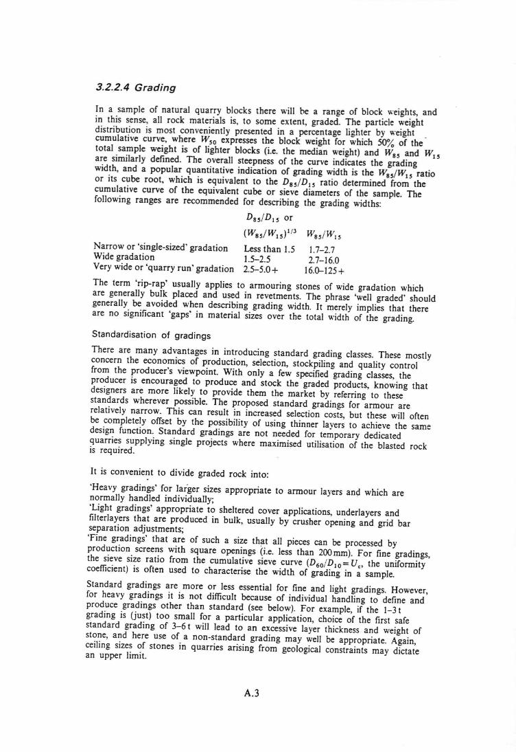
3.2.2.4 Grading

In a sample of natural quarry blocks there will he a range of block. weigh~s, andin this sense, all rock materials is, to some extent, graded, The partiele weightdistribution is most conveniently presented in a percentage lighter by weightcumulative curve, where Wso expresses the block weight for which 50% of thetotal sample weight is of lighter blocks (i.e. the median weight) and Was and WISare similarly defined. The overall steepness of the curve indicates the gradingwidth, and a popular quantitative indication of grading width is the Was/WIs ratioor its cube root, which is equivalent to the Das/DIs ratio deterrnined from thecumulative curve of the equivalent cube or sieve diameters of the sample. Thefollowing ranges are recommended for describing the grading widths:

Das/DIs or(Was/WIs)I!3

Narrow or 'single-sized' gradation Less than 1.5Wide gradation 1.5-2.5Very wide or 'quarry run' gradation 2.5-5.0+

1.7-2.72.7-16.016.0-125+

The term 'rip-rap' usually applies to armouring stones of wide gradation whichare generally bulk placed and used in revetments. The phrase 'well graded' shouldgenerally be avoided when describing grading width. It merely implies that thereare no significant 'gaps' in material sizes over the total width of the grading.

Standardisation of gradings

There are many advantages in introducing standard grading classes. These mostlyconcern the economics of production, selection, stockpiling and quality controlfrom the producer's viewpoint. With only a few specified grading classes, theproducer is encouraged to produce and stock the graded products, knowing thatdesigners are more likely to provide them the market by referring to thesestandards wherever possible. The proposed standard gradings for armour arerelatively narrow. This can result in increased selection costs, but these will oftenbe completely offset by the possibility of using thinner layers to achieve the samedesign function. Standard gradings are not needed for temporary dedicatedquarries supplying single projects where maximised utilisation of the blasted rockis required.

It is convenient to divide graded rock into:

'Heavy gradings' for larger sizes appropriate to armour layers and which arenormally handled individually;'Light gradings' appropriate to sheltered cover applications, underlayers andfilterlayers that are produced in bulk, usually by crusher opening and grid barseparation adjustments;'Fine gradings' that are of such a size that all pieces can be processed byproduction sereens with square openings (i.e. less than 200mm). For fine gradings,the sieve size ratio from the cumulative sieve curve (D6oIDlo= Ue, the uniformitycoefficient) is often used to characterise the width of grading in a sample.

Standard gradings are more or less essential for fine and light gradings. However,for heavy gradings it is not difficult because of individual handling to define andproduce gradings other than standard (see below). For example, if the 1-3 tgrading is (just) too small for a particular application, choice of the first safestandard grading of 3-6 t will lead to an excessive layer thickness and weight ofstone, and here use of a non-standard grading may well be appropriate. Again,ceiling sizes of stones in quarries arising from geological constraints may dictatean upper limit.

A.3

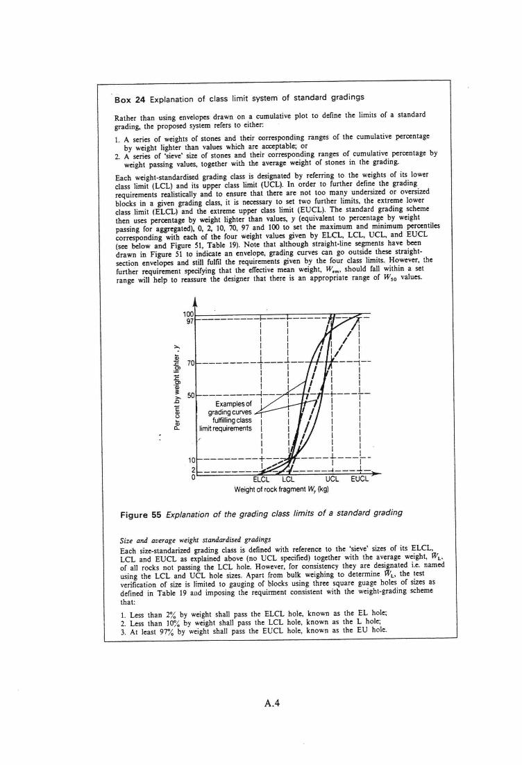
Box 24 Explanation of class limit system of standard gradings

Rather than using envelopes drawn on a cumulative plot to define the limits of a standardgrading, the proposed system relers to either:I. A series of weights of stones and their eertesponding ranges of the eumulative percentage

by weight lighter than values whieh are acceptable; or2. A series of 'sieve' size of stones and their corresponding ranges of eumulative percentage by

weight passing values, together with the average weight of stones in the grading.

Eaeh weight-standardised grading class is designated by referring to the weights of its lowerclass limit (LCL) and its upper class limit (VCL). In order to further define the gradingrequirements realistically and to ensure that there are not too many undersized or oversizedbloeks in a given grading class, it is necessary to set two further limits, the extreme lowerclass limit (ELCL) and the extreme upper class limit (EVCL). The standard grading schemethen uses percentage by weight lighter than values, y (equivalent to percentage by weightpassing for aggregated), 0, 2, 10, 70, 97 and 100 to set the maximum and minimum percentilescorresponding with each of the four weight values given by ELCL, LCL, VCL, and EVCL(sec below and Figure SI, Table 19). Note that although straight-line segments have beendrawn in Figure SI to indicate an envelope, grading curves can go outside these straight­sectien envelopes and still fulfil the requirements given by the four class limits. However, thefurther requirement specifying that the efTectivemean weight, Wem' should fall within a setrange will help to reassure the designer that there is an appropriate range of W50 values.

Examplesofgrading curvesfulfilling class

limit requirements

Weight of rock fragment Wy (kg)

Figure 55 Explanationof the grading class limits of a standard grading

Size and average weighl slandardised gradingsEach size-standarized grading class is defined with reference to the 'sieve' sizes of its ELCL,LCL and EVCL as explained above (no VCL specified) rogether with the average weight, WL,

of all rocks not passing the LCL hole. However, for consisteney they are designated i.e. namedusing the LCL and VCL hole sizes, Apart from bulk weighing to determine WL, the testverification of size is limited to gauging of bleeks using three square guage holes of sizes asdefined in Table 19 and imposing the requirment consistent with the weight-grading sehemethat:I. Less than 2% by weight shall pass the ELCL hole, known as the EL hole;2. Less than 10% by weight shall pass the LCL hole, known as the L hole;3. At least 97% by weight shall pass the EVCL hole, known as the EV hole.

A.4

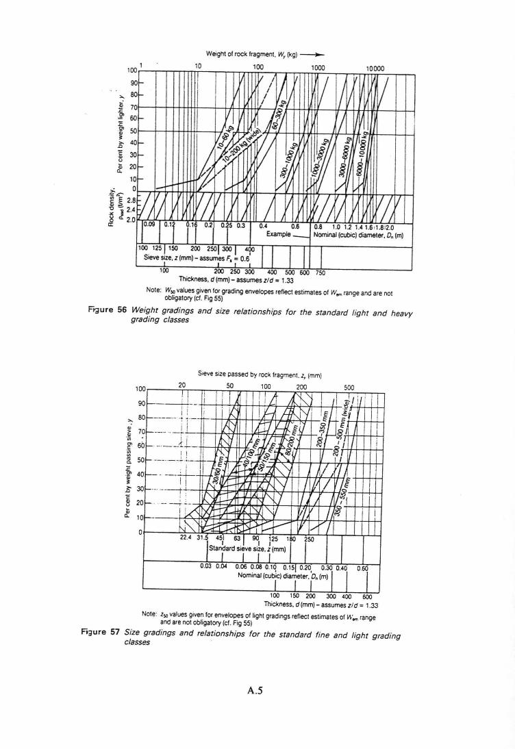
Weight of rock fragment, Wy (kg) ~

100 1251 ISO 200 2S01300 1 4Cfl ISieve s:ze.z (mm)- assum;s F, ~ 0.6. I 1

100 200 2SO 300 400 500 600 750Thicl<ness.d (mm)- assumes zl d = 1.33

Note: Wso values given for grading envelopes reflect estimales of Wem rangeand are nolobligatory (cf. Fig55)

Ft;ure 56 Weight gradings and size relationships for the standard light and heavygrading classes

Sievesize passed by rock fragment. zr (mm)

100

90

":- 80

'" 7>'"'ij;Ol 60c'ij;lil

'" 50Q,

:E.2' 40'"~>- 30.D'E'" 20uQ:;a. 10

0

20 50 100 200 500

100 ISO 200 300 400 600Thickness. d (mm)- assumes zl d = 1.33

Note: lso values given for envelopes of light gradings reflect estimates of "';'" rangeand are not obligalory (cf. Fig 55)

Fi3ure 57 Size gradings and relationships for the standard fine and light gradingclasses '

~--W--I 11 Á L /::-K' 1/ il il 1ii: i . K: H fAN"'! If k~------··7 "'!---t1& è

o~--- .._J.L IL rJ 'rlIt'J_ o è It-.7 81 II' 1i I )'î'-,rI lJiVll~~'s '7/ J i. /. It- _.___L.,__ .

I~ 11 ~/ 1II I 't!~:l~Vt- --_..__.u._._BI1!)t--. --++- ~~~..z~"1 /rD~'/I.~rl~ ~1p::y / it' / 7lI,t-._.._--:~-

'r::-"(J:..~ 1('\ J 1/.4 'S?I: J IV1r1-" ,,-- -~. __.

>Qt:r 'U "f ~ZV r/~10 it--

N"""~ Er k-tpa"~::::r-Ijl 1"""-",,122.4 31.5 45) 63 90 125 180 2SO~1Statard Sir site. {(mm) f f

0.03 0.04 0.06 0.08 0.10 0.151 0.20 o'i 0.41 o'iNominal (CUb!C)"T"t" (m)

A5

The weight envelopes for the standard light and heavy gradings are shown inFigure 56 with appropriate size-weight conversion. In this figure, rocks of anydensity and weight can be related to the correponding nominal diameter, Dn' sievesize, z, and minimum rock thickness, d, using the alternative horizontal scales onthis chart. The 'sieve' size, z, enveloped for the standard fine and light gradingsare shown in Figure 57, again with conversions to D; and d.The standard fine and light gradings are produced by sereens and grids andsometimes with eye selection to remove oversize material in the 6(}-300kg and 1(}-200 kg classes. The poor screening efficiency that occurs in practice means that acorrection factor would be needed in addition to the given theoretical relationshipsfor sieve size, z, and minimum stone thicknesses, d, should a producer wish to useFigures 56 and 57 to indicate the combination of sereens and grids that wouldyield the standard gradings. For the 1(}-200kg more widely graded class,experience in the UK quarries using simpIe grizzlies to remove undersize materialand eye selection to remove oversize material suggests that for rock of average(2.7 t/rn '] density, setting the grizzly c1ear spacing at 225mm and using eyeselection of material above 450 mm will be a good starting point. This advicemust be tempered, however, by individual quarry managers' own experience attheir particular quarry.

The grading envelopes become progressively narrower in the 'heavy grading'classes, consistent with design requirements and the geological constraints onproducing large sizes of blocks. However, projects requiring blocks larger than 10 tshould not make the (non-standard) grading class excessively narrow because ofthe producer's extreme difTiculty in selecting accurately and the wastage fromoversize block production. For example at Pr=2.7t/m3, D'; for a 15t block=1.7m,and D; for a 20 t block = 1.95m, a difTerence of about 10%, which is very difTicultto select precisely except by individual weighing.

Box 25 Median and eHective meanweight

A number of parameters in addition to the designated class limits may be required Ior designand specification purpose. An acceptance range Ior the important design parameter, Wso(median weight), is also useful for each grading class. However, in some circumstances aneITective mean weight Wem for a particular consignment may be more easily obtained simplyby bulk weighing and counting. In order to avoid including fragments and splinters in thedistribution, Wem is defined as the arithmetic average weight of all blocks in the consignmentor sample, excluding those which fall below the ELCL weight for the grading class. Anempirical conversion factor relating Wem to Wso allows an estimate of Wso without thenecessity of weighing each piece to obtain a weight-distribution curve. As the grading becomeswider, so will Wso depart more from Wem. Approximate relations are as follows:

1~60kg~300kg300-1000 kg1~3000kg3~6000 kg and~IOOOOkg

A.6

CONCRETE BLOCKS

TOOG..EA~·GROOvl TYPt SHoP.lAP ryp(

STEI'PEO ryp(

WA"lE TyP(

B INi ERLOCKING • BLOCKS

<ill,,,o,

[@JC. SVEE.BLOCKS

rITFn ~t1l1lj tj·cjjj

F. ARMQRFLEX • BLOCK

MOOIFIED TONGUE· ANOGIlOOVE BLOCK

~

~

o GOal. BLOCK

E BUILDING· BLOCKS

G. iERRAFIX· BLOCKS

A.7

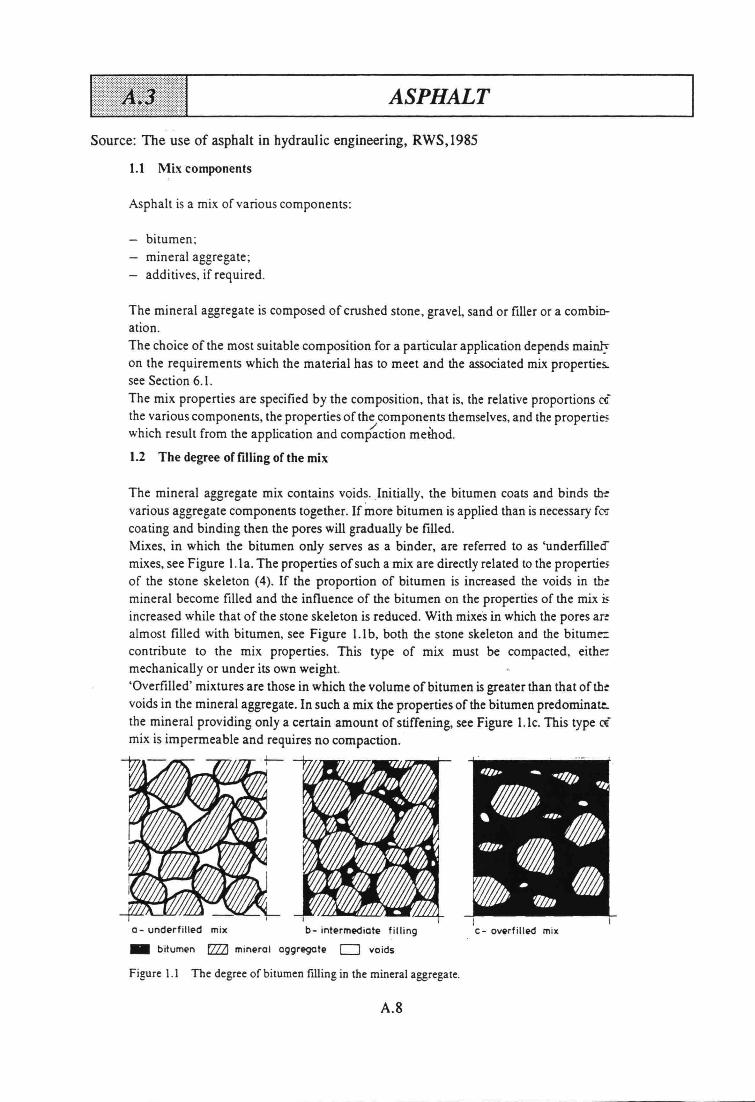
ASPHALT

Souree: The use of asphalt in hydraulic engineering, RWS,1985

1.1 Mix components

Asphalt is a mix ofvarious components:

bitumen;mineral aggregate;additives, if required.

The mineral aggregate is composed of crushed stone, gravel, sand or filler or a combin­ation.The choice of the most suitable composition for a particular application depends mainlvon the requirements which the material has to meet and the associated mix properties.see Section 6.1.The mix properties are specified by the composition, that is, the relative proportions ofthe various components, the properties of the components thernselves,and the propertieswhich result from the application and compaction rnejhod.

1.2 The degree of filling of the mix

The mineral aggregate mix contains voids. .Initially, the bitumen coats and binds thevarious aggregate components together. If more bitumen is applied than is necessary forcoating and binding then the pores will gradually be filled.Mixes, in which the bitumen only serves as a binder, are referred to as 'underfilled'mixes, see Figure l.Ia. The properties ofsuch a mix are directly related to the propertiesof the stone skeleton (4). If the proportion of bitumen is increased the voids in tbo!mineral become filled and the influence of the bitumen on the properties of the mix isincreased while that of the stone skeleton is reduced. With mixes in which the pores ar:almost filled with bitumen, see Figure 1.1b, both the stone skeleton and tbe bitumezcontribute to the mix properties. This type of mix must be compacted, eithermechanically or under its own weight.'Overfilled' mixtures are those in which the volume of bitumen is greater than that of'thevoids in the mineral aggregate. In such a mix the properties of the bitumen predominate..the mineral providing only a certain amount of stiffening, see Figure l.Ic, This type ofmix is impermeable and requires no compaction.

0- underfilled mix b- intermediote filling

_ bitumen f'2ZZI minerol oggregote 0 voids

Figure 1.1 The degree of bitumen filling in the mineral aggregate.

A.8

C - overfilled mix

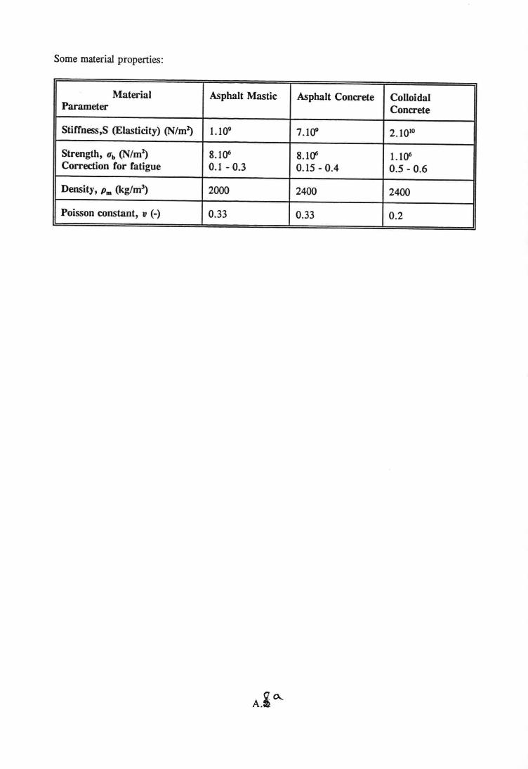
Some material properties:

Material Asphalt Mastic Asphalt Concrete ColloidalParameter Concrete

Stiffness,S (Elasticity) (N/m~ 1.109 7.Hf 2.1010

Strength, Ub (NIm; 8.1()6 8.106 1.1()6Correction for fatigue 0.1 - 0.3 0.15 - 0.4 0.5 - 0.6

Density, Pat (kg/nr') 2000 2400 2400

Poisson constant, v (-) 0.33 0.33 0.2

A.io...

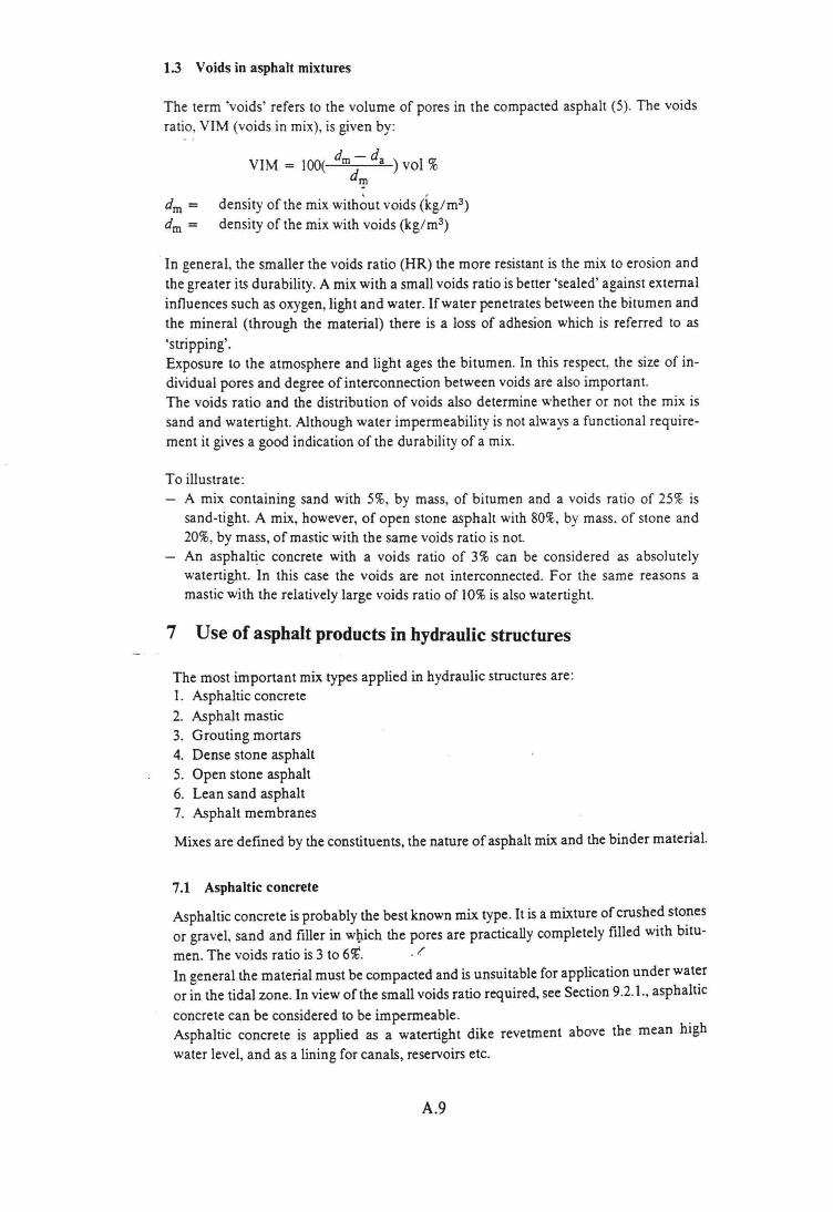
1.3 Voids in asphalt mixtures

The term 'voids' refers to the volume of pores in the compacted asphalt (5). The voidsratio, VIM (voids in mix), is given by:

d -dVIM = lOO( ma) vol %dm

dm = density ofthe mix without voids (kg/rn")dm = density of the mix with voids (kg/m")

. In general, the smaller the voids ratio (HR) the more resistant is the mix to erosion andthe greater its durability. A mix with a smal! voids ratio is better 'sealed' against externalinfluences such as oxygen, light and water. Ifwater penetrates between the bitumen andthe mineral (through the material) there is a loss of adhesion which is referred to as'stripping' .Exposure to the atmosphere and light ages the bitumen. In this respect, the size of in­dividual pores and degree ofinterconnection between voids are also important.The voids ratio and the distribution of voids also determine whether or not the mix issand and watertight. Although water impermeability is not always a functional require­ment it gives a good indication of the durability of a mix.

To illustrate:A mix containing sand with 5%, by mass, of bitumen and a voids ratio of 25% issand-tight. A mix, however, of open stone asphalt with 80%,by mass, of stone and20%,by mass, of mastic with the same voids ratio is not.An asphaltic concrete with a voids ratio of 3% can be considered as absolutelywatertight. In this case the voids are not interconnected. For the same reasons amastic with the relatively large voids ratio of 10%is also watertight.

7 Use of asphalt produets in hydraulic structures

The most important mix types applied in hydraulic structures are:I. Asphaltic concrete2. Asphalt mastic3. Grouting mortars4. Dense stone asphalt5. Open stone asphalt6. Lean sand asphalt7. Asphalt membranes

Mixes are defined by the constituents, the nature of asphalt mix and the binder material.

7.1 Asphaltic concrete

Asphaltic concrete is probably the best known mix type. lt is a mixture of crushed stonesor gravel, sand and filler in which the pores are practically completely filled with bitu-men. The voids ratio is 3 to 6%'. . ~In general the material must be compacted and is unsuitable for application under wateror in the tidal zone. In view ofthe small voids ratio required, see Section 9.2.1., asphalticconcrete can be considered to be impermeable.Asphaltic concrete is applied as a watertight dike revetment above the mean highwater level, and as a lining for canals, reservoirs etc.

A.9

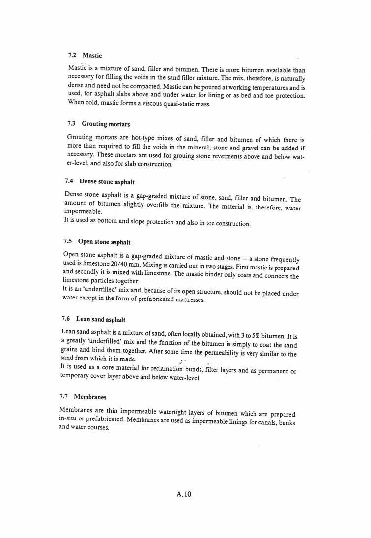
7.2 Mastic

Masiiè is a mixture of sand, filler and bitumen. There is more bitumen available thannecessary for filling the voids in the sand filler mixture. The mix, therefore, is naturallydense and need not be cornpacted. Mastic can be poured at werking temperatures and isused, for asphalt slabs above and under water for lining or as bed and toe protection.When cold, mastic forms a viseous quasi-statie mass.

7.3 Grouting mortars

Grouting mortars are hot-type mixes of sand, filler and bitumen of which there ismore than required to fill the voids in the mineral; stone and gravel ean be added ifneeessary. These mortars are used for grouing stone revetments above and below wat­er-level, and also for slab construction.

7.4 Dense stone asphalt

Dense stone asphalt is a gap-graded mixture of stone, sand, filler and bitumen. Theamount of bitumen slightly overfills the mixture. The material is, therefore, waterimpermeable.It is used as bottom and slope proteetion and also in toe construetion.

7.5 Open stone asphalt

Open stone asphalt is a gap-graded mixture of mastie and stone - a stone frequentlyused is limestone 20/40 mmoMixing is earried out in two stages. First mastic is preparedand seeondly it is mixed with limestone. The mastie binder only coats and conneets thelimestone particles together.It is an 'underfilled' mix and, because ofits open structure, should not be placed underwater exeept in the form of prefabricated mattresses.

7.6 Lean sand asphalt

Lean sand asphalt is a mixture of'sand, often loeally obtained, with 3 to 5%bitumen. It isa greatly 'underfilled' mix and the function of the bitumen is simply to coat the sandgrains and bind them together. After some time the permeability is very similar to thesand from which it is made. ,I. ,

It is used as a core material for recIamation bunds, filter layers and as permanent ortemporary cover layer above and below water-level.

7.7 Membranes

Membranes are thin impermeable watertight layers of bitumen which are preparedin-situ or prefabricated. Membranes are used as impermeable linings for eanals, banksand water courses.

A.1O

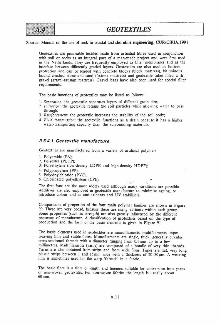
GEOTEXTILES

Souree: Manual on the use of rock in coastal and shoreline engineering, CUR/CIRIA,1991

Geotextiles are permeable textiles made from articifial fibres used in conjunctionwith soil or rocks as an integral part of a man-made project and were first usedin the Netherlands. They are frequently employed as filter membranes and as theinterface between differently graded layers. Geotextiles are also used as bottomproteetion and can be loaded with concrete blocks (block mattress), bituminousbound crushed stone and sand (fixtone mattress) and geotextile tubes filled withgravel (gravel-sausage mattress). Gravel bags have also been used for special filterrequirements.

The basic functions of geotextiles may be listed as follows:

1. Separation: the geotextile separates layers of different grain size;2. Filtration: the geotextile retains the soil particles while allowing water to pass

through;3. Reinforcement: the geotextile increases the stability of the soil body;4. Fluid transmission: the geotextile functions as a drain because it has a higher

water-transporting capacity than the surrounding materiais.

3.5.4.1 Geotextile manufacture

Geotextiles are manufactured from a variety of artificial polymers:

1. Polyamide (PA);2, Polyester (PETP);3. Polyethylene (Iow-density LDPE and high-density HDPE);4. Polypropylene (PP);5. Polyvinylchloride (PVC);6. Chlorinated polyethylene (ePE).

. /' ~The first four are the most widely used although many variátions are possible.Additives are also employed in geotextile manufacture to minimise ageing, tointroduce colour and as anti-oxidants and UV stabilisers.

Comparisons of properties of the four main polymer families are shown in Figure90. These are very broad, because there are many variants within each group.Some properties (such as strength) are also greatly influenced by the differentprocesses of manufacture. A classification of geotextiles based on the type ofproduction and the form of the basic elements is given in Figure 91.

The basic elements used in geotextiles are monofilaments, multifilaments, tapes,weaving film and stabie fibres. Monofilaments are single, thick, generally circularcross-sectioned threads with a diameter ranging from 0.1 mm up to a fewmillimetres. Multifilaments (yams) are composed of a bundie of very thin threads.Yams are also obtained from strips and from wide films. Tapes are flat, very longplastic strips between 1 and 15mm wide with a thickness of 2(}-SO J..lm. A weavingfilm is sometimes used for the warp 'threads' in a fabric.

The basic fibre is a fibre of length and fineness suitable for conversion into yamsor non-woven geotextiles. For non-woven fabrics the length is usually about60mm.

A.11

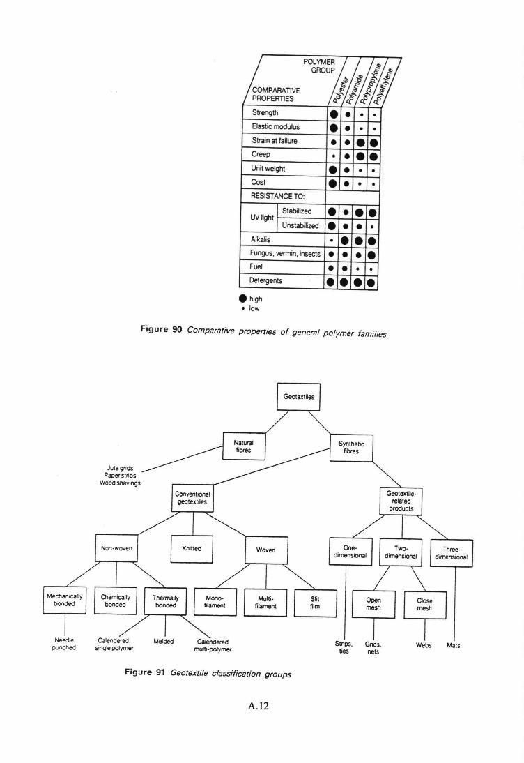
Mecnan1callybended

Neediepuncned

~~!J!JlJfGROUP s ~... ff ~ .,!P.I!!#o,E-

COMPARATIVE jJ ~ ~ q;'i:S~~~PROPERTIES e q_0 e eStrength • • • •Elastic modulus • • • •Strain at failure • • ••Creep • • ••Unitweight • • • •Cost • • • •RESISTANCE TO:

Stabilized • • ••UV light •Unstabilized • • •AJkalis • •••Fungus, vermin, insects • • • •Fuel • • • •Detergents ••••

• high• low

Figure 90 Comparativeproperties of general polymer families

Geotextiles

JutegndsPaperstrips

Woodsnavings

Naturalfibres

Non-woven Knined

Mono­filament

Catencerec.singlepolymer

Melded Calenderedmuiti-polymer

Woven

Multi­filament

Syntneticlibres

Geotextile­relatedproducts

One- Two- Three-dimenSional dimensional dimensional

Slit Open Closefilm mesh mesll

Figure 91 Geotextileclassification groups

A.12

Strips, Grids.ties nets

Webs Mats

Woven geotextiles

A woven fabric is a flat structure of at least two sets of threads. The sets arewoven together, one referred to as the warp, running in a lengthwise direction,and the other, the weft, running across. Woven geotextiles can be categorized bythe type of thread from which the fabric is manufactured.

Monofilament [abrics are used for gauzes of meshes which offer relatively smallresistance to through-flow. The mesh size must obviously be adapted to the grainsize of the material to be retained. Monofilament fabrics are made principallyfrom HOPE and PP.

Tape fabrics are made from very long strips of usually stretched HOPE or PPfilm, which are laid untwisted and flat in the fabric. They are laid closelytogether, and as aresuIt there are only limited openings in the fabric (Figure 92).

Split-fiim fabrics are made from mostly fibrillated yams of PP or HOPE (Figure93). The size of the openings in the fabric depends on the thickness and form ofthe cross-sectien of the yams and on the fabric construct ion. These split-filmfabrics are generally heavy. Tape and split-film fabrics are often ca lied slit-films.

Multifiiament fabrics are often described as c1oth. because they tend to have atextile appearance and are twisted or untwisted multifilament yams. The fabricsare usually made from PA 6, PA 6.6 or from PETP.

Besides the above-rnentioned monofilament fabrics, special mes/Hype constructionsare produced such as those with a monofilament warp and a multifilament weftwhich have outstanding water-perrneability and sand-retention properties. Otherexamples inc1ude open meshes in which the woven or unwoven warp and weftthreads are attached at crossing points by chemicalor thermal bonding and othermeshes constructed by using knitting techniques.

Non-woven ge.otextiles

A non-woven geotextile is a textile structure produced by bonding or interlockingof staple fibres, either monofilaments or multifilaments arranged at random,accomplished by mechanical, chemical, thennal or solvent means. Non-wovengauzes are structures with large meshes which are fonned by placing threads ortapes at predetennined distances on top of one another and bonding them at theintersections by a chemical, thennal or mechanical process.

Geotextile-related produets

These products are distinguished in one-dimensional (strips, ties), two-dimensional(gids, nets, webs) and three-dimensional (mats) products. Grids are lattices madefrom perforated and then stretched polymer sheets. Three-dimensional mats areproduced by extruding monofilaments into a rotating profile roller, followed bycoating so th at the threads adhere to each other at crossings which are spatiallyarranged. The matting material itself occupies less then 10% of the mat volume.The mats are 5-25mm thick and about 1-6m wide.

A.13

3.5.4.2 Characteristics and properties

TIle geotextile properties stem primarily from their functional requirements. Sincethe geotextile can have a variety of functions, requirements are diverse. Forreinforcement the emphasis is on mechanical properties such as E-modulus andstrength, for filters it is on properties such as water permeability and soiltightness. The durability required wiJl depend on the specific application andlifetime required. Geotextiles must also fulfil secondary functional requirementsrelated to the execution of the work (e.g. a certain amount of UV resistance isneeded) or it must have resistance to mechanical wear and tear if constructionequipment is to be driven over the fabric. The suitability of a geotextile should bechecked against these functional requirements during the design phase of theproject.

. t' .Although specification requirement tests need only he carried out once, thefollowing quality control tests may be required during production: tearing strength,grab test strength, tensile strength, strain at breaking load, moduli and massdistribution. These tests should be made in both the length and width directions.The thickness, the mass per unit area and the bursting strength mayalso need tobe checked, and in some applications water permeability and sand-retainingproperties will be important. A large number of national and a few internationalstandard test methods are available covering these requirements.

Dimensions

The maximum standard width available for both woven and non-woven fabrics is5-5.5 m. The length is limited by the available transport facilities and ease ofhandling on-site. Depending on the mass per unit area, the length generally lies inthe range 5~200m.

Jointing is necessary to obtain greater dimensions. In practice, large areas can becovered by overlapping sheets. Where physical continuity is required withoutoverlap then heat welding (some non-wovens) or stiching may he used. The seamforms the weakest link in the geotextile construction and should therefore bechecked thoroughly against the specifications. The thickness of most geotextiles liesbetween 0.2 and 10mm when unloaded, although this may sometimes reduceunder pressure.

In general, the mass of non-woven geotextiles lies in the range 10~1000gjm2,l00-3oogjm2 being the most commonly used. Woven fabrics can be heavier andrnasses between 100 and 2000 g/m? are possible. The greater demand is for thelighter grades in the range 100-200 g/m '. Generally, the lighter types of geotextilesare used as separators, the heavier woven fabrics for reinforcement and theheavier non-wovens for fluid transmission.

Chemical properties

One of the characteristic features of synthetic polymers is their relative insensitivityto the action of a great number of chemieals and environmental efTects.Nonetheless, each plastic has a number of weaknesses which must be taken intoaccount in the design and application. Specifically, the life of geotextiles can beafTected by oxidation and by some types of soil/water/air pollution. Manysynthetic polymers are sensitive to oxidation. The end result of oxidation is thatmechanical properties such as strength, elasticity and strain absorption capacitydeteriorate and the geotextile eventually becomes brittIe and cracks.

A.14

COMPOSITE MATER/ALS

Souree: Manual on the use of rock in coastal and shoreline engineering, CUR/CIRIA,1991

3.5.5 COMPOSITE MATERlALS

Composite systems are normally adopted where improved stability of the rockmaterials being used is sought (see Section 5.1.3.9) or where ease of placing theproteetion system is important.

3.5.5.1 Gabions

A gabion is a box or mattress-shaped container made out of hexagonal (orsometimes square) steel wire mesh strengthened by selvedges of heavier wire, andin some cases by mesh diaphragms which divide it into compartments (Figure 94).AssembIed gabions are wired together in position and filled with quarried stone orcoarse shingle to form a retaining or anti-erosion structure. The wire diametervaries but is typically 2-3 mmo The wire is usually galvanised or PVC-coated.PVC-coated wire should be used for marine applications and for pollutedconditions.

The durability of gabions depends on the chemical quality of the water and thepresence of waterborne attrition agents. The influence of the pH on the loss ofthe galvanic zinc proteetion is small for pH values in the range 6-12 and thereare examples of gabions with negligible loss over 15 years. Grouting of the stone­filled gabions or mattresses can give some proteetion to the wire mesh againstabrasion and corrosion, but this depends on the type of grout and the amountused.

The dimensions of gabions vary; but typically range in length from 2 to 4 m(mattress, 6 m), with widths about 1m (mattress, 2m), and height 0.3-1.0 m(mattress, max. 0.3m). The mesh size is typically 50-100mm.

The units are flexible and conform to changes in the ground surface due tosettlement. Prefabricated gabions can be placed under water. Gabions can thus beused in a wide variety of marine works: groynes, dune and cliff protection,proteetion of pipelines and cables, and as toe protection. Mattress-shaped gabionsare flexible and are therefore able to follow bed profiles both initially and afterany scouring which may take place. Gabions can also be piled up to the formretaining walls or revetments (see Section 6.2, Box 80). In order to preventmigration of solid through the structure they may be used in conjunction withgeotextile filter layers.

In certain applications the gabion structure needs impermeability or weight tocounter uplift. To give these characteristics, the stone is grouted with mastic or acement-bp_ll!!!_groutil'!_g:_]"~eweight of the structure can also be influenced by thechoice of the density of the stone blocks with which the gabion or gabion­mattress is filled.

A.15

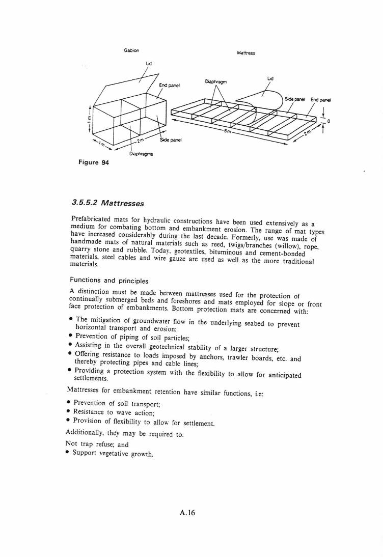
Gabion Mattress

Lid

Diaplyagms

Figure 94

3.5.5.2 Mattresses

Prefabricated mats for hydraulic constructions have been used extensively as amedium for combating bottom and embankment erosion. The range of mat typeshave increased considerably during the last decade. Formerly, use was made ofhandmade mats of natural materials such as reed, twigsjbranches (willow), rope,quarry stone and rubble. Today, geotextiles, bituminous and cement-bondedmateriais, steel cables and wire gauze are used as weil as the more traditionalmateriais.

Functions and principles

A distinction must be made between mattresses used for the protection ofcontinually submerged beds and foreshores and mats employed for slope or frontface proteetion of embankments. Bottom protection mats are concerned with:

• The mitigation of groundwater flow in the underlying seabed to preventhorizontal transport and erosion:

• Prevention of piping of soil particles;• Assisting in the overall geotechnical stability of a larger structure;• Offering resistance to. loads irnposed by anchors, trawler boards, etc. andthereby protecting pipes and cable lines;

• Providing a proteetion system with the flexibility to allow for anticipatedsettlements.

Mattresses for embankment retention have similar functions, i.e:

• Prevention of soil transport;• Resistance to wave action;• Provision of flexibility to allow for settlement.Additionally, they may be required to:Not trap refuse; and• Support vegetative growth.

A.16

Mats are manufactured from the following e1ements:

1. The carrier: Fabric, gauze, cables and bundlings by which the necessary strengthis obtained for its manufacture, transport and installation.

2. The filter: A geotextile which satisfies the conditions with respect to .permeability, soil density, strength, etc. In some embankment-mat constructrensthe geotextile is applied separately.

3. The ballast: Concrete blocks, packaged sand, gravel, stone or asphalt necessaryfor the stability of the protection. Quarry stone can be used to serve as amaterial to sink the mat.

4. The connections: Pegs, wires, etc. by which the ballast material is fixed to thefilter and the carrier materiaIs.

In addition to the mat proper, a further deposit of gravel, aggregates, quarrystone, slag, etc. may be necessary when the ballast material stability in itself isinsufficiënt or when extra proteetion is demanded.

The carrier and the filter can often be combined in the form of a single geotextilewith the necessary mechanical and hydraulic properties. Sometimes the filter iscombined with the ballast, which is then dimensioned as a granular filter.

Manufacture and placingFascine mats are typically up 10 lOOm long and ICr20m wide. Historically, thesemats were manufactured from osiers which were c1amped between the so-called'raster' of bundIes of twigs/branches bound together to a circumference of 0.3m.

'Plugs' were driven into the crossing-points of the bundIes to serve as anchorpoints for towing and sinking the mats (for bottom protection) or collar-pieces(for foreshore protection). Because of the destruction of the osiers by pile-wormattack, a reed layer was incorporated into the mats. These fascine mats weremade on embankments in tidal areas or on special slipways.

The finished mat or collar-piece was then towed to its destination and sunk usmgquarry stones which were placed in position by hand, with the uppermostrasterwork of bundIes serving to maintain the stone in place during sinking. Aftersinking, more and heavier stones were discharged onto the mat if this was fouedto be necessary.

Modern mats are made in accordance with the same principles. The twigs/branches and reed are replaced by a geotextile into which loops are woven andto which the rasterwork of bundies are affixed. A reed mat may be affixed ontothe geotextile in order to prevent damage to the cloth during the discharge ofstones onto the mat. The geotextile extends out beyond the rasterwork with tbeaid of lath outriggers so that, on sinking, the mats overlap. Sometimes a doublerasterwork is applied to give the mats a greater rigidity and more edge supponto the quarry stone load. The mat construction can serve as a proteetion for thebottom, a foreshore and even as an embankment protector. In the last case themat is hauled up against the embankment itself.

Modern alternatives to fascine mats include mats where the quarried stone isreplaced by open-stone asphalt reinforeed with steel mesh, or by 'sausages' ofcloth or gauze filled with a ballast material such as sand, gravel, bituminous orcement-bound mixtures.

A.I7

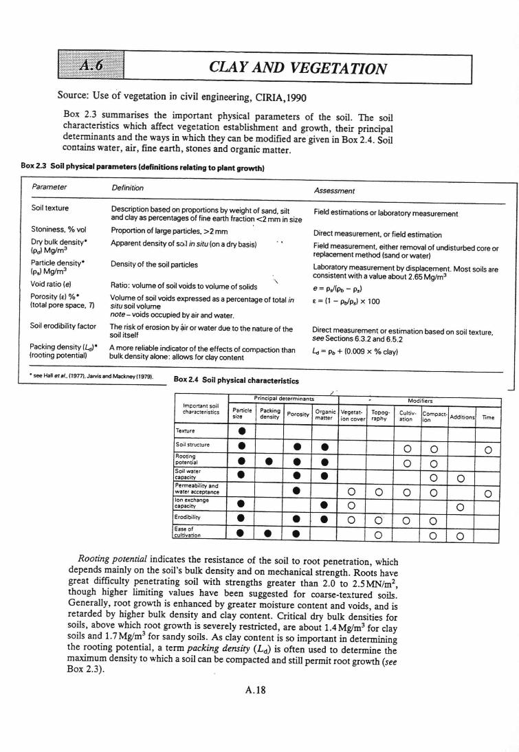
CLAY AND VEGETATION

Souree: Use of vegetation in civil engineering, CIRIA,I990

Box 2.3 summarises the important physical parameters of the soit. The soilcharacteristics which affect vegetation establishment and growth, their principaldeterminants and the ways in which they can be modified are given in Box 2.4. Soitcontainswater, air, fine earth, stones and organicmatter.

Parameter

Box2.3 Soil physical parameters (definitions relating to plant growthl

Definition Assessment

Soil texture

Stoniness. % vol

Dry bulk densitv"(Pd) Mg/m3

Partieledensitv"(p.) Mg/m3

Void ratio (e)Porositv (E) %.(total pore space. 7)

Soil erodibility factor

Packingdensity (I..!).(rooting potential)

Box2.4 Soil physical characteristics• see HaR618/.. (1977).Jarvis endMacl:ney (1979).

Description based on proportions byweight of sand, siltand day as percentages of fine earth fraction <2mm in sizeProportion of large particles.>2 mm

Apparent density of sa:! in situ (ona dry basis)

Fieldestimations or laboratory measurement

Direct measurement. or field estimation

Fieldmeasurement. either removal of undisturbed core orreplacement method (sandor water)

Laboratorymeasurement by displacement. Most soils areconsistent with avalue about 2.65Mgfm3

e = P"f(Pb - Ps)E = (1 - pJps) x 100

Density of the soil partieles

Ratio: volume of soil voids to volume of solids

Volume of soil voids expressed asapercentage of total insitu soil volumenote - voids occupied by air andwater.

The risk of erosion by àiror water due to the nature of thesoil itself

A more reliable indicator of the effects of compaction thanbulk density alone: allows for day content

Direct measurement or estimation based on soil texture.see Sections 6.3.2 and 6.5.2

I..!= Pb+ (0.009 x % dav)

,,'Principal determinants . Modjfiers

tmccrtanr soilPartiele Packing Organic Vegetat· Topog· Cultiv-characteristics Porosity Compact· Additions Timesite density matter ion cover raphy ation ion

TextlJre •Soil structure • • • 0 0 0Rooring • • • • 0 0potenti.,Soilwater • • • 0 0capacityPermeability and • 0 0 0 0 0water acceptanceIon exchange • • 0 0capacity

Erodibility • • • 0 0 0 0E.se of • • • 0 0 0cultivarion

Rooting potenrial indicates the resistance of the soil to root penetration, whichdepends mainly on the soil's bulk density and on mechanical strength. Roots havegreat difficulty penetrating soil with strengths greater than 2.0 to 2.5MN/m2,

though higher limiting values have been suggested for coarse-textured soils.Generally, root growth is enhanced by greater moisture content and voids, and isretarded by higher bulk density and clay content. Critical dry bulk densities forsoils, above which root growth is severely restricted, are about 1.4Mg/rrr'for daysoils and 1.7Mg/m! for sandy soils. As clay content is so important in determiningthe rooting potential, a term packing density (Ld) is often used to determine themaximumdensity to whicha soil cao be compacted and stillpermit root growth (seeBox 2.3).

A.I8

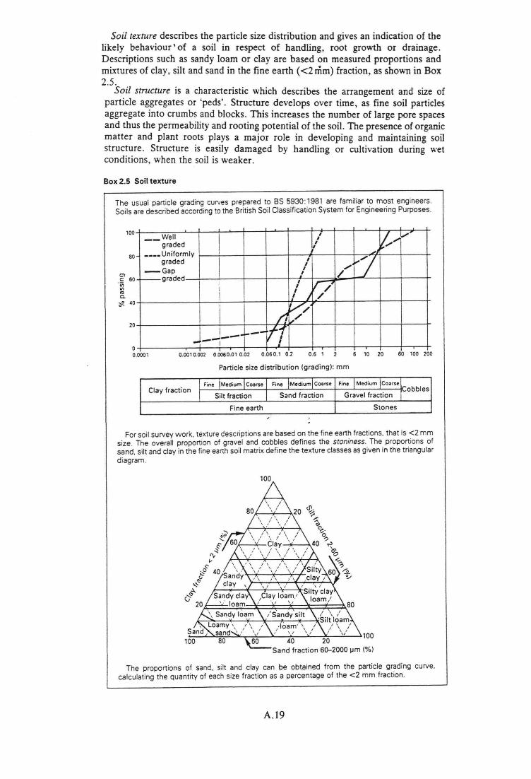
SoU texture describes the partiele size distribution and givesan indication of thelikely behaviour' of a soil in respect of handling, root growth or drainage.Descriptions such as sandy loam or clay are based on measured proportions andmixtures of clay, silt and sand in the fine earth «2 rûm) fraction, as shown in Box2.5.

Soil structure is a characteristic which describes the arrangement and size ofpartiele aggregates or 'peds'. Structure develops over time, as fine soil particlesaggregate into crumbs and blocks. This increases the number of large pore spacesand thus the permeability and rooting potentialof the soil. The presence of organicmatter and plant roots plays a major role in developing and maintaining soilstructure. Structure is easily damaged by handling or cultivation during wetconditions, when the soil is weaker.

Box2.5 Soil texture

The usual particIe grading curves prepared to SS 5930: 1981 are familiar to most engineers.Soils are described according10 the British Soil Classification System for Engineering Purposes.

100 __ Weil

I,

~/,,'I

graded II

.;J____Uniformly I

graded

II ~7I

/'-Gap II

r--graded I "ri~i

III I /

I /Jv/IJ/I ...--tI._---ï 1

80

Cle 60,ii'"ct>c.'t!fl. 40

20

o0.0001 0.6 1 6 10 20 60 100 2000.0010.002 0.0060.01 0.02 0.060.1 0.2

ParticIesizedistribution (grading): mm

I Fine IMedium lcoarseJ. Fine )Mediumlcoarse Fine IMedium ICoarseLClay fraction Cobbles

I Silt fraction I Sand fraction Gravel fraction rFine earth Stones

For soil survey work. texture descriptions are based on the fine earth fractions. that is <2 mmsize. The overall proportion of gravel and cobbles defines the stoniness. The proportions ofsand. silt and clay in the fine earth soil matrix define the texture classesasgiven in the triangulardiagram.

100

Sand fraction 60-2000 IJm (%)

The proportions of sand. s:lt and clay can be obtained from the particIe grading curve.calculating the quantity of each size fraction as a percentage of the <2 mm traction.

A.19

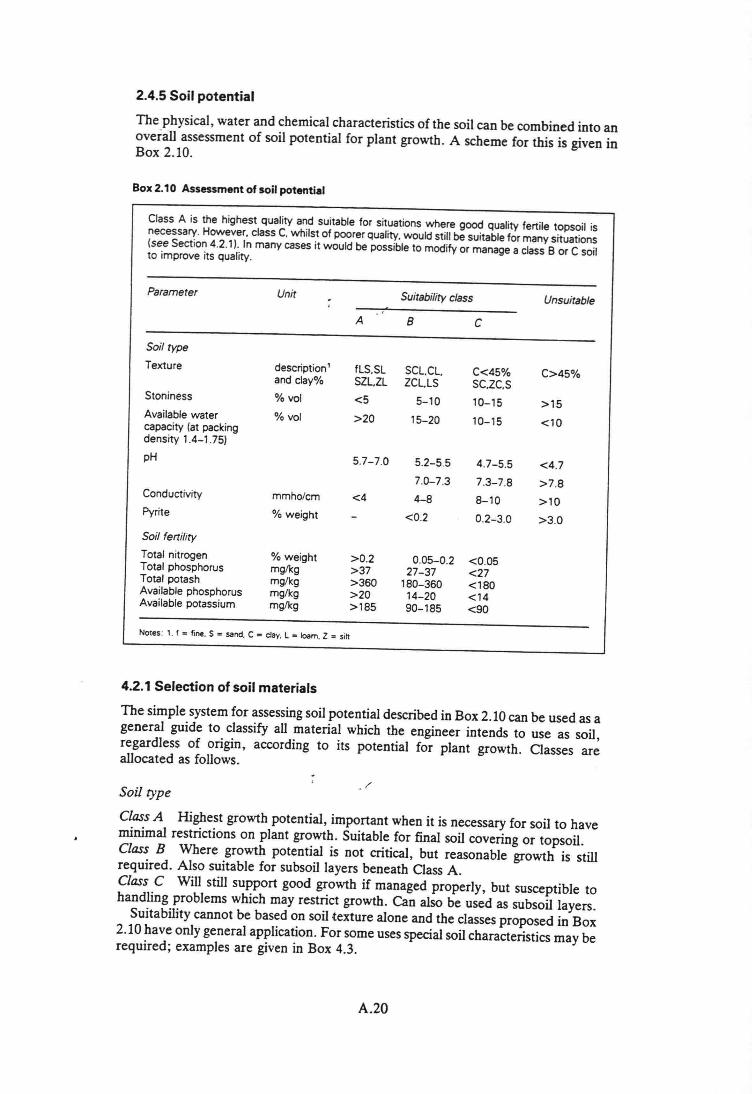
2.4.5 Soil potential

The physical, water and chemical characteristics of the soit can be combined into anoverall assessment of soit potential for plant growth. A scheme for this is given inBox 2.10.

Box2.10 Assessment of soil potential

Class A is the highest quality and suitable for situations where good quality fertile topsoil isnecessary. However. class C.whilst of poorer quality. would still be suitable for many situations(see Section 4.2.1). In many cases it would be possible to modify or manage a class B or C soilto improve its quality.

Parameter Unit Suitability class Unsuitable

A 8 C

Soil type

Texture description' fLS.SL SCL.CL. C<45% C>45%and clay% SZL.ZL ZCL.LS SC.ZC.SStoniness % vol <5 5-10 10-15 >15Available water % vol >20 15-20 10-15 <10capacity (at packingdensity 1.4-1.75)pH 5.7-7.0 5.2-5.5 4.7-5.5 <4.7

7.0-7.3 7.3-7.8 >7.8Conductivity mmho/cm <4 4-8 8-10 >10Pyrite % weight <0.2 0.2-3.0 >3.0Soil fertilityTotal nitrogen % weight >0.2 0.05-0.2 <0.05Total phosphorus mg/kg >37 27-37 <27Total potash mg/kg >360 180-360 <180Available phosphorus mg/kg >20 14-20 <14Available potassium mg/kg >185 90-185 <90

Notes: t. f = fine. 5 = sand. C = clav, L = Joam. Z = siJt

4.2.1 Selection of soil materials

The simple systemfor assessingsoitpotential described inBox2.10can be used as ageneral guide to classify all material which the engineer intends to use as soil,regardless of origin, according to its potential for plant growth, Classes areallocated as follows.

SoU type

ClassA Highest growth potential, important when it is necessary for soil to haveminimal restrictions on plant growth. Suitable for final soil covering or topsoil.Class B Where growth potential is not critical, but reasonable growth is stillrequired. Also suitable for subsoit layers beneath ClassA.Class C Will still support good growth if managed properly, but susceptible tohandling problems which may restriet growth. Can also be used as subsoil layers.Suitability cannot be based on soil texture alone and the classesproposed in Box

2.10 have only general application. For someuses specialsoitcharacteristicsmay berequired; examples are given in Box 4.3.

A.20

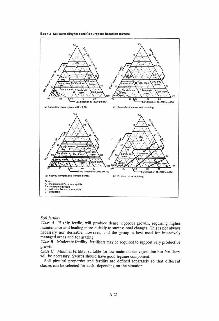
Box 4.3 Soil suitabiity tor specific purposes based on texture

100

(a) Suitability classes ;iven in Box 2.10 (b) Esse of cultivation and handling

100 100

(c) Hesvily tramplet and trafficked arees (d) Erosion risk (erodibility)

NotesA - most suitable/lee:r. susceptibleB - moderstely sui:rieC - just suitable/mo!:: susceptibleU - unsuitable

Soil [ertilityClass A Highly fertile, will produce dense vigorous growth, requiring highermaintenance and leading more quickly to successionalchanges. This is not alwaysnecessary nor desirabie, however, and the group is best used for intensivelymanaged areas and for grazing.ClassB Moderate fertility; fertilisers may be required to support very productivegrowth.Class C Minimal fertility, suitable for low-maintenance vegetation but fertiliserswill be necessary. Swards should have good legume component.Soil physical properties and fertility are defined separately so that different

classes can be selected for each, depending on the situation.

A.21

APPENDIX

B

The relation between the proteetion of the interface of land and water and the environment ismanyfold. Three aspects are selected:

I - The influence that a construction can have on the environment. A reprint is presented, dealingwith Environmental Assessment.

2 - The incorporation of environmental aspects in the design itself. Both the demands from anecological point of view, as well as examples of designs that are "friendly to the environment" arepresented.

3 - The environmental demands in the use of different materials, like slags or other waste material,with emphasis on leaching in water.

B.I

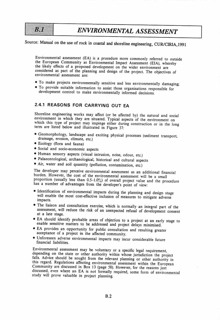
ENVIRONMENTAL ASSESSMENT

Souree: Manual on the use of rock in coastal and shoreline engineering, CURICIRIA,1991

Environmental assessment (EA) is a procedure more commonly referred to outsidethe European Community as Environmental Impact Assessment (EIA), wherebythe likely efTects of a proposed development on the wider environment areconsidered as part of the planning and design of the project. The objectives ofenvironmental assessment are:

• To make projects environmentally sensitive and less environmentally damaging;• To provide suitable information to assist those organisations responsible fordevelopment con trol to make environmentally informed decisions.

2.4.1 REASONS FOR CARRYING OUT EA

Shoreline engineering works may afTect (or be afTected by) the natural and socialenvironment in which they are situated. Typical aspects of the environment onwhich this type of project may impinge either during construct ion or in the longterm are listed below and iIIustrated in Figure 37:

• Geomorphology, landscape and exciting physical processes (sediment transport,drainage, erosion, c1imate, etc.)

• Ecology (flora and fauna)• Social and socio-economie aspects• Human sensory aspects (visual intrusion, noise, odour, etc.)• Palaeontological, archaeological, historical and cultural aspects• Air, water and soil quantity (pollution, contamination, etc.)

The developer may perceive environmental assessment as an additional financialburden. However, the cost of the environmental assessment will be a smallproportion (usually less than 0.5-1.0%) of overall project value and the procedurehas a number of advantages from the developer's point of view:

• Jdentification of environmental impacts during the planning and design stagewill enable the most cost-efTective inclusion of measures to mitigate adverseimpacts.

• The liaison and consultation exercise, which is normally an integral part of theassessment, will reduce the risk of an unexpected refusal of development consentat a late stage.

• EA should identify pro babIe areas of objection to a project at an early stage toenable sensitive matters to he addressed and project delays minimised.

• EA provides an opportunity for public consultation and resulting greateracceptance of a project in the afTected community.

• Unforeseen adverse environmental impacts may incur considerable futurefinancial Iiabilities.

Environmental assessment may he voluntary or aspecific legal requirement,depending on the state or other authority within whose jurisdiction the projectfalls. Advice should he sought from the relevant planning or other authority inthis regard. Regulations afTecting environmental assessment within the EuropeanCommunity are discussed in Box 13 (page 58). However, for the reasons justdiscussed, even where an EA is not formally required, some form of environmentalstudy will prove valuable in project planning.

B.2

Box 13 European Community (EC) environmental assessment regulations

_ Legal requiremenlSJn mid-1988 the requirements for environmental assessment in the European Community becameformalised with the implementation of EC Directive 85/337 (Council Directive of 27 June 1985'on the assessment of the efTectsof certain public and private projects on the environment'refers). Relevant statutory instruments, regulations and guidelines are lisred in Appendix 7. TheEA regulations, recommendations and publications are continually being updated. lf in doubt,reference should be made to the appropriate authorities before undertaking a formal assessment.

EC Directive 85/337 states that environmental assessment shall be a mandatory part of theplanning process for project types listed in Annex I of the directive, For projects listed in Annex11,which covers most typical shoreline engineering works using rock; the requirement forenvironmental assessment is at the diseretien of the planning authority or other body responsiblefor granting consent for the development to proceed, (Ir an environmental assessment is requiredas part of an application for planning consent an increased period may be allowed for theplanning authority to determine the consent.)

Scoping; aspects to be addressed

Artiele 3 of EC Directive 85/337 gives a particular description of the aspects to be covered inany EA:

I. Human beings, fauna and flora;2. Soil, water, air, elimate and the landscape;3. Interaction between the factors mentioned in (I) and (2) above;4. Material assets and the cultural heritage.

Requiremenls for the Environmenta/ Statement

There is no precise definition with EC Directive 85,"337as to the form of the EnvironmentalStatement. The only requirement is that it contains the information specified in Articles 3 and 5and Annex 111of the Directive and incJudes a 'non-technica] surnrnary'. More detailed formatsfor the ES may be specified in national regulations,

Statutory consultees

In addition to the issuance of public notlees as required by regulations, the proponent of thescherne may be under a statutory obligation to notiïy or consult certain authorities andorganisations specified in 'EA or planning regulations as part of the formal environmentalassessment process.

(Continued opposite)

'"0> <DC<D a.s <11 <11 êii (ij al

C ~ oe :> 0 ·ö (ij ~ .5 '"al <11 ü: en :!: "0E u. Ü C

<11:::J ...J::t:

Human beings (Cd) (b) (b) (c~ (c~ (c~ (ca) (da)

Fauna (b) (b) ~i;~;j:'iî;;(b) (b~ (b~ (b~ (ba) (ba)

Flora (b) (b) (b) Ifll'!;~ (b~ (b~ (b~ (ba) (ba)

Soil (ij (fe) (tb) (tb).(~(f) (fa) (fa)

Water (~ (Ic) (fb) (tb) (~ r~lii~':;;'(ij (fa) (Ia)

Air (~ (fe) (tb) (tb) (~ (~ ~ (fa) (Ia)

Climate (a) (ac) (ab) (ab) (a~ (a~ (af) ~:i'i!r~;t!;,: (a)Landscape (a) (ad) (ab) (ab) (a~ (a~ (a~ (a) 1;;~;2:;Material assets (ce)

Cultural heritage (e)

Note: Letters in the above matrix reler to the discipline-basedenvironmental aspects discussed in Section2.4.1

Figure 38 EG Directive 85/337 aspect and aspect interaction scoping chart

B.3

Box 13 (Continued)

Consent from other bodles may be required whether or not a development is outside th:jurisdiction of the local planning authority. For exarnple, shoreline works may require a Iicencefor placing material on the seabed or approval for navigation. These bodles mayalso requirean environmental assessment as part of the application for their consent, Jicence or approval.Statutory consultees for the UK are listed in Appendix 7.

Sensitir:e locations

Projects which impinge on particular sensitive locations (such as these listed in Appendix 7)wiJl require special attention. Development directly or indirectly alTecting such sites is Iil:ly tomake the requirement for environmental assessment mandatory.

This categorisation of environmental aspects is peculiar to the EC directive, but it iscompatible with a more conventional discipline-based aspect listing such as that given inSection 2.4.1. Figure 40 indicates in each of the matrix boxes by letter (referring to the iist inSection 2.4.1) the discipline-based aspects which are relevant to each of the EC enviroru::entalcategories,

2.4.3 METHOD OF ASSESSMENT

Phases of an assessment

An environmental assessment wiJl normally comprise three phases:

1. The baseline survey, to define the existing environment;2. The projection of the proposed project onto the existing environment and the

assessment of the pro babie impacts (beneficial arid adverse);3. Where impacts are found to be adverse, the investigation of measures to

mitigate those impacts and the possible incorporation of those measures intothe design.

Scoping

The aspects of the environment on which rock coastal and shoreline engineeringworks may have significant etTects will include those listed in Section 2.4.1 and thevarious interactions between them. For an EA to be cost-etTective, the distributionof time and etTort must match the relative needs of the ditTerent aspects. At thestart of an assessment it wiJl be necessary to decide on the probable scope of theinvestigations and the appropriate level of detail required from the results.

Where the assessment is to be carried out under European Community Directive85/337 or its derivative national regulations, a particular presentation of theaspects is required. This is compatible with the aspects as Iisted in Section 2.4.1and is detailed in the scoping diagram in Box 13.

B.4

ENVIRONMENTAL DEMANDS - DESIGN

Souree: Translation of parts of ftMilieuvriendelijke Oevers ft (Environment -friendl y banks), RWS, 1988

Po1icy on the design of banks

Policy on the design and management of banks has been revised.

The new approach is set forth in several policy documents, not

only in the above-mentioned Policy Document on "Living with

Water", but also in the Third Policy Document on Water

Management drawn up by the Ministry of Transport and Public

Works, the National Environmental Policy Plan drawn up by the

Ministry of Housing, Physical Planning and the Environment ,

and the National Nature Policy Plan drawn up by the Ministry

of Agricul ture and Fisheries , all of which appeared in 1989.

The Environmentally Friendly Banks Project deals with the

development, acceptance and application of this policy from a

pragmatic angle.

The managem~nt of a watercourse should be related to the

management of connected waters and the functions of the

adjacent land. What is required is integrated management of a

water basin. This approach demands that a thorough analysis be

made of the functions, management and general situation in the

whole of the area concerned. Such analysis is of prime

importance in th~ case of the design and management of banks,

which form the boundary between water and land and therefore

themselves consist of both elements. A functional analysis

based solely on criteria deriving from hydraulic engineering

is no longer adequate; other requirements and related criteria

must also be taken into account.

In functional terms a watercourse bank may be variously

described as:

B.S

at once a dividing-line and a transition between water and

land, each having Lts own functionsi

a means of protecting the land against the water: it

affords protection against high water levels, waves andcurrentsi

a means of protecting the water against the land: it

affords protection against cave-ins and the formation ofshallows;

a habitat for specific aquatic plants and animaIs. In this

sense banks play an ecological role, one that is related to

the genera 1 ecological function of the aquatic environment

as expounded in the Indicative Multi-Year Programme forWater;

an environment through which specific bank-related plants

may spread, and animals move, across the land, thus forming

part of the ecological infrastructure;

a scenic element affecting the

enjoyment of the landscape;

an element in water-related activities, such as shipping,

overall recreational

fishing and recreation.

There are many types of banks, which differ

functions, morphology, soil composition,

conditions and vegetation. In actual fact, no

in respect of

hydrological

two banks arealike. But even on one long bank considerable variations can

occur, or even be introduced, greatly enhancing the diversity

of the scenery and its wildlife.

It is therefore futile, or ill-advised, to seek one uniform

type of environmentally friendly bank. It would be wrong to

try to eradicate the diversity which has arisen, which is in

many cases of great value. The term "environmentally friendly"

was opted for in the new policy to emphasise the contrast with

the usual civil engineering approach to bank protection. The

qualification "multipurpose" would, perhaps, have been more tothe point.

B.6

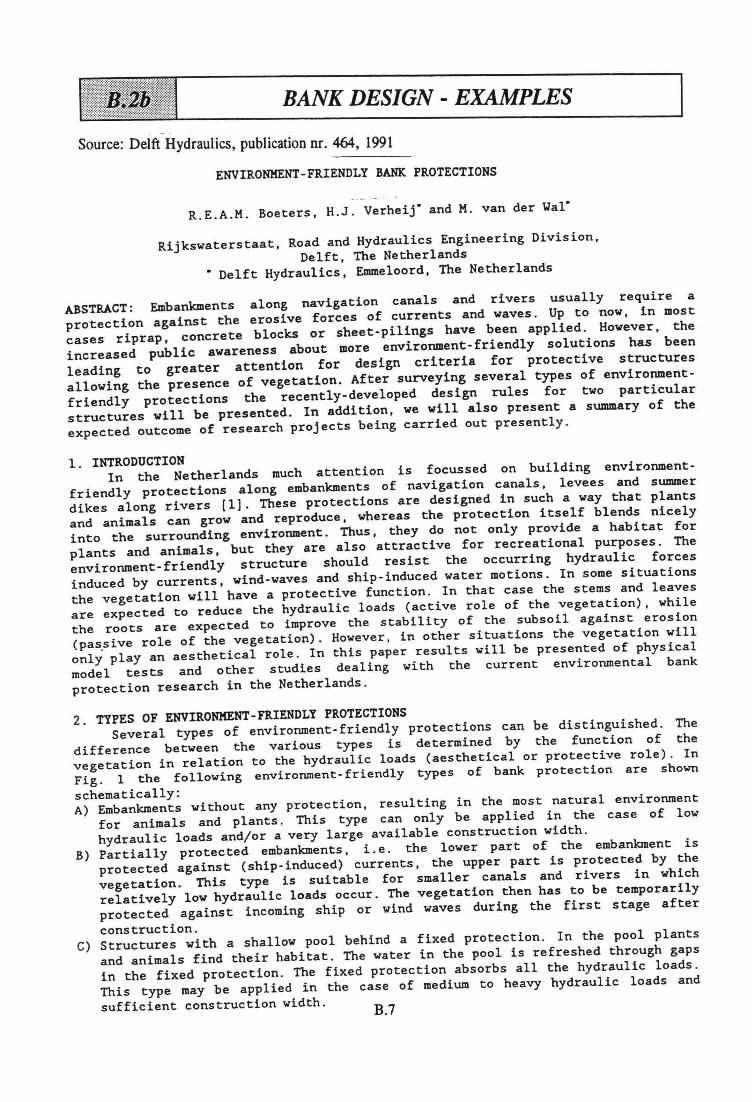
BANK DESIGN - EXAMPLES

Souree: Delft Hydraulics, publication nr. 464, 1991

ENVIRONHENT-FRIENDLYBANK PROTECTIONS

R.E.A.M. Boeters, H.J. Verheij*and M. van der Yal*

Rijkswaterstaat, Road and Hydraulics Engineering Division,Delft, The Netherlands

* Delft Hydraulics, Emmeloord, The Netherlands

ABSTRACT: Embankments along navigation canals and rivers usually require aprotection against the erosive forces of currents and waves. Up to now, in mostcases riprap, concrete blocks or sheet-pilings have been applied. However, theincreased public awareness about more environment-friendly solutions has beenleading to greater attention for design criteria for protective structuresallowing the presence of vegetation. After surveying several types of environment­friendly protections the recently-developed design rules for two particularstructures wil1 be presented. In addition, we wil1 a1so present a summary of theexpected outcome of research projects being carried out presently.

1. INTRODUCTIONIn the Netherlands much attention is focussed on building environment-

friend1y protections along embankments of navigation canals, 1evees and summerdikes along rivers [1]. These protections are designed in such a way that plantsand animals can grow and reproduce, whereas the protection itse1f blends nicelyinto the surrounding environment. Thus, they do not only provide a habitat forplants and animals, but they are also attractive for recreational purposes. Theenvironment-friendly structure should resist the occurring hydraulic forcesinduced by currents, wind-waves and ship-inducedwater motions. In some situationsthe vegetation will have a protective function. In that case the stems and leavesare expected to reduce the hydraulic loads (active role of the vegetation), whilethe roots are expected to improve the stability of the subsoil against erosion(passLve ro1e of the vegetation). However, in other situations the vegetation willonly play an aesthetical role. In this paper results will be presented of physicalmodel tests and other studies dealing with the current environmental bankprotection research in the Netherlands.

2. TYPES OF ENVIRONMENT-FRIENDLYPROTECTIONSSeveral types of environment-friendlyprotections can be distinguished. The

difference between the various types is determined by the function of thevegetation in relation to the hydraulic loads (aestheticalor protective role). InFig. 1 the following environment-friendly types of bank protectiortare shown

schematically:A) Embankments without any protection, resulting in the most natural environment

for animals and plants. This type can only be applied in the case of lowhydraulic loads and/or a very large available constructionwidth.

B) Partially protected embankments, i.e. the lower part of the embankment isprotected against (ship-induced)currents, the upper part is protected by thevegetation. This type is suitable for smaller canals and rivers in whichrelatively low hydraulic loads occur. The vegetation then has to be temporarilyprotected against incoming ship or wind waves during the first stage after

construction.C) Structures with a shallow pool behind a fixed protection. In the pool plants

and animals find their habitat. The water in the pool is refreshed through gapsin the fixed protection. The fixed protection absorbs all the hydraulic loads.This type may be applied in the case of medium to heavy hydraulic loads and

sufficient constructionwidth. B.7

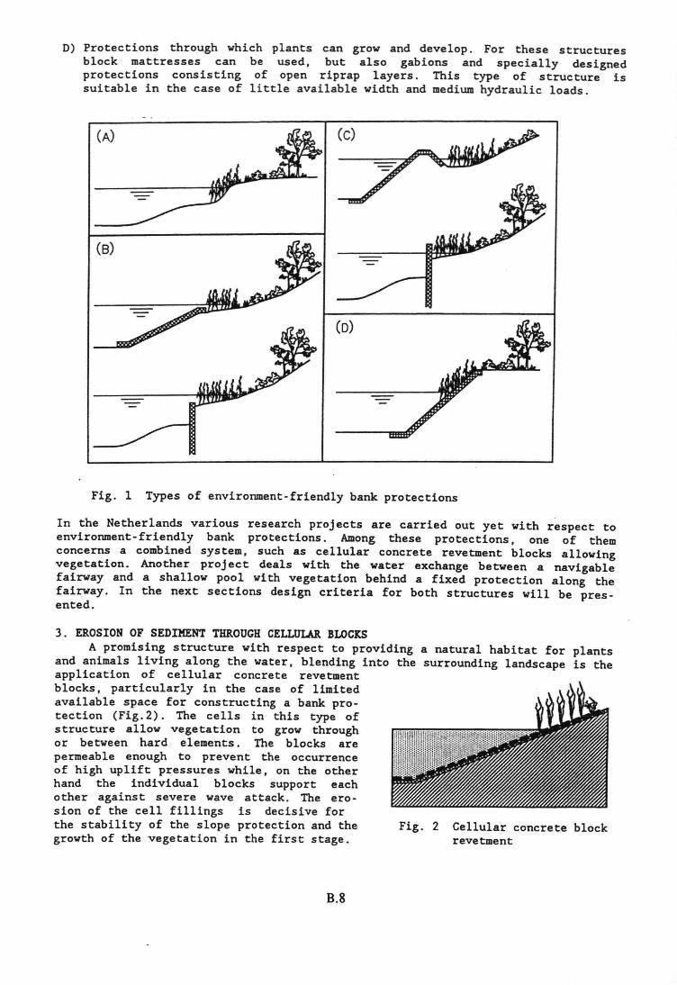
D) Protections through which plants can grow and develop. For these structuresblock mattresses can be used, but also gabions and specially designedprotections consisting of open riprap layers. This type of structure issuitable in the case of little available width and medium hydraulic loads.

(A)

(0)

Fig. 1 Types of environment-friendlybank protections

In the Netherlands various research projects are carried out yet with respect toenvironment-friendly bank protections. Among these protections, one of themconcerns a combined system, such as cellular concrete revetment blocks allowingvegetation. Another project deals with the water exchange between a navigablefairway and a shallow pool with vegetation behind a fixed protection along thefairway. In the next sections design criteria for both structures will be pres­ented.

3. EROSION OF SEDIMENT THROUGH CELLtJLAR BLOCKSA promising structure with respect to providing a natural habitat for plants

and animals living along the water, blending into the surroundinglandscape is theapplication of cellular concrete revetmentblocks, particularly in the case of limitedavailable space for constructing a bank pro­tection (Fig.2). The cells in this type ofstructure allow vegetation to grow throughor between hard elements. The blocks arepermeable enough to prevent the occurrenceof high uplift pressures while, on the otherhand the individual blocks support eachother against severe wave attack. The ero­sion of the cell fillings is decisiveforthe stability of the slope protectionand the Fig. 2 Cellular concrete blockgrowth of the vegetation in the first stage. revetment

B.8

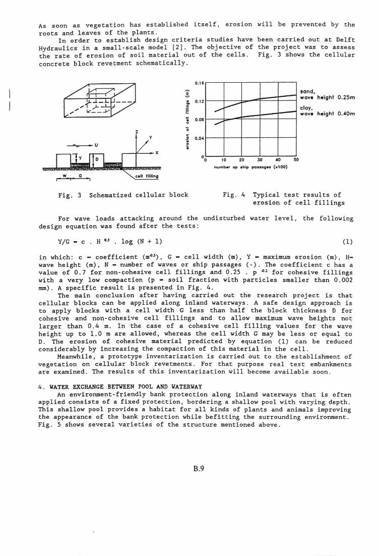
As soon as vegetation has established itself, erosionroots and leaves of the plants.

In order to establish design criteria studies haveHydraulics in a small-scale model [2]. The objective ofthe rate of erosion of soil material out of the celis.concrete block revetment schematically.

will be prevented by the

been carried out at Delftthe project was to assessFig. 3 shows the cellular

(11ti)0.16

:[.. 0.12.,.~"" ",,--y .. 0.08u

Z Ö

y c:0 0.04öi!!•x

-.,..,.,.~ -.,..,.,.

sand,wave height O.25m

clay,wave height O.40m

10 20 30 50

numbe, op .hip po •• oge. (xl00)

Fig. 3 Sehematized cellular bloek Fig. 4 Typical test results oferosion of eell fillings

For wave loads attaeking around the undisturbed water level, the followingdesign equation was found after the tests:

Y/G - e . H 0-' • log (N + 1) (1)

in which: e - eoeffieient (m.o·,,),G - eell width (m), Y - maximum erosion (m), H­wave height (m), N - number of waves or ship passages (-). The eoeffieient e has avalue of 0.7 for non-eohesive eell fillings and 0.25 . p .o~for eohesive fillingswith a very low compaction (p - soil fraction with particles smaller than 0.002mm). A speeifie result is presented in Fig. 4.

The main conelusion after having carried out the research project is thateellular blocks can be applied along inland waterways. A safe design approach isto apply bloeks with a cell width G less than half the block thickness D foreohesive and non-cohesive cell fillings and to allow maximum wave heights notlarger than 0.4 m. In the case of a eohesive cell filling values for the waveheight up to 1.0 mare allowed , whereas the eell width G may be less or equal toD. The eros ion of eohesive material predicted by equation (1) ean be reducedconsiderably by inereasing the compaction of this material in the cello

Meanwhile, a prototype inventarization is earried out to the establishment ofvegetation on cellular block revetments. For that purpose reaI test embankmentsare examined. The results of this inventarization will beeome available soon.

4. VATER EXCHANGE BETVEEN POOL AND VATERVAYAn environment-friendly bank protection along inland waterways that is often

applied consists of a fixed protection, bordering a shallow pool with varying depth.This shallow pool provides a habitat for all kinds of plants and animals improvingthe appearanee of the bank protection while befitting the surrounding environment.Fig. 5 shows several varieties of the structure mentioned above.

B.9

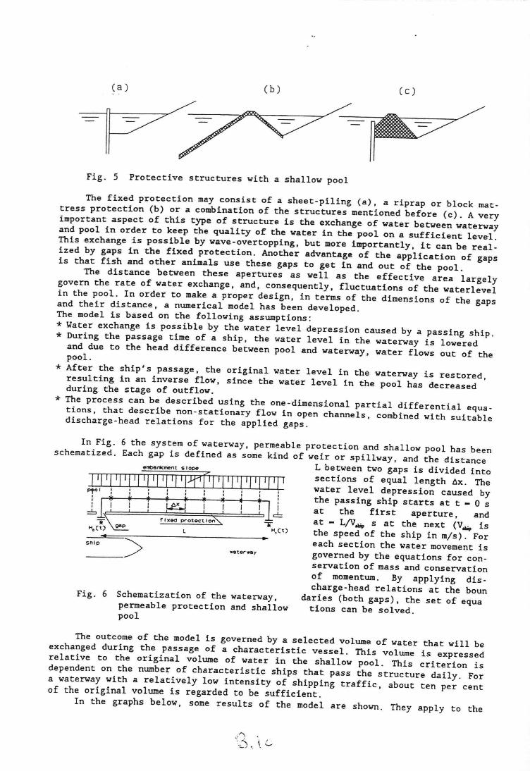
Ca) eb)

~ //-~~~ -===---~

Cc)

Fig. 5 Protective structures with a shallow pool

The fixed protection may consist of a sheet-piling (a), a riprap or block mat­tress protection (b) or a combination of the structures mentioned before (c). A veryimportant aspect of this type of structure is the exchange of water between waterwayand pool in order to keep the quality of the water in the pool on a sufficient level.This exchange is possible by wave-overtopping, but more importantly, it can be real­ized by gaps in the fixed protection. Another advantage of the application of gapsis that fish and other animals use these gaps to get in and out of the pool.

The distance between these apertures as weIl as the effective area largelygovern the rate of water exchange, and, consequently, fluctuations of the waterlevelin the pool. In order to make a proper design, in terms of the dimensions of the gapsand their distance, a numerical model has been developed.The model is based on the following assumptions:* Water exchange is possible by the water level depression caused by a passing ship.* During the passage time of a ship, the water level in the waterway is lowered

and due to the head difference between pool and waterway, water flows out of thepool.

* Af ter the ship's passage, the original water level in the waterway is restored,resulting in an inverse flow, since the water level in the pool has decreasedduring the stage of outflow.

* The process can be described using the one-dimensional partial differential equa­tions, that describe non-stationary flow in open channels, combined with suitabledischarge-head relations for the applied gaps.

In Fig. 6 the system of waterway, permeable protection and shallow pool has beenschematized. Each gap is defined as some kind of weir or spillway, and the distance

enc:>IIrkment SIe>pe L between two gaps is divided into

l'I'I'I'I'I'I'I'I'I'I?f1rl'I'I'I'I'I'I'[' sections of equal length ~x. The.......... ·----. . . . . . . . water level depression caused byptOI I I I I I I • I I I

, + j' j' ~ rt ~ ~ ~ ,': the passing ship starts at t - 0 sII j j j }e..[ j j j j11 at the first aperture , andT~ fix,", protactiO"", T at - LfVtIlips at the next (VtIlipis

H.Ct) ~ L H,Ct) the speed of the ship in mis). For

> each section the water movement issnip

waterway governed by the equations for con----- servation of mass and conservation

of momentum. By applying dis­charge-head relations at the boun

daries (both gaps), the set of equations can be solved.

Fig. 6 Schematization of the waterway,permeable protection and shallowpool

The outcome of the model is governed by a selected volume of water that will beexchanged during the passage of a characteristic vessel. This volume is expressedrelative to the original volume of water in the shallow pool. This criterion isdependent on the number of characteristic ships that pass the structure daily. Fora waterway with a relatively low intensity of shipping traffic, about ten per centof the original volume is regarded to be sufficient.

In the graphs below, some results of the model are shown. They apply to the

i"'\

\:_). \ (._

depicted situation. In this case, the relation between discharge and head for asharp-crest~d weir has been applied at the gaps [3J:

Q(t) =1c".pg mbH(t)1.5 (2)

in which: c, - coefficient for submerged flow (-), m - discharge coefficient (-), bgap width (m), g - acceleration due to gravity (mZls), Q(t) - discharge (m3/s), H(t)

_ water level (m).

40

35

30

g25Ol

§ 20Ö>~ 15..

10

5

_-\ O.~OoCl.50

\ O.50oCl.75....O.SO.I.O

\~\-. -,<,-.~~ ..____

~ ;::---=~ __,

o o 3020 40 5010distonce between gaps. l (m)

Fig. 7 An example of the use of the derived mathematical model

The example shows that in order to exchange a relative volume of about ten percent per passage, for the smallest gap a distance of 20 meters is necessary, whilefor the largest gap a distance of 40 metres suffices.

Sy using the model, the proper distance between the gaps and their geometry canbe assessed, related to a selected level of water movement in the shallow pool.Sesides structures using all sorts of sheet-piling, the model can handle riprap orblock mattress protections with lowered crests (Figure 5 (b» or pipes (culverts) asaperture, simply by adapting the discharge-head relations. Also the water exchangevia a riprap protection without any gap can be calculated. In this situation waterflows through the pores between the stones, which can be described using Forchhei­mer's equation for combined turbulent and laminar flow through stones [4J.

The establishment and development of vegetation in the pool, and the use of thepool as habitat or breeding place by fish or other animals depends largelyon thequality of the water and the intensity of water movements inside the pool. With themodel described above, a proper design of the structure and the pool can be realized.

S. RECENT AND FUTORE DEVELOPMENTSThe trend to environment-friendly sol­

utions for protective structures hasresulted in many other research projects inthe Netherlands. For example, at this momentresearch is carried out in order to developconceptual models for the behaviour of nonor less protected banks. The influence on anon-protected embankment of the hydraulicloads under normal daily conditions will bea gradual eros ion of the original profile(Fig. 8) eventually resulting in an equili­brium profile. Small-scale model tests to­gether with theoretical considerations

Fig. 8 Schematized gradual erosionof a non-protected embankment

B.Il

should allow to develop a mathematical model describing the time-dependenc erosionof the embankment profile. The results of the studies will a1so be important fordetermining maintenance strategies.

Another research project deals with the properties of geotextiles as a filterlayer in which the question is: does geotextile allow vegetation? If the openings ina particular geotextile do not allow the vegetation to grow through the geotextilevegetation will not develop in the way it was expected. Obviously, a compromise hasto be found between the traditional requirements, viz. water permeability and soiltightness, and the properties of the geotextile. Ten geotextiles are investigated ofwhich one is made of the natura1 fibre jute.

A third project deals with the damping of waves by p1ants like reed or bulrushon a horizontal berm at the embankment (Fig. 9). For this purpose a special facilitywas built at Delft Hydraulics next to a wave basin, in which in fourteen test sec.tions reed and bul rush on a substrate of sand or clayey sand are growing in the openair (Fig. 10). During the growing season and in wintertime waves wi1l be generated

40 in the basin and the wave damping caused by vegeta­tion will be studied. In addition, the inf1uence ofthe roots of the p1ants on the prevention or retar­dation of the substrate wil1 be studied as we11.Resu1ts of earl ier tests are presented in Fig 11.

The resu1ts of all the research projectsdescribed above wil1 be inc1uded in the mathemat­ica1 design program DIPRO (DImensioning PROtec­tions) [SJ. This program yet contains the designformu1as for traditional bank protections. In thenear future it wil1 a1so al10w the determination ofstabie environment-friendly protections. DIPRO wil 1then be of particular interest for consultants,contractors and management and maintenance author­ities of waterway systems.

Fig. 9 Vegetated berm asbank protection

::ë......1:.

• 10"0•

00 2 4 6wldlh of vegelatlon (m)

Fig. 11 Previous resu1ts ofwave damping charac­teristics of reed

plMttng wldtb

Fig. 10 Cross-section of a test section with reedfor wave damping tests

REFERENCES:

[I} Pilarczyk, K.W., Havinga, H., Klaassen, G.J., Verheij, H.J., Mosselman, E. andLeemans, J .A.A.M. (1989). "Control of bank erosion in The Netherlands . State-of­the-art", 3rd Nat. Conf. on Hydr. Eng. of ASCE, New Orleans.

[2} Klein Breteler, M., Laboyrie, J.H. and Verheij, H.J. (1988). "Erosion of sedimentthrough ce1lu1ar blocks applied as slope protection along coasts and inlandwaterways", Proc. Symp. on Modelling Soil-Water-Structure Interactions, Delft,The Netherlands.

[3J Chow, Ven te (1959). "Open Channel Hydraulics", McGraw-Hill.[4J Forchheimer, P. (1930) "Hydraulik", Teubner Verlag, Leipzig.[SJ Delft Hydraulics (1991). "DIPRO, a computer aided design system for bank

protections along navigation fairways", Delft, The Netherlands.

B.12

WASTE MATER/AL

2.4.2 Eisèh met betrekking~tot het milieu

Waterbouwkundige werken vormen in het algemeen een ingreep in het milieu.

Het effect dat deze ingreep heeft, wordt ten dele veroorzaakt door de

materiaalkeuze bij de uitvoering van de werken.

Vanuit milieuhygiênisch oogpunt kunnen eisen worden geformuleerd waaraan

bepaalde bouwmaterialen en hun alternatieven moeten voldoen. Deze eisen

worden enerzijds bepaald door het feit dat met de materialen een

verontreiniging in het milieu kan worden gebracht en anderzijds dat deze

materialen een verandering van de natuurlijke omgeving teweegbrengen.

Het milieu-effect bij een bepaalde materiaalkeuze wordt beoordeeld aan de

hand van:

- chemische samenstelling van de materialen;

- emissie van ongewenste stoffen die een bepaalde toepassing van de

materialen tot gevolg heeft;

- geschiktheid van een materiaal als drager van flora, fauna of menselijke

activiteiten.

Deze beoordeling moet worden gebaseerd op van overheidswege gestelde

richtwaarden of normen. Deze zijn (nog) niet opgesteld voor waterbouwkundige

werken. Wel is er een aantal milieuwetten, uitvoeringsvoorstellen en

beleidsbeslissingen die van toepassing kunnen zijn. In het geval van

hergebruik van afvalstoffen is er echter een tegenstrijdigheid aanwezig

tussen enerzijds het beperken van de hoeveelheid afval door stimulering van

hergebruik, en anderzijds bescherming van het milieu. Deze problematiek

wordt waarschijnlijk van materiaal tot materiaal verschillend benaderd en

opgelost. Vooral voor wat betreft alternatieve bulkmaterialen moet een keuze

gemaakt worden tussen het zoeken naar toepasingen binnen de huidige

regelgeving of aanpassing van de regelgeving aan een bepaalde toepassing.

De toepassing van richtwaarden of normen moet steeds worden gerelateerd aan

de waarde en de kwetsbaarheid van het systeem waarin de ingreep plaatsvindt.

In het Indicatief Meerjarenprogramma (IMP) Water 1985-1989 worden de

ecologisch~ kwaliteitsdoelstellingen voor Nederlandse oppervlaktewateren

geformuleerd, gebaseerd op de rapportage van de CUWVO (Commissie Uitvoering

Wet Verontreiniging Oppervlaktewater), werkgroep V (1984) [2.20].

Chemische samenstelling

De samenstelling van materialen geeft informatie over het potentieel nadeli­

ge effect dat een materiaal op het milieu kan hebben.

Een beoordeling kan geschieden aan de hand van :

- Zwarte en grijze stoffenlijsten. Deze lijsten (officieel lijsten I en 11)

zijn onder andere opgesteld in het kader van het Rijnchemieverdrag , een

EG-richtlijn en het Verdrag van Parijs. De zwarte-lijst-stoffen zijn

voornamelijk geselecteerd op basis van hun toxiciteit, persistentie enbio-accumulatie.

- Toetsingskader van de interimwet bodemsanering. In dit toetsingskader zijn

voor een groot aantal verontreinigingen concentratiewaarden vermeld die

als beoordelingscriteria gelden voor de mate van verontreiniging in zowelde "droge" grond als het grondwater.

- Wet chemische afvalstoffen. Bij algemene maatregel van bestuur, het

stoffen- en processenbesluit, wordt aangegeven wat wordt verstaan onderchemisch afval.

- Toetsingscriteria baggerslib. Rijkswaterstaat, Directie Benedenrivieren

heeft een toetsingssysteem ontworpen voor vergelijking van onderwater­

bodems, rekening houdend met onderlinge verschillen in samenstelling en

textuur, specifiek voor het benedenrivierengebied (en dus niet directvertaalbaar voor andere materialen).

Het in het milieu brengen van milieuvreemde stoffen in grote hoeveelheden

wordt door de wet slechts toegestaan indien deze toepassing gelsoleerd,

beheersbaar en controleerbaar is (lBC-criteria). Dit betekent in de praktijk

dat aan toepassing van materialen, die een potentieel nadelig effect hebben

op het milieu, de eis kan worden gesteld dat ze "herneembaar" moeten worden

toegepast en niet mogen worden gemengd met niet-verontreinigd materiaal.

Indien het materiaal wordt hernomen, ontstaan mogelijk extra kosten indien

een verwerkingsmogelijkheid voor het afval met potentieel verontreinigende

stoffen moet worden gevonden. Ook dient een systeem te worden opgezet om demilieueffecten te beheersen.

s.u,

Het uitlooggedrag van een stof kan worden getoetst aan verschillend

richtwaarden, afhankelijk van de vraag naar welk milieucompartiment d

emissie is gericht:_ interimwet bodemsanering, bijvoorbeeld in het geval van kwel door he

materiaal naar het grondwater en de bodem;

_ waterkwaliteitsdoelstellingen, zoals opgenomen in het "IMP-Water 1985

1989";_ toetsingscriteria voor baggerslib in het geval van emissie naar (

onderwaterbodem.

Bij deze beoordeling moeten zowel de totale belasting van het milieu aJ

specifieke concentratie-eisen worden betrokken.

Een beoordeling van de totale emissie is afhankelijk van zowel de tijdsdu1

waarover deze plaatsvindt als het systeem waarop de emissie effect heef·

Chloride-emissie naar zeewater is onschadelijk, maar een korte doch ho;

emissie (bijvoorbeeld na hoge waterstanden) van koper naar het oppervla:

tewater kan dodelijk zijn voor vissen.

Emissie als gevolg van mechanische verwering treedt alleen op indien h

materiaal als toplaag of filterlaag wordt toegepast. Duurzaamheidseise

gesteld en acceptabel geacht vanuit civieltechnische hoek, kunnen t

milieuhygiênisch onaanvaardbare emissies van fijn verdeeld verontreini

materiaal leiden.

Milieuwetgeving

Een aantal milieuwetten is van toepassing op het gebruik van afvalstoffen

reststoffen in en onder water, te weten;

Wet verontreiniging oppervlaktewater (WVO) voor onder andere het in h

oppervlaktewater brengen van stoffen.

_ Wet chemische afvalstoffen voor de verwijdering van chemisch afval.

_ Afvalstoffenwet voor de verwerking van afval via vergunningen.

_ Wet bodembescherming voor de bescherming van de bodem via richtlijnen

algemene maatregelen van bestuur.

6. \5"'

TOETSINGST ABEL voor de beoordeling van de konceItratieniveaus van dMlrI8 verontreinigingen in de bodem.Indikatieve richtwaarden: A.relerenliewaaJóe. B.loetsingswaarde t.b.v. (nad8r)onder2oek. C·I08Ising6waarde tb.v. sanering.

Voorkomen in grond (mgikg droge slol) grondwater ()lgII)

~nivaau A B C A B C

1. Metalen

Cr (Î) 250 800 1 50 200Co 20 50 300 20 50 200NI (Î) 100 500 15 50 200Cu (Î) 100 500 15 50 200Zn (Î) 500 3000 150 200 800As (Î) 30 50 10 30 1001.10 10 40 200 5 20 100Cd (Î) 5 20 1.5 2.5 10Sn 20 50 300 10 30 150Ba 200 400 2000 50 100 500Hg (Î) 2 10 0.05 0.5 2Pb (Î) 150 600 15 50 2002. Anorganische vetbtndlngenNH4 (als N) . (2) 1000 3000F (totaal) (Î) 400 2000 (2) 1200 4000CN (tala»vrf!) 1 10 100 5 30 100CN (1oIaaI-~r) 5 50 500 10 50 200S (laIaal·sulllden) 2 20 200 10 100 300Br (1aIaaI) 20 50 300 (2) 500 2000POt (ala P) . (2) 200 7003. AronBlllICIMI wrblndlngenBenzeen O.05(d) 0.5 5 O.2(d) 1 5Elhytbenzeen 0.05(d) 5 50 O.2(d) 20 60Tol..... 0.05(d) 3 30 0.2(d) 15 50XY**I O.05(d) 5 50 0.2(d) 20 60Fenolen 0.05(d) 1 10 0.2(d) 15 50AromaIen (IC11aa1) 7 70 . 30 1004. PoIyqelsche 1II'OInBI1sc:he

IItIoIwatBtltollenNaftaIIIen (3) 5 50 0.2(d) 7 30Fenantl'88rl (3) 10 100 0.005(d) 2 10Antraceen (3) 10 100 0.005(d) 2 10A__

(3) 10 100 O.OO5(d) 1 5ChrylMn (3) 5 50 0.005(d) 0.5 2Benzo(a)anlraC88n Cl) 5 50 O.OO5(d) 0.5 2Benzo(a)pyreen Cl) 1 10 O.OO5(d) 0.2 1Benzo(k)fluoranl88l1 (3) 5 50 0.005(d) 0.5 2Indeno( 1.2.300)pyreen (3) 5 50 0.005(d) 0.5 2Benzo(ghl}peryt88l1 (3) 10 100 O.OO5{d) 1 5PAK (talaaI) 1 20 200 - 10 405.~~_lIlIIenAIIarlsc:he dlloorkwal (1ndiv.) (3) 5 50 0.0 1(d) 10 50AlfarIadIe dlloorllwal (1oIaaI) - 7 70 15 70ChIDorbenz_ (IncIv.) Cl) 1 10 O.OI(d) 0.5 2Chloorbenzenen (1oIaaI) 2 20 1 5Chlaorfenolen (inciv.) (3) 0.5 5 0.01(d) 0.3 1.5Chlaorfenoten (talaal) 1 10 0.5 2Chioorpck'a (tOIaaI) Cl) 1 10 0.2 1PCB's (talaaI) Cl) 1 10 O.OI(d) 0.2 1EOCI (totaal) 0.1 8 80 1 15 706. Be.lri!I'lngsmiddeten

Organisdl dlloor (IndIv.) Cl) 0.5 5 11O.01(d) 0.2 1Organildl dlloor (lotaaI) 1 10 0.5 2NIIII dlloor (IndIv.) Cl) 1 10 11O.01(d) 0.5 2NIIII chloor (totaal) 2 20 t 57. ~v~m~in~1ngenTetrahydroluran 0.1 4 40 0.5 20 60Pyridine 0.1 2 20 0.5 10 30TetrahydrOlhlof .. n 0.1 5 50 0.5 20 60Cydohexanon 0.1 6 60 0.5 15 50Styreen 0.1 5 50 0.5 20 60Ftalaten (tOlaa~ 0.1 50 500 0.5 10 50Geoxyde8rde PAK (tOIaaI) I 200 2000 0.2 100 400 IMinerale olie e 1000 I 5000 5O(d) 200 600 I

I Jd • deleerlelimiet ~. zie tabel 1.2 en 3 U~: leidraad BCXlemsanering(afl.•. noven1)er I1I88)

6. ,6"

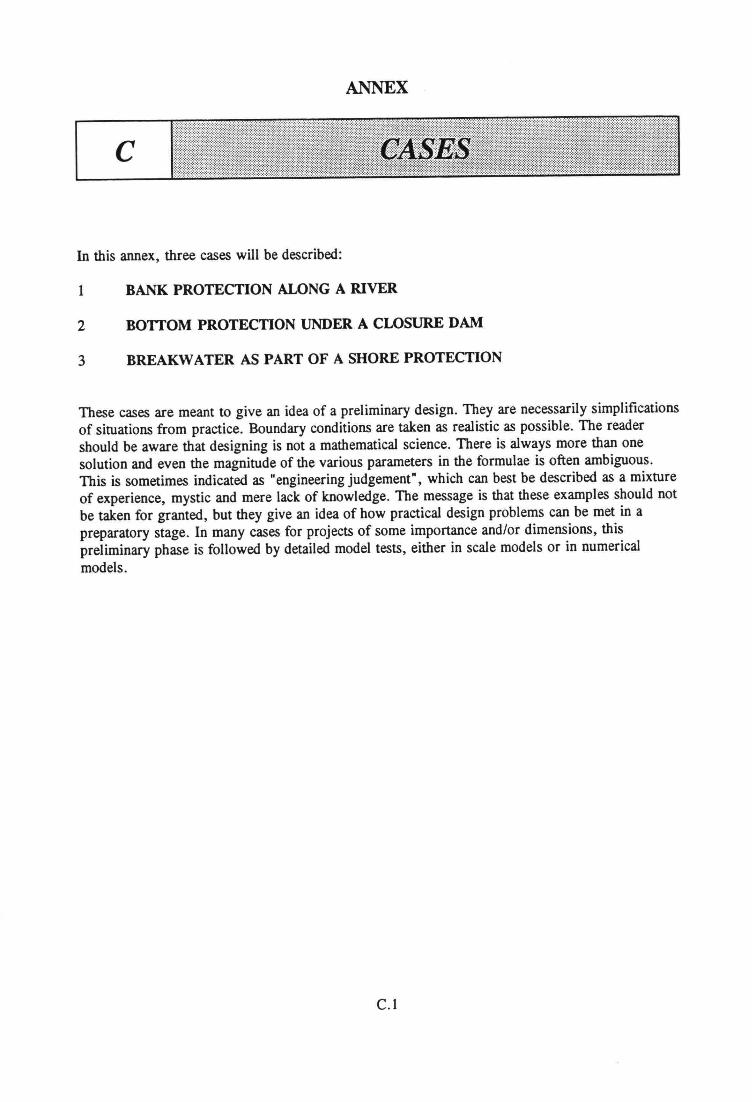
ANNEX

c

In this annex, three cases will be described:

1 BANKPROTECTION ALONGARIVER

2 BOTTOM PROTECTION UNDERA CLOSUREDAM

3 BREAKWATER AS PART OF A SHORE PROTECTION

These cases are meant to give an idea of a preliminary design. They are necessarily simplificationsof situations from practice. Boundary conditions are taken as realistic as possible. The readershould be aware that designing is not a mathematical science. There is always more than onesolution and even the magnitude of the various parameters in the formulae is often ambiguous.This is sometimes indicated as "engineering judgement", which can best be described as a mixtureof experience, mystic and mere lack of knowiedge. The message is that these examples should notbe taken for granted, but they give an idea of how practical design problems can be met in apreparatory stage. In many cases for projects of some importance and/or dimensions, thispreliminary phase is followed by detailed model tests, either in scale models or in numericalmodeis.

C.1

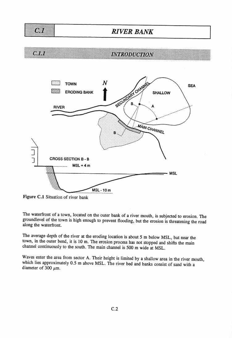
RIVERBANK

]]

k:::::::1 TOWN

~ ERODING BANK

SEA

SHALLOW

CROSS SECnON B - B

MSL+4m

Figure C.I Situation of river bank

The waterfront of a town, located on the outer bank of a river mouth, is subjected to erosion. Thegroundlevel of the town is high enough to prevent tlooding, but the erosion is threatening the roadalong the waterfront.

The average depth of the river at the eroding location is about 5 m below MSL, but near thetown, in the outer bend, it is lOm. The erosion process has not stopped and shifts the mainchannel continuously to the south. The main channel is 500 m wide at MSL.

Waves enter the area from sector A. Their height is limited by a shallow area in the river mouth,which lies approximately 0.5 m above MSL. The river bed and banks consist of sand with adiameter of 300 JLm.

C.2

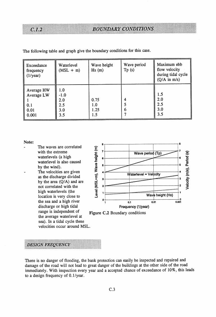
The following table and graph give the boundary conditions for this case.

Exceedance Waterlevel Wave height Wave period Maximum ebbfrequency (MSL + m) Hs (m) Tp (s) flow velocity(l/year) during tidal cycle

(Q/A in mis)

Average HW 1.0Average LW -1.0 1.51 2.0 0.75 4 2.00.1 2.5 1.0 5 2.50.01 3.0 1.25 6 3.00.001 3.5 1.5 7 3.5

Note:The waves are correlatedwith the extremewaterlevels (a highwaterlevel is also causedby the wind).The veloeities are givenas the discharge dividedby the area (Q/A) and arenot correlated with thehigh waterlevels (thelocation is very close tothe sea and a high riverdischarge or high tidalrange is independent ofthe average waterlevel atsea). In a tidal cycle theseveloeities occur around MSL.

8 8

Wave pariD<~------------Water1evel- Vel )city~-----

..................... ........................................................ Wav~height (Hs)

7 :E

o1

o0.0010.1

Frequency (1/year)0.01

Figure C.2 Boundary conditions

There is no danger of flooding, the bank proteetion can easily be inspected and repaired anddamage of the road will not lead to great danger of the buildings at the other side of the roadimmediately. With inspeetion every year and a accepted chance of exceedance of 10%, this leadsto a design frequency of O.l/year.

C.3

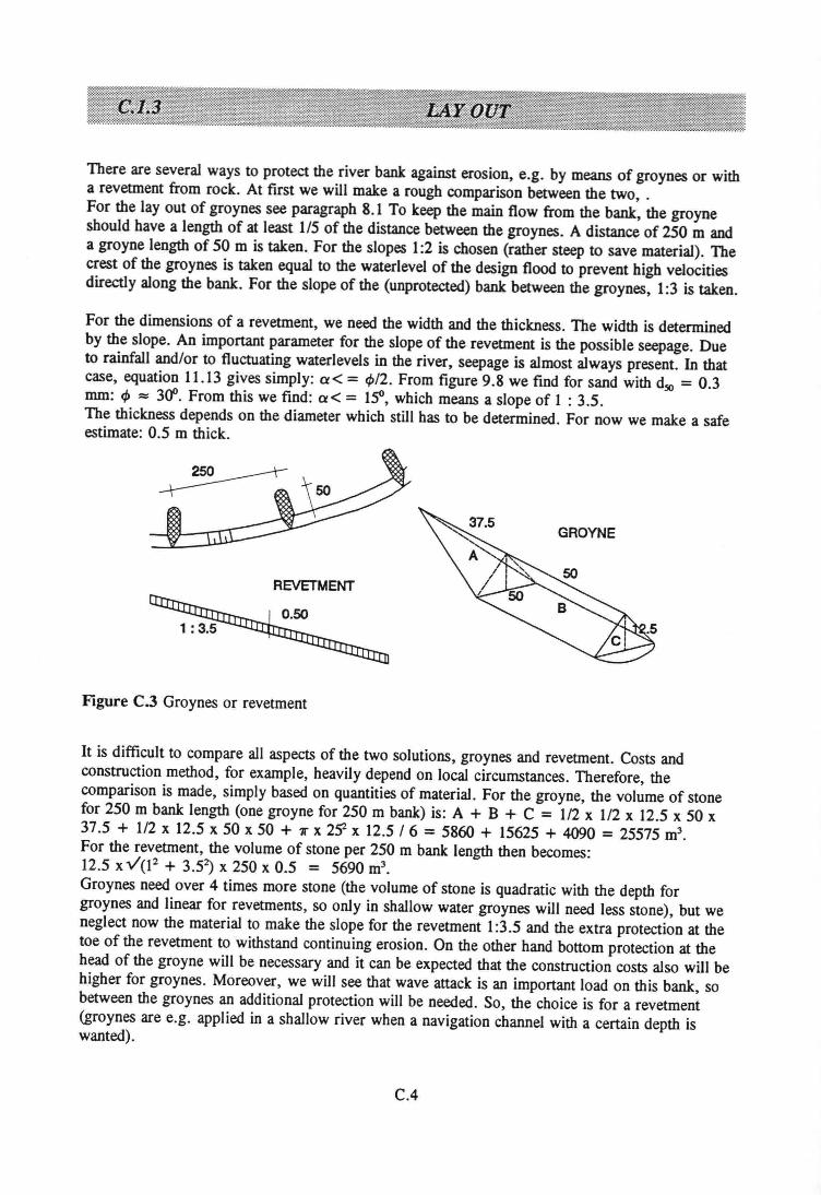
There are several ways to proteet the river bank against erosion, e.g. by means of groynes or witha revetment from rock. At first we will make a rough comparison between the two, .For the lay out of groynes see paragraph 8.1 To keep the main flow from the bank, the groyneshould have a length of at least 1/5 of the distance between the groynes. A distance of 250 m anda groyne length of 50 m is taken. For the slopes 1:2 is chosen (rather steep to save material). Thecrest of the groynes is taken equal to the waterlevel of the design flood to prevent high veloeitiesdirectly along the bank. For the slope of the (unprotected) bank between the groynes, 1:3 is taken.

For the dimensions of a revetment, we need the width and the thickness. The width is determinedby the slope. An important parameter for the slope of the revetment is the possible seepage. Dueto rainfall and/or to fluctuating waterlevels in the river, seepage is almost always present. In thatcase, equation 11.13 gives simply: a < = tb/2. From figure 9.8 we find for sand with dso = 0.3mm: tb =:: 300. From this we find: ce< = ISO,which means a slope of 1 : 3.5.The thickness depends on the diameter which still has to be determined. For now we make a safeestimate: 0.5 m thick.

GROYNE

REVETMENT

Figure C.3 Groynes or revetment

It is difficult to compare all aspects of the two solutions, groynes and revetment. Costs andconstruction method, for example, heavily depend on local circumstances. Therefore, thecomparison is made, simply based on quantities of materiaI. For the groyne, the volume of stonefor 250 m bank length (one groyne for 250 m bank) is: A + B + C = 1/2 x 1/2 x 12.5 x 50 x37.5 + 1/2 x 12.5 x 50 x 50 + 7f x 29 x 12.5/6 = 5860 + 15625 + 4090 = 25575 m".For the revetment, the volume of stone per 250 m bank length then becomes:12.5 x v(12 + 3.5~ x 250 x 0.5 = 5690 nr'.Groynes need over 4 times more stone (the volume of stone is quadratic with the depth forgroynes and linear for revetments, so only in shallow water groynes will need less stone), but weneglect now the material to make the slope for the revetment 1:3.5 and the extra proteetion at thetoe of the revetment to withstand continuing erosion. On the other hand bottom proteetion at thehead of the groyne will be necessary and it can be expected that the construction costs also will behigher for groynes. Moreover, we will see that wave attack is an important load on this bank, sobetween the groynes an additional proteetion will be needed. So, the choice is for arevetment(groynes are e.g. applied in a shallow river when a navigation channel with a certain depth iswanted).

C.4

The river bank is attacked both by flow and by waves. To start with the flow, we need the designvelocity near the bank. The values from the boundary conditions can not be used directly, sincethey represent an average in the cross section (Q/A). Since the bank is located in an outer bend ofthe river, the velocity will be higher than this average. For a first estimate we take 40% higher,leading to a design velocity of 1:4 * 2.5 = 3.5 mis (measurements are, of course, preferabie andnot so difficult to obtain!). We further assume that this velocity occurs at the average depth on theslope (= 6 m during design conditions).

From the Shields equation, with 1/t= 0.03 and A = 1.65, we find iteratively with C =18*log(12*h/k) and k = 2*dn: dn = U2/(C2*1/t*A)= 0.13 m.This is however for uniform flow in a flume and with a horizontal bed. The flow in a river ismore turbulent than in a uniform flow, due to variations in cross section and the stones lie on aslope of 1:3.5. To take this into account we apply two correction factors.KL takes the extra load due to turbulence into account and is assumed 1.2 (in a vortex street wefind KL :::::1.4 and in uniform flow, by definition, 1, so we take a value in between).Ka takes the decreased strength into account and is calculated with: Ka = V(1 - sin2a/sin2<b). Fora = 16° and <b = 400this leads to Ka = 0.9. dn then becomes: KL2*dnShie'dslKa= 0.2 m (KL isan amplification factor for the velocity, hence KL2 is used for the diameter; Ka is already definedas a correction factor for the diameter). From the curves in annex A we find that this is equivalentwith stone 10 - 60 kg.

For the wave attack, we will use the van der Meer formula (for a rough ürst estimate also Hudsoncan be used, but for revetments, van der Meer is preferred since the porosity of a revetment isquite different from that in a breakwater, for which Hudson was derived).With H = 1 m, cote = 3.5, P = 0.1 (relatively short waves hardly penetrate into the subsoil,hence it is considered "impermeable"), Tm = 0.85 * Tp = 4.25, S = 2 (threshold of damage,since the chosen boundary conditions already have a rather high probability of exceedance: 10%)and N = 7000 (maximum value, for the same reason), we find: ~ = 1.5, while for the transitionbetween the two van der Meer formulae ~t = 2.2, so we are dealing with the formula forplunging breakers. With A = 1.65 this leads to a dn = 0.38 m.From the curves in annex A we find that this comes down to rock 60 - 300 kg.

It is obvious that the wave attack is dominating. The wave attack, however, does not act on thewhole slope. The region of wave attack lies approximately 2*Hs around the waterlevel. For thefinal design we also have to take into account lower waterlevels (with lower wave heights). Apractical measure (also for construction) is then that we apply 60 -300 kg from Mean Low Water(MSL - 1 m) up to MSL + design waterlevel + 2* design Hs = MSL + 4.5 m. Depending onthe height of the bank, a practical transition to what lies above has to be made.In this case we deal with a city waterfront with a road along the river, so, one can think of a wallof masonry. Below the low waterlevel, the attack on the slope comes from the flow only. So,down to the bottom, the stone 10 - 60 kg can be applied.

C.5

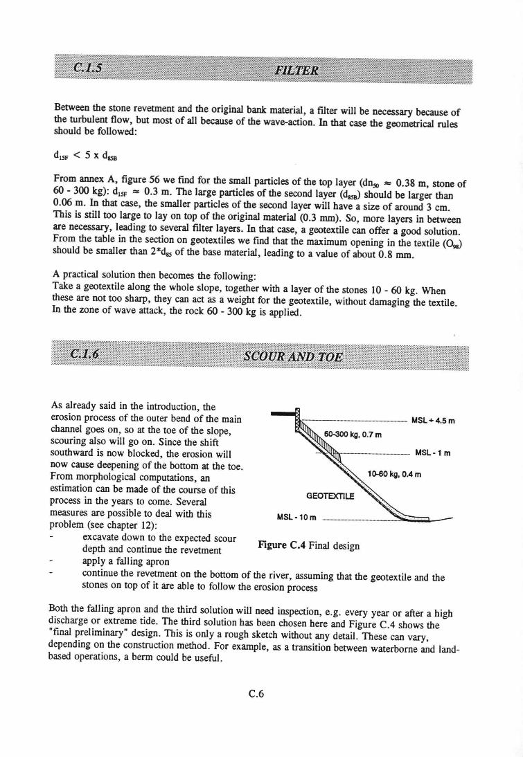
Between the stone revetment and the original bank material, a filter will be necessary because ofthe turbulent flow, but most of all because of the wave-action. In that case the geometrical rulesshould be followed:

From annex A, figure 56 we find for the smalI particles of the top layer (dn50 == 0.38 m, stone of60 - 300 kg): d,SF :::::0.3 m. The large partieles of the second layer (d8SB) should be larger than0.06 m. In that case, the smaller particles of the second layer will have a size of around 3 cm.This is still too large to lay on top of the original material (0.3 mm). So, more layers in betweenare necessary, leading to several filter layers. In that case, a geotextile can offer a good solution.From the table in the section on geotextiles we find that the maximum opening in the textile (098)

should be smaller than 2*dgsof the base material, leading to a value of about 0.8 mmo

A practical solution then becomes the following:Take a geotextile along the whole slope, together with a layer of the stones 10 - 60 kg. Whenthese are not too sharp, they can act as a weight for the geotextile, without damaging the textile.In the zone of wave attack, the rock 60 - 300 kg is applied.

As already said in the introduction, theerosion process of the outer bend of the mainchannel goes on, so at the toe of the slope,scouring also will go on. Since the shiftsouthward is now blocked, the erosion willnow cause deepening of the bottom at the toe.From morphological computations, anestimation can be made of the course of thisprocess in the years to come. Severalmeasures are possible to deal with thisproblem (see chapter 12):

excavate down to the expected scourdepth and continue the revetmentapply a falling aproncontinue the revetment on the bottom of the river, assuming that the geotextile and thestones on top of it are able to follow the erosion process

._- MSL+4.5m

---.-------- MSL- 1m

10-60 kg, 0.4 m

MSL-10m

Figure C.4 Final design

Both the falling apron and the third solution will need inspection, e.g. every year or after a highdischarge or extreme tide. The third solution has been chosen here and Figure CA shows the"final preliminary" design. This is only a rough sketch without any detail. These can vary,depending on the construction method. For example, as a transition between waterborne and land­based operations, a berm could be useful.

C.6

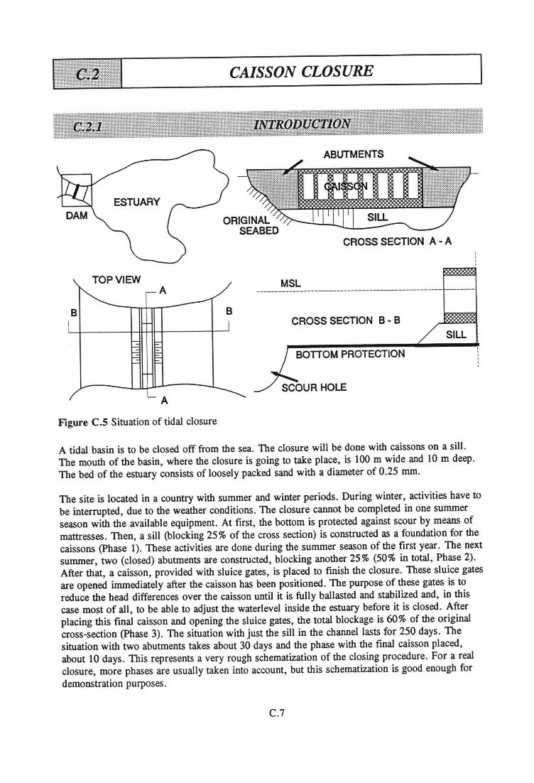
CAISSON CLOSURE

ABUTMENTS

CROSSSECTION A - A

TOPVIEW

B

AMSL

BCROSSSECTION B - B

BonOM PROTECTION

RHOLE

Figure C.S Situation of tidal closure

A tidal basin is to be closed off from the sea. The closure will be done with caissons on a sill.The mouth of the basin, where the closure is going to take place, is 100 m wide and 10 m deep.The bed of the estuary consists of loosely packed sand with a diameter of 0.25 mmo

The site is located in a country with summer and winter periods. During winter, activities have tobe interrupted, due to the weather conditions. The closure cannot be completed in one summerseason with the available equipment. At first, the bottom is protected against scour by means ofmattresses. Then, a sill (blocking 25% of the cross section) is constructed as a foundation for thecaissons (phase 1). These activities are done during the summer season of the first year. The nextsummer, two (closed) abutments are constructed, blocking another 25% (50% in total, Phase 2).After that, a caisson, provided with sluice gates, is placed to finish the closure. These sluice gatesare opened immediately after the caisson has been positioned. The purpose of these gates is toreduce the head differences over the caisson until it is fully ballasted and stabilized and, in thiscase most of all, to be able to adjust the waterlevel inside the estuary before it is closed. Afterplacing this final caisson and opening the sluice gates, the total blockage is 60% of the originalcross-section (phase 3). The situation with just the sill in the channel lasts for 250 days. Thesituation with two abutments takes about 30 days and the phase with the final caisson placed,about 10 days. This represents a very rough schematization of the closing procedure. For a realclosure, more phases are usually taken into account, but this schematization is good enough fordemonstration purposes.

C.?

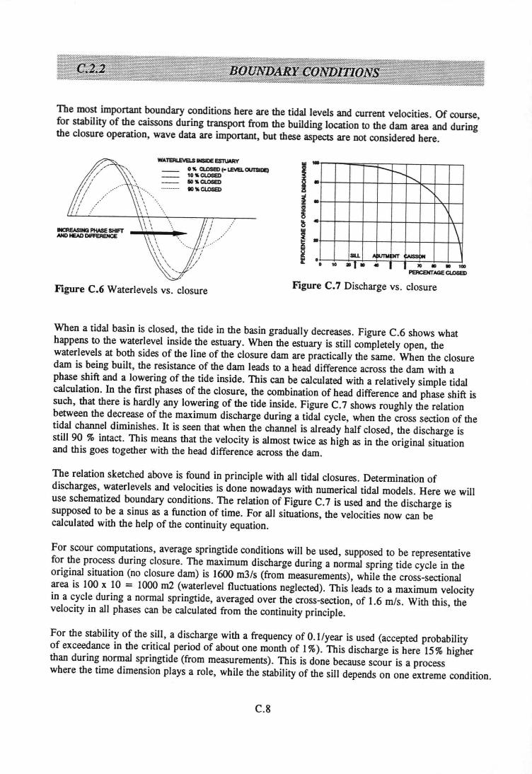
The most important boundary conditions here are the tidal levels and current velocities. Of course,for stability of the caissons during transport from the building location to the dam area aod duringthe closure operation, wave data are important, but these aspects are not considered here.

WATEJILEVELS liISIlE ESTUARY0.. CI.OSED(- LEVELOUTSIDE)10 .. c:LOSEDlO .. c:LOSEDIO,.CLOSED

r-r-r-;~

1'\\1\

~.

\su A~ fHT ~ )lil

• 10 al_ • 10 ID ., 1

Figure C.6 Waterlevels VS. closure Figure C.7 Discharge vs. closure

Wben a tidal basin is closed, the tide in the basin gradually decreases. Figure C.6 shows whathappens to the waterlevel inside the estuary. When the estuary is still completely open, thewaterlevels at both sides of the line of the closure dam are practically the same. When the closuredam is being built, the resistance of the dam leads to a head difference across the dam with aphase shift aod a lowering of the tide inside. This cao be calculated with a relatively simple tidalcalculation. In the first phases of the closure, the combination of head difference and phase shift issuch, that there is hardly any lowering of the tide inside. Figure C.7 shows roughly the relationbetween the decrease of the maximum discharge during a tidal cycle, when the cross section of thetidal channel diminishes. It is seen that when the channel is already half c1osed, the discharge isstill 90 % intact. This means that the velocity is almost twice as high as in the original situationand this goes together with the head difference across the dam.

The relation sketched above is found in principle with all tidal c1osures. Determination ofdischarges, waterlevels and veloeities is done nowadays with numerical tidal modeIs. Here we willuse schematized boundary conditions. The relation of Figure C.7 is used and the discharge issupposed to be a sinus as a function of time. For all situations, the veloeities now can becalculated with the help of the continuity equation.

For scour computations, average springtide conditions will be used, supposed to be representativefor the process during closure. The maximum discharge during a normal spring tide cycle in theoriginal situation (no closure dam) is 1600 m3/s (from measurements), while the cross-sectionalarea is 100 x 10 = 1000m2 (waterlevel tluctuations neglected). This leads to a maximum velocityin acycIe during anormal springtide, averaged over the cross-section, of 1.6 mIs. With this, thevelocity in all phases can be calculated from the continuity principle.

For the stability of the sill, a discharge with a frequency of O.lIyear is used (accepted probabilityof exceedance in the critical period of about one month of 1%). This discharge is here 15% higherthan during normal springtide (from measurements). This is done because scour is a processwhere the time dimension plays a role, while the stability of the sill depends on one extreme condition.

C.S

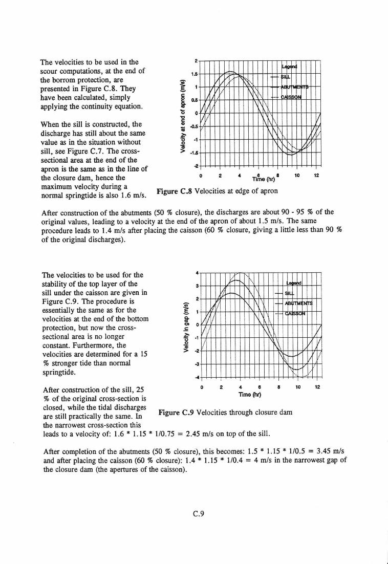
The veloeities to be used in thescour computations, at the end ofthe borrom protection, arepresented in Figure C.S. Theyhave been calculated, simplyapplying the continuity equation.

211.Jg4~

11/ v .. ..~~"I

IV .... \r\ ..../ / .- ..VI .... 1\ \ \.

'.

V""'. V\\\\\ VII

/1/""\" J~~.,-; .'

1.5

When the sill is constructed, thedischarge has still about the samevalue as in the situation withoutsill, see Figure C.7. The cross­sectional area at the end of theapron is the same as in the line ofthe closure dam, hence themaximum velocity during anormal springtide is also 1.6 mIs.

o 2 4 l1~ (hr)I

Figure C.8 Veloeities at edge of apron

10 12

After construction of the abutments (50 % closure), the discharges are about 90 - 95 % of theoriginal values, leading to a velocity at the end of the apron of about 1.5 mIs. The sameprocedure leads to 1.4 mIs after placing the caisson (60 % closure, giving a little less than 90 %of the original discharges).

The veloeities to be used for thestability of the top layer of thesill under the caisson are given inFigure C.9. The procedure isessentially the same as for theveloeities at the end of the bottomprotection, but now the cross­sectional area is no longerconstant. Furthermore, theveloeities are determined for a 15% stronger tide than normalspringtide.

2

.'.8~1d

l~ r-.. , SIL'7 \

-, \ '.'4/ \fN

lil! \\ '. .... c"'" ~:o~'.

I! \ \ , V1\ 11 I

1\\ I

,\1-- [..-V1/:;...

~ J...-.'

3

:5 ·1o~> -2

After construction of the sill, 25% of the original cross-section isclosed, while the tidal dischargesare still practically the same. In Figure C.9 Veloeities through closure damthe narrowest cross-section thisleads to a velocity of: 1.6 * 1.15 * 1/0.75 = 2.45 mIs on top of the sill.

o 2 4 8l1me (hr)

8 10 12

After completion of the abutments (50 % closure), this becomes: 1.5 * 1.15 * 1/0.5 = 3.45 mIsand after placing the caisson (60 % closure): 1.4 * 1.15 * 1/0.4 = 4 mIs in the narrowest gap ofthe closure dam (the apertures of the caisson).

C.9

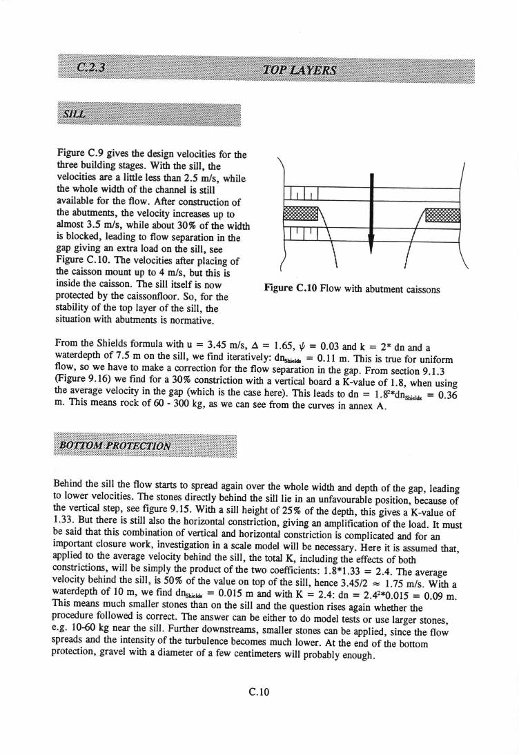
Figure C.9 gives the design veloeities for thethree building stages. With the sill, theveloeities are a little less than 2.5 mis, whilethe whole width of the channel is stillavailable for the flow. After construction ofthe abutments, the velocity increases up toalmost 3.5 mis, while about 30% of the widthis blocked, leading to flow separation in thegap giving an extra load on the sill, seeFigure C.IO. The veloeities after placing ofthe caisson mount up to 4 mis, but this isinside the caisson. The sill itself is now Figure C.I0 Flow with abutment caissonsprotected by the caissonfloor. So, for thestability of the top layer of the sill, thesituation with abutments is normative.

From the Shields formula with u = 3.45 mis, À = 1.65, 1f = 0.03 and k = 2* dn and awaterdepth of 7.5 m on the sill, we find iteratively: dllsmelda= 0.11 m. This is true for uniformflow, so we have to make a correction for the flow separation in the gap. From section 9.1.3(Figure 9.16) we find for a 30% constriction with a vertical board a K-value of 1.8, when usingthe average velocity in the gap (which is the case here). This leads to dn = I.W*dnShieIda = 0.36m. This means rock of 60 - 300 kg, as we can see from the curves in annex A.

Behind the sill the flow starts to spread again over the whole width and depth of the gap, leadingto lower velocities. The stones directly behind the sill lie in an unfavourable position, because ofthe vertical step, see figure 9.15. With a sill height of 25% of the depth, this gives a K-value of1.33. But there is still also the horizontal constriction, giving an amplification of the load. It mustbe said that this combination of vertical and horizontal constriction is complicated and for animportant closure work, investigation in a scale model will be necessary. Here it is assumed that,applied to the average velocity behind the sill, the total K, including the effects of bothconstrictions, will be simply the product of the two coefficients: 1.8*1.33 = 2.4. The averagevelocity behind the sill, is 50% of the value on top of the sill, hence 3.45/2 ::< 1.75 mis. With awaterdepth of 10 m, we find dnShieIda = 0.015 m and with K = 2.4: dn = 2.42*0.015 = 0.09 m.This means much smaller stones than on the sill and the question rises again whether theprocedure followed is correct. The answer can be either to do model tests or use larger stones,e.g. 10-60 kg near the sill. Further downstreams, smaller stones can be applied, since the flowspreads and the intensity of the turbulence becomes much lower. At the end of the bottomprotection, gravel with a diameter of a few centimeters will probably enough.

C.1O

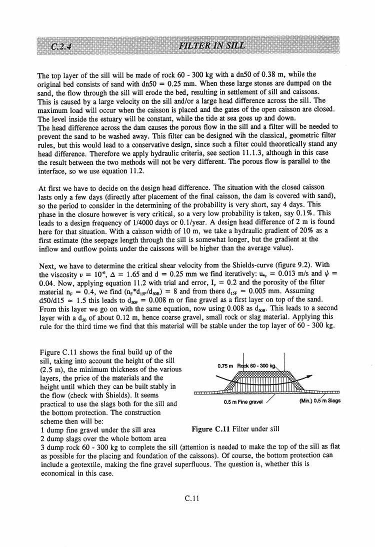
The top layer of the sill will be made of rock 60 - 300 kg with a dn50 of 0.38 m, while theoriginal bed consists of sand with dn50 = 0.25 mmoWhen these large stones are dumped on thesand, the flow through the sill will erode the bed, resulting in settlement of sill and caissons.This is caused by a large velocity on the sill and/or a large head difference across the sill. Themaximum load will occur when the caisson is placed and the gates of the open caisson are closed.The level inside the estuary will be constant, while the tide at sea goes up and down.The head difference across the dam causes the porous flow in the sill and a filter will be needed toprevent the sand to be wasbed away. This filter can be designed wih the classical, geometrie filterrules, but this would lead to a conservative design, since such a filter could theoretically stand anyhead difference. Therefore we apply hydraulic criteria, see section 11.1.3, although in this casethe result between the two methods will not be very different. The porous flow is parallel to theinterface, so we use equation 11.2.

At first we have to decide on the design head difference. The situation with the closed caissonlasts only a few days (directly after placement of the final caisson, the dam is covered with sand),so the period to consider in the determining of the probability is very short, say 4 days. Thisphase in the closure however is very critical, so a very low probability is taken, say 0.1 %. Thisleads to a design frequency of 1/4000 days or O.l/year. A design head difference of 2 m is foundhere for that situation. With a caisson width of 10 m, we take a hydraulie gradient of 20% as afirst estimate (the seepage length through the sill is somewhat longer, but the gradient at theinflow and outflow points under the caissons will be higher than the average value).

Next, we have to determine the critical shear velocity from the Shields-curve (figure 9.2). Withthe viscosity ti = 10-6,.6 = 1.65 and d = 0.25 mm we find iteratively: u.., = 0.013 mis and '" =0.04. Now, applying equation 11.2 with trial and error, I, = 0.2 and the porosity of the filtermaterial n, = 0.4, we find (nF*dISF/dsoB)= 8 and from there dlSF = 0.005 mmoAssumingd50/dl5 :::: 1.5 this leads to dSOF = 0.008 m or fine gravel as a first layer on top of the sand.From this layer we go on with the same equation, now using 0.008 as dSOB.This leads to a secondlayer with a dsoof about 0.12 m, hence coarse gravel, small rock or slag material. Applying thisrule for the third time we find that this material will be stabie under the top layer of 60 - 300 kg.

Figure C.ll shows the final build up of thesill, taking into account the height of the sill(2.5 m), the minimum thickness of the variouslayers, the price of the materials and theheight until which they can be built stably inthe flow (check with Shields). It seemspractical to use the slags both for the sill and 0.5m Finegravel (Min.)0.5m Slags

the bottom protection. The constructionscheme then will be:1 dump fine gravel under the sill area Figure C.ll Filter under sill2 dump slags over the whole bottom area3 dump rock 60 - 300 kg to complete the sill (attention is needed to make the top of the sill as flatas possible for the placing and foundation of the caissons). Of course, the bottom proteetion caninclude a geotextile, making the fine gravel superfluous. The question is, whether this iseconomical in this case.

C.l1

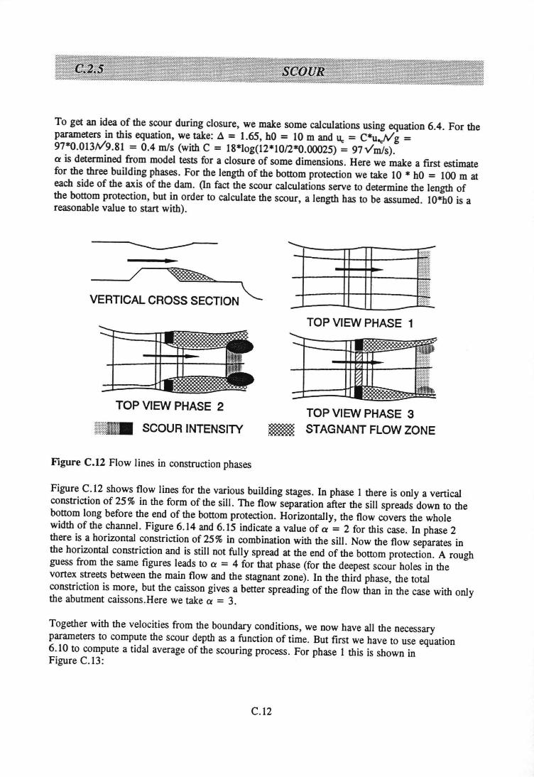
To get an idea of the scour during closure, we make some caIculations using equation 6.4. For theparameters in this equation, we take: .d = 1.65, hO = 10 m and u" = C*u..,JV g =97*O.013tV9.81 = 0.4 mis (with C = 18*log(12*1O/2*O.OOO25)= 97vmls).Ct is determined from model tests for a closure of some dimensions. Here we make a fust estimatefor the three building phases. For the length of the bottom proteetion we take 10 * hO = 100 m ateach side of the axis of the dam. (In fact the scour calculations serve to determine the length ofthe bottom protection, but in order to caIculate the scour, a length has to be assumed. 1O*hOis areasonable value to start with).

_----.J/ ~VERTICAL CROSS SECTION~

TOP VIEW PHASE 2

SCOUR INTENSITY

Figure C.12 Flow lines in construction phases

TOP VIEW PHASE 1

TOP VIEW PHASE 3m; STAGNANT FLOWZONE

Figure C.12 shows flow lines for the various building stages. In phase 1 there is only averticalconstrietion of 25% in the form of the sill. The flow separation after the sill spreads down to thebottom long before the end of the bottom protection. Horizontally, the flow covers the wholewidth of the channel. Figure 6.14 and 6.15 indicate a value of Ct = 2 for this case. In phase 2there is a horizontaI constriction of 25% in combination with the sill. Now the flow separates inthe horizontaI constriction and is still not fully spread at the end of the bottom protection. A roughguess from the same figures leads to Ct = 4 for that phase (for the deepest scour holes in thevortex streets between the main flow and the stagnant zone). In the third phase, the totalconstriction is more, but the caisson gives a better spreading of the flow than in the case with onlythe abutment caissons.Here we take Ct = 3.

Together with the veloeities from the boundary conditions, we now have all the necessaryparameters to compute the scour depth as a function of time. But first we have to use equation6.10 to compute a tidal average of the scouring process. For phase 1 this is shown inFigure C.13:

C.12

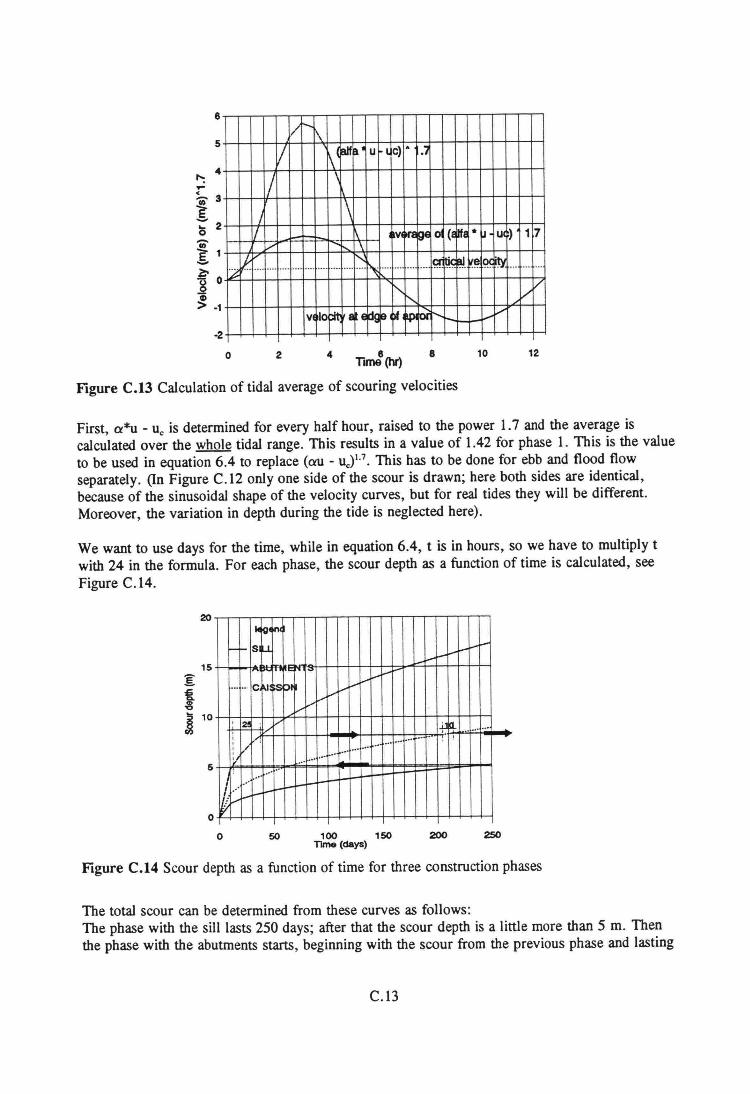
8

5/ r-I\

1/ r\ ~~.U 'l c) A .1

IJ \

) 1\1/ l- r-~ 1-- v~ ~ la (I~I .~uc) 17V . ....;,;;

lf ~ \ .g~ç.~.~~ l~,~12 ........ _ ....... ........ ........ ........ _••• __0' _.- ... ...

~ /'/

~v 10 ::ft i Ed~9~ .....VrPjUli

4"":....s, 3

i6 2'ii)E 1-foa>> -1

-2

8Time (hr)

Figure C.13 Calculation of tidal average of scouring veloeities

o 2 4 8 10 12

First, a*u - u, is determined for every half hour, raised to the power 1.7 and the average iscalculated over the whole tidal range. This results in a value of 1.42 for phase 1. This is the valueto be used in equation 6.4 to replace (au - uet7• This has to be done for ebb and flood flowseparately. (In Figure C.12 only one side of the scour is drawn; here both sides are identical,because of the sinusoidal shape of the velocity curves, but for real tides they will be different.Moreover, the variation in depth during the tide is neglected here).

We want to use days for the time, while in equation 6.4, t is in hours, so we have to multiply twith 24 in the formula. For each phase, the scour depth as a function of time is calculated, seeFigure C.14.

20

5

~~~I-1-8,"-, 1... ..1-~ ~

l..-~ ~~" I'"

I--"Vj.-I-

__0." clu:~SPI j.-v

VVvV

2 t> l.l.lla-, i. •••• 0"·

; ..' ., ! .......; ......, ~/ ...... .'lil .' ..'...... ..,

.'.... ..'i;..' -I-

->-j.-I-~

15

oo 50 100 150

TIme (days)200 250

Figure C.14 Scour depth as a function of time for three construction phases

The total scour can be determined from these curves as follows:The phase with the sill lasts 250 days; after that the scour depth is a little more than 5 m. Thenthe phase with the abutments starts, beginning with the scour from the previous phase and lasting

C.13

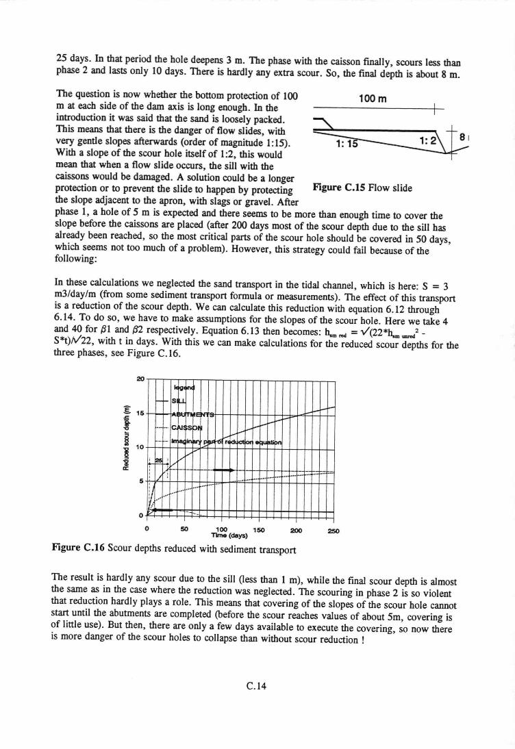
25 days. In that period the hole deepens 3 m. The phase with the caisson finally, scours less thanphase 2 and lasts only 10 days. There is hardly any extra scour. So, the final depth is about 8 m.

The question is now whether the bottom proteetion of 100mateach side of the dam axis is long enough. In theintroduetion it was said that the sand is loosely packed.This means that there is the danger of flow slides, withvery gentle slopes afterwards (order of magnitude 1:15).With a slope of the scour hole itself of 1:2, this wouldmean that when a flow slide occurs, the siJl with thecaissons would be damaged. A solution could be a longerproteetion or to prevent the slide to happen by protectingthe slope adjacent to the apron, with slags or gravel. Afterphase 1, a hole of 5 m is expected and there seems to be more than enough time to cover theslope before the caissons are placed (after 200 days most of the scour depth due to the sill hasalready been reached, so the most critical parts of the scour hole should be covered in 50 days,which seems not too much of a problem). However, this strategy could fail because of thefollowing:

lOOm

Figure C.IS Flow slide

In these calculations we neglected the sand transport in the tidal channel, which is here: S = 3m3/day/m (from some sediment transport formula or measurements). The effect of this transportis a reduction of the scour depth. We can calculate this reduction with equation 6.12 through6.14. To do so, we have to make assumptions for the slopes of the scour hole. Here we take 4and 40 for f31 and f32 respectively. Equation 6.13 then becomes: h.mred = V(22*h.m1IIJrOd2 _

S*t)1V'22, with t in days. With this we can make calculations for the reduced scour depths for thethree phases, see Figure C.16.

kiG'~r--s~- ,~~~-S 15~~~~.EN~~++~~~~~4F~~'~~~ ~~~1 c~:~bl I-~~

~ ....1-i r-t-lln\al:linIIrl'J ~f15 ~!ctlfdjor ~ull.tiPnI1 10 ; ~; v ..............~ ! .{ - - - _.~ .... ,...-+~-+.,+:..+...-.t...-1. r-..r..+...+...r::: .:: .::

5 ; 1/ : .......I ••••••

Voo- 0·- .- .0-I:t:

01/

o 50 100 150 200 250TIme (da)'$)

Figure C.16 Scour depths reduced with sediment transport

The result is hardly any scour due to the sill (less than 1 m), while the final scour depth is almostthe same as in the case where the reduction was neglected. The scouring in phase 2 is so violentthat reduction hardly plays a role. This means that covering of the slopes of the scour hole cannotstart until the abutments are completed (before the scour reaches values of about 5m, covering isof little use). But then, there are only a few days available to execute the covering, so now thereis more danger of the scour holes to collapse than without scour reduction !

C.14

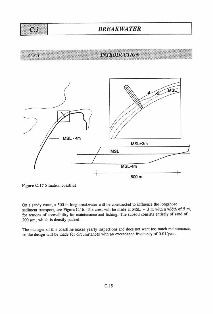
BREAKWATER

MSL-4m

Figure C.17 Situation coastline

MSL+3m

/ MSL :J

500m

On a sandy coast, a 500 m long breakwater will be constructed to influence the longshoresediment transport, see Figure C.16. The crest will be made at MSL + 3 m with a width of 5 m,for reasons of accessibility for maintenance and fishing. The subsoil consists entirely of sand of200 JLm, which is densily packed.

The manager of this coastline makes yearly inspections and does not want too much maintenance,so the design will be made for circurnstances with an exceedance frequency of O.OI/year.

C.15

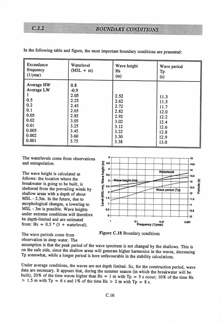
In the following table and figure, the most important bouodary cooditions are presented:

Exceedance Waterlevel Wave height Wave periodfrequeocy (MSL + m) Us Tp(lIyear) (m) (s)

AverageHW 0.8Average LW -0.91 2.05 2.52 11.30.5 2.25 2.62 11.50.2 2.45 2.72 11.70.1 2.65 2.82 12.00.05 2.85 2.92 12.20.02 3.05 3.02 12.40.01 3.25 3.12 12.60.005 3.45 3.22 12.80.002 3.60 3.30 12.90.001 3.75 3.38 13.0

The waterlevels come trom observationsand extrapolatioo.

The wave height is calculated asfollows: the location where thebreakwater is goiog to be built, issheltered from the prevailiog winds byshallow areas with a depth of aboutMSL - 2.5m. In the future, due tomorphological changes, alowering toMSL - 3m is possible. Wave heightsuoder extreme conditions will thereforebe depth-limited and are estimatedtrom: Hs =:: 0.5 * (3 + waterlevel).

6,--.---,--,--.---,--,--,,--.--,

ÊU+--4--~--+--4--~--+-~~-+ __~._~ .+-~---r--+-~---r~~~~-r--+~ VII flter1e el; 3~+--4--~--+--4--~--+~--~~F--+

~ 3i~w~~I~a·~~~~··ËIM~'~~~~::t:~~~.~~...~....t::Ji'2.6 1__............. ... .. .....=:l....3 2 ~,.....- Wal e peilt'" (Tp~ ..i 1.5 ........>~ 1+-~---r--+-~--~--+--4---r--+

0.1 0.01Frequency (1Jyear)

16

1U

1.~ 13.6

13 stil

12.5 ~lil

12 0-

11.5

11

10.5

10

0.001

O.s+---+---t---+----+---t---+-_r--+__-+

O+-~--~--+-~--~--+- __~_+--~

Figure C.IS Boundary conditionsThe wave periods come tromobservation in deep water. Theassumption is that the peak period of the wave spectrum is not changed by the shallows. This ison the safe side, since the shallow areas will generate higher harmonies in the waves, decreasingTp somewhat, while a longer period is here unfavourable in the stability calculations.

Under average conditions, the waves are oot depth limited. So, for the construction period, wavedata are necessary. It appears that, during the summer season (in which the breakwater will bebuilt), 20% of the time waves higher than Hs = 1 m with Tp =:: 5 s occur; 10% of the time Hs> 1.5 m with Tp ::::6 s and 1% of the time Hs > 2 m with Tp ::::8 s.

C.16

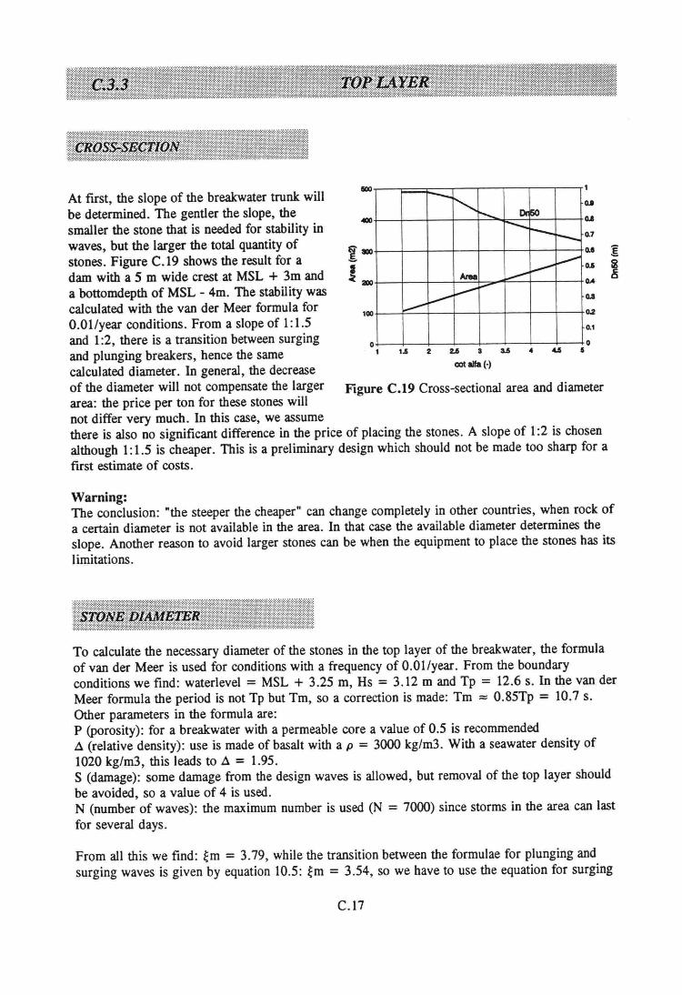
At first, the slope of the breakwater tronk willbe determined. The gentler the slope, thesmaller the stone that is needed for stability inwaves, but the larger the total quantity ofstones. Figure C.19 shows the result for adam with a 5 m wide crest at MSL + 3m anda bottomdepth of MSL - 4m. The stability wascalculated with the van der Meer formula forO.Ollyear conditions. From a slope of 1:1.5and 1:2, there is a transition between surgingand plunging breakers, hence the samecalculated diameter. In general, the decreaseof the diameter will not compensate the largerarea: the price per ton for these stones willnot differ very much. In this case, we assumethere is also no significant difference in the price of placing the stones. A slope of 1:2 is chosenalthough 1:1.5 is cheaper. This is a preliminary design which should not be made too sharp for afirst estimate of costs.

.._~ r--.... Or~--....t--r--

_...... ,___....Area ___.

,___.... ~V l.-"'"

G.2

o.ao.a0.7

o.eG.I

100

0.1

o1

oI2 3 4Ui

cat lIfa (.)

Figure C.19 Cross-sectional area and diameter

Warning:The conclusion: "the steeper the cheaper" can change completely in other countries, when rock ofa certain diameter is not available in the area. In that case the available diameter determines theslope. Another reason to avoid larger stones can be when the equipment to place the stones has itslimitations.

To calculate the necessary diameter of the stones in the top layer of the breakwater , the formulaof van der Meer is used for conditions with a frequency of O.Ol/year. From the boundaryconditions we find: waterlevel = MSL + 3.25 m, Hs = 3.12 m and Tp = 12.6 s. In the van derMeer formula the period is not Tp but Tm, so a correction is made: Tm = 0.85Tp = 10.7 s.Other parameters in the formula are:P (porosity): for a breakwater with a permeabie core a value of 0.5 is recommended~ (relative density): use is made of basalt with a p = 3000 kg/m3. With a seawater density of1020 kg/m3, this leads to ~ = 1.95.S (damage): some damage from the design waves is allowed, but removal of the top layer shouldbe avoided, so a value of 4 is used.N (number of waves): the maximum number is used (N = 7000) since storms in the area can lastfor several days.

From all this we find: ~m = 3.79, while the transition between the formulae for plunging andsurging waves is given by equation 10.5: ~m = 3.54, so we have to use the equation for surging

C.17

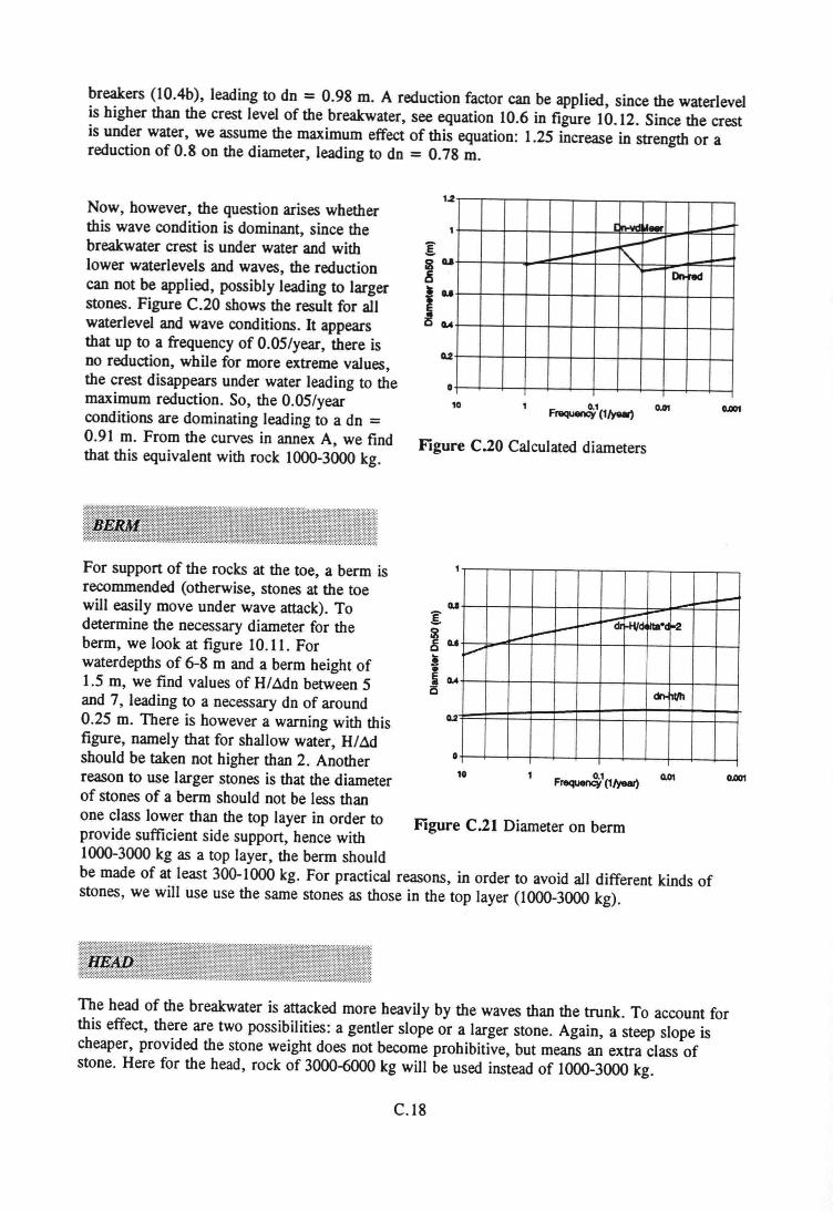
breakers (10.4b), leading to dn = 0.98 m. A reduction factor cao be applied, since the waterlevelis higher than the crest level of the breakwater, see equation 10.6 in figure 10.12. Since the crestis under water, we assume the maximum effect of this equation: 1.25 increase in strength or areduction of 0.8 on the diameter, leading to do = 0.78 m.

For support of the rocks at the toe, a berm isrecommended (otherwise, stones at the toewill easily move under wave attack). Todetermine the necessary diameter for theberm, we look at figure 10.11. Forwaterdepths of 6-8 m and a berm height of1.5 m, we find values of H/..1dnbetween 5and 7, leading to a necessary dn of around0.25 m. There is however a warning with thisfigure, namely that for shallow water, H/..1dshould be taken not higher than 2. Anotherreason to use larger stones is that the diameterof stones of a berm should not be less thanone class lower than the top layer in order to Flgure C.21 Diameter on bermprovide sufticient side support, hence with1000-3000 kg as a top layer, the berm shouldbe made of at least 300-1000 kg. For practical reasons, in order to avoid all different kinds ofstones, we will use use the same stones as those in the top layer (1000-3000 kg).

Now, however, the question arises whetherthis wave condition is dominant, since thebreakwater crest is under water and withlower waterlevels and waves, the reductioncao oot be applied, possibly leading to largerstones. Figure C.20 shows the result for allwaterlevel and wave conditions. It appearsthat up to a frequeocy of 0.05/year, there is00 reduction, while for more extreme values,the crest disappears under water leading to themaximum reduction. So, the 0.05/yearconditions are dominating leading to a dn =0.91 m. From the curves in annex A, we findthat this equivalent with rock 1000-3000 kg.

[In-va~- I,...-

~ rç~L--I,...- I--

~ en.reet

CL2

o10

Flgure C.20 Calculated diameters

u -~ ~~ ~ ~

f...-L-- - .....~1-2~

"....

cIn-~

o10

The head of the breakwater is attacked more heavily by the waves than the trunk. To account forthis effect, there are two possibilities: agentler slope or a larger stone. Again, asteep slope ischeaper, provided the stone weight does not become prohibitive, but means an extra class ofstone. Here for the head, rock of 3000-6000 kg will be used instead of 1000-3000 kg.

C.18

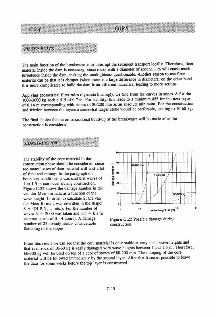
The main function of the breakwater is to interrupt the sediment transport locally. Therefore, finermaterial inside the dam is necessary, since rocks with a diameter of around 1 m will cause muchturbulence inside the dam, making the sandtightness questionable. Another reason to use finermaterial cao be that it is cheaper (when there is a large difference in diameter); on the other handit is more complicated to build the dam from different materials, leading to more actions.

Applying geometrical filter rules (dynamie loading!), we find from the curves in annex A for the1000-3000 kg rock a diS of 0.7 m. For stability, this leads to a minimum d85 for the next layerof 0.14 m corresponding with stones of 80/200 mm as an absolute minimum. For the constructionand friction between the layers a somewhat larger stone would be preferabie, leading to 10-60 kg.

The final choice for the cross-sectional build-up of the breakwater will be made after theconstruction is considered.

The stability of the core material in theconstruction phase should be considered, sincetoo many losses of dam material will oost a lotof time and money. In the paragraph onboundary conditions it was said that waves of1 to 1.5 m can occur during construction.Figure C.22 shows the damage number in thevan der Meer formula as a function of thewave height. In order to calculate S, the vander Meer formula was rewritten in the shape:S = f(H,P,N, ... etc.). For the number ofwaves N = 2000 was taken and Tm = 6 s (asummer storm of 3 - 4 hours). A damagenumber of 25 already means considerableflattening of the slopes.

601

I1111

~ I!OC mTl

I11111

10fs<> kg IIII

1///

//

V/ J60130p~ --

~~ --,-~ ..

t> ..- ..-- ~~ ....... .-..... ---

10

oo Wave'height Hs (m)1.1

2

Figure C.22 Possible damage duringconstruction

From this result we can see that the core material is only stabie at very small wave heights andthat even rock of 10-60 kg is easily damaged with wave heights between 1 and 1.5 m. Therefore,60-300 kg will be used on top of a core of stones of 80-200 mmoThe dumping of the corematerial will be followed immediately by the second layer. After that it seems possible to leavethe dam for some weeks before the top layer is constructed.

C.19

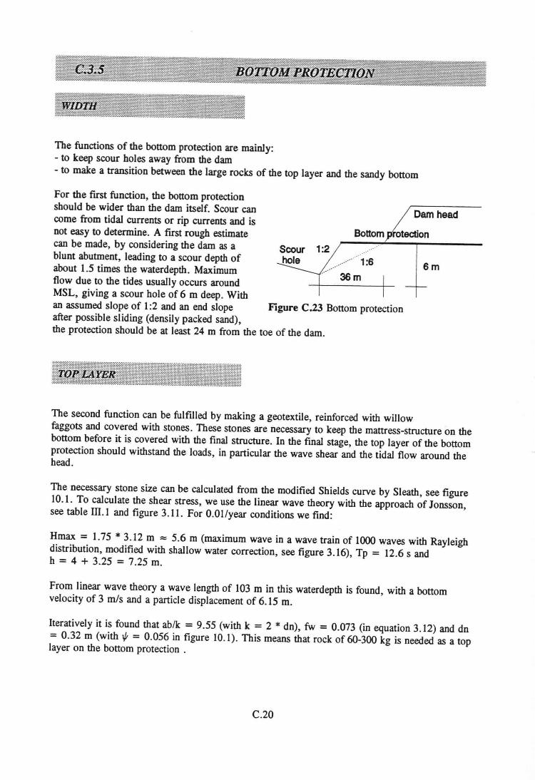
The functions of the bottom proteetion are mainly:- to keep scour holes away from the dam- to make a transition between the large rocks of the top layer and the sandy bottom

For the fust function, the bottom proteetionshould be wider than the dam itself. Scour caocome from tidal currents or rip currents and isnot easy to determine. A first rough estimatecao be made, by considering the dam as ablunt abutment, leading to a scour depth ofabout 1.5 times the waterdepth. Maximumflow due to the tides usually occurs aroundMSL, giving a scour hole of 6 m deep. Withan assumed slope of 1:2 and an end slopeafter possible sliding (densily packed sand),the proteetion should be at least 24 m from the toe of the dam.

Dam head

Bottom otectionScour 1:2hole

......

Sm.... 1·S............. .36m

Figure C.23 Bottom proteetion

The second function can be fulfilled by making a geotextile, reinforeed with willowfaggots and covered with stones. These stones are necessary to keep the mattress-structure on thebottom before it is covered with the final structure. In the final stage, the top layer of the bottomproteetion should withstand the loads, in particular the wave shear and the tidal flow around thehead.

The necessary stone size can be calculated from the modified Shields curve by Sleath, see figure10.1. To calculate the shear stress, we use the linear wave theory with the approach of Jonsson,see table lIl. 1 and figure 3.11. For O.Ollyear conditions we find:

Hmax = 1.75 * 3.12 m == 5.6 m (maximum wave in a wave train of 1000 waves with Rayleighdistribution, modified with shallow water correction, see figure 3.16), Tp = 12.6 s andh = 4 + 3.25 = 7.25 m.

From linear wave theory a wave length of 103 m in this waterdepth is found, with a bottomvelocity of 3 mIs and a partiele displacement of 6.15 m.

Iteratively it is found that ab/k = 9.55 (with k = 2 * dn), fw = 0.073 (in equation 3.12) and dn= 0.32 m (with Vt = 0.056 in figure 10.1). This means that rock of 60-300 kg is needed as a toplayer on the bottom proteetion .

C.20

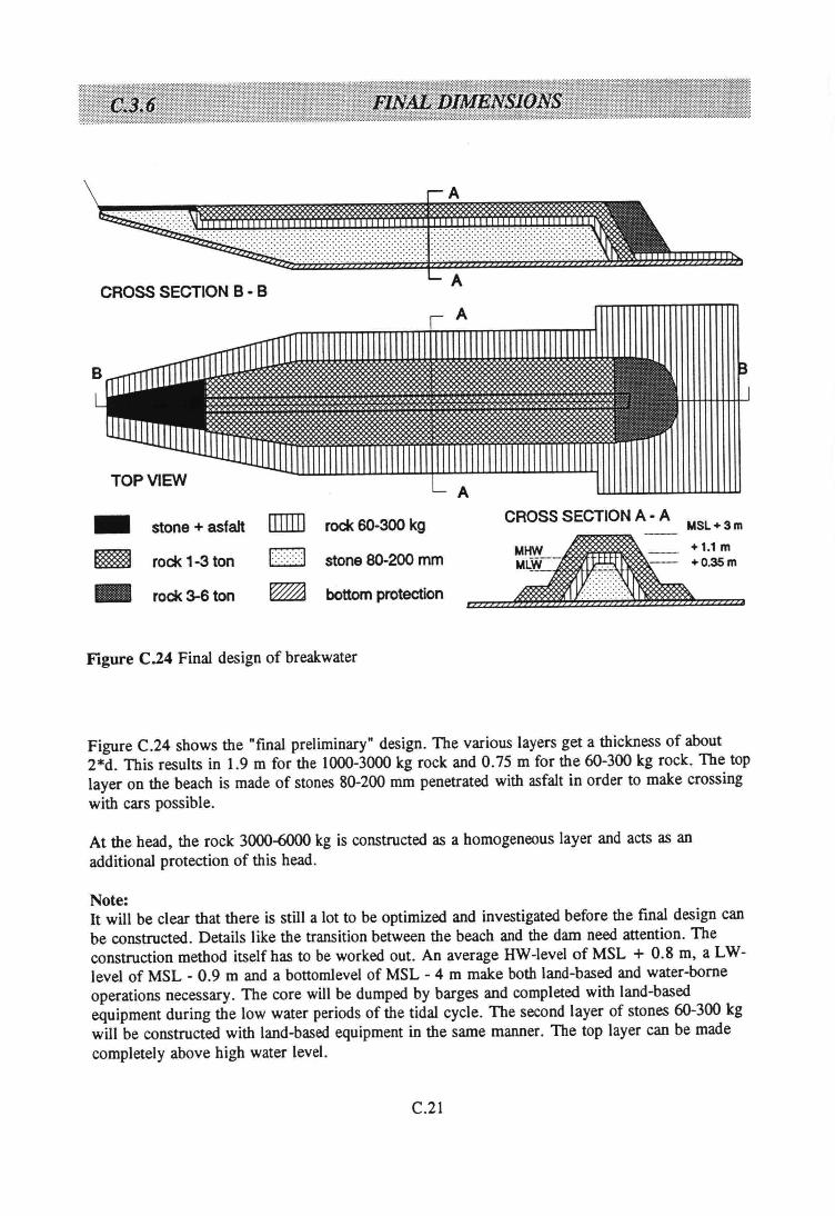
CROSS SECTION B • B

TOP VIEWA

.. stone + asfalt rnnn rock 60-300 kg

~ rock 1-3 ton EJ stone 80-200 mm

l1li rock 3-6 ton ~ bottom protection

CROSS SECTION A· A MSL+3m

~,.,mMLW-- .':.::n>:.. _. +0.35m

""""~"""'"

Figure C.24 Final design of breakwater

Figure C.24 shows the "final preliminary" design. The various layers get a thickness of about2*d. This results in 1.9 m for the 1000-3000 kg rock and 0.75 m for the 60-300 kg rock. The toplayer on the beach is made of stones 80-200 mm penetrated with asfalt in order to make crossingwith cars possible.

At the head, the rock 3000-6000 kg is constructed as a homogeneous layer and acts as anadditional proteetion of this head.

Note:It will be clear that there is still a lot to be optimized and investigated before the final design caobe constructed. Details like the transition between the beach and the dam need attention. Theconstruction method itself has to be worked out. An average HW-level of MSL + 0.8 m, a LW­level of MSL - 0.9 m and a bottomlevel of MSL - 4 m make both land-based and water-borneoperations necessary. The core will be dumped by barges and completed with land-basedequipment during the low water periods of the tidal cycle. The second layer of stones 60-300 kgwill be constructed with land-based equipment in the same manner. The top layer can be madecompletely above high water level.

C.21

-------- - -- -- -

l