Embed Size (px)
Citation preview


Turkish Journal of Agricultural Engineering
Research (TURKAGER)
Volume 2,
Issue 2,
Year 2021
Indexing

EDITOR-in-CHIEF
Ebubekir ALTUNTAŞ / Tokat Gaziosmanpaşa University, TURKEY
ASSISTANT EDITOR-in-CHIEF
Sedat KARAMAN / Tokat Gaziosmanpaşa University, TURKEY
TECHNICAL EDITOR
Bahadır ŞİN / Sakarya Unıversity of Applied Scıences, TURKEY
LANGUAGE EDITOR:
Gülay KARAHAN / Çankırı Karatekin University, TURKEY
Fatih YILMAZ / Tokat Gaziosmanpaşa University, TURKEY
STATISTICS EDITOR
Yalçın TAHTALI / Tokat Gaziosmanpaşa University, TURKEY
SECTETARIAT (*)
Necati ÇETİN, Erciyes University, TURKEY
Esra Nur GÜL, Tokat Gaziosmanpaşa University, TURKEY
Esra KAPLAN, Tokat Gaziosmanpaşa University, TURKEY
Ayşe Nida KAYAALP, Muş Alparslan University, TURKEY
Nurettin KAYAHAN, Selçuk University, TURKEY
(*): The list is based on the surname of the editors in alphabetical order.
Turkish Journal of Agricultural Engineering Research
(TURKAGER)
EDITORIAL BOARD TEAM

SECTION EDITORS (*)
• Zümrüt AÇIKGÖZ, Ege University, TURKEY
• Sefa ALTIKAT, Iğdır University, TURKEY
• Servet ARSLAN, Akdeniz University, TURKEY
• Elman BAHAR, Tekirdağ Namık Kemal University,
TURKEY
• Mehmet Fırat BARAN, Siirt University, TURKEY
• İlkay BARITÇI, Dicle University, TURKEY
• Zeki BAYRAMOĞLU, Selçuk University, TURKEY
• Ekrem BUHAN, Tokat Gaziosmanpaşa University,
TURKEY
• Bilal CEMEK, Ondokuz Mayıs University, TURKEY
• Bilge Hilal ÇADIRCI EFELİ, Tokat Gaziosmanpaşa
University, TURKEY
• Selahattin ÇINAR, Kilis 7 Aralık University,
TURKEY/KT Manas University, KYRGYZSTAN
• Hasan Gökhan DOĞAN, Kırşehir Ahi Evran
University, TURKEY
• Ahmet ERTEK, Isparta University of Applied
Sciences, TURKEY
• Tanzer ERYILMAZ, Yozgat Bozok University,
TURKEY
• Cafer GENÇOĞLAN, Kahramanmaraş Sütçü İmam
University, TURKEY
• Zeki GÖKALP, Erciyes University, TURKEY
• Osman GÖKDOĞAN, Isparta University of Applied
Sciences TURKEY
• Ziya Gökalp GÖKTOLGA, Sivas Cumhuriyet
University, TURKEY
• Mevlüt GÜL, Isparta University of Applied
Sciences, TURKEY
• Orhan GÜNDÜZ, Malatya Turgut Özal University,
TURKEY
• Ali İrfan İLBAŞ, Erciyes University, TURKEY
• Yaşar KARADAĞ, Muş Alparslan University,
TURKEY
• Gülay KARAHAN, Çankırı Karatekin University,
TURKEY
• Duran KATAR, Eskişehir Osmangazi University,
TURKEY
• Kenan KILIÇ, Niğde Ömer Halisdemir University,
TURKEY
• Hasan Rüştü KUTLU, Çukurova University,
TURKEY
• Tamer MARAKOĞLU, Selçuk University, TURKEY
• Yusuf Ziya OĞRAK, Sivas Cumhuriyet University,
TURKEY
• Hidayet OĞUZ, Necmettin Erbakan University,
TURKEY
• Mustafa ÖNDER, Selçuk University, TURKEY
• Mahir ÖZKURT, Muş Alparslan University,
TURKEY
• Taşkın ÖZTAŞ, Atatürk University, TURKEY
• Ahmet ÖZTÜRK, Ondokuz Mayıs University,
TURKEY
• Mehmet POLAT, Isparta University of Applied
Sciences, TURKEY
• Onur SARAÇOĞLU, Tokat Gaziosmanpaşa
University, TURKEY
• Şenay SARICA, Tokat Gaziosmanpaşa University,
TURKEY
• Abdulvahit SAYASLAN, Karamanoğlu Mehmetbey
University, TURKEY
• Bahadır SAYINCI, Mersin University, TURKEY
• Serkan SELLİ, Çukurova University, TURKEY
• Bedrettin SELVİ, Tokat Gaziosmanpaşa
University, TURKEY
• Osman SÖNMEZ, Erciyes University, TURKEY
• Sezer ŞAHİN, Tokat Gaziosmanpaşa University,
TURKEY
• Ahmet ŞEKEROĞLU, Niğde Ömer Halisdemir
University, TURKEY
• Şerife TOPKAYA, Tokat Gaziosmanpaşa University,
TURKEY
• Atnan UĞUR, Ordu University, TURKEY
• Serkan YEŞİL, Selçuk University, TURKEY
• Melih YILAR, Kırşehir Ahi Evran University,
TURKEY
• Adil Koray YILDIZ, Yozgat Bozok University,
TURKEY
• Güngör YILMAZ, Yozgat Bozok University,
TURKEY
• Semih YILMAZ, Erciyes University, TURKEY
(*): The list is based on the surname of the editors in alphabetical order.

REGIONAL EDITORS (*)
• Omar Ali Al-KHASHMAN, Al-Hussein Bin
Talal University, Ma'an-JORDAN
• Tewodros AYALEW, Hawassa University,
ETHIOPIA
• Hatem BENTAHER, Sfax University,
TUNISIA
• Ramadan ELGAMAL, Suez Canal University,
Ismailia, EGYPT
• Hamideh FARIDI, Tehran University, IRAN
• Simon V. IRTWANGE, Agriculture
University, Makurdi, NIGERIA
• Tomislav JEMRIC, Zagreb University,
CROATIA
• Avinash Suresh KAKADE,
• Vasantrao Naik Marathwada University,
Krushi Vidyapeeth (M.S), INDIA
• Zdzisław KALINIEWICZ, Uniwersytet
Warminsko-Mazurski, ul. Olsztyn, POLAND
• Manal H.G. KANAAN, Middle Technical
University, Baghdad, IRAQ
• Wasim Jan KHAN, Muhammad, Institute of
Southern Punjab (ISP), Multan, PAKISTAN
• Alltane J. KRYEZIU, of Prishtina
University, Pristina, Republic of KOSOVO
• Ahmed Moustafa Mohamed Ibrahim
MOUSA, Al-Azhar University, Cairo, EGYPT
• Shahid MUSTAFA, Sargodha University,
Sargodha, PAKISTAN
• Muhammad Ather NADEEM, Sargodha
University, Sargodha, PAKISTAN
• Seyed Mehdi NASIRI, Shiraz University,
Shiraz, IRAN
• Chinenye Macmanus NDUKWU, Michael
Okpara Agriculture University,
Umudike, Umuahia, Abia, NIGERIA
• Zhongli PAN, California University, Davis,
California, USA
• Gheorghe Cristian POPESCU, Pitesti
University, ROMANIA
• Monica POPESCU, Pitesti University,
ROMANIA
• Y. Aris PURWANTO, IPB University,
INDONESIA
• Shafiee SAHAMEH, Tarbiat Modares
University, Tehran, IRAN
• Gordana SEBEK, Montenegro University,
Podgorica, MONTENEGRO
• Marisennayya SENAPATHY, Wolaita Sodo
University, Ethiopia, EAST AFRICA
• Feizollah SHAHBAZI, Lorestan University,
Khoram Abad, IRAN
• Alaa SUBR, Baghdad University, IRAQ
• Hilary UGURU, Delta State Polytechnic,
Ozoro, Delta State, NIGERIA
(*): The list is based on the surname of the editors in alphabetical order/
PUBLISHING BOARD (*)
• Şenol AKIN, Şenol, Yozgat Bozok University,
TURKEY
• Abdullah BEYAZ, Ankara University,
TURKEY
• Özer ÇALIŞ, Akdeniz University, TURKEY
• Ahmet ÇELİK, Erzurum Atatürk University,
TURKEY
• Aslıhan DEMİRDÖVEN, Tokat
Gaziosmanpaşa University, TURKEY
• Alper DURAK, Malatya Turgut Özal
University, TURKEY
• Ali İSLAM, Ordu University, TURKEY
• Esen ORUÇ, Tokat Gaziosmanpaşa
University, TURKEY
• Mehmet Ali SAKİN, Tokat Gaziosmanpaşa
University, TURKEY
• İsmail SEZER, Ondokuz Mayıs University,
TURKEY
• Metin SEZER, Karamanoğlu Mehmetbey
University, TURKEY
(*): The list is based on the surname of the editors in alphabetical order/

Turkish Journal of Agricultural Engineering Research
(TURKAGER)
Volume 2,
Issue 2,
December 31, 2021
SECTION EDITORS & REFEREES (*)
• Olufemi ADETOLA, Federal University of Technology
Akure, NIGERIA
• Aydın AKIN, Selçuk University, TURKEY
• Pelin ALABOZ, Isparta University of Applied Sciences,
TURKEY
• İlknur ALİBAŞ, Uludağ University, TURKEY
• Sefa ALTIKAT, Iğdır University, TURKEY
• Arda AYDIN, Çanakkale Ondokuz Mart University,
TURKEY
• Fatih AYDIN, Necmettin Erbakan University, KONYA
• Elman BAHAR, Tekirdağ Namık Kemal University,
TURKEY
• Mehmet Fırat BARAN, Siirt University, TURKEY
• Erman BEYZİ, Erciyes University, TURKEY
• Ali Volkan BİLGİLİ, Harran University, TURKEY
• Mehmet Emin BİLGİLİ, Eastern Mediterranean
Agricultural Research Institute, TURKEY
• İsmail DEMİR, Kırşehir Ahi Evran University,
TURKEY
• Aslıhan DEMİRDÖVEN, Tokat Gaziosmanpaşa
University, TURKEY
• Ali Rıza DEMİRKIRAN, Bingöl University, TURKEY
• Ramadan ELGAMAL, Suez Canal University, EGYPT
• Ahmet Konuralp ELİÇİN, Dicle University, TURKEY
• Ömer EREN, Mustafa Kemal University, TURKEY
• Gazanfer ERGÜNEŞ, Tokat Gaziosmanpaşa University,
TURKEY
• Ömer ERTUĞRUL, Kırşehir Ahi Evran University,
TURKEY
• Paul Chukwuka EZE, Enugu State University of
Science and Technology, NIGERIA
• Osman GÖKDOĞAN, Isparta University of Applied
Sciences, TURKEY
• Ali İ̇rfan İLBAŞ, Erciyes University, TURKEY
• Sevil KARAASLAN, Isparta University of Applied
Sciences, TURKEY
• Gülay KARAHAN, Çankırı Karatekin University,
TURKEY
• Yasin Bedrettin KARAN, Tokat Gaziosmanpaşa
University, TURKEY
• Ali İhsan KAYA, Adıyaman University, TURKEY
• Songül KESEN, Gaziantep University, TURKEY
• Kenan KILIÇ, Niğde Ömer Halisdemir University,
TURKEY
• Kürşat KORKMAZ, Ordu University, TURKEY
• İlknur KORKUTAL, Tekirdağ Namık Kemal University,
TURKEY
• Demir KÖK, Tekirdağ Namık Kemal University,
TURKEY
• Hilal İŞLEROĞLU, Tokat Gaziosmanpaşa University,
TURKEY
• Manoj Kumar MAHAWAR, Indian Council of
Agrıcultural Research, New Delhi, INDIA
• Mehmet Zahid MALASLI, Necmettin Erbakan
University, KONYA
• Christopher OBINECHE, Federal College of Land
Resources Technology, Owerri. Imo State. NIGERIA
• Hidayet OGUZ, Necmettin Erbakan University,
KONYA
• Nuri ORHAN, Selçuk University, TURKEY
• Görkem ÖRÜK, Siirt University, TURKEY
• Mehmet Metin ÖZGÜVEN, Tokat Gaziosmanpaşa
University, TURKEY
• Taşkın ÖZTAŞ, Atatürk University, TURKEY
• Ahmet ÖZTÜRK, Ondokuz Mayıs University, TURKEY
• Tuba ÖZTÜRK, Tekirdağ Namık Kemal University,
TURKEY
• Fatih POLAT, Tokat Gaziosmanpaşa University,
TURKEY
• Hakan POLATCI, Tokat Gaziosmanpaşa University,
TURKEY
• Bahadır SAYINCI, Mersin University, TURKEY
• Adewale SEDARA, The Federal University of
Technology, Akure, NIGERIA
• Serkan SELLİ, Çukurova University, TURKEY
• Onur SARAÇOĞLU, Tokat Gaziosmanpaşa University,
TURKEY
• Abdullah SESSİZ, Dicle University, TURKEY
• Onur SEVİNDİK, Çukurova University, TURKEY
• Osman SÖNMEZ, Erciyes University, TURKEY
• Levent ŞEN, Giresun University, TURKEY
• Fatih ŞAHİN, Gazi University, TURKEY
• Rüveyde TUNÇTÜRK, Van Yüzüncü Yıl University,
TURKEY
• Hilary UGURU, Delta State University of Science and
Technology, Ozoro, NIGERIA
• Elçin YEŞİLOĞLU CEVHER, Ondokuz Mayıs
University, TURKEY
• Adil Koray YILDIZ, Yozgat Bozok University, TURKEY
• Gülçin YILDIZ, Iğdır University, TURKEY
• Taner YILDIZ, Ondokuz Mayıs University, TURKEY
• Hüseyin YÜRDEM, Ege University, TURKEY
(*): The list is based on the surname of the editors in
alphabetical order.

Turkish Journal of Agricultural Engineering Research (TURKAGER)
Volume 2,
Issue 2,
December 31, 2021
No Articles Author/s Pages
1 Evaluating the Effects of Milling Speed and Screen Size on
Power Consumed During Milling Operation Ademola Adebukola ADENIGBA
Samuel Dare OLUWAGBAYIDE
260-275
2 Sulama Suyu pH’sının Asma Anaçlarının Biyokütle,
Köklenme, Kök ve Sürgün Gelişimi Üzerine Etkisi
Influence of Irrigation Water pH on Biomass, Rooting, Root and Shoot Growth of Grapevine Rootstocks
Selda DALER
Rüstem CANGİ
276-288
3 Modelling Kinetics of Extruded Fish Feeds in a Continuous
Belt Dryer Funmilayo OGUNNAIKE
Pius OLALUSI
289-297
4 Effects of Different Carbonization Conditions on the Color
Change of Biochar
Alperay ALTIKAT
Mehmet Hakkı ALMA
298-307
5 Effect of Moisture Content on the Mechanical Properties of
Watermelon Seed Varieties
Paul Chukwuka EZE
Chikaodili Nkechi EZE
Patrick Ejike IDE
308-320
6 Multipurpose Fruit Juice Machine for Preventing Fruit
Wastage in Nigeria Villages Ayoola Olawole JONGBO 321-329
7 LabVIEW Based Real-time Color Measurement System Abdullah BEYAZ 330-338
8 Eskişehir Ekolojik Koşullarında Farklı Anason (Pimpinella anisum L.) Populasyonlarının Verim ve Verim Öğelerinin
Karşılaştırılması
Comparison of Yield and Yield Components of Different Anise (Pimpinella anisum L.) Populations Under Eskişehir Ecological Conditions
Nimet KATAR
Mustafa CAN
Duran KATAR
339-347
9 Development and Performance Evaluation of a Solar
Powered Lawn Mower
Babatunde Oluwamayokun SOYOYE 363-375
10 Mathematical Modelling of Drying Characteristics of
Coconut Slices
John ISA
Kabiru Ayobami JIMOH
376-389
11 Erzurum İli Çiftçilerinin Traktör Marka Tercihini Etkileyen
Faktörlerin Belirlenmesi
Determination of Factors Affecting Tractor Brand Preference Of Erzurum Province Farmers
Servan BAYBAS
Adem AKSOY
376-389
12 Prediction the Performance Rate of Chain Type Trenching
Machine Mohamed Ibrahim GHONIMY
390-402
13 Important Physical and Mechanical Properties of Dominant
Potato Variety Widely Grown in Ethiopia
Dereje ALEMU
403-412
14 Optimization of Operational Parameters of an Improved
Maize Sheller Using Response Surface Methodology
Adewale SEDARA
Emmanuel ODEDİRAN
413-424
15 Physicochemical Characterization of Selected Pomegranate
(Punica granatum L.) Cultivars
Vijay Singh MEENA
Bhushan BIBWE
Bharat BHUSHAN
Kirti JALGAONKAR
Manoj Kumar MAHAWAR
425-433
16 Optimization of Mechanical Oil Expression from Sandbox
(Hura crepitans Linn.) Seeds
David ONWE
Adeleke Isaac BAMGBOYE
434-449
17 Assessment of Spatial Variability of Heavy Metals (Pb and
Al) in Alluvial Soil around Delta State University of Science
and Technology, Ozoro, Southern Nigeria
Hilary UGURU
Ovie Isaac AKPOKODJE
Goodnews Goodman AGBI
450-459

18 Thermal Properties of New Developed Nigerian Illa and
Ekpoma Rice Flour Varieties as Effected with Moisture
Content
Ide PATRICK EJIKE
Ikoko OMENAOGOR
460-471
Review Article
19 Mathematical Modeling of Food Processing Operations: A
Basic Understanding and Overview
Manibhushan KUMAR
Siddhartha VATSA
Mitali MADHUMITA
Pramod Kumar PRABHAKAR
472-492
20 Toprakta Ağır Metal Kirliliği ve Giderim Yöntemleri
Heavy Metal Pollution in Soil and Removal Methods
Osman SÖNMEZ
Fatma Nur KILIÇ
493-507
21 Chemical Coagulation An Effective Treatment Technique for
Industrial Wastewater
Aijaz Ali PANHWAR
Aftab KANDHRO
Sofia QAİSAR
Mudasir GORAR
Eidal SARGANİ
Humaira KHAN
508-516

Turkish Journal of Agricultural
Engineering Research
https://dergipark.org.tr/en/pub/turkager https://doi.org/10.46592/turkager.2021.v02i02.001
Research Article
Turk J Agr Eng Res
(TURKAGER)
e-ISSN: 2717-8420
2021, 2(2): 260-275
Evaluating the Effects of Milling Speed and Screen Size on Power
Consumed During Milling Operation
Ademola Adebukola ADENIGBAIDa Samuel Dare OLUWAGBAYIDEIDa*
aDepartment of Agricultural and Bio- Environmental Engineering, Federal Polytechnic, Ilaro, Ogun State, NIGERIA,
(*): Corresponding author, [email protected]
ABSTRACT
This study was conducted to evaluate the effect of rotor speed and
screen size on power consumed during milling operation. The
milling system was tested using three fish feed ingredients; bone
meal, groundnut cake and maize. The moisture contents of the
ingredients bought from the market are 13.1%, 14.7% and 17.5%
dry basis, respectively. The milling machine was evaluated with
the 3 kg of each feed ingredient and was replicated three times for
each of the experimental parameters. The machine parameters
varied during the experiment includes four screen sizes (1.5 mm,
2.0 mm, 2.5 mm and 3.0 mm) and five rotor speeds (1500 rpm,
1800 rpm, 2100 rpm, 2400 rpm and 2700 rpm). Regression
analysis was carried out on the data collated. The analysis was
used to develop a model which is capable of predicting the
electrical energy (kJ) consumed. There was no significant effect of
screen size on the average power consumed during milling since
there is no linear relationship between power consumed and
screen size. However, there is a significant effect of speed on
average power consumed, the power consumed increases as speed
decreases therefore making milling operation at higher speed to
be cost effective since it doesn’t require much power to achieve the
required output. The P-Value depicts that screen size has no
significant effect on the electrical energy consumed during the
milling operation while speed has a significant effect on the
electrical energy used at 95% confidence level.
To cite: Adenigba AA, Oluwagbayide SD (2021). Evaluating the Effects of Milling Speed and
Screen Size on Power Consumed During Milling Operation. Turkish Journal of Agricultural
Engineering Research (TURKAGER), 2(2): 260-275.
https://doi.org/10.46592/turkager.2021.v02i02.001
RESEARCH ARTICLE
Received: 04.12.2020
Accepted: 29.01.2021
Keywords:
➢ Electrical energy,
➢ Milling,
➢ Power,
➢ Screen size,
➢ Fish feed and rotor
speed,
➢ Kernel size

ADENIGBA and OLUWAGBAYIDE / Turk J. Agr Eng Res (TURKAGER), 2021, 2(2), 260-275 261
INTRODUCTION
In ancient times, cereal grains were crushed between two stones and made into crude
cake. The advent of modern automated systems employing steel material such as
hammer mills has revolutionized the processing of cereals and their availability as
human foods and for other purposes (Donnel, 1983). Most of the existing hammer mill
machines are designed for very large-scale production by the multinational companies
such as breweries, feed mills and flour mills. But due to the recent sensitization of the
public on the need for self-employment, there is an increase in small-scale companies.
Thus, there is a very high demand for small-scale hammer mill machines
(Adeomaya and Samuel, 2014). Nowadays there are increasing attempts to develop
standard practical diets for farmed fish in Nigeria. A wide range of feed stuffs are
produced as by-products from animal processing industries. Some of this feed stuffs are
currently used in rations for both terrestrial animals and fish (Udo and Umoren, 2011).
Since fish feeds are generally the largest single cost item of most fish farm operations,
it follows that the selection of meal ingredients for use within diets will play a major
role in dictating its ultimate nutritional and economic success (Ovie and Eze, 2013).
This project aims to alleviate the problems of peasant farmers in rural settlements
and animal feed production companies, whose wish is to process their grain/cereal into
animal feed at the minimum energy cost. Due to the exorbitant fee being levied as
energy (power) tariff, some millers don’t do adequate milling in order to cut down the
energy consumed during the milling process, this recurrent behavior has led to
production of feed with inappropriate particle size. The primary aim of this work is to
evaluate the effect of milling (rotor) speed and screen size on the energy consumed
during milling operation.
MATERIALS AND METHODS
Materials
The fish feed ingredients used for the performance evaluation were sourced from
commercial feed milling centers (freedom feed mill and K2 feed mill) within Akure,
Ondo State, Nigeria. The ingredients used are bone meal, groundnut cake and maize
grain.
The Milling Machine
An existing milling machine was used to carryout the research. The milling system
consists of the following components, the electric motor, transmission system,
pneumatic system, hammering unit, screen, pressure relief unit, cyclone and the
support frame.
Power unit: The system is driven by an electric motor of 10 hp which has a revolution
of 2900 rpm.
Transmission system: It consists of shafts, pulleys and belts. The electric motor is the
prime mover of the machine, as the pulley which is connected to the shaft of the electric
motor is being propelled into action by the rotation of the electric motor; power is being
transmitted from this pulley via a belt to another pulley which is connected to the shaft
of the hammering unit.

ADENIGBA and OLUWAGBAYIDE / Turk J. Agr Eng Res (TURKAGER), 2021, 2(2), 260-275 262
Hammering unit: The hammering unit consists of four sets of hammers; each set is
positioned on a role and each role has six hammers thereby making a total of
24 hammers. Individual hammers are of 5.1 by 7.2 cm.
Screen: The screens used for this research work are of varying aperture sizes; 1.5 mm,
2 mm, 2.5 mm and 3 mm.
Pneumatic system: The pneumatic system has a blower which positioned above the
screen in the hammering unit. This blower consists of blades which are of 1.5 by 7.8 cm
in dimension. The blower sucks the milled products which drops from the screen and
subsequently transports the milled product pneumatically via the duct down into the
cyclone.
Pressure relief unit: The air pressure in the pneumatically conveyed material is
separated with the aid of the pressure relief fabric. The air pressure is able to escape
through the fabric material while the milled particle dust gradually settles in the
cyclone.
Bone meal Groundnut cake Maize
Figure 1. Fish feed ingredients.
Figure 2. A milling system with pneumatic conveyor and cyclone.

ADENIGBA and OLUWAGBAYIDE / Turk J. Agr Eng Res (TURKAGER), 2021, 2(2), 260-275 263
Determination of average power consumed
A digital volt meter was used to measure the voltage consumed by the milling and
mixing system during the period of operation of the machines, the voltmeter has
accuracy specification of +/- 0.5% rdg and maximum input of 1000 VDC, 750 VAC for
direct and alternating current, respectively. The ammeter used during the performance
evaluation is a 3 phase, 4 wire, 10 (100) amps (whole current) electronic credit meter
(Figure 3).
Figure 3. Measuring instrument (Ammeter & Digital volt meter).
Moisture content determination
An oven (Searchtech instrument DHG-9053A) was used to determine the ingredients
moisture content.
Description of the dry oven
The drying chamber: This is the upper part of the mechanical dryer. It has a door, which
is keyed to the top of the dryer, where the specimens are being loaded and off loaded. It
allows contains four suspended sample baskets which are made of stainless steel. This
is where the drying takes place. The base of the drying chamber is made up of perforated
steel.
The heating chamber: This contains the heating element which is located at the lower
part of the oven.
The centrifugal fan: This is attached to one side of the oven. It is operated by an electric
motor. The fan sucks fresh air from the surrounding and blows it across the drying
element which is located at the lower part of the dryer. The speed of the fan was
regulated by electric voltage regulator.
The heating element: This serves as a source of heat for the dryer located at the lower
part of the dryer. Heat is circulated into the drying chamber when the fan is blown
across the heating element.

ADENIGBA and OLUWAGBAYIDE / Turk J. Agr Eng Res (TURKAGER), 2021, 2(2), 260-275 264
The exhaust: Also called the chimney, a square shaped hole on the top of upper part of
the oven to allow moist air to leave, and regulate the airflow and temperature within
the oven.
The drying layers: The drying layers are located inside the oven, they are made of
stainless steel, and they are suspended inside the oven to ensure uniform drying.
Control panel: This is where the dryer is switched on and off. The heating element of
the oven is trigged on from the switch on the control panel to pre-heat the oven to a
certain air temperature before the agricultural product is introduced into the oven on
the sleeve (Figure 4).
Figure 4. Laboratory oven (search tech instrument DHG-9053A).
Methods
Determination of machine speed
The milling and mixing machine was evaluated at five different speeds, in order to
achieve the required speeds, the revolution per minute of the electric motor on the
milling and mixing system needs to be reduced with the aid of pulleys. The pulley size
required was determined with the equation bellow.
𝑁1𝐷1 = 𝑁2𝐷2 (1)
Where: N1 is speed of the driving pulley in rpm (speed of the electric motor)
D1 is diameter of the driving pulley (mm), N2 is speed of the driven pulley in rpm (speed
of the hammering unit) and D2 is diameter of the driven pulley (Pyarelal et al., 2017)
and (Aderemi et al., 2020). The pulleys’ diameters were measured with a venire caliper
and the speed (2900 rpm, 10 HP) of the electric motor was specified on the electric motor
by the manufacturer.
Pulley diameter
In order to achieve the required speed for the evaluation of the milling machine, it is
imperative to vary the pulley diameters on the driven shaft. Below are the calculated
pulley diameters and the corresponding speeds.

ADENIGBA and OLUWAGBAYIDE / Turk J. Agr Eng Res (TURKAGER), 2021, 2(2), 260-275 265
Table1. Required pulley diameter and the corresponding speed on the milling machine.
Pulley diameter (mm) Speed (rpm)
145 1500
120 1800
105 2100
90 2400
80 2700
Determination of the ingredient’s moisture content
The percentage moisture content of the ingredients was determined on dry basis.
𝑀𝐶 =𝑊𝑤−𝑊𝑑
𝑊𝑑× 100 (2)
Where:
Ww is weight of wet material
Wd is weight of dry material (Chambliss, 2002).
Table 2. Ingredients moisture content.
Ingredients Moisture content (db)
Bone meal (BM) 13.1%
Groundnut cake (GNC) 14.7%
Maize (M) 17.5%
Evaluation of the milling machine
Masses of 3 kg of bone mill, ground nut cake and corn grain were measured using a
mass balance and each of the samples measured was replicated three times. These
measured samples in three replicates were milled respectively at five different speeds
(1500 rpm, 1800 rpm, 2100 rpm, 2400 rpm and 2700 rpm) and four different screen sizes
(1.5 mm, 2 mm, 2.5 mm, 3 mm). The time taken to mill the ingredients was recorded
using a stop watch while the average milling time and machine output for the three
replicates of each ingredient at various speeds and its corresponding screen size was
calculated. The electrical power consumed during each milling operation was recorded
with an electric meter and the corresponding average voltage was measured with a
digital volt meter.
Determination of machine power consumption
i) To measure power requirement an ammeter was connected between the electric motor
of the grinding mill and the electrical supply.
ii) The current taken up by the machine when there is no input of grain i.e. the idle
current before commencement of milling process was measured using an
ammeter.
iii) The feed was emptied into the milling machine at a constant feed rate. Meter
readings were taken at every 5 seconds intervals until all the grains were milled.
This was indicated by the meter reading when it goes back to the idle power.
iv) Voltage readings were taken using a voltmeter across the power supplies.

ADENIGBA and OLUWAGBAYIDE / Turk J. Agr Eng Res (TURKAGER), 2021, 2(2), 260-275 266
v) Power was obtained by using
𝑝 = (𝐴 × 𝑉 × 𝑃𝐹)/100 (3)
Where:
P is the power (kW),
A is the current (ampere),
V is the voltage and
PF is the dimensionless power factor between (-1) and +1 generated respectively
with grinding time read from the clamp meter.
The power factor of an electrical power system is defined as the ratio of the real power
flowing to the load with the apparent power in the circuit (Norazatul et al., 2015).
Electrical energy consumption during milling
The electrical energy consumption during milling was calculated using Eqaution (3).
𝐸 = 𝑃 × 𝑡 (4)
Where E is the energy (kWs with conversion of 1 kWh = 3600 kJ) and t is grinding
time.
The specific energy consumption during milling operation was calculated using
Equation (4).
𝐸𝑠𝑐 =𝑖𝑛𝑝𝑢𝑡 𝑒𝑙𝑒𝑐𝑡𝑟𝑖𝑐𝑎𝑙 𝑒𝑛𝑒𝑟𝑔𝑦;𝐸(𝑘𝑗)
𝑤𝑒𝑖𝑔ℎ𝑡 𝑜𝑓 𝑚𝑖𝑙𝑙𝑒𝑑 𝑝𝑟𝑜𝑑𝑢𝑐𝑡 (𝑘𝑔) (5)
Where: Esc is the specific energy input (kJ kg-1) (Norazatul et al., 2015).
Statistical analysis
Milling performances parameters’ values (average power consumed and electrical
energy used during milling) were subjected to statistical analysis to determine the
mean, standard deviation, coefficient of variation, linear and nonlinear regressions.
One-way ANOVA was used to test for significance among the treatments and post hoc
comparison using Tukey test to separate significantly differing treatment means after
main effects were found significant at p < 0.05. The significance tests of the milling
performances parameters’ (average power consumed and electrical energy used during
milling) of the main treatment effects (speed and screen size) and their interactions
were performed using the Analysis of Variance (ANOVA) within the General Linear
Model (GLM) procedure using Minitab 17 statistical software. Multiple Range Test
(DMRT) was used to compare the mean at 95% confidence level.

ADENIGBA and OLUWAGBAYIDE / Turk J. Agr Eng Res (TURKAGER), 2021, 2(2), 260-275 267
RESULTS AND DISCUSSION
The Tables (3-7) below show the relatioship between varying milling speeds, mass of
product (BM, GNCand MAIZE), screen sizes, milling time and pulley size and their
corresponding effect on power consummmed during milling.
Table 3. Evaluation of the hammer mill at 1500 rpm. Speed
(rpm)
Mass of
feed
3 kg
(Mf)
Mass of
product
(kg) (Mp)
Milling
time
(minutes)
Power
(kW)
Pulley
size
(mm)
Screen size
(mm)
GNC BM Maize
1500 3 1.6 18 0.3 145 2
1500 3 1 12 0.25 145 2
1500 3 1.8 14.1 0.26 145 2
1500 3 1.8 18.01 0.28 145 1.5
1500 3 1.5 17.13 0.3 145 1.5
1500 3 2 15.2 0.27 145 1.5
1500 3 2.9 9.5 0.2 145 2.5
1500 3 2.3 19 0.4 145 2.5
1500 3 2.1 18.31 0.3 145 3
1500 3 2.1 17.1 0.3 145 3
1500 3 2.6 10 0.1 145 3
1500 3 2.4 17.03 0.3 145 2.5
Table 4. Evaluation of the hammer mill at 1800 rpm. Speed
(rpm)
Mass of
feed
3 kg (Mf)
Mass of
product
(kg) (Mp)
Milling
time
(minutes)
Power
(KW)
Pulley size
(mm)
Screen
size (mm)
GNC BM Maize
1800 3 2.9 9.3 0.23 120 2
1800 3 1.6 11.18 0.35 120 2
1800 3 2.9 5.01 0.1 120 2
1800 3 2.1 8.15 0.2 120 1.5
1800 3 2.3 6.01 0.1 120 1.5
1800 3 2.85 4.12 0.07 120 1.5
1800 3 1.7 12.17 0.2 120 3
1800 3 2.5 10.02 0.3 120 3
1800 3 2.2 4.3 0.1 120 2.5
1800 3 2.85 5 0.1 120 3
1800 3 2.5 4.45 0.1 120 2.5
1800 3 2.5 3.25 0.1 120 2.5
Table 5. Evaluation of the hammer mill at 2100 rpm. Speed
(rpm)
Mass of
feed
3 kg (Mf)
Mass of
product
(kg) (Mp)
Milling
time
(minutes)
Power
(kW)
Pulley size
(mm)
Screen
size (mm)
GNC BM Maize
2100 3 2.8 1.16 0.1 105 2
2100 3 2.7 2.15 0.1 105 2
2100 3 2.9 2.1 0.07 105 2
2100 3 2.7 4.4 0.1 105 1.5
2100 3 2.85 7.49 0.2 105 1.5
2100 3 3 4.03 0.1 105 1.5
2100 3 2.6 11.1 0.3 105 3
2100 3 2.1 8 0.1 105 3
2100 3 3 3.55 0.1 105 3
2100 3 2.7 2.35 0.1 105 2.5
2100 3 2 4.1 0.1 105 2.5
2100 3 2.6 3.58 0.1 105 2.5

ADENIGBA and OLUWAGBAYIDE / Turk J. Agr Eng Res (TURKAGER), 2021, 2(2), 260-275 268
Table 6. Evaluation of the hammer mill at 2400 rpm. Speed
(rpm)
Mass of
feed
3 kg (Mf)
Mass of
product
(kg) (Mp)
Milling
time
(minutes)
Power
(kW)
Pulley size
(mm)
Screen
size (mm)
GNC BM Maize
2400 3 3 3.02 0.1 90 2
2400 3 3 4.16 0.05 90 1.5
2400 3 2.6 9.01 0.1 90 1.5
2400 3 2.6 6.15 0.1 90 1.5
2400 3 3 3.3 0.1 90 3
2400 3 2.3 7 0.2 90 3
2400 3 3 3.14 0.1 90 3
2400 3 2.7 2.4 0.1 90 2.5
2400 3 2.7 3 0.1 90 2
2400 3 3 2 0.05 90 2
2400 3 3 1.56 0.1 90 2
2400 3 2.9 1.5 0.1 90 2.5
Table 7. Evaluation of the hammer mill at 2700 rpm. Speed
(rpm)
Mass of
feed
3 kg (Mf)
Mass of
product
(kg) (Mp)
Milling
time
(minutes)
Power
(kW)
Pulley
size (mm)
Screen
size (mm)
GNC BM Maize
2700 3 2.9 1.46 0.05 80 2.5
2700 3 2.95 2.45 0.1 80 2
2700 3 2.95 2.25 0.1 80 2
2700 3 2.75 3.18 0.1 80 2.5
2700 3 2.9 3.41 0.1 80 2
2700 3 2.85 6.02 0.1 80 1.5
2700 3 3 4.01 0.2 80 1.5
2700 3 2.9 5 0.1 80 1.5
2700 3 3 1.45 0.05 80 3
2700 3 3 2.07 0.06 80 3
2700 3 2.6 4.15 0.1 80 3
2700 3 2.87 2.03 0.1 80 2.5
Power consumed during milling
The chart (Figure 5 and 6) shows that there is no significant effect of screen size on the
average power consumed during milling, this can be seen in the chart as it shows no
linear relationship between power consumed and screen size. From the data gathered
during the research in the tables above, Table (3-7) shows that screen size does not have
a significant effect on the power consumed during milling. In table 3, 0.1 kW of power
was recorded at all the screen sizes during some of the milling operations, same thing
was obtained in Table 3, where 0.3 kW power was also recorded to be consumed during
some of the milling operations carried out with all the screen sizes. It is also shown in
Table 3 that the highest power (0.4 kW) consumed occurred at 2.5 mm screen. However,
there is a significant effect of speed on average power consumed as it is shown in
Figure 6, the power consumed increases as speed decreases therefore making milling
operation at higher speed to be cost effective since it doesn’t require much power to
achieve the required output. It was observed during the process of the research that
lower milling speeds takes more time to mill the same quantity of product when
compared with higher speeds, this observation shows that power consumption during
milling is a factor of speed and the retention time (duration of milling).

ADENIGBA and OLUWAGBAYIDE / Turk J. Agr Eng Res (TURKAGER), 2021, 2(2), 260-275 269
Figure 5. Effect of screen size on power consumed during milling.
0,00
0,05
0,10
0,15
0,20
0,25
0,30
1,5 2 2,5 3
Po
wer
(kW
)
Screen size (mm)
Bone meal 1500 rpm
1800 rpm
2100 rpm
2400 rpm
2700 rpm
0,00
0,05
0,10
0,15
0,20
0,25
0,30
0,35
0,40
0,45
1,5 2 2,5 3
Po
wer
(kW
)
Screen size (mm)
Maize 1500 rpm
1800 rpm
2100 rpm
2400 rpm
2700 rpm
0,00
0,05
0,10
0,15
0,20
0,25
0,30
0,35
1,5 2 2,5 3
Po
wer
(kW
)
Screen size (mm)
Groundnut cake 1500 rpm
1800 rpm
2100 rpm
2400 rpm
2700 rpm

ADENIGBA and OLUWAGBAYIDE / Turk J. Agr Eng Res (TURKAGER), 2021, 2(2), 260-275 270
Figure 6. Effect of speed on power consumed during milling.
Effect of speed and screen size on electrical energy consumption
The effect of screen size and rotor (milling) speed was evaluated on the performance of
a milling system, the tables below (Table 8) show the factors considered and Table 9
shows the level of significance of the factors. The P-Value depicts that screen size has
no significant effect on the electrical energy consumed during the milling operation
while speed has significant effect on the electrical energy used at 95% confidence level.
0,00
0,05
0,10
0,15
0,20
0,25
0,30
0,35
1500 1800 2100 2400 2700
Po
wer
(kW
)
Speed(rpm)
Groundnut cake 1.5 Screen size
2 Screen size
2.5 Screen size
3 Screen size
0,00
0,05
0,10
0,15
0,20
0,25
0,30
1500 1800 2100 2400 2700
Po
wer
(kW
)
Speed (rpm)
Bone meal1.5 Screen size
2 Screen size
2.5 Screen size
3 Screen size
0,00
0,05
0,10
0,15
0,20
0,25
0,30
0,35
0,40
0,45
1500 1800 2100 2400 2700
Po
wer
(kW
)
Speed (rpm)
Maize 1.5 Screen size
2 Screen size
2.5 Screen size
3 Screen size

ADENIGBA and OLUWAGBAYIDE / Turk J. Agr Eng Res (TURKAGER), 2021, 2(2), 260-275 271
For more precise verification of the level of significance and the interaction differences
between the various factors, the factors were subjected to Turkey and Bonferroni
simultaneous test at 95% confidence level. Figure 8 shows the difference of means for
electrical energy, there is a slight difference in the electrical energy consumed between
(2400-1800 rpm) and (2400-1500 rpm) while there is significant difference between
(2700-1500 rpm) and (2700-1800 rpm). Nonetheless, there is no significant difference
when the effect of screen size was compared in Figure 9.
Table 8. Factor information (electrical energy).
Table 9. Analysis of variance (electrical energy).
Figure 7. Differences of means for electrical energy (milling speed, rpm).
Factor Type Levels Values
Speed (rpm) Fixed 5 1500, 1800, 2100, 2400, 2700
Screen size (mm) Fixed 4 1.5, 2.0, 2.5, 3.0
Source DF Adj SS Adj MS F-Value P-Value
Speed (rpm) 4 42549 10637 4.19 0.006
Screen size (mm) 3 5416 1805 0.71 0.551
Speed (rpm)*Screen size (mm) 12 56264 4689 1.85 0.073
Error 40 101573 2539
Total 59 205803

ADENIGBA and OLUWAGBAYIDE / Turk J. Agr Eng Res (TURKAGER), 2021, 2(2), 260-275 272
Figure 8. Differences of means for electrical energy (milling screen size, mm).
The electrical energy main effect plot in Figure 7 shows there is no significant
difference in the electrical energy consumed between 1500 rpm and 1800 rpm and there
is a subsequent decrease in the electrical energy used as the speed increase further.
Figure 9 and 10 shows that screen size does not have a significant effect on the energy
used.
Figure 9. Electrical energy versus speed and screen size.

ADENIGBA and OLUWAGBAYIDE / Turk J. Agr Eng Res (TURKAGER), 2021, 2(2), 260-275 273
Figure 10. Effect of speed on electrical energy consumption (milling).
In Figure 9 above, it is shown that the electrical energy consumed reduces as speed
increases, at lower speed more electrical energy is consumed because the ingredient
spends longer time in the milling chamber before adequate milling is achieved.
Statistical model
Regression Analysis: Electrical Energy (milling) (kJ)
Table 10. Regression analysis: Electrical energy (milling, kJ).
Model No Model Equation R2
I 16.9 - 0.0078Sp + 4.9Ss+ 5.61Mt 0.296
II -510 + 0.467Sp + 5.5Ss+ 8.44Mt - 0.000107Sp² 0.344
III -96 - 0.0033Sp + 100Ss+ 6.09Mt - 21.1Ss² 0.304
IV -79.2 + 0.0045Sp + 8.8Ss+ 25.65Mt - 1.015Mt² 0.460
V 546 + 0.18Sp + 248Ss+ 24.9Mt - 0.00006Sp²- 80.7Ss 1.22Mt²+ 0.05Sp*Ss +
0.0018Sp*Mt + 2.44Ss*Mt
0.569
VI -590 + 0.20Sp + 278Ss+ 42.2Mt - 0.00005Sp²- 77.3Ss²- 1.19Mt²+ 0.03Sp*Ss -
0.009Sp*Mt - 5.7Ss*Mt + 0.005Sp*Ss*Mt
0.573
Evaluation of the statistical models
Energy used during milling (kJ)
The model that best described data characteristic is the one that gives the highest R2 as
shown in Table 11 below with the lowest χ2 and RMSE values. Based on these criteria,
Model 6 is the best fit for the data with R2, χ2 and RMSE values of 0.57, 1504.03 and
38.45 respectively.

ADENIGBA and OLUWAGBAYIDE / Turk J. Agr Eng Res (TURKAGER), 2021, 2(2), 260-275 274
Table 11. Model of lowest χ2 and RMSE values.
Models R² MSE RMSE X²
1 0.296 2413.650 49.129 2454.560
2 0.344 2249.820 47.432 2287.950
3 0.304 2388.450 48.872 2428.930
4 0.460 1852.440 43.040 1883.840
5 0.569 1480.910 38.483 1506.010
6 0.573 1478.960 38.457 1504.030
CONCLUSION
There is no significant effect of screen size on the average power consumed during
milling since there is no linear relationship between power consumed and screen size.
However, there is a significant effect of speed on average power consumed, the power
consumed increases as speed decreases thereby making milling operation at higher
speed to be cost effective since it doesn’t require much power to achieve the required
output. It was observed during the process of the research that lower milling (rotor)
speeds takes more time to mill the same quantity of product when compared with higher
speeds. This observation shows that power consumption during milling is a factor of
speed and the retention time. The P-Value depicts that screen size has no significant
effect on the electrical energy consumed during the milling operation while speed has a
significant effect on the electrical energy used at 95% confidence level.
DECLARATION OF COMPETING INTEREST
The authors declare that there are no conflict of interest
CREDIT AUTHORSHIP CONTRIBUTION STATEMENT
Ademola Adebukola Adenigba: Conceptualization, methodology, investigation and
writing of the original draft.
Samuel Dare Oluwagbayide: Data analysis and edting of drafted copy.
REFERENCES
Adeomaya SO and Samuel OD (2014). Design and development of a petrol-powered hammer mill for rural
Nigerian farmers. Journal of Energy Technologies and Policy, 4(4): 65-74.
Aderemi AM, Adedipe JO, Aluko KA, Odetoyinbo AP and Raji AA (2020). Development of a multi seed
pneumatic cleaner. Journal of Multidisciplinary Engineering Science and Technology, 7(9): 12617-
12624.
Chambliss CG (2002). Forage moisture content testing. AG-181. University of Florida cooperative extension
service, University of Florida, Gainesville.
Donnel H (1983). Farm power and machinery. McGraw Hill, New Delhi, India. Anon. 1980. Encyclopedia
Britanica, Vol. 21, pp.1157-72. William Benton, Chicago, IL, USA.
Norazatul HM, Nyuk LC and Yusof YA (2015). Grinding characteristics of Asian originated peanuts
(Arachis hypogaea L.) and specific energy consumption during ultra-high-speed grinding for natural
peanut butter production. Journal of Food Engineering, 152: 1-7.
Ovie SO and Eze SS (2013). Lysine requirement and its effect on the body composition of Oreochromis
Niloticus fingerlings. Journal of Fisheries and Aquatic Science, 8: 94-100.

ADENIGBA and OLUWAGBAYIDE / Turk J. Agr Eng Res (TURKAGER), 2021, 2(2), 260-275 275
Pyarelal SP, Swapnil CW, Gaurav RD, Akash GC, Vogita DK and Shradh HB (2017). Deshelling of
“Semecarpus anacardium” (Bibba Seed): A review study. International Journal of Advance Research
and Innovative Ideas in Education, 3(2): 1432-1439.
Udo IU and Umoren UE (2011). Nutritional evaluation of some locally available ingredients uses for least-
cost ration formulation for African Catfish (Claris gariepinus) in Nigeria. Asian Journal of Agricultural
Research, 5: 164-175.

Turkish Journal of Agricultural
Engineering Research
https://dergipark.org.tr/en/pub/turkager https://doi.org/10.46592/turkager.2021.v02i02.002
Research Article (Araştırma Makalesi)
Turk J Agr Eng Res
(TURKAGER)
e-ISSN: 2717-8420
2021, 2(2): 276-288
Influence of Irrigation Water pH on Biomass, Rooting, Root and Shoot
Growth of Grapevine Rootstocks
Selda DALERIDa* Rüstem CANGİIDb
aBahçe Bitkileri Bölümü, Ziraat Fakültesi, Yozgat Bozok Üniversitesi, 66900, Erdoğan Akdağ Kampüsü, Yozgat, TÜRKİYE
bBahçe Bitkileri Bölümü, Ziraat Fakültesi, Tokat Gaziosmanpaşa Üniversitesi, 60240, Taşlıçiftlik Yerleşkesi, Tokat,
TÜRKİYE
(*): Corresponding author, [email protected]
ABSTRACT
In this study, the effects of irrigation water pH on root and
shoot developments in grapevine rootstocks were investigated.
Cuttings of Kober 5 BB and 41 B rootstocks were planted in
plastic pots containing perlite and irrigated with 6 different pH
values (5.5, 6.0, 6.5, 7.0, 7.5 and 8.0). At the end of the 90-day
growing period, root and shoot characteristics of rootstocks
were examined and determined that the highest rooting rates
occurred at neutral and about neutral pH levels. In both
rootstocks, it was recorded that the value of fresh and dry root
weight reached the highest level at pH: 6.0. In addition, the
highest dry matter ratios were obtained from pH: 6.0 (6.15%) in
41 B rootstocks, and from pH: 6.0 and 6.5 (respectively, 4.46%
and 4.20) in 5 BB rootstocks. It was determined that the highest
values of mean shoot weight and mean shoot length of
rootstocks were obtained from pH: 6.5. chlorophyll
measurement in SPAD, it was seen that there was no
statistically significant difference between irrigation solutions
with pH 5.5-7.5 on both rootstocks. As a result of the research,
it was determined that irrigation solutions with different pH
levels played an important role on the morphological and
physiological characteristics of grapevine rootstocks.
To cite: Daler S, Cangi R (2021). Influence of Irrigation Water pH on Biomass, Rooting, Root
and Shoot Growth of Grapevine Rootstocks. Turkish Journal of Agricultural Engineering
Research (TURKAGER), 2(2): 276-288. https://doi.org/10.46592/turkager.2021.v02i02.002
RESEARCH ARTICLE
Received: 11.06.2021
Accepted: 03.08.2021
Keywords:
➢ Irrigation water
quality,
➢ 41 B,
➢ 5 BB,
➢ Root and shoot growth,
➢ Chlorophyll content
DALER and CANGI/ Turk J. Agr Eng Res (TURKAGER), 2021, 2(2), 276-288 277
Sulama suyu pH’sının Asma Anaçlarının Biyokütle, Köklenme, Kök ve
Sürgün Gelişimi Üzerine Etkisi
ÖZET
Bu çalışmada, sulama suyu pH’sının asma anaçlarında kök ve
sürgün gelişimi üzerine etkileri incelenmiştir. Kober 5 BB ve 41 B
anaçlarına ait çelikler perlit içeren plastik potlara dikilerek, 6 farklı
pH değerine sahip (5.5, 6.0, 6.5, 7.0, 7.5 ve 8.0) sulama çözeltisi ile
sulanmışlardır. 90 günlük yetiştirme periyodunun sonucunda,
anaçlara ait kök ve sürgün özellikleri incelenmiş ve en yüksek
köklenme oranının nötr ve nötre yakın pH derecelerinde meydana
geldiği belirlenmiştir. Her iki anaçta da yaş ve kuru kök ağırlığı
değerlerinin pH: 6.0’da en yüksek seviyeye ulaştığı kaydedilmiştir.
Ayrıca, en yüksek kuru madde oranının 41 B anacında pH: 6.0’dan
(%6.15), 5 BB anacında ise pH: 6.0 ve 6.5 derecelerinden (sırasıyla,
%4.46 ve %4.20) alındığı belirlenmiştir. Anaçların ortalama sürgün
ağırlığı ve ortalama sürgün uzunluğu değerlerinin en yüksek pH:
6.5 derecesinden elde edildiği belirlenirken; SPAD cinsinden
gerçekleştirilen klorofil ölçümleri sonucunda her iki anaçta da pH’sı
5.5-7.5 olan sulama solüsyonları arasında istatistiksel olarak
önemli bir farklılığın bulunmadığı saptanmıştır. Araştırma
sonucunda, farklı pH derecelerine sahip sulama çözeltilerinin asma
anaçlarının morfolojik ve fizyolojik özellikleri üzerinde önemli rol
oynadığı belirlenmiştir.
GİRİŞ
Bitki gelişimini sınırlandıran faktörlerin başında kök bölgesinde bulunan yarayışlı suyun
eksikliği gelmektedir (Lal, 1991; Falkenmark ve Rockström, 1993). Sulama suyu
kalitesinin toprağa ve bitkiye olan etkileri; toprağın fiziksel ve kimyasal özelliklerine,
yetiştirilen bitkinin adaptasyon derecesine, bölgenin iklim koşullarına, uygulanan sulama
yöntemine, sulama aralığına ve sulama suyu miktarına bağlı olarak değişiklik
göstermektedir (Rhoades, 1972). Bununla birlikte sulama suyunun en önemli kalite
göstergelerinden biri olan pH değeri, ortamın fiziksel, kimyasal ve mikrobiyolojik
özellikleri üzerine etkilidir (Şinik, 2011).
pH değeri, hidrojen iyonu konsantrasyonunun 10 tabanına göre negatif logaritmasıdır.
Suların pH değerleri 0-14 arasında değişmekte ve pH’sı 7 olan sular nötr olarak ifade
edilmektedir. Nötr pH’da hidrojen ve hidroksit iyonları denge halinde olup, asit ve alkali
reaksiyonlar bulunmamaktadır. Sulama suyunun hidrojen iyonu konsantrasyonunun
artması asit (pH<7); hidroksit iyonu konsantrasyonunun artması ise bazik (pH>7)
karakter almasına neden olmaktadır. Genel olarak yeraltı suları, pH’sı 7’nin altında
asidik özellik taşıyan sular olarak bilinirken; yüzeysel sular pH’sı genellikle 8’in üstünde
bazik özellikteki sular olarak tanımlanmaktadır (Tuncay, 1994; Güler, 1997;
Şimşek ve ark., 2017). Alkali koşullarda bazı bitki besin elementlerinin, özellikle de N, P,
K, Ca, Mg ve Mo minerallerinin bitkiler tarafından alınabilirliği artmakta ve ortamın
mikrobiyal aktivitesi yükselmektedir. Alkaliliğin fazla yüksek olması, başta K olmak
üzere bazı besin elementlerinin yarayışlılığını azaltmaktadır. Asidik koşullarda ise H, Al,
Alıntı için: Daler S, Cangi R (2021). Sulama suyu pH’sının Asma Anaçlarının Biyokütle,
Köklenme, Kök ve Sürgün Gelişimi Üzerine Etkisi. Turkish Journal of Agricultural Engineering
Research (TURKAGER), 2(2): 276-288. https://doi.org/10.46592/turkager.2021.v02i02.002
ARAŞTIRMA MAKALESİ
Alınış tarihi: 11.06.2021
Kabul tarihi: 03.08.2021
Anahtar Kelimeler:
➢ Sulama suyu
kalitesi,
➢ 41 B,
➢ 5 BB,
➢ Kök ve sürgün
gelişimi,
➢ Klorofil içeriği
DALER and CANGI/ Turk J. Agr Eng Res (TURKAGER), 2021, 2(2), 276-288 278
Mn ve Cu iyonlarının bitkilere toksik etki yapabilecek düzeyde çözünürlüklerinin arttığı
ifade edilmektedir (Zhao, 2003; Rosas ve ark., 2007; Zhao ve ark., 2013).
Sulama sularında pH’nın sınır değerleri aşması, bitkilerde dengesiz beslenmeye veya
toksik maddelerin birikimine neden olmaktadır (Anonim, 1994).
Sulama sularının optimum pH aralığı, bitki türlerine göre değişiklik göstermektedir ve
her bitki türü yalnızca uygun pH aralığında ihtiyacı olan tüm besin maddelerini absorbe
ederek normal gelişimini sürdürebilmektedir (Zhao, 2003).
Kanber ve ark. (1992), tarımsal amaçlı kullanılan sulama sularında pH değerlerinin
6.5-8.0 aralığında olması gerektiğini ifade ederken; Iyengar ve ark. (2011), ideal toprak
pH’sının 5.5 ile 6.5 aralığında ve sulama suyu pH’sının ise 5.5 ile 7.0 aralığında olması
gerektiğini bildirmektedir.
Dünya bağcılığında on yedinci yüzyılın sonlarından itibaren, filoksera (Daktulosphaira
vitifoliae) salgını, tüm Avrupa’da Vitis vinifera L. ile yapılan eski bağcılığın bitmesine
neden olmuştur (Riley, 1891). Amerikan asma anaçları kullanılarak aşılama metoduyla
yeni bağcılığa geçilmiştir (Spoerr, 1902). Seleksiyon yardımıyla asma anaçlarının ıslahı
ise son yüzyılda hız kazanmış olup, bunlar içerisinde Vitis vinifera L. türüne giren
çeşitlerle iyi bir uyuşma gösteren, üzerine aşılanan çeşitlerin verim ve kalite özellikleri
üzerine olumlu etkilerde bulunan, çoğaltımları kolay ve filokseraya dayanıklı
Vitis riparia, Vitis rupestris ve Vitis berlandieri Amerikan asma türleri tespit edilmiştir
(Ruckenbauer ve Traxler, 1974). Ardından, türler arası melezlemelerle (Amerikan ×
Amerikan; Vinifera × Amerikan) hibrit anaçlar elde edilerek günümüzde aşı randımanı,
afinitesi, ekolojik koşullara adaptasyon yeteneği, köklenme kabiliyeti, beslenme, büyüme
ve gelişme kuvveti gibi verim ve kalite özellikleri bakımından farklılık gösteren pek çok
anaç geliştirilmiştir (Mullins ve ark., 1992; Çelik, 1996). Asmaların kök sistemini
oluşturan anaçların asıl görevi, bitki-su ilişkilerini kontrol ederek, besin maddelerinin
alımı, taşınması ve depolanmasını sağlamak ve bununla birlikte büyümeyi düzenleyici
maddelerin sentezlenmesinde rol alarak bitki metabolizmasını yönetmektir
(Richards, 1983; Çelik, 1996).
Bağcılıkta kullanılan anaçların iklim ve toprak şartlarına adaptasyonları ile üzerlerine
aşılanan çeşitlerle uyuşma kabiliyetleri farklı olduğundan gelişme ve verim düzeyleri de
değişiklik göstermektedir. Bununla birlikte, yapılan araştırmalar farklı anaçların
bünyelerinde depolayabilecekleri besin maddesi içeriği bakımından geniş bir varyasyon
gösterdiklerini ve toprakta mevcut besin maddesi miktarına göre en uygun anacın
seçilmesinin mümkün olabileceğini ortaya koymuştur (Cirami ve ark., 1985; Scienze ve
ark., 1986; Hayes ve Mannini, 1988; Tangolar ve Ergenoğlu, 1989; Loué, 1990; Volpe ve
Boselli, 1990; Fardossi ve ark., 1991; Rühl, 1991; Williams ve Smith, 1991; Boselli ve
Volpe, 1993; Çelik, 1996).
Bitki besin elementlerinin farklı pH koşullarında alınım miktarları da farklı
olmaktadır. Bitkiler için mutlak gerekli olan besin elementleri özellikle bitkilerin
bulundukları ortamların pH değerlerine göre ele alınmalı ve eğer toprak reaksiyonu için
bir düzenleme yapılacaksa, elementlerin uygun olmayan pH derecelerinde toksisite ya da
noksanlıklarının ortaya çıkabileceği göz ardı edilmemelidir (Şinik, 2011). Topraktaki pH,
bitki gelişimi üzerinde önemli bir rol oynamaktadır (Zhao ve ark., 2013).
Bu araştırmada farklı pH derecelerine (pH: 5.5, 6.0, 6.5, 7.0, 7.5 ve 8.0) sahip sulama
solüsyonlarının, 41 B ve 5 BB anaçlarında morfolojik (köklenme oranı, yaş kök ağırlığı,
kuru kök ağırlığı, kuru madde oranı, sürgün sayısı, ortalama sürgün ağırlığı ve ortalama
DALER and CANGI/ Turk J. Agr Eng Res (TURKAGER), 2021, 2(2), 276-288 279
sürgün uzunluğu) ve fizyolojik özellikler (klorofil miktarı) üzerindeki etkilerinin
belirlenmesi amaçlanmıştır.
MATERYAL ve YÖNTEM
Materyal
Bu araştırma, Yozgat Bozok Üniversitesi Ziraat Fakültesi Bahçe Bitkileri Bölümü’ne ait
sıcaklık ve nem kontrollü iklim odasında yürütülmüştür. Araştırmada bitkisel materyal
olarak kullanılan 41 B ve 5 BB Amerikan asma anacı çelikleri, Tokat Gaziosmanpaşa
Üniversitesi Ziraat Fakültesi’nden temin edilmiştir.
41 B Millardet et de Grasset (41 B MGt): V. vinifera × V. berlandieri melezidir.
Vejetasyon periyodu kısa olan, erkencilik ve yüksek verim sağlayan anaç, kirece karşı çok
yüksek bir dayanım gösterirken, filokseraya orta derecede toleranslı, ilkbahar
yağışlarına, nematodlara, mildiyöye ve tuza karşı hassastır. Çelikleri zor köklenir, masa
başı aşılamadaki başarı oranı düşükken, bağda aşılamada daha yüksektir Çelik (1996).
Kober 5 BB: V. berlandieri × V. riparia melezidir. Kuvvetli gelişen, vejetasyon süresi
kısa, kök-ur nematodlarına ve kirece dayanımı orta derece, nemli ve kumlu topraklara iyi
uyum sağlayabilen, kurak koşullara hassas bir anaçtır. Çelikleri kolay köklenir, bağda
aşılamada kalemden kök oluşturma eğilimi yüksektir Çelik (1996).
Yöntem
Dinlenme döneminde alınan çelikler, 5 gözlü ve 35-40 cm uzunluğunda hazırlanarak,
içerisinde perlit bulunan plastik potlara (15×15×18 cm) dikilmişlerdir. pH ayarlama
çözeltileri olarak 0.1 N sodyum hidroksit (NaOH, Merck-Germany) ve 0.1 N hidroklorik
asit (HCl, Merck-Germany) kullanılmış olup, pH dereceleri 5.5, 6.0, 6.5, 7.0, 7.5 ve 8.0 olan
6 farklı sulama suyu stok çözeltisi hazırlanmıştır. Nötr pH uygulaması (pH: 7.0) kontrol
olarak kabul edilmiştir. Çalışmanın yürütüldüğü iklim odası; 25 ± 2˚C sıcaklık, %70 nem
ve 16/8 (gündüz/gece) fotoperiyot koşullarına sahiptir. Kontrollü koşullarda yetiştirilen
çelikler 90 günlük yetiştirme periyodu süresince haftada 2 kez farklı pH derecelerine
sahip sulama çözeltileriyle sulanmışlardır. Her sulama uygulamasına, solüsyon drenaj
deliklerinden çıkıncaya kadar devam edilmiştir. Besin çözeltisi ise
Hoagland ve Arnon (1950) tarafından önerilen prosedüre göre hazırlanmış olup, HCI ve
NaOH ile sulama suyu pH değerlerine uyumlu olacak şekilde ayarlanarak 10’ar gün
aralıklarla bitki kök bölgesine verilmiştir. 90 günlük gelişme süresini takiben anaçlarda
morfolojik ve fizyolojik analizler gerçekleştirilmiştir.
Morfolojik incelemeler
Köklenme oranı (%): Kök oluşturan çeliklerin sayısının, toplam anaç sayısına oranlanması
ile % olarak belirlenmiştir.
Yaş kök ağırlığı (mg): Köklerin yaş ağırlıkları 0.0001 g hassasiyetindeki analitik terazi ile
tartılmıştır.
Kuru kök ağırlığı (mg): Kökler, 72 saat süreyle, 65˚C sıcaklıktaki hava sirkülasyonlu
etüvde kurutularak, tartılmıştır.

DALER and CANGI/ Turk J. Agr Eng Res (TURKAGER), 2021, 2(2), 276-288 280
Kuru madde oranı (%): Kuru kök ağırlıklarının, yaş kök ağırlıklarına oranlanması ile %
olarak hesaplanmıştır.
Sürgün sayısı (adet): Her uygulamaya ait çeliklerden süren sürgünler sayılarak
kaydedilmiştir.
Ortalama sürgün ağırlığı (mg): 0.0001 g hassas analitik terazi ile tartılmıştır.
Ortalama sürgün uzunluğu (cm): Sürgünün uç kısmından itibaren dip noktasına kadar
olan mesafe bir cetvel yardımıyla ölçülerek ortalamaları cm olarak kaydedilmiştir.
Fizyolojik incelemeler
Klorofil miktarı (SPAD): Yaprakların klorofil içerikleri Konica Minolta SPAD-502 Plus
Klorofilmetre cihazı kullanılarak SPAD cinsinden hesaplanmıştır.
İstatistiksel analizler
Deneme; tesadüf parselleri deneme desenine göre 3 tekerrürlü ve her tekerrürde 50 adet
olmak üzere toplam 900 bitki üzerinde yürütülmüştür. Çalışmadan elde edilen sayısal
verilerin değerlendirilmesinde SPSS (20.0) istatistiki analiz programından
yararlanılmıştır (p<0.05). Uygulamalar arasındaki farklılıklar Duncan çoklu ortalama
karşılaştırma metodu ile belirlenmiştir.
BULGULAR ve TARTIŞMA
Sulama suyunun farklı pH değerleri, anaçlara göre değişmekle birlikte morfolojik ve
fizyolojik özellikler üzerinde önemli istatistiksel farklılıklara neden olmuştur (Çizelge 1
ve 2). Çalışmadan elde edilen bulgular, 5 BB anacının köklenme oranının, 41 B’ye göre
daha yüksek olduğunu göstermektedir (Çizelge 1; Şekil 1 ve 2).
Şekil 1. Farklı pH derecelerinin 41 B anacının kök gelişimi üzerine etkisi.
Figure 1. The effect of different pH degrees on root development of 41 B rootstock.
DALER and CANGI/ Turk J. Agr Eng Res (TURKAGER), 2021, 2(2), 276-288 281
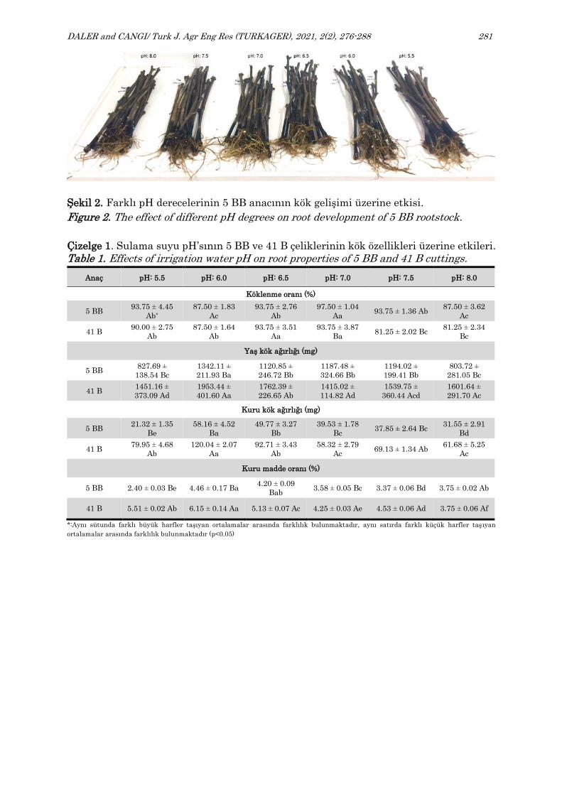
Şekil 2. Farklı pH derecelerinin 5 BB anacının kök gelişimi üzerine etkisi.
Figure 2. The effect of different pH degrees on root development of 5 BB rootstock.
Çizelge 1. Sulama suyu pH’sının 5 BB ve 41 B çeliklerinin kök özellikleri üzerine etkileri.
Table 1. Effects of irrigation water pH on root properties of 5 BB and 41 B cuttings.
Anaç pH: 5.5 pH: 6.0 pH: 6.5 pH: 7.0 pH: 7.5 pH: 8.0
Köklenme oranı (%)
5 BB 93.75 ± 4.45
Ab*
87.50 ± 1.83
Ac
93.75 ± 2.76
Ab
97.50 ± 1.04
Aa 93.75 ± 1.36 Ab
87.50 ± 3.62
Ac
41 B 90.00 ± 2.75
Ab
87.50 ± 1.64
Ab
93.75 ± 3.51
Aa
93.75 ± 3.87
Ba 81.25 ± 2.02 Bc
81.25 ± 2.34
Bc
Yaş kök ağırlığı (mg)
5 BB 827.69 ±
138.54 Bc
1342.11 ±
211.93 Ba
1120.85 ±
246.72 Bb
1187.48 ±
324.66 Bb
1194.02 ±
199.41 Bb
803.72 ±
281.05 Bc
41 B 1451.16 ±
373.09 Ad
1953.44 ±
401.60 Aa
1762.39 ±
226.65 Ab
1415.02 ±
114.82 Ad
1539.75 ±
360.44 Acd
1601.64 ±
291.70 Ac
Kuru kök ağırlığı (mg)
5 BB 21.32 ± 1.35
Be
58.16 ± 4.52
Ba
49.77 ± 3.27
Bb
39.53 ± 1.78
Bc 37.85 ± 2.64 Bc
31.55 ± 2.91
Bd
41 B 79.95 ± 4.68
Ab
120.04 ± 2.07
Aa
92.71 ± 3.43
Ab
58.32 ± 2.79
Ac 69.13 ± 1.34 Ab
61.68 ± 5.25
Ac
Kuru madde oranı (%)
5 BB 2.40 ± 0.03 Be 4.46 ± 0.17 Ba 4.20 ± 0.09
Bab 3.58 ± 0.05 Bc 3.37 ± 0.06 Bd 3.75 ± 0.02 Ab
41 B 5.51 ± 0.02 Ab 6.15 ± 0.14 Aa 5.13 ± 0.07 Ac 4.25 ± 0.03 Ae 4.53 ± 0.06 Ad 3.75 ± 0.06 Af
*:Aynı sütunda farklı büyük harfler taşıyan ortalamalar arasında farklılık bulunmaktadır, aynı satırda farklı küçük harfler taşıyan
ortalamalar arasında farklılık bulunmaktadır (p<0.05)

DALER and CANGI/ Turk J. Agr Eng Res (TURKAGER), 2021, 2(2), 276-288 282
Çizelge 2. Sulama suyu pH’sının 5 BB ve 41 B çeliklerinin sürgün özellikleri üzerine
etkileri.
Table 2. Effects of irrigation water pH on shoot properties of 5 BB and 41 B cuttings.
Anaç pH: 5.5 pH: 6.0 pH: 6.5 pH: 7.0 pH: 7.5 pH: 8.0
Sürgün sayısı (adet)
5 BB 1.94 ± 0.093
Aab*
1.56 ± 0.062
Ad
1.75 ± 0.077
Ac
2.06 ± 0.118
Aa
1.81 ± 0.054
Ab
1.81 ± 0.015
Ab
41 B 1.63 ± 0.0074
Aa
1.50 ± 0.0041
Ab
1.69 ± 0.0125
Aa
1.50 ± 0.0089
Bb
1.50 ± 0.0051
Ab
1.38 ± 0.0062
Bc
Ort. sürgün ağırlığı (mg)
5 BB 4372.82 ±
381.65 Bb
3681.75 ±
320.08 Bd
4737.01 ±
273.41 Ba
4449.62 ±
255.52 Ab
4319.17 ±
416.19 Bb
3895.42 ±
248.24 Bc
41 B 6274.92 ±
563.14 Aa
5941.55 ±
423.92 Ab
6282.41 ±
208.39 Aa
5819.23 ±
636.75 Abc
6076.64 ±
194.88 Ab
5478.08 ±
301.25 Ac
Ort. sürgün uzunluğu (cm)
5 BB 29.73 ± 1.45 b 28.40 ± 0.94 bc 32.17 ± 2.21 a 27.75 ± 1.87 c 29.94 ± 1.59 b 25.33 ± 1.68 d
41 B 41.58 ± 2.67 c 43.39 ± 2.09 b 45.88 ± 3.15 a 41.48 ± 2.53 c 41.40 ± 4.48 c 33.72 ± 3.76 d
Klorofil miktarı (SPAD)
5 BB 17.03 ± 0.64
Aab
17.66 ± 0.81
Aab
19.79 ± 1.17
Aa
19.32 ± 0.55
Aa
19.37 ± 1.06
Aa
16.11 ± 1.28
Ab
41 B 15.04 ± 0.14
Aab
16.25 ± 0.65
Aa
15.82 ± 0.98
Ba
16.06 ± 1.02
Ba
15.51 ± 0.39
Bab
14.28 ± 1.37
Bb
*: Aynı sütunda farklı büyük harfler taşıyan ortalamalar arasında farklılık bulunmaktadır, aynı satırda farklı küçük harfler
taşıyan ortalamalar arasında farklılık bulunmaktadır (p<0.05)
İncelenen anaçlarda en yüksek köklenme oranının 41 B anacında %93.75 ile pH: 6.5 ve
7.0’den; 5 BB anacında ise %97.50 ile pH: 7.0 derecesinden alındığı belirlenmiştir
(Şekil 3). Bulgularla uyumlu olarak Bates ve ark. (2002), Concord üzüm çeşidinde pH
derecesinin 4.5’in altına düştüğünde kök ve sürgün biyokütlesinde önemli oranda azalma
olduğunu; 7.5 pH seviyesinde sürgün biyokütlesinde düşüşlerin meydana geldiğini ve 5.0-
7.5 aralığındaki değerlerde ise vejetatif büyümede önemli bir fark bulunmadığını
kaydetmişlerdir.
Araştırmada her iki anaçta da yaş (41 B, 1 953.44 mg; 5 BB, 1 342.11 mg) ve kuru
(41 B, 120.04 mg; 5 BB, 58.16 mg) kök ağırlıklarına ait en yüksek değerlerin pH: 6.0
derecesinden elde edildiği belirlenmiştir (Şekil 4 ve 5). Sonuçlara paralel olarak Çakır ve
Atalay (2020) tarafından Sultani Çekirdeksiz / 5 BB ve Sultani Çekirdeksiz / 41 B aşı
kombinasyonunda farklı pH derecelerinin (4.5, 7.0 ve 8.5) yaş kök ağırlığı üzerine etkili
olduğu; artan pH ile yaş kök ağırlığının önemli ölçüde azaldığı ifade edilmiştir.
Valdez-Aguilar ve ark. (2009)’de alkali pH’ya sahip sulama suyunun düğünçiçeği
bitkisinin kök ağırlığında önemli oranda azalmaya neden olduğunu ve alkaliliğin bitki
büyümesi üzerinde stres yarattığını ifade etmektedirler. Vršič ve ark. (2016), 6 farklı asma
anacını içerisinde farklı tabakalar halinde çakıl, yüksek kireçli Rendzina toprağı
(pH: 8.54) ve turba-toprak karışımı (pH: 4.94) bulunan saksılarda yetiştirmişler ve
sonuçta yüksek pH koşullarına daha iyi uyum sağlayabilen Fercal anacının kuru kök
ağırlığı bakımından daha yüksek değerlere sahip olduğunu ifade etmişlerdir.
Kuru kök ağırlığının, yaş kök ağırlığına oranlanması ile elde edilen kuru madde oranı;
41 B anacında en yüksek pH: 6.0 derecesinde %6.15 olarak belirlenirken; 5 BB anacında
pH: 6.0 ve 6.5 derecelerinde sırasıyla, %4.46 ve 4.20 olarak tespit edilmiştir (Şekil 6).
Çakır ve Atalay (2020), yüksek pH’nın asma çeşit ve anaçları üzerindeki olumsuz etkisinin

DALER and CANGI/ Turk J. Agr Eng Res (TURKAGER), 2021, 2(2), 276-288 283
kök gelişimine kıyasla sürgün gelişimi üzerinde daha belirgin olduğunu ifade etmişlerdir.
Araştırmadan elde edilen bulgulara göre 41 B anacında en fazla sürgünün pH: 5.5 ve 6.5
derecelerinden sırasıyla, 1.63 ve 1.69 adet olduğu belirlenirken; 5 BB anacında pH: 5.5 ve
7.0 derecelerinden sırasıyla, 1.94 ve 2.06 adet olduğu kaydedilmiştir (Şekil 7). Bulgulara
benzer şekilde Fischer ve ark. (2016), Briteblue ve Delite yaban mersini çeşitlerinde 4.5,
5.5, 6.0 ve 6.9 (kontrol) pH derecelerine sahip sulama suyu ile Indol Bütirik Asidin (IBA)
etkilerini araştırmışlar ve çelik başına ortalama sürgün sayısının sulama suyunun
asitlenmesi ile arttığını tespit etmişlerdir. Zhao ve ark. (2013), şakayık (Paeonia lactiflora
Pall.) bitkisinde pH’sı 4.0 ve 10.0 olan ortamların kontrolle (pH 7.0) karşılaştırıldığında
yaprak sayısı hariç bitkinin tüm morfolojik parametrelerinde azalmaya neden olduğunu
bildirmişlerdir.
Ortalama sürgün ağırlıklarına ait en yüksek değerlerin 41 B anacında 6 282.41 mg ve
5 BB anacında 4 737.01 mg olarak; pH: 6.5 derecesinden elde edildiği belirlenmiştir (Şekil
8). Bavaresco ve ark. (2003) tarafından da benzer sonuçlar kaydedilmiş, topraktaki yüksek
karbonat içeriği, yaprak ve sürgün gelişimi ile toplam kuru madde üretimini azaltmıştır.
Vršič ve ark. (2016), yüksek pH koşullarına daha iyi uyum sağlayabilen Fercal dahil üç
anacın biyokütle üretimi bakımından daha yüksek değerlere sahip olduğunu ifade
etmişlerdir. Valdez-Aguilar ve ark. (2009) ise kum kültürlerinde yetiştirilen düğünçiçeği
bitkisinde (Ranunculus asiaticus) elektriki iletkenliği (EC) 2, 3, 4 ve 6 dS m−1 ve pH
kontrolü olan (pH: 6.4) ve olmayan (pH: 7.8) sulama suyunda; pH: 7.8’in, pH: 6.4 ile
karşılaştırıldığında sürgün kuru ağırlığında önemli oranda azalmaya neden olduğunu
bildirmektedirler.
Çalışmadan elde edilen bulgulara göre, anaçların ortalama sürgün uzunluklarına ait
en yüksek değerlerin 41 B’de 45.88 cm ve 5 BB’de 32.17 cm olmak üzere sulama suyu pH’sı
6.5 olan ortamdan alındığı kaydedilmiştir (Şekil 9). Bulgularla benzer olarak
Çakır ve Atalay (2020), farklı pH derecelerinin Sultani Çekirdeksiz / 5 BB aşı
kombinasyonunda sürgün uzunluğu ve yaprak alanı değerlerini önemli ölçüde
etkilediğini; pH değeri arttıkça sürgün uzunluğu ve yaprak alanının azaldığını
belirlemişlerdir. Valdez-Aguilar ve ark. (2009), tuzluluğun, alkali pH ile kombinasyonu
sonucunda düğünçiçeği bitkisinin gövde uzunluğunda önemli derecede azalmaya neden
olduğunu bildirmişlerdir. Zhao ve ark. (2013) ise şakayık bitkisinde büyümenin, sulama
suyundaki aşırı pH’dan önemli ölçüde etkilendiğini ve en ciddi stresin pH: 10.0’da
gerçekleştiğini bildirmektedir.
SPAD cinsinden gerçekleştirilen klorofil ölçümleri sonucunda her iki anaçta da pH’sı
5.5-7.5 olan sulama çözeltileri arasında istatistiksel olarak önemli bir farklılık
bulunmadığı; bununla birlikte en düşük değerlerin pH derecesi 8.0 olan çözeltiden elde
edildiği kaydedilmiştir (Şekil 10). Zhao ve ark. (2013), pH derecesi 4.0 ve 10.0 olan
çözeltilerle sulanan şakayık bitkisinde pH: 7.0 ile sulananlarla karşılaştırıldığında,
klorofil a, klorofil b, klorofil a + b gibi fizyolojik indekslerin arttığını kaydederek, şakayık
bitkisinin klorofil miktarı açısından asit ve alkali ortam direnci gösterdiğini ifade
etmişlerdir.

DALER and CANGI/ Turk J. Agr Eng Res (TURKAGER), 2021, 2(2), 276-288 284
Şekil 3. Anaçlara ait köklenme oranları.
Figure 3. Rooting ratio of the rootstocks.
Şekil 4. Anaçlara ait yaş kök ağırlıkları.
Figure 4. Fresh root weight of the rootstocks.
Şekil 5. Anaçlara ait kuru kök ağırlıkları.
Figure 5. Dry root weight of the rootstocks.
0
20
40
60
80
100
5,5 6,0 6,5 7,0 7,5 8,0
Kök
len
me o
ran
ı (%
)
pH değerleri
41B 5BB
0
500
1.000
1.500
2.000
2.500
5,5 6,0 6,5 7,0 7,5 8,0
Yaş
kök
ağır
lığı
(mg)
pH değerleri
41B 5BB
0
25
50
75
100
125
5,5 6,0 6,5 7,0 7,5 8,0
Ku
ru k
ök
ağır
lığı
(mg)
pH değerleri
41B 5BB

DALER and CANGI/ Turk J. Agr Eng Res (TURKAGER), 2021, 2(2), 276-288 285
Şekil 6. Anaçlara ait kuru madde oranları.
Figure 6. Dry matter ratio of the rootstocks.
Şekil 7. Anaçlara ait sürgün sayıları.
Figure 7. Shoot number of the rootstocks.
Şekil 8. Anaçlara ait ortalama sürgün ağırlıkları.
Figure 8. Mean shoot weight of the rootstocks.
0
2
4
6
8
10
5,5 6,0 6,5 7,0 7,5 8,0
Ku
ru m
ad
de o
ran
ı (%
)
pH değerleri
41B 5BB
0
0,5
1
1,5
2
2,5
5,5 6,0 6,5 7,0 7,5 8,0
Sü
rgü
n s
ayıs
ı (a
det)
pH değerleri
41B 5BB
0
1.500
3.000
4.500
6.000
7.500
5,5 6,0 6,5 7,0 7,5 8,0
Ort
. sü
rgü
n a
ğır
lığı
(mg)
pH değerleri
41B 5BB

DALER and CANGI/ Turk J. Agr Eng Res (TURKAGER), 2021, 2(2), 276-288 286
Şekil 9. Anaçlara ait ortalama sürgün uzunlukları.
Figure 9. Mean shoot length of the rootstocks.
Şekil 10. Çeşitlere ait klorofil miktarları.
Figure 10. Chlorophyll content of the rootstocks.
SONUÇ
Sulama suyu pH’sının asma anaçlarının biyokütle, köklenme, kök ve sürgün gelişimi
üzerine etkisinin incelendiği bu çalışmada, köklenme oranı bakımından en yüksek
değerlerin nötr ve nötre yakın pH derecelerinden elde edildiği tespit edilmiştir. Yaş ve
kuru kök ağırlıklarına ait en yüksek değerlerin her iki çeşitte de 6.0 pH derecesinden; en
yüksek kuru madde oranlarının ise pH: 6.0 ve 6.5 derecelerinden elde edildiği
kaydedilmiştir. Sürgün sayısı bakımından en yüksek değerlerin pH’sı 5.5, 6.5 ve 7.0 olan
sulama solüsyonlarından alındığı belirlenirken; çeşitlerin ortalama sürgün ağırlığı ve
ortalama sürgün uzunluklarına ait en yüksek değerlerin pH: 6.5 derecesinden elde
edildiği saptanmıştır. Her iki çeşitte de 5.5-7.5 pH aralığındaki sulama çözeltileri
arasında klorofil içeriği bakımından önemli bir farklılık bulunmazken, pH’sı 8.0 olan
sulama solüsyonlarında yapraklardaki klorofil miktarının azaldığı belirlenmiştir.
Araştırma sonuçları düşük pH derecelerinden ziyade alkali pH’ya sahip sulama
solüsyonlarının her iki asma anacı için de hem morfolojik hem de fizyolojik kriterler
bakımından sınırlayıcı etki gösterdiğini kanıtlamıştır. Elde edilen bulgular sulama suyu
pH değerlerinin asmanın büyüme ve gelişmesi üzerindeki rolünün göz ardı
edilemeyeceğini göstermiştir.
0
10
20
30
40
50
60
5,5 6,0 6,5 7,0 7,5 8,0
Ort
. sü
rgü
n u
zu
nlu
ğu
(cm
)
pH değerleri
41B 5BB
0
5
10
15
20
25
5,5 6,0 6,5 7,0 7,5 8,0
Klo
rofi
l m
ikta
rı (
SP
AD
)
pH değerleri
41B 5BB

DALER and CANGI/ Turk J. Agr Eng Res (TURKAGER), 2021, 2(2), 276-288 287
ÇIKAR ÇATIŞMASI
Yazarlar olarak, çalışmanın planlanması, yürütülmesi ve makalenin hazırlanması
aşamalarında herhangi bir çıkar çatışması içerisinde olmadığımızı beyan ederiz.
YAZAR KATKISI
Yazarlar, makalenin altta belirtilen iş planına göre yürütüldüğünü beyan ederler.
Rüstem Cangi: Çalışmanın planlanması, bitkisel materyallerin temin edilmesi,
istatistiksel analizlerin gerçekleştirilmesi ve makaleye son şeklinin verilmesinde katkı
sağlamıştır.
Selda Daler: Denemenin kurulması, morfolojik ve fizyolojik analizlerin yürütülmesi,
verilerin yorumlanması ve makalenin yazılmasında katkı sağlamıştır.
KAYNAKLAR
Anonim (1994). FAO, water quality for agriculture. Irrigation and Drainage Paper, Rome.
Bates TR, Dunst RM, Taft T and Vercant M (2002). The vegetative response of ‘Concord’ grapevines to soil pH.
The American Society for Horticultural Science, 37(6): 890-893.
Bavaresco L, Giachino E and Pezutto S (2003). Grapevine rootstocks effects on lime-induced chlorosis, nutrient
uptake, and source-sink relationships. Journal of Plant Nutrition, 26: 1451-1465.
Boselli M and Volpe B (1993). Influence of rootstock on potassium content, the pH and concentration of organic
acids of the must of cv "Chardonnay". Papers of the School of Viticulture and Enology, University of Turin
(Italy), 16: 37-40.
Cirami RM, McCarthy MG and Furkaliev DG (1985). Minimum pruning of Shiraz vines - effects on yield and
wine colour. Australian & New Zealand Grapegrower & Winemaker, 263: 26-27.
Çakır B and Atalay YI (2020). pH, ‘Sultani Çekirdeksiz’, Kober 5 BB, 41 B, plant growth, mineral content. 30.
International Horticultural Congress IHC2018: International Symposium on Viticulture: Primary
Production and Processing, 12-16 August 2018. Istanbul-Turkey (in English).
Çelik H (1996). Bağcılıkta anaç kullanımı ve yetiştiricilikteki önemi. Anadolu Ege Tarımsal Araştırma
Enstitüsü Dergisi, 6(2): 127-148.
Falkenmark M and Rockstrom J (1993). Curbing rural exodus from tropical drylands. Food fiber need sand to
enhance water use efficiency. USDA-ARS Water Management User Unit Bushland, Texas.
Fardossi A, Hepp E, Mayer C and Kalchgruber R (1991). Untersuchungen über den Einfluß verschiedener
Unterlasgssorten auf die Nährstoffgehalte bei Grümer Veltliner im Gefaßversuch. Mitteilungen
Klosterneuburg, 41: 137-142.
Fischer DLO, Fernandes GW, Borges EA, Piana CFB and Pasa MS (2016). Rooting of blueberry hardwood
cuttings as affected by irrigation water pH and IBA. Acta Horticulturae, 1130: 431-436.
Güler Ç (1997). Su kalitesi kitabı. Çevre Sağlığı Temel Kaynak Dizisi, Ankara.
Hayes PF and Mannini F (1988). Nutrient levels in Sauvignon Blanc garafted to different rootstocks. In
‘Second international seminar cool climate viticulture and oenology’ pp. 43-44. 11-15 January 1988.
Auckland, New Zealand.
Hoagland DR and Arnon DI (1950). The water culture method for growing plants without soil. Circular -
California Agricultural Experiment Station, 347: 32.
Iyengar K, Gahrotra S, Mishra A, Kaushal A, Kumar K and Dutt M (2011). Greenhouse a reference manual.
National Committee on Plasticulture Applications in Horticulture, Ministry of Agriculture, India.
Kanber R, Kırda C ve Tekinel O (1992). Sulama suyu niteliği ve sulamada tuzluluk sorunları. Çukurova
Üniversitesi Ziraat Fakültesi Yayınları: 6.
Lal D (1991). Cosmic ray labeling of erosion surfaces: in situ nuclide production rates and erosion models.
Earth and Planetary Science Letters, 104(2-4): 424-439.
Loue A (1990). Le diagnostic foliaire (ou pétiolaire) dans les enquêtes de nutrition minérale des vignes. Progrès
agricole et viticole (Montpellier), 107: 439-453.
Mullins MG, Bouquet A and Williams LE (1992). Biology of the grapevine. Cambridge University Press, 239p.
Rhoades JD (1972). Quality of water for irrigation. Soil Science, 113: 227-284.

DALER and CANGI/ Turk J. Agr Eng Res (TURKAGER), 2021, 2(2), 276-288 288
Richards D (1983). The grape root system. Horticultural reviews, AVI Publishing Company, Westport,
Connecticut.
Riley CV (1891). The Phylloxera and American resistant stocks. Scientific American, 31(788): 12596-12597.
Rosas A, Rengel Z and de la Luz Mora M (2007). Manganese supply and pH influence growth, carboxylate
exudation and peroxidase activity of ryegrass and white clover. Journal of Plant Nutrition, 30: 253-270.
Ruckenbauer W and Traxler H (1974). Weinbau heute. Handbuch für Beratung, Schule und Praxis, Stutgard.
Rühl EH (1991). Effect of potassium supply on cation uptake and distribution in grafted Vitis campinii and
Vitis berlandieri × Vitis rupestris rootstocks. Australian Journal of Experimental Agriculture, 31: 687-691.
Scienze A, Failla O and Romano F (1986). Untersuchungen zur sortenspezifischen Mineralstoffaufnahme bei
Reben. Vitis, 25: 160-168.
Spoerr R (1902). Nurseries for grapevine grafts. American Scientific, 53: 21904-21906.
Şimşek G, Çanlı M, Karadavut U, Yazıcı ME ve Soğancı K (2017). Sulama yapılan alanların bazı su
parametreleri açısından ayırma (discriminant) analizi kullanılarak incelenmesi. Türk Tarım ve Doğa
Bilimleri Dergisi 4(3): 339–346.
Şinik E (2011). Edirne ilinde bulunan asit karakterli toprakların bitki besin elementleri ve bazı ağır metal
içeriklerinin belirlenmesi üzerine bir araştırma. Yüksek Lisans Tezi, Namık Kemal Üniversitesi, Fen
Bilimleri Enstitüsü, Toprak Bilimi ve Bitki Besleme Anabilim Dalı, 48 s., Tekirdağ.
Tangolar S ve Ergenoğlu F (1989). Değişik anaçların erkenci bazı üzüm çeşitlerinde yaprakların mineral besin
maddesi ve çubukların karbonhidrat içerikleri üzerine etkisi. Doğa, 13(3B): 1267-1283.
Tuncay H (1994). Su kalitesi (I. Basım). Ege Üniversitesi Ziraat Fakültesi Yayınları, İzmir.
Valdez-Aguilar LA, Grieve CM and Poss J (2009). Hypersensitivity of Ranunculus asiaticus to salinity and
alkaline pH in irrigation water in sand cultures. Hortscience, 44(1): 138-144.
Volpe B and Boselli M (1990). The effect of the rootstock on the mineral nutrition and on certain qualitative
and quantitative parameters of the grapevine cultivar Croatina. Vignevini,17(4): 51-55.
Vršič S, Kocsis L and Pulko B (2016). Influence of substrate pH on root growth, biomass and leaf mineral
contents of grapevine rootstocks grown in pots. Journal of Agricultural Science and Technology, 18: 483-
490.
Williams LE and Smith RJ (1991). The effect of rootstock on the partitioning of dry weight, nitrogen and
potassium and root distribution of Cabernet Sauvignon grapevines. American Journal of Enology and
Viticulture 42(2): 118-122.
Zhao D, Hao Z, Wang J and Tao J (2013). Effects of pH in irrigation water on plant growth and flower quality
in herbaceous peony (Paeonia lactiflora Pall.). Scientia Horticulturae, 154: 45-53.
Zhao JX (2003). Studies on the soil pH and plant growth. Inner Mongolia Agricultural Science and Technology,
6: 33-42.

Turkish Journal of Agricultural
Engineering Research
https://dergipark.org.tr/en/pub/turkager https://doi.org/10.46592/turkager.2021.v02i02.003
Research Article
Turk J Agr Eng Res
(TURKAGER)
e-ISSN: 2717-8420
2021, 2(2): 289-297
Modelling Kinetics of Extruded Fish Feeds in a Continuous Belt Dryer
Funmilayo OGUNNAIKEIDa* Ayoola Patrick OLALUSIIDb
aDepartment of Agricultural and Bio-Environmental Engineering, The Federal Polytechnic, Ado, Ekiti State, NIGERIA bDepartment of Agricultural Engineering, Federal University of Technology, Akure, Ondo State, NIGERIA
(*): Corresponding author, [email protected]
ABSTRACT
Feed is the major inputs in aquaculture production which affects
the development growth of aquaculture in the African continent.
Extruded fish feeds are dried to desire moisture content to
increase the shelf life. Conventional method of drying fish feeds
had gained attention recently in Nigeria in order to reduce high
cost of producing fish feeds. However, this method is still grossly
underutilized. Extrude floating fish feed was dried using
continuous belt dryer at drying air temperature from 60°C to
100°C at an interval of 10°C, velocity of air using for drying from
0.8 m s-1 to 1.0 m s-1 at an interval of 0.1 m s-1 using a constant
linear belt speed of 50 m s-1. Various moisture contents gotten at
different conditions were changed to ratio of the dried extrudates
moisture so as to obtain curves of drying by plotting the ratio of
moisture against time. The dried extrudates behaviour was
determined by fixing the drying curves with five well known
models. Model with high determination coefficient and low
reduced chi-square, low standard error, low value of least square
and low standard deviation error (SEE) was used as best model.
Midilli et al model was found suitable in describing the behaviour
of extruded fish feed during drying. The temperature of air used
for drying was discovered to have a major influence on the drying
kinetics of the extruded fish feeds based on the conditions of this
experiment.
INTRODUCTION
Extruded feed is the most typical form of animal feed produced in the western world.
Fish feed which contributes a global demand of 50 - 75 million tons per year; has shown
an annual growth rate of more than 6% in the last few decades. According to FAO (2020)
the global fish production in 2018 is estimated as 179 million tones and this is expected
to increase to 204 million by 2030 as a result of increase in production of extruded fish
feeds. Although, either floating or sinking feed can produce satisfactory growth, but
To cite: Ogunnaike F, Olalusi P (2021). Modelling Kinetics of Extruded Fish Feeds in a
Continuous Belt Dryer. Turkish Journal of Agricultural Engineering Research (TURKAGER),
2(2): 289-297. https://doi.org/10.46592/turkager.2021.v02i02.003
RESEARCH ARTICLE
Received: 29.05.2021
Accepted: 22.08.2021
Keywords:
➢ Kinetic of drying,
➢ Extruded fish feed,
➢ Drying curves,
➢ Belt dryer,
➢ Drying model

OGUNNAIKE and OLALUSI / Turk J. Agr Eng Res (TURKAGER), 2021, 2(2), 289-297 290
most fish species prefer floating than sinking. This is due to the fact that extruded feed
have superior water stability, better floating properties, ease in digestion, zero water
pollution, optimized labour usage, zero wastage of raw materials (Amalraaj, 2010) and
a higher energy than sinking pelleted feed (Hilton et al., 1981; Johnson and
Wanderwick, 1991; Momo et al., 2016). Drying according to Kallia and Patankar (2001)
can be defined has the universal method of conditioning the material by removing
moisture to such a level that it is in equilibrium with the normal atmospheric air in
order to preserve the quality and nutritive value of the food product. According to
Misha et al. (2013), to obtain the best conditions of drying and for energy saving during
procedure for drying, it is imperative to know the solid temperature and effects of the
drying variables (temperature of air use for drying, velocity of air use for drying etc) in
moisture removal. Drying of temperature sensitive materials such as food and
agricultural products, particularly at temperatures sensitive enough to cells, lead to
probable cell damage and gelatinization (Fernando et al., 2008). Pacheco et al. (2011)
stated that low temperature between 30°C to 70°C is the sorption isotherms required
for an extruded fish feed and that the energy equilibrium of thermal system is
delineated by heat and mass transfer in a continuous convective dryer. In estimating
the coefficient of heat and mass transfer, the heat transfer coefficient is often used
because of its reliability than the mass transfer coefficient (Sander et al., 2001).
Haubjerg et al. (2014) opined that this is true since surface temperature can more easily
be measured over the course of drying. Barati and Esfahani (2011) also reported that
the center and surface temperature are almost same especially when drying with for
Biot numbers less than one especially for small fish feed pellets convectively exposed
hot air use for drying (Haubjerg et al., 2014). For the best management of operation
parameters and prediction of process involved in drying, mathematical models are used.
According to Brooker et al. (1992), semi−empirical and empirical models are used to
estimate how moisture varies in feed materials. The condition of drying, dryer type and
the characterization of the feeds (Ozdemir and Devres, 1999) to be dried are factors that
affect drying kinetics of the feeds. Most aquatic and pet feeds are dry mostly in belt
dryer, this is due to the fact that it has high efficiency and simple design (FAO, 2020).
Although, there had been studies on kinetic modeling of fish feeds, but few literatures
on kinetic modeling of extruded fish feeds in a continuous belt dryer. Investigating the
influence of drying variables on the drying kinetics of fish feed extrudates using
continuous flow belt dryer and using seven known models with the objectives of
selecting the most well adopted model were objectives of the research.
MATERIALS AND METHODS
Feed ingredients were procured from a retail outlet at Akure, Ondo State. The feedwas
formulated using ingredients used for catfish feed production in Nigeria according to
Fagbenro and Adebayo (2005). The materials were extruded byusing a single screw
extruder, developed at The Federal University of Technology, Akure. The extruded fish
feed preliminary moisture content was evaluated by drying the sample in an oven at
102°C until the weights remain steady. A continuous flow belt dryer (Figure 1) was used
in drying the extruded feeds.
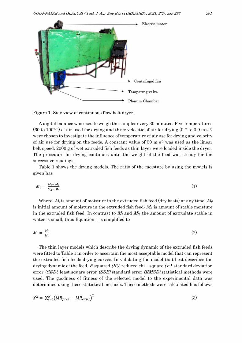
OGUNNAIKE and OLALUSI / Turk J. Agr Eng Res (TURKAGER), 2021, 2(2), 289-297 291
Figure 1. Side view of continuous flow belt dryer.
A digital balance was used to weigh the samples every 30 minutes. Five temperatures
(60 to 100°C) of air used for drying and three velocitie of air for drying (0.7 to 0.9 m s-1)
were chosen to investigate the influence of temperature of air use for drying and velocity
of air use for drying on the feeds. A constant value of 50 m s-1 was used as the linear
belt speed. 2000 g of wet extruded fish feeds as thin layer were loaded inside the dryer.
The procedure for drying continues until the weight of the feed was steady for ten
successive readings.
Table 1 shows the drying models. The ratio of the moisture by using the models is
given has
𝑀𝑖 = 𝑀𝑡− 𝑀𝑠
𝑀𝑜− 𝑀𝑠 (1)
Where; Mi is amount of moisture in the extruded fish feed (dry basis) at any time; M0
is initial amount of moisture in the extruded fish feed; Ms is amount of stable moisture
in the extruded fish feed. In contrast to Mt and M0, the amount of extrudate stable in
water is small, thus Equation 1 is simplified to
𝑀𝑖 = 𝑀𝑡
𝑀𝑜 (2)
The thin layer models which describe the drying dynamic of the extruded fish feeds
were fitted to Table 1 in order to ascertain the most acceptable model that can represent
the extruded fish feeds drying curves. In validating the model that best describes the
drying dynamic of the feed, R squared (R2), reduced chi − square (x2), standard deviation
error (SEE), least square error (SSE) standard error (RMSE) statistical methods were
used. The goodness of fitness of the selected model to the experimental data was
determined using these statistical methods. These methods were calculated has follows
𝑋2 = ∑ (𝑀𝑅𝑝𝑟𝑒𝑖 − 𝑀𝑅𝑒𝑥𝑝,𝑖)2𝑁
𝑖=1 (3)

OGUNNAIKE and OLALUSI / Turk J. Agr Eng Res (TURKAGER), 2021, 2(2), 289-297 292
RMSE = (4)
𝑅2 = 1 − ∑ (𝐴𝑅𝑒𝑥𝑝𝑠 − 𝐴𝑅𝑝𝑟𝑒 𝑠)
2𝑊𝑠 =1
∑ (𝐴𝑅exp 𝑠 − 𝐴𝑅𝑝𝑟𝑒 𝑠)2𝑊
𝑠 =1
(5)
where ARpre,i is ratio of the moisture in nth predictions, ARexpi is ratio of observed
experment in nth predictions, 𝐴𝑅𝑒𝑥𝑝 𝑠 is mean value of experimental dimensionless ratio
of the moisture, N is amount of observations and n is the amount of constant in a model.
A plot of curve drying model was used to determine the value of each model coefficient.
MATLAB 2014R software was used to find the best model fit and the mathematical
model coefficients.
Table 1. Mathematical model to predict the procedure of drying.
Model Type Reference
Newton MR = exp (-kt) Mujumdar (1987)
Page MR = exp (-kt)n Diamante and Munro (1993)
Modified Page 1 MR = exp [- (kt)n] Whith et al. (1978)
Midilli, Kucuk and Yapar MR = a exp (-ktn) + bt Midilli et al. (2002)
Tow term MR = a exp (k0t) + b exp(-k
it) Henderson (1974)
Tow- term exponential MR = a exp (-kt) + (1 – a) exp (-kat) Sharaf-eldeen et al. (1980)
Wang and Singh MR = a exp (-kt) + (1 – a) exp (kbt) Yaldız et al. (2001)
RESULTS AND DISCUSSION
Figures 2 to 4 show the drying curve of extruded fish feeds dried in continuous flow belt
dryer. It was observed that as the drying time increase, there is progressive reduction
in the moisture ratio of the extrudate. The increase in the drying temperature of 60C
to 100C leads to an increase in the amount moisture loss by the extrudate over the
drying time considered in this study. This explains the fact that moisture at the surface
of the extrudates evaporated at a faster rate when the temperature is high. This shows
that the moisture on the outer surface layer of the sample evaporated very fast at higher
temperatures. A similar trend has been reported by many researchers such as
Arumuganathan et al. (2009) when drying mushroom; Meziane (2011) in drying pomace
made from olive, Gorjian et al. (2011) when drying barberry. Also, similar result was
reported by Haujerg et al. (2014) when drying extruded fish feed in a hot air convective
dryer using temperature between 50C and 80C, Aghbashlo et al. (2012) in carrot
drying, Ruiz-Celma et al. (2012) when drying tomatoes and corn drying
(Odjo et al., 2012).

OGUNNAIKE and OLALUSI / Turk J. Agr Eng Res (TURKAGER), 2021, 2(2), 289-297 293
Figure 2. Influence of temperature on the moisture ratio vs time for drying for velocity
of air for drying at 0.8 m s-1.
Figure 3. Influence of temperature on the moisture ratio vs time for drying for velocity
of air for drying at 0.9 m s-1.
Figure 4. Influence of temperature on the moisture ratio vs time for drying for velocity
of air for drying at 1.0 m s-1.
0
0,2
0,4
0,6
0,8
1
0 75 150 225 300
Mois
ture
ra
tio
Time (min)
S = 50 m s-1
V = 0.8 m s-1
60 ⁰C
70 ⁰C
80 ⁰C
90 ⁰C
100 ⁰C
0
0,2
0,4
0,6
0,8
1
0 75 150 225 300
Mois
ture
ra
tio
Time (min)
S = 50 m s-1
V = 0.9 m s-1
60 ⁰C
70 ⁰C
80 ⁰C
90 ⁰C
100 ⁰C
0
0,2
0,4
0,6
0,8
1
0 75 150 225 300
Mois
ture
ra
tio
Time (min)
S = 50 m s-1
V = 1.0 m s-1
60 ⁰C
70 ⁰C
80 ⁰C
90 ⁰C
100 ⁰C
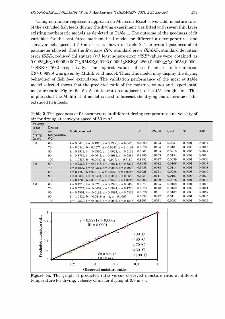
OGUNNAIKE and OLALUSI / Turk J. Agr Eng Res (TURKAGER), 2021, 2(2), 289-297 294
Using non-linear regression approach on Microsoft Excel solver add, moisture ratio
of the extruded fish feeds during the drying experiment was fitted with seven thin layer
existing mathematic models as depicted in Table 1. The outcome of the goodness of fit
variables for the best fitted mathematical model for different air temperatures and
conveyor belt speed at 50 m s-1 is as shown in Table 2. The overall goodness of fit
parameter showed that the R square (R2), standard error (RMSE), standard deviation
error (SEE), reduced chi-square (χ2), least square error (SSE) values were obtained as
0.9923≤R2≤0.9995,0.0071≤RMSE≤0.0193,0.0091≤SEE≤0.2860,0.0000≤χ2≤0.0954,0.000
1≤SEE≤0.7632 respectively. The highest values of coefficient of determination
(R2≥ 0.9995) was given by Midilli et al model. Thus, this model may display the drying
behaviuor of fish feed extrudates. The validation performance of the most suitable
model selected shows that the predicted ratio of the moisture values and experiential
moisture ratio (Figure 5a, 5b, 5c) data scattered adjacent to the 45 straight line. This
implies that the Midilli et al model is used to forecast the drying characteristic of the
extruded fish feeds.
Table 2. The goodness of fit parameters at different drying temperature and velocity of
air for drying at conveyor speed of 50 m s-1. Velocity
of air
for
drying
(m s-1)
Drying
air
temperature
(°C)
Model constant
R² RMSE SEE X² SSE
0.8 60 k = 0.0418, b = -0.1319, a = 0.9906, n = 0.6473 0.9923 0.0193 0.025 0.0001 0.0037
70 k = 0.0844, b = 0.0377, a = 0.9843, n = 2.1488 0.9976 0.0124 0.016 0.0003 0.0015
80 k = 0.4818, b = -0.0565, a = 1.0024, n = 0.5134 0.9961 0.0165 0.0213 0.0005 0.0027
90 k = 0.8786, b = -0.0047, a = 0.9989, n = 0.5886 0.9983 0.0109 0.0154 0.0002 0.001
100 k = 1.0585, b = -0.0047, a = 0.997, n = 0.5189 0.9992 0.0077 0.0099 0.0001 0.0006
0.9 60 k = 0.2323, b = -0.0448, a = 1.0014, n = 0.8232 0.9988 0.0082 0.0106 0.0001 0.0007
70 k = 0.4207, b = -0.0321, a = 0.9966, n = 0.7006 0.9988 0.0088 0.0114 0.0001 0.0008
80 k = 0.1266, b = 0.0016, a = 1.0457, n = 1.0047 0.9928 0.0221 0.0286 0.0008 0.0049
90 k = 0.8309, b = -0.0424, a = 0.9831, n = 0.3685 0.998 0.014 0.0197 0.0004 0.002
100 k = 0.1266, b = 0.0016, a = 1.0457, n = 1.0047 0.9995 0.0059 0.0076 0.0001 0.0003
1.0 60 k = 0.4719, b = -0.0219, a = 0.9999, n = 0.6659 0.9974 0.0125 0.0162 0.0001 0.0016
70 k = 0.5775, b = -0.0461, a = 1.0024, n = 0.4736 0.9979 0.0118 0.0152 0.0002 0.0014
80 k = 0.7961, b = -0.0182, a = 0.9997, n = 0.5329 0.9976 0.013 0.0167 0.0003 0.0017
90 k = 1.0522, b = -0.0119, a = 1, n = 0.4685 0.9992 0.0077 0.011 0.0001 0.0005
100 k = 1.2539, b = -0.0015, a = 0.9997, n = 0.4848 0.9993 0.0071 0.0091 0.0001 0.0005
Figure 5a. The graph of predicted ratio versus observed moisture ratio at different
temperature for drying, velocity of air for drying at 0.8 m s-1.
y = 0,9991x + 0,0002
R² = 0.9991
0
0,2
0,4
0,6
0,8
1
0 0,2 0,4 0,6 0,8 1
Pre
dic
ted
mois
ture
ra
tio
Observed moisture ratio
V= 0.8 m s-1
S= 50 m s-1
90 ⁰C
80 ⁰C
70 ⁰C
60 ⁰C
100 ⁰C

OGUNNAIKE and OLALUSI / Turk J. Agr Eng Res (TURKAGER), 2021, 2(2), 289-297 295
Figure 5b. The graph of predicted ratio versus observed moisture ratio at different
temperature for drying, velocity of air for drying at 0.9 m s-1.
Figure 5c. The graph of predicted ratio versus observed moisture ratio at different
temperature for drying, velocity of air for drying at 1.0 m s-1.
CONCLUSION
The modeling kinetic of extruded floating fish feeds and influence of the temperature of
air used for drying, velocity of air used for drying and a constant linear belt speed under
different machine operational condition was investigated. A rise in the temperature of
air for drying leads to reduction of time required to dry the fish feeds. Temperature of
air for drying and velocity of air for drying were discovered to be the major influence on
drying behavior of the fish feed with belt linear speed having the least effect. In
predicting the drying kinetics of the extruded fish feeds, Midilli et al model was
ascertained to be the most fitting model to use.
DECLARATION OF COMPETING INTEREST
The authors declare that there are no conflict of interest
y = 0,999x + 0,0001
R² = 0,9993
0
0,2
0,4
0,6
0,8
1
0 0,2 0,4 0,6 0,8 1
Pre
dic
ted
mois
ture
ra
tio
Observed moisture ratio
V= 0.9 m s-1
S= 50 m s-1
90 ⁰C
80 ⁰C
70 ⁰C
60 ⁰C
100 ⁰C
y = 0,9995x - 4E-06
R² = 0,9993
0
0,2
0,4
0,6
0,8
1
0 0,2 0,4 0,6 0,8 1
Pre
dic
ted
mois
ture
ra
tio
Observed moisture ratio
V= 1.0 m s-1
S= 50 m/s
90 ⁰C 80 ⁰C
70 ⁰C 60 ⁰C
100 ⁰C

OGUNNAIKE and OLALUSI / Turk J. Agr Eng Res (TURKAGER), 2021, 2(2), 289-297 296
CREDIT AUTHORSHIP CONTRIBUTION STATEMENT
Funmilayo Ogunnaike: Investigation of the manuscript, materials and methods used in
the research, conceptualization, data analysis and validation and writing of the original
draft of the manuscript.
Pius Olalusi: Investigation of the manuscript, materials and methods used in the
research, conceptualization, edition of the manuscript and reviewing of the manuscript.
REFERENCES
Aghbashlo M, Mobli H, Rafiee S and Madadlou A (2012). Energy and exergy analyses of thespray drying
process of fish oil microencapsulation. Biosystems Engineering, 111(2): 229-241.
Amalraaj S (2010). Extruded floating fish feed a boon for farmers. Online Publication The Hindus Science
Tech/Agriculture.
Arumuganathan T, Manikantan MR, Rai RD, Anandakumar S and Khare V (2009). Mathematical modeling
of drying kinetics of milky mushroom in a fluidized bed dryer. International Agrophys. 23: 1-7.
Barati E and Esfahani JA (2011). Mathematical modeling of convective drying: Lumpedtemperature and
spatially distributed moisture in slab. Energy, 36(4): 2294-2301.
Brooker DB, Bakker-Arkema FW and Hall CW (1992). Drying and storage of grains and oilseeds. Westport:
International Journal of Engineering and Advancement Technology Studies, 23(2): 10-15.
Diamente LM and Munro PA (1993). Mathematical modeling of the thin layer solar drying of sweet potato
slices. Solar Energy, 51(4): 271-276.
FAO (2020). The state of World fisheries and aquaculture 2020. Sustainability in action. Rome.
Fagbenro OA and Adebayo OT (2005). A review of the animal and aqua feed industries in Nigeria. A
synthesis of the formulated animal and aqua feed industry in sub-Saharan Africa, CIFA Occasion Paper
No. 26: 66.
Fernando WJN, Ahmad LA, AbdShuko SR and Lok YK (2008). A model for constant temperature drying
rates of case hardened slices of papaya and garlic. Journal of Food Engineering,88: 229-238.
Gorjian SH, Tavakoli Hashjin T, Khoshtaghaza MH and Nikbakht AM (2011). Drying kinetics and quality
of barberry in a thin layer dryer. Journal of Agricultural ScienceTechnology, 13, 303–314.
Henderson SM (1974). Progress in developing the thin layer drying equation. Transactions of the American
Society of Agricultural Engineers, 17: 1167-1172.
Haubjerg AF, Veje1 CT, Jørgensen BN, Simonsen B and Løvgreen S (2014). Mathematical modelling of the
drying of extruded fish feed and its experimental demonstration. 19th International Drying Symposium, (IDS 2014), Lyon, France, August 24-27, 2014.
Hilton JW, Cho CY and Slingers SJ (1981). Effect of extrusion processing and steam pelleting diets on pellet
durability and pellet water absorption and physiological response of rainbowtrout. Aquaculture, 25:
185-194.
Johnson TA and Wandsvick SK (1991). Fish nutrition and development in aquaculture. Published by C and
H. 2-6 Boundary Row, London SEI 8HN 1-119.
Kallia KK and Patankar SV (2011). Performance analysis of a double-deck conveyor dryer computational
approach. Drying Technology, 17: 255-267.
Meziane S (2011). Drying kinetics of olive pomace in a fluidized bed dryer. Energy Conservation
Management, 52: 1644-1649.
Midilli A, Kucuk H and Yapar Z (2002). A new model for single layer drying. Drying Technology, l20(7):
1503-1513.
Misha S, Mat S, Rusian MH, Sopian K. and Salleh E (2013): The effect of drying air temperature and
humidity on the drying kinetic of kenaf core. Applied Mechanics and Material, 315: 710-714.
Momo, AT, Abubakar, MY and Ipinjolu, JK (2016). Effect of ingredients substitution on binding, water
stability and floatation of farm- made fish feed. International Journal of Fisheries and Aquatic Studied,
4(3): 92- 97
Mujumdar AS (1987). Handbook of industrial drying. New York: Marcel Dekker.
Odjo S, Malumba P, Dossou J, Janas S and Bera F (2012). Influence of drying and hydrothermal treatment
of corn on the denaturation of salt-soluble proteins and color parameters. Journal of Food Engineering,
109: 561–570.

OGUNNAIKE and OLALUSI / Turk J. Agr Eng Res (TURKAGER), 2021, 2(2), 289-297 297
Ozdemir M and Devres YO (1999). The thin layer drying characteristics of hazelnuts during roasting,
Journal of Food Engineering, 42: 225-233.
Pacheco ACW, Katekawa ME and Silva MA (2011). Modeling of drying and adsorption isotherms of the fish
feed. Brazilian Archives of Biology and Technology, 54: 577-588.
Ruiz − Celma A, Cuadros F and Lopez-Rodriguez F (2012). Convective drying characteristics of sludge from
treatment plants in tomato processing industries. Food Biophysics Process, 90: 224-234.
Sander A, Kardum JP and Skansi D (2001). Transport properties in drying of solids. Chemical and
Biochemical Engineering, 15(3): 131-137.
Sharaf-eldeen YI, Blaisdell JL and Hamdy MY (1980). A model for ear corn drying. Transaction of the
ASAE, 23(5): 1261-1271.
Whith G. MT, Brldges C, Loewer, OJ and Ross. I.J (1978). Seed coat damage in thin layer drying of
soybeans as affected by drying conditions. ASAE paper no. 3052.
Yaldiz O, Ertekin C, and Uzun HI (2001). Mathematical modeling of thin layer solar drying of Sultana
grapes, Energy, 26: 457-465.

Turkish Journal of Agricultural
Engineering Research
https://dergipark.org.tr/en/pub/turkager https://doi.org/10.46592/turkager.2021.v02i02.004
Research Article
Turk J Agr Eng Res
(TURKAGER)
ISSN: 2717-8420
2021, 2(2): 298-307
Effects of Different Carbonization Conditions on the Color Change of Biochar
Alperay ALTIKATIDa* Mehmet Hakkı ALMAIDb
aDepartment of Biosystem Engineering, Faculty of Agriculture, University of Iğdır, 76000, Iğdır -TURKEY b Department of Biosystem Engineering, Faculty of Agriculture, University of Iğdır, 76000, Iğdır –TURKEY (*): Corresponding author, [email protected]
ABSTRACT
The aim of this research was to determine the effects of different
carbonization temperature, gas flow rate and heating rates on
biochar's color change. Three different carbonization
temperatures (400°C, 500°C, and 600°C), two different gas flow
rates (0.2 l min-1 and 0.5 l min-1) and two different heating
temperature rates (30°C min-1 and 60°C min-1) were used in the
experiments. The color changes of biochar were examined
utilizing the international approved L*, a*, b* system. Atriplex
nitens Schkuhr was used as a biomass source in the experiments.
High carbonization temperature and high gas flow rate caused a
decrease in the “L” value of biochar. It is an indication that the
color is getting darker, when the L value approaches zero. In the
study, only the effect of gas flow rate on the "a" value was found
to be statistically significant (P≤0.05). The increase in gas flow
rate caused the biochar to become darker by increasing the deep
red tone. Heating rate and gas flow speed significantly
influenced the "b" values of biochar. The slow heating rate and
high gas flow rates made the biochar color darker. At end of the
research, it can be said that the biochar produced at high
carbonization temperature, low heating rate and high gas flow
rates will have darker tones.
To cite: Altıkat A, Alma MH (2021). Effects of Different Carbonization Conditions on the Color
Change of Biochar. Turkish Journal of Agricultural Engineering Research (TURKAGER),
2(2): 298-307. https://doi.org/10.46592/turkager. 2021.v02i02.004
INTRODUCTION
Biochar is a high carbon content combustion product formed by the combustion of organic
material by thermochemical transformation processes in oxygen-free or limited oxygen
conditions (Hardie et al., 2014). Biochar contains between 60% and 80% C, depending on the
RESEARCH ARTICLE
Received: 09.05.2021
Accepted: 11.09.2021
Keywords :
➢ Atriplex nitens Schkuhr,
➢ Pyrolysis,
➢ Color Analysis,
➢ Biochar,
➢ Biomass

ALTIKAT and ALMA / Turk J. Agr Eng Res (TURKAGER), 2021, 2(2), 298-307 299
production properties (Castellini and Ventrella, 2015). Due to this feature, it can be applied
as a soil amendatory at the agricultural soils which have low carbon content
(Genesio et al., 2015). At the several studies have examined the effects of biochar on
agricultural soils. According to the obtained results; biochar increases soil carbon content
(Lal, 2015) and crop yield (Brassard et al., 2016), reduces CO2 emission from soil to
atmosphere. In addition, the biochar improves soil physical bulk density, porosity, infiltration
rate and water holding capacity, chemical pH, electrical conductivity, cation exchange
capacity, organic matter content and biological (microbial mass, microbial mass, enzyme
activity quality criteria (Ding et al., 2016; Brassard et al., 2016; Mukherjee and Lal, 2017;
Lehmann et al., 2011).
The thermal properties of the soil were affected by soil bulk density, (Abu-Hamdeh and
Reeder, 2000; Usowicz et al., 2013) soil moisture content, (Usowicz et al., 2006) organic
matter level, (Dec et al., 2009) and application method into the soil (Paz-Ferreiro et al., 2014).
Addition of biochar into the soil changes soil temperature (Logsdon et al., 2010;
Genesio et al., 2012; Meyer et al., 2012). The dark color of biochar darkens the soil color and
changes the albedo of the soil surface. Albedo is the ratio of solar radiation reflected from the
soil to the atmosphere. Dark colored soils absorb more sunlight and have lower surface
reflection than other soils.
Biochar added soils have lower reflectance than other soils. This situation reduces
evaporation and increases soil moisture content. The studies (Zhang et al., 2013;
Usowicz et al., 2016) have shown that when biochar was added into the soil at the rate of
4.5 to 30 Mg ha-1, the albedo rate decreases. The effect of biochar application on soil
temperature differs in daytime and nighttime measurements. From this point of view, it can
be said that biochar application is an alternative method that can prevent fluctuations in soil
temperature. In some studies, it has been concluded that the application of biochar into the
soil increases soil temperature at night and reduces it during the day (Zhang et al., 2013;
Usowicz et al., 2016; Ventura et al., 2012). Oguntunde et al. (2008), stated that biochar
application into the soil reduced soil albedo by 8%. In another study, when biochar at
30-60 t ha-1 norm was mixed into the soil, the albedo decreased more than 80%
(Genesio et al., 2012). In another study conducted in Germany, a 12% reduction in soil albedo
was observed when the mixing biochar into the soil. (Meyer et al., 2012).
The aim of this research is to determine how the carbonization temperature, heating rate
and gas flow speed parameters used in the carbonization process cause a change in the color
of biochar. In this research, biochar was produced in a laboratory type carbonization reactor
at 3 different carbonization temperatures, 2 different heating rates and 2 different gas flow
speeds.
MATERIALS and METHODS
Atriplex nitens S. plant was used as biomass material in the study (Figure 1a). After the
plant was harvested, it was extracted from its branches, and the trunk part was ground in a
laboratory type mill (Figure 1b) so that the aggregate diameter was less than 2 mm. The
ground biomass was dried in the oven at 105°C for 24 hours (Suthar et al., 2018).

ALTIKAT and ALMA / Turk J. Agr Eng Res (TURKAGER), 2021, 2(2), 298-307 300
A fixed bed laboratory type carbonization reactor (Figure 2) was used for the carbonization
experiments. In the experiments three carbonization levels, two heating rates and two gas
flow rates were used for biochar production. The experimental factors and levels were given
in the Table 1.
a b
Figure 1. Atriplex nitens Schkuhr (a) and laboratory type mill (b).
Figure 2. Fixed bed carbonization reactor and its schematic view.

ALTIKAT and ALMA / Turk J. Agr Eng Res (TURKAGER), 2021, 2(2), 298-307 301
Figure 3. Biochar obtained from the experiments.
Table 1. Experimental factors and factor levels.
Experimental factors Factor levels
Carbonization temperature (°C) 400, 500, 600
Heating rate (°C min.-1) 30, 60
Gas flow speed (l min.-1) 0.2, 0.5
Before starting the experiments, the ground and oven dried biomass sample weighing
10 grams was placed in the carbonization reactor. Before the carbonization process, nitrogen
gas was supplied to the system to eliminate the existing oxygen. In order to determine the
color changes of biochar, color measurements were made after the carbonization process.
Color measurement was carried out the international L*, a*, b* system in the study
(Figure 4). The “L” value represents brightness and ranges from 0 to 100 values. In the
L value, zero (0) means blackness and hundred (100) means whiteness. In addition, "a” and
"b" value is an indicator of redness - greenness, and blueness - yellowness, respectively. The
"a" and "b" values vary between -90 - +90. A color measurement device (PCE-CSM 4) was
used to determine the "L", "a" and "b" values (Figure 5).
The data received from each experiment with three replications were analyzed
statistically to test for differences among treatments. An ANOVA procedure was used to
perform the analysis of variance. Means were separated by Duncan when treatment effects
were significant. IBM SPSS Statistic 25 program was used for statistical analyses.

ALTIKAT and ALMA / Turk J. Agr Eng Res (TURKAGER), 2021, 2(2), 298-307 302
Figure 4. CIE L*, a*, b* color space.
Figure 5. Color measurement device used in the experiments.
RESULTS and DISCUSSION
Variance analysis of the results regarding the L value of biochar produced under different
conditions was given in Table 2. According to the results of the variance analysis, it can be
said that the carbonization temperature and gas flow speed have statistically significant
effects on the L parameter.

ALTIKAT and ALMA / Turk J. Agr Eng Res (TURKAGER), 2021, 2(2), 298-307 303
Table 2. Variance analysis results of L change in the biochar color.
Factors L
F P
Carbonization temperature (C.T) 19.72 0.000**
Heating rate (H.R) 2.99 0.097ns
Gas flow speed (G.S) 18.14 0.000**
C.T.* H.R 6.07 0.007**
C.T. * G.S 3.28 0.055ns
H.R. * G.S 0.054 0.818ns
C.T.* H.R. *G.S 2.2 0.133ns
Mean square error 46.004
C.T: Carbonization temperature; H.R: Heating rate; G.S.: Gas flow speed; **: Statistically highly significant
(P <0.01); *: Statistically significant (P <0.05), ns: Statistically non-significant
In the study, due to the increase in carbonization temperature, a decrease in the L value
occurred. The lowest "L" value was obtained at a carbonization temperature of 600°C with
19.26 value. In addition, at the 400°C temperature "L" values were determined as 36.04. As
a result of the experiments, an inverse relationship was determined between gas flow speed
and the "L" value. It was observed that the "L" value decreased due to the increase in gas
flow speed (Figure 6).
Figure 6. The change of "L" value according to carbonization temperature and gas flow speed.
The "L" value is considered a measure of black and whiteness. It means that the color gets
darker as the "L" value approaches 0, and becomes white as it approaches 100. According to
the results, it was concluded that the biochar produced at 600°C carbonization temperature
and 0.5 l min-1 gas flow speed was darker color. The increase in gas flow speed caused an
oxygen-free environment in the system at the time of carbonization, thus the raw material
was completely carbonized without burning and turned darker.
Variance analysis results regarding the "a" value of biochar in the study are given in
Table 3. According to the results, among the main factors, only the effect of gas flow speed on
the "a" value was found to be statistically significant (P ≤0.05). The “a” values of biochar were
determined as -8.76 and -1.67 for 0.2 and 0.5 l min-1 gas flow speed, respectively (Figure 7).
36.40 a31.59 a
19.26 b
0
10
20
30
40
50
400 500 600
L
Carbonization temperature(°C)
24.15 b
33.78 a
0
5
10
15
20
25
30
35
40
45
50
0.5 0.2
L
Gas flow speed (lmin-1)

ALTIKAT and ALMA / Turk J. Agr Eng Res (TURKAGER), 2021, 2(2), 298-307 304
The "a" value denotes the red and greenness of the material color and takes a value between
-90 and +90. Negative and positive values refer to red and green shades, respectively. As an
expected result, the green shade of biochar was not observed.
Table 3. Variance analysis results of “a” change in the biochar color.
Factors a
F P
Carbonization temperature (C.T) 2.011 0.156ns
Heating rate (H.R) 1.280 0.269ns
Gas flow speed (G.S.) 6.096 0.021*
C.T.* H.R 7.478 0.003**
C.T. * G.S. 4.026 0.031*
H.R. * G.S. 0.034 0.856ns
C.T.* H.R. *G.S. 2.466 0.106ns
Mean square error 74,290
C.T: Carbonization temperature; H.R: Heating rate; G.S.: Gas flow speed; **: Statistically highly significant
(P<0.01); *: Statistically significant (P<0.05), ns: Statistically non-significant
Figure 7. The change of "a" value according to gas flow speed.
The "b" value in the material color denotes tones of blue and yellow. The value of "b" takes
a value between (-90) and +90. Negative and positive values refer to blue and yellow color
tone, respectively.
Variance analysis results of the b value of biochar were given in Table 4. As a result of the
variance analysis, it is seen that among the main factors, the heating rate and gas flow speed
were statistically highly important (P ≤0.01) and important and (P ≤0.05), respectively.
-8.76 b
-1.67 a
-10
-9
-8
-7
-6
-5
-4
-3
-2
-1
0
0,2 0,5
a
Gas flow speed (l min-1)

ALTIKAT and ALMA / Turk J. Agr Eng Res (TURKAGER), 2021, 2(2), 298-307 305
Table 4. Variance analysis results of “b” change in the biochar color.
Factors
b
F P
1.80 0.187ns
Carbonization temperature (C.T) 12.90 0.001**
Heating rate (H.R) 4.88 0.037*
Gas flow speed (G.S) 9.35 0.001**
C.T.* H.R 1.99 0.158ns
C.T. * G.S. 0.13 0.712ns
H.R. * G.S. 3.08 0.064ns
C.T.* H.R. *G.S. 306.276
C.T: Carbonization temperature; H.R: Heating rate; G.S.: Gas flow speed; **: Statistically highly significant
(P<0.01); *: Statistically significant (P<0.05), ns: Statistically non-significant
The "b" values of biochar were determined to be negative. This result means that the
biochar does not have a yellow tone and contains a tone close to navy blue. In the study, "b"
values at 30°C min-1 and 60°C min-1 heating rates were determined as -43.63 and -22.68,
respectively (Figure 8). Based on this result, it can be said that the color of biochar obtained
at slow heating rates has a dark blue tone. In the study, the increase in gas flow rate caused
the blue tone of biochar to darken. As a result of the experiments, the b value was determined
as -26.71 at 0.5 l min-1 gas flow rate. Figure 8 illustrated that the change of "b" value
according to heating rate and gas flow speed.
Figure 8. The change of "b" value according to heating rate and gas flow speed.
CONCLUSION
Due to its high carbon content and porous structure, biochar improves soil quality if mixed
in to the soil with suitable methods. The biochar added soils have darker tones compared to
other soils. This property of biochar affects soil albedo. The soils which were mixed with
-43.63 a
-22.68 b
-50
-45
-40
-35
-30
-25
-20
-15
-10
-5
0
60 30
b
Heating rate (°C min-1)
-39.6 a
-26.71 b
-45
-40
-35
-30
-25
-20
-15
-10
-5
0
0.2 0.5
b
Gas flow rate (l min-1)

ALTIKAT and ALMA / Turk J. Agr Eng Res (TURKAGER), 2021, 2(2), 298-307 306
biochar have more darkness color compare to other soils. Therefore, this type of soil absorbs
more sunlight than other soils thus the soil temperature rises. This effect changes accordance
with day and night measurements.
In this study, the effects of different carbonization temperatures, gas flow rates and
heating rates used in biochar production on changes in the color of biochar were investigated.
As the carbonization temperature increased, the "L" value of biochar decreased. The fact that
the L value approaches zero is an indication that black tones are more dominant. According
to these results, high carbonization temperature leads to the formation of darker colored
biochar. However, the issue to be considered here is the selection of gas flow rate and heating
rates that are compatible with high carbonization temperature. If the carbonization
temperature rises, an oxygen-free environment must be obtained in the system. In order to
achieve such an environment, it may be suggested to increase the gas flow rate and decrease
the heating rate. A similar trend was determined between gas flow rate and "L" values. In
the study, due to the increase in the gas flow rate, a decrease in the "L" value occurred and
darker biochar was obtained.
In the study, only the effect of gas flow rate on the "a" value was found to be statistically
significant. The increase in gas flow rate caused the biochar to become darker by increasing
the deep red tone. Heating rate and gas flow speed significantly influenced the "b" values of
biochar. According to "b" values at the slow heating rate and high gas flow rates made the
biochar color darker. Based on these data it can be said that the biochar produced at high
carbonization temperature, low heating rate and high gas flow rates will have darker shades.
DECLARATION OF COMPETING INTEREST
The authors hereby declare that they have no conflict of interest whatsoever.
CREDIT AUTHORSHIP CONTRIBUTION STATEMENT
The authors hereby declare that the contributions given are correct.
Alperay Altıkat: Laboratory experiments, statistical analysis, writing the manuscript.
Mehmet Hakkı Alma: Examination, editing and formal analysis of manuscript.
REFERENCES
Abu-Hamdeh NH and Reeder RC (2000). Soil thermal conductivity: effects of density, moisture, salt concentration,
and organic matter. Soil Science Society of America Journal, 64: 1285-1290.
Brassard P, Stephane G and Vijaya R (2016). Soil biochar amendment as a climate change mitigation tool: Key
parameters and mechanisms involved. Journal of Environmental Management, 181: 484-497.
Castellini M and Ventrella D (2015). Impact of conventional and minimum tillage on soil hydraulic conductivity
in typical cropping system in Southern Italy. Soil & Tillage Research, 154: 1-13.
Dec D, Dörner J and Horn R (2009). Effect of soil management on their thermal properties. Journal of Plant
Nutrition and Soil Science, 9: 26-39.
Ding Y, Liu YG, Liu SB, Li, ZW, Tan XF and Huang XX (2016). Biochar to improve soil fertility: A review.
Agronomy for Sustainable Development, 36: 36.

ALTIKAT and ALMA / Turk J. Agr Eng Res (TURKAGER), 2021, 2(2), 298-307 307
Genesio L, Miglietta F, Baronti S and Vaccari FP (2015). Biochar increases vineyard productivity without
affecting grape quality: results from a four years field experiment in Tuscany.
Agriculture, Ecosystems & Environment, 201: 20-25.
Genesio L, Miglietta F, Lugato E, Baronti S, Pieri M and Vaccari FP (2012). Surface albedo following biochar
application in durum wheat. Environmental Research Letters, 7: 014025.
Hardie M, Clothier B, Bound S, Oliver, G and Close, D (2014). Does biochar influence soil physical properties and
soil water availability? Plant Soil, 376: 347-361.
Lal R (2015). Biochar and soil carbon sequestration. In: M. Guo, Z. He, and M. Uchimiya, editors, Agricultural
and environmental applications of biochar: Advances and barriers. SSSA Spec. Pub. 63. SSSA, Madison, WI.
Lehmann J, Rillig MC, Thies J, Masiello CA, Hockaday WC and Crowley D (2011). Biochar effects on soil biota:
A review. Soil Biology & Biochemistry, 43: 1812-1836.
Logsdon SD, Green TR, Bonta JV, Seyfried MS and Evett SR (2010). Comparison of electrical and thermal
conductivities for soils from five states. Soil Science, 175: 573-578.
Meyer S, Bright RM, Fischer D, Schulz H and Glaser B (2012). Albedo impact on the suitability of biochar systems
to mitigate global warming. Environmental Science & Technology, 46: 12726-12734. Mukherjee A and Lal R (2017). Biochar and soil characteristics. In R. Lal, ed. Encyclopedia of soil science. 3rd ed.
Taylor & Francis, Abingdon, UK. p. 183-188.
Oguntunde PG, Abiodun BJ, Ajayi AE and Van De Giesen N (2008). Effects of charcoal production on soil physical
properties in Ghana. Journal of Plant Nutrition and Soil Science, 171: 591-596.
Paz-Ferreiro J, Méndez J, Tarquis AM, Cerdà and Gascó G (2014). Preface: environmental benefits of biochar.
Solid Earth, 5: 1301-1303.
Suthar RG, Wang C, Nunes MCN, Chen J, Sargent SA, Bucklin RA, Gao B (2018). Bamboo biochar pyrolyzed at
low temperature improves tomato plant growth and fruit quality. Agriculture, 8(10): 153.
Usowicz B, Lipiec J and Ferrero A (2006). Prediction of soil thermal conductivity based on penetration resistance
and water content or air-filled porosity. International Journal of Heat and Mass Transfer, 49: 5010-5017.
Usowicz B, Lipiec J, Lukowski M, Marczewski W and Usowicz J (2016). The effect of biochar application on
thermal properties and albedo of loess soil under grassland and fallow. Soil & Tillage Research, 164: 45-51.
Usowicz B, Lipiec J, Usowicz J and Marczewski W (2013). Effects of aggregate size on soil thermal conductivity:
comparison of measured and model-predicted data. International Journal of Heat and Mass Transfer, 57:
536-541.
Ventura F, Salvatorelli F, Piana, S, Pieri L, and Pisa PR (2012). The effects of biochar on the physical properties
of bare soil. Earth Environ. Earth and Environmental Science Transactions of the Royal Society of Edinburgh, 103: 5-11.
Verma M, Godbout S, Brar SK, Solomatnikova O, Lemay S P and Larouche JP (2012). Biofuels production from
biomass by thermochemical conversion technologies. International Journal of Chemical Engineering, 2012,
542426.
Zhang Q, Wang X, Du Z, Liu X and Wang Y (2013). Impact of biochar on nitrate accumulation in an alkaline soil.
Soil Research, 51: 521-528.

Turkish Journal of Agricultural
Engineering Research
https://dergipark.org.tr/en/pub/turkager https://doi.org/10.46592/turkager.2021.v02i02.005
Research Article
Turk J Agr Eng Res
(TURKAGER)
ISSN: 2717-8420
2021, 2(2): 308-320
Effect of Moisture Content on the Mechanical Properties of Watermelon Seed
Varieties
Paul Chukwuka EZEIDa, Chikaodili Nkechi EZEIDa, Patrick Ejike IDEIDa*
aDepartment of Agricultural and Bioresource Engineering, Faculty of Engineering, Enugu State University of Science and
Technology,Enugu State, NIGERIA
(*): Corresponding author, [email protected]
ABSTRACT
The effect of moisture content on the mechanical properties of
agricultural material is essential during design and adjustment of
machines used during harvest, cleaning, separation, handling and
storage. This study determined some mechanical properties of Black
and Brown colored of watermelon seed grown in Nigeria under
different moisture contents range of 6.5 to 27.8% (d.b). The results for
the mechanical properties obtained ranged from 15.68-29.54 N for
compressive force; 1.95-3.40 mm for compressive extension; 0.13-0.33
N mm-2 for compressive strength; and 0.17-1.93 kJ for deformation
energy at vertical loading position while at horizontal loading
position, results obtained ranged from 14.71-38.36 N for compressive
force; 1.94-4.20 mm for compressive extension; 0.16-0.32 N mm-2 for
compressive strength; and 1.47-76.39 kJ for deformation energy for
Black colored watermelon seed. The compressive force, compressive
extension, compressive strength, deformation energy ranged from
14.18-36.49 N, 1.85-5.20 mm, 0.19 0.76 N mm-2, 26.23-189.75 kJ at
vertical loading position and 16.47-41.82 N, 1.68-11.08 mm,
0.34- 0.57 N mm-2, 27.67-319.99 kJ at horizontal loading position for
Brown colored watermelon seed. The correlation between the
mechanical properties and moisture content was statistically
significant at (p≤0.05) level. It is also economical to load Black colored
in vertical loading position at 27.8% moisture content and Brown
colored in vertical loading position at 27.8% moisture content to
reduce energy demand when necessary to crack or compress the seed.
This research has generated data that are efficiently enough to design
and fabricate processing and storage structures for Black and Brown
water melon seeds.
To cite: Eze PC, Eze CN and Ide PE (2021). Effect of Moisture Content on the Mechanical Properties of
Watermelon Seed Varieties. Turkish Journal of Agricultural Engineering Research (TURKAGER),
2(2): 308-320. https://doi.org/10.46592/turkager.2021.v02i02.005
RESEARCH ARTICLE
Received: 01.08.2021
Accepted: 27.09.2021
Keywords :
➢ Loading positions,
➢ Compressive force,
➢ Seeds varieties,
➢ Water content

EZE et al. / Turk J. Agr Eng Res (TURKAGER), 2021, 2(2), 308-320 309
INTRODUCTION
The effect of moisture content on the mechanical characteristics of agricultural material is
essential during design and adjustment of machines used during harvest, cleaning,
separation, handling and storage. This knowledge of mechanical properties of biomaterials
is a prerequisite in the processing of agricultural products into different food products. Many
researchers (Ide et al., 2019; Eze and Eze 2017; Aviara et al., 2012; Bart- Plange et al., 2012;
Sarpong and Earnest 2016; Altuntas et al., 2005; Baumler et al., 2006; Manuwa and
Muhammad 2001; Guner et al., 2003; Vursavus and Ozguven, 2004; Kibar et al., 2010; Koya
et al., 2002; Oni and Olaoye, 2001; Sadeghi et al., 2005; Aydın and Özcan 2002; Maduako et
al., 2001; Obi et al., 2015; Paksoy et al., 2010; Baumler et al., 2006; Zareiforoush et al., 2010)
reported on the mechanical properties of different agricultural products under different
treatments. Their results showed that under different treatments, the biomaterial displays
different behavior (Ide et al., 2019). Data on these properties are useful for application in
designing equipment for milling, handling, storage, transportation, food processing (Aviara
et al., 2013; Agu and Oluka, 2013; Singh and Goswani, 1998). The mechanical ruptures on
grain and seed as a result of threshing and handling operations causes reduction in
germination power and viability of seeds, increases the chances of insect and pest infestation
and also affects the quality of the final product (Ide et al., 2019). Therefore, there is a need
to understand these damages and bring solutions to it (Ide et al., 2019; Aviara et al., 2013;
Amoah et al., 2016).
According to Seyed and Elnaz (2006), It is a drought-docile crop which belongs to the
Cucurbitaceae family of flowering plants. It is known as Citrullus species and it is known as
Citrullus vulgaris (Okey and Luky, 2015; Mustafa et al., 2010). According to Mustafa et al.
(2010), watermelon seed had average value of 31.9%, 4.4%, 57.1%, 8.2%, 6.2%, 130 mg,
456 mg, 7.5 mg for protein, carbohydrate, fat, fiber, ash, calcium, phosphorus and Iron,
respectively. Watermelon seeds also contain the vital amino acids such as Leucine,
Isoleucine, Tryptophan and Valine (Gladvin et al., 2017). Its essential benefits attracted this
research on the mechanical properties in order to develop a method to ensure the mass
processing of the watermelon seeds to various food products and exploit the numerous
benefits of this underutilized biomaterial. The objective of this research was to
experimentally study mechanical properties of watermelon seed and correlation with
moisture content. The properties studied were compressive strength, toughness, stiffness,
compressive force, compressive extension, deformation energy and moisture content.
MATERIALS and METHODS
Source of sample
Watermelon seeds samples used in this experiment were obtained from a local farm in Enugu
North Local Government Area of Enugu State, Nigeria at stable moisture content. The two
varieties were local varieties dominant in the study area and they were identified by the color
of the seeds. These samples were Black and Brown varieties as shown in the Figure 1 below.

EZE et al. / Turk J. Agr Eng Res (TURKAGER), 2021, 2(2), 308-320 310
Black-coloured Watermelon seeds Brown-coloured watermelon seeds
Figure 1. Watermelon seed samples used for the experiment.
Sample Preparation
The seeds were properly sorted and cleaned to select viable seeds. After that, the sample were
wrapped with polythene bag and covered in plastic containers to avoid change in moisture
contents. Then the samples were taken to the laboratory where the mechanical properties
were carried out. The apparatus used include Mettler-Toledo Electric digital weighing
balance with model number XP204 and 0.001 sensitive, for weighing the samples at intervals
OEM Multi- Purpose Oven Dryer with model 0A12ES, drying the sample and 3345-
INSTRON Universal Testing Machine (IUTM), of Blue Hill 3 software, and Dell computer
system of windows 8 software, for force-deformation characteristics determination. The
moisture content of the samples at which the experiments were conducted were varied using
the method reported by (Ide et al., 2019) see Equation 5.
Determination of the Mechanical Properties
Compression tests were determined the sample at five different moisture levels at two
different loading orientations namely horizontal and vertical using INSTRON Universal
Testing Machine (IUTM) Model RVA 4500 Newport Scientific Australia controlled by a
computer system. The cross-head load of 5 kN s-1 was used to compress the samples at speed
of 5 mins. As the compression continues, the automated load deformation curve was plotted
in relation to the behavior of each sample under compressive test. Fifty (50) randomly
selected samples were tested at each loading orientation and at five different moisture
contents. The force-deformations curves and its parameters were obtained. The sample were
compressed at two different loading positions (horizontal and vertical loading). The samples
were placed in the compressive jaws device ensuring that the center of the tool is aligned
with the peak of the curvature of the watermelon seed. Force load was applied by clicking
start test bottom on the computer system after zeroing the load and extension from the IUTM
to avoid errors on the machine and in results. The IUTM compressed the sample until its
cracks in the compressing arm of the testing load are noted. At the end of the compression
test maximum at load, compressive extension at maximum load, Energy at maximum load
and slope at maximum load were tabulated as reported by Ide et al., 2019.

EZE et al. / Turk J. Agr Eng Res (TURKAGER), 2021, 2(2), 308-320 311
Figure 2. 3345-INSTRON Universal Testing Machine (IUTM), of Blue Hill 3 software, and
Dell computer system of windows 8 software.
Compressive force (N): This is the load or force needed to cause crack on the sample at
different moisture content. At this point other properties were determined. Compressive force
values were generated in relation to the behavior of each sample under compressive test
(Ide, et al., 2019).
Compressive extension (mm): This is the change in size or shape of a body in response to the
applied force. This is known as deformation, which depends on many factors such as rate of
applied force, loading position, moisture content and biomaterial composition. Compressive
extension values were generated in relation to the behavior of each sample under compressive
test (Ide et al., 2019).
Energy at maximum load (J): This is the maximum energy at maximum load required to
crack the sample under compressive test. Energy at maximum values and energy at which
the sample ruptured were generated in relation to the behavior of each sample under
compressive test (Ide et al., 2019).
Compressive strength (N mm-1): This measures the strength at which each sample under a
compressive test will crack. Compressive strength was determined using Equation 1 as
recommended by Eze and Eze (2017). It was calculated as the ratio of applied force to the
area of the sample, it is denoted as δc.
𝛿𝑐 =𝑓𝑐
𝐴(
𝑁
𝑚𝑚2 ) (1)
Where; δc is the compressive strength (N mm-2); fc is the maximum load at fracture (𝑁);
𝐴 is the crosssectional area of the sample (mm2).
EZE et al. / Turk J. Agr Eng Res (TURKAGER), 2021, 2(2), 308-320 312
Stiffness (N mm-2): Stiffness is rigidity of a material under compression and the extent at
which it resists deformation in response to applied load. The stiffness, St, of a material is
measure of the resistance offered by an elastic material to deformation. It is given as the ratio
of the stress to strain. It was determined using the Equation 2 reported by Ide et al., (2019).
(δ ε-1), it is given as
𝑆𝑡 =𝐹
𝛿 (2)
Where St is the stiffness (N mm-2); F is the force on the material; δ is the deformation on
the material.
Toughness (J m-3): This is define as the amount of energy per unit volume that a material
under compression can absorb before rupture occurs. It is also defined as a material's
resistance to fracture when stressed. It is approximated under the stress–strain curve using
the Equation 3 reported by Ide et al., (2019).
𝑇𝑜𝑢𝑔ℎ𝑛𝑒𝑠𝑠 = 𝑅𝑢𝑝𝑡𝑢𝑟𝑒 𝐸𝑛𝑒𝑟𝑔
𝑉𝑜𝑙𝑢𝑚𝑒 𝑜𝑓 𝑡ℎ𝑒 𝑚𝑎𝑡𝑒𝑟𝑖𝑎𝑙 (3)
Deformation Energy (N mm-1): This is the total spent energy of a sample under a compressive
test at which deformation occurs. It is determined using the Equation 4 reported by
Ide et al., (2019).
𝐷𝑒𝑓𝑜𝑟𝑚𝑎𝑡𝑖𝑜𝑛 𝐸𝑛𝑒𝑟𝑦 =
𝑅𝑢𝑝𝑡𝑢𝑟𝑒 𝑓𝑜𝑟𝑐𝑒 𝜒 𝐷𝑒𝑓𝑜𝑟𝑚𝑎𝑡𝑖𝑜𝑛 𝑎𝑡 𝑟𝑢𝑝𝑡𝑢𝑟𝑒 (4)
Moisture content (MC) %:
This is the quality of water contains in the sample. The experiment was carried out under
the influence of three (3) different moisture contents 6.5, 10.5, 15.4, 18.6 and 27.8% under
dry basis. The oven dry method of moisture content determination using a multi-purpose
drying oven (OKH – HX – IA) drying oven was used to determine the moisture content (MC)
of the samples. The weight of the wet sample and the weight of the dry sample were
determined and moisture content is calculated using the Equation 5 reported by
Ide et al., (2019).
Analysis of variance
The results obtained were submitted to analysis of variance (ANOVA), with the means
compared by Duncan's test at 5% of significance. All results were expressed as the mean
value standard error (SE). Statistical analyses were performed using SPSS for Windows 8.0.
𝑀𝐶 = 𝑊𝑤−𝑊𝐷
𝑊𝐷𝑋 100% (5)
Where; MC is the moisture content (%); Ww is the weight of wet sample (g); WD is the weight
of dry sample (g).

EZE et al. / Turk J. Agr Eng Res (TURKAGER), 2021, 2(2), 308-320 313
RESULTS and DISCUSSION
Effect of moisture content the mechanical properties of watermelon seed
Maximum load (N) The Table 1 presented the effect of moisture content on mechanical
properties of water melon seeds and Figure 3-7 presented the force-deformation curve of
mechanical properties water melon seed as effected by moisture content. It was observed that
the maximum force required to crack the sample at horizontal loading position for black and
brown watermelon sample ranged from 14.71 – 38.36 N and 16.47 – 41.82 respectively. Black
and Brown colored samples had compressive forces at vertical loading position ranging from
1.95 to 3.40 and 1.85 – 5.20 N respectively for moisture content range of 6.5 – 27.8%. It was
observed that, as the moisture content of both samples varied, the maximum force required
to crack the sample at both horizontal and vertical loading position. The trend of the variation
in moisture content and cracking force of the sample were found to be parabolic. It was
observed that the sample required higher force at the horizontal loading position than
vertical loading position and this could be attributed to structural lining of the sample was
at vertical position. This findings gave an insight the maximum load required to crack both
samples varies. Therefore it would be implored during the design and fabrication of
processing machine for both samples.
Compressive strength: The results in Table 1, the compressive strength of Black and Brown
coloured samples were 0.16 to 0.32 N mm-2 and 0.34–0.57 N mm-2 under horizontal loading
position while 0.17–1.93 N mm-2 and 26.23–189.75 N mm-2 for vertical loading position
respectively at moisture content range of 6.5–27.8% (db). It implies that the strength of
watermelon seeds was found to be higher at vertical loading position than that of horizontal
loading position and this may be attributed to the smaller contact that occurred during
loading of the sample at vertical loading position. This position has higher resistance of the
seed to be cracked. This finding reveals the required strength to process the seed samples
and also generated data for strength properties of water melon in the design of handling
machine.
Compressive extension (mm): The results in Table 1, the compressive extension of Black and
Brown samples were 1.94–4.20 mm and 1.68–11.08 mm under horizontal loading position
while 0.01–0.07 mm and 0.01–0.03 mm for vertical loading position at moisture content range
of 6.5–27.8% (db) respectively. It was observed that as the moisture content varied the
compressive extension. The moisture content variation displays parabolic trends for both
samples. The compressive extension of a biomaterial under compressive test tells the extent
a particular load/force causes deformation at different applied load. This research therefore,
reveals that, the Black water melon deforms faster than Brown water melon and this should
be considered during the design and fabrication of handling machine.
Energy: The maximum energy required to crack the samples were presented in Table 1. The
energy ranged from 0.03 to 0.70 J and 0.02–0.14, 0.29 J for Black and Brown coloured samples
respectively at the moisture content range of 6.5–27.8% for horizontal loading position.

EZE et al. / Turk J. Agr Eng Res (TURKAGER), 2021, 2(2), 308-320 314
However, these values ranged from 0.2 to 1.54 J and 0.33–1.22 J respectively at the moisture
content range of 6.5–27.8% for vertical loading position. The energy was found to be varied
with increase in moisture content at horizontal and vertical loading position but the energy
variation with moisture content was not linear but parabolic in nature. It implies that lesser
energy is required to crack the sample at vertical loading position than horizontal loading
position for both samples across the moisture content tested.
Toughness (J mm-2): The toughness of the sample as shown in the Table 1 ranged from
0.60–14.81 J m-2 and 0.81–6.97 J m-2 at the horizontal loading position for Black and Brown
colored sample respectively at 6.5–27.8% moisture range and 0.20–1.54 J m-2 and
0.34–1.22 J m-2 for Black colored samples and Brown coloured sample in the vertical loading
position respectively at moisture range of 6.5–27.8%. It was observed that, as the moisture
content increases the toughness of the material also varied at vertical loading position while
the variation of moisture content with toughness at horizontal loading position displayed a
parabolic trend. The toughness of the samples were found to be higher at horizontal loading
position. It was observed that the Black coloured sample is tougher in terms of cracking at
horizontal position than vertical loading position.
Stiffness (N mm-2) Tthe stiffness of the samples at different loading position were presented
in the Table 1. As seen the Table 1, at horizontal loading position was recorded as 3.56 to
15.66 N mm-1 and 2.61–11.98 N mm-1 for Black and Brown coloured samples respectively at
6.5–27.8% moisture content while at vertical loading, stiffness were found to range from
0.17–0.33 N mm-1 and 0.26–0.76 N mm-1 for Black and Brown coloured samples respectively
at 6.5–27.8% moisture content range. This result is similar to what was reported by Eze and
Eze (2017) on Mucuna Veracruz. The stiffness of the samples revealed would be helpful
during the design and fabrication of its handling equipment.
Deformation Energy (J): The values were presented in Table 1 at 6.5–27.8% moisture content
range. The results obtained at horizontal loading position ranged from 0.76–76.39 kJ and
27.67 to 319.9 kJ for Black and Brown colored samples respectively at 6.5–27.8% moisture
content respectively while at vertical loading position 0.17–1.93 kJ and 26.23–189.75 kJ for
Black and Brown colored samples respectively at 6.5–27.8% moisture content respectively. It
was observed that the increase in moisture content of the samples varied the total energy
that will cause rupture on the samples. It was noticed that the deformation energy of Brown
colored samples on both loading positions was higher than Black colored samples. It implies
that, Brown colored sample is stronger at each of the loading positions It was observed that,
at different moisture content level the energy required to rupture on the samples varies. It
was noticed that the deformation energy of Brown colored sample on both loading positions
was higher than Black colored sample. It implies that, Brown colored sample is stronger at
each of the loading positions. But for both samples, deformation energy was found to be
higher at every vertical loading position.

EZE et al. / Turk J. Agr Eng Res (TURKAGER), 2021, 2(2), 308-320 315
Table.1. Mechanical properties of black and brown colored watermelon seed at different
moisture contents and loading orientations.
Properties Moisture content (%)
Black Colour Species Loading
position
27.8 18.6 15.4 10.5 6.5
Compressive force (N) Vertical 15.68 17.13 24.54 27.61 29.54
Horizontal 38.36 25.45 22.81 18.19 14.71
Compressive extension (mm) Vertical 1.95 2.61 3.40 3.25 2.19
Horizontal 2.45 1.94 3.92 4.20 4.13
Energy at Maximum load (J) Vertical 0.02 0.01 0.07 0.07 0.02
Horizontal 0.06 0.03 0.70 0.20 0.10
Toughness (J m-2) Vertical 0.39 0.20 1.48 1.54 0.47
Horizontal 1.16 0.60 14.81 4.39 2.34
Stiffness (N mm) Vertical 59.32 6.56 7.22 8.50 13.49
Horizontal 15.66 13.19 5.82 4.33 3.56
Compressive Strength (N mm-2) Vertical 0.13 0.17 0.25 0.29 0.33
Horizontal 0.32 0.25 0.23 0.19 0.16
Deformation Energy (kJ) Vertical 0.31 0.17 1.72 1.93 0.59
Horizontal 2.30 0.76 15.97 76.39 1.47
Brown Colour Specie
Compressive force (N) Vertical 14.18 16.15 19.01 31.42 36.49
Horizontal 41.82 35.43 28.88 24.68 16.47
Compressive extension (mm) Vertical 1.85 2.93 2.15 2.34 5.20
Horizontal 3.49 3.48 11.08 4.32 1.68
Energy at Maximum load (J) Vertical 0.01 0.01 0.03 0.01 0.01
Horizontal 0.03 0.04 0.02 0.02 0.14
Toughness (J m-2)
Vertical 0.34 0.37 1.22 0.44 0.50
Horizontal 1.02 1.49 0.81 0.88 6.97
Stiffness (N mm) Vertical 7.66 5.51 8.84 13.43 7.02
Horizontal 11.98 10.18 2.61 5.71 9.80
Compressive Strength (N mm-2)
Vertical 0.19 0.26 0.30 0.55 0.76
Horizontal 0.56 0.57 0.46 0.43 0.34
Deformation Energy (kJ) Vertical 26.23 47.32 40.87 73.52 189.75
Horizontal 145.95 123.29 319.99 106.62
Deformation (mm)
Figure 3. Force-Deformation curve of watermelon seed at 27.8% (d.b) under vertical and
horizontal loading positions.

EZE et al. / Turk J. Agr Eng Res (TURKAGER), 2021, 2(2), 308-320 316
Deformation (mm)
Figure 4. Force-Deformation curve of watermelon seed at 18.6% (d.b) under vertical and
horizontal loading positions.
Deformation (mm)
Figure 5. Force-Deformation curve of watermelon seed at 15.4% (d.b) under vertical and
horizontal loading positions.

EZE et al. / Turk J. Agr Eng Res (TURKAGER), 2021, 2(2), 308-320 317
Deformation (mm)
Figure 6. Force-Deformation curve of watermelon seed at 10.5% (d.b) under vertical and
horizontal loading positions.
Figure 7. Force-Deformation curve of watermelon seed at 6.5% (d.b) under vertical and
horizontal loading positions.
The effect of loading position, variety and moisture content on the force deformation
characteristics were presented in Tables 2. It can be observed that they exhibited varying
relationships with moisture content and loading positions. The R2 values were found to range
from 0.848-0.978. It was also observed that the relationship between species, moisture
content and the vertical loading position was mainly quadratic in nature with the exception
of seed samples at 15.4% (db). Here they exhibited linear (black) and logarithmic (brown)
relationships. Similarly for moisture contents 10.5% db and lower the relationship between

EZE et al. / Turk J. Agr Eng Res (TURKAGER), 2021, 2(2), 308-320 318
seed samples and loading position (horizontal) were also quadratic. However, as moisture
content increased black seed samples exhibited linear relationship at horizontal loading
while brown maintained its quadratic relationship. It can be inferred therefore that the force
deformation characteristics of the samples tested showed that loading position, variety and
moisture content had a significant effect on the mechanical properties.
Table 2. Relationships between mechanical properties of black and brown colored watermelon
seeds at different moisture contents.
CONCLUSION
It was concluded that the data generated from mechanical properties of Black colored
watermelon seed cannot be used in designing of food processing, handling and storage
systems for Brown coloured watermelon seed as mechanical properties of both species tested
varied with moisture content. This research work have solved a big problem as it revealed
the variations existed between Black and Brown water melon seeds. It also generated data
which aids the design and fabrication of handling equipment. The results of the force-
performance properties of the Watermelon seed were observed to be moisture content
dependent (6.5-27.8% db). The correlation that existed between moisture content and the
force-deformation properties was statistically significant at (p<0.05) level. It is economical
Sample Effect of moisture content on force-deformation curves of watermelon seeds at 27.8% (db)
Horizontal Vertical
Black F= 24.04 df - 11.12 R² = 0.921 F = -4.833 df 2 + 22.07 df - 9.579 R² = 0.978
Brown F= -3.891 df 2 + 32.08 df
- 13.68 R² = 0.886 F = 2.438 df 2 + 3.083 df - 1.399 R² = 0.933
Effect of moisture content on force-deformation curves of watermelon seeds at 18.6 % (db)
Horizontal Vertical
Black F = 15.55 df - 7.442 R² = 0.931 F = -7.542 df 2 + 29.31 df - 12.93 R² = 0.97
Brown F= 0.203 df 2 + 17.60 df - 9.414 R² =0.817 F = 4.798 df
2 - 1.200 df - 0.081 R² = 0.962
Effect of moisture content on force-deformation curves of watermelon Seeds at 15.4% (db)
Horizontal Vertical
Black F = -3.124 df 2 + 22.40 df - 9.966 R² = 0.972 F = 16.51 df - 9.400 R² = 0.863
Brown F = 14.01 df - 5.530 R² = 0.884 F = 13.22ln( df ) + 9.182 R² = 0.964
Effect of moisture content on force-deformation curves of watermelon seeds at 10.5 % (db)
Horizontal Vertical
Black F = -1.868 df 2 + 15.22 df - 7.700 R² = 0.897 F = -2.367 df
2 + 21.99 df - 10.86 R² = 0.925
Brown F = 1.123 df 2 + 9.095 df - 4.483 R² = 0.848 F = 8.005 df
2 + 0.535 df - 0.648 R² = 0.952
Effect of moisture content on force-deformation curves of watermelon seeds at 6.5 % (db)
Horizontal Vertical
Black F = 1.379df2 + 6.057df - 2.867 R² = 0.942 F = -1.317 df
2 + 20.38 df - 10.62 R² = 0.891
Brown F = 3.803df2 + 1.877df - 1.238 R² = 0.953 F = 2.069 df
2 + 12.49 df - 6.127 R² = 0.803

EZE et al. / Turk J. Agr Eng Res (TURKAGER), 2021, 2(2), 308-320 319
to crack the Black and Brown samples at vertical loading position and at 27.85% moisture
content in order to reduce energy and strength demand when necessary to crack and
compress the samples properly.
DECLARATION OF COMPETING INTEREST
The authors declare that they have no conflict of interest.
CREDIT AUTHORSHIP CONTRIBUTION STATEMENT
The authors declare the contributions to the manuscript such as the sections
Paul Chukwuka EZE decleared methodology, conceptualization and review.
Chikaodili Nkechi EZE decleared validation and visualization.
Patrick Ejike IDE decleared investigation, formal analysis, data curation, writing, original
draft and editing.
REFERENCES
Agu O and Oluka I (2013). Selected physical and mechanical properties of Nerica paddy. Journal of Experimental
Research, 1: 49-62.
Altuntas E and Yildiz M (2005). Effect of moisture content on some physical and mechanical properties of faba
bean (Vicia faba L.) grains. Journal of Food Engineering 78: 174-183.
Amoah R, Abano EE and Anyidoho EK (2016). Effect of moisture and loading orientation on some physical and
mechanical properties of ‘Tafo Hybrid’ and ‘Amelonado’ cocoa beans. Journal of Food Process
Engineering, 40(1): 1-9.
Aviara NA, Onuh OA and Ehiabhi SE (2012). Influence of moisture content and loading orientation on some
mechanical properties of Mucuna flagellipes nut. Research in Agricultural Engineering, 58: 66-72.
Aviara NA, Power PP and Abbas T (2013). Moisture-dependent on physical properties of Moringa oleifera seed
relevant in bulk handling and mechanical processing. Industrial Crop and Production, 42: 96-104.
Aydın C and Özcan M (2002). Some physico-mechanical properties of terebinth (Pistacia terebinthus L.) fruits.
Journal of Food Engineering, 53: 97-101.
Bart-Plange A, Mohammed-Kamil AP, Addo A and Teye E (2012). Some physical and mechanical properties of
cashew nut and kernel growth. International of Journal of Science and Nature (I.J.S.N), 3(2): 406-415.
Baumler E, Cuniberti A, Nolasco SM and Riccobene IC (2006). Moisture dependent physical and compression
properties of safflower seed. Journal of Food Engineering. 72: 134-140.
Eze PC and Eze CN (2017). Determination of some physical and mechanical properties of horse eye-bean (Mucuna
sloanei) from South East Nigeria. Journal of Experimental Research, 5(1): 33-41.
Gladvin G, Sudhaakr G, Swathi V and Santhisri KV (2017) Mineral and Vitamin Gordon and Breach. Green
healthy farmer 2019. Kenaf seeds. Journal of Food Science and Technology, 52(6): 3254-3263.
Guner M, Dursun E and Dursun IG (2003). Mechanical behaviour of hazelnut under compression loading.
Biosystem Engineering, 85(4): 485-491.
Ide PE, Eze PC and Offor BC (2019) Effect of moisture content on the physico-mechanical properties of Mucuna
sloanei. International Journal of Scientific Engineering and Research (IJSER), 7(2): 91-96.
Kibar H, Esen B and Ozturk T (2010). The effect of moisture content on physical and mechanical properties of
rice. Spanish Journal of Agricultural Research, 8(3): 741-748.
Koya OA, Idowu A and Faborode MO (2002). Some properties of palm kernel and shell relevant in nut cracking
and product seperation. Journal of Agricultural Engineering, 12: 33-43.
Maduako JN, Istifanus AB and Maunde FA (2001). Determination of some mechanical properties of bambara nuts
(Vigna subterranea Verds) relevant to shelling. Department of Agricultural Engineering, Federal University
of Technology, Yola. pp 1-10.

EZE et al. / Turk J. Agr Eng Res (TURKAGER), 2021, 2(2), 308-320 320
Manuwa SI and Muhammad HA (2011). Effects of moisture content and compression axis on mechanical
properties of shea kernel. Journal of Food Engineering, 105: 144-148.
Mohsenin NN (1986). Physical properties of plant and animal material structure, physical characteristics and
mechanical properties of 2 AUlf891, Seiten, Zahlr. ABB. Und Tab. Gordon and Breach Science Publisher, New
York Press: 140.
Mustafa, RA, Abdul Hamid, Azizah and Mohamed, Suhaila (2010) Total phenolic compounds, flavonoids, and
radical scavenging activity of 21 selected tropical plants. Journal of Food Science, 75(1): 28-35.
Paksoy M, Aydin C, Türkmen Ö and Seymen M (2010). Modeling of some physical properties of watermelon
(Citrullus lanatus (Thunb.) Mansf.) seeds depending on moisture contents and mineral compositions. Pakistan
Journal of Botonic, 42(4):2775-2783.
Obi OF, Offorha LC and Yıldız F (2015). Moisture-dependent physical properties of melon (Citrullus colocynthis
L.) seed and kernel relevant in bulk handling. Cogent Food & Agriculture, 1(1): 1020743.
Okey Francis Obi and Lucky Chikadibia Offorha (2015). Moisture-dependent physical properties of melon
(Citrullus colocynthis L.) seed and kernel relevantin bulk handling, Cogent Food & Agriculture, 1(1): 1-14.
Oni KC and Olaoye JO (2001). Some physical and mechanical properties of selected grain crops. Department of
Agricultural Engineering, University of Ilorin. Proceedings of Nigerian Institution of Agricultural Engineers,
23: 315-318.
Sadeghi M, Hemmat A and Ashtiani H (2005). Physico-mechanical properties of rough rice (Oryza sativa L.) grain
as affected by variety and moisture content. Agricultural Engineering International. CIGR E-journal. 12(3):
129-136.
Sarpong RA and Ekow E (2016). Effect of moisture and loading orientation on some physical and mechanical
properties of ‘TafoHybrid’ and “Amelonado” Cocoa Beans. Journal of Food Process Engineering, 40(1):1-9.
Seyed M. A. Razavi and Elnaz Milani (2006) Some physical properties of the watermelon seeds Seyed. African
Journal of Agricultural Research, 1(3): 65-69.
Razavi SMA and Milani E (2006). Some physical properties of the watermelon seeds. African Journal of
Agricultural Research, 1(3): 65-69.
Singh KK and Goswami TK (1998). Mechanical properties of cumin seed (Cuminum cyminum linn.) under
compressive loading. Journal of Food Engineering, 36: 311-321.
Vursavus K and Ozguven F (2004). Mechanical behaviour of apricot pit under compression loading. Journal of
Food Engineering, 65: 255–261.
Zareiforoush H, Mohtasebi SS, Tavakoli H and Alizadeh MR (2010). Effect of loading rate on mechanical
properties of rice straw. Australian Journal of Crop Science, 4(3): 190-194.

Turkish Journal of Agricultural
Engineering Research
https://dergipark.org.tr/en/pub/turkager https://doi.org/10.46592/turkager.2021.v02i02.006
Research Article
Turk J Agr Eng Res
(TURKAGER)
ISSN: 2717-8420
2021, 2(2): 321-329
Multipurpose Fruit Juice Machine for Preventing Fruit Wastage in Nigeria
Villages
Ayoola Olawole JONGBOa*ID
a Department of Agricultural and Environmental Engineering, School of Engineering and Engineering Technology, Federal
University of Technology, PMB 704, Akure, Ondo State, NIGERIA
(*): Corresponding author, [email protected]
ABSTRACT
Fruits are produced in large quantities in developing countries
because of the favourable climatic conditions but the level of spoilage
is high. It is essential to extract and preserve fruit juice to have a
regular supply throughout the year. Therefore, it was necessary to
develop a machine that could be used to extract juice from several
fruits. Thus, the objective of the research work was to develop a
multipurpose small scale fruit juice machine that could be adopted by
an average farmer in the rural regions to increase their juice intake.
A fruit juice extractor was designed, developed and tested. The
machine utilised a serrated auger for crushing the fruits before
squeezing out the juice. The performance evaluation showed that the
machine has an extraction capacity of 88.4 kg h-1 and 84.5 kg h-1 for
pineapple and sweet orange respectively. The efficiencies of the juice
extractor for pineapple and sweet orange were 91.13% and 85.96%
respectively. The average production cost of the machine was
estimated as 390 US dollars.
To cite: Jongbo AO (2021). Multipurpose Fruit Juice Machine for Preventing Fruit Wastage in Nigeria
Villages. Turkish Journal of Agricultural Engineering Research (TURKAGER), 2(2): 321-329.
https://doi.org/10.46592/turkager.2021.v02i02.006
INTRODUCTION
The demand for agricultural produce was forecast to increase by about 40% between 2012
and 2050 and that it would exert more pressure on the global natural resources (FAO, 2019).
Food production, “from an environmental perspective, is resource-intensive” and its wastage
could negatively impact the environment (FAO, 2019). Globally, about 14% of the food
produced is lost after harvesting (FAO, 2019). For farmers in low-income countries such as
Nigeria, minimizing on-farm losses could allow them to improve their food availability,
RESEARCH ARTICLE
Received: 20.08.2021
Accepted: 01.10.2021
Keywords :
➢ Extraction capacity,
➢ Compressive force,
➢ Seeds varieties,
➢ Water content

JONGBO / Turk J. Agr Eng Res (TURKAGER), 2021, 2(2), 321-329 322
supply, and incomes. Furthermore, an additional reduction in food losses could be
experienced with food processing, leading to higher food supply and security. Fruit
processing, an arm of the food processing industry, involves the conversion of fruits into pulp
and juice that could be preserved for consumption year-round (El-ramady et al., 2015).
Even though the environment and climatic condition of the tropical region favour the
production of fruits in large quantities, fruits are found to be scarce during off-seasons
because of the wastage incurred due to inadequate storage and processing facilities. Fruits
are one of the highly perishable agricultural products that require negligible processing steps
to fulfill effective inactivation of pathogens (Ojha et al., 2021). Fruit juices are popularly
perceived to be natural and that for them to retain the nutritional, colour, taste, composition
and organoleptic features of the initial fruits, it is expected that the fruits are suitably
processed without containing preservatives, sugar, artificial flavours and other ingredients
(Cendres et al., 2011; Rajauria and Tiwali, 2018).
Fruit juice extraction involves crushing, squeezing, and pressing fruits to produce juice
and pulp. It could also be described as a process of physically changing the nature of the fruits
to liquid and pulp. A few decades ago, manual extraction of juice from the fruit was the most
common method in use which could be very slow and tedious. However, with the introduction
of various techniques of extracting juice, the limitations and problems of manual fruit
extraction have been reduced or eliminated. With the advent of fruit juice extractors, fruit
processors have been able to save time, improved their efficiency and produce a large quantity
of juice at a particular period with ease. Various mechanical fruit juicers had been developed
and well-reviewed (Mushtaq, 2018; Nnamdi et al., 2020). In Nigeria, various fruit juicing
machines had recently been developed. These varied from manually operated fruit juice
machines (Eyeowa et al., 2017) to mechanically operated fruit juicing machines
(Adejumo et al., 2014; Aviara et al., 2013; Omoregie et al., 2018; Suleiman et al., 2020).
Though the machines were reported to be very cheap, they could be time-consuming
(manually operated machine) and also result in crushing the seeds during processing which
could affect the sensory and quality of the fruit juice (Mphahlele et al., 2018).
Over the year, the production rate of fruits has increased in some regions of the tropical
humid climate at some months of the year and become scarce during the remaining months
of the year due to lack of storage facilities and processing techniques in the villages in
Nigeria. Most of the small-scale machines that were developed were inaccessible for most of
the villagers. In addition, if the machines were available, they were time-consuming and
could also crush the seeds in the fruit during processing. Therefore, developing a time-saving
and highly efficient multipurpose fruit juicing machine that could carefully extract juice from
the fruits without affecting the quality of the juice would improve the standard of living of
the villagers in Nigeria and at the same time reduce food wastage and losses.
The specific objectives of this study were; (1) to design and fabricate a multipurpose fruit
juice machine capable of extracting juice without affecting its quality and (2) to test and
evaluate the performance of the machine.
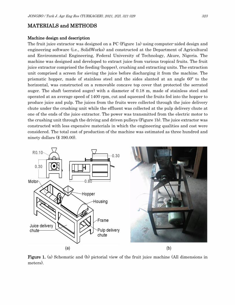
JONGBO / Turk J. Agr Eng Res (TURKAGER), 2021, 2(2), 321-329 323
MATERIALS and METHODS
Machine design and description
The fruit juice extractor was designed on a PC (Figure 1a) using computer-aided design and
engineering software (i.e., SolidWorks) and constructed at the Department of Agricultural
and Environmental Engineering, Federal University of Technology, Akure, Nigeria. The
machine was designed and developed to extract juice from various tropical fruits. The fruit
juice extractor comprised the feeding (hopper), crushing and extracting units. The extraction
unit comprised a screen for sieving the juice before discharging it from the machine. The
prismatic hopper, made of stainless steel and the sides slanted at an angle 60º to the
horizontal, was constructed on a removable concave top cover that protected the serrated
auger. The shaft (serrated auger) with a diameter of 0.18 m, made of stainless steel and
operated at an average speed of 1400 rpm, cut and squeezed the fruits fed into the hopper to
produce juice and pulp. The juices from the fruits were collected through the juice delivery
chute under the crushing unit while the effluent was collected at the pulp delivery chute at
one of the ends of the juice extractor. The power was transmitted from the electric motor to
the crushing unit through the driving and driven pulleys (Figure 1b). The juice extractor was
constructed with less expensive materials in which the engineering qualities and cost were
considered. The total cost of production of the machine was estimated as three hundred and
ninety dollars ($ 390.00).
Figure 1. (a) Schematic and (b) pictorial view of the fruit juice machine (All dimensions in
meters).

JONGBO / Turk J. Agr Eng Res (TURKAGER), 2021, 2(2), 321-329 324
Shaft design
A shaft of a total length of 0.41 m has a uniformly distributed serrated auger of the length of
0.27 m. The machine has a strong frame that could absorb any possible stress and load. To
determine the shear force and a bending moment of the shaft (beam) of the juicing machine,
the weights of the shaft’s component were mathematically determined. The weight of the
pulley, made of mild steel, was estimated at 5.0 N. The weight of the serrated auger per unit
length was estimated as 86.59 N m-1 and the machine was expected to be loaded with fruits
of an average weight per unit length of 181.67 N m-1.
The power required by the shaft
The linear velocity (𝑉) of the shaft was estimated as 13.29 m s-1 using
𝑉 = 𝑟𝑤 (1)
where 𝑟 is the radius of the pulley and 𝑤 is the angular velocity (revolution per second) of
the pulley. The maximum bending moment (𝑀𝑏) was estimated as 4.43 N m-1 using bending
moment diagram (BMD) and the torsional moment (𝑀𝑡) of 27.39 Nm was estimated using
𝑀𝑡 =𝑃
2𝜋𝑛 (2)
Where; 𝑃 is the estimated power required (4.044 kW or 5.4 HP) and 𝑛 is the number of
revolutions of the shaft per second. The diameter (𝑑) of the shaft was estimated as 21.6 mm
using
𝑑3 =16
𝜋𝑆𝑠√(𝐾𝑏𝑀𝑏)2 + (𝐾𝑡𝑀𝑡)2 (3)
where 𝑆𝑠 is the allowable stress (34.6 MPa), 𝐾𝑏 is the bending stress factor (1.5), 𝐾𝑡 is the
torsional stress factor (1.0), 𝑀𝑏 is the maximum bending moment, and 𝑀𝑡 is the torsional
moment. The factor of safety considered suitable for the shaft diameter was 1.35. In this
work, a standard shaft diameter of 25 mm was selected for the machine since a 21.6 mm
diameter shaft was not readily available for the work.
Design of auger
The auger on the shaft (Figure 2) was designed to convey the pulps of the fruit to the pulp
delivery chute. For the auger design, the theoretical capacity of the auger, which would
convey materials of an average mass of materials of 5.0 kg, was estimated as
0.0222 m3 min-1 using
𝑄 =(𝐷2−𝑑2)×𝑃𝑎×𝑛×∅
36.6 (4)

JONGBO / Turk J. Agr Eng Res (TURKAGER), 2021, 2(2), 321-329 325
Where D is the pitch diameter of the auger (m), d is the diameter of the shaft (m), 𝑃𝑎 is the
pitch of the auger, n is the shaft speed (revolution per minute), ∅ is the filling factor (0.45).
The torque 𝑇𝑐 of the auger was estimated as 2.80 N m-1 using
𝑇𝑐 =975×𝑃
𝑛 (5)
Where; P and n are the power required and the speed of the auger respectively. The load
propulsion speed 𝑉𝑐 and load per unit length 𝑉𝑐 of the auger of 0.94 m s-1 and
6.56 × 10⁻³ N m-1 were estimated using
𝑉𝑐 =𝑃𝑎×𝑛
60 (6)
and
𝐿𝑐 =𝑄
3.6𝑉 (7)
respectively. The axial thrust (Th) of the auger of 7.08 × 10⁻⁴ N was estimated using
𝑇ℎ = 𝐿𝑐 × 𝐿 × 𝜇 (8)
Where; L is the length of the auger and μ is the friction coefficient (0.4).
Figure 2. The serrated auger (all measurements in metres).
Belt and pulley design
The choice of the belt for the machine, over other power transmission devices such as chain,
was based on its ability to prevent vibration transmission, less expensive, ability to transmit
power between the axes of widely spaced shafts, and that its damage during operation would
not negatively affect the machine. Therefore, the design details of the belt (Figure 3) of the
machine are as follows. The wrap angle 𝛽 of the belt was estimated as 180° using

JONGBO / Turk J. Agr Eng Res (TURKAGER), 2021, 2(2), 321-329 326
𝛽 = 180° + 2𝑠𝑖𝑛−1 (𝑅1−𝑅2)
𝐶 (9)
Where; 𝑅1 and 𝑅2 are the radius of two pulleys (note that the pulleys have the same diameter),
𝐶 is the distance between the centers of two pulleys. The length of the belt was estimated as
0.90 m using
𝐿𝑏 = 2𝐶 +𝜋
2(𝐷1 + 𝐷2) (10)
Where; 𝐷1 and 𝐷2 are the diameters of the two pulleys. The tensions (𝑇1 and 𝑇2) on the belt
were estimated at 76.8 N and 24.97 N using
𝑇1 = 𝐴𝑙𝑙𝑜𝑤𝑎𝑏𝑙𝑒 𝑠𝑡𝑟𝑒𝑠𝑠 (0.06 𝑀𝑃𝑎) × 𝑇ℎ𝑖𝑐ℎ𝑛𝑒𝑠𝑠 𝑜𝑓 𝑏𝑒𝑙𝑡 (0.02𝑚) × 𝑤𝑖𝑑𝑡ℎ 𝑜𝑓 𝑏𝑒𝑙𝑡 (11)
and
𝑇1−𝑚𝑉2
𝑇2−𝑚𝑉2 = ℮𝜇𝛽 (12)
where 𝑚 is the mass of the belt (kg), 𝑉 is the estimated belt’s speed (m s-1), µ (0.25) is the
friction coefficient between the belt and the pulley. The power capacity (𝑃𝑏) of the belt was
estimated as 0.25 kW using
𝑃𝑏 = (𝑇1 − 𝑇2)𝑉. (13)
Figure 3. Belt design details
Experimental design and data analysis
The machine was tested with some fruits (sweet oranges and pineapple) based on their
cultivation by most of the farmers. A total of 15 kg of each of the fruits was acquired from the
local market during the study. The performance of the juice extractor was evaluated based
on the machine speed (1400 rpm) and the two different types of fruits used (sweet oranges
and pineapple). A motor with 1400 rpm was selected because of its price and availability in
the local market. Most of the motors with variable speeds are expensive and farmers could

JONGBO / Turk J. Agr Eng Res (TURKAGER), 2021, 2(2), 321-329 327
find it difficult to replace if the need arises. The test was repeated three times with each
containing 5 kg of the fruits. The time taken (minutes) by the machine to complete the
extraction was noted. The extracted juice was collected and weighed as kg. The juice
extraction capacity (kg h-1) and the juice extraction efficiency (%) of the machine were
determined using appropriate expressions.
Juice extraction capacity (kg ℎ𝑟−1) =mass of juice extracted
Time spent for the extraction (14)
Juice extraction efficiency (%) =mass of juice extracted
mass of maximum extractable juice× 100 (15)
The data were processed using Microsoft Excel 2019 and analysed using JMP® Pro 13.0.0
(SAS Institute Inc., 2016). The data was subjected to statistical analysis (t-test) to determine
the performance of the machine at a statistical significance of 5%.
RESULTS and DISCUSSION
The performance of the fruit juice machine was evaluated based on its extraction capacity
and extraction efficiency. As shown in Figure 4, it could be observed that a higher mean
extraction capacity per unit time (88.4 kg h-1) of the machine was obtained from the
pineapples. Since the fruits were ripe and peeled before being loaded into the machine, it
could indicate that the machine was able to crutch and extract almost all the juice in the
pineapple than it could with the sweet orange (84.50 kg h-1). Eyeowa et al. (2017), reported
that a manual juice extractor has an average extraction capacity of about 53% for both
pineapple and orange while about 1.0 kg of the total orange (3.80 kg) loaded into a fruit
juicing machine developed by Omoregie et al. (2018) was reported not be properly processed.
Similarly, Aviara et al. (2013) reported that a multipurpose fruit juicer could produce about
79% and 77% of juice from the peeled pineapple and orange loaded into it respectively. The
t-test analysis carried out showed that there was a significant difference (p = 0.0047) between
the mean extraction capacity of the machine when tested with pineapple and sweet orange.
Figure 4. Juice extraction capacity of the fruit juicing machine.

JONGBO / Turk J. Agr Eng Res (TURKAGER), 2021, 2(2), 321-329 328
The extraction efficiency of the fruit juice machine, as shown in Figure 5, indicated that the
efficiency of the machine, when tested with pineapple (91.13%), was higher than that of sweet
orange (85.96%). Higher efficiencies were reported by Aviara et al. (2013) who indicated that
their multipurpose juice extractor achieved 97% and 94% extraction efficiencies when tested
with peeled pineapple and orange respectively. However, the findings of Eyeowa et al. (2017)
showed that the efficiency of a manually operated juicing machine when tested with orange
(about 66%) was higher than that of pineapple (about 64%). The result of the statistical
analysis (t-test) conducted showed that there was a significant difference (p < 0.0001)
between the mean extraction efficiencies of the fruit juice machine when tested with
pineapple and sweet orange.
Figure 5. Juice extraction efficiency of the fruit juicing machine.
CONCLUSION
A multipurpose juicing machine with a serrated auger was developed and tested with peeled
pineapples and sweet oranges. The results of this study have shown that replacing the
smooth edge screw auger in the juicing machine with a serrated auger could increase the
extraction capacity (kg h-1) and efficiency (%) of the fruit juice machine. It has also been found
out that using a serrated auger could increase the extraction of juice from pineapple which
had been reported “to possess valuable bioactive compounds for medical purposes, increase
appetite for food nourishment” and many other benefits (Mohd Ali et al., 2020).
DECLARATION OF COMPETING INTEREST
The author would like to declare that there is no conflict of interest.
CREDIT AUTHORSHIP CONTRIBUTION STATEMENT
The author would like to declare that he solely developed all the sections in this manuscript.

JONGBO / Turk J. Agr Eng Res (TURKAGER), 2021, 2(2), 321-329 329
REFERENCES Adejumo OA, Adamade CA, Ayuba LO and Ozumba IC (2014). Performance evaluation of an improved NCAM
multi-fruit juice extractor. Journal of Agricultural Engineering and Technology (JAET), 22: 37-42.
Aviara NA, Lawal AA, Nyam DS and Bamisaye J (2013). Development and performance evaluation of a multi-
fruit juice extractor. Global Journal of Engineering, Design and Technology, 2: 16-21.
Cendres A, Chemat F, Maingonnat J and Renard CMGC (2011). An innovative process for extraction of fruit juice
using microwave heating. LWT - Food Science and Technology, 44: 1035-1041.
El-ramady HR, Domokos-szabolcsy É, Abdalla NA, Taha HS and Fári M (2015). Postharvest management of fruits
and vegetables storage postharvest management of fruits, in: Lichtfouse E. (Ed.), Sustainable Agriculture
Reviews. Springer International Publishing Switzerland, pp. 65–152.
Eyeowa AD, Adesina BS, Diabana PD and Tanimola OA (2017). Design, fabrication and testing of a manual juice
extractor for small scale applications. Current Journal of Applied Science and Technology, 22: 1-7.
FAO (2019). The state of food and agriculture 2019: Moving forward on food loss and waste reduction. Rome.
Mohd Ali M, Hashim N, Abd Aziz S and Lasekan O (2020). Pineapple (Ananas comosus): A comprehensive review
of nutritional values, volatile compounds, health benefits, and potential food products. Food Research
International, 137: 109675.
Mphahlele RR, Genis T, Fawole OA and Opara UL (2018). Sensory, quality and biochemical attributes of
pomegranate juice as affected by method of extraction. Acta Horticulturae, 1201: 115-121.
Mushtaq M (2018). Extraction of fruit juice: an overview, in: Rajauria, G., Tiwari, B.K. (Eds.), Fruit Juices:
Extraction, Composition Quality and Analysis. Elsevier, London, UK, pp. 131-159.
Nnamdi UB, Onyejiuwa CT and Ogbuke CR (2020). Review of orange juice extractor machines. Advances in
Science, Technology and Engineering Systems, 5: 485-492.
Ojha S, Fröhling, A, Durek J, Ehlbeck J, Tiwari BK, Schlüter OK and Bußler S (2021). Principles and application
of cold plasma in food processing, in: Innovative Food Processing Technologies. Elsevier, pp. 519-540.
Omoregie MJ, Francis-Akilaki TI and Okojie TO (2018). Design and fabrication of a juice extractor. Journal of
Applied Sciences and Environmental Management, 22: 207-212. Rajauria G and Tiwali BK (2018). Fruit juices: an overview, in: Rajauria, G., Tiwari, B.K. (Eds.), Fruit Juices:
Extraction, Composition Quality and Analysis. Academic Press, Elsevier, London, UK, pp. 3-14.
SAS Institute Inc. (2016). Using JMP® 13. SAS Institute Inc., Cary, NC, USA.
Suleiman AI, Bello S, Eguoaje SO and Michael O (2020). Fabrication and testing of a motorized turmeric juice
extracting machine. International Journal of Scientific Research and Engineering Development, 3: 523-531.

Turkish Journal of Agricultural
Engineering Research
https://dergipark.org.tr/en/pub/turkager https://doi.org/10.46592/turkager. 2021.v02i02.007
Research Article
Turk J Agr Eng Res
(TURKAGER)
ISSN: 2717-8420
2021, 2(2): 330-338
LabVIEW Based Real-time Color Measurement System
Abdullah BEYAZa*ID
a Department of Agricultural Machinery and Technologies Engineering, Faculty of Agriculture, Ankara University, 06130, Diskapi, Ankara, TURKEY
(*): Corresponding author, [email protected]
ABSTRACT
Colorimetry is of paramount importance to the agricultural industry.
Colorimetry refers to the processing of agricultural products for
consumer needs from a marketing point of view, and therefore the
agricultural industry spends a lot of money and time classifying each
product. In the past, agricultural professionals had to use program
codes that are difficult to learn, and even the most basic image
analysis for agricultural product classification required mastering
different program libraries. Today, the LabVIEW platform offers a
flexible, fast, easy-to-learn, and complete image analysis
infrastructure with various useful modules. For this reason, in this
study, a method analysis for color perception with a simple USB
webcam and software developed for real-time color analysis on the
LabVIEW platform is presented and its success in the basic color
analysis is tried to be revealed. The basic application developed for
this purpose in LabVIEW v2019 using NI Vision Development Module
v19 and NI IMAQ v19 modules. The basic fact that is the LabVIEW
application is the idea that LabVIEW can only be analyzed with
expensive IEEE 1394, but it should be known that these analyzes can
be done with USB webcams. For this purpose, the application includes
a USB webcam driver that can be stacked seamlessly. USB Webcam
and colorimeter measurement-based results of ƔR factors for each of
RGB color channels are 1.161232, 0.506287, 0.432229; ƔG factors for
each of RGB color channels are 0.519619, 1.025383, 1.201444; at last
ƔB factors for each of RGB color channels are 0.600362, 0.714016,
1.413406, respectively.
To cite: Beyaz A (2021). LabVIEW Based Real-time Color Measurement System. Turkish Journal of
Agricultural Engineering Research (TURKAGER), 2(2): 330-338.
https://doi.org/10.46592/turkager.2021.v02i02.007
RESEARCH ARTICLE
Received: 15.08.2021
Accepted: 14.10.2021
Keywords :
➢ Color recognition,
➢ Colorimeter,
➢ Real-time measurement,
➢ Webcam,
➢ LabVIEW
BEYAZ / Turk J. Agr Eng Res (TURKAGER), 2021, 2(2), 330-338 331
INTRODUCTION
Agricultural production areas have a lot of industrial applications. The application of
technology to agricultural processes has resulted in significant revenues. In addition, the use
of technology provides for precision and speed in tasks that individuals are unable to perform.
This situation leads to changes in agricultural output and processing. Different processes in
agriculture benefit from the use of technology, such as robotic weed control systems,
automatic harvesting systems, sorting machine systems, packing systems, grading and
identification of agricultural products, and so on.
For all of these types of cases, we employ color measurements. As a result, the use of color
sensors in agriculture is extremely important. Professional spectrometers, on the other hand,
are useless in agricultural applications from the low-cost product perspective. In general,
they are beneficial for data collection in laboratories. As a result, low-cost color sensors with
repeatable errors are required for field measurements. There is also a lot of application in
the literature about colormeter measurements.
The color of the fruit on the outside is an important factor for consumers when purchasing
agricultural products (Leon et al., 2006). The aesthetic quality standards of the items have
an impact on the prices of fruits and vegetables. As a result, distinguishing the color change
of fruits from the original fruits is difficult (Xing et al., 2006). For the quality analysis of
agricultural products, computer vision technology has advanced significantly
(Brosnan and Wen Sun, 2004). Computer vision units are also commonly employed in
industrial applications to identify fruit damage based on external color.
For evaluating faults on vegetables and fruits, Mendoza et al. (2006) investigated image
analysis units that assess standard sRGB color, HSV, and L*, a*, b* color spaces.
Ratule et al. (2006) studied the effects of cold storage on the chilling injury of the ‘Berangan'
banana (Musa cv. berangan).
Color measurement may be employed instead of chemical analysis, according to Fouda and
Salah (2014). A link between the colored component and the chemical in the food may also
exist. Color measurement is said to be easier and faster than chemical analysis.
Pawar and Dale (2016) used the Raspberry Pi 2 to detect flaws in 15 lemons and sort them
into categories. They used the Python programming language with OpenCV to create
algorithms for detecting and sorting lemons. They discovered that the faulty skin area may
be recognized for one pixel up to 4.3677 x 10⁻⁶ cm2. They further emphasize that their
technology was discovered to be more cost-effective and clever.
Narendra and Hareesh (2010) discuss the current development and application of image
analysis and computer vision systems in the agricultural and food industries for sorting and
grading items. According to them, computer vision systems are rapidly being used in the
business for inspection and evaluation. They also claim that the sorting and grading devices
can deliver a quick, cost-effective, sanitary, uniform, and objective assessment. However,
they point out that challenges remain, as seen by the comparatively delayed commercial
adoption of computer vision technologies across all industries.
According to Mahendran et al. (2011), computer vision is a fast, consistent, and objective
inspection tool that has spread across a wide range of industries. For completely automated

BEYAZ / Turk J. Agr Eng Res (TURKAGER), 2021, 2(2), 330-338 332
processes, the approaches' speed and precision meet ever-increasing production and quality
criteria.
The following factors influence the quality of agricultural products: size, color, shape, and
type of skin defects according to the international marketing standard. The color of the food
surface for customers is the first quality parameter. This is crucial in gaining market
acceptance for the product. The goal of the study was to use color analysis to assess color
change at RGB color samples.
MATERIALS and METHODS
The X-Rite Ci60 model colorimeter was used to determine the color of the primer (Figure 1).
A white reflecting plate was used to calibrate an X-Rite Ci60 colorimeter.
Figure 1. Calibration plate and X-Rite Ci60 portable spectrometer.
The Ci6x line of portable spectrometers (Ci60, Ci62, Ci64, and Ci64UV) provide a quick
and accurate way to determine the color at any point of the manufacturing process. The Ci6x
Series allows us to manage color in a simple, portable, and cost-effective manner. It allows
for all sizes of color measures due to the different alternatives of product family software.
Repeatable performances are also possible with this robust measurement technology. As a
result, the Ci6x series is a solid choice for a variety of agricultural tasks. Table 1 displays the
spectrometer's technical parameters.

BEYAZ / Turk J. Agr Eng Res (TURKAGER), 2021, 2(2), 330-338 333
Table 1. Technical specifications of X-Rite Ci60 spectrometer (Anonymous, 2021).
Properties Explanations
Measurement Geometrics
d/8°, DRS spectral engine, choice of optical aperture:
4 mm measurement area/6.5 mm target window
8 mm measurement area/14 mm target window
14 mm measurement area/20 mm target window
Receiver Blue-enhanced silicon photodiodes
Light Source Gas-filled tungsten lamp
Illuminant Type A, C, D50, D55, D65, F2, F7, F11, and F12
Standard Observer 2° and 10°
Spectral Range 400nm – 700nm
Spectral Interval 10nm – measured, 10nm – output
Measurement Range 0 to 200% reflectance
Measuring Time Approx. 2 seconds
Inter-Instrument Agreement (Ci60)
CIE L*a*b*:
Avg. 0.40 ΔE*ab, based on avg. of 12 BCRA series II
tiles
(specular component included)
Max. 0.60 ΔE*ab on any tile (specular component
included)
Short-Term Repeatability (Ci60) 10 ΔE*ab on white ceramic (standard deviation)
RGB color plate webcam video was measured firstly with LabVIEW color measurement
software to compare them with colorimeter measurements to get calibration factors.
Measurements were done in the room light condition and it was 250 lux. The webcam was
placed 25 cm far from the color plates for the measurements (Figure 2).
Figure 2. Webcam.
For graphical programming, LabVIEW software comprises two parts: a front panel and a
block diagram. The front panel is an interactive software component that contains an
interface area with several components and allows the user to insert data into the software
(Figure 3).

BEYAZ / Turk J. Agr Eng Res (TURKAGER), 2021, 2(2), 330-338 334
Figure 3. Color measurement application's front panel.
The actual programming procedure was carried out on the block diagram. The source codes
run into this problem, which is caused by the use of virtual object linkages (Figure 4).
Figure 4. Application block diagram for color measurement.

BEYAZ / Turk J. Agr Eng Res (TURKAGER), 2021, 2(2), 330-338 335
In the block diagram of the color determination software, first, a session is opening with
an image acquisition tool by this way video source is open for color sensitivity selection, after
that color spectrum is determined by the software. In the end, colors are determined by the
given ranges of the color spectrum.
RESULTS and DISCUSSION
According to test results, utilizing calibration factors, webcam-based LabVIEW software can
deliver satisfactory accurate RGB data. As a result, a webcam can be used in agricultural
and industrial applications. Table 2 displays the RGB color plate calibration factors. In the
table, RRN, RGN, RBN values are red, green, blue values of red plate measured by using
National Instruments LabVIEW software; RR, RG, RB values are red, green, blue values of
red plate measured by using colorimeter; GRN, GGN, GBN values are red, green, blue values
of green plate measured by using National Instruments LabVIEW software; GR, GG, GB
values are red, green, blue values of green plate measured by using colorimeter; BRN, BGN,
BBN values are red, green, blue values of plate measured by using National Instruments
LabVIEW software; BR, BG, BB values are red, green, blue values of blue plate measured by
using colorimeter.
Table 2. Calibration factors for the test materials.
ƔR ƔG ƔB
Red plate 1,161232 0,519619 0,600362
Green plate 0,506287 1,025383 0,714016
Blue plate 0,432229 1,201444 1,413406
Red, green, and blue color plate measurements were taken at both devices to improve RGB
color measuring efficiency (Figure 2).
Figure 2. Plates in red, green, and blue color.

BEYAZ / Turk J. Agr Eng Res (TURKAGER), 2021, 2(2), 330-338 336
Table 3. Color measurements on red, green, and blue plates.
RRN RGN RBN RR RG RB GRN GGN GBN GR GG GB BRN BGN BBN BR BG BB
160 72 81 161 68 81 68 138 94 59 138 93 59 149 180 62 159 183
160 72 80 161 68 81 68 136 92 72 139 97 56 154 175 52 156 181
159 71 80 159 71 83 69 138 94 72 139 96 56 155 178 61 160 184
160 71 80 161 72 84 69 138 95 60 139 94 57 157 182 62 159 183
158 70 79 161 72 84 69 138 95 62 141 96 58 160 185 60 159 183
163 69 79 160 72 83 68 136 94 70 138 95 57 156 182 60 159 183
160 70 80 160 71 83 67 135 93 72 139 97 56 155 180 63 160 183
158 70 79 160 71 83 68 136 94 67 135 93 56 155 180 59 159 183
158 70 79 160 71 83 68 136 95 70 136 94 56 154 175 60 159 183
158 70 80 160 71 83 68 136 94 68 136 93 57 155 181 60 159 183
159 70 79 160 71 83 68 136 95 70 137 94 56 155 181 61 160 184
158 70 80 160 70 82 69 138 96 68 135 93 56 157 181 62 160 184
159 71 80 161 72 83 69 138 95 70 137 94 56 157 180 61 160 184
159 70 79 161 72 84 68 136 94 67 135 92 57 157 182 53 156 181
161 71 79 160 69 82 68 136 95 70 137 94 57 157 181 52 156 181
163 71 80 160 71 83 70 139 98 68 135 93 59 162 185 52 156 181
160 71 80 160 72 83 69 138 96 70 136 94 60 166 189 51 156 181
164 72 80 160 71 83 68 136 95 69 137 95 61 166 191 52 156 181
164 73 80 160 71 83 68 136 94 72 138 96 61 167 191 53 156 181
164 73 80 160 71 83 71 139 96 73 140 97 60 166 189 52 156 181
There are a lot of applications for color analysis in the literature. For example,
Yeni and Shaowei (2017) used LabVIEW and machine vision to develop a fault inspection
system for the carbonized bamboo cane. According to the findings of the experiments, this
system can classify five different types of bamboo canes with flaws at a speed of 70 mm s-1,
and the average recognition rate of defect bamboo canes can exceed 90.6%.
The creation of a flame detection system in LabVIEW is the focus of Riyadi and Aisyah's
study. They imply that for the development of fire early warning systems, flame detection
systems are useful. In general, traditional fire detection systems that rely on heat detectors
to detect temperature changes are unable to detect the presence of fire. A camera acting as
an image scanner sensor could be used to identify the shape or color of a flame. The goal of
the research is to create an image processing flame detection system using image
enhancement, color segmentation, and filtering techniques, all of which are implemented
using LabVIEW's Vision Assistant. They stress that, the system runs at 30 frames per second
with a resolution of 1024 x 768 pixels, with a 98 percent accuracy.
Rice clusters were separated at the rice harvest by Yu et al. (2021), who worked for high
yield and grain quality. They created a system that utilized X-ray and RGB scanning as well
as deep learning. They created a pipeline for analysis and came up with five distinct ways to
count rice. As a result, good accuracy (R 2 = 0.99) and speed were achieved. The classification
of indica and japonica yielded a 91 percent accuracy. It is worth noting that this is a positive
outcome for rice breeding.

BEYAZ / Turk J. Agr Eng Res (TURKAGER), 2021, 2(2), 330-338 337
Given the literature results, the research findings appear to be more successful than those
found in the literature.
CONCLUSION
It is required to meet the ever-increasing requirements of the agriculture business due to the
development of color vision technology. As a result, imaging technology will see more use and
popularity in the future years. After reviewing the literature and evaluating the results, we
can conclude that a LabVIEW video processing-based color detection system is functional and
may be used as part of a sorting machine for this purpose.
High quality and safety standards have begun to be sought as consumer expectations for
agricultural products have risen. These product characteristics should be determined
precisely, rapidly, and objectively. To achieve these objectives, the new vision offers an
alternative to an automated, non-destructive, and cost-effective technique. Various image
processing methods based on image analysis in the agriculture business have been developed
in response to these requirements.
The image investigation in this study was conducted using a color detection system based
on LabVIEW video processing. We can easily and inexpensively obtain data in the sector by
utilizing computer vision frameworks. This article shows how these procedures, as well as
further calibration, can help attain accuracy. On three color plates, the study is conducted
for agricultural purposes. Automation of sorting applications for improving and classifying
item quality is a significant advancement. This study shows how LabVIEW can be used in
agriculture. This technique is adaptable and is being employed in a variety of agricultural
products. More productive work can be done with the help of developed algorithms and
efficient working methods. Snapshot analysis is based on picture analysis and is still in the
early stages of development.
DECLARATION OF COMPETING INTEREST
The author would like to declare that there is no conflict of interest.
CREDIT AUTHORSHIP CONTRIBUTION STATEMENT
The author would like to declare that he solely developed all the sections in this manuscript.
REFERENCES
Anonymous (2021). Ci6X series spectrophotometer user manual. https://www.xrite.com/-
/media/xrite/files/manuals_and_userguides/c/i/ci6x-500/ci6x-500_user_guide_en.pdf (29.08.2021)
Brosnan T and Wen Sun D (2004). Improving quality inspection of food products by computer vision-a review.
Journal of Food Engineering, 61: 3-16.
Fouda T and Salah, S (2014). Using imaging analyses to predict chemical properties of orange fruits. Scientific
Papers Series Management. Economic Engineering in Agriculture and Rural Development, 14(3): 83-86.
Leon K, Mery D and Leon J (2006). Colour measurment in L*a*b* units from RGB digital images. Food Research
International, 39: 1084-1091.

BEYAZ / Turk J. Agr Eng Res (TURKAGER), 2021, 2(2), 330-338 338
Mahendran R and Jayashree GC and Alagusundaram K (2011). Application of computer vision technique on
sorting and grading of fruits and vegetables. Journal of Food Process Technology, S1-001.
Mendoza F, Dejmek P and Aguilera JM (2006). Calibrated colour measurements of agricultural foods using image
analysis. Postharvest Biology and Technology, 41: 285-295.
Narendra VG and Hareesh KS (2010). Prospects of computer vision automated grading and sorting systems in
agricultural and food products for quality evaluation. International Journal of Computer Applications,
(0975 – 8887), 1(4): 1-9.
Pawar SS and Dale MP (2016). Lemon detection and sorting system based on computer vision. 3rd International
Conference on Electrical, Electronics, Engineering Trends, Communication, Optimization and Sciences
(EEECOS) -2016, 376-379.
Ratule MT, Osman A, Ahmad SH and Saari N (2006). Development of chilling injury of ‘Berangan’ banana (Musa
cv. Berangan (AAA)) during storage at low temperature. Journal of Food Agriculture & Environment, 4(1):
128-134.
Riyadi DS and Aisyah S (2018). Vision based flame detection system for surveillance camera. In 2018
International Conference on Applied Engineering (ICAE) (pp. 1-6). IEEE.
Yu L, Shi J, Huang C, Duan L, Wu D, Fu D, Wu C, Xiong L, Yang W and Liu Q (2021). An integrated rice panicle
phenotyping method based on X-ray and RGB scanning and deep learning. The Crop Journal, 9(1): 42-56.
Xing J, Bravo C, Moshou D, Roman H and Baerdemaeker JD (2006). Bruise detection on ‘Golden Delicious’ apples
by vis/NIR spectroscopy. Computers and Electronics in Agriculture, 52: 11-20.
Yeni L and Shaowei Y (2017). Defect inspection system of carbonized bamboo cane based on LabView and Machine
Vision. In 2017 International Conference on Information, Communication and Engineering (ICICE) pp. 314-
317. IEEE.

Turkish Journal of Agricultural
Engineering Research
https://dergipark.org.tr/en/pub/turkager https://doi.org/10.46592/turkager.2021.v02i02.008
Research Article (Araştırma Makalesi)
Turk J Agr Eng Res
(TURKAGER)
e-ISSN: 2717-8420
2021, 2(2): 339-347
Comparison of Yield and Yield Components of Different Anise
(Pimpinella anisum L.) Populations Under Eskişehir Ecological Conditions
Nimet KATARIDa, Mustafa CANIDb*, Duran KATARIDc
aİl Tarım ve Orman Müdürlüğü, Eskişehir, TÜRKİYE bİl Tarım ve Orman Müdürlüğü, Uşak, TÜRKİYE cTarla Bitkileri Bölümü, Ziraat Fakültesi, Eskişehir Osmangazi Üniversitesi, Eskişehir,TÜRKİYE (*): Corresponding author, [email protected]
ABSTRACT
In this study, it was aimed to reveal the effect of different
genotypes (population) of anise (Pimpinella anisum L.) on yield
and yield components. The experiment was carried out under
Eskişehir ecological conditions in the growing season of 2017
and 2018. Four different anise population (Afyon, Bilecik,
Çeşme and Burdur) obtained from different parts of Turkey was
used in the study. Plant materials were cultivated in
randomized complete block design with three replications. The
results showed that the populations had a significant
differences on other all parameters examined except 1000 seed
weight (g). The highest seed yield (80.56 and 76.31 kg da-1,
respectively) and the highest essential oil yield (2.17 and
2.22 L da-1, respectively) were obtained from Bilecik and Çeşme
populations. On the other hand, the essential oil contents
obtained from the populations varied between 2.67-2.92%, and
it is seen that these values are above the 2% limit stated in the
European pharmacopoeia. As a result, it was determined that
Bilecik and Çeşme populations are superior populations among
the populations examined in terms of high seed and essential
oil yields.
To cite: Katar N, Can M, Katar D (2021). Comparison of Yield and Yield Components of Different
Anise (Pimpinella anisum L.) Populations Under Eskişehir Ecological Conditions. Turkish
Journal of Agricultural Engineering Research (TURKAGER), 2(2): 339-347.
https://doi.org/10.46592/turkager.2021.v02i02.008
RESEARCH ARTICLE
Received: 19.08.2021
Accepted: 24.10.2021
Keywords:
➢ Pimpinella anisum,
➢ Genotype,
➢ Yield,
➢ Essential oil content,
➢ Essential oil yield

KATAR et al., / Turk J. Agr Eng Res (TURKAGER), 2021, 2(2), 339-347 340
Eskişehir Ekolojik Koşullarında Farklı Anason (Pimpinella anisum L.)
Populasyonlarının Verim ve Verim Öğelerinin Karşılaştırılması
ÖZET
Bu çalışmada, farklı genotiplerin (populasyon) anasonun
(Pimpinella anisum L.) verim ve verim bileşenleri üzerindeki
etkisini ortaya çıkarmak amaçlanmıştır. Deneme, Eskişehir
ekolojik koşullarında 2017 ve 2018 yılları yetiştirme döneminde
gerçekleştirilmiştir. Çalışmada Türkiye’nin farklı bölgelerinden
temin edilen dört farklı anason populasyonu (Afyon, Bilecik, Çeşme
ve Burdur) kullanılmıştır. Bitki materyalleri, tesadüf blokları
deneme desenine göre üç tekerrürlü olarak yetiştirilmiştir.
Sonuçlar, populasyonların 1000 tohum ağırlığı (g) hariç incelenen
diğer tüm parametrelerde önemli farklılığa sahip olduğunu
göstermiştir. Bilecik ve Çeşme populasyonlarından en yüksek
tohum verimi (sırasıyla 80.56 ve 76.31 kg da-1) ve en yüksek uçucu
yağ verimi (sırasıyla 2.17 ve 2.22 L da-1) elde edilmiştir. Diğer
taraftan çalışmada elde edilen uçucu yağ oranı %2.67-2.92 arasında
değişmiş, Avrupa farmakopesinde belirtilen % 2 sınırının üzerinde
olduğu görülmüştür. Netice olarak; çalışmada yer alan
populasyonlar arasında yüksek tohum ve uçucu yağ verimleri
açısından Bilecik ve Çeşme populasyonlarının öne çıktığı
belirlenmiştir.
GİRİŞ
Apiaceae familyası Dünya’da 300 cins ve yaklaşık 3000 türü ihtiva etmektedir. Bu familya
içinde yer alan anason (Pimpinella anisum) bitkisi, Akdeniz havzasında ve Güney Batı
Asya’da doğal yayılış gösteren tek yıllık aromatik bir bitkidir (Albulushi ve ark., 2014;
Salim ve ark., 2016; Karac ve Efe, 2017). Yaklaşık 90 cm boyuna kadar büyüyen ve otsu
bir bitki olan anason; şemsiye şeklinde, yaklaşık 3 mm çapında ve beyaz renkte çiçeklere
sahip olup şizokarp meyveleri 3-5 mm uzunluğundadır (Albulushi ve ark., 2014;
Hassan ve Elhassan, 2017). Ayrıca bitkinin meyveleri 1-3 mm genişlik ve 3-6 mm
uzunlukta, kısa saplı, ters armut biçiminde, yeşilimsi-sarı veya gri-yeşil renkli olup üzeri
tüylerle kaplıdır (Orav ve ark., 2008; Shojaii ve Abdollahi Fard, 2012). Son yıllarda
yapılan birçok bilimsel çalışma, ilaç kaynağı olarak kullanılan birçok bitki türü olduğunu
göstermiştir. Tıbbi amaçlı kullanılan önemli bitkilerden biri olan anason
(Pimpinella anisum L.) bitkisinin özellikle meyveleri pek çok ülkenin halk hekimliğinde
gaz giderici, mide koruyucu, aromatik ve dezenfektan olarak kullanılmıştır.
Bugüne kadar, anason tohumları üzerinde çok sayıda farklı bilimsel çalışma yapılmış,
antimikrobiyal, antifungal, antiviral, antioksidan, kas gevşetici, ağrı kesici ve anti-
spazmodik etkilerinin yanı sıra sindirim sistemi üzerinde farklı etkileri olduğu
bildirilmiştir (Shojaii ve Abdollahi Fard, 2012; Salim ve ark., 2016). Günümüzde anason,
eczane, parfümeri, gıda ve kozmetik endüstrilerinde kullanılan önemli bir hammaddedir
(Albulushi ve ark., 2014). Ayrıca morfinizmi azaltıcı etkisinin yanı sıra kadınlarda adet
ağrılarına ve menopozdaki kadınlarda yüksek ateşe karşı etkilidir. Şeker hastaları için,
Alıntı için: Katar N, Can M, Katar D (2021). Eskişehir Ekolojik Koşullarında Farklı Anason
Pimpinella anisum L.) Populasyonlarının Verim ve Verim Öğelerinin Karşılaştırılması. Turkish
Journal of Agricultural Engineering Research (TURKAGER), 2(2): 339-347.
https://doi.org/10.46592/turkager.2021.v02i02.008
ARAŞTIRMA MAKALESİ
Alınış tarihi: 19.08.2021
Kabul tarihi: 24.10.2021
Anahtar Kelimeler:
➢ Pimpinella anisum,
➢ Genotip,
➢ Verim,
➢ Uçucu yağ oranı,
➢ Uçucu yağ verimi

KATAR et al., / Turk J. Agr Eng Res (TURKAGER), 2021, 2(2), 339-347 341
anason tohumları kandaki glikoz değerini ve lipid seviyesini düşürmekle birlikte aynı
zamanda lipid peroksidasyonunu da azaltmaktadır (Shojaii ve Abdollahi Fard, 2012).
Diğer taraftan anason, gıda endüstrisinde deniz ürünleri, dondurma, tatlılar ve sakız gibi
farklı ürünlere lezzet ve aroma vermek için kullanılmaktadır (Salim ve ark., 2016).
Anason esansiyel yağı ve çayı aromaterapide nefes darlığını gidermek için kullanıldığı
gibi doğal bir astım ilacı olarak da kullanılmaktadır. Ayrıca anason esansiyel yağı, bitler
ve diğer böceklerin neden olduğu kaşıntı tedavisinde, baş ve vücut bitleri ile mücadelede
etkili olmakla birlikte uçucu yağından elde edilen merhemlerin uyuz tedavisinde haricen
kullanımı tavsiye edilmektedir (Albulushi ve ark., 2014). Anason tohumunun kalitesi,
uçucu yağın oranı ve uçucu yağın bileşimi ile doğrudan ilgili olup, uçucu yağın bileşimi ise
bitkinin genotipi ile yetiştirme yöntemine bağlı olarak önemli ölçüde değişmektedir
(Albulushi ve ark., 2014 ).
Anason tohumunun, %9-13 nem, %18 protein, %8-23 yağ, %1.5-7.0 (ort. %2-3) uçucu
yağ, %5 nişasta, %22-28 N-içermeyen özüt ve %12-25 ham lif ihtiva ettiği bildirilmiştir
(Salim ve ark., 2016; Karac ve Efe, 2017). Avrupa farmakopesine göre ilaç olarak
kullanılacak anason tohumlarının en az %2 uçucu yağ içermesi gerekmektedir
(Albulushi ve ark., 2014). Anason tohumunun %1.5-7'sini oluşturan uçucu yağın en önemli
bileşikleri trans-anethole, estragolle, γ-hymachalene, paraanisaldehyde ve methyl
cavicol'dur (Shojaii ve Abdollahi Fard, 2012; Khalid, 2015; Hassan ve Elhassan, 2017).
Bazı çalışmalar, anason uçucu yağının en önemli bileşiği olan trans-anetholün uçucu
yağın %80-90'ını oluşturduğunu göstermiştir (Albulushi ve ark., 2014;
Salim ve ark., 2016). Diğer taraftan yapılan farklı bir çalışmada ise anason uçucu yağının
ana bileşeninin küminaldehit olarak belirlendiği rapor edilmiştir (Katar ve Katar, 2020).
Bitkilerin büyümesinde ve gelişmesinde etkili olan faktörler genellikle içsel ve dışsal
faktörler olarak ikiye ayrılmaktadır. İçsel faktörler, bitkilerin genetik yapısı ile doğrudan
ilgili olduğundan çeşitli kalıtsal özelliklere sahip bitkilerin büyüme ve gelişme
performansları, genlerinin etkisine göre farklılık göstermektedir (Hussain ve ark., 2006).
Tarımda daha yüksek verim ve kalite elde etmenin en önemli faktörlerinden biri, bölgeye
adapte olmuş uygun genotip (tescilli çeşit/populasyon) seçimidir. Yerli bitki
populasyonları genellikle bölgesel koşullara daha iyi uyum sağlamakla birlikte özellikle
tescilli çeşit sayısı çok az olan ülkemiz tıbbi ve aromatik bitkilerin tarımında
populasyonların tohumluk olarak kullanımı daha yaygındır. Nitekim yapılan bir
araştırmada önemli tıbbi ve aromatik bitkilerden olan çörek otu tarımında çiftçilerin
tescilli bir çeşit (Çameli) bulunmasına rağmen bu çeşidi sadece %1.37 oranında üretimde
kullandığı, bir başka ifade ile %98.63 oranında çörek otu populasyonları tohumluğunu
kullanarak üretim yaptığını ortaya koymuştur (Can, 2020). Bu nedenle çeşitli ekolojik
koşullar altında bu popülasyon verim ve kalite potansiyelinin belirlenmesi gerekmektedir.
Anason genotiplerinin verim, verim bileşenleri ve kalite karakterleri üzerindeki etkisi
birçok araştırmacılar tarafından incelenmiştir (İpek ve ark., 2004; Nabizadeh ve ark.,
2012; Faravani ve ark., 2013; Sönmez, 2018; Karık, 2020). Ancak bu çalışmaların her biri
farklı ekolojik koşullar altında farklı anason genotipleri ile yapılmıştır.
Bu nedenle Eskişehir ekolojik koşullarında yürütülen bu çalışmada, farklı anason
genotiplerinin (popülasyon) verim ve verim bileşenleri açısından performanslarının
ortaya çıkarılması amaçlanmıştır.

KATAR et al., / Turk J. Agr Eng Res (TURKAGER), 2021, 2(2), 339-347 342
MATERYAL ve YÖNTEM Çalışma 2017 ve 2018 yıllarının ürün yetiştirme döneminde Eskişehir Osmangazi
Üniversitesi Ziraat Fakültesi Tarla Bitkileri deneme tarlalarında gerçekleştirilmiştir.
Denemede bitki materyali olarak Afyon, İzmir-Çeşme, Bilecik ve Burdur yörelerinde
anason yetiştiriciliği yapan çiftçilerden temin edilen 4 farklı anason populasyonu
kullanılmıştır. Çalışma alanı topraklarının özellikleri Çizelge 1'de verilmiştir. Buna göre
toprağın tınlı tekstürde, hafif alkalin karakterde, orta kireçli, tuzluluk problemi olmayan,
organik madde içeriğinin orta, faydalanılabilir fosfor oranının orta ve faydalanılabilir
potasyum oranının yüksek olduğu belirlenmiştir.
Çizelge 1. Deneme alanı toprağının bazı fiziksel ve kimyasal özellikleri*.
Table 1. Some physical and chemical characteristics of soils in experimental field.
Tekstür
Toplam
Kireç
(%)
EC
(ds m-1)
Faydalanılabilir
P2O5 (kg da-1)
Faydalanılabilir
K2O (kg da-1)
pH
Organik
Madde (%)
Tınlı
(2017) 5.55 0.035 5.96 195.28 7.18 2.43
Tınlı
(2018) 5.32 0.042 6.61 248.27 7.53 2.82
* Toprak analizleri Geçit Kuşağı Tarımsal Araştırma Enstitüsü Müdürlüğü Toprak-Su Laboratuvarında yapılmıştır.
Deneme alanının 2017, 2018 ve uzun dönem (1970-2011) ortalama sıcaklık ve toplam
yağış verileri Çizelge 2'de sunulmuştur. 2017 (374.4 mm) ve 2018 (411.8 mm) yılları
toplam yağış miktarı değerlerinin uzun dönem toplam yıllık yağış miktarı ortalamasından
(338.8 mm) daha yüksek olduğu görülmüştür. Ayrıca, uzun dönemde gözlemlenen
ortalama sıcaklık değerinin, hem 2017 hem de 2018 ortalama sıcaklık değerlerinden daha
düşük olduğu görülmektedir. 2017 ve 2018'de ortalama sıcaklık sırasıyla 11.29°C ve
12.50°C olarak gerçekleşmiştir (Çizelge 2).
Çizelge 2. Deneme alanına ait bazı iklim verileri*.
Table 2. Some climatic data of the experimental area.
Aylar Toplam yağış (mm) Ortalama sıcaklık (°C)
2017 2018 UY 2017 2018 UY
Ocak 33.0 30.0 30.6 -2.0 1.4 -0.2
Şubat 9.2 28.8 26.1 1.9 5.6 0.9
Mart 16.2 49.8 27.6 7.6 8.9 4.9
Nisan 62.0 16.8 43.1 9.6 13.6 9.6
Mayıs 50.8 72.0 40.0 14.4 16.4 14.9
Haziran 44.8 60.6 23.7 19.1 19.3 19.1
Temmuz 13.4 42.0 13.1 23.1 21.9 22.1
Ağustos 31.4 19.3 9.2 22.0 22.7 21.8
Eylül 3.0 3.8 18.1 19.6 18.3 16.7
Ekim 46.6 30.1 32.8 10.8 13.0 11.7
Kasım 27.8 18.6 34.0 5.5 7.4 5.6
Aralık 36.2 40.0 40.5 3.9 1.7 1.7
Toplam 374.4 411.8 338.8 - - -
Ortalama - - - 11.3 12.5 10.7
*Veriler Eskişehir Meteoroloji 3. Bölge Müdürlüğü’nden temin edilmiştir. UY: Uzun Yıllar (1970-2011)

KATAR et al., / Turk J. Agr Eng Res (TURKAGER), 2021, 2(2), 339-347 343
Tarla denemeleri tesadüf blokları deneme desenine göre 3 tekerrürlü olarak
kurulmuştur. Tohumlar, dekara 2 kg hesabıyla, 2-3 cm derinliğe ve 20 cm sıra aralığında
elle ekilmiştir. Ekim, birinci yıl 13 Nisan 2017 tarihinde, ikinci yıl 20 Nisan 2018 tarihinde
gerçekleştirilmiştir. Her deneme parselinin uzunluğu 5 m olup 6 sıradan oluşmaktadır.
Yabancı ot kontrolü gerektiğinde elle yapılmış, sulama uygulanmamıştır. Deneme
parselleri, saf olarak dekara 5 kg N ve 4 kg P2O5 olacak şekilde gübrelenmiştir.
7 Temmuz 2017 ve 10 Temmuz 2018 tarihlerinde parsellerin her iki tarafından bir sıra
kenar tesiri olarak bırakılmış ve ardından parsellerdeki bitkiler elle hasat edilmiştir.
Uçucu yağ oranları su distilasyonu yöntemiyle belirlenmiştir. Uçucu yağların distilasyonu
için 100 g tohum örnekleri 2000 ml’lik balonlara yerleştirildikten sonra 1 litre saf su
eklenerek 3 saat boyunca distilasyon işlemi gerçekleştirilmiştir. Distilasyon işlemi
tamamlandıktan sonra clevenger aparatının dereceli kısmından yağ miktarı okunarak %
olarak belirlenmiştir (Anonim, 2010).
Çalışmadan elde edilen veriler SPSS paket programı kullanılarak tesadüf blokları
deneme desenine göre varyans analizine tabi tutulmuş, incelenen özelliklerin önemlilik
düzeyleri belirlenmiştir. Önemli çıkan ortalama değerler arasındaki farklar Tukey testi
(p≤0.05) ile karşılaştırılmıştır.
BULGULAR ve TARTIŞMA
Çalışmada yer alan anason populasyonları, yıllar ve yıl x populasyon interaksiyonu bitki
boyunda önemli (p≤0.01) farklılığa sebep olmuştur. Genotipler karşılaştırıldığında yıllar
ortalamasında en yüksek bitki boyu Afyon (49.30 cm) ve Çeşme (48.23 cm)
populasyonlarında belirlenirken, en düşük bitki boyu Burdur (43.14 cm) ve Bilecik (44.56
cm) populasyonlarında belirlenmiştir. 2017 yılında elde edilen ortalama bitki boyu değeri
(45.85 cm) ile karşılaştırıldığında 2018 yılında daha yüksek bitki boyu değeri (46.77 cm)
elde edilmiştir (Çizelge 3). Bu durum, yıllık toplam yağış değeri ile bitkinin ilk gelişim
gösterdiği aylardaki (Nisan-Mayıs) ortalama sıcaklık değerlerinin 2018 yılında bir önceki
yıla göre daha yüksek olmasından kaynaklandığı düşünülmektedir (Çizelge 2). Bitki boyu
her ne kadar çevresel faktörlerden ve agronomik uygulamalardan etkilense de esas olarak
bitki materyalinin genetik yapısı tarafından kontrol edilmektedir (Baloch ve ark., 2010).
Bitki boyu değerleri yıl x populasyon interaksiyonu açısından incelendiğinde, 2017 yılında
bitki boyu maksimum Afyon (48.80 cm), minimum Bilecik (42.79 cm) populasyonlarında,
2018 yılında ise bitki boyu maksimum Çeşme (49.90 cm), minimum Burdur (41.03 cm)
populasyonlarında kaydedilmiştir. İpek ve ark. (2004) anasonda bitki boyunu 44.7-50.2
cm arasında, Yıldırım (2010), ise 33.73-39.73 cm arasında bulmuşlardır. Çalışmalarda
elde edilen bitki boyu değerleri arasındaki farklılık, kullanılan bitki materyallerinin
genetik yapısındaki değişim ve çalışma bölgelerinin farklı ekolojik koşulları ile
açıklanabilir.
Yıllar ve populasyonlar bitki başına şemsiyeli dal sayısı üzerine p≤0.01 düzeyinde
önemli bir farklılık göstermiştir. 2018 yılında (4.99 adet) 2017 yılına (3.78 adet) kıyasla
daha yüksek bir bitki başına şemsiyeli dal sayısı değeri belirlenmiştir. Denemenin ikinci
yılı (2018) toplam yağış ve ortalama sıcaklık değerlerinin ilk yıla (2017) kıyasla yüksek
gerçekleşmesi bitkinin daha iyi gelişimini ve dallanmasını netice vermiş, bitki başına
şemsiyeli dal sayısı daha fazla olmuştur. İki yıllık ortalama olarak bitki başına şemsiyeli
dal sayısı 3.89-5.21 adet arasında değişmiş ve en yüksek değer Bilecik populasyonunda

KATAR et al., / Turk J. Agr Eng Res (TURKAGER), 2021, 2(2), 339-347 344
tespit edilmiştir (Çizelge 3). Benzer olarak Katar ve Katar (2020) anasonda bitki başına
şemsiyeli dal sayısını 3.09-6.50 adet arasında bulmuşlardır.
Bin tohum ağırlığı açısından sadece yıllar arasında önemli bir fark bulunmuştur.
Populasyonların ortalaması olarak 1000 tane ağırlığı 2017'de 3.46 g, 2018'de 4.29 g olarak
kaydedilmiştir (Çizelge 3). Çalışmadan elde edilen 1000 tohum ağırlığı değerleri,
incelenen anason populasyonlarının bu parametre üzerinde önemli bir etkisi olmadığını
göstermiştir. Bununla birlikte, en yüksek bin tohum ağırlığı 2017 yılında Burdur (3.17 g)
popülasyonundan, en düşük bin tohum ağırlığı ise 2018 yılında Çeşme (4.36 g)
popülasyonundan alınmıştır. Yıllar ortalamasında ise Bilecik ve Burdur Afyon
popülasyonlarından en düşük (3.77 g) ve Çeşme popülasyonundan en yüksek (4.02 g)
değerler ölçülmüştür. Yapılan birçok araştırmada anasonda bin tohum ağırlığının 2.64-
5.62 g arasında elde edildiği rapor edilmiştir (İpek ve ark., 2004; Faravani ve ark., 2013;
Sönmez, 2018; Katar ve Katar, 2020).
Yılların ve populasyonların tohum verimi (kg da-1) üzerindeki etkisi önemli olmuştur.
Ortalama tohum verimi 2017'de 65.02 kg da-1 iken 2018'de 70.27 kg da-1 olarak
belirlenmiştir. İki yıllık ortalamaya göre tohum verimi 56.66 ile 80.56 kg da-1 arasında
değişmiş, en yüksek değer Bilecik populasyonunda tespit edilmiştir. Ancak tohum verimi
açısından Bilecik (80.56 kg da-1) ve Çeşme (76.31 kg da-1) populasyonları arasında
istatistiksel olarak anlamlı bir fark bulunmamıştır (Çizelge 3). Nabizadeh ve ark. (2012),
anasonda tohum verimini 17.91-128.64 kg da-1 arasında, Faravani ve ark. (2013) ise 37.08-
40.36 kg da-1 arasında aldıklarını rapor etmişlerdir. Bulgularımıza benzer sonuçlar
sırasıyla 42.20-87.00 kg da-1 ve 62.16-86.20 kg da-1 olmak üzere İpek ve ark. (2004) ile
Sönmez (2018) tarafından da elde edilmiştir.
Aromatik bitkilerden olan anason bitkisinin en önemli kalite kriterlerinden biri hiç
şüphesiz uçucu yağ oranıdır. İki yıllık ortalamaya göre uçucu yağ oranı değerleri
%2.67-2.92 arasında değişmiş olup, en yüksek değer Çeşme populasyonunda elde
edilirken, bu populasyonu Burdur ve Bilecik populasyonları takip etmiştir. Her üç
populasyon istatistiki olarak aynı grupta yer almıştır. 2017 ve 2018 yıllarında uçucu yağ
oranları ise sırasıyla %2.68 ve %2.88 olarak belirlenmiştir (Çizelge 3). Bu çalışmada elde
edilen tüm uçucu yağ oranı değerlerinin Avrupa farmakopesinde belirtilen eşik değerin
(%2) üzerinde olduğu tespit edilmiştir. Aydın ekolojik koşullarında 4 anason genotipi
(Gölhisar, Fethiye, Denizli ve Çeşme) ile yürütülen çalışmada uçucu yağ oranının
%1.47-1.60 arasında bulunduğu rapor edilmiştir (Doğramacı ve Arabacı, 2015). Diğer
taraftan Sönmez (2018), tarafından İzmir koşullarında Türkiye, İspanya ve Suriye orijinli
anason genotiplerinin uçucu yağ oranının sırasıyla %2.95, %3.06 ve %2.84 olarak elde
edildiği belirtilmiştir. Tıbbi ve aromatik bitkilerde uçucu yağ oranı ve veriminin bitkinin
genotipine, bitkinin yaşına, yetiştirme lokasyonuna, hasat zamanlarına, gübreleme,
sulama, kurutma, depolama ve damıtma işlemlerine bağlı olarak değiştiği bildirilmiştir
(Mammadov, 2014; Sourestani ve ark., 2014; Kotyuk, 2015; Sönmez ve Bayram, 2017;
Katar ve ark., 2020; Can ve Katar, 2020).
Yılların ve anason populasyonlarının uçucu yağ verimi üzerinde önemli etkileri
(sırasıyla p≤0.05 ve p≤0.01) olmuştur. 2018 yılında elde edilen uçucu yağ verimi değeri
(2.03 L da-1) 2017 verilerinden (1.74 L da-1) daha yüksek olmuştur. Tohum verimi ve uçucu
yağ oranı değerlerinin ikinci yıl (2018) fazla olması, bu yılın uçucu yağ veriminin de
yüksek çıkmasını netice vermiştir. İki yıllık ortalamaya göre populasyonların uçucu yağ
verimi 1.52 ile 2.22 L da-1 arasında değişiklik göstermiş, en yüksek değer Bilecik

KATAR et al., / Turk J. Agr Eng Res (TURKAGER), 2021, 2(2), 339-347 345
populasyonu ile aynı istatistiki grupta yer alan Çeşme populasyonunda belirlenmiştir
(Çizelge 3).
Çizelge 3. Farklı anason populasyonlarının verim ve verim komponentleri.
Table 3. Yield and yield components of different anise populations.
Populasyon Bitki boyu (cm) Şemsiyeli dal sayısı (adet bitki-1)
2017 2018 Ortalama 2017 2018 Ortalama
Afyon 48.80 a 49.80 a 49.30 a 3.09 c 4.68 b 3.89 c
Çeşme 46.55 b 49.90 a 48.23 a 3.96 b 4.98 ab 4.47 b
Bilecik 42.79 d 46.33 a 44.56 b 4.67 a 5.74 a 5.21 a
Burdur 45.24 c 41.03 b 43.14 b 3.40 bc 4.57 b 3.99 c
Ortalama 45.85 B 46.77 A 46.31 3.78 B 4.99 A 4.39
Yıl (Y) - - ** - - **
Populasyon (P) ** ** ** ** * **
Y x P - - ** - - öd
VK (%) 5.03 8.46 6.91 17.53 11.26 19.66
Populasyon Bin tohum ağırlığı (gr) Tohum verimi (kg da-1)
2017 2018 Ortalama 2017 2018 Ortalama
Afyon 3.60 4.31 3.96 54.16 b 59.16 b 56.66 b
Çeşme 3.61 4.43 4.02 73.81 a 78.81 a 76.31 a
Bilecik 3.47 4.07 3.77 79.06 a 82.06 a 80.56 a
Burdur 3.17 4.36 3.77 53.03 b 61.03 b 57.03 b
Ortalama 3.46 B 4.29 A 3.88 65.02 B 70.27 A 67.64
Yıl (Y) - - * - - *
Populasyon (P) öd öd öd ** ** **
Y x P - - öd - - öd
VK (%) 11.11 8.04 14.28 19.99 16.68 18.33
Populasyon Uçucu Yağ Oranı (%) Uçucu Yağ Verimi (L da-1)
2017 2018 Ortalama 2017 2018 Ortalama
Afyon 2.57 ab 2.77 2.67 b 1.40 b 1.64 b 1.52 b
Çeşme 2.87 a 2.96 2.92 a 2.10 a 2.33 a 2.22 a
Bilecik 2.48 b 2.90 2.69 ab 1.96 a 2.38 a 2.17 a
Burdur 2.81 ab 2.90 2.86 ab 1.49 b 1.77 b 1.63 b
Ortalama 2.68 2.88 2.78 1.74 B 2.03 A 1.88
Yıl (Y) - - öd - - *
Populasyon (P) * öd * ** ** **
Y x P - - öd - - öd
VK (%) 7.64 5.48 7.41 19.49 18.56 20.23
*:p≤0.05; **:p≤0.01; öd: önemli değil. VK: Varyasyon katsayısı
Uçucu yağ verimine ilişkin bulgularımız Faravani ve ark. (2013) ile Doğan (2018)’ın
değerlerinden (sırasıyla 0.68-2.01 ve 0.46-1.15 L da-1) yüksek, Sönmez (2018)’in
değerlerinden (1.67-2.93 L da-1) düşük olmuştur.
Sonuçlar, bitki boyu (cm), bitki başına şemsiyeli dal sayısı, 1000 tohum ağırlığı (g),
tohum verimi (kg da-1) ve uçucu yağ verimi (L da-1) üzerine yılların etkisinin önemli
olduğunu göstermiştir. Bu durum, yağış, sıcaklık gibi gibi iklim faktörlerinin yıldan yıla
değişmesi ile açıklanabilir. Nitekim değişen iklim koşulları bitki büyümesi ve
gelişmesinde dolayısıyla ürünün verimi ve kalitesinde etkili olmaktadır (Turhan, 2006;
Bieńkowski ve ark., 2016). Ayrıca populasyonların 1000 tohum ağırlığı (g) hariç incelenen
diğer tüm parametreler üzerinde önemli etkiye sahip olduğu belirlenmiştir. Bu ise
kullanılan materyalin genetik farklılığı ile izah edilebilir. Tıbbi ve aromatik bitkilerin
verim ve kalitesi üzerine ekolojik koşullardan ziyade bitkinin genetik yapısının etkili
olduğu bildirilmiştir (Mammadov, 2014). Özellikle varyasyon katsayıları (VK)
incelendiğinde çalışmada yer alan anason populasyonları arasında en fazla değişim
aralığının uçucu yağ veriminde (%20.23) olduğu gözlemlenmiştir. Diğer taraftan
populasyonlar arasında bitki boyu ile uçucu yağ oranı değerleri bakımından düşük
KATAR et al., / Turk J. Agr Eng Res (TURKAGER), 2021, 2(2), 339-347 346
varyasyon katsayıları (VK) dikkate alındığında daha az değişim olduğu belirlenmiştir
(Çizelge 3).
SONUÇ
Bu araştırmanın sonucuna göre; iki yılın ortalama değerleri incelendiğinde, tohum verimi
ile uçucu yağ verimi en yüksek Bilecik ve Çeşme populasyonlarında tespit edilmiş olup
her iki populasyon arasında istatistiki olarak önemli bir fark görülmemiştir. Bilecik ve
Çeşme populasyonlarına kıyasla daha az tohum ve uçucu yağ verimi elde edilen Afyon ve
Burdur populasyonları arasında da istatistiki açıdan önemli bir fark bulunmamıştır.
Netice olarak; çalışmada yer alan populasyonlar arasında yüksek tohum ve uçucu yağ
verimleri açısından Bilecik ve Çeşme populasyonlarının öne çıktığı belirlenmiştir.
ÇIKAR ÇATIŞMASI
Yazarlar herhangi bir çıkar çatışması olmadığını beyan ederler.
YAZAR KATKISI
Yazarlar olarak makaleye aşağıdaki katkıların sunulduğunu beyan ederiz.
Nimet Katar: Arazi ve laboratuvar çalışmaları, istatistik analizi, makalenin yazılması.
Mustafa Can: Arazi ve laboratuvar çalışmaları, istatistik analizi, makalenin yazılması.
Duran Katar: Arazi ve laboratuvar çalışmaları, istatistik analizi, makalenin yazılması.
KAYNAKLAR
Albulushi SMA, Al Saidi H, Amaresh N and Mullaicharam AR (2014). Study of physicochemical properties,
antibacterial and gc-ms analysis of essential oil of the aniseed (Pimpinella anisum Linn.) in Oman.
Research and Revıews: Journal of Pharmacognosy and Phytochemistry, 2(4): 24-33.
Anonim (2010). European pharmacopoeia (E.P.) 7th ed. European Directorate for the Quality of Medicines&
Health Care (EDQM): Strasbourg, France, p.1231.
Baloch MS, Shah ITH, Nadim MA, Khan MI and Khakwani AA (2010). Effect of seeding density and planting
time on growth and yield attributes of wheat. The Journal of Animal & Plant Sciences, 20(4): 239-240.
Bienkowski T, Zuk-Golaszewska K, Kurowski T and Golaszewski J (2016). Agrotechnical indicators for
Trigonella foenum-Gracum L. production in the environmental conditions of Northeastern Europe. Turkish
Journal of Field Crops, 21(1): 16-28.
Can M ve Katar D (2020). Yapraktan uygulanan farklı organik gübrelerin Mentha x piperita L. ve Mentha
spicata L. türlerinin tarımsal ve kalite özelliklerine etkisi. Anadolu Tarım Bilimleri Dergisi, 35(3): 361-
373.
Can M (2020). Çörek otu tarımında üretici davranışlarının belirlenmesi, sorunlar ve çözümler: Uşak ili
örneği. Ziraat Mühendisliği, 370: 18-33.
Doğan Ö (2018). Anason populasyonlarında verim ve kalite ile genetik ilişkilerin araştırılması. Yüksek Lisans
Tezi, Süleyman Demirel Üniversitesi, Fen Bilimleri Enstitüsü, Tarımsal Biyoteknoloji Ana Bilim Dalı,
s. 47, Isparta.
Doğramacı S ve Arabacı O (2015). Anason (Pimpinella anisum L.) çeşit ve ekotiplerinin bazı teknolojik
özellikleri üzerine organik ve inorganık gübre uygulamalarının etkisi. Adnan Menderes Üniversitesi
Ziraat Fakültesi Dergisi, 12(1): 41-47.
Faravani M, Salari B, Heidari M, Kashki TM and Gholami BA (2013). Effects of fertilizer and plant density
on yield and quality of anise (Pimpinella anisum L.). Journal of Agricultural Sciences, 58(3): 209-215.
KATAR et al., / Turk J. Agr Eng Res (TURKAGER), 2021, 2(2), 339-347 347
Hassan OM and Elhassan IA (2017). Characterization of essential oils from fruits of umbelliferous crop
cultivated in Sudan I. Pimpinella anisum L (Anise) and Anethum graveolens L. (Dill). Journal of
Pharmacognosy and Phytochemistry, 6(1): 109-112.
Haşimi N, Tolan V, Kizil S ve Kilinc E (2014). Anason (Pimpinella anisum L.) ve kimyon (Cuminum cyminum
L.) tohumlarının uçucu yağ kompozisyonu ile antimikrobiyal ve antioksidan özelliklerinin belirlenmesi.
Tarım Bilimleri Dergisi, 20: 19-26.
Hussain A, Anjum F, Rab A and Sajid M (2006). Effects of nitrogen on the growth and yield of asparagus
(Asparagus officinalis). Journal of Agricultural and Biological Science, 2: 41-47.
İpek A, Demirayak S, Gürbüz B and Tarihi G (2004). A study on the adaption of some anise
(Pimpinella anisum L.) population to Ankara conditions. Tarım Bilimleri Dergisi, 10(2): 202-205.
Karaç T ve Efe L (2017). Anason (Pimpinella anisum L.) bitkisinin farmakolojik özellikleri ve tedavi amaçlı
kullanımı. 12. Tarla Bitkileri Kongresi, Kahramanmaraş Sütçü İmam Üniversitesi, Kahramanmaraş.
Karık Ü (2020). Türkiye anason (Pimpinella anisum L.) genetik kaynakları ve yabancı anason genotiplerinin
uçucu yağ bileşenleri. Anadolu Ege Tarımsal Araştırma Enstitüsü Dergisi, 2: 163-178.
Katar D, Can M ve Katar N (2020). Farklı lokasyonların lavandin (Lavandula × intermedia Emeric ex
Loisel.)’de uçucu yağ oranı ve kimyasal kompozisyonu üzerine etkisi. Uluslararası Tarım ve Yaban Hayatı
Bilimleri Dergisi, 6(3): 546-553.
Katar N and Katar D (2020). Effect of different row spaces on yield and quality of anise (Pimpinella anisum)
under Eskisehir ecological conditions. Biyolojik Çeşitlilik ve Koruma, 13(3): 314-321.
Khalid AK (2015). Quality and quantity of Pimpinella anisum L. essential oil treated with macro and
micronutrients under desert conditions. International Food Research Journal, 22(6): 2396-2402.
Kotyuk L (2015). Hyssop composition depending on age and plants development phases. Biotechnologia Acta,
8: 55-63.
Mammadov R (2014). Tohumlu bitkilerde sekonder metabolitler. Nobel Akademik Yayıncılık, Yayın No: 841,
Ankara.
Nabizadeh E, Salari B and Hosainpour M (2012). The effect of fertilizers and biological nitrogen and planting
density on yield quality and quantity Pimpinella anisum L. European Journal of Experimental Biology,
2(4): 1326-1336.
Orav A, Raal A and Arak E (2008). Essential oil composition of Pimpinella anisum L. fruits from various
European countries. Natural Product Research, 22(3): 227-232.
Salim EA, Yagi S and Elyass HMM (2016). Histology, phytochemistry and bacterial activity of anise
(Pimpinella anisum L.) seed and essential oil. Journal of Bacteriology & Mycology Open Access, 3(4): 1-6.
Shojaii A and Abdollahi Fard M (2012). Review of pharmacological properties and chemical constituents of
Pimpinella anisum. ISRN Pharmaceutics, 1-8.
Sourestani MM, Malekzadeh M and Tava A (2014). Influence of drying, storage and distillation times on
essential oil yield and composition of anise hyssop [Agastache foeniculum (Pursh.) Kuntze]. Journal of
Essential Oil Research, 26(3): 177-184.
Sönmez Ç and Bayram E (2017). The influence of different water and nitrogen applications on some yield
parameters and antioxidant activity in sage (Salvia officinalis L.) Turkish Journal of Field Crops, 22(1):
96-103.
Sönmez Ç (2018). Effect of phosphorus fertilizer on some yield components and quality of different anise
(Pimpinella anisum L.) populations. Turkish Journal of Field Crops, 23(2): 100-106.
Turhan H (2006). Lemon balm. In K.V. Peter (eds.) Handbook of herbs and spices (Chapter 23, pp.390-399).
Cambridge, England: Woodhead Publishing.
Yıldırım V (2010). Türk anason genotiplerinin (Pimpinella anisum L.) Tekirdağ koşullarında tohum verimi ve
bazı bitkisel özellikleri üzerinde bir çalışma. Yüksek Lisans Tezi, Namık Kemal Üniversitesi, Fen Bilimleri
Enstitüsü, Tarla Bitkileri Ana Bilim Dalı, 47s, Tekirdağ.

Turkish Journal of Agricultural
Engineering Research
https://dergipark.org.tr/en/pub/turkager https://doi.org/10.46592/turkager.2021.v02i02.009
2021.v02i02.007
Research Article
Turk J Agr Eng Res
(TURKAGER)
ISSN: 2717-8420
2021, 2(2), 348-3622(2): 333-341
Development and Performance Evaluation of a Solar Powered Lawn Mower
Babatunde Oluwamayokun SOYOYE*ID
*Department of Agricultural and Environmental Engineering, School of Engineering and Engineering Technology, Federal
University of Technology Akure, Ondo State, NIGERIA
(*): Corresponding author, [email protected]
ABSTRACT
The continuous increase in the cost of fuel and the effect of
emission of gases from burned fuel into the atmosphere when
operating engine powered lawn mower has necessitated the use of
the abundant solar energy from the sun as a power source of a lawn
mower. A solar powered lawn mower was designed, fabricated and
assembled on the basis of the general principle of mowing. The
components of the lawn mower are; direct current (DC) motor,
rechargeable battery, solar panel, galvanized steel blade of various
thicknesses and shapes, and a speed controller. The required
torque needed to drive the galvanized steel blade was achieved
through the DC motor. The speed of the DC motor was controlled
by the speed controller with the resistance in the circuit and
allowed the motor to drive the blade at varied speeds. The battery
recharged through the solar charging circuit, which comprises of a
solar panel and charge controller. Performance evaluation was
conducted on the developed mower with various thicknesses
(1 mm, 1.5 mm and 2 mm) and shapes of the cutting blade (two,
three and four blades). It was found that the cutting efficiency of
the mower ranges from 70.50% - 84.10%, also the cutting capacity
ranges from 0.05 ha h-1 - 0.27 ha h-1, the uncut area was also found
to range from 15.90% - 29.50%.
To cite: Soyoye BO (2021). Development and Performance Evaluation of a Solar Powered Lawn
Mower. Turkish Journal of Agricultural Engineering Research (TURKAGER), 2(2), 348-362.
https://doi.org/10.46592/turkager.2021.v02i02.009
INTRODUCTION
The previous technology of grass cutting was manually operated using hand tools like
pruning shreds, scissors etc., these tools weren’t efficient because they require more human
effort and time. With the incorporation of lawn mowers into grass cutting, human effort and
time was being saved (Prasanthi and Balaiah, 2017). Lawn mowers are classified based on
different criteria and according to the axis of rotation of blades; reel lawn mowers
(that which axis is horizontal) and rotary lawn mowers (that which axis is vertical).
RESEARCH ARTICLE
Received: 30.09.2021
Accepted: 04.11.2021
Keywords:
➢ Lawn mower,
➢ Solar panel,
➢ Environmental
pollution,
➢ Cutting efficiency,
➢ Cutting capacity

SOYOYE/ Turk J. Agr Eng Res (TURKAGER), 2021, 2(2), 348-362 349
The reel mower is made of a cylindrical blade, it achieves a clean cut by scissors action.
Rotary mowers are often powered by gasoline or electricity (Dutta et al., 2016).
The sun supply viable amount of energy used for several purposes on earth. Every minute
the sun radiates about 5.68x10¹⁸ calories of energy and the earth intercept only 2.55x10¹⁸
calories (NRF, 2010). This represents only 2000 millionth of the total solar energy is sent
into space. The total solar energy is estimated to be 30000 times greater than the total
annual energy of the world (Mgbemu, 2005). The solar powered lawn mower works on the
same principle as other lawn mowers; the only difference is the energy source. It uses the
photovoltaic panel to generate the energy needed to power the mower
(Tanimola et al., 2014). In recent times, the environment has become one of the paramount
global concern, especially with the surge of pollution, the depletion of natural resources and
environmental degradation. As a result of this, lot of researches are ongoing to find
alternative solutions that encourage environmental preservation
(Fernandez and Krishnasamy, 2018). Due to the present revolution in green energy,
industries are starting to change their perspective about power utilization. They now tend
to lean toward the usage of green energy i.e., renewable energy which reduces effort, cost
and pollution (Fernandez and Krishnasamy, 2018). A solar powered lawn mower is a lawn
mower that uses solar energy as its source of power. It uses the electricity gotten from the
solar energy to power the electric motor which in turn drives the blade that mows the lawn
(Satwik et al., 2015). Solar lawn mower is a manually operated grass cutting vehicle
powered by solar energy. The electric current is derived from the solar panel powers the
electric motor, which then drives the blades Tanimola et al. (2014). The only difference
between it and gas-powered lawn mowers is the application of different power sources.
Satwik et al. (2015) researched on design and fabrication of lever operated solar lawn mower
and contact stress analysis of spur gears. They worked on the adjustment of the mower’s
rotor blades heights with the aid of a spur gear displacement mechanism and a lever to
achieve efficient cutting of grasses of different heights. The mechanism involves a pair of
spur gears of different face width and the lever, which is used to adjust the rotor height in
a way that the smaller spur gear slides against the face width of the larger spur gear. An
Arduino board was incorporated to control the speed of the motor manually, also an
ultrasonic sensor is placed in front of the machine which sends signal to the board before
collision with an obstacle. A Buzzer receives a signal from the board and produces an alarm
that prevents the collision. Dalal et al. (2016) researched on manufacturing of solar grass
cutter which consists basically of direct current (D.C) motor, a rechargeable battery, solar
panel, a stainless-steel blade and control switch. It was reported that solar panels were
mounted in such a way that it can receive solar radiation with high intensity easily from
the sun. These arranged solar panels converted solar energy into electrical energy. This
electrical energy was stored in batteries through the solar charger. The motor was
connected to the batteries through two mechanical circuit breaker switches, which aided
the ON and OFF of the motor. The rotary power from the motor was transmitted to the
blade, which resulted in the cutting of grasses. Igbokwe et al. (2019) worked on the
development of a solar powered lawn mower which is made of a twin solar panel of
75A/130W capacity each. The purpose of this research work is to design, fabricate, assemble
and evaluate a solar powered lawn mower using Design Expert software and MS Excel.

SOYOYE/ Turk J. Agr Eng Res (TURKAGER), 2021, 2(2), 348-362 350
MATERIALS and METHODS
Machine Conception
The components of the solar lawn mower include; the machine frame, electric motor, solar
panel, steel blades, connecting wires, tyres, battery, charging circuit and machine handle.
The machine frame holds every other component of the machine together. The solar panel
charges the battery while the battery powers the electric motor, which in turn rotates the
attached blades at a high speed using the control switch. The machine has a handle which
is used to maneuver it in the direction the handler intends it to go, with the help of the
rotary wheels (Figure 1).
Figure 1. 3D Front view of the machine concept.
Design Analysis
The necessary components needed for the fabrication of the machine was designed following
the standard design procedure used by Igbokwe et al. (2019).
Power selection
Mower blades are the cutting components of lawn mowers. They are usually made of sturdy
metals as they must be able to withstand high-speed contact with various objects in addition
to grass. The materials used (as well as size, thickness, and design of the blades) vary by
manufacturer. Galvanized steel was selected with a density of 7922 kg m-3 in accordance
with what was used by Igbokwe et al (2019). The shearing force of most annual and
perennial grasses found on most lawns is usually between 9.20 N and 11.51 N, however, it
depends on the height of the grass, type of grass as well as grass density in the area. The
calculations (a to j) were done in accordance to Igbokwe et al (2019).
a) 𝐴𝑟𝑒𝑎 𝑜𝑓 𝑏𝑙𝑎𝑑𝑒 = 𝐿𝑒𝑛𝑔𝑡ℎ × 𝐵𝑟𝑒𝑎𝑑𝑡ℎ = 300 𝑚𝑚 × 50 𝑚𝑚 = 15000 𝑚𝑚2
b) 𝑉𝑜𝑙𝑢𝑚𝑒 𝑜𝑓 𝑏𝑙𝑎𝑑𝑒 = 𝐴𝑟𝑒𝑎 × 𝑇ℎ𝑖𝑐𝑘𝑛𝑒𝑠𝑠 = 15000 𝑚𝑚2 × 2 𝑚𝑚 = 30000 𝑚𝑚3
c) 𝑀𝑎𝑠𝑠 𝑜𝑓 𝑏𝑙𝑎𝑑𝑒 (𝑀) = 𝐷𝑒𝑛𝑠𝑖𝑡𝑦 × 𝑉𝑜𝑙𝑢𝑚𝑒 = 7922 × 30000 x 10−9 = 0.238 𝑘𝑔
d) 𝑊𝑒𝑖𝑔ℎ𝑡 𝑜𝑓 𝑡ℎ𝑒 𝑏𝑙𝑎𝑑𝑒 = 𝑀𝑎𝑠𝑠 × 𝐴𝑐𝑐𝑒𝑙𝑒𝑟𝑎𝑡𝑖𝑜𝑛 𝑑𝑢𝑒 𝑡𝑜 𝑔𝑟𝑎𝑣𝑖𝑡𝑦 = 0.238 × 9.81
= 2.335 𝑁

SOYOYE/ Turk J. Agr Eng Res (TURKAGER), 2021, 2(2), 348-362 351
e) 𝑇𝑜𝑟𝑞𝑢𝑒 𝑝𝑟𝑜𝑑𝑢𝑐𝑒𝑑 𝑏𝑦 𝑏𝑙𝑎𝑑𝑒 = 𝑊𝑒𝑖𝑔ℎ𝑡 × 𝑅𝑎𝑑𝑖𝑢𝑠 = 2.335 ×0.3
2= 0.35 𝑁 𝑚
f) 𝑊ℎ𝑒𝑟𝑒 𝑁 𝑖𝑠 𝑡ℎ𝑒 𝑟𝑜𝑡𝑎𝑡𝑖𝑜𝑛𝑎𝑙 𝑠𝑝𝑒𝑒𝑑 𝑜𝑓 𝑡ℎ𝑒 𝑠𝑒𝑙𝑒𝑐𝑡𝑒𝑑 𝑚𝑜𝑡𝑜𝑟 (1800 𝑟𝑝𝑚), 𝑡ℎ𝑒𝑛
g) 𝐴𝑛𝑔𝑢𝑙𝑎𝑟 𝑣𝑒𝑙𝑜𝑐𝑖𝑡𝑦 = 2𝜋𝑁
60=
2 × 𝜋 × 1800
60= 188.50 𝑟𝑎𝑑𝑠 𝑠⁄
h) 𝑇ℎ𝑒 𝑝𝑜𝑤𝑒𝑟 𝑑𝑒𝑣𝑒𝑙𝑜𝑝𝑒𝑑 𝑖𝑠 𝑡ℎ𝑒𝑟𝑒𝑓𝑜𝑟𝑒 𝑡ℎ𝑒 𝑝𝑟𝑜𝑑𝑢𝑐𝑡 𝑜𝑓 𝑡𝑜𝑟𝑞𝑢𝑒 𝑎𝑛𝑑 𝑎𝑛𝑔𝑢𝑙𝑎𝑟 𝑣𝑒𝑙𝑜𝑐𝑖𝑡𝑦
= 0.35 × 188.50 = 66 𝑊𝑎𝑡𝑡𝑠.
i) 𝐶𝑜𝑛𝑣𝑒𝑟𝑡𝑖𝑛𝑔 𝑑𝑒𝑡𝑒𝑟𝑚𝑖𝑛𝑒𝑑 𝑝𝑜𝑤𝑒𝑟 𝑡𝑜 ℎ𝑜𝑟𝑠𝑒𝑝𝑜𝑤𝑒𝑟 = 66 × 0.00134 = 0.088 𝐻𝑃
Battery sizing
The design power was determined using Equation 1 (Igbokwe et al., 2019);
Design power = 𝐼 × 𝑉
𝑃𝑜𝑤𝑒𝑟 𝑓𝑎𝑐𝑡𝑜𝑟 𝑜𝑓 𝑡ℎ𝑒 𝑚𝑎𝑐ℎ𝑖𝑛𝑒 (1)
Where I is the expected current to be drawn by the motor, V is the expected voltage of the
battery (12 V), and the power factor is 0.8. Current used to power the motor is given as;
𝐼 =𝐷𝑒𝑠𝑖𝑔𝑛 𝑝𝑜𝑤𝑒𝑟 × 𝑃𝑜𝑤𝑒𝑟 𝑓𝑎𝑐𝑡𝑜𝑟 𝑜𝑓 𝑡ℎ𝑒 𝑚𝑎𝑐ℎ𝑖𝑛𝑒
𝑉=
66×0.8
12= 4.40 𝐴𝑚𝑝𝑠
The battery selected is 45 Ah at 12 volts, it is expected to discharge after; (45 Ah/4.40 A);
10.23 hours.
Solar sizing
The average sunshine in Akure, Nigeria is about 5 hours (Sinha and Mathur, 2020).
The solar panel selected is 2.88 Amps rated at 50 Watts
𝐴𝑣𝑒𝑟𝑎𝑔𝑒 𝑏𝑎𝑡𝑡𝑒𝑟𝑦 𝑐ℎ𝑎𝑟𝑔𝑒 𝑝𝑒𝑟 𝑑𝑎𝑦 = 2.88 𝐴𝑚𝑝𝑠 × 5 ℎ𝑜𝑢𝑟𝑠 = 14.4 𝐴ℎ
Battery will be fully charged in (charging rate) = 45 Ah / 14.4 A = 3.125 hours.
Component Assembly
Frame: The mower frame was fabricated from an angle iron, cut and welded with the aid of
cutter, grinder and welding machine. Positions of two bearings were also provided on the
metal plate at the base of the machine to prevent excessive vibration of machine while it’s
at work. A room is provided for the solar panel at the top of the frame in such a way that it
can easily be removed and slotted in (Figure 2).
Handle: The handle is made of galvanized hollow pipe having an internal diameter of
25 mm. The pipe was cut into 100 mm on both sides spaced 46 mm, then joined together by
another 45.50 mm long pipe of the same internal diameter through welding. The other open
end was welded to the base of the machine frame. The handle was designed in such a way
that it can be detachable for future modifications.
Tyres/wheels: Two (2) Swivel caster wheels were attached to the front of the machine and
two (2) fixed caster wheels were attached to the back of the machine. This is to enable easy
maneuverability of the machine during operation when handled from the handle.

SOYOYE/ Turk J. Agr Eng Res (TURKAGER), 2021, 2(2), 348-362 352
DC motor: A DC motor with speed of 1800 rpm was used. The shaft of the motor was fixed
into the bearing and threaded at the end to screw the blades. The motor was supported by
three rods screwed and welded to the top of the base frame.
Blades: The blade is made of galvanize steel, 300 mm long, 50 mm wide and 0.1 mm thick.
The blade was sharpened and screwed to the end of the threaded motor shaft. The panel
was connected to a charge controller before connected to the battery.
Battery and solar panel: The battery is placed beside the motor and the panel was affixed
to the space provided by the frame at the top of the machine.
Painting: After the completion of the fabrication, the machine was painted to cover weld
and scratch marls and enhance the beauty as shown in Figure 3.
Figure 2. Orthogonal view of the designed lawn mower.

SOYOYE/ Turk J. Agr Eng Res (TURKAGER), 2021, 2(2), 348-362 353
Figure 3. Assembled lawn mower.
Speed controller
The circuit used for the lawn mower uses similar PWM (Pulse Width Modulation) technique
to control the motor speed and uses IC 555 to generate PWM signals. The PWM, is a
modulation technique in which the width of the output pulse varies with respect to time.
Therefore, changes the duty cycle of the wave, which in turn modify on and off time of this
PWM signal. The heart of this circuit is an astable multivibrator built out of IC 555. This
multivibrator produces a series of square wave pulses as the output of the fixed frequency.
A 555 astable multivibrator output duty cycle can never fall below 50%. In order to achieve
the PWM signal in the output, the duty cycle should be able to be modified to the required
optimum level. This is achieved through the use of D2, D1 and RV1 (Figure 4).
Figure 4. Circuit design of the speed controller.
Working of this astable multivibrator depends on the resistors and capacitor used with
pin 7, pin 6 and pin 2. When the circuit is powered ON capacitor C2 charges via resistor R1
and RV1. But in the circuit, the current from R1 can pass through only one terminal of

SOYOYE/ Turk J. Agr Eng Res (TURKAGER), 2021, 2(2), 348-362 354
the variable resistor since D2 is reverse biased. Hence, D1 allows current to flow through it
and RV1 exhibits some resistance to the current, which depends on the position of the pot.
When the capacitor is charging output of IC 555 will be in a high state. Once the capacitor
charges up to 2/3 VCC (Voltage Common Collector), internal discharge transistor connected
to pin 7 goes high. Now, the output of IC 555 will go low. This forces the capacitor to
discharge through RV1. But this time the discharging current goes through diode D2 since
D1 is reverse biased. The resistance exhibited by RV1 to discharging current will be
different from what exhibited to charge current of capacitor. Therefore, the discharge time
of capacitor will be different from charging time. These varied charging and discharging
time will modify the width of the output pulse. This results in a PWM output signal in the
output. When RV1 is set up, it exhibits very high resistance to charging current coming
from D1, output pulse will have longer ON time. On the other hand, this will leave low
resistance path for the discharge current going out via D2, therefore, capacitor discharges
quickly make the OFF time shorter. Thus, a high duty cycle PWM pulse will be generated.
If the resistance is reversed, low time will be longer and high time will be much shorter
comparatively. This will make PWM signal much lower than 50% be generated.
Charging time and discharge time were determined using Equations 2 and 3;
𝐶ℎ𝑎𝑟𝑔𝑖𝑛𝑔 𝑡𝑖𝑚𝑒 𝑜𝑟 𝑂𝑁 𝑡𝑖𝑚𝑒 = 0.693(𝑅1 + 𝑅𝑉1)𝐶2 (2)
𝐷𝑖𝑠𝑐ℎ𝑎𝑟𝑔𝑒 𝑡𝑖𝑚𝑒 𝑜𝑟 𝑂𝐹𝐹 𝑡𝑖𝑚𝑒 = 0.693 𝑥 𝑅𝑉1 𝑥 𝐶2 (3)
If the variable resistor was set to exhibit 10 kΩ resistance between terminals 1 and 2.
Then, this will be the resistance to charging path by RV1. At this point terminal 2 and 3 in
RV1 will exhibit 90kΩ resistance to discharge path. Substituting the values into equation
(2) and (3);
𝑂𝑁 𝑡𝑖𝑚𝑒 = 0.693 (100 + 10)0.1 = 0.7 𝑚𝑠
𝑂𝐹𝐹 𝑡𝑖𝑚𝑒 = 0.693 × 90 × 0.1 = 6.237 𝑚𝑠
𝑇 = 𝑂𝑁 𝑡𝑖𝑚𝑒 + 𝑂𝐹𝐹 𝑡𝑖𝑚𝑒 = 0.7 𝑚𝑠 + 6.237 𝑚𝑠 = 6.937 𝑚𝑠
𝐷𝑢𝑡𝑦 𝑐𝑦𝑐𝑙𝑒 = 0.7 𝑚𝑠 / 6.937 𝑚𝑠 = 10%
Now if RV1 is altered to make the resistance in terminal 1 and 2 as 90 kΩ and terminal
2 and 3 as 10kΩ. The duty cycle changes vastly;
𝑂𝑁 𝑡𝑖𝑚𝑒 = 0.693 (100 + 90)0.1 = 6.24 𝑚𝑠
𝑂𝐹𝐹 𝑡𝑖𝑚𝑒 = 0.693 × 10 × 0.1 = 0.693 𝑚𝑠
𝑇 = 6.24 𝑚𝑠 + 0.693 𝑚𝑠 = 6.933 𝑚𝑠
𝐷𝑢𝑡𝑦 𝑐𝑦𝑐𝑙𝑒 = 6.24 𝑚𝑠 / 6.933 𝑚𝑠 = 90%
From the above calculations, providing different charging and discharging path with
different resistance will give room for the production of PWM pulse from IC 555. Modifying
the resistance value of RV1 between its terminals will modify the duty cycle.
Motor driver
The output of the IC 555 is pretty low to drive a motor that can consume 500 mA. Therefore,
a transistor TIP122, a Darlington transistor that can drive motor load up to 5A was used
as a switch and a current driver. The PWM signal will drive the base of transistor Q1. This
drives the motor according to the incoming signal from the output of the 555 IC. When the
duty cycle of the PWM signal is high then the speed of the motor will be high and vice versa.

SOYOYE/ Turk J. Agr Eng Res (TURKAGER), 2021, 2(2), 348-362 355
Diode D3 is used to arrest the reverse current from motor when it is turned off. Figure 5
shows the fabricated speed controller. The 0 point on the speed controller signifies OFF
while 1, 2, 3 and 4 signify the varying speeds of the blade.
Figure 5. Speed controller.
Cutting blades
For the purpose of performance evaluation, three pairs of blades made of galvanized steel
were fabricated, each having different shapes. As shown Figure 6, the first pair is double-
bladed, the second is triple-bladed, while the third is quadruple-bladed. Each pair have two
different thickness, 1 mm and 1.3 mm. Designs were first made on a drawing paper, then
cut out and pasted on the galvanized steel plate, the shape was then reproduced on the
plate, which was then cut out with the aid of a hand grinder.
Figure 6. Blades of different shapes and thickness.
RESULTS and DISCUSSION
Cutting Efficiency
The graphical representations of the cutting efficiency of the mower at different number of
blades, blade thickness and machine speed are shown in Figures 7 to 9. According to the

SOYOYE/ Turk J. Agr Eng Res (TURKAGER), 2021, 2(2), 348-362 356
figures, the cutting efficiency of the mower ranges from 70.50% to 84.10%. The number of
blades and blade thickness has an inverse relationship with the cutting efficiency
(Figure 7). The machine speed is proportional to the cutting efficiency (Figures 8 and 9). As
deduced from the linear relationship in Equation 4, a unit increase in the machine speed
resulted in an average increase in the cutting efficiency by 0.008%, whereas a unit increase
in the number of blades and thickness resulted in an average decrease in the cutting
efficiency of the solar powered lawn mower by 0.278% and 1.789%, respectively, which
might be as a result of the increase in weight of the blades as the number and thickness
increases.
𝐸 = +69.229 − 0.2778𝑛 − 1.7889𝑡 + 0.0083𝑆 (4)
The mathematical relationship between the cutting efficiency and the input parameters
(number of blades, thickness and machine speed) are shown in Equation 5 with a
determination coefficient of thickness and this shows that the equation can significantly
(p<0.05) predict the 99.01% change in the cutting efficiency as a function of number of
blades, thickness and machine speed.
𝐸 = +57.76 + 11.37𝑛 − 3.08𝑡 + 1.27𝑥10ˉ³𝑆 − 0.38𝑛𝑡 − 2.90𝑥10ˉ⁴𝑛𝑆 − 2.20𝑥10ˉ⁵𝑡𝑆 − 1.78𝑛² +
0.82𝑡² + 2.98𝑥10ˉ⁶𝑆² (5)
Where E is the machine efficiency, n is no of blades (blades), t is thickness of the blade
(mm) and S is machine speed (rpm).
Table 1 shows the results of the analysis of variance (ANOVA) of the cutting efficiency.
Based on the table, the number of blades do not have significant effect on the efficiency of
the mower but the blade thickness and the machine speed significantly affect its efficiency.
The combination of number of blades, thickness and machine speed can significantly
explain the variation in the cutting efficiency at 95% probability level. However, the change
in the cutting efficiency significantly (p<0.05) depends on the machine speed followed by
blade thickness and number of blades has the least significant effect on the cutting
efficiency of the Solar Powered Lawn Mower. The result has a similar trend with that
reported by Sinha and Mathur (2020) when they evaluated the performance of a solar
powered lawn mower, where they also experimented with various thickness of blade and
the cutting efficiency obtained was 78.06%.

SOYOYE/ Turk J. Agr Eng Res (TURKAGER), 2021, 2(2), 348-362 357
Figure 7. Contour and 3D surface plot of cutting efficiency at different blade thickness and
number of blades.
Figure 8. Contour and 3D surface plot of cutting efficiency at different machine speeds and
number of blades.

SOYOYE/ Turk J. Agr Eng Res (TURKAGER), 2021, 2(2), 348-362 358
Figure 9. Contour and 3D surface plot of cutting efficiency at different machine speeds and
blade thickness.
Table 1. ANOVA Table for the cutting efficiency.
Source Sum of Squares Df Mean F-value p-value Remark
Model 422.353 9 46.9281 189.1794029 3.04 × 10⁻¹⁵ Significant
A-Number of blades 1.233 1 1.2326 4.968975514 0.039585437
B-Blade thickness 14.211 1 14.2113 57.2896481 7.69 × 10⁻⁷ Significant
C-Machine speed 385.494 1 385.4939 1554.027487 3.75 × 10⁻¹⁸ Significant
AB 0.441 1 0.4408 1.777115376 0.200094605
AC 0.314 1 0.3135 1.263996204 0.276521067
BC 0.000 1 0.0004 0.001733877 0.967270957
A² 18.963 1 18.9630 76.44470257 1.07 × 10⁻⁷
B² 0.254 1 0.2535 1.021999979 0.326218455
C² 4.076 1 4.0757 16.4303131 0.000825884 Significant
Residual 4.217 17 0.2481
Cor Total 426.570 26
Df = degree of freedom, F-value = F- statistics (Fisher’s) value and p-value = Probability value
Cutting Capacity
Figures 10 to 12 show the graphical representation of the cutting capacity of the developed
solar powered lawn mower in different number of blades, thickness and machine speed.
According to the figure, the cutting capacity of the mower ranges from 0.05 ha h-1 - 0.27 ha
h-1. As deduced from the linear relationship in the Figures (10 to 12) and Equation 6, a unit
increase in the thickness resulted in an average increase in the cutting capacity by 0.027%,
whereas a unit increase in the number of blades and machine speed resulted in an average
decrease in the cutting capacity of the solar powered lawn mower by 0.01% and 0%,
respectively, this is due to the increase in weight of the blades.

SOYOYE/ Turk J. Agr Eng Res (TURKAGER), 2021, 2(2), 348-362 359
𝐶 = +0.3443 − 0.0102𝑛 + 0.0269𝑡 − 0.0002𝑆 (6)
The mathematical relationship between the cutting capacity and the input parameters
(number of blades, thickness and machine speed) is shown in Equation 7 with a
determination coefficient of thickness and this shows that the equation can significantly
(p<0.05) predict the 99.70% change in the cutting capacity as a function of number of blades,
thickness and machine speed.
𝐶 = +57.76 + 11.37𝑛 − 3.08𝑡 + 1.27𝑥10ˉ³𝑆 − 0.38𝑛𝑡 − 2.90𝑥10ˉ⁴𝑛𝑆 − 2.20𝑥10ˉ⁵𝑡𝑆 − 1.78𝑛² +
0.82𝑡² + 2.98𝑥10ˉ⁶𝑆² (7)
Where C is the machine capacity, n is no of blades (blades), t is thickness of blade (mm)
and S is machine speed (rpm).
Table 2 shows the result of the analysis of variance (ANOVA) of the cutting capacity.
Based on the table, all the considered parameters (number of blades, thickness and machine
speed) significantly affect the cutting capacity of the mower and this can significantly
explain the variation in the cutting capacity at 95% probability level. However, the change
in the cutting capacity significantly (p<0.05) depends on the machine speed followed by
blade thickness and number of blades has the least significant effect on the cutting
efficiency of the solar powered lawn mower.
Tanimola et al. (2014) reported in their research that the effective field capacity of the
solar powered lawn mower was 0.000111 ha h-1. Sinha and Mathur (2020) also reported that
the maximum and minimum field capacity of the mower was 0.0306 ha h-1 and 0.0282 ha
h-1, respectively.
Figure 10. Contour and 3D surface plot of the cutting capacity at different blade thickness
and number of blades.

SOYOYE/ Turk J. Agr Eng Res (TURKAGER), 2021, 2(2), 348-362 360
Figure 11. Contour and 3D surface plot of the cutting capacity at different machine speeds
and number of blades.
Figure 12. Contour and 3D surface plot of the cutting capacity at different machine speeds
and blade thickness.

SOYOYE/ Turk J. Agr Eng Res (TURKAGER), 2021, 2(2), 348-362 361
Table 2. ANOVA Table for the cutting capacity.
Source Sum of Squares Df Mean Square F-value p-value Remark
Model 0.1427 9 0.0159 629.18 < 0.0001 Significant
A-Number of blades 0.0019 1 0.0019 76.64 < 0.0001 Significant
B-Blade thickness 0.0033 1 0.0033 129.79 < 0.0001 Significant
C-Machine speed 0.1236 1 0.1236 4905.99 < 0.0001 Significant
AB 0.0002 1 0.0002 8.27 0.0105
AC 0.0001 1 0.0001 3.27 0.0884
BC 0 1 0 1.07 0.3161
A² 0.0005 1 0.0005 20.42 0.0003 Significant
B² 1.29E-06 1 1.29E-06 0.051 0.824
C² 0.0034 1 0.0034 135.61 < 0.0001 Significant
Residual 0.0004 17 0
Cor Total 0.1431 26
Df = degree of freedom, F-value = F- statistics (Fisher’s) value and p-value = Probability value
CONCLUSION
In recent times, machines are designed with the aim of reducing or eliminating greenhouse
gas emissions, which are the major causes of climate change. This project has met the
challenges of environmental pollution and high cost of operation by producing a solar
powered lawn mower from locally sorted materials. The cutting efficiency and cutting
capacity were evaluated using Design-Expert software and MS Excel and found to range
from 70.5% to 84.10% and 0.05 ha/h to 0.27 ha h-1 respectively. The following conclusions
can be drawn from this study:
a) Utilization of solar energy in lawn mowing is more efficient compared to other
means.
b) Light weighted materials used in construction aids easy movement of the operator.
c) The machine’s capacity is adequate for its purpose.
d) The machine has proved to be a possible replacement for the gasoline powered lawn
mowers.
DECLARATION OF COMPETING INTEREST
The author of this manuscript declare that there is no conflict of interest.
CREDIT AUTHORSHIP CONTRIBUTION STATEMENT
The author would like to declare that he solely developed all the sections in this manuscript.
REFERENCES Dalal SS, Sonune VS and Gawande DB (2016). Manufacturing of solar grass cutter. International Journal of
Research in Advent Technology, 352–355. Special Issue. National Conference “CONVERGENCE 2016”,
06th-07th, April 2016.
Dutta PP, Baruah A, Konwar A and Kumar VA (2016). Technical review of lawn mower technology. ADBU
Journal of Engineering Technology, 4(1): 4-7.

SOYOYE/ Turk J. Agr Eng Res (TURKAGER), 2021, 2(2), 348-362 362
Fernandez G and Krishnasamy VA (2018). Fully automated lawn mower using solar panel. Journal of Advanced
Research in Dynamical and Control Systems. 7(07): 977-983.
Igbokwe JO, Okafor BE and Ehujuo US (2019). Development of a solar powered lawn mower. International
Journal of Engineering and Technology, 6(03): 104-108.
Mgbemu EN (2005). Modern physics, First Edition. Spectrum Limited, Ibadan. pp72.
National Research Foundation (NRF) (2010). Communication astronomy in school. Astronomy
Activities/Demostrations, Cape Town, South Africa.
Prasanthi SG and Balaiah R (2017). Fabrication of solar powered lawnmower. International Journal of Scientific
Research in Science, Engineering and Technology (IJSRSET). 3(8): 477-480.
Satwik D, Rao NR and Reddy GS (2015). Design and Fabrication of lever operated solar lawn mower and contact
stress analysis of spur gears. International Journal of Science, 4(8): 2815-2821.
Sinha Y and Mathur SM (2020). Development and performance evaluation of solar powered lawn mower.
International Journal of Current Microbiology and Applied Sciences, 9(5): 3378-3384.
Tanimola O, Diabana P and Bankole Y (2014). Design and development of a solar powered lawn mower.
International Journal of Science and Engineering Research, 5(6): 215-220.

Turkish Journal of Agricultural
Engineering Research
https://dergipark.org.tr/en/pub/turkager https://doi.org/10.46592/turkager.2021.v02i02.010
2021.v02i02.007
Research Article
Turk J Agr Eng Res
(TURKAGER)
ISSN: 2717-8420
2021, 2(2), 363-375 333-341
Mathematical Modelling of Drying Characteristics of Coconut Slices
John ISAIDa Kabiru Ayobami JIMOHIDb*
a* Department of Agricultural and Environmental Engineering, Federal University of Technology Akure, NIGERIA,
b Department of Agricultural and Environmental Engineering, Federal University of Technology Akure, NIGERIA
(*): Corresponding author, [email protected]
ABSTRACT
Mathematical modelling is one of the most important
Engineering considerations for the effective representation of
drying processes. Therefore, the drying behaviour of the
coconut slices was modelled using non-linear regression (fitting
existing mathematical models). The three thickness of the
coconut samples (4 mm, 8 mm and 12 mm) were dried using
laboratory oven under five different temperature (40C, 50C,
60C, 70C and 80C) and constant air velocity (1 m s-1). Drying
properties such as moisture content, moisture ratio, drying
rate, drying time, effective moisture diffusivity coefficient (Deff)
and activation energy of the process was used to define the
behaviour of the coconut slices, the experimentally observed
moisture ratios were fitted into fifteen (15) existing thin-layer
mathematical model to forecast the behaviour of the coconut
slices during process. The result of the modelling showed that
the modified Henderson and pabis, Page and Peleg model had
the most acceptable level of accuracy in predicting the drying
behaviour of the coconut slices at 4mm, 8mm and 12mm,
respectively. The obtained values for the effective moisture
diffusivity ranges between 6.06×10⁻¹¹ 𝑚2 𝑠-1 and
3.16×10⁻¹⁰ 𝑚2 𝑠-1 for 4mm thickness; 5.46×10⁻¹⁰ 𝑚2 𝑠-1 and
1.44×10⁻⁹ 𝑚2 𝑠-1 for 8mm thickness; 5.97×10⁻¹⁰ 𝑚2 𝑠-1 and
2.83×10⁻⁹ 𝑚2 𝑠-1 for 12mm thickness, whilst the activation
energy ranges between 27.44892 and 27.563 𝑘𝐽 𝑚𝑜𝑙-1 for 4mm
thickness; 27.45371 and 27.53017 𝑘𝐽 𝑚𝑜𝑙-1 for 8mm thickness;
35.64817 and 35.84369 𝑘𝐽 𝑚𝑜𝑙-1 for 12 mm. Therefore, the
Modified Henderson and Pabis, Page and Peleg thin-layer
mathematical models were chosen for the best prediction of the
dehydration behaviour of coconut slices of 4 mm, 8 mm and
12 mm thickness respectively.
To cite: Isa J, Jimoh KA (2021). Mathematical Modelling of Drying Characteristics of Coconut
Slices. Turkish Journal of Agricultural Engineering Research (TURKAGER), 2(2), 363-375.
https://doi.org/10.46592/turkager.2021.v02i02.010
RESEARCH ARTICLE
Received: 18.07.2021
Accepted: 09.11.2021
Keywords:
➢ Coconut,
➢ Drying characteristics,
➢ Mathematical models,
➢ Oven drying

ISA and JIMOH/ Turk J. Agr Eng Res (TURKAGER), 2021, 2(2), 363-375 364
INTRODUCTION
Coconut (Cocos nucifera) is a tree and a member of the Arecaceae family that is grown for
a variety of reason, the most important of which are its nutritional and therapeutic
properties. In the traditional coconut arming locations, all the components are used in
some form in the everyday lives of the inhabitants, it is a good source of natural materials
for the creation of medications for a variety of ailments as well as industrial goods. The
tender coconut kernel and water, for example contain anti-bacteria, antifungal, antiviral,
antiparasitic, anti-dermatophytes, and antioxidant hypoglycemic, characteristics, also, it
contains micro-minerals and nutrients that were important for health, thus, it is widely
consumed by people all over the world, mostly in the tropical areas. Coconut is one of the
most highly significant crop in the tropics, its highly cultivated in over 80 countries
worldwide, with total annual production of 61 mt (FAO, 2010). Between 2004 and 2008,
Nigeria produced 1.088.500 million tons of coconut palm (Uwubanwen, 2011). Coconut
milk, juice, flour and oil are just a few examples of coconut-derived goods
(Madhiyanon et al., 2009). Desiccated coconut, which has a moisture level of around 3%
dry weight, may be used to decorate ice cream, cakes, and doughnuts, as well as to flavor
chocolate bars, candies, and biscuits (Madhiyanon et al., 2009; FAO, 2010).
Drying method is one of the oldest methods for improving the shelf life ethnic foods. It's
becoming more well-known as one of the rising technologies that necessitates new study
methods. There are two basic principles that govern drying. To begin, hot air must be
delivered to the material, followed moist air (vapour) migration from the material to its
immediate environment (Sigge et al., 1998). Because moisture removal in an energy
intensive process, it’s effectiveness might be enhanced by increasing the rate of drying,
which affects the time taken. Long drying times might result in worse final goods
(Sigge et al., 1998; Horner, 1993). Higher drying rates are desired in order to produce
acceptable end products that are both economically and nutritionally viable
(Sigge et al., 1998). The modelling of the drying method is one of the vital parts of drying
technology and developments. Modelling represents the development of a set of equations
that accurately represent the real time systems and processes. Scientific models for
prediction of drying process are mostly used in the design of new drying structures,
enhance the performance of the existing systems, and even control the process of drying.
Several models and methods for forecasting of the drying behaviour was proposed in
literatures, with thin layer drying models being the most widely used. Several studies
were recently carried out to highlight the drying behaviour of fruit (Yaldiz et al., 2001;
Akpinar, 2006), vegetables (Karaaslan and Tuncer, 2008), spices
(Murthy and Manohar, 2012), oilseeds (Gowen et al., 2008), nuts (Moreira et al., 2005),
red pepper (Doymaz and Pala, 2002), and other foods. To this end, the study models the
characteristics of coconut slice during drying using existing thin-layer mathematical
models and the specific objectives of the study are to determine the influence of the
temperature and slice thickness on drying behaviour of coconut slices in a laboratory oven,
model the drying behaviour of the coconut slices using fifteen (15) existing models and
choose the best model for predicting the behaviour of the coconut slices during the drying.
ISA and JIMOH/ Turk J. Agr Eng Res (TURKAGER), 2021, 2(2), 363-375 365
MATERIALS and METHODS
Sample preparation
Experimental drying of the coconut slices was done in the Crop Processing Laboratory of
the Department of Agricultural and Environmental Engineering, using some available
materials which include laboratory oven, weighing scale, desiccators: weighing balance,
and thermometer. The coconuts in this research were acquired from a local municipal
market in Akure (Oja-Oba market), Nigeria's south-western area. The coconut meat was
manually taken from the coconuts and cleaned with water before being cut into a standard
rectangular form (30 x 10 mm) with thicknesses of 4 mm, 8 mm, and 12 mm, respectively.
The coconut slices were carefully cleaned, and those that had black stains were removed.
The oven-drying approach was utilized for the measurement of the initial moisture content
of the coconut slices, which was done 105C for 24 hours in the laboratory oven and
moisture content was measured in replicate using three samples in total.
Drying experimentation
Before each drying cycle, The laboratory oven (Searchtech Instruments, DHG-9053 Model)
was turned on for roughly 30 minutes to create steady-state conditions. The coconut slices
were then put in a stainless tray and placed inside the laboratory oven; the hot air flows
perpendicular to the samples in the drying trays. Prior to the experiment, the tray's and
sample's original weights were recorded. Thereafter, the trays were taken out every
30 minutes and weighed using a smart weighing balance. After cooling of the sample in
the desiccator at room temperature, the dry product was packed in low-density polyethene
bags and kept in a desiccator, the moisture removal experiment were done at different
temperature (40, 50, 60, 70 and 80°C), the drying tests were conducted three times
(Kaveh et al., 2018).
Determination of moisture content and moisture ratio
The subsequent equations are related to the modeling of the behaviour of coconut slices
during drying. Though some of the equation is computed by the computer in the validation
of the statistical data. However, the moisture content equation given by the Equation
(1 and 2) is used in the computation of the coconut moisture content with the weight
of coconut at time T=0 and T= t.
𝑀𝑡 =𝑊𝑡−𝑊𝑜
𝑊𝑜× 100 (1)
𝑀𝑡 =𝑊𝑡−𝑊𝑒
𝑊𝑒× 100 (2)
The experimental data for the coconut slices during the drying experiments were used
to represent the dimensionless form of moisture ratio (MR) as reported by
Midilli and Kucuk (2003) and Ng et al. (2015) presented in Equation 3.
𝑀𝑅 =(𝑀𝑡−𝑀𝑒)
(𝑀0−𝑀𝑒) (3)

ISA and JIMOH/ Turk J. Agr Eng Res (TURKAGER), 2021, 2(2), 363-375 366
Where MR is the moisture ratio, Mt is the moisture content of the coconut slices at each
time (%), Mo is the initial moisture content of coconut slices (%) and Me is the moisture
coconut of the coconut slice (%) at saturation point.
Determination drying rate
The rate of drying for the coconut slices were estimated using the Equation (4), which was
utilized in the drying studies by Guine and Fernandes (2006).
dm
dt=
m0−mt
t−t0 (4)
Where 𝑑𝑚
𝑑𝑡 is the drying rate, 𝑚0 − 𝑚𝑡 is the change in coconut moisture content and
𝑡 − 𝑡0 is the change in the time of drying.
Determination of effectiveness moisture diffusivity and activation energy
Garcia et al. (2007) reported a model equation using Fick’s second law of diffusion that
state the relation between the effective moisture diffusivity, dimensionless moisture ratio,
diffusivity constant and minimal shrinkage, which is given in the Equation (5).
𝑀𝑅 = (8
𝜋2) exp [−𝐷𝑒𝑓𝑓
4𝐿2 𝜋2 t] (5)
Where 𝐷𝑒𝑓𝑓 is moisture diffusivity constant (m2 s-1), t is time of drying (s) and L is
sample thickness.
For estimation of the activation energy, the moisture diffusivity was defined as a
function of temperature using Arrhenius equation (Dissa et al., 2011) as shown Equation
(6):
𝐷𝑒𝑓𝑓 = 𝐷𝑜 exp (−𝐸𝑎
𝑅(𝑇 + 273.15)) (6)
Where 𝐷𝑒𝑓𝑓 is moisture diffusivity constant (m² s-1), 𝐷𝑂 is pre-exponential constant
(m² s-1), 𝐸𝑎 is the activation energy (kj mol-1), T is hot air temperature (°C) and R is the
universal gas constant (kJ mol-1 K) as stated by Celen et al. (2010);
Caliskan and Dirim, (2017) and Demiray et al. (2017). The Equation (6) above can further
be simplified as shown in Equation (7).
lnD𝑒𝑓𝑓 = ln 𝐷𝑜 −Ea
R(T+273.15) (7)
Model Fitting
The experimental moisture ratio data was fitted into 15 mathematical models (Table 1)
using solver addin on Microsoft Excel software version 2016, the most suitable model was
chosen based on some parameters such as determination coefficient (R²), chi square (χ²)
and root mean squared error (RMSE).

ISA and JIMOH/ Turk J. Agr Eng Res (TURKAGER), 2021, 2(2), 363-375 367
Table 1. Selected models for prediction of the drying characteristics.
S/N Model Equation Reference
1 Newton 𝑀𝑅 = Exp (−𝑘𝑡) Ayensu (1997); Toğrul and Pehlivan
(2004)
2 Henderson and
pabis
𝑀𝑅 = 𝑎Exp (−𝑘𝑡) Kashaninejad et al. (2007)
3 Page 𝑀𝑅 = 𝐸𝑥𝑝(−𝑘𝑡𝑛) Kaleemullah and Kailappan (2006)
4 Logarithmic 𝑀𝑅 = 𝑎Exp (−𝑘𝑡) + 𝑐 Onwude et al. (2018)
5 Two term 𝑀𝑅 = 𝑎Exp (−𝑘𝑡) + 𝑏𝐸𝑥𝑝(−𝑔𝑡) Wang et al. (2007)
6 Verma et al. 𝑀𝑅 = 𝑎Exp (−𝑘𝑡) + (1 +𝑎)𝐸𝑥𝑝(−𝑔𝑡)
Yaldiz and Ertekin (2001)
7 Diffusion
approach
𝑀𝑅 = 𝑎Exp (−𝑘𝑡) + (1− 𝑎)𝐸𝑥𝑝(−𝑔𝑡)
Wang et al. (2007)
8 Midilli et al. 𝑀𝑅 = 𝑎𝐸𝑥𝑝(−𝑘𝑡𝑛) + 𝑏𝑡 Midilli and Kucuk (2003)
9 Wang and Singh 𝑀𝑅 = 1 + 𝑎𝑡 + 𝑎𝑡2 Wang and Singh (1978)
10 Hii et al. 𝑀𝑅 = 𝑎℮−𝑘𝑡𝑛+ 𝑐𝐸𝑥𝑝(−𝑔𝑡𝑛) Hii et al. (2009)
11 Modified
henderson pabis
𝑀𝑅 = 𝑎Exp (−𝑘𝑡) +𝑏𝐸𝑥𝑝(−𝑔𝑡) + 𝑐𝐸𝑥𝑝(−ℎ𝑡)
Doymaz (2005); Karathanos (1999);
12 Modified Page 𝑀𝑅 = 𝑎𝐸𝑥𝑝(−(𝑘𝑡)𝑛) Lahsasni et al. (2004); Wang et al. (2007)
14 Two term
exponential
𝑀𝑅 = 𝑎𝐸𝑥𝑝(−𝑘𝑡) + (1 +𝑎)𝐸𝑥𝑝(−𝑘𝑎𝑡)
Midilli and Kucuk (2003); Sacilik et al. (2006); Tarigan et al. (2007)
15 Peleg MR= 1 −𝑡
(𝑎+𝑏𝑡) Da Silva et al. (2014)
RESULTS and DISCUSSION
Drying Curves
The curves of the time against time against moisture content, time against moisture ratio,
time against drying rate and moisture content against drying rate for coconut samples of
4 mm, 8 mm and 12 mm thickness are presented in Figures 1-3 respectively at different
hot-air temperature (40, 50, 60, 70 and 80°C). It was observed from the Figures that the
drying rate, moisture ratio and moisture content decrease continuously with increase in
the time (Doymaz, 2005). The total period taken to dry the coconut sample increases and
the moisture content reduces, the rate of drying significantly reduce as well. The rate at
which moisture migrates in the laboratory oven started slow and then gradually increased
before decreasing as the sample approached equilibrium similar observation was reported
by Arslan and Ozcan (2010), Sharma et al. (2009) and Bozkir et al. (2018) for onion, garlic
cloves and garlic respectively. More specifically, due to low diffusion process, about 2/3 of
the total time taken might be spent in drying of the final 1/3 of moisture in the sample.
Also, higher amount of moisture removal was recorded at high temperature and the
required total time taken to dry the sample was reduced significantly with the rise in the
hot-air temperature. Decrease in the amount of moisture removed from the sample at
higher time might be due to the fact the moisture content in the sample is low and it
requires more energy to vaporize the moisture which therefore shows that the drying of
the coconut slices is guided by diffusion and this finding agrees with the study of
Kingsley et al. (2007) and Piga et al. (2004). The drying time and final moisture content of
the product was reduces with increase in the thickness of the sample similar findings was

ISA and JIMOH/ Turk J. Agr Eng Res (TURKAGER), 2021, 2(2), 363-375 368
reported by Ikrang and Umani (2019) during optimization of process condition for the
drying of catfish using response surface methodology.
Figure 1. Drying curves of coconut slices of 4 mm diameter at different temperature for
laboratory oven.
0
20
40
60
0 500 1000 1500 2000
Mo
istu
re c
on
ten
t (%
wb
)
Time (min)
4 mm 80 ⁰C
70 ⁰C
60 ⁰C
50 ⁰C
40 ⁰C
0
0,6
1,2
0 500 1000 1500 2000M
ois
ture
rat
ioTime (min)
4 mm 80 ⁰C
70 ⁰C
60 ⁰C
50 ⁰C
40 ⁰C
0
0,4
0,8
0 500 1000 1500 2000
Dry
ing
rate
(%
/min
)
Time (min)
4 mm 80 ⁰C
70 ⁰C
60 ⁰C
50 ⁰C
40 ⁰C
0
0,4
0,8
0 20 40 60
Dry
ing
rate
(%
/min
)
Moisture content (%)
4 mm 80 ⁰C
70 ⁰C
60 ⁰C
50 ⁰C
40 ⁰C

ISA and JIMOH/ Turk J. Agr Eng Res (TURKAGER), 2021, 2(2), 363-375 369
Figure 2. Drying curves of coconut slices of 8 mm diameter at different temperature for
laboratory oven.
0
20
40
60
0 500 1000 1500 2000
Mo
istu
re c
on
ten
t (%
wb
)
Time (min)
8 mm 80 ⁰C
70 ⁰C
60 ⁰C
50 ⁰C
40 ⁰C
0
0,6
1,2
0 500 1000 1500 2000
Mo
istu
re r
atio
Time (min)
8 mm 80 ⁰C
70 ⁰C
60 ⁰C
50 ⁰C
40 ⁰C
0
0,1
0,2
0,3
0,4
0,5
0,6
0 500 1000 1500 2000
Dry
ing
rate
(%
/min
)
Time (min)
8 mm 80 ⁰C
70 ⁰C
60 ⁰C
50 ⁰C
40 ⁰C
0
0,1
0,2
0,3
0,4
0,5
0,6
0 20 40 60
Dry
ing
rate
(%
/min
)
Moisture content (%)
8 mm 80 ⁰C
70 ⁰C
60 ⁰C
50 ⁰C
40 ⁰C

ISA and JIMOH/ Turk J. Agr Eng Res (TURKAGER), 2021, 2(2), 363-375 370
Figure 3. Drying curves of coconut slices of 12 mm diameter at different temperature for
laboratory oven.
Evaluation of drying models
Experimental moisture ratio was fitted into 15 mathematical models (Table 1), the most
suitable mode was chosen based on some statistical parameters which include the highest
value of determination coefficient (R²), low value of reduced-chi-square (χ²) and root-mean-
square-error (RMSE). The goodness of fit statistics and model coefficient of each of the
model under different slice thicknesses (4 mm, 8 mm and 12 mm) and air temperature
(40, 50, 60, 70 and 80°C) are shown in Table 2.
For the thickness of 4 mm, Modified henderson and pabis model, Modified Henderson
and pabis model, Peleg model, Modified Henderson and pabis model and Peleg model
recorded the best performance with high R² (0.9720, 0.9971, 0.9991, 0.9989, and 0.9995
respectively), low χ² (0.0021, 0.0002, 0.0001, 0.0001, and 0.0001 respectively) and RMSE
(0.0.037, 40.0117, 0.0080,0.0069, and 0.0030 respectively) for the drying air temperature
of 80°C, 70°C, 60°C, 50°C, and 40°C, respectively.
For the thickness of 8 mm, the diffusion approach model, Peleg model, Modified page II
model Peleg model and page model recorded has the most suitable performance with high
0
10
20
30
40
50
60
0 500 1000 1500 2000
Mo
istu
re c
on
ten
t (%
wb
)
Time (min)
12 mm 80 ⁰C
70 ⁰C
60 ⁰C
50 ⁰C
40 ⁰C
0
0,6
1,2
0 500 1000 1500 2000
Mo
istu
re r
atio
Time (min)
12 mm 80 ⁰C
70 ⁰C
60 ⁰C
50 ⁰C
40 ⁰C
0
0,1
0,2
0,3
0,4
0,5
0 500 1000 1500 2000
Dry
ing
rate
(%
/min
)
Time (min)
12 mm 80 ⁰C
70 ⁰C
60 ⁰C
50 ⁰C
40 ⁰C
0
0,1
0,2
0,3
0,4
0,5
0 20 40 60
Dry
ing
rate
(%
/min
)
Moisture content (%)
12 mm 80 ⁰C
70 ⁰C
60 ⁰C
50 ⁰C
40 ⁰C

ISA and JIMOH/ Turk J. Agr Eng Res (TURKAGER), 2021, 2(2), 363-375 371
R² (0.9747, 0.9815, 0.9843, 0.9897 and 0.9972 respectively), low χ² (0.0049, 0.0040, 0.0027,
0.0296, and 0.0056 respectively) and low RMSE (0.0678, 0.0610, 0.0490, 0.1678 and 0.0732
respectively) for the drying air temperature of 80°C, 70°C, 60°C, 50°C, and 40°C,
respectively.
For the thickness of 12 mm, the best fitting performance was observed in the Verma et
al. model, Verma et al. model, Page model, Logarithmic and Modified page II model, with
high R² (0.9894, 0.9992. 0.9984, 0.9990, and 0.9967 respectively), low χ² (0.0007, 0.0001,
0.0001, 0.0001, and 0.0001 respectively) and low RMSE (0.0233, 0.0078, 0.0089, 0.0064,
and 0.0085 respectively) for the drying air temperature of 80°C, 70°C, 60°C, 50°C, and
40°C, respectively. The range of accuracy of the model agrees with the report of
Younis et al. (2018) for garlic slice with the Page, Logarithmic, Midilli and Hii et al. models
as the best model for prediction the drying characteristics, also, Onwude et al. (2018)
reported the Page, Logarithmic, and Midilli model as the best model for predicting the
drying behavior of sweet potato.
Table 2. Drying model constants and goodness of fit parameters for coconut samples of
4 mm thickness.
Temp. Model Model constant R² RMSE X²
80 ⁰C
Newton K = 0.5771 0.8788 0.1176 0.0146
Henderson and
Pabis K = 0.4248, a = 0.8255 0.8042 0.1099 0.0136
Page K = 0.8608, n = 0.4524 0.9236 0.0608 0.0042
Logarithmic K = 0.0505, a = 1.4893, c = -0.9414 0.5127 0.1531 0.0281
Two term K = 0.3747, g = 0.3734, a = 13.7957, c = -12.9931 0.7868 0.1103 0.0156
Verma et al. K = 0.7329, g = 0.0059, a = 0.8756 0.9278 0.0662 0.0053
Diffusion K = 0.5094, g = 0.9994, a = 122.4643 0.8655 0.1184 0.0168
Midili et al. K = 0.0133, b = -0.0567, a = 0.5225, n = 0.3652 0.4773 0.1585 0.0323
Wang and smith a = -0.3457, b = 0.0313 0.7702 0.1409 0.0223
Hii et al. K = 0.041, g = -0.0009, a = 15.5101, c = -14.4773,
n = 0.1829 0.8909 0.0725 0.0073
Modified
Henderson and
pabis
K = -10.827, a = 0.5601, g = 4.4332, b = 0.3778, h
= 7.4428, c = 0.7429 0.972 0.0374 0.0021
Modified Page I K = 0.718, n = 0.4524 0.9236 0.0608 0.0042
Modified Page II K = 1.0037, a = 0.0358, n = 0.4846, L = 0.0015 0.9231 0.0612 0.0048
Two term
exponentials K = -0.0902, a = -0.2636 0.4224 0.1669 0.0313
Peleg a = 0.6386, b = 1.0769 0.959 0.0447 0.0022
70 ⁰C
Newton K = 0.2438 0.9636 0.0726 0.0054
Henderson and
Pabis K = 0.201, a = 0.8574 0.9353 0.0617 0.0041
Page K = 0.4277, n = 0.6444 0.979 0.032 0.0011
Logarithmic K = 0.3534, a = 0.8397, c = 0.1246 0.9969 0.0123 0.0002
Two term K = 0.1685, g = 0.1663, a = 9.0072, c = -8.1707 0.9257 0.0631 0.0046
Verma et al. K = 0.6881, g = 0.1135, a = 0.5282 0.989 0.0241 0.0006
Diffusion K = 0.2376, g = 0.9992, a = 25.5376 0.9629 0.0727 0.0058
Midili et al. K = 0.3634, b = 0.0065, a = 0.9905, n = 0.8409 0.9963 0.0135 0.0002
Wang and smith a = -0.1767, b = 0.0083 0.9225 0.0888 0.0084
Hii et al. K = 0.4111, g = -0.3791, a = 1.0194, c = 0.0054, n
= 0.7564 0.9955 0.0146 0.0003

ISA and JIMOH/ Turk J. Agr Eng Res (TURKAGER), 2021, 2(2), 363-375 372
Table 2 (continues). Drying model constants and goodness of fit parameters for coconut
samples of 4 mm thickness.
70 ⁰C
Modified
Henderson and
pabis
K = -1.487, a = 0.0969, g = 0.3982, b = 0.0321, h
= 1.0607, c = 0.3147 0.9971 0.0117 0.0002
Modified Page I K = 0.2677, n = 0.6444 0.979 0.032 0.0011
Modified Page II K = 1.0417, a = 0.0056, n = 0.616, L = 0.0008 0.9802 0.0313 0.0011
Two term
exponentials K = -0.0615, a = -0.2375 0.6034 0.138 0.0203
Peleg a = 2.057, b = 0.9846 0.9923 0.0195 0.0004
60 ⁰C
Newton K = 0.2846 0.9882 0.0475 0.0023
Henderson and
Pabis K = 0.2477, a = 0.8868 0.9791 0.0371 0.0015
Page K = 0.427, n = 0.7265 0.9981 0.0102 0.0001
Logarithmic K = 0.3446, a = 0.8914, c = 0.0656 0.9892 0.0235 0.0006
Two term K = 0.1673, g = 0.1472, a = 2.5277, c = -1.6963 0.9648 0.0436 0.0021
Verma et al. K = 0.2856, g = 0.2848, a = -1.3819 0.9886 0.045 0.0022
Diffusion K = 0.234, g = 0.9923, a = 20.6985 0.9862 0.0478 0.0025
Midili et al. K = 0.3036, b = 0.002, a = 0.9234, n = 0.9212 0.9916 0.0207 0.0005
Wang and smith a = -0.1605, b = 0.0063 0.9067 0.1103 0.0128
Hii et al. K = 0.3665, g = 0.7653, a = 0.9606, c = 0, n =
0.7916 0.9958 0.0148 0.0003
Modified
Henderson and
pabis
K = -7.2489, a = 0.0807, g = 1.7682, b = 0.0375, h
= 6.33, c = 0.1105 0.97 0.039 0.0018
Modified Page I K = 0.3099, n = 0.7257 0.9982 0.0097 0.0001
Modified Page II K = 1.9946, a = 0.0008, n = 0.7492, L = 0.0002 0.9979 0.0106 0.0001
Two term
exponentials K = -0.0508, a = -0.265 0.6404 0.1355 0.0194
Peleg a = 2.0627, b = 0.9157 0.9991 0.0069 0.0001
50 ⁰C
Newton K = 0.2323 0.9933 0.0336 0.0012
Henderson and
Pabis K = 0.2177, a = 0.9434 0.989 0.0302 0.001
Page K = 0.3107, n = 0.8237 0.9946 0.0184 0.0004
Logarithmic K = 0.2887, a = 0.935, c = 0.0665 0.9988 0.0085 0.0001
Two term K = 0.2718, g = 0.3036, a = 2.7455, c = -1.7971 0.9895 0.0349 0.0014
Verma et al. K = 0.235, g = -0.4294, a = 1 0.9923 0.0279 0.0008
Diffusion K = 0.2586, g = 1.006, a = 18.0861 0.9938 0.0352 0.0013
Midili et al. K = 0.3508, b = 0.0027, a = 1.0567, n = 0.8338 0.9965 0.0142 0.0002
Wang and smith a = -1.1448, b = 0.0052 0.9347 0.0874 0.008
Hii et al. K = 0.3497, g = -0.4188, a = 1.0427, c = 0, n =
0.7765 0.9949 0.0177 0.0004
Modified
Henderson and
pabis
k = -16.4817, a = 0.2603, g = 1.034, b = 0.1467, h
= 16.4595, c = 0.2694 0.9989 0.008 0.0001
Modified Page I K = 0.2417, n = 0.8163 0.9943 0.0189 0.0004
Modified Page II K = 1.0387, a = 0.0008, n = 0.7801, L = 0.0004 0.9947 0.018 0.0004
Two term
exponentials K = -0.0505, a = -0.2494 0.6332 0.1453 0.0222
Peleg a = 2.7545, b = 0.8894 0.9937 0.0196 0.0004
40 ⁰C
Newton K = 0.0588 0.8644 0.0942 0.0091
Henderson and
Pabis K = 0.0388, a = 0.8116 0.8315 0.056 0.0033
Page K = 0.2186, n = 0.4641 0.9732 0.0225 0.0005
Logarithmic K = 0.048, a = 0.7172, c = 0.1031 0.8471 0.0534 0.0031
Two term K = 0.0414, g = 0.0426, a = 2.2248, c = -1.4108 0.832 0.0561 0.0035
Verma et al. K = 0.0741, g = -0.2838, a = 0.9989 0.9159 0.0628 0.0043
Diffusion K = 0.0665, g = 1.0052, a = 22.6842 0.8642 0.0948 0.0097
Midili et al. K = 0.236, b = 0.0012, a = 1.0138, n = 0.4474 0.9735 0.0214 0.0005

ISA and JIMOH/ Turk J. Agr Eng Res (TURKAGER), 2021, 2(2), 363-375 373
Table 2 (continues). Drying model constants and goodness of fit parameters for coconut
samples of 4 mm thickness.
40 ⁰C
Wang and smith a = -0.065, b = 0.0017 0.9055 0.0652 0.0044
Hii et al. K = 0.2136, g = -0.1505, a = 0.9868, c = 0, n =
0.4497 0.9625 0.0255 0.0007
Modified
Henderson and
pabis
k = -9.6475, a = 0.0945, g = 3.2654, b = 0.0498, h
= 7.3452, c = 0.1176 0.9943 0.01 0.0001
Modified Page I K = 0.0321, n = 0.4181 0.9665 0.0244 0.0006
Modified Page II K = 1.0396, a = 0.0014, n = 0.397, L = 0.00 0.9687 0.0234 0.0006
Two term
exponentials K = -0.0338, a = -0.1564 0.6574 0.0774 0.0062
Peleg a = 5.2046, b = 1.534 0.9995 0.003 0.0001
Effective Moisture Diffusivity and Activation Energy
The moisture diffusivity that was obtained for the coconut slices were presented in
Table 3, the values ranges between 6.06 × 10⁻¹¹ 𝑚2 𝑠−1and 3.16 × 100−10 𝑚2 𝑠−1 for 4
mm thickness, 5.46 × 10⁻¹⁰ 𝑚𝑚2 𝑠−1and 1.44 × 10⁻⁹ 𝑚2𝑠−1 for 8 mm thickness, 5.97 ×
10−10 𝑚2 𝑠−1and 2.83 × 10⁻⁹ 𝑚2 𝑠−1 for 12 mm thickness. In addition, the rise in the
temperature of the laboratory oven increases the moisture diffusivity coefficient of the
coconut slices sample. The 𝐷𝑒𝑓𝑓 values recorded for the coconut slices was within the
10ˉ¹²-10ˉ⁰⁸ m² s-1 posited for moisture removal from agricultural material by
Doymaz (2005).
The activation energy was measured based on the slope of ln( 𝐷𝑒𝑓𝑓) against temperature
inverse (1
𝑇+273.15). The activation energy of the coconut slices ranges between 27.44892 and
27.563 𝑘𝐽 𝑚𝑜𝑙−1 for 4 mm thickness, 27.45371 and 27.53017 𝑘𝐽 𝑚𝑜𝑙−1 for 8 mm thickness,
35.64817 and 35.84369 𝑘𝐽 𝑚𝑜𝑙−1 for 12 mm, respectively.
Table 3. Activation energy, Ea and Effective moisture diffusivity, Deff.
Thickness 80 ⁰C 70 ⁰C 60 ⁰C 50 ⁰C 40 ⁰C
4 mm Deff× 10−10 2.91 2.14 3.16 2.64 6.06 × 10⁻¹
Ea 27.449 27.496 27.515 27.527 27.563
do × 10−10 0.244 0.179 0.264 0.221 0.051
8 mm Deff× 10−9 1.09 9.44× 10⁻¹ 1.44 5.46× 10⁻¹ 3.57× 10⁻¹
Ea 27.454 27.500 27.511 27.530 27.46955
do × 10−9 0.192 0.142 0.209 0.174 0.040
12 mm Deff× 10−9 2.83 2.64 1.57 1.19 5.97× 10⁻¹
Ea 35.648 35.737 35.719 35.741 35.844
do × 10−9 0.465 0.435054 0.259 0.196 0.098
CONCLUSION
In conclusions of the mathematical modelling of the drying characteristics of coconut
slices:
1. The drying process happened in a continuous falling rate and no constant drying
rate was recorded.
2. The moisture diffusivity value ranges between 6.06 × 10⁻¹¹ 𝑚2 𝑠−1 and
3.16 × 10⁻¹⁰ 𝑚2 𝑠−1 or 4 mm thickness, 5.46 × 10⁻¹⁰ 𝑚2𝑠−1 and
1.44 × 10⁻⁹ 𝑚2 𝑠−1 for 8 mm thickness, 5.97 × 10⁻¹⁰ 𝑚2 𝑠−1 and 2.83 ×
10−9 𝑚2 𝑠−1 for 12 mm thickness.

ISA and JIMOH/ Turk J. Agr Eng Res (TURKAGER), 2021, 2(2), 363-375 374
3. The activation energy of the sample ranges between 27.44892 and
27.563 𝑘𝐽 𝑚𝑜𝑙−1 for the 4mm thickness, 27.45371 and 27.53017 𝑘𝐽 𝑚𝑜𝑙−1 for 8mm
thickness, 35.64817 and 35.84369 𝑘𝐽 𝑚𝑜𝑙−1 for 12mm, respectively.
4. Among the fifteen thin-layer mathematical model considered in this study, the
Modified Henderson Pabis, Page and Peleg model were chosen as the most
appropriate model for effective prediction of the experimental data for 4 mm, 8 mm
and 12 mm thickness respectively. Therefore, they are recommended for effective
prediction of the drying characteristics of the coconut slices.
DECLARATION OF COMPETING INTEREST
The authours declare that they have no conflict of interest.
CREDIT AUTHORSHIP CONTRIBUTION STATEMENT
John Isa: Conceptualization, methodology, investigation, review and writing original.
Kabiru Ayobami Jimoh: Formal analysis, data curation, validation, visualisation and
editing.
REFERENCES Akpinar EK (2006). Determination of suitable thin layer drying curve model for some vegetables and fruits.
Journal of Food Engineering, 73: 75-84.
Arslan D and Ozcan MM (2010). Study the effect of sun, oven and microwave drying on the quality of onion
slices. LWT Food Science Technology, 43: 1121-1127.
Ayensu A (1997). Dehydration of food crops using a solar dryer with convective heat flow. Solar Energy, 59:
121-126.
Bozkir H, Ergun AR, Tekgu Y and Baysa T (2018). Ultrasound as pretreatment for drying garlic slices in
microwave and convective dryer. Food Science and Biotechnology, 28: 347-354.
Caliskan G, Dirim SN (2017). Drying characteristics of pumpkin (Cucurbita moschata) slices in convective and
freeze dryer. Heat Mass Transfer, 53: 2129-2141.
Celen S, Kahveci K, Akyol U and Haksever A (2010). Drying behaviour of cultured mushrooms. Journal of
Food Processing and Preservation, 34(1): 27-42.
Da Silva, WP, eSilva, CMDPS, Gama FJA and Gomes JP (2014). Mathematical models to describe thin-layer
drying and to determine drying rate of whole bananas. Journal of the Saudi Society of Agricultural
Sciences, 13(1): 67-74.
Demiray E, Seker A and Tulek Y (2017). Drying kinetics of onion (Allium cepa L.) slices with convective and
microwave drying. Heat Mass Transfer, 53: 1817-1827.
Dissa AO, Bathiebo DJ, Desmorieux H, Coulibaly O and Koulidiati J (2011). Experimental characterisation
and modelling of thin layer direct solar drying of Amelie and Brooks mangoes. Energy, 36(5): 2517-2527.
Doymaz I (2005). Sun drying of figs: An experimental study. Journal of Food Engineering, 71: 403-407.
Doymaz I and Pala M (2002). Hot-air drying characteristics of red pepper. Journal of Food Engineering, 55(4):
331-335.
FAO (2010). Food and Agricultural Organization of the United Nation. Economic and Social Department.
Statistic Division.
Garcia CC, Mauro MA and Kimura M (2007). Kinetics of osmotic dehydration and air drying of pumpkins
(Cucurbita moschata). Journal of Food Engineering, 82: 284-291.
Gowen AA, Abu-Ghannam N, Frias J and Oliveira J (2008). Modelling dehydration and rehydration of cooked
soybeans subjected to combined microwave-hot-air drying. Innovative Food Science and Emerging
Technologies, 9(1): 129-137.
Guine RPF and Fernandes RMC (2006). Analysis of the drying kinetics of chestnuts. Journal of Food
Engineering, 76: 460-467.

ISA and JIMOH/ Turk J. Agr Eng Res (TURKAGER), 2021, 2(2), 363-375 375
Hii CL, Law CL, Cloke M and Suzannah M (2009). Thin layer drying kinetics of cocoa and dried product
quality. Biosystems Engineering, 102(2): 153-161.
Horner WFA (1993). Drying: chemical changes in: Macrae R, Robinson R. K., Sadler M. J. (Eds) Encyclopedia
of Food Science, Food Technology and Nutrition, Academic Press, London, Pp. 1485-1489.
Ikrang EG and Umani, KC (2019). Optimization of process conditions for drying of catfish (Clarias gariepinus)
using Response Surface Methodology (RSM). Food Science and Human Wellness, 8: 46-52.
Kaleemullah S and Kailappan R (2006). Modelling of thin- layer drying kinetics of red chilies. Journal of Food
Engineering, 76(4): 531-537.
Karaaslan SN and Tuncer IK (2008). Development of a drying model for combined microwave fan assisted
convection drying of spinach. Biosystems Engineering, 100(1): 44-52.
Karathanos VT (1999). Application of thin layer equation to drying data of fresh and semi dried fruits. Journal
of Agricultural Engineering Research, 74(4): 355-361.
Kashaninejad M, Mortazavi A, Safekordi, A and Tabil LG (2007). Thin-layer drying characteristics and
modelling of pistachio nuts. Journal of Food Engineering, 78: 98-108.
Kaveh M, Sharabiani VR, Chayjan RA, Taghinezhad E, Gilandeh YA and Golpour I (2018). ANFIS and ANNs
model for prediction of moisture diffusivity and specific energy consumption potato, garlic and cantaloupe
drying under convective hot air dryer. Information Processing in Agriculture, 5: 372-381.
Lahsasni S, Kouhila M, Mohrouz M and Jaouhari JJ (2004). Thin layer convective solar drying and
mathematical modeling of prickly pear peel (Opuntia ficus indica). Energy, 29: 211-224.
Madhiyanon T, Phila A and Soponronnarit S (2009). Models of fluidized bed drying for thin-layer chopped
coconut. Applied Thermal Engineering, 29: 2849-2854.
Midilli A and Kucuk H (2003). Mathematical modeling of thin layer drying of pistachio by using solsr energy.
Energy Conversion Management, 44(11): 11-22.
Moreira R, Chenlo F, Chaguri L and Vázquez G (2005). Mathematical modelling of the drying kinetics of
chestnut (Castanea Sativa Mill.): Influence of the natural shells. Food and Bioproducts Processing, 83(4):
306-314.
Murthy TPK and Manohar B (2012). Microwave drying of mango ginger (Curcuma amada Roxb): prediction of
drying kinetics by mathematical modelling and artificial neural network. International Journal of Food
Science and Technology, 47(6): 1229-1236.
Onwude DI, Hashim N, Abdan K, Janius R and Chen G (2018). Modelling the mid-infrared drying of sweet
potato: Kinetics, mass and heat transfer parameters, and energy consumption. Heat Mass Transfer, 54:
2917-2933.
Piga A, Pinna I, Ozer KB Agabbio M and Aksoy U (2004). Hot air dehydration of figs (Ficus carica L.): drying
kinetics and quality loss. International Journal of Food Science Technology, 39: 793-799.
Sacilik K, Keskin R and Elicin AK (2006). Mathematical modeling of solar tunnel drying of thin layer organic
tomato. Journal of Food Engineering, 73: 281-289.
Sharma GP, Prasad S, Chahar VK (2009). Moisture transport in garlic cloves undergoing microwave-
convective drying. Food and Bioproducts Processing, 87: 11-16.
Sigge GO, Hansmann CF and Joubert E (1998). Effect of temperature and relative humidity on the drying
rates and drying times of green bell papers (Capsicum annum L.). Drying Technology, 16: 1703-1714.
Tarigan E, Prateepchaikul G, Yamsaengsung R, Sirichote A and Tekasakul P (2007). Drying characteristics
of unshelled kernels of candle nuts. Journal of food Engineering, 79: 828-833.
Toğrul IT and Pehlivan D (2002). Mathematical modeling of solar drying of apricots in thin layers. Journal of
Food Engineering, 55: 209-216.
Uwubanwen IO (2011). Harnessing the potentials of the coconut palm in the Nigeria economy. Journal of
Agricultural Engineering, 23: 3-27.
Wang CY and Singh RP (1978). A single layer drying equation for rough rice. American society Agricultural
Engineering, Paper No. 78-3001, St. Joseph, MI, USA.
Wang Z, Sun J, Liao X, Chen F, Zhao G, Wu J and Hu X (2007). Mathematical modeling on hot air drying of
thin layer apple pomace. Food Research International, 40: 39-46.
Yaldiz O and Ertekin C (2001). Thin layer solar drying of some vegetables. Drying Technology, 19: 583-596.
Yaldiz O, Ertekin C and Uzun HI (2001). Mathematical modelling of thin layer solar drying of Sultana grapes.
Energy, 26(5): 457-465.
Younis M, Abdelkarim D and El-abdein AZ (2018). Kinetics and mathematical modeling of infrared thin-layer
drying of garlic slices. Saudi Journal of Biological Science, 25: 332–338.

Turkish Journal of Agricultural
Engineering Research
https://dergipark.org.tr/en/pub/turkager https://doi.org/10.46592/turkager.2021.v02i02.011
Research Article (Araştırma Makalesi)
Turk J Agr Eng Res
(TURKAGER)
e-ISSN: 2717-8420
2021, 2(2): 376-389
Determination of Factors Affecting Tractor Brand Preference Farmer of
Erzurum Province
Servan BAYBASIDa, Adem AKSOYIDb*
aBingöl Tarım Kredi Kooperatifi 1200, Merkez, Bingöl, TÜRKİYE bTarım Ekonomisi Bölümü, Ziraat Fakültesi, Atatürk Üniversitesi, 25240, Erzurum, TÜRKİYE (*): Corresponding author, [email protected]
ABSTRACT
In this study; it is aimed to identify and reveal the factors which
affect the choice of tractor farmers about brand of tractor in
Erzurum where mechanization in agriculture, particularly the
number of tractors, is increasing day by day. Another aim of the
studyis to revealif the farmers are conscious or not about
purchasing tractors. With this aim one to interviews were
reconciled with 200 bussinesses which own tractors in Erzurum
in 2020 and a number of questions were asked to the producers
to decide the factors, affect the manufacturers brand selection.
probit and Multinominal regression model were used in the
study. According to the results of the research farmers attach
the most importance to endurance fuel consumption spare parts
status, service status, dealer network and brand image, in turn.
75% of the farmers prefer the same brand when they change
their tractors. Spare parts and brand image were effective in
the prefence of brand A fuel and service in the prefence of brand
B and durability in the prefence of other brand groups.
According to the results of the study, farmers must be trained
about the maintenance and use of tractors. This training can be
provided by tractor manufacturers or various official
institutions.
To cite: Baybas S, Aksoy A (2021). Determination of Factors Affecting Tractor Brand Preference
of Erzurum Province Farmers. Turkish Journal of Agricultural Engineering Research
(TURKAGER), 2(2), 376-389. https://doi.org/10.46592/turkager.2021.v02i02.011
RESEARCH ARTICLE
Received: 08.09.2021
Accepted: 18.11.2021
Keywords:
➢ Mark preference,
➢ Tractor,
➢ Erzurum,
➢ Probit,
➢ Farmer

BAYBAS and AKSOY/ Turk J. Agr Eng Res (TURKAGER), 2021, 2(2), 376-389 377
Erzurum İli Çiftçilerinin Traktör Marka Tercihini Etkileyen Faktörlerin
Belirlenmesi
ÖZET
Bu çalışmada; tarımda mekanizasyonun özellikle de traktör
sayısının her geçen gün arttığı Erzurum ilinde çiftçilerin traktör
alırken marka tercihinde etkili olan faktörlerin tespit edilerek
ortaya konması amaçlanmıştır. Çiftçilerin traktör satın alımında
bilinçli davranıp davranmadığının ortaya konması çalışmanın bir
diğer amacıdır. Bu amaçla 2020 yılında Erzurum ilinde traktör
sahibi olan 200 işletme ile anket yapılarak çiftçilerin marka
seçiminde etkili olan faktörler belirlenmeye çalışılmıştır.
Çalışmada, Probit ve Multinominal Probit Regresyon Modelleri
kullanılmıştır. Araştırma sonuçlarına göre çiftçiler sırasıyla en çok
dayanıklılık, yakıt tüketimi, yedek parça durumu, servis hizmetleri,
bayi ağı ve marka imajına önem vermektedir. Çiftçilerin %75’i
traktörlerini değiştirmeleri durumunda aynı markayı tercih
etmektedirler. A markasının tercih edilmesinde yedek parça ve
marka imajı, B Markasının tercih edilmesinde yakıt ve servis
hizmetleri, diğer marka gruplarının tercih edilmesinde ise
dayanıklılık kriteri etkili olmuştur. Çalışma sonucunda çiftçilere
mutlaka traktör bakım ve kullanımı konusunda eğitim verilmesinin
gerekli olduğu ortaya çıkmıştır.
GİRİŞ
Tarımda çağdaş üretim tekniklerinin uygulanabildiği gelişmiş araç ve makinelerin
kullanılmasına tarımsal mekanizasyon denir. Tarımda makine kullanımı kırsal alanda
yapılacak olan işlerin hem kolaylaşmasını hem de verimliliğin ve karlılığın artmasını
sağlamaktadır (Koçtürk ve Avcıoğlu, 2007).
Tarımsal mekanizasyonda ilk uygulamalar, “toprak işleme” alanında basit el
aletlerinin kullanımı ile başlamıştır. Sonraki zamanlarda bu basit el aletlerinin çekimi
güçlü iş hayvanları ile sağlanmıştır. 1800’lü yılların sonlarına doğru, buhar gücü ile
çalışan traktörler üretilip 1900'lü yılların ilk çeyreğine kadar kullanılmıştır. 1950 yılına
kadar mekanizasyon uygulamalarının artmasıyla birlikte üretimde ciddi artışlar
yaşanmıştır. 1970’lerden sonra belli başlı tarım teknikleri uygulanmaya başlanmıştır.
1990’lı yılların başında kontrol sistemleri ve bilgisayar, elektronik teknikler tarımda
kullanılmıştır. 1995’ten bu yana arazilerdeki parametreleri hesaba katan ''hassas
uygulamalı tarım teknolojileri'' uygulanmıştır. Bu ve benzer teknolojiler üzerine yapılan
bilimsel çalışmalar yoğun bir şekilde sürmektedir. Bugün, tarımda sürücüsüz biçerdöver
ve traktör kullanımı uygulamaları mevcuttur (Anonim, 2014).
Tarımsal mekanizasyonda yaşanan hızlı gelişmeler sayesinde birim alandan elde
edilen ürünlerde önemli artışlar olmuştur. Ayrıca kırsal alanlarda üretim tekniklerinin
ve yeni yöntemlerin gelişmesini sağlamıştır. Buna ek olarak tarımsal mekanizasyon
birçok teknolojik uygulamanın ekonomik ve teknik anlamda etkinliğini arttırıp, çalışma
Alıntı için: Baybas S, Aksoy A (2021). Erzurum İli Çiftçilerinin Traktör Marka Tercihini
Etkileyen Faktörlerin Belirlenmesi. Turkish Journal of Agricultural Engineering Research
(TURKAGER), 2(2), 376-389. https://doi.org/10.46592/turkager.2021.v02i02.011
ARAŞTIRMA MAKALESİ
Alınış tarihi: 08.09.2021
Kabul tarihi: 18.11.2021
Anahtar Kelimeler:
➢ Marka tercihi,
➢ Traktör,
➢ Erzurum,
➢ Probit,
➢ Çiftçi
BAYBAS and AKSOY/ Turk J. Agr Eng Res (TURKAGER), 2021, 2(2), 376-389 378
koşullarını iyileştirmektedir. Böylelikle uygun teknoloji kullanımı ile çiftçilerin daha fazla
verim almasına yardımcı olmaktadır (Saral ve ark., 2000).
Tarım işletmelerinde mekanizasyon, en büyük paya sahip girdi yatırımıdır. İşletmeler
zamanı daha verimli kullanmak ve daha fazla ekonomik fayda sağlayabilmek için
makineleşmeye gitmektedirler. Yine ülkeler üretim maliyetini minimuma çekmek için iş
gücü yerine makine ikamesine gitmektedirler. Bu durum da mekanizasyonun önemini her
geçen gün arttırmaktadır. Bu nedenlerle özellikle traktör; bölge ve ülkelerin tarımsal
mekanizasyon seviyelerinin belirlenmesinde göz önünde bulundurulması gereken en
önemli araçtır (Moens ve Wanders, 1984; Işık, 1988; Sümer ve ark., 2003).
Özellikle traktör, uzun yıllar boyunca tarımsal mekanizasyonun tek göstergesi
olmuştur (Akdemir ve ark., 1999). Bu sebeple işletmecilerin rantabl karlı bir üretim
yapabilmesi için ihtiyaçlara en iyi şekilde yanıt verecek traktör seçimi yapması
gerekmektedir. Traktör seçimine işletmenin büyüklüğü, arazi yapısı, toprak özelliği, iklim
koşulları, üretim şekli ve işletmecinin sosyo-ekonomik yapısı etki eden faktörlerdendir
(Işık, 1996).
Çiftçiler traktör marka seçiminde yeni teknolojili birçok seçenekle karşı karşıyadırlar.
Reklam, broşür, satış elemanı ve arkadaş tavsiyesi faktörü gibi bir takım kaynaktan
etkilenmektedirler (Cankurt ve ark., 2009; Cankurt ve Miran, 2010). İşletmeciler ürünün
performansı hakkında net bir bilgiye sahip olmayıp seçeneklerin zaman içerisinde
değişmesi marka tercihlerinin de değişimine neden olabilmektedir
(Aytuğ ve Karadibak, 1998).
Bu çalışmanın amacı, Erzurum ilinde çiftçilerin traktör marka tercihinde etkili olan
faktörlerin tespit edilerek ortaya konması ve üretici firma yetkilileri ve politika
yapıcılarına faaliyetlerini yönlendirmelerinde yardımcı olabilecek bilgiler sunmaktır. Bu
çerçevede; çiftçilerin traktör satın almasını etkileyen faktörlerin irdelenmesi ve traktör
marka tercihi ile çiftçi ve işletme özellikleri arasında bir ilişki olup olmadığının tespiti ve
çiftçilerin traktör kullanım memnuniyetinin belirlenmesi amaçlanmıştır.
MATERYAL ve YÖNTEM
Tarımsal mekanizasyon; teknolojik uygulama faaliyetlerinin arttırılması, çalışma
koşullarının iyileştirilmesi ve böylece üretimde ekonomikliğin sağlanması yönünden
önemli bir öğedir (Altuntaş ve Demirtola 2004). Mekanizasyon, tarım işletmelerinin
ekonomik ve teknik yapısına bağlı olarak farklı düzeylerde uygulanmaktadır
(Zeren ve ark., 1995).
Erzurum il geneli toplam 12429 adet traktör bulunmaktadır. Bu traktörlerin 12067’si
(%97) iki akslı traktörlerden oluşmaktadır. İki akslı traktörler içerisinde 51-70 kW güç
grubunda bulunan traktörler sayıca en fazladır (TÜİK, 2020).
Materyal
Çalışmada 2020 yılı Erzurum merkez ve ilçelerinde traktör sahibi olan 200 üreticiden
anket yoluyla elde edilen veriler birincil veri kaynağını oluşturmuştur. İkincil veriler ise
ilgili internet sayfaları, Birleşmiş Milletler Gıda ve Tarım Teşkilatı (FAO), Türkiye
İstatistik Kurumu (TÜİK) Yayınları, ulusal ve uluslararası düzeyde yapılan
çalışmalardan elde edilmiştir. Çalışmada Etik Kurul Kararı alınmıştır.

BAYBAS and AKSOY/ Turk J. Agr Eng Res (TURKAGER), 2021, 2(2), 376-389 379
Metot
Erzurum ilinin, ilçeleri her biri kendi aralarında benzerlik içeren 4 farklı alt bölgeye
ayrılmıştır. İlçelerin seçiminde her bir agroekolojik alt bölge içerisinden diğer ilçeleri de
yansıtan bir ilçe seçilmiştir. Böylece Erzurum ilini temsil edecek 4 ilçe araştırma alanı
olarak belirlenmiştir (Oltu, Horasan, Pasinler, Karayazı). Alt bölgelerdeki ilçelerin
seçiminde ilçelerin sahip olduğu traktör sayıları dikkate alınarak seçim yapılmıştır
(Anonim, 2004).
Bu çalışmada, 2020 yılı Erzurum ilinde traktör sahibi olan işletmelerle bire bir
görüşülüp üreticilere bazı sorular sorularak üreticilerin marka seçiminde etkili olan
faktörler belirlenmeye çalışılmıştır. Bunun için örnek hacmi; oransal örnekleme yöntemi
ile belirlenmiştir. Örnek hacminin belirlenmesinde yüzde 90 güven aralığı, yüzde 5 hata
payı ile çalışılmıştır. Aksoy ve ark. (2019) bölgede yaptıkları benzer çalışmada traktör
değişiminde çiftçilerin %77’sinin aynı markayı tercih edeceklerini ifade ettikleri için
çalışmada p: 0.77 alınmıştır. Örnek sayısının belirlenmesinde kullanılan formül aşağıda
verilmiştir (Newbold, 1995; Miran, 2007).
𝑛 =𝑁∗𝑝∗(1−𝑝)
(𝑁−1)∗𝜎2𝑝+𝑝∗(1−𝑝)
(1)
n: Örnek hacmi
N: Erzurum ilinde traktöre sahip işletme sayısı
p: Traktör değişiminde aynı markayı tercih eden çiftçilerin oranı, (maksimum örnek
hacmine ulaşmak için 0.77 alınmıştır)
𝜎2𝑝: Varyansı vermektedir. (0.00092)
Erzurum ilinde toplam 12429 adet traktör mevcuttur. %90 güven aralığı ve %5 hata ile
örnek hacmi 192 bulunmuştur. Anketlerden bazılarının eksik doldurulabileceği düşüncesi
ile 8 adet artırılarak örnek hacmi 200’e çıkarılmıştır.
Probit Model
Bağımlı değişkenin temelde iki değer alabilmesi durumunda sınırlı bağımlı değişken
modelleri kullanılır. Olayın varlığı ya da yokluğu gibi iki durum var ise olayın olma
durumunda bağımlı değişken “1”, olmama durumunda ise “0” değerini almaktadır
(Yavuz 2001; Gujarati, 2006).
Bu durumlarda model tahmininde dört yöntem kullanılmaktadır. Bunlar; Doğrusal
Olasılık Modeli, Logit Modeli, Probit Modeli ve Tobit Modeli’dir. Doğrusal Olasılık
Modelinde olasılık sınırları bazı durumlarda 0-1 sınırları dışına düşmektedir. Probit ve
Logit modellerinde tahmin edilen olasılık 0-1 aralığındadır. Bağımlı değişkeni “evet-
hayır” ya da “var-yok” yanıtlarından oluşan regresyon modellerinde Logit ya da Probit
modelleri güvenilir sonuçlar vermektedir (İnal ve ark., 2006). Logit ve Probit modelleri
birbirine benzer olduğundan bunlardan hangisinin kullanılacağına araştırmacı karar
vermektedir (Sarımeşeli, 2000; Gujarati, 2006). Tobit modelinde ise sınırlanmış alt veya
üst limite sahip bağımlı değişken bulunmaktadır. Bu modelde sansürlenmiş ya da
kesilmiş bağımlı değişkenler bulunmaktadır.
Probit modelinde, bir olayın olma ya da olmama durumu veya kararı gözlenmeyen bir
fayda indeksine bağlı olduğu varsayılmaktadır. Söz konusu fayda indeksi iI ile ifade

BAYBAS and AKSOY/ Turk J. Agr Eng Res (TURKAGER), 2021, 2(2), 376-389 380
edilecek olur ise; iI , bağımsız değişkenlere bağlıdır: Öyle ki, iI indeksinin büyüklüğü
ölçüsünde söz konusu olayın olma yani gerçekleşme ihtimali artmaktadır. iI , indeksi,
ii XI 21 += (2)
Burada;
=1 Sabit değer,
=2 X ile ifade edilen değişkene ait katsayı,
=iX Bağımsız değişken değeri şeklinde ifade edilmektedir. iI ile bir olayın gerçekleşme
ya da geçekleşmeme durumu arasındaki ilişki olay gerçekleşmiş ise “1”, gerçekleşmemiş
ise “0” ile ifade edilmektedir. Her bağımlı değişken için iI ’nin kritik veya başlangıç
değerinden itibaren söz konusu olayın gerçekleşme durumu ortaya çıkmaktadır.
Başlangıç değeri iI * ile ifade edilecek olursa; iI değeri ancak iI * değerini aştığında olay
meydana gelecek aksi halde gelmeyecektir. iI *’ın Ii ’den küçük veya eşit olma ihtimali
aşağıdaki şekilde yazılabilir. Formül 3’te iP olayın gerçekleşme ihtimalini,
rP ise Probit
modelini ifade etmektedir (Gujarati, 2006).
Pi = Pr (Y = 1) = Pr (Ii*≤Ii) = F(Ii) (3)
Probit modellerinde belirlilik katsayısını ifade eden 2R değeri, modelin fonksiyonel
biçiminin iyi seçilip seçilmediği konusunda göz önüne alınmamaktadır. Bu nedenle
modelin en uygun şekilde belirlenmesi konusunda değişkenlerin katsayıları ve P değerleri
dikkate alınmaktadır (Gujarati, 2006; Akkaya ve Pazarlıoğlu, 1998).
Multinominal Probit Model
Multinominal Probit Modeli, çıktı kategorileri içerisinde tüm olası karşılaştırmalar için
iki değerli logit modellerinin eş anlı biçimde tahminlenmesidir. Multinominal Probit
Modeli iki değerli logit modelinin genişletilmiş halidir. İki değerli probit modelinden elde
edilen tahminler Multinominal Probit Modeli'nin parametrelerinin tahminlerinin tutarlı
olmasını sağlamaktadır (Begg ve Gray, 1984).
Araştırmada, Erzurum ili çiftçilerinin satın alınan traktörün parasını ödeme şekli
üzerinde etkili olan yaş, eğitim, hanedeki birey sayısı, arazi miktarı, tarım dışı gelir, sulu
arazi, traktörle işlenen ve arazi gibi faktörler kriterler olduğundan, etkili olabilecek
kriterlerin değerlendirilmesinde multinominal probit modeli kullanılmıştır. Bu
kapsamda, çiftçilerin mevcut traktörlerinden memnunum, memnun değilim, kararsızım
şeklinde cevap verenler için ayırt edici olan etkenler tespit edilmeye çalışılmıştır.
Multinomial probit regresyonda bağımlı değişkenler K sayıda kategoriye sahipse;
karşılığında bağımlı ve bağımsız parametreleri tanımlayan ve kategorileri referans
kategoriyle mukayese eden K-1 sayıda eşitlik olmalıdır (Menard, 2002).
gh(X1,X2, ........, Xk) =e(ah+b
h1X
1+bh2
X2+.....+b
hkX
k)
h = 1, 2, ...... , M − 1 , (0.1)

BAYBAS and AKSOY/ Turk J. Agr Eng Res (TURKAGER), 2021, 2(2), 376-389 381
k simgesi özel bağımsız X değişkenlerini işaret ederken, simge h, Y bağımsız değişkenin,
g0(x
1, x
2, ...... x
k ) = 1. Y’nin h0 dışındaki h’nin herhangi bir değerine eşit olma olasılığı;
Y’nin h0 dışındaki h’nin herhangi bir değerine eşit olma olasılığı;
𝑃(𝑌 = ℎ 𝐼 𝑋1,𝑋2, … 𝑋𝑘 ) =𝑒(𝑎ℎ + 𝑏ℎ1𝑋1 + 𝑏ℎ2𝑋2+. . . . . +𝑏ℎ𝑘𝑋𝑘)
1 + ∑ 𝑒(𝑎ℎ + 𝑏ℎ1𝑋1 + 𝑏ℎ2𝑋2+. . . . . +𝑏ℎ𝑘𝑋𝑘)𝑀−1ℎ=1
h= 1, 2, .... , M − 1, (0.2)
h0 = M ya da 0 için,
𝑃(𝑌 = ℎ 𝐼 𝑋1,𝑋2, … 𝑋𝑘 ) =1
1 + ∑ 𝑒(𝑎ℎ + 𝑏ℎ1𝑋1 + 𝑏ℎ2𝑋2+. . . . . +𝑏ℎ𝑘𝑋𝑘)𝑀−1ℎ=1
h = 1, 2, .... M − 1. (0.3)
uxxxY nn ++++= ..................22110 (4)
=Y Ödeme şekli: peşin (0), taksitli (1), banka kredili (2)
=1x İşletmecinin yaşını,
=2x İşletmecinin eğitim durumunu,
=3x Hanedeki birey sayısı,
=4x Toplam arazi büyüklüğü (51-100)
=5x Toplam arazi büyüklüğü (101-200)
=6x Toplam arazi büyüklüğü (201- >)
=7x Tarım dışı gelir
=8x Sulu arazi miktarı
=9x Traktörle işlenen arazi miktarı
= Değişkenlerle ilgili katsayıları (0, 1, 2,…, n)
=u Hata terimini göstermektedir.
BULGULAR ve TARTIŞMA
Araştırma bölgesindeki işletmelerin sahip oldukları traktör markalarının dağılımı
Çizelge 1’de verilmiştir. Çizelgede traktörler markalarına göre sınıflara ayrılmış üç grup
belirtilmiştir. Grupların belirlenmesinde; anketlerde A marka grubu en çok tercih edilen
marka, B marka grubu ikinci sırada tercih edilen marka ve son olarak diğer marka grubu
bulunmaktadır. Traktör marka grupları içerisinde A markasını tercih edenlerin %40’lık,
B markasını tercih edenler %23.5, diğer markaların ise %36.5 paya sahip oldukları
görülmektedir.
Çizelge 1. İşletmelerin bulundurdukları traktör markalarına göre dağılımı
Table 1. Distribution of tractors in the enterprises according to the brand category
Traktör Markası İşletme Sayısı Toplam İçerisindeki Payı (%)
A Marka 80 40.0
B Marka 47 23.5
Diğer Markalar 73 36.5
Toplam 200 100.0
Orijinal hesaplamalar

BAYBAS and AKSOY/ Turk J. Agr Eng Res (TURKAGER), 2021, 2(2), 376-389 382
Çizelge 2’de araştırma bölgesinde bulunan işletmelerin traktörlerini değiştirmeleri
durumunda aynı traktör markasını tercih etmelerine göre dağılımı verilmiştir. Çizelgede
aynı traktörleri tercih edecek olan işletmelerin toplam işletmelerdeki payı (%75.5) ve
farklı marka traktör grubunu tercih edecek olan işletmelerin payı (%24.5) olarak
belirlenmiştir. İşletmecilerin büyük bir bölümü mevcut traktörlerinden memnundurlar.
Daha önce yapılan çalışmada çiftçilerin %77.8’i traktörlerini değiştirmeleri durumunda
yine aynı marka traktör grubunu tercih etmişlerdir (Aksoy ve ark., 2019).
Çizelge 2. İşletmelerin aynı traktör markasını tercih etme durumlarına göre dağılımı.
Table 2. Distribution according to the same tractor preference brand of enterprices.
Tercih durumu İşletme Sayısı Toplam İçerisindeki Payı (%)
Evet 151 75.5
Hayır 49 24.5
Toplam 200 100.0
Orijinal hesaplamalar
Anket sonuçlarına göre çalışma alanında işletmelerin ilçe merkezine uzaklığı ortalama
16.48 km olduğu tespit edilmiştir. İşletmelerin ekilen arazi miktarı 5 ile 2000 da arasında
değişmektedir. Ortalama 175 da olarak bulunmuştur. İşletmelerin sahip oldukları
arazilerin parsel sayısına oranı 9.21 olarak tespit edilmiştir. Bu oran, Türkiye’de işletme
başına düşen tarım arazisi parça sayısından (5.9) oldukça yüksek iken parsellerin
ortalama büyüklüğüne bakıldığında anket uygulanan işletmelerin ortalama parsel
büyüklüğü 19.21 da ile Türkiye ortalamasından (12.9 da) oldukça yüksek olduğu dikkati
çekmektedir (TÜİK, 2020). İşletmelerin %91’i mülk arazide üretim yapmakta ve %12’lik
kesim kiralama yoluyla üretim yaparken ortaklık yok denecek kadar azdır (Çizelge 3).
Anket uygulanan işletmelerde ortalama büyükbaş hayvan varlığı 18 olarak tespit
edilmiştir. Bölgede daha önce yapılan bir çalışma incelendiğinde ortalama büyükbaş
hayvan varlığını 19 adet hesaplamışlardır (Yıldırım, 2016).
Çizelge 3. İncelenen işletmelerle ilgili temel istatistikler.
Table 3. Descriptive statistics about the enterprises. İşletme bilgileri Min. Maks. Ortalama Std. Sapma
İl merkezine uzaklık (km) 5 199 72.38 35.826
İlçe merkezine uzaklık (km) 0 134 16.48 14.352
Arazi varlığı ve dağılımı Ekilen alan (da) 5 2000 175.50 286.748
Ekilen sulu alan (da) 0 800 33.42 96.981
Ekilen Kuru alan (da) 0 850 119.58 148.957
Nadasa bırakılan alan (da) 0 300 14.15 42.055
Çayır alanı(da) 0 700 21.80 59.329
Sebze alanı (da) 0 20 0.29 1.959
Parsel sayısı 1 42 9.21 7.016
Ort parsel büyüklüğü (da) 1 133 19.21 21.820
Parselin işletmeye uzaklığı (km) 0 60 6.45 8.314
Arazinin Mülkiyet durumu Mülk arazi 0 1 0.91 0.294
Kira 0 1 0.12 0.332
Ortak 0 1 0.04 0.196
Büyükbaş hayvan varlığı 0 110 17.81 19.741
Küçükbaş hayvan varlığı 0 400 7.04 33.697
Hayvanları merada kalma süresi (ay) 0 8 4.41 2.576
Süt sağım makinası 0 1 0.24 0.428
Tarım sigortası yaptırma 0 1 0.62 0.488
Orijinal hesaplamalar

BAYBAS and AKSOY/ Turk J. Agr Eng Res (TURKAGER), 2021, 2(2), 376-389 383
Araştırma bölgesinde anket uygulanan tüm çiftçilerin en az bir traktörü olup iki veya
daha fazla traktöre sahip olan çiftçilerin oranı %3.5 olarak tespit edilmiştir. Çiftçilerin
%53’ü tek çeker traktör tercih etmişlerdir. Traktör sahibi çiftçilerin %59’u traktörlerini
sıfır ve %41‘i ise ikinci el almışlardır. Çiftçilerin %49’u traktörü kredili almışlardır.
Traktörlerin model yılına göre dağılımı Çizelge 4’te verilmiş olup 0-5 yaş (%32.5) ve 6-10
yaş (%31) aralığındaki traktörler yoğunluk göstermektedir. Çiftçilerin büyük bir bölümü
yüksek modelli traktörleri tercih etmişlerdir. Traktörlerin bakım periyodu ağırlıklı olarak
yıllık (%56.3) ve sezonluk (%35.5) yapılmakta olup günlük traktör bakımı
yapılmamaktadır.
Çizelge 4. İşletmelerin sahip oldukları traktöre ait temel bilgiler.
Table 4. Basic information of tractors owned by enterprises.
Özellikler Sayı %
Tek Traktörü olan 193 100
İki ve daha fazla traktörü olan 7 3.5
Çekiş tipi
2WD
4WD
106
94
53.0
47.0
Yılı
2015->
2014-2010
2009-2000
1999- <
65
62
40
16
32.5
31.0
20.0
16.5
Gücü (hp)
50-<
51-70
71->
38
114
48
19.0
57.0
24.0
Alınış Şekli
Sıfır
İkinci el
118
82
59.0
41.0
Kredili
Peşin
102
98
51.0
49.0
Traktörün bakım periyodu
Günlük
Haftalık
Aylık
Sezonluk
Yıllık
0
4
12
71
113
0.0
2.0
6.0
35.5
56.5
Orijinal hesaplamalar
Çizelge 5’e göre anket yapılan işletmelerin toplam alet makina varlığı 1086 adettir.
Alet makina varlığında (traktör ve biçerdöver varlığı hariç) en yüksek paya sırasıyla tarım
arabası (%18,3), ot toplama tırmığı (%15.5) ve pulluk (%14.5) sahiptir. Traktörü olan her
işletmenin tarım arabası da mevcut olup, şeker pancarı hasat makinasına anket yapılan
hiçbir işletmede rastlanmamıştır.

BAYBAS and AKSOY/ Turk J. Agr Eng Res (TURKAGER), 2021, 2(2), 376-389 384
Çizelge 5. İşletmelerin sahip oldukları alet makina varlığı ve traktör başına düşen makina
sayısı.
Table 5. The number of tools and machinery owned by the enterprises and the number of machines per tractor.
Makine cinsi Sayı % Makina Traktör-1
Römork 199 18.3 1.00
Pulluk 157 14.5 0.79
Kültivatör 35 3.2 0.18
Dipkazan 74 6.8 0.37
Toprak Frezesi 16 1.5 0.08
Merdane 80 7.4 0.40
Ekim makinası 68 6.3 0.34
Gübre dağıtma makinası 45 4.1 0.23
Patates dikim makinası 5 0.5 0.03
Çapa makinası 27 2.5 0.14
Çayır biçme makinası 125 11.5 0.63
Ot toplama tırmığı 168 15.5 0.84
İlaçlama makinası 25 2.3 0.13
Balya makinası 32 2.9 0.16
Harman makinası 14 1.3 0.07
Silaj makinası 9 0.8 0.05
Patates hasat makinası 7 0.6 0.04
Şeker Pancarı Hasat Makinası 0 0.0 0.00
Orijinal hesaplamalar
Yapılan anketler sonucunda çiftçilerin traktör marka tercihinde ilk sırada traktör
fiyatına (4.73), ikinci sırada traktörün dayanıklılığına (4.66), üçüncü sırada traktörün seri
olmasına (4.62) ve dördüncü sırada traktörün gücüne (4.56) önem vermektedirler
(Çizelge 6). Marka seçiminde en az önem verilen kriterler ise tanıtım ve reklam (2.68),
renk (2.72), satış elemanı/bayi tavsiyesi (3.03), dış görünümü (3.04) ve satış sonrası
müşteri ziyaretleri (3.19) olarak sıralanmaktadır. Araştırma alanında daha önce yapılan
çalışma incelendiğinde; ilk sırada yakıt tüketimi (4.8), ikinci sırada traktörün fiyatı (4.7)
ve üçüncü sırada yedek parça (4.6) kriterinin önemli olduğu görülmektedir
(Aksoy ve ark., 2019). Her iki çalışmada da traktör fiyatı benzer düzeyde önemli
bulunmuştur.

BAYBAS and AKSOY/ Turk J. Agr Eng Res (TURKAGER), 2021, 2(2), 376-389 385
Çizelge 6. Mevcut traktör markasının tercihinde etkili olan faktörler.
Table 6. Factors influencing the brand preference of current tractor.
Faktörler 1 2 3 4 5 Ort
Marka imajı 13.0 15.0 5.5 29.0 37.5 3.63
Dayanıklılık 0.0 2.5 2.0 23.0 72.5 4.66
Yakıt tüketimi 0.0 4.0 2.5 26.0 67.5 4.57
Yedek parça 1.5 2.5 3.5 30.0 62.5 4.50
Servis hizmetleri 4.0 5.0 6.5 35.0 49.5 4.21
Ürünün arkasında durması 8.5 5.5 8.0 36.5 41.5 3.97
Bayi ağı 17.0 12.5 18.0 28.5 24.0 3.30
Tanıtım ve reklam 38.0 13.0 8.5 24.5 16.0 2.68
Fiyat 5.0 4.0 0.0 12.5 83.0 4.73
İkici elinin kıymetli olması 4.0 7.0 5.0 27.0 57.0 4.26
İkinci elde kolay satımı 4.0 6.0 8.0 29.0 53.0 4.20
Satış sonrası müşteri ziyaretleri 17.5 20.5 11.0 27.0 24.0 3.19
Çift çeker olması 13.0 13.5 2.0 16.0 55.5 3.87
Soğutma (Klima) sistemi olması 10.5 15.5 2.0 24.5 47.5 3.83
Traktörün kabinli olması 9.0 7.5 1.5 21.0 61.0 4.17
Hidrolik direksiyon 3.5 6.0 1.0 34.5 55.0 4.31
Traktörün gücü 0.0 3.5 2.0 29.5 65.0 4.56
Tecrübe 1.0 7.0 2.5 43.5 46.0 4.27
Yeni nesil şanzıman sistemi 7.0 11.0 7.0 37.0 38.0 3.88
Aile (anne baba eş çocuklar) tavsiyesi 10.0 13.0 2.0 32.0 43.0 3.85
Arkadaş tavsiyesi 14.0 12.5 4.0 32.0 37.5 3.66
Bölgede yaygın kullanımı 12.0 9.5 6.0 35.0 37.5 3.76
Yakın çevrede kullanılıyor olması 11.5 8.5 8.5 34.5 37.0 3.77
Yetkili servis/tamirci tavsiyesi 16.5 17.0 5.5 34.0 27.0 3.38
Satış elemanı/bayi tavsiyesi 22.0 21.5 9.5 25.0 22.0 3.03
Renk 33.0 19.0 7.0 24.5 16.5 2.72
Dış görünümü 27.5 17.0 2.0 31.0 22.5 3.04
Seri olması 1.5 1.0 1.5 26.0 70.0 4.62
Servis masrafı 2.5 5.5 2.0 23.0 67.0 4.47
Kredi faizlerinin oranı 24.5 5.5 1.5 13.5 55.0 3.69
1= Hiç önemi yok, 2= Biraz önemli, 3=Kararsızım, 4=Oldukça önemli 5= Çok önemli
Çizelge 7 incelendiğinde Tarım dışı gelir ile A markası arasında çok önemli (p<0.01)
ters yönlü bir ilişki olduğu dikkati çekmektedir.
Çiftçilerin traktör seçimi, yaptıkları üretime yönelik olması önemli olup arazi tipi ve
arazi büyüklüğü en önemli değişkenlerdendir (Sağlam ve Çetin, 2017). Yine B markası ile
arazi parsel sayısı ve parsel uzaklığı arasında %10 önem seviyesinde ters yönlü ilişki
olduğu tespit edilmiştir. Parsel sayısı fazla olan ve parsel uzaklığı fazla olan çiftçiler B
markasını tercih etmedikleri görülmektedir. Diğer traktör markaları ile parsel sayısı
arasında pozitif önemli (p<0.05) ilişki bulunmuştur. Parsel sayısı artıkça çiftçiler diğer
traktörleri satın almaktadırlar. Küçükbaş hayvan sayısı artıkça diğer markalara yönelme
azalmaktadır. Bu durum istatistiki açıdan %5’te önemli bulunmuştur.
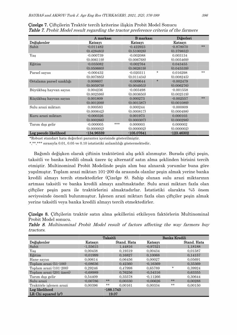
BAYBAS and AKSOY/ Turk J. Agr Eng Res (TURKAGER), 2021, 2(2), 376-389 386
Çizelge 7. Çiftçilerin Traktör tercih kriterine ilişkin Probit Model Sonucu
Table 7. Probit Model result regarding the tractor preference criteria of the farmers
A markası B markası Diğerleri
Değişkenler Katsayı Katsayı Katsayı
Sabit -0.011482 -0.422923 -0.878070 **
(0.428483) (0.510028) (0.379852)
Yaş -0.000739 -0.002088 0.003134
(0.006119) (0.006768) (0.005469)
Eğitim -0.035082 -0.002764 0.043455
(0.050660) (0.062619) (0.045539)
Parsel sayısı -0.000432 -0.020311 * 0.016298 **
(0.007885) (0.011434) (0.008245)
Ortalama parsel uzaklığı 0.008607 -0.009644 * -0.002479
(0.005979) (0.004953) (0.006276)
Büyükbaş hayvan sayısı 0.004236 -0.003498 -0.001558
(0.002598) (0.003650) (0.002519)
Küçükbaş hayvan sayısı 0.001809 0.000273 -0.002557 **
(0.001209) (0.001387) (0.001089)
Sulu arazi miktarı 0.000583 0.000244 -0.000809
(0.000642) (0.000817) (0.000498)
Kuru arazi miktarı -0.000326 0.001973 0.000103
(0.000266) (0.000307) (0.000298)
Tarım dışı gelir -0.000005 *** 0.000003 0.000002
(0.000002) (0.000002) (0.000002)
Log pseudo likelihood -134.96339 -105.07641 -123.46302
*Robust standart hata değerleri parantez içerisinde gösterilmiştir.
*,**,*** sırasıyla 0.01, 0.05 ve 0.10 istatistiki anlamlılığı göstermektedir.
Bağımlı değişken olarak çiftinin traktörünü alış şekli alınmıştır. Burada çiftçi peşin,
taksitli ve banka kredili olmak üzere üç alternatif satın alma şeklinden birisini tercih
etmiştir. Multinominal Probit Modelinde peşin alım baz alınarak yorumlar buna göre
yapılmıştır. Toplam arazi miktarı 101-200 da arasında olanlar peşin almak yerine banka
kredili almayı tercih etmektedirler (Çizelge 8). Sahip olunan sulu arazi miktarının
artması taksitli ve banka kredili almayı azaltmaktadır. Sulu arazi miktarı fazla olan
çiftçiler peşin para ile traktörlerini almaktadırlar. İstatistiki olarakta %5 önem
seviyesinde önemli bulunmuştur. İşlenen arazi miktarı fazla olan çiftçiler peşin almak
yerine taksitli veya banka kredili almayı tercih etmektedirler.
Çizelge 8. Çiftçilerin traktör satın alma şekillerini etkileyen faktörlerin Multinominal
Probit Model sonucu.
Table 8. Multinominal Probit Model result of factors affecting the way farmers buy tractors.
Taksitli Banka Kredili
Değişkenler Katsayı Stand. Hata Katsayı Stand. Hata
Sabit -1,55615 1,44816 -0,97521 1,18188
Yaş 0,00438 0,19319 0,00434 0,01587
Eğitim -0,01999 0,16827 0,10068 0,14157
Hane sayısı 0,00614 0,06456 0,00027 0,05691
Toplam arazi (51-100) -0,08636 0,42360 -0,16369 0,35369
Toplam arazi (101-200) 0,29246 0,47998 0,65789 * 0,39924
Toplam arazi (201 üzeri) -0,68989 0,76256 -0,54316 0,63355
Tarım dışı gelir 0,54409 0,35578 -0,11266 0,30644
Sulu arazi -0,00786 ** 0,00330 -0,00626 ** 0,00288
Traktörle işlenen arazi 0,00396 ** 0,00161 0,00334 ** 0,00150
Log likelihood
LR Chi squared (x2)
-188.1743
19.07
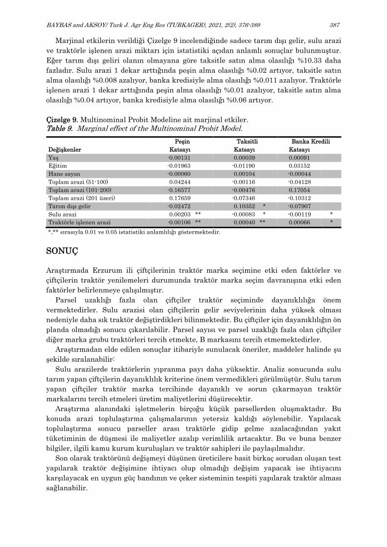
BAYBAS and AKSOY/ Turk J. Agr Eng Res (TURKAGER), 2021, 2(2), 376-389 387
Marjinal etkilerin verildiği Çizelge 9 incelendiğinde sadece tarım dışı gelir, sulu arazi
ve traktörle işlenen arazi miktarı için istatistiki açıdan anlamlı sonuçlar bulunmuştur.
Eğer tarım dışı geliri olanın olmayana göre taksitle satın alma olasılığı %10.33 daha
fazladır. Sulu arazi 1 dekar arttığında peşin alma olasılığı %0.02 artıyor, taksitle satın
alma olasılığı %0.008 azalıyor, banka kredisiyle alma olasılığı %0.011 azalıyor. Traktörle
işlenen arazi 1 dekar arttığında peşin alma olasılığı %0.01 azalıyor, taksitle satın alma
olasılığı %0.04 artıyor, banka kredisiyle alma olasılığı %0.06 artıyor.
Çizelge 9. Multinominal Probit Modeline ait marjinal etkiler.
Table 9. Marginal effect of the Multinominal Probit Model.
Peşin Taksitli Banka Kredili
Değişkenler Katsayı Katsayı Katsayı
Yaş -0.00131 0.00039 0.00091
Eğitim -0.01963 -0.01190 0.03152
Hane sayısı -0.00060 0.00104 -0.00044
Toplam arazi (51-100) 0.04244 -0.00116 -0.04128
Toplam arazi (101-200) -0.16577 -0.00476 0.17054
Toplam arazi (201 üzeri) 0.17659 -0.07346 -0.10312
Tarım dışı gelir -0.02472 0.10352 * -0.07907
Sulu arazi 0.00203 ** -0.00083 * -0.00119 *
Traktörle işlenen arazi -0.00106 ** 0.00040 ** 0.00066 *
*,** sırasıyla 0.01 ve 0.05 istatistiki anlamlılığı göstermektedir.
SONUÇ
Araştırmada Erzurum ili çiftçilerinin traktör marka seçimine etki eden faktörler ve
çiftçilerin traktör yenilemeleri durumunda traktör marka seçim davranışına etki eden
faktörler belirlenmeye çalışılmıştır.
Parsel uzaklığı fazla olan çiftçiler traktör seçiminde dayanıklılığa önem
vermektedirler. Sulu arazisi olan çiftçilerin gelir seviyelerinin daha yüksek olması
nedeniyle daha sık traktör değiştirdikleri bilinmektedir. Bu çiftçiler için dayanıklılığın ön
planda olmadığı sonucu çıkarılabilir. Parsel sayısı ve parsel uzaklığı fazla olan çiftçiler
diğer marka grubu traktörleri tercih etmekte, B markasını tercih etmemektedirler.
Araştırmadan elde edilen sonuçlar itibariyle sunulacak öneriler, maddeler halinde şu
şekilde sıralanabilir:
Sulu arazilerde traktörlerin yıpranma payı daha yüksektir. Analiz sonucunda sulu
tarım yapan çiftçilerin dayanıklılık kriterine önem vermedikleri görülmüştür. Sulu tarım
yapan çiftçiler traktör marka tercihinde dayanıklı ve sorun çıkarmayan traktör
markalarını tercih etmeleri üretim maliyetlerini düşürecektir.
Araştırma alanındaki işletmelerin birçoğu küçük parsellerden oluşmaktadır. Bu
konuda arazi toplulaştırma çalışmalarının yetersiz kaldığı söylenebilir. Yapılacak
toplulaştırma sonucu parseller arası traktörle gidip gelme azalacağından yakıt
tüketiminin de düşmesi ile maliyetler azalıp verimlilik artacaktır. Bu ve buna benzer
bilgiler, ilgili kamu kurum kuruluşları ve traktör sahipleri ile paylaşılmalıdır.
Son olarak traktörünü değişmeyi düşünen üreticilere basit birkaç sorudan oluşan test
yapılarak traktör değişimine ihtiyacı olup olmadığı değişim yapacak ise ihtiyacını
karşılayacak en uygun güç bandının ve çeker sisteminin tespiti yapılarak traktör alması
sağlanabilir.
BAYBAS and AKSOY/ Turk J. Agr Eng Res (TURKAGER), 2021, 2(2), 376-389 388
ÇIKAR ÇATIŞMASI
Yazarlar herhangi bir çıkar çatışması olmadığını beyan ederler.
YAZAR KATKISI*
Yazarlar olarak makaleye aşağıdaki katkıların sunulduğunu beyan ederiz.
Servan Baybas: Literatür taraması, giriş ve sonuç bölümlerinin yazımı.
Adem Aksoy: Araştırmanın planlanması, analizlerin yapımı, araştırma bulgularının
yazımı.
*Çalışma, Servan Baybas’ın Yüksek Lisans tezinden türetilmiştir.
KAYNAKLAR
Akdemir B, Sağlam C ve Aktaş T (1999). Tarım traktörleri kitabı. Tekirdağ.
Akkaya Ş ve Pazarlıoğlu MV (1998). Ekonometri II. İkinci Baskı, İstanbul.
Aksoy A, Demir N ve Demir O (2019). Erzurum ilinde çiftçilerin traktör satın alma davranışlarının
belirleyicileri üzerine bir analiz. Atatürk Üniversitesi Ziraat Fakültesi Dergisi, 50(1): 75-83.
Altuntaş E ve Demirtola H (2004). Ülkemizin tarımsal mekanizasyon düzeyinin coğrafik bölgeler bazında
değerlendirilmesi. Gaziosmanpaşa Üniversitesi Ziraat Fakültesi Dergisi, 21(2): 63-70.
Anonim (2004). Erzurum Master planı, İl Tarım ve Kırsal Kalkınma Master Planlarının Hazırlanmasına
Destek Projesi, Tarım ve Köyişleri Bakanlığı Erzurum İli Müdürlüğü, Erzurum.
Anonim, (2014). Dünyada ve ülkemizde tarımsal mekanizasyonun tarihi ve gelişimi
http://www.tarmakbir.org/haberler/tmtarihi.pdf (03.02.2020).
Aytuğ S ve Karadibak A G T (1998). Türk traktör kullanıcılarının marka tercihlerinin belirlenmesi üzerine
bir araştırma. Süleyman Demirel Üniversitesi İktisadi ve İdari Bilimler Fakültesi Dergisi, 3(3): 73-80.
Begg CB and Gray R (1984). Calculation of polychotomous logistic regression parameters using individualized
regressions. Biometrica, 71: 11-18.
Cankurt M, Miran B ve Gülsoylu E (2009). Çiftçilerin traktör tercihlerinin konjoint analizi ile belirlenmesi.
Tarım Makinaları Bilimi Dergisi, 5(1): 29-34.
Cankurt M ve Miran B (2010). Aydın yöresinde çiftçilerin traktör satın alma eğilimleri üzerine bir araştırma.
Ege Üniversitesi Ziraat Fakültesi Dergisi, 47(1): 43-51.
Gujarati DN (2006). Basic econometrics. Forth Edition, Mc Graw-Hill, USA.
Işık A (1988). Sulu tarımda kullanılan mekanizasyon araçlarının optimum makina ve güç seçimine yönelik
işletme değerlerinin belirlenmesi ve uygun seçim modellerinin oluşturulması üzerinde bir araştırma.
Tarımsal Mekanizasyon Anabilim Dalı, Doktora Tezi. Çukurova Üniversitesi, s. 226, Adana-Türkiye.
Işık A (1996). İşletme özelliklerine uygun traktör seçimine yönelik uzman sistem geliştirilmesi üzerine bir
araştırma. 6. Uluslararası Tarımsal Mekanizasyon ve Enerji Kongresi Bildiri Kitabı, s. 302-314, Ankara-
Türkiye.
İnal ME, Topuz D ve Uçan O (2006). Doğrusal olasılık ve logit modelleri ile parametre tahmini. Sosyoekonomi
/ 2006-1 / 060103.
Koçtürk D ve Avcıoğlu A (2007). Türkiye’de bölgelere ve illere göre tarımsal mekanizasyon düzeyinin
belirlenmesi. Tarım Makinaları Bilimi Dergisi, 3(1): 17-24.
Menard SW (2002). Applied logistic regression analysis. 2nd Edn Series, Quantitative Applications in the
Social Sciences, Sage Publications (CA), No. 106.
Miran B (2007). Temel istatistik. Gama Kitabevi, Ders Kitabı, ISBN:975-93088-00, İzmir.
Moens A and Wanders AA (1984). Planning requirements of agricultural machinery. Xth Congress of CIGR,
Budapest, 1-16.
Newbold P (1995). Statistics for business and economics, Prentice-Hall International, New Jersey.
Sağlam C ve Çetin N (2017). Kayseri yöresindeki çiftçilerin traktör seçimi ve satın alma davranışlarını
etkileyen faktörlerin belirlenmesi. Uludağ Üniversitesi Ziraat Fakültesi Dergisi, 31(2): 109-121.
Saral A, Vatandaş M, Güner M, Ceylan M ve Yenice T (2000). Türkiye tarımının makinalaşma durumu.
Türkiye Ziraat Mühendisliği Teknik Kongresi. 17-21 Ocak. S. 901-924. Ankara-Türkiye.

BAYBAS and AKSOY/ Turk J. Agr Eng Res (TURKAGER), 2021, 2(2), 376-389 389
Sarımeşeli M (2000). Ekonometri el kitabı. Gazi Kitabevi, s.210, Birinci Baskı, Ankara-Türkiye.
Sümer SK., Say SM, Has M ve Sabancı A (2003). Türkiye’de ekonomik traktör parkı ve gelişimi. Çukurova
Üniversitesi Ziraat Fakültesi Dergisi, 18: 45-52.
TÜİK (2020). Türkiye İstatistik Kurumu, https://tuikweb.tuik.gov.tr/PreÇizelge.do?alt_id=1003 (04.12.2020).
Yavuz F (2001). Ekonometri teori ve uygulama. Atatürk Üniversitesi Ziraat Fakültesi Ders Yayınları, Yayın
No: 185, Erzurum-Türkiye.
Yıldırım A (2016). IPARD programı kapsamındaki hibelerin etkinliğinin belirlenmesi üzerine bir çalışma:
Erzurum, Kars ve Ağrı illeri örneği. Yüksek Lisans Tezi, Atatürk Üniversitesi Fen Bilimleri Enstitüsü,
Tarım Ekonomisi Ana Bilim Dalı, s.123, Erzurum-Türkiye.
Zeren Y, Tezer E, Tuncer İK, Evcim Ü, Güzel E ve Sındır KO (1995). Tarım alet-makine ve ekipman kullanım
ve üretim sorunları. Ziraat Mühendisliği Teknik Kongresi Tarım Haftası 95 Kongresi, 9-13 Ocak 1995,
Ankara-Türkiye.
Turkish Journal of Agricultural
Engineering Research
https://dergipark.org.tr/en/pub/turkager https://doi.org/10.46592/turkager.2021.v02i02.012
Research Article
Turk J Agr Eng Res
(TURKAGER)
e-ISSN: 2717-8420
2021, 2(2): 390-402
Prediction the Performance Rate of Chain Type Trenching Machine
Mohamed Ibrahim GHONIMYIDa,b*
aDepartment of Plant Production and Protection, College of Agriculture and Veterinary Medicine, Qassim
University, Buraydah, SAUDI ARABIA
b Department of Agricultural Engineering, Faculty of Agriculture, Cairo University, Giza, EGYPT (*): Corresponding author; [email protected]
ABSTRACT
The mathematical analysis for estimating the performance rate
"RP" of chain-type trenching machine was studied. The
mathematical analysis ended with an equation for this type. This
mathematical equation was checked under different operating
conditions. The practical study of the performance rate showed
that the deviation of the theoretical performance rate from the
actual performance rate ranged from -3.4 to +2% only for the 150.7
cm and 120.7 cm trench depth respectively. The machine field
efficiency ranged from 46.7 to 57% for the 150.7 cm and 120.7 cm
depth respectively. It also showed an increase in machine field
efficiency by decreasing the trench depth.
INTRODUCTION
The drainage of agricultural land is one of the main operations which affecting the
production of agricultural crops (Vlotman et al., 2020). The productivity of the agricultural
crops increased by 22-35% when implementing agricultural drainage projects (Kovalenko
et al., 2020). Several trenching machines excavate the tile drainage trenches. There are
mainly three types of trenching machines different in their construction and way of
To cite: Ghonimy MI (2021). Prediction the Performance Rate of Chain type Trenching Machine.
Turkish Journal of Agricultural Engineering Research (TURKAGER), 2(2): 390-402.
https://doi.org/10.46592/turkager.2021.v02i02.012
RESEARCH ARTICLE
Received: 23.09.2021
Accepted: 26.11.2021
Keywords:
➢ Chain-type,
➢ Mathematical analysis,
➢ Performance rate,
➢ Drainage,
➢ Trencher
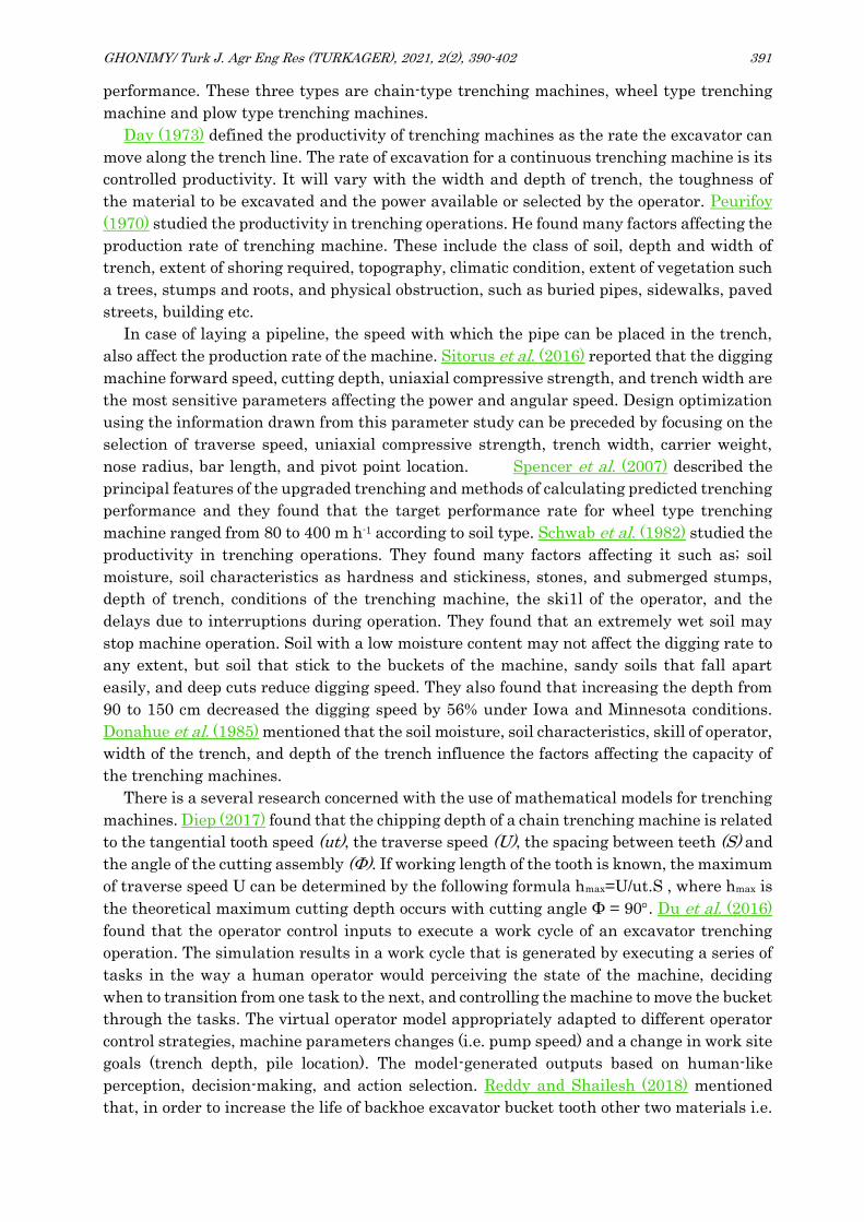
GHONIMY/ Turk J. Agr Eng Res (TURKAGER), 2021, 2(2), 390-402 391
performance. These three types are chain-type trenching machines, wheel type trenching
machine and plow type trenching machines.
Day (1973) defined the productivity of trenching machines as the rate the excavator can
move along the trench line. The rate of excavation for a continuous trenching machine is its
controlled productivity. It will vary with the width and depth of trench, the toughness of
the material to be excavated and the power available or selected by the operator. Peurifoy
(1970) studied the productivity in trenching operations. He found many factors affecting the
production rate of trenching machine. These include the class of soil, depth and width of
trench, extent of shoring required, topography, climatic condition, extent of vegetation such
a trees, stumps and roots, and physical obstruction, such as buried pipes, sidewalks, paved
streets, building etc.
In case of laying a pipeline, the speed with which the pipe can be placed in the trench,
also affect the production rate of the machine. Sitorus et al. (2016) reported that the digging
machine forward speed, cutting depth, uniaxial compressive strength, and trench width are
the most sensitive parameters affecting the power and angular speed. Design optimization
using the information drawn from this parameter study can be preceded by focusing on the
selection of traverse speed, uniaxial compressive strength, trench width, carrier weight,
nose radius, bar length, and pivot point location. Spencer et al. (2007) described the
principal features of the upgraded trenching and methods of calculating predicted trenching
performance and they found that the target performance rate for wheel type trenching
machine ranged from 80 to 400 m h-1 according to soil type. Schwab et al. (1982) studied the
productivity in trenching operations. They found many factors affecting it such as; soil
moisture, soil characteristics as hardness and stickiness, stones, and submerged stumps,
depth of trench, conditions of the trenching machine, the ski1l of the operator, and the
delays due to interruptions during operation. They found that an extremely wet soil may
stop machine operation. Soil with a low moisture content may not affect the digging rate to
any extent, but soil that stick to the buckets of the machine, sandy soils that fall apart
easily, and deep cuts reduce digging speed. They also found that increasing the depth from
90 to 150 cm decreased the digging speed by 56% under Iowa and Minnesota conditions.
Donahue et al. (1985) mentioned that the soil moisture, soil characteristics, skill of operator,
width of the trench, and depth of the trench influence the factors affecting the capacity of
the trenching machines.
There is a several research concerned with the use of mathematical models for trenching
machines. Diep (2017) found that the chipping depth of a chain trenching machine is related
to the tangential tooth speed (ut), the traverse speed (U), the spacing between teeth (S) and
the angle of the cutting assembly (Φ). If working length of the tooth is known, the maximum
of traverse speed U can be determined by the following formula hmax=U/ut.S , where hmax is
the theoretical maximum cutting depth occurs with cutting angle Φ = 90. Du et al. (2016)
found that the operator control inputs to execute a work cycle of an excavator trenching
operation. The simulation results in a work cycle that is generated by executing a series of
tasks in the way a human operator would perceiving the state of the machine, deciding
when to transition from one task to the next, and controlling the machine to move the bucket
through the tasks. The virtual operator model appropriately adapted to different operator
control strategies, machine parameters changes (i.e. pump speed) and a change in work site
goals (trench depth, pile location). The model-generated outputs based on human-like
perception, decision-making, and action selection. Reddy and Shailesh (2018) mentioned
that, in order to increase the life of backhoe excavator bucket tooth other two materials i.e.

GHONIMY/ Turk J. Agr Eng Res (TURKAGER), 2021, 2(2), 390-402 392
HSS and HCHCr has been analyzed for the similar force and boundary conditions. 3D model
was prepared in solid works and software in finite element method (FEM) domain was
utilized for analyzing the model or excavator bucket tooth behavior. Computational
approach will give the closer results to practical values through simulation.
Computer Aided Engineering (CAE) can drastically reduce the costs associated with the
product lifecycle.
Whatever the type of the trenching machine is, it has the advantage of quite high rate of
performance, since it simultaneously digs the trench, lays down the tiles or the pipes and,
in some types, it also refills the ditches with the soil. This means fulfilling its did define this
complete function in a short period within the same day. It is characterized with the high
accuracy in laying the pipes or the tiles at the required depth and slope. Besides, these types
of trenching machines suppress the manual way of digging and laying drainage pipes by its
lower costs of operation (Schaufelberger and Migliaccio, 2019).
The aim of this work was to find out the main factors affecting chain-type trenching
machine performance rate, relate these affecting factors in mathematical relationship, and
validate the mathematical relationship to predict the performance rate of chain-type
trenching machine.
MATERIALS AND METHODS
Mathematical analysis approach
The mathematical analysis had to be preceded with the two main steps which were to state
the theory, the construction the specifications and the dimensions of the applied mechanism
for chain-type trenching machine, Figure 1, and to state the expected affecting factors on
the performance of the applied mechanism, the nature and the magnitude of their effects.
The performance rate of the trenching machine depends, to a great extent, on the forward
speed of the machine. This forward speed in return, is related to both the size of the power
source of the trenching machine and the magnitude of the consumed power during the
performance of the machine. Therefore, the mathematical analysis depended on expressing
the magnitude of any required power of the trenching machine as a function of machine
forward speed. By equating the size of the power source with the summation of the required
powers during machine performance (equation 1), the magnetite of the maximum machine
forward speed can be estimated, and hence, the rate of performance of the machine can be
determined.
𝑃𝑏 = 𝑃𝑐 + 𝑃𝑟 + 𝑃𝑖 + 𝑃𝑠 + 𝑃𝑡 + 𝑃𝑒 ± 𝑃𝑎 + 𝑃𝑛 (1)
Where:
Pb = brake power of the engine of the machine, kW;
Pc = pulling power needed for cutting, kW;
Pr = pulling power to overcome rolling resistance, kW;
Pi = pulling power to overcome slope resistance, kW;
Ps = power lost in slop resistance, kW;
Pt = power 1ost in transmission systems, kW;
Pe = power required to lift the cut soil, kW;

GHONIMY/ Turk J. Agr Eng Res (TURKAGER), 2021, 2(2), 390-402 393
Pa = power required to overcome air resistance, kW;
Pn = power required to accelerate the machine to the operating speed due to its
inertia, kW.
Both Pa and Pn could be neglected since the operating forward speeds of the trenching
machine are very limited compared with any other moving truck. Therefore, equation (1)
can be simplified as shown in the following equation (2).
𝑃𝑏 = 𝑃𝑐 + 𝑃𝑟 + 𝑃𝑖 + 𝑃𝑠 + 𝑃𝑡 + 𝑃𝑒 (2)
A) Endless rotating chain B) Cutters attached to chain
C) Shoe to smooth trench bottom D) Tubing (or tile) shute
Figure 1. Chain-type trenching machine. "After Shady 1989"
The theory, construction, and specifications of the mechanisms of chain-type trenching
machine:
The excavating unit of the chain-type trenching machine, Figure 2, mainly consists of an
endless chain, which moves along a boom at a speed (Vc). The angle of the chain with the
vertical direction is (θ). On the chain, there are attached cutter buckets equipped with teeth.
The inclined distance between the cutting edges of any two consecutive buckets is (Sb). The
depth of the digged trench is (d). The performance theory of chain-type trenching machine
is that the machine moves horizontally at a veracity (Vm), the chain moves in an inclined
direction with an angle equals (θ) at a speed (Vc). The absolute speed of the cutting edge of
the bucket (Vb) can be considered as the summation of the vectors of (Vm) and (Vc) as shown
in Figure 3. The cutting edges of the consecutive buckets cut the soil in thin inclined layers.
The buckets elevate the cut soil and throw it outside the digged trench.

GHONIMY/ Turk J. Agr Eng Res (TURKAGER), 2021, 2(2), 390-402 394
Figure 2. The mechanism of chain-type trenching machine.
Factors affecting the performance of the trenching machines
There are many factors affecting the performance rate of the trenching machines. These
factors can be classified into two groups; soil factors which include soil specific weight (ω),
N cm-3, soil unit draft (U), N cm-2, traction coefficient, rolling resistance coefficient (RR),
angle between inclined soil surface and the horizontal direction (ψ), and friction coefficients
between soil and soil and between soil and metal (Fms).
Machine factors, which include machine weight (Wm), N, machine brake power (Pb), kW,
machine forward speed (Vm), m s-1, trench cutting width (Wt), cm, vertical depth of the cut
trench (d), cm, slip percentage of the tractor device of the machine (S), machine
transmission efficiency (ηt), and machine field efficiency (ηf), chain speed (Vc), m s-1, and
angle of chain with vertical direction (θ).
Some assumptions and simplifications were done in order to facilitate mathematical
manipulation. These include Homogeneous and isotropic soil, with a constant unit draft.
Constant velocities for any moving element, i.e., constant forward machine speed, and
constant chain speed were assumed. The paths of the cutting edge for the chain-type
trenching machines were considered as straight lines.
Mathematical analysis for estimating the performance rate
The mathematical analysis for estimating the performance rate (RP) of the chain-type-
trenching machine is expected to be in the form of the equation (2):
𝑅𝑃 = 60 × 𝑉𝑚 × 𝜂𝑓 (3)
Where:
RP = the actual performance rate of the machine, m min-1;
Vm = the machine forward speed, m s-1;
ηf = the field efficiency, decimal.
To find out the value of Vm, the components of equation (2) were obtained as the following:
a) Determination of Pc

GHONIMY/ Turk J. Agr Eng Res (TURKAGER), 2021, 2(2), 390-402 395
Referring to Figure 4:
𝑃𝑐 = 0.001 (𝐹𝑐 + 𝐹𝑓) × 𝑉𝑏 = 0.001(𝑈. 𝑊𝑡 . 𝛿. 𝑁 + 𝐹𝑚𝑠(1000 𝑃𝑏. 𝜂𝑡/𝑉𝑚)𝑐𝑜𝑠𝜙) × 𝑉𝑏 (4)
𝑃𝑐 = 0.001 × 𝑈∗ × 𝑊𝑡 × 𝛿 × 𝑁 × 𝑉𝑏 (5)
Where:
U* = K*. U
𝐾∗ =𝑈∗
𝑈=
[𝑈. 𝑊𝑡 . 𝛿. 𝑁(1000. 𝐹𝑚𝑠. 𝑃𝑏 . 𝜂𝑡/𝑉𝑚)𝑐𝑜𝑠𝜙]. 𝑉𝑏
𝑈. 𝑊𝑡. 𝛿. 𝑁. 𝑉𝑏
𝐾∗ = 1 +(1000. 𝐹𝑚𝑠. 𝑃𝑏 . 𝜂𝑡/𝑉𝑚). 𝑐𝑜𝑠𝜙
𝑈. 𝑊𝑡. 𝛿. 𝑁. 𝑉𝑏≅ 𝑓𝑟𝑜𝑚 5 𝑡𝑜 15
Using reasonable values for chain-type trenching machines, means that utilizing unit draft
(U*) including friction can be as much as about twelve times the unit draft (U) used in soil
ploughing.
Referring to Figures 2 and 3;
𝑁 =𝑑
𝑐𝑜𝑠𝜃. 𝑆𝑏 𝑎𝑛𝑑 𝛿 =
𝑉𝑚
𝑉𝑏. 𝑐𝑜𝑠𝜃. 𝑆𝑏
∴ 𝑃𝑐 = 0.001 𝐾∗. 𝑈. 𝑊𝑡 . 𝑑. 𝑉𝑚 ∴ 𝑃𝑐 = 0.001 𝐾∗. 𝑈. 𝑊𝑡 . 𝑑. 𝑉𝑚 (6)
b) Determination of Pr
𝑃𝑟 = 0.001 𝐹𝑟. 𝑉𝑚 (7)
The resistance force (Fr) due to rolling resistance depends on machine weight (Wm), the
weight of cut soil (Ws), the rolling resistance coefficient (RR), the vertical component of the
cutting force (Fcv), and the angle ψ between inclined soil surface and the horizontal
direction.
𝐹𝑟 = 𝑅𝑅. 𝑐𝑜𝑠𝜓. (𝑊𝑚 + 𝑊𝑠 + 𝐹𝑐𝑣)𝐹𝑟 = 𝑅𝑅. 𝑐𝑜𝑠𝜓. (𝑊𝑚 + 𝑊𝑠 + 𝐹𝑐𝑣) (8)
𝑊𝑠 =1
2𝑊𝑡 . 𝛿. 𝑁. 𝑙. 𝜔 𝑏𝑢𝑡 𝑉𝑏 . 𝑡 = 𝑙
𝑉𝑐 . 𝑡 = 𝑆𝑏 . 𝑁 =𝑑
cos 𝜃
𝑊𝑠 =𝜔. 𝑊𝑡 . 𝑑2. 𝑉𝑚
2 𝑐𝑜𝑠𝜃 . 𝑉𝑐
𝐹𝑐𝑣 = (𝐾∗. 𝑈. 𝑊𝑡. 𝑑. 𝑉𝑚
𝑉𝑏) . 𝑐𝑜𝑠𝜙
𝑏𝑢𝑡 𝑐𝑜𝑠𝜙 =𝑉𝑐 . 𝑐𝑜𝑠𝜃
𝑉𝑏 𝑎𝑛𝑑 𝑣𝑏 = [(𝑉𝑚)2 + 2𝑉𝑐 . 𝑉𝑚. 𝑐𝑜𝑠𝜃 + (𝑉𝑐)2]
12⁄
𝐹𝑐𝑣 =𝐾∗. 𝑈. 𝑊𝑡 . 𝑑. (𝑉𝑐 𝑉𝑚)⁄ . 𝑐𝑜𝑠𝜃
1 + 2(𝑉𝑐 𝑉𝑚)⁄ . 𝑐𝑜𝑠𝜃 + (𝑉𝑐 𝑉𝑚)⁄ 2
Substituting into equations (8) and (7) gives
𝑃𝑟 = 0.001 𝑉𝑚. 𝑅𝑅. 𝑐𝑜𝑠𝜓. [𝑊𝑚 +𝜔. 𝑊𝑡 . 𝑑2
2 𝑐𝑜𝑠𝜃. (𝑉𝑐 𝑉𝑚)⁄+
𝐾∗. 𝑈. 𝑊𝑡 . 𝑑. (𝑉𝑐 𝑉𝑚)⁄ . 𝑐𝑜𝑠𝜃
1 + 2. (𝑉𝑐 𝑉𝑚).⁄ 𝑐𝑜𝑠𝜃 + (𝑉𝑐 𝑉𝑚)⁄ 2]

GHONIMY/ Turk J. Agr Eng Res (TURKAGER), 2021, 2(2), 390-402 396
𝑃𝑟 = 0.001 𝑉𝑚. 𝑅𝑅. 𝑐𝑜𝑠𝜓. [𝑊𝑚 +𝜔.𝑊𝑡.𝑑2
2 𝑐𝑜𝑠𝜃.(𝑉𝑐 𝑉𝑚)⁄+
𝐾∗.𝑈.𝑊𝑡.𝑑.(𝑉𝑐 𝑉𝑚)⁄ .𝑐𝑜𝑠𝜃
1+2.(𝑉𝑐 𝑉𝑚).⁄ 𝑐𝑜𝑠𝜃+(𝑉𝑐 𝑉𝑚)⁄ 2] (9)
Vm= machine speed.
Vc = chain speed
Vb = resultant speed of
the bucket edge
N= number of bucket in
the cutting action.
δ = thickness of cut for
one bucket.
Figure 3. Bucket resultant speed. Figure 4. Determination of the friction
force Ff acting on bucket edge.
c) Determination of Pi
𝑃𝑖 = 0.001 (𝑊𝑚 + 𝑊𝑆). 𝑠𝑖𝑛𝜓. 𝑉𝑚 (10)
𝑃𝑖 = 0.001 𝑉𝑚. 𝑠𝑖𝑛𝜓. [𝑊𝑚 +𝜔.𝑊𝑡.𝑑2
2 𝑐𝑜𝑠𝜃.(𝑉𝑐 𝑉𝑚)⁄] (11)
d) Determination of Ps
𝑃𝑠 = 0.001 𝐹𝑠. 𝑉𝑠 = 0.001 (𝐹𝑐 + 𝐹𝑟). 𝑉𝑠 (12)
Where;
Ps is the power lost in slip resistance.
Fc is the cutting force,
Fr is the resistance force due to rolling and
Vs is the loss in machine speed due slippage (S).
𝑉𝑠 = (𝑆
100−𝑆) . 𝑉𝑚 (13)
𝑃𝑠 = 0.001 [(𝑆
100−𝑆) . 𝑉𝑚] . [
𝐾∗.𝑈.𝑊𝑡.𝑑
[1+2.(𝑉𝑐 𝑉𝑚).⁄ 𝑐𝑜𝑠𝜃+(𝑉𝑐 𝑉𝑚)⁄ 2]1 2⁄ + 𝑅𝑅. 𝑐𝑜𝑠𝜓. (𝑊𝑚 +
𝜔.𝑊𝑡.𝑑2
2 𝑐𝑜𝑠𝜃.(𝑉𝑐 𝑉𝑚)⁄) +
𝐾∗.𝑈.𝑊𝑡.𝑑.(𝑉𝑐 𝑉𝑚)⁄ .𝑐𝑜𝑠𝜃
1+2.(𝑉𝑐 𝑉𝑚).⁄ 𝑐𝑜𝑠𝜃+(𝑉𝑐 𝑉𝑚)⁄ 2] (14)
e) Determination of Pt
𝑃𝑡 = 𝑃𝑏 . (1 − 𝜂𝑡) (15)
f) Determination of Pe
𝑃𝑒 = 0.001 𝑊𝑠. 𝑉𝑐 . 𝑐𝑜𝑠𝜃 = 0.001 ×𝜔.𝑊𝑡.𝑑2.𝑉𝑚
2 (16)
From equations 2, 3, 9, 11, 14, 15 and 16
𝑃𝑐 + 𝑃𝑟 + 𝑃𝑖 + 𝑃𝑠 + 𝑃𝑡 + 𝑃𝑒 − 𝑃𝑏 = 0 (17)

GHONIMY/ Turk J. Agr Eng Res (TURKAGER), 2021, 2(2), 390-402 397
𝑉2𝑚 [(
𝜔.𝑊𝑡.𝑑2
2𝑐𝑜𝑠𝜃.𝑉𝑐) . (𝑅𝑅. 𝑐𝑜𝑠𝜓 + 𝑠𝑖𝑛𝜓 + 𝑅𝑅. 𝑐𝑜𝑠𝜓.
𝑠
100−𝑆)] + 𝑉𝑚 [𝐾∗. 𝑈. 𝑤𝑡 . 𝑑 + 𝑅𝑅. 𝑐𝑜𝑠𝜓. 𝑊𝑚 +
𝑊𝑚. 𝑠𝑖𝑛𝜓 +𝐾∗.𝑈.𝑊𝑡.𝑑.(
𝑆
100−𝑆)
[1+2.(𝑉𝑐 𝑉𝑚).⁄ 𝑐𝑜𝑠𝜃+(𝑉𝑐 𝑉𝑚)⁄ 2]
1 2⁄ + 𝑅𝑅. 𝑐𝑜𝑠𝜓. 𝑊𝑚. (𝑆
100−𝑆) +
𝜔.𝑊𝑡.𝑑2
2] +
[(𝑅𝑅.𝑐𝑜𝑠𝜓.𝐾∗.𝑈.𝑊𝑡.𝑑.𝑐𝑜𝑠𝜃.𝑉𝑐
1+2.(𝑉𝑐 𝑉𝑚).⁄ 𝑐𝑜𝑠𝜃+(𝑉𝑐 𝑉𝑚)⁄ 2) . (1 +𝑆
100−𝑆) − 1000𝑃𝑏. 𝜂𝑡] = 0
𝑉2𝑚 +
𝐺
𝑄. 𝑉𝑚 −
𝐽
𝑄= 0 (18)
Where:
𝑄 = (𝜔.𝑊𝑡.𝑑2
2𝑐𝑜𝑠𝜃.𝑉𝑐) . (𝑅𝑅. 𝑐𝑜𝑠𝜓 (
100
100−𝑆) + 𝑠𝑖𝑛𝜓) (19)
𝐺 = 𝐺1 + 𝐺2 + 𝐺3 (20)
𝐺1 = 𝐾∗. 𝑈. 𝑤𝑡. 𝑑. [1 + (𝑆
100−𝑆) . [1 + 2. (𝑉𝑐 𝑉𝑚).⁄ 𝑐𝑜𝑠𝜃 + (𝑉𝑐 𝑉𝑚)⁄ 2
]−1 2⁄
] (21)
𝐺2 = 𝑅𝑅. 𝑐𝑜𝑠𝜓. [𝑉𝑚 + 𝑊𝑚. (𝑆
100−𝑆)] (22)
𝐺3 = 𝑊𝑚. 𝑠𝑖𝑛𝜓 +𝜔.𝑊𝑡.𝑑2
2𝐺3 = 𝑊𝑚. 𝑠𝑖𝑛𝜓 +
𝜔.𝑊𝑡.𝑑2
2 (23)
𝐽 = (𝑅𝑅.𝑐𝑜𝑠𝜓.𝐾∗.𝑈.𝑊𝑡.𝑑.𝑐𝑜𝑠𝜃.𝑉𝑐
1+2.(𝑉𝑐 𝑉𝑚).⁄ 𝑐𝑜𝑠𝜃+(𝑉𝑐 𝑉𝑚)⁄ 2) . (1 +100
100−𝑆) − 1000𝑃𝑏. 𝜂𝑡 (24)
Applying the rule:
𝑉𝑚 = −𝑏
2± √(
𝑏
2)
2
−𝐶
𝑎 (25)
𝑏
2=
𝐺
2𝑄 (26)
𝐶 =𝐽
𝑄 (27)
𝑏
2= (
𝑐𝑜𝑠𝜃.𝑉𝑐
𝜔.𝑊𝑡.𝑑2.(𝑅𝑅.𝑐𝑜𝑠𝜓(100
100−𝑆)+𝑠𝑖𝑛𝜓)
) × {𝐾∗. 𝑈. 𝑤𝑡 . 𝑑. (1 + (𝑆
100−𝑆) . [1 + 2. (𝑉𝑐 𝑉𝑚).⁄ 𝑐𝑜𝑠𝜃 +
(𝑉𝑐 𝑉𝑚)⁄ 2]
−1 2⁄) + 𝑅𝑅. 𝑐𝑜𝑠𝜓. 𝑊𝑚. (1 +
𝑆
100−𝑆) + (𝑊𝑚. 𝑠𝑖𝑛𝜓 +
𝜔.𝑊𝑡.𝑑2
2)} (28)
𝐶 =2 𝑐𝑜𝑠𝜃.𝑉𝑐
𝜔.𝑊𝑡.𝑑2.(𝑅𝑅.𝑐𝑜𝑠𝜓(100
100−𝑆)+𝑠𝑖𝑛𝜓)
× [(𝑅𝑅.𝑐𝑜𝑠𝜓.𝐾∗.𝑈.𝑊𝑡.𝑑.𝑐𝑜𝑠𝜃.𝑉𝑐
1+2.(𝑉𝑐 𝑉𝑚).⁄ 𝑐𝑜𝑠𝜃+(𝑉𝑐 𝑉𝑚)⁄ 2) . (100
100−𝑆) − 1000𝑃𝑏. 𝜂𝑡] (29)
Equation (25) could be solved by trial-and-error method using reasonable initial values
of Vm in equations (28) and (29) and the value of K* ≈12. When different values of K* ranging
from 1 to 15 were used, the estimated values of Vm ranged from 2.92 to o.26 m sec-1
respectively.
The actual performance rate (RP) could be obtained from equation (3) using field
efficiency ηf= ηs. ηw. ηti, where ηs is the efficiency of utilizing the geared speed, ηw is the
efficiency of utilizing the proposed width of the machine, and ηti is the efficiency of utilizing
the time. However, due to the very low speed of the machine, both ηs and ηw could be
considered equal to 1.0.
Field experimental work
The experimental work was carried out through a period of almost one year. It was
conducted in Gharbia Governorate, in Sawahel El-Neel region, in which the chain-type
trenching machine (Figure 5) was tested. The specification of the machine is shown in Table
1. Trench depths of 120 and 150 cm were tested.

GHONIMY/ Turk J. Agr Eng Res (TURKAGER), 2021, 2(2), 390-402 398
Figure 5. The tested chain-type trenching machine. "i-bidder.com 2015"
Table 1. Technical specifications of the chain-type trenching machine. Model Barth Holland K171
Engine Deutz diesel type
Power 149 kW (203 HP) - 2150 rpm
Tank capacity Fuel 320 lit., Hydraulic oil 120 lit
Electricity 24 V.
Speed variable (0 - 5000 m h-1)
Ground pressure 3 N cm-2
Transmission efficiency 90%
Cutting system speed 1 gear: 1.04 m s-1
2 gear: 2.15 m s-1
3 gear: 3.26 m s-1
4 gear: 4.35 m s-1
5 gear: 5.75 m s-1
r. gear: 1.02 m s-1
Max. trench depth 1750 mm
Trench width 230 or 280 mm
The angle of the chain with the
vertical direction
30 degree
Chain pitch 100 mm
TRANSPORT DATA
length 10905 mm
Width 2500 mm
Height 1000 mm
Weight 13 tons
RESULTS AND DISCUSSION
The average rolling resistance coefficient of the experimental field was taken as 4.0%, since
it was found ranging between 3.0 and 5.0% (Jia et al., 2018). The average specific weight of
the soil (ω) was found to be 0.011 N cm-3 (Jia et al., 2018). In addition, the average draft was
taken as 10 N cm-2 (Jia et al., 2018). The average values of field measurements were as
shown in Table 2.

GHONIMY/ Turk J. Agr Eng Res (TURKAGER), 2021, 2(2), 390-402 399
Table 2. Average values of field measurements for chain-type trenching machine.
d = Trench depth, Wt = Trench width, S = slip percentage, Vm= Machine forward speed, Vc = Chain forward speed, K* = A dimensionless coefficient
= (U*/U), ψ = angle between inclined soil surface and the horizontal direction.
Actual performance rate (RP) and field efficiency (ηf)
The average values of breakdown items of the daily machine time, machine performance
rate (RP), field efficiency (ηf) as practically measured in the field are shown in Table 3. It is
clear that the average values of RP were 13 and 9 m min-1 for 120 and 150 cm trench depth
respectively while the ηf were 57 and 46.7% for 120 and 150 cm trench depth respectively.
Table 3. Breakdown items of the daily machine item for chain-type trenching machine and
its average performance rate and field efficiency.
* Average value of ten estimates, each for a different operating day.
**Average value (m/day) of the total excavated trench lengths within the ten days period.
***Average field efficiency within the ten days period.
Theoretical deterioration of the performance rate of the chain-type trenching machine
To theoretically predict the performance rate, equations (3), (25), (28), and (29) were
applied. Using the above-mentioned data into equation (28) for the value of b/2 and into
equation (29) for the value of C gave the following equations:
For 120.7 cm depth
𝑏
2= 6154.28 +
316.97
√1 +5.65𝑉𝑚
+10.63𝑉2
𝑚
𝐶 =1431.77
1 +5.65𝑉𝑚
+10.63𝑉2
𝑚
− 4827.6
Nominal trench depth, cm 120 150
Field measurements Ave. SD Ave. SD
d, cm 120.70 2.37 150.7 2.15
Wt, cm 23.10 0.34 23.1 0.34
S, % 5.00 --- 6.00 ---
Vm, m s-1 0.40 0.05 0.34 0.04
Vc, m s-1 3.26 --- 2.15 ---
K* 12.00 --- 12.00 ---
ψ, degree 0.00 --- 0.00 ---
Activities
*Average spent time, min day-1 SD, min day-1
Trench depth, cm Trench depth, cm
120 150 120 150
Net excavating and pipe laydown 229 215 7.26 5.81
Turning and travelling to start digging
another trench
55 65 2.49 3.12
Setup time for reaching the depth 23 29 1.76 2.18
Rest periods 60 66 1.76 3.26
Field quick maintenances 30 30 2.17 1.73
Refill of water and oil tank 30 34 2.23 1.48
Other lost time 10 18 1.49 1.73
Average total time, min day-1 485 455 8.15 7.21 **Total installed length, m day-1 6305 4095 6.12 4.23
Actual performance rate, m min-1 13.0 9.0 1.15 0.92 *** Field efficiency, % 57.0 46.7 0.89 0.81

GHONIMY/ Turk J. Agr Eng Res (TURKAGER), 2021, 2(2), 390-402 400
For 150.7 cm depth
𝑏
2= 3196.18 +
199.98
√1 +3.72𝑉𝑚
+4.62𝑉2
𝑚
𝐶 =4964.60
1 +3.72𝑉𝑚
+4.62𝑉2
𝑚
− 2011.5
Solving equation (18) by trial-and-error method, gave the computed values of the Vm,
Table 4. Applying the computed values of the Vm into equation (3) gave the predicted value
of the performance rate of the chain-type trenching machine:
RP (120.7 cm depth) = 60 x 0.388 x 0.57 = 13.26 m min-1
This computed value was very close to the experimentally determined value of the
performance rate for the 120.7 cm trench depth, which was found to be 13 m min-1., Table 3
and Figure 6. The deviation of the theoretically computed value from the field determined
value for the performance rate was only about + 2%.
RP (150.7 cm depth) = 60 x 0.31 x 0.467 = 8.69 m min-1
This computed value was very close to the experimentally determined value of the
performance rate for the 150.7 cm trench depth, which was found to be 9.00 m min-1, Table
3 and Figure 6. The deviation of the theoretically computed value from the field determined
value for the performance rate was only about - 3.4%.
Table 4. The initially proposed and the computed values in the interaction process for the
determination of the forward speed of the chain-type trenching machine at different trench
depths. (Using trial and error method).
Trench depth, cm Vm, m s-1 Trial 1 Trial 2 Trial 3 Trial 4
120.7 proposed value 3.000 1.000 0.400 0.388
computed value 0.355 0.301 0.389 0.388
150.7 proposed value 3.000 1.000 0.400 0.310
computed value 0.278 0.300 0.309 0.310
The findings of the used chain-type trenching machine show the degree of accuracy of
the mathematically derived equations. This derived equation can be used with enough
confidence to theoretically predict the performance rate of chain-type trenching machine
depending on the prevailing operating conditions.

GHONIMY/ Turk J. Agr Eng Res (TURKAGER), 2021, 2(2), 390-402 401
Figure 6. The actual & predicted performance rate and field efficiency of the chain-type
trenching machine.
CONCLUSION
The digging of the trenches is an important process in order to implement the tail drainage
projects. This research is concerned with studying the relationship that correlate the
performance of the chain-type trenching machine with the factors affecting them, so that
the rate of performance can be predicted or controlled through the factors affecting it. A
mathematical analysis of chain-type trenching machine was performed. Also, a field
operation study was conducted under actual operating conditions to test the validity of the
derived mathematical equations.
The study showed the validity of the derived equations in predicting the performance
rate of chain-type trenching machine. The percentage difference between the performance
rate calculated from the equations and the actual field estimated performance rate were -
3.4% and +2% at a trench depth of 150.7 and 120.7 cm respectively. The results of the field
study also showed that the field efficiency was 46.7 and 57% for the chain-type trenching
machine at a trench depth of 150.7 and 120.7 cm respectively. The finial equation of the
mathematical model can be used to increase the performance rate of the chain-type
trenching machine by maximizing all the factors in the numerator or by minimizing all the
factors in the denominator.
Finally, the derived mathematical equation can be used with enough confidence to
theoretically predict the performance rate of chain-type trenching machine depending on
the prevailing operating conditions.
DECLARATION OF COMPETING INTEREST
The author declares that he has no conflict of interest.

GHONIMY/ Turk J. Agr Eng Res (TURKAGER), 2021, 2(2), 390-402 402
CREDIT AUTHORSHIP CONTRIBUTION STATEMENT
The author, Mohamed Ghonimy, is responsible for the various parts of this paper.
ACKNOWLEDGMENTS
The author wishes to express here sincere thanks and appreciation to the spirit of
Prof. Dr. Monier A. Morcos and Prof. Dr. Abdalla E. Badr, former professors, Agricultural
Engineering Dept., Faculty of Agriculture, Cairo University for continues help supports.
REFERENCES
Day DA (1973). Construction equipment guide. John Wiley and Sons.,Inc., N. Y., USA, 206-208.
Diep DD (2017). Analysis the Factors Affecting Conveyance Rate of Unbucket Chain Trenching Machine.
Agricultural, Forest and Transport Machinery and Technologies, 4(1): 38-44.
Donahue RL, Miller RW and Shickluna GC (1985). Soil an introduction to soil and plant growth. 4th Ed. Prentice
Hall, Inc., Englewood cliffs, New Jersey, USA. 98-106.
Du Y, Dorneich MC and Steward B (2016). Virtual operator modeling method for excavator
trenching. Automation in Construction, 70: 14-25.
i-bidder.com 2015. Barth holland k171 trencher. [Online] Available from: https://www.i-bidder.com/en-
gb/auction-catalogues/ml/catalogue-id-morris10019/lot-dd3f8267-bddc-47be-ab61-a50900a797df. (Accessed
November 24, 2021).
Jia J, Jia and Schmidt (2018). Soil dynamics and foundation modeling. Springer, New York.
Kovalenko P, Rokochinskiy A, Mazhayskiy Y, Volk P, Volk L and Chernikova O (2020). Construction and
agricultural drainage parameter optimization considering economic and environmental
requirements. Engineering for Rural Development, 19: 1009-1017.
Peurifoy RL (1970). Construction planning, equipment, and methods. 2nd ed. McGraw, Hill Kogakusha, Ltd.,
Tokyo, Japan, pp 695.
Reddy Y and Shailesh P (2018). Design and analysis of excavator bucket tooth. International Journal of Modern Trends in Engineering and Research, 5(4): 79-86.
Shady AM (1989). Irrigation drainage and flood control in Canada. Canadian international development agency,
Quebec, Canada.
Schaufelberger JE and Migliaccio GC (2019). Construction equipment management. Routledge.
Schwab GO, Frevert RK, Edminster TW and Barnes KK (1982). Soil and water conservation engineering. Soil Science, 134(2): 146.
Sitorus PE, Ko JH and Kwon OS (2016). Parameter study of chain trenching machines of Underwater
Construction Robots via analytical model. In OCEANS 2016 MTS/IEEE Monterey (pp. 1-6). IEEE.
Spencer A, Machin J and Jackson E (2007). Rock cutting With the T750 super trenching. Unmanned
Intervention, New Orleans, LA, 30.
Vlotman WF, Smedema LK and Rycroft DW (2020). Modern land drainage: Planning, design and management
of agricultural drainage systems. CRC Press.

Turkish Journal of Agricultural
Engineering Research
https://dergipark.org.tr/en/pub/turkager https://doi.org/10.46592/turkager.2021.v02i02.013
Research Article
Turk J Agr Eng Res
(TURKAGER)
e-ISSN: 2717-8420
2021, 2(2): 403-412
Important Physical and Mechanical Properties of Dominant Potato
Variety Widely Grown in Ethiopia
Dereje ALEMUIDa*
a Department of Agricultural Engineering Research, Melkassa Agricultural Research Centre, Ethiopian
Institute of Agricultural Research, Addis Ababa, ETHIOPIA
(*): Corresponding author. [email protected]
ABSTRACT
The physical attributes of agricultural product are utmost
essential in developing technologies for different unit operations.
Pertinent potato tuber attributes were studied. 100 samples of
dominant and popular potato tuber varieties grown in Ethiopia
which are free from any injuries from each variety were obtained
from Holeta Agricultural Research Center. In this study, the
physical attributes of potato tubers were determined at a moisture
content of 70.75, 69.99, 71.75, 69.70 and 72.38% (wet basis) for
Belete, Jalenie, Gera, Gudene and Chala varieties, respectively.
Except specific gravity of potato tuber, other physical properties
studied were significantly different at 5% of level of significance.
Analysis of variance showed that there is also a significant
difference in coefficient of static friction and angle of repose of all
potato tuber varieties under four different materials and dynamic
coefficient of friction under mild steel sheet metal and galvanized
sheet.
INTRODUCTION
Potato is the first in terms of production from tuber and root crops grown in more than
125 countries (Alemu et al., 2021). It is used for daily consumption for a billion people
(Gebru et al., 2017). It plays a significant role in improving food security and Ethiopian
smallholder potato grower’s income due to its high yield potential per hectare
(Ayalew, 2014; CSA, 2015; Alemu et al., 2021). It is widely grown in eastern, southern,
central and northwestern region of Ethiopia, which is around 83% of potato growers
(CSA, 2009). Around 1,288,146 households are dependent on potato production and
about 67,361.87 ha of land is under potato production which has 31.13% area coverage
among root crops (CSA, 2015: Alemu et al., 2021). It can be used for cooking, processing,
To cite: Alemu D (2021). Important physical and mechanical properties of dominant potato
variety widely grown in Ethiopia. Turkish Journal of Agricultural Engineering Research
(TURKAGER), 2(2): 403-412. https://doi.org/10.46592/turkager.2021.v02i02.013
RESEARCH ARTICLE
Received: 08.10.2021
Accepted: 28.11.2021
Keywords:
➢ Physical,
➢ Mechanical,
➢ Potato tuber,
➢ Property,
➢ Variety,
➢ Attribute

ALEMU / Turk J. Agr Eng Res (TURKAGER), 2021, 2(2), 403-412 404
feed, seed tubers, starch and alcohol production (Alemu et al., 2021). Within 30 years,
the average potato crop productivity in Africa, Asia and Latin America has increased
by 44, 25 and 71 percent, respectively (FAO, 2009).
Physical attributes of agricultural products are important in many grains/seeds and
vegetables, and food materials handling and processing operation. Physical
characteristics of agricultural products plays a significant role during development of
equipment used for different operation (Malcolm et al., 1986; Razavi et al., 2007;
Joshi and Raisoni, 2016). In addition to physical attributes, mechanical properties have
to be taken into account during development of machines. Therefore, the objective of
this study was to determine pertinent physical and mechanical attributes of potato
tuber variety widely grown in Ethiopia.
MATERIALS AND METHODS
Source of experimental material
The study was conducted at Melkassa Agricultural Research Center (MARC); which is
found in Oromia National Regional State, Ethiopia. It is located at an altitude of 1550
meters above sea level (masl) and lies between 8° 24' 0" to 8° 30' 12'' N, 39° 21' 0" to 39°
35' 14'' E latitude and longitude, respectively. Agro-ecologically, the area is
characterized as arid and semi-arid.
100 samples free from any injuries of dominant and popular potato varieties (Belete,
Jalenie, Gera, Gudene and Chala) grown in Ethiopia were used from Holeta
Agricultural Research Centers as shown in Figure 1. The samples were kept in a
refrigerator at a temperature of 4°C and relative humidity of 95% for 24 hours as
recommended by Hurst et al. (1993) to offset the effect of the environment.
Figure 1. Potato variety used during physical and mechanical attributes measurements.

ALEMU / Turk J. Agr Eng Res (TURKAGER), 2021, 2(2), 403-412 405
Determination of Physical Attributes
Shape and size
To measure potato tuber mass digital balance with accuracy of 0.10 g was used. As
shown in Figure 2, major, minor and intermediate diameters of each tuber were
measured using digital caliper with an accuracy of 0.01 mm and measuring range of
0-150 mm.
Figure 2. Measurement of principal dimensions of potato tuber.
Geometric mean diameter
Geometric mean diameter (GMD) was determined using the three measured
perpendicular diameters as shown in Equation 1 (Kamat et al., 2020).
𝐺𝑀𝐷 = √𝑎𝑏𝑐3
(1)
Where: -
GMD = geometric mean diameter, mm
𝑎, b and c = major, intermediate and minor diameter respectively, mm
Surface area
Surface area (S, mm2) of the potato tuber was determined using Equation 2
(Mohsenin, 1986).
𝑆 = 𝜋(𝐺𝑀𝐷)2 (2)
Volume
As shown in Figure 3 the volume of a potato tuber was determined based on the water
displacement method (Mohsenin, 1986).

ALEMU / Turk J. Agr Eng Res (TURKAGER), 2021, 2(2), 403-412 406
Figure 3. Measurement of volume of potato tuber by using water displacement method.
Sphericity
The sphericity (φ) of potato tubers was determined with presumption that the volume
of solid can be approximating to the volume of a triaxial ellipsoid with a diameter equal
to the minor, intermediate and major diameters using Equation 3 (Mohsenin, 1986).
𝜑 = √𝑎𝑏𝑐
𝑎
3 (3)
Moisture content
Potato tuber moisture content was determined using hot air oven method and
Equation 4 (Asoegwu, 1995). The weight of the potato tuber was measured before and
after oven-drying at 105°C until constant weight was obtained using a digital balance
with an accuracy of 0.01 g.
𝑀𝐶 = 𝑊1− 𝑊2
𝑊2 (4)
Where:-
Mc= moisture content (% wb),
W1= mass of potato tuber before oven-drying (g) and
W2= mass of potato tuber after oven-drying (g).
Tuber density (ρp)
Tuber density is described as mass of a tuber divided to its actual volume (Equation 5).
Internal pores are included (Mohsenin, 1986).
𝜌𝑃 = 𝑀𝑡𝑉𝐶
(5)
Where:
ρp = particle density (g cm-3),
Mt = mass of a tuber (g) and
Vc = volume of a tuber (cm3).
Bulk density (ρbulk)
Bulk density (ρbulk) was determined from mass and volume of potato tuber using
Equation 6. (Rahman, 2014).

ALEMU / Turk J. Agr Eng Res (TURKAGER), 2021, 2(2), 403-412 407
𝜌𝑏𝑢𝑙𝑘 = 𝑀𝑎𝑠𝑠 (𝑔)
𝑉𝑜𝑙𝑢𝑚𝑒 (𝑚3) (6)
Specific gravity (Gs)
The specific gravity of potato tuber was determined based on the water displaced
method and Equation 7.
𝐺𝑠 = 𝑊𝑒𝑖𝑔ℎ𝑡 𝑖𝑛 𝑎𝑖𝑟 (𝑁)
𝑊𝑒𝑖𝑔ℎ𝑡 𝑖𝑛 𝑎𝑖𝑟 (𝑁)−𝑊𝑒𝑖𝑔ℎ𝑡 𝑖𝑛 𝑤𝑎𝑡𝑒𝑟(𝑁) (7)
Where N =Newton
Frictional properties of potato tuber
Static coefficient of friction
The static coefficients of friction between potato tuber and four different surfaces (Mild
steel sheet metal, galvanized sheet, wood and rubber) were determined by using
Equation 8 (Almaiman and Ahmad, 2002).
𝜇𝑠 = 𝑡𝑎𝑛𝛼 (8)
Where:
μs = static coefficient of friction,
α = angle of inclination at which potato tuber start to slide down.
Dynamic coefficient of friction
The dynamic coefficient of friction was determined using a topless and bottomless
plywood box with dimensions of 250 × 250 × 90 mm3. The box was placed on a test
surface and filled with a known quantity of potato tubers; then force was applied to
bottomless plywood box until it moved uniformly with a horizontal pull. The friction test
was replicated three times for the surfaces under investigation. For each replication,
the box was refilled with a different sample. The dynamic coefficient of friction was
determined using Equation 9 (Puchalski et al., 2003; Amin et al., 2004).
𝜇𝑑 = 𝐹
𝑚𝑔 (9)
Where:
μd = dynamic coefficient of friction,
F = friction force that will be measured using pull force gauge (N),
m = mass tuber (kg) and
g = gravitational acceleration (m s-2).
Angle of repose
Angle of repose for potato tuber was determined with a bottomless cylinder. The
cylinder was placed over a smooth surface and filled with potato tuber. The cylinder was
then raised slowly allowing the tuber to flow down and form a natural slope. The height

ALEMU / Turk J. Agr Eng Res (TURKAGER), 2021, 2(2), 403-412 408
and diameter of the heap formed were measured and angle of repose was estimated
using Equation 10.
𝛼 = tan−1 𝐻𝑒𝑖𝑔ℎ𝑡 𝑜𝑓 𝑝𝑜𝑡𝑎𝑡𝑜 𝑡𝑢𝑏𝑒𝑟 𝑝𝑖𝑙𝑒
𝑏𝑎𝑠𝑒 𝑜𝑓 𝑝𝑜𝑡𝑎𝑡𝑜 𝑡𝑢𝑏𝑒𝑟 𝑝𝑖𝑙𝑒/2 (10)
Where α is expressed in degree.
RESULTS AND DISCUSSION
Physical properties
The physical properties of potato tubers were determined at a moisture content of 70.75,
69.99, 71.75, 69.70 and 72.38% (w.b) for Belete, Jalenie, Gera, Gudene and Chala
varieties, respectively. The temperature recorded in the laboratory during the
experiments was 20-28°C.
The weight measurement of each potato tubers showed that Belete variety had the
maximum weight of 102.24 g while the minimum value was recorded for Chala Variety
59.66 g.
The mean major diameters of 66.96, 56.28, 55.43, 63.45 and 54.09 mm were observed
for Belete, Giera, Jalenie, Gudene and Chala varieties, respectively. The maximum and
minimum tubers major diameters of 106.82 mm and 76.90 mm were obtained for Belete
and Jalenie varieties, respectively.
The intermediate diameters ranged between 38.72 and 73.63, 30.18 and 71.31, 32.95
and 65.49, 33.17 and 58.67, and 34.15 and 58.19 mm for Belete, Gera, Gudene, Jalenie
and Chala varieties, respectively. The maximum tuber intermediate diameter was
observed with Belete variety (73.63 mm) and the minimum was observed was Chala
(58.19 mm).
The minor diameter ranged between 31.97 and 57.39, 25.56 and 57.05, 30.47 and
52.04, 26.83 and 46.82 and 29.09 and 50.23 mm for Belete, Gera, Gudene, Jalenie and
Chala varieties respectively. The maximum tuber intermediate diameter was observed
with Belete variety (57.39 mm) and the minimum was observed in Jalenie variety
(46.82 mm).
As shown in Table 1, multiple regression equations were determined to describe the
relationship between the weight of tubers and its main dimensions for each variety. The
equations show that the dimensions of each tuber’s varieties were directly proportional
with its weight.
Table 1. Multiple regression model of weight of potato tuber and main dimension of
potato tuber varieties.
Variety Regression Model R Square
Belete Weight = 1.61𝑎 +2.48b +1.67c -204.54 R2 = 0.91
Jalene Weight = 1.21 𝑎 +1.39b +0.70c -95.29 R2 = 0.97
Chala Weight = 1.32 𝑎 +1.53b +1.77c -148.27 R2 = 0.95
Gera Weight = 1.06 𝑎 +1.76b +1.64c -139.83 R2 = 0.88
Gudene Weight = 1.32 𝑎 +1.53b +1.77c -148.27 R2 = 0.95
Where:𝑎, b and c = major, intermediate and minor diameter respectively, mm

ALEMU / Turk J. Agr Eng Res (TURKAGER), 2021, 2(2), 403-412 409
The geometric mean diameters of the selected potato tubers were 52.68, 45.28, 49.87,
47.88 and 44.52 mm for Beleta, Jalenie, Giera, Gudene and Chala varieties,
respectively. The maximum geometric mean diameter was observed with Belete variety
(75.60 mm) followed by Gudenie variety (67.13 mm) and the minimum was obtained
with Giera variety (30.39 mm). The measured surface areas were 8959.30, 6545.70,
7924.10, 7333.10 and 6311.70 mm2 for Beleta, Jalenie, Gera, Gudene and Chala
varieties, respectively.
The measured volumes were 83924.00, 83924.00, 68979, 60943 and 48697 mm3 for
Beleta, Jalenie, Giera, Gudene and Chala varieties respectively. The calculated volumes
were 83089, 50994, 67696, 60750 and 48152 mm3 for Beleta, Jalene, Gera, Gudene and
Chala varieties, respectively. The sphericity of the selected potato varieties was found
to be 0.80, 0.82, 0.87, 0.76 and 0.82 for Beleta, Jalene, Gera, Gudene and Chala,
respectively.
Tuber densities of selected varieties of potato were determined to be 1.23, 1.22, 1.19,
1.20 and 1.25 g cm-3 for Beleta, Jalene, Gera, Gudene and Chala, respectively. The
maximum and minimum tuber densities were recorded for Chala and Gera varieties,
respectively. Bulk densities of 525.94, 529, 523.60, 519.10 and 518.03 kg m-3 were
recorded for Belete, Gera, Jalene,Gudene and Chala varieties, respectively.
The specific gravity of potato tubers of selected varieties ranged from 1.05 to 1.09. As
shown in Table 2, the maximum specific gravity was recorded for Belete variety and the
minimum one is recorded for Gera variety. All potato tuber varieties in this study,
except Chala and Gera with specific gravity of 1.06 and 1.05, respectively, had a specific
gravity greater than 1.07. Except specific gravity of potato tuber, all other physical
properties of each variety of potato tuber are significantly different at 5% of level of
significance. There was no significant difference among varieties of potato tuber in their
specific gravity. The summarized value of important physical and engineering
properties of potato tuber variety is shown in Table 2.

ALEMU / Turk J. Agr Eng Res (TURKAGER), 2021, 2(2), 403-412 410
Table 2. Physical and engineering attributes of potato tuber varieties.
Where, SD = standard deviation and CV = coefficient of variation.
Mechanical properties of potato tubers
As shown in Table 3, the mean angle of repose of potato tubers ranged from 23.12 to
31.74° on mild steel sheet metal, 23.01 to 41.14° on Galvanized sheet, 22.61 to 38.39°
on wood and 25.68 to 36.61° on rubber surface. The maximum and minimum angle of
repose was recorded as 41.14 and 22.61° for Belete and Chala varieties on Galvanized
sheet and wood surface, respectively.
The static coefficients of friction of the different variety’s potato tubers ranged from
0.22 to 0.27 on mild steel sheet metal, from 0.18 to 0.30 on galvanized sheet, from 0.29
to 0.43 on wood and from 0.27 to 0.47 on rubber. The minimum and maximum static
coefficients of friction were recorded as 0.18 and 0.47 for Gera and Belete variety on
Galvanized sheet and rubber, respectively.
The dynamic coefficients of friction ranged from 0.48 to 0.67 on mild steel sheet
metal, from 0.52 to 0.65 on galvanized sheet, from 0.62 to 0.68 on wood and from 0.61
to 0.68 on rubber surfaces. The minimum and maximum dynamic coefficients of friction
were recorded as 0.48 and 0.68 for Belete and Chala varieties on mild steel sheet metal
and rubber surfaces, respectively.
Variety Variable Mean SD C.V. Minimum Maximum
Belete
Weight(g) 102.42 54.80 53.51 38.00 363.60
Geometric mean diameter (mm) 52.68 8.81 16.72 39.17 75.76
Calculated volume (mm3) 82699 43093 52.11 31477 227654
Particle density (g cm-3) 1.24 0.12 9.97 1.08 2.19
Specific gravity 1.09 0.13 11.74 1.01 2.10
Shape index 1.42 0.18 12.51 1.09 1.84
Jalenie
Weight(g) 61.55 21.81 35.66 27.20 134.30
Geometric mean diameter (mm) 45.28 5.81 12.82 32.91 58.27
Calculated volume(mm3) 50681 19149 37.78 18668 103612
Particle density (g cm-3) 1.22 0.14 11.49 1.03 1.84
Specific gravity 1.07 0.09 8.06 0.99 1.90
Shape index 1.35 0.13 9.45 1.07 1.66
Gera
Weight(g) 80.24 28.34 35.32 18 166.80
Geometric mean diameter (mm) 49.87 5.99 12. 30.39 64.67
Calculated volume(mm3) 67263 23958 35.62 14698 141623
Particle density (g cm-3) 1.19 0.11 9.43 0.83 1.56
Specific gravity 1.05 0.09 8.27 0.58 1.49
Shape index 1.20 0.10 8.01 1.05 1.87
Gudene
Weight(g) 72.50 31.15 42.96 34.6 201.10
Geometric mean diameter (mm) 47.88 6.52 13.63 37.74 67.13
Calculated volume(mm3) 60750 27093 44.60 28137 158396
Particle density (g cm-3) 1.20 0.07 5.95 1.04 1.48
Specific gravity 1.07 0.21 19.38 0.49 2.32
Shape index 1.52 0.17 11.51 1.14 1.94
Chala
Weight(g) 59.66 21.49 36.01 32.9 141.30
Geometric mean diameter (mm) 44.52 5.20 11.68 36.61 61.33
Calculated volume(mm3) 48152 18362 38.13 25701 120812
Particle density (g cm-3) 1.25 0.06 5.21 1.02 1.43
Specific gravity 1.06 0.02 2.22 1.00 1.21
Shape index 1.34 0.14 10.50 1.09 1.89

ALEMU / Turk J. Agr Eng Res (TURKAGER), 2021, 2(2), 403-412 411
Table 3. Mechanical attributes of dominant and popular potato varieties.
As shown in Table 4, the result of analysis of variance showed that static coefficient
of friction and angle of repose of all potato tuber varieties under four different materials
and dynamic coefficient of friction under mild steel sheet metal and galvanized sheet is
significantly different. There is no significant difference in dynamic coefficient of friction
of all varieties of potato tuber between wood and rubber surface.
Table 4. Analysis of variance on mechanical properties of potato tuber (source of
variation: between varieties).
Property Material SS df MS F P-value
Static
Coefficient
of friction
Mild steel sheet metal 0.0077 4 0.0019 8.0600 0.0036
Galvanized sheet metal 0.0300 4 0.0067 19.3900 0.0001
Wood 0.0340 4 0.0085 4.9300 0.0200
Rubber 0.0700 4 0.0200 10.1200 0.0015
Dynamic
coefficient
of friction
Mild steel sheet metal 0.0800 4 0.0200 53.6400 0.0000
Galvanized sheet metal 0.0300 4 0.0073 7.0000 0.0000
Wood 0.0066 4 0.0017 1.1780 0.3800
Rubber 0.0100 4 0.0027 1.6100 0.2500
Angle
of repose
Mild steel sheet metal 280.9700 4 70.2400 22.8100 0.0001
Galvanized sheet metal 733.3300 4 183.3300 21.5800 0.0001
Wood 652.5300 4 163.1300 13.2200 0.0005
Rubber 202.0600 4 50.5200 9.3800 0.0020
Where, SS: sum of square, MS: mean square, df: degree of freedom, F: F ratio and P: significance level at 5%
CONCLUSION Pertinent physical and mechanical attributes of the potato tuber relevant to develop
equipment for potato production were studied. The study revealed that for five different
varieties of potato tubers; the mean major, intermediate and minor diameters were
66.00, 50.94 and 42.27 mm, respectively. The mean geometric diameters, surface area,
Property Material
Varieties
Belete Jalenie Giera Gudenie Chala Average
Coefficient of
static friction
Mild steel sheet metal 0.23 0.274 0.2309 0.2614 0.2187 0.2430
Galvanized sheet metal 0.3 0.243 0.1824 0.2248 0.1885 0.277
Wood 0.43 0.332 0.3122 0.3512 0.2937 0.3438
Rubber 0.47 0.365 0.2742 0.3252 0.2805 0.3430
Average 0.3575 0.3035 0.2499 0.2906 0.2453 0.2894
Coefficient of
dynamic
friction
Mild steel sheet metal 0.4762 0.6556 0.6664 0.6455 0.6698 0.6227
Galvanized sheet metal 0.5203 0.5981 0.6477 0.5497 0.5524 0.5736
Wood 0.6716 0.623 0.6803 0.6505 0.6664 0.6584
Rubber 0.6147 0.6805 0.6786 0.6435 0.6846 0.6604
Average 0.5707 0.6393 0.6683 0.6223 0.6433 0.6288
Angle of
repose
Mild steel sheet metal 31.6033 26.7033 31.74 35.4967 23.12 29.7327
Galvanized sheet metal 41.1433 23.01 36.2 28.9667 24.14 30.692
Wood 38.3867 27.4433 38 37.9733 22.61 32.8827
Rubber 36.6133 29.9167 31.56 33.6967 25.68 31.4933
Average 36.9367 26.7683 34.36 34.0333 23.8875 31.2002

ALEMU / Turk J. Agr Eng Res (TURKAGER), 2021, 2(2), 403-412 412
percent and Sphericity of the potato tubers were found to be 48.06 mm, 7414.77 mm2
and 81.92%, respectively. For tubers of five different varieties, tuber density, bulk
density and specific gravity were found to be 1.22 g cm-3, 518.03 kg m-3 and 1.07
respectively.
DECLARATION OF COMPETING INTEREST
The author declares that they have no conflict of interest.
CREDIT AUTHORSHIP CONTRIBUTION STATEMENT
The author confirms sole responsibility for the following: investigation, methodology,
conceptualization, formal analysis, data curation, validation, writing - original draft,
review, editing and visualization etc.
REFERENCES Alemu DA, Fanta A and Getnet B (2021). Performance evaluation of engine operated potato grader;
Ethiopian Journal of Agricultural Science, 31(2): 61-71. Almaiman S and Ahmad D (2002). Changes in physical and chemical properties during pomegranate
(Punica granatum L.) fruit maturation. Journal of Food Chemistry, 76: 437-441.
Amin MN, Hossain MA and Roy C (2004). Effects of moisture content on some physical properties of lentil
seeds. Journal of Food Engineering, 65: 83-87. Asoegwu SN (1995). Some physical properties and cracking energy of conophor nuts at different moisture
content. International Agrophysics, 9(2): 131-142. Ayalew T (2014). Potato seed systems in Ethiopia. Asian Journal of Agricultural Research, 8(3): 122-135. Central Statistical Agency (CSA) 2009. Agricultural sample survey Report on area and production of crops,
Addis Ababa, (p. 126), Ethiopia.
Central Statistical Agency (CSA) 2015. Report on area and production of major crops (Vol. I). Addis Ababa,
Ethiopia.
Food and Agricultural Organization (FAO) (2009). Sustainable potato production-Guidelines for Developing
Countries. Agricultural and Forest Meteorology (Vol. 127)
https://doi.org/10.1016/j.agrformet.2004.08.003.
Gebru H, Mohammed A, Dechassa N and Belew D (2017). Assessment of production practices of smallholder
potato (Solanum tuberosum L.) farmers in Wolaita zone, Southern Ethiopia. Journal of Agricultural and Food Security, 6 (31): 1-11.
Hurst WC, Reynolds AE, Schuler GA and Christian JA (1993). Maintaining Food Quantity in Storage.
University Of Georgia Cooperative Extension Service Bulletin 914.
Joshi AV and Raisoni GH (2016). Review Paper on Physical and Mechanical Properties of Citrus Fruits and
Various Techniques used in Fruit Grading system based on their sizes. International Journal of Science Technology & Engineering, 3(4): 129-132.
Kamat V, Sisodiya JH, Mahawar MK and Jalgaonkar K (2020). Determination of some physical properties
of Plum (cv. Kala Amritsari) fruits. International Journal of Chemical Studies, 8(3): 225-228. Malcolm EW, Tappan JH and Sister FE (1986). The size and shape of typical sweet potatoes. Transactions
of the ASAE, 29: 678-682. Mohsenin NN (1986). Physical properties of plant and animal materials. Department of Agricultural
Engineering, Pennsylvania State University, Gordon & Breach Science Publishers, New York.
Puchalski C, Brusewitz G and Slipek Z (2003). Coefficients of friction for apple on various surfaces as
affected by velocity. Agricultural Engineering International: the CIGR Journal of Scientific Research and Development”. Manuscript FP 03 002. Vol. V. December 2003.
Rahman MS (2014). Engineering properties of foods, 4th Edition. Newyork: CRC Press Taylor & Francis Group. https://doi.org/International Standard Book Number-13: 978-1-4665-5643-0 (eBook - PDF). Boca
Ratan, London,
Razavi SMA, Emadzadeh B, Rafe A and Mohammad Amini A (2007). The physical properties of pistachio
nut and its kernel as a function of moisture content and variety: Part I. Geometrical properties. Journal
of Food Engineering, 81: 209-217.

Turkish Journal of Agricultural
Engineering Research
https://dergipark.org.tr/en/pub/turkager https://doi.org/10.46592/turkager.2021.v02i02.014
2021.v02i02.007
Research Article
Turk J Agr Eng Res
(TURKAGER)
ISSN: 2717-8420
2021, 2(2), 413-424
Optimization of Operational Parameters of an Improved Maize Sheller
Using Response Surface Methodology
Adewale Moses SEDARAIDa* Emmanuel Olutope ODEDIRANIDb
*aDepartment of Agricultural and Environmental Engineering, School of Engineering and Engineering Technology,
The Federal University of Technology, Akure, NIGERIA
bDepartment of Agricultural and Environmental Engineering, School of Engineering and Engineering Technology,
The Federal University of Technology, Akure, NIGERIA
(*): Corresponding author, [email protected]
ABSTRACT
The research was carried out to optimize parameters for
evaluating an improved motorize maize sheller. Statistical
analysis was performed using response surface methodology
(RSM) with 3 by 3 factorial experiment with 3 replicates. The
three parameters are speed (850 rpm, 950 rpm and 1100 rpm),
moisture content (12, 15, and 17%) and feed rate (120 kg h-1,
130 kg h-1 and 140 kg h-1) used to illustrate the ability of the
machine to shell maize (throughput capacity, shelling rate and
machine efficiency). Results obtained showed that for optimum
throughput capacity of 630.97 kg h-1; shelling rate
485.34 kg h-1 and machine efficiency 93.86% of the machine; is
maximum for 129.6 kg h-1 feed rate and moisture content
16.49% and machine speed of 1026.9 rpm. The machine can be
used on commercial farms with these operational results.
To cite: Sedara AM, Odediran EO (2021). Optimization of Operational Parameters of an Improved
Maize Sheller Using Response Surface Methodology. Turkish Journal of Agricultural Engineering
Research (TURKAGER), 2(2), 413-424. https://doi.org/10.46592/turkager.2021.v02i02.014
INTRODUCTION
Maize (Zea mays) is an essential cereals crop that have its place to a grass family (Poaceae)
creating trivial eatable seeds (Aremu et al., 2015). In maize processing shelling is consider
a major operation that is very important to study. Shelled maize grains are important
because they are consumed worldwide and are used for different purposes in different
industries that’s why its shelling is considered to be crucial (Sedara et al., 2020).
When maize seeds are removed from cob this is referred to as shelling and it’s a
postharvest process. It’s performed on the farm or processing facilities
RESEARCH ARTICLE
Received: 12.09.2021
Accepted: 20.11.2021
Keywords:
➢ Maize sheller,
➢ Optimization,
➢ ANOVA,
➢ Machine efficiency,
➢ Throughput capacity
➢ Shelling rate

SEDARA and ODEDIRAN/ Turk J. Agr Eng Res (TURKAGER), 2021, 2(2), 413-424 414
(Nwakaire et al., 2011). To produce finished products like flour from maize it is important
to shell. Maize shelling operation could be performed manually, mechanically or electro-
mechanically. The operation is should be able to remove the grain without inflicting
damages to the kernels. According to Okure and Ssekanyo (2017), the traditional method
of maize dehusking was done manually with hand and shelling was by beating the
dehusked cob of maize with sticks, sickle, finger, etc., mostly done by rural women.
Olaoye (2004) claimed that appropriate change of functioning condition in motorised
thresher has been discovered by scholars to be the best critical success feature in grain
threshing. Key variables of notice are mostly categorised as machine factors, crop
characteristics and swaying eco-friendly or handling conditions. Nkakini et al. (2007)
reported that the sheller used abrasion mechanism to strip maize. Manually functioned
lever was used to alternate two shafts, one of which explained revolving motion to direct
motion a slider crank. Maize cobs are push into the machine by the slider which is a
continuous process. Despite the fact that of its operation, it provided constant flow with
kernels dropping through the chute. Ojomo and Alemu (2012) reported that most of locally
fabricated maize sheller/thresher have low efficiency due to limited knowledge on how to
optimize parameters for improve performance. Different designs for maize shelling still
the operational conditions still need to be optimized. Nsubuga et al. (2020) worked on
optimizing the maize shelling operation of a multipurpose maize thresher and got
optimum moisture content and speed of 13% and 896 rpm. The aim of the research was to
establish optimum performance indicators between operation variables (moisture content,
speed and feedrate) and their effect on shelling rate, throughput capacity and machine
efficiency using 3D surface response methodology, thereby improving the quality of
shelling/threshing and productivity.
MATERIALS and METHODS
Principles of Operation
The shelling is achieved by the shearing by the rotating spikes auger, which releases the
grains from the maize cobs holding them. Different grain crops and different varieties of
the same grain crop have varying characteristics, which require different speeds of the
cylinder for achieving the best result of shelling, therefore adjustment of cylinder speed
and proper feeding of cobs is essential.
Design and Fabrication
The hopper was designed to be a frustum, trapezoidal in shape and has the following
dimensions that were chosen based on proportionality and aesthetics. The angle of the
base to the vertical is 490 with volume of hopper 0.04749 m3. The total number of spikes
on the shelling cylinder 28, and the power required was 1.5753 hp. The shelling/threshing
chamber was 65 mm in diameter and length was 750 mm. The overall dimensions of frame
were 77 cm length, 42.5 cm width and 128 cm height. Hopper receives and conveys
maize cobs to the shelling unit, shelling chamber is where the maize encounters impact
force on maize cob during shelling. Shaft and bearing allows the rotation cylinder and
spikes and screen receives and screen the shelled grains, while frame supports the weight
of the entire machine. V-Belt transmits power from engine to the shaft

SEDARA and ODEDIRAN/ Turk J. Agr Eng Res (TURKAGER), 2021, 2(2), 413-424 415
The machine was designed using AutoCAD 16 as shown in Figure 1. Shows the side
view of the fabricated motorize maize sheller.
Figure 1. Side view of developed motorized maize sheller.
Experimental design and performance evaluation
Complete Randomised Design was used in the test as experimental design. A tachometer
was used to measure the speed in rpm of the motor and the machine pulleys. The range of
instrument was 10-10000 rpm. Stopwatch was used to measure time taken to run the
machine during performance test and weighing balance to measure mass of maize.
Moisture content was determined gravimetric method, Samples at all levels of moisture
contents was randomly assigned to the sequence of test runs. Each test at a particular
moisture content was replicated three times. This is carried out to ascertain the efficiency
and effectiveness of the machine in terms of throughput capacity, shelling rate and
machine efficiency. The developed machine performance was tested using maize at
different variables such as moisture content (12, 15, and 17%) with variation in the
machine speed (850 rpm, 950 rpm and 1100 rpm) and the feed rates (120 kg h-1,
130 kg h-1 and 140 kg h-1).
The feed rate was calculated using equation 1
(i) Feeding rate (kg h-1) =𝑊𝑚𝑓
𝑇𝑡 (1)
where, 𝑊𝑚𝑓 is total weight of maize cob fed into the hopper, 𝑇𝑡is total time taken
(ii) Shelling rate (kg h-1) The weight of the maize kernels (whole + broken) detached
from the cobs in unit time was taken as shelling rate. It was calculated using Equation 2:
Shelling rate (kg h-1) =𝑊𝑚ℎ
𝑇𝑡ℎ (2)
𝑊𝑚ℎ is total weight of material handled and 𝑇𝑡ℎ is total time taken.

SEDARA and ODEDIRAN/ Turk J. Agr Eng Res (TURKAGER), 2021, 2(2), 413-424 416
(iii) Machine efficiency (%): It is the percentage by weight of shelled kernels from all
outlets of the sheller with respect to total kernel input. It is calculated using Equation 3:
Machine Efficiency (%) =𝑇𝑤𝑠
𝑇𝑤𝑐× 100 (3)
𝑇𝑤𝑠 is total weight of shelled grains from the outlets and 𝑇𝑤𝑐 total weight of cobs input
(iv) Throughput capacity (kg h-1): The weight of the maize cobs with kernels attached
attempted by the machine in unit time was taken as rate of throughput and it was
calculated using Equation 4;
𝑇𝑤𝑔𝑐
𝑇𝑡× 100 (4)
𝑇𝑤𝑔𝑐 is total weight of grains attached with cobs and 𝑇𝑡 is total time taken.
Data analysis
The analysis entails Response surface methodology (RSM) on Design Expert 12. The
factors (speed, moisture content and feed rate) were set in range while the responses
(throughput capacity, shelling rate and machine efficiency) were set to maximize. It can
be expressed as the dependent variable y is a function of X1, X1 and X3.
Y=f (X1) + f (X2)+ f (X3)+e (5)
where Y is the response (dependent variable), X1 and X2 are independent variables and e
is the experimental error.
RESULTS and DISCUSSION
The factors were optimized to result the level of responses of throughput volume, shelling
rate and efficiency. To maximized productivity in terms of shelling the machine operations
at different speed, feed rate and moisture content. The RSM (response surface
methodology) stayed functional on motorize sheller/threshing with a total of
18 experiments was performed. For accurate results, three-dimensional surfaces
representation describing the behaviour of the structure inside the experiment design.
Throughput capacity (kg h-1)
Table 1 shows that the model established is not significant with F-value of 1.05. This
means that the value is large (46.49%) and this could be caused by no-symmetry between
the factors to give a better response. The "Prob> F" show model relationships are
significant. It was observed that only feed rate that have significant effect on the
throughput volume for the machine while the other factors are insignificant, and they can
be revisited to improve the model. "Lack of Fit F-value" 3.29 infers it’s not significant with
only 10.84% given the model a fit.

SEDARA and ODEDIRAN/ Turk J. Agr Eng Res (TURKAGER), 2021, 2(2), 413-424 417
Throughput capacity (kg h-1) = 541.44-23.89*A+1.19*B+5.04*C+15.49*AB-8.57*AC-3.59
*BC+36.34*A²+5.2 *B²6-7.46 *C² (6)
where A is feed rate, B is moisture content and C is machine speed. Equation 6 shows that
speed and moisture content had positive coefficient (little effect) while feed rate was
negative showing less effect on throughput capacity. Equation 1 is suitable for classifying
the virtual effect of the factors by linking the factor coefficients. Throughput capacity
shows a ratio of 5.158 (ratio>4) which indicates an adequate signal as shown in Table 4.3.
The model is quadratic in nature which describes the fits. Equation (6) was used to
calculate the predicted value and compared with actual value of throughput for the
experiment as shown in Figure 2 with a coefficient of determination (R² = 0.6513) as shown
in Table 2. This means the model can significantly explain 65.13% variation in throughput
capacity of the machine.
Table 1. Effect of feed rate, moisture content and machine throughput capacity.
Response 1. Throughput capacity.
Source Sum of Squares df Mean Square F-value P-value
Model 31688.75 9 3520.97 1.05 0.4649 not significant
A-feed rate 7797.59 1 7797.59 2.33 0.1579 not significant
B-moisture content 19.34 1 19.34 0.0058 0.9409 not significant
C-machine speed 346.38 1 346.38 0.1035 0.7543 not significant
AB 1918.59 1 1918.59 0.5734 0.4664 not significant
AC 587.73 1 587.73 0.1757 0.6840 not significant
BC 103.32 1 103.32 0.0309 0.8640 not significant
A² 19030.61 1 19030.61 5.69 0.0383 significant
B² 398.47 1 398.47 0.1191 0.7372 not significant
C² 801.42 1 801.42 0.2395 0.6351 not significant
Residual 33459.27 10 3345.93
Lack of Fit 25664.87 5 5132.97 3.29 0.1084 not significant
Pure Error 7794.39 5 1558.88
Cor Total 65148.01 19
Where df is degree of freedom, F-value is critical value and P-value is significant value
Table 2. Fit statistics for the throughput capacity of maize sheller.
Std. Dev. 51.80
R² 0.6513
Mean 517.66
Adjusted R² 0.3374
C.V. % 10.01
Predicted R² -1.2381
Adeq Precision 5.1576
Where Std. Dev. is standard deviation, C.V. % is coefficient of variation, R2 is coefficient of determination,
Adjusted R2 is adjusted coefficient of determination, Predicted R² is predicted coefficient of determination and
Adeq Precision is adequate precision.

SEDARA and ODEDIRAN/ Turk J. Agr Eng Res (TURKAGER), 2021, 2(2), 413-424 418
Figure 2. Predicted against actual values of throughput of maize sheller.
Figure 3. Effect of feed rate and moisture content on throughput capacity of machine.
Figure 3 depicts the interaction feed rate and moisture content on throughput capacity
of machine. It is clear that the throughput capacity of machine to be minimum at
520 kg h-1 and maximum at 580 kg h-1 i.e., as the feed rate and moisture increased. This
may be due to the reduction in the resistance to detachment from the cobs and the
operational energy required to remove the grains from the cobs as moisture content
reduced which agrees with Oriaku et al. (2014) and Ogunlade et al. (2014), when the
moisture content reduced, it resulted into increase in throughput capacity.
Actual
Pred
icte
d
Predicted vs. Actual
350
400
450
500
550
600
650
350 400 450 500 550 600 650
throughput capacity
Color points by value of
throughput capacity:
396.91 613.5
12
13
14
15
16
17
120
125
130
135
140
350
400
450
500
550
600
650
thro
ug
hp
ut
cap
acit
y (k
g/h
)
A: feed rate (kg/h)B: moisture content (%)
3D SurfaceFactor Coding: Actual
Design Points:
Above Surface
Below Surface
396.91 613.5
X1 = A: feed rate
X2 = B: moisture content
Actual Factor
C: machine speed = 975
Factor Coding: Actual
Design Points:
Above Surface
Below Surface
396.91 613.5
X1 = A: feed rate
X2 = B: moisture content
Actual Factor
C: machine speed = 975

SEDARA and ODEDIRAN/ Turk J. Agr Eng Res (TURKAGER), 2021, 2(2), 413-424 419
Shelling rate (kg h-1)
Table 3 shows the analysis of the variance (ANOVA) of the shelling rate, it was observed
that the three conditions have no significant effects on shelling rate. However, the most
effective of the factors was the feed rate with a contribution of 35.5%. The model is
significant with p-value of 0.0236. The product of (federate)², (moisture content) ², (speed)²
are significant model terms compared to other terms having a lower contribution to 0.05.
Shelling rate= 426.626 + -1.8713 * A -2.94736 * B -12.5042 * C + 0.1575 * AB -2.2525 * AC
+ -4.04 * BC + -30.7692 * A^2 + -28.4711 * B^2 + 21.8749 * C^2 (7)
where A is feed rate, B is moisture content and C is machine speed. The model for shelling
rate is given by Equation 7 and can be used to calculate the predicted value and compared
with actual value of shelling rate for the experiment as shown in Figure 4 with a coefficient
of determination (R² = 0.7759) as shown in Table 4
Table 3. Effect of feed rate, moisture content and machine throughput capacity on
shelling rate.
Source Sum of Squares df Mean Square F-value p-value
Model 36396.23 9 4044.03 3.85 0.0236 significant
A-feed rate 47.82 1 47.82 0.0455 0.8354 not significant
B-moisture content 118.64 1 118.64 0.1128 0.7439 not significant
C-machine speed 2135.31 1 2135.31 2.03 0.1846 not significant
AB 0.1985 1 0.1985 0.0002 0.9893 not significant
AC 40.59 1 40.59 0.0386 0.8482 not significant
BC 130.57 1 130.57 0.1242 0.7318 not significant
A² 13643.77 1 13643.77 12.98 0.0048 significant
B² 11681.82 1 11681.82 11.11 0.0076 significant
C² 6895.98 1 6895.98 6.56 0.0283 significant
Residual 10514.11 10 1051.41
Lack of Fit 9835.22 5 1967.04 14.49 0.0054 significant
Pure Error 678.89 5 135.78
Cor Total 46910.34 19 135.78
Where df is degree of freedom, F-value is critical value and P-value is significant value
Table 4. Fit statistics for the throughput capacity of maize sheller.
Std. Dev. 32.43
R² 0.7759
Mean 401.11
Adjusted R² 0.5741
C.V. % 8.08
Predicted R² -0.6080
Adeq Precision 7.5486
Where Std. Dev. is standard deviation, C.V. % is coefficient of variation, R2 is coefficient of determination,
Adjusted R2 is adjusted coefficient of determination, Predicted R² is predicted coefficient of determination and
Adeq Precision is adequate precision.

SEDARA and ODEDIRAN/ Turk J. Agr Eng Res (TURKAGER), 2021, 2(2), 413-424 420
Figure 4. Predicted against actual values of throughput of maize sheller.
Figure 5. Feed rate and moisture content effect on shelling rate.
Figure 5 shows the interaction of feed rate and moisture content on shelling rate. It was
observed that shelling rate was highest at 130 kg h-1 and minimum at 120 kg h-1 which
means as shelling rate of grain from cob improved with feed rate and vice-versa, this shows
shelling rate slightly improved with increased in moisture content. Also increased shelling
speed increased the shelling rate. This may be due to the increased ease of detachment of
the maize grains from the cobs with higher impacts and friction created between the
shelling drum and the concave as the shelling speed increases which is in agreement with
Oriaku et al. (2014).
Machine Efficiency
Table 5 shows the ANOVA for the machine efficiency, it was observed that the three
conditions have significant effect on the efficiency of the machine (p<0.05). the product of
(feed rate)², (moisture content)², (speed)² also shows they significantly contributes to model
terms.
Actual
Pred
icte
d
Predicted vs. Actual
300
350
400
450
500
550
300 350 400 450 500 550
shelling rate
Color points by value of
shelling rate:
304.04 488.1

SEDARA and ODEDIRAN/ Turk J. Agr Eng Res (TURKAGER), 2021, 2(2), 413-424 421
Machine Efficiency (%) = 90.0015 + 0.23421 * A + -0.220268 * B + 0.120386 * C + 0.35 *
AB + -0.0975 * AC + -0.095 * BC + 1.13928 * A^2 + 1.33197 * B^2 +
0.74684 * C^2 (8)
Equation 8 was used to calculate the predicted value and compared with actual value
of machine efficiency for the experiment as shown in Figure 6 with a coefficient of
determination (R²=0.5905) as shown in Table 6.
Table 5. Effect of feed rate, moisture content and speed on machine efficiency.
Source Sum of Squares df Mean Square F-value P-value
Model 47.09 9 5.23 3.94 0.0219 Significant
A-feed rate 0.7491 1 0.7491 0.5637 0.04701 Significant
B-moisture content 0.6626 1 0.6626 0.4986 0.04963 Significant
C-machine speed 0.1979 1 0.1979 0.1489 0.04076 Significant
AB 0.9800 1 0.9800 0.7374 0.4106 not significant
AC 0.0761 1 0.0761 0.0572 0.8158 not significant
BC 0.0722 1 0.0722 0.0543 0.8204 not significant
A² 18.71 1 18.71 14.07 0.0038 Significant
B² 25.57 1 25.57 19.24 0.0014 Significant
C² 8.04 1 8.04 6.05 0.0337 Significant
Residual 13.29 10 1.33
Lack of Fit 8.70 5 1.74 1.90 0.2494 not significant
Pure Error 4.59 5 0.9171
Cor Total 60.38 19
Where df is degree of freedom, F-value is critical value and P-value is significant value
Table 6. Fit statistics for the machine efficiency of maize sheller.
Std. Dev. 1.67 R² 0.5905
Mean 91.69 Adjusted R² 0.2220
C.V. % 1.82 Predicted R² 0.0340 Adeq Precision 4.8365
Where Std. Dev. is standard deviation, C.V. % is coefficient of variation, R2 is coefficient of determination,
Adjusted R2 is adjusted coefficient of determination, Predicted R² is predicted coefficient of determination and
Adeq Precision is adequate precision.
Figure 6. Predicted against actual values of machine efficiency of maize sheller.
Actual
Pre
dic
ted
Predicted vs. Actual
88
90
92
94
96
98
88 90 92 94 96 98
machine efficiency
Color points by value of
machine efficiency:
89.24 95.06
SEDARA and ODEDIRAN/ Turk J. Agr Eng Res (TURKAGER), 2021, 2(2), 413-424 422
Figure 7. Feed rate and moisture content effects on machine efficiency.
Figure 7 shows the interaction of moisture level and feed rate on efficiency of the
machine. The highest efficiency of 92.6% was observed at the peak interaction of feed
rapture and moisture level and lowest value of 85%, as machine efficiency decreased with
increased in feed rate and vice-versa, machine efficiency slightly improved and reduced
with increased in moisture content. These results were in agreement with the findings of
Roy et al. (2017). A reduction in moisture resulted into an increase in the machine
efficiency of the improved maize sheller at the same shelling speed. This may be due to
less time required to detach the maize grains from the cob as the moisture content reduced
as explained by Chaudhary (2016). The machine efficiency was greatest at a moisture
content of 12% and lowest at 17%.
Optimize parameters
The optimization of the interactions between factor terms and the evaluation of the
machine is has presented in Figure 8 using surface response methodology. The results
were found that at 129.6 kg h-1 feed rate, moisture content 16.49% and machine speed of
1026.9 rpm the throughput capacity of 630.97 kg h-1; shelling rate 485.34 kg h-1 and
machine efficiency 93.86 % of machine is maximum as shown in Figure 8. It was observed
that the desirability at run 1 of 73 was the best compared to other runs.

SEDARA and ODEDIRAN/ Turk J. Agr Eng Res (TURKAGER), 2021, 2(2), 413-424 423
Figure 8. Optimize parameters of machine.
CONCLUSION
A motorized maize sheller machine has been designed and fabricated with the use of
locally available materials. The machine was tested at three levels of moisture content
(12, 15 and 17%), three levels of feed rate (120, 130 and 140 kg h-1) and three levels of
machine speed (850, 950 and 1100 rpm) had different machine efficiency (%), throughput
capacity (kg h-1) and shelling rate (kg h-1). The throughput capacity of machine varied from
480 kg/h to 755.03 kg h-1 at different moisture content and different speed of operation.
Regression analysis showed a quadratic relationship for throughput capacity, shelling rate
and machine efficiency having coefficient of determination R2 of 0.6513, 0.7759 and 0.5905
respectively. The moisture content had no effect on the throughput capacity of motorized
maize shelling machine. The shelling rate decreased with increase in moisture content
and decreased with increase in moisture content. The machine speed had great effect on
the shelling rate. With the increased in speed of operation, the machine efficiency
increased. It showed an increasing trend with the increased in speed of operation. The
overall machine efficiency of machine had approximately 95.06%. The optimized results
show shelling rate and throughput capacity was determined; with throughput capacity of
630.97 kg h-1; shelling rate 485.34 kg h-1 and machine efficiency 93.86% of machine is
maximum for 129.6 kg h-1 feed rate and moisture content 16.49% and machine speed of
1026.9 rpm.
DECLARATION OF COMPETING INTEREST
The authors of this manuscript declare that there is no conflict of interest.

SEDARA and ODEDIRAN/ Turk J. Agr Eng Res (TURKAGER), 2021, 2(2), 413-424 424
CREDIT AUTHORSHIP CONTRIBUTION STATEMENT
Adewale Moses Sedara: Methodology, conceptualization,, validation, writing - original
draft, review and editing.
Emmanuel Olutope Odediran: Investigation, formal analysis, data curation, visualization.
REFERENCES
Aremu DO, Adewumi IO and Ijadunola JA (2015). Design, fabrication and performance evaluation of a
motorized maize shelling machine. Journal of Biology, Agriculture and Healthcare, 5(5): 154-164
Chaudhary S (2016). Development and performance evaluation of modified maize dehusker cum sheller. Ph.D
diss., Sam Higginbottom Institute of Agriculture, Technology and Sciences.
Nkakini SO, Ayotamuno MJ, Maeba GPD, Ogaji SOT and Probert SD (2007). Manually-powered continuous
flow maize sheller. Applied Energy, 84: 1175-1186.
Nsubuga D, Kabenge I, Zziwa A, Kiggundu N, Wanyama J and Banadda N (2020). Performance evaluation
and optimization of the maize shelling operation of the multi-purpose farm vehicle. Agricultural
Engineering International: CIGR Journal, 22(4): 174-183.
Nwakaire JN, Ugwuishiwu BO and Ohagwu CJ (2011). Design, construction and performance analysis of a
maize thresher for rural dweller, Nigerian Journal of Technology, 30(2): 49-54.
Ogunlade CA, Aremu DO, Babajide NA and Akinyele AO (2014). Design, fabrication and performance
evaluation of a power (motorised) maize shelling machine. In Proceedings of the Third International
Conference on Engineering and Technology Research, 117-125, ISBN 978-2902-58-6 5-7
Ojomo AO and Alemu MO (2012). Response surface methodology approach to optimising performance
parameters of a locally fabricated maize shelling machine. Journal of Science and Multidisciplinary
Research, 4(2): 70-79.
Okure D and Ssekanyo S (2017). User perception towards a motorized thresher (‘Kungula’) in Uganda:
A need finding survey. African Journal of Agricultural Research, 12(12): 997-1004.
Olaoye JO (2004). An Analytical modeling of the performance of tooth peg grain crop thresher. Ph.D. Thesis,
Department of Agricultural Engineering and Bio-systems, University of Ilorin, Ilorin, Nigeria, 2004.
Oriaku EC, Agulanna CN, Nwannewuihe HU, Onwukwe MC and Adiele ID (2014). Design and performance
evaluation of a corn de-cobbing and separating machine. American Journal of Engineering Research, 3(6):
127-136.
Roy SK, Albu M and Rob A (2017). Business rationale for investment on power operated maize sheller in
Bangladesh. Agricultural Engineering International: CIGR Journal, 9(3): 1-13.
Sedara A, Odediran E and Manuwa S (2020). Design and Fabrication of an Improved Motorized Maize
Sheller/Threshing Machine, Journal of Engineering Studies and Research, 26(4): 119-130.

Turkish Journal of Agricultural
Engineering Research
https://dergipark.org.tr/en/pub/turkager https://doi.org/10.46592/turkager.2021.v02i02.015
Research Article
Turk J Agr Eng Res
(TURKAGER)
e-ISSN: 2717-8420
2021, 2(2): 425-433
Physicochemical Characterization of Selected Pomegranate
(Punica granatum L.) Cultivars
Vijay Singh MEENAIDa, Bhushan BIBWEIDb, Bharat BHUSHANIDc, Kirti JALGAONKARIDd,
Manoj Kumar MAHAWARIDd*
aICAR- National Bureau of Plant Genetic Resources, New Delhi, INDIA bICAR- Central Institute of Post-Harvest Engineering and Technology, Abohar (Punjab); INDIA cICAR- Indian institute of Maize Research, Ludhiana (Punjab), INDIA dICAR- Central Institute for Research on Cotton Technology, Mumbai (Maharashtra), INDIA
(*): Corresponding author. [email protected]
ABSTRACT
The physical and chemical characteristics of five pomegranate
cultivars (Mridula, Ganesh, White muscut, G-137 and Jalor
seedless) were examined in the present investigation. Physical
properties of different cultivars were determined such as major
diameter (85.05 to 91.62 mm), intermediate diameter (76.85 to
87.83 mm), minor diameter (79.86 to 90.01 mm), sphericity (0.903
to 0.937), fruit weight (294.4 to 404.14 g), fruit volume (289 to 387
mL), number of arils per fruit, weight of 100 arils were evaluated
and analysed for the varietal difference. In addition, properties
such as peel moisture content (68.72 to 74.15% w.b.), aril moisture
content (78.25 to 81.82% w.b.), peel ash content (0.81 to 1.51%),
aril ash content (0.29 to 0.53%), juice pH (3.47 to 3.96), total
soluble solids (11.60 to 13.00 °Brix), titratable acidity (0.42 to
0.58%), total phenolic content, juice yield per fruit (104 to 186 mL)
juice turbidity (142.20 to 364.50 NTU) and textural properties,
like fruit compressive strength/firmness of arils (23.09 to 34.54 N),
cutting strength of peel (84.33 to 111.35 N) and aril skin puncture
force (0.28 to 0.38 N) were also investigated. Overall results
suggested that the measured physico-chemical properties were
quite different by the cultivar differences.
INTRODUCTION
Pomegranate (Punica granatum L.) is a fruit of Punicacea family and is one of the
prominent and commercial fruits in the world. The fruits are mostly consumed either
in fresh form or processed as juice, jellies and syrup for domestic as well as industrial
market. Pomegranate is commercially grown for its sweet and acidic taste of the arils.
To cite: Meena VS, Bıbve B, Bhushan B, Jalgaonkar K, Mahawar MK (2021). Physicochemical
Characterization of Selected Pomegranate (Punica granatum L.) Cultivars. Turkish Journal of
Agricultural Engineering Research (TURKAGER), 2(2): 425-433.
https://doi.org/10.46592/turkager.2021.v02i02.015
RESEARCH ARTICLE
Received: 08.10.2021
Accepted: 06.12.2021
Keywords:
➢ Cultivars,
➢ Juice,
➢ Physical properties,
➢ Pomegranate,
➢ Textural properties

MEENA et al., / Turk J. Agr Eng Res (TURKAGER), 2021, 2(2), 425-433 426
Arils are the edible part of the fruit which represents around 52-58% of the whole fruit
weight comprised of 64-78% juice and 22-36% of seeds (Al-Maiman and Ahmad, 2002;
Kandylis and Kokkinomagoulos, 2020). The remaining parts like flowers, leaves, and
roots can be utilized for medicinal purpose (Lansky and Newman, 2007). Arils contain
plentiful of vitamins, sugars, polysaccharides, polyphenols, and minerals making it
nutritionally important for human health (Al-Said et al., 2009; Meena et al., 2020).
The estimation of physical and engineering properties of any agricultural commodity
is important from the design and development aspect of machineries for harvest,
handling and storage. For horticultural crops, especially fruits and vegetables, shape is
very imperative factor in sorting, sizing and estimating the number of fruits that can
be kept in shipping or storage containers.
Although, some research studies involving the quantification of physical properties
of pomegranate are reported (Al-Maiman and Ahmad 2002; Fadavi et al., 2005;
Kingsly et al., 2006).
It is very important to understand the variation in the physico-chemical properties
of fruits like juice yield, number of arils per fruit, total phenol content and so on, due to
the existing cultivar difference. Therefore, this study was envisaged to determine the
various physico-chemical properties of selected pomegranate cultivars of the semi-arid
region of Punjab (India).
MATERIALS AND METHODS
Fresh pomegranate fruits of all the cultivars were harvested from the farm orchard of
ICAR-Central Institute of Post-Harvest Engineering and Technology (CIPHET),
Abohar region (30.1489°N, 74.2253°E) of Punjab in India in 2018. Fruits were subjected
to cleaning and washing to remove any foreign material present before using them for
experimental purpose. A sample of 10 freshly harvested fruits of each variety was taken
for the estimation of physical and chemical attributes.
Fruit dimensions such as the major diameter (L), intermediate diameter (W), minor
diameter (T), length of calyx (Lcalyx) was determined using digital vernier callipers (M/s
Mitutoyo, ±0.01mm). Individual fruit weight (g) was recorded using digital weighing
balance (M/s Mettler Toledo, ±0.01 g) and volume was determined using water
displacement method (Mohsenin 1970). Geometric mean diameter, GMD (Dp) and
sphericity (Φs) was calculated using the following relationship as reported by
(Mohsenin 1970; Mahawar et al., 2017; Mahawar et al., 2019;
Altuntas and Mahawar, 2021).
𝐷𝑝 = (L ×𝑊 × 𝑇)1/3 (1)
𝛷𝑠 =(𝐿𝑊𝑇)1/3
𝐿 (2)
Surface area (S) of the fruits was calculated by keeping the equivalence with a sphere
having equivalent GMD, using the following formula as reported by
Altuntas et al. (2005); Mahawar et al. (2017):
𝑆 = 𝜋𝐷𝑝2 (3)
Where, S is the surface area (mm2); Dp is the geometric mean diameter (mm).
MEENA et al., / Turk J. Agr Eng Res (TURKAGER), 2021, 2(2), 425-433 427
Arils (edible portion) were separated manually from the fruit and total aril weight
per fruit was observed. In addition, the total number of arils in a fruit were also counted
and presented. The ratio of peel weight and fruit weight signifies the average peel
yield (%) and similarly, aril yield (%) was determined as the ratio between aril weight
and fruit weight. After the determination of aril properties, juice of each variety was
extracted using a juice extractor (M/s Kalsi, Machine No. 10) in the laboratory for
evaluation of chemical properties.
Moisture content of both peel and arils was determined using hot air oven method
(78±2°C) until constant values are not obtained (Riyahi et al., 2011).
The juice samples were subjected to the estimation of total juice yield, pH, total
soluble solids (TSS), turbidity, acidity and vitamin C content. TSS was determined
using a digital refractometer (M/s Atago, 0-85% Brix) as reported by
Mahawar et al. (2018). Titratable acidity (TA) was determined by adopting the method
of AOAC (2009). Juice pH was measured using a digital pH meter (M/s Eutech,
range 0-14) at 20ºC. Juice turbidity was determined using digital turbidity meter
(M/s Systronics, range: 0-1000 NTU). Ash content of arils and peel samples was
determined using muffle furnace keeping the samples at 650°C for 8 hours.
The total phenolic content (TPC) was determined by the Folin–Ciocalteu method
following a described procedure as reported by Mena et al. (2012). Results were
expressed as mg 100 mL-1 of gallic acid equivalents (GAE).
Colorimetric aluminium chloride method was used for the measurement of total
flavonoid content as described by Huang et al. (2005). Catechin was used as a standard
for preparation of calibration curve.
The anthocyanin content of pomegranate aril was determined by pH differential
method (Wrolstad et al., 2005).
All the samples were kept for centrifugation at 7500 rpm using refrigerated
centrifuge (M/s. Remi, India) for 15 min at 4°C. The in vitro free radical scavenging
activity of the samples was determined using the DPPH free radical
(Gonzalez-Molina et al., 2008).
Textural properties like firmness of fruit, skin puncture of aril and cutting strength
of peel of respective cultivars were determined using Texture Analyser (M/s Stable
Micro Systems Ltd). Aril firmness was determined using 25 mm diameter cylindrical
probe (contact area 490.87 mm2) with the settings as: pre-test speed (1.50 mm s-1), test
speed (1 mm s-1), post- test speed (10 mm s-1), target mode (strain 30%), trigger force (30
g). Cutting strength of peel was determined by blade probe with the settings as; pre-
test speed (2 mm s-1), test speed (2 mm s-1), post- test speed (10 mm s-1), target mode
(strain 70%), trigger force (60 g).
Statistical analysis of the observed data was performed using SPSS version 16.0
software. Univariate analysis in general linear model was done for analysis of variance
(ANOVA) at 5% level of significance.
RESULTS AND DISCUSSION
The difference among the measured physical properties of selected pomegranate
cultivars was observed to be significant at 5% level of significance (Table 1). White
Muscut cultivar had the highest major diameter of 91.62 mm, minor diameter of 90.01
mm and intermediate diameter of 87.83 mm, while the lowest values were observed in

MEENA et al., / Turk J. Agr Eng Res (TURKAGER), 2021, 2(2), 425-433 428
Mridula cultivar that is major diameter of 85.43 mm, minor diameter of 76.85 mm and
thickness of 79.86 mm. An individual fruit of White Muscut cultivar having highest
weight of 404.14 g, while among all cultivars weight of Jalore seedless cultivar was
lowest 293.18 g. The existing variation in fruit is dependent on climatic conditions and
production practices (Radunic et al., 2015). Tehranifar et al. (1997) observed the fruit
weight in the range of 196.89–315.28 g.
The average volume of a single fruit of White Muscut was higher 387 mL and the
lowest value 289 mL was recorded for cv. Mridula. Total arils weight was highest and
lowest for White Muscut 255.09 g and G-137 139.44 g, respectively. Similarly, peel
weight was highest 160 g and lowest 99.45 g for G-137 and Jalore seedless, respectively.
Being larger as well as heavier, the total number of arils per individual fruit was higher
974 in White Muscut variety and the number was lowest 606 in Mridula cultivar. Fruit
size may fluctuate depending on climatic conditions and production practices
(Radunic et al., 2015). Calyx length varied between 16.38 (G-137) to 21.79 (White
Muscut) cultivar. These results are consistent with previous studies, where calyx length
ranged between 13.45 to 24.0 mm (Tehranifar et al., 1997) and Radunic et al. (2015)
observed 14.3-19.2 mm of calyx length in their study. Moisture values were higher for
arils as compared to peels irrespective of the varieties.
The aril moisture content of G-137 (81.82%) cultivar found higher as compared to
other accessions, whereas peel moisture content was higher in Jalore seedless
(74.15 ± 0.01). It was also observed that, peel moisture contents of all cultivars had
significant inter- varietal differences. The juice yield and total soluble solids was higher
in White Muscat (186.00±2.00 ml and 13°Brix) followed by G-137 cultivar (152.00 ±
0.15 ml and 12.50°Brix). It was lowest in Jalore seedless (104±0.05 ml and 11.60°Brix).
Mir et al. (2012) reported higher TSS in Ganesh (14.46°Brix), Mridula (15.60°Brix) and
G-137 (15.57°Brix) cultivars. Similarly, some Spanish cultivars reported to have TSS in
the range 12.36 to 16.32% (Martinez et al., 2006).

MEENA et al., / Turk J. Agr Eng Res (TURKAGER), 2021, 2(2), 425-433 429
Table 1. Physical properties of selected pomegranate cultivars.
L: Major intercept, W: intermediate intercept, T: minor intercept of fruit, GMD: Geometric mean diameter (excluding
calyx), Lcalyx: Length of calyx, W100 aril: Weight of 100 arils, Waril: total weight of arils per fruit, Wpeel: Total weight of
peel per fruit. S: Surface area, S: Significant (P≤0.05), NS: Non- significant, All the values presented as mean ± SD
Cultivar L (mm) W (mm)
T (mm)
Lcalyx (mm)
GMD (mm)
S
(mm2)
Φs Volume
(ml)
Weight
(g)
No. of
arils
Weight
of 100
arils
(g)
Total
arils
weight
(g)
Total
peel
weight
(g)
Mridula 85.43±
1.57c
79.86±
1.09e
76.85±
1.83e
17.26±
1.80cb
80.63±
1.42ed
20424.11±
654.28ed
0.90±
0. 01e
289±
17.13d
294.4±
16.83d
795±
5.00d
26.65±
0.23c
188.21±
6.80c
106.55±
10.06d
Ganesh 87.11±
0.96ba
84.78±
0.98c
82.12±
1.33ca
18.31±
1. 09b
84.64±
0.92cb
22506.15±
442.91cb
0.93±
0. 01ba
317.4±11
.15cb
324.58±
7.89c
1000±
20.00cb
30.02±
0.11b
207.07±
2.44b
122.05±
15.70c
White
Muscut
91.62±
1.54a
90.01±
1.63a
87.83±
1.28a
21.79±
0.70a
89.80±
1.26a
25333.93±
644.52a
0.94±
0. 01a
387±
23.58a
404.14±
18.26a
1141±
9.00a
36.67±
0.21a
255.09±
7.98a
143.45±
7.71a
Jalore
seedless
85.05±
2.73c
81.08±
1.24d
77.12±
2.85d
18.78±
0.75b
81.30±
2.19d
20764.95±
1012.70d
0.91±
0. 01dc
290±
25.59d
293.18±
22.46d
734±
6.00ed
23.14±
0.58d
186.34±
3.28dc
99.45±
3.56d
G-137 89.86±
2.75a
87.44±
2.73ba
84.16±
3.12ba
16.38±
2.46d
87.12±
2.72ba
23844.35±
1371.70b
0.92±
0. 01cb
329±
19.21b
348.44±
32.78b
1045±
5.00b
21.53±
0.21e
139.44±
1.98e
160±
20.14b
ANOVA
F value 1.70NS 6.88S 3.98S 6.24S 4.25S 4.20S 3.66S 3.72S 4.24S 210.75S 61.99S 109.16S
Significance 0.198 0.002 0.020 0.003 0.016 0.016 0.027 0.025 0.016 0.000 0.000 0.000
LSD 6.55 4.85 7.05 7.22 5.43 2.78 0.00 6.25 6.93 4.53 0.91 19.53

MEENA et al., / Turk J. Agr Eng Res (TURKAGER), 2021, 2(2), 425-433 430
Table 2. Chemical properties of juice obtained from selected pomegranate cultivars.
All the values presented as mean ± SD S: Significant (P≤0.05), NS: Non- significant
Table 3. Bio-chemical properties of juice obtained from selected pomegranate cultivars.
All the values presented as mean ± SD S: Significant (P≤0.05), NS: Non- significant
The juice pH depicted the acidic taste of the juice was higher in Mridula cultivar
(3.96) which was in confirmation with the results obtained by Cemeroglu et al. (1992).
The juice pH of G137, White Muscut and Jalore seedless was significantly acidic than
other cultivars. Titratable acidity of the different cultivars taken in this study was in
the range of 0.42 to 0.58. The acidity of pomegranate varieties grown in Iran were found
in the range of 0.35 to 3.36% (Akbarpour et al., 2009). The turbidity of juice was highest
for the White Muscut cultivar (364.50 NTU), whereas it was below 200 NTU in all other
cultivars and lowest for Ganesh cultivar (145 NTU). The information is presented in
Table 2.
Total phenolics and flavonoid content of fresh arils of the five pomegranate varieties
are presented in Table 3. The phenol content of juice extracted from five different
cultivar varied from 53.63 to 104.33 (GAE mg 100 g-1), whereas the flavonoid content
varied from 15.72 to 20.3 (CE mg 100 g-1). Mridula cultivar had highest TPC whereas
Jallore has the highest content of flavonoids. The quantifiable amounts of flavonoids
range from 15.72 to 20.3 mg CE 100 g-1. The reported values in this study were
considerably lower than those reported by Tehranifar et al. (1997); Cam et al. (2009);
Pande and Akoh (2009) in their respective studies. The anthocyanin content of juice
extracted from different cultivars varied from 0.26 (Muscat) to 33.33 (Mridula) (C3G mg
100 g-1). Mridula cultivar had the highest amount of total anthocyanins compared with
Cultivar
Moisture
(% w.b.)
Ash
(%) pH TSS TA (%)
Juice
yield/
fruit
(ml)
Turbidity
(NTU) Aril Peel Aril Peel
Mridula 80.82±0
.39ba
68.72±
0.01e
0.38±
0.03cb
1.51±
0.01a
3.96±
0.02a
12.50±
0.50ba
0.56±
0.02d
108±
0.02d
142.20±
0.20ed
Ganesh 79.69±0
.01cb
69.06±
0.01d
0.53±
0.02a
0.86±
0.00dc
3.47±
0.01edc
11.75±
0.25cba
0.58±
0.01b
142±
0.10c
145±
2.00d
White
muscut
79.59±0
.01dcb
70.35±
0.02c
0.29±
0.01ed
0.81±
0.01e
3.50±
0.00c
13.00±
0.00a
0.50±
0.04ed
186±
2.00a
364.50±
3.50a
Jalore
seedless
78.25±0
.01edcb
74.15±
0.01a
0.44±
0.00b
1.02±
0.00b
3.49±
0.01cd
11.60±
0.60dcba
0.42±
0.02a
104±
0.05ed
157.25±
3.15c
G-137 81.82±0
.11a
72.62±
0.02b
0.30±
0.00d
0.89±
0.01c
3.66±
0.01b
12.50±
0.50ba
0.48±
0.02c
152±
0.15b
195.50±
0.70b
ANOVA
F value 64.16S 2.94×
104S
40.65S 1.31×
103S
458.95S 1.75NS 2.00S 3.57S
1.41×
103
Significance 0.001 0.00 0.002 0.00 0.00 0.301 0.00 0.00 0.00
LSD 0.66 0.00 0.00 0.00 0.00 1.73 0.12 7.02 9.83
Phenols
(GAE mg 100 g-1)
Flavanoids
(CE mg 100 g-1 )
Anthocyanins
(mg 100 g-1)
DPPH
(TE mg 100 g-1)
Mridula 104.33a±0.80 18.62b±0.05 1.33a±0.04 16.01a±0.01
Ganesh 70.56c±0.76 17.3c±0.07 1.18b±0.01 12.17c±0.03
G 137 64.12d±0.60 15.72e±0.15 0.74c±0.00 7.47e±0.03
Muscat 53.63e±0.31 17.06d±0.02 0.26e±0.00 8.86d±0.03
Jallore 87.12b±0.23 20.3a±0.05 0.44d±0.00 13.35b±0.07
ANOVA
F value 1.52×10³S 576.10S 5.52×10⁵S 7.04×10³S
Significance 0.00 0.00 0.00 0.00
LSD 1.67 0.24 0.06 0.13

MEENA et al., / Turk J. Agr Eng Res (TURKAGER), 2021, 2(2), 425-433 431
other cultivars and the range (5.56 and 30.11 mg 100 g-1) was in accordance with
previously published reports for different pomegranate cultivars
(Tehranifar et al., 2010).
The presence of anthocyanin and phenolic acids, and other biomolecules determines
the antioxidant activity of pomegranate arils and juice color
(Shahkoomahally et al., 2021).
The free radical scavenging capacity of juice extracted from five different cultivar
varied from 7.47 to 16.01 (TE mg 100 g-1). The antioxidant capacity in reference with
DPPH radical inhibition values were found in the sequence Mridula> Jallore> Ganesh
>White Muscat> G-137. The results were found in corroboration with the findings of
high antioxidant activity in pomegranate cultivars as reported by
Zaouay and Mars (2011). This existing variation was attributed to the inherent
differences in cultivars and extraction methodologies. The information about the
evaluated bio-chemical properties of fruit juice is depicted in Table 3.
Table 4. Textural properties of selected pomegranate cultivars.
All the values presented as mean ± SD S: Significant (P≤0.05), NS: Non- significant
It was observed that, firmness of whole fruit (34.54 N) and arils (0.38 N) of Jalore
seedless cultivar was higher. Owing of the higher peel thickness of Mridula cultivar,
the peel cutting force was highest as 112.62 N. Aril skin puncture force of Ganesh and
G137 cultivars were at par and was significantly different for all other cultivars (Table
4). The variation in the physical as well as chemical properties among the cultivars is
attributed to the genotype of the cultivars. The agro-climatic conditions, postharvest
practices, processing techniques, type of cultivar have influenced the quality and
quantity of pomegranates juice (Martinez et al., 2012).
CONCLUSION
In this study, various physico-chemical and textural properties of five different
pomegranate cultivars were determined. The results authenticated that there was
significant variation in the determined properties among the selected cultivars. The
variations could be originated from genotype of cultivar or due to agro-climatic and
environmental conditions. This information about variation of physico-chemical
attributes is pertinent for easy identification of pomegranate cultivars, particularly for
juice extraction and preparation of suitable value-added products. It will also be helpful
for pomegranate producers and processors from cultivation and processing point of view
and to the breeders for improvement in desirable traits.
Cultivar Peel cutting force
(N)
Fruit compressive strength
(N)
Aril skin puncture
(N)
Mridula 111.35±4.52a 29.34±1.18cb 0.29±0.01b
Ganesh 101.67±8.51b 27.64±1.11d 0.26±0.01c
White muscut 89.68±6.48d 31.73±1.66ba 0.29±0.01b
Jalore seedless 84.33±11.60ed 34.54±2.09a 0.38±0.01a
G-137 99.99±5.49cb 23.09±1.47ed 0.25±0.02dc
ANOVA
F value 1.70NS 6.95S 19.91S
Significance 0.178 0.000 0.000
LSD 23.57 4.66 0.00

MEENA et al., / Turk J. Agr Eng Res (TURKAGER), 2021, 2(2), 425-433 432
DECLARATION OF COMPETING INTEREST
The authors declares that they have no conflict of interest.
CREDIT AUTHORSHIP CONTRIBUTION STATEMENT
Vijay Singh Meena: Conceptualization, data curation, formal analysis, resources, software,
validation, writing-original draft, writing-review & editing.
Bhushan Bibwe: Conceptualization, methodology, resources, writing-review & editing.
Bharat Bhushan: Conceptualization, formal analysis, validation, writing-original draft.
Kirti Jalgaonkar: Formal analysis, methodology, supervision, writing-original draft.
Manoj Kumar Mahawar: Supervision, validation, visualization, writing-review & editing.
REFERENCES
Akbarpour V, Hemmati K and Sharifani M (2009). Physical and chemical properties of Pomegranate
(Punica granatum L.) fruit in maturation stage. American Eurasian Journal of Agriculture
Environment and Science, 6(4): 411-416.
Al-Maiman S, and Ahmad D (2002). Changes in physical and chemical properties during pomegranate
(Punica granatum L.) fruit maturation. Journal of Food Chemistry, 76(4): 437-441.
Al-Said FA, Opara LU and Al-Yahyai RA (2009). Physico-chemical and textural quality attributes of
pomegranate cultivars (Punica granatum L.) grown in the Sultanate of Oman. Journal of Food
Engineering, 90(1): 129-134.
Altuntas E, Özgöz E, and Taşer, ÖF (2005). Some physical properties of fenugreek (Trigonella foenum-
graceum L.) seeds. Journal of Food Engineering, 71(1): 37-43.
Altuntas E, and Mahawar MK (2021). Mass prediction of cherry laurel genotypes based on physical
attributes using linear regression models. Journal of Agricultural Faculty of Gaziosmanpasa
University. 38(2): 87-94.
AOAC (2009). Association of official analytical chemistry. Official methods of analysis. 16th ed. Washington.
1141.
Cam M, Hisil Y and Durmaz G (2009). Classification of eight pomegranate juices based on antioxidant
capacity measured by four methods. Food Chemistry, 112: 721-726.
Cemeroglu B, Artik N and Erbas S (1992). Extraction and composition of pomegranate juice. Fluessiges
Obst, 59(6): 335-340.
Fadavi A, Barzegar M, Azizi MH and Bayat M (2005). Physicochemical composition of ten pomegranate
cultivars (Punica granatum L.) grown in Iran. Food Science Technology International, 11: 113-119.
Gonzalez-Molina E, Moreno DA and Garcia-Viguera C (2008). Genotype and harvest time influence the
phytochemical quality of fino lemon juice (Citrus lemon L. Burm. f.) for industrial use. Journal of
Agricultural and Food Chemistry, 56(5): 1669-1675.
Huang D, Ou B, and Prior RL (2005). The Chemistry behind antioxidant capacity assays. Journal of
Agricultuiral and Food Chemistry, 53(6): 1841-1856.
Kandylis P and Kokkinomagoulos E (2020). Food applications and potential health benefits of pomegranate
and its derivatives. Foods, 9(2): 122.
Kingsly ARP, Singh DB, Manikantan MR and Jain RK (2006). Moisture dependent physical properties of
dried pomegranate seed (Anaradana). Journal of Food Engineering, 75: 492-496.
Lansky EP and Newman RA (2007). Punica granatum (pomegranate) and its potential for prevention and
treatment of inflammation and cancer. Journal of Ethnopharmacology, 109: 177-206.
Mahawar MK, Jalgaonkar K, Kumar M, Meena VS and Bhushan B (2017). Determination of some physical
properties of date palm fruits (cv. Khadrawy and Medjool). Acta Agrophysica, 24(2): 217-223.
Mahawar MK, Jalgaonkar K, Bibwe B, Kulkarni T, Bhushan B and Meena VS (2018). Optimization of
blended Aonla-Guava fruit bar through Response surface methodology. Nutrition and Food Science.
48(4): 621-630.
Mahawar MK, Bibwe B, Jalgaonkar K and Ghodki BM (2019). Mass modeling of kinnow mandarin based
on some physical attributes. Journal of Food Process Engineering, 42(5).

MEENA et al., / Turk J. Agr Eng Res (TURKAGER), 2021, 2(2), 425-433 433
Martinez JJ, Melarejo P, Hernandez F, Salazar DM and Martinez R (2006). Arils characterization of five
new pomegranate (Punica granatum L.) varieties. Scientia Horticulturae, 110: 241-246.
Martinez JJ, Hernández F, Abdelmajid H, Legua, P, Martínez R, El Amine, A and Melgarejo P (2012).
Physico-chemical characterization of six pomegranate cultivars from Morocco: processing and fresh
market aptitudes. Scientia Horticulturae, 140: 100-106.
Meena VS, Jalgaonkar K, Mahawar MK, Bhushan B, Bhushan B, Kashyup P (2020). Optimization of
process variables for preparation of Pomegranate juice fortified aonla candy. Current Science, 118(1):
114-118.
Mena P, Gironés-Vilaplana A, Marti N and García-Viguera C (2012). Pomegranate varietal wines:
Phytochemical composition and quality parameters. Food Chemistry, 133: 108-115.
Mir MM, Umar I, Mir SA, Rehman MU, Rather GH and Banday SA (2012). Quality evaluation of
pomegranate crop – a review. International Journal of Agriculture Biology, 14: 658-667.
Mohsenin NN (1970). Physical properties of plant and animal materials. Gordon and Breach Science
Publishers, New York.
Pande G and Akoh CC (2009). Antioxidant capacity and lipid characterization of six Georgia-grown
pomegranate cultivars. Journal of Agricultural and Food Chemistry, 57: 9427-9436.
Radunic M, Špika MJ, Ban SG, Gadze J, Diáz-Pérez JC and MacLean D (2015). Physical and chemical
properties of pomegranate fruit accessions from Croatia. Food Chemistry, 177: 53-60.
Rice-Evans CA, Miller NJ and Paganga G (1997). Antioxidant properties of phenolic compounds. Trends in
Plant Sciences, 2: 152-159.
Riyahi R, Rafiee S, Dalvand MJ and Keyhani A (2011). Some physical characteristics of pomegranate seeds
and arios. Journal of Agricultural Technology, 7(6): 1523-1537.
Shahkoomahally S, Khadivi A, Brecht JK and Sarkhosh A (2021). Chemical and physical attributes of fruit
juice and peel of pomegranate genotypes grown in Florida, USA. Food Chemistry, 342: 128302.
Tehranifar A, Zarei M, Nemati Z, Esfandiyari B and Vazifeshenas MR (1997). Investigation of physic-
chemical properties and antioxidant activity of twenty Iranian pomegranate (Punica granatum L.).
Scientia Horticulturae, 126: 180-185.
Wrolstad RE, Durst RW and Lee J (2005). Tracking color and pigment changes in anthocyanin products.
Trends in Food Science and Technology, 16: 423-428.
Zaouay F and Mars M (2011). Diversity among Tunisian pomegranate (Punica granatum L.) cultivars as
assessed by pomological and chemical traits. International Journal of Fruit Science, 11(2):151-166.

Turkish Journal of Agricultural
Engineering Research
https://dergipark.org.tr/en/pub/turkager https://doi.org/10.46592/turkager.2021.v02i02.016
Research Article
Turk J Agr Eng Res
(TURKAGER)
e-ISSN: 2717-8420
2021, 2(2): 434-449
Optimization of Mechanical Oil Expression from Sandbox
(Hura crepitans Linn.) Seeds
David Nwabueze ONWEIDa* Adeleke Isaac BAMGBOYEIDb
aDepartment of Agricultural and Food Engineering, Faculty of Engineering, University of Uyo, P. M. B. 1017, Uyo, Akwa Ibom State, NIGERIA
bDepartment of Agricultural and Environmental Engineering, Faculty of Technology, University of Ibadan, NIGERIA
(*): Corresponding author. [email protected]
ABSTRACT
Optimization of process variables has become very vital in oil
extraction processes to obtain maximum oil yield from oilseeds and
nuts. This work focussed on the optimization of process oil extraction
process from sandbox seed by mechanical expression. Effects of
moisture content, roasting temperature, roasting time, expression
pressure and expression time on oil yield from sandbox seed was
studied using a 5×5 Central Composite Rotatable Design of Response
Surface Methodology experimental design. Results obtained were
subjected to Analysis of Variance (ANOVA) and SPSS statistical tool at
(p = 0.05). Optimum conditions predicted were validated by
experiments. All the processing factors were significant at (p = 0.05) for
the sandbox oil yield except roasting temperature. The experimental
results and predicted values showed low deviation (0.01-0.62). Oil
yields obtained from the sandbox seed at varying process conditions
varied from 16.38-38.68%. The maximum oil yield of 38.68% was
obtained when the sandbox seed was subjected to process conditions of
6% moisture content, 85°C roasting temperature, 15 min roasting time,
expression pressure of 20 MPa and 8 min pressing time. Mathematical
equations to predict sandbox seed oil yield at varying process conditions
were developed with an R2 (0.8908). The optimum extractable oil yield
of 38.95% was predicted for sandbox seed at processing conditions of
7.03% moisture content, 97.72°C roasting temperature, 11.32 min
roasting time, 15.11 MPa expression pressure and 8.57 min expression
time. The study results provide data for designs of process and
equipment for oil extraction from sandbox and other oilseeds.
To cite: Onwe, DN, Bamgboye AI (2021). Optimization of Mechanical Oil Expression from Sandbox
(Hura crepitans Linn.) Seeds. Turkish Journal of Agricultural Engineering Research
(TURKAGER), 2(2): 434-449. https://doi.org/10.46592/turkager.2021.v02i02.016
RESEARCH ARTICLE
Received: 03.10.2021
Accepted: 08.12.2021
Keywords:
➢ Process optimization,
➢ Sandbox seed,
➢ Oil extraction,
➢ Mechanical
expression

ONWE and BAMGBOYE / Turk J. Agr Eng Res (TURKAGER), 2021, 2(2), 434-449 435
INTRODUCTION
The sandbox (Hura crepitans Linn.) tree is of the (Euphorbiaceae) family, indigenous to the
humid zones of the American continents. The sandbox is referred to as the dynamite tree
because of the shooting reverberations of the matured pods as they split before dropping. The
sandbox seeds are flattened, about 2 cm, arranged as carpel of 14-16 seeds in fruit capsules
of height 3-5 cm and diameter of 5-8 cm (Feldkamp, 2006; Okolie et al., 2012). Consumption
of sandbox seed has been reported to cause sicknesses such as burning throat, suffocation,
headache, nausea, stomach pain, vomiting and diarrhea, while the plant sap coming in
contact with the eye can cause blindness. Sandbox leaves have been recognized to be used as
curatives, but the seed has not really been harnessed and used (Allen, 2000; Clarke, 2000).
Sandbox seed has been noted to contain a number of important properties that can be useful
for the production of feeds, paints, and cosmetics amongst others (Olatidoye et al., 2010;
Idowu et al., 2012). Sandbox seed was noted amongst seeds with high oil content (Idowu et
al., 2012; Basumatary, 2013). Sandbox seed properties, proximate composition and its oil’s
chemical characterization have been studied (Fowomola and Akindahunsi, 2007; Idowu et
al., 2012; Okolie et al., 2012). However, sandbox has been classified amongst underutilized
species of plants; in most parts of the world, the trees have been used as shade due to their
large spreading branches (Idowu et al., 2012). In Nigeria, the trees are grown as cover plants,
while the seeds were thrown away as waste (Adewuyi et al., 2012).
Oil extraction from sandbox seeds by earlier studies was focused mainly on solvent
extraction (Okolie et al., 2012; Muhammed et al., 2013; Adewuyi et al., 2014; Nwanorh, 2015;
Ottih et al., 2015; Shonekan and Ajayi, 2015). Oil extraction by solvent methods has
increased oil recovery up to 98% and has made it economically attractive for some oilseeds
(Matthäus, 2012). However, oil extraction by mechanical methods still remains a good option
for oil extraction from seeds and nuts.
Mechanical oil expression from many agricultural products has been studied, viz: almond
seed (Akubude et al., 2017); groundnut (Pominski et al., 1970; Adeeko and Ajibola, 1990;
Olajide et al., 2014); dika kernels (Abidakun et al., 2012; Ogunsina et al., 2014); African oil
bean (Aremu and Ogunlade, 2016); various clones of rubber seed (Ebewele et al., 2010); fine
and coarse roselle seed (Bamgboye and Adejumo, 2011); sesame seeds (Tunde-Akintunde et
al., 2000; Akinoso et al., 2006; Hashim et al., 2014; Elkhaleefa and Shigidi, 2015); soybean
seed (Mwithiga and Moriasi, 2007; Lawson et al., 2010); bitter gourd (Umamaheshwari and
Dinesh Sankar Reddy, 2016); neem seed (Awolu et al., 2013; Orhevba et al., 2013); avocado
fruit (Southwell and Haris, 1990); rice bran respectively (Sivala et al., 1991); coconut
(Hammonds et al., 1991); shea butter (Olaniyan and Oje, 2007); melon (Ajibola et al., 1990);
conophor nuts (Fasina and Ajibola, 1989); peanut (Badwaik et al., 2012); sunflower kernels
(Southwell and Harris, 1992); African star apple seed (Ajala and Adeleke, 2014); Moringa
seed (Adejumo et al., 2013; Fakayode and Ajav, 2016).
According to Mwithiga and Moriasi (2007), seed quality is the first determinant of the
quantity and quality of producible oil from an oilseed, before the consideration of the process
and machine to be used. Variations in seed and machine parameters including seed size,
moisture level, preparation temperature and time, expression pressure and duration of
extraction greatly influence oil yields from oilseeds and nuts during mechanical expression

ONWE and BAMGBOYE / Turk J. Agr Eng Res (TURKAGER), 2021, 2(2), 434-449 436
(Khan and Hanna, 1984). It is therefore of optimum importance to control these parameters
during oil extraction for optimal oil extraction. Improper management of these variables
during mechanical expression may possibly lead to low oil yield and oil quality. Therefore,
quality lipid feedstocks and effective handing before expression are vital to achieving quality
and higher oil yield (Bamgboye and Adejumo, 2011).
Data for mechanical oil extraction from sandbox seed and process optimization of same is
however scarce. To quantify and predict oil yield from sandbox seed by mechanical expression
relatively to process factors, the Response Surface Methodology (RSM) was employed.
According to Giwa et al. (2015), process optimization where other process factors are kept
constant and varying one, does not correctly capture the inter-relationship existing amongst
the factors. Hence, such procedure may not accurately predict the best combination of
interaction of factors that gives the optimum outcome of the process. The (RSM) was
developed as an appropriate statistical tool for optimization of processes. It employs the use
of Central Composite Design (CCD), Box-Behnken design and D-optimal experimental
designs (Triveni et al., 2001). According to Hamzat and Clarke (1993), accurate knowledge of
interactions between oil expression devices and processing variables improves the efficiency
of oil extraction. RSM has shown to be a tool in effectively relate the inter-relationship
occurring amongst process variables such as effect of moisture, heat application and heating
time, pressing pressure and duration on oil yield. Superior to normal methods, the RSM uses
minimal experimental investigations to predict the values of process factor combination for
optimum result(s) and also generates model equation(s) connecting the factors and
response(s) (Giwa et al., 2015). RSM utilizes results from practical experiments to generate
models that can predict response such as oil yield in relation to process factors. In this work,
how process factors: moisture content, treating temperature and time, expression pressure
and time influence oil expression and yield from sandbox seed was investigated and
optimized using the RSM.
MATERIALS AND METHODS
Design of experimental
Among processing factors, seed moisture, treating temperature and time, expression
pressure and time have been observed to significantly at (p = 0.05) increase oil yield by
mechanical expression methods (Fakayode and Ajav, 2016). The process of oil extraction from
sandbox seed by mechanical means was optimized by varying these factors. The design of
experiment adopted was 5×5 factorial Central Composite Rotatable Design (CCRD) of
Response Surface Methodology developed by Box et al. (1978). According to Fakayode and
Ajav (2016), CCRD is combining factorial, (df), axial, (da) and central, (dc) design points
respectively. 𝑡 = 2𝑐(𝑑𝑓) + 2𝑐(𝑑𝑎) + 𝑐(𝑑𝑐), represents the total number of treatments, where ‘c’
is the number of process factors. The average experiment of the CCRD design was 32
combinations, representing 𝑇 = 2𝑐−1 + 2𝑐 + (𝑡0) design points, consisting of 16 factorial CCD,
10 axial points and 6 replications of the center points.
The initial moisture content of the mature sandbox seed influenced the decision of the
moisture content range selected for the experiment. There is a lack of information on

ONWE and BAMGBOYE / Turk J. Agr Eng Res (TURKAGER), 2021, 2(2), 434-449 437
mechanical extraction of oil from sandbox seed, its oil yield and optimization of the process.
Thus, data from previous studies on oil extraction by mechanical methods from other oilseeds
was used to carry out preliminary investigations on the sandbox seed. Results obtained
informed the varying values of process factors selected for the experiment. Values used were;
moisture content, mc (4, 6, 8, 10 and 12% wet-basis); roasting temperature, ɤtp (80, 85, 90, 95
and 100oC) and time, ɤtm (0, 5, 10, 15 and 20 min); expression pressure, ɛPr (5, 10, 15, 20 and
25 MPa) and time, ɛxtm (2, 4, 6, 8 and 10 min).
Development of laboratory screw press
A five-barrel pilot screw press (Figure 1) was developed and used for the experiment.
Designed for 25MPa maximum capacity, the screw pitch diameter was calibrated by length
to vary the applied pressure. Preliminary test was conducted by placing a piece of wire gauze
into the base of the screw press barrel, and 500 gram sample of the ground sandbox was
placed on the wire gauze and another piece of wire gauze was placed on the specimen. The
25 MPa mark was got with a spring gauge as a point where the press screw could not push
the sample any further. Pitch lengths were used to mark the other pressure points; 20, 15,
10 and 5 MPa respectively. The multiple barrel press designed was adopted to easily cover
the multiple experiments carried out.
Preparation of sample
About 100 kg of mature sandbox fruits were collected from under the trees in Uyo metropolis,
Akwa Ibom State, Nigeria between 2106-2018. The fruits (Figure 2) were cracked to remove
the seeds (Figure 3) and the seeds peeled to get the kernel (mesocarp) (Figure 4).
Figure 1. Screw press. Figure 2. Sandbox fruits.
Figure 3. Sandbox seeds. Figure 4. Sandbox kernels.
Moisture content determination
Initial moisture content of the sandbox seeds was determined using ASABE standard for
oven drying method as adopted by Olaoye (2000), Ozguven and Vursavus (2005), Fakayode
and Ajav (2016) and Onwe et al. (2020) for castor nut, pine nuts, African star apple and

ONWE and BAMGBOYE / Turk J. Agr Eng Res (TURKAGER), 2021, 2(2), 434-449 438
Moringa seeds respectively. Three 50 g ground samples of the sandbox box seed designated
A, B, C were used for the experiment. The three different samples were placed and dried in
the oven at 105C and weighed after 6 hours and subsequently at intervals until a constant
weight was attained. Equation 1 below was used to calculate the mc (wet-basis).
𝑀𝐶 (% 𝑤. 𝑏. ) =𝑊𝑖−𝑊𝑓
𝑊𝑖× 100 (1)
Wi = initial sample weight and Wf = final sample weight
1 kg each of the samples were subjected to 4, 6, 8, 10 and 12% wet basis moisture content
respectively using Equation 2 as adopted by Olajide (2000); Fakayode and Ajav (2016).
𝑄 = (100−𝑆𝑖
100−𝑆𝑑− 1) × 𝑊𝑠 (2)
Q = quantity of required moisture to be absorbed (ml); Si = initial sample moisture (%wb);
Sd = required sample moisture (%wb); Ws = weight of sample (g)
The conditioned samples were wrapped in fabrics and placed in polyethylene bags and stored
in a refrigerator at 5C for two days for the required moisture content to even up.
After that, the samples were stored in a desiccator to retain them at the conditioned
moisture content for the experiment.
Experimental procedures
From the already conditioned samples of the sandbox seed at 4, 6. 8, 10, 12% wb moisture
content, the various experiments were conducted using 500 g weight. A hotplate was used for
roasting the sandbox seed samples. The various roasting temperature levels of 80, 85, 90, 95
and 100°C were achieved by regulating the hotplate temperature. A frying pot was placed on
top of the hotplate, and a digital thermometer probe was used to check the pot temperature
until the required temperatures were obtained before pouring the sandbox seed samples for
frying. A stopwatch was used to time the roasting periods for 0, 5, 10, 15 and 20 min
respectively. Afterwards, the samples were fed into the extraction chamber (barrel); wire
gauze was placed at the base of the barrel and on top of the samples before pressing. The
samples were subjected to 5, 10, 15, 20 and 25 MPa extraction pressure, at 2, 4, 6, 8 and 10
min extraction duration. The experiments were replicated three times. Pressed samples were
left to drain into containers for three days before the weight of the oil was determined
(Weiss, 2000). Oil yields were determined by Equation 3, used by Bello and Daniel, (2015) for
groundnut oil yield determination.
𝑂𝑖𝑙 𝑌𝑖𝑒𝑙𝑑 (%) = 𝑊𝑖𝑒𝑔ℎ𝑡 𝑜𝑓 𝑜𝑖𝑙 𝑒𝑥𝑝𝑟𝑒𝑠𝑠𝑒𝑑
𝑊𝑖𝑒𝑔ℎ𝑡 𝑜𝑓 𝑠𝑎𝑛𝑑𝑏𝑜𝑥 𝑠𝑒𝑒𝑑 𝑠𝑎𝑚𝑝𝑙𝑒 𝑏𝑒𝑓𝑜𝑟𝑒 𝑝𝑟𝑒𝑠𝑠𝑖𝑛𝑔× 100 (3)

ONWE and BAMGBOYE / Turk J. Agr Eng Res (TURKAGER), 2021, 2(2), 434-449 439
Response Surface Methodology (RSM)
The experiment was designed using a software package of RSM Design Expert (6.0.6). The
software generated sets of combinations of experimental factors when their ranges were
keyed in. These combinations of factors were used for the experiments. The oil expressions
were carried out using these combinations. The percentage of expressed oil for each
experiment was keyed in as the response of the particular combination. The Design Expert
contains four different models, which include the linear, the two factorial interactions (2FI),
the quadratic and the cubic models respectively. These four models analyses the outcome of
the experiments in terms of the probability of error value (p-value) and coefficient of
determination (R2), which are statistical parameters indicating the degree of relationship
between process factors and oil yield. The decision on the best model for the oil expression
process was based on their p and R2 values. The chosen model was subjected to Analysis Of
Variance (ANOVA) to further prove the model’s level of significance and fitness in explaining
the relationship between the process factors and oil yield. Then the tests of between-subjects
of effects of processing conditions on oil yield were analyzed using Windows 20.0 SPSS
statistical software package. Combination conditions suggested to be optimal for oil
expression by the model were used to conduct fresh experiments for validation. Then, the
results from real experimental and model predicted values were also compared to test for
similarities.
RESULTS AND DISCUSSION
The moisture content of 6.12% wb was obtained as the initial moisture content of the sandbox
seed. The oil yields from the combination of varying process conditions are as shown in Table
1. Plots relating the process factors and the oil yield are presented in Figures. 5-9. The
sandbox oil yield varied from 16.38-38.68%. The optimum oil yield of 38.68% was obtained
when the sandbox seed was subjected to process conditions of 6% moisture content, 85oC
roasting temperature, 15 min roasting time, expression pressure of 20 MPa and 8 min
pressing time. Relatively to sandbox seed oil extraction by solvent methods; Ottih et al. (2015)
and Okolie et al. (2012) obtained 57.26% and 53.61% oil yield respectively using n-hexane.
Nwanorh (2015) obtained 42.70% oil yield using petroleum ether. According to Bockisch
(1998), the reason why solvent extraction produces better oil yield when compared to other
extraction methods could be as a result of solvents permeation ability to solubilize lipids in
the cell structures to extract as much oil as possible. However, Adewuyi et al. (2014) and
Shonekan and Ajayi (2015) obtained 37.75 and 36.70% oil yield respectively using n-hexane.
Difference in oil yield during extraction is a function of extraction methods employed, and
also biological and environmental conditions (Anwar et al., 2006; Orhevba et al., 2013).

ONWE and BAMGBOYE / Turk J. Agr Eng Res (TURKAGER), 2021, 2(2), 434-449 440
Table 1. Oil yield from sandbox seed at various processing conditions.
Run
Factor 1
A: mc
(%)
Factor 2
B: ɤtp
(%)
Factor 3
C: ɤtm
(min)
Factor 4
D: ɛPr
(MPa)
Factor 5
E: ɛxtm
(min)
Response
Oil yield
(%)
1 8 90 10 15 6 36.14
2 6 85 5 10 8 32.77
3 6 95 15 10 8 35.09
4 10 95 15 10 4 23.66
5 8 90 10 15 2 16.38
6 8 90 10 15 6 35.00
7 10 85 15 20 4 24.43
8 8 90 10 15 10 37.02
9 8 80 10 15 6 32.66
10 4 90 10 15 6 32.22
11 8 90 10 15 6 36.22
12 6 85 15 10 4 24.68
13 8 90 10 15 6 35.00
14 10 95 5 20 4 19.44
15 10 85 5 20 8 25.00
16 8 100 10 15 6 36.00
17 6 95 15 20 4 25.00
18 6 95 5 10 4 21.66
19 8 90 20 15 6 34.33
20 8 90 10 15 6 36.77
21 10 95 15 20 8 32.88
22 8 90 10 5 6 18.66
23 8 90 10 25 6 30.00
24 12 90 10 15 6 20.49
25 6 95 5 20 8 30.66
26 10 85 5 10 4 24.99
27 8 90 10 15 6 35.66
28 8 90 0 15 6 18.62
29 10 95 5 10 8 32.54
30 10 85 15 10 8 34.65
31 6 85 15 20 8 38.68
32 6 85 5 20 4 23.11
Where mc = moisture content of sandbox seed, ɤtp = Roasting temperature, ɤtm = Roasting time, ɛPr = Expression pressure and
ɛxtm = Extraction time
The oil recovery from the sandbox seed increased substantially at the moisture content
range of 4-8% wb, but declined when the moisture level exceeded 8% wb (Figures 5-6). This
could be attributed to the observation by Sivala et al. (1992), that moisture addition pushes
particles faster to saturation points during oil expression. Nevertheless, in the presence of
excess moisture, the particle’s liquid phase absorbs the expression pressure and debar it from
reaching the oil capillaries, thereby, decreasing oil yield.
Figure 5. Extraction time and moisture content against oil yield.

ONWE and BAMGBOYE / Turk J. Agr Eng Res (TURKAGER), 2021, 2(2), 434-449 441
Figure 6. Roasting temperature and moisture content against oil yield.
The highest oil yield was obtained for sandbox seed at the moisture level of 8% wb (Figures
5-6). The trend agrees to earlier results from groundnut, neem, avocado, roselle, dika and
locust beans (Southwell et al., 1990; Owolarafe et al., 2003; Ogunsina et al., 2008; Bamgboye
and Adejumo, 2011; Orhevba et al., 2013; Olajide et al., 2014) and many other authors as the
most suitable moisture level for mechanical oil extraction.
Increase in the sandbox box oil yield was observed as the roasting temperature increased
from 80-90C. The oil yield decreases as the roasting temperature increased from 90-100C
(Figs. 6-7). Roasting temperature has been recognized as one of the factors that greatly
enhance oil yield (Costa et al., 2014; Terigar et al., 2011; Martinez et al., 2013). According to
Fakayode and Ajav, (2016), expected oil yield cannot be got from oil samples at lower heating
temperatures. At the same time, roasting at high temperatures hardens oil samples, causing
them to resist applied pressure during extraction, and thus, leading to lower oil yield. In
comparison, the roasting temperature value for maximum oil recovery from sandbox seed
was similar to 81.93°C heating temperature reported by Olajide, (2000) for groundnut kernel
(Arachis hypogeae), 90°C reported by Aremu and Ogunlade, (2016) for African oil bean seed.
The sandbox seed grain is very soft and roasting at 90°C was suitable heat treatment to
release optimum oil yield from it.
Figure 7. Roasting time and roasting temperature against oil yield.

ONWE and BAMGBOYE / Turk J. Agr Eng Res (TURKAGER), 2021, 2(2), 434-449 442
Figure 8. Expression pressure and roasting time against oil yield.
Findings from Ajibola et al. (1993); Alonge et al. (2003); Bamgboye and Adejumo (2011)
are all in agreement with this heat treatment observed for sandbox seed, which was
attributed to the phenomenon of oilseeds undergoing concurrent decrease in moisture
content, oil viscosity and protein coalescence by heat injection, which enhances oil expression.
However, at higher temperatures, excessive moisture loss can occur, causing seed hardening,
thereby reducing the oil yield. This observation conforms to findings on dika nut, groundnut,
and shea kernel respectively (Olaniyan and Oje, 2007; Abidakun et al., 2012; Olajide et al.,
2014;).
Roasting the sandbox samples up to 15 min increased the oil yield (Figures 7-8). It was
observed that the oil yield was least for the un-roasted sample which represents the 0-minute
roasting time. The unroasted samples yielding the lowest oil is an indication of the
importance of heat-treating oil samples before extraction. Sandbox oil yield decreased at
roasting time above 15 min. Kagwacie and Anozie (1995) observed that the flow of oil is
inversely proportional to the kinematic viscosity. Thus, as heat treatment progresses,
kinematic viscosity of samples is lowered for oil to flow. According to Fakayode and Ajav
(2016), heating oilseed samples at lowered temperatures requires more time to allow for the
adjustment of moisture content to the optimum level that would lead to the folding of oil
vessels, congealing of protein and allow flowability, but heating at higher temperature would
take shorter time to reach these conditions, that additional heat would cause a reduction in
oil yield. Movement of moisture during heat treatment creates a vacuum which becomes an
accommodating capacity for the rupturing oil capillaries as heating continue. Oil yield is
higher and faster and proportional to the rate of protein coalescence and decline in kinematic
viscosity (Ajibola et al., 2000; Akintunde et al., 2001). This phenomenon enables the
emergence of oil from the oil tubes into the inter-grain vacuum (Adeeko and Ajibola, 1990).
This occurrence could be obtained at higher roasting temperatures and short time
respectively, while extended roasting time at higher temperatures causes drastic drop in
moisture content, leading to hardening of oilseeds which results in decrease in oil yield. The
sandbox oil yield was highest when seed samples were roasted at 85oC for 15 min (Figures 7-
8). Similar conditions were reported for groundnut and sheanut (Adeeko and Ajibola, 1990;
Olajide, 2000; Ajav and Olatunde, 2011).
The sandbox oil yield was observed to increase with increase in expression pressure of 5-
20 MPa, which decreased as the pressure increased to 25 MPa (Figures 8-9). It was observed

ONWE and BAMGBOYE / Turk J. Agr Eng Res (TURKAGER), 2021, 2(2), 434-449 443
that the pressed sandbox mash slurried and clogged the screw press oil holes and overflowing
the pressing plate at pressure above 20 MPa. This may be that at pressing pressure beyond
20 MPa, the sandbox oil bearing capillaries were crushed, hence blocking the flow of oil.
Bamgboye and Adejumo (2011) observed that seed cells rupture during oil expression due to
pressure on seed cell walls, which causes them to release their lipid contents. Conversely, as
the applied pressure increases, oil capillaries are repeatedly compressed, disrupted and could
eventually become blocked (Ward, 1976). This finding on sandbox seed is similar
to reports on other oilseeds and nuts: groundnut, rice bran, melon, roselle, dika, soybean,
conophor (Fasina and Ajibola, 1989; Adeeko and Ajibola, 1990; Ajibola et al., 1990; Sivala et
al., 1992; Akintunde et al., 2001; Bamgboye and Adejumo, 2011; Ogunsina et al., 2014).
The sandbox oil yield increased with increase in expression time from 2-8 min and dropped
as the pressing time exceeded 8 min (Figure 9). The result is similar to those reported by
Olajide et al. (2014) on groundnut kernel and Mwithiga and Moriasi (2007) on soybeans.
Figure 9. Roasting temperature and moisture content against oil yield.
Response surface optimization of oil extraction from sandbox seed
Out of the four models of the RSM software, the one chosen for the prediction of oil yield from
sandbox seed by mechanical means was based on the model with the best statistics as regards
the polynomial order with the largest number non- aliasing significant additional terms,
insignificant lack-of-fit and high Adjusted and Predicted (R2). The quadratic model with the
highest R2 and lower standard deviation values (Table 2) was selected.
Table 2. Model comparison.
Models
Statistics Linear 2Factorial Interaction Quadratic Cubic
Standard Deviation, SD 4.84 5.86 3.72 2.21
R2 0.5623 0.6053 0.8907 0.9789
Mean 29.39 29.39 29.39 29.39
Adjusted R2 0.4781 0.2353 0.6921 0.8909
Coefficient of Variation, C.V. 16.47 19.93 12.65 7.53
Predicted R2 0.3910 -2.1284 -1.8079 -19.9477
PRESS 847.71 4352.06 3906.19 29140.84
Adequate Precision 9.272 5.449 7.280 10.349
PRESS = Predicted Sum of Square.

ONWE and BAMGBOYE / Turk J. Agr Eng Res (TURKAGER), 2021, 2(2), 434-449 444
Mathematical relationship for predicting oil yield from sandbox relatively to the process
factors is given in Equation 5.
OY = 35.35 – 1.5mc – 0.03ɤtp + 2.5ɤtm + 0.49ɛPr + 4.8ɛxtm – 1.91mc2 + 0.086ɤtp2 – 2.41ɛPr
2 –
1.83ɛxtm2 + 0.39mcɤtp – 0.098mcɤtm – 1.09mcɛPr – 0.64mcɛxtm – 0.27ɤtpɤtm + 0.058ɤtpɛP +
0.47ɤtpɛxtm + 1.04ɤtmɛPr + 0.74ɤtmɛxtm – 0.30ɛPrɛxtm (5)
[SD = 3.72, R2 = 0.8908, Mean = 29.39, Adjusted R2 = 0.6922, C.V. = 12.66, Predicted R2 = –
1.8061, PRESS = 3910.93, Adequate Precision = 7.301 and F-value of 4.49 (Tables 2 and 3)]
OY = Oil Yield (%), mc = moisture content of sandbox seed, ɤtp = Roasting temperature, ɤtm =
Roasting time, ɛPr = Expression pressure and ɛxtm = Extraction time
From the equation, the oil yield varies directly with factors with positive sign and inversely
with factors with negative sign. The values of “Prob > F" in Figure 3, lower than 0.05, such
as ɤtm, ɛxtm, mc2, ɤtm2, ɛPr
2, and ɛxtm2, represents significant model parameters for sand box oil
extraction.
Table 3. ANOVA for Response Surface Quadratic Model of the Oil Extraction
Source Sum of squares DF Mean square F value Prob > F
Model 1241.52 20 62.08 4.49 0.0069s
mc 58.56 1 58.56 4.23 0.0642
ɤtp 0.022 1 0.022 0.0016 0.9688
ɤtm 151.76 1 151.76 10.97 0.0069s
ɛpr 5.82 1 5.82 0.42 0.5299
ɛtm 568.13 1 568.13 41.06 0.0001s
mc2 106.76 1 106.76 7.47 0.0180s
ɤtp2 0.22 1 0.22 0.016 0.9026
ɤtm2 103.43 1 103.43 7.47 0.0194s
ɛpr2 171.01 1 171.01 12.36 0.0048s
ɛtm2 98.39 1 98.39 7.11 0.0219s
mcɤtp 2.44 1 2.44 0.18 0.6825
mcɤtm 0.15 1 0.15 0.011 0.9179
mcɛpr 18.86 1 18.86 1.36 0.2677
mcɛtm 6.46 1 6.46 0.47 0.5084
ɤtpɤtm 1.14 1 1.14 0.082 0.7795
ɤtpɛpr 0.054 1 0.054 0.004 0.9513
ɤtpɛtm 3.51 1 3.51 0.25 0.6246
ɤtmɛpr 17.28 1 17.28 1.25 0.2875
ɤtmɛtm 8.69 1 8.69 0.63 0.4449
ɛtpɛtm 1.47 1 1.47 0.11 0.7506
Residue 152.21 11 13.84
Lack of fit 149.68 6 24.95 49.25 0.0003s
Pure Error 2.53 5 0.51
Cor Total 1393.74 31
The quadratic model had a high R2 of 0.8908 and very low p-value of less than 0.0001 and
thus was concluded to be significant (Table 4). The R2 of 0.89 is an indication of a direct
relationship between the oil yield and the process factors, showing 89.08% confidence that
the model explained 89.08% of every irregularity as regards the process factors and oil yield.

ONWE and BAMGBOYE / Turk J. Agr Eng Res (TURKAGER), 2021, 2(2), 434-449 445
Table 4. Test of between-subjects effect of process conditions on oil yield from sandbox seed
Source df Mean Square F Significance
Corrected Model 27 51.439 86.003 0.0001s
Intercept 1 10656.051 17816.504 0.0001 s
mc 3 67.567 112.970 0.0001 s
ɤtp 2 4.189 7.004 0.049
ɤtm 2 122.883 205.456 0.0001 s
ɛPr 2 124.977 208.957 0.0001 s
ɛxtm 2 164.746 275.449 0.0001 s
Error 4 0.598
Total 32
Corrected Total 31
The 4.49 model F-value (Table 3) indicated that the model effectively explained the inter-
relationships between process factors and oil yield. The quadratic curve relationship is one
of optimum and minimum. That means that there are process parameters values in which
oil yield would be optimum or minimum. The sandbox seed grain is very soft, similar to melon
seed, thus a mild roasting temperature of 85C for 15 min was enough heat treatment to
release optimum oil yield from it. The sandbox mash slurried and clogged the screw press oil
holes and overflowing the pressing plate at pressure above 20 MPa and pressing time above
8 min and moisture content above 6% wb. The optimum oil yield for sandbox seed was
obtained at the process variable ranges. From the findings, process parameter values for
optimal sandbox oil yield were determined. Findings from Ebewele et al. (2010); Bamgboye
and Adejumo (2011); Olajide et al. (2014); Yusuf et al. (2014); Aremu and Ogunlade (2016);
Akubude et al. (2017) agrees with this finding as regards mechanical oil expression.
Model validation
Figure 10. Predicted oil yield against actual oil yield
A similarity plot of correlation relationship of the laboratory results and predicted results
of oil yield from the sandbox seed is shown in Figure 10. The R2 of 0.8908 of the relationships
is an indication of high correlation between the predicted oil yield values and the values
80
85
90
95
100
105
80 85 90 95 100 105
Pre
dic
ted
oil
yie
ld o
f
san
db
ox s
eed
(%
)
Experimental oil yield of sandbox seed (%)
Actual

ONWE and BAMGBOYE / Turk J. Agr Eng Res (TURKAGER), 2021, 2(2), 434-449 446
gotten from the actual experiment. This is an indication that without distortions that
accompany practical experiments, the model represents a reliable equivalent for the
estimation of extractable oil from sandbox seed by mechanical means within the range of
process variables studied. At the range of process factors: 8-12% wb moisture content, 80-
100oC roasting temperature, 0-20 min roasting time, 5-25 MPa expression pressure and 2-10
min expression time, the maximum oil yield of 38.68% was obtained at 6% wb moisture
content, 85oC roasting temperature, 15 min roasting time, expression pressure of 20 MPa and
8 min pressing time, while the predicted optimum oil yield was 38.95% at processing
conditions of 7.03% moisture content, 97.72C roasting temperature, 11.32 min roasting time,
15.11 MPa expression pressure and 8.57 min extraction time. Experiments carried out under
the predicted optimum conditions produced an oil yield of 38.90%, validating the predicted
oil yield and the processing conditions. The variations between the experimental and
predicted results were low at the ranged 0.01-0.62. This is an indication that model used
reasonably predicted the oil yield from sandbox seed by mechanical screw press.
CONCLUSION
Oil extraction process from sandbox seed using screw press was optimized. From the
variations of process factors studied, the extracted oil from sandbox seed varied from 16.38-
38.68%. The 38.68% oil yield, which was the highest, was attained at the process factor
combination of 6% wb moisture content, 85C roasting temperature, 15 min roasting time,
20 MPa expression pressure and 8 min pressing time. The model maximum predicted oil yield
was 38.95% at 7.03% moisture content, 97.72C roasting temperature, 11.32 min roasting
time, 15.11 MPa expression pressure and 8.57 min extraction. Experiments carried out under
the predicted optimum conditions produced an oil yield of 38.90%, validating the predicted
oil yield and the processing conditions. The variations between the experimental and
predicted results were low at the range of 0.01-0.62. All process factors considered seem to
have greatly influenced the oil yield, with roasting temperature been insignificant. The model
developed for the sandbox oil expression, with R2 of 0.8908 indicates a high correlation
between the process factors. The similarity between the values oil yield from actual
experiment and predicted values, indicates that the model adequately predicted the oil yield
from sandbox seed by mechanical expression.
DECLARATION OF COMPETING INTEREST
The authors declare that they have no conflict of interest.
CREDIT AUTHORSHIP CONTRIBUTION STATEMENT
David Nwabueze ONWE: Conceptualization, Sample collection, Methodology, Investigation,
Data collection, Analysis, Validation, Writing of Report.
Adeleke Isaac BAMGBOYE: Supervision, Visualization, Review, Correction and Editing of
Report.

ONWE and BAMGBOYE / Turk J. Agr Eng Res (TURKAGER), 2021, 2(2), 434-449 447
REFERENCES
Abidakun OA, Koya OA and Ajayi OO (2012). Effect of expression conditions on the yield of Dika Nut (Irvingia
gabonesis) oil under uniaxial compression. In: 2012 International Conference on Clean Technology and
Engineering Management (ICCEM 2012), 12th-15th, p. 315-320. Mechanical Engineering,Covenant
University, Ota, Nigeria.
Adeeko KA and Ajibola OO (1990). Processing factors affecting yield and quality of mechanically expressed
groundnut oil. Journal of Agricultural Engineering Research, 45(1): 31-43.
Adejumo BA, Alakowe AT and Obi DE (2013). Effect of heat treatment on the characteristics and oil yield of
moringa oleifera seeds. The International Journal of Engineering and Science (IJES), 2 (1): 232-239.
Adewuyi A, Paul O, Awolade PO and Oderinde RA (2014). Hura crepitans seed oil: an alternative feedstock for
biodiesel production. Journal of Fuels, (8): 464590.
Adewuyi A, Gopfert A, Wolff T, Rao BVSK and Prasad RBN (2012). Synthesis of azidohydrin from Hura crepitans
seed oil: a renewable resource for oleochemical industry and sustainable development. ISRN Organic
Chemistry, 2012/ID 873046.
Ajala AS and Adeleke SA (2014). Effect of drying temperatures on physicochemical properties and oil yield of
african star apple (Chrysophyllum alibidum) seeds. Global Journal of Engineering Design and Technology
(G.J. E.D.T.), 3(3): 12-16.
Ajav EA and Olatunde OB (2011). Mechanical oil expression from groundnut (Arachishypogaea). held between
October 17–20 at Ilorin, Kwara State In: Proceedings of the 11th International Conference and 32nd Annual
General Meeting of The Nigerian Institution of Agricultural Engineers, 32: 427-430.
Ajibola OO, Adetunji SO and Owolarafe OK (2000). Oil point pressure of sesame seed. Ife Journal of Technology,
9(2): 57-62.
Ajibola OO, Eniyemo SE, Fasina OO and Adeeko KA (1990). Mechanical expression of oil from melon seeds.
Journal of Agricultural Engineering Research, 45: 45-53.
Ajibola OO, Owolarafe OK, Fasina OO and Adeeko KA (1993). Expression of oil from sesame seeds. Canada
Agricultural Engineering, 35: 83-88.
Akinoso R, Igbeka J and Olayanju T (2006). Process optimization of oil expression from sesame seed (Sesamum
indicum Linn.). Agricultural Engineering International: The CIGR Ejournal. Manuscript FP 06 011: Vol. VIII.
Akintunde TY, Akintunde BO and Igbeka JC (2001). Effects of processing factors on yield and quality of
mechanically expressed soybean oil. Journal of Agricultural Engineering Technology, 9: 39-45.
Akubude VC, Maduako JN, Egwuonwu CC, Olaniyan AM, Ozumba IC, Nwosu C and Ajala OE (2017). Effect of
process parameters on oil yield mechanically expressed from almond seed (Using Response Surface
Methodology). American Journal of Food Science and Nutrition Research, 4(1): 1-8.
Allen TF (2000). Hura crepitan L. The Encyclopedia of pure material medical. Homeopathe International, , pp. 1-
2, New Delhi, India.
Alonge AF, Olaniyan AM, Oje K and Agbaje CO (2003). Effects of dilution ratio, water temperature and pressing
time on oil yield from groundnut oil expression. Journal of Food Science and Technology, 40: 652-655.
Anwar F, Zafar SN and Rashid U (2006). Characterization of Moringa oleifera seed oil from drought and irrigated
regions of Punjab, Pakistan. Grasas Aceites, 57(2): 60-168.
Aremu AK and Ogunlade CA (2016). Effect of operating parameters on mechanical oil expression from African oil
bean seed. Global Journal of Science Frontier Research: Agriculture and Veterinary, 16(1): 1.
Awolu OO, Obafaye RO and Ayodele BS (2013). Optimization of solvent extraction of oil from neem (Azadirachta
indica) and its characterizations. Journal of Scientific Research and Reports, 2(1): 304-314.
Badwaik LS, Prasad K and Deka SC (2012). Optimization of extraction conditions by Response Surface
Methodology for preparing partially defatted peanut. International Food Research Journal, 19(1): 341-346.
Bamgboye AI and Adejumo OI (2011). Effects of processing parameters of roselle seed on its oil yield. International
Journal of Agricultural and Biological Engineering, 4(1): 82-86. Basumatary S (2013). Non-conventional seed oils as potential feedstocks for future biodiesel industries: A Brief
Review Research Journal of Chemical Sciences. 3(5): 99-103.
Bockisch M (1998). Fats and Oils Handbook. Manuals by AOCS Press.
ONWE and BAMGBOYE / Turk J. Agr Eng Res (TURKAGER), 2021, 2(2), 434-449 448
Bello EI and Daniel F (2015). Optimization of Groundnut Oil Biodiesel Production and characterization. Applied
Science Report, 9(3): 172-180.
Box GPE, Hunter WG and Hunter JS (1978). Statistics for Experiments. John Wileyand Sons Inc, pp. 335-375,
New York.
Clarke JH (2000). Hura crepitan. A Dictionary of Practical Material Medical. Homeopathe International, 1-2, New
Delhi, India
Costa SS, Gariepy Y, Rocha SCS and Raghavan V (2014). Microwave extraction of mint essential oil-temperature
calibration for the oven. Journal of Food Engineering, 126: 1-6.
Ebewele RO, Iyayi AF and Hymore FK (2010). Considerations of the extraction process and potential technical
applications of Nigerian rubber seed oil. International Journal of the Physical Sciences, 5(6): 826-831.
Elkhaleefa A and Ihab Shigidi I (2015). Optimization of sesame oil extraction process conditions. Advances in
Chemical Engineering and Science, 5: 305-310.
Fakayode OA and Ajav EA (2016). Process optimization of mechanical oil expression from Moringa (Moringa
oleifera) seeds. Industrial Crops and Products, 90: 142-151.
Fasina OO and Ajibola OO (1989). Mechanical expression of oil from Conophor nut (Tetracarpidium conophorum).
Journal of Agricultural Engineering Research, 46: 45-53.
Feldkamp S (2006). Modern Biology. Holt, Rinehart, and Winston. p. 618, United States
Fowomola MA and Akindahunsi AA (2007). Nutritional quality of sandbox tree (Hura crepitans Linn.). Journal
of Medicinal Food, 10(1): 159-64.
Giwa A, Bello A and Giwa SO (2015). Artificial Neural Network Modeling of a Reactive Distillation Process for
Biodiesel Production. International Journal of Scientific and Engineering Research, 6(1): 1175-1191.
Hammonds TW, Harris RV and Head SW (1991). The influence of moisture content on the extraction of oil from
fresh grated Coconut. Tropical Science, 31: 73-81.
Hamzat KO and Clarke B (1993). Prediction of oil yield from Groundnuts using the concept of Quasi-equilibrium
oil yield. Journal of Agricultural Engineering Research, 55: 79-87.
Hashim AB, Giwa SO, Ibrahim M and Giwa A (2014). Finding the optimum parameters for oil extraction from
sesame seed using Response Surface Methodology. International Journal of Scientific Research and
Management Studies (IJSRMS), 2(1): 1-13.
Idowu DO, Abegunrin TP, Ola FA, Adediran AA and Olaniran JA (2012). Measurement of some engineering
properties of sandbox seeds (Hura crepitans). Agriculture and Biology Journal of North America, 3(8): 318-
325.
Islau M, Marks B and Bakker-Arkema F (2002). Optimization of commercial ear-corn dryers. Agricultural
Engineering International: The CIGR Journal of Scientific Research and Development, 04 (007): VI.
Kagwacie OC and Anozie NA (1995). Effect of processing conditions on solvent extraction of oil from rubber seeds.
Journal of Agricultural Technology, 3(1): 31-40.
Khan LM and Hanna MA (1984). Expression of soybean oil, Transaction of the ASAE, 27(1): 190.
Lawson OS, Oyewumi A, Ologunagba FO and Ojomo AO (2010). Evaluation of the parameters affecting the solvent
extraction of soybean oil. ARPN Journal of Engineering and Applied Sciences, 5(10).
Martínez ML, Penci MC, Marin MA, Ribota PD and Maestri DM (2013). Screw press extraction of almond (Prunus
dulcis (Miller) D.A. Webb): Oil recovery and oxidative stability. Journal of Food Engineering, 119: 40-45.
Matthäus B (2012). Oil technology. S.K. Gupta (ed.), Technological Innovations in Major World Oil Crops, 2.
Muhammed NA, Isiaka AA and Adeniyi OA (2013). Chemical composition of hura crepitans seeds and
antimicrobial activities of its oil. International Journal of Science and Research (IJSR), 2(3).
Mwithiga G and Moriasi L (2007). A study of yield characteristics during mechanical oil extraction of preheated
and ground soybeans. Journal of Applied Sciences Research, 3(10): 1146-1151.
Nwanorh KO (2015). Extraction and characterization of oil from Hura crepitans (sandbox tree). International
Research Journal of Education and Innovation, 1(5).
Ogunsina BS, Koya OA and Adeosun OO (2008). Deformation and fracture of Dika nut (Irvingia gabonensis)
under uni-axial compressive loading. International Agrophysics, 22: 249-253.
Ogunsina BS, Olatunde GA and Adeleye O (2014). Effect of pre-treatments on mechanical oil expression from
Dika kernels. Journal of Agricultural Technology, 10(2): 309-319.
Okolie PN, Uaboi-Egbenni PO and Ajekwene AE (2012). Extraction and quality evaluation of sandbox tree seed
(Hura crepitan). Oil World Journal of Agricultural Sciences, 8(4): 359-365.

ONWE and BAMGBOYE / Turk J. Agr Eng Res (TURKAGER), 2021, 2(2), 434-449 449
Olajide JO (2000). Process Optimization and Modling of Oil Expression from Groundnut and Sheanut Kernels. A
Ph.D. Thesis. Department of Agricultural Engineering, University of Ibadan, Nigeria.
Olajide JO, Afolabi JO and Adeniran JA (2014). Optimization of oil yield from groundnut kernel (Arachis
hypogeae) in a hydraulic press Using Response Surface Methodology. Journal of Scientific Research and
Reports, 3(14): 1916-1926.
Olaniyan AM and Oje K (2007). Development of mechanical expression rig for dry extraction of Shea butter from
shea kernel. Journal of Food Science and Technology, 44(5): 465-470.
Olaoye JO (2000). Some Physical Properties of Castor Nut relevant to the Design of Processing Equipment.
Journal of Agricultural Engineering Research, 77 (1): 113-118.
Olatidoye OP, Adeleke AE, Adegbite SA and Sobowale SA (2010). Chemical composition and nutritional
evaluation of sandbox (Hura crepitan) seed flour for domestic consumption and industrial. Journal of
Medical and Applied Biosciences. 2: 72-83.
Onwe DN, Umani KC, Olosunde WA and Ossom IS (2020). Comparative analysis of moisture-dependent physical
and mechanical properties of two varieties of African star apple (Chrysophyllum albidum) seeds relevant in
engineering design. Scientific African, 8, e00303.
Orhevba BA, Chukwu O, Osunde ZD and Ogwuagwu V (2013). Influence of moisture content on the yield of
mechanically expressed neem seed kernel oil. Academic Research International, 4(5).
Ottih OP, Aneke NAG and Ejikeme PC (2015). Production and characterization of paint driers from sand box seed
oil (Hura crepitans). International Journal of Innovative Science, Engineering and Technology, 2(2).
Owolarafe OK, Adegunloye AT and Ajibola OO (2003). Effects of processing condition on oil point pressure of
locust bean. Journal of Food Processing Engineering, 26(51): 489-497.
Ozguven F and Vursavus K (2005). Some physical, mechanical and aerodynamic properties of pine nuts. Journal
of Food Engineering, 68: 191-196.
Pominski J, Pearce HM and Spadero JJ (1970). Partially defatted Peanuts-factors affecting oil removal during
pressing. Food Technology, 24(6): 92-94.
Sivala K, Bhole NG and Mukherjee RK (1991). Effect of moisture on rice bran oil expression. Journal of
Agricultural Engineering Research, 50: 81-91.
Shonekan FO and Ajayi JO (2015). The biochemical analysis of Hura crepitans (Sandbox Tree) seed oil and meal.
Globalacademicgroup.com, (January 15, 2016).
Southwell KH and Harris RV (1992). Extraction of oil from oilseeds using the hot water flotation method. Tropical
Science, 82: 251-256.
Terigar BG, Balasubramanian S, Sabliov CM, Lima M and Boldor D (2011). Soybean and rice bran oil extraction
in a continuous microwave system: From laboratory- to pilot-scale. Journal of Food Engineering, 104: 208-
217.
Triveni R, Shamala TR and Rastogi NK (2001). Optimized production and utilization of exopolysaccharide from
Agrobacterium radiobacter. Process Biochemistry, 36: 787-795.
Tunde-Akintunde, TY, Akintunde BO and Igbeka JC (2001). Effect of processing factors on yield and quality of
mechanically expressed soybeans oil. Journal of Agricultural Engineering Technology, 55: 86-92.
Umamaheshwari P and Dinesh Sankar Reddy P (2016). Effect of operating parameters on extraction of oil from
Bitter gourd seeds: a kinetic and thermodynamic study. International Journal of Science and Research
(IJSR), 5(2).
Ward JA (1976). Processing high oil content seeds in continuous screw press. Journal of American Oil Chemist
Society, 53, 261-264.
Weiss EA (2000). Oilseed Crop. pp.131-164, 2nd ed. Blackwell Longman Group Ltd, USA.
Yusuf KA, Olaniyan AM, Atanda EO and Sulieman LA (2014). Effects of heating temperature and seed condition
on the yield and quality of mechanically expressed groundnut oil. International Journal of Technology
Enhancements and Emerging Engineering Research, 2(7): 73-78.
Turkish Journal of Agricultural
Engineering Research
https://dergipark.org.tr/en/pub/turkager https://doi.org/10.46592/turkager.2021.v02i02.017
Research Article
Turk J Agr Eng Res
(TURKAGER)
e-ISSN: 2717-8420
2021, 2(2): 450-459
Assessment of Spatial Variability of Heavy Metals (Pb and Al) in Alluvial
Soil around Delta State University of Science and Technology, Ozoro,
Southern Nigeria
Hilary UGURUIDa*, Ovie Isaac AKPOKODJEIDb, Goodnews Goodman AGBIIDc
aDepartment of Agricultural Engineering, Delta State University of Science and Technology, Ozoro, NIGERIA
bDepartment of Civil and Water Resources Engineering, Delta State University of Science and Technology, Ozoro,
NIGERIA
cDepartment of Civil Engineering, Delta State University, Oleh Campus, NIGERIA
(*): Corresponding author. [email protected]
ABSTRACT
Soil heavy metals pollution is a major global threat, because of
its impact to plants, animals, and the soil geotechnical
properties. Geostatistical method was used to investigate the
spatial distributions of aluminum and lead within a section of
the Delta State University of Science and Technology, Ozoro,
Nigeria. A total area of 1 km2 (100 hectares) was covered within
the school environment. Twenty -five (25) topsoil samples were
collected, at the end of the dry season (March 2021); when the
water table in the study area was very low. The lead and
aluminum concentrations of the 25 samples were measured by
using the Association of Official Analytical Chemists (AOAC)
approved methods. Using a geostatistical tool, the lead and
aluminum concentrations and distribution in the soil were
plotted on predication maps. The maps revealed irregular
spatial distributions of lead and aluminum ions within the study
area. The lead concentration was highest at the North-central
region of the study area; while lead concentration was lowest at
the Eastern region of the study area. In terms of the aluminum
metal, the highest aluminum concentration was observed in the
North eastern region; while aluminum concentration was lowest
at the South western region. Data obtained from this study will
be useful for agricultural and civil engineering purposes, mainly
in the area of decision-making.
To cite: Uguru H, Akpokodje OI, Agbi GG (2021). Assessment of Spatial Variability of Heavy
Metals (Pb and Al) in Alluvial Soil around Delta State University of Science and Technology,
Ozoro, Southern Nigeria. Turkish Journal of Agricultural Engineering Research (TURKAGER),
2(2): 450-459. https://doi.org/10.46592/turkager.2021.v02i02.017
RESEARCH ARTICLE
Received: 22.09.2021
Accepted: 09.12.2021
Keywords:
➢ Geotechnical
properties,
➢ Heavy metals,
➢ Predication map,
➢ Soil properties,
➢ Spatial distribution

UGURU et al., / Turk J. Agr Eng Res (TURKAGER), 2021, 2(2), 450-459 451
INTRODUCTION
Soil is a vital component of the ecosystem that is mainly used for agricultural and
constructional purposes; hence, it needs to be protected. According to Alloway (1990)
the knowledge of the heavy metals and minerals status of the soil is necessary, in order
to ascertain the concentrations of the essential micronutrients in the environment.
Spatial heterogeneity of heavy metals concentrations in soil is an important factor
affecting agricultural productivity and geotechnical properties of the soil
(Cemek et al., 2007). Geotechnical properties of soil are one of the major factors to be
considered during foundation design of farm structures and other residential buildings.
Soil productivity in agricultural technology is influenced by its texture, structure,
chemical composition, heavy metals concentration, amongst others. The availability
(solubility) of a metal in the soil is a factor of the immediate environmental condition
(Ogbaran and Uguru, 2021a); as solubility is higher in fine grained soils with high
moisture content, compared to coarse grained soils with low water content. Hence,
aquatic environments tend to have higher metals content, which will results in high
buildup of these metals by aquatic organisms in their bodies
(Sobhanardakani et al., 2011).
Lead (Pb) and aluminum (Al) are some of the most toxic and abundant heavy metals
(elements) in the world. They occur in soils mostly as a result of the weathering of rocks;
although, leachates from waste dumpsites and other anthropogenic sources also
contribute greatly to their concentrations in the soil. The environment acquires its
heavy metals contamination through direct atmospheric deposition, geologic
weathering, anthropogenic sources, etc. (Wang and Rainbow, 2008; EPA, 2020;
Ogbaran and Uguru, 2021a; Ogbaran and Uguru, 2021b). Multiple factors such as, soil
pH, soil moisture content and its holding capacity, texture, organic materials content,
vegetation type, etc., usually influenced the concentration and distribution of metals in
the soil (Marques et al., 2009; Rakesh et al., 2013).
According to previous researches (Giller et al., 1998; Friedlov´a, 2010;
Chibuike and Obiora, 2014; Akpokodje and Uguru, 2019), heavy metals toxicity is
dependent on the soil temperature, soil pH, organic materials present, chemical forms
of the metal, etc. Lead and aluminum contamination of the environment had become an
alarming issue, mainly due to their impact on the soil’s geotechnical and physiochemical
properties (Kidd and Proctor, 2001; Ohadi et al., 2015). Therefore, the presence of these
heavy metals in the soils did not only have adverse effects on plants and human beings,
but altered the soil’s mechanical/geotechnical properties (Begun et al., 2009).
Ohadi et al. (2015) worked on the impact of lead metal on the liquid limit of sand–clay
soil samples, and they observed a decline in the liquid limit as the lead concentration
increased. Accordingly, Negahdar et al. (2017) studied the influence of lead on sandy
clay soils, and observed that the soil’s cohesion decreased non-linearly, as the lead
concentration increases; although, the soils internal friction angle was not affected by
the lead concentration. Furthermore, Jafer et al. (2021) stated that aluminum had great
effect on the unconfined compressive strength (UCS) of contaminated soils samples, as
a reduction in the soil’s UCS was observed as the aluminum concentration increased.
Regarding the impact of these heavy metals on plants, Nas and Ali (2018) reported
that high lead concentration in the soil could result in retardation of crops’ growth,
inhabitation of the photosynthesis process, and several other factors. Likewise,

UGURU et al., / Turk J. Agr Eng Res (TURKAGER), 2021, 2(2), 450-459 452
Barceló and Poschenrieder (2002) in their study reported that a high concentration of
aluminum can results in extensive plants roots injuries, resulting in poor ion and water
uptake by the plants’ roots. According to Sivaguru and Horst (1998), the toxicity of
aluminum in plants includes callose buildup in the plants’ roots cells, thus hindering
cell-cell trafficking, and disrupting the structure of the plant cytoskeleton
(Panda et al., 2009).
Although many studies (Atikpo and Ihimekpen, 2018; Hua et al., 2012;
Burgos et al., 2006; Stirbescu et al., 2018) had investigated spatial variation patterns
of heavy metals in the environment, there is no recorded literature on the spatial
variability of lead and aluminum metals in the soils in the Niger Delta area with
particular reference to the Ozoro community of Delta State, Nigeria. Ozoro is a center
for agricultural and commercial development, and is presently undergoing
construction/development activities. Therefore, this study is aimed at investigating the
concentration and spatial distribution of lead and aluminum metals in the topsoil in a
selected area of Ozoro community, Delta State, by using geostatistical method.
MATERIALS AND METHODS
Description of experimental area
The study was done at Delta State University of Science and Technology, Ozoro, located
in Delta State, Nigeria. Ozoro falls within the tropical forest zone of Nigeria, and is
characterized by two major climatic seasons (rainy and dry season); with rainfall of
about 1800 mm annually. The study area usually experiences tropical rain storms and
flood during the rainy season (Eboibi et al., 2018). The geographical coordinates of the
university are: 5.549o N and 5.570o N, 6.241oE and 6.249oE; and is made up of developed
and undeveloped areas. The undeveloped area of the university is covered with natural
vegetation, and the soil is mainly the alluvial type; while the built up area is covered by
both alluvial deposits and imported laterite and sands.
The total experimental area used for this study was 1 km by 1 km (as shown in
Figure 1) and was gridded at 200 m intervals (Figure 2). The central portion of the study
area is occupied by administrative buildings and students’ lecture halls; while the north
and eastern regions are covered with dense natural vegetation.

UGURU et al., / Turk J. Agr Eng Res (TURKAGER), 2021, 2(2), 450-459 453
Figure 1. The layout map of the study area.
Figure 2. Grid Lines revealing the sampling locations at 200 m grids superimposed on
layout map.
Soil sampling
At each grid point, the topsoil (0-30cm) was collected by using a soil auger. The co-
ordinates of the spatial location were measured by using a global positioning system
(GPS) device.
After collection, the soil samples were poured into a black plastic bag (Figure 3), and
coded according to the sample location. The samples were collected during the peak of
the dry season (March 2021); when the water table in the study area was very low. A
total of 25 soil samples were collected for this study.
A1A2A3A4A5
B1B2B3B4B5
C1C2C3C4C5
D1D2D3D4D5
E1E2E3E4E5
Legend
= sampling point
= Grid lines
N

UGURU et al., / Turk J. Agr Eng Res (TURKAGER), 2021, 2(2), 450-459 454
Figure 3. The collected soil samples.
Heavy metals concentrations and analysis
Each soil sample was air-dried, ground in a porcelain mortar, and then filtered with a
2 mm gauge nylon filter, as described by Agbi et al. (2021). The powdered soil sample
(10 g) was measured with a digital balance and emptied into a heat resistance beaker.
To this was then added a 15 mL mixture of concentrated inorganic acids (HNO3, HCl,
and H2SO4) in the ratio of 5:1:1, and heated in a water bath at a temperature of 1000C
until a transparent solution was obtained (Akpomrere and Uguru, 2020). The digested
soil sample was cooled to room temperature under ambient environmental conditions,
and filtered into a measuring cylinder using filter paper. Then distilled water was added
to the filtrate to dilute it the 100 mL mark of the measuring cylinder. Lead and
aluminum concentrations of the diluted digested solution were measured with the aid
of the Atomic Absorption Spectrophotometer (AOAC, 2019; Turek et al., 2019;
Akpomrere and Uguru, 2020).
Data Analysis
The variability of lead and aluminum concentrations in the soil was carried out by using
the ArcGIS geostatistical tool, and adopting the Kriging model.
RESULTS AND DISCUSSION
The mean concentrations of lead and aluminum in the soils collected from all the
sampled locations are presented in Table 1. As shown in Table 1, the Pb and Al
concentrations varied extensively across the area investigated in this study. Although
the Pb concentration across the study area was fairly high, it was below the 85 mg/kg
maximum allowable limit approved by the World Health Organization (WHO, 1996).
Therefore, there is no clear Pb pollution risk on agricultural practices; although, it may
have significant effects on the soil geotechnical properties.

UGURU et al., / Turk J. Agr Eng Res (TURKAGER), 2021, 2(2), 450-459 455
Table 1. Metal concentration in soil samples.
Mean± standard deviation; n: 3
The results obtained in this study were plotted in variation maps shown in Figure 4
and Figure 5. The variation maps revealed that the lead concentration in the topsoil
was lower when compared to the aluminum concentration in the topsoil. Based on the
results outcome, the lead concentration in the topsoil within the study area ranged
between 5.92 mg kg-1 and 26.2 mg kg-1; while the aluminum concentration in the topsoil
area ranged between 499 mg kg-1 and 1840 mg kg-1. It can be observed from the soil
predication maps that, the lead and aluminum concentrations were non-uniformly
distributed across the study area.
As revealed in Figure 4, high lead concentration was recorded at the North-central
part of the area studied; while low lead concentration was recorded at the North-eastern
and Southern parts of the area studied. As depicted by the soil map, the lead
concentration generally increased from the Eastern region to the Western region, with
the peak lead concentration (26.2 mg kg-1) recorded at the north-central region of the
study area. In terms of the spatial distribution of aluminum in the topsoil, Figure 5
revealed that the highest aluminum concentration was recorded in the north-eastern
and southern-eastern regions of the study area. However, the lowest aluminum
concentration was recorded at the North-western region of the study area. Generally,
the North-central part of the area studied had a fairly low aluminum concentration. As
we moved from the north central part region to the Southern region of the study area,
it was observed that aluminum concentration generally decreased, before it started to
increase again, reaching a peak at the distant south-eastern region. These observations
are similar to the previous report of Stirbescu et al. (2018), where the soil lead
Location GPS
co-ordinates
Metal concentration
(mg kg-1)
Location GPS
co-ordinates
Metal concentration
(mg kg-1)
Pb Al Pb Al
A1 5.563 N,
6.249 E
16.3±0.4 998.44±23 B1 5.564 N, 6.249
E
16.1±0.9 844.49±8
A2 5.562 N,
6.248 E
12.8±0.3 641.22±14 B2 5.563 N, 6.248
E
12.8±1.1 3041.28±9
A3 5.562 N,
6.246 E
21.7±0.5 1120±32 B3 5.564 N, 6.246
E
18.9±0.8 1301.9±11
A4 5.560 N,
6.243 E
18.9±0.9 948.9±18 B4 5.562N, 6.243
E
15.2±0.5 1235.2±9
A5 5.560 N,
6.241 E
18.1±0.8 1018.1±13 B5 5.562N, 6.241
E
14.5±0.3 1514.5±15
C1 5.566 N,
6.248 E
26.2 1219±11 D1 5.568 N, 6.246
E
13.7±0.8 849.25±9
C2 5.566 N,
6.246 E
25.4 779.5±12 D2 5.568 N, 6.248
E
12.1±0.5 1266±14
C3 5.566 N,
6.244 E
17.3 499±8 D3 5.568 N, 6.245
E
13.3±0.4 1840±18
C4 5.566 N,
6.243 E
10.8 549±11 D4 5.568 N, 6.242
E
14.8±0.9 1393±11
C5 5.566 N,
6.240 E
15.8±0.5 515.8±8 D5 5.568 N, 6.241
E
16.5±2.2 1538±18
E1 5.570 N,
6.249 E
5.9±0.3 1840±10
E2 5.570 N,
6.246 E
8.1±0.5 1245±13
E3 5.568 N,
6.245 E
6.8±0.8 577.48±15
E4 5.570 N,
6.243 E
10.6±0.4 1410±9
E5 5.570 N,
6.241 E
12.5±1.2 1212±14

UGURU et al., / Turk J. Agr Eng Res (TURKAGER), 2021, 2(2), 450-459 456
concentration was at the peak at the central region of the study area (Targoviste city).
A similar trend of non- uniformity distribution of soil lead concentration was also
observed by Atikpo and Ihimekpen (2018), in Amaonye forest of Ebonyi State, Nigeria.
According to Naveen et al. (2018) the heavy metals concentrations often declined non-
uniformly, as the spatial locations moved away from the main polluting source(s).
The high heavy metals concentration generally recorded in the north-central region
may be attributed mainly to anthropogenic sources. According to Agbi et al. (2021) and
Atikpo and Ihimekpen (2018), anthropogenic activities can cause a surge in heavy
metals pollution in the soil. Similarly, the low soil lead concentration recorded at the
far North-Eastern region of the study area could be attributed to the presence of dense
natural vegetation; which acts as a phytoremediation agent. According to
Akpokodje and Uguru (2019) and Palmroth et al. (2006), green plant helps to reduce the
heavy metals and other toxic materials concentrations in the soil, by removing,
containing and detoxifying the contaminants in the soil.
The findings of this research work will be helpful in planning frameworks for
agricultural and constructional activities. Hani et al. (2014) reported that spatial
locations and source capturing of soil heavy metals are essential for the identification
of pollution hot-spot zones, and the assessment of potential pollutants generators in
geotechnical related soil attributes.
Figure 4. Prediction map of spatial variability of lead in the top soil.

UGURU et al., / Turk J. Agr Eng Res (TURKAGER), 2021, 2(2), 450-459 457
Figure 5. Prediction map of spatial variability of Aluminum in the top soil.
CONCLUSION
This study investigated the lead and aluminum concentrations in the topsoil, across a
section of Ozoro community of Delta State, Nigeria. Twenty-five topsoil samples
(0-30 cm depth) were collected at specified grid points. The lead and aluminum
concentrations of the soil samples were determined in accordance to approved
procedures. Generally, the study findings depicted that the lead concentration was
lower than the aluminum concentration in the soil. Also, the findings of the study
revealed that the lead and aluminum concentrations varied non-uniformly across the
study area. Lead concentrations ranged from 5.92 mg kg-1 to 26.2 mg kg-1; while the
aluminum concentration ranged from 499 mg kg-1 to 1840 mg kg-1. The study further
revealed that the north-central region had the highest lead concentration; while the
north-eastern and south-eastern parts were hot-spots of aluminum accumulation.
Findings obtained from this study will be useful for agricultural and geotechnical
purposes.
DECLARATION OF COMPETING INTEREST
The authors declare that they have no conflict of interest.
CREDIT AUTHORSHIP CONTRIBUTION STATEMENT
The authors declared that the following contributions are correct.
Hilary Uguru: Designed the research
Ovie Isaac Akpokodje: Edited the manuscript.
Goodnews Goodman Agbi: Write the original draft.
REFERENCES
Agbi GG, Akpokodje OI and Uguru H (2021). Evaluating the impact of traffic activities on the heavy metals
concentrations along a major highway in Delta State, Nigeria. Direct Research Journal of Public
Health and Environmental Technology, 6: 45-51.

UGURU et al., / Turk J. Agr Eng Res (TURKAGER), 2021, 2(2), 450-459 458
Akpokodje OI and Uguru H (2019). Phytoremediation of petroleum products contaminated soil. Archives of
Current Research International, 18(1): 1-8.
Akpomrere OR and Uguru H (2020). Uptake of heavy metals by native plants growing around an abandon
crude oil refining site in southern Nigeria: A case study of African stargrass. Direct Research Journal
of Public Health and Environmental Technology. 5(2): 19-27.
Akpokodje OI and Uguru H (2019). Bioremediation of hydrocarbon contaminated soil: assessment of
compost manure and organic soap. Transactions on Machine Learning and Artificial Intelligence, 7(5):
13-23.
Alloway BJ (1990). Heavy Metals in soils. Blackie Glasgow, UK.
AOAC (2019). Official Methods of Analysis of AOAC INTERNATIONAL, 21st Edition. Association Official
Analytical Chemists, Washington, DC., USA.
Atikpo E and Ihimekpen NI (2018). Spatial distribution of lead In Amaonye forest Soils of Ishiagu
communities In Ebonyi State of Nigeria. Nigerian Journal of Technology (NIJOTECH), 37(4): 1120-
1127.
Barceló J and Poschenrieder C (2002). Fast root growth responses, root exudates and internal detoxification
as clues to the mechanisms of aluminum toxicity and resistance. Environmental and Experimental
Botany, 48:75–92.
Begun A, Ramaiah M, Harikrishna O, Irfanulla K and Veena K (2009). Analysis of Heavy Metal
Concentrations in Soil and Litchen from Various Localities of Hosur Road, Bangalore, India. CODEN
ECJHAO, E-A Journal of Chemistry, 6(1): 13-22.
Burgos P, Madejon E, Perez-de-Mora A and Cabrera F (2006). Spatial variability of the chemical
characteristics of a trace element contaminated soil before and after remediation. Geoderma, 130: 157-
175.
Cemek B, Güler M, KiliÇ K, Demir Y, Arslan H (2007). Assessment of spatial variability in some soil
properties as related to soil salinity and alkalinity in Bafra plain in northern Turkey. Environmental
Monitory and Assessment, 124: 223-234.
Chibuike GU and Obiora SC (2014). Heavy metal polluted soils: Effect on plants and bioremediation
methods. Applied and Environmental Soil Science Volume 2014, Article ID 752708, 12 pages.
Eboibi O, Akpokodje OI and Uguru H (2018). Growth performance of five bean (Phaseolus spp) varieties as
influenced by organic amendment. Journal of Applied Sciences & Environmental Management, 22:
759-763.
EPA (2020). Lead in Soil. Available online at: https://www.epa.gov/sites/default/files/2020-
10/documents/lead-in-soil-aug2020.pdf (June, 2021)
Friedlov´a M (2010). The influence of heavy metals on soil biological and chemical properties. Soil and
Water Research, 5(1): 21-27.
Giller KE, Witter E and Mcgrath SP (1998). Toxicity of heavy metals to microorganisms and microbial
processes in agricultural soils. Soil Biology and Biochemistry, 30(10-11): 1389–1414.
Hani A, Sinaei N and Gholami A (2014). Spatial variability of heavy metals in the soils of ahwaz using
geostatistical methods. International Journal of Environmental Science and Development, 5(3):294-
298.
Hua S, Juan L, Xiaojun M (2012). Heavy metals spatial distribution characteristics in a copper mining area
of Zhejiang province. Journal of Geographic Information System, 4: 46-54.
Jafer HM, Mahdi BO, Majeed ZH and Jawad IT (2021). The Effect of local waste aluminium material on
the geotechnical properties of soft soil. International Journal Of Engineering Research & Technology
(IJERT). 10(6): 437-441.
Kidd PS and Proctor J (2001). Why plants grow poorly on very acid soils: are ecologists missing the obvious?
Journal of Experimental Botany, 52: 791-799.
Marques APGC, Rangel AOSS and Castro PML (2009). Remediation of heavy metal contaminated soils:
phytoremediation as a potentially promising clean-up technology. Critical Reviews in Environmental
Science and Technology, 39(8):622-654.
Naveen BP, Sumalatha J and Malik RK (2018). A study on contamination of ground and surface water
bodies by leachate leakage from a landfll in Bangalore, India. International Journal of Geo-Engineering, 9(1):1-20.
Nas FS and Ali M (2018). The effect of lead on plants in terms of growing and biochemical parameters: a
review. MOJ Ecology & Environmental Sciences, (4):265‒268.
Negahdar A, Shabanian M and NikGhalbPour M (2017). The effect of heavy metal contaminants on the
shear strength parameters of sandy clay. Amirkabir Journal of Civil Engineering, 50(5): 263-266.

UGURU et al., / Turk J. Agr Eng Res (TURKAGER), 2021, 2(2), 450-459 459
Ogbaran N and Uguru H (2021a). Assessment of Groundwater Quality Around an Active Dumpsite using
Pollution Index. Civil Enginering Research Journal 11(3): 1-8.
Ogbaran AN and Uguru H (2021b). Evaluating the contamination degree and risk assessment of heavy
metals around active dumpsite environment: A case study of Ozoro Community, Delta State, Nigeria.
Physical Science International Journal, 25(1): 39-51.
Ohadi V, Amiri M and Ohadi M (2015). Micro-structural evaluation of lead heavy metal retention in
stabilization and solidification with bentonite and cement. The Journal of Engineering Geology,
9(1):2575–2592.
Palmroth MRT, Koskinen PEP, Pichtel J, Vaajasaari K, Joutti A, Tuhkanen AT and Puhakka AJ (2006).
Field-scale assessment of phytotreatment of soil contaminated with weathered hydrocarbons and
heavy metals. Journal of Soil and Sediments, 6(3): 128-136.
Panda SK, Baluska F and Matsumoto H (2009). Aluminum stress signaling in plants. Plant Signaling &
Behavior, 4(7): 592–597.
Rakesh Sharma MS and Raju NS (2013). Correlation of heavy metal contamination with soil properties of
industrial areas of Mysore, Karnataka, India by cluster analysis. International Research Journal of
Environment Sciences, 2(10): 22–27.
Sivaguru M and Horst WJ (1998). The distal part of the transition zone is the most aluminum-sensitive
apical root zone of maize. Plant Physiology, 116:155-163.
Sobhanardakani S, Tayebi L and Farmany A (2011). Toxic metal (Pb, Hg, and As) contamination of muscle,
gill and liver tissues of Otolithes ruber, Pampus argenteus, Parastromateus niger, Scomberomorus
commerson and Onchorynchus mykiss. World Applied Sciences Journal, 14(10): 1453-1456.
Stirbescu RM, Radulescu C, Stihi C, Dulama ID, Chelarescu ED, Bucurica IA and Pehoiu G (2018). Spatial
distribution of heavy metals in urban soils. Romanian Reports in Physics, 1-15.
Turek A, Wieczorek K and Wolf WM (2019). Digestion procedure and determination of heavy metals in
sewage sludge— An analytical problem. Sustainability, 11: 1-10.
Wang WX and Rainbow PS (2008) Comparative approaches to understand metal bioaccumulation in
aquatic animals. Comparative Biochemistry and Physiology. Toxicology and Pharmacology, 148(4):
315-323.
WHO (1996). Permissible limits of heavy metals in soil and plants (Geneva: World Health Organization),
Switzerland.
Turkish Journal of Agricultural
Engineering Research
https://dergipark.org.tr/en/pub/turkager https://doi.org/10.46592/turkager.2021.v02i02.018
2021.v02i02.007
Research Article
Turk J Agr Eng Res
(TURKAGER)
ISSN: 2717-8420
2021, 2(2), 460-471 41
Thermal Properties of New developed Nigerian Illa and Ekpoma Rice Flour
Varieties as Effected with Moisture Content
Omenogor IKOKOIDa Patrick Ejike IDEIDb*
aDepartmet of Agricultural and Bioenvironmental Engineering, Delta State Polytechnic Ogwashi Uku, Delta State,
NIGERIA
b*Department of Agricultural and Bioresource Engineering, Enugu State University of Science and Technology, Enugu
State, NIGERIA
(*): Corresponding author, [email protected]
ABSTRACT
Thermal parameters of food flour moisture content and temperature
give an insight in the development and prediction of models that
meet the needs of process design models, it also determine the
thermal load of a particular product during handling. The bulk
density (𝜌), thermal conductivity (k), specific-heat capacity (Cp) and
diffusivity (α) of Illa and Ekpoma rice flour were studied at varied
(MC) moisture content (%) level. The results showed significance in
thermal properties values at the different MC levels. The MC
increased from 10.56 to 18.50%, increased the specific heat capacity
(Cp) from 5.72 to 48.61kJ kg-1 C-1 and 6.84 to 29.41 kJ kg-1 C-1 for
Illa and Ekpoma rice variety respectively and thermal
conductivity(k) from 0.03 to 1.56 W/m0C and 0.03 to 0.38 W m-1 C-1
for Illa and Ekpoma rice flour samples. Thermal diffusivity(α) and
bulk density (𝜌) of the processed Illa and Ekpoma rice flour samples
decreased across the MC range of 10.56 to 18.50% (d.b). Thermal
diffusivity(α) decreased from 4.38 to 1.25 x 10⁻⁴ m2 s-1 and 3.42 to
1.30 x 10⁻⁴ m2 s-1 for Illa and Ekpoma rice flour respectively while
the values of bulk density (𝜌) decreased from 697.72 to 676.34 kg m-3 and 687.49 to 664.26 kg m-3 for Illa and Ekpoma rice flour
respectively.The developed model equations can be applied in
estimation of thermal parameters of rice flour. Finally, Ekpoma and
Illa rice flour sample displayed good thermal characteristics and it
can be used as an alternative to imported wheat flour. .
To cite: Ikoko O, Ide PE (2021). Thermal Properties of New Developed Nigerian Illa and Ekpoma
Rice Flour Varieties as Effected with Moisture Content. Turkish Journal of Agricultural
Engineering Research (TURKAGER), 2(2), 460-471.
https://doi.org/10.46592/turkager.2021.v02i02.018
RESEARCH ARTICLE
Received: 04.09.2021
Accepted: 10.12.2021
Keywords:
➢ Thermal property,
➢ Moisture content,
➢ Rice varieties,
➢ Temperature,
➢ Rice flour

IKOKO and IDE/ Turk J. Agr Eng Res (TURKAGER), 2021, 2(2), 460-471 461
INTRODUCTION
Rice is the most food crop in the world with higher demand that feeds almost more than
half of the world population (Pokhrel et al., 2020; Danbaba et al., 2019; Singh et al., 2005).
It is the second most beneficial cereal crop after wheat mostly in Nigeria that is cultivated
throughout the world (Oko et al., 2012). It belongs to the family of Poaceae and its origin
was traced via ancient civilization native in Southeast Asia (Pokhrel et al., 2020). Pokhrel
et al. (2020) and Bandumula, (2018), reported that ninety percent (90%) consumed rice in
Asia and eleven Asian countries contributed globally, 87% rice production in the world,
while Nigeria is the number one importer in African and third importer in the whole world
(Sowunmi et al., 2014). Rice after proper cooking is consumed and it contains about 40%
to 80% of the calorie intake (Thomas et al., 2013). The rice landrace has played important
role in livelihood and food security of the populace as it serves as food (Pokhrel et al., 2020;
Bhat and Riar, 2017). The rice breed has diverse agro-morphological properties, and some
of the breeds do very well in terms of yield (Sharma et al., 2020). According to Pokhrel et
al. (2020), the traditional landraces have been adopted as a result of their higher
nutritional value than the hybrid and also have been used medically for treatments of
some different diseases like diarrhoea, vocal clarity, vomiting, fever improve eyesight,
haemorrhage, burns, infertility (Pokhrel et al., 2020). With ever growing population in
Nigeria, the demand and consumption of rice equally expected to increase.
The rice consumption rate in Nigeria have been estimated to 40kg rice per capita and it
will continue to rise as long as the population rises (Adekoyeni et al., 2018; Asiru et al.,
2018; Maji et al., 2017; Nahemiah et al., 2004). Among the 4.6million hectares of land
readily available for cultivation, only 1.7 million hectares are utilized (GAIN, 2016 and
Nwachukwu et al., 2018). In 2016, globally, rice demand was approximately estimated to
be 6.3 million metric tons while the short change in local supply was estimated to be 2.3
million metric tons (FMARD, 2016; Asiru et al., 2018 ). The unsupplied 4 million metric
tons were expected to be supplied by rice importation (Asuming-Brempong and Osei-
Asare, 2007). The importation of rice (foreign) has caused a profuse effect on Nigeria’s
economy as it caused a severe danger in foreign exchange earnings and it also reduces
nations’ foreign reserve (Asiru et al., 2018). As a result of all forgoing, there is a need to
increase the landrace of rice with mind of improving quality and reducing the shortfall in
rice and its based products supply.
This research work tends to in determination of the thermal properties of Illa and Ekpoma
rice flour which will in due cause facilitate the thermal processing of the rice varieties.
According to Mahapatra et al., (2011) and Jica (2013) thermal treatments like drying,
pasteurization, parboiling, cooling, sterilization, thawing, cooking are regularly in food
handling and processing (Heldman, 2001). The information on thermal properties of
agricultural materials like flour are vital for designing updated handling and storage
systems (Lan et al., 2000; Qi et al., 2000; Kim et al., 2003). The specific data of thermal
properties of biomaterials are needed for both already existing food and newly developed
products with their processes. In terms of processing and storage, thermal properties
effects sensory and nutritional quality of food products. (Kamath et al., 1994; Muramatsu
et al., 2005; Bozikova, 2003, Ide et al., 2020). Despite that, thermal properties of rough
rice have been reported in literatures, but the rice flour has limited literature to date. The
growing demand for imported rice and high import demand have catalyzed the interest in

IKOKO and IDE/ Turk J. Agr Eng Res (TURKAGER), 2021, 2(2), 460-471 462
the development of domestic rice varieties. Nigeria is the highest importer of rice in Africa,
and the second highest in the World. Rice imports in Nigeria have represented a good
proportion of total food imports overtime and there exists a threat to the Nigerian economy
due to large volume of milled rice imports into Nigeria, with an import bill currently
exceeding US$2 billion (Thomas et al., 2013; Premium Time, 2017).
As a result of high demand for processed flour by food processors and industries. It is
important to study their behavior of Illa and Ekpoma rice under different heat treatments.
Therefore, the objectives of this research work was to investigate some thermal
parameters of Illa and Ekpoma rice flour at different moisture content, and temperature
using standard method.
MATERIALS and METHOD
Source of samples
Ekpoma rice was sourced from a local farm located Esan West, Local Government Area of
Edo State while Illah rice was sourced from a local farm located in Oshimili North Local
Government Area of Delta State both in Nigerian. Delta and Edo States are South-South
part of Southern States in Nigeria. Delta State located within Latitude of 6.20590N and
langitude of 6.69590E while Edo State is located 5.600N latitude and 6.320E longitude. Edo
and Delta State are in tropical equatorial climate with mean annual temperature of 32.80C
and annual rainfall ammount of 2673.8mm.
Preparation of the sample
The method reported by Jideani (2005) was used to prepare the rice sample into rice flour.
The rice grains (1 kg) of Ekpoma and Illah rice species were selected and properly washed
using warm distilled water at (65°C) water to remove unwanted materials attached on
them from point of source capable of influencing the results. The partly processed samples
were oven-dried (Multipurpose oven, with Model number OKH-HX-1A China) at 24 h for
50°C milled and sieved using locally fabricated attrition mill and sieved through 200 μm
size respectively in order to obtain fine rice flour. The flour samples were further processed
to three different moisture level 18.5, 12.50 and 10.56% (db), thereafter stored in a sealed
plastic with appropriate labels and carried to the lab where the experiment was conducted.
Determination of the specific heat of rice flour
After the caloric values has been generated using bomb calorimeter, the specific heat
capacity of rice flour was calculated using the method and equations reported by
Association of Official Agricultural Chemists AOAC (2000) and Ide et al. (2020) on
persimmon and horse-eye bean flour respectively.
𝐸𝑛𝑒𝑟𝑔𝑦 𝐶𝑜𝑛𝑡𝑒𝑛𝑡 = 𝐸∆𝑇−2.3𝐵−𝑉
𝑔(
𝐾𝐽
𝑘𝑔) (1)
Where;
𝐸 = 𝐸𝑛𝑒𝑟𝑔𝑦 𝑒𝑞𝑢𝑖𝑣𝑎𝑙𝑒𝑛𝑡 𝑜𝑓 𝑡ℎ𝑒 𝑐𝑎𝑙𝑜𝑟𝑖𝑚𝑒𝑡𝑒𝑟 = 13039
∆𝑇 = 𝑇𝑒𝑚𝑝𝑒𝑟𝑎𝑡𝑢𝑟𝑒 𝑟𝑖𝑠𝑒
𝐵 = 𝐿𝑒𝑛𝑔𝑡ℎ 𝑜𝑓 𝑏𝑢𝑟𝑛𝑡 𝑤𝑖𝑟𝑒
𝑉 = 𝑇𝑖𝑡𝑟𝑎𝑡𝑖𝑜𝑛 𝑣𝑜𝑙𝑢𝑚𝑒
𝑔 = 𝑊𝑒𝑖𝑔ℎ𝑡 𝑜𝑓 𝑡ℎ𝑒 𝑠𝑎𝑚𝑝𝑙𝑒

IKOKO and IDE/ Turk J. Agr Eng Res (TURKAGER), 2021, 2(2), 460-471 463
Determination of the thermal conductivity of the rice flour
The thermal conductivity of rice flour was determined using the line heat source probe
approach method on non-stable state heat conduction with equation reported by Ide et al.
(2020); Bart-Plange et al. (2009); Mortaza et al. (2008); Sahin and Sumnu (2006).
𝐾 = 𝑄
4𝜋∆𝑇 (2)
Where;
𝐾 = 𝑇ℎ𝑒𝑟𝑚𝑎𝑙 𝑐𝑜𝑛𝑑𝑢𝑐𝑡𝑖𝑣𝑡𝑦 (Wm-1 0 C-1)
𝑄 = 𝑃𝑜𝑤𝑒𝑟 𝑟𝑎𝑡𝑖𝑛𝑔 𝑜𝑓 𝑡ℎ𝑒 𝑐𝑎𝑙𝑜𝑟𝑖𝑚𝑒𝑡𝑒𝑟 (𝐽)
∆𝑇 = 𝐶ℎ𝑎𝑛𝑔𝑒 𝑖𝑛 𝑡𝑒𝑚𝑝𝑒𝑟𝑎𝑡𝑢𝑟𝑒 (𝑘)
Determination of thermal diffussivity of the rice flour.
The thermal diffusivity (α) of the rice flour samples were determined by adopting bulk
density, specific heat capacity and thermal conductivity values of the rice flour. The
equation reported by Ide et al. (2020); Bart et al., (2009) on determination of thermal
parameters of Horse-eye bean and maize and cowpea flour respectively was used to
calculate thermal diffusivity of rice flour.
𝛼 = 𝐾
⍴𝑏 𝐶𝑃
(3)
Where;
∝ = 𝑡ℎ𝑒𝑟𝑚𝑎𝑙 𝑑𝑖𝑓𝑓𝑢𝑠𝑖𝑣𝑖𝑡𝑦 (m2 s-1)
𝑘 = 𝑡ℎ𝑒𝑟𝑚𝑎𝑙 𝑐𝑜𝑛𝑑𝑢𝑐𝑡𝑖𝑣𝑖𝑡𝑦 (Wm-1 0 C-1)
𝜌𝑏 = 𝑏𝑢𝑙𝑘 𝑑𝑒𝑛𝑠𝑖𝑡𝑦 (kg m-3)
𝐶𝑝 = 𝑠𝑝𝑒𝑐𝑖𝑓𝑖𝑐 ℎ𝑒𝑎𝑡 𝑐𝑎𝑝𝑎𝑐𝑣𝑖𝑡𝑦 (𝐽/𝐾(𝐾𝐺))
Determination of the moisture content of rice flour
This is the quality of water contains in the sample. The experiment was conducted under
the influence of three (3) different moisture contents 10.56%, 12.50%, and 18.5% under
wet base. The method reported by Ide et al. (2019) on effect of moisture content on the
thermal properties of Horse-Eye Bean was adopted in determining the moisture content
of the samples. The hydrated samples and the moisture content of the samples were
measured using determined weight of wet sample and weight of dried sample using the
following equation reported by Ide et al. (2019).
𝑀𝑐 =𝑊𝑤−𝑊𝐷
𝑊𝐷 𝑥 100% (4)
Where;
𝑀𝑐 = moisture content, %; 𝑊𝑤 = wet samples; and 𝑊𝐷 = dried samples.
Determination of the bulk density of rice flour
The method described by Sadiku and Bamgboye (2014) was used to determine the bulk
density of the rice flour at various conditions.

IKOKO and IDE/ Turk J. Agr Eng Res (TURKAGER), 2021, 2(2), 460-471 464
𝑝𝑏 = 𝑀𝑠
𝑉𝑠 (5)
Where;
𝜌𝑏 = 𝑏𝑢𝑙𝑘 𝑑𝑒𝑛𝑠𝑖𝑡𝑦 𝑜𝑓 𝑡ℎ𝑒 𝑟𝑖𝑐𝑒 𝑓𝑙𝑜𝑢𝑟 (kg m-3)
𝑉𝑠 = 𝑣𝑜𝑙𝑢𝑚𝑒 𝑜𝑓 𝑡ℎ𝑒 𝑟𝑖𝑐𝑒 𝑓𝑙𝑜𝑢𝑟 (m3)
𝑀𝑠 = 𝑚𝑎𝑠𝑠 𝑜𝑓 𝑡ℎ𝑒 𝑓𝑙𝑜𝑢𝑟 𝑠𝑎𝑚𝑝𝑙𝑒 (𝑘𝑔)
Analysis of Variance
The data generated from this research work were subjected to analysis of variance
(ANOVA), with the means compared by Duncan's test at 5% of significance. All results
were expressed as the mean value standard error (SE). Statistical analyses were
performed using SPSS for Windows 8.0 SAS 1988 version. The best fit regression
equations were generated using excel world application package
RESULTS and DISCUSSION
The summary of results of the determined thermal parameters of Illa and Ekpoma rice
flour are presented in the Table 1.
Table 1. Effect of moisture content on the thermal properties of milled rice flour at
temperature range of 50 to 350C. Samples Moisture
content (%)
Bulk density (BD)
kg m-3
Specific heat
Capacity
(kJ kg-1 0C-1)
Thermal
conductivity
(W m-1 0C-1)
Thermal
diffusivity
(x10-4 m2 s-1)
ILLA
18.50 676.34(1.05) 48.61(2.-5) 1.56(2.04) 1.25(3.08)
12.50 692.67(3.05) 7.34(1.07) 0.069(3.23) 1.57(3.05)
10.56 697.72(3.24) 5.72(3.06) 0.036(0.95) 4.38(2.03)
Mean value 13.85 688.91 20.55 0.55 2.40
EKPOMA
18.50 664.26(1.32) 29.41(0.45) 0.386(0.93) 1.305(3.05)
12.50 681.29(3.90) 9.31(2.04) 0.068(2.04) 1.488(1.23)
10.56 687.49(3.01) 6.84(2.06) 0.033(3.12) 3.428(0.33)
Mean value 13.85 677.68 15.18 0.15 2.06
The values in brackets are the standard deviation of the replicated data.
The bulk density of processed Illa and Ekpoma rice flour samples presented in Figure
1 showed that the bulk density of Illa and Ekpoma rice flour sample were 697.72, 692.67
and 676.34 kg m-3 for Illa rice flour and 687.49, 681.29, 664.26 kg m-3 for Ekpoma rice
samples at MC range of 10.56, 12.50 and 18.50% respectively. It was observed that, the
increase in MC from 10.56 to 18.50% of rice flour samples decreased the bulk densities of
both Illa and Ekpoma rice flour from 697.72 to 676.43 kg m-3 and 687.49 to 664.26 kg m-3
respectively (Anita et al., 2019; Mahapatra et al., 2011).

IKOKO and IDE/ Turk J. Agr Eng Res (TURKAGER), 2021, 2(2), 460-471 465
Figure 1. Moisture content effect on the bulk density of Milled ILLA and EKPOMA rice
flour.
The observed different in bulk density and varieties were significant in MC (p < 0.05).
This finding could be attributed to the fact that bulk density of the flour sample depends
on thermal diffusivity. Bulk density effects both packing and transportation of food
materials, the Illa rice flour sample with higher bulk density at 10.56% moisture content
are known to exhibit better packaging factor and transportation advantages than those
with low bulk density, based on this fact as the moisture content decreases the packing
factor and transportation advantages increases (Arinola and Jeje, 2017). The relationship
that existed between the bulk density and moisture content were best described in the
following Equations (6) and (7).
BD= 19.902ln (MC) + 677.02T R² = 0.9789 (6)
BD = 21.514ln (MC) + 664.83T R² = 0.9873 (7)
for Illa and Ekpoma rice flour respectively. The trend of the bulk density graph of both
sample exhibited logarithmic trend of best fit modelling equation on the effect of MC on
the bulk density of processed rice flour samples (Table 2).
640
650
660
670
680
690
700
710
18,5 12,5 10,56
Bu
lk d
ensi
ties
(kg
m-3
)
Moisture content (%)
ILLA RICE EKPOMA RICE

IKOKO and IDE/ Turk J. Agr Eng Res (TURKAGER), 2021, 2(2), 460-471 466
Table 2. Relationships of thermal properties with rice varieties, moisture content and
temperature.
Thermal properties Illa rice R² Ekpoma rice R²
Bulk density
(kg m-3) BD= 19.902ln(MC) + 677.02T 0.9789 BD = 21.514ln(MC) + 664.83T 0.9873
Specific heat
capacity
(kJ kg-3 C-1)
Cp = 42.685(MC)-2.032T 0.9305 Cp = 27.827(mc)-1.363T 0.9708
Thermal
conductivity
(W m-1C-1)
K = 1.3421(MC)-3.694T 0.9706 K = 0.3693(MC)-2.33T 0.9973
Thermal diffusivity
(x10-4 m2 s-1) α = 4.1394(MC)-1.178T 0.9597
α = 3.2422(MC)-0.915T
0.9415
BD=Bulk density, Cp= specific heat capacity, k= thermal conductivity, α=thermal diffusivity, R² = R squared value.
The specific heat capacity of agricultural flour determines the quantity of thermal
energy a unit of the food flour retains at every unite increase in temperature (Sandra and
Bernarda 2015). It is basically important in thermal analysis of packaged food products.
From the table and figure 1, it was observed that specific-heat capacity was measured
with respect to changes in moisture content and temperature. It was noticed that specific-
heat-capacity of the rice flour samples showed that Illa rice flour samples increased from
5.72, 7.34 and 48.61 kJ kg-3 C-1 while Ekpoma rice flour samples increased from 6.84, 9.31
and 29.41 kJ kg-3 C-1 as MC increased from 10.56, 12.50 and 18.50%, respectively.
Figure 2. Moisture content effect on the specific heat capacity of Milled ILLA and
EKPOMA rice flour.
The observed moisture content increase of the samples showed that, the moisture
content and specific heat capacity varied significantly at (p>0.005) interval and this in line
with the report of Anita et al. (2019) and Akbari and Chayjan (2017) reported on the effect
of dry basis moisture content (MC) on African Walnut and persimmon for modelling of
0
10
20
30
40
50
60
18,5 12,5 10,56
Spec
ific
hea
t ca
pac
ity
(kJ
kg-1
0C
-1)
Moisture content (MC db %)
ILLA RICE EKPOMA RICE

IKOKO and IDE/ Turk J. Agr Eng Res (TURKAGER), 2021, 2(2), 460-471 467
thermal properties of the samples. The relationship that existed between Cp (specific heat
capacity) of the rice flour varieties as it was influenced by dry basis MC and heating
temperature was stated via the quadratic regression equation with their R squared values
as a drying constant as Cp= 42.685(MC)-2.032T R² = 0.9305 and Cp = 27.827(mc)-1.363T
R² = 0.9708 (Table 2) for Illa and Ekpoma rice flour samples respectively. Almost in all
cases, there was no relationship in the specific heat values of two rice varieties, the specific
heat increased with increase in both moisture and temperature (Azadbakht et al., 2013)
and this is in line with Shrivastava and Datta (1999) and Singh and Goswami (2000)
reported on thermal properties of mushrooms and cumin-seed revealed that the moisture
content when correlate with the temperature it had a highly valid significant effect on Cp
tested. The thermal conductivity of the processed rice flour samples was presented in the
Figure 3.
Figure 3. Moisture content and thermal conductivity relationship of Milled ILLA and
EKPOMA rice flour.
The thermal conductivity of a food material measures the magnitude of thermal energy
that transferred during thermal processing of the food material
(Sandra and Bernarda, 2015). Thermal conductivity of both samples species was observed
to be varied as moisture content (MC) increases. The corresponding increase in MC from
10.56 to 1.50% (db) caused the thermal conductivity (k) of the Illa and Ekpoma rice flour
samples to be noticeably-increased from 0.036 to 1.56 W m-1 0C-1 and 0.03 to
0.38 W m-1 C-1 at MC range of 10.56 to 18.50% respectively. It implies that thermal
conductivity (k) determined at three (MC) level were differently significant at (p < 0.05).
This increase in thermal conductivity of rice flour with increase in MC is due to magnitude
of heat transferred in the flour and this is preferred when the sample is wet than when it
is dried (Jibril et al., 2016). The relationship of thermal conductivity of rice flour varieties
and its moisture content is best expressed in the equations below, K = 1.3421(MC)-3.694T R²
= 0.9706 and K = 0.3693(MC)-2.33T R² = 0.9973 for Illa and Ekpoma rice flour respectively
(Table 2). This is very similar with what Aviara and Haque (2001) on thermal-properties
of Guna seed and Mahapatra et al. (2013) on thermal-properties of Cowpea flour.
The thermal diffusivity of Illa and Ekpoma rice flour were presented Figure 4, showed
that the thermal diffusivity of Ekpoma were 1.30, 1.48 and 3.42 x10⁻⁴ m2 s-1 and for Illa
-0,2
0
0,2
0,4
0,6
0,8
1
1,2
1,4
1,6
1,8
18,5 12,5 10,56The
rmal
co
nd
uct
ivit
y(W
m-1
0C
-1)
Moisture content (MC db) (%)
ILLA RICE EKPOMA RICE

IKOKO and IDE/ Turk J. Agr Eng Res (TURKAGER), 2021, 2(2), 460-471 468
were1.25, 1.57 and 4.38 x10⁻⁴ m2 s-1 at moisture content range of 18.50, 12.50 and 10.56%,
respectively.
Figure 3. Moisture content effect on thermal diffusivity of Milled ILLA and EKPOMA rice
flour.
It was observed that, the MC of rice flour- showed decreased in the thermal diffusivity
of the processed samples. Thermal diffusivity reveals the extent at which food material
retain heat either under storage or during thermal processing, it was therefore indicated
that the Illa rice flour sample displayed higher rate of heat energy circulation among the
particles of the flour than the Ekpoma rice flour. This is because the Illa rice flour recorded
higher thermal diffusivity value of 4.38 x 10⁻⁴ m2 s-1 at 10.56% (db) moisture content and
have the tendency of retaining much heat than Ekpoma rice sample. The findings were
not similar with what Opoku et al. (2006) reported on hay timothy, where increase in
moisture in the range of 7.7% to 17.1% will cause increase in their thermal properties
(thermal conductivity and diffusivity) from 0.284 to 0.0605 W m-1 °C-1 and 1.024 to
3.03110-7 m2 s-1. The observed different in MC and thermal diffusivity were validly
significant (p < 0.05). This is attributed to the fact that thermal diffusivity of the flour
sample depends on bulk density of food samples as they decreased with increase in
moisture content. The relationship between the thermal diffusivity and MC was best
described in the following equations below α = 4.1394(MC)-1.178T R² = 0.9597 and α =
3.2422(MC)-0.915T R² = 0.9415 for Illa and Ekpoma rice flour samples respectively (Table 2).
CONCLUSION
The thermal parameters of rice flour of Illa and Ekpoma rice varieties were determined at
different moisture levels. The research results showed that the validly significant
variation in thermal parameters values were varied per respect to different moisture
content levels. The observed increase in MC from 10.56 to 18.50 %, had same correspond
increased the specific heat capacity from 5.72 to 48.61 kJ kg-3 C-1 and 6.84 to
0
0,5
1
1,5
2
2,5
3
3,5
4
4,5
5
18,5 12,5 10,56
The
rmal
dif
fusi
vity
(x1
0-4
m2
s-1)
Moisture content(MC,db %)
ILLA RICE EKPOMA RICE

IKOKO and IDE/ Turk J. Agr Eng Res (TURKAGER), 2021, 2(2), 460-471 469
29.41 kJ kg-3 C-1 for Illa and Ekpoma rice variety respectively and thermal conductivity
from 0.03 to 1.56 W m-1 0C-1 and 0.03 to 0.38 W m-1 0C-1 for Illa and Ekpoma rice flour
samples. Thermal diffusivity and bulk density of the processed Illa and Ekpoma rice flour
samples decreased across the MC range of 10.56 to 18.50% (db). Thermal diffusivity
decreased from 4.38 to 1.25 x10⁻⁴ m2 s-1 and 3.42 to 1.30 x10⁻⁴ m2 s-1 for Illa and Ekpoma
rice flour respectively while the bulk density also decreased from 697.72 to 676.34 kg m-3
and 687.49 to 664.26 kg m-3 for Illa and Ekpoma rice flour, respectively. The developed
model equations from the Figure 1 to Figure 4 can be applied in the estimation the thermal
processing parameters of rice flour around the range treatments.
REFERENCES
Adekoyeni OO, Fagbemi SA and Ismaila AR (2018). Ofada rice identity, physical qualities and processing
technology options for upgrading:A review. Annual Research & Review in Biology 23(2): 1-9. Article no.
ARRB.38938
Akbari S and Chayjan RA (2017): Moisture content modelling of thermal properties of persimmon (cv. 'Kaki').
Research Agricultural Engineering, 63: 71-78.
Anita C, Ezeagba, Ike S. Oluka and Ejike PI (2019). Effect of moisture content and drying methods on the
thermal properties of African walnut flour. The Pacific Journal of Science and Technology, 217.
AOAC (2000). Official Methods of Analysis 16 Ed. Association of Official Analysis Chemist. Washington
DC.USA.
Arinola SO and Jeje OA (2017). Drying characteristics and thermalproperties of two local varieties of unripe
plantain. American Journal of Science and Technology, 4(5): 74-79.
Asiru MA, Agada IG and Kolade O (2018). Impacts of rice importation on Nigeria’s economy. Journal of
Scientific Agriculture, 2: 71-75..
Asuming-Brempong S and Osei-Asare Y (2007). Has imported rice crowded-out domestic rice production in
Ghana? What has been the role of policy? African Association of Agricultural Economists (AAAE)
Conference Proceedings.
Aviara NA and Haque MA (2001). Moisture dependence of thermal properties of shea nut kernel. Journal of
Food Engineering, 47: 109-113.
Azadbakht M, Khoshtaghaza MH, Ghobadian B and Minaei S (2013). Thermal properties of soybean pod as a
function of moisture content and temperature. American Journal of Food Science and Technology, 1(2): 9-
13.
Bandumula N (2018). Rice production in Asia: Key to global food security. Proceedings of the National
Academy of Sciences, India Section B: Biological Sciences, 88(4): 1323-1328.
Bart-Plange A, Asare V and Addo A (2009). Thermal conductivity of maize and cowpea. Journal of Engineering
and Technology, 2(3): 6-11.
Bhat FM and Riar CS (2017). Physicochemical, cooking, and textural characteristics of grains of different rice
(Oryza sativa L.) cultivars of temperate region of India and their interrelationships. Journal of Texture
Studies, 48(2): 160-170.
Božiková M (2003). Thermophysical parameters of corn and wheat flour. Research in Agricultural
Engineering, 49(4): 157-160.
Danbaba N, Idakwo PY, Kassum AL, Bristone C, Bakare SO, Aliyu U, Kolo IN, Abo ME, Mohammed A,
Abdulkadir AN, Nkama I, Badau MH, Kabaraini MA, Shehu H, Abosede AO and Danbaba MK (2019). rice
postharvest technology in Nigeria: An overview of current status, constraints and potentials for sustainable
development. Open Access Library Journal, 6: e5509.
emefiele.html. 2015; accessed 17.04.2017
Federal Ministry of Agriculture and Rural Development (2016). The agriculture promotion policy (2016-2020).
Federal Ministry of Agriculture and Rural Development, Abuja, Nigeria.
Global Agricultural Information Network (2016). Nigeria’s grain and feed annual report. https://gain fas.
usda.gov/Recent%20GAIN%20Publications/Grain%20and%20Feed%20Annual_Lagos_Nigeria_4-21-2016.
pdf. 2016; Accessed 22.02.2021.
Heldman DR (2001). Prediction models for thermophysical properties of foods. In food processing operations
modeling, design, and analysis; Irudayaraj, J., Ed.; Marcel Dekker, Inc.: New York, 2001; 1-24.

IKOKO and IDE/ Turk J. Agr Eng Res (TURKAGER), 2021, 2(2), 460-471 470
Ide PE, Eze PC and Offor BC (2019). Effect of moisture content on the physicomechanical properties of Mucuna
sloanei. International Journal of Scientific Engineering and Research (IJSER), 7(2): 91-96.
Ide PE, Ike O and Eze PC (2020) Effect of moisture content on the thermal properties of horse-eye bean seeds
relevant to its processing. University of Belgrade Faculty of Agriculture Institute of Agricultural
Engineering. Scientific Journal Agricultural Engineering, Year XLV No. 4, pp: 71 – 80.
JICA (2013). Status of NRDS Implementation in Nigeria, Presentation at the Fifth General Meeting of CARD,
5-6 February 2013, Dakar, Senegal. JICA 2013 Status of NRDS Implementation in Nigeria, Presentation
at the Fifth General Meeting of CARD, 5-6 February 2013, Dakar, Senegal.
Jibril N, Yadav KC, Binni MI and Kabir MH (2016). Study on effect of moisture content on thermal properties
of bambara groundnut (Vigna subterranea l. Verdc.) seed. Report and Opinion, 4(6): 52-58.
Jideani VA (2005). Characteristics of local pearl millet (Pennisetum glaucum) grains. Nigerian Food
Journal, 23(1): 193-204.
Kamath S, Puri VM and Manbeck HB (1994). Flow property measurement using the Jenike cell for wheat
flour at various moisture contents and consolidation times. Powder Technology, 81: 293-297.
Kim YS, Flores RA, Chung OK and Bechtel DB (2003). Physical, chemical, and thermal characteristics of
wheat flour milling coproducts. Journal of Food Process Engineering, 26(5): 469-488.
Lan Y, Fang Q, Kocher M and Hanna MA (2000). Thermal properties of tapioca starch. International Journal
of Food Properties, 3(1): 105-116.
Mahapatra AK, Lan Y and Harris DL (2011). Influence of moisture content and temperature on thermal
conductivity and thermal diffusivity of rice flours. International Journal of Food Properties, 14(3): 675-683.
Mahapatra AK, Melton SL and Isang EM (2013). Effect of moisture content on thermal properties of cowpea
flours. Agricultural Engineering International: The CIGR Journal. 15(2): 251-255.
Maji AT, Ukwungwu MN, Danbaba N, Abo ME and Bakare SO (2017). Rice: History, Research and
Development in Nigeria. In: Nahemiah, D., Nkama, I., Maji, A.T. and Ukwungwu, M.N., Eds., Rice in
Nigeria, Traditional Recipes & Research Needs, Ronab Graphix Print, Bida, Nigeria, 65-84.
Mortaza A, Mohammad HK and Seyed RH (2008). Specific heat and thermal conductivity of berberis fruit
(Berberis vulgaris). American Journal of Agricultural and Biological Sciences, 3(1); 330-336.
Muramatsu Y, Tagawa, A, Kasai, T. (2005). Effective thermal conductivity of rice flour and whole and skim
milk powder. Journal of Food Science, 70(4): 279-287.
Nahemiah D, Alabi MO, Nkama I and Abo ME (2004). Utilization of rice and rice by-products in Nigeria. In:
Abo, M.E. and Abdullahi, A.S., Eds., Nigerian Rice Memorabilia, Project Synergy Limited, Abuja, Nigeria,
343-349.
Nwachukwu IM, Agwu NM and Ezeh CI (2008). Comparative study of consumer purchase attitude of local
and foreign rice in Abia State. Proceedings of 42nd meeting of Agricultural Society of Nigeria held at Ebonyi
State University, Abakaliki, 19-23 October 2008; pp.764-767.
Oko AO, Ubi BE and Dambaba N (2012). Rice cooking quality and physico-chemical characteristics: A
comparative analysis of selected local and newly introduced rice varieties in Ebonyi State, Nigeria. Food
and Public Health, 2(1): 43-49.
Opoku A, Tabil LG, Crerar B and Shaw MD (2006). Thermal conductivity and thermal diffusivity of timothy
hay. Canadian Biosystems Engineering. 48: 31-37.
Pokhrel A, Dhakal A, Sharma S and Poudel A (2020) Evaluation of physicochemical and cooking
characteristics of rice (Oryza sativa L.) landraces of Lamjung and Tanahun districts, Nepal. Hindawi
International Journal of Food Science, Volume 2020, Article ID 1589150, 11 pages.
Premium Times (2017). Nigeria spends $2.41b on rice importation in 3 y–Emefiele.
Qi F, Lan Y, Kocher MF and Hanna MA (2000). Thermal conductivity of granular rice starches. International
Journal of Food Properties, 3(2): 283-293.
Sadiku AO and Bamgboye I (2014). Moisture dependent mechanical and thermal properties of Locust bean
(Parkia biglobosa). Agricultural Engineering International: CIGR Journal 16(1): 99-106.
Sahin S and Sumnu SG (2006). Physical properties of foods. Springer Science Business Media, LLC., 233
Spring Street, New York, NY 10013.
Sandra Budžaki and Bernarda Šeruga (2015) Specific heat and thermal conductivity of the croatian
unleavened dough, International Journal of Food Properties, 18:10, 2300-2311.
SAS (1988). SAS/STAT users guide, release 6.03, SAS institute Inc.,Carey NC.
Sharma S, Pokhrel A, Dhakal A and Poudel A (2020). Agro-morphological characterization of rice (Oryza sativa
L.) landraces of Lamjung and Tanahun District, Nepal. Annals of Plant Sciences, 9(2): 3731-3741.
Shrivastava M and Datta AK (1999). Determination of specific heat and thermal conductivity of mushrooms
(Pleurotus- florida). Journal of Food Engineering, 39: 255-260.

IKOKO and IDE/ Turk J. Agr Eng Res (TURKAGER), 2021, 2(2), 460-471 471
Singh KK and Goswami TK (2000) Thermal properties of cumin seed. Journal of Food Engineering, 45: 181-
187.
Singh, N, Kaur L, Sodhi NS and Sekhon KS (2005). Physicochemical, cooking and textural properties of milled
rice from different Indian rice cultivars. Food Chemistry, 89(2): 253-259.
Sowunmi FA, Omigie OC and Daniel DT (2014). Consumers’ perception on Ofada rice in Ibadan North Local
Government Area of Oyo State, Nigeria. Journal of Economics and Sustainable Development, 5(16):78.
Thomas R, Wan-Nadiah WA and Bhat R (2013). Physiochemical properties, proximate composition, and
cooking qualities of locally grown and imported rice varieties marketed in Penang, Malaysia. International
Food Research Journal, 20(3): 1345-1351.

Turkish Journal of Agricultural
Engineering Research
https://dergipark.org.tr/en/pub/turkager https://doi.org/10.46592/turkager.2021.v02i02.019
Review Article
Turk J Agr Eng Res
(TURKAGER)
e-ISSN: 2717-8420
2021, 2(2): 472-492
Mathematical Modeling of Food Processing Operations: A Basic
Understanding and Overview
Manibhushan KUMARIDa Siddhartha VATSAIDb Mitali MADHUMITAIDc Pramod Kumar
PRABHAKARIDd*
aDepartment of Food Science and Technology, National Institute of Food Technology Entrepreneurship and
Management, Kundli, Sonepat, HR, INDIA
bDepartment of Agriculture and Environmental Sciences, National Institute of Food Technology Entrepreneurship and
Management, Kundli, Sonepat, HR, INDIA
cDepartment of Agricultural Engineering, School of Agriculture and Bio-Engineering, Centurion University of
Technology and Management, Paralakhemundi, Odisha, INDIA
dDepartment of Food Science and Technology, National Institute of Food Technology Entrepreneurship and
Management, Kundli, Sonepat, HR, INDIA
(*): Corresponding author, [email protected]
ABSTRACT
Modeling is the core of food processing supported by many
approaches and governed by heat, mass, and momentum transfer
equations. The objective of this paper is to mainly discuss and
introduce mathematical modeling of some food processes. Food
processing is unique from other material processing, as it includes
complex multiphase transport and change in material properties
during processing. It poses a great challenge in food process
engineering. Now a day’s, consumers are taking more precautions
before eating something. The way of food processing effectively
impacts food quality. Most of the conventional industries use
thermal processes like pasteurization, sterilization, and freezing.
In recent years the main aim has been to improve these
conventional processing technologies. Characterization of
temperature distribution is done by mathematical modeling
during processing, so this review paper aims to introduce
mathematical modeling as a potential tool for the food processing
industry. The mathematical models discussed in this article
captures the essential features of a complex object or process
based on a theoretical understanding of the phenomena and
available measurements.
To cite: Kumar M, Vatsa S, Madhumita, Prabhakar P K (2021). Mathematical Modeling of Food
Processing Operations: A Basic Understanding and Overview. Turkish Journal of Agricultural
Engineering Research (TURKAGER), 2(2): 472-492.
https://doi.org/10.46592/turkager.2021.v02i02.019
RESEARCH ARTICLE
Received: 12.04.2021
Accepted: 09.08.2021
Keywords:
➢ Simulation,
➢ Thermodynamic
model,
➢ Retorting,
➢ Roasting,
➢ Microbial
inactivation,
➢ Thermal processing

KUMAR et al., / Turk J. Agr Eng Res (TURKAGER), 2021, 2(2), 472-492 473
INTRODUCTION
Food processing is a transformation of the raw product into consumer-ready product by
introducing several treatments like thermal (pasteurization, sterilization, drying,
cooking etc.), mechanical (crushing, churning, or homogenization etc.) or combination
(e.g., extrusion), and several other processes. Food materials are quite complex and non-
homogeneous in nature. So, food processing is done to transfer raw ingredients into food
or transfer food products into another form. Physico-structural properties and transport
phenomenon is involved readily in food processing. Food constantly changes whether
food is processed or not because it absorbs moisture (when kept in humidified
conditions) or loses (when kept in dehumidified conditions or high temperatures).
During processing like thermal treatment (pasteurization, sterilization, or cooling
process), along with product temperature, other properties like biochemical (colour,
flavour, nutrition etc.), physical (shrinkage, texture, bulk density etc.), chemical
(denaturation, Maillard reaction, oxidation etc.) also change. Other dependent
properties of food like thermal and electrical conductivity, specific heat, effective
moisture diffusivity, permeability, and viscosity are a function of moisture content,
temperature, and composition. So, during processing, all the properties mentioned
above change, and the degree of changes depend on the extent of treatment. So, before
processing food, optimization is done to have a more efficient process, with minimum
losses. While optimizing any process, there needs to be detailed information about the
characteristics and problems of food processing operations. Major food processing
problems are covered in the following contexts: (a) While giving a thermal treatment or
in a cooling process, the temperature change and biochemical changes like changes in
nutrient profile, color, and texture have equal weightage to be understood. (b) When the
food has continuous gain (from humid surroundings) or moisture loss (heating especially
due to evaporation). (c) The basic properties like density, thermal conductivity,
diffusivity, specific heat, permeability etc., are functions of composition, moisture
content, and temperature, which keeps on changing, and thus their structure and
changing behaviour needs to be understood thoroughly (d) The shrinkage (loss of
moisture) or swelling (gain of moisture as a function of changing hygroscopicity can
bring continuous changes in the food structure. (e) Irregular spaces are yet another
problem. (f) Sometimes, multiple processes like temperature, moisture content, and
phase change are often coupled with each other.
The prediction of different models has been developed based on the environmental
conditions and the type of treatment offered to the corresponding primary food product.
For example, suppose the prediction is done on the basis of microbial growth. In that
case, it is extremely important to understand the responses of different microbes to the
factors responsible for their growth. Thus, in the case of microbiological context, a model
will be a mathematical expression that can integrate the survival, growth, and other
biochemical processes under provided conditions (Prabbhakar et al., 2019). Similarly,
for other food processes, like evaporation of milk to form skimmed milk powder or let’s
say conversion of barley into beverage, all will include an expression which will describe
the process, considering all parameters in the similar conditions at which the
experiment is to be or has been done. As per Balsa-Canto et al. (2016), there are six
major areas of division of drivers in innovations according to consumers survey, which
can be classified as health value, pleasure, safety, ethics, convenience, and physical.

KUMAR et al., / Turk J. Agr Eng Res (TURKAGER), 2021, 2(2), 472-492 474
The competitiveness has thus increased many folds due to the increasing consumer
demand which has added pressure on the companies to continuously modify with the
market change. These goals can be efficiently and effectively achieved by optimization
of models and computer-aided simulation. In recent years, several researchers have
studied to understand the mechanism of food processing by conducting several
experiments and using mathematical models.
Models have a vast scope. The relationships between the input and output processes
make any model suitable to analyse the physical processes occurring in food. We term
it as “research objective” in modeling. To say, if we consider the modeling of a
sterilization process, the input parameter will be steam temperature, and output
parameter will be bacterial death; thus, the impact of input on output parameters will
be understood. After the revolution came in hardware and software parts and recent
emerging computing techniques, the use of the model to design processes, and checking
the “what if” situations arose. Hence, taking the above example, one can easily check
the effect of the process variable (temperature) on the quality of sterilization
undergoing. Future developments for a better change will introduce an optimization
software that will bring the complete temperature profile in front of the researcher for
best sterilization quality. This further increases the scope of modeling. Thus, the major
drivers for advances in modeling are product processes and equipment design. There
have been emerging technologies of food processing in today's date, including pulsed
electric field, ultrasonic processing, non-ionizing radiations, etc. All these processes are
characterized by some features. The research and development team generally have big
challenges in front of them during competencies for developing an appropriate modeling
approach due to (a) more and more complex food operations, (b) oversimplifying the food
engineering phenomenon, and (c) generating compliance to food safety standards.
Along with process development, model modification and development are also
taking place. Hence, making a selection of a proper model for a particular process is also
important. For example, for understanding heat and mass transfer in drying, frying,
baking, cooking, roasting, toasting, etc., selecting a model is important. Most
researchers use a diffusion-based or single-phase model for heat and mass transfer for
the above-mentioned process. These models are very simplified and do not consider the
fundamentals of the physics of food processing (Khan et al., 2018). In contrast to these
models, the multiphase model is the best one, as it considers all phases’ (liquid water,
vapor, air) transport mechanisms separately. So, this model gives a better insight view
of the transport mechanism. Mercier et al. (2014), Gulati et al. (2015),
Kumar et al. (2016), Gulati et al. (2016) used the multiphase model to explain food
processing in a more explicit way.
Models have numerous applications in food industries, whether it is logistic, quality,
designing, or R&D, costing, energy consumption, processing. Friis et al. (2002) have
shown CFD as a qualitative tool for designing hygienic process equipment using a 3-D
flow model. Using this model, we can know a set of hydrodynamic parameters that play
a crucial role in cleaning the closed process system; by using this, we can design complex
equipment parts that will be very easy to clean. Current and novel applications of
logistic optimization by industries are important and necessary because factors such as
perishability, safety, variability, and flat payoff costs, because of its biological nature,
the food supply chain is affected by increasing demand, pollution, water availability,
and increasing costs and complexity. Modeling and simulation play an important role

KUMAR et al., / Turk J. Agr Eng Res (TURKAGER), 2021, 2(2), 472-492 475
in scheduling operations, assessing sustainability, reducing waste, designing
transportation networks, and planning the infrastructure of food supply chains.
(García-Flores et al., 2015), along with this modeling, also plays an important role in
total quality management (TQM). Quality costing is the first step for preparing a case
for the TQM initiative. Moreover, a realistic estimation of quality costs is an essential
element of any TQM initiative. However, very few organizations use this method as it
is very costly.
Baking is one of complex food processing where several phenomena occur
simultaneously, which is chemical, biochemical, and physical phenomena such as
gelatinization and formation of the porous structure. These changes affect the final
quality of the product. These qualities also depend on flour type, fermentation time,
protein content, and type of additives etc. Mohammadi et al., (2020) has developed a
mathematical model to predict crust temperature and weight loss of toast bread at
different oven temperatures and time.
Zugarramurdi et al. (2007) have developed a mathematical model for the calculation
of the costs associated with a specific quality level due to HACCP-based system
implementation. The confidence development and validation of models is still a
challenge even though there have been endless efforts in building rigorous models and
simulation of numerical. In this paper, we will describe how model is formulated, with
their actual application in food industries, and show up to what extent models wok like
a physical prototype and how it is reconciled with experimental data.
MODELING APPROACH
Model is a mathematical analogue of a physical process. In modeling, different processes
are expressed in the form of equations (mathematical) which are based on fundamental
physics and have the general form of partial differential equations. Computational way
of process simulation is achieved by the solution set of such partial differential
equations. Model is generally used for understanding of physical process by using
relationship between input and output parameters or used for designing or in checking
the ‘what if’ scenarios, which helps in avoiding laborious and time-consuming
experiments. Trystram (2012) has explained the main step necessary for modeling food
or food processing. Modeling is widely used as a tool for optimum design, to understand
process, prediction, used in different sector-wise innovation like automotive and
aerospace industries, while this tool’s contribution is unutilized in the food sector. The
advantages of modeling as explained by Datta et al., (2007) are many like providing
insights into the process deeper as in the case of physics-based models which was not
possible while experiments, then reducing the total number of experiments to few,
which reduces time and expenses, optimization of processes, the prediction-based
working (what if scenarios), automating complete process with control capability.
In modern science, all simple problems are solved easily. What remain problems are
complex ones, which cannot be solved by simple experiments and deductions.
To understand these problems, we have to decompose them into their constituting
processes, and each of these processes has to be studied, analyzed, and modeled
separately. In food processing, a mathematical model is used for the approximate
representation of processes in mathematical terms. As processes are very complex and
difficult to understand, it will be impossible for mathematical models to provide actual

KUMAR et al., / Turk J. Agr Eng Res (TURKAGER), 2021, 2(2), 472-492 476
representation of a whole process. In formulating a mathematical model as shown in
Figure 1, we only consider major input and output; negligible inputs and outputs are
not considered. Still, mathematical modeling is an effective tool to evaluate the effect of
process parameters on the outcome of certain processes as it is a rapid and expensive
method. Mathematical modeling is only done after getting data in tabular or graphical
form.
Figure 1. Comparison input/out for process and model.
The knowledge of fundamental physical mechanisms governing processes is a
requirement in physical-based mathematical modeling. Integrated knowledge of
engineering, chemistry, and microbiology is required to understand the
multidisciplinary character of food processing. Erdogdu et al. (2017) have mentioned
essential steps for mathematical modeling. Mathematical models may be classified into
the In-observation model and physical-based models based on the selection of initial
points while designing a model. In-observational models have the data from
experiments which is the base for developing the model. This type of model is entirely
empirical. The empirical model comes from introspection or observation (both). There is
usually no theoretical background for them; these models are generally used to classify
and characterize data, know generalized behaviour from the given measurements, and
learn something from these observations. An empirical model is only applicable within
the range of data during the experiment.
In contrast to observational models, the starting point for the physical-based models
is universal laws of physics that determine the physics and the related equations. The
very fundamental laws, such as Newton’s laws of motion, define the models which are
based on fundamental physics. These models have been validated against the data set
generated during experiments, but the data doesn’t exist before the existence of the
model itself. Physics-based models are generally overweighed against others in the way
that they are more trustable and calculations are more precise (since the initial point is
universal conservation laws); also, the parameters can be easily measured with the help
of available techniques. Among the various physical models, the most popular are
continuum (macroscale) models (Datta, 2008). Many of the models based on observation
and physical models are reported by Datta et al. (2007). Datta, 2008 has also mentioned
that just like in other areas, analytical approaches were the foremost for the start of
physics-based models, the first one being the work in sterilization and dehydration.
Sterilization was also the base for the start of numerical modeling. Until the late 1980s,
the analytical model was used for most of the problems. The mid-1990s became a
revolution in the field of modeling of food processing as by then, there were so many

KUMAR et al., / Turk J. Agr Eng Res (TURKAGER), 2021, 2(2), 472-492 477
improvements in numerical methods assisted with computer technology which was
boomed by the introduction of Computational fluid dynamics (CFD) software making
modeling very easy and user-friendly. Mathematical modeling may be categorized as
per Figure 2.
Figure 2. Different methods of modeling with some examples (Datta, 2008).
MODELING OF FOOD AND FOOD PROCESS
Keeping the base as existing theory and measurements, the main aim of modeling is to
capture the essential mechanisms during the processing of food. The main steps are
given below. Some of them being the structural design of the model: variable to be
chosen, nature of the relationship, the ability of calculations are validated by test of
identification of design of the structure.
Figure 3. Framework of steps in modeling (design to validation) (Erdogdu et al., 2017).
In the current generation, the physics-based models are becoming more realistic by
including more detailed physics, which is possible due to advances in computer

KUMAR et al., / Turk J. Agr Eng Res (TURKAGER), 2021, 2(2), 472-492 478
technology, making modeling more user-friendly, thus increasing its scope and
application in product, process, and research and equipment design. Due to the
unavailability of correlations between food quality, food safety and process parameters
in physics-based models, physics-based models have not been made ready for food
quality and safety yet. In observational models, physical processes are not required;
hence these are highly preferred for modeling food safety and quality. In food industries,
most of the problems of fluid mechanics are solved by modeling which use the
application of laws of motion of Newton in fluids, such as dryer, cooler, designs for ovens,
refrigerated vehicles, pasteurization systems, extrusion, heating and cooling systems.
In the food sector, our focus is mainly upon quality or safety and, in many cases, both
of them. Figure 4 represents that the modeling can be of two types: Safety model or
Quality model. Product, process, and equipment designs are covered in the physical
processes of a process model. The quality/safety model includes a quantitative
description of quality and safety characteristics such as colour or microbes’
concentration as a function of temperature.
Figure 4. Modeling in food manufacturing as process model and quality/safety model.
Many qualities of food products during dryings like bulk density, porosity, stress
cracking, shrinkage, crust formation, and case hardening are major concerns. Final
texture during drying is relied upon the following factors: (1) different process
parameters during drying and their histories like deformation, temperature, and
moisture content, (2) the material’s state: whether it is rubbery or glassy, and (3) the
conditions of drying along with supporting external environment. Gulati et al. (2015)
studied the phase transition between rubbery and glassy states of materials along
which the deformation developed. Using these, a fundamental-based model for the
coupled physics of transport was developed. The case hardening concept, along with
various other quality attributes was known using this model. Due to the versatility of
this modeling framework, the same can be applied in various other drying conditions to
develop enhanced quality food products and highly efficient designed equipment based
on food quality. Thus, food processing technologies’ characterization, improvisation, and
optimization can be easily achieved with the help of modeling. There are various fields
where we can apply mathematical modeling like a model for HPP, canning, baking,
KUMAR et al., / Turk J. Agr Eng Res (TURKAGER), 2021, 2(2), 472-492 479
roasting, grilling, frying, fouling, extrusion, brewing, microbial and enzymatic
inactivation, heat & mass transfer (pasteurization, UHT etc.) models, which will be
useful in the prediction of temperature profiles in a large solid-type of food, freezing,
modeling of growth of ice crystal especially for ice-cream and lot more others. This paper
contains modeling of conventional processing (freezing, retorting, pasteurization) which
is mostly used in all food processing industries, and their effect on food (microbial
inactivation) and equipment (Fouling). As food undergoes a complex transformation
during processing, it makes the physics-based model less common in food processing
(equipment design) compared to other sectors having major use like aerospace and
automobile industry.
Scope of modeling
The standard methods used for food design, known as mathematical modeling, have not
been effectively utilized in food process engineering; thus, enormous scope underlies
there (Erdogdu et al., 2017). A wide range of scales is covered in food processing based
on physics-based models, which are,
(a) Molecular dynamics - micro-scale,
(b) Lattice-Boltzmann models - meso-scale, and s
(c) Macro-scale continuum models which are completely dependent on fluid flow,
structural mechanics, heat and mass transfer and kinetics.
Empirical Methods were used where mutual relationships between variables are not
unclear specially in a complex situation. MacFie (1994) theorized that new product
development, a complex manufacturing process, can be developed using mathematical
models, and it involved less work and more computing.
FOULING
Fouling is an unintended accumulation of food on a channel wall while processing which
causes deposition. Fouling is a very common problem in food processing, majorly
occurring in heat exchangers during thermal treatment due to the thermal instability
of food ingredients. There are many structural and chemical changes during the heat
treatment of food products. These changes result in making the constituents like
proteins and minerals forming a film-like structure and being sticked upon the surface
of food equipment. The layer which has been deposited is foulant, and the whole process
is known as fouling. For example, milk fouling occurs in PHE, mainly due
𝛽-lactoglobulin (Georgiadis et al., 2000). When milk temperature goes above 65oC,
𝛽-lactoglobulin becomes thermal unstable and starts forming insoluble particles by
irreversible polymerization.
It directly impacts operation performance by reducing heat exchanger efficiency,
causing an increase in production loss, energy, and water losses because of repetitive
cleaning operation and reduced system performance because of the pressure drop
through the heat exchanger. Lots of authors have studied these deposits prevalent
across different products. Optimization to the best-operating conditions can be achieved
by using a specific model to minimize undesirable effects while heating in fouling. The
prevalent models check upon the increasing heat transfer resistance and relate it with
a rate of fouling. In the induction period, the thermal resistance doesn’t increase with
time; hence it is not considered except for boiling conditions. The basic mechanism of

KUMAR et al., / Turk J. Agr Eng Res (TURKAGER), 2021, 2(2), 472-492 480
the film forming process is very much required for understanding the concept. There
are two major thoughts regarding this fouling process: there is no role of mass transfer,
a bulk controlled homogeneous reaction or the surface reaction process, and the mass
transfer between the fluid containing protein and the thermal boundary layer. The
deposition of protein is due to aggregated protein adhering to surface equipment which
causes fouling, and this rate is directly proportional to the concentration of aggregation
of proteins (Balsubramanian et al., 2008). Few authors assumed that fouling is only due
to protein aggregation, and few assuming that it is due to denaturation of protein. Few
others believe that fouling is due to both protein denaturation and aggregation. So,
based on different assumptions, there are various models. Manika et al. (2004) have
mentioned that understanding heat exchanger fouling during pasteurization was still
incomplete. So, he proposed a new model whose objective was to achieve profit per unit
during one heating-cleaning cycle.
Figure 5. Fouling model.
The model considers two regions of fluid where fouling takes place: bulk and thermal
layer. Deposit thickness at the end of the heating stage is
𝛿ℎ(𝜉) = 𝛿0(𝜉) + 𝑟(𝜉) ∙ 𝑡ℎ (1)
Model of cleaning phase assumes two steps, namely swelling of deposit with the rate
𝜔𝑦, and removal of swell deposit with the rate 𝑤𝑥.
𝛿𝑐(𝜉) =𝜔𝑦
𝜔𝑥∙ exp(−𝜔𝑥𝑡𝑐) ∙ [ exp (
𝜔𝑥
𝜔𝑦∙ 𝛿ℎ(𝜉)) − 1 ] (2)
Where, t= time (c= cleaning time, h = heating time), 𝜉 = Bulk layer condition (0≤ 𝜉 ≤
1), 𝜔 = 𝑑𝑒𝑝𝑜𝑠𝑖𝑡 𝑟𝑎𝑡𝑒 (y =for swelling, x= removal), 𝛿 = Deposit thickness (0 =initial
condition, c = after cleaning, h= at the end of heating).
This model gives the dependence of deposit thickness after cleaning 𝛿𝑐, versus initial
(at the end of heating) thickness 𝛿ℎ and cleaning time 𝑡𝑐. This model concludes that

KUMAR et al., / Turk J. Agr Eng Res (TURKAGER), 2021, 2(2), 472-492 481
optimum pasteurization units consist of a long heating stage followed by short,
infrequent cleaning.
Hydrodynamic and Thermodynamic Model
Jun et al. (2005b) have categorized fouling model into hydrodynamic and
thermodynamic models, and integrated fouling dynamics models. In hydrodynamic and
thermodynamic models, their patterns of flow streams made the mechanism of fouling
clear in heat exchangers. Dynamic performance of plate heat exchangers was simulated
by cinematic models; the time and space both are independent here. The main
advantage here is the number of simulations is minimum which leads to an evaluation
of performance in heat exchangers. A very simple approach to design problems is
covered through one sweep of steady-state as well as dynamic profile view with the help
of this model. Fouling behaviour in plate heat exchangers was studied with the help of
3-dimensional model in which the calculation gives virtual flow velocity fields, which
further helped in forming new plate designs, and thus, the fouling on the surface was
reduced, which was not possible in 2-dimensional configuration. In the 3-dimensional
model, a region of turbulent backflow was also found, which emerged as a cause for
elevated temperatures in specific regions and these regions were finally responsible for
fouling. So, the CFD model has immense potential to help design a better plate that
minimizes such occurrence of regions in a plate for reducing fouling. Continuity and
momentum equations are used for describing flow equations in a 3-dimensional model.
The continuity equation is defined below:
𝜕𝑢
𝜕𝑥+
𝜕𝑣
𝜕𝑦+
𝜕𝑤
𝜕𝑧= 0 (3)
Momentum equations in all directions (x, y and z) are described below
x-momentum: 𝜕𝑢
𝜕𝑡+ 𝑢
𝜕𝑢
𝜕𝑥+ 𝑣
𝜕𝑢
𝜕𝑦+ 𝑤
𝜕𝑢
𝜕𝑧= −
1
𝜌
𝜕𝑝
𝜕𝑥+ 𝜗 [
𝜕2𝑢
𝜕𝑥2 + 𝜕2𝑢
𝜕𝑦2 + 𝜕2𝑢
𝜕𝑧2] (4)
y-momentum: 𝜕𝑣
𝜕𝑡+ 𝑢
𝜕𝑣
𝜕𝑥+ 𝑣
𝜕𝑣
𝜕𝑦+ 𝑤
𝜕𝑣
𝜕𝑧= −
1
𝜌
𝜕𝑝
𝜕𝑦+ 𝜗 [
𝜕2𝑣
𝜕𝑥2 + 𝜕2𝑣
𝜕𝑦2 + 𝜕2𝑣
𝜕𝑧2] (5)
z-momentum: 𝜕𝑤
𝜕𝑡+ 𝑢
𝜕𝑤
𝜕𝑥+ 𝑣
𝜕𝑤
𝜕𝑦+ 𝑤
𝜕𝑤
𝜕𝑧= −
1
𝜌
𝜕𝑝
𝜕𝑧+ 𝜗 [
𝜕2𝑤
𝜕𝑥2 + 𝜕2𝑤
𝜕𝑦2 + 𝜕2𝑤
𝜕𝑧2 ] (6)
Transient energy equation for incompressible flow is given below
𝜕𝑇
𝜕𝑡+ 𝑢
𝜕𝑇
𝜕𝑥+ 𝑣
𝜕𝑇
𝜕𝑦+ 𝑤
𝜕𝑇
𝜕𝑧=
𝑘
𝜌𝐶𝑝[
𝜕2𝑇
𝜕𝑥2 + 𝜕2𝑇
𝜕𝑦2 + 𝜕2𝑇
𝜕𝑧2] (7)
Where, u, v, w is velocity of component in x, y, and z direction respectively, t is time,
𝜗 is kinematic viscosity, 𝜌 is density, P is pressure, k is thermal conductivity, Cp is the
specific heat capacity of the substance. The above model can be used by coupling with
CFD software, fouling behaviour in PHE system can be understood. Jun et al. (2005a)
have studied 3-dimensional milk fouling using the computational fluid dynamics
package FLUENT. Thus, the new surface configuration can be designed with the help
of a 3-dimensional model, which would help in reducing the fouling.

KUMAR et al., / Turk J. Agr Eng Res (TURKAGER), 2021, 2(2), 472-492 482
Dynamic Fouling Model Incorporating Physico-Chemical Changes
The basis for developing the dynamic model is that the fouling is a transient process.
The model was developed across various phases of fouling as it collects over the
equipment with the time. The study of the denaturation of 𝛽- LG is conducted with the
help of dynamic models, and the observations are recorded for the fouling.
Delplace et al. (1996) conducted an experiment to calculate the dry mass of deposits
with the help of a complex configuration of 13 plates. Native 𝛽- LG’s amount at the
outlet of the heat exchanger can be predicted with the help of the model. The numerical
calculation of temperature profiles for each channel and steady-state conditions was
used as a basis for simulating the amount of denatured protein and was used for testing
the model. 𝛽- LG at the outlet of the exchanger was found with an experimental error
of less than 10% (Balsubramanian et al., 2008).
𝐶(𝑡) = 𝐶0
1+𝑘𝐶0𝑡 (8)
For T less than 363.15 K, log k = 37.95 – 14.51 (103/T),
For T greater than 363.15 K, log k = 5.98 – 2.86 (103/T)
Where, C and C0 = concentration of 𝛽- LG at time t and initial condition respectively.
k = second order constant rate, t = time, T = temperature.
Milk fouling in heat exchanger has been clearly understood, because of tremendous
volume of milk and dairy product being processed worldwide, so intensive studies were
done on it and most of the literature is limited to dairy products. Fouling problem has
been a critical issue for other food products such as grape juice, tomato and orange juice.
For cleaning and heat exchanging, understanding of interaction between foulants and
contact surface is very critical. In food processing industries fouling may also be
occurring across multiphase flowing foods through pipe. Kim et al. (2020) have
developed a model by adopting the most common fouling model for a heat exchanger to
predict deposition thickness of food channel.
DRYING
Drying involves coupled heat and mass transfer among the all-other food processing
methods, making it a multi-physics model. However, food structure has many scales,
but in food processing, specially drying, microstructural features play an important role.
The quality of food materials and the structure have a good correlation. To design any
food drying process, it is imperative to know the structure and behavior of the products
& relationship between the structure and properties of food materials. However, the
fundamental structure-property relationships are not very clearly understood till now;
it may be due to the heterogeneous nature of food. Hence, food process engineers design
the drying process by relying upon empirical data. The microstructure and product
properties are completely different for different products. A recent trend approximates
material’s structure by using food drying models. A representative elementary volume
exists that considers fluid phases as a fictitious continuum by adopting a larger
description scale. Thus, models have a limited ability to capture the heterogeneity of
the material (Welsh et al., 2021).

KUMAR et al., / Turk J. Agr Eng Res (TURKAGER), 2021, 2(2), 472-492 483
The micro-level transport processes involved in multiscale modeling overcomes the
above limitation. A simple macroscopic model will describe very less of drying
phenomena. To describe all drying phenomena, multiscale modeling is required
(Rahman et al., 2018). Multiscale modeling is powerful technique that incorporate
cellular homogeneity with micro-scale heat and mass transfer during drying. Multiscale
model is combination of macro-scale model and micro-scale model (Figure 6). Thus, in
the field of drying technology, multiscale modeling is a new yet very advanced approach.
Welsh et al. (2018) has gave complete overview of multiscale modeling, there
frameworks, and how factor affecting this model.
Figure 6. Multiscale approach in drying technology (Rahman et al., 2018).
Effective Moisture Diffusion
Diffusion is a very complex phenomenon to understand during drying which includes
majorly Knudsen flow, molecular diffusion, surface diffusion, and hydrodynamic flow.
Welsh et al. (2021) have considered two spatial scales, which are microscale and
macroscale. The macroscale model included applications of temperature and moisture-
dependent diffusivity, while both microscale and macroscale included homogenized
diffusivity. Effective homogenized diffusion was calculated by application of
homogenization to the microscale domain. In macroscale mass transport phenomena,
Fick’s law of diffusion was used to derive the transport equation, given below:
𝜕𝐶
𝜕𝑡+
1
𝑟
𝜕
𝜕𝑟 [−𝐷𝑖, 𝑒𝑓𝑓𝑟
𝜕𝐶
𝜕𝑟] +
𝜕
𝜕𝑧[−𝐷𝑖, 𝑒𝑓𝑓
𝜕𝐶
𝜕𝑧] = 0 (9)
A kind of Arrhenius relation is used to define the temperature-dependent effective
diffusivity approach used for food drying in the macroscopic model, which is:
𝐷𝑇, 𝑒𝑓𝑓 = 𝐷0𝑒−𝐸𝑎𝑅𝑇 (10)

KUMAR et al., / Turk J. Agr Eng Res (TURKAGER), 2021, 2(2), 472-492 484
Similarly, for products undergoing deformation, a shrinkage dependent effective
diffusivity as a function of moisture content in relation to moisture dependent effective
diffusivity in macroscopic model is defined as:
𝐷𝑟𝑒𝑓
𝐷𝑀, 𝑒𝑓𝑓= (
𝑏0
𝑏)
2 (11)
The need of representation of heterogenous structure of food material was satisfied by
introduction of microscale model. The previous macroscale mass transport equation has
a coupled microscale mass transport equation defined as,
𝜕
𝜕𝑡𝑐(𝑥, 𝑦, 𝑡) + ∇ ∙ (−𝐷(𝑥, 𝑦) ∇c(x, y, t)) = 0 (12)
2-D homogenized effective tool called as tensor is used for calculation of microscopic
effective diffusivity defined as,
𝐷𝐻, 𝑒𝑓𝑓 = [
1
𝜔∫ 𝐷(𝑥, 𝑦)∇(𝑢1(𝑥, 𝑦) + 𝑒1)𝑑𝜔
𝜔
1
𝜔∫ 𝐷(𝑥, 𝑦)∇(𝑢2(𝑥, 𝑦) + 𝑒2)𝑑𝜔
𝜔1
𝜔∫ 𝐷(𝑥, 𝑦)∇(𝑢1(𝑥, 𝑦) + 𝑒1)𝑑𝜔
𝜔
1
𝜔∫ 𝐷(𝑥, 𝑦)∇(𝑢2(𝑥, 𝑦) + 𝑒2)𝑑𝜔
𝜔
](13)
,
Where, C = instantaneous moisture concentration (mol m-3), t = time (s),
Di, eff = effective moisture diffusivity (m2 s-1) with I = T, M, H.
Where T = temperature dependent, M = moisture dependent, H = homogenized
diffusivity respectively, D = cellular diffusivity (m2 s-1), D0 = integration constant
(m2 s-1), Ea = activation energy (J mol-1), Dref = reference diffusivity (m2 s-1), b0 = initial
product’s thickness (m), b = product’s thickness (m) at time t (s), ω = area of the
macroscale domain, u1 and u2 = corrective factors and the solution of the periodic cell
problem.
The knowledge of microstructure evolution is applied to provide new insights in
consideration of the distribution of water molecules with the help of a homogenous
diffusivity model. A more mechanistic approach is involved in determining diffusivity
using the above model, which will further assist in the advanced food drying process.
Welsh et al. (2021) have proven that there was greatly reduced error in convective
drying of apples at 45°C and 60°C using this model, while at 70°C, the errors were
increased due to more microstructure deformation resulting from an increase in
temperature.
ROASTING PROCESS
Roasting is a process of cooking that uses dry heat where the hot air covers the food. To
get optimum culinary from roasting process, setting of process parameters is done by
experiencing judgment or skill of an individual. In such a case, it is really tough to
upscale the oven roasting process, especially while transferring the technology to a new

KUMAR et al., / Turk J. Agr Eng Res (TURKAGER), 2021, 2(2), 472-492 485
equipment or setting up a new process design. Numerous researchers have developed
models of mass transfer during roasting based on different hypotheses, and most of
them are based on diffusion. A pure diffusion-based model cannot fully describe the
moisture transport phenomenon while the food is being roasted because of the
shrinkage effect and capacity of water binding, both of which are not considered. During
roasting of meat, protein denaturation occurs, which reduces the water holding capacity
and the protein network has also induced shrinkage. This phenomenon greatly
accelerates the gradient of pressure inside muscles, and modeling of such phenomena
requires poro-elastic theory. Van der Sman, (2007) used this theory to explain water
transport phenomena during meat cooking. As per his statement, there was a quite
large increment in moisture content at the centre of whole meat and another author has
disagreed on this. Feyissa et al. (2013) studied roasting of meat, developed a coupled
heat and mass transfer model in a convection oven, and solved it using the COMSOL
Multiphysics model. He concluded that there was no rise in water content at the centre,
which contradicted the previous statement. Temperature and moisture distribution was
understood as a function of moisture content and time in this model. The change in
microstructure water-holding capacity and elastic modulus in meat could be easily
incorporated with the help of this model. The physics of meat while roasting can be
easily understood with the help of this process, and the temperature along with the
moisture content can be predicted quickly. Aiming at correct and effective moisture loss
maintaining the quality of food safety during roasting, this model will completely fit the
purpose.
Microbial Biomass Modeling
Microbial modeling is used to predict microbial growth or decline under specific
environmental conditions with the help of mathematical expression. The journey of
microbial modeling started in 1920s with thermal death time, D and Z value calculation
for canned food to ensure that food was free from Clostridium botulinum (food poisoning
bacteria) (Whiting and Whiting, 2009). Microbial models are a function of mainly many
extrinsic (Temperature, gaseous atmosphere) and intrinsic variables (pH, aw) and are
mainly the mathematical expressions that describe the number of microorganisms at a
macroscopic scale in a given environment. There is a major role of probability of a
microorganism while defining any microbial model since it lies in the context of
population of microorganisms. Mathematical model of microbial growth estimation is
most commonly used in the field of food safety research, but along with this, few
alternative models like Monte Carlo simulation modeling, artificial neural network,
individual based model etc., also used widely in the field of risk assessment studies
(Esser et al., 2015). Using this mathematical model, one can determine the
mathematical growth curve; for this, we have to find a function relationship between
the number of live cells and temperature. While collecting data of above mention
parameters for understanding growth kinetics, it is necessary to maintain a controlled
environment like temperature, pH, water activity (aw), salt and sugar of medium. As
per doing this, only principal factors play significant role in growth kinetics. Other
factors like changes in solubility, gas diffusion, nutrients, and heat transfer were
neglected. As of now, there are several models have been developed for microbial
prediction. However, the model selection will depend on the quality and quantity of the
generated data and the complete knowledge of the system. Currently, the data and

KUMAR et al., / Turk J. Agr Eng Res (TURKAGER), 2021, 2(2), 472-492 486
knowledge are not adequate to form mechanistic or fundamental microbial models;
hence there are only empirical, and some phenological models are currently available.
There are mainly three classifications: primary, secondary, and tertiary.
The primary model is a mathematical expression which describes microbial growth
as a function of time or survival curve (after heat treatment, i.e., sterilization). The
primary model is either empirical, phenological, growth rate model, inactivation or
survival model, or combination. This model does not explain the reason behind a
particular pattern. Among empirical growth models, the Gompertz model is most widely
used (McKellar et al., 2003). This model can be written in the following equation.
𝑙𝑜𝑔𝑒𝑁 (𝑡) = 𝐴 + 𝐶 𝑒𝑥𝑝 { 𝑒𝑥𝑝[−𝐵 (𝑡 − 𝑚)]} (14)
Where N(t) is no of a cell at time t, A is the logarithmic value of initial population, c
is asymptomatic logarithmic growth ratio, B is the relative growth rate, t is time, and
M is time for maximum growth rate.
Major parameters that are considered in this are initial population size, or
asymptotic population size, and relative growth rate. Because of flexibility in the
Gompertz model, it has numerous applications in various sectors. As per
Esser et al. (2015), Gompertz model, another model like the three-phase linearized
growth or Buchanam model, and the logistic model are also widely used. These models
do not describe all phase of microbial growth curve. Those models were used to predict
density of population, but growth rate model is used to predict population growth rate
as the name itself implies. As shown in equation no 14, the Gompertz model can be
converted into a rate model (Peleg et al., 2011). Verhulst (logistic) and Baranyi-Roberts
model is the most commonly known rate growth model. Chick, (1908) has proposed a
primary model to understand microbial inactivation kinetics and this model can be used
if it is assumed that inactivation follows first-order kinetics. In the secondary model we
apply the concept of D-value, though this concept may be insufficient. In secondary
inactivation model, it describes k or D with respect to product T, pH and a_w.
𝐷 = 𝐷𝑟𝑒𝑓 × 10𝑇𝑟𝑒𝑓−𝑇
𝑍𝑇 × 10
𝑝𝐻𝑟𝑒𝑓−𝑝𝐻
𝑍𝑝𝐻 × 101−𝑎𝑤𝑧𝑎𝑤 (15)
Where, D = decimal reduction at T temperature, 𝐷𝑟𝑒𝑓= required time at the reference
temperature (𝑇𝑟𝑒𝑓) to decrease the bacterial concentration to 1/10, 𝑍𝑇 = required
elevation in temperature to reduce the D value to 1/10, 𝑍𝑝𝐻 = pH variation that
enhances a reduction of 1/10th of the D value, 𝑧𝑎𝑤 = difference of water activity (aw)
from 1 resulting in10-fold reduction of the D value.
Secondary mathematical model describe microorganism growth rate is affected by
external factors such as pH and temperature, and water activity (aw) (Peleg et al., 2011).
So, this model establishes a relationship between primary models and other intrinsic or
extrinsic parameters. For quantitative study of microbial growth, Arrhenius model is
still used as most prominently. McMeekin et al. (1993) have mentioned that

KUMAR et al., / Turk J. Agr Eng Res (TURKAGER), 2021, 2(2), 472-492 487
applicability of Arrhenius model for microbial growth is because of inability to account
for optimal growth temperature. Limitation of this model is that, it validated for
restricted temperature range (i.e., growth rate of microorganism increases
monotonically with temperature). Other mathematical models like Ratkowsky model
(Ratkowsky et al., 1983) or peleg-Corradini-Model (Peleg et al., 2011) has explained how
growth rate is dependent on temperature, pH and other factors. Primary and secondary
models may be characterized as segregated or non-segregated, linear or non-linear,
structured or non-structured (Whiting and Whiting, 2009). Tertiary models make the
prediction tool complete by combining the other two models (primary and/or secondary
model) with a computer interface. Computer program calculate microbial response with
changing conditions, and do their comparison, or contrast the behaviour of several
microorganisms. These models will help in various sectors like industries, extension,
academia in food safety to understand, design or modify the outcome of several “what
if” scenario.
In food sector, microbial growth plays important role in respect to food safety and
quality, especially when we talk about perishable product like meat, milk etc.
Contamination and growth are two major concerns for food industries. Traditionally,
inspection and sampling used to maintain quality and safety of food products. Now
using model one can predict microbial growth and their population, and how
environmental factor (pH, storage temperature, packaging material) affect them.
Cárdenas et al., (2008) has shown the effect of a range of pH (6.1,5.8, and 5.6) at a
variety of storage temperatures (0, 4, and 10°C) and was packed two films having
different gas permeabilities (polyethylene and EVA SARAN EVA) on beef muscle
extracted three bacteria (Klebsiella sp., E. coli and Pseudomonas sp.), which was
inoculated on sample of ground meat and Gompertz model was used for microbial
growth and linear equation and effect of temperature on specific microbial growth and
lag phase duration value were modelled through Arrhenius type equation, to
determining the corresponding activation energy. Swinnen et al. (2004) has covered well
predictive modeling of microbial lag phase.
RETORT PROCESS
Packaged self-stable food products generally utilise thermal processing. An advanced
form of food preservation is canning which includes retorting in semi-rigid flexible
pouches. This process of thermal sterilization consists of heating food packed container
in pressurized retort at specific temperature for particular length of time, depending
upon nature of food. This time is calculated based on inactivation of bacteria in each
container. If process fails in delivering sufficient lethality, causing risk of public health,
probability of spoilage, further it will damage industries reputation. Loss of heat
sensitive ingredient is always associated with any thermal process. So, both quality and
safety require attention, while calculating process time and temperature, to avoid over
or under-processing. Understanding temperature profile inside food container is very
important, especially cold point, and it is majorly affected by heat transfer. The process
time in canning is based on a specific degree of sterilization, while sensory properties
and the texture present define the degradation of nutrients. Thermal processing has
two opposing effects (desirable and undesirable), which are both time and temperature
dependent. Thus, temperature change of any product is determined for a target

KUMAR et al., / Turk J. Agr Eng Res (TURKAGER), 2021, 2(2), 472-492 488
sterilization value with the help of mathematical modeling of heat transfer focused on
decreasing the rate of reduction of nutrients simultaneously assuring food safety. Some
of author tried to understand retort process by experimentally, but due to high cost and
time consumption in experiment did not find in-depth result (Mosna et al., 2015). But
in recent years, with the help numerical simulation these problems are understood
deeply and allow us to set best thermal setting of particular process. Mosna et al. (2015)
mentioned that among all other different numerical approach, CFD (computational
fluid dynamics) is the most suitable for understanding the temperature profile inside
the container during the retort process. Using this approach, most of the studies were
done by considering the real configuration of the packaging; they all avoided the flow of
steam-water movement inside a retort chamber. Mosna et al. (2015) have used three-
dimensional geometric configuration to study internal temperature of cold spot in order
to control time-temperature trend. Based on the results, they mention that chamber’s
internal configuration affects the heat exchange process. Cold point temperature is also
affected by water content and total solids (plant origin); Gokhale et al. (2014) have
suggested that must be a unified approach to mathematical modeling. They also have
developed a semi-empirical unified model that is successfully extrapolated to predict
product temperature over a range of process conditions for various products with a
relative error is <10%.
BAKING PHENOMENA
There are a series of reactions taking place physically, chemically and biologically while
baking which include volume expansion, formation of pores, starch gelatinization,
protein denaturation, formation of crust and browning. Thus, there is simultaneously
heat and water transport inside the chambers’ environment as well as the product. Heat
and water transport to product occur mainly through conduction from mold, radiation,
natural and forced convection, condensing steam and evaporation of water. Baking is a
high energy consuming process, so, overall energy consumption can be reduced with
improving of product quality with the help of optimization of operating conditions
(Sablani et al., 1998). These transformations took place due to heat and mass transfer
as well as mechanical deformation during baking of bread. The overall mechanism of
baking not yet being clear makes it really difficult for predicting models under baking
conditions. Any attempt to modify or alter the baking process requires an
understanding of the physico-chemical changes involved in the process, so usually
empirical and mathematical modeling approach is used. Model was solved by finite
difference numerical method. Zhang et al., (2016) has used spatial reaction engineering
approach (S-REA) for modeling of browning kinetics while miniature bread baking
using. Many equations of heat and mass transfer are used in S-REA which uses
multiphase model approach where evaporation and condensation rates locally are
described by the reaction engineering approach (REA). The models, as well as browning
kinetics, are changed when the combination of S-REA approach with equations of
moisture content and temperature with respect to colour change takes place.
Golchin et al., (2021) have developed mathematical models of weight loss and crust
temperature of toast bread containing guar gum during baking process, and the
predicted bread crust temperature and weight loss of bread (control and containing guar
gum) were in a reasonable agreement with the experimental temperature with a

KUMAR et al., / Turk J. Agr Eng Res (TURKAGER), 2021, 2(2), 472-492 489
coefficient of determination of 0.98 and 0.99, respectively. Zhang et al., (2006) have
developed fully coupled model, it is developed for deformation and multiphase heat and
mass transfer in bread baking. This model considers heat and moisture transport that
is fully coupled with large volume change. Viscoelastic material property is used and is
a function of temperature. The model displays the same transport and deformation
characteristics as that observed from a baking experiment in terms of temperature,
moisture loss, and surface browning. So, this model shows the interaction between
transport and deformation and enables us to understand the baking process better.
INTEGRATION OF MODEL
Many processing steps are included in food processing which are all dependent. The
models are present at all the stages of food processing, but they are built for specific
purposes and the hypotheses are set accordingly having limitations to their
applicability. The integration of all of these models is also complex (Figure 7).
Considering these, three areas are only viable (1) Process engineering (mass transfer
and heat transfer’s characterization and modeling), (2) Microbiology, (production of
metabolite along with characterization and modeling of bacterial load), and (3) Applied
thermodynamics (modeling of physico-chemical characteristics in food). Physics-based
models can be integrated with microbial growth or inactivation models. This type of
model may be partially kept in the category of tertiary models under food microbiology
literature (Perez-Rodriguez et al., 2013). Amezquita et al. (2005) have modeled
integrated heat transfer and dynamic growth of clostridium Perfringens in boneless
ham and the results were validated for three cooling scenarios. There was one input to
this growth model, which was predicted temperature history of the microbes; as a
consequence, it was known that the observed and predicted readings were same, thus
validating the model sufficiently where the largest value of deviation came out to be
0.37 log10 CFU/g in 6 out of 7 test scenarios. Pradhan et al., (2007) have integrated
kinetic and heat-mass transfer models to measure different properties like temperature,
moisture content, survival of microbes, etc. under specific conditions in air stream
impingement oven. There was difference between observed and predicted values. The
absolute reason for this was that the water bath cooking for all products except chicken
breasts used kinetic parameters along with the temperature histories which had been
used for survival of bacteria. Marks, (2008) has given some limitations for integration
models to be used with food processing models as: 1) The range of parameters are
limited against collected data; 2) standard methodologies are absent; and 3) inadequate
information regarding variability and uncertainty.

KUMAR et al., / Turk J. Agr Eng Res (TURKAGER), 2021, 2(2), 472-492 490
Figure 7. Variables and models involved in an integrated modeling approach, (Isabelle
et al., 2006).
CONCLUSION
This paper has appraised a fundamental understanding of mathematical models and
how modeling has vast food and process design scope. The designing, optimizing, and
innovation of the food processes underlie the very high potentials of modeling. Several
parameters on quality and safety have enhanced effects because the number of overall
experiments is reduced, which is conducted, being possible due to modeling. Hence,
giving the consumer the exact food they want to eat with the help of reducing the
microbial growth completely not affecting the quality and safety standards is the main
aim of food processing, and how modeling could help to achieve such final quality has
been explained in this paper. Implementing a mode in food processing will be a key
feature for uncovering the actual micro-level physics involved in any process. So,
modeling is undoubtedly one of the main areas for research in the food sector in the
coming years.
ACKNOWLEDGEMENT
The authors are thankful to National Institute of Food Technology Entrepreneurship
and Management, Kundli for providing the necessary support for this work.
DECLARATION OF COMPETING INTEREST
The authors declare that they have no conflict of interest.
CREDIT AUTHORSHIP CONTRIBUTION STATEMENT
Manibhushan Kumar: Conceptualization, writing -original draft, review, editing and
visualization.
Siddhartha Vatsa: Writing -original draft, review, and editing.
Mitali Madhumita: Review, and editing.
Pramod K Prabhakar: Conceptualization, writing -original draft, review, editing and
visualization.

KUMAR et al., / Turk J. Agr Eng Res (TURKAGER), 2021, 2(2), 472-492 491
REFERENCES
Amezquita A, Weller CL, Wang L, Thippareddi H and Burson DE (2005). Development of an integrated
model for heat transfer and dynamic growth of Clostridium perfringens during the cooling of cooked
boneless ham. International journal of food microbiology, 101(2): 123-144.
Balsa-Canto E, Alonso AA, Arias-Méndez A, García MR, López-Núñez A, Mosquera-Fernández M, Vázquez
C and Vilas C (2016). Modeling and optimization techniques with applications in food processes, bio-
processes and bio-systems. In Numerical Simulation in Physics and Engineering (pp.187-216).
Springer, Cham.
Balsubramanian S, Puri VM and Jun S (2008). Fouling models for heat exchangers. Food Process Operat
Model, 107: 235.
Cárdenas FC, Giannuzzi L and Zaritzky NE (2008). Mathematical modelling of microbial growth in ground
beef from Argentina. Effect of lactic acid addition, temperature and packaging film. Meat Science, 79(3):
509-520.
Chick H (1908). An investigation of the laws of disinfection. Epidemiology & Infection, 8(1): 92-158.
Datta AK (2008). Status of physics‐based models in the design of food products, processes, and
equipment. Comprehensive Reviews in Food Science and Food Safety, 7(1): 121-129.
Datta AK (2016). Toward computer-aided food engineering: Mechanistic frameworks for evolution of
product, quality and safety during processing. Journal of Food Engineering, 176: 9-27.
Datta AK and Sablani SS (2007). Mathematical modeling techniques in food and bioprocess: an
overview (pp. 1-11). CRC Press, Boca Raton, FL, USA.
Delplace F, Leuliet JC and Tissier JP (1996). Fouling experiments of a plate heat exchanger by whey
proteins solutions. EUR (Luxembourg), 1-8.
Erdogdu F, Sarghini F and Marra F (2017). Mathematical modeling for virtualization in food
processing. Food Engineering Reviews, 9(4): 295-313.
Esser DS, Leveau JH and Meyer KM (2015). Modeling microbial growth and dynamics. Applied
microbiology and biotechnology, 99(21): 8831-8846.
Feyissa AH, Gernaey KV and Adler-Nissen J (2013). 3D modelling of coupled mass and heat transfer of a
convection-oven roasting process. Meat science, 93(4): 810-820.
Friis A and Jensen BBB (2002). Prediction of hygiene in food processing equipment using flow
modelling. Food and bioproducts processing, 80(4): 281-285.
García-Flores R, de Souza Filho OV, Martins RS, Martins CVB and Juliano P (2015). Using logistic models
to optimize the food supply chain. In Modeling Food Processing Operations (pp. 307-330). Woodhead
Publishing.
Georgiadis MC and Macchietto S (2000). Dynamic modelling and simulation of plate heat exchangers under
milk fouling. Chemical Engineering Science, 55(9): 1605-1619.
Gokhale SV and Lele SS (2014). Retort process modelling for Indian traditional foods. Journal of Food
Science and Technology, 51(11): 3134-3143.
Golchin FM, Movahhed S, Eshaghi M and Chenarbon HA (2021). Mathematical modeling of weight loss
and crust temperature of toast bread containing guar gum during baking process. Food Science &
Nutrition, 9(1): 272.
Gulati T and Datta AK (2015). Mechanistic understanding of case-hardening and texture development
during drying of food materials. Journal of Food Engineering, 166: 119-138.
Gulati T, Zhu H and Datta AK (2016). Coupled electromagnetics, multiphase transport and large
deformation model for microwave drying. Chemical Engineering Science, 156: 206-228.
Isabelle L and Andre L (2006). Quantitative prediction of microbial behaviour during food processing using
an integrated modelling approach: a review. International Journal of Refrigeration, 29(6): 968-984.
Jun S and Puri VM (2005a). 3D milk fouling model of plate heat exchangers using computational fluid
dynamics. In 2005 ASAE Annual Meeting (p.l1). American Society of Agricultural and Biological
Engineers.
Jun S and Puri VM (2005b). Fouling models for heat exchangers in dairy processing: a review. Journal of
Food Process Engineering, 28(1): 1-34.
Kumar C, Joardder M U H, Farrell TW and Karim MA (2016). Multiphase porous media model for
intermittent microwave convective drying (IMCD) of food. International Journal of Thermal
Sciences, 104: 304-314.
Khan IH, Joardder MUH, Kumar C, Karim MA, Khan IH, Joardder MUH and Kumar C (2018). Multiphase
porous media modelling : A novel approach to predicting food processing performance.8398.

KUMAR et al., / Turk J. Agr Eng Res (TURKAGER), 2021, 2(2), 472-492 492
Kim DH, Zohdi TI and Singh RP (2020). Modeling, simulation and machine learning for rapid process
control of multiphase flowing foods. Computer Methods in Applied Mechanics and Engineering, 371:
113286.
MacFie H (1994). Computer assisted product development. World of Ingredients, 10(11): 45-49.
Manika MH, Bildeaa CS, Grievinka J and Marshmanb C (2004). Modelling and optimisation of milk
pasteurisation processes. In Computer Aided Chemical Engineering, 18: 955-960.
Marks BP (2008). Status of microbial modeling in food process models. Comprehensive Reviews in Food
Science and Food Safety, 7(1): 137-143.
McKellar RC and Lu X (2003). Modeling microbial responses in food. (Eds.). CRC Press.
McMeekin TA, Olley J, Ross T and Ratkowsky DA (1993). Predictive microbiology: theory and
application. Biotechnologia, 2(25): 94.
Mercier S, Marcos B, Moresoli C, Mondor M and Villeneuve S (2014). Modeling of internal moisture
transport during durum wheat pasta drying. Journal of Food Engineering, 124 : 19-27.
Mohammadi Golchin F, Movahhed S, Eshaghi M and Ahmadi Chenarbon H (2021). Mathematical modeling
of weight loss and crust temperature of toast bread containing guar gum during baking process. Food
Science & Nutrition, 9(1): 272-281.
Mosna D and Vignali G (2015). Three-dimensional CFD simulation of a “steam water spray” retort process
for food vegetable products. International Journal of Food Engineering, 11(6): 715-729.
Peleg M and Corradini MG (2011). Microbial growth curves: what the models tell us and what they
cannot. Critical Reviews in Food Science and Nutrition, 51(10): 917-945.
Perez-Rodriguez F and Valero A (2013). Predictive microbiology in foods. In Predictive Microbiology in
Foods (pp. 1-10). Springer, New York, NY.
Prabhakar PK, Srivastav PP, and Pathak SS (2019). Kinetics of total volatile basic nitrogen and
trimethylamine formation in stored rohu (Labeo rohita) fish. Journal of Aquatic Food Product
Technology, 28(5): 452-464.
Pradhan AK, Li Y, Marcy JA, Johnson MG and Tamplin ML (2007). Pathogen kinetics and heat and mass
transfer–based predictive model for Listeria innocua in irregular-shaped poultry products during
thermal processing. Journal of Food Protection, 70(3): 607-615.
Rahman MM, Joardder MU, Khan MIH, Pham ND and Karim MA (2018). Multi-scale model of food drying:
Current status and challenges. Critical Reviews in Food Science and Nutrition, 58(5): 858-876.
Ratkowsky DA, Lowry RK, McMeekin TA, Stokes AN and Chandler R (1983). Model for bacterial culture
growth rate throughout the entire biokinetic temperature range. Journal of Bacteriology, 154(3): 1222-
1226.
Sablani SS, Marcotte M, Baik OD and Castaigne F (1998). Modeling of simultaneous heat and water
transport in the baking process. LWT-Food Science and Technology, 31(3): 201-209.
Swinnen IAM, Bernaerts K, Dens EJ, Geeraerd AH and Van Impe JF (2004). Predictive modelling of the
microbial lag phase: a review. International journal of Food Microbiology, 94(2): 137-159.
Trystram G (2012). Modelling of food and food processes. Journal of Food Eengineering, 110(2): 269-277.
Van der Sman RGM (2007). Moisture transport during cooking of meat: An analysis based on Flory–Rehner
theory. Meat Science, 76(4): 730-738.
Welsh ZG, Khan MIH and Karim MA (2021). Multiscale modeling for food drying: A homogenized diffusion
approach. Journal of Food Engineering, 292: 110252.
Welsh Z, Simpson MJ, Khan IH and Karim MA (2018). Multiscale Modeling for Food Drying. State of the
Art. 17, 1293-1308.
Whiting RC and Whiting RC (2009). Critical Reviews in Food Science & Nutrition Microbial modeling in
foods Microbial Modeling in Foods. 8398 (1995).
Zhang J and Datta AK (2006). Mathematical modeling of bread baking process. Journal of Food
Engineering, 75(1): 78-89.
Zhang L, Putranto A, Zhou W, Boom RM, Schutyser MA and Chen XD (2016). Miniature bread baking as
a timesaving research approach and mathematical modeling of browning kinetics. Food and
Bioproducts Processing, 100: 401-411.
Zugarramurdi A, Parin MA, Gadaleta L and Lupin HM (2007). A quality cost model for food processing
plants. Journal of Food Engineering, 83(3): 414-421.

Turkish Journal of Agricultural
Engineering Research
https://dergipark.org.tr/en/pub/turkager https://doi.org/10.46592/turkager.2021.v02i02.020
Review Article (Derleme Makale)
Turk J Agr Eng Res
(TURKAGER)
e-ISSN: 2717-8420
2021, 2(2): 493-507
Heavy Metal Pollution in Soil and Removal Methods
Osman SÖNMEZIDa*, Fatma Nur KILIÇIDa
a Toprak Bilimi ve Bitki Besleme Bölümü, Ziraat Fakültesi, Erciyes Üniversitesi, 38039, Melikgazi Kayseri, TÜRKİYE (*): Corresponding author, [email protected]
ABSTRACT
Heavy metals decompose in the soil and cause pollution that is
difficult to remove, due to their inability to turn into other
compounds. Recently, the increase in population and increasing
demand and industrialization and intensive agricultural practices in
line with this cause environmental pollution. Heavy metal pollution
can also occur from the parent material. Among the heavy metals in
the soil, cadmium (Cd), copper (Cu), lead (Pb), cobalt (Co), arsenic
(As), mercury (Hg) and zinc (Zn) have an important place. Heavy
metal pollution can cause losses in agricultural areas, as well as
adversely affect human health with the consumption of products
grown in these areas. Heavy metal pollution in the soil can be
controlled by physical, chemical or biological methods and/or
processes, by isolation techniques, replacing contaminated soil,
electrokinetic techniques, leaching and bioremediation techniques.
In this review, heavy metal pollution and removal methods were
evaluated.
To cite: Sönmez O, Kılıç FN (2021). Toprakta Ağır Metal Kirliliği ve Giderim Yöntemleri
Turkish Journal of Agricultural Engineering Research (TURKAGER), 2(2): 493-507.
https://doi.org/10.46592/turkager.2021.v02i02.020
REWIEV ARTICLE
Received: 06.09.2021
Accepted: 02.11.2021
Keywords:
➢ Soil pollution,
➢ Heavy metal,
➢ Remediation
techniques

SONMEZ and KILIC / Turk J. Agr Eng Res (TURKAGER), 2021, 2(2), 493-507 494
Toprakta Ağır Metal Kirliliği ve Giderim Yöntemleri
ÖZET
Ağır metaller toprakta ayrışarak kirliliğe yol açmaktadır ve bu
kirliliğin giderilmesi metallerin başka bileşiklere
dönüşememesinden dolayı zordur. Son zamanlarda nüfusun artış
hızı ve artan ihtiyaç talebi ile bunun doğrultusunda sanayileşme,
yoğun tarımsal uygulamalar çevre kirliliğine yol açmaktadır. Ağır
metal kirliliği ana materyal kaynaklı da meydana gelebilmektedir.
Toprakta yer alan ağır metaller arasında kadmiyum (Cd), bakır (Cu),
kurşun (Pb), kobalt (Co), arsenik (As), civa (Hg) ve çinko (Zn) önemli
bir yer tutmaktadır. Ağır metal kirliliği tarımsal alanlarda kayıplara
neden olabildiği gibi, bu alanlarda yetiştirilen ürünlerin tüketimiyle
birlikte insan sağlığını da olumsuz etkilemektedir. Toprakta ağır
metal kirliliği fiziksel, kimyasal veya biyolojik yöntem ve/veya
süreçlerle izolasyon teknikleri, kirlenmiş toprağın değiştirilmesi,
elektrokinetik teknikler, yıkama, biyoremediasyon teknikleri ile
kontrol altına alınabilmektedir. Bu derlemede ağır metal kirliliği ve
giderim yöntemleri değerlendirilmiştir.
GİRİŞ
Son yıllarda hızla artan dünya nüfusu, sanayileşme ve yoğunlaşan tarımsal
uygulamalardan kaynaklı olarak, toprak ve çevrede ağır metal kirliliği hızlanmaktadır.
Nüfus artışı ile gıda talebi, gıda tüketimi ve endüstriyel ürünlerdeki artış sonucu çevre
kirliliği oluşmaktadır (Mikhailenko ve ark., 2020). Toprak kirliliği, temelde taşıma
kapasitesini aşan ve toprak kalitesini değiştiren zehirli maddeler anlamına
gelmektedir (Golui ve ark., 2019). Toprak kirliliğinin temel sebepleri ağır metaller,
kanalizasyon ve mahsul tarlası gibi tarım alanlarına uygulanan büyük miktarlarda
gübre ve pestisitler de dahil olmak üzere endüstriyel kentsel atıklardır
(Chen ve ark., 2015). Endüstriyel üretim faaliyetlerinin sürekli emisyonu nedeniyle,
metal toprak kirliliğinde sürekli bir artış söz konusudur (Weissmannová ve ark., 2019).
Kirli topraklarda en çok bulunan ağır metaller sırasıyla Cr, Pb, Cu, Cd, Zn, Hg ve As’dır
(Khalid ve ark., 2017). Ağır metaller yüksek bağıl yoğunluğa sahiptir ve düşük
konsantrasyonda bile canlılar üzerinde toksik etkiler meydana getirmektedir
(Ackova, 2018). İnsan sağlığı açısından kritik ağır metal limitleri Çizelge 1’de
verilmiştir. Toprakta ağır metal kirliliği ekolojik çevre, gıda güvenliği, sürdürülebilir
tarımın gelişimi için tehdit oluşturmaktadır (Yao ve ark., 2012). Gıda güvenliği ve
sürdürülebilir tarım gelişimi için tehdit oluşturması, metallerin biyolojik olarak
parçalanamaması ve yalnızca bir kimyasal durumdan diğerine aktarılabilir ve toprakta
oldukça kalıcı olmasından ileri gelmektedir (Naila ve ark., 2019; Sun ve ark., 2020).
Toprak, yer kürenin çoğunu örtü halinde kaplayan, iklim ve canlıların, topoğrafik
koşullara bağlı olarak zamanla ana materyal üzerine yaptıkları ortak etkiler sonucu
ortaya çıkmış, belirli karakteristiklere sahip, dinamik, açık, üç boyutlu, üç fazlı doğal
bir bütündür. Toprak pH’ sının değişmeye karşı gösterdiği dirence yani toprak
Alıntı için: Sönmez O, Kılıç FN (2021). Heavy metal pollution in soil and removal methods.
Turkish Journal of Agricultural Engineering Research (TURKAGER), 2(2): 493-507.
https://doi.org/10.46592/turkager.2021.v02i02.020
DERLEME MAKALESİ
Alınış tarihi: 06.09.2021
Kabul tarihi: 02.11.2021
Anahtar Kelimeler:
➢ Toprak kirliliği,
➢ Ağır metal,
➢ Islah teknikleri

SONMEZ and KILIC / Turk J. Agr Eng Res (TURKAGER), 2021, 2(2), 493-507 495
tamponlama özelliğine bağlı olarak toprak kirleticileri toprak bünyesinde
tutulmaktadır. Ağır metaller parçalanabilir olmadığından
(Kirpichtchikova ve ark., 2006), biyolojik birikim yoluyla besin zincirinin tüm
halkalarında ağır metal aktarımı meydana gelebilmektedir. Besin zincirinde oluşan
ekolojik kirlilik farklı hastalıklara ve zehirlenmelere neden olabilmektedir
(Adriano ve ark., 2004; Vareda ve ark., 2016; Almasi ve ark., 2016). Madencilik sektörü,
farklı endüstri kolları, fosil yakıt kullanımı ve tarımsal ilaçların kullanımı gibi insan
kaynaklı faaliyetler sonucunda ağır metallerin biyoyararlı ve hareketli formları çevreye
yayılmaktadır (Kabata-Pendias, 2000: Bolan ve ark., 2003; Wuana ve Okieimen, 2011).
Antropojenik etkiler ile ağır metal kirliliği toprağın mevcut biyotik özelliklerinin
zamanla negatif yönde etkilenmesine yol açmaktadır (Çağlarırmak ve Hepçimen, 2010).
Ağır metallerin toprakta birikmesi bitki bünyesindeki fizyolojik ve biyokimyasal
faaliyetleri yüksek oranda etkilemektedir (Asri ve Sönmez, 2006). Ağır metal
kirliliğinin olumsuz sonuçlarının zamanla artması ile çeşitli fiziksel, kimyasal ve
biyolojik giderim teknikleri geliştirilmiştir örneğin üzerine çalışmalarda
bulunulmuştur. Toprakta oluşan kirliliğin giderilmesinde belirlenen temel yaklaşımlar
insan sağlığı ve ekolojik ortamın refahı için uygun ortam oluşturulması üzerinedir.
Toprak kirliliği için uygun giderim yöntemlerinin seçilmesi toprakta bulunan ağır
metalin tipine, doğasına, fizikokimyasal özelliklerine ve dağılımına bağlıdır
(Schwalfenberg ve ark., 2018; Wuana ve Okieimen, 2011). Toprakta ağır metallerin
giderimi için fiziksel, kimyasal, biyolojik teknikler olarak üç temel giderim tekniği
bulunmaktadır. Toprakta ağır metal giderim tekniğinin belirlenmesinde uygulanan
tekniğin az maliyetli, geniş alanlarda uygulanabilir, olumsuzluğun görüldüğü kirli
alanda ağır metalin ciddi oranda mevcut ortamdan giderilebileceği bir teknik seçiminde
bulunulması oluşan çevre kirliliğinin önlenmesinde veya kontrol altına alınabilmesinde
önemli bir yer edinebilir.
Çizelge 1. Türkiye topraklarındaki insan sağlığı açısından ağır metal sınır değerleri
(Başbakanlık Mevzuatı Geliştirme ve Yayın Genel Müdürlüğü, 2010).
Table 1. Heavy metal limit values in terms of human health in Turkey (Prime Ministry Legislation Development and Publication General Directorate, 2010).
Kirletici
Toprağın
yutulması ve deri
teması yoluyla
emilim
Uçucu
maddelerin dış
ortamda
solunması
Kaçak tozların
dış ortamda
solunması
Kirleticilerin yeraltı
suyuna taşınması ve
yeraltı suyunun
içilmesi 1 (mg kg -1 fırın
kuru toprak)
(mg kg -1 fırın
kuru toprak)
(mg kg -1 fırın
kuru toprak)
(mg kg -1 fırın
kuru toprak)
SF = 10 SF=1
Arsenik 0.4 e - 471 e 3 ı
Bakır 3129 b,c - - f 514 b,g
Kadmiyum 70 b,m - 1124 e 27 b,g
Kobalt 23 b,c - 225 e 5 b,g
Krom
(toplam)
235 b,c - 24 e 900000 ı
Kurşun 400 n - - f 135 b,g
Nikel 1564 b,c - - f 13 ı
Arsenik 0.4 e - 471 e 3 ı
Bakır 3129 b,c - - f 514 b,g

SONMEZ and KILIC / Turk J. Agr Eng Res (TURKAGER), 2021, 2(2), 493-507 496
1 Akifere olan mesafenin 3m’den az olması, akiferin çatlaklı veya karstik olması ya da kirlilik kaynağı alanının 10
hektar veya daha büyük olması koşullarından herhangi birinin geçerli olması halinde seyrelme faktörü SF DF“1” ; diğer
durumlarda SF “10” olarak kabul edilmelidir. a Jenerik Kirletici Sınır Değerlerinin hesaplanmasında insan sağlığı üzerine riskler dikkate alınmıştır. b Bu değerin hesaplanmasında tehlike endeksi “1” olarak kabul edilmiştir. c Bu kirletici için deri emilim faktörü bulunmadığından sadece toprağın yutulması maruziyet yolu dikkate
alınmıştır. d Toprak doygunluk konsantrasyonu (Csat). e Bu değerin hesaplanmasında kanser riski “10-6” olarak kabul edilmiştir. f Bu maruziyet yolu için toksikolojik değer bulunmamaktadır. g Bu değerin hesaplanmasında HBL değeri kullanılmıştır. h Bu değerin hesaplanmasında Dünya Sağlık Örgütü’nün belirlediği içme suyu standardı kullanılmıştır. ı Bu değerin hesaplanmasında TS-266 İnsani Tüketim Amaçlı Sular standardında içme ve kullanma suları için
verilmiş olan sınır değer kullanılmıştır. i Bu kirleticiye ait Di, ve Dw değerleri bulunmadığı için bu maruziyet yolu için sınır değer hesaplanamamıştır. j Topraktaki kirletici konsantrasyonu ne olursa olsun, kimyasala özgü özellikler nedeniyle, bu maruziyet yolunun
dikkate alınmasına gerek bulunmamaktadır. k Bu sınır değer vinilklorür’e ömür boyunca sürekli olarak maruz kalındığı varsayılarak hesaplanmıştır. l Bu sınır değer vinilklorür’e yetişkinlik döneminde sürekli olarak maruz kalındığı varsayılarak hesaplanmıştır. m Bu sınır değerin hesaplanmasında kadmiyum’un besin yoluyla vücuda alınması için belirlenen RFDa değeri
kullanılmıştır. nBu değer ABD EPA, 1994'den alınmıştır (U.S. Environmental Protection Agency. 1994.
RevisedInterimSoilLeadGuidancefor CERCLA Sitesand RCRA Corrective Action Facilities, EPA/540/F-94/043, Office of
Solid WasteandEmergencyResponse, Washington, D.C. Directive 9355.4-12.). ö Bu değer talyum sülfat (CAS No. 7446-18-6) için belirlenen RFDa değeri kullanılarak hesaplanmıştır.
Ağır metallerin tanımı ve ağır metal kaynakları
Ağır metaller metalik özelliklere sahip, yoğunluğu 5 g cm-3’den büyük ve atomik kütlesi
20’den büyük olan elementlerdir (Şekil 1). Ağır metal sözcüğü, literatüre çevre kirliliği
ile dahil olmuştur. Çevrede yaygın olarak kadmiyum (Cd), bakır (Cu), kurşun (Pb),
kobalt (Co), arsenik (As), cıva (Hg) ve çinko (Zn)ağır metalleri bulunmaktadır. Zn, Cd,
Cu ve Pb'nin tahmini kalıcılık süreleri 70–510 yıl, 13–1100 yıl, 310–1500 yıl ve 740–
5900 yıl iken, (Lindsay ve Doxtader, 1981) ılıman iklim koşullarında tahminen Cd için
75-380 yıl, Hg için 500-1000 yıl ve Cu, Ni, Pb ve Zn için 1000-3000 yıl olarak
bildirilmiştir (He ve ark., 2005).
Şekil 1. Periyodik cetvel içerisinde mevcut ağır metaller (Ali ve Khan, 2018).
Figure 1. Heavy metals present in the periodic table (Ali and Khan, 2018).
Ağır metaller genellikle toprak partiküllerine adsorbe halde bulunabildikleri gibi
organik bileşikler meydana getirerek, minerallerin yapısına bağlı şekilde, şelatlı
bileşiklerin bünyesinde çözünmüş halde, farklı hallerde bağlı iyon ya da katı halde

SONMEZ and KILIC / Turk J. Agr Eng Res (TURKAGER), 2021, 2(2), 493-507 497
çözeltiler formunda bulunabilmektedirler (Kafadar ve Saygıdeǧer, 2010). Ağır metaller
toprağın oluşumu esnasında ana materyalin bünyesinde silikat, sülfür ve karbonat
halinde sabit bileşik şeklinde ya da doğal olarak silikatların bünyesinde adsorbe halde
bulunabilmektedir (Okçu ve ark., 2009). Doğal olarak yer kürenin yapısında yer
almasının yanında antropojenik faaliyetler ile sanayileşme, kentleşme ve yoğun
tarımsal işlemler, toprakların ve çevrenin ağır metal yayılımının temel kaynaklarıdır
(He ve ark., 2005).
Ağır metal kirliliği
Ağır metaller topraklarda uzun süre kalması, geri döndürülemez, az miktarda transfer
miktarı, yüksek toksisite, karmaşık kimyasal özellikler ve ekolojik tepki gibi özelliklere
sahip olmasından dolayı toprak kirliliğinde önemli bir terimdir. Ağır metaller inorganik
kirleticiler arasında yer almaktadır. Toprağa doğal ve insan faaliyetleri ile ulaşan ağır
metaller katyon değişim kapasitesi ve demir ve alüminyum oksitler, kil, toprak organik
maddesi ile toprakta hareketsiz yani immobil olan ağır metallerin toprak içerisindeki
birikimi indirgenebilmektedir. Bunların haricinde örneğin, organik karbon, toprak
tekstürü, toprak sıcaklığı, toprağın su içeriği, kil tipi, fosfor, bikarbonatlar ve karbonat
gibi farklı faktörlerde ağır metallerin toprak mevcudundaki aktif hareketlerini
etkilemektedir (Yerli ve ark., 2020). Toprak çözeltisindeki katyonların değişebilir
durumu fazla olan kil miktarı yüksek topraklar ve organik madde bakımından zengin
topraklar, yüksek miktarda ağır metali tutabilmektedir. Bu tip topraklarda ağır metal
kirliliği daha fazla etkili olmaktadır. Ağır metallerin kil ve organik maddeye
bağlanmaları nedeniyle toprağın üst katmanında yoğun olarak bulunmaktadırlar
(Kızıloğlu ve ark., 2008; Montiel ve ark., 2016). Ağır metallerin meydana getirdiği
kirlilik bir ekosistemden diğer ekosistemlere besin zinciri yoluyla kolayca
aktarılmaktadır. Ekosistem zincirinde oluşan kirlilik, canlıların bünyesine alınması ile
büyük olumsuzluklara neden olmaktadır (Vareda ve ark., 2016). FAO tarafından
sulama suyu, toprak ve bitkilerde toksik ağır metal konsantrasyonu için izin verilen
sınır değerleri Çizelge 2’de gösterilmiştir. Bazı ülkelerin tarım topraklarındaki ağır
metallerin kritik limitleri Çizelge 3’ te gösterilmiştir. Ülkemiz topraklarında ağır metal
konsantrasyonu gün geçtikçe artmaktadır. Ağır metal kirliliği için bazı çalışmalar
yapılmıştır. Bu çalışmalardan bazıları aşağıda yer almaktadır.
Varol ve Erdem (2020), tarafından yapılan çalışmada; Özellikle sanayi
faaliyetlerinin yoğun olduğu bölgelerden, toprak kirliliği seviyesini belirlemek için
çalışma yapılmıştır. ICP MS cihazıyla yapılan ölçümlerde baryum (Ba) 135.5-389.7 mg
kg-1 değerleri arasında bulunmuştur ve mevzuatta izin verilen limitlerin üzerinde bir
değer olduğu saptanmıştır. Ni, Co ve Cr gibi elementler mevzuatta izin verilen
limitlerin altında değerlerde ölçülmüştür.
Özkul (2019) tarafından yapılan çalışmada, Kütahya ilinde çocuk parklarındaki
toprakların ağır metal içerikleri değerlendirilmiştir. Kütahya il merkezi yerleşim
bölgesinde olan 19 çocuk parkından 0-10 cm derinliğinde toprak örnekleri alınmış ve
Cd, As, Hg, Cu, Cr, Zn, Pb ve Ni ağır metallerinin analizleri ICP-MS yöntemi
ölçülmüştür. Arsenik (As) için 9.60-260.90 mg kg-1, kadmiyum (Cd) için 0.07-1.24 mg
kg-1, krom (Cr) için 16.10-55.50 mg kg-1, bakır (Cu) için 9.13-65.23 mg kg-1, civa (Hg) için
0.02-0.60 mg kg-1, nikel (Ni) için 24.70-121.30 mg kg-1, kurşun (Pb) için 13.06-113.60 mg
kg-1 ve Zn için 28.70-252.90 mg kg-1 aralığında ağır metal konsantrasyonlarında olduğu
tespit edilmiştir.

SONMEZ and KILIC / Turk J. Agr Eng Res (TURKAGER), 2021, 2(2), 493-507 498
Özkan (2017) yaptığı çalışmada; Antakya-Cilvegözü karayolu çevresindeki tarım
alanlarında ağır metal kirliliği ve karayolu uzaklığının toprakta ağır metal birikimi
üzerine değişim durumu araştırılmıştır. ICP-OES cihazı kullanılarak ağır metaller, Pb
0.130-0.780 mg kg-1, Cd 0-0.265 mg kg-1, Ni 0.370-3.97 mg kg-1, Cr 0-0.120 mg kg-1, Co
0-1.83 mg kg-1, Al 0-0.700 mg kg-1, Fe 1.45-22.8 mg kg-1, Cu 0.385-5.43 mg kg-1, Mn 1.96-
27 mg kg-1, Zn 0-4.26 mg kg-1 değerleri arasında ölçülmüştür. Topraktaki demir (Fe)
elementinin izin verilen sınır değerlerinin üzerinde olduğu saptanmıştır. Toprakta ağır
metal konsantrasyonunun karayolu ile uzaklık arttıkça azaldığı tespit edilmiştir.
Topraktaki ağır metallerin toprak çözeltisi içerindeki hareketliliği toprak pH sına
bağlı olarak değişmektedir. Toprakta ağır metal toksisitesi ile toprak pH’ı etkileşim
içindedir (Cherfouh ve ark., 2018; Leuther ve ark., 2019). Toprakta hidrojen iyonlarının
konsantrasyonlarının artışı sonucu toprakta asidik koşullar artmakta ve hidrojen
iyonları ağır metallere göre yüksek çekimle toprağa bağlanmakta bu durum sonucunda
da ağır metallerin serbest hale gelebilmektedir (Singh ve ark., 2016).
Yüksek seviyelerdeki ağır metaller bitki büyümesi için zararlıdır (Ghani, 2010).
Bitkinin metabolik olaylarının olumsuz etkilenmesiyle bitkisel üretimde verim
düşüklüğü meydana getirmektedir. Ağır metaller tohumların çimlenmesini birçok
yönden etkilemektedir ve bundan dolayı potansiyel olarak mahsul verimini
azaltmaktadır (Ahmad ve Ashraf, 2011). Özel yapıdaki bazı bitki türleri zarara
uğramadan bünyelerinde ağır metalleri biriktirebilmektedirler (Wei ve Chen, 2006).
Ağır metallerin olumsuz etkilerine rağmen tolerans göstererek bünyelerinde ağır
metalleri muhafaza eden bitkilere akümülatör bitkiler denir. Örneğin; Mohsenzadeh ve
Mohammadzadeh (2018) tarafından yapılan çalışmada fitoremediasyon testleri
deneysel saksılar kullanılarak yapılmış, İran’ın Hamedan şehrinde bulunan çinko ve
kurşun maden alanında yetiştirilen bitkilerin ağır metali bünyelerini alma
kapasitelerini araştırmak için, Conium maculatum, Stachys inflata ve Reseda lutea üç
baskın bitkinin vejatatif aksamında Cu, Pb, Zn, Cd ve Ni konsantrasyonlarına atomik
absorpsiyon spektrometresi ile ölçülmüştür. C. maculatum Pb ve Zn'nin giderilmesinde,
S. inflata Ni'nin azaltılmasında ve R. lutea Cu'nun azaltılmasında etkili olabileceği
saptanmıştır.
Çizelge 2. Sulama suyu, toprak ve bitkilerde toksik ağır metal konsantrasyonu için izin
verilen sınır değerleri (WHO/FAO, 2007).
Table 2. Allowable limit values for toxic heavy metal concentration in irrigation water, soil and plants (WHO/FAO, 2007).
Metal Sulama suyu (μg ml-1) Toprak (μg g -1) Bitki (μg g -1)
Cd 0.01 3 0.2
Cu 0.20 140 40
Ni 1.40 50 67
Pb 0.015 300 0.30
Zn 2.0 300 60
Hg 0.01 30 0.03
Cr 0.10 150 5
As 0.01 20 0.1
Fe 0.50 50.000 450
Mn 0.20 80 500

SONMEZ and KILIC / Turk J. Agr Eng Res (TURKAGER), 2021, 2(2), 493-507 499
Çizelge 3. Bazı ülkelerin tarım topraklarındaki bazı ağır metallerin kritik limitleri
(Chokor ve Ekanem, 2016).
Table 3. Critical limits of some heavy metals in agricultural soils of some countries (Chokor and Ekanem, 2016).
Toprakta ağır metal giderim yöntemleri
Topraklarda meydana gelen ağır metal kirliliğinin iyileştirilmesi için birçok yöntem
geliştirilmiştir. Temelde ikiye ayrılan bu yöntemler kirlenmiş toprağın yerinde
iyileştirilmesi (in-situ) ve kirlenmiş toprağın alınarak başka yerde iyileştirilmesidir
(ex-situ) (Gomes ve ark., 2013). Toprakta ağır metal kirliliğini iyileştirme yönteminin
seçimi, sahanın özelliklerine, giderilecek kirleticilerin türlerine, kirleticinin
konsantrasyonuna ve kirlenmiş ortamın son kullanıldığı duruma bağlı yapılmalıdır
(Bhandari ve ark., 2007). İyileştirme yöntemleri fiziksel, kimyasal ve biyolojik
işlemlerle gerçekleştirilmektedir.
Fiziksel iyileştirme yöntemleri: toprak değiştirme, izolasyon, çevreleme yöntemi ve
ısıl işlem dahil olmak üzere fiziksel teknolojileri kullanarak toprağa verilen hasarı
tersine çevirme veya durdurma süreci içeren işlemlerdir (Yao ve ark., 2012).
Toprak değiştirme teknolojilerinde, toprak yüzeyini kaplamak için fazla miktarda
kirlenmemiş toprak kullanılmaktadır. Bu işlem ağır iş yükü ve yüksek maliyeti
nedeniyle dar alanlar için daha uygundur.
Toprak izolasyonu teknolojileri, kirlenmiş alanların çevresine kirliliği taşımasını
engellemek için bariyer duvarlarla etrafının kaplanması sağlanan sistemlerdir. Çelik,
çimento, bentonit ve harç gibi geçirimsiz malzemelerden yapılmış fiziksel bariyerler,
dikey ve yatay muhafaza için kullanılır. Toprak izolasyonu veya çevreleme yöntemleri
doğrudan iyileştirme yöntemleri içerisinde yer almamaktadır (Jankaite ve
Vasarevičius, 2005). Isıl işlemde toprağın ısıtılarak iyileştirilmesi için kirleticinin
uçuculuğu ile gerçekleştirilir (Song ve ark., 2017).
Kimyasal iyileştirilme yöntemleri: kirlenmiş ortamdaki kirleticileri çıkarmak veya
stabilize etmek için kimyasalların kullanımını içermektedir. Toprak yıkama ve
immobilizasyon teknikleri (katılaştırma/stabilizasyon, vitrifikasyon ve elektrokinetik
yöntem) dahil olmak üzere çeşitli kimyasal iyileştirme yöntemlerini içermektedir.
Toprakta yıkama yöntemleri, kirlenmiş toprağı temiz su, reaktifler ve diğer sıvılar
ile topraktan kirleticileri süzmek amacıyla toprağın yıkanmasından meydana
gelmektedir (Derakhshan Nejad ve ark, 2018). Ağır metal giderimi için su
(Dermont ve ark., 2008), saponin (Maity ve ark., 2013), organik asit (Kim ve ark., 2013),
şelatlayıcı maddeler (Jiang ve ark., 2011) yüzey aktif maddeler (Sun ve ark., 2011) ve
Ülke
Bazı ağır metallerin tarım topraklarında kritik limitleri (mg kg -1)
(Chokor and Ekanem, 2016)
Cd Cr Cu Pb Zn
Kanada 0.5 20 30 25 50
Danimarka 0.3 50 30 40 100
Finlandiya 0.3 80 32 38 90
İsviçre 0.8 75 50 50 200
İrlanda 1.0 100 50 50 150
Rusya 0.2 90 55 32 100

SONMEZ and KILIC / Turk J. Agr Eng Res (TURKAGER), 2021, 2(2), 493-507 500
düşük moleküler ağırlıklı organik asitler (Almaroai ve ark., 2012) gibi maddelerin
topraklardaki kirleticilerin desorpsiyonunu etkilediği saptanmıştır.
Zhai ve ark. (2018) tarafından yapılan çalışmada, kireç, biochar ve siyah karbon
kullanılarak toprak yıkama işlemi ve yerinde hareketsizleştirme çalışılmıştır. FeC
kombinasyonu ile yıkama işleminden sonra Cd, Pb, Zn ve Cu metallerinde sırasıyla
%62.9, %52.1, %30.0 ve %16.7 azalma saptanmıştır. Kireç ilavesi ile Cd, Cu, Pb ve
Zn'nin biyoyararlanımında %36.5, %73.6, %70.9 ve %53.4 azalma belirlenmiştir. Aynı
zamanda toprakta mikrobiyolojik iyileşmede olumlu etki gösterdiği tespit edilmiştir.
İmmobilizasyon teknikleri, çözünmeyen veya zor hareket eden, düşük toksik
maddeler oluşturmak amacıyla kirlenmiş toprağa reaktifler veya materyaller
eklenmesiyle ağır metallerin su, bitki ve diğer çevresel ortamlara geçişini
azaltılmasının sağlanmasıyla yapılan tekniklerdir (Yao ve ark., 2012).
Ren ve ark. (2020) yaptıkları çalışmada, Ca(H2PO4 )2 domuz gübresi biyokömürü
(PSMB) hazırlanmış ve toksik metallerin (Cd ve Pb) içeriği ve toprak besin elementi
düzeyi üzerindeki etkilerini değerlendirmek için araştırılmıştır. PSMB'nin maksimum
%3 oranında eklenmesi, Fengxian ve Kunming toprağında DTPA ile ekstrakte edilebilir
Cd (%34.02 ve %47.73) ve Pb (%18.70 ve %24.58) konsantrasyonlarını önemli seviyede
azalttığı saptanmıştır.
Vitrifikasyon teknikleri, aşırı yüksek sıcaklıkta çoğu inorganik kirleticiyi hareketsiz
hale dönüştürülmesi ile oluşan tekniklerdir (USAEC, 2000).
Navarro ve ark. (2013) yaptığı çalışmada, İspanya'daki gümüş ve kurşun
madenlerinden çıkan kirleticilerin güneş enerjisi teknolojisini kullanarak vitrifikasyon
tekniği ile ıslahı çalışılmıştır. Vitrifikasyonun 1350°C'de Mn, Zn, Cu, Fe ve Ni' in
immobilizasyonuna ile sonuçlandığını, 1050 °C' de ise Mn, Ni, Zn ve Cu'nun mobilize
olduğunu saptamışlardır.
Elektrokinetik teknikler, kirletici yüklü türleri hareketli hale getirerek elektrotlarla
doğru akım uygulamasıyla sağlanan tekniklerdir (Dindar ve ark., 2017).
Azhar ve ark. (2016) yılında yapılan çalışmada, elektrokinetik ve biyoremediasyon
ıslah teknikleri birlikte kullanılmıştır. 50 V m-1 elektrik gradyanı kullanılarak 7 gün
boyunca, anotta Lysinibacillus fusiformis bakterisi uygulanmıştır. Uygulama sonucu
yaklaşık %78 civarında cıva konsantrasyonunda azalma olduğu tespit edilmiştir.
Kim ve ark. (2012) tarafından yapılan çalışmada, arsenik (As) ile kontamine olmuş
toprağın ex-situ elektrokinetik ıslahı değerlendirilmiştir. As'ın desorpsiyonunu
arttırmak için sırasıyla katolit ve anolit olarak etilendiamin tetraasetik asit (EDTA) ve
sodyum hidroksit, siltli ve kumlu killi toprakta uygulanmıştır. Arsenik ortalama %78'i
sekiz hafta sonra iki toprak tipinden uzaklaştırılmıştır. Toprak tiplerinde ortalama
kaldırma oranları sırasıyla 1.06 ve 1.55 mg kg-1 gün-1 olduğu saptanmıştır.
Biyolojik iyileştirme teknikleri: Biyoremediasyon işlemleri, kirlenmiş ortamın çevre
dostu bir şekilde bitkilerin ve makro ve mikro organizmaların kullanılarak
iyileştirilmesi temelinde yapılan işlemlerden oluşur (Dindar ve ark., 2017).
Biyoremediasyon işlemlerinde, kirlenmiş ortamdan kirleticileri uzaklaştırmak, tümden
gidermek veya hareketsiz duruma getirmek amacıyla bitkilerin ve
mikroorganizmaların biyolojik mekanizmaları kullanılmaktadır
(Ayangbenro ve Babalola, 2017). Biyoremediasyon teknikleri diğer fiziksel ve kimyasal
tekniklerle kıyaslandığında büyük alanlar için daha az maliyetli ve çevre dostu bir
tekniktir (Blaylock ve ark., 1997). Biyoremediasyon teknikleri sıcaklık, pH, nem,
oksijen gibi faktörlerden etkilenebilmektedir (Dandan ve ark., 2007; Yao ve ark., 2012).

SONMEZ and KILIC / Turk J. Agr Eng Res (TURKAGER), 2021, 2(2), 493-507 501
Kirlenmiş ortamların temizlenmesi için yararlanılan mikroorganizmalar toprak
içerisinde bulunan ağır metalleri ayrıştıramaz/parçalayamaz ancak ağır metalleri
çeşitli fiziksel ve kimyasal formlarına dönüştürerek bünyelerine alabilmektedirler
(Bosecker, 1999). Kirlenmiş topraklarda genelde ağır metallerin uzaklaştırılmasında
kullanılan mikroorganizmalar bakteri ve mantarlardır fakat maya ve algler de ağır
metal uzaklaştırılmasında kullanılmaktadır (Coelho ve ark., 2015). Kirlenmiş
ortamlarda ağır metallerin uzaklaştırılmasında bitki ve mikroorganizmaların birlikte
kullanılması ile daha hızlı ve etkili sonuç alınmaktadır (Vangronsveld ve ark., 2009).
Biyoremediasyon ile ağır metallerin uzaklaştırılması işlemlerinin iyi bir sonuç vermesi
için ortam şartlarının biyoremediasyonu sağlayacak organizmalar için uygun olması ve
uzaklaştırılması yapılacak ortamda yeterli organizma bulunması gerekmektedir.
Biyobirikim, biyoliç (metallerin çözünebilir forma dönüşümü), biyosorpsiyon,
biyotransformasyon ve biyomineralizasyon ve metal ile mikroorganizma etkileşimleri
biyoremediasyonun bazı mekanizmaları olarak yer almaktadır (Sikkema ve ark., 1995).
De ve ark. (2008) tarafından yapılan çalışmada, Kadmiyum ve kurşun detoksifiye etme
potansiyellerini değerlendirmek için 25 ppm'de veya daha yüksek cıva
konsantrasyonlarında büyüyebilen cıvaya karşı oldukça dirençli olan Alcaligenes
faecalis, Bacillus pumilus, Pseudomonas aeruginosa, Brevibacterium iodinium
bakterileri 100 ppm olan büyüme ortamından sırasıyla 72 ve 96 saat içinde Cd'nin
%70'inden fazlasını ve Pb'nin %98'ini çıkardığı gözlemlenmiştir. Hg, Cd ve Pb için
detoksifikasyon etkinlikleri, ağır metallerin biyoremediasyonunda önemli bir uygulama
olabileceği saptanmıştır.
Özbucak ve ark. (2018) yaptığı çalışmada, Cu (bakır), Pb (kurşun), Zn (çinko) maden
yatağı topraklarından izole edilen bazı bakterilerin, Biyoremediasyon potansiyelleri
araştırılmıştır. Pseudomonas luteola, Paenibacillus polymyxa ve Pseudomonas stutzeri
ağır metal absorbe potansiyeli yüksek olan bu türler, kültür ile çoğaltılmıştır. P.
polymyxa ve P. luteola bakterilerinin birbirlerinden ayrı olarak bakır elementini, P.
luteola ve P. polymyxa bakterilerinin kombinasyonlarında ise çinko elementini
uzaklaştırmada etkili oldukları tespit edilmiştir. P. polymyxa ve P. luteola bakterinin
ayrı ve birlikte olduğu uygulama ortamda kurşun miktarının saptanmıştır.
Fitoremediasyon teknolojileri: Fitoremediasyon, kirlenmiş toprakta kirleticiyi
azaltarak temizlemek için kirleticileri sabitlemek veya adsorbe etmek amacıyla
kullanılan tekniklerdir (Yao ve ark., 2012). Fitoremediasyon teknolojileri arasında
fitoekstraksiyon, rizofiltrasyon, fitostabilizasyon, fitovolatilizasyon ve fitodegradasyon
yer almaktadır (Kong ve Glick, 2017).
Toprakta metal kirleticilerin temizlenmesinde, rizofiltrasyon, fitostabilizasyon
fitoekstraksiyon yöntemleri kullanılmaktadır. Toprakta organik kirleticilerin
temizlenmesinde ise rizodegradasyon, fitovolatizasyon, fitodegradasyon yöntemleri
kullanılmaktadır (Aybar ve ark., 2015). Akümülatör bitkiler, toprakta olan metal
varlığına kıyasla toprak üstü aksamına daha fazla metal biriktirebilen ve toprak ağır
metal ıslahında kullanılabilen bitkilerdir (Baker ve Walker, 1990). Hiperakümülatör
bitkiler, topraktaki metal seviyesinden 50-500 kat daha fazla toprak üstü aksamlarında
metal biriktirebilen bitkilerdir (Clemens, 2006). En çok bilinen hiperakümülatör
bitkilerden, Thlaspi, Chenopodium, Urtica, Polygonum sachalase ve Allyssim bitkisel
aksamlarında kadmiyum, nikel, bakır, çinko ve kurşun gibi metalleri biriktirme
potansiyelleri yüksek bitkilerdir (Mulligan ve ark., 2001).

SONMEZ and KILIC / Turk J. Agr Eng Res (TURKAGER), 2021, 2(2), 493-507 502
Fitostabilizasyon, çevredeki kirleticilerin hareketliliğini ve biyoyararlanımını
azaltmayı amaçlamaktadır (Radziemska ve ark., 2018). Genelde erozyonun meydana
geldiği alanlarda kirlilik görülen yerden kirleticinin toprakla temasını önlemek ve yer
altı sularına sızmasının önüne geçilmesi amacıyla yapılmaktadır (Bert ve ark., 2009).
Fitostabilizasyon tekniğinde bitkiler kökleri ile kirleticiyi fiziksel ve kimyasal olarak
sabitlemektedirler (Jabeen ve ark., 2009).
Zeng ve ark. (2018) tarafından yapılan çalışmada, Osmanthus fragrans (OF),
Ligustrum vicaryi L. (LV), Loropetalum chinense var. rubrum (LC), Cinnamomum
camphora (CC) ve Euonymus japonicas cv. aureomar (EJ) beş farklı süs bitkisinde, sera
koşullarında; Cd (NO3)2.4H2O formunda uygulanan kadmiyum (0, 6, 21 mg kg-1)
dozlarında bitkilere uygulanmıştır. Sonuçlara olarak, süs bitkilerinin toprak
kadmiyum içeriği 24.6 mg kg-1 'den az bulunmuştur. Gelişimlerinde herhangi bir sorun
olmadığı ve kadmiyumun OF, LV, LC ve EJ bitkilerinin köklerinde biriktiği
saptanmıştır. Süs bitkilerinin fitostabilizasyon da kullanılmasının önemli olabileceği
düşünülmektedir.
Yang ve ark. (2014) yaptıkları çalışmada, Alternanthera philoxeroides, Artemisia
princeps, Bidens frondosa, Bidens pilosa, Cynodon dactylon, Digitaria sanguinalis,
Erigeron canadensis ve Setaria plicata bitki türlerinin Cd, Mn, Pb ve Zn ağır
metallerinin biyokonsantrasyonları üzerine çalışılmıştır. Cd, Mn, Pb ve Zn için ilişkili
topraklardan, biyokonsantrasyon faktörleri sürgünler ve köklerde 1’den az
bulunmuştur. Özellikle mangan (Mn) fitostabilizasyonu için, sekiz bitki çeşidinin, ağır
metallere karşı gösterdiği toleransın yüksek olduğu ve fitostabilizasyon tekniği için
potansiyel bitki olabileceklerini saptamışlardır.
Fitoekstraksiyon, ortamdaki kirleticileri uzaklaştırmak ve toprağın uzun süreli
temizliğini sağlamak amacıyla bitki kökleri tarafından topraktan kirleticilerin
alınması, topraktan alınan kirleticilerin sürgüne veya diğer hasat edilebilir bitki
aksamlarına taşınması anlamına gelmektedir (Bhargava ve ark., 2012).
Hiperakümülatör bitkiler, kirleticileri bünyelerinde biriktirme potansiyelleri yüksek
olabildiği için, fitoekstraksiyon da kullanılabilen bitki türleri arasında
kullanılmalarının avantajlı olabileceği düşünülmektedir (Cristaldi ve ark., 2017).
Guo ve Miano (2010) tarafından yapılan bir çalışmada; çok yıllık otsu bitki Arundo
donax'ın kadmiyum (Cd) ile kirlenmiş bir toprağa karşı fitoekstraksiyon kapasitesini
değerlendirmişler sonucunda, yapraklarda ve rizomlarda sırasıyla 2.92-4.02 mg kg-1 ve
0.57-1.42 mg kg-1 arasında değerler elde etmişlerdir. Cd ile kirlenmiş toprağın
fitoekstraksiyonda kullanılan Arundo donax'ın Cd’ı biriktirme kapasitesi açısından
önemli olduğu saptanmıştır.
Salam ve ark. (2019) tarafından yapılan çalışmada, bakır (Cu) ve çinko (Zn) kirliliği
görülen maden sahasında, dört Salix çeşidinin bitki gelişimi, bakır, çinko alımı ve
fitoekstraksiyon kabiliyetleri değerlendirilmiştir. Çeşitlerde sürgünler, yapraklar ve
köklerdeki toplam bakır konsantrasyonları 163-474 mg kg-1 ve çinko konsantrasyonları
776 -1823 mg kg-1 arasında bulunmuştur. Sonuç olarak, Salix çeşitlerinin önemli
miktarda Cu ve Zn biriktirme potansiyelinin olduğu saptanmıştır.
Rizofiltrasyon, karasal veya sucul ekosisteme ait bitkilerin, köklerinden kirleticiyi
emerek, konsantre etmek ve biriktirmek amacıyla kullanılmasıdır
(Jadia ve Fulekar, 2009). Kara bitkileri kök alan miktarlarını arttırması ve potansiyel
olarak toksik metalleri etkili bir şekilde ortadan kaldıran lifli ve uzun kök sistemlerine

SONMEZ and KILIC / Turk J. Agr Eng Res (TURKAGER), 2021, 2(2), 493-507 503
sahip olmaları nedeniyle sucul bitkilere göre daha çok tercih edilmektedirler
(Ghori ve ark., 2015).
Ignatius ve ark. (2014) yapılan çalışmada, Pb içeren atık suyun P. amboinicus bitkisi
tarafından rizofiltrasyonunun araştırılmıştır. 15 gün süresince hidroponik ortamda
yetiştirilen aynı boyutlardaki P. amboinicus bitkileri, Pb (NO3)2 olarak sağlanan
5-200 mg l-1 Pb içeren 100 ml damıtılmış su içerinde uygulanmıştır. 20 günlük
uygulamada bitki 100 mg l-1 Pb'ye kadar tolere etmiş ve (0, 5, 15, 25, 50, 100, 200)
mg l-1 Pb konsantrasyonlarında sırasıyla (8.7, 9.26, 10.5, 11.11, 11.36, 11.76, 12.02)
mg kg-1 ölçülmüştür. Pb'yi genelde köklerde biriktirerek toprak üstü aksamına
taşınmasını kısıtladığı saptanmıştır.
Meyers ve ark. (2018) tarafından yapılan çalışmada, hidroponik ortamda yetiştirilen
Brassica juncea (Hardal otu), 14 günlük büyüme periyodunda (3 günlük uygulama;
kurşun (Pb) aktiviteleri 3.2, 32 ve 217) tarafından tutulan kurşun alımı ve dağılımı
araştırılmıştır. X-ışını fotoelektron spektroskopisi ile yapılan ölçümde kurşun (Pb)
birikimi kök uçlarında yoğun bir şekilde tespit edilmiştir. B. juncea fazla dallanan
kökleri nedeniyle ağır metal rizofiltrasyonunda kullanılabileceği saptanmıştır.
Fitoremediasyon için bitki türleri hızlı büyümeli, bol vejetatif aksam, yüksek
konsantrasyonlu metallere tolerans ve yüksek metal biriktirme yeteneği gibi özelliklere
sahip olması gerekmektedir (Jabeen k 2009).
SONUÇ
Doğal ve insan faaliyetleri sonucu toprak kirliliği oluşmaktadır. Ağır metaller yüksek
yoğunluklu toksik metallerdir. Başta toprakta ağır metal birikimiyle birlikte bitkinin
bünyesine alınarak, özellikle insanların ve hayvanların tüketimi ile çok büyük riskler
meydana getirmektedir. Ağır metallerin toprakta birikmesi toprakta kalite kaybı,
bitkinin metabolik olaylarında gerileme meydana gelmesi ve devamında durması, insan
ve hayvanlarda nörolojik ve kanserojenik olumsuzluklar doğurabilmektedir. Önemli bir
sorun olan ağır metal kirliliğinin toprak bünyesinden giderilmesi veya en az düzeye
indirilmesi büyük önem taşımaktadır. Bu açıdan yapılacak olan çalışmaların daha fazla
kirliliğe sebep olmaması, ekosistemin korunması adına çevre dostu ve geniş alanlarda
uygulanabilir olmalarına dikkat edilmesi gerekmektedir. Sonuç olarak, ıslah teknikleri
göz önüne alınacak olunursa biyoremediasyon ve fitoremediasyon teknolojilerinin çevre
dostu ve uygun maliyetli olmaları nedeniyle ağır metal kirliliğinin giderimi ve toprak
sağlığının düzeltilmesi üzerine yapılan çalışmaların daha çok arttırılması
gerekmektedir. Biyoremediasyon ve fitoremediasyon teknolojilerinde kullanılan
tekniklerin kombinasyonlarının daha etkili ve hızlı sonuç verebileceği
düşünülmektedir.
ÇIKAR ÇATIŞMASI
Yazar olarak herhangi bir çıkar çatışması olmadığını beyan ederiz.
YAZAR KATKISI
Yazarlar olarak makaleye aşağıdaki katkıların sunulduğunu beyan ederiz.

SONMEZ and KILIC / Turk J. Agr Eng Res (TURKAGER), 2021, 2(2), 493-507 504
Osman Sönmez: Verilerin incelenmesi, makalenin son şeklinin verilmesi.
Fatma Nur Kılıç: Çalışmanın planlanması, literatür taraması, makalenin genel
kontrolü.
KAYNAKLAR
Ackova DG (2018). Heavy metals and their general toxicity on plants, Plant Science Today, 5: 15-19.
Adriano DC, Wenzel WW, Vangronsveld J and Bolan NS (2004). Role of assisted natural remediation in
environmental cleanup. Geoderma, 122: 121-142.
Ahmad MSA and Ashraf M (2011). Essential roles and hazardous effects of nickel in plants. Reviews of
Environmental Contamination and Toxicology, 214: 125-167.
Ali H and Khan E (2018). What are heavy metals? Long-standing controversy over the scientific use of the
term ‘heavy metals’–proposal of a comprehensive definition. Toxicological & Environmental Chemistry,
100: 6-19.
Almaroai YA, Usman ARA, Ahmad M, Kim KR, Moon DH, Lee SS and Ok YS (2012). Effects of synthetic
chelators and low-molecular-weight organic acids on chromium, copper, and arsenic uptake and
translocation in Maize (Zea mays L.). Soil Science, 177: 655-663.
Almasi A, Dargahi A, Ahagh MMH, Janjani H, Mohammadi M and Tabandeh L (2016). Efficiency of a
constructed wetland in controlling organic pollutants, nitrogen, and heavy metals from sewage. Journal
of Chemical and Pharmaceutical Sciences, 9: 2924-2928.
Asri FÖ ve Sönmez S (2006). Ağır metal toksisitesini bitki metabolizması üzerine etkileri. Derim 23: 36-45.
Ayangbenro AS and Babalola OO (2017). A new strategy for heavy metal polluted environments: A review
of microbial biosorbents. International Journal of Environmental Research and Public Health, 14(1):
94.
Aybar M, Bilgin A ve Sağlam B (2015). Fitoremediasyon yöntemi ile topraktaki ağır metallerin giderimi,
Artvin Çoruh Üniversitesi Doğal Afetler Uygulama ve Araştırma Merkezi Doğal Afetler ve Çevre
Dergisi, 1(1-2): 59-65.
Azhar ATS and Nabila ATA, Nurshuhaila MS, Zaidi E, Azim, MAM and Farhana SMS (2016). Assessment
and comparison of electrokinetic and electrokinetic bioremediation techniques for mercury
contaminated soil. International engineering research and innovation symposium (IRIS) IOP
Publishing IOP Conference Series. Materials Science Engineering, 160: 1-8.
Başbakanlık Mevzuatı Geliştirme ve Yayın Genel Müdürlüğü (2010).
https://www.resmigazete.gov.tr/eskiler/2010/06/20100608-3.htm (08/06/2010).
Baker AJM and Walker PL (1990). Ecophysiology of metal uptake by tolerant plants, in: Shaw A.J. (Ed.),
Heavy metal tolerance in plants: Evolutionary Aspects, CRC Press, Boca Raton, 155-177.
Bert V, Seuntjens P, Dejonghe W, Lacherez S, Thuy HTT and Vandecasteele B (2009). Phytoremediation
as a management option for contaminated sediments in tidal marshes, flood control areas and dredged
sediment landfill sites. Environmental Science and Pollution Research, 16: 745-764.
Bhandari A, Surampalli, RY, Champagne P, Ong SK, Tyagi RD and Lo IMC (2007). Remediation
technologies for soils and groundwater. Remediat. Remediation Technologies for Soils and
Groundwater, 60: 1-449.
Bhargava A, Carmona FF, Bhargava M and Srivastava S (2012). Approaches for enhanced phytoextraction
of heavy metals. Journal of Environmental Management, 105: 103-120.
Blaylock MJ, Salt DE, Dushenkov S, Zakharova O, Gussman C, Kapulnik Y, Ensley BD and Raskin I
(1997). Enhanced accumulation of Pb in Indian mustard by soil-applied chelating agents.
Environmental Science & Technology, 31: 860-865.
Bolan NS, Adriano DC and Naidu R (2003). Role of phosphorus in (im)mobilization and bioavailability of
heavy metals in the soil-plant system. Reviews of Environmental Contamination and Toxicology, 177:
1-44.
Bosecker K (1999). Microbial leaching in environmental clean-up programmes. Process Metall, 9: 533-536.
Chen M, Xu P, Zeng G, Yang, C, Huang D and Zhang J (2015). Bioremediation of soils contaminated with
polycyclic aromatic hydrocarbons, petroleum, pesticides, chlorophenols and heavy metals by
composting: Applications, microbes and future research needs. Biotechnology Advances, 33: 745-755.
Cherfouh R, Lucas Y, Derridj A and Merdy P (2018). Long-term, low technicality sewage sludge amendment
and irrigation with treated wastewater under Mediterranean climate: impact on agronomical soil
quality. Environmental Science and Pollution Research, 25: 35571-35581.

SONMEZ and KILIC / Turk J. Agr Eng Res (TURKAGER), 2021, 2(2), 493-507 505
Chokor AA and Ekanem EO (2016). Heavy metals contamination profile in soil from automobile workshops
in sapele, Nigeria. World Journal of Analytical Chemistry, 4(2): 26-28.
Clemens S (2006). Toxic metal accumulation, responses to exposure and mechanisms of tolerance in plants.
Biochimie, 88(11): 1707-1719.
Coelho M, Luciene M, Rezende HC, Coelho Luciana M, de Sousa PAR, Melo DFO and Coelho NMM (2015).
Bioremediation of polluted waters using microorganisms. Adv. Bioremediation Wastewater Polluted
Soil, 1-22.
Cristaldi A, Conti G, Jho EH, Zuccarello P, Grasso A, Copat C, and Ferrante M (2017). Phytoremediation
of contaminated soils by heavy metals and PAHs. A brief review. Environmental Technology &
Innovation, 8: 309-326.
Çağlarırmak N ve Hepçimen Z (2010.) Ağır metal toprak kirliliğinin gıda zinciri ve insan sağlığına etkisi.
Akademik Gıda, 8: 31-35.
Dandan W, Huixin L, Feng H and Xia W (2007). Role of earthworm-straw interactions on phytoremediation
of Cu contaminated soil by ryegrass. Acta Ecologica Sinica, 27: 1292-1298.
De J, Ramaiah N and Vardanyan L (2008). Detoxification of toxic heavy metals by marine bacteria highly
resistant to mercury. Marine Biotechnology, 10(4): 471-477.
Derakhshan NZ, Jung MC and Kim KH (2018). Remediation of soils contaminated with heavy metals with
an emphasis on immobilization technology. Environmental Geochemistry and Health, 40: 927-953.
Dermont G, Bergeron M, Mercier G and Richer-Laflèche M (2008). Soil washing for metal removal: a review
of physical/chemical technologies and field applications. Elsevier, 152(1): 1-31.
Dindar E, Şen CN, Topaç ŞFO ve Başkaya HS (2017). Topraklarda organik azot fraksiyonlarının
belirlenmesi. Gazi Üniversitesi Mühendislik-Mimarlık Fakültesi Dergisi, 32: 767-775.
Ghani A (2010). Toxic effects of heavy metals on plant growth and metal accumulation in maize (Zea mays).
Iranian Journal of Toxicology, 3: 325-334.
Ghori Z, Iftikhar H, Bhatti MF, Nasar UM, Sharma I, Kazi AG and Ahmad P (2015). Phytoextraction: The
use of plants to remove heavy metals from soil. Plant Metal Interaction: Emerging Remediation
Techniques, 29: 361-384.
Golui D, Datta SP, Dwivedi BS, Meena MC, Varghese E, Sanyal SK, Ray P, Shukla AK and Trivedi VK
(2019). Assessing soil degradation in relation to metal pollution–a multivariate approach. Soil and
Sediment Contamination, 28: 630-649.
Gomes HI, Dias FC and Ribeiro AB (2013). Overview of in situ and ex situ remediation technologies for
PCB-contaminated soils and sediments and obstacles for full-scale application. Science of The Total
Environment, 237-260.
Guo ZH and Miao XF (2010). Growth changes and tissues anatomical characteristics of giant reed (Arundo
donax L.) in soil contaminated with arsenic, cadmium and lead. Journal of Central South University of
Technology, 17(4): 770-777.
Hakeem KR (2015). Crop production and global environmental issues. Crop Production and Global
Environmental, Issues 1-598.
He ZL, Yang XE and Stoffella PJ (2005). Trace elements in agroecosystems and impacts on the
environment. Journal of Trace Elements in Medicine and Biology, 19: 125-140.
Ignatius A, Arunbabu V, Neethu J and Ramasamy EV (2014). Rhizofiltration of lead using an aromatic
medicinal plant Plectranthus amboinicus cultured in a hydroponic nutrient film technique (NFT)
system. Environmental Science and Pollution Research, 21(22): 13007-13016.
Jabeen R, Ahmad A and Iqbal M (2009). Phytoremediation of heavy metals: Physiological and molecular
mechanisms. The Botanical Review, 75: 339-364.
Jadia CD and Fulekar MH (2009). Phytoremediation of heavy metals: Recent techniques. African Journal
of Biotechnology, 8: 921-928.
Jankaite A and Vasarevičius S (2005). Remediation technologies for soils contaminated with heavy metals.
Journal of Environmental Engineering and Landscape Management, 13: 109-113.
Jiang W, Tao T and Liao ZM (2011). Removal of heavy metal from contaminated soil with chelating agents.
Open Journal of Soil Science, 01: 70-76.
Kabata-Pendias A (2000). Trace elements in soils and plants. CRC Press.
Kafadar FN ve Saygıdeǧer S (2010). Gaziantep ilinde organize sanayi bölgesi atik sulari ile sulanan bazı
tarım bitkilerinde kurşun (pb) miktarlarinin belirlenmesi. Ekoloji, 48: 41-48.
Khalid S, Shahid M, Niazi NK, Murtaza B, Bibi I and Dumat C (2017). A comparison of technologies for
remediation of heavy metal contaminated soils. Journal of Geochemical Exploration, 182: 247-268.
Kızıloğlu FM, Turan M, Sahin U, Kuslu Y ve Dursun A (2008). Effects of untreated and treated wastewater
irrigation on some chemical properties of cauliflower (Brassica olerecea L. var. botrytis) and red cabbage

SONMEZ and KILIC / Turk J. Agr Eng Res (TURKAGER), 2021, 2(2), 493-507 506
(Brassica olerecea L. var. rubra) grown on calcareous soil in Turkey. Agricultural Water Management,
95: 716-724.
Kim JO, Lee YW and Chung J (2013). The role of organic acids in the mobilization of heavy metals from
soil. KSCE Journal of Civil and Environmental Engineering Research, 17: 1596-1602.
Kirpichtchikova TA, Manceau A, Spadini L, Panfili F, Marcus MA and Jacquet T (2006). Speciation and
solubility of heavy metals in contaminated soil using X-ray microfluorescence, EXAFS spectroscopy,
chemical extraction, and thermodynamic modeling. Geochimica et Cosmochimica Acta, 70: 2163-2190.
Kim YH, Kim DH, Jung HB, Hwang BR, Ko SH and Baek K (2012). Pilot scale ex-situ electrokinetic
remediation of arsenic-contaminated soil. Separation Science and Technology, 47(14-15): 2230-2234.
Kong Z and Glick BR (2017). The role of plant growth-promoting bacteria in metal phytoremediation.
Advances in microbial physiology, 71: 97-132.
Leuther F, Schlüter S, Wallach R and Vogel HJ (2019). Structure and hydraulic properties in soils under
long-term irrigation with treated wastewater. Geoderma, 333.
Lindsay WL and Doxtader KG (1981). Environmental chemistry of the elements. Journal of Environmental
Quality, 10: 249-249.
Maity JP, Huang YM, Fan CW, Chen CC, Li CY, Hsu CM, Chang YF, Wu CI, Chen CY and Jean JS (2013).
Evaluation of remediation process with soapberry derived saponin for removal of heavy metals from
contaminated soils in Hai-Pu, Taiwan. Journal of Environmental Sciences, 25: 1180-1185.
Meyers DE Auchterlonie GJ, Webb RI and Wood B (2008). Uptake and localisation of lead in the root system
of Brassica juncea. Environmental Pollution, 153(2): 323-332.
Mikhailenko AV, Ruban DA Ermolaev VA and Loon AJ (2020). Cadmium pollution in the tourism
environment: A literature review. Geosciences, 10: 1-18.
Mohsenzadeh F and Mohammadzadeh R (2018). Phytoremediation ability of the new heavy metal
accumulator plants. Environmental and Engineering Geoscience, 24(4): 441-450.
Montiel MM, Madejón E and Madejón P (2016). Effect of heavy metals and organic matter on root exudates
(low molecular weight organic acids) of herbaceous species: An assessment in sand and soil conditions
under different levels of contamination. Environmental Pollution, 216: 273-281.
Mulligan CN, Yong RN and Gibbs BF (2001). Remediation technologies for metalccontaminated soils and
groundwater: an evaluation, Engineering Geology, 60: 193-207.
Naila A, Meerdink G, Jayasena V, Sulaiman AZ, Ajit AB and Berta G (2019). A review on global metal
accumulators mechanism, enhancement, commercial application, and research trend. Environmental
Science and Pollution Research, 26: 26449-26471.
Navarro A, Cardellach E, Cañadas I and Rodríguez J (2013). Solar thermal vitrification of mining
contaminated soils. International Journal of Mineral Processing, 119: 65-74.
Okçu M, Tozlu E, Kumlay A and Pehluvan M (2009). Ağır metallerin bitkiler üzerine etkileri. Alınteri
Journal of Agriculture Science, 17(2): 14-26.
Özbucak T, Ertürk Ö, Ergen AÖ, Polat G ve Özbucak S (2018). Maden yataklarında bulunan bazı
bakterilerin ağır metallerin biyoremidasyonunda kullanılabilme potansiyellerinin belirlenmesi. Ordu
Üniversitesi Bilim ve Teknoloji Dergisi, 8(1): 114-124.
Özkan A (2017). Antakya-Cilvegözü karayolu etrafındaki tarım arazilerinde ve bitkilerdeki ağır metal
kirliliği. Çukurova Üniversitesi Mühendislik-Mimarlık Fakültesi Dergisi, 32(3): 9-18.
Özkul C (2019). Kütahya şehir merkezinde yer alan çocuk parklarındaki toprakların ağır metal kirliliğinin
belirlenmesi. Afyon Kocatepe Üniversitesi Fen ve Mühendislik Bilimleri Dergisi, 19(1): 226-240.
Radziemska M, Koda E, Bilgin A and Vaverková MD (2018). Concept of aided phytostabilization of
contaminated soils in postindustrial areas. International Journal of Environmental Research and
Public Health, 15(24).
Ren J, Zhao Z, Ali A, Guan W, Xiao R, Wang JJ and Li R (2020). Characterization of phosphorus engineered
biochar and its impact on immobilization of Cd and Pb from smelting contaminated soils. Journal of
Soils and Sediments, 20(8): 3041-3052.
Salam MMA, Mohsin M, Kaipiainen E, Villa A, Kuittinen S, Pulkkinen P and Pappinen A (2019). Biomass
growth variation and phytoextraction potential of four Salix varieties grown in contaminated soil
amended with lime and wood ash. International journal of phytoremediation, 21(13): 1329-1340.
Schwalfenberg G, Rodushkin I and Genuis SJ (2018). Heavy metal contamination of prenatal vitamins,
Toxicology Reports, 5: 390-395.
Sikkema J, De Bont JAM and Poolman B (1995). Mechanisms of membrane toxicity of hydrocarbons.
Microbiological reviews, 59: 201-222.
Singh S, Parihar P, Singh R, Singh VP and Prasad SM (2016). Heavy metal tolerance in plants: Role of
transcriptomics, proteomics, metabolomics, and ionomics. Frontiers in Plant Science, 6: 1-36.

SONMEZ and KILIC / Turk J. Agr Eng Res (TURKAGER), 2021, 2(2), 493-507 507
Song B, Zeng G, Gong J, Liang J, Xu P, Liu Z, Zhang Y, Zhang C, Cheng M, Liu Y, Ye S, Yi H and Ren X
(2017). Evaluation methods for assessing effectiveness of in situ remediation of soil and sediment
contaminated with organic pollutants and heavy metals. Environment International, 105: 43-55.
Sönmez S ve Asri F (2006). Ağir metal toksisitesini bitki metabolizması üzerine etkileri. Derim, 23: 36-45.
Sun H, Wang H, Qi J, Shen L and Lian X (2011). Study on surfactants remediation in heavy metals
contaminated soils. ISWREP 2011- Proc. 2011 Int. Symp. Water Resources Environmental Protection,
3: 1862-1865.
Sun R, Yang J, Xia P, Wu S, Lin T and Yi Y (2020). Contamination features and ecological risks of heavy
metals in the farmland along shoreline of Caohai plateau wetland. Chemosphere, 254: 126828.
U.S. Environmental Protection Agency (1994). Revised interim soil lead guidance for CERCLA sites and
RCRA corrective action facilities. Report No.: OSWER Directive No. 9355.4-12. EPA/540/F-94/043.
PB94-963282. Washington, DC: U.S. Environmental Protection Agency, Office of Emergency and
Remedial Response.
USAEC (2000). In-situ electrokinetic remediation of metal contaminated soils technology status report US
Army Environmental Center. https://cluin.org/download/toolkit/thirdednew/insituelectrokinetic.pdf
(07.16.2020).
Vangronsveld J, Herzig R, Weyens N, Boulet J, Adriaensen K, Ruttens A, Thewys T, Vassilev A, Meers E,
Nehnevajova E, Lelie D and Mench M (2009). Phytoremediation of contaminated soils and groundwater:
Lessons from the field. Environmental Science and Pollution Research, 16: 765-794.
Vareda JP, Valente AJM and Durães L (2016). Heavy metals in Iberian soils: Removal by current
adsorbents/amendments and prospective for aerogels. Advances in Colloid and Interface Science, 237:
28-42.
Varol Z ve Erdem DB (2020). Çorlu deresi ve yakın çevresi (Çerkezköy-Çorlu hattı) topraklarının ağır metal
kirliliğinin değerlendirilmesi . Toprak Bilimi ve Bitki Besleme Dergisi, 8(1): 26-35.
Wei CY and Chen TB (2006). Arsenic accumulation by two brake ferns growing on an arsenic mine and
their potential in phytoremediation. Chemosphere, 63: 1048-1053.
Weissmannová HD, Mihočová S, Chovanec P and Pavlovský J (2019). Potential ecological risk and human
health risk assessment of heavy metal pollution in industrial affected soils by coal mining and
metallurgy in Ostrava, Czech Republic. International Journal of Environmental Research and Public
Health, 16(22): 4495.
WHO/FAO (2007). Joint FAO/WHO Food Standard Programme Codex Alimentarius Commission 13th
Session. Report of the Thirty-Eight Session of the Codex Committee on Food Hygiene, Houston, United
States of America (07/30/13).
Wuana RA and Okieimen FE (2011). Heavy Metals in Contaminated Soils: A Review of sources, chemistry,
risks and best available strategies for remediation. ISRN Ecology, 1-20.
Yao Z, Li J, Xie H and Yu C (2012). Review on remediation technologies of soil contaminated by heavy
metals. Procedia Environmental Sciences, 16: 722-729.
Yang S, Liang S, Yi L, Xu B, Cao J, Guo Y and Zhou Y (2014). Heavy metal accumulation and
phytostabilization potential of dominant plant species growing on manganese mine tailings. Frontiers
of Environmental Science & Engineering, 8(3): 394-404.
Yerli C, Çakmakcı T, Şahin U ve Tüfenkçi Ş (2020). Ağır metallerin toprak, bitki, su ve insan sağlığına
etkileri. Türk Doğa ve Fen Dergisi, 9(Özel Sayı): 103-114.
Zeng P, Guo Z, Cao X, Xiao X, Liu Y and Shi L (2018). Phytostabilization potential of ornamental plants
grown in soil contaminated with cadmium, International Journal of Phytoremediation, 20 (4): 311-320.
Zhai X, Li Z, Huang B, Luo N, Huang M, Zhang Q and Zeng G (2018). Remediation of multiple heavy metal-
contaminated soil through the combination of soil washing and in situ immobilization. Science of the
Total Environment, 635: 92-99.

Turkish Journal of Agricultural
Engineering Research
https://dergipark.org.tr/en/pub/turkager https://doi.org/10.46592/turkager.2021.v02i02.021
Review Article
Turk J Agr Eng Res
(TURKAGER)
e-ISSN: 2717-8420
2021, 2(2): 508-516
Chemical Coagulation: An Effective Treatment Technique for Industrial
Wastewater
Aijaz PANHWARIDa*, Aftab KANDHROIDb, Sofia QAISARIDa. Mudasir GORARIDc, Eidal SARGANIIDd,
Humaira KHANIDe
a PCSIR Laboratories Complex, Karachi, PAKISTAN
b M.A. Kazi Institute of Chemistry, University of Sindh Jamshoro, PAKISTAN
c Government Degree College Mehar District Dadu, Sindh, PAKISTAN
d Government Degree College Malir Cantonment, Karachi PAKISTAN
e M. A. Kazi Institute of Chemistry, University of Sindh, Jamshoro, PAKISTAN
(*): Corresponding author, [email protected]
ABSTRACT
Industrial sector is a backbone of the economy throughout the
world. Despite that there are a lot of benefits; such as
development of urbanization, major contributor in economy’s
growth is sign of industrial development. There are a lot of
adverse effects on environment including depletion and damage
of our natural and precious resources. Textile, cement, paper and
pulp, sugarcane, food, pharmaceuticals, chemical, paint and
other industries are largest consumers of the freshwater; for
meeting the requirements of industrial production requirement
for the industrial sector for their production. As a result the
discharged huge amount of water in form of highly polluted
water, this is a great threat to our ecosystem. The unplanned
industrialization is a prime responsible for degradation of
environment. If industrial wastewater is not properly treated
instantly, it may create foulest and septic conditions in adjacent
parts of the industrial areas. The discharges acute poisonous
wastewater by different industries is responsible for reduction of
penetration in crops, and severely affects aquatic life. There are
many treatment techniques such as coagulation, adsorption,
membrane, biological etc. by different research studies disclosed
that coagulation with different chemicals alum, ferric chloride,
lime, PACl, PVA and ferrous sulphate are very effective for
remove of pollution. The industrial wastewater creates several
problems such as health problems, aquatic life including water
pollution. In this paper reviews the chemical coagulation
treatment technologies for industrial wastewater.
To cite: Panhwar A, Kandhro A, Qaisar S, Gorar M, Sargani E, Khan H (2021). Chemical
Coagulation: An Effective Treatment Technique for Industrial Wastewater. Turkish Journal of
Agricultural Engineering Research (TURKAGER), 2(2): 508-516.
https://doi.org/10.46592/turkager.2021.v02i02.021
RESEARCH ARTICLE
Received: 20.10.2021
Accepted: 04.12.2021
Keywords:
➢ Alum,
➢ Chemical coagulation,
➢ Industrial wastewater,
➢ Polyaluminum,
➢ Chloride,
➢ Treatment techniques

PANHWAR et al., / Turk J. Agr Eng Res (TURKAGER), 2021, 2(2), 508-516 509
INTRODUCTION
Water is a most vital and valuable source for all living organisms and also important
role in environment. Decontaminated water is an important requirement for all living
organisms including human beings. Wastewater may be considered as wealth, if we use
it after treatment properly; due to utilization of treated wastewater we can increase
agricultural production to tide over the hunger in world. otherside it seems a biggest
problem of future not only in developing countries but it will affect in developed world
by industrial development and rapid growth of population. Industrial wastewater has
becomes environmental and health threat to urban populated areas as well it is assets
if properly treated (Drechsel et al., 2015: UN Water, 2015). Over the years, the
industrial wastewater has been a cause of pollution due to rapid urbanization;
industrial revolution and luxury life style are the main factors. Now a day, an estimated
80% of global industrial saline wastewater is discharging without proper treatment into
the environment. Industrial wastewater is a gateway to environmental degradation and
diseases by contaminated water. Industrial wastewater is defined as waste generated
by manufacturing or industrial processes. Natural waters may be more contaminated
by the discharge of industrial waste by different industries. Wastewater word is used
for the mixture by industries, municipal and agriculture actions. It comprises biological,
chemical and physical pollutants. Unregulated and indiscriminate discharge of
industrial pollution is the greatest threat and is degrading the environment of the
vicinity areas. Harmful compounds in wastewater may extremely interrupt marine
ecosystems. The wastewater chunks the photosynthesis process which is basic need for
plants. There is a major role of industrial wastewater for soil and water bodies polluting
within the nearby areas; and also equally responsible for the contamination of canals,
groundwater, other water resources as well as coastal line areas. Textile, sugarcane,
leather, pulp and paper, cement, paint, tannery, chemical industries, food processing,
packaging, ghee, fertilizer, pesticides, petroleum refineries, pharmaceuticals, rubber,
thermal power houses (electricity generation), mainly plants by coal fire, are a main
cause of industrial saline wastewater. Among these almost all industries are
responsible for discharge of wastewater without any prior treatment, with significant
levels of pollutants and metals such as chromium, mercury lead, and cadmium as well
as selenium, arsenic, and nitrates and nitrites. Pollutants in industrial saline
wastewater can be removed, converted or broken down during the treatment process.
Industrial saline wastewater treatment is not an easy and affordable way to remove
pollutants from wastewater especially in developing countries. It requires huge
amount/budget for proper treatment to fulfill the mandatory requirements set by
regulatory authorities. Around 80% of wastewater is released to the environment with
none prior treatment, ultimately resulting in a rising worsening of overall water quality
with harmful impacts on human similarly as ecosystems (UN WWAP, 2017). How does
wastewater affect the environment; waterways are generally most at risk to the
harmful effects of wastewater. Textile industry is one of the largest industrial sectors.
It boosts the economic development worldwide (Ghaly et al., 2014). The industry is
responsible for generation of around one-fifth of industrial saline wastewater pollution
throughout the world; using around twenty thousand chemicals which are highly toxic,

PANHWAR et al., / Turk J. Agr Eng Res (TURKAGER), 2021, 2(2), 508-516 510
used to make clothes and ultimately discharge without proper treatment, into
environment. Textile sector is consumer of freshwater as compared to other industries.
The industry is also a biggest threat to the environment. Other side textile sector is
a great contributor of economic development. Industrial saline wastewater is a main
hurdle for growth of the textile industry. The wastewater is responsible for numerous
complications such as health issues, and aquatic life in form of contamination of water
(Isık and Sponza, 2006). Due to industrialization there is a prominently increasing
pollution issues; a huge quantity of organic and industrial saline wastewater, the water
and land is polluting gradually. It reduces sunlight, and disturbing photosynthesis
process of aquatic plants (Zaharia et al., 2009). The cement manufacturing industries
are considered as one of the major environmental polluting industries in the world
(Akeem, 2008). Sugarcane industry is also one of the biggest users of freshwater and
responsible for addition of wastewater in environment. Wastewater generation by
sugarcane industry is very hazard and threat to the environment, comprises of in high
quantity of chemical oxygen demand (COD), biological oxygen demand (BOD), total
dissolved solids (TDS), and Total suspended solids (TSS), which are mainly responsible
for reduction of oxygen. If wastewater by industries is not treated at right time, it may
create very worst conditions (foul smelling and septic condition) in vicinity of industrial
areas. This toxic wastewater is also responsible for less penetration, and threat to crops
and aquatic life (Zaharia et al., 2009). The food and its allied packaging materials is
around fifty percent of generated municipal solid waste (US EPA, 2014). The total
generation of MSW in 2018 was 292.4 million tons, which was approximately 23.7
million tons more than the amount generated in 2017. This is an increase from the
268.7 million tons generated in 2017 and the 208.3 million tons in 1990 (US EPA, 2021).
It is projected for millions ton of plastic made up of trillions of quantities swirling in
oceans. Around 5% of the used plastic mass is noticeable on the surface; while the
remaining is floating settled into the oceans (Winn, 2016; Thompson et al., 2009;
Khalil et al., 2016; Nurul et al., 2016).
CHEMICAL COAGULATION
Coagulation is used for the wastewater treatment around more than one century ago
(Guven et al., 2009). The chemical coagulation (conventional) is best method for removal
of organic; if dose of the coagulant and adjustment of pH in optimal range. The
increasing dose (more than use for turbidity removal) of the coagulant (alum) can
achieve the best results for the removal of organic. Alum dose and pH are very
important variables in industrial wastewater treatment process
(Sahu and Chaudhary, 2013). Coagulation-flocculation is particularly employed for
effective removal of colloidal sized particles. Aluminum salts are widely used as
coagulants in water treatment process due to its effectiveness in removing a broad range
of impurities, including colloidal particles and dissolved organic substances
(Teh et al., 2016; Zonoozi et al., 2008). The alum as the coagulant is capable of achieving
significant organic removal. The pH of the wastewater during coagulation has profound
influences on the effectiveness of coagulation for organic removal. Organic
removal is much better in slightly acidic condition. For water of higher
organic content, the optimum pH is displaced to slightly more acidic values (Sahu,
2019); chemical coagulation (Sahu and Chaudhari, 2014), electrochemical treatment

PANHWAR et al., / Turk J. Agr Eng Res (TURKAGER), 2021, 2(2), 508-516 511
(Sahu and Chaudhari, 2015). (Noppakhun and Thunyalux, 2016) used different
coagulants (Al2(SO4)3.18H2O), Polyaluminum chloride (PACl), Ferric chloride
hexahydrate; and ferric sulfate hepta hydrate for removal of pollutants such as color by
FeCl3, turbidity by Alum, FeCl3 and Fe2(SO4)3. Coagulation is considerably affected by
pH changes and results in a significant removal of colored impurities
(Tchamango et al., 2010). Aluminum is easily available economically fit and highly
efficient as compared to other metals for industrial effluent and drinking water
treatment (Moussa et al., 2017) reported that Alum shows decrease of COD and color
reduction as compared to aluminum chloride which showed much reductions of ferrous
sulfate. Coagulation and flocculation are usually followed by sedimentation, filtration
and disinfection. The problems with this treatment process include poor % recovery,
operational issues, arbitrary guidelines and dependency on various operational
parameters (Holt et al., 2002). Samsuddin et al. (2019) used alum, ferric chloride and
Polyaluminum chloride (PACl) for selection of suitable coagulant. The optimum
condition of the coagulant (pH, coagulant dosage, fast mixing speed) was determined by
using Design Expert software. Results showed that alum can be used to effectively for
removal of COD and TSS at high dosage. Polyaluminum chloride (PACl) allows
formation of floc faster compared to other coagulant as it has high positive electrical
charge so it can neutralize the charges of the colloidal easily and reduce the repellent
between particles thus allows the particles to form larger flocs (Poddar and Sahu, 2017).
By using PACl, percentage of COD that can be removed was much better and same for
TSS removal (Aziz et al., 2017). The most suitable coagulant was determined based on
its efficiency to reduce COD and TSS in the wastewater at different dosages. By using
alum and PACl as coagulant, the percentage of turbidity can be removed effectively
(Ghafari et al., 2010). FeCl3 and alum has high percentage of turbidity removal at high
dosage and achieved the reduction target. In contrast, PACl shows decreasing of
percentage of turbidity removal at high dosage and did not achieve the target. This
reduction may be due to charge reversal and re-stabilization of colloidal particles by
reason of overdosing (Radhi and Borghei, 2017). By using PACl, the percentage of TSS
removal was remarkable (Sahu, 2013: Aziz et al., 2017). Similarly, 100% of TSS can be
removed by using alum as coagulant. This removal is more than a percentage removal
achieved by (Sahu, 2013: Alkaya and Demirer, 2011). In this case, PACl is the most
efficient in removing TSS in the wastewater since it can reduce the same amount of TSS
as alum at low dosage. In contrast, FeCl3 gives less efficient result of TSS removal
(Sahu, 2013). In chemical coagulation the alum, polyaluminum chloride, ferric chloride,
polyvinyl alcohol and ferrous sulphate are effective for the reduction biochemical oxygen
demand, chemical oxygen demand, suspended solids and oil & grease
(Panhwar and Bhutto, 2020; Panhwar et al., 2021).
Coagulants
Almost chemical coagulants are iron based or aluminum based chemicals, which can
change the magnetic charge of particles in the water causing them to attract instead of
repel each other. Arsenic, organic matter, chemical phosphorus, and pathogens are
removed by chemical coagulants effectively.

PANHWAR et al., / Turk J. Agr Eng Res (TURKAGER), 2021, 2(2), 508-516 512
pH Control
The control of pH adds acidic or basic chemicals to the wastewater, thereby allowing
hydroxide ions to bond with heavy metals and precipitate out of the solution. In
addition, greater acidity will kill bacteria and organic compounds by breaking them
down at a cellular level.
Selection of Coagulant
Principally, there are four major categories of the coagulation as per application and
nature; such as Aluminum salts (alum) Ferric and ferrous salts Lime Polymers Cationic
Anionic and non-ionic polymers Natural (Kawamura, 1996; Sahu and Chaudhari, 2013).
Before treatment of the industrial wastewater the selection of the coagulants is very
crucial. There is a different work of coagulants in different quality parameter of
wastewater. Many researchers have been reported on the effectiveness and optimal
performance of different chemical coagulants (Table 1) for using in the treatment of
industrial wastewater (Holt et al., 2002).
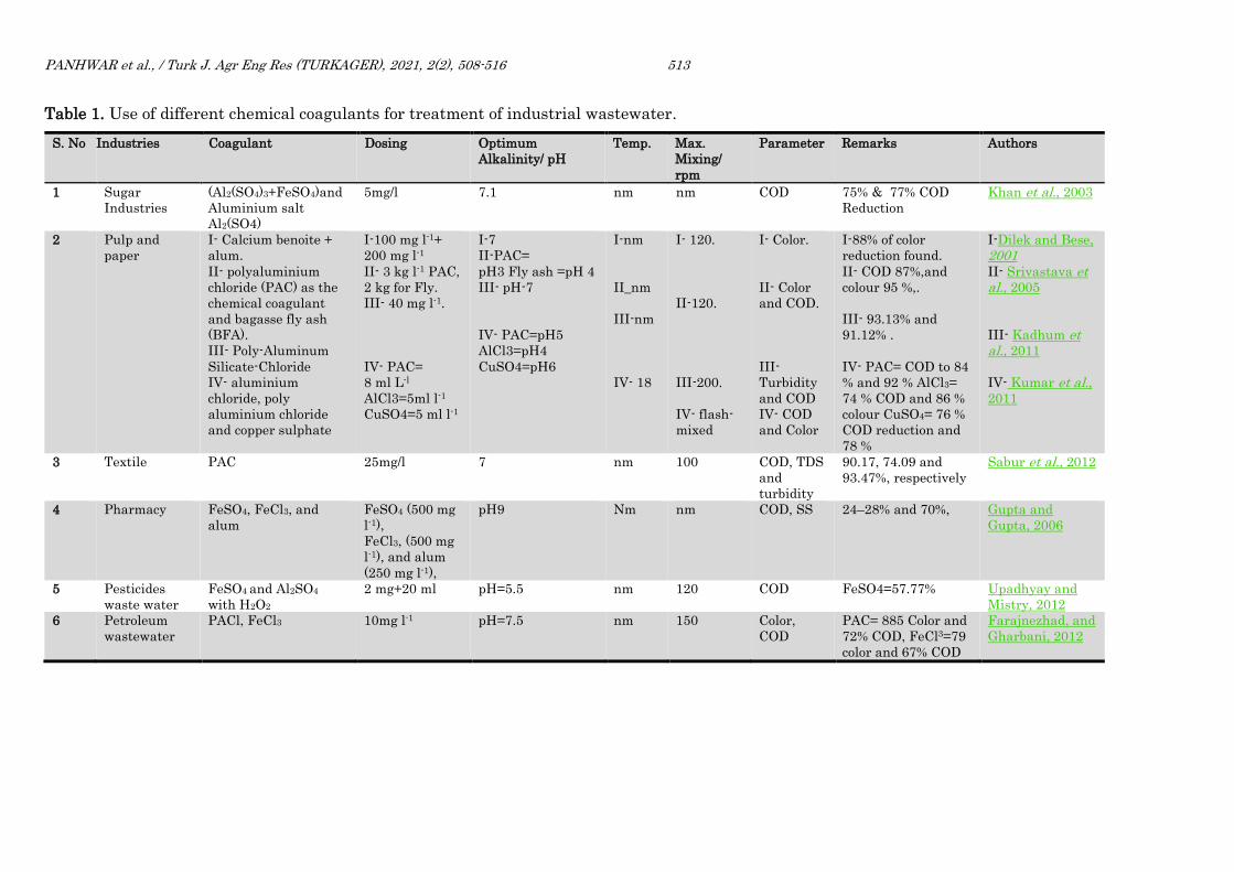
PANHWAR et al., / Turk J. Agr Eng Res (TURKAGER), 2021, 2(2), 508-516 513
Table 1. Use of different chemical coagulants for treatment of industrial wastewater.
S. No Industries Coagulant Dosing Optimum
Alkalinity/ pH
Temp. Max.
Mixing/
rpm
Parameter Remarks Authors
1 Sugar
Industries
(Al2(SO4)3+FeSO4)and
Aluminium salt
Al2(SO4)
5mg/l 7.1 nm nm COD 75% & 77% COD
Reduction
Khan et al., 2003
2 Pulp and
paper
I- Calcium benoite +
alum.
II- polyaluminium
chloride (PAC) as the
chemical coagulant
and bagasse fly ash
(BFA).
III- Poly-Aluminum
Silicate-Chloride
IV- aluminium
chloride, poly
aluminium chloride
and copper sulphate
I-100 mg l-1+
200 mg l-1
II- 3 kg l-1 PAC,
2 kg for Fly.
III- 40 mg l-1.
IV- PAC=
8 ml L-l
AlCl3=5ml l-1
CuSO4=5 ml l-1
I-7
II-PAC=
pH3 Fly ash =pH 4
III- pH-7
IV- PAC=pH5
AlCl3=pH4
CuSO4=pH6
I-nm
II_nm
III-nm
IV- 18
I- 120.
II-120.
III-200.
IV- flash-
mixed
I- Color.
II- Color
and COD.
III-
Turbidity
and COD
IV- COD
and Color
I-88% of color
reduction found.
II- COD 87%,and
colour 95 %,.
III- 93.13% and
91.12% .
IV- PAC= COD to 84
% and 92 % AlCl3=
74 % COD and 86 %
colour CuSO4= 76 %
COD reduction and
78 %
I-Dilek and Bese, 2001 II- Srivastava et al., 2005
III- Kadhum et al., 2011
IV- Kumar et al., 2011
3 Textile PAC 25mg/l 7 nm 100 COD, TDS
and
turbidity
90.17, 74.09 and
93.47%, respectively
Sabur et al., 2012
4 Pharmacy FeSO4, FeCl3, and
alum
FeSO4 (500 mg
l-1),
FeCl3, (500 mg
l-1), and alum
(250 mg l-1),
pH9 Nm nm COD, SS 24–28% and 70%, Gupta and
Gupta, 2006
5 Pesticides
waste water
FeSO4 and Al2SO4
with H2O2
2 mg+20 ml pH=5.5 nm 120 COD FeSO4=57.77% Upadhyay and
Mistry, 2012
6 Petroleum
wastewater
PACl, FeCl3 10mg l-1 pH=7.5 nm 150 Color,
COD
PAC= 885 Color and
72% COD, FeCl3=79
color and 67% COD
Farajnezhad, and
Gharbani, 2012

PANHWAR et al., / Turk J. Agr Eng Res (TURKAGER), 2021, 2(2), 508-516 514
CONCLUSION
Wastewater may be considered as wealth, if we use it after treatment properly; due to
utilization of treated wastewater we can increase agricultural production to tide over
the hunger in world. According to this study the recent developments elucidate that
the physical treatment processes (primary treatment) has becomes an effective
treatment technique and helpful before further treatment processes, which constitute
the tertiary treatment. It would require the chemicals process only and time saving and
treat huge quantity of water as compared to biological treatment which is time
consuming. The same process used to produce water for re-use in industries and
agriculture production. In chemical coagulation process the decontaminated process is
very easy and time saving techniques and almost chemicals are easily available. It is
an edge to this technique by adding or increasing dose of different chemical coagulants
can improve the treatment efficiency for treatment of industrial wastewater. Due to this
process the impressive results are achieved to reduce BOD, COD and suspended solids.
It is feasible and affording treatment processes and well-known disposal procedure for
discharge of industrial wastewater in freshwater bodies.
DECLARATION OF COMPETING INTEREST
The authors declare that they have no conflict of interest.
CREDIT AUTHORSHIP CONTRIBUTION STATEMENT
Aijaz Panhwar: Investigation, conceptualization, writing original draft.
Aftab Kandhro: Methodology, writing original draft.
Sofia Qaisar: Conceptualization
Mudasir Gorar: Review, and editing, references.
Eidal Sargani: Review, and editing, references.
Humaira Khan: Review, and editing, references.
REFERENCES
Akeem AO (2008). Impact of Ewekoro cement factory on the surrounding water resources. Bachelor of water
resources and hydrology management research project, Federal University of Agriculture, Abeokuta,
Nigeria, 2008.
Alkaya E, Demirer GN (2011) Anaerobic-fed and sequencing-batch treatment of sugar-beet processing
wastes: a comparative study. Water Environment Research, 83(3): 247-255.
Aziz N, Effendy and Basuki KT (2017) Comparison of poly aluminium chloride (PAC) and aluminium
sulphate coagulants efficiency in waste water treatment. Plant, 2(1): 24-31.
Dilek FB and Bese S (2001). Treatment of pulping effluents by using alum and clay-colour removal and
sludge characteristics. Water SA, 27(3): 361-366.
Drechsel P, Wichelns D and Qadir M (2015). Wastewater: economic asset in an urbanizing world. In
Drechsel, Pay; Qadir, Manzoor; Wichelns, D. (Eds.). Amsterdam, Netherlands: Springer, 3-14.
Farajnezhad H and Gharbani P (2012). Coagulation treatment of wastewater in petroleum ındustry using
poly aluminum chloride and ferric chloride. International Journal of Recent Research and Applied
Studies, 131(1): 306-310.

PANHWAR et al., / Turk J. Agr Eng Res (TURKAGER), 2021, 2(2), 508-516 515
Ghafari S, Aziz HA, Bashir MJK. (2010). The use of poly-aluminum chloride and alum for the treatment of
partially stabilized leachate: A comparative study. Desalination, 257(1-3): 110-116.
Ghaly A, Ananthashankar R, Alhattab M and Ramakrishnan V (2014) Production, characterization and
treatment of textile effluents: a critical review. Journal of Chemical Engineering Process Technology,
5(1): 1-19.
Gupta SK and Gupta SK (2006). Treatment of Pharmaceutical Wastes, Taylor & Francis Group.
Guven G, Perendeci A and Tanyolac A (2009). Electrochemical treatment of simulated beet sugar factory
wastewater. Journal of Chemical Engineering, 151(1-3): 149-159.
Holt PK, Barton GW, Wark M and Mitchell CA (2002) A quantitative comparison between chemical dosing
and electrocoagulation. Colloids and Surfaces A: Physicochemical and Engineering Aspects, 211(2-3):
233-248.
Isık M and Sponza DT (2006) Biological treatment of acid dyeing wastewater using a sequential
anaerobic/aerobic reactor system. Enzyme and Microbial Technology, 38(7):887-892.
Kadhum MS, Abdulbari HA, Abbas AA (2011). Treatment of pulp and paper mill wastewater by poly-
aluminum-silicate-chloride (pasic) through coagulation-flocculation process. Al-Qadisiya Journal For
Engineering Sciences 4(4): 546-555.
Khan M, Kalsoom U, Mahmood T, Riaz M and Khan AR (2003). Characterization and treatment of
industrial effluent from sugar industry. Journal Chemical Society, 25(3): 242-247.
Kumar P, Teng TT, Chand S and Kailas L (2011). Wastewater, treatment of paper and pulp mill effluent
by coagulation. International Journal of Civil and Environmental Engineering 3: 3.
Kawamura S (1996). Optimization of Basic Water Treatment Processes, Design and Operation: Coagulation
and Flocculation. Journal Water Supply Research and Technology AQUA, 45(1): 35-47.
Khalil HA, Davoudpour Y, Saurabh CK, Hossain MS, Adnan A, Dungani R, Paridah M, Sarker MZI, Fazita,
MN and Syakir M (2016). A review on nanocellulosic fibres as new material for sustainable packaging:
Process and applications. Renewable and Sustainable Energy Reviews, 64: 823-836.
Moussa DT, El-Naas MH, Nasser M and Al-Marri MJ (2017). A comprehensive review of electrocoagulation
for water treatment: potentials and challenges. Journal of Environmental Management, 186: 24-41.
Noppakhun P and Thunyalux R (2016). Removal of color, turbidity, UV254 in treated wastewater of sugar
factory by aluminum and iron based coagulants. KKU Engineering Journal. 43(2): 364-366.
Samsudin NS, Kabbashi NA and Jami MS (2019). Selection of Various Coagulants for sugar ındustry
wastewater treatment. Biological and Natural Resources Engineering Journal, 2(1): 1-9.
Nurul MF, Jayaraman K, Bhattacharyya D, Mohamad MH, Saurabh CK, Hussin MH and HPS AK (2016).
Green composites made of bamboo fabric and poly (lactic) acid for packaging applications. A review.
Materials, 9: 435.
Panhwar AA., Almani KF and Kandhro AA (2020). Environmental Degradation by Textile Industry;
Performance of Chemical Coagulants and Activated Carbon for Removal of COD, BOD. Technical
Journal, 25(4): 16-20.
Panhwar A and Bhutto S (2021). Improved Reduction of COD, BOD, TSS and Oil & Grease from Sugarcane
Industry Effluent by Ferric Chloride and Polyaluminum Chloride Coupled with Polyvinyl Alcohol.
Ecological Engineering & Environmental Technology, 22(2): 8-14.
Poddar PK and Sahu O (2017). Quality and Management of Wastewater in Sugar Industry. Applied Water
Science, 7(1): 461-468.
Radhi AA and Borghei M (2017). Investigate the optimal dose for COD and TSS removal using chemical
treatment, The International Journal of Computation and Applied Sciences (IJOCAAS), 3(3): 271-277.
Sabur MM, Khan AA and Safiullah S (2012). Treatment of textile wastewater by coagulation precipitation
method. Journal of Scientific Research 4(3): 623-633.
Sahu OP (2019). Electro-oxidation and chemical oxidation treatment of sugar industry wastewater with
ferrous material: An investigation of physicochemical characteristic of sludge. South African Journal of
Chemical Engineering, 28: 26-38.
Sahu OP and Chaudhari PK (2014). Physicochemical treatment of sugar industry wastewater: Coagulation
processes, Environment Quality Management, 23(4): 49-69.
Sahu OP and Chaudhari PK (2015). Electrochemical treatment of sugar industry wastewater: COD and
color removal. Journal of Electroanalytical Chemistry, 739; 122-129.
Sahu OP and Chaudhari PK (2013) Review on chemical treatment of industrial waste. Journal of Applied
Science and Environmental Management. 17(2): 241-257.

PANHWAR et al., / Turk J. Agr Eng Res (TURKAGER), 2021, 2(2), 508-516 516
Srivastava VC, Mall ID and Mishra IM (2005). Treatment of pulp and paper mill wastewaters with
Polyaluminium chloride and bagasse fly ash. Colloids and Surface A: Physiochemical Engineering
Aspects 260: 17-28.
Tchamango S, Njiki CPN, Ngameni E, Hadjiev D and Darchen A (2010). Treatment of dairy effluents by
electrocoagulation using aluminium electrodes. Science Total Environment, 408(4): 947-952.
Teh CY, Budiman PM, Shak KPY and Wu TY (2016) Recent advancement of coagulation–flocculation and
its application in wastewater treatment. Industrial Engineering Chemical Research, 55(16): 4363-4389.
Thompson RC, Moore CJ, vom Saal FS and Swan SH (2009b). Plastics, the environment and human health:
current consensus and future trends. Philosophical Transactions of the Royal Society B, 364: 2153-2166.
UN Water (2015). Wastewater management-A UN-Water analytical brief. (2015). (World Meteorological
Organization, Geneva, Switzerland), 1-52.
UN WWAP (2017). United Nations World Water Assessment Programme. The United Nations World Water
Development Report. Wastewater: The Untapped Resource. Paris.
Upadhyay AP and Mistry NJ (2012). Feasibility of combined Fenton & coagulation method for the
treatment of pesticides waste water. International Journal of Engineering Research & Technology ,1(3):
1-7.
US EPA (2014). US Environmental Protection Agency, Reducing Wasted Food & Packaging: A Guide for
Food Services and Restaurants. EPA. Retrieved March 7, 2019, from
[https://www.epa.gov/sites/production/files/201508/documents/reducing_wasted_food_pkg_tool.pdf].
US EPA (2021). US Environmental Protection Agency. https://www.epa.gov/facts-and-figures-about-
materials-waste-and-recycling/national-overview-facts-and-figures-materials Wastes and Recycling.
(01-09-2021).
Zaharia C, Suteu D, Muresan A, Muresan R and Popescu A (2009). Textile wastewater treatment by
homogenous oxidation with hydrogen peroxide. Environmental Engineering and Management Journal
8(6): 1359-1369.
Zonoozi MH, Moghaddam MRA, Arami M (2008). Removal of acid red 398 dyes from aqueous solutions by
coagulation/flocculation process. Environment Engineering Management Journal, 7(6): 695-699.