TWI for an unknown symmetric lossless wall

2876 IEEE TRANSACTIONS ON GEOSCIENCE AND REMOTE SENSING, VOL. 49, NO. 8, AUGUST 2011

TWI for an Unknown Symmetric Lossless WallRaffaele Solimene, Rosario Di Napoli, Francesco Soldovieri, and Rocco Pierri

Abstract—A through-wall-imaging problem where the scatter-ers are located beyond a 1-D nonhomogeneous unknown wall isconsidered. As is well known, as part of the propagation takesplace within the wall, the knowledge of its electromagnetic prop-erties is mandatory in order to obtain properly focused images.Accordingly, this paper’s focus is on the wall estimation problem.To this end, a simple procedure to estimate the wall transmissioncoefficient is introduced and validated by synthetic data. Theproposed estimation procedure works for a symmetric losslesswall and does not rely on optimization schemes but requires amultistatic configuration. As a proof of the principle, we addressthe problem for a 2-D scalar configuration. Moreover, the role ofobscured scatterers on the estimation procedure is discussed, anda procedure for mitigating their effect is proposed as well. Finally,the procedure is also checked against a wall with losses.

Index Terms—Linear inverse scattering problem, obstacle es-timation, singular value decomposition, through-wall imaging(TWI).

I. INTRODUCTION

THROUGH-WALL imaging (TWI) is an emerging field ofresearch within the broader realm of radar imaging [1]–

[3] because it finds a lot of applications, both in civilian andmilitary contexts. In this framework, a typical scenario consistsin detecting and localizing scatterers which are hidden beyondan opaque obstacle [4], such as a building wall [5], or even indetermining a building layout [6].

What makes TWI problems different and definitely moredifficult than free space imaging is the presence of the wall.

First of all, the wall is the primary source of clutter whichcan obscure the field scattered by the objects located beyond it.Therefore, a clutter cancellation technique, which increases thesignal-to-clutter ratio, is required. This often can be achievedby simply gating data in the time domain. However, whenmultiple reflections within the wall have a level comparableto the field scattered by the obscured objects, this techniqueis not very effective. Hence, alternative and more sophisticatedmethods have been devised. For example, wall reflection can be

Manuscript received November 6, 2009; revisedJune 22, 2010, October 13,2010, and November 5, 2010; accepted December 28, 2010. Date of publicationMarch 14, 2011; date of current version July 22, 2011.

R. Solimene and R. Pierri are with Dipartimento di Ingegneriadell’Informazione, Seconda Università di Napoli, 81031 Aversa, Italy (e-mail:[email protected]; [email protected]).

R. Di Napoli was first with Dipartimento di Ingegneria dell’Informazione,Seconda Università di Napoli. Now he is with Istituto per il RilevamentoElettromagnetico Ambientale-Consiglio Nazionale delle RIcerche (e-mail:[email protected]).

F. Soldovieri is with Istituto per il Rilevamento ElettromagneticoAmbientale-Consiglio Nazionale delle Ricerche, 80125 Napoli, Italy(e-mail: [email protected]).

Color versions of one or more of the figures in this paper are available onlineat http://ieeexplore.ieee.org.

Digital Object Identifier 10.1109/TGRS.2011.2110656

mitigated by adopting a differential measurement configurationwhere the difference between two consecutive spatial dataacquisitions is used as input to the imaging procedure [7].More generally, since the wall has a much larger transversalspatial extent than the obscured scatterers, a filtering proce-dure which suppresses the low harmonic spatial content, andhence the wall reflection, can be adopted [8], [9]. However,in both cases, a suitable processing is needed to restore thestandard point-spread function. Polarization diversity can alsobe employed to remove wall clutter when the scatterers are notpolarization insensitive by forming the so-called polarization-difference images [10]. Such a method is particularly effectivewhen changes occur in the scene. In the latter case, also theincoherent difference imaging proved to work very well [11].

Second, the illuminating radiation must be able to passthrough the obstacle with a “relatively low” attenuation. Thislimits the exploitable frequencies to the low part of the mi-crowave spectrum, for example, from a few hundreds of mega-hertz to 2–3 GHz [12].

Finally, in order to avoid blurring and delocalization in thereconstructions, the imaging algorithms must account for thepresence of the wall. Many imaging algorithms achieving sucha task have been developed [4], [13]–[15]. Of course, in order toobtain correctly focalized reconstructions, the wall parametersshould be known. However, in practical situations, they areunknown or known with some degree of uncertainty. Therefore,a wall estimation stage should be run before imaging.

Estimating the wall parameters entails solving an inversescattering problem quantitatively: that is, to determine thepermittivity and the conductivity spatial distributions of thewall. To achieve such a task is generally more difficult thanimaging itself. Indeed, as is well known, such a problem isnonlinear, and hence, the inversion procedures generally sufferfrom false solutions and are computationally demanding andtime consuming, also when the wall can be assumed as a 1-Dmedium (see [16] and the reference therein).

In many cases, the wall can be assimilated as a singlehomogeneous slab [4], [15]. In such cases, if the field scatteredby the obscured objects is available (for example, after a cluttercancellation procedure), the methods proposed in [17]–[19] canbe exploited. In particular, these methods require achieving thescene image at each step of the estimation procedure. This canbe avoided by estimating the wall directly from its reflectioncoefficient measurements [15], [20].

All these methods cast the estimation problem as an opti-mization and benefit from the single-layer homogeneous wallassumption which leads to a limited number of unknowns (twoor three) to be looked for. However, in many other situations,such a hypothesis does not hold, and the typical problems ofnonlinear optimization turn out to be relevant.

0196-2892/$26.00 © 2011 IEEE

SOLIMENE et al.: TWI FOR AN UNKNOWN SYMMETRIC LOSSLESS WALL 2877

Therefore, when dealing with more complex wall structures,new estimation strategies not based on an optimization stage areneeded.

This paper exactly focuses on a new nonoptimization-basedwall estimation procedure in the case of walls varying onlyalong the depth. The idea is to estimate the wall transmissioncoefficient rather than its electromagnetic properties. As willbe seen, this allows to obtain highly focused images withthe advantage of tackling a linear inverse problem. By con-trast, while achieving the scene image, one must be contentto determine only the target relative positions (with respectto the wall) and not the absolute ones as the transmissioncoefficient estimation does not give explicit information onthe wall thickness. Moreover, the transmission coefficient hasto be estimated as a function of the temporal as well as thespatial frequency. This necessarily entails using a multistatic(and possibly multiview also) measurement configuration. Inaddition, as the measurements are collected in a reflection modeconfiguration, the estimation procedure can be applied to thecase of symmetric (i.e., the dielectric permittivity profile is aneven function of depth with respect to the wall median depth)and lossless walls only. However, the wall can be multilayered(with the number of layers being unknown) or can be continu-ously varying in depth. Therefore, a considerable enlargementof the tractable kind of walls is achieved.

The plan of this paper is as follows. In Section II, we brieflyrecall the mathematical background pertinent for TWI. Thus,the needed mathematical notation is introduced, and the role ofthe wall parameters on the imaging procedure is highlighted. InSection III, the estimation procedure is introduced, and someconsiderations concerning the measurement setup design aregiven. In Section IV, the performance achievable by the esti-mation procedure is assessed by means of a numerical analysisalso in the case of noisy data and against the disturbance due toscatterers beyond the wall. Moreover, a procedure to counteracttheir effect is presented and validated. Finally, the case of alossy wall is briefly addressed as well.

Conclusions end this paper.

II. TWI MATHEMATICAL FORMULATION

AND PRELIMINARIES

We refer to the TWI scenario depicted in Fig. 1. For the sakeof simplicity, we move within a 2-D scalar geometry so thatinvariance along the y-axis is assumed.

Targets are located in region 3, whereas scattered field mea-surements are taken in region 1 after an impinging electromag-netic radiation, still coming from region 1, probed the scene.Regions 1 and 3 are assumed to be the free space with dielectricpermittivity and magnetic permeability denoted as ε0 and μ0,respectively. Region 2 is a nonmagnetic (hence, its magneticpermeability is equal to μ0) slab representative of the wall.Its thickness is denoted by d, whereas its equivalent complexdielectric permittivity is εeq(ω, z), where ω is the workingangular frequency.

Accordingly, the TWI problem amounts to retrieving anobject function O(x, z), which accounts for the shape and/orthe electromagnetic properties of the obscured scatterers, from

Fig. 1. Geometry of the problem.

scattered field measurements ES(rs, ro, ω) collected over ameasurement aperture, ro ∈ Σ, at different frequencies if amultifrequency configuration is exploited. rs is the sourceposition.

The scattered field consists of two contributions

ES(rs, ro, ω) = EwS (rs, ro, ω) + EO

S (rs, ro, ω) (1)

that is, the field reflected back from the wall EwS (·) and the field

scattered from the obscured scatterers EOS (·).

Therefore, the first step is to extract EOS (·) from the total

scattered field. As mentioned in the introduction, this can beachieved by exploiting some clutter mitigation technique. OnceEO

S (·) is obtained, the imaging problem can be cast as theinversion of an integral equation for O(x, z) [21]

EOS (rs, ro, ω) = k20

∫∫D

G(ro, r, ω)Et(rs, r, ω)O(x, z)dr

(2)

where G(·) is the background Green’s function, D is the spatialregion (beyond the wall) which is under investigation, and Et(·)is the field inside D.

This is a nonlinear inverse problem. In order to overcomethe difficulties characterizing this kind of problems (reliability,time and resources, expensive imaging procedures, etc.), alinear formulation is implicitly or explicitly adopted in mostimaging algorithms [22]. Accordingly, the field Et(·) is as-sumed as the one in the absence of the scatterers [14].

Now, we represent the field radiated by the source in termsof its plane-spectrum A(·), i.e.,

Ei(rs, r, ω) =

∫A(ω, kx) exp (−jkz|z − zs|)

× exp [−jkx(x− xs)] dkx (3)

where r = (x, z) is the field point, rs = (xs, zs), and kz =√k20 − k2x, k0 is the free-space wavenumber.


Hence, Et(·) can be expressed as

Et(rs, r, ω) =

∫τ(ω, kx)A(ω, kx) exp(jkzzs)

× exp [−jkz(z − d)] exp [−jkx(x− xs)] dkx (4)

where τ(·) is the wall transmission coefficient and the referenceframe outlined in Fig. 1 has been adopted.

The Green’s function has a similar plane-wave spectrumrepresentation given by

G(ro, r, ω) =j

4π

∫τ(ω, kx)

kzexp [−jkz(z − d)]

× exp(jkzzo) exp [−jkx(xo − x)] dkx. (5)

Equations (4) and (5) make it clear that, when the wallis unknown, the TWI problem entails dealing with a linear(because of the adopted approximation) and in some sense blindinverse problem. This is because the wall parameters enter inthe definition of the kernel of the linear operator to be invertedthrough the functions Et(·) and G(·).

III. WALL ESTIMATION PROCEDURE

As explained earlier, in order to avoid blurred and delocalizedreconstructions, the wall properties should be estimated beforeimaging. This entails dealing with an optimization problemwhich can lead to unreliable time consuming estimations whenthe structure of the wall becomes more complex than a merehomogeneous slab.

However, by looking at (4) and (5), one can note that theeffect of the wall is embodied within the transmission coeffi-cient τ(·). Therefore, it is easily realized that, for imaging pur-poses, what is really needed is the wall transmission coefficientfunction and not the spatial map of the wall electromagneticproperties.

Accordingly, here, we present an estimation procedure aim-ing at directly retrieving τ(·).

While pursuing such a task, one must take into accountthat, for TWI configuration, the available data concern thescattered field collected in a reflection mode configuration.Therefore, direct transmission coefficient measurements are notpossible. Furthermore, the field reflected from the wall has to beextracted from the total scattered field (incidentally, this is justthe opposite job that clutter rejection techniques do).

As to the latter point, here, we assume that no scatterers arepresent beyond the wall. Such a hypothesis will be relaxed inthe next section.

As far as the wall estimation is concerned, we adopted a two-step-based solution strategy. First, we retrieve the wall Fresnelreflection coefficient, and then, from the reflection coefficient,the transmission coefficient is estimated. As will be seen, thiscan be easily achieved by a simple algebraic relation in thecase of symmetric lossless walls. Moreover, according to (4)and (5), the estimation procedure should return the transmissioncoefficient as a function not only of the angular frequency ωbut also of the spatial frequency kx. This makes it impossible

to adopt the usual multimonostatic measurement configuration:a multistatic configuration is required.

Let us now go into the details of the estimation procedure.According to the previous section, the field reflected from the

wall can be expressed as

EwS (xs, xo, ω) =

k0∫−k0

Γ(ω, kx)A(ω, kx) exp(2jkzzs)

× exp [−jkx(xo − xs)] dkx (6)

where Γ(·) is the wall reflection coefficient and the observationpoints are taken over the segment Σ = [−XO, XO] along thex-axis at the same quota (i.e., zo = zs) as the source position.Moreover, the integration domain is limited to the visible do-main [−k0, k0] which entails neglecting the evanescent part ofthe incident field spectrum. Such an assumption holds when thesource antenna is not in close proximity to the air/wall interfacein terms of probing wavelength.

Accordingly, the wall reflection determination amounts tosolving a linear inverse problem by inverting (6) for Γ(·).

Equation (6) can be rewritten as

EwS (η, ω)=

k0∫−k0

Γ(ω, kx)A(ω, kx)exp(2jkzzs) exp[−jηkx]dkx

(7)

where we have considered η = xo − xs as the observation vari-able which ranges within the interval [−XO − xs, XO − xs].For convenience, we denote as A the operator in (7).

The necessity of a multistatic configuration is now clear. Infact, a multimonostatic as well as a multibistatic configurationwould allow to collect data only for η = 0 or η = Δx, respec-tively, with Δx being the transmitting and receiving antennaoffset. A multiview configuration is instead useful as it wouldresult in an enlargement of the η observation interval.

As is easily seen from (7), operator A is of theHilbert–Schmidt class, and hence, it is compact. This meansthat, in order to determine Γ(·), an ill-posed inverse problemhas to be tackled. Accordingly, a meaningful solution requiresexploiting a regularization scheme. To cope with this question,a truncated singular value decomposition (TSVD) inversionscheme is adopted here. Accordingly, the generalized solutionΓ(·) of (7) can be expressed as

Γ(ω, kx) =

NT∑n=0

〈EwS (η, ω), vn(η, ω)〉

σnun(ω, kx) (8)

where {vn, un, σn}∞n=0 is the singular system of A, 〈·, ·〉 de-notes the scalar product in the data space, and NT is the TSVDtruncation index.

Note that Γ(ω, kx) is the reflection coefficient retrieved at theparticular frequency ω. Hence, the estimation procedure mustbe rerun as the frequency changes.

The key question in (8) is the choice of the truncationNT upon which the tradeoff between accuracy and stabilitydepends [23].


To this end, we introduce the auxiliary operator B given by

k0∫−k0

Γ(ω, kx)max {|A(ω, kx)|} exp(2jkzzs) exp[−jηkx]dkx

(9)where max{·} takes the maximum over kx. Now, as

‖Ag‖ ≤ ‖Bg‖ ∀g ∈ L2[−k0, k0] (10)

we have that [24]

σn ≤ σn(B) ∀n. (11)

As the singular system of the operator B is related to the pro-late spheroidal functions [25], its singular values have a steplikebehavior with the knee occurring at the index [2Δηk0/π], [·]denoting the integer part operator, and Δη = (ηmax − ηmin)/2.Therefore, by virtue of (11), we deduce that an upper bound forthe truncation index in (8) is just NT = [2Δηk0/π]. A lowerbound can be estimated by following the theory developed in[26]. However, if a wide plane-wave source spectrum (nondi-rective antennas are, in general, useful in imaging as they allowto form a large synthetic aperture) is considered, the previousestimation works fairly well.

Note that, according to the properties of the prolatespheroidal functions, NT also represents the so-called numberof degrees of freedom of the reflected field. Therefore, it givesinsight about the minimum number of measurements (in the ηdomain) required to stably retrieve the reflection coefficient.

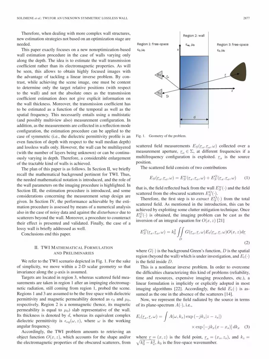
Once the reflection coefficient has been determined, wehave to consider the problem of the estimation of the walltransmission coefficient. This problem benefits of the circuitalperspective depicted in Fig. 2. There, the two transmission linesaccount for the propagation in the free space, whereas the two-port circuit represents the wall. This two-port circuit can beconveniently represented in terms of its scattering matrix [27]

S(ω, kx) =

(S11(ω, kx) S12(ω, kx)S21(ω, kx) S22(ω, kx)

)(12)

where, of course, its entries depend on ω and kx. The scatteringparameters S11 is the reflection coefficient Γ to be determinedaccording to the step described earlier, whereas S21 is thetransmission coefficient τ to be estimated. Now, the questionis how to estimate S21 from S11.

This can be easily done for lossless and symmetrical walls(of course, reciprocity is implicitly assumed).

In more detail, the lossless hypothesis means that εeq is apure real function εw(z) and entails that

SS† = I (13)

with I being the identity matrix and S† being the adjoint of S.From (13), it follows that

|τ(ω, kx)| =√1− |Γ(ω, kx)|2. (14)

Fig. 2. Circuital representation of the background medium.

However, we also need the phase of τ . By assuming that thewall is symmetric, i.e., εw(z) = εw(d− z), we have that S11 =S22. Therefore, by also accounting for (13), we obtain that

φτ (ω, kx) = φΓ(ω, kx) + (2n+ 1)π/2 (15)

with φτ (·) and φΓ(·) being the phases of τ(·) and Γ(·), respec-tively.

Note that the choice of n in (15) is immaterial because itintroduces a phase term which does not depend on ω or on kxeither.

Finally, as mentioned earlier, the two-step estimation proce-dure must be repeated for each adopted frequency.

We conclude this section by noting that, even though thetransmission coefficient has been estimated, we have no infor-mation concerning the wall thickness d. However, in (4) and (5),the exponential term exp [−jkz(z−d)] appears. Accordingly, ifthe wall thickness is not a priori known, while imaging, ob-scured scatterers will appear at their relative (with respect to thewall) positions and not at their actual positions as indicated bythe absolute reference frame. If it is a priori known that the wallis a single homogenous layer, then multifrequency data wouldallow to obtain an upper bound for its thickness (by neglectingwall dielectric permittivity which is indeed unknown) by mea-suring the time between the first two returned pulses. However,this does not appear easy to do for multilayered walls.

IV. NUMERICAL EXAMPLES

In this section, in order to assess the performances achievableby the estimation procedure, some numerical tests are shown.First, we consider the case of a wall consisting of a homo-geneous slab. Afterward, we turn to address a three-layeredwall and, then, a wall having a continuously varying (along thedepth) dielectric permittivity. The effect of the noise and of thelosses is also considered.

Finally, as the estimation procedure has been derived byassuming no scatterers beyond the wall, we analyze how their


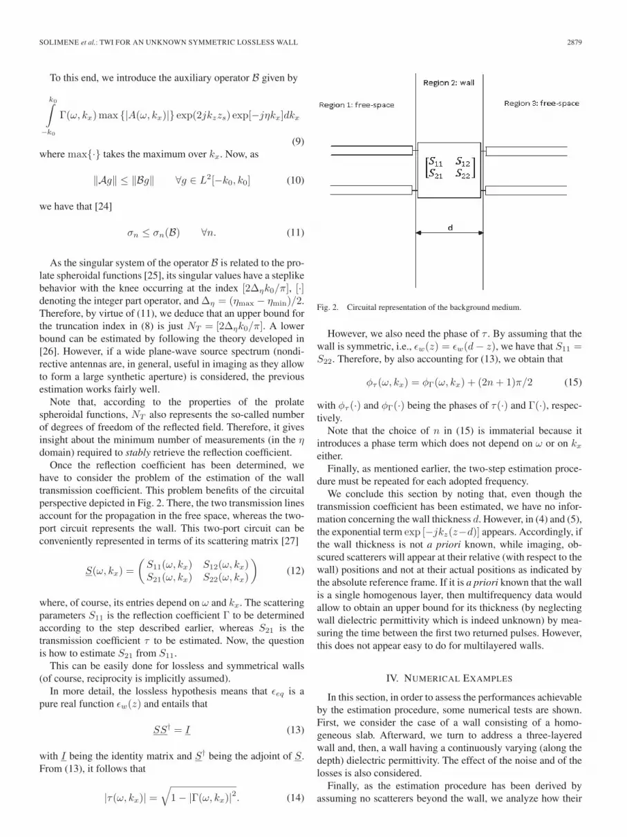
Fig. 3. Case of a homogeneous single-layer wall. (a) Comparison between the actual and the estimated transmission coefficient amplitudes. (b) Comparisonbetween the actual and the estimated transmission coefficient phases. (c) Cut view along kx = 0 of the coefficient amplitudes. (d) Cut view along kx = 0 of thecoefficient phases. (e) Normalized amplitude reconstruction obtained by exploiting the actual transmission coefficient and scattered field. (f) Normalized amplitudereconstruction obtained by exploiting the estimated scattered field and transmission coefficient.

presence affects the estimation. In particular, a procedure rely-ing on a multiview configuration is proposed to counteract theireffect.

A. Homogeneous Single-Layer Wall

In this first case, we consider a homogeneous dielectric layer,of thickness d = 20 cm and dielectric permittivity εeq = 9ε0, asrepresentative of a single concrete wall. We assume the need toknow the wall transmission coefficient for 21 frequencies takenwithin the band [0.3, 1] GHz. Of course, the frequency band andthe number of frequencies are, in general, determined accordingto the imaging purposes as discussed in [14].

The transmitting source is located at (0, −15 cm), whereasthe reflected field is collected over 15 measurement pointsuniformly distributed over the aperture Σ = [−1, 1] m locatedat the same quota as the source. We note that the number ofmeasurement points is chosen according to the criterion sug-gested in the previous section at the highest adopted frequencyand maintained for all the frequencies.

The estimated transmission coefficient along with the actualone is reported in Fig. 3(a)–(d). As can be seen, the es-timation procedure works very well. Indeed, the estimatedtransmitted coefficient is very similar to the actual one (seepanels c and d where the cut views for kx = 0 are displayed)even though some rapidly oscillating artifacts appear in the


Fig. 4. Case of a three-layered wall. (a) Comparison between the actual and the estimated transmission coefficient amplitudes. (b) Comparison between the actualand the estimated transmission coefficient phases. (c) Cut view along kx = 0 of the coefficient amplitudes. (d) Cut view along kx = 0 of the coefficient phases.(e) Normalized amplitude reconstruction obtained by exploiting the actual transmission coefficient and scattered field. (f) Normalized amplitude reconstructionobtained by exploiting the estimated scattered field and transmission coefficient.

estimation. These, of course, are due to the truncation in (8)which, in turn, is needed for regularization purposes. However,these do not significantly impact the quality of the recon-struction. This can be seen in Fig. 3(e) and (f) where thereconstructions of a perfect electric conducting scatterer ofelliptical cross section (having half axes of 20 and 10 cm,respectively, and its center at (0, 0.7) m) are reported. Inparticular, the reconstruction in panel e is obtained by em-ploying the actual transmission coefficient and scattered field,with the latter returned by (2), whereas for the reconstructionin Fig. 3(f), the scattered field is obtained by subtracting theestimated reflected field from the total one and by consider-

ing the estimated transmission coefficient within the imagingalgorithm based on a linear inverse scattering formulationdescribed in [14].

B. Three-Layered Wall

We now consider a more complex wall structure consistingof a three-layered slab. The first and the third layers aretuff walls with εeq = 4ε0 and a thickness of 12 cm.The second layer, which is located between the first andthe third one, is a void layer (hence, εeq = ε0) having athickness of 4 cm. Such a layer is generally used to increase


Fig. 5. Dielectric profile for the third example.

the thermal insolation. The overall wall thickness is28 cm.

For such a wall structure, six parameters should be estimatedif the dielectric profile was to be retrieved. The picture is indeedeven more complex as, generally, the number of layers is nota priori known.

However, by our approach, the complexity of the problemremains the same as that of the previous simpler case. Theresults obtained for the case at hand are reported in Fig. 4.The parameters of the configuration and the scatterer to bereconstructed are the same as those in the previous example.

As can be seen, the estimation procedure works as well asin the previous example [look at Fig. 4(a)–(d)]. This is alsoconfirmed from the reconstruction comparison [Fig. 4(e) and(f)] where the scatterer is very well detected and localized.

C. Continuously Varying Wall

The last kind of wall that we consider is a dielectric slabwhose dielectric permittivity varies continuously along thez variable. Of course, to stay within the range dictated bythe working hypotheses, εeq(z) = εeq(d− z). In particular, weassume that εeq varies from 4ε0 (at the wall edges) to 9ε0(at the wall center) according to the Gaussian law depicted inFig. 5. The wall thickness is 26 cm. For such a case, the wallstructure has been simulated by a cascade of thirteen 2-cm-long transmission lines with characteristic impedance varyingaccording to the law of variation of εeq .

It is worth remarking that this example is particularly relevantin highlighting the usefulness of the circuital point of view (theone employed here) for the wall estimation problem. In fact, forsuch a case, the number of unknowns increases, as compared tothe previous examples, and this would make the wall estimationby means of some optimization scheme cumbersome and unre-liable. Once again, our approach ensures that the complexity andreliability of the problem remain unchanged.

The results concerning this case are reported in Fig. 6 andpresented following the same rationale as that for the twoprevious cases. Also, for this case, the estimation procedureworks very well.

We turn now to study how the estimation procedure behaveswhen data are corrupted by noise. To this end, we add tothe reflected field a complex white Gaussian noise so thatthe SNR = 25 dB. The corresponding estimation results arereported in Fig. 7. Even though a slight worsening can beobserved in the estimation, results are still very good. The sameconclusion holds for the other examples as well (not shownhere). Of course, when the SNR decreases, things get worse.However, 25 dB is a quite reasonable SNR, particularly for astepped-frequency radar.

D. Estimation in Presence of Scatterers Beyond the Wall

In all the previous examples, the estimation stage has beencarried out by assuming that no scatterers were present beyondthe wall. However, when it is not possible to identify a regionwhere no scatterers are present beyond the wall, the datum iscorrupted by the field scattered by the obscured objects. In otherwords, while estimating the wall transmission coefficient, thescatterers act as a source of clutter which can strongly impairthe success in estimating the wall.

To show this, we once again consider the case reported inFig. 4 but, now, with the scatterer already present beyond thewall during the estimation stage. The estimation results andthe corresponding object reconstruction are reported in Fig. 8.As can be seen, the presence of the scatterer leads to totallymeaningless results (see the left sides of Fig. 8(a) and (b) and,in particular, the reconstruction of Fig. 8(e); see also the dashedlines in Fig. 8(c) and (d) concerning the cut views for kx = 0).

Therefore, to render the estimation procedure applicablealso in these situations, the clutter arising from the obscuredscatterers should be mitigated. To this end, a clutter rejectiontechnique adopted for imaging purposes (as the ones that welisted in the introduction) can be, in principle, used, providedto reverse the perspective concerning what should be retained.For example, the technique described in [8] mitigates the clutterarising from the wall by rejecting the zero-frequency spatialharmonic of the scattered field. In the estimation procedure,instead, we just have to retain such a spectral component byrejecting the other ones. In particular, in [8], a multimonostatic(or multibistatic) measurement configuration is employed. Asthe field reflected from the wall is always the same for eachmeasurement, its effect is mitigated by subtracting from datatheir mean value (obtained by averaging over the differentmeasurement positions). Here, we should instead retain sucha mean value. However, we already explained that the multi-monostatic and the multibistatic configurations cannot be usedfor estimation. In order to adopt a similar procedure, we need amultiview configuration.

Let us consider a multiview/multistatic configuration withNs sources whose positions rs are uniformly taken over theobservation aperture Σ. Accordingly, the scattered field is nowa function of both rs and ro. However, there exist different cou-ples of (rs, ro) which return the same value of the observationvariable η. The point is that, while the reflected field Ew

S (·)is constant for each couple (rs, ro) which corresponds to thesame value of η, the scattered field EO

S (·) instead changes. Ac-cordingly, we can mitigate the role of the scattering objects by


Fig. 6. Case of a continuously varying wall. (a) Comparison between the actual and the estimated transmission coefficient amplitudes. (b) Comparison betweenthe actual and the estimated transmission coefficient phases. (c) Cut view along kx = 0 of the coefficient amplitudes. (d) Cut view along kx = 0 of thecoefficient phases. (e) Normalized amplitude reconstruction obtained by exploiting the actual transmission coefficient and scattered field. (f) Normalized amplitudereconstruction obtained by exploiting the estimated scattered field and transmission coefficient.

Fig. 7. Case of a continuous wall with noisy data (SNR = 25 dB). (a) Comparison between the actual and the estimated transmission coefficient amplitudes.(b) Comparison between the actual and the estimated transmission coefficient phases.


Fig. 8. Case of a three-layered wall. Illustrating how a scatterer located beyond the wall can affect the estimation and the positive role of the multiviewfiltering, respectively. (a) Transmission coefficient amplitude without and with filtering. (b) Transmission coefficient phase without and with filtering, respectively.(c) Cut view along kx = 0 of the coefficient amplitudes. (d) Cut view along kx = 0 of the coefficient phases. (e) Normalized amplitude reconstruction obtainedby exploiting the transmission coefficient estimated using single-view data. (f) Normalized amplitude reconstruction obtained by exploiting the transmissioncoefficient estimated using multiview data.

adopting an averaged reflected field in the estimation procedure,i.e.,

EwS (η, ω) =

1

Nη

∑Iη

ES(rs, ro, ω) (16)

where Iη = {(rs, ro) : xo − xs = η} and Nη is the cardinalityof Iη .

The estimation results for the case of the three-layered wallare reported in the right sides of Fig. 8(a) and (b) where theimprovement in the estimation can be clearly appreciated. This

is also well evident by looking at panels c and d where thecuts along kx = 0 of the resulting estimation are reported.Such estimation has been obtained by considering 15 sourceand observation positions uniformly taken over Σ: then, foreach source position, the scattered field has been collected oversuch a set of measurement points. In particular, for this case,−2XO ≤ η ≤ 2XO. However, in the estimation procedure, weused only Ew

S (η, ω) for −XO ≤ η ≤ XO for two reasons. First,in order to compare results to the single-view case. Second, be-cause this way the averaging is more effective as it is achievedfor larger Nη .


Fig. 9. Case of a lossy wall with parameter taken from [7]. (a) Normalizedreconstruction obtained by exploiting the wall knowledge. (b) Normalized re-construction obtained by exploiting the estimated wall transmission coefficient.

Once the transmission coefficient has been estimated,the field scattered by possible objects beyond the wall isobtained as

EOS (η, ω) = ES(η, ω)− Ew

S (η, ω) (17)

and then, a single-view (once again to adapt the comparison)imaging algorithm is run.

As can be seen from Fig. 8(f), differently from the previouscase, now, the object is correctly localized and well discernablein the reconstruction. However, the typical effect, due to thelack of the continuous component [7] [because of (17)], isclearly visible in the reconstruction. A further processing stepcould be adopted to compensate for such a lack [7], but thispoint is not of concern in this paper.

Finally, we point out that, by increasing the measurementcomplexity, i.e., by increasing the number of transmitting andreceiving antennas, even better results can be, of course, ob-tained.

E. Lossy Wall

As explained before, the proposed procedure allows to dealwith lossless walls. However, walls generally do have losses.Hence, in this section, we check how the procedure works whenwalls are lossy. To this end, here, we limit to consider single-layer walls whose parameters are taken from the literature.In more detail, we consider the cases of a poured concretewall, with a relative dielectric permittivity equal to six and aconductivity of 0.02 S/m [7], and of a dry concrete wall, havinga complex dielectric permittivity of 6.2− j0.7 [28]. In bothcases, the walls are considered 20 cm thick.

In order to stay within the frequency band for which wallparameters are given in [7] and [28], differently from theprevious examples, here, we consider a frequency band of [1,1.7] GHz. Instead, the same scatter as before is considered.

The corresponding reconstructions, obtained after wall esti-mation, along with the ideal reconstructions obtained by em-ploying the actual wall parameters, are reported in Figs. 9 and10, respectively. As can be seen and as it can be expected,reconstructions appear delocalized from the actual object’s po-sition. However, this is a minor problem as, by our method, wealready are not able to estimate the actual scatterer’s location.

Fig. 10. Case of a lossy wall with parameter taken from [28]. (a) Normalizedreconstruction obtained by exploiting the wall knowledge. (b) Normalized re-construction obtained by exploiting the estimated wall transmission coefficient.

Moreover, they are still well focused and allow clearly to detectthe scatterer.

V. CONCLUSION

In this paper, we addressed a TWI problem for an unknownwall.

As is well known, wall knowledge is mandatory to obtainproperly focused scene reconstructions. To this end, here, wefocused on the wall estimation problem. In particular, a simplewall estimation procedure has been presented and validatedagainst synthetic data.

The idea subtended by the proposed procedure is to estimatethe wall transmission coefficient instead of the electromagneticproperties (dielectric permittivity, thickness, etc.) of the wall.This allowed to cast the estimation problem as a linear inverseone, thus avoiding optimization algorithms which can be timeand resource consuming when the wall structure is not a meresingle homogeneous slab.

It is shown that the procedure works for lossless symmetricwalls. However, layered walls (with the number of layers beingunknown) can be dealt with as well.

We also studied the role played by the obscured scatterers onthe estimation procedure. In particular, it is shown that they actas a source of clutter that can make the wall estimation, as wellas the corresponding reconstruction, completely unreliable. Tocope with this question, we proposed a procedure requiring amultiview configuration.

As the proposed procedure is founded on the absence oflosses, we checked it against lossy walls whose parameters aretaken from the literature. In these cases, we observed a delo-calization of the scatterer reconstructions. Notwithstanding, thereconstructions appeared still well focalized.

It is worth remarking that, while the determination ofthe transmission coefficient from the reflected one requiresthe work hypotheses (concerning the wall structure) to hold,the reflection coefficient retrieving does not. This is interestingsince the first step of the estimation procedure allows to retrievethe reflection coefficient as a function not only of ω but alsoof kx. In other words, multiview information, aside from thefrequency ones, could be adopted by all the inversion schemes(usually nonlinear optimizations) which adopt the reflection


coefficient as the datum. This could lead to a benefit in thefalse solution problem which, as known, strongly depends onthe number of available independent data.

Finally, we remark that, for the sake of simplicity, we haveconsidered a 2-D scalar configuration and checked the esti-mation procedure against synthetic data. Of course, to addresspractical scenarios, where data are provided by measurements,requires extending the present analysis to the case of a 3-Dgeometry.

REFERENCES

[1] “Special issue on advances in indoor radar imaging,” J. Franklin Inst.,vol. 345, pp. 553–722, 2008.

[2] M. Amin and K. Sarabandi, “Special issue on remote sensing of buildinginterior,” IEEE Trans. Geosci. Remote Sens., vol. 47, no. 5, pp. 1267–1268, May 2009.

[3] L. P. Song, C. Yu, and Q. H. Liu, “Through-wall imaging (TWI) by radar:2-D tomographic results and analyses,” IEEE Trans. Geosci. RemoteSens., vol. 43, no. 12, pp. 2793–2798, Dec. 2005.

[4] F. Ahmad, M. G. Amin, and S. A. Kassam, “Synthetic aperture beam-former for imaging through a dielectric wall,” IEEE Trans. Aerosp. Elec-tron. Syst., vol. 41, no. 1, pp. 271–283, Jan. 2005.

[5] R. Solimene, A. Brancaccio, R. Pierri, and F. Soldovieri, “TWI exper-imental results by a linear inverse scattering approach,” Prog. Electro-magn. Res., vol. PIER 91, pp. 259–272, 2009.

[6] T. Dogaru and C. Le, “SAR images of rooms and buildings based onFDTD computer models,” IEEE Trans. Geosci. Remote Sens., vol. 47,no. 5, pp. 1388–1401, May 2009.

[7] M. Dehmollaian, M. Thiel, and K. Sarabandi, “Through-the-wall imagingusing differential SAR,” IEEE Trans. Geosci. Remote Sens., vol. 47, no. 5,pp. 1289–1296, May 2009.

[8] D. Potin, E. Duflos, and P. Vanheeghe, “Landmines ground-penetratingradar signal enhancement by digital filtering,” IEEE Trans. Geosci. Re-mote Sens., vol. 44, no. 9, pp. 2393–2406, Sep. 2006.

[9] Y. S. Yoon and M. Amin, “Spatial filtering for wall clutter mitigationin through-the-wall radar imaging,” IEEE Trans. Geosci. Remote Sens.,vol. 47, no. 9, pp. 3192–3208, Sep. 2009.

[10] K. M. Yemelyanov, N. Engheta, A. Hoofar, and J. A. McVay, “Adaptivepolarization contrast techniques for through-wall microwave imaging ap-plications,” IEEE Trans. Geosci. Remote Sens., vol. 47, no. 5, pp. 1362–1374, May 2009.

[11] F. Soldovieri, R. Solimene, and R. Pierri, “A simple strategy to detectchanges in through the wall imaging,” Prog. Electromagn. Res. M, vol. 7,pp. 1–13, 2009.

[12] A. Muqaibel and A. Safaai-Jazi, “Characterization of wall dispersive andattenuative effects on UWB radar signals,” J. Franklin Inst., vol. 345,pp. 640–658, 2008.

[13] Y. S. Yoon and M. G. Amin, “High-resolution through-the wall radarimaging using beamspace MUSIC,” IEEE Trans. Antennas Propag.,vol. 56, no. 6, pp. 1763–1774, Jun. 2008.

[14] F. Soldovieri and R. Solimene, “Through-wall imaging via a linear inversescattering algorithm,” IEEE Geosci. Remote Sens. Lett., vol. 4, no. 4,pp. 513–517, Oct. 2007.

[15] M. Dehmollaian and K. Sarabandi, “Refocusing through building wallsusing synthetic aperture radar,” IEEE Trans. Geosci. Remote Sens.,vol. 46, no. 6, pp. 1589–1599, Jun. 2008.

[16] R. Solimene and R. Pierri, “Detection and localization of homogeneousslab’s interfaces by a linear-like δ-approach,” J. Opt. Soc. Amer. A, Opt.Image Sci., vol. 24, pp. 2661–2672, 2007.

[17] G. Wang, M. G. Amin, and Y. Zhang, “New approach for target locationsin the presence of wall ambiguities,” IEEE Trans. Aerosp. Electron. Syst.,vol. 42, no. 1, pp. 301–315, Jan. 2006.

[18] G. Wang and M. G. Amin, “Imaging through unknown walls using dif-ferent standoff distances,” IEEE Trans. Signal Process., vol. 54, no. 10,pp. 4015–4025, Oct. 2006.

[19] F. Ahmad, M. G. Amin, and G. Mandapati, “Autofocusing of through-the-wall radar imagery under unknown wall characteristics,” IEEE Trans.Image Process., vol. 16, no. 7, pp. 1785–1795, Jul. 2007.

[20] R. Solimene, F. Soldovieri, G. Prisco, and R. Pierri, “Three-dimensionalthrough-wall imaging under ambiguous wall parameters,” IEEE Trans.Geosci. Remote Sens., vol. 47, no. 5, pp. 1310–1317, May 2009.

[21] W. C. Chew, Waves and Fields in Inhomogeneous Media. Piscataway,NJ: IEEE Press, 1995.

[22] F. Soldovieri and R. Solimene, “Ground penetrating radar subsurfaceimaging of buried objects,” in Radar Technology, G. Kouemou, Ed.Vienna, Austria: In-Tech, 2010, pp. 105–126.

[23] M. Bertero and P. Boccacci, Introduction to Inverse Problems in Imaging.Bristol, U.K.: Inst. Phys., 1998.

[24] G. Newsam and R. Barakat, “Essential dimension as a well-defined num-ber of degrees of freedom of finite-convolution operators appearing inoptics,” J. Opt. Soc. Amer. A, Opt. Image Sci., vol. 2, no. 11, pp. 2040–2045, Nov. 1985.

[25] D. Slepian and H. O. Pollak, “Prolate spheroidal wave functions, Fourieranalysis and uncertainty—I,” Bell Syst. Tech. J., vol. 40, pp. 43–64, 1961.

[26] R. Solimene, R. Barresi, and G. Leone, “Localizing a buried planar perfectelectric conducting interface by multi-view data,” J. Opt. A: Pure Appl.Opt., vol. 10, no. 1, pp. 1–11, Jan. 2008.

[27] R. E. Collin, Foundations for Microwave Engineering. Piscataway, NJ:IEEE Press, 2001.

[28] N. Maaref, P. Millot, C. Pichot, and O. Picon, “A study of UWB FM-CWradar for the detection of human beings in motion inside a building,” IEEETrans. Geosci. Remote Sens., vol. 47, no. 5, pp. 1297–1300, May 2009.

Raffaele Solimene was born in Italy in 1974. Hereceived the Laurea (summa cum laude) and Ph.D.degrees in electronic engineering from the SecondaUniversità di Napoli, Aversa, Italy, in 1999 and 2003,respectively.

From 2002 to 2006, he was an Assistant Professorwith the University Mediterranea of Reggio Calabria,Reggio Calabria, Italy. Since 2006, he has been withthe Dipartimento di Ingegneria dell’Informazione,Seconda Università di Napoli. His main fields of in-terest are inverse scattering problems and microwave

imaging for subsurface and through-wall-imaging applications.

Rosario Di Napoli received the Laurea degree inelectronic engineering from the Second University ofNaples, Aversa, Italy, in 2009.

From 2009 to 2010, he worked with the De-partment of Information Engineering, Second Uni-versity of Naples. He is currently with the Istitutoper il Rilevamento Elettromagnetico Ambientale-Consiglio Nazionale delle Ricerche, Italian NationalResearch Council, Naples, Italy, where he is work-ing on the development and validation strategies forprocessing ground-penetrating-radar data. His main

scientific interests include through-the-wall and subsurface radar imaging.

Francesco Soldovieri, photograph and biography not available at the time ofpublication.

Rocco Pierri received the Laurea degree (summacum laude) in electronic engineering from theUniversity of Naples “Federico II,” Naples, Italy,in 1976.

He was with the University of Naples “Fed-erico II.” He has been a Visiting Scholar at manyuniversities, such as the University of Illinois atUrbana–Champaign, Urbana, Harvard University,Cambridge, MA, Northeastern University, Boston,MA, Supelec, Paris, France, and the University ofLeeds, Leeds, U.K. He has also lectured extensively

abroad at many universities and research centers. He is currently a FullProfessor with the Second University of Naples, Aversa, Italy, where he is alsothe Head of the Department of Information Engineering. His scientific interestsinclude antennas, near-field techniques, phase retrieval, inverse scattering,subsurface sensing, electromagnetic diagnostics, and tomography.

Mr. Pierri was the recipient of the 1999 Honorable Mention for the H.A.Wheeler Applications Prize Paper Award of the IEEE Antennas and Propaga-tion Society.

Documents

TWI for an unknown symmetric lossless wall