Embed Size (px)
Citation preview
Two-Level Probabilistic Grammars
for Natural Language Parsing
Gabriel G. Infante-Lopez
Contents
Acknowledgments vii
1 Introduction 11.1 Probabilistic Language Models . . . . . . . . . . . . . . . . . . . . . 2
1.2 Designing Language Models . . . . . . . . . . . . . . . . . . . . . . 4
1.2.1 W-Grammars as the Backbone Formalism . . . . . . . . . . . 5
1.3 Formal Advantages of a Backbone Formalism . . . . . . . . . . . .. 6
1.4 Practical Advantages of a Backbone Formalism . . . . . . . . .. . . 7
1.5 What Can You Find in this Thesis? . . . . . . . . . . . . . . . . . . . 8
1.6 Thesis Outline . . . . . . . . . . . . . . . . . . . . . . . . . . . . . . 8
2 Background and Language Modeling Landscape 112.1 The Penn Treebank . . . . . . . . . . . . . . . . . . . . . . . . . . . 11
2.1.1 Transformation of the Penn Treebank to Dependency Trees . . 13
2.2 Probabilistic Regular Automata . . . . . . . . . . . . . . . . . . . .. 14
2.2.1 Inferring Probabilistic Deterministic Finite Automata . . . . . 16
2.2.2 The MDI Algorithm . . . . . . . . . . . . . . . . . . . . . . 17
2.2.3 Evaluating Automata . . . . . . . . . . . . . . . . . . . . . . 19
2.3 Probabilistic Context Free Grammars . . . . . . . . . . . . . . . .. 21
2.4 W-Grammars . . . . . . . . . . . . . . . . . . . . . . . . . . . . . . 23
2.5 Further Probabilistic Formalisms . . . . . . . . . . . . . . . . . .. . 27
2.5.1 Dependency Based Approaches . . . . . . . . . . . . . . . . 27
2.5.2 Other Formalisms . . . . . . . . . . . . . . . . . . . . . . . . 29
2.6 Approaches Based on Machine Learning . . . . . . . . . . . . . . . .31
iii
3 The Role of Probabilities in Probabilistic Context Free Grammars 393.1 Introduction . . . . . . . . . . . . . . . . . . . . . . . . . . . . . . . 393.2 Maximum Probability Tree Grammars . . . . . . . . . . . . . . . . . 41
3.2.1 Filtering Trees Using Probabilities . . . . . . . . . . . . . .. 423.3 Expressive Power . . . . . . . . . . . . . . . . . . . . . . . . . . . . 433.4 Undecidability . . . . . . . . . . . . . . . . . . . . . . . . . . . . . . 473.5 The Meaning of Probabilities . . . . . . . . . . . . . . . . . . . . . . 50
3.5.1 Using Probabilities for Comparing PCFG . . . . . . . . . . . 503.5.2 Using Probabilities for Boosting Performance . . . . . .. . . 54
3.6 Conclusions and Future Work . . . . . . . . . . . . . . . . . . . . . . 55
4 Constrained W-Grammars 574.1 Grammatical Framework . . . . . . . . . . . . . . . . . . . . . . . . 57
4.1.1 Constrained W-Grammars . . . . . . . . . . . . . . . . . . . 574.1.2 Probabilistic CW-Grammars . . . . . . . . . . . . . . . . . . 634.1.3 Learning CW-Grammars from Treebanks . . . . . . . . . . . 644.1.4 Some Further Technical Notions . . . . . . . . . . . . . . . . 65
4.2 Capturing State-of-the-Art Grammars . . . . . . . . . . . . . . .. . 664.2.1 Bilexical Grammars . . . . . . . . . . . . . . . . . . . . . . 674.2.2 Markovian Context Free Grammars . . . . . . . . . . . . . . 714.2.3 Stochastic Tree Substitution Grammars . . . . . . . . . . . .75
4.3 Discussion and Conclusion . . . . . . . . . . . . . . . . . . . . . . . 79
5 Alternative Approaches for Generating Bodies of Grammar Rules 815.1 Introduction . . . . . . . . . . . . . . . . . . . . . . . . . . . . . . . 815.2 Overview . . . . . . . . . . . . . . . . . . . . . . . . . . . . . . . . 825.3 From Automata to Grammars . . . . . . . . . . . . . . . . . . . . . . 835.4 Building Automata . . . . . . . . . . . . . . . . . . . . . . . . . . . 84
5.4.1 Building the Sample Sets . . . . . . . . . . . . . . . . . . . . 845.4.2 Learning Probabilistic Automata . . . . . . . . . . . . . . . . 845.4.3 Optimizing Automata . . . . . . . . . . . . . . . . . . . . . 88
5.5 Parsing the PTB . . . . . . . . . . . . . . . . . . . . . . . . . . . . . 925.6 Related Work and Discussion . . . . . . . . . . . . . . . . . . . . . . 935.7 Conclusions . . . . . . . . . . . . . . . . . . . . . . . . . . . . . . . 94
6 Splitting Training Material Optimally 956.1 Introduction . . . . . . . . . . . . . . . . . . . . . . . . . . . . . . . 956.2 Overview . . . . . . . . . . . . . . . . . . . . . . . . . . . . . . . . 976.3 Building Grammars . . . . . . . . . . . . . . . . . . . . . . . . . . . 98
iv
6.3.1 Extracting Training Material . . . . . . . . . . . . . . . . . . 986.3.2 From Automata to Grammars . . . . . . . . . . . . . . . . . 98
6.4 Splitting the Training Material . . . . . . . . . . . . . . . . . . . .. 1016.4.1 Initial Partitions . . . . . . . . . . . . . . . . . . . . . . . . . 1016.4.2 Merging Partitions . . . . . . . . . . . . . . . . . . . . . . . 103
6.5 Parsing the Penn Treebank . . . . . . . . . . . . . . . . . . . . . . . 1106.6 Related Work . . . . . . . . . . . . . . . . . . . . . . . . . . . . . . 1146.7 Conclusions and Future Work . . . . . . . . . . . . . . . . . . . . . . 115
7 Sequences as Features 1177.1 Introduction . . . . . . . . . . . . . . . . . . . . . . . . . . . . . . . 1177.2 Detecting and Labeling Main Verb Dependents . . . . . . . . . .. . 1187.3 PCW-Grammars for Detecting and Labeling Arguments . . . .. . . . 1197.4 Transforming the Penn Treebank to Labeled Dependency Structures . 1217.5 Building the Grammars . . . . . . . . . . . . . . . . . . . . . . . . . 124
7.5.1 Grammars for Detecting Main Dependents . . . . . . . . . . 1247.5.2 Grammars for Labeling Main Dependents . . . . . . . . . . . 1267.5.3 Grammars for Detecting and Labeling Main Dependents .. . 130
7.6 Optimizing Automata . . . . . . . . . . . . . . . . . . . . . . . . . . 1317.7 Experiments . . . . . . . . . . . . . . . . . . . . . . . . . . . . . . . 1327.8 Related Work . . . . . . . . . . . . . . . . . . . . . . . . . . . . . . 1387.9 Conclusions and Future Work . . . . . . . . . . . . . . . . . . . . . . 139
8 Conclusions 1418.1 PCW-Grammars as a General Model . . . . . . . . . . . . . . . . . . 1428.2 PCW-Grammars as a New Parsing Paradigm . . . . . . . . . . . . . . 1428.3 Two Roads Ahead . . . . . . . . . . . . . . . . . . . . . . . . . . . . 144
A Parsing PCW-Grammars 145A.1 Introduction . . . . . . . . . . . . . . . . . . . . . . . . . . . . . . . 145A.2 Theoretical Issues . . . . . . . . . . . . . . . . . . . . . . . . . . . . 146A.3 Practical Issues . . . . . . . . . . . . . . . . . . . . . . . . . . . . . 148
A.3.1 Levels of visibility . . . . . . . . . . . . . . . . . . . . . . . 149A.3.2 Optimization aspects . . . . . . . . . . . . . . . . . . . . . . 149
A.4 Conclusions . . . . . . . . . . . . . . . . . . . . . . . . . . . . . . . 152
B Revising theSTOP Symbol for Markov Rules 153B.1 The Importance of theSTOP Symbol . . . . . . . . . . . . . . . . . . 153B.2 Collins’s Explanation . . . . . . . . . . . . . . . . . . . . . . . . . . 153B.3 Background on Markov Chains . . . . . . . . . . . . . . . . . . . . . 155
v
B.4 TheSTOP Symbol Revisited . . . . . . . . . . . . . . . . . . . . . . 157B.5 Conclusions . . . . . . . . . . . . . . . . . . . . . . . . . . . . . . . 159
vi

Chapter 1
Introduction
Natural language is a very complex phenomenon. Undoubtedly, the sentences we utterare organized according to a set of rules or constraints. In order to communicate withothers, we have to stick to these rules up to a certain degree.This set of rules, whichis language dependent, is well-known to all speakers of a given language, and it isthis common knowledge that makes communication possible. Every sentence has aclear organization: words in an utterance glue together to describe complex objectsand actions. This hidden structure, called syntactic structure, is to be recovered by aparser. Aparseris a program that takes a sentence as input and tries to find itssyntacticorganization. A parser searches for the right structure among a set of possible analyses,which are defined by agrammar. The language model decides what the syntacticcomponents of the sentence are and how they are related to each other, depending onthe required level of detail.
Natural language parsers are used as part of many applications that deal with natu-ral language. Applications like question answering, semantic analyses, speech recog-nition, etc. may rely heavily on parsers. The degree of detail in the information outputby the parser may change according to the application, but some amount of parsingplays a role in many language technology applications, and parser performance maybe crucial for the overall performance of the end-to-end application.
Designing and building language models is not a trivial task; the design cycle usu-ally comprises designing a model of syntax, understanding its underlying mathematicaltheory, defining its probability distribution, and finally,implementing the parsing al-gorithm. The building of every new language model has to complete at least thesethree steps. Each of these three steps is very complex and a line of research in itself.To help handling the intrinsic complexity of the three itemsa good level ofabstrac-tion is required. Abstraction is important as it helps us deal with complex objects byrepresenting them with a subset of their characteristic features. The selected features
1
2 Chapter 1. Introduction
characterize the object for a given task or context. For example, the way we under-stand or see cars depends very much on the task we want to carryout with them; if wewant to drive them, we do not need to know how their engines work, whereas if weare trying to fix a mechanical problem we better do. Moreover,abstraction has provento be an important scientific principle. The way abstractionhelps humans in dealingwith complex systems can best be illustrated by the history of computer science. Thecomplexity of systems has increased hand in hand with the introduction of program-ming languages that allow for increasing levels of abstraction, climbing all the wayfrom machine code to assembly language to imperative languages such as Pascal andC, to today’s object-oriented languages such as Java.
Back to natural language parsing — what does abstraction have to do with pars-ing? Our view is that state-of-the-art natural language models lack abstraction; theirdesign is oftenad hoc, and they mix many features that, at least conceptually, shouldbe kept separated. In this thesis, we explore new levels of abstraction for natural lan-guage models. We survey state-of-the-art probabilistic language models looking forcharacteristic features, and we abstract away from these features to produce a generallanguage model. We formalize this abstract language model,we establish unknownproperties of the models surveyed, and with our abstract model we investigate newdirections based on different parameterizations.
1.1 Probabilistic Language Models
Roughly speaking, the syntactic analysis of natural language utterances aims at theextraction of linguistic structures that make explicit howwords interrelate within utter-ances. Syntactic structures for a sentencex are usually conceived as treest1(x), . . . ,tn(x) whose leaves form the sentencex under consideration. Agrammaris a devicethat specifies a set of trees. The trees in this set are said to begrammatical trees. Indi-rectly, the concept of a grammatical sentence is defined as follows: a sentencex is saidto begrammaticalif there is a grammatical tree that yieldsx.
Most natural language grammars tend to assign many possiblesyntactic structuresto the same input utterance. In such situations, we say that the sentence isambigu-ous. Ambiguity is the most important unsolved problem that natural language parsersface. This contrasts with human language processing, whichin most cases selects asingle analysis as the preferred one for a given utterance. The task of selecting thesingle analysis that humans tend to perceive for an input utterance — disambiguation— is an active area of research in the field of natural languageprocessing. Becauseof the roles of world knowledge, cultural preferences and other extra-linguistic fac-tors, disambiguation can be seen as a decision problem underuncertainty. In recent
1.1. Probabilistic Language Models 3
years, there have been different proposals for a solution, mainly based on probabilisticmodels. Probabilistic models assign probabilities to trees and then disambiguate byselecting the tree with the highest probability.
From a formal language perspective, the notion of alanguagecoincides with theformal notion of aset of strings. Probabilistic languagesextend this definition sothat a language is aprobability distributionover a set of trees. In particular, a prob-abilistic language model is a probability distribution over a set of utterance-analysispairs. Usually, a recursive generative grammar is used to describe a set of possibleutterance-analysis pairs, possibly allowing multiple pairs for the same utterance. Cru-cially, defining a probabilistic language model allows us toview disambiguation as anoptimization task, where themost probable analysisT ∗ is selected from among thosethat a grammarG generates together with an input utteranceU . If P is a probabilityfunction over utterance-analysis pairs, i.e., alanguage model, we may describe thisoptimization task as follows:
T ∗ = argmaxT∈G
P (T |U)
= argmaxT∈G
P (T, U)
P (U)
= argmaxT∈G
P (T, U),
whereargmaxx∈X f(x) stands for thex ∈ X such thatf(x) is maximal, and whereP (U) is the same for all trees and, consequently, can be left out.
The step of enriching a given generative grammar with probabilities is a non-trivialtask. Apart from the empirical question of how to do so in a waythat allows gooddisambiguation, in the sense that the model selects the samepreferred analysis as hu-mans do, there are various formal and practical issues concerning the definition of acorrect model. In order to fully understand a language model, it is necessary to abstractaway from specific peculiarities and to identify its relevant features. The latter can besummarized as follows.
Set of possible trees:For a given utterance, the language model chooses a tree thatarticulates the syntactic structure of the utterance from afixed set of possibletrees. For example, in a Context Free Grammar (CFG), this setis defined by thegrammar’s tree language.
Probabilities Probabilistic language models assign a probability value to each tree,and this probability value is then used as a way to filter out unwanted trees. Asignificant part of the definition of a language model is used to establish the wayprobabilities are assigned to trees. For example, in a probabilistic context free
4 Chapter 1. Introduction
grammar, each rule has a probability value associated to it,and the probability ofa tree is defined as the product of the probabilities assignedto the rules buildingup the tree.
Parameter estimation Probabilistic models contain many parameters that define thegrammar’s disambiguation behavior. These parameters haveto be estimated.The probability model specifies the set of values the parameters might take. This,in turn, defines the set of possible grammars.
Expressive power The expressive power of language models gives us an idea of theiralgorithmic complexity, and it allows us to compare different models. For prob-abilistic models, determining expressive power is a difficult job because the pa-rameter estimation algorithm has to be taken into account.
Tweaking State-of-the-art parsing algorithms are not just languagemodels — theyhave been optimized considerably in order to improve their performance on realnatural language sentences. Some of the optimized parameters are hard to modeland are usually outside the language model.
Parsing complexity Parsing complexity has become an issue again in recent years,because of the appearance of theoretically appealing models that seem very hardto implement efficiently. Parsing complexity should be as low as possible. Theaim is to emulate the apparently linear time humans take to process a sentence.
Addressing all of these items in a single thesis would be overly ambitious. This list ismeant to provide the context — throughout this thesis we study various specific aspectsagainst this general background.
1.2 Designing Language Models
Designing a parsing algorithm involves a sequence of decisions about:
1. the grammatical formalism,
2. a probabilistic version of the formalism,
3. techniques for estimating probabilities, and
4. a parsing algorithm.
This cycle can be seen almost everywhere in the parsing literature (Collins, 1999; Eis-ner, 2000; Bod, 1999; Charniak, 1999; Ratnaparkhi, 1999). It seems that any new in-teresting parser often uses new formalism. The design is time consuming, and usually
1.2. Designing Language Models 5
parsers are only evaluated empirically. It is clear, however, that better empirical re-sults do not necessarily convey a better understanding of the parsing problem. Usually,descriptions of state-of-the-art language models do not clearly state how the featurespresented in the previous section are defined or implemented, or how they fit in thedesign cycle. The grammatical framework is rarely the only decision responsible forthe parsers’s performance; on top of the decision, there is alot of tweaking involved.For example, Collins (1997) defines a simple formalism, but in order to achieve hisresults, all the tweaking reported in (Bikel, 2004) is needed.
Designers of parsers often conflate their decisions about the different features weidentify in Section 1.1. For example, let us zoom in on one of the characteristicsidentified in Section 1.1 and then step back to adopt a more abstract perspective, andsee what this gives us. In the definition of today’s state-of-the-art language models,Markov chains, and more specificallyn-grams, are widely used because they are easyto specify and their probabilities easy to estimate.N-grams are both a componentin the definition of a model and a technique to assign probabilities. They are cen-tral to language models, and, consequently, every propertyof language models mustbe evaluated with respect ton-grams. It might be helpful, though, to step back fromn-grams, and think of them as special cases of probabilistic regular languages. Math-ematical properties of probabilistic regular languages are as well understood as thoseof n-grams, but they fit more directly into the overarching theory of formal languages.This perspective allows us to clearly separate the definition of the model (using regularlanguages) and the procedure for estimating probabilities(using probabilistic regularlanguage induction techniques).
In this thesis, we propose a language modeling formalism that abstracts away fromany particular instance. We investigate three state-of-the-art language models and dis-cover that they have one very noticeable feature: the set of rules they use for buildingtrees is built on the fly, meaning that the set of rules is not defined a priori. Theformalisms we review have two different levels of derivations even though this is notexplicitly stated. One level is for generating the set of rules to be used in the secondstep, and the second step is for building the set of trees thatcharacterize a given sen-tence. Our formalism, based onVan Wijngaarden grammars(W-grammars), makesthese two levels explicit.
1.2.1 W-Grammars as the Backbone Formalism
W-grammarswere introduced in the 1960s by Van Wijngaarden (1965). Theyare avery well-known and well understood formalism that is used for modeling program-ming languages (Van Wijngaarden, 1969) as well as natural languages (Perrault, 1984).W-grammars have been shown to be equivalent to Turing machines (Perrault, 1984),
6 Chapter 1. Introduction
which are more powerful than we need: most state-of-the-artlanguage models usegrammatical formalisms that are much closer to context freeness than to Turing ma-chines. In this thesis, we constrain the set of possible W-grammars in order to comecloser to the expressive power of these grammatical formalisms. We denote this con-strained version asCW-grammars.
Originally, W-grammars did not use probabilities, but partof the work presentedbelow extends the formalism with probabilities. In this way, we define probabilisticCW-grammars (PCW-grammars). We show that probabilities are an essential com-ponent of the resulting formalism, not only because of the statistical perspective theybring, but also because of the expressivity they add. With PCW-grammars, we provethat Markovian context free grammars (Collins, 1999; Charniak, 1997), bilexical gram-mars (Eisner, 2000) and stochastic tree substitution grammars (Bod, 1999) are par-ticular instances of probabilistic CW-grammars. The probabilistic version of CW-grammars helps us to prove properties for these models that were previously unknown.
1.3 Formal Advantages of a Backbone Formalism
From a theoretical point of view, general models help us to clarify the set of param-eters a particular instance has fixed, and to make explicit assumptions that underlie aparticular instance. It might be the case that these assumptions are not clear, or that,without taking the abstract model into account, the designer of a particular instance iscompletely unaware of them.
The role of probabilities: Our approach to parsing comes from a formal languageperspective: we identify features that are used by state-of-the-art language mod-els and take a formalism off the shelf and modify it to incorporate the necessaryfeatures. When analyzing the necessary features from the formal language per-spective, the need for probabilities and their role in parsing are the first issue toaddress. In Chapter 3, we answer many questions regarding the role of prob-abilities in probabilistic context free grammars. We focuson these grammarsbecause they are central to the formalism we present.
Consistency properties: General models do not add anythingper se. Their impor-tance is rather in the set of instances they can capture and the new directions theyare able to suggest. In Chapter 4, we show that bilexical grammars, Markoviancontext free grammars and stochastic tree substitution grammars are instances ofour general model. Our model has well-established consistency properties whichwe use to derive consistency properties of these three formalisms.
1.4. Practical Advantages of a Backbone Formalism 7
1.4 Practical Advantages of a Backbone Formalism
From a computational point of view, general models for whicha clear parsing algo-rithm and a relatively fast implementation can be defined, produce fast and clear im-plementations for all particular instances. New research directions are also suggestedby a general formalism. These directions are a consequence of instantiating the mod-els’s parameters in a different way or by re-thinking the setof assumptions the partic-ular instances have made. A brief description of the directions explored in this thesisfollows.
Explicit use of probabilistic automata: Earlier, we mentioned that Markov modelsare heavily used in parsing models and that they can be replaced by probabilisticregular languages. Since our formalism is not bound to Markov models, wecan use any algorithm for inducing probabilistic automata.In Chapter 5, weexplore this idea. We define a type of grammar that uses probabilistic automatafor building the set of rules. We compare two different classes of grammarsdepending on the algorithm used for learning the probabilistic automata. One ofthem is based onn-grams, and the other one is based on the minimum divergencealgorithm (MDI). We show that the MDI algorithm produces both smaller andbetter performing grammars.
Splitting the training material: The fact that probabilistic automata replace Markovchains in the definition of our model allows us to think of a regular language asthe union of smaller, more specific sublanguages. Our intuition is that the sub-languages are easier to induce and that the combination of them fully determinesthe whole language. In Chapter 6, we explore this idea by splitting the trainingmaterial before inducing the probabilistic automata, theninducing one automa-ton for each component, and, finally, combining them into onegrammar. Weshow that in this way, a measure that correlates well with parsing performancecan be defined over grammars.
Sequences as features:Our formalism allows us to isolate particular aspects of pars-ing. For example, the linear order in which arguments appearin a parse tree isa fundamental feature used by language models. In Chapter 7,we investigatewhich sequences of information better predict sequences ofdependents. Wecompare sequences of part-of-speech tags to sequences of non-terminal labels.We show that part-of-speech tags are better predictors of dependents.
8 Chapter 1. Introduction
1.5 What Can You Find in this Thesis?
In my opinion there are two different types of research. The first one pushes the frontierof knowledge forward, jumping from one point to a more advanced, better performingone. This pushing forward is sometimes carried out in a disorderly way, leaving manygaps along the way. The second line of research tries to fill inthese gaps. Both types arevery important, and neither of them can exist without the other. The second provides asolid foundation to the first one in order to make new jumps possible. After a jump, ahuge a amount of work is waiting to be done by the second type ofresearch.
This thesis belongs solidly to the second type of research. Here, the reader willfind a formal analysis of existing models. The reader will also find a general modelthat encompasses many of the models studied, as well as some properties these mod-els enjoy — properties that we want the models to have and properties that were notknown before and the general models let us prove. Finally, the reader will find a fewexplorations along new research directions also suggestedby our model.
We hope that after having read the thesis, the reader will understand the languagemodeling task better. We also hope to have provided the area of natural languagemodeling with a more solid background. This background comprises consistency andexpressive properties generally believed but not formallyproven. We also provide inthe thesis initial steps in promising new research directions.
In contrast, the reader will not find here a state-of-the-artlanguage model. Thereader will not find either any claims regarding the universal structure natural languagepossesses. It is very clear to me that the structure of natural language is, at this point,as unknown as it was when I first started. I can only see, so far,that formal languageswith complexity up to context freeness can help us quite a lotin handling most syntacticstructures.
1.6 Thesis Outline
Chapter 2 (Background and Landscape):This chapter introduces the machinery offormal languages. It covers formal language theory from regular languages tomachine learning-based parsing algorithms, touching on context free grammars,W-grammars, and other formalisms.
Chapter 3 (The Role of Probabilities):This chapter investigates the role of probabil-ities in probabilistic context free grammars. Among othersit answers questionslike: “can probabilities be mimicked with rules?”, “can a grammar fully disam-biguate a language?”.
1.6. Thesis Outline 9
Chapter 4 (CW-Grammars as a General Model): This chapter presents our for-malism. It shows that bilexical grammars, Markovian context free grammarsand stochastic tree substitution grammars are instances ofour formalism.
Chapter 5 (Alternative Approaches for Generating Bodies ofGrammar Rules):This chapter explores the replacement ofn-gram models by a more general algo-rithm for inducing probabilistic automata. It shows that the alternative algorithmproduces smaller and better performing grammars.
Chapter 6 (Splitting training material optimally): This chapter investigates differ-ent ways to split the training material before it is used for inducing probabilisticautomata. It defines a measure over grammars that correctly predicts their pars-ing performance.
Chapter 7 (Sequences as Features):This chapter focuses on a very specific as-pect of syntax. We compare how two different features, each of them based onsequences of information, help to predict dependents of verbs. One of the fea-tures is based on sequences of part- of-speech tags while theother is based onsequences of non-terminals labels.
Chapter 8 (Conclusions): This chapter summarizes and combines conclusions of allthe chapters.
Appendix A (Parser Implementation): This appendix discusses aspects related tothe implementation of our parsing algorithm for probabilistic CW-grammars. Itdiscusses the prerequisites a grammar has to fulfill for a parser to return themost probable tree. It also discusses some of the optimization techniques weimplemented to reduce parsing time.
Appendix B (STOP symbol): This appendix reviews Collins’s (1999) explanation ofthe necessity of theSTOP symbol. The appendix uses Markov chains theory tore-explain and justify its necessity.

Chapter 2
Background and Language ModelingLandscape
This chapter has two main goals. The first is to present the background material re-quired for most of the forthcoming chapters, the second one is to situate this thesisin the landscape of natural language parsing. When presenting different approachesfor dealing with language models, we adopt a formal languageperspective Section 2.2presents regular automata, Section 2.3 context free grammars, Section 2.4 W-grammars,and Section 2.5 deals with other formalisms that do not fall in any of the previous cat-egories but that are used for natural language parsing. Finally, Section 2.6 deals withapproaches used for natural language parsing that are mainly based on machine learn-ing techniques.
2.1 The Penn Treebank
We start by presenting the material that indirectly defines our task. The Penn treebank(PTB) (Marcus et al., 1993, 1994) is the largest collection of syntactically annotatedEnglish sentences, and probably the most widely used corpusin computational linguis-tics. It is also the basis for the experiments reported in this thesis, and it defines thekind of information we are going to try to associate to naturally occurring sentences.
The PTB project started in 1989. Between then and 1992,4.5 million words ofAmerican English were automatically part of speech (POS) tagged and then manuallycorrected. Then, each sentence was associated to a parse tree that reflected its syntacticstructure. The first release of the PTB uses basically a content free phrase structureannotation for parse trees, where node labels are mostly standard syntactic categorieslike NP,PP,VP,S,SBAR, etc. In 1995, a new version was released; this second versionapplied a much richer annotation scheme, including co-indexed null elements (traces)
11
12 Chapter 2. Background and Language Modeling Landscape
to indicate non-local dependencies, and function tags attached to the node labels toindicate the grammatical function of the constituents.
The parsed texts come from the 1989 Wall Street Journal (WSJ)corpus, and fromthe Air Travel Information System (ATIS) corpus (Hemphill et al., 1990). The secondrelease is the basis for the experiments in Chapters 5, 6 and 7. A third release came outlater on, using basically the same annotation schema as the second but also includinga parsed version of the Brown Corpus (Kucera and Francis, 1967).
The POS tag set is the same in all three releases. It is based onthe Brown Corpustag set, but the PTB project collapses many Brown tags. The reason for this simplifica-tion is that the statistical methods, which were used for thefirst automatic annotationand envisaged as potential “end users” of the treebank, are sensitive to thesparse dataproblem. This problem comes into play if certain statistical events(e.g., the occurrenceof a certain trigram of POS tags) do not occur in the training data, so that their prob-ability cannot be properly estimated. The sparseness of thedata is related to the sizeof the corpus and the size of the tag set. Thus, given a fixed corpus size, the sparsedata problem can be reduced by decreasing the number of tags.Consequently, the finalPTB tag set has only 36 POS tags for words and 9 tags for punctuation and currencysymbols. Most of the reduction was achieved by collapsing tags that are recoverablefrom lexical or syntactic information. For example, the Brown tag set had separatetags for the (potential) auxiliariesbe, do andhave, as these behave syntactically quitedifferently from main verbs. In the tag set of the PTB, these words have the same tagsas main verbs. However, the distinction is easily recoverable by looking at the lexicalitems. Other tags that are conflated are prepositions and subordinating conjunctions(conflated inIN) and nominative and accusative pronouns (conflated inPRP), as thesedistinctions are recoverable from the parse tree by checking wetherIN is underPP orunderSBAR, and whetherPRP is underS or underVP or PP.
The syntactic annotation is guided by the same considerations as POS tagging. Forinstance, there is only one syntactic category, labeledSBAR, for that- or wh- clausesand only oneS for finite and non-finite (infinitival or participal) clauses, although thetwo types behave syntactically quite differently. Again, the argument is that thesedistinctions are recoverable by inspecting the lexical material in the clause; and parsersbasically use the simple treebank categories.
In general, only maximal projections (NP, VP, . . .) are annotated, i.e., intermediateX-bar levels (N’, V’) are left unexpressed, with the exception ofSBAR. In the firstrelease of the PTB, the distinction between complements andadjuncts of verbs wasexpressed by attaching complements under aVP as sisters of the verb and by adjoiningadjuncts at theVP level. In the second release, both complements and adjunctsareattached underVP.
In our experiments, we used the PTB as training and test material. We train models
2.1. The Penn Treebank 13
on the data provided by the PTB and we try to obtain, for instances not used in thetraining material, the tree that the PTB would have associated to them. In our exper-iments, we did not work directly with the PTB, but with a dependency version of thetrees in the PTB. That is, we transformed the PTB into dependency trees to obtain thetraining material for our experiments.
2.1.1 Transformation of the Penn Treebank to Dependency Trees
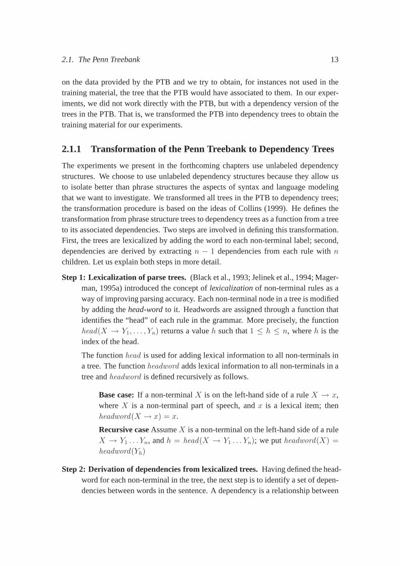
The experiments we present in the forthcoming chapters use unlabeled dependencystructures. We choose to use unlabeled dependency structures because they allow usto isolate better than phrase structures the aspects of syntax and language modelingthat we want to investigate. We transformed all trees in the PTB to dependency trees;the transformation procedure is based on the ideas of Collins (1999). He defines thetransformation from phrase structure trees to dependency trees as a function from a treeto its associated dependencies. Two steps are involved in defining this transformation.First, the trees are lexicalized by adding the word to each non-terminal label; second,dependencies are derived by extractingn − 1 dependencies from each rule withnchildren. Let us explain both steps in more detail.
Step 1: Lexicalization of parse trees.(Black et al., 1993; Jelinek et al., 1994; Mager-man, 1995a) introduced the concept oflexicalizationof non-terminal rules as away of improving parsing accuracy. Each non-terminal node in a tree is modifiedby adding thehead-wordto it. Headwords are assigned through a function thatidentifies the “head” of each rule in the grammar. More precisely, the functionhead(X → Y1, . . . , Yn) returns a valueh such that1 ≤ h ≤ n, whereh is theindex of the head.
The functionhead is used for adding lexical information to all non-terminalsina tree. The functionheadword adds lexical information to all non-terminals in atree andheadword is defined recursively as follows.
Base case:If a non-terminalX is on the left-hand side of a ruleX → x,whereX is a non-terminal part of speech, andx is a lexical item; thenheadword(X → x) = x.
Recursive caseAssumeX is a non-terminal on the left-hand side of a ruleX → Y1 . . . Yn, andh = head(X → Y1 . . . Yn); we putheadword(X) =
headword(Yh)
Step 2: Derivation of dependencies from lexicalized trees.Having defined the head-word for each non-terminal in the tree, the next step is to identify a set of depen-dencies between words in the sentence. A dependency is a relationship between
14 Chapter 2. Background and Language Modeling Landscape
two word-tokens in a sentence, amodifierand itshead, which we will write asmodifier → head . The dependencies for a given tree are derived in two ways:
• Every ruleX → Y1 . . . Yn such thatY1, . . . , Yn are non-terminals andn ≥ 2 contributes the following set of dependencies:{headword(Yi) →headword(Yh) : 1 ≤ i ≤ n, i 6= h}, whereh = head(X → Y1 . . . Yn).
• If X is the root non-terminal in the tree, andx is its headword, thenx →END is a dependency
Clearly, the key component in the transformation process isthe functionhead . Thisfunction has been implemented mainly as a lookup table. For further details on thedefinition of the functionhead , see (Collins, 1999, Appendix A).
The PTB provides us with the training material for inducing our own grammars.The grammars learnt in this thesis are Probabilistic Constrained W-Grammars (PCWGrammars), a new formalism which is presented in Chapter 4. Our formalism is re-lated to probabilistic regular languages, probabilistic context free grammars and W-grammars. In this chapter we present these three different formalisms. The relation ofPCW Grammars to each of the three formalism will become clearin the remainder ofthe thesis.
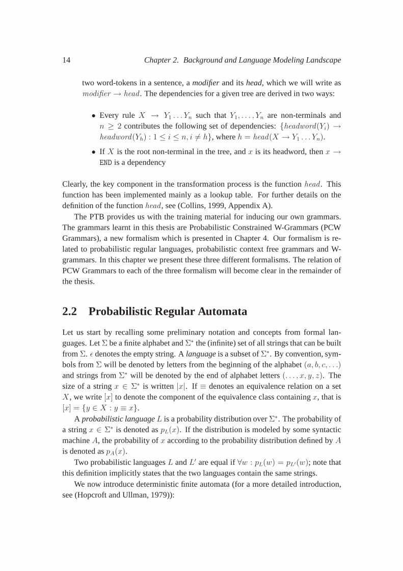
2.2 Probabilistic Regular Automata
Let us start by recalling some preliminary notation and concepts from formal lan-guages. LetΣ be a finite alphabet andΣ∗ the (infinite) set of all strings that can be builtfrom Σ. ǫ denotes the empty string. Alanguageis a subset ofΣ∗. By convention, sym-bols fromΣ will be denoted by letters from the beginning of the alphabet(a, b, c, . . .)
and strings fromΣ∗ will be denoted by the end of alphabet letters(. . . , x, y, z). Thesize of a stringx ∈ Σ∗ is written |x|. If ≡ denotes an equivalence relation on a setX, we write[x] to denote the component of the equivalence class containingx, that is[x] = {y ∈ X : y ≡ x}.
A probabilistic languageL is a probability distribution overΣ∗. The probability ofa stringx ∈ Σ∗ is denoted aspL(x). If the distribution is modeled by some syntacticmachineA, the probability ofx according to the probability distribution defined byAis denoted aspA(x).
Two probabilistic languagesL andL′ are equal if∀w : pL(w) = pL′(w); note thatthis definition implicitly states that the two languages contain the same strings.
We now introduce deterministic finite automata (for a more detailed introduction,see (Hopcroft and Ullman, 1979)):
2.2. Probabilistic Regular Automata 15
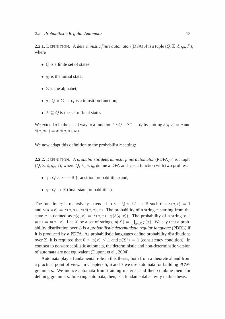
2.2.1.DEFINITION. A deterministic finite automaton(DFA)A is a tuple(Q,Σ, δ, q0, F ),where
• Q is a finite set of states;
• q0 is the initial state;
• Σ is the alphabet;
• δ : Q× Σ→ Q is a transition function;
• F ⊆ Q is the set of final states.
We extendδ in the usual way to a functionδ : Q×Σ∗ → Q by puttingδ(q, ǫ) = q andδ(q, aw) = δ(δ(q, a), w).
We now adapt this definition to the probabilistic setting:
2.2.2.DEFINITION. A probabilistic deterministic finite automaton(PDFA)A is a tuple(Q,Σ, δ, q0, γ), whereQ, Σ, δ, q0 define a DFA andγ is a function with two profiles:
• γ : Q× Σ→ R (transition probabilities) and,
• γ : Q→ R (final-state probabilities).
The functionγ is recursively extended toγ : Q × Σ∗ → R such thatγ(q, ǫ) = 1
andγ(q, ax) = γ(q, a) · γ(δ(q, a), x). The probability of a stringx starting from thestateq is defined asp(q, x) = γ(q, x) · γ(δ(q, x)). The probability of a stringx isp(x) = p(q0, x). LetX be a set of strings,p(X) =
∏
x∈X p(x). We say that a prob-ability distribution overL is aprobabilistic deterministic regular language(PDRL) ifit is produced by a PDFA. As probabilistic languages define probability distributionsoverΣ, it is required that0 ≤ p(x) ≤ 1 andp(Σ∗) = 1 (consistency condition). Incontrast to non-probabilistic automata, the deterministic and non-determinstic versionof automata are not equivalent (Dupont et al., 2004).
Automata play a fundamental role in this thesis, both from a theoretical and froma practical point of view. In Chapters 5, 6 and 7 we use automata for building PCW-grammars. We induce automata from training material and then combine them fordefining grammars. Inferring automata, then, is a fundamental activity in this thesis.
16 Chapter 2. Background and Language Modeling Landscape
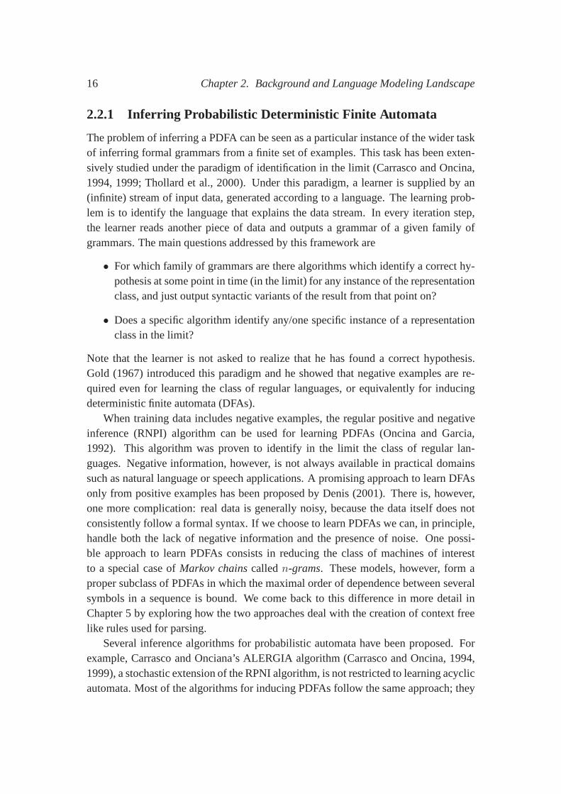
2.2.1 Inferring Probabilistic Deterministic Finite Autom ata
The problem of inferring a PDFA can be seen as a particular instance of the wider taskof inferring formal grammars from a finite set of examples. This task has been exten-sively studied under the paradigm of identification in the limit (Carrasco and Oncina,1994, 1999; Thollard et al., 2000). Under this paradigm, a learner is supplied by an(infinite) stream of input data, generated according to a language. The learning prob-lem is to identify the language that explains the data stream. In every iteration step,the learner reads another piece of data and outputs a grammarof a given family ofgrammars. The main questions addressed by this framework are
• For which family of grammars are there algorithms which identify a correct hy-pothesis at some point in time (in the limit) for any instanceof the representationclass, and just output syntactic variants of the result fromthat point on?
• Does a specific algorithm identify any/one specific instanceof a representationclass in the limit?
Note that the learner is not asked to realize that he has founda correct hypothesis.Gold (1967) introduced this paradigm and he showed that negative examples are re-quired even for learning the class of regular languages, or equivalently for inducingdeterministic finite automata (DFAs).
When training data includes negative examples, the regularpositive and negativeinference (RNPI) algorithm can be used for learning PDFAs (Oncina and Garcia,1992). This algorithm was proven to identify in the limit theclass of regular lan-guages. Negative information, however, is not always available in practical domainssuch as natural language or speech applications. A promising approach to learn DFAsonly from positive examples has been proposed by Denis (2001). There is, however,one more complication: real data is generally noisy, because the data itself does notconsistently follow a formal syntax. If we choose to learn PDFAs we can, in principle,handle both the lack of negative information and the presence of noise. One possi-ble approach to learn PDFAs consists in reducing the class ofmachines of interestto a special case ofMarkov chainscalledn-grams. These models, however, form aproper subclass of PDFAs in which the maximal order of dependence between severalsymbols in a sequence is bound. We come back to this difference in more detail inChapter 5 by exploring how the two approaches deal with the creation of context freelike rules used for parsing.
Several inference algorithms for probabilistic automata have been proposed. Forexample, Carrasco and Onciana’s ALERGIA algorithm (Carrasco and Oncina, 1994,1999), a stochastic extension of the RPNI algorithm, is not restricted to learning acyclicautomata. Most of the algorithms for inducing PDFAs follow the same approach; they
2.2. Probabilistic Regular Automata 17
start by building an acyclic automaton, called theinitial automaton, that accepts onlythe strings in the training material. Next, the algorithms generalize over the train-ing material by merging states in the initial automaton. In other words, they usuallybuild a sequence of automataA0, . . . , Ak, whereA0 is the initial automaton andAjresults from merging some states inAj−1 into a single state inAj . For example, theALERGIA algorithm (Carrasco and Oncina, 1994, 1999) mergesstates locally, whichmeans that pairs of states will be merged if the probabilistic languages associated totheir suffixes are close enough. This local merging implies that there is no explicitway to bind the divergence between the distribution defined by the initial automatonand the distribution defined by any automaton in the sequenceof automata built by thealgorithm.
To avoid this problem, the minimal divergence algorithm (MDI) (Thollard et al.,2000) trades off minimal size and minimal divergence from the training sample. Weuse the MDI algorithm in our experiments, and, since it is a key component in theforthcoming chapters, we will now provide a more detailed presentation of its workingprinciple.
2.2.2 The MDI Algorithm
Before discussing the MDI algorithm, let us introduce some useful concepts and nota-tions.
2.2.3.DEFINITION. Therelative entropyor Kullback-Leibler divergencebetween twoprobability distributionsP (x) andQ(x), defined over the same alphabetAX , is
DKL(P ||Q) =∑
x
P (x) log
(
P (x)
Q(x)
)
,
wherelog denotes the logarithm base2.
The Kullback-Leibler divergence is a quantity which measures the difference betweentwo probability distributions. One might be tempted to callit a “distance,” but thiswould be misleading, as the Kullback-Leibler divergence isnot symmetric.
Let I+ denote thepositive sample, i.e., a set of strings belonging to the probabilisticlanguage we are trying to model. LetPTA(I+) denote theprefix tree acceptorbuiltfrom the positive sampleI+. The prefix tree acceptor is an automaton that only acceptsthe strings in the sample and in which common prefixes are merged, resulting in a tree-shaped automaton. LetPPTA(I+) denote theprobabilistic prefix tree acceptor. This isthe probabilistic extension of thePTA(I+), in which each transition has a probabilityproportional to the number of times it is used while generating, or equivalently parsing,
18 Chapter 2. Background and Language Modeling Landscape
the sample of positive examples. LetC(q) denote the count of stateq, that is, thenumber of times the stateq was used while generatingI+ from PPTA(I+).
Let C(q, END) denote the number of times a stringI+ ended onq. Let C(q, a)
denote the count of the transition(q, a) in PPTA(I+). ThePPTA(I+) is the maxi-mal likelihood estimate built fromI+. In particular, forPPTA(I+), the probabilityestimates are:
γ(q, a) =C(q, a)
C(q)andγ(q) =
C(q, END)
q
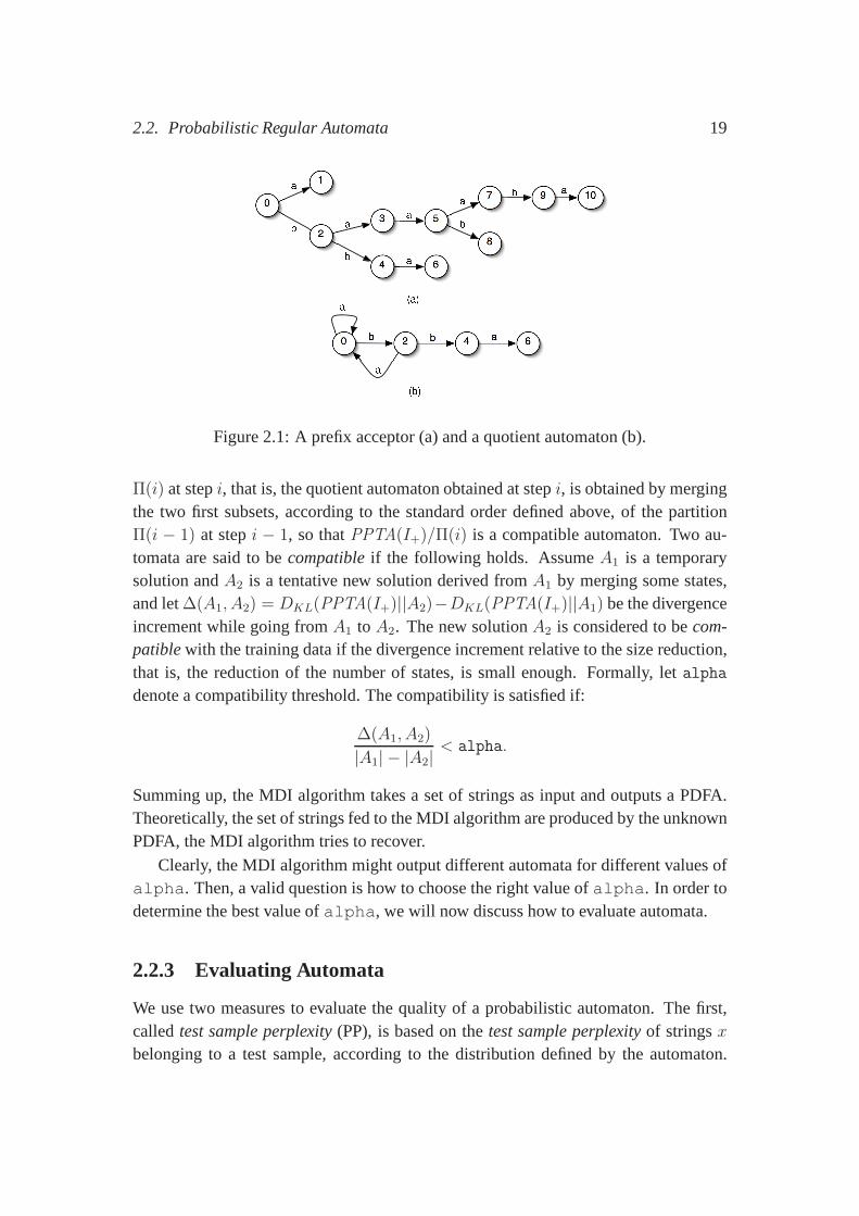
Figure 2.1.(a) shows a prefix tree acceptor built from the sample
I+ = {a, bb, bba, baab, baaaba}.
Let A be an automaton with set of statesQ, and letΠ be a partition ofQ. The prob-abilistic automatonA/Π denotes the automaton derived fromA with respect to thepartitionΠ. A/Π is called thequotient automatonand it is obtained by merging statesof A belonging to the same componentπ in Π. When a stateq in A/Π results from themerging of statesq′ andq′′ in Q, the following equalities must hold:
γ(q, a) =C(q′, a) + C(q′′, a)
C(q′) + C(q′′), ∀a ∈ Σ, andγ(q) =
C(q′, END) + C(q′′, END)
C(q′) + C(q′′).
Quotient Automata and Inference Search Space
We defineLat(PPTA(I+)) to be thelattice of automatawhich can be derived fromPPTA(I+), that is, the set of all probabilistic automata that can be derived fromPPTA(I+), by merging some states. This lattice defines the search space of all possiblePDFAs that generalize the training sample (Dupont et al., 1994).
Figure 2.1.(b) shows the quotient automatonPPTA(I+)/Π corresponding to thepartition
Π = {{0, 1, 3, 5, 7, 10}, {2, 8, 9}, {4}, {6}}.for the prefix tree acceptor in Figure 2.1.(a). Each component of the partition representsa set of merged states. Recall that each state is named with a natural number. Eachcomponent is denoted with the number of the minimal state inside it.
By construction, each of the states inPPTA(I+) corresponds to a unique prefix.The prefixes may be sorted according to the standard order< on strings. The standardorder is the lexical order found in dictionaries. For instance, acording to the standardorder, the first string on the alphabetΣ = a, b areǫ < a < b < aa < ab < ba <
bb < aaa < . . .. This order also applies to the prefix tree states. A partition of the setof states ofPPTA(I+) consists of an ordered set of subsets, each subset receivingtherank of its state of minimal rank in the standard order. The MDI algorithm proceeds inN − 1 steps, whereN = O(I+) is the number of states ofPPTA(I+). The partition
2.2. Probabilistic Regular Automata 190 12 34 560
1 0987a2 4 6
a aa a aaaa
b bb b
b b( a )
( b )Figure 2.1: A prefix acceptor (a) and a quotient automaton (b).
Π(i) at stepi, that is, the quotient automaton obtained at stepi, is obtained by mergingthe two first subsets, according to the standard order definedabove, of the partitionΠ(i − 1) at stepi − 1, so thatPPTA(I+)/Π(i) is a compatible automaton. Two au-tomata are said to becompatibleif the following holds. AssumeA1 is a temporarysolution andA2 is a tentative new solution derived fromA1 by merging some states,and let∆(A1, A2) = DKL(PPTA(I+)||A2)−DKL(PPTA(I+)||A1) be the divergenceincrement while going fromA1 to A2. The new solutionA2 is considered to becom-patiblewith the training data if the divergence increment relativeto the size reduction,that is, the reduction of the number of states, is small enough. Formally, letalphadenote a compatibility threshold. The compatibility is satisfied if:
∆(A1, A2)
|A1| − |A2|< alpha.
Summing up, the MDI algorithm takes a set of strings as input and outputs a PDFA.Theoretically, the set of strings fed to the MDI algorithm are produced by the unknownPDFA, the MDI algorithm tries to recover.
Clearly, the MDI algorithm might output different automatafor different values ofalpha. Then, a valid question is how to choose the right value ofalpha. In order todetermine the best value ofalpha, we will now discuss how to evaluate automata.
2.2.3 Evaluating Automata
We use two measures to evaluate the quality of a probabilistic automaton. The first,called test sample perplexity(PP), is based on thetest sample perplexityof stringsxbelonging to a test sample, according to the distribution defined by the automaton.
20 Chapter 2. Background and Language Modeling Landscape
Let A be an automaton, and letp be the probability distribution defined byA. Theperplexity PP associated toA is defined as
PP = 2LL,
where
LL = − 1
||S||∑
x∈S
logP (x).
P (x) is the probability assigned to the stringx by the automataA, S is a sampleset of strings that follow the right distribution, and||S|| is the number of symbolsin S. The minimal perplexityPP = 1 is reached when the next symbol is alwayspredicted with probability1 from the current state, whilePP = |Σ| corresponds touniformly guessing from an alphabet of size|Σ|. Intuitively, perplexity (PP) measuresthe uncertainty faced by an automaton when it is fed a new string.
It is hard to track down the origin ofLL, the most appealing explanation we foundin (Jurafsky and Martin, 2000) is related to cross entropy. Let us see how. The cross en-tropy is useful when we do not know the actual probability distributionp that generatedsome data. It allows us to estimate somepwhich is a model ofp, i.e., an approximationto p. Thecross entropyof p onp is defined by
H(p, p) = limn→∞
1
n
∑
W∈L
p(w1, . . . , wn) log p(w1, . . . , wn).
That is, we draw sequences of words according to the probability distributionp, butsum thelog of their probability according top.
If the automaton is a stationary ergodic process, then usingthe Shannon-McMillan-Breiman theorem we rewrite
H(p, p) = limn→∞
−1
nlog p(w1, . . . , wn).
For sufficiently largen, we can rewrite:
H(p, p) = −1
nlog p(w1, . . . , wn),
which corresponds to our definition ofLL.The second measure we use to evaluate the quality of an automaton is the number of
missed samples(MS). A missed sample is a string in the test sample that the automatonfailed to accept. One such instance is enough to have PP undefined (LL infinite).Since an undefined value of PP only witnesses the presence of at least one MS, wedecided to count the number of MS separately, and compute PP without taking MS intoaccount. This choice leads to a more accurate value of PP, and, moreover, the value
2.3. Probabilistic Context Free Grammars 21
of MS provides us with information about the generalizationcapacity of automata: thelower the value of MS, the larger the generalization capacities of the automaton. Theusual way to circumvent undefined perplexity is to smooth theresulting automatonwith unigrams, thus increasing the generalization capacity of the automaton, which isusually paid for with an increase in perplexity. We decided not to use any smoothingtechniques, as we want to compare bigram-based automata with MDI-based automatain the cleanest possible way.
2.3 Probabilistic Context Free Grammars
Context free grammars are a key component in our formalism, PCW-grammars. Weuse them for proving the consistency properties of our own formalism and as the back-bone of our parsing algorithm. We present them here following the standard conven-tions (e.g., (Aho and Ullman, 1972; Hopcroft and Ullman, 1979)).
A context free grammar(CFG) is defined as quadruple〈T ,N , S,R〉, consisting ofa terminal vocabularyT , a non-terminal vocabularyN , a distinguished symbolS ∈ N ,usually called thestart symbolor axiomand a set of productions or rewriting rulesP .The setsT , N , andR are finite;T andN are disjoint(T ∩ N = ∅), and their unioncan be denotedV (V = T ∪ N). In the case of a CFG, the rules of the grammar willbe written asA → α, whereA ∈ N andα ∈ V ∗. Rules of the formA → w, wherew ∈ T are referred to aslexical rules.
Given a CFGG, a parse treebased onG is a rooted, ordered tree whose non-terminal nodes are labeled with elements ofN and whose terminal nodes are labeledwith elements ofT . Those nodes immediately dominating terminal nodes will bere-ferred to aspreterminal; the other non-terminal nodes will be referred to as non-lexical.A syntactic tree based onG is said to bewell-formedwith respect toG if for every non-terminal node with labelA and daughter nodes labeledA1, . . . , Ak, there is a rule inP of the formA → A1 . . . Ak. We shall distinguish between a tree that is compatiblewith the rules of the grammar, and a tree that also spans a sentence. A syntax tree issaid to be generated by a grammarG if
1. The root node is labeled withS (the distinguished symbol).
2. The tree is well-formed with respect toG.
The conventional rewrite interpretation of CFGs (see e.g.,(Hopcroft and Ullman, 1979))will also be used in the definition of our stochastic models. Given two stringsw1 andw2 ∈ V ∗, we say thatw1 directly derivesw2, if w1 = δAγ, w2 = δαγ, andA → α isa rule inP . Similarly,w1 derivesw2 (in one or more steps) if the reflexive transitive
22 Chapter 2. Background and Language Modeling Landscape
closure ofA directly derivesα (writtenA →∗ α to indicate the application of one ormore rules in order to derive stringα from non-terminalA).
A probabilistic context free grammar(PCFG) is a content free grammar in whicha probability has been attached to every rule. That is, for every rule of a grammarG,A → α ∈ PG, it must be possible to define a probabilityP (A → α). Moreover, theprobabilities associated to all the rules that expand the same non-terminal must sum upto 1.
∑
A→α∈PG
P (A→ α) = 1.
Using an auxiliary notationAi,j to denote a non-terminal nodeA of the parse tree span-ning positions of the sentence fromi throughj, we can define the three assumptions ofthe model:
1. Place invariance:∀i, P (Ai,i+|ζ|→ ζ) is the same.
2. Context freedom:P (Aij → ζ |anything outsidei throughj) = P (Aij → ζ).
3. Ancestor freedom:P (Aij → ζ | any ancestor nodes aboveAij) = P (Aij → ζ).
The probabilities attached to the rules can be used either toheuristically guide theparsing process or to select the most probable parse tree(s). The probability of a certainderivation, i.e., a parse tree, can be computed by multiplying the probabilities of all theproductions applied in the derivation process. Letψ be a finite parse tree, well-formedwith respect toG, and letf be the counting function, such thatf(A→ α;ψ) indicatesthe number of times ruleA→ α has been used to build treeψ. Then we can write:
P (ψ) =∏
A→α∈PG
P (A→ α)f(A→α;ψ).
In contrast to PDFAs, where the consistency property is defined over the setΣ∗, theconsistency property for PCFGs is defined over the setψG of trees accepted byG. Pis said to beconsistentif
∑
ψ∈ΨG
P (ψ) = 1.
The consistency property for PCFGs is not always satisfied, (see, for instance (Boothand Thompson, 1973)), because it depends on the probabilitydistribution over therules,P (A → α). However, if, as usual, the estimation of the probabilitiesis carriedout by means of the maximum likelihood estimator (MLE) algorithm, it can be provedthat this property holds. (Chi and Geman, 1998) generalizesthis approach by meansof the relative weighted frequency method.
2.4. W-Grammars 23
2.4 W-Grammars
In the mid-1960s, Aad van Wijngaarden developed a grammar formalism specially forthe formal definition of programming languages, based on a combination of generalityand simplicity. The formalism was first presented by Van Wijngaarden (1965) andwas adopted for a new programming language design project that eventually producedALGOL 68. Grammars within this formalism are calledvan Wijngaarden grammarsoften shortened tovW-grammarsor W-grammars. Some authors used the nametwo-level grammars, but this could lead to confusion, since affix-grammarians also use itto name the general class that includes W-grammars, affix grammars and the rest ofvariants of AGs as well. Therefore, the name W-grammars is preferred here.
We use the concept of two-level grammars to develop our own formalism, which isa constrained version of W-grammars. W-grammars are too expressive and the compu-tational complexity of dealing with such big expressivity is very high. Our formalismis very close to the PCFG formalism in expressivity but it uses many ideas found inW-grammars. We give here a brief introduction to W-grammarsfor comparisons withour own formalism.
The basic idea of W-grammars is that, rather than enumerating a finite set of rulesover a finite symbol alphabet, a W-grammar constructs a finitemeta-grammar that gen-erates the symbols and rules of the grammar. In this way, one can define a Chomsky-type grammar with infinitely many non-terminals and rules.
The definition given here follows (Chastellier and Colmerauer, 1969):
2.4.1.DEFINITION. A W-grammaris defined by the 6th-tuple(V,NT, T, S,m−→, s−→)
such that:
• V is a set of symbols calledvariables. Elements inV are noted with calligraphiccharacters, e.g.,A,B,C.
• NT is a set of symbols callednon-terminals. Elements inNT are noted withupper-case letters, e.g.,X, Y , Z.
• T is a set of symbols calledterminals, noted with lower-case letters,e.g.,a, b, c,such thatV , T andNT are pairwise disjoint.
• S is an element ofV calledstart symbol.
• m−→ is a finite binary relation defined on(V ∪ NT ∪ T )∗ such that ifxm−→ y
thenx ∈ V . The elements ofm−→ are calledmeta-rules.
• s−→ is a finite binary relation on(V ∪NT ∪ T )∗ such that ifrs−→ s thens 6= ǫ.
The elements ofs−→ are calledpseudo-rules.
24 Chapter 2. Background and Language Modeling Landscape
W-grammars are rewriting devices. As rewriting devices, they consist of rewritingrules, but, in contrast to standard rewriting systems, the rewriting rules of W-grammarsdo not exist a-priori. Pseudo-rules and meta-rules providemechanisms for building therules that will actually be used in the rewriting process. The rewriting rules are denotedby
w=⇒ and are defined below. In general, a ruleα
w=⇒ β indicates thatα should be
rewritten asβ. For W-grammars, these rules are built by first selecting a pseudo-rule,and second, using meta-rules for instantiating all the variables that the pseudo-rulemight contain. Once all variables have been instantiated, the resulting relation canbe viewed as a derivation rule, like in context free grammars. The different values avariable in a pseudo-rule can take are given by the meta-rules. In other words, therelation generated by meta-rules defines the set of values a variable can have. Once allvariables in a pseudo-rule have been instantiated, we obtain a “real” rule.
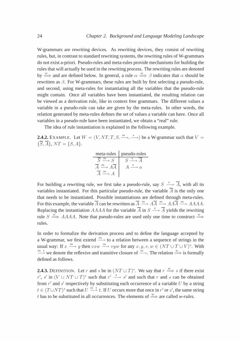
The idea of rule instantiation is explained in the followingexample.
2.4.2.EXAMPLE . LetW = (V,NT, T, S,m−→, s−→) be a W-grammar such thatV =
{S,A},NT = {S,A}.
meta-rules pseudo-rulesS
m−→ S Ss−→ A
Am−→ AA A
s−→ a
Am−→ A
For building a rewriting rule, we first take a pseudo-rule, say Ss−→ A, with all its
variables instantiated. For this particular pseudo-rule,the variableA is the only onethat needs to be instantiated. Possible instantiations aredefined through meta-rules.For this example, the variableA can be rewritten asA
m−→ AAm−→ AAA
m−→ AAAA.Replacing the instantiationAAAA for the variableA in S
s−→ A yields the rewritingrule S
w=⇒ AAAA. Note that pseudo-rules are used only one time to construct
w=⇒
rules.
In order to formalize the derivation process and to define thelanguage accepted bya W-grammar, we first extend
m−→ to a relation between a sequence of strings in theusual way: Ifx
m−→ y thenvxwm−→ vyw for anyx, y, v, w ∈ (NT ∪ T ∪ V )∗. With
m ∗−→ we denote the reflexive and transitive closure ofm−→. The relation
w=⇒ is formally
defined as follows.
2.4.3.DEFINITION. Let r ands be in(NT ∪ T )∗. We say thatrw=⇒ s if there exist
r′, s′ in (V ∪ NT ∪ T )∗ such thatr′s−→ s′ and such thatr ands can be obtained
from r′ ands′ respectively by substituting each occurrence of a variableU by a stringt ∈ (T∪NT )∗ such thatU
m ∗−→ t. If U occurs more that once inr′ or s′, the same stringt has to be substituted in all occurrences. The elements of
w=⇒ are calledw-rules.
2.4. W-Grammars 25
A w-rule αw=⇒ β defines only one step in the rewriting process. The entire rewriting
procedure is defined by extendingw=⇒ to elements in(T ∪NT )∗ as follows. Ifr
w=⇒ s
thenp, r, qw=⇒ p, s, q for anyr, s, p andq in (T ∪ NT )∗. Also,
w=⇒∗
is the reflexiveand transitive closure of
w=⇒. When a string is rewritten using w-rules, we call that
derivation aw-derivation.
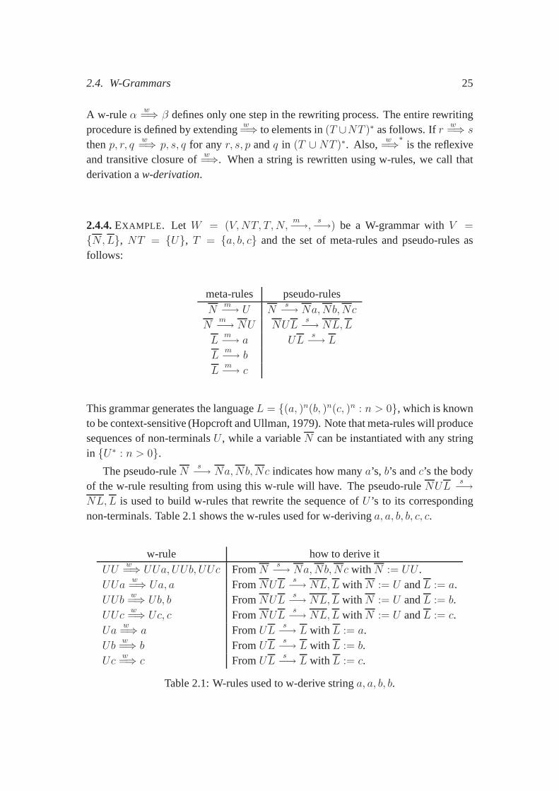
2.4.4.EXAMPLE . Let W = (V,NT, T,N,m−→, s−→) be a W-grammar withV =
{N,L}, NT = {U}, T = {a, b, c} and the set of meta-rules and pseudo-rules asfollows:
meta-rules pseudo-rulesN
m−→ U Ns−→ Na,Nb,Nc
Nm−→ NU NUL
s−→ NL,L
Lm−→ a UL
s−→ L
Lm−→ b
Lm−→ c
This grammar generates the languageL = {(a, )n(b, )n(c, )n : n > 0}, which is knownto be context-sensitive (Hopcroft and Ullman, 1979). Note that meta-rules will producesequences of non-terminalsU , while a variableN can be instantiated with any stringin {U∗ : n > 0}.
The pseudo-ruleNs−→ Na,Nb,Nc indicates how manya’s, b’s andc’s the body
of the w-rule resulting from using this w-rule will have. Thepseudo-ruleNULs−→
NL,L is used to build w-rules that rewrite the sequence ofU ’s to its correspondingnon-terminals. Table 2.1 shows the w-rules used for w-deriving a, a, b, b, c, c.
w-rule how to derive itUU
w=⇒ UUa, UUb, UUc FromN
s−→ Na,Nb,Nc with N := UU .UUa
w=⇒ Ua, a FromNUL
s−→ NL,L with N := U andL := a.UUb
w=⇒ Ub, b FromNUL
s−→ NL,L with N := U andL := b.UUc
w=⇒ Uc, c FromNUL
s−→ NL,L with N := U andL := c.Ua
w=⇒ a FromUL
s−→ L with L := a.Ub
w=⇒ b FromUL
s−→ L with L := b.Uc
w=⇒ c FromUL
s−→ L with L := c.
Table 2.1: W-rules used to w-derive stringa, a, b, b.
26 Chapter 2. Background and Language Modeling Landscape
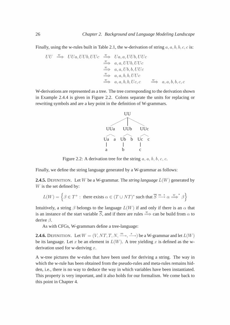
Finally, using the w-rules built in Table 2.1, the w-derivation of stringa, a, b, b, c, c is:
UUw=⇒ UUa, UUb, UUc
w=⇒ Ua, a, UUb, UUcw=⇒ a, a, UUb, UUcw=⇒ a, a, Ub, b, UUcw=⇒ a, a, b, b, UUcw=⇒ a, a, b, b, Uc, c
w=⇒ a, a, b, b, c, c
W-derivations are represented as a tree. The tree corresponding to the derivation shownin Example 2.4.4 is given in Figure 2.2. Colons separate the units for replacing orrewriting symbols and are a key point in the definition of W-grammars.
UU
UUa
Ua
a
a
UUb
Ub
b
b
UUc
Uc
c
c
Figure 2.2: A derivation tree for the stringa, a, b, b, c, c.
Finally, we define the string language generated by a W-grammar as follows:
2.4.5.DEFINITION. LetW be a W-grammar. Thestring languageL(W ) generated byW is the set defined by:
L(W ) ={
β ∈ T+ : there existsα ∈ (T ∪NT )∗ such thatSm ∗−→ α
w=⇒∗
β}
Intuitively, a stringβ belongs to the languageL(W ) if and only if there is anα thatis an instance of the start variableS, and if there are rules
w=⇒ can be build fromα to
deriveβ.As with CFGs, W-grammars define a tree-language:
2.4.6.DEFINITION. LetW = (V,NT, T,N,m−→, s−→) be a W-grammar and letL(W )
be its language. Letx be an element inL(W ). A tree yieldingx is defined as the w-derivation used for w-derivingx.
A w-tree pictures the w-rules that have been used for deriving a string. The way inwhich the w-rule has been obtained from the pseudo-rules andmeta-rules remains hid-den, i.e., there is no way to deduce the way in which variableshave been instantiated.This property is very important, and it also holds for our formalism. We come back tothis point in Chapter 4.
2.5. Further Probabilistic Formalisms 27
2.5 Further Probabilistic Formalisms
In the literature, many different approaches have been proposed for dealing with naturallanguage parsing. In this section we present a brief review of existing formalisms toplace our approaches into a bigger context of probabilisticformalism. Since manyformalisms have been proposed, we can only provide a short overview of only some ofthem. There are many relations between the formalisms discussed in this section andthe work presented in this thesis, but we only sketch the mostfundamental relationshere. More specific relations are described in Chapter 4, where we relate our formalismto three specific formalisms: bilexical grammars, Markovian CFGs, and data-orientedparsing.
2.5.1 Dependency Based Approaches
The probabilistic link grammar model of Lafferty et al. (1992), grammatical trigrams,might be considered the earliest work on probabilistic dependency grammars. It is agenerative model that specifies a probability distributionover the space of parse/sentencepairs, and it is trained in an unsupervised way, by means of anapproach similar tothe Inside-Outside algorithm (Manning and Schutze, 1999). Another related proposalis Lynx (Venable, 2001). Like grammatical trigrams, Lynx are probabilistic modelsbased on link grammars (Sleator and Temperley, 1993, 1991).Eisner (1996), in hismodel C, uses a dependency grammar, with unlabeled links (asopposed to the labeledlinks or connectors representing grammatical relationships between words of the linkgrammars). Carroll and Charniak (1992) focus on dependencygrammars as well. Theydefine an inductive algorithm to create the grammar, which performs incrementally: anew rule is introduced only if one of the sentences in the learning corpus is not correctlyanalyzed by means of the current rule set.
Head Automaton Grammars. Alshawi (1996) describes lexicalized head automata,a formalism representing parse trees by means of head-modifier relations. For eachhead, a sequence of left and right modifier words is defined together with their corre-sponding relations. A head automaton grammar (HAG), is defined as a function thatdefines a head automaton for each element of its (finite) domain. A head automaton isan acceptor for a language of string pairs〈x, y〉 (the left and right modifiers), so thatthe language generated by the entire grammar is defined by expanding the special startsymbol$ intox$y for some〈x, y〉, and then recursively expanding the words in stringsx andy. A generative probability model is provided (Alshawi describes five parametertypes), as well as a parsing algorithm which is analogous to the CKY algorithm (witha cost ofO(n5)). Eisner and Satta (1999) provide a translation from head automaton
28 Chapter 2. Background and Language Modeling Landscape
grammars to bilexical CFGs, obtaining a parsing algorithm for HAGs performing intime O(n4). Moreover, if the HAGs belong to the particular subclass of split headautomaton grammars, aO(n3) parsing algorithm is provided.
Eisner (2000) introduces weighted bilexical grammars, a formalism derived fromdependency grammars which can be considered a particular case of head automatongrammars. Weighted bilexical grammars extend the idea of bilexical grammars sothat, instead of capturing black-and-white selection restrictions (say, either a certainverb subcategorises a certain noun or not), gradient selection restrictions are captured:each specific word is equipped with a probability distribution over possible dependents.Then, the task of the parser will be to find the highest-weighted grammatical depen-dency tree given an input sentence. A new parsing algorithm for bilexical grammars (avariant of the one described in (Eisner, 1996)) is introduced, improving performancewith respect to the previous and usually used version. This work also shows how theformalism can be used to model other bilexical approaches. Bilexical grammars arevery important in this thesis; many of the grammars we build can be seen as bilex-ical grammars. In Section 4.2.1, we show that bilexical grammars are a subclass ofPCW-grammars.
(Lexicalized) Tree Adjoining Grammars. Lexicalized tree adjoining grammars (LT-AGs) present an example of a lexicalized probabilistic formalism. They are an exten-sion of tree adjoining grammars (TAG) (Joshi, 1987)), for which a probabilistic modelwas devised in (Resnik, 1992). In LTAGs, each elementary structure has a lexicalitem on its frontier, the anchor. Schabes (1992) describes avery similar probabilis-tic model, and derives an unsupervised version of the inside-outside algorithm to dealwith stochastic TAGs. The main difficulty lies in defining theinitial grammar rules.Joshi and Srinivas (1994) usen-gram statistics in order to find an elemental structurefor each lexical item. Then, richer structures can be attached to lexical items, creatingsupertags, so that each elementary tree corresponds to a supertag, which combines bothphrase structure information and dependency information in a single representation.
The disambiguation performed by supertags can be regarded as a preliminary syn-tactic parse (almost-parsing), which filters an important number of elementary treesbefore the conventional steps of combining of trees by meansof adjunction and sub-stitution operations. Srinivas (1997) gives additional models and results. It is not ourintention to provide full details about the extensive literature on this formalism, butwe will add some pointers about some aspects of TAGs that are specially interestingin relation to our own work. Nederhof et al. (1998) propose analgorithm for effi-ciently computing prefix probabilities for a stochastic TAG. Satta (1998) provides anexcellent review of techniques for recognition and parsingfor TAGs. Eisner and Satta(1999) describe a proposal of a more efficient algorithm for parsing LTAGs. Xia et al.
2.5. Further Probabilistic Formalisms 29
(2001) describe a methodology to extract LTAG grammars fromannotated corpora,and Sarkar (2001) explores state-of-the-art machine learning techniques to enable sta-tistical parsers to take advantage of unlabeled data, by exploiting the representationof stochastic TAGs to view parsing as a classification task. Emphasis is given to theuse of lexicalized elementary trees and the recovery of the best derivation for a givensentence rather than the best parse tree.
Lexicalized Context Free Grammars. Eisner and Satta (1999) define a bilexicalcontent free grammar as a CFG in which every non-terminal is lexicalized at some ter-minal symbol (its lexical head), which is inherited from theconstituent’s head child inthe parse tree. Such grammars have the obvious advantages ofencoding lexically spe-cific preferences and controlling word selection, at the cost of a significant incrementin size; the number of rules grows at a rate of the square of thesize of the terminalvocabulary. As a consequence, the increment in the grammar size makes standard con-tent free grammar parsers quite inefficient. For example, CKY-based variants performatO(n5). Eisner and Satta (1999) present aO(n4) recognition algorithm for bilexicalCFGs (in CNF), plus an improved version which, while having the same asymptoticcomplexity, is often faster in practice. By recursively reconstructing the highest proba-bility derivation for every item at the end of the parse, thisalgorithm can be straightfor-wardly converted into an algorithm capable of recognizing stochastic bilexical CFGs,where each lexicalized non-terminal has attached a probability distribution over allproductions with the same non-terminal as a left-hand side.
Satta (2000) defines lexicalized content free grammars (LCFG) as CFGs in whichevery non-terminal is lexicalized at one or more terminal symbols, which are inheritedfrom the non-terminals in the production right-hand side. Then, the degree of lexical-ization of a LCFG can be defined, so that bilexical CFGs have a degree of lexicalizationof 2. Their major limitation is that they cannot capture relationships involving lexicalitems outside the actual constituent, in contrast with history-based models.
2.5.2 Other Formalisms
Stochastic Unification Formalisms. Brew (1995) presents a stochastic version ofthe head-driven phrase structure grammar (HPSG) formalismwhich allows one to as-sign probabilities to type-hierarchies. Re-entrancy poses a problem: in some cases,even if two features have been constrained to the same value by unification, the prob-abilities of their productions are assumed to be independent. The resulting probabilitydistribution is then normalized so that probabilities sum to one, which leads to prob-lems with grammar induction, as pointed out by Abney (1997).This latter work de-fines stochastic attribute-value grammars, shows why one cannot directly transfer con-
30 Chapter 2. Background and Language Modeling Landscape
tent free grammar methods to the attribute-value grammar case (which is essentiallywhat was done in (Brew, 1995)) and gives an adequate algorithm for computing themaximum-likelihood estimate of their parameters using Monte Carlo sampling tech-niques, although it is yet unclear whether this algorithm isactually practicable, dueto its computational costs. Johnson et al. (1999) argue thatthis algorithm cannot beused for realistic-size grammars, and instead propose two methods based on a differenttype of log-linear model, Markov random fields. They apply these algorithms to theestimation of the parameters of a stochastic version of a lexical-functional grammar.
Data Oriented Parsing. Bod (1995)’s approach is different from other stochasticapproaches in that it skips the step of inducting a stochastic grammar from a corpus.Instead of a grammar, the parser uses a corpus annotated withsyntactic information,so that all fragments (i.e., subtrees) in this manually annotated corpus, regardless ofsize and lexicalization, are considered as rules of a probabilistic grammar. The un-derlying formalism in DOP is calledstochastic tree substitution grammars(STSG). InSection 4.2.3, we show that STSGs are a subclass of PCW-grammars.
For the time being, we will describe an STSG as a device that constructs the entiretree for an input sentence as a combination of tree fragments, in such a way that theproduct of the probabilities is maximal. During the training procedure, a parameteris explicitly estimated for each sub-tree. Calculating thescore for a parse in principlerequires summing over an exponential number of derivationsunderlying a tree, whichin practice is approximated by sampling a sufficiently largenumber of random parsingderivations from a forest, using Monte Carlo techniques.
Markovian Rules. Markovian rules have been successfully used for natural lan-guage parsing. The methodology followed by a Markovian ruleconsists in attachingheadwords to each syntactic category in the parse tree, to incorporate lexical probabil-ities into a stochastic model. Markovian rules are studied in detail Section 4.2.2.
A remarkable and highly popular parser that uses Markovian rules as a componentis Collins’s parser. Initially described in (Collins, 1996), it was improved in (Collins,1997), and fully described in (Collins, 1999; Bikel, 2004).Collins uses a supervisedlearning approach, with the PTB as a knowledge source, for estimating the parame-ters of his model. The key of his proposal is a well motivated trade-off between theexpressiveness of the statistical model and the independence assumptions that mustbe made for assuring a sound estimation of the parameters given the corpus. In themodel, a parse tree is represented as a sequence of decisionscorresponding to a head-centered top-down derivation of the tree. Independence assumptions are linguisticallymotivated and encoded in the X-bar schema, subcategorization preferences, orderingof the complements, placement of adjuncts, and lexical dependencies, among others.
2.6. Approaches Based on Machine Learning 31
All these preferences are expressed by means of probabilities conditioned on lexicalheads. The generative model involves the estimation of the probability of each rulefrom the PTB, i.e., the probability of generating the right part conditioned on the leftpart. Collins decomposes this probability into three factors: (1) accounting for theprobability of generating the headH, (2) given the parent, the probability of generat-ing the components to the left, and (3) the probability of generating the componentsto the right. Independence assumption is introduced in order to make the model feasi-ble. This basic model is further extended by introducing distances (taking into accountsome idiosyncratic features). The parser was trained with the PTB. (Charniak, 1997)presents a similar proposal which combines head word bigramstatistics with a PCFG.The system adds a new useful statistic to guide the parser decisions: the type of the par-ent will also condition the probability of a rule. When parsing a sentence, the systemmakes no attempt to find all possible parses, but it uses techniques presented in (Cara-ballo and Charniak, 1998) to select constituents that promise to contribute to the mostprobable parses (according to the simple probabilistic CFGdistribution). However, asthe probability distribution is different, these techniques allow us to ignore improbableparses. Moreover, the resulting chart contains the constituents along with informationon how they combine to form parses. The constituents are assigned the probabilitygiven the lexicalized model, and the parser returns the parse with the overall highestprobability according to this full distribution.
All these formalisms give a clear picture of all the grammatical formalism that weredefined and used for language modeling. In Chapter 4 we present another formalism.The relations between our formalism and the most representative formalism presentedabove are presented in Chapter 4.
2.6 Approaches Based on Machine Learning
The approaches to language modeling presented in the previous section are mainlybased on a formal grammatical device, i.e., most of them havesome kind of grammarsthat generates and accepts sentences; the syntactical analysis of a sentence is the re-sult of such a derivation. Clearly, there exists a wide variety of approaches based onwhat is commonly know asmachine learning techniques. Under this perspective lan-guage modeling is treated as a pattern recognition problem,and hence, not necessarilyrelated to the theory of formal languages. In this section, we present the most repre-sentative approaches. It is also difficult to draw hard conclusions on separation linebetween the “formal” approaches and the “machine learning”approaches because usu-ally approaches combine the two. In this section we group models whose underlyingformalism is very simple, e.g., context free grammar, and that heavily rely on machine
32 Chapter 2. Background and Language Modeling Landscape
learning (ML) techniques for achieving good performance inparsing.
Increase Context Sensitivity. The systems Pearl (Magerman and Marcus, 1991) andPicky (Magerman and Weir, 1992) use context-sensitive derivation probabilities. Thebasic idea is to try and maximize the probability of a correctderivation for each of thesentences in the corpus (as opposed to the inside-outside idea of maximizing the addi-tion of the probabilities of the sentences in the corpus given a grammar). In Pearl, forinstance, the application probability of a rule is modeled as a conditional probability,conditioned on the context in which the mother category appears. A chart parser (PUN-DIT) is employed, and probabilities are estimated by simplycounting the applicationsof the rules in the ATIS portion of the PTB.
History Based Grammars. Black et al. (1993) present a more general frameworkcalledhistory based grammars. In this system, the term history is equivalent to con-text: the application of a rule is conditioned on arbitrary aspects of the context ofthe parse tree (the context information being both the dominating production and thesyntactic and semantic categories of the words in the prior derivations. In his model,decision trees (see (Jelinek et al., 1994)), are trained from a treebank (computer manu-als domain) and they are used to score the different derivations of sentences producedby a hand-written broad-coverage feature-based unification grammar (672 rules, 21features).
Hermjakob and Mooney (1997) present a knowledge and context-based system(CONTEX) which, applying machine learning techniques, uses examples to generatea deterministic shift-reduce parser. The learning algorithm uses an extended version ofthe standard ID3 model (Mitchell, 1997) for more general hybrid decision structures,in combination with decision lists; it starts by assigning to each parse tree from thetraining corpus a sequence of shift-reduce parsing operations needed to produce thetree. In order to learn the specific action to be performed at any point of the derivation,the system relies heavily on an enriched context (to the leftand right of each word),encoded in features which include morphological, syntactic, and semantic information(the previously built structure, a subcategorization table, and a knowledge base withsemantic information about the words in the lexicon. The methodology is evaluatedon a subset of sentences from the WSJ (only the ones fully covered by the 3000 mostfrequent words in the corpus).
Probabilistic LR Parsing. The standard LR parsing methodology performs a left-to-right scan of the input and constructs a rightmost derivation in reverse. Ng and Tomita(1991) extend the well-known generalized LR parsing algorithm from (Tomita, 1996)by attaching probabilities to the nodes of the graph structured stack which constitutes
2.6. Approaches Based on Machine Learning 33
the kernel of the algorithm. Part of their proposal deals with how to consistently main-tain these probabilities (initially derived from the probabilities attached to the rules ofthe PCFG) considering the three operations of the graph-structured stack (merging, lo-cal ambiguity packing, and splitting). However, it is not possible to use an algorithmlike Viterbi in order to compute the most probable parse.
Other LR parsing approaches use PCFGs as a source including (Wright, 1990;Wright and Wrigley, 1989; Wright et al., 1991). In all of them, an LR parse tableis derived from the content free grammar but, in addition, the rule probabilities aredistributed among sets of actions in the LR table. The distribution is carried out so thatit can be assured that the product of the probabilities associated to those LR actionsperformed in the derivation of any analysis will be exactly the same as the probabilitywhich would have been assigned to this analysis by the PCFG.
Carrol (1993) discusses the latter as well as other methodologies, and presents,together with Ted Briscoe, a more ambitious proposal. They start from a unificationgrammar (the ANLT grammar), from which a content free backbone grammar is au-tomatically derived, together with an associated residue containing the dependenciesbetween features and values not contained in the content free grammar. The parsermust associate the reduce operations of the LR table with a filter based on the unifica-tion of the features contained in the residue. The backbone grammar generated fromthe ANLT grammar had 575 categories and more than 2,000 productions, and an LRparse table was automatically generated for this grammar. Unlike (Ng and Tomita,1991), the probabilistic model consists in attaching probabilities not to the content freerules, but to the actions in the LR table. The model is then more context sensitive. Inthe experiments described, the learning is supervised, thetraining corpus consisting ofa set of LR parse histories (with human intervention to correct the transition in the LRparse table). Inui et al. (1998) build on Bricoe and Carrol’swork, and improve it byformalizing their model in such a way that it provides probabilistically well-foundeddistributions. Although they focus on the formal and qualitative aspects of the model,they show how their refinement is expected to improve parsingperformance. It isworth noting that recent work by Nederhof and Satta (2002), which investigates theproblem of extending parsing strategies to probabilistic parsing strategies. They con-clude that LR parsing cannot be extended to become a probabilistic parsing strategy,because it lacks the property denoted as strong predictiveness property (SPP). In otherwords, probabilistic LR parsing algorithms might not preserve all the properties of thePCFG probability distributions, which means that LR parsers may sometimes lead toless accurate models than the grammars from which they are constructed.
Transformation Based (Error-Driven) Learning (TBL). Brill (1993) has appliedTBL to grammar induction and parsing. The approach consistsin learning a ranked
34 Chapter 2. Background and Language Modeling Landscape
list of transformational rules so that, starting from an initial imperfect binary right-branching tree for a sentence, the sequential application of each rule may transforma piece of the original tree, and in the end obtain a parse treewith fewer errors. Thefiring of each rule is conditioned on a context of one or two tags, so that the learningprocess (performed through a greedy search according to thelargest error decreasecriterion) needs quite a few number of sentences (150 /250 sentences for the ATIS andWSJ corpora) for obtaining the same accuracy of contemporary systems.
Instance-Based, Memory Based or Case-Based Learning.Instance-based algo-rithms (IBL) are a supervised way of inductively learning from examples, that are takeninto account in order to classify new examples by analogy (the most similar instancesare retrieved from memory, and used for extrapolation). Memory-based learning is adirect descendant of the classical k-NN (k nearest neighbor) approach to classification.Simmons and Yu (1992) apply the idea to a context sensitive shift reduce (SR) parser.SR parsing is suitable for this classification proposal, since it breaks the parsing pro-cess into simple parse actions (shift, reduce, and fin), allowing the construction of anexample base of parse states with their correct parse actions. A parse action is assignedto each parse state on the basis of the on information of the parse stack and the inputbuffer. The parser works on the level of POS tags and windows over the text with acontext of five words to the left and to the right.
The ILK Group at Tilburg University has developed the TiMBL (Tilburg memory-based learning) environment, a general instance-based algorithm which compresses ofthe base of examples into a tree-based structure, the IGTree(see (Daelemans et al.,1997)), which in turn is used to classify new examples. The memory-based algorithmsimplemented in the TiMBL package have been successfully applied to a large rangeof NLP tasks, including shallow parsing (see (Daelemans et al., 1999)) and more re-cently, full parsing: Veenstra and Daelemans (2000). They construct a memory-basedshift reduce parser, inspired by (Simmons and Yu, 1992). Cardie (1993a) addresses thelexical, semantic, and structural disambiguation of full sentences, within an informa-tion extraction environment. In a supervised training phase, the parser creates a casebase of domain-specific context-sensitive word definitions. Then, given an unknownword and the context in which it occurs, an eventual robust parser could retrieve thedefinitions from the case base in order to infer the necessarysyntactic and semanticfeatures for the unknown word and then continue processing the text. The case re-trieval algorithm is basically a k-NN algorithm, but it assumes all features are equallyimportant for learning each type of knowledge, which, intuitively does not seem to betrue. Therefore, the system takes advantage of decision trees for identifying the rele-vant features to be included in the k-NN case retrieval; the approach is fully describedin (Cardie, 1993b).
2.6. Approaches Based on Machine Learning 35
Decision Tree Models. Magerman (1995b) has been a pioneer in the use of decisiontrees for syntactic parsing: he explores a wide variety of possible conditioning infor-mation and uses a decision-tree learning scheme to pick those analyses that seem togive the most purchase. Three different decision-tree models are used for (1) the POStagging, (2) the node expansion, and (3) the node labeling. The decisions are based onlexical and contextual information of the parent and the child of the node.
Probabilistic Feature Grammars. Goodman (1997, 1998) presents probabilisticfeature grammars in which each non-terminal is representedas a vector of feature-value pairs. Then, assuming binary-branching rules, the probability of the applicationof a rule can be decomposed as the incremental prediction of the feature values of eachof the two members of its right-hand side. As all conditioning variables are encodedthrough features, different factors such as lexical dependencies or distance featurescan be dealt with in a unified way. Probabilistic feature grammars put the emphasison parameter estimation: having chosen the features, the parameters of the model arespecified by choosing an order for the features being predicted and then applying theindependence assumptions and choosing a back-off order forsmoothing. The modelis tested on the WSJ portion of the PTB, where the following features are considered:the non-terminal label, the headword, the head POS, distance features, and additionalcontext (modifier non-terminals generated at earlier stages of the derivation).
Maximum Entropy Models. The use of maximum entropy (ME) models, has be-come very popular lately in various areas of NLP. Rosenfeld (1994) applied it tospeech recognition tasks and Berger et al. (1996) to automatic translation, Ratnaparkhi(1998) applies to several tasks: segmentation, morpho-syntactic disambiguation, PP-attachment, and syntactic parsing. Ratnaparkhi (1999) describes the latter application,which is also an example of lexicalized parser. Maximum entropy (ME) models over-come the limitations of independence among the variables. Without the need for anexplicit grammar, they can learn, from a labeled set of examples, the model which hasmaximum entropy out of all the models compatible with this set of examples. In otherwords, given a collection of facts, ME models choose a model which is consistent withall the facts, but otherwise as uniform as possible. The basic element of any ME modelare the features, binary-valued functions with two parameters, a context and an output.
Ratnaparkhi trains his system on a set of templates that are attached to each of theparsing procedures. These templates incorporate the type of factors the author consid-ers relevant for the analysis: constituent headwords, headword combinations, gener-alizations (morpho-syntactic categories, constituent syntactic categories), and limitedforms of look-ahead. The learning process is very simple, itis just counting, so thatthe features that appear less than 5 times in the corpus are rejected. Using 40,000 sen-
36 Chapter 2. Background and Language Modeling Landscape
tences from the PTB corpus, 1,060,000 features are incorporated in the model (most ofthem lexicalized), and each one is attached to one of the procedures.
Charniak (2000) presents a parser based upon a probabilistic generative model, anextension of the ones described above (Charniak, 1997; Collins, 1997). The prob-abilistic model is maximum-entropy-inspired, since it reformulates the basic maxi-mum entropy probability function such that it considers theconditioning informationof Markov grammar statistics as features. Moreover it is ultimately smoothed by meansof deleted interpolation (instead of the standard feature selection of pure ME models).Charniak (1997) uses his bottom-up best-first chart parser to generate the candidateparses, and his top-down generative model to evaluate them (in a process which, foreach constituent, first guesses its preterminal, then its lexical head, and last its expan-sion into further constituents).
Other ML-based Models. The idea in explanation-based learning (EBL; (Raynerand Cater, 1996)) is that some of the grammar rules (specially in specific domains)tend to combine much more frequently in a certain way than others. Given a suffi-ciently large corpus parsed by the original (general) grammar, it is possible to learn thecommon combinations of rules and chunk them into macrorules; Samuelsson (1994),for example, defines an entropy threshold for automaticallyderiving these macrorules.The result is a specialized grammar, with a larger number of rules but with a simplerstructure. In practice, parsing is shown to be faster — 3 to 4 times speed up for anLR parser — at a price of only 5% coverage loss, using a training corpus of a fewthousand utterances. Zelle and Mooney (1996) describe a methodology to automatethe construction of parsers based on another ML-based learning methodology, induc-tive logic programming (ILP). They have developed a system,CHILL, which beginswith a well-defined parsing framework, shift-reduce parsing, and uses ILP to learn con-trol strategies within this framework, inductively learning a deterministic shift-reduceProlog parser that maps sentences into parses. CHILL represents a highly flexible ap-plication of ILP, allowing the induction over unbounded lists, stacks, and trees. Theydescribe the application of the system to the automatic induction of parses that mapnatural language database queries into an executable logical form. In addition, therehas been research using both neural networks and symbolic induction to learn parsersthat produce case-role analyses (Miikkulainen, 1996). In NLP, neural networks havemostly been used basically to address low-level problems, although there are examplesof applications to more complex problems such as parsing (sometimes in combinationwith symbolic approaches such as the above mentioned example).
Parser Combination and Reranking. Henderson and Brill (1999) describe a method-ology for combining three input parsers in order to improve parsing results. The three
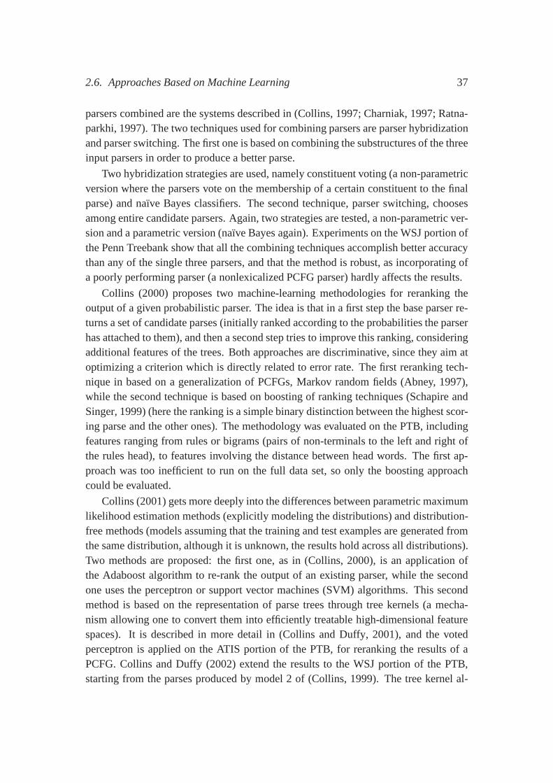
2.6. Approaches Based on Machine Learning 37
parsers combined are the systems described in (Collins, 1997; Charniak, 1997; Ratna-parkhi, 1997). The two techniques used for combining parsers are parser hybridizationand parser switching. The first one is based on combining the substructures of the threeinput parsers in order to produce a better parse.
Two hybridization strategies are used, namely constituentvoting (a non-parametricversion where the parsers vote on the membership of a certainconstituent to the finalparse) and naıve Bayes classifiers. The second technique, parser switching, choosesamong entire candidate parsers. Again, two strategies are tested, a non-parametric ver-sion and a parametric version (naıve Bayes again). Experiments on the WSJ portion ofthe Penn Treebank show that all the combining techniques accomplish better accuracythan any of the single three parsers, and that the method is robust, as incorporating ofa poorly performing parser (a nonlexicalized PCFG parser) hardly affects the results.
Collins (2000) proposes two machine-learning methodologies for reranking theoutput of a given probabilistic parser. The idea is that in a first step the base parser re-turns a set of candidate parses (initially ranked accordingto the probabilities the parserhas attached to them), and then a second step tries to improvethis ranking, consideringadditional features of the trees. Both approaches are discriminative, since they aim atoptimizing a criterion which is directly related to error rate. The first reranking tech-nique in based on a generalization of PCFGs, Markov random fields (Abney, 1997),while the second technique is based on boosting of ranking techniques (Schapire andSinger, 1999) (here the ranking is a simple binary distinction between the highest scor-ing parse and the other ones). The methodology was evaluatedon the PTB, includingfeatures ranging from rules or bigrams (pairs of non-terminals to the left and right ofthe rules head), to features involving the distance betweenhead words. The first ap-proach was too inefficient to run on the full data set, so only the boosting approachcould be evaluated.
Collins (2001) gets more deeply into the differences between parametric maximumlikelihood estimation methods (explicitly modeling the distributions) and distribution-free methods (models assuming that the training and test examples are generated fromthe same distribution, although it is unknown, the results hold across all distributions).Two methods are proposed: the first one, as in (Collins, 2000), is an application ofthe Adaboost algorithm to re-rank the output of an existing parser, while the secondone uses the perceptron or support vector machines (SVM) algorithms. This secondmethod is based on the representation of parse trees throughtree kernels (a mecha-nism allowing one to convert them into efficiently treatablehigh-dimensional featurespaces). It is described in more detail in (Collins and Duffy, 2001), and the votedperceptron is applied on the ATIS portion of the PTB, for reranking the results of aPCFG. Collins and Duffy (2002) extend the results to the WSJ portion of the PTB,starting from the parses produced by model 2 of (Collins, 1999). The tree kernel al-
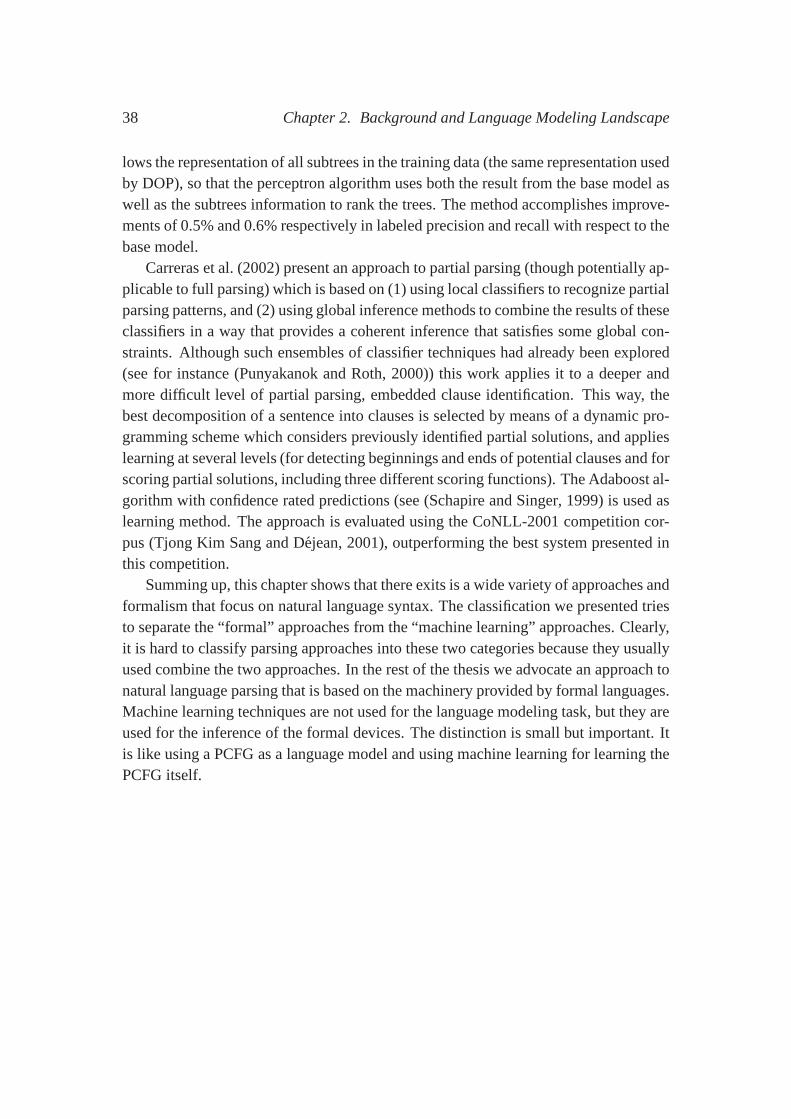
38 Chapter 2. Background and Language Modeling Landscape
lows the representation of all subtrees in the training data(the same representation usedby DOP), so that the perceptron algorithm uses both the result from the base model aswell as the subtrees information to rank the trees. The method accomplishes improve-ments of 0.5% and 0.6% respectively in labeled precision andrecall with respect to thebase model.
Carreras et al. (2002) present an approach to partial parsing (though potentially ap-plicable to full parsing) which is based on (1) using local classifiers to recognize partialparsing patterns, and (2) using global inference methods tocombine the results of theseclassifiers in a way that provides a coherent inference that satisfies some global con-straints. Although such ensembles of classifier techniqueshad already been explored(see for instance (Punyakanok and Roth, 2000)) this work applies it to a deeper andmore difficult level of partial parsing, embedded clause identification. This way, thebest decomposition of a sentence into clauses is selected bymeans of a dynamic pro-gramming scheme which considers previously identified partial solutions, and applieslearning at several levels (for detecting beginnings and ends of potential clauses and forscoring partial solutions, including three different scoring functions). The Adaboost al-gorithm with confidence rated predictions (see (Schapire and Singer, 1999) is used aslearning method. The approach is evaluated using the CoNLL-2001 competition cor-pus (Tjong Kim Sang and Dejean, 2001), outperforming the best system presented inthis competition.
Summing up, this chapter shows that there exits is a wide variety of approaches andformalism that focus on natural language syntax. The classification we presented triesto separate the “formal” approaches from the “machine learning” approaches. Clearly,it is hard to classify parsing approaches into these two categories because they usuallyused combine the two approaches. In the rest of the thesis we advocate an approach tonatural language parsing that is based on the machinery provided by formal languages.Machine learning techniques are not used for the language modeling task, but they areused for the inference of the formal devices. The distinction is small but important. Itis like using a PCFG as a language model and using machine learning for learning thePCFG itself.
Chapter 3
The Role of Probabilities in ProbabilisticContext Free Grammars
3.1 Introduction
Probabilities have been used in many aspects of natural language processing. In thecontext of CFGs, probabilities have been used to define a probability distribution overthe set of trees defined by a CFG. The resulting formalism, probabilistic context freegrammars (PCFGs), extends a context free grammar by assigning probabilities to theproduction rules of the grammar. PCFGs have been successfully used as the underlyingformalism in many approaches to natural language parsing, see e.g., (Eisner, 1996;Charniak, 1995; Collins, 1999; Eisner, 2000; Klein and Manning, 2003), to name justa few. In such approaches, probabilities have a very specificrole: they are used as afiltering mechanism. In order to clarify this, we can think ofthe parsing procedure fora PCFG as a twofold procedure. Suppose a sentence is given. First, a set of candidatetrees is proposed, and, second, a tree is non-deterministically chosen from the set ofcandidate trees. The selected tree is returned as output.
CFGs define the set of candidate trees as the set containing all trees that yield thegiven sentence. In contrast, PCFGs define the set of candidate trees as the set of treesthat yield the given sentence with maximum probability. In other words, probabilitiesare used to reduce the set of candidate trees suggested by thebare CFG. The size ofthe set of candidate trees gives an impression of how ambiguous a sentence is for agiven input. It is well-known that ambiguity is a serious problem for parsers; in somecases, the number of parse trees assigned to a sentence may grow exponentially inthe length of the sentence (Wich, 2001, 2000), and, consequently, probabilities play avery important role in parsing: they decrease the size of theset of candidate trees, andconsequently, they decrease the amount of ambiguity.
39
40 Chapter 3. The Role of Probabilities in Probabilistic Context Free Grammars
The role probabilities play in the context of formal languages has been widely stud-ied in the literature, but the focus of such studies was not onthe ability to reduce am-biguity. Properties of formal languages regarding consistency (Booth and Thompson,1973; Wetherell, 1980; Chaudhuri and Rao, 1986), learnability conditions (Horning,1969), parameter estimation (Manning and Schutze, 1999),etc, are very well-known.However, very little is known about the power of probabilities as a mechanism forambiguity reduction.
We are interested in the following research issues: how important and how power-ful are probabilities as a filtering mechanism? Clearly, different filtering mechanismsexist; as an example, suppose that a PCFGG is given and its probabilities are usedto select a subsetT ′ of trees in the tree language generated byG. It may be the casethat there exists a non-probabilistic CFGG′ such that its tree language is equal toT .Clearly, if such a grammarG′ exists for all PCFGG’s, then probabilities are not reallyneeded. In contrast, if that is not the case, the role probabilities play in parsing be-comes relevant, and different questions than those answered in (Booth and Thompson,1973; Wetherell, 1980; Chaudhuri and Rao, 1986) need to be researched.
In this chapter we focus on answers to basic questions regarding the use of proba-bilities as a filtering mechanism. We pay special attention to the following questions:
1. Is it possible to select the same set of candidate trees as with a PCFG using avanilla context free grammar? The question is relevant because, if the answeris affirmative, this means that for a given PCFG there is a CFG that specifiesthe same set of candidate trees as the PCFG for all sentences;as a consequenceprobabilities are not really essential.
2. Can we decide whether a given PCFG filters out all but one tree for all sentencesin the language? Answering this question is equivalent to saying that the givenPCFG has solved all ambiguities in the language accepted by the grammar.
3. What is the meaning of the probabilities associated with the set of candidatetrees? Can this meaning be used in a useful manner?
In this chapter, we answer all these questions. We show
1. that probabilities cannot be mimicked by rules, i.e., their use is fundamentalfrom a formal language perspective: whenever used as a filtering mechanism,probabilities can define a set of treesnot capturable by CFGs,
2. that it is not possible to decide whether a PCFG filters all trees but one for all sen-tences, i.e., it is not possible to decide whether the filtering mechanism resolvesall ambiguities,
3.2. Maximum Probability Tree Grammars 41
3. that the probability measure assigned to the selected setof candidate trees can beinterpreted as the probability of having captured in the setof candidate trees thecorrect tree. Moreover, this semantics can be used to asses the quality of PCFGs.We also show that under certain circumstances, which we describe in detail, itis advisable to add to the set of candidate trees, trees that do not have maximumprobability in order to augment the probability of capturing the correct tree.
The chapter is organized as follows. Section 3.2 presents some background notation,Section 3.3, 3.4, and 3.5 address questions 1, 2, and 3 listedabove respectively. Finally,Section 3.6 concludes the chapter.
3.2 Maximum Probability Tree Grammars
In this section we define the basic concepts we need in our discussion. LetG =
(T,NT, S,R) be a context free grammar. For our purposes, CFGs play two very im-portant roles. The first one is to provide sentences with a syntactic explanation. Asis well-known, this syntactic explanation is given by the way in which a sentence isrewritten from the start symbol. Formally, letG be a CFG andx a sentence inT ∗. Aleft-derivationt(x) is a sequence of rules〈r1, . . . , rm〉 such that
Sr1⇒ α1
r2⇒ α2r3⇒ . . .
rm⇒ αm,
whereαi ∈ (T ∪ NT )∗, αm = x, andri is a rule inR that rewrites the left-mostnon-terminal ofαi−1. The set of all left-most derivations, called thetree language, isdenoted byT (G), andx is called theyield of t(x).
The second main role of CFGs is to define the set of sentences that are consideredto be grammatical by the grammar. More precisely, letG be a CFG. ThelanguageacceptedbyG (notation:L(G)) isL(G) = {x : T (x) ∈ T (G)}.
In order to use CFGs to help us understand natural language, aprocedure for findingderivations has to be defined. LetG be a CFG andx a sentence. Acomplete parserisa procedure that computes the following set:
T (x) = {t(x) ∈ T (G)},
while a parser is a procedure that, besides computingT (x), chooses one tree non-deterministically from it. Formally,
Parser(x) = random(T (x))
whererandom(X) is a function that selects an element from the setX assigning to
42 Chapter 3. The Role of Probabilities in Probabilistic Context Free Grammars
each element the same probability of being chosen.1 For a given grammarG and asentencex in L(G) there may be multiple trees yielding the same sentencex.
In some cases the size of the setT (x) grows exponentially in the length ofx (see(Wich, 2000) for an example), and many of the trees inT (x) are trees that we do notwant as an answer. These undesired trees need to be filtered out from the setT (x).One way to achieve this is to use probabilistic context free grammars. Aprobabilisticcontext free grammar(PCFG) is a pair(G, p), whereG is a CFG andp a positivefunction defined over the set of rules such that for allA in NT :
∑
α∈(N∪NT )∗
p(A→ α) = 1.
Even though probabilities in a PCFG are defined over the set ofrules, they are used todefine a probability distributionp over the set of derivationsT (G). The probability ofa tree inT (G) is defined as follows. Let(G, p) be a PCFG, and lett(x) = 〈r1, . . . , rm〉be a tree inT (G). Theprobabilityassigned tot(x) is p(t(x)) = p(r1) · . . . · p(rm). Inwords, the probability assigned to a tree is the product of the probabilities assigned tothe rules building up the tree.
The distribution generated by the probabilities is used to select a subset of treesfrom the set of all possible trees yielding a sentence. A procedure that computes thissubset is called a probabilistic parser. More formally, letG be a PCFG and letx bea sentence inL(G). A probabilistic complete parserfor a grammarG is a procedurethat takes as input a sentence in the language and computes the following function:
PParser(x) = {t(x) ∈ T (G) : arg maxt(x){p(t(x))}}.
Finally, aprobabilistic parseris defined as the non-deterministic choice of a tree re-turned by a probabilistic complete parser. We can see a probabilistic parser as a twocomponent algorithm, one implementing a probabilistic complete parser and a secondimplementing a non-deterministic choice.
3.2.1 Filtering Trees Using Probabilities
In this subsection, we consider the class of languages induced by probabilities whenwe consider them as a filtering mechanism. LetG be a PCFG. The set ofmost probabletreesproduced byG (notedM(G)) is a subset ofT (G) defined as follows:
M(G) =⋃
x∈L(G)
PParser(x).
1Note that non-deterministic choice and uniformly distributed choice are not the same concept, non-determinism implies that there is no information about the underlying distribution, which clearly isnot the case when using a uniform distribution. In the context of this thesis we use the two termsindistinguishably.
3.3. Expressive Power 43
Note that there may be more than one tree bearing maximum probability for a givensentence. We allow for this:M(G) contains them all. Note also thatM(G) is a subsetof T (G). Furthermore, the setsM(G) andT (G) are the same set if, and only if, for allsentences all trees inL(G) share the same probability mass.
Based on the set of most probable treesM(G), we define a new class of tree lan-guages. The idea behind this class of languages is that they are like PCFGs but insteadof taking the whole set of trees they only take the most probable ones. More formally,a maximum probability tree grammar(MPTG) is a PCFG where its tree language isdefined as the set of most probable trees, while the set of strings accepted by the MTPGremains the same.
Note that all state-of-the-art parsers based on PCFG filter trees out in the way wehave just defined. They return the trees yielding a given sentence that bear maximumprobability, and thus, they, implicitly define an MPTG.
3.3 Expressive Power
We are interested in understanding what kind of expressiveness MPTGs have. In par-ticular, can they be captured by CFGs? More concretely, doesthe mechanism of re-taining only trees with maximum probability defined in MPTGsdefine tree languagesthat cannot be captured by CFGs? In this section we show that the set of trees iden-tified by a probabilistic CFG plus a maximization procedure cannot be generated orspecified directly by any CFG. In other words, we prove that probabilistic CFGs plusa maximization step define tree languages that are beyond theexpressive power of theCFGs. To put it more formally: MPTGs are not strongly equivalent to CFGs. That is,the tree language generated by probabilistic context free grammars plus a maximiza-tion algorithm is beyond context free grammars. This section is devoted to prove thisstatement, which is formally expressed in the following theorem.
3.3.1.THEOREM. MPTGs are not strongly equivalent to CFGs.
Our strategy for proving the above theorem is based on a context free inherently am-biguous language. Recall that a context free inherently ambiguous languageL is a lan-guage such that all CFGs generating it, have at least one string inL that has two treesyielding it. What we present below is an inherently ambiguous language generated by aPCFG that assigns a unique tree bearing maximum probabilityto each string in the lan-guage. As a consequence, the MPTG induced by the grammar is unambiguous, but thetree language cannot be captured by a CFG because the language is inherently ambigu-ous, i.e., for all CFGs generating it, there is at least one sentence being yielded by twodifferent trees. Let us make matters concrete now, the grammarG = (T,NT, S,R) we
44 Chapter 3. The Role of Probabilities in Probabilistic Context Free Grammars
S →2/3 AB S →1/3 S2
A→1/2 aAb S2 →1/2 aS2d
A→1/2 ab S2 →1/2 aCd
B →1/2 cBd C →1/2 bCc
B →1/2 cd C →1/2 bc
Figure 3.1: An MPTG for an inherently ambiguous language.
suggest is defined as follows. PutT = {a, b, c, d},NT = {S, S2, A,B, C}, and let theset of rulesR be as described in Figure 3.1.
In order to better understand the complexity ofG we split it into two differentgrammarsG1 = (T1, NT1, S, R1) andG2 = (T2, NT2, S, R2), where
1. T1 = {a, b, c, d},
2. NT1 = {S,A,B},
3. T2 = {a, b, c, d}, and
4. NT2 = {S, S2, C};
5. R1 andR2 as defined by Figure 3.2.
Observe thatG generates the following string language:
L = {anbncmdm : n,m ∈ N} ∪ {anbmcmdn : n,m ∈ N}.
L can be described as the union of the two context free languages generated byG1
andG2, respectively, namelyL1 = {anbncmdm : n,m ∈ N} andL2 = {anbmcmdn :
n,m ∈ N}.We will now describe the tree language generated byG. Remember thatG is
a MPTG, and not just a PCFG. The set of its derivations is the set of trees bearingmaximum probability. DefineL3 = {anbncndn : n ∈ N}, and letT (L3) denote the set
R1 R2
S →2/3 AB S →1/3 S2
A→1/2 aAb S2 →1/2 aS2d
A→1/2 ab S2 →1/2 aCd
B →1/2 cBd C →1/2 bCc
B →1/2 cd C →1/2 bc
Figure 3.2: A decomposition ofG.
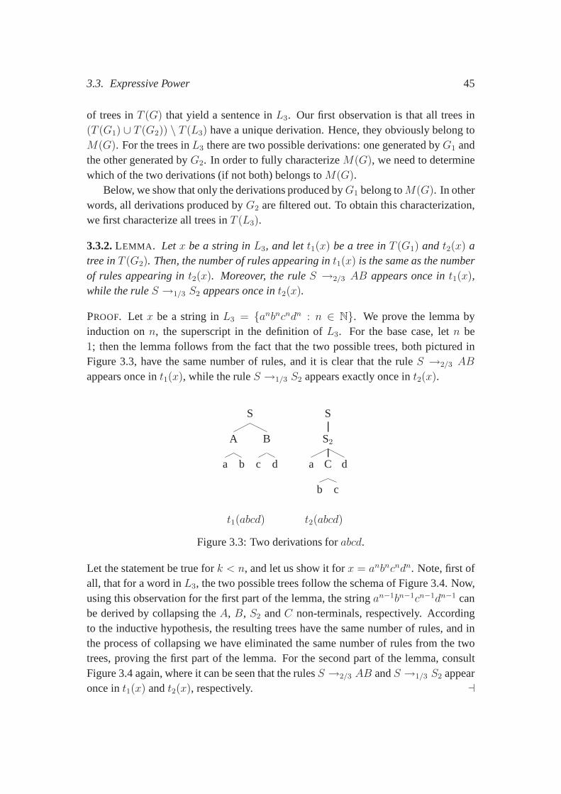
3.3. Expressive Power 45
of trees inT (G) that yield a sentence inL3. Our first observation is that all trees in(T (G1) ∪ T (G2)) \ T (L3) have a unique derivation. Hence, they obviously belong toM(G). For the trees inL3 there are two possible derivations: one generated byG1 andthe other generated byG2. In order to fully characterizeM(G), we need to determinewhich of the two derivations (if not both) belongs toM(G).
Below, we show that only the derivations produced byG1 belong toM(G). In otherwords, all derivations produced byG2 are filtered out. To obtain this characterization,we first characterize all trees inT (L3).
3.3.2.LEMMA . Let x be a string inL3, and lett1(x) be a tree inT (G1) and t2(x) atree inT (G2). Then, the number of rules appearing int1(x) is the same as the numberof rules appearing int2(x). Moreover, the ruleS →2/3 AB appears once int1(x),while the ruleS →1/3 S2 appears once int2(x).
PROOF. Let x be a string inL3 = {anbncndn : n ∈ N}. We prove the lemma byinduction onn, the superscript in the definition ofL3. For the base case, letn be1; then the lemma follows from the fact that the two possible trees, both pictured inFigure 3.3, have the same number of rules, and it is clear thatthe ruleS →2/3 AB
appears once int1(x), while the ruleS →1/3 S2 appears exactly once int2(x).
S
A
a b
B
c d
S
S2
a C
b c
d
t1(abcd) t2(abcd)
Figure 3.3: Two derivations forabcd.
Let the statement be true fork < n, and let us show it forx = anbncndn. Note, first ofall, that for a word inL3, the two possible trees follow the schema of Figure 3.4. Now,using this observation for the first part of the lemma, the string an−1bn−1cn−1dn−1 canbe derived by collapsing theA, B, S2 andC non-terminals, respectively. Accordingto the inductive hypothesis, the resulting trees have the same number of rules, and inthe process of collapsing we have eliminated the same numberof rules from the twotrees, proving the first part of the lemma. For the second partof the lemma, consultFigure 3.4 again, where it can be seen that the rulesS →2/3 AB andS →1/3 S2 appearonce int1(x) andt2(x), respectively. ⊣
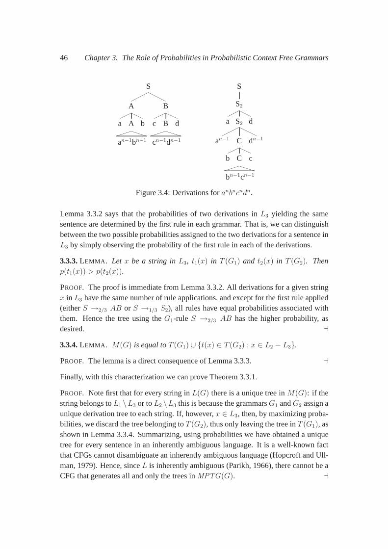
46 Chapter 3. The Role of Probabilities in Probabilistic Context Free Grammars
S
A
a A
an−1bn−1
b
B
c B
cn−1dn−1
d
S
S2
a S2
an−1 C
b C
bn−1cn−1
c
dn−1
d
Figure 3.4: Derivations foranbncndn.
Lemma 3.3.2 says that the probabilities of two derivations in L3 yielding the samesentence are determined by the first rule in each grammar. That is, we can distinguishbetween the two possible probabilities assigned to the two derivations for a sentence inL3 by simply observing the probability of the first rule in each of the derivations.
3.3.3.LEMMA . Let x be a string inL3, t1(x) in T (G1) and t2(x) in T (G2). Thenp(t1(x)) > p(t2(x)).
PROOF. The proof is immediate from Lemma 3.3.2. All derivations fora given stringx in L3 have the same number of rule applications, and except for thefirst rule applied(eitherS →2/3 AB or S →1/3 S2), all rules have equal probabilities associated withthem. Hence the tree using theG1-rule S →2/3 AB has the higher probability, asdesired. ⊣
3.3.4.LEMMA . M(G) is equal toT (G1) ∪ {t(x) ∈ T (G2) : x ∈ L2 − L3}.
PROOF. The lemma is a direct consequence of Lemma 3.3.3. ⊣
Finally, with this characterization we can prove Theorem 3.3.1.
PROOF. Note first that for every string inL(G) there is a unique tree inM(G): if thestring belongs toL1 \L3 or toL2 \L3 this is because the grammarsG1 andG2 assign aunique derivation tree to each string. If, however,x ∈ L3, then, by maximizing proba-bilities, we discard the tree belonging toT (G2), thus only leaving the tree inT (G1), asshown in Lemma 3.3.4. Summarizing, using probabilities we have obtained a uniquetree for every sentence in an inherently ambiguous language. It is a well-known factthat CFGs cannot disambiguate an inherently ambiguous language (Hopcroft and Ull-man, 1979). Hence, sinceL is inherently ambiguous (Parikh, 1966), there cannot be aCFG that generates all and only the trees inMPTG(G). ⊣
3.4. Undecidability 47
In this section we have answered question (1) from the introduction, showing that thereis no way to mimic probabilities using rules. In the next section we focus on question(2).
Ours is not the first study of the expressive power of weightedformal devices.Cortes and Mohri (2000) show that the expressive power of weighted automata is be-yond regular languages. This result has in common with the result we present in Sec-tion 3.3 that they both show that weighted systems accept a wider set of languagesthan bare systems. The two results also use the same strategy; they present a languagethat does not belong to the bare grammatical formalism but that is capturable by theweighted version.
The two approaches differ in that in ours probabilities are used to select subtreesas a side product of filtering. Cortes and Mohri (2000) show that they found a well-known context free language to be accepted by a weighted automata under a generaldefinition of acceptance. The approaches also differ in thatours is concerned with thetree-language and theirs with the string language. Finally, the two results also differ inthat our proof is technically trivial, while the other is rather involved.
The result presented in this section is not directly linked to statistics. As alreadydiscussed in (Abney, 1996), probabilities can help in many aspects of syntax (e.g., dis-ambiguation, degrees of grammaticality, error tolerance,naturalness, structural prefer-ences, learning, lexical acquisition). In that sense, weights are enough for capturingthese phenomena. In this section we deal with probabilities(weights) as they are cur-rently used for disambiguation in the literature. We respond to the question “What canwe do with probabilities (weights)?” more than “How can we compute the probabili-ties (weights)?”. Abney argues that, intuitively, probabilities can help disambiguating,but this section shows that they provide a mechanism that simply cannot be mimickedwith rules. To put it very bluntly, we present a technical fact, not an intuition.
We have shown that probabilities add not only a statical perspective but also ex-pressive power to CFGs. We think that this increment in the expressive power is dueto a probabilistic parser’s implicit but global requirement that it sees all rules buildingup a tree for choosing the one with maximum probability.
3.4 Undecidability
While probabilities buy us additional expressive power on top of CFGs, they do notbuy us everything. Specifically, given that probabilities help to disambiguate their ownlanguage, would it not be nice if we could predict, that is, determine before parsing,whether a PCFG is capable of fully disambiguating its language?
We show that this is not possible. We establish the result by transforming an ar-
48 Chapter 3. The Role of Probabilities in Probabilistic Context Free Grammars
bitrary CFG into a PCFG such that the given CFG is unambiguousif, and only if, thecorresponding PCFG has only one tree in the candidate list ofeach sentence. Our resultthen follows from the well-known fact that determining whether a CFG is unambigu-ous is undecidable.
Probabilities single out, for each sentencex, a setPParser(x) of trees bearingmaximum probability. Anidealgrammar is one that filters out all trees but one for eachsentence in the language. In other words, an ideal PCFG defines for each sentencex,its setPParser(x) with cardinality equal to1.
We want to prove that it is undecidable to determine whether aPCFG is ideal. Tothis end, we first prove that for every context free grammarG there is a way to extendit with probabilities such that the resulting setM(G) contains the same set of trees asG. In other words, for any CFG we build a probabilistic versionthat does not filter outany tree. Our undecidability result follows from the fact that our question is equivalentto determining whether a CFG is unambiguous.
We have to build the probabilistic correlate of a CFG, in sucha way that all treesassociated to a given sentence bear the same probability. Inthis case, the set of treeswith maximal probability is exactly the set of trees. We showthe result for grammarsin Chomsky Normal Form whose definition we now recall.
A context free grammarG = (T,NT,R, S) is said to be in Chomsky Normal Form(CNF) if, and only if, every rule inR is of one of the following forms:
• A→ a for someA ∈ NT and somea ∈ T .
• A→ BC, for someA ∈ NT andB,C ∈ NT − {S}.Our strategy is to show that any grammar in CNF assigns the same probability to alltrees yielding the same string. To this end we show that all trees yielding the samestring in a CNF use the same number of rules; we then build a grammar assigning thesame probability to all rules and we obtain what we are looking for.
We now present the lemmas needed.
3.4.1.LEMMA . Let G = (T,NT, S,R) be a grammar in CNF. All trees yielding ak-length sub-string ofNT ∗ use the same number of rules.
PROOF. Let us define a sequenceA0, . . . , An, . . . of subsets ofNT ∗ as follows:A0 =
{S},A1 consists of elementsα in NT ∗ such thatα is derived fromS in one step, and,in general,α is in Ai if there is an elementα′ in Ai−1 such thatα′ ⇒ α. The lemmais immediate from the fact that that all sets are pairwise disjoint, i.e.,Ai ∩ Aj = ∅ foreveryi 6= j. ⊣
3.4.2.COROLLARY. LetG be a CFG. Every derivation producing a stringx of lengthk in L(G) has the same number of rules.
3.4. Undecidability 49
3.4.3.LEMMA . LetG be a context free grammar.G can be transformed into a prob-abilistic context free grammarG′ with the special property that all rules have exactlythe same probability value.
PROOF. LetG be a grammar in CNF, and letR be its set of rules. LetX be the mostfrequent non-terminal in the left-hand sides of rules. Letn be the number of timesXis the left hand-side of a rule. LetZ1, . . . , Zn be brand new non-terminal symbols. Forevery non-terminalY we add as many rulesY → Zi as needed to have the number ofrules havingY in the left-hand side equal ton. We add probability1/n to each of thesenew rules. The resulting grammar is a well-defined, though not necessarily consistent,probabilistic context free grammar, and all rules have exactly the same probabilityvalues as required. ⊣
The PCF grammarG′, obtained from a grammarG as described in Lemma 3.4.3, iscalled theuniform versionof G.
Note that the resulting grammar need not be consistent, given that some probabilitymass is going to non-terminating derivations — derivationsthat end up in the dummynon-terminal. Still, what is important to us is that the set of trees accepted by thePCFG remains the same, and, even more importantly, that every derivation producingthe same sentence has the same probability value.
3.4.4.LEMMA . LetG be a context free grammar, and letG′ be its uniform version.Let x be a string inL(G). Then all left-most derivations producingx have the sameprobability.
PROOF. Since every string in the language has the same set of trees asG, the dummyrule is not used in any derivation of final strings. Accordingto Lemma 3.4.1, every treehas the same number of rules. And since every rule has the sameprobability, every treefor the sentencel has the same probability. Finally, the set of trees bearing maximumprobability is exactly the set of trees in the original grammarG. ⊣
As this lemma proves, trees defined throughMPT include the class of trees definedvia CFG. As a direct consequence, we have the following lemma:
3.4.5.LEMMA . Deciding whether a PCFG disambiguates a tree language is undecid-able.
PROOF. We have built a grammar that assigns the same probability mass to all possibletrees for a given string. As a consequence, the PCFG is unambiguous if, and onlyif, the non-probabilistic grammar is. Deciding whether thePCFG is unambiguous isequivalent to decided whether a CFG in CNF is unambiguous, which is known to beundecidable (Hopcroft and Ullman, 1979). ⊣
50 Chapter 3. The Role of Probabilities in Probabilistic Context Free Grammars
The above lemma answers question (2) from the introduction,saying that it is notpossible to decide whether a PCFG has completely managed to solve all ambiguities.Note that the results in the present section combined with the results in the previousone imply that the class of tree languages described by PCFGsis a strict subclass of thetree languages described by MPTGs. The inclusion is impliedby the present sectionwhile the proper inclusion is implied by the previous one.
3.5 The Meaning of Probabilities
Whenever only a single tree is required as output, all CF parsers face the question ofhow to select that single tree from a set of trees yielding thesame sentence. Theyusually choose a tree non-deterministically, by randomly selecting a tree among allpossible trees. The selection is made under the assumption that all trees in the candidatelist (suggested by the grammar) have the same probability ofbeing selected.
The use of probabilities is meant to reduce the size of the setof candidate trees.On the one hand, the probability value assigned to a tree captures that tree’s chanceof being generated by the grammar and, consequently, of being found in a tree-bankgenerated by the grammar. On the other hand, the idea ofcorrectnessis usually un-derstood in terms of a comparison to a manually annotated tree-bank. The two thingscombined suggest that the probability assigned to a tree canbe thought of as its chanceof being the correct one. On this view, parsers try to find the tree that has the highestprobability of being the correct one. Clearly, some non-determinism remains: theremight be more than one tree bearing maximum probability and,consequently, parsershave to non-deterministically choose among all trees bearing maximum probability.
In the following two subsections we use the just defined semantics for two differentpurposes. First, we use it as a way to compare grammars. The general idea is tocompare grammars according to the amount of non-determinism they have left for thenon-deterministic choice. Second, we want to use it for boosting the probability ofpicking the right tree from the set of candidate trees by adding trees to it that do notbear maximum probability but that increase the probabilitymass of the candidate listin substantial way.
3.5.1 Using Probabilities for Comparing PCFG
Recall that a grammar isambiguousif there is a sentence in the language that has acandidate list containing more than one analysis. Following (Wich, 2000, 2001), wecan think of the degree of ambiguity of a PCFG as a quantity proportional to the sizeof the candidate lists, one per sentence in the language. That degree is related to both
3.5. The Meaning of Probabilities 51
the set of rules in the grammar and to the probabilities associated to the rules. Clearly,a grammar with a lower degree of ambiguity is preferred over one with a higher degreeof ambiguities given that the first reduces the level of non-determinism by choosingnon-deterministically from smaller sets, in the second phase.
We propose a measure that compares grammars with respect to the way they re-duce nondeterminism in the second phase of the parsing process. The measure isbased on the probabilistic distribution they generate overthe set of trees. Our approachis sample-based, i.e., the measure is computed over a finite sample set of sentences,because is not possible to compute it for the whole language,as we will also show.The measure we propose computes the probability of a tree of being chosen under thetwo-stage parsing schema defined previously. This proposalhas the advantage of tak-ing into account two things: first, the confidence the probability measure has over theproposed list of candidates, and, second, the non-deterministic choice in the final step.
One important desideratum that we have for our measure for determining a gram-mar’s ability to reduce ambiguity is that it should capture the remaining non-determi-nism after trees have been filtered out using probabilities.Clearly, the reduction onnon-determinism is related to the size of the set of candidate trees. However, it is nota good idea to simply use the fraction of trees that were filtered out as a quality mea-sure, or the size of the candidate list. The first idea is unsuitable because, in case thegrammar generates only a single tree per sentence, the probabilities do not filter outany tree, and we would be assigning a very low score to the filtering mechanism. Thesecond idea fails because there is no information on the sizeof the list of trees beforeusing probabilities.
There has been quite a lot of research in the area of parsing evaluation (Lin, 1995;Marcus et al., 1994; Carroll et al., 1998; Musillo and Sima’an, 2002), but it does notseem appropriate to use any of these parser evaluation measures for quantifying ambi-guity reduction. Parser evaluation measures are aimed at determining how well parsersperform on parsing standard sentences. Under these approaches, only grammars thatoutput trees that follow the structure found in the tree-bank can be compared (or thosefor whom a transformation between formats exists (Watkinson and Manandhar, 2001)).Moreover, these approaches do not produce any information about the way in whichthe grammar has dealt with ambiguity.
There have been some attempts, both to show that PCFGs do indeed reduce am-biguity and to determine the extent to which they do this. Forinstance, Atsumi andMasuyama (1998) compare the size of the list of candidate analyses before and afterhaving filtered out syntactic analysis with lower probability. Even though their moti-vations are very similar to ours, they do not offer an explicit measure for comparingdifferent PCFGs with respect to their ambiguity reduction abilities.
Before giving the formal definition, let us give some more intuitions. The amount
52 Chapter 3. The Role of Probabilities in Probabilistic Context Free Grammars
of determinism for a given sentencex in the two-stage parsing procedure is given bytwo main ingredients: the (size of the) set of treesT (x) yielding the sentencex, andthe (size of the) set of trees bearing maximum probabilityPParser(x). Both sets con-tribute to ambiguity reduction. The sizes ofT (x) andPParser(x) capture the amountof ambiguity produced by the grammar before and after havingused probabilities forfiltering out trees, respectively.
PCFGs reduce the set of trees in the candidate list using a probability distribu-tion over the set of possible analysis. The distribution specifies the probability eachtree has of being the correct tree given the sentence.2 Under our two-stage procedurethe probability of selecting a particular tree is given by the product of the probabilitymass accumulated in the setPParser(x) (that is, the probability of having the correcttree inPParser(x)) and the probability of uniformly selecting a particular tree fromPParser(x). More specifically, suppose the grammar defines a probability distribu-tion p over the set of trees, specifying the probability each tree has of being the correctone. Suppose, moreover, that for a given sentencex from the sample set, we select theset of trees bearing maximum probabilityPParser(x). The probability of selectingany particular instance of the trees inPParser(x) using a uniform distribution is
Q{x}(G) = p(PParser(x))1
|PParser(x)|,
wherep(PParser(x)) is the probability that the correct tree is inPParser(x), while1
|PParser(x)|is the probability of selecting it. The probability takes into account the
probability mass concentrated inPParser(x) and its size: the bigger the probabilitythe better the output.
Since all trees inPParser(x) have the same probability valuepx,Q{x}(G) can besimplified as follows
Q{x}(G) = px|PParser(x)|1
|PParser(x)| = px.
Finally, assuming that parsing sentences are independent experiments, our measure isdefined as follows:
QS(G) =∏
x∈S
px,
whereS is a sample set of sentences from the grammar’s accepted language, andpxis the probability assigned to the tree returned by the parser. QS(G) is equal to1 if,and only if, there is a unique tree with maximum probability for each sentence inS.The measure is easily computable if we work with probabilistic parsers that return bothtrees and the probability value associated to the trees returned.
2“Correct” in the sense that is the one that appears in a sampletree-bank.
3.5. The Meaning of Probabilities 53
Finally, we say that a grammarG1 is betterthan a grammarG2 (based on a samplesetS) if, and only if,
QS(G1) < QS(G2).
The measure does not capture the ambiguity reduction over the set of all possible sen-tence. Why? In the following section we show that it is simplynot possible to computeit for the whole language.
In what follows we show that it is necessary to relativize ourmeasure to a sampleset: it is not possible to computeQS(G) if S is equal to the language accepted by thegrammarL(G). Suppose that it were possible to computeQL(G)(G). Then, we wouldalso know whetherQL(G)(G) is equal to one. SinceQL(G)(G) = 1 if, and only if,G has singled out exactly one element in the candidate list of each sentence, beingable to computeQL(G)(G) would imply that it is possible to determine whetherG hascompletely disambiguated the language.
We have presented a measure for assessing grammars with respect to their abilityto reduce ambiguity. The measure we presented can also be applied to state-of-art-parsers that return the selected analysis tree for a given input sentencetogether with itsprobability (Collins, 1997; Eisner, 1996; Klein and Manning, 2003).
Our measure has at least three kinds of advantages in comparison to standard parserevaluation methods:
1. It can be applied to unsupervised learned grammars for which the learned syn-tactic structure is not as clearly defined as the ones inducedfrom tree-banks.
2. Our measure is not domain dependent. Since a grammar induced from a tree-bank is usually evaluated on the same type of sentences that were used for in-ducing it, its evaluated performance does not tell us much about the grammars’performance on sentences belonging to different domains from those covered inthe tree-bank.
3. Our measure yields information about the parser that is complementary to thekind of information usually obtained by evaluating parsers(Lin, 1995; Marcuset al., 1994; Carroll et al., 1998), given that it does not provide any kind of infor-mation about the correctness of the resulting trees, and, moreover, the measuredoes need to have access to the ‘right’ tree. The precise relation between per-formance measured using existing parser evaluation measures and performancemeasured with our new measure (applied to parsers) remains to be explored.
This subsection showed a possible use of probabilities other than probabilities as fil-tering mechanism. The new semantics provides an answer to question (3) of the intro-duction; in the next section we show yet another application.
54 Chapter 3. The Role of Probabilities in Probabilistic Context Free Grammars
3.5.2 Using Probabilities for Boosting Performance
In this section we use the new semantics associated to probabilities for increasing theprobability of guessing the right tree. We provide evidencethat under certain circum-stances the probability of getting the correct tree can be increased by adding trees withless than maximal probability to the set of candidates.
Note that the probability ofPParser(x) is the probability of having the correcttree in it. We can forget for a moment thatPParser(x) only contains trees bearingmaximum probability and add trees to it in an attempt to increment its probability.Incrementing its probability has the advantage of incrementing the probability of cap-turing the correct tree, but has the disadvantage of decrementing the probability ofrandomly choosing the correct one. Clearly, there is a trade-off between the number ofnon-maximum probability trees we can add toPParser(x) and the probability gainedat the end of the random selection procedure. Let us take a closer look, and give condi-tions under which the probability of selecting the correct trees increases when pickingfrom a set of trees properly extends the set of trees bearing maximum probability.
LetR be a set of trees disjoint withPParser(x). We show that the probability ofchoosing the correct tree increases whenR is added to the candidate listPParser(x)if, and only if,
p(R)
px> |R|+ |PParser(x)| − 1. (3.1)
The proof is simple. Letpx be the probability of selecting only fromPParser(x).Then, the condition in (3.1) above is fulfilled if, and only if,
p(R) + px > px|R|+ px|PParser(x)|,
which is equivalent top(R) + px
|R|+ |PParser(x)| > px,
which, in turn, holds if, and only if,
p(R ∪ PParser(x))|R ∪ PParser(x)| > px.
The final result follows from the fact thatp(R∪PParser(x))|R∪PParser(x)|
is the probability of selectingthe correct tree from the expanded list.
Extending the set of candidates is not new in the literature.Collins and Duffy(2001, 2002); Bod (2003) propose approaches other than uniformly selecting a tree.Our result gives an estimate of the number of trees one needs to consider in the selec-tion phase to gain a significant amount of probability mass.
3.6. Conclusions and Future Work 55
The present section focused on new uses of probabilities associated to trees. We an-swered question (3) by giving two new applications. We show that probabilities can beused for evaluation purposes and that they can be used to boost parsing performance.
As trivial as the results might look, it is very hard to find a parser implementationthat reports on the probability values associated to its trees. In order to be able tocompare parsers using the probability values they assign totheir most probable trees,the probabilistic models used by the parsers should be consistent. If this is not the case,the probability values are meaningless. Clearly, this requirement is not trivial to fulfill.For most of the probabilistic parsers it is unknown whether their underlying modelsare consistent. Given the importance of the consistency conditions, we establish inChapter 4, consistency properties for bilexical grammars,and Markovian context freegrammars.
3.6 Conclusions and Future Work
This chapter has focused on questions related to the importance of probabilities in thecontext of parsing and on investigating uses of probabilities others than filtering. Wehave shown that probabilities, when used as a filtering mechanism, can add expres-sive power to grammars defining a class of tree languages beyond the expressivity ofcontext free grammars. We also showed that it is not possibleto decide whether prob-abilities solve all ambiguities in the language.
We also gave examples that probabilities can be used in otherways others than asfiltering mechanism. We proposed to use them for evaluating the quality of PCFGsand for boosting the performance of parsers. Experiments toback up this theoreticalfinding would be of great value. We leave them out of the thesisand consider them asfuture work.
We argued that in order to used these ideas, it is fundamentalthat the underlyingprobability models be consistent. We show in Chapter 4 that PCW-grammars provideus with the machinery necessary to prove the consistency of bilexical grammars andMarkovian rules whenever they are induced from tree-banks usingn-grams. Despitethis, proving consistency properties for the grammars we induce in Chapters 5, 6 and 7are desirable results on the todo list.

Chapter 4
Constrained W-Grammars
This chapter consists of two sections. First, the grammatical formalism we propose isintroduced. Our framework is based on so-called W-grammars, due originally to VanWijngaarden (Van Wijngaarden, 1965; Mateescu and Salomaa,1997). We constrainW-grammars to obtainconstrained W-grammars(CWG) which are more suitable forstatistical natural language parsing than W-grammars. As we have seen in the previouschapter, probabilities are a fundamental part of state-of-the-art natural language pars-ing technology. We extend CW-grammars with probabilities,defining probabilisticconstrained W-grammars(PCWGs).
In the second part of this chapter we show that the formalism we introduce is gen-eral enough to capture grammatical frameworks used in threestate-of-the-art parsers:bilexical grammars, Markovian context free grammars, and stochastic tree substitutiongrammars (STSGs). For each we provide an embedding into PCW-grammars, whichallows us to discover properties about their expressive power and consistency, and re-lations between the formalisms studied.
4.1 Grammatical Framework
In this section we describe the grammatical framework we will be working with. Weintroduce constrained W-grammars, then present a probabilistic version, and also in-troduce technical notions needed in later sections.
4.1.1 Constrained W-Grammars
A constrained W-grammar(CW-grammar) is a 6-tuple(V ,NT , T , S,m−→,
s−→) suchthat:
57
58 Chapter 4. Constrained W-Grammars
• V is a set of symbols calledvariables. Elements inV are denoted with overlinedcapital letters, e.g.,A, B, C.
• NT is a set of symbols callednon-terminals; elements inNT are denoted withupper-case letters, e.g.,X, Y , Z.
• T is a set of symbols calledterminals, denoted with lower-case letters, e.g.,a, b,c.
• V , T andNT are pairwise disjoint.
• S is an element ofNT called thestart symbol.
• m−→ is a finite binary relation defined on(V ∪ NT ∪ T )∗ such that ifxm−→ y,
thenx ∈ V . The elements ofm−→ are calledmeta-rules.
• s−→ is a finite binary relation on(V ∪ NT ∪ T )∗ such that ifus−→ v then
u ∈ NT , v is not empty and no variable inv appears more than once. Theelements of
s−→ are calledpseudo-rules.
CW-grammars differ from Van Wijngaarden’s original W-grammars in that pseudo-rules have been constrained. Comparing the above definitionwith the one presented inSection 2.4, we see that the original W-grammars allow pseudo-rules to have variableson the left-hand side as well as repeated variables on both the right- and left-handside. The constrained version defined above yields a dramatic reduction in the ex-pressive power of W-grammars. CW-grammars are weakly equivalent to context freegrammars. Despite the reduction of expressivity, CW grammars are capable of fullycapturing grammar formalism used in state-of-the-art parsers, something that contextfree grammars can not do by themselves.
CW-grammars are rewriting devices, and as such they consistof rewriting rules.They differ from the usual rewriting systems in that the rewriting rules do not existapriori . Using pseudo-rules and meta-rules one builds ‘real’ rulesthat can be used in therewriting process. The rewriting rules produced are denoted by
w=⇒ and are calledw-
rules. These rules are built by first selecting a pseudo-rule, and then using meta-rulesfor instantiating all the variables the pseudo-rule might contain.
For example, letW = (V , NT , T , S,m−→,
s−→) be a CW-grammar whereV =
{ADJ}, NT = {S, Adj , Noun}, T = {ball , big , fat , red , green, . . .}, andm−→ and
s−→ are given by the following table:
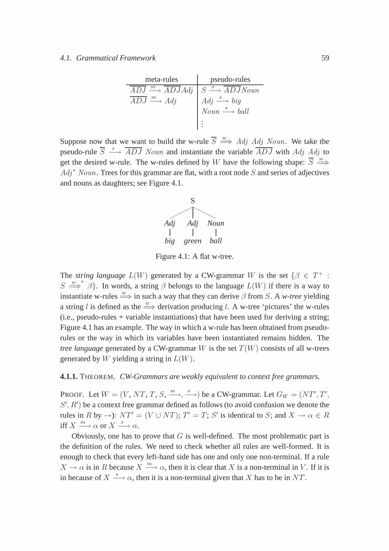
4.1. Grammatical Framework 59
meta-rules pseudo-rulesADJ
m−→ ADJAdj Ss−→ ADJNoun
ADJm−→ Adj Adj
s−→ big
Nouns−→ ball
...
Suppose now that we want to build the w-ruleSw=⇒ Adj Adj Noun. We take the
pseudo-ruleSs−→ ADJ Noun and instantiate the variableADJ with Adj Adj to
get the desired w-rule. The w-rules defined byW have the following shape:Sw=⇒
Adj ∗ Noun. Trees for this grammar are flat, with a root nodeS and series of adjectivesand nouns as daughters; see Figure 4.1.
S
Adj
big
Adj
green
Noun
ball
Figure 4.1: A flat w-tree.
The string languageL(W ) generated by a CW-grammarW is the set{β ∈ T+ :
Sw
=⇒∗β}. In words, a stringβ belongs to the languageL(W ) if there is a way to
instantiate w-rulesw=⇒ in such a way that they can deriveβ from S. A w-treeyielding
a stringl is defined as thew=⇒ derivation producingl. A w-tree ‘pictures’ the w-rules
(i.e., pseudo-rules + variable instantiations) that have been used for deriving a string;Figure 4.1 has an example. The way in which a w-rule has been obtained from pseudo-rules or the way in which its variables have been instantiated remains hidden. Thetree languagegenerated by a CW-grammarW is the setT (W ) consists of all w-treesgenerated byW yielding a string inL(W ).
4.1.1.THEOREM. CW-Grammars are weakly equivalent to context free grammars.
PROOF. LetW = (V , NT , T , S,m−→, s−→) be a CW-grammar. LetGW = (NT ′, T ′,
S ′, R′) be a context free grammar defined as follows (to avoid confusion we denote therules inR by→): NT ′ = (V ∪ NT ); T ′ = T ; S ′ is identical toS; andX → α ∈ Riff X
m−→ α orXs−→ α.
Obviously, one has to prove thatG is well-defined. The most problematic part isthe definition of the rules. We need to check whether all rulesare well-formed. It isenough to check that every left-hand side has one and only onenon-terminal. If a ruleX → α is inR becauseX
m−→ α, then it is clear thatX is a non-terminal inV . If it isin because ofX
s−→ α, then it is a non-terminal given thatX has to be inNT .
60 Chapter 4. Constrained W-Grammars
Next we show that the two grammars generate the same language. To prove thiswe just prove that ifr
w=⇒∗
s thenr →∗ s. The proof is divided in three parts: (i) ifrm ∗−→ s thenr →∗ s; (ii) if r
s−→ s thenr → s; (iii) if rw=⇒ s thenr →∗ s. (i) If
rm ∗−→ s thenr →∗ s follows immediately from the definition ofGW ;
m−→ is a subsetof→. (ii) If r
s−→ s thenr → s also follows from the definition ofGW . (iii) Let r ands be such thatr
w=⇒∗
s. This implies that there existr′ ands′ such that
r′s−→ s′
↓m∗ ↓m∗r s
Sincer′ ∈ NT , the only possibility forr′m ∗−→ r is for r to be equal tor′, leading to
the following situation:r
s−→ s′
↓m∗s
But, under the assumption that every variable appears once and only once in the bodyof s′, both
s−→ andm ∗−→ can be emulated by→, implying thatr →∗ s as required.
In the other direction, any CFGG can define a CW-grammarW . The only nec-essary step for transformingG into a CW-grammar consists of partitioning the set ofrules inG into two different subsets, one functioning as the set of meta-rules, and theother functioning as the the set of pseudo-rules. ⊣
Note that the previous result does not follow directly from any of the results given inChapter 2. In the literature there are examples of differentconstraints applied to W-grammars (Mateescu, 1989a,b). These constraints were meant to make subclasses ofenumerable languages. In contrast, our constraints are meant to reduce the expressivepower of W-grammars to a level that allows us to capture the grammatical formalismsunderlying state-of-the-art-parsers. The previous lemmashows that our constraintsreduce the expressive power of W-grammars from Turing computable to context free.
Given a CW-grammarW , thecontext free grammar underlyingW , which we de-note byCFG(W ), is the grammarGW defined in the proof of Theorem 4.1.1. In orderto facilitate our forthcoming discussion we suppose that rules inG have been markedsomehow to allow us to decide whether a rule inG corresponds to a meta-rule or to apseudo-rule in the original CW-grammar. We refer to the set of rules inG marked asmeta-rules as meta-rules and to the set of rules marked as pseudo-rules as pseudo-rules.
Let W be a W-Grammar and letG = CFG(W ) be its underlying context freegrammar. Theorem 4.1.1 shows that bothW andG accept the same string language.In what follows we turn to study the relation betweenW ’s tree language andG’s tree
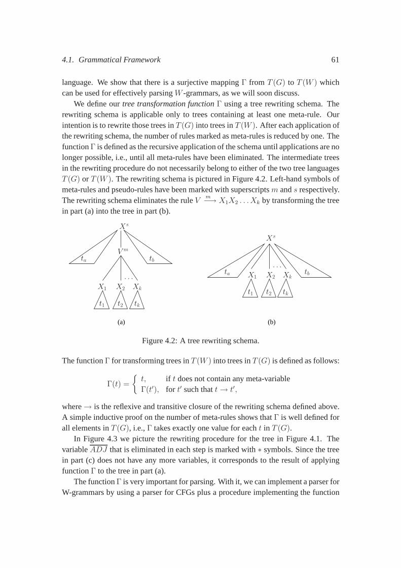
4.1. Grammatical Framework 61
language. We show that there is a surjective mappingΓ from T (G) to T (W ) whichcan be used for effectively parsingW -grammars, as we will soon discuss.
We define ourtree transformation functionΓ using a tree rewriting schema. Therewriting schema is applicable only to trees containing at least one meta-rule. Ourintention is to rewrite those trees inT (G) into trees inT (W ). After each application ofthe rewriting schema, the number of rules marked as meta-rules is reduced by one. ThefunctionΓ is defined as the recursive application of the schema until applications are nolonger possible, i.e., until all meta-rules have been eliminated. The intermediate treesin the rewriting procedure do not necessarily belong to either of the two tree languagesT (G) or T (W ). The rewriting schema is pictured in Figure 4.2. Left-hand symbols ofmeta-rules and pseudo-rules have been marked with superscriptsm ands respectively.The rewriting schema eliminates the ruleV
m−→ X1X2 . . .Xk by transforming the treein part (a) into the tree in part (b).
(a) (b)
t1 t2 tk
tbta
Xs
tb
V m
ta
X1 X2 Xk
X2X1 Xk
t2 tkt1
. . .
. . .
Xs
Figure 4.2: A tree rewriting schema.
The functionΓ for transforming trees inT (W ) into trees inT (G) is defined as follows:
Γ(t) =
{
t, if t does not contain any meta-variableΓ(t′), for t′ such thatt→ t′,
where→ is the reflexive and transitive closure of the rewriting schema defined above.A simple inductive proof on the number of meta-rules shows thatΓ is well defined forall elements inT (G), i.e.,Γ takes exactly one value for eacht in T (G).
In Figure 4.3 we picture the rewriting procedure for the treein Figure 4.1. ThevariableADJ that is eliminated in each step is marked with∗ symbols. Since the treein part (c) does not have any more variables, it corresponds to the result of applyingfunctionΓ to the tree in part (a).
The functionΓ is very important for parsing. With it, we can implement a parser forW-grammars by using a parser for CFGs plus a procedure implementing the function
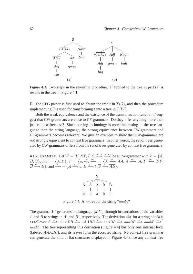
62 Chapter 4. Constrained W-Grammars
S
∗ADJ∗
ADJ
Adj
big
Adj
green
Noun
ball
S
∗ADJ∗
Adj
big
Adj
green
Noun
ball
(a) (b)
Figure 4.3: Two steps in the rewriting procedure.Γ applied to the tree in part (a) isresults in the tree in Figure 4.1.
Γ. The CFG parser is first used to obtain the treet in T (G), and then the procedureimplementingΓ is used for transformingt into a tree inT (W ).
Both the weak equivalence and the existence of the transformation functionΓ sug-gest that CW-grammars are close to CF-grammars. Do they offer anything more thanjust context freeness? Since parsing technology is more interesting in the tree lan-guage than the string language, the strong equivalence between CW-grammars andCF-grammars becomes relevant. We give an example to show that CW-grammars arenotstrongly equivalent to context free grammars. In other words, the set of trees gener-ated by CW-grammars differs from the set of trees generated by context free grammars.
4.1.2.EXAMPLE . LetW = (V,NT, T, S,m ∗−→, s ∗−→) be a CW-grammar withV = {A,
B, S}, NT = {A,B}, T = {a, b}, m−→ = {A m−→ AA, Am−→ A, B
m−→ BB,B
m−→ B}, ands−→ = {A s−→ a, B
s−→ b, Ss−→ AB}.
S
A
a
A
a
A
a
B
b
B
b
Figure 4.4: A w-tree for the string “aaabb”
The grammarW generates the language{a∗b∗} through instantiations of the variablesA andB to strings inA∗ andB∗, respectively. The derivation
w=⇒ for a stringaaabb is
as follows:Sw=⇒ AAABB
w=⇒ aAABB
w=⇒ aaABB
w=⇒ aaaBB
w=⇒ aaabB
w=⇒∗
aaabb. The tree representing this derivation (Figure 4.4) has only one internal level(labeledAAABB ), and its leaves form the accepted string. No context free grammarcan generate the kind of flat structures displayed in Figure 4.4 since any context free
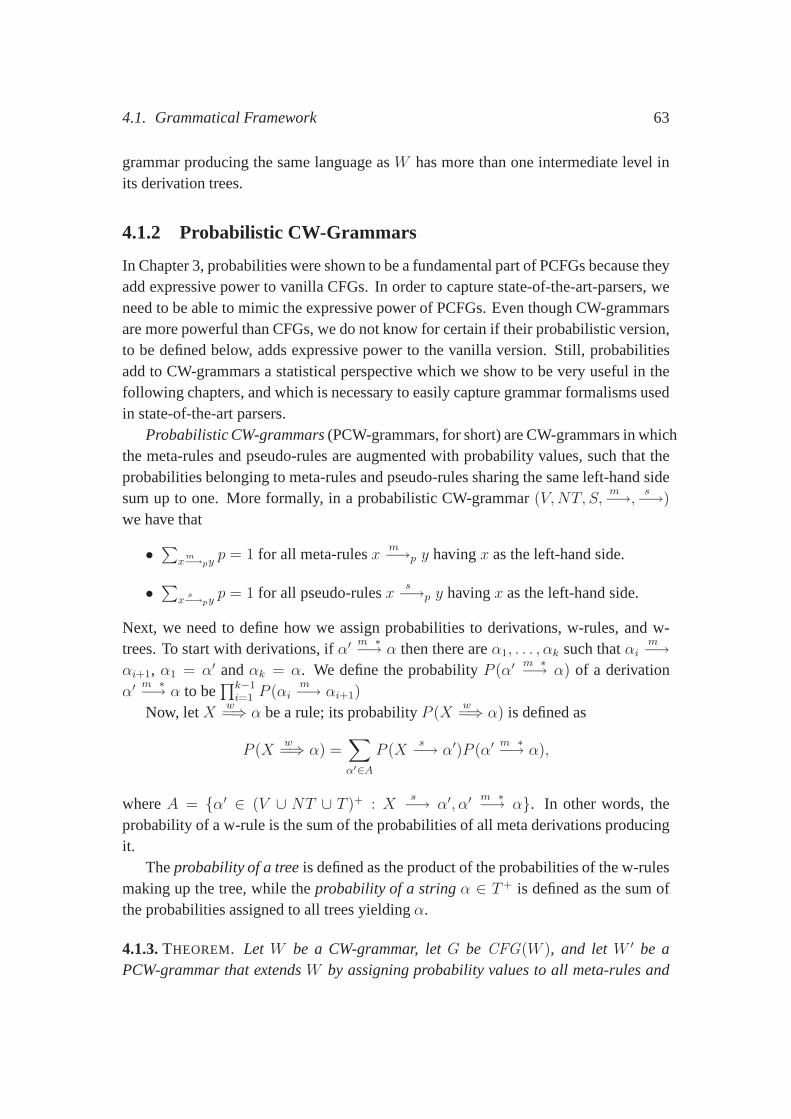
4.1. Grammatical Framework 63
grammar producing the same language asW has more than one intermediate level inits derivation trees.
4.1.2 Probabilistic CW-Grammars
In Chapter 3, probabilities were shown to be a fundamental part of PCFGs because theyadd expressive power to vanilla CFGs. In order to capture state-of-the-art-parsers, weneed to be able to mimic the expressive power of PCFGs. Even though CW-grammarsare more powerful than CFGs, we do not know for certain if their probabilistic version,to be defined below, adds expressive power to the vanilla version. Still, probabilitiesadd to CW-grammars a statistical perspective which we show to be very useful in thefollowing chapters, and which is necessary to easily capture grammar formalisms usedin state-of-the-art parsers.
Probabilistic CW-grammars(PCW-grammars, for short) are CW-grammars in whichthe meta-rules and pseudo-rules are augmented with probability values, such that theprobabilities belonging to meta-rules and pseudo-rules sharing the same left-hand sidesum up to one. More formally, in a probabilistic CW-grammar(V,NT, S,
m−→, s−→)
we have that
• ∑
xm−→py
p = 1 for all meta-rulesxm−→p y havingx as the left-hand side.
• ∑
xs−→py
p = 1 for all pseudo-rulesxs−→p y havingx as the left-hand side.
Next, we need to define how we assign probabilities to derivations, w-rules, and w-trees. To start with derivations, ifα′ m ∗−→ α then there areα1, . . . , αk such thatαi
m−→αi+1, α1 = α′ andαk = α. We define the probabilityP (α′ m ∗−→ α) of a derivationα′ m ∗−→ α to be
∏k−1i=1 P (αi
m−→ αi+1)
Now, letXw=⇒ α be a rule; its probabilityP (X
w=⇒ α) is defined as
P (Xw=⇒ α) =
∑
α′∈A
P (Xs−→ α′)P (α′ m ∗−→ α),
whereA = {α′ ∈ (V ∪ NT ∪ T )+ : Xs−→ α′, α′ m ∗−→ α}. In other words, the
probability of a w-rule is the sum of the probabilities of allmeta derivations producingit.
Theprobability of a treeis defined as the product of the probabilities of the w-rulesmaking up the tree, while theprobability of a stringα ∈ T+ is defined as the sum ofthe probabilities assigned to all trees yieldingα.
4.1.3.THEOREM. Let W be a CW-grammar, letG be CFG(W ), and letW ′ be aPCW-grammar that extendsW by assigning probability values to all meta-rules and
64 Chapter 4. Constrained W-Grammars
pseudo-rules inW . There is a way to extendG into a PCFGG′ such thatW ′ andG′
assign the same probability mass to all strings in the language accepted byG (whichcoincides with the language accepted byW ).
PROOF. LetG = (NT ′, T ′, S ′, R′) be a PCFG withNT ′, T ′, S ′ as defined in the proofof Theorem 4.1.1 andR′ such thatX → α ∈ R iff X
m−→ α orXs−→ α. Note that a
w=⇒ derivationτ might be the product of many different derivations using rules inR′
(G-derivations for short); let us notate this set ofG-derivations withD(τ). From thedefinitions it is clear thatp(τ) =
∑
υ∈D(τ) p(υ). To prove the theorem we need to show
1. that for two differentw=⇒ derivations of the stringα τ andτ ′, it holds thatD(τ)∩
D(τ ′) = ∅, and
2. that for everyG-derivationυ there is aw=⇒ derivationτ such thatυ ∈ D(τ).
Item (1) follows from the facts thatΓ(υ) = τ for all υ in D(τ) and thatΓ(υ′) = τ ′ forall υ′ in D(τ ′); consequently, if there is an element inD(τ)∩D(τ ′), thenτ is equal toτ ′. Item (2) follows from the fact thatΓ is defined for allG-derivations. ⊣
The above result does not follow from Theorem 4.1.1 because that result does not takeprobabilities into account.
For a given PCW-grammarW , the PCFG defined in the proof of Theorem 4.1.3 iscalled thePCFG underlyingW .
As in the case of non-probabilistic CW-grammars, the tree language ofT (G) isrelated to the tree languageT (W ) through the tree transformation functionΓ definedabove. The functionΓ can also be used for computing the probability of a treet inT (W ); its probability is equal to the sum of the probabilities of all trees t′ in T (G)
such thatΓ(t′) = t. Moreover, since every tree inT (G) is mapped to a tree inT (W ),we obtain that theW grammar is consistent if, and only if, its underlying PCFG isconsistent.
4.1.3 Learning CW-Grammars from Treebanks
Suppose we have a collection of w-trees, from which we would like to induce a CW-grammar. We distinguish two different strategies for solving this problem. One strat-egy is aimed at usingsupervisedtechniques for learning PCFGs while the second isaimed at usingunsupervisedtechniques for learning PCFGs.
The first approach consists of three steps.
1. Handcraft a set of meta-rules that might be used for meta-derivation.
4.1. Grammatical Framework 65
2. Expand each tree with all meta-derivations. Such a procedure has the effect oftransforming the CW-treebank into a CF-treebank.
3. Use any PCFG inducing mechanisms, like those discussed inSection 2.3 forinducing a PCFG from the transformed treebank.
Instead of returning a CW-grammar, the procedure returns the underlying PCFGG ofa W-grammar. Since all meta-rules are known, a unique W-grammar can be definedfromG.
Step (2) is straightforward only if meta-derivations produce unambiguous deriva-tions, i.e., if for each string produced by meta-derivations produce there is only oneway to derive it. In the case of ambiguous meta-derivations,a way to distribute theprobability mass among all possible derivations has to be designed. In the literaturethere are different proposals for re-assigning probabilities (Sima’an and Buratto, 2003;Bod, 1998; Krotov et al., 1998). Most of these references refer to estimation techniquesfor STSGs that, as we will see, deal these problems from the very beginning.
The second approach consists of 2 steps.
1. Extract all bodies of rules from the w-treebank where eachbody of a rule is astring of non-terminal and terminal symbols.
2. Use the extracted strings to induce a PCFG grammar.
In contrast with the previous approach, the induced PCFG is not the underlying PCFGof any CW-grammar; instead, it is the grammar describing themeta-derivation a PCW-grammar should have. Pseudo-rules have to be handcrafted inorder to make the meta-rules interact with pseudo-rules to rebuild the trees that have appeared in the CW-grammar.
Both approaches are different and require different techniques. Both have in com-mon that one set of rules, either pseudo-rules or meta-ruleshave to be handcrafted.The presentation we have given here is rather abstract; the differences between the twobecome more evident in the rest of the thesis. In Section 4.2 we show that the learn-ing methodology used for state-of-the-art parsers is an instance of the first approach,while the grammars used in the experiments of Chapter 5 are instances of the secondapproach.
4.1.4 Some Further Technical Notions
Below we will use PCW-grammars to “capture” models underlying a number of state-of-the-art parsers. The following will prove useful. LetF andG be two grammars withtree languagesT (G) andT (F ) and languagesL(F ) andL(G), respectively. Then,F is
66 Chapter 4. Constrained W-Grammars
f -equivalenttoG if L(F ) = L(G) and there is a bijective functionf : T (F )→ T (G).Given two grammatical formalismsA andB, we say thatA is f -transformableto B,if for every grammarF in A there is a grammarG in B such thatF is f -equivalenttoG. Note that the definition off -transformable is a generalization of the concepts ofweak and strong equivalence; both can be seen asf -equivalence for particular choicesof the functionf . Namely, two grammars are weakly equivalent if the functionf
is surjective, and they are equivalent if the functionf is bijective andt andf(t) areisomorphic trees, for all trees in the domain off .
4.2 Capturing State-of-the-Art Grammars
In this section we show that PCW-grammars are a powerful formalism; we show thatthey are powerful enough to capture the models underlying a number of state-of-the-artparsers. Clearly, the grammatical framework underlying a parser is a key componentof the overall definition of the parser which determines important characteristics of theparser, either directly or indirectly. Among others things, the grammatical frameworkdefines the set of languages the parser can deal with, a lower bound on the parser’scomplexity, and the type of items that should be learned by the second component men-tioned in Section 4.1.3. Hence, a thorough understanding ofthe grammatical frame-work on which a parser is based, provides a great deal of information about the parseritself. We are particularly interested in the following properties:
1. The expressive power of a grammar formalism.
2. Conditions under which the probability distribution defined over the set of pos-sible syntactic analyses is consistent: if this is the case,the probabilities asso-ciated with an analysis can be used as meaningful probabilistic indicators bothfor further stages of processing (Manning and Schutze, 1999) and for evaluation(Infante-Lopez and de Rijke, 2004b).
3. The relation to other grammatical frameworks; this provides insights about theassumptions made by the various frameworks.
Since building a parser is a time consuming process, formal properties of the under-lying grammatical framework are not always a priority. Also, comparisons betweenparser models are usually based on experimental evidence. In order to establish formalproperties of parsers and to facilitate the comparison of parsers we believe that a uni-fying grammatical framework, from which the grammars of different parsers can beobtained as instances, is instrumental. We show that the PCWframework is capableof capturing three state-of-the-art grammatical formalisms, namely bilexical grammars
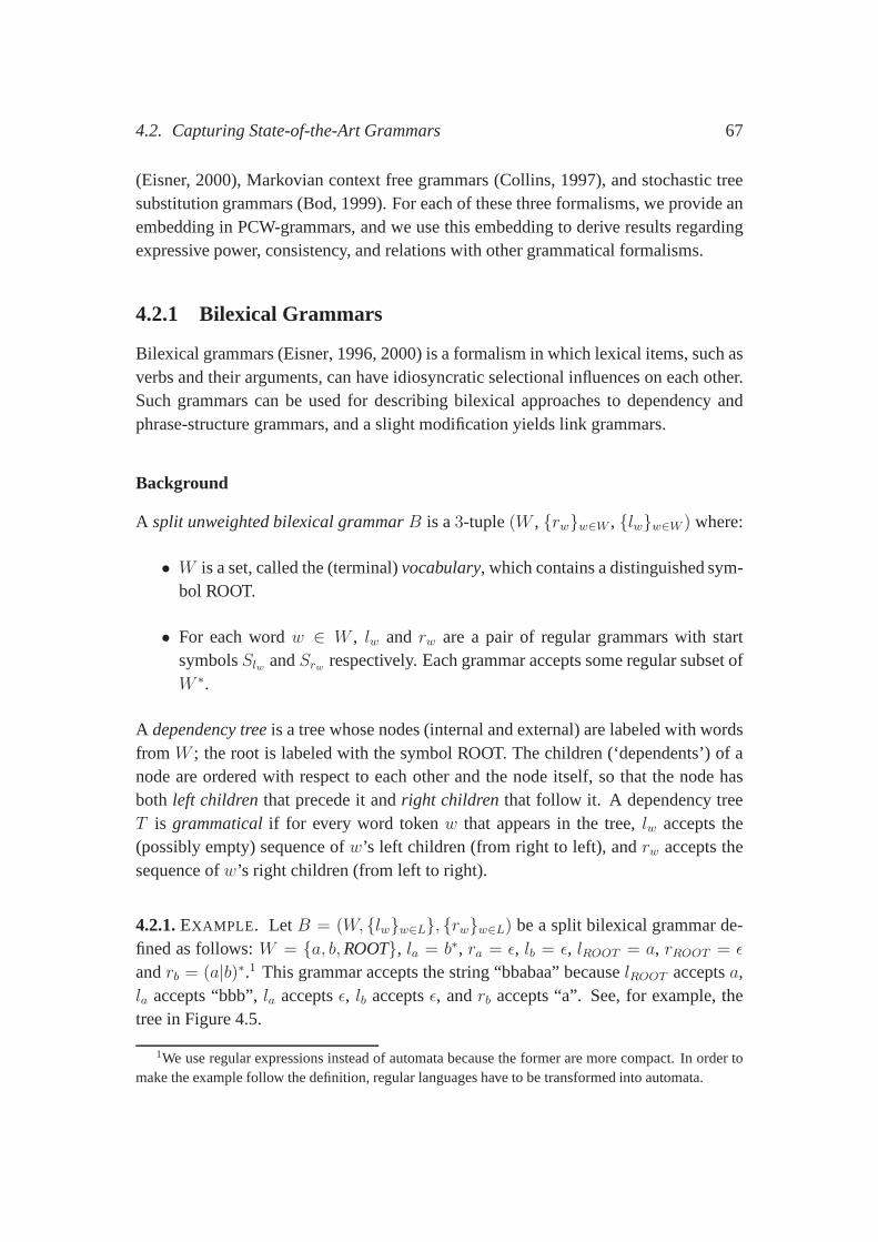
4.2. Capturing State-of-the-Art Grammars 67
(Eisner, 2000), Markovian context free grammars (Collins,1997), and stochastic treesubstitution grammars (Bod, 1999). For each of these three formalisms, we provide anembedding in PCW-grammars, and we use this embedding to derive results regardingexpressive power, consistency, and relations with other grammatical formalisms.
4.2.1 Bilexical Grammars
Bilexical grammars (Eisner, 1996, 2000) is a formalism in which lexical items, such asverbs and their arguments, can have idiosyncratic selectional influences on each other.Such grammars can be used for describing bilexical approaches to dependency andphrase-structure grammars, and a slight modification yields link grammars.
Background
A split unweighted bilexical grammarB is a3-tuple(W , {rw}w∈W , {lw}w∈W ) where:
• W is a set, called the (terminal)vocabulary, which contains a distinguished sym-bol ROOT.
• For each wordw ∈ W , lw and rw are a pair of regular grammars with startsymbolsSlw andSrw respectively. Each grammar accepts some regular subset ofW ∗.
A dependency treeis a tree whose nodes (internal and external) are labeled with wordsfrom W ; the root is labeled with the symbol ROOT. The children (‘dependents’) of anode are ordered with respect to each other and the node itself, so that the node hasboth left childrenthat precede it andright children that follow it. A dependency treeT is grammaticalif for every word tokenw that appears in the tree,lw accepts the(possibly empty) sequence ofw’s left children (from right to left), andrw accepts thesequence ofw’s right children (from left to right).
4.2.1.EXAMPLE . LetB = (W, {lw}w∈L}, {rw}w∈L) be a split bilexical grammar de-fined as follows:W = {a, b,ROOT}, la = b∗, ra = ǫ, lb = ǫ, lROOT = a, rROOT = ǫ
andrb = (a|b)∗.1 This grammar accepts the string “bbabaa” becauselROOT acceptsa,la accepts “bbb”,la acceptsǫ, lb acceptsǫ, andrb accepts “a”. See, for example, thetree in Figure 4.5.
1We use regular expressions instead of automata because the former are more compact. In order tomake the example follow the definition, regular languages have to be transformed into automata.
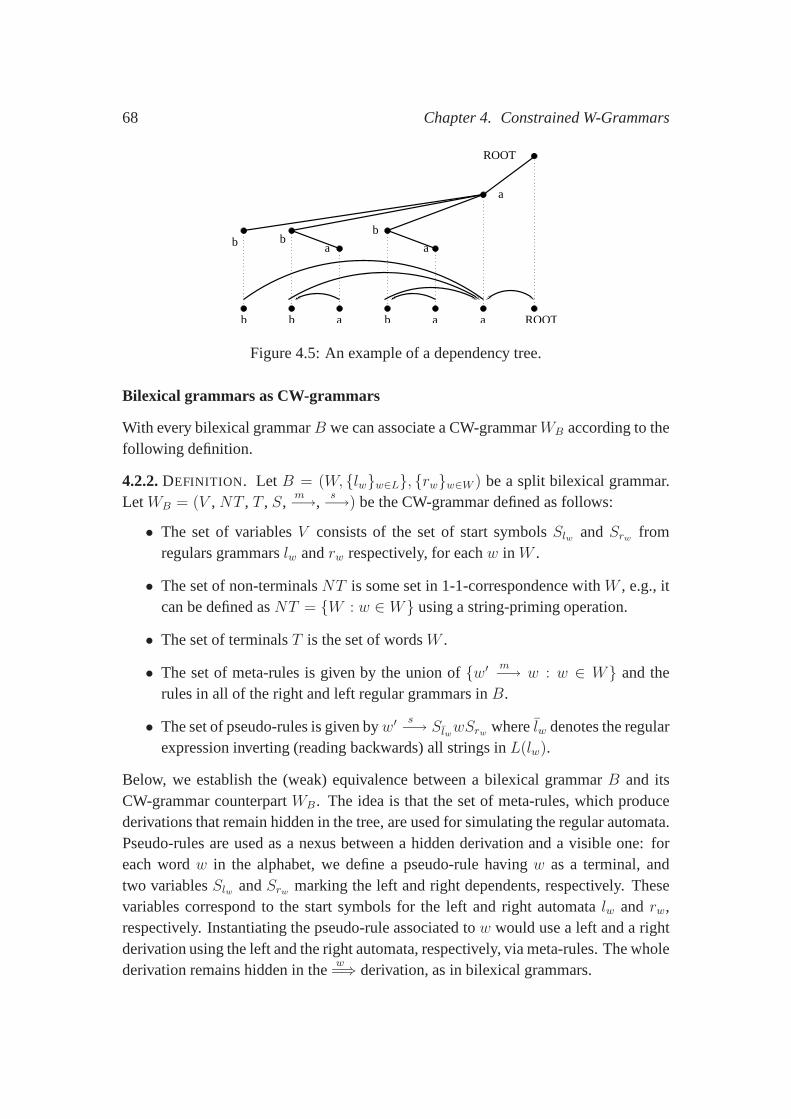
68 Chapter 4. Constrained W-Grammars
b b a b a a ROOT
b
a a
a
bb
ROOT
Figure 4.5: An example of a dependency tree.
Bilexical grammars as CW-grammars
With every bilexical grammarB we can associate a CW-grammarWB according to thefollowing definition.
4.2.2.DEFINITION. LetB = (W, {lw}w∈L}, {rw}w∈W ) be a split bilexical grammar.LetWB = (V ,NT , T , S,
m−→,s−→) be the CW-grammar defined as follows:
• The set of variablesV consists of the set of start symbolsSlw andSrw fromregulars grammarslw andrw respectively, for eachw in W .
• The set of non-terminalsNT is some set in 1-1-correspondence withW , e.g., itcan be defined asNT = {W : w ∈ W} using a string-priming operation.
• The set of terminalsT is the set of wordsW .
• The set of meta-rules is given by the union of{w′ m−→ w : w ∈ W} and therules in all of the right and left regular grammars inB.
• The set of pseudo-rules is given byw′ s−→ SlwwSrw wherelw denotes the regularexpression inverting (reading backwards) all strings inL(lw).
Below, we establish the (weak) equivalence between a bilexical grammarB and itsCW-grammar counterpartWB. The idea is that the set of meta-rules, which producederivations that remain hidden in the tree, are used for simulating the regular automata.Pseudo-rules are used as a nexus between a hidden derivationand a visible one: foreach wordw in the alphabet, we define a pseudo-rule havingw as a terminal, andtwo variablesSlw andSrw marking the left and right dependents, respectively. Thesevariables correspond to the start symbols for the left and right automatalw and rw,respectively. Instantiating the pseudo-rule associated tow would use a left and a rightderivation using the left and the right automata, respectively, via meta-rules. The wholederivation remains hidden in the
w=⇒ derivation, as in bilexical grammars.
4.2. Capturing State-of-the-Art Grammars 69
4.2.3.LEMMA . Bilexical grammars aref -transformable to CW-grammars.
PROOF. We have to give a functionf : T (B)→ T (WB), whereB is a bilexical gram-mar andWB the grammar defined in Definition 4.2.2, such thatf is invertible. A bilex-ical tree yielding the strings = w1, . . . , wn can be described as a sequenceu1, . . . , unof 3-tuples〈αi, wi, βi〉 such thatlwi
acceptsαi andrwiacceptsβ. The desired function
f transforms a dependency tree in a w-tree by transforming thesequence of tuples intoa
w=⇒ derivation. We definef asf(〈α,wi, β〉) = Wi
w=⇒ αwiβ. The rule correspond-
ing to 〈α,wi, β〉 is the one produced by using the pseudo ruleW ′i
s−→ S ¯lwxSrw andinstantiatingS ¯lw andSrw with α andβ respectively. Since the sequence of tuples formsa dependency tree, the sequence of w-rules builds up a correct w-tree. ⊣
Weighted bilexical grammarsare like unweighed bilexical grammars but all of their au-tomata assign weights to the strings they generate. Lemma 4.2.3 implies that weightedbilexical grammars are a subset of PCW-grammars.
Expressive Power and Consistency
By Lemma 4.2.3 bilexical grammars are weakly equivalent to context free grammars.In order to prove that they are not strongly equivalent it is enough to note that thegrammar in Example 4.2.1 can generate trees like the ones pictured in Figure 4.6 forarbitraryk. That is, the grammar in Example 4.2.1 can generate flat treeslike theones pictured in Figure 4.6 where nodes can have arbitrarilymany siblings. Any CFGgenerating the same string language will produce non-flat structures.
a ROOTb b bb
a ROOTb b
k
a ROOTb
(a) (b)
(c)
Figure 4.6: Different dependency trees that can not be generated by CFGs.
We now show that the learning mechanism proposed in (Eisner,1996) produces consis-tent probability distributions. We start by presenting theway Eisner induces a bilexicalgrammarB from a bilexical treebank; next, we show how the given treebank can betransformed into a CF treebank. Finally, we show that the transformed treebank can beused to learn the underlying PCFGG of a PCW-grammarW such thatW is equivalenttoB.
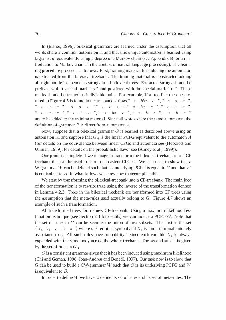
70 Chapter 4. Constrained W-Grammars
In (Eisner, 1996), bilexical grammars are learned under theassumption that allwords share a common automatonA and that this unique automaton is learned usingbigrams, or equivalently using a degree one Markov chain (see Appendix B for an in-troduction to Markov chains in the context of natural language processing). The learn-ing procedure proceeds as follows. First, training material for inducing the automatonis extracted from the bilexical treebank. The training material is constructed addingall right and left dependents strings in all bilexical trees. Extracted strings should beprefixed with a special mark “-s-” and postfixed with the special mark “-e-”. Thesemarks should be treated as indivisible units. For example, if a tree like the one pic-tured in Figure 4.5 is found in the treebank, strings “−s− bba− e−”, “−s− a− e−”,“−s − a − e−”,“−s − a − e−”,“−s − b − e−”, “−s − ba − e−”, “−s − a − e−”,“−s − a − e−”, “−s − b − e−”, “−s − ba − e−”, “−s − b − e−”,“−s − b − e−”are to be added to the training material. Since all words share the same automaton, thedefinition of grammarB is direct from automatonA.
Now, suppose that a bilexical grammarG is learned as described above using anautomatonA, and suppose thatGA is the linear PCFG equivalent to the automatonA
(for details on the equivalence between linear CFGs and automata see (Hopcroft andUllman, 1979); for details on the probabilistic flavor see (Abney et al., 1999)).
Our proof is complete if we manage to transform the bilexicaltreebank into a CFtreebank that can be used to learn a consistent CFGG. We also need to show that aW-grammarW can be defined such that its underlying PCFG is equal toG and thatWis equivalent toB. In what follows we show how to accomplish this.
We start by transforming the bilexical-treebank into a CF-treebank. The main ideaof the transformation is to rewrite trees using the inverse of the transformation definedin Lemma 4.2.3. Trees in the bilexical treebank are transformed into CF trees usingthe assumption that the meta-rules used actually belong toG. Figure 4.7 shows anexample of such a transformation.
All transformed trees form a new CF-treebank. Using a maximum likelihood es-timation technique (see Section 2.3 for details) we can induce a PCFGG. Note thatthe set of rules inG can be seen as the union of two subsets. The first is the set{Xa →1 −s− a− s−} wherea is terminal symbol andXa is a non-terminal uniquelyassociated toa. All such rules have probability1 since each variableXa is alwaysexpanded with the same body across the whole treebank. The second subset is givenby the set of rules inGA.
G is a consistent grammar given that it has been induced using maximum likelihood(Chi and Geman, 1998; Joan-Andreu and Benedı, 1997). Our task now is to show thatG can be used to build a CW-grammarW such thatG is its underlying PCFG andWis equivalent toB.
In order to defineW we have to define its set of rules and its set of meta-rules. The
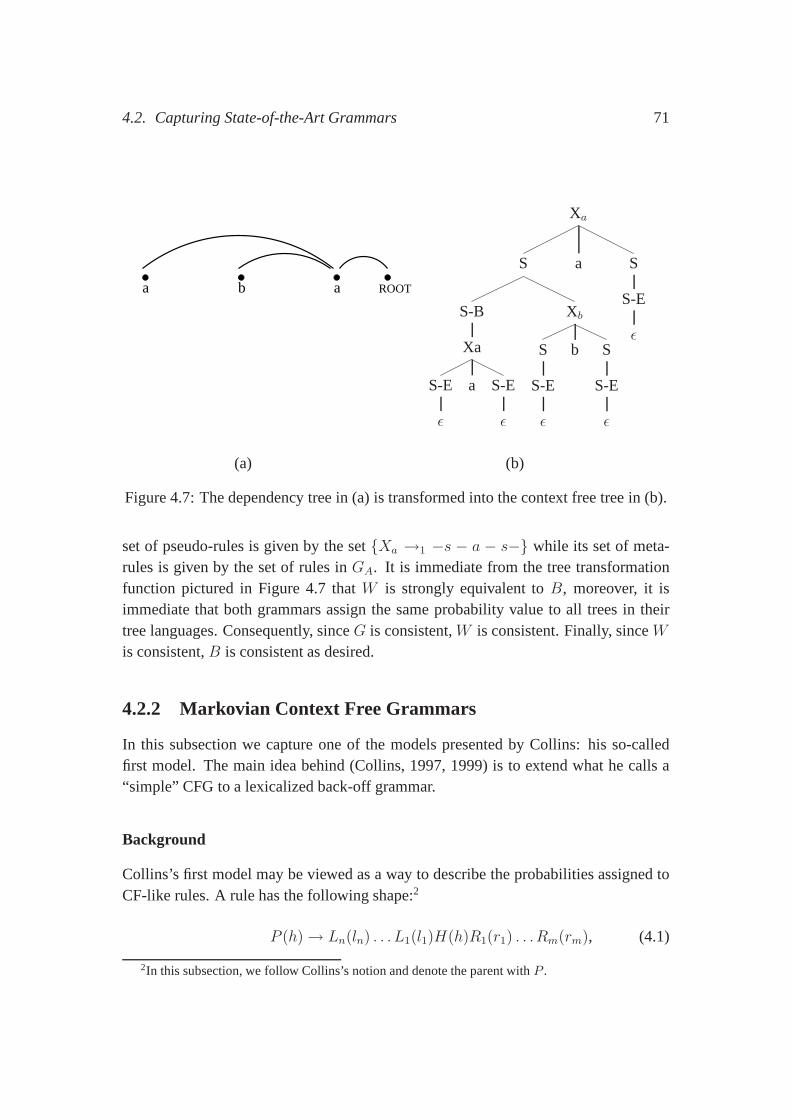
4.2. Capturing State-of-the-Art Grammars 71
a ROOTa b
(a)
Xa
S
S-B
Xa
S-E
ǫ
a S-E
ǫ
Xb
S
S-E
ǫ
b S
S-E
ǫ
a S
S-E
ǫ
(b)
Figure 4.7: The dependency tree in (a) is transformed into the context free tree in (b).
set of pseudo-rules is given by the set{Xa →1 −s − a − s−} while its set of meta-rules is given by the set of rules inGA. It is immediate from the tree transformationfunction pictured in Figure 4.7 thatW is strongly equivalent toB, moreover, it isimmediate that both grammars assign the same probability value to all trees in theirtree languages. Consequently, sinceG is consistent,W is consistent. Finally, sinceWis consistent,B is consistent as desired.
4.2.2 Markovian Context Free Grammars
In this subsection we capture one of the models presented by Collins: his so-calledfirst model. The main idea behind (Collins, 1997, 1999) is to extend what he calls a“simple” CFG to a lexicalized back-off grammar.
Background
Collins’s first model may be viewed as a way to describe the probabilities assigned toCF-like rules. A rule has the following shape:2
P (h)→ Ln(ln) . . . L1(l1)H(h)R1(r1) . . .Rm(rm), (4.1)
2In this subsection, we follow Collins’s notion and denote the parent withP .
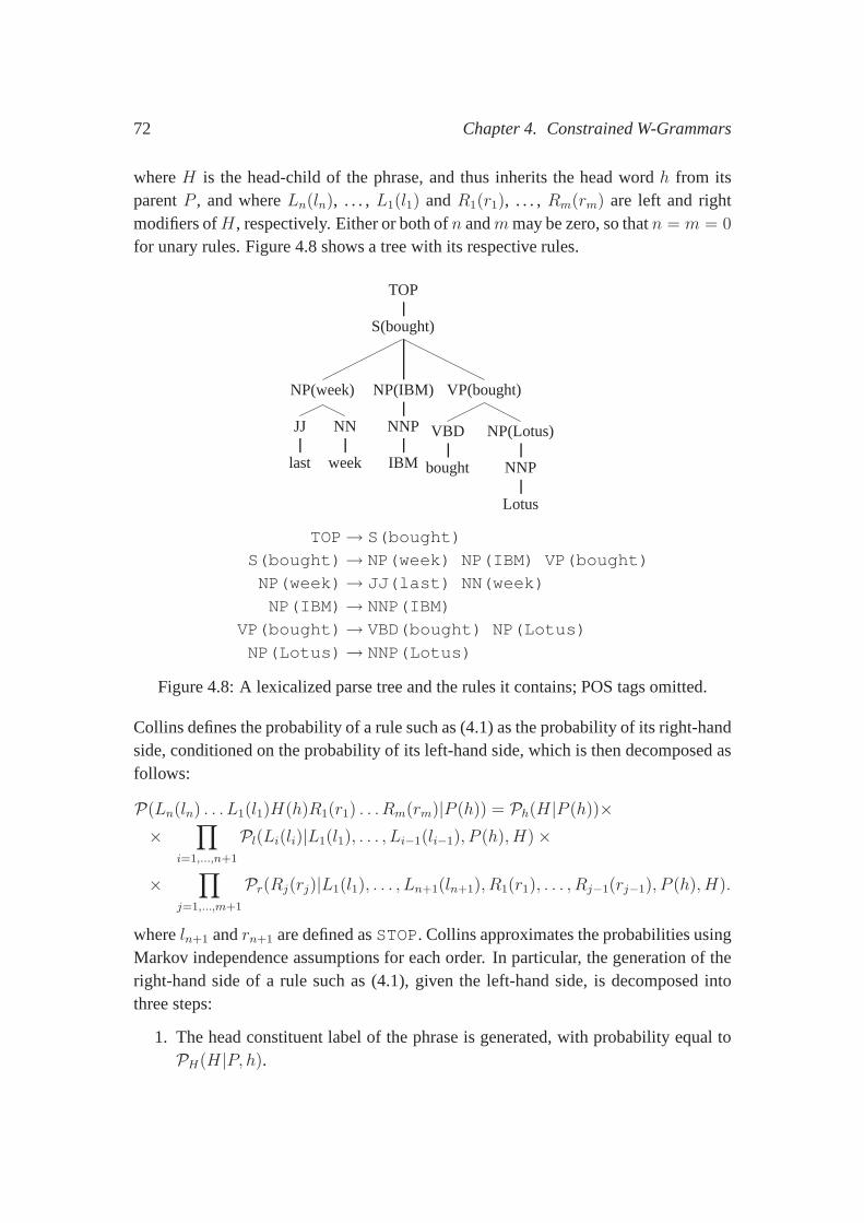
72 Chapter 4. Constrained W-Grammars
whereH is the head-child of the phrase, and thus inherits the head word h from itsparentP , and whereLn(ln), . . . , L1(l1) andR1(r1), . . . , Rm(rm) are left and rightmodifiers ofH, respectively. Either or both ofn andmmay be zero, so thatn = m = 0
for unary rules. Figure 4.8 shows a tree with its respective rules.
TOP
S(bought)
NP(week)
JJ
last
NN
week
NP(IBM)
NNP
IBM
VP(bought)
VBD
bought
NP(Lotus)
NNP
Lotus
TOP→ S(bought)
S(bought)→ NP(week) NP(IBM) VP(bought)
NP(week)→ JJ(last) NN(week)
NP(IBM)→ NNP(IBM)
VP(bought)→ VBD(bought) NP(Lotus)
NP(Lotus)→ NNP(Lotus)
Figure 4.8: A lexicalized parse tree and the rules it contains; POS tags omitted.
Collins defines the probability of a rule such as (4.1) as the probability of its right-handside, conditioned on the probability of its left-hand side,which is then decomposed asfollows:
P(Ln(ln) . . . L1(l1)H(h)R1(r1) . . .Rm(rm)|P (h)) = Ph(H|P (h))××
∏
i=1,...,n+1
Pl(Li(li)|L1(l1), . . . , Li−1(li−1), P (h), H)×
×∏
j=1,...,m+1
Pr(Rj(rj)|L1(l1), . . . , Ln+1(ln+1), R1(r1), . . . , Rj−1(rj−1), P (h), H).
whereln+1 andrn+1 are defined asSTOP. Collins approximates the probabilities usingMarkov independence assumptions for each order. In particular, the generation of theright-hand side of a rule such as (4.1), given the left-hand side, is decomposed intothree steps:
1. The head constituent label of the phrase is generated, with probability equal toPH(H|P, h).
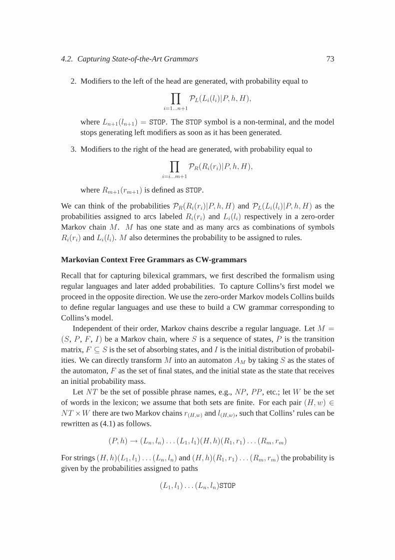
4.2. Capturing State-of-the-Art Grammars 73
2. Modifiers to the left of the head are generated, with probability equal to∏
i=1...n+1
PL(Li(li)|P, h,H),
whereLn+1(ln+1) = STOP. TheSTOP symbol is a non-terminal, and the modelstops generating left modifiers as soon as it has been generated.
3. Modifiers to the right of the head are generated, with probability equal to∏
i=i...m+1
PR(Ri(ri)|P, h,H),
whereRm+1(rm+1) is defined asSTOP.
We can think of the probabilitiesPR(Ri(ri)|P, h,H) andPL(Li(li)|P, h,H) as theprobabilities assigned to arcs labeledRi(ri) andLi(li) respectively in a zero-orderMarkov chainM . M has one state and as many arcs as combinations of symbolsRi(ri) andLi(li). M also determines the probability to be assigned to rules.
Markovian Context Free Grammars as CW-grammars
Recall that for capturing bilexical grammars, we first described the formalism usingregular languages and later added probabilities. To capture Collins’s first model weproceed in the opposite direction. We use the zero-order Markov models Collins buildsto define regular languages and use these to build a CW grammarcorresponding toCollins’s model.
Independent of their order, Markov chains describe a regular language. LetM =
(S, P , F , I) be a Markov chain, whereS is a sequence of states,P is the transitionmatrix,F ⊆ S is the set of absorbing states, andI is the initial distribution of probabil-ities. We can directly transformM into an automatonAM by takingS as the states ofthe automaton,F as the set of final states, and the initial state as the state that receivesan initial probability mass.
Let NT be the set of possible phrase names, e.g.,NP , PP , etc.; letW be the setof words in the lexicon; we assume that both sets are finite. For each pair(H,w) ∈NT ×W there are two Markov chainsr(H,w) andl(H,w), such that Collins’ rules can berewritten as (4.1) as follows.
(P, h)→ (Ln, ln) . . . (L1, l1)(H, h)(R1, r1) . . . (Rm, rm)
For strings(H, h)(L1, l1) . . . (Ln, ln) and(H, h)(R1, r1) . . . (Rm, rm) the probability isgiven by the probabilities assigned to paths
(L1, l1) . . . (Ln, ln)STOP
74 Chapter 4. Constrained W-Grammars
and(R1, r1) . . . (Rm, rm)STOP
in the Markov chainsl(H,h) andr(H,h) respectively.
4.2.4.DEFINITION. Let B = (NT , W , {l(H,w)}w∈W,h∈NT}, {r(H,w)}w∈W,h∈NT ) be agrammar based on Markov rules. LetWB = (V,NT, T, S,
m−→, s−→) be the CW-grammar defined as follows:
• The set of variablesV is given by the set of start symbolsSl(H,w)andSr(H,w)
fromthe regular grammarsl(H,w) andr(H,w) respectively for eachw in W .
• The set of non-terminalsNT is some set in 1-1-correspondence withW , e.g., itcan be defined asNT = {w′ : w ∈W}, where ′ is a string priming operation.
• The set of terminalsT is the set of wordsW .
• The set of probabilistic meta-rules is given by the union of the rules in each of theright and left regular grammars (i.e., the set given byA m−→ α iff A→ α ∈ l(H,w)
orA → α ∈ r(H,w) for someH and somew) plus the set{w′ m−→ w : w ∈ W}.
• The set of pseudo-rules is given by(P, h)s−→PH(H|(P,h)) Sl(H,h)
(H, h)Sr(H,h).
4.2.5.LEMMA . Markov rules as used in Collins’s first model aref -transformable toCW-grammars.
The proof of this lemma is similar to the proof of Lemma 4.2.3 and we omit it here.
Expressive Power and Consistency
By Lemma 4.2.5 Collins’s first model is weakly equivalent to context free grammars.Moreover, the idea behind Example 4.1.2 can be used to show that Collins’s first modelis not strongly equivalent to CFGs: Collins’s first model canproduce flat structuresthat cannot be captured by PCFGs (see Example 4.6 and Example4.1.2 for examplesof flat structures non-capturable by CFGs); as a consequence, the probabilistic versionof Collins’s first model cannot be captured using PCFGs.
As a consequence of Lemma 4.2.5, learning Markov rule-basedgrammars is equiv-alent to learning PCW-grammars, which, in turn, is equivalent to learning the PCFGsunderlying PCW-grammars. Collins (1997) assumes that all hidden derivations areproduced by Markov chains. Under the PCW-paradigm, his methodology is equivalentto transforming all trees in the training material by makingall their hidden derivationsvisible and inducing the underlying PCFG from the transformed trees. Variables in theequivalent PCW-grammar are defined according to the degree of the Markov chain.
4.2. Capturing State-of-the-Art Grammars 75
If the Markov chain used is of degree zero, there is only one variable (the Markovchain contains a unique state), and the induced Markov rule-based grammar is consis-tent. This consistency result follows from the fact that inducing a zero-degree Markovchain is the same as inducing the underlying PCFG in the equivalent PCW-grammarusing maximum likelihood estimation, plus the fact that using maximum likelihood forinducing PCFGs produces consistent grammars (Chi and Geman, 1998; Joan-Andreuand Benedı, 1997).
Finally, the embedding of Collins’s and Eisner’s models into CW-grammars allowsus to compare them. Both models have quite similar meta-rules and pseudo-rules. Themain difference between their rules is that Collins’s codify more information as vari-ables. The embedding into CW-grammars allows us to see theirlearning step as atreebank rewriting procedure, followed by a CFG induction step. The treebank gener-ated in the first step is the one used as training material in the second. According tothis perspective, the two approaches differ in the rewriting function they use in the firststep, while both approaches use maximum likelihood in the second step.
4.2.3 Stochastic Tree Substitution Grammars
Data-oriented parsing (DOP) is a memory-based approach to syntactic parsing. Thebasic idea is to use the subtrees from a syntactically annotated corpus directly as astochastic grammar. The DOP-1 model (Bod, 1995) was the firstversion of DOP, andmost later versions of DOP are variations on it. The underlying grammatical formalismis stochastic tree substitution grammars (STSG), which is the grammatical formalismwe capture here.
Background
The grammatical formalism is extremely simple and can be described as follows:for every sentence in a parsed training corpus, extract every subtree. Now, we usethese trees to form a stochastic tree substitution grammar.Formally, astochastic tree-substitution grammar(STSG)G is a 5-tuple〈VN , VT , S, R, P 〉 where:
• VN is a finite set of nonterminal symbols.
• VT is a finite set of terminal symbols.
• S ∈ VN is the distinguished symbol.
• R is a finite set of trees, calledelementary trees, whose top nodes and interiornodes are labeled by nonterminal symbols and whose yield nodes are labeled byterminal or nonterminal symbols.
76 Chapter 4. Constrained W-Grammars
• P is a function which assigns to every elementary treet ∈ R a probabilityP (t).For a treet with a root node symbolroot(t) = α, P (t) is interpreted as theprobability of substitutingt for a nodeα. We require, therefore, for a givenαthat
∑
{t:root(t)=α} = 1 (wheret’s root node symbol isα).
If t1 andt2 are elementary trees such that the left-most non-terminal leaves node sym-bol of t1 is equal to the root node symbol oft2, then t1 ◦ t2 is the tree that resultsfrom substitutingt2 in this left-most non-terminal leaves node symbol int1. The par-tial function◦ is calledleftmost substitutionor simplysubstitution. Trees are derivedusing leftmost substitution.
STSGs as CW-grammars
A STSG is not a context free grammar. The main difference, andthe hardest to capturein a CFG-like setting, is the way in which probabilities are computed for a given tree.The probability of a tree is given by the sum of the probabilities of all derivationsproducing it. CW-grammars offer a similar mechanism: the probability of the body ofa w-rule is the sum of the probabilities of all meta-derivations producing it. The ideaof the equivalence is to associate to every tree produced by aSTSG a w-rule of thePCW-grammar in such a way that the body of the w-rule codifies the whole tree.
To implement this idea, we need to code up trees as strings. The simplest way toachieve this is to visit the nodes in a depth-first left-to-right order. For each inner node,we write the CFG production, while for the leaves, we write the symbol itself if thesymbol is a terminal and a primed version of it if the symbol isa non-terminal. Forexample, the code describing the tree in Figure 4.9(a) is
(A,BAB)B′(A,BAB)B′A′B′(B, a)a.
The first step in capturing STSGs is to build meta-rules capturing elementary treesusing the notation just introduced. Specifically, lett be an elementary tree belongingto a STSG. LetS be its root andα its string representation. The CF-like ruleS ′ → α
is called theelementary ruleof t. Elementary rules store all information about theelementary tree. They have primed non-terminals where a substitution can be carriedout. For example, ift is the elementary tree pictured in Figure 4.9.(b), its elementaryrule isS ′ → (S,AB)(A,B)(A, ab)ab(B,AC)(A, ab)abC ′. Note the primed versionof C in the frontier of the derivation.
4.2.6.DEFINITION. LetH = (VN , VT , S, R, P ) be a STSG. LetWH = (V , NT , T ,S ′,
m−→,s−→) be the following CW-grammar.
• V is the primed version ofVT .
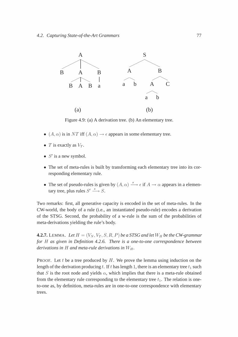
4.2. Capturing State-of-the-Art Grammars 77
A
B A
B A B
B
a
S
A
a b
B
A
a b
C
(a) (b)
Figure 4.9: (a) A derivation tree. (b) An elementary tree.
• (A, α) is inNT iff (A, α)→ ǫ appears in some elementary tree.
• T is exactly asVT .
• S ′ is a new symbol.
• The set of meta-rules is built by transforming each elementary tree into its cor-responding elementary rule.
• The set of pseudo-rules is given by(A, α)s−→ ǫ if A→ α appears in a elemen-
tary tree, plus rulesS ′ s−→ S.
Two remarks: first, all generative capacity is encoded in theset of meta-rules. In theCW-world, the body of a rule (i.e., an instantiated pseudo-rule) encodes a derivationof the STSG. Second, the probability of a w-rule is the sum of the probabilities ofmeta-derivations yielding the rule’s body.
4.2.7.LEMMA . LetH = (VN , VT , S, R, P ) be a STSG and letWH be the CW-grammarfor H as given in Definition 4.2.6. There is a one-to-one correspondence betweenderivations inH and meta-rule derivations inWH .
PROOF. Let t be a tree produced byH. We prove the lemma using induction on thelength of the derivation producingt. If t has length1, there is an elementary treet1 suchthatS is the root node and yieldsα, which implies that there is a meta-rule obtainedfrom the elementary rule corresponding to the elementary treet1. The relation is one-to-one as, by definition, meta-rules are in one-to-one correspondence with elementarytrees.
78 Chapter 4. Constrained W-Grammars
Suppose the lemma is true for derivation lengths less than orequal ton. Supposetis generated by a derivation of lengthn+1. Assume there are treest1, t2 with t1◦t2 = t.By definition there is a unique meta-ruler1 corresponding witht1 and by the inductivehypothesis there is a unique derivation fort2. ⊣
4.2.8.LEMMA . LetH = (VN , VT , S, R, P ) be a STSG, and letWH be the CW-grammarfor H as given in Definition 4.2.6. ThenWH accepts the same set of strings asH, i.e.,STSGs and PCW-grammars are weakly equivalent.
PROOF. Let α be a string inL(H). There is at least one tree derivationt1 ◦ . . . ◦ tkyieldingα. From Lemma 4.2.7 we know that there is a w-ruleS ′ w
=⇒ α such that afterapplying rules(A, β)
s−→ ǫ, α is obtained. ⊣
4.2.9.COROLLARY. LetH = (VN , VT , S, R, P ) be a STSG, and letWH be the CW-grammar forH as given in Definition 4.2.6. There is a one-to-one correspondencebetween derivations inH andWH .
4.2.10.COROLLARY. STSGs are f-transformable to CW-grammars.
PROOF. The result is a direct consequence of Lemma 4.2.8 and Lemma 4.2.9. ⊣
4.2.11.LEMMA . Let H = (VN , VT , S, R, P ) be a STSG, and letWH be the CW-grammar given in Definition 4.2.6. Both grammars assign the same probability massto trees related through the one-to-one mapping described in Corollary 4.2.9.
PROOF. A tree has a characteristic w-rule, defined by its shape. In other words, theprobability of a w-rule according to the definition of PCW-grammars is given by thesum of the probabilities of all derivations producing the rule’s body, i.e., all STSGderivations producing the same tree. As a consequence, a particular STSG tree, iden-tified by the body of the corresponding w-rule, has the same probability mass as theamount assigned to its corresponding w-rule by the equivalent CW-Grammar. ⊣
Expressive Power and Consistency
By Corollary 4.2.10, STSGs are weakly equivalent to contextfree grammars. The con-sistency of a STSG depends on the methodology used for computing the probabilitiesassigned to its elementary trees. DOP-1 is one particular approach to computing theseprobabilities. Under the DOP-1 perspective, a treet contributes all its possible sub-trees to a new treebank from which the probabilities of elementary trees are computed.Probabilities of an elementary tree are computed using maximum likelihood. Since
4.3. Discussion and Conclusion 79
the events in the new treebank are not independently distributed, the resulting proba-bilities are inconsistent and biased (Johnson, 2002). Solutions taking into account thedependence between trees in the resulting treebanks have been suggested (Sima’an andBuratto, 2003).
Consistency conditions cannot be derived for the DOP-1 estimation procedure be-cause it does not attempt to learn the underlying PCFG. In fact, our formalism suggeststhat probabilities should be computed differently than they are done in DOP-1. By ourembedding, a treet in the treebank corresponds to the body of a pseudo-rule instanti-ated through meta-derivations;t is the final “string” and does not have any informationabout the derivation that took place. But viewingt as a final string changes the prob-lem definition! Now, we have as input a set of elementary rulesand a set of acceptedtrees. The problem is to compute probabilities for these rules: an unsupervised problemthat can be solved using any unsupervised technique. The consistency of the resultingSTSG depends on the consistency properties of the unsupervised method.
4.3 Discussion and Conclusion
In this chapter we introduced constrained W-grammars and weaugmented them withprobabilities. Probabilities provide a disambiguation mechanism and a statistical per-spective. It is still an open question whether probabilities add expressive power toCW-grammars; the strategy used in Chapter 3 can not be used for PCW-grammars. Tosee this, one should note that CW-grammars do not have any inherently ambiguouslanguages: any CW-grammarW with start symbolS, meta-rulesM and pseudo-rulesP can be transformed into an unambiguous grammarG′ by definingG′’s start symbolto beS ′, its unique meta-rule to beS ′ m−→ S and its meta-rules to beM ∪ P . G′ isunambiguous because it hides inside meta-derivations practically all derivations. Alltrees inT (G′) are very flat, and there is exactly one tree for each string in the language.
Do PCW-grammars add anything? We think that the importance and contributionof our grammatical formalism has to be considered from the perspective of grammat-ical formalisms underlying state-of-the-art parsers. It is usually the case that gram-matical formalisms used in parsers are not clearly stated, they are hard to identifyfrom the definition of the parser (see (Bikel, 2004) for an account of the details ofCollins’s parser) and their formal properties require ad-hoc proofs (see (Bod, 1999)for expressive power properties of STSGs) or are not proven at all. We have shownthat PCW-grammars provide a common formalism based on a well-known grammat-ical framework with computational properties that are verywell understood. Clearly,PCW-grammars greatly reduce the expressive power of W-grammars, but still, we man-age to capture the grammatical formalisms underlying state-of-the-art parsers with the
80 Chapter 4. Constrained W-Grammars
remaining expressive power and to establish new and important facts about them.In particular, we examioned the expressive power of three formalisms (bilexical
grammars, Markovian context free rules, and stochastic tree substitution grammars)together with some conditions under which the inferred grammars are consistent. Fi-nally, we should point out that, despite their similarities, there is a fundamental differ-ence between PCW-grammars and PCFGs, and this is the two-level mechanism of theformer. This mechanism allows us to capture three state-of-the-art natural languageparsers, which cannot be done using standard PCFGs only.
The results in this chapter shed light on the relationship between a number of gram-matical formalisms, not just between context free grammarsand PCW-grammars. Inparticular, we have shown that, from a formal perspective, bilexical grammars andMarkovian context free grammars do not differ in a principled way: both are basedon approximating bodies of rules using Markov models. We also found that STSGsand Markov rules have certain similarities. Markov rules and STSGs suppose that rulebodies are obtained by collapsing hidden derivations. Thatis, for Markov rules a rulebody is a regular expression (or equivalently a Markov chain). Similarly, STSGs takethis idea to the extreme by taking the whole sentence to be theyield of a hidden deriva-tion. PCW-grammars naturally suggest intermediate levelsof abstraction; in Chapter 5we show that these levels can be used to reduce the size of grammars induced fromtreebanks, and, hence, to optimize parsing procedures.
From a theoretical point of view, the concept off -transformable grammars, whichwe use heavily in our proofs, is a novel and very powerful concept that relaxes theknown equivalence notions between grammars. Since arbitrary functionsf can bedefined between arbitrary tree languages and CFG-like trees, they can be used tomap other formalisms like tree adjoining grammars (Joshi, 1985) or categorial gram-mars (Wood, 1993) to context free trees. As part of our futureresearch, we aim tocapture further grammatical formalisms and to characterize the nature of the functionsf used to achieve this.
Chapter 5
Alternative Approaches for Generating Bodiesof Grammar Rules
5.1 Introduction
So far, we have developed a grammatical formalism capable ofcapturing differentstate-of-the-art language models, which gave us a novel perspective on state-of-the-artlanguage models. In Chapter 4 we identified that some language models usen-gramsfor building bodies of rules. From the literature, we know thatn-grams have had a bigimpact on the state-of-the-art in natural language models.They are central to many lan-guage models (Charniak, 1997; Collins, 1997; Eisner, 1996;Collins, 2000), and despitetheir simplicity,n-gram models have been very successful. Modeling withn-grams isan induction task (Gold, 1967): given a sample set of strings, the task is to guessthe grammar that produced that sample. Usually, the grammaris not chosen from anarbitrary set of possible grammars, but from some given restricted class. Grammar in-duction consists of two parts: choosing the class of languages amongst which to searchand designing the procedure for performing the search. By using n-grams for gram-mar induction one addresses the two parts in one go, and the use of n-grams impliesthat the solution will be searched for in the class of probabilistic regular languages,sincen-grams induce probabilistic automata and, consequently, probabilistic regularlanguages. But probabilistic regular languages induced using n-grams form a propersubclass of the class of all probabilistic regular languages; for instance,n-grams areincapable of capturing long-distance relations between words. At the technical levelthe restricted nature ofn-grams is witnessed by the special structure of the automatainduced from them, as we will see in Section 5.4.2.
N-grams are not the only way to induce regular languages, and they are not themost powerful way to do so. There is a variety of general methods capable of inducing
81
82 Chapter 5. Alternative Approaches for Generating Bodies ofGrammar Rules
all regular languages (Denis, 2001; Carrasco and Oncina, 1994;Thollard et al., 2000).What is their relevance for natural language parsing? Recall from Chapter 4 that regu-lar languages are used for describing the bodies of rules in agrammar. Consequently,the quality and expressive power of the resulting grammar istied to the quality andexpressive power of the regular languages used to describe them. And these proper-ties, in turn, are influenced directly by the method used to induce them. At this pointa natural question arises: can we gain anything in parsing from using general methodsfor inducing regular languages instead of methods based onn-grams? Specifically, canwe describe the bodies of grammatical rules more accuratelyand more concisely byusing general methods for inducing regular languages?
In the context of natural language parsing we present an empirical comparisonbetween algorithms for inducing regular languages usingn-grams on the one hand,and more general algorithms for learning the general class of regular language on theother. We proceed as follows. We generate our training data from the Wall StreetJournal section of the Penn Tree Bank (PTB), transforming itto projectivedependencystructures, following (Collins, 1996). Since projective dependency structures can beseen as a special type of context free grammars (Gaifman, 1965), word dependents canbe seen as bodies of context free rules. We extract these rulebodies and use them astraining material for the rule induction algorithms we consider. The automata producedthis way are then used to build grammars which, in turn, are used for parsing.
We are interested in two aspects of the use of probabilistic regular languages fornatural language parsing: the quality of the induced automata and the performance ofthe resulting parsers. For evaluation purposes, we use two metrics: perplexity for thefirst aspect and percentage of correct attachments for the second, both explained indetail in Section 2.2.3. The main results of the chapter are that, measured in terms ofperplexity, automata induced by algorithms other thann-grams describe rule bodiesbetter than automata induced usingn-gram-based algorithms. Moreover, the gain inautomata quality is reflected by an improvement in parsing performance. The pars-ing performance of both methods (n-grams vs. general automata) can be substantiallyimproved by splitting the training material into POS categories. As a side product,we find empirical evidence to explain the effectiveness of rule lexicalization (Collins,1997; Sima’an, 2000) and parent annotation techniques (Klein and Manning, 2003) interms of a reduction in perplexity in the automata induced from training corpora.
5.2 Overview
We want to build grammars using different algorithms for inducing their rules. Ourmain question is aimed at understanding how different algorithms for inducing regular
5.3. From Automata to Grammars 83
languages impact the parsing performance with those grammars. A second issue thatwe want to explore is how the grammars perform when the quality of the trainingmaterial is improved, that is, when the training material isseparated into part of speech(POS) categories before the regular language learning algorithms are run.
The first step is to transform the PTB into projective dependencies structures fol-lowing (Collins, 1996). From the resulting tree bank we delete all lexical informationexcept POS tags. Every POS in a tree belonging to the tree-bank has associated to ittwo different, possibly empty, sequences of right and left dependents, respectively. Weextract all these sequences for all trees, producing two different sets containing rightand left sequences of dependents, respectively.
These two sets form the training material used for building four different gram-mars. The four grammars differ along two dimensions: the number of automata usedfor building them and the algorithm used for inducing the automata. As to the latterdimension, in Section 5.4 we use two algorithms: the MinimumDiscriminative Infor-mation (MDI) algorithm, and a bigram-based algorithm. As tothe former dimension,two of the grammars are built using only two different automata, each of which isbuilt using the two sample set generated from the PTB. The other two grammars arebuilt using two automata per POS, exploiting a split of the training samples into mul-tiple samples, two samples per POS, to be precise, each containing only those sampleswhere the POS appeared as the head.
5.3 From Automata to Grammars
In this section we describe how to learn PCW-grammars from the automata that we aregoing to induce in Section 5.4. Since we will induce two families of automata (“Many-Automata” where we use two automata per POS, and “One-Automaton” where we useonly two automata to fit every POS), we need to describe two automata-to-grammartransformations.
Let us start with the case where we build two automata per POS.Let w be a POSin the PTB; letAwL andAwR be the two automata associated to it. LetGw
L andGwR be
the PCFGs equivalent toAwL andAwR, respectively, following (Abney et al., 1999), andlet SwL andSwR be the start symbols ofGw
L andGwR, respectively. We build our final
grammarG with start symbolS, by defining its meta-rules as the disjoint union of allrules inGw
L andGwR (for all POSw), its set of pseudo-rules as the union of the sets
{W s−→1 SwLwS
wR}
andS
s−→1 SwLwS
wR},
84 Chapter 5. Alternative Approaches for Generating Bodies ofGrammar Rules
whereW is a unique new variable symbol associated tow.When we use two automata for all parts of speech, the grammar is defined as fol-
lows. LetAL andAR be the two automata learned. LetGL andGR be the PCFGsequivalent toAL andAR, and letSL andSR be the start symbols ofGL andGR, re-spectively. Fix a POSw in the PTB. Since the automata are deterministic, there existstatesSwL andSwR that are reachable fromSL andSR, respectively, by following the arclabeled withw. Define a grammar as in the previous case. Its start symbol isS, its setof meta-rules is the disjoint union of all rules inGw
L andGwR (for all POSw), its set of
pseudo-rules is{W s−→1 SwLwS
wR , S
s−→1 SwLwS
wR : w is a POS in the PTB andW is
a unique new variable symbol associated tow}.
5.4 Building Automata
The four grammars we intend to induce are completely defined once the underlyingautomata have been built. We now explain how we build those automata from thetraining material. The process of building the automata consists of three steps:
1. Extracting the training material from the transformed PTB.
2. Applying the algorithm to learn automata to the training material.
3. Searching for the optimal automata.
Sections 5.4.1, 5.4.2 and 5.4.3 deal with steps 1, 2, and 3, respectively.
5.4.1 Building the Sample Sets
The training material is obtained as follows. We transform the PTB, sections 2–22, todependency structures, as suggested by (Collins, 1999). All sentences containingCCtags are filtered out, following (Eisner, 1996). We also eliminate all word information,leaving only POS tags. For each resulting dependency tree weextract a sample setof right and left sequences of dependents. Figure 5.1 shows an example of a phasestructure, Figure 5.2 shows its corresponding dependency tree, and Table 5.1 showsthe sample sets of right and left dependents we extracted from it. The sample set usedfor automata induction is the union of all individual tree sample sets.
5.4.2 Learning Probabilistic Automata
Probabilistic deterministic finite state automata (PDFA) inference is the problem ofinducing a stochastic regular grammar from a sample set of strings belonging to an
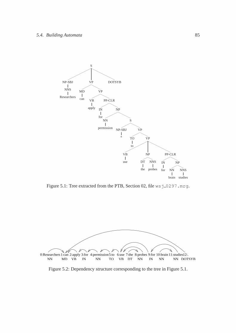
5.4. Building Automata 85
S
NP-SBJ
NNS
Researchers
VP
MD
can
VP
VB
apply
PP-CLR
IN
for
NP
NN
permission
S
NP-SBJ
*
VP
TO
to
VP
VB
use
NP
DT
the
NNS
probes
PP-CLR
IN
for
NP
NN
brain
NNS
studies
DOTSYB
Figure 5.1: Tree extracted from the PTB, Section 02, filewsj 0297.mrg.
0:Researchers 1:can 2:apply 3:for 4:permission5:to 12:.NN MD VB IN NN TO
8:probes7:the6:use 9:for 10:brain 11:studiesNN NNINNNDTVB DOTSYB
Figure 5.2: Dependency structure corresponding to the treein Figure 5.1.
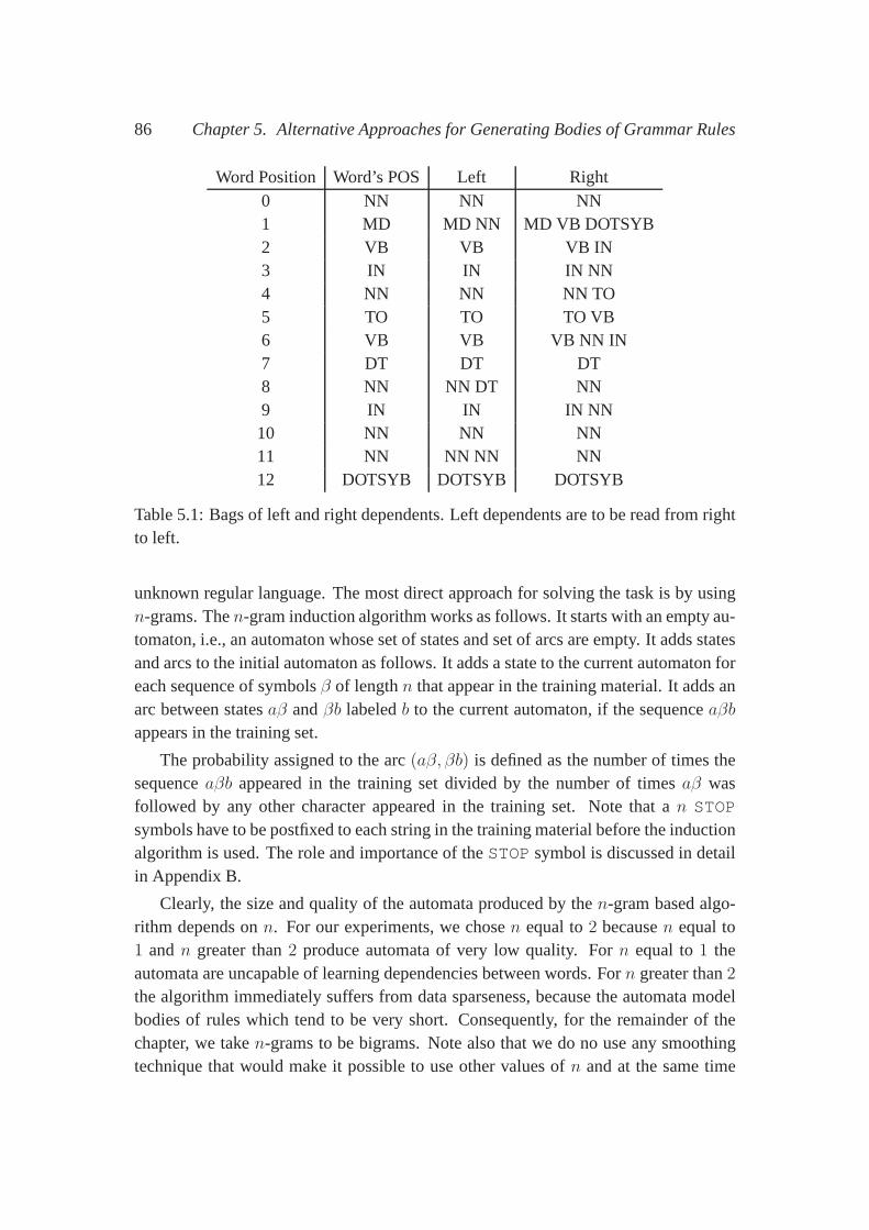
86 Chapter 5. Alternative Approaches for Generating Bodies ofGrammar Rules
Word Position Word’s POS Left Right0 NN NN NN1 MD MD NN MD VB DOTSYB2 VB VB VB IN3 IN IN IN NN4 NN NN NN TO5 TO TO TO VB6 VB VB VB NN IN7 DT DT DT8 NN NN DT NN9 IN IN IN NN10 NN NN NN11 NN NN NN NN12 DOTSYB DOTSYB DOTSYB
Table 5.1: Bags of left and right dependents. Left dependents are to be read from rightto left.
unknown regular language. The most direct approach for solving the task is by usingn-grams. Then-gram induction algorithm works as follows. It starts with an empty au-tomaton, i.e., an automaton whose set of states and set of arcs are empty. It adds statesand arcs to the initial automaton as follows. It adds a state to the current automaton foreach sequence of symbolsβ of lengthn that appear in the training material. It adds anarc between statesaβ andβb labeledb to the current automaton, if the sequenceaβb
appears in the training set.
The probability assigned to the arc(aβ, βb) is defined as the number of times thesequenceaβb appeared in the training set divided by the number of timesaβ wasfollowed by any other character appeared in the training set. Note that an STOP
symbols have to be postfixed to each string in the training material before the inductionalgorithm is used. The role and importance of theSTOP symbol is discussed in detailin Appendix B.
Clearly, the size and quality of the automata produced by then-gram based algo-rithm depends onn. For our experiments, we chosen equal to2 becausen equal to1 andn greater than2 produce automata of very low quality. Forn equal to1 theautomata are uncapable of learning dependencies between words. Forn greater than2the algorithm immediately suffers from data sparseness, because the automata modelbodies of rules which tend to be very short. Consequently, for the remainder of thechapter, we taken-grams to be bigrams. Note also that we do no use any smoothingtechnique that would make it possible to use other values ofn and at the same time
5.4. Building Automata 87
avoid the problems mentioned. If we want to carry out a fair comparison of both meth-ods, smoothing techniques used for optimizing automata based onn-grams should alsobe used for optimizing MDI-based automata. Two or moren-gram based automatasmoothed into a single automaton would have to be compared against two or moreMDI-based automata smoothed into a single automaton. It would be hard to determinewhether the differences between the final automata are due tothe smoothing procedureor to the algorithms used for creating the initial automata.By leaving smoothing outof the picture, we obtain a clearer understanding of the differences between the twoalgorithms to induce automata.
There are other approaches to inducing regular grammars besides ones based onn-grams. The first algorithm to learn PDFAs was ALERGIA (Carrasco and Oncina,1994); it learns cyclic automata with the so-called state-merging method. The Min-imum Discrimination Information (MDI) algorithm (Thollard et al., 2000) improvesover ALERGIA and uses Kullback-Leibler divergence for deciding when to mergestates. We opted for the MDI algorithm as an alternative ton-gram based inductionalgorithms, mainly because its working principles are radically different from then-gram-based algorithm. The MDI algorithm first builds an automaton that only acceptsthe strings in the sample set by merging common prefixes, thusproducing a tree-shapedautomaton in which each transition has a probability proportional to the number oftimes it is used while generating the positive sample; see Section 2.2.2 for details.
For comparison purposes, let us repeat here the working principle of the MDI algo-rithm. The MDI algorithm traverses the lattice of all possible partitions for this generalautomaton, attempting to merge states that satisfy a trade-off that can be specified bythe user. Specifically, assume thatA1 is a temporary solution of the algorithm and thatA2 is a tentative new solution derived fromA1. ∆(A1, A2) = D(A0||A2)−D(A0||A1)
denotes the divergence increment while going fromA1 toA2, whereD(A0||Ai) is theKullback-Leibler divergenceor relative entropybetween the two distributions gener-ated by the corresponding automata (Cover and Thomas, 1991). The new solutionA2 is compatiblewith the training data if the divergence increment relativeto thesize reduction, that is, the reduction of the number of states, is small enough. For-mally, letalpha denote a compatibility threshold; then the compatibility is satisfiedif ∆(A1,A2)
|A1|−|A2|< alpha. For this learning algorithm,alpha is the unique parameter; we
tuned it to get better quality automata.
Note that the working principles of then-gram-based algorithm and the MDI algo-rithm are completely different. Then-gram based algorithm works locally by addingarcs and states depending on the local configuration of strings in the sample set. In con-trast, the MDI algorithm starts by building an automaton that accepts only the stringsin the training sample and it over-generalizes over the sample set by merging states thatit considers that can be merged. In this way, the MDI algorithm is capable of detecting
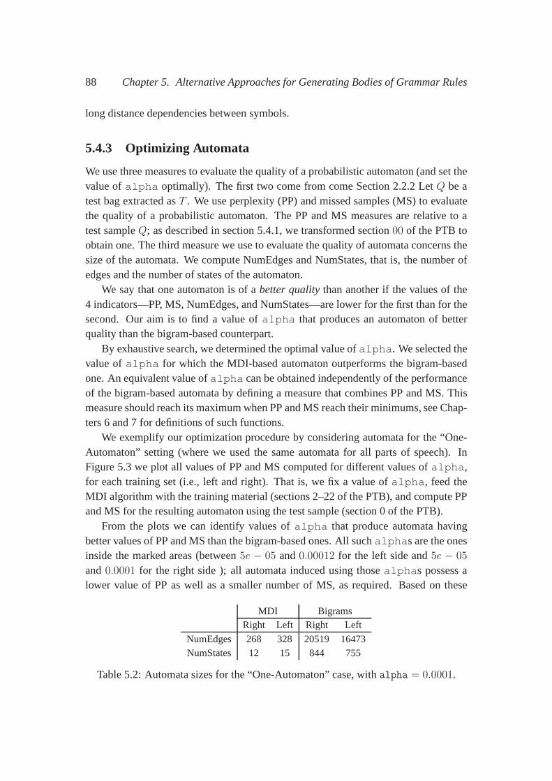
88 Chapter 5. Alternative Approaches for Generating Bodies ofGrammar Rules
long distance dependencies between symbols.
5.4.3 Optimizing Automata
We use three measures to evaluate the quality of a probabilistic automaton (and set thevalue ofalpha optimally). The first two come from come Section 2.2.2 LetQ be atest bag extracted asT . We use perplexity (PP) and missed samples (MS) to evaluatethe quality of a probabilistic automaton. The PP and MS measures are relative to atest sampleQ; as described in section 5.4.1, we transformed section00 of the PTB toobtain one. The third measure we use to evaluate the quality of automata concerns thesize of the automata. We compute NumEdges and NumStates, that is, the number ofedges and the number of states of the automaton.
We say that one automaton is of abetter qualitythan another if the values of the4 indicators—PP, MS, NumEdges, and NumStates—are lower forthe first than for thesecond. Our aim is to find a value ofalpha that produces an automaton of betterquality than the bigram-based counterpart.
By exhaustive search, we determined the optimal value ofalpha. We selected thevalue ofalpha for which the MDI-based automaton outperforms the bigram-basedone. An equivalent value ofalpha can be obtained independently of the performanceof the bigram-based automata by defining a measure that combines PP and MS. Thismeasure should reach its maximum when PP and MS reach their minimums, see Chap-ters 6 and 7 for definitions of such functions.
We exemplify our optimization procedure by considering automata for the “One-Automaton” setting (where we used the same automata for all parts of speech). InFigure 5.3 we plot all values of PP and MS computed for different values ofalpha,for each training set (i.e., left and right). That is, we fix a value ofalpha, feed theMDI algorithm with the training material (sections 2–22 of the PTB), and compute PPand MS for the resulting automaton using the test sample (section 0 of the PTB).
From the plots we can identify values ofalpha that produce automata havingbetter values of PP and MS than the bigram-based ones. All suchalphas are the onesinside the marked areas (between5e − 05 and0.00012 for the left side and5e − 05
and0.0001 for the right side ); all automata induced using thosealphas possess alower value of PP as well as a smaller number of MS, as required. Based on these
MDI BigramsRight Left Right Left
NumEdges 268 328 20519 16473NumStates 12 15 844 755
Table 5.2: Automata sizes for the “One-Automaton” case, with alpha = 0.0001.
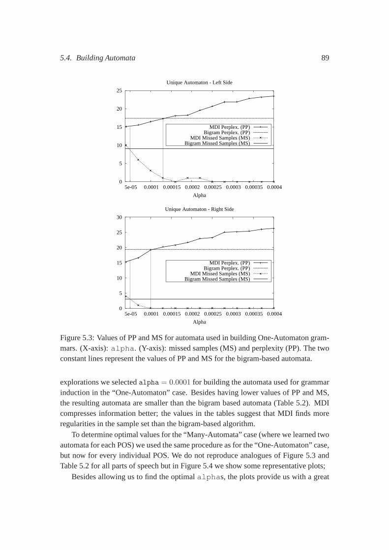
5.4. Building Automata 89
0
5
10
15
20
25
5e-05 0.0001 0.00015 0.0002 0.00025 0.0003 0.00035 0.0004
Alpha
Unique Automaton - Left Side
MDI Perplex. (PP)Bigram Perplex. (PP)
MDI Missed Samples (MS)Bigram Missed Samples (MS)
0
5
10
15
20
25
30
5e-05 0.0001 0.00015 0.0002 0.00025 0.0003 0.00035 0.0004
Alpha
Unique Automaton - Right Side
MDI Perplex. (PP)Bigram Perplex. (PP)
MDI Missed Samples (MS)Bigram Missed Samples (MS)
Figure 5.3: Values of PP and MS for automata used in building One-Automaton gram-mars. (X-axis):alpha. (Y-axis): missed samples (MS) and perplexity (PP). The twoconstant lines represent the values of PP and MS for the bigram-based automata.
explorations we selectedalpha = 0.0001 for building the automata used for grammarinduction in the “One-Automaton” case. Besides having lower values of PP and MS,the resulting automata are smaller than the bigram based automata (Table 5.2). MDIcompresses information better; the values in the tables suggest that MDI finds moreregularities in the sample set than the bigram-based algorithm.
To determine optimal values for the “Many-Automata” case (where we learned twoautomata for each POS) we used the same procedure as for the “One-Automaton” case,but now for every individual POS. We do not reproduce analogues of Figure 5.3 andTable 5.2 for all parts of speech but in Figure 5.4 we show somerepresentative plots;
Besides allowing us to find the optimalalphas, the plots provide us with a great
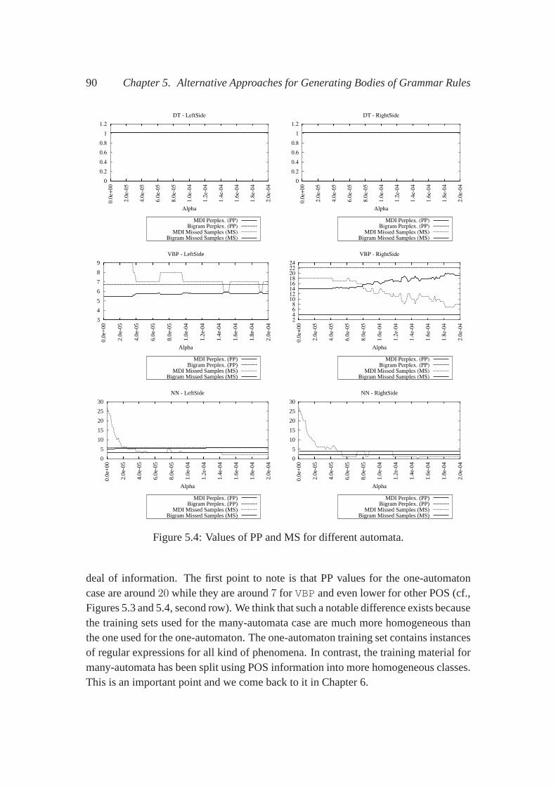
90 Chapter 5. Alternative Approaches for Generating Bodies ofGrammar Rules
0
0.2
0.4
0.6
0.8
1
1.2
0.0
e+0
0
2.0
e-0
5
4.0
e-0
5
6.0
e-0
5
8.0
e-0
5
1.0
e-0
4
1.2
e-0
4
1.4
e-0
4
1.6
e-0
4
1.8
e-0
4
2.0
e-0
4
Alpha
DT - LeftSide
MDI Perplex. (PP)Bigram Perplex. (PP)
MDI Missed Samples (MS)Bigram Missed Samples (MS)
0
0.2
0.4
0.6
0.8
1
1.2
0.0
e+0
0
2.0
e-0
5
4.0
e-0
5
6.0
e-0
5
8.0
e-0
5
1.0
e-0
4
1.2
e-0
4
1.4
e-0
4
1.6
e-0
4
1.8
e-0
4
2.0
e-0
4
Alpha
DT - RightSide
MDI Perplex. (PP)Bigram Perplex. (PP)
MDI Missed Samples (MS)Bigram Missed Samples (MS)
3
4
5
6
7
8
9
0.0e
+00
2.0e
-05
4.0e
-05
6.0e
-05
8.0e
-05
1.0e
-04
1.2e
-04
1.4e
-04
1.6e
-04
1.8e
-04
2.0e
-04
Alpha
VBP - LeftSide
MDI Perplex. (PP)Bigram Perplex. (PP)
MDI Missed Samples (MS)Bigram Missed Samples (MS)
2 4 6 8
10 12 14 16 18 20 22 24
0.0
e+0
0
2.0
e-0
5
4.0
e-0
5
6.0
e-0
5
8.0
e-0
5
1.0
e-0
4
1.2
e-0
4
1.4
e-0
4
1.6
e-0
4
1.8
e-0
4
2.0
e-0
4
Alpha
VBP - RightSide
MDI Perplex. (PP)Bigram Perplex. (PP)
MDI Missed Samples (MS)Bigram Missed Samples (MS)
0
5
10
15
20
25
30
0.0e
+00
2.0e
-05
4.0e
-05
6.0e
-05
8.0e
-05
1.0e
-04
1.2e
-04
1.4e
-04
1.6e
-04
1.8e
-04
2.0e
-04
Alpha
NN - LeftSide
MDI Perplex. (PP)Bigram Perplex. (PP)
MDI Missed Samples (MS)Bigram Missed Samples (MS)
0
5
10
15
20
25
30
0.0e
+00
2.0e
-05
4.0e
-05
6.0e
-05
8.0e
-05
1.0e
-04
1.2e
-04
1.4e
-04
1.6e
-04
1.8e
-04
2.0e
-04
Alpha
NN - RightSide
MDI Perplex. (PP)Bigram Perplex. (PP)
MDI Missed Samples (MS)Bigram Missed Samples (MS)
Figure 5.4: Values of PP and MS for different automata.
deal of information. The first point to note is that PP values for the one-automatoncase are around20 while they are around7 for VBP and even lower for other POS (cf.,Figures 5.3 and 5.4, second row). We think that such a notabledifference exists becausethe training sets used for the many-automata case are much more homogeneous thanthe one used for the one-automaton. The one-automaton training set contains instancesof regular expressions for all kind of phenomena. In contrast, the training material formany-automata has been split using POS information into more homogeneous classes.This is an important point and we come back to it in Chapter 6.
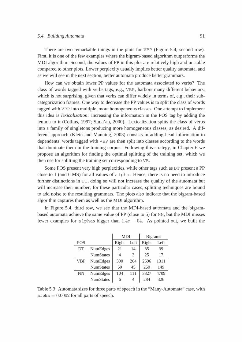
5.4. Building Automata 91
There are two remarkable things in the plots forVBP (Figure 5.4, second row).First, it is one of the few examples where the bigram-based algorithm outperforms theMDI algorithm. Second, the values of PP in this plot are relatively high and unstablecompared to other plots. Lower perplexity usually implies better quality automata, andas we will see in the next section, better automata produce better grammars.
How can we obtain lower PP values for the automata associatedto verbs? Theclass of words tagged with verbs tags, e.g.,VBP, harbors many different behaviors,which is not surprising, given that verbs can differ widely in terms of, e.g., their sub-categorization frames. One way to decrease the PP values is to split the class of wordstagged withVBP into multiple, more homogeneous classes. One attempt to implementthis idea islexicalization: increasing the information in the POS tag by adding thelemma to it (Collins, 1997; Sima’an, 2000). Lexicalizationsplits the class of verbsinto a family of singletons producing more homogeneous classes, as desired. A dif-ferent approach (Klein and Manning, 2003) consists in adding head information todependents; words tagged withVBP are then split into classes according to the wordsthat dominate them in the training corpus. Following this strategy, in Chapter 6 wepropose an algorithm for finding the optimal splitting of thetraining set, which wethen use for splitting the training set corresponding toVB.
Some POS present very high perplexities, while other tags such asDT present a PPclose to1 (and0 MS) for all values ofalpha. Hence, there is no need to introducefurther distinctions inDT, doing so will not increase the quality of the automata butwill increase their number; for these particular cases, splitting techniques are boundto add noise to the resulting grammars. The plots also indicate that the bigram-basedalgorithm captures them as well as the MDI algorithm.
In Figure 5.4, third row, we see that the MDI-based automata and the bigram-based automata achieve the same value of PP (close to 5) forNN, but the MDI missesfewer examples foralphas bigger than1.4e − 04. As pointed out, we built the
MDI BigramsPOS Right Left Right Left
DT NumEdges 21 14 35 39NumStates 4 3 25 17
VBP NumEdges 300 204 2596 1311NumStates 50 45 250 149
NN NumEdges 104 111 3827 4709NumStates 6 4 284 326
Table 5.3: Automata sizes for three parts of speech in the “Many-Automata” case, withalpha = 0.0002 for all parts of speech.
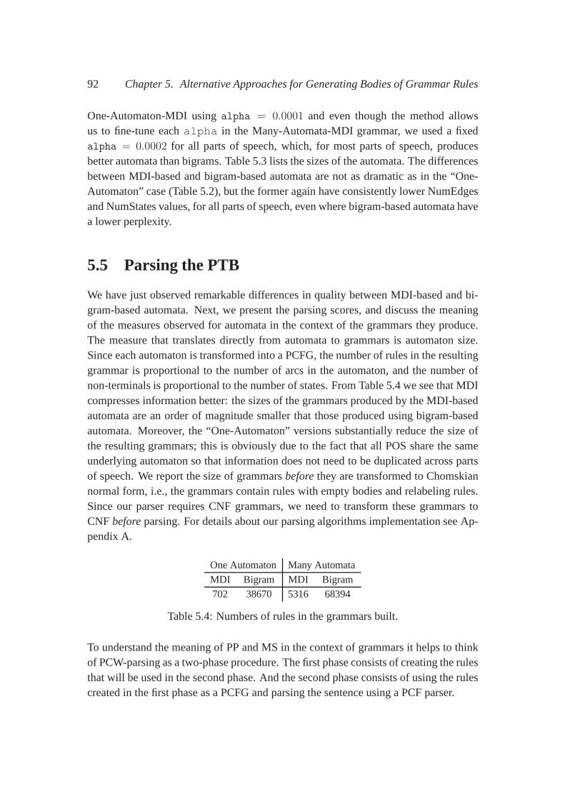
92 Chapter 5. Alternative Approaches for Generating Bodies ofGrammar Rules
One-Automaton-MDI usingalpha = 0.0001 and even though the method allowsus to fine-tune eachalpha in the Many-Automata-MDI grammar, we used a fixedalpha = 0.0002 for all parts of speech, which, for most parts of speech, producesbetter automata than bigrams. Table 5.3 lists the sizes of the automata. The differencesbetween MDI-based and bigram-based automata are not as dramatic as in the “One-Automaton” case (Table 5.2), but the former again have consistently lower NumEdgesand NumStates values, for all parts of speech, even where bigram-based automata havea lower perplexity.
5.5 Parsing the PTB
We have just observed remarkable differences in quality between MDI-based and bi-gram-based automata. Next, we present the parsing scores, and discuss the meaningof the measures observed for automata in the context of the grammars they produce.The measure that translates directly from automata to grammars is automaton size.Since each automaton is transformed into a PCFG, the number of rules in the resultinggrammar is proportional to the number of arcs in the automaton, and the number ofnon-terminals is proportional to the number of states. FromTable 5.4 we see that MDIcompresses information better: the sizes of the grammars produced by the MDI-basedautomata are an order of magnitude smaller that those produced using bigram-basedautomata. Moreover, the “One-Automaton” versions substantially reduce the size ofthe resulting grammars; this is obviously due to the fact that all POS share the sameunderlying automaton so that information does not need to beduplicated across partsof speech. We report the size of grammarsbeforethey are transformed to Chomskiannormal form, i.e., the grammars contain rules with empty bodies and relabeling rules.Since our parser requires CNF grammars, we need to transformthese grammars toCNF beforeparsing. For details about our parsing algorithms implementation see Ap-pendix A.
One Automaton Many Automata
MDI Bigram MDI Bigram
702 38670 5316 68394
Table 5.4: Numbers of rules in the grammars built.
To understand the meaning of PP and MS in the context of grammars it helps to thinkof PCW-parsing as a two-phase procedure. The first phase consists of creating the rulesthat will be used in the second phase. And the second phase consists of using the rulescreated in the first phase as a PCFG and parsing the sentence using a PCF parser.
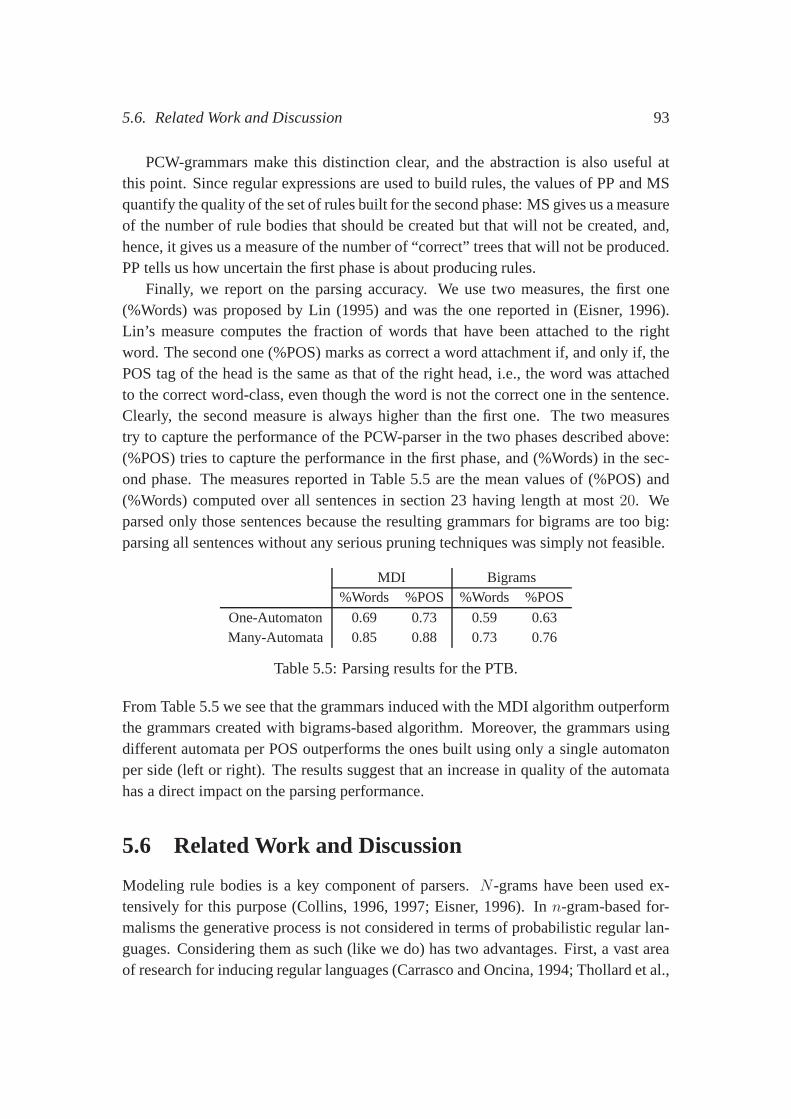
5.6. Related Work and Discussion 93
PCW-grammars make this distinction clear, and the abstraction is also useful atthis point. Since regular expressions are used to build rules, the values of PP and MSquantify the quality of the set of rules built for the second phase: MS gives us a measureof the number of rule bodies that should be created but that will not be created, and,hence, it gives us a measure of the number of “correct” trees that will not be produced.PP tells us how uncertain the first phase is about producing rules.
Finally, we report on the parsing accuracy. We use two measures, the first one(%Words) was proposed by Lin (1995) and was the one reported in (Eisner, 1996).Lin’s measure computes the fraction of words that have been attached to the rightword. The second one (%POS) marks as correct a word attachment if, and only if, thePOS tag of the head is the same as that of the right head, i.e., the word was attachedto the correct word-class, even though the word is not the correct one in the sentence.Clearly, the second measure is always higher than the first one. The two measurestry to capture the performance of the PCW-parser in the two phases described above:(%POS) tries to capture the performance in the first phase, and (%Words) in the sec-ond phase. The measures reported in Table 5.5 are the mean values of (%POS) and(%Words) computed over all sentences in section 23 having length at most20. Weparsed only those sentences because the resulting grammarsfor bigrams are too big:parsing all sentences without any serious pruning techniques was simply not feasible.
MDI Bigrams%Words %POS %Words %POS
One-Automaton 0.69 0.73 0.59 0.63Many-Automata 0.85 0.88 0.73 0.76
Table 5.5: Parsing results for the PTB.
From Table 5.5 we see that the grammars induced with the MDI algorithm outperformthe grammars created with bigrams-based algorithm. Moreover, the grammars usingdifferent automata per POS outperforms the ones built usingonly a single automatonper side (left or right). The results suggest that an increase in quality of the automatahas a direct impact on the parsing performance.
5.6 Related Work and Discussion
Modeling rule bodies is a key component of parsers.N-grams have been used ex-tensively for this purpose (Collins, 1996, 1997; Eisner, 1996). In n-gram-based for-malisms the generative process is not considered in terms ofprobabilistic regular lan-guages. Considering them as such (like we do) has two advantages. First, a vast areaof research for inducing regular languages (Carrasco and Oncina, 1994; Thollard et al.,
94 Chapter 5. Alternative Approaches for Generating Bodies ofGrammar Rules
2000; Dupont and Chase, 1998) comes in sight. Second, the parsing device itself canbe viewed under a unifying grammatical paradigm like PCW-grammars.
In our comparison we optimized the value ofalpha, but we did not optimize then-grams, as doing so would mean two different things. First, smoothing techniqueswould have to be used to combine different ordern-grams. As pointed out, we wouldalso have to smooth different MDI-based automata, which would leave us in the samepoint. Second, the degree of then-gram. We opted forn = 2 as it seems the rightbalance of informativeness and generalization. In this chapter n-grams are used tomodel sequences of arguments, and these hardly ever have length> 3, making higherdegrees useless. To make a fair comparison for the Many-Automata grammars we didnot tune the MDI-based automata individually, but we pickeda uniformalpha.
MDI presents a way to compress rule information on the PTB; ofcourse, otherapproaches exists. In particular, Krotov et al. (1998) try to induce a CW-grammar fromthe PTB with the underlying assumption that some derivations that were supposed tobe hidden were left visible. The attempt to use algorithms other thann-grams-basedfor inducing of regular languages in the context of grammar induction is not new; forexample, Kruijff (2003) uses profile hidden models in an attempt to quantify free ordervariations across languages; we are not aware of evaluations of his grammars as parsingdevices.
5.7 Conclusions
Our experiments in this chapter support two kinds of conclusions. First, modeling ruleswith algorithms other thann-grams not only produces smaller grammars but also betterperforming ones. Second, the procedure used for optimizingalpha reveals that somePOS behave almost deterministically for selecting their arguments, while others donot. These conclusions suggest that splitting classes thatbehave non-deterministicallyinto homogeneous ones could improve the quality of the inferred automata. We sawthat lexicalization and head-annotation seem to attack this problem. Obvious follow-up questions arise: Are these two techniques the best way to split non-homogeneousclasses into homogeneous ones? Is there an optimal splitting? Answers to these ques-tion will be given in Chapter 6.
Chapter 6
Splitting Training Material Optimally
6.1 Introduction
Our approach to parsing can be viewed as a simple CF parser with the special featurethat our context free rules do not exist a priori. Instead, there is a device for generatingthem on demand. The device produces strings and these strings are used as CF bodiesof rules. In the previous chapter, we used probabilistic automata for generating bodiesof rules. These automata were not built manually, but we induced them from sampleinstances obtained from tree-banks. The general idea used for building the probabilisticautomata model bodies of rules, consists of copying all bodies of rules inside the PennTree-bank (PTB) to a bodies of rules sample bag. This sample bag is treated as thesample set of a regular language and probabilistic automataare induced from it. Oncethe probabilistic automata have been built, they are used for defining a grammar thatuses them for building rules on the fly.
The sample bag of rule bodies to be used as training material contains many differ-ent types of strings. For example, some strings may describearguments of transitiveverbs, while others may describe arguments of intransitiveverbs. Chapter 5, togetherwith previous work from the literature (Galen et al., 2004),suggests that models whichare induced from the sample bag can be substantially improved as follows. First, splitthe training material into sets containing only homogeneous material; second, induce amodel for each class, and third, combine the different models into one general model.
The assumption underlying this three step procedure is thatthe regular languagewe want to model is in fact the union of several languages. We split the materialguided by the aim of keeping apart strings that belong to different languages. In thisway, the models induced from each of the bags created after splitting the material arecleaner, because the algorithm that induces a regular language from one of the resultingtraining bags simply does not see any string belonging to other bags. By splitting the
95
96 Chapter 6. Splitting Training Material Optimally
data splitting we try to minimize the noise to which the learning algorithm is exposed.To help shape our intuitions, let us consider two examples. First, suppose that the
language we try to learn is the set{a, aa, aaa, aaaa, aaaaa}. Suppose that we havea bag of instances of this language and that we want to infer the original languagefrom it. The learning algorithm might consider the bag of samples as instances of thelanguagea∗, while if we split the sample bag into five different bags, each containingstrings of the same length, it is more clear for the learning algorithm that each of thebags is produced by a language containing only one element.
Second, suppose that we want to model verb arguments. Simplifying, verb argu-ments can be thought of as the union of transitive verb arguments and intransitive verbarguments. Our working hypothesis is that a better model canbe induced for verbarguments if we first split the training material into two different samples, one contain-ing all the instances of transitive verbs and the other containing all the instances forintransitive verbs. Once the training material has been split, two models are induced,one modeling transitive verbs and the other modeling intransitive ones. The originalmaterial is divided into two bags to avoid the data instancesfrom these two differentphenomena from interfering with each other. Conceptually,if the data is not split,the algorithm for inducing a regular language for intransitive verbs sees the sampleinstances of transitive verbs as noise and vice-versa.
How do we split the training material? One possible way consists in defining a splitby hand. Chapter 5 provides an example of this approach. There, the training materialwas split according to the head word of the dependency rules.As a consequence, twodifferent automata for each part-of-speech (POS) were induced, one modeling rightdependents and one modeling left dependents. In contrast, the approach we pursue inthis chapter aims at finding an optimal splitting in an unsupervised manner. For thispurpose we define a quality measure that quantifies the quality of a partition, and wesearch among a subset of all possible partitions for the one maximizing the proposedquality measure. Thus, one of our main challenges will be to find such a measure.Once the partition that optimizes our quality measure has been found, we use it forbuilding as many automata as there are components in the partition. Finally, we usethe induced automata for building PCW grammars, which we then use for parsing thePTB.
In this chapter we present a measure that quantifies the quality of a partition, wealso show that the measure we found correlates with parsing performance. As a conse-quence, the procedure we use for splitting the material is a procedure that can be usedfor finding optimal grammars, optimal in the sense of parsingperformance, withouthaving to parse the PTB.
This chapter is organized as follows. Section 6.2 presents an overview of the chap-ter; Section 6.3 explains how to build grammars once the optimal partition has been
6.2. Overview 97
found; Section 6.4 explains how we search for the optimal partition, and Section 6.5reports on the results on parsing the PTB. Section 6.6 discusses related work, and Sec-tion 6.7 states conclusions and describes future work.
6.2 Overview
We want to build grammars using training material that has been split into homoge-neous classes of strings. Our main research goal is to understand how the elements inthe training material interfere with each other, thus diminishing the quality of the re-sulting grammars. We also want to quantify the gain in terms of parsing performancethat can be obtained by splitting the training material. Furthermore, we are interestedin finding a quality measure for grammars that only takes the grammar’s structure intoconsideration and helps us to predict the grammar’s performance in parsing withoutactually parsing.
We proceed as follows. As in Chapter 5, we first transform the PTB into projectivedependency structures following (Collins, 1996); see Section 2.1.1 for details. Fromthe resulting tree-bank we delete all lexical information except POS tags. Every occur-rence of a POS in a tree belonging to the tree-bank has associated to it two different,possibly empty, sequences of right and left dependents, respectively. We extract thesesequences for all trees, producing two different bags containing right and left sequencesof dependents, respectively.
We then proceed with a first splitting of the training material. For this purpose weuse the POS tag of the head word as described in Chapter 5. Thisfirst splitting producestwo different sample bags for each POS, one containing instances of left dependents,and the other containing instances of right dependents.
To keep our experiments focused we decided to split the training material of a sin-gle POS tag only:VB. VB is one of the POS with the highest value of perplexity (PP);experiments in Chapter 5 suggest that higher values of PP aredue to the use of a sin-gle automaton for modeling different regular languages. Recall that, for instance, thevalues of PP drop considerably when the training material issplit using the POS tagof the head word. Since the PP value associated toVB is one of the highest,VB seemsto include words with substantially different behaviors, an intuition that is clearly con-firmed by the literature (Levin, 1993; Merlo and Stevenson, 2001). We isolate thesentences containing theVB tag and see how dealing only withVB affects other tags.
The initial partition of the training set corresponding to theVB tag is split usingsyntactic information such as father tag, number of dependents, depth in the tree, etc.So, all instances in the training material that share the same feature are placed in thesame bag. The initial partition aims at using external knowledge to split the material;
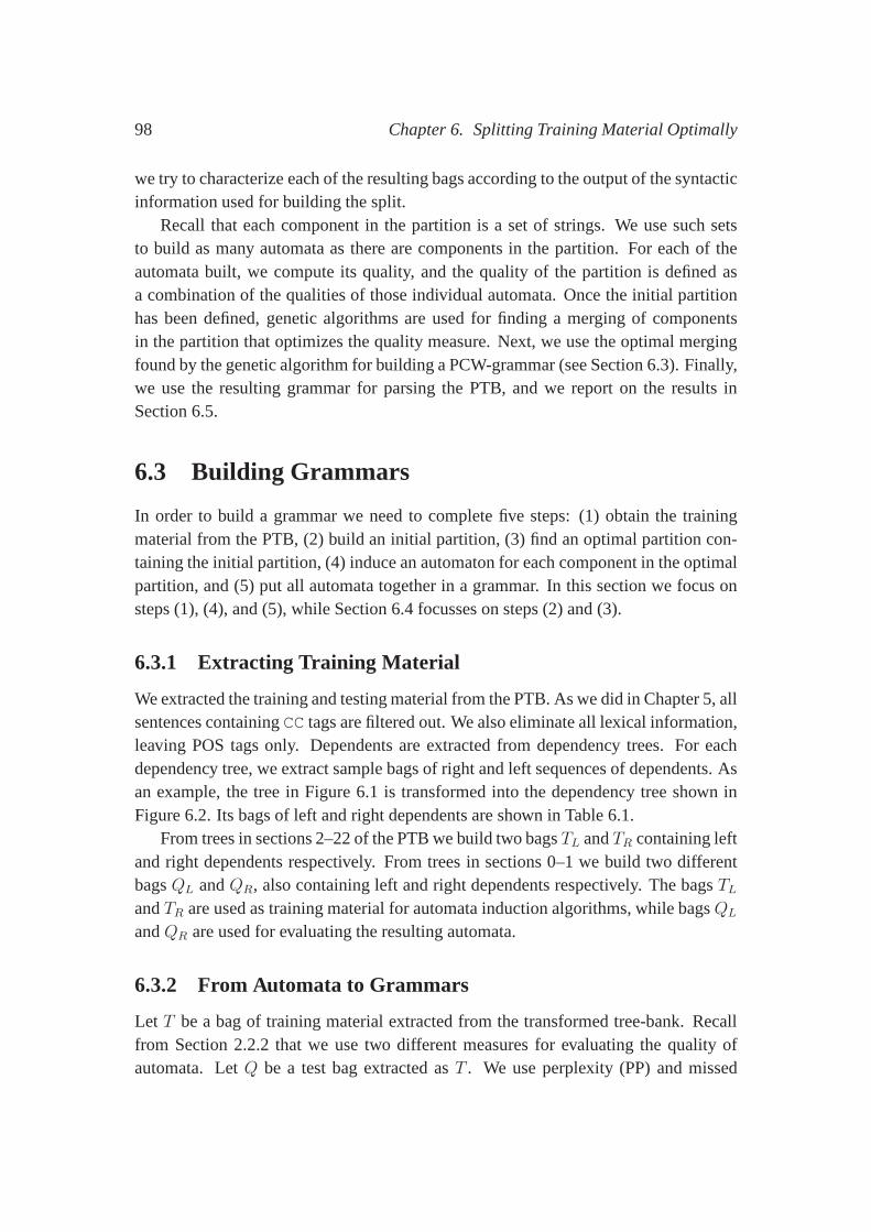
98 Chapter 6. Splitting Training Material Optimally
we try to characterize each of the resulting bags according to the output of the syntacticinformation used for building the split.
Recall that each component in the partition is a set of strings. We use such setsto build as many automata as there are components in the partition. For each of theautomata built, we compute its quality, and the quality of the partition is defined asa combination of the qualities of those individual automata. Once the initial partitionhas been defined, genetic algorithms are used for finding a merging of componentsin the partition that optimizes the quality measure. Next, we use the optimal mergingfound by the genetic algorithm for building a PCW-grammar (see Section 6.3). Finally,we use the resulting grammar for parsing the PTB, and we report on the results inSection 6.5.
6.3 Building Grammars
In order to build a grammar we need to complete five steps: (1) obtain the trainingmaterial from the PTB, (2) build an initial partition, (3) find an optimal partition con-taining the initial partition, (4) induce an automaton for each component in the optimalpartition, and (5) put all automata together in a grammar. Inthis section we focus onsteps (1), (4), and (5), while Section 6.4 focusses on steps (2) and (3).
6.3.1 Extracting Training Material
We extracted the training and testing material from the PTB.As we did in Chapter 5, allsentences containingCC tags are filtered out. We also eliminate all lexical information,leaving POS tags only. Dependents are extracted from dependency trees. For eachdependency tree, we extract sample bags of right and left sequences of dependents. Asan example, the tree in Figure 6.1 is transformed into the dependency tree shown inFigure 6.2. Its bags of left and right dependents are shown inTable 6.1.
From trees in sections 2–22 of the PTB we build two bagsTL andTR containing leftand right dependents respectively. From trees in sections 0–1 we build two differentbagsQL andQR, also containing left and right dependents respectively. The bagsTLandTR are used as training material for automata induction algorithms, while bagsQL
andQR are used for evaluating the resulting automata.
6.3.2 From Automata to Grammars
Let T be a bag of training material extracted from the transformedtree-bank. Recallfrom Section 2.2.2 that we use two different measures for evaluating the quality ofautomata. LetQ be a test bag extracted asT . We use perplexity (PP) and missed

6.3. Building Grammars 99
S
NP-SBJ
NNS
Researchers
VP
MD
can
VP
VB
apply
PP-CLR
IN
for
NP
NN
permission
S
NP-SBJ
*
VP
TO
to
VP
VB
use
NP
DT
the
NNS
probes
PP-CLR
IN
for
NP
NN
brain
NNS
studies
DOTSYB
Figure 6.1: Tree extracted from the PTB, Section 02, filewsj 0297.mrg.
0:Researchers 1:can 2:apply 3:for 4:permission5:to 12:.NN MD VB IN NN TO
8:probes7:the6:use 9:for 10:brain 11:studiesNN NNINNNDTVB DOTSYB
Figure 6.2: Dependency structure corresponding to the treein Figure 6.1.
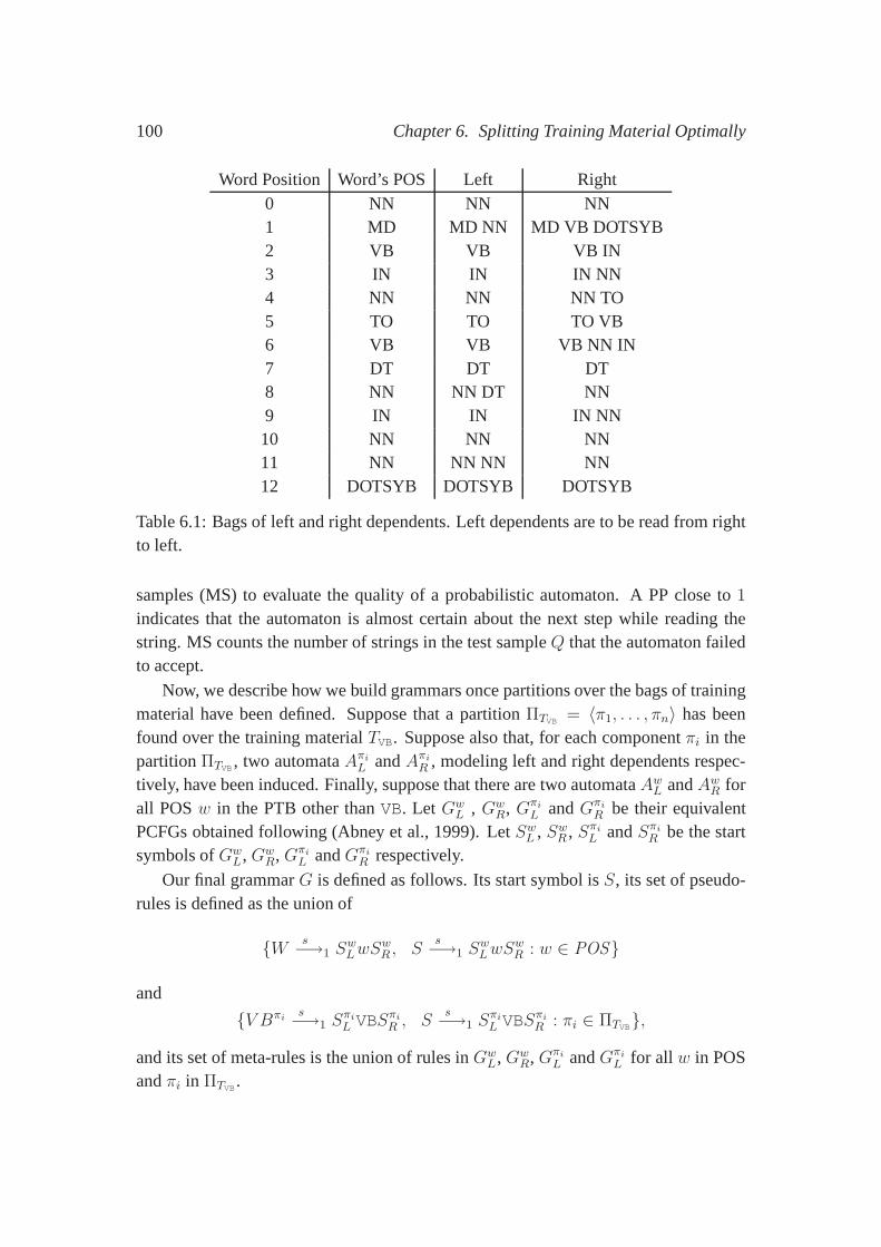
100 Chapter 6. Splitting Training Material Optimally
Word Position Word’s POS Left Right0 NN NN NN1 MD MD NN MD VB DOTSYB2 VB VB VB IN3 IN IN IN NN4 NN NN NN TO5 TO TO TO VB6 VB VB VB NN IN7 DT DT DT8 NN NN DT NN9 IN IN IN NN10 NN NN NN11 NN NN NN NN12 DOTSYB DOTSYB DOTSYB
Table 6.1: Bags of left and right dependents. Left dependents are to be read from rightto left.
samples (MS) to evaluate the quality of a probabilistic automaton. A PP close to1indicates that the automaton is almost certain about the next step while reading thestring. MS counts the number of strings in the test sampleQ that the automaton failedto accept.
Now, we describe how we build grammars once partitions over the bags of trainingmaterial have been defined. Suppose that a partitionΠTVB = 〈π1, . . . , πn〉 has beenfound over the training materialTVB. Suppose also that, for each componentπi in thepartitionΠTVB , two automataAπi
L andAπi
R , modeling left and right dependents respec-tively, have been induced. Finally, suppose that there are two automataAwL andAwR forall POSw in the PTB other thanVB. Let Gw
L , GwR, Gπi
L andGπi
R be their equivalentPCFGs obtained following (Abney et al., 1999). LetSwL , SwR , Sπi
L andSπi
R be the startsymbols ofGw
L,GwR,Gπi
L andGπi
R respectively.
Our final grammarG is defined as follows. Its start symbol isS, its set of pseudo-rules is defined as the union of
{W s−→1 SwLwS
wR , S
s−→1 SwLwS
wR : w ∈ POS}
and
{V Bπis−→1 S
πi
L VBSπi
R , Ss−→1 S
πi
L VBSπi
R : πi ∈ ΠTVB},
and its set of meta-rules is the union of rules inGwL,Gw
R,Gπi
L andGπi
L for all w in POSandπi in ΠTVB.
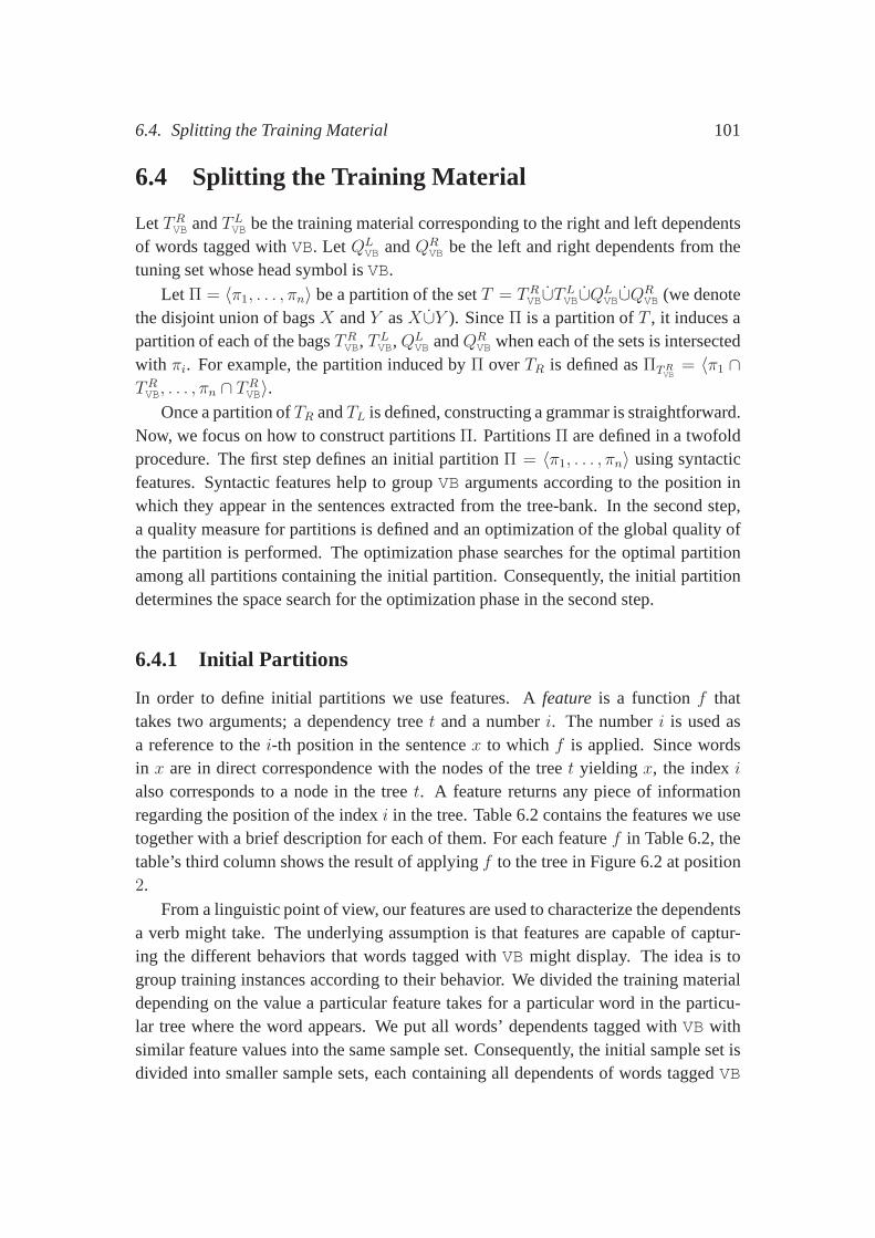
6.4. Splitting the Training Material 101
6.4 Splitting the Training Material
Let TRVB andTLVB be the training material corresponding to the right and leftdependentsof words tagged withVB. LetQL
VB andQRVB be the left and right dependents from the
tuning set whose head symbol isVB.
Let Π = 〈π1, . . . , πn〉 be a partition of the setT = TRVB∪TLVB∪QLVB∪QR
VB (we denotethe disjoint union of bagsX andY asX∪Y ). SinceΠ is a partition ofT , it induces apartition of each of the bagsTRVB, T
LVB,Q
LVB andQR
VB when each of the sets is intersectedwith πi. For example, the partition induced byΠ overTR is defined asΠTR
VB= 〈π1 ∩
TRVB, . . . , πn ∩ TRVB〉.Once a partition ofTR andTL is defined, constructing a grammar is straightforward.
Now, we focus on how to construct partitionsΠ. PartitionsΠ are defined in a twofoldprocedure. The first step defines an initial partitionΠ = 〈π1, . . . , πn〉 using syntacticfeatures. Syntactic features help to groupVB arguments according to the position inwhich they appear in the sentences extracted from the tree-bank. In the second step,a quality measure for partitions is defined and an optimization of the global quality ofthe partition is performed. The optimization phase searches for the optimal partitionamong all partitions containing the initial partition. Consequently, the initial partitiondetermines the space search for the optimization phase in the second step.
6.4.1 Initial Partitions
In order to define initial partitions we use features. Afeature is a functionf thattakes two arguments; a dependency treet and a numberi. The numberi is used asa reference to thei-th position in the sentencex to whichf is applied. Since wordsin x are in direct correspondence with the nodes of the treet yielding x, the indexialso corresponds to a node in the treet. A feature returns any piece of informationregarding the position of the indexi in the tree. Table 6.2 contains the features we usetogether with a brief description for each of them. For each featuref in Table 6.2, thetable’s third column shows the result of applyingf to the tree in Figure 6.2 at position2.
From a linguistic point of view, our features are used to characterize the dependentsa verb might take. The underlying assumption is that features are capable of captur-ing the different behaviors that words tagged withVB might display. The idea is togroup training instances according to their behavior. We divided the training materialdepending on the value a particular feature takes for a particular word in the particu-lar tree where the word appears. We put all words’ dependentstagged withVB withsimilar feature values into the same sample set. Consequently, the initial sample set isdivided into smaller sample sets, each containing all dependents of words taggedVB
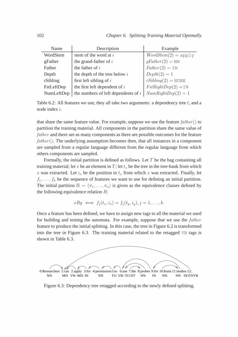
102 Chapter 6. Splitting Training Material Optimally
Name Description ExampleWordStem stem of the word ati WordStem(2) = apply
gFather the grand-father ofi gFather(2) = NN
Father the father ofi Father(2) = IN
Depth the depth of the tree belowi Depth(2) = 1
rSibling first left sibling ofi rSibling(2) = NONE
FstLeftDep the first left dependent ofi FstRightDep(2) =IN
NumLeftDep the numbers of left dependents ofi NumRightDep(2) = 1
Table 6.2: All features we use; they all take two arguments: adependency treet, and anode indexi.
that share the same feature value. For example, suppose we use the featurefather() topartition the training material. All components in the partition share the same value offather and there are as many components as there are possible outcomes for the featurefather(). The underlying assumption becomes then, that all instances in a componentare sampled from a regular language different from the regular language from whichothers components are sampled.
Formally, the initial partition is defined as follows. LetT be the bag containing alltraining material; letx be an element inT ; let tx be the tree in the tree-bank from whichx was extracted. Letix be the position intx from whichx was extracted. Finally, letf1, . . . , fk be the sequence of features we want to use for defining an initial partition.The initial partitionΠ = 〈π1, . . . , πn〉 is given as the equivalence classes defined bythe following equivalence relationR:
xRy ⇐⇒ fj(tx, ix) = fj(ty, iy), j = 1, . . . , k.
Once a feature has been defined, we have to assign new tags to all the material we usedfor building and testing the automata. For example, supposethat we use thefatherfeature to produce the initial splitting. In this case, the tree in Figure 6.2 is transformedinto the tree in Figure 6.3. The training material related tothe retaggedVB tags isshown in Table 6.3.
2:applyNNVB−MD IN
3:for 5:to 12:.11:studies10:brainNN
9:forIN
8:probesNN
7:theDT
6:useVB−TOTO
4:permissionNN
0:ResearchersNN
1:canMD DOTSYB
Figure 6.3: Dependency tree retagged according to the newlydefined splitting.
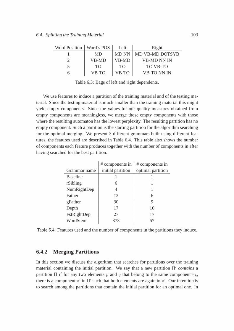
6.4. Splitting the Training Material 103
Word Position Word’s POS Left Right1 MD MD NN MD VB-MD DOTSYB2 VB-MD VB-MD VB-MD NN IN5 TO TO TO VB-TO6 VB-TO VB-TO VB-TO NN IN
Table 6.3: Bags of left and right dependents.
We use features to induce a partition of the training material and of the testing ma-terial. Since the testing material is much smaller than the training material this mightyield empty components. Since the values for our quality measures obtained fromempty components are meaningless, we merge those empty components with thosewhere the resulting automaton has the lowest perplexity. The resulting partition has noempty component. Such a partition is the starting partitionfor the algorithm searchingfor the optimal merging. We present8 different grammars built using different fea-tures, the features used are described in Table 6.4. This table also shows the numberof components each feature produces together with the number of components in afterhaving searched for the best partition.
# components in # components inGrammar name initial partition optimal partitionBaseline 1 1rSibling 6 1NumRightDep 4 1Father 13 6gFather 30 9Depth 17 10FstRightDep 27 17WordStem 373 57
Table 6.4: Features used and the number of components in the partitions they induce.
6.4.2 Merging Partitions
In this section we discuss the algorithm that searches for partitions over the trainingmaterial containing the initial partition. We say that a newpartition Π′ containsapartition Π if for any two elementsp andq that belong to the same componentπk,there is a componentπ′ in Π′ such that both elements are again inπ′. Our intention isto search among the partitions that contain the initial partition for an optimal one. In
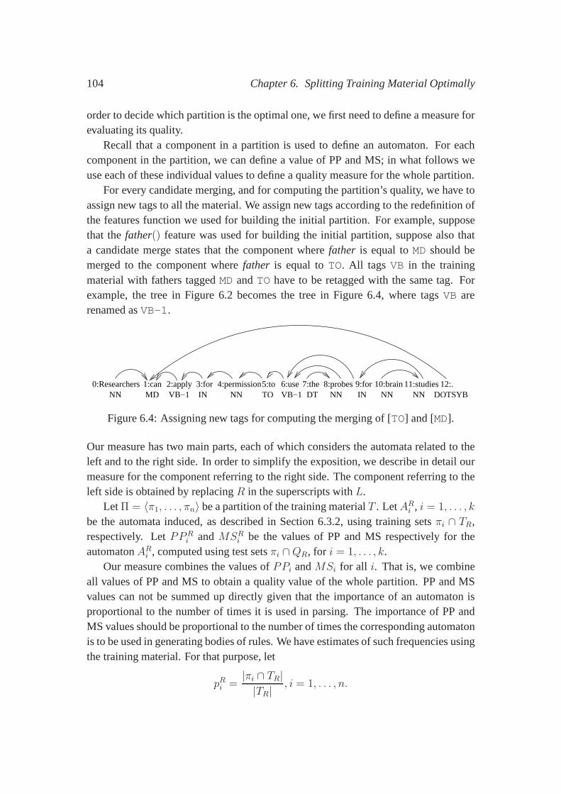
104 Chapter 6. Splitting Training Material Optimally
order to decide which partition is the optimal one, we first need to define a measure forevaluating its quality.
Recall that a component in a partition is used to define an automaton. For eachcomponent in the partition, we can define a value of PP and MS; in what follows weuse each of these individual values to define a quality measure for the whole partition.
For every candidate merging, and for computing the partition’s quality, we have toassign new tags to all the material. We assign new tags according to the redefinition ofthe features function we used for building the initial partition. For example, supposethat thefather() feature was used for building the initial partition, suppose also thata candidate merge states that the component wherefather is equal toMD should bemerged to the component wherefather is equal toTO. All tags VB in the trainingmaterial with fathers taggedMD andTO have to be retagged with the same tag. Forexample, the tree in Figure 6.2 becomes the tree in Figure 6.4, where tagsVB arerenamed asVB-1.
2:applyNNIN
3:for 5:to 12:.11:studies10:brainNN
9:forIN
8:probesNN
7:theDT
6:useTO
4:permissionNN
0:ResearchersNN
1:canMD VB−1 VB−1 DOTSYB
Figure 6.4: Assigning new tags for computing the merging of [TO] and [MD].
Our measure has two main parts, each of which considers the automata related to theleft and to the right side. In order to simplify the exposition, we describe in detail ourmeasure for the component referring to the right side. The component referring to theleft side is obtained by replacingR in the superscripts withL.
Let Π = 〈π1, . . . , πn〉 be a partition of the training materialT . LetARi , i = 1, . . . , k
be the automata induced, as described in Section 6.3.2, using training setsπi ∩ TR,respectively. LetPPR
i andMSRi be the values of PP and MS respectively for theautomatonARi , computed using test setsπi ∩QR, for i = 1, . . . , k.
Our measure combines the values ofPPi andMSi for all i. That is, we combineall values of PP and MS to obtain a quality value of the whole partition. PP and MSvalues can not be summed up directly given that the importance of an automaton isproportional to the number of times it is used in parsing. Theimportance of PP andMS values should be proportional to the number of times the corresponding automatonis to be used in generating bodies of rules. We have estimatesof such frequencies usingthe training material. For that purpose, let
pRi =|πi ∩ TR||TR|
, i = 1, . . . , n.
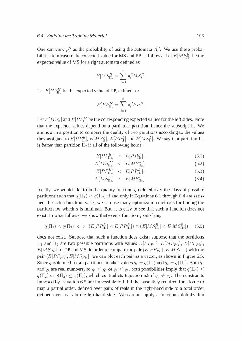
6.4. Splitting the Training Material 105
One can viewpRi as the probability of using the automataARi . We use these proba-bilities to measure the expected value for MS and PP as follows. LetE[MSRΠ ] be theexpected value of MS for a right automata defined as
E[MSRΠ ] =n
∑
i=1
pRi MSRi .
LetE[PPRΠ ] be the expected value of PP, defined as:
E[PPRΠ ] =
n∑
i=1
pRi PPRi .
LetE[MSLΠ] andE[PPLΠ ] be the corresponding expected values for the left sides. Note
that the expected values depend on a particular partition, hence the subscriptΠ. Weare now in a position to compare the quality of two partitionsaccording to the valuesthey assigned toE[PPR
Π ], E[MSRΠ ], E[PPLΠ ] andE[MSLΠ]. We say that partitionΠ1
is betterthan partitionΠ2 if all of the following holds:
E[PPRΠ1
] < E[PPRΠ2
], (6.1)
E[MSRΠ1] < E[MSRΠ2
], (6.2)
E[PPLΠ1
] < E[PPLΠ2
], (6.3)
E[MSLΠ1] < E[MSLΠ2
]. (6.4)
Ideally, we would like to find a quality functionq defined over the class of possiblepartitions such thatq(Π1) < q(Π2) if and only if Equations 6.1 through 6.4 are satis-fied. If such a function exists, we can use many optimization methods for finding thepartition for whichq is minimal. But, it is easy to see that such a function does notexist. In what follows, we show that even a functionq satisfying
q(Π1) < q(Π2) ⇐⇒(
E[PPRΠ1
] < E[PPRΠ2
])
∧(
E[MSRΠ1] < E[MSRΠ2
])
(6.5)
does not exist. Suppose that such a function does exist; suppose that the partitionsΠ1 andΠ2 are two possible partitions with valuesE[PPPi1], E[MSPi1 ], E[PPPi2],E[MSPi2 ] for PP and MS. In order to compare the pair(E[PPPi1], E[MSPi1 ]) with thepair (E[PPPi2], E[MSPi2 ]) we can plot each pair as a vector, as shown in Figure 6.5.Sinceq is defined for all partitions, it takes valuesq1 = q(Π1) andq2 = q(Π1). Bothq1andq2 are real numbers, soq1 ≤ q2 or q2 ≤ q1, both possibilities imply thatq(Π1) ≤q(Π2) or q(Π2) ≤ q(Π1), which contradicts Equation 6.5 ifq1 6= q2. The constraintsimposed by Equation 6.5 are impossible to fulfill because they required functionq tomap a partial order, defined over pairs of reals in the right-hand side to a total orderdefined over reals in the left-hand side. We can not apply a function minimization
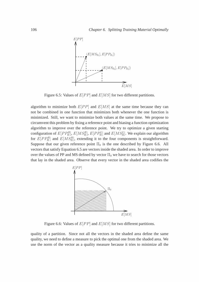
106 Chapter 6. Splitting Training Material Optimally
E[MS]
E[PP ]
(E[MSΠ2], E[PPΠ2
])
(E[MSΠ1], E[PPΠ1
])
Figure 6.5: Values ofE[PP ] andE[MS] for two different partitions.
algorithm to minimize bothE[PP ] andE[MS] at the same time because they cannot be combined in one function that minimizes both wheneverthe one function isminimized. Still, we want to minimize both values at the sametime. We propose tocircumvent this problem by fixing a reference point and biasing a function optimizationalgorithm to improve over the reference point. We try to optimize a given startingconfiguration ofE[PPR
Π ], E[MSRΠ ], E[PPLΠ ] andE[MSLΠ]. We explain our algorithm
for E[PPRΠ ] andE[MSRΠ ], extending it to the four components is straightforward.
Suppose that our given reference pointΠ0 is the one described by Figure 6.6. Allvectors that satisfy Equation 6.5 are vectors inside the shaded area. In order to improveover the values of PP and MS defined by vectorΠ0 we have to search for those vectorsthat lay in the shaded area. Observe that every vector in the shaded area codifies the
������������������������������������������������������������������������������������������������������������������������������������������������������������������������������������������������������������������������������������������������������������
������������������������������������������������������������������������������������������������������������������������������������������������������������������������������������������������������������������������������������������������������������
E[PP ]
E[MS]
Π0
Figure 6.6: Values ofE[PP ] andE[MS] for two different partitions.
quality of a partition. Since not all the vectors in the shaded area define the samequality, we need to define a measure to pick the optimal one from the shaded area. Weuse the norm of the vector as a quality measure because it tries to minimize all the
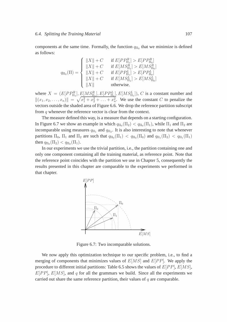
6.4. Splitting the Training Material 107
components at the same time. Formally, the functionqΠ0 that we minimize is definedas follows:
qΠ0(Π) =
‖X‖+ C if E[PPRΠ1
] > E[PPRΠ0
]
‖X‖+ C if E[MSRΠ1] > E[MSRΠ0
]
‖X‖+ C if E[PPLΠ1
] > E[PPLΠ0
]
‖X‖+ C if E[MSLΠ1] > E[MSLΠ0
]
‖X‖ otherwise,
whereX = (E[PPRΠ1
], E[MSRΠ1], E[PPL
Π1], E[MSLΠ1
]), C is a constant number and‖(x1, x2, . . . , xn)‖ =
√
x21 + x2
2 + . . .+ x2n. We use the constantC to penalize the
vectors outside the shaded area of Figure 6.6. We drop the reference partition subscriptfrom q whenever the reference vector is clear from the context.
The measure defined this way, is a measure that depends on a starting configuration.In Figure 6.7 we show an example in whichqΠ0(Π2) < qΠ0(Π1), while Π1 andΠ2 areincomparable using measuresqΠ1 andqΠ2 . It is also interesting to note that wheneverpartitionsΠ0, Π1 andΠ2 are such thatqΠ0(Π1) < qΠ0(Π0) andqΠ1(Π2) < qΠ1(Π1)
thenqΠ0(Π2) < qΠ0(Π1).In our experiments we use the trivial partition, i.e., the partition containing one and
only one component containing all the training material, asreference point. Note thatthe reference point coincides with the partition we use in Chapter 5, consequently theresults presented in this chapter are comparable to the experiments we performed inthat chapter.
E[PP ]
E[MS]
Π2
Π1
Π0
Figure 6.7: Two incomparable solutions.
We now apply this optimization technique to our specific problem, i.e., to find amerging of components that minimizes values ofE[MS] andE[PP ]. We apply theprocedure to different initial partitions: Table 6.5 showsthe values ofE[PP ],E[MS],E[PP ], E[MS], andq for all the grammars we build. Since all the experiments wecarried out share the same reference partition, their values of q are comparable.
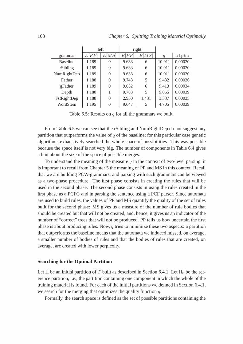
108 Chapter 6. Splitting Training Material Optimally
left rightgrammar E[PP ] E[MS] E[PP ] E[MS] q alpha
Baseline 1.189 0 9.633 6 10.911 0.00020rSibling 1.189 0 9.633 6 10.911 0.00020
NumRightDep 1.189 0 9.633 6 10.911 0.00020Father 1.188 0 9.743 5 9.432 0.00036gFather 1.189 0 9.652 6 9.413 0.00034Depth 1.180 1 9.783 5 9.065 0.00039
FstRightDep 1.188 0 2.950 1.431 3.337 0.00035WordStem 1.195 0 9.647 5 4.705 0.00039
Table 6.5: Results onq for all the grammars we built.
From Table 6.5 we can see that the rSibling and NumRightDep donot suggest anypartition that outperforms the value ofq of the baseline; for this particular case geneticalgorithms exhaustively searched the whole space of possibilities. This was possiblebecause the space itself is not very big. The number of components in Table 6.4 givesa hint about the size of the space of possible merges.
To understand the meaning of the measureq in the context of two-level parsing, itis important to recall from Chapter 5 the meaning of PP and MS in this context. Recallthat we are building PCW-grammars, and parsing with such grammars can be viewedas a two-phase procedure. The first phase consists in creating the rules that will beused in the second phase. The second phase consists in using the rules created in thefirst phase as a PCFG and in parsing the sentence using a PCF parser. Since automataare used to build rules, the values of PP and MS quantify the quality of the set of rulesbuilt for the second phase: MS gives us a measure of the numberof rule bodies thatshould be created but that will not be created, and, hence, itgives us an indicator of thenumber of “correct” trees that will not be produced. PP tellsus how uncertain the firstphase is about producing rules. Now,q tries to minimize these two aspects: a partitionthat outperforms the baseline means that the automata we induced missed, on average,a smaller number of bodies of rules and that the bodies of rules that are created, onaverage, are created with lower perplexity.
Searching for the Optimal Partition
Let Π be an initial partition ofT built as described in Section 6.4.1. LetΠ0 be the ref-erence partition, i.e., the partition containing one component in which the whole of thetraining material is found. For each of the initial partitions we defined in Section 6.4.1,we search for the merging that optimizes the quality function q.
Formally, the search space is defined as the set of possible partitions containing the
6.4. Splitting the Training Material 109
initial one. LetΠ andΠ′ be two partitions overT , and leta andb be two elements inT . Recall that a partitionΠ contains another partitionΠ′ if all components inΠ resultfrom merging components inΠ′. Consequently, a partition containingΠ′ can be easilygenerated by merging some of its components.
In order to search for the partition giving the minimum valueof q we use GeneticAlgorithms (GAs). We use GAs because our problem can naturally be re-phrased as aGA optimization problem.
In GAs, a population of individuals competes for survival. Each individual is des-ignated by a bag of genes that define its behavior. Individuals that perform better (asdefined by the fitness function) have a higher chance of matingwith other individuals.A GA implementation runs for a discrete number of steps, called generations. Whathappens during each generation can vary greatly depending on the strategy being used.Typically, a variation of the following happens at each generation:
1. Selection. The performance of all the individuals is evaluated based onthe fit-ness function, and each is given a specific fitness value. The higher the value,the bigger the chance of an individual passing its genes on tofuture generationsthrough mating (crossover).
2. Crossover. Selected individuals are randomly paired up for crossover (alsoknown as sexual reproduction). This is further controlled by the crossover ratespecified and may result in a new offspring individual that contains genes fromeach of its parents. New individuals are injected into the current population.
3. Mutation. Each individual is given the chance to mutate based on the mutationprobability specified. Each gene of an individual is looked at separately to decidewhether it will be mutated or not. Mutation is decided based upon the mutationrate (or probability). If a mutation is to happen, the value of the gene is switchedto some other possible value.
In order to use GAs for our purposes we have to provide the following:
1. A definition of individuals: We design our individuals to codify two things.First, a value ofalpha to be used for building the automata and second a par-tition of the training material.alpha is simply codified as the first gene in thevector; the partition containing the initial partition is codified as follows. Notethat in order to describe a partition for the training material it is enough to de-scribe a way to merge components in the initial partition. Individuals in thepopulation specify a way to merge components belonging to the initial partitioninto new components. A numberk in thei-th position in the vectorV indicatesthat componenti in the original partition should be added to the new component
110 Chapter 6. Splitting Training Material Optimally
k. Formally, letV = 〈a1, . . . , an〉 be a vector withi ≤ ai ≤ n. The vectorV defines the partitionΠ′ = 〈π′
1, . . . , π′n′〉 such thatπ′
i = ˙⋃{πk : V [k] = i}.Intuitively, the number of components in the resulting partition is equal to thenumber of different values stored in vectorV . E.g., if all entries inV are thesame, the new partition defined byV contains only one component.
2. A fitness function defined on individuals:The fitness function for an individualis defined as the quality measureq we defined in Section 6.4.2.
3. A strategy for evolution: The strategy we follow is defined as follows. Weapply two different operations to genes, namely crossover and mutation. Wedecide which operation to apply by flipping a biased coin. Crossover get 0.95probability of being applied while mutation gets 0.05. Oncethe operation ischosen, genes to which the operations apply are selected from the population.We select individuals using theroulette wheel strategy(Gen and Cheng, 1997),in which the probability for an individual to be selected is proportional to itsfitness score. Crossover is implemented as follows, two points are selected alongthe chromosomes of both parents. The chromosomes are then cut at those points,and the middle parts are swapped, creating two child chromosomes. If matingoccurs, two new genes are added to the population. If no mating occurs, no newgene is add to the population. Mutation is implemented as follows. Each gene ofan individual is looked at separately to decide whether it will be mutated or not.Mutation is decided based upon the mutation rate (or probability). If a mutationis to happen, then the value of the gene is switched to some other possible value.For further details on the implementation of GAs we used see (Qumsieh, 2003)
Finally, the population of each of our generation consists of 50 individuals; we let thepopulation evolve for100 generations. We decided to use100 generations because thecomputation of the quality of partitionq is time consuming and, moreover the qualitymeasure and the number of partition are stable around generation 65 as pictured inFigure 6.8.
6.5 Parsing the Penn Treebank
Finally, we report on the accuracy in parsing. As in Chapter 5we use two measures,%Words and %Pos. The former computes the fraction of the words that have beenattached to their correct father, the latter computes the fraction of words that wereattached to the correct word-class. As explained in Chapter5 the two measures try tocapture the performance of the PCW-parser in the two phases procedure described in
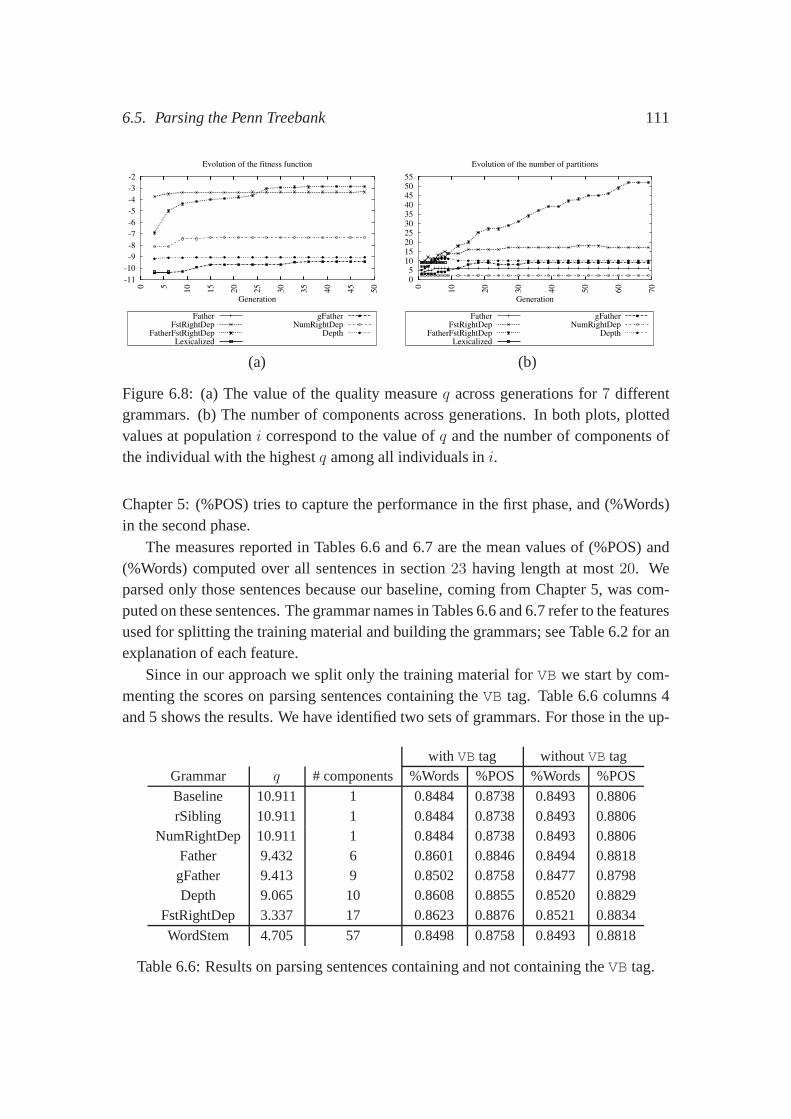
6.5. Parsing the Penn Treebank 111
-11
-10
-9
-8
-7
-6
-5
-4
-3
-2
0 5
10
15
20
25
30
35
40
45
50
Generation
Evolution of the fitness function
FatherFstRightDep
FatherFstRightDepLexicalized
gFatherNumRightDep
Depth
0 5
10 15 20 25 30 35 40 45 50 55
0
10
20
30
40
50
60
70
Generation
Evolution of the number of partitions
FatherFstRightDep
FatherFstRightDepLexicalized
gFatherNumRightDep
Depth
(a) (b)
Figure 6.8: (a) The value of the quality measureq across generations for7 differentgrammars. (b) The number of components across generations.In both plots, plottedvalues at populationi correspond to the value ofq and the number of components ofthe individual with the highestq among all individuals ini.
Chapter 5: (%POS) tries to capture the performance in the first phase, and (%Words)in the second phase.
The measures reported in Tables 6.6 and 6.7 are the mean values of (%POS) and(%Words) computed over all sentences in section23 having length at most20. Weparsed only those sentences because our baseline, coming from Chapter 5, was com-puted on these sentences. The grammar names in Tables 6.6 and6.7 refer to the featuresused for splitting the training material and building the grammars; see Table 6.2 for anexplanation of each feature.
Since in our approach we split only the training material forVB we start by com-menting the scores on parsing sentences containing theVB tag. Table 6.6 columns 4and 5 shows the results. We have identified two sets of grammars. For those in the up-
with VB tag withoutVB tagGrammar q # components %Words %POS %Words %POS
Baseline 10.911 1 0.8484 0.8738 0.8493 0.8806rSibling 10.911 1 0.8484 0.8738 0.8493 0.8806
NumRightDep 10.911 1 0.8484 0.8738 0.8493 0.8806Father 9.432 6 0.8601 0.8846 0.8494 0.8818gFather 9.413 9 0.8502 0.8758 0.8477 0.8798Depth 9.065 10 0.8608 0.8855 0.8520 0.8829
FstRightDep 3.337 17 0.8623 0.8876 0.8521 0.8834
WordStem 4.705 57 0.8498 0.8758 0.8493 0.8818
Table 6.6: Results on parsing sentences containing and not containing theVB tag.
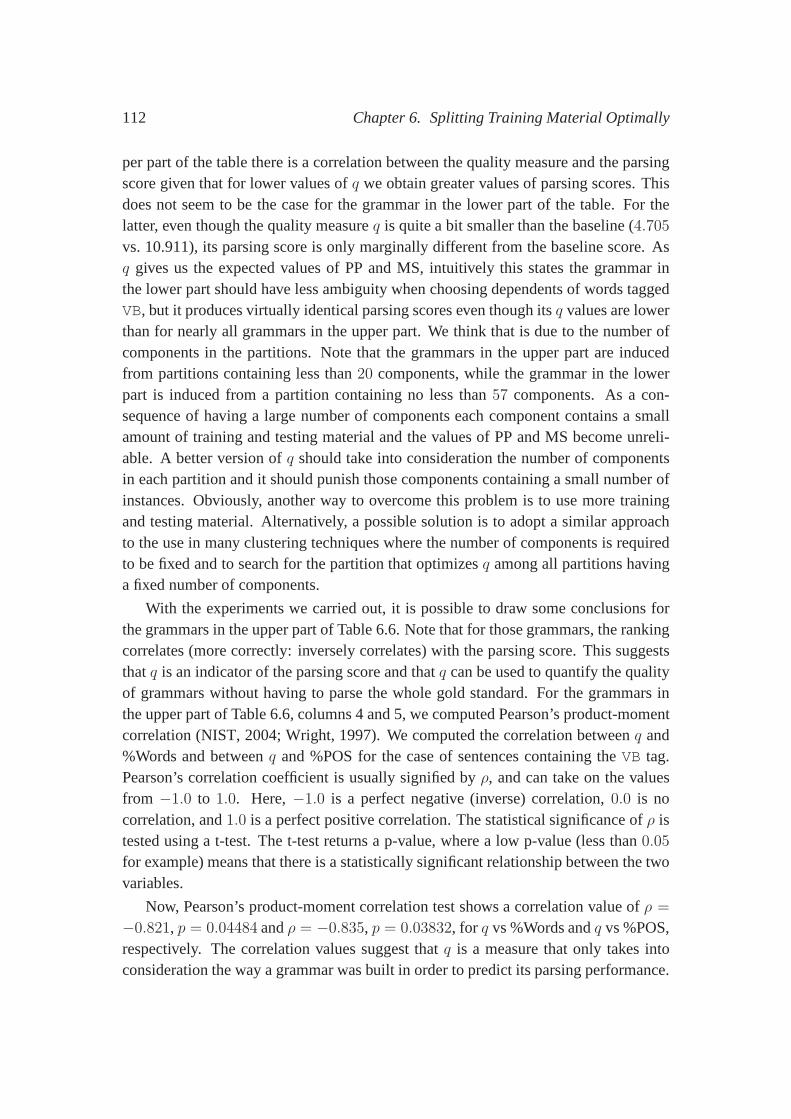
112 Chapter 6. Splitting Training Material Optimally
per part of the table there is a correlation between the quality measure and the parsingscore given that for lower values ofq we obtain greater values of parsing scores. Thisdoes not seem to be the case for the grammar in the lower part ofthe table. For thelatter, even though the quality measureq is quite a bit smaller than the baseline (4.705
vs. 10.911), its parsing score is only marginally differentfrom the baseline score. Asq gives us the expected values of PP and MS, intuitively this states the grammar inthe lower part should have less ambiguity when choosing dependents of words taggedVB, but it produces virtually identical parsing scores even though itsq values are lowerthan for nearly all grammars in the upper part. We think that is due to the number ofcomponents in the partitions. Note that the grammars in the upper part are inducedfrom partitions containing less than20 components, while the grammar in the lowerpart is induced from a partition containing no less than57 components. As a con-sequence of having a large number of components each component contains a smallamount of training and testing material and the values of PP and MS become unreli-able. A better version ofq should take into consideration the number of componentsin each partition and it should punish those components containing a small number ofinstances. Obviously, another way to overcome this problemis to use more trainingand testing material. Alternatively, a possible solution is to adopt a similar approachto the use in many clustering techniques where the number of components is requiredto be fixed and to search for the partition that optimizesq among all partitions havinga fixed number of components.
With the experiments we carried out, it is possible to draw some conclusions forthe grammars in the upper part of Table 6.6. Note that for those grammars, the rankingcorrelates (more correctly: inversely correlates) with the parsing score. This suggeststhatq is an indicator of the parsing score and thatq can be used to quantify the qualityof grammars without having to parse the whole gold standard.For the grammars inthe upper part of Table 6.6, columns 4 and 5, we computed Pearson’s product-momentcorrelation (NIST, 2004; Wright, 1997). We computed the correlation betweenq and%Words and betweenq and %POS for the case of sentences containing theVB tag.Pearson’s correlation coefficient is usually signified byρ, and can take on the valuesfrom −1.0 to 1.0. Here,−1.0 is a perfect negative (inverse) correlation,0.0 is nocorrelation, and1.0 is a perfect positive correlation. The statistical significance ofρ istested using a t-test. The t-test returns a p-value, where a low p-value (less than0.05
for example) means that there is a statistically significantrelationship between the twovariables.
Now, Pearson’s product-moment correlation test shows a correlation value ofρ =
−0.821, p = 0.04484 andρ = −0.835, p = 0.03832, for q vs %Words andq vs %POS,respectively. The correlation values suggest thatq is a measure that only takes intoconsideration the way a grammar was built in order to predictits parsing performance.
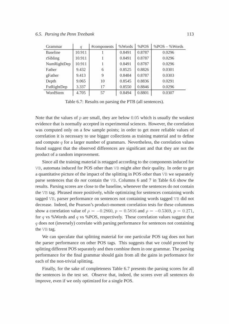
6.5. Parsing the Penn Treebank 113
Grammar q #components %Words %POS %POS – %Words
Baseline 10.911 1 0.8491 0.8787 0.0296rSibling 10.911 1 0.8491 0.8787 0.0296NumRightDep 10.911 1 0.8491 0.8787 0.0296Father 9.432 6 0.8525 0.8826 0.0301gFather 9.413 9 0.8484 0.8787 0.0303Depth 9.065 10 0.8545 0.8836 0.0291FstRightDep 3.337 17 0.8550 0.8846 0.0296
WordStem 4.705 57 0.8494 0.8801 0.0307
Table 6.7: Results on parsing the PTB (all sentences).
Note that the values ofp are small, they are below0.05 which is usually the weakestevidence that is normally accepted in experimental sciences. However, the correlationwas computed only on a few sample points; in order to get more reliable values ofcorrelation it is necessary to use bigger collections as training material and to defineand computeq for a larger number of grammars. Nevertheless, the correlation valuesfound suggest that the observed differences are significantand that they are not theproduct of a random improvement.
Since all the training material is retagged according to thecomponents induced forVB, automata induced for POS other thanVB might alter their quality. In order to geta quantitative picture of the impact of the splitting in POS other thanVB we separatelyparse sentences that donot contain theVB. Columns 6 and 7 in Table 6.6 show theresults. Parsing scores are close to the baseline, wheneverthe sentences do not containtheVB tag. Phrased more positively, while optimizing for sentences containing wordstaggedVB, parser performance on sentences not containing words taggedVB did notdecrease. Indeed, the Pearson’s product-moment correlation tests for these colummnsshow a correlation value ofρ = −0.2860, p = 0.5816 andρ = −0.5369, p = 0.271,for q vs %Words andq vs %POS, respectively. These correlation values suggest thatq does not (inversely) correlate with parsing performance for sentences not containingtheVB tag.
We can speculate that splitting material for one particularPOS tag does not hurtthe parser performance on other POS tags. This suggests thatwe could proceed bysplitting different POS separately and then combine them inone grammar. The parsingperformance for the final grammar should gain from all the gains in performance foreach of the non-trivial splitting.
Finally, for the sake of completeness Table 6.7 presents theparsing scores for allthe sentences in the test set. Observe that, indeed, the scores over all sentences doimprove, even if we only optimized for a single POS.
114 Chapter 6. Splitting Training Material Optimally
6.6 Related Work
There are several perspectives from which we can analyze theapproach and the exper-iments in this chapter. A first analysis sees our procedure tofind optimal grammarsas a way to induce preterminal symbols from the PTB. They are optimized for pars-ing and they provide information about the behavior of wordstagged withVB. Thesepreterminal symbols define a classification of verbs based ontheir syntactic behav-ior. There is a large collection of work on classification of verbs; most of them tryto induce a classification of verbs using syntactic features, in some cases the resultingclassification is evaluated (Merlo and Stevenson, 2001; Stevenson and Merlo, 2000),while in others the resulting classification (Decadt and Daelemans, 2004) is comparedto the hand-crafted classification made by Levin (1993). We ran some experiments ontrying to classify verbs according to the components they belong to. We checked thematch between our classification and Levin’s manual classification of verbs. Unfortu-nately, we did not see any clear match between the two. We alsoexplored manuallythe classification induced by our procedure, but we could notdetect any linguistic ex-planation of the classification. We think that in order to geta linguistically meaningfulclassification, more training material and material taggedwith other verb tags shouldbe used.
A second analysis sees our procedure as a method for finding labels for estimatingbetter probabilities. We can replace words by more general categories, like POS tags,in order to induce better parameters. The clusters we found can be viewed as newlabels because these labels group words having comparable syntactic behavior. Touse our labels in order to obtain better probabilities we need to retag not only thetraining material but also the gold standard. When the gold standard is retagged newtags codify some structural information. The whole approach is a simplified version ofsupertagging (Joshi and Srinivas, 1994; Srinivas, 1997) for PCW-grammars.
A third analysis considers the procedure as a way to induce sub-categorizationframes (Manning, 1993; Carroll and Fang, 2004) for words tagged withVB. Our sub--categorization frames have the peculiarity that there is aninfinite number of them giventhat each string accepted by our automata is a possible sub-categorization frame. Ourinduced sub-categorization frames are used for improving the parsing performanceand are induced specially for this purpose. Only recently (Carroll and Fang, 2004;Yoshinaga, 2004; Hara et al., 2002) some work appeared wherethe induced sub-categorization frames are used for improving the parsing task.
Outside the context of parsing, the methodology we presented in this chapter canalso be used for inducing regular languages. The idea of using clustering before induc-ing automata is not new. Dupont and Chase (1998) clustered symbols using standardclustering techniques (Brown et al., 1992; Ney and Kneser, 1993) before inferring the
6.7. Conclusions and Future Work 115
automata. The main difference between our approach and theirs is that our algorithmpresupposes that the target language is the union of different languages and the methodtries to automatically detect the different components. Our algorithm also tries to de-tect the number of components automatically, while in (Dupont and Chase, 1998) thenumber of components is a parameter of the algorithm. From a more technical point ofview, and still within the setting of inducing probabilistic regular languages, the pro-cedure of, first, splitting the training material and, second, inducing as many regularlanguages as there are components, is a technique that guides the merging of statesin the MDI algorithm and that disallows some of the possible merging. Recall fromSection 2.2.2 that the MDI algorithm builds an automata, first, by building an initialautomaton and, second, by merging some of the states in the initial automaton. Whenthe material is split, not one but many initial automata are built. For this case, the MDIalgorithm searches for candidate merges within each of the initial automaton. As aconsequence, some candidate merges that were possible wheninducing one automa-ton are not available any more in the case of many automata. Clearly, there are twoquestions that the splitting approach has to address, the first one is how to recombinethe different automata in one single regular language, and the second, what criteriashould we follow for splitting the training material?. For our particular case, we usePCW-grammars for recombining the automata and syntactic information for splittingthe training material.
From the optimization perspective, we present a solution for optimizing two func-tions at the same time. The problem of optimizing more than one function at the sametime is known asmultiobjective optimization(Coello Coello, 1999). Briefly, multi-objective optimization techniques try to optimize a combination of many functions,called objectives, by finding a trade-off between the objectives. Under the multiobjec-tive optimization perspective, it is possible to optimize the combination of objectivesby optimizing one of them while others are not optimized.
6.7 Conclusions and Future Work
We presented an approach that aims at finding an optimal splitting of the training ma-terial, which in turn, is meant for improving parsing performance. For this purposewe defined a quality measure that quantifies the quality of partitions. Using this mea-sure, we search among a subset of all possible partitions forthe one maximizing theproposed quality measure. Our measure combines a quality measure defined for eachcomponent in a partition. To measure each component’s quality, we compute an au-tomaton for each of component and we computed the automaton’s MS and PP. Themeasure we presented combines values of PP and MS for all resulting automata, one
116 Chapter 6. Splitting Training Material Optimally
per component, and it uses the resulting components to buildgrammars that are subse-quently used for parsing the PTB.
For our particular case, it is not clear how to combine the functionsE[PP ] andE[MS] in such a way that the optimization of the combined values produces betterparsing scores. What we know, is that if we optimize the four values (E[PP ] andE[MS] for the left and right side) at the same time, we gain in parsing performance.While searching for the definition of the optimal functionq, we noticed that theremight be a measure that uses only a subset of these four values. It seems that thefour functions are not fully independent but the underlyingrelation remains an openproblem.
We have shown that the quality measure we defined can be used for comparingparsing scores of two grammars whenever the grammars are built from partitions hav-ing a similar number of components. It would be interesting to define a measure thatcorrelates with parsing performance independent of the number of components in thepartition. The natural next step is, then, to define a measurethat takes into accountthe number of components and the number of elements in each component. It is alsoimportant to investigate the impact a bigger corpus has in the measure we defined.
In this chapter we used PCW-grammars as the backbone for our experiments. Theyprovide us with the appropriate level of abstraction for carrying out the experiments,and an easy way to combine all automata we induced for the different components intoone single grammar. In contrast to the grammars in Chapter 5,the grammars we builtin this chapter are not bilexical grammars. But, since the parser we implemented (seeAppendix A for details) is a parser for PCW-grammars, it can handle both types ofgrammars. Grammars in Chapter 5 and the grammars in this chapter have in commonthat they search for unlabeled links.
Finally, this chapter changes the way the parsing task is usually addressed. Parsingis usually treated more as a modeling task than as an optimization task. A modelingtask is a task where a model is designed and its parameters estimated from trainingmaterial. Once these parameters are estimated, the model istested on the parsing taskand its results reported. In contrast, an optimization taskis a task where a model isdesigned and its parameters are optimized according to the performance of the modeland parameters in the final task. The difficulty of treating parsing as an optimizationtask resides in the time it takes to test a set of candidate values for the parameters. Sinceour measureq is a good indicator of the parsing performance we can treat parsing as anoptimization task without having to parse. As a consequence, the procedure we definedis a procedure for building optimal grammars.
Chapter 7
Sequences as Features
7.1 Introduction
In the parsing activities and methods discussed so far in this thesis, we set out to dis-cover syntactic structure, and in particular word dependents, using only sequences ofPOS tags. In contrast, nearly all other parsing approaches discussed in the literature useboth sequences of POS tags and sequences of grammatical relations (GRs). Grammati-cal relations are labels describing the relation between the main verb and its dependentsand they can be viewed as a kind of non-terminal labels. This observation suggests anobvious research question: which of the two types of information helps more for thediscovery of word dependents, sequences of POS tags or sequences of GRs? This isour main research question in this chapter. Let us make more precise what it means.
In order to obtain phrase structures like the ones retrievedin (Collins, 1999), thedependents of a POS tag should consist of pairs of POS tags andnon-terminal labelsinstead of sequences of POS tags alone (Markovian rules capture such pairs; see Chap-ter 4 for details on how PCW-grammars capture them). Like sequences of POS tags,sequences of pairs of POS tags and non-terminal labels can beviewed as instancesof a regular language: a regular language whose alphabet is the product of the set ofpossible POS tags and the set of possible non-terminal labels. Moreover, they can beviewed as instances of the combination of two different regular languages: one regularlanguage modeling sequences of POS tags, and another regular language modeling se-quences of non-terminal labels. Under this perspective, itis clear that Chapters 5 and 6only use the first regular language, while non-lexicalized approaches use the secondregular language, and Markovian rules use a combination of the two.
From the literature, it is clear that combining the regular language of POS tags andthe regular language of non-terminal labels boosts parsingperformance, but it is notclear why this is the case. Chapter 5 suggests that lexicalization improves the quality
117
118 Chapter 7. Sequences as Features
of the automata modeling sequences of POS tags, but it does not provide any insightabout the differences or the interplay between these two regular languages.
In this chapter we design and implement experiments for exploring the differencesbetween the regular language of POS tags and the regular language of non-terminallabels in a parsing setup. Our research aims at quantifying the difference between thetwo and at understanding their contribution to parsing performance. In order to clearlyassess the contribution of these two features, we need to carry out an evaluation in termsof a task that clearly isolates the two regular languages. Wedecided to use the task ofdetecting and labeling dependents of the main verb of a sentence. Labels describingthe relation between the main verb and its dependents are what we call grammaticalrelations(GRs), and they can be viewed as a kind of non-terminal labels.
We present two different approaches for dealing with the task of finding grammat-ical relations. In the first approach, we develop two grammars: one for detecting de-pendents and another for labeling them. The first grammar uses sequences of POS tagsas the main feature for detecting dependents, and the secondgrammar uses sequencesof GRs as the main feature for labeling the dependents found by the first grammar. Thetask of detecting and labeling dependents as a whole is done by cascading these twogrammars. In the second approach, we build a single grammar that uses sequences ofGRs as the main feature for detecting dependents and for labeling them. The task ofdetecting and labeling dependents as a whole is done in one goby this grammar. Thetwo approaches differ in that the first one uses sequences of GRs and sequences of POStags, while the second only uses sequences of GRs.
We show that English GRs follow a very strict sequential order, but not as strict asPOS tags of verbal dependents. We show that the latter is moreeffective for detectingand labeling dependents, and, hence, it provides a more reliable instrument for detect-ing them. We argue that this feature is responsible for boosting parsing performance.
The rest of the chapter is organized as follows. Section 7.2 details the task we usefor testing the two features. Section 7.3 explains how to encode this task as parsing.Section 7.4 discusses how the training material used in our experiments is obtained.Section 7.5 explains how the grammars we use are built. Section 7.6 discusses theoptimization phase for those grammars. Section 7.7 shows the experimental results;Section 7.8 discusses related work and, Section 7.9 concludes the chapter.
7.2 Detecting and Labeling Main Verb Dependents
The task we use for our experiments is to find main verbs dependents and to determinetheir GR. In this section we describe the selected task as a black-box procedure. Wespecify its input and its output. The input of the task consists of the following items:
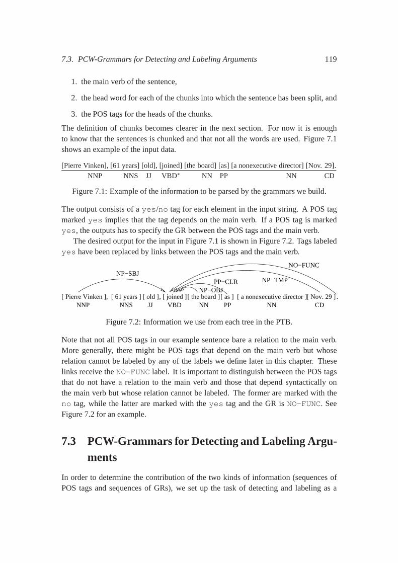
7.3. PCW-Grammars for Detecting and Labeling Arguments 119
1. the main verb of the sentence,
2. the head word for each of the chunks into which the sentencehas been split, and
3. the POS tags for the heads of the chunks.
The definition of chunks becomes clearer in the next section.For now it is enoughto know that the sentences is chunked and that not all the words are used. Figure 7.1shows an example of the input data.
[Pierre Vinken], [61 years] [old], [joined] [the board] [as] [a nonexecutive director] [Nov. 29].
NNP NNS JJ VBD∗ NN PP NN CD
Figure 7.1: Example of the information to be parsed by the grammars we build.
The output consists of ayes/no tag for each element in the input string. A POS tagmarkedyes implies that the tag depends on the main verb. If a POS tag is markedyes, the outputs has to specify the GR between the POS tags and themain verb.
The desired output for the input in Figure 7.1 is shown in Figure 7.2. Tags labeledyes have been replaced by links between the POS tags and the main verb.
[ Pierre Vinken ], [ 61 years ] [ old ], [ joined ][ the board ][ as ] [ a nonexecutive director ]JJ
[ Nov. 29 ] .NNP PP
NP−SBJNO−FUNC
NP−TMPPP−CLRNP−OBJ
CDNNNNVBDNNS
Figure 7.2: Information we use from each tree in the PTB.
Note that not all POS tags in our example sentence bare a relation to the main verb.More generally, there might be POS tags that depend on the main verb but whoserelation cannot be labeled by any of the labels we define laterin this chapter. Theselinks receive theNO-FUNC label. It is important to distinguish between the POS tagsthat do not have a relation to the main verb and those that depend syntactically onthe main verb but whose relation cannot be labeled. The former are marked with theno tag, while the latter are marked with theyes tag and the GR isNO-FUNC. SeeFigure 7.2 for an example.
7.3 PCW-Grammars for Detecting and Labeling Argu-ments
In order to determine the contribution of the two kinds of information (sequences ofPOS tags and sequences of GRs), we set up the task of detectingand labeling as a
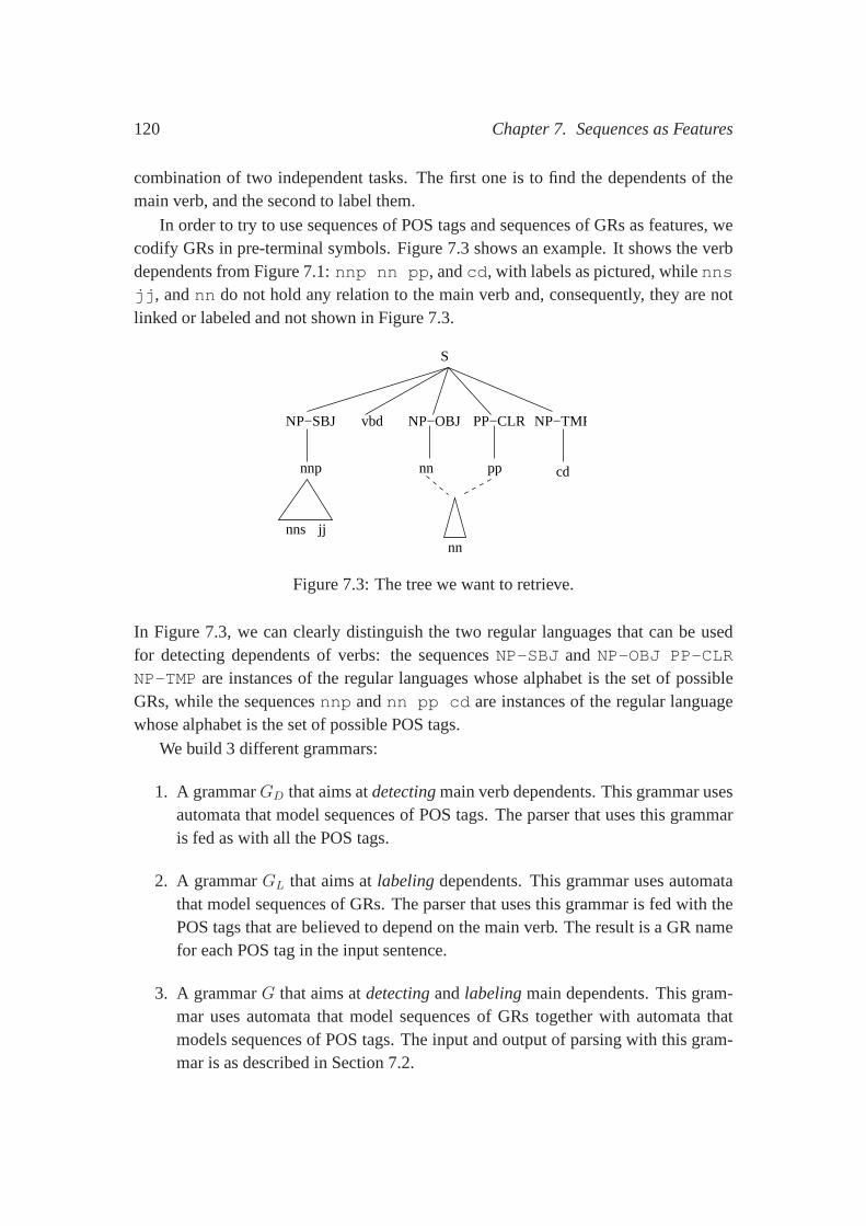
120 Chapter 7. Sequences as Features
combination of two independent tasks. The first one is to find the dependents of themain verb, and the second to label them.
In order to try to use sequences of POS tags and sequences of GRs as features, wecodify GRs in pre-terminal symbols. Figure 7.3 shows an example. It shows the verbdependents from Figure 7.1:nnp nn pp, andcd, with labels as pictured, whilennsjj, andnn do not hold any relation to the main verb and, consequently, they are notlinked or labeled and not shown in Figure 7.3.
PP−CLR
pp
NP−TMP
cd
NP−OBJ
nn
nnjjnns
vbd
S
NP−SBJ
nnp
Figure 7.3: The tree we want to retrieve.
In Figure 7.3, we can clearly distinguish the two regular languages that can be usedfor detecting dependents of verbs: the sequencesNP-SBJ andNP-OBJ PP-CLR
NP-TMP are instances of the regular languages whose alphabet is theset of possibleGRs, while the sequencesnnp andnn pp cd are instances of the regular languagewhose alphabet is the set of possible POS tags.
We build 3 different grammars:
1. A grammarGD that aims atdetectingmain verb dependents. This grammar usesautomata that model sequences of POS tags. The parser that uses this grammaris fed as with all the POS tags.
2. A grammarGL that aims atlabelingdependents. This grammar uses automatathat model sequences of GRs. The parser that uses this grammar is fed with thePOS tags that are believed to depend on the main verb. The result is a GR namefor each POS tag in the input sentence.
3. A grammarG that aims atdetectingandlabelingmain dependents. This gram-mar uses automata that model sequences of GRs together with automata thatmodels sequences of POS tags. The input and output of parsingwith this gram-mar is as described in Section 7.2.
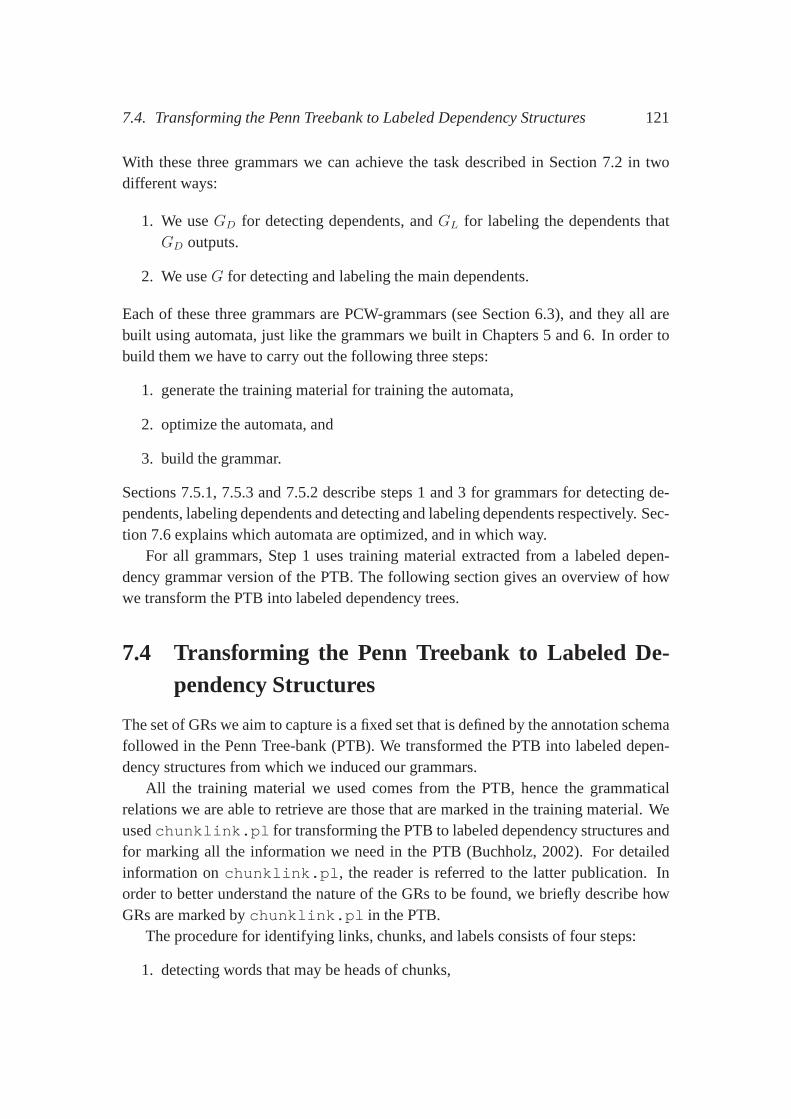
7.4. Transforming the Penn Treebank to Labeled Dependency Structures 121
With these three grammars we can achieve the task described in Section 7.2 in twodifferent ways:
1. We useGD for detecting dependents, andGL for labeling the dependents thatGD outputs.
2. We useG for detecting and labeling the main dependents.
Each of these three grammars are PCW-grammars (see Section 6.3), and they all arebuilt using automata, just like the grammars we built in Chapters 5 and 6. In order tobuild them we have to carry out the following three steps:
1. generate the training material for training the automata,
2. optimize the automata, and
3. build the grammar.
Sections 7.5.1, 7.5.3 and 7.5.2 describe steps 1 and 3 for grammars for detecting de-pendents, labeling dependents and detecting and labeling dependents respectively. Sec-tion 7.6 explains which automata are optimized, and in whichway.
For all grammars, Step 1 uses training material extracted from a labeled depen-dency grammar version of the PTB. The following section gives an overview of howwe transform the PTB into labeled dependency trees.
7.4 Transforming the Penn Treebank to Labeled De-pendency Structures
The set of GRs we aim to capture is a fixed set that is defined by the annotation schemafollowed in the Penn Tree-bank (PTB). We transformed the PTBinto labeled depen-dency structures from which we induced our grammars.
All the training material we used comes from the PTB, hence the grammaticalrelations we are able to retrieve are those that are marked inthe training material. Weusedchunklink.pl for transforming the PTB to labeled dependency structures andfor marking all the information we need in the PTB (Buchholz,2002). For detailedinformation onchunklink.pl, the reader is referred to the latter publication. Inorder to better understand the nature of the GRs to be found, we briefly describe howGRs are marked bychunklink.pl in the PTB.
The procedure for identifying links, chunks, and labels consists of four steps:
1. detecting words that may be heads of chunks,
122 Chapter 7. Sequences as Features
2. drawing dependency relations (links) between these words,
3. assigning labels to these relations and
4. detecting chunks.
As to step (1)chunklink.pl detects heads using a head table, pretty much as ex-plained in Section 2.1.1. Still, the application of tables described in Section 2.1.1 isdifferent from the strategy used bychunklink.pl. In the latter, the head is eitherthe right-most pre-terminal child that matches the (regular expression) POS tags list inthe table, or all non-terminal children that match the (regular expression) constituentlist. Consequently, there is a preference for lexical over non-lexical head children, butno preference within these groups. In the approach presented in Section 2.1.1, the listis ordered by preference and it also has an associated direction (starting left or rightdepending on the index of the table). The head detection algorithm first tries to finda child of the kind indicated by the first element of the list inthe indicated direction,and stops as soon as it finds one. If no child of this kind can be found, the algorithmnext looks for a child of the kind of the second element of the list, and so on, downto the last. If even the last kind of child cannot be found, thealgorithm takes theleft/rightmost child (of any kind) to be the head. The two different approaches, accord-ing to (Buchholz, 2002), differ mainly with respect to coordinated structures. For us,this difference is irrelevant, because we compare our approaches in each of the casesusing the corresponding training material. Buchholz (2002) has an extensive descrip-tion of the strategy followed bychunklink.pl for handling special cases that cannot be described in the table. Clearly, the result of both heuristics may be “unknown.”For these caseschunklink.pl returns an unknown head. In our experiments wediscarded all sentences that contain at least one “unknown”head.
Once heads have been marked, the algorithm proceeds with step (2). Links (de-pendency relations) are drawn in a bottom-up fashion. In theprocess of drawing links,the tree ends up in an intermediate structure, which is then used in the third step. Wedescribe here how the tree is transformed into a directed graph; the resulting graphscontain a partial dependency structure like the one used in previous chapters, plus linksbetween non-terminals in the original tree and words in their yield. Step (3) uses thelatter links for labeling relations in the dependency tree and completing the dependencytree; it finally eliminates them from the the graph producinga labeled dependency tree.
Step (2) starts by adding a link for each word in the yield of the tree that linksthe word to itself. Recall that, for each non-terminal, the algorithm knows which ofits child nodes contains the head word. Step (2) traverses the tree in a bottom-upfashion: it adds a link between the current non-terminal andwhatever the head child ispointing at. The result is a link between the non-terminal and a word in the yield. Step
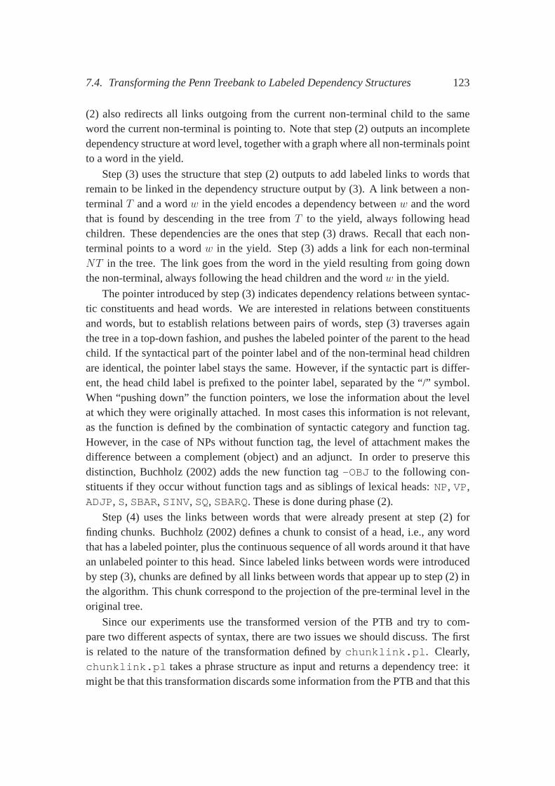
7.4. Transforming the Penn Treebank to Labeled Dependency Structures 123
(2) also redirects all links outgoing from the current non-terminal child to the sameword the current non-terminal is pointing to. Note that step(2) outputs an incompletedependency structure at word level, together with a graph where all non-terminals pointto a word in the yield.
Step (3) uses the structure that step (2) outputs to add labeled links to words thatremain to be linked in the dependency structure output by (3). A link between a non-terminalT and a wordw in the yield encodes a dependency betweenw and the wordthat is found by descending in the tree fromT to the yield, always following headchildren. These dependencies are the ones that step (3) draws. Recall that each non-terminal points to a wordw in the yield. Step (3) adds a link for each non-terminalNT in the tree. The link goes from the word in the yield resultingfrom going downthe non-terminal, always following the head children and the wordw in the yield.
The pointer introduced by step (3) indicates dependency relations between syntac-tic constituents and head words. We are interested in relations between constituentsand words, but to establish relations between pairs of words, step (3) traverses againthe tree in a top-down fashion, and pushes the labeled pointer of the parent to the headchild. If the syntactical part of the pointer label and of thenon-terminal head childrenare identical, the pointer label stays the same. However, ifthe syntactic part is differ-ent, the head child label is prefixed to the pointer label, separated by the “/” symbol.When “pushing down” the function pointers, we lose the information about the levelat which they were originally attached. In most cases this information is not relevant,as the function is defined by the combination of syntactic category and function tag.However, in the case of NPs without function tag, the level ofattachment makes thedifference between a complement (object) and an adjunct. Inorder to preserve thisdistinction, Buchholz (2002) adds the new function tag-OBJ to the following con-stituents if they occur without function tags and as siblings of lexical heads:NP, VP,ADJP, S, SBAR, SINV, SQ, SBARQ. These is done during phase (2).
Step (4) uses the links between words that were already present at step (2) forfinding chunks. Buchholz (2002) defines a chunk to consist of ahead, i.e., any wordthat has a labeled pointer, plus the continuous sequence of all words around it that havean unlabeled pointer to this head. Since labeled links between words were introducedby step (3), chunks are defined by all links between words thatappear up to step (2) inthe algorithm. This chunk correspond to the projection of the pre-terminal level in theoriginal tree.
Since our experiments use the transformed version of the PTBand try to com-pare two different aspects of syntax, there are two issues weshould discuss. The firstis related to the nature of the transformation defined bychunklink.pl. Clearly,chunklink.pl takes a phrase structure as input and returns a dependency tree: itmight be that this transformation discards some information from the PTB and that this
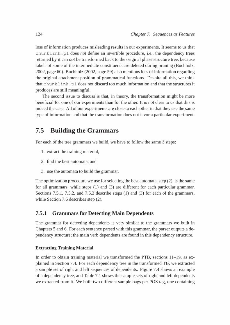
124 Chapter 7. Sequences as Features
loss of information produces misleading results in our experiments. It seems to us thatchunklink.pl doesnot define an invertible procedure, i.e., the dependency treesreturned by it cannot be transformed back to the original phase structure tree, becauselabels of some of the intermediate constituents are deletedduring pruning (Buchholz,2002, page 60). Buchholz (2002, page 59) also mentions loss of information regardingthe original attachment position of grammatical functions. Despite all this, we thinkthatchunklink.pl does not discard too much information and that the structures itproduces are still meaningful.
The second issue to discuss is that, in theory, the transformation might be morebeneficial for one of our experiments than for the other. It isnot clear to us that this isindeed the case. All of our experiments are close to each other in that they use the sametype of information and that the transformation does not favor a particular experiment.
7.5 Building the Grammars
For each of the tree grammars we build, we have to follow the same3 steps:
1. extract the training material,
2. find the best automata, and
3. use the automata to build the grammar.
The optimization procedure we use for selecting the best automata, step (2), is the samefor all grammars, while steps (1) and (3) are different for each particular grammar.Sections 7.5.1, 7.5.2, and 7.5.3 describe steps (1) and (3) for each of the grammars,while Section 7.6 describes step (2).
7.5.1 Grammars for Detecting Main Dependents
The grammar for detecting dependents is very similar to the grammars we built inChapters 5 and 6. For each sentence parsed with this grammar,the parser outputs a de-pendency structure; the main verb dependents are found in this dependency structure.
Extracting Training Material
In order to obtain training material we transformed the PTB,sections11–19, as ex-plained in Section 7.4. For each dependency tree in the transformed TB, we extracteda sample set of right and left sequences of dependents. Figure 7.4 shows an exampleof a dependency tree, and Table 7.1 shows the sample sets of right and left dependentswe extracted from it. We built two different sample bags per POS tag, one containing
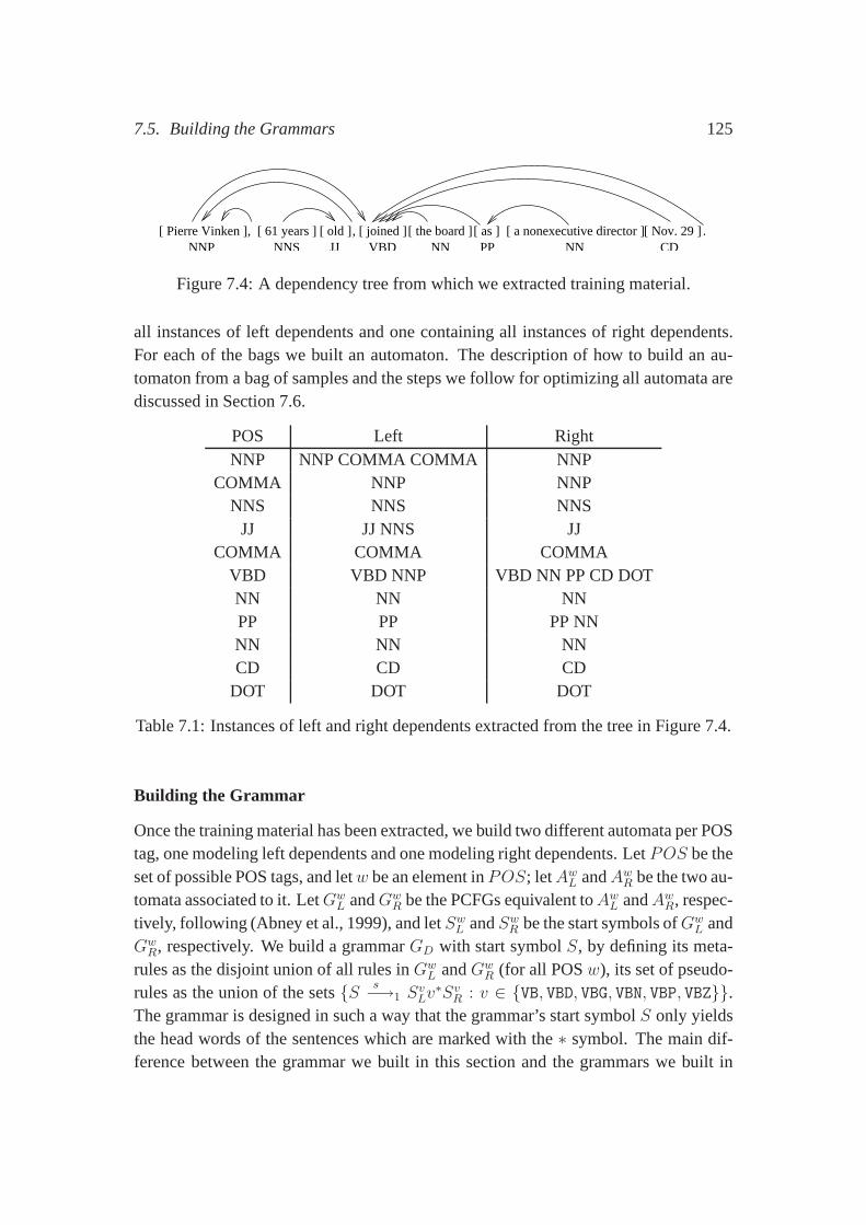
7.5. Building the Grammars 125
[ Pierre Vinken ], [ 61 years ] [ old ], [ joined ][ the board ][ as ] [ a nonexecutive director ]JJ
[ Nov. 29 ] .NNP PP CDNNNNVBDNNS
Figure 7.4: A dependency tree from which we extracted training material.
all instances of left dependents and one containing all instances of right dependents.For each of the bags we built an automaton. The description ofhow to build an au-tomaton from a bag of samples and the steps we follow for optimizing all automata arediscussed in Section 7.6.
POS Left RightNNP NNP COMMA COMMA NNP
COMMA NNP NNPNNS NNS NNS
JJ JJ NNS JJCOMMA COMMA COMMA
VBD VBD NNP VBD NN PP CD DOTNN NN NNPP PP PP NNNN NN NNCD CD CD
DOT DOT DOT
Table 7.1: Instances of left and right dependents extractedfrom the tree in Figure 7.4.
Building the Grammar
Once the training material has been extracted, we build two different automata per POStag, one modeling left dependents and one modeling right dependents. LetPOS be theset of possible POS tags, and letw be an element inPOS; letAwL andAwR be the two au-tomata associated to it. LetGw
L andGwR be the PCFGs equivalent toAwL andAwR, respec-
tively, following (Abney et al., 1999), and letSwL andSwR be the start symbols ofGwL and
GwR, respectively. We build a grammarGD with start symbolS, by defining its meta-
rules as the disjoint union of all rules inGwL andGw
R (for all POSw), its set of pseudo-rules as the union of the sets{S s−→1 S
vLv
∗SvR : v ∈ {VB, VBD, VBG, VBN, VBP, VBZ}}.The grammar is designed in such a way that the grammar’s startsymbolS only yieldsthe head words of the sentences which are marked with the∗ symbol. The main dif-ference between the grammar we built in this section and the grammars we built in
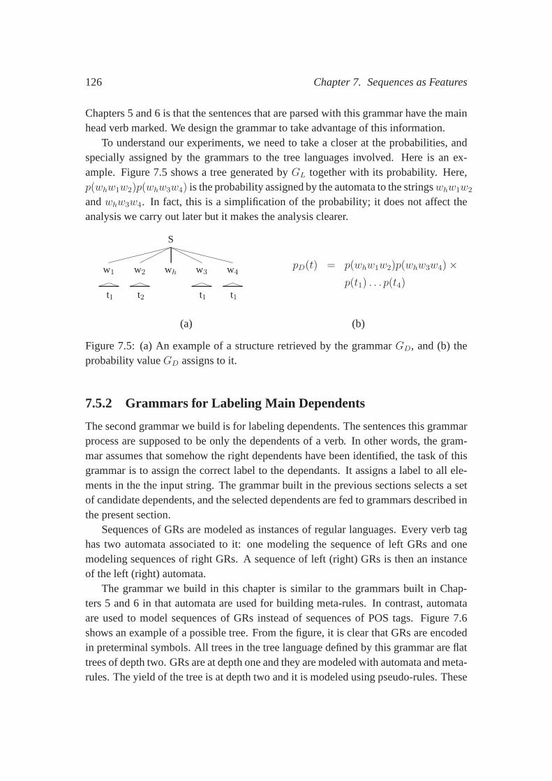
126 Chapter 7. Sequences as Features
Chapters 5 and 6 is that the sentences that are parsed with this grammar have the mainhead verb marked. We design the grammar to take advantage of this information.
To understand our experiments, we need to take a closer at theprobabilities, andspecially assigned by the grammars to the tree languages involved. Here is an ex-ample. Figure 7.5 shows a tree generated byGL together with its probability. Here,p(whw1w2)p(whw3w4) is the probability assigned by the automata to the stringswhw1w2
andwhw3w4. In fact, this is a simplification of the probability; it doesnot affect theanalysis we carry out later but it makes the analysis clearer.
S
w1
t1
w2
t2
wh w3
t1
w4
t1
pD(t) = p(whw1w2)p(whw3w4)×p(t1) . . . p(t4)
(a) (b)
Figure 7.5: (a) An example of a structure retrieved by the grammarGD, and (b) theprobability valueGD assigns to it.
7.5.2 Grammars for Labeling Main Dependents
The second grammar we build is for labeling dependents. The sentences this grammarprocess are supposed to be only the dependents of a verb. In other words, the gram-mar assumes that somehow the right dependents have been identified, the task of thisgrammar is to assign the correct label to the dependants. It assigns a label to all ele-ments in the the input string. The grammar built in the previous sections selects a setof candidate dependents, and the selected dependents are fed to grammars described inthe present section.
Sequences of GRs are modeled as instances of regular languages. Every verb taghas two automata associated to it: one modeling the sequenceof left GRs and onemodeling sequences of right GRs. A sequence of left (right) GRs is then an instanceof the left (right) automata.
The grammar we build in this chapter is similar to the grammars built in Chap-ters 5 and 6 in that automata are used for building meta-rules. In contrast, automataare used to model sequences of GRs instead of sequences of POStags. Figure 7.6shows an example of a possible tree. From the figure, it is clear that GRs are encodedin preterminal symbols. All trees in the tree language defined by this grammar are flattrees of depth two. GRs are at depth one and they are modeled with automata and meta-rules. The yield of the tree is at depth two and it is modeled using pseudo-rules. These
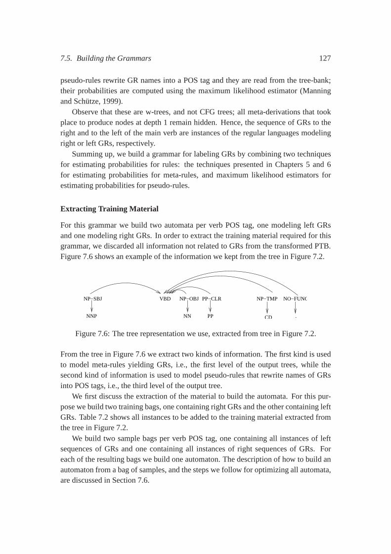
7.5. Building the Grammars 127
pseudo-rules rewrite GR names into a POS tag and they are readfrom the tree-bank;their probabilities are computed using the maximum likelihood estimator (Manningand Schutze, 1999).
Observe that these are w-trees, and not CFG trees; all meta-derivations that tookplace to produce nodes at depth 1 remain hidden. Hence, the sequence of GRs to theright and to the left of the main verb are instances of the regular languages modelingright or left GRs, respectively.
Summing up, we build a grammar for labeling GRs by combining two techniquesfor estimating probabilities for rules: the techniques presented in Chapters 5 and 6for estimating probabilities for meta-rules, and maximum likelihood estimators forestimating probabilities for pseudo-rules.
Extracting Training Material
For this grammar we build two automata per verb POS tag, one modeling left GRsand one modeling right GRs. In order to extract the training material required for thisgrammar, we discarded all information not related to GRs from the transformed PTB.Figure 7.6 shows an example of the information we kept from the tree in Figure 7.2.
VBDNP−SBJ NP−OBJ PP−CLR NP−TMP NO−FUNC
NNP NN PP CD .
Figure 7.6: The tree representation we use, extracted from tree in Figure 7.2.
From the tree in Figure 7.6 we extract two kinds of information. The first kind is usedto model meta-rules yielding GRs, i.e., the first level of theoutput trees, while thesecond kind of information is used to model pseudo-rules that rewrite names of GRsinto POS tags, i.e., the third level of the output tree.
We first discuss the extraction of the material to build the automata. For this pur-pose we build two training bags, one containing right GRs andthe other containing leftGRs. Table 7.2 shows all instances to be added to the trainingmaterial extracted fromthe tree in Figure 7.2.
We build two sample bags per verb POS tag, one containing all instances of leftsequences of GRs and one containing all instances of right sequences of GRs. Foreach of the resulting bags we build one automaton. The description of how to build anautomaton from a bag of samples, and the steps we follow for optimizing all automata,are discussed in Section 7.6.
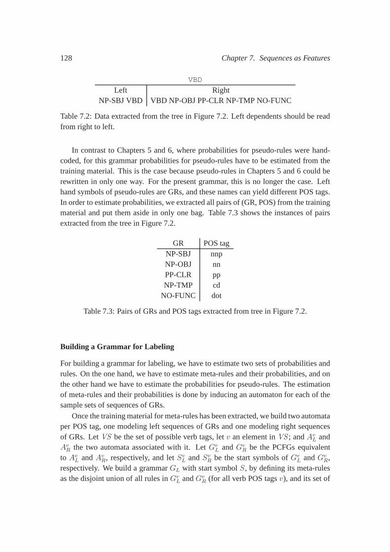
128 Chapter 7. Sequences as Features
VBD
Left RightNP-SBJ VBD VBD NP-OBJ PP-CLR NP-TMP NO-FUNC
Table 7.2: Data extracted from the tree in Figure 7.2. Left dependents should be readfrom right to left.
In contrast to Chapters 5 and 6, where probabilities for pseudo-rules were hand-coded, for this grammar probabilities for pseudo-rules have to be estimated from thetraining material. This is the case because pseudo-rules inChapters 5 and 6 could berewritten in only one way. For the present grammar, this is nolonger the case. Lefthand symbols of pseudo-rules are GRs, and these names can yield different POS tags.In order to estimate probabilities, we extracted all pairs of (GR, POS) from the trainingmaterial and put them aside in only one bag. Table 7.3 shows the instances of pairsextracted from the tree in Figure 7.2.
GR POS tagNP-SBJ nnpNP-OBJ nnPP-CLR ppNP-TMP cd
NO-FUNC dot
Table 7.3: Pairs of GRs and POS tags extracted from tree in Figure 7.2.
Building a Grammar for Labeling
For building a grammar for labeling, we have to estimate two sets of probabilities andrules. On the one hand, we have to estimate meta-rules and their probabilities, and onthe other hand we have to estimate the probabilities for pseudo-rules. The estimationof meta-rules and their probabilities is done by inducing anautomaton for each of thesample sets of sequences of GRs.
Once the training material for meta-rules has been extracted, we build two automataper POS tag, one modeling left sequences of GRs and one modeling right sequencesof GRs. LetVS be the set of possible verb tags, letv an element inVS ; andAvL andAvR the two automata associated with it. LetGv
L andGvR be the PCFGs equivalent
to AvL andAvR, respectively, and letSvL andSvR be the start symbols ofGvL andGv
R,respectively. We build a grammarGL with start symbolS, by defining its meta-rulesas the disjoint union of all rules inGv
L andGvR (for all verb POS tagsv), and its set of
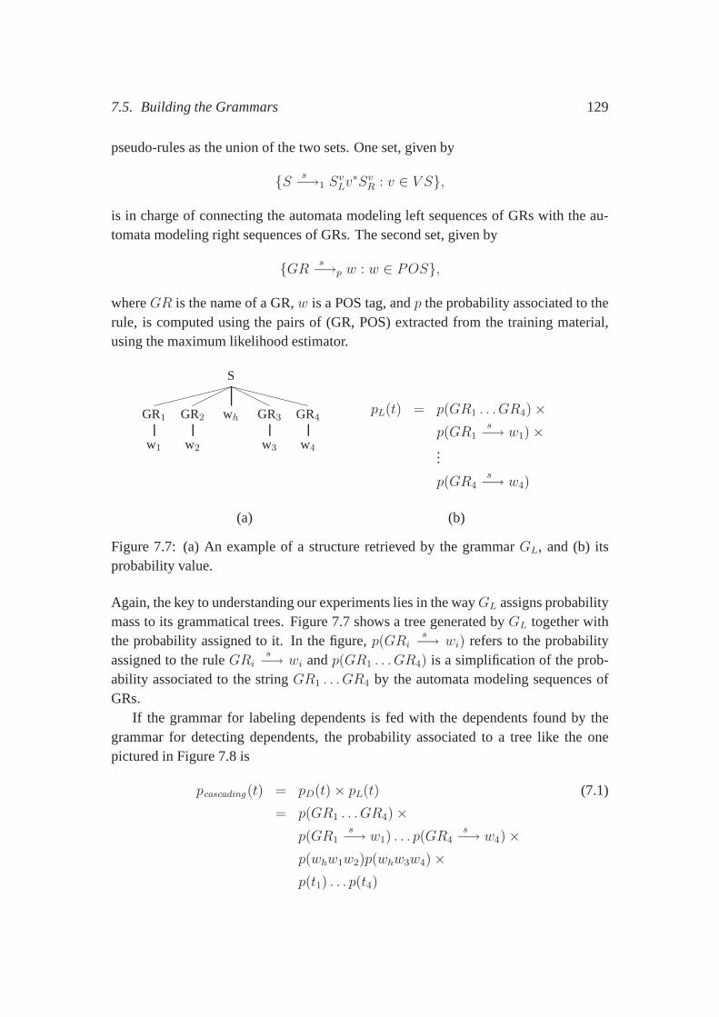
7.5. Building the Grammars 129
pseudo-rules as the union of the two sets. One set, given by
{S s−→1 SvLv
∗SvR : v ∈ V S},
is in charge of connecting the automata modeling left sequences of GRs with the au-tomata modeling right sequences of GRs. The second set, given by
{GR s−→p w : w ∈ POS},
whereGR is the name of a GR,w is a POS tag, andp the probability associated to therule, is computed using the pairs of (GR, POS) extracted fromthe training material,using the maximum likelihood estimator.
S
GR1
w1
GR2
w2
wh GR3
w3
GR4
w4
pL(t) = p(GR1 . . . GR4)×p(GR1
s−→ w1)×...
p(GR4s−→ w4)
(a) (b)
Figure 7.7: (a) An example of a structure retrieved by the grammarGL, and (b) itsprobability value.
Again, the key to understanding our experiments lies in the wayGL assigns probabilitymass to its grammatical trees. Figure 7.7 shows a tree generated byGL together withthe probability assigned to it. In the figure,p(GRi
s−→ wi) refers to the probabilityassigned to the ruleGRi
s−→ wi andp(GR1 . . . GR4) is a simplification of the prob-ability associated to the stringGR1 . . . GR4 by the automata modeling sequences ofGRs.
If the grammar for labeling dependents is fed with the dependents found by thegrammar for detecting dependents, the probability associated to a tree like the onepictured in Figure 7.8 is
pcascading (t) = pD(t)× pL(t) (7.1)
= p(GR1 . . . GR4)×p(GR1
s−→ w1) . . . p(GR4s−→ w4)×
p(whw1w2)p(whw3w4)×p(t1) . . . p(t4)
130 Chapter 7. Sequences as Features
That is,pcascading is the product of the probability assigned byGL andGD, the maindifference between this probability andpone-go (the one assigned by the grammarG
defined in Section 7.5.3 below), is thatpcascading uses the probability of the sequenceswhw1w2 andwhw3w4 for detecting and labeling dependents.
Summing up, we have two probabilitt distributions for the very same task, oneof the distributions uses one more feature. An empirical comparison of these twodistributions would provide us with information about the value of the extra feature;this is what we turn to in Section 7.7.
S
GR1
w1
t1
GR1
w2
t2
wh GR3
w3
t1
GR1
w4
t1
Figure 7.8: The result of cascading the grammars for detecting and labeling depen-dents.
7.5.3 Grammars for Detecting and Labeling Main Dependents
This grammar to be defined in this section does in one go what the two grammars inSection 7.5.1 and 7.5.2 do in two steps.
Extracting Training Material
The training material we used for building this grammar is the union of the trainingmaterials we used for building the two previous grammars.
Building the Grammar
The automata we used for building this grammar are the same asthe automata usedin the previous two grammars, but the set of rules is different. Let POS be the set ofpossible POS tags, letw be a an element inPOS; letAwL andAwR be the two automatabuilt for each POS tag in Section 7.5.1. LetVS be the set of possible verb tags,v anelement inVS ; letAvL andAvR the two automata built for verb tags in Section 7.5.2. LetGvL, Gv
R, GwL, andGw
R be the PCFGs equivalent toAvL, AvR, AwL andAwR, respectively,and letSvL, SvR, SwL andSwR be the start symbols ofGv
L andGvR, respectively. We build
a grammarG with start symbolS, by defining its meta-rules as the disjoint union of

7.6. Optimizing Automata 131
all rules inGvL, Gv
R, GvL andGv
R, for all POS tags and all verbs tags, while its set ofpseudo-rules is the union of the following sets:
{S s−→1 SvLv
∗SvR : v ∈ V S}, {W s−→1 SwLwS
wR : w ∈ POS}, and
{GR s−→p SwLwS
wR : w ∈ POS},
wherep is the probability assigned to the rule{GR s−→p w : w ∈ POS} in Sec-tion 7.5.2.
The difference between this grammar and the grammar for detecting dependents isthat this grammar uses sequences of GRs for detecting the main dependents, while thegrammar for detecting dependents uses sequences of POS tags.
Figure 7.9 shows an example of a tree accepted byG together with the probabilityG assigns to it.
S
GR1
w1
t1
GR1
w2
t2
wh GR3
w3
t1
GR1
w4
t1
pone-go(t) = p(GR1 . . . GR2)×p(GR1 → w1)×. . .
p(GR4 → w4)×p(t1) . . . p(t4)
(a) (b)
Figure 7.9: (a) An example of a structure retrieved by the grammarG, and (b) itsprobability value.
Now that we have the tree probability distributions we can establish the relation be-tween the two. Letpcascading be the probability distribution generated over trees bycascading the two first grammars, and letpone-gobe exactly the probability distributiongenerated byG. The probability distributionspone-goandpcascadingassign probabilitiesto the same set of trees, and the two are related as follows
pcascading(t) = pone-go(t)× p(whw1w2)p(whw3w4) (7.2)
As is clear from Equation 7.2, the difference between the twodistributions is the prob-ability of the sequence of POS tagsw1 . . . w4.
7.6 Optimizing Automata
Let T be a bag of training material extracted from the transformedtree-bank. Thenature ofT depends on the grammar we are trying to induce. But since we use the
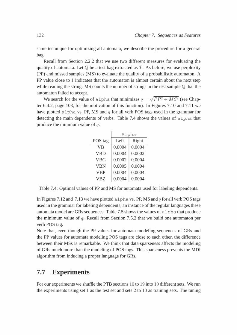
132 Chapter 7. Sequences as Features
same technique for optimizing all automata, we describe theprocedure for a generalbag.
Recall from Section 2.2.2 that we use two different measuresfor evaluating thequality of automata. LetQ be a test bag extracted asT . As before, we use perplexity(PP) and missed samples (MS) to evaluate the quality of a probabilistic automaton. APP value close to1 indicates that the automaton is almost certain about the next stepwhile reading the string. MS counts the number of strings in the test sampleQ that theautomaton failed to accept.
We search for the value ofalpha that minimizesq =√PP 2 +MS2 (see Chap-
ter 6.4.2, page 103, for the motivation of this function). InFigures 7.10 and 7.11 wehave plottedalpha vs. PP, MS andq for all verb POS tags used in the grammar fordetecting the main dependents of verbs. Table 7.4 shows the values ofalpha thatproduce the minimum value ofq.
Alpha
POS tag Left RightVB 0.0004 0.0004
VBD 0.0004 0.0002VBG 0.0002 0.0004VBN 0.0005 0.0004VBP 0.0004 0.0004VBZ 0.0004 0.0004
Table 7.4: Optimal values of PP and MS for automata used for labeling dependents.
In Figures 7.12 and 7.13 we have plottedalpha vs. PP, MS andq for all verb POS tagsused in the grammar for labeling dependents, an instance of the regular languages theseautomata model are GRs sequences. Table 7.5 shows the valuesof alpha that producethe minimum value ofq. Recall from Section 7.5.2 that we build one automaton perverb POS tag.Note that, even though the PP values for automata modeling sequences of GRs andthe PP values for automata modeling POS tags are close to eachother, the differencebetween their MSs is remarkable. We think that data sparseness affects the modelingof GRs much more than the modeling of POS tags. This sparseness prevents the MDIalgorithm from inducing a proper language for GRs.
7.7 Experiments
For our experiments we shuffle the PTB sections10 to 19 into 10 different sets. We runthe experiments using set1 as the test set and sets2 to 10 as training sets. The tuning
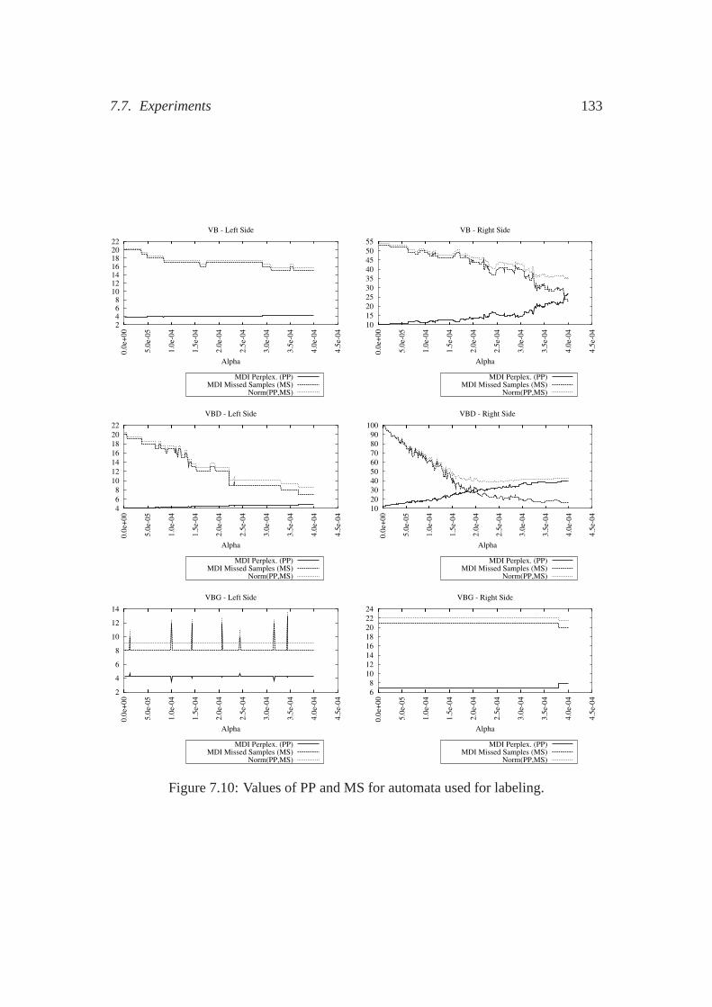
7.7. Experiments 133
2 4 6 8
10 12 14 16 18 20 22
0.0
e+00
5.0
e-05
1.0
e-04
1.5
e-04
2.0
e-04
2.5
e-04
3.0
e-04
3.5
e-04
4.0
e-04
4.5
e-04
Alpha
VB - Left Side
MDI Perplex. (PP)MDI Missed Samples (MS)
Norm(PP,MS)
10
15
20
25
30
35
40
45
50
55
0.0
e+00
5.0
e-05
1.0
e-04
1.5
e-04
2.0
e-04
2.5
e-04
3.0
e-04
3.5
e-04
4.0
e-04
4.5
e-04
Alpha
VB - Right Side
MDI Perplex. (PP)MDI Missed Samples (MS)
Norm(PP,MS)
4
6
8
10
12
14
16
18
20
22
0.0
e+00
5.0
e-05
1.0
e-04
1.5
e-04
2.0
e-04
2.5
e-04
3.0
e-04
3.5
e-04
4.0
e-04
4.5
e-04
Alpha
VBD - Left Side
MDI Perplex. (PP)MDI Missed Samples (MS)
Norm(PP,MS)
10
20
30
40
50
60
70
80
90
100
0.0
e+00
5.0
e-05
1.0
e-04
1.5
e-04
2.0
e-04
2.5
e-04
3.0
e-04
3.5
e-04
4.0
e-04
4.5
e-04
Alpha
VBD - Right Side
MDI Perplex. (PP)MDI Missed Samples (MS)
Norm(PP,MS)
2
4
6
8
10
12
14
0.0
e+00
5.0
e-05
1.0
e-04
1.5
e-04
2.0
e-04
2.5
e-04
3.0
e-04
3.5
e-04
4.0
e-04
4.5
e-04
Alpha
VBG - Left Side
MDI Perplex. (PP)MDI Missed Samples (MS)
Norm(PP,MS)
6
8
10
12
14
16
18
20
22
24
0.0
e+00
5.0
e-05
1.0
e-04
1.5
e-04
2.0
e-04
2.5
e-04
3.0
e-04
3.5
e-04
4.0
e-04
4.5
e-04
Alpha
VBG - Right Side
MDI Perplex. (PP)MDI Missed Samples (MS)
Norm(PP,MS)
Figure 7.10: Values of PP and MS for automata used for labeling.
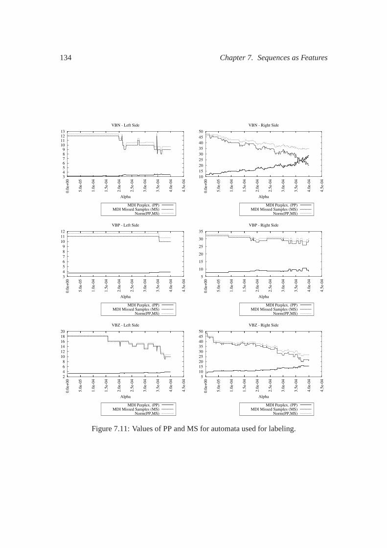
134 Chapter 7. Sequences as Features
3 4 5 6 7 8 9
10 11 12 13
0.0
e+00
5.0
e-05
1.0
e-04
1.5
e-04
2.0
e-04
2.5
e-04
3.0
e-04
3.5
e-04
4.0
e-04
4.5
e-04
Alpha
VBN - Left Side
MDI Perplex. (PP)MDI Missed Samples (MS)
Norm(PP,MS)
10
15
20
25
30
35
40
45
50
0.0
e+00
5.0
e-05
1.0
e-04
1.5
e-04
2.0
e-04
2.5
e-04
3.0
e-04
3.5
e-04
4.0
e-04
4.5
e-04
Alpha
VBN - Right Side
MDI Perplex. (PP)MDI Missed Samples (MS)
Norm(PP,MS)
3
4
5
6
7
8
9
10
11
12
0.0
e+00
5.0
e-05
1.0
e-04
1.5
e-04
2.0
e-04
2.5
e-04
3.0
e-04
3.5
e-04
4.0
e-04
4.5
e-04
Alpha
VBP - Left Side
MDI Perplex. (PP)MDI Missed Samples (MS)
Norm(PP,MS)
5
10
15
20
25
30
35
0.0
e+00
5.0
e-05
1.0
e-04
1.5
e-04
2.0
e-04
2.5
e-04
3.0
e-04
3.5
e-04
4.0
e-04
4.5
e-04
Alpha
VBP - Right Side
MDI Perplex. (PP)MDI Missed Samples (MS)
Norm(PP,MS)
2
4
6
8
10
12
14
16
18
20
0.0
e+00
5.0
e-05
1.0
e-04
1.5
e-04
2.0
e-04
2.5
e-04
3.0
e-04
3.5
e-04
4.0
e-04
4.5
e-04
Alpha
VBZ - Left Side
MDI Perplex. (PP)MDI Missed Samples (MS)
Norm(PP,MS)
5
10
15
20
25
30
35
40
45
50
0.0
e+00
5.0
e-05
1.0
e-04
1.5
e-04
2.0
e-04
2.5
e-04
3.0
e-04
3.5
e-04
4.0
e-04
4.5
e-04
Alpha
VBZ - Right Side
MDI Perplex. (PP)MDI Missed Samples (MS)
Norm(PP,MS)
Figure 7.11: Values of PP and MS for automata used for labeling.
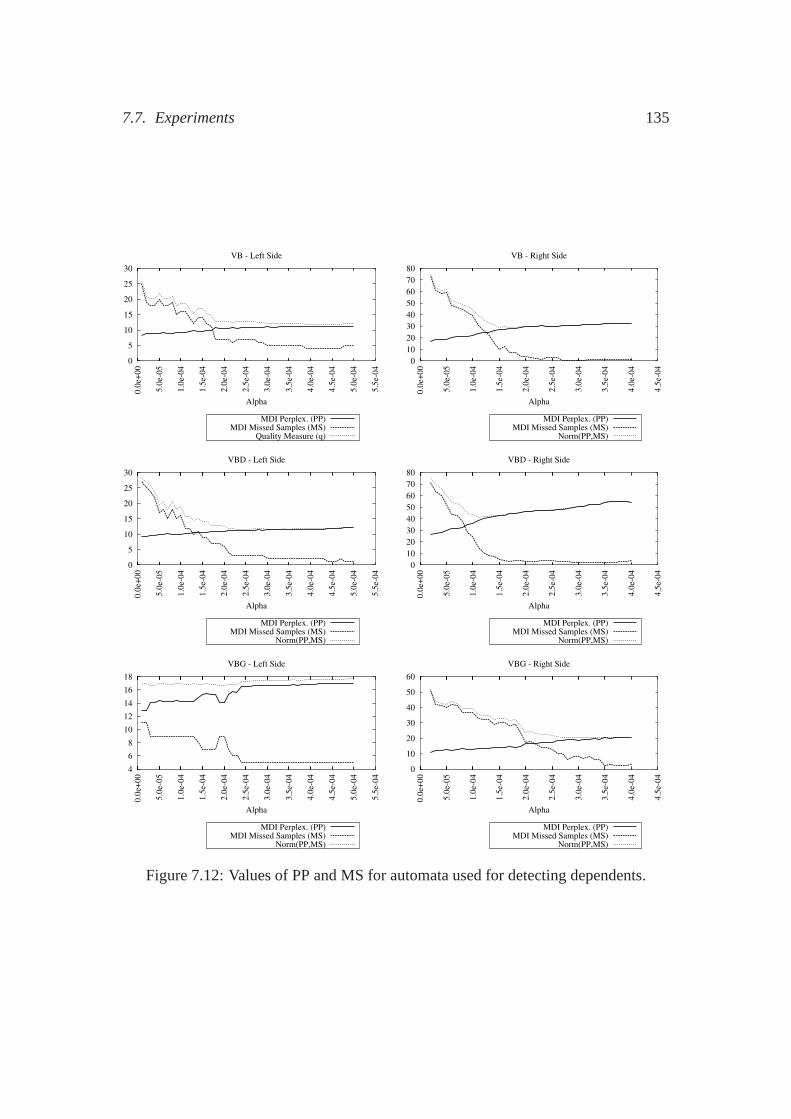
7.7. Experiments 135
0
5
10
15
20
25
30
0.0
e+00
5.0
e-05
1.0
e-04
1.5
e-04
2.0
e-04
2.5
e-04
3.0
e-04
3.5
e-04
4.0
e-04
4.5
e-04
5.0
e-04
5.5
e-04
Alpha
VB - Left Side
MDI Perplex. (PP)MDI Missed Samples (MS)
Quality Measure (q)
0
10
20
30
40
50
60
70
80
0.0
e+00
5.0
e-05
1.0
e-04
1.5
e-04
2.0
e-04
2.5
e-04
3.0
e-04
3.5
e-04
4.0
e-04
4.5
e-04
Alpha
VB - Right Side
MDI Perplex. (PP)MDI Missed Samples (MS)
Norm(PP,MS)
0
5
10
15
20
25
30
0.0
e+00
5.0
e-05
1.0
e-04
1.5
e-04
2.0
e-04
2.5
e-04
3.0
e-04
3.5
e-04
4.0
e-04
4.5
e-04
5.0
e-04
5.5
e-04
Alpha
VBD - Left Side
MDI Perplex. (PP)MDI Missed Samples (MS)
Norm(PP,MS)
0
10
20
30
40
50
60
70
80
0.0
e+00
5.0
e-05
1.0
e-04
1.5
e-04
2.0
e-04
2.5
e-04
3.0
e-04
3.5
e-04
4.0
e-04
4.5
e-04
Alpha
VBD - Right Side
MDI Perplex. (PP)MDI Missed Samples (MS)
Norm(PP,MS)
4
6
8
10
12
14
16
18
0.0
e+00
5.0
e-05
1.0
e-04
1.5
e-04
2.0
e-04
2.5
e-04
3.0
e-04
3.5
e-04
4.0
e-04
4.5
e-04
5.0
e-04
5.5
e-04
Alpha
VBG - Left Side
MDI Perplex. (PP)MDI Missed Samples (MS)
Norm(PP,MS)
0
10
20
30
40
50
60
0.0
e+00
5.0
e-05
1.0
e-04
1.5
e-04
2.0
e-04
2.5
e-04
3.0
e-04
3.5
e-04
4.0
e-04
4.5
e-04
Alpha
VBG - Right Side
MDI Perplex. (PP)MDI Missed Samples (MS)
Norm(PP,MS)
Figure 7.12: Values of PP and MS for automata used for detecting dependents.
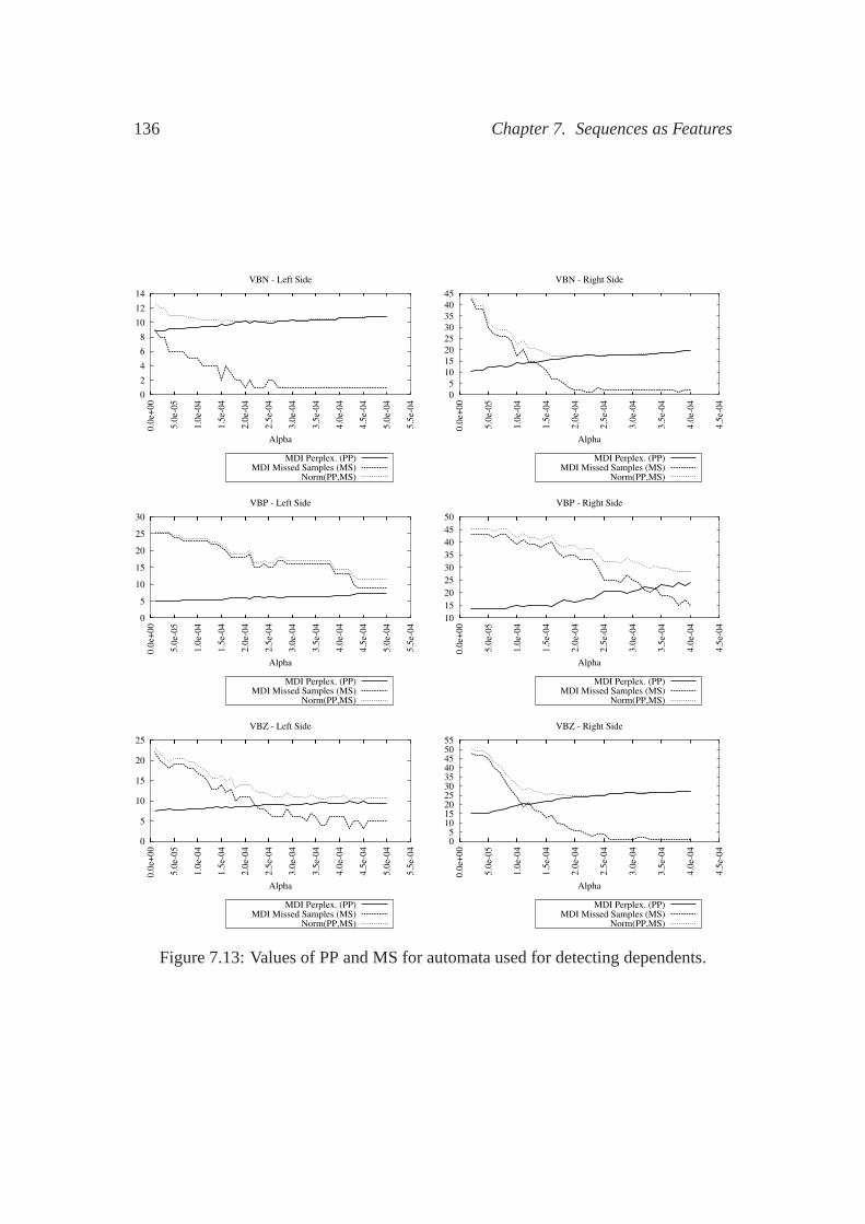
136 Chapter 7. Sequences as Features
0
2
4
6
8
10
12
14
0.0
e+00
5.0
e-05
1.0
e-04
1.5
e-04
2.0
e-04
2.5
e-04
3.0
e-04
3.5
e-04
4.0
e-04
4.5
e-04
5.0
e-04
5.5
e-04
Alpha
VBN - Left Side
MDI Perplex. (PP)MDI Missed Samples (MS)
Norm(PP,MS)
0
5
10
15
20
25
30
35
40
45
0.0
e+00
5.0
e-05
1.0
e-04
1.5
e-04
2.0
e-04
2.5
e-04
3.0
e-04
3.5
e-04
4.0
e-04
4.5
e-04
Alpha
VBN - Right Side
MDI Perplex. (PP)MDI Missed Samples (MS)
Norm(PP,MS)
0
5
10
15
20
25
30
0.0
e+00
5.0
e-05
1.0
e-04
1.5
e-04
2.0
e-04
2.5
e-04
3.0
e-04
3.5
e-04
4.0
e-04
4.5
e-04
5.0
e-04
5.5
e-04
Alpha
VBP - Left Side
MDI Perplex. (PP)MDI Missed Samples (MS)
Norm(PP,MS)
10
15
20
25
30
35
40
45
50
0.0
e+00
5.0
e-05
1.0
e-04
1.5
e-04
2.0
e-04
2.5
e-04
3.0
e-04
3.5
e-04
4.0
e-04
4.5
e-04
Alpha
VBP - Right Side
MDI Perplex. (PP)MDI Missed Samples (MS)
Norm(PP,MS)
0
5
10
15
20
25
0.0
e+00
5.0
e-05
1.0
e-04
1.5
e-04
2.0
e-04
2.5
e-04
3.0
e-04
3.5
e-04
4.0
e-04
4.5
e-04
5.0
e-04
5.5
e-04
Alpha
VBZ - Left Side
MDI Perplex. (PP)MDI Missed Samples (MS)
Norm(PP,MS)
0 5
10 15 20 25 30 35 40 45 50 55
0.0
e+00
5.0
e-05
1.0
e-04
1.5
e-04
2.0
e-04
2.5
e-04
3.0
e-04
3.5
e-04
4.0
e-04
4.5
e-04
Alpha
VBZ - Right Side
MDI Perplex. (PP)MDI Missed Samples (MS)
Norm(PP,MS)
Figure 7.13: Values of PP and MS for automata used for detecting dependents.
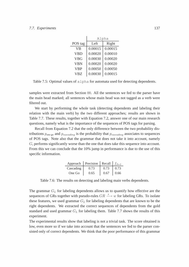
7.7. Experiments 137
Alpha
POS tag Left RightVB 0.00015 0.00015
VBD 0.00020 0.00010VBG 0.00030 0.00020VBN 0.00020 0.00020VBP 0.00050 0.00050VBZ 0.00030 0.00015
Table 7.5: Optimal values ofalpha for automata used for detecting dependents.
samples were extracted from Section00. All the sentences we fed to the parser havethe main head marked; all sentences whose main head was not tagged as a verb werefiltered out.
We start by performing the whole task (detecting dependentsand labeling theirrelation with the main verb) by the two different approaches; results are shown inTable 7.7. These results, together with Equation 7.2, answer one of our main researchquestions, namely what is the importance of the sequences ofPOS tags for parsing.
Recall from Equation 7.2 that the only difference between the two probability dis-tributionspone-goandpcascading is the probability thatpcascading associates to sequencesof POS tags. Note also that the grammar that does not take it into account, namelyG, performs significantly worse than the one that does take this sequence into account.From this we can conclude that the 10% jump in performance is due to the use of thisspecific information.
Approach Precision Recall fβ=1
Cascading 0.73 0.73 0.73One Go 0.65 0.67 0.66
Table 7.6: The results on detecting and labeling main verbs dependents.
The grammarGL for labeling dependents allows us to quantify how effectiveare thesequences of GRs together with pseudo-rulesGR
s−→ w for labeling GRs. To isolatethese features, we used grammarGL for labeling dependents that are known to be theright dependents. We extracted the correct sequences of dependents from the goldstandard and used grammarGL for labeling them. Table 7.7 shows the results of thisexperiment.The experimental results show that labeling is not a trivialtask. The score obtained islow, even more so if we take into account that the sentences wefed to the parser con-sisted only of correct dependents. We think that the poor performance of this grammar
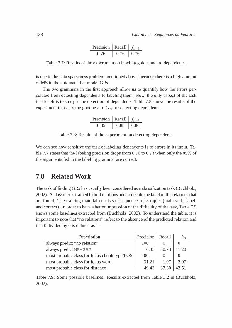
138 Chapter 7. Sequences as Features
Precision Recall fβ=1
0.76 0.76 0.76
Table 7.7: Results of the experiment on labeling gold standard dependents.
is due to the data sparseness problem mentioned above, because there is a high amountof MS in the automata that model GRs.
The two grammars in the first approach allow us to quantify howthe errors per-colated from detecting dependents to labeling them. Now, the only aspect of the taskthat is left is to study is the detection of dependents. Table7.8 shows the results of theexperiment to assess the goodness ofGD for detecting dependents.
Precision Recall fβ=1
0.85 0.88 0.86
Table 7.8: Results of the experiment on detecting dependents.
We can see how sensitive the task of labeling dependents is toerrors in its input. Ta-ble 7.7 states that the labeling precision drops from0.76 to 0.73 when only the 85% ofthe arguments fed to the labeling grammar are correct.
7.8 Related Work
The task of finding GRs has usually been considered as a classification task (Buchholz,2002). A classifier is trained to find relations and to decide the label of the relations thatare found. The training material consists of sequences of 3-tuples (main verb, label,and context). In order to have a better impression of the difficulty of the task, Table 7.9shows some baselines extracted from (Buchholz, 2002). To understand the table, it isimportant to note that “no relations” refers to the absence of the predicted relation andthat0 divided by0 is defined as1.
Description Precision Recall Fβalways predict “no relation” 100 0 0always predictNP-SBJ 6.85 30.73 11.20most probable class for focus chunk type/POS100 0 0most probable class for focus word 31.21 1.07 2.07most probable class for distance 49.43 37.30 42.51
Table 7.9: Some possible baselines. Results extracted fromTable 3.2 in (Buchholz,2002).
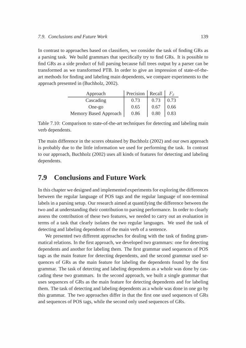
7.9. Conclusions and Future Work 139
In contrast to approaches based on classifiers, we consider the task of finding GRs asa parsing task. We build grammars that specifically try to findGRs. It is possible tofind GRs as a side product of full parsing because full trees output by a parser can betransformed as we transformed PTB. In order to give an impression of state-of-the-art methods for finding and labeling main dependents, we compare experiments to theapproach presented in (Buchholz, 2002).
Approach Precision Recall FβCascading 0.73 0.73 0.73
One-go 0.65 0.67 0.66Memory Based Approach 0.86 0.80 0.83
Table 7.10: Comparison to state-of-the-art techniques fordetecting and labeling mainverb dependents.
The main difference in the scores obtained by Buchholz (2002) and our own approachis probably due to the little information we used for performing the task. In contrastto our approach, Buchholz (2002) uses all kinds of features for detecting and labelingdependents.
7.9 Conclusions and Future Work
In this chapter we designed and implemented experiments forexploring the differencesbetween the regular language of POS tags and the regular language of non-terminallabels in a parsing setup. Our research aimed at quantifyingthe difference between thetwo and at understanding their contribution to parsing performance. In order to clearlyassess the contribution of these two features, we needed to carry out an evaluation interms of a task that clearly isolates the two regular languages. We used the task ofdetecting and labeling dependents of the main verb of a sentence.
We presented two different approaches for dealing with the task of finding gram-matical relations. In the first approach, we developed two grammars: one for detectingdependents and another for labeling them. The first grammar used sequences of POStags as the main feature for detecting dependents, and the second grammar used se-quences of GRs as the main feature for labeling the dependents found by the firstgrammar. The task of detecting and labeling dependents as a whole was done by cas-cading these two grammars. In the second approach, we built asingle grammar thatuses sequences of GRs as the main feature for detecting dependents and for labelingthem. The task of detecting and labeling dependents as a whole was done in one go bythis grammar. The two approaches differ in that the first one used sequences of GRsand sequences of POS tags, while the second only used sequences of GRs.
140 Chapter 7. Sequences as Features
We showed that English GRs follow a very strict sequential order, but not as strictas POS tags of verbal dependents. We showed that the latter ismore effective for de-tecting and labeling dependents, and, hence, it provides a more reliable instrument fordetecting them. Moreover, we have shown that sequences of POS tags are fundamen-tal for parsing performance: they provide a reliable sourcefor predicting and detectingdependents. Our experiments also show that sequences of GRsare not as reliable assequences of POS tags.
The usual perspective on parsing is that all features that improve parsing perfor-mance are used without clearly stating why these features improve. Our approach aimsat changing this perspective; we designed grammars and experiments for isolating,testing and explaining two particular features: sequencesof POS tags and sequencesof GRs, both for detecting and labeling and labeling dependents. PCW-grammars al-low us to do these. Note that trees returned by our parser are flat trees and they can notbe modeled either by PCFGs nor by bilexical grammars. This isthe case because someof the dependencies we model using automata in this chapter do not yield terminals butpreterminal symbols.
Chapter 8
Conclusions
In this thesis we have applied an abstract model to learn moreabout natural languageparsing. We have surveyed three state-of-the-art probabilistic parsers and we haveidentified their characteristic features. We have abstracted from these particular fea-tures and models to produce and formalize a general, and abstract, language model.This abstract language model provides us with a suitable framework to carry out prin-cipled investigations of new directions in parsing based ondifferent parameterizationsof the general model.
While reviewing state-of-the-art parsers, we focused on crucial issues like the roleof probabilities in the context of parsing, their importance and their possible uses. Wehave shown that, when used as a filtering mechanism, probabilities can add expres-sive power to context free grammars, defining a class of tree languages beyond theexpressivity of context free grammars. We have shown that itis not possible to decidewhether probabilities solve all ambiguities in a language.In addition, we have shownthat probabilities can be used for purposes other than the mere filtering of unwantedtrees. We have illustrated this claim with some examples, like using probabilities toevaluate the quality of PCFGs and to boost the performance ofparsers.
The general language model we have presented is based on W-grammars. We haveintroduced constrained W-grammars and have augmented themwith probabilities. Theresulting formalism, probabilistic constrained W-grammars, is the backbone formalismfor all our experiments. Like every general model, the suitability of PCW-grammars ismainly given by two aspects: that they can capture multiple existing formalisms in asingle formalism, and that they provide a structured framework where new directionsof research can be identified and pursued in a principled way.
141
142 Chapter 8. Conclusions
8.1 PCW-Grammars as a General Model
We have shown that PCW-grammars provide an encompassing formalism to explainthree state-of-the-art language models. PCW-grammars arebased on a well knowngrammatical framework, and their computational properties are well-understood. Itis true that the expressive power of PCW-grammars is significantly lower than thatof W-grammars, but their expressiveness is perfectly adequate to capture grammaticalformalisms underlying state-of-the-art parsers.
For example, we have shown that probabilistic constrained W-grammars are ca-pable of capturing bilexical grammars, Markovian context free rules, and stochastictree substitution grammars. We have described the expressive power of these threeformalisms, together with some conditions under which grammars inferred from tree-banks are consistent. Despite the similarities between PCW-grammars and PCFGs,they are distinguished by a fundamental difference: the two-level mechanism of PCW-grammars. This mechanism allowed us to capture these three state-of-the-art naturallanguage models, which cannot be done using standard PCFGs only.
The suitability of the general language model provided by PCW-grammars is thatit allowed us to compare three apparently different formalisms within the same formalperspective. We have shown that the essence of bilexical grammars and Markoviancontext free grammars is quite comparable: both are based onapproximating bodies ofrules using Markov models. We also found similarities between STSGs and Markovrules: both suppose that rule bodies are obtained by collapsing hidden derivations.More concretely, for Markovian rules, a rule body is a regular expression (or a Markovchain, which is equivalent) and STSGs take this idea to the extreme by considering thewhole sentence as the yield of a hidden derivation.
8.2 PCW-Grammars as a New Parsing Paradigm
PCW-grammars are not only useful for capturing the formalisms underlying state-of-the-art parsers, but also for suggesting new research directions. These come as a con-sequence of different instantiations of the parameters of the general model, or by re-thinking the set of assumptions the particular instances have made. A brief descriptionof the directions explored in this thesis follows.
Explicit Use of Probabilistic Automata: PCW-grammars allowed us to use generalmethods for inducing regular languages instead of the usualn-based algorithms.Our experiments along this line lead to two types of conclusions. First, that mod-eling rules with algorithms other thann-grams does not only produce smallergrammars, but also better performing ones. Second, that theprocedure used for
8.2. PCW-Grammars as a New Parsing Paradigm 143
optimizing the parameters of the parser reveals that some POS behave almostdeterministically for selecting their dependents, while others do not. This con-clusion suggests that splitting classes that behave non-deterministically into ho-mogeneous ones could improve the quality of the inferred automata. We arguedthat lexicalization and head-annotation seem to take advantage of the propertiesof splitting.
Splitting the Training Material: We have presented an approach that aims at findingan optimal splitting of the material before inducing a PCW-grammar. The split-ting was aimed at improving parsing performance. For this purpose, we defineda quality measure to quantify the quality of different partitions of the material.Using this measure, we searched among a subset of all possible partitions for theone maximizing the proposed quality measure. This measure is a combinationof a quality measure defined for each component in a partition. For each com-ponent, we built an automaton and computed the automaton’s missed samplesand perplexity. The measure we presented combines the values of perplexityand missed samples for all resulting automata. We used the resulting automatato build grammars that were subsequently used for parsing the Penn Treebank.We have shown that the quality measure we defined can be used for comparingtwo grammars’ parsing scores if the grammars are built from partitions havinga similar number of components. Since our measureq is a good indicator ofthe parsing performance, the process of inferring grammarscan be treated as anoptimization task. This implies that this procedure sparesus the need to assessthe performance of a particular grammar by parsing.
Sequences as Features:The usual perspective on parsing is that all features that im-prove parsing performance are used for parsing, without a clear study ofhowthese features improve parsing. Our approach is aimed at changing this per-spective; we have designed grammars and experiments for isolating, testing andexplaining the value of two particular features that are known to improve parsingperformance: sequences of POS tags and sequences of GRs. We have shown thatsequences of POS tags are fundamental for parsing performance, because theyprovide a reliable source for predicting and detecting dependents. Our experi-ments have also shown that sequences of GRs are not as reliable as sequencesof POS tags. We think this is the case because the training material for GRs issmall compared to the training material for sequences of POS.
PCW-grammars are versatile enough to allow us to address thevariety of experimentalquestions and aspects we tried out in this thesis. For all of them we used only oneparsing algorithm and a unified mathematical theory. PCW-grammars have reduced
144 Chapter 8. Conclusions
the design cycle for all of our experiments; we only need to focus on very specificaspects of parsing, and we could leave aside all conditions on expressive power, com-plexity of parsing, and parsing algorithms. We think that PCW-grammars have proventheir suitability: the formalism is abstract enough to capture the formalisms underlyingstate-of-the-art parsers and to suggest new research directions in parsing.
8.3 Two Roads Ahead
This thesis presents a rather unusual perspective on parsing. The usual perspectiveaims at designing and building parsers that produce better scores on parsing the Penntreebank. In contrast, we presented measures, grammars, tasks and experiments thatwere designed for testing particular aspects of syntax, language modeling and parsing.
In my opinion, these two approaches are exponents of two different research direc-tions. The first one focuses on understanding why particularfeatures improve parsingperformance, while the second focuses on finding new features that can improve pars-ing performance. The second direction has reached a plateau; different approaches donot differ substantially in terms of their parsing scores and it is hard to identify the keyfeatures that may produce a future jump in performance scores. It is also difficult todetermine which differences in performance are statistically significant. I think that inthe forthcoming years the research focus will shift from thesecond line of research tothe first one. I think that this shift will result in deeper, more detailed knowledge of thestructure of human language, and its impact on parsing performance.
The ultimate aim of parsing is twofold: understanding humanlanguage and pro-ducing parsers that process naturally ocurring sentences with an acceptable error rate.The interest for these two aims is disjoint in the different disciplines: linguistics aimsat understanding human language, while statistical parsing aims at producing compu-tational models that process natural language with an acceptable level of performance.
It seems to me that if there is any flow of ideas, it goes mostly from the linguisticsside to the statistical one. The reverse direction is blocked to the point that somelinguists claim that the knowledge that can be inferred by statistical methods cannotbe considered as a reliable model of language (Andor, 2004).I hope this situationwill change in the years to come. I think that the parsing community has to focuson two main research areas. One area will focus on identifying, understanding andtesting particular aspects of features used for parsing which will provide linguists withinteresting data about language as they understand it. The second stream will try toincorporate insights suggested by the first line of researchin parsers. I hope that thisthesis has suggested new directions; translating them intoimprovements in state-of-the-art parsing performance is the next step.
Appendix A
Parsing PCW-Grammars
A.1 Introduction
In this appendix we focus on two different aspects of our PCW-grammar parsing algo-rithm. One aspect, the most theoretical one, is related to the study of the capacity andcomputational complexity of our implementation for handling PCW-grammars. Sincevarious meta-derivations can produce the same w-rule, it isimportant to distinguish be-tween the most probable derivation tree and the most probable w-tree. As described inChapter 4, different meta-derivations can yield the same w-rule and consequently thesame w-tree. A parser returning the most probable derivation tree considers the proba-bility of a w-rule as the probability value of the most probable meta-derivation. In con-trast, a parsing algorithm searching for the most probable tree considers the probabilityof a w-rule as the sum of all probabilities assigned to the meta-derivations producing it.In this appendix we investigate the differences between these two approaches, focusingon necessary and sufficient conditions for both approaches to return the same tree.
The second aspect we focus on, is related to technical issuesof our PCW-grammarparsing algorithm implementation. In some of the experiments we performed, theparser had to handle grammars containing a number of rules close to one million. Theparsing algorithm is an optimization algorithm, it searches for the best solution amonga set of possible solutions. At each step in the optimizationprocess, the algorithmbuilds possible solutions retrieving new rules from the grammar. When working withlarge grammars, as we did, the complexity of the parsing algorithm becomes unman-ageable if the retrieval step takes more than constant time.In this appendix, we brieflydescribe the approach we followed to minimize the computational costs of this step.
The rest of the appendix is organized as follows. Section A.2discusses the theoret-ical issues related to the parsing algorithm, Section A.3 discusses the Java implemen-tation, and Section A.4 concludes the appendix.
145
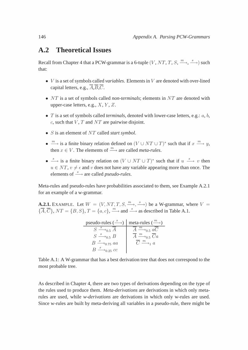
146 Appendix A. Parsing PCW-Grammars
A.2 Theoretical Issues
Recall from Chapter 4 that a PCW-grammar is a 6-tuple(V ,NT , T , S,m−→,
s−→) suchthat:
• V is a set of symbols calledvariables. Elements inV are denoted with over-linedcapital letters, e.g.,A,B,C.
• NT is a set of symbols callednon-terminals; elements inNT are denoted withupper-case letters, e.g.,X, Y , Z.
• T is a set of symbols calledterminals, denoted with lower-case letters, e.g.:a, b,c, such thatV , T andNT are pairwise disjoint.
• S is an element ofNT calledstart symbol.
• m−→ is a finite binary relation defined on(V ∪ NT ∪ T )∗ such that ifxm−→ y,
thenx ∈ V . The elements ofm−→ are calledmeta-rules.
• s−→ is a finite binary relation on(V ∪ NT ∪ T )∗ such that ifus−→ v then
u ∈ NT , v 6= ǫ andv does not have any variable appearing more than once. Theelements of
s−→ are calledpseudo-rules.
Meta-rules and pseudo-rules have probabilities associated to them, see Example A.2.1for an example of a w-grammar.
A.2.1.EXAMPLE . Let W = (V,NT, T, S,m−→, s−→) be a W-grammar, whereV =
{A,C},NT = {B, S}, T = {a, c}, m−→ ands−→ as described in Table A.1.
pseudo-rules (s−→) meta-rules (
m−→)S
s−→0.5 A Am−→0.5 aC
Ss−→0.5 B A
m−→0.5 Ca
Bs−→0.75 aa C
m−→1 a
Bs−→0.25 cc
Table A.1: A W-grammar that has a best derivation tree that does not correspond to themost probable tree.
As described in Chapter 4, there are two types of derivationsdepending on the type ofthe rules used to produce them.Meta-derivationsare derivations in which only meta-rules are used, whilew-derivationsare derivations in which only w-rules are used.Since w-rules are built by meta-deriving all variables in a pseudo-rule, there might be
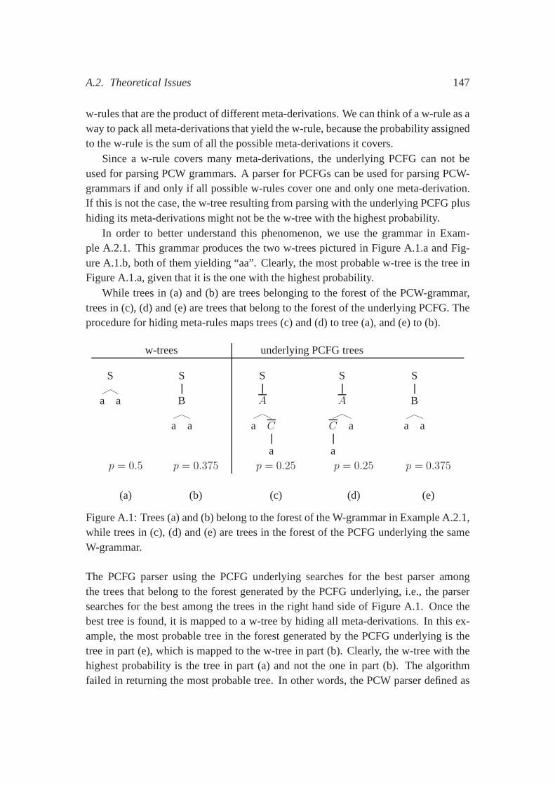
A.2. Theoretical Issues 147
w-rules that are the product of different meta-derivations. We can think of a w-rule as away to pack all meta-derivations that yield the w-rule, because the probability assignedto the w-rule is the sum of all the possible meta-derivationsit covers.
Since a w-rule covers many meta-derivations, the underlying PCFG can not beused for parsing PCW grammars. A parser for PCFGs can be used for parsing PCW-grammars if and only if all possible w-rules cover one and only one meta-derivation.If this is not the case, the w-tree resulting from parsing with the underlying PCFG plushiding its meta-derivations might not be the w-tree with thehighest probability.
In order to better understand this phenomenon, we use the grammar in Exam-ple A.2.1. This grammar produces the two w-trees pictured inFigure A.1.a and Fig-ure A.1.b, both of them yielding “aa”. Clearly, the most probable w-tree is the tree inFigure A.1.a, given that it is the one with the highest probability.
While trees in (a) and (b) are trees belonging to the forest ofthe PCW-grammar,trees in (c), (d) and (e) are trees that belong to the forest ofthe underlying PCFG. Theprocedure for hiding meta-rules maps trees (c) and (d) to tree (a), and (e) to (b).
w-trees underlying PCFG trees
S
a a
S
B
a a
S
A
a C
a
S
A
C
a
a
S
B
a a
p = 0.5 p = 0.375 p = 0.25 p = 0.25 p = 0.375
(a) (b) (c) (d) (e)
Figure A.1: Trees (a) and (b) belong to the forest of the W-grammar in Example A.2.1,while trees in (c), (d) and (e) are trees in the forest of the PCFG underlying the sameW-grammar.
The PCFG parser using the PCFG underlying searches for the best parser amongthe trees that belong to the forest generated by the PCFG underlying, i.e., the parsersearches for the best among the trees in the right hand side ofFigure A.1. Once thebest tree is found, it is mapped to a w-tree by hiding all meta-derivations. In this ex-ample, the most probable tree in the forest generated by the PCFG underlying is thetree in part (e), which is mapped to the w-tree in part (b). Clearly, the w-tree with thehighest probability is the tree in part (a) and not the one in part (b). The algorithmfailed in returning the most probable tree. In other words, the PCW parser defined as
148 Appendix A. Parsing PCW-Grammars
the procedure of, first, searching for the most probable treein the forest generated bythe PCFG underlying and, second, hiding all of its meta-derivations, might not returnthe most probable w-tree.
Clearly, if the hiding procedure maps one tree in the forest generated by the PCFGunderlying to one tree in the forest generated by the W-grammar, then a parser for W-grammar is equivalent to the process of using a PCFG parser plus post tree-processing.
There are two configurations for which the mapping between the two forests is nota one-to-one map. The first one occurs when there is at least one meta-variable thatcan be instantiated with a value that can be meta-derived in two different ways. Thesecond one occurs when there is a pseudo-rule that has only one terminal in its body,and that body can be generated with another w-rule. For the grammar in Example A.1,the mapping between two forests is not a one-to-one mapping because the variableAin pseudo-ruleS
s−→0.5 A can be instantiated with two different meta-derivations.
Note that in all our experiments, meta-rules come from probabilistic determinis-tic automata. Since they are deterministic, all possible variable instantiations have aunique way to derive them. Also, not all the pseudo-rules we used in our grammarshave a variable in their body. Consequently, since, for all the grammars we developedin this thesis, there is a one-to-one mapping between the forest generated by the w-grammar and the forest generated by the PCFG underlying, we decided to implementour parser as a Cocke-Younger-Kasami (CYK) parsing algorithm plus a procedure thathides all meta-derivations from the tree returned by the CYKalgorithm.
The parser we implemented can be used as a parser that returnsthe most probabletree, because we know that the most probable tree corresponds to the most probablederivation tree. The problem of knowing when these two treesare the same is nota trivial one. As we discussed before, the two trees are the same tree if there areno variables that can be instantiated in the same way with twodifferent derivations.Since variables are instantiated through a context free like system, the problem ofknowing whether there are two ways to derive the same string becomes equivalent tothe problem of knowing whether a context free grammar is unambiguous. It is well-known that the latter is an undecidable problem, which implies that it is is undecidablewhether the most probable tree is the same as the most probable derivation tree for agiven grammar.
A.3 Practical Issues
Conceptually, our parsing algorithm consists of two different modules. One module,a CYK parser, searches for the most probable derivation in the underlying PCFG (seeChapter 4 for the definition of the underlying PCFG). The second module, the function
A.3. Practical Issues 149
devoted to hiding meta-derivations, is in charge of transforming the most probablederivation tree into a w-tree.
The rules handled by the version of the CYK algorithm we implemented have annumber associated to them. This integer, calledlevel of visibility, is a generalization ofthe concept of meta-rules and pseudo-rules. The tree returned by the CYK algorithmis transformed to many different trees, depending on the visibility level of the rules tobe hidden.
A.3.1 Levels of visibility
Trees to be transformed can be thought of as trees in which, for each node, there is aninteger marking the node’s level of visibility. In order to transform a tree by hiding alevel of visibility, we implemented a function that takes two arguments, one argumentis the tree to be transformed and the second argument is the level of visibility to behidden. The algorithm traverses the tree in a bottom up fashion and, for each nodehaving the visibility level to be replaced, it replaces the node itself with the sub-treeshanging from that node in the original tree. Figure A.2 showsan example of hidingoperations for different levels of visibility. Since the hide operation can be applied toa tree which was already transformed, a tree has many possible sets of visibility levelsto hide. For example, the tree in Figure A.2.d is the result ofhiding level of visibility1
from the tree in Figure A.2.c, which is in turn the result of hiding visibility level2 fromthe tree in Figure A.2.a. Note that the order in which the visibility levels are applieddoes not matter.
The PCW parser is a particular case of the parser we implemented. In order toobtain a PCW-parser, we marked meta-rules with visibility level 1 and pseudo-ruleswith visibility level 0. In order to obtain a w-tree from the tree output by the CYKcomponent, we hide nodes whose level of visibility equals1.
A.3.2 Optimization aspects
The core of our algorithm is a Probabilistic CYK parsing algorithm capable only ofparsing grammars in Chomsky Normal Form (CNF). Probabilistic CYK parsing wasfirst described by Ney (1991), but the version we discuss hereis adapted from Collins(1999) and Aho and Ullman (1972).
The CYK algorithm assumes the following input, output and data structures.
• Input
– A CNF PCFG. Assume that the|N | not-terminals have indices1, 2, . . . , |N |,and that the start symbolS has index1.
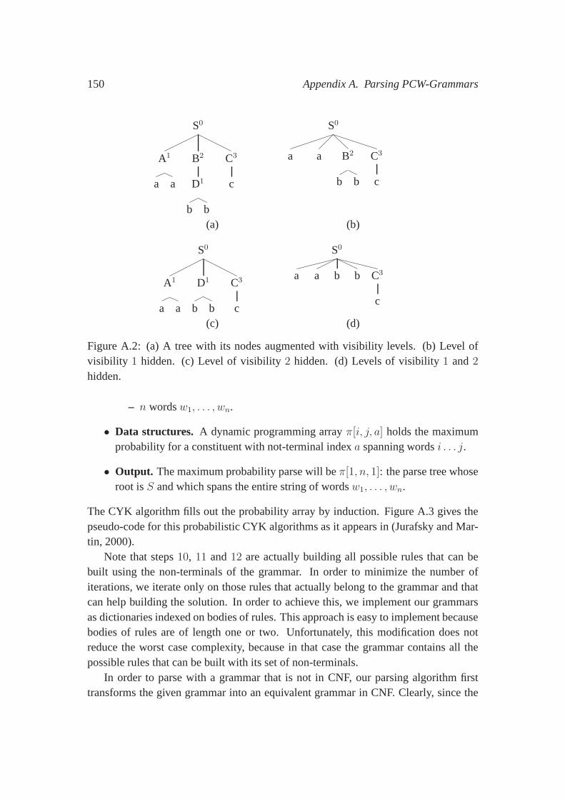
150 Appendix A. Parsing PCW-Grammars
S0
A1
a a
B2
D1
b b
C3
c
S0
a a B2
b b
C3
c
(a) (b)
S0
A1
a a
D1
b b
C3
c
S0
a a b b C3
c
(c) (d)
Figure A.2: (a) A tree with its nodes augmented with visibility levels. (b) Level ofvisibility 1 hidden. (c) Level of visibility2 hidden. (d) Levels of visibility1 and2
hidden.
– n wordsw1, . . . , wn.
• Data structures. A dynamic programming arrayπ[i, j, a] holds the maximumprobability for a constituent with not-terminal indexa spanning wordsi . . . j.
• Output. The maximum probability parse will beπ[1, n, 1]: the parse tree whoseroot isS and which spans the entire string of wordsw1, . . . , wn.
The CYK algorithm fills out the probability array by induction. Figure A.3 gives thepseudo-code for this probabilistic CYK algorithms as it appears in (Jurafsky and Mar-tin, 2000).
Note that steps10, 11 and12 are actually building all possible rules that can bebuilt using the non-terminals of the grammar. In order to minimize the number ofiterations, we iterate only on those rules that actually belong to the grammar and thatcan help building the solution. In order to achieve this, we implement our grammarsas dictionaries indexed on bodies of rules. This approach iseasy to implement becausebodies of rules are of length one or two. Unfortunately, thismodification does notreduce the worst case complexity, because in that case the grammar contains all thepossible rules that can be built with its set of non-terminals.
In order to parse with a grammar that is not in CNF, our parsingalgorithm firsttransforms the given grammar into an equivalent grammar in CNF. Clearly, since the
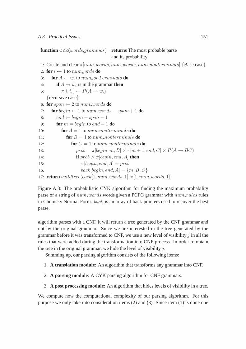
A.3. Practical Issues 151
function CYK(words,grammar) returns The most probable parseand its probability.
1: Create and clearπ[num words, num words, num nonterminals] {Base case}2: for i← 1 to numwords do3: for A← wi to numnonTerminals do4: if A→ wi is in the grammarthen5: π[i, i, ]← P (A→ wi)
{recursive case}6: for span← 2 to num words do7: for begin← 1 to num words− spam + 1 do8: end← begin+ span− 1
9: for m = begin to end− 1 do10: for A = 1 to num nonterminals do11: for B = 1 to num nonterminals do12: for C = 1 to num nonterminals do13: prob = π[begin,m,B]× π[m+ 1, end, C]× P (A→ BC)
14: if prob > π[begin, end, A] then15: π[begin, end, A] = prob
16: back[begin, end, A] = {m,B,C}17: return buildtree(back[1, num words, 1], π[1, num words, 1])
Figure A.3: The probabilistic CYK algorithm for finding the maximum probabilityparse of a string ofnum words words given a PCFG grammar withnum rules rulesin Chomsky Normal Form.back is an array of back-pointers used to recover the bestparse.
algorithm parses with a CNF, it will return a tree generated by the CNF grammar andnot by the original grammar. Since we are interested in the tree generated by thegrammar before it was transformed to CNF, we use a new level ofvisibility j in all therules that were added during the transformation into CNF process. In order to obtainthe tree in the original grammar, we hide the level of visibility j.
Summing up, our parsing algorithm consists of the followingitems:
1. A translation module: An algorithm that transforms any grammar into CNF.
2. A parsing module: A CYK parsing algorithm for CNF grammars.
3. A post processing module: An algorithm that hides levels of visibility in a tree.
We compute now the computational complexity of our parsing algorithm. For thispurpose we only take into consideration items (2) and (3). Since item (1) is done one
152 Appendix A. Parsing PCW-Grammars
time for each grammar, we only consider it indirectly: we take into consideration howthe transformation to CNF affects the size of the grammar.
We want to compute the computational complexity of the threeitems whenever agrammarG is used to parse a sentences.
By (Ney, 1991), the computational complexity of the CYK algorithm for parsing asentences using grammarG is 2nQ+ (n3/6)R, wheren is the length of the sentence,Q the number of preterminal rules in the grammar, andR the number of rules in thegrammar. Note that the number of rules and preterminal rulesrefer to the transformedgrammar.
According to (Hopcroft and Ullman, 1979), if a grammarG with R rules is trans-formed to CNF, the resulting grammar containsO(R2) rules. The complexity of thepost processing time depends on the number of rules in the CNFtree. Since a CNF treeyielding a sentence of lengthn has
∑n−1i=1 i rules, the post processing step takes time
∑n−1i=1 i. Finally, the complexity for the whole algorithm becomes2nQ+ (n3/6)R2.
A.4 Conclusions
In this appendix we have dealt with two particular aspects ofour implementation. First,we showed that it may happen that our implementation does notalways return the mostprobable tree. We also showed that there are some grammars for which our grammardoes return the most probable tree. For all grammars used in this thesis, however,the parser does return the most probable tree. We also showedthat the problem ofdetermining whether the parser returns the most probable tree or the most probablederivation tree is undecidable.
The second aspect we focused on was related to the actual implementation of theparser. We decomposed our implementation into three different modules, we gavethe computational complexity of each of them, and showed that the computationalcomplexity of the whole algorithm isO(n3R2), wheren is the length of the sentenceandR the size of the grammar.
Appendix B
Revising theSTOP Symbol for Markov Rules
B.1 The Importance of theSTOP Symbol
In this section we discuss Section 2.4.1 of Collins PhD thesis, where he discusses theimportance of theSTOP symbol for generating Markovian sequences. The idea is thatany sequence of strings that is generated by a Markovian process should end in aSTOPsymbol. He argues that without theSTOP symbol the probability distribution generatedby a Markovian process over finite strings is not really a probability distribution.
We argue that the even though theSTOP symbol is indeed important, the justifica-tion Collins provides is not fully correct. We show that the mere existence of theSTOPsymbol is not enough to guarantee consistency. We argue thatprobability distributionsgenerated by Markovian process over finite sequences of symbols should be thoughtof as probability distributions defined over infinite sequences of symbols instead ofprobability distributions defined over finite sequences.
The rest of the appendix is organized as follows. In Section B.2 we present Collins’sexplanation onSTOP symbols; in Section B.3 we provide background definitions onMarkov chains; in Section B.4 we use Markov chains for rethinking the importance ofSTOP symbols, and in Section B.5 we conclude the appendix.
B.2 Collins’s Explanation
Suppose we want to assign a probabilityp to sequences of symbolsw1, w2, w3, . . . , wn,where each symbolwi belongs to a finite alphabetΣ.
We first rewrite the probability of the given sequence using the chain rule of prob-
153
154 Appendix B. Revising theSTOP Symbol for Markov Rules
abilities as:
P (w1, w2, w3, . . . , wn) =
n∏
i=1
P (wi|w1, . . . , wi−1). (B.1)
Second, we usem-order Markovian independence assumptions and the equation abovebecomes:
P (w1, w2, w3, . . . , wn) =n
∏
i=1
P (wi|w1, . . . , wi−m). (B.2)
Collins (1999, page 46) argues that such a definition of probabilities is not correct: theproblems arises becausen, the sentence length, is variable. In his argumentation, hestates that Equation B.1 would be correct if the event space under consideration wouldhave been the space ofn-dimensional vectorsΣn instead of the set of all strings in thelanguageΣ∗. Writing the probability under consideration asP (w1, w2, w3, . . . , wn)
implies thatΣn is the event space. To avoid this confusion he writes the probabilityof a sequence〈w1, w2, . . . , wn〉 asP (〈w1, w2, . . . , wn〉): the angled braces imply that〈w1, w2, . . . , wn〉 is a sequence of variable length rather than ann-dimensional vector.
He states that in the case of speech recognition, the lengthn of strings is often largeand thatSTOP probabilities in that case may not be too significant. In Collins’s use ofMarkov processes, the sequences under consideration are typically of length0, 1 or 2,and for this case theSTOP probabilities certainly become important.
He presents the following example to support his point on thefailing of Equa-tion B.1
B.2.1.EXAMPLE . Consider the following.
• AssumeΣ = {a, b}, and therefore thatΣ∗ is {ǫ, a, b, aa, bb, ab, bb, . . .}.
• Assume that we will model the probability overΣ∗ with a 0’th order Markovprocess, with parametersP (a) = P (b) = 0.5
We can now calculate the probability of several strings using the formula in Equa-tion B.2:P (〈a〉) = 0.5, P (〈b〉) = 0.5, P (〈aa〉) = 0.52, P (〈bb〉) = 0.25 and so on. Wealready see from these4 probabilities that the sum, over the event space will be greaterthan1: P (〈a〉) + P (〈b〉) + P (〈aa〉) + P (〈bb〉) = 1.5!. An additional problem is thatthe probability of the empty string,P (〈〉), wheren = 0, is undefined.
Collins argues that addingSTOP symbols fixes this inconsistency. He addsSTOPsymbols with the parameters of the Markov process modified toinclude. For example,let P (a) = P (b) = 0.25, P (STOP) = 0.5). In this case we haveP (〈STOP〉) = 0.5,P (〈aSTOP〉) = 0.25 ∗ 0.5 = 0.125, P (〈bSTOP〉) = 0.25 ∗ 0.5 = 0.125, P (〈aaSTOP〉) =
0.252 ∗ 0.5 = 0.03125, P (〈bbSTOP〉) = 0.03125 and so on. Thus far the sum of
B.3. Background on Markov Chains 155
probabilities does not exceed1, and the distribution looks much better behaved. Wecan prove that the sum over all sequences is1 by noting that the probability of anysequence of lengthn is 0.25n ∗ 0.5, and that there are2n sequences of lengthn, giving:
∑
W∈Σ∗
=
∞∑
n=0
2n ∗ 0.25n ∗ 0.5
=
∞∑
n=0
0.5n ∗ 0.5
=
∞∑
n=0
0.5n+1
=
∞∑
n=0
0.5n
= 1
In a 0’th order Markov process the distribution over length of strings is related di-rectly toP (STOP) — the probability of a string having lengthn is the probability ofgeneratingn non-STOP symbols followed by theSTOP symbol:
P (length = n) = (1− P (STOP))n ∗ p(STOP).
With higher order Markov processes, where the probability is conditioned on pre-viously generated symbols, the conditional probabilityP (STOP|wi−m, . . . , wi−1) en-codes the preference for certain symbols or sequences of symbols to end or nor to enda sentence. For example, if we were building a bigram (1st order Markov) model ofEnglish we would expect the wordthe to end a sentence very rarely, and the corre-sponding parameterP (STOP|the) to be very low. TheSTOP symbol not only ensuresthe probability distributions to be well defined, but also tohave useful interpretation.
B.3 Background on Markov Chains
Markovian process like the one described in Example B.2.1 are better described throughMarkov chains (Taylor and Karlin, 1998).
B.3.1.DEFINITION. A Markov chainis 3-tupleM = (W,P, I) whereW is a set ofstates,P is a real|W |×|W |matrix with entries inR, such that
∑|W |j=1 pij = 1; pij is the
probability of jumping from statei to statej, andI is |W |-dimensional vector definingthe initial probability distribution.
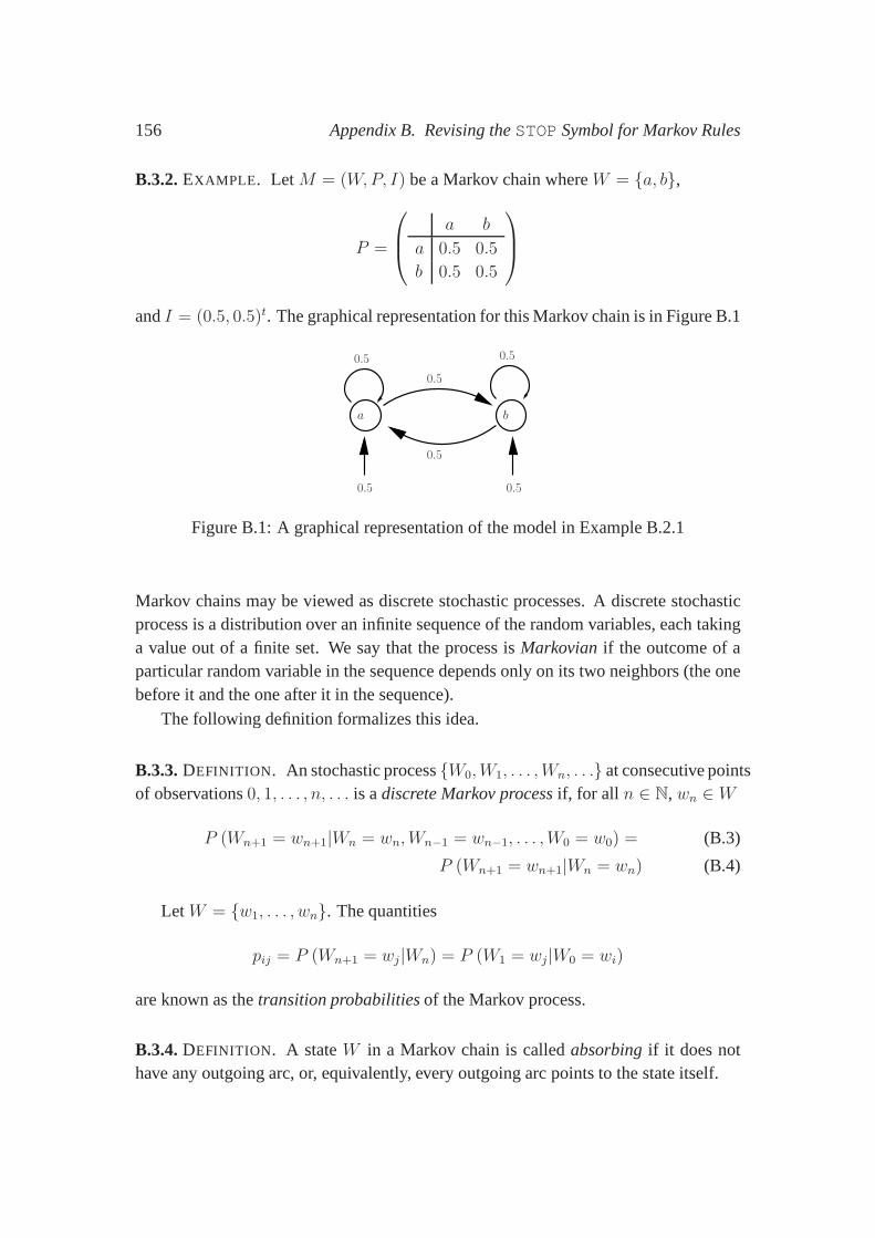
156 Appendix B. Revising theSTOP Symbol for Markov Rules
B.3.2.EXAMPLE . LetM = (W,P, I) be a Markov chain whereW = {a, b},
P =
a b
a 0.5 0.5
b 0.5 0.5
andI = (0.5, 0.5)t. The graphical representation for this Markov chain is in Figure B.1
ba
0.5 0.5
0.5
0.5
0.5 0.5
Figure B.1: A graphical representation of the model in Example B.2.1
Markov chains may be viewed as discrete stochastic processes. A discrete stochasticprocess is a distribution over an infinite sequence of the random variables, each takinga value out of a finite set. We say that the process isMarkovian if the outcome of aparticular random variable in the sequence depends only on its two neighbors (the onebefore it and the one after it in the sequence).
The following definition formalizes this idea.
B.3.3.DEFINITION. An stochastic process{W0,W1, . . . ,Wn, . . .} at consecutive pointsof observations0, 1, . . . , n, . . . is adiscrete Markov processif, for all n ∈ N, wn ∈W
P (Wn+1 = wn+1|Wn = wn,Wn−1 = wn−1, . . . ,W0 = w0) = (B.3)
P (Wn+1 = wn+1|Wn = wn) (B.4)
LetW = {w1, . . . , wn}. The quantities
pij = P (Wn+1 = wj|Wn) = P (W1 = wj|W0 = wi)
are known as thetransition probabilitiesof the Markov process.
B.3.4.DEFINITION. A stateW in a Markov chain is calledabsorbingif it does nothave any outgoing arc, or, equivalently, every outgoing arcpoints to the state itself.
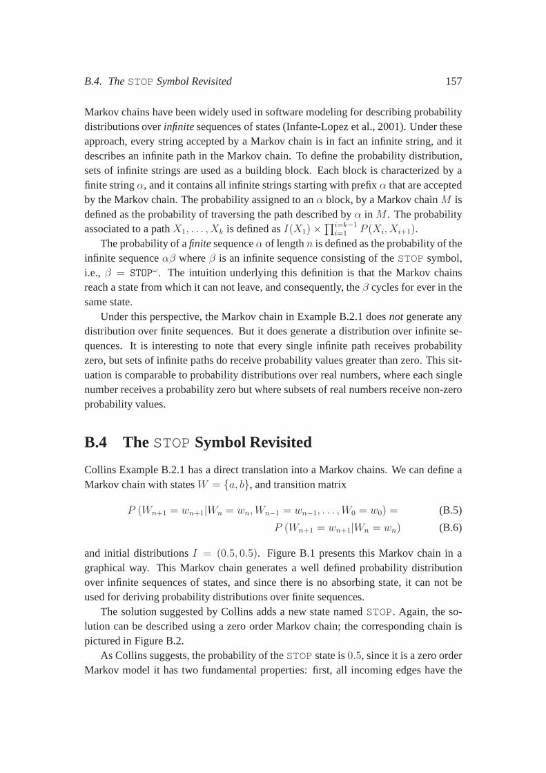
B.4. TheSTOP Symbol Revisited 157
Markov chains have been widely used in software modeling fordescribing probabilitydistributions overinfinitesequences of states (Infante-Lopez et al., 2001). Under theseapproach, every string accepted by a Markov chain is in fact an infinite string, and itdescribes an infinite path in the Markov chain. To define the probability distribution,sets of infinite strings are used as a building block. Each block is characterized by afinite stringα, and it contains all infinite strings starting with prefixα that are acceptedby the Markov chain. The probability assigned to anα block, by a Markov chainM isdefined as the probability of traversing the path described by α in M . The probabilityassociated to a pathX1, . . . , Xk is defined asI(X1)×
∏i=k−1i=1 P (Xi, Xi+1).
The probability of afinitesequenceα of lengthn is defined as the probability of theinfinite sequenceαβ whereβ is an infinite sequence consisting of theSTOP symbol,i.e., β = STOPω. The intuition underlying this definition is that the Markovchainsreach a state from which it can not leave, and consequently, theβ cycles for ever in thesame state.
Under this perspective, the Markov chain in Example B.2.1 doesnot generate anydistribution over finite sequences. But it does generate a distribution over infinite se-quences. It is interesting to note that every single infinitepath receives probabilityzero, but sets of infinite paths do receive probability values greater than zero. This sit-uation is comparable to probability distributions over real numbers, where each singlenumber receives a probability zero but where subsets of realnumbers receive non-zeroprobability values.
B.4 TheSTOP Symbol Revisited
Collins Example B.2.1 has a direct translation into a Markovchains. We can define aMarkov chain with statesW = {a, b}, and transition matrix
P (Wn+1 = wn+1|Wn = wn,Wn−1 = wn−1, . . . ,W0 = w0) = (B.5)
P (Wn+1 = wn+1|Wn = wn) (B.6)
and initial distributionsI = (0.5, 0.5). Figure B.1 presents this Markov chain in agraphical way. This Markov chain generates a well defined probability distributionover infinite sequences of states, and since there is no absorbing state, it can not beused for deriving probability distributions over finite sequences.
The solution suggested by Collins adds a new state namedSTOP. Again, the so-lution can be described using a zero order Markov chain; the corresponding chain ispictured in Figure B.2.
As Collins suggests, the probability of theSTOP state is0.5, since it is a zero orderMarkov model it has two fundamental properties: first, all incoming edges have the
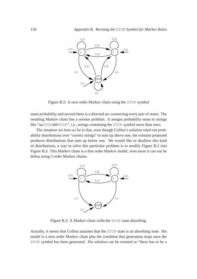
158 Appendix B. Revising theSTOP Symbol for Markov Rules
b
STOP
a0.25
0.250.25
0.25
0.25
0.25
0.5
0.50.5
0.25 0.25
0.5
Figure B.2: A zero order Markov chain using theSTOP symbol
same probability and second there is a directed arc connecting every pair of states. Theresulting Markov chain has a serious problem. It assigns probability mass to stringslike “aaSTOPabbSTOP”, i.e., strings containing theSTOP symbol more than once.
The situation we have so far is that, even though Collins’s solution ruled out prob-ability distributions over “correct strings” to sum up above one, the solution proposedproduces distributions that sum up below one. We would like to disallow this kindof distributions, a way to solve this particular problem is to modify Figure B.2 intoFigure B.3. This Markov chain is a first order Markov model, even more it cannot bedefine using0 order Markov chains.
b
STOP
a0.25
0.250.25
0.25
0.25
0.25
0.5
0.50.5
Figure B.3: A Markov chain witht theSTOP state absorbing.
Actually, it seems that Collins assumes that theSTOP state is an absorbing state. Hismodel is a zero order Markov chain plus the condition that generation stops once theSTOP symbol has been generated. His solution can be restated as “there has to be a
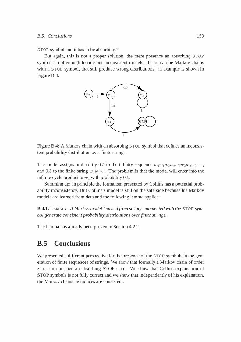
B.5. Conclusions 159
STOP symbol and it has to be absorbing.”But again, this is not a proper solution, the mere presence anabsorbingSTOP
symbol is not enough to rule out inconsistent models. There can be Markov chainswith a STOP symbol, that still produce wrong distributions; an exampleis shown inFigure B.4.
STOP
0.5
0.5
1
1
1
w0 w1
w3
w2
1
Figure B.4: A Markov chain with an absorbingSTOP symbol that defines an inconsis-tent probability distribution over finite strings.
The model assigns probability0.5 to the infinity sequencew0w1w2w2w2w2w2w2 . . .,and0.5 to the finite stringw0w1w3. The problem is that the model will enter into theinfinite cycle producingw4 with probability0.5.
Summing up: In principle the formalism presented by Collinshas a potential prob-ability inconsistency. But Collins’s model is still on the safe side because his Markovmodels are learned from data and the following lemma applies:
B.4.1.LEMMA . A Markov model learned from strings augmented with theSTOP sym-bol generate consistent probability distributions over finite strings.
The lemma has already been proven in Section 4.2.2.
B.5 Conclusions
We presented a different perspective for the presence of theSTOP symbols in the gen-eration of finite sequences of strings. We show that formallya Markov chain of orderzero can not have an absorbing STOP state. We show that Collins explanation ofSTOP symbols is not fully correct and we show that independently of his explanation,the Markov chains he induces are consistent.

Bibliography
Abney, S., 1996. Statistical methods and linguistics. In J.Klavans and P. Resnik (eds.),The Balancing Act: Combining Symbolic and Statistical Approaches to Language.Cambridge, MA: The MIT Press.
Abney, S., 1997. Stochastic attribute-value grammars.Computational Linguistics, 23(4):597–618.
Abney, S., D. McAllester, and F. Pereira, 1999. Relating probabilistic grammars andautomata. InProceedings of the 37th Annual Meeting of the ACL. Maryland.
Aho, A. and J. Ullman, 1972.The Theory of Parsing, Translation and Compiling,volume I. Prentice-Hall Series in Automatic Computation.
Alshawi, H., 1996. Head automata and bilingual tiling: Translation with minimalrepresentations. InProceedings of the 34th Annual Meeting of the Association forComputational Linguistics. Santa Cruz.
Andor, J., 2004. The master and his performance: An interview with Noam Chomsky.Intercultural Pragmatics, 1(1).
Atsumi, K. and S. Masuyama, 1998. On the ambiguity reductionability of a proba-bilistic context-free grammar.IEICE Transanctions on Fundamentals of Electronics,Communications and Computer Sciences, E81-A(5):825–831.
Berger, A., S. Della Pietra, and V. Della Pietra, 1996. A maximum entropy approachto natural language processing.Journal of Computational Linguistics, 22(1):39–71.
Bikel, D., 2004. Intricacies of Collins’ parsing model.Computational Linguistics. Toappear.
161
162 BIBLIOGRAPHY
Black, E., F. Jelinek, J. Lafferty, D. Magerman, R. Mercer, and S. Roukos, 1993. To-wards history-based grammars: Using richer models for probabilistic parsing. InProceedings of 31st Annual Meeting of the ACL. Ohio.
Bod, R., 1995.Enriching Linguistics with Statistics: Performance models of NaturalLanguage. Ph.D. thesis, University of Amsterdam, The Netherlands.
Bod, R., 1998.Beyond Grammar: An Experience-Based Theory of Language. Stan-ford: CSLI Publications.
Bod, R., 1999.Beyond Grammar — An Experience-Based Theory of Language. Eng-land: Cambridge University Press.
Bod, R., 2003. An efficient implementation of a new DOP model.In Proceedings ofthe 10th Conference of the European Chapter of the Association for ComputationalLinguistics. Budapest.
Booth, T. and R. Thompson, 1973. Applying probability measures to abstract lan-guages.IEEE Transaction on Computers., C-33(5):442–450.
Brew, C., 1995. Stochastic HPSG. InProceedings of the 7th Conference of the Euro-pean Chapter of the Association for Computational Linguistics. Dublin.
Brill, E., 1993. Automatic grammar induction and parsing free text: A transformation-based approach. InProceedings of the 31st Annual Meeting of the Association forComputational Linguistics. Ohio.
Brown, P., V. Della Pietra, P. de Souza, J. C. Lai, and R. L. Mercer, 1992. Class-basedn-gram models of natural language.Computational Linguistics, 18(4):467–479.
Buchholz, S., 2002.Memory-Based Grammatical Relation Finding. Ph.D. thesis,Universiteit van Tilburg.
Caraballo, S. and E. Charniak, 1998. New figures of merit for best-first probabilisticchart parsing.Computational Linguistics, 24-2:275–298.
Cardie, C., 1993a. A case-based approach to knowledge acquisition for domain-specific sentence analysis. InProceedings of the 11th National Conference on Arti-ficial Intelligence. AAAI Press / MIT Press.
Cardie, C., 1993b. Using decision trees to improve case-based learning. InProceedingsof the 10th International Conference on Machine Learning.
BIBLIOGRAPHY 163
Carrasco, R. and J. Oncina, 1994. Learning sthocastic regular grammars by means ofstate merging method. InGrammatical Inference and Applications, Springer LectureNotes in Artificial Intelligence. Berlin: Springer-Verlag.
Carrasco, R. and J. Oncina, 1999. Learning deterministic regular grammars fromstochastic samples in polynomial time.Theoretical Informatics and Applications,1(33):1–20.
Carreras, X., L. Marquez, V. Punyakanok, and D. Roth, 2002.Learning and infer-ence for clause identification. InProceedings of the 14th European Conference onMachine Learning.
Carrol, J., 1993.Practical Unification-based Parsing of Natural Language. Ph.D.thesis, Computer Lab., University of Cambridge.
Carroll, J., T. Briscoe, and A. Sanfilippo, 1998. Parser evaluation: a survey and anew proposal. InProceedings of the 1st International Conference on LanguageResources and Evaluation. Granada, Spain.
Carroll, J. and E. Charniak, 1992. Two experiments on learning probabilistic depen-dency grammars from corpora. InCarl Weir, Stephen Abney, Ralph Grishman, andRalph Weischedel (eds.), Working Notes of the Workshop Statistically-Based NLPTechniques. Menlo Park.
Carroll, J. and A. Fang, 2004. The automatic acquisition of verb subcategorisationsand their impact on the performance of an HPSG parser. InProceedings of the 1stInternational Joint Conference on Natural Language Processing (IJCNLP).
Charniak, E., 1995. Parsing with context-free grammars andword statistics. TechnicalReport CS-95-28, Department of Computer Science, Brown University, Providence.
Charniak, E., 1997. Statistical parsing with a context-free grammar and word statistics.In Proceedings of the 14th National Conference on Artificial Intelligence. MenloPark: AAAI Press/MIT Press.
Charniak, E., 1999. A maximum-entropy-inspired parser. InTechnical Report CS-99-12. Providence, Rhode Island.
Charniak, E., 2000. A Maximum-Entropy-Inspired Parser. InProceedings ANLP-NAACL’2000, Seattle, Washington.
Chastellier, G. and A. Colmerauer, 1969. W-Grammars. InProceedings of the 24thNational Conference.
164 BIBLIOGRAPHY
Chaudhuri, R. and A. N. V. Rao, 1986. Approximating grammar probabilities: Solutionof a conjecture.Journal of the ACM., 33(4):702–705.
Chi, Z. and S. Geman, 1998. Estimation of probabilistic context-free grammars.Com-putational Linguistics, 24(2):299–305.
Coello Coello, C., 1999. A comprehensive survey of evolutionary-based multiobjectiveoptimization techniques.Knowledge and Information Systems, 3(1):269–308.
Collins, M., 1996. A new statistical parser based on bigram lexical dependencies. InProceedings of the 34th Annual Meeting of the ACL.
Collins, M., 1997. Three generative, lexicalized models for statistical parsing. InProceedings of the 35th Annual Meeting of the ACL and the 8th Conference of theEuropean Chapter of the ACL. Madrid, Spain.
Collins, M., 1999. Head-Driven Statistical Models for Natural Language Parsing.Ph.D. thesis, University of Pennsylvania, PA.
Collins, M., 2000. Discriminative reranking for natural language parsing. InProceed-ings of the 7th International Conference on Machine Learning (ICML). Stanford.
Collins, M., 2001. Parameter estimation for statistical parsing models: Theory andpractice of distribution-free methods. InProceedings of the 7th International Work-shop on Parsing Technologies (Invited Talk). Beijing.
Collins, M. and N. Duffy, 2001. Convolution kernels for natural language. InProceed-ings of Neural Information Processing Systems (NIPS 14).
Collins, M. and N. Duffy, 2002. New ranking algorithms for parsing and tagging:Kernels over discrete structures, and the voted perceptron. In Proceedings of the40th Annual Meeting of the ACL.
Cortes, C. and M. Mohri, 2000. Context-free recognition with weighted automata.Grammars, 2-3(3).
Cover, T. and J. Thomas, 1991.Elements of Information Theory. New York: JonhWiley and Sons.
Daelemans, W., S. Buchholz, and J. Veenstra, 1999. Memory-based shallow pars-ing. In Proceedings of the Computational Natural Language Learning Workshop(CoNLL99). Bergen.
BIBLIOGRAPHY 165
Daelemans, W., A. van den Bosch, and A. Weijters, 1997. Igtree: using trees forcompression and classification in lazy learning algorithms. Artificial IntelligenceReview, 11:407–423.
Decadt, B. and W. Daelemans, 2004. Verb classification — machine learning experi-ments in classifying verbs into semantic classes. InProceedings of the LREC 2004Workshop Beyond Named Entity Recognition - Semantic Labelling for NLP Tasks.
Denis, F., 2001. Learning regular languages from simple positive examples.MachineLearning, 44(1/2):37–66.
Dupont, P. and L. Chase, 1998. Using symbol clustering to improve probabilisticautomaton inference. In V. Honavar and G. Slutzki (eds.),Lecture Notes in ComputerScience. Springer-Verlag.
Dupont, P., F. Denis, and Y. Esposito, 2004. Links between probabilistic automataand hidden markov models: probability distributions, learning models and induc-tion algorithms. to appear in Pattern Recognition: Special Issue on GrammaticalInference Techniques & Applications.
Dupont, P., L. Miclet, and E. Vidal, 1994. What is the search space of the regularinference? In R. Carrasco and J. Oncina (eds.),Lecture Notes in Computer Science.Springer-Verlag.
Eisner, J., 1996. Three new probabilistic models for dependency parsing: An explo-ration. InProceedings of 16th International Conference on Computational Linguis-tics (COLING). Copenhagen, Denmark.
Eisner, J., 2000. Bilexical grammars and their cubic-time parsing algorithms. InH. Bunt and A. Nijholt (eds.),Advances in Probabilistic and Other Parsing Tech-nologies. Kluwer Academic Publishers, pages 29–62.
Eisner, J. and G. Satta, 1999. Efficient parsing for bilexical context-free grammars andhead automaton grammars. InProceedings of the 37th Annual Meeting of the ACL.Maryland.
Gaifman, G., 1965. Dependency systems and phrase-structure systems.Informationand Control, 8(3):304–337.
Galen, A., T. Grenager, and C. Manning, 2004. Verb sense and subcategorization: Us-ing joint inference to inprove performance on complementary tasks. InProceedingsof Empirical Methods in Natural Language Processing (EMNLP).
166 BIBLIOGRAPHY
Gen, M. and R. Cheng, 1997.Genetic Algorithms and Engineering Design. New York:John Wiley and Sons.
Gold, E. M., 1967. Language identification in the limit.Information and Control,10:447–474.
Goodman, J., 1997. Probabilistic feature grammars. InProceedings of the 5th Inter-national Workshop on Parsing Technologies. MIT, Cambridge, MA.
Goodman, J., 1998.Parsing Inside-Out. PhD thesis, Departement of Computer Sci-ence, Harvard University, Cambridge, Massachusetts.
Hara, T., Y. Miyao, and J. Tsujii, 2002. Clustering for obtaining syntactic classes ofwords from automatically extracted ltag grammars. InProceedings of the sixth Inter-national Workshop on Tree Adjoining Grammars and Related Frameworks (TAG+6).
Hemphill, C., J. Godfrey, and G. Doddington, 1990. The ATIS Spoken LanguageSystems pilot corpus. InProceedings of the DARPA Speech and Natural LanguageWorkshop. Hidden Valley, Pa.
Henderson, J. and E. Brill, 1999. Exploiting diversity in natural language processing:Combining parsers. InProceedings of the 1999 Joint SIGDAT Conference on Em-pirical Methods in Natural Language Processing (EMNLP) andVery Large Corpora(VLC). Maryland.
Hermjakob, U. and R. J. Mooney, 1997. Learning parse and translation decisions fromexamples with rich context. InProceedings of the 35th Annual Meeting of the ACLand 8th Conference of the European Chapter of the ACL. Madrid.
Hopcroft, J. and J. Ullman, 1979.Introduction to Automata Theory, Lanaguges, andComputation. Reading, MA: Addison Wesley.
Horning, J. J., 1969. A study of grammatical inference. Unpublished doctoral disser-tation, Standford University.
Infante-Lopez, G. and M. de Rijke, 2003. Natural language parsing with W-grammars.CLIN03.
Infante-Lopez, G. and M. de Rijke, 2004a. Alternative approaches for generatingbodies of grammar rules. InProceedings of the 42nd Annual Meeting of the ACL.Barcelona.
Infante-Lopez, G. and M. de Rijke, 2004b. Comparing the ambiguity reduction abili-ties of probabilistic context-free grammars. InProceedings of LREC’04.
BIBLIOGRAPHY 167
Infante-Lopez, G., H. Hermanns, and J.-P. Katoen, 2001. Beyond memoryless distri-butions: Model checking semi-markov chains. InPAPM-ProbMiV 2001, SpringerLNCS 2165..
Infante-Lopez, G., K. Sim’aan, and M. de Rijke, 2002. A general model for depen-dency parsing. InProceedings of BNAIC’02.
Inui, K., V. Sornlertlamvanich, H. Tanaka, and T. Tokunaga,1998. Probabilistic GLRparsing: a new formatisation and its impact on parsing performance. Journal ofNatural Language Processing, 5(3).
Jelinek, F., J. Lafferty, D. Magerman, R. Mercer, A. Ratnaparkhi, and S. Roukos, 1994.Decision tree parsing using a hidden derivation model. InProceedings of the 1994Human Language Technology Workshop. DARPA.
Joan-Andreu, S. and J.-M. Benedı, 1997. Consistency of stochastic context-free gram-mars from probabilistic estimation based on growth transformations. IEEE Trans-actions on Pattern Analysis and Machine Intelligence, 19(9):1052–1055.
Johnson, M., 2002. The DOP estimation method is biased and inconsistent.Computa-tional Linguistics, 28(1):71–76.
Johnson, M., S. Geman, S. Canon, Z. Chi, and S. Riezler, 1999.Estimators for stochas-tic unification-based grammars. InProceedings of the 37th Annual Meeting of theACL. Maryland.
Joshi, A., 1985. Tree Adjoining Grammars: How much context sensitivity is requiredto provide a reasonable structural description. In I. K. D. Dowty and A. Zwicky(eds.),Natural Language Parsing. Cambridge, U.K.: Cambridge University Press.
Joshi, A., 1987. An introduction to tree adjoining grammars. In A. Manaster Ramer(ed.), Mathematics and Language. Amsterdam: John Benjamins Publishing Co,pages 87–115.
Joshi, A. and B. Srinivas, 1994. Disambiguation of super parts of speech (or supertags):Almost parsing. InProceedings of the 17th International Conference on Computa-tional Linguistics (COLING), Kyoto, Japan..
Jurafsky, D. and J. Martin, 2000.Speech and Language Processing: An Introduction toNatural Language Processing, Computational Linguistics,and Speech Recognition.Prentice Hall PTR.
Klein, D. and C. Manning, 2003. Accurate unlexicalized parsing. In Proceedings ofthe 41st Annual Meeting of the ACL.
168 BIBLIOGRAPHY
Krotov, A., M. Hepple, R. J. Gaizauskas, and Y. Wilks, 1998. Compacting the Penntreebank grammar. InProceedings of the 36th Annual Meeting of the ACL and 17thInternational Conference on Computational Linguistics COLING.
Kruijff, G., 2003. 3-Phase grammar learning. InProceedings of the Workshop on Ideasand Strategies for Multilingual Grammar Development.
Kucera, H. and W. N. Francis, 1967.Computational analysis of present-day AmericanEnglish. RI: Brown University Press.
Lafferty, J., D. Sleator, and D. Temperley, 1992. Grammatical trigrams: A probabilisticmodel of link grammar. InProceedings of the AAAI Conference on ProbabilisticApproaches to Natural Language Processing.
Levin, B., 1993.English Verb Classes and Alternations: A preliminary Investigation.Chicago: The University of Chicago Press.
Lin, D., 1995. A dependency-based method for evaluating broad-coverage parsers. InProceedings of IJCAI-95.
Magerman, D., 1995a.Parsing as Statistical Pattern Recognition. Ph.D. thesis, Stan-ford University.
Magerman, D., 1995b. Statistical decision-tree models forparsing. InProceedings ofthe 33rd Annual Meeting of the ACL. Cambridge, MA.
Magerman, D. and M. Marcus, 1991. Pearl: A Probabilistic Chart Parser. InProceed-ings the European Chapter of the ACL. Berlin.
Magerman, D. and C. Weir, 1992. Efficiency, robustness and accuracy in picky ChartParsing. InProceedings of the 30th Annual Meeting of the ACL. Newark, Delaware.
Manning, C., 1993. Automatic acquisition of a large subcategorization dictionary fromcorpora. InProceedings of the 31st Annual Meeting of the ACL.
Manning, C. and H. Schutze, 1999.Foundations of Statistical Natural Language Pro-cessing. The MIT Press, Cambridge, MA.
Marcus, M., G. Kim, M. Marcinkiewicz, R. MacIntyre, A. Bies,M. Ferguson, K. Katz,and B. Schasberger, 1994. The Penn treebank: Annotating predicate argument struc-ture. InARPA Human Language Technology Workshop.
Marcus, M., B. Santorini, and M. Marcinkiewicz, 1993. Building a large annotatedcorpus of English: The Penn treebank.Computational Linguistics, 19:313–330.
BIBLIOGRAPHY 169
Mateescu, A., 1989a. Van Wijngaarden grammars and systems.Annals University ofBucharest, 2:75–81.
Mateescu, A., 1989b. van Wijngaarden grammars and the generative complexity ofrecursively enumerable languages.Annals University of Bucharest, 2:49–54.
Mateescu, A. and A. Salomaa, 1997. Aspects of classical language theory. In Rozem-berg and Salomaa (1997), pages 175–251.
Merlo, P. and S. Stevenson, 2001. Automatic verb classification based on statisticaldistributions of argument structure.Computational Linguistics, 27(3):373–408.
Miikkulainen, R., 1996. Subsymbolic case-role analysis ofsentences with embeddedclauses.Cognitive Science, 1(20).
Mitchell, T., 1997.Machine Learning. McGraw-Hill Series in Computer Science.
Musillo, G. and K. Sima’an, 2002. Towards comparing parsersfrom different linguisticframeworks: An information theoretic approach. InProceedings of Beyond PARSE-VAL: Towards Improved Evaluation Measures for Parsing Systems, LREC’02. LasPalmas, Gran Canaria, Spain, 2002.
Nederhof, M.-J., A. Sarkar, and G. Satta, 1998. Prefix probabilities from probabilistictree adjoining grammars. InProceedings of the 36th Annual Meeting of the ACL and17th International Conference on Computational Linguistics (COLING). Montreal.
Nederhof, M.-J. and G. Satta, 2002. Probabilistic parsing strategies. In J. Dassow,M. Hoeberechts, H. Jurgensen, and D. Wotschke (eds.),Descriptional Complexityof Formal Systems (DCFS), Pre-Proceedings of a Workshop. London.
Ney, H., 1991. Dynamic programming parsing for context-free grammars in continu-ous speech recognition.IEEE Transactions on Signal Processing, 39(2):336–340.
Ney, H. and R. Kneser, 1993. Inproved clustering techniquesfor class-based statis-tical language modelling. InEuropean Conference on Speech Communication andTechnology..
Ng, S.-K. and M. Tomita, 1991. Probabilistic LR parsing for general contextfree gram-mars. InProceedings of the 2nd International Workshop on Parsing Technologies.
NIST, 2004. NIST/SEMATECH e-Handbook of Statistical Methods. NIST. URL:http://www.itl.nist.gov/div898/handbook/.
170 BIBLIOGRAPHY
Oncina, J. and P. Garcia, 1992. Inferring regular languagesin polynomial update time.In Pattern Recognition and Image Analysis, volume 1 of Series in Machine Percep-tion and Artificial Intelligence. pages 49–61.
Parikh, R. J., 1966. On context-free languages.Journal of the ACM, 13:570–581.
Perrault, R., 1984. On the mathematical properties of linguistic theories.Computa-tional Linguistics - Special issue on mathematical properties of grammatical for-malisms, 10(3-4):165–176.
Punyakanok, V. and D. Roth, 2000. The use of classifiers in sequential inference. InProceedings of NIPS-13, The 2000 Conference on Advances in Neural InformationProcessing Systems.
Qumsieh, A., 2003. Ai::genetic - a pure perl genetic algorithm implementation. PerlPackage, http://search.cpan.org/ aqumsieh/AI-Genetic-0.02/Genetic.pm.
Ratnaparkhi, A., 1997. A linear observed time statistical parser based on maximumentropy models. InEmpirical Methods in Natural Language Processing (EMNLP).
Ratnaparkhi, A., 1998.Maximum Entropy Models for Natural Language AmbiguityResolution. Ph.D. thesis, University of Pennsylvania.
Ratnaparkhi, A., 1999. Learning to parse natural language with maximum entropymodels.Machine Learning, 34:151–175.
Rayner, M. and D. Cater, 1996. Fast parsing using pruning andgrammar specialization.In Proceedings of the 34th Annual Meeting of the Association for ComputationalLinguistics. Santa Cruz.
Resnik, P., 1992. Probabilistic tree-adjoining grammar asa framework for statisticalnatural language processing. InProceedings of the 14th International Conferenceon Computational Linguistics (COLING). Nantes.
Rosenfeld, R., 1994.Adaptive Statistical Language Modeling: A Maximum EntropyApproach. Ph.D. thesis, University of Carnegie Mellon.
Rozemberg, G. and A. Salomaa (eds.), 1997.Handbook of Formal Languages.
Samuelsson, C., 1994. Grammar specialization through entropy thresholds. InPro-ceedings of the 32nd Annual Meeting of the ACL.
Sarkar, A., 2001. Applying co-training methods to statistical parsing. InProceed-ings of the 2nd Meeting of the North American Chapter of the ACL (NAACL 2001).Pittsburgh.
BIBLIOGRAPHY 171
Satta, G., 1998. Recognition and parsing for tree adjoininggrammars. InTutorialpresented at the 4th International Workshop on Tree Adjoining Grammars (TAG+4).Pennsylvania.
Satta, G., 2000. Parsing techniques for lexicalized context-free grammars. InProceed-ings of the 6th International Workshop on Parsing Technologies (IWPT). Trento,Italy.
Schabes, Y., 1992. Stochastic lexicalized tree-adjoininggrammars. InProceedings ofthe 14th International Conference on Computational Linguistics (COLING). Nantes.
Schapire, R. E. and Y. Singer, 1999. Improved boosting algorithms using confidence-rated predictions.Machine Learning, 37(3).
Sima’an, K., 2000. Tree-gram parsing: Lexical dependencies and structual relations.In Proceedings of the 38th Annual Meeting of the ACL. Hong Kong, China.
Sima’an, K. and L. Buratto, 2003. Backoff parameter estimation for the dop model. InProceedings of ECML.
Simmons, R. and Y. Yu, 1992. The acquisition and use of context-dependent grammarsfor English.Computational Linguistics, 4(18).
Sleator, D. and D. Temperley, 1991. Parsing English with a link grammar. TechnicalReport CMU-CS-91-196, Carnegie Mellon University, Schoolof Computer Science.
Sleator, D. and D. Temperley, 1993. Parsing English with a link grammar. InProceed-ings of the 3rd International Workshop on Parsing Technologies (IWPT). Bergen,Norway.
Srinivas, B., 1997.Complexity of Lexical Descriptions and its Relevance to PartialParsing. PhD thesis, Computer and Information Science, Universityof Pennsylva-nia.
Stevenson, S. and P. Merlo, 2000. Automatic lexical acquisition based on statisticaldistributions. In17th conference on Computational linguistics.
Taylor, H. and S. Karlin, 1998.An Introduction to Stochastic Modeling. AcademicPress.
Thollard, F., P. Dupont, and C. de la Higuera, 2000. Probabilistic DFA inference usingKullback-Leibler divergence and minimality. InProceedings of the 7th InternationalConference on Machine Learning (ICML). Stanford.
172 BIBLIOGRAPHY
Tjong Kim Sang, E. and H. Dejean, 2001. Introduction to the CoNLL-2001 sharedtask: clause identification. InProceedings of the Computational Natural LanguageLearning Workshop (CoNLL-2001). Toulouse.
Tomita, M., 1996.Efficient Parsing for Natural Language. The Netherlands: KluwerAcademic Publishers.
Van Wijngaarden, A., 1965. Orthogonal design and description of a formal language.Technical Report MR76, Mathematisch Centrum. Amsterdam.
Van Wijngaarden, A., 1969. Report on the algorithmic language ALGOL 68. Nu-merische Mathematik, 14:79–218.
Veenstra, J. and W. Daelemans, 2000. A memory-based alternative for connectionistshift-reduce parsing. Technical Report ILK Report 00-12.
Venable, P., 2001. Lynx: Building a statistical parser froma rule-based parser. InProceedings of the Student Research Workshop of the NAACL. Pittsburgh.
Watkinson, S. and S. Manandhar, 2001. Translating treebankannotation for evaluation.In Workshop on Evaluation for Language and Dialogue Systems, ACL/EACL.
Wetherell, C. S., 1980. Probabilistic languages: A review and some questions.ACMComputer Surveys., 4(12):361–379.
Wich, K., 2000. Exponential ambiguity of context-free grammars. InProceedings ofthe 4th International Conference on Developments in Language Theory.
Wich, K., 2001. Characterization of context-free languages with polynomiallybounded ambiguity. InProceedings of the 26th International Symposium on Math-ematical Foundations of Computer Science (MFCS).
Wood, M., 1993.Categorial Grammars. London: Routledge.
Wright, D., 1997. Understanding Statistics. An Introduction for the Social Sciences.London: Thousand Oaks, New Delhi: Sage.
Wright, J., 1990. LR parsing of probabilistic grammars withinput uncertainty forspeech recognition.Computer Speech and Language, 4:297–323.
Wright, J. and E. Wrigley, 1989. Probabilistic LR parsing for speech recognition. InProceedings of the 1st International Workshop on Parsing Technologies. Pittsburgh.
BIBLIOGRAPHY 173
Wright, J., E. Wrigley, and R. Sharman, 1991. Adaptive probabilistic generalized LRparsing. InProceedings of the 2nd International Workshop on Parsing Technologies.Cancun, Mexico.
Xia, F., C. Han, M. Palmer, and A. Joshi, 2001. Automaticallyextracting and com-paring lexicalized grammars for different languages. InProceedings of the 17thInternational Joint Conference on Artificial Intelligence(IJCAI 2001). Seattle.
Yoshinaga, N., 2004. Improving the accuracy of subcategorizations acquired fromcorpora. InStudent Session ACL04.
Zelle, J. and R. Mooney, 1996. Learning to parse database queries using inductivelogic programming. InProceedings of the 13th National Conference on ArtificialIntelligence. Portland, OR.


