J Optim Theory Appl (2009) 140: 419–430DOI 10.1007/s10957-008-9461-8

Two-Point Boundary Value Problems for DuffingEquations across Resonance

X.J. Chang · Q.D. Huang

Published online: 25 October 2008© Springer Science+Business Media, LLC 2008

Abstract In this paper, we consider the equation y′′ + f (x, y) = 0 with a nonres-onance condition of the form A ≤ fy(x, y) ≤ B, where (k − 1)2 < A ≤ k2 < · · · <

m2 ≤ B < (m + 1)2, k,m ∈ Z+. With optimal control theory and the Schauder fixed-

point theorem, by introducing a new cost functional, we obtain a new existence anduniqueness result for the above equation with two-point boundary-value conditions.

Keywords Boundary-value problems · Duffing equation · Resonance · Optimalcontrol · Schauder fixed-point theorem

1 Introduction

In this paper, we consider the following two-point boundary-value problem (BVP)

y′′ + f (x, y) = 0, (1)

y(0) = c, y(π) = d, (2)

where c, d ∈ R.In [1], Lazer and Leach proved that, if the Lazer-Leach condition

n2 < A ≤ fy(x, y) ≤ B < (n + 1)2, n ∈ Z+, (3)

Communicated by D.A. Carlson.

This work was supported by NSFC Grant 10501017 and 985 Project of Jilin University.

X.J. Chang (�)Institute of Mathematics, Jilin University, Changchun 130012, People’s Republic of Chinae-mail: changxj@email.jlu.edu.cn

Q.D. HuangCollege of Mathematics, Jilin University, Changchun 130012, People’s Republic of China

420 J Optim Theory Appl (2009) 140: 419–430

holds, then the BVP (1)–(2) has a unique solution. In general, the set {m2 : m ∈ Z+}

is called the set of resonance points for the BVP (1)–(2). Obviously, the Lazer-Leachcondition does not cross any point of resonance. Wang and Li [2] dealt with the casewhere the interval [A,B] contains many resonance points. There, they obtained thefollowing result.

Theorem 1.1 Assume that:

(i) f (x, y), fy(x, y) are continuous on [0,π] × R;(ii) A ≤ fy(x, y) ≤ β(x) ≤ B for (x, y) ∈ [0,π]×R, where (k−1)2 < A ≤ k2 ≤ B ,

k ∈ Z+;

(iii)∫ π

0 β(x)dx < (A+B)α1 +A, where α1 is the smallest positive root of the equa-tion

√A cot

(√A

π − x

2

)

= √B tan

(√B

x

2

)

.

Then, the BVP (1)–(2) has a unique solution.

As stated in [2], the authors defined a suitable admissible control set and a costfunctional J [u] ≡ ∫ π

0 u(x)dx, where u(x) is the admissible control function of thecorresponding linear problem, and then they applied optimal control theory combinedwith the Schauder fixed-point theorem to get Theorem 1.1. In their sense, if [A,B]does not contain any resonance points, i.e., the Lazer-Leach condition holds, the ad-missible set is empty and consequently the linear problem corresponding to BVP(1)–(2) has only a trivial solution which shows that the BVP (1)–(2) has a uniquesolution. With the same idea, they have investigated several BVPs of ordinary dif-ferential equations crossing resonance [3–8]. However, if the condition (iii) is notsatisfied, i.e.,

∫ π

0 fy(x, y)dx ≥ (A + B)α1 + A, then when does BVP (1)–(2) have aunique solution? In this paper, again by utilizing the ideas of optimal control theory,we introduce a new cost functional to partially give an answer to this question. In ourdiscussion, the cost functional J [u] are defined by J [u] ≡ ∫ π

0 |u(x) − L|dx, whereu(x) is the admissible control function of the corresponding linear problem, L ∈ R

+has the same bound with u(x) and L �= n2 for any n ∈ Z

+. With the same reasonas in [2], we can also obtain the Lazer-Leach result. Furthermore, some interestingapplications of optimal control theory to BVPs for ordinary differential equationswere presented in [9–18]. However, the conditions mentioned there are actually notall across points of resonance, a situation different from ours.

Throughout the paper, we make the following assumptions.

(H1) f (x, y), fy(x, y) are continuous on [0,π] × R;(H2) A ≤ fy(x, y),L ≤ B , where A,B,L ∈ R

+ and there are positive integers k,m

such that (k − 1)2 < A ≤ k2 < · · · < m2 ≤ B < (m + 1)2. In addition, L �= n2

for any n ∈ Z+.

Now, we state the main result of this paper.

Theorem 1.2 Suppose that (H1)–(H2) hold. Assume that one of the following condi-tions is satisfied:

J Optim Theory Appl (2009) 140: 419–430 421

(i) (k − 1)2 < A ≤ L < k2 < · · · < m2 ≤ B < (m + 1)2 and∫ π

0|fy(x, y) − L|dx ≤ μ < (B − L)αk,

for some μ > 0, where αk is the smallest positive root of the equation

√L cot

(√L

2k(π − x)

)

= √B tan

(√B

2kx

)

; (4)

(ii) (k − 1)2 < A ≤ k2 < · · · < m2 < L ≤ B < (m + 1)2 and∫ π

0|fy(x, y) − L|dx ≤ μ < (L − A)αm,

for some μ > 0, where αm is the smallest positive root of the equation

√L cot

(√L

2m(π − x)

)

= √A tan

(√A

2mx

)

; (5)

(iii) (k − 1)2 < A ≤ k2 < · · · < (r − 1)2 < L < r2 < · · · < m2 ≤ B < (m + 1)2 and∫ π

0|fy(x, y) − L|dx ≤ μ < min{(L − A)αr−1, (B − L)αr}

for some μ > 0, where αr−1 and αr are respectively the smallest positive rootsof the following equations:

√L cot

( √L

2(r − 1)(π − x)

)

= √A tan

( √A

2(r − 1)x

)

(6)

and

√L cot

(√L

2r(π − x)

)

= √B tan

(√B

2rx

)

. (7)

Then, the BVP (1)–(2) has a unique solution.

Remark 1.1 Let us compare Theorem 1.1 with Theorem 1.2. When one of the condi-tions (i), (ii), (iii) in Theorem 1.2 is satisfied while condition (iii) in Theorem 1.1 isnot, the BVP (1)–(2) still has a unique solution.

The paper is organized as follows. In Sect. 2, we consider the problem of linearDuffing equations across resonance. With the optimal control theory method, intro-ducing a suitable admissible set and a cost functional, we obtain an explicit form ofthe optimal control functions and the existence and uniqueness of nontrivial solutionsof the linear problem. In Sect. 3, as an application of the results in Sect. 2, we givethe proof of our main result. Finally, in Sect. 4, we state the conclusions.

422 J Optim Theory Appl (2009) 140: 419–430

2 Linear Problem

This section concerns the linear BVP

y′′ + u(x)y = 0, (8)

y(0) = y(π) = 0. (9)

Here, B > A > 0 are given and A ≤ u(x) ≤ B .We seek a function u = u∗(x) with A ≤ u∗(x) ≤ B such that, for every u(x) ∈

L1[0,π], A ≤ u(x) ≤ B , if∫ π

0|u(x) − L|dx <

∫ π

0|u∗(x) − L|dx,

L ∈ [A,B] being given, then the BVP (8)–(9) has only the trivial solution y(x) ≡ 0.Define the admissible set and the cost functional as follows:

� = {u(x) ∈ L1[0,π] : A ≤ u(x),L ≤ B, (8)–(9) has a nontrivial solution},J [u] ≡

∫ π

0|u(x) − L|dx, u ∈ �.

This leads the BVP (8)–(9) to be an optimal control problem.

Remark 2.1 We point out here that the fact that L �= n2 for any n ∈ Z+ is very impor-

tant. If not, i.e., L = n2 for some n ∈ Z+ with n ∈ [A,B], we just take u∗(x) ≡ n2;

consequently J [u∗] = 0, which then implies that the method outlined above is notvalid.

Note that u∗(x) ≡ k2 ∈ �, so � is nonempty. With a standard argument, we havethe following lemma as in [2].

Lemma 2.1 There exists a u∗ ∈ � such that

J [u∗] = inf�

J [u].

To obtain our results, we need some auxiliary lemmas.

Lemma 2.2 Let a, b ∈ R+. Define

ρ(x) = 2√a

arcsin(√

ax) + 2√b

arccos

√bx

√1 + (b − a)x2

.

If there exists n ∈ Z+ such that min{a, b} ≤ n2 ≤ max{a, b}, then the equation

ρ(x) = πn

has a unique positive root on [0, 1√a].

Proof By direct computation, we have

ρ(0) = π√b, ρ

(1√a

)

= π√a, ρ′(x) = 2√

1 − ax2

(b − a)x2

1 + (b − a)x2.

J Optim Theory Appl (2009) 140: 419–430 423

Then, we can easily obtain the result. �

Remark 2.2 If n2 < min{a, b} ≤ max{a, b} ≤ (n + 1)2 holds for some n ∈ Z+, a

similar discussion to that in Lemma 2.2 shows that ρ(x) = πn

has no root.

Lemma 2.3 The equation

√a cot(

√aλ(π − x)) = √

b tan(√

bλx) (10)

has the smallest positive root α(λ) for every λ ∈ I1 ≡ [ 12m

, 12k

], where (k − 1)2 <

min{a, b} ≤ k2 < · · · < m2 ≤ max{a, b} < (m + 1)2. In addition, we have

d

dλα(λ) =

{< 0, if a < b,

> 0, if a > b.

Proof Denote f1(x) = √a cot(

√aλ(π − x)), f2(x) = √

b tan(√

bλx). Assume thata > b. When (k − 1)2 < b < k2, for any λ ∈ I1, it is not difficult to see that f1(x) andf2(x) are both strictly increasing on [0,π] and we have

f1(0) < 0 < f1(π) = +∞, f2(0) = 0 < f2(π) < +∞.

Hence, (10) has the smallest positive root α(λ). When b = k2, the argument is thesame as above for λ ∈ I1 \ { 1

2k}. When b = k2 and λ = 1

2k, we have α(λ) = π .

If a < b, the proof is completely similar to that of Lemma 1.2 in [2].A simple derivation shows that

dα(λ)

dλ= −a(1 + cot2(

√aλ(π − α(λ)))π + (b − a)α(λ)

λ(b − a).

Therefore, the conclusion is easily obtained. �

Now, we consider the problem (8)–(9) with min{a, b} ≤ u(x) ≤ max{a, b}, wherea, b ∈ R

+. Define the corresponding admissible set and cost functional by

� = {u(x) ∈ L1[0,π] : min{a, b} ≤ u(x) ≤ max{a, b},(8)–(9) has a nontrivial solution}

and

J [u] ≡∫ π

0|u(x) − a|dx, u ∈ �.

Then, we have the same optimal control as in Lemma 2.1 and the following lemma.

424 J Optim Theory Appl (2009) 140: 419–430

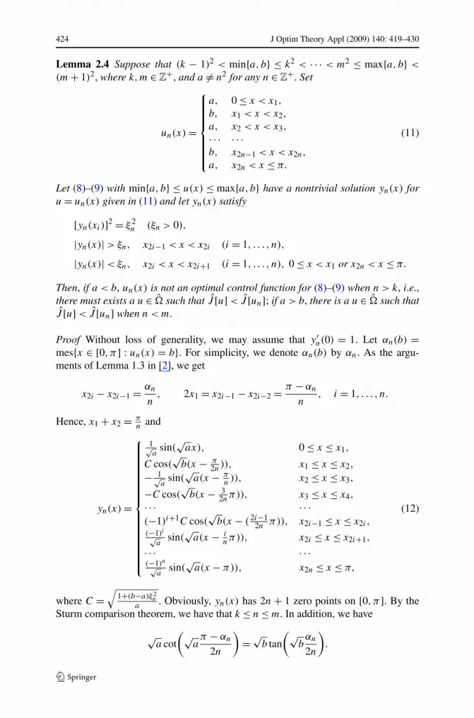
Lemma 2.4 Suppose that (k − 1)2 < min{a, b} ≤ k2 < · · · < m2 ≤ max{a, b} <

(m + 1)2, where k,m ∈ Z+, and a �= n2 for any n ∈ Z

+. Set

un(x) =

⎧⎪⎪⎪⎪⎪⎪⎨

⎪⎪⎪⎪⎪⎪⎩

a, 0 ≤ x < x1,

b, x1 < x < x2,

a, x2 < x < x3,

· · · · · ·b, x2n−1 < x < x2n,

a, x2n < x ≤ π.

(11)

Let (8)–(9) with min{a, b} ≤ u(x) ≤ max{a, b} have a nontrivial solution yn(x) foru = un(x) given in (11) and let yn(x) satisfy

[yn(xi)]2 = ξ2n (ξn > 0),

|yn(x)| > ξn, x2i−1 < x < x2i (i = 1, . . . , n),

|yn(x)| < ξn, x2i < x < x2i+1 (i = 1, . . . , n), 0 ≤ x < x1 or x2n < x ≤ π.

Then, if a < b, un(x) is not an optimal control function for (8)–(9) when n > k, i.e.,there must exists a u ∈ � such that J [u] < J [un]; if a > b, there is a u ∈ � such thatJ [u] < J [un] when n < m.

Proof Without loss of generality, we may assume that y′n(0) = 1. Let αn(b) =

mes{x ∈ [0,π] : un(x) = b}. For simplicity, we denote αn(b) by αn. As the argu-ments of Lemma 1.3 in [2], we get

x2i − x2i−1 = αn

n, 2x1 = x2i−1 − x2i−2 = π − αn

n, i = 1, . . . , n.

Hence, x1 + x2 = πn

and

yn(x) =

⎧⎪⎪⎪⎪⎪⎪⎪⎪⎪⎪⎪⎪⎪⎪⎪⎨

⎪⎪⎪⎪⎪⎪⎪⎪⎪⎪⎪⎪⎪⎪⎪⎩

1√a

sin(√

ax), 0 ≤ x ≤ x1,

C cos(√

b(x − π2n

)), x1 ≤ x ≤ x2,

− 1√a

sin(√

a(x − πn)), x2 ≤ x ≤ x3,

−C cos(√

b(x − 32n

π)), x3 ≤ x ≤ x4,

· · · · · ·(−1)i+1C cos(

√b(x − ( 2i−1

2nπ)), x2i−1 ≤ x ≤ x2i ,

(−1)i√a

sin(√

a(x − inπ)), x2i ≤ x ≤ x2i+1,

· · · · · ·(−1)n√

asin(

√a(x − π)), x2n ≤ x ≤ π,

(12)

where C =√

1+(b−a)ξ2n

a. Obviously, yn(x) has 2n + 1 zero points on [0,π]. By the

Sturm comparison theorem, we have that k ≤ n ≤ m. In addition, we have

√a cot

(√aπ − αn

2n

)

= √b tan

(√bαn

2n

)

.

J Optim Theory Appl (2009) 140: 419–430 425

By (12)∫ π

0|un(x) − a|dx = |b − a|αn.

Let

uk(x) =

⎧⎪⎪⎪⎪⎪⎪⎪⎪⎪⎨

⎪⎪⎪⎪⎪⎪⎪⎪⎪⎩

a, 0 ≤ x <π−αk

2k,

b,π−αk

2k< x <

π+αk

2k,

· · · · · ·a,

(2i−1)π+αk

2k< x <

(2i+1)π−αk

2k,

b,(2i+1)π−αk

2k< x <

(2i+1)π+αk

2k,

· · · · · ·a,

(2k−1)π+αk

2k< x ≤ π,

(13)

where αk = α( 12k

) is the smallest positive root of (10). If a < b, by Lemma 2.3, whenn > k, we have

∫ π

0|uk(x) − a|dx = (b − a)αk < (b − a)αn =

∫ π

0|un(x) − a|dx.

If a > b, the discussion is similar. The proof is completed. �

Remark 2.3 When a < b, Lemma 2.4 reduces to Lemma 1.3 in [2].

Theorem 2.1 Let (k − 1)2 < A ≤ k2 < · · · < m2 ≤ B < (m + 1)2. We have:

(i) If (k − 1)2 < A ≤ L < k2 < · · · < m2 ≤ B < (m + 1)2, then the optimal controlfunction u∗(x) of problem (8)–(9) has the form (13), where a = L,b = B .

(ii) If (k − 1)2 < A ≤ k2 < · · · < m2 < L ≤ B < (m + 1)2, then the optimal controlfunction u∗(x) takes the form (13) for a = L,b = A.

(iii) If (k − 1)2 < A ≤ k2 < · · · < (r − 1)2 < L < r2 < · · · < m2 ≤ B < (m + 1)2,where r ∈ Z

+, then if (B −L)αr > (L−A)αr−1, we have u∗(x) = ur−1; if (B −L)αr < (L − A)αr−1, we have u∗(x) = ur . Here αr−1 and αr are respectivelythe smallest positive roots of (6) and (7), ur−1 takes the form (13) with k replacedby r − 1 for a = L,b = A, ur takes the form (13) with k replaced by r fora = L,b = B .

Proof Obviously, � is nonempty. Then, by Lemma 2.1, u∗(x) exists. Let y1 = y,y2 = y′. Then, y′′ + u∗(x)y = 0 is transformed into

y′1 = y2, y′

2 = −u∗(x)y1.

From the Pontryagin maximum principle (see [19]), the Hamiltonian is

H ≡ −sign(u∗(x) − L)(u∗(x) − L) + λ1y2 + λ2(−u∗(x)y1)

= −[sign(u∗(x) − L) + λ2y1]u∗(x) + λ1y2 + sign(u∗(x) − L)L,

426 J Optim Theory Appl (2009) 140: 419–430

with adjoint equations

dλ1

dx= u∗λ2,

dλ2

dx= −λ1,

and transversality condition

λ2(0) = λ2(π) = 0.

If λ2y1 ≥ 1, when L ≤ u∗(x) ≤ B , it is easy to obtain that u∗(x) = L andH = −λ2y1L + λ1y2. When A ≤ u∗(x) ≤ L, similarly we have u∗(x) = A andH = −(−1 + λ2y1)A + λ1y2 − L. However,

−λ2y1L + λ1y2 − (−(−1 + λ2y1)A + λ1y2 − L)

= (A − L)(λ2y1 − 1) ≤ 0.

Hence, u∗(x) = A.If −1 < λ2y1 < 1, an analogous argument implies that, when u∗(x) = L, we have

the maximum H = −λ2y1L + λ1y2.If λ2y1 ≤ −1, we have u∗ = B and H = −(1 + λ2y1)B + λ1y2 + L.

Then, u∗ takes the following form:

u∗(x) =⎧⎨

⎩

A, λ2(x)y1(x) ≥ 1,

L, −1 ≤ λ2(x)y1(x) ≤ 1,

B, λ2(x)y1(x) ≤ −1,

where y1(x) is a nontrivial solution of (8)–(9) for u = u∗(x). Note that λ2(x) andy1(x) are all solutions of (8)–(9). Hence, there exists a constant c �= 0 such thatλ2(x) = cy1(x), for x ∈ [0,π]. Thus, 1 + λ2(x)y1(x) = 1 + cy2

1(x). Consequently,

u∗(x) =⎧⎨

⎩

A, cy21(x) ≥ 1,

L, −1 ≤ cy21(x) ≤ 1,

B, cy21(x) ≤ −1.

If (k − 1)2 < A ≤ L < k2 < · · · < m2 ≤ B < (m+ 1)2, we claim that c < 0. If not,we have c > 0 and

u∗(x) =⎧⎨

⎩

A, |y1(x)| ≥√

1c,

L, |y1(x)| ≤√

1c.

By Theorem 1.4 in [6], we see that the BVP

y′′ + u(x)y = 0, y(0) = y(π) = 0

has only a trivial solution, which is contrary to the fact that u∗ ∈ �. Therefore, theclaim of the theorem is correct. So,

u∗(x) =⎧⎨

⎩

B, |y1(x)| ≥√

− 1c,

L, |y1(x)| ≤√

− 1c.

J Optim Theory Appl (2009) 140: 419–430 427

Let

S = {x ∈ [0,1] : cy21(x) = −1}.

By the Sturm comparison theorem, S is finite. Without loss of generality, we may

assume y′(0) = 1. Then, by the expression of u∗(x), y(x) =√

−1c

≡ ξ , for x ∈ S,

and by the proof of Lemma 2.4 with a = L,b = B , we see that u∗ and y(x) havethe forms of un(x) and yn(x) given in Lemma 2.4. By Lemma 2.4, n ≤ k, and againby the Sturm comparison theorem, n ≥ k. Hence, n = k, i.e., u∗(x) = uk(x), whereuk(x) is given in (13) for a = L,b = B .

Let (k − 1)2 < A ≤ k2 < · · · < m2 < L ≤ B < (m + 1)2. With analogous dis-cussion as above, we have u∗(x) = um(x), where um(x) takes the form (13) with k

replaced by m for a = L,b = A.Let (k − 1)2 < A ≤ k2 < · · · < (r − 1)2 < L < r2 < · · · < m2 ≤ B < (m + 1)2,

where r ∈ Z+ and r ∈ [k,m]. Similarly, when c < 0, we have u∗(x) = ur(x), where

ur(x) is given in (13) with k replaced by r and αr = α( 12r

) is the smallest positive rootof (10) for a = L,b = B , and J [u∗] = (B − L)αr . When c > 0, u∗(x) = ur−1(x),where ur−1(x) takes the form (13) with k replaced by r − 1 for a = L,b = A, andJ [u∗] = (L−A)αr−1. Then, if (B −L)αr > (L−A)αr−1, by the optimality propertyof u∗, there must be c > 0, so we have u∗(x) = ur−1; if (B − L)αr < (L − A)αr−1,

similarly we have u∗(x) = ur .This completes the proof. �From this theorem, we have the main result of this section as follows.

Theorem 2.2 Let (k − 1)2 < A ≤ k2 < · · · < m2 ≤ B < (m + 1)2 and A ≤ u(x),L ≤ B . Let one of the following conditions holds:

(i) (k − 1)2 < A ≤ L < k2 < · · · < m2 ≤ B < (m + 1)2 and∫ π

0|u(x) − L|dx ≤ μ < (B − L)αk,

for some μ > 0, where αk is the minimal positive root of (4);(ii) (k − 1)2 < A ≤ k2 < · · · < m2 < L ≤ B < (m + 1)2 and

∫ π

0|u(x) − L|dx ≤ μ < (L − A)αm,

for some μ > 0, where αm is the minimal positive root of (5);(iii) (k − 1)2 < A ≤ k2 < · · · < (r − 1)2 < L < r2 < · · · < m2 ≤ B < (m + 1)2 and

∫ π

0|u(x) − L|dx ≤ μ < min{(L − A)αr−1, (B − L)αr },

for some μ > 0, where αr−1 and αr are respectively the smallest positive rootsof (6) and (7).

Then the BVP

y′′ + u(x)y = h(x), y(0) = c, y(π) = d (14)

has a unique solution for each h ∈ L1[0,π].

428 J Optim Theory Appl (2009) 140: 419–430

3 Proof of Theorem 1.2

Proof Let us suppose that condition (i) holds; the proof for (ii) and (iii) is totallyanalogous.

We first prove uniqueness. Let y1(x) and y2(x) be any two solutions of the BVP(1)–(2). Then, y(x) = y1(x) − y2(x) is a solution of the problem

y′′ +∫ 1

0fy(x, y2(x) + θy(x))dθy = 0, y(0) = y(π) = 0.

From assumption (i), it follows that

∫ π

0

∣∣∣∣

∫ 1

0fy(x, y2(x) + θy(x))dθ − L

∣∣∣∣dx

≤∫ π

0

∫ 1

0|(fy(x, y2(x) + θy(x)) − L)|dθdx

≤ μ < (B − L)αk,

where αk is the smallest positive root of (4). Owing to Theorem 2.2(i), we obtain thaty(x) ≡ 0.

Now, we prove existence. Rewrite (1) in the equivalent form

y′′ + b(x, y)y = −f (x,0), (15)

where b(x, y) = ∫ 10 fy(x, θy)dθ . Then, condition (i) allows us to apply Theorem 2.2

in order to have a well-posed operator P : X → X, Pz = yz, with yz the uniquesolution of the BVP

y′′ + b(x, z)y = −f (x,0), y(0) = c, y(π) = d,

where z ∈ X ≡ C1([0,π],R) with the norm ‖ · ‖ defined by ‖z‖ = max[0,π] |z(x)| +max[0,π] |z′(x)|. A standard argument shows that P is completely continuous.

We will prove that PX is bounded, which together with the Schauder fixed-pointtheorem provides for P a fixed point which is a solution of (1)–(2). In fact, if not, therewould exist a sequence {zn(x)} ⊂ X such that ‖yzn‖ → ∞(n → ∞). Noting that A ≤b(x, zn(x)) ≤ B , x ∈ [0,π], passing to a subsequence if necessary, we may assumethat b(x, zn(x)) is weakly convergent in L2[0,π] to a function V0(x) satisfying A ≤V0(x) ≤ B a.e. in �. In addition, by the Fatou lemma, we have

∫ π

0|V0(x) − L|dx ≤ lim

n⇀∞

∫ π

0|b(x, zn(x)) − L|dx ≤ μ < (B − L)αk.

On the other hand, by the Arzela-Ascoli theorem, passing to a subsequence ifnecessary, we may assume that

yzn

‖yzn‖→ y0,

y′zn

‖yzn‖→ w0, n → ∞,

J Optim Theory Appl (2009) 140: 419–430 429

uniformly on [0,π] for suitable y0,w0 ∈ C1[0,π]. It is easily seen that ‖y0‖ = 1 andy0(x) is a nontrivial solution of the BVP

y′′ + V0(x)y = 0, y(0) = y(π) = 0. (16)

Clearly, V0(x) satisfies Theorem 2.2(i), which implies that problem (16) has a uniquesolution y0(x) ≡ 0, a contradiction. This completes the proof. �

4 Conclusions

In this paper, we have explored the use of optimal control theory combined withthe Schauder fixed-point theorem for determining solutions of two-point BVPs forDuffing equations across resonance. By introducing a new cost functional, we getan existence and uniqueness result of above problem containing the cases that can-not be dealt with in [2], which is an extension of this method for BVPs of ordinarydifferential equations across resonance.

References

1. Lazer, A.C., Leach, D.E.: On a nonlinear two-point boundary value problem. J. Math. Anal. Appl. 26,20–27 (1969)

2. Wang, H., Li, Y.: Two point boundary value problems for second order ordinary differential equationsacross many resonant points. J. Math. Anal. Appl. 179, 61–75 (1993)

3. Li, Y., Wang, H.: Neumann problems for second order ordinary differential equations across reso-nance. Z. Angew. Math. Phys. 46, 393–406 (1995)

4. Lin, Y.H., Li, Y., Zhou, Q.D.: Second order boundary value problems for nonlinear ordinary differen-tial equations across resonance. Nonlinear Anal. 28, 999–1009 (1997)

5. Wang, H., Li, Y.: Existence and uniquness of periodic solutions for duffing equations across manypoints of resonance. J. Differ. Equ. 108, 152–169 (1994)

6. Wang, H., Li, Y.: Periodic solutions for duffing equations. Nonlinear Anal. 24, 961–979 (1995)7. Wang, H., Li, Y.: Neumann boundary value problems for second-order ordinary differential equations

across resonance. SIAM J. Control Optim. 33(5), 1312–1325 (1995)8. Wang, H., Li, Y.: Existence and uniquness of solutions to two point boundary value problems for

ordinary differential equations. Z. Angew. Math. Phys. 47, 373–384 (1996)9. Melentsova, Yu., Mil’shtein, G.N.: An optimal estimate of the interval on which a multipoint boundary

value problem possesses a solution. Differ. Equ. 10, 1257–1265 (1974)10. Eloe, P.W., Henderson, J.: Optimal intervals for third order Lipschitz equations. Differ. Integral Equ.

2, 397–404 (1989)11. Henderson, D., Henderson, J.: Optimality for boundary value problems for Lipschitz equations. J. Dif-

fer. Equ. 77, 392–404 (1989)12. Henderson, J.: Best interval lengths for boundary value problems for third order Lipschitz equations.

SIAM J. Math. Anal. 18, 293–305 (1987)13. Henderson, J.: Boundary value problems for Nth order Lipschitz equations. J. Math. Anal. Appl. 134,

196–210 (1988)14. Henderson, J., Mcgwier, R.: Uniqueness, existence and optimality for fourth order Lipschitz equa-

tions. J. Differ. Equ. 67, 414–440 (1987)15. Jackson, L.K.: Existence and uniqueness of solutions for boundary value for Lipschitz equations.

J. Differ. Equ. 32, 76–90 (1979)16. Jackson, L.K.: Boundary value problems for Lipschitz equations. In: Differential Equations (Pro-

ceeding of the Eighth Fall Conference), Oklahoma State University, Stillwater, Oklahoma, 1979, pp.31–50. Academic Press, New York (1980)

430 J Optim Theory Appl (2009) 140: 419–430

17. Melentsova, Yu.: A best possible estimate of the nonoscillation interval for a linear differential equa-tion with coefficients bounded in Lr . Differ. Equ. 13, 1236–1244 (1977)

18. Melentsova, Yu., Mil’shtein, G.N.: Optimal estimation of the nonoscillation interval for linear differ-ential equations with bounded coefficients. Differ. Equ. 17, 1368–1379 (1981)

19. Lee, E., Markus, L.: Foundations of Optimal Control Theory. Wiley, New York (1967)