UNDERSTANDING VISUAL APPEARANCE ONTHE WEB USING LARGE-SCALE

CROWDSOURCING AND DEEP LEARNING

A Dissertation

Presented to the Faculty of the Graduate School

of Cornell University

in Partial Fulfillment of the Requirements for the Degree of

Doctor of Philosophy

by

Sean Cameron Bell

August 2016

c© 2016 Sean Cameron Bell

ALL RIGHTS RESERVED

UNDERSTANDING VISUAL APPEARANCE ON THE WEB USING

LARGE-SCALE CROWDSOURCING AND DEEP LEARNING

Sean Cameron Bell, Ph.D.

Cornell University 2016

Automatically understanding scenes is the holy grail of computer vision. Real-

world scenes have a vast array of interesting objects, materials, textures, and

surfaces. With scenes, people want to edit photographs, search by object and

material properties, visualize changes to rooms and buildings, browse collections

by visual similarity, and explain images to the visually impaired. However,

the tools and data that we have for recognizing, editing, and exploring the

application of scene properties for everyday problems are still quite limited. We

cannot easily understand, search, and aggregate visual concepts in the billions of

photos that are uploaded every day to the web.

Recently, large data collections combined with machine learning have opened

new frontiers in scene understanding. In this thesis, we introduce new large-

scale crowdsourced datasets for material and visual understanding in the wild.

Using these new datasets, we develop new state-of-the-art algorithms for scene

understanding of materials, objects, shapes, and style.

We propose multiple new large-scale, first-of-their-kind datasets in the wild.

OpenSurfaces contains thousands of segmented surfaces annotated with mate-

rial, texture, and contextual information. MINC (Materials in Context) includes

millions of points annotated with materials. Both are at least an order of magni-

tude larger than prior datasets. The Intrinsic Images in the Wild (IIW) dataset

includes millions of crowdsourced annotations of relative comparisons of ma-

terial properties at pairs of points in each scene. These datasets all require

careful crowdsourcing and use the ability of humans to judge materials despite

variations in illumination, viewpoint, imaging conditions, and context.

Using these large-scale datasets we demonstrate state-of-the-art algorithms

for material recognition using OpenSurfaces and MINC, and intrinsic image

decomposition using IIW. We also develop state-of-the-art algorithms for object

detection (Inside-Outside Network, ION) and visual search for style similarity

(ProductNet).

In this thesis we have demonstrated how the combination of crowdsourcing

at scale and new deep learning architectures can create new tools to let consumers

understand and edit images, scenes, materials and objects.

BIOGRAPHICAL SKETCH

Sean Bell was born in Toronto, Canada. When first asked “what do you want to

be when you grow up?”, he would answer “computer programmer!”, not even

knowing what they did—he just loved computers. In early high school, he would

spend his spare time in the computer lab, working on making graphical effects

and animations with Java Applets. From 2007 to 2011, he studied Engineering

Science at the University of Toronto. In his second year, his team won first place

in the AER201 Engineering Design Project, programming the micro-controller for

a robot that dispenses an exact number of candies at high speed (a very useful

device). In his last year, he built a ray-tracer that “borrowed” unused computers

across campus to render his scenes, one scanline at a time.

During his undergrad, Sean spent five summers working at Hill & Schu-

macher, a patent law firm, and almost went into patent law as a possible career.

However, he was more interested in writing software to help draft patents than

the patents themselves. This turned into his undergraduate thesis, which was a

real-time system to detect inconsistencies in patents as they were being drafted.

Since 2011, Sean has been studying for his doctorate degree in Computer

Science at Cornell University. When he first arrived, he wasn’t sure whether to

work on natural language processing, computer graphics, or machine learning.

He quickly found his place in the boundary between graphics and vision, and

has since enjoyed five wonderful years studying at Cornell. Upon graduation in

2016, he is co-founding a deep learning company, GrokStyle, based on his work

in visual search and style similarity.

iii

This thesis is dedicated to my parents, for their love and support,

and to Stephanie Sang, for putting up with so much.

iv

ACKNOWLEDGEMENTS

This thesis would not have been possible without the support, guidance, and

mentorship of my advisor Prof. Kavita Bala. Kavita has always encouraged me

to strive for the best possible version of anything that I work on, and has been

central to learning how to do research. I would like to thank Prof. Noah Snavely,

as my close collaborator and committee member; his ideas and feedback have

been invaluable to research meetings. I would also like to thank collaborators

Paul Upchurch, Larry Zitnick, and Ross Girshick, and my other PhD committee

member, Prof. Charles Van Loan, as well as Profs. David Bindel and Serge

Belongie for serving as proxies on my committee.

I thank my friends and colleagues in the Graphics and Vision Lab, for their

camaraderie, willingness to discuss research ideas and read paper drafts, and

for making it such a great place to work: Kevin Matzen, Tim Langlois, Balazs

Kovacs, and Paul Upchurch, as well as Albert Liu, Pramook Khungurn, Daniel

Hauagge, Kyle Wilson, Nicolas Savva, Scott Wehrwein, Eston Schweikart, Jui-

hsien Wang, Wenzel Jakob, and Steven An. I would also like to thank computer

graphics professors Steve Marschner and Doug James, as well as the entire

Cornell Computer Science department, for always attending my talks with great

feedback.

At the University of Toronto, I would like to thank my colleagues and friends

for making undergrad so enjoyable, and for cultivating friendly competition:

Trevor Campbell, Konstantine Tsotsos, Jamie Liu, Rick Zhang, Manan Arya,

Sanae Rosen, Catherine Chen, Amy Chen, Angela Yoo, Zoya Gavrilov, Mark

Harfouche, Adam Pan, and Casey Scott-Songin. I thank Prof. Kyros Kutulakos

for inspiring me to consider research in computer graphics.

v

I would like to thank the collaborators and colleagues that I meet at confer-

ences and internships, all those who attended my talks and posters, and those

who emailed me about my work, with exciting ideas, questions, and discus-

sions about research, in particular Abhinav Shrivastava, Ishan Misra, Jon Barron,

Andrej Karpathy, Peter Gehler.

I owe everything to my family, including my grandparents, cousins, aunts,

uncles, my siblings Ian and Robyn, and especially my parents Sally and Graydon,

for creating such a wonderful and supportive environment, helping me at every

stage in life, and for putting up with me being away for so long. I am grateful to

my grandpa Scotty Bell for funding my undergraduate education.

To my girlfriend Stephanie Sang, who supported me through the crunch

times, kept me company, listened to my research struggles, sent me hand-drawn

comics, brought me home-cooked meals to the lab, and helped give my life

meaning outside the lab. You put up with so much, and I am eternally grateful.

Finally, I would like to thank the Zabs sandwich from Collegetown Bagels,

and the latte from Gimme Coffee, for being so delicious.

vi

TABLE OF CONTENTS

Biographical Sketch . . . . . . . . . . . . . . . . . . . . . . . . . . . . . . iiiDedication . . . . . . . . . . . . . . . . . . . . . . . . . . . . . . . . . . . ivAcknowledgements . . . . . . . . . . . . . . . . . . . . . . . . . . . . . . vTable of Contents . . . . . . . . . . . . . . . . . . . . . . . . . . . . . . . viiList of Tables . . . . . . . . . . . . . . . . . . . . . . . . . . . . . . . . . . xList of Figures . . . . . . . . . . . . . . . . . . . . . . . . . . . . . . . . . xiii

1 Introduction 1

2 OpenSurfaces: A Richly Annotated Catalog of Surface Appearance 72.1 Introduction . . . . . . . . . . . . . . . . . . . . . . . . . . . . . . . 72.2 Related work . . . . . . . . . . . . . . . . . . . . . . . . . . . . . . . 102.3 Overview . . . . . . . . . . . . . . . . . . . . . . . . . . . . . . . . . 12

2.3.1 Community photo collections . . . . . . . . . . . . . . . . . 132.3.2 Human annotation . . . . . . . . . . . . . . . . . . . . . . . 132.3.3 OpenSurfaces data representation . . . . . . . . . . . . . . 152.3.4 Annotation stages . . . . . . . . . . . . . . . . . . . . . . . 16

2.4 The OpenSurfaces annotation pipeline . . . . . . . . . . . . . . . . 172.4.1 Stage 1: Filtering images by scene category . . . . . . . . . 182.4.2 Stage 2: Flag images with improper white balance . . . . . 192.4.3 Stage 3: Material segmentation . . . . . . . . . . . . . . . . 202.4.4 Stages 4 and 5: Naming materials and objects . . . . . . . . 232.4.5 Stage 6: Planarity voting . . . . . . . . . . . . . . . . . . . . 242.4.6 Stage 7: Rectified textures . . . . . . . . . . . . . . . . . . . 252.4.7 Stage 8: Appearance matching . . . . . . . . . . . . . . . . 26

2.5 Results . . . . . . . . . . . . . . . . . . . . . . . . . . . . . . . . . . 302.5.1 OpenSurfaces statistics . . . . . . . . . . . . . . . . . . . . . 302.5.2 Task analytics . . . . . . . . . . . . . . . . . . . . . . . . . . 34

2.6 Proof-of-Concept Applications . . . . . . . . . . . . . . . . . . . . 372.6.1 Texturing . . . . . . . . . . . . . . . . . . . . . . . . . . . . 372.6.2 Informed scene similarity . . . . . . . . . . . . . . . . . . . 382.6.3 Future applications . . . . . . . . . . . . . . . . . . . . . . . 38

2.7 Conclusions and future work . . . . . . . . . . . . . . . . . . . . . 402.8 Impact . . . . . . . . . . . . . . . . . . . . . . . . . . . . . . . . . . 41

3 Material Recognition in the Wild with the Materials in ContextDatabase 473.1 Introduction . . . . . . . . . . . . . . . . . . . . . . . . . . . . . . . 473.2 Prior Work . . . . . . . . . . . . . . . . . . . . . . . . . . . . . . . . 503.3 The Materials in Context Database (MINC) . . . . . . . . . . . . 52

3.3.1 Sources of data . . . . . . . . . . . . . . . . . . . . . . . . . 533.3.2 Segments, Clicks, and Patches . . . . . . . . . . . . . . . . 54

vii

3.4 Material recognition in real-world images . . . . . . . . . . . . . . 583.4.1 Training procedure . . . . . . . . . . . . . . . . . . . . . . . 583.4.2 Full scene material classification . . . . . . . . . . . . . . . 59

3.5 Experiments and Results . . . . . . . . . . . . . . . . . . . . . . . . 613.5.1 Patch material classification . . . . . . . . . . . . . . . . . . 613.5.2 Full scene material segmentation . . . . . . . . . . . . . . . 643.5.3 Comparing MINC to FMD . . . . . . . . . . . . . . . . . . 673.5.4 Comparing CNNs with prior methods . . . . . . . . . . . . 68

3.6 Conclusion . . . . . . . . . . . . . . . . . . . . . . . . . . . . . . . . 693.7 Impact . . . . . . . . . . . . . . . . . . . . . . . . . . . . . . . . . . 70

4 Intrinsic Images in the Wild 714.1 Introduction . . . . . . . . . . . . . . . . . . . . . . . . . . . . . . . 714.2 Related work . . . . . . . . . . . . . . . . . . . . . . . . . . . . . . . 744.3 Database . . . . . . . . . . . . . . . . . . . . . . . . . . . . . . . . . 76

4.3.1 What judgements should we collect? . . . . . . . . . . . . . 764.3.2 Which images and which pairs of points? . . . . . . . . . . 784.3.3 Annotation interface . . . . . . . . . . . . . . . . . . . . . . 814.3.4 Data verification . . . . . . . . . . . . . . . . . . . . . . . . 834.3.5 Error metric: WHDR . . . . . . . . . . . . . . . . . . . . . . 864.3.6 Discussion and results . . . . . . . . . . . . . . . . . . . . . 87

4.4 Intrinsic Images Algorithm . . . . . . . . . . . . . . . . . . . . . . 894.4.1 Initialization . . . . . . . . . . . . . . . . . . . . . . . . . . . 924.4.2 Stage 1: Optimize reflectance . . . . . . . . . . . . . . . . . 934.4.3 Stage 2: Optimize for shading . . . . . . . . . . . . . . . . . 99

4.5 Results . . . . . . . . . . . . . . . . . . . . . . . . . . . . . . . . . . 1024.5.1 Training . . . . . . . . . . . . . . . . . . . . . . . . . . . . . 1024.5.2 Ranking . . . . . . . . . . . . . . . . . . . . . . . . . . . . . 1034.5.3 MIT Intrinsic Images dataset . . . . . . . . . . . . . . . . . 108

4.6 Limitations and future work . . . . . . . . . . . . . . . . . . . . . . 1084.7 Conclusion . . . . . . . . . . . . . . . . . . . . . . . . . . . . . . . . 1104.8 Impact . . . . . . . . . . . . . . . . . . . . . . . . . . . . . . . . . . 111

5 Inside-Outside Net: Detecting Objects in Context with Skip Poolingand Recurrent Neural Networks 1125.1 Introduction . . . . . . . . . . . . . . . . . . . . . . . . . . . . . . . 1125.2 Prior work . . . . . . . . . . . . . . . . . . . . . . . . . . . . . . . . 1155.3 Architecture: Inside-Outside Net (ION) . . . . . . . . . . . . . . . 117

5.3.1 Pooling from multiple layers . . . . . . . . . . . . . . . . . 1185.3.2 Context features with IRNNs . . . . . . . . . . . . . . . . . 119

5.4 Results . . . . . . . . . . . . . . . . . . . . . . . . . . . . . . . . . . 1225.4.1 Experimental setup . . . . . . . . . . . . . . . . . . . . . . . 1225.4.2 PASCAL VOC 2007 . . . . . . . . . . . . . . . . . . . . . . . 1275.4.3 PASCAL VOC 2012 . . . . . . . . . . . . . . . . . . . . . . . 128

viii

5.4.4 MS COCO . . . . . . . . . . . . . . . . . . . . . . . . . . . . 1295.4.5 Improvement for small objects . . . . . . . . . . . . . . . . 130

5.5 Design evaluation . . . . . . . . . . . . . . . . . . . . . . . . . . . . 1315.5.1 Pool from which layers? . . . . . . . . . . . . . . . . . . . . 1315.5.2 How should we normalize feature amplitude? . . . . . . . 1325.5.3 How much does segmentation loss help? . . . . . . . . . . 1335.5.4 How should we incorporate context? . . . . . . . . . . . . 1345.5.5 Which IRNN architecture? . . . . . . . . . . . . . . . . . . . 1355.5.6 Other variations . . . . . . . . . . . . . . . . . . . . . . . . . 136

5.6 Conclusion . . . . . . . . . . . . . . . . . . . . . . . . . . . . . . . . 1375.7 Impact . . . . . . . . . . . . . . . . . . . . . . . . . . . . . . . . . . 137

6 Learning visual similarity for product design with convolutional neu-ral networks 1386.1 Introduction . . . . . . . . . . . . . . . . . . . . . . . . . . . . . . . 1386.2 Related Work . . . . . . . . . . . . . . . . . . . . . . . . . . . . . . 1416.3 Background: learning a distance metric with siamese networks . 1446.4 Our approach . . . . . . . . . . . . . . . . . . . . . . . . . . . . . . 1466.5 Learning our visual similarity metric . . . . . . . . . . . . . . . . . 147

6.5.1 Collecting Training Data . . . . . . . . . . . . . . . . . . . . 1476.5.2 Learning a distance metric . . . . . . . . . . . . . . . . . . . 152

6.6 Results and applications . . . . . . . . . . . . . . . . . . . . . . . . 1566.6.1 Visual search . . . . . . . . . . . . . . . . . . . . . . . . . . 1586.6.2 Evaluating the metric . . . . . . . . . . . . . . . . . . . . . 1596.6.3 Discussion, limitations, and future work . . . . . . . . . . 164

6.7 Conclusion . . . . . . . . . . . . . . . . . . . . . . . . . . . . . . . . 1666.8 Impact . . . . . . . . . . . . . . . . . . . . . . . . . . . . . . . . . . 166

7 Conclusion 1687.1 Impact . . . . . . . . . . . . . . . . . . . . . . . . . . . . . . . . . . 1687.2 Future work . . . . . . . . . . . . . . . . . . . . . . . . . . . . . . . 170

Bibliography 171

ix

LIST OF TABLES

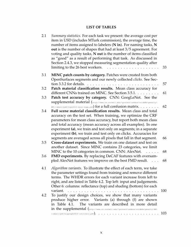
2.1 Summary statistics. For each task we present: the average cost peritem in USD (includes MTurk commission), the average time, thenumber of items assigned to labelers (N in). For naming tasks, Nout is the number of shapes that had at least 3/5 agreement. Forvoting and quality tasks, N out is the number of items classifiedas “good” as a result of performing that task. As discussed inSection 2.4.3, we stopped measuring segmentation quality afterlimiting to the 26 best workers. . . . . . . . . . . . . . . . . . . . 33

3.1 MINC patch counts by category. Patches were created from bothOpenSurfaces segments and our newly collected clicks. See Sec-tion 3.3.2 for details. . . . . . . . . . . . . . . . . . . . . . . . . . . 57

3.2 Patch material classification results. Mean class accuracy fordifferent CNNs trained on MINC. See Section 3.5.1. . . . . . . . . 61

3.3 Patch test accuracy by category. CNN: GoogLeNet. See thesupplemental material (http://www.cs.cornell.edu/\protect\unhbox\voidb@x\penalty\@M\sbell/pdf/cvpr2015-minc-supp.pdf) for a full confusion matrix. . . . . . . . 62

3.4 Full scene material classification results. Mean class and totalaccuracy on the test set. When training, we optimize the CRFparameters for mean class accuracy, but report both mean classand total accuracy (mean accuracy across all examples). In oneexperiment (a), we train and test only on segments; in a separateexperiment (b), we train and test only on clicks. Accuracies forsegments are averaged across all pixels that fall in that segment. 66

3.5 Cross-dataset experiments. We train on one dataset and test onanother dataset. Since MINC contains 23 categories, we limitMINC to the 10 categories in common. CNN: AlexNet. . . . . . 68

3.6 FMD experiments. By replacing DeCAF features with oversam-pled AlexNet features we improve on the best FMD result. . . . 68

4.1 Algorithm variants. To illustrate the effect of each term, we takethe parameter settings found from training and remove differentterms. The WHDR errors for each variant increase from left toright, and are listed in Table 4.2. Top left: input and judgements.Other 6: columns: reflectance (top) and shading (bottom) for eachvariant. . . . . . . . . . . . . . . . . . . . . . . . . . . . . . . . . . 100

4.2 To justify our design choices, we show that many variantsproduce higher error. Variants (a) through (f) are shownin Table 4.1. The variants are described in more detailin the supplemental (http://www.cs.cornell.edu/\protect\unhbox\voidb@x\penalty\@M\sbell/pdf/siggraph2014-intrinsic.pdf). . . . . . . . . . . . . . . . . . . . . . . 103

x

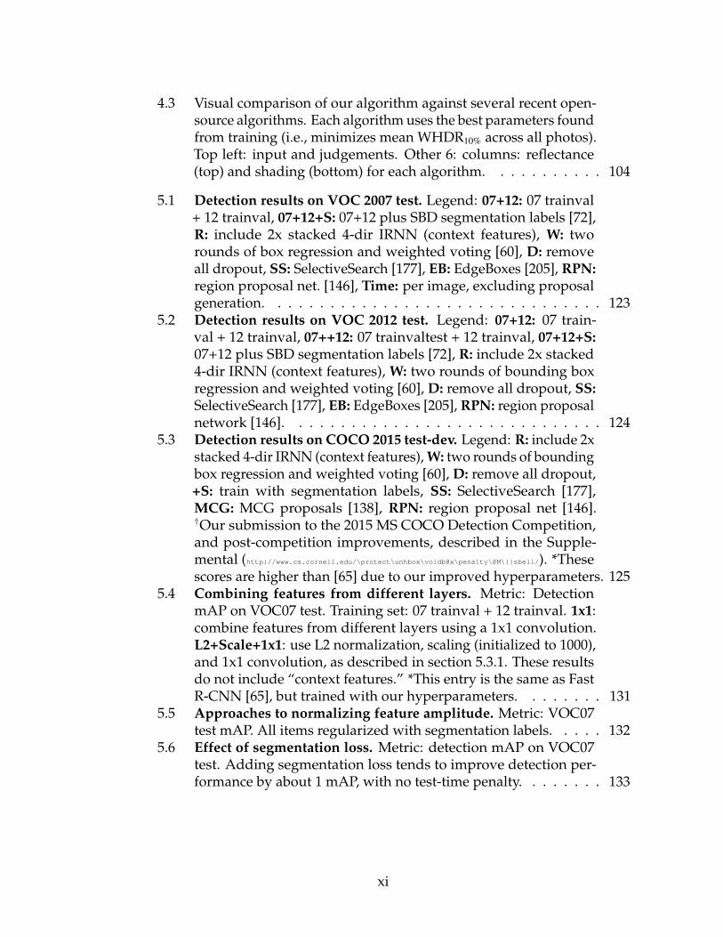
4.3 Visual comparison of our algorithm against several recent open-source algorithms. Each algorithm uses the best parameters foundfrom training (i.e., minimizes mean WHDR10% across all photos).Top left: input and judgements. Other 6: columns: reflectance(top) and shading (bottom) for each algorithm. . . . . . . . . . . 104

5.1 Detection results on VOC 2007 test. Legend: 07+12: 07 trainval+ 12 trainval, 07+12+S: 07+12 plus SBD segmentation labels [72],R: include 2x stacked 4-dir IRNN (context features), W: tworounds of box regression and weighted voting [60], D: removeall dropout, SS: SelectiveSearch [177], EB: EdgeBoxes [205], RPN:region proposal net. [146], Time: per image, excluding proposalgeneration. . . . . . . . . . . . . . . . . . . . . . . . . . . . . . . . 123

5.2 Detection results on VOC 2012 test. Legend: 07+12: 07 train-val + 12 trainval, 07++12: 07 trainvaltest + 12 trainval, 07+12+S:07+12 plus SBD segmentation labels [72], R: include 2x stacked4-dir IRNN (context features), W: two rounds of bounding boxregression and weighted voting [60], D: remove all dropout, SS:SelectiveSearch [177], EB: EdgeBoxes [205], RPN: region proposalnetwork [146]. . . . . . . . . . . . . . . . . . . . . . . . . . . . . . 124

5.3 Detection results on COCO 2015 test-dev. Legend: R: include 2xstacked 4-dir IRNN (context features), W: two rounds of boundingbox regression and weighted voting [60], D: remove all dropout,+S: train with segmentation labels, SS: SelectiveSearch [177],MCG: MCG proposals [138], RPN: region proposal net [146].†Our submission to the 2015 MS COCO Detection Competition,and post-competition improvements, described in the Supple-mental (http://www.cs.cornell.edu/\protect\unhbox\voidb@x\penalty\@M\sbell/). *Thesescores are higher than [65] due to our improved hyperparameters. 125

5.4 Combining features from different layers. Metric: DetectionmAP on VOC07 test. Training set: 07 trainval + 12 trainval. 1x1:combine features from different layers using a 1x1 convolution.L2+Scale+1x1: use L2 normalization, scaling (initialized to 1000),and 1x1 convolution, as described in section 5.3.1. These resultsdo not include “context features.” *This entry is the same as FastR-CNN [65], but trained with our hyperparameters. . . . . . . . 131

5.5 Approaches to normalizing feature amplitude. Metric: VOC07test mAP. All items regularized with segmentation labels. . . . . 132

5.6 Effect of segmentation loss. Metric: detection mAP on VOC07test. Adding segmentation loss tends to improve detection per-formance by about 1 mAP, with no test-time penalty. . . . . . . . 133

xi

5.7 Comparing approaches to adding context. All rows also poolout of conv3, conv4, and conv5. Metric: detection mAP on VOC07test. Seg: if checked, the top layer received extra supervision fromsemantic segmentation labels. . . . . . . . . . . . . . . . . . . . . 134

5.8 Varying the hidden transition. We vary the number of unitsand try either learning recurrent transition Whh initialized to theidentity, or entirely removing it (same as setting Whh = I). . . . . 136

5.9 Other variations. Metric: VOC07 test mAP. We list some othervariations that all perform about the same. . . . . . . . . . . . . . 137

6.1 Product search: uncurated random queries from the test set. For eachquery Iq, we show the top 3 retrievals using our method as well asthe tagged canonical image Ip from Houzz.com. Object categoriesare not known at test time. Note that sometimes the retrievedresults are closer to the query than Ip. . . . . . . . . . . . . . . . . 157

6.2 Style search: example cross-category queries. For each object category(“armchairs”, “rugs”, etc.), we show the closest product of thatcategory to the input Iq, even though the input (usually) doesnot belong to that category. We show this for 12 different objectcategories. Note that object category is not used to compute thedescriptor xq; it is only used at retrieval time to filter the set ofproducts. . . . . . . . . . . . . . . . . . . . . . . . . . . . . . . . . 161

xii

LIST OF FIGURES

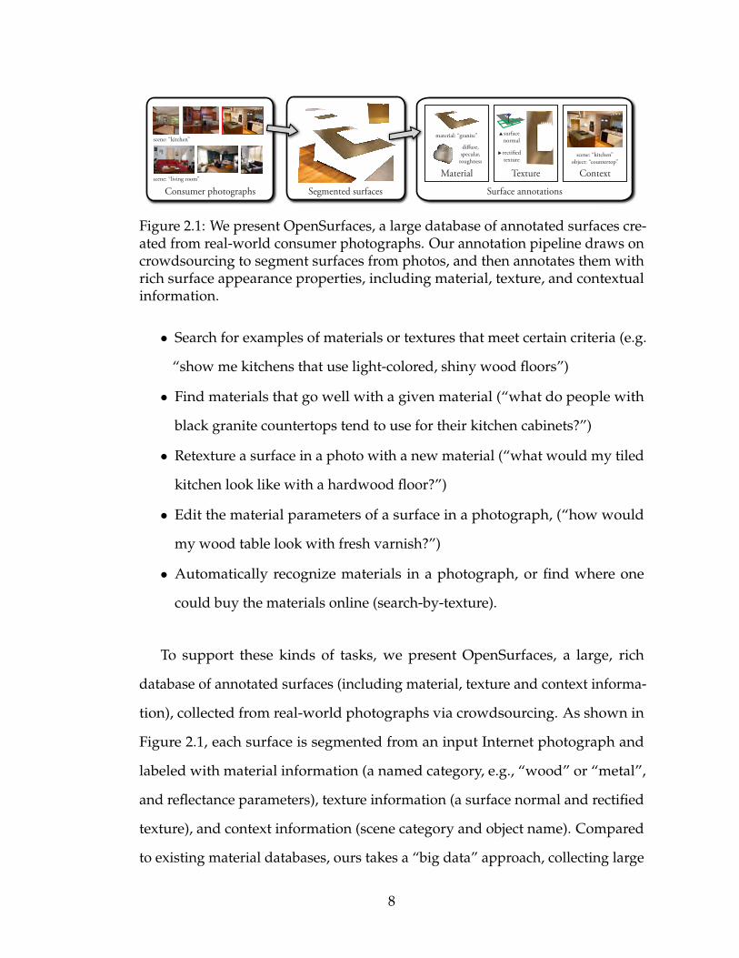
2.1 We present OpenSurfaces, a large database of annotated surfacescreated from real-world consumer photographs. Our annota-tion pipeline draws on crowdsourcing to segment surfaces fromphotos, and then annotates them with rich surface appearanceproperties, including material, texture, and contextual informa-tion. . . . . . . . . . . . . . . . . . . . . . . . . . . . . . . . . . . . 8

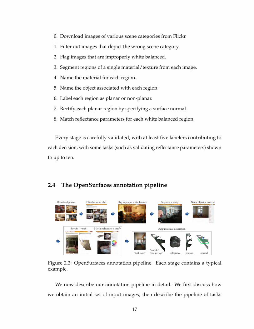
2.2 OpenSurfaces annotation pipeline. Each stage contains a typicalexample. . . . . . . . . . . . . . . . . . . . . . . . . . . . . . . . . . 17

2.3 (a) Stage 7: Rectifying planar textures interface. This figure showsa successfully completed task, where the perspective grid onthe left appears to lie flat against the surface, and the texture,shown on the right, is correctly rectified. (b) Stage 8: Interface forappearance matching to recover material parameters. . . . . . . 43

2.4 Example segmented surfaces labeled “wood” (top row) and “car-pet” (bottom row). Each item shows the number of vertices andthe time spent. . . . . . . . . . . . . . . . . . . . . . . . . . . . . . 43

2.5 Statistics over shapes in our database. Left: Histogram of vertexcounts, Center: Histogram of CUBAM scores from voting onshape quality, Right: Average CUBAM score for each vertex count. 44

2.6 Example rectified textures. Left: original photographs with seg-mented surface highlighted and user-specified surface normal.Right: rectified texture with provided surface normal. . . . . . . 44

2.7 Example rectified textures. Each row: textures rectified using nor-mals from our database, sorted by decreasing vertex count. Eachrow contains a single type of material: wood, tile, marble, andgranite. . . . . . . . . . . . . . . . . . . . . . . . . . . . . . . . . . 44

2.8 Example reflectance parameters. First and third rows: material seg-mentations from our database. Second and fourth rows: blobsrendered with user-specified perceptual Ward parameters. . . . 45

2.9 Example reflectance parameters. Left: original photograph. Cen-ter: region to be annotated. Right: blob rendered with the user-specified perceptual Ward parameters. . . . . . . . . . . . . . . . 45

2.10 Better exemplars for texture synthesis. (a) Synthesis using an unrec-tified exemplar, showing artifacts of foreshortening. (b) A texturesynthesized from a rectified exemplar from our database. . . . . 45

2.11 Retexturing example. The input target is a segmented photo. Arectified granite countertop surface from OpenSurfaces is synthe-sized and applied to the input using the correct perspective. . . . 46

2.12 Informed scene similarity. Left: query object. Right: photos contain-ing objects of the same name and material, sorted by diffuse colorsimilarity to the query object. . . . . . . . . . . . . . . . . . . . . 46

xiii

3.1 Overview. (a) We construct a new dataset by combining Open-Surfaces [12] with a novel three-stage Amazon Mechanical Turk(AMT) pipeline. (b) We train various CNNs on patches fromMINC to predict material labels. (c) We transfer the weights to afully convolutional CNN to efficiently generate a probability mapacross the image; we then use a fully connected CRF to predictthe material at every pixel. . . . . . . . . . . . . . . . . . . . . . . 48

3.2 Example patches from all 23 categories of the Materials in Con-text Database (MINC). Note that we sample patches so that thepatch center is the material in question (and not necessarily theentire patch). See Table 3.1 for the size of each category. . . . . . 50

3.3 AMT pipeline schematic for collecting clicks. (a) Workers filterby images that contain a certain material, (b) workers click onmaterials, and (c) workers validate click locations by re-labelingeach point. Example responses are shown in orange. . . . . . . . 55

3.4 Pipeline for full scene material classification. An image (a) isresized to multiple scales [1/

√2, 1,

√2]. The same sliding CNN

predicts a probability map (b) across the image for each scale;the results are upsampled and averaged. A fully connected CRFpredicts a final label for each pixel (c). This example shows pre-dictions from a single GoogLeNet converted into a sliding CNN(no average pooling). . . . . . . . . . . . . . . . . . . . . . . . . . 57

3.5 Varying patch scale. We train/test patches of different scales (thepatch locations do not vary). The optimum is a trade-off betweencontext and spatial resolution. CNN: AlexNet. . . . . . . . . . . . 61

3.6 Varying database size. Patch accuracy when trained on randomsubsets of MINC. Equal size is using equal samples per category(size determined by smallest category). CNN: AlexNet. . . . . . 63

3.7 Accuracy vs patch scale by category. Dots: peak accuracy foreach category; colored lines: sky, wallpaper, mirror; gray lines:other categories. CNN: AlexNet. While most materials are opti-mally recognized at 23.3% or 32% patch scale, recognition of sky,wallpaper and mirror improve with increasing context. . . . . . . . 63

3.8 Full-scene material classification examples: high-accuracy testset predictions by our method. CNN: GoogLeNet (with the av-erage pooling layer removed). Right: legend for material colors.See Table 3.4 for quantitative evaluation. . . . . . . . . . . . . . . 64

3.9 Optimizing for click accuracy leads to sloppy boundaries. In(a), we optimize for mean class accuracy across segments, result-ing in high quality boundaries. In (b), we optimize for meanclass accuracy at click locations. Since the clicks are not neces-sarily close to object boundaries, there is no penalty for sloppyboundaries. CNN: GoogLeNet (without average pooling). . . . 65

xiv

3.10 High confidence predictions. Top two rows: correct predictions.Bottom row: incorrect predictions (T: true, P: predicted). Percent-ages indicate confidence (the predictions shown are at least thisconfident). CNN: GoogLeNet. . . . . . . . . . . . . . . . . . . . . 67

4.1 We introduce a public dataset of indoor scenes for intrinsic imagesin the wild (a). (b) Our crowdsourcing pipeline lets users annotatepairs of points in each image with relative reflectance judgements.(c) Our intrinsic image decomposition algorithm performs wellin respecting the human judgements and is based on a fully-connected conditional random field (CRF) that incorporates long-range interactions in the reflectance layer while simultaneouslymaintaining local detail. All source images are licensed underCreative Commons ( ). . . . . . . . . . . . . . . . . . . . . . . . . 71

4.2 Our data collection pipeline. (a) We sample points and edges fromover 5,000 photographs, (b) workers flag points on mirrors andtransparent surfaces, (c) users judge pairs of points and indicatewhich point has a darker surface reflectance (or if they are equal),and (d) we aggregate judgements from 5 users for each pair ofpoints (each edge is styled according to the aggregate results, asdescribed in Figure 4.3). . . . . . . . . . . . . . . . . . . . . . . . 77

4.3 Aggregated human judgements for an example scene. The edges con-necting points indicate the aggregated reflectance judgement com-paring the two points. We sample points at two different densities:(a) sparsely, at 7% of the image width and (b) densely, at 3%. . . 80

4.4 Histograms of worker performance (left) and time spent (right). Verticalaxis on both plots: number of users. Left: percentage of sentineldata answered correctly. Right: time spent and effective wage(pay per task / time spent). . . . . . . . . . . . . . . . . . . . . . . 83

4.5 Points on a fabric surface with a cast shadow. . . . . . . . . . . . 854.6 Example decompositions using our algorithm for a variety of

scenes. All outputs are rescaled and mapped to sRGB for display. 964.7 Quantitative comparison of our algorithm against several recent

open-source algorithms, using mean weighted human disagree-ment rate (WHDR10%). For (c), only the 397 densely sampledphotos are considered (about 900 judgements per photo with aminimum separation of 3% of the image diameter). All values arecomputed using leave-one-out cross validation. See Section 4.5.2for details. . . . . . . . . . . . . . . . . . . . . . . . . . . . . . . . 105

4.8 Challenging scenes that violate our assumptions. Using the pa-rameters from Sec. 4.5.1, we obtain WHDR = 67%, 45%, 43%. . . . 110

xv

5.1 Inside-Outside Net (ION). In a single pass, we extractVGG16 [166] features and evaluate 2000 proposed regions ofinterest (ROI). For each proposal, we extract a fixed-size descrip-tor from several layers using ROI pooling [65]. Each descriptoris L2-normalized, concatenated, scaled, and dimension-reduced(1x1 convolution) to produce a fixed-length feature descriptor foreach proposal of size 512x7x7. Two fully-connected (fc) layersprocess each descriptor and produce two outputs: a one-of-Kclass prediction (“softmax”), and an adjustment to the boundingbox (“bbox”). . . . . . . . . . . . . . . . . . . . . . . . . . . . . . . 113

5.2 Four-directional IRNN architecture. We use “IRNN” units [105]which are RNNs with ReLU recurrent transitions, initialized tothe identity. All transitions to/from the hidden state are com-puted with 1x1 convolutions, which allows us to compute therecurrence more efficiently (Eq. 5.1). When computing the con-text features, the spatial resolution remains the same throughout(same as conv5). The semantic segmentation regularizer has a 16xhigher resolution; it is optional and gives a small improvement ofaround +1 mAP point. . . . . . . . . . . . . . . . . . . . . . . . . 117

5.3 Interpretation of the first IRNN output. Each cell in the outputsummarizes the features to the left/right/top/bottom. . . . . . . 121

5.4 VOC 2007 normalized AP by size. Left to right: increasing com-plexity. Left-most bar in each group: Fast R-CNN; right-most bar:our best model that achieves 79.2% mAP on VOC 2007 test. Ourdetector has a particularly large improvement for small objects.See Hoiem [79] for details on these metrics. . . . . . . . . . . . . 127

5.5 Receptive field of different layer types. When considering asingle cell in the input, what output cells depend on it? (a) If weadd two stacked 3x3 convolutions on top of conv5, then a cell inthe input influences a 5x5 window in the output. (b) Similarly, fora 5x5 convolution, one cell influences a 9x9 window in the output.(c) For global average pooling, every cell in the output dependson the entire input, but the output is the same value repeated. (d)For IRNNs, every cell in the output depends on the entire input,but also varies spatially. . . . . . . . . . . . . . . . . . . . . . . . . 135

xvi

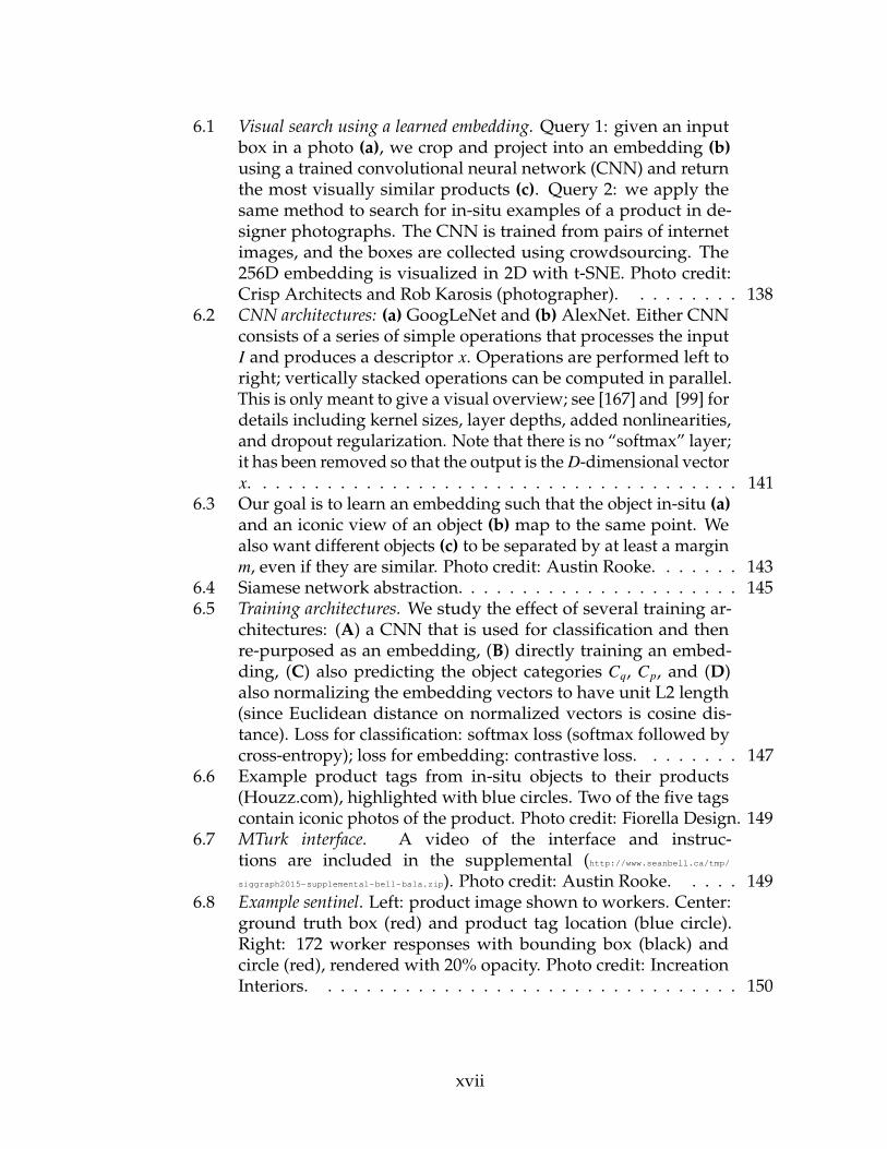
6.1 Visual search using a learned embedding. Query 1: given an inputbox in a photo (a), we crop and project into an embedding (b)using a trained convolutional neural network (CNN) and returnthe most visually similar products (c). Query 2: we apply thesame method to search for in-situ examples of a product in de-signer photographs. The CNN is trained from pairs of internetimages, and the boxes are collected using crowdsourcing. The256D embedding is visualized in 2D with t-SNE. Photo credit:Crisp Architects and Rob Karosis (photographer). . . . . . . . . 138

6.2 CNN architectures: (a) GoogLeNet and (b) AlexNet. Either CNNconsists of a series of simple operations that processes the inputI and produces a descriptor x. Operations are performed left toright; vertically stacked operations can be computed in parallel.This is only meant to give a visual overview; see [167] and [99] fordetails including kernel sizes, layer depths, added nonlinearities,and dropout regularization. Note that there is no “softmax” layer;it has been removed so that the output is the D-dimensional vectorx. . . . . . . . . . . . . . . . . . . . . . . . . . . . . . . . . . . . . . 141

6.3 Our goal is to learn an embedding such that the object in-situ (a)and an iconic view of an object (b) map to the same point. Wealso want different objects (c) to be separated by at least a marginm, even if they are similar. Photo credit: Austin Rooke. . . . . . . 143

6.4 Siamese network abstraction. . . . . . . . . . . . . . . . . . . . . . 1456.5 Training architectures. We study the effect of several training ar-

chitectures: (A) a CNN that is used for classification and thenre-purposed as an embedding, (B) directly training an embed-ding, (C) also predicting the object categories Cq, Cp, and (D)also normalizing the embedding vectors to have unit L2 length(since Euclidean distance on normalized vectors is cosine dis-tance). Loss for classification: softmax loss (softmax followed bycross-entropy); loss for embedding: contrastive loss. . . . . . . . 147

6.6 Example product tags from in-situ objects to their products(Houzz.com), highlighted with blue circles. Two of the five tagscontain iconic photos of the product. Photo credit: Fiorella Design. 149

6.7 MTurk interface. A video of the interface and instruc-tions are included in the supplemental (http://www.seanbell.ca/tmp/siggraph2015-supplemental-bell-bala.zip). Photo credit: Austin Rooke. . . . . 149

6.8 Example sentinel. Left: product image shown to workers. Center:ground truth box (red) and product tag location (blue circle).Right: 172 worker responses with bounding box (black) andcircle (red), rendered with 20% opacity. Photo credit: IncreationInteriors. . . . . . . . . . . . . . . . . . . . . . . . . . . . . . . . . 150

xvii

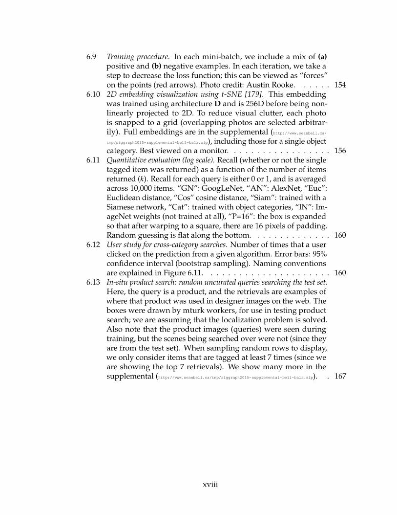
6.9 Training procedure. In each mini-batch, we include a mix of (a)positive and (b) negative examples. In each iteration, we take astep to decrease the loss function; this can be viewed as “forces”on the points (red arrows). Photo credit: Austin Rooke. . . . . . 154

6.10 2D embedding visualization using t-SNE [179]. This embeddingwas trained using architecture D and is 256D before being non-linearly projected to 2D. To reduce visual clutter, each photois snapped to a grid (overlapping photos are selected arbitrar-ily). Full embeddings are in the supplemental (http://www.seanbell.ca/tmp/siggraph2015-supplemental-bell-bala.zip), including those for a single objectcategory. Best viewed on a monitor. . . . . . . . . . . . . . . . . . 156

6.11 Quantitative evaluation (log scale). Recall (whether or not the singletagged item was returned) as a function of the number of itemsreturned (k). Recall for each query is either 0 or 1, and is averagedacross 10,000 items. “GN”: GoogLeNet, “AN”: AlexNet, “Euc”:Euclidean distance, “Cos” cosine distance, “Siam”: trained with aSiamese network, “Cat”: trained with object categories, “IN”: Im-ageNet weights (not trained at all), “P=16”: the box is expandedso that after warping to a square, there are 16 pixels of padding.Random guessing is flat along the bottom. . . . . . . . . . . . . . 160

6.12 User study for cross-category searches. Number of times that a userclicked on the prediction from a given algorithm. Error bars: 95%confidence interval (bootstrap sampling). Naming conventionsare explained in Figure 6.11. . . . . . . . . . . . . . . . . . . . . . 160

6.13 In-situ product search: random uncurated queries searching the test set.Here, the query is a product, and the retrievals are examples ofwhere that product was used in designer images on the web. Theboxes were drawn by mturk workers, for use in testing productsearch; we are assuming that the localization problem is solved.Also note that the product images (queries) were seen duringtraining, but the scenes being searched over were not (since theyare from the test set). When sampling random rows to display,we only consider items that are tagged at least 7 times (since weare showing the top 7 retrievals). We show many more in thesupplemental (http://www.seanbell.ca/tmp/siggraph2015-supplemental-bell-bala.zip). . 167

xviii

CHAPTER 1

INTRODUCTION

Automatically understanding scenes is the holy grail of computer vision.

Real-world scenes have a vast array of interesting objects, materials, textures,

and surfaces. With scenes, people want to edit photographs, search by object and

material properties, visualize changes to rooms and buildings, browse collections

by visual similarity, and explain images to the visually impaired. Scenes also play

a key role in robotics—agents need to understand the materials and properties of

objects in its environment in order to interact with the physical world. Materials

and objects are at the core of all of these tasks. However, the tools and data that

we have for recognizing, editing, and exploring applying scene properties for

everyday problems are still quite limited. We cannot easily understand, search,

and aggregate visual concepts in the billions of photos that are uploaded every

day to the web.

Scene recognition is a long-standing, challenging problem due to the totally

unknown relationship between the input image (an array of pixel intensities),

and the semantic properties represented in that image. Pixels contain an un-

known combination of objects, materials, geometry, lighting, occlusions, and

camera intrinsics, so that separating these properties is nearly impossible in a

fully general algorithmic way. Despite these difficulties, humans are adept at

recognizing all of these concepts in images. There is the potential to ask people to

provide millions of examples of answers, allowing computer vision researchers

to pose recognition as a learning problem. Posed this way, the challenge is de-

coupled into two new problems: (1) how to get people to efficiently, cheaply,

and accurately label the properties you want in images, and (2) how to learn a

1

model that matches the answers provided by people. To obtain labels at scale,

we turn to crowdsourcing online, which introduces new challenges—workers

are unreliable, inconsistent, and do not have the expertise to directly label the

properties we need. Once we have these labels, the final challenge is using

the right learning algorithm. For that, we use deep learning and convolutional

neural networks.

In this thesis we further our understanding of scenes along many facets—we

develop new crowdsourcing methods as well as new state-of-the-art algorithms

that learn from data. Further, we model scenes at many levels of abstraction.

At the lowest levels of abstraction, one can study the physics and interaction

of light as it bounces around the scene—light traveling from light sources in

the scene, absorbed by surfaces, transmitted through media, and ultimately

absorbed by cameras and projected onto an image sensor. At an intermediate

level of abstraction, we can consider the human-centric semantics imposed on

the world, and group them into distinct surfaces, materials, and objects. At the

highest level of visual abstraction, we consider which objects are visually and

stylistically compatible together—which ensembles of items go well together in

a scene.

Our first contributions are to collect appearance information at a large-scale,

which has not been done before for materials (Chapter 2). We use this to inform

and drive new algorithms to understand materials at pixel-level material cat-

egories (Chapter 3) and pixel-level reflectance (Chapter 4). We then develop

higher level algorithms to detect objects in images (Chapter 5), and recognize ob-

jects at a fine-grained per-object level (Chapter 6). Together, these contributions

significantly advance our knowledge of what information can be extracted from

2

an image.

Chapter 2 presents our first major contribution, OpenSurfaces, a rich, labeled

database consisting of thousands of examples of surfaces segmented from con-

sumer photographs of interiors. These surfaces are annotated with material

parameters (reflectance, material names), texture information (surface normals,

rectified textures), and contextual information (scene category, and object names).

We use human annotations and present a new methodology for segmenting and

annotating materials in Internet photo collections suitable for crowdsourcing

(e.g., through Amazon’s Mechanical Turk). Because of the noise and variability

inherent in Internet photos and novice annotators, designing this annotation

engine was a key challenge; we present a multi-stage set of annotation tasks with

quality checks and validation. We demonstrate the use of this database in proof-

of-concept applications including surface retexturing and material and image

browsing, and discuss future uses. OpenSurfaces is a public resource available

at http://opensurfaces.cs.cornell.edu/. Since releasing our interface,

researchers from Microsoft have used our segmentation interface to power the

Microsoft Commons Objects in Context (MS COCO) project which labeled over

2.5 million objects; this data has significantly advanced the state-of-the-art in

object detection.

Chapter 3 considers the mid-level visual problem of recognizing materials

in an image, building on the dataset from Chapter 2. We present the Materials

in Context Database (MINC), a new, large-scale, open dataset of materials in

the wild, and combine this dataset with deep learning to achieve state-of-the-

art material recognition and segmentation of images in the wild. MINC is

an order of magnitude larger than previous material databases, while being

3

more diverse and well-sampled across its 23 categories. Using MINC, we train

convolutional neural networks (CNNs) for two tasks: classifying materials from

patches, and simultaneous material recognition and segmentation in full images.

For patch-based classification on MINC we found that the best performing CNN

architectures can achieve 85.2% mean class accuracy. We convert these trained

CNN classifiers into an efficient fully convolutional framework combined with

a fully connected conditional random field (CRF) to predict the material at

every pixel in an image, achieving state-of-the-art accuracy. Our experiments

demonstrate that having a large, well-sampled dataset such as MINC is crucial

for real-world material recognition and segmentation. Since releasing MINC,

new semantic segmentation algorithms have been proposed that were trained

on our data to further advance the state of the art.

Chapter 4 considers a related problem of a challenging low-level visual

property: surface reflectance. This problem is usually posed as the “intrinsic

images” problem, the separation of an image into a reflectance layer and a

shading layer. In this chapter, we present Intrinsic Images in the Wild (IIW), a large-

scale, public dataset for evaluating intrinsic image decompositions of indoor

scenes. We create this benchmark through millions of crowdsourced annotations

of relative comparisons of material properties at pairs of points in each scene.

Crowdsourcing enables a scalable approach to acquiring a large database, and

uses the ability of humans to judge material comparisons, despite variations in

illumination. Given our database, we develop a dense CRF-based intrinsic image

algorithm for images in the wild that outperforms a range of state-of-the-art

intrinsic image algorithms. Intrinsic image decomposition remains a challenging

problem; we release our code and database publicly to support future research

on this problem, available online at http://intrinsic.cs.cornell.edu/.

4

Since releasing our dataset, others have used our data to further advance the

state-of-the-art by training deep learning models and expanding on our CRF-

based algorithm.

Chapter 5 develops a new object detection algorithm that is significantly

more accurate than the previous state-of-the-art for this problem. Specifically, we

present the Inside-Outside Net (ION), an object detector that exploits information

both inside and outside the region of interest. In the chapter, we will explain our

new architecture that uses contextual information with recurrent neural networks

and skip pooling. Through extensive experiments we evaluate the design space

and provide readers with an overview of what tricks of the trade are important.

ION improves state-of-the-art on object detection by a significant margin. In

the 2015 MS COCO Detection Challenge, our ION model won “Best Student

Entry” and finished 3rd place overall. As intuition suggests, our detection results

provide strong evidence that context and multi-scale representations improve

small object detection.

Chapter 6 explores the highest level of visual abstraction—visual similarity.

In this chapter we learn an embedding for visual search in interior design. Our

embedding contains two different domains of product images: products cropped

from internet scenes, and products in their iconic form. With such a multi-domain

embedding, we demonstrate several applications of visual search including

identifying products in scenes and finding stylistically similar products. To obtain

the embedding, we train a convolutional neural network on pairs of images. We

explore several training architectures including re-purposing object classifiers,

using siamese networks, and using multitask learning. We evaluate our search

quantitatively and qualitatively and demonstrate high quality results for search

5

across multiple visual domains, enabling new applications in interior design.

Since releasing our paper, other researchers have shown that this approach also

works for 3D shapes, clothing, and sketches.

In this thesis we have introduced first-of-their-kind large scale datasets for

material and reflectance annotation of images in the wild. We combine these

datasets with innovative techniques in learning to create state-of-the-art algo-

rithms in material recognition, intrinsic image decomposition, object detection,

and visual and style similarity.

6

CHAPTER 2

OPENSURFACES: A RICHLY ANNOTATED CATALOG OF SURFACE

APPEARANCE

2.1 Introduction

In this chapter, we address the first challenge in scene understanding—efficiently

collecting large-scale visual data from photographs. While there has been work

on collecting object categories and scene labels [176, 43, 195, 152], materials,

reflectances, and textures are largely unexplored. While this kind of visual

data is immensely valuable for training deep learning algorithms (as used in

Chapter 3), in this chapter we also show its direct use: exploring photo collec-

tions by materials, visualizing changes to scenes, visualizing what materials

go together, and others. We release our data as a public resource available at

http://opensurfaces.cs.cornell.edu/.

The tools and data that we have for exploring and applying materials and

textures for everyday problems are currently quite limited. For instance, consider

a homeowner planning a kitchen renovation, who would like to create a scrap-

book of kitchen photographs from which to draw inspiration for materials, find

appliances with a certain look, visualize paint samples, etc. Even simply finding

a set of good kitchen photos to look at can be a time-consuming process. Interior

design websites, such as Houzz, are starting to provide forums where people

share photos of interior scenes, tag elements such as countertops with brand

names, and ask and answer questions about material design. Their popularity

indicates the demand and need for better tools. For example, people want to:

7

Consumer photographs Segmented surfaces Surface annotations

scene: “kitchen”

scene: “living room”

diuse, specular,

roughness

surface normal

rectied texture

scene: “kitchen”object: “countertop”

material: “granite”

Material Texture Context

Figure 2.1: We present OpenSurfaces, a large database of annotated surfaces cre-ated from real-world consumer photographs. Our annotation pipeline draws oncrowdsourcing to segment surfaces from photos, and then annotates them withrich surface appearance properties, including material, texture, and contextualinformation.

• Search for examples of materials or textures that meet certain criteria (e.g.

“show me kitchens that use light-colored, shiny wood floors”)

• Find materials that go well with a given material (“what do people with

black granite countertops tend to use for their kitchen cabinets?”)

• Retexture a surface in a photo with a new material (“what would my tiled

kitchen look like with a hardwood floor?”)

• Edit the material parameters of a surface in a photograph, (“how would

my wood table look with fresh varnish?”)

• Automatically recognize materials in a photograph, or find where one

could buy the materials online (search-by-texture).

To support these kinds of tasks, we present OpenSurfaces, a large, rich

database of annotated surfaces (including material, texture and context informa-

tion), collected from real-world photographs via crowdsourcing. As shown in

Figure 2.1, each surface is segmented from an input Internet photograph and

labeled with material information (a named category, e.g., “wood” or “metal”,

and reflectance parameters), texture information (a surface normal and rectified

texture), and context information (scene category and object name). Compared

to existing material databases, ours takes a “big data” approach, collecting large

8

numbers of example materials captured in situ in their surrounding context.

Just as massive databases of images and objects have led to new advances in

image editing [76, 103] and object recognition [152], we believe that a large and

comprehensive catalog of contextual surface appearance properties is critical for

everyday applications involving exploring, editing, and recognizing materials

and textures. To our knowledge, ours is the first large-scale database of rich,

annotated surface appearance information of its kind.

A central challenge in creating such a catalog is that automatically recovering

material properties from images is a notoriously difficult inverse problem that

requires careful calibration [193] or strong assumptions about the image forma-

tion model [147]. Our images are scraped from Flickr, so objects appear under a

wide range of uncontrolled lighting conditions, with unknown scene geometry.

These properties raise the question of whether it is possible to recover any usable

material information from such images. This drives a key aspect of our system:

we ask humans to judge these properties in uncalibrated settings, leveraging

the fact that people are good at recognizing and categorizing materials across a

range of lighting conditions and image quality. To scale to the large numbers of

images, materials, and textures we want, we use crowdsourcing on Amazon’s

Mechanical Turk (MTurk).

Even with humans in the loop, creating a useful surface catalog is very

challenging. Internet photos are noisy, the quality of results from MTurk labelers

can vary widely, and interfaces involving material parameters can be difficult

for novice users to understand. To get usable results, we designed a multi-

stage annotation pipeline, involving multiple types of tasks, to collect and verify

surface annotations, including material, texture, and contextual information.

9

We evaluate the quality of this approach and demonstrate the utility of this

database in proof-of-concept applications including surface retexturing and

appearance browsing. We believe that the availability of such a database can

be helpful to many applications in graphics and vision, beyond the ones we

demonstrate.

This chapter makes the following contributions:

• A new, large-scale open source database of surface appearance (with thou-

sands of entries and growing) annotated with material, texture, and contex-

tual information available at http://opensurfaces.cs.cornell.edu/.

• A methodology for creating such a database through crowdsourcing anno-

tations of Internet photo collections.

• A publicly available annotation pipeline to spur further exploration and

use of such data in graphics and vision applications.

• A demonstration of proof-of-concept uses of such richly annotated surface

information.

2.2 Related work

Image databases. Over the past few years, researchers have shown the utility

of “big data”—in the form of large, annotated image databases—for addressing

difficult problems in graphics and vision. These databases include 80 Million

Tiny Images [176], ImageNet [43], the SUN scene database [195], and the LabelMe

dataset [152]. LabelMe has similar goals to ours and uses a significant amount of

user annotation, but their focus is on labeling objects, rather than materials. Other

10

work has extended systems such as LabelMe to material name annotations [47].

While the work described above comprises very large databases of images,

objects, and scenes, existing databases of natural images of materials are relatively

small. This category includes the Flickr Materials Database (FMD) [114] and the

datasets of Hu, et al. [81]. These datasets are largely made up of close-up photos

of objects made of a single substance, such as wood or glass, and have primarily

been used for the problem of material categorization. The PSU Near-Regular

Texture Database consists of closeups of textured patterns, including material

textures [118].

In contrast, our aim is to build a database of materials in context in photos

of everyday scenes, so that we can support applications like interior design

that involve whole scenes, rather than single objects or materials. Moreover,

prior databases annotate each image with a single category label (e.g. “wood,”

“glass”), while we collect a much richer set of annotations that include reflectance

parameters and surface normals, enabling a wider class of potential applications.

Crowdsourcing. The use of crowdsourcing to collect data is gaining adoption,

and has been used in recent approaches to a range of problems, including un-

derstanding shape through gauge figures [38], creating a mesh segmentation

database [32], devising a retargeting evaluation framework [148], and for inte-

grating humans into the loop for microtasks [61]. The experiences from this body

of prior work has informed our design process.

Material acquisition and databases. Material acquisition is an active area of

research (for a recent survey, see [193]). A few public databases exist with

11

carefully calibrated measurements, including the MERL database [121] with

4D BRDF measurements for 105 materials, fit to various BRDF models [124],

and CUReT [39], with 6D measured BTFs (bidirectional texture functions) for 61

samples with various lighting and illumination conditions. The complexity of

acquisition and quality of these databases has typically limited their size. To help

address these issues, appearance acquisition research has focused on hardware

solutions [145], but large databases of measured materials are still difficult to

acquire.

Rather than capture detailed, high-quality reflectance information for a small

number of materials under controlled conditions, our goal is complementary; we

aim to gather large numbers of surface annotations, in situ, from photographs

taken under a wide variety of uncontrolled settings. Since humans provide

annotations, we aim for perceptually plausible appearance data.

2.3 Overview

We present an overview of OpenSurfaces, and discuss some of our key design

decisions. Our annotation pipeline takes as input a set of consumer photos

depicting one or more surfaces, in context, in an interior scene, such as a kitchen.

Each photo is processed in multiple stages, resulting in segmented surface regions

(e.g., countertops, floors, cabinets, drawer handles, etc.), where each segment is

annotated with material, texture and contextual information.

Creating this database involves several challenges:

• How can we create a high-quality database from consumer photographs?

12

What kinds of photos should we use?

• How can we help novice labelers annotate surfaces? How can we scale this

annotation to build a very large database?

• What information is represented in the database?

• What tasks are needed to build this database?

2.3.1 Community photo collections

One important motivation of our work is to collect a large range of everyday

surfaces in context from everyday imagery. By “in context,” we mean that we

want to capture the settings in which various surfaces appear—for instance,

where a given type of material tends to appear in an image, what kinds of objects

it belongs to, and what other materials it appears in combination with. We chose

to focus on indoor locations such as kitchens, living rooms, and dining rooms,

which contain indoor materials of practical use, though it is easy to generalize

our approach to broader categories.

We use Creative-Commons-licensed Flickr photos as the main source for our

images, as we found that Flickr contains a vast range of real, everyday materials

in context in high-quality photos. Images from the SUN database [195] were not

usable for our purposes because they are typically not of high enough resolution.

2.3.2 Human annotation

Online consumer photos are far removed from the carefully calibrated, high-

dynamic range images typical of material acquisition. Our photos contain mul-

13

tiple materials on surfaces of unknown geometry, are captured under widely

varying and unknown lighting conditions, lack radiometric calibration, and may

have been post-processed. Hence, extracting meaningful surface properties from

these images is well beyond the state-of-the-art of automatic inverse rendering

algorithms. Optimization [147] and machine learning approaches [46, 114] to

inferring materials have been studied recently, but do not yet demonstrate the

performance necessary to annotate materials in noisy, real-world images. These

considerations motivate another major design choice in our approach: using hu-

mans to annotate our images via crowdsourcing. Humans are reasonably good at

identifying materials and their properties over a range of lighting conditions [53],

and the availability of crowdsourcing lets us collect annotations at scale for large

image collections.

In this chapter we focus on an annotation pipeline we deployed on Amazon’s

Mechanical Turk (MTurk), as MTurk provides a platform for annotating many

images in a short amount of time and at low cost. However, our system can also

be run as a stand-alone interface hosted on our servers, so that new photos can

continue to be annotated (similar to [152] for object labeling).

We faced two main challenges in getting useful annotations from labelers.

First, annotating surface properties in a photo is not a familiar task to most people,

and even communicating what we mean by a “surface,” “material,” or “texture”

to a novice is difficult. Second, MTurk annotators can be unreliable—users can

ignore instructions or intentionally provide bad labels. To deal with these sources

of noise, we split our material annotation tasks into several subtasks, with the

goal of making each subtask as simple, modular, and intuitive as possible. We

also use techniques to account for noise, and to verify the results of each subtask.

14

To improve robustness to noise, we use the CUBAM machine learning algorithm

of Welinder, et al. [191] which uses a model of noisy user behavior for binary

tasks (e.g., voting for the quality of a surface) to extract better results. In part,

it models the competence and bias of each user based on how often they are in

agreement with other users.

2.3.3 OpenSurfaces data representation

Real-world surfaces can be characterized in many ways, including (in increasing

order of complexity): names of material categories (e.g., “wood” vs. “metal” vs.

“paper”), image exemplars, simple diffuse reflectance models, parametric BRDF

models, 4D BRDF measurements, and 6D BTDF measurements. In choosing

a surface representation for our database, we considered several factors. First,

different representations are suitable for different tasks. For a material recog-

nition task, one might want a database with segmented materials labeled with

a category name (“wood” vs. “plastic”), for use in training classifiers. Other

applications, such as interior design (“replace the wood floor in this photo with

a shinier one”), might warrant a richer description of materials in terms of their

reflectance. Hence, we collect multiple types of annotations for each surface,

including material names and reflectance parameters.

Surface normals and rectified textures. While some types of surfaces we con-

sider have a uniform BRDF, many, such as granite or wood, are highly textured.

Thus, we chose to store texture information to describe surfaces as well. Because

textures in photos can be significantly foreshortened by perspective, we create a

subtask where labelers mark regions as planar or non-planar, and indicate the

15

surface normal of planar regions using a 3D perspective grid; this allows us to

create and store rectified textures.

Reflectance. We ask labelers to annotate material parameters for segmented

surfaces. Ideally, we would collect the most detailed BRDF information possible;

we especially want to move beyond simple Lambertian models, because specular

and glossy materials are extremely common in indoor scenes. On the other

hand, there is only so much information that can be recovered from a single,

uncalibrated image; moreover, our tasks should not be too difficult for human

labelers. Thus, we chose to represent the materials using a simple parametric

BRDF model (Section 2.4.7).

Data representation. Our final surface representation includes the following

information for each surface (illustrated in Figure 3.2): material data (a material

name, and reflectance parameters including diffuse albedo, gloss contrast, and

gloss roughness), texture data (a surface normal and rectified texture (if planar)),

and context data (an object name for the surface, and a scene category in which

the surface occurs). Each surface also stores quality information, including a

segmentation quality score and a planarity score.

2.3.4 Annotation stages

To build this representation for surfaces, our labelers perform a series of tasks in

an annotation pipeline consisting of the following stages (Stage 0 is automatic,

and the rest involve humans in the loop):

16

0. Download images of various scene categories from Flickr.

1. Filter out images that depict the wrong scene category.

2. Flag images that are improperly white balanced.

3. Segment regions of a single material/texture from each image.

4. Name the material for each region.

5. Name the object associated with each region.

6. Label each region as planar or non-planar.

7. Rectify each planar region by specifying a surface normal.

8. Match reflectance parameters for each white balanced region.

Every stage is carefully validated, with at least five labelers contributing to

each decision, with some tasks (such as validating reflectance parameters) shown

to up to ten.

2.4 The OpenSurfaces annotation pipeline

Segment + verifyFlag improper white balanceFilter by scene label Name object + material

Rectify + verify

“marble”“countertop”“bathroom”

Download photos

reectance texture normal

Output surface descriptionMatch reectance + verify

Figure 2.2: OpenSurfaces annotation pipeline. Each stage contains a typicalexample.

We now describe our annotation pipeline in detail. We first discuss how

we obtain an initial set of input images, then describe the pipeline of tasks

17

performed on each image and segmented region. We ran several pilot studies for

each of these tasks; we describe how these studies guided the design of our final

interfaces and tasks. More details on each task are available in the supplementary

document.1 Figure 4.2 shows a block diagram of the annotation pipeline.

Stage 0: Collecting images. First, we needed to gather a set of high-quality

images of indoor scenes. We obtain our images from Flickr, using search terms

for each room type, such as “kitchen” and “living room” (see supplementary2

for full list). Since our goal is to recover realistic parameters, we exclude images

with the tag “hdr,” which are typically highly stylized. We also limit our search

to Creative Commons photos that allow “sharing” and “remixing,” to ensure

that our database can be used in a variety of applications.

We then group the remaining images by scene type. In total, we downloaded

1,099,277 images. We further pruned the list keeping only those photos that are:

(a) color JPEG high-resolution (≥ 6 megapixels), (b) at most 32MB in size (to

control our disk footprint), and (c) have focal length information in their Exif

headers (which we use for the rectification in Section 2.4.6). After this filtering

step, we were left with a final set of approximately 207K images; we picked a

few scene categories to focus on, giving us about 92K images.

2.4.1 Stage 1: Filtering images by scene category

Though we use the text tags associated with Flickr photos to download an initial

set of photos, in practice these tags are quite noisy. For example, an image tagged

1http://www.cs.cornell.edu/˜sbell/pdf/siggraph2013-opensurfaces-supp.pdf

2http://www.cs.cornell.edu/˜sbell/pdf/siggraph2013-opensurfaces-supp.pdf

18

“kitchen” may depict a bar named “The Kitchen,” or something else entirely. As

in previous work on obtaining images of categories [43], we must curate the

images of each scene category to find the relevant ones. In this task a labeler is

shown a grid of 50 images drawn from a given category (e.g., “dining room”),

and is asked to select all the images that belong to that category.

Each image was shown to five labelers. We found that labelers are very fast

and reliable at this task, and pruned the image list down to about 25K images.

Our database mostly contains scenes from the following categories: kitchen,

living room, bedroom, bathroom, staircase, dining room, hallway, family room,

and foyer.

2.4.2 Stage 2: Flag images with improper white balance

While human beings are able to judge material properties in a range of lighting

conditions due to color constancy, there are limits to this ability [21], and the

lighting conditions in online consumer photographs can be poor and highly

variable from photo to photo. So that our labelers can reason about the true

color of a surface as accurately and reliably as possible, we filter images that are

significantly distorted in color space. To do so, we designed a task where labelers

click on objects that they believe are white, and use this feedback to reject images

that appear to be improperly white balanced. Users are prevented from clicking

on pixels that are close to saturated (R,G, B ≥ 253), or within 70 pixels of another

point.

Each selected pixel is converted to L∗a∗b∗ color space. If the median value

of ||(a∗, b∗)|| is ≤ 15, then that user’s submission counts as one vote towards the

19

photo being white balanced. Each photo is seen by five labelers; we run CUBAM

on the full set of resulting votes, which yields a score (positive or negative) for

each photo. If a photo receives a positive CUBAM score, then we consider it

white balanced. We opted for this stringent rule because of the large size of our

image collection; we can eliminate many images, and still have a large pool of

remaining images to label. Compared to majority (3 out of 5) voting, CUBAM

changed 14% of labels from good (white balanced) to bad (not white balanced),

and 0.8% from bad to good.

Since material recognition is still possible in distorted color spaces [161], we

only use white balancing to filter inputs for appearance matching (Stage 8).

2.4.3 Stage 3: Material segmentation

The next task is to segment regions of constant material or texture from each

image. These regions will become the surfaces that are annotated in later tasks.

Pilot study. This task is related to the object segmentation task in LabelMe, but

when we tried adapting LabelMe for our task, the interface proved to be cum-

bersome. We created a new interface with features (smooth zoom, undo/redo,

automatic pan) designed to encourage better material segmentations; user feed-

back was very positive. The smooth zoom and automatic pan features were

especially important, yielding segmentations with greater accuracy and more

vertices. Without automatic pan (scrolling the view when users click near the

edge), users often submitted clipped polygons.

For this task, a labeler is presented with an image and instructed to segment

20

six regions based on material and texture, and not object boundaries. The user is

shown several examples of good and bad segmentations. An ideal segmentation

contains a single material or texture, and tightly hugs the boundary of that

material region. The user creates polygons by clicking in the image, or entering

a mode where they can adjust an existing polygon (the interface zooms in for

fine-scale adjustments; the user can also zoom in or out). The interface saves

a full undo/redo stack, and logs all actions with a timestamp for later replay.

The interface disallows self-intersecting polygons, but separate polygons can be

nested or overlapping.

Once a labeler has segmented regions from the image, we post-process the

polygons to create a set of disjoint shapes. This step is to address common

cases that arise in these kinds of tasks where a large region of a single material

contains a smaller region of a second material (e.g., a door with a handle, or a

shower stall with a drain). The easiest way to label these kinds of surfaces is to

provide the boundary of the outer shape, and separately the boundary of the

inner shapes. Our post-processing stage detects such intersections and yields

new shapes as follows: if one shape contains another shape, the inner shape is

unchanged, and the outer shape has a hole corresponding to the inner shape; if

two shapes partially intersect, three regions are generated to capture cases where

the foreground partially intersects the background. The output is stored as a 2D

mesh triangulated by [26]. The supplementary material3 describes this process

in more detail. While this technique can occasionally over-segment overlapping

regions, we found it to be very useful in addressing common configurations.

3http://www.cs.cornell.edu/˜sbell/pdf/siggraph2013-opensurfaces-supp.pdf

21

Voting for material segmentation quality

The quality of segmentations from this task varies widely; while many regions

were surprisingly well-segmented, some were too small, or had sloppy bound-

aries, and others were good object (but not material) segmentations. We created

an additional task where users vote on the quality of each segmentation; these

votes are used to determine a quality score for each segmented surface region.

This voting task is somewhat subjective, since it is not always clear what

constitutes a “single material” or how labelers interpret the word “texture”.

Thus, we accept shapes as high quality only if there is a certain amount of

consensus. We asked five voters to vote on the quality of each segmentation, and

ran CUBAM on the resulting votes. Compared to majority (3 out of 5) voting,

CUBAM changed about 7.0% of the bad examples to good, and about 8.38%

of the good examples to bad. By default, we discard shapes with a CUBAM-

computed quality score below a threshold, but this threshold can be adjusted

for applications that need higher-quality segmentations, or which can tolerate

lower-quality segmentations.

As we ran the material segmentation task, we noticed that a few users pro-

duced exceptionally detailed segmentations, with an accuracy higher than the

output of the above voting step. After collecting about 30,000 segmentations,

we restricted the task to the best 26 workers (out of 530, using MTurk qualifica-

tions) and removed the voting step. This doubled the average detail from 11.6 to

20.3 vertices while reducing our total effective cost from $0.035 to $0.025/shape

(including bonuses), since we were no longer paying for voting or for shapes

that we later rejected. Even with the smaller set of workers, submission rates

remained above 4,000 shapes/day.

22

2.4.4 Stages 4 and 5: Naming materials and objects

Finally, we want semantic information for each material segmentation: a material

name, such as granite or wood, and an object name, such as wall, floor, or

countertop. These kinds of labels can enable better searching of the database,

interesting analytics (“what materials do countertops tend to be made of?”), and

category labels for recognition and search.

Material names. The material name is meant to indicate the “stuff” [2] that

gives the surface its appearance. In a pilot study, we designed an interface,

inspired by LabelMe [152], where a user is presented with a material segment

and asked to enter a freeform text label, with an “auto complete” feature to

suggest material names from a database. However, we found a huge amount

of noise in the labels that users entered—multiple different words for the same

substance, and misspelled or non-English terms were common. Based on this

study, we moved to an interface where a user chooses a material name from

a discrete set of choices. We selected the potential names from the results of

our pilot study, and taxonomies in interior design [87]. In total, we selected 34

possible material names. After observing that labelers struggled with painted

surfaces (walls and ceilings), we introduced the category “painted” to include

all surfaces with an outer layer of opaque paint. Without this label, users would

guess the underlying surface, causing a split between “wallboard”, “wood”,

“plaster”, and “concrete”. Users also struggled with laminate surfaces designed

to resemble wood or granite. This was resolved by instructing workers to place

fake granite and real granite into the same “granite” category (similarly for

wood). Users were also given the option of selecting “not on list,” “more than

23

one material,” and “I can’t tell.” As the task progressed, we added 6 items to

the list by observing items consistently labeled “not on list”. The full list of 34

material names is provided in the supplementary material.4

Object names. We also create a separate task in which we collect object names,

such as “floor” and “countertop,” for each segmented surface region. Because

we are most interested in categories of objects involved in material design, such

as structural elements or worktops, we also limit users to a discrete set of object

labels, where the list of labels depends on the material (e.g., “clothing” for fabric,

“handles” for metal). We otherwise use the same interface as in the material

naming task above. The full list of object names is provided in the supplementary

material.5

To handle noise, we only keep a semantic label if 3 out of 5 labelers agree,

which we found to be reliable. For both types of labels, labelers agreed on a label

for about 80% of the segmentations.

2.4.5 Stage 6: Planarity voting

To rectify each surface region, or transfer that region to a new photo, we need

to know the geometry of that surface. For many regions (e.g., a chandelier),

the geometry can be quite complex; hence, we chose to identify regions with

simple, planar geometry and treat these specially in our database. Planar regions

are very common and account for an interesting class of objects that one might

want to transfer between images (such as floors and countertops). Thus, we

4http://www.cs.cornell.edu/˜sbell/pdf/siggraph2013-opensurfaces-supp.pdf

5http://www.cs.cornell.edu/˜sbell/pdf/siggraph2013-opensurfaces-supp.pdf

24

created a task in which workers vote for whether a given segment lies on a single

plane. For this task, we use an interface similar to that of the quality voting task,

presenting workers with a grid of images zoomed into segments and instructing

them to click on all segments that are planar. Each segment is shown to five

users, and the results are aggregated using CUBAM.

2.4.6 Stage 7: Rectified textures

For each planar surface, we seek to create a rectified texture that appears to look

“head on” at that surface. For this task, labelers are shown a photo with a planar

region annotated in red, with a small grid and surface normal inside the region.

They are instructed to “drag the blue arrow to point away from the surface.” As

they drag the grid, the surface is transformed in real time, via a homography

computed from the normal and the image’s Exif focal length, and shown to the

right of the photo (see Figure 2.3(a)). The user adjusts the grid until the normal

looks correct and the texture looks rectified. Users can also adjust the rectified

result directly by dragging on it. We instruct users “tiles and wood patterns

should appear parallel, and rectangles inside the shape should have 90 degree

right angles.” We also provide many examples of good and bad rectifications,

and found that users produced higher quality results when shown negative

examples featuring rectifications that are only slightly incorrect.

The grid and surface normal are rendered in perspective according to the

image focal length. We set the 3D depth so that the grid projects to a constant

width when facing forward. The live rectification is performed by constructing a

WebGL scene and encoding the desired homography into the camera projection

25

matrix. Since the scaling within the texture plane is arbitrary, we apply a scaling

transform to the homography so that the bounding box of the rectified shape fits

exactly within the view.

While prior work typically uses a gauge figure to represent a surface normal

figure [93, 38], we found a 3D perspective grid to be much more effective. We

collected 10,000 normals of each type, and found that the RMS error between the

submitted normals and final selected normals was 32.1 degrees for gauge figures

and 14.9 degrees for planar grids.

When given a continuous space to explore, we found that users did not

provide surface normals of sufficient accuracy to rectify surfaces, and so there

was often some skew left in the rectified texture. We address this by detecting

vanishing points (VPs) and snapping normals to the closest VP. We obtain VPs

by finding line segments with LSD [185], then clustering the segments with

J-Linkage [174], and solving for the optimal VP for each cluster [171, 52]. We

then have five users vote on both the original and snapped normals. If both are

voted “correct”, we use the snapped normal.

2.4.7 Stage 8: Appearance matching

Our final task is to find reflectance parameters that match the appearance of each

segmented surface (Figure 2.3(b)). In this task, a synthetic object is rendered

alongside the surface to be matched (and with the photo as a backdrop). The

design of this task involved several considerations, especially (1) the choice of

synthetic scene to render (so as to give effective, accurate visual feedback to

labelers with the goal of good appearance matching) and (2) the generality of the

26

material representation and ease of use of the interface.

Choice of synthetic scene. To create a synthetic scene for effective appearance

matching, we had to choose a shape, material, and lighting to be rendered with

the current user-selected parameters to give the labeler feedback. We ran several

pilot studies before we settled on a set of design choices for our scene and

interface.

Shape. Vangorp et al. [181] recommend the use of a blob shape for improved

perception of material reflectances. We ran a study with an interface that included

both a sphere and a blob, but found that the blob shape was preferred; our final

interface uses just the blob (see Figure 2.3(b)).

Lighting. Initially, we hypothesized that matching the lighting of the input

photo in our synthetic scene would provide the most effective cues to the user

in this task. Because automatically inferring lighting is difficult, we ran a pilot

study where we asked labelers to adjust spherical harmonic coefficients of an

environment map to roughly match the lighting of the input photo—for instance,

making the left or right side brighter based on windows present in the real

scene. However, we found that users were not skilled at recreating lighting [140],

especially in the low-dynamic range input images we provide. Fleming et al. [54]

recommend the use of environment maps with natural lighting statistics to

improve material perception. We selected the high dynamic range environment

map of the Ennis-Brown House [42] (a high-quality environment map of an

indoor scene). Other techniques for recreating lighting with user annotation

(e.g. [90]) would be worth considering in the future.

27

Material choice. The choice of material representation was a tradeoff between

accuracy and ease of labeling. Common choices in graphics are Ward-based

models and microfacet-based models (e.g., Cook-Torrance and variants). We

made our choice based on pilot studies as well as the material design study of

Kerr and Pellacini [91], which found no preference between three broad classes

of models: Ward [188], perceptual Ward [135], and a microfacet-based model. In

our pilot studies with these models, we found that the intuitive explanation of

the perceptual Ward parameters (contrast gloss (c), and distinctness of image (d)

respectively) worked well in the MTurk setting, so we selected the perceptual

Ward with a balanced optimization for grazing angles [59] as our model of choice.

Note that because the intensity of the input illumination is unknown for our

photos, the user-specified diffuse albedo is only correct up to a scale factor;

however, the roughness values are absolute.

In another preliminary study we found that matching the color to the real

object was the hardest part of the task (as also reported in [91]). To assist labelers

with color matching, we modified our interface in three ways. First, we simplified

our model to avoid having two separate color wheels for diffuse and specular

color. Instead, we let the user select either: (a) a diffuse color, with uncolored

specularity and specular roughness (shown in Figure 2.3(b)); or (b) a colored

specular material with roughness, but no diffuse component for colored gloss.

Second, to start our users off on the right track, we initialize the diffuse color

based on an analysis of the photo. We perform a k-means clustering (with

4 clusters), on the pixels of the segmented surface, and use the mean of the

largest cluster to initialize the color widget. Third, users may click on pixels in

the segmented surface to set the color. These three modifications significantly

improved the quality of our appearance matches, as users spent less time hunting

28

for matching colors; users stopped reporting that they had trouble finding colors,

and 85% of submissions were voted to have a perceptual match for color.

Figure 2.3(b) shows our interface, including a target image region to be

matched cropped from the photo, the surrounding context with the region

highlighted in red, the rendered 3D blob, and a series of perceptual sliders to

edit blob appearance. To specify color, we use a HSV (hue, saturation, value)

widget, as in [91].

Rendering and precomputation. Since the task runs in the browser, we made

minimal assumptions about users’ graphics cards and bandwidth capabilities.

This precluded the use of sophisticated precomputation-based methods [16] with

high compute and memory requirements. To achieve interactive performance,

we ignore inter-reflections in the blob. Instead, we prefilter environment maps

to obtain a diffuse map and 16 gloss maps at different roughnesses sampled

according to the d axis from the perceptual Ward model, with α ∈ [0, 0.2]. The

HDR prefiltered maps are packed into RGBE textures and encoded as PNG files

(1.6MB). At render time, the blob normal is rasterized, and two texture lookups

are performed for the diffuse and gloss components from the prefiltered maps;

the result is tone-mapped using Reinhard [144]. We assume that the log-average

luminance (required by [144]) is approximately constant, so it can be stored

offline.

Quality. To filter out low quality submissions, we show every match to ten

users: five evaluate the color, and five evaluate the gloss if the color matches. We

found that evaluating both properties at once causes users to ignore gloss and

focus only on color. As with the other voting tasks, we aggregate the results with

29

CUBAM.

2.5 Results

In this section, we analyze the OpenSurfaces data collected to date (these statistics

reflect a snapshot in time, and will change as the database continues to grow).

We also discuss the cost and effectiveness of each task (see Table 2.1).

2.5.1 OpenSurfaces statistics

We present statistics on the surface data (segmentations, textures, reflectances,

and contextual data) collected using our methodology.

Images. Our database currently contains 25,357 curated images, from an ini-

tial set of 91,868 sent through the curation task. From our large set of down-

loaded photos, we prioritized room categories with the largest number of images:

kitchens, bathrooms, and living rooms; these have the greatest representation in

our database.

Material segmentations. Our database consists of 70,005 segmentations

deemed to be good by CUBAM out of 103,513 user-submitted polygons. Fig-

ure 2.5 summarizes the shapes in our database, as well as their quality, as deter-

mined by user voting and the CUBAM outputs. Figure 2.4 shows examples of our

segmented surfaces (see the website (http://opensurfaces.cs.cornell.

edu/)) for many more). Figure 2.5 (left) shows a histogram of vertex counts over

30

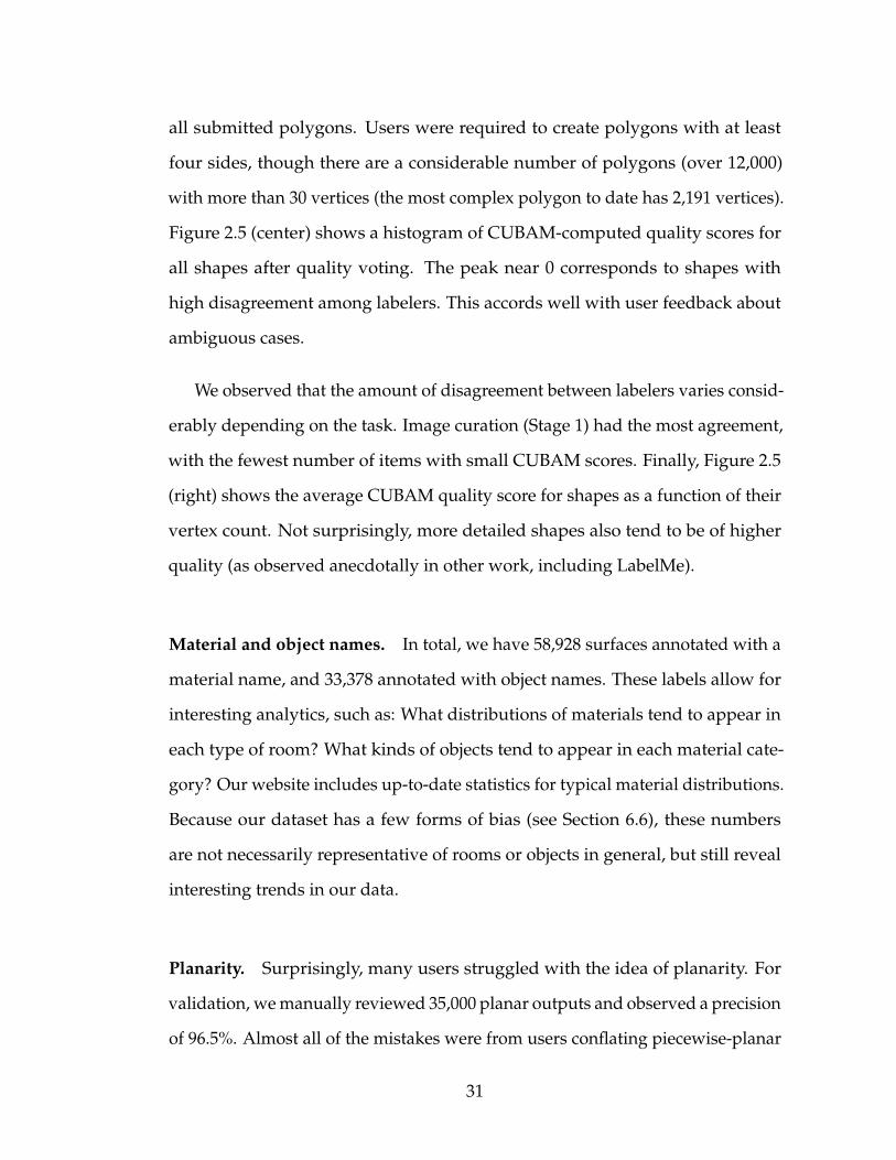
all submitted polygons. Users were required to create polygons with at least

four sides, though there are a considerable number of polygons (over 12,000)

with more than 30 vertices (the most complex polygon to date has 2,191 vertices).

Figure 2.5 (center) shows a histogram of CUBAM-computed quality scores for

all shapes after quality voting. The peak near 0 corresponds to shapes with

high disagreement among labelers. This accords well with user feedback about

ambiguous cases.

We observed that the amount of disagreement between labelers varies consid-

erably depending on the task. Image curation (Stage 1) had the most agreement,

with the fewest number of items with small CUBAM scores. Finally, Figure 2.5

(right) shows the average CUBAM quality score for shapes as a function of their

vertex count. Not surprisingly, more detailed shapes also tend to be of higher

quality (as observed anecdotally in other work, including LabelMe).

Material and object names. In total, we have 58,928 surfaces annotated with a

material name, and 33,378 annotated with object names. These labels allow for

interesting analytics, such as: What distributions of materials tend to appear in

each type of room? What kinds of objects tend to appear in each material cate-

gory? Our website includes up-to-date statistics for typical material distributions.

Because our dataset has a few forms of bias (see Section 6.6), these numbers

are not necessarily representative of rooms or objects in general, but still reveal

interesting trends in our data.

Planarity. Surprisingly, many users struggled with the idea of planarity. For

validation, we manually reviewed 35,000 planar outputs and observed a precision

of 96.5%. Almost all of the mistakes were from users conflating piecewise-planar

31

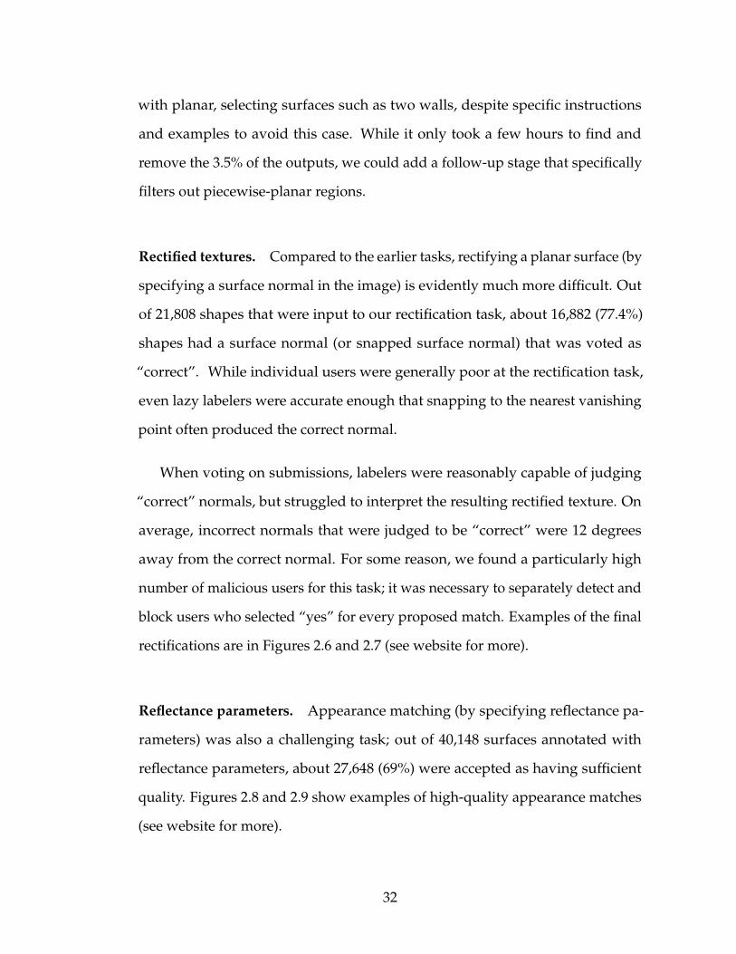
with planar, selecting surfaces such as two walls, despite specific instructions

and examples to avoid this case. While it only took a few hours to find and

remove the 3.5% of the outputs, we could add a follow-up stage that specifically

filters out piecewise-planar regions.

Rectified textures. Compared to the earlier tasks, rectifying a planar surface (by

specifying a surface normal in the image) is evidently much more difficult. Out

of 21,808 shapes that were input to our rectification task, about 16,882 (77.4%)

shapes had a surface normal (or snapped surface normal) that was voted as

“correct”. While individual users were generally poor at the rectification task,

even lazy labelers were accurate enough that snapping to the nearest vanishing

point often produced the correct normal.

When voting on submissions, labelers were reasonably capable of judging

“correct” normals, but struggled to interpret the resulting rectified texture. On

average, incorrect normals that were judged to be “correct” were 12 degrees

away from the correct normal. For some reason, we found a particularly high

number of malicious users for this task; it was necessary to separately detect and

block users who selected “yes” for every proposed match. Examples of the final

rectifications are in Figures 2.6 and 2.7 (see website for more).

Reflectance parameters. Appearance matching (by specifying reflectance pa-

rameters) was also a challenging task; out of 40,148 surfaces annotated with

reflectance parameters, about 27,648 (69%) were accepted as having sufficient

quality. Figures 2.8 and 2.9 show examples of high-quality appearance matches

(see website for more).

32

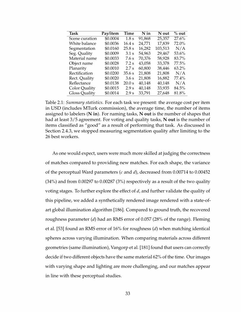
Task Pay/item Time N in N out % outScene curation $0.0004 1.8 s 91,868 25,357 27.6%White balance $0.0036 16.4 s 24,771 17,839 72.0%Segmentation $0.0160 25.8 s 16,282 103,513 N/ASeg. Quality $0.0009 3.1 s 54,963 29,467 53.6%Material name $0.0033 7.6 s 70,376 58,928 83.7%Object name $0.0028 7.2 s 43,058 33,378 77.5%Planarity $0.0010 2.7 s 60,800 38,446 63.2%Rectification $0.0200 35.6 s 21,808 21,808 N/ARect. Quality $0.0020 3.6 s 21,808 16,882 77.4%Reflectance $0.0138 20.0 s 40,148 40,148 N/AColor Quality $0.0015 2.9 s 40,148 33,935 84.5%Gloss Quality $0.0014 2.9 s 33,791 27,648 81.8%

Table 2.1: Summary statistics. For each task we present: the average cost per itemin USD (includes MTurk commission), the average time, the number of itemsassigned to labelers (N in). For naming tasks, N out is the number of shapes thathad at least 3/5 agreement. For voting and quality tasks, N out is the number ofitems classified as “good” as a result of performing that task. As discussed inSection 2.4.3, we stopped measuring segmentation quality after limiting to the26 best workers.

As one would expect, users were much more skilled at judging the correctness

of matches compared to providing new matches. For each shape, the variance

of the perceptual Ward parameters (c and d), decreased from 0.00714 to 0.00452

(34%) and from 0.00297 to 0.00287 (3%) respectively as a result of the two quality

voting stages. To further explore the effect of d, and further validate the quality of

this pipeline, we added a synthetically rendered image rendered with a state-of-

art global illumination algorithm [186]. Compared to ground truth, the recovered

roughness parameter (d) had an RMS error of 0.057 (28% of the range). Fleming

et al. [53] found an RMS error of 16% for roughness (d) when matching identical

spheres across varying illumination. When comparing materials across different

geometries (same illumination), Vangorp et al. [181] found that users can correctly

decide if two different objects have the same material 62% of the time. Our images

with varying shape and lighting are more challenging, and our matches appear

in line with these perceptual studies.

33

2.5.2 Task analytics

We now present statistics about our set of tasks, as well as additional observations

about the results. Table 2.1 shows summary statistics for each type of task,

including (1) the average payment for each item per task, (2) the average amount

of time spent per item, (3) the number of input items processed, and (4) the

fraction of output items that were rated as “good”. A total of 1,770 MTurk

labelers contributed to the database. As shown in the table, we observe a large

disparity in the time and cost required across the set of tasks (by up to two orders

of magnitude, in terms of cost). The fastest and least expensive task was curating

the initial photo set, where each processed photo cost a fraction of a cent. The

other voting tasks were also relatively inexpensive and fast, each taking less than

4 seconds. Interestingly, it required more pay to get labelers to quickly name

materials compared to objects; labelers seemed to prefer thinking about objects

instead of materials. The task which took the most time per item was rectification,

which took more than 30 seconds per shape, on average. In our experience with

this task, it often takes a significant amount of fine adjustment of the surface

normal to achieve a good rectification. Perhaps unsurprisingly, rectification and

appearance matching were the two most expensive tasks.

An important metric for evaluating MTurk use in collecting a large database

is the rate of data collection at a particular price point. We found that submission

rate was strongly correlated with price, the speed at which we approve tasks, and

the reputation we built with workers. Our submission rate continued to improve

as we built trust and communicated with workers. With a cost of about 13 cents

per surface (10 cents if non-planar), our initial submission rates improved from

a few hundred per day to rates of 4,200 segmentations, 4,500 reflectances, and

34

15,000 semantic labels per day.

Observations. In developing our tasks and working with labelers on MTurk,

we made a number of interesting observations. Many users told us they really

enjoyed the segmentation task, and produced beautifully detailed segmented

surfaces. We found that our best segmentations were produced by a handful of

people, some of whom created thousands of surfaces. On the other hand, some

people created good object segmentations. In the future, these shapes could be

sent back into the pipeline for further segmentation.

The two most difficult tasks were rectification and appearance matching.

For appearance matching, users especially struggled with matching near-mirror

materials. While they were skilled at selecting color using our interface, many

labelers seemed hesitant to select low roughness (high d). This could be due to

the fact that at low roughness, users can see the difference between the reflected

environment map and the true scene. In the future, we plan to test specialized

reflectance models for objects labeled as “mirror” or “glass”. On the other hand,

we observed that users often correctly used contextual information, such as the

appearance of a different object in the image, to aid in appearance matching.

This was especially helpful for matching gloss, where highlights suggesting

appearance may only appear in other parts of the scene. For example, labelers

might use the gloss on nearby cabinet doors to attribute roughness parameters to

the similar surface being annotated, despite no discernible gloss being visible on

it. Finally, some surfaces in our database are multicolored; we found that in such

cases, users consistently matched the dominant color as initialized by k-means

clustering.

35

Feedback and quality incentives. Rather than raising the pay for all tasks

uniformly, which did not result in higher quality (as has been observed by

others [120]), we targeted good users for bonuses and feedback on the quality of

their work. For segmentation, we paid up to 10 times the base rate depending on

the complexity of the submission. On average, we paid an extra 25% in bonuses.

Since users are paid a fixed rate by default, there is otherwise no incentive to

spend extra time producing detailed submissions. One user replied “It’s difficult

but I appreciate your positive feedback when you approve/reject the HITs, so

I’m motivated to please you!” In addition to providing positive feedback, we

found it was necessary to prevent 159 users from doing our tasks because they

were either malicious or had an accuracy below 50%. The use of sentinels is

recommended by [61] to check labeler quality. However, we found that our

tasks are not amenable to this approach since our surfaces occur in distinctive

photographs, and repetition tips off the labeler. We would like to revisit this in

future work.

Sources of bias. In terms of representing places and surfaces, our dataset

is biased in a few ways. First, our photos are from Flickr, which is biased

towards higher-quality imagery (compared to other sites, such as Facebook),

and geographically (Flickr is more widely used in the U.S. and Europe). Second,

the keywords we use when searching for photos (intentionally) bias our data

towards clean, uncluttered rooms. Third, our users are likely biased towards

segmenting certain types of surfaces (as we require that they segment a fixed

number of surfaces per image, not the entire photo). Factors such as saliency

or ease of labeling likely play a role in a user’s decision about what surfaces to

label. Finally, since our environment map is fixed, differences in lighting between

36

the true scene and our proxy environment map could affect the reflectance

judgement of users and introduce small color shifts. Our pipeline reduces this

effect by rejecting improperly white balanced photos. However, further study

is needed to understand the extent of these errors. In Chapter 3, we discuss

an alternate method of collecting material labels that has a reduced bias against

complex boundaries: individual point clicks.

2.6 Proof-of-Concept Applications

Our surface catalog can both assist and enhance existing and new applications

in material search, browsing, editing, and classification. Here we describe a

few such supporting proof-of-concept uses of the database, and discuss future

applications.

2.6.1 Texturing

Richer texture exemplars. OpenSurfaces provides a large set of rectified real-

world textures for use as texture exemplars. These improve over the corre-

sponding unrectified and foreshortened textures, letting users of the catalog to

expand their access to interesting real-world textures. Figure 2.10 illustrates this

advantage.

Retexturing. Consider a user with a photograph containing a segmented sur-

face (e.g., a countertop) who wants to visualize a home remodeling change to

that surface. The user can browse OpenSurfaces for a suitable replacement using

37

the rich annotated data to search on color, material properties, object name, or

substance type. The rectified textures found in our catalog can be used as the

input to a texture synthesis algorithm (see Figure 2.11 for a synthesized granite

texture drawn from our database to retexture a kitchen counter, with minor

touch-ups applied as a post-process). While texture synthesis requires a clean

example, and most of our shapes contain shadows or lighting, we did not find

it difficult to select suitable shapes, since many shapes with undesired effects

contain a clean inner region.

2.6.2 Informed scene similarity

Our database can be used to enhance image and material search (e.g., to generate

ideas for interior design projects), by allowing for more targeted queries. With

our rich annotations, we can explore interior scenes in ways previously not

possible. For example, Figure 2.12 shows a search for wood flooring in kitchens

and a search for fabric sofas in living rooms. Using our user-annotated reflectance

parameters, we can further refine and sort the results by diffuse color similarity to

the input query. While the input query is a segmented material from our database,

the query can also be constructed by searching for a phrase (e.g. “kitchen wood

floor”) and selecting photos that have the desired color.

2.6.3 Future applications

There are many potential applications of a database of materials and surfaces

beyond the proofs-of-concept we describe.

38

Search. Searching for photos that contain shiny or rough materials, or particular

colors, can aid people interested in material design (e.g., interior decorating or

home remodeling). Another search problem, search-by-material, could identify

which paint or fabric can be bought from a store to best match an object in a photo.

Further, our large database of community-gathered photos can be analyzed to

discover common co-occurrences or relationships between certain materials.

For example, we could tell what materials, objects or colors are often found

above, below or nearby a given object. Similarly, we could offer suggestions

to homeowners, answering such questions as: “for kitchens with black granite

countertops, what kinds of materials are often used for cabinets?” We could

also use existing materials to automatically recognize that the query contained

black granite countertops, thus requiring the user to only submit an input photo.

As our database grows, we could discover geographic or temporal trends in

material design, given suitably tagged imagery.

Editing. Aside from search, material editing and transfer is also useful. Syn-

thetic object insertion into photographs [42, 90] could use our material parameters

for accurate compositing. Alternatively, one can imagine extending Photo Clip

Art [103] to the domain of material compositing, where rather than attempting

to accurately simulate lighting and shadows, one could search for a surface that

contains the desired effects. The presence of surface normals can also aid rea-

soning about perspective or scene geometry. Finally, surfaces such as wood may

appear very different depending on how the surfaces are treated (e.g., painted,

or unfinished). Our database can potentially be combined with image editing

software to visualize such effects.

39

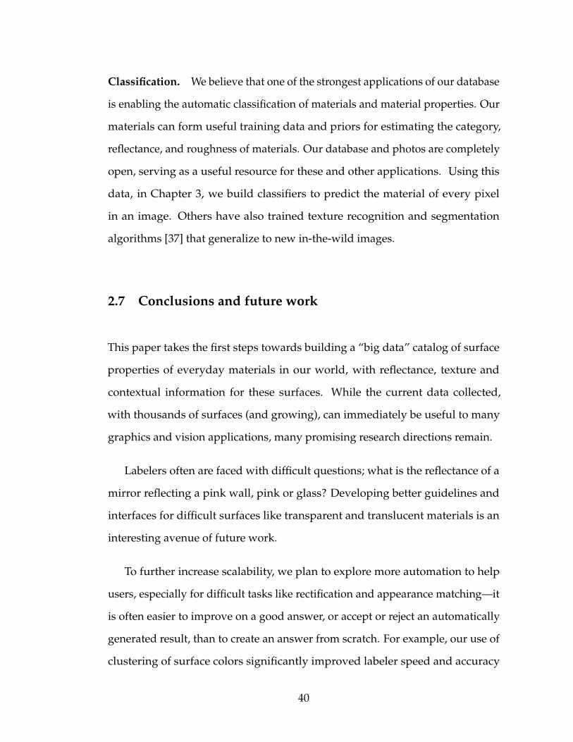
Classification. We believe that one of the strongest applications of our database

is enabling the automatic classification of materials and material properties. Our

materials can form useful training data and priors for estimating the category,

reflectance, and roughness of materials. Our database and photos are completely

open, serving as a useful resource for these and other applications. Using this

data, in Chapter 3, we build classifiers to predict the material of every pixel

in an image. Others have also trained texture recognition and segmentation

algorithms [37] that generalize to new in-the-wild images.

2.7 Conclusions and future work

This paper takes the first steps towards building a “big data” catalog of surface

properties of everyday materials in our world, with reflectance, texture and

contextual information for these surfaces. While the current data collected,

with thousands of surfaces (and growing), can immediately be useful to many

graphics and vision applications, many promising research directions remain.

Labelers often are faced with difficult questions; what is the reflectance of a

mirror reflecting a pink wall, pink or glass? Developing better guidelines and

interfaces for difficult surfaces like transparent and translucent materials is an

interesting avenue of future work.

To further increase scalability, we plan to explore more automation to help

users, especially for difficult tasks like rectification and appearance matching—it

is often easier to improve on a good answer, or accept or reject an automatically

generated result, than to create an answer from scratch. For example, our use of

clustering of surface colors significantly improved labeler speed and accuracy

40

in appearance matching. Similarly, detecting vanishing points assisted in the

rectification task. Indeed, our database can effectively bootstrap itself, by creating

large amounts of training data useful for improving algorithms for tasks like

material recognition [114] and reflectance estimation [46]. In Chapter 3, we build

on our dataset and train per-pixel material classifiers.

Further, we would like to address the sources of bias in our input collections,

by expanding to include more categories, and develop incentive systems to get a

more complete annotation of images.

While we include quality controls at every stage of the pipeline, we are inter-

ested in further evaluating the quality of our data in comparison to controlled,

in-lab methodologies. For reflectance, we plan to physically insert known objects

into scenes and compare the reflectance returned by the pipeline to the measured

material properties for those known objects. In addition, we plan to render

and annotate a larger collection of synthetic scenes to validate surface normals,

reflectances, and segmentations.

2.8 Impact

Our work was published at SIGGRAPH 2013 [12]. Our annotations from Open-

Surfaces have enabled others to train texture recognition and segmentation algo-

rithms [37, 36], and to redecorate rooms by automatically suggesting materials

for indoor digital scenes [29]. Our dataset has also been expanded with new

“describable texture attributes” and re-released as an augmented dataset [36].

Researchers from Microsoft have used our segmentation interface to power the

Microsoft Commons Objects in Context (MS COCO) project [113] which labeled

41

over 2.5 million objects; this data has significantly advanced the state-of-the-art

in object detection as part of the yearly MS COCO object detection challenge.

42

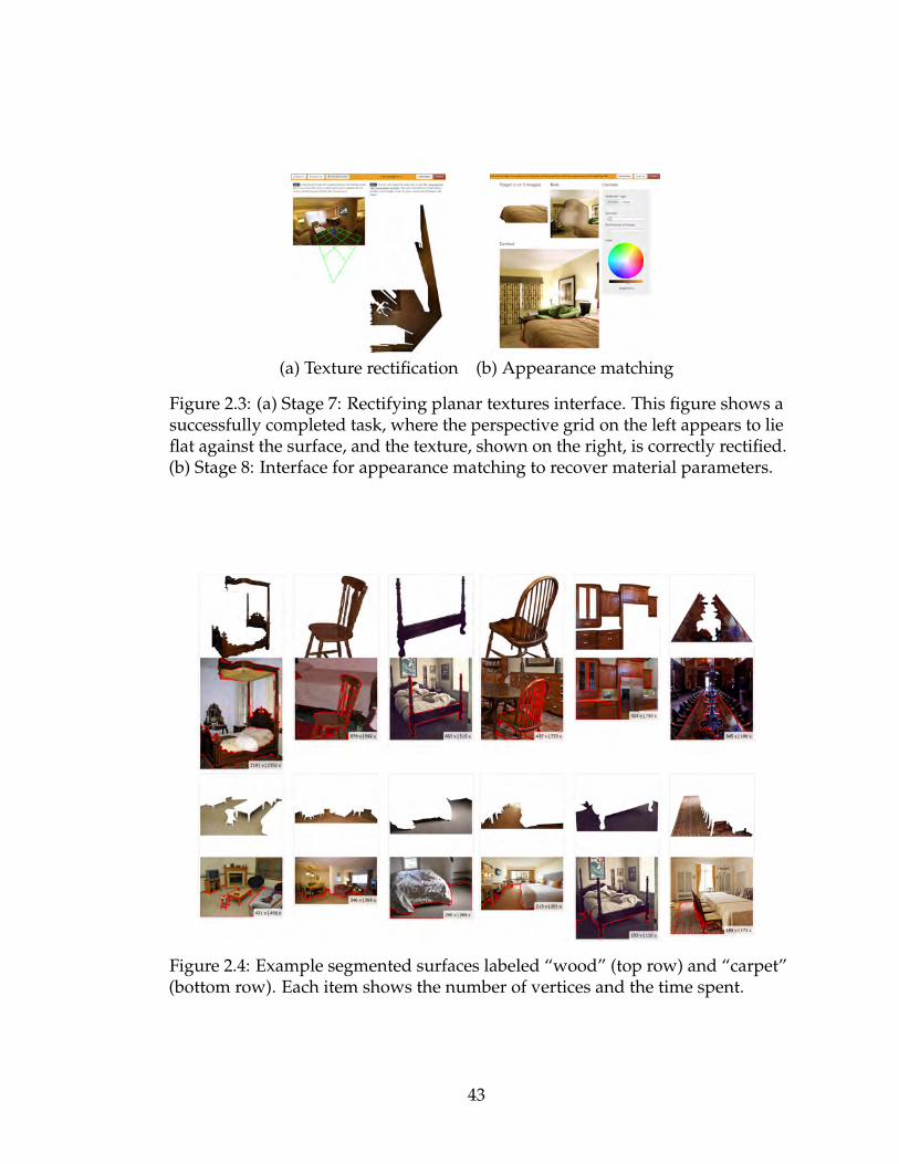
(a) Texture rectification (b) Appearance matching

Figure 2.3: (a) Stage 7: Rectifying planar textures interface. This figure shows asuccessfully completed task, where the perspective grid on the left appears to lieflat against the surface, and the texture, shown on the right, is correctly rectified.(b) Stage 8: Interface for appearance matching to recover material parameters.

Figure 2.4: Example segmented surfaces labeled “wood” (top row) and “carpet”(bottom row). Each item shows the number of vertices and the time spent.

43

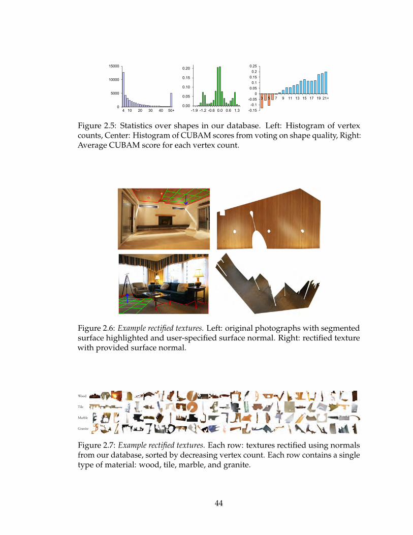
0

5000

10000

15000

4 10 20 30 40 50+0.00

0.05

0.10

0.15

0.20

-1.9 -1.2 -0.6 0.0 0.6 1.3 -0.15-0.1-0.05

00.050.10.150.20.25

3 5 7 9 11 13 15 17 19 21+

Figure 2.5: Statistics over shapes in our database. Left: Histogram of vertexcounts, Center: Histogram of CUBAM scores from voting on shape quality, Right:Average CUBAM score for each vertex count.

Figure 2.6: Example rectified textures. Left: original photographs with segmentedsurface highlighted and user-specified surface normal. Right: rectified texturewith provided surface normal.

Wood

Tile

Marble

Granite

Figure 2.7: Example rectified textures. Each row: textures rectified using normalsfrom our database, sorted by decreasing vertex count. Each row contains a singletype of material: wood, tile, marble, and granite.

44

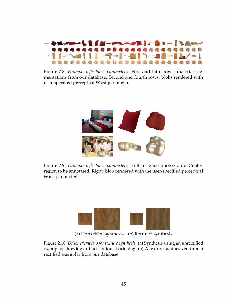
Fabric

Wood

Figure 2.8: Example reflectance parameters. First and third rows: material seg-mentations from our database. Second and fourth rows: blobs rendered withuser-specified perceptual Ward parameters.

Figure 2.9: Example reflectance parameters. Left: original photograph. Center:region to be annotated. Right: blob rendered with the user-specified perceptualWard parameters.

(a) Unrectified synthesis (b) Rectified synthesis

Figure 2.10: Better exemplars for texture synthesis. (a) Synthesis using an unrectifiedexemplar, showing artifacts of foreshortening. (b) A texture synthesized from arectified exemplar from our database.

45

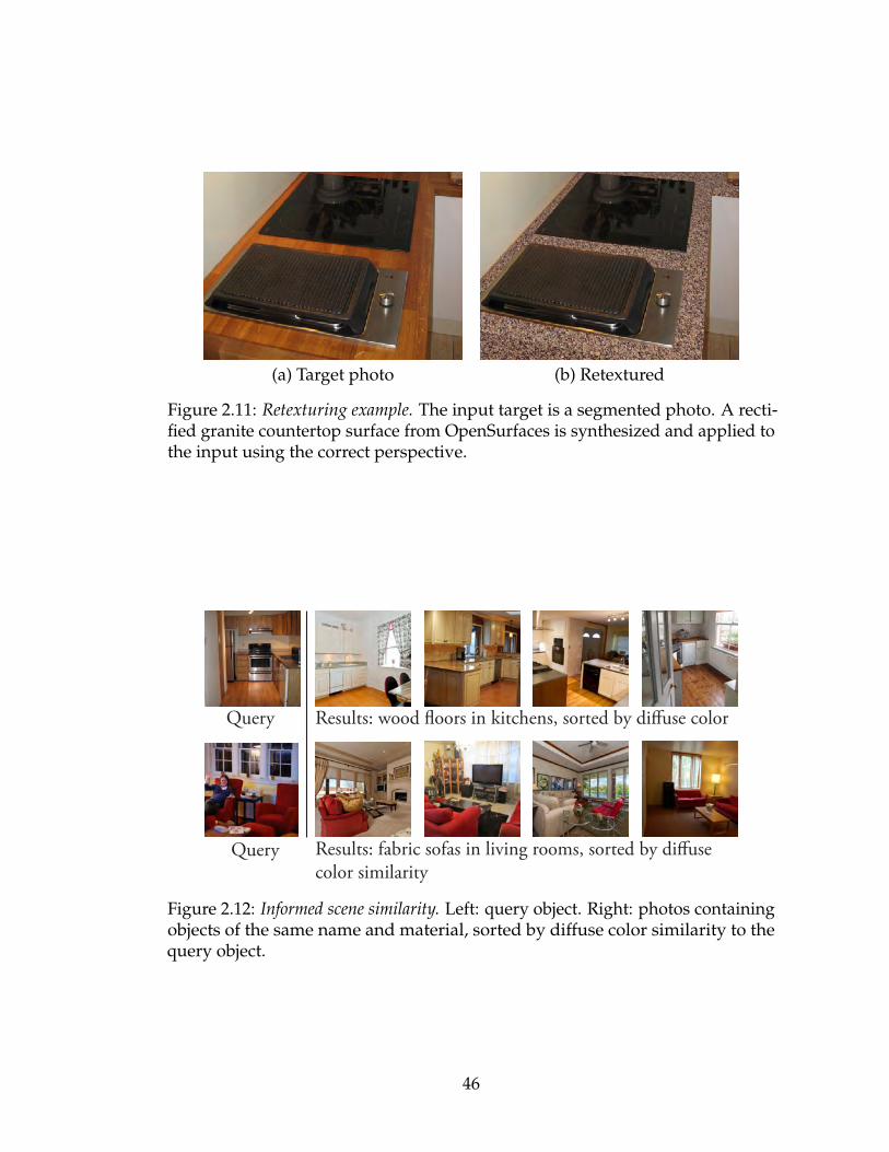
(a) Target photo (b) Retextured

Figure 2.11: Retexturing example. The input target is a segmented photo. A recti-fied granite countertop surface from OpenSurfaces is synthesized and applied tothe input using the correct perspective.

Query

Query Results: fabric sofas in living rooms, sorted by diuse color similarity

Results: wood oors in kitchens, sorted by diuse color

Figure 2.12: Informed scene similarity. Left: query object. Right: photos containingobjects of the same name and material, sorted by diffuse color similarity to thequery object.

46

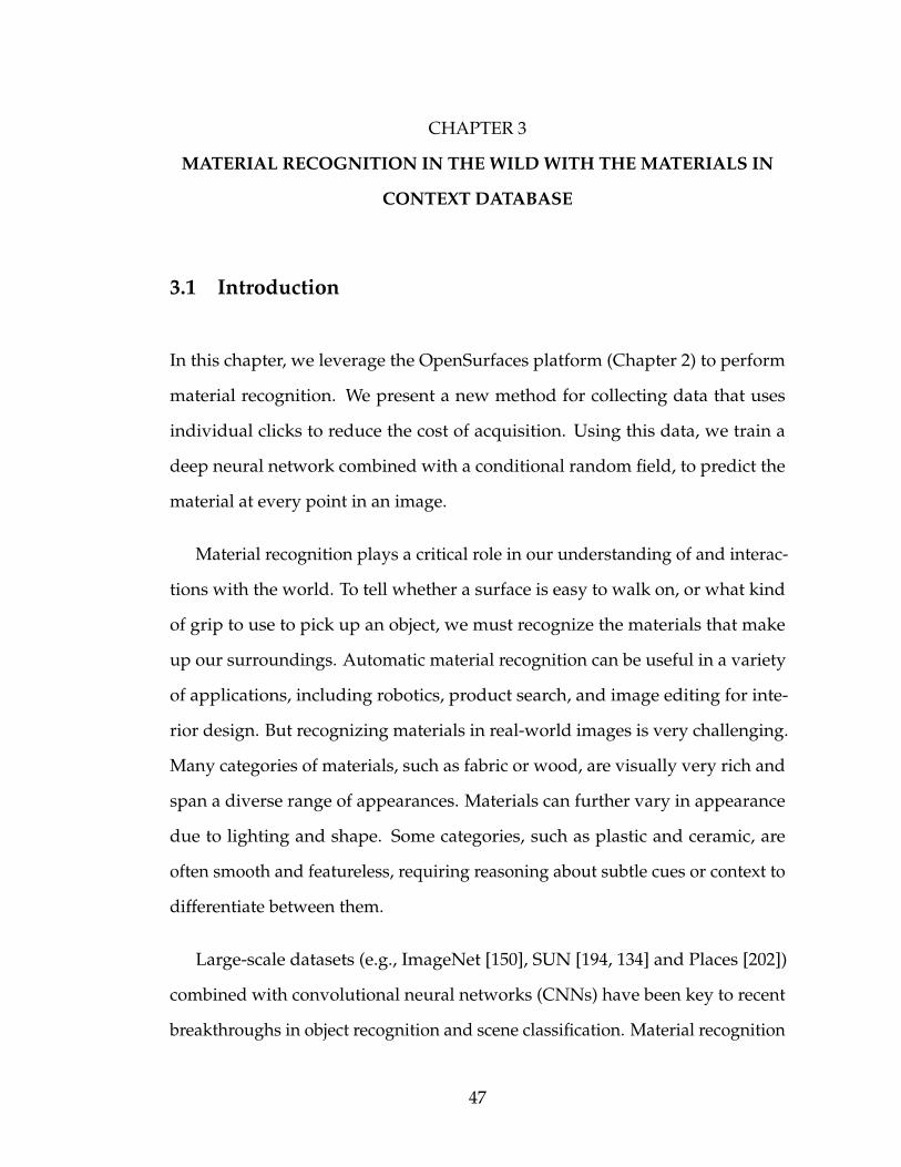
CHAPTER 3

MATERIAL RECOGNITION IN THE WILD WITH THE MATERIALS IN

CONTEXT DATABASE

3.1 Introduction

In this chapter, we leverage the OpenSurfaces platform (Chapter 2) to perform

material recognition. We present a new method for collecting data that uses

individual clicks to reduce the cost of acquisition. Using this data, we train a

deep neural network combined with a conditional random field, to predict the

material at every point in an image.

Material recognition plays a critical role in our understanding of and interac-

tions with the world. To tell whether a surface is easy to walk on, or what kind

of grip to use to pick up an object, we must recognize the materials that make

up our surroundings. Automatic material recognition can be useful in a variety

of applications, including robotics, product search, and image editing for inte-

rior design. But recognizing materials in real-world images is very challenging.

Many categories of materials, such as fabric or wood, are visually very rich and

span a diverse range of appearances. Materials can further vary in appearance

due to lighting and shape. Some categories, such as plastic and ceramic, are

often smooth and featureless, requiring reasoning about subtle cues or context to

differentiate between them.

Large-scale datasets (e.g., ImageNet [150], SUN [194, 134] and Places [202])

combined with convolutional neural networks (CNNs) have been key to recent

breakthroughs in object recognition and scene classification. Material recognition

47

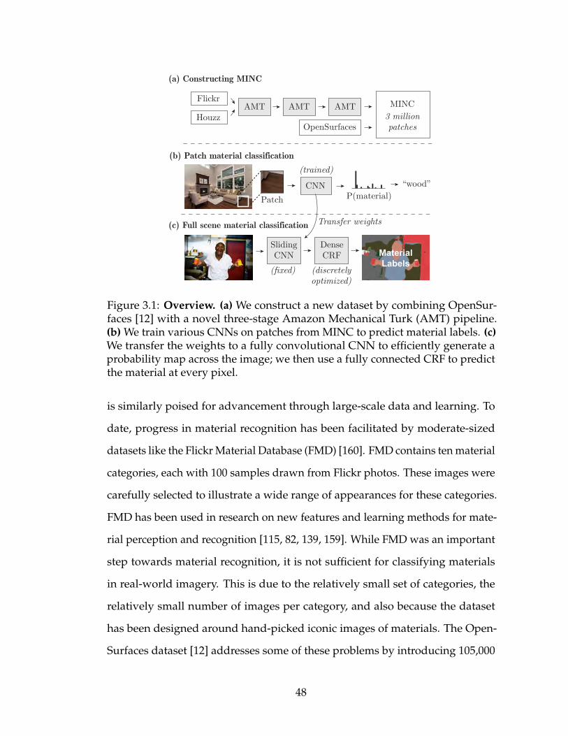
CNN

SlidingCNN

“wood”

Transfer weights

(trained)

(discretely optimized)

(fixed)

AMT AMT AMT MINC3 millionpatchesOpenSurfaces

Flickr

Houzz

(a) Constructing MINC

MaterialLabels

(b) Patch material classification

(c) Full scene material classification

P(material)

DenseCRF

Patch

Figure 3.1: Overview. (a) We construct a new dataset by combining OpenSur-faces [12] with a novel three-stage Amazon Mechanical Turk (AMT) pipeline.(b) We train various CNNs on patches from MINC to predict material labels. (c)We transfer the weights to a fully convolutional CNN to efficiently generate aprobability map across the image; we then use a fully connected CRF to predictthe material at every pixel.

is similarly poised for advancement through large-scale data and learning. To

date, progress in material recognition has been facilitated by moderate-sized

datasets like the Flickr Material Database (FMD) [160]. FMD contains ten material

categories, each with 100 samples drawn from Flickr photos. These images were

carefully selected to illustrate a wide range of appearances for these categories.

FMD has been used in research on new features and learning methods for mate-

rial perception and recognition [115, 82, 139, 159]. While FMD was an important

step towards material recognition, it is not sufficient for classifying materials

in real-world imagery. This is due to the relatively small set of categories, the

relatively small number of images per category, and also because the dataset

has been designed around hand-picked iconic images of materials. The Open-

Surfaces dataset [12] addresses some of these problems by introducing 105,000

48

material segmentations from real-world images, and is significantly larger than

FMD. However, in OpenSurfaces many material categories are under-sampled,

with only tens of images.

In this chapter we introduce a new, well-sampled material dataset, called

the Materials in Context Database (MINC), with 3 million material samples.

MINC is more diverse, has more examples in less common categories, and is

much larger than existing datasets. MINC draws data from both Flickr images,

which include many “regular” scenes, as well as Houzz images from professional

photographers of staged interiors. These sources of images each have different

characteristics that together increase the range of materials that can be recognized.

See Figure 3.2 for examples of our data. We make our full dataset available online

at http://minc.cs.cornell.edu/.

We use this data for material recognition by training different CNN architec-

tures on this new dataset. We perform experiments that illustrate the effect of

network architecture, image context, and training data size on subregions (i.e.,

patches) of a full scene image. Further, we build on our patch classification re-

sults and demonstrate simultaneous material recognition and segmentation of an

image by performing dense classification over the image with a fully connected

conditional random field (CRF) model [97]. By replacing the fully connected

layers of the CNN with convolutional layers [157], the computational burden is

significantly lower than a naive sliding window approach.

In summary, we make two new contributions:

• We introduce a new material dataset, MINC, and 3-stage crowdsourcing

pipeline for efficiently collecting millions of click labels (Section 3.3.2).

49

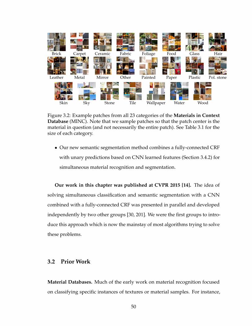
Brick Carpet Ceramic Fabric Foliage Food Glass Hair

Leather Metal Mirror Other Painted Paper Plastic Pol. stone

Skin Sky Stone Tile Wallpaper Water Wood

Figure 3.2: Example patches from all 23 categories of the Materials in ContextDatabase (MINC). Note that we sample patches so that the patch center is thematerial in question (and not necessarily the entire patch). See Table 3.1 for thesize of each category.

• Our new semantic segmentation method combines a fully-connected CRF

with unary predictions based on CNN learned features (Section 3.4.2) for

simultaneous material recognition and segmentation.

Our work in this chapter was published at CVPR 2015 [14]. The idea of

solving simultaneous classification and semantic segmentation with a CNN

combined with a fully-connected CRF was presented in parallel and developed

independently by two other groups [30, 201]. We were the first groups to intro-

duce this approach which is now the mainstay of most algorithms trying to solve

these problems.

3.2 Prior Work

Material Databases. Much of the early work on material recognition focused

on classifying specific instances of textures or material samples. For instance,

50

the CUReT [40] database contains 61 material samples, each captured under 205

different lighting and viewing conditions. This led to research on the task of

instance-level texture or material classification [107, 182], and an appreciation of

the challenges of building features that are invariant to pose and illumination.

Later, databases with more diverse examples from each material category began

to appear, such as KTH-TIPS [75, 24], and led explorations of how to generalize

from one example of a material to another—from one sample of wood to a

completely different sample, for instance. Real-world texture attributes have also

recently been explored [35].

In the domain of categorical material databases, Sharan et al. released

FMD [160] (described above). Subsequently, Bell et al. released OpenSurfaces [12]

which contains over 20,000 real-world scenes labeled with both materials and ob-

jects, using a multi-stage crowdsourcing pipeline. Because OpenSurfaces images

are drawn from consumer photos on Flickr, material samples have real-world

context, in contrast to prior databases (CUReT, KTH-TIPS, FMD) which feature

cropped stand-alone samples. While OpenSurfaces is a good starting point for a

material database, we substantially expand it with millions of new labels.

Material recognition. Much prior work on material recognition has focused on

the classification problem (categorizing an image patch into a set of material

categories), often using hand-designed image features. For FMD, Liu et al. [115]

introduced reflectance-based edge features in conjunction with other general

image features. Hu et al. [82] proposed features based on variances of oriented

gradients. Qi et al. [139] introduced a pairwise local binary pattern (LBP) feature.

Li et al. [108] synthesized a dataset based on KTH-TIPS2 and built a classifier

from LBP and dense SIFT. Timofte et al. [173] proposed a classification framework

51

with minimal parameter optimization. Schwartz and Nishino [156] introduced

material traits that incorporate learned convolutional auto-encoder features.

Recently, Cimpoi et al. [35] developed a CNN and improved Fisher vector (IFV)

classifier that achieves state-of-the-art results on FMD and KTH-TIPS2. Finally,

it has been shown that jointly predicting objects and materials can improve

performance [82, 200].

Convolutional neural networks. While CNNs have been around for a few

decades, with early successes such as LeNet [106], they have only recently led to

state-of-the-art results in object classification and detection, leading to enormous

progress. Driven by the ILSVRC challenge [150], we have seen many successful

CNN architectures [197, 157, 167, 165], led by the work of Krizhevsky et al.on

their SuperVision (a.k.a. AlexNet) network [99], with more recent architectures

including GoogLeNet [167]. In addition to image classification, CNNs are the

state-of-the-art for detection and localization of objects, with recent work includ-

ing R-CNNs [66], Overfeat [157], and VGG [165]. Finally, relevant to our goal

of per-pixel material segmentation, Farabet et al. [50] use a multi-scale CNN to

predict the class at every pixel in a segmentation. Oquab et al. [129] employ a

sliding window approach to localize patch classification of objects. We build on

this body of work in deep learning to solve our problem of material recognition

and segmentation.

3.3 The Materials in Context Database (MINC)

We now describe the methodology that went into building our new material

database. Why a new database? We needed a dataset with the following proper-

52

ties:

• Size: It should be sufficiently large that learning methods can generalize

beyond the training set.

• Well-sampled: Rare categories should be represented with a large number

of examples.

• Diversity: Images should span a wide range of appearances of each mate-

rial in real-world settings.

• Number of categories: It should contain many different materials found

in the real world.

3.3.1 Sources of data

We decided to start with the public, crowdsourced OpenSurfaces dataset [12] as

the seed for MINC since it is drawn from Flickr imagery of everyday, real-world

scenes with reasonable diversity. Furthermore, it has a large number of categories

and the most samples of all prior databases.

While OpenSurfaces data is a good start, it has a few limitations. Many

categories in OpenSurfaces are not well sampled. While the largest category,

wood, has nearly 20K samples, smaller categories, such as water, have only tens

of examples. This imbalance is due to the way the OpenSurfaces dataset was

annotated; workers on Amazon Mechanical Turk (AMT) were free to choose

any material subregion to segment. Workers often gravitated towards certain

common types of materials or salient objects, rather than being encouraged to

label a diverse set of materials. Further, the images come from a single source

(Flickr).

53

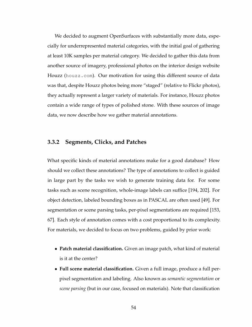
We decided to augment OpenSurfaces with substantially more data, espe-

cially for underrepresented material categories, with the initial goal of gathering

at least 10K samples per material category. We decided to gather this data from

another source of imagery, professional photos on the interior design website

Houzz (houzz.com). Our motivation for using this different source of data

was that, despite Houzz photos being more “staged” (relative to Flickr photos),

they actually represent a larger variety of materials. For instance, Houzz photos

contain a wide range of types of polished stone. With these sources of image

data, we now describe how we gather material annotations.

3.3.2 Segments, Clicks, and Patches

What specific kinds of material annotations make for a good database? How

should we collect these annotations? The type of annotations to collect is guided

in large part by the tasks we wish to generate training data for. For some

tasks such as scene recognition, whole-image labels can suffice [194, 202]. For

object detection, labeled bounding boxes as in PASCAL are often used [49]. For

segmentation or scene parsing tasks, per-pixel segmentations are required [153,

67]. Each style of annotation comes with a cost proportional to its complexity.

For materials, we decided to focus on two problems, guided by prior work:

• Patch material classification. Given an image patch, what kind of material

is it at the center?

• Full scene material classification. Given a full image, produce a full per-

pixel segmentation and labeling. Also known as semantic segmentation or

scene parsing (but in our case, focused on materials). Note that classification

54

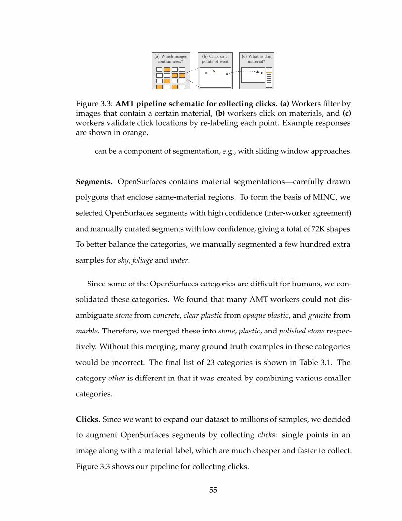
(a) Which images contain wood?

(b) Click on 3 points of wood

(c) What is this material?

Figure 3.3: AMT pipeline schematic for collecting clicks. (a) Workers filter byimages that contain a certain material, (b) workers click on materials, and (c)workers validate click locations by re-labeling each point. Example responsesare shown in orange.

can be a component of segmentation, e.g., with sliding window approaches.

Segments. OpenSurfaces contains material segmentations—carefully drawn

polygons that enclose same-material regions. To form the basis of MINC, we

selected OpenSurfaces segments with high confidence (inter-worker agreement)

and manually curated segments with low confidence, giving a total of 72K shapes.

To better balance the categories, we manually segmented a few hundred extra

samples for sky, foliage and water.

Since some of the OpenSurfaces categories are difficult for humans, we con-

solidated these categories. We found that many AMT workers could not dis-

ambiguate stone from concrete, clear plastic from opaque plastic, and granite from

marble. Therefore, we merged these into stone, plastic, and polished stone respec-

tively. Without this merging, many ground truth examples in these categories

would be incorrect. The final list of 23 categories is shown in Table 3.1. The

category other is different in that it was created by combining various smaller

categories.

Clicks. Since we want to expand our dataset to millions of samples, we decided

to augment OpenSurfaces segments by collecting clicks: single points in an

image along with a material label, which are much cheaper and faster to collect.

Figure 3.3 shows our pipeline for collecting clicks.

55

Initially, we tried asking workers to click on examples of a given material in a

photo. However, we found that workers would get frustrated if the material was

absent in too many of the photos. Thus, we added an initial first stage where

workers filter out such photos. To increase the accuracy of our labels, we verify

the click labels by asking different workers to specify the material for each click

without providing them with the label from the previous stage.

To ensure that we obtain high quality annotations and avoid collecting labels

from workers who are not making an effort, we include secret known answers

(sentinels) in the first and third stages, and block workers with an accuracy below

50% and 85% respectively. We do not use sentinels in the second stage since it

would require per-pixel ground truth labels, and it turned out not to be necessary.

Workers generally performed all three tasks so we could identify bad workers in

the first or third task.

Material clicks were collected for both OpenSurfaces images and the new

Houzz images. This allowed us to use labels from OpenSurfaces to generate the

sentinel data; we included 4 sentinels per task. With this streamlined pipeline

we collected 2,341,473 annotations at an average cost of $0.00306 per annotation

(stage 1: $0.02 / 40 images, stage 2: $0.10 / 50 images, 2, stage 3: $0.10 / 50

points).

Patches. Labeled segments and clicks form the core of MINC. For training

CNNs and other types of classifiers, it is useful to have data in the form of

fixed-sized patches. We convert both forms of data into a unified dataset format:

square image patches. We use a patch center and patch scale (a multiplier of the

smaller image dimension) to define the image subregion that makes a patch.

For our patch classification experiments, we use 23.3% of the smaller image

56

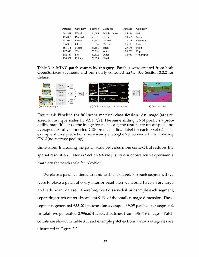
Patches Category Patches Category Patches Category

564,891 Wood 114,085 Polished stone 35,246 Skin465,076 Painted 98,891 Carpet 29,616 Stone397,982 Fabric 83,644 Leather 28,108 Ceramic216,368 Glass 75,084 Mirror 26,103 Hair188,491 Metal 64,454 Brick 25,498 Food147,346 Tile 55,364 Water 23,779 Paper142,150 Sky 39,612 Other 14,954 Wallpaper120,957 Foliage 38,975 Plastic

Table 3.1: MINC patch counts by category. Patches were created from bothOpenSurfaces segments and our newly collected clicks. See Section 3.3.2 fordetails.

Sky

Water

Foliage

Tile

(a) Multiscale input (b) Probability map (12 of 23 shown) (c) Predicted labels

SlidingCNN

DenseCRF

Wood

PlasticSlidingCNN

SlidingCNN

Avg.

Glass

Hair

Fabric PolishedstoneStone Paper

Water

Sky

Foliage

Tile

Paper

Wood

Stone

Wood

Tile

Figure 3.4: Pipeline for full scene material classification. An image (a) is re-sized to multiple scales [1/

√2, 1,

√2]. The same sliding CNN predicts a prob-

ability map (b) across the image for each scale; the results are upsampled andaveraged. A fully connected CRF predicts a final label for each pixel (c). Thisexample shows predictions from a single GoogLeNet converted into a slidingCNN (no average pooling).

dimension. Increasing the patch scale provides more context but reduces the

spatial resolution. Later in Section 6.6 we justify our choice with experiments

that vary the patch scale for AlexNet.

We place a patch centered around each click label. For each segment, if we

were to place a patch at every interior pixel then we would have a very large

and redundant dataset. Therefore, we Poisson-disk subsample each segment,

separating patch centers by at least 9.1% of the smaller image dimension. These

segments generated 655,201 patches (an average of 9.05 patches per segment).

In total, we generated 2,996,674 labeled patches from 436,749 images. Patch

counts are shown in Table 3.1, and example patches from various categories are

illustrated in Figure 3.2.

57

3.4 Material recognition in real-world images

Our goal is to train a system that recognizes the material at every pixel in an

image. We split our training procedure into multiple stages and analyze the

performance of the network at each stage. First, we train a CNN that produces

a single prediction for a given input patch. Then, we convert the CNN into a

sliding window and predict materials on a dense grid across the image. We do

this at multiple scales and average to obtain a unary term. Finally, a dense CRF

[97] combines the unary term with fully connected pairwise reasoning to output

per-pixel material predictions. The entire system is depicted in Figure 3.1, and

described more below.

3.4.1 Training procedure

MINC contains 3 million patches that we split into training, validation and test

sets. Randomly splitting would result in nearly identical patches (e.g., from

the same OpenSurfaces segment) being put in training and test, thus inflating

the test score. To prevent correlation, we group photos into clusters of near-

duplicates, then assign each cluster to one of train, validate or test. We make

sure that there are at least 75 segments of each category in the test set to ensure

there are enough segments to evaluate segmentation accuracy. To detect near-

duplicates, we compare AlexNet CNN features computed from each photo (see

the supplemental1 for details). For exact duplicates, we discard all but one of the

copies.

We train all of our CNNs by fine-tuning the network starting from the weights1http://www.cs.cornell.edu/˜sbell/pdf/cvpr2015-minc-supp.pdf

58

obtained by training on 1.2 million images from ImageNet (ILSVRC2012). When

training AlexNet, we use stochastic gradient descent with batchsize 128, dropout

rate 0.5, momentum 0.9, and a base learning rate of 10−3 that decreases by a factor

of 0.25 every 50,000 iterations. For GoogLeNet, we use batchsize 69, dropout 0.4,

and learning rate αt = 10−4√

1 − t/250000 for iteration t.

Our training set has a different number of examples per class, so we cycle

through the classes and randomly sample an example from each class. Failing

to properly balance the examples results in a 5.7% drop in mean class accuracy

(on the validation set). Further, since it has been shown to reduce overfitting,

we randomly augment samples by taking crops (227 × 227 out of 256 × 256),

horizontal mirror flips, spatial scales in the range [1/√

2,√

2], aspect ratios from

3:4 to 4:3, and amplitude shifts in [0.95, 1.05]. Since we are looking at local

regions, we subtract a per-channel mean (R: 124, G: 117, B: 104) rather than a

mean image [99].

3.4.2 Full scene material classification

Figure 3.4 shows an overview of our method for simultaneously segmenting

and recognizing materials. Given a CNN that can classify individual points in

the image, we convert it to a sliding window detector and densely classify a

grid across the image. Specifically, we replace the last fully connected layers

with convolutional layers, so that the network is fully convolutional and can

classify images of any shape. After conversion, the weights are fixed and not

fine-tuned. With our converted network, the strides of each layer cause the

network to output a prediction every 32 pixels. We obtain predictions every 16

59

pixels by shifting the input image by half-strides (16 pixels). While this appears

to require 4x the computation, Sermanet et al. [157] showed that the convolutions

can be reused and only the pool5 through fc8 layers need to be recomputed for

the half-stride shifts. Adding half-strides resulted in a minor 0.2% improvement

in mean class accuracy across segments (after applying the dense CRF, described

below), and about the same mean class accuracy at click locations.

The input image is resized so that a patch maps to a 256x256 square. Thus,

for a network trained at patch scale s, the resized input has smaller dimension

d = 256/s. Note that d is inversely proportional to scale, so increased context

leads to lower spatial resolution. We then add padding so that the output

probability map is aligned with the input when upsampled. We repeat this

at 3 different scales (smaller dimension d/√

2, d, d√

2), upsample each output

probability map with bilinear interpolation, and average the predictions. To

make the next step more efficient, we upsample the output to a fixed smaller

dimension of 550.

We then use the dense CRF of Krahenbuhlet al. [97] to predict a label at every

pixel, using the following energy:

E(x | I) =∑

i

ψi(xi) +∑i< j

ψi j(xi, x j) (3.1)

ψi(xi) = − log pi(xi) (3.2)

ψi j(xi, x j) = wp δ(xi , x j) k(fi − f j) (3.3)

where ψi is the unary energy (negative log of the aggregated softmax probabili-

ties) and ψi j is the pairwise term that connects every pair of pixels in the image.

We use a single pairwise term with a Potts label compatibility term δ weighted by

wp and unit Gaussian kernel k. For the features fi, we convert the RGB image to

60

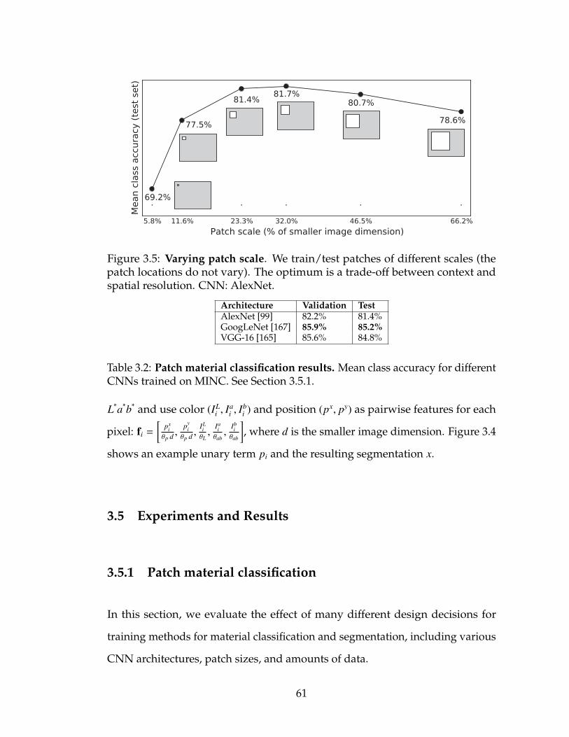
Figure 3.5: Varying patch scale. We train/test patches of different scales (thepatch locations do not vary). The optimum is a trade-off between context andspatial resolution. CNN: AlexNet.

Architecture Validation TestAlexNet [99] 82.2% 81.4%GoogLeNet [167] 85.9% 85.2%VGG-16 [165] 85.6% 84.8%

Table 3.2: Patch material classification results. Mean class accuracy for differentCNNs trained on MINC. See Section 3.5.1.

L*a*b* and use color (ILi , I

ai , I

bi ) and position (px, py) as pairwise features for each

pixel: fi =

[px

iθp d ,

pyi

θp d ,ILiθL,

Iaiθab,

Ibiθab

], where d is the smaller image dimension. Figure 3.4

shows an example unary term pi and the resulting segmentation x.

3.5 Experiments and Results

3.5.1 Patch material classification

In this section, we evaluate the effect of many different design decisions for

training methods for material classification and segmentation, including various

CNN architectures, patch sizes, and amounts of data.

61

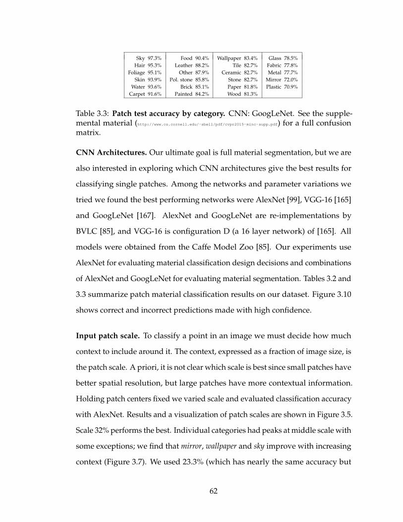
Sky 97.3% Food 90.4% Wallpaper 83.4% Glass 78.5%Hair 95.3% Leather 88.2% Tile 82.7% Fabric 77.8%

Foliage 95.1% Other 87.9% Ceramic 82.7% Metal 77.7%Skin 93.9% Pol. stone 85.8% Stone 82.7% Mirror 72.0%

Water 93.6% Brick 85.1% Paper 81.8% Plastic 70.9%Carpet 91.6% Painted 84.2% Wood 81.3%

Table 3.3: Patch test accuracy by category. CNN: GoogLeNet. See the supple-mental material (http://www.cs.cornell.edu/˜sbell/pdf/cvpr2015-minc-supp.pdf) for a full confusionmatrix.

CNN Architectures. Our ultimate goal is full material segmentation, but we are

also interested in exploring which CNN architectures give the best results for

classifying single patches. Among the networks and parameter variations we

tried we found the best performing networks were AlexNet [99], VGG-16 [165]

and GoogLeNet [167]. AlexNet and GoogLeNet are re-implementations by

BVLC [85], and VGG-16 is configuration D (a 16 layer network) of [165]. All

models were obtained from the Caffe Model Zoo [85]. Our experiments use

AlexNet for evaluating material classification design decisions and combinations

of AlexNet and GoogLeNet for evaluating material segmentation. Tables 3.2 and

3.3 summarize patch material classification results on our dataset. Figure 3.10

shows correct and incorrect predictions made with high confidence.

Input patch scale. To classify a point in an image we must decide how much

context to include around it. The context, expressed as a fraction of image size, is

the patch scale. A priori, it is not clear which scale is best since small patches have

better spatial resolution, but large patches have more contextual information.

Holding patch centers fixed we varied scale and evaluated classification accuracy

with AlexNet. Results and a visualization of patch scales are shown in Figure 3.5.

Scale 32% performs the best. Individual categories had peaks at middle scale with

some exceptions; we find that mirror, wallpaper and sky improve with increasing

context (Figure 3.7). We used 23.3% (which has nearly the same accuracy but

62

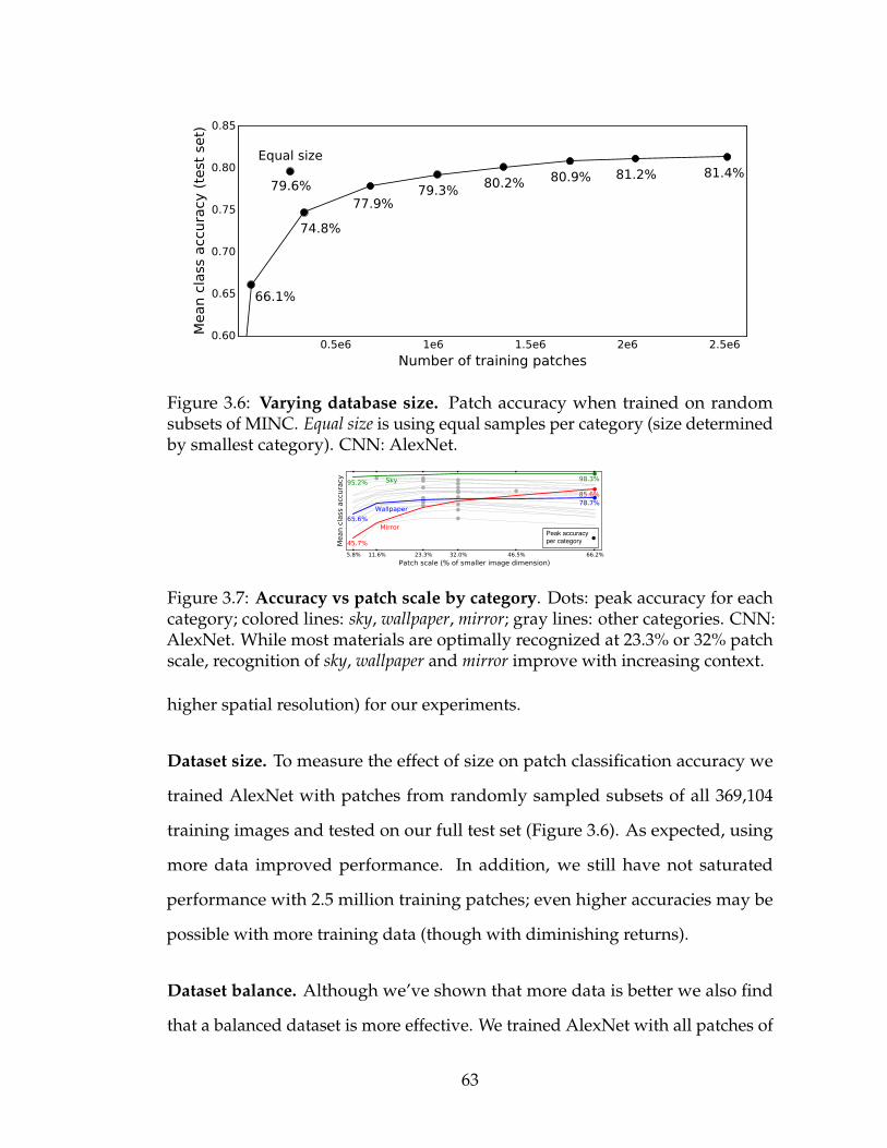
0.5e6 1e6 1.5e6 2e6 2.5e6

Number of training patches

0.60

0.65

0.70

0.75

0.80

0.85

Mean c

lass

acc

ura

cy (

test

set)

66.1%

74.8%

77.9%79.3%

80.2% 80.9% 81.2% 81.4%Equal size

79.6%

Figure 3.6: Varying database size. Patch accuracy when trained on randomsubsets of MINC. Equal size is using equal samples per category (size determinedby smallest category). CNN: AlexNet.

Peak accuracyper category

Figure 3.7: Accuracy vs patch scale by category. Dots: peak accuracy for eachcategory; colored lines: sky, wallpaper, mirror; gray lines: other categories. CNN:AlexNet. While most materials are optimally recognized at 23.3% or 32% patchscale, recognition of sky, wallpaper and mirror improve with increasing context.

higher spatial resolution) for our experiments.

Dataset size. To measure the effect of size on patch classification accuracy we

trained AlexNet with patches from randomly sampled subsets of all 369,104

training images and tested on our full test set (Figure 3.6). As expected, using

more data improved performance. In addition, we still have not saturated

performance with 2.5 million training patches; even higher accuracies may be

possible with more training data (though with diminishing returns).

Dataset balance. Although we’ve shown that more data is better we also find

that a balanced dataset is more effective. We trained AlexNet with all patches of

63

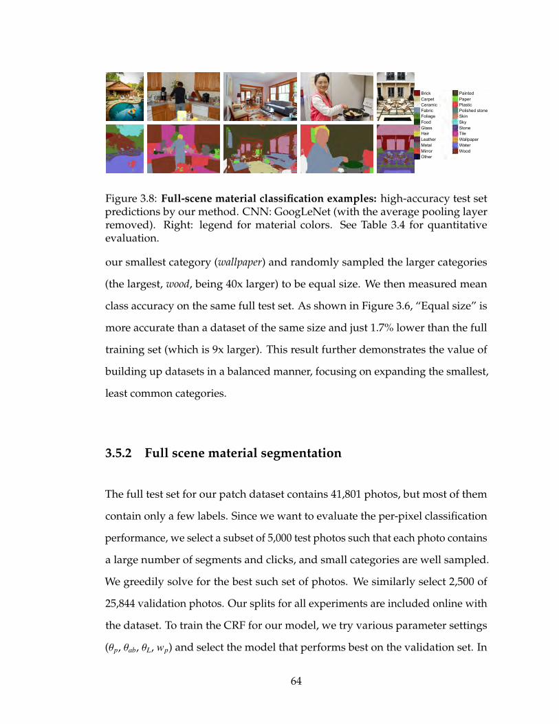
Brick

Wood

Carpet

WaterWallpaperTileStoneSkySkinPolished stonePlasticPaperPainted

OtherMirrorMetalLeatherHairGlassFoodFoliageFabricCeramic

Figure 3.8: Full-scene material classification examples: high-accuracy test setpredictions by our method. CNN: GoogLeNet (with the average pooling layerremoved). Right: legend for material colors. See Table 3.4 for quantitativeevaluation.

our smallest category (wallpaper) and randomly sampled the larger categories

(the largest, wood, being 40x larger) to be equal size. We then measured mean

class accuracy on the same full test set. As shown in Figure 3.6, “Equal size” is

more accurate than a dataset of the same size and just 1.7% lower than the full

training set (which is 9x larger). This result further demonstrates the value of

building up datasets in a balanced manner, focusing on expanding the smallest,

least common categories.

3.5.2 Full scene material segmentation

The full test set for our patch dataset contains 41,801 photos, but most of them

contain only a few labels. Since we want to evaluate the per-pixel classification

performance, we select a subset of 5,000 test photos such that each photo contains

a large number of segments and clicks, and small categories are well sampled.

We greedily solve for the best such set of photos. We similarly select 2,500 of

25,844 validation photos. Our splits for all experiments are included online with

the dataset. To train the CRF for our model, we try various parameter settings

(θp, θab, θL, wp) and select the model that performs best on the validation set. In

64

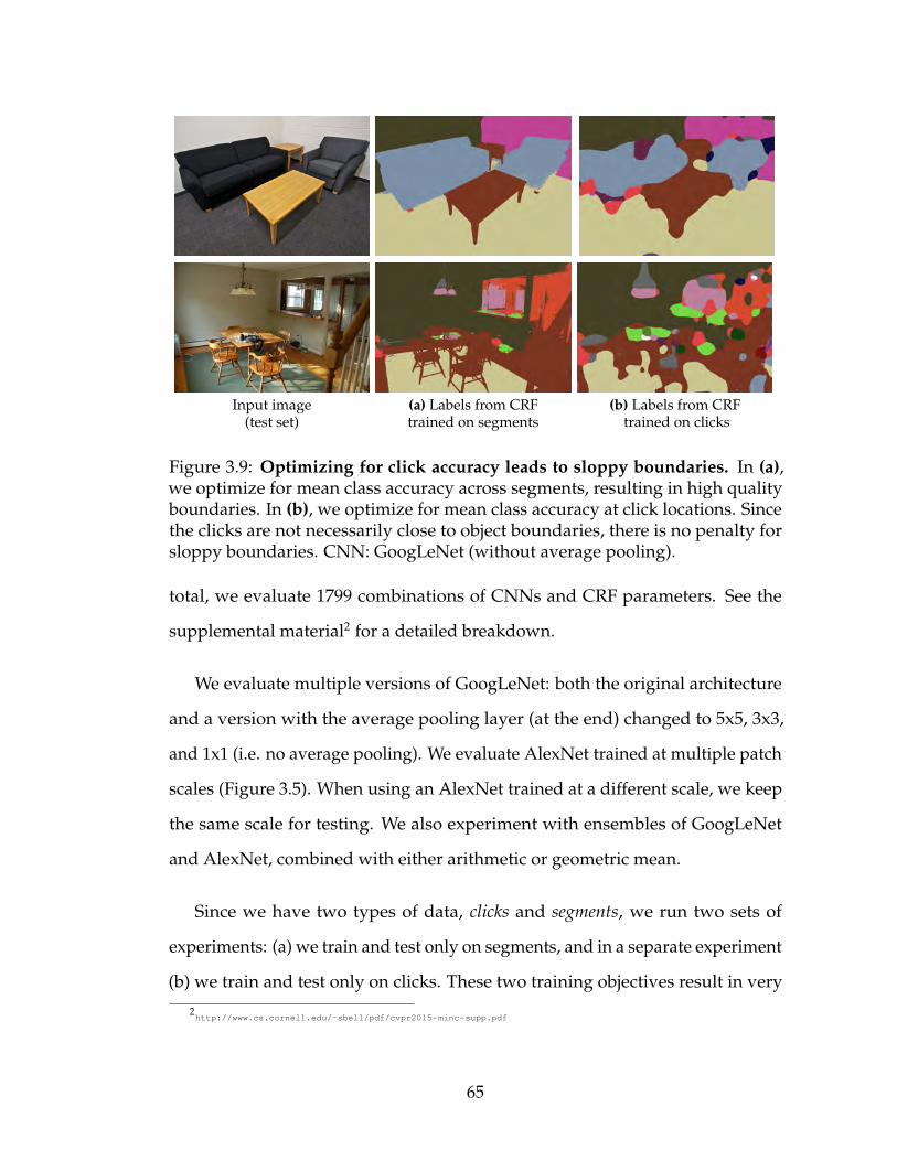
Input image (a) Labels from CRF (b) Labels from CRF(test set) trained on segments trained on clicks

Figure 3.9: Optimizing for click accuracy leads to sloppy boundaries. In (a),we optimize for mean class accuracy across segments, resulting in high qualityboundaries. In (b), we optimize for mean class accuracy at click locations. Sincethe clicks are not necessarily close to object boundaries, there is no penalty forsloppy boundaries. CNN: GoogLeNet (without average pooling).

total, we evaluate 1799 combinations of CNNs and CRF parameters. See the

supplemental material2 for a detailed breakdown.

We evaluate multiple versions of GoogLeNet: both the original architecture

and a version with the average pooling layer (at the end) changed to 5x5, 3x3,

and 1x1 (i.e. no average pooling). We evaluate AlexNet trained at multiple patch

scales (Figure 3.5). When using an AlexNet trained at a different scale, we keep

the same scale for testing. We also experiment with ensembles of GoogLeNet

and AlexNet, combined with either arithmetic or geometric mean.

Since we have two types of data, clicks and segments, we run two sets of

experiments: (a) we train and test only on segments, and in a separate experiment

(b) we train and test only on clicks. These two training objectives result in very

2http://www.cs.cornell.edu/˜sbell/pdf/cvpr2015-minc-supp.pdf

65

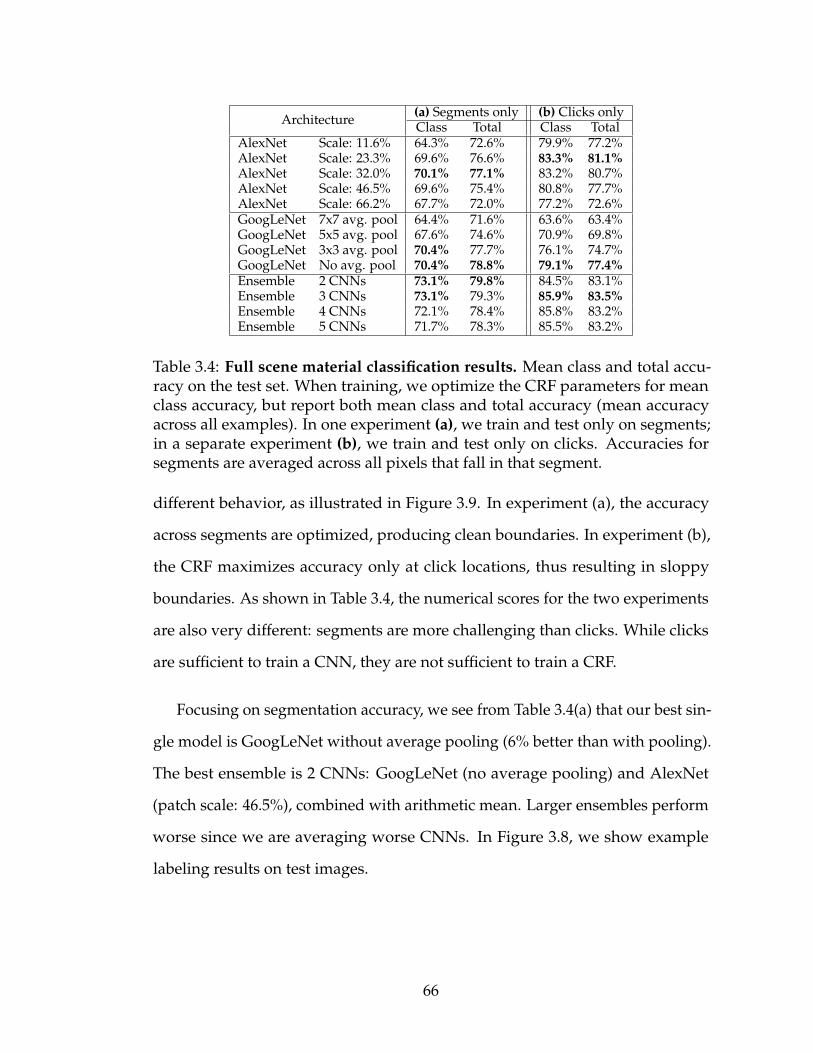
Architecture (a) Segments only (b) Clicks onlyClass Total Class Total

AlexNet Scale: 11.6% 64.3% 72.6% 79.9% 77.2%AlexNet Scale: 23.3% 69.6% 76.6% 83.3% 81.1%AlexNet Scale: 32.0% 70.1% 77.1% 83.2% 80.7%AlexNet Scale: 46.5% 69.6% 75.4% 80.8% 77.7%AlexNet Scale: 66.2% 67.7% 72.0% 77.2% 72.6%GoogLeNet 7x7 avg. pool 64.4% 71.6% 63.6% 63.4%GoogLeNet 5x5 avg. pool 67.6% 74.6% 70.9% 69.8%GoogLeNet 3x3 avg. pool 70.4% 77.7% 76.1% 74.7%GoogLeNet No avg. pool 70.4% 78.8% 79.1% 77.4%Ensemble 2 CNNs 73.1% 79.8% 84.5% 83.1%Ensemble 3 CNNs 73.1% 79.3% 85.9% 83.5%Ensemble 4 CNNs 72.1% 78.4% 85.8% 83.2%Ensemble 5 CNNs 71.7% 78.3% 85.5% 83.2%

Table 3.4: Full scene material classification results. Mean class and total accu-racy on the test set. When training, we optimize the CRF parameters for meanclass accuracy, but report both mean class and total accuracy (mean accuracyacross all examples). In one experiment (a), we train and test only on segments;in a separate experiment (b), we train and test only on clicks. Accuracies forsegments are averaged across all pixels that fall in that segment.

different behavior, as illustrated in Figure 3.9. In experiment (a), the accuracy

across segments are optimized, producing clean boundaries. In experiment (b),

the CRF maximizes accuracy only at click locations, thus resulting in sloppy

boundaries. As shown in Table 3.4, the numerical scores for the two experiments

are also very different: segments are more challenging than clicks. While clicks

are sufficient to train a CNN, they are not sufficient to train a CRF.

Focusing on segmentation accuracy, we see from Table 3.4(a) that our best sin-

gle model is GoogLeNet without average pooling (6% better than with pooling).

The best ensemble is 2 CNNs: GoogLeNet (no average pooling) and AlexNet

(patch scale: 46.5%), combined with arithmetic mean. Larger ensembles perform

worse since we are averaging worse CNNs. In Figure 3.8, we show example

labeling results on test images.

66

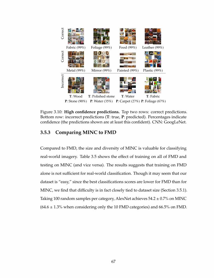
Cor

rect

Fabric (99%) Foliage (99%) Food (99%) Leather (99%)

Cor

rect

Metal (99%) Mirror (99%) Painted (99%) Plastic (99%)

Inco

rrec

t

T: Wood T: Polished stone T: Water T: FabricP: Stone (90%) P: Water (35%) P: Carpet (27%) P: Foliage (67%)

Figure 3.10: High confidence predictions. Top two rows: correct predictions.Bottom row: incorrect predictions (T: true, P: predicted). Percentages indicateconfidence (the predictions shown are at least this confident). CNN: GoogLeNet.

3.5.3 Comparing MINC to FMD

Compared to FMD, the size and diversity of MINC is valuable for classifying

real-world imagery. Table 3.5 shows the effect of training on all of FMD and

testing on MINC (and vice versa). The results suggests that training on FMD

alone is not sufficient for real-world classification. Though it may seem that our

dataset is “easy,” since the best classifications scores are lower for FMD than for

MINC, we find that difficulty is in fact closely tied to dataset size (Section 3.5.1).

Taking 100 random samples per category, AlexNet achieves 54.2 ± 0.7% on MINC

(64.6 ± 1.3% when considering only the 10 FMD categories) and 66.5% on FMD.

67

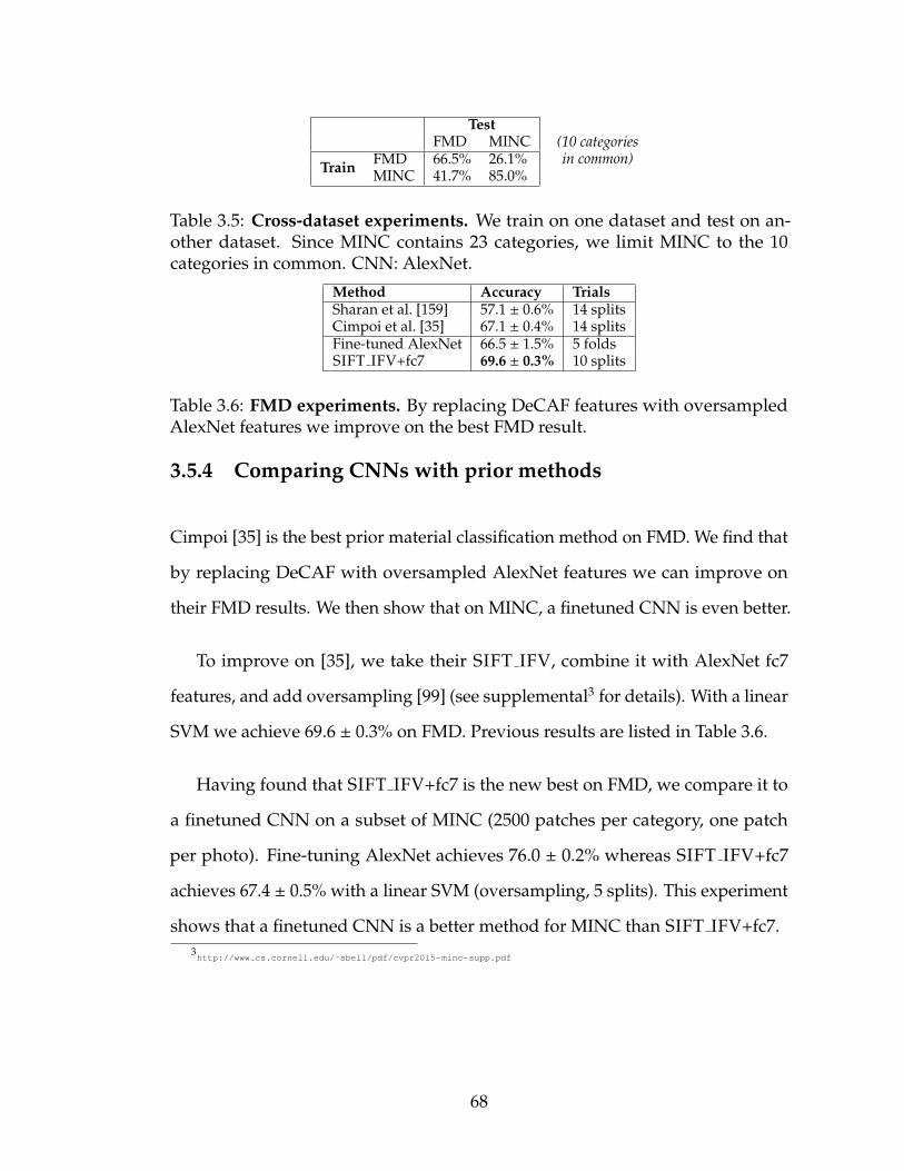
TestFMD MINC

Train FMD 66.5% 26.1%MINC 41.7% 85.0%

(10 categoriesin common)

Table 3.5: Cross-dataset experiments. We train on one dataset and test on an-other dataset. Since MINC contains 23 categories, we limit MINC to the 10categories in common. CNN: AlexNet.

Method Accuracy TrialsSharan et al. [159] 57.1 ± 0.6% 14 splitsCimpoi et al. [35] 67.1 ± 0.4% 14 splitsFine-tuned AlexNet 66.5 ± 1.5% 5 foldsSIFT IFV+fc7 69.6 ± 0.3% 10 splits

Table 3.6: FMD experiments. By replacing DeCAF features with oversampledAlexNet features we improve on the best FMD result.

3.5.4 Comparing CNNs with prior methods

Cimpoi [35] is the best prior material classification method on FMD. We find that

by replacing DeCAF with oversampled AlexNet features we can improve on

their FMD results. We then show that on MINC, a finetuned CNN is even better.

To improve on [35], we take their SIFT IFV, combine it with AlexNet fc7

features, and add oversampling [99] (see supplemental3 for details). With a linear

SVM we achieve 69.6 ± 0.3% on FMD. Previous results are listed in Table 3.6.

Having found that SIFT IFV+fc7 is the new best on FMD, we compare it to

a finetuned CNN on a subset of MINC (2500 patches per category, one patch

per photo). Fine-tuning AlexNet achieves 76.0 ± 0.2% whereas SIFT IFV+fc7

achieves 67.4 ± 0.5% with a linear SVM (oversampling, 5 splits). This experiment

shows that a finetuned CNN is a better method for MINC than SIFT IFV+fc7.3http://www.cs.cornell.edu/˜sbell/pdf/cvpr2015-minc-supp.pdf

68

3.6 Conclusion

Material recognition is a long-standing, challenging problem. We introduce

a new large, open, material database, MINC, that includes a diverse range

of materials of everyday scenes and staged designed interiors, and is at least

an order of magnitude larger than prior databases. Using this large database

we conduct an evaluation of recent deep learning algorithms for simultaneous

material classification and segmentation, and achieve results that surpass prior

attempts at material recognition.

Some lessons we have learned are:

• Training on a dataset which includes the surrounding context is crucial for

real-world material classification.

• Labeled clicks are cheap and sufficient to train a CNN alone. However,

to obtain high quality segmentation results, training a CRF on polygons

results in much better boundaries than training on clicks.

Many future avenues of work remain. Expanding the dataset to a broader

range of categories will require new ways to mine images that have more variety,

and new annotation tasks that are cost-effective. Inspired by attributes for

textures [35], in the future we would like to identify material attributes and

expand our database to include them. We also believe that further exploration

of joint material and object classification and segmentation will be fruitful [82]

and lead to improvements in both tasks. Our database, trained models, and all

experimental results are available online at http://minc.cs.cornell.edu/.

69

3.7 Impact

Our work in this chapter was published at CVPR 2015 [14]. Our approach of

using “click” labels to train semantic segmentation algorithms was later shown

to yield a large improvement for objects, resulting in the most accurate models

given a fixed annotation budget, out of squiggle-level, point-click, and full-image

supervision [9]. Further, our MINC database has been used to train new state-of-

the-art material recognition algorithms that go beyond the fully-connected CRF

algorithm of Krahenbuhl et al. [98] by directly learning pairwise potentials [83] or

using “bilateral inceptions” [55]. Others have used our data to integrate multiple

features obtained by different CNNs, obtaining close to human performance on

the Flickr Material Dataset [160] with transfer learning [198].

70

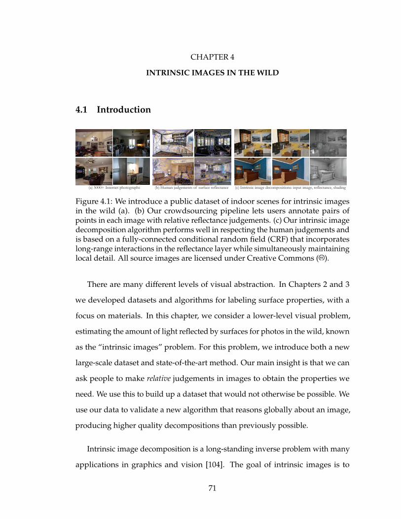
CHAPTER 4

INTRINSIC IMAGES IN THE WILD

4.1 Introduction

(b) Human judgements of surface reflectance(a) 5000+ Internet photographs (c) Intrinsic image decompositions: input image, reflectance, shading

WalkingGeek Christer Edvartsen atravellingmom bgv23 atravellingmom

Bill Wilson Jerine Lay TravelingOtter Jesus Rodriguez Bill Wilson

Figure 4.1: We introduce a public dataset of indoor scenes for intrinsic imagesin the wild (a). (b) Our crowdsourcing pipeline lets users annotate pairs ofpoints in each image with relative reflectance judgements. (c) Our intrinsic imagedecomposition algorithm performs well in respecting the human judgements andis based on a fully-connected conditional random field (CRF) that incorporateslong-range interactions in the reflectance layer while simultaneously maintaininglocal detail. All source images are licensed under Creative Commons ( ).

There are many different levels of visual abstraction. In Chapters 2 and 3

we developed datasets and algorithms for labeling surface properties, with a

focus on materials. In this chapter, we consider a lower-level visual problem,

estimating the amount of light reflected by surfaces for photos in the wild, known

as the “intrinsic images” problem. For this problem, we introduce both a new

large-scale dataset and state-of-the-art method. Our main insight is that we can

ask people to make relative judgements in images to obtain the properties we

need. We use this to build up a dataset that would not otherwise be possible. We

use our data to validate a new algorithm that reasons globally about an image,

producing higher quality decompositions than previously possible.

Intrinsic image decomposition is a long-standing inverse problem with many

applications in graphics and vision [104]. The goal of intrinsic images is to

71

separate an image into two layers, a reflectance (albedo) image and a shading (ir-

radiance) image, which multiply to form the original image. Reliable algorithms

for separating illumination from reflectance in scenes would enable a range of

applications, such as image-based resurfacing, texture transfer between images,

relighting, material recognition, and other interior design tasks. There has been

significant recent progress on the problem of intrinsic image decomposition,

aided by the release of the MIT Intrinsic Images dataset [69], which contains

carefully constructed ground truth for images of objects. However, intrinsic

image decomposition is still very challenging, especially on images of real-world

scenes. There is currently no standard dataset for evaluating intrinsic images

on images of such scenes, due in part to the challenge of capturing real-world

photos with known ground truth reflectance and illumination. To span the rich

range of real-world scenes we need a large set of images. For this scenario, both

careful measurement (as in [69]) and using rendered images of synthetic scenes

are not practical or satisfactory. Instead, to cover a rich variety of real-world

conditions, we select thousands of images from public photo collections [13]

and leverage human perception by turning to crowdsourcing to collect material

annotations for each image.

We present a new, large-scale database of Intrinsic Images in the Wild—real-

world photos of indoor scenes, with crowdsourced annotations of reflectance

comparisons between points in a scene. Rather than creating per-pixel (absolute)

annotations, we designed a scalable approach to human annotation involving

humans reasoning about the relative reflectance of pairs of pixels in each image.

This dataset is the first of its kind for intrinsic images, both in its scale and in

its use of human annotation: the dataset contains over 5,000 images featuring

a wide variety of scenes, and has been annotated with millions of individual

72

reflectance comparisons (on average 100 judgements per image). This makes

our dataset several orders of magnitude larger than existing intrinsic image

datasets. In addition, we include a dataset of about 400 images with a dense

set of annotations (on average 900 per image). Figure 4.1 illustrates our dataset,

including the pairwise comparisons we collect (Figure 4.1(b)).

Motivated by our new dataset, we have also created a new intrinsic image de-

composition algorithm designed for images of real-world scenes. Our algorithm

makes use of the fact that many surfaces in indoor scenes share the same material

and reflectance, resulting in long-range sharing of reflectances across a scene (for

example, a painted wall spanning an entire image). We build on recent work

in fully connected conditional random field (CRF) inference [98] to enable such

long-range connections in our algorithm. We evaluate our method on our new

benchmark, and show that it outperforms several state-of-the-art algorithms.

In summary, our contributions are:

• A new, large-scale dataset for intrinsic images annotated via crowdsourcing

that includes more than 5,000 images. This dataset is completely open and

public, including both images and annotations, with the aim of enabling

others to design and evaluate new algorithms for scene-level intrinsic

images.

• A new intrinsic images algorithm based on a dense CRF formulation that

considers long-range material relations to achieve better decomposition on

our new database.

We evaluate our new algorithm, as well as a suite of other public intrinsic image

algorithms, on our dataset. For each algorithm, we perform extensive cross-

73

validation to find the optimal parameters on our dataset, and find that our new

algorithm outperforms these recent algorithms. Nonetheless, intrinsic image

decomposition for real-world scenes of this complexity remains a challenging

problem, with much room for improvement. We release our database of images

and annotations to help drive future research in this problem.

4.2 Related work

Intrinsic images. Intrinsic image decomposition has a rich history in computer

graphics and vision, and has been studied since the 1970s. One of the earliest

observations is that large discontinuities in image intensity correspond to changes

in reflectance, and all other variations are due mostly to changes in shading [104].

This led to the Retinex algorithm in which each image gradient is classified as

belonging to either the reflectance layer or the shading layer according to its

magnitude. The resulting decomposition is obtained by solving for the pair of

layers whose gradients best match these classified gradients. Nearly forty years

later, a version of this algorithm was the best performing on the MIT Intrinsic

Images dataset [69]. Subsequent algorithms perform much better on this dataset,

as described below.

Many others ideas have been proposed to solve the problem. Some recent

techniques use classifiers trained on local grayscale patterns [170, 169], priors on

texture statistics [126, 117], complex priors on shape, albedo, and illumination [6,

5, 8], meso- and macro-scales of shading [110], chromaticity segmentation [57],

sparse sets of basis reflectances [128, 58], non-local texture constraints [163, 199],

and red-black wavelets [164].

74

Further, many methods have been proposed that require additional input to

solve the problem. With user interaction, Bousseau [19] showed that a very high-

quality decomposition can be obtained, and Carroll [25] showed that diffuse

interreflections can be separated. Others have addressed the problem using

additional photos of the same scene either registered as an image stack [189, 74],

or taken from different angles (enabling additional 3D reasoning) [70, 102, 101].

Finally, recent methods have been proposed for RGB-D (Kinect-style) imagery [7,

31]. In contrast, our paper is focused on completely automated methods that

work on a single image.

Crowdsourcing. Recently many authors have shown how to effectively gather

high-quality data from workers online in an economical and scalable way. Many

types of problems have been addressed this way, including: acquiring material

and object labels [13], solving micro-problems with humans in the loop [62],

labeling parts and attributes of birds [22], evaluating image retargeting [148],

and using gauge figures for understanding shape perception [38]. Additionally,

many studies of worker dynamics have guided the design of tasks in this space,

such as modeling workers with a confusion matrix [41] or with multidimen-

sional classifiers that incorporate notions of user competence, bias, and expertise

(CUBAM model) [190].

Intrinsic images databases. Our goal is to scale to the wide diversity of scenes

in the real world in various lighting situations, and to acquire “ground truth” data

for such scenes. One could create such a dataset in a few different ways. The MIT

Intrinsic Images dataset [69] captured images of single objects and rigorously

acquired irradiance by spray painting the objects for diffuse measurements.

However, this approach does not scale to large numbers of scenes in the wild.

75

Another approach is to render synthetic scenes along with their reflectance and

illumination (as has been done in prior work on a few test scenes, or on CG

movie sequences [31]); but these approaches are constrained by the availability

of models that span the range of real world materials, lightings and scenes.

Instead, we chose to use human judgements as our ground truth data.

4.3 Database

We designed a crowdsourcing pipeline where human subjects (on Amazon

Mechanical Turk (AMT)) report which of two points in an image has a darker

surface reflectance. Our pipeline (shown in Figure 4.2) scales to millions of

human judgements across thousands of real-world images. We aimed to produce

a dataset that was broad enough to draw conclusions about intrinsic image

algorithms. To design this pipeline we needed to address several questions:

• What judgements should the human annotators make?

• Which images and points should we show each user?

• How to present tasks to the user in an intuitive interface?

• How to identify users who are correctly performing the task and how to

aggregate accurate judgements across users?

4.3.1 What judgements should we collect?

We would ideally collect ground truth reflectance information for each point in

an image. However, there are several challenges in collecting such information

76

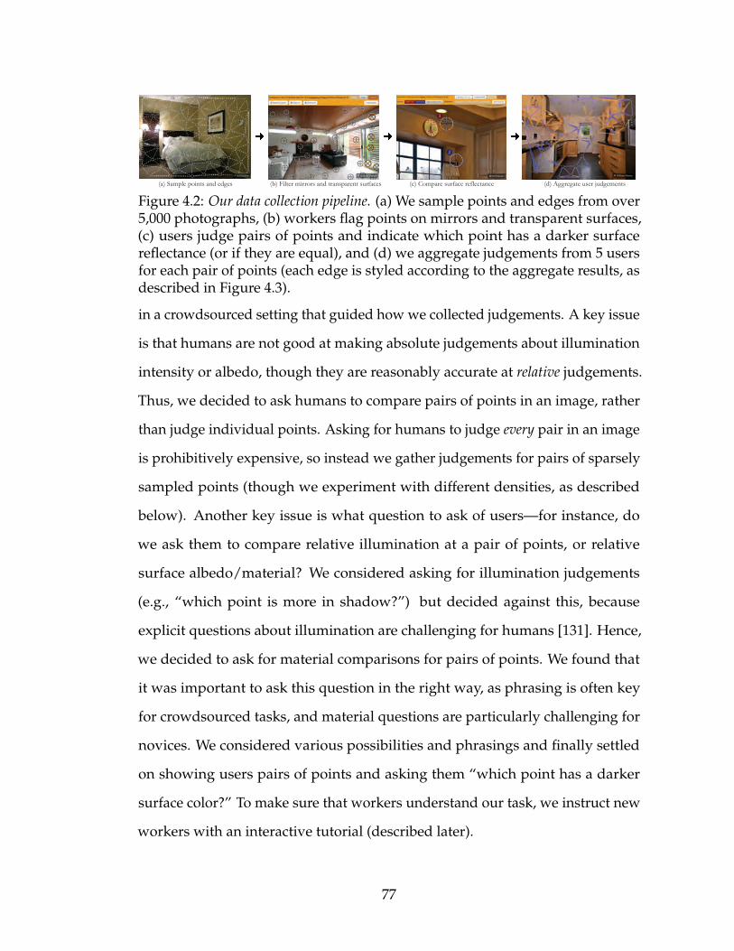
(a) Sample points and edges (b) Filter mirrors and transparent surfaces (c) Compare surface reflectance (d) Aggregate user judgementsbfishadow Jeremy Levine Bill Wilson William Warby

Figure 4.2: Our data collection pipeline. (a) We sample points and edges from over5,000 photographs, (b) workers flag points on mirrors and transparent surfaces,(c) users judge pairs of points and indicate which point has a darker surfacereflectance (or if they are equal), and (d) we aggregate judgements from 5 usersfor each pair of points (each edge is styled according to the aggregate results, asdescribed in Figure 4.3).

in a crowdsourced setting that guided how we collected judgements. A key issue

is that humans are not good at making absolute judgements about illumination

intensity or albedo, though they are reasonably accurate at relative judgements.

Thus, we decided to ask humans to compare pairs of points in an image, rather

than judge individual points. Asking for humans to judge every pair in an image

is prohibitively expensive, so instead we gather judgements for pairs of sparsely

sampled points (though we experiment with different densities, as described

below). Another key issue is what question to ask of users—for instance, do

we ask them to compare relative illumination at a pair of points, or relative

surface albedo/material? We considered asking for illumination judgements

(e.g., “which point is more in shadow?”) but decided against this, because

explicit questions about illumination are challenging for humans [131]. Hence,

we decided to ask for material comparisons for pairs of points. We found that

it was important to ask this question in the right way, as phrasing is often key

for crowdsourced tasks, and material questions are particularly challenging for

novices. We considered various possibilities and phrasings and finally settled

on showing users pairs of points and asking them “which point has a darker

surface color?” To make sure that workers understand our task, we instruct new

workers with an interactive tutorial (described later).

77

4.3.2 Which images and which pairs of points?

Given the task described above, we next had to select our images and the points

in each image for which we collect annotations.

Images. Our goal was to assemble a broad collection of images from the real

world that are representative and free from image editing and other filters. We

chose images from the OpenSurfaces dataset [13], which were gathered from

Flickr and contain a variety of indoor scenes (kitchens, living rooms, bedrooms,

and so on). We manually curated photos to remove images that do not represent

how the world looks to the naked eye, with effects such as blur, excessive

defocus, high noise, depth-of-field, fisheye, poor exposure, black-and-white,

visible vignetting, washed out colors, infrared filters, distorted color tones, long-

exposure effects, visible HDR artifacts, stitched panoramas, text overlays, and

extra borders.

Points. Next, we must decide which points in each image to compare. To

achieve good image coverage, and since it can be difficult to reason about the

relative diffuse reflectance of points that are far apart in an image, we select

points that are approximately equally spaced. In particular, we sample image

points using Poisson disk sampling with a minimum radius (we use 7% of the

image diameter).

Since we are sampling points that could lie on reflectance discontinuities,

we remove potentially difficult judgements from the initial set of Poisson-disk-

sampled points. Specifically, we remove (a) points within 4 pixels of a strong

edge (as determined with a Canny edge detector), (b) over- or under-saturated

78

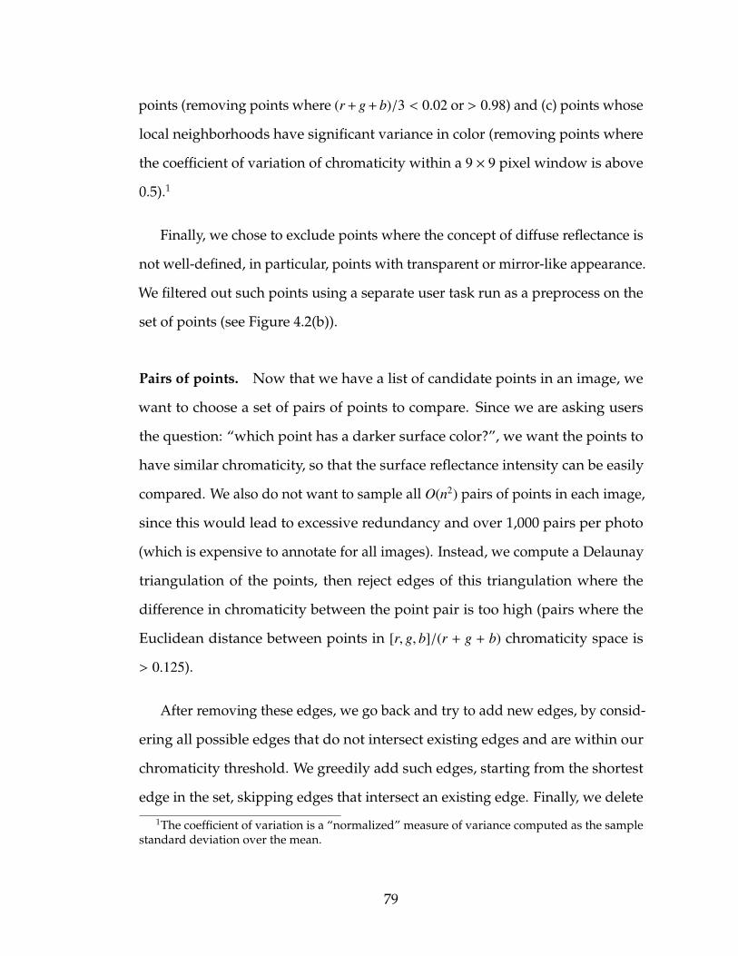
points (removing points where (r+g+b)/3 < 0.02 or > 0.98) and (c) points whose

local neighborhoods have significant variance in color (removing points where

the coefficient of variation of chromaticity within a 9 × 9 pixel window is above

0.5).1

Finally, we chose to exclude points where the concept of diffuse reflectance is

not well-defined, in particular, points with transparent or mirror-like appearance.

We filtered out such points using a separate user task run as a preprocess on the

set of points (see Figure 4.2(b)).

Pairs of points. Now that we have a list of candidate points in an image, we

want to choose a set of pairs of points to compare. Since we are asking users

the question: “which point has a darker surface color?”, we want the points to

have similar chromaticity, so that the surface reflectance intensity can be easily

compared. We also do not want to sample all O(n2) pairs of points in each image,

since this would lead to excessive redundancy and over 1,000 pairs per photo

(which is expensive to annotate for all images). Instead, we compute a Delaunay

triangulation of the points, then reject edges of this triangulation where the

difference in chromaticity between the point pair is too high (pairs where the

Euclidean distance between points in [r, g, b]/(r + g + b) chromaticity space is

> 0.125).

After removing these edges, we go back and try to add new edges, by consid-

ering all possible edges that do not intersect existing edges and are within our

chromaticity threshold. We greedily add such edges, starting from the shortest

edge in the set, skipping edges that intersect an existing edge. Finally, we delete

1The coefficient of variation is a “normalized” measure of variance computed as the samplestandard deviation over the mean.

79

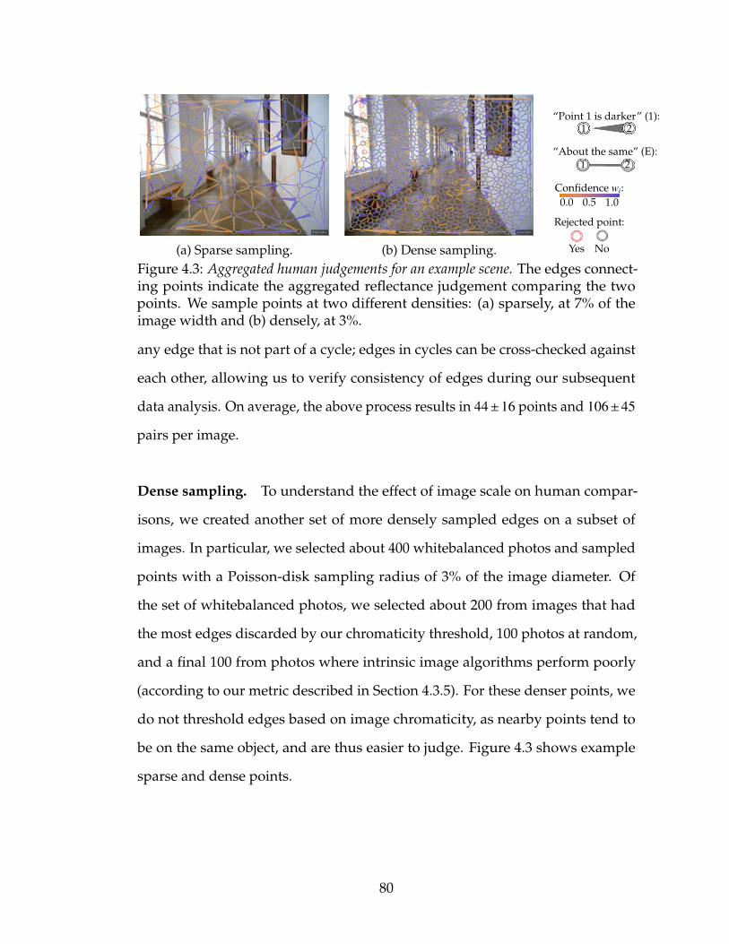
Bev Sykes

(a) Sparse sampling.

Bev Sykes

(b) Dense sampling.

1 2“Point 1 is darker” (1):

“About the same” (E):1 2

Confidence wi:0.0 0.5 1.0

Yes No

Rejected point:

Figure 4.3: Aggregated human judgements for an example scene. The edges connect-ing points indicate the aggregated reflectance judgement comparing the twopoints. We sample points at two different densities: (a) sparsely, at 7% of theimage width and (b) densely, at 3%.

any edge that is not part of a cycle; edges in cycles can be cross-checked against

each other, allowing us to verify consistency of edges during our subsequent

data analysis. On average, the above process results in 44±16 points and 106±45

pairs per image.

Dense sampling. To understand the effect of image scale on human compar-

isons, we created another set of more densely sampled edges on a subset of

images. In particular, we selected about 400 whitebalanced photos and sampled

points with a Poisson-disk sampling radius of 3% of the image diameter. Of

the set of whitebalanced photos, we selected about 200 from images that had

the most edges discarded by our chromaticity threshold, 100 photos at random,

and a final 100 from photos where intrinsic image algorithms perform poorly

(according to our metric described in Section 4.3.5). For these denser points, we

do not threshold edges based on image chromaticity, as nearby points tend to

be on the same object, and are thus easier to judge. Figure 4.3 shows example

sparse and dense points.

80

4.3.3 Annotation interface

Our user interface for collecting annotations, shown in Figure 4.2(c), shows the

user an image and asks them, for a particular pair of pixels (indicated with

crosshairs and labeled Points 1 and 2), which of the two points has a darker

surface color. The user can then select one of three options: Point 1, Point 2, and

About the same. We ask users to specify their confidence in their assessment as

Guessing, Probably, or Definitely, as was done by [22].

Tutorial. While humans are skilled at brightness and color constancy—i.e.,

discounting lighting when comparing surface reflectance (across a range of

typical illumination conditions)—they are not used to explicitly thinking about

this effect. We found that if one asks users to compare surface color and ignore

lighting, a sizeable portion (almost half) of workers misunderstand the task

as “which image pixel is darker?”. We were able to reduce this proportion to

about 25% by adding a tutorial which explains exactly the distinction between

pixel intensity difference and surface reflectance difference. The tutorial then

presents several test scenes and provides feedback and the correct answer if

the worker makes a mistake. We chose difficult test scenes that force users to

understand concepts such as: local highlights do not affect surface reflectance,

and viewing the scene as a whole is sometimes necessary to visually comprehend

and compare reflectance. The tutorial we developed is shown in the video and

included on our website.2

Efficient input. Since users are to provide thousands of answers, we designed

an interface that allows for rapid input. For each photo, our interface displays the

2http://intrinsic.cs.cornell.edu/

81

photo in its entirety, pauses for 1 second, and then zooms to show a pair of points.

Once the user indicates their answer for that pair, the interface smoothly zooms

to the next pair of points. We use van Wijk smooth zooming [180] (implemented

by D3 [18]) to quickly show the next pair of points. At any time, users can zoom

in/out, pan around the image, or repeat the zoom animation and have the points

flash to make them easier to see. Users can also return to the previous pair and

enter a new answer.

Users had unanimously positive feedback regarding our task UI:

• “Fun. It’s exactly what I wish there was more of on MTurk as far as image

categorization/similar HITs go.”

• “This task is very well-designed and easy to understand and complete. The

zoom function is quite helpful.”

• “These are addicting as all hell.”

Mirror and transparent surfaces. Prior to asking users to judge relative surface

reflectance, we filter points through an initial stage in which users flag points

as being either on a mirror or on a transparent surface (Figure 4.2(b)). As with

our comparison task, a tutorial explains the types of surfaces we want filtered

and lets users practice. See the video3 for more illustrations of our two user

interfaces.3http://intrinsic.cs.cornell.edu/

82

Figure 4.4: Histograms of worker performance (left) and time spent (right). Verticalaxis on both plots: number of users. Left: percentage of sentinel data answeredcorrectly. Right: time spent and effective wage (pay per task / time spent).

4.3.4 Data verification

After showing a pair of surface points to multiple workers, we want to classify

that pair into one of three categories: (1) Point 1 has a darker reflectance than

Point 2, (2) Point 2 has a darker reflectance than Point 1, and (3) they have

approximately the same reflectance. We could do simple majority voting on the

user-provided input to determine the category; however, consistent with other

work on crowdsourcing, we found that the raw input is too noisy for this simple

approach to work well.

On Mechanical Turk, there are thousands of workers of varying skill. While

we believe that almost all the workers are capable of performing the task, we

found that a significant fraction of workers (about 31%, based on our analysis

below) either did not try to do the task correctly, or did not understand the

instructions, even after the tutorial where they can try out the task and receive

feedback explaining the correct answer. To address this problem, we take three

steps to ensure high-quality data: (1) we replicate every task (i.e., each pair of

points) to at least 5 workers, (2) we insert “sentinel” objects with known answers

into each task, and (3) we use the CUBAM machine learning algorithm [190]

to automatically model user competence and bias when computing consensus

labels.

83

Sentinels. Inspired by the microtasks work of Gingold, et al. [62], each of our

tasks (also known as a “HIT” on AMT) contains 25 comparisons plus 5 “sentinel”

comparisons drawn from a set of known answers. To hide which items are

sentinels, our server dynamically selects 5 test items that the worker has not seen

before. As a user submits tasks, we measure their accuracy on the sentinels. The

moment a user makes at least 5 mistakes and has an average accuracy below

80%, that user is blocked from performing the task. We add the test for average

accuracy to avoid prematurely blocking users. When a given user has seen all

test items, we stop serving the 5 extra comparisons, as the user has proven to be

accurate enough on all sentinels. We chose to test a user across HITs, rather than

including a large amount of sentinel items inside each HIT since we found that

workers maintain approximately the same accuracy between submissions. This

wastes less resources ensuring that workers are behaving correctly. Figure 4.4

shows the distribution of worker scores on sentinel items. With this method,

about 31% of users were blocked. Users seemed appreciative of the fact that the

effective pay increased after the sentinels were finished, and we only identified a

single user who passed our tests and later began submitting random answers

(some time after the sentinels finished).

Modeling workers. Once we have filtered out users who are not correctly

performing the task, we must aggregate the reliable answers to obtain a single

judgement Ji for each pair of points. Since some comparisons can be genuinely

ambiguous, we would like to assign a confidence (or weight) wi to each judge-

ment Ji. Further, different users may have different competence and internal

thresholds when comparing surface reflectances, and we would like to compen-

sate for these effects. The CUBAM user model [190] lends itself to these issues,

but requires that the questions have binary answers, while our judgements have

84

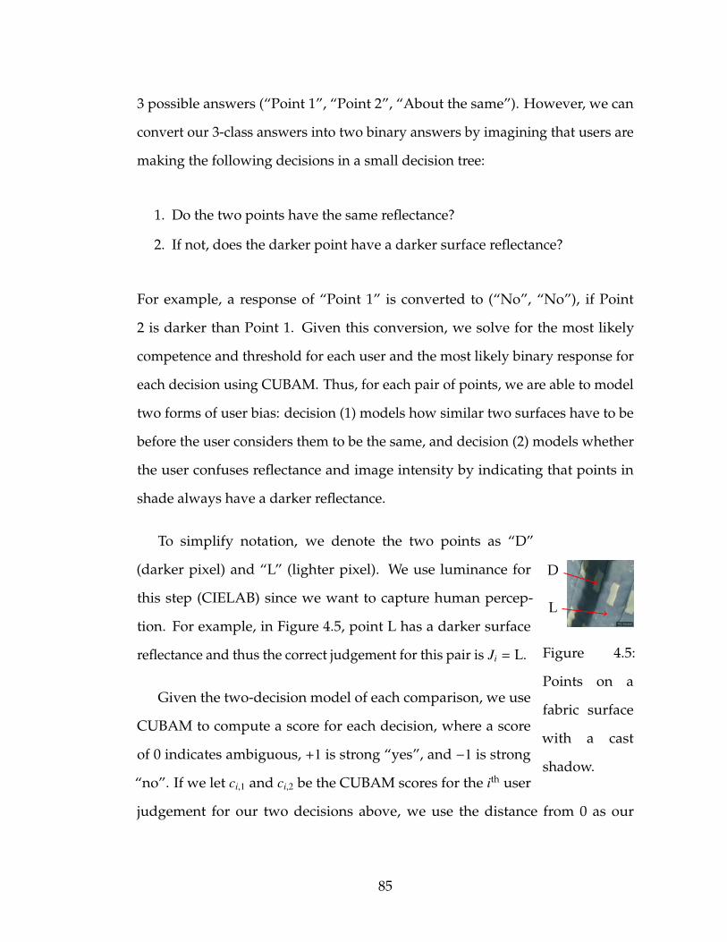
3 possible answers (“Point 1”, “Point 2”, “About the same”). However, we can

convert our 3-class answers into two binary answers by imagining that users are

making the following decisions in a small decision tree:

1. Do the two points have the same reflectance?

2. If not, does the darker point have a darker surface reflectance?

For example, a response of “Point 1” is converted to (“No”, “No”), if Point

2 is darker than Point 1. Given this conversion, we solve for the most likely

competence and threshold for each user and the most likely binary response for

each decision using CUBAM. Thus, for each pair of points, we are able to model

two forms of user bias: decision (1) models how similar two surfaces have to be

before the user considers them to be the same, and decision (2) models whether

the user confuses reflectance and image intensity by indicating that points in

shade always have a darker reflectance.

L

D

K. Kendall

Figure 4.5:

Points on a

fabric surface

with a cast

shadow.

To simplify notation, we denote the two points as “D”

(darker pixel) and “L” (lighter pixel). We use luminance for

this step (CIELAB) since we want to capture human percep-

tion. For example, in Figure 4.5, point L has a darker surface

reflectance and thus the correct judgement for this pair is Ji = L.

Given the two-decision model of each comparison, we use

CUBAM to compute a score for each decision, where a score

of 0 indicates ambiguous, +1 is strong “yes”, and −1 is strong

“no”. If we let ci,1 and ci,2 be the CUBAM scores for the ith user

judgement for our two decisions above, we use the distance from 0 as our

85

confidence/weight wi for judgement Ji:

(Ji,wi) =

(E, ci,1) if ci,1 > 0

(D, ci,2) if ci,1 ≤ 0 and ci,2 > 0

(L,−ci,2) else

(4.1)

where E indicates that users judge the points to have equal or “about the same”

reflectance intensity. Finally, we map the judgements from E,L,D to the original

set of possible answers E, 1, 2.

Running the experiment. As workers were performing tasks, we periodically

reviewed subsets of the aggregated answers. Whenever we decided that the

aggregated answer for an unambiguous comparison was incorrect, we corrected

the comparison, excluded it from future aggregation with CUBAM, and added it

to our set of sentinel test items. This ensures that our sentinel items are difficult—

i.e., discriminative in selecting workers who are not trying very hard. This

strategy is similar to “hard negative mining” used in machine learning [51] (the

idea of using hard examples to train good classifiers).

To fairly compensate workers, we approved all submissions instantly (even

those performed incorrectly). We were surprised to discover that this strategy

roughly doubled the number of simultaneous workers for the same rate of pay.

Users were very appreciative of the fast and certain approval.

4.3.5 Error metric: WHDR

In order to use our judgements to evaluate intrinsic image decompositions, we

need a way to numerically evaluate a decomposition (R, S ) given judgements

86

Ji and weights wi. We propose a new metric, the “weighted human disagree-

ment rate” (WHDR), which measures the percent of human judgements that an

algorithm disagrees with, weighted by the confidence of each judgement:

WHDRδ(J,R) =

∑i wi · 1

(Ji , Ji,δ(R)

)∑i wi

(4.2)

where R is the algorithm output reflectance layer, 1(·) is the unit indicator, Ji,δ is

the judgement predicted by the algorithm being evaluated, and δ is the relative

difference between two surface reflectances where people just begin to switch

between saying “they are about the same” (E) to “one point is darker” (1 or

2). To transform the algorithm reflectance layer R into the same units as the

judgements (answers in the set 1, 2,E), we must threshold differences between

the points used in the human judgement in the reflectance layer R. Because R is

only defined up to a scale factor, we compare two reflectances using their ratio,

as:

Ji,δ(R) =

1 if R2,i/R1,i > 1 + δ

2 if R1,i/R2,i > 1 + δ

E else

(4.3)

where R1,i is the reflectance sampled at point 1 for the ith judgement (and similarly

for R2,i). For all of our results, we set δ = 10%.

4.3.6 Discussion and results

Using our AMT pipeline, we obtained 4,880,372 responses from 1,381 workers

which we aggregated to obtain 875,833 comparisons across 5,230 photos. Of these,

397 photos were also sampled at a higher density to obtain 358,293 comparisons.

In Figure 4.3, we show example aggregated judgements, where directed edges

87

indicate which point is darker, blue/orange edges have high/low confidence,

and red points are on a mirror or transparent surface.

Judgement self-consistency. Since we discarded edges that are not part of

cycles, we can estimate the self-consistency of our dataset by measuring the

fraction of triangles that are consistent (e.g., inequalities R1 > R2,R2 > R3,R3 >

R1 are not consistent). For each photo, we divide the total weight of consistent

triangles by the total weight of all triangles (the “weight” of a triangle is the

sum of the weights of its edges). Averaging across all photos, we find a mean

weighted triangle consistency of 92.8%.

User-reported confidence. To assess the accuracy of user-reported confidence,

we correlated our judgement weights wi with user-reported confidence by com-

puting the mean weight wi for all answers at each level of confidence. We found

that inter-user agreement and user-reported confidence were indeed correlated:

“Guessing”, “Probably”, and “Definitely” responses had a mean weight (± stan-

dard deviation) of 0.54 ± 0.41, 0.63 ± 0.39, and 0.74 ± 0.34, respectively. However,

we found that in general, most users did not reliably report their confidence,

and thus, despite the positive correlation, we chose not to use the user-reported

confidence for any further analysis. In future runs of this task we could eliminate

the confidence question to decrease both annotation time and cost.

Validation: varying lighting. To further validate our user judgements, we

collected 11 photographs across 4 scenes with identical camera viewpoint but

varying lighting conditions from [20], and then measured the extent to which user

judgements changed as a result of the lighting change. The scenes are included

88

on our website and in the supplemental material4. On average, we found that for

sparsely sampled points, 10.3% of the judgements changed state, and for densely

sampled points, 8.7% changed. Judgements that change state are incorrect in

at least one of the photos, so we would like our confidence score to be lower

for these judgements. Indeed, we find that the mean confidence for consistent

judgements (dense: 0.80, sparse: 0.75) is about twice that of judgements that

change state (dense: 0.38, sparse: 0.48). This indicates that CUBAM is correctly

assigning a lower weight to unreliable judgements.

4.4 Intrinsic Images Algorithm

Our overarching goal is to develop algorithms that can perform accurate intrinsic

image decompositions for real-world photographs of whole scenes “in the wild.”

For images of scenes, our hypothesis is that it is important to model long-range

interactions in which objects tend to share a small number of reflectance values.

With this in mind, we designed a new algorithm that has a discrete working set

of hypothesis reflectances, and considers all O(n2) pairs of pixels simultaneously

when computing reflectances. Further, because we have collected a large dataset

of image judgements, we can explore new algorithms whose parameters can be

automatically learned using training data, rather than by hand.

Problem formulation. To recap, an intrinsic image algorithm takes as input

a photograph (in our case, an Internet photo of an indoor scene), and seeks

to decompose the image into a product of reflectance (albedo) and shading

(irradiance) at each point. This is a very under-constrained problem, as there are

4http://www.cs.cornell.edu/˜sbell/pdf/siggraph2014-intrinsic.pdf

89

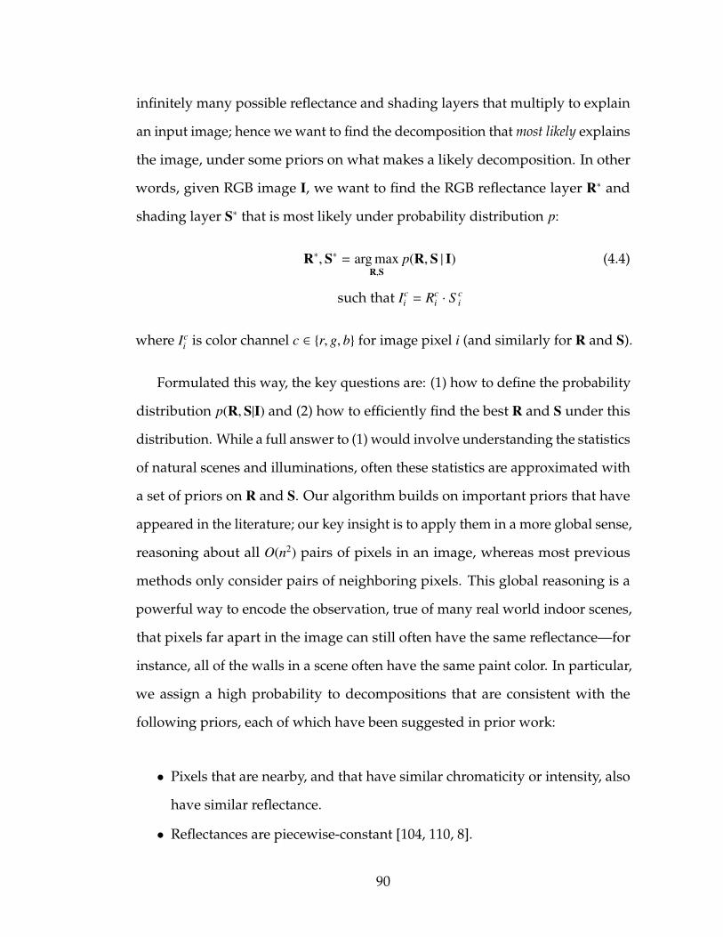
infinitely many possible reflectance and shading layers that multiply to explain

an input image; hence we want to find the decomposition that most likely explains

the image, under some priors on what makes a likely decomposition. In other

words, given RGB image I, we want to find the RGB reflectance layer R∗ and

shading layer S∗ that is most likely under probability distribution p:

R∗,S∗ = arg maxR,S

p(R,S | I) (4.4)

such that Ici = Rc

i · Sci

where Ici is color channel c ∈ r, g, b for image pixel i (and similarly for R and S).

Formulated this way, the key questions are: (1) how to define the probability

distribution p(R,S|I) and (2) how to efficiently find the best R and S under this

distribution. While a full answer to (1) would involve understanding the statistics

of natural scenes and illuminations, often these statistics are approximated with

a set of priors on R and S. Our algorithm builds on important priors that have

appeared in the literature; our key insight is to apply them in a more global sense,

reasoning about all O(n2) pairs of pixels in an image, whereas most previous

methods only consider pairs of neighboring pixels. This global reasoning is a

powerful way to encode the observation, true of many real world indoor scenes,

that pixels far apart in the image can still often have the same reflectance—for

instance, all of the walls in a scene often have the same paint color. In particular,

we assign a high probability to decompositions that are consistent with the

following priors, each of which have been suggested in prior work:

• Pixels that are nearby, and that have similar chromaticity or intensity, also

have similar reflectance.

• Reflectances are piecewise-constant [104, 110, 8].

90

• Reflectances are sampled from a sparse set [128, 58, 164].

• Certain shading values are a priori more likely than others [8].

• Neighboring pixels have similar shading [57].

• Shading is grayscale, or the same color as the light source.

These priors are not new, and different methods of global reasoning have been

proposed, such as connecting distant image regions with similar texture [199] or

optimizing for sparsity in the reflectance layer [164, 8]. Our method constructs

the reflectance layer by drawing from a sparse set of reflectances, a technique

inspired by [58].

Our key contribution is that we show how to incorporate all these priors in a

global sense, simultaneously reasoning about all O(n2) pairs of pixels. To do so,

we make use of recent work on efficient inference for dense conditional random

fields (CRFs) by Krahenbuhl and Koltun [96, 98], but show how to apply their

framework to the problem of intrinsic image decomposition.

Algorithm Overview. Our algorithm works as follows. First, we hypothesize

a set of reflectances R that are likely to exist in the image—one can think of this

set as a “palette” of reflectances that we can draw on for that image. The set R

is unique for each image and, for a typical run of our algorithm, will contain

20 entries once our algorithm converges. After first choosing an initial set of

reflectance colors R using clustering, we iterate between two stages:

1. We label each pixel with a reflectance chosen from R such that p(R,S | I) is

maximized.

2. We adjust the reflectances in R by minimizing discontinuities in the shading

layer S.

91

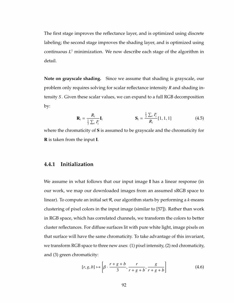
The first stage improves the reflectance layer, and is optimized using discrete

labeling; the second stage improves the shading layer, and is optimized using

continuous L1 minimization. We now describe each stage of the algorithm in

detail.

Note on grayscale shading. Since we assume that shading is grayscale, our

problem only requires solving for scalar reflectance intensity R and shading in-

tensity S . Given these scalar values, we can expand to a full RGB decomposition

by:

Ri =Ri

13

∑c Ic

i

Ii Si =

13

∑c Ic

i

Ri[1, 1, 1] (4.5)

where the chromaticity of S is assumed to be grayscale and the chromaticity for

R is taken from the input I.

4.4.1 Initialization

We assume in what follows that our input image I has a linear response (in

our work, we map our downloaded images from an assumed sRGB space to

linear). To compute an initial set R, our algorithm starts by performing a k-means

clustering of pixel colors in the input image (similar to [57]). Rather than work

in RGB space, which has correlated channels, we transform the colors to better

cluster reflectances. For diffuse surfaces lit with pure white light, image pixels on

that surface will have the same chromaticity. To take advantage of this invariant,

we transform RGB space to three new axes: (1) pixel intensity, (2) red chromaticity,

and (3) green chromaticity:

[r, g, b] 7→[β ·

r + g + b3

,r

r + g + b,

gr + g + b

](4.6)

92

Under ideal conditions (white lighting, colored diffuse surfaces, no inter-

reflections), this transform perfectly separates different reflectance colors along

the second two axes. While more sophisticated color spaces have been pro-

posed [128], we find that Equation 4.6 is sufficient for initialization. When

computing color distances, we scale the intensity axis by β since chromaticity is

a better predictor of reflectance than intensity. Training against our dataset, we

found that a weight of β = 0.5 works well.

After performing k-means clustering in this color space, we transform back

to RGB and collect the cluster centers as our initial set R. Note that while each

reflectance in R is a RGB color, we only use its intensity for the final output. We

find that for our algorithm, keeping R as RGB colors and then projecting down

to scalar intensities produces better results than simply using scalar intensity

values. In practice, we found that our algorithm is reasonably insensitive to the

number of clusters k, though k ≈ 20 performs the best. Variations on our method

are explored later in Table 4.1(b) and Table 4.2.

As described above, our algorithm then alternates between (1) assigning

each pixel with a reflectance selected from R and (2) optimizing the palette of

reflectances R itself to improve shading intensity S .

4.4.2 Stage 1: Optimize reflectance

In the first stage, we would like to label every pixel in the input image with a

reflectance chosen from R. We use x to denote the labeling, where x maps each

pixel i to a reflectance chosen from our hypothesis reflectances R, denoted as

R(xi). Each xi can be thought of as an integer from 0 to k − 1 that acts as an index

93

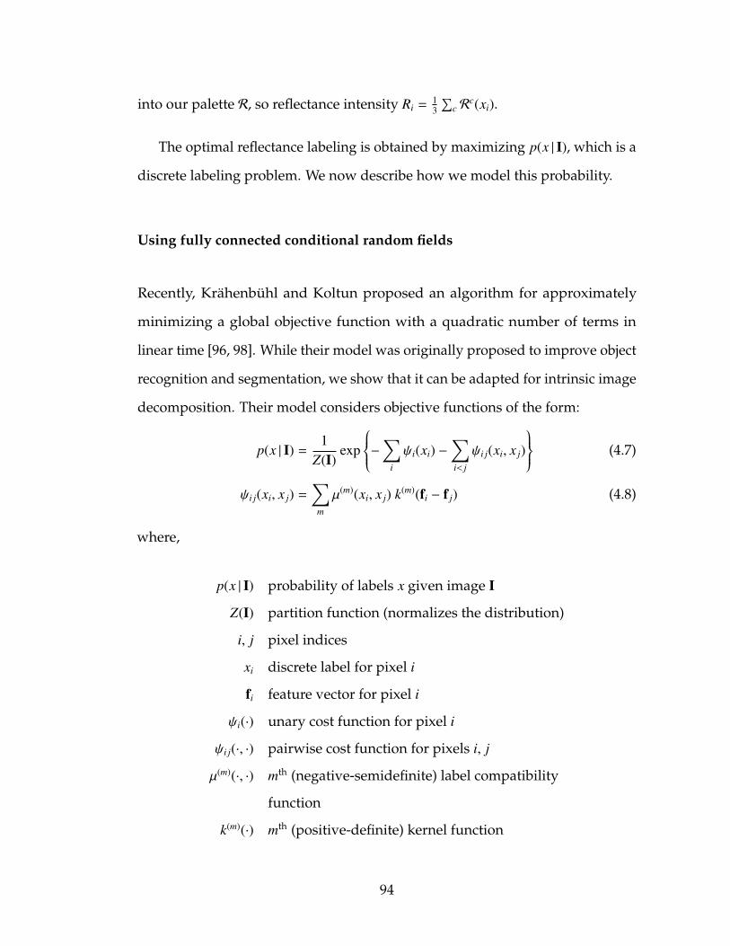
into our palette R, so reflectance intensity Ri =13

∑c R

c(xi).

The optimal reflectance labeling is obtained by maximizing p(x | I), which is a

discrete labeling problem. We now describe how we model this probability.

Using fully connected conditional random fields

Recently, Krahenbuhl and Koltun proposed an algorithm for approximately

minimizing a global objective function with a quadratic number of terms in

linear time [96, 98]. While their model was originally proposed to improve object

recognition and segmentation, we show that it can be adapted for intrinsic image

decomposition. Their model considers objective functions of the form:

p(x | I) =1

Z(I)exp

−∑i

ψi(xi) −∑i< j

ψi j(xi, x j)

(4.7)

ψi j(xi, x j) =∑

m

µ(m)(xi, x j) k(m)(fi − f j) (4.8)

where,

p(x | I) probability of labels x given image I

Z(I) partition function (normalizes the distribution)

i, j pixel indices

xi discrete label for pixel i

fi feature vector for pixel i

ψi(·) unary cost function for pixel i

ψi j(·, ·) pairwise cost function for pixels i, j

µ(m)(·, ·) mth (negative-semidefinite) label compatibility

function

k(m)(·) mth (positive-definite) kernel function

94

The objective is maximized when x is chosen to minimize the costs incurred

by ψi(xi) and ψi j(xi, x j). An important feature of this objective function is that

there are O(n2) pairwise terms ψi j. When maximizing p(x | I), we can omit the

partition function Z(I) and minimize the negative logarithm to arrive at an energy

function:

E(x) = − log p(x | I) + const (4.9)

=∑

i

ψi(xi) +∑i< j

ψi j(xi, x j)

The key insight of their algorithm is that when using a mean field approximation

to the CRF distribution, message passing (which is O(n2)) can be approximated

as high-dimensional filtering if certain pairwise functions are used. They use

the permutohedral lattice of Adams et al. [1], to perform filtering in linear time,

thus obtaining an O(nd) algorithm that approximately maximizes p(x | I), despite

having O(n2) terms, where d is the dimensionality of features f. While their prior

work does not quantify the error introduced by their approximation, the model

performs well in practice and converges quickly. For example, with 640 × 480

images and 5-dimensional features, optimization takes about 1 second with one

CPU thread.

Probability model

Recall that in our model, the layer of labels x maps each pixel to a reflectance

chosen from our hypothesis reflectances R. We now explain how we design

functions ψi, ψi j, µ, k and features f such that the optimal labeling x is a good

estimate of reflectance according to our priors.

Our energy function consists of two types of costs: (1) unary costs ψi for each

95

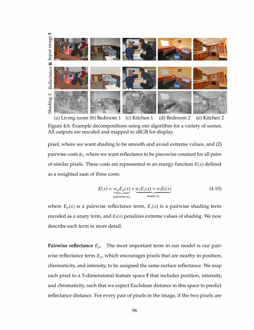
Inpu

t im

age

I

georgia James Emery The Co-operative Patty Ho Dru Bloomfield

Refl

ecta

nce

RSh

adin

gS

(a) Living room (b) Bedroom 1 (c) Kitchen 1 (d) Bedroom 2 (e) Kitchen 2

Figure 4.6: Example decompositions using our algorithm for a variety of scenes.All outputs are rescaled and mapped to sRGB for display.

pixel, where we want shading to be smooth and avoid extreme values, and (2)

pairwise costs ψi j where we want reflectance to be piecewise constant for all pairs

of similar pixels. These costs are represented in an energy function E(x) defined

as a weighted sum of three costs:

E(x) = wpEp(x)︸ ︷︷ ︸pairwise ψi j

+wsEs(x) + wlEl(x)︸ ︷︷ ︸unary ψi

(4.10)

where Ep(x) is a pairwise reflectance term, Es(x) is a pairwise shading term

encoded as a unary term, and El(x) penalizes extreme values of shading. We now

describe each term in more detail.

Pairwise reflectance Ep. The most important term in our model is our pair-

wise reflectance term Ep, which encourages pixels that are nearby in position,

chromaticity, and intensity, to be assigned the same surface reflectance. We map

each pixel to a 5-dimensional feature space f that includes position, intensity,

and chromaticity, such that we expect Euclidean distance in this space to predict

reflectance distance. For every pair of pixels in the image, if the two pixels are

96

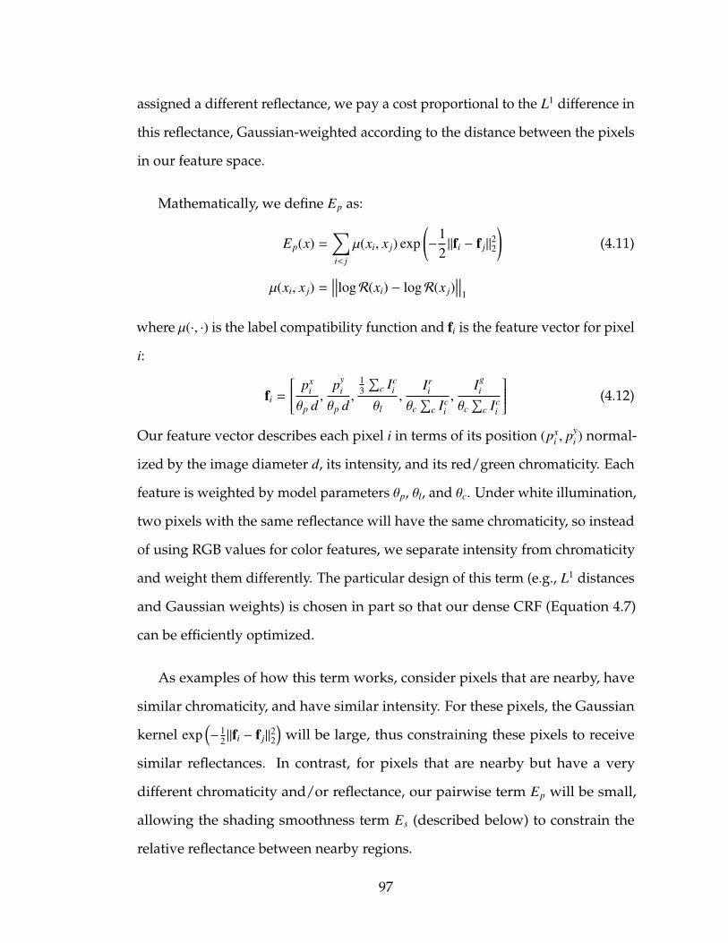
assigned a different reflectance, we pay a cost proportional to the L1 difference in

this reflectance, Gaussian-weighted according to the distance between the pixels

in our feature space.

Mathematically, we define Ep as:

Ep(x) =∑i< j

µ(xi, x j) exp(−

12||fi − f j||

22

)(4.11)

µ(xi, x j) =∣∣∣∣∣∣logR(xi) − logR(x j)

∣∣∣∣∣∣1

where µ(·, ·) is the label compatibility function and fi is the feature vector for pixel

i:

fi =

pxi

θp d,

pyi

θp d,

13

∑c Ic

i

θl,

Iri

θc∑

c Ici,

Igi

θc∑

c Ici

(4.12)

Our feature vector describes each pixel i in terms of its position (pxi , py

i ) normal-

ized by the image diameter d, its intensity, and its red/green chromaticity. Each

feature is weighted by model parameters θp, θl, and θc. Under white illumination,

two pixels with the same reflectance will have the same chromaticity, so instead

of using RGB values for color features, we separate intensity from chromaticity

and weight them differently. The particular design of this term (e.g., L1 distances

and Gaussian weights) is chosen in part so that our dense CRF (Equation 4.7)

can be efficiently optimized.

As examples of how this term works, consider pixels that are nearby, have

similar chromaticity, and have similar intensity. For these pixels, the Gaussian

kernel exp(− 1

2 ||fi − f j||22

)will be large, thus constraining these pixels to receive

similar reflectances. In contrast, for pixels that are nearby but have a very

different chromaticity and/or reflectance, our pairwise term Ep will be small,

allowing the shading smoothness term Es (described below) to constrain the

relative reflectance between nearby regions.

97

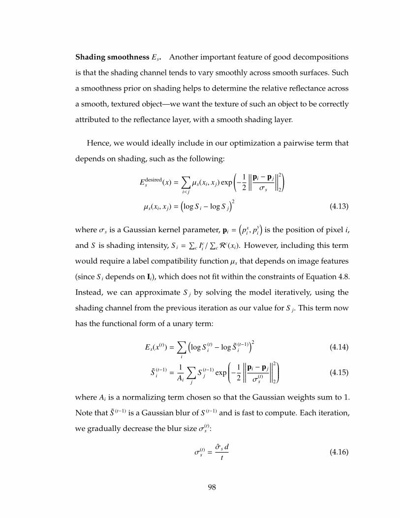
Shading smoothness Es. Another important feature of good decompositions

is that the shading channel tends to vary smoothly across smooth surfaces. Such

a smoothness prior on shading helps to determine the relative reflectance across

a smooth, textured object—we want the texture of such an object to be correctly

attributed to the reflectance layer, with a smooth shading layer.

Hence, we would ideally include in our optimization a pairwise term that

depends on shading, such as the following:

Edesireds (x) =

∑i< j

µs(xi, x j) exp(−

12

∣∣∣∣∣∣∣∣∣∣pi − p j

σs

∣∣∣∣∣∣∣∣∣∣22

)µs(xi, x j) =

(log S i − log S j

)2(4.13)

where σs is a Gaussian kernel parameter, pi =(px

i , pyi

)is the position of pixel i,

and S is shading intensity, S i =∑

c Ici /

∑c R

c(xi). However, including this term

would require a label compatibility function µs that depends on image features

(since S i depends on Ii), which does not fit within the constraints of Equation 4.8.

Instead, we can approximate S j by solving the model iteratively, using the

shading channel from the previous iteration as our value for S j. This term now

has the functional form of a unary term:

Es(x(t)) =∑

i

(log S (t)

i − log S (t−1)i

)2(4.14)

S (t−1)i =

1Ai

∑j

S (t−1)j exp

−12

∣∣∣∣∣∣∣∣∣∣∣∣pi − p j

σ(t)s

∣∣∣∣∣∣∣∣∣∣∣∣22

(4.15)

where Ai is a normalizing term chosen so that the Gaussian weights sum to 1.

Note that S (t−1) is a Gaussian blur of S (t−1) and is fast to compute. Each iteration,

we gradually decrease the blur size σ(t)s :

σ(t)s =

σs dt

(4.16)

98

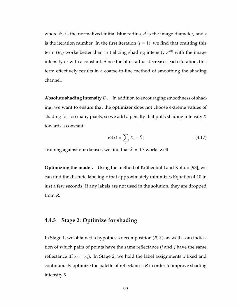
where σs is the normalized initial blur radius, d is the image diameter, and t

is the iteration number. In the first iteration (t = 1), we find that omitting this

term (Es) works better than initializing shading intensity S (0) with the image

intensity or with a constant. Since the blur radius decreases each iteration, this

term effectively results in a coarse-to-fine method of smoothing the shading

channel.

Absolute shading intensity El. In addition to encouraging smoothness of shad-

ing, we want to ensure that the optimizer does not choose extreme values of

shading for too many pixels, so we add a penalty that pulls shading intensity S

towards a constant:

El(x) =∑

i

|S i − S | (4.17)

Training against our dataset, we find that S = 0.5 works well.

Optimizing the model. Using the method of Krahenbuhl and Koltun [98], we

can find the discrete labeling x that approximately minimizes Equation 4.10 in

just a few seconds. If any labels are not used in the solution, they are dropped

from R.

4.4.3 Stage 2: Optimize for shading

In Stage 1, we obtained a hypothesis decomposition (R, S ), as well as an indica-

tion of which pairs of points have the same reflectance (i and j have the same

reflectance iff xi = x j). In Stage 2, we hold the label assignments x fixed and

continuously optimize the palette of reflectances R in order to improve shading

intensity S .

99

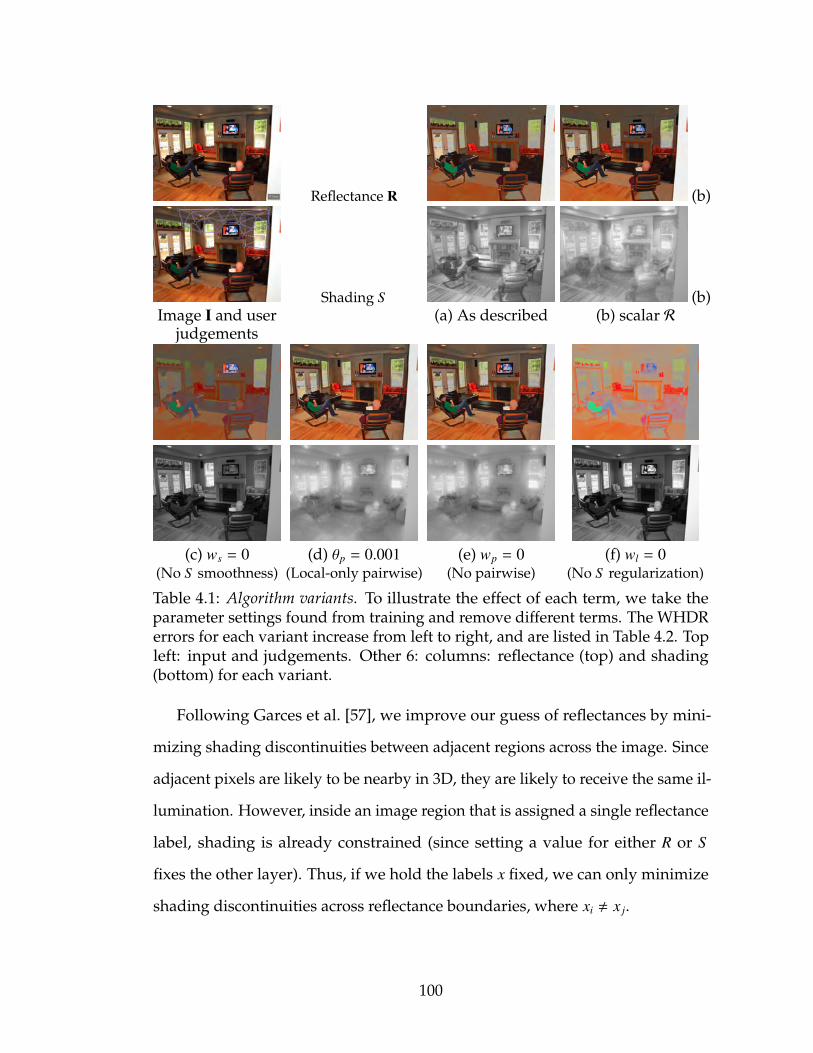
Sally Reflectance R (b)

Shading S (b)Image I and user (a) As described (b) scalar R

judgements

(c) ws = 0 (d) θp = 0.001 (e) wp = 0 (f) wl = 0(No S smoothness) (Local-only pairwise) (No pairwise) (No S regularization)

Table 4.1: Algorithm variants. To illustrate the effect of each term, we take theparameter settings found from training and remove different terms. The WHDRerrors for each variant increase from left to right, and are listed in Table 4.2. Topleft: input and judgements. Other 6: columns: reflectance (top) and shading(bottom) for each variant.

Following Garces et al. [57], we improve our guess of reflectances by mini-

mizing shading discontinuities between adjacent regions across the image. Since

adjacent pixels are likely to be nearby in 3D, they are likely to receive the same il-

lumination. However, inside an image region that is assigned a single reflectance

label, shading is already constrained (since setting a value for either R or S

fixes the other layer). Thus, if we hold the labels x fixed, we can only minimize

shading discontinuities across reflectance boundaries, where xi , x j.

100

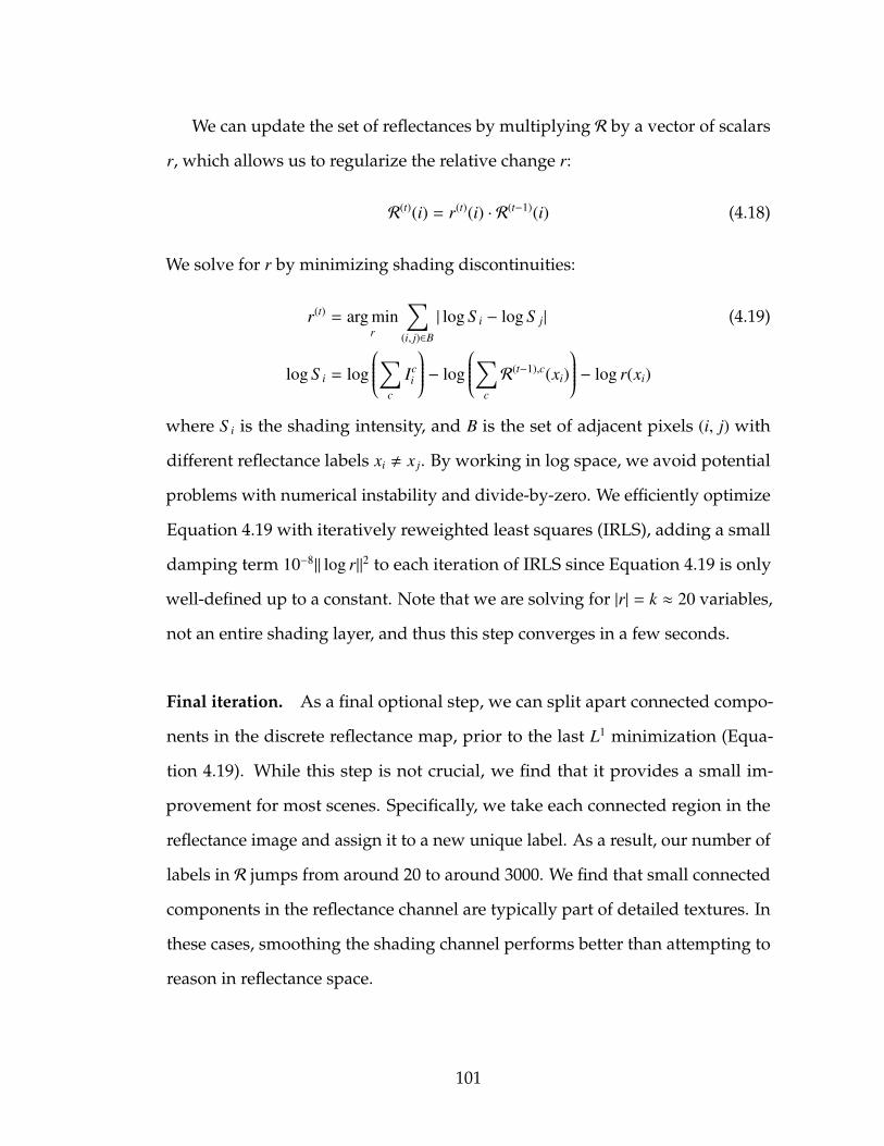
We can update the set of reflectances by multiplying R by a vector of scalars

r, which allows us to regularize the relative change r:

R(t)(i) = r(t)(i) · R(t−1)(i) (4.18)

We solve for r by minimizing shading discontinuities:

r(t) = arg minr

∑(i, j)∈B

| log S i − log S j| (4.19)

log S i = log

∑c

Ici

− log

∑c

R(t−1),c(xi)

− log r(xi)

where S i is the shading intensity, and B is the set of adjacent pixels (i, j) with

different reflectance labels xi , x j. By working in log space, we avoid potential

problems with numerical instability and divide-by-zero. We efficiently optimize

Equation 4.19 with iteratively reweighted least squares (IRLS), adding a small

damping term 10−8|| log r||2 to each iteration of IRLS since Equation 4.19 is only

well-defined up to a constant. Note that we are solving for |r| = k ≈ 20 variables,

not an entire shading layer, and thus this step converges in a few seconds.

Final iteration. As a final optional step, we can split apart connected compo-

nents in the discrete reflectance map, prior to the last L1 minimization (Equa-

tion 4.19). While this step is not crucial, we find that it provides a small im-

provement for most scenes. Specifically, we take each connected region in the

reflectance image and assign it to a new unique label. As a result, our number of

labels in R jumps from around 20 to around 3000. We find that small connected

components in the reflectance channel are typically part of detailed textures. In

these cases, smoothing the shading channel performs better than attempting to

reason in reflectance space.

101

Number of iterations. We always run the algorithm for a fixed number of

iterations since our shading smoothness term Es changes every iteration (the blur

radius decreases). We find that while the algorithm produces a reasonable result

in just a few iterations, the decomposition continues to improve, and that about

25 iterations is sufficient. As listed in Table 4.2, we obtain mean error (WHDR10%)

of 23.5%, 21.5%, and 21.0% after 1, 10, and 25 iterations respectively.

4.5 Results

In this section we use our dataset to evaluate our algorithm and a range of public

algorithms for intrinsic image decomposition. We evaluated our algorithm on all

images in our dataset. Some example decompositions are shown in Figure 4.6.

Generally we find that our algorithm performs very well for real-world scenes.

While it is particularly good at finding a single reflectance to explain large

continuous regions, it can also handle intricate textures such as wallpapers and

bricks. Even when there are many surfaces that do not fit the diffuse reflectance

model (such as glossy metals or tinted windows), the model often returns a

reasonable result.

4.5.1 Training

Using our large dataset, we explored the effects of changing both the parameters

and the structure of our algorithm. We can delete different terms from our energy

function E(x) (Equation 4.10) or we can try adding new terms such as priors on

absolute reflectances. Table 4.1 shows the effect of deleting different terms and

102

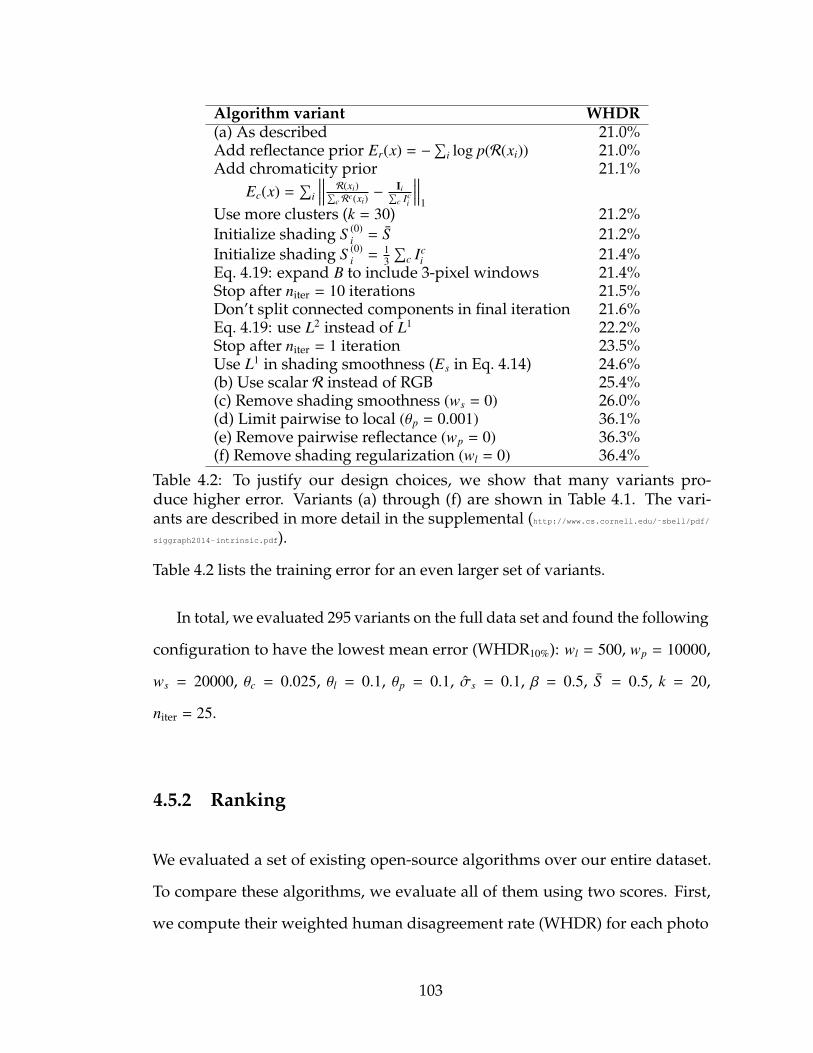
Algorithm variant WHDR(a) As described 21.0%Add reflectance prior Er(x) = −

∑i log p(R(xi)) 21.0%

Add chromaticity prior 21.1%Ec(x) =

∑i

∣∣∣∣∣∣∣∣ R(xi)∑c R

c(xi)−

Ii∑c Ic

i

∣∣∣∣∣∣∣∣1

Use more clusters (k = 30) 21.2%Initialize shading S (0)

i = S 21.2%Initialize shading S (0)

i =13

∑c Ic

i 21.4%Eq. 4.19: expand B to include 3-pixel windows 21.4%Stop after niter = 10 iterations 21.5%Don’t split connected components in final iteration 21.6%Eq. 4.19: use L2 instead of L1 22.2%Stop after niter = 1 iteration 23.5%Use L1 in shading smoothness (Es in Eq. 4.14) 24.6%(b) Use scalar R instead of RGB 25.4%(c) Remove shading smoothness (ws = 0) 26.0%(d) Limit pairwise to local (θp = 0.001) 36.1%(e) Remove pairwise reflectance (wp = 0) 36.3%(f) Remove shading regularization (wl = 0) 36.4%

Table 4.2: To justify our design choices, we show that many variants pro-duce higher error. Variants (a) through (f) are shown in Table 4.1. The vari-ants are described in more detail in the supplemental (http://www.cs.cornell.edu/˜sbell/pdf/siggraph2014-intrinsic.pdf).

Table 4.2 lists the training error for an even larger set of variants.

In total, we evaluated 295 variants on the full data set and found the following

configuration to have the lowest mean error (WHDR10%): wl = 500, wp = 10000,

ws = 20000, θc = 0.025, θl = 0.1, θp = 0.1, σs = 0.1, β = 0.5, S = 0.5, k = 20,

niter = 25.

4.5.2 Ranking

We evaluated a set of existing open-source algorithms over our entire dataset.

To compare these algorithms, we evaluate all of them using two scores. First,

we compute their weighted human disagreement rate (WHDR) for each photo

103

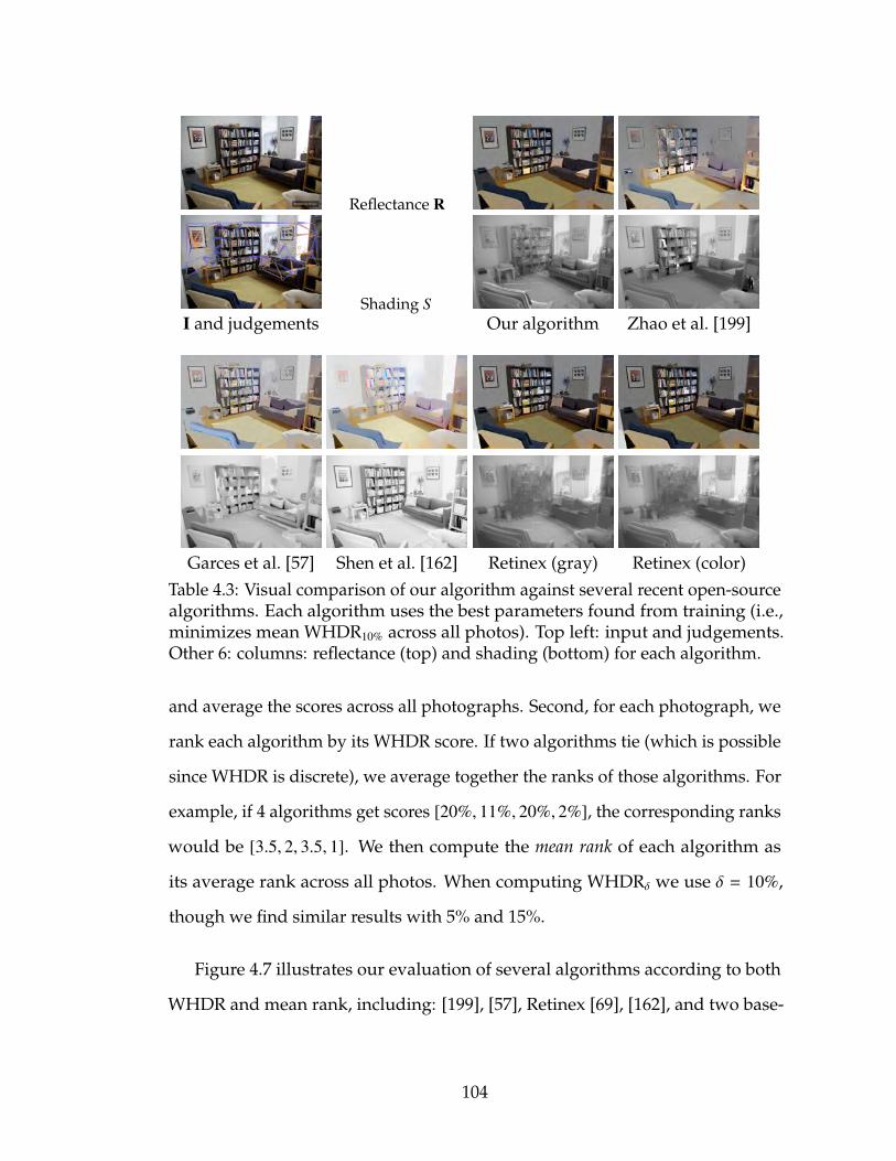
Ramsey Beyer Reflectance R

Shading SI and judgements Our algorithm Zhao et al. [199]

Garces et al. [57] Shen et al. [162] Retinex (gray) Retinex (color)Table 4.3: Visual comparison of our algorithm against several recent open-sourcealgorithms. Each algorithm uses the best parameters found from training (i.e.,minimizes mean WHDR10% across all photos). Top left: input and judgements.Other 6: columns: reflectance (top) and shading (bottom) for each algorithm.

and average the scores across all photographs. Second, for each photograph, we

rank each algorithm by its WHDR score. If two algorithms tie (which is possible

since WHDR is discrete), we average together the ranks of those algorithms. For

example, if 4 algorithms get scores [20%, 11%, 20%, 2%], the corresponding ranks

would be [3.5, 2, 3.5, 1]. We then compute the mean rank of each algorithm as

its average rank across all photos. When computing WHDRδ we use δ = 10%,

though we find similar results with 5% and 15%.

Figure 4.7 illustrates our evaluation of several algorithms according to both

WHDR and mean rank, including: [199], [57], Retinex [69], [162], and two base-

104

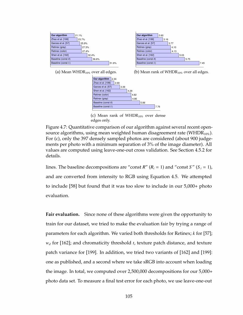
21.1%Our algorithm

23.7%Zhao et al. [199]

25.9%Garces et al. [57]

27.3%Retinex (gray)

27.4%Retinex (color)

32.4%Shen et al. [162]

36.6%Baseline (const R)

51.6%Baseline (const S )

(a) Mean WHDR10% over all edges.

2.60Our algorithm

3.16Zhao et al. [199]

3.77Garces et al. [57]

4.10Retinex (gray)

4.13Retinex (color)

5.03Shen et al. [162]

5.75Baseline (const R)

7.45Baseline (const S )

(b) Mean rank of WHDR10% over all edges.

2.30Our algorithm

2.69Zhao et al. [199]

3.39Garces et al. [57]

4.29Shen et al. [162]

4.82Retinex (color)

4.86Retinex (gray)

5.89Baseline (const R)

7.76Baseline (const S )

(c) Mean rank of WHDR10% over denseedges only.

Figure 4.7: Quantitative comparison of our algorithm against several recent open-source algorithms, using mean weighted human disagreement rate (WHDR10%).For (c), only the 397 densely sampled photos are considered (about 900 judge-ments per photo with a minimum separation of 3% of the image diameter). Allvalues are computed using leave-one-out cross validation. See Section 4.5.2 fordetails.

lines. The baseline decompositions are “const R” (Ri = 1) and “const S ” (S i = 1),

and are converted from intensity to RGB using Equation 4.5. We attempted

to include [58] but found that it was too slow to include in our 5,000+ photo

evaluation.

Fair evaluation. Since none of these algorithms were given the opportunity to

train for our dataset, we tried to make the evaluation fair by trying a range of

parameters for each algorithm. We varied both thresholds for Retinex; k for [57];

wd for [162]; and chromaticity threshold t, texture patch distance, and texture

patch variance for [199]. In addition, we tried two variants of [162] and [199]:

one as published, and a second where we take sRGB into account when loading

the image. In total, we computed over 2,500,000 decompositions for our 5,000+

photo data set. To measure a final test error for each photo, we use leave-one-out

105

cross-validation (i.e., test each photo using the best parameters for all other

photos).

Our algorithm. Out of all the methods we evaluated, our algorithm both has

the lowest mean error and the best average rank, averaged across all photos.

This is consistent with our visual judgement of the results.

Zhao et al. [199]. We find that for real-world images, [199] performs quite well.

The method has the strength of Retinex in that it is accurate at decomposing

texture on smooth surfaces, while also having sparse global constraints to connect

distant parts of the image together.

Garces et al. [57]. The next best performing algorithm is [57], which is designed

for real-world scenes. Most errors in output from [57] appear to come from

incorrect clustering of surface reflectances. Highly textured regions are often

merged together into a single component, causing the texture to incorrectly

appear in the shading layer.

Retinex [69]. The Retinex algorithm [69] is the simplest algorithm, and per-

forms surprisingly well for its algorithmic complexity. We found that the opti-

mal threshold for whole scenes (color threshold 0.7, gray threshold 0.5) is very

different than the optimal threshold for the MIT Intrinsic Images dataset (color

threshold 0.075, gray threshold 1.0). We were also surprised to find that grayscale

intensity was a better predictor of reflectance than color, for scenes “in the wild”.

Consistent with [69], we note that the L2 variant of Retinex performs significantly

worse than L1 (41.8% versus 27.4%).

106

Shen et al. [162]. Finally, we found [162] to perform only slightly better than

the baseline in terms of mean error. This seems to correspond to our visual

judgement of the output, in which high-frequency texture details are often put in

the shading channel, and shading details are not removed from the reflectance

layer.

Visual comparison. To understand the typical kinds of visual artifacts made by

each algorithm, we include an example decomposition in Table 4.3. Since there is

significant variety across photos, and the relative ranking between algorithms

changes for each photo, this single example is not sufficient to rank algorithms.

More visual comparisons are included in the supplemental material.5

Dense vs sparse edges. We have two edge lengths: “sparse”, with a point spac-

ing of 7% of the image diameter, and “dense”, with a point spacing of 3% of the

image diameter. We can repeat the evaluation with only dense edges, as shown

in Figure 4.7(c). We find that [162] performs better in a close-range evaluation,

which is to be expected since the method optimizes over local windows. To make

sure that it is not the distribution over edge types that is affecting the results,

we compared the distribution of edges and found that it was about the same for

both groups: for sparse edges, 62.8% are equal (“about the same”) and 63.9% of

the dense edges are equal.

Median individual human. Finally, we can place humans on the scale in the

same units, by excluding some user responses from the aggregation and then

testing them against the user majority, using our WHDR metric. We exclude

100 random users from the aggregation, and test the excluded users against the

5http://www.cs.cornell.edu/˜sbell/pdf/siggraph2014-intrinsic.pdf

107

responses aggregated from the remaining users. Blocked users are excluded

from both sets. Since we are evaluating algorithms against humans, who are

inconsistent, this is effectively the lowest error we can expect an algorithm to

obtain. Averaged across all photos in our dataset, we find that humans have a

median WHDR = 7.5%.

4.5.3 MIT Intrinsic Images dataset

We have validated our algorithm against the MIT Intrinsic Images dataset [69],

and found that it performs reasonably. We obtained a mean training and test

error of LMSE20 = 0.027 and LMSE20 = 0.031 respectively (which matches color

Retinex LMSE20 = 0.031). This is certainly not the lowest error reported for this

dataset. For example, [8] explicitly models shape and illumination and achieves

a lower error, but is limited to individual objects. Our method focuses on real-

world scenes, which have very different statistics from small, cleanly segmented

purely diffuse objects.

4.6 Limitations and future work

Weaknesses of WHDR. When visually evaluating decompositions, there are

many different mistakes that algorithms make: texture variations in S, shad-

ows/highlights in R, etc. No algorithm avoids all mistakes. An important

motivation was therefore to have a large dataset to evaluate algorithms on a wide

variety of scenes, each with their own challenges. The question of ranking algo-

rithms becomes: how much should we penalize each mistake? Our “weighted

108

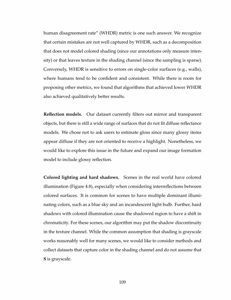
human disagreement rate” (WHDR) metric is one such answer. We recognize

that certain mistakes are not well captured by WHDR, such as a decomposition

that does not model colored shading (since our annotations only measure inten-

sity) or that leaves texture in the shading channel (since the sampling is sparse).

Conversely, WHDR is sensitive to errors on single-color surfaces (e.g., walls),

where humans tend to be confident and consistent. While there is room for

proposing other metrics, we found that algorithms that achieved lower WHDR

also achieved qualitatively better results.

Reflection models. Our dataset currently filters out mirror and transparent

objects, but there is still a wide range of surfaces that do not fit diffuse reflectance

models. We chose not to ask users to estimate gloss since many glossy items

appear diffuse if they are not oriented to receive a highlight. Nonetheless, we

would like to explore this issue in the future and expand our image formation

model to include glossy reflection.

Colored lighting and hard shadows. Scenes in the real world have colored

illumination (Figure 4.8), especially when considering interreflections between

colored surfaces. It is common for scenes to have multiple dominant illumi-

nating colors, such as a blue sky and an incandescent light bulb. Further, hard

shadows with colored illumination cause the shadowed region to have a shift in

chromaticity. For these scenes, our algorithm may put the shadow discontinuity

in the texture channel. While the common assumption that shading is grayscale

works reasonably well for many scenes, we would like to consider methods and

collect datasets that capture color in the shading channel and do not assume that

S is grayscale.

109

Roland Tanglao Thomas Bernhardt John Lloyd

Figure 4.8: Challenging scenes that violate our assumptions. Using the parame-ters from Sec. 4.5.1, we obtain WHDR = 67%, 45%, 43%.

Synthetic images. We would like to further evaluate the quality of human

judgements by using ground truth synthetic rendered images. However, the

main challenge with synthetic images is that it is extremely difficult to replicate

the true diversity and variety found in Internet photo collections. Further, many

3D scenes available online do not accurately model reality and include features

such as meso-scale geometry in albedo maps.

Photograph variety. While our dataset does a reasonable job of covering typical

indoor photographs, there are only a few outdoor and nature scenes (e.g., in

the “staircase” category), and thus it does not fully represent the statistics of all

images available online. Future work could include determining whether the

same priors (piece-wise constant reflectances, sparse set of intensities, etc.) are

useful in decomposing outdoor photographs.

4.7 Conclusion

In this chapter we introduced a large scale dataset (5000+ images) for Intrinsic

Images in the Wild, with crowdsourced pairwise annotations of reflectance in-

tensity comparisons. We also introduced a dense-CRF-based intrinsic image

110

decomposition algorithm that considers long-range interactions to achieve better

decomposition on our new database, while maintaining local detail. While we

have taken steps towards intrinsic images for real-world scenes and uncalibrated

photos, many challenges and avenues of future work remain on this problem.

Just as the availability of the MIT Intrinsic Images dataset was important to

galvanizing research on intrinsic image algorithms, we hope our public database

and code will help drive improvements in intrinsic image decomposition in the

wild.

4.8 Impact

Our work was published at SIGGRAPH 2014 [11]. Our IIW judgement dataset

has been used to train and validate new models that use deep learning to pre-

dict reflectance and lightness variations in an image [203, 206, 123]. Using our

data, others have proposed extensions of our algorithm that use deeply learned

priors [203], or entirely new algorithms using global least squares optimiza-

tions [206], L1 image transforms [17], or near-L0 image transforms [44]. Our

pairwise reflectance judgements have inspired others to extend our relative re-

flectance judgements to relative depth judgements [206] which can be globalized

to solve for a full depth map.

111

CHAPTER 5

INSIDE-OUTSIDE NET: DETECTING OBJECTS IN CONTEXT WITH SKIP

POOLING AND RECURRENT NEURAL NETWORKS

5.1 Introduction

Scene understanding requires a complete description of many different aspects

of a scene, including objects, materials, depth, surfaces, and lighting. In previous

chapters, we focused on materials, surfaces, and lighting. In this chapter, we

address a different but important piece of the scene understanding problem—

which objects are present in an image and where are they? In order to have a

fully general method of understanding images in the world, automatic detec-

tion and localization of objects is a critical piece. To address this problem, we

develop a new deep-learning-based object detection architecture with several

new components.

Reliably detecting an object requires a variety of information, including the

object’s fine-grained details and the context surrounding it. Current state-of-the-

art detection approaches [60, 146] only use information near an object’s region of

interest (ROI). This places constraints on the type and accuracy of objects that

may be detected.

We explore expanding the approach of [65] to include two additional sources

of information. The first uses a multi-scale representation [92] that captures

fine-grained details by pooling from multiple lower-level convolutional layers

in a ConvNet [166]. These skip-layers [158, 116, 119, 73] span multiple spatial

resolutions and levels of feature abstraction. The information gained is especially

112

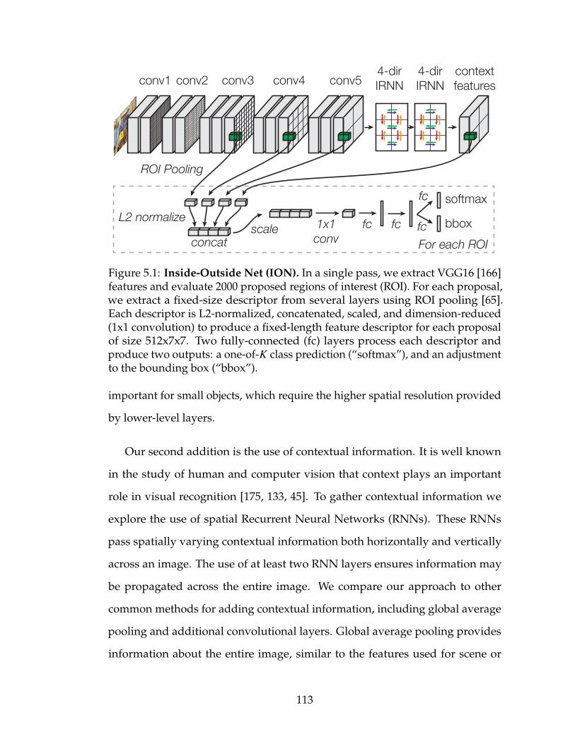
scale 1x1conv

fc fc

softmax

bboxFor each ROI

fc

fcL2 normalize

concat

ROI Pooling

conv2conv1 conv5conv4conv34-dirIRNN

4-dirIRNN

context features

Figure 5.1: Inside-Outside Net (ION). In a single pass, we extract VGG16 [166]features and evaluate 2000 proposed regions of interest (ROI). For each proposal,we extract a fixed-size descriptor from several layers using ROI pooling [65].Each descriptor is L2-normalized, concatenated, scaled, and dimension-reduced(1x1 convolution) to produce a fixed-length feature descriptor for each proposalof size 512x7x7. Two fully-connected (fc) layers process each descriptor andproduce two outputs: a one-of-K class prediction (“softmax”), and an adjustmentto the bounding box (“bbox”).

important for small objects, which require the higher spatial resolution provided

by lower-level layers.

Our second addition is the use of contextual information. It is well known

in the study of human and computer vision that context plays an important

role in visual recognition [175, 133, 45]. To gather contextual information we

explore the use of spatial Recurrent Neural Networks (RNNs). These RNNs

pass spatially varying contextual information both horizontally and vertically

across an image. The use of at least two RNN layers ensures information may

be propagated across the entire image. We compare our approach to other

common methods for adding contextual information, including global average

pooling and additional convolutional layers. Global average pooling provides

information about the entire image, similar to the features used for scene or

113

image classification [127, 99].

Following previous approaches [66], we use object proposal detectors [80, 177,

205] to identify ROIs in an image. Each ROI is then classified as containing one

or none of the objects of interest. Using dynamic pooling [77] we can efficiently

evaluate thousands of different candidate ROIs with a single forwards pass of

the network. For each candidate ROI, the multi-scale and context information is

concatenated into a single layer and fed through several fully connected layers

for classification.

We demonstrate that both sources of additional information, context and

multi-scale, are complementary in nature. This matches our intuition that context

features look broadly across the image, while multi-scale features capture more

fine-grained details. We show large improvements on the PASCAL VOC [48]

and Microsoft COCO [112] object detection datasets and provide a thorough

evaluation of the gains across different object types. We find that they are most

significant for object types that have been historically difficult. For example, we

show improved accuracy for potted plants which are often small and amongst

clutter. In general, we find that our approach is more adept at detecting small

objects than previous state-of-the-art methods. For heavily occluded objects like

chairs, gains are found when using contextual information.

While the technical methods employed (spatial RNNs [68, 23, 184], skip-layer

connections [158, 116, 119, 73]) have precedents in the literature, we demonstrate

that their well-executed combination has an unexpectedly positive impact on

the detector’s accuracy. As always, the devil is in the details [27] and thus this

chapter aims to provide a thorough exploration of design choices and their

outcomes.

114

Contributions. We make the following contributions:

1. We introduce the ION architecture that leverages context and multi-scale

skip pooling for object detection.

2. We achieve state-of-the-art results on PASCAL VOC 2007, with a mAP of

80.1%, VOC 2012, with a mAP of 77.9%, and on COCO, with a mAP of

33.1%.

3. We conduct extensive experiments evaluating choices like the number of

layers combined, using a segmentation loss, normalizing feature ampli-

tudes, different RNN architectures, and other variations.

4. We analyze ION’s performance and find improved accuracy across the

board, especially for small objects.

5.2 Prior work

ConvNet object detectors. ConvNets with a small number of hidden layers

have been used for object detection for the last two decades (e.g., from [178]

to [158]). Until recently, they were successful in restricted domains such as

face detection. Recently, deeper ConvNets have led to radical improvements

in the detection of more general object categories. This shift came about when

the successful application of deep ConvNets to image classification [99] was

transferred to object detection in the R-CNN system of Girshick et al. [66] and

the OverFeat system of Sermanet et al. [157]. Our work builds on the rapidly

evolving R-CNN (“region-based convolutional neural network”) line of work.

Our experiments are conducted with Fast R-CNN [65], which is an end-to-end

trainable refinement of He et al.’s SPPnet [77]. We discuss the relationship of

115

our approach to other methods later in the paper in the context of our model

description and experimental results.

Spatial RNNs. Recurrent Neural Networks (RNNs) exist in various extended

forms, including bidirectional RNNs [155] that process sequences left-to-right

and right-to-left in parallel. Beyond simple sequences, RNNs exist in full multi-

dimensional variants, such as those introduced by Graves and Schmidhuber [68]

for handwriting recognition, or as hierarchical recurrent pyramids (the Neural

Abstraction Pyramid [10]). As a lower-complexity alternative, [23, 184] explore

running an RNN spatially (or laterally) over a feature map in place of convolu-

tions. In this paper, we employ spatial RNNs as a mechanism for computing

contextual features for use in object detection.

Skip-layer connections. Skip-layer connections are a classic neural network

idea wherein activations from a lower layer are routed directly to a higher layer

while bypassing intermediate layers. The specifics of the wiring and combination

method differ between models and applications. Our usage of skip connections

is most closely related to those used by Sermanet et al. [158] (termed “multi-stage

features”) for pedestrian detection. Different from [158], we find it essential to

L2 normalize activations from different layers prior to combining them.

The need for activation normalization when combining features across layers

was recently noted by Liu et al.(ParseNet [116]) in a model for semantic segmen-

tation that makes use of global image context features. Skip connections have

also been popular in recent models for semantic segmentation, such as the “fully

convolutional networks” in [119], and for object instance segmentation, such as

the “hypercolumn features” in [73].

116

conv5 context features

semanticsegmentation

(optional regularizer)

deconv

concatconcat

1x1conv

1x1conv

1x1 conv+ReLU

recurrent transitions

(shared input-to-hidden

transition)

(shared input-to-hidden

transition)

(hidden-to-output

transition)

4x copy 4x copy512

H

W

2048 512

16W

21

16H

H

W

2048

(hidden-to-hidden, equation 1)recurrent transitions

(hidden-to-hidden, equation 1)

512512

512 512

Figure 5.2: Four-directional IRNN architecture. We use “IRNN” units [105]which are RNNs with ReLU recurrent transitions, initialized to the identity. Alltransitions to/from the hidden state are computed with 1x1 convolutions, whichallows us to compute the recurrence more efficiently (Eq. 5.1). When computingthe context features, the spatial resolution remains the same throughout (sameas conv5). The semantic segmentation regularizer has a 16x higher resolution; itis optional and gives a small improvement of around +1 mAP point.

5.3 Architecture: Inside-Outside Net (ION)

In this section we describe ION (Figure 5.1), a detector with an improved de-

scriptor both inside and outside the ROI. We begin with a brief overview of the

entire architecture, followed by specific details. To detect objects, a single deep

ConvNet processes an image, and the convolutional feature maps from each

layer are stored in memory. At the top of the network, a 2x stacked 4-directional

IRNN (Figure 5.2, explained later) computes context features that describe the

image both globally and locally. The context features have the same dimensions

as “conv5.” This is done once per image. In addition, we have thousands of

proposal regions (ROIs) that might contain objects. For each ROI, we extract a

fixed-length feature descriptor from several layers (“conv3”, “conv4”, “conv5”,

and “context features”). The descriptors are L2-normalized, concatenated, re-

scaled, and dimension-reduced (1x1 convolution) to produce a fixed-length

feature descriptor for each proposal of size 512x7x7. Two fully-connected (FC)

layers process each descriptor and produce two outputs: a one-of-K object class

117

prediction (“softmax”), and an adjustment to the proposal region’s bounding

box (“bbox”). The rest of this section explains the details of ION and motivates

why we chose this particular architecture.

5.3.1 Pooling from multiple layers

Recent successful detectors such as Fast R-CNN, Faster R-CNN [146], and SPPnet,

all pool from the last convolutional layer (“conv5 3”) in VGG16 [166]. In order

to extend this to multiple layers, we must consider issues of dimensionality and

amplitude.

Since we know that pre-training on ImageNet is important to achieve state-of-

the-art performance [3], and we would like to use the previously trained VGG16

network [166], it is important to preserve the existing layer shapes. Therefore, if

we want to pool out of more layers, the final feature must also be shape 512x7x7

so that it is the correct shape to feed into the first fully-connected layer (fc6).

In addition to matching the original shape, we must also match the original

activation amplitudes, so that we can feed our feature into fc6.

To match the required 512x7x7 shape, we concatenate each pooled feature

along the channel axis and reduce the dimension with a 1x1 convolution. To

match the original amplitudes, we L2 normalize each pooled ROI and re-scale

back up by an empirically determined scale. Our experiments use a “scale layer”

with a learnable per-channel scale initialized to 1000 (measured on the training

set). We later show in Section 5.5.2 that a fixed scale works just as well.

As a final note, as more features are concatenated together, we need to corre-

118

spondingly decrease the initial weight magnitudes of the 1x1 convolution, so we

use “Xavier” initialization [172].

5.3.2 Context features with IRNNs

Our architecture for computing context features in ION is shown in more detail

in Figure 5.2. On top of the last convolutional layer (conv5), we place RNNs

that move laterally across the image. Traditionally, an RNN moves left-to-right

along a sequence, consuming an input at every step, updating its hidden state,

and producing an output. We extend this to two dimensions by placing an RNN

along each row and along each column of the image. We have four RNNs in total

that move in the cardinal directions: right, left, down, up. The RNNs sit on top

of conv5 and produce an output with the same shape as conv5.

There are many possible forms of recurrent neural networks that we could use:

gated recurrent units (GRU) [33], long short-term memory (LSTM) [78], and plain

tanh recurrent neural networks. In this chapter, we explore RNNs composed of

rectified linear units (ReLU). Le et al. [105] recently showed that these networks

are easy to train and are good at modeling long-range dependencies, if the

recurrent weight matrix is initialized to the identity matrix. This means that

at initialization, gradients are propagated backwards with full strength. Le

et al. [105] call a ReLU RNN initialized this way an “IRNN,” and show that it

performs almost as well as an LSTM for a real-world language modeling task,

and better than an LSTM for a toy memory problem. We adopt this architecture

because it is very simple to implement and parallelize, and is much faster than

LSTMs or GRUs to compute.

119

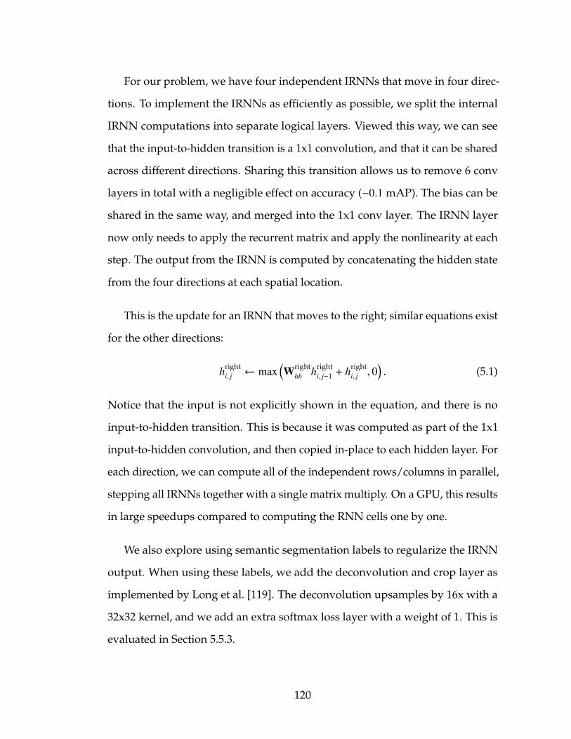
For our problem, we have four independent IRNNs that move in four direc-

tions. To implement the IRNNs as efficiently as possible, we split the internal

IRNN computations into separate logical layers. Viewed this way, we can see

that the input-to-hidden transition is a 1x1 convolution, and that it can be shared

across different directions. Sharing this transition allows us to remove 6 conv

layers in total with a negligible effect on accuracy (−0.1 mAP). The bias can be

shared in the same way, and merged into the 1x1 conv layer. The IRNN layer

now only needs to apply the recurrent matrix and apply the nonlinearity at each

step. The output from the IRNN is computed by concatenating the hidden state

from the four directions at each spatial location.

This is the update for an IRNN that moves to the right; similar equations exist

for the other directions:

hrighti, j ← max

(Wright

hh hrighti, j−1 + hright

i, j , 0). (5.1)

Notice that the input is not explicitly shown in the equation, and there is no

input-to-hidden transition. This is because it was computed as part of the 1x1

input-to-hidden convolution, and then copied in-place to each hidden layer. For

each direction, we can compute all of the independent rows/columns in parallel,

stepping all IRNNs together with a single matrix multiply. On a GPU, this results

in large speedups compared to computing the RNN cells one by one.

We also explore using semantic segmentation labels to regularize the IRNN

output. When using these labels, we add the deconvolution and crop layer as

implemented by Long et al. [119]. The deconvolution upsamples by 16x with a

32x32 kernel, and we add an extra softmax loss layer with a weight of 1. This is

evaluated in Section 5.5.3.

120

“Right of me”“Left of me”

“Above me”“Below me”

(a) Output of rst IRNN (b) Slice of single cell

Figure 5.3: Interpretation of the first IRNN output. Each cell in the outputsummarizes the features to the left/right/top/bottom.

Variants and simplifications. We explore several further simplifications.

1. We fixed the hidden transition matrix to the identity Wrighthh = I, which

allows us to entirely remove it:

hrighti, j ← max

(hright

i, j−1 + hrighti, j , 0

). (5.2)

This is like an accumulator, but with ReLU after each step. In Section 5.5.5

we show that removing the recurrent matrix has a surprisingly small im-

pact.

2. To prevent overfitting, we include dropout layers (p = 0.25) after each

concat layer in all experiments. We later found that in fact the model is

underfitting and there is no need for dropout anywhere in the network.

3. Finally, we trained a separate bias b0 for the first step in the RNN in each

direction. However, since it tends to remain near zero after training, this

component is not really necessary.

Interpretation. After the first 4-directional IRNN (out of the two IRNNs), we

obtain a feature map that summarizes nearby objects at every position in the

image. As illustrated in Figure 5.3, we can see that the first IRNN creates a sum-

121

mary of the features to the left/right/top/bottom of every cell. The subsequent

1x1 convolution then mixes this information together as a dimension reduction.

After the second 4-directional IRNN, every cell on the output depends on

every cell of the input. In this way, our context features are both global and local.

The features vary by spatial position, and each cell is a global summary of the

image with respect to that specific spatial location.

5.4 Results

We train and evaluate our dataset on three major datasets: PASCAL

VOC2007 [48], VOC2012, and on MS COCO [112]. We demonstrate state-of-

the-art results on all three datasets.

5.4.1 Experimental setup

All of our experiments use Fast R-CNN [65] built on the Caffe [86] framework,

and the VGG16 architecture [166], all of which are available online. As is common

practice, we use the publicly available weights pre-trained on ILSVRC2012 [151]

downloaded from the Caffe Model Zoo.1

We make some changes to Fast R-CNN, which give a small improvement

over the baseline. We use 4 images per mini-batch, implemented as 4 for-

ward/backward passes of single image mini-batches, with gradient accumula-

tion. We sample 128 ROIs per image leading to 512 ROIs per model update. We

1https://github.com/BVLC/caffe/wiki/Model-Zoo

122

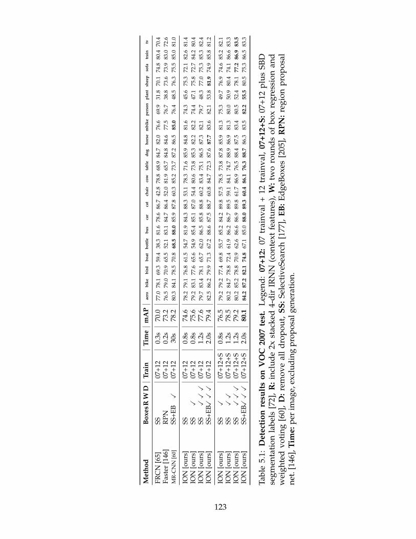
Met

hod

Box

esR

WD

T rai

nT i

me

mA

Pae

robi

kebi

rdbo

atbo

ttle

bus

car

cat

chai

rco

wta

ble

dog

hors

em

bike

pers

onpl

ant

shee

pso

fatr

ain

tv

FRC

N[6

5]SS

07+1

20.

3s70

.077

.078

.169

.359

.438

.381

.678

.686

.742

.878

.868

.984

.782

.076

.669

.931

.870

.174

.880

.470

.4Fa

ster

[146

]R

PN07

+12

0.2s

73.2

76.5

79.0

70.9

65.5

52.1

83.1

84.7

86.4

52.0

81.9

65.7

84.8

84.6

77.5

76.7

38.8

73.6

73.9

83.0

72.6

MR

-CN

N[6

0]SS

+EBX

07+1

230

s78

.280

.384

.178

.570

.868

.588

.085

.987

.860

.385

.273

.787

.286

.585

.076

.448

.576

.375

.585

.081

.0

ION

[our

s]SS

07+1

20.

8s74

.678

.279

.176

.861

.554

.781

.984

.388

.353

.178

.371

.685

.984

.881

.674

.345

.675

.372

.182

.681

.4IO

N[o

urs]

SSX

07+1

20.

8s75

.679

.283

.177

.665

.654

.985

.485

.187

.054

.480

.673

.885

.382

.282

.274

.447

.175

.872

.784

.280

.4IO

N[o

urs]

SSXXX

07+1

21.

2s77

.679

.783

.478

.165

.762

.086

.585

.888

.860

.283

.475

.186

.587

.382

.179

.748

.377

.075

.385

.382

.4IO

N[o

urs]

SS+E

BXXX

07+1

22.

0s79

.482

.586

.279

.971

.367

.288

.687

.588

.760

.884

.772

.387

.687

.783

.682

.153

.881

.974

.985

.881

.2

ION

[our

s]SS

X07

+12+

S0.

8s76

.579

.279

.277

.469

.855

.785

.284

.289

.857

.578

.573

.887

.885

.981

.375

.349

.776

.974

.685

.282

.1IO

N[o

urs]

SSXX

07+1

2+S

1.2s

78.5

80.2

84.7

78.8

72.4

61.9

86.2

86.7

89.5

59.1

84.1

74.7

88.9

86.9

81.3

80.0

50.9

80.4

74.1

86.6

83.3

ION

[our

s]SS

XXX

07+1

2+S

1.2s

79.2

80.2

85.2

78.8

70.9

62.6

86.6

86.9

89.8

61.7

86.9

76.5

88.4

87.5

83.4

80.5

52.4

78.1

77.2

86.9

83.5

ION

[our

s]SS

+EBXXX

07+1

2+S

2.0s

80.1

84.2

87.2

82.1

74.8

67.1

85.0

88.0

89.3

60.4

86.1

76.3

88.7

86.3

83.5

82.2

55.5

80.5

75.3

86.5

83.3

Tabl

e5.

1:D

etec

tion

resu

lts

onV

OC

2007

test

.L

egen

d:

07+1

2:07

trai

nval

+12

trai

nval

,07

+12+

S:07

+12

plu

sSB

Dse

gmen

tati

onla

bels

[72]

,R

:inc

lud

e2x

stac

ked

4-d

irIR

NN

(con

text

feat

ure

s),

W:t

wo

rou

nds

ofbo

xre

gres

sion

and

wei

ghte

dvo

ting

[60]

,D

:rem

ove

all

dro

pou

t,SS

:Sel

ecti

veSe

arch

[177

],EB

:Ed

geB

oxes

[205

],R

PN:r

egio

np

rop

osal

net.

[146

],Ti

me:

per

imag

e,ex

clud

ing

prop

osal

gene

rati

on.

123

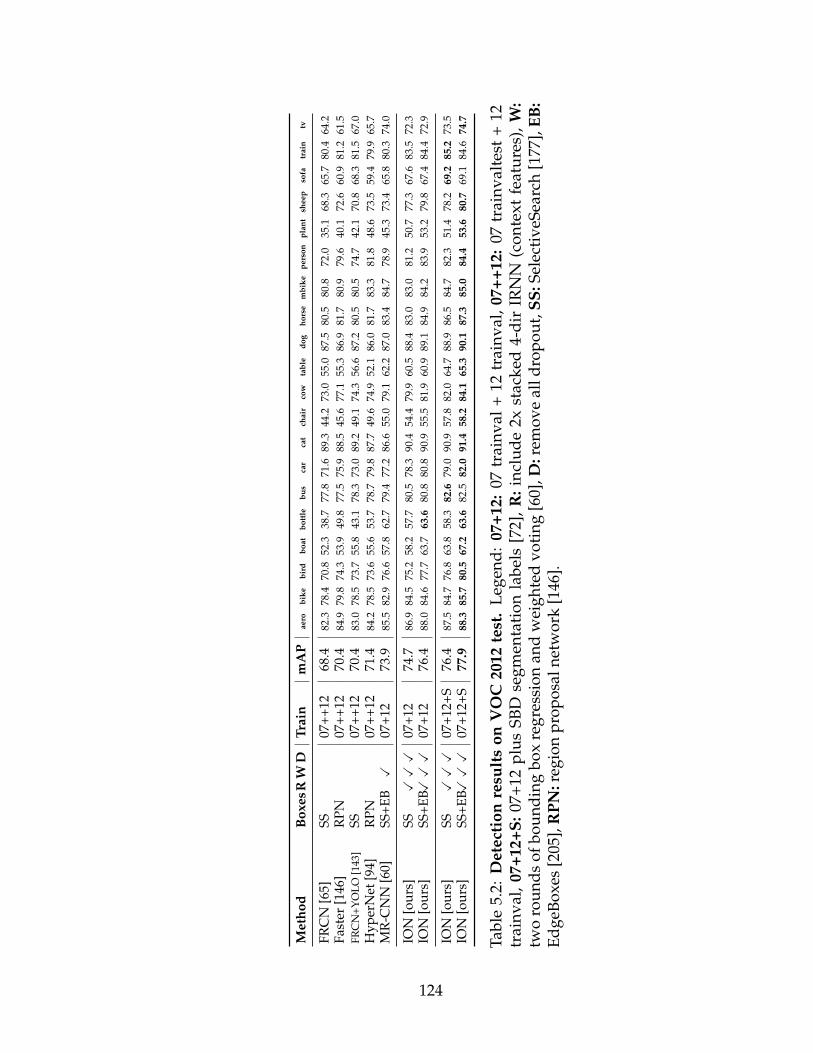
Met

hod

Box

esR

WD

T rai

nm

AP

aero

bike

bird

boat

bott

lebu

sca

rca

tch

air

cow

tabl

edo

gho

rse

mbi

kepe

rson

plan

tsh

eep

sofa

trai

ntv

FRC

N[6

5]SS

07++

1268

.482

.378

.470

.852

.338

.777

.871

.689

.344

.273

.055

.087

.580

.580

.872

.035

.168

.365

.780

.464

.2Fa

ster

[146

]R

PN07

++12

70.4

84.9

79.8

74.3

53.9

49.8

77.5

75.9

88.5

45.6

77.1

55.3

86.9

81.7

80.9

79.6

40.1

72.6

60.9

81.2

61.5

FRC

N+Y

OLO

[143

]SS

07++

1270

.483

.078

.573

.755

.843

.178

.373

.089

.249

.174

.356

.687

.280

.580

.574

.742

.170

.868

.381

.567

.0H

yper

Net

[94]

RPN

07++

1271

.484

.278

.573

.655

.653

.778

.779

.887

.749

.674

.952

.186

.081

.783

.381

.848

.673

.559

.479

.965

.7M

R-C

NN

[60]

SS+E

BX

07+1

273

.985

.582

.976

.657

.862

.779

.477

.286

.655

.079

.162

.287

.083

.484

.778

.945

.373

.465

.880

.374

.0

ION

[our

s]SS

XXX

07+1

274

.786

.984

.575

.258

.257

.780

.578

.390

.454

.479

.960

.588

.483

.083

.081

.250

.777

.367

.683

.572

.3IO

N[o

urs]

SS+E

BXXX

07+1

276

.488

.084

.677

.763

.763

.680

.880

.890

.955

.581

.960

.989

.184

.984

.283

.953

.279

.867

.484

.472

.9

ION

[our

s]SS

XXX

07+1

2+S

76.4

87.5

84.7

76.8

63.8

58.3

82.6

79.0

90.9

57.8

82.0

64.7

88.9

86.5

84.7

82.3

51.4

78.2

69.2

85.2

73.5

ION

[our

s]SS

+EBXXX

07+1

2+S

77.9

88.3

85.7

80.5

67.2

63.6

82.5

82.0

91.4

58.2

84.1

65.3

90.1

87.3

85.0

84.4

53.6

80.7

69.1

84.6

74.7

Tabl

e5.

2:D

etec

tion

resu

lts

onV

OC

2012

test

.L

egen

d:

07+1

2:07

trai

nval

+12

trai

nval

,07+

+12:

07tr

ainv

alte

st+

12tr

ainv

al,0

7+12

+S:0

7+12

plu

sSB

Dse

gmen

tati

onla

bels

[72]

,R:i

nclu

de

2xst

acke

d4-

dir

IRN

N(c

onte

xtfe

atu

res)

,W:

two

roun

ds

ofbo

und

ing

box

regr

essi

onan

dw

eigh

ted

voti

ng[6

0],D

:rem

ove

alld

ropo

ut,S

S:Se

lect

iveS

earc

h[1

77],

EB:

Edge

Boxe

s[2

05],

RPN

:reg

ion

prop

osal

netw

ork

[146

].

124

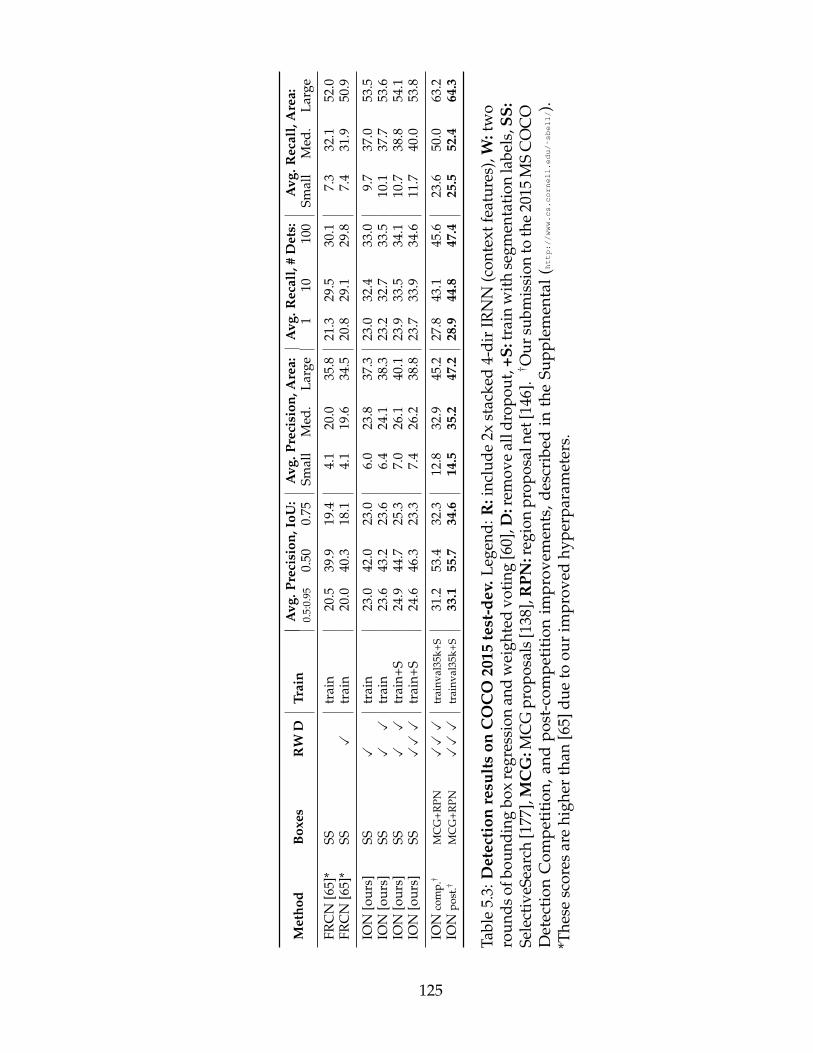
Met

hod

Box

esR

WD

Trai

nA

vg.P

reci

sion

,IoU

:A

vg.P

reci

sion

,Are

a:A

vg.R

ecal

l,#

Det

s:A

vg.R

ecal

l,A

rea:

0.5:

0.95

0.50

0.75

Smal

lM

ed.

Larg

e1

1010

0Sm

all

Med

.La

rge

FRC

N[6

5]*

SStr

ain

20.5

39.9

19.4

4.1

20.0

35.8

21.3

29.5

30.1

7.3

32.1

52.0

FRC

N[6

5]*

SSX

trai

n20

.040

.318

.14.

119

.634

.520

.829

.129

.87.

431

.950

.9

ION

[our

s]SS

Xtr

ain

23.0

42.0

23.0

6.0

23.8

37.3

23.0

32.4

33.0

9.7

37.0

53.5

ION

[our

s]SS

XX

trai

n23

.643

.223

.66.

424

.138

.323

.232

.733

.510

.137

.753

.6IO

N[o

urs]

SSXX

trai

n+S

24.9

44.7

25.3

7.0

26.1

40.1

23.9

33.5

34.1

10.7

38.8

54.1

ION

[our

s]SS

XXX

trai

n+S

24.6

46.3

23.3

7.4

26.2

38.8

23.7

33.9

34.6

11.7

40.0

53.8

ION

com

p.†

MC

G+R

PNXXX

trai

nval

35k+

S31

.253

.432

.312

.832

.945

.227

.843

.145

.623

.650

.063

.2IO

Npo

st.†

MC

G+R

PNXXX

trai

nval

35k+

S33

.155

.734

.614

.535

.247

.228

.944

.847

.425

.552

.464

.3

Tabl

e5.

3:D

etec

tion

resu

lts

onC

OC

O20

15te

st-d

ev.L

egen

d:R

:inc

lude

2xst

acke

d4-

dir

IRN

N(c

onte

xtfe

atur

es),

W:t

wo

roun

dsof

boun

ding

box

regr

essi

onan

dw

eigh

ted

votin

g[6

0],D

:rem

ove

alld

ropo

ut,+

S:tr

ain

with

segm

enta

tion

labe

ls,S

S:Se

lect

iveS

earc

h[1

77],

MC

G:M

CG

prop

osal

s[1

38],

RPN

:reg

ion

prop

osal

net[

146]

.†O

ursu

bmis

sion

toth

e20

15M

SC

OC

OD

etec

tion

Com

pet

itio

n,an

dp

ost-

com

pet

itio

nim

pro

vem

ents

,des

crib

edin

the

Sup

ple

men

tal(

http://www.cs.cornell.edu/˜sbell/).

*The

sesc

ores

are

high

erth

an[6

5]du

eto

our

impr

oved

hype

rpar

amet

ers.

125

measure the L2 norm of the parameter gradient vector and rescale it if its norm

is above 20 (80 when accumulating over 4 images).

To accelerate training, we use a two-stage schedule. As noted by Girshick [65],

it is not necessary to fine-tune all layers, and nearly the same performance can

be achieved by fine-tuning starting from conv3 1. With this in mind, we first

train for 40k iterations with conv1 1 through conv5 3 frozen, and then another

100k iterations with only conv1 1 through conv2 2 frozen. All other layers are

fine-tuned. When training for COCO, we use 80k and 320k iterations respectively.

We found that shorter training schedules are not enough to fully converge.

We also use a different learning rate (LR) schedule. The LR exponentially

decays from 5 · 10−3 to 10−4 in the first stage, and from 10−3 to 10−5 in the second

stage. To reduce the effect of random variation, we fix the random seed so that

all variants see the same images in the same order. For PASCAL VOC we use

the same pre-computed selective search boxes from Fast R-CNN, and for COCO

we use the boxes precomputed by Hosang et al. [80]. Finally, we modified the

test thresholds in Fast R-CNN so that we keep only boxes with a softmax score

above 0.05, and keep at most 100 boxes per image.

When re-running the baseline Fast R-CNN using the above settings, we see a

+0.8 mAP improvement over the original settings on VOC 2007 test. We compare

against the baseline using our improved settings where possible.

126

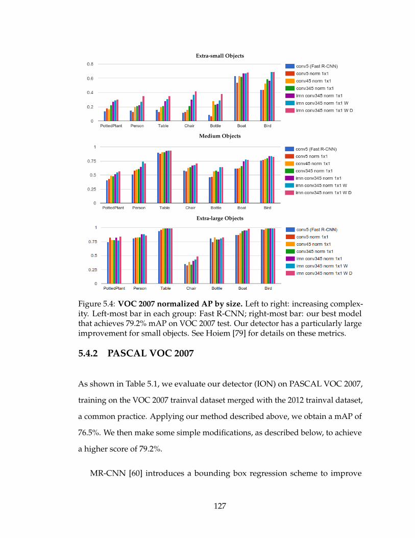
Extra-small Objects

Medium Objects

Extra-large Objects

Figure 5.4: VOC 2007 normalized AP by size. Left to right: increasing complex-ity. Left-most bar in each group: Fast R-CNN; right-most bar: our best modelthat achieves 79.2% mAP on VOC 2007 test. Our detector has a particularly largeimprovement for small objects. See Hoiem [79] for details on these metrics.

5.4.2 PASCAL VOC 2007

As shown in Table 5.1, we evaluate our detector (ION) on PASCAL VOC 2007,

training on the VOC 2007 trainval dataset merged with the 2012 trainval dataset,

a common practice. Applying our method described above, we obtain a mAP of

76.5%. We then make some simple modifications, as described below, to achieve

a higher score of 79.2%.

MR-CNN [60] introduces a bounding box regression scheme to improve

127

results on VOC, where bounding boxes are evaluated twice: (1) the initial pro-

posal boxes are evaluated and regressed to improved locations and then (2)

the improved locations are passed again through the network. All boxes are

accumulated together, and non-max supression is applied. Finally, a weighted

vote is computed for each kept box (over all boxes, including those suppressed),

where boxes that overlap a kept box by at least 0.5 IoU contribute to the average.

For our method, we use the softmax scores as the weights. When adding this

scheme to our method, our mAP rises from 76.5% to 78.5%. Finally, we observed

that our models are underfitting and we remove dropout from all layers to get a

further gain up to 79.2%.

For a direct comparison to MR-CNN, we also trained our method on both

SelectiveSearch [177] and EdgeBoxes [205] (SS+EB) but not segmentation labels.

With these settings, we achieve 79.4% mAP with a runtime of 2s/image,2 while

MR-CNN achieves 78.2% mAP at 30s/image. See Table 5.1.

5.4.3 PASCAL VOC 2012

We also evaluate on the slightly more challenging VOC 2012 dataset, submitting

to the public evaluation server.3 In Table 5.2, we show the top methods on the

public leaderboard as of the time of submission. Our detector obtains a mAP of

76.4%, which is several points higher than the next best submission, and is the

most accurate for most categories.

2On a single Titan X GPU, excluding proposal generation3Anonymous URL: http://host.robots.ox.ac.uk:8080/anonymous/B3VFLE.html

128

5.4.4 MS COCO

Microsoft has recently released the Common Objects in Context dataset, which

contains 80k training images (“2014 train”) and 40k validation images (“2014

val”). There is an associated MS COCO challenge with a new evaluation metric,

that averages mAP over different IoU thresholds, from 0.5 to 0.95 (written as

“0.5:0.95”). This places a significantly larger emphasis on localization compared

to the PASCAL VOC metric which only requires IoU of 0.5.

We are only aware of one baseline performance number for this dataset, as

published in the Fast R-CNN paper, which cites a mAP of 19.7% on the 2015

test-dev set [65]. We trained our own Fast R-CNN model on “2014 train” using

our longer training schedule and obtained a higher mAP of 20.5% mAP on the

same set, which we use as a baseline. As shown in Table 5.3, when trained on the

same images with the same schedule, our method obtains a large improvement

over the baseline with a mAP of 24.9%.

Applying box voting [60] gives us a further improvement (+1.6 mAP) on the

original PASCAL VOC metric (IoU 0.5), but interestingly decreases performance

(-0.3 mAP) on the new COCO metric (IOU 0.5:0.95). We note that this effect is

entirely due to the change in metric, which weights localization errors differently.

As described in the Supplemental,4 we fixed this for our competition submission

by raising the box voting IoU threshold from 0.5 to ∼ 0.85.

We submitted ION to the 2015 MS COCO Detection Challenge and won

the Best Student Entry with 3rd place overall. Using only a single model (no

ensembling), our submission achieved 31.0% on test-competition score and

4http://www.cs.cornell.edu/˜sbell/

129

31.2% on test-dev score (Table 5.3). After the competition, we further improved

our test-dev score to 33.1% by adding left-right flipping and adjusting training

parameters. See the Supplemental,5 for details on our challenge submission.

5.4.5 Improvement for small objects

In general, small objects are challenging for detectors: there are fewer pixels

on the object, they are harder to localize, and there can be many more of them

per image. Small objects are even more challenging for proposal methods. For

all experiments, we are using selective search [177] for object proposals, which

performs very poorly on small objects in COCO with an average recall under

10% [137].

We find that our detector shows a large relative improvement in this category.

For COCO, if we look at small6 objects, average precision and average recall

improve from 4.1% to 7.0% and from 7.3% to 10.7% respectively. We highlight

that this is even higher than the baseline proposal method, which is only possible

because we perform bounding box regression to predict improved box locations.

Similarly, we show a size breakdown for VOC2007 test in Figure 5.4 using

Hoiem’s toolkit for diagnosing errors [79], and see similarly large improvements

on this dataset as well.

130

ROI pooling from: Merge features using:C2 C3 C4 C5 1x1 L2+Scale+1x1

X *70.8 71.5X X 69.7 74.4

X X X 63.6 74.6X X X X 59.3 74.6

Table 5.4: Combining features from different layers. Metric: Detection mAP onVOC07 test. Training set: 07 trainval + 12 trainval. 1x1: combine features fromdifferent layers using a 1x1 convolution. L2+Scale+1x1: use L2 normalization,scaling (initialized to 1000), and 1x1 convolution, as described in section 5.3.1.These results do not include “context features.” *This entry is the same as FastR-CNN [65], but trained with our hyperparameters.

5.5 Design evaluation

In this section, we explore changes to our architecture and justify our design

choices with experiments on PASCAL VOC 2007. All numbers in this section are

VOC 2007 test mAP, trained on 2007 trainval + 2012 trainval, with the settings

described in Section 5.4.1. Note that for this section, we use dropout in all

networks, and a single round of bounding box regression at test time.

5.5.1 Pool from which layers?

As described in Section 5.3.1, our detector pools regions of interest (ROI) from

multiple layers and combines the result. A straightforward approach would be

to concatenate the ROI from each layer and reduce the dimensionality using a

1x1 convolution. As shown in Table 5.4 (left column), this does not work. In

VGG16, the convolutional features at different layers can have very different

amplitudes, so that naively combining them leads to unstable learning. While it

5Ibid6“Small” means area ≤ 322 px; about 40% of COCO is “small.”

131

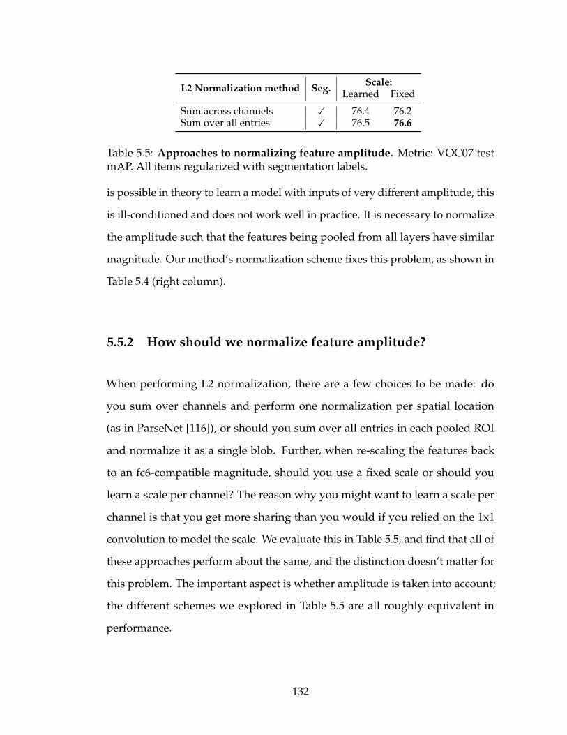
L2 Normalization method Seg. Scale:Learned Fixed

Sum across channels X 76.4 76.2Sum over all entries X 76.5 76.6

Table 5.5: Approaches to normalizing feature amplitude. Metric: VOC07 testmAP. All items regularized with segmentation labels.

is possible in theory to learn a model with inputs of very different amplitude, this

is ill-conditioned and does not work well in practice. It is necessary to normalize

the amplitude such that the features being pooled from all layers have similar

magnitude. Our method’s normalization scheme fixes this problem, as shown in

Table 5.4 (right column).

5.5.2 How should we normalize feature amplitude?

When performing L2 normalization, there are a few choices to be made: do

you sum over channels and perform one normalization per spatial location

(as in ParseNet [116]), or should you sum over all entries in each pooled ROI

and normalize it as a single blob. Further, when re-scaling the features back

to an fc6-compatible magnitude, should you use a fixed scale or should you

learn a scale per channel? The reason why you might want to learn a scale per

channel is that you get more sharing than you would if you relied on the 1x1

convolution to model the scale. We evaluate this in Table 5.5, and find that all of

these approaches perform about the same, and the distinction doesn’t matter for

this problem. The important aspect is whether amplitude is taken into account;

the different schemes we explored in Table 5.5 are all roughly equivalent in

performance.

132

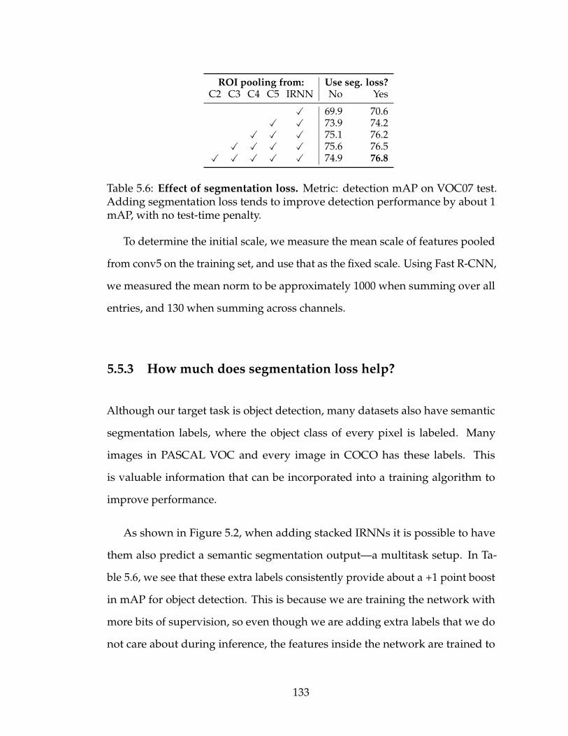
ROI pooling from: Use seg. loss?C2 C3 C4 C5 IRNN No Yes

X 69.9 70.6X X 73.9 74.2

X X X 75.1 76.2X X X X 75.6 76.5

X X X X X 74.9 76.8

Table 5.6: Effect of segmentation loss. Metric: detection mAP on VOC07 test.Adding segmentation loss tends to improve detection performance by about 1mAP, with no test-time penalty.

To determine the initial scale, we measure the mean scale of features pooled

from conv5 on the training set, and use that as the fixed scale. Using Fast R-CNN,

we measured the mean norm to be approximately 1000 when summing over all

entries, and 130 when summing across channels.

5.5.3 How much does segmentation loss help?

Although our target task is object detection, many datasets also have semantic

segmentation labels, where the object class of every pixel is labeled. Many

images in PASCAL VOC and every image in COCO has these labels. This

is valuable information that can be incorporated into a training algorithm to

improve performance.

As shown in Figure 5.2, when adding stacked IRNNs it is possible to have

them also predict a semantic segmentation output—a multitask setup. In Ta-

ble 5.6, we see that these extra labels consistently provide about a +1 point boost

in mAP for object detection. This is because we are training the network with

more bits of supervision, so even though we are adding extra labels that we do

not care about during inference, the features inside the network are trained to

133

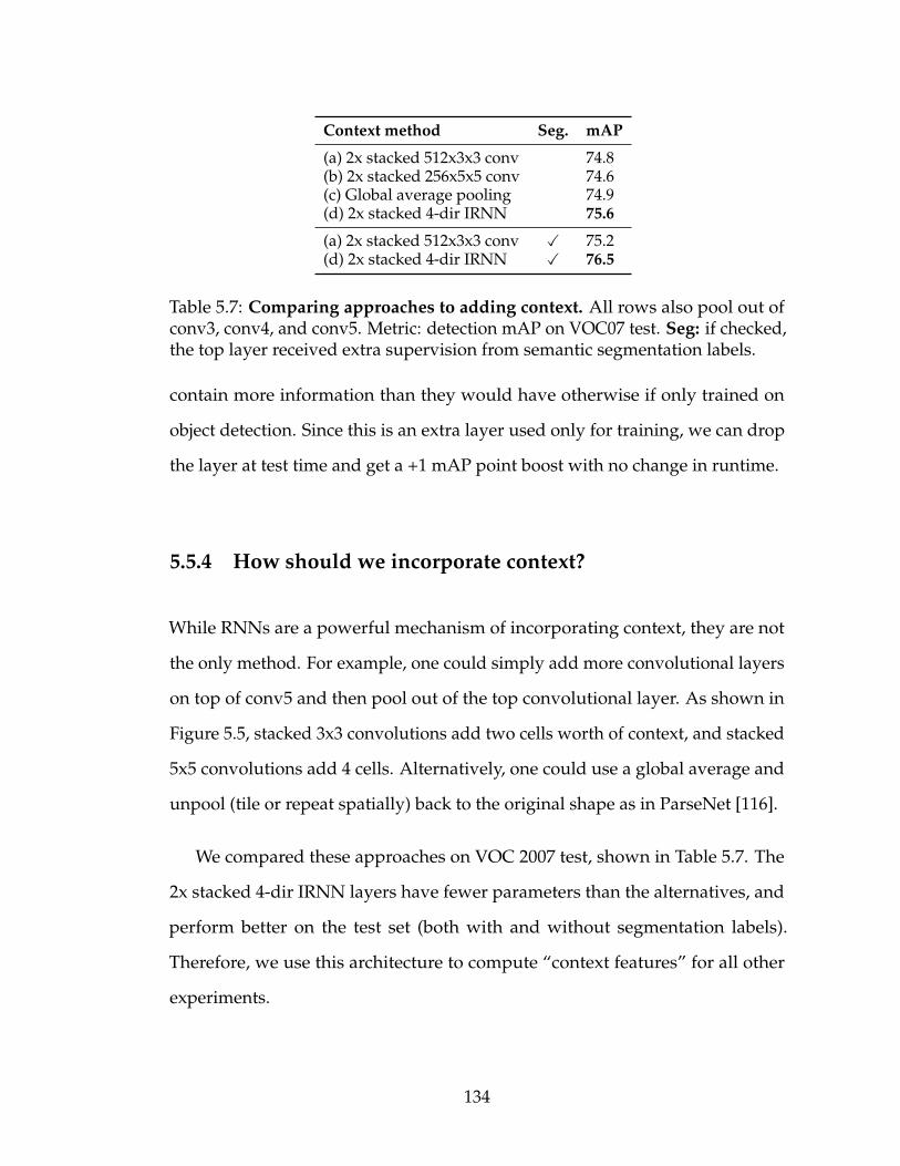
Context method Seg. mAP

(a) 2x stacked 512x3x3 conv 74.8(b) 2x stacked 256x5x5 conv 74.6(c) Global average pooling 74.9(d) 2x stacked 4-dir IRNN 75.6

(a) 2x stacked 512x3x3 conv X 75.2(d) 2x stacked 4-dir IRNN X 76.5

Table 5.7: Comparing approaches to adding context. All rows also pool out ofconv3, conv4, and conv5. Metric: detection mAP on VOC07 test. Seg: if checked,the top layer received extra supervision from semantic segmentation labels.

contain more information than they would have otherwise if only trained on

object detection. Since this is an extra layer used only for training, we can drop

the layer at test time and get a +1 mAP point boost with no change in runtime.

5.5.4 How should we incorporate context?

While RNNs are a powerful mechanism of incorporating context, they are not

the only method. For example, one could simply add more convolutional layers

on top of conv5 and then pool out of the top convolutional layer. As shown in

Figure 5.5, stacked 3x3 convolutions add two cells worth of context, and stacked

5x5 convolutions add 4 cells. Alternatively, one could use a global average and

unpool (tile or repeat spatially) back to the original shape as in ParseNet [116].

We compared these approaches on VOC 2007 test, shown in Table 5.7. The

2x stacked 4-dir IRNN layers have fewer parameters than the alternatives, and

perform better on the test set (both with and without segmentation labels).

Therefore, we use this architecture to compute “context features” for all other

experiments.

134

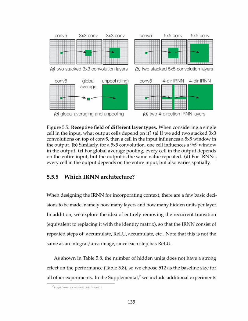
(a) two stacked 3x3 convolution layers

(d) two 4-direction IRNN layers

conv5 3x3 conv 3x3 conv

conv5 4-dir IRNN 4-dir IRNN

(b) two stacked 5x5 convolution layers

conv5 5x5 conv 5x5 conv

(c) global averaging and unpooling

conv5 unpool (tiling)globalaverage

Figure 5.5: Receptive field of different layer types. When considering a singlecell in the input, what output cells depend on it? (a) If we add two stacked 3x3convolutions on top of conv5, then a cell in the input influences a 5x5 window inthe output. (b) Similarly, for a 5x5 convolution, one cell influences a 9x9 windowin the output. (c) For global average pooling, every cell in the output dependson the entire input, but the output is the same value repeated. (d) For IRNNs,every cell in the output depends on the entire input, but also varies spatially.

5.5.5 Which IRNN architecture?

When designing the IRNN for incorporating context, there are a few basic deci-

sions to be made, namely how many layers and how many hidden units per layer.

In addition, we explore the idea of entirely removing the recurrent transition

(equivalent to replacing it with the identity matrix), so that the IRNN consist of

repeated steps of: accumulate, ReLU, accumulate, etc.. Note that this is not the

same as an integral/area image, since each step has ReLU.

As shown in Table 5.8, the number of hidden units does not have a strong

effect on the performance (Table 5.8), so we choose 512 as the baseline size for

all other experiments. In the Supplemental,7 we include additional experiments

7http://www.cs.cornell.edu/˜sbell/

135

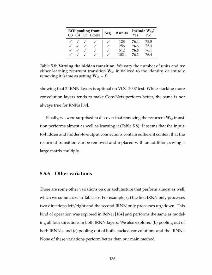
ROI pooling from: Seg. # units Include Whh?C3 C4 C5 IRNN Yes No

X X X X X 128 76.4 75.5X X X X X 256 76.5 75.3X X X X X 512 76.5 76.1X X X X X 1024 76.2 76.4

Table 5.8: Varying the hidden transition. We vary the number of units and tryeither learning recurrent transition Whh initialized to the identity, or entirelyremoving it (same as setting Whh = I).

showing that 2 IRNN layers is optimal on VOC 2007 test. While stacking more

convolution layers tends to make ConvNets perform better, the same is not

always true for RNNs [89].

Finally, we were surprised to discover that removing the recurrent Whh transi-

tion performs almost as well as learning it (Table 5.8). It seems that the input-

to-hidden and hidden-to-output connections contain sufficient context that the

recurrent transition can be removed and replaced with an addition, saving a

large matrix multiply.

5.5.6 Other variations

There are some other variations on our architecture that perform almost as well,

which we summarize in Table 5.9. For example, (a) the first IRNN only processes

two directions left/right and the second IRNN only processes up/down. This

kind of operation was explored in ReNet [184] and performs the same as model-

ing all four directions in both IRNN layers. We also explored (b) pooling out of

both IRNNs, and (c) pooling out of both stacked convolutions and the IRNNs.

None of these variations perform better than our main method.

136

Variation mAP

Our method 76.5(a) Left-right then up-down 76.5(b) Pool out of both IRNNs 75.9(c) Combine 2x stacked 512x3x3 conv and IRNN 76.5

Table 5.9: Other variations. Metric: VOC07 test mAP. We list some other varia-tions that all perform about the same.

5.6 Conclusion

This paper introduces the Inside-Outside Net (ION), an architecture that lever-

ages context and multi-scale knowledge for object detection. Our architecture

uses a 2x stacked 4-directional IRNN for context, and multi-layer ROI pool-

ing with normalization for improved object description. To justify our design

choices, we conducted extensive experiments evaluating choices like the number

of layers combined, using segmentation loss, normalizing feature amplitudes,

different IRNN architectures, and other variations. We achieve state-of-the-art

results on both PASCAL VOC and COCO, and find our proposed architecture is

particularly effective at improving detection of small objects.

5.7 Impact

Our work in this chapter was first presented at the MS COCO 2015 Detection

Challenge, where we won Best Student Entry, and later published as a paper at

CVPR 2016 [15]. Concurrently with our work, the second place entry in the MS

COCO competition revisited skip connections with a similar architecture [196].

Our ION architecture has inspired similar approaches of combining skip pooling

and context to obtain more accurate results [204].

137

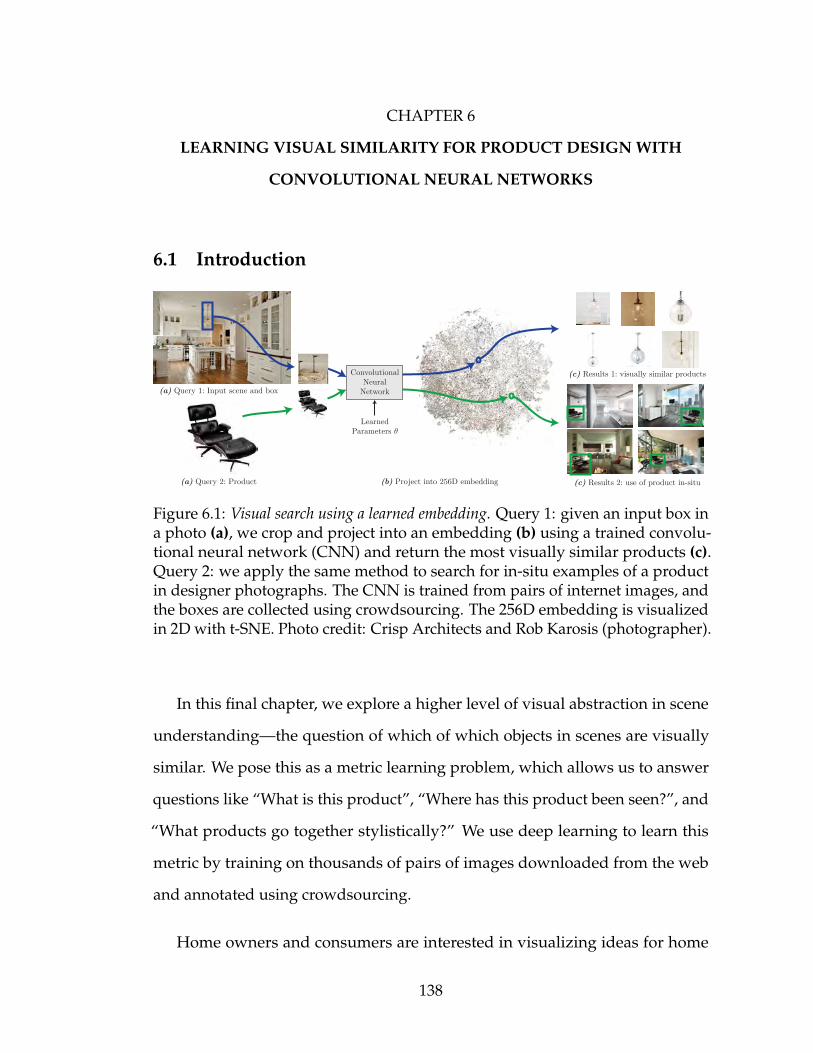
CHAPTER 6

LEARNING VISUAL SIMILARITY FOR PRODUCT DESIGN WITH

CONVOLUTIONAL NEURAL NETWORKS

6.1 Introduction

(a) Query 1: Input scene and box

(b) Project into 256D embedding (c) Results 2: use of product in-situ

ConvolutionalNeural

Network

Learned Parameters θ

(a) Query 2: Product

(c) Results 1: visually similar products

Figure 6.1: Visual search using a learned embedding. Query 1: given an input box ina photo (a), we crop and project into an embedding (b) using a trained convolu-tional neural network (CNN) and return the most visually similar products (c).Query 2: we apply the same method to search for in-situ examples of a productin designer photographs. The CNN is trained from pairs of internet images, andthe boxes are collected using crowdsourcing. The 256D embedding is visualizedin 2D with t-SNE. Photo credit: Crisp Architects and Rob Karosis (photographer).

In this final chapter, we explore a higher level of visual abstraction in scene

understanding—the question of which of which objects in scenes are visually

similar. We pose this as a metric learning problem, which allows us to answer

questions like “What is this product”, “Where has this product been seen?”, and

“What products go together stylistically?” We use deep learning to learn this

metric by training on thousands of pairs of images downloaded from the web

and annotated using crowdsourcing.

Home owners and consumers are interested in visualizing ideas for home

138

improvement and interior design. Popular sites like Houzz, Pinterest, and

LikeThatDecor have large active communities of users that browse the sites for

inspiration, design ideas and recommendations, and to pose design questions.

For example, some topics and questions that come up are:

• “What is this chair, lamp, wallpaper in this photograph? Where can I

find it?”, or, “Find me chairs, . . . similar to this one.” This kind of query

may come from a user who sees something they like in an online image on

Flickr or Houzz, a magazine, or a friend’s home.

• “How has this armchair been used in designer photos?” Users can search

for the usage of a product for design inspiration.

• “Find me a compatible chair matching this table.” For example, a home

owner is replacing furniture in their home and wants to find a chair that

matches their existing table (and bookcase).

Currently, sites like Houzz have active communities of users that answer design

questions like these with (sometimes informed) guesses. Providing automated

tools for design suggestions and ideas can be very useful to these users.

The common thread between these questions is the need to find visually

similar objects in photographs. In this chapter we learn a distance metric between

an object in-situ (i.e., a sub-image of a photograph) and an iconic product image

of that object (i.e., a clean well-lit photograph, usually with a white background).

The distance is small between the in-situ object image and the iconic product

image, and large otherwise. Learning such a distance metric is challenging

because the in-situ object image can have many different backgrounds, sizes,

orientations, or lighting when compared to the iconic product image, and, it

139

could be significantly occluded by clutter in the scene.

Recently, the area of deep learning using convolutional neural networks

(CNNs) has made incredible strides in recognizing objects across a variety of

viewpoints and distortions [167, 99]. Therefore, we build our method around

this powerful tool to learn functions that can reason about object similarity

across wide baselines and wide changes in appearance. To apply deep learning,

however, we need ground truth data to train the network. We use crowdsourcing

to collect matching information between in-situ images and their corresponding

iconic product images to generate the data needed to train deep networks.

We make the following contributions:

• We develop a crowdsourced pipeline to collect pairings between in-situ

images and their corresponding product images.

• We show how this data can be combined with a siamese CNN to learn a

high quality embedding. We evaluate several different training methodolo-

gies including: training with contrastive loss, object classification softmax

loss, training with both, and the effect of normalizing the embedding vector.

• We apply this embedding to image search applications like finding a prod-

uct, finding designer scenes that use a product, and finding visually similar

products across categories.

Figure 3.2 illustrates how our visual search works. On the left are two types

of queries: (1) an object in a scene marked with a box and (2) an iconic product

image. The user sends the images as queries to the CNN we have learned. The

queries map to different locations in our 256D learned embedding (visualized in

the middle). A nearest neighbor query in the embedding produces the results on

140

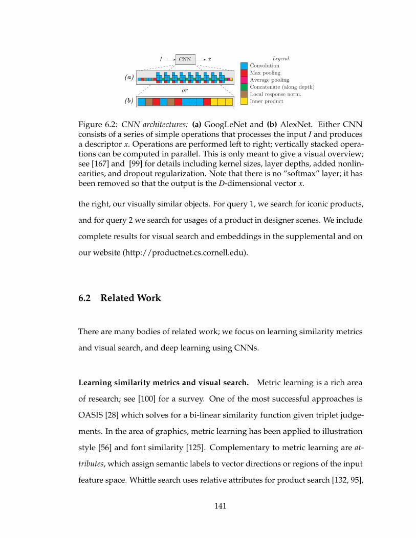
Convolution

Local response norm.

Max poolingAverage poolingConcatenate (along depth)

(b)

LegendCNN

or

(a)

Inner product

I x

Figure 6.2: CNN architectures: (a) GoogLeNet and (b) AlexNet. Either CNNconsists of a series of simple operations that processes the input I and producesa descriptor x. Operations are performed left to right; vertically stacked opera-tions can be computed in parallel. This is only meant to give a visual overview;see [167] and [99] for details including kernel sizes, layer depths, added nonlin-earities, and dropout regularization. Note that there is no “softmax” layer; it hasbeen removed so that the output is the D-dimensional vector x.

the right, our visually similar objects. For query 1, we search for iconic products,

and for query 2 we search for usages of a product in designer scenes. We include

complete results for visual search and embeddings in the supplemental and on

our website (http://productnet.cs.cornell.edu).

6.2 Related Work

There are many bodies of related work; we focus on learning similarity metrics

and visual search, and deep learning using CNNs.

Learning similarity metrics and visual search. Metric learning is a rich area

of research; see [100] for a survey. One of the most successful approaches is

OASIS [28] which solves for a bi-linear similarity function given triplet judge-

ments. In the area of graphics, metric learning has been applied to illustration

style [56] and font similarity [125]. Complementary to metric learning are at-

tributes, which assign semantic labels to vector directions or regions of the input

feature space. Whittle search uses relative attributes for product search [132, 95],

141

Furniture-geek [130] understands fine-grained furniture attributes. In addition to

modeling visual similarity, there are many approaches to solving the instance re-

trieval problem. For example, Girod et al. [64] use the CHoG descriptor to match

against millions of images of CDs, DVDs, and book covers. Many papers have

built methods around feature representations including Fisher Vectors [136] and

VLAD [84]. In contrast to the above approaches that mostly use “hand-tuned”

features, we want to learn features end-to-end directly from input pixels, using

convolutional neural networks.

In industry, there have been examples of instance retrieval for different prob-

lem domains like books and movies. Proprietary services like Google Goggles

and Amazon Flow attempt to handle any arbitrary input image and recognize

specific products. Other services like TinEye.com perform “reverse image search”

to find near-duplicates across the entire internet. In contrast, we focus on model-

ing a higher level notion of visual similarity.

Convolutional neural networks (CNNs). A full review of deep learning and

convolutional neural networks is beyond the scope of this thesis; please see [27].

Here, we cover the most relevant background, and focus our explanation to

how we use this tool for our problem. CNNs are functions for processing

images, consisting of a number of stages (“layers”) such as convolution, pooling,

and rectification, where the parameters of each stage are learned to optimize

performance on some task, given training data. While CNNs have been around

for many years, with early successes such as LeNet [106], it is only recently

that they have shown competitive results for tasks such as object classification

or detection. Driven by the success of Krizhevsky et al. [99]’s “SuperVision”

submission to the ILSVRC2012 image classification challenge, there has been

142

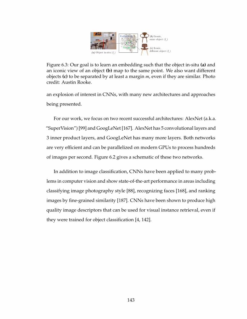
Embedding

Margin (m)

(a) Object in-situ (Iq )

(b) Iconic,same object (Ip )

(c) Iconic,different object (In )

Figure 6.3: Our goal is to learn an embedding such that the object in-situ (a) andan iconic view of an object (b) map to the same point. We also want differentobjects (c) to be separated by at least a margin m, even if they are similar. Photocredit: Austin Rooke.

an explosion of interest in CNNs, with many new architectures and approaches

being presented.

For our work, we focus on two recent successful architectures: AlexNet (a.k.a.

“SuperVision”) [99] and GoogLeNet [167]. AlexNet has 5 convolutional layers and

3 inner product layers, and GoogLeNet has many more layers. Both networks

are very efficient and can be parallelized on modern GPUs to process hundreds

of images per second. Figure 6.2 gives a schematic of these two networks.

In addition to image classification, CNNs have been applied to many prob-

lems in computer vision and show state-of-the-art performance in areas including

classifying image photography style [88], recognizing faces [168], and ranking

images by fine-grained similarity [187]. CNNs have been shown to produce high

quality image descriptors that can be used for visual instance retrieval, even if

they were trained for object classification [4, 142].

143

6.3 Background: learning a distance metric with siamese net-

works

In this section, we provide a brief overview of the theory behind siamese net-

works and contrastive loss functions [71], and how they may be used to train a

similarity metric from real data.

Given a convolutional neural network (such as AlexNet or GoogLeNet), we

can view the network as a function f that maps each image I into an embedding

position x, given parameters θ: x = f (I; θ). The parameter vector θ contains all the

weights and biases for the convolutional and inner product layers, and typically

contains 1M to 100M values. The goal is to solve for the parameter vector θ such

that the embedding produced through f has desirable properties and places

similar items nearby.

Consider a pair of images (Iq, Ip) that are two views of the same object, and

a pair of images (Iq, In) that show different objects. We can map these images

into our embedding to get xq, xp, xn. If we had a good embedding, we would find

that xq and xp are nearby, and xq and xn are further apart. This can be formalized

as the contrastive loss function L, which measures how well f is able to place

similar images nearby and keep dissimilar images separated. As implemented

in Caffe [85], L has the form:

L(θ) =∑

(xq,xp)

Lp(xq, xp)︸ ︷︷ ︸Penalty for similar images

that are far away

+∑

(xq,xn)

Ln(xq, xn)︸ ︷︷ ︸Penalty for dissimilar

images that are nearby

(6.1)

Lp(xq, xp) = ||xq − xp||22 (6.2)

Ln(xq, xn) = max(0,m2 − ||xq − xn||

22

)(6.3)

144

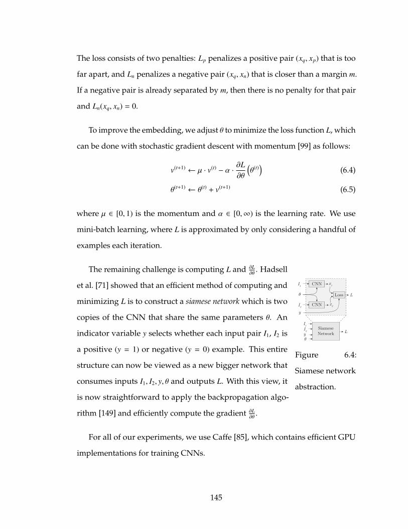
The loss consists of two penalties: Lp penalizes a positive pair (xq, xp) that is too

far apart, and Ln penalizes a negative pair (xq, xn) that is closer than a margin m.

If a negative pair is already separated by m, then there is no penalty for that pair

and Ln(xq, xn) = 0.

To improve the embedding, we adjust θ to minimize the loss function L, which

can be done with stochastic gradient descent with momentum [99] as follows:

v(t+1) ← µ · v(t) − α ·∂L∂θ

(θ(t)

)(6.4)

θ(t+1) ← θ(t) + v(t+1) (6.5)

where µ ∈ [0, 1) is the momentum and α ∈ [0,∞) is the learning rate. We use

mini-batch learning, where L is approximated by only considering a handful of

examples each iteration.

CNN

Lossθ

I1

I2CNN x2

x1

L

y

SiameseNetwork

I1

I2 y θ

L

Figure 6.4:

Siamese network

abstraction.

The remaining challenge is computing L and ∂L∂θ

. Hadsell

et al. [71] showed that an efficient method of computing and

minimizing L is to construct a siamese network which is two

copies of the CNN that share the same parameters θ. An

indicator variable y selects whether each input pair I1, I2 is

a positive (y = 1) or negative (y = 0) example. This entire

structure can now be viewed as a new bigger network that

consumes inputs I1, I2, y, θ and outputs L. With this view, it

is now straightforward to apply the backpropagation algo-

rithm [149] and efficiently compute the gradient ∂L∂θ

.

For all of our experiments, we use Caffe [85], which contains efficient GPU

implementations for training CNNs.

145

6.4 Our approach

For our work, we build a database of millions of products and scenes downloaded

from Houzz.com. We focus on learning a single embedding that contains two

types of images: in-situ examples of products Iq (cropped sub-images) and iconic

product images Ip, as shown in Figure 6.3. Rather than hand-design the mapping

Iq 7→ xq, we use a siamese network, described above, to automatically learn a

mapping that is both high quality and fast to compute.

While siamese architectures [71] are quite effective, there are many ways

to train the weights for a CNN. We explore different methods of training an

embedding as shown in Figure 6.5. Some of these variations have been used

before; for example, Razavian [142] used architecture A for instance retrieval,

Chopra [34] used B for identity verification, Wang [187] used a triplet version of

B with L2 normalization for fine-grained visual similarity, and Weston [192] used

C for MNIST digits and semantic role labeling. We evaluate these architectures

on a real-world internet dataset.

To train our CNN, we explore a new source of training data. We collect

a hundred thousand examples of matching in-situ products and their iconic

images. We use MTurk to collect the necessary in-situ bounding boxes for

each product (Section 6.5). We then train multiple CNN architectures using

this data and compare different multitask loss functions and different distance

metrics. Finally, we demonstrate how the learned mapping can be used in visual

search applications both across all object categories and within specific categories

(Section 6.6). We perform searches in two directions, returning either product

images or in-situ products in scenes.

146

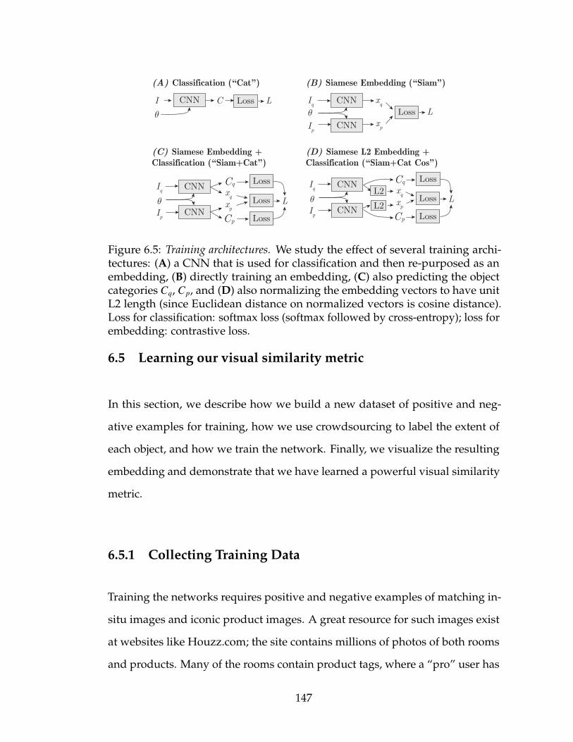
CNN

Lossθ

Iq

IpCNN

xp

xqL

Cq Loss

Cp Loss

CNNLossθ

Iq

IpCNN xp

xq

L

CNN

Lossθ

Iq

IpCNN

xp

xqL

Cq Loss

Cp Loss

L2

L2

CNN LossI C L

(A) Classification (“Cat”) (B) Siamese Embedding (“Siam”)

(C) Siamese Embedding +Classification (“Siam+Cat”)

(D) Siamese L2 Embedding +Classification (“Siam+Cat Cos”)

θ

Figure 6.5: Training architectures. We study the effect of several training archi-tectures: (A) a CNN that is used for classification and then re-purposed as anembedding, (B) directly training an embedding, (C) also predicting the objectcategories Cq, Cp, and (D) also normalizing the embedding vectors to have unitL2 length (since Euclidean distance on normalized vectors is cosine distance).Loss for classification: softmax loss (softmax followed by cross-entropy); loss forembedding: contrastive loss.

6.5 Learning our visual similarity metric

In this section, we describe how we build a new dataset of positive and neg-

ative examples for training, how we use crowdsourcing to label the extent of

each object, and how we train the network. Finally, we visualize the resulting

embedding and demonstrate that we have learned a powerful visual similarity

metric.

6.5.1 Collecting Training Data

Training the networks requires positive and negative examples of matching in-

situ images and iconic product images. A great resource for such images exist

at websites like Houzz.com; the site contains millions of photos of both rooms

and products. Many of the rooms contain product tags, where a “pro” user has

147

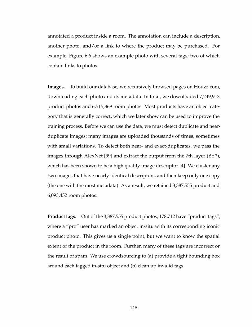
annotated a product inside a room. The annotation can include a description,

another photo, and/or a link to where the product may be purchased. For

example, Figure 6.6 shows an example photo with several tags; two of which

contain links to photos.

Images. To build our database, we recursively browsed pages on Houzz.com,

downloading each photo and its metadata. In total, we downloaded 7,249,913

product photos and 6,515,869 room photos. Most products have an object cate-

gory that is generally correct, which we later show can be used to improve the

training process. Before we can use the data, we must detect duplicate and near-

duplicate images; many images are uploaded thousands of times, sometimes

with small variations. To detect both near- and exact-duplicates, we pass the

images through AlexNet [99] and extract the output from the 7th layer (fc7),

which has been shown to be a high quality image descriptor [4]. We cluster any

two images that have nearly identical descriptors, and then keep only one copy

(the one with the most metadata). As a result, we retained 3,387,555 product and

6,093,452 room photos.

Product tags. Out of the 3,387,555 product photos, 178,712 have “product tags”,

where a “pro” user has marked an object in-situ with its corresponding iconic

product photo. This gives us a single point, but we want to know the spatial

extent of the product in the room. Further, many of these tags are incorrect or

the result of spam. We use crowdsourcing to (a) provide a tight bounding box

around each tagged in-situ object and (b) clean up invalid tags.

148

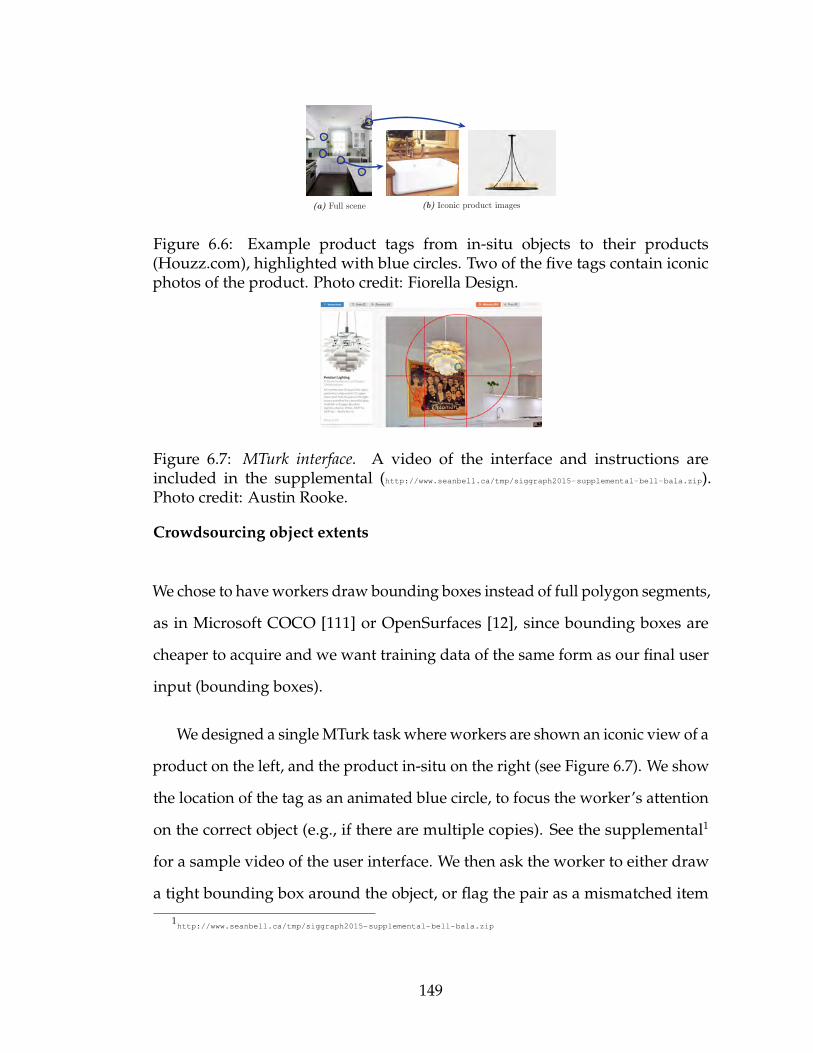
(a) Full scene (b) Iconic product images

Figure 6.6: Example product tags from in-situ objects to their products(Houzz.com), highlighted with blue circles. Two of the five tags contain iconicphotos of the product. Photo credit: Fiorella Design.

Figure 6.7: MTurk interface. A video of the interface and instructions areincluded in the supplemental (http://www.seanbell.ca/tmp/siggraph2015-supplemental-bell-bala.zip).Photo credit: Austin Rooke.

Crowdsourcing object extents

We chose to have workers draw bounding boxes instead of full polygon segments,

as in Microsoft COCO [111] or OpenSurfaces [12], since bounding boxes are

cheaper to acquire and we want training data of the same form as our final user

input (bounding boxes).

We designed a single MTurk task where workers are shown an iconic view of a

product on the left, and the product in-situ on the right (see Figure 6.7). We show

the location of the tag as an animated blue circle, to focus the worker’s attention

on the correct object (e.g., if there are multiple copies). See the supplemental1

for a sample video of the user interface. We then ask the worker to either draw

a tight bounding box around the object, or flag the pair as a mismatched item

1http://www.seanbell.ca/tmp/siggraph2015-supplemental-bell-bala.zip

149

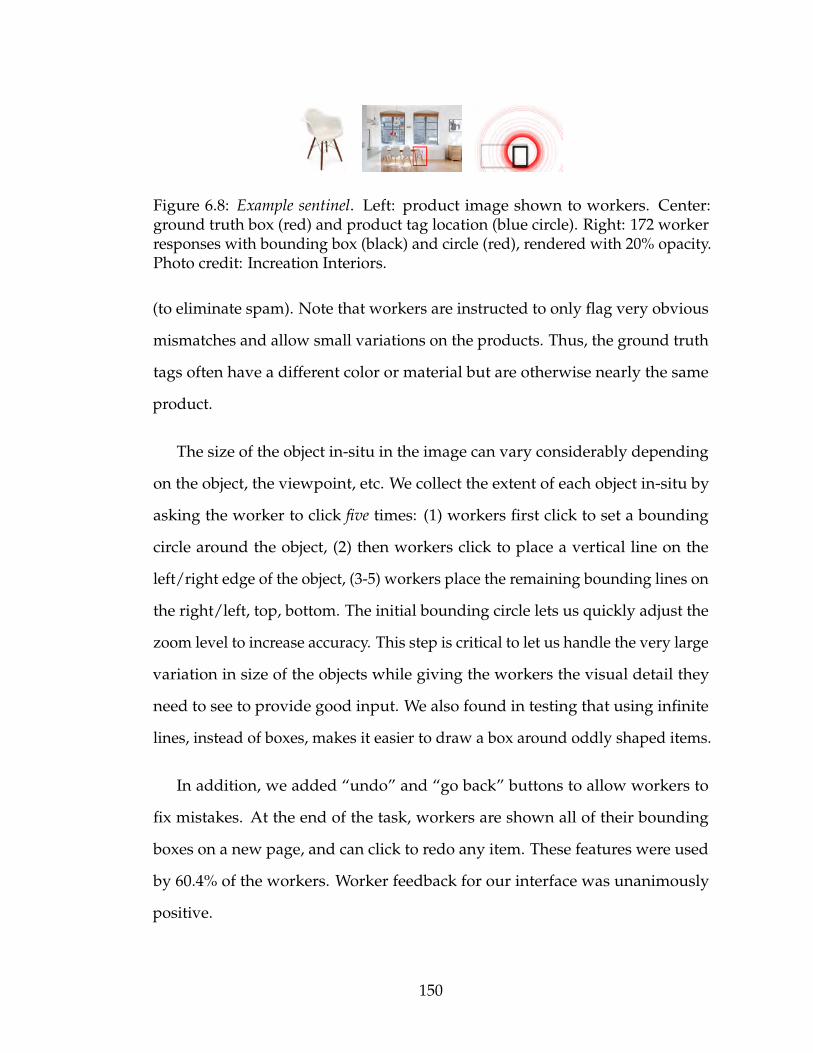
Figure 6.8: Example sentinel. Left: product image shown to workers. Center:ground truth box (red) and product tag location (blue circle). Right: 172 workerresponses with bounding box (black) and circle (red), rendered with 20% opacity.Photo credit: Increation Interiors.

(to eliminate spam). Note that workers are instructed to only flag very obvious

mismatches and allow small variations on the products. Thus, the ground truth

tags often have a different color or material but are otherwise nearly the same

product.

The size of the object in-situ in the image can vary considerably depending

on the object, the viewpoint, etc. We collect the extent of each object in-situ by

asking the worker to click five times: (1) workers first click to set a bounding

circle around the object, (2) then workers click to place a vertical line on the

left/right edge of the object, (3-5) workers place the remaining bounding lines on

the right/left, top, bottom. The initial bounding circle lets us quickly adjust the

zoom level to increase accuracy. This step is critical to let us handle the very large

variation in size of the objects while giving the workers the visual detail they

need to see to provide good input. We also found in testing that using infinite

lines, instead of boxes, makes it easier to draw a box around oddly shaped items.

In addition, we added “undo” and “go back” buttons to allow workers to

fix mistakes. At the end of the task, workers are shown all of their bounding

boxes on a new page, and can click to redo any item. These features were used

by 60.4% of the workers. Worker feedback for our interface was unanimously

positive.

150

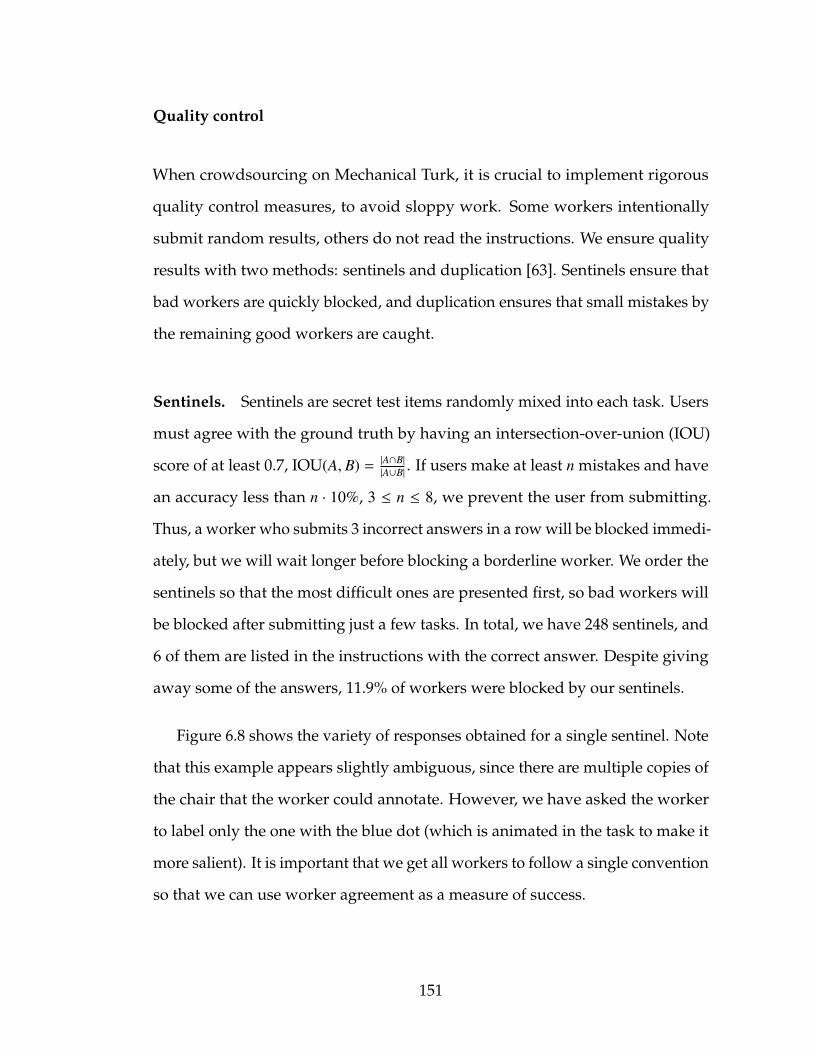
Quality control

When crowdsourcing on Mechanical Turk, it is crucial to implement rigorous

quality control measures, to avoid sloppy work. Some workers intentionally

submit random results, others do not read the instructions. We ensure quality

results with two methods: sentinels and duplication [63]. Sentinels ensure that

bad workers are quickly blocked, and duplication ensures that small mistakes by

the remaining good workers are caught.

Sentinels. Sentinels are secret test items randomly mixed into each task. Users

must agree with the ground truth by having an intersection-over-union (IOU)

score of at least 0.7, IOU(A, B) = |A∩B||A∪B| . If users make at least n mistakes and have

an accuracy less than n · 10%, 3 ≤ n ≤ 8, we prevent the user from submitting.

Thus, a worker who submits 3 incorrect answers in a row will be blocked immedi-

ately, but we will wait longer before blocking a borderline worker. We order the

sentinels so that the most difficult ones are presented first, so bad workers will

be blocked after submitting just a few tasks. In total, we have 248 sentinels, and

6 of them are listed in the instructions with the correct answer. Despite giving

away some of the answers, 11.9% of workers were blocked by our sentinels.

Figure 6.8 shows the variety of responses obtained for a single sentinel. Note

that this example appears slightly ambiguous, since there are multiple copies of

the chair that the worker could annotate. However, we have asked the worker

to label only the one with the blue dot (which is animated in the task to make it

more salient). It is important that we get all workers to follow a single convention

so that we can use worker agreement as a measure of success.

151

Duplication. Even if a worker is reliable, they may be given a difficult example,

or they may make occasional small mistakes. Therefore, we collect two copies of

every bounding box and check whether the workers agree. If the intersection-

over-union (IOU) of the two boxes is above 0.7, then we choose the box from the

worker with the higher average sentinel score. If the workers disagree, we collect

more boxes (up to 5) until we find a pair of responses that agrees (IOU ≥ 0.7).

Results With 1,742 workers, we collected 449,107 total responses which were

aggregated to 101,945 final bounding boxes for an average cost of $0.0251 per

final box. An additional 2,429 tags were “mismatched”, i.e., at least half of the

workers labeled mismatch. Workers were paid $0.05 to label 7 boxes (1 of which

is a sentinel) and spent an average of 17.1 seconds per response.

6.5.2 Learning a distance metric

From crowdsourcing, we have collected a dataset of positive examples—the

same product in-situ and in an iconic image. We now describe how we convert

this data into a full dataset, how we train the network, and finally visualize the

resulting embedding.

Generating positive and negative training data

The contrastive loss function consists of two types of examples: positive examples

of similar pairs and negative examples of dissimilar pairs. Figure 6.9 shows how

the contrastive loss works for positive and negative examples respectively for

152

our domain. The gradient of the loss function acts like a force (shown as a red

arrow) that pulls together xp and xq and pushes apart xq and xn.

We have 101,945 pairs of the form: (in-situ bounding box, iconic product

image). This forms all of our positive examples (Iq, Ip). To build negative exam-

ples, we take each in-situ image Iq and pick 80 random product images of the

same object category, and 20 random product images of a different category. We

repeat the positive pair 5 times, to give a 1:20 positive to negative ratio. We also

augment the dataset by re-cropping the in-situ images with different amounts of

padding: 0, 8, 16, 32, 48, 64, 80 pixels, measured with respect to a fixed 256x256

square input shape (for example, 16 pixels of padding means that 1/8th of each

dimension is scene context).

We split all of these examples into training, validation, and test sets, making

sure to separate bounding boxes by photo to avoid any contamination. This

results in 63,820,250 training and 3,667,769 pairs. We hold out 6,391 photos

for testing which gives 10,000 unseen test bounding boxes. After splitting the

examples, we randomly shuffle the pairs within each set.

Training the network

Various parameter choices have to be made when training the CNN.

Selecting the training architecture. As shown earlier in Figure 6.5, we ex-

plore multiple methods of training the CNN: (A) training on only category

labels (no product tags), (B) training on only product tags (no category la-

bels), (C) training on both product tags and category labels, and (D) addi-

153

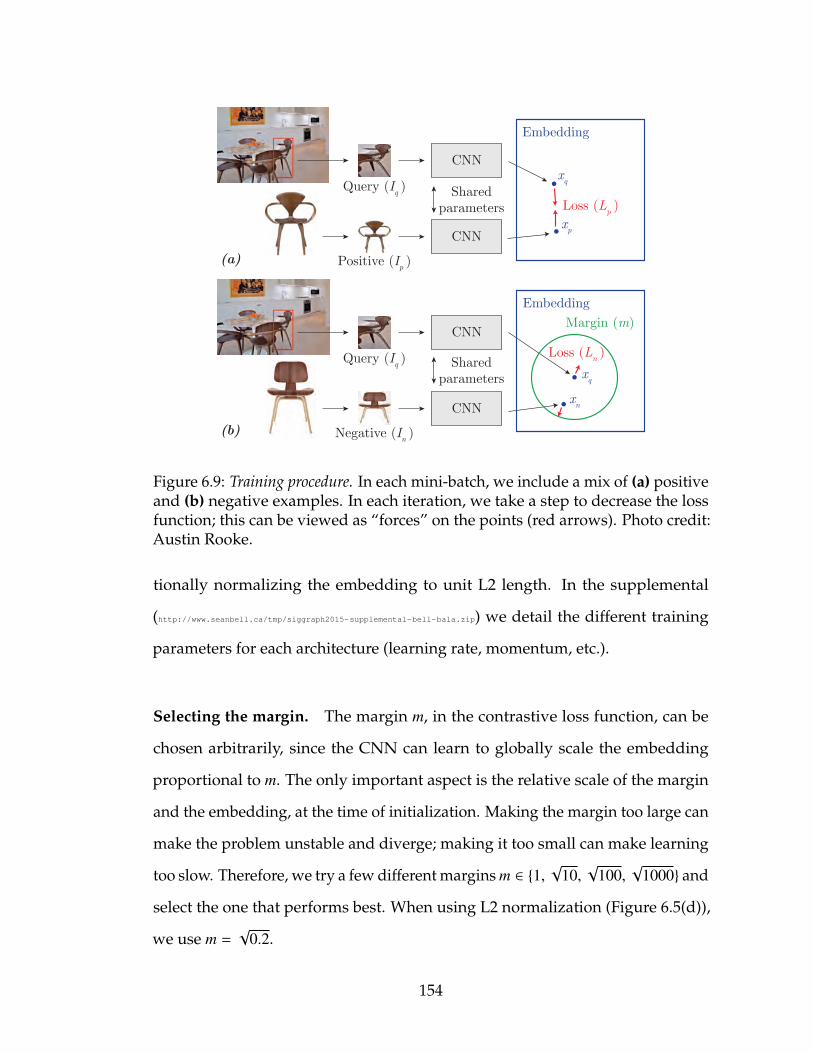
CNN

CNNLoss (Ln )

Embedding

Negative (In )

Sharedparameters xq

xn

Query (Iq )

Margin (m)

(b)

CNN

CNN

Loss (Lp )

Positive (Ip )

xq

xp

Query (Iq )

Embedding

(a)

Sharedparameters

Figure 6.9: Training procedure. In each mini-batch, we include a mix of (a) positiveand (b) negative examples. In each iteration, we take a step to decrease the lossfunction; this can be viewed as “forces” on the points (red arrows). Photo credit:Austin Rooke.

tionally normalizing the embedding to unit L2 length. In the supplemental

(http://www.seanbell.ca/tmp/siggraph2015-supplemental-bell-bala.zip) we detail the different training

parameters for each architecture (learning rate, momentum, etc.).

Selecting the margin. The margin m, in the contrastive loss function, can be

chosen arbitrarily, since the CNN can learn to globally scale the embedding

proportional to m. The only important aspect is the relative scale of the margin

and the embedding, at the time of initialization. Making the margin too large can

make the problem unstable and diverge; making it too small can make learning

too slow. Therefore, we try a few different margins m ∈ 1,√

10,√

100,√

1000 and

select the one that performs best. When using L2 normalization (Figure 6.5(d)),

we use m =√

0.2.

154

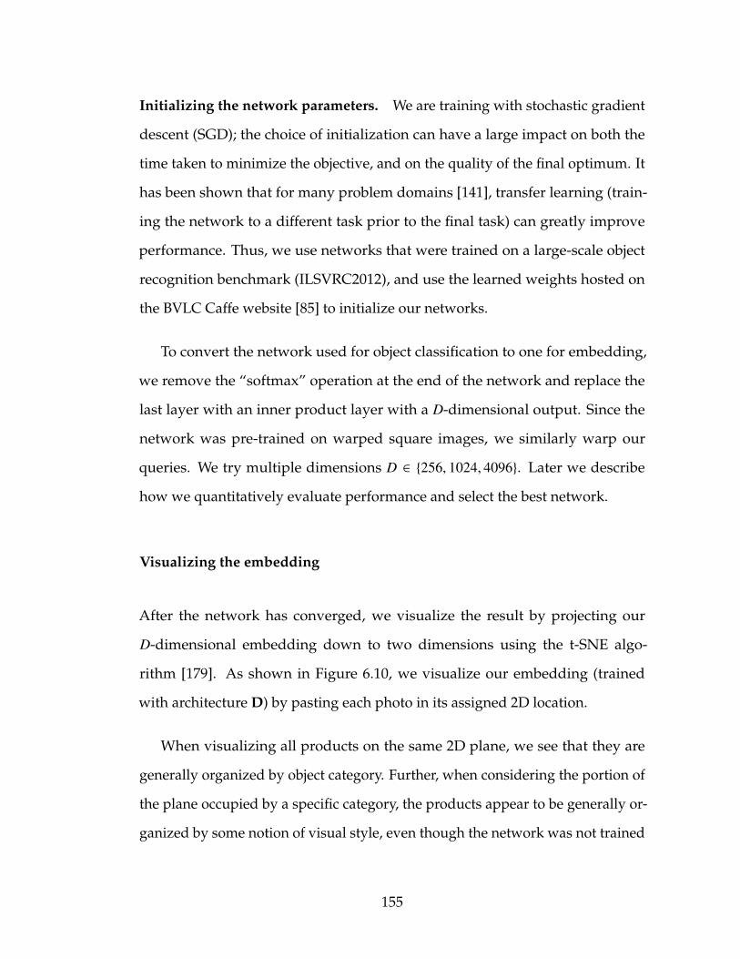
Initializing the network parameters. We are training with stochastic gradient

descent (SGD); the choice of initialization can have a large impact on both the

time taken to minimize the objective, and on the quality of the final optimum. It

has been shown that for many problem domains [141], transfer learning (train-

ing the network to a different task prior to the final task) can greatly improve

performance. Thus, we use networks that were trained on a large-scale object

recognition benchmark (ILSVRC2012), and use the learned weights hosted on

the BVLC Caffe website [85] to initialize our networks.

To convert the network used for object classification to one for embedding,

we remove the “softmax” operation at the end of the network and replace the

last layer with an inner product layer with a D-dimensional output. Since the

network was pre-trained on warped square images, we similarly warp our

queries. We try multiple dimensions D ∈ 256, 1024, 4096. Later we describe

how we quantitatively evaluate performance and select the best network.

Visualizing the embedding

After the network has converged, we visualize the result by projecting our

D-dimensional embedding down to two dimensions using the t-SNE algo-

rithm [179]. As shown in Figure 6.10, we visualize our embedding (trained

with architecture D) by pasting each photo in its assigned 2D location.

When visualizing all products on the same 2D plane, we see that they are

generally organized by object category. Further, when considering the portion of

the plane occupied by a specific category, the products appear to be generally or-

ganized by some notion of visual style, even though the network was not trained

155

Figure 6.10: 2D embedding visualization using t-SNE [179]. This embedding wastrained using architecture D and is 256D before being non-linearly projectedto 2D. To reduce visual clutter, each photo is snapped to a grid (overlappingphotos are selected arbitrarily). Full embeddings are in the supplemental (http://www.seanbell.ca/tmp/siggraph2015-supplemental-bell-bala.zip), including those for a single objectcategory. Best viewed on a monitor.

to model the concept of “style”. The supplementary material2 includes more

visualizations of embeddings including embeddings computed for individual

object classes. These are best viewed on a monitor.

6.6 Results and applications

We now qualitatively and quantitatively evaluate the results. We demonstrate

visual search in three applications: finding similar products, in-situ usages of a

product, and visually similar products across different object categories.2http://www.seanbell.ca/tmp/siggraph2015-supplemental-bell-bala.zip

156

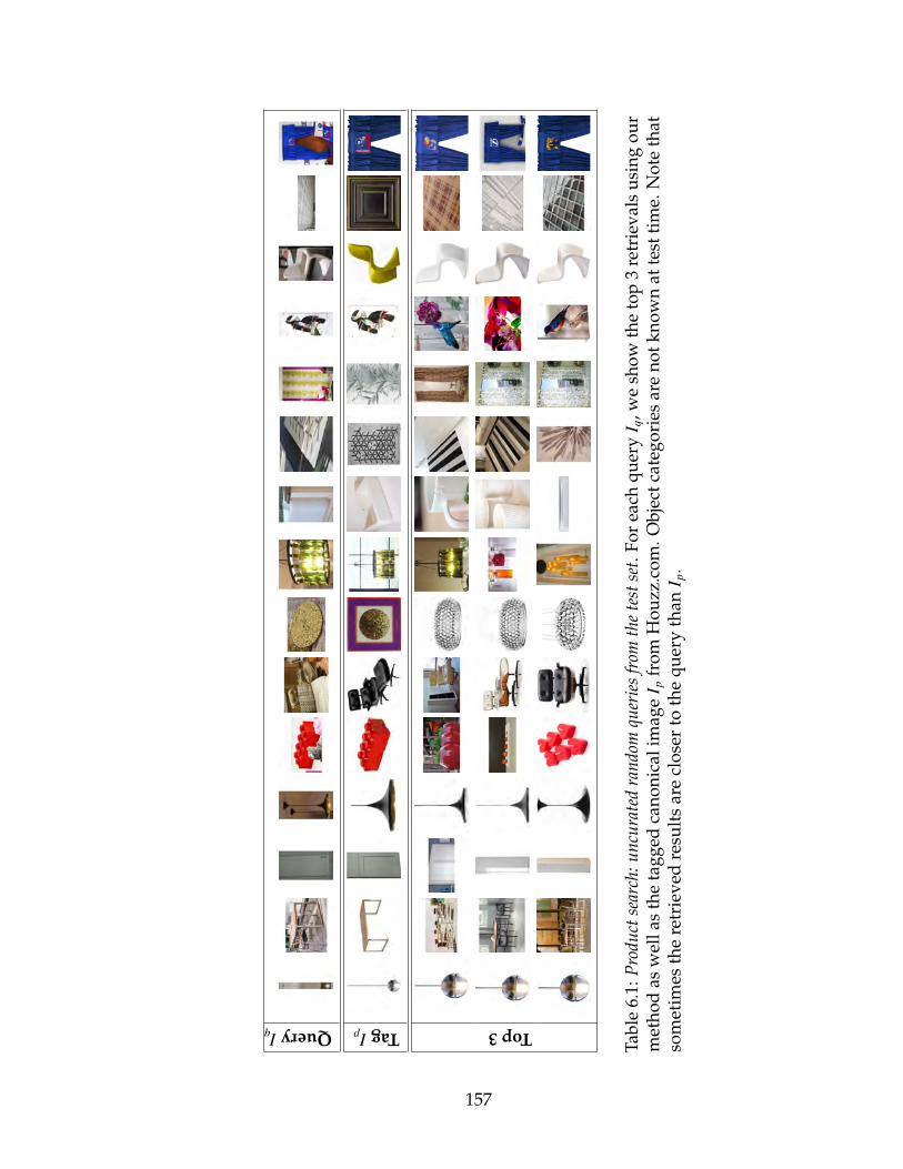
QueryIq TagIp Top3

Tabl

e6.

1:Pr

oduc

tsea

rch:

uncu

rate

dra

ndom

quer

ies

from

the

test

set.

For

each

quer

yI q

,we

show

the

top

3re

trie

vals

usin

gou

rm

etho

das

wel

las

the

tagg

edca

noni

cali

mag

eI p

from

Hou

zz.c

om.O

bjec

tcat

egor

ies

are

notk

now

nat

test

time.

Not

eth

atso

met

imes

the

retr

ieve

dre

sult

sar

ecl

oser

toth

equ

ery

than

I p.

157

6.6.1 Visual search

Product search. The main use of our projection Iq 7→ xq is to look up visually

similar images. Table 6.1 shows several example queries randomly sampled

from the test set. The results are not curated and are truly representative of a

random selection of our output results. The query object may be significantly

occluded, rotated, scaled, or deformed; or, the product image may be a schematic

representation rather than an actual photo; or, the in-situ image is of a glass or

transparent object, and therefore visually very different from the iconic product

image. Nonetheless, we find that our descriptor generally performs very well. In

fact, in some cases our results are closer than the tagged iconic product image

because the ground truth often shows related items of different colors. Usually

when the search fails, it tends to still return items that are similar in some way. In

the supplemental3 we show 500 more random uncurated examples of searches

returned from our test set.

In-situ search. Since we have a descriptor that can model both iconic and

in-situ cropped images, we can search in the “reverse” direction, where the

query is a product and the returned results are cropped boxes in scenes. We use

the bounding boxes we already collected from crowdsourcing as the database

to search over. Figure 6.13 shows random examples sampled from the test

set. Notice that since the scenes being searched over are designer photos, this

becomes a powerful technique for exploring design ideas. For example, we could

discover which tables go well with a chair by finding scenes that contain the

chair and then looking for tables in the scenes.3http://www.seanbell.ca/tmp/siggraph2015-supplemental-bell-bala.zip

158

Cross-category search. When retrieving very large sets of items for an input

query, we found that when items show up from a different object category, these

items tend to be visually or stylistically similar to the input query in some way.

Despite not training the descriptor to reason about visual style, the descriptor is

powerful enough to place stylistically similar items nearby in the space. We can

explore this behavior further by explicitly searching only products of a different

object category than the query (e.g. finding a table that is visually similar to a

chair). Note that before we can do these sorts of queries, it is necessary to clean

up the category labels on the dataset, since miscategorized items will show up

in every search. Therefore, we use the “GN Cat” CNN (architecture A) [167] to

predict a category for every product, and we remove all labels that either aren’t

in the top-20 or have confidence ≤ 1%. Table 6.2 shows example queries across

a variety of object categories. These results are curated, since most queries do

not have a distinctive style to them, and thus it is not apparent that anything has

been matched. In the next section, we show a user study that evaluates to what

extent our CNNs return stylistically similar items.

The product search and “in-situ” search are both trained with architecture D,

and “cross-category” search uses architecture B (Figure 6.5). In the next section

we detail how we quantitatively evaluated each architecture and selected the

best.

6.6.2 Evaluating the metric

For our dataset, we cannot measure precision, since we only have a list of image

positive pairs (in-situ image Iq and iconic product image Ip). However, we can

159

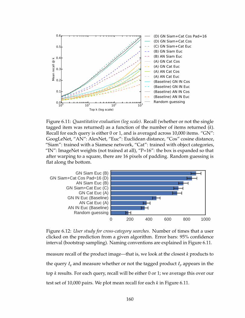
100 101 102 103

Top k (log scale)

0.0

0.1

0.2

0.3

0.4

0.5

0.6

Mean r

eca

ll @

k

(D) GN Siam+Cat Cos Pad=16(D) GN Siam+Cat Cos(C) GN Siam+Cat Euc(B) GN Siam Euc(B) AN Siam Euc(A) GN Cat Cos(A) GN Cat Euc(A) AN Cat Cos(A) AN Cat Euc(Baseline) GN IN Cos(Baseline) GN IN Euc(Baseline) AN IN Cos(Baseline) AN IN EucRandom guessing

Figure 6.11: Quantitative evaluation (log scale). Recall (whether or not the singletagged item was returned) as a function of the number of items returned (k).Recall for each query is either 0 or 1, and is averaged across 10,000 items. “GN”:GoogLeNet, “AN”: AlexNet, “Euc”: Euclidean distance, “Cos” cosine distance,“Siam”: trained with a Siamese network, “Cat”: trained with object categories,“IN”: ImageNet weights (not trained at all), “P=16”: the box is expanded so thatafter warping to a square, there are 16 pixels of padding. Random guessing isflat along the bottom.

0 200 400 600 800 1000

Random guessingAN IN Euc (Baseline)

AN Cat Euc (A)GN IN Euc (Baseline)

GN Cat Euc (A)GN Siam+Cat Euc (C)

AN Siam Euc (B)GN Siam+Cat Cos Pad=16 (D)

GN Siam Euc (B)

Figure 6.12: User study for cross-category searches. Number of times that a userclicked on the prediction from a given algorithm. Error bars: 95% confidenceinterval (bootstrap sampling). Naming conventions are explained in Figure 6.11.

measure recall of the product image—that is, we look at the closest k products to

the query Iq and measure whether or not the tagged product Ip appears in the

top k results. For each query, recall will be either 0 or 1; we average this over our

test set of 10,000 pairs. We plot mean recall for each k in Figure 6.11.

160

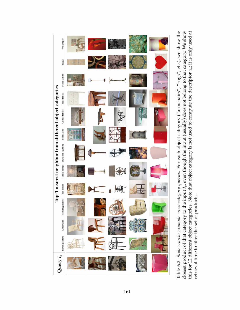
Que

ryI q

T op-

1ne

ares

tnei

ghbo

rfr

omdi

ffer

ento

bjec

tcat

egor

ies

Din

ing

chai

rsA

rmch

airs

Roc

king

chai

rsB

arst

ools

Tabl

ela

mps

Out

door

ligh

ting

Boo

kcas

esC

offe

eta

bles

Side

tabl

esFl

oor

lam

psR

ugs

Wal

lpap

er

Tabl

e6.

2:St

yle

sear

ch:

exam

ple

cros

s-ca

tego

ryqu

erie

s.Fo

rea

chob

ject

cate

gory

(“ar

mch

airs

”,“r

ugs

”,et

c.),

we

show

the

clos

estp

rodu

ctof

that

cate

gory

toth

ein

putI

q,ev

enth

ough

the

inpu

t(us

ually

)doe

sno

tbel

ong

toth

atca

tego

ry.W

esh

owth

isfo

r12

diff

eren

tobj

ectc

ateg

orie

s.N

ote

that

obje

ctca

tego

ryis

notu

sed

toco

mpu

teth

ede

scri

ptor

x q;i

tis

only

used

atre

trie

valt

ime

tofil

ter

the

seto

fpro

duct

s.

161

It is important to note that image Ip is usually not the best match for Iq, as

there is significant redundancy in the product images, even after accounting for

near-duplicates. Often Iq and Ip differ in materials or in color. Nonetheless, a

visual similarity metric should be able to deal with these issues, and place xq and

xp reasonably close together in the embedding (so that its rank is small). So while

a lower rank is better, a rank of 1 is not a reasonable expectation.

Baseline. To evaluate our embedding, we compare how well it can rank prod-

ucts compared to two high quality image descriptors for two different CNNs

when trained on ImageNet (“IN”). For each CNN, we use the output from the

last hidden layer and call them “AN IN” (i.e., AlexNet layer fc7) and “GN IN”

(i.e., GoogLeNet layer pool5/7x7 s1). These two architectures are popular

and have become the basis of a wide variety of state-of-the-art algorithms for

image retrieval [4, 142]. We tried applying PCA since it has been shown that it

can improve performance [142], but we found that it performed the same as the

original descriptors, and thus is not shown.

Distance metrics. We compare two versions of each descriptor: a Euclidean

version (“Euc”) and a L2 normalized version (“Cos”, since cosine distance is

equal to Euclidean distance on normalized vectors). We evaluated other metrics

including L1, Canberra, and Bray-Curtis dissimilarity on the baseline networks.

We found that other metrics performed either comparably or worse than Cosine,

and thus we only evaluate Cosine for the full dataset. For example, in Fig-

ure 6.11, “GN Cat Cos” means that we train GoogLeNet with object categories,

and measure cosine distance using the last layer.

162

Padding. At test time, we experimented with adding different amounts of

padding to the input query. We find that a modest amount of padding, 16 pixels,

is optimal. Since all algorithms benefit from padding, we only show the effect on

the best algorithm. The supplemental4 includes our full padding evaluation.

Training architectures. As shown in Figure 6.11 the best architecture for image

retrieval is D, which is a siamese GoogLeNet CNN trained on both image pairs

and object category labels, with cosine as the distance metric. For all experiments,

we find that GoogLeNet (GN) consistently outperforms AlexNet (AN), and

thus we only consider variations of C and D using GoogLeNet. Architecture

A is the commonly used technique of fine-tuning a CNN to the target dataset.

It performs better than the ImageNet baselines, but not as well as any of the

siamese architectures B, C, D. It might appear that C is the best curve (which is

missing L2 normalization), but we emphasize that we show up to k = 1000 only

for completeness and the top few results k < 10 matter the most (where D is the

best).

Embedding dimension. We studied the effect of dimension on architecture C.

Using more dimensions makes it easier to satisfy constraints, but also signifi-

cantly increases the amount of space and time required to search. We find that

256, 1024, and 4096 all perform about the same, and thus use 256 dimensions for

all experiments. See the supplemental5 for the full curves.

Runtime. One of the key benefits of using CNNs is that computing Iq 7→ xq is

very efficient. Using a Grid K520 GPU (on an Amazon EC2 g2.2xlarge instance),

4http://www.seanbell.ca/tmp/siggraph2015-supplemental-bell-bala.zip

5Ibid.

163

we can compute xq in about 100 ms, with most of the time spent loading the

image. Even with brute force lookup (implemented as dense matrix operations),

we can rank xq against all 3,387,555 products in about one second on a single CPU.

This can be accelerated using approximate nearest neighbor techniques [122],

and is left for future work.

User study. As described in Section 6.6.1, Table 6.2 shows examples of cross-

category searches. Since our siamese CNNs were trained on image pairs and/or

object categories, it is unclear which (if any) should work as a style descriptor for

this type of search. Therefore, we set up a user study where a user is shown an

item of one category and 9 items of a second category (e.g. one chair in context,

and 9 table product images) and instructed to choose the best match, stylistically.

We run this experiment on MTurk, where each of the 9 items are generated by

a different model (8 models, plus one random). Each grid of 9 items is shown

to 5 users, and only grids where a majority agree on an answer are kept. The

supplemental6 contains screenshots of our user study. The results are shown

in Figure 6.12, and we can see that all methods outperform random guessing,

siamese architectures perform the best, and not training at all (baseline) performs

the worst.

6.6.3 Discussion, limitations, and future work

There are many avenues to further improve the quality of our embedding, and

to generalize our results.6http://www.seanbell.ca/tmp/siggraph2015-supplemental-bell-bala.zip

164

Multitask predictions. We found that traning for object category along with

the embedding performs the best for product search. Since the embedding

and the object prediction are related by fully connected layers, the two spaces

are similar. Thus, we effectively expand our training set of 86,945 pairs with

additional 3,387,555 product category labels. At test time, we currently don’t use

the predicted object category—it is only a regularizer to improve the embedding.

However, we could use the object category and use it to prune the set of retrieved

results, potentially improving precision.

Style similarity vs. image similiarity. While we have not trained the CNN to

model visual style, it seems to have learned a visual similarity metric powerful

enough to place stylistically similar items nearby in the space. But style similarity

and visual similarity are not the same. Two objects being visually similar often

implies that they are also stylistically similar, but the converse is not true. Thus,

if our embedding were to be used by designers interested in searching across

compatible styles, we would need to explicitly train for this behavior. In future

work, we hope to collect new datasets of style relationships to explore this

behavior.

Active learning. We have a total of 3,387,555 product photos and 6,093,452

scene photos, but only 101,945 known pairs (Iq, Ip). As a result, dissimilar pairs

of images that are not part of our known relationships may be placed nearby

in the space, but there is no way to train or test for this. A human-in-the-loop

approach may be useful here, where workers filter out false positives while

training progresses. We propose exploring this in the future.

165

6.7 Conclusion

We have presented a visual search algorithm to match in-situ images with iconic

product images. We achieved this by using a crowdsourcing pipeline for gener-

ating training data, and training a multitask siamese CNN to compute a high

quality embedding of product images across multiple image domains. We demon-

strated the utility of this embedding on several visual search tasks: searching

for products within a category, searching across categories, and searching for

usages of a product in scenes. Many future avenues of research remain, includ-

ing: training to understand visual style in products, and improved faceted query

interfaces, among others.

6.8 Impact

Since presenting our work on visual similarity at SIGGRAPH 2015, other re-

searchers have shown that the approach presented in ProductNet also works for

3D shapes [109], clothing style [183], and sketches [154]. Buiding on the success

of this approach, I am now co-founding a deep learning startup GrokStyle, based

on this technology for visual search.

166

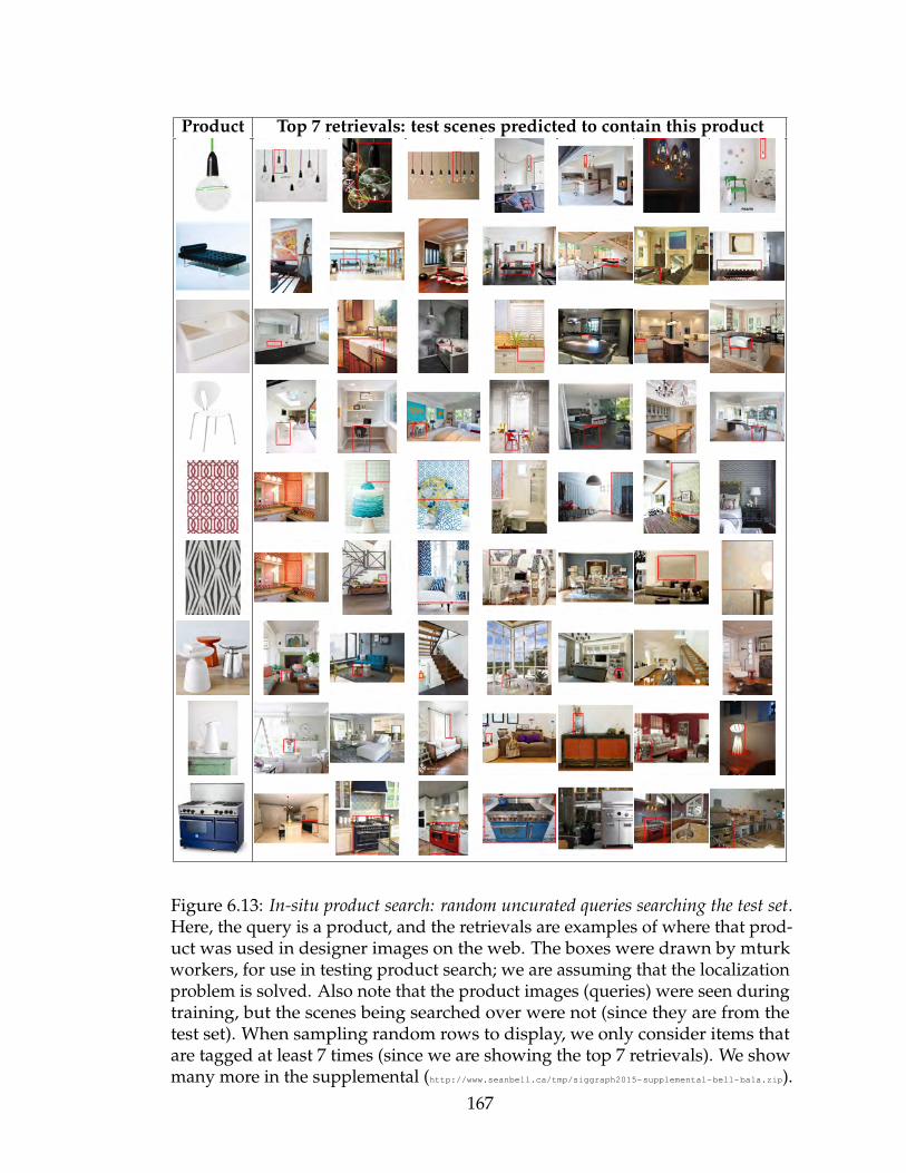
Product Top 7 retrievals: test scenes predicted to contain this product

Figure 6.13: In-situ product search: random uncurated queries searching the test set.Here, the query is a product, and the retrievals are examples of where that prod-uct was used in designer images on the web. The boxes were drawn by mturkworkers, for use in testing product search; we are assuming that the localizationproblem is solved. Also note that the product images (queries) were seen duringtraining, but the scenes being searched over were not (since they are from thetest set). When sampling random rows to display, we only consider items thatare tagged at least 7 times (since we are showing the top 7 retrievals). We showmany more in the supplemental (http://www.seanbell.ca/tmp/siggraph2015-supplemental-bell-bala.zip).

167

CHAPTER 7

CONCLUSION

The tools and data that we have for recognizing, editing, and exploring applying

scene properties for everyday problems are slowly improving. As we develop

more sophisticated methods of collecting data, train larger and richer models,

we can solve increasingly important problems for humanity.

This thesis explores several directions that improve automatic scene under-

standing. In Chapter 2, we collected appearance information at a large-scale,

which had not been done before for materials. In Chapters 3 and 4, we used this

to inform and drive new algorithms to understand materials at pixel-level ma-

terial categories and pixel-level reflectance. In Chapters 5 and 6, we developed

higher level algorithms to detect objects in images, and recognized objects at a

fine-grained per-object level. Together, these contributions significantly advance

our knowledge of what information can be extracted from an image.

7.1 Impact

The work presented in this thesis has had a large impact on the community.

OpenSurfaces. Our annotations from OpenSurfaces have enabled others to

train texture recognition and segmentation algorithms [37, 36], and to redecorate

rooms by automatically suggesting materials for indoor digital scenes [29]. Our

dataset has also been expanded with new “describable texture attributes” and

re-released as an augmented dataset [36]. Researchers from Microsoft have used

168

our segmentation interface to power the Microsoft Commons Objects in Context

(MS COCO) project [113] which labeled over 2.5 million objects; this data has

significantly advanced the state-of-the-art in object detection as part of the yearly

MS COCO object detection challenge.

IIW (Intrinsic Images in the Wild). Our IIW judgement dataset has been used

to train and validate new models that use deep learning to predict reflectance

and lightness variations in an image [203, 206, 123]. Using our data, others have

proposed extensions of our algorithm that use deeply learned priors [203], or

entirely new algorithms using global least squares optimizations [206], L1 image

transforms [17], or near-L0 image transforms [44]. Our pairwise reflectance

judgements have inspired others to extend our relative reflectance judgements to

relative depth judgements [206] which can be globalized to solve for a full depth

map.

MINC (Materials in Context). Our approach of using “click” labels to train

semantic segmentation algorithms was later shown to yield a large improve-

ment for objects, resulting in the most accurate models given a fixed annotation

budget, out of squiggle-level, point-click, and full-image supervision [9]. Fur-

ther, our MINC database has been used to train new state-of-the-art material

recognition algorithms that go beyond the fully-connected CRF algorithm of

Krahenbuhl et al. [98] by directly learning pairwise potentials [83] or using “bi-

lateral inceptions” [55]. Others have used our data to integrate multiple features

obtained by different CNNs, obtaining close to human performance on the Flickr

Material Dataset [160] with transfer learning [198].

169

ION (Inside-Outside Net). Our work in this chapter was first presented at the

MS COCO 2015 Detection Challenge, where we won Best Student Entry, and

later published as a paper at CVPR 2016 [15]. Concurrently with our work, the

second place entry in the MS COCO competition revisited skip connections with

a similar architecture [196]. Our ION architecture has inspired similar approaches

of combining skip pooling and context to obtain more accurate results [204].

ProductNet. Since presenting our work on visual similarity at SIGGRAPH

2015, Other researchers have shown that the approach presented in ProductNet

also works for 3D shapes [109], clothing style [183], and sketches [154]. Buiding

on the success of this approach, I am now co-founding a deep learning startup

GrokStyle, based on this technology for visual search of decor.

7.2 Future work

The scene understanding problem is still far from being solved. In particular,

most methods, including our own, address one specific sub-problem at a time,

such as material segmentation, intrinsic images, or object detection. In the future,

we would like to explore jointly solving these problems, so that solutions for one

problem can inform potentially ambiguous decisions in another problem. Further,

it has been shown that for deep learning, jointly training multiple problems raises

the accuracy of all of the individual sub-problems.

170

BIBLIOGRAPHY

[1] Andrew Adams, Jongmin Baek, and Abe Davis. Fast high-dimensionalfiltering using the permutohedral lattice. Computer Graphics Forum (Euro-graphics), 29(2), 2010. 95

[2] Edward H. Adelson. On seeing stuff: the perception of materials byhumans and machines. Proc. SPIE Human Vision and Electronic Imaging,4299, 2001. 23

[3] Pulkit Agrawal, Ross Girshick, and Jitendra Malik. Analyzing the perfor-mance of multilayer neural networks for object recognition. In ECCV, 2014.118

[4] Artem Babenko, Anton Slesarev, Alexander Chigorin, and Victor S. Lem-pitsky. Neural codes for image retrieval. In ECCV, 2014. 143, 148, 162

[5] Jonathan T. Barron and Jitendra Malik. Color constancy, intrinsic images,and shape estimation. In ECCV, 2012. 74

[6] Jonathan T. Barron and Jitendra Malik. Shape, albedo, and illuminationfrom a single image of an unknown object. In CVPR, 2012. 74

[7] Jonathan T. Barron and Jitendra Malik. Intrinsic scene properties from asingle rgb-d image. In CVPR, 2013. 75

[8] Jonathan T. Barron and Jitendra Malik. Shape, illumination, and reflectancefrom shading. Technical report, MIT, 2013. 74, 90, 91, 108

[9] Amy Bearman, Olga Russakovsky, Vittorio Ferrari, and Li Fei-Fei. What’sthe Point: Semantic Segmentation with Point Supervision. ECCV, 2016. 70,169

[10] Sven Behnke. Hierarchical Neural Networks for Image Interpretation. PhDthesis, Freie Universitat Berlin, 2003. 116

[11] Sean Bell, Kavita Bala, and Noah Snavely. Intrinsic images in the wild.SIGGRAPH Conf. Proc., 33(4), 2014. 111

[12] Sean Bell, Paul Upchurch, Noah Snavely, and Kavita Bala. OpenSurfaces:A richly annotated catalog of surface appearance. ACM Trans. on Graphics(SIGGRAPH), 32(4), 2013. xiv, 41, 48, 51, 53, 149

171

[13] Sean Bell, Paul Upchurch, Noah Snavely, and Kavita Bala. OpenSurfaces:A richly annotated catalog of surface appearance. ACM Trans. on Graphics(SIGGRAPH), 32(4), 2013. 72, 75, 78

[14] Sean Bell, Paul Upchurch, Noah Snavely, and Kavita Bala. Material recog-nition in the wild with the materials in context database. Computer Visionand Pattern Recognition (CVPR), 2015. 50, 70

[15] Sean Bell, C. Lawrence Zitnick, Kavita Bala, and Ross Girshick. Inside-outside net: Detecting objects in context with skip pooling and recurrentneural networks. Computer Vision and Pattern Recognition (CVPR), 2016.137, 170

[16] Aner Ben-Artzi, Ryan Overbeck, and Ravi Ramamoorthi. Real-time BRDFediting in complex lighting. In SIGGRAPH Conf. Proc., 2006. 29

[17] Sai Bi, Xiaoguang Han, and Yizhou Yu. An l1 image transform for edge-preserving smoothing and scene-level intrinsic decomposition. SIGGRAPHConf. Proc., 2015. 111, 169

[18] Mike Bostock. D3. http://d3js.org/, 2013. [Online; accessed 24-Mar-2014]. 82

[19] Adrien Bousseau, Sylvain Paris, and Fredo Durand. User assisted intrinsicimages. In SIGGRAPH Asia Conf. Proc., 2009. 75

[20] Ivaylo Boyadzhiev, Sylvain Paris, and Kavita Bala. User-assisted imagecompositing for photographic lighting. ACM Trans. Graph., 32(4):36:1–36:12,July 2013. 88

[21] David H. Brainard, Wendy Brunt, and Jon Speigle. Color constancy in thenearly natural image. J. of the Optical Society of America, 14(9), 1997. 19

[22] Steve Branson, Catherine Wah, Boris Babenko, Florian Schroff, Peter Welin-der, Pietro Perona, and Serge Belongie. Visual recognition with humans inthe loop. In Proc. European Conference on Computer Vision, 2010. 75, 81

[23] Wonmin Byeon, Thomas M. Breuel, Federico Raue, and Marcus Liwicki.Scene labeling with LSTM recurrent neural networks. In CVPR, 2015. 114,116

172

[24] Barbara Caputo, Eric Hayman, and P. Mallikarjuna. Class-specific materialcategorisation. In ICCV, pages 1597–1604, 2005. 51

[25] Robert Carroll, Ravi Ramamoorthi, and Maneesh Agrawala. Illumina-tion decomposition for material recoloring with consistent interreflections.ACM Trans. on Graphics (SIGGRAPH), 2011. 75

[26] CGAL, Computational Geometry Algorithms Library.http://www.cgal.org/. 21

[27] K. Chatfield, K. Simonyan, A. Vedaldi, and A. Zisserman. Return of thedevil in the details: Delving deep into convolutional nets. In BMVC, 2014.114, 142

[28] Gal Chechik, Varun Sharma, Uri Shalit, and Samy Bengio. Large scaleonline learning of image similarity through ranking. JMLR, 2010. 141

[29] Kang Chen, Kun Xu1, Yizhou Yu, Tian-Yi Wang, and Shi-Min Hu. Magicdecorator: Automatic material suggestion for indoor digital scenes. InSIGGRAPH Asia Conf. Proc., 2015. 41, 168

[30] Liang-Chieh Chen, George Papandreou, Iasonas Kokkinos, Kevin Murphy,and Alan L Yuille. Semantic image segmentation with deep convolutionalnets and fully connected crfs. In ICLR, 2015. 50

[31] Qifeng Chen and Vladlen Koltun. A simple model for intrinsic image de-composition with depth cues. In Proc. International Conference on ComputerVision, 2013. 75, 76

[32] Xiaobai Chen, Aleksey Golovinskiy, and Thomas Funkhouser. A bench-mark for 3D mesh segmentation. In SIGGRAPH Conf. Proc., 2009. 11

[33] K. Cho, B. van Merrienboer, D. Bahdanau, and Y. Bengio. On the propertiesof neural machine translation: Encoder-decoder approaches. arXiv preprintarXiv:1409.1259, 2014. 119

[34] Sumit Chopra, Raia Hadsell, and Yann LeCun. Learning a similarity metricdiscriminatively, with application to face verification. In CVPR. IEEE Press,2005. 146

[35] Mircea Cimpoi, Subhransu Maji, Iasonas Kokkinos, Sammy Mohamed,

173

and Andrea Vedaldi. Describing textures in the wild. In CVPR, pages3606–3613. IEEE, 2014. 51, 52, 68, 69

[36] Mircea Cimpoi, Subhransu Maji, Iasonas Kokkinos, and Andrea Vedaldi.Deep filter banks for texture recognition, description, and segmentation.IJCV, 2016. 41, 168

[37] Mircea Cimpoi, Subhransu Maji, and Andrea Vedaldi. Deep filter banksfor texture recognition and segmentation. In CVPR, 2015. 40, 41, 168

[38] Forrester Cole, Kevin Sanik, Doug DeCarlo, Adam Finkelstein, ThomasFunkhouser, Szymon Rusinkiewicz, and Manish Singh. How well do linedrawings depict shape? In SIGGRAPH Conf. Proc., 2009. 11, 26, 75

[39] K.J. Dana, B. Van-Ginneken, S.K. Nayar, and J.J. Koenderink. Reflectanceand texture of real world surfaces. ACM Transactions on Graphics, 18(1),1999. 12

[40] Kristin J Dana, Bram Van Ginneken, Shree K Nayar, and Jan J Koenderink.Reflectance and texture of real-world surfaces. ACM Transactions on Graph-ics (TOG), 18(1):1–34, 1999. 51

[41] A. P. Dawid and A. M. Skene. Maximum likelihood estimation of observererror-rates using the EM algorithm. In J. Roy. Statistical Society, 1979. 75

[42] Paul Debevec. Rendering synthetic objects into real scenes: bridgingtraditional and image-based graphics with global illumination and highdynamic range photography. In SIGGRAPH Conf. Proc., 1998. 27, 39

[43] J. Deng, W. Dong, R. Socher, L.-J. Li, K. Li, and L. Fei-Fei. ImageNet: Alarge-scale hierarchical image database. In Proc. Comp. Vision and PatternRecognition, 2009. 7, 10, 19

[44] Shouhong Ding, Bin Sheng, Zhifeng Xie, and Lizhuang Ma. Intrinsic imageestimation using near-l0 sparse optimization. 111, 169

[45] S.K. Divvala, D. Hoiem, J.H. Hays, A.A. Efros, and M. Hebert. An empiricalstudy of context in object detection. In CVPR, 2009. 113

[46] R.O. Dror, E. H. Adelson, and A. Willsky. Estimating surface reflectanceproperties from images under unknown illumination. In Proc. SPIE HumanVision and Electronic Imaging, 2001. 14, 41

174

[47] Ian Endres, Ali Farhadi, Derek Hoiem, and David Forsyth. The benefitsand challenges of collecting richer object annotations. In Workshop onAdvancing Computer Vision with Humans in the Loop, 2010. 11

[48] M. Everingham, L. Van Gool, C. K. I. Williams, J. Winn, and A. Zisserman.The PASCAL Visual Object Classes (VOC) Challenge. IJCV, 2010. 114, 122

[49] M. Everingham, L. Van Gool, C. K. I. Williams, J. Winn, and A. Zisserman.The Pascal Visual Object Classes (VOC) Challenge. IJCV, 88(2):303–338,June 2010. 54

[50] Clement Farabet, Camille Couprie, Laurent Najman, and Yann LeCun.Learning hierarchical features for scene labeling. PAMI, 35(8):1915–1929,2013. 52

[51] Pedro Felzenszwalb, David McAllester, and Deva Ramanan. A discrimina-tively trained, multiscale, deformable part model. In Proc. Computer Visionand Pattern Recognition, 2008. 86

[52] Chen Feng, Fei Deng, and Vineet R. Kamat. Semi-automatic 3D reconstruc-tion of piecewise planar building models from single image. In Int. Conf.on Construction Appl. of Virtual Reality, 2010. 26

[53] Roland W. Fleming, Ron O. Dror, and Edward H. Adelson. Real-worldillumination and the perception of surface reflectance properties. J. ofVision, 3(5), 2003. 14, 33

[54] Roland W. Fleming, Antonio Torralba, and Edward H. Adelson. Specularreflections and the perception of shape. Journal of Vision, 4(9):798–820, 2004.27

[55] Raghudeep Gadde, Varun Jampani, Martin Kiefel, Daniel Kappler, andPeter Gehler. Superpixel convolutional networks using bilateral inceptions.In ECCV, 2016. 70, 169

[56] Elena Garces, Aseem Agarwala, Diego Gutierrez, and Aaron Hertzmann.A similarity measure for illustration style. ACM Trans. Graph., 33(4), July2014. 141

[57] Elena Garces, Adolfo Munoz, Jorge Lopez-Moreno, and Diego Gutierrez.Intrinsic images by clustering. Computer Graphics Forum (EurographicsSymposium on Rendering), 31(4), 2012. 74, 91, 92, 100, 104, 105, 106

175

[58] P. Gehler, C. Rother, M. Kiefel, L. Zhang, and B. Scholkopf. Recoveringintrinsic images with a global sparsity prior on reflectance. In NIPS, 2011.74, 91, 105

[59] David Geisler-Moroder and Arne Dur. A new Ward BRDF model withbounded albedo. In Proc. Eurographics Symp. on Rendering, 2010. 28

[60] Spyros Gidaris and Nikos Komodakis. Object detection via a multi-region& semantic segmentation-aware CNN model. In ICCV, 2015. xi, 112, 123,124, 125, 127, 129

[61] Yotam Gingold, Ariel Shamir, and Daniel Cohen-Or. Micro perceptualhuman computation. ACM Transactions on Graphics, 31(5), 2012. 11, 36

[62] Yotam Gingold, Ariel Shamir, and Daniel Cohen-Or. Micro perceptualhuman computation. ACM Trans. on Graphics, 31(5), 2012. 75, 84

[63] Yotam Gingold, Ariel Shamir, and Daniel Cohen-Or. Micro perceptualhuman computation. TOG, 31(5), 2012. 151

[64] Bernd Girod, Vijay Chandrasekhar, David M. Chen, Ngai-Man Cheung,Radek Grzeszczuk, Yuriy Reznik, Gabriel Takacs, Sam S. Tsai, and Ramakr-ishna Vedantham. Mobile visual search, 2011. 142

[65] Ross Girshick. Fast R-CNN. In ICCV, 2015. xi, xvi, 112, 113, 115, 122, 123,124, 125, 126, 129, 131

[66] Ross Girshick, Jeff Donahue, Trevor Darrell, and Jitendra Malik. Richfeature hierarchies for accurate object detection and semantic segmentation.In CVPR, 2014. 52, 114, 115

[67] S. Gould, R. Fulton, and D. Koller. Decomposing a scene into geometric andsemantically consistent regions. In Proceedings of the International Conferenceon Computer Vision (ICCV), 2009. 54

[68] Alex Graves and Jurgen Schmidhuber. Offline handwriting recognitionwith multidimensional recurrent neural networks. In NIPS, 2009. 114, 116

[69] Roger Grosse, Micah K. Johnson, Edward H. Adelson, and William T.Freeman. Ground truth dataset and baseline evaluations for intrinsicimage algorithms. In Proc. International Conference on Computer Vision, 2009.72, 74, 75, 104, 106, 108

176

[70] Tom Haber, Christian Fuchs, Philippe Bekaer, H-P Seidel, Michael Goesele,and Hendrik PA Lensch. Relighting objects from image collections. InCVPR, 2009. 75

[71] Raia Hadsell, Sumit Chopra, and Yann LeCun. Dimensionality reductionby learning an invariant mapping. In CVPR. IEEE Press, 2006. 144, 145,146

[72] Bharath Hariharan, Pablo Arbelaez, Lubomir Bourdev, Subhransu Maji,and Jitendra Malik. Semantic contours from inverse detectors. In ICCV,2011. xi, 123, 124

[73] Bharath Hariharan, Pablo Arbelaez, Ross Girshick, and Jitendra Malik.Hypercolumns for object segmentation and fine-grained localization. InCVPR, 2015. 112, 114, 116

[74] Daniel Hauagge, Scott Wehrwein, Kavita Bala, and Noah Snavely. Photo-metric ambient occlusion. CVPR, 2013. 75

[75] Eric Hayman, Barbara Caputo, Mario Fritz, and Jan olof Eklundh. On thesignificance of real-world conditions for material classification. In ECCV,2004. 51

[76] James Hays and Alexei A Efros. Scene completion using millions of pho-tographs. In SIGGRAPH Conf. Proc., pages 4:1–4:7, 2007. 9

[77] Kaiming He, Xiangyu Zhang, Shaoqing Ren, and Jian Sun. Spatial pyramidpooling in deep convolutional networks for visual recognition. In ECCV,2014. 114, 115

[78] S. Hochreiter and J. Schmidhuber. Long short-term memory. Neural Com-putation, 1997. 119

[79] Derek Hoiem, Yodsawalai Chodpathumwan, and Qieyun Dai. Diagnosingerror in object detectors. In ECCV, 2012. xvi, 127, 130

[80] Jan Hendrik Hosang, Rodrigo Benenson, Piotr Dollar, and BerntSchiele. What makes for effective detection proposals? arXiv preprintarXiv:1502.05082, 2015. 114, 126

[81] Diane Hu, Liefeng Bo, and Xiaofeng Ren. Toward robust material recog-

177

nition for everyday objects. In Proc. British Machine Vision Conf., 2011.11

[82] Diane Hu, Liefeng Bo, and Xiaofeng Ren. Toward robust material recogni-tion for everyday objects. In BMVC, pages 1–11. Citeseer, 2011. 48, 51, 52,69

[83] Varun Jampani, Martin Kiefel, and Peter V. Gehler. Learning sparse high di-mensional filters: Image filtering, dense crfs and bilateral neural networks.In CVPR, 2016. 70, 169

[84] H. Jegou, F. Perronnin, M. Douze, J. Sanchez, P. Perez, and C. Schmid.Aggregating local image descriptors into compact codes. PAMI, 34(9), 2012.142

[85] Yangqing Jia, Evan Shelhamer, Jeff Donahue, Sergey Karayev, JonathanLong, Ross Girshick, Sergio Guadarrama, and Trevor Darrell. Caffe: Con-volutional architecture for fast feature embedding. arXiv:1408.5093, 2014.62, 144, 145, 155

[86] Yangqing Jia, Evan Shelhamer, Jeff Donahue, Sergey Karayev, JonathanLong, Ross Girshick, Sergio Guadarrama, and Trevor Darrell. Caffe:Convolutional architecture for fast feature embedding. arXiv preprintarXiv:1408.5093, 2014. 122

[87] J.A. Juracek. Surfaces: Visual Research for Artists and Designers. Norton, 1996.23

[88] Sergey Karayev, Matthew Trentacoste, Helen Han, Aseem Agarwala,Trevor Darrell, Aaron Hertzmann, and Holger Winnemoeller. Recognizingimage style. In BMVC, 2014. 143

[89] Andrej Karpathy, Justin Johnson, and Fei-Fei Li. Visualizing and under-standing recurrent networks. arXiv preprint arXiv:1506.02078, 2015. 136

[90] Kevin Karsch, Varsha Hedau, David Forsyth, and Derek Hoiem. Renderingsynthetic objects into legacy photographs. In SIGGRAPH Asia Conf. Proc.,2011. 27, 39

[91] W. B. Kerr and F. Pellacini. Toward evaluating material design interfaceparadigms for novice users. ACM Transactions on Graphics, 29(4), 2010. 28,29

178

[92] J. J. Koenderink and A. J. van Doorn. Representation of local geometry inthe visual system. Bio. cybernetics, 1987. 112

[93] Jan J. Koenderink, Andrea J. Van Doorn, and Astrid M. L. Kappers. Surfaceperception in pictures. Perception & Psychophysics, 1992. 26

[94] Tao Kong, Anbang Yao, Yurong Chen, and Fuchun Sun. HyperNet: to-wards accurate region proposal generation and joint object detection. InCVPR, 2016. 124

[95] Adriana Kovashka, Devi Parikh, and Kristen Grauman. Whittlesearch:Image search with relative attribute feedback. In CVPR, 2012. 141

[96] Philipp Krahenbuhl and Vladlen Koltun. Efficient inference in fully con-nected CRFs with gaussian edge potentials. In Neural Information ProcessingSystems, 2011. 91, 94

[97] Philipp Krahenbuhl and Vladlen Koltun. Parameter learning and conver-gent inference for dense random fields. In Proceedings of the 30th Interna-tional Conference on Machine Learning (ICML-13), pages 513–521, 2013. 49,58, 60

[98] Philipp Krahenbuhl and Vladlen Koltun. Parameter learning and conver-gent inference for dense random fields. In Proc. International Conference onMachine Learning, 2013. 70, 73, 91, 94, 99, 169

[99] Alex Krizhevsky, Ilya Sutskever, and Geoffrey E Hinton. Imagenet classifi-cation with deep convolutional neural networks. In NIPS, 2012. xvii, 52,59, 61, 62, 68, 114, 115, 140, 141, 142, 143, 145, 148

[100] Brian Kulis. Metric learning: A survey. Foundations and Trends in MachineLearning, 5(4), 2012. 141

[101] P. Laffont, A. Bousseau, and G. Drettakis. Rich intrinsic image decomposi-tion of outdoor scenes from multiple views. IEEE Trans. on Visualizationand Computer Graphics, 19(2), 2013. 75

[102] Pierre-Yves Laffont, Adrien Bousseau, Sylvain Paris, Fredo Durand, andGeorge Drettakis. Coherent intrinsic images from photo collections. ACMTrans. Graph., 31(6), 2012. 75

[103] Jean-Francois Lalonde, Derek Hoiem, Alexei A. Efros, Carsten Rother, John

179

Winn, and Antonio Criminisi. Photo clip art. In SIGGRAPH Conf. Proc.,2007. 9, 39

[104] Edwin H. Land and John J. McCann. Lightness and retinex theory. J. Opt.Soc. Am., 61(1), 1971. 71, 74, 90

[105] Quoc V. Le, Navdeep Jaitly, and Geoffrey E. Hinton. A simple wayto initialize recurrent networks of rectified linear units. arXiv preprintarXiv:1504.00941, 2015. xvi, 117, 119

[106] Yann LeCun, Bernhard Boser, John S Denker, Donnie Henderson, Richard EHoward, Wayne Hubbard, and Lawrence D Jackel. Backpropagationapplied to handwritten zip code recognition. Neural computation, 1(4), 1989.52, 142

[107] Thomas Leung and Jitendra Malik. Representing and recognizing thevisual appearance of materials using three-dimensional textons. IJCV,43(1):29–44, June 2001. 51

[108] Wenbin Li and Mario Fritz. Recognizing materials from virtual examples.In Computer Vision–ECCV 2012, pages 345–358. Springer, 2012. 51

[109] Yangyan Li, Hao Su1, Charles R. Qi, Noa Fish, Daniel Cohen-Or, andLeonidas J. Guibas. Joint embeddings of shapes and images via cnn imagepurification. SIGGRAPH Asia Conf. Proc., 2015. 166, 170

[110] Zicheng Liao, Jason Rock, Yang Wang, and David Forsyth. Non-parametricfiltering for geometric detail extraction and material representation. InProc. Computer Vision and Pattern Recognition, 2013. 74, 90

[111] Tsung-Yi Lin, Michael Maire, Serge Belongie, James Hays, Pietro Perona,Deva Ramanan, Piotr Dollar, and C. Lawrence Zitnick. Microsoft COCO:common objects in context. ECCV, 2014. 149

[112] Tsung-Yi Lin, Michael Maire, Serge Belongie, James Hays, Pietro Perona,Deva Ramanan, Piotr Dollr, and C. Lawrence Zitnick. Microsoft coco:Common objects in context. In European Conference on Computer Vision,2014. 114, 122

[113] Tsung-Yi Lin, Michael Maire, Serge J. Belongie, Lubomir D. Bourdev,Ross B. Girshick, James Hays, Pietro Perona, Deva Ramanan, Piotr Dollar,

180

and C. Lawrence Zitnick. Microsoft COCO: common objects in context.arXiv:1412.6574, 2014. 41, 169

[114] Ce Liu, L. Sharan, E.H. Adelson, and R. Rosenholtz. Exploring features ina Bayesian framework for material recognition. In Proc. Comp. Vision andPattern Recognition, 2010. 11, 14, 41

[115] Ce Liu, Lavanya Sharan, Edward H Adelson, and Ruth Rosenholtz. Ex-ploring features in a bayesian framework for material recognition. InComputer Vision and Pattern Recognition (CVPR), 2010 IEEE Conference on,pages 239–246. IEEE, 2010. 48, 51

[116] Wei Liu, Andrew Rabinovich, and Alexander C. Berg. ParseNet: Lookingwider to see better. arXiv e-prints, arXiv:1506.04579 [cs.CV], 2015. 112, 114,116, 132, 134

[117] Xiaopei Liu, Lei Jiang, Tien-Tsin Wong, and Chi-Wing Fu. Statistical in-variance for texture synthesis. Visualization and Computer Graphics, IEEETransactions on, 2012. 74

[118] Yanxi Liu, Wen-Chieh Lin, and James Hays. Near regular texture analysisand manipulation. In SIGGRAPH Conf. Proc., 2004. 11

[119] Jonathan Long, Evan Shelhamer, and Trevor Darrell. Fully convolutionalnetworks for semantic segmentation. In CVPR, 2015. 112, 114, 116, 120

[120] Matthew Marge, Satanjeev Banerjee, and Alexander I. Rudnicky. Usingthe Amazon Mechanical Turk for transcription of spoken language. In Int.Conf. on Acoustics, Speech, and Signal Processing, 2010. 36

[121] Wojciech Matusik, Hanspeter Pfister, Matt Brand, and Leonard McMillan.A data-driven reflectance model. ACM Transactions on Graphics, 22(3), 2003.12

[122] Marius Muja and David G. Lowe. Scalable nearest neighbor algorithmsfor high dimensional data. PAMI, 2014. 164

[123] Takuya Narihira, Michael Maire, and Stella X. Yu. Learning lightness fromhuman judgement on relative reflectance. In CVPR, 2015. 111, 169

[124] Addy Ngan, Fredo Durand, and Wojciech Matusik. Experimental analysis

181

of brdf models. In Proceedings of the Sixteenth Eurographics conference onRendering Techniques, EGSR’05, 2005. 12

[125] Peter O’Donovan, Janis Lıbeks, Aseem Agarwala, and Aaron Hertzmann.Exploratory font selection using crowdsourced attributes. ACM Trans.Graph., 33(4), 2014. 141

[126] Byong Mok Oh, Max Chen, Julie Dorsey, and Fredo Durand. Image-basedmodeling and photo editing. In Proceedings of the 28th annual conference onComputer graphics and interactive techniques, SIGGRAPH ’01, 2001. 74

[127] Aude Oliva and Antonio Torralba. Modeling the shape of the scene: aholistic representation of the spatial envelope. In IJCV, 2001. 114

[128] I. Omer and M. Werman. Color lines: image specific color representation.In CVPR, 2004. 74, 91, 93

[129] M. Oquab, L. Bottou, I. Laptev, and J. Sivic. Learning and transferringmid-level image representations using convolutional neural networks. InCVPR, 2014. 52

[130] V. Ordonez, V. Jagadeesh, Wei Di, A. Bhardwaj, and R. Piramuthu.Furniture-geek: Understanding fine-grained furniture attributes fromfreely associated text and tags. In WACV, pages 317–324, March 2014.142

[131] Yuri Ostrovsky, Patrick Cavanagh, and Pawan Sinha. Perceiving illumina-tion inconsistencies in scenes. Perception, 34(11):1301–1314, 2005. 77

[132] Devi Parikh and Kristen Grauman. Relative attributes. In ICCV, pages503–510, 2011. 141

[133] Devi Parikh, C. Lawrence Zitnick, and Tsuhan Chen. Exploring tiny im-ages: The roles of appearance and contextual information for machine andhuman object recognition. PAMI, 2011. 113

[134] Genevieve Patterson, Chen Xu, Hang Su, and James Hays. The SUNAttribute Database: Beyond Categories for Deeper Scene Understanding.IJCV, 108(1-2):59–81, 2014. 47

[135] Fabio Pellacini, James A. Ferwerda, and Donald P. Greenberg. Toward

182

a psychophysically-based light reflection model for image synthesis. InSIGGRAPH Conf. Proc., 2000. 28

[136] F. Perronnin and C. Dance. Fisher kernels on visual vocabularies for imagecategorization. In CVPR, June 2007. 142

[137] Pedro O. Pinheiro, Ronan Collobert, and Piotr Dollar. Learning to segmentobject candidates. In NIPS, 2015. 130

[138] J. Pont-Tuset, P. Arbelaez, J. Barron, F. Marques, and J. Malik. Multiscalecombinatorial grouping for image segmentation and object proposal gen-eration. In arXiv:1503.00848, March 2015. xi, 125

[139] Xianbiao Qi, Rong Xiao, Jun Guo, and Lei Zhang. Pairwise rotation in-variant co-occurrence local binary pattern. In Computer Vision–ECCV 2012,pages 158–171. Springer, 2012. 48, 51

[140] G. Ramanarayanan, J. Ferwerda, B. Walter, and K. Bala. Visual equivalence:Towards a new standard for image fidelity. In SIGGRAPH Conf. Proc., NewYork, NY, USA, 2007. 27

[141] Ali Sharif Razavian, Hossein Azizpour, Josephine Sullivan, and StefanCarlsson. CNN features off-the-shelf: an astounding baseline for recogni-tion. Deep Vision (CVPR Workshop), 2014. 155

[142] Ali Sharif Razavian, Josephine Sullivan, Atsuto Maki, and StefanCarlsson. Visual instance retrieval with deep convolutional networks.arXiv:1412.6574, 2014. 143, 146, 162

[143] Joseph Redmon, Santosh Divvala, Ross Girshick, and Ali Farhadi. Youonly look once: Unified, real-time object detection. arXiv preprintarXiv:1506.02640, 2015. 124

[144] Erik Reinhard, Michael Stark, Peter Shirley, and James Ferwerda. Photo-graphic tone reproduction for digital images. In SIGGRAPH Conf. Proc.,2002. 29

[145] Peiran Ren, Jiaping Wang, John Snyder, Xin Tong, and Baining Guo. Pocketreflectometry. In SIGGRAPH Conf. Proc., 2011. 12

[146] Shaoqing Ren, Kaiming He, Ross Girshick, and Jian Sun. Faster R-CNN:

183

Towards real-time object detection with region proposal networks. In NIPS,2015. xi, 112, 118, 123, 124, 125

[147] Fabiano Romeiro and Todd Zickler. Blind reflectometry. In Proc. EuropeanConf. on Comp. Vision, 2010. 9, 14

[148] Michael Rubinstein, Diego Gutierrez, Olga Sorkine, and Ariel Shamir. Acomparative study of image retargeting. In SIGGRAPH Asia Conf. Proc.,2010. 11, 75

[149] David E Rumelhart, Geoffrey E Hinton, and Ronald J Williams. Learning in-ternal representations by error-propagation. Parallel Distributed Processing,1, 1986. 145

[150] Olga Russakovsky, Jia Deng, Hao Su, Jonathan Krause, Sanjeev Satheesh,Sean Ma, Zhiheng Huang, Andrej Karpathy, Aditya Khosla, Michael Bern-stein, Alexander C. Berg, and Li Fei-Fei. ImageNet Large Scale VisualRecognition Challenge, 2014. 47, 52

[151] Olga Russakovsky, Jia Deng, Hao Su, Jonathan Krause, Sanjeev Satheesh,Sean Ma, Zhiheng Huang, Andrej Karpathy, Aditya Khosla, Michael Bern-stein, Alexander C. Berg, and Li Fei-Fei. ImageNet Large Scale VisualRecognition Challenge. arXiv preprint arXiv:1409.0575, 2014. 122

[152] Bryan C. Russell, Antonio Torralba, Kevin P. Murphy, and William T.Freeman. LabelMe: A database and web-based tool for image annotation.Int. J. of Computer Vision, 77(1-3), 2008. 7, 9, 10, 14, 23

[153] Bryan C. Russell, Antonio Torralba, Kevin P. Murphy, and William T.Freeman. LabelMe: A database and web-based tool for image annotation.IJCV, 77(1-3):157–173, May 2008. 54

[154] Patsorn Sangkloy, Nathan Burnell, Cusuh Ham, and James Hays. Thesketchy database: Learning to retrieve badly drawn bunnies. SIGGRAPHConf. Proc., 2016. 166, 170

[155] M. Schuster and K. K. Paliwal. Bidirectional recurrent neural networks.IEEE Transactions on Signal Processing, 1997. 116

[156] Gabriel Schwartz and Ko Nishino. Visual material traits: Recognizingper-pixel material context. In Proceedings of the International Conference onComputer Vision Workshops (ICCVW), pages 883–890. IEEE, 2013. 52

184

[157] Pierre Sermanet, David Eigen, Xiang Zhang, Michael Mathieu, Rob Fer-gus, and Yann LeCun. Overfeat: Integrated recognition, localization anddetection using convolutional networks. arXiv, 2013. 49, 52, 60, 115

[158] Pierre Sermanet, Koray Kavukcuoglu, Soumith Chintala, and Yann LeCun.Pedestrian detection with unsupervised multi-stage feature learning. InCVPR, 2013. 112, 114, 115, 116

[159] Lavanya Sharan, Ce Liu, Ruth Rosenholtz, and Edward Adelson. Rec-ognizing materials using perceptually inspired features. IJCV, 2013. 48,68

[160] Lavanya Sharan, Ruth Rosenholtz, and Edward Adelson. Material percep-tion: What can you see in a brief glance? Journal of Vision, 9(8):784–784,2009. 48, 51, 70, 169

[161] Lavanya Sharan, Ruth Rosenholtz, and Edward H. Adelson. Materialperception: What can you see in a brief glance? J. of Vision, 9(8), 2009. 20

[162] Jianbing Shen, Xiaoshan Yang, Yunde Jia, and Xuelong Li. Intrinsic imagesusing optimization. In Proc. Computer Vision and Pattern Recognition, 2011.104, 105, 107

[163] Li Shen, Ping Tan, and S. Lin. Intrinsic image decomposition with non-localtexture cues. In CVPR, 2008. 74

[164] Li Shen and Chuohao Yeo. Intrinsic images decomposition using a localand global sparse representation of reflectance. In CVPR, 2011. 74, 91

[165] Karen Simonyan and Andrew Zisserman. Very deep convolutional net-works for large-scale image recognition. arXiv, 2014. 52, 61, 62

[166] Karen Simonyan and Andrew Zisserman. Very deep convolutional net-works for large-scale image recognition. In ICLR, 2015. xvi, 112, 113, 118,122

[167] Christian Szegedy, Wei Liu, Yangqing Jia, Pierre Sermanet, Scott Reed,Dragomir Anguelov, Dumitru Erhan, Vincent Vanhoucke, and AndrewRabinovich. Going deeper with convolutions. CVPR, 2015. xvii, 52, 61, 62,140, 141, 143, 159

185

[168] Yaniv Taigman, Ming Yang, Marc Aurelio Ranzato, and Lior Wolf. Deep-face: Closing the gap to human-level performance in face verification. InCVPR, 2014. 143

[169] Marshall F. Tappen, Edward H. Adelson, and William T. Freeman. Estimat-ing intrinsic component images using non-linear regression. In Proc. Comp.Vision and Pattern Recognition, pages 1992–1999, 2006. 74

[170] M.F. Tappen, W.T. Freeman, and E.H. Adelson. Recovering intrinsic im-ages from a single image. Pattern Analysis and Machine Intelligence, IEEETransactions on, 2005. 74

[171] Jean-Philippe Tardif. Non-iterative approach for fast and accurate vanish-ing point detection. In Proc. Int. Conf. on Comp. Vision, 2009. 26

[172] Understanding the difficulty of training deep feedforward neural networks.Xavier glorot and yoshua bengio. In AISTATS, 2010. 119

[173] Radu Timofte and Luc J Van Gool. A training-free classification frameworkfor textures, writers, and materials. In BMVC, pages 1–12, 2012. 51

[174] Roberto Toldo and Andrea Fusiello. Robust multiple structures estimationwith J-linkage. In Proc. European Conf. on Comp. Vision, 2008. 26

[175] Antonio Torralba. Contextual priming for object detection. IJCV, 2003. 113

[176] Antonio Torralba, Rob Fergus, and William T. Freeman. 80 million tinyimages: A large data set for nonparametric object and scene recognition.Trans. on Pattern Analysis and Machine Intelligence, 30(11), 2008. 7, 10

[177] J. Uijlings, K. van de Sande, T. Gevers, and A. Smeulders. Selective searchfor object recognition. IJCV, 2013. xi, 114, 123, 124, 125, 128, 130

[178] R. Vaillant, C. Monrocq, and Y. LeCun. Original approach for the localisa-tion of objects in images. IEE Proc. on Vision, Image, and Signal Processing,1994. 115

[179] L. Van Der Maaten and G Hinton. Visualizing data using t-SNE. In Journalof Machine Learning, 2008. xviii, 155, 156

[180] Jarke J. van Wijk and Wim A.A. Nuij. Smooth and efficient zooming and

186

panning. In Proc. IEEE Conference on Information Visualization (INFOVIS),2003. 82

[181] P. Vangorp, J. Laurijssen, and P. Dutre. The influence of shape on theperception of material reflectance. ACM Transactions on Graphics, 26(3),2007. 27, 33

[182] Manik Varma and Andrew Zisserman. A statistical approach to textureclassification from single images. IJCV, 62(1-2):61–81, April 2005. 51

[183] Andreas Veit, Balazs Kovacs, Sean Bell, Julian McAuley, Kavita Bala, andSerge Belongie. Learning visual clothing style with heterogeneous dyadicco-occurrences. In The IEEE International Conference on Computer Vision(ICCV), December 2015. 166, 170

[184] Francesco Visin, Kyle Kastner, Kyunghyun Cho, Matteo Matteucci, AaronCourville, and Yoshua Bengio. ReNet: A recurrent neural network basedalternative to convolutional networks. arXiv e-prints, arXiv:1505.00393[cs.CV], 2015. 114, 116, 136

[185] Rafael Grompone von Gioi, Jeremie Jakubowicz, Jean-Michel Morel, andGregory Randall. LSD: A fast line segment detector with a false detectioncontrol. Trans. on Pattern Analysis and Machine Intelligence, 32(4), 2010. 26

[186] Bruce Walter, Pramook Khungurn, and Kavita Bala. Bidirectional lightcuts.In SIGGRAPH Conf. Proc., 2012. 33

[187] Jiang Wang, Yang Song, Thomas Leung, Chuck Rosenberg, Jingbin Wang,James Philbin, Bo Chen, and Ying Wu. Learning fine-grained image simi-larity with deep ranking. In CVPR, 2014. 143, 146

[188] G.J. Ward. Measuring and modeling anisotropic reflection. In SIGGRAPHConf. Proc., 1992. 28

[189] Y. Weiss. Deriving intrinsic images from image sequences. In ICCV, 2001.75

[190] P. Welinder, S. Branson, S. Belongie, and P. Perona. The multidimensionalwisdom of crowds. In NIPS, 2010. 75, 83, 84

[191] Peter Welinder, Steve Branson, Serge Belongie, and Pietro Perona. The

187

multidimensional wisdom of crowds. In Proc. Neural Information ProcessingSystems, 2010. 15

[192] Jason Weston, Frederic Ratle, and Ronan Collobert. Deep learning viasemi-supervised embedding. In ICML, 2008. 146

[193] Tim Weyrich, Jason Lawrence, Hendrik P. A. Lensch, Szymon Rusinkiewicz,and Todd Zickler. Principles of appearance acquisition and representation.Found. Trends. Comput. Graph. Vis., 4(2), 2009. 9, 11

[194] Jianxiong Xiao, Krista A. Ehinger, James Hays, Antonio Torralba, and AudeOliva. SUN Database: Exploring a large collection of scene categories. IJCV,2014. 47, 54

[195] Jianxiong Xiao, James Hays, Krista A. Ehinger, Aude Oliva, and AntonioTorralba. SUN database: Large-scale scene recognition from abbey to zoo.In Proc. Comp. Vision and Pattern Recognition, 2010. 7, 10, 13

[196] S. Zagoruyko, A. Lerer, T.-Y. Lin, P. Pinheiro, S. Gross, S. Chintala, andP. Dollar. A multipath network for object detection. 2016. 137, 170

[197] Matthew D Zeiler and Rob Fergus. Visualizing and understanding convo-lutional networks. In Computer Vision–ECCV 2014, pages 818–833. Springer,2014. 52

[198] Yan Zhang, Mete Ozay, Xing Liu, and Takayuki Okatani. Integrating deepfeatures for material recognition. https://arxiv.org/abs/1511.06522, 2015. 70,169

[199] Qi Zhao, Ping Tan, Qiang Dai, Li Shen, Enhua Wu, and Stephen Lin. Aclosed-form solution to retinex with nonlocal texture constraints. IEEETrans. on Pattern Analysis and Machine Intelligence, 34(7), 2012. 74, 91, 104,105, 106

[200] Shuai Zheng, Ming-Ming Cheng, Jonathan Warrell, Paul Sturgess, VibhavVineet, Carsten Rother, and Philip HS Torr. Dense semantic image segmen-tation with objects and attributes. In CVPR, pages 3214–3221. IEEE, 2014.52

[201] Shuai Zheng, Sadeep Jayasumana, Bernardino Romera-Paredes, Vib-hav Vineet, Zhizhong Su adn Dalong Du, Chang Huang, and Philip

188

H. S. Torr. Conditional random fields as recurrent neural networks.https://arxiv.org/abs/1502.03240, 2015. 50

[202] B. Zhou, A. Lapedriza, J. Xiao, A. Torralba, and A. Oliva. Learning deepfeatures for scene recognition using Places database. NIPS, 2014. 47, 54

[203] Tinghui Zhou, Philipp Krahenbuhl, and Alexei A. Efros. Learning data-driven reflectance priors for intrinsic image decomposition. In ICCV, 2015.111, 169

[204] Chenchen Zhu, Yutong Zheng, Khoa Luu, and Marios Savvides. Cms-rcnn:Contextual multi-scale region-based cnn for unconstrained face detection.2016. 137, 170

[205] C. Lawrence Zitnick and Piotr Dollar. Edge boxes: Locating object propos-als from edges. In ECCV, 2014. xi, 114, 123, 124, 128

[206] Daniel Zoran, Phillip Isola, Dilip Krishnan, and William T. Freeman. Learn-ing ordinal relationships for mid-level vision. In ICCV, 2015. 111, 169

189