Unfolding degenerate grazing dynamics in impact actuators

JNL: NON PIPS: 199398 TYPE: PAP TS: NEWGEN DATE: 30/11/2005 EDITOR: BA

INSTITUTE OF PHYSICS PUBLISHING NONLINEARITY

Nonlinearity 19 (2006) 1–20 doi:10.1088/0951-7715/19/2/. . .

Unfolding degenerate grazing dynamics in impactactuators

Xiaopeng Zhao1 and Harry Dankowicz2

1 Department of Biomedical Engineering, Duke University, Durham, NC 27708, USA2 Department of Mechanical and Industrial Engineering, University of Illinois atUrbana-Champaign, Urbana, IL 61801, USA

E-mail: [email protected] and [email protected]

Received 4 May 2005, in final form 25 October 2005PublishedOnline at stacks.iop.org/Non/19

Recommended by C Liverani

AbstractIn this paper, a selected analysis of the dynamics in an example impactmicroactuator is performed through a combination of numerical simulationsand local analysis. Here, emphasis is placed on investigating the systemresponse in the vicinity of the so-called grazing trajectories, i.e. motions thatinclude zero-relative-velocity contact of the actuator parts, using the conceptof discontinuity mappings that account for the effects of low-relative-velocityimpacts and brief episodes of stick–slip motion. The analysis highlights theexistence of isolated co-dimension-two grazing bifurcation points and theway in which these organize the behaviour of the impacting dynamics. Inparticular, it is shown how higher-order truncations of local maps of the near-grazing dynamics predict and enable the computation of global bifurcationcurves emanating from such degenerate bifurcation points, thereby unfoldingthe near-grazing dynamics. Although the numerical results presented hereare specific for the chosen model of an electrically driven and previouslyexperimentally realized impact microactuator, the methodology generalizesnaturally to arbitrary systems with impacts. Moreover, the qualitative natureof the near-grazing dynamics is expected to generalize to systems with similarnonlinearities.

Mathematics Subject Classification: XXX

1. Introduction

AQ1

Microactuators may be designed to rely on repeated impact events to generate large-scaledisplacements from the accumulation of many small displacements [26]. Such actuators

0951-7715/06/020001+20$30.00 © 2006 IOP Publishing Ltd and London Mathematical Society Printed in the UK 1

http://dx.doi.org/10.1088/0951-7715/19/2/$protect global let OT1extellipsis .kern �ontdimen 3�ont .kern �ontdimen 3�ont .kern �ontdimen 3�ont OT1extellipsis $

mailto: [email protected]

mailto: [email protected]

http://stacks.iop.org/no/19

2 X Zhao and H Dankowicz

overcome the constraints on the magnitudes of actuation forces and stroke length of traditionalactuators and could find use in a variety of applications where precise positioning is desired,such as microscopes, optical devices, nanoscale data storage and during microsurgery[1–3, 5, 13–15, 17, 18, 20, 22, 27]. In a couple of papers [7, 32], the present authors haveconsidered the nonlinear dynamics of an impact microactuator studied experimentally by Mitaet al [20]. Here, vibro-impacting motion of an internal actuator element is used to initiatesliding events of the overall actuator that contribute on the order of hundredths of micronsof displacement relative to the substrate. Through the use of suitable periodic excitation,controlled gross sliding may be generated for position control of a mechanical system connectedto the actuator. Previous work has considered the nonlinear response of the Mita actuator toperiodic excitation over narrow ranges in frequency space and, to a limited extent, in theimmediate vicinity of the transition between nonimpacting and impacting behaviour. Thesestudies have identified the central influence of low-velocity impacts on the bifurcations ofthe impacting dynamics and, consequently, on the design, function and control of impactmicroactuators.

In this paper, the Mita impact microactuator serves to illustrate three fundamentalobservations and techniques that pertain to the general study of discontinuity-inducedbifurcations in systems involving vibration, impacts and friction. Firstly, this work establishesthe use of the so-called discontinuity mappings to analyse the dynamics in the vicinity of grazingperiodic trajectories in systems that combine impact and dry-friction discontinuities. Here,grazing contact refers to tangential contact between a state-space trajectory and a state-spacediscontinuity surface, for example, that resulting from zero-relative-velocity contact betweenmoving components in an impacting mechanical system. In contrast to periodic trajectories insmooth systems, the local description in the vicinity of such grazing trajectories is well known tobe non-differentiable with dramatic implications to the stability and persistence of the periodicmotion under further parameter variations [10,23]. As shown in [6,7,9,11,12,21,23,24], thelocal dynamics in the vicinity of a grazing trajectory can be analysed through the introduction ofa discontinuity mapping that (i) captures the local dynamics in the vicinity of the grazing contactincluding variations in time-of-flight to the discontinuity and the impact mapping, (ii) can beentirely characterized by conditions at the grazing contact, (iii) is nonsmooth in the deviationfrom the point of grazing contact and (iv) can be studied to arbitrary order of accuracy. Properlyformulated, the discontinuity mapping thus introduces the correction to the otherwise smoothdynamics that is due to the brief interaction with the discontinuity. Following [7], in this paper,this technique is extended to include brief sliding episodes associated with low-relative-velocityimpacts.

Secondly, this paper investigates the presence of degenerate bifurcation scenarios thatare generic to a large class of vibro-impact oscillators with or without friction. In particular,the changes in the system response that result from variations in system parameters neara critical choice of values corresponding to the existence of a grazing periodic trajectoryare known as grazing bifurcations and are examples of the general class of discontinuity-induced bifurcations. Grazing bifurcation scenarios associated with the transition betweennonimpacting and impacting periodic orbits in a linear impact oscillator have been documentedby a number of authors, for example, Nordmark [23] and Foale and Bishop [10]. Here, as shownby Foale and Bishop [10], a combination of closed-form analysis and numerical simulations canbe used to predict the existence of branches of period-doubling bifurcations and saddle–nodebifurcations of post-grazing impacting periodic trajectories that emanate from isolated pointsof grazing bifurcation in parameter space. Indeed, such degenerate, co-dimension-two grazingbifurcation points serve to separate the characteristically different transition scenarios discussedabove. Similar degenerate grazing bifurcations may be found in other vibro-impacting systems,

Degenerate grazing dynamics in impact actuators 3

such as the highly nonlinear impact microactuator mentioned previously. For example, in [7],a co-dimension-two grazing bifurcation scenario is found that is qualitatively identical to thatfound in the linear impact oscillator case. In this paper, this sample scenario is shown to belongto a larger class of degenerate grazing bifurcations.

Thirdly, the present work illustrates how the concept of discontinuity mappings offersa way to analyse the near-grazing dynamics even when closed-form analysis, such as thatused in the case of the linear impact oscillator, is not possible. In contrast to the latterexample, the discontinuity-mapping approach captures the near-grazing behaviour throughseries expansions that, in practice, must be truncated at some arbitrary order. As shown byNordmark [23] and Fredriksson and Nordmark [11,12], away from certain co-dimension-twograzing bifurcation points, lowest-order truncation may be effectively used to make rigorousclaims as to the qualitative persistence of a local system attractor near the original grazingperiodic trajectory under variations in system parameters. These authors further argue thatthe degeneracy associated with a co-dimension-two grazing bifurcation point requires thathigher-order truncations be used to capture the near-grazing dynamics. Quantitative studiesof the near-grazing dynamics of the linear impact oscillator using the lowest-order truncationof the discontinuity mapping have been reported by, for example, Chin et al [4] and de Wegeret al [8]. As suggested above, this analysis fails to capture the near-grazing dynamics on anopen neighbourhood of the co-dimension-two bifurcation points. Indeed, in Chin et al [4],due to a rescaling assumption, the analysis only applies to one side of the co-dimension-twobifurcation point found by Foale and Bishop [10]. In the present paper, higher-order truncationsare used to qualitatively and quantitatively capture the near-grazing dynamics in the vicinityof the selected co-dimension-two grazing bifurcation points. In particular, it is shown how thediscontinuity-mapping approach can be used to analytically predict the presence of bifurcationcurves for the impacting dynamics emanating from the co-dimension-two bifurcation points.Moreover, it is shown that this quantitative information may serve as a basis for numericalcontinuation algorithms to map out the bifurcation curves away from the near-grazingregion.

The paper is organized as follows. Section 2 reviews the piecewise-smooth formulationof the mathematical model of the impact microactuator. The smooth dynamics of the actuatorin the absence of impacts are briefly studied in section 3 to guide the development of the near-grazing analysis. Section 4 considers the dynamics of the actuator in the vicinity in parameterspace of parameter values corresponding to zero-impact-velocity periodic orbits. Specifically,a local nonsmooth analysis is combined with numerical continuation techniques to map outthe near-grazing and global behaviour of the selected bifurcation curves for the impactingdynamics. A concluding discussion is presented in section 5.

2. Mathematical model

Due to strong nonlinearities originating in electrostatic actuation, impacts and stick–slipphenomena, the overall dynamics of impact microactuators are complicated and exhibit avariety of bifurcations including grazing bifurcations and chatter (see [7,32,33]). This sectionreviews the mathematical model of the Mita impact microactuator [20] used in the theoreticaland numerical analyses below. For a more detailed discussion, see [7, 32, 33].

Figure 1 shows a schematic two-degree-of-freedom model of the impact microactuator.Here, impulsive forces are generated as electrostatic actuation results in collisions between asilicon micromass (represented by a movable block of mass m2) and two stoppers. Specifically,the silicon micromass serves as one in a pair of electrodes across which a time-varying voltageis applied. The other electrode and the stoppers are, in turn, rigidly fixed to a frame that rests


Figure 1. Schematic of the Mita et al [20] impact microactuator. Reprinted from [32] withpermission from the publisher.

on a horizontal substrate and is allowed to slide relative to the substrate. When a drivingvoltage V (t) is applied between the electrodes, the movable block is accelerated toward thestoppers until an impact occurs with the stoppers. In the analysis below, it is assumed thatthe impact impulse is large enough to overcome the static friction between the frame and thesubstrate for all impact velocities. As a result, an impact produces a small displacement ofthe frame. When a periodically varying voltage is applied, repeated impacts produce a desireddisplacement over some period of time.

Let the silicon micromass be connected to a frame of mass m1 through a linear springand damper. Friction between the frame and the ground is modelled using Coulomb frictionduring slip and Amonton’s law during stick. Here, the coefficient of static friction is denotedby µs and that of dynamic friction by µd . The dynamics of the microactuator can then bedecomposed into distinct phases separated by the occurrence of impacts and the associatedonset of slip as well as the subsequent cessation of slip through an instantaneous transition tostick. Specifically, we introduce the state vector

x = (q1 u1 q2 u2 θ

)T, (1)

where q1 and u1 are the displacement and velocity, respectively, of the frame relative tothe ground; q2 and u2 are the displacement and velocity, respectively, of the movable blockrelative to the frame and θ = ωtmod2π is the phase of the sinusoidally varying driving voltageV (t) = Vamp sin(ωt).

During stick, the equations of motion can then be written as

dxdt

= fstick(x) =

00u2

1

m2

(αV 2

amp sin2 θ

(d − q2)2− kq2 − cu2

)

ω

. (2)


Here, α = (1/2)ε0 A, where ε0 is the permittivity of free space, A is the overlap area and d isthe zero-voltage gap between the electrodes. These equations of motion are valid as long as

hfront(x) = q2 − δ < 0, (3)

hback(x) = q2 + δ > 0, (4)

hstick+(x) = kq2 + cu2 − αV 2amp sin2 θ

(d − q2)2− µsN < 0 (5)

and

hstick−(x) = kq2 + cu2 − αV 2amp sin2 θ

(d − q2)2+ µsN > 0, (6)

where N is the normal reaction from the ground. We assume that gravity is the only externalforce, in which case N = (m1 + m2)g, where g ≈ 9.81 m s−2 is the acceleration of gravity.

During slip, the equations of motion can be written as

dxdt

= fslip±(x) =

u1

1

m1F

u2

1

m2

(αV 2

amp sin2 θ

(d − q2)2− kq2 − cu2

)− 1

m1F

ω

, (7)

where

F = kq2 + cu2 − αV 2amp sin2 θ

(d − q2)2∓ µdN (8)

and we use the upper sign when u1 > 0 and the lower sign when u1 < 0. Again, thecorresponding equations of motion are valid as long as

hfront(x) = q2 − δ < 0, (9)

hback(x) = q2 + δ > 0 (10)

and

hslip(x) = u1 �= 0. (11)

At the moment that contact is established between the movable block and the stoppers,hfront(x) or hback(x) equals zero. Since impacts only occur when the relative displacementbetween m1 and m2 equals δ, i.e. q2 = ±δ, there is no drift of the impact surface in the statespace (in contrast to vibro-impacting systems with drift, see [25]). Assuming an inelasticcollision with a coefficient of restitution e and using conservation of momentum, the relationbetween the state immediately after impact to the state immediately prior to impact is givenby the jump map

gimpact(x) =(

q1 u1 +(1 + e)m2

m1 + m2u2 q2 −eu2 θ

)T

. (12)

The transition from slip to stick occurs as the velocity of the frame relative to the groundbecomes zero, i.e. as hslip(x) equals zero. Although there is a discontinuous change in thevector field as a result of this transition, there is no associated instantaneous change of state, i.e.

gstick(x) = x. (13)


As seen from the above equations of motion, since the forcing term is always in thepositive direction, the oscillatory motion of the movable mass is shifted in the direction ofpositive values of q2. It follows that, under increasing values of Vamp, impacting motions thatimpact with q2 = δ will occur before impacting motions that impact with q2 = −δ. Here,we focus on recurrent motions that only impact with q2 = δ and, consequently, for which therelative velocity between the frame and the substrate is positive during sliding episodes. Forsymmetric impacts between two stoppers, we refer the readers to the work of Shaw [29, 30]and Kleczka et al [16].

In the numerical results reported below, we have normalized mass, length, time andvoltage by m2, d ,

√m2/k and V0, respectively, where V0 is some characteristic voltage.

The nondimensional system parameter values used for numerical computations are m1 = 5,m2 = 1, k = 1, c = 0.04, d = 1, δ = 0.5, e = 0.8, µs = 0.4, µd = 0.27 and α = 1.

3. Nonimpacting dynamics

In order to understand the occurrence of grazing bifurcations and subsequent impactingdynamics, it is necessary to investigate the smooth, nonimpacting dynamics of the movablemass. To this end, ignore for the time being the presence of the stoppers and assume thatthe frame remains stationary with respect to the ground. The system response is then solelygoverned by equation (2). The only limit on the observed motion is the snap-through of themovable electrode to the fixed one, also known as dynamic pull-in [28, 31].

3.1. Periodic orbits

When the driving voltage is low, it is easy to show through a perturbation analysis that aunique small-amplitude periodic orbit exists and is stable to small perturbations in the initialconditions. Moreover, this orbit has the same period as that of the forcing term (note that thevoltage input appears as squared in the forcing term, i.e. the angular frequency of the forcingterm equals 2ω). To visualize the bifurcation behaviour of the periodic orbit under variationsin system parameters, consider intersections of the system attractor with a Poincare section Pcorresponding to the zero-level surface of the event function hP(x) = u2 for u2 decreasing.By construction, such intersections correspond to local maxima in the displacement q2 alongsystem trajectories.

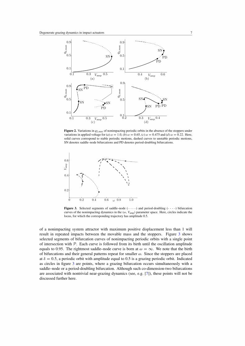
Figure 2 shows some example voltage-response scenarios for discrete choices of ω

obtained through numerical continuation of periodic system attractors. Here, the variationin the maximum positive displacement of the movable mass from its neutral position is plottedagainst the variation in the amplitude of the applied voltage. Since the position of the fixedelectrode is normalized to be 1, the maximum displacement must be less than 1. Whenthe maximum displacement is near 1, numerical continuation becomes difficult due to theproximity of the periodic orbit to the basin of attraction of the snapped-through equilibrium.

We note that each panel in figure 2 shows at least one saddle–node bifurcation. A pair ofperiod-doubling bifurcations is encountered in panels (b), (c) and (d). Panels (c) and (d) showmultiple saddle–node bifurcations; thus multiple stable periodic motions coexist over certainranges of ω. We further note that the left and right period-doubling bifurcations in panels (b)and (d) are subcritical and supercritical, respectively, while both period-doubling bifurcationsin panel (c) are supercritical.

When the periodic orbit passes through a saddle–node bifurcation or a subcritical period-doubling bifurcation, the system dynamics either jumps to another attractor through transientsor evolves to dynamic pull-in [28, 31]. When the stoppers are reintroduced, the absence


Figure 2. Variations in q2,max of nonimpacting periodic orbits in the absence of the stoppers undervariations in applied voltage for (a) ω = 1.0, (b) ω = 0.65, (c) ω = 0.475 and (d) ω = 0.22. Here,solid curves correspond to stable periodic motions, dashed curves to unstable periodic motions,SN denotes saddle–node bifurcations and PD denotes period-doubling bifurcations.

Figure 3. Selected segments of saddle–node (· · · · · ·) and period-doubling (- - - -) bifurcationcurves of the nonimpacting dynamics in the (ω, Vamp) parameter space. Here, circles indicate thelocus, for which the corresponding trajectory has amplitude 0.5.

of a nonimpacting system attractor with maximum positive displacement less than 1 willresult in repeated impacts between the movable mass and the stoppers. Figure 3 showsselected segments of bifurcation curves of nonimpacting periodic orbits with a single pointof intersection with P . Each curve is followed from its birth until the oscillation amplitudeequals to 0.95. The rightmost saddle–node curve is born at ω = ∞. We note that the birthof bifurcations and their general patterns repeat for smaller ω. Since the stoppers are placedat δ = 0.5, a periodic orbit with amplitude equal to 0.5 is a grazing periodic orbit. Indicatedas circles in figure 3 are points, where a grazing bifurcation occurs simultaneously with asaddle–node or a period-doubling bifurcation. Although such co-dimension-two bifurcationsare associated with nontrivial near-grazing dynamics (see, e.g. [7]), these points will not bediscussed further here.


Figure 4. Graph of the collection � of pairs of parameter values (ω, Vamp) for which there existsa period-1 nonimpacting grazing trajectory. Here, solid lines represent stable grazing orbits anddotted represent unstable grazing orbits.

3.2. Grazing curve in parameter space

We return to the full dynamics of the microactuator, i.e. with stoppers attached to the frame.For notational convenience, consider the following definition

D = {x|hD(x)def=hfront(x) = 0}, (14)

D+ = {x ∈ D|hDx (x) · fstick(x) = u2 > 0}, (15)

D0 = {x ∈ D|hDx (x) · fstick(x) = u2 = 0}, (16)

D− = {x ∈ D|hDx (x) · fstick(x) = u2 < 0}, (17)

where hDx represents the gradient of hD. Since gimpact maps D+ to D−, trajectories that reach

D+ experience an instantaneous jump to D− (as the incoming velocity u2 > 0 is changed to anoutgoing velocity −eu2 < 0). By a grazing periodic trajectory, we refer to a periodic trajectoryon which there exists a locally unique point x∗ ∈ D0, since such a trajectory experiences nojump in state upon reaching D. As discussed in Zhao et al [32], we can use a Newton methodto numerically locate parameter values for ω and Vamp for which grazing periodic trajectoriesexist. Figure 4 shows the grazing curve � = {(ω, Vamp)|V = V ∗

amp, such that ∃ period-1nonimpacting grazing trajectory} for the range of 0.1 � ω � 1.0 in parameter space. Everychoice of parameter on � thus corresponds to the existence of a grazing nonimpacting periodictrajectory of the fundamental period of the forcing term.

Intersections of � with bifurcation curves for the nonimpacting dynamics correspondto changes in stability of the grazing periodic orbit (cf circles in figure 3 representingperiodic orbits of amplitude 0.5). For example, while the nonimpacting periodic grazingorbits corresponding to the extreme right part of the curve are unstable, the grazing orbitbecomes stable as ω is reduced past ω ≈ 0.908 where � intersects a saddle–node bifurcationcurve of the nonimpacting dynamics. Further changes in the stability of the grazing orbitare associated with the intersections of � with a supercritical period-doubling bifurcationnear ω ≈ 0.693, a subcritical period-doubling bifurcation at ω ≈ 0.613 and a saddle–nodebifurcation at ω ≈ 0.481. The dynamics near the latter bifurcation point have been previouslyreported by Zhao et al [32] and studied in detail by Dankowicz and Zhao [7].

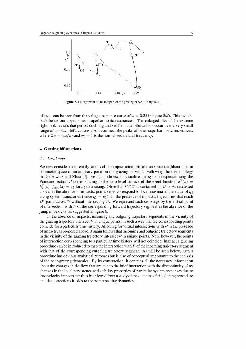
As can be seen more clearly in the enlargement of � shown in figure 5, the grazing curverepeatedly switches direction with multiple critical values of V ∗

amp values coexisting over rangesof values of ω. This corresponds to the coexistence of multiple grazing orbits for a single value


Figure 5. Enlargement of the left part of the grazing curve � in figure 4.

of ω, as can be seen from the voltage-response curve of ω = 0.22 in figure 2(d). This switch-back behaviour appears near superharmonic resonances. The enlarged plot of the extremeright peak reveals that period-doubling and saddle–node bifurcations occur over a very smallrange of ω. Such bifurcations also occur near the peaks of other superharmonic resonances,where 2ω = (ω0/n) and ω0 = 1 is the normalized natural frequency.

4. Grazing bifurcations

4.1. Local map

We now consider recurrent dynamics of the impact microactuator on some neighbourhood inparameter space of an arbitrary point on the grazing curve �. Following the methodologyin Dankowicz and Zhao [7], we again choose to visualize the system response using thePoincare section P corresponding to the zero-level surface of the event function hP(x) =hD

x (x) · fstick(x) = u2 for u2 decreasing. (Note that P ∩ D is contained in D0.) As discussedabove, in the absence of impacts, points on P correspond to local maxima in the value of q2

along system trajectories (since q2 = u2). In the presence of impacts, trajectories that reachD+ jump across P without intersecting P . We represent such crossings by the virtual pointof intersection with P of the corresponding forward trajectory segment in the absence of thejump in velocity, as suggested in figure 6.

In the absence of impacts, incoming and outgoing trajectory segments in the vicinity ofthe grazing trajectory intersect P in unique points, in such a way that the corresponding pointscoincide for a particular time history. Allowing for virtual intersections with P in the presenceof impacts, as proposed above, it again follows that incoming and outgoing trajectory segmentsin the vicinity of the grazing trajectory intersect P in unique points. Now, however, the pointsof intersection corresponding to a particular time history will not coincide. Instead, a glueingprocedure can be introduced to map the intersection with P of the incoming trajectory segmentwith that of the corresponding outgoing trajectory segment. As will be seen below, such aprocedure has obvious analytical purposes but is also of conceptual importance to the analysisof the near-grazing dynamics. By its construction, it contains all the necessary informationabout the changes in the flow that are due to the brief interaction with the discontinuity. Anychanges in the local persistence and stability properties of particular system responses due tolow-velocity impacts can thus be inferred from a study of the outcome of the glueing procedureand the corrections it adds to the nonimpacting dynamics.


Figure 6. Intersections of nonimpacting and impacting trajectories with the Poincare section P .The nonimpacting trajectory reaches its local maximum in q2 at the intersection. The impactingtrajectory reaches P virtually by neglecting the existence of the discontinuity surface D. Reprintedfrom [7]. Copyright (2005), with permission from Elsevier.

Following these observations (see also Dankowicz and Zhao [7]), we wish to associatea Poincare mapping P with the Poincare section P introduced above. Ignore, for a moment,the jump map associated with the discontinuity D and assume that the dynamics is governedentirely by the vector field fstick and constrained to a constant-q1 slice of the submanifold Scorresponding to the zero-level surface of the event function hS(x) = u1. Suppose that forsome values ω = ωref and Vamp = V ref

amp, the forward trajectory based at a point xref ∈ Pintersects P transversally after some time t ref , i.e.

hP(Φstick(xref , t ref; ωref , V refamp)) = 0 (18)

and

hP,i (Φstick(xref , t ref; ωref , V ref

amp)) · f istick(Φstick(xref , t ref; ωref , V ref

amp)) < 0. (19)

where Φstick is the smooth flow corresponding to the vector field fstick. Here, the latter conditioncorresponds to the requirement that u2 is decreasing, i.e. that the acceleration of the movablemass relative to the frame is negative. Then, as shown in Dankowicz and Zhao [7], a smoothPoincare mapping Psmooth can be defined on a neighbourhood of (xref , ωref , V ref

amp) by theexpression

Psmooth(x, ω, Vamp) = Φstick(x, τ (x, ω, Vamp); ω, Vamp), (20)

where the smooth function τ(x, ω, Vamp) is the time of flight from x back to P , such thatτ(xref , ωref , V ref

amp) = t ref .If we reintroduce the nontrivial jump map gimpact associated with D, the above expression

is still valid as long as hD(x) � 0. If, instead, hD(x) > 0, we again define the Poincaremapping by the above formula but include an initial correction to account for the virtual natureof the initial point x for the impacting flow. To this end, consider the Poincare mapping Pdefined by

P(x, ω, Vamp) = Psmooth(D(x, ω, Vamp), ω, Vamp), (21)

where the discontinuity mapping D : P → P maps x to some point on P in such a way that thesubsequent dynamics respects those of the corresponding actual trajectory (for more discussionof the concept of discontinuity mappings and their derivation, see also [6, 9, 11, 21, 23]).


Figure 7. Trajectories associated with the discontinuity mapping D. Here S stands for the stickmanifold, D is the discontinuity surface and P is the Poincare section. We note that S, D and Pare all four-dimensional hypersurfaces in a five-dimensional space. Reprinted from [7]. Copyright(2005), with permission from Elsevier.

Restrict attention to points x ∈ P ∩ S near x∗ ∈ P ∩ S ∩ D, where x∗ corresponds to thepoint of tangential contact of a grazing periodic orbit with the discontinuity surface D for somefrequency ω∗ and an associated amplitude V ∗

amp. To arrive at an expression for D, considerthe trajectory segments shown in figure 7. Here, an incoming trajectory (solid) in S governedby the vector field fstick reaches the discontinuity surface D at a point xin ∈ D+, experiencesa jump to a point gimpact(xin) ∈ D−, flows under the vector field fslip+ until reaching the stickmanifold S at a point xout and then continues to flow in S under the vector field fstick. Thedashed trajectory segments correspond to a flow in S governed by the vector field fstick from xin

forward in time until reaching P at a point x0; and from xout backward in time until reachingP at a point x1. The sought correction to the smooth flow given by Φstick is then obtained bymapping x0 to x1, as this correctly accounts for the effects of the jump map and the subsequentsliding episode.

Thus, given an initial point x ∈ P , such that hD(x) > 0, we define D as the compositionof the following steps:

(i) flow for a time t1 < 0 with the vector field fstick until reaching D;(ii) apply the jump map gimpact;

(iii) Flow for a time t2 > 0 with the vector field fslip+ until reaching S;(iv) Flow for a time t3 < 0 with the vector field fstick until reaching P .

For general forms of the event functions hD, hP and hS and under certain conditions onthe properties of the vector field and the functions hD, hP and hS on a neighbourhood of x∗,the analysis in Dankowicz and Zhao [7] employs the implicit function theorem to derive seriesexpansions for the flow times t1, t2 and t3 and for the corresponding points on D, S and P interms of the deviations x = x − x∗, ω = ω − ω∗ and Vamp = Vamp − V ∗

amp. Combiningthe resulting expansions, we get

D(x, ω, Vamp) ={

x when hD(x) � 0

β√

−(2/a0)hD,x · x + x + · · · when hD(x) > 0,

(22)

where

β =(

hP,x · gimpact,x · fstick

hP,x · fstick

−(

hS,x · gimpact,x · fstick

hS,x · fslip+

)(hP

,x · fslip+

hP,x · fstick

))fstick

−gimpact,x · fstick +

(hS

,x · gimpact,x · fstick

hS,x · fslip+

)fslip+ (23)


and

a0 = hP,x · fstick < 0 (24)

and the absence of an argument indicates evaluation at x = x∗, ω = ω∗ and Vamp = V ∗amp.

Here, the discontinuity mapping includes contributions from low-velocity impacts as well asfrom the short slip episodes that result from the impacts.

From the definition of β, it follows that β is tangential to P , D and S. Indeed, it isstraightforward to show that hP

,x · β = hS,x · β = 0. Moreover, hD

,x · fstick|x∗ = hD,x · fslip+|x∗ = 0

(since u2 = 0 for x = x∗) and hD,x ·gimpact,x ·fstick|x∗ = 0 (since gimpact maps D to itself and equals

the identity on D0) imply that hD,x ·β = 0 (this is a universal property of impacting mechanical

systems (see Nordmark [19])). It follows that the first nontrivial correction in the discontinuitymapping is tangential to P ∩ S ∩ D. Specifically, after some algebraic manipulations, onefinds that, when hD(x) > 0,

D(x, ω, Vamp) = x∗ +

(0 0 0 0 θ − m1(1 + e)

(m1 + m2)ω

√− 2

a0

√q2

)T

+ O(2), (25)

where O(nt) refers to terms of the form (q2t)n1/2(θ)n2(ω)n3(Vamp)

n4 , for whichn1 + n2 + n3 + n4 = n. Thus, to the lowest order, the discontinuity mapping introduces acorrection only in the phase θ .

While Psmooth results in no change in q1, the inclusion of the jump mapping gimpact andthe associated sliding episode yields a discrete change in q1 described by the discontinuitymapping D and, consequently, by the composite Poincare map P. As the system is invariantunder variations in q1 and as, for low-velocity impacts P(x) ∈ P ∩ S, we consider below thereduced system obtained by restricting attention to the third and fifth components of P.

4.2. Near-grazing dynamics

A periodic impacting orbit near the grazing orbit with one impact per period corresponds toa fixed point of the composite Poincare map P. To obtain an analytical expression for thelocation of such a fixed point in terms of ω and Vamp, consider the introduction of a smallparameter ε � 1, such that ω and Vamp are both O(ε).

Now suppose that Pq2

smooth,θ (x∗) is nonzero and O(1). As shown in appendix A, it follows

that there is a locally unique fixed point near x∗ on one or the other side of the grazing curve� depending on the sign of P

q2

smooth,θ (x∗) (cf figures 8(a) and (b)).

If, instead, Pq2

smooth,θ (x∗) = O(

√ε), the analysis in appendix A shows that there is either

a locally unique fixed point on one side of the grazing curve and no fixed point on the otherside or a locally unique fixed point on one side of the grazing curve and a pair of fixed pointson some neighbourhood of the grazing curve on the other side (cf figures 8(c) and (d)).

From the analysis in the case when Pq2

smooth,θ (x∗) = O(1) it is well established that a co-

dimension-two bifurcation occurs when Pq2

smooth,θ (x∗) switches sign. Since P

q2

smooth,θ (x∗) may be

computed from the nonimpacting dynamics, it is possible to identify various co-dimension-twograzing bifurcation points on the grazing curve in the parameter space, as shown in figure 9.

4.3. Local analysis of co-dimension-two bifurcations

Consider the co-dimension-two grazing bifurcation point corresponding to ω∗ ≈ 0.613 650and V ∗

amp ≈ 0.581 634 (indicated as the second star from the left in figure 9), for which thecorresponding grazing orbit is given by

x∗ ≈ (· 0 0.5 0 3.122 254)T. (26)


Figure 8. Schematic of fixed points of the composite Poincare map P corresponding to period-1nonimpacting orbits (——), period-1 impacting orbits with a single impact per period (- - - -):(a), (b) for P

q2smooth,θ (x

∗) = O(1) and (c), (d) for Pq2smooth,θ (x

∗) = O(√

ε). Here, µ represents acombination of the parameters Vamp and ω, such that µ = 0 corresponds to the grazing periodicorbit. Without loss of generality, it is assumed here that nonimpacting orbits reside on the sideof µ < 0.

Figure 9. Grazing curves in parameter space with co-dimension-two grazing bifurcations denotedby stars. Here, P1 refers to a branch of period-1 grazing orbits, P2 refers to a branch of period-2grazing orbits, stable orbits are denoted by solid lines, unstable orbits are denoted by dashed lines,SN denotes a saddle–node bifurcation and PD denotes a period-doubling bifurcation.

Here, the dot in the first component of x∗ indicates that it is arbitrary, since the value of q1

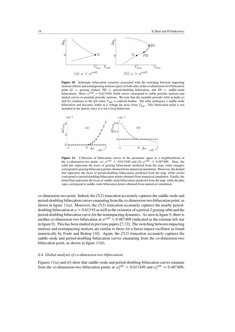
does not influence the system dynamics as can be seen from the equations of motion in theprevious section. Numerical integration reveals that the transition between nonimpacting andimpacting differs between the two sides of the co-dimension-two bifurcation point, as shownin figure 10.

Following the methodology in the previous section, we study bifurcations in the vicinityof the co-dimension-two bifurcation point at ωcod2 ≈ 0.613 650, using both O(1) and O(2)

truncations of the discontinuity mapping (and the associated composite Poincare mapping).For both ω < ωcod2 and ω > ωcod2, the O(1) truncation predicts a bifurcation diagram similarto that shown in figure 10(a). This verifies the degeneracy of the O(1) truncation. On theother hand, using the O(2) truncation, the predicted bifurcation diagrams agree with thoseobtained from numerical simulations of the original differential equations on both sides of the


Figure 10. Schematic bifurcation scenarios associated with the switching between impactingmotions (black) and nonimpacting motions (grey) at both sides of the co-dimension-two bifurcationpoint (G = grazing contact, PD = period-doubling bifurcation, and SN = saddle–nodebifurcation). Here, ωcod2 ≈ 0.613 650. Solid curves correspond to stable periodic motions anddashed curves to unstable periodic motions. We note that the unstable periodic orbit in both (a)and (b) continues to the left when Vamp is reduced further. The orbit undergoes a saddle–nodebifurcation and becomes stable at a voltage far away from V ∗

amp. This bifurcation point is notincluded in the sketch, since it is not a local behaviour.

Figure 11. Collection of bifurcation curves in the parameter space in a neighbourhood ofthe co-dimension-two point: (a) ωcod2 ≈ 0.613 650 and (b) ωcod2 ≈ 0.487 809. Here, thesolid line represents the locus of grazing bifurcations predicted from the map, while trianglescorrespond to grazing bifurcation points obtained from numerical simulation. Moreover, the dashedline represents the locus of period-doubling bifurcations predicted from the map, while circlescorrespond to period-doubling bifurcation points obtained from numerical simulation. Finally, thedotted line represents the locus of saddle–node bifurcations predicted from the map, while the plussigns correspond to saddle–node bifurcation points obtained from numerical simulation.

co-dimension-two point. Indeed, the O(2) truncation accurately captures the saddle–node andperiod-doubling bifurcation curves emanating from the co-dimension-two bifurcation point, asshown in figure 11(a). Moreover, the O(2) truncation accurately captures the nearby period-doubling bifurcation at ω ≈ 0.613 93 as well as the existence of a period-2 grazing orbit and theperiod-doubling bifurcation curve for the nonimpacting dynamics. As seen in figure 9, there isanother co-dimension-two bifurcation at ωcod2 ≈ 0.487 809 (indicated as the extreme left starin figure 9). This has been studied in previous papers [7,32]. The switching between impactingmotions and nonimpacting motions are similar to those for a linear impact oscillator as foundnumerically by Foale and Bishop [10]. Again, the O(2) truncation accurately captures thesaddle–node and period-doubling bifurcation curves emanating from the co-dimension-twobifurcation point, as shown in figure 11(b).

4.4. Global analysis of co-dimension-two bifurcations

Figures 11(a) and (b) show that saddle–node and period-doubling bifurcation curves emanatefrom the co-dimension-two bifurcation points at ωcod2

2 ≈ 0.613 650 and ωcod21 ≈ 0.487 809,


Figure 12. Collection of bifurcation curves in the (ω, Vamp) parameter space. Here, � representsthe grazing curve, V sn

amp represents the locus of saddle–node bifurcations, and Vpdamp represents

the locus of period-doubling bifurcations. The grazing curve is dashed when it is unstable andstars denote the co-dimension-two grazing bifurcations analysed in the previous section. We notethat �imp represents grazing contact of an impacting periodic orbit with one impacting and onenonimpacting oscillation period (see the inset).

respectively. The global extensions of these curves obtained by parameter continuation areshown in figure 12. The saddle–node bifurcation curves emanating from ωcod2

1 and ωcod22 merge

and terminate in a cusp near ω ≈ 0.746. The period-doubling bifurcation curve emanatingfrom ωcod2

2 , on the other hand, persists under increases of ω. In contrast, the period-doublingbifurcation curve emanating from ωcod2

1 winds upwards until it intersects another grazing curve�imp, where it terminates. Here, �imp represents the grazing contact of an impacting periodicorbit with one impacting and one nonimpacting oscillation per period.

To understand the significance of the bifurcation curves in figure 12, a global bifurcationstudy is necessary. For example, a voltage-response curve for ω = 0.56 is shown in figure 13(a). Note that when the impact velocity of a trajectory is sufficiently high, the trajectory snapsthrough to the fixed electrode in the absence of the stoppers. Such a trajectory would thusnot intersect the previously defined Poincare surface P . To appropriately represent suchtrajectories, we plot variations of the maximum negative displacement under changes involtage amplitude. Here, as depicted in figure 8(a), a branch of stable nonimpacting periodicorbits and a branch of unstable impacting periodic orbits emanate on the same side from thegrazing bifurcation point at V ∗

amp ≈ 0.532. The impacting motion becomes stable through asaddle–node bifurcation at V SN

amp ≈ 0.271. Increasing the voltage amplitude, a pair of period-doubling bifurcations are encountered atV PD1

amp ≈ 0.661 andV PD2amp ≈ 0.755, respectively. Under

further increases in the voltage, the periodic impacting motion becomes stable and eventuallyreaches a grazing bifurcation point at V ∗

amp ≈ 0.761 (cf the inset shown in figure 12).Another voltage-response curve for ω = 0.65 is shown in figure 13(b). Here, as

depicted in figure 8(b), a branch of unstable nonimpacting periodic orbits and a branch ofunstable impacting periodic orbits emanate on opposite sides from the grazing bifurcationpoint at V ∗

amp ≈ 0.594. The nonimpacting periodic orbit becomes stable in a period-doublingbifurcation for Vamp ≈ 0.55 (cf figure 9). On the other hand, the impacting periodic motionbecomes stable through a period-doubling bifurcation at Vamp ≈ 0.601. The impacting periodicmotion subsequently undergoes a pair of saddle–node bifurcations at Vamp ≈ 0.602 andVamp ≈ 0.489, respectively. Here, the left saddle–node point in figure 13(b) correspondsto the saddle–node point in figure 13(a), which originates in the co-dimension-two grazingbifurcation at ωcod2 ≈ 0.487 809 (left star in figure 12). Similarly, the right saddle–node pointin figure 13(b) originates in the co-dimension-two grazing bifurcation at ωcod2 ≈ 0.613 650


Figure 13. Variations in q2,min per period under variations in the applied voltage: (a) ω = 0.56and (b) ω = 0.65. Here, nonimpacting motions are represented by grey lines, impacting motionsare represented by black lines, solid curves correspond to stable motion, dashed curves correspondto unstable motion, G denotes a grazing bifurcation, SN denotes a saddle–node bifurcation and PDdenotes a period-doubling bifurcation.

(the right star in figure 12). As indicated in figure 12, the two saddle–node points infigure 13(b) approach and annihilate each other as the excitation frequency increases. Sincefigures 13(a) and (b) show the coexistence of multiple stable orbits, one would encounterhysteresis phenomena under the variations of excitation voltage.

4.5. General phenomenology

The numerical results reported in the previous sections are representative of a broad class ofimpacting mechanical systems, possessing similar nonlinearities and with or without friction,although the specific quantitative details naturally refer to the example actuator considered here.

The discontinuity mapping derived above correctly accounts for low-velocity impacts andan accompanying brief episode of the sliding motion. As in the study of forced single-degree-of-freedom impact oscillators, the resultant map is essentially two-dimensional. Indeed, thediscontinuity mapping has the generic form found for impact oscillators near grazing, sincethe square-root singularity of the discontinuity mapping is a universal property of systems withdiscontinuous states or vector fields [9]. As a result, the analysis of the co-dimension-one andco-dimension-two bifurcations are not restricted to the impact actuator. Observations madehere regarding the near-grazing dynamics thus apply to a large class of systems.

Similar conclusions may be drawn regarding the unfolding of co-dimension-two grazingbifurcations as discussed here. Indeed, the bifurcation diagram shown in figure 11(b) agreesqualitatively with that shown in Foale and Bishop [10]. Moreover, in addition to the two sampleunfoldings shown here, several distinct and previously unreported unfoldings have been foundfor the impact actuator as well as the linear impact oscillator considered in [10].

Finally, the notion that bifurcation curves emanating from the co-dimension-twobifurcation points serve to organize the global impacting dynamics has also been confirmedfor other regions of parameter space in the case of impact actuator as well as the linear impactoscillator. As shown here, such global analysis for systems with similar grazing singularitiesmay be undertaken through continuation analysis of the bifurcation curves predicted using thediscontinuity mapping technique.

5. Conclusions

The analysis in previous sections has employed a combination of numerical techniques andlocal analysis near periodic grazing trajectories to analyse the near-grazing dynamics of the


Mita impact microactuator. Although the numerical results reported above specifically relate tothe Mita actuator, the methodology is easily modified to apply to arbitrary impacting systems.Moreover, the qualitative nature of the near-grazing dynamics is expected to generalize tosystems with similar nonlinearities.

A particular contribution of this work is a selective description of the bifurcation behaviourof the nonimpacting and impacting dynamics of the microactuator and, specifically, the wayin which co-dimension-two grazing bifurcation points serve to organize the bifurcation curvesof the impacting dynamics. In addition to providing a basis for the understanding of the near-grazing dynamics, the analysis of the nonimpacting dynamics also establishes properties ofthe dynamic pull-in phenomenon in MEMS devices whose actuating part is modelled as amass-spring-damper oscillator.

The discovery of an additional grazing curve for period-one impacting orbits with oneimpacting and one nonimpacting loop per period opens up an opportunity for further studyof the impacting dynamics. Indeed, the analysis of the near-grazing dynamics in the vicinityof this secondary grazing curve is expected to follow the same lines of reasoning as in thepresent discussion. We conjecture the existence of tertiary grazing curves with period-oneimpacting orbits with two impacting and one nonimpacting loop per period and so on. Ofcourse, additional grazing curves are also likely to exist for period-two impacting orbits andso on. The accumulation of additional impacting loops for period-one motions is expected tobe associated with the phenomenon of chattering. This is a topic that we hope to pursue in afurther publication.

Acknowledgment

This material is based upon work supported by the National Science Foundation under GrantNo 0237370.

Appendix A. Impacting periodic orbits

Suppose that Pq2

smooth,θ (x∗) = O(1). Then, a consistent expansion of a fixed point of P is given

by the ansatz

q2 = ε2q(2)2 + O(ε3), θ = εθ(1) + O(ε2). (A.1)

A fixed point of P corresponding to a periodic impacting orbit with one impact per period mustthen satisfy the equations

0 = ε

(P

q2

smooth,θ (x∗)β

√q

(2)2 + P

q2

smooth,θ (x∗)θ(1) + c1

)+ O(ε2), (A.2)

εθ(1) = ε

(P θ

smooth,θ (x∗)β

√q

(2)2 + P θ

smooth,θ (x∗)θ(1) + c2

)+ O(ε2), (A.3)

where

β = − m1

m1 + m2(1 + e)ω

√− 2

a0< 0, (A.4)

εc1 = Pq2

smooth,ω(x∗)ω + Pq2

smooth,Vamp(x∗)Vamp, (A.5)

εc2 = P θsmooth,ω(x∗)ω + P θ

smooth,Vamp(x∗)Vamp. (A.6)


It follows that √q

(2)2 = − c

Pq2

smooth,θ (x∗)β

, (A.7)

θ(1) = −P θsmooth,θ (x∗)c1 + P

q2

smooth,θ (x∗)c2

Pq2

smooth,θ (x∗)

, (A.8)

where

c = (1 − P θsmooth,θ (x

∗)) c1 + Pq2

smooth,θ (x∗)c2. (A.9)

Since β < 0, it follows that a fixed point exists for c > 0 when Pq2

smooth,θ (x∗) > 0 and for c < 0

when Pq2

smooth,θ (x∗) < 0. Since the periodic grazing contact point is a fixed point of Psmooth

corresponding to q2 = 0, i.e.

Pq2

smooth,θ (x∗)θ + P

q2

smooth,ω(x∗)ω + Pq2

smooth,Vamp(x∗)Vamp = 0, (A.10)

P θsmooth,θ (x

∗)θ + P θsmooth,ω(x∗)ω + P θ

smooth,Vamp(x∗)Vamp = θ, (A.11)

eliminating θ from the above equations reveals that c = 0 corresponds to the grazing curvein parameter space (Vamp, ω).

If, instead, P q2


√ε), a consistent expansion for the position of a fixed point

of P is given by the ansatz

q2 = εq(1)2 + O(ε2), θ = √

εθ(1/2) + εθ(1) + O(ε3/2). (A.12)

A fixed point of P corresponding to a periodic impacting orbit with one impact per period mustthen satisfy the equations

εq(1)2 = ε

Pq2

smooth,θ (x∗)√

εβ

√q

(1)2 +

Pq2

smooth,θ (x∗)√

εθ(1/2)

+c1 + a11q(1)2 + a12

√q

(1)2 θ(1/2) + a13(θ(1/2))2

+ O(ε3/2), (A.13)

√εθ(1/2) + εθ(1) = √

ε

[P θ

smooth,θ (x∗)β

√q

(1)2 + P θ

smooth,θ (x∗)θ(1/2)

]

+ε

[P θ

smooth,θ (x∗)θ(1) + c2 + a21q

(1)2 + a22

√q

(1)2 θ(1/2)

+a23(θ(1/2))2

]+ O(ε3/2),

(A.14)

where a11, a12, a13, a21, a22 and a23 are constants. It follows that

0 = a q(1)2 + b

√q

(1)2 − c, (A.15)

where

a = (1 − a11 − a12γβ − a13γ2β2), (A.16)

b = −Pq2

smooth,θ (x∗)√

εβ(1 + γ ), (A.17)

c = c1, (A.18)

γ = P θsmooth,θ (x

∗)(1 − P θsmooth,θ (x

∗))−1. (A.19)

Here it is assumed that a < 0 and 1 −P θsmooth,θ (x

∗) > 0. It follows that (i) if Pq2

smooth,θ (x∗) > 0,

there exists one fixed point near x∗ when c/a > 0 and two fixed points near x∗ when−(b/a)2/4 � c/a � 0, whereas (ii) if P

q2

smooth,θ (x∗) < 0, there exists one fixed point near

x∗ when c/a � 0 and no fixed point near x∗ when c/a < 0. Substituting the assumptionP

q2


√ε) and equation (A.12) into equations (A.10) and (A.11), one again finds

that the grazing curve in parameter space corresponds to c = 0.


References

[1] Breguet J M, Schmitt C, Bergander A and Clavel R 1998 Micropositioner for microscopy applications based onstick-slip effect Proc. 2000 Micromechatronics and Human Science pp 213–6 AQ2

[2] Breguet J M and Clavel R 1998 Stick and slip actuators: design, control, performances and applications Proc.1998 Micromechatronics and Human Science pp 89–95

[3] Cusin P, Sawai T and Konish S 2000 Compact and precise positioner based on the inchworm principleJ. Micromech. Microeng. 10 516–21

[4] Chin W, Ott E, Nusse H E and Grebogi C 1994 Grazing bifurcations in impact oscillators Phys. Rev. E 504427–44

[5] Daneman M J, Tien N C, Solgaard O, Pisano A P, Lau K Y and Muller R S 1996 Linear microvibromotor forpositioning optical components IEEE J. Microelectromech. Syst. 5 159–65

[6] Dankowicz H and Nordmark A B 1999 On the origin and bifurcations of stick-slip oscillations Physica D 136280–302

[7] Dankowicz H and Zhao X 2005 Local analysis of co-dimension-one and co-dimension-two grazing bifurcationsin impact microactuators Physica D 202 238–57

[8] de Weger J, van de Water W and Molenaar J 2000 Grazing impact oscillations Phys. Rev. E 62 2030–41[9] Di Bernardo M, Budd C J and Champneys A R 2000 Normal form maps for grazing bifurcations in n-dimensional

piecewise-smooth dynamical systems Physica D 160 222–54[10] Foale S and Bishop R 1994 Bifurcations in impacting systems Nonlinear Dyn. 6 285–99[11] Fredriksson M H and Nordmark A B 1997 Bifurcations caused by grazing incidence in many degrees of freedom

impact oscillators Proc. R. Soc. Lond. Ser. A 453 1261–76[12] Fredriksson M H and Nordmark A B 2000 On normal form calculations in impact oscillators Proc. R. Soc. Lond.

Ser. A 456 315–30[13] Higuchi T, Yamagata Y, Furutani K and Kudoh K 1990 Precise positioning mechanism utilizing rapid

deformations of piezoelectric elements IEEE Conf. on Microelectromechanical Systems pp 222–6[14] Jungnickel U, Eicher D and Schlaak H F 2002 Miniaturized micro-positioning system for large displacements

and large forces based on an inchworm platform 8th Int. Conf. on New Actuators pp 684–7[15] Kim C H and Kim Y K 2002 Micro xy-stage using silicon on a glass substrate J. Micromech. Microeng. 12

103–7[16] Kleczka M, Kreuzer E and Schiehlen W 1992 Local and global stability of a piecewise linear oscillator Phil.

Trans. Phys. Sci. Eng. 338 533–46[17] Lee A P, Nikkel D J Jr and Pisano A P 1993 Polysilicon linear microvibromotors Proc. 7th Int. Conf. Solid-State

Sensors and Actuators vol 1, pp 46–9[18] Liu Y T and Higuchi T 2001 Precision positioning device utilizing impact force of combined piezo-pneumatic

actuator IEEE Trans. Mechatronics 6 467–73AQ3[19] Nordmark A B 2001 Existence of periodic orbits in grazing bifurcations of impacting mechanical oscillators

Nonlinearity 14 1517–42[20] Mita M, Arai M, Tensaka S, Kobayashi D and Fujita H 2003 A micromachined impact microactuator driven by

electrostatic force IEEE J. Microelectromech. Syst. 12 37–41[21] Molenaar J, de Weger J G and Van de Water W 2001 Mappings of grazing impact oscillators Nonlinearity 14

301–21AQ4[22] Morita T, Yoshida R, Okamoto Y, Kurosawa M K and Higuchi T 1999 A smooth impact rotation motor

using a multi-layered torsional piezoelectric actuator IEEE Trans. Ultrason. Ferroelectr. Freq. Control 46439–144

[23] Nordmark A B 1991 Non-periodic motion caused by grazing incidence in an impact oscillator J. Sound Vib. 145279–97

[24] Nordmark A B 1997 Universal limit mapping in grazing bifurcations Phys. Rev. E 55 266–70[25] Pavloskaia E, Wiercigroch M and Grebogi C 2001 Modeling of an impact system with drift Phys. Rev. E 64

(056224)1–9AQ5[26] Ragulsikis K, Bansevicus, Barausleas R and Kulvietis G 1988 Vibromotors for Precision Microrobots (New York:

Hemisphere)[27] Saitou K, Wang D A and Wou S J 2000 Externally resonated linear microvibromotor for microassembly IEEE

J. Microelectromech. Syst. 9 36–346[28] Seeger J I and Bernhard E 2003 Boser Charge control of parallel-plate, electrostatic actuators and the tip-in

instability J. Microelectromech. Syst. 12 656–71[29] Shaw S W 1985 The dynamics of a harmonically excited system having rigid amplitude constraints, part I:

subharmonic motions and local bifurcations ASME J. Appl. Mech. 52 453–8


[30] Shaw S W 1985 The dynamics of a harmonically excited system having rigid amplitude constraints, part II:chaotic motions and global bifurcations ASME J. Appl. Mech. 52 459–64

[31] Varghese M and Senturia S D 1997 Resistive damping of pulse-sensed capacitive position sensorsTechnical Digest 1997 Int. Conf. Solid-State Sensors and Actuators (Transducers ’97) (June) pp 1121–4

[32] Zhao X, Dankowicz H, Reddy C K and Nayfeh A H 2004 Modelling and simulation methodology for impactmicroactuators J. Micromech. Microeng. 14 775–84

[33] Zhao X, Reddy C K and Nayfeh A H 2005 Nonlinear dynamics of an electrically driven impact microactuatorsNonlinear Dyn. 40 227–39

QUERIES

Page 1AQ1Please provide mathematics classification codes.

Page 19AQ2Please provide place of proceedings for refs. [1], [2], [13], [14] and [31].

Page 19AQ3Please check if the edit to the word ‘exitence’ in ref. [19] is in order.

Page 19AQ4Please check if the page numbers are in order for ref. [22].

Page 19AQ5Please provide initials for author ‘Bansevicus’ in ref. [26].

Documents

Unfolding degenerate grazing dynamics in impact actuators