UNIT – I – Chemical Reaction Engineering – SCHA1411

SCHOOL OF BIO AND CHEMICAL ENGINEERING

UNIT – I – Chemical Reaction Engineering – SCHA1411

DEPARTMENT OF CHEMICAL ENGINEERING

1.1 Basic Reaction Theory

A chemical reaction is a process that leads to the transformation of one set of chemical

substances to another. The substance (or substances) initially involved in a chemical reaction are

called reactants or reagents. Chemical reactions are usually characterized by a chemical change

and they yield one or more products which usually have properties different from the reactants.

Reactions often consist of a sequence of individual sub-steps, the so-called elementary reactions,

and the information on the precise course of action is part of the reaction mechanism. Chemical

reactions are described with chemical equations which symbolically present the starting

materials, end products, and sometimes intermediate products and reaction conditions.

Chemical reactions happen at a characteristic reaction rate at a given temperature and chemical

concentration. Typically, reaction rates increase with increasing temperature because there is

more thermal energy available to reach the activation energy necessary for breaking bonds

between atoms.

1.2 Classification Of Reactions

Reactions may be classified by (a) the number of phases involved, (b) the presence or absence of

a catalyst, and (c) the nature of the overall reaction.

If all the reactants and products, and catalysts, if any, are in a single phase, the reaction is said to

be homogeneous. An example is provided by the thermal cracking of ethane to ethylene

C2H6(g) →C2H4(g) + H2(g)

On the other hand, if more than one phase is involved, the reaction is said to be heterogeneous.

An example is provided by the chemical vapour deposition (CVD) of Si on a substrate

SiH4(g) → Si(s) + 2 H2(g)

an enzyme called glucose isomerase catalyzes the isomerization of glucose to fructose in the

liquid phase. It can be noted that this is the largest bioprocess in the chemical industry. As fructose

is five times sweeter than glucose, the process is used to make high-fructose corn syrup for the

soft drink industries. The overall reaction, as written, may represent either an elementary reaction

or a non-elementary reaction. An example of the former is given by the gas-phase reaction

NO2(g) + CO(g) →NO(g) + CO2(g)

Here NO is formed by the collision between molecules of NO2 and CO, and the rate expression

conforms to the stoichiometry shown. On the other hand,

SiH4(g) → Si(s) + 2 H2(g)

represents a non-elementary reaction, as it actually proceeds by the sequence of reactions shown

below

SiH4(g)→ SiH2(g) + H2(g)

SiH2(g) + ∗→ SiH2 ∗

SiH2 ∗→ Si(s) + H2(g) where * represents an active site on the substrate.

Irreversible Reactions: Reactions that proceed unidirectionally under the conditions of interest

Reversible Reactions: Reactions that proceed in both forward and reverse directions under

conditions of interest. Thermodynamics tells us that all reactions are reversible. However, in many

cases the reactor is operated such that the rate of the reverse reaction can be considered negligible.

Homogeneous Reactions: reactions that occur in a single-phase (gas or liquid) NOx formation

NO (g) + 0.5 O 2 (g) ↔ NO2 (g ) Ethylene Production C 2 H 6 (g) ↔ C 2 H 4 (g) + H 2 (g )

Heterogeneous Reactions: reactions that require the presence of two distinct phases Coal

combustion C ( s) + O 2 (g) ↔ CO 2 (g ) SO 3(for sulphuric acid production) SO 2 (g) + 1/2 O 2

(g) ↔ SO 3 (g) Vanadium catalyst (s)

Single and Multiple reactions:

Single reaction: When a single stoichiometric equation and single rate equation are chosen to

represent the progress of the reaction, then it is said to be ‘single reaction’. Multiple reactions:

When more than one stoichiometric equation is chosen to represent the observed changes, then

more than one kinetic expression is needed to follow the changing composition of all the reaction

components, it is said to be ‘multiple reactions’. Multiple reactions may be classified as; Series

reactions, Parallel reactions, and SeriesParallel reactions.

Elementary and Non- Elementary reactions

The reactions in which the rate equation corresponds to a stoichiometric equation are called

elementary reaction. The reactions in which there is no correspondence between stoichiometry

and rate equation are known as Non-elementary reaction

1.3 Kinetic Models of Non- Elementary reactions

Free radicals, ions and polar substances, molecules, transition complexes are the various

intermediates that can be formed in a non-elementary reaction.

In testing the kinetic models that involve a sequence of elementary reaction, we hypothesize the

existence of two types of intermediates; Type-I: An unseen and unmeasured intermediate ‘X’

usually present at such small concentration that its rate of change in the mixture can be taken to

be zero. Thus, we have [X] is small and d[X]/dt = 0. This is called the ‘steady-state

approximation’. Type-II: Where a homogeneous catalyst of initial concentration Co is present in

two forms, either as free catalyst ‘C’ or combined in an appreciable extent to form the

intermediate ‘X’, an accounting for the catalyst gives [Co] = [C] + [X]. We then also assume that

either (dX/dt) = 0 or that the intermediate is in equilibrium with its reactants. Using the above

two types of approach, we can test the kinetic model or search a good mechanism; Trial and error

procedure is involved in searching for a good mechanism.

1.4 Reaction rate and kinetics

Reaction rate

The rate expression provides information about the rate at which a reactant is consumed.

Consider a single phase reaction aA + b B → rR + Ss. Rate of reaction is defined as number of

moles of reactant disappearing per unit volume per unit time

- rA = - 1 dNA = ( amount of Adisappearing) , mol

-----------

V dt

-----------------------------------------

(volume) ( time)

------------

m3.s

In addition, the rates of reaction of all materials are related by

- rA = - rB = rR = rS

----- -----

a b

------ ------

c d

Rate constant k

When the rate expression for a homogeneous chemical reaction is written in the form

- rA= kCAaCBb…..CDd , a+b+…….+d = n

The dimensions of the rate constant k for the nth order reaction are

(time) -1(concentration)1-n

Which for a first order reaction becomes

(time) -1

1.5 Factors affecting rate of reaction

Many variables affect the rate of reaction of a chemical reaction. In homogeneous systems

the temperature, pressure, and composition are obvious variables. In heterogeneous

systems, material may have to move from phase to phase during reaction; hence, the rate of

mass transfer can be important. In addition, the rate of heat transfer may also become a

factor. In short, the variables affecting the rate of the reaction are (1) temperature (2) Pressure

and (3) Composition of materials involved.

1.6 Various forms of rate equation

Based on unit volume of the reaction mixture

Based on unit mass in fluid-solid system

Based on unit surface of solid in fluid-solid system or unit interfacial area in two fluid systems

Based on unit volume of solid in fluid-solid system

Based on unit volume of reactor when different from unit volume of the reaction mixture

Rates defined on various basis are interchangeable and the following may be shown

Or

Power law kinetics is simply put rate is proportional to concentration of species 1 to the power

q 1 concentration of species 2 to the power q 2. So, products of all the, such C 1 raise to q 1

C 2 raise to q 2, up to C N raise to raise to q n. In a compact form, we can express this as rate

equal to K, K is that proportionality constant, product of C j rise to q j, j going from 1 to N.

So, q j is the order of the reaction with respect to species A j; and this is the simplest form

of form of power law power law kinetics. Now, we call this q j as order with respect to A j

and if you sum up all these q j s, we get q, what we call as overall overall order. reaction

of hydrogen iodide getting decomposed to H 2 plus I 2. Now, it turns out for this particular

reaction, the rate of reaction is proportional to concentration of hydrogen iodide raise to power

2. So, clearly in this case, q is 2 there is only one species in the reactant side, so our q j and q r

q r are same. So, this is the this is the order of the reaction, so q can be integer. Let

us take another example, decomposition of acetaldehyde to give us methane and carbon

monoxide. Now, it turns out the rate of these reactions is proportional to concentration of

acetaldehyde raise to power 3 by 2. So, q in this case is 3 by 2, or in other words, orders can be

integers, they can be even fractions.

1.7 Molecularity

It is the number of molecules taking part in the reaction

e.g. A → C : Unimolecular reaction

A+ B → C : Bimolecular reaction

1.8 Order

It is defined as the sum of the powers to which the concentration terms are raised. The

overall kinetic order of a reaction is defined by how many concentrations appear on the right

side of the rate expression. The order of the reaction with respect to a particular species

is defined by whether that species appears one or more times. For example, if the right side

of the rate law is [A]m[B]n, then the overall order of the reaction is m+n and the reaction is

m’th order with respect to [A] and n’th order with respect to [B]. Zeroth order means that

the reaction rate does not change as the concentration of a species is changed. There are no

biochemical reactions that are zeroth order overall.

e.g. A+ B → C

-- rA = kCACB

n (order) = 1+1=2

1.9 Concentration dependent term of rate equation

Rate of reaction is defined as number of moles of reactant disappearing per unit volume per unit

time

- rA = - 1 dNA

-----------

V dt

If constant volume systems are considered , the rate of reaction is modified to

- rA = - dCA

-----------

dt

The definition of rate of a chemical reaction describing change in molar concentration with

respect to time, i.e., is not general and valid only when the volume of the mixture

does not change during the course of the reaction. This may be only true for liquid phase

reactions where volume changes are not significant. The volume of a gas also changes due

to changes in operating conditions (temperature and pressure) in addition to changes in number

of moles.

1.10 Rate equation in terms of partial pressure

For isothermal (elementary) gas reactions where the number of moles of material ’ to

The changes during reaction, the relation between the total pressure of the system ‘ changing

concentration or partial pressure of any of the reaction component is r R + s S + …a A + b B

+ ... o)] - n) (For the component ‘A’, pA = CA R T = pAo – [(a/ o)] - n) (For the

component ‘R’, pR = CR R T = pRo + [(r/ And the rate of the reaction, for any component ‘i',

is given by ri = (1/RT) (dpi/dt)

1.12 Effect of temperature on reaction

Temperature dependency from Arrhenius law

For many reactions and particularly elementary reactions, the rate expression can be written as a

P

roduct of a temperature . The excess energy of the reactants required to dissociate into products

is known as activation energy. The temperature dependency on the reaction rate constant is

given by Arrhenius Law. That is, k = ko e-E/RT Where k = rate constant, k0 = frequency

factor, E = Activation energy The temperature dependence of the rate constant k is usually

fitted by the Arrhenius equation . Arrhenius equation is frequently applied to approximate

the temperature dependency of reaction rate and the rate constant or velocity constant,

k, is related to temperature, T, by the following expression:

k = k0e− E/ R T

Where, k0 = pre-exponential factor and has units similar to that of k. Ea = activation energy,

J·mol–1

where the pre-exponential factor k0 and the activation energy E are treated as constants and T is

the absolute temperature. If a plot of ln k versus 1/T shows a significant curvature, the

rate constant k is a function of temperature

k = k0 e-Ea/RT

The higher the temperature the more molecules that have enough energy to make it over

the barrier Arrhenius Plot k = A exp(-Ea/RT) lnk = lnA -Ea/RT straight line plot y = b + mx y =

lnk x = 1/T b = lnA m = -Ea/R Plot lnk vs 1/T, slope = -Ea/R intercept = lnA. A plot of lnk vs

1/T will be straight line, the slope of which is Ea /R. The units of the slope are K. A large

slope of Arrhenius plot means large value of Ea and vice versa. Reactions having large value

of Ea are more temperature sensitive while with low value of Ea are less temperature dependent.

Transition state theory

Transition state theory (TST) explains the reaction rates of elementary chemical reactions.

The theory assumes a special type of chemical equilibrium (quasi-equilibrium) between

reactants and activated transition state complexes. Describes the flow of systems from

reactants-to-products over potential energy surfaces. Predicts the rate of an elementary equation

in term of reactant concentration.

k = T A e-Ea/RT

Collision theory This theory was proposed by Trautz (1916) and Lewis (1918) for gas phase

reactions. It is based on the kinetic theory of dilute gases. Consider an elementary reaction of the

form A1 + A2 → products The reaction rate, i.e the number of molecules of A1 consumed per

unit volume per unit time is assumed to be equal to the number of collisions per unit volume

per unit time between molecules of A1 and A2. The latter may be estimated as follows.

Using the Maxwell-Boltzmann velocity distribution for each species, the activation energy

can be found from

k = T 1/2A e-Ea/RT

1.13 Constant volume reactions

1. Integral method

2. Differential method

Method of analysis of data

1.13.1 Integral method

General Procedure

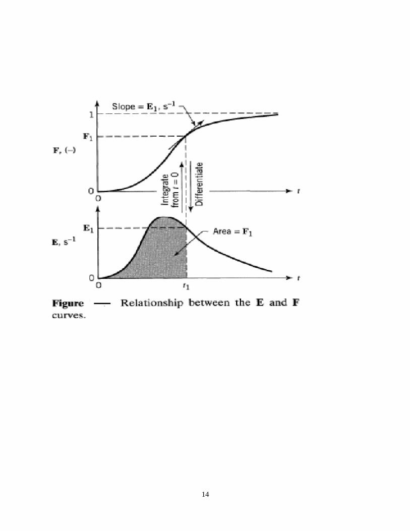
The integral method of analysis always puts a particular rate equation to the test by

integrating and comparing the predicted C versus t curve with the experimental C versus t

data. If the fit is unsatisfactory, another rate equation is guessed and tested. This procedure is

shown in the figure. It should be noted that the integral method is especially useful for fitting

simple reaction types corresponding to

elementary reactions.

1.13.2 Differential method

Plot the concentration versus time data and then carefully draw a smooth curve to represent the

data. This curve will most likely not pass through all experimental points. Determine the slope

of the curve at suitably selected concentration values. These slopes are rates of the reactant

at particular concentration. Search for a rate expression to represent this rate versus

concentration data either by fitting and testing a particular rate equation or by trail and

error method or by testing the nth order equation.

1.14 Irreversible Unimolecular-type first order reaction

First order (unimolecular) reaction:

Suppose we wish to test the first-order rate equation of the following type, for this reaction.

Reaction: A → B

Rate Law: -d[A]/dt = k[A]

Integrated solution: ∫ d[A]/[A] = -k ∫ dt ln [A] = -kt + ln [Ao] [A] = [Ao] e –kt

Separating and integrating we obtain a plot of In (1 - XA) or In (CA/CAo) vs. t, a straight line

through the origin for this form of rate of equation. If the experimental data seems to be

better fitted by a curve than by a straight line, try another rate form because the first-order

reaction does not satisfactorily fit the data.

Fractional conversion XA

Fractional conversion of a reactant A is defined as fractional reactant converted into product at

any time. It is given by the equation, XA = (NAO – NA) / NAO Where ‘NAO’ is the initial

no. of moles of reactant ‘A’ at t = 0. ‘NA‘ is the remaining no. of moles of reactant at any time

‘t’ in the reaction.

1.15 Irreversible Unimolecular-type second order reaction

Second-order reaction (dimerization) (like molecules)

Reaction: 2A → Product

Rate Law: - d[A]/dt = k[A]2

Integrated solution: ∫ d[A]/[A]2 = -k ∫ dt 1/[A] = k (t) + 1/[A0] [A] = A0/(A0kt + 1)

The equation is a hyperbolic equation, and second-order, dimerization kinetics are often

called hyperbolic kinetics.

Bimolecular reactions with different reactants: (unlike molecules)

Reaction: A+B → AB

Rate Law: -d[A]/dt = -d[B]/dt = k[A][B]

Integrated solution:

-rA =CAO dXA/dt = k(CAO-CAOXA)(CBO-CBOXA)

Let M= CBO/CAO be the initial molar ratio of reactants , we obtain

-rA =CAO dXA/dt = kCAO 2( 1-XA)(M-XA)

after breakdown into partial fractions, integration and rearrangement , the final result in a number

of different forms is

ln (1-XB /1-XA) = ln (M-XA/M(1-XA) = ln CBCAO/CBOCA = ln CB/MCA = CAO (M-

1)kt=(CBO-CAO)kt

M≠1

A linear plot will be obtained between the concentration function and time for this second order

rate law.

1.16 Half life

The half-life (t 1/2) for a reaction is the time required for half of the reactants to convert to

products.

For a first-order reaction, t 1/2 is a constant and can be calculated from the rate constant as:

t 1/2 = -ln(0.5)/k = 0.693/k

1.17 Pseudo First order reaction

A second order rate equation which follows the first order rate equation is defined as pseudo First

order reaction. Example: Ester hydrolysis. CH 3COOH + C 2H 5OHCH3 COO C2 H5 + H

2O (A) (B) (C) (D) When C BO >>C Ao, Concentration of H 2O is very large, - rA = - dCA/dt

=k ‘CA

1.18 Zero order reaction

When the rate of the reaction is independent of the concentration of the reactants, it is called

as Zero order reaction. Example: Decomposition of HI

1.19 Third-order reaction

An irreversible trimolecular-type third-order reaction may fall on two categories; Products with

corresponding rate equation(1) The reaction A + B + D -rA = - (dCA/dt) = k CA CB CD. If

CDo is much greater than both CAo and CBo, the reaction becomes second order. Products with

corresponding rate equation(2) The reaction A + 2B -rA = - (dCA/dt) = k CA CB 2 .

1.20 nth order

The empirical rate equation of nth order, -rA = - dCA/dt = k CA n (constant volume).

Separating the variables and integrating, we get CA 1-n - CAo 1-n = (n - 1) k t. Case i) n>1,

CAo 1-n = (1 -n) k t. The slope is (1 - n) k is negative Or the time decreases. Case ii) n

1.21 Steady-State approximation

The kinetics of reactions of this type can also be also analyzed by writing the overall

expression for the rate of change of B and setting this equal to 0. By doing this, we

are making the assumption that the concentration of B rapidly reaches a constant, steady-

state value that does not change appreciably during the reaction. d[B]/dt = k1[A] - k-1[B] -

k2[B] = k1[A] - (k-1+k2) [B] = 0 (k-1+k2)[B] = k1[A] [B] = (k1)/(k-1 + k2) [A] substituting

into d[C]/dt = k2[B] gives: d[C]/dt = (k1k2)/(k-1 + k2) [A] now if k-1 >> k2 d[C]/dt ≈

(k1 k2)/(k-1) [A], if k2 >> k-1 d[C]/dt ≈ (k1k2)/(k2) [A] = k1[A]

Limiting reactant

Usually in a reaction, one of the reactants is present in excess to that required stoichiometrically. If

the reactants are added in stoichiometric amounts, there is no point using the concept of

limiting reactant. The limiting reactant is the one which is consumed first and may be indicated by

dividing the number of moles of each reactant in feed to the corresponding stoichiometric amount

(form a balanced chemical equation) of the reactant. The reactant with the lowest ratio is the limiting

reactant and will be the first to fully consumed in the reaction, if the reaction goes to completion.

Constant volume method: It refers to the volume of reaction mixture, and not the volume

of reactor. It actually means a constant density reaction system, that is, the composition of

reaction mixture is constant.Most of the liquid phase as well as gas phase reactions

occurring in a constant volume bomb fall in this class. In a constant volume system, the

measure of reaction rate of component ‘i’ (reactant 4 or product) becomes ri = (1 / V)

(dNi / dt) = dCi / dt. Conversion of reactant ‘A’ in this method is given by XA = 1 –

(CA/CAo). Variable volume method: It actually means the composition of reaction mixture

varies with time by the presence of inerts. Gas phase reactions involving the presence of inerts

or of impure reactants occurringin a reactor fall in this class. The measure of reaction rate of

component ‘i’ (reactant or product), in this method, i) [d (ln V) / dt).becomes ri = (Cio /In

variable volume system, the fractional change in volume of the system between the initial

and final stage of the reaction will be accounted. Thus, conversion of reactant A

(CA/CAo)].‘A’ becomes XA = [1 – (CA/CAo)] / [1 + ‘A(CA/CAo)]



UNIT – II – Chemical Reaction Engineering – SCHA1411

Reactor Design for Single Reactions

2.1 CLASSIFICATION OF REACTORS

Reactors are classified based on

1. Method of operation: Batch or Continuous reactor

2. Phases: Homogeneous or Heterogeneous reactor

2. 2 REACTOR TYPES

Equipment in which homogeneous reactions are effected can be one of three general types : the

batch , the steady –state flow and the un-steady-state flow or semibatch reactor. The batch

reactor is simple, needs little supporting equipment and is therefore ideal for small scale

experimental studies on reaction kinetics. Industrially it is used when relatively small amounts

of material are to be treated. The steady state flow reactor is ideal for industrial purposes

when large quantities of material are to be processed and when the rate of the reaction is fairly

high to extremely high. Extremely good product quality control can be obtained. This is a

reactor which is widely used in the oil industry. The semibatch reactor is a flexible system but

is more difficult to analyze than the other reactor types. It offers good control of reaction

speed because the reaction proceeds as reactants are added. Such reactors are used in a variety

of applications from the calorimetric titrations in the laboratory to the large open hearth

furnaces for steel production.

2.3 Reactor Design

The starting point for all design is the material balance expressed for any reactant

2.3.1 Material balance

Rate of reactant flow into element of volume =rate of reactant flow out of element of volume

+ rate of reactant loss due to chemical reaction within the element of volume + rate

of accumulation of reactant in element of volume.

In non isothermal operations energy balance must be used in conjunction with material balances

2.3.2 Energy balance

Rate of heat flow into element of volume =rate of heat flow out of element of volume + rate

of disappearance of heat by reaction within the element of volume + rate of accumulation of

heat in element of volume.

2.3.3. Factors to be considered for design of reactor

The different factors required for reactor design are (i) Size of reactor (ii) Type of reactor (iii)

Time or duration of reaction (iv) Temperature & Composition of reacting material in the

reactor (v) Heat removal or added and (vi) Flow pattern of fluid in the reactor.

2.4 Ideal Reactors

Ideal reactors (BR, PFR, and MFR) are relatively easy to treat. In addition, one or other

usually represents the best way of contacting the reactants – no matter what the operation.

For these reason, we often try to design real reactors so that their flows approach these ideals.

2.4.1 Ideal Batch Reactor

A batch reactor (BR) is one in which reactants are initially charged into a container, are

well mixed, and are left to react for a certain period. The resultant mixture is then

discharged. This is an unsteady state operation where composition changes with time;

however at any instant the composition throughout the reactor is uniform. The advantages

of a batch reactor are (i) small instrumentation cost and (ii) flexibility of operation. A batch

reactor has the disadvantages of (i) high labour (ii) poor quality control of the product

and (iii) considerable shutdown time has taken to empty, clean out and refill.

Making a material balance for component A. Noting that no fluid enters or leaves the reaction

mixture

Input = output + disappearance +accumulation (1)

Input = 0

Output = 0

Disappearance of A by reaction moles/time = ( -rA)V

Accumulation of A by reaction moles/time = dNA/dt

By replacing these two terms

( -rA)V = NAO dXA/dt

Rearranging and integrating gives

t= NAO ∫ dXA/ ( -rA)V

t= CAO ∫ dXA/ ( -rA) = - ∫ dCA/ ( -rA) FOR ϵA =0

2.4.2 Space time and space velocity

Space velocity: It is the reciprocal of space time and applied in the analysis of continuous flow

reactors such as plug flow reactor and CSTR. It is defined as the number of rector volumes of a

feed at specified conditions which can be treated in unit time. A space velocity of 10 h ‒1

means that ten reactor volumes of the feed at specified conditions are treated in a reactor per

hour.

Space time and space velocity are the proper performance measures of flow reactors.

Space time

τ = 1/s = time required to process one reactor volume of feed measured at specified conditions

(time)

Space velocity

s= 1/τ = number of reactor volumes of feed at specified conditions which can be treated in

unit time (time-1)

τ = VCAO/FAO = 1/s

Holding time: It is the mean residence time of flowing material in the reactor. It is given by

the expression t = CAo + d XA)/] / [(-rA) (1+ AXA)

For constant density systems (all liquids and constant density gases) t = τ Where ‘V’ is the

volume of the reactor and ‘v’ is the volumetric flow rate of reacting fluid

For constant density systems, the performance equation for Batch reactor and Plug flow

reactor are identical.

2.5 Steady state mixed flow reactor or Continuous stirred tank reactor (CSTR)

Mixed flow reactor (MFR) is also called as back mix reactor or continuous stirred rank reactor

(CSTR) or constant flow stirred tank reactor (CFSTR). In this reactor, the contents are

well stirred and uniform throughout. The exit stream from the reactor has the same composition

as the fluid within the reactor.

Since the composition is uniform throughout , the accounting can be made about the reactor as a

whole.


Accumulation = 0

Input of A.moles /time = FAO

Output of A.moles /time = FA = FAO (1-XA)

Disappearance of A by reaction moles/time = ( -rA)V

Introducing all these terms in eqn 2

FAO XA = ( -rA)V

Which on rearrangement becomes

V/ FAO = τ / CAO = XA / ( -rA)

2.6 Steady state Plug flow reactor or Tubular reactor

Plug flow reactor (PFR) is also referred as slug flow, piston flow, ideal tubular, and unmixed

flow reactor. It specifically refers to the pattern of flow as plug flow. It is characterized by

the fact that the flow of fluid through the reactor is orderly no element of fluid overtaking or

mixing with any other element ahead or behind. Actually, there may be lateral mixing of fluid

in a PFR; however, there must be no mixing or diffusion along the flow path. The necessary

and sufficient condition for plug flow is the residence time in the reactor to be the same for all

elements of fluid


Accumulation = 0

Input of A.moles /time = FAO

Output of A.moles /time = FA + d FA

Disappearance of A by reaction moles/time = ( -rA)dV

Introducing all these terms in eqn 3

FA = FA + d FA + ( -rA)dV

Noting that

d FA = d [FA ( 1-XA) ] = - FAO dXA

we obtain on replacement

FAO dXA = ( -rA)dV

Grouping the terms accordingly and integrating

V/ FAO = τ / CAO = ∫ dXA / ( -rA)

ideal reactors are based on simple models of flow patterns and mixing in the reaction vessel. In

an ideal batch reactor, the concentration and temperature fields are assumed to be spatially

uniform. In practice, the condition can be approximately realized by vigorous agitation

or stirring. In the absence of stirring, beautiful spatial patterns, caused by an interaction

between diffusion and reactions, may develop in some systems . All the elements of the fluid

spend the same amount of time in the reactor, and hence have the same residence time. From

the viewpoint of thermodynamics, a batch reactor represents a closed system. The steady

states of the batch reactor correspond to states of reaction equilibria. Batch reactors

are often used in the pharmaceutical industry, where small volumes of high-value

products are made.

The ideal continuous stirred tank reactor (CSTR) like in an ideal batch reactor, the

concentration and temperature fields in an ideal CSTR are spatially uniform. As there are no

spatial gradients, the species concentrations in the exit stream are identical to the

corresponding values in the reactor. On the other hand, the species concentrations in the

inlet stream are in general different from those in the reactor. Unlike the batch reactor, the

CSTR is an open system as it can exchange heat and mass with the surroundings. Hence it

operates away from equilibrium, and steady states are usually not states of reaction equilibria.

On account of the assumption of perfect mixing, the sequence in which fluid elements leave

the reactor is uncorrelated with the sequence in which they enter. As shown later, this leads

to a distribution of residence times for the fluid leaving the reactor. These reactors are widely

used for polymerization reactions such as the polymerization of styrene, production of

explosives, synthetic rubber, etc. Compared to tubular reactors, CSTRs are easier to clean and

permit better control of the temperature. (c) The plug flow reactor (PFR) The PFR is an

idealization of a tubular reactor. The velocity, temperature, and concentration fields are

assumed to be uniform across the cross section of the reactor. In practice, this situation can be

approximately realized for the case of turbulent flow through a tube with a large ratio of the

length to the diameter. The latter condition ensures that axial mixing has a negligible effect

on the conversion. In a PFR, there is perfect mixing in the radial or transverse direction.

Further, there is no mixing or diffusion in the axial direction. Like a CSTR, the PFR also

represents an open system, and hence steady states are not states of reaction equilibrium.

Owing to the assumption of plug flow, all the fluid elements have the same residence time.

The velocity of the fluid is often treated as a constant, but this assumption must be relaxed

when the density of the fluid changes significantly along the length of the tube. The steady

state equations for a PFR are similar in form to the dynamic equations for an ideal batch

reactor. In many cases, the results for the latter can be translated into results for a PFR

operating at a steady state. Tubular reactors are used for many gas phase and liquid phase

reactions, such as the oxidation of NO and the synthesis of NH3. These reactors are

often modelled as PFRs, but more detailed models involving complications such as radial

gradients, may be required in some cases.

2.7 Steady state reactor

Reactors those in which the properties of the system do not change with time is said to be

a steady state reactor. Example: Continuous stirred Tank reactor, plug flow reactor. Total

mass inflow = Total mass outflow

2.8 Unsteady state reactor

Reactors are those in which the properties of the system changes with time and rate of reaction

decreases with time expect for zero order reaction are said to be unsteady state reactor.

Example: Batch reactor, Semi-batch reactor. There is accumulation in these reactors.

Accumulation = input - output + generation - consumption.

2.9 Semi batch reactor

It is an unsteady state reactor. Reactors which are partially batch and partially continuous are

referred to as semi-batch reactor. The semi batch reactors offers good control of reaction speed,

because the reaction proceeds as reactants are added. Types: (i) volume changes but

composition is unchanged (ii) composition changes but volume is constant.

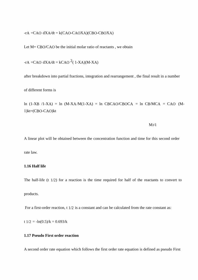
2.10 Recycle reactor

In some reaction system, it is advantageous to divide the product stream and a part returned to

reactor as recycle to increase the conversion rate. These reactors are called recycle reactors. The

recycling provides a means for obtaining various degree of backmixing. Recycle ratio ‘R’ can be

defined as the ratio of the volume fluid returned to the reactor entrance to the volume of fluid

leaving the system or reactor. Significance: Recycle ratio can be made to vary from zero to

infinity. Reflection suggests that as the recycle ratio is raised, the behavior shifts from plug flow

(R = 0) to ). mixed flow (R =).), the recycle reactor. When the recycle ratio ‘R’ becomes or tends

to infinity (R= behaves like a CSTR. When material is to be processed to some fixed final

conversion in a recycle reactor, there must be a particular recycle ratio ‘R’ that minimizes the

reactor volume or space time. That recycle ratio is said to be optimum and the operation is said

to be optimum recycle operation.


UNIT – III - Chemical Reaction Engineering – SCHA1411


DESIGN OF MULTIPLE REACTORS FOR SINGLE REACTIONS

There are many ways of processing a fluid: in a single batch or flow reactor, in a chain of reactors

possibly with interstage feed injection or heating and in a reactor with recycle of the product stream

using various feed ratios and conditions. The reactor system selected will influence the economics

of the process by dictating the size of the units needed and by fixing the ratio of products formed.

The first factor, reactor size, may well vary a hundredfold among competing designs while the

second factor, product distribution, is usually of prime consideration where it can be varied and

controlled. For single reactions product distribution is fixed; hence, the important factor in

comparing designs is the reactor size. The size comparison of various single and multiple ideal

reactor systems is considered.

3.1 SIZE COMPARISON OF SINGLE REACTORS

3.1.1 Batch Reactor

The batch reactor has the advantage of small instrumentation cost and flexibility of operation (may

be shut down easily and quickly). It has the disadvantage of high labor and handling cost, often

considerable shutdown time to empty, clean out, and refill, and poorer quality control of the

product. Hence it may be generalized to state that the batch reactor is well suited to produce small

amounts of material and to produce many different products from one piece of equipment. On the

other hand, for the chemical treatment of materials in large amounts the continuous process is

nearly always found to be more economical.

3.1.2 Mixed Versus Plug Flow Reactors, First- and Second-Order Reactions

For a given duty the ratio of sizes of mixed and plug flow reactors will depend on the extent of

reaction, the stoichiometry, and the form of the rate equation.

- rA = - 1 dNA

----------- = kCAn

V dt

(τ CAO n-1 ) m / (τ CAO n-1 ) m

Is represented by the following graph

To provide a quick comparison of the performance of plug flow with mixed flow reactors, the

performance graph is used. For identical feed composition CAo and flow rate FA, the ordinate of

this figure gives directly the volume ratio required for any specified conversion.

1. For any particular duty and for all positive reaction orders the mixed reactor is always

larger than the plug flow reactor. The ratio of volumes increases with reaction order.

2. When conversion is small, the reactor performance is only slightly affected by flow type.

The performance ratio increases very rapidly at high conversion; consequently, a proper

representation of the flow becomes very important in this range of conversion.

3. Density variation during reaction affects design; however, it is normally of secondary

importance compared to the difference in flow type. Dashed lines represent fixed values of the

dimensionless reaction rate group, defined as

kτ for first-order reaction

kCA0τ for second-order reaction

With these lines we can compare different reactor types, reactor sizes, and conversion levels.

Second-order reactions of two components and of the type behave as second-order reactions of

one component when the reactant ratio is unity. Thus

-rA = kCACB = kc; when M = 1

On the other hand, when a large excess of reactant B is used then its concentration does not

change appreciably (CB= CBO) and the reaction approaches first-order behavior with respect to

the limiting component A, or

-rA = kCACB = (kCBO)C=A krCA when M + 1

Thus terms of the limiting component A, the size ratio of mixed to plug flow reactors is

represented by the region between the first-order and the second-order curves.

For reactions with arbitrary but known rate the performance capabilities of mixed and plug flow

reactors are best illustrated in above figure. The ratio of shaded and of hatched areas gives the ratio

of space-times needed in these two reactors. The rate curve drawn in above figure is typical of the

large class of reactions whose rate decreases continually on approach to equilibrium (this includes

all nth-order reactions, n > 0). For such reactions it can be seen that mixed flow always needs a

larger volume than does plug flow for any given duty.

3.2 Plug Flow Reactors in Series and / or in Parallel

Consider N plug flow reactors connected in series, and let X1, X2, . . . , XN, be the fractional

conversion of component A leaving reactor 1, 2, . . . , N. Basing the material balance on the feed

rate of A to the first reactor, we find for the

ith reactor

Vi/ FO = τ i/ CAO = ∫ dX /( -r)

or for the N reactors in series

V/ FO =Ʃ Vi / FO = ∫ dX/( -r)

Hence, N plug flow reactors in series with a total volume V gives the same conversion as a

single plug flow reactor of volume V.

3.2.1 Operating A Number Of Plug Flow Reactors

The reactor setup shown in Figure consists of three plug flow reactors in two parallel branches.

Branch D has a reactor of volume 50 liters followed by a reactor of volume 30 liters. Branch E has

a reactor of volume 40 liters. What fraction of the feed should go to branch D?

Branch D consists of two reactors in series; hence, it may be considered to be a single reactor of

volume

VD = 50 + 30 = 80 liters

Now for reactors in parallel V/F must be identical if the conversion is to be the same in each

branch. Therefore, two-thirds of the feed must be fed to branch D.

3.3 Equal-Size Mixed Flow Reactors in Series

In plug flow, the concentration of reactant decreases progressively through the system; in mixed

flow, the concentration drops immediately to a low value. Because of this fact, a plug flow reactor

is more efficient than a mixed flow reactor for reactions whose rates increase with reactant

concentration, such as nth-order irreversible reactions, n > 0. Consider a system of N mixed flow

reactors connected in series. Though the concentration is uniform in each reactor, there is,

nevertheless, a change in concentration as fluid moves from reactor to reactor. This stepwise drop

in concentration, illustrated in above figure, suggests that the larger the number of units in series,

the closer should the behavior of the system approach plug flow. This will be shown to be so.

Quantitatively evaluate the behavior of a series of N equal-size mixed flow reactors. Density

changes will be assumed to be negligible; hence ρ = 0 . As a rule, with mixed flow reactors it is

more convenient to develop the necessary equations in terms of concentrations rather than

fractional conversions.

3.4 Comparison Charts

At present 90% of reactant A is converted into product by a second-order reaction in a single

mixed flow reactor. We plan to place a second reactor similar to theone being used in series with

it.

(a) For the same treatment rate as that used at present, how will this additionaffect the conversion

of reactant?

For the same 90% conversion, by how much can the treatment rate be increased?

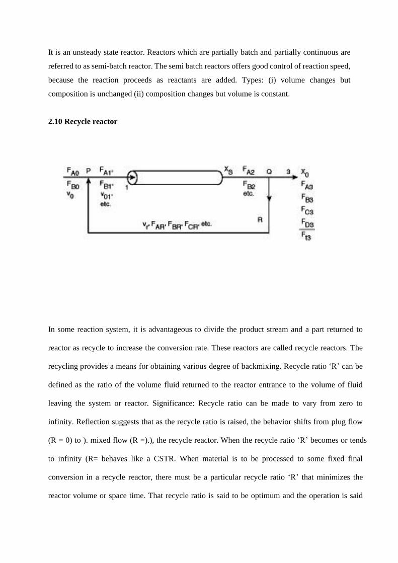
(a) Find the conversion for the same treatment rate. For the single reactor at 90% conversion

we have from chart

kCoτ = 90

For the two reactors the space-time or holding time is doubled; hence, the operation will be

represented by the dashed line of chart where

kCoτ= 180

This line cuts the N = 2 line at a conversion X = 97.4%, point a.

(b) Find the treatment rate for the same conversion. Staying on the 90% conversion

line, we find for N = 2 that

kCoτ = 27.5, point b

Comparing the value of the reaction rate group for N = 1 and N = 2, we find

Since V2 = 2V1 the ratio of flow rates becomes

Thus, the treatment rate can be raised to 6.6 times the original.

3.5 Mixed Flow Reactors of Different Sizes in Series

For arbitrary kinetics in mixed flow reactors of different size, two types of questions may be

asked: how to find the outlet conversion from a given reactor system, and the inverse question,

how to find the best setup to achieve a given conversion. Different procedures are used for these

two problems.

3.5.1 Finding the Conversion in a Given System

A graphical procedure for finding the outlet composition from a series of mixed flow reactors of

various sizes for reactions with negligible density change has been presented by Jones (1951). All

that is needed is an r versus C curve for component A to represent the reaction rate at various

concentrations. It is illustrated by the use of this method by considering three mixed flow reactors

in series with volumes, feed rates, concentrations, space-times (equal to residence timesbecause ρ

= O), and volumetric flow rates as shown in figure below. Now from equation noting that ρ = 0,

we may write for component A in the first reactor

τ 1 = V1/ v = CO-C1/( -

r1) -1/ τ 1 = ( -r1) / C1-

C0

For i th reactor

-1/ τ i = ( -ri) / Ci-Ci-1

Plot the C versus r curve for component A and it is as shown in figure above. To find the conditions

in the first reactor note that the inlet concentration Co is known (point L), that C, and ( - r ) ,

correspond to a point on the curve to be found (point M), and that the slope of the line LM = MNINL

= (-r),l (C, - Co) = -(l/rl) from equation. Hence, from Co draw a line of slope - (l/r,) until it cuts the

rate curve; this gives C1. Similarly, we find from equation, that a line of slope -(1/r2) from point N

cuts the curve at P, giving the concentration C2 of material leaving the second reactor. This procedure

is then repeated as many times as needed. With slight modification this graphical method can be

extended to reactions in which density changes are appreciable.

3.5.2 Determining the Best System for a Given Conversion

To find the minimum size of two mixed flow reactors in series to achieve a specified conversion of

feed which reacts with arbitrary but known kinetics, the following procedure is followed. The basic

performance expressions, from equations, give, in turn, for the first reactor

τ 1/ Co = X 1 / (-r1)

and for the second reactor

τ 2 / Co = X 2- X 1 / (-r2)

as the intermediate conversion XI changes, so does the size ratio of the units (represented by the two

shaded areas) as well as the total volume of the two vessels required (the total area shaded). Figure

shows that the total reactor volume is as small as possible (total shaded area is minimized) when the

rectangle KLMN is as large as possible. This brings us to the problem of choosing XI (or point M on

the curve) so as to maximize the area of this rectangle. This is done according to Maximization of

Rectangles concept.In the below figure, construct a rectangle between the x-y axes and touching the

arbitrary curve at point M(x, y). The area of the rectangle is then

A =xy

This area is maximized when

da = 0 =xdy+ydx

or when –dy/dx =y/x

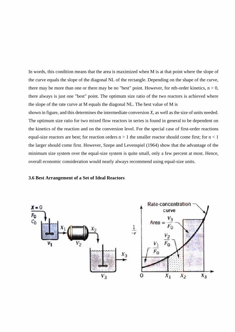
In words, this condition means that the area is maximized when M is at that point where the slope of

the curve equals the slope of the diagonal NL of the rectangle. Depending on the shape of the curve,

there may be more than one or there may be no "best" point. However, for nth-order kinetics, n > 0,

there always is just one "best" point. The optimum size ratio of the two reactors is achieved where

the slope of the rate curve at M equals the diagonal NL. The best value of M is

shown in figure, and this determines the intermediate conversion X, as well as the size of units needed.

The optimum size ratio for two mixed flow reactors in series is found in general to be dependent on

the kinetics of the reaction and on the conversion level. For the special case of first-order reactions

equal-size reactors are best; for reaction orders n > 1 the smaller reactor should come first; for n < 1

the larger should come first. However, Szepe and Levenspiel (1964) show that the advantage of the

minimum size system over the equal-size system is quite small, only a few percent at most. Hence,

overall economic consideration would nearly always recommend using equal-size units.

3.6 Best Arrangement of a Set of Ideal Reactors

For the most effective use of a given set of ideal reactors we have the following general rules:

1. For a reaction whose rate-concentration curve rises monotonically (any nth-order reaction, n >

0) the reactors should be connected in series. They should be ordered so as to keep the concentration

of reactant as high as possible if the rate-concentration curve is concave (n > I), and as low as possible

if the curve is convex (n < 1). As an example, for the case of above figure the ordering of units should

be plug, small mixed, large mixed, for n > 1; the reverse order should be used when n < 1.

2. For reactions where the rate-concentration curve passes through a maximum or minimum the

arrangement of units depends on the actual shape of curve, the conversion level desired, and the units

available. No simple rules can be suggested.

3. Whatever may be the kinetics and the reactor system, an examination of the l/(-r) vs. CA curve is

a good way to find the best arrangement of units.



UNIT – IV - Chemical Reaction Engineering – SCHA1411

2

3

4

5

6

7

8

9

10

11

12

13

(2)

14

15

16

17

18

19

20

Book Reference 1. Octave Levenspiel, Chemical Reaction Engineering, 3rd Edition,

Wiley Publications Ltd., 2007.

2. Smith. J.M., Chemical Engineering Kinetics, 3rd Edition, McGraw

Hill, 1981. 3. Gavhane. K. A,. Chemical Reaction Engineering – II, 2nd Edition,

Nirali Prakashan, 2013.

4. Fogler.H.S., Elements of Chemical Reaction Engineering, 3rd Edition, Prentice Hall of India Ltd., 2001.

5. Froment. G.F and Bischoff.K.B.,Chemical Reactor Analysis and

Design, 2nd Edition, John Wiley and Sons, 1979.


UNIT – 5 CATALYTIC REACTIONS SCHA1411


Catalytic Reaction Kinetic Model

Introduction:

This section deals with the class off heterogeneous reactions in which a gas or liquid

contacts with a solid, reacts with it, and transform it into product. Such reactions may

be represented by:

A(fluid) + bB(Solid) fluid products

Solid products

fluid and solid products

Fluid-solid reactions are numerous and of great industrial importance. Those in which

the solid does not appreciably change in size during reaction are as follows:

a) The roasting (or oxidation) of sulfide ores to yield the metal oxides. For example, in

the preparation of zinc oxide the sulfide ore is mined, crushed, separated from the

gangue by flotation, and then roasted in a reactor to form hard white zinc oxide

particles according to the reaction.

Similarly, iron pyrites reacts as follows:

b) The preparation of metals from their oxides by reaction in reducing atmospheres.

For example, iron is prepared from crushed and sized magnetite ore in continuous-

countercurrent, three stage, fluidized bed reactors according to the reaction:

The most common example of reactions where the solid changes its size are

carbonaceous reactions. For example, with an insufficient amount of air, producer gas

is formed by the following reactions:

------- (1)

------- (2)

------- (3)

With steam, water gas is obtained by the reactions-

Still other examples are the dissolution reactions, the attack of metal chips by acids, and

the rusting of iron.

Selection of a Model

The requirement for a good engineering model is that it be the closest representation of

reality which can be treated without too many mathematical complexities. It is of little

use to select a model which very closely mirrors reality but which is so complicated that

we cannot do anything with it. Unfortunately, in today's age of computers, this all too

often happens.

For the non-catalytic reaction of particles with surrounding fluid, we consider two

simple idealized models, the progressive-conversion model and the shrinking

unreacted-core model.

Progressive-Conversion Model (PCM):

In present model, we assume that reactant gas enters and reacts throughout the particle

at all times, most likely at different rates at different locations within the particle. Thus,

solid reactant is converted continuously and progressively throughout the particle as

shown in Figure 2.8.

Figure 2.8: According to the PCM, reaction proceeds continuously throughout the solid particle

Shrinking-Core Model:

In this model a different approach of reaction taking place within solid surface has been

visualized. In this visualization, we assume that the reaction occurs first at the outer skin

of the particle. The reaction zone is then moves into the solid and leaves behind

completely converted material and inert solid. This is referred to as “ash”. Thus, at any

time there exists an unreacted core of material which shrinks in size during reaction, as

shown in Figure 2.9.

Figure 2.9: According to the shrinking-core model, reaction proceeds at a narrow front which moves

into the solid particle. Reactant is completely converted as the front passes by.

In most cases the shrinking-core model (SCM) approximates real particles more closely

than does the progressive-conversion model (PCM).

SHRINKING-CORE MODEL FOR SPHERICAL PARTICLES OF

UNCHANGING SIZE:

Since the SCM seems to reasonably represent reality in a wide variety of situations, we

need to develop its kinetic equations in the following section. In doing this we consider

the surrounding fluid to be a gas. However, this is done only for convenience since the

analysis applies equally well to liquids.

The model was first developed by Yagi and Kunii (1955, 1961), who visualized five

steps occurring in succession during reaction as described by figure 2.10.

Figure 2.10: Representation of concentrations of reactants and products for the reaction

A(g) + bB(s) solid product for a particle of unchanging size.

Step 1. Diffusion of gaseous reactant A through the film surrounding the particle to the

surface of the solid.

Step 2. Penetration and diffusion of A through the blanket of ash to the surface of the

unreacted core.

Step 3. Reaction of gaseous A with solid at this reaction surface.

Step 4. Diffusion of gaseous products through the ash back to the exterior surface of the

solid.

Step 5. Diffusion of gaseous products through the gas film back into the main body of

fluid.

The above mentioned steps can vary according to the reactions. For example, if there is

no gaseous products generation then step 4 & 5 is neglected and does not contribute

towards resistance to the reaction. In the analysis of determining kinetic model we will

only consider the resistances from step 1, 2 & 3.

1. Diffusion through gas film controls:

Whenever the resistance of the gas film controls, the concentration profile for

gaseous reactant A will be shown as in figure 2.11.

Figure 2.11: Representation of a reacting particle when diffusion through the gas film is the

controlling resistance.

From the above figure we can observe that, no gaseous reactant is present at the

particle surface; hence, the concentration driving force, CAg – CAs becomes CAg and

is constant at all times during reaction of the particle. Considering the stoichiometry

from equations 1, 2 & 3, and taking unchanging exterior surface as Sex we can write

–

------- (4)

let ρB, be the molar density of B in the solid and V be the volume of a particle, the

amount of B present in a particle is –

The decrease in volume or radius of unreacted core accompanying the disappearance

of dNB moles of solid reactant is then given by –

Replacing eqn 6 in 4 gives the rate of reaction in terms of the shrinking radius of

unreacted core, or –

where kg is the mass transfer coefficient between fluid and particle. Rearranging and

integrating eqn 7 –

let the time for complete conversion of a particle be τ, then by taking rc = 0 in eqn 8

we get –

The radius of unreacted core in terms of fractional time for complete conversion is

obtained by combining Eqs. 8 and 9, or

------- (5)

------- (6)

------- (7)

------- (8)

------- (9)

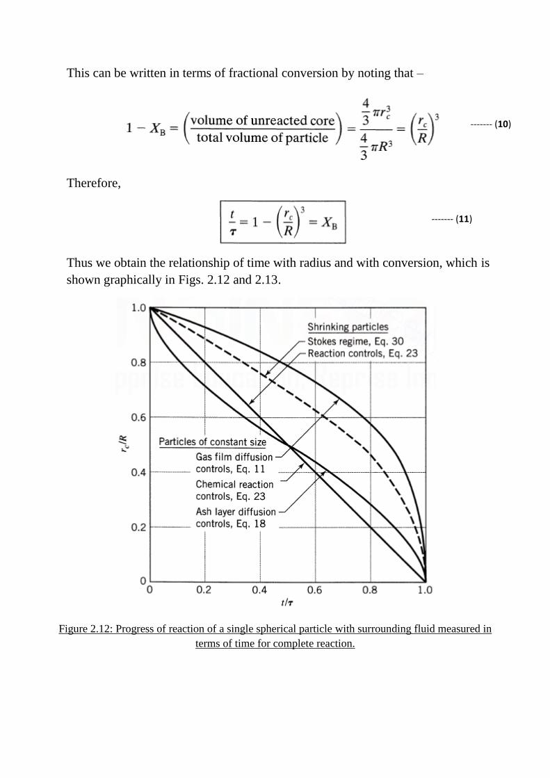
This can be written in terms of fractional conversion by noting that –

Therefore,

Thus we obtain the relationship of time with radius and with conversion, which is

shown graphically in Figs. 2.12 and 2.13.

Figure 2.12: Progress of reaction of a single spherical particle with surrounding fluid measured in

terms of time for complete reaction.

------- (10)

------- (11)

Figure 2.13: Progress of reaction of a single spherical particle with surrounding fluid measured in

terms of time for complete reaction.

2. Diffusion through Ash Layer Controls:

Figure 2.14 illustrates the situation in which the resistance to diffusion through the

ash controls the rate of reaction. To develop an expression between time and radius,

such as Eq. 8 for film resistance, requires a two-step analysis. First examine a typical

partially reacted particle, writing the flux relationships for this condition. Then apply

this relationship for all values of rc; in other words, integrate r, between R and 0.

Consider a partially reacted particle as shown in Fig. 2.14. Both reactant A and the

boundary of the unreacted core move inward toward the center of the particle. But

for GIS systems the shrinkage of the unreacted core is slower than the flow rate of

A toward the unreacted core by a factor of about 1000, which is roughly the ratio of

densities of solid to gas. Because of this it is reasonable for us to assume, in

considering the concentration gradient of A in the ash layer at any time that the

unreacted core is stationary.

Figure 2.14: Representation of a reacting particle when diffusion through the ash layer is the

controlling resistance.

For GIS systems the use of the steady-state assumption allows great simplification

in the mathematics which follows. Thus the rate of reaction of A at any instant is

given by its rate of diffusion to the reaction surface, or –

For convenience, let the flux of A within the ash layer be expressed by Fick's law for

equimolar counter diffusion. Then, noting that both QA and dCA/dr are positive, we

have –

where De is the effective diffusion coefficient of gaseous reactant in the ash layer.

------- (12)

------- (13)

Combining equations 12 & 13 for any r,

Integrating across the ash layer from R to rc, we obtain

or,

The above expression represents the conditions of a reacting particle at any time.

In the second part of the analysis we let the size of unreacted core change with time.

For a given size of unreacted core, dNA/dt is constant; however, as the core shrinks

the ash layer becomes thicker, lowering the rate of diffusion of A. Consequently, Eq.

15 contains three variables, t, NA, and rc, one of which must be eliminated or written

in terms of the other variables before integrating the equation with respect to time

and other variables. As with film diffusion, let us eliminate NA by writing it in terms

of rc. This relationship is given by Eq. 6; hence, replacing in Eq. 15, separating

variables, and integrating, we obtain –

For the complete conversion of a particle, rc = 0, and the time required is –

The progression of reaction in terms of the time required for complete conversion is

found by dividing equation 16 by equation 17, or

------- (14)

------- (15)

------- (16)

------- (17)

which in terms of fractional conversion, as given in equation 10, becomes –

The above results are presented graphically by figures 2.12 & 2.13.

3. Chemical Reaction Controls:

Figure 2.15 illustrates concentration gradients with in a particle when chemical

reaction controls.

Figure 2.15: Representation of a reacting particle when chemical reaction is the controlling resistance,

the reaction being A(g) + bB(s) products.

Since the progress of the reaction is unaffected by the presence of any ash layer, the

rate is proportional to the available surface of unreacted core. Thus, based on unit

surface of unreacted core, rc, the rate of reaction for the stoichiometry of equations

1, 2 & 3, is –

------- (18a)

------- (18b)

------- (19)

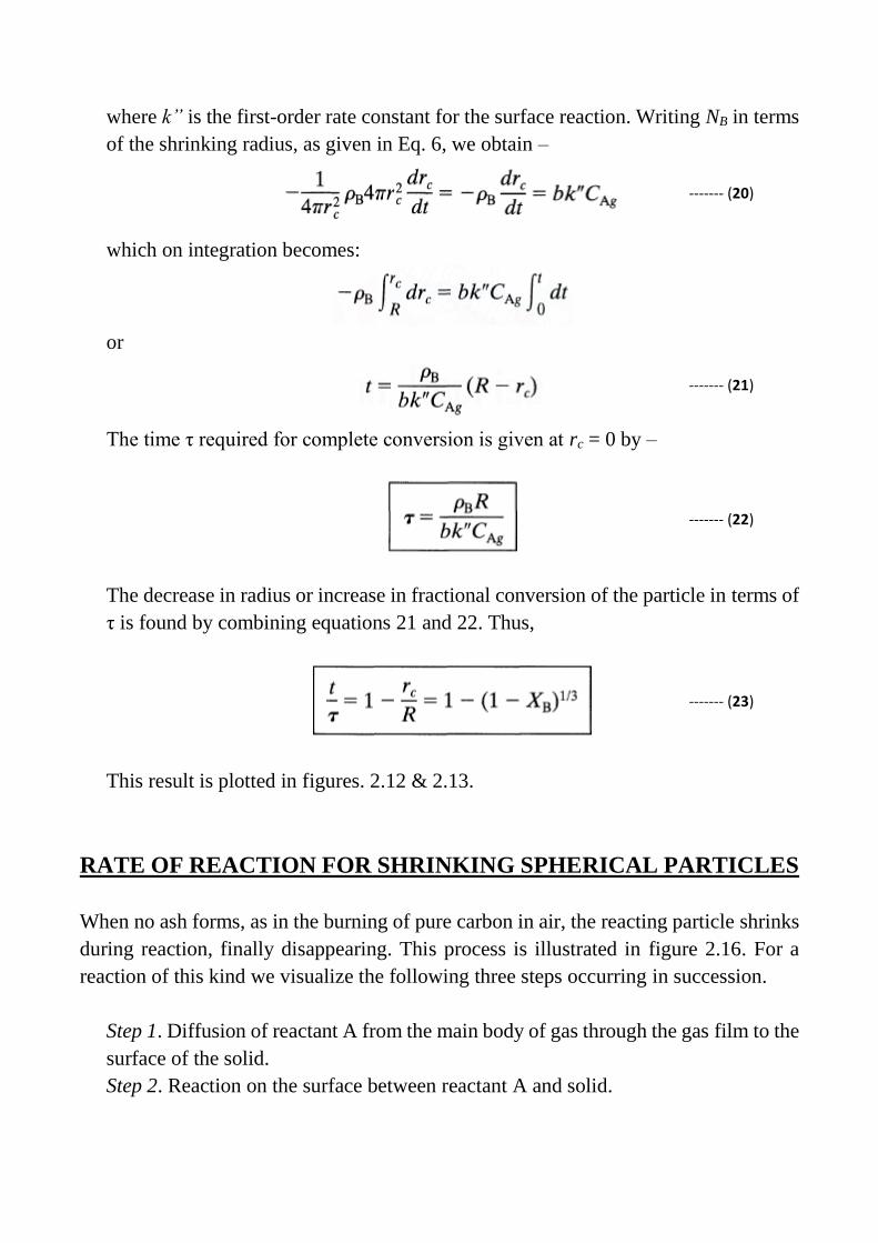
where k” is the first-order rate constant for the surface reaction. Writing NB in terms

of the shrinking radius, as given in Eq. 6, we obtain –

which on integration becomes:

or

The time τ required for complete conversion is given at rc = 0 by –

The decrease in radius or increase in fractional conversion of the particle in terms of

τ is found by combining equations 21 and 22. Thus,

This result is plotted in figures. 2.12 & 2.13.

RATE OF REACTION FOR SHRINKING SPHERICAL PARTICLES

When no ash forms, as in the burning of pure carbon in air, the reacting particle shrinks

during reaction, finally disappearing. This process is illustrated in figure 2.16. For a

reaction of this kind we visualize the following three steps occurring in succession.

Step 1. Diffusion of reactant A from the main body of gas through the gas film to the

surface of the solid.

Step 2. Reaction on the surface between reactant A and solid.

------- (20)

------- (21)

------- (22)

------- (23)

Step 3. Diffusion of reaction products from the surface of the solid through the gas

film back into the main body of gas. Note that the ash layer is absent and does not

contribute any resistance.

As with particles of constant size, let us see what rate expressions result when one or

the other of the resistances controls.

Figure 2.16: Representation of concentration of reactants and products for the reaction

A(g) + bB(s) rR(g) between a shrinking solid particle and gas.

1. Chemical Reaction Control:

When chemical reaction controls, the behavior is identical to that of particles of

unchanging size; therefore, Fig. 25.7 and Eq. 21 or 23 will represent the conversion-

time behavior of single particles, both shrinking and of constant size.

2. Gas Film Diffusion Controls:

Film resistance at the surface of a particle is dependent on numerous factors, such as

the relative velocity between particle and fluid, size of particle, and fluid properties.

These have been correlated for various ways of contacting fluid with solid, such as

packed beds, fluidized beds, and solids in free fall. As an example, for mass transfer

of a component of mole fraction y in a fluid to free-falling solids Froessling (1938)

gives –

During reaction a particle changes in size; hence kg also varies. In general kg rises for

an increase in gas velocity and for smaller particles. As an example eqn. 24 shows

that –

Equation 25 represents particles in Stokes law regime. Now we will develop

expression for conversion-time for such particles.

Stokes Regime (Smaller particles): When a particle, originally of size R0 has

shrunk to size R, we may write –

Thus, similar to equation 7, we have

Since in the Stokes regime equation 24 reduces to

combining equation 27 & 28 and integrating

------- (24)

------- (25)

------- (26)

------- (27)

------- (28)

or,

The time for complete disappearance of a particle is thus

and on combining we get

This relationship of size versus time for shrinking particles in the Stokes regime is

shown in Figs. 2.12 and 2.13, and it well represents small burning solid particles and

small burning liquid droplets.

Particles of Different Shape: Conversion-time equations similar to those developed

above can be obtained for various –shaped particles, and table 2.2 summarizes these

expressions.

------- (29)

------- (30)

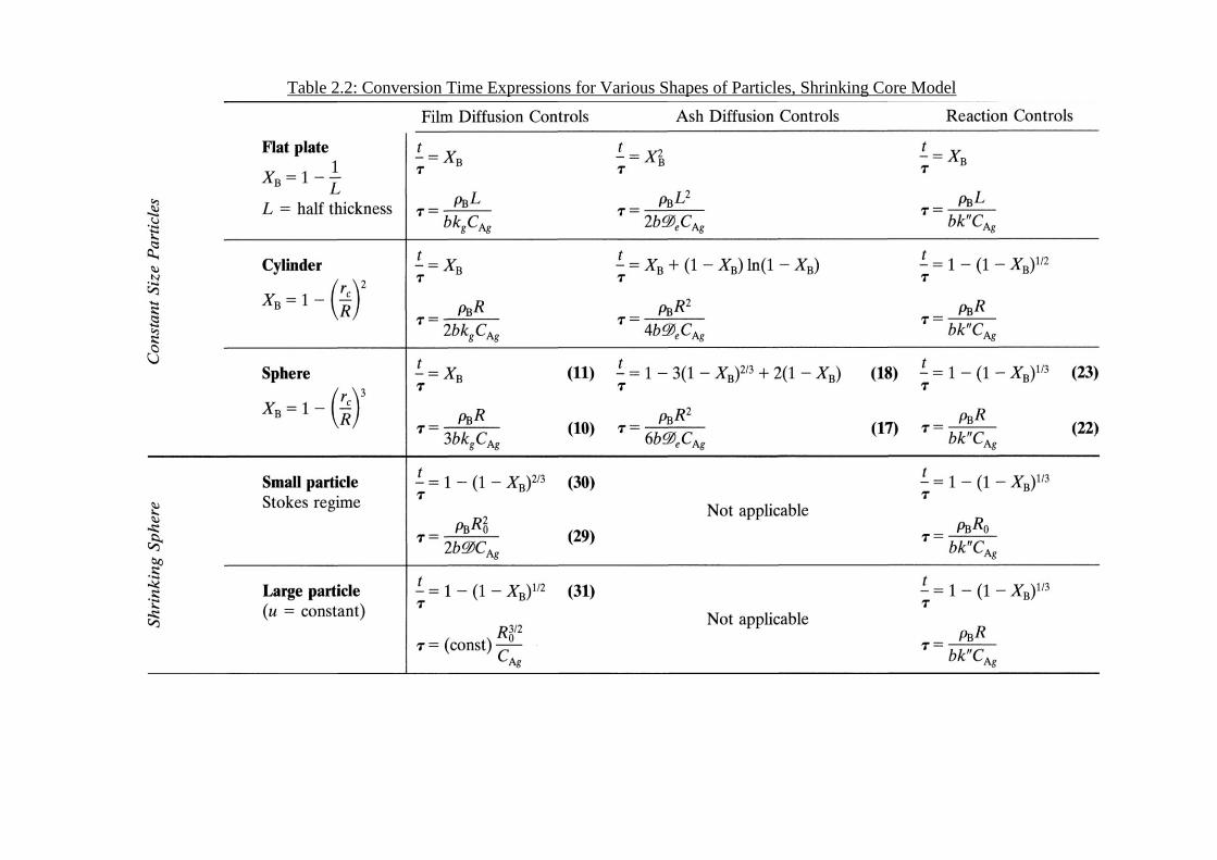
Table 2.2: Conversion Time Expressions for Various Shapes of Particles, Shrinking Core Model

DETERMINATION OF THE RATE-CONTROLLING STEP

The kinetics and rate-controlling steps of a fluid-solid reaction are deduced by noting

how the progressive conversion of particles is influenced by particle size and operating

temperature. This information can be obtained in various ways, depending on the

facilities available and the materials at hand. The following observations are a guide to

experimentation and to the interpretation of experimental data.

a) Temperature: The chemical step is usually much more temperature-sensitive than

the physical steps; hence, experiments at different temperatures should easily

distinguish between ash or film diffusion on the one hand and chemical reaction on

the other hand as the controlling step.

b) Time: Figures 2.12 and 2.13 show the progressive conversion of spherical solids

when chemical reaction, film diffusion, and ash diffusion in turn control. Results of

kinetic runs compared with these predicted curves should indicate the rate

controlling step. Unfortunately, the difference between ash diffusion and chemical

reaction as controlling steps is not great and may be masked by the scatter in

experimental data.

c) Particle Size: Equations 8, 16 and 21, along with equations 24 and 25 shows that the

time needed to achieve the same fractional conversion for particle of different but

unchanging sizes is given by –

Thus kinetic runs with different sizes of particles can distinguish between reactions

in which the chemical and physical steps control.

d) Ash versus Film Resistance: When a hard solid ash forms during reaction, the

resistance of gas-phase reactant through this ash is usually much greater than through

the gas film surrounding the particle. Hence in the presence of a non-flaking ash

layer, film resistance can safely be ignored. In addition, ash resistance is unaffected

by changes in gas velocity.

e) Predictability of Film Resistance: The magnitude of film resistance can be

estimated from dimensionless correlations such as eqn. 24. Thus an observed rate

approximately equal to the calculated rate suggests that film resistance controls.

2

Catalysts work by providing alternative mechanism involving a different transition

state of lower energy. Thereby, the activation energy of the catalytic reaction is

lowered compared to the uncatalyzed reaction as shown in Fig 3.1.

Figure 3.1 Comparison of activation energies of exothermic catalytic and non-

catalytic reactions

A catalyst accelerates both the rates of the forward and reverse reaction.

Equilibrium of a reversible reaction is not altered by the presence of the catalyst.

For example, when oxidation of SO2 is carried out in the presence of three different

catalysts, namely Pt, Fe2O3 and V2O5, the equilibrium composition is the same in

all three cases. Another important characteristic of catalyst is its effect on

selectivity. The presence of different catalysts can result in different product

distribution from the same starting material. For example, decomposition of

ethanol in the presence of different catalysts results in different products as shown

CATALYSTS AND CATALYTIC REACTIONS

Because the chemical, petrochemical, and petroleum industries rely heavily on

catalytic processing operations and because of the utility of catalysts in

remediating environmental problems (e.g., emissions from motor vehicles),chemical

engineers must be cognizant of the fundamental and applied aspects of catalysis.

In more modern terms the following definition is appropriate: A catalyst is a

substance that affects the rate or the direction of a chemical reaction, but is not

appreciably consumed in the process. There are three important aspects of the

definition. First, a catalyst may increase or decrease the reaction rate. Second, a

catalyst may influence the direction or selectivity of a reaction. Third, the amount

of catalyst consumed by the reaction is negligible compared to the consumption of

reactants.

3

below.

Types of catalytic reactions

Catalytic reactions can be divided into two main types –

1. Heterogeneous

2. Homogeneous

Heterogeneous catalysis

In heterogeneous catalytic reaction, the catalyst and the reactants are in different

phases. Reactions of liquid or gases in the presence of solid catalysts are the typical

examples. An example is the Contact Process for manufacturing sulphuric acid, in

which the sulphur dioxide and oxygen are passed over a solid vanadium oxide

catalyst producing sulphur trioxide. Several hydrocarbon transformation reactions

such as cracking, reforming, dehydrogenation, and isomerization also fall in this

category.

Homogeneous catalysis

In a homogeneous catalytic reaction, the catalyst is in the same phase as the

reactants. Typically, all the reactants and catalysts are either in one single liquid

phase or gas phase. Most industrial homogeneous catalytic processes are carried

out in liquid phase. Ester hydrolysis involving general acid-base catalysts,

polyethylene production with organometallic catalysts and enzyme catalysed

processes are some of the important examples of industrial homogeneous catalytic

processes.

SURFACE AREA AND ADSORPTION

Since a catalytic reaction occurs at the fluid-solid interface, a large interfacial area

can be helpful or even essential in attaining a significant reaction rate. In many

catalysts, this area is provided by a porous structure; the solid contains many fine

pores, and the surface of these pores supplies the area needed for the high rate of

reaction. The area possessed by some porous materials is surprisingly large. A

typical silica-alumina cracking catalyst has a pore volume of 0.6 cm3/g and an

average pore radius of 4 nm. The corresponding surface area is 300 m2/g.

A catalyst that has a large area resulting from pores is called a porous catalyst.

Examples of these include the Raney nickel used in the hydrogenation of vegetable

and animal oils, the platinum-on-alumina used in the reforming of petroleum

naphtha to obtain higher octane ratings, and the promoted iron used in ammonia

synthesis. Sometimes pores are so small that they will admit small molecules but

prevent large ones from entering. Materials with this type of pore are called

4

molecular sieves, and they may be derived from natural substances such as certain

clays and zeolites, or be totally synthetic.

Not all catalysts need the extended surface provided by a porous structure,

however. Some are sufficiently active so that the effort required to create a porous

catalyst would be wasted. For such situations one type of catalyst is the monolithic

catalyst. Monolithic catalysts are normally encountered in processes where

pressure drop and heat removal are major considerations.

For the moment, let us focus our attention on gas-phase reactions catalysed by

solid surfaces. The molecules at a surface of a material experience imbalanced

forces of intermolecular interaction which contribute to the surface energy. It

causes accumulation of molecules of a solute or gas in contact with the substance.

This preferential accumulation of substrate molecules at the surface is called

adsorption which is purely surface phenomenon.

The surface active material is referred to as the adsorbent and the molecules which

are accumulated on the adsorbent called adsorbate molecules. The strength by

which adsorbate molecules are attached with the adsorbents determines the nature

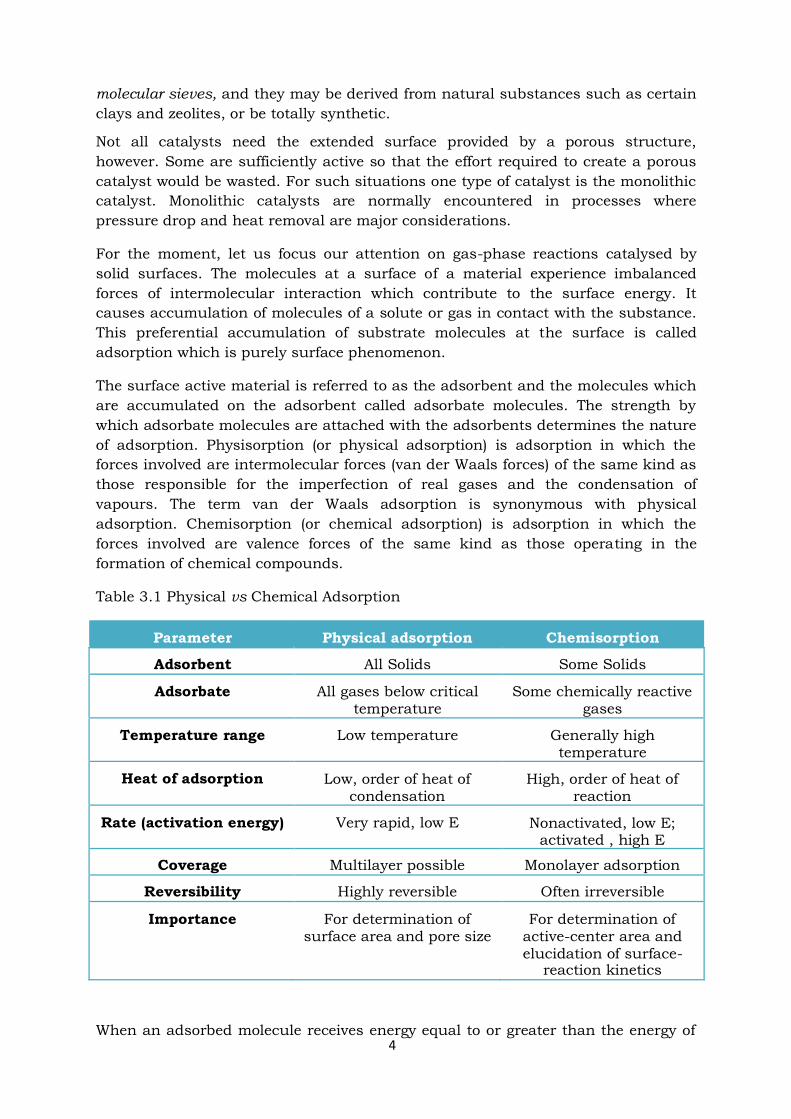
of adsorption. Physisorption (or physical adsorption) is adsorption in which the

forces involved are intermolecular forces (van der Waals forces) of the same kind as

those responsible for the imperfection of real gases and the condensation of

vapours. The term van der Waals adsorption is synonymous with physical

adsorption. Chemisorption (or chemical adsorption) is adsorption in which the

forces involved are valence forces of the same kind as those operating in the

formation of chemical compounds.

Table 3.1 Physical vs Chemical Adsorption

Parameter Physical adsorption Chemisorption

Adsorbent All Solids Some Solids

Adsorbate All gases below critical temperature

Some chemically reactive gases

Temperature range Low temperature Generally high temperature

Heat of adsorption Low, order of heat of condensation

High, order of heat of reaction

Rate (activation energy) Very rapid, low E Nonactivated, low E; activated , high E

Coverage Multilayer possible Monolayer adsorption

Reversibility Highly reversible Often irreversible

Importance For determination of surface area and pore size

For determination of active-center area and

elucidation of surface- reaction kinetics

When an adsorbed molecule receives energy equal to or greater than the energy of

5

adsorption, it will leave the surface. This phenomenon is the reverse of adsorption

and is called as desorption. When the number of molecules striking the surface and

staying there is equal to the number of molecules that are leaving (evaporating) the

surface is called to be in equilibrium.

Adsorption Isotherms

A relation between the amount of adsorbate adsorbed on a given surface at

constant temperature and the equilibrium concentration of the substrate in contact

with the adsorbent is known as Adsorption Isotherm. They are generally classified

in the five main categories. In Figure 3.2, adsorbate partial pressures (P) are

normalized by dividing by the saturation pressure at the temperature in question

(P0).

Figure 3.2 Five types of isotherms for adsorption.

6

Type I, referred to as Langmuir-type adsorption, is characterized by a monotonic

approach to a limiting amount of adsorption, which presumably corresponds to

formation of a monolayer. This type of behaviour is that expected for

chemisorption. No other isotherms imply that one can reach a saturation limit

corresponding to completion of a monolayer.

Type II is typical of the behaviour normally observed for physical adsorption. At

values of P∕P0 approaching unity, capillary and pore condensation phenomena

occur. The knee of the curve corresponds roughly to completion of a monolayer. A

statistical monolayer is built up at relatively low values of P∕P0 (0.1 to 0.3).

Type IV behaviour is similar to type II behaviour except that a limited pore volume

is indicated by the horizontal approach to the right-hand ordinate axis. This type of

curve is relatively common for porous structures of many kinds. Hysteresis effects

associated with pore condensation are often, but not always, encountered in this

type of system. They arise from the effects of surface curvature on vapour pressure.

Types III and V are relatively rare. They are typical of cases in which the forces

giving rise to monolayer adsorption are relatively weak. Type V differs from type III

in the same manner that type IV differs from type II.

Freundlich Adsorption Isotherm

It is an empirical relation between the amount of an adsorbate adsorbed per unit

weight (x/m, mg/g) of adsorbent and the adsorbate equilibrium concentration

(Ce,moles/l) in the fluid as follows:

Where, K and n are Freundlich coefficients x = weight of adsorbate adsorbed on m unit weight of adsorbent Ce = equilibrium concentration of adsorbate

From equation (3.1), we get

(3.2)

The coefficients K and n can be determined from the intercept and slope of a plot of

log(x/m) versus logCe.

Langmuir Adsorption Isotherm

In the Langmuir model the adsorbent surface is considered to possess a number of

active interaction sites for adsorption. Langmuir derived a relation between

adsorbed material and its equilibrium concentration. His assumptions are:

1. There are fixed adsorption sites on the surface of the adsorbent. At a given

temperature and pressure some fraction of these sites are occupied by

adsorbate molecules. Let this fraction be θ

7

2. Each site on the surface of the adsorbent can hold one adsorbate molecule.

3. The heat of adsorption is the same for each site and is independent of .

4. There is no interaction between molecules on different sites.

Since the adsorption is limited to complete coverage by a monomolecular layer, the

surface may be divided into two parts: the fraction θ covered by the adsorbed

molecules and the fraction 1 – θ, which is bare. Since only those molecules striking

the uncovered part of the surface can be adsorbed, the rate of adsorption per unit

of total surface will be proportional to 1 – θ; that is,

(3.3)

The rate of desorption will be proportional to the fraction of covered surface

(3.4)

At equilibrium,

Rate of adsorption = Rate of desorption

(3.5)

Where,

K = k/k’ is adsorption equilibrium constant, expressed in units of (pressure)–1.

The concentration form of Eq. (3.5) can be obtained by introducing the concept of

an adsorbed concentration , expressed in moles per gram of catalyst. If

represents the concentration corresponding to a complete monomolecular layer on

the catalyst, then the rate of adsorption, (moles/s. g catalyst) is, by analogy with

Eq.(3.3),

(3.6)

Where is the rate constant for the catalyst and is the concentration of

absorbable component in the gas. Similarly, Eq.3.4 becomes

(3.7)

At equilibrium the rates given by Eqs. (3.6) and (3.7) are equal, so that

8

Rearranging equation (3.8), we get

(3.9)

17

For a chosen value of p/p0, Eqs. (3.26) and (3.27) give the pore radius above which

all pores will be empty of capillary condensate. Hence, if the amount of desorption

is measured for various p/ p0, the pore volume corresponding to various radii can

be evaluated. By combining mercury-penetration and nitrogen-desorption

measurements, pore-volume information can be obtained over the complete range

of radii in a pelleted catalyst containing both macro- and micropores.

Some models for quantitative treatment of the effectiveness of the internal catalyst

surface require only the average pore radius , rather than the distribution of pore

volumes. Wheeler has developed a simple equation for which requires only

surface-area and pore-volume measurements. Suppose all the pores in a

hypothetical particle are straight, cylindrical, not interconnected, and have the

same radius and length L. The average pore radius may be found by writing

equations for the total surface and volume in the hypothetical particle and equating

these quantities to the surface mpSg and volume mpVg in the actual particle; i.e.

(3.28)

(3.29)

Where mp and n are the mass and number of pores per particle. Dividing the two

equations gives the Wheeler average pore radius,

(3.30)

CATALYST PREPARATION

Experimental methods and techniques for catalyst manufacture are particularly

important because chemical composition is not enough by itself to determine

activity. The physical properties of surface area, pore size, particle size, and particle

structure also have an influence. These properties are determined to a large extent

by the preparation procedure. The two most commonly used techniques for catalyst

preparation are the only ones we shall consider:

1. Precipitation or gel formation of the active component or components

through the interaction of aqueous solutions of two or more chemical

compounds.

2. Impregnation of a carrier using a solution containing a compound of the

catalyst component desired.

Precipitation or gel formation

Precipitation provides a method of obtaining the solid material in a porous form. It

consists of adding a precipitating agent to aqueous solutions of the desired

components. Washing, drying, and sometimes calcination and activation are

18

subsequent steps in the process. For example, a magnesium oxide catalyst can be

prepared by precipitating the magnesium from nitrate solution by adding sodium

carbonate. The precipitate of MgCO3 is washed, dried, and calcined to obtain the

oxide. Such variables as concentration of the aqueous solutions, temperature, and

time of the drying and calcining steps may influence the surface area and pore

structure of the final product. This illustrates the difficulty in reproducing catalysts

and indicates the necessity of carefully following tested recipes. Of particular

importance is the washing step to remove all traces of impurities, which may act as

poisons.

A special case of the precipitation method is the formation of a colloidal precipitate

which gels. The steps in the process are essentially the same as for the usual

precipitation procedure. Catalysts containing silica and alumina are especially

suitable for preparation by gel formation, since their precipitates are of a colloidal

nature.

In some instances a porous material can be obtained by mixing the components

with water, milling to the desired grain size, drying, and calcining. Such materials

must be ground and sieved to obtain the proper particle size. A mixed magnesium

and calcium oxide catalyst can be prepared in this fashion. The carbonates are

milled wet in a ball machine, extruded, dried, and reduced by heating in an oven.

Impregnation

One of the simplest, most commonly used techniques for preparing a catalyst

involves dispersing an active component (or components) on a support material.

Catalyst carriers (support) provide a means of obtaining a large surface area with a

small amount of active material. This is important when expensive agents such as

platinum, nickel, and silver are used.

The steps in the preparation of a catalyst impregnated on a carrier may include

1. Evacuating the carrier,

2. Contacting the carrier with the impregnating solution,

3. Removing the excess solution,

4. Drying,

5. Calcination and activation.

For example, a nickel hydrogenation catalyst can be prepared on alumina by

soaking the evacuated alumina particles with nickel nitrate solution, draining to

remove the excess solution, and heating in an oven to decompose the nitrate to

nickel oxide. The final step, reduction of the oxide to metallic nickel, is best carried

out with the particles in place in the reactor by passing hydrogen through the

equipment. Activation in situ prevents contamination with air and other gases

which might poison the reactive nickel.

The nature of the support can affect catalyst activity and selectivity. This effect

presumably arises because the support can influence the surface structure of the

atoms of dispersed catalytic agent. For example, changing from silica to alumina

carrier may change the electronic structure of deposited platinum atoms.

This question is related to the optimum amount of catalyst that should be

Documents

UNIT – I – Chemical Reaction Engineering – SCHA1411