Working Paper Series

This paper can be downloaded without charge from: http://www.richmondfed.org/publications/

Unsecured Debt with Public Insurance: FromBad to Worse∗

Kartik B. Athreya†

Research Department

Federal Reserve Bank of Richmond

Nicole B. Simpson‡

Department of Economics

Colgate University

Revised November 24, 2004

Abstract

In U.S. data, income interruptions, the receipt of public insurance, and the incidence

of personal bankruptcy are all closely related. The central contribution of this paper

is to evaluate both bankruptcy protection and public insurance in a unified setting

where each program alters incentives in the other. Specifically, we explicitly allow for

distortions created by the default option and public insurance to affect 1) risk-taking,

2) borrowing, and 3) search effort. Our analysis delivers two striking conclusions.

First, we find that U.S. personal bankruptcy law is an important barrier to allowing

the public insurance system to improve welfare. Second, contrary to popular belief,

we find that increases in the generosity of public insurance will lead to more, not less,

bankruptcy.

Keywords: Incomplete Markets, Bankruptcy, Unemployment.

JEL Codes: D52, G33, J64

∗We thank Elise Couper, Dora Gicheva and especially Jon Petersen for excellent research assistance.

We thank Gwendolyn Alexander, Ahmet Akyol, Chris Carroll, Huberto Ennis, Jonathan Fisher, Richard

Hynes, Bob King, Narayana Kocherlakota, Igor Livshits, Jim MacGee, Sophie Mitra, Roisin O’Sullivan, Bob

Rebelein, Pierre Sarte, Steve Williamson, and seminar participants at U. Western Ontario, Iowa, Richmond

Fed., Kansas City Fed, Fed. Res. Board, Virginia, Delhi School of Economics, ISI-Delhi, York, Toronto, and

the 2004 AEA, EEA and Midwest Macro Meetings.†Corresponding author. Research Department, P.O. Box 27622, Richmond, VA 23261; (804)697-8225,

kartik.athreya@rich.frb.org.‡Department of Economics, 13 Oak Drive, Hamilton, NY 13346; (315)228-7991, nsimp-

son@mail.colgate.edu.

1

Working Paper No. 03-14R

1 Introduction

In U.S. data, income interruptions, public insurance, and personal bankruptcy are closely

related. Most households are in overt economic distress when they file for bankruptcy,

and nearly half receive public insurance at the time of filing (Fisher (2003), Sullivan et

al. (2000)). In recent years, several proposals have been advanced to reform both the U.S.

personal bankruptcy system and the U.S. public insurance system. Existing work has thus far

studied each system in detail, but only in isolation from the other.1 The central contribution

of this paper is to demonstrate that public insurance and personal bankruptcy should be

studied jointly. The interactions between these systems are strong and generate surprising

implications.

Our analysis delivers two main conclusions. First, we find that the U.S. bankruptcy code

is an important barrier to the efficacy of the U.S. public insurance system. In particular,

we find that under current bankruptcy law, generous public insurance lowers welfare sub-

stantially. However, when default is prohibited, we find that generous insurance regains the

ability to improve welfare. Our second main finding is also striking, whereby we find that

generous public insurance, instead of sheltering households and reducing financial distress,

bolsters the incentives to borrow more, search less, and take larger risks over re-employment.

In turn, personal bankruptcy rates rise with more public insurance. In sum, for the U.S.,

personal bankruptcy law limits the ability of the public insurance system to improve welfare,

and reverses its ability to reduce financial distress.

Intuitively, any force that makes bankruptcy easier will distort search effort and borrow-

ing. This is noteworthy because, in the U.S., a principal consequence of bankruptcy is that

lenders penalize filers by excluding them from credit markets in the future (Musto [2002]).

An insured income stream will, however, lower the value of access to credit markets for

consumption smoothing and thereby encourage default, all else equal. Furthermore, these

incentives also imply that improved insurance may simply make households even more will-

ing to smooth by issuing debt, even when employed. Quantitatively, this is precisely what

we find.

Our results for the corrosive effects of easy default can be understood intuitively as

follows. Lax bankruptcy law encourages borrowing at the expense of search, as households

know that consumption can be shielded through bankruptcy if immediate re-employment

does not occur.2 To the extent that lengthy unemployment spells alter earnings prospects,

income risk itself is partially endogenous. This fact is particularly relevant because the1On the former, see Athreya (2002), Athreya (2004), Chatterjee et al. (2002), and Li and Sarte (2002).

On the latter, examples include Hansen and Imrohoroglu (1992) and Wang and Williamson (2002).2We will use the words “default” and “bankruptcy” interchangeably in this paper.

2

predominant share of income insurance schemes are purely public and therefore tax-financed.3

Our work is novel along three dimensions. First, a central innovation of our work is

to study bankruptcy in a model that incorporates both transitory income risk, as well as

the large and persistent income reductions associated with separations from employment

(e.g. Ljungqvist and Sargent (1998)). Given that purely transitory risk is well-smoothed

by self-insurance, the omission of large persistent risks is not only counterfactual, but also

assumes away any role for bankruptcy protection.4 By contrast, in the presence of long-term

income risk, bankruptcy may be useful to households. In particular, households’ willingness

to smooth transitory fluctuations via borrowing depends critically on whether or not they

may suffer severe long-term shocks. Without a default option, a shock that sharply lowers

expected future labor income will require a sharp reduction in average consumption. If the

household is indebted at the onset of such a shock, the burden of servicing such debt alone

will force consumption further downward. In such a world, households will be less willing

to use credit to smooth even very transitory shocks. Our work is the first to capture and

quantify the role of bankruptcy in enhancing the value of credit markets to households.5 We

find, as evidence for this role, that ignoring long-term risk leads to substantially overstating

the gains from eliminating bankruptcy.

The second innovation of this paper is to improve on the modeling of the outside insurance

options available to unemployed households. Specifically, we endogenize both credit limits

and interest rates on debt, and allow them to respond to changes in default incentives created

by public insurance. This follows work by Alvarez and Veracierto (2001), and recently, Young

(2004), and Lentz and Tranaes (2004) who each allow for endogenous interest rates, but

restrict borrowing via exogenous credit limits. In our model, public insurance alters default

risk, and will therefore affect the cost and availability of credit.

The third innovation of our work is that, to our knowledge, we are the first to explicitly

capture the increased incentives for risk-taking through borrowing and reduced search created

by bankruptcy as a “fall-back” option. In particular, we allow households to affect their own

employment prospects and risk of skill-loss through search, especially in the wake of changes

to both public insurance and default law. We find that these incentives are important,3Our work respects the insight that insurance programs should be studied as a whole, not in isolation.

See, for example, Attansio and Rios-Rull (2000) and Krueger and Perri (2003).4Quantitatively, the power of self-insurance against transitory shocks has been known at least since Deaton

(1991).5Our specfication applies strictly to the household income process, and is closest to the theoretical

motvation given in Zame (1993). Our work differs from the large catastrophic “expense” shocks, or “asset

destruction” shocks for which bankruptcy may also prove useful. Such shocks are studied in Livshits et al.

(2003) and Chatterjee at al. (2002), respectively. For consistency, we will calibrate our model to exclude

bankruptcies attributable to such shocks.

3

qualitatively and quantitatively.

Several features of U.S. data reveal the important interactions between income risk,

public insurance, and personal bankruptcy. For example, Sullivan et al. (2000) find that the

median household income of bankruptcy filers in the year of filing is approximately one-third

less than their non-bankrupt counterparts. Much of the reduction in income arises from the

employment status of filers. Estimates for the unemployment rate among bankruptcy filers

are dramatically higher than for the population at large, at between three to four times the

national average.6 Conversely, the bankruptcy rate among the unemployed, at roughly 3.5%,

is nearly four times higher than the overall population rate (approximately 1% annually in

recent years).

Even if employed at the time of the survey, many bankrupt households report recent

unemployment spells. PSID data indicate that 12% of bankruptcy filers in 1995 lost their

jobs between 1994-1995 as compared with only 2.15% of non-filers. Bankruptcy filers also

have shorter job tenure than non-filers. Median job tenure for the bankrupt population

is just two years, compared to 4.7 years for the general population (Bermant and Flynn

(2002)). Sullivan et al. (2000) find that more than two-thirds of all households who file for

bankruptcy report job-related income disruptions. Thus, the interaction between personal

bankruptcy, employment disruptions and public insurance appears to be non-trivial (Fisher

(2003)).

The remainder of the paper is organized as follows. In the next section, we lay out

a simple textbook model of consumption and savings to clarify the relationship between

shock persistence, optimal consumption and debt paths. This simple environment has im-

portant implications on the relationship between bankruptcy and long-term income shocks.

In Section 3, we extend the simple model to more closely represent households’ decisions

regarding borrowing and lending and also incorporate unobservable search effort. In Section

4, we provide the details of the parameterization. Section 5 presents the results and identi-

fies combinations of bankruptcy policy and public insurance schemes that improve welfare.

Finally, Section 6 concludes and Section 7 contains the Appendix.6Bermant and Flynn (2002) estimate a rate of 19% in 2002 from self-reported unemployment data. We

find a rate of 16% from PSID data.

4

2 Borrowing and The Persistence of Shocks: An Ex-

ample

Personal bankruptcy is a better substitute for insurance against long-term shocks than short-

term shocks. A long-term shock, which changes the present value of future income non-

trivially, requires the household to adjust, rather than smooth, consumption. By effectively

delivering a payment (equal to unsecured debts) to those households who are indebted at

the time such a shock occurs, bankruptcy may help smooth consumption in a way not

otherwise possible. To more precisely motivate the differential response of borrowing and

saving to temporary and persistent income risk, consider the following standard textbook

consumption-savings problem.7 Households solve:

maxE0

∞Xs=t

βs−t(cs −κ2c2s), κ > 0 (1)

s.t.

cs + as+1/(1 + r) ≤ ys + as (2)

where β ∈ (0, 1) is the discount factor, cs is consumption at time s, as is asset holdings attime s, and r is the interest rate. Income, ys, follows:

yt+1 − y = γ(yt − y) + ²t+1, 0 ≤ γ ≤ 1, cov(²t,²t0) = 0 ∀t 6= t0 (3)

where ²t+1 is a serially uncorrelated and unexpected shock to income and γ governs the

persistence of the shock. A permanent shock requires γ = 1. Note that equation 3 can be

written as:

yt = y +tX

s=−∞γt−s²s (4)

so that the effect of the shock diminishes over time (except when γ = 1). The optimal period

t consumption function for this problem is given by:

ct = rbt + y +rγ

1 + r − γ(yt−1 − y) +

r

1 + r − γ²t (5)

Therefore, the desired change in assets in period t is:

bt+1 − bt = γ1− γ

1 + r − γ(yt−1 − y) +

1− γ

1 + r − γ²t (6)

7See Obstfeld and Rogoff (1996), pp. 79-84.

5

Equation 6 makes clear that as γ rises, the change in borrowing falls. In the limit,

when shocks are permanent, optimal consumption approaches ct = rbt + yt−1 + ²t, while

the change in debt approaches bt+1 − bt = 0. If bt is large, as is the case for the average

U.S. household in bankruptcy, at $19,000, the term “rbt” will be large for even relatively

low interest rates. A long-term shock to an already indebted household therefore makes

bankruptcy attractive. Notice that without bankruptcy, the income change forces a one-for-

one change in consumption. Moreover, since bankruptcy typically creates exclusion for credit

markets, the penalty imposed by exclusion from credit markets shrinks as the persistence

of the shock grows. That is, bankruptcy is most valuable to the household precisely when

ex-post exclusion is least costly. We now describe the benchmark model.

3 Model

3.1 Preferences

The economy consists of a continuum of ex ante identical, infinitely lived agents with unit

mass. Agents maximize the present discounted value of expected lifetime utility under a

additively separable utility function in consumption and search effort:

E0

∞Xt=0

βt [u(ct) + v(1− nt)] . (7)

The discount factor is denoted β ∈ (0, 1), ct is consumption at time t and nt ∈ [0, 1) denotessearch effort when unemployed. Employed agents do not search (i.e. nt = 0).

3.2 Endowments

The example of the preceding section makes clear that for understanding bankruptcy, it is

important to distinguish risks that are short-term in nature from those that are long-term.

Short-term risks include unemployment, temporary illness, reductions in available overtime,

etc. Longer-term shocks in our model are aimed at capturing the loss in the level or value

of human capital, particularly those associated with prolonged spells of unemployment.

3.2.1 Short-Term Shocks

In any given period, households are either employed or unemployed. Employed households

receive random, possibly serially dependent, income eY in each period. Stochastic income

for the employed represent within-household changes in labor supply besides unemployment,

such as movements out of the labor force, reductions in labor hours arising from temporary

6

illness, and plant-level variations (due to the availability of overtime work, for example).

All employed households face the risk of becoming unemployed, which occurs with i.i.d.

probability ρ each period.8

Households who are unemployed search for work. However, search effort reduces utility

and is not freely observable, making it a source of moral hazard. We denote search effort by

n ∈ [0, 1] and let the probability of re-employment in the following period be represented bythe (time-invariant) function πe(n,ω), where ω > 0 is an index of search effectiveness. We

specify πe(n,ω) to be increasing in both n and ω.

Unemployed households, if qualified, receive unemployment insurance (UI) that replaces

a fraction θ of their average pre-unemployment labor income, Y . Qualification for UI depends

on the length of the unemployment spell and search effort. Let πdqk (n, ν), for k = 1, 2, ...,

denote the probability of disqualification from UI in the k+1-st period of an unemployment

spell if effort in the k-th period was n. The parameter ν partially dictates the amount of moral

hazard in our model, whereby πdqk (n, ν) is increasing in ν. Households who are disqualified

from UI receive a government transfer of Ymin > 0 units of the consumption good. Yminrepresents an aggregate of social insurance (denoted by SI) that non-working households are

eligible for, such as welfare and disability insurance. That is, households initially claim UI

and only later claim SI, thus capturing the observation that many of those who eventually

file claims for longer-term welfare assistance first pass through the UI system.9

3.2.2 Long-Term Shocks

Taking long-term risk seriously is crucial, as our focus on bankruptcy requires us to represent

the type of risk that default is particularly well-suited to mitigating. We wish to capture

the feature that prolonged absences from employment are associated with the risk of large

drops in the level and value of human capital. Keane and Wolpin (1997), for example,

report that annual rates of skill depreciation are as high as 30% for white-collar workers in

the US.10 Following Ljungqvist and Sargent (1998), we assume that skills probabilistically

depreciate with unemployment. Specifically, we assume that households unemployed for J8As in Lentz and Tranaes (2003) and Young (2004), we abstract from on-the-job search. As all jobs are

identical, on-the-job search is irrelevant.9It is important to note that some households face a catastrophic event while employed and are immedi-

ately classified as disabled, for example. These households are not captured in our model. Nonetheless, it is

possible that these households still pass through the UI system.10Similarly, Arulampalam et al.(1998), Corcoran and Duncan (1979), and Kim and Polachek (1994) docu-

ment the ‘scarring’ consequences of unemployment spells, and present estimates of the depreciation of human

capital arising from interruptions in work.

7

periods are prone to a long-term shock to their labor productivity with probability π`.11

Skill loss makes re-employment less rewarding than prior employment: mean income for

employed households who have received long-term shocks is lower than that of other employed

households by a factor µ < 1. Households are assumed to regain human capital in subsequent

periods with an i.i.d. probability η.12 We will set π` and η to match the observed stock of

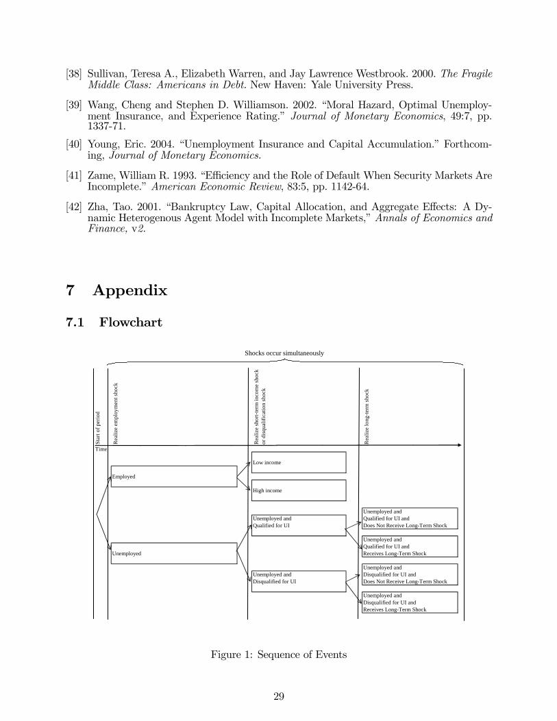
households who face long-term shocks.13 Appendix 7.1 contains a flowchart illustrating all

of the possible outcomes for each household given the shock processes and public insurance

schemes described above.

The presence of search, the possibility of human capital loss, and the option of bankruptcy

imply that both earnings and earnings risk are endogenous in our model. Specifically, as

with generous public insurance, the possibility of default may encourage reductions in search

effort that in turn lengthen unemployment spells, and thereby increase the risk of long-term

shocks to income. By contrast, preceding research such as Zha (2001), Chatterjee et al.

(2002), Livshits et al. (2003), Li and Sarte (2002) and Athreya (2002, 2004) all study the

consequences of altering current bankruptcy law under exogenous income shock processes

that hold earnings risk fixed.

3.2.3 Credit Market Arrangement

In order to smooth consumption, households may borrow on a competitive market and may

also default on these loans in the future. A household that is a net borrower pays the rate

rl(a) on a loan of size a. If households choose to save, they are modeled as buying a bond

at price qd, and therefore earn a fixed interest rate rd ≡ 1qd− 1 on risk-free savings deposits.

The return on savings is exogenous.

Borrowing is modeled following Livshits et al. (2003) and Chatterjee et al. (2002).

Namely, households are assumed in the current period to issue one-period “bonds.” These

bonds are sold at a price ql(a0) discounted by the market according to the likelihood of

default. The interest rate on loans is therefore rl(a) ≡ 1ql(a)− 1. While the probability

of default depends on many factors, we assume that lenders face a transactions cost δ in

processing loans and furthermore can only observe the total debt issuance of a household.

Bond prices will therefore be conditioned solely on loan size. In equilibrium, the zero profit

condition implies that the difference between the interest rate on loans and that on savings11This also captures depreciations of human capital arising from plant closings or other restructuring

where households may not immediately know the likelihood of returning to work. The latter may arise from

the strong cyclical component of displacement rates, whereby an agent may not be immediately able to

differentiate between a firm-level shock and one that is more aggregate or permanent in nature.12We assume that households can at most be faced with one long-term shock during their lifetime.13Details concerning the parameterization are in Section 4.

8

must satisfy the following:

rl(a) =(rd + δ)

(1− πbk(a))(8)

where πbk(a) is the equilibrium probability of default given debt level a. We denote interest

rates for the entire domain of asset holdings by the function:

r(a)=

½rd

rl(a)

if a ≥ 0if a < 0

(9)

Beyond denying credit to households who file for bankruptcy, the financial intermediary

charges all borrowers in “good standing” the same interest rate schedule.

An innovation of the preceding credit arrangement is that it allows credit constraints to

respond to incentives created by public insurance. Quantitative work on U.S. unemployment

insurance (UI), such as Wang and Williamson (2002), Alvarez and Veracierto (2001), Lentz

and Tranaes (2003) and Young (2004) has investigated the effects of allowing for an outside

insurance option such as storage, or a risk-free asset. However, in each of these studies,

borrowing is either prohibited, or is allowed only up to exogenous credit limits that remain

invariant to policy. In our model, endogenously determined household default risk determines

both the cost of loans and the effective limit on borrowing. This allows us to determine the

equilibrium provision of outside insurance provided by credit markets, arising both from

changes in bankruptcy law or public insurance policy. As a quantitative matter, we find that

both credit costs and the generosity of public insurance affect credit markets.

3.2.4 Bankruptcy

Bankruptcy in this model follows the environment in Athreya (2002). We consider only

Chapter 7 bankruptcy filings, whereby unsecured debt is discharged. After bankruptcy, the

household is not allowed to borrow on the unsecured market for an uncertain period of

time. Households may, however, save during this time. Following bankruptcy, a borrowing

constrained household is returned to solvency, whereby they may once again borrow and file

for bankruptcy, with probability ψ. Given the time-independence of ψ, the average time

that a household is borrowing constrained is simply 1/(1 − ψ). As documented in Dubey

et al. (2003) and Athreya (2002), the penalties for bankruptcy filers usually do not transfer

wealth from debtors to creditors. Sullivan et al. (2000) find that in at least 95% of Chapter

7 bankruptcies, assets are not sold to satisfy creditors. Let λ denote all costs of bankruptcy

beyond credit market exclusion, measured in utility. Therefore, λ includes legal fees, time

costs, and any stigma that may be associated with filing for bankruptcy. Given the current

average length of credit market exclusion, we set λ to match observed bankruptcy filing rates

among households.

9

3.3 The Household’s Problem

We will employ specifications of the income shocks, disqualification function, and long-term

shock functions that render the problem recursive in today’s income shock, asset level and

labor income, and if unemployed, search effort. Therefore, the household’s value function is

defined on a state vector containing the preceding four objects. Denote credit market status

by CS, and after-tax labor income by y. With respect to credit status, households are either

solvent (S) or borrowing constrained (BC). Those who have full access to credit markets and

have the option to file for bankruptcy are deemed solvent. Borrowing constrained households

on the other hand are those who have filed for bankruptcy in the past, but have not yet been

readmitted to credit markets. As discussed earlier, the labor income of a household depends

on its unemployment status and whether or not it has received a long-term shock.

With respect to asset holdings, AB and ABC are limits to net wealth imposed by a

credit status applying to newly bankrupt and previously bankrupt households, respectively.

The restriction for solvent households will be determined endogenously in equilibrium. For

notational convenience, suppression of the dependence of income expectations on current

employment status and UI eligibility yields the following recursive representation of the

household’s problem.14 The value of being solvent V S is given as follows:

V S(y, a) = max[WS(y, a),WB(y, a)] (10)

where WS denotes the value of not filing for bankruptcy in the current period and satisfies:

W S(y, a) = max{u(c) + βEV S(y0, a0)} (11)

s.t.

c+a0

1 + r(a0)≤ y + a (12)

When the household qualifies for bankruptcy and chooses to file, it has its debt removed,

pays the non-pecuniary cost λ and then is automatically sent to the borrowing constrained

(i.e. “bad credit history”) state, where it obtains value V BC. Therefore, the value of filing

for bankruptcy, denoted WB, satisfies

WB(y, a) = max{u(c)− λ+ βEV BC(y0, a0)} (13)

s.t

c+a0

1 + rd≤ y (14)

14As it is inessential to represent it here, we relegate a full description of the set of possibilities for labor

income to Section 7.2 of the Appendix. These depend on the precise specifications detailed in Section 4.

10

a0 ≥ AB (15)

To define V BC above, note that borrowing constrained households face a lottery, whereby

they are returned to solvency (i.e., they are free to borrow and default in the following period)

with probability ψ, or remain restricted from borrowing with probability (1− ψ). Thus, we

have:

V BC(y, a) = max{u(c) + ψβEV S(y0, a0) + (1− ψ)βEV BC(y0, a0) (16)

s.t.

c+a0

1 + rd≤ y + a (17)

a0 ≥ ABC (18)

3.4 Public Insurance and Government

We define a public insurance policy (PIP) to be a collection of all the state-contingent transfer

programs undertaken by the government. Therefore, this list is described fully by the min-

imum income received by unemployed households who are disqualified from unemployment

insurance Ymin and the unemployment replacement ratio θ. That is,

PIP = {Ymin, θ}. (19)

The government finances its public insurance policies by taxing labor income at a flat

rate (τ), and we restrict attention to cases where total tax revenues equal total expenditures,

which is explicitly defined below.

3.5 Equilibrium

We focus on stationary equilibria, defined in the standard manner. We begin by constructing

a law of motion for the distribution of households over the state space. While the state of the

household evolves over time, only a portion of next period’s state is chosen by the household

in the current period. The remainder of the state is determined by stochastic shocks occurring

at the beginning of the following period. For example, the unemployed solvent household

chooses effort n, credit status CS0, and assets a0, and the unemployed borrowing constrained

household chooses only n and a0. In both cases, however, next period’s state is partially

decided by the employment and productivity shocks.

11

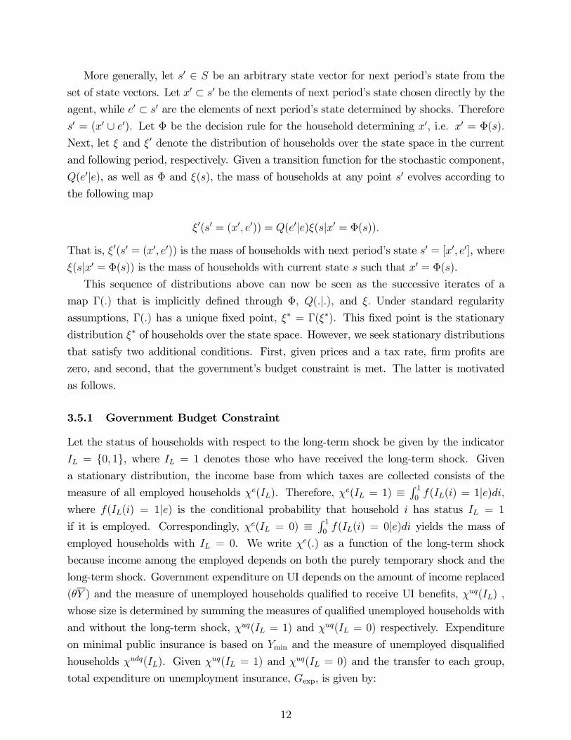
More generally, let s0 ∈ S be an arbitrary state vector for next period’s state from the

set of state vectors. Let x0 ⊂ s0 be the elements of next period’s state chosen directly by theagent, while e0 ⊂ s0 are the elements of next period’s state determined by shocks. Therefores0 = (x0 ∪ e0). Let Φ be the decision rule for the household determining x0, i.e. x0 = Φ(s).

Next, let ξ and ξ0 denote the distribution of households over the state space in the current

and following period, respectively. Given a transition function for the stochastic component,

Q(e0|e), as well as Φ and ξ(s), the mass of households at any point s0 evolves according to

the following map

ξ0(s0 = (x0, e0)) = Q(e0|e)ξ(s|x0 = Φ(s)).

That is, ξ0(s0 = (x0, e0)) is the mass of households with next period’s state s0 = [x0, e0], where

ξ(s|x0 = Φ(s)) is the mass of households with current state s such that x0 = Φ(s).

This sequence of distributions above can now be seen as the successive iterates of a

map Γ(.) that is implicitly defined through Φ, Q(.|.), and ξ. Under standard regularity

assumptions, Γ(.) has a unique fixed point, ξ∗ = Γ(ξ∗). This fixed point is the stationary

distribution ξ∗ of households over the state space. However, we seek stationary distributions

that satisfy two additional conditions. First, given prices and a tax rate, firm profits are

zero, and second, that the government’s budget constraint is met. The latter is motivated

as follows.

3.5.1 Government Budget Constraint

Let the status of households with respect to the long-term shock be given by the indicator

IL = {0, 1}, where IL = 1 denotes those who have received the long-term shock. Given

a stationary distribution, the income base from which taxes are collected consists of the

measure of all employed households χe(IL). Therefore, χe(IL = 1) ≡R 10f(IL(i) = 1|e)di,

where f(IL(i) = 1|e) is the conditional probability that household i has status IL = 1

if it is employed. Correspondingly, χe(IL = 0) ≡R 10f(IL(i) = 0|e)di yields the mass of

employed households with IL = 0. We write χe(.) as a function of the long-term shock

because income among the employed depends on both the purely temporary shock and the

long-term shock. Government expenditure on UI depends on the amount of income replaced

(θY ) and the measure of unemployed households qualified to receive UI benefits, χuq(IL) ,

whose size is determined by summing the measures of qualified unemployed households with

and without the long-term shock, χuq(IL = 1) and χuq(IL = 0) respectively. Expenditure

on minimal public insurance is based on Ymin and the measure of unemployed disqualified

households χudq(IL). Given χuq(IL = 1) and χuq(IL = 0) and the transfer to each group,

total expenditure on unemployment insurance, Gexp, is given by:

12

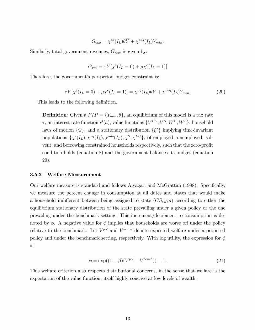
Gexp = χuq(IL)θY + χudq(IL)Ymin.

Similarly, total government revenues, Grev, is given by:

Grev = τY [χe(IL = 0) + µχe(IL = 1)]

Therefore, the government’s per-period budget constraint is:

τY [χe(IL = 0) + µχe(IL = 1)] = χuq(IL)θY + χudq(IL)Ymin. (20)

This leads to the following definition.

Definition: Given a PIP = {Ymin, θ}, an equilibrium of this model is a tax rateτ , an interest rate function rl(a), value functions {V BC , V S,WB,WS}, householdlaws of motion {Φ}, and a stationary distribution {ξ∗} implying time-invariantpopulations {χe(IL),χuq(IL),χudq(IL),χS,χBC}, of employed, unemployed, sol-vent, and borrowing constrained households respectively, such that the zero-profit

condition holds (equation 8) and the government balances its budget (equation

20).

3.5.2 Welfare Measurement

Our welfare measure is standard and follows Aiyagari and McGrattan (1998). Specifically,

we measure the percent change in consumption at all dates and states that would make

a household indifferent between being assigned to state (CS, y, a) according to either the

equilibrium stationary distribution of the state prevailing under a given policy or the one

prevailing under the benchmark setting. This increment/decrement to consumption is de-

noted by φ. A negative value for φ implies that households are worse off under the policy

relative to the benchmark. Let V pol and V bench denote expected welfare under a proposed

policy and under the benchmark setting, respectively. With log utility, the expression for φ

is:

φ = exp((1− β)(V pol − V bench))− 1. (21)

This welfare criterion also respects distributional concerns, in the sense that welfare is the

expectation of the value function, itself highly concave at low levels of wealth.

13

4 Parameterization

A model period is one quarter. We calibrate the following five parameters: the probability

of job loss (ρ), the cost of filing for bankruptcy (λ), the discount rate (β), the effectiveness

of search (ω), and the probability of receiving a long-term shock conditional on being un-

employed for J or more periods (π`). All other parameters are exogenously fixed with direct

reference to data. Table 1 reports the eight steady state targets for the model to match.

Table 2 lists all of the parameter values for the benchmark parameterization. We set both

search disutility and preferences over consumption to be logarithmic.15 The probability of

job loss (ρ) is calibrated most directly to match the average unemployment rate in the U.S.

during the last two decades, 5.8%. The transaction cost of intermediation (δ) reflects the

difference between interest rates charged by lenders and interest rates earned on deposits.

We follow Athreya (2002) (who used the estimates of Evans and Schmalensee (1999)) to get

a quarterly measure of δ = 0.0085. Credit limits for solvent households are endogenous in

the model and turn out to be slightly higher than half of annual income, or approximately

$20,000. For simplicity, we set AB and ABC to zero.

For income risk among the employed, we use panel data estimates from the PSID (1978-

1998) on continuously working households to parameterize an AR(1) income process that

captures both the serial correlation and volatility of household income. We approximate the

income process using a two-state Markov chain, and normalize mean income (Y ) to 1. If a

household is employed, they experience a low or high income shock, so that eY = {Yl, Yh}where Yl < Yh. The conditional probability of receiving each income level is given by

P (eY 0 = Yl|eY = Yl) = pll and P (eY 0 = Yh|eY = Yh) = phh. Income in the low state (Yl)

consists of 0.85 units of output and income in the high state (Yh) yields 1.15 units of output.

The process is symmetric so that the conditional probabilities of low and high shocks (plland phh) are 0.97.

4.1 Long-Term Shocks

To parameterize long-term income risk, we follow several recent studies on displaced workers,

as well as recent estimates on the depreciation rate of human capital. With respect to the

former, estimates of Jacobson, LaLonde and Sullivan (1993) place long term wage losses from

displacement at approximately 30%. As Kletzer (1998) documents however, the estimates of

wage loss of Jacobson et al. (1993) are larger than the estimates for the overall population of

displaced workers. In particular, Kletzer (1998) reports that only 14% of displaced workers15Our specification is most similar to Alvarez and Veracierto (2001), who also choose log utility over

consumption, but choose linear disutility from search.

14

have 10 or more years of job tenure, and hence lose substantially from displacement. With

respect to the latter, Keane and Wolpin (1997) estimate that annual depreciation rates for

human capital arising from work interruptions are 10% for blue-collar workers, and 30%

per year for white-collar workers. Lastly, Stevens (1997) also finds that while earnings fall

post-displacement, the losses are not as great as measured in Jacobson et al. (1993), and

estimates that wages remain approximately 9% below their pre-displacement levels six or

more years after displacement. We therefore set µ = 0.90, whereby the long-term shock

results in a 10% reduction in wages.

We target the fraction of workers affected by such shocks as follows. According to Kletzer

(1998), the two-year displacement rate was 4% in 1992-93. Given the twenty-year displace-

ment period and uniform age distribution assumed by Rogerson and Schindler (2002), the

long-run stock of workers who have experienced a displacement is then 40%. Using the esti-

mate of Kletzer (1998) that long-tenure workers are 14% of the pool of displaced workers, the

fraction we target is 5.6%. We calibrate the likelihood of receiving long-term income shocks

conditional on being unemployed in part to match this stock of workers, and set π` = 0.05.

Lastly, following Rogerson and Schindler (2002), we assume that the displacement lasts an

average of twenty years, or eighty quarters, and therefore choose η =0.0125.

For robustness, we analyze the sensitivity of our results to changes in µ. In particular,

we evaluate the implications of both a 30% reduction in wages (µ = 0.70), as well as the

elimination of all long-term risk. Quantitatively, we find that accounting for long-term risk

is important in assessing the costs of bankruptcy. Nonetheless, our qualitative finding that

bankruptcy impedes public insurance turns out to be robust to the precise specification of

the long-term shock.

4.2 Search

To parametrically represent the probability of re-employment, we employ the function πe(n,ω) =

min(1, n1−ω ) where ω > 0 is an index of search effectiveness. Therefore, higher search effort

(n) improves job prospects linearly, which is increasing in ω. We calibrate ω in the bench-

mark so that the model replicates two summary statistics for unemployment duration (from

Wang and Williamson (2002)): that approximately 69.8% of unemployed workers remain

unemployed for 13 weeks or less while 15.5% remain unemployed for 14-26 weeks.

To capture the observed limits on the duration of UI benefits of two quarters, we assume

that if households are unemployed for two or more consecutive periods, the likelihood of

getting disqualified from UI is one. Thus, πdqk = 1 for k > 2. During the first two quarters

of an unemployment spell, however, this function is not degenerate. In the first period of

unemployment, we assume no households are disqualified from UI, so that πdq1 (n, ν) = 0.

15

Qualification for UI in the second period of a spell depends on search effort in the previous

period. We assume that πdq2 (n) = min[1, ν(1− n)] where ν ≥ 0. In the benchmark case, weassume ν = 1 for simplicity, but consider alternate values of ν in the experiments.

4.3 Public Insurance

The generosity of public insurance policies are dictated by the parameters θ and Ymin. The

replacement ratio for unemployment insurance (θ) is set to 0.50, as is standard (see, e.g.

Wang and Williamson (2002)). The floor on income, Ymin, consists of cash assistance be-

yond UI, including welfare payments. Because long-term shocks in our model are meant to

capture shocks to human capital arising from market forces, an appropriate measure of the

relevant long-term replacement rate is that applying to programs such as TANF (Temporary

Assistance to Needy Families). As a bound, we note that these programs offer much lower

replacement rates than programs to overcome physical disabilities. For example, Autor and

Duggan (2003) measure replacement rates for disability insurance at approximately 40%,

while Fisher (2003) finds that average monthly household transfers through the AFDC pro-

gram (the predecessor to TANF) were $376 in 1994. This implies an annual payment of

approximately $4,500, or roughly 11% of median household income. This estimate is also

consistent with that of Martin (1996), who finds that the average replacement rate for un-

employment and other related welfare benefits for households beyond their second year of

unemployment to be 8%. Therefore, we assume that households who no longer qualify for

UI receive a publicly funded transfer that replaces 10% of pre-displacement mean income,

or 0.1Y . For robustness, we will also consider different values of θ and Ymin.

4.4 Bankruptcy

There are two parameters in the model related to the cost of filing for bankruptcy: ψ governs

credit market exclusion and λ dictates the out-of-pocket costs of bankruptcy arising from

legal fees, court costs, etc. We target an average length of post-bankruptcy exclusion of 4

years (16 quarters), following Athreya (2002). Thus, ψ must be set to 0.9375. The out-of-

pocket cost λ is calibrated to help match bankruptcy filings as defined below.

Total non-business bankruptcy filings have been stable in the past several years at roughly

1.5 million filings annually. Of these, roughly 70% are Chapter 7 bankruptcies. In the data,

roughly 20% of filings involve large medical expense shocks. Debts emerging from large

health-related events such as hospitalization are not well captured in a model of voluntary

borrowing, but are better dealt with as shocks to “expenses”.16 We therefore omit these16See Livshits et al. (2003).

16

cases when calibrating our model’s filing rate.

Given the preceding selection process, the target annual filing rate is 0.84%, or 0.21%

per quarter. Our calibration yields a value for λ of 2.3 utils, or approximately $1,860.17 We

set the annual discount rate (β) to 0.9853, in line with standard values in the literature (for

example, Cooley and Prescott (1995)). The discount rate is calibrated in the benchmark

economy to match the ratio of debt discharged in bankruptcy to unsecured debt, which is

approximately 4.8% per year, or 1.2% per quarter (as reported in Sullivan et al. (2000)).

Our calibration matches two other facts. First, the ratio of unsecured debt to income,

if proxied by the ratio of revolving debt to personal disposable income, is approximately

9.6% in the data, and 10% in the benchmark model.18 Second, the median household filing

for bankruptcy discharges $19,000 in our model, close to $18,321 estimated for 1997 data in

Sullivan et al. (2000).

5 Results

The results are organized as follows. In Section 5.1, we study equilibrium allocations under

current U.S. bankruptcy provisions, and contrast them with allocations obtained when bank-

ruptcy is eliminated. In the latter case, the model collapses to one of purely risk-free loans,

such as Huggett (1993). In Section 5.2, we consider the consequences of public insurance

provision, under current U.S. bankruptcy law. Lastly, Section 5.3 addresses the question of

how, and to what extent, U.S. policymakers can usefully coordinate personal bankruptcy

and public insurance.

Before evaluating the results, it is important to document the sources of welfare gains

and losses in our model. The policy experiments we study each have a direct effect on

the constraints faced by individual households, and an indirect effect on constraints that17Let x = {CS, a, y} be any value for the state vector, and let ymed be the median value of earnings among

those filing for bankruptcy. The expected discounted utility from filing for bankruptcy is:

WB(ymed, a) = max{u(c)− λ+ βEV (BC, e0, a0)} (22)

s.t

c+a0

1 + rd≤ ymed (23)

s.t.

a0 ≥ ABC (24)

We solve for the reduction in income 4y such that optimizing under the remaining income y∗ ≡ ymed−4y,yields a utility loss of λ units. This is the consumption value of the penalty to a representative member of

the group who receives it. For our benchmark, this value is approximately 0.186 units, or $1860.18Revolving debt was $625 billion in 2000, relative to a disposable personal income of $6,500 billion.

17

arise from equilibrium conditions. For example, any policy allowing either more generous

bankruptcy, or more generous public insurance has a direct effect of insuring the household

that is unambiguously positive. However, at the aggregate level, the changes to household

incentives are reflected in prices, which may accentuate, or undo, any gains at the individual

level. These price effects in our model arise from an “interest rate” effect and a “tax rate”

effect. The interest rate effect measures the extent to which policy changes the equilibrium

interest rate on loans, and thereby changes the limits and costs of borrowing. The tax

rate effect measures the change in average consumption due to changes in the tax rate, the

change to the return to searching, as well as any smoothing benefits of proportional taxes.

Lastly, because bankruptcy occurs in equilibrium, the administrative costs of bankruptcy

also account for a portion of the welfare gains and losses, as they are “transactions” costs

that are deadweight in nature.

5.1 Bankruptcy

At the individual level, the possibility of bankruptcy has three major consequences. First,

perhaps most importantly, we find that bankruptcy “inverts” the relationship between wealth

and search effort. In Figure 2, we display outcomes, with and without bankruptcy, for

search effort and borrowing behavior across households that are a) unemployed for more

than 1 quarter (‘u’), and b) newly unemployed (i.e. for less than 1 quarter, ‘unew’). In a

standard model, without default, search effort falls with wealth (e.g. Wang and Williamson

(2002)), as seen in the first row of Figure 2. When bankruptcy is allowed, however, this is

completely reversed. Search effort under current bankruptcy law decreases as wealth falls.

That is, households for whom bankruptcy is likely (i.e., those with negative net wealth)

search less than wealthier households. However, for the very poorest households, borrowing

costs increase by enough to lead households to increase search effort.

The second main implication of default for household behavior is that the sharpest reduc-

tions in search effort are always associated with the sharpest increases in borrowing. This is

also seen in Figure 2 (row 3). Unsecured credit is therefore clearly encouraged at the expense

of search, and this behavior is most pronounced among low wealth unemployed households.

That is, bankruptcy distorts search effort the most for households in which default is most

likely.

The third implication of bankruptcy is that, in addition to discouraging search and

encouraging borrowing, search incentives created by the possibility of skill loss (i.e., receiving

a long-term shock) are significantly muted. In Figure 2, it is clear that the availability

of default is most corrosive for households who have been unemployed for more than one

period, even though such households face increased risk of long-term loss to human capital.

18

By contrast, newly unemployed households search harder and also borrow relatively less.

The preceding household-level decision making has several notable aggregate implica-

tions. The inability to use bankruptcy as an insurance mechanism clearly motivates house-

holds to search harder. The increase in search effort rises by enough to sharply lower un-

employment, as seen in Table 3. Relative to the benchmark, the elimination of bankruptcy

leads to a 4 percentage-point decrease in the fraction of unemployment spells of duration

greater than two quarters, from 11.1% to 7.6% (see ‘u3’ in Table 7). In turn, this leads to

a nontrivial fall in the fraction of households suffering skill-loss, from 5.65% to 3.52% (i.e.

‘LTS rate’ in Table 7). In sum, banning state-contingent debt by eliminating bankruptcy

actually turns out to be useful, as it reduces borrowing costs and lowers taxes for the large

measure of employed households. Thus, both the interest rate and tax effects are positive,

leading to welfare gains (relative to the benchmark economy).

It is remarkable that even though households borrow much less when bankruptcy is elim-

inated, they actually experience less variation in consumption compared to the benchmark.

This is evident in Table 3: ‘σc’ falls from 0.172 to 0.141. Part of this derives from the reduc-

tion in the incentives to “gamble” so that search effort rises. The other part emerges from

an appreciable shift away from large debt holdings (‘borrow’ falls).

In Figure 3, we plot the asset distributions across the bankruptcy experiments and observe

that borrowing falls as the option of bankruptcy disappears. What is more striking is that the

elimination of bankruptcy does not lead households to avoid hardship by accumulating large

buffer stocks of wealth. In fact, holding the cost of funds fixed shows that the unconditional

mean of wealth actually falls (‘avg. assets’ in Table 6). This is precisely the sense in which

the current system appears to reward households for increased risk-taking for re-employment.

Households wish to smooth search effort, in principle, but the incentives created by default

turn out to induce an inefficiently low level of search.19

Intuitively, the elimination of bankruptcy produces two competing effects on borrowing.

First, relatively easy bankruptcy, all else equal, will increase the price of borrowing, hinder-

ing households’ use of debt to smooth consumption when compared with a world without

bankruptcy. The consumption distributions in Figure 4 show that this force is operative.

Figure 2 (row 2) makes it clear that lenders offer uniformly lower rates in the world without

bankruptcy. Second, because the option to default is removed, households may in the end be

less willing to assume debts. In the case below, the latter effect dominates, and we find that

eliminating bankruptcy is associated with a lower level of debt, conditional on borrowing,

than in the benchmark.19For completeness, we also considered various quintiles of the wealth distributions and compared their

expected values with and without bankruptcy (under benchmark public insurance). For each group, the

average welfare was higher without bankruptcy than with it.

19

We also consider a reduction in the cost of bankruptcy filing, by lowering λ from 2.3 in

the benchmark to 1. This reduction makes the filing cost equivalent to $900. Recall that the

cost of bankruptcy is an aggregate of all costs beyond credit market exclusion. Therefore,

reductions in these costs are to be interpreted as arising from, most obviously, changes in

the law allowing discharge of debt. Examples include the length of time elapsing between

the application for bankruptcy and the extent to which debts are discharged. The results go

through as above, as incentives continue to be distorted in the same manner, and underline

our conclusion that increasing the generosity of the bankruptcy code should be approached

with care.20

5.2 Public Insurance

In this section, our goal is to understand the incentive effects of changes in the public

insurance system, given the self-insurance options created by current U.S. bankruptcy law.

In particular, we assess the claim that improved public insurance will reduce the demand

for bankruptcy protection. With respect to the UI system, we consider policies aimed at

1) changing the generosity of benefits, as measured by the UI replacement ratio (θ), and

2) extending the duration of benefits. With respect to minimal social insurance (SI), we

systematically evaluate changes in the generosity of the lower bound on transfer income

(Ymin).

5.2.1 Unemployment Insurance (UI)

Replacement Ratios We first consider the effects of increasing the replacement ratio θ

for all households, from 50% to 75%, while holding the length of eligibility fixed. The effects

on individual decisions can be seen in Figure 5. The borrowing decision (row 3 of Figure

5), as a function of wealth, responds only marginally across replacement ratios. However,

the net effect of reduced search effort outweighs these decisions, and leads, in the aggregate,

to an increase in the bankruptcy rate from 0.85% to 0.904% (see Table 4). Lower search

effort is also reflected in the unemployment rate, which rises to 5.97%. By making short-

term exclusion from credit markets less painful, greater replacement ratios generate more

borrowing and higher bankruptcy rates.

In particular, the preceding results suggest that generous UI has the effect of insuring

those populations at the expense of those who suffer income shocks that are not covered by

these programs. Because one effect of more generous insurance is to enhance the desire to20Intuitively, the need to limit self-insurance in order to realize gains from public insurance is important

here. See Golosov and Tsyvinski (2003), who find that implementing optimal disability insurance may involve

a tax on savings. See also Kocherlakota (2004).

20

file for bankruptcy, all else equal, the interest rate effect makes borrowing more expensive for

all households. This, of course, imposes costs disproportionately on those households whose

income has fallen due to the many circumstances not covered through the narrow definitions

allowed for receiving unemployment-based insurance. As the bulk of the population is not

unemployed at any given time, the welfare costs of unemployment benefits are large and

outweigh the benefits accruing to the small minority of unemployed households. In addition,

the distortion to search effort also leads households at the margin to substitute borrowing for

search effort. As a result, in such a world, more households will ultimately find bankruptcy

useful. However, this appears to be, on net, relatively inefficient, as welfare typically falls

with higher tax rates and public insurance. The source of the inefficiency is that bankruptcy

generates deadweight costs, as it is paid for via increased interest rates, and also because

it creates ex-post deadweight costs as captured in the parameters λ and ρ. In other words,

generous public insurance requires high taxes, distorts search effort, and also reduces the

pain from credit exclusion. These effects are large enough that they lead households to use

bankruptcy with excessive frequency.

In contrast, decreases in the replacement rates of the same magnitude (θ = 0.25) lowers

the incentive to borrow. Table 4 shows that mean debt holdings (‘borrow’) fall by roughly

one-fourth, as households realize that becoming unemployed will result in a short, sharp

shock to their income. As a consequence, households file for bankruptcy less frequently.

Unemployed households, however, are more likely to file with lower UI, consistent with the

empirical findings of Fisher (2003). Specifically, the bankruptcy rate among the unemployed

sharply increases from 2.93% to 3.39%. In addition, less UI motivates households to increase

their search efforts, resulting in less unemployment and improvements in welfare (φ > 0).

An implication of the latter is, of course, that the currently observed U.S. replacement ratio

generates nontrivial welfare loss relative to a stricter UI regime.

Figure 5 also compares how unemployment duration affects search effort across various

wealth levels. We see that search effort falls less steeply with wealth under low replacement

ratios. This is intuitive, as subsequent unemployment is less pleasant under low replacement

ratios. Similarly, the willingness to borrow in order to consumption smooth is attenuated,

relative to that under a high replacement ratio.

Our results for the behavior of filing rates are consistent with empirical findings of Shepard

(1984), Buckley and Brinig (1996), Domowitz and Eovaldi (1993), and most recently, Fay,

Hurst and White (2002). The latter do not directly evaluate the impact of social insurance

on filing decisions, but do find that the household’s propensity to file increases with the

“financial benefit” of bankruptcy, which is precisely what increasing UI benefits does.21

21Some care should be taken in directly linking our results to that of empirical work. Our equilibrium

concept is inherently a long-run one, whereby our results should be interpreted as the long-run outcome from

21

Extension of BenefitsA second natural dimension along which to evaluate the effects of increasing the generosity

of UI is to extend the duration of benefits. Currently in the U.S., households typically

receive two quarters of UI benefits. In our model, all households are therefore disqualified

from UI after two periods (πdqk = 1 ∀ k > 2). We study the consequences of increasing

the generosity of benefits by allowing half of the formerly disqualified households to remain

eligible for additional periods of UI benefits.22 Specifically, we set πdqk = 0.5 ∀k > 2. In

the aggregate, we see that the results in Table 4 support the view that extended UI benefits

lead to a reduction in the bankruptcy rate. However, this reduction is also accompanied by

an increase in the unemployment rate, the tax rate, and average consumption. With longer

UI eligibility, households increase their borrowing levels by 9% but file for bankruptcy less

frequently. This is consistent with the findings of Fisher (2003), and occurs because, for

many agents, the likelihood of a prolonged fall in income is lower under the extended UI

system. Bankruptcy rates fall non-trivially for both unemployed households and households

who receive long-term income shocks.23

Surprisingly, despite this additional availability of public insurance, average consumption

is slightly more volatile, whereby σc increases from 0.172 to 0.176, and welfare (φ) falls by

0.81%. The majority of the drop in welfare costs come directly from the tax rate effect. As

in Wang and Williamson (2002) and Lentz and Tranaes (2003), we find that extending UI

benefits reduces effort levels and increases the unemployment rate. Therefore, these findings

imply that increased public insurance, at least in the form of extended eligibility for UI

benefits, will not improve matters.

Lastly, we combine the reduction in the UI replacement ratio with an extension of UI

benefits (that is, we set θ = 0.25 and πdqk = 0.5 ∀k > 2). The results are quite similar to thecase with only a reduction in UI; however, this policy has larger effects on both bankruptcy

and unemployment rates. As before, borrowing is much lower than in the benchmark, and

this is associated with a dramatic fall in the bankruptcy rate, especially among unemployed

households. Combining low UI with extended benefits however leads to decreases in the

volatility in consumption: σc falls to 0.169. With considering low UI and extended benefits

independently, we found that σc increases (0.176 and 0.175, respectively). In addition,

welfare gains under this policy are high (as with low UI replacement ratios alone), but the

significant reductions in consumption volatility, bankruptcy rates, and unemployment are

particularly noteworthy.

implementing a given policy nationwide.22This is also in part to assess the effects of the current practice of extending UI benefits periodically. For

example, Congress extended UI benefits in January and May of 2003.23Refer to Table 6 in the Appendix.

22

5.2.2 Minimal Social Insurance (SI)

A second facet of public insurance is that, in the U.S., those who have been unemployed

long enough to run out of UI benefits typically still qualify for some form of minimal income

support. Examples of such longer-term income insurance include, but are not limited to,

publicly-provided disability insurance (OASDHI) and welfare assistance (e.g. TANF). To

the extent that bankruptcy is most useful to households who have been hit with a long-term

shock, public insurance against such lengthy unemployment spells is likely to interact with

bankruptcy in meaningful ways. In the benchmark economy, we set the replacement rate

for long-term public insurance programs (SI) to 10%. We now evaluate the effect of both

more and less generous social insurance programs (i.e., replacement rates of 15% and 5% of

income, respectively). Results are reported in Table 5. It turns out that, like UI, generous

SI also increases bankruptcy via the same channels as generous UI, the strongest aspect of

which is the tendency to borrow instead of search. For brevity, we do not report the details

here.

In summary, introducing bankruptcy has rather negative effects, given current U.S. public

insurance. It distorts search dramatically, encourages suboptimally risky borrowing and also

risk-taking among the unemployed. Bankruptcy lengthens unemployment spells, increases

skill loss, and reduces credit availability. Most interestingly, and quite in contrast to the view

of Sullivan et al. (2000), more generous public insurance will increase bankruptcy, while it

is actually reductions in public insurance relative to current practice that will reduce filing

rates. Furthermore, increased default crowds out the unsecured credit markets and thereby

lowers welfare.

5.3 Coordinating Public Insurance Policy with Personal Bank-

ruptcy Law

In the preceding two sections, we evaluated the effects of bankruptcy on incentives under

current public insurance policy, and conversely, the effects of public insurance under current

bankruptcy policy. We now address the natural question of the role of public insurance in

conjunction with bankruptcy policy. That is, if a policymaker could change both public

insurance and bankruptcy costs, what combination of insurance and bankruptcy law should

he choose or avoid? For simplicity, we restrict attention to studying cases where bankruptcy

is allowed as per the benchmark, against cases where bankruptcy is prohibited.

Consider the following four polar cases involving uniform changes in public insurance,

whereby all households face the same UI replacement ratio θ and minimal income floor Ymin.

We consider the welfare implications of various UI/SI combinations. Low UI is defined as

θ = 0.25 while high UI implies θ = 0.75. Similarly, low SI is defined as Ymin = 0.05Y while

23

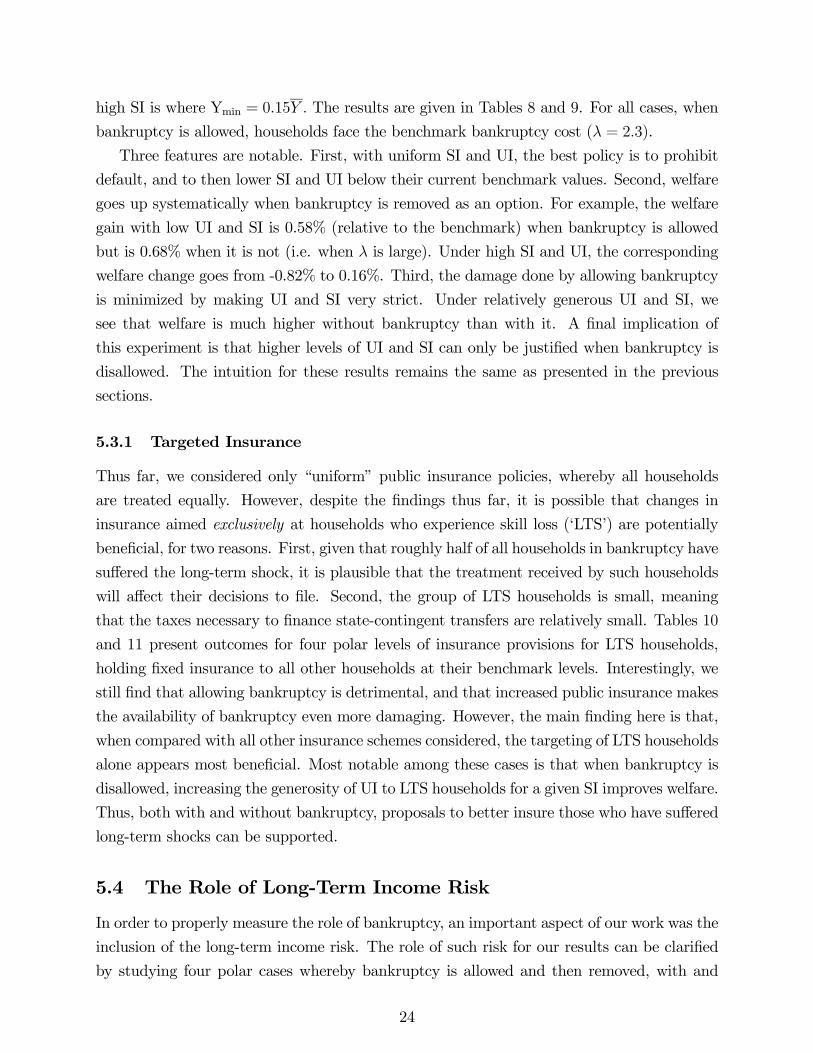
high SI is where Ymin = 0.15Y . The results are given in Tables 8 and 9. For all cases, when

bankruptcy is allowed, households face the benchmark bankruptcy cost (λ = 2.3).

Three features are notable. First, with uniform SI and UI, the best policy is to prohibit

default, and to then lower SI and UI below their current benchmark values. Second, welfare

goes up systematically when bankruptcy is removed as an option. For example, the welfare

gain with low UI and SI is 0.58% (relative to the benchmark) when bankruptcy is allowed

but is 0.68% when it is not (i.e. when λ is large). Under high SI and UI, the corresponding

welfare change goes from -0.82% to 0.16%. Third, the damage done by allowing bankruptcy

is minimized by making UI and SI very strict. Under relatively generous UI and SI, we

see that welfare is much higher without bankruptcy than with it. A final implication of

this experiment is that higher levels of UI and SI can only be justified when bankruptcy is

disallowed. The intuition for these results remains the same as presented in the previous

sections.

5.3.1 Targeted Insurance

Thus far, we considered only “uniform” public insurance policies, whereby all households

are treated equally. However, despite the findings thus far, it is possible that changes in

insurance aimed exclusively at households who experience skill loss (‘LTS’) are potentially

beneficial, for two reasons. First, given that roughly half of all households in bankruptcy have

suffered the long-term shock, it is plausible that the treatment received by such households

will affect their decisions to file. Second, the group of LTS households is small, meaning

that the taxes necessary to finance state-contingent transfers are relatively small. Tables 10

and 11 present outcomes for four polar levels of insurance provisions for LTS households,

holding fixed insurance to all other households at their benchmark levels. Interestingly, we

still find that allowing bankruptcy is detrimental, and that increased public insurance makes

the availability of bankruptcy even more damaging. However, the main finding here is that,

when compared with all other insurance schemes considered, the targeting of LTS households

alone appears most beneficial. Most notable among these cases is that when bankruptcy is

disallowed, increasing the generosity of UI to LTS households for a given SI improves welfare.

Thus, both with and without bankruptcy, proposals to better insure those who have suffered

long-term shocks can be supported.

5.4 The Role of Long-Term Income Risk

In order to properly measure the role of bankruptcy, an important aspect of our work was the

inclusion of the long-term income risk. The role of such risk for our results can be clarified

by studying four polar cases whereby bankruptcy is allowed and then removed, with and

24

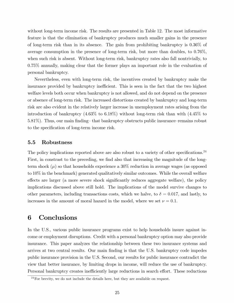
without long-term income risk. The results are presented in Table 12. The most informative

feature is that the elimination of bankruptcy produces much smaller gains in the presence

of long-term risk than in its absence. The gain from prohibiting bankruptcy is 0.36% of

average consumption in the presence of long-term risk, but more than doubles, to 0.76%,

when such risk is absent. Without long-term risk, bankruptcy rates also fall nontrivially, to

0.75% annually, making clear that the former plays an important role in the evaluation of

personal bankruptcy.

Nevertheless, even with long-term risk, the incentives created by bankruptcy make the

insurance provided by bankruptcy inefficient. This is seen in the fact that the two highest

welfare levels both occur when bankruptcy is not allowed, and do not depend on the presence

or absence of long-term risk. The increased distortions created by bankruptcy and long-term

risk are also evident in the relatively larger increase in unemployment rates arising from the

introduction of bankruptcy (4.63% to 6.18%) without long-term risk than with (4.45% to

5.81%). Thus, our main finding— that bankruptcy obstructs public insurance—remains robust

to the specification of long-term income risk.

5.5 Robustness

The policy implications reported above are also robust to a variety of other specifications.24

First, in constrast to the preceding, we find also that increasing the magnitude of the long-

term shock (µ) so that households experience a 30% reduction in average wages (as opposed

to 10% in the benchmark) generated qualitatively similar outcomes. While the overall welfare

effects are larger (a more severe shock significantly reduces aggregate welfare), the policy

implications discussed above still hold. The implications of the model survive changes to

other parameters, including transactions costs, which we halve, to δ = 0.017, and lastly, to

increases in the amount of moral hazard in the model, where we set ν = 0.1.

6 Conclusions

In the U.S., various public insurance programs exist to help households insure against in-

come or employment disruptions. Credit with a personal bankruptcy option may also provide

insurance. This paper analyzes the relationship between these two insurance systems and

arrives at two central results. Our main finding is that the U.S. bankruptcy code impedes

public insurance provision in the U.S. Second, our results for public insurance contradict the

view that better insurance, by limiting drops in income, will reduce the use of bankruptcy.

Personal bankruptcy creates inefficiently large reductions in search effort. These reductions24For brevity, we do not include the details here, but they are available on request.

25

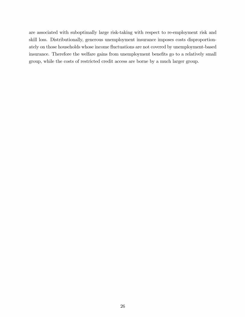
are associated with suboptimally large risk-taking with respect to re-employment risk and

skill loss. Distributionally, generous unemployment insurance imposes costs disproportion-

ately on those households whose income fluctuations are not covered by unemployment-based

insurance. Therefore the welfare gains from unemployment benefits go to a relatively small

group, while the costs of restricted credit access are borne by a much larger group.

26

References[1] Aiyagari, S. Rao and Ellen R. McGrattan. 1998. “The Optimum Quantity of Debt.”

Journal of Monetary Economics, 42:3, pp. 447-69.

[2] Alvarez, Fernando, and Marcelo Veracierto, “Severance Payments in an Economy WithFrictions”, 2001, Journal of Monetary Economics, 47:3, pp. 477-98.

[3] Arulampalam, W, Allison Lee Booth and Mark P. Taylor 2000, “Unemployment Persis-tence” Oxford Economic Papers ; 52:24-50

[4] Autor, David H. and Mark G. Duggan. 2003. “The Rise in the Disability Rolls and theDecline in Unemployment.” Quarterly Journal of Economics, 118:1, pp. 157-205.

[5] Athreya, Kartik B. 2002. “Welfare Implications of the Bankruptcy Reform Act of 1999.”Journal of Monetary Economics, 49:8, pp. 1567-95.

[6] Athreya, Kartik B. 2004. “Shame As It Ever Was: Stigma and Personal Bankruptcy.”Federal Reserve Bank of Richmond Economic Quarterly, 90:2.

[7] Attanasio, Orazio and Jose-Victor Rios-Rull. 2000. “Consumption Smoothing in IslandEconomies: Can Public Insurance Reduce Welfare?” European Economic Review, 44:7,pp. 1225 - 1258.

[8] Bermant, Gordon and Ed Flynn. 2002. “Just Recently Hired: Job Tenure Among No-asset Chapter 7 Debtors.” American Bankruptcy Institute.

[9] Buckley, Frank and Margaret Brinig. 1996. “The Market for Deadbeats.” Journal ofLegal Studies, 25:1, pp. 201-232.

[10] Chatterjee, Satyajit, Dean Corbae, Makoto Nakajima, and Jose-Victor Rios-Rull. 2002.“A Quantitative Theory of Unsecured Consumer Credit with Risk of Default.” FederalReserve Bank of Philadelphia: Working Paper 02-6.

[11] Cooley, Thomas F. and Edward C. Prescott. 1995. Frontiers of Business Cycle Research.Princeton University Press: Princeton.

[12] Corcoran, M., and G. Duncan, 1979, “Work history, labor force attachment, and earn-ings differences between the races and sexes”, Journal of Human Resources, 14(1),pp.3-20

[13] Deaton, Angus. 1991. “Saving and Liquidity Constraints.” Econometrica, 59:5, pp. 1221-48.

[14] Domowitz, Ian and Thomas L. Eovaldi. 1993. “The Impact of the Bankruptcy ReformAct of 1978 on Consumer Bankruptcy.” Journal of Law and Economics, 36:2, pp. 803-35.

[15] Dubey, Pradeep, John Geanakoplos, andMartin Shubik. 2003. “Default and Punishmentin General Equilibrium.” Cowles Foundation Discussion Paper, No. 1304RRR.

[16] Evans, David S and Richard Schmalensee. 1999. Paying with Plastic: The Digital Rev-olution in Buying and Borrowing. Cambridge, Mass.: MIT Press.

[17] Fay, Scott, Erik Hurst and Michelle White. 2002. “The Household Bankruptcy Deci-sion.” American Economic Review, 92:3, pp. 706-718.

[18] Fisher, Jonathan D. 2003. “The Effect of Government Unemployment Benefits, Wel-fare Benefits, and Other Income on Personal Bankruptcy.” Bureau of Labor StatisticsManuscript.

27

[19] Golosov, Mikhail and Aleh Tsyvinski. 2003. “Designing Optimal Disability Insurance.”Federal Reserve Bank of Minneapolis, Working Paper 628.

[20] Hansen, Gary D. and Ayse Imrohoroglu. 1992. “The Role of Unemployment Insurancein an Economy with Liquidity Constraints and Moral Hazard.” Journal of PoliticalEconomy, 100:1, pp. 118-42.

[21] Huggett, Mark. 1993. “The Risk-Free Rate in Heterogeneous-Agent Incomplete-Insurance Economies.” Journal of Economic Dynamics and Control, 17:5-6, pp. 953-69.

[22] Jacobson, Louis S, Robert J. LaLonde, and Daniel G Sullivan. 1993. “Earnings Lossesof Displaced Workers.” American Economic Review, 83:4, pp. 685-709.

[23] Keane, Michael, and Kenneth I. Wolpin “The Career Decisions of Young Men”, Journalof Political Economy, 105 (473-522).

[24] Kletzer, Lori G. 1998. “Job Displacement.” Journal of Economic Perspectives, 12:1, pp.115-36.

[25] Kocherlakota, Narayana R. 2004. “Zero Expected Walth Taxes: A Mirrlees Approachto Optimal Taxation.” Stanford University Working Paper.

[26] Krueger, Dirk and Fabrizio Perri. 2003. “Does Income Inequality Lead to ConsumptionInequality? Evidence and Theory.” Mimeo, NYU.

[27] Lentz, Rasmus and Torben Tranaes, “Job Search and Savings: Wealth Effects andDuration Dependence”, mimeo, Boston University, November 2003.

[28] Li, Wenli and Pierre-Daniel Sarte. 2002. “The Macroeconomics of U.S. Consumer Bank-ruptcy Choice: Chapter 7 or Chapter 13?” Federal Reserve Bank of Richmond WorkingPaper #02-1.

[29] Livshits, Igor, James MacGee, and Michele Tertilt. 2003. “Consumer Bankruptcy: AFresh Start.” Federal Reserve Bank of Minneapolis, Working Paper 617.

[30] Ljungqvist, Lars and Thomas J. Sargent. 1998. “The European UnemploymentDilemma.” Journal of Political Economy, 106:3, pp. 514-50.

[31] Martin, John. 1996. “Measures of Replacement Rates for the Purpose of InternationalComparisons: A Note.” OECD Economic Studies No. 26:1.

[32] Musto, David. 2002. “What Happens when Information Leaves a Market? Evidencefrom Post-Bankruptcy Consumers.” Journal of Business, forthcoming.

[33] Obstfeld, Maurice and Kenneth Rogoff. 1996. Foundations of International Macroeco-nomics. Cambridge, Mass. and London: MIT Press.

[34] Pissarides, Christopher A. 1992. “Loss of Skill during Unemployment and the Persis-tence of Employment Shocks.” Quarterly Journal of Economics, 107:4, pp. 1371-91.

[35] Rogerson, Richard and Martin Schindler. 2002. “The Welfare Costs of Worker Displace-ment.” Journal of Monetary Economics, 49:6, pp. 1213-34.

[36] Shepard, Lawrence. 1984. “Personal Failures and the Bankruptcy Reform Act of 1978.”Journal of Law and Economics, 27:2, pp. 419-437.

[37] Stevens, Ann Huff. 1997. “Persistent Effects of Job Displacement: The Importance ofMultiple Job Losses.” Journal of Labor Economics, 15:1, pp. 165-88.

28

[38] Sullivan, Teresa A., Elizabeth Warren, and Jay Lawrence Westbrook. 2000. The FragileMiddle Class: Americans in Debt. New Haven: Yale University Press.

[39] Wang, Cheng and Stephen D. Williamson. 2002. “Moral Hazard, Optimal Unemploy-ment Insurance, and Experience Rating.” Journal of Monetary Economics, 49:7, pp.1337-71.

[40] Young, Eric. 2004. “Unemployment Insurance and Capital Accumulation.” Forthcom-ing, Journal of Monetary Economics.

[41] Zame, William R. 1993. “Efficiency and the Role of Default When Security Markets AreIncomplete.” American Economic Review, 83:5, pp. 1142-64.

[42] Zha, Tao. 2001. “Bankruptcy Law, Capital Allocation, and Aggregate Effects: A Dy-namic Heterogenous Agent Model with Incomplete Markets,” Annals of Economics andFinance, v2.

7 Appendix

7.1 Flowchart

Star

t of p

erio

d

Rea

lize

empl

oym

ent s

hock

Rea

lize

shor

t-ter

m in

com

e sh

ock

or d

isqu

alifi

catio

n sh

ock

Rea

lize

long

-term

shoc

k

Low income

Employed

High income

Unemployed and Unemployed and Qualified for UI andQualified for UI Does Not Receive Long-Term Shock

Unemployed and Qualified for UI and

Unemployed Receives Long-Term Shock

Unemployed and Unemployed and Disqualified for UI andDisqualified for UI Does Not Receive Long-Term Shock

Unemployed and Disqualified for UI andReceives Long-Term Shock

Time

Shocks occur simultaneously

Figure 1: Sequence of Events

29

7.2 Labor Income By Employment and Long-Term Shock StatusLabor income y be defined as follows:

y =

⎧⎪⎪⎪⎪⎪⎪⎨⎪⎪⎪⎪⎪⎪⎩

eY ∈ {Yl,Yh} if employed without long-term shock (IL = 0)eY ∈ {µYl,µYh} if employed with long-term shock (IL = 1)

θY if unemployed, qualified for UI, (IL = 0)

θ(µY ) if unemployed, qualified for UI, (IL = 1)

Ymin if unemployed and disqualified from UI

(25)

Employment status evolves as follows. Let IU denote an indicator function over unem-ployment. If employed in the current period (i.e. IU = 0), households are unemployed nextperiod according to:

(I 0U |IU = 0) =½

1 with prob. ρ0 with prob. 1− ρ

(26)

If unemployed in the current period, the likelihood of becoming employed in the followingperiod depends on search effort:

(I 0U |IU = 1) =(

1 with prob. 1− πe(n)

0 with prob. πe(n) = min(1, n1−ω )

(27)

For those who are currently suffering the effects of the long-term shock (i.e., IL = 1), theshock evolves according to:

(I 0L|IL = 1) =½1 with prob. 1− η

0 with prob. η(28)

For those who are currently not affected by the long-term shock, the law of motion is:

(I 0L|IL = 0) =½

0 if IU = 0π` if IU = 1 and IU(t− 2) = 1

(29)

where we abuse notation slightly by using IU(t− 2) to denote unemployment status two pe-riods ago. That is, households are susceptible to the long-term shock only after experiencingtwo successive periods of unemployment.

30

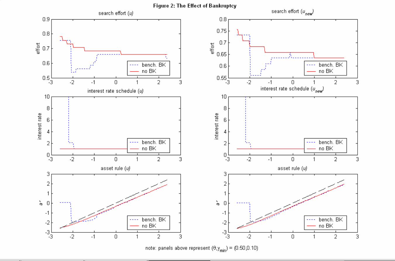
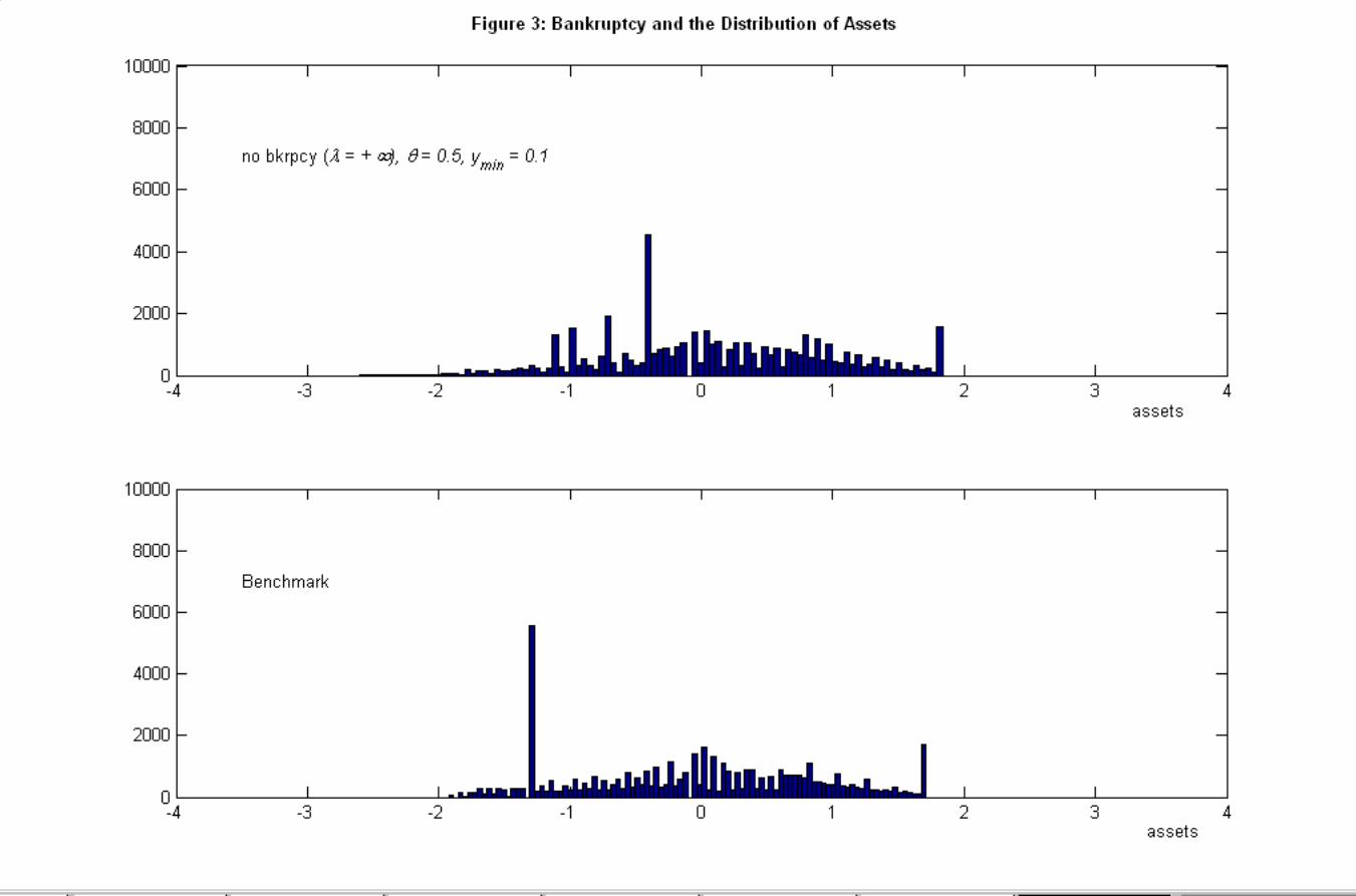
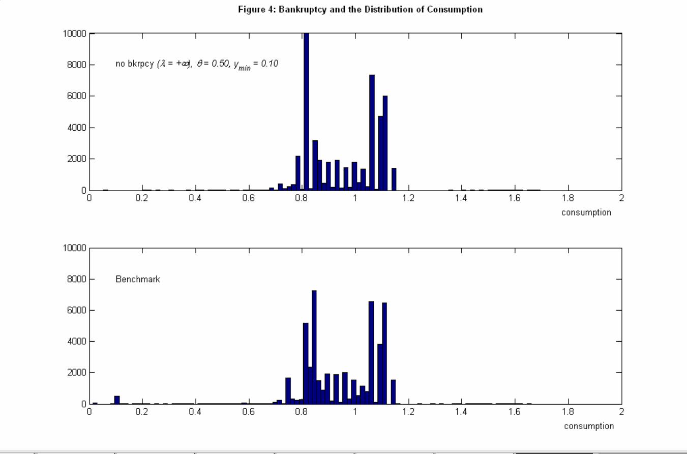
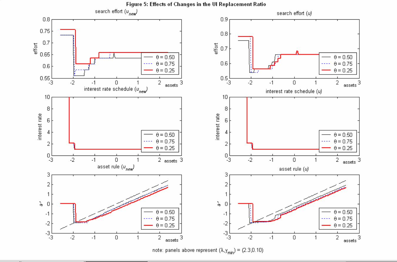
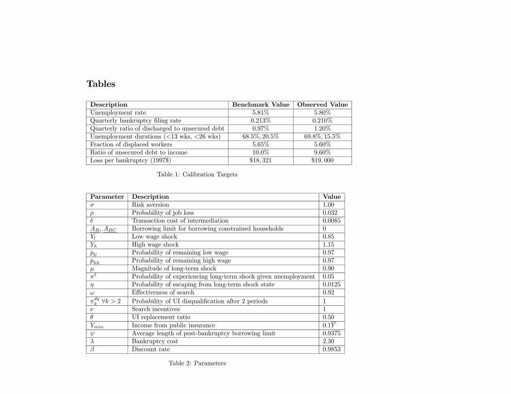
Tables

Description Benchmark Value Observed ValueUnemployment rate 5.81% 5.80%Quarterly bankruptcy filing rate 0.213% 0.210%Quarterly ratio of discharged to unsecured debt 0.97% 1.20%Unemployment durations (<13 wks, <26 wks) 68.5%, 20.5% 69.8%, 15.5%Fraction of displaced workers 5.65% 5.60%Ratio of unsecured debt to income 10.0% 9.60%Loss per bankruptcy (1997$) $18, 321 $19, 000

Table 1: Calibration Targets

Parameter Description Valueσ Risk aversion 1.00ρ Probability of job loss 0.032δ Transaction cost of intermediation 0.0085AB, ABC Borrowing limit for borrowing constrained households 0Yl Low wage shock 0.85Yh High wage shock 1.15pll Probability of remaining low wage 0.97phh Probability of remaining high wage 0.97µ Magnitude of long-term shock 0.90π` Probability of experiencing long-term shock given unemployment 0.05η Probability of escaping from long-term shock state 0.0125ω Effectiveness of search 0.92

πdqk ∀k > 2 Probability of UI disqualification after 2 periods 1ν Search incentives 1θ UI replacement ratio 0.50

Ymin Income from public insurance 0.1Yψ Average length of post-bankruptcy borrowing limit 0.9375λ Bankruptcy cost 2.30β Discount rate 0.9853

Table 2: Parameters

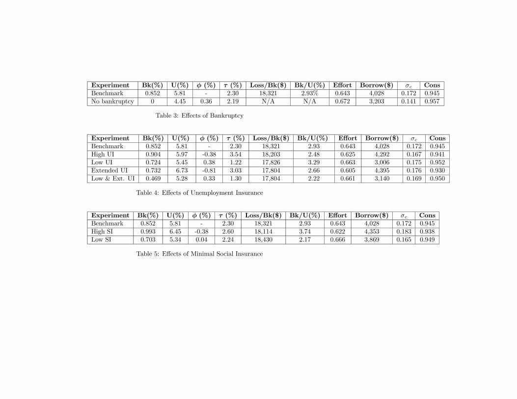
Experiment Bk(%) U(%) φ (%) τ (%) Loss/Bk($) Bk/U(%) Effort Borrow($) σc ConsBenchmark 0.852 5.81 - 2.30 18,321 2.93% 0.643 4,028 0.172 0.945No bankruptcy 0 4.45 0.36 2.19 N/A N/A 0.672 3,203 0.141 0.957

Table 3: Effects of Bankruptcy

Experiment Bk(%) U(%) φ (%) τ (%) Loss/Bk($) Bk/U(%) Effort Borrow($) σc ConsBenchmark 0.852 5.81 - 2.30 18,321 2.93 0.643 4,028 0.172 0.945High UI 0.904 5.97 -0.38 3.54 18,203 2.48 0.625 4,292 0.167 0.941Low UI 0.724 5.45 0.38 1.22 17,826 3.29 0.663 3,006 0.175 0.952Extended UI 0.732 6.73 -0.81 3.03 17,804 2.66 0.605 4,395 0.176 0.930Low & Ext. UI 0.469 5.28 0.33 1.30 17,804 2.22 0.661 3,140 0.169 0.950

Table 4: Effects of Unemployment Insurance

Experiment Bk(%) U(%) φ (%) τ (%) Loss/Bk($) Bk/U(%) Effort Borrow($) σc ConsBenchmark 0.852 5.81 - 2.30 18,321 2.93 0.643 4,028 0.172 0.945High SI 0.993 6.45 -0.38 2.60 18,114 3.74 0.622 4,353 0.183 0.938Low SI 0.703 5.34 0.04 2.24 18,430 2.17 0.666 3,869 0.165 0.949

Table 5: Effects of Minimal Social Insurance

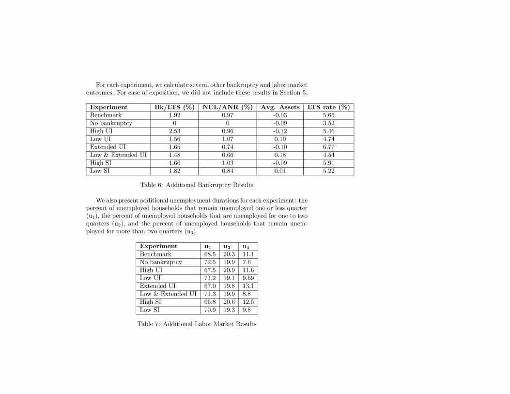
For each experiment, we calculate several other bankruptcy and labor marketoutcomes. For ease of exposition, we did not include these results in Section 5.

Experiment Bk/LTS (%) NCL/ANR (%) Avg. Assets LTS rate (%)Benchmark 1.92 0.97 -0.03 5.65No bankruptcy 0 0 -0.09 3.52High UI 2.53 0.96 -0.12 5.46Low UI 1.56 1.07 0.19 4.74Extended UI 1.65 0.74 -0.10 6.77Low & Extended UI 1.48 0.66 0.18 4.54High SI 1.66 1.03 -0.09 5.91Low SI 1.82 0.84 0.01 5.22

Table 6: Additional Bankruptcy Results

We also present additional unemployment durations for each experiment: thepercent of unemployed households that remain unemployed one or less quarter(u1), the percent of unemployed households that are unemployed for one to twoquarters (u2), and the percent of unemployed households that remain unem-ployed for more than two quarters (u3).

Experiment u1 u2 u3Benchmark 68.5 20.3 11.1No bankruptcy 72.5 19.9 7.6High UI 67.5 20.9 11.6Low UI 71.2 19.1 9.69Extended UI 67.0 19.8 13.1Low & Extended UI 71.3 19.9 8.8High SI 66.8 20.6 12.5Low SI 70.9 19.3 9.8

Table 7: Additional Labor Market Results

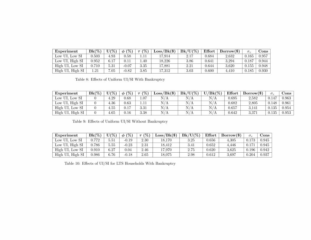
Experiment Bk(%) U(%) φ (%) τ (%) Loss/Bk($) Bk/U(%) Effort Borrow($) σc ConsLow UI, Low SI 0.503 4.93 0.58 1.11 17,914 2.17 0.684 2,632 0.165 0.957Low UI, High SI 0.952 6.17 0.11 1.40 18,226 3.86 0.641 3,294 0.187 0.944High UI, Low SI 0.710 5.31 -0.07 3.35 17,881 2.21 0.644 3,620 0.155 0.948High UI, High SI 1.21 7.05 -0.82 3.85 17,312 3.03 0.600 4,410 0.185 0.930

Table 8: Effects of Uniform UI/SI With Bankruptcy

Experiment Bk(%) U(%) φ (%) τ (%) Loss/Bk($) Bk/U(%) U/Bk(%) Effort Borrow($) σc ConsLow UI, Low SI 0 4.29 0.68 1.07 N/A N/A N/A 0.695 2,582 0.147 0.963Low UI, High SI 0 4.36 0.63 1.11 N/A N/A N/A 0.682 2,805 0.148 0.961High UI, Low SI 0 4.55 0.17 3.31 N/A N/A N/A 0.657 3,141 0.135 0.954High UI, High SI 0 4.65 0.16 3.38 N/A N/A N/A 0.642 3,371 0.135 0.953

Table 9: Effects of Uniform UI/SI Without Bankruptcy

Experiment Bk(%) U(%) φ (%) τ (%) Loss/Bk($) Bk/U(%) Effort Borrow($) σc ConsLow UI, Low SI 0.772 5.51 -0.19 2.30 18,170 3.25 0.656 4,305 0.173 0.945Low UI, High SI 0.786 5.55 -0.23 2.31 18,412 3.41 0.652 4,446 0.171 0.945High UI, Low SI 0.910 6.27 0.04 2.46 17,970 2.75 0.620 3,625 0.196 0.942High UI, High SI 0.986 6.76 -0.18 2.65 18,075 2.98 0.612 3,697 0.204 0.937

Table 10: Effects of UI/SI for LTS Households With Bankruptcy

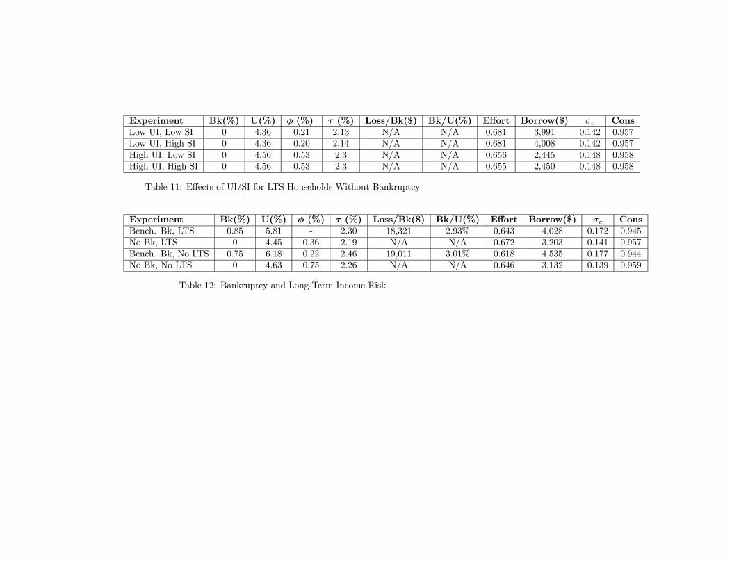
Experiment Bk(%) U(%) φ (%) τ (%) Loss/Bk($) Bk/U(%) Effort Borrow($) σc ConsLow UI, Low SI 0 4.36 0.21 2.13 N/A N/A 0.681 3,991 0.142 0.957Low UI, High SI 0 4.36 0.20 2.14 N/A N/A 0.681 4,008 0.142 0.957High UI, Low SI 0 4.56 0.53 2.3 N/A N/A 0.656 2,445 0.148 0.958High UI, High SI 0 4.56 0.53 2.3 N/A N/A 0.655 2,450 0.148 0.958

Table 11: Effects of UI/SI for LTS Households Without Bankruptcy

Experiment Bk(%) U(%) φ (%) τ (%) Loss/Bk($) Bk/U(%) Effort Borrow($) σc ConsBench. Bk, LTS 0.85 5.81 - 2.30 18,321 2.93% 0.643 4,028 0.172 0.945No Bk, LTS 0 4.45 0.36 2.19 N/A N/A 0.672 3,203 0.141 0.957Bench. Bk, No LTS 0.75 6.18 0.22 2.46 19,011 3.01% 0.618 4,535 0.177 0.944No Bk, No LTS 0 4.63 0.75 2.26 N/A N/A 0.646 3,132 0.139 0.959

Table 12: Bankruptcy and Long-Term Income Risk