Embed Size (px)
Citation preview

www.elsevier.com/locate/cviu
Computer Vision and Image Understanding 102 (2006) 22–41
Unsupervised scene analysis: A hidden Markov model approach
Manuele Bicego 1, Marco Cristani, Vittorio Murino *
Dipartimento di Informatica, University of Verona, Ca� Vignal 2, Strada Le Grazie 15, 37134 Verona, Italy
Received 23 November 2004; accepted 22 September 2005Available online 8 November 2005
Abstract
This paper presents a new approach to scene analysis, which aims at extracting structured information from a video sequence usingdirectly low-level data. The method models the sequence using a forest of Hidden Markov models (HMMs), which are able to extract twokinds of data, namely, static and dynamic information. The static information results in a segmentation that explains how the chromaticaspect of the static part of the scene evolves. The dynamic information results in the detection of the areas which are more affected byforeground activity. The former is obtained by a spatial clustering of HMMs, resulting in a spatio-temporal segmentation of the videosequence, which is robust to noise and clutter and does not consider the possible moving objects in the scene. The latter is estimated usingan entropy-like measure defined on the stationary probability of the Markov chain associated to the HMMs, producing a partition of thescene in activity zones in a consistent and continuous way. The proposed approach constitutes a principled unified probabilistic frame-work for low level scene analysis and understanding, showing several key features with respect to the state of the art methods, as itextracts information at the lowest possible level (using only pixel gray-level temporal behavior), and is unsupervised in nature. Theobtained results on real sequences, both indoor and outdoor, show the efficacy of the proposed approach.� 2005 Elsevier Inc. All rights reserved.
Keywords: Scene analysis; Video processing; Hidden Markov models; Video segmentation; Scene understanding; Video surveillance
1. Introduction
Video analysis and understanding is undoubtedly animportant research area, whose interest has grown in thelast decade, promoting a set of interesting applications,each one characterized by different goals. For instance, vid-eo summarization [1,2] aims at subdividing a video in sig-nificant shots which characterize it overall. In videoretrieval by content [3,4] the target is to retrieve videosfrom a database only on the basis of its content, tryingto identify it using some specific features. Another classof approaches has increased its importance in the last fewyears, generally grouped under the name of ‘‘scene under-standing,’’ whose aim is to infer knowledge about a scene,
1077-3142/$ - see front matter � 2005 Elsevier Inc. All rights reserved.
doi:10.1016/j.cviu.2005.09.001
* Corresponding author. Fax: +39 045 8027068.E-mail addresses: [email protected] (M. Bicego), [email protected]
(M. Cristani), [email protected] (V. Murino).1 Present address: DEIR, University of Sassari, via Torre Tonda 34,
07100 Sassari, Italy.
easily interpretable by a human operator by analyzing avideo sequence. An example is represented by video surveil-lance approaches [5,6], where the goal is to find ‘‘atypical’’situations and behaviors in an outdoor/indoor environ-ment. Furthermore, one can go beyond the detection ofsuch situations, by carrying out higher-level analysis in sev-eral ways. In this class, methods classifying the activitiesoccurring in a scene by analyzing the object trajectorieshave been proposed [7,8], other approaches studied theinteractions between the objects in a scene [9–12]; model-ling and synthesis of general complex behaviors have beenalso devised [13,48,49].
The key concept under all these approaches is the‘‘learning,’’ i.e., the capability of gaining such knowledgeby training a particular model on the basis of the informa-tion extracted from a video sequence. In this way, thetrained model can be subsequently used to generalize toother situations. All these approaches can be classified asgenerative models [14,15], in which the goal is to developflexible models that can explain (generate) visual input as

M. Bicego et al. / Computer Vision and Image Understanding 102 (2006) 22–41 23
a combination of hidden variables and can adapt to newinput types. A recent and complete review on generativemodels for scene analysis is presented in [14].
In this paper, we propose a computational frameworkaimed at processing low level data (the pixel gray levels)coming from a typical video surveillance sequence in whichthe camera is in a fixed location. The final aim is to provideknowledge usable to:
(1) draft a description about how the backgroundevolves (e.g., periodic chromatic fluctuations possiblydue to local/global illumination changes): this isaccomplished via a segmented image in which eachregion corresponds to a compact patch of backgroundpixels with similar gray level and with similar time-chromatic behavior1;
(2) detect the degree of foreground activity in the scene:this is performed by an activity map, based on anentropy-driven measure;
(3) improve the preprocessing steps of the classical videosurveillance flowchart, as background initialization[22,23], and other related tasks (listed in Section 4.4).
The first two points encourage us to define the proposedanalysis as low-level scene understanding. This term high-lights the fact that the analysis is performed on rough videodata and the fact that, taken as independent process, ourapproach is able to easily extract human-interpretableknowledge about an observed scene.
This method presents several key characteristics that dif-ferentiate it from the state of the art, which will be reportedand justified in the following.
Actually, many approaches in the literature [16,17,48]base their analysis on typical and well known operations,i.e., segmentation and tracking. Typically, these proceduresare adequate when a priori knowledge is available (forexample, the shape of an object to be identified, the numberof objects to be tracked, the location of appearing/disap-pearing objects), but they are weak when this informationis not provided. This problem occurs, for instance, whena camera is monitoring a crowded scene, in which multipleocclusions and clutter are present.
Our approach circumvents this problem by performingan analysis at the lowest level, i.e., by considering directlyand only the temporal pixel-level behavior.
A somewhat similar idea is at the basis of the methodsproposed in [18–21,54], in which the extraction of semanticinformation is carried out without segmentation or trajec-tory extraction, but performing low- (pixel) and mid-level(blob) analysis, after a background analysis modelling.Nevertheless, our approach is only similar in spirit to the
1 In the paper, the use of the words chromo or chromatic concerns theaspects related to the gray-level values of the image pixels as all theprocessed sequences are converted in gray-level values. Nevertheless, theextension to the RGB scale is straightforward, and does not raiseparticular issues to the proposed method.
above quoted work since, unlike those approaches, onlylow-level analysis at pixel level is performed and a differentprobabilistic method is used.
Another important characteristic of the approachregards the modelling tool used to analyze the videosequence. The sequence is modelled using a forest of Hid-den Markov models (HMMs) [24], each one modellingthe temporal evolution of a pixel. HMMs represent a wide-ly employed generative model for probabilistic sequentialdata modelling [24], also used in the context of visual pro-cessing, using either the basic structure [48] or extensions(like transformed HMM [1], distance HMM [53], ordynamically multi-linked HMM [54]). An interested readermay refer to [51] for a complete review of the use of theHMMs in computer vision and other applications, andmore in general to [14] for the use of the generative graph-ical models in the context of learning and understandingscene activity.
The popularity of HMMs derives from three appealingcharacteristics: the intrinsic capability to deal with sequen-tial evolution, the effective and fast training algorithm(derived from the expectation maximization (EM)[27,28]), and the clear Bayesian semantic interpretation.The HMMs appear a suitable choice for our task: they rep-resent a good combination between expressivity power andlow computational complexity; in addition, we developedHMM clustering techniques that allow to infer similaritydegrees among models, while exploiting inter-pixelsanalysis.
The main difference between our approach and thosepresented in the related literature based on HMMs is thatin our case these models are used at the lowest possible level
to directly model the evolution of each pixel gray level in ascene, rather than modelling high-level structured objects.In this sense, the modelling used by our approach is similarto that used in [29,30], where the temporal evolution ofeach pixel is modelled by a HMM. However, in these cases,the aim was not to infer knowledge from a sequence, butonly to realize a robust background modelling module.
Moreover, our approach is inherently unsupervised inthe sense that no learning step is necessary before process-ing the video data. The HMMs are actually trained usingexactly the video sequence to analyze, and the inferencesover the trained models provide the results of the analysis.
Finally, another characteristic feature of the proposedapproach concerns its versatility, being able to contempo-rarily infer two types of data about a scene, namely static
and dynamic information (Fig. 1). The terms static anddynamic indicates that we are extracting information aboutentities that are static or dynamic in a spatial sense.
The former gives some insight about the chromaticbehavior of the static part of a scene, i.e., the background,whereas the latter aims at discovering the extent of fore-ground activity in the observed scene.
In this paper, we consider as ‘‘activity’’ a temporal pat-tern which cannot be classified as regular, or, in otherwords, which has not a predictable behavior. The static

Fig. 1. Input and output of the proposed analysis: starting from the roughpixel data (top), the analysis performed can be represented using twoimages (bottom). On the left, the activity map, indicating the total amountof foreground activity in the scene (dynamic information). On the right,the chromo-spatio temporal segmentation, that describes how the chro-matic aspect of the background evolve (static information): each region ischaracterized by a homogeneous gray-level and a similar temporalevolution. In the bottom of both the boxes, the related applications towhich our analysis can be devoted, described in Section 4.4.
24 M. Bicego et al. / Computer Vision and Image Understanding 102 (2006) 22–41
information is extracted by performing a chromo-spatio-temporal segmentation of the background, obtained byclustering the pixelwise HMMs. To this end, a new similar-ity measure between HMMs is proposed, able to removenon-stationary components of the sequence. Using thismeasure and a simple region-growing procedure, a segmen-tation of the scene is obtained in which the regions show ahomogeneous gray level and a similar temporal evolution.In this case, the resulting segmentation is a spatial segmen-tation of the scene, obtained by using all available informa-tion: chromatic (different regions have different gray-levelvalues), spatial (each region is connected in the imagespace), and temporal (each region varies its color homoge-neously along time). Actually, our approach has two mainadvantages: first, the spatial knowledge, typically used toobtain standard segmentation, is augmented with temporalinformation. This is useful to discover, in a region withhomogeneous color, additional subregions subjected toperiodic chromatic fluctuations (caused for example bychanges of illumination). Therefore, this segmentationcould generally appear as over-segmented, but each regionis however meaningful for the addressed task. The secondadvantage is that moving objects have not to be removedfrom the sequence (as in the single image segmentation),since this operation is automatically accomplished by theenvisioned similarity measure.
The dynamic information is obtained by looking at themodel parameters, and by inferring which pixels are mainlydealt with foreground ‘‘activity.’’ To compute this activitymeasure, the stationary probability distribution of theMarkov chain associated with the HMMs is used. By
visualizing all these measures, we estimate the ‘‘activitymap’’ of the scene, in which are recognizable the areas thatare more engaged with activities, i.e., more affected by fore-ground motion.
The proposed approach has been tested using real exper-iments, showing that it represents a useful tool for sceneanalysis, which, starting from the lowest-level data repre-sentation, is able to support and increase the understandingof a monitored scene, as either an independent analysismodule or embedded in a classical video-surveillanceframework. Other perspective applications of this informa-tion are proposed at the end of the paper.
Summarizing, the main features of the proposedapproach are: (1) scene analysis is carried out at the lowestpossible level by directly processing the temporal behaviorof the pixels� values, and without resorting to an explicitsegmentation of moving objects; (2) this analysis is usefulper se or embedded in a typical video surveillance structureas a preprocessing step (see Section 4.4); (3) the trainingphase represents the core of the process, from which fol-lows the unsupervised character of the analysis; (4) theapproach is based on a unified probabilistic framework,the hidden Markov modelling, which is able to simulta-neously derive both static and dynamic information.
The rest of the paper is organized as follows. In Section 2,the basic principles of the Hidden Markov models are pre-sented. The proposed strategy is then detailed in Section 3,and extensive experimental results and a comparativeanalysis are presented in Section 4, showing the superiorityof the proposed approach. Finally, in Section 5, conclusionsare drawn and future perspectives are envisaged.
2. Fundamentals
In this section, the fundamental instruments of the pro-posed approach are described. In particular, in Section 2.1the definition of the Hidden Markov model approach isgiven, while in Section 2.2 the concept of stationary prob-ability of a HMM, representing a key entity in theapproach proposed in this paper, is introduced. Finally,Section 2.3 contains the description of the HMM-basedclustering approach.
2.1. Hidden Markov models
A Hidden Markov model k can be viewed as a Markovmodel whose states cannot be explicitly observed: eachstate has associated a probability distribution function,modelling the probability of emitting symbols from thatstate. The HMM methodology is not exhaustivelydescribed in this paper, and interested readers are referredto [24]. Briefly, a HMM is defined by the following entities:
• S = {S1,S2, . . . ,SN} the finite set of the possible hiddenstates;
• the transition matrix A = {aij, 1 6 j 6 N} representingthe probability of going from state Si to state Sj

M. Bicego et al. / Computer Vision and Image Understanding 102 (2006) 22–41 25
aij ¼ P ½Si ! Sj�; 1 6 i; j 6 N
with aij P 0 andPN
j¼1aij ¼ 1;• the emission matrix B = {b(o|Sj)}, indicating the proba-
bility of the emission of the symbol o when system stateis Sj. In this paper continuous HMMs are employed,hence b(o|Sj) is represented by a Gaussian distribution,i.e.
bðojSjÞ ¼ N ðojlj;RjÞ; ð1Þ
where N ðojl;RÞ denotes a Gaussian density of mean l andcovariance R, evaluated at o;• p = {pi}, the initial state probability distribution, repre-
senting probabilities of initial states, i.e.
pi ¼ P ½q1 ¼ Si�; 1 6 i 6 N
with pi P 0 andPN
i¼1pi ¼ 1.
For convenience, we denote a HMM as a triplet k = (A,B,p).
The training of the model, given a set of sequences {Oi},is usually performed using the standard Baum–Welch re-estimation technique [24], able to determine the parameters(A,B,p) that maximize the probability P ({Oi}|k). The eval-uation step, i.e., the computation of the probability P (O|k),given a model k and a sequence O to be evaluated, is per-formed using the forward–backward procedure [24].
2.2. The stationary probability distribution
In this section, the stationary probability distribution ofa HMM is defined, which represents the core of ourapproach.
Given a HMM k = (A,B,p), consider the associated Mar-kov chain Q = Q1,Q2,Q3. . . with state set S = {S1, . . . ,SN},stochastic transition matrix A, and initial state probability p.We can define the vector of state probabilities at time t as
pt ¼ pt 1ð Þ; . . . ; pt jð Þ; . . . ; pt Nð Þ½ �¼ P Qt ¼ S1ð Þ; . . . ; P Qt ¼ Sj
� �; . . . ; P Qt ¼ SNð Þ
� �;
where pt(i) represents the probability of being in state Si attime t. Obviously, pt can be computed recursively fromp1 = pA, p2 = p1A = pAA, and so on. In short, pt = pAt.
We are interested in the stationary probability distribution
p1, which characterizes the equilibrium behavior of theMarkov chain, i.e. when we let it evolve indefinitely. Thisvector represents the probability that the system is in a par-ticular state after an infinite number of iterations. Since it isa stationary distribution, p1 has to be a solution of
p1 ¼ p1A
or, in other words, it has to be a left eigenvector of A asso-ciated with the unit eigenvalue. Under some conditions (see[31] for details), the Perron–Frobenius theorem states thatmatrix A has a unit (left) eigenvalue and the correspondingleft eigenvector is p1. All other eigenvalues of A are strictlyless than 1, in absolute value. Finding p1 for a given A
then amounts to solving the corresponding eigenvalue/eigenvector problem.
2.3. HMM-based clustering
HMMs have not been extensively employed for cluster-ing sequences, so that only a few papers exploring thisdirection appeared in the literature. Even if some alterna-tive approaches to HMM-based clustering have been pro-posed (e.g. [32,33]), the typically employed method is theso-called proximity-based approach [50], which uses theHMM modelling to compute distances between sequences,using another standard approach based on pairwise dis-tance matrices (as hierarchical agglomerative) to obtainclustering [34–37]. The distance between sequences is typi-cally based on the likelihood of the HMM, and could beobtained using several methods (for example, see[37,38,48]).
In more detail, given a set of R sequences {O1, . . . ,OR},the standard approach to clustering trains one HMM ki foreach sequence Oi. Subsequently, a pairwise distancebetween sequences is defined using these models, in whichthe key entity is the likelihood Lij, defined as Lij = P (Oj|ki).This probability is used to devise a distance (or a similarity)measure between sequences. The simplest example has beenproposed in [50], and is defined as
Dði; jÞ ¼ 1
2ðLij þ LjiÞ. ð2Þ
A more complex one, inspired from the Kullback–Leiblermeasure [39] and proposed in [37], is defined as
Dði; jÞ ¼ 1
2
Lij � Ljj
Ljjþ Lji � Lii
Lii
� �. ð3Þ
Once given these distances, any standard pairwise distance-based clustering algorithm could be used, such as thosebelonging to the hierarchical agglomerative family.
In Section 3.2, we will see how this standard methodcould be extended to deal with spatial segmentation, whichrepresents a particular kind of clustering.
3. The proposed approach
In this section the proposed approach is presented. InSection 3.1, the probabilistic modelling of the sequenceis introduced, while the following two sections describehow this representation is used to infer static (Section3.2) and dynamic (Section 3.3) information about thescene.
3.1. The probabilistic modelling of video sequences
The proposed approach models the whole sequence as aset of independent per pixel processes (x,y, t), each onedescribing the temporal gray-level evolution of the location(x,y) of a scene (since the camera is fixed). Given this set ofsequences, we want to model them to capture their most

26 M. Bicego et al. / Computer Vision and Image Understanding 102 (2006) 22–41
important characteristics. In particular, we need a modelable to determine: (1) the most stable gray-level compo-nents measured in the whole sequence; (2) the temporalchromatic variation of these components; (3) the sequen-tiality in which the components vary. An adequate compu-tational framework showing these features is constituted bythe Hidden Markov model (HMM) [24]. Using this model,all the above requirements can be accomplished. In partic-ular, using HMMs with continuous Gaussian emissionprobability, the most important gray-level componentsare modelled by the means li of the Gaussian functionsassociated to the states, the variability of those componentsare encoded in the covariance matrices Ri, and the sequen-tiality is encoded in the transition matrix A. The HMMmethodology has been preferred to other similar modellingtechniques, such as Gaussian Mixture models (GMM [40]),due to its important characteristic of being able to dealwith the temporal sequentiality of the data, which is crucialwhen analyzing video sequences. GMMs are indeed notable to capture the temporal variability, i.e., the model doesnot change if the frames of the video-sequence are random-ly shuffled, as temporal information is not considered.
Summarizing, the sequence is modelled using a forestof HMMs, one for each pixel. For what concerns themodel selection, the different approaches for determiningthe number of states of a HMM directly from data (e.g.[41–44]) are typically computationally demanding. Sincethe proposed approach trains one HMM per pixel, wehave chosen to fix a priori the number of states tomaintain the computational effort at a reasonable level.This choice is not critical and can be guided fromopportune considerations about the complexity of thescene, especially in relation to the complexity of thebackground. Actually, three states are considered a rea-sonable choice, taking into account the possibility of abimodal BG, and one component for the foregroundactivity [46].
Once fixed the number of states, the HMM training hasbeen carried out using the standard Baum–Welch proce-dure, paying particular attention to the initialization. Sincethe Baum–Welch procedure, starting from some initial esti-mates, converges to the nearest local maximum of the like-lihood function, which is typically highly multi-modal, theinitialization issue is particularly crucial for the effective-ness of the training. In our approach, a Gaussian Mixturemodel (GMM) [40] clustering is used to initialize the emis-sion matrix of the HMM before training. In particular, theinitialization phase first considers the sequence of pixelgray levels as a set of scalar values (no matter in whichorder the coefficients appear); second, these values aregrouped into three clusters by following a GMM clusteringapproach, i.e., fitting the data by using three Gaussian dis-tributions, in which the Gaussian parameters are estimatedby an EM-like [27,28] method. Finally, the mean and var-iance of each cluster are used to initialize the Gaussian ofeach state, with a direct correspondence between clustersand states.
The computational complexity of the training phase isO(nImaxN2T), where n is the number of the pixels, ImaxN2T
is due to the standard complexity of the Baum–Welchtraining phase for each pixel; Imax is the maximum numberof iterations permitted during the learning step, N2T is dueto the forward and backward variables calculation, whereN is the number of the states and T is the length of thesequence.
3.2. Static information: the spatio-temporal segmentation
The first kind of information extracted with the pro-posed approach is a static information, that providesknowledge about the structure of the scene. The probabilis-tic representation of the video sequence is used to obtain a‘‘chromo-spatio-temporal segmentation’’ of the back-ground. In other words, we want to segment the back-ground of the video sequence in regions showing ahomogeneous color and a similar temporal evolution, con-sidering pixel-wise information. In this case, the result is aspatial segmentation, obtained by using all available infor-mation: chromatic (different regions have different gray-level values), spatial (each region is connected in the imagespace), and temporal (each region varies its color similarlyalong time). In this way, spatial knowledge, typically usedto obtain spatial segmentation, is augmented with temporalinformation, allowing a more detailed and informativepartitioning.
The proposed HMM representation implies to definea similarity measure, to decide when a group (at least, acouple) of neighboring pixels must be labelled asbelonging to the same region. The basic idea is to definea distance between locations on the basis of the distancebetween the trained Hidden Markov models: in this waythe segmentation process is obtained using a spatialclustering of the HMMs. The similarity measure shouldexhibit some precise characteristics: two sequences haveto be considered similar if they share a comparablemain chromatic and temporal behavior, independentlyfrom the values assumed by the less important compo-nents. By using the measure proposed in Eqs. (2) or(3), we have that the Gaussian of each state contributesin the same way at the computation of the probability,because of the forward–backward procedure. For ourgoal, however, we need that the Gaussian of each statecontributes differently to the probability computation,depending on the ‘‘importance’’ of the correspondingstate.
To this end, we have regularized the HMMs� states Si,for every HMMs, with respect to the related p1 (i), whichis a quantitative index of the state importance. Actually,p1 indicates the ‘‘average’’ occupation of each state, afterthe Markov chain has achieved the stationary state [44],hence, it represents the degree of saliency associated tothe states. This operation allows to normalize the behaviorof the several HMMs so as to allow an effective and reliablecomparison between them.

M. Bicego et al. / Computer Vision and Image Understanding 102 (2006) 22–41 27
The normalization operation is carried out by operatingon the Gaussian parameters of each state, in particular,each original model k is transformed into a new modelk 0, where all components remain unchanged, except vari-ances ri of state Si, for each state i = 1, . . . ,N, for allHMMs, i.e.
r0i ¼ri
p1ðiÞ. ð4Þ
The new distance, called DES (Enhanced Stationary), isthen computed using Eq. (3) on the modified HMMs k0k.The normalization of the state variances ri with respectto the related p1 (i), corresponds to associate the correctsignificance to the Gaussian N ðli; r
2i Þ, and has two benefi-
cial effects: (1) Gaussians of unimportant states are under-graded, reducing their contribution to the probabilitycomputation, which results in eliminating moving objectsfrom the video sequence, as they are considered as non-stationary components of the background model; (2) thepossibility of match between Gaussians of importantstates of different models is increased. These concepts areexemplified in Fig. 2.
Assuming this kind of similarity measure betweensequences, the segmentation process can be developed asan ordinary segmentation process of static images. Weadopt a simple region growing algorithm: starting the pro-cess from some seed-points, we use a threshold h to esti-mate when two adjacent sequences are similar using thedistance DES. In our case, the threshold has been heuristi-cally fixed after few experimental trials, and is not a partic-ular critical parameter to set up. The complexity of thesegmentation process is O(nN2T), where N2T is due tothe calculation of the distance among models, and n isthe total number of the pixels.
0 50 100 150 200 2500
0.005
0.01
0.015
0.02
0.025
0.03
S1
S2
S3
S2
S1
S3
A
Fig. 2. Normalized variances: in (A) the original representation of the pdf of eablue solid). The variances of each state are r1 = 2.2500, r2 = 3.5865, r3 = 27.40p1 is Æ0.0228, 0.7752, 0.2020æ for S1, S2, S3 of k1 and Æ0.0001, 0.9998, 0.0001æ fshown in (B): one could notice the high importance of states S2 for both k1 anmeasure computation their contribution results therefore low. (For interpretatithe web version of this paper.)
We will see in the experimental section that the modifi-cation of the metric in Eq. (3), with the integration of thechromatic-temporal information of the video-sequence,allows us to obtain a meaningful segmentation.
3.3. Dynamic information: the activity maps
The proposed method is also able to infer the degree offoreground activity in the scene; we characterize such infor-mation as dynamic, highlighting the main aspect of theforeground, i.e., of being (spatially) dynamic in the scene.Strictly speaking, we define a measure which is able toquantify for each pixel the related level of activity. By visu-alizing all these measures, we estimate the ‘‘activity map’’of the scene, in which the areas more affected by fore-ground motion are recognizable.
A similar goal was achieved in [45], where the activityzones were found by clustering the object trajectoriesderived from the tracking. Nevertheless, in our case theanalysis is performed without resorting to trajectories,but by the direct use of the pixel signals. Other approachessimilar in spirit to our objectives are presented in [49], inwhich a motion energy image (MEI) is used to representand index human gestures, in [55], where an enhancementof the MEI is proposed, namely the motion history image(MHI), and in [57], where spatio-temporal entropy image(STEI) were used to detect foreground activity. Some ofthese approaches are summarized in the experimental sec-tion, where they have been experimentally compared withour approach.
In our framework, we define a measure which is able toquantify for each pixel the level of activity related to thatpixel, and this is carried out by analyzing the parametersof the associated HMM. The key idea is that the temporalevolution of the pixel gray level could be considered as
0 50 100 150 200 2500
0.005
0.01
0.015
0.02
0.025
0.03
S1
S2
S3 S1 S3
S2
B
ch HMM state is shown, for 2 HMM models, k1 (in red, dashed) and k2 (in72 for k1 and r1 = 1.8804, r2 = 2.3042, r3 = 24.6667 for k2. The associatedor S1, S2, S3 of k2, respectively. The result of the variance normalization isd k2, and the low importance of the other state variances: in the similarityon of the references to colour in this figure legend, the reader is referred to

2 All the video sequences presented in this section are available at the website profs.sci.univr.it/~bicego/VideoSequences/Scene Understanding.htm.
28 M. Bicego et al. / Computer Vision and Image Understanding 102 (2006) 22–41
composed by different components, each one assigned to aparticular state during the HMM training. Each compo-nent is then characterized by a degree of importance: someare more important, i.e., ‘‘explain’’ more data, others areless important since they result from disturbing sources(e.g., noise). Therefore, if we are able to measure the ‘‘im-portance’’ of a state, we could infer the importance of thecomponents of the signal which represents the informationthat we will use to determine the activity zones. Asexplained in Section 3.2, the ‘‘state importance’’ can bemeasured using the stationary probability distribution ofthe Markov Chain associated with the HMM.
Given a HMM kxy with N states, trained on thesequence of the gray-level values assumed by the pixel(x,y), all the information we need is in the vector pxy
1.The activity measure AL (x,y) should show some precisecharacteristics, i.e., it should discard the components rela-tive to the background (unimodal or multimodal), andshould clearly detect those relative to the foreground, giv-ing a response proportional to the amount of foregroundpassed over the pixel. These requirements are accomplishedby the following measure:
ALðx; yÞ ¼XN
i¼1
xxyi pxy1ðiÞlog2
1
pxy1ðiÞ
ð5Þ
with
wxyi ¼ logð1þ rxy
i Þ; ð6Þwhere rxy
i is the variance of the Gaussian associated to thestate Si of the HMM kxy. The term 1 added to the varianceensures that the weights are all positive.
We use the logarithm to ensure a smoother increasingbehavior of the weights. This formula is a sort of ‘‘weightedentropy,’’ and is the result of two ideas: the use of theentropy, and the weighting of the components in the entro-py computation. The measure of entropy has been chosensince it is able to quantify the uncertainty linked to themodel of the pixel gray-level evolution. The idea of weight-ing has been introduced to deal with multi-modal back-ground (for example a moving foliage), which producesan erroneous high entropy: the idea is to assign lowerweight to the terms of the computation that are most relat-ed to the background. In this case, we are in fact moreinterested in the entropy of the states that most probablydo not correspond to background, since they representthe activity. The weight is linked to the variance of theGaussian of the state, so that the lower the variance, thehigher the probability that the state corresponds to a back-ground component. By computing this quantity for all theframe pixels, we could finally obtain an activity map of theobserved scene. The computational effort required to calcu-late the activity map is O(Nn).
An immediate consideration that could arise is why wedo not directly use the entropy of the gray-level evolutionof the pixel, rather that the pseudo entropy of the model
of the gray-level evolution. The reasons are essentiallytwo: first, the use of a HMM permits to recover from noise
that is present in the video sequence, which cannot beaccomplished by the raw entropy computation. Second,and more important, the use of HMMs permits to deal alsowith multimodal background: the entropy of the raw signalresults large in case of multimodal background, whereaswith our approach this does not occur since the back-ground states are in some way disregarded from the mea-sure computation. This behavior is confirmed by resultspresented in the experimental section. Moreover, it isimportant to note that the dynamic information is onlyone of the by-products of the proposed approach: usingthe same probabilistic modelling we are also able to inferstatic information.
4. Experimental trials and comparative analysis
In this section, some comparative experimentalevaluations of the proposed approaches are presented.2
In particular, in Section 4.1 some results regarding thevideo-segmentation are presented, while Section 4.2 con-tains results from the activity maps detection process. Inthe above two sections, some experiments are related tothe same sequence, and others are related to differentsequences to highlight the particular features of each partof the methodology. Global experiments are then presentedin Section 4.3, in which the strengths and the limitations ofthe whole proposed approach are discussed. Finally,Section 4.4 contains some suggestions about the possibleuse of the information extracted from the video sequence.
4.1. Static information: the spatio-temporal segmentation
The approach proposed in Section 3.2 is tested usingtwo real sequences: the first one regards a person walkingin a corridor in which several doors are present. Someframes of the sequence are presented in Fig. 3. Lookingat the figure (video sequence), you can notice that somedoors are opened and closed several times, each one witha random different frequency. The action of opening/clos-ing a door determines a local variation of the illumina-tion, i.e., there are two particular regions of thecorridor in which the illumination changes with differentfrequencies, that it would be reasonable to separate. Thesedifferent spatial chromatic zones are highlighted in Fig. 4:one is on the left part of the corridor, and the other onthe right part. This example shows all the potentialitiesof the proposed approach: the sequential informationemployed by our approach is essential to recover all thedifferent semantic regions of the scene. As an example,let us consider only the median (or the mean) of thesequence, i.e., the image formed by the median (mean)values of each pixel signal, displayed in Fig. 5. From theseimages it is not possible to detect the two semantically

Fig. 3. Frames of the first indoor sequence.
Fig. 5. (A) Average frame; (B) median frame.
Fig. 4. Different spatial chromatic zones.
M. Bicego et al. / Computer Vision and Image Understanding 102 (2006) 22–41 29
different zones of the background. Actually, any spatialsegmentation technique applied to these images wouldsegment the zone between the two doors as belonging tothe same region. In Fig. 6, the segmentation resultingfrom our approach is displayed. One can easily noticethat our approach clearly separates the two zones,labelled as different regions of the scene. To assess the
gain obtained with the Enhanced Stationary similaritymeasure DES, the segmentation of the corridor sequencebased on the measure of the Eq. (3) is depicted inFig. 7. It is evident that the noise affecting the videosequence and the presence of foreground produce a verynoisy and heavy over-segmentation, whereas ourapproach is able to manage foreground objects and noise.

Fig. 7. Segmentation of the first indoor sequence using the similaritymeasure without the HMM states� normalization.
Fig. 6. Static information: spatio-temporal segmentation of the firstindoor sequence.
30 M. Bicego et al. / Computer Vision and Image Understanding 102 (2006) 22–41
The second sequence used for testing is obtained from[29] and regards the monitoring of an indoor environmentwith one moving object. The sequence is formed by 135frames (320 · 240 pixels) acquired at 20 frame/s. Some ofthe frames of the sequence are presented in Fig. 8, showinga sudden not uniformly distributed change of the illumina-tion. Such non-uniform luminosity change could drastical-ly affect the comprehension of the sequence, and only amethod that uses spatio-temporal information can be ableto correctly identify the semantically separated regions. To
Fig. 8. Frames of the sec
slow down the computational effort, we partitioned thefield of view in a grid with circular Gaussian filters of5 · 5 pixels, and at each time step each filter provides onesingle weighted value (this improvement has drasticallyreduced the computation time). The result of the segmenta-tion, after the HMM training is reported in Fig. 9: the seg-mentation is highly informative in that the foreground doesnot appear in the resulting segmentation, and the change ofillumination does not influence the spatial chromatic struc-ture of the scene. Actually, areas of different chromaticity(the floor, portions of the wall) remain separated despitethe light reduction narrows down the chromatic differenceamong them.
4.2. Dynamic information: the activity maps
The method for the extraction of dynamic information,described in Section 3.3, is first tested using three videosequences, to highlight the specific features of this part.Some further comparative evaluations could also be foundin the following section, in which complete examples areproposed. As comparative techniques, we considered meth-ods present in the literature (see [49,57]) and simple modi-fied versions of them. Summarizing, all the approachesemployed in this section are named as follows:
• Motion energy image (MEI) [49]: the MEI is the sum ofthe squared differences between each frame and one cho-sen as reference (the first of the sequence); in particular,to each difference image is applied a threshold TMEI todisregard little values due to noise. The best results ofthis approach have been obtained using TMEI = 4.
• Modified motion energy image (MMEI): the sameapproach as above, but the differences are calculatedbetween consecutive frames. This measure will weightmuch more sudden foreground activities.
• Median over reference squared difference (MedReF):the median operator is applied over the volume of thesquared differences with respect to the first frame.
ond indoor sequence.

Fig. 9. Static information: spatio-temporal segmentation of the secondindoor sequence.
M. Bicego et al. / Computer Vision and Image Understanding 102 (2006) 22–41 31
• Median over consecutive squared difference (MedCDif):the median operator is applied over the volume of theconsecutive squared differences.
• Simple entropy: for each pixel, we calculate the associat-ed signal entropy in a range of 255 gray-level values.This measure is quite similar to that proposed in [57]:in such approach the entropy is calculated over a timeinterval of five frames, and over a square spatial windowof 3 · 3 pixels.
• The proposed approach.
The first test sequence is composed of 390 frames,acquired at a rate of 15 frames/s. The sequence regardsan indoor scene, where a man is entering from the left,walking to a desk, and making a phone call. After thephone call, he leaves the scene going out to the right. Someframes of the sequence are shown in Fig. 10.
The activity zones resulting from the application of theproposed approach and the comparative methods are dis-played in Fig. 11, in which higher gray-level values corre-spond to larger activity. All the output values of the
Fig. 10. Some frames of t
different methods are scaled in the pictures in the interval[0,255]. The results show that the methods based on thedifferences with respect to an initial frame (Figs. 11Aand C) are ‘‘complementary’’ with respect to the onesbased on consecutive differences (Figs. 11B and D). Inthe former case, the person near the phone representsthe biggest amount of activity, while in the latter the slowmotion of the person makes the vibrating phone wire asthe strongest activity. The simple entropy method(Fig. 11E) includes both the person and the wire as ener-getic objects in the scene, and it is also visible in the cen-ter of the scene a mild energy zone, due to theapproaching phase of the person to the phone. Anotherdrawback of this method is that also the background sig-nals (due to reflecting effects in the scene and in thedecoding of the movie) are taken into account in the cal-culus of the activity map. Therefore, high energy patternsare detected in correspondence of the bookshelf, over thechair and under the phone; moreover, a general energyamount is detected over all the scene, due to the compres-sion coding of the sequence. Our method (Fig. 11F)avoids all the noise due to the background, highlightinga more precise description of the activity present in thescene. The resulting image is very informative: one couldsee that the walking zone (i.e., the zone to the left of thedesk) is quite active, while the zone near the phone is veryactive. The zone in the top of the image, where no fore-ground objects pass, is darker, i.e. no activity is present,and only some noisy behavior is visible.
Another interesting example is proposed in Fig. 12,where some frames of the video sequence are shown. Thecamera is monitoring an outdoor scene, where there is astarting fire (please note the smoke in the middle). This isa clear example in which object-centered trajectories can-not be extracted, since the moving object has neither a clearshape nor a well-defined contour. The sequence is 450frames long, which represents 30 s of observation. Theactivity zones, extracted from this video sequence usingall the methods, are shown in Fig. 13.
he original sequence.

Fig. 11. Activity zones resulting from: (A) MEI over reference frame; (B) MEI over consecutive difference (MMEI); (C) median over reference squareddifference (MedReF); (D) median over consecutive squared difference (MedCDif); (E) simple entropy; (F) the proposed approach. The whiter the pixels thehigher the activity.
Fig. 12. Some frames of the sequence of the fire.
32 M. Bicego et al. / Computer Vision and Image Understanding 102 (2006) 22–41

Fig. 13. Activity zones resulting from: (A) MEI over reference frame; (B) MEI over consecutive difference; (C) median over reference squared difference(MedReF); (D) median over consecutive squared difference (MedCDif); (E) simple entropy; (F) the proposed approach. The whiter the pixels the higherthe activity.
M. Bicego et al. / Computer Vision and Image Understanding 102 (2006) 22–41 33
In this case, all the methods based on consecutive differ-ences (Figs. 13B and D) fail due to the slow motion of thesmoke. The methods based on the difference with respect toa reference frame (Figs. 13A and C) perform better, even ifa clear pattern is not identifiable. In general, all these meth-ods are able to absorb the background noise. The entropyof the sequence, shown in Fig. 13E, highlights also thebackground noise, resulting in a overall high energy scene.Using our approach, depicted in Fig. 13F, it is possible toclearly identify the smoke zone, indicating that there is acertain activity. Further, it is important to note that the firehas been detected analyzing only 30 s of the scene. Theholes present in the image can derive from the lamp-postswhich are located ahead of the smoke, as can be noticedby looking at Fig. 12. Comparing the two last images wecan also notice that they carry similar information: in bothcases the smoke area is clearly identified. This is obvious,
since the same guiding principle is used: in our case, it isthe entropy of the model of the signal, whereas in the sec-ond it is the entropy of the signal itself. However, the imageresulting from our approach clearly separates activity frominactivity (all the remaining part of the scene is dark), whileusing the ‘‘simple entropy’’ approach the activity in themountains zone is larger than that of the sky, and this rep-resents an erroneous interpretation.
Another interesting aspect has to be pointed out. In theMEI and MedReF approaches, the reference frame has tobe carefully chosen: essentially, being the reference framefixed over time, the evolution of the light and the weather(the background) is not modelled. Our method, as shownin the following example, is able to deal with such kindsof situations. We employed the video sequence presentedin Fig. 8, applying the different approaches: results are pre-sented in Fig. 14.

Fig. 14. Activity zones resulting from: (A) MEI over reference frame; (B) MEI over consecutive difference (MMEI); (C) median over reference squareddifference (MedReF); (D) median over consecutive squared difference (MedCDif); (E) simple entropy; (F) the proposed approach. The whiter the pixels thehigher the activity.
34 M. Bicego et al. / Computer Vision and Image Understanding 102 (2006) 22–41
The change of illumination in the sequence produceserroneous activity maps in the methods based on differ-ences over a reference frame (Figs. 14A and C). As statedbefore, all these methods work well in the situations inwhich the background is highly static, as in the case ofwell constrained indoor environments, or environmentsconsidered over short periods of time. In situations inwhich the chromatic aspect of the background is changingover time, all these methods are not applicable. In themethods based on consecutive differences (Figs. 14B andD), the change of illumination is better absorbed: it is 5frames long, therefore, each consecutive difference imagehas smaller pixel (absolute) values than the one builtbetween the current frame and the reference one. Never-theless, that quantity is bigger with respect to the valuesof the consecutive differences due to the moving personin the scene: the overall result is that the change of
illumination visually predominates on the moving object.Looking at the Fig. 14E, we can notice that the ‘‘simpleentropy’’ method completely fails in that the illuminationchange occurring in the middle of the sequence makes notpossible to recover any meaningful information. Actually,one can notice that the resulting image does not provideany expressive interpretation being quite uniform. Onthe other side, our method is able to recover useful infor-mation about the movement of the person in the hallway.In particular, looking at Fig. 17F, we could infer threecorrect information: (1) the top part of the scene is notactive, which is correct; (2) there is something movingin the bottom, going through all the scene, and this is alsocorrect; (3) the right part of the scene is more active thanthe left part: this is still correct, since the man starts walk-ing (Fig. 8) in the middle part of the scene and come backin from the right.
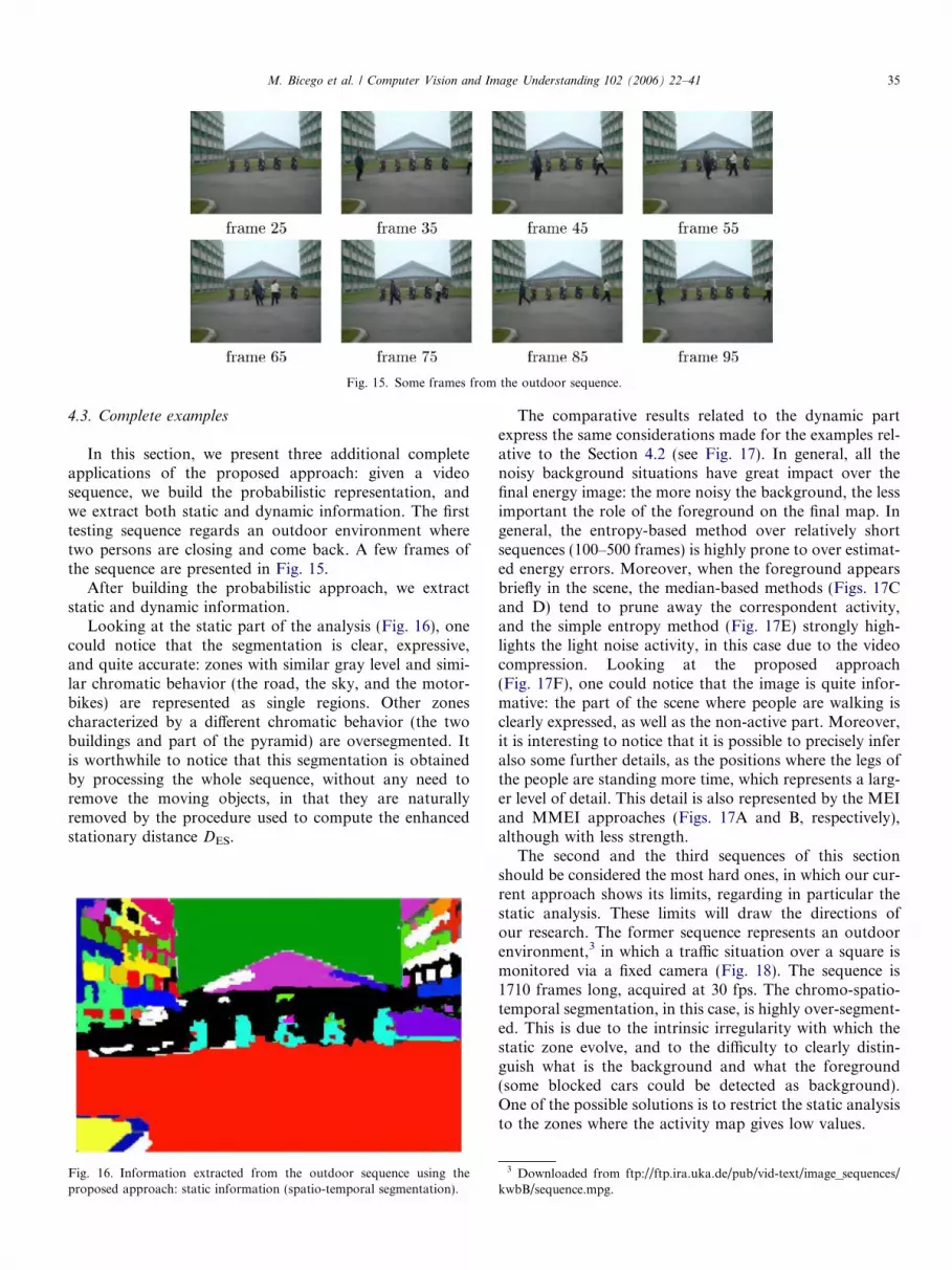
Fig. 15. Some frames from the outdoor sequence.
M. Bicego et al. / Computer Vision and Image Understanding 102 (2006) 22–41 35
4.3. Complete examples
In this section, we present three additional completeapplications of the proposed approach: given a videosequence, we build the probabilistic representation, andwe extract both static and dynamic information. The firsttesting sequence regards an outdoor environment wheretwo persons are closing and come back. A few frames ofthe sequence are presented in Fig. 15.
After building the probabilistic approach, we extractstatic and dynamic information.
Looking at the static part of the analysis (Fig. 16), onecould notice that the segmentation is clear, expressive,and quite accurate: zones with similar gray level and simi-lar chromatic behavior (the road, the sky, and the motor-bikes) are represented as single regions. Other zonescharacterized by a different chromatic behavior (the twobuildings and part of the pyramid) are oversegmented. Itis worthwhile to notice that this segmentation is obtainedby processing the whole sequence, without any need toremove the moving objects, in that they are naturallyremoved by the procedure used to compute the enhancedstationary distance DES.
Fig. 16. Information extracted from the outdoor sequence using theproposed approach: static information (spatio-temporal segmentation).
The comparative results related to the dynamic partexpress the same considerations made for the examples rel-ative to the Section 4.2 (see Fig. 17). In general, all thenoisy background situations have great impact over thefinal energy image: the more noisy the background, the lessimportant the role of the foreground on the final map. Ingeneral, the entropy-based method over relatively shortsequences (100–500 frames) is highly prone to over estimat-ed energy errors. Moreover, when the foreground appearsbriefly in the scene, the median-based methods (Figs. 17Cand D) tend to prune away the correspondent activity,and the simple entropy method (Fig. 17E) strongly high-lights the light noise activity, in this case due to the videocompression. Looking at the proposed approach(Fig. 17F), one could notice that the image is quite infor-mative: the part of the scene where people are walking isclearly expressed, as well as the non-active part. Moreover,it is interesting to notice that it is possible to precisely inferalso some further details, as the positions where the legs ofthe people are standing more time, which represents a larg-er level of detail. This detail is also represented by the MEIand MMEI approaches (Figs. 17A and B, respectively),although with less strength.
The second and the third sequences of this sectionshould be considered the most hard ones, in which our cur-rent approach shows its limits, regarding in particular thestatic analysis. These limits will draw the directions ofour research. The former sequence represents an outdoorenvironment,3 in which a traffic situation over a square ismonitored via a fixed camera (Fig. 18). The sequence is1710 frames long, acquired at 30 fps. The chromo-spatio-temporal segmentation, in this case, is highly over-segment-ed. This is due to the intrinsic irregularity with which thestatic zone evolve, and to the difficulty to clearly distin-guish what is the background and what the foreground(some blocked cars could be detected as background).One of the possible solutions is to restrict the static analysisto the zones where the activity map gives low values.
3 Downloaded from ftp://ftp.ira.uka.de/pub/vid-text/image_sequences/kwbB/sequence.mpg.
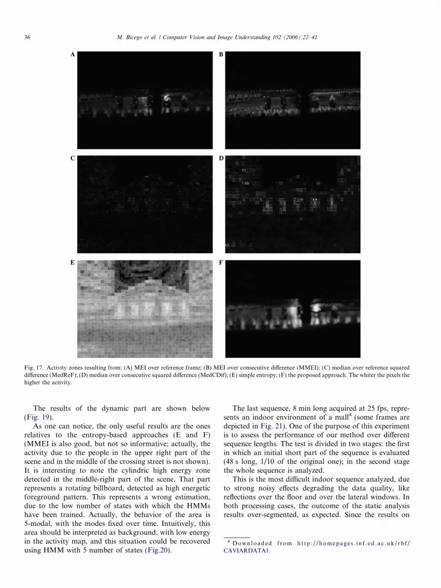
Fig. 17. Activity zones resulting from: (A) MEI over reference frame; (B) MEI over consecutive difference (MMEI); (C) median over reference squareddifference (MedReF); (D) median over consecutive squared difference (MedCDif); (E) simple entropy; (F) the proposed approach. The whiter the pixels thehigher the activity.
4 D o w n l oa d e d f r o m h t t p : / / h o me pa g e s . i n f . ed . a c . u k / r b f /CAVIARDATA1.
36 M. Bicego et al. / Computer Vision and Image Understanding 102 (2006) 22–41
The results of the dynamic part are shown below(Fig. 19).
As one can notice, the only useful results are the onesrelatives to the entropy-based approaches (E and F)(MMEI is also good, but not so informative; actually, theactivity due to the people in the upper right part of thescene and in the middle of the crossing street is not shown).It is interesting to note the cylindric high energy zonedetected in the middle-right part of the scene. That partrepresents a rotating billboard, detected as high energeticforeground pattern. This represents a wrong estimation,due to the low number of states with which the HMMshave been trained. Actually, the behavior of the area is5-modal, with the modes fixed over time. Intuitively, thisarea should be interpreted as background, with low energyin the activity map, and this situation could be recoveredusing HMM with 5 number of states (Fig.20).
The last sequence, 8 min long acquired at 25 fps, repre-sents an indoor environment of a mall4 (some frames aredepicted in Fig. 21). One of the purpose of this experimentis to assess the performance of our method over differentsequence lengths. The test is divided in two stages: the firstin which an initial short part of the sequence is evaluated(48 s long, 1/10 of the original one); in the second stagethe whole sequence is analyzed.
This is the most difficult indoor sequence analyzed, dueto strong noisy effects degrading the data quality, likereflections over the floor and over the lateral windows. Inboth processing cases, the outcome of the static analysisresults over-segmented, as expected. Since the results on

Fig. 18. Some frames from the traffic sequence.
Fig. 19. Activity zones resulting from: (A) MEI over reference frame; (B) MEI over consecutive difference (MMEI); (C) median over reference squareddifference (MedReF); (D) median over consecutive squared difference (MedCDif); (E) simple entropy; (F) the proposed approach. The whiter the pixels thehigher the activity.
M. Bicego et al. / Computer Vision and Image Understanding 102 (2006) 22–41 37

Fig. 22. Information extracted from the whole outdoor sequence using theproposed approach: static information.
Fig. 20. Traffic sequence: the detail of the billboard in Fig. 19, whosepixels are trained with HMMs having 3 (A) or 5 states (B). It is possible toevaluate the decreasing of activity detected in (B) due to the correctestimation of the five modalities which characterize the billboard behavior.
38 M. Bicego et al. / Computer Vision and Image Understanding 102 (2006) 22–41
the short sequence are not significative, only the resultsrelated to the longer sequence are shown in Fig. 22.
Looking at this figure, it is possible to reason aboutwhat are the biggest areas whose chromatic behavior issimilar in time, so as to detect the most ‘‘stable’’ sceneareas. In particular, it is possible to detect stable zones inproximity of the lateral columns, and in some parts ofthe floor, while the area corresponding to the left wall, withseveral glass windows, is in general over-segmented.
For what concerns the dynamic analysis, the techniquesbased on differences between frames give poor results inboth tests, hence only the method based on the entropyand the proposed approach are presented.
As shown in the previous results, the proposed approachworks better compared to the entropy method, individuat-ing the zones in which the foreground activity is located,disregarding the noise. In particular, in Fig. 23F1 is possi-ble to clearly detect the left drift of energy, that models thefact that the people enters frequently in the mall. InFig. 23E1 this aspect is not so clearly highlighted. More-over, augmenting the sequence length, the effect of theentropy takes strongly into account the noise due to thereflection on the floor: this results in an activity map that‘‘forgets’’ the amount of activity present in the bottom partof the hallway. Conversely, our approach is able to repre-sent all the foreground activity as shown in Fig. 23F2.
Summarizing, the experiments have assessed that theproposed method, concerning the static informationextraction, provides a novel kind of analysis able to explain
Fig. 21. Some frames from
the chromatic evolution of the static part of the sequence,individuating regions with similar temporal-chromatic pro-file. The main drawback results in the generation of an oversegmentation, which occurs in noisy cases. For what con-cerns the dynamic analysis of the foreground, the proposedapproach outperforms in general all the tested comparativemethods, showing a certain degree of robustness over allthe input (long/short sequences with low/high noise levels).
4.4. Possible applications
In this section, the possible uses of the informationextracted with the proposed approach are investigated. Afirst example can be found in [22], where this informationhas been used in order to initialize an integrated pixel-and region-based approach to background modelling, pro-posed in [23]. This background model uses informationderived from a spatial segmentation of the scene in orderto modulate the response of a standard pixel-level back-ground modelling scheme [46], increasing the robustnessagainst local non uniform illumination changes. Theinformation extracted with our approach is used to initial-ize this model: in particular, the initialization of the pixellevel part of the model straightforwardly derives from the
the traffic sequence.

Fig. 23. Activity zones resulting from: (E1) simple entropy and (F1) the proposed approach calculated over the 48 s sequence; (E2) simple entropy and(F2) the proposed approach calculated over the entire 8 min sequence; the whiter the pixels the higher the activity.
M. Bicego et al. / Computer Vision and Image Understanding 102 (2006) 22–41 39
probabilistic modelling of the video sequence, while the ini-tialization of the region level part is the spatio temporalsegmentation described in Section 3.2.
There are two other ways of employing the informationextracted from the proposed approach, which are currentlyin progress. The first is to use the activity map to decide thelevel of detail of a variable resolution background model-ling scheme: the idea is that in those zones where no activ-ities typically occur, a very accurate background analysis isnot necessary, and a coarse analysis could be sufficient. Thesecond application can be to use the activity maps to inferthe zones of appearance of the foreground with high prob-ability, the so-called source detection problem [47]. Theidea is that it is not useful to accurately monitor the zonesof the scene where typically no foreground objects arelikely to occur.
One constraint of the described approach regards therequirement of a fixed camera. In principle, this conditioncan be relaxed by performing a pre-registration of theimage pixels using an estimate of dominant motion of thescene so that temporal gray-level profiles can be reliablyevaluated. Further, such registration could not be criticalif small local areas are considered instead of single pixelslike in one of the experiments above.
5. Conclusions
In this paper, a new method for scene analysis fromvideo sequences has been proposed, using only very
low-level data, that is just pixel behavior. The proposedapproach models the sequence using a forest of HiddenMarkov models, each one devoted to modelling the tempo-ral evolution of the gray level of each pixel. Given this rep-resentation, two kinds of analysis have been developed: thefirst one clusters the HMMs to obtain a spatio-temporalsegmentation of the background, and the second onedefines an entropy based measure computed on the station-ary probability distribution of each HMM to infer theactivity zones of the scene. The proposed approach has sev-eral key features with respect to the methods in the state ofthe art: it extracts information from the lowest possiblelevel (the pixel level), it is unsupervised in nature, it usesHMM at a very basic level, and it employs the same prin-cipled probabilistic modelling to infer both static anddynamic information. The results obtained from realexperiments have shown the effectiveness of the proposedapproach, also with respect to state of the art methods,able to get a better insight of the scene and on the interpre-tation of the activities occurring therein.
References
[1] N. Jojic, N. Petrovic, B. Frey, T. Huang, Transformed hiddenMarkov models: Estimating mixture models of images and inferringspatial transformations in video sequences, in: Proc. IEEE Conf. onComputer Vision and Pattern Recognition, 2000, pp. 26–33.
[2] M. Naphade, T. Huang, A probabilistic framework for semanticindexing and retrieval in video, in: Proc. IEEE Internat. Conf. onMultimedia and Expo(I), 2000, pp. 475–478.

40 M. Bicego et al. / Computer Vision and Image Understanding 102 (2006) 22–41
[3] M. Flickner, H. Sawhney, W. Niblack, J. Ashley, Q. Huang, B. Dom,M. Gorkani, J. Hafner, D. Lee, D. Petkovic, D. Steele, P. Yanker,Query by image and video content: the qbic system, IEEE Computer28 (9) (1995) 23–32.
[4] S. Maillet, Content-based video retrieval: An overview, available athttp://viper.unige.ch/ marchand/CBVR/overview.html (2000).
[5] PAMI, Special issue on video surveillance, IEEE Trans. Pattern Anal.Mach. Intell. 22 (8), 2000.
[6] R. Collins, A. Lipton, T. Kanade, H. Fujiyoshi, D. Duggins, Y. Tsin,D. Tolliver, N. Enomoto, O. Hasegawa, A system for videosurveillance and monitoring, Tech. Rep. CMU-RI-TR-00-12, Robot-ics Institute, Carnegie Mellon University, 2000.
[7] N. Johnson, D. Hogg, Learning the distribution of object trajectoriesfor event recognition, Image Vision Comput. 14 (1996) 609–615.
[8] D. Gavrila, The visual analysis of human movement: a survey,Comput. Vision Image Understand. 73 (1) (1999) 82–98.
[9] M. Brand, N. Oliver, S. Pentland, Coupled hidden markov models forcomplex action recognition, in: Proc. IEEE Conf. on ComputerVision and Pattern Recognition, 1997, pp. 994–999.
[10] T. Jebara, A. Pentland, Action reaction learning: Automatic visualanalysis and synthesis of interactive behavior, in: Proc. Internat.Conf. on Computer Vision Systems, 1999.
[11] R. Morris, D. Hogg, Statistical models of object interaction, Internat.J. Comput. Vision 37 (2000) 209–215.
[12] N. Oliver, B. Rosario, A. Pentland, Graphical models for recognisinghuman interactions, in: Advances in Neural Information ProcessingSystems, 1998.
[13] A. Galata, N. Jonhson, D. Hogg, Learning variable-length markovmodels of behavior, Comput. Vision Image Understand. 81 (2001)398–413.
[14] H. Buxton, Learning and understanding dynamic scene activity: areview, Image Vision Comput. 21 (2003) 125–136.
[15] B. Frey, N. Jojic, Transformation-invariant clustering using the EMalgorithm, IEEE Trans. Pattern Anal. Mach. Intell. 25 (1) (2003) 1–17.
[16] I. Haritaoglu, D. Harwood, L. Davis, W4: real-time surveillance ofpeople and their activities, IEEE Trans. Pattern Anal. Mach. Intell.22 (8) (2000) 809–830.
[17] T. Wada, T. Matsuyama, Multiobject behavior recognition by eventdriven selective method, IEEE Trans. Pattern Anal. Mach. Intell. 22(8) (2000) 873–887.
[18] S. Gong, J. Ng, J. Sherrah, On the semantics of visual behaviour,structured events and trajectories of human action, Image VisionComput. 20 (12) (2002) 873–888.
[19] J. Ng, S. Gong, Learning pixel-wise signal energy for understandingsemantics, in: Proc. of the British Machine Vision Conference,BMVA Press, 2001, pp. 695–704.
[20] J. Sherrah, S. Gong, Continuous global evidence-based bayesianmodality fusion for simultaneous tracking of multiple objects, in:Proc. Internat. Conf. on Computer Vision, 2001, pp. 42–29.
[21] T. Xiang, S. Gong, D. Parkinson, Autonomous visual event detectionand classification without explicit object-centred segmentation andtracking, in: Proc. of the British Machine Vision Conference, BMVAPress, 2002, pp. 233–242.
[22] M. Cristani, M. Bicego, V. Murino, Multi-level background initial-ization using hidden markov models, in: Proc. ACM SIGMMWorkshop on Video Surveillance, 2003, pp. 11–19.
[23] M. Cristani, M. Bicego, V. Murino, Integrated region- and pixel-based approach to background modelling, in: Proc. IEEE Workshopon Motion and Video Computing, 2002, pp. 3–8.
[24] L. Rabiner, A tutorial on Hidden Markov Models and selectedapplications in speech recognition, Proc. IEEE 77 (2) (1989) 257–286.
[27] A. Dempster, N. Laird, D. Rubin, Maximum likelihood fromincomplete data via the EM algorithm, J. Roy. Statist. Soc. B 39(1977) 1–38.
[28] C. Wu, On the convergence properties of the EM algorithm, Ann.Stat. 11 (1) (1983) 95–103.
[29] B. Stenger, V. Ramesh, N. Paragios, F.Coetzee, J.M. Buhmann,Topology free hidden Markov models: application to background
modeling, in: Proc. Internat. Conf. Computer Vision, vol. 1, 2001, pp.294–301.
[30] J. Rittscher, J. Kato, S. Joga, A. Blake, A probabilistic backgroundmodel for tracking, in: Proc. Eur. Conf. on Computer Vision, 2000,pp. 336–350.
[31] P. Bremaud, Markov Chains, Springer, Berlin, 1999.[32] M. Bicego, V. Murino, M. Figueiredo, Similarity-based clustering of
sequences using hidden Markov models, in: P. Perner, A. Rosenfeld(Eds.), Machine Learning and Data Mining in Pattern Recognition,vol. LNAI 2734, Springer, Berlin, 2003, pp. 86–95.
[33] M. Law, J. Kwok, Rival penalized competitive learning for model-based sequence, in: Proc. Internat. Conf. on Pattern Recognition, vol.2, 2000, pp. 195–198.
[34] P. Smyth, Clustering sequences with hidden Markov models, in: M.Mozer, M. Jordan, T. Petsche (Eds.), Advances in Neural Informa-tion Processing Systems, vol. 9, MIT Press, Cambridge, 1997, p. 648.
[35] C. Li, G. Biswas, A bayesian approach to temporal data clusteringusing hidden Markov models, in: Proc. Internat. Conf. on MachineLearning, 2000, pp. 543–550.
[36] C. Li, G. Biswas, Applying the Hidden Markov Model methodologyfor unsupervised learning of temporal data, Int. J. Knowl.-basedIntell. Eng. Syst. 6 (3) (2002) 152–160.
[37] A. Panuccio, M. Bicego, V. Murino, A Hidden Markov Model-basedapproach to sequential data clustering, in: T. Caelli, A. Amin, R.Duin, M. Kamel, D. de Ridder (Eds.), Structural, Syntactic andStatistical Pattern Recognition, Lecture Notes in Computer Series,vol. 2396, Springer, 2002, pp. 734–742.
[38] C. Bahlmann, H. Burkhardt, Measuring HMM similarity with theBayes probability of error and its application to online handwritingrecognition, in: Proc. Internat. Conf. on Document Analysis andRecognition, 2001, pp. 406–411.
[39] S. Kullback, R. Leibler, On information and sufficiency, Ann. Math.Stat. 22 (1951) 79–86.
[40] G. McLachlan, D. Peel, Finite Mixture Models, Wiley, New York,2000.
[41] A. Stolcke, S. Omohundro, Hidden Markov Model induction byBayesian model merging, in: S. Hanson, J. Cowan, C. Giles (Eds.),Advances in Neural Information Processing Systems, vol. 5, MorganKaufmann, San Mateo, CA, 1993, pp. 11–18.
[42] M. Brand, An entropic estimator for structure discovery, in: M.Kearns, S. Solla, D. Cohn (Eds.), Advances in Neural InformationProcessing Systems, vol. 11, MIT Press, Cambridge, 1999, pp. 723–729.
[43] M. Bicego, A. Dovier, V. Murino, Designing the minimal structure ofHidden Markov Models by bisimulation, in: M. Figueiredo, J.Zerubia, A. Jain (Eds.), Energy Minimization Methods in ComputerVision and Pattern Recognition, Lecture Notes in Computer Series,vol. 2134, Springer, 2001, pp. 75–90.
[44] M. Bicego, V. Murino, M. Figueiredo, A sequential pruning strategyfor the selection of the number of states in Hidden Markov Models,Patt. Recogn. Lett. 24 (9–10) (2003) 1395–1407.
[45] D. Demirdjian, K. Tollmar, K. Koile, N. Checka, T. Darrell, Activitymaps for location-aware computing, in: Proc. IEEE Workshop onApplications of Computer Vision, 2002, pp. 70–75.
[46] C. Stauffer, W. Grimson, Adaptive background mixture models forreal-time tracking, in: Proc. Internat. Conf. on Computer Vision andPattern Recognition, vol. 2, 1999, pp. 246–252.
[47] C. Stauffer, Estimating tracking sources and sinks, in: Proc. IEEEWorkshop on Event Mining, 2003, p. 34.
[48] J. Alon, S. Sclaroff, G. Kollios, V. Pavlovic, Discovering clusters inmotion time-series data, in: Proc. Internat. Conf. on Computer Visionand Pattern Recognition, 2003, pp. 375–381.
[49] A. Bobick, J. Davis, An appearance-based representation of action,in: Proc. Internat. Conf. on Pattern Recognition (ICPR �96), vol. 1,1996, pp. 307–310.
[50] B. Juang, L. Rabiner, A probabilistic distance measure for HiddenMarkov Models, AT&T Tech. J. 64 (2) (1985) 391–408.
[51] O. Cappe, Ten years of HMMs. Available from: http://www.tsi.enst.fr/cappe/docs/hmmbib.html, 2001.

M. Bicego et al. / Computer Vision and Image Understanding 102 (2006) 22–41 41
[53] S. Zhong, J. Ghosh, HMMs and coupled HMMs for multi-channelEEG classification, in: Proc. IEEE Internat. Joint Conf. on NeuralNetworks, vol. 2, 2002, pp. 1154–1159.
[54] S. Gong, T. Xiang, Recognition of group activities using a dynamicprobabilistic network, in: IEEE Proc. Internat. Conf. on ComputerVision, 2003, pp. 742–749.
[55] J.W. Davis, A.F. Bobick, The representation and recognition of humanmovement using temporal templates, in: IEEE Proc. Internat. Conf. onComputer Vision and Pattern Recognition, 1997, pp. 928–934.
[57] G. Jing, C.E. Siong, D. Rajan, Foreground motion detection bydifference-based spatial temporal entropy image, in: IEEE Tencon2004, 2004.


