Embed Size (px)
Citation preview

Using a Model of Human Cognition of Causality to Orient Arcs in Structural Learning
A dissertation submitted in partial fulfillment of the requirements for the degree ofDoctor of Philosophy at George Mason University
By
Jee VangMaster of Science
The George Washington University, 2001Bachelor of Science
Georgetown University, 1999
Director: Dr. Farrokh Alemi, ProfessorDepartment of Computational and Data Sciences
Fall Semester 2008George Mason University
Fairfax, VA

Copyright c© 2008 by Jee VangAll Rights Reserved
ii

Dedication
To my mother, Mao Yang, and to my father, Yee Vang, for their love and support.
iii

Acknowledgments
I would like to thank Dr. Farrokh Alemi for his guidance and challenging me throughoutthe years. I would also like to thank Dr. Kathryn B. Laskey for making my thesis strongerand education in Bayesian networks more in-depth. I would like to thank Drs. EdwardJ. Wegman and Larry Kerschberg for their inputs to fine tune my thesis. For their helpand assistance with BNGenerator, I would like to thank Drs. Jaime S. Ide and Fabio G.Cozman. For answering all my emails and questions, I would also like to thank Dr. JieCheng. I would also like to thank Dr. Michael R. Waldmann for answering questionsregarding models of human cognition of causality.
iv

Table of Contents
Page
List of Tables . . . . . . . . . . . . . . . . . . . . . . . . . . . . . . . . . . . . . . . . viiiList of Figures . . . . . . . . . . . . . . . . . . . . . . . . . . . . . . . . . . . . . . . . xv
Abstract . . . . . . . . . . . . . . . . . . . . . . . . . . . . . . . . . . . . . . . . . . . xvii1 Introduction . . . . . . . . . . . . . . . . . . . . . . . . . . . . . . . . . . . . . . 12 Bayesian Networks . . . . . . . . . . . . . . . . . . . . . . . . . . . . . . . . . . . 4
2.1 Quantitative Aspect of a Bayesian Network . . . . . . . . . . . . . . . . . . 5
2.2 Qualitative Aspect of a Bayesian Network . . . . . . . . . . . . . . . . . . . 6
2.2.1 Directed Acyclic Graph (DAG) . . . . . . . . . . . . . . . . . . . . . 6
2.2.2 Direction dependent-separation (d-separation) . . . . . . . . . . . . 7
2.2.3 Elementary structures . . . . . . . . . . . . . . . . . . . . . . . . . . 9
2.2.4 Markov Blanket . . . . . . . . . . . . . . . . . . . . . . . . . . . . . 102.2.5 Causal Bayesian Network . . . . . . . . . . . . . . . . . . . . . . . . 10
3 Learning a Bayesian Network . . . . . . . . . . . . . . . . . . . . . . . . . . . . . 12
3.1 Parameter Learning . . . . . . . . . . . . . . . . . . . . . . . . . . . . . . . 12
3.2 Structure Learning . . . . . . . . . . . . . . . . . . . . . . . . . . . . . . . . 13
3.2.1 Search and Scoring Algorithms . . . . . . . . . . . . . . . . . . . . . 13
3.2.2 Constraint-based Algorithms . . . . . . . . . . . . . . . . . . . . . . 16
4 Novel Structure Learning Algorithms . . . . . . . . . . . . . . . . . . . . . . . . 20
4.1 Discovering the Markov blanket . . . . . . . . . . . . . . . . . . . . . . . . . 22
4.2 Constructing an Undirected Graph using Markov Blankets (CrUMB) . . . . 26
4.3 Orienting the edges in an undirected graph by detecting colliders . . . . . . 29
4.4 Orienting the undirected edges in a PDAG inductively . . . . . . . . . . . . 30
4.5 Orienting the edges using a model of human cognition of causation . . . . . 31
4.6 Orienting the undirected edges using Genetic Algorithms . . . . . . . . . . . 34
4.7 SC* Algorithm . . . . . . . . . . . . . . . . . . . . . . . . . . . . . . . . . . 37
5 Methods . . . . . . . . . . . . . . . . . . . . . . . . . . . . . . . . . . . . . . . . 405.1 Procedure for Generating Data for Structure Learning Algorithms . . . . . 40
5.2 Generating Bayesian Networks . . . . . . . . . . . . . . . . . . . . . . . . . 40
v

5.3 Simulating Data . . . . . . . . . . . . . . . . . . . . . . . . . . . . . . . . . 44
5.4 Applying the Structure Learning Algorithms on Simulated Data . . . . . . 45
5.5 Output–Qualitative Performance . . . . . . . . . . . . . . . . . . . . . . . . 46
5.6 Output–Quantitative Performance . . . . . . . . . . . . . . . . . . . . . . . 48
5.7 Analysis of Variance–ANOVA . . . . . . . . . . . . . . . . . . . . . . . . . . 51
6 Results and Analysis . . . . . . . . . . . . . . . . . . . . . . . . . . . . . . . . . . 53
6.1 Total Arc Errors . . . . . . . . . . . . . . . . . . . . . . . . . . . . . . . . . 536.2 KL Divergence Transformation Differences . . . . . . . . . . . . . . . . . . . 62
7 Applying BN structure learning on a Real Dataset of Patients Treated for Sub-
stance Abuse Who are also Criminal Justice Offenders . . . . . . . . . . . . . . . 707.1 Introduction . . . . . . . . . . . . . . . . . . . . . . . . . . . . . . . . . . . . 707.2 Motivation . . . . . . . . . . . . . . . . . . . . . . . . . . . . . . . . . . . . 717.3 The Data . . . . . . . . . . . . . . . . . . . . . . . . . . . . . . . . . . . . . 737.4 The Variables . . . . . . . . . . . . . . . . . . . . . . . . . . . . . . . . . . . 747.5 Data Transformation . . . . . . . . . . . . . . . . . . . . . . . . . . . . . . . 777.6 Transformed Data Set . . . . . . . . . . . . . . . . . . . . . . . . . . . . . . 817.7 Information Loss . . . . . . . . . . . . . . . . . . . . . . . . . . . . . . . . . 827.8 Data Set Size Reduction . . . . . . . . . . . . . . . . . . . . . . . . . . . . . 857.9 Time Dimension . . . . . . . . . . . . . . . . . . . . . . . . . . . . . . . . . 867.10 K-Fold Cross-Validations of Algorithms and Learned Networks . . . . . . . 86
7.11 Learning a Bayesian Network from the Complete Dataset . . . . . . . . . . 89
8 Summary and Conclusions . . . . . . . . . . . . . . . . . . . . . . . . . . . . . . 95
8.1 Future Work . . . . . . . . . . . . . . . . . . . . . . . . . . . . . . . . . . . 97A One Way ANOVA Tables for Total Arc Errors for Singly-Connected Bayesian
Networks . . . . . . . . . . . . . . . . . . . . . . . . . . . . . . . . . . . . . . . . . 98B HSD Tables for Total Arc Errors for Singly-Connected Bayesian Networks . . . . 105
C One Way ANOVA Tables for Direction Omission and Commission Errors for
Singly-Connected Bayesian Networks . . . . . . . . . . . . . . . . . . . . . . . . . 118
D HSD Tables for Direction Omission and Commission Errors for Singly-Connected
Bayesian Networks . . . . . . . . . . . . . . . . . . . . . . . . . . . . . . . . . . . 125
E One Way ANOVA Tables for Total Arc Errors for Multi-Connected Bayesian
Networks . . . . . . . . . . . . . . . . . . . . . . . . . . . . . . . . . . . . . . . . . 138F HSD Tables for Total Arc Errors for Multi-Connected Bayesian Networks . . . . 145
G One Way ANOVA Tables for Direction Omission and Commission Errors for
Multi-Connected Bayesian Networks . . . . . . . . . . . . . . . . . . . . . . . . . 158
vi

H HSD Tables for Direction Omission and Commission Errors for Multi-ConnectedBayesian Networks . . . . . . . . . . . . . . . . . . . . . . . . . . . . . . . . . . . 165
I Box and Whisker Plots of Total Arc Errors for Singly- and Multi-Connected BNs 178
J One Way ANOVA Tables for KL Differences for Singly-Connected Bayesian Net-
works . . . . . . . . . . . . . . . . . . . . . . . . . . . . . . . . . . . . . . . . . . . 191K HSD Tables for KL Differences for Singly-Connected Bayesian Networks . . . . . 198
L One Way ANOVA Tables for KL Differences for Multi-Connected Bayesian Networks211
M HSD Tables for KL Differences for Multi-Connected Bayesian Networks . . . . . 218
N Correlations and Ranks of Variables in Original and Transformed Data Set . . . 231
Bibliography . . . . . . . . . . . . . . . . . . . . . . . . . . . . . . . . . . . . . . . . . 237
vii

List of Tables
Table Page
2.1 Elementary structures . . . . . . . . . . . . . . . . . . . . . . . . . . . . . . 9
3.1 Elementary structures and Conditional Independence . . . . . . . . . . . . . 19
5.1 BNGenerator Parameters . . . . . . . . . . . . . . . . . . . . . . . . . . . . 425.2 Summary Statistics for Arcs for Generated Singly-Connected BNs . . . . . 43
5.3 Summary Statistics for Arcs for Generated Multi-Connected BNs . . . . . . 44
5.4 Omission and Commission Errors . . . . . . . . . . . . . . . . . . . . . . . . 485.5 Example of Learning Results for Total Arc Errors used in ANOVA . . . . . 52
6.1 ANOVA Results for Qualitative Performances . . . . . . . . . . . . . . . . . 54
6.2 Counts of best learned BNs for each algorithm by size for singly-connected
BNs . . . . . . . . . . . . . . . . . . . . . . . . . . . . . . . . . . . . . . . . 616.3 Counts of best learned BNs for each algorithm by size for multi-connected BNs 62
6.4 ANOVA Results for Quantitative Performances . . . . . . . . . . . . . . . . 63
7.1 Variables in Study . . . . . . . . . . . . . . . . . . . . . . . . . . . . . . . . 75
7.2 Binary Variable Value Coding Scheme . . . . . . . . . . . . . . . . . . . . . 75
7.3 Summary Statistics for Binary Variables . . . . . . . . . . . . . . . . . . . . 76
7.4 Summary Statistics for Integer Variables . . . . . . . . . . . . . . . . . . . . 77
7.5 Number and Percentage of Patients with Values ≥ 1 for Integer Variables . 78
7.6 Frequency of Values for Discretized Age Variable . . . . . . . . . . . . . . . 78
7.7 Frequency of Values for Discretized Followup Variable . . . . . . . . . . . . 79
7.8 Frequency of Values for Discretized Probation Variable . . . . . . . . . . . . 80
7.9 Transformed Variables . . . . . . . . . . . . . . . . . . . . . . . . . . . . . . 817.10 Correlation Matrix for Ranks of Correlations in Original and Transformed
Data Sets . . . . . . . . . . . . . . . . . . . . . . . . . . . . . . . . . . . . . 857.11 Huber Taxonomy of Data Set Sizes . . . . . . . . . . . . . . . . . . . . . . . 86
7.12 Average quadratic loss values from k-fold cross-validation . . . . . . . . . . 88
7.13 ANOVA results for quadratic loss values from k-fold cross-validation . . . . 88
7.14 HSD results for quadratic loss from k-fold cross-validations . . . . . . . . . 89
7.15 Sensitivity Analysis . . . . . . . . . . . . . . . . . . . . . . . . . . . . . . . . 91
viii

A.1 ANOVA results for total arc errors for singly-connected BNs of size 4 . . . . 98
A.2 ANOVA results for total arc errors for singly-connected BNs of size 5 . . . . 98
A.3 ANOVA results for total arc errors for singly-connected BNs of size 6 . . . . 99
A.4 ANOVA results for total arc errors for singly-connected BNs of size 7 . . . . 99
A.5 ANOVA results for total arc errors for singly-connected BNs of size 8 . . . . 100
A.6 ANOVA results for total arc errors for singly-connected BNs of size 9 . . . . 100
A.7 ANOVA results for total arc errors for singly-connected BNs of size 10 . . . 101
A.8 ANOVA results for total arc errors for singly-connected BNs of size 11 . . . 101
A.9 ANOVA results for total arc errors for singly-connected BNs of size 12 . . . 102
A.10 ANOVA results for total arc errors for singly-connected BNs of size 13 . . . 102
A.11 ANOVA results for total arc errors for singly-connected BNs of size 14 . . . 103
A.12 ANOVA results for total arc errors for singly-connected BNs of size 15 . . . 103
A.13 ANOVA results for total arc errors for singly-connected BNs of size 20 . . . 104
B.1 HSD results for total arc errors for singly-connected BNs of size 4 . . . . . . 105
B.2 HSD results for total arc errors for singly-connected BNs of size 5 . . . . . . 106
B.3 HSD results for total arc errors for singly-connected BNs of size 6 . . . . . . 107
B.4 HSD results for total arc errors for singly-connected BNs of size 7 . . . . . . 108
B.5 HSD results for total arc errors for singly-connected BNs of size 8 . . . . . . 109
B.6 HSD results for total arc errors for singly-connected BNs of size 9 . . . . . . 110
B.7 HSD results for total arc errors for singly-connected BNs of size 10 . . . . . 111
B.8 HSD results for total arc errors for singly-connected BNs of size 11 . . . . . 112
B.9 HSD results for total arc errors for singly-connected BNs of size 12 . . . . . 113
B.10 HSD results for total arc errors for singly-connected BNs of size 13 . . . . . 114
B.11 HSD results for total arc errors for singly-connected BNs of size 14 . . . . . 115
B.12 HSD results for total arc errors for singly-connected BNs of size 15 . . . . . 116
B.13 HSD results for total arc errors for singly-connected BNs of size 20 . . . . . 117
C.1 ANOVA results for direction omission and commission errors for singly-
connected BNs of size 4 . . . . . . . . . . . . . . . . . . . . . . . . . . . . . 118C.2 ANOVA results for direction omission and commission errors for singly-
connected BNs of size 5 . . . . . . . . . . . . . . . . . . . . . . . . . . . . . 118C.3 ANOVA results for direction omission and commission errors for singly-
connected BNs of size 6 . . . . . . . . . . . . . . . . . . . . . . . . . . . . . 119C.4 ANOVA results for direction omission and commission errors for singly-
connected BNs of size 7 . . . . . . . . . . . . . . . . . . . . . . . . . . . . . 119
ix

C.5 ANOVA results for direction omission and commission errors for singly-
connected BNs of size 8 . . . . . . . . . . . . . . . . . . . . . . . . . . . . . 120C.6 ANOVA results for direction omission and commission errors for singly-
connected BNs of size 9 . . . . . . . . . . . . . . . . . . . . . . . . . . . . . 120C.7 ANOVA results for direction omission and commission errors for singly-
connected BNs of size 10 . . . . . . . . . . . . . . . . . . . . . . . . . . . . . 121C.8 ANOVA results for direction omission and commission errors for singly-
connected BNs of size 11 . . . . . . . . . . . . . . . . . . . . . . . . . . . . . 121C.9 ANOVA results for direction omission and commission errors for singly-
connected BNs of size 12 . . . . . . . . . . . . . . . . . . . . . . . . . . . . . 122C.10 ANOVA results for direction omission and commission errors for singly-
connected BNs of size 13 . . . . . . . . . . . . . . . . . . . . . . . . . . . . . 122C.11 ANOVA results for direction omission and commission errors for singly-
connected BNs of size 14 . . . . . . . . . . . . . . . . . . . . . . . . . . . . . 123C.12 ANOVA results for direction omission and commission errors for singly-
connected BNs of size 15 . . . . . . . . . . . . . . . . . . . . . . . . . . . . . 123C.13 ANOVA results for direction omission and commission errors for singly-
connected BNs of size 20 . . . . . . . . . . . . . . . . . . . . . . . . . . . . . 124D.1 HSD results for direction omission and commission errors for singly-connected
BNs of size 4 . . . . . . . . . . . . . . . . . . . . . . . . . . . . . . . . . . . 125D.2 HSD results for direction omission and commission errors for singly-connected
BNs of size 5 . . . . . . . . . . . . . . . . . . . . . . . . . . . . . . . . . . . 126D.3 HSD results for direction omission and commission errors for singly-connected
BNs of size 6 . . . . . . . . . . . . . . . . . . . . . . . . . . . . . . . . . . . 127D.4 HSD results for direction omission and commission errors for singly-connected
BNs of size 7 . . . . . . . . . . . . . . . . . . . . . . . . . . . . . . . . . . . 128D.5 HSD results for direction omission and commission errors for singly-connected
BNs of size 8 . . . . . . . . . . . . . . . . . . . . . . . . . . . . . . . . . . . 129D.6 HSD results for direction omission and commission errors for singly-connected
BNs of size 9 . . . . . . . . . . . . . . . . . . . . . . . . . . . . . . . . . . . 130D.7 HSD results for direction omission and commission errors for singly-connected
BNs of size 10 . . . . . . . . . . . . . . . . . . . . . . . . . . . . . . . . . . . 131D.8 HSD results for direction omission and commission errors for singly-connected
BNs of size 11 . . . . . . . . . . . . . . . . . . . . . . . . . . . . . . . . . . . 132D.9 HSD results for direction omission and commission errors for singly-connected
BNs of size 12 . . . . . . . . . . . . . . . . . . . . . . . . . . . . . . . . . . . 133
x

D.10 HSD results for direction omission and commission errors for singly-connected
BNs of size 13 . . . . . . . . . . . . . . . . . . . . . . . . . . . . . . . . . . . 134D.11 HSD results for direction omission and commission errors for singly-connected
BNs of size 14 . . . . . . . . . . . . . . . . . . . . . . . . . . . . . . . . . . . 135D.12 HSD results for direction omission and commission errors for singly-connected
BNs of size 15 . . . . . . . . . . . . . . . . . . . . . . . . . . . . . . . . . . . 136D.13 HSD results for direction omission and commission errors for singly-connected
BNs of size 20 . . . . . . . . . . . . . . . . . . . . . . . . . . . . . . . . . . . 137E.1 ANOVA results for total arc errors for multi-connected BNs of size 4 . . . . 138E.2 ANOVA results for total arc errors for multi-connected BNs of size 5 . . . . 138E.3 ANOVA results for total arc errors for multi-connected BNs of size 6 . . . . 139E.4 ANOVA results for total arc errors for multi-connected BNs of size 7 . . . . 139E.5 ANOVA results for total arc errors for multi-connected BNs of size 8 . . . . 140E.6 ANOVA results for total arc errors for multi-connected BNs of size 9 . . . . 140E.7 ANOVA results for total arc errors for multi-connected BNs of size 10 . . . 141E.8 ANOVA results for total arc errors for multi-connected BNs of size 11 . . . 141E.9 ANOVA results for total arc errors for multi-connected BNs of size 12 . . . 142E.10 ANOVA results for total arc errors for multi-connected BNs of size 13 . . . 142E.11 ANOVA results for total arc errors for multi-connected BNs of size 14 . . . 143E.12 ANOVA results for total arc errors for multi-connected BNs of size 15 . . . 143E.13 ANOVA results for total arc errors for multi-connected BNs of size 20 . . . 144F.1 HSD results for total arc errors for multi-connected BNs of size 4 . . . . . . 145F.2 HSD results for total arc errors for multi-connected BNs of size 5 . . . . . . 146F.3 HSD results for total arc errors for multi-connected BNs of size 6 . . . . . . 147F.4 HSD results for total arc errors for multi-connected BNs of size 7 . . . . . . 148F.5 HSD results for total arc errors for multi-connected BNs of size 8 . . . . . . 149F.6 HSD results for total arc errors for multi-connected BNs of size 9 . . . . . . 150F.7 HSD results for total arc errors for multi-connected BNs of size 10 . . . . . 151F.8 HSD results for total arc errors for multi-connected BNs of size 11 . . . . . 152F.9 HSD results for total arc errors for multi-connected BNs of size 12 . . . . . 153F.10 HSD results for total arc errors for multi-connected BNs of size 13 . . . . . 154F.11 HSD results for total arc errors for multi-connected BNs of size 14 . . . . . 155F.12 HSD results for total arc errors for multi-connected BNs of size 15 . . . . . 156F.13 HSD results for total arc errors for multi-connected BNs of size 20 . . . . . 157G.1 ANOVA results for direction omission and commission errors for multi-connected
BNs of size 4 . . . . . . . . . . . . . . . . . . . . . . . . . . . . . . . . . . . 158G.2 ANOVA results for direction omission and commission errors for multi-connected
BNs of size 5 . . . . . . . . . . . . . . . . . . . . . . . . . . . . . . . . . . . 158
xi

G.3 ANOVA results for direction omission and commission errors for multi-connectedBNs of size 6 . . . . . . . . . . . . . . . . . . . . . . . . . . . . . . . . . . . 159
G.4 ANOVA results for direction omission and commission errors for multi-connectedBNs of size 7 . . . . . . . . . . . . . . . . . . . . . . . . . . . . . . . . . . . 159
G.5 ANOVA results for direction omission and commission errors for multi-connectedBNs of size 8 . . . . . . . . . . . . . . . . . . . . . . . . . . . . . . . . . . . 160
G.6 ANOVA results for direction omission and commission errors for multi-connectedBNs of size 9 . . . . . . . . . . . . . . . . . . . . . . . . . . . . . . . . . . . 160
G.7 ANOVA results for direction omission and commission errors for multi-connectedBNs of size 10 . . . . . . . . . . . . . . . . . . . . . . . . . . . . . . . . . . . 161
G.8 ANOVA results for direction omission and commission errors for multi-connectedBNs of size 11 . . . . . . . . . . . . . . . . . . . . . . . . . . . . . . . . . . . 161
G.9 ANOVA results for direction omission and commission errors for multi-connectedBNs of size 12 . . . . . . . . . . . . . . . . . . . . . . . . . . . . . . . . . . . 162
G.10 ANOVA results for direction omission and commission errors for multi-connectedBNs of size 13 . . . . . . . . . . . . . . . . . . . . . . . . . . . . . . . . . . . 162
G.11 ANOVA results for direction omission and commission errors for multi-connectedBNs of size 14 . . . . . . . . . . . . . . . . . . . . . . . . . . . . . . . . . . . 163
G.12 ANOVA results for direction omission and commission errors for multi-connectedBNs of size 15 . . . . . . . . . . . . . . . . . . . . . . . . . . . . . . . . . . . 163
G.13 ANOVA results for direction omission and commission errors for multi-connectedBNs of size 20 . . . . . . . . . . . . . . . . . . . . . . . . . . . . . . . . . . . 164
H.1 HSD results for direction omission and commission errors for multi-connectedBNs of size 4 . . . . . . . . . . . . . . . . . . . . . . . . . . . . . . . . . . . 165
H.2 HSD results for direction omission and commission errors for multi-connectedBNs of size 5 . . . . . . . . . . . . . . . . . . . . . . . . . . . . . . . . . . . 166
H.3 HSD results for direction omission and commission errors for multi-connectedBNs of size 6 . . . . . . . . . . . . . . . . . . . . . . . . . . . . . . . . . . . 167
H.4 HSD results for direction omission and commission errors for multi-connectedBNs of size 7 . . . . . . . . . . . . . . . . . . . . . . . . . . . . . . . . . . . 168
H.5 HSD results for direction omission and commission errors for multi-connectedBNs of size 8 . . . . . . . . . . . . . . . . . . . . . . . . . . . . . . . . . . . 169
H.6 HSD results for direction omission and commission errors for multi-connectedBNs of size 9 . . . . . . . . . . . . . . . . . . . . . . . . . . . . . . . . . . . 170
H.7 HSD results for direction omission and commission errors for multi-connectedBNs of size 10 . . . . . . . . . . . . . . . . . . . . . . . . . . . . . . . . . . . 171
H.8 HSD results for direction omission and commission errors for multi-connectedBNs of size 11 . . . . . . . . . . . . . . . . . . . . . . . . . . . . . . . . . . . 172
xii

H.9 HSD results for direction omission and commission errors for multi-connectedBNs of size 12 . . . . . . . . . . . . . . . . . . . . . . . . . . . . . . . . . . . 173
H.10 HSD results for direction omission and commission errors for multi-connectedBNs of size 13 . . . . . . . . . . . . . . . . . . . . . . . . . . . . . . . . . . . 174
H.11 HSD results for direction omission and commission errors for multi-connectedBNs of size 14 . . . . . . . . . . . . . . . . . . . . . . . . . . . . . . . . . . . 175
H.12 HSD results for direction omission and commission errors for multi-connectedBNs of size 15 . . . . . . . . . . . . . . . . . . . . . . . . . . . . . . . . . . . 176
H.13 HSD results for direction omission and commission errors for multi-connectedBNs of size 20 . . . . . . . . . . . . . . . . . . . . . . . . . . . . . . . . . . . 177
J.1 ANOVA results for KL differences for singly-connected BNs of size 4 . . . . 191
J.2 ANOVA results for KL differences for singly-connected BNs of size 5 . . . . 191
J.3 ANOVA results for KL differences for singly-connected BNs of size 6 . . . . 192
J.4 ANOVA results for KL differences for singly-connected BNs of size 7 . . . . 192
J.5 ANOVA results for KL differences for singly-connected BNs of size 8 . . . . 193
J.6 ANOVA results for KL differences for singly-connected BNs of size 9 . . . . 193
J.7 ANOVA results for KL differences for singly-connected BNs of size 10 . . . 194
J.8 ANOVA results for KL differences for singly-connected BNs of size 11 . . . 194
J.9 ANOVA results for KL differences for singly-connected BNs of size 12 . . . 195
J.10 ANOVA results for KL differences for singly-connected BNs of size 13 . . . 195
J.11 ANOVA results for KL differences for singly-connected BNs of size 14 . . . 196
J.12 ANOVA results for KL differences for singly-connected BNs of size 15 . . . 196
J.13 ANOVA results for KL differences for singly-connected BNs of size 20 . . . 197
K.1 HSD results for arc KL differences singly-connected BNs of size 4 . . . . . . 198
K.2 HSD results for KL differences for singly-connected BNs of size 5 . . . . . . 199
K.3 HSD results for KL differences for singly-connected BNs of size 6 . . . . . . 200
K.4 HSD results for KL differences for singly-connected BNs of size 7 . . . . . . 201
K.5 HSD results for KL differences for singly-connected BNs of size 8 . . . . . . 202
K.6 HSD results for KL differences for singly-connected BNs of size 9 . . . . . . 203
K.7 HSD results for KL differences for singly-connected BNs of size 10 . . . . . 204
K.8 HSD results for KL differences for singly-connected BNs of size 11 . . . . . 205
K.9 HSD results for KL differences for singly-connected BNs of size 12 . . . . . 206
K.10 HSD results for KL differences for singly-connected BNs of size 13 . . . . . 207
K.11 HSD results for KL differences for singly-connected BNs of size 14 . . . . . 208
K.12 HSD results for KL differences for singly-connected BNs of size 15 . . . . . 209
xiii

K.13 HSD results for KL differences for singly-connected BNs of size 20 . . . . . 210
L.1 ANOVA results for KL differences for multi-connected BNs of size 4 . . . . 211L.2 ANOVA results for KL differences for multi-connected BNs of size 5 . . . . 211L.3 ANOVA results for KL differences for multi-connected BNs of size 6 . . . . 212L.4 ANOVA results for KL differences for multi-connected BNs of size 7 . . . . 212L.5 ANOVA results for KL differences for multi-connected BNs of size 8 . . . . 213L.6 ANOVA results for KL differences for multi-connected BNs of size 9 . . . . 213L.7 ANOVA results for KL differences for multi-connected BNs of size 10 . . . . 214L.8 ANOVA results for KL differences for multi-connected BNs of size 11 . . . . 214L.9 ANOVA results for KL differences for multi-connected BNs of size 12 . . . . 215L.10 ANOVA results for KL differences for multi-connected BNs of size 13 . . . . 215L.11 ANOVA results for KL differences for multi-connected BNs of size 14 . . . . 216L.12 ANOVA results for KL differences for multi-connected BNs of size 15 . . . . 216L.13 ANOVA results for KL differences for multi-connected BNs of size 20 . . . . 217M.1 HSD results for KL differences for multi-connected BNs of size 4 . . . . . . 218M.2 HSD results for KL differences for multi-connected BNs of size 5 . . . . . . 219M.3 HSD results for KL differences for multi-connected BNs of size 6 . . . . . . 220M.4 HSD results for KL differences for multi-connected BNs of size 7 . . . . . . 221M.5 HSD results for KL differences for multi-connected BNs of size 8 . . . . . . 222M.6 HSD results for KL differences for multi-connected BNs of size 9 . . . . . . 223M.7 HSD results for KL differences for multi-connected BNs of size 10 . . . . . . 224M.8 HSD results for KL differences for multi-connected BNs of size 11 . . . . . . 225M.9 HSD results for KL differences for multi-connected BNs of size 12 . . . . . . 226M.10HSD results for KL differences for multi-connected BNs of size 13 . . . . . . 227M.11HSD results for KL differences for multi-connected BNs of size 14 . . . . . . 228M.12HSD results for KL differences for multi-connected BNs of size 15 . . . . . . 229M.13HSD results for KL differences for multi-connected BNs of size 20 . . . . . . 230N.1 Correlations and Ranks of Variables in Original and Transformed Data Set 231
N.2 Table N.1 Continued . . . . . . . . . . . . . . . . . . . . . . . . . . . . . . . 232N.3 Table N.1 Continued . . . . . . . . . . . . . . . . . . . . . . . . . . . . . . . 233N.4 Table N.1 Continued . . . . . . . . . . . . . . . . . . . . . . . . . . . . . . . 234N.5 Table N.1 Continued . . . . . . . . . . . . . . . . . . . . . . . . . . . . . . . 235N.6 Table N.1 Continued . . . . . . . . . . . . . . . . . . . . . . . . . . . . . . . 236
xiv

List of Figures
Figure Page
2.1 Serial Connection . . . . . . . . . . . . . . . . . . . . . . . . . . . . . . . . . 92.2 Diverging Connection . . . . . . . . . . . . . . . . . . . . . . . . . . . . . . 9
2.3 Converging Connection . . . . . . . . . . . . . . . . . . . . . . . . . . . . . . 10
2.4 Markov blanket . . . . . . . . . . . . . . . . . . . . . . . . . . . . . . . . . . 114.1 DAG of a Bayesian network. . . . . . . . . . . . . . . . . . . . . . . . . . . . 28
4.2 An undirected graph learned by CrUMB. . . . . . . . . . . . . . . . . . . . 29
4.3 Orienting an undirected graph learned by CrUMB by detecting colliders. . . 30
6.1 Average total arc errors for singly-connected BNs . . . . . . . . . . . . . . . 55
6.2 Average total arc errors for multi-connected BNs . . . . . . . . . . . . . . . 56
6.3 Average arc omission and commission errors for singly-connected BNs . . . 57
6.4 Average arc omission and commission errors for multi-connected BNs . . . 58
6.5 Average direction omission and commission errors for singly-connected BNs 59
6.6 Average direction omission and commission errors for multi-connected BNs 60
6.7 Average KLDT difference between True and Learned Graphs for singly-
connected BNs . . . . . . . . . . . . . . . . . . . . . . . . . . . . . . . . . . 646.8 Average KLDT difference between True and Learned Graphs for multi-connected
BNs . . . . . . . . . . . . . . . . . . . . . . . . . . . . . . . . . . . . . . . . 656.9 Average number of directed arcs learned arcs for singly-connected BNs . . . 66
6.10 Average number of directed arcs learned arcs for multi-connected BNs . . . 67
6.11 Average number of correct arcs learned for singly-connected BNs . . . . . . 68
6.12 Average number of correct arcs learned for multi-connected BNs . . . . . . 69
7.1 Monitoring model of treatment. . . . . . . . . . . . . . . . . . . . . . . . . . 71
7.2 Drug reduction model of treatment. . . . . . . . . . . . . . . . . . . . . . . 71
7.3 Histogram of Age Values . . . . . . . . . . . . . . . . . . . . . . . . . . . . . 79
7.4 Histogram of Followup Values . . . . . . . . . . . . . . . . . . . . . . . . . . 80
7.5 Histogram of Probation Values . . . . . . . . . . . . . . . . . . . . . . . . . 80
7.6 Learned BN for real world dataset. . . . . . . . . . . . . . . . . . . . . . . . 907.7 Monitoring model superimposed on learned BN for real world dataset. . . . 93
xv

7.8 Drug reduction model superimposed on learned BN for real world dataset. . 94
I.1 Box Plot of Total Arc Errors for Singly-Connected BN of Size 4 . . . . . . . 178
I.2 Box Plot of Total Arc Errors for Singly-Connected BN of Size 5 . . . . . . . 178
I.3 Box Plot of Total Arc Errors for Singly-Connected BN of Size 6 . . . . . . . 179
I.4 Box Plot of Total Arc Errors for Singly-Connected BN of Size 7 . . . . . . . 179
I.5 Box Plot of Total Arc Errors for Singly-Connected BN of Size 8 . . . . . . . 180
I.6 Box Plot of Total Arc Errors for Singly-Connected BN of Size 9 . . . . . . . 180
I.7 Box Plot of Total Arc Errors for Singly-Connected BN of Size 10 . . . . . . 181
I.8 Box Plot of Total Arc Errors for Singly-Connected BN of Size 11 . . . . . . 181
I.9 Box Plot of Total Arc Errors for Singly-Connected BN of Size 12 . . . . . . 182
I.10 Box Plot of Total Arc Errors for Singly-Connected BN of Size 13 . . . . . . 182
I.11 Box Plot of Total Arc Errors for Singly-Connected BN of Size 14 . . . . . . 183
I.12 Box Plot of Total Arc Errors for Singly-Connected BN of Size 15 . . . . . . 183
I.13 Box Plot of Total Arc Errors for Singly-Connected BN of Size 20 . . . . . . 184
I.14 Box Plot of Total Arc Errors for Multi-Connected BN of Size 4 . . . . . . . 184I.15 Box Plot of Total Arc Errors for Multi-Connected BN of Size 5 . . . . . . . 185I.16 Box Plot of Total Arc Errors for Multi-Connected BN of Size 6 . . . . . . . 185I.17 Box Plot of Total Arc Errors for Multi-Connected BN of Size 7 . . . . . . . 186I.18 Box Plot of Total Arc Errors for Multi-Connected BN of Size 8 . . . . . . . 186I.19 Box Plot of Total Arc Errors for Multi-Connected BN of Size 9 . . . . . . . 187I.20 Box Plot of Total Arc Errors for Multi-Connected BN of Size 10 . . . . . . 187I.21 Box Plot of Total Arc Errors for Multi-Connected BN of Size 11 . . . . . . 188I.22 Box Plot of Total Arc Errors for Multi-Connected BN of Size 12 . . . . . . 188I.23 Box Plot of Total Arc Errors for Multi-Connected BN of Size 13 . . . . . . 189I.24 Box Plot of Total Arc Errors for Multi-Connected BN of Size 14 . . . . . . 189I.25 Box Plot of Total Arc Errors for Multi-Connected BN of Size 15 . . . . . . 190I.26 Box Plot of Total Arc Errors for Multi-Connected BN of Size 20 . . . . . . 190
xvi

Abstract
USING A MODEL OF HUMAN COGNITION OF CAUSALITY TO ORIENT ARCS INSTRUCTURAL LEARNING
Jee Vang, PhD
George Mason University, 2008
Dissertation Director: Dr. Farrokh Alemi
In this thesis, I present three novel heuristic algorithms for learning the structure of
Bayesian networks (BNs). Two of the algorithms are based on Constructing an Undirected
Graph Using Markov Blankets (CrUMB), and differ in the way they orient arcs. CrUMB−
uses traditional arc orientation and CrUMB+ uses a model of human cognition of causality
to orient arcs. The other algorithm, SC*, is based on the Sparse Candidate (SC) algorithm.
I compare the average qualitative and quantitative performances of these algorithms with
two state-of-the-art algorithms, PC and Three Phase Dependency Analysis (TPDA) algo-
rithms. There are correctness proofs for both these algorithms, and both are implemented
in software packages. The average performance of these algorithms is evaluated using one-
way, within-group Analysis of Variance (ANOVA). I also apply BN structure learning to
a real world dataset of drug-abuse patients who are also criminal justice offenders. The
purpose of this application is to address two key issues: 1) does drug treatment increase
technical violations and arrests/incarceration, which in turn influences probation, and 2)
does drug treatment lead to more probation, which in turn influences violations and ar-
rests/incarceration? The BN models learned on this dataset were validated using k-fold
cross-validation.

The key contributions of this thesis are 1) the development of novel algorithms to address
some of the disadvantages of existing approaches including the use of a model of human
cognition of causation to orient arcs, and 2) the application of BN structure learning to a
dataset coming from a domain where research and analysis have been limited to traditional
statistical methods.

Chapter 1: Introduction
Bayesian networks (BNs) have been used by experts to model uncertainty in reasoning
and learning [1]. Without going into much detail now and as will be elaborated later, a
BN has two components, a qualitative component composed of a directed acyclic graph
(DAG), and a quantitative component composed of the joint distribution of the variables
(or alternatively, nodes) in the graph. BNs have been applied in a wide variety of fields
ranging from medicine, remote sensing, biology, security, and software development [2–13].
BNs have been successfully applied to real world problems because they are able to represent
probabilistic and causal relationships. A few types of reasoning that may be achieved using
a BN are predictive, diagnostic, inter-causal influence, and explaining away [1].
This thesis focuses on algorithms to learn the structure—the graph component. Struc-
ture learning of BNs continues to be a difficult and open problem. For one thing, the number
of possible structures increases tremendously as the number of variables grows. Searching
through this space of possible graphs usually employs heuristic algorithms to find the best so-
lutions without any guarantee of the global maximum. Furthermore, the search may require
background knowledge in the form of node ordering, which may not be possible to specify
if the number of nodes is large or an expert is unavailable. Structure learning algorithms
of this type are called search and scoring algorithms. Additionally, other approaches to
structure learning may use statistical tests to constrain the relationships between variables
by adding or removing arcs, and are called constraint-based algorithms. These algorithms
may find arcs, but often fail to find the direction of some of those arcs (the cause-and-effect
relationships), and a partially directed acyclic graph (PDAG) (a graph with both undi-
rected and directed arcs) may be the output. In fact, some of these algorithms may resort
to randomly assigning directions to the undirected arcs to produce a DAG. Although giving
1

arc directions randomly may suffice to learn a DAG, in the event when one is interested in
learning a BN structure to discover possible cause-and-effect relationships, this method of
using mere chance alone as a component to orient arcs is arguably an inadequate way of
discovering such relationships. In this thesis, I present a way of orienting arcs based on a
model of human cognition of causation to give directions to some of the arcs left undirected.
As a part of the goal to learn BN structures, novel algorithms are developed to mitigate
some of the shortcomings of existing approaches.
Another goal of this dissertation is to apply BN structure learning to learn the causal
relationships between variables involved in the treatment of drug-abuse patients who are
also criminal justice offenders. In this field of research, traditional statistical methods such
as regression have been employed to understand multivariable interactions. Particularly
in the case of regression, it has been argued and/or shown that this statistical method
is neither suited for causal inference [14] nor a sufficient method for discovering causal
relationships [1]. For regression models, any independent (regressor) variable can be used
to reduce the unexplained variance in the dependent variable. However, eliminating from the
regression model those independent variables for which there is no statistically significant
association to the dependent variable (or for which there is a spurious relationship) has been
described as “elaborate guessing” [14] and “ad-hoc rather than principled” [1]. The problem
of finding non-spurious associations between variables is sometimes referred to as variable
selection in statistics. On the other hand, with causal discovery in BN structure learning,
identifying causes can be justified due to the relation between d-separation in causal graphs
and conditional independence in probability distributions [1].
The outline of this thesis is as follows. In Chapter 2, I provide background about BNs,
including basic theory and properties. In Chapter 3, I discuss both parameter and struc-
ture learning of BNs including the advantages, disadvantages, and limitations of existing
approaches. In Chapter 4, I describe the novel BN structure learning algorithms developed
to address some of the limitations of existing approaches. In Chapter 5, I compare the qual-
itative and quantitative performances of the novel BN structure learning algorithms with
2

two existing state-of-the-art approaches. Chapter 6 discusses the results from Chapter 5. In
Chapter 7, I apply the BN structure learning methods under consideration to a real-world
dataset on drug-abuse patients who are also criminal justice offenders. Finally, in Chapter
8, I summarize the work, make conclusions, and point to future work.
3

Chapter 2: Bayesian Networks
A Bayesian network (BN) is a pair (G,P ), where P is a joint probability distribution over
a set, U = {X1, X2, X3, · · · , Xn}, of random variables, and G is a directed acyclic graph
(DAG) that expresses dependencies among the Xi [15]. The joint probability distribution
over the set of variables is denoted, P (U) = P (X1, X2, X3, · · · , Xn). A graph is composed
of vertices (also called nodes), V , and edges, E, and may be written as G = (V,E). The
vertices in V have a one-to-one correspondence with the variables in U . In this paper, in the
context of describing a BN, nodes, vertexes and variables will be used interchangeably, and
will be denoted by Xi (i.e. X1, X2, X3, etc...). The values of each variable will be denoted
by its lowercase equivalent xi (i.e. x1, x2, x3, etc...). The edges of G are all directed and
denoted by an arrow, → (the direction of the arrow is irrelevant). When two vertices are
connected by a directed edge, the vertex at the tip of the arrow is called the child, and the
vertex at the end of arrow is called the parent. Arcs and edges will be used interchangeably.
A DAG is a graph in which all the arcs are directed and there is no path starting with a
node and leading back to itself in the direction of the edges. The pair, (G,P ), satisfies the
Markov condition if for each variable Xi ∈ V , Xi is conditionally independent of the set of
all its nondescendants given the set of all its parents (see Sections 2.2.2 and 2.2.4). We may
view the joint probability distribution as the quantitative aspect of a BN and the DAG is
its qualitative aspect.
When a variable, Xi, is set to a value, xi, Xi is said to be instantiated to xi. An
observation is a statement of the form, Xi = xi, and is also called hard evidence [16].
In this paper, knowing a variable is synonymous to knowing which value the variable is
instantiated to or observed to be. Only categorical variables will be considered in this
paper, although the variables in a BN may be used to represent numeric or mixed variable
4

types [17–19].
2.1 Quantitative Aspect of a Bayesian Network
A BN represents the joint probability distribution of a set of variables, U = {X1, X2, · · · , Xn}.
If we let P (.) be a joint probability function over the variables U = {X1, X2, · · · , Xn}, then
the joint probability distribution of U is denoted
P (U) = P (X1, X2, · · · , Xn). (2.1)
We can factorize this joint probability according to the chain rule as:
P (U) = P (X1, X2, · · · , Xn) (2.2)
= P (X1)P (X2|X1)P (X3|X1, X2)· · ·P (Xn|X1, · · · , Xn−1),
and hence,
P (U) = P (X1)P (X2|X1)n∏
i=3
P (Xi|X1, · · · , Xi−1). (2.3)
In a BN, due to the Markov condition, we can further rewrite the factorized representation
of the joint probability distribution as
P (U) = P (X1)P (X2|X1)n∏
i=3
P (Xi|X1, · · · , Xi−1) (2.4)
=n∏i
P (Xi|pa(Xi)),
where pa(Xi) are the parents of Xi.
Each node in a BN has a local probability model. The parameters of the local probability
models are the parameters of the BN. A widely used representation of the local probability
5

model is in the form of a conditional probability table (CPT). The CPT specifies the
conditional probabilities of the values of a variable for all the possible combination of values
of its parents. Root nodes have a single probability distribution.
We may use the local probability models for probabilistic reasoning and learning. Prob-
abilistic reasoning and learning is achieved through what is known as belief propagation or
information propagation [20,21]. A widely used algorithm is called the Junction Tree Algo-
rithm [21], and another algorithm is the Message Passing Algorithm [20]. Other algorithms
are reported [22–25]. Belief propagation algorithms are outside the scope of this paper’s
objective.
2.2 Qualitative Aspect of a Bayesian Network
2.2.1 Directed Acyclic Graph (DAG)
A BN is represented by a special type of graph known as a directed acyclic graph (DAG).
In a DAG, edges are directed, and there is no cyclic directed path allowed. A directed path
is defined as a walk from one variable to another in the direction of the arrows/edges. In
a DAG, there is no such path beginning with a variable and leading back to itself. A path
that connects two nodes without consideration of the direction of arcs is called an adjacency
path or chain [26]. Two nodes, Xi and Xj , that are connected are adjacent and denoted
as Xi → Xj . Note that Xi → Xj can also be written as (Xi, Xj) ∈ E. Xi → Xj may be
interpreted as Xi is the cause of Xj or Xi influences the probability distribution of Xj [15].
The children of a node Xi, denoted as ch(Xi), are all nodes adjacent to Xi with directed
edges leading from Xi. The parents of a node Xi, denoted as pa(Xi), are all nodes adjacent
to Xi with directed edges going into Xi. The neighbors of a node, ne(Xi), are any node
connected directly to Xi—ch(Xi) and pa(Xi). All nodes with a directed path leading to Xi
are referred to as the ancestral set of Xi, denoted as an(Xi). All nodes with a directed path
leading from Xi are referred to as the descendants of Xi, denoted as de(Xi). The co-parents
of a node Xi are defined as the parents of its children, (∪pa(ch(Xi))). A node without any
6

parents is called a root node, a node without any children is called a leaf node, and a node
with parents and children is called an intermediate node [1].
The skeleton of a DAG is the undirected graph that results from ignoring the direction
of the edges [27]. A v-structure in a DAG is formed by three nodes, Xi, Xj , and Xk, where
Xi → Xj ← Xk and Xi and Xk are not adjacent (see Section 2.2.3). Two DAGs are said
to belong to the same DAG equivalent class if and only if they have the same skeleton and
same v-structures [27]. A DAG equivalent class is represented by a partially directed acyclic
graph (PDAG) [28]. A PDAG is a graph, G = (V,E), having both directed and undirected
edges. PDAGs are also referred to as chain graphs. Chain graphs generalize DAGs and
undirected graphs (also called Markov random fields), where DAGs are at one extreme with
all their arcs directed, and undirected graphs are at the other extreme with all their arcs
undirected [29]. The minimal PDAG representing a class of DAG equivalent structures is the
skeleton of the DAGs with all the directed edges participating in v-structure configurations
preserved. A compelled edge is one with invariant orientation for all DAG structures in
an equivalence class. A completed PDAG (CPDAG) is a PDAG where every directed edge
corresponds to a compelled edge and every undirected edge corresponds to a reversible edge
for every DAG in the equivalence class. A CPDAG contains an arc Xi → Xj if and only
if the arc is a part of a v-structure or required to be directed due to other v-structures (to
avoid forming a new v-structure or creating a directed cycle) [28].
2.2.2 Direction dependent-separation (d-separation)
In a joint probability distribution, P , over U = {X1, X2, · · · , Xn}, two variables, Xi and
Xj , are conditionally independent if there is a subset, Xk, where Xk∈U\{Xi, Xj}, such
that, P (Xi, Xj |Xk) = P (Xi|Xk)P (Xj |Xk). When two variables, Xi and Xj , are con-
ditionally independent given a third variable (or some subset of U), Xk, this is written
as I(Xi, Xj |Xk). When referring to a conditional independence relationship in P , the
relationship will be written as I(Xi, Xj |Xk)P . We can generalize P and the equation
7

P (Xi, Xj |Xk) = P (Xi|Xk)P (Xj |Xk) as a dependency model. A dependency model, M ,
is a pair, M = (U,R), where U is a set of variables and R is a rule whose arguments are dis-
joint subsets of U that assigns truth values to the three-place predicate, R(Xi, Xk, Xj), for
the assertion “Xi is independent of Xj given Xk” [20,30,31]. When referring to a conditional
independence relationship in M , the relationship will be written as I(Xi, Xj |Xk)M .
On the other hand, direction dependent-separation (d-separation) is a rule that can be
used to read off the conditional independence relationships from a DAG. According to Pearl,
if Xi, Xj , and Xk are three mutually exclusive sets of variables, then Xi is d-separated from
Xj by Xk if along every path between a node in Xi and a node in Xj there is a node Xm
satisfying: 1) Xm has converging arrows and none of Xm or its descendants are in Xk, or 2)
Xm does not have converging arrows and Xm is in Xk [20]. When Xi is d-separated from
Xj by Xk, this relationship means that Xi is conditionally independent of Xj given Xk.
That is, conditioned on Xk, Xi adds no further information about Xj [32]. Two variables
that are not d-separated are said to be d-connected. A d-separation relationship in a BN
DAG will be written as 〈Xi, Xj |Xk〉G.
G is called an independence map, I-map, of M if every d-separation in G implies in-
dependence in M , 〈Xi, Xj |Xk〉G ⇒ I(Xi, Xj |Xk)M . An I-map guarantees that vertices
not connected in G correspond to independent variables in M [20]. G is called a depen-
dence map, D-map, of M if every independence relation in M implies d-separation in G,
I(Xi, Xj |Xk)M ⇒ 〈Xi, Xj |Xk〉G. A D-map guarantees that vertices connected in G corre-
spond to dependent variables in M . G is a perfect map, P-map, of M if it is both an I-map
and D-map of M . When G is a P-map, G and M are said to be faithful to each other. M is
said to be graph-isomorphic if there exists a graph which is a P-map of M [31]. Not every
M is graph-isomorphic.
8

2.2.3 Elementary structures
A configuration between three nodes, {Xi, Xj , Xk}, in a graph, G, where (Xi, Xj) ∈ E,
(Xj , Xk) ∈ E, and (Xi, Xk) 6∈ E, is called an uncoupled meeting [15]. The three types
of uncoupled meeting possible in a DAG are serial, diverging, and converging [33] (Table
2.1). A serial configuration is denoted, Xi → Xj → Xk, or Xi ← Xj ← Xk, where Xi
is the cause (or parent) of Xj , and Xj is the cause (or parent) of Xk (Figure 2.1). A
diverging configuration is denoted, Xi ← Xj → Xk, where Xj is the cause (or parent) of
both Xi and Xk (Figure 2.2). A converging configuration is denoted, Xi → Xj ← Xk,
where Xi and Xk are the causes (or parents) of Xj (Figure 2.3). Serial, diverging, and
converging configurations are also referred to as causal chain, common effect, and common
cause configurations, respectively [1]. Furthermore, a serial connection is also called a head-
to-tail meeting, a diverging configuration is called a tail-to-tail meeting, and a converging
configuration is called a head-to-head meeting [15]. A head-to-head meeting is also called
a v-structure.
Table 2.1: Elementary structures.
Name Configurationserial Xi → Xj → Xk
diverging Xi ← Xj → Xk
converging Xi → Xj ← Xk
X1 X2 X3
Figure 2.1: Serial Connection. Also known as a casual chain or head-to-tail meeting.
X2
X1 X3
Figure 2.2: Diverging Connection. Also known as a common cause or tail-to-tail meeting.
9

X1 X3
X2
Figure 2.3: Converging Connection. Also known as a common effect, head-to-headmeeting or v-structure.
It can be seen that in the serial configuration, Xi → Xj → Xk, Xi and Xk are d-
separated by Xj , or equivalently, 〈Xi, Xk|Xj〉G. In the diverging configuration, Xi ←
Xj → Xk, Xi and Xk are d-separated by Xj , or equivalently, 〈Xi, Xk|Xj〉G. However,
in the converging configuration, Xi → Xj ← Xk, Xi and Xk are d-connected by Xj—
conditional on Xj , Xi and Xk are dependent. In the context of a converging configuration
in which Xi and Xk have no common ancestors, then Xi and Xk are said to be marginally
independent.
2.2.4 Markov Blanket
In a BN, the Markov blanket of a variable Xi is defined as its parents (pa(Xi)), children
(ch(Xi)), and co-parents (∪pa(ch(Xi))) (Figure 2.4) [20]. The Markov blanket of a variable
d-separates the variable from any other variable outside of its Markov blanket [20, 34] and
is said to shield it from variables outside the Markov blanket. When we know the values of
the variables in the Markov blanket of a variable, 1) we know everything we need to know
to predict the value of the variable and 2) knowing the values of any other variable (outside
the variable’s Markov blanket) gives us no additional information to predict the variable’s
state.
2.2.5 Causal Bayesian Network
Relationships between variables in a BN may be interpreted as dependency or cause-and-
effect relationships. In the former case, if two variables are connected by a directed edge,
this adjacency implies probabilistic influence or associational information [35]. If we know
10

X7
X1 X2
X3 X5
X4
X6
Figure 2.4: The Markov blanket of X3 is {X1, X2, X4, X5} which is outlined with the dottedline; pa(X3) = {X1, X2}; ch(X3) = {X4}; ∪pa(ch(X3)) = {X5}. Knowing all the valuesof the variables in the Markov blanket of X3, we are able to predict the value of X3. Ifwe know the values of the Markov blanket of X3, knowing X7 or X6 gives us no additionalinformation on state of X3.
the value of one variable, we are able to predict the probability distribution of the other.
When two variables are not connected by a directed edge, this nonadjacency implies that
there is no direct dependence.
On the other hand, one may interpret the relationships in a BN as cause-and-effect
relationships. For example, in Xi → Xj , Xi is the cause and Xj is the effect. A causal
DAG is one where we draw Xi → Xj for every Xi, Xj ∈ V if and only if Xi is a direct cause
of Xj relative to V [15]. If Xi causes Xj relative to V , it is meant that a manipulation of
Xi changes the probability distribution of Xj , and that there is no subset W ⊆ V − X,Y
such that if we instantiate the variables in W a manipulation of Xi no longer changes the
probability distribution of Xj [15]. This definition of causation is called the manipulation
definition of causation. According to [15], using any definitions of causation and direct
causal influence, when the DAG in a BN is a causal DAG, then the BN is called a causal
network [15,36].
11
Chapter 3: Learning a Bayesian Network
An active area of research and application is learning BNs from data. Learning a BN requires
learning both the structure (DAG) and parameters (local probability models). Two classes
of BN structure learning algorithms are 1) search and scoring (SS) and 2) constraint-based
(CB) algorithms. In SS algorithms, candidate BNs are searched to find one maximizing
a scoring criteria. In CB algorithms, the conditional independence relationships between
variables are used to construct the BN. Some of these algorithms incorporate background
knowledge such as causal and temporal node ordering such as in the case of SS algorithms.
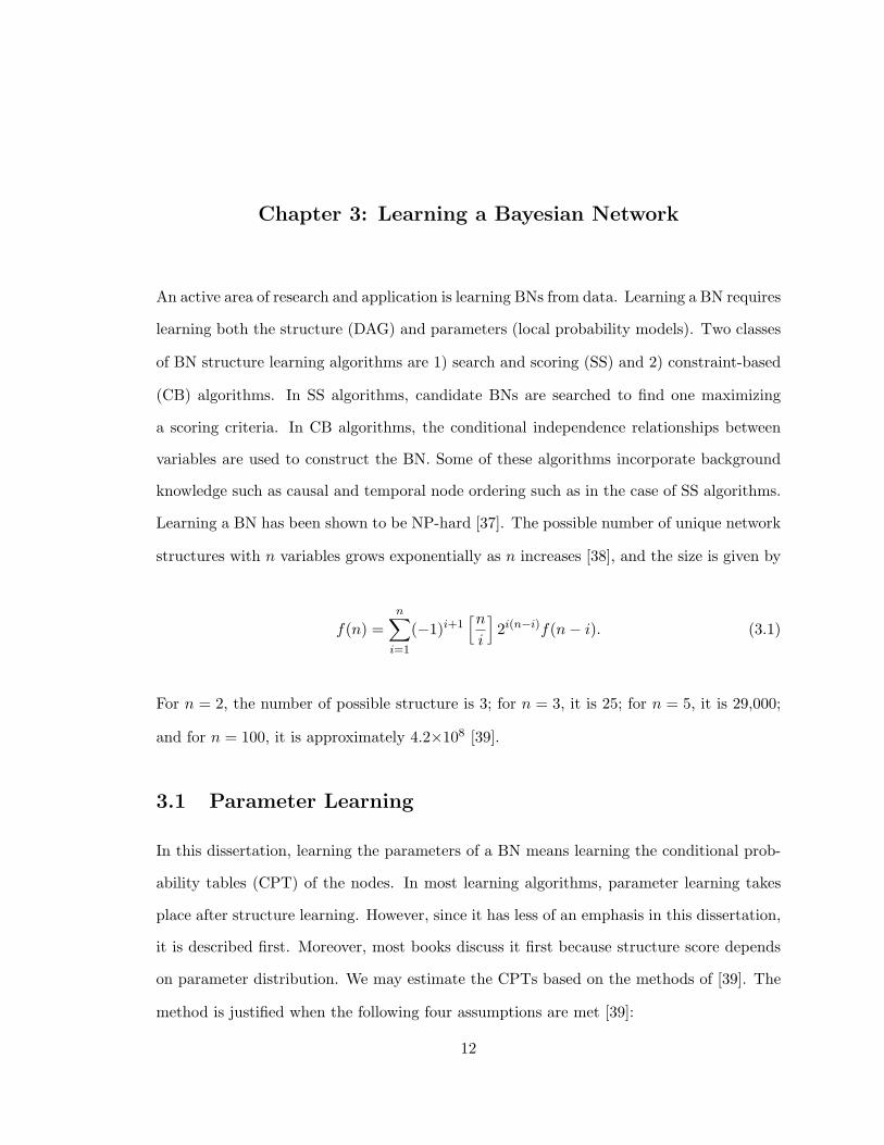
Learning a BN has been shown to be NP-hard [37]. The possible number of unique network
structures with n variables grows exponentially as n increases [38], and the size is given by
f(n) =n∑
i=1
(−1)i+1[n
i
]2i(n−i)f(n − i). (3.1)
For n = 2, the number of possible structure is 3; for n = 3, it is 25; for n = 5, it is 29,000;
and for n = 100, it is approximately 4.2×10⁸ [39].
3.1 Parameter Learning
In this dissertation, learning the parameters of a BN means learning the conditional prob-
ability tables (CPT) of the nodes. In most learning algorithms, parameter learning takes
place after structure learning. However, since it has less of an emphasis in this dissertation,
it is described first. Moreover, most books discuss it first because structure score depends
on parameter distribution. We may estimate the CPTs based on the methods of [39]. The
method is justified when the following four assumptions are met [39]:
12
1. The database variables are discrete.
2. Given the belief-network model, cases occur independently.
3. There are no cases that have variables with missing values.
4. Prior probabilities of all parameters are uniform.
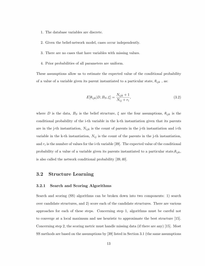
These assumptions allow us to estimate the expected value of the conditional probability
of a value of a variable given its parent instantiated to a particular state, θijk , as:
E[θijk|D,BS , ξ] =Nijk + 1Nij + ri
, (3.2)
where D is the data, BS is the belief structure, ξ are the four assumptions, θijk is the
conditional probability of the i-th variable in the k-th instantiation given that its parents
are in the j-th instantiation, Nijk is the count of parents in the j-th instantiation and i-th
variable in the k-th instantiation, Nij is the count of the parents in the j-th instantiation,
and ri is the number of values for the i-th variable [39]. The expected value of the conditional
probability of a value of a variable given its parents instantiated to a particular state,θijk,
is also called the network conditional probability [39,40].
3.2 Structure Learning
3.2.1 Search and Scoring Algorithms
Search and scoring (SS) algorithms can be broken down into two components: 1) search
over candidate structures, and 2) score each of the candidate structures. There are various
approaches for each of these steps. Concerning step 1, algorithms must be careful not
to converge at a local maximum and use heuristic to approximate the best structure [15].
Concerning step 2, the scoring metric must handle missing data (if there are any) [15]. Most
SS methods are based on the assumptions by [39] listed in Section 3.1 (the same assumptions
13

used in parameter learning). However, not all these assumptions may necessarily hold and
some of these assumptions may be relaxed. The assumptions of having discrete variables
and no missing values may be relaxed [15].
Under a Bayesian framework, the posterior probability of a graph, G, given the data,
D, P (G|D), is given by
P (G|D) =P (D|G)P (G)
P (D), (3.3)
where P (D|G) is the likelihood function, P (G) is the prior probability of the DAG, and
P (D) is the normalizing constant. P (D) is often ignored when computing P (G|D) since it
is not dependent on the structure. Furthermore, without prior knowledge of the BN DAGs,
P (G) is often assumed to uniformly distributed. The likelihood function, P (D|G), is used
as a scoring criterion [15]. A scoring criterion is a function that assigns a value to each
DAG based on the data [15]. The Bayesian scoring criterion [15] or Bayesian scoring metric
(BD) [41] (both terms will be used interchangeably) is defined as,
P (D|G) =n∏
i=1
qi∏j=1
Γ(N ′ij)
Γ(N ′ij + Nij)
ri∏k=1
Γ(N ′ijk + Nijk)Γ(N ′
ijk), (3.4)
where n be the number of variables, qi be the number of unique parent instantiations for
the i-th variable, ri be the number of values for the i-th variable, Nijk be the number of
observed samples for the i-th variable in the k-th instantiation and its parents in the j-th
instantiation, N ′ijk be the prior sample size for the i-th variable in the k-th instantiation and
its parents in the j-th instantiation, N ′ij =
∑rik=1 N ′
ijk, Nij =∑ri
k=1 Nijk, and Γ(n) = (n−1)!.
When the prior sample sizes are estimated as
N ′ijk = 1, (3.5)
the Bayesian scoring metric is called the K2 scoring metric [39]. When the prior sample
14

sizes are estimated as
N ′ijk = N ′p(xi = k, pa(xi) = j), (3.6)
where N ′ is the user’s equivalent sample size and pa(xi) = j is the parent of the i-th variable
in the j-th instantiation, the Bayesian scoring metric is called the BDe scoring metric [41,42].
When the prior sample sizes are estimated as
N ′ijk =
N
riqi, (3.7)
where N is the sample size, the Bayesian scoring criterion is called the BDeu scoring met-
ric[43,44]. The BDeu scoring metric is a special case of the BDe scoring metric [41]. Other
scoring metrics are based on minimum description length (MDL) [45], minimum message
length (MML) [46], Akaike information criteria (AIC) [47], and Bayesian information crite-
ria (BIC) [48].
A scoring criterion is node decomposable if the score of the network is the sum of the
scores of each node, and the score of each node depends only on its parent [49]. A node
decomposable score may be written in the form:
score(G,D) =∑Xi
score(Xi,pa(Xi)), (3.8)
where D is the observed data and G is the candidate BN DAG (see [50] for an alternative
expression in the probability space). A scoring metric is said to be score equivalent if it
gives the same score to DAG equivalent structures [51]. MDL, MML, AIC, BIC, BDe, and
BDeu are all score equivalent [51]. BD and K2 are not score equivalent [52, 53]. Examples
of search and scoring algorithms are K2 [39], the use of evolutionary and genetic algorithms
[54–56], and DAG pattern searching [57].
The primary disadvantages of SS algorithms are that they may be slow to converge,
15

require node ordering to learn the BN DAG structure, may not necessarily find the best
global solution (there is no achievable algorithm that finds the best global solution since
the problem is NP-hard [37]), and may find a BN fitting the distribution of the data but
have relationships in the DAG that are contrary to human judgment and expectations
[26, 39, 58, 59]. In the absence of an expert and/or when dealing with a dataset with many
variables, the requirement of node ordering may be viewed as a disadvantage. However,
when an expert is available and/or the dataset has few variables, the ability of an algorithm
to incorporate domain knowledge into structure learning may be considered as an advantage.
While both SS and CB algorithms are able to incorporate node ordering to guide structure
learning, some SS algorithms require a node ordering, while CB algorithms allow the option
of incorporating such domain knowledge. Therefore, node ordering is usually listed as a
primary disadvantage for SS algorithms and not CB algorithms. The primary advantages of
SS algorithms are that they can handle missing data (however, not every single SS algorithm
can handle missing data), distinguish qualitatively and quantitatively between structures,
incorporate prior probabilities over the structures and parameters, and can perform model
averaging [26,60].
3.2.2 Constraint-based Algorithms
Given the set of conditional independencies in a joint probability distribution, P , over a
set of variables, U = {X1, X2, · · · , Xn}, CB algorithms try to find a DAG for which the
Markov condition entails all and only those conditional independencies. CB algorithms
can also be broken into two components: 1) use of statistical test to establish conditional
independence or dependence among the variables, and 2) use the established conditional
independence or dependence relationships to constrain the relationships in the BN DAG.
There are many different assumptions required by CB algorithms [14,26,34]. However, the
set of assumptions shared in common by most CB algorithms are as follows.
1. The database variables are discrete.
16

2. The cases in the dataset are independently and identically distributed.
3. There are no missing data.
4. Statistical tests are reliable.
5. The joint probability distribution is faithful (graph-isomorphic) to a BN DAG (see
Section 2.2.2).
As in the case with the assumptions for SS methods, these CB method assumptions may
not necessarily hold and can also be relaxed.
When two variables, Xi and Xj , are independent, this is denoted as Xi⊥Xj . Xi⊥Xj
means P (Xi, Xj) = P (Xi)P (Xj) or alternatively, P (Xi|Xj) = P (Xi). Two independence
tests commonly used by CB algorithms are based on the Chi-square goodness of fit test
(Equation 3.9) and mutual information (Equation 3.11). When Xi and Xj are dependent,
this is denoted as Xi>Xj . The Chi-squared, χ2, goodness of fit test for two variables, X
and Y , is given by:
χ2 =∑x∈X
∑y∈Y
(oxy − exy)2
exy, (3.9)
where oxy is the number of observations for X = x and Y = y and exy is the expected
number of observations for X = x and Y = y. The expected value, exy, is given by:
exy =nx × ny
n, (3.10)
where n is the number of samples, nx is the number of X = x, and ny is the number of Y = y.
The degrees of freedom for the Chi-squared test is df = (NX −1)(NY −1), where NX is the
number of values of X and NY is the number of values of Y . The Chi-squared test’s null
hypothesis, H0, is that there is no difference between the expected and observed frequency,
and the alternative hypothesis, Ha, is that there is a difference between the expected and
observed frequency. If fail to reject the Chi-squared H0, then we may interpret that X and
17

Y are independent. If we reject the Chi-squared H0, then we may interpret that X and Y
are dependent. The mutual information between two variables, X and Y , is given by:
Mi(X,Y ) =∑x∈X
∑y∈Y
p(x, y)p(x, y)
p(x)p(y), (3.11)
where p(x, y) is the joint probability of X = x and Y = y, p(x) is probability of X = x,
and p(y) is the probability of Y = y. The mutual information between two variables is
always greater than zero, Mi(X,Y ) > 0. Mutual information values closer to zero imply
independence between X and Y .
When two variables, Xi and Xj , are conditionally independent given (or conditioned
on) a third variable, Xk, this is denoted as Xi⊥Xj |Xk or I(Xi, Xj |Xk). Xi⊥Xj |Xk means
P (Xi, Xj |Xk) = P (Xi|Xk)P (Xj |Xk) or P (Xi|Xj , Xk) = P (Xi|Xk). Two conditional inde-
pendence tests commonly used by CB algorithms are also based on the chi-squared statistic
and mutual information. The chi-squared test of conditional independence is given by
χ2 =∑
xi∈Xi
∑xj∈Xj
∑xk∈Xk
(oxixjxk− exixjxk
)2
exixjxk
, (3.12)
where oxixjxkis the number of observations for Xi = xi, Xj = xj and Xk = xk, and exixjxk
is the expected number of observations for Xi = xi, Xj = xj and Xk = xk. The degrees
of freedom is given by df = (NXi)(NXj )(NXk), where NXi is the number of values for Xi,
NXj is the number of values for Xj , and NXkis the number of values for Xk. The mutual
information conditional independence test is given by
Mi(Xi, Xj |Xk) =∑
xi∈Xi
∑xj∈Xj
∑xk∈Xk
p(xi, xj , xk)p(xi, xj |xk)
p(xi|xk)p(xj |xk). (3.13)
When Xi and Xj are conditionally dependent given Xk, this is denoted Xi>Xj |Xk.
18

Independence and conditional independence tests are used in CB approaches to learn
undirected arcs between two nodes. However, using conditional independence tests, CB
approaches go one step further to give arc orientation. The idea behind using conditional
independence tests to orient arcs is to find v-structures. Of the three elementary structures
(see Section 2.2.3), the v-structure is the only one that can be statistically distinguished from
the other two; serial and diverging structures both entail the same conditional independence,
I(Xi, Xk |Xj). In other words, if we find I(Xi, Xk |Xj), then we do not know which way
the arcs are oriented since there are 2 structures that equivalently describe the conditional
independence; these structures are Markov equivalent graphs since they capture the same
Markov conditions. However, in the v-structure, Xi and Xk become conditionally dependent
given Xj , and the orientation of arcs can only be Xi→Xj←Xk. Some examples of constraint-
based methods are Three Phase Dependency Analysis (TPDA) [26], the PC algorithm
by [14], polytree recovery algorithm [20], inductive causation (IC) algorithm [27], Sprites,
Glymour, and Scheines (SGS) algorithm [14], Grow-Shrink (GS) algorithm [61], and Fast
Casual Inference (FCI) algorithm [62].
Table 3.1: Elementary structures and Conditional Independence.
Name Configuration Conditional Independenceserial Xi → Xj → Xk I(Xi, Xk |Xj)diverging Xi ← Xj → Xk I(Xi, Xk |Xj)converging Xi → Xj ← Xk ¬I(Xi, Xk |Xj)
The primary disadvantages of CB methods are that they may lack statistical power with
small sample sizes, have a higher running time complexity when conducting conditional
independence test if the conditioning set is large, and not all network structure learned will
necessarily be a DAG [26, 39]. The primary advantage is that CB methods may learn the
correct structure if the probability distribution of the data is graph-isomorphic [15, 26, 63]
(see Section 2.2.2).
19

Chapter 4: Novel Structure Learning Algorithms
In this section, the development of novel BN structure learning algorithms to address some
of the disadvantages of the SS and CB approaches is discussed. BN parameter learning
will be implemented according to Section 3.1. BN structure learning will be accomplished
using a combination of the SS and CB methods. Three algorithms have been developed;
two of these algorithms I have developed are based on Constructing an Undirected Graph
Using Markov Blanket (CrUMB), and the other algorithm is based on the Sparse Candidate
(SC) algorithm [49] and called, SC*. CrUMB− and CrUMB+ refer to when CrUMB uses
traditional or a model of human cognition of causality to orient arcs, respectively. In case
CrUMB− and CrUMB+ cannot orient all arcs, genetic algorithm (GA) is used to orient
the rest of the arcs, and the combination of these algorithms in their entirety are called,
CrUMB−-GA and CrUMB+-GA, respectively. When the context is clear, these algorithms
may be simply referred to as CrUMB− and CrUMB+.
CrUMB−-GA, CrUMB+-GA, and SC* are all hybrid approaches to BN structure learn-
ing since they employ a CB and SS phase. Hybrid approaches of SS and CB methods have
been reported [49, 59, 64–67]. These hybrid approaches use the output of a CB method as
input for a SS method (or vice-versa). CrUMB−-GA, CrUMB+-GA, and SC* all have two
phases: a CB learning phase followed by a SS phase.
For CrUMB−-GA and CrUMB+-GA, the CB learning phase is based on the CrUMB
algorithm. The problems CrUMB addresses are the exponential number of conditional inde-
pendence tests required by CB methods, complicated heuristics used to find a conditioning
set between two variables, and high running time complexity to learn structure. To address
these obstacles, in CrUMB, the Markov blanket, B(Xi), of each variable, Xi, is estimated,
and from B(Xi), the coparents, copa(Xi), are identified and removed from B(Xi), leaving
20

us with the neighbors, ne(Xi). As will be illustrated in Section 4.2, it is required for two
variables, Xi and Xj , if Xi ∈ ne(Xj), then Xj ∈ ne(Xi); Xi ∈ ne(Xj) ⇒ Xj ∈ ne(Xi).
Furthermore, as mentioned in Section 3.2.2, CB methods may not necessarily learn a DAG,
and this statement is also true of CrUMB. In fact, CrUMB does not orient any arc, and
the output is just an undirected graph. After applying conditional independence tests to
the undirected graph learned by CrUMB to detect collider configurations (see Sections 3.2.2
and 4.3), the output may a PDAG (see Section 2.2.1). From this point, we may either orient
the rest of the arcs with the traditional approach (see 4.4) or use asymmetric correlation,
justified in part by a model of human cognition of causality (see 4.5), to orient the arcs.
After this step, there is also no guarantee that the learned graph will be a DAG. Thus, in
the second phase of the CrUMB−-GA and CrUMB+-GA approaches, structure learning is
taken one step further from a PDAG to a DAG by orienting the undirected edges with a SS
method. I will be using genetic algorithms (GA) to orient the remaining undirected edges.
This second SS phase using GA address the problem of structure learning stopping at a
PDAG, which is the case for many CB algorithms.
The second algorithm is called Sparse Candidate* (SC*) since it is a special case of the
general Sparse Candidate (SC) algorithm [49]. It may also be viewed as a hybrid approach
since it uses conditional independence tests to constrain the relationships between variables
to guide a search and scoring step [67,68]. The original SC algorithm iterates between two
phases until convergence; the first phase, Restrict, estimates candidate parents of a variable,
pa(Xi), and the second phase, Maximize, searches for high scoring DAGs where the parent-
child relationship are consistent with the first phase. The SC* algorithm does not need
to iterate between the two phases, Restrict and Maximize. The Restrict phase is required
to run only once. In SC*, candidate pa(Xi) for each variable are taken from its estimated
B(Xi). The reason why variables in the estimated Markov blanket, B(Xi), of a variable, Xi,
are the best candidate to be the parents of Xi, pa(Xi), is that they are d-connected to Xi—
no subset of any other variables, Xk = U \ B(Xi), will render the variables in Xj ⊆ B(Xi)
independent of Xi. SC* improves on the SC algorithm by going through the Restrict and
21

Maximize steps only once, and also by using GA in the Maximize step instead of greedy
hill-climbing and simulated annealing. The benefits of GA over greedy hill-climbing and
simulated annealing have been reported [55]. Furthermore, the primary limitation of SS
methods SC* addresses is reducing the search space and lack of node ordering requirement.
4.1 Discovering the Markov blanket
Markov blanket discovery algorithms have been reported [34, 69]. In this dissertation, the
Grow-Shrink (GS) algorithm [34] is used to discover the Markov blanket, B(Xi), of a vari-
able, Xi (see Algorithm 1). The assumptions made by the GS algorithms are as follows.
1. Causal sufficiency: There exist no common unobserved variable in the domain that
are parent of one or more observed variables of the domain.
2. Markov assumption: Given a BN, any variable is independent of all its non-descendants
in the BN given its parents.
3. Faithfulness (see Section 2.2.2).
4. There are no errors in the independence tests.
The GS algorithm has a running time complexity of O(n) and assumes faithfulness and
that conditional independence tests are reliable [34]. Conditional independence tests may
become unreliable when the data set is small or the conditioning set is large. Although the
former problem cannot be handled by GS, the latter can be mitigated to some extent. To
reduce the conditioning set of a variable, Xi, the other variables, U \Xi, are tested in order
of magnitude of correlation to Xi when applying conditional independence tests. Variations
of GS offering alternatives to this problems are Incremental Association Markov blanket
(IAMB) and Interleaved-IAMB (Inter-IAMB) [69].
22

Algorithm 1 Grow-Shrink Algorithm [34]. Finds the candidate Markov blanket,B(Xi), of a variable, Xi.1: procedure GrowShrink(D,Xi,U = {X1, X2, · · · , Xn} \ Xi)2: B(Xi) ← ∅3: while ∃Xj ∈ U \ Xi such that Xj>Xi |B(Xi) do4: B(Xi) ← B(Xi) ∪ Xj . grow5: end while
6: while ∃Xj ∈ B(Xi) such that Xj⊥Xi |B(Xi) do7: B(Xi) ← B(Xi) \ Xj . shrink8: end while
9: return B(Xi) . Markov blanket10: end procedure
From the estimated B(Xi), we can go one step further and estimate pa(Xi) [40,70]. We
can use a node decomposable scoring metric (see Section 3.2.1) to evaluate which subset of
B(Xi) are the most probable parents. An algorithm partially based on [40] for estimating
the parent set from B(Xi) is shown in Algorithm 2.
Algorithm 2 Parent Set Algorithm. Finds the candidate set of parents, pa(Xi), of avariable, Xi, from B(Xi). Partially based on [40].1: procedure ParentSet(Markov blanket, B(Xi))2: pa(Xi) ← ∅3: s ← score(Xi,pa(Xi))4: for Xj ∈ B(Xi) do5: s* ← score(Xi, pa(Xi) ∪ Xj)6: if s* > s then
7: pa(Xi) ← pa(Xi) ∪ Xj
8: end if
9: end for
10: return pa(Xi) . parent set11: end procedure
Results (not reported) show, however, that all variables discovered to be in the Markov
blanket of a variable contribute to increasing the score (parents, children, and coparents);
thus children and coparents will be incorrectly considered as candidate parents of a variable.
On the other hand, there is room to exploit the discovered Markov blanket by identifying
23

and removing coparents that are not also neighbors. All coparents, copa(Xi), of a variable,
Xi, are related to Xi through v-structures. For a variable, Xi, and one variable, Xj ∈ B(Xi),
if Xj is a coparent of Xi, then there must be a variable, Xk, that is the child of both Xi and
Xj . We can identify a coparent, Xj , by measuring its correlation (using correlation loosely
to include measures of associations such as mutual information) or flow of information to
Xi, ρ(Xi, Xj), and then find a child of Xi and Xj , such that ρ(Xi, Xj) < ρ(Xi, Xj |Xk).
The marginal correlation (or flow of information) between a variable, Xi, and its coparent,
Xj , should be less than the conditional correlation (or flow of information) given one of
their children. The first justification for identifying coparents in this manner is that a BN
may be viewed as a system of information channels, where nodes are valves and edges are
channels [63]. In the path between two nodes, Xi and Xj , nodes may exist as colliders
(v-structures) or non-colliders (serial or diverging); if a node, Xk, exists as a collider in
the path between Xi and Xj , then information cannot flow between Xi and Xj unless the
status of Xk is altered (conditioned on); if Xk exists as a non-collider, then information may
flow between Xi and Xj unless the status of Xk is altered (conditioned on). The second
justification for identifying coparents in this manner is based on empirical results. First,
100 converging BN structures, Xi → Xj ← Xk, were created with different parameters.
The parameters were generated by sampling from Dirichlet distributions as in [71,72] (also
see Section 5.2). From these 100 converging BN structures, 10 datasets were generated
for each using logic sampling (also see Section 5.3) for a total of 1000 datasets. In 956
datasets, the flow of information between Xi and Xk—the mutual information of Xi and
Xk, MI(Xi, Xk)—was compared to the flow of information between Xi and Xk altering
the state of Xj—the mutual information of Xi and Xk given Xj , MI(Xi, Xk|Xj). The
condition MI(Xi, Xk|Xj) > MI(Xi, Xk) was found in 956 datasets, and the condition
MI(Xi, Xk|Xj) < MI(Xi, Xk) was found in 44 datasets. Second, there is the question if
this idea of information flow holds true when Xi and Xk share a common parent Xl. To
see test this idea, the same converging BN structure was created but now Xi and Xk have
24

a common parent Xl. Again, 100 BN structures with different parameters were generated
(now with 4 variables and Xi and Xk as the children of Xl), and for each BN 10 datasets
were simulated for a total of 1000 datasets. The condition MI(Xi, Xk|Xj) > MI(Xi, Xk)
was found in 847 datasets, and the condition MI(Xi, Xk|Xj) < MI(Xi, Xk) was found
in 153 datasets. Empirically, for two coparents (sharing a common parent or not), it is
expected that altering the state of their child should increase flow of information between
them.
Algorithm 3 describes how we may identify coparents in the Markov blanket of a variable.
Once we identify the coparents of a variable, we may remove them from the Markov blanket;
all we are left with are the neighbors of the variable.
Algorithm 3 Identify Coparents Algorithm. Finds nodes that are coparents of a
variable.1: procedure IdCoParents(Xi, B(Xi))2: copa(Xi) ← ∅3: while ∃Xj , Xk ∈ B(Xi) such that MI(Xi,Xj) < MI(Xi,Xj |Xk) do4: copa(Xi) ← copa(Xi) ∪ Xj
5: end while
6: return copa(Xi) . coparent set7: end procedure
Using and refining algorithms that discover the Markov blanket is beneficial to both
CrUMB and SC*. For CrUMB, we identify and remove copa(Xi) from B(Xi) resulting in
ne(Xi). For SC*, we may use the candidate parents estimated from B(Xi) for the Restrict
step; the Restrict step never has to be visited again since the variables in the estimated
parent set are dependent on and score high as the parents of a variable.
25

4.2 Constructing an Undirected Graph using Markov Blan-
kets (CrUMB)
Using the Markov blankets of each variable, it is possible to construct an undirected graph
as described by the CrUMB algorithm (see Algorithm 4). CrUMB requires as input a data
set, D, and set of variables, U , in D. The output of CrUMB is an undirected graph, G. Since
CrUMB uses the GS algorithm, it also requires the same assumptions including the ones
listed for CB methods in Section 3.2.2. In Step 3, the GS algorithm is called to learn the
Markov blanket for each variable. In Step 8, the coparents in the Markov blanket of each
variable are identified and removed, and we are left with the neighbors of each variable. In
Step 14, an undirected graph is constructed from the set of neighbors of each variable.
Algorithm 4 CrUMB Algorithm. Construct an undirected graph using Markov blan-
kets.1: procedure Crumb(D, U)2: B ← ∅ . Set Markov blankets to empty
3: for Xi ∈ U do
4: B(Xi) ← GS(D,Xi,U \ Xi) . learn Markov-blanket5: B ← B(Xi) . Add Markov blanket to B6: end for
7: Ne ← ∅ . Set neighbors to empty
8: for Xi ∈ U do
9: copa(Xi) ← IdCoParents(Xi,BL(Xi)) . id copa10: ne(Xi) ← B(Xi) \ copa(Xi) . set neighbors11: Ne ← Ne ∪ ne(Xi) . add neighbors to Ne12: end for
13: initialize undirected graph, G(V,E)14: for Xi and ne(Xi) ∈ Ne do15: Add arcs between Xi and every node in ne(Xi) . add arc between neighbors16: end for
17: return G . undirected graph
18: end procedure
26

I now illustrate how the CrUMB algorithm works using a fictional example. Let’s say
we have the BN in Figure 4.1 and a dataset generated by this BN. We will feed the dataset
as input into CrUMB to try to recover the skeletal structure of the original DAG. After
calling the GS algorithm, the learned Markov blankets for each variable are
• BL(X1) = {X3},
• BL(X2) = {X3},
• BL(X3) = {X1, X2, X4, X5, X6},
• BL(X4) = {X3, X6},
• BL(X5) = {X3, X7},
• BL(X6) = {X3, X4}, and
• BL(X7) = {X5}.
The coparents identified from each Markov blankets are
• copa(BL(X1)) = {∅},
• copa(BL(X2)) = {∅},
• copa(BL(X3)) = {X4},
• copa(BL(X4)) = {X3},
• copa(BL(X5)) = {∅},
• copa(BL(X6)) = {∅}, and
• copa(BL(X7)) = {∅}.
After the coparents are removed from the Markov blankets of each variable, we are left with
the neighbors of each variable:
27

X1 X2
X3 X4
X5 X6
X7
Figure 4.1: A DAG of a Bayesian network.
• ne(X1) = {X3},
• ne(X2) = {X3},
• ne(X3) = {X1, X2, X5, X6},
• ne(X4) = {X6},
• ne(X5) = {X3, X7},
• ne(X6) = {X3, X4}, and
• ne(X7) = {X5}.
Looking at the neighbor sets, one can see that if Xj ∈ ne(Xi), then Xi ∈ ne(Xj); Xj ∈
ne(Xi) ⇒ Xi ∈ ne(Xj). Using these neighbor sets, we construct the undirected graph in
Figure 4.2.
In CB algorithms such as PC [14], SGS [14], IC [27], and TPDA [63], an arc is added
between two variables, Xi and Xj , only if there is a not a set, Xk ⊆ U \{Xi, Xj}, called the
conditioning set, that can render Xi and Xj conditionally independent given Xk. Except for
TPDA, these algorithms apply conditional independence tests between Xi and Xj against all
permutations of the conditioning set Xk resulting in an exponential number of conditional
independence tests. In the worst case for TPDA, O(n4) conditional independence tests are
used [73]. CrUMB avoids this exponential number of conditional independence tests by
28

X1 X2
X3 X4
X5 X6
X7
Figure 4.2: An undirected graph learned by CrUMB based on data generated by the BN inFigure 4.1.
identifying the Markov blankets of each variable, and then removing non-neighbors from
the Markov blankets.
4.3 Orienting the edges in an undirected graph by detecting
colliders
The result of the CrUMB algorithm is an undirected graph. To orient edges in an undirected
graph, G(V,E), a common first step is to apply conditional independence tests to all uncou-
pled meetings between three variables Xi, Xj , and Xk, where (Xi, Xj) ∈ E, (Xj , Xk) ∈ E,
and (Xi, Xk) 6∈ E. If I(Xi, Xk|Xj) does not hold (if Xi and Xk are dependent given Xj ,
D(Xi, Xk|Xj)), then we know that Xi→Xj←Xk [74, 75]. (This method of orienting arcs
will not work if Xi and Xk have a common parent). After all the v-structures or colliders
are identified in G and oriented accordingly, then the graph becomes a minimal PDAG.
Algorithm 5 outlines how colliders are identified and oriented and take as input an undi-
rected graph, G, dataset, D, and set of variables, U . In Step 2, we go through each detected
uncoupled meeting and apply a conditional independence test. If we find that Xi and Xk
are dependent given Xj in Step 3, then in Step 4 we orient the arcs in the uncoupled
meeting to form a collider configuration. In the running example from Figure 4.2, the
set of uncoupled meetings examined are X1–X3–X2, X1–X3–X5, X1–X3–X6, X2–X3–X5,
29

X1 X2
X3 X4
X5 X6
X7
Figure 4.3: An undirected graph learned by CrUMB in Figure 4.2 whose colliders have beendetected and the arcs oriented accordingly.
X2–X3–X6, X3–X6–X4, X3–X5–X7, and X5–X3–X6. It is expected that only one of these
uncoupled meeting, X3–X6–X4, is identified as a collider, and the two arcs participating in
this uncoupled meeting are directed as shown in Figure 4.3.
Algorithm 5 Identify and Orient Colliders. This algorithm takes as input an undi-
rected graph, G, dataset, D, and set of variable over the dataset, U .1: procedure IdentifyAndOrientColliders(G, D, U)2: for each Xi–Xj–Xk in G do . Identify uncoupled meeting3: if D(Xi, Xk|Xj) then . Identify collider4: Orient Xi → Xj ← Xk . Orient collider5: end if
6: end for
7: end procedure
4.4 Orienting the undirected edges in a PDAG inductively
After identifying colliders and orienting arcs accordingly, the other remaining undirected
edges may be oriented inductively [26, 30]. Edges are directed so as to avoid forming new
v-structures (unless they prohibit cycles) or directed cyclic paths. In [30], the rules to orient
the edges in a minimal PDAG, G(V,E), are:
1. If Xi → Xj − Xk, and (Xi − Xk) 6∈ E, then direct Xj → Xk.
30

2. If (Xi − Xj) ∈ E, and Xi → . . . → Xj , then direct Xi → Xj .
3. If (Xi − Xj), (Xi − Xk), (Xi − Xl), (Xj → Xl), (Xk → Xl) ∈ E, then direct Xi → Xl.
4. If (Xi − Xj), (Xj − Xk), (Xk − Xl), (Xl → Xi), (Xi − Xk), then direct Xi → Xj and
Xk → Xj .
These rules may not necessarily transform the minimal PDAG to a DAG, however, they
may transform the minimal PDAG to a complete PDAG (see Section 2.2.1). Furthermore,
the use of these rules to orient arcs are not consistently used. In [30], use of these rules
terminates if a new v-structure is added, while [73] reported that all collider identification
based methods only use the first two rules. In our running example in Figure 4.3, applying
all of these rules cannot orient the rest of the undirected edges. The arcs that remain
undirected are (X1 − X3), (X2 − X3), (X3 − X5), and (X5 − X7).
4.5 Orienting the edges using a model of human cognition of
causation
When there is a cause and associated effect, inference in the direction from cause to effect
is called prediction, and inference in the reverse direction is called diagnosis. It has been
reported 1) that humans view predictive relations as stronger than diagnostic relations
and 2) that prediction from cause to effect can be made with greater confidence than a
vice-versa by humans [76]. This observation forms the basis of what is called inferential
asymmetry or predicted asymmetry—causes are better predictors of effects than vice-versa.
One reason why effects are known to yield low predictive ratings of their causes by humans
may be due to the difficulty inherent in diagnostic learning which “involves retrospective
revisions of an already formed casual model on the basis of new effect information” [77].
An example given by [20] and elaborated by [78] illustrate why diagnostic reasoning is
difficult. Suppose one knew that rain causes the grass to become wet and green. Then
knowing that it rained would allow one to predict that the grass is greener and wetter than
31

yesterday. However, if one observed that the grass is wet and have additional evidence that
a sprinkler was the cause, the rain becomes less possible as a cause than before. In this
sense, multiple alternative causes of an effect compete against one another in diagnostic
inference. In addition to knowledge of cause-to-effect dependencies, diagnostic reasoning
requires adjudication among competing alternative causes [78]. Moreover, the use of effects
to predict causes can be confusing for humans [79] because it contradicts the temporal
sequence of events in the world [80].
It is not claimed that in the physical world, causes are always better predictors of effects
than vice-versa. In some cases, an effect can be used to predict a cause better than vice-
versa. For example, marijuana is known as a gateway drug (viewed as the cause) leading
to the use of more dangerous substances such as heroin (viewed as the effect). However,
it has been reported that few marijuana users will become heroin addicts, but most heroin
addicts have previously used marijuana [81]. In some cases, causes and effects may be
equally informative [76]. For example, mothers with blue eyes (viewed as the cause) and
daughters with blue eyes (viewed as the effect) are equally informative [76].
Predictive asymmetry rooted in human cognition is used to give direction to an undi-
rected arc between two variables. The main point is that if we find an undirected arc
between two variables and are able to determine which variable is the better predictor of
the other, based on predictive asymmetry, the one found as the better predictor should
be the cause the other should be the effect. The natural question that follows is, for two
variables, how do we determine if one variable is a better predictor of the other? Determin-
ing predictive asymmetry is based on the idea of asymmetric correlation or proportional
reduction of error (PRE) measure [82]. At a high level, for a dependent variable Xj and
an independent variable Xi, a PRE measure tells you ratio of reduction in predictive error
made on Xj given Xi to the predictive error made on knowing Xj alone. A larger PRE value
indicates more reduction in predictive error of the dependent variable by the independent
variable, and hence, the independent variable is a better predictor.
In orienting undirected arcs between two variables, Xi and Xj , the PRE of Xj given
32

Xi, PRE(Xj |Xi), is compared with the PRE of Xi given Xj , PRE(Xi|Xj). It is expected if
Xi is the cause of Xj , then PRE(Xj |Xi) should be larger than PRE(Xi|Xj); a cause should
be a better predictor of an an effect than vice-versa. Such PRE measure for validating
cause-and-effect relationships has been proposed [83] in the machine learning literature for
decision tree construction in ID3, C4.5, CART, and CHAID [84–89]. While quite a few PRE
measures are available [83], the one used in this dissertation is based on Goodman-Kruskal’s
lambda (GKL) [82]. GKL is defined as,
λXa|Xb=
(∑
j maxj) − fd
n − fd, (4.1)
where Xa is the dependent variable with i values, Xb is the independent variable with j
values, maxj is the maximum value of the j-th column for the two-way i by j contingency
table formed by Xa and Xb, fd is the maximum marginal of the rows, and n is the total
number of samples. GKL is also called an asymmetric correlation [82,83], since for any two
variables, Xi and Xj , PRE(Xj |Xi) is usually not equal to PRE(Xi|Xj). In decision tree
construction, the use of GKL has been reported to construct simpler trees with competitive
accuracy to other methods [90, 91]. GKL has also been used to identify predictors in gene
expression data; the classifiers built were shown to be robust for discretized data and small
data sets [92].
To my knowledge, GKL has not been used to discover cause-and-effect relationships in
BN structure learning, and in particular, for orienting undirected arcs. Algorithm 6 uses
GKL to orient undirected arcs in a PDAG. In Step 2, a list of all undirected edges from
the PDAG (represented as input into the algorithm, as G(V,E)) is created. In Step 3, for
each undirected arc, the two corresponding PRE values are computed; we store the larger
PRE value in the variable c for sorting descendingly in Step 8. The sort is descending as
we want to orient arcs starting with those that have the largest PRE values. In Step 17, an
attempt is made to orient the arcs according to what the PRE values for each arc indicate
33

(Step 11); arcs creating directed cycles are skipped and left as undirected. In the running
example, it is expected that applying Algorithm 6 will fully recover the original DAG in
Figure 4.1 from Figure 4.3.
Algorithm 6 Arc orientation using asymmetric measure.1: procedure OrientArcsByAsymmetricCorrelation(G(V,E))2: Eu ←
∪(Xi, Xj) ∈ E where Xi − Xj . List of undirected arcs
3: for each (Xi, Xj) ∈ Eu do . Compute PREs values for each arc4: (Xi, Xj)a ← λXi|Xj
5: (Xi, Xj)b ← λXj |Xi
6: (Xi, Xj)c ← the larger of (Xi, Xj)a and (Xi, Xj)b
7: end for
8: Sort Eu descendingly by (Xi, Xj)c . Sort arcs descendingly9: for each (Xi, Xj) ∈ Eu do . Try to orient each arc
10: e ← ∅
11: if (Xi, Xj)b > (Xi, Xj)a then12: e = Xi → Xj
13: else if (Xi, Xj)b < (Xi, Xj)a then14: e = Xi ← Xj
15: end if
16: if e 6= ∅ then17: Orient (Xi, Xj) as e in G unless a cycle is formed18: end if
19: end for
20: end procedure
4.6 Orienting the undirected edges using Genetic Algorithms
To orient the remaining undirected edges in a PDAG, we can use search and scoring methods
to orient these edges. One common approach is to use genetic algorithms (GA). The uses
of GA to aid in discovering Bayesian network structure have been reported [54, 55]. I will
simply permute the undirected edges by giving them direction, and search for a directed
acyclic graph (DAG) consistent with the PDAG. A DAG is consistent with a PDAG if every
directed edge in the PDAG is also in the DAG. I will be using the K2 scoring metric since it
34

is not score equivalent (see Section 3.2.1) and is node decomposable. A scoring metric that
is not score equivalent is desired since the PDAG may be a complete PDAG, in which case
all DAG belonging to this equivalence class will receive the same score. A scoring metric
that is node decomposable is desired so to avoid recalculating scores [28]. When using GA
with CrUMB, regardless of the arc orientation method, the combination of these algorithms
will be referred to as CrUMB-GA. If CrUMB− or CrUMB+ learns a DAG, the GA phase
is avoided completely.
Algorithm 7 is a general procedure for GA [93–95], and is listed here for completeness
and to discuss how GA was actually used. The algorithm takes a parameter, maxIter, that
limits the number of iterations if there is no convergence on finding the best solution. In
Step 3, an initial population of chromosomes is generated. A chromosome is composed of
genes. A gene is a binary sequence of length n, where n is the number of variables; a value
of 0 in the i-th position indicates that the i-th variable is not a parent of the variable for
which the gene represents; a value of 1 in the i-th position indicates that the i-th variable
is a parent of the variable for which the gene represents. For n variables, we have n genes,
and each chromosome is composed of these n genes, representing a graph. The initial
population of chromosome is based on the PDAG learned from CrUMB− or CrUMB+; all
chromosomes generated must encode the PDAG, where the j-th gene has values of 1 for all
the i-th positions of its parents. An undirected arc between two variables, Xi and Xj , is
given orientation the following way; a random number from a uniform distribution in the
interval [0.0,1.0) is generated, if it is less than 0.50, Xi is made the parent of Xj (the j-th
gene has its i-th position in the binary sequence set to 1), otherwise, Xj is made the parent
of Xi (the i-th gene has its j-th position in the binary sequence set to 1). In other words,
undirected arcs are given an orientation in either way with a 50/50 chance.
In Step 5 of Algorithm 7, each chromosome in the population is evaluated according to
the K2 metric. For chromosomes that encode a cyclic directed graph, they are removed.
In Step 6, tournament selection is used to select individuals for reproduction; three chro-
mosomes are randomly chosen, and the best chromosome is selected. Elitism was used,
35

and the top 10 percent of the best scoring chromosomes were kept for mating in the next
generation (they were not subjected to tournament selection). Recombination was made by
randomly choosing k genes between 2 chromosomes, and swapping these genes to produce
new offspring [55]. The mutation operator is defined by reversing arcs. First, the total
number of mutations to be performed on the population of chromosome is computed as,
Nm = ceil(M(R − 1)C), where Nm is the number of mutations, M is the mutation rate in
the interval [0,1.0), R is the number of chromosomes, C is the number of bits per gene, and
the ceil function returns a rounded down integer value of its argument[93]. Second, a chro-
mosome is chosen randomly, a j-th gene from this chromosome is chosen at random, and an
arc as encoded by the j-th gene and i-th position of the binary sequence is chosen at random
and reversed. The termination criteria is when the iterations exceed maxIter or when there
is convergence, defined as g consecutive generations without finding a better solution. From
trail and error, it was found that a large initial population of size 1000 with the termination
criteria as maximum iterations equal to 10 and convergence as 3 consecutive generations
without finding a better solution performed better than a smaller initial population and
termination criteria with larger maximum iterations and convergence constraint. A larger
initial population is important since during this phase (of generating chromosomes), as
many unique DAG extensions of the PDAG as possible should be created to broaden the
search space.
36

Algorithm 7 Genetic Algorithm.1: procedure GeneticAlgorithm(maxIter)
2: i = 0
3: Initialize population, pi
4: while i < maxIter and not converged do
5: Evaluate fitness of individuals in pi
6: Select individuals for reproduction7: Apply genetic operations (recombination and mutation) to produce offspring8: Replace parents with offspring, pi+1 ← pi
9: i + +
10: end while
11: end procedure
4.7 SC* Algorithm
The SC* algorithm is listed in Algorithm 8. SC* requires as input a data set, D, a list of
all the variables, U , in D, and a node decomposable score, S. The output of SC* is a DAG,
G. SC* starts at step 3 by estimating the Markov blanket, B(Xi), for each variable, Xi.
This step is accomplished by calling the GS algorithm. At step 4, coparents are identified
from B(Xi), and removed from B(Xi) in step 5 to give the neighbors, ne(Xi). Steps 3
through 6 correspond to the Restrict step of the SC algorithm. At step 8, a search for a
DAG, G, maximizing S is searched. G is subject to the constraint that the parents of every
variable are only those found in step 6. Step 8 corresponds to the Maximize step of the SC
algorithm. I will be using the K2 scoring metric for S and GA for the search method.
37

Algorithm 8 SC* Algorithm. The SC* algorithm is generalized by the SCalgorithm [49].1: procedure SC*(D, U , S)2: for Xi ∈ U do . Restrict
3: B(Xi) ← GS(Xi,{U \ Xi}) . Grow-Shrink4: copa(Xi) ← IdCoPa(Xi,B(Xi)) . Identify Coparents5: ne(Xi) ← B(Xi) \ copa(Xi) . Neighbors6: pa(Xi) ← ne(Xi) . Candidate parents7: end for
8: find a G maximizing S such that ∀Xi, paG(Xi) ⊆ pa(Xi) . Maximize9: return G . directed acyclic graph
10: end procedure
For GA, the outline of Algorithm 7 was used, however, the details in some of the steps
differed from what was described of how GA was used for CrUMB−-GA and CrUMB+-GA
(Section 4.6). To begin, an initial population of chromosomes was generated as follows.
Each i-th position in a binary sequence for a gene was given a value of 0 or 1 with a 50/50
chance. There are two problems with this approach: 1) this parent assignment per variable
obviously did not conform to the candidate parent set in the Restrict phase of Algorithm
8, and 2) two variables may be the parents of each other. To make the parent assignment
per variable consistent with the Restrict step, for each j-th gene, corresponding to the Xj
variable, if the i-th position, corresponding to the variable Xi, is not in the candidate parent
set of Xj and has a value of 1 (i.e. the gene encodes that Xi is a parent of Xj when Xi
is not in the candidate parent set of Xj), the value was changed to 0. When two variables
are parents of each other (i.e. the j-th gene has a value of 1 for the i-th position and the
i-th gene has a value of 1 for the j-th position), one bit is selected with a 50/50 chance
and removed. The fitness function used was the K2 metric. Tournament selection of size 3
was used to choose parent chromosomes for mating in the next generation, and elitism was
also used. The recombination and mutation operators were also as described previously,
however, the mutation operator was forbidden to change any bits in the genes that would
produce a parent-child relationship inconsistent with the Restrict phase of Algorithm 8.
38

The same termination criteria was also used as described above.
39

Chapter 5: Methods
5.1 Procedure for Generating Data for Structure Learning
Algorithms
To compare the qualitative and quantitative performances of BN structure learning algo-
rithms, the following steps were used.
1. Generate a BN, referred to as the true BN and denoted as, BNT .
2. Simulate z datasets, D = {D1,D2,. . .,Dz}, from the generated BNT .
3. Use D as input into a BN structure learning algorithm to produce the learned BNs,
BNL = {BNL1 , BNL2 , . . ., BNLz}.
4. Compare BNT and BNL in terms of structural errors in BNL (see 5.5) and the KL
distances between BNT and BNL (see 5.6).
As well be elaborated below, these steps were repeated for BNs of different types and
sizes, and data simulated from these BNs were subjected to the BN structure learning
algorithms of interest. Results for the BN structure learning algorithms per BN type and
size were subjected to ANOVA.
5.2 Generating Bayesian Networks
BNs were generated using BNGenerator. BNGenerator randomly generates DAGS from a
uniform distribution using Markov chain Monte Carlo (MCMC) methods [71,72]. BNGener-
ator has been reported to generate “realistic” BNs [71] and used to compare BN structure
learning algorithms [96, 97]. BNGenerator was also used so that the performances of the
40

algorithms could be observed as the size of the BN grew (it would be prohibitively difficult
to find an existing and available collection of BNs to allow for this observation and experi-
mentation). BNs were generated according to type and size. The two types of BN graphs
generated were either of type singly- or multi-connected. In singly-connected BN graphs,
also called polytrees, there exists exactly one path between every pair of nodes ignoring
the direction of the edges; a multi-connected BN graph is one that is not singly-connected.
The size of a BN is the number of nodes in the graph. The range of BN sizes were arbi-
trarily selected at 4, 5, 6, 7, 8, 9, 10, 11, 12, 13, 14, 15, 20. The required parameters for
BNGenerator were all left to their default values except for maximum degree of any node
in the networks (maxDegree), number of incoming arcs (maxInDegree), and number of out-
going arcs (maxOutDegree). The parameters set to their default values were maximum
induced width (set to -1, meaning there is no constraint), maximum values per node (set
to 2), and number of transitions (computed automatically by the software as 4N2, where
N is the number of nodes). Table 5.1 shows the values for the maxDegree, maxInDegree,
and maxOutDegree parameters. The justification for modifying these parameters (and not
others) and specifying such low values was to keep the BN generated simple (by simple, I
mean BN with a low number of arcs).
For each size and type, 10 (an arbitrary number) BNs were generated. For example,
there were 10 singly-connected BNs generated of size 4, 10 singly-connected BNs generated
of size 5, 10 singly-connected BNs generated of size 6, and so on. In this paper, a generated
BN is denoted by its type, size, and i-th order in which it was generated. For example,
s4BN1, refers to the first BN generated of type singly-connected and size 4; m4BN10 refers to
the tenth BN generated of type multi-connected and size 4. When referring to a generated
BN without care for the order in which it was generated, the BN may be denoted with i
as the subscript indicating the order, s4BNi, or without any subscript indicating the order
at all, s4BN. Tables 5.2 and 5.3 show the average, minimum, and maximum arcs in the BN
graphs generated for singly- and multi-connected BNs by size, respectively.
41

Table 5.1: BNGenerator Parameters. BNGenera-
tor parameters for generating singly- and multi-connected
BNs for the maximum degree of any node in the networks(maxDegree), number of incoming arcs (maxInDegree),and number of outgoing arcs (maxOutDegree).
Singly-Connected Multi-Connected
maxDegree 2 3
maxInDegree 1 2
maxOutDegree 1 2
42

Table 5.2: Summary Statistics for Arcs for Generated
Singly-Connected BNs. This table shows the average, min-
imum, and maximum number of arcs in the singly-connected
BNs generated by size. For each size, there are 10 BNs.
Size Average Minimum Maximum
4 3 3 3
5 4 4 4
6 5 5 5
7 6 6 6
8 7 7 7
9 8 8 8
10 9 9 9
11 10 10 10
12 11 11 11
13 12 12 12
14 13 13 13
15 14 14 14
20 19 10 19
43

Table 5.3: Summary Statistics for Arcs for Generated
Multi-Connected BNs. This table shows the average, mini-
mum, and maximum number of arcs in the multi-connected BNs
generated by size. For each size, there are 10 BNs.
Size Average Minimum Maximum
4 3.8 3 5
5 4.6 4 5
6 6.5 5 7
7 7.3 6 8
8 9.0 7 10
9 10.3 9 11
10 11.4 10 12
11 12.1 10 14
12 13.5 12 14
13 14.4 13 16
14 15.8 14 17
15 17.0 16 18
20 22.9 21 24
5.3 Simulating Data
Datasets were simulated from each generated BN after being compiled using Netica [98].
Netica uses forward sampling with rejection to simulate data for compiled BNs [98,99]. For
each BN, 10 different datasets were simulated, with each dataset having 1000 cases and no
percentage of missing data. Ten different datasets per BN were simulated since different
simulation runs for the same BN may show different strengths of association between the
44

variables. The size of each dataset, however, was set to 1000; it was found subjectively
through trial and error that dataset sizes over 1000 did not greatly improve the performance
of the learning algorithms, where performance is defined in terms of total arc errors (see
Section 5.5). Generating multiple datasets from a BN and taking the average value of the
performances by a BN structure learning algorithm (over these multiple datasets) to be the
performance associated with that algorithm and BN has been reported [14,100].
5.4 Applying the Structure Learning Algorithms on Simu-
lated Data
After a BN was used to simulate 10 different datasets, the datasets were then used as
input for the BN structure learning algorithms: CrUMB−-GA, CrUMB+-GA, SC*, PC,
and TPDA. PC and TPDA are state-of-the-art BN structure learning algorithms; the proof
of correctness for recovering a BN structure given that certain assumptions are met for PC
[14, 101, 102] and TPDA [73] have been reported. Furthermore, the PC algorithm is used
in a popular software, Hugin [103–105]. TPDA is also available as a standalone software
called Belief Network PowerConstructor.
The assumptions required by PC are as follows.
1. The set of observed variables is causally sufficient (see Section 4.1).
2. Every unit in the population has the same causal relations among the variables.
3. The probability distribution of the observed variables is faithful to a DAG of the
causal structure.
4. The statistical decisions required by the algorithm are correct for the population (the
statistical decisions about conditional independence are correct) [14].
The assumptions required by TPDA are as follows.
1. The observations are independently and identically distributed.
45

2. The dataset comes from a probability distribution that is graph-isomorphic (see Sec-
tion 2.2.2).
3. The variables are discrete and there are no missing data.
4. The dataset is large enough for CI tests to be reliable [26].
It was quite possible that a different BN structure was learned for each dataset by the
same algorithm. This result meant that there would be different performances per dataset
by the same BN structure learning algorithm. Thus, for 10 different datasets generated by
the same BN, for each BN structure learning algorithm, there were 10 different outputs of
performances. The average value of the outputs was taken to be the performance value of
the algorithm. For example, for s4BN, 10 different datasets were simulated. Each of these
datasets was then used as input into a BN structure learning algorithm. The output of
the structure learning algorithm was 10 (possibly different) graphs. These learned graphs
were then compared with the true graph structure, and the number of total arc errors was
recorded for each learned graph. The average value of all the total arc errors (for each
learned graph) was then taken to be simply the number of arc errors committed by the
structure learning algorithm for s4BN.
All the algorithms compared were coded in Java v1.4. The database storing the sim-
ulated data sets was MySQL. All the BN structure learning experiments were run on a
computer with 3 GB of memory running at a CPU clockspeed of 2.6 GHz.
5.5 Output–Qualitative Performance
When learning BN structures from data, BN structure learning algorithms make structural
errors (qualitative errors) related to the arcs. The structural errors are known as arc
omission, arc commission, direction omission, and direction commission [14,26,106]. These
errors are defined in Table 5.4. Arc omission and commission errors and direction omission
and commission errors may have different importances depending on the application of BN
46

structure learning [107]. Summarizing from [107], the major drawback of using arc omission
and commission alone to evaluate structure learning algorithms is that a learned structure
having no arc omission and commission errors does not necessarily mean it presents the
same independence model as in the true BN graph. For example, if the true BN graph is
Xi ← Xj → Xk, and the learned BN graph is Xi → Xj ← Xk, then the count of errors
is zero according to arc omission and commission. However, the learned BN graph has
a different independence model from the true BN graph. On the other hand, the major
drawback of using direction omission and commission alone to evaluate structure learning
algorithms is that a learned BN graph having these types of errors does not necessarily mean
it will not present the same independence model as in the true BN graph [107]. For example,
if the true BN graph is Xi ← Xj → Xk, and the learned BN graph is Xi → Xj → Xk, then
there is one direction commission error (the learned structure has Xi → Xj instead of what
is in the true graph Xi ← Xj), but both BN graphs present the same independence model.
It is possible to attach weights signifying importances to each of these error types, but
determining the weights will be application specific and may be difficult to define [1]. As
a side note, direction omission and commission errors are more important when structure
learning is used for the purpose of causal discovery [107].
In this thesis, I am interested in the total errors composed of all of these 4 structural
errors. For reasons mentioned above, I have weighted all arc errors equally. For each BN
learned, the sum of these 4 structural errors are simply referred to as the arc error (also
total arc error). Since there are 10 datasets simulated per generated BN, a BN structure
learning algorithm will produce 10 (possibly different) learned BNs. The average of all the
structural errors of the learned BNs is taken to be the structural errors associated with the
BN structure learning algorithm for the BN used to simulate the datasets.
47

Table 5.4: Omission and Commission Errors.
Error Type Description
arc omission learned model fails to have an arc in the true model
arc commission learned model has an arc not in the true model
direction omission learned model has not directed an arc required
by the patterns of the true model
direction commission learned model orients an arc incorrectly
according to the pattern of the true model
5.6 Output–Quantitative Performance
The Kullback-Leibler (KL) divergence measures the difference between two probability dis-
tributions. In probability theory, if P and Q are two probability distributions over a discrete
variable X with i states, then the KL divergence is written and defined as
KL(P |Q) =∑
i
P (i) logP (i)Q(i)
. (5.1)
In information theory, if P and Q are two probability distributions over a discrete variable
X with i states, then the cross entropy, C, between P and Q is written and defined as
C(P,Q) =∑
i
P (i) logP (i)Q(i)
. (5.2)
The KL divergence and cross entropy between two probability distributions are equivalent,
as can be seen from Equations 5.1 and 5.2, and are used interchangeably in this thesis. The
KL divergence may be interpreted as a distance measure between P and Q, where a smaller
number indicates closer proximity of Q to P.
48

In [108], it was proven that of all the possible spanning tree distributions representing
the data, the maximum weight spanning tree distribution is the one that minimizes the
cross entropy to the distribution of the data. A spanning tree, T, of a graph, G, is one
having all nodes in G and some of the edges in G. If weights are given to each edge in
G, then a maximum weight spanning tree is any spanning tree whose summation over the
weights of its edges are as large as possible. The weight for an arc connected two nodes Xi
and Xj is defined as the mutual information of Xi and Xj (see Equation 3.11).
Based on [108], a transformation of the KL divergence between the probability distri-
bution, P, associated to the database, and probability distribution, PG, associated to a BN,
has been reported [28,45] (see Equation 5.3).
KL(P |PG) =∑
x∈U,paG(x) 6=∅
MIP (x, paG(x)). (5.3)
In Equation 5.3, P is the probability distribution associated to the data, PG is the probability
distribution associated to a BN, KL(P |PG) is the divergence between P and PG, x is a
variable, U is the set of all the variables, paG(x) is the set of variables that are parents
of x, and MIP (x, paG(x)) is the mutual information between x and its parents. Two key
differences should be noted between the metrics reported by [108] and [28, 45]. First, in
[108], the weights are defined for each arc, while in [28,45], the weights are defined for each
node. In [108], weights are assigned to each arc connecting two nodes and defined as the
mutual information of the two nodes. The weight of a graph is defined as the summation
of the weights of the arcs in the graph. In [28,45], weights are assigned to each node (with
a non-empty set of parents) and defined as the mutual information of the node and its
set of parents. The weight of a graph is defined as the summation of the weights of the
nodes in the graph. Second, in [108], a smaller value suggests a smaller distance between
the probability distributions, while in [28, 45], a higher value suggests a smaller distance
between the probability distributions. Additionally, in Equation 5.3, a network with many
49

arcs will also have a high value. This transformation of the KL divergence is used in this
paper as the foundation for measuring the quantitative performance. Equation 5.3 will
be referred to as KLDT (KL divergence transformation) to avoid confusion with the KL
divergence in Equations 5.1 and 5.2.
To illustrate how Equation 5.3 is used, an example is as follows. As stated before, we
generate 10 datasets, D = {D1,D2,. . .,D10}, from a generated BN, BNT (denoted as BNT
since we know the true structure of this BN). These datasets are then used as input for a BN
structure learning algorithm, and there are 10 corresponding learned BNs, BNL = {BNL1 ,
BNL2 , . . ., BNL10}. Two sets of KLDT distances are computed; one set comparing BNT with
each of the datasets in D, KLT = {KLDTT1 , KLDTT2 , . . ., KLDTT10}; one set comparing
the learned BN in BNL with the corresponding dataset in D, KLDTL = {KLL1 , KLL2 ,
. . ., KLL10}. For each corresponding pair in KLDTT and KLDTL, we take the absolute
value of the difference between the KLDT values, KLDTD = {KLDTD1 , KLDTD2 , . . .,
KLDTD10} (i.e. KLDTD1 = |KLDTT1 − KLDTL1 |). The average of the values in KLDTD
was interpreted as how close the KL divergence of the learned BNs were to the KL divergence
of the true BNs. In this thesis, KLDTD is referred to as the KLDT difference.
The KLDT of the learned networks are compared to the KLDT of the true network
because, as mentioned before, a network with many arcs will have a high KLDT value. If
the quantitative performance of an algorithm is based alone on the KLDT of the learned
network, BN structure learning algorithms that produce more directed arcs may have a
better fit to the data, and thus, may appear to have better performance. Comparing
quantitative performance as illustrated above, however, means that learned BN structures
should not overfit the data, and should be as close as possible to the KLDT of the true BN
structure. A smaller value of the KLDT difference is interpreted as a closer KL divergence
of the learned structure to the true structure. KL divergence has been reported to be used
as the basis for quantitative measure of performance [1, 28,45,109].
50

5.7 Analysis of Variance–ANOVA
One-factor within-group Analysis of Variance (ANOVA) was applied to the results of each
set of BNs generated per type per size. The factor is the BN structure learning algorithm,
with the levels as the algorithms of interest. The ANOVA is within-group since the same
datasets are repeatedly subjected to each of the levels of the factor (BN structure learning
algorithms). ANOVA is a parametric test and makes certain assumptions of the data,
however, when these assumptions are violated, ANOVA is still a robust test as long as
there are equal number of subjects per level of the independent variable [110], which is
the situation with the experiments in this dissertation. Table 5.5 is an example of the
results of total arc errors committed by the five algorithms on singly-connected BNs of
size 4 used for ANOVA. When applying ANOVA to analyze qualitative performance, the
dependent variable is the number of errors and the independent variable (factor) is the
algorithm. When applying ANOVA to analyze quantitative performance, the dependent
variable is the absolute value of the differences between the true and learned KL distances
and the independent variable (factor) is the algorithm. The subjects could be taken to be
the generated BNs or the simulated data (from the generated BNs).
51

Table 5.5: Example of Learning Results for Total Arc
Errors used in ANOVA. Example of total arc errors results
used for ANOVA on singly-connected BNs of size 4.
PC TPDA CrUMB−-GA CrUMB+-GA SC*
s4BN1 2.7 3.0 2.0 2.0 2.0
s4BN2 2.8 3.0 1.8 1.4 1.8
s4BN3 2.6 3.0 2.0 1.7 2.0
s4BN4 2.7 3.0 1.9 1.8 2.1
s4BN5 3.0 3.0 2.9 2.9 2.9
s4BN6 2.6 3.0 1.9 1.9 1.9
s4BN7 2.5 3.0 1.9 1.9 2.7
s4BN8 2.5 3.0 1.3 1.3 1.6
s4BN9 1.7 1.8 2.7 1.8 1.2
s4BN10 2.7 3.0 3.0 2.8 3.0
52
Chapter 6: Results and Analysis
6.1 Total Arc Errors
The ANOVA results of p-values for the BN structure learning algorithms on singly- and
multi-connected BNs of different sizes for average total arc errors are shown in Table 6.1.
The summary tables for each ANOVA test for singly-connected BNs for average total arc
errors are shown in Tables A.1–A.13, and for multi-connected BNs in Tables E.1–E.13. With
a significant p-value of 0.01, there are significant differences in the average total arc errors
for the both singly- and multi-connected datasets over all sizes. For each of these ANOVA
test, the pair-wise comparisons between each algorithm (by BN size and type), using the
Honestly Significant Difference (HSD) test, also with a significant p-value set to 0.01, are
shown in Tables B.1–B.13 for singly-connected BNs and F.1–F.13 for multi-connected BNs.
While the ANOVA test tells you if there is (or is not) a significant difference between the
averages, it does not tell you which pairs of averages are significantly different. The HSD
test is like a t-test but makes the criteria for a significant difference more stringent than
would normally be the case if you simply used a t-test to compare a pair of means [110]. It
is possible to observe a significant p-value in the ANOVA test but no significant p-values
in the corresponding HSD test. This observation is possible when the ANOVA p-value is
borderline significant or when the samples are small [110]. In general, for both singly- and
multi-connected BNs, the HSD tests show that the average total arc errors of CrUMB+-GA,
CrUMB−-GA, and SC* are significantly different from TPDA and PC. However, there are
no significant differences detected between CrUMB+-GA, CrUMB−-GA, and SC*.
53

Table 6.1: ANOVA Results for Qualitative Performances. ANOVA p-values fromcomparing averages of qualitative (total arc errors) performances for singly- and multi-connected Bayesian Networks of different sizes.
Size singly-connected multi-connected
4 0.0004 0.0002
5 0.0000 0.0000
6 0.0000 0.0000
7 0.0001 0.0000
8 0.0000 0.0000
9 0.0000 0.0000
10 0.0000 0.0000
11 0.0000 0.0002
12 0.0000 0.0000
13 0.0000 0.0000
14 0.0000 0.0000
15 0.0000 0.0000
20 0.0000 0.0000
Figures 6.1 and 6.2 show the overall average total arc errors committed by each algorithm
for different BN sizes for singly- and multi-connected BNs, respectively. As can be seen
visually in these figures, the differences between the average total arc errors tend to increase
as the size of the BN increases. Figures 6.1 and 6.2 show that CrUMB+-GA had the lowest
average total arc errors for larger BN sizes for singly- and multi-connected BNs, respectively.
Figures I.1–I.13 are box-and-whisker plots of the total arc errors grouped by BN size for
singly-connected BNs. Figures I.14–I.26 are box-and-whisker plots of the total arc errors
grouped by BN size for multi-connected BNs.
54
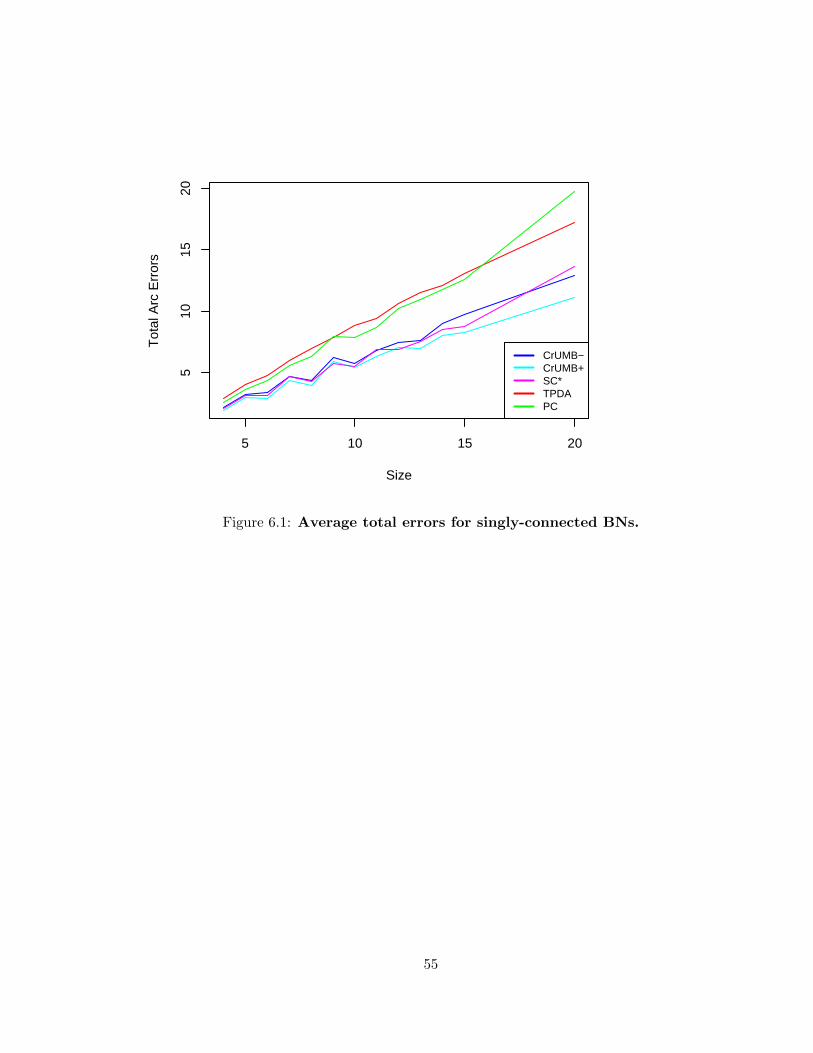
5 10 15 20
510
1520
Size
Tot
al A
rc E
rror
s
CrUMB−CrUMB+SC*TPDAPC
Figure 6.1: Average total errors for singly-connected BNs.
55

5 10 15 20
510
1520
Size
Tot
al A
rc E
rror
s
CrUMB−CrUMB+SC*TPDAPC
Figure 6.2: Average total errors for multi-connected BNs.
Figures 6.3 and 6.4 show the overall average total arc omission and commission errors
corresponding to Figures 6.1 and 6.2, respectively. As can be seen in Figures 6.3 and 6.4,
with the exception of PC, all the algorithms had very similar overall total arc omission and
commission errors for singly- and multi-connected BNs.
56

5 10 15 20
02
46
810
12
Size
Arc
Om
issi
on +
Com
mis
sion
CrUMB−CrUMB+SC*TPDAPC
Figure 6.3: Average arc omission and commission errors for singly-connected
BNs.
57

5 10 15 20
02
46
810
12
Size
Arc
Om
issi
on +
Com
mis
sion
CrUMB−CrUMB+SC*TPDAPC
Figure 6.4: Average arc omission and commission errors for multi-connected BNs.
The summary tables for each ANOVA test for singly-connected BNs for average direction
omission and commission errors are shown in Tables C.1–C.13, and for multi-connected BNs
in Tables G.1–G.13. With a significant p-value of 0.01, there are significant differences in
the average arc omission and commission errors for the both singly- and multi-connected
datasets over all sizes. For each of these ANOVA test, the pair-wise comparisons between
each algorithm (by BN size and type), using the HSD test, also with a significant p-value
set to 0.01, are shown in Tables D.1–D.13 for singly-connected BNs and H.1–H.13 for multi-
connected BNs. Figures 6.5 and 6.6 show the overall average total direction omission and
commission errors corresponding to Figures 6.1 and 6.2, respectively. As can be seen in
Figures 6.3 and 6.4, CrUMB+-GA showed the lowest overall average total direction omission
and commission errors, and is followed by CrUMB−-GA and SC*. TPDA showed the highest
overall average total direction omission and commission errors. For multi-connected BNs
of larger sizes (15 and 20), the differences in performance, in terms of average direction
58

omission and commission errors, between CrUMB+-GA and CrUMB−-GA were statistically
significant. The same observation is also true between CrUMB+-GA and SC*.
5 10 15 20
02
46
810
Size
Dire
ctio
n O
mis
sion
+ C
omm
issi
on
CrUMB−CrUMB+SC*TPDAPC
Figure 6.5: Average direction omission and commission errors for singly-
connected BNs.
59

5 10 15 20
02
46
810
Size
Dire
ctio
n O
mis
sion
+ C
omm
issi
on
CrUMB−CrUMB+SC*TPDAPC
Figure 6.6: Average direction omission and commission errors for multi-
connected BNs.
Tables 6.2 and 6.3 show the number of times each algorithm learned the best BN struc-
ture for singly- and multi-connected BNs per size, respectively, where the best BN structure
is taken to be the one with the fewest arc errors. As can be seen in Table 6.2, SC* learned
the highest number of best graphs for sizes 4, 9, 12, and 14, and CrUMB+-GA learned the
highest number of best graphs for the rest of the different sizes for singly-connected BNs.
In Table 6.3, SC* learned the highest number of best graphs for size 7, and CrUMB+-GA
learned the highest number of best graphs for the rest of the different sizes for multi-
connected BNs.
60

Table 6.2: Counts of best learned BNs for each algorithm by size for singly-
connected BNs.
Algorithm
Size SC* PC TPDA CrUMB−-GA CrUMB+-GA Best
4 81 38 28 84 94 CrUMB+-GA
5 81 39 27 78 92 CrUMB+-GA
6 74 13 9 66 89 CrUMB+-GA
7 82 27 15 78 91 CrUMB+-GA
8 82 15 0 76 96 CrUMB+-GA
9 82 2 5 59 69 SC*
10 69 3 0 58 72 CrUMB+-GA
11 59 11 2 53 79 CrUMB+-GA
12 74 2 0 48 68 SC*
13 58 0 4 40 62 CrUMB+-GA
14 52 4 7 24 68 CrUMB+-GA
15 52 1 0 19 65 CrUMB+-GA
20 21 0 6 22 76 CrUMB+-GA
61
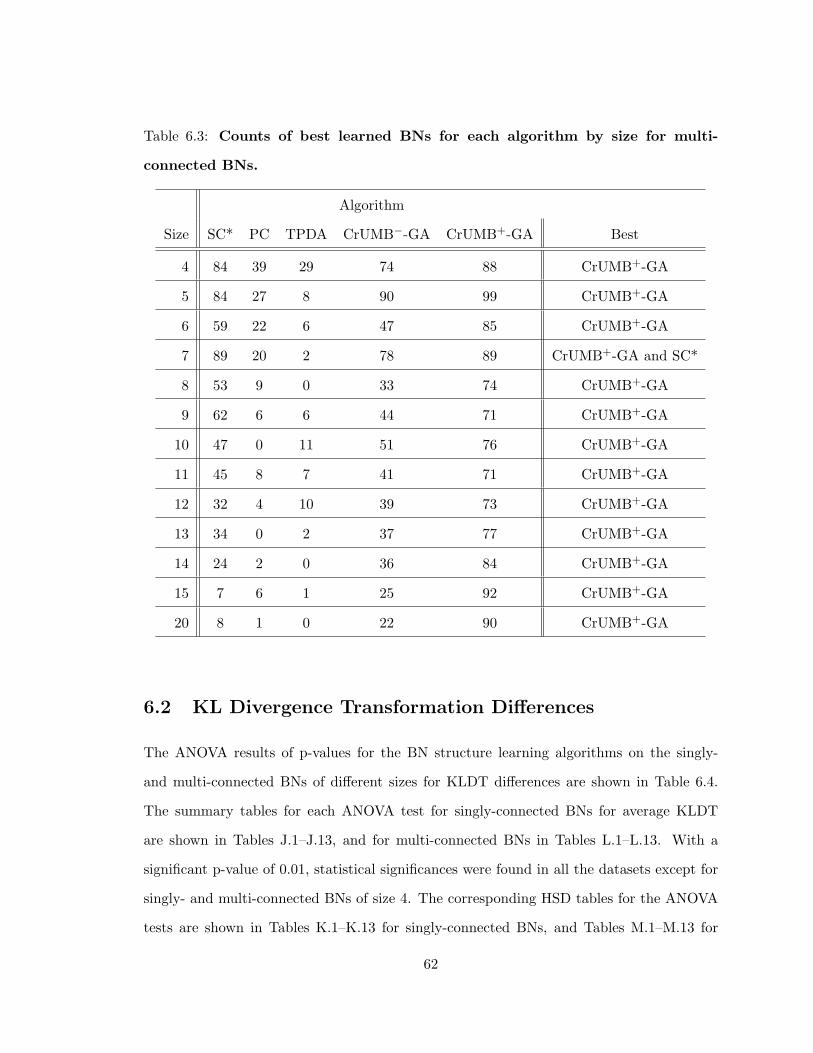
Table 6.3: Counts of best learned BNs for each algorithm by size for multi-
connected BNs.
Algorithm
Size SC* PC TPDA CrUMB−-GA CrUMB+-GA Best
4 84 39 29 74 88 CrUMB+-GA
5 84 27 8 90 99 CrUMB+-GA
6 59 22 6 47 85 CrUMB+-GA
7 89 20 2 78 89 CrUMB+-GA and SC*
8 53 9 0 33 74 CrUMB+-GA
9 62 6 6 44 71 CrUMB+-GA
10 47 0 11 51 76 CrUMB+-GA
11 45 8 7 41 71 CrUMB+-GA
12 32 4 10 39 73 CrUMB+-GA
13 34 0 2 37 77 CrUMB+-GA
14 24 2 0 36 84 CrUMB+-GA
15 7 6 1 25 92 CrUMB+-GA
20 8 1 0 22 90 CrUMB+-GA
6.2 KL Divergence Transformation Differences
The ANOVA results of p-values for the BN structure learning algorithms on the singly-
and multi-connected BNs of different sizes for KLDT differences are shown in Table 6.4.
The summary tables for each ANOVA test for singly-connected BNs for average KLDT
are shown in Tables J.1–J.13, and for multi-connected BNs in Tables L.1–L.13. With a
significant p-value of 0.01, statistical significances were found in all the datasets except for
singly- and multi-connected BNs of size 4. The corresponding HSD tables for the ANOVA
tests are shown in Tables K.1–K.13 for singly-connected BNs, and Tables M.1–M.13 for
62

multi-connected BNs. (The HSD tests for the two ANOVA tests without a significant p-
value are shown for completeness). From these HSD tables, it can be summarized for both
singly- and multi-connected BNs that the average KLDT differences of PC and TPDA
are different significantly from CrUMB+-GA, CrUMB−-GA, and SC*. In Figure 6.7 for
singly-connected BNs and Figure 6.8 for multi-connected BNs, the overall average KLDT
differences of the CrUMB+-GA, CrUMB−-GA, and SC* algorithms are almost identical.
The average KLDT differences for TPDA is the largest followed by PC.
Table 6.4: ANOVA Results for Quantitative Performances. ANOVA p-values fromcomparing means of quantitative (differences between KLDT) performances for singly- andmulti-connected Bayesian Networks of different sizes.
Size singly-connected multi-connected
4 0.0005 0.0305
5 0.0084 0.0000
6 0.0000 0.0000
7 0.0000 0.0000
8 0.0000 0.0000
9 0.0000 0.0000
10 0.0000 0.0000
11 0.0000 0.0000
12 0.0000 0.0000
13 0.0000 0.0000
14 0.0000 0.0000
15 0.0000 0.0000
20 0.0000 0.0000
63

5 10 15 20
0.0
0.2
0.4
0.6
0.8
1.0
1.2
Size
KLD
T d
iffer
ence
CrUMB−CrUMB+SC*TPDAPC
Figure 6.7: Average KLDT difference between True and Learned Graphs for
singly-connected BNs.
64
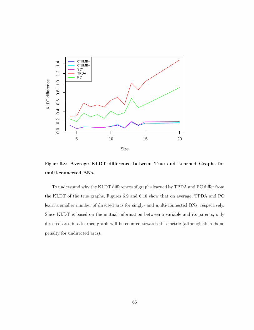
5 10 15 20
0.0
0.2
0.4
0.6
0.8
1.0
1.2
1.4
Size
KLD
T d
iffer
ence
CrUMB−CrUMB+SC*TPDAPC
Figure 6.8: Average KLDT difference between True and Learned Graphs for
multi-connected BNs.
To understand why the KLDT differences of graphs learned by TPDA and PC differ from
the KLDT of the true graphs, Figures 6.9 and 6.10 show that on average, TPDA and PC
learn a smaller number of directed arcs for singly- and multi-connected BNs, respectively.
Since KLDT is based on the mutual information between a variable and its parents, only
directed arcs in a learned graph will be counted towards this metric (although there is no
penalty for undirected arcs).
65

5 10 15 20
02
46
810
12
Size
Dire
cted
Arc
s
CrUMB−CrUMB+SC*TPDAPC
Figure 6.9: Average number of directed arcs learned arcs for singly-connected
BNs.
66

5 10 15 20
05
1015
Size
Dire
cted
Arc
s
CrUMB−CrUMB+SC*TPDAPC
Figure 6.10: Average number of directed arcs learned arcs for multi-connected
BNs.
While Figures 6.9 and 6.10 show the average number of directed arcs learned for singly-
and multi-connected BN, respectively, Figures 6.11 and 6.12 show the corresponding average
number of correct directed arcs learned. A correct directed arc is defined as an arc in the
learned BN DAG that also exist in the true graph and is given the correct orientation as
in the true graph. As can be seen in Figures 6.11 and 6.12, on average, CrUMB+-GA
learned the most number of correct directed arcs and TPDA learned the least number of
correct directed arcs. For singly-connected BNs, CrUMB−-GA and SC*, showed almost the
same average number of correct directed arcs, but for multi-connected BNs, CrUMB−-GA
showed a higher average number of correct directed arcs. The results displayed in Figures
6.9, 6.10, 6.11, and 6.12 suggest that there is an inverse relationship between the KLDT
differences and number of directed and correctly directed arcs learned; the more directed
arcs learned, the smaller the KLDT difference between the true and learned graphs; the
67

more correct directed arcs learned, the smaller the KLDT difference between the true and
learned graphs.
5 10 15 20
02
46
8
Size
Cor
rect
Dire
cted
Arc
s
CrUMB−CrUMB+SC*TPDAPC
Figure 6.11: Average number of correct arcs learned for singly-connected BNs.
68

5 10 15 20
02
46
810
Size
Cor
rect
Dire
cted
Arc
s
CrUMB−CrUMB+SC*TPDAPC
Figure 6.12: Average number of correct arcs learned for multi-connected BNs.
69

Chapter 7: Applying BN structure learning on a Real
Dataset of Patients Treated for Substance Abuse Who are
also Criminal Justice Offenders
7.1 Introduction
In this chapter I apply BN structure learning algorithms on a real dataset of drug-abuse
patients who are also criminal justice offenders. Before any of the structure learning al-
gorithms under consideration in this paper can be applied, to the dataset, the dataset
was first be transformed into a format accepted by the algorithms. I discuss this data
transformation process and its consequences. The big picture in learning a BN on this
dataset is to address two key issues: 1) does drug treatment increase technical violations
and arrests/incarceration which in turn increases probation, and 2) does treatment lead to
fewer positive drug tests, which in turn reduces probation, which in turn reduces techni-
cal violations and arrest/incarceration? The first question captures the monitoring model
of treatment (Figure 7.1), and the second question captures the drug reduction model of
treatment (Figure 7.2). The monitoring model is a view of how many treatment methods
actually work, while the drug reduction model is a view of how treatment methods should
work to prevent relapse to drug use. A drug-abuse patient under treatment of the moni-
toring model has received no real or effective treatment. The patient ends up committing
a technical violation and/or arrested/incarcerated which leads to downstream probation
and increases his chance for relapse to drug use. On the other hand, a drug-abuse patient
under treatment of the drug reduction model has received effective treatment. Effective
treatment for drug-abuse leads to less positive drug tests, less positive drug tests leads to
less probation, and less probation reduces technical violation and/or arrest/incarceration.
By avoiding arrest/incarceration, the patient decreases his chance for relapse to drug use. I
70

attempt to use the BN learned to address which of these two models are supported by the
data (if at all).
T
V A
P
Figure 7.1: Monitoring model of treatment. T denotes treatment, V denotes technicalviolation, A denotes arrest/incarceration, and P denotes probation.
T
D
P
V A
Figure 7.2: Monitoring model of treatment. T denotes treatment, D denotes pos-
itive drug test, P denotes probation, V denotes technical violation, and A denotes ar-rest/incarceration.
7.2 Motivation
The connection between drug use and crime for adults and juveniles is well known. It is
estimated that over 4.9 million American adults are under probation or parole supervision in
2003 [111]. A Bureau of Justice Statistics (BJS) survey estimated in 1997 that about 70% of
71

State and 57% of Federal prisoners used drugs regularly [112]. The BJS survey also reported
that fewer than 15% of incarcerated prisoners with drug abuse problem received treatment in
prison [112]. Approximately 650,000 inmates are released back into the community annually,
often without having received drug abuse treatment, or being connected to community-
based drug treatment and services [113]. The Institute of Medicine (IOM) reported that
one fifth of the nation’s population in need of drug treatment is on either probation or
parole supervision [114], and 40% of criminal justice offenders are in need of substance
abuse treatment [115,116].
Untreated substance abusing offenders are more likely to relapse to drug abuse and
return to criminal drug behavior [117]. Furthermore, effective drug abuse treatment can
help individuals to overcome persistent physical drug effects and lead to healthy, produc-
tive lives [117]. The effectiveness of drug treatment depends on both the individual and
program, and on whether intervention and treatment services are available and appropriate
for the individual’s needs. Research indicates that offenders who are in need of substance
abuse treatment can be matched to an appropriate and effective treatment option based on
their characteristics and risk profiles to reduce the probability of re-incarceration and/or
recidivism [118]. Moreover, offenders participating in drug treatment services have a lower
incidence of criminal behavior and longer overall length of crime-free time [119]. The risk
factors for released offenders include but are not limited to associating with violent peers,
lack of employment opportunities, lack of safe housing, and stress from compliance with
probation [117]. The cost to society of drug abuse was $180.9 billion in 2002, of which
$107.8 billion was associated with drug-related crime, including criminal justice system
costs and costs related to victims of crime [120]. It is estimated that every $1 invested in
addiction treatment programs yields a return between $4 and $7 in reduced drug-related
crime, criminal justice cost, and theft alone [121].
Although many research studies provide treatment guidelines taking into account risk
factors involved in effective treatment, few analyze the interactions between these risk fac-
tors, patient characteristics, and outcomes simultaneously; analysis of variables related
72

to effective treatment and outcomes have been limited to standard statistical methods
[122–127]. By learning a BN model of and from the data, we are able to observe the multi-
variable interactions simultaneously. Furthermore, we are also able to query the BN model
and obtain multiple answers with probabilities attached.
7.3 The Data
The data set is based on 272 offenders (also referred to as patients) undergoing substance
abuse treatment. The study period began in November 1997 and continued through March
2003, spanning a total of 1,996 days. However, the follow-up length per patient differed as
patients were right- or left-censored (or both) depending on when they entered or left the
study. The range of drug addiction problems suffered by these patients included (but was
not limited to) marijuana, alcohol, and cocaine. The patients who participated in the study
came from Virginia or Maryland.
Offenders were randomly assigned into a seamless or traditional supervision treatment
approach. The most important aspect of this program was that its experimental design
allowed for the opportunity to quantitatively asses the costs and benefits of the two dif-
ferent approaches [128], and to assess the impacts of varying components of the treatment
and supervision services on offender outcomes. Under the seamless approach, probation
and treatment staffs worked together as a team in delivering services. The teamwork is
facilitated by the probation and treatment staffs working in the same building and co-
administering services. At all times, the probation staff is aware of the treatment progress
of the offender, and likewise, the treatment staff is aware of the probation status of the
offender. In contrast to the seamless approach, under the traditional supervision approach,
probation and treatment staffs occupy different buildings, and communication of probation
or treatment progress is heavily based on the effort of the offender.
73

7.4 The Variables
In this paper, a variable refers to a symbol representing one of a set of mutually exclusive and
collectively exhaustive values [15]. A variable (random variable) may also be defined more
precisely, as in the field of statistics, as a function that maps the values of an experiment
to a numeric value [129]. The set of values of a variable is also called the domain or space
of the variable [15, 35]. If we classify variables according to their set of values, then we
have two classes of variables, categorical and numeric. A categorical variable has a set of
values that are mutually exclusive and exhaustive. Mutually exclusive means that the set
of values must be distinct enough that no observations will fall into more than one value.
Exhaustive means that there must be enough values that all the observations will fall into
some value. Categorical variables may be further classified if there is ordering implied in the
set of values; categorical variables with order implied in the set of values are called ordinal
variables; categorical variables without order implied in the set of values are called nominal
variables. A categorical variable having only 2 values is called a binary variable. On the
other hand, a numeric variable takes on a number of real values. When a numeric variable
takes on values in an interval of the real line, it is called a continuous variable. When a
numeric variable assumes a finite number of real numbers, it is called a discrete variable.
In this paper, integer variables refer to numeric variables whose values are integer.
Followup of each patient included the 17 variables in Table 7.1. There were 6 binary
variables and 11 integer variables. The values of the binary variables were mapped to 0
and 1 from their original values (Table 7.2). As can be seen in Table 7.3, the majority of
patients were black (87.5%) and male (85%), over half of these patients were from Virginia
(56%) and considered as high risk for rearrest (53%), and nearly half of these patients were
randomized into the seamless treatment approach (48%). Only one-third (33%) of these
patients were in violation of their probation during the study period.
In regards to the integer variables, with the exception of age, observations were recorded
over time. The study kept track of the number of days certain services were used by each
74

Table 7.1: Variables in Study. This table shows and describes the variablesin the study. The name (Variable), abbreviation (Abbrev.) of the name, expla-nation, and type of the variable are shown.
Variable Abbrev. Explanation Typeage age age of patient entering study integerarrest arr number of arrests integeremployed emp number of days employed integerfollowup fol number of followup days integergender gen gender (male or female) binaryincarceration inc number of days incarcerated integermental men number of days patient was integer
hospitalized for mental reasonsphysical phy number of days patient was integer
hospitalized for physical reasonsprobation pro number of days on probation integerrace rac race (White or Black) binaryrisk ris risk of re-arrest(medium or high) binaryshelter she number of days patient used homeless integer
shelter servicesstate sta state patient is from (VA or MD) binarytest tes number of positive drug tests integertreatment tre number of days patient was in treatment integertype typ treatment type (traditional or seamless) binaryviolation vio indicates if patient was in binary
violation of probation during anytime of the study (false or true)
Table 7.2: Binary Variable Value Coding Scheme.The values of binary variables are coded into 0 or 1 fromtheir original values as displayed in this table.
Variable 0 1race White Blackgender female malestate Virginia Marylandrisk moderate–risk high–risktype traditional seamlessviolation false true
75

Table 7.3: Summary Statistics for Binary Variables.The probability (q) of a variable taking on its value rep-resented by 0, the probability (p) of a variable taking onits value represented by 1, the expected value (Exp) ofthe variable, and standard deviation (StDev) are shown.
Variable q p Exp StDevrace 0.125 0.875 238 5.5gender 0.15 0.85 232 5.8state 0.44 0.56 152 8.2risk 0.47 0.53 144 8.2type 0.52 0.48 131 8.2violation 0.62 0.33 89 7.7
patient such as homeless shelter, hospitals, and treatment. The study also recorded the
number of days of employment and probation for each patient. The age of the patient was
recorded at the time he or she entered the study. The number of arrests and positive drug
test results were also recorded for each patient. Table 7.4 shows the summary statistics for
the integer variables. The age of the patients ranged from [18–62] years, and the average
age was 30.1 years. The number of arrests ranged from [0–8] and averaged 0.9 times per
patient. Positive drug test ranged from 0–34 and averaged 3.3. Employment days ranged
from [0–1649] days, and averaged 301.8 days. Followup days ranged from [325–1877] days
and averaged 862.7 days. The average number of days spent in homeless shelters per patient
was comparably small at 2.9 days and the range was [0–366] days. The average number
of days patients were incarcerated was 97.4 days and ranged [0–937] days. The average
number of days a patient was hospitalized for mental and physical reasons were 0.6 and 0.3
days, respectively, and the ranges were [0–212] and [0–11] days, respectively. On average,
patients spent 395.4 days on probation, and the range was [0–1093] days. Patients had on
average 120.7 days of treatment ranging from [0–1238] days.
76

Table 7.4: Summary Statistics for Integer Variables. Theminimum (Min), maximum (Max), average (Avg), and standarddeviation (StDev) are given for each integer variables. The averageand standard deviation values are rounded to the nearest tenth.Variable Min Max Avg StDevage 18 62 30.1 9.4arrest 0 8 0.9 1.2employment 0 1649 301.8 399.4followup 325 1877 862.7 388.3shelter 0 366 2.9 25.5incarceration 0 937 97.4 186.4mental 0 212 0.6 7.4physical 0 11 0.3 1.4probation 0 1093 395.4 203.2test 0 34 3.3 6.2treatment 0 1238 120.7 202.0
7.5 Data Transformation
The original data set was transformed for further analysis. Data transformation was neces-
sary since the BN structure learning algorithms under investigation in this thesis required
all variables to be categorical. The 6 binary variables were left alone, however, the 11
integer variables required transformation into categorical form. In this paper, the term
data transformation refers to the process of changing a variable from its integer type to
categorical type, and discretization refers to the actual technique used to implement the
transformation. Although discretization leads to a loss of information, many studies show
that induction tasks can benefit from discretization including but not limited to improved
learning speed and predictive accuracy [130,131].
The first phase of data transformation was based on whether over half the patients had
a value ≥ 1 for each variable. As can be see in Table 7.5, only the age, followup, and
probation variables had near or equal to 100% of the patients having a frequency of ≥ 1.
With the exception of the employment variable, all other integer variables had less than
50% of the patients having a frequency of ≥ 1. For the former integer variables, a second
phase of data transformation based on background knowledge or equal-width discretization
77

Table 7.5: Number and Percentage of Patients with Values ≥ 1for Integer Variables. This table shows the number and percentage ofpatients out of 272 having a value ≥ 1 for each of the integer variables.
Variable Counts Percentage (%)age1 272 100arrest2 124 46drug2 128 47employment2 148 54followup1 272 100shelter2 7 3incarceration2 136 50mental2 5 2physical2 14 5probation1 266 98treatment2 133 491 Integer variable was discretized from integer to categorical type.2 Integer variable was discretized from integer to binary type.
Table 7.6: Frequency of Values for DiscretizedAge Variable.
Value Range Counts Percentage (%)young [18–39] 223 82middle-aged [40–59] 47 17older [60–74] 2 1
[131] was used to discretize the values, and for the latter integer variables, for each variable,
if a patient had ≥ 1 count, then a value of 1 was assigned to the variable, otherwise, 0 was
assigned.
The histogram for the age variable is shown in Figure 7.3. Age classifications have been
reported in the psychology research field [132–134]. Following the extensive work of [132],
age was discretized into young [18–39], middle-aged [40–59], and older [60–74]. As can be
seen in Table 7.6, there is only 1% of patients falling in the older category. For this reason,
the middle-aged and older category were merged into one. The discretized age variable was
further discretized into a binary variable with the value 0 representing the age range [18–39]
and 1 representing the age range [40–74].
78

0
5
10
15
20
25
17 22 27 32 37 42 47 52 57 62N
o.
ofPati
ents
Age
Figure 7.3: Histogram of Age Values.
Table 7.7: Frequency of Values for DiscretizedFollowup Variable.
Value Range Counts Percentage (%)short [325–842.3) 125 46medium [842.3–1359.6) 121 44long [1359.6–1877] 26 10
Figure 7.4 shows the histogram for the followup variable. This figure is interesting in that
it shows a cluster of patients having followup close to 1 year; there are 41 patients having
a year of followup and 19 patients having a year and 1 day of followup. This variable was
discretized using equal-with discretization [131] with the number of bins selected arbitrarily
to 3; using 3 bins, we may rename the intervals to short, medium, and long to signify the
length of the followup. Equal-width discretization was favored over equal-frequency since
the latter approach may group the same value into different bins [131]. To compute the
cut-points, the absolute value of the difference of the minimum (325) and maximum (1877)
values was computed at 1552 (|325 − 1877| = 1552). The difference was then divided by
three (1552/3 = 517.3) to get the value by which to increment from the minimum value to
the next cut-point. For k bins, we need k − 1 cut-points. The cut-points produced were
842.3 (325 + 517.3) and 1359.6 (842.3 + 517.3). The 3 intervals or bins resulting from these
cut-points were mapped to the values short [325–842.3), medium [842.3–1359.6), and long
[1359.6–1877]. Table 7.7 shows the frequency of the new and discretized values for the
followup variable.
The probation variable was also discretized using equal-width discretization like the
79
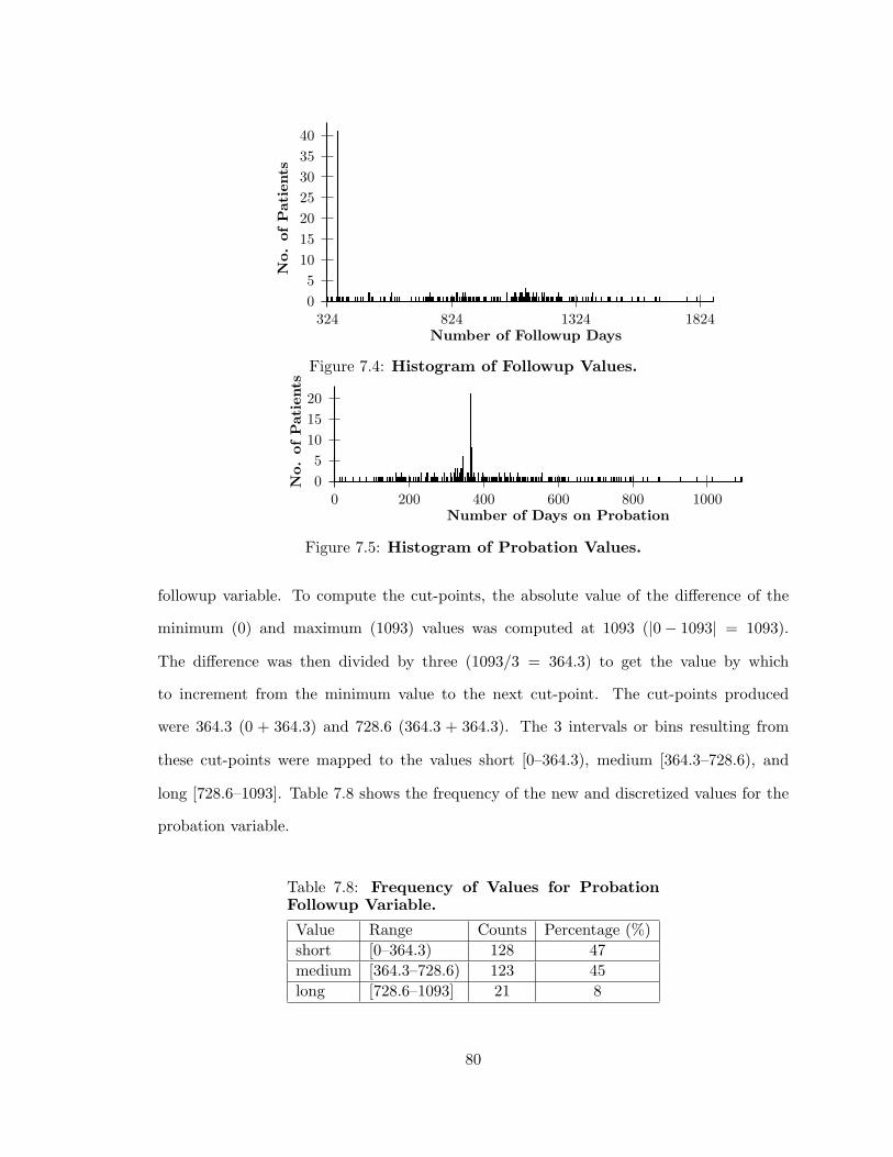
0
5
10
15
20
25
30
35
40
324 824 1324 1824
No.
ofPati
ents
Number of Followup Days
Figure 7.4: Histogram of Followup Values.
0
5
10
15
20
0 200 400 600 800 1000
No.
ofPati
ents
Number of Days on Probation
Figure 7.5: Histogram of Probation Values.
followup variable. To compute the cut-points, the absolute value of the difference of the
minimum (0) and maximum (1093) values was computed at 1093 (|0 − 1093| = 1093).
The difference was then divided by three (1093/3 = 364.3) to get the value by which
to increment from the minimum value to the next cut-point. The cut-points produced
were 364.3 (0 + 364.3) and 728.6 (364.3 + 364.3). The 3 intervals or bins resulting from
these cut-points were mapped to the values short [0–364.3), medium [364.3–728.6), and
long [728.6–1093]. Table 7.8 shows the frequency of the new and discretized values for the
probation variable.
Table 7.8: Frequency of Values for ProbationFollowup Variable.
Value Range Counts Percentage (%)short [0–364.3) 128 47medium [364.3–728.6) 123 45long [728.6–1093] 21 8
80

Table 7.9: Transformed Variables.Variable Explanation Typeage1 age of patient entering study binaryarrest2 indicates if patient was arrested binaryemployed2 indicates if patient was employed binaryfollowup3 number of followup days ordinalgender gender (male or female) binaryincarceration2 indicates if patient was incarceration binarymental2 indicates if patient was hospitalized binary
for mental reasonsphysical2 indicates if patient was hospitalized binary
for physical reasonsprobation3 number of days on probation ordinalrace race (white or black) binaryrisk risk (high or medium) binaryshelter2 indicates if patient used homeless shelter services binarystate state patient is from binarytest2 number of positive drug tests binarytreatment2 number of days patient was in treatment binarytype treatment type binaryviolation indicates if patient was in violation of probation binary1 Integer variable was discretized from integer to categorical to binary type.2 Integer variable was discretized from integer to binary type.3 Integer variable was discretized from integer to ordinal type.
7.6 Transformed Data Set
The transformed variables are summarized in Table 7.9. All the variables are now categor-
ical; all but two variables are binary. Three important changes should be noted. The first
is that discretization results in a loss of information. I am most concerned with the loss of
correlation relationships resulting from the data transformation. The second change to note
is the size of the data set. The third change to note is that the temporal dimension of the
variables is lost in this transformation process. Each of these changes and their implications
are addressed below.
81

7.7 Information Loss
In this research, it is desired to have the data transformation preserve as much as possible
the correlations in the original data set. To quantify how much of the correlations were
preserved, the correlations in the original data set was compared to those in the transformed
data set. In the original data set, correlations between integer variables were computed
using Pearson and Spearman measures [135], and correlations between integer and binary
variables were computed using the point-biserial correlation measure [136].
Since the Pearson correlation measure assumes a linear relationship between two vari-
ables, the Spearman correlation was also used in case the relationship between two variables
was non-linear. The Pearson correlation measure, rXY , between two variables, X and Y , is
given by:
rXY =∑n
i (xi − X)(yi − Y )sXsY
, (7.1)
where n is the number of samples, i is the i-th instance (or value) of the variable, X is
the average value of X, Y is the average value of Y , sX is the standard deviation of X,
and sY is the standard deviation of Y . The Pearson correlation coefficient lie in the range
[-1,1]. The significance testing for the Pearson correlation between two variables, X and Y ,
is given by:
t = rXY
√n − 2
1 − r2XY
, (7.2)
where rXY is the correlation between X and Y , n is the sample size, and the degrees of
freedom is n− 2 for a 2-tail test and n− 1 for a 1-tail test. The null hypothesis, H0, of the
significance test is that there is no correlation between the two variables, rXY = 0. The
alternative hypothesis, Ha, of the significance test is that there is a correlation between the
two variables, rXY 6=0 [135]. Before the Spearman correlation measure may be applied to
two continuous variables, the values must be ranked. The Spearman correlation measure,
82

kXY , between two variables, X and Y , is given by:
kXY =n(n2 − 1) − 6(
∑ni D2
i + U + V )√n(n2 − 1) − 12U
√n(n2 − 1) − 12V
, (7.3)
where n is the number of samples, i is the i-th instance (or value) of the variable, Di is the
difference between the ranks of xi and yi, U is a correction for the number of tied ranks in
X, and V is a correction for the number of tied ranks in Y . U is given by:
112
∑i
mi(m2i − 1), (7.4)
where mi is the number of tied ranks for X of the i-th value. V is given by:
112
∑j
nj(n2j − 1), (7.5)
where nj is the number of tied ranks for Y of the j-th value. The Spearman correlation
coefficient lie in the range [-1,1]. The significance testing for the Spearman correlation
between two variables, X and Y , is given by:
t =kXY√1−k2
XYn−2
, (7.6)
where n is the sample size and kXY is the Spearman correlation coefficient. The point-
biserial correlation measure, bXY , between an integer variable, X, and a binary variable,
Y , is given by:
bXY =(X1 − X0)
√pq
sX, (7.7)
where x1 is the average value of X when Y = 1, X0 is the average value of X when Y = 0, p
83

is the probability of Y = 1, q is the probability of Y = 0, and sX is the standard deviation of
X. The point-biserial correlation coefficient lie in the range [-1,1]. The same significance test
for the Pearson correlation coefficient is used for the point-biserial correlation coefficient.
Measures of association for the categorical variables (a binary variable is a special case of
categorical variable) are computed using Cramer’s Phi and mutual information (see 3.11).
Cramer’s Phi is based on the Chi-squared goodness of fit test (see 3.9). Cramer’s Phi, φXY ,
for two variables is given by:
φXY =
√χ2
n(k − 1), (7.8)
where n is the number of samples, k = min(NX , NY ) (NX is the number of values for X and
NY is the number of values for Y ), and χ2 is the Chi-squared value. The value of Cramer’s
Phi lie in the range [0,1].
The pairwise correlations for the variables in the original and transformed data sets are
shown in Tables N.1–N.6. The ranks of these correlations are also shown in the tables. To
measure if the correlations in the original data set were preserved in the transformed data
set, Pearson’s correlation measure is applied to the ranks of the correlations in the original
and transformed data set. The idea is that the ranks of the correlations in the original data
set should hold a linear relationship with the ranks of the correlations in the transformed
data set. Table 7.10 shows correlation matrix between the ranks of the correlation in the
original and transformed data set. Although the correlations in Table 7.10 appear to be
weak, they are all significant (p < 0.001).
In concluding this section, although there is loss of information as a result of discretiza-
tion, we gain other benefits. The discretized values have more meaning than the numbers
they represent [130, 131]. For example, for the variable capturing the number of days of
probation, abstracted values of high, medium, and low may be more meaningful than a
single number. We are also able to use correlation measures handling categorical data to
analyze the data set consistently without the concern of mixed variable types. Moreover,
84

Table 7.10: Correlation Matrix for Ranks of Cor-relations in Original and Transformed Data Sets.This table shows the Pearson correlation coefficients be-tween the ranks of correlations in the original (Spearman,k, and Pearson, p) and transformed data sets (mutual in-formation, mi, and Cramer’s phi, phi). All correlationsare significant (p < 0.001).
k r mi phik 1.000 0.996 0.354 0.358p - 1.000 0.369 0.354mi - - 1.000 0.650phi - - - 1.000
the transformation does preserve the correlations from the original data set at a significant
level.
7.8 Data Set Size Reduction
If we use Huber’s taxonomy of data set size [137] to describe the size of this data set in its
original form, it would be described as a medium to large data set (see Table 7.11) [138].
In comma-separated value (csv) format, the original data set was 45,289,472 bytes. The
transformed data set is only 26,407 bytes in csv format, and would be described as small.
It is not clear how size reduction may negatively impact the BN modeling and learning,
although the size reduction may help to speed up analysis.
85

Table 7.11: Huber Taxonomy of Data Set Sizes.
Descriptor Data Set Size (Bytes) Storage Mode
tiny 102 piece of paper
small 104 a few pieces of paper
medium 106 a floppy disk
large 108 hard disks
huge 1010 multiple hard disks
massive 1012 robotic magnetic tape
7.9 Time Dimension
It is very important to not disregard the temporal dimension of the variables, however, they
are transformed to a static form for the purpose of applying the BN learning algorithms un-
der investigation. There are BN learning algorithms that address the temporal interactions
between variables [139–141], but this paper only deals with learning static BNs. Moreover,
from speaking with experts in this research domain on drug abuse treatment, 1) it is not
expected that the influence of the variables will change over time and 2) a more rigorous
approach to modeling the temporal aspect of the data (such as the use of dynamic BNs)
may be difficult for the policy makers to understand.
7.10 K-Fold Cross-Validations of Algorithms and Learned
Networks
After the dataset underwent discretization, all five learning algorithms under consideration
in this thesis were applied to the dataset for structure learning. Parameter learning was
implemented according to [39] (see Section 3.1). The algorithms and the BNs they learned
were validated using k-fold cross-validation, with k=10. In k-fold cross-validation, the
86

dataset was split into 10 equal partitions (272 / 10 = 27 with remainder 2, so 2 partition
had 28 samples). Each partition was used as the testing data, while the other nine partitions
were used as the training data. The BNs learned from the training data were then validated
against the corresponding testing data using the quadratic loss (also known as the Brier
score) scoring rule [142,143]. The quadratic loss value is between 0 and 2 with 0 indicating
the best prediction (a value closer to 0 means better prediction). In k-fold cross-validation,
there is usually a class variable that the testing data is used to predict. In this dataset,
there was no class variable. However, I used the incarceration variable as the class variable
(the variable whose state will be predicted). The justification for using incarceration as
the class variable was to see how well the models predicted recidivism, which would involve
incarceration (patients who go back to jail are more likely relapse back into drug use, see
Section 7.2).
The average quadratic loss values for each algorithm from running k-fold cross-validation
are displayed in Table 7.12. As can be seen in Table 7.12, CrUMB+-GA had the lowest
average quadratic loss value. An ANOVA test was applied to these averages to detect for
significant differences (p=0.01). The summary of the ANOVA test is shown in Table 7.13.
As can be seen in Table 7.13, the p-value was less than 0.01. The results of the HSD test is
shown in Table 7.14. From Table 7.14, it can be see that the average quadratic loss value
of CrUMB+-GA is different significantly from all the other algorithms except for SC*. The
average quadratic loss value of SC* is different significantly from TPDA and CrUMB−-GA.
87
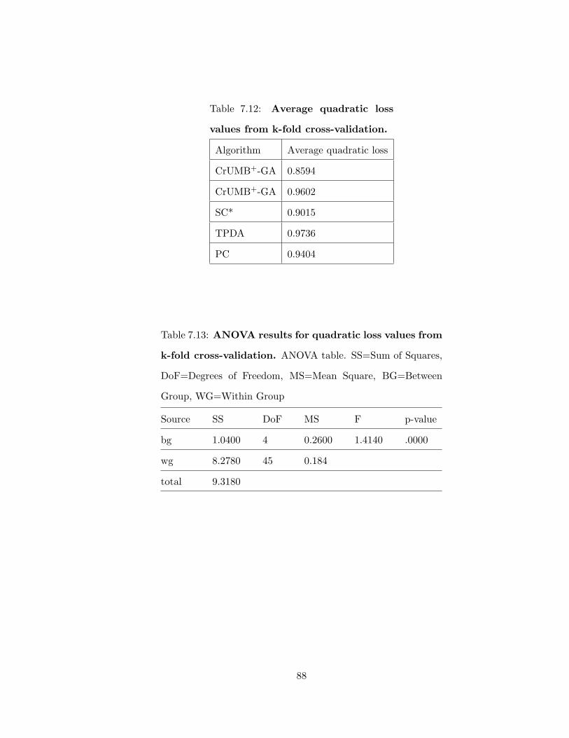
Table 7.12: Average quadratic loss
values from k-fold cross-validation.
Algorithm Average quadratic loss
CrUMB+-GA 0.8594
CrUMB+-GA 0.9602
SC* 0.9015
TPDA 0.9736
PC 0.9404
Table 7.13: ANOVA results for quadratic loss values from
k-fold cross-validation. ANOVA table. SS=Sum of Squares,
DoF=Degrees of Freedom, MS=Mean Square, BG=Between
Group, WG=Within Group
Source SS DoF MS F p-value
bg 1.0400 4 0.2600 1.4140 .0000
wg 8.2780 45 0.184
total 9.3180
88

Table 7.14: HSD results for quadratic loss from k-fold
cross-validations. HSD table. k=5, DoFWG=45.0
Algorithm1 Algorithm2 p
CrUMB+-GA CrUMB−-GA 0.0000
CrUMB+-GA PC 0.0000
CrUMB+-GA TPDA 0.0000
SC* TPDA 0.0010
CrUMB−-GA SC* 0.0080
CrUMB+-GA SC* 0.0960
PC SC* 0.1450
PC TPDA 0.2750
CrUMB−-GA PC 0.7520
CrUMB−-GA TPDA 0.9240
7.11 Learning a Bayesian Network from the Complete Dataset
In this section I used CrUMB+-GA to learn a BN from the complete dataset of drug-abuse
patients who are also criminal justice offenders. The justifications for using this algorithm
alone is due to the comparatively higher performances of CrUMB+-GA (see Sections 6.1,
6.2, and 7.10). The DAG of the BN learned using this algorithm is shown in Figure 7.6.
The BN for CrUMB+-GA was further subjected to sensitivity analysis as shown in Table
7.15. Sensitivity analysis measures quantitatively how the variables influence one another.
For BNs, sensitivity analysis may be conducted using entropy reduction or variance [1,20].
For this BN learned, I looked at the entropy reduction to see how all the variables influence
one another. Table 7.15 shows the sensitivity analysis; non-root nodes are listed in the
columns and all nodes are listed in the rows. In Table 7.15, a lower number indicates
89

a higher influence (more entropy reduction) of the variable in the corresponding row on
the variable in the corresponding column. The positive and negative signs following each
number in Table 7.15 indicates the direction of the influence between the variables in the
original variable space (before transformation to categorical variables).
P E H
Y S
T L
V I M R
G A K D W
Figure 7.6: Learned BN for real world dataset. P denotes probation, E denotes em-
ployment, H denotes physical hospitalization, Y denotes treatment type, S denotes state, T
denotes treatment, L denotes homeless shelter, V denotes technical violation, I denotes in-
carceration, M denotes mental hospitalization, R denotes race, G denotes gender, A denotes
arrest, K denotes risk, D denotes positive drug test, and W denotes age.
90

Table 7.15: Sensitivity Analysis. This table shows the sensi-
tivity analysis for the BN learned in Figure 7.6. Non-root nodes
are listed in the columns and all nodes are listed in the rows. The
numbers in each cell indicate the magnitude of influence by the
variable in the row over the variable in the column. Smaller num-
bers indicate more influence and larger numbers indicating less
influence. Influence with mutual information less than 0.001 are
ignored and the corresponding cells are left empty. The positive
and negative signs following each number indicate the direction
of influence. Direction of influence are determined by Spearmancorrelation (see Tables N.1–N.6) in the undiscretized domain.
arr emp inc men phy pro she tes tre vio
age 1-
arr 6- 3+
emp 3- 4+ 1+ 1+ 6+ 4-
gen 2+
inc 1+ 1+ 2+ 2+ 2+ 2+
men 3+
phy 2+ 8+
pro 3+
rac 7+ 4+
ris 2+
she 7+
sta 7+ 5- 1- 1+
tes 1+
tre 4+ 1+ 1+ 3+
typ 6+ 3+
vio 5- 2+ 5+91

I now return to the big picture in learning a BN on this dataset which is to observe if
the monitoring model or drug reduction model is supported. For the monitoring model,
from sensitivity analysis in Table 7.15, technical violation and incarceration are influenced
by treatment, but arrest is not influenced by treatment; neither technical violation nor
arrest influence probation. The monitoring model superimposed on the BN learned is
shown in Figure 7.7. Only the arc from treatment to incarceration is learned. For the drug
reduction model, from sensitivity analysis in Table 7.15, positive drug test is not influenced
by treatment, probation is not influenced by positive drug test, and technical violation and
arrests are not influenced by probation. The drug reduction model superimposed on the
BN learned is shown in Figure 7.8. It is interesting to note that probation shows no direct
connection to technical violation, arrest, or incarceration. This observation is explained by
the lack of fidelity and adherence to treatment protocols in this study from which the data
was obtained [144]. Probation, however, shows a direct connection to employment, which
is expected since patients on probation were explicitly required to maintain employment.
The learned model supports the monitoring model of treatment indicating that treatment
implementation was ineffective. The policy implication of this learned BN model is that
treatment should be implemented more effectively to prevent relapse to drug use.
92
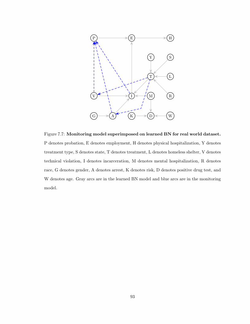
P E H
Y S
T L
V I M R
G A K D W
Figure 7.7: Monitoring model superimposed on learned BN for real world dataset.
P denotes probation, E denotes employment, H denotes physical hospitalization, Y denotes
treatment type, S denotes state, T denotes treatment, L denotes homeless shelter, V denotes
technical violation, I denotes incarceration, M denotes mental hospitalization, R denotes
race, G denotes gender, A denotes arrest, K denotes risk, D denotes positive drug test, and
W denotes age. Gray arcs are in the learned BN model and blue arcs are in the monitoring
model.
93

P E H
Y S
T L
V I M R
G A K D W
Figure 7.8: Drug reduction model superimposed on learned BN for real world
dataset. P denotes probation, E denotes employment, H denotes physical hospitalization,
Y denotes treatment type, S denotes state, T denotes treatment, L denotes homeless shelter,
V denotes technical violation, I denotes incarceration, M denotes mental hospitalization, R
denotes race, G denotes gender, A denotes arrest, K denotes risk, D denotes positive drug
test, and W denotes age. Gray arcs are in the learned BN model and blue arcs are in the
monitoring model.
94

Chapter 8: Summary and Conclusions
The ANOVA tests showed significant differences in terms of average total arc errors between
the BN structure learning algorithms for both singly- and multi-connected BNs across all
sizes. Generally speaking, the HSD tests showed that the average total arc errors committed
by CrUMB+-GA, CrUMB−-GA, and SC* were significantly different from TPDA and PC.
The former set of algorithms learned a smaller average of total arc errors than the latter
algorithms. Although there is no statistically significant differences between the average
total arc errors committed by CrUMB+-GA, CrUMB−-GA, and SC* across all singly- and
multi-connected BN sizes, CrUMB+-GA was able to learn the most number of BN structures
with the lowest total arc errors for a majority of the BN sizes and types. With the exception
of PC, all the algorithms made similar average arc omission and commission errors. As for
direction omission and commission errors, TPDA and PC made the most errors of this type
on average. This result is not surprising since these algorithms employ the traditional arc
orientation methods, which may not orient all arcs.
The ANOVA tests showed that for learning singly- and multi-connected BNs, the KLDT
differences of the graphs learned by CrUMB+-GA, CrUMB−-GA, and SC* to the true
graphs were significantly different from those by PC and TPDA. Generally speaking, the
HSD tests show that CrUMB+-GA, CrUMB−-GA, and SC* were significantly different
from TPDA and PC. It is highly likely that the KLDT differences of PC and TPDA were
higher because these algorithms learned less directed arcs (although undirected arcs are not
penalized when computing the KL distance, only directed arcs count towards computing
the KL distance, see Section 5.6).
Although CrUMB+-GA outperformed SC* in terms of qualitative and quantitative per-
formances and k-fold cross-validation, it is interesting to note that no statistically significant
95
differences were found between these two algorithms in these areas. Perhaps an explanation
of the competitive performance of SC* with CrUMB+-GA is due to the BNs generated. The
BNs generated were sparse (see Section 5.2), and SC* is a special instance of SC, which is
specifically designed to recover sparse BN structures. It would be difficult to decide between
the two algorithms if one were to choose only one for BN structure learning based on the
results in this thesis. However, it is argued that CrUMB+-GA provides two advantages over
SC*. First, although the performances of CrUMB+-GA is not significantly different from
SC*, the performance is nevertheless better on average. Second, CrUMB+-GA has specifi-
cally designed into the algorithm a way to orient arcs based on psychological understanding
of causation. In other words, the directed arcs in CrUMB+-GA given orientation due to
testing for predictive power of one variable given another has a link to the way humans
view causation. While SC* orient arcs purely based on random mutations and fit to the
data, these arcs oriented do necessarily, if at all, have any basis in causation. Additionally,
perhaps CrUMB+-GA was able to make fewer direction omission and commission errors
than the other algorithms due to the way the data were generated from the BNs using logic
sampling. In [20], logic sampling is said to “retain the merits of causal modeling in that it
conducts the simulation along the flow of causation.”
Using predictive asymmetry clearly improved directing (orienting) arcs in BN structure
learning. For larger multi-connected BNs, the performance of CrUMB+-GA, in terms of
average direction omission and commission errors, was significantly different from all the
algorithms.
From applying these structure learning algorithms on a real-world dataset, CrUMB+-
GA had the lowest average quadratic loss. The ANOVA test on all the average quadratic
loss values showed a significant difference. The HSD test showed that the average quadratic
loss of CrUMB+-GA was significantly different from all the algorithms except for SC*.
The BN model learned by CrUMB+-GA on the complete dataset supported the monitoring
model of treatment.
96

8.1 Future Work
Future work based on this thesis should compare CrUMB+-GA with other SS [39,41,45,46,
109, 145–147], CB [148–151], and hybrid BN structure learning algorithms [49, 59, 64–67].
As an alternative to using BNGenerator, the BN structure learning algorithms compared in
this paper could also be applied to additional available real world datasets [14, 26, 96, 106].
It should be investigated if the asymmetric correlation arc orientation method used in this
thesis would help to improve other CB methods to orient arcs when they learn a PDAG.
Additionally, there is room to explore where using predictive asymmetry to orient arcs may
fail either due to the method of BN generation or data generation. As for learning a BN
from the dataset on drug-abuse patients who are also criminal justice offenders, future work
may extend the learned BN to decision nets for utility assessments.
97

Appendix A: One Way ANOVA Tables for Total Arc Errors
for Singly-Connected Bayesian Networks
Table A.1: ANOVA results for total arc errors for singly-
connected BNs of size 4. ANOVA table. SS=Sum of Squares,
DoF=Degrees of Freedom, MS=Mean Square, BG=Between
Group, WG=Within Group
Source SS DoF MS F p-value
bg 5.9348 4 1.4837 6.3262 .0004
wg 10.5540 45 .2345
total 16.4888 49
Table A.2: ANOVA results for total arc errors for singly-
connected BNs of size 5. ANOVA table. SS=Sum of Squares,
DoF=Degrees of Freedom, MS=Mean Square, BG=Between
Group, WG=Within Group
Source SS DoF MS F p-value
bg 7.1812 4 1.7953 9.4611 .0000
wg 8.5390 45 .1898
total 15.7202 49
98

Table A.3: ANOVA results for total arc errors for singly-
connected BNs of size 6. ANOVA table. SS=Sum of Squares,
DoF=Degrees of Freedom, MS=Mean Square, BG=Between
Group, WG=Within Group
Source SS DoF MS F p-value
bg 27.5160 4 6.8790 12.3407 .0000
wg 25.0840 45 .5574
total 52.6000 49
Table A.4: ANOVA results for total arc errors for singly-
connected BNs of size 7. ANOVA table. SS=Sum of Squares,
DoF=Degrees of Freedom, MS=Mean Square, BG=Between
Group, WG=Within Group
Source SS DoF MS F p-value
bg 18.7692 4 4.6923 7.7080 .0001
wg 27.3940 45 .6088
total 46.1632 49
99

Table A.5: ANOVA results for total arc errors for singly-
connected BNs of size 8. ANOVA table. SS=Sum of Squares,
DoF=Degrees of Freedom, MS=Mean Square, BG=Between
Group, WG=Within Group
Source SS DoF MS F p-value
bg 74.8180 4 18.7045 15.0891 .0000
wg 55.7820 45 1.2396
total 130.6000 49
Table A.6: ANOVA results for total arc errors for singly-
connected BNs of size 9. ANOVA table. SS=Sum of Squares,
DoF=Degrees of Freedom, MS=Mean Square, BG=Between
Group, WG=Within Group
Source SS DoF MS F p-value
bg 46.7372 4 11.6843 14.8370 .0000
wg 35.4380 45 .7875
total 82.1752 49
100

Table A.7: ANOVA results for total arc errors for singly-
connected BNs of size 10. ANOVA table. SS=Sum
of Squares, DoF=Degrees of Freedom, MS=Mean Square,
BG=Between Group, WG=Within Group
Source SS DoF MS F p-value
bg 99.8840 4 24.9710 34.1798 .0000
wg 32.8760 45 .7306
total 132.7600 49
Table A.8: ANOVA results for total arc errors for singly-
connected BNs of size 11. ANOVA table. SS=Sum
of Squares, DoF=Degrees of Freedom, MS=Mean Square,
BG=Between Group, WG=Within Group
Source SS DoF MS F p-value
bg 72.4252 4 18.1063 10.6199 .0000
wg 76.7220 45 1.7049
total 149.1472 49
101

Table A.9: ANOVA results for total arc errors for singly-
connected BNs of size 12. ANOVA table. SS=Sum
of Squares, DoF=Degrees of Freedom, MS=Mean Square,
BG=Between Group, WG=Within Group
Source SS DoF MS F p-value
bg 131.2508 4 32.8127 27.2677 .0000
wg 54.1510 45 1.2034
total 185.4018 49
Table A.10: ANOVA results for total arc errors for
singly-connected BNs of size 13. ANOVA table. SS=Sum
of Squares, DoF=Degrees of Freedom, MS=Mean Square,
BG=Between Group, WG=Within Group
Source SS DoF MS F p-value
bg 184.0908 4 46.0227 20.7278 .0000
wg 99.9150 45 2.2203
total 284.0058 49
102

Table A.11: ANOVA results for total arc errors for
singly-connected BNs of size 14. ANOVA table. SS=Sum
of Squares, DoF=Degrees of Freedom, MS=Mean Square,
BG=Between Group, WG=Within Group
Source SS DoF MS F p-value
bg 146.0408 4 36.5102 11.5756 .0000
wg 141.9330 45 3.1541
total 287.9738 49
Table A.12: ANOVA results for total arc errors for
singly-connected BNs of size 15. ANOVA table. SS=Sum
of Squares, DoF=Degrees of Freedom, MS=Mean Square,
BG=Between Group, WG=Within Group
Source SS DoF MS F p-value
bg 199.5460 4 49.8865 32.7559 .0000
wg 68.5340 45 1.5230
total 268.0800 49
103

Table A.13: ANOVA results for total arc errors for
singly-connected BNs of size 20. ANOVA table. SS=Sum
of Squares, DoF=Degrees of Freedom, MS=Mean Square,
BG=Between Group, WG=Within Group
Source SS DoF MS F p-value
bg 487.2868 4 121.8217 29.5076 .0000
wg 185.7820 45 4.1285
total 673.0688 49
104

Appendix B: HSD Tables for Total Arc Errors for
Singly-Connected Bayesian Networks
Table B.1: HSD results for total arc errors for singly-
connected BNs of size 4. HSD table. k=5, DoFWG=45.0
Algorithm1 Algorithm2 p
TPDA CrUMB+-GA .0008
SC* TPDA .0087
TPDA CrUMB−-GA .0099
PC CrUMB+-GA .0425
SC* PC .2280
PC CrUMB−-GA .2475
PC TPDA .6401
CrUMB−-GA CrUMB+-GA .9195
SC* CrUMB+-GA .9337
SC* CrUMB−-GA 1.0000
105

Table B.2: HSD results for total arc errors for singly-
connected BNs of size 5. HSD table. k=5, DoFWG=45.0
Algorithm1 Algorithm2 p
TPDA CrUMB+-GA .0000
SC* TPDA .0006
TPDA CrUMB−-GA .0018
PC CrUMB+-GA .0092
SC* PC .1052
PC CrUMB−-GA .2152
PC TPDA .3325
CrUMB−-GA CrUMB+-GA .6714
SC* CrUMB+-GA .8649
SC* CrUMB−-GA .9963
106

Table B.3: HSD results for total arc errors for singly-
connected BNs of size 6. HSD table. k=5, DoFWG=45.0
Algorithm1 Algorithm2 p
TPDA CrUMB+-GA .0000
SC* TPDA .0001
PC CrUMB+-GA .0005
TPDA CrUMB−-GA .0009
SC* PC .0049
PC CrUMB−-GA .0295
CrUMB−-GA CrUMB+-GA .6072
PC TPDA .7353
SC* CrUMB+-GA .9355
SC* CrUMB−-GA .9641
107

Table B.4: HSD results for total arc errors for singly-
connected BNs of size 7. HSD table. k=5, DoFWG=45.0
Algorithm1 Algorithm2 p
TPDA CrUMB+-GA .0003
TPDA CrUMB−-GA .0033
SC* TPDA .0040
PC CrUMB+-GA .0145
PC CrUMB−-GA .0974
SC* PC .1103
PC TPDA .6988
SC* CrUMB+-GA .9195
CrUMB−-GA CrUMB+-GA .9368
SC* CrUMB−-GA 1.0000
108

Table B.5: HSD results for total arc errors for singly-
connected BNs of size 8. HSD table. k=5, DoFWG=45.0
Algorithm1 Algorithm2 p
TPDA CrUMB+-GA .0000
SC* TPDA .0000
TPDA CrUMB−-GA .0000
PC CrUMB+-GA .0002
SC* PC .0024
PC CrUMB−-GA .0036
PC TPDA .6019
CrUMB−-GA CrUMB+-GA .8940
SC* CrUMB+-GA .9398
SC* CrUMB−-GA .9999
109

Table B.6: HSD results for total arc errors for singly-
connected BNs of size 9. HSD table. k=5, DoFWG=45.0
Algorithm1 Algorithm2 p
SC* PC .0000
PC CrUMB+-GA .0000
SC* TPDA .0000
TPDA CrUMB+-GA .0001
PC CrUMB−-GA .0006
TPDA CrUMB−-GA .0016
SC* CrUMB−-GA .7878
CrUMB−-GA CrUMB+-GA .9110
PC TPDA .9974
SC* CrUMB+-GA .9987
110

Table B.7: HSD results for total arc errors for singly-
connected BNs of size 10. HSD table. k=5, DoFWG=45.0
Algorithm1 Algorithm2 p
TPDA CrUMB+-GA .0000
SC* TPDA .0000
TPDA CrUMB−-GA .0000
PC CrUMB+-GA .0000
SC* PC .0000
PC CrUMB−-GA .0000
PC TPDA .0750
CrUMB−-GA CrUMB+-GA .9259
SC* CrUMB−-GA .9410
SC* CrUMB+-GA 1.0000
111

Table B.8: HSD results for total arc errors for singly-
connected BNs of size 11. HSD table. k=5, DoFWG=45.0
Algorithm1 Algorithm2 p
TPDA CrUMB+-GA .0000
TPDA CrUMB−-GA .0005
SC* TPDA .0007
PC CrUMB+-GA .0018
PC CrUMB−-GA .0201
SC* PC .0287
PC TPDA .7122
SC* CrUMB+-GA .8645
CrUMB−-GA CrUMB+-GA .9169
SC* CrUMB−-GA .9999
112

Table B.9: HSD results for total arc errors for singly-
connected BNs of size 12. HSD table. k=5, DoFWG=45.0
Algorithm1 Algorithm2 p
SC* TPDA .0000
TPDA CrUMB+-GA .0000
SC* PC .0000
TPDA CrUMB−-GA .0000
PC CrUMB+-GA .0000
PC CrUMB−-GA .0000
SC* CrUMB−-GA .7143
PC TPDA .9180
CrUMB−-GA CrUMB+-GA .9307
SC* CrUMB+-GA .9898
113

Table B.10: HSD results for total arc errors for singly-
connected BNs of size 13. HSD table. k=5, DoFWG=45.0
Algorithm1 Algorithm2 p
TPDA CrUMB+-GA .0000
SC* TPDA .0000
TPDA CrUMB−-GA .0000
PC CrUMB+-GA .0000
SC* PC .0001
PC CrUMB−-GA .0001
PC TPDA .8775
CrUMB−-GA CrUMB+-GA .8895
SC* CrUMB+-GA .9261
SC* CrUMB−-GA 1.0000
114

Table B.11: HSD results for total arc errors for singly-
connected BNs of size 14. HSD table. k=5, DoFWG=45.0
Algorithm1 Algorithm2 p
TPDA CrUMB+-GA .0001
PC CrUMB+-GA .0002
SC* TPDA .0004
SC* PC .0015
TPDA CrUMB−-GA .0030
PC CrUMB−-GA .0099
CrUMB−-GA CrUMB+-GA .7171
SC* CrUMB−-GA .9649
SC* CrUMB+-GA .9737
PC TPDA .9935
115

Table B.12: HSD results for total arc errors for singly-
connected BNs of size 15. HSD table. k=5, DoFWG=45.0
Algorithm1 Algorithm2 p
TPDA CrUMB+-GA .0000
SC* TPDA .0000
PC CrUMB+-GA .0000
SC* PC .0000
TPDA CrUMB−-GA .0000
PC CrUMB−-GA .0001
CrUMB−-GA CrUMB+-GA .0642
SC* CrUMB−-GA .3499
PC TPDA .8999
SC* CrUMB+-GA .9064
116

Table B.13: HSD results for total arc errors for singly-
connected BNs of size 20. HSD table. k=5, DoFWG=45.0
Algorithm1 Algorithm2 p
PC CrUMB+-GA .0000
PC CrUMB−-GA .0000
TPDA CrUMB+-GA .0000
SC* PC .0000
TPDA CrUMB−-GA .0002
SC* TPDA .0023
SC* CrUMB+-GA .0573
PC TPDA .0619
CrUMB−-GA CrUMB+-GA .2812
SC* CrUMB−-GA .9347
117
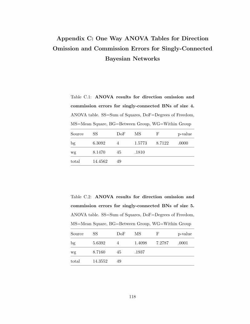
Appendix C: One Way ANOVA Tables for Direction
Omission and Commission Errors for Singly-Connected
Bayesian Networks
Table C.1: ANOVA results for direction omission and
commission errors for singly-connected BNs of size 4.
ANOVA table. SS=Sum of Squares, DoF=Degrees of Freedom,
MS=Mean Square, BG=Between Group, WG=Within Group
Source SS DoF MS F p-value
bg 6.3092 4 1.5773 8.7122 .0000
wg 8.1470 45 .1810
total 14.4562 49
Table C.2: ANOVA results for direction omission and
commission errors for singly-connected BNs of size 5.
ANOVA table. SS=Sum of Squares, DoF=Degrees of Freedom,
MS=Mean Square, BG=Between Group, WG=Within Group
Source SS DoF MS F p-value
bg 5.6392 4 1.4098 7.2787 .0001
wg 8.7160 45 .1937
total 14.3552 49
118

Table C.3: ANOVA results for direction omission and
commission errors for singly-connected BNs of size 6.
ANOVA table. SS=Sum of Squares, DoF=Degrees of Freedom,
MS=Mean Square, BG=Between Group, WG=Within Group
Source SS DoF MS F p-value
bg 26.7508 4 6.6877 19.3634 .0000
wg 15.5420 45 .3454
total 42.2928 49
Table C.4: ANOVA results for direction omission and
commission errors for singly-connected BNs of size 7.
ANOVA table. SS=Sum of Squares, DoF=Degrees of Freedom,
MS=Mean Square, BG=Between Group, WG=Within Group
Source SS DoF MS F p-value
bg 14.8272 4 3.7068 8.7788 .0000
wg 19.0010 45 .4222
total 33.8282 49
119

Table C.5: ANOVA results for direction omission and
commission errors for singly-connected BNs of size 8.
ANOVA table. SS=Sum of Squares, DoF=Degrees of Freedom,
MS=Mean Square, BG=Between Group, WG=Within Group
Source SS DoF MS F p-value
bg 47.3380 4 11.8345 27.7849 .0000
wg 19.1670 45 .4259
total 66.5050 49
Table C.6: ANOVA results for direction omission and
commission errors for singly-connected BNs of size 9.
ANOVA table. SS=Sum of Squares, DoF=Degrees of Freedom,
MS=Mean Square, BG=Between Group, WG=Within Group
Source SS DoF MS F p-value
bg 33.5940 4 8.3985 15.0146 .0000
wg 25.1710 45 .5594
total 58.7650 49
120

Table C.7: ANOVA results for direction omission and
commission errors for singly-connected BNs of size 10.
ANOVA table. SS=Sum of Squares, DoF=Degrees of Freedom,
MS=Mean Square, BG=Between Group, WG=Within Group
Source SS DoF MS F p-value
bg 73.2608 4 18.3152 50.6722 .0000
wg 16.2650 45 .3614
total 89.5258 49
Table C.8: ANOVA results for direction omission and
commission errors for singly-connected BNs of size 11.
ANOVA table. SS=Sum of Squares, DoF=Degrees of Freedom,
MS=Mean Square, BG=Between Group, WG=Within Group
Source SS DoF MS F p-value
bg 64.7400 4 16.1850 16.8985 .0000
wg 43.1000 45 .9578
total 107.8400 49
121

Table C.9: ANOVA results for direction omission and
commission errors for singly-connected BNs of size 12.
ANOVA table. SS=Sum of Squares, DoF=Degrees of Freedom,
MS=Mean Square, BG=Between Group, WG=Within Group
Source SS DoF MS F p-value
bg 118.1440 4 29.5360 36.4982 .0000
wg 36.4160 45 .8092
total 154.5600 49
Table C.10: ANOVA results for direction omission and
commission errors for singly-connected BNs of size 13.
ANOVA table. SS=Sum of Squares, DoF=Degrees of Freedom,
MS=Mean Square, BG=Between Group, WG=Within Group
Source SS DoF MS F p-value
bg 126.8452 4 31.7113 43.9147 .0000
wg 32.4950 45 .7221
total 159.3402 49
122
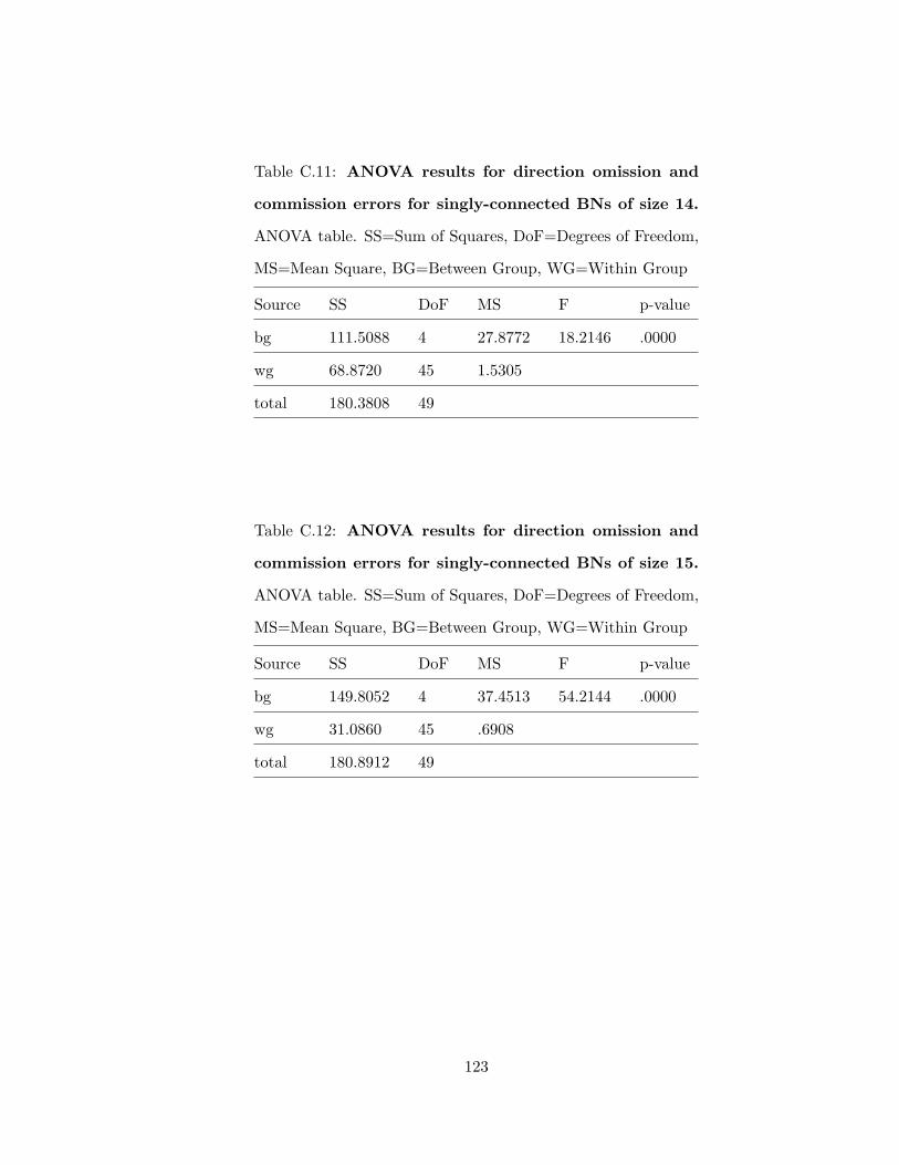
Table C.11: ANOVA results for direction omission and
commission errors for singly-connected BNs of size 14.
ANOVA table. SS=Sum of Squares, DoF=Degrees of Freedom,
MS=Mean Square, BG=Between Group, WG=Within Group
Source SS DoF MS F p-value
bg 111.5088 4 27.8772 18.2146 .0000
wg 68.8720 45 1.5305
total 180.3808 49
Table C.12: ANOVA results for direction omission and
commission errors for singly-connected BNs of size 15.
ANOVA table. SS=Sum of Squares, DoF=Degrees of Freedom,
MS=Mean Square, BG=Between Group, WG=Within Group
Source SS DoF MS F p-value
bg 149.8052 4 37.4513 54.2144 .0000
wg 31.0860 45 .6908
total 180.8912 49
123

Table C.13: ANOVA results for direction omission and
commission errors for singly-connected BNs of size 20.
ANOVA table. SS=Sum of Squares, DoF=Degrees of Freedom,
MS=Mean Square, BG=Between Group, WG=Within Group
Source SS DoF MS F p-value
bg 270.3988 4 67.5997 31.6231 .0000
wg 96.1950 45 2.1377
total 366.5938 49
124

Appendix D: HSD Tables for Direction Omission and
Commission Errors for Singly-Connected Bayesian Networks
Table D.1: HSD results for direction omission and com-
mission errors for singly-connected BNs of size 4. HSD
table. k=5, DoFWG=45.0
Algorithm1 Algorithm2 p
TPDA CrUMB+-GA .0001
TPDA CrUMB−-GA .0009
SC* TPDA .0029
PC CrUMB+-GA .0113
PC CrUMB−-GA .0822
SC* PC .1771
PC TPDA .4872
SC* CrUMB+-GA .7758
CrUMB−-GA CrUMB+-GA .9327
SC* CrUMB−-GA .9960
125

Table D.2: HSD results for direction omission and com-
mission errors for singly-connected BNs of size 5. HSD
table. k=5, DoFWG=45.0
Algorithm1 Algorithm2 p
TPDA CrUMB+-GA .0001
SC* TPDA .0031
TPDA CrUMB−-GA .0101
PC CrUMB+-GA .0341
SC* PC .2914
PC TPDA .3427
PC CrUMB−-GA .5207
CrUMB−-GA CrUMB+-GA .6166
SC* CrUMB+-GA .8466
SC* CrUMB−-GA .9941
126

Table D.3: HSD results for direction omission and com-
mission errors for singly-connected BNs of size 6. HSD
table. k=5, DoFWG=45.0
Algorithm1 Algorithm2 p
TPDA CrUMB+-GA .0000
SC* TPDA .0000
PC CrUMB+-GA .0000
TPDA CrUMB−-GA .0000
SC* PC .0008
PC CrUMB−-GA .0017
CrUMB−-GA CrUMB+-GA .4829
PC TPDA .5301
SC* CrUMB+-GA .6260
SC* CrUMB−-GA .9994
127
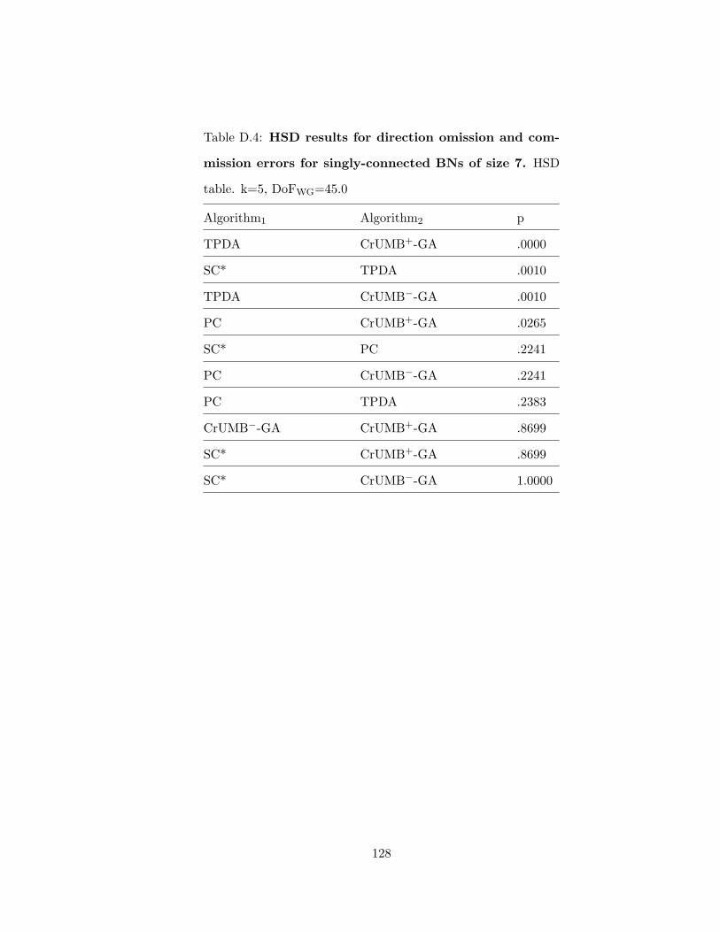
Table D.4: HSD results for direction omission and com-
mission errors for singly-connected BNs of size 7. HSD
table. k=5, DoFWG=45.0
Algorithm1 Algorithm2 p
TPDA CrUMB+-GA .0000
SC* TPDA .0010
TPDA CrUMB−-GA .0010
PC CrUMB+-GA .0265
SC* PC .2241
PC CrUMB−-GA .2241
PC TPDA .2383
CrUMB−-GA CrUMB+-GA .8699
SC* CrUMB+-GA .8699
SC* CrUMB−-GA 1.0000
128

Table D.5: HSD results for direction omission and com-
mission errors for singly-connected BNs of size 8. HSD
table. k=5, DoFWG=45.0
Algorithm1 Algorithm2 p
TPDA CrUMB+-GA .0000
SC* TPDA .0000
TPDA CrUMB−-GA .0000
PC CrUMB+-GA .0000
SC* PC .0016
PC CrUMB−-GA .0034
PC TPDA .0050
CrUMB−-GA CrUMB+-GA .5415
SC* CrUMB+-GA .6914
SC* CrUMB−-GA .9992
129

Table D.6: HSD results for direction omission and com-
mission errors for singly-connected BNs of size 9. HSD
table. k=5, DoFWG=45.0
Algorithm1 Algorithm2 p
TPDA CrUMB+-GA .0000
SC* TPDA .0000
TPDA CrUMB−-GA .0001
PC CrUMB+-GA .0001
SC* PC .0004
PC CrUMB−-GA .0038
PC TPDA .8323
CrUMB−-GA CrUMB+-GA .8323
SC* CrUMB−-GA .9514
SC* CrUMB+-GA .9974
130

Table D.7: HSD results for direction omission and com-
mission errors for singly-connected BNs of size 10. HSD
table. k=5, DoFWG=45.0
Algorithm1 Algorithm2 p
TPDA CrUMB+-GA .0000
SC* TPDA .0000
TPDA CrUMB−-GA .0000
PC CrUMB+-GA .0000
SC* PC .0000
PC CrUMB−-GA .0000
PC TPDA .0001
CrUMB−-GA CrUMB+-GA .7569
SC* CrUMB+-GA .8521
SC* CrUMB−-GA .9997
131

Table D.8: HSD results for direction omission and com-
mission errors for singly-connected BNs of size 11. HSD
table. k=5, DoFWG=45.0
Algorithm1 Algorithm2 p
TPDA CrUMB+-GA .0000
TPDA CrUMB−-GA .0000
SC* TPDA .0000
PC CrUMB+-GA .0010
PC CrUMB−-GA .0229
PC TPDA .0344
SC* PC .0957
SC* CrUMB+-GA .4498
CrUMB−-GA CrUMB+-GA .8073
SC* CrUMB−-GA .9753
132
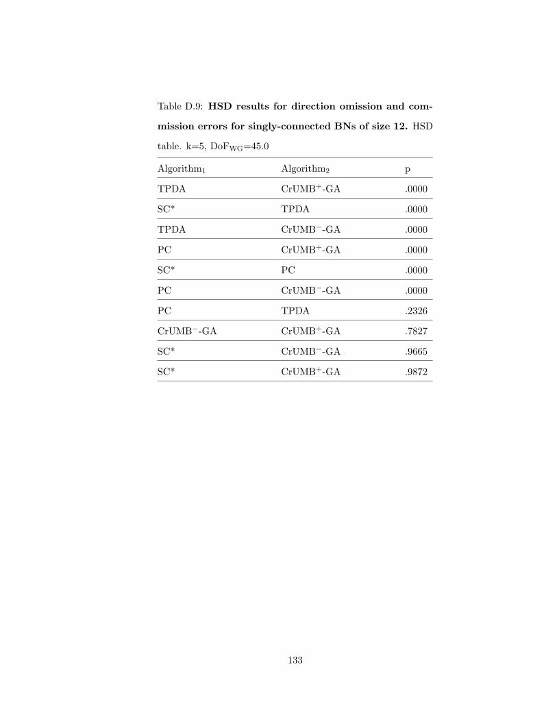
Table D.9: HSD results for direction omission and com-
mission errors for singly-connected BNs of size 12. HSD
table. k=5, DoFWG=45.0
Algorithm1 Algorithm2 p
TPDA CrUMB+-GA .0000
SC* TPDA .0000
TPDA CrUMB−-GA .0000
PC CrUMB+-GA .0000
SC* PC .0000
PC CrUMB−-GA .0000
PC TPDA .2326
CrUMB−-GA CrUMB+-GA .7827
SC* CrUMB−-GA .9665
SC* CrUMB+-GA .9872
133
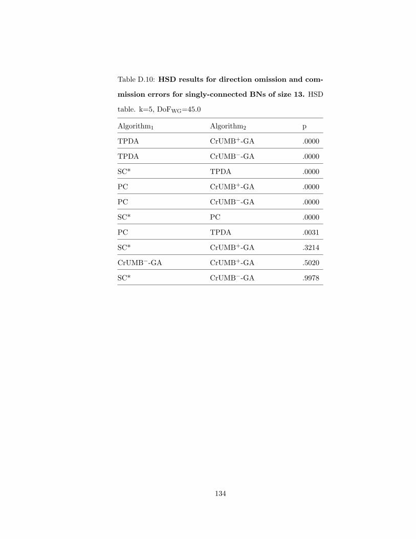
Table D.10: HSD results for direction omission and com-
mission errors for singly-connected BNs of size 13. HSD
table. k=5, DoFWG=45.0
Algorithm1 Algorithm2 p
TPDA CrUMB+-GA .0000
TPDA CrUMB−-GA .0000
SC* TPDA .0000
PC CrUMB+-GA .0000
PC CrUMB−-GA .0000
SC* PC .0000
PC TPDA .0031
SC* CrUMB+-GA .3214
CrUMB−-GA CrUMB+-GA .5020
SC* CrUMB−-GA .9978
134

Table D.11: HSD results for direction omission and com-
mission errors for singly-connected BNs of size 14. HSD
table. k=5, DoFWG=45.0
Algorithm1 Algorithm2 p
TPDA CrUMB+-GA .0000
SC* TPDA .0000
TPDA CrUMB−-GA .0000
PC CrUMB+-GA .0000
SC* PC .0047
PC CrUMB−-GA .0138
PC TPDA .2101
CrUMB−-GA CrUMB+-GA .3524
SC* CrUMB+-GA .5791
SC* CrUMB−-GA .9954
135

Table D.12: HSD results for direction omission and com-
mission errors for singly-connected BNs of size 15. HSD
table. k=5, DoFWG=45.0
Algorithm1 Algorithm2 p
TPDA CrUMB+-GA .0000
SC* TPDA .0000
TPDA CrUMB−-GA .0000
PC CrUMB+-GA .0000
SC* PC .0000
PC TPDA .0001
PC CrUMB−-GA .0015
CrUMB−-GA CrUMB+-GA .0016
SC* CrUMB+-GA .1864
SC* CrUMB−-GA .3553
136

Table D.13: HSD results for direction omission and com-
mission errors for singly-connected BNs of size 20. HSD
table. k=5, DoFWG=45.0
Algorithm1 Algorithm2 p
TPDA CrUMB+-GA .0000
PC CrUMB+-GA .0000
TPDA CrUMB−-GA .0000
SC* TPDA .0000
PC CrUMB−-GA .0001
SC* PC .0029
SC* CrUMB+-GA .0034
CrUMB−-GA CrUMB+-GA .0662
PC TPDA .1919
SC* CrUMB−-GA .7970
137
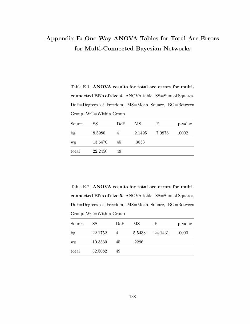
Appendix E: One Way ANOVA Tables for Total Arc Errors
for Multi-Connected Bayesian Networks
Table E.1: ANOVA results for total arc errors for multi-
connected BNs of size 4. ANOVA table. SS=Sum of Squares,
DoF=Degrees of Freedom, MS=Mean Square, BG=Between
Group, WG=Within Group
Source SS DoF MS F p-value
bg 8.5980 4 2.1495 7.0878 .0002
wg 13.6470 45 .3033
total 22.2450 49
Table E.2: ANOVA results for total arc errors for multi-
connected BNs of size 5. ANOVA table. SS=Sum of Squares,
DoF=Degrees of Freedom, MS=Mean Square, BG=Between
Group, WG=Within Group
Source SS DoF MS F p-value
bg 22.1752 4 5.5438 24.1431 .0000
wg 10.3330 45 .2296
total 32.5082 49
138

Table E.3: ANOVA results for total arc errors for multi-
connected BNs of size 6. ANOVA table. SS=Sum of Squares,
DoF=Degrees of Freedom, MS=Mean Square, BG=Between
Group, WG=Within Group
Source SS DoF MS F p-value
bg 41.1072 4 10.2768 12.1240 .0000
wg 38.1440 45 .8476
total 79.2512 49
Table E.4: ANOVA results for total arc errors for multi-
connected BNs of size 7. ANOVA table. SS=Sum of Squares,
DoF=Degrees of Freedom, MS=Mean Square, BG=Between
Group, WG=Within Group
Source SS DoF MS F p-value
bg 65.3452 4 16.3363 14.5496 .0000
wg 50.5260 45 1.1228
total 115.8712 49
139

Table E.5: ANOVA results for total arc errors for multi-
connected BNs of size 8. ANOVA table. SS=Sum of Squares,
DoF=Degrees of Freedom, MS=Mean Square, BG=Between
Group, WG=Within Group
Source SS DoF MS F p-value
bg 83.5052 4 20.8763 13.1789 .0000
wg 71.2830 45 1.5841
total 154.7882 49
Table E.6: ANOVA results for total arc errors for multi-
connected BNs of size 9. ANOVA table. SS=Sum of Squares,
DoF=Degrees of Freedom, MS=Mean Square, BG=Between
Group, WG=Within Group
Source SS DoF MS F p-value
bg 102.1968 4 25.5492 15.3590 .0000
wg 74.8560 45 1.6635
total 177.0528 49
140

Table E.7: ANOVA results for total arc errors for multi-
connected BNs of size 10. ANOVA table. SS=Sum
of Squares, DoF=Degrees of Freedom, MS=Mean Square,
BG=Between Group, WG=Within Group
Source SS DoF MS F p-value
bg 164.8660 4 41.2165 18.9310 .0000
wg 97.9740 45 2.1772
total 262.8400 49
Table E.8: ANOVA results for total arc errors for multi-
connected BNs of size 11. ANOVA table. SS=Sum
of Squares, DoF=Degrees of Freedom, MS=Mean Square,
BG=Between Group, WG=Within Group
Source SS DoF MS F p-value
bg 83.4748 4 20.8687 6.8374 .0002
wg 137.3470 45 3.0522
total 220.8218 49
141

Table E.9: ANOVA results for total arc errors for multi-
connected BNs of size 12. ANOVA table. SS=Sum
of Squares, DoF=Degrees of Freedom, MS=Mean Square,
BG=Between Group, WG=Within Group
Source SS DoF MS F p-value
bg 167.8560 4 41.9640 17.5616 .0000
wg 107.5290 45 2.3895
total 275.3850 49
Table E.10: ANOVA results for total arc errors for
multi-connected BNs of size 13. ANOVA table. SS=Sum
of Squares, DoF=Degrees of Freedom, MS=Mean Square,
BG=Between Group, WG=Within Group
Source SS DoF MS F p-value
bg 183.9332 4 45.9833 19.0985 .0000
wg 108.3460 45 2.4077
total 292.2792 49
142

Table E.11: ANOVA results for total arc errors for
multi-connected BNs of size 14. ANOVA table. SS=Sum
of Squares, DoF=Degrees of Freedom, MS=Mean Square,
BG=Between Group, WG=Within Group
Source SS DoF MS F p-value
bg 273.2292 4 68.3073 31.6844 .0000
wg 97.0140 45 2.1559
total 370.2432 49
Table E.12: ANOVA results for total arc errors for
multi-connected BNs of size 15. ANOVA table. SS=Sum
of Squares, DoF=Degrees of Freedom, MS=Mean Square,
BG=Between Group, WG=Within Group
Source SS DoF MS F p-value
bg 208.0632 4 52.0158 19.5259 .0000
wg 119.8770 45 2.6639
total 327.9402 49
143

Table E.13: ANOVA results for total arc errors for
multi-connected BNs of size 20. ANOVA table. SS=Sum
of Squares, DoF=Degrees of Freedom, MS=Mean Square,
BG=Between Group, WG=Within Group
Source SS DoF MS F p-value
bg 522.6988 4 130.6747 22.9080 .0000
wg 256.6950 45 5.7043
total 779.3938 49
144

Appendix F: HSD Tables for Total Arc Errors for
Multi-Connected Bayesian Networks
Table F.1: HSD results for total arc errors for multi-
connected BNs of size 4. HSD table. k=5, DoFWG=45.0
Algorithm1 Algorithm2 p
TPDA CrUMB+-GA .0012
SC* TPDA .0017
TPDA CrUMB−-GA .0082
PC CrUMB+-GA .0370
SC* PC .0499
PC CrUMB−-GA .1592
PC TPDA .7410
CrUMB−-GA CrUMB+-GA .9658
SC* CrUMB−-GA .9840
SC* CrUMB+-GA .9999
145

Table F.2: HSD results for total arc errors for multi-
connected BNs of size 5. HSD table. k=5, DoFWG=45.0
Algorithm1 Algorithm2 p
TPDA CrUMB+-GA .0000
TPDA CrUMB−-GA .0000
SC* TPDA .0000
PC CrUMB+-GA .0001
PC CrUMB−-GA .0003
SC* PC .0013
PC TPDA .0441
SC* CrUMB+-GA .9004
CrUMB−-GA CrUMB+-GA .9899
SC* CrUMB−-GA .9933
146

Table F.3: HSD results for total arc errors for multi-
connected BNs of size 6. HSD table. k=5, DoFWG=45.0
Algorithm1 Algorithm2 p
TPDA CrUMB+-GA .0000
SC* TPDA .0001
PC CrUMB+-GA .0004
TPDA CrUMB−-GA .0013
SC* PC .0060
PC CrUMB−-GA .0394
CrUMB−-GA CrUMB+-GA .5184
PC TPDA .7431
SC* CrUMB+-GA .9048
SC* CrUMB−-GA .9545
147

Table F.4: HSD results for total arc errors for multi-
connected BNs of size 7. HSD table. k=5, DoFWG=45.0
Algorithm1 Algorithm2 p
SC* TPDA .0000
TPDA CrUMB+-GA .0000
TPDA CrUMB−-GA .0000
SC* PC .0014
PC CrUMB+-GA .0019
PC CrUMB−-GA .0062
PC TPDA .4387
SC* CrUMB−-GA .9863
CrUMB−-GA CrUMB+-GA .9944
SC* CrUMB+-GA 1.0000
148

Table F.5: HSD results for total arc errors for multi-
connected BNs of size 8. HSD table. k=5, DoFWG=45.0
Algorithm1 Algorithm2 p
PC CrUMB+-GA .0000
TPDA CrUMB+-GA .0000
PC CrUMB−-GA .0011
SC* PC .0012
TPDA CrUMB−-GA .0013
SC* TPDA .0014
SC* CrUMB+-GA .7157
CrUMB−-GA CrUMB+-GA .7261
PC TPDA 1.0000
SC* CrUMB−-GA 1.0000
149

Table F.6: HSD results for total arc errors for multi-
connected BNs of size 9. HSD table. k=5, DoFWG=45.0
Algorithm1 Algorithm2 p
TPDA CrUMB+-GA .0000
SC* TPDA .0000
TPDA CrUMB−-GA .0001
PC CrUMB+-GA .0001
SC* PC .0015
PC CrUMB−-GA .0036
PC TPDA .6605
CrUMB−-GA CrUMB+-GA .8353
SC* CrUMB+-GA .9445
SC* CrUMB−-GA .9983
150
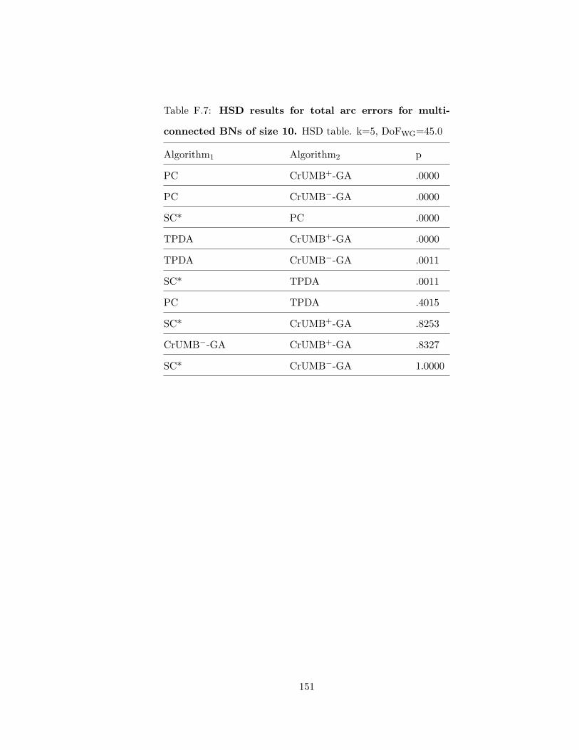
Table F.7: HSD results for total arc errors for multi-
connected BNs of size 10. HSD table. k=5, DoFWG=45.0
Algorithm1 Algorithm2 p
PC CrUMB+-GA .0000
PC CrUMB−-GA .0000
SC* PC .0000
TPDA CrUMB+-GA .0000
TPDA CrUMB−-GA .0011
SC* TPDA .0011
PC TPDA .4015
SC* CrUMB+-GA .8253
CrUMB−-GA CrUMB+-GA .8327
SC* CrUMB−-GA 1.0000
151

Table F.8: HSD results for total arc errors for multi-
connected BNs of size 11. HSD table. k=5, DoFWG=45.0
Algorithm1 Algorithm2 p
TPDA CrUMB+-GA .0006
SC* TPDA .0073
TPDA CrUMB−-GA .0116
PC CrUMB+-GA .0171
SC* PC .1222
PC CrUMB−-GA .1709
PC TPDA .7918
CrUMB−-GA CrUMB+-GA .8604
SC* CrUMB+-GA .9234
SC* CrUMB−-GA .9998
152

Table F.9: HSD results for total arc errors for multi-
connected BNs of size 12. HSD table. k=5, DoFWG=45.0
Algorithm1 Algorithm2 p
TPDA CrUMB+-GA .0000
PC CrUMB+-GA .0000
TPDA CrUMB−-GA .0001
SC* TPDA .0002
PC CrUMB−-GA .0003
SC* PC .0004
SC* CrUMB+-GA .4063
CrUMB−-GA CrUMB+-GA .4750
PC TPDA .9993
SC* CrUMB−-GA 1.0000
153

Table F.10: HSD results for total arc errors for multi-
connected BNs of size 13. HSD table. k=5, DoFWG=45.0
Algorithm1 Algorithm2 p
PC CrUMB+-GA .0000
TPDA CrUMB+-GA .0000
PC CrUMB−-GA .0000
TPDA CrUMB−-GA .0000
SC* PC .0004
SC* TPDA .0007
SC* CrUMB+-GA .2130
CrUMB−-GA CrUMB+-GA .6680
SC* CrUMB−-GA .9226
PC TPDA .9996
154
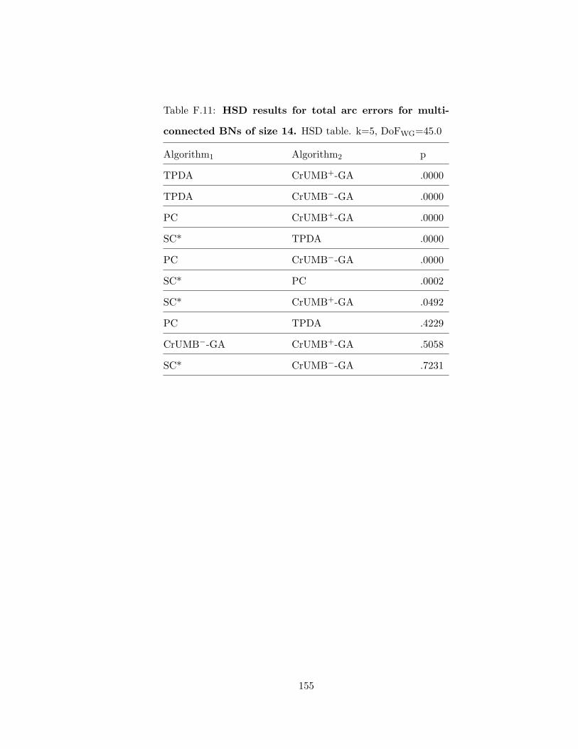
Table F.11: HSD results for total arc errors for multi-
connected BNs of size 14. HSD table. k=5, DoFWG=45.0
Algorithm1 Algorithm2 p
TPDA CrUMB+-GA .0000
TPDA CrUMB−-GA .0000
PC CrUMB+-GA .0000
SC* TPDA .0000
PC CrUMB−-GA .0000
SC* PC .0002
SC* CrUMB+-GA .0492
PC TPDA .4229
CrUMB−-GA CrUMB+-GA .5058
SC* CrUMB−-GA .7231
155

Table F.12: HSD results for total arc errors for multi-
connected BNs of size 15. HSD table. k=5, DoFWG=45.0
Algorithm1 Algorithm2 p
TPDA CrUMB+-GA .0000
PC CrUMB+-GA .0000
TPDA CrUMB−-GA .0000
SC* CrUMB+-GA .0007
SC* TPDA .0038
PC CrUMB−-GA .0128
CrUMB−-GA CrUMB+-GA .0596
PC TPDA .2761
SC* PC .3970
SC* CrUMB−-GA .5119
156

Table F.13: HSD results for total arc errors for multi-
connected BNs of size 20. HSD table. k=5, DoFWG=45.0
Algorithm1 Algorithm2 p
TPDA CrUMB+-GA .0000
PC CrUMB+-GA .0000
TPDA CrUMB−-GA .0000
SC* TPDA .0001
PC CrUMB−-GA .0008
SC* CrUMB+-GA .0065
SC* PC .0206
CrUMB−-GA CrUMB+-GA .1088
PC TPDA .4701
SC* CrUMB−-GA .7983
157

Appendix G: One Way ANOVA Tables for Direction
Omission and Commission Errors for Multi-Connected
Bayesian Networks
Table G.1: ANOVA results for direction omission and
commission errors for multi-connected BNs of size 4.
ANOVA table. SS=Sum of Squares, DoF=Degrees of Freedom,
MS=Mean Square, BG=Between Group, WG=Within Group
Source SS DoF MS F p-value
bg 5.9772 4 1.4943 4.8035 .0026
wg 13.9990 45 .3111
total 19.9762 49
Table G.2: ANOVA results for direction omission and
commission errors for multi-connected BNs of size 5.
ANOVA table. SS=Sum of Squares, DoF=Degrees of Freedom,
MS=Mean Square, BG=Between Group, WG=Within Group
Source SS DoF MS F p-value
bg 15.7332 4 3.9333 26.5325 .0000
wg 6.6710 45 .1482
total 22.4042 49
158

Table G.3: ANOVA results for direction omission and
commission errors for multi-connected BNs of size 6.
ANOVA table. SS=Sum of Squares, DoF=Degrees of Freedom,
MS=Mean Square, BG=Between Group, WG=Within Group
Source SS DoF MS F p-value
bg 24.2952 4 6.0738 12.6438 .0000
wg 21.6170 45 .4804
total 45.9122 49
Table G.4: ANOVA results for direction omission and
commission errors for multi-connected BNs of size 7.
ANOVA table. SS=Sum of Squares, DoF=Degrees of Freedom,
MS=Mean Square, BG=Between Group, WG=Within Group
Source SS DoF MS F p-value
bg 41.9348 4 10.4837 21.6427 .0000
wg 21.7980 45 .4844
total 63.7328 49
159

Table G.5: ANOVA results for direction omission and
commission errors for multi-connected BNs of size 8.
ANOVA table. SS=Sum of Squares, DoF=Degrees of Freedom,
MS=Mean Square, BG=Between Group, WG=Within Group
Source SS DoF MS F p-value
bg 44.8352 4 11.2088 14.5192 .0000
wg 34.7400 45 .7720
total 79.5752 49
Table G.6: ANOVA results for direction omission and
commission errors for multi-connected BNs of size 9.
ANOVA table. SS=Sum of Squares, DoF=Degrees of Freedom,
MS=Mean Square, BG=Between Group, WG=Within Group
Source SS DoF MS F p-value
bg 59.9792 4 14.9948 14.2197 .0000
wg 47.4530 45 1.0545
total 107.4322 49
160

Table G.7: ANOVA results for direction omission and
commission errors for multi-connected BNs of size 10.
ANOVA table. SS=Sum of Squares, DoF=Degrees of Freedom,
MS=Mean Square, BG=Between Group, WG=Within Group
Source SS DoF MS F p-value
bg 71.0260 4 17.7565 12.8507 .0000
wg 62.1790 45 1.3818
total 133.2050 49
Table G.8: ANOVA results for direction omission and
commission errors for multi-connected BNs of size 11.
ANOVA table. SS=Sum of Squares, DoF=Degrees of Freedom,
MS=Mean Square, BG=Between Group, WG=Within Group
Source SS DoF MS F p-value
bg 74.9012 4 18.7253 22.7919 .0000
wg 36.9710 45 .8216
total 111.8722 49
161

Table G.9: ANOVA results for direction omission and
commission errors for multi-connected BNs of size 12.
ANOVA table. SS=Sum of Squares, DoF=Degrees of Freedom,
MS=Mean Square, BG=Between Group, WG=Within Group
Source SS DoF MS F p-value
bg 104.3012 4 26.0753 20.5002 .0000
wg 57.2380 45 1.2720
total 161.5392 49
Table G.10: ANOVA results for direction omission and
commission errors for multi-connected BNs of size 13.
ANOVA table. SS=Sum of Squares, DoF=Degrees of Freedom,
MS=Mean Square, BG=Between Group, WG=Within Group
Source SS DoF MS F p-value
bg 124.6852 4 31.1713 24.2222 .0000
wg 57.9100 45 1.2869
total 182.5952 49
162

Table G.11: ANOVA results for direction omission and
commission errors for multi-connected BNs of size 14.
ANOVA table. SS=Sum of Squares, DoF=Degrees of Freedom,
MS=Mean Square, BG=Between Group, WG=Within Group
Source SS DoF MS F p-value
bg 166.1372 4 41.5343 28.6075 .0000
wg 65.3340 45 1.4519
total 231.4712 49
Table G.12: ANOVA results for direction omission and
commission errors for multi-connected BNs of size 15.
ANOVA table. SS=Sum of Squares, DoF=Degrees of Freedom,
MS=Mean Square, BG=Between Group, WG=Within Group
Source SS DoF MS F p-value
bg 207.2588 4 51.8147 42.0741 .0000
wg 55.4180 45 1.2315
total 262.6768 49
163

Table G.13: ANOVA results for direction omission and
commission errors for multi-connected BNs of size 20.
ANOVA table. SS=Sum of Squares, DoF=Degrees of Freedom,
MS=Mean Square, BG=Between Group, WG=Within Group
Source SS DoF MS F p-value
bg 399.0248 4 99.7562 55.7699 .0000
wg 80.4920 45 1.7887
total 479.5168 49
164

Appendix H: HSD Tables for Direction Omission and
Commission Errors for Multi-Connected Bayesian Networks
Table H.1: HSD results for direction omission and com-
mission errors for multi-connected BNs of size 4. HSD
table. k=5, DoFWG=45.0
Algorithm1 Algorithm2 p
TPDA CrUMB+-GA .0092
SC* TPDA .0129
TPDA CrUMB−-GA .0494
PC CrUMB+-GA .1220
SC* PC .1558
PC CrUMB−-GA .3840
PC TPDA .8343
CrUMB−-GA CrUMB+-GA .9674
SC* CrUMB−-GA .9848
SC* CrUMB+-GA 1.0000
165

Table H.2: HSD results for direction omission and com-
mission errors for multi-connected BNs of size 5. HSD
table. k=5, DoFWG=45.0
Algorithm1 Algorithm2 p
TPDA CrUMB+-GA .0000
TPDA CrUMB−-GA .0000
SC* TPDA .0000
PC CrUMB+-GA .0005
PC TPDA .0012
PC CrUMB−-GA .0024
SC* PC .0110
SC* CrUMB+-GA .8328
SC* CrUMB−-GA .9846
CrUMB−-GA CrUMB+-GA .9846
166

Table H.3: HSD results for direction omission and com-
mission errors for multi-connected BNs of size 6. HSD
table. k=5, DoFWG=45.0
Algorithm1 Algorithm2 p
TPDA CrUMB+-GA .0000
SC* TPDA .0001
TPDA CrUMB−-GA .0003
PC CrUMB+-GA .0049
PC TPDA .0430
SC* PC .2258
CrUMB−-GA CrUMB+-GA .2675
PC CrUMB−-GA .4577
SC* CrUMB+-GA .5171
SC* CrUMB−-GA .9911
167

Table H.4: HSD results for direction omission and com-
mission errors for multi-connected BNs of size 7. HSD
table. k=5, DoFWG=45.0
Algorithm1 Algorithm2 p
TPDA CrUMB+-GA .0000
SC* TPDA .0000
TPDA CrUMB−-GA .0000
PC CrUMB+-GA .0009
SC* PC .0011
PC CrUMB−-GA .0081
PC TPDA .0196
CrUMB−-GA CrUMB+-GA .9461
SC* CrUMB−-GA .9609
SC* CrUMB+-GA 1.0000
168
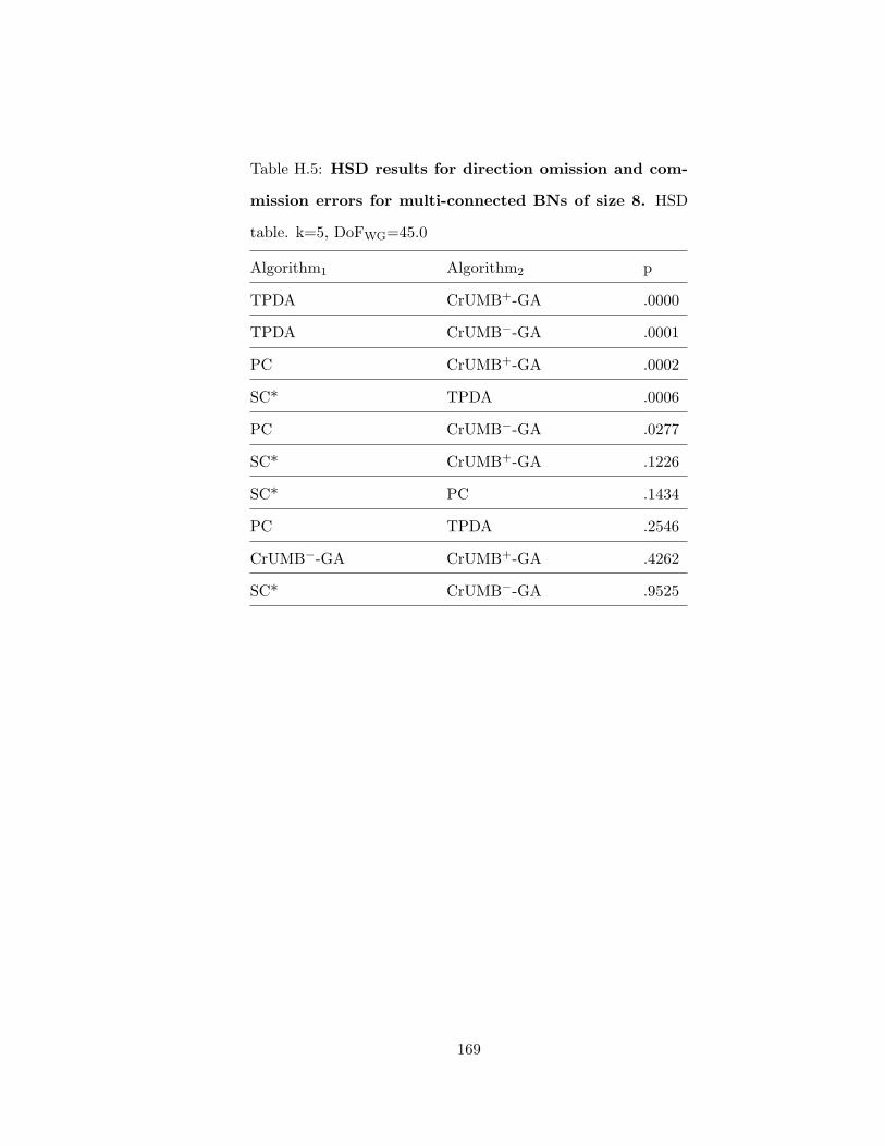
Table H.5: HSD results for direction omission and com-
mission errors for multi-connected BNs of size 8. HSD
table. k=5, DoFWG=45.0
Algorithm1 Algorithm2 p
TPDA CrUMB+-GA .0000
TPDA CrUMB−-GA .0001
PC CrUMB+-GA .0002
SC* TPDA .0006
PC CrUMB−-GA .0277
SC* CrUMB+-GA .1226
SC* PC .1434
PC TPDA .2546
CrUMB−-GA CrUMB+-GA .4262
SC* CrUMB−-GA .9525
169

Table H.6: HSD results for direction omission and com-
mission errors for multi-connected BNs of size 9. HSD
table. k=5, DoFWG=45.0
Algorithm1 Algorithm2 p
TPDA CrUMB+-GA .0000
SC* TPDA .0000
TPDA CrUMB−-GA .0000
PC CrUMB+-GA .0026
SC* PC .0513
PC TPDA .0733
PC CrUMB−-GA .0849
CrUMB−-GA CrUMB+-GA .6886
SC* CrUMB+-GA .8114
SC* CrUMB−-GA .9995
170

Table H.7: HSD results for direction omission and com-
mission errors for multi-connected BNs of size 10. HSD
table. k=5, DoFWG=45.0
Algorithm1 Algorithm2 p
TPDA CrUMB+-GA .0000
TPDA CrUMB−-GA .0002
PC CrUMB+-GA .0002
SC* TPDA .0010
PC CrUMB−-GA .0105
SC* PC .0423
SC* CrUMB+-GA .3510
PC TPDA .6733
CrUMB−-GA CrUMB+-GA .6733
SC* CrUMB−-GA .9835
171

Table H.8: HSD results for direction omission and com-
mission errors for multi-connected BNs of size 11. HSD
table. k=5, DoFWG=45.0
Algorithm1 Algorithm2 p
TPDA CrUMB+-GA .0000
SC* TPDA .0000
TPDA CrUMB−-GA .0000
PC CrUMB+-GA .0005
PC TPDA .0012
SC* PC .0676
PC CrUMB−-GA .0715
CrUMB−-GA CrUMB+-GA .3858
SC* CrUMB+-GA .3997
SC* CrUMB−-GA 1.0000
172

Table H.9: HSD results for direction omission and com-
mission errors for multi-connected BNs of size 12. HSD
table. k=5, DoFWG=45.0
Algorithm1 Algorithm2 p
TPDA CrUMB+-GA .0000
PC CrUMB+-GA .0000
TPDA CrUMB−-GA .0000
SC* TPDA .0001
PC CrUMB−-GA .0062
SC* CrUMB+-GA .0267
SC* PC .0419
CrUMB−-GA CrUMB+-GA .1398
PC TPDA .2055
SC* CrUMB−-GA .9523
173

Table H.10: HSD results for direction omission and com-
mission errors for multi-connected BNs of size 13. HSD
table. k=5, DoFWG=45.0
Algorithm1 Algorithm2 p
TPDA CrUMB+-GA .0000
TPDA CrUMB−-GA .0000
SC* TPDA .0000
PC CrUMB+-GA .0000
PC CrUMB−-GA .0028
PC TPDA .0195
SC* CrUMB+-GA .0359
SC* PC .0729
CrUMB−-GA CrUMB+-GA .4123
SC* CrUMB−-GA .7387
174

Table H.11: HSD results for direction omission and com-
mission errors for multi-connected BNs of size 14. HSD
table. k=5, DoFWG=45.0
Algorithm1 Algorithm2 p
TPDA CrUMB+-GA .0000
TPDA CrUMB−-GA .0000
SC* TPDA .0000
PC CrUMB+-GA .0001
PC TPDA .0002
SC* CrUMB+-GA .0132
PC CrUMB−-GA .0217
CrUMB−-GA CrUMB+-GA .3075
SC* PC .4073
SC* CrUMB−-GA .6243
175

Table H.12: HSD results for direction omission and com-
mission errors for multi-connected BNs of size 15. HSD
table. k=5, DoFWG=45.0
Algorithm1 Algorithm2 p
TPDA CrUMB+-GA .0000
TPDA CrUMB−-GA .0000
PC CrUMB+-GA .0000
SC* TPDA .0000
SC* CrUMB+-GA .0000
PC TPDA .0001
CrUMB−-GA CrUMB+-GA .0018
PC CrUMB−-GA .0145
SC* CrUMB−-GA .2152
SC* PC .7689
176

Table H.13: HSD results for direction omission and com-
mission errors for multi-connected BNs of size 20. HSD
table. k=5, DoFWG=45.0
Algorithm1 Algorithm2 p
TPDA CrUMB+-GA .0000
TPDA CrUMB−-GA .0000
SC* TPDA .0000
PC CrUMB+-GA .0000
PC TPDA .0000
SC* CrUMB+-GA .0000
CrUMB−-GA CrUMB+-GA .0006
PC CrUMB−-GA .0015
SC* PC .0225
SC* CrUMB−-GA .8743
177

Appendix I: Box and Whisker Plots of Total Arc Errors for
Singly- and Multi-Connected BNs
CrUMB− CrUMB+ PC SC* TPDA
1.5
2.0
2.5
3.0
Algorithms
Cou
nt
Figure I.1: Box Plot of Total Arc Errors for Singly-Connected BN of Size 4.
CrUMB− CrUMB+ PC SC* TPDA
2.0
2.5
3.0
3.5
4.0
Algorithms
Cou
nt
Figure I.2: Box Plot of Total Arc Errors for Singly-Connected BN of Size 5.
178

CrUMB− CrUMB+ PC SC* TPDA
1.5
2.5
3.5
4.5
Algorithms
Cou
nt
Figure I.3: Box Plot of Total Arc Errors for Singly-Connected BN of Size 6.
CrUMB− CrUMB+ PC SC* TPDA
3.0
4.0
5.0
6.0
Algorithms
Cou
nt
Figure I.4: Box Plot of Total Arc Errors for Singly-Connected BN of Size 7.
179

CrUMB− CrUMB+ PC SC* TPDA
23
45
67
8
Algorithms
Cou
nt
Figure I.5: Box Plot of Total Arc Errors for Singly-Connected BN of Size 8.
CrUMB− CrUMB+ PC SC* TPDA
45
67
89
Algorithms
Cou
nt
Figure I.6: Box Plot of Total Arc Errors for Singly-Connected BN of Size 9.
180

CrUMB− CrUMB+ PC SC* TPDA
45
67
89
Algorithms
Cou
nt
Figure I.7: Box Plot of Total Arc Errors for Singly-Connected BN of Size 10.
CrUMB− CrUMB+ PC SC* TPDA
46
810
Algorithms
Cou
nt
Figure I.8: Box Plot of Total Arc Errors for Singly-Connected BN of Size 11.
181

CrUMB− CrUMB+ PC SC* TPDA
56
78
911
Algorithms
Cou
nt
Figure I.9: Box Plot of Total Arc Errors for Singly-Connected BN of Size 12.
CrUMB− CrUMB+ PC SC* TPDA
68
1012
Algorithms
Cou
nt
Figure I.10: Box Plot of Total Arc Errors for Singly-Connected BN of Size 13.
182

CrUMB− CrUMB+ PC SC* TPDA
68
1012
Algorithms
Cou
nt
Figure I.11: Box Plot of Total Arc Errors for Singly-Connected BN of Size 14.
CrUMB− CrUMB+ PC SC* TPDA
810
1214
16
Algorithms
Cou
nt
Figure I.12: Box Plot of Total Arc Errors for Singly-Connected BN of Size 15.
183

CrUMB− CrUMB+ PC SC* TPDA
1015
20
Algorithms
Cou
nt
Figure I.13: Box Plot of Total Arc Errors for Singly-Connected BN of Size 20.
CrUMB− CrUMB+ PC SC* TPDA
1.5
2.5
3.5
4.5
Algorithms
Cou
nt
Figure I.14: Box Plot of Total Arc Errors for Multi-Connected BN of Size 4.
184

CrUMB− CrUMB+ PC SC* TPDA
2.5
3.5
4.5
Algorithms
Cou
nt
Figure I.15: Box Plot of Total Arc Errors for Multi-Connected BN of Size 5.
CrUMB− CrUMB+ PC SC* TPDA
34
56
7
Algorithms
Cou
nt
Figure I.16: Box Plot of Total Arc Errors for Multi-Connected BN of Size 6.
185

CrUMB− CrUMB+ PC SC* TPDA
34
56
78
Algorithms
Cou
nt
Figure I.17: Box Plot of Total Arc Errors for Multi-Connected BN of Size 7.
CrUMB− CrUMB+ PC SC* TPDA
46
810
Algorithms
Cou
nt
Figure I.18: Box Plot of Total Arc Errors for Multi-Connected BN of Size 8.
186

CrUMB− CrUMB+ PC SC* TPDA
45
67
89
11
Algorithms
Cou
nt
Figure I.19: Box Plot of Total Arc Errors for Multi-Connected BN of Size 9.
CrUMB− CrUMB+ PC SC* TPDA
68
1014
Algorithms
Cou
nt
Figure I.20: Box Plot of Total Arc Errors for Multi-Connected BN of Size 10.
187

CrUMB− CrUMB+ PC SC* TPDA
68
1012
14
Algorithms
Cou
nt
Figure I.21: Box Plot of Total Arc Errors for Multi-Connected BN of Size 11.
CrUMB− CrUMB+ PC SC* TPDA
68
1012
14
Algorithms
Cou
nt
Figure I.22: Box Plot of Total Arc Errors for Multi-Connected BN of Size 12.
188
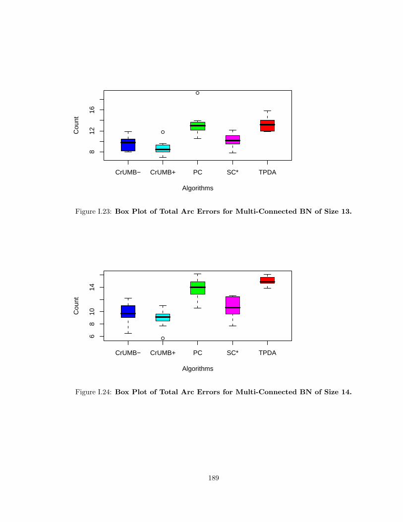
CrUMB− CrUMB+ PC SC* TPDA
812
16
Algorithms
Cou
nt
Figure I.23: Box Plot of Total Arc Errors for Multi-Connected BN of Size 13.
CrUMB− CrUMB+ PC SC* TPDA
68
1014
Algorithms
Cou
nt
Figure I.24: Box Plot of Total Arc Errors for Multi-Connected BN of Size 14.
189

CrUMB− CrUMB+ PC SC* TPDA
810
1418
Algorithms
Cou
nt
Figure I.25: Box Plot of Total Arc Errors for Multi-Connected BN of Size 15.
CrUMB− CrUMB+ PC SC* TPDA
1015
2025
Algorithms
Cou
nt
Figure I.26: Box Plot of Total Arc Errors for Multi-Connected BN of Size 20.
190

Appendix J: One Way ANOVA Tables for KL Differences for
Singly-Connected Bayesian Networks
Table J.1: ANOVA results for KL differences for singly-
connected BNs of size 4. ANOVA table. SS=Sum of Squares,
DoF=Degrees of Freedom, MS=Mean Square, BG=Between
Group, WG=Within Group
Source SS DoF MS F p-value
bg .3291 4 .0823 6.1898 .0005
wg .5981 45 .0133
total .9272 49
Table J.2: ANOVA results for KL differences for singly-
connected BNs of size 5. ANOVA table. SS=Sum of Squares,
DoF=Degrees of Freedom, MS=Mean Square, BG=Between
Group, WG=Within Group
Source SS DoF MS F p-value
bg .3902 4 .0975 3.9051 .0084
wg 1.1240 45 .0250
total 1.5141 49
191
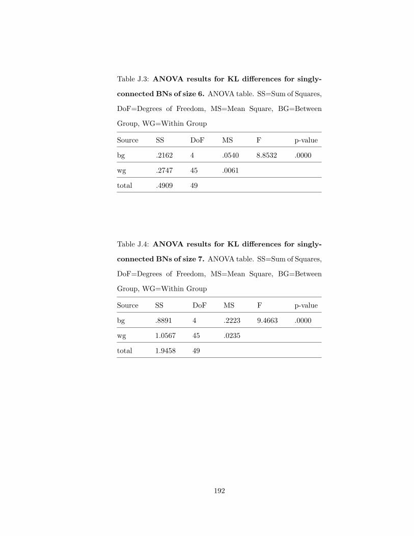
Table J.3: ANOVA results for KL differences for singly-
connected BNs of size 6. ANOVA table. SS=Sum of Squares,
DoF=Degrees of Freedom, MS=Mean Square, BG=Between
Group, WG=Within Group
Source SS DoF MS F p-value
bg .2162 4 .0540 8.8532 .0000
wg .2747 45 .0061
total .4909 49
Table J.4: ANOVA results for KL differences for singly-
connected BNs of size 7. ANOVA table. SS=Sum of Squares,
DoF=Degrees of Freedom, MS=Mean Square, BG=Between
Group, WG=Within Group
Source SS DoF MS F p-value
bg .8891 4 .2223 9.4663 .0000
wg 1.0567 45 .0235
total 1.9458 49
192

Table J.5: ANOVA results for KL differences for singly-
connected BNs of size 8. ANOVA table. SS=Sum of Squares,
DoF=Degrees of Freedom, MS=Mean Square, BG=Between
Group, WG=Within Group
Source SS DoF MS F p-value
bg 1.7931 4 .4483 15.6674 .0000
wg 1.2875 45 .0286
total 3.0806 49
Table J.6: ANOVA results for KL differences for singly-
connected BNs of size 9. ANOVA table. SS=Sum of Squares,
DoF=Degrees of Freedom, MS=Mean Square, BG=Between
Group, WG=Within Group
Source SS DoF MS F p-value
bg 2.9974 4 .7494 31.5829 .0000
wg 1.0677 45 .0237
total 4.0651 49
193

Table J.7: ANOVA results for KL differences for singly-
connected BNs of size 10. ANOVA table. SS=Sum
of Squares, DoF=Degrees of Freedom, MS=Mean Square,
BG=Between Group, WG=Within Group
Source SS DoF MS F p-value
bg 1.5360 4 .3840 20.2603 .0000
wg .8529 45 .0190
total 2.3889 49
Table J.8: ANOVA results for KL differences for singly-
connected BNs of size 11. ANOVA table. SS=Sum
of Squares, DoF=Degrees of Freedom, MS=Mean Square,
BG=Between Group, WG=Within Group
Source SS DoF MS F p-value
bg 2.1238 4 .5310 26.9985 .0000
wg .8850 45 .0197
total 3.0088 49
194

Table J.9: ANOVA results for KL differences for singly-
connected BNs of size 12. ANOVA table. SS=Sum
of Squares, DoF=Degrees of Freedom, MS=Mean Square,
BG=Between Group, WG=Within Group
Source SS DoF MS F p-value
bg 3.7252 4 .9313 21.8081 .0000
wg 1.9217 45 .0427
total 5.6469 49
Table J.10: ANOVA results for KL differences for singly-
connected BNs of size 13. ANOVA table. SS=Sum
of Squares, DoF=Degrees of Freedom, MS=Mean Square,
BG=Between Group, WG=Within Group
Source SS DoF MS F p-value
bg 5.5490 4 1.3873 46.5311 .0000
wg 1.3416 45 .0298
total 6.8906 49
195

Table J.11: ANOVA results for KL differences for singly-
connected BNs of size 14. ANOVA table. SS=Sum
of Squares, DoF=Degrees of Freedom, MS=Mean Square,
BG=Between Group, WG=Within Group
Source SS DoF MS F p-value
bg 3.1397 4 .7849 43.4360 .0000
wg .8132 45 .0181
total 3.9529 49
Table J.12: ANOVA results for KL differences for singly-
connected BNs of size 15. ANOVA table. SS=Sum
of Squares, DoF=Degrees of Freedom, MS=Mean Square,
BG=Between Group, WG=Within Group
Source SS DoF MS F p-value
bg 5.1755 4 1.2939 24.6393 .0000
wg 2.3631 45 .0525
total 7.5386 49
196

Table J.13: ANOVA results for KL differences for singly-
connected BNs of size 20. ANOVA table. SS=Sum
of Squares, DoF=Degrees of Freedom, MS=Mean Square,
BG=Between Group, WG=Within Group
Source SS DoF MS F p-value
bg 14.0387 4 3.5097 113.6981 .0000
wg 1.3891 45 .0309
total 15.4278 49
197

Appendix K: HSD Tables for KL Differences for
Singly-Connected Bayesian Networks
Table K.1: HSD results for arc KL differences singly-
connected BNs of size 4. HSD table. k=5, DoFWG=45.0
Algorithm1 Algorithm2 p
SC* TPDA .0037
TPDA CrUMB−-GA .0037
TPDA CrUMB+-GA .0038
SC* PC .1520
PC CrUMB−-GA .1522
PC CrUMB+-GA .1552
PC TPDA .5873
SC* CrUMB+-GA 1.0000
CrUMB−-GA CrUMB+-GA 1.0000
SC* CrUMB−-GA 1.0000
198

Table K.2: HSD results for KL differences for singly-
connected BNs of size 5. HSD table. k=5, DoFWG=45.0
Algorithm1 Algorithm2 p
SC* TPDA .0322
TPDA CrUMB−-GA .0322
TPDA CrUMB+-GA .0333
SC* PC .3479
PC CrUMB−-GA .3479
PC CrUMB+-GA .3552
PC TPDA .7789
SC* CrUMB+-GA 1.0000
CrUMB−-GA CrUMB+-GA 1.0000
SC* CrUMB−-GA 1.0000
199

Table K.3: HSD results for KL differences for singly-
connected BNs of size 6. HSD table. k=5, DoFWG=45.0
Algorithm1 Algorithm2 p
TPDA CrUMB−-GA .0002
TPDA CrUMB+-GA .0002
SC* TPDA .0002
PC TPDA .0846
PC CrUMB−-GA .2196
PC CrUMB+-GA .2204
SC* PC .2207
SC* CrUMB−-GA 1.0000
CrUMB−-GA CrUMB+-GA 1.0000
SC* CrUMB+-GA 1.0000
200

Table K.4: HSD results for KL differences for singly-
connected BNs of size 7. HSD table. k=5, DoFWG=45.0
Algorithm1 Algorithm2 p
TPDA CrUMB+-GA .0002
TPDA CrUMB−-GA .0002
SC* TPDA .0002
PC CrUMB+-GA .0586
PC CrUMB−-GA .0586
SC* PC .0597
PC TPDA .2932
SC* CrUMB+-GA 1.0000
SC* CrUMB−-GA 1.0000
CrUMB−-GA CrUMB+-GA 1.0000
201

Table K.5: HSD results for KL differences for singly-
connected BNs of size 8. HSD table. k=5, DoFWG=45.0
Algorithm1 Algorithm2 p
TPDA CrUMB−-GA .0000
SC* TPDA .0000
TPDA CrUMB+-GA .0000
PC CrUMB−-GA .0123
SC* PC .0123
PC CrUMB+-GA .0123
PC TPDA .0562
CrUMB−-GA CrUMB+-GA 1.0000
SC* CrUMB+-GA 1.0000
SC* CrUMB−-GA 1.0000
202

Table K.6: HSD results for KL differences for singly-
connected BNs of size 9. HSD table. k=5, DoFWG=45.0
Algorithm1 Algorithm2 p
TPDA CrUMB−-GA .0000
SC* TPDA .0000
TPDA CrUMB+-GA .0000
PC CrUMB−-GA .0000
SC* PC .0000
PC CrUMB+-GA .0000
PC TPDA .8047
CrUMB−-GA CrUMB+-GA 1.0000
SC* CrUMB+-GA 1.0000
SC* CrUMB−-GA 1.0000
203

Table K.7: HSD results for KL differences for singly-
connected BNs of size 10. HSD table. k=5, DoFWG=45.0
Algorithm1 Algorithm2 p
TPDA CrUMB−-GA .0000
TPDA CrUMB+-GA .0000
SC* TPDA .0000
PC CrUMB−-GA .0018
PC CrUMB+-GA .0018
SC* PC .0022
PC TPDA .0401
SC* CrUMB−-GA 1.0000
SC* CrUMB+-GA 1.0000
CrUMB−-GA CrUMB+-GA 1.0000
204

Table K.8: HSD results for KL differences for singly-
connected BNs of size 11. HSD table. k=5, DoFWG=45.0
Algorithm1 Algorithm2 p
TPDA CrUMB−-GA .0000
TPDA CrUMB+-GA .0000
SC* TPDA .0000
PC TPDA .0008
PC CrUMB−-GA .0023
PC CrUMB+-GA .0023
SC* PC .0027
SC* CrUMB−-GA 1.0000
SC* CrUMB+-GA 1.0000
CrUMB−-GA CrUMB+-GA 1.0000
205

Table K.9: HSD results for KL differences for singly-
connected BNs of size 12. HSD table. k=5, DoFWG=45.0
Algorithm1 Algorithm2 p
TPDA CrUMB−-GA .0000
SC* TPDA .0000
TPDA CrUMB+-GA .0000
PC CrUMB−-GA .0003
SC* PC .0003
PC CrUMB+-GA .0003
PC TPDA .1397
CrUMB−-GA CrUMB+-GA 1.0000
SC* CrUMB+-GA 1.0000
SC* CrUMB−-GA 1.0000
206

Table K.10: HSD results for KL differences for singly-
connected BNs of size 13. HSD table. k=5, DoFWG=45.0
Algorithm1 Algorithm2 p
TPDA CrUMB−-GA .0000
TPDA CrUMB+-GA .0000
SC* TPDA .0000
PC CrUMB−-GA .0000
PC CrUMB+-GA .0000
SC* PC .0000
PC TPDA .0016
SC* CrUMB−-GA 1.0000
SC* CrUMB+-GA 1.0000
CrUMB−-GA CrUMB+-GA 1.0000
207

Table K.11: HSD results for KL differences for singly-
connected BNs of size 14. HSD table. k=5, DoFWG=45.0
Algorithm1 Algorithm2 p
TPDA CrUMB−-GA .0000
SC* TPDA .0000
TPDA CrUMB+-GA .0000
PC CrUMB−-GA .0000
SC* PC .0000
PC CrUMB+-GA .0000
PC TPDA .0299
CrUMB−-GA CrUMB+-GA 1.0000
SC* CrUMB+-GA 1.0000
SC* CrUMB−-GA 1.0000
208

Table K.12: HSD results for KL differences for singly-
connected BNs of size 15. HSD table. k=5, DoFWG=45.0
Algorithm1 Algorithm2 p
TPDA CrUMB−-GA .0000
SC* TPDA .0000
TPDA CrUMB+-GA .0000
PC CrUMB−-GA .0009
SC* PC .0010
PC CrUMB+-GA .0010
PC TPDA .0092
CrUMB−-GA CrUMB+-GA 1.0000
SC* CrUMB−-GA 1.0000
SC* CrUMB+-GA 1.0000
209

Table K.13: HSD results for KL differences for singly-
connected BNs of size 20. HSD table. k=5, DoFWG=45.0
Algorithm1 Algorithm2 p
TPDA CrUMB−-GA .0000
TPDA CrUMB+-GA .0000
SC* TPDA .0000
PC CrUMB−-GA .0000
PC CrUMB+-GA .0000
SC* PC .0000
PC TPDA .0013
SC* CrUMB−-GA .9957
SC* CrUMB+-GA .9968
CrUMB−-GA CrUMB+-GA 1.0000
210

Appendix L: One Way ANOVA Tables for KL Differences for
Multi-Connected Bayesian Networks
Table L.1: ANOVA results for KL differences for multi-
connected BNs of size 4. ANOVA table. SS=Sum of Squares,
DoF=Degrees of Freedom, MS=Mean Square, BG=Between
Group, WG=Within Group
Source SS DoF MS F p-value
bg .3321 4 .0830 2.9422 .0305
wg 1.2697 45 .0282
total 1.6018 49
Table L.2: ANOVA results for KL differences for multi-
connected BNs of size 5. ANOVA table. SS=Sum of Squares,
DoF=Degrees of Freedom, MS=Mean Square, BG=Between
Group, WG=Within Group
Source SS DoF MS F p-value
bg .5799 4 .1450 14.9960 .0000
wg .4351 45 .0097
total 1.0150 49
211

Table L.3: ANOVA results for KL differences for multi-
connected BNs of size 6. ANOVA table. SS=Sum of Squares,
DoF=Degrees of Freedom, MS=Mean Square, BG=Between
Group, WG=Within Group
Source SS DoF MS F p-value
bg 2.1488 4 .5372 11.5104 .0000
wg 2.1002 45 .0467
total 4.2490 49
Table L.4: ANOVA results for KL differences for multi-
connected BNs of size 7. ANOVA table. SS=Sum of Squares,
DoF=Degrees of Freedom, MS=Mean Square, BG=Between
Group, WG=Within Group
Source SS DoF MS F p-value
bg 1.4447 4 .3612 26.3699 .0000
wg .6163 45 .0137
total 2.0610 49
212

Table L.5: ANOVA results for KL differences for multi-
connected BNs of size 8. ANOVA table. SS=Sum of Squares,
DoF=Degrees of Freedom, MS=Mean Square, BG=Between
Group, WG=Within Group
Source SS DoF MS F p-value
bg 1.8488 4 .4622 12.2589 .0000
wg 1.6966 45 .0377
total 3.5454 49
Table L.6: ANOVA results for KL differences for multi-
connected BNs of size 9. ANOVA table. SS=Sum of Squares,
DoF=Degrees of Freedom, MS=Mean Square, BG=Between
Group, WG=Within Group
Source SS DoF MS F p-value
bg 1.4267 4 .3567 19.7041 .0000
wg .8146 45 .0181
total 2.2413 49
213

Table L.7: ANOVA results for KL differences for multi-
connected BNs of size 10. ANOVA table. SS=Sum
of Squares, DoF=Degrees of Freedom, MS=Mean Square,
BG=Between Group, WG=Within Group
Source SS DoF MS F p-value
bg 2.5043 4 .6261 19.0877 .0000
wg 1.4760 45 .0328
total 3.9803 49
Table L.8: ANOVA results for KL differences for multi-
connected BNs of size 11. ANOVA table. SS=Sum
of Squares, DoF=Degrees of Freedom, MS=Mean Square,
BG=Between Group, WG=Within Group
Source SS DoF MS F p-value
bg 2.5017 4 .6254 15.8124 .0000
wg 1.7799 45 .0396
total 4.2815 49
214
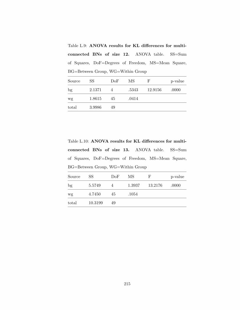
Table L.9: ANOVA results for KL differences for multi-
connected BNs of size 12. ANOVA table. SS=Sum
of Squares, DoF=Degrees of Freedom, MS=Mean Square,
BG=Between Group, WG=Within Group
Source SS DoF MS F p-value
bg 2.1371 4 .5343 12.9156 .0000
wg 1.8615 45 .0414
total 3.9986 49
Table L.10: ANOVA results for KL differences for multi-
connected BNs of size 13. ANOVA table. SS=Sum
of Squares, DoF=Degrees of Freedom, MS=Mean Square,
BG=Between Group, WG=Within Group
Source SS DoF MS F p-value
bg 5.5749 4 1.3937 13.2176 .0000
wg 4.7450 45 .1054
total 10.3199 49
215

Table L.11: ANOVA results for KL differences for multi-
connected BNs of size 14. ANOVA table. SS=Sum
of Squares, DoF=Degrees of Freedom, MS=Mean Square,
BG=Between Group, WG=Within Group
Source SS DoF MS F p-value
bg 4.3863 4 1.0966 13.3777 .0000
wg 3.6887 45 .0820
total 8.0750 49
Table L.12: ANOVA results for KL differences for multi-
connected BNs of size 15. ANOVA table. SS=Sum
of Squares, DoF=Degrees of Freedom, MS=Mean Square,
BG=Between Group, WG=Within Group
Source SS DoF MS F p-value
bg 5.8504 4 1.4626 26.3540 .0000
wg 2.4974 45 .0555
total 8.3479 49
216

Table L.13: ANOVA results for KL differences for multi-
connected BNs of size 20. ANOVA table. SS=Sum
of Squares, DoF=Degrees of Freedom, MS=Mean Square,
BG=Between Group, WG=Within Group
Source SS DoF MS F p-value
bg 14.0084 4 3.5021 18.5263 .0000
wg 8.5065 45 .1890
total 22.5149 49
217

Appendix M: HSD Tables for KL Differences for
Multi-Connected Bayesian Networks
Table M.1: HSD results for KL differences for multi-
connected BNs of size 4. HSD table. k=5, DoFWG=45.0
Algorithm1 Algorithm2 p
SC* TPDA .0923
TPDA CrUMB−-GA .0924
TPDA CrUMB+-GA .1038
SC* PC .4073
PC CrUMB−-GA .4076
PC CrUMB+-GA .4386
PC TPDA .9255
SC* CrUMB+-GA 1.0000
CrUMB−-GA CrUMB+-GA 1.0000
SC* CrUMB−-GA 1.0000
218

Table M.2: HSD results for KL differences for multi-
connected BNs of size 5. HSD table. k=5, DoFWG=45.0
Algorithm1 Algorithm2 p
TPDA CrUMB−-GA .0000
SC* TPDA .0000
TPDA CrUMB+-GA .0000
PC CrUMB−-GA .0149
SC* PC .0149
PC CrUMB+-GA .0149
PC TPDA .0652
CrUMB−-GA CrUMB+-GA 1.0000
SC* CrUMB+-GA 1.0000
SC* CrUMB−-GA 1.0000
219

Table M.3: HSD results for KL differences for multi-
connected BNs of size 6. HSD table. k=5, DoFWG=45.0
Algorithm1 Algorithm2 p
SC* TPDA .0000
TPDA CrUMB−-GA .0000
TPDA CrUMB+-GA .0000
SC* PC .0280
PC CrUMB−-GA .0288
PC CrUMB+-GA .0303
PC TPDA .2078
SC* CrUMB+-GA 1.0000
CrUMB−-GA CrUMB+-GA 1.0000
SC* CrUMB−-GA 1.0000
220

Table M.4: HSD results for KL differences for multi-
connected BNs of size 7. HSD table. k=5, DoFWG=45.0
Algorithm1 Algorithm2 p
TPDA CrUMB−-GA .0000
SC* TPDA .0000
TPDA CrUMB+-GA .0000
PC CrUMB−-GA .0015
SC* PC .0015
PC CrUMB+-GA .0016
PC TPDA .0021
CrUMB−-GA CrUMB+-GA 1.0000
SC* CrUMB+-GA 1.0000
SC* CrUMB−-GA 1.0000
221

Table M.5: HSD results for KL differences for multi-
connected BNs of size 8. HSD table. k=5, DoFWG=45.0
Algorithm1 Algorithm2 p
TPDA CrUMB−-GA .0000
SC* TPDA .0000
TPDA CrUMB+-GA .0000
PC CrUMB−-GA .0255
SC* PC .0258
PC CrUMB+-GA .0302
PC TPDA .1505
CrUMB−-GA CrUMB+-GA 1.0000
SC* CrUMB+-GA 1.0000
SC* CrUMB−-GA 1.0000
222

Table M.6: HSD results for KL differences for multi-
connected BNs of size 9. HSD table. k=5, DoFWG=45.0
Algorithm1 Algorithm2 p
SC* TPDA .0000
TPDA CrUMB−-GA .0000
TPDA CrUMB+-GA .0000
PC TPDA .0029
SC* PC .0192
PC CrUMB−-GA .0194
PC CrUMB+-GA .0204
SC* CrUMB+-GA 1.0000
CrUMB−-GA CrUMB+-GA 1.0000
SC* CrUMB−-GA 1.0000
223
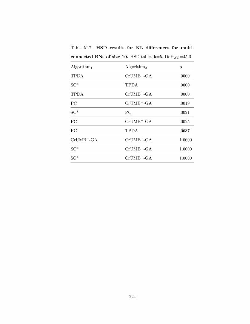
Table M.7: HSD results for KL differences for multi-
connected BNs of size 10. HSD table. k=5, DoFWG=45.0
Algorithm1 Algorithm2 p
TPDA CrUMB−-GA .0000
SC* TPDA .0000
TPDA CrUMB+-GA .0000
PC CrUMB−-GA .0019
SC* PC .0021
PC CrUMB+-GA .0025
PC TPDA .0637
CrUMB−-GA CrUMB+-GA 1.0000
SC* CrUMB+-GA 1.0000
SC* CrUMB−-GA 1.0000
224

Table M.8: HSD results for KL differences for multi-
connected BNs of size 11. HSD table. k=5, DoFWG=45.0
Algorithm1 Algorithm2 p
TPDA CrUMB−-GA .0000
SC* TPDA .0000
TPDA CrUMB+-GA .0000
PC TPDA .0013
PC CrUMB−-GA .1373
SC* PC .1588
PC CrUMB+-GA .1982
CrUMB−-GA CrUMB+-GA .9997
SC* CrUMB+-GA 1.0000
SC* CrUMB−-GA 1.0000
225

Table M.9: HSD results for KL differences for multi-
connected BNs of size 12. HSD table. k=5, DoFWG=45.0
Algorithm1 Algorithm2 p
TPDA CrUMB−-GA .0000
SC* TPDA .0000
TPDA CrUMB+-GA .0000
PC CrUMB−-GA .0072
SC* PC .0079
PC CrUMB+-GA .0095
PC TPDA .3389
CrUMB−-GA CrUMB+-GA 1.0000
SC* CrUMB+-GA 1.0000
SC* CrUMB−-GA 1.0000
226

Table M.10: HSD results for KL differences for multi-
connected BNs of size 13. HSD table. k=5, DoFWG=45.0
Algorithm1 Algorithm2 p
TPDA CrUMB−-GA .0000
TPDA CrUMB+-GA .0000
SC* TPDA .0000
PC CrUMB−-GA .0111
PC CrUMB+-GA .0146
SC* PC .0149
PC TPDA .1881
SC* CrUMB−-GA 1.0000
CrUMB−-GA CrUMB+-GA 1.0000
SC* CrUMB+-GA 1.0000
227

Table M.11: HSD results for KL differences for multi-
connected BNs of size 14. HSD table. k=5, DoFWG=45.0
Algorithm1 Algorithm2 p
TPDA CrUMB−-GA .0000
SC* TPDA .0000
TPDA CrUMB+-GA .0000
PC CrUMB−-GA .0392
PC TPDA .0438
SC* PC .0466
PC CrUMB+-GA .0488
CrUMB−-GA CrUMB+-GA 1.0000
SC* CrUMB−-GA 1.0000
SC* CrUMB+-GA 1.0000
228

Table M.12: HSD results for KL differences for multi-
connected BNs of size 15. HSD table. k=5, DoFWG=45.0
Algorithm1 Algorithm2 p
TPDA CrUMB−-GA .0000
TPDA CrUMB+-GA .0000
SC* TPDA .0000
PC TPDA .0004
PC CrUMB−-GA .0041
PC CrUMB+-GA .0043
SC* PC .0108
SC* CrUMB−-GA .9969
SC* CrUMB+-GA .9976
CrUMB−-GA CrUMB+-GA 1.0000
229

Table M.13: HSD results for KL differences for multi-
connected BNs of size 20. HSD table. k=5, DoFWG=45.0
Algorithm1 Algorithm2 p
TPDA CrUMB−-GA .0000
TPDA CrUMB+-GA .0000
SC* TPDA .0000
PC CrUMB−-GA .0035
PC CrUMB+-GA .0044
SC* PC .0059
PC TPDA .0379
SC* CrUMB−-GA .9998
SC* CrUMB+-GA 1.0000
CrUMB−-GA CrUMB+-GA 1.0000
230

Appendix N: Correlations and Ranks of Variables in Original
and Transformed Data Set
Table N.1: Correlations of Variables and Ranks of Correla-
tions in Original and Transformed Data Set. This table showsthe Spearman (k) and Pearson (r) correlations between two variablesX and Y in the original data set. When computing correlation be-
tween an integer and binary variable, the point-biserial correlation
measure was used. This table also shows the mutual information
(mi) and Phi (phi) correlation between two variables in the trans-formed data set. The corresponding ranks of each correlation (Rk,Rr, Rphi, Rmi) are also displayed.
X Y kXY rXY miXY phiXY Rk Rr Rphi Rmi
age arr -0.06 -0.05 0.01 0.14 23 25 43 108
age emp -0.01 0 0.01 0.11 41 43 30 88
age fol 0.11 0.07 0.01 0.12 111 92 37 97
age gen -0.11 -0.11 0 0.03 16 14 8 30
age inc -0.01 -0.01 0 0.01 42 41 1 8
age men -0.06 -0.05 0 0.06 25 26 22 57
age phy -0.05 -0.04 0 0.02 28 27 6 26
age pro 0.02 0.01 0 0.05 60 57 11 47
age rac 0.03 0.03 0 0.06 69 69 16 55
age ris -0.11 -0.11 0.01 0.17 14 12 47 115
age she 0.04 0.03 0 0.02 74 71 3 14
231

Table N.2: Table N.1 ContinuedX Y kXY rXY miXY phiXY Rk Rr Rphi Rmi
age sta -0.25 -0.25 0.02 0.18 3 3 50 118age tes -0.23 -0.17 0.02 0.17 4 6 49 116age tre 0.24 0.17 0.01 0.13 127 124 40 103age typ 0.06 0.06 0 0.03 86 87 7 29age vio 0 0 0 0.04 44 44 10 39arr emp -0.12 -0.09 0.02 0.02 11 18 55 20arr fol 0.09 0.06 0.01 0.12 95 90 35 95arr gen 0.09 0.09 0.11 0.11 96 101 105 89arr inc 0.42 0.35 0.35 0.35 132 133 133 128arr men 0.03 0.03 0.04 0.04 65 65 69 38arr phy 0.05 0.05 0.02 0.02 83 82 54 19arr pro -0.12 -0.09 0.01 0.13 12 19 39 102arr rac 0.11 0.11 0.12 0.12 108 112 111 98arr ris 0.13 0.13 0.12 0.12 113 118 112 99arr she 0.04 0.04 0.08 0.08 75 75 95 74arr sta -0.19 -0.19 0.2 0.2 6 5 126 120arr tes 0.01 0.01 0.05 0.05 55 56 79 51arr tre 0.14 0.11 0.14 0.14 116 113 118 106arr typ -0.02 -0.02 0.05 0.05 36 35 74 44arr vio 0.23 0.23 0.26 0.26 126 127 129 123emp fol 0.46 0.35 0.08 0.37 135 134 88 129emp gen -0.04 -0.04 0.05 0.05 29 29 73 43emp inc 0.02 0 0.22 0.22 57 46 128 122emp men 0.11 0.1 0.13 0.13 109 106 113 100emp phy 0.15 0.13 0.18 0.18 117 116 124 117emp pro 0.17 0.13 0.01 0.16 122 117 46 111emp rac -0.09 -0.09 0.08 0.08 18 16 89 69emp ris -0.12 -0.12 0.01 0.01 10 10 41 9emp she -0.01 -0.01 0.01 0.01 39 38 38 7
232

Table N.3: Table N.1 ContinuedX Y kXY rXY miXY phiXY Rk Rr Rphi Rmi
emp sta 0.01 0.01 0.03 0.03 50 51 64 33emp tes 0.05 0.04 0.09 0.09 82 78 101 82emp tre 0.11 0.09 0.2 0.2 106 99 127 121emp typ 0.01 0.01 0.02 0.02 53 54 52 16emp vio -0.06 -0.06 0.01 0.01 26 24 34 5fol gen -0.11 -0.11 0 0.09 13 11 23 81fol inc 0.48 0.36 0.1 0.44 136 135 104 135fol men 0.03 0.02 0.01 0.1 66 64 29 84fol phy 0.09 0.08 0 0.05 99 94 12 50fol pro 0.34 0.24 0.09 0.4 130 128 98 130fol rac 0.06 0.06 0.01 0.1 88 89 31 85fol ris -0.06 -0.06 0 0.07 24 23 18 62fol she 0.13 0.11 0 0.06 115 111 14 52fol sta -0.5 -0.5 0.13 0.49 1 1 114 136fol tes -0.05 -0.04 0 0.06 27 28 13 53fol tre 0.45 0.34 0.08 0.4 134 131 94 131fol typ 0 0 0 0.02 45 45 4 17fol vio 0.29 0.29 0.05 0.3 128 129 72 125gen inc 0.04 0.04 0.04 0.04 73 76 70 41gen men -0.16 -0.16 0.1 0.1 8 8 102 83gen phy 0.03 0.03 0 0 67 67 19 1gen pro -0.08 -0.08 0 0.06 21 21 15 56gen rac 0.41 0.41 0.41 0.41 131 136 135 133gen ris 0.13 0.13 0.13 0.13 114 119 115 101gen she 0.05 0.05 0.07 0.07 79 80 81 58
233

Table N.4: Table N.1 ContinuedX Y kXY rXY miXY phiXY Rk Rr Rphi Rmi
gen sta 0.09 0.09 0.09 0.09 98 104 99 78gen tes 0.1 0.1 0.04 0.04 101 107 68 37gen tre -0.04 -0.04 0.01 0.01 30 30 45 11gen typ 0.01 0.01 0.01 0.01 51 52 28 4gen vio 0.02 0.02 0.02 0.02 62 62 53 18inc men 0.11 0.1 0.14 0.14 110 110 117 105inc phy 0.06 0.05 0.1 0.1 89 84 103 86inc pro 0.1 0.07 0 0.04 105 91 9 40inc rac 0.08 0.08 0.09 0.09 93 97 96 75inc ris 0.22 0.22 0.12 0.12 125 126 110 96inc she 0.1 0.09 0.12 0.12 104 100 109 94inc sta -0.21 -0.21 0.3 0.3 5 4 130 124inc tes 0.02 0.01 0.07 0.07 58 58 84 64inc tre 0.44 0.35 0.42 0.42 133 132 136 134inc typ 0.06 0.06 0.01 0.01 85 86 36 6inc vio 0.2 0.2 0.34 0.34 124 125 132 127men phy 0.09 0.09 0.09 0.09 100 105 100 80men pro -0.08 -0.07 0 0.09 22 22 25 79men rac -0.17 -0.17 0.11 0.11 7 7 108 92men ris 0.06 0.06 0.07 0.07 87 88 86 66men she -0.02 -0.02 0.02 0.02 33 33 56 21men sta 0.04 0.04 0.01 0.01 77 77 44 10men tes 0.1 0.09 0.15 0.15 103 103 119 109men tre -0.02 -0.02 0.02 0.02 34 36 60 27men typ 0.06 0.06 0.02 0.02 84 85 59 24men vio -0.02 -0.02 0.08 0.08 37 37 91 71phy pro 0.04 0.03 0 0.02 76 70 5 25phy rac -0.12 -0.12 0.11 0.11 9 9 107 91phy ris -0.11 -0.11 0.08 0.08 15 13 92 72phy she -0.04 -0.04 0.04 0.04 31 31 67 36
234
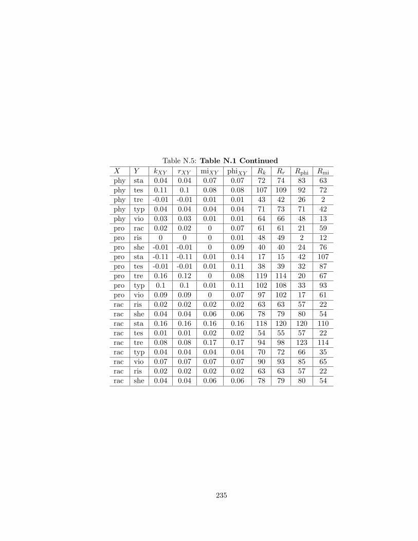
Table N.5: Table N.1 ContinuedX Y kXY rXY miXY phiXY Rk Rr Rphi Rmi
phy sta 0.04 0.04 0.07 0.07 72 74 83 63phy tes 0.11 0.1 0.08 0.08 107 109 92 72phy tre -0.01 -0.01 0.01 0.01 43 42 26 2phy typ 0.04 0.04 0.04 0.04 71 73 71 42phy vio 0.03 0.03 0.01 0.01 64 66 48 13pro rac 0.02 0.02 0 0.07 61 61 21 59pro ris 0 0 0 0.01 48 49 2 12pro she -0.01 -0.01 0 0.09 40 40 24 76pro sta -0.11 -0.11 0.01 0.14 17 15 42 107pro tes -0.01 -0.01 0.01 0.11 38 39 32 87pro tre 0.16 0.12 0 0.08 119 114 20 67pro typ 0.1 0.1 0.01 0.11 102 108 33 93pro vio 0.09 0.09 0 0.07 97 102 17 61rac ris 0.02 0.02 0.02 0.02 63 63 57 22rac she 0.04 0.04 0.06 0.06 78 79 80 54rac sta 0.16 0.16 0.16 0.16 118 120 120 110rac tes 0.01 0.01 0.02 0.02 54 55 57 22rac tre 0.08 0.08 0.17 0.17 94 98 123 114rac typ 0.04 0.04 0.04 0.04 70 72 66 35rac vio 0.07 0.07 0.07 0.07 90 93 85 65rac ris 0.02 0.02 0.02 0.02 63 63 57 22rac she 0.04 0.04 0.06 0.06 78 79 80 54
235

Table N.6: Table N.1 ContinuedX Y kXY rXY miXY phiXY Rk Rr Rphi Rmi
rac sta 0.16 0.16 0.16 0.16 118 120 120 110rac tes 0.01 0.01 0.02 0.02 54 55 57 22rac tre 0.08 0.08 0.17 0.17 94 98 123 114rac typ 0.04 0.04 0.04 0.04 70 72 66 35rac vio 0.07 0.07 0.07 0.07 90 93 85 65ris she -0.09 -0.09 0.08 0.08 19 17 90 70ris sta 0.05 0.05 0.05 0.05 81 83 77 48ris tes 0.08 0.08 0.14 0.14 92 96 116 104ris tre -0.02 -0.02 0.05 0.05 35 34 78 49ris typ 0.01 0.01 0.01 0.01 49 50 27 3ris vio 0.02 0.02 0.02 0.02 59 60 51 15she sta -0.08 -0.08 0.09 0.09 20 20 97 77she tes 0 0 0.03 0.03 47 48 63 32she tre 0.18 0.16 0.17 0.17 123 122 122 113she typ 0.08 0.08 0.08 0.08 91 95 87 68she vio -0.03 -0.03 0.04 0.04 32 32 65 34sta tes 0.17 0.17 0.11 0.11 121 123 106 90sta tre -0.34 -0.34 0.4 0.4 2 2 134 132sta typ 0.03 0.03 0.03 0.03 68 68 62 31sta vio 0.33 0.33 0.33 0.33 129 130 131 126tes tre 0 0 0.05 0.05 46 47 76 46tes typ 0.01 0.01 0.07 0.07 56 59 82 60tes vio 0.01 0.01 0.03 0.03 52 53 61 28tre typ 0.16 0.16 0.19 0.19 120 121 125 119tre vio 0.12 0.12 0.16 0.16 112 115 121 112typ vio 0.05 0.05 0.05 0.05 80 81 75 45
236

Bibliography
237

Bibliography
[1] K. B. Korb and A. E. Nicholson, Bayesian artificial intelligence. Chapman and Hall,2003.
[2] D. Heckerman, Probabilistic Similarity Networks. MIT, 1991.
[3] S. Andreassen, F. V. Jensen, S. K. Andersen, B. Falck, U. Kjaerulff, M. Woldbye,A. R. Sorensen, and A. Rosenfalck, MUNIN–an expert EMG assistant. Elsevier,1989.
[4] S. Andreassen, J. Benn, R. Hovorks, K. Olesen, and R. Carson, “A probabilisticaproach to glucose prediction and insulin dose adjustment,” Computer Methods andPrograms in Biomedicine, vol. 41, pp. 153–165, 1994.
[5] L. C. van der Gaag, S. Renooij, C. L. M. Witteman, B. M. P. Aleman, and B. G.Taal, “Probabilities for probabilistic network: A case-study in oesophageal cancer,”Artificial Intelligence in Medicine, vol. 25, no. 2, pp. 123–148, 1999.
[6] A. Onisko, M. Druzdzel, and H. Wasyluk, “A probabilistic model for diagnosis ofliver disorders,” in Seventh Symposium on Intelligent Information Systems, 1998, pp.379–387.
[7] B. E. Burnside, D. L. Rubin, and R. Shachter, “A Bayesian network for mammogra-phy,” Stanford Medical Informatics Department, Tech. Rep., 2000.
[8] B. Abramson and A. Finizza, “Using belief networks to forecast oil prices,” Interna-tional Journal of Forecasting, vol. 7, no. 3, pp. 299–315, 11 1991.
[9] P. Dagum, A. Galper, and E. Horvitz, “Dynamic network models for forecasting,” inUncertainty in Artificial Intelligence, 1992, pp. 41–48.
[10] E. Horvitz, J. Breese, D. Heckerman, D. Hovel, and K. Rommelse, “Display of infor-mation for time-critical descision making,” in Uncertainty in Artificial Intelligence,P. Besnard and S. Hanks, Eds., 1995, pp. 296–305.
[11] ——, “The Lumiere project: Bayesian user modeling for inferring the goals and needsof software projects,” in Uncertainty in Artificial Intelligence. Morgan Kaufmann,1999, pp. 256–265.
[12] A. E. Nicholson and J. M. Brady, “Sensor validation using dynamic belief networks,”in Tenth European Conference on Artificial Intelligence, 1992, pp. 689–693.
238

[13] D. Pynadeth and M. P. Wellman, “Accounting for context in plan recognition, withapplication to traffic monitoring,” in Uncertainty in Artificial Intelligence, P. Besnardand S. Hanks, Eds., 1995, pp. 472–481.
[14] P. Spirtes, C. Glymour, and R. Scheines, Causation, Prediction, and Search. Springer-Verlag, 2000.
[15] R. E. Neopolitan, Learning Bayesian Networks. Prentice Hall, 2004.
[16] C. Huang and A. Darwiche, “Inference in belief networks: A procedural guide,” In-ternational Journal of Approximate Reasoning, vol. 15, no. 3, pp. 225–263, 1996.
[17] S. L. Lauritzen, “Propagation of probabilities, means and variances in mixed graphicalassociation models,” Journal of the American Statistical Association, vol. 87, no. 420,pp. 1098–1108, 1992.
[18] A. L. Madsen, “All good things comes to those who are lazy: Efficient inference inBayesian networks and influence diagrams based on lazy evaluations,” Ph.D. disser-tation, Department of Computer Science, Denmark University, 1999.
[19] B. R. Cobb, R. Rumi, and A. Slameron, “Modeling conditional distributions of contin-uous variables in Bayesian networks,” Lecture Notes in Computer Science, vol. 3646,pp. 36–45, 2005.
[20] J. Pearl, Probabilistic Reasoning in Intelligent Systems. Morgan Kaufmann, 1988.
[21] F. V. Jensen, S. L. Lauritzen, and K. G. Olesen, “Bayesian updating in casual prob-abilistic networks by local computation,” Computational Statistical Quarterly, vol. 4,1990.
[22] Z. Li and B. D’Ambrosio, “Efficient inference in bayes’ networks as a combinatorialoptimization problem,” International Journal of Approximate Inference, vol. 11, 1994.
[23] R. D. Shachter, “Probabilistic inference and influence diagrams,” Operations Research,vol. 36, 1988.
[24] E. Castillo, J. M. Gutierrez, and A. S. Hadi, Expert Systems and Probabilistic NetworkModels. Springer-Verlag, 1997.
[25] R. Fung and K. Chang, “Weighing and integrating evidence for stochastic simulationin Bayesian networks,” in Uncertainty in Artificial Intelligence, M. Henrion, R. D.Shachter, L. N. Kanal, and J. F. Lemmer, Eds., 1990.
[26] J. Cheng, R. Greiner, J. Kelly, D. A. Bell, and W. Liu, “Learning Bayesian net-works from data: an information-theory based approach,” The Artificial IntelligenceJournal, vol. 137, pp. 43–90, 2002.
[27] T. Verma and J. Pearl, “Equivalence and synthesis of causal models,” UCLA, Tech.Rep., 1990.
[28] S. Acid and L. M. de Campos, “Searching for Bayesian network structures in thespace of restricted acyclic partially directed graph,” Journal of Artificial IntelligenceResearch, vol. 18, pp. 445–490, 2003.
239

[29] W. L. Buntine, “Chain graphs for learning,” in Uncertainty in Artificial Intelligence,1995, pp. 46–54. [Online]. Available: citeseer.ist.psu.edu/buntine95chain.html
[30] T. Verma and J. Pearl, “An algorithm for deciding if a set of observed independencieshas a causal explanation,” in Uncertainty in Artificial Intelligence, 1992, pp. 323–330.
[31] L. M. de Campos, “Characterizations of decomposable dependency models,” JournalArtificial Intelligence Research, vol. 5, pp. 289–300, 1996.
[32] D. Geiger and J. Pearl, “Logical and algorithmic properties of conditional indepen-dence,” Cognitive Systems Laboratory, UCLA, Tech. Rep., 1988.
[33] F. V. Jensen, Introduction to Bayesian networks. Springer-Verlag Telos, 1996.
[34] D. Margaritis, “Learning Bayesian network model structure from data,” Ph.D. dis-sertation, Carnegie Mellon University, 2003.
[35] J. Pearl, Causality: Models, Reasoning, and Inference. Cambridge University Press,2000.
[36] J. Williamson, Bayesian Nets and Causality: Philosophical and Computational Foun-dations. Oxford University Press, 2005.
[37] G. F. Cooper, “Probabilistic inference using belief networks is NP-hard,” MedicalComputer Science Group, Stanford University, Tech. Rep., 1987.
[38] R. W. Robinson, Counting unlabeled acyclic digraphs, ser. Lecture notes in mathe-matics. Springer-Verlag, 1977, no. 622.
[39] G. F. Cooper and E. Herskovits, “A Bayesian method for the induction of probabilisticnetworks from data,” Machine Learning, vol. 9, pp. 309–347, 1992.
[40] M. G. Madden, “Evaluation of the performance of the Markov blanket Bayesian clas-sifier algorithm,” Department of Information Technology, National University of Ire-land, Tech. Rep., 2002.
[41] D. Heckerman, D. Geiger, and D. Chickering, “Learning Bayesian networks: the com-bination of knowledge and statistical data,” in Uncertainty in Artificial Intelligence.Morgan Kauffman, 1994, pp. 293–301.
[42] T. Silander, P. Kontkanen, and P. Myllymaki, “On sensitivity of the MAP Bayesiannetwork structure to the equivalent sample size parameter,” in Uncertainty in Artifi-cial Intelligence, R. Parr and L. van der Gaag, Eds. AUAI Press, 2007, pp. 360–367.
[43] D. Heckerman, D. Geiger, and D. Chickering, “Learning Bayesian networks: Thecombination of knowledge and statistical data,” Machine Learning, vol. 20, pp. 197–243, 1995.
[44] W. L. Buntine, “Theory refinement on Bayesian networks,” in Uncertainty in ArtificialIntelligence, 1991, pp. 52–60.
[45] W. Lam and F. Bacchus, “Learning Bayesian belief networks: An approach based onthe MDL principle,” Computational Intelligence, vol. 10, pp. 269–293, July 1994.
240

[46] C. S. Wallace, K. B. Korb, and H. Dai, “Causal discovery via MML,” in InternationalConference on Machine Learning, 1996, pp. 516–524.
[47] H. Akaike, “A new look at the statistical model identification,” IEEE Transactionson Automatic Control, vol. 19, no. 6, pp. 716–723, 1974.
[48] G. Schwarz, “Estimating the dimension of a model,” Annals of Statistics, vol. 6, 1978.
[49] N. Friedman, I. Nachman, and D. Peer, “Learning Bayesian network struc-ture from massive datasets: The ”sparse candidate” algorithm,” in Un-certainty in Artificial Intelligence, 1999, pp. 206–215. [Online]. Available:citeseer.ist.psu.edu/article/friedman99learning.html
[50] D. Chickering, D. Geiger, and D. Heckerman, “Learning Bayesian networks: Searchmethods and experimental results,” in International Workshop on Artificial Intelli-gence and Statistics, 1995, pp. 112–128.
[51] D. M. Chickering, “A transformational characterization of equivalent Bayesian net-work structures,” in Uncertainty in Artificial Intelligence, S. Hanks and P. Besnard,Eds. Morgan Kaufmann, 1995, pp. 87–98.
[52] S. Yang and K. C. Chang, “Comparison of score metrics for Bayesian network learn-ing,” IEEE Transactions on Systems, Man, and Cybernetics, Part A, vol. 32, no. 3,pp. 419–428, May 2002.
[53] C. Cotta and J. Muruzabal, “On the learning of Bayesian network graph structuresvia evolutionary programming,” in European Workshop on Probabilistic GraphicalModels, 2004.
[54] P. Larranaga, M. Poza, Y. Yurramendi, R. H. Murga, and C. M. H. Kuijpers, “Struc-ture learning of Bayesian networks by genetic algorithms: a performance analysis ofcontrol parameters,” Pattern Analysis and Machine Intelligence, IEEE Transactionon, vol. 18, no. 9, pp. 912–926, 1996.
[55] J. W. Meyers, K. B. Laskey, and K. A. DeJong, “Learning Bayesian networks fromincomplete data using evolutionary algorithms,” in Genetic and Evolutionary Com-putation Conference, 1999.
[56] J. W. Meyers, K. B. Laskey, and T. S. Levitt, “Learning Bayesian networks from in-complete data stochastic search algorithms,” in Uncertainty in Artificial Intelligence,1999.
[57] D. Chickering, “Learning equivalence classes of Bayesian network structures,” in Un-certainty in Artificial Intelligence, E. Horvitz and F. V. Jensen, Eds. Morgan Kauf-mann, 1996.
[58] D. Heckerman, “A tutorial on learning Bayesian networks,” Microsoft Research, Ad-vanced Technology Division, Tech. Rep., 1995.
[59] D. Dash and M. J. Druzdzel, “A hybrid anytime algorithm for the construction ofcausal models from sparse data,” in Uncertainty in Artificial Intelligence. MorganKuafmann, 1999, pp. 142–149.
241

[60] D. Heckerman, M. Meeks, and G. F. Cooper, A Bayesian approach to causal discovery,C. Glymour and G. F. Cooper, Eds. The MIT Press, 1999.
[61] D. Margaritis, “Learning Bayesian network model structure from data,” Ph.D. dis-sertation, Carnegie Mellon University, 2003.
[62] P. Spirtes, “An anytime algorithm for causal inference,” Carnegie Mellon University,Tech. Rep., 2000.
[63] J. Cheng, D. A. Bell, and W. Liu, “An algorithm for Bayesian belief network con-struction from data,” in Proceedings of the 6th International Workshop on ArtificialIntelligence and Statistics, 1997.
[64] M. Singh and M. Valtorta, “An algorithm for the construction of Bayesian networkstructures from data,” in Uncertainty in Artificial Intelligence. Morgan Kaufmann,1993, pp. 259–265.
[65] R. Sanguesa and U. Cortes, “Learning causal networks from data: a survey and anew algorithm for learning possibilistic causal networks,” Artificial Intelligence Com-munications, vol. 10, pp. 31–61, 1997.
[66] S. Acid and L. de Campos, “BENEDICT: An algorithm for learning probabilisticbelief networks,” Universidad de Granada, Tech. Rep., 1996.
[67] M. L. Wong, S. Y. Lee, and K. S. Leung, “A hybrid data mining approach to discoverBayesian networks using evolutionary programming,” in Genetic and EvolutionaryComputation Conference. Morgan-Kaufmann, 2002.
[68] S. van Dijk, L. C. van der Gaag, and D. Thierens, “A skeleton-based approach tolearning Bayesian networks from data,” in Principles and Practice of Knowledge Dis-covery in Databases, N. Lavrac, D. Gamberger, L. Todorovski, and H. Blockeel, Eds.Springer, 2003, pp. 132–143.
[69] I. Tsamardinos, C. Aliferis, and A. Statnikov, “Algorithms for large scale markovblanket discovery,” in International Florida Artificial Intelligence Research SocietyConference, 2003.
[70] C. Barbacioru, D. J. Cowden, and J. Saltz, “An algorithm for reconstruction of markovblankets in Bayesian networks of gene expression datasets,” in IEEE ComputationalSystems Bioinformatics Conference, 2004.
[71] J. S. Ide, F. G. Cozman, and F. T. Ramos, “Generating random bayesian networkswith constraints on induced width, with applications to the average analysis odd-connectivity, quasi-random sampling, and loopy propagation,” University of SaoPaulo, Tech. Rep., 2003.
[72] ——, “Generating random bayesian networks with constraints on induced width,”in Sixteenth European Conference on Artificial Intelligence. IOS Press, 2004, pp.323–327.
[73] J. Cheng, D. Bell, and W. Liu, “Learning Bayesian networks from data: An efficientapproach based on information theory,” University of Alberta, Tech. Rep., 1998.
242

[74] G. Rebane and J. Pearl, “The recovery of causal poly-trees from statistical data,”UCLA Cognitive System Laboratory, Tech. Rep., 1987.
[75] ——, “The recovery of causal poly-trees from statistical data,” Uncertainty in Artifi-cial Intelligence, vol. 3, pp. 175–182, 1989.
[76] A. Tversky and D. Kahneman, Causal schemas in judgments under uncertainty,D. Kahneman and A. Tverskey, Eds. Cambridge University Press, 1982.
[77] M. R. Waldmann, “Competition among causes but not effects in predictive and di-agnostic learning,” Journal of Experimental Psychology, vol. 26, no. 1, pp. 53–76,2000.
[78] ——, “Predictive and diagnostic learning within causal models: asymmetries in cuecompetition,” Journal of Experimental Psychology: General, vol. 121, no. 2, pp. 222–236, 1992.
[79] H. J. Einhorn and R. M. Hogarth, “Judging probable cause,” Psychological Bulletin,vol. 99, pp. 3–19, 1986.
[80] W. K. Ahn and B. A. Nosek, “Heuristics used in reasoning with mutiple causes andeffects,” in Proceedings of the Twentieth Annual Conference of the Cognitive ScienceSociety, M. A. Gernsbacher and S. J. Derry, Eds., 1998, pp. 24–29.
[81] A. Golub and B. D. Johnson, “Variation in youthful risks of progression from alcoholand tobacco to marijuana and to hard drugs across generations,” American Journalof Public Health, vol. 91, no. 2, pp. 225–232, 2001.
[82] L. A. Goodman and W. H. Kruskal, Measures of association for cross classifications.Springer-Verlag, 1079.
[83] A. Hilbert, “Some remarks about the usage of asymmetric correlation measurementsfor the induction of decision trees,” University of Augsburg, Tech. Rep., 2002.
[84] G. V. Kass, “An exploratory technique for investigating large quantities of categoricaldata,” Journal of Applied Statistics, vol. 29, no. 2, pp. 119–127, 1980.
[85] L. Breiman, J. Friedman, C. J. Stone, and R. A. Olshen, Classification and RegressionTrees. Chapman and Hall, 1984.
[86] S. K. Murthy, “Automatic construction of decision trees from data: A multi- disci-plinary survey,” Data Mining and Knowledge Discovery, vol. 2, pp. 345–389, 1998.
[87] J. R. Quinlan, “Induction of decision trees,” Machine Learning, vol. 1, pp. 81–106,1986.
[88] ——, C4.5 Programs for Machine Learning. Morgan KaufmannMorgan Kaufmann,1993.
[89] X. Zhou and T. S. Dillon, “A statistical-heuristic feature criterion for decision treeinduction,” IEEE Transactions on Pattern Analysis and Machine Intelligence, vol. 13,pp. 834–841, 1991.
243

[90] S. Wu and P. Flach, “Data mining on thrombin dataset,” SolomonEuropean Network, Tech. Rep., August 2001. [Online]. Available:http://www.cs.bris.ac.uk/ SolEuNet/Tools/Reports/Ps/wu-flach-kddcup.pdf
[91] D. Simovici and S. Jaroszewicz, “A metric approach to building decision trees basedon Goodman-Kruskal association index,” in PAKDD 2004, ser. LNAI 3056. Sydney,Australia: Springer-Verlag, May 2004, pp. 181–190.
[92] S. Jaroszewicz, D. A. Simovici, W. P. Kuo, and L. Ohno-Machado, “The Goodman-Kruskal coefficient and its applications in genetic diagnosis of cancer,” IEEE Trans-actions on Biomedical Engineering, vol. 51, no. 7, pp. 1095–1102, 2004.
[93] R. L. Haupt and S. E. Haupt, Practical Genetic Algorithms. Wiley-Interscience,2004.
[94] R. Ghanea-Hercock, Applied Evolutionary Algorithms in Java. Springer-Verlag, 2003.
[95] D. E. Goldberg, Genetic Algorithms in search, optimization, and machine learning.Addison Wesley Longman, Inc., 1989.
[96] R. Castelo and T., “On inclusion-driven learning of Bayesian networks,” Journal ofMachine Learning Research, vol. 4, pp. 527–574, 2003.
[97] J. Cerquides and R. L. de Mantras, “TAN classifiers based on decomposable distri-butions,” Machine Learning, vol. 59, pp. 323–354, 2005.
[98] N. S. Corp, Netica-J Manual. Norsys Software Corp, July 2007.
[99] Y. Lin and M. J. Druzdzel, “Stochastic sampling and search in belief updating algo-rithms for very large Bayesian networks,” Working Notes of AAAI Spring Symposiumon Search Techniques for Problem Solving Under Uncertainty, pp. 77–82, 1999.
[100] T. Du, S. S. Zhang, and Z. Wang, Computational Intelligence and Security. Springer,2006, ch. Efficient Learning Bayesian Networks using PSO, pp. 151–156.
[101] J. P. Pellet and A. Elisseeff, Advances in Intelligent Data Analysis VII. SpringerBerlin, 2007, ch. A Partial Correlation-Based Algorithm for Causal Structure Discov-ery with Continuous Variables, pp. 229–239.
[102] M. Kalisch and P. Buhlmann, “Estimating high-dimensional directed acyclic graphswith the PC-algorithm,” The Journal of Machine Learning, vol. 8, pp. 613–636, 2007.
[103] A. L. Madsen, M. Lang, U. B. Kjaerulff, and F. V. Jensen, “The Hugin tool for learningBayesian networks,” in Proceedings of seventh ECSQARU, 2003, pp. 594–605.
[104] H. E. A/S, Hugin Lite. Hugin Expert, 2008.
[105] H. Steck, “Constraint-based structural learning in Bayesian networks using finite datasets,” Ph.D. dissertation, Munich University, 2001.
[106] R. Scheines, P. Spirtes, C. Glymour, and C. Meek, TETRAD II: Tools for Discover.Lawrence Erlbaum Associate, 1994.
244

[107] J. Liu, “Model learning with probabilistic networks,” Ph.D. dissertation, George Ma-son University, 1997.
[108] C. Chow and C. Liu, “Approximating discrete probability distributions with depen-dence trees,” IEEE Transactions Information Theory, vol. 14, no. 11, pp. 462–467,1968.
[109] J. Suzuki, “Learning Bayesian belief networks based on the minimum descriptionlength principle,” in Thirteenth International Conference on Machine Learning,L. Saitta, Ed. Morgan Kaufman, 1996, pp. 462–470.
[110] M. J. Roberts and R. Russo, A Student’s Guide to Analysis of Variance. Routledge,1999.
[111] L. E. Glaze and S. Palla, “Probation and parole in the united states, 2003,” Bureauof Justice Statistics, 2004.
[112] C. J. Mumola, “Substance abuse and treatement, state and federal prisoners,” Bureauof Justice Statistics, 1999.
[113] N. I. on Drug Abuse, “Treating offenders with drug problems: Integrating publichealth and public safety,” http://www.drugabuse.gov/DrugPages/CJfactsheet.html,February 2007.
[114] I. of Medicine, “Broadening the base of treatment for alcohol problems,” NationalAcademy Press, 1990.
[115] S. Belenko, “Research on drug courts: a critical review,” National Drug Court Insti-tute Review, vol. 1, no. 1, pp. 1–42, 1998.
[116] F. S. Taxman, “Unraveling ’what works’ for offenders in substance abuse treatmentservices,” National Drug Court Institute Review, vol. 2, no. 2, pp. 93–134, 1999.
[117] N. I. on Drug Abuse, “Principles of drug abuse treatment for criminal justice popu-lations,” NIH Publication, 2006.
[118] D. A. Andrews and J. Bonta, The psychology of criminal conduct (2nd ed.). AndersonPublishing Company, 1998.
[119] F. S. Taxman and D. L. Spinner, “Jail addiction services (JAS) demonstration projectin Montgomery County, MD: Jain and community based substance abuse treatmentprogram model,” University of Maryland, Tech. Rep., 1997.
[120] O. of National Drug Control Policy, “The economic costs of drug abuse in the unitedstates,” Executive Office of the President, 2004.
[121] N. I. on Drug Abuse, “Principles of drug addiction treatment, a research-based guide,”NIH Publication, 2000.
[122] M. Plant, P. Miller, C. Thornton, M. Plant, and K. Bloomfield, “Life stage, alcoholconsumption patterns, alcohol-related consequences, and gender,” Substance Abuse,vol. 21, no. 4, pp. 265–281, 2000.
245

[123] N. D. Kasarabada, M. D. Anglin, E. Stark, and A. Paredes, “Cocaine, crime, familyhistory of deviance–are psychosocial correlates related to these phenomena in malecocaine abusers?” Substance Abuse, vol. 21, no. 2, pp. 67–78, 2000.
[124] S. Wicks, J. Hammar, M. Heilig, and O. Wisen, “Factors affecting the short-termprognosis of alcohol dependent patients undergoing inpatient detoxification,” Sub-stance Abuse, vol. 22, no. 4, pp. 235–245, 2001.
[125] L. Siqueira, M. Diab, C. Bodian, and L. Rolnitzky, “The relationship of stress andcoping methods to adolescent marijuana use,” Substance Abuse, vol. 22, no. 3, pp.157–166, 2001.
[126] R. C. Smith, M. Infante, A. Ali, S. Nigam, and A. Kotsaftis, “Effects of cigarettesmoking on psychopathology scores in patients with schizophrenia: An experimentalstudy,” Substance Abuse, vol. 22, no. 3, pp. 175–186, 2001.
[127] S. E. Ramsey, R. A. Brown, G. L. Stuart, E. S. Burgess, and I. W. Miller, “Cognitivevariables in alcohol dependent patients with elevated depressive symptoms: Changesand predictive utility as a function of treatment modality,” Substance Abuse, vol. 23,no. 3, pp. 171–182, 2002.
[128] F. Alemi, F. Taxman, V. Doyon, M. Thanner, and J. Vang, “Costs and benefitsof combining probation and substance abuse treatment,” Journal of Mental HealthPolicy Economics, vol. 9, no. 2, pp. 57–70, 2006.
[129] A. Papoulis, Probability, Random Variables, and Stochastic Processes. McGraw-Hill,1984.
[130] J. Dougherty, R. Kohavi, and M. Sahami, “Supervised and unsupervised discretizationof continuous features,” in Twelfth International Conference on Machine Learning.Morgan Kaufmann Internationals, 1995, pp. 194–202.
[131] H. Liu, F. Hussain, C. L. Tan, and M. Dash, “Discretization: an enabling technique,”Data Mining and Knowledge Discovery, vol. 6, pp. 393–423, 2002.
[132] N. Charness and K. Dijkstra, “Age, luminance, and print legibility in homes, offices,and public places,” Human Factors, vol. 41, no. 2, pp. 173–193, 1999.
[133] T. A. Nichols, W. A. Rogers, A. D. Fisk, and L. D. West, “How old are your par-ticipants? an investigation of age classifications as reported in human factors,” inProceedings of the Human Factors and Ergonomics Society 45th Annual Meeting,2001, pp. 260–261.
[134] M. Ziefle, “Aging, visual performance and eyestrain in different screen technologies,”in Proceedings of the Human Factors and Ergonomics Society 45th Annual Meeting,2001, pp. 262–266.
[135] A. M. Liebetrau, Measures of Association. Sage University Paper, 1983.
[136] J. Newsom, “Stats notes,” Website, 2000, http://www.upa.pdx.edu/IOA/newsom/pa551/lectur15.htm.
246

[137] P. J. Huber, “Huge data sets,” in Compstat, R. Dutter and W. Grossmann, Eds.Physica Verlag, 1994.
[138] E. J. Wegman, “Huge data sets and the frontiers of computational feasibility,” Jour-nal of Computational and Graphical Statistics, vol. 4, no. 4, pp. 281–295, 1995, cite-seer.ist.psu.edu/wegman95huge.html.
[139] Z. Ghahramani, “Learning dynamic Bayesian networks,” Lecture Notes inComputer Science, vol. 1387, pp. 168–197, 1998. [Online]. Available: cite-seer.ist.psu.edu/ghahramani97learning.html
[140] N. Friedman, K. Murphy, and S. Russell, “Learning the structure of dynamicprobabilistic networks,” in Uncertainty in Artificial Intelligence, 1998, pp. 139–147.[Online]. Available: http://citeseer.ist.psu.edu/friedman98learning.html
[141] T. Choudhury, J. Rehg, V. Pavlovic, and A. Pentland, “Boosting and structure learn-ing in dynamic Bayesian networks for audio-visual speaker detection,” in 16th Inter-national Conference on Pattern Recognition, vol. 3, 2002, pp. 789–794.
[142] J. Pearl, “An economic basis for certain methods of evaluating probabilistic forecasts,”International Journal of Man-Machine Studies, vol. 10, pp. 175–183, 1978.
[143] M. G. Morgan, Uncertainty: A Guide to Dealing with Uncertainty in QuantitativeRisk and Policy Analysis. Cambridge University Press, 1990.
[144] F. Alemi, F. Taxman, V. Doyon, M. Thanner, and H. Baghi, “Activity based costingof probation with and without substance abuse treatment: a case study,” Journal ofMental Health Policy Economics, vol. 7, no. 2, pp. 51–57, 2004.
[145] S. K. M. Wong and Y. Xiang, “Construction of a Markov network from data forprobabilistic inference,” in Third International Workshop on Rough Sets and SoftComputing, 1994, pp. 562–569.
[146] M. Singh and M. Valtorta, “Constructing Bayesian network structures from data: abrief survey and efficient algorithm,” International Journal of Approximate Reasoning,vol. 12, pp. 111–131, 1995.
[147] N. Friedman and M. Goldszmidt, “Learning Bayesian networks with local structure,”in Twelfth International Conference on Uncertainty in Artificial Intelligence, 1996.
[148] N. Wermuth and S. Lauritzen, “Graphical and recursive models for contingency ta-bles,” Biometrika, vol. 72, pp. 537–552, 1983.
[149] S. Srinivas, S. Russell, and A. Agogino, “Automated construction of sparse Bayesiannetworks from unstructured probabilistic models and domain information,” in FifthAnnual Conference on Uncertainty in Artificial Intelligence, M. Henrion, R. D.Shachter, L. N. Kanal, and J. F. Lemmer, Eds. North-Holland Publishing Co.,1990, pp. 295–308.
[150] R. M. Fung and S. L. Crawford, “Constructor: a system for the induction of proba-bilistic models,” in Seventh National Conference on Artificial Intelligence, 1990.
247

[151] P. Spirtes, C. Glymour, and R. Scheines, “Causality from probability,” in AdvancedComputing for the Social Sciences, 1990.
248

Curriculum Vitae
Jee Vang received his Bachelor of Science in Biology in 1999 from Georgetown University,Washington, DC. He received his Master of Science in Health Services Administration fromThe George Washington University, Washington, DC in 2001. In 2002, he began the PhDprogram in Computational Sciences and Informatics at George Mason University, Fairfax,VA. He has worked for 7 years as a software engineer utilizing multiple programming lan-guages and frameworks such as .NET and J2EE. He has also worked as a researcher in theareas of biology and health informatics. His research interests include machine learning,artificial intelligence, data mining, Bayesian networks, information retrieval, data discretiza-tion, and computational statistics and intelligence.
249