Issued for Discussion

DRG Studies Series

Development Research Group (DRG) has been constituted in the Reserve Bank of India in its Department of Economic Analysis and Policy. Its objective is to undertake quick and effective policy-oriented research, backed by strong analytical and empirical basis on subjects of current interest. The DRG studies are the outcome of collaborative efforts between experts from outside the Reserve Bank and the pool of research talents within the Bank. These studies are reIeased for wider circulation with a view to generating constructive discussion among the professional economists and policy makers.

Responsibility for the views expressed and for the accuracy of statements contained in the contributions rests with the author@).

There is no objection to the material published herein being reproduced, provided an acknowledgement for the source is made.

Director Development Research Group

Requests relating to DRG studies may be addressed to : Director, Development Research Group, Department of Econarnic Analysis and Policy, Rcserve Bank of India, Post Box No. 1036, Bombay-4OO 023.

Development Research Group

THE CHANGING MONETARY PROCESS IN THE INDIAN ECONOMY

The Interlinks between Money, Exchange Parity, Share Prices and Wholesale Prices

P.R. Brahmananda D. Anjaneyulu R.B. Barman D.V.S. Sastry

l'rintcd at Knrnatak Orion I'rcss, Bomb,~y-400 001. 'l'cl. : 20.1 HH43/201 4578.

ACKNOWLEDGEMENTS

Professor P.R. Brahmananda has benefited from !he discussions on various points with Shri T.R. Venkatachalam, Managing Director, DFHI, and Shri K. Kanagasabapathy, Director, Department of Economic Analysis and Policy, RBI. He would also like to acknowledge his thanks to Dr. A.C. Shah, Chairman, Bank of Baroda for some clarifications regarding operations in commercial bank portfolio management in Government securities and Shri M.R. Mayya, Executive Director, Bombay Stock Exchange (BSE). Professor Brahmananda and the team were helped by Shri Balwant Singh, Shri Ajay Prakash, Shri S.K. Adhikary, and Kum. Daksha Parajia, from the Department of Economic Analysis and Policy, RBI and Shri O.P. Mall, and Shri Ghanashyam Upadhyay from the Department of Statistical Analysis and Computer Services of RBI in regard to the voluminous computational work. The authors thank them as well as Shri A.B. Joshirao, Stenographer for the excellent stenographic and word-processing assistance.

The study outlines the dynamic monetarist approach under Indian conditions. Professor Brahmananda would like to take responsibility for any weaknesses and biases that may be present in the hypotheses, theories and methodologies adopted in this study as also for excesses, errors and omissions, if any, in the paper.

THE CHANGING MONETARY PROCESS IN THE INDIAN ECONOMY

I. INTRODUCTION

THE DYNAMIC MONETARIST FRAMEWORK

The monetary process involves (A) variations in narrow money (MI), broad money (M3), the components of M1 consisting of currency and demand deposits and, of M3 comprising MI and time deposits; (B) variations in the factors determining money supply, like, for instance, the net RBI credit to the Government, Commercial banks 'credit' to the Government, meaning thereby. changes in the portfolio of commercial' banks in ~overnmekt securities; commercial banks' credit to the commercial sector and net foreign exchange assets of the banking system; (C) effects of the above on the general price level (Wholesale Prices Index) and the price level of wage-goods and other leading categories of prices like the prices of shares; (D) interest rate changes and effects of the same on money supply magnitudes, the components of money supply, and prices; and (E) interaction between changes in money supply, changes in levels of prices of commodities and shares, changes in interest rates and changes in levels of real activity, like, real investment, real savings, growth rates of industrial and other products and the growth rate in general.

1.02 Several of the above variables mentioned are subject to trends and fluctuations. In general, these variables are susceptible to changes in the short-period. Hence, the analysis of monetary process in a general sense concerns itself with short-period, often sequential, changes and their effects.

1.03 The framework of analysis is the usual segmented or genera- lised quantity theory in its various consis tent versions. Where changes involving shifts in proportion occur, one would be concerned with the inter-mixture of the quantity theory framework with that of portfolio analysis which essentially deals with changes in thc preferences for different assets specially financial assets and placenicxlts.

I

1.04 The generalised monetarist approach based on the classical quantity theory examines, among others, the effects of money supply variation on (a) non-durable goods and services; (b) durable goods consisting of capital goods and consumer durables; (c) non-reproducible durable assets like land; and (d) financial assets like Government bonds, debentures and equities. If we assume that an economy is in static equilibrium, with real conditions maintained in that state, any permanent variation in money supply tends to lead to a proportionate variation in money prices of non-durable goods, money rate of wages and emoluments, money prices of durable goods and of their services and money value of non-reproducible assets like land.

1.05 However, the volu~ne of shares, bonds and debentures will be so increased as to keep the real rate of return on assets, like, the rate of profit and rate of interest unchanged.

1.06 In the immediate short period, when money supply is increased, prices of goods respond more quickly than prices of labour services; prices of non-durable goods respond more quickly than durable goods. Prices of services of durable goods also respond less quickly than prices of non-durable goods and services. Prices of financial assets move up in the immediate short period. The yield rates on shares and bonds will fall but after a rather long time lag, the supplies of financial placements will go up and the yield rates will return to their ~ri~inal ' levels.

1.07 Thus, the general theoren? that variations in the supply of money by themselves tend to lead to proportionate variations in the level of prices of goods and services, and nominal assets must be taken with ' reference to static equilibrium state with due allowance for time lags. In a static equilibrium framework, the underlying expectations will not be subject to change.

1.08 In any actual economy through time, the hypothesis of static equilibrium cannot be applied. There will be changes, ofleq continuing, in the real capital stock and output states and Money

Supply. The lag effects among these variables, however, cannot be taken as of fixed lengths. The supply of financial assets will also be undergoing a variation dependent of the response to changing yields and rates of return. Expectations will not be static; they will surely be not self-maintaining. Even in a closed economy, it will be difficult for us to empirically perceive, during short periods, unit elasticity response in the price levels with respect to variations in the quantity 04 money.

1.09 A more troublesome problem would be that the factors determining money supply may not have a proportionate varia- tion effect on the supply of components of money. If the relative components of m.oney vary, along wit11 changes in the supply of money, there will be alterations in the aggregate velocity of money with consequent effects on money prices of goods, and services and, in the interregnum, on assets.

1.10 Another difficult problem would be that there may emerge substitutes for traditional money supply components.

1.11 The generalised quantity theory theorem assumes a more or less static or slowly changing institutional framework. This assumption cannot be accepted in dynamic states even in the short-period and specially in regard to the monetary framework.

1.12 If we find it difficult to obtain a one to one correspondence hetween money supply changes and changes in the level of prices, the reasons may be sought more in the bewildering complex of changes that occur in successive short-period intervals rather than in any deficiency in the basic theory itself. What we should reasonably expect empirically in short-period situation would be the tendency for a strong and significant and positive effect of money supply on prices of goods. So far as financial assets are concerned, the elasticity in respect of the supplies of these assets in response to falling yields may not be noticed, till some length of time, at least in full measure.

1.13 When we deal with the Indian economy, particularly with reference to the recent period, we are also confronted with the impact of fundamental dynamic changes also in institutions and policies; as the economy is being incresingly opened up, new variables are seen to be entering the scene. Changes are also taking place in a number of magnitudes, because of the structural adjustments.

1.14 New exogenous elements have entered the economy. Further, because of the slow real responses in the supply of real stocks etc. and because of a share boom of unprecedented dimensions, there have been disturbances in the working of the monetary mechanism. New channels of transmission of monetary impulses have also emerged.

1.15 The quantity theory fruinework of analysis more than the basic quantity theory theorem is extremely useful in this context. This framework will enable us to perceive the economy not necessarily as an equilibrating process, not in any case, as a quickly equilibrating process, but as successions of temporary equilibrium- groping states, continuously getting disturbed by exogenous, or largely so, changes and their feedbacks. We have to permit here changes in the monetary framework, monetary-cum-financial institutions, and evolution of new credit /liquidi ty instruments. The policy makers will themselves be hard put to understand the bewilderingly complex processes and iteration therefore has to be the watchword. The policy approach has to be, what may be best described as discretionary monetarism, rather than rules/ automatic monetarism. Short period disturbances would be the order of the day. We, therefore, place emphasis on sequential weekly/ fortnigh tly/monthly monitoring of information with a look out always for new data. Whereas, rules monetarism with set limits dispenses'with a central bank, the discretionary monetarism would perceive a strong role for the same as also for monetary policy. Money matters; however, money alone does not always matter; money matters in new and unpredictable ways; and the real variables too often interact with the monetary variables in the

same non-routine manner. Discretionary monetarism in successive temporary - equilibrium - groping states subject to continuous shocks is the heart of the economics of sequential short periods.

1.16 This paper in three parts hopes to demonstrate to the extent possible, the methodology of dynamic monetarist approach to the Indian economy.

1.17 Our objective is to examine some of the changes in the effects of factors determining money supply and components thereof, in the new situations. We then examine the factors determining the wholesale prices of commodities and of sub-set of wage-goods and the price index of industrial shares. The reference period is from January 1990 to May 1992. We have experimented with multiple regressions for both monthly time series and weekly time series. Since the reference period is of very great interest from the point of economic and specially monetary policy and changes have occurred in the political regimes during this period, we have also broken up the whole period into convenient sub-periods.

1.18 At the outset, we may refer to the limitations concerning the basic data. Not all time series are available on weekly basis. The RBI's own data are available on weekly basis. The commercial banks' data are not, but are available on fortnightly basis. We have to use some surrogate concerning real domestic product. Here the split up on the monthly basis is based on the quarterly split up and its forecasts concerning the saxme. We have not been able to get suitable velocity measures. Exchange parity i.e. rupees per dollar, the interest rate data and the prices data are available on both weekly and monthly basis. The non-homogeneity in the data base of the weekly series has been unavoidable. Our defence is that the longer the interval period in the time series, the more do underlining tendencies get smoothened out. Structural changes are not very easily discernible. Also monitoring becomes more difficult.

1.19 It is ~7~11-known that regression results on time series very conspicuously suffer from autocorrelation. This is Inore so parti-

cularly in regard to data on successive intervals of weeks and months. It is possible to experiment by removing au tocorrela tion through the usual Cochrane-Orcu t t and/or Hildreth - Lu proce- dures; it is also possible to enter lagged variables. We have preferred to present the uncorrected and unmodified DW values. The au tocorrela tion emerges because of the powerful trend element in the different variables. If we introduce the trend element as a separate variable, often the regression coefficients of the primary variables becomes unimportant. Since much of economic and specially monetary policy is aimed at operating on money supply, exchange rate and the call rate and supply variables like supplies through public distribution, it is accepted that the authorities seek to treat them as instrument variables. It is only after a very long period of observations that we may be able to perceive the random nature of the policy shocks.

1.20 Theory treats many of the above variables as capable of being altered by quick economic policy.

1.21 We have taken for a detailed examination the monetary process during the broad period from January 1990 to May 1992 with convenient sub-periods; and for this purpose weekly, fort- nightly and monthly data series have been utilised. The above period has been subject to considerable changes. Some of them are stochastic in character. During 1990-91 the Indian economy was subjected to the impact of Gulf oil crisis. At the same time, a major boom in share prices was taking place though its process was interrupted briefly by the impact of the Gulf crisis. Commodity prices were also rising very sharply with the rate of inflation going u p and from the latter part of 1990-91 till July 1992 the economy was subjected to a severe foreign exchange crisis. There were also two changes in Governments, and the yearly Budget for 1991-92 had to be postponed. India had to sell/mortgage a portion of its gold stock. A new economic era with the advent of a new Govern- ment, seems to have commenced from July 1991. Beginning with the depreciation of the exchange value of the rupee, a number of 11cw cconomic policy mcasures have been announced. The I r~d i an

economy started expanding with an increasing measure of openness; fiscal and monetary incentives were introduced with a view to attracting non-resident and foreign capital and foreign exchange. Major revisions in interest rates and in credit policies were also effected. The fiscal system was also altered in two bouts. The latter half of 1991 also witnessed a continued acceleration of the boom in share prices. It is hoped that an in-depth empirical study of the whole period from January 1990 to May 1992 would be of considerable interest from the point of view of understanding the past and of learning lessons for the future.

1.22 Our study concerns itself first with the changes in the narrow monetary process and magnitude of money supply, MI and M3, their components and factors influencing the same. We seek to examine whether the monetary process has witnessed the emergence of new factors in money supply determination and whether various factors influencing money supply have a neutral impact on the components of M1 and M3. The second part of the paper deals with the determination of the share prices and the factors concerning the behaviour of the share prices during the period. We examine the various factors which exercise an impact on the share prices and we proceed to pinpoint the connection between monetary factors and share prices. In the third part of the paper we have taken. up the examination of the course of the wholesale prices and the factors determining the same. A subset of prices concerned with wage goods is also taken into account. Thereafter, in the fourth part, we outline the broad propositions emerging from the study and in the next part, we briefly note the theoretical and policy significance of the above. The statistical statements including results of regression exercises are given at the end.

11. THE MONEY SUPPLY PROCESS

The monetary and financial process has been undergoing significant changes in the recent period. Statement No.1 at the end gives some relevant and significant data in respect of the Indian economy concerning its real, money, financial, trade, stock market sectors for the financial years 1990-91 and 1991-92.

(i) Whereas during 1990-91 there was not much of a differe nce in the growth rates of M3 and MI, during 1991-92 M1 has grown significantly at a higher rate than M3.

(ii) During 1990-91 the growth rates of currency with the public, demand deposits of the public and the time deposits of the public were more o; less the same as the growth rates of MI and M3. During 1991-92 demand deposits of the public have grown at a rate about double of that in currency with the public and time deposits of the public.

(iii) Whereas in 1990-91 the growth rate of net RBI credit to the Government was as high as 21 per cent, during 1991-92 it came down to about 1/4th of the rate of growth in 1990-91; however, commercial bank credit to the Govern- ment (which also includes cooperative banks' credit to Government but which in our analysis is subsumed and not explicitly referred to) expanded in 1991-92 at a rate one quarter above that in 1990-91.

(iv) There has been a significant acceleration in the growth rate of net foreign exchange assets of the banking system. In 1991-92, net foreign exchange assets increased at a rate five times of that during 1990-91.

(v) The proportion of currency to 1M3 and MI had come down significantly in 1991-92 as compared to 1990-91.

(vi) The growth rate of reserve money was about the same in 1991-92 as in 1990-91. However, both the average and incremental money (MI and M3) multipliers have moved up significantly during 1991-92 as compared to 1990-91. The incremental MI multiplier went up by about 60 per cent.

(vii) The financial year 1991-92 witnessed substantially higher annual average rate of inflation than during 1990-91. This was despite a major reduction in the monetised deficit to GDP. The rate of increase in wholesale prices was also higher during 1991-92 as compared to 1990-91.

2.02 It should seem from the above that the monetary process during 1991-92 witnessed some structural alterations. The traditional view so strongly put up by the Chakravarty Committee on the Working of the Monetary System that substantial reduction in the growth rate of net RBI credit to the Government is the primary-instrument for bringing out a major reduction in money supply magnitudes seems to be no longer tenable. Again the view that by controlling the reserve money growth rate and by holding it constant one can keep the overall growth rate in money magnitudes constant has also become untenable. The incremental money inultipliers which were generally stable in the previous year went up significantly indicating the importance of the need for new instruments of money supply regulation. T l~e money market process seems to have generated its own devices to bring about increases in short term liquidity credit and money. The traditional view that the various factors influencing money supply are structurally inter-linked and they all tend to have a neutral effect on the money supply process has also not been borne out.

2.03 While it is not possible to examine all the above aspects in detail in one paper, we have subjected the factors influencing money supply on the growth rates of compo~lents of money

supply to some detailed study. We also seek to throw some light on the growing importance of net foreign exchange assets and of commercial bank portfolio management in Government securities as important faclors affecting rate of growth of money supply. It seems the commercial bank operations with their portfolios of Government securities did have an important effect on the growth of bank money particularly of demand deposits. This may partly explain why the incremental money multiplier rose so sharply in 1991-92.

2.04 The money supply process is generally analysed in terms of changes in high powered, or reserve money, consisting of aggregate of the currency with the public and banks' cash balances in their vaults and with the RBI, and money multiplier, or as a result of changes in the net RBI credit to the Government and to the commercial sector, and net foreign exchange assets of the RBI. The money multiplier would vary depending upon the cash ratio maintained by the banks partly as a result of statutory require- ments and changes therein, and the ratio of deposits to the currency with the public, the latter ratio being determined by the public's preference as between currency and deposits. If there are any au tonomous factors affecting money supply and changes thereof, the money multiplier would certainly undergo a change.

2.05 Autonomous factors would emerge when the institutional process is undergoing a change and new instruments facilitating credit/money generation are emerging; also when excess liquidity in the monetary-cum-financial system is being activised in the form of money/credit. These factors would depend a great deal, upon shifts in the'dernand schedule for active funds in the market. When such shifts come about, the money multiplier would undergo a change sometimes in a significant way depending upon the circumstances. It is, therefore, often contended that traditional money mu1 tiplier approach concentrating on the high powered money, cash ratio and the ratio of deposits to the currency with the pirblic becomes inadequate when shifts in the denland schcdule for loanable funds emerge, bringing in new instruments a n d ncw

channels for augmenting the flow of supply of loanable funds. Such influences from the side of demand for loanable funds can arise when the short term funds market is affected by the emergence of high and rising implicit rates of return in transaction in shares out of alignment with the return rate for other uses of funds. The money multiplier process would not then proceed on a smooth trajectory. The traditional approach to money supply process in India has been to lay emphasis on reduction in the fiscal and monetised deficits or in their ratios to GDP with a view to restricting money supply and bank credit. The above is supple- mented bv variations in the cash reserve ratios within the statutorv

J ./ limits. In order to restrict commercial banks' credit to the commercial sector, margins are raised and often some proportions of incremental deposits are impounded. Despite such measures, it is possible that money supply process may go u p beyond the usually desired rate and may even get accelerated. It is possible to conceive of changes in money supply even when all formal factors affecting money supply are constant. Portfolio operations with given stocks of securities may bring excess liquidity into monetary form.

2.06 The weekly statistical supplement of the Reserve Bank of India publishes the fortnightly data on monetary aggregates like MI, M3 their components alongwith the sources of M3. The data for the period January 12, 1990 to May 15, 1992 form the basis for our analysis. The monitoring of the monetary policy can best be done if these aggregates were measured on a weekly basis. In the absence of these, the factors affecting money supply were studied on the available fortnightly data and to show the relevance of weekly data in such exercises, the weekly data on the monetary aggregates were artificially created by using the fortnightly data. The need for weekly data is felt because aberrations if any, get smoothened ou t within a fortnight thus not allowing the authorities a scope for close scrutiny.

2.07 It is well known that the time series data on economic , variables generally suffer from serial correlations in then^. There-

fore, the regression equations have to be interpreted with care, after convincing oneself that the explanatory variables are properly specified and ascertaining the proper functional form. With this in mind, the results of the regression equations in the original form and after adjusting for au to-correla tion through Cochrane/Orcu tt and similar procedures form the basis for conclusions; but we have presented the uncorrected results in the statements. The results based on fortnightly data are first discussed followed by results based on weekly data. Regressions on monthly data were alsd conducted. The results on all the three sets of data are generally harmonious.

2.08 Net foreign exchange assets (NFEA), net RBI credit to Government (NRCG), commercial banks' credit to commercial sector (BCC) showed significant impact on narrow money (MI), currency (C), broad money (M3) and demand deposits (DD) during the entire study period. However, the imp ct has varied 1 among these variables. The equations have high R (0.94 to 0.99) and the coefficients of these variables are highly significant though the D.W. is low (0.56 to 0.85). An increase of Rs.100 crore in net foreign exchange assets increases MI by Rs.96 crore, Rs.37 crore in currency, Rs.45 crore in demand deposits, Rs.10 crore in time deposits, Rs.106 crore in M3. Thus the impact is large on M1 and M3. This has an important implication on MI growth when exchange reserves are built up as it happened during July 1991 to May 1992 (Statement No.4).

2.09 Net RBI credit to Government has a positive impact on all the variables. The coefficient is highly significant except in case of demand deposits. Its impact is largely felt on M3, in which an increase of Rs.100 crore causes an increase of Rs.56 crore in M3. Surprisingly, contrary to the general impression, net RBI credit to Government has relatively low impact on currency. It has a signi- ficant impact on demand deposits and time deposits but not on currency, thus implying that funds are locked up in the banking system. (Statement No.4). Banks' Credit to Government involves portfolio management and switches and swaps intra-bank wise.

Because of lags, there is a float element which can become active leading to, say, transactions in shares, and credit generation thereof.

2.10 The regression equations after adjusting for auto-correla- tions through Cochrane Orcutt procedure substantiates the earlier findings. The net Reserve Bank credit to Government continued to have an impact on currency and time deposits.

2.11 Commercial bank credit to government showed a highly significant impact on time deposits whereas its impact-is-signi@- cant on demand deposits, thus confirming our earlier observation 05-locking of funds in the banking sector. In the case of com- mercial bank credit to commercial sector there is a significant impact on currency and time deposits but not on demand deposits. These observations also emanated from first difference equations.

2.12 In order to capture the nature of changes that have taken place in the economy during the study period and their differential impact on the monetary variables in various periods, the study period was conceived originally in terms of three periods. The periodisation was made on the basis of net foreign exchange assets. The net foreign exchange assets stood at Rs.6,407 crore at the beginning of the study period and there was a depletion of these assets to Rs.4,134 crore on October 5, 1990. On October 15, 1990, gold was revalued close to international market prices. This kind of appreciation has a corresponding effect on RBI net non- monetary liabilities. With this revaluation the value of NFEA has grown more than 2-1 / 2 times on October 19, 1990. However, the depletion of foreign currency assets (i.e., excluding gold) continued upto October 4, 1991. Subsequently, the increasing trend in net foreign currency assets (and thereby in NFEA) was observed mainly due to non-resident inflow and investments. The first two periods will be similar as far as the behaviour of the variables is concerned and therefore it was felt that the entire period could be divided into two instead of three periods which indeed is distinct and will be optimal to know the varied impact of the variables,

as can easily be seen from Statement No.5. This presents the compound rate of growth estimated through semi-log trend equations. From this it can be seen that the rate of growth in the second period is almost double to those observed in first period in case of currency and demand deposits. In the case of time deposits, it is the same.in both the periods and there was an increase in M3. The net Reserve Bank credit to Government which was sharply rising at a rate of 0.69 per cent per fortnight in the first period, showed a decline to 0.03 per cent per fortnight in the second period. The higher increase in the NFEA in the first period reflec- ted the revaluation of gold in that period. It may be interesting to note that the rates of growth are higher in the second period in case of banks' credit to government and banks' credit to commer- cial sector. (Statement No.5).

2.13 The ratio of currency to MI which was on the average around 57 per cent in the first period, declined to 54 per cent in the second period, thus showing a corresponding increase in the demand deposits. There was not much of a change in the propor- tion of currency to M3 in the two periods whereas there was a decline in TD/M3 in the second period, thus showing that the increase in DD/M3 confirms that the funds are gravitating to the Banking system.

2.14 The regression equations for t e first period (Jan.12, 1990 to -9 October 4, 1991) have shown high R with D.W. ranging between 0.88 to 1.05. The standard errors are low with reference to the mean of the dependent variable. The general observations are: NRCG and BCC and BCG are statistically significant for TD and M3. The signs are proper and an increase of 100 crore in BCG, NRCG and BCC will have respectively an increase of Rs.167, 27 and 42 crore ih TD; 136,71 and 107 crore in M3. The NFEA turned out to be insignificant though it has a positive impact on TD and M3. The coefficients turned out to be more or less similar after Cochrane-Orcu tt (CO) correction, implying the importance of these variables. In case of DD, BCG and BCC have significant impact. (Sfa tement No.6)

2.15 The impact of these four variables is shown with proper sign in M3 and M1 for the second period. The impact of NFEA, NRCG, BCC is highly significant in M3 whereas NRCG and BCC are significant in MI. NFEA and BCC are highly significant for TD. An increase of Rs.100 crore in NFEA showed an increase of Rs.131 crore in M3, Rs.97 crore in TD and Rs.33 crore in MI. The findings are more or less substantiated even after the equations are adjusted for autocorrelation. This clearly suggests that net foreign exchange inflow has shown its impact on M3. (Statement No.6).

2.16 The changes in money stock measures can be looked at in another way. During the period many important policy changes have taken place in regard to liberalising industry, trade, etc. These changes in turn will have a say in the behaviour of the money stock measures. It is, therefore, felt that the study period can be divided into two periods : pre-liberalisation period and post- liberalisation period. The impact of the liberalisat ion policies has changed the financial variables as revealed by the compound growth rates. Excepting for net Reserve Bank credit to Govern- ment, all the other variables had shown increase in growth rates in the post-liberalisation period. In the case of time deposits and bank credit to commercial sector, the increase was marginal whereas the growth rate in net foreign exchanges assets in post liberalisation period was six times that of the first period. The growth rate in demand deposits in the second period was two times that of the first period. This clearly brings out the differences in these two periods. (Statement No.7).

2.17 The variables that explain the money stock measures also showed varied impact in the two periods. Banks' credit to com- mercial sector was a significant variable in explaining the money stock measures in both the periods; however its impact was felt

'more on M3 in the first period. An increase of Rs.100 crore in BCC increased Rs.115 crore in M3 during the first period and Rs.67 crore in the second period. Net foreign exchange assets had also showed a significant impact in the second period on h43 through

time deposits. A Rs.100 crore increase in NFEA contributed to an increase of Iis.41 crore in time deposits and Rs.96 crore in M3. Net Reserve Bank credit to Government had shown significant impact in currency as well as demand deposits in the second period. An increase of Rs.100 crore in NRCG increased Rs.53 crore in terms of- currency and Rs.24 crore in demand deposits. Its impact was Rs.96 crore in MI. Banks' credit to Government has a significant contribution on time deposits and M3 in both the periods and in the second period on M1 and demand deposits. A Rs.100 crore increase in BCG increased time deposits by Rs.146 in the first period and Rs.160 crore in the second period. The impact of this variable on MI is significant and positive in the second period. An increase of Rs.100 crore in BCG caused an increase of Rs. 79 crore in M1 and thus Rs.239 crore in M3. (Statement No.8).

111. INTERLINK BETWEEN MONEY AND SHARE PRICES

3.01 The Indian stock market which has a history of more than a century and a score and has seen several cycles of intensive fluctuations in the past has experienced a major boom phase from around the middle of the financial year of 1990-91. The BSE national index of equity prices (1983-84 = 100) moved up sharply from around 430 in the beginning of June, and 450 in the beginning of July, to around 550 in the beginning of August and further galloped to around 710 by the end of September 1990. In other words, within a period of 4 months, the index had gone up by about 70 per cent. The index stood at around 800 in August 1991 and then moved up to around 900 by the first week of January 1992. Thereafter, it started moving up and specially in an accelerated manner between the beginning of February 1992 when the index was around 1050 to around 1900 and above by the beginning of April 1992 manifesting an increase of about 80 per cent in just three months. It may be noticed that there were two major bouts of rapid increase; one during the middle of 1990 and the second during the early months of 1992. As the boom was

advancing, the probability of losses was becoming less and less as reflected in the dips in share prices index. Taking the period from mid-June 1990 to the beginning of April 1992, the index of share prices seems to have more than quadrupled. The turn-over data indicates that monthly turn-over in the stock market which deals primarily in equities, preference shares and debentures, went u p from around Rs.3,800 crore in mid-June 1990 (with an average daily turn-over rate of around Rs.175 crore) to around Rs.6,500 crore in the monthly turnover in June 1991 (with an average daily turnover rate of around Rs.340 crore). In March 1992 the monthly turn-over had reached around Rs.8,760 crore (with a daily turn- over of ~ s . 9 1 7 crore) and in April 1992 the monthly turn-over was around Rs.7,400 crore (with a daily turn-over of around Rs.620 crore). During 1990-91 the aggregate turn-over was around Rs.38,000 crore and in 1991-92 this jumped to around Rs.70,000 crore. In 1990-91 the annual transactions were around 7.5 per cent of GDP at market prices; in 1991-92 it had gone u p to above 1 2 per cent. The total capital raised in 1990-91 through the stock market was around Rs.4,230 crore. In 1991-92 it was around Rs.5,749 crore. It would seem that the .extraordinary boom in the share prices and the increase in the volume of transactions did not appear to have been accompanied by any significant increase in the levels of capital raised even in nominal terms. The elasticity of response of nominal capital issues to the boom in share prices seems to have been rather low. The RBI data on gross savings indicates that whereas in 1990 and 1991 the gross domestic savings were around 22.2 per cent of GDP, in 1991-92 it was around 23.2 per cent. Household savings in the financial assets was 8.9 per cent and 9.5 per cent respectively in these two years. There is no evidence that the share boon1 had led to any substantial rise in the savings rate. Statement No.1 gives some useful statistical details.

3.02 The causes for the galloping rise in share prices could be several. The upward trend certainly started as mentioned above even before the advent of New Econon~ic Policy in July 1991. As noted, there was, however, no underlying real basis for extra- ordinary rate of growth in share prices. No doubt, the index of

industrial production as also 'agricultural supplies went up at a reasonably high rate during 1990-91. But there was no major uptrend in real investment. Investment and saving ratios were also a t their usual level : nevertheless the gallop occurred.

3.03 Will there be a substantial acceleration in the capital raised in the stock market as a lagged response to the.share boom of the previous period? This does not seem probable at this stage. There seems to be, therefore, strong sbpport to the hypothesis that the recent share boom is primarily monetary in character, as reflected in the enormous increase in the turnover ratios of given scrips. It is true that this increase in activity and turnover has been reflected in the rapid increase in the number of investments currently placed at about 15 million. The numbe;.of companies' shares which were traded in the stock market wei t up only by a small amount, from 6,200 in mid-June 1991 to qound 6,500 in August 1992. Because of the high extent of rise in- the index of share prices the market capitalization rate movechup substantially and currently stands at about 40 per cent of GPP' but this high level in the ratio again seems to have been the result of the high turnover caused by monetary factors.

3.04 A number of factorsigave enormous liquidity specially with banks an'd other financial institutions. The rate of growth in MI was very high. The rate .of inflation was also very high and consequently the real return from interest rate which was already relatively low, was turning negative. The banks were also subjected to constraints for investing a large part of their deposits in Government securities earning low interest. At the same time, they had to earn profit for the managements to show their efficiency. The natural question is whether these factors led to a condition for diversion of funds to stock market particularly as the opportunity for investment in real sector was curtailed due to supply-based sectoral recession in 1991-92. Before we go into these aspects, let us briefly explain the theoretical considerations to prepare the setting for the empirical analysis.

Theore tical Explanation of Share Price Movement

3.05 According to the theory of business cycles, a boom in share prices is generally occasioned by spurts in the real economic activity as reflected in the levels of real investment, growth in industry, trade, construction and various services. Concomitantly there would be rise in employment. The spurt in share prices is also promoted by expectational factors resting with future levels of real economic activity. Thus the possibility of a recovery in real economic activity, be it due to change in economic policy, inven- tion of new technology or discovery of natural resources like oil, may kindle high expectation about the future growth of the economy and thereby create a favourable climate for investment in share market. The policy initiatives to create a favourable invest- ment climate through, for instance, fiscal and /or monetary policy measures, thus raise the potential for new investment and contri- bute to rise in share prices.

3.06 The international economic scenario, which also influences domestic economy, was however not very conducive in 1990 for inflow of funds from abroad to the share market. Most of the countries in the western world were fighting recession and had balance of payment problem. India had a similar balance of payment problem at the beginning of 1991, leading to devaluation of her currency by the middle of 1991, and prior to it, imposed various restrictions on imports. Therefore, the opportunities' for investment in the real sector were greatly restrained by foreign exchange crunch. But the devaluation and the rising exchange parity in rupees made foreign currency worth high in terms of its purchasing power in India. This could lure non-resident Indians to remitting money for investment in profitable opportunities. And .

the boom in share prices provided that opportunity. In view of this, exchange parity appears to be an important factor in explaining changes in share prices.

3.07 The above considerations indicate that the change in share prices would depend to a .large extent on impulses of growth in

the real sector, favourable exchange rate and incentives provided through economic policies.

3.08 In case the share prices increase substantially in spite of the fact that the real economic factors did not give a cause for boost in share prices, then the onus should squarely be on monetary factors bccause all transactions in share market have to be settled through matching monetary transactions. This implies that there must have been a high rise in the supply of money to support huge transad- lions in the share market.

3.09 Another important factor is that investment in shares is considered as a means to supplement wage income. If returns on shares are much higher than the interest earned elsewhere then there will be a rush of funds to the share market. As share market has attracted huge funds, it implies that the return on shares was much higher than what was available as interest rate from other investments. This can possibly be measured by anticipated future growth in price of shares. We have taken the growth in share prices to account for this factor in our explanation of share market boom.

3.10 The theoretical considerations above indicate that in the absence of any impetus from the real sector the boom in the share market has been occasioned by monetary factors. In other words, the share boom according to us is a monetary phenomenon. We agree that normally one does not witness a sustained correlation between money and share prices. But in the case of the recent share boom in India, this seems to be the distinct possibility. Therefore, we perceive a strong relationship between growth in money, specially in deposits and share prices. The spurt in monetary expansion has also been accompanied by inflow of capital from abroad. This has been facilitated by rise in exchange parity rate. High and rising net rates of return after adjusting for probability of loss has also led to 'imaginative' means of raising funds through operations in Government securities. Also the flow of funds to the share market has been accelerated by the direct and

indirect effects of further expectations concerning the course of share prices.

3.11 The share boom could not have lasted long without the accelerating pace of investment in real sector. The process of reduction in the growth rates of money supply and in relatively upward drifts in interest rates in the other sectors would naturally bring down the pace of the boom. Further, when the expectational factors supported by monetary expansion get reversed, there are bound to be huge capital losses. Therefore, we call this share boom a bubble.

3.12 There are limitations to the extent to which the monetary expansion process can go on blowing the bubble. There are various other implications of share market bubble including its positive effect on prices, to which we will turn later.

Data

3.13 We have selected RBI index of share prices in preference to other indices. The reason is that the RBI Index is comprehensive in its coverage and therefore, gives a more realistic representative picture of movement in share prices compared to others. The RBI index of share prices went u p over the period of 72 weeks at a semi-log weekly rate of 0.7 per cent. The rise in share prices during the whole period 'from January 1990 to March 1992 thus works out to 43.7 per cent. However, the trend in respect of these different periods are widely different. During the first period from January 1990 to December 1990, the weekly semi-log rate of rise was around 55 per cent on annual basis. For the second period it was around 50 per cent, for the third period from May 1991 to December 1991 it was 80 per cent. But in the last period from December 1991 to May 1992, the rise was sky high at 188 per cent which was fuelled to a considerable extent by fiscal incentives by way of reduced rate of capital gains tax on return from stock operations provided in 1992-93 budget. The semi-log rate of rise for the entire period from January 1990 to May 1992 works out to

46 per cent which indicates that the galloping rise in share prices continued for a long time. (Statement No.3). It is interesting to note that there were several weeks during which the weekly rate of rise was above 6 per cent. The highest rate of rise was around 12 per cent. To recapitulate, the bulk of the overall rise in the index seems to have occurred between end-June 1991 and end-September 1991 and again between end-January 1992 and end-May 1992. What is important to note is that though we have a large number of observations (124), it is only in less than 20 per cent of the above number of obserktions that decline or moderate decline in share prices were noticed. The crude probability for a rise was 4 to 1. Obviously there must have been a strong and sustained expecta- tion of a continuous rise in share prices. The upward gallop was quite strong even before the budget of 1992-93.

3.14 Our data on liquidity indicate that MI had powerful jumps during the period of boom in share prices. The semi-log growth in M1 between January 1990 to December 1990 was 10 per cent which went up to over 26 per cent during December 1990 to May 1991. The rise was at 17 per cent during May 1991 to December 1991 which jumped to 23 per cent in the next period i.e. December 1991 to May 1992. Demand deposits, being the major component of MI, had aIso increased at a high rate during this period. (Statement No.3).

3.15 The exchange parity of the Indian rupees per U.S. dollar also started moving up from 1990-91 onwards. Between January 1991 to January 1992 the parity moved from 18.29 to 25.87 with major shift coming in the month of July 1991 through the devaluation of the rupee. The next major jump in exchange parity occurred in March 1992 with the partial convertibility of the rupee. The upward movement in the exchange parity provided an oppor- tunity for inflow of foreign currency into India; and the boom in stock market provided an avenue for parking a part of this fund in shares. The flow of foreign currency as reflected from net foreign exchange assets, which combine both official and private transac- tions, registered a growth (semi-log) of 33 per cent in 1990. The

annual rate of rise was highest at 102 per cent between May 1991 to December 1991 and in the next few months up to May 1992 the rate was 88 per cent. It is thus evident that net foreign exchange assets contributed sizeably in the growth in liquidity measured by MI. (Statement No.3).

3.16 Commercial banks' portfolio in government securities, though relatively inconsequential in the past, became an important instrument in the hands of banks for diverting funds to the stock market during the recent period. The question examined is that from which period this factor started exerting positive influence on share prices.

3.17 The other important variable included in the model relates to growth in share prices representing expectational impulse that propelled share market boom. As noted earlier, share prices conti- nued to grow at a very high rate resulting in funds gravitating continuously towards the share market.

3.18 The above analysis of data indicates a positive relationsl~ip between share prices and MI, its various components, exchange rate, expectations arising from continued rise in share prices. The theoretical considerations explained earlier justifies inclusion of these variables for explaining the boom in share prices. This relationship will be brought into sharper focus when the para- meters are estimated by the regression method.

Results

3.19 Statements 9 to 12 present the results of the empirical exercises to understand the behaviour of share prices in the recent period. In Statements 9 and 10 we have taken month-end data from January 1990-March 1992. The whole period has been divided into two sub-periods - January 1990 to March 1991 and January 1991 to March 1992. The dependent variable is the RBI Index of share prices. The independent variables are : Narrow Money (MI), Commercial Banks' Credit to the Commercial Sector

(BCC), Commercial Banks' Investment in Government Securities (LBIG), Net Foreign Exchange Assets (FEA), Exchange parity of rupees per U.S. dollar (XR), Nominal Capital Issues (CPI), Growth Rate in the Index of Share Prices during the' past month (PSHG) and Call Iiate (CLL). The regressions have been on the logs of variables. From Statement 9, it would appear that commercial bank credit to the commercial sector seems to be having a positive effect on share prices. So also foreign exchange assets and the exchange rate. Capital issues are having broadly a positive but fccble effect. The growth rate in share prices is having a positive effect. The sign of the effect of the call rate is negative. Commercial banks' investment in Government securities is having a strong effect depending upon the assortment of independent variables in the regression. The crucial result is that money is having, in all the equations, a positive effect on share prices which is also largely significant. Turning to the period-wise data, money, exchange rate, commercial banks' investment in Government securities, and the growth rate in share prices are taken as independent variables. Money's positive effect is felt over the whole period and very strongly in the second period. Commercial banks investment in Government securities is having a strong positive effect in the second period. The exchange parity too is having a strong positive effect in the second period. (Statement No.10).

3.20 We now turn to the exercises based on the week-end series. (Statements 11 and 12). Here the periodisation is in four parts - the first period from January 1990 to December 1990; the second from December 1990 to May 1991; the third from May 1991 to December 1991 and the fourth from December 1991 to May 1992. The week- end values are important because they reduce to a minimum the smoothening impact of the dynamics of the variables. We have also taken demand deposits and a proxy of velocity as an indepen- dent variable. For the whole period, money has a very significant positive effect on share prices. So are the call rate and the exchange parity. Theory would expect the call rate to have a negative effect on share prices. In equation 2 for the whole period, in place of money we have included demand deposits. It is interesting to note

that demand. deposits have a very strong positive effect on share prices, the elasticity being close to two.

3.21 Looking at the sub-period-wise data, money becomes important with a positive effect in the second period and strongly so in the last period. The call rate has a negative sign only in period 3. The growth rate of share prices is having a strong positive effect in period 4. The demand deposits too emerge with a very strong positive effect in period 4. It seems that exchange parity had a very powerful effect in periods 1 to 4. (Statement No.11).

3.22 We have also studied the effect of some of the factors deter- mining money supply on share prices. We have taken three factors (i) Commercial banks' investment in Government securities; (ii) Commercial bank credit to the commercial sector; and (iii) Net foreign exchange assets of the banking system. Both for the whole period and for the sub-periods 1, 3 and 4, commercial banks' port- folio in Government securities is seen to be having a very strong positive effect on share prices. It seems that for the whole period a 10 percent change in Commercial banks portfolio in Government securities has a 46 percent upward effect on share prices. For the fourth period a 10 percent change in commercial banks' portfolio in Government securities has had a 68 per cent change effect on share prices. Commercial banks investment in Government securi- ties would be having effects mostly through demand deposits, which too are seen to be having a very strong positive effect on share prices. (Statement No.12).

3.23 The equations generally explain to a high extent the course of share prices; this should be deemed as surprising and contrary to expectations as per theory which would expect the course to be a random walk. This is one of the important reasons why we have termed the share boom as primarily a monetary phenomenon. The exercises give some hope to the belief that if a surrogate to the call rate in the official interest rate structure existed and had it been quickly responsive and flexible over a wide range, probably the

intensity of the share boom could have been moderated to a great deal.

3.24 Again, contrary to theory, the commercial banks' operations in Government securities seem to be having a strong positive effect on share prices. The boom seems to have been accelerated because of this factor. We wanted to find out through sequential roll-over regression exercises, the probable month from which commercial bank operations in Government securities tended to exercise a positive effect on share prices. A perusal of Statement No.13 indicates that it is from the period July 1990 the sign of the effect of the variable representing commercial banks' portfolios in Govern- ment securities started having a positive effect. It is seen that the effect persists for all subsequent roll-over periods. Commercial banks' portfolio in Government securities seems to have a theoreti- cally satisfactory negative effect in periods beginning. with June 1990 and earlier. It may be recollected that the first bout of the share boom began during the middle of the calendar year of 1990. The boom persisted despite the Gulf oil crisis in a manner contrary to world trends elsewhere where the share prices started tumbling down as an aftermath of the crisis. Probably, this is a hunch based on the empirical results, the monetary factors affecting the boom started exerting their potent influence from around June 1990 onwards. Certainly the monetary factor did have an acceleration effect on the boom also during the post-December 1991 phase.

3.25 As noted earlier, the share boom seems to have commenced around June 1990. We have noticed that the portfolio management operations of commercial banks have started having their effect on share prices from around that period. These operations involving sweeps and swaps in Government securities among the banks generated additional liquid credit and money specially in the form of demand deposits. These were directed .towards the share market bringing about a large rise in share prices. With the expectation that more funds would be injected in this manner as well as through other channels to the share market, the share prices kept on rising. However, the Gulf oil crisis placed a

dampener on the share prices and other upward trends in share prices. This situation seems to have continued for quite some time but from the middle of 1991 share prices again resumed their steady upward movement. The various new economic policy measures alongwith the increase of foreign exchange in the context of the prospect of a reduction in government's share in economic activity seem to have created conditions ideal for the resump tion of the boom. Portfolio management operations got a boost when all around there were expectations of steps to increase profitability of commercial banks' operations. The Budget for 1992-93 seem to have been given a further fillip to the share market. But no boom can be sustained without being propelled by continuous injection and prospects of some movement of funds to the market. A mone- tary boom is defined as a boom which is carried forward primarily by expansion of money and liquidity and expectations of a conti- nuance of such expansion. A monetary boom can sustain itself for quite some length of time by the sequential impulses. We wanted to find out whether M1 or demand deposits per se had a more significant role in the share boom. We took the period from January 1990 to March 1992. (Statement 13A). The notional BSE Index of share prices was taken as the dependent variable. While working out an index of turnover in share transactions and dividing the above by the index of share prices we obtained the index representing the quantum of activity in share market. The independent variables now are MI, Call Rate in the prices, Exchange parity, Yield of Government securities and the index of quantum of activity in the share market. It is found in the regression exercises on logarithmic form that MI has a strong positive effect on share prices. For a 1 per cent change in MI, the index of share prices goes up by 2 per cent. Gold prices have a negative though insignificant effect. The exchange parity has a positive and significant effect. Yield of Government bonds has a significant negative effect. The call rate has a moderate negative effect. The index of quantum of real activity has negligible effect. We now substitute demand deposits in place of MI. The regression results indicated that demand deposits had a strong /significant positive effect on share prices. As compared to MI the effect of

demand deposits is greater and significant. The other variables are the same as in the earlier exercises and have same effects. It appears from the comparison of the two exercises for the same period that demand deposits had a more powerful effect on share prices than MI. It may also be noticed that the explained value of the equation in demand deposits (0.87) is more than the MI (0.85). The standard error in the equation is also lower than that with MI. The share boom which was earlier termed as a monetary bubble may more appropriately be characterised as a 'bank money bubble'.

IV. MONEY, WHOLESALE PRICES AND WAGE-GOODS PRICES

4.01 In the previous Chapters we have noted the changes in the money supply process and how it has affected the course of share prices. The monetary process engulfs a number of markets for example, the markets in financial assets, as well as in new capital issues, the rriarket in gold and silver, the markets in commodities (including futures) and of course the market in foreign exchange. All these come under the rubric of monetary process in one way or the other. In this connection, these markets are also inter-linked as the various categories act and interact with each other.

4.02 The Wl~olesale Price Index went up by about 32 per cent between January 1990 and May 1992. The simple average monthly rate of rise was more than one per cent. Except between November 1991 and December 1992, when it fell by about 1 percentage point, the index was by and large rising continuously. If we take July 1991 as the beginning month of the structural adjustment process, between that month and May 1992, the WPI had risen by about 9 per cent (i.e.) it recorded almost the same percentage rise as during the period from October 1990 to July 1992. Against the above backdrop, a major concern for the Government has been the containment of inflation rate which was set as a top goal of its short-term economic policy. The Finance Minister had been

repeatedly stressing that inflation containment has to be the dominant objective in a developing economy like ours where the majority of workers do not get their money incomes and balances indexedly compensated for inflation. Incidentally, the Inter- national Monetary Fund with whom we are having a stand-by arrangement treats inflation rate reduction as the most important objective.

4.03 The object of this section is to (a) find out the probable factors responsible at the proximate level for the inflation' during January 1990 to May 1992 on the basis of time seriks data on monthly and weekly basis, (b) ascertain the hypothetical effect on wholesale prices, in the event of a lower order of money supply growth, (c) examine the factors affecting wage-goods prices, and (d) note some implications of the results for future monetary policy.

4.04 We begin with monthly data as the basis. There are four magnitudes or variables which according to monetary theory have an effect upon the price level. These are : (i) money supply, narrow or broad money as the case may be, as a measure of aggregate monetary demand for commodities and services; (ii) a measure for aggregate supplies/production bf commodities, normally real net domestic product; (iii) a measure of an active interest rate; (iv) a measure for incorporating the influence of price level expectations; and (v) a measure of velocity.

4.05 In an international context, the exchange parity say, in terms of Rupees per U.S. Dollar, the inverse of the exchange rate, is an imporlan t variable affecting the domes tic price level. It is generally established that under Indian conditions, narrow money, MI, consisting of currency with the public and demand deposits with the public, is the proper measure of aggregate monetary demand. Since currency constitutes nearly 60 per cent of MI, one may take currency with the public also as an alternative to narrow money (MI). MI, or, in the alternative, currency with the public, will tend to have o powerful direct impact on the price level. Strict theory would maintain that if the supply side does not undergo any

variation and other conditions are equal, a 10 per cent increase in MI should have an effect of a 10 per cent increase in the level of prices. But this, strict mathematical relation will not hold true as thc supply side itself would be changing and the other conditions would not be equal. Real national product, the proxy for aggregate supplies, should theoretically have a negative effect on the price lcvcl. But if MI changes are very high, the supply effect may be dampened out. Aggregate production or measure of supplies may not necessarily imply market supplies. It is possible that hoarding and dishoarding of commodities may enter as a barrier. The measure of short-term interest rate has to be the highest noticeable in the market. In our case, the highest short-term rate, .which theoretically is the market determined rate, a very short-term rate, is the call rate. The call rate was freed by Reserve Bank sometime ago and it has been fluctuating in a wide range thereafter. Sharp rises in the call rate should tend to exercise a dampening effect on the level of commodity prices, other conditions being equal. To the extent the official rate of interest in the short-term corresponds to the call rate, the effect could be more powerful. Unfortunately, in India the Bank Rate is rather rigid and/or varies very infrequently. Hence we have preferred to treat the call rate as a more powerful market signal. Certainly under ideal conditions of monetary policy, the Bank Rate should be fluctuating within a wide range and should tend to be above the call rate. There are wide choices in regard to the price expectational variable. We have preferred to take the rate of change in the price level in the current month over the previous month as the price expectation variable from our standpoint. Generally, if prices are going up in the past up to the present there would be a feeling that the prices would be going up in the future also. Common people stubbornly believe that if prices are rising, they will continue to be rising.

4.06 We have taken initially four important short period varia- bles whose impact on the price level may be studied in the monthly series data. Since we are concerned with the short-period, and this happens to b e . the dominating reference standard in economic/rnonetary policy, we have to hit upon an ideal reference interval. Monthly time series are not available in respect of magni-

tudes like the real GDP. While real GDP estimates are available for the whole year, quarterly estimates of GDP magnitudes could be worked out based on assumptions some of which may not always be tenable. Since there is no superior alternative at present and a s we are concerned with macro behaviour, we take the quarterly estimates as our basis and split them for different months of a particular quarter. For 1990-91, the quick estimates point to a 5.2 per cent growth rate in real GDP and for 1991-92 the forecast rate is 2.5 per cent. Quarterly break-ups are made out of this on the basis of past averages derived from past studies and out-of the latter monthly figures have been computed.

4.07 We may now express the form of the equation for the price level:

Pwh = F (MI, Y, rc, Px)

where M1 is narrow money, Y is real GDP, rc is the call rate and Px is the price expectational variable.

When econometrically presented, we have to provide for the constant term and an unobservable error term. The ideal function is the double logarithmic form, since we think of the course of the price level in terms of percentage rates of change.

4.08 The period under observation, to repeat, is from January 1990 to May 1992. We have on the whole 29 observations. We graphed the price level series and divided the whole period into two sub-periods. The first period has 18 and the second 11 observations. Statements 15 and 16 give the detailed regression results. We give below the results of regression exercises for the whole period.

Log Pwh = -2.64 + 0.67 LM1 + 0.03LY (-4.07) (16.15) (0.52)

-0.02 Lrc + 0.01 Px (-0.142) (1.68)

4.09 The meaning of the results of the exercises for the whole period is given below:

ML has n very powerful effect upon the Wholesale prices. A 10 per cent increase in M1 has an effect of near 7 per cent increase on the level of prices. The effect of real supply is insignificant. However, the call ra te has a negative effect upon the level of prices. The effect is not significant but the sign has to be noted. Looking to the nature of the short period which we were examining, the effect may be considered as reasonably important. The price expectation variable has a reasonably important positive effect upon the level of wholesale prices.

4.10 I-Iad money supply been checked severely, the course of the price level would not have probably risen. Had market interest rates risen sufficiently high, the price level again would not have risen and if rising price expectations had been smothered, the price level would not have risen as much.

4.11 We now give the results for the first sub-period i.e., January 1990 to June 1991 :

Log Pwh = -3.30 + 0.75 LMI (-2.82) (8.22)

In the first sub period, a 10 per cent increase in money supply seems to have had the effect of nearly 8 per cent increase in the level of prices and the relationship is significant and powerful. The effect of real supply is negligible but the important point is its negative sign which means that if the real supply side had

increased, the price level would have been negatively affected. The call rate again has a negative effect and its effect is important a s in the earlier case. The price expectation variable has an insignificant, negative effect.

4.12 Let us now come to the second sub-period i.e. July 1991 to May 1992.

This is the period when the structural adjustment process has been introduced at several layers. Let us examine the results :-

Log Pwh = 1.81 + 0.27 LM + 0.05 LY -0.005 Lrc (3.11) (5.85) (1.30) (-0.56)

-0.001 Px (-0.36)

4.13 Let us note the meaning of the results :- Again MI has a significant effect on the price level. A 10 per cent increase in MI leads to a 3 per cent increase in the level of prices. The supply effect however is insignificant though the sign is proper. The call rate and the price expectation variables have no significant effect on the price level.

4.14 ' What is important to note is that the elasticity of Pwh to M1 has got reduced to 0.27 in the second period as compared to 0.75 in the first period. This may mean that the effect of money supply on prices has got a bit diluted. Probably money has shifted from commodity markets to some other markets. The hunch is that more of money has gone in the second period to the share market than in the first period.

4.15 In the above analytical frame-work, we have not brought in two additional independent variables, viz., the measure of the velocity of money and the exchange rate in terms of Rupees. We

have also to examine the influence of Public Distribution System in place of Net Domestic Product. The equation thus is :

Log Pwh = [Log MI (or Log Cu), Log Y, (or Log PDS), Log Xr, Log rc, and Log V]

where PDS refers to substitutes through Public Distribution System, Xr to exchange rate in terms of Rupees per US Dollar, V to the velocity measure.

4.16 The proxy for the velocity we have chosen is the measure of cheque clearances in Bombay and Calcutta divided by the monthly deposits in these two centres. Sta tement-16 gives the results of the regression exercises first for the whole period January - May 1992 and the second for the 2 sub-periods - (1) January 1990 - June 1991 and (2) July 1991 - May 1992.

4.17 The broad meaning of the results is given below : Money supply has a powerful effect all through. When the equation is specified in terms of all relevant variables, a 10 per cent increase in money supply i.e. M1 would lead to 3.3 per cent increase in the level of wholesale prices. The monetary variable also emerged statistically significant in both the sub periods. It may be noted that in the second sub-period, the influence of money, however, got reduced with a corresponding decline in the elasticity coefficient. The call rate throughout has exercised a negative influence on the level of prices, though its coefficient is not statistically significant. The effects of velocity and of NDP (or of Public Distribution System) are not significant. However, when we take the two sub-periods, the sign concerning both NDP and PDS becomes negative. Probably, the shorter the period of obser- vation, the greater the impact of the supply factors,on the whole- sale prices. Velocity effects are not significant. It is the exchange parity, rupees per dolhr, which shows up as having o rather significant effect on the level of prices. A 10 per cent rise in the exchange rate of Rupees per Dollar would imply nearly a 2 per cent effect upon the level of wholesale prices. Interestingly, in the

second period, the significance of the effect is at a lower end as compared to that in the first period.

4.18 In order to -find out the change in the impact of different independent variables on the wholesale price index, we conducted rolled-over regression exercises sequentially for time spans from January 1990 to January 1991 consisting of 13 observations and January 1990 to May 2992 consisting of 29 observations. Statement 17 gives the full results of these rolling econometric exercises. A study of these results may throw some light upon the dynamically changing impact of crucial independent variables on the level of prices. This technique may also give some clue to the probable quantitative effect of policy changes. The main findings are given below :

(i) The impact of money supply as reflected in the measure of elasticity of Log Pwh on Log MI went on falling from a time span of January - May 1992 to that of April 1991 - May 1992. The elasticity came down about 0.34 to about 0.18. Thereafter, the elasticity started rising and for the time span August 1991 to May 1992 it had gone up to 0.22

(ii) The impact on Log Pwh of Log CLL increased from its value as found in January 1990 - May 1992 to a higher value in May 1991 - May 1992. Thereafter, the coefficient started declining and the significance was also coming down.

(iii) The impact on Log Pwh of Log Xr (exchange parity) from January 1990 - May 1992 to July 1990 - May 1992 showed a steady rise for spans thereafter, the coefficient, however, started declining. It had almost become negligible by August 1991 - May 1992. For the whole period of 29 observations, a 10 per cent rise in the exchange parity would have led to a 2.23 per cent rise in the level of prices. There is some evidence that in the post-July 1991 period, the exchange parity's effect has been tapering out.

4.19 The following policy conclusions may be tentatively drawn : An active call market with rates reflecting supply-demand influen- ces in the funds market can certainly have a downward effect on the level of prices provided the short-term discount rate and cluan t ita t ive credit control ' policies and the supply-demand forces are influenced by the Authorities. The Bank Rate should theoreti- cally be above the call rate. Since the call rate has been fluctuating within wide limits, to the extent that the Bank Rate is also allowed to vary in response to market influences and policy goals, it may be possible to exercise some influence on the behaviour of prices. The exercises reveal that the exchange rate docs play an important role in influencing the price behaviour; a reduction in the exchange parity (Rupees per US Dollar) tends to have an upward effect on the price level; under Indian conditions, a rising exchange rate (in terms of Dollars per Rupees) is a damper on domestic inflation. The rolling exercises reveal that the exchange rate has been having a strong and significant impact on the price level. The inverse relation between the exchange parity in terms of Rupees per Dollar and the price level is too important that it can not be ignored. The influence of the exchange rate is reflected on the prices of various articles and more particularly on the prices of imported articles. Among the latter, the prices of bulk imports and products dependent upon them are susceptible to greater influence. The authorities have so far dampened the potential effect of the foreign exchange rate by the application of the official exchange rate to 40 per cent of the exchange earnings with a view to keeping down the domestic prices of bulk imports. Any quick shift towards full convertibility will give a boost to the price level and this would be independent in the short period of the monetary factors.

4.20 The wholesale price index went up during January 1990 - May 1992 at a semi-logari thmic rate of 1.03 per cent per month, the annual rate being about 12.9 per cent. During the first sub-period January 1990 - June 1991, the monthly rate of progression was 0.97 per cent and during the second sub-period June 1991 - May 1992, when the adjustment process has been mostly at work, monthly progression rate was 0.81 per cent. (Statement 14). The above order

of progression of the price level which would imply a double digit inflation rate xvas contrary to the officially pronounced policy. As we have noted, i t is t11c high MI growth rate which was having a dominant effect on the wl~olesnle price index. For the entire pcriod of 29 ~nonths, M1 had been progressing at a monthly rate of about 1.49 per cent. The ani-tual rate of this would have worked out to about 18 per cent. During the first sub-period, the monthly progressiol~ was at 1.29 per cent giving ail annual rate of about 15 per cent. In the second period the monthly progression rate was 2.28 per cent giving an annual rate of 27 per cent. (Statement 14). We put ourselves a question as to what would have been the course of the price level had growt l~ rate of money supply during the above pcriod of 29 months been 50 per cent less or about 1 / 2 of what it actually was? The methodology behind this exercise is given in the Appendix. The results are extremely important. We find that the wl~olesale price index, ui-tder the above assumption of a 50 per cent decline in the growth rate of MI during the period, would have risen at a n~onthly rate of 0.51 per cent. The annual rate for the same would be around 6.08 per cent. In other words, a substantial reduction in the rate of inflation could have been obtained by a uniformly proportionate reduction in the M1 growth rate. Any simulation is subject to certain assumptions. We abstract from the hypothetical effect of a reduced growth rate of M1 upon real GDP growth, and upon the exchange rate changes and the call rate changes. It is believed that the GDP growth rate under Indian conditions is largely autonomous. The au tl-tori ties call certainly, within limits, regulate the exchange rate and the call rate. Thus, to hold the proposition that a substantial reduction in the M1 growth rate would lead to a near proportionate reduction in the rate of inflation is probably not wide off the truth.

4.21 We now turn to the regressions on weekly time series. The il-tdex of wholesale prices, to repeat, is a most important policy goal variable. The r~~onetnry, fiscal and supply authorities seek to influcncc this variable by nleans of policies connected with variations in IIIOI-I~JT supply, and in pl-tysical supplies through the public Jistribu tion system. The authorities also are concerned with

the effects of exchange rate variations on prices. Monetary theory would induct short-period interest rate variations also as an important instrument in the moderation of the course of prices. Since it is only the call rate that is the most highly sensitive variable in the short-period and the normal official rates are rather sluggish, we seek to perceive the influence of the call rate on prices. The period under study has witnessed a phenomenal boom i n shore prices. We are also interested in knowing as to whether share prices have an important effect on wholesale prices of commodities. Monetary theory has also indicated velocity as an important variable in understanding of the behaviour of prices. Data in this respect at a macro level for short period purposes is difficult to obtain. We have, as indicated earlier, taken a surrogate for velocity by obtaining numbers by dividing cheque clearances at Rombay and Calcutta by demand deposits for all-India. This is because we could not obtain at the time of study, suitable reliable data concerning all-India cheque clearances.

4.22 T11e basic equation is set out below in the logarithmic form.

LPWEI = f [MI (alternatively CU or M3), PDS, rc, Xr, PSH, VTYI where PDS = Public Distribution Supplies,

rc = Call Rate, Xr = Exchange parity of Rupees per US$,

PSH = Index of share prices VTY = Surrogate for velocity.

4.23 This is a comprehensive equation entering all the important, relevant, independent variables (other than the constant term). Statement 18 gives the results of regression exercises for the four sub-periods, (1) January 1990 to December 1990, (2) December 1990 to May 1991, (3) May 1991 to December 1991, (4) December 1991 to May 1992; and for t h e whole period (5) January 1990 to May 1992. The broad drift of the rcsuIts is given below:

i ) The explained portions are generally very high in all the ecluations;

ii) In general, CU (currency) or narrow money (MI) or broad money (M3) has defifzitely exercised a statistically signifi- cant effect in the different equation-sets on the price index. For the entire period, nll the monetary magnitudes have statistically significant, and reasonably strong coefficients.

iii) Except in period January 1990 to December 1990, in all other periods, generally, there is no definite and/or positive auto-correla tion element in the equations involving more than 3 independent variables.

iv) An extremely important finding is that when we choose currency with the public as the monetary variable, the autocorrelation is throughout low. It seems that the currency variable is least affected among the monetary variables by the trend element.

v) The coefficients for MI and for currency varies in the equations between 0.3 and 0.7. The coefficient in M3 is higher and generally above 0.5 and close to 0.8. One may not casually dismiss the high value of the effect of money on prices.'

vi) The call rate is having a highly significant negative effect as theory would expect in sub-period January 1990 to December 1990 and in some equations for the whole period. In most equations, it emerges with a negative sign. The inverse relation between call rate and wholesale prices seems to be-worth further probing.

vii) The exchange parity i.e., Rupees per US $ which has been generally going u p has a strong positive upward effect for the whole period and for most of the sub-periods except for the period between December 1991 to May 1992. For the whole period, in many equations, share prices have had a significant upward effect. This is strongly noticed dul-ing the period May 1991 to December 1991.

viii) In ninny equations, the public distribution system emerges with n negative sign though it seems to be highly signifi- cant also with a negative sign during May 1991 to Deccmber 1991 and also, though mildly during December 2991 to May 1992.

ix) The velocity factor seems to be significant in some equations generally, though often, with a negative sign. This may be because of the absence of a crucial correct data series regarding this variable.

4.24 One broad monetarist stance seems to be in empirical order. Currency or MI or M3 is a crucially important magnitude affecting wholesale price index. This would imply that monetary policy stance emphasising the strong relations between money and prices is well founded even in the short period. It is generally true that over a longer period the relationship becomes stronger and stronger. The regression results also support the general hunch that exchange parity in terms of Rupees per $ has a n upward effect on commodity prices. Policy makers should be on guard in isolating the trade segment from the general economy. Many c o l n ~ l ~ o d i t ~ prices, because of direct or indirect import content o r iinport relation, are sensitive to the exchange parity and rightly so. This observation is specially true in regard to many adn~inistered prices. Hasty decisions in this respect by considering only the export sector or the fiscal sector may land the economy in a tight spot. The stability of the exchange rate is an important constituent of stability in general prices. Since w e notice that the public distribution system has probably a negative effect, the strengthen- ing of the public distribution system would be a useful instru- ment/weapon in the fight against inflation. The relationship between PDS and prices will have to be further explored.

4.25 It seems that in the Indian economic policy framework, the potency of monetarism would be considerably enhanced to t hc extent that administered prices d o not go on increasing, at the same lime as policy is aitned at reducing the rate of g,rowth of

n~onetary magnitudes. Yet the important factor is that despite all the hurdles in the way of effective monetarism, the monetary magnitude does come out with an empirically strong and signi- ficant impact on prices. If we treat the exchange parity also as an indirect money magnitude, the two together can empirically dominate the price level behaviour.

4.26 Wage-goods are the sub-set of commodities which are generally consumed by labour who constitute the mass of the population. These are generally essential consumption goods like food articles including foodgrains, edible oils, sugar etc; and items like clothing and kerosene. We have taken the sub-set from wholesale prices and have tried to study factors determining their fluctuations during January 1990 to May 1992 and the four sub-periods therein. The data base is the weekly time series. The regression are in log form.

4.27 Narrow money (MI), or currency (C) Public distribution supplies (PDS), exchange parity (XR), cell rate (rc), share prices (LSH) and the expected growth rate of wage-goods prices (LRWG) are the independent variables (Statement-19). For the whole period MI or C is having the usual strong and significant effect. rc is 11aving a significant negative effect. Xr is having a rather strong upward effect. A 10 per cent upward change in rupee per dollar will imply a 2.8 per cent increase in wage-goods prices. Share prices are having a n upward effect. In the sub-periods, during January 1990-December 1990 money (also currency) and share prices have a strong upward and the call rate a strong downward effect. During December 1990 to May 1991 currency has an upward effect. During May 1991 - December 1991 exchange parity has the strong upward effect as also share prices. During December 1991 - May 1992 MI has a strong upward effect; so does share prices, though moderately.

4.28 Regression exercises show that invariably wage-goods prices inove strongly in the same direction as general wholesale prices. As expected currency is a stronger factor than MI. And the

exchange parity does have a rather powerful upward effect. The sign of the call rate is always negative. We should conclude that the monetary magnitude alongwith the exchange parity is the crucial factor in wage-goods prices in the short period. PDS is yet feeble but the sign is not negative in all periods.

V. IMPLICATIONS AND LOOKING BEYOND

5.01 A few key propositions seem to emerge from our investigations.

i) The money supply process, specially when connected with high powered money, is no longer dominated by the increase in the net RBI credit to the Government (also termed as monetised deficit). One element that has entered the process is the spurt in foreign exchange inflows (non-IMF drawing-inflows) in 1991-92.

ii) Secondly, commercial bank operations in Government securities, have been an important source for generating credit, 1,iquidity and money. Portfolio management involving switches and swaps in Government securities among the banks have created liquid instruments (e.g., Bankers' Receipts) on whose basis credit and money can expand because of the lags involved between intentions of sale/purchase and the actual sale/purchase of Govern- ment securities. We notice that the money multipliers have expanded when the growth rate of reserve money is largely unchanged.

iii) The monetary process as described above has coincided with and probably in an indirect way contribute to the boom in share markets. Consequently, the implicit rates of return after adjustment for crude probability of losses have tended to move u p to levels significantly out of alignment with profitability in investments in conven tio-

nal portfolios of investors. Expectations of continuous injections of fresh funds to the share market and the consequent scope for capital gains to parties with access to funds have been the major factors in sustenance of the boom. The wide and rising differentials in the net earning rates in operations in the share market and those else- where, support the dictum that in the market, the highest rate of return rules the roost and that funds often tend to gravitate to that sector with the highest rate of return.

iv) The hinterland interest rates and rates of return on short-term deployment of funds have been substantially lower than the implicit rates of return in the operations in the share market. The movements in the call rate d o not seem to have checked the boom; so too the Bank Rate, the structure of discount rates and rates of interest o n short-term deposits etc.

v) The injection of funds to the stock market has been helped by the inflow of foreign currency associated with the amnesty, creating in the process domestic counterpart funds.

vi) The money supply process and specially the changes in the factors influencing money supply have not been neutral in their effects. The concept of a homogeneous 'factor' influencing money supply is not tenable. So also, when components of money are changing, the homoge- neity of money gets vitiated since such changes would affect velocity.

vii) The monetary process has witnessed both new sources of injection of money as well as an upward drift in velocity. It seems that the opening u p of the economy as well as the freeing of restrictions on portfolio management by commercial banks, i n the context of the relative rigidity in hinterland interest rates, seem to have led to a distortion

in the flow of short-term funds. To the extent that the economy has targets of real gross investment allocation in a short period, the distortion in the use of short-term funds is bound to vitiate the real credit process. This is apart from losses to genuine depositors of banks.

viii) The share boom is primarily a monetary phenomenon since the supplies of sl~ares have not responded adequa- tely to the upward drift in share prices. There seems to be no real impact in terms of a substantial rise in real investment arising as a result of the share boom.

ix) Our study of factors determining commodity prices indicates that there is a strong relation between money and its components, and/or commodity prices, We have also noticed an interesting correlatio~~ between share prices and commodity prices. Further, exchange parity in terms of Rupees per Dollar seems to have 11ad a powerful upward effect on con~~nodity prices. A most important result is that the call rate seems to show a perspectively strong negative effect on commodity prices. The public distribution process seems to have only a feeble effect on prices.

x) That money plays an important role in the short-period in causing upward drift in prices gives support to the policies to restrict growth rates of money supply with a view to reducing the inflation rate. However, the fact that the exchange parity also seems to be having an upward effect on prices points to the caution that is required in regard to fixation of the exchange rate. Contrary to the general impression, the strong relation between the exchange parity and the commodity prices points out the futility of the treatment of depreciation process of the exchange rate as a factor which can promote exports since any depreciation will tend to have an upward effect on commodity prices in general as also o n prices of export-

able commodities. One cannot treat exchange rate management in isolation from the effects of such manage- ment C ~ I I the general economy.

xi) The negc7tive effect of the call rate on commodity prices points to the need for adopting the short-term interest rate changes as a way of dealing with the problem of inflation.

xii) I t is probably true that if the public distribution system is enlarged substantially, it may have L? favourable effect on prices in course of time.

xiii) Our sttldy shows that a proportionate reduction in monetary growth rate uniformly through time can lead to a similar proportionate reduction in commodity prices.

xiv) On account of paucity of data we have not been able to capture suitable surrogates for studying changes in the velocity and the effects of the same. There is a general impression that velocity factors have moved up.

xr7) From the point of view of short-period monetary policy to' contain inflation, it seems that reductions in the growth rates of credit/money supply as also stability of exchange rates accompanied by flexible short-term interest rate policies are in~portant. In order to freeze or reduce the impact of foreign exchange inflows, it may be necessary to bring into play new instruments.

sui) Our study also indicates that the share boom seems to have begun in 'the middle of June 1990. Our study does not support the view that the new economic policy measures since the middle of 1991 were a direct cause of SOIIIC of the adverse consequences of the monetary process and the share boom.

xvii) Wage-goods prices so important from the angle of labour classes are positively affected by monetary magnitudes

and exchange parity in terms of rupees per dollar. The PDS has a feeble impact.

5.02 Since the dynamics of the economy are continuously getting disturbed and changes are occurring in speeds of expansion, in proportions and in ratios, the monetary process which bears the full impact of the above, needs to be monitored in a close, careful and sustained manner. From the angle of policy, discretionary monetarism rather than rules monetarism per se is a better presumption. But the interaction between monetary factors and real variables is a complex matter and a one to one correspondence will not emerge. Again the system has deficiencies and gaps which lead to distortions in the real process. It is proposed to touch briefly on a theory that may throw some light on the period under study.

5.03 The period is underlined by a strong boom in share prices. All indicators do not bear out to any underlying boom trend in real activity levels.

5.04 We place the origins of the boom at around the middle of the calendar year of 1990. The implicit rates of return through speculative transactions went out of alignment with hinterland rates. This hiatus prevailed almost throughout the period.

5.05 In Wicksell's terminology in a nominal and not real context, the market rates of return in short-period speculative transactions ruled higher than the formal, short-period, lending rates of banks, the rediscount rates of the Discount House, the treasury bill rate, the implicit short-period rate of return in the holding of gold etc. The expected and actual usual profit rates in the operations of companies were also lower than the marginal efficiency of specula- tive placements in the share market.

5.06 The above hiatus which persisted by and large along the period caused a pull-out of funds from other uses to transactions in shares. The fiscal environment was also conducive for the same.

Probably a great deal of unaccounted funds could have moved to the share market.

5.07 But if overall money supply was static or only changing at a very slow and low rate, the boom in share prices could not have lasted. This however was not possible because of large inflows of foreign exchange especially since the latter part of 1991-92. Inter-bank transactions for portfolio management helped sustain liquidity.

5.08 In Wicksell's market, a sudden and steep rise in the money market rates brings the boom to a halt. We had nothing corresponding to the above; our formal rates of interest were relatively rigid. But the boom did get a jolt when there was a discontinuous closure of the share market. The rapid roll-over of the churning of funds in the market had to cease. And this further upset the sequential upward gallop in share prices and expecta- tions thereof. If the boom had a real basis probably this sort of a climb down in share prices may not have occurred. Of course on a real basis, the pace of rise in share prices would have been substal~tially lower.

5.09 What are the lessons from all this? If our reasoning is correct, and we have some statistical support for the same, the idea of stinlulating a real boom through a monetary-cum-fiscally attractive environment has not caught off in the economy. Business cycle history does not warrant the faith in economic policy processes by themselves causing and sustaining a real boom. Animal spirits as motivate the latter are not a function of economic reforms per sc. O n the other hand business cycle history has several instances of a strong boom dragging the monetary process with it.

5.10 We have termed the share boom as a monetary bubble or bank nioney bubble. Such a bubble had to burst one day or the other, sooner or later, with all its attendant consequences to the banking system and probably to exchange inflows. That it burst soon enough has mitigated the extent of the potential damage that would have been caused eventually.

5.11 In the ~neantirne lest the experience recur again we have to fill t11e crucial systemic gaps and shortfalls which can detect, check and nip in the bud a purely monetary boom. To do so the Central Banking Authority has to be strengthened. Its spheres of super- vision, control a r~d operations have to be enlarged. A Central Bank is the only body that can, and is expected to function in a detached and alert manner. All this means a need for more autonomy to it and for this, i t is necessary to expand the ambit of its operations and to remove the deficiencies inhibiting its functioning.

5.12 We now propose to touch briefly on the deficiencies in the monetary system and in its working particularly in the context of the rapid changes in policies, environments and perspectives that are taking place in India and abroad. Our perception which of course may be challenged is that, had some of these deficiencies and inadequacies not existed, the monetary process including the price level process could have been managed more suitably according to the overall requirements in the community and the policy goals broadly accepted by the authorities. It is agreed that whereas over the immediate future substantial reductions in the inflation rate is the primary goal of the economy, we have to go a long way to get on to a long term process in which the price level is reasonably stable year by year and is strongly expected to be so. This is necessary both from the point of view of economic security to the vast masses whose incomes and nominal balances are unindexed but also to promote exports, to keep the exchange rate stable, to develop the propensities of thrift and the habit of investment in medium-term and long-term financial and other assets. The motive to 'invest' primarily for making capital gains has to give m7ay to the motive to invest with a view to obtaining a steady and stable yield. The financial system in its evolution and the instruments offered by it must satisfy the above requirement.

5.13 We have noticed that the Monetary Authority of the country which has been assigned the task of achieving and maintaining monetary stability does not yet possess the all desired autl~ority, discrctionnry powers and independence to achieve the monetary

goal specified to it. Monetary stability in our conditions cannot be divorced from price stability. Since different sets of prices are inter-connected and since share prices influence commodity prices, stability in the markets in shares, bonds and debentures is an important concomitant of monetary and price level stability. It is necessary that the Reserve Bank of India's ambit of monitoring, control and supervision must encompass both the commodity and the financial asset markets. Obviously, stability in these markets is upset by operations of financial institutions like Mutual Funds, Finance Companies, Finance Houses, etc. It is, therefore, necessary that the Reserve Bank of India's power to impose liquidity, cash reserve and portfolio management discipline must encompass these institutions as well. Probably, a National Financial Council with the Reserve Bank of India at it; helm, and including all the financial institutions and the stock market agencies not excluding the SEBI may be constituted for the purpose.

5.14 Over the next few years, efforts should tmly be made to develop a broad, deep and resilient market in government securities. Currently commercial banks are large holders of the government securities primarily because of the statutory liquidity ratio requirements. The incremental statutory liquidity ratio is going to be lowered. But this may not lead to a large scale disinvestment of Government securities. Open market operations would have to be turned to bring about appropriate yield structure of the securities as well as liquidity. It is suggested that in all these matters further steps should be taken with great care.

5.15 Any reduction in the inflation rate in any one year does not automa tically imply that medium-term and longer time yields can come down. In the case of such yields the expectation year by year of a low rate of inflation has to be strongly built into the framework. This is perhaps one reason why an upper bound to overall rate of growth of money and quasi-money supplies a s suggested by some Indian economists a few years ago (The FULLMANGAL RULE - Five per cent upper linear limit in money's annual growth rate as per law) could be of help.

5.16 We have noticed that the monetary process has been influenced by foreign exchange inflows and inter-bank switch- and-swap operations in Government securities. While we have to think in terms of new instruments for reducing the liquidity of the monetary counterparts of foreign exchange inflows, the Reserve Bank of India has also to influence inter-bank transactions in Government securities.

5.17 It is, in this connection that attention may be drawn to the most important limitation in the operation of the monetary-cum- '

financial system. During the period under study, a formal modera- tion of the rise in net RBI credit to the Government did not prevent high growth rates in MI. Unfortunately, the monetary authorities did not have sufficient flexibility and maneuverability in regard to short-term interest rates. When outside rates of return are not aligned with normal/official market rates, there is bound to be an exodus of funds to the booming market. Had the short-term rates gone up, the boom would have chocked at an early stage.

5.18 We have noticed that the call rate which has now been liberated has been extremely sensitive but the call rate is an internal market rate and not a formal/official rate. There are wide gaps between the call rate and the treasury bill discount rate. The Bank Rate is virtually in a 'Nirvana'. The official/formal rates have to emerge as true signals of opportunity and real cost of credit in the market. They have to be above the net return rates in specula- tion in shares and in hoarding of commodities. It is true that shares and commodity prices may fall but what the formal/official rates framework will have to adhere to would be a wide ranged flexi- bility in terms of upper and lower bounds of these rates. It may be suggested that the Bank Rate could be linked to the broad mean of explicit and implicit rates of return in the previous week/ for [night. Theoretically, the Bank Rate will have to be slightly above the mean of previous weeks/fortnights' rates. Without this sort of fundamental reform in rates, i t is extremely difficult to establish monetary stability in future.

5.19 In a wider sense, the rate of a price rise either on a sustained or on an expected basis is a sort of a gross interest rate. The formal, official, rate of interest in the shortest end will have to be such as to discourage the tendency towards speculative purchases of any commodity/input which is essential in the economy. It should similarly be so in regard to many assets which are not easily/ quickly reproducible on an expanded basis and for which substi- tutes are hard to come by. In a poor, developing country, generally all speculative tendencies tend to get out of control and attract funds to themselves. The monetary framework has only the interest instrument to combat the above tendencies. Probably, in the above extended sense interest policy is going to become more and more important in the years to come. To provide a strong empirical/practical basis for the same, considerable further research in this area is required. The environment in which the Chakravarty Committee made its recommendations no longer holds good. If discretionary monetarism is to get a sound policy basis for the new environment, surely more work is needed particularly, in the sphere of optimum interest rate policy.

APPENDIX

A note on the method of estimation of parameters assuming that the growth rate in MI is 50 per cent

of what actually obtained

Steps

1. We adjusted MI reducing the growth rate by half.

2. We estimated WPI assuming that the parameters estimated earlier remained same but MI (ADJUSTED) is taken as independent variable instead of MI.

3. The estimated value of WPI (WP STAR) was taken as dependent variable and MI along with other variables as independent variables in order to estimate the parameters afresh. !

4. With parameters at (3), we estimated (WPSTAR2).

5. We took WPSTAR2 as the dependent variable and reestimated the parameters using MI along with others as independent variables.

6. We continued this exercise till the parameters got stabilised and the estimated dependent variable (WPSTAR) converged.

7. We estimated the parameters replacing M1 with MI (ADJUSTED).

This exercise gives us the estimates of parameters under the assumption that the growth rate in money supply (MI) is hypothetically restricted to half of the actuals. This also gives what would have been the rise in prices under the above assumptions.

List of Statements

Statement No.

Title

-- -

Indian Economy - Select Indicators

Weekly Data on Select Variables (January 1990 to May 1992)

Monthly Data on Select Variables (January 1990 to May 1992)

Semi-log Growth Rates of Select Variables (Annualised on Weekly Rates)

Regression Equation - Monetary Components (Whole Period)

Compound Rate of Growth (Fortnight) Estimated through Semi-Log

Trend Equations - Regression Equation Results explaining Monetary Components (Fortnightly Basis) (Two Periods)

Compound Rate of Growth (Fortnight) estimated through Semi-Log Trend Equations (Pre-liberalisation and Pos t-liberalisa tion Periods)

Regression Equation Results Explaining Money Stock Measures (Pre-liberalisa tion and Post-liberalisa tion Periods)

Variables Affecting Share Prices (January 1990 to March 1992)

Variables Affecting Share Prices (Sub-periods)

Variables Affecting RBI Index of Share Prices (Week-end Values)

List of Statements (Contd.)

Statement No.

Title

Money Supply Factors and RBI Index of Share Prices (Week-end Values)

Variables Affecting Share Prices - Roll-over Regression Results (Month-end Values)

Variables Affecting Share Prices (Monthly Data Basis)

Regression Derived Semilog Growth Rates of Key Variables on Monthly Basis

Regression Results on Wholesale Prices (Monthly Data)

Additional Regression Results on Wholesale Prices (Period-wise)

Roll-over Regressions on Wholesale Prices

Factors Determining Wholesale Prices (Weekly Series)

Factors Determining Price Level of Wage-goods (Weekly Series)

Inter-Correlation Matrix of Select Variables (on Weekly Basis)

Statement 1 : Indian Economy - Select Indicators

-

GDP Growth Rate (%) Domestic Saving Rate (%) Gross Aggregate Investment (%) Industry Growth Rate (%) Infrastructure Growth Rate (%) Index of Agricultural Growth (%) Wholesale Price Index Increase Rate (%) Offtake from Public Distribution System (million tonnes) Average Annual Rate of Inflation (%) Growth Rate of Government Expenditure (%) Ratios of Monetised Deficit to GDP Ratib of Gross Central Fiscal Deficit to GDP Reserve Money Growth Rate (%) M3 Growth Rate (%) MI Growth Rate (%) DD Growth Rate (%) C Growth Rate (%) TD Growth Rate (%) NRCG Growth Rate (%) BCG Growth Rate (%) BCC Growth Rate (%) NFEA Growth Rate (%) Credit Deposit Ratio of Banks Cash Ratio of Banks Currency to M3 Proportion (%) Bank ate Internal Debt of Central Government (Ratio of GDP) Highest Coupon Rate on Government Bond (%) Call Rate [Average months (%)I

Statement 1 : Indian Economy - Select Indicators (Contd.)

Estimated Income Velocity M1 M3

Average Narrow Money Multiplier Average Broad Money Mu1 tiplier Incremental MI Multiplier Incremental M3 Multiplier RBI Index of Share Prices [Growth Rate (%)I B.S.E. National Index Coefficient of variation thereof (%) . Range Capital raised from Stock Markets (Rs.crore) Public Sector Bond Issues (Rs. crore) Stock Market Annual Turn-over (Rs. crores) Rakio of above to GDP (%) No. of days of Working of Stock Market Average Daily Turnover of Stock Market (Rs. crore) Growth in Assistance by Financial Institutions - Disbursals Disc0u.n t House Cumulative Turnover (Rs. lakh crores) Increase in Gold Prices (%) Merchandise Deficit (Billion Dollars) Current Account Deficit (Billion DoIla,rs) Current Account Deficit as rate of GDP % External Debt (Billion Dollars) Debt Service Ratio (%) Exchange Parity [(Rs. per dollar) (Yearly average)]

STATEMENT 2: TIME SERIES DATA ON WEEKLY BASIS (JANUARY 1990 TO MAY 1992)

Period M1 M3 C DD TD NRCG NFEA BCG BCC WPI SHARE PDS CLL EXRT WGIND VTY

JAN3 '90 78247 221615 44215 33507 143369 72458 6279 42511 95639 167.4 396.3 0.318 11.12 16.9887 167.32 46.95 jAN.12 '90 78262 222332 44957 32814 143070 73550 6407 42429 96212 168.0 404.6 0.318 10.26 16.9453 168.49 47.56

7806.1 222673 4689 32869 144609 73761 6242 42816 96344 168.3 411.4 0.318 10.69 16.9612 168.66 48.19 JAN 26 77866 223013 44420 32923 143147 73671 6076 43202 96475 168.3 399.2 0.318 8.77 17.0074 168.57 48.82

78410 223579 45081 32834 145169 73835 6269 43194 96894 168.4 387.1 0.318 9.39 17.0293 168.55 46.86 FEB. 9 78954 224145 45741 32744 145191 73999 6461 43186 97312 168.7 377.8 0.318 9.82 17.0051 169.17 U.98

79370 225114 45742 33156 145744 74106 6414 43146 97333 169.0 368.0 0.318 11.59 16.9845 169.83 43.17 FEB.23 79785 226082 45743 33567 146297 74212 6367 43106 97354 169.0 371.5 0.318 13.86 17.0173 169.43 41.44

80360 227143 46360 33366 146783 74517 6310 43167 980.23 169.5 372.6 0.318 15.77 16.9708 170.83 41.17 MAR 9 80934 228203 46977 33165 147269 74821 6252 43228 98731 169.7 370.6 0.325 9.89 17.0181 171.12 47.08

81178 228929 46812 33536 147751 73935 6420 43345 99651 169.6 367.1 0.325 17.74 17.1138 170.85 50.19

rn MAR 23 81421 2296% 46646 33947 148233 73049 6588 43462 100571 170.6 367.2 0.325 13.79 17.1138 170.63 53.49 V 83330 232673 46905 35560 149343 74054 6569 4043 102366 171.1 385.7 0.325 34.29 17.2392 171.60 57.02

APR. 6 85238 235691 47163 37173 150453 75058 6549 44624 101161 172.2 400.0 0.265 14.56 17.1997 173.25 53.02 85243 236693 47991 36427 151451 75732 6462 44769 104131 172.8 405.7 0.28 13.63 17.2693 174.06 49.30

APR. 20 85247 237695 48818 35680 152448 76406 6375 44914 104100 172.9 396.7 0.265 13.66 17.3413 174.24 45.85 85190 237721 49092 35261 152531 76807 6071 45384 101796 173.5 395.6 0.265 19.76 17.3135 175.05 42.63

MAY 4 85133 237746 49365 34841 152613 77207 5766 45854 105492 173.7 401.6 0.275 18.01 17.3501 175.41 41.01

83384 238309 49981 34647 152925 78391 5699 45829 10.2944 174.4 402.7 0.275 17.85 17.3088 176.57 45.49

MAY 18 85635 238871 50596 34452 153236 79575 5631 45803 101395 174.5 409.7 0.275 21.99 17.3310 176.67 46.99

85796 239184 50327 34574 153388 79374 5928 45887 101351 174.6 411.7 0.275 21.33 17.3723 177.19 48.3

JUNE I 85957 239496 50057 34696 153539 79173 6224 45969 101307 175.3 413.5 0.242 17.32 17.3920 178.19 47.15

85828 239517 50542 34379 153689 79520 6114 46122 101146 176.2 420.0 0.242 14.97 17.4211 179.58 45.79

JUN. 15 85699 239537 51027 34062 153838 79867 6004 46274 103984 177.1 414.2 0.212 9.39 17.4827 180.55 44.48

85687 240521 50084 34891 154835 79789 6120 46406 103928 177.7 408.9 02-12 12.80 17.4539 181.21 43.20

JUN. 29 85674 241505 49140 35719 155831 79710 6236 46538 103871 178.2 412.1 0.242 9 . 7 17.4809 182.33 41.96

85614 241955 49478 35283 15W1 80916 5997 46459 101255 178.8 419.3 0.295 12.63 17.4645 183.34 42.Q

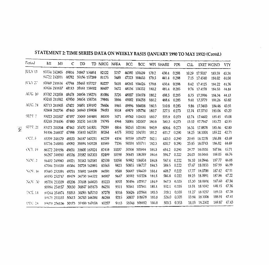
STA'ITMENT 2: TIME SERIES DATA ON WEEKLY BASIS (JANUARY 1990 TO MAY 1992) (Contd.)

I'c ri cki hfl M3 C DD TD NRCG NFEA BCC BCC WPI SHARE PDS CLL EXRT WGIND VTY

IcLI' 1.3 Y5F1 242405 49816 34847 156851 82122 5757 46380 104639 179.2 430.4 0.298 10.29 17.5037 183.59 43.34 $122 242011 48782 35156 157289 81175 5688 47323 104633 179.5 441.4 0.298 7.15 17.4540 184.02 44.04

! i : L j ' 2 : 83889 241616 47748 35465 157727 80227 5618 48265 104626 179.8 450.4 0.298 8.62 17.4125 184.22 43.76 SS6 241837 48113 35161 158002 80657 5672 48136 104352 180.2 481.4 0.285 9.76 17.4178 184.53 44.44

:JL'C. 10 S3B2 242058 48478 34856 158276 81086 5726 48007 104078 180.2 498.5 0.285 8.75 17.3996 184.34 44.13 83218 241982 47950 3@% 158734 79846 5846 49002 104058 180.2 488.6 0.285 9.61 17.3779 184.26 43.82

: 4 82713 241905 47422 34851 159192 78606 5965 49996 104038 180.3 510.8 0.285 9.86 17.3403 184.46 43.51 82868 242706 47460 34960 159838 79453 5518 49879 303734 180.7 527.5 0.273 12.74 17.3710 185.06 43.20

STATEMENT 2: TIME SERIES DATA ON WEEKLY BASIS (JANUARY 1990 TO MAY 1992) (Contd.)

Period MI M3 C DD TD NRCG NFEA BCG BCC WPI SHARE PDS CLL EXRT WGIND VTY

JAN 4 '91 I I 18 23

FEB 1 8

15 22

MAR I 8

13

UI 22

Q 29

APRIL 5 12 19 26

MAY 3 10 17 24 3 1

JUNE 7 14

21 28

STATEMENT 2: TIME SERIES DATA ON WEEKLY BASIS (JANUARY 1990 TO MAY 1992) (~ontd.)

Period MI M3 C DD TD NRCG NFEA BCG BCC WPI SHARE. PDS CLL EXRT WGIND ir7Y

I L I L y S 99143 277579 56990 40693 178436 97027 7108 54923 117600 201.0 568.6 0.405 25.70 24.7781 209.03 32.09 99252 277744 57125 40567 178492 98125 6875 55104 1176iM 201.8 569.3 0.405 22.36 25.9253 210.04 43.6% 98442 277867 55840 41309 179425 97899 6821 55464 117531 202.6 601.9 0.405 20.87 25.9381 211.29 45.23

26 97631 277989 54555 42051 180358 97672 6766 55823 117458 205.8 615.9 0.332 14.81 25.7327 212.89 46.90 AuGus*2 976% 27868~4 54821 42028 181038 97660 7626 56205 117009 207.3 644.3 0.332 15.62 25.7890 214.19 46.33

9 97660 279378 55086 42004 181718 97648 8486 56586 116559 208.4 692.4 0.332 12.53 25.6822 216.19 46.20 16 97075 279559 5.1553 41755 182484 97530 8361 56846 116247 209.6 697.0 0.332 13.80 25.8726 218.00 45.86 23 96489 279739 54019 41506 183250 97412 8236 57105 115935 210.4 708.5 0.332 13.33 25.8058 219.40 45.52 30 96961 280802 54200 41721 183842 97695 8246 57117 115838 210.3 724.5 0.398 12.17 25.8884 2i9.1g 45.18

W'T. 6 97432 281865 54381 41936 184433 97977 8256 57129 115740 210.6 752.2 0.398 11.83 25.95% 219.86 43.27 13 97268 282748 54064 42'211 185480 96944 8355 57623 115840 210.6 751.8 0.398 13.25 25.9795 219.80 41.44 20 97104 283630 53746 42485 186526 95910 8453 58116 115940 210.4 763.6 0.398 11.19 25.8571 219.10 39.69 27 98250 286081 53644 43777 187831 96644 8522 58330 117429 210.1 792.3 0.423 14.39 25.8769 218.99 38.01

L v . 1 99396 288532 53541 45069 189136 97378 8591 58543 118918 210.0 779.9 0.323 28.19 25.8981 218.60 39.72 11 101512 290541 54720 45357 189030 98179 9107 58831 119CN9 210.1 781.3 0.423 24.27 25.8228 218.63 41.50 18 103627 292550 55899 45644 188923 98979 9623 59118 119180 210.2 755.9 0.423 18.99 25.9300 218.82 43.37 23 103515 292447 56075 46019 188932 97854 10022 59888 119089 210.4 750.9 0.300 18.56 25.8816 219.37 45.32

so\'. 1 103402 2923a 56250 46394 188941 96728 10420 60657 118997 211.2 756.7 0.300 15.39 25.9032 220.32 43.18 8 105383 294374 57790 46851 188991 98054 10577 60536 119095 212.1 781.8 0.300 17.93 25.8981 220.74 41.72

13 107363 29MM 59330 47308 189041 99380 10733 60414 119193 212.6 792.4 0.300 26.23 25.9030 221.45 40.W

22 107933 297462 58630 48069 189510 99730 11326 60647 119634 213.0 797.6 0.300 30.15 25.9385 221.75 38.41

29 108512 298520 57930 48830 189978 100079 11918 60880 120075 212.9 821.4 0.395 20.92 25.7671 221142 36.85'

DEC. 6 109791 30M65 59037 48612 190674 101466 12510 61307 119821 211.4 813.4 0.395 14.92 25.9912 220.81 38.86

13 111N9 302409 60144 48393 191370 102852 13102 61733 119567 211.1 821.0 0.395 9.65 25.8875 219.59 40.98

20 111400 303749 60457 48686 192349 102361 13933 61988 120167 210.6 803.6 0.395 12.41 25.8997 218.42 43.21

27 108781 301168 59206 48746 192384 96994 15079 62175 119579 212.0 788.5. 0.308 10.28 25.9159 219.06 45.57

STATEMENT 2: TIME SERIES DATA ON WEEKLY BASIS (JANUARY 1990 TO MAY 1992) (Contd.)

Period h41 M3 C DD TD NRCG NFEA BCG BCC WPI SHARE PDS CLL EXRT WGIND VTY

JAN'923 110273 303129 59988 48862 192856 99432 14922 62209 120173 214.9 808.7 0.308 15.41 25.8.137 222.07 45.45 10 111761 303089 60769 48978 193328 101870 14764 62243 120766 215.1 823.1 0.308 12.10 25.7384 222.52 45.33 17 111723 305550 60439 49393 193827 101405 14937 62294 120842 215.5 822.1 0.308 10.75 25.8788 223.69 45.20 24 11 1684 306010 60109 49808 194326 100939 15109 62344 120918 215.6 848.6 0.308 10.28 25.8999 223.81 45.08 31 112776 307503 60728 50139 194727 101757 15217 62426 121247 215.8 868.8 0.388 10.17 25.8368 223.80 44.96

FEB 92 7 113868 308993 61347 50469 195127 102575 15325 62507 121576 215.7 923.3 0.388 7.78 25.9506 223.78 44.19 14 113706 309839 61247 50637 196133 102087 15977 62762 121626 214.8 943.1 0.388 9.77 25.9045 225.32 43.43 21 113544 310682 61147 50804 197138 101599 16628 63016 121676 215.0 973.9 0.388 10.01 25.8789 225.24 42.69 28 113967 312684 61396 50767 198717 100989 16813 63441 121745 215.2 1015.8 0.365 9.79 25.8249 225.86 41.96

MAR926 114389 314685 61644 50730 200296 100378 16998 63865 121813 215.8 1095.3 0.365 9.45 27.8833 225.44 43.95 13 115269 315967 61888 51121 200698 99367 17602 64044 123324 216.5 1271.5 0.36; 10.54 27.8632 225.59 46.05 20 116149 317248 62131 51511 201099 98355 18205 64222 124835 216.5 1279.3 0.365 12.86 28.6581 225.40 48.25 27 115918 318473 61797 52010 202556 97565 18853 64933 127156 216.4 1312.9 0.310 21.46 29.1149 224.62 50.54

APR923 115686 319698 61462 52508 204012 9675 19500 65644 129176 217.1 1485.4 0.310 33.76 29.1513 227.09 48.39 10 117866 321934 63045 53002 204068 97968 19303 65629 130320 2175 1625.7 0.310 20.38 29.0531 227.87 46.33

2 17 120046 324169 64627 53495 204123 99160 19106 65613 131163 218.5 1587.9 0.310 24.84 29.0023 227.75 44.37 24 120060 32476 64513 53537 204416 98533 19108 66078 131503 218.6 1600.5 0.363 31.79 28.8129 227.42 42.48

MAY 92 1 120074 324783 64399 53578 201709 97906 19110 66542 131842 218.5 1630.1 0.363 51.74 28.7273 228 57 15.56 8 121255 326081 65393 53371 204826 98806 18527 66651 132783 218.9 1509.9 0.363 43.83 28.6350 229.72 48.86

15 122435 327378 66386 53163 2M943 99706 17943 66760 133723 219.5 1354.4 0.363 36.63 28.4744 230.59 52.39

Legend : NRCC : Net Reserve Bank Credit to Government (Both Centre WGIND : Index of Wage-goods Prices

&States) (Rs. Crorcs) VT( : Velocity (Cheque clcarances/Demmd Deposits) NFEA : Net Foreign Exchange Assets of the Banking Sector MI : Narrow Money (Rs.Crore)

(Rs. Crorn) M3 : Broad Money (Rs. Crores) BCG : Commercial & Cooperative Banks' Credit to C : Currency (Rs. Crores)

Goverx~ment Sector (Rs. Crores) DD : Demand Deposits (Rs. Crores) BCc : Commercial Banks' Crdit to Commercial Sector (Rs. TD : Time Deposits (Rs. Crores)

Crores) WPI : olesa sale Price Index of tZll Cornmoditin SHARE : Index of Share Prices (All-India RBI Index, Base (1951-82=100)

1980-81=100) SOURCE : Reserve Bank of India (for Ml, 513, C, DD, TD, NRCG,

PDS : Monthly offtake at Public Distribution System NFEA, WPI, SHARE. XRT, G q u e CIearances) (Wheat,Rice & Coarse grains in MT.) Ministry od Food &Civil Supplies, Government od

CLL : Call Rate India (for PIX) EXRT : Exchange Rate (Rs. per Dollar)

Statement 2(A) : Monthly Data on Select Variables (January 1990 to May 1992)

- -

Period PDS XRATE MTSH BIGS GOLD RDYILD WGIND

Legend :

PDS : Monthly off-take from Public Distribution System (Wheat, Rice, Coarse Grains) (in Million Tonnes)

XRATE : Exchange Rate (Rs.pcr U.S.S) MTSH : Monthly Turn over of shares (Rs. Crores) BIGS : All Scheduled Banks' Investment in Covcrnmcnt Sccuritics (Month End)

(Rs. Crores) GOLD : Price of Gold in Bombay (Rs. per 10 gms.) KDYILD : I<rdcmption Yield on Covcrnmcmt kcuritics (per ccnt pcr annurn! WGlND : Indcx of Wage-goods J'riccs (Cornpilc~l) YOIJKCES : I ( c ~ u ~ v c Clank of india, ,Ministry of Food and Civil Supplicsq, I : o m i ~ ~ v ';to( k

i:xr.ha ngc:

Statement 3 : Semi-Log Growth Rates of Select Variables (Annualised on Weekly .Rates)

Jan. 90 - Dec. 90 - May 91 - Dec.91 - Jan.90 - Dec. 90 May 91 Dec. 91 May 91 May92

MI 10.06 26.29 17.28 23.1 7 16.91

M3 13.53 20.36 15.82 20.05 15.32

NRCG 16.1 21.08 6.64 -8.10 14.84

NFEA 33.37 5.77 102.05 88.39 44.57

BCG 21.09 19.64 25.31 19.41 18.07

BCC 10.31 21.53 3.06 26.37 10.98

Share 54.57 49.94 79.56 1 87.68 49.45

WPI 11.29 8.52 14.32 7.57 1.2.04

Lcgcnd

M 1 M3 C DD TD N liCG NFEA BCC. BCC Sharc \Vl)I

: Narrow Money (Rs. crore) : Broad Money (Rs. crore) : Currcncy ( Ik . crorc) : Dcmand Dcposits (Rs. crorc) : Time Dcposits (Iis. crow) : Nct Rcscrvc Bank Crsdit to Government : Nct Forcign Exchange Assets of Banking Sector : Comnicrcinl and Co-opcrative Bank Crtdit to Government : Comrncrcial Dank C r ~ d i t to Comrncrcial Sector : All India Indcx of Share Prices of IIBI. : 1Vholczalc I'ricc Indcx.

Statement 4 : Regression Equation-Monetary Components (Whole Period)

Fortnightly Data (Period : January 1990 to May 1992)

- 2 Constant BCG NFEA NRCG BCC R D.W. SEE

Currency -2759.28 -0.195 0.368* 0.205' 0.399* 0.94 0.85 1325.70

Demand Deposits -2612.22 0.562* 0.446' 0.015 0.067 0.95 0.66 1375.70

MI -6640.92 0.253 0.963* 0.267* 0.495" 0.97 0.56 2000.90

Time Deposits 13309.53 1.574' 0.098 0.296* 0.430' 0.99 0.74 1220.80

M3 6668.62 1.827, 1.061+ 0.563* 0.923* 0.99 0.78 2042.60

Legend :

BCG : Commercial and Co-operataive Bank Credit to Government

NFEA : Net Foreign Exchange Assets of the Banking Sector.

NRCG : Net Reserve Bank Credit to Government.

BCC .: Commercial Bank Credit to Commercial Scctor * : Significant.at 5.per centlevel of significance.

Statement 5 : Compound Rate of Growth (Fortnight) Estimated Through Semilog Trend Equations

(Per cent)

Period I Period I1

(A) (B) (A) (B)

C

DD

MI

TD

M3 NRCG

NFEA

BCS

BCC

Period 1 : January 12 1990 to October 4 1991 Period 2 : October 19 1991 to May 15 1992

Legend : C : DD : MI : M3 : NJICC : NFEA : BCG : BCC :

Currcncy Demand Deposits Narrow Money Broad Moncy

Nct Rcscr\~c Bank Crcdit to Govcrnment Nct Forcign Exchange Assets of the Banking Sector Cornmcrcial and Co-operative Bank Cr~d i t to Government

Commcrcial Bank Credit to Commercial Sector.

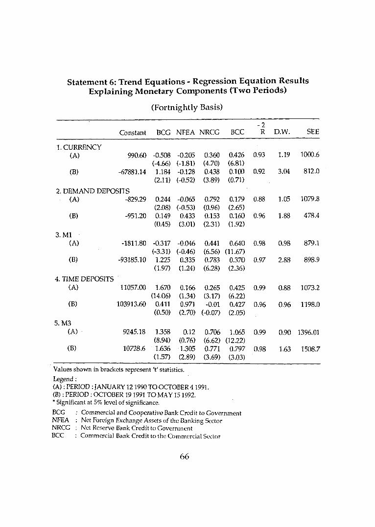
Statement 6: Trend Equations - Regression Equation Results Explaining Monetary Components (Two Periods)

(Fortnightly Basis)

- 2 Constant BCG NFEA NRCG BCC R D.W. SEE

1. CURRENCY (A) 990.60 -0.508

(-4.66) (8) -67881.14 1.184

(2.11)

2. DEMAND DEPOSITS (A) -829.29 0.244

(2.08) (B) -951.20 0.149

(0.45)

3. MI (A) -1811.80 -0.317

(-3.3 1 ) (B) -93185.10 1.225

(1.97)

4. TIME DEPOSITS (A) 11057.00 1.670

(14.06) (B) 103913.60 0.411

(0.50)

- ---

Values shown in brackets represent 't' statistics.

Legend : (A) : PERIOD :JANUARY 12 1990 TO OCTOBER 4 1991. (B) : PERIOD : OCTOBER 19 1991 TO MAY 15 1992. * Significant at 5% level of significance.

BCG : Commercial and Cooperative Bank Crcdit to Government NFEA : Ne t Foreign Exchange Assets of the Banking Scctor NRCG : Net Reserve Bank Credit to Covcrnmcn t BCC : Commercial Bank Crcdit to thc Commercial Scutor

Statement Through

7 : Compound Rate of Growth (~ortnight) Estimated Semi-Log Trend Equations (Pre-liberalisation and

Post-liberalisation Periods)

(Per cent)

Period I Period I1

C

DD

MI

TD

M3

NRCG

NFE A

BCG

BCC - - - - - - - -- -- -

(A) Compound Growth Rate on Fortnightly Basis (B) Annual Compound Growth Rate

Period 1 : January 12,1990 to June 28,1991 Period 2 : July 12,1991 to May 15,1992

Legend : C : Currency DD : Demand Deposits M1 : Narrow Money M3 : Broad Money NRCG : Net Reserve Bank Credit to Government NFEA : Net Foreign Exchange Assets of the Banking Sector BCG : Commercial and Co-operative Bank Credit to Government BCC : Commercial Bank Credit to Commercial Sector.

Statement 8: Regression Equation Results Explaining Money Stock Measures

(Pre Liberalisation & Post Liberalisation Periods)

(Fortnightly Basis)

- 2 Constant BCG NFEA NRCG BCC R D.W. SEE

I . CURRENCY (A) 570.44 -0.441 -0.279

(-4.09) (-2.63) (B) -38515.01 -0.132 0.41 2

(-0.43) (1.91)

2. DEMAND DEPOSITS (A) 125.71 0.053 -0.009

(0.61) (-0.1 1 ) (B) -39691.98 0.968 0.129

(4.62) (0.87) 3. MI

(A) -1396.30 -0.394 (-3.68)

(B) -1 03666.10 0.792 (2.39)

4. TIME DEPOSITS (A) 11918.82 1.460

(13.41) (B) 87937.88 1.603

(3.90) 5. M3.

(A) 10522.51 1.066 (8.20)

(B) -15728.24 2.395 (5.91)

Values shown in brackets represent 't' statistic

Legend : (A) : PERIOD : JANUARY 12 1990 TO JUNE 28,1991 (B) : PERIOD : JULY 12,1991 to MAY 15,1992 * Significant at 5% level of significance.

UCC : Cornmcrcial and Cooperative Bank Crcdit to Government NEA : Nct Forcign Exchange Assets of the B'lnking k c t o r NKCC; : Net Rcstlrvc Rank Crcdit to Covcrnment BCC : Commcrcial Bank Crcdit to tho Comrnrrcial Sx-tor

Statement 9 : Variables Affecting Share Prices (Period : January 1990 to March 1992) Dependent Variable : RBI Index of Share Prices

Constant LMI LBCC LBIG LFXA LXR LCPI LPSHG LCLL -2 D.W. SEE Term R

24.22 0.05 -7.10 0.92 0.06 0.83 0.50 0.14 (0.60) (1.49) (-0.84) (2.46)' (1.89)*

-32.58 2.62 1.25 0.29 0.04 0.73 0.51 0.18 (-0.54) (3.13) (3.13)* (1.76) (0.82)

Values shown in brackets represent 't' statistic * Statistically significant

Legend LMI' = Log of Money Supply (MI) LBCC = Log of Commercial Banks' loans to the Commercial Sector. LBIG = Log of Commercial Banks' investments in Government Securities LFXA = Log of net Foreign Exchange assets of Banking Sector LXR = Log of Exchange Rate (Rupees per US Dollar) LCPI , = Log of Capital Issues (Naminal Values) LPSHG = Log of growth rate in the Index of Share prices during the past month. LCLL = Log of Call Rate

Statement 10 : Variables Affeding Share Prices (Sub-Periods)

Dependent Variable : RBI Index of Share Prices (Monthend Values) Independent Variables

No. of Constant LMI LXR' LBlC LPSHG - 2 D.W. S,E,E, Obscr- Term R seliuns

Whole Period : January17990 fo March 1992

1st Period : January 1990 to March 1991

2nd Period : lanuary- 1992 to March 1992

\r',~iut's sht>~sr\.n in brackets rcprcscnt 't' statistic

* Statistically significant

L X I I : Lot; of hfl LYE: : Log of Exchnngc Rate LB1G : Log of Cnmmcrcial Banks' fnvestmcnt in Govcmmcnk Securities LIYIIC : I.ctg of Growth rate in tho Indcxof Share pricvsd;lnrjng the past month.

Statement 11 : Variables Affecting RBI Index of Share Prices

(Week-cnd Values) ~e~cndent 'var iab le : RBI Index of Share Prices

Sr. Period Constant LMl LCLL LEXR DVTY ESHR LDD - 2 D.W. No. Term R

Whole Period

Period I

Period I1

Statement 12 : Money supply Factors and RBI Index of Share Prices

(Week-end Values) Dependent Variable : RBI Index of Share Prices

Sr. Period Constant LBCG LBCC LNFEA - 2 D.W. No. Term R

Whole Period

1. Jan.90-May 92

Period I

2. Jan9QDec. 90

Period I1

3. Dec.90-May 91

Period I11

4. May 91-Dec.91,

Period IV

5. Dcc.91-May 92

Valucs shown in brackets rcprcsc?t 't' statistic

LBCG : Log of Commercial and Co-operative Bank Credit t o Government LBCC : Log of Commercial Bank Credit to the Commercial Sector LNFEA : Log of Net Foreign Exchange Asxts of the Banking Sector

Statement 33 : Variables Affecting Share Prices (Roll-over Regression Results)

(Month - cnd Values) Ilcpcndcnt Variable : RBI Ir-rdcx of Share Prices

Sr. I'criocl Constant Indcpcndent Variables R-2 D.W. SEE No. Tcrm LM'I LXTi LBlG LPSF-IG

Values shown in brackets represent 't' statistic Legend : LMI : Log of Money Supply (MI) LXR : Log of Exchange Rate LBIG : Log of Bank Invqtment jn Government kcuritjes LPSHG : Log of Growth Rate of Index of Share Prices during the past month.

Statement 13(A): Variables affecting Share Prices (Monthly Data Basis)

Dependent Variable : BSE Index of Share Prices

SR. PERIOD CONSTANT LMI LCLL LGOLD LXRATE LRYILD LIMTJB LDD R2 D.W. NO. TERM

1. JAN. 90 - MAR.92 -12.99 2.01 -0.16 -0.48 1.28 -1.71 0.0002 0.85 0.63 (3.05) (-1.69) (-0.73) (2.70) (-2.32) (0.003)

2. JAN. 90 - MAR.92 -1 1.22 -0.10 -0.71 0.99 -1.83 -0.008 2.28 0.87 0.89 (-1.23) - 1 3 (2.10) (0.70) (-0.1 4) (3.65)

Valucs shown in brackets represent 't' statistic

;)11 Legend :

LMI : Log of Money Supply (MI) LCLL : Log of Call Rate LGOLD : Log of Gold prices LXRATE : Log of Exchange Rate LRYILD : Log of Redemption Yield of Government Securities LIMTIB : Log of ratio of Monthly turn over of shares to BSE Index LDD : Log of Demand Deposits

SOURCE : Reserve Bank Of India Bombay Stock Exchange

Stalc~ncnt 14 : Regression Derived Semilog Growth Rates of Key Variables on Monthly Basis

(In per ccn t ) --

W holc Period I I'eriod 11 Extcnt of Vi~riC~l~lc Pcri od (Jnn.90 - (June 91 Change of

Junc 90 May 92) 11 over 1 - ( 1 ) (2) (3) (4) ( 5 )

Narrow Motlc?y 1.49 1.29 2.28 + 77.0

Currency 1.20 1.22 1.79 47.0

'I'imc Deposi ts 1.23 1.25 1.31 5 .0

Index of Wholcsalc Prices 1.03 .O. 97 0.81 -8.4

Call Rate 1.15 3.53 0.73 . -80.0

Supplies of Public Distribution Systen~

Velocity & Cheque Clearings

Exchange Rate (Rupees per Dollar)

Net Domestic Product 0.17 -0.062 0.43 -

Cheque Clearings 1.61 1.01 2.99 19.60

Statement 15 : Regression Results on W~olesale Prices (Monthly Data)

Dependent Variable : Log of Wholesale Price Index

Sr. Period No.

Constant MI LY Lr P - - 7 D. W. Term c x R

Jan. 9 0-May 92

1. -2.64 0.67 0.029 -0.022 0.01 0.91 0.43 (16.15) (0.52) (-1.42) (1.68)

Jan. 90-June 91

2. -3.30 0.75 -0.0035 -0.03 0.002 0.84 0.73 (8.24) (-0.05) (-1.49) (0.7 6)

July 91-May 92

3. 1.81 0.27 0.05 -0.005 -0.001 0.82 1.71 (5.84) (1.30) (-0.56) (-0.36)

Values in brackets represent 't' statistic

LMl : Log of Money Supply (MI) LY : Log of Net Domestic Product Real GDP Lrc : Log of Call Rate

PX ; Price Expectational Variable { = WPI (T-1) } ( ----- x l o o )

1 WPI (T-2) 1

Statement 16 : Additional Regression Results on Wholesale Prices (Monthly Series)

Dependent Variable : Index Number of Wholesale Prices

Independent Variables Form of Functior~ Double Log

Period Constant LMl LCU LY LPDS LNDP LXRATE LCLL LV - 2 D.W. Term R

jan.90 - May 92 .91

(Contd.)

Statement 16 : Additional Regression Results of Wholesale Prices (Contd.) (1) January 1990 -June 1991

(2) July 1991 - May 1992

Dependent Variable : LWPl

Period Covercd Independent Variables

Constant LMI LCLL LPDS LNDP LXRATE LVELC - 2 D.W. Term R

V July 91-May 92 2.234 0.202 -0.013 0.050 0.239 -0.049 0.82 1.80

(3.49) (3.15) (-1.35) (0.64) (1.58) (-1.02)

Values in brackets represent 't' statistic

Legend : LMI LCLL LPDS LNDP LXRATE LVELC LCU LY

: Log of Money Supply (MI 1 : Log of Call Rate : Log of Monthly Off-take from Public Distribution System (Wheat, Rice, Coarse Grains) : Log of Net Domestic Product : Log of Exchange Rate : Log of Velocity : Log of Currency : Log of Iieal GDP

Slatement 17 : Roll-over Regression on Wholesale Prices (Monthly Series) Dcpcndent Variable : Index of Wholesale Prices

Pcriod Log MI Log Call Log - 2 D.W. Rate Exchange R

Rate

Jan.90 - May 92 0.337 (3.83)

February 1990 0.302 (3.43)

March 1990 0.269 (3.26)

April 1990 0.238 (3.06)

May 1990 0.226 (3.31)

June 1990 0.218 (3.80)

July 1990 0.216 (4.51

August 1990 0.210 (4.70)

September 1990 0.202 (4.57)

October 1990 0.193 (5.36)

November 1990 0.187 (4.92)

December 1990 0.182 (4.67)

January 1991 0.1 78 (4.59)

February 1991 0.179 (4.42)

March 1991 0.179 (4.18)

April 1991 0.176 (3.79)

May 1991 0.184 (4.08)

June 1991 0.192 (3.79)

July 1991 0.221 (2.70)

August 91-May 92 0.218 (12.0())

Valuos in brackets rcprownt 't' statistic

Statement 18 : Factors Determining Wholesale Prices (Weekly Series)

Dependent Variable : LWPI

Constant C MI M3 PDS CLL XR PSH VTY 2 - DW SEE Term R

Period : January 1990 to December 1990

0.31 0.36 - - 0.01 -0.21 0.37 0.10 Neg.' 0.95 0.96 0.77 (-0.88) (0.82) (-5.61) (2.20) (5.90) (Neg.)

-1.16 - 0.50 - 0.01 0.02 0.03 0.11 Neg. 0.96 0.85 0.70 (-2.990) (7.79) (1.01) (-5.36) (0.16) (6.87) (Neg.) .

-3.46 - - 0.70 Neg. -0.01 -0.12 0.05 Neg. 0.98 0.76 0.01 (-9.16) (14.10) (Neg.) (-5.00) (-1,05) (6.53) (Neg.)

2 -3.10 - 0.74 - 0.01 - - - Neg. 0.70 0.11 0.18 (-3.72) (9.97) (0.39) (Neg.)

-4.58 - - 0.79 0.01 - - - Neg. 0.95 0.20 0.74 (-13.89) (29.64) (0.65)

Period : December 1990 to May 1991

2.28 0.27 - - Neg. -0.86 0.18 -0.08 Neg. 0.92 1.50 0.34 (3.26) (3.47) (Neg.) (-1 53) (2.33) (-3.1 1 ) (Neg.)

4.1 1 - 0.06 - 0.01 Neg. 0.34 -0.91 Neg. 0.86 1.14 0.01 (3.28) (0.45) (0.29) (Neg.) (2.53) (-2.67) (Neg.)

- 1.53 - 0.33 - 0.01 - - Neg. 0.81 0.62 0.01 (3.72) (8.86) (0,27)

- -0.23 - - 0.44 0.01 - Neg. 0.81 0.56 0.01 (-0.37) (8.80) (0.39)

Statement 18 : Factors Determining Wholesale )Prices (Contd.) (Weekly Series)

Constant C M1 M3 PDS CLL XR rSH VTY 2 - DW SEE Term R

Period : May 1991 to December 1991

4.62 - -0.04 - -0.03 -0.01 -0.10 0.13 Neg. 0.97 1.30 0.01 (12.63) (-1.06) (-4.09) (-1.45) (6.64) (10.50) (Neg.)

5.34 - - -0.10 -0.03 -0.01 0.10 0.14 Neg. 0.97 1.34 0.01 (6.12) (-1.27) (-4.23) - 1 1 8 (6.71) (8.14) (Neg.) 5.33 - 0.01 - -0.01 ' - - - -0.01 0.22 0.13 0.02

2 (2.90) (0.07) . (-1.70) (-2.22)

-3.06 - - 0.67 -0.01 - - - Neg. 0.47 0.08 0.01 (-1.19) (3.32) (-0.33)

Period : December 1991 to May 1992

3.47 0.18 - - -0.24 -0.35 -0.15 0.43 0.96 0.82 1.34 0.01 (3.68) (2.25) (-1.99) (-1.99) (-1.93) (2.48) (1.80)

2.07 - 0.29 - -0.03 Neg. -0.12 0.24 Neg. 0.85 1.50 0.01 (1 -77) (1 -77)- (-2.65) (Neg.) (-1.70) (1.27) (Neg.)

1.95 - 0.29 -0.03 Neg. 0.82 0.72 0.01

(4.64) (7.89) (-2.46) (Neg.) - - 1 .O1 .. - 0.34 -0.02 - Neg. 0.81 0.60 0.01

(1.78) (7.46) (-1.63)

Statement 18 : Factors Determining Wholesale Prices (Contd.) (Weekly Series)

Constant C MI M3 PDS CLL XR PSH VTY - 2 DW SEE Term R

Period : December 1990 to May 1992

1.05 0.32 - - 0.03 -0.01 0.23 0.25 -0.37 0.95 1.41 0.02 (2.72) (7.68) (2.06) (-2.01) (8.19) (2.18) (-34)

0.93 - 0.32 - 0.03 Neg. 0.21 0.01 Ncg. 0.95 0.10 0.02 (2.14) (7.01) (1.92) (Neg.) (6.91) (0.59) (Neg.)

-3.12 - - 0.66 0.01 -0.01 0.12 -0.03 Neg. 0.98 0.16 0.01 (-7.35) (16.79) (0.50) (-2.05) (6.20) (-3.65) (Neg.)

-1.67 - 0.62 - 0.06 - - - Neg. 0.92 0.14 0.02 (-6.73) (30.13) i3.58)

-2.54 - 0.70 - 0.06 - - - Neg. 0.92 0.15 0.03 (-8.76) (29.19) (3.41) (Neg.)

Values in brackets represent 't' statistic

Legend :

C : Currency M1 : Narrow Money M3 : Broad Money PDS ; Monthly offtake of Public Distribution System (Wheat, Rice and Coarcegrains in hfI? CLL. ; Call Rate XR : Exchange Rate (Rs. per dollar) PSH : The growth rate of share indexSduring the past month

VTY : Velocity (Cheque clearances/Demand Deposits)

Statement 19 : Factors Determining Price Level of Wage Goods (LWGIND) (Weekly Series)

Constant LM1 LC LPDS LCLL LEXRT LSHARE LRWG - 2 D.W. SEE Term R

January 1990 to December 1990

-2.26 0.63 - Neg -0.03 -0.19 0.16 -0.48 0.93 0.81 0.1 (-3.50) (6.30) (Neg.) (-6.35) (-0.70) (6.45) (-0.98)

December 1990 to May 1991

May 1991 to December 1991

Statement 19 : Factors Determining Price Level of Wage Goods (LWGIND) (Contd.) (Weekly Series)

Constant LM1 LC LPDS LCLL LEXRT LSHARE LRWG - 2 D.W. SEE Term R

December 1991 to May 1992

-0.01 -0.02 -0.12 0.03 (-0.82) (-0.68) (-1.58) (1.69)

-0.01 .Neg. -0.12 0.05 (0.25) (NQ.) (-1.44) (2.59)

December 1990 to May 1992

0.34 -0.01 0.27 0.02 (2.02) (-1.55) 17.96) (1.61)

0.03 -0.01 0.28 0.03 (1.98) (-2.52) (9.07) (2.53)

Values in brackets represent 't' statistic

Legend :

LMI : Log of Money Supply (MI) LC : Log of Currency LPDS : Log of Monthly off-take from Public Distribution System (Wheat, Rice, Coarse Grains) LCLL : Log of Call Rate LEXRT : Log of Exchange Rate LSHARE : Log of Index of Share Prices LRWG : Log of Expected Growth Rate of Wage-goods Prices

Statement 20 : Intercorrelation Matrix of Select Variables (On Weekly Basis)

MI M3 C WPI SHARE PDS CLL EXRT WGIND

LEGEND : M l : Narrow Money h.13 : Broad Money C : Currency WPI : Whole Price Index of All Commodities SHARE : Index of Share Prices (All India RBI Index Base 1980-81=100) PDS : Monthly Take-off from Public Distribution System (Wheat, Rice & Coarse Grains) CLL : Call Rate EXRT : Exchange Rate WGIND : Index of Wage-goods Prices