arX

iv:0

805.

4620

v1 [

cs.IT

] 29

May

200

8

1

Uplink Macro Diversity of Limited BackhaulCellular Network

Amichai Sanderovich∗, Oren Somekh†, H. Vincent Poor†, and Shlomo Shamai(Shitz)∗

∗ Department of Electrical Engineering, Technion, Haifa 32000, Israel† Department of Electrical Engineering, Princeton University, Princeton, NJ

08544, USAEmail: amichi@tx.technion.ac.il, orens@princeton.edu,poor@princeton.edu,

sshlomo@ee.technion.ac.il

Abstract

In this work new achievable rates are derived, for the uplinkchannel of a cellular networkwith joint multicell processing, where unlike previous results, the ideal backhaul network has finitecapacity per-cell. Namely, the cell sites are linked to the central joint processor via lossless linkswith finite capacity. The cellular network is abstracted by symmetric models, which render analyticaltreatment plausible. For this idealistic model family, achievable rates are presented for cell-sites thatuse compress-and-forward schemes combined with local decoding, for both Gaussian and fadingchannels. The rates are given in closed form for the classical Wyner model and the soft-handovermodel. These rates are then demonstrated to be rather close to the optimal unlimited backhaul jointprocessing rates, already for modest backhaul capacities,supporting the potential gain offered by thejoint multicell processing approach. Particular attention is also given to the low-SNR characterizationof these rates through which the effect of the limited backhaul network is explicitly revealed. Inaddition, the rate at which the backhaul capacity should scale in order to maintain the original high-SNR characterization of an unlimited backhaul capacity system is found.

Index Terms

Distributed Antenna Array, Fading, Limited Backhaul, Multicell Processing, Multiuser Detection,Shannon Theory, Wyner’s Cellular Model.

I. INTRODUCTION

The growing demand for ubiquitous access to high-data-rateservices has produced a sig-nificant amount of research analyzing the performance of wireless communications systems.Cellular systems are of major interest as the most common method for providing continuousservices to mobile users, in both indoor and outdoor environments. In particular, the use of joint

This work was presented in part at the IEEE 2007 ISIT, June 2007, Nice, France.This research was supported by a Marie Curie Outgoing International Fellowship and the NEWCOM++ network of

excellence within the 6th and 7th European Community Framework Programmes, respectively, by the U.S. National ScienceFoundation under Grants ANI-03-38807 and CNS-06-25637, and the REMON consortium for wireless communication.

2

multicell processing (MCP) has been identified as a key tool for enhancing system performance(see [1] [2] and references therein for recent results on MCP).

Analysis of MCP has been so far based primarily on the assumption that all the base-stations(BSs) in the network are connected to a remote central processor (RCP) via an ideal backhaulnetwork that is reliable, has infinite capacity and full connectivity. In this case, the set of BSseffectively acts as a multiantenna transmitter (downlink)or receiver (uplink) with the caveatthat the antennas are geographically distributed over a large area. Since the assumption ofan ideal backhaul network is quite unrealistic for large networks, more recently, there havebeen attempts to alleviate some of the conditions by considering alternative models. In [3] alimited-connectivity backhaul network model is studied inwhich only a subset of neighboringcells is connected to a central joint processor. In [4][5] a topological constraint is imposed inwhich there exist unlimited capacity links only between adjacent cells, and message passingtechniques are employed in order to perform joint decoding in the uplink. Finally, [6] dealswith practical aspects of limited capacity backhaul cellular systems incorporating MCP, whereeach BS quantizes its received signal and forwards it to the RCP via a finite-capacity reliablelink. It is noted that [6] uses a simple quantization scheme that does not use the correlationbetween the received signals at neighboring BSs to reduce the compression rate.

Since its introduction in [7], the Wyner cellular model family has provided a framework formany studies dealing with multicell processing. Despite its simplicity, this model captures theessential structure of a cellular system and facilitates analytical treatment. The uplink channelsof the Wyner linear and planar models are analyzed in [7] for optimal and linear minimummean square error (MMSE) MCP receivers, and Gaussian channels. In [8], the Wyner model isextended to include fading channels and the performance of single and two cell-site processingunder various situations is addressed. In [9] the results of[7] are extended to include flat fadingchannels (the reader is referred to [1] for a comprehensive survey of studies dealing with theWyner model family).

As mentioned earlier, most works dealing with MCP assume that the backhaul networkconnecting the cell-sites to the RCP is error-free with infinite capacity. In this work we use thenew, recently presented result from [10] to relax this assumption and allow each cell-site toconnect to the RCP via a reliable error-free connection, butwith limited capacity. Such a modelsuits cellular networks, where joint decoding can improve the overall network performance,with the underlying assumption that the received signals are forwarded to one location to bejointly processed. Since network resources are finite, in particular when the cell-sites are infact “hot spots” with limited complexity, the inclusion of finite backhaul resources facilitatesbetter prediction of the performance gain offered by MCP.

Recently, the common problem of nomadic terminals sending information to a remotedestination via agents with lossless connections has been investigated in [11] and in [10] andthen extended in [12] and [13] to include multiple-input multiple-output (MIMO) channels.The main difference between the scalar channels and the vector channels, is the inability to geta tight upper bound, due to the entropy power inequality. These works focus on the nomadicregime, in which the nomadic terminals use codebooks that are unknown to the agents, butare fully known to the remote destination. Such setting suits the uplink channel of the limitedbackhaul cellular system with MCP, where the oblivious cell-sites play the role of the agents.

3

Adhering to [10],[12], we assess the impact of limited backhaul capacity on the performanceof two transmission schemes: (a) the “oblivious” scheme - inwhich the cell-sites are unawareof the users’ codebooks, and use a distributed Wyner-Ziv compress-and-forward scheme tosend a compressed version of their received signal to the RCPfor joint decoding; and (b) the“partial local decoding” scheme - in which the users split their messages into two parts, wherethe first part is decoded according to the “oblivious” scheme, while the second part is decodedlocally by the relevant BSs (treated as a version of the broadcast channel).

Throughout this work we use two variants of the linear Wyner cellular setup [7], whichprovide a homogenous framework with respect to the mobile users and cell-sites. The firstmodel is the circular Wyner model where the cells are arranged on a circle and each user“sees” three BSs, its local BS and the the two neighboring BSs. The second model is referredto as the circular soft-handoff (SH) model, in which the cells are arranged on a circle butthe users “see” only two BSs, their local BS and the left neighboring BS. This setup focuseson users that are located on a cell edge, and thus are simultaneously received by two BSs.This type of situation is often referred to as soft-handoff.Due to its simplicity and the uniquetwo-block diagonal structure of its channel transfer matrix, the SH model facilitates analyticaltreatment which provides additional insight. For both of these setups we are interested in theasymptotic scenario of infinitely many nodes, in which case the circular and linear modelsare equivalent. We consider both non-fading (Gaussian) andflat Rayleigh fading channels,although most of the results apply almost verbatim to other fading distributions.

Special attention is given to the low-signal to noise ratio (SNR) characterization of theresulting achievable rates. We apply the tools of [14] and provide closed-form expressions forthe minimum energy per-bit required for reliable communication, and to the low-SNR rate slopefor the suggested transmission schemes. In particular, thelow-SNR parameters are expressedin a uniform way for both the limited and unlimited backhaul versions. This, in turn, revealsthe effects of the limited backhaul network in a simple and concise manner. The high-SNRregime is also studied. In particular we provide the rate in which the backhaul capacity shouldscale with the SNR, in order for both schemes to preserve the high-SNR characterization oftheir parallel unlimited backhaul capacity counterparts.

The rest of the paper is organized as follow. In Section II we define the system models.Section III includes a short review of useful previous results that are used in the sequel. InSection IV we derive an achievable rate for oblivious cell-sites, while in Section V we extendthe result to the case where cell-sites can perform local decoding. Numerical examples arepresented in Section VI, which demonstrate the effect of limited backhaul capacity on MCPperformance. Several proofs and the analysis of the low-SNRcharacterization, are relegatedto the appendices.

II. SYSTEM MODEL

Throughout this paper we consider two variants of the linearWyner cellular uplink channel[7] (see also [15]): (a) the circular Wyner model, and (b) the“soft-handoff” model. Since bothmodels resemble one another to a certain extent, the circular Wyner model is presented in fullwhile the “soft-handoff” model is briefly described emphasizing its unique characterization.See Figure 1 for a simple illustration of the network topology.

4

A. The Circular Wyner Model

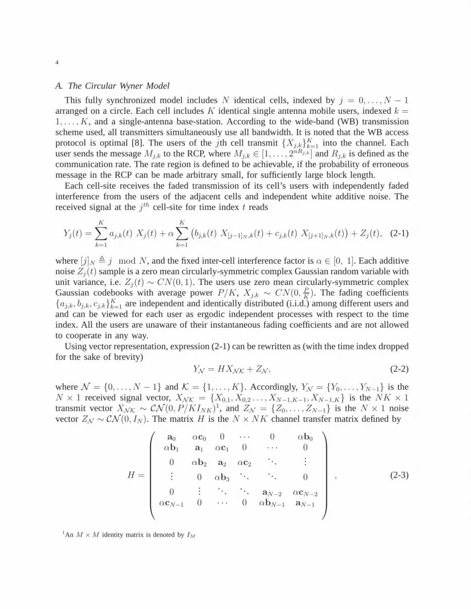
This fully synchronized model includesN identical cells, indexed byj = 0, . . . , N − 1arranged on a circle. Each cell includesK identical single antenna mobile users, indexedk =1, . . . , K, and a single-antenna base-station. According to the wide-band (WB) transmissionscheme used, all transmitters simultaneously use all bandwidth. It is noted that the WB accessprotocol is optimal [8]. The users of thejth cell transmit{Xj,k}K

k=1 into the channel. Eachuser sends the messageMj,k to the RCP, whereMj,k ∈ [1, . . . , 2nRj,k] andRj,k is defined as thecommunication rate. The rate region is defined to be achievable, if the probability of erroneousmessage in the RCP can be made arbitrary small, for sufficiently large block length.

Each cell-site receives the faded transmission of its cell’s users with independently fadedinterference from the users of the adjacent cells and independent white additive noise. Thereceived signal at thejth cell-site for time indext reads

Yj(t) =

K∑

k=1

aj,k(t) Xj(t) + α

K∑

k=1

(bj,k(t) X[j−1]N ,k(t) + cj,k(t) X[j+1]N ,k(t)

)+ Zj(t), (2-1)

where[j]N , j mod N , and the fixed inter-cell interference factor isα ∈ [0, 1]. Each additivenoiseZj(t) sample is a zero mean circularly-symmetric complex Gaussian random variable withunit variance, i.e.Zj(t) ∼ CN(0, 1). The users use zero mean circularly-symmetric complexGaussian codebooks with average powerP/K, Xj,k ∼ CN(0, P

K). The fading coefficients

{aj,k, bj,k, cj,k}Kk=1 are independent and identically distributed (i.i.d.) among different users and

and can be viewed for each user as ergodic independent processes with respect to the timeindex. All the users are unaware of their instantaneous fading coefficients and are not allowedto cooperate in any way.

Using vector representation, expression (2-1) can be rewritten as (with the time index droppedfor the sake of brevity)

YN = HXNK + ZN , (2-2)

whereN = {0, . . . , N − 1} andK = {1, . . . , K}. Accordingly,YN = {Y0, . . . , YN−1} is theN × 1 received signal vector,XNK = {X0,1, X0,2 . . . , XN−1,K−1, XN−1,K} is the NK × 1transmit vectorXNK ∼ CN (0, P/KINK)1, and ZN = {Z0, . . . , ZN−1} is the N × 1 noisevectorZN ∼ CN (0, IN). The matrixH is theN × NK channel transfer matrix defined by

H =

a0 αc0 0 · · · 0 αb0

αb1 a1 αc1 0 · · · 0

0 αb2 a2 αc2. ..

...... 0 αb3

. . . . .. 0

0...

. . . . . . aN−2 αcN−2

αcN−1 0 · · · 0 αbN−1 aN−1

, (2-3)

1An M × M identity matrix is denoted byIM

5

where,aj = {aj,1, . . . , aj,K}, bj = {bj,1, . . . , bj,K} and cj = {cj,1, . . . , cj,K} are 1 × K rowvectors denoting the fading coefficients, experienced by the K users of thejth, [j−1]N th, and[j + 1]N th cells, respectively, and received by thejth cell-site.

The above description relates to the WB protocol where all users transmit simultaneously.For an intra-cell time-division multiple-access (TDMA) protocol, only one user is active per-cell, transmitting1/K of the time using the total cell transmit powerP . So for TDMA protocolwe setK = 1 in (2-2) and (2-3).

Each cell-site is connected to the RCP through a unidirectional lossless link, with bandwidthof Cj bits per channel use. The RCP, which is aware of all the users’fading coefficients, jointlyprocesses the signals and decodes the messages sent by all the users of the cellular system,where the code rate in bits-per-channel-use of thekth user of thejth cell is Rj,k.

B. The“Soft-Handoff” model (SH)

According to a circular variant of this model,N cells are arranged on a circle. Unlike theWyner model, the users are located on the cell edges and each user is received by the twoclosest cell-sites. Hence, the channel transfer matrix of this model is given by

Hsh =

a0 0 · · · 0 αb0

αb1 a1. . . . . .

...

0. . . . . . . . .

......

. . . . . . . . . 0

0 · · · 0 αbN−1 aN−1

, (2-4)

whereaj = {aj,1, . . . , aj,K}, and bj = {bj,1, . . . , bj,K} are 1 × K row vectors denoting thefading coefficients, experienced by the signals of theK users of thejth, and[j − 1]N th cells,respectively, when received by thejth cell-site. As with the Wyner modelα ∈ [0, 1] representsthe inter-cell interference factor.

All other definitions and assumptions made for the Wyner model in the previous sectionshold for the “soft-handoff” model as well.

III. PRELIMINARIES

In this section we review previous results derived for the Wyner and SH models withunlimited backhaul capacity (C → ∞), which will be useful in the sequel. As mentionedearlier, the central receiver is aware of all the users’ codebooks and channel state information(CSI), and the users are not allowed to cooperate. Accounting for the underlying assumptions,the overall channel is a Gaussian multiple access channel (MAC) with KN single antennausers and a one,N distributed antenna receiver. Assuming an optimal joint MCP the per-cellsum-rate capacity of the unlimited backhaul Wyner model is given by

R =1

NEH

{log2 det

(I +

P

KHH†

)}, (3-1)

6

while the respective rate of the SH model is achieved by replacing H with Hsh in (3-1).Due to the unique symmetric power profile of the channel transfer matrices involved, the rate(3-1) is known analytically only for certain special cases,which are reviewed in the followingsubsections2.

Extreme SNR behavior of various rates of interest are considered throughout this work. Inthe low-SNR regime, rates are approximated by an affine expression which is characterized bytwo parameters:Eb

N0 minis the minimal energy which is required to reliably transmitone bit; and

S0 is the slope (atEb

N0 min) of the rate as a function of the SNR [14]. An affine expressionis also

used to approximate the rates in the high-SNR regime. In thiscase the rate is characterizedby the high-SNR power slopeS∞ (or multiplexing gain), and the high-SNR power offsetL∞

[17].

A. Gaussian Channels, No Fading (nf)

Let us start with non-fading channels (soai,j , bi,j, ci,j are constantly unity) and further focuson the asymptotic case whereN → ∞.

1) Wyner Model:The per-cell sum-rate capacity supported by the Wyner modelis givenby [7]

Rnf =

∫ 1

0

log2

(1 + P (1 + 2α cos(2πθ))2

)dθ . (3-2)

Since the entries of1K

HH† are independent ofK for a fixedP and non-fading channels, thisrate is achievable (not uniquely) by both intra-cell TDMA and WB protocols. The low-SNRregime of (3-2) is characterized by [1]

Eb

N0

nf

min

=log 2

1 + 2α2; Snf

0 =2(1 + 2α2)2

1 + 12α2 + 6α4. (3-3)

2) SH Model: The per-cell sum-rate of the SH setup is given by [18][19] (see also [20])

Rshnf = log2

(1 + (1 + α2)P +

√1 + 2(1 + α2)P + (1 − α2)2P 2

2

). (3-4)

As with the Wyner model, intra-cell TDMA and WB protocols arecapacity achieving pro-tocols (not uniquely) under a total cell power constraintP . The low-SNR regime of (3-4) ischaracterized by [18][19]

Eb

N0

sh−nf

min

=log 2

1 + α2; Ssh−nf

0 =2(1 + α2)2

1 + 4α2 + α4. (3-5)

2The reader is referred to [16] for further details on the intricate analytical issues concerning the spectrum of large randomHermitian finite-band matrices.

7

B. Rayleigh Flat Fading (rf) channels

Introducing Rayleigh flat fading channels, intra-cell TDMAis no longer optimal and theWB protocol is known to be the capacity achieving transmission scheme [9]. A tight (for largeK) upper bound for the per-cell sum-rate of the WB protocol is given by [9]. This rate isequal to the rate of a single-user SISO non-fading link with an additional channel gain due tothe multiple cell-sites, which is1+2α2 for the Wyner model and1+α2 for the soft handovermodel.

1) Wyner Model:For the Wyner model, the upper bound for the per-cell sum-rate of theWB protocol is given by

Rrf−lk = log2

(1 + (1 + 2α2)P

). (3-6)

On the other hand, the low-SNR exact characterization of therate is given by

Eb

N0

rf

min

=log 2

1 + 2α2; Srf

0 =2

1 + 1K

. (3-7)

It is noted that upper and lower moment bounds on the intra-cell TDMA protocol per-cellsum-rate are reported in [9] for fading channels as well. Since, these bounds are involved andare tight only in the low-SNR region, which is already covered by (3-7), we will not use themin the sequel.

2) Soft-Handoff Model:Turning to Rayleigh flat fading channels, the per-cell rate of theintra-cell TDMA scheme is derived in [18][19] for the special case ofα = 1 (based on aremarkable result of [21] calculating the capacity of an equivalent two tap time varying inter-symbol interference (ISI) channel)

Rshtdma−rf =

∫∞

1(log(x))2e−

xP dx

Ei(

1P

)P log 2

, (3-8)

whereEi(x) =∫∞

x

exp(−t)t

dt is the exponential integral function. For the WB protocol wehavethat the per-cell sum-rate is tightly upper bounded (with increasingK) by

Rshub−rf = log2

1 + (1 + α2)P +

√(1 + (1 + α2)P )2 − 4α2P 2/K

2

. (3-9)

This result was proved in [21] forK = 1 (intra-cell TDMA protocol) and was extended forarbitraryK in [22].

Taking K → ∞, this rate becomes

Rshrf−lk = log2

(1 + (1 + α2)P

). (3-10)

Finally, the low-SNR regime of the rate achieved by the WB protocol in the SH model ischaracterized in [18][19] by

Eb

N0

sh−rf

min

=log 2

1 + α2; Ssh−rf

0 =2

1 + 1K

. (3-11)

8

C. Upper Bound

The following “cut-set-like” bound applies to both setups

Proposition III.1 For the two multicell setups at hand with equal limited backhaul C, theper-cell sum-rate is upper bounded by

Rub = min {C, R} , (3-12)

whereR is the rate supported by the respective unlimited setup withMCP.

Proof: This result follows by considering a cut-set bound [23] for two cuts, the first isby separating the central processor from the BSs, while the second is by separating the BSsfrom the MSs. For the second cut, it is easily verified that thenormalized mutual informationis equal to the per-cell sum-rate of the respective unlimited setup. We refer to this bound as a“cut-set-like” bound since we also account for the assumption of no MSs cooperation in theMS-BS cutIt is emphasized that the cut-set upper bound is general and particular bounds for the twosetups under various conditions of interest, are achieved by replacingR in (3-12) with therespective rates, reported in Section III. Furthermore, itis easily verified that replacingR withan upper bound (such as (3-9)), results in a valid upper boundfor the per-cell sum-rate.

IV. OBLIVIOUS CELL-SITES

In this section we consider cell-sites that are oblivious tothe users’ codebooks and cannotperform local decoding. Instead, each cell-site forwards acompressed version ofYj , namelyUj ,to the RCP, through the lossless link of bandwidthCj . The RCP then receives the compressed{Uj} and decodes the messages sent by all the users.

A. Gaussian Channels

Using similar argumentation as in [7], it is easy to verify that an intra-cell TDMA protocolis optimal in terms of the achievable throughput, for the non-fading homogenous modelconsidered.

We begin by stating the following achievable rate-region for the MAC.

Proposition IV.1 An achievable rate region for a generalN user MAC with obliviousN cell-sites, connected to the RCP by error-free limited capacity links having capacities{Cj} is givenby

∀L ⊆ {0, . . . , N − 1} :∑

t∈L

Rt ≤ minS⊆N

{∑

j∈S

[Cj − rj] + I(XL; USC |XLC)

}, (4-1)

where

PXN ,UN ,YN(xN , uN , yN ) =

N∏

j=1

PXj(xj)

N∏

j=1

PYj |XN(yj|xN )

N∏

j=1

PUj |Yj(uj|yj) , (4-2)

9

andrj = I(Yj; Uj |XN ).

An outline of the proof, based on [10], appears in part I of theAppendix and is given forany channel matrixH, including a random ergodic channel. When the channel is nota fadingchannel, such as in Proposition IV.1, the proof from Appendix I is applied by takingH to bea known constant (which is also ergodic stationary process).

For the Gaussian channel we use{Xj, Uj} that are complex Gaussian and also the jointprobability (4-2) is Gaussian. It is noted that the Gaussianstatistics are used due to thesimplicity and relevancy of the reported results, with no claim of optimality. In fact, a bettersignalling approach is already suggested in [10], with direct implications here. For the Gaussianchannel, the mutual information included in (4-1) reduces to [10][12]

I(XL; USC |XLC) = log2 det(I + Pdiag(1 − 2−rj)j∈SCHSCLH∗SCL), (4-3)

whereHSCL is the transfer matrix between the output vectorYSC and the input vectorXL,and rj are positive parameters that are subjected to optimizationover 0 ≤ rj ≤ Cj. Focusingon the setup at hand, whereHi,j is zero forN − 1 > |i − j| > 1 for both Wyner and SHmodels, equation (4-1) becomes

∑

t∈L

Rt ≤ minS⊆[L+1]N∪[L−1]N∪L

∑

j∈S

[Cj − rj ] + I(XL; USC |XLC),

where [L ± 1]N , {j : j = (i ± 1) mod N, i ∈ L}. Let us defineHS = HSN , which is thetransfer matrix betweenXN andYS .

Hereafter, we limit our attention to the symmetric case ofCi = C for all cell-sites, andRt = R for all users. By symmetry and concavity, this limits the optimal rj to be invariantwith respect toj: rj = r, and the sum-rate inequality (L = {0, . . . , N −1}) to be the dominantinequality in (4-1).

Consequently we get the following.

Corollary IV.2 An achievable rate for both Wyner and SH models with equal capacity linksC, equal rate users and oblivious cell-sites is given by

Robl =1

Nmax0≤r

{minS⊆N

{|S|[C − r] + log2 det

(I + P (1 − 2−r)HSCH∗

SC

)}}

. (4-4)

This rate is achieved by complex Gaussian{Uj, Xj}.

Next, we need to calculate the logarithm of the determinant in (4-4). In the case whereno inter-cell interference is present (α = 0), it is easily verified thatHSCH∗

SC is an |SC |identity matrix, and in this case the rate equals the rate achieved by an equivalent single-usersingle-agent Gaussian channel [10], which is given by

Robl−g = log2

(1 + P

1 − 2−C

1 + P2−C

). (4-5)

10

For α > 0, we focus on the case where the number of cellsN is large. An achievable ratefor this asymptotic scenario is given by the following proposition, which is one of the centralresults in this paper.

Proposition IV.3 An achievable rate for the circular models with equal limited capacities,oblivious cell-sites and an infinite number of cells (N → ∞), is given by

Robl = F (r∗), (4-6)

wherer∗ is the solution ofF (r∗) = C − r∗, (4-7)

andF (r) , lim

N→∞

1

Nlog2 det

(I + (1 − 2−r)PHH†

). (4-8)

Notice that whenC → ∞, then alsor∗ → ∞, and (4-6) reduces to the per-cell sum-ratecapacity with optimal joint processing and unlimited backhaul capacity [7]. For finiteC, theimplicit equation (4-7) is easily solved numerically, since F (r) is monotonic for the symmetricmodels at hand.

The following lemma is required for the proof of PropositionIV.3. This lemma is proved inpart II of the Appendix for ergodic fading channels, where taking H to be a known constantis a special case.

Lemma IV.4 Any subsetS such that |S| = f(N) (f : R+ 7→ R+, limN→∞f(N)

N= λ,

0 ≤ λ ≤ 1), which minimizes equation (4-4), whenN → ∞, includes only consecutive indices(considering also modulo operation).

Denote a subset which contains only consecutive indices byS(c).Proof of Proposition IV.3 (outline):First, note that by applying Szego’s theorem [7], on

log2 det(I + P (1 − 2−r)HS(c)H∗S(c)) when |S(c)| → ∞, we get the following simple explicit

expression

lim|S(c)|→∞

1

|S(c)|log2 det(I + P (1 − 2−r)HS(c)H∗

S(c)) = F (r).

Let us defines = |S(c)|, so that

log2 det(I + P (1 − 2−r)HS(c)H∗S(c)) = sF (r) + ǫ(s), (4-9)

wherelims→∞ ǫ(s)/s = 0.Secondly, from Lemma IV.4, whenN → ∞, a minimum for equation (4-4) is within

the subspace of subsets that contain only consecutive indices{S(c)}. Combining (4-9), whenN → ∞, equation (4-4) becomes

Robl = limN→∞

{max0≤r

{min

0≤s≤N

{N − s

N[C − r] +

s

NF (r) +

ǫ(s)

N

}}}

= max0≤r

{min

0≤λ≤1{(1 − λ)[C − r] + λF (r)}

}.

(4-10)

11

Since F (r) is monotonically increasing, (4-10) is maximized byr∗, which is defined byF (r∗) = C − r∗.

1) Low-SNR Characterization:Next we study the low-SNR characterization of the obliviousschemes. The analysis is general and the results are used forvarious channels of interest. Itis noted that throughout this section we assume that the finite backhaul capacityC is muchlarger than the resulting rates.

Focusing on the low-SNR regime, whereP ≪ 1, the per-cell sum-rate of Proposition IV.3in [bits/sec/Hz] is well approximated by the first three terms of its Taylor series:

F (r∗) ≈ FP (1 − 2−r∗) log2 e +1

2FP 2(1 − 2−r∗)2 log2 e + o(P 2) , (4-11)

whereF , dF (∞)dP

∣∣∣P=0

andF , d2F (∞)dP 2

∣∣∣P=0

, are the first and second derivative of the unlimitedbackhaul rate function in [nats/sec/Hz] (whenr∗ = ∞) with respect to the SNRP at P = 0.Substituting (4-11) in (4-7) we get the following equation:

FP (1 − 2−r∗) +1

2FP 2(1 − 2−r∗)2 = (C − r∗) loge 2 . (4-12)

Observing (4-7) it is clear that for low-SNR,F (r∗) is small, which means thatC − r∗ ≪ 1.Hence,2C−r∗ is well approximated by

2C−r∗ ≈ 1 + (C − r∗) loge 2 + o((C − r∗)2

). (4-13)

Substituting (4-11) into (4-12) and some additional algebra we get the following quadraticequation for the rate (in nats/dimension) of Proposition IV.3 in the low-SNR regime

1

2FP 22−2C R2−

(FP2−C + FP 2(1 − 2−C)2−C + 1

)R+FP (1−2−C)+

1

2FP 2(1−2−C)2 = 0 .

(4-14)Neglecting theR2 term we have that

R ≈FP (1 − 2−C) + 1

2FP 2(1 − 2−C)2

FP2−C + FP 2(1 − 2−C)2−C + 1. (4-15)

Finally, by applying the definitions of the low-SNR parameters of [14] to (4-15) and someadditional algebra, we get the following proposition.

Proposition IV.5 The low-SNR characterization of the channel with the oblivious scheme andlimited backhaul capacityC is given by

Eb

N0 min

=Eb

N0 min

1

1 − 2−C; S0 = S0

1

1 + S02−C

1−2−C

, (4-16)

where Eb

N0 minand S0 are the minimum transmitted energy per bit required for reliable commu-

nication, and the low-SNR slope of the unlimited channelF (∞), respectively.

It is easily verified that with increasing backhaul capacity, the low-SNR characterization of thelimited channel (4-16) coincides with that of the unlimitedchannel. Examining (4-16), it can

12

also be verified that by allocating at leastC ≈ 3.2 [bits/sec/Hz] to the backhaul network, theminimum energy required for reliable communication of the limited channel will not increaseby more than0.5 [dB] when compared to that of the unlimited backhaul.

Proposition IV.5 is especially useful in cases where (4-7) can not be solved explicitly.Nevertheless, we can use the few cases where (4-7) can be explicitly solved (e.g. the single-antenna single-agent Gaussian channel (4-5)) in order to validate the result of (4-16). Indeed,extracting the low-SNR characterization of the latter can be achieved by applying the definitionsof [14] directly to (4-5):

Eb

N0 min

=loge 2

1 − 2−C; S0 = 2

1 − 2−C

1 + 2−C. (4-17)

The same result can be also derived by substituting the low-SNR characterization of the single-user single-antenna Gaussian case,

Eb

N0 min

= loge 2 ; S0 = 2 , (4-18)

into (4-16).2) High-SNR characterization:Here we study the high-SNR characterization of the obliv-

ious scheme. Similar to the previous subsection, the high-SNR analysis is general and theresults are applicable for various channels of interest. Specifically, the case of a fading channelis covered. From (4-7) it is evident that for a fixed backhaul capacityC and increasing SNRP , the rate converges toC. Hence, for fixedC the rate is finite and the system loses itsmultiplexing gain (i.e.S∞ = 0). The latter can be also concluded immediately from the upperbound (3-12). Thus in the sequel, we are interested in the rate at which the backhaul capacityC should scale withP , in order for the system to maintain it original (unlimited backhaulcapacity setup) high-SNR characterization.

Following [17], the achievable rate of the unrestricted-backhaul system (F (∞)) can be wellapproximated by the following affine expression for high SNR:

F (∞) ∼= S∞(log2 P − L∞) , (4-19)

whereS∞ andL∞ are the high-SNR parameters from [17].Observing equation (4-3), for high SNR purposes, we can makethe following argument:

WhenP ′ , P (1 − 2−r⋆

) is very large, an unlimited system withP ′ has the same high SNRcharacteristics as a limited-backhaul system withP . So that for very highP (1 − 2−r⋆

) wehave

F (r⋆) ∼= F (∞)|P ′=P (1−2−r⋆)∼= S∞(log2 P − L∞ + log2(1 − 2−r⋆

)). (4-20)

Additionally, since we want the rate of the backhaul-limited system (4-7) to scale the sameway as (4-19), we require the following asymptotic equivalences to hold:

Robl = F (r⋆) ∼= S∞(log2 P − L∞) (4-21)

Robl = C − r⋆ ∼= S∞(log2 P − L∞). (4-22)

13

Taking r∗ → ∞ asP → ∞, such thatP (1−2−r∗) → P , the right hand side of the asymptoticequivalence (4-20) can replace the left hand side of the asymptotic equivalence of (4-21). Onthe other hand, (4-22) requires that

C ∼= S∞(log2 P −L∞) + r∗. (4-23)

Thus takingC ∼= S∞(log2 P −L∞)+Θ(P ), whereΘ(P ) → ∞ asP → ∞ suffices to achievethe high-SNR characterization of the unrestricted-backhaul network. The exact scaling ofr∗

can be very slow, for examplelog2 log2 P . Nonetheless, the larger the gap betweenC andF becomes (Θ(P ) is increasing faster withP ), the faster the asymptotic equivalence in thehigh-SNR is achieved.

Corollary IV.6 In order to preserve the high-SNR characterization of the original unlimitedbackhaul capacity setup (S∞ andL∞), it is sufficient for the backhaul capacity to scale withthe SNR on the order ofC(P ) = S∞ log2 P + Θ(P ), where Θ(P ) → ∞ as P → ∞, atarbitrary rate.

In the next stage, we write closed-form expressions forF , using known results for both theWyner and the SH models.

3) The Wyner Model - Gaussian Channels:For the Wyner model,F (r) can be easily derivedusing (3-2), to be

Fnf(r) =

∫ 1

0

log2(1 + P (1 − 2−r)(1 + 2α cos 2πθ)2)dθ . (4-24)

So that for the unlimited scenario, the achievable rate is indeed the joint cell-site capacity:

Rnf−obl = Fnf(∞) =

∫ 1

0

log2(1 + P (1 + 2α cos 2πθ)2)dθ.

Next, we consider the low-SNR regime for the Wyner model. Themain result stated inProposition IV.5 is that the low-SNR characterization in this case can be expressed by thelow-SNR characterization of the same channel but with unlimited backhaul. Using this resultand the low-SNR characterization of the non-fading unlimited Wyner model (3-3), we get thelow-SNR characterization of the per-cell sum-rate of the Wyner uplink channel with limitedbackhaul capacity:

Eb

N0 min

=log 2

(1 + 2α2)(1 − 2−C); S0 =

2(1 + 2α2)2(1 − 2−C)

1 + 12α2 + 6α4 + (1 − 4α2 + 2α4)2−C. (4-25)

From (4-25), we see that the deleterious effect of limited backhaul is an increase in theminimum energy per-bit required for reliable communication and a decrease in the rate’slow-SNR slope. This effect clearly diminishes whenC increases.

14

4) The SH Model - Gaussian Channels:Following similar arguments to those made forthe Wyner setup, and capitalizing on the fact that the rate ofthe unlimited model is givenin an explicit closed-form expression [19], we have the following closed form expression forthe achievable per-cell sum-rate of the uplink SH model withoblivious BSs, average transmitpowerP , and equal limited backhaul capacity linksC:

Rsh−obl =

log2

(1 + (1 + α2)P + 2α22−CP 2 +

√1 + 2(1 + α2)P + ((1 − α2)2 + 4α22−C) P 2

2(1 + 2−CP )(1 + α22−CP )

).

(4-26)

See Appendix III for the derivation.Next we consider the achievable rateRsh−obl under several asymptotic scenarios. For either

increasingC or increasingP while the other is kept fixed, the rate coincides with the cut-setbound (min{Rsh, C}).

Applying the definitions of [14] directly to (4-26) we get that for fixed C the low-SNRregime ofRsh−obl is characterized by

Eb

N0 min

=loge 2

(1 + α2)(1 − 2−C); S0 =

2(1 + α2)2(1 − 2−C)

1 + 4α2 + α4 + (1 + α4)2−C. (4-27)

As with the Wyner model, we see that the deleterious effects of the limited backhaul is anincrease in the minimum energy per-bit required for reliable communication with a correspond-ing decrease in the rate’s low-SNR slope. These effects clearly diminish whenC increases. Itis noted that the same result can be obtained by applying Proposition IV.5 and substituting thelow-SNR parameters of the unlimited SH model (3-5) in (4-16).

B. Fading Channels

Upon the introduction of flat fading, the intra-cell TDMA protocol is no longer optimaleven for the unlimited backhaul model, and the WB protocol isthe capacity-region-achievingscheme (see [9]).

Proposition IV.7 The per-cell achievable ergodic sum-rate of the WB protocoldeployed inthe infinite circular model with equal limited capacities and in the presence of fading is givenby (4-6) where

F (r∗) =

limN−→∞

maxri : CN×NK → R+

s.t. Eri(HN) = r∗

E

(1

Nlog2

(det

(IN +

P

Kdiag

(1 − 2−ri(H)

)Ni=1

HNH†N

))).

(4-28)

Proof: The proof for the fading channel follows along the same linesas the proof forthe Gaussian channel in Proposition IV.3, and is based on [13]. The main differences consist

15

of an additional conditioning onH in all the mutual information expressions in PropositionIV.1 (where the proof of Proposition IV.1 in Appendix I already accounts for the fading), in anadditional expectation with respect toH in (4-4), and since the auxiliary variableU dependsalso on the channel, so doesr (so the expectation will be also overri), and with an updateto Lemma IV.4, such that it will be suited to the fading channel (where the proof of LemmaIV.4 in Appendix II, already accounts for the fading).

For the sake of compactness and usability, we use a lower bound to F (r∗) from equation(4-28), by consideringr to be a constantr∗, regardless of the instantaneous channelH. Thisgives

F (r∗) = limN−→∞

E

(1

Nlog2

(det

(IN +

P

K

(1 − 2−r∗

)HNH

†N

))). (4-29)

Since the channel is ergodic, for a large number of usersK, this bound is tight (see [13]), wherealready atK = 2 there are 6 received signals at each cell-site and a very small gap is expected.

Unfortunately, the sum-rateF (r∗) (and evenF (∞)) is explicitly known or can be boundedonly for a few special cases. In the sequel we use the results presented in Section III-B toassess the impact of limited backhaul in these special cases.

1) Wyner Model: We start with the case where the number of usersK per-cell is largewhile the total cell average transmit powerP is fixed. In this case we have that

F (r∗) = Rrf−lk(P (1 − 2−r∗)) , (4-30)

whereRrf−lk is given in (3-6). Solving the fixed point equationF (r∗) = C − r∗ for (4-30),we get an explicit expression for the rate

Robl−rf−lk = log2

(1 +

(1 + 2α2)P (1 − 2−C)

1 + (1 + 2α2)P2−C

). (4-31)

Hence, the rate of the limited network equals the rate of the single user Gaussian channel(4-5) but with enhanced power(2α2 + 1)P . It is noted that replacingF (r∗) with an upperbound that increases withP and equals zero whenP = 0, provides an upper bound to therate. Examining (4-31) it is easily verified that the rate achieves the cut-set bound when eitherC or P increases while the other is fixed. It is further noted that the rate (4-31) is also a tightupper bound for any arbitrary number of users per-cell.

Turning now to the low-SNR region with an arbitrarily numberof users per-cell, we applythe general results of Proposition IV.5 and substitute the low-SNR parameters of the unlimitedWyner setup (3-7) in (4-16) to get the following per-cell sum-rate characterization for theWyner Model with the WB protocol, in the presence of Rayleighfading:

Eb

N0 min

=log 2

(1 + 2α2)(1 − 2−C); S0 =

2(1 − 2−C)

1 + 1K

+(1 − 1

K

)2−C

. (4-32)

Here also, the deleterious effect of the limited backhaul isagain manifested in an increase inthe minimum energy per-bit required for reliable communication and a decrease in the rate’slow-SNR slope.

16

To conclude this section we note that the extreme results obtained for largeK and low-SNRcan be easily extended to include a general fading distribution and are omitted for the sake ofconciseness. In addition, for the intra-cell TDMA protocol(K = 1) we can use the momentbounds of [9] to provide respective lower and upper bounds tothe rate in the limited backhaulcase. Since these bounds are tight only in the low-SNR regime, which is basically covered byProposition IV.5, they are omitted as well.

2) The Soft-Handoff Model:We start by claiming that the per-cell sum-rate supported bythe SH model and WB protocol in the presence of fading is givenby (4-29) while replacingthe Wyner channel transfer matrix with the SH matrix (2-4). Here, as with the Wyner model,closed form expressions for the unlimited backhaul case areknown only for a few limitedcases (see Section III-B.2).

We consider first the intra-cell TDMA protocol (K = 1). Using the remarkable result of [21]which calculates the capacity for time-variant two-tap ISIchannel (3-8), we have the followingper-cell sum-rate capacity for the infinite circular SH model with oblivious BSs, an intra-cellTDMA protocol (K = 1), Rayleigh fading channels, andα = 1

F (r∗) = Rshtdma−rf(P (1 − 2−r∗)) =

∫∞

1(loge(x))2e

− x

P (1−2−r∗ ) dx

Ei(

1P (1−2−r∗)

)P (1 − 2−r∗) loge 2

, (4-33)

whereEi(x) =∫∞

x

exp(−t)t

dt is the exponential integral function. Unfortunately, we are able tocalculate the rate itself only numerically by solving (4-6)with (4-33).

Turning to the WB protocol where allK users are active simultaneously, we use the upperbound of (3-9) to state the following upper bound:

Rubobl−rf = log2

1 + P (1 + α2) + 2P 2α22−C/K +

√(1 + P (1 + α2))2 − 4P 2α2(1 − 2−C)/K

2 (1 + P (1 + α2)2−C + P 2α22−2C/K)

.

(4-34)See Appendix IV for the derivation.

Next we consider the upper boundRubobl−rf under several asymptotic scenarios. ForC → ∞

and fixedP , Rubobl−rf coincides with the respective unlimited setup (3-9). On theother hand,

for P → ∞ and fixedC, the upper boundRubobl−rf → C, achieving the cut-set bound. In

addition, it is easily verified thatC should scale likelog2 P for Rubobl−rf to achieve the optimal

multiplexing gain of1. Finally, for increasing number of usersK ≫ 1, fixed total-cell powerP and finiteC, the upper boundRub

obl−rf reduces to

Rubobl−rf →

K→∞log2

(1 + P

(1 + α2)(1 − 2−C)

1 + P (1 + α2)2−C

), (4-35)

which equals the rate of a limited Gaussian single user SISO channel (see (4-5)) with enhancedpower P (1 + α2). It is noted that this result can be derived directly by setting F (r∗) =Rsh

rf−lk(P (1 − 2−r∗)) and solvingF (r∗) = C − r, whereRshrf−lk is the asymptotic expression

(with increasingK) given in (3-10). Therefore, it is concluded that the boundRubobl−rf is tight

for K ≫ 1.

17

To assess the impact of limited backhaul in the low-SNR regime for Rayleigh fading channelswe apply Proposition IV.5 and substitute the low-SNR parameters of the unlimited soft-handoff,to obtain

Eb

N0 min

=log 2

(1 + α2)(1 − 2−C); S0 =

2(1 − 2−C)

1 + 1K

+ 2−C(1 − 1

K

) . (4-36)

V. CELL-SITES WITH DECODING

In order to better utilize the backhaul bandwidth between the cell-sites and the RCP, weconsider using local decoding at the cell-sites. In this case the cell-sites should be aware ofthe associated codebooks, and thus do not operate in the nomadic regime [10]. It is noted thatin general, decoding decreases the noise uncertainty, thusincreasing the efficiency of backhaulusage.

In this section we present an intuitive, simple scheme whichprovides an achievable rateaccounting for this local processing. According to this scheme, each user employs rate splittingand divides its message into two parts: one that is decoded atthe RCP and another which isdecoded at the local cell-site. In this case the message thatis intended for the RCP to decode,interferes with the local decoding of the relevant message at the cell-site. Let the power usedfor the former beβP and the latter(1 − β)P , where0 ≤ β ≤ 1.

There are two strategies for the cell-site to execute: to decode only its local user’s message,or to decode also the interfering users’ messages, emergingfrom the neighboring cells (see[8] Section III.D). The locally decoded information rate isdenoted byRd(β).

Forwarding the decoded information through the lossless links reduces the bandwidth avail-able for compression, so the achievable rate isRsd(C) (sd stands forseparate decoding) givenby

Rsd(C) = maxβ

{Fβ(r∗d) + Rd(β)

}, (5-1)

whereRd(β) = min{Rd(β), C} , (5-2)

r∗d is the solution ofFβ(r∗d) = C − Rd(β) − r∗d, (5-3)

and using equation (3-2),Fβ(r) = Rnf(βP (1− 2−r)) for the Wyner model, or using equation(3-4) Fβ(r) = Rsh

nf (βP (1 − 2−r)) for the SH model.For α = 0 this scheme is optimal, since there is no inter-cell interference and each cell-site

can decode messages at the same rate as the RCP can.Note that the rateRsd(C) is not concave inC in general, and thus time-sharing may improve

the achievable rate, which leads to the following proposition (ch stands for theconvex-hull).

Proposition V.1 An achievable rate of the rate-splitting scheme deployed inthe infinite circularWyner model with limited equal capacitiesC, is given by

Rsdch,1 = maxλ,C1,C2: λC1+(1−λ)C2≤C

{λRsd(C1) + (1 − λ)Rsd(C2)} . (5-4)

18

In fact, numerical calculations reveal that a good strategyis to do time-sharing betweenthe two extreme approaches: using decoding at the cell-sites, with no decoding at the RCP,and decoding only at the RCP (4-10), rather than simultaneously using the mixed approach of(5-1). Thus, definingt = Rd(0), the rateRsdch,1 of (5-4) can be written as

Rdec = maxr≥r∗

{t + (C − t)

F (r) − t

F (r) + r − t

}, (5-5)

where F (r) = Rnf(P (1 − 2−r)), using equation (3-2) for the Wyner model andF (r) =Rsh

nf (P (1 − 2−r)), using equation (3-4) for the SH model. The value ofr∗ is calculated by(4-7). A more detailed derivation is given in Appendix V.

It is expected that decoding at the cell-site will be beneficial whenα is small (low inter-cellinterference), or whenC is small, so that decoding before transmission saves bandwidth, whichotherwise would have been wasted on noise quantization.

3) Low SNR Characterization:To derive the low-SNR characterization (P ≪ 1) of (5-5),with general ratesF (r) and t, we use (4-11) and

t ≈ tP log2 e +1

2tP 2 log2 e + o(P 2) , (5-6)

where t , dtdP

∣∣P=0

and t , d2tdP 2

∣∣∣P=0

, are the first and second derivative of the rate function in[nats/sec/Hz] with respect to the SNRP at P = 0.

We start by noting that(C−t) ≈ C, and sincer∗ ≈ C and the maximization is overr ≥ r∗,we have also thatF (r) − t + r ≈ r. Hence, (5-5) can be rewritten in the low-SNR regime as

R ≈ t + C maxr≥C

F (r) − t

r. (5-7)

By substituting (5-6) and (4-11) into (5-7) we get

R ≈

{tP +

1

2tP 2 + C max

r≥C

P (F (1 − 2−r) − t) + 12P 2(F (1 − 2−r)2 − t)

r

}loge 2 . (5-8)

NeglectingP 2 terms and recalling thatF ≥ t, it is easily verified that the maximization of(5-8) is achieved at

rm = max {C, rm} , (5-9)

where rm is the unique solution to the following fixed point equation with respect tor :

2−r(1 + r loge 2) = 1 −t

F, (5-10)

which can be rewritten explicitly as

2−r(1 + r loge 2) = 1 −

Eb

N0 min

Eb

N0

d

min

, (5-11)

19

where Eb

N0 minand Eb

N0

d

minare the minimum transmitted energy per-bit of the local decoding

scheme and the unlimited setup, respectively.Using rm, the optimal time-sharing parameterλo (see (V.2)) can be approximated in the

low-SNR region as

λo ≈ 1 −C

rm

. (5-12)

Furthermore, usingrm the fixed equation (V.1) can be approximated in the low-SNR regionby

F (r) = C ′ − r , (5-13)

whereC ′ is the effective backhaul capacity, which can be approximated in the low-SNR regionas

C ′ =C − λt

1 − λ≈ rm . (5-14)

Finally, by applying the definitions of the low-SNR parameters of [14] to second equation of(V.1), using Proposition IV.5, and some additional algebra, we get the following proposition.

Proposition V.2 The general low-SNR characterization of the channel with central and localdecoding scheme, and limited backhaul capacityC is given by

Eb

N0

dec

min

=1

λo

(Eb

N0

d

min

)−1

+ (1 − λo)(

Eb

N0

obl

min(rm)

)−1

Sdec0 =

(Eb

N0

dec

min

)−2

λo

(Sd

0

)−1(

Eb

N0

d

min

)−2

+ (1 − λo)(Sobl

0 (rm))−1(

Eb

N0

obl

min(rm)

)−2 ,

(5-15)

where the superscript(·)obl(rm) indicates the low-SNR parameters of the oblivious scheme(calculated using Proposition IV.5 withrm replacing C), and the notation(·)d indicates thelow-SNR parameters of the local decoding rate.

Here, we are able to express the low-SNR parameters of the hybrid decoding scheme asfunctions of the low-SNR parameters of the respective localdecoding and the obliviousschemes. The latter can be further expressed in terms of the low-SNR parameters of the non-limited scheme according to the results of Proposition IV.5. Examining (5-15) it is observedthat for λo = 0 (or C ≥ rm in (5-9)) the low-SNR parameters coincide with those of theoblivious scheme (Proposition IV.5). Hence, allocating resources to local decoding in the low-SNR regime is beneficial whenC is below a certain thresholdrm (see (5-10)).

20

4) High-SNR Characterization:Similarly to the oblivious scheme, for any fixed backhaulcapacityC, the rate of the partial local decoding scheme loses its multiplexing gain in thehigh-SNR regime. This is easily concluded from the upper-bound (3-12). So we focus on thecase in whichC is allowed to increase with SNR and inter-cell interferenceis present (i.e.α > 0). From the time-sharing behavior of (5-5), and since it is easily observed that localdecoding does not attain the high SNR parameters of the unrestricted joint processing, it isconcluded that the high-SNR solution to the time sharing (5-5), is only oblivious processing,which meansr ∼= r∗. Hence, in this case no local decoding is performed and all resources areallocated to the oblivious scheme. Thus, in the high-SNR regime the two schemes are equivalentand Cor. IV.6 holds for the the partial local decoding schemeas well. It is noted that whenno inter-cell interference is present (i.e.α = 0), MCP is not beneficial and all resources canequivalently be devoted to local decoding at the BSs. In order for the corresponding rate tomaintain the high-SNR characterization of the original unlimited backhaul capacity setup, weshould setC = Rd(0). Hence,C should scale asSd

∞(log2 P − Ld∞) (whereSd

∞, andLd∞ are

the high-SNR parameters ofRd(0)).

A. Gaussian Channels

1) The Wyner Model:For the Wyner model, local decoding can be performed in threeways:decoding all three messages that arrive at the destination;decoding only the strongest message,treating the rest as interference; and decoding only the signals from the adjacent cells. Thisgives the following rate for local decoding [8]:

Rd = max

{log2

(1 +

(1 − β)P

1 + (β + 2α2)P

), min

{1

2log2

(1 +

(1 − β)2α2P

1 + β(1 + 2α2)P

),

1

3log2

(1 +

(1 + 2α2)(1 − β)P

1 + β(1 + 2α2)P

)}}. (5-16)

Substituting (5-16) in (5-1) and (5-4) gives the achievablerate.To consider the low-SNR regime we apply the results of Proposition V.2 which approximate

the low-SNR parameters of (5-5) for general rate expressions F (r) andRd(0). Noting that thelow-SNR characterization ofRd(0) is given by

Eb

N0

d

min

= log 2 ; Sd0 =

2

1 + 4α2, (5-17)

the low-SNR characterization of (5-5) is obtained by substituting the low-SNR parameters of(4-25) and (5-17) in the general expressions (5-15), whererm = max{C, rm} and rm is theunique solution of

2−rm(1 + rm log 2) =2α2

1 + 2α2. (5-18)

Note that according to Proposition V.2 the time ratio dedicated to decoding at the BSs inthe low-SNR region isλo = 1 − C

rm. In addition, examining (5-18) it is evident thatrm is a

21

decreasing function of the intra-cell interference factorα. Therefore, it is concluded that in thelow-SNR region, decoding also at the BSs is beneficial if the backhaul capacityC is below acertain threshold which decreases withα. For example, when there is no inter-cell interferenceα = 0 then rm = ∞ and decodingonly at the BSs is optimal for anyC. On the other hand,for α = 0.2 numerical calculation reveals thatrm ≈ 2.15 [bits]. Hence, incorporating decodingalso at the BSs is beneficial whenC . 2.15 [bits].

2) The Soft-Handoff Model:Similarly to the local decoding scheme applied for the Wynermodel, here each user employs rate splitting and divides itsmessage into two parts: one thatis decoded at the RCP with power(1− β)P , and another that is decoded at the local cell-sitewith powerβP . As before there are two strategies for the cell-site to execute: to decode onlyits local user’s message; or to decode also the interfering users’ messages emerging from theleft neighboring cell (see [8] Section III.D). Such approach allows decoding of messages withrate

Rshd = max

{log2

(1 +

(1 − β)P

1 + (β + α2)P

),1

2log2

(1 +

(1 − β)(1 + α2)P

1 + β(1 + α2)P

)}. (5-19)

Repeating steps (5-1)-(5-3) with the proper rate expressions for the SH model (expressions(5-19) and (4-26)) we get an achievable rate similar to (5-4).

As with the Wyner model, by using time sharing between the extreme casesβ = 0 andβ = 1,we get an explicit achievable rate expressionRsh

dec similar to (5-5) witht = min{C, Rshd (0)}.

It is noted that unlike the Wyner model, herer∗ is explicitly given byr∗ = C − Rshobl, where

Rshobl is given by (4-26).To consider the low-SNR regime we apply the results of Proposition V.2. Noting that the

low-SNR characterization ofRshd (0) is given by

Eb

N0

sh−d

min

= log 2 ; Ssh−d0 =

2

1 + 2α2, (5-20)

we obtain a similar result as with the Wyner model, withrm = max{C, rm} and whererm isnow the unique solution of

2−rm(1 + rm log 2) =α2

1 + α2. (5-21)

Similar observations as those made for the non-fading Wynermodel are evident.

B. Fading Channels

1) The Wyner Model:Introducing fading, and adhering to the simple scheme introduced inthe previous section, decoding at an arbitrary BS (the cell index is omitted) yields the following

22

rate

Rd−rf = max

{E

(log2

(1 +

(1 − β) 1K|a|2 P

1 +(β 1

K|a|2 + α2( 1

K|b|2 + 1

K|c|2)

)P

)),

min

{1

2E

(log2

(1 +

(1 − β)α2(

1K|b|2 + 1

K|c|2)P

1 + β(

1K|a|2 + α2( 1

K|b|2 + 1

K|c|2)

)P

)),

1

3E

(log2

(1 +

(1 − β)(

1K|a|2 + α2

(1K|b|2 + 1

K|c|2))

P

1 + β(

1K|a|2 + α2( 1

K|b|2 + 1

K|c|2)

)P

))}}, (5-22)

where the expectations are taken with respect to the fading coefficient vectorsa, b, andc. 3

Repeating steps (5-1)-(5-3) while settingF (r) with (4-28) (or with (4-29) for a compactyet suboptimal rate), we can get a similar result as (5-4) forthe fading channels with finitenumber of users per-cellK.

Focusing on the scenario of a large number of users per-cellK ≫ 1 with a fixed total cellSNR P , it can be verified using the strong law of large numbers (SLLN) (see [8]) that (5-22)reduces to (5-16), and that repeating steps (5-1)-(5-3) while settingF (r) = Rrf−lk(P (1−2−r)),we get the following achievable rate:

Rrf−lk−ld = maxβ

{log2

(1 +

(1 + 2α2)βP (1− 2−(C−Rd(β)))

1 + (1 + 2α2)βP2−(C−Rd(β))

)+ Rd(β)

}. (5-23)

Moreover, using time sharing between the two extremeβ = 0 andβ = 1, we obtain

Rrf−lk−ld2 = maxr≥r∗

{t + (C − t)

log2 (1 + (1 + 2α2)P (1 − 2−r)) − t

log2 (1 + (1 + 2α2)P (1 − 2−r)) + r − t

}, (5-24)

where (via (4-31))

r∗ = log2

2C + (1 + 2α2)P

1 + (1 + 2α2)P. (5-25)

For the low-SNR regime, with a finite number of users per-cell(K finite) we apply theresults of Proposition V.2. The low-SNR characterization of Rd−rf(0) is given by (see [1])

Eb

N0

rf−d

min

= log 2 ; Srf−d0 =

2

1 + 4α2 + 12K

, (5-26)

while (4-32) is then also used in the general expressions (5-15), whererm = max{C, rm} isequal to that of (5-18).

Similar conclusions as those of the non-fading channels areevident.

3It is noted that the expressions included in (5-22) can be rewritten as integrations over certain hypergeometric functions(see [8]). Since these integrals are numerically unstable,especially for largeK they are omitted here.

23

C. The Soft-Handoff Model - Fading Channels

Introducing fading, and adhering to the simple scheme introduced in the previous section,decoding at an arbitrary BS yields the following rate

Rshd−rf = max

{E

(log2

(1 +

(1 − β) 1K|a|2 P

1 +(β 1

K|a|2 + α2 1

K|b|2)

)P

)),

1

2E

(log2

(1 +

(1 − β)α2 1K|b|2 P

1 + β(

1K|a|2 + α2 1

K|b|2)P

))}, (5-27)

where the expectations are taken with respect to the fading coefficient vectorsa andb.As with the Wyner model, we repeat steps (5-1)-(5-3) settingF (r) with specific expressions

providing achievable rates for several cases of interest: (a) finite number of usersK - using(4-28) (or with (4-29) for a compact yet suboptimal rate) while replacingHN with the SHchannel transfer matrixHsh

N ; (b) upper bounds for finite number of usersK - using (4-34);and (c) TDMA with Rayleigh fading channels andα = 1 - using the exact rate expression(4-33).

Focusing on the scenario of a large number of users per-cellK ≫ 1 with fixed total cellSNR P , it is can be verified using the SLLN (see [8]) that (5-27) reduces to (5-19), andthat by repeating steps (5-1)-(5-3) while settingF (r) = Rsh

rf−lk(P (1 − 2−r)), we get similarexpressions as those derived for the Wyner model while replacing the Wyner array power gain(1 + 2α2) with the power gain of the SH array(1 + α2) in expressions (5-23), (5-24), and(5-25), respectively.

Finally, to consider the low-SNR regime we apply the resultsof Proposition V.2. Noticingthat the low-SNR characterization ofRsh

d−rf(0) is given by

Eb

N0

sh−rf−d

min

= log 2 ; Ssh−rf−d0 =

2

1 + 2α2 + 1K

, (5-28)

we have that the low-SNR characterization is obtained by using the low-SNR characterizationof the local decoding (5-28) and of the oblivious processing(4-36) in the general expression(5-15), whererm = max{C, rm} is equal to that of (5-21).

VI. NUMERICAL RESULTS

In this section we demonstrate the effects of limited-capacity backhaul links by severalnumerical examples. For the sake of conciseness, only the Wyner model is considered sincesimilar conclusions apply for the SH model.

Achievable rates of the (a) oblivious scheme, (b) local-decoding scheme, and (c) unlimitedsetup, are plotted as functions of the inter-cell interference factorα for total cell powerP = 10[dB] and Gaussian (non-fading) channels, in Figures 2 and 3 for backhaul link capacity ofC = 3 [bits/channel use] andC = 6, respectively. Upon examining the figures the deleteriouseffects of limited backhaul are revealed. In addition, the benefits of local decoding are evidentfor interference levels below a certain threshold which decreases with increasing values ofC.

24

In particular, in Figure 2 whereC = 3, the local decoding rate achieves the upper bound of thelimited backhaul rate for interference levels below a certain threshold. This range reduces toa single pointα = 0 for large values ofC (e.g. Figure 3 whereC = 6), where local decodingat the BSs alone is optimal since no inter-cell interferenceis present. On the other hand theoblivious approach cannot achieve the upper bound for finitevalues ofC.

Introducing Rayleigh fading channels, the same rates are plotted for several values of thenumber of users per-cellK in Figures 4 and 5 for backhaul link capacity ofC = 3 [bits/channeluse] andC = 6 respectively. Examining the figures, similar observationsas those for theGaussian channels are evident. As with the unlimited setup studied in [9], the rates in generalincrease with the number of users per-cellK, in the presence of fading.

In Figures 6 and 7, the upper-bound (which is the minimum between the unrestrictedbackhaul rate and the backhaul capacity) and the achievablerates of the oblivious and local-decoding schemes are plotted as functions of the total-cellpowerP with C = 6 andα = 0.15,for Gaussian and flat Rayleigh fading channels respectively. For Gaussian channels, the curvesof the oblivious and the local decoding schemes are very close since the interference level issmall, so decoding at the BSs brings marginal improvement. It is also observed that the rate ofthe oblivious scheme approaches the upper bound for low SNR values whereC is much largerthan the unlimited rate, and for large SNR values where the unlimited rate is much larger thanC. Similar behavior is observed for fading channels.

In Figures 8 and 9, the upper bound and the achievable rates are plotted as functions ofthe backhaul link capacity withP = 10 and α = 0.4, for Gaussian and flat Rayleigh fadingchannels respectively. For both Gaussian and fading channels, it is observed that the rates ofboth schemes approach the upper bound for low values ofC, where the unlimited rates aremuch higher thanC, or for large values ofC, whereC is much higher than the unlimited rates.Moreover, the benefit of the local decoding scheme is evidentwhere in fact its rate achievesthe upper boundC, below a certain threshold. As before, similar observations are made forthe fading channels.

To conclude this section we verify the low-SNR regime analytical results derived for theoblivious and local decoding schemes with some numerical results derived for the Wynersetup with Gaussian channels. In Figures 10-12 the spectralefficiencies of the per-cell sum-rates of the (a) unlimited setup with optimal MCP, (b) the local decoding scheme, and (c) theoblivious scheme, are plotted forC = 2, 4 and 6 [bits] respectively. For the two schemes,both the exact rates and low-SNR approximations (based on Propositions IV.5 and V.2) areplotted. Examining the curves it is observed that while the approximated minimumEb

N0fairly

matches the numerical results, the approximated low-SNR slope is somewhat optimistic whencompared to the exact curves. Moreover, the benefit of the local decoding scheme is evidentwhen the backhaul capacityC is small.

VII. CONCLUDING REMARKS

In this paper we have considered symmetric cellular models with limited backhaul capacity.Simple and tractable achievable rates have been derived forthe case of cell-sites that use signalprocessing alone, and also when combined with local decoding. Both schemes considered no

25

network planning, so inter-cell interference dominates. Closed form expressions have beendeveloped for both the classical Wyner model and the SH model. Additional explicit low-SNRapproximations for the achievable rates have also been derived. The rate at which the backhaulcapacity should scale with SNR, in order for the various schemes to maintain their original high-SNR characterization, have also been derived. All results in this paper have included analysisfor both Gaussian and Rayleigh fading channels. Numerical calculations reveal that unlimitedoptimal joint processing performance can be closely approached with a rather limited backhaulcapacity, and that additional local decoding is beneficial only for low inter-cell interferencelevels.

APPENDIX IPROOF OUTLINE OF PROPOSITION IV.1

The proof of Proposition IV.1 is based on the proof of Theorem3 from [13]. We need thefollowing lemma.

Lemma I.1 Generalized Markov LemmaLet

PAS ,YS |H(aS , yS|h) = PYS |H(yS|h)∏

j∈S

PAj |Yj ,H(aj |yj, h) . (I.1)

Given randomly generatedyS according toPYS |H, for everyj ∈ S, randomly and independentlygenerateNj ≥ 2nI(Aj ;Yj |H) vectorsaj according to

∏n

t=1 PAj |H(aj(t)|h(t)), and index them by

a(v)j (1 ≤ v ≤ Nj). Then there exist|S| functionsv∗

j = φj(yj , a(1)j , . . . , a

(Nj)j ) taking values in

[1 . . . Nj], such that for anyǫ > 0 and sufficiently largen,

Pr(({a(v∗j )

j }j∈S , yS) ∈ Tǫ(h)) ≥ 1 − ǫ. (I.2)

Proof: Lemma I.1 is Lemma 3.4 (Generalized Markov Lemma) in [24].

A. Code construction:

For every channel realizationh, determine the maximizingπ. Fix δ > 0 and thenI) For every userk, within the jth cell,

• Randomly choose2nRj,k vectorsxj,k, with probabilityPXj,k(xj,k) =

∏t PXj,k

(xj,k(t)).• Index these vectors byMj,k whereMj,k ∈ [1, 2nRj,k].

II) For the compressor at the cell-sitesFor every cell-sitej and every channel realizations matrixH

• Randomly generate2n[Rj−Cj ] vectorsuj of lengthn according to∏

t PUj |H(uj(t)|h(t)).• Repeat the last step forsj = 1, . . . , 2nCj , define the resulting set ofuj of each

repetition bySsj.

• Index all the generateduj with zj ∈ [1, 2nRj ]. We will interchangeably use thenotationSsj

for the set of vectorsuj as well as for the set of the correspondingzj .• Notice that the mapping between the indiceszj and the vectorsuj depends onh.

So we will write uj(zj, h) to denoteuj which is indexed byzj for some specifich.

26

B. Encoding:

Let M = (Mj,k)N,Kj=1,k=1 be the joint messages to be sent. The transmitters then send the

corresponding(xj,k)N,Kj=1,k=1 to the channel.

C. Processing at the cell-sites:

The jth cell-site chooses any of thezj such that(uj(zj , h), yj

)∈ T

jǫ(h) , (I.3)

where

Tjǫ(h) ,

uj , yj :

∀u ∈ Uj , h ∈ H : 1n

∣∣N(u, h|uj, h) − PUj |H(u|h)N(h|h)∣∣ < ǫ

|Uj |

∀y ∈ Yj, h ∈ H : 1n

∣∣N(y, h|yj, h) − PYj |H(y|h)N(h|h)∣∣ < ǫ

|Yj |

u ∈ Uj , y ∈ Yj, h ∈ H : 1n

∣∣N(u, y, h|uj, yj , h) − PUj ,Yj |H(u, y|h)N(h|h)∣∣ < ǫ

|Yj ||Uj |

.

(I.4)

The event where no suchzj is found is defined as the error eventE1. After deciding onzj thecell-site transmitssj , which fulfills zj ∈ Ssj

, to the RCP through the lossless link.

D. Decoding (at the RCP):

The destination retrievessN , (s0, . . . , sN−1) from the lossless links.It then finds the set of indiceszN , {z1, . . . , zN} of the compressed vectorsuN and themessagesM which satisfy{(

xN ,K(MN ,K), uN (zN , h))∈ T

3ǫ (h)

zN ∈ Ss0 × · · · × SsN−1

(I.5)

whereT3ǫ is defined in the standard way, as (I.4). If there is no suchzN , MN ,K, or if there

is more than one, the destination chooses one arbitrarily. Define errorE2 as the event whereMN ,K 6= MN ,K.Correct decoding means that the destination decidesMN ,K = MN ,K. An achievable rate regionRN ,K was defined as when the RCP receives the transmitted messageswith an error probabilitywhich is made arbitrarily small for sufficiently large blocklengthn.

E. Error analysis

The error probability is upper bounded by

Pr{error} = Pr (E1 ∪ E2) ≤ Pr(E1) + Pr(E2) , (I.6)

whereI) E1 is the event that nouj(zj, h) is jointly typical with yj , and

II) E2 is the event that there is a decoding errorMN ,K 6= MN ,K.Next, we will upper bound the probabilities of the individual error events by arbitrarily smallǫ.

27

1) E1: According to Lemma I.1, the probabilityPr{E1} can be made as small as desired,for n sufficiently large, as long as

Rj > I(Uj; Yj|H). (I.7)

2) E2: Consider the case whereML,Z 6= ML,Z and zS 6= zS , whereS,L ⊆ N andZ ⊆ K.There are

2n[P

j∈L,k∈Z Rj,k+P

i∈S [Ri−Ci]]

such vectors, and the probability of(xN ,K(MN ,K), uN (zN )) to be jointly typical is upperbounded by [13]

2n[h(XN ,K,UN |H)−h(USC ,X

{N ,K}C |H)−P

i∈S h(Ui|H)−P

j∈L,k∈Z h(Xj,k)+ǫ],

whereh functions here also as the differential entropy. ThusPr{E2} can be made arbitrarilysmall as long as the rate regionRN ,K for all L,S ⊆ N andZ ⊆ K satisfies

∑

j∈L,k∈Z

Rj,k <∑

i∈S

[Ci − Ri + h(Ui|H) − h(Ui|H, XN ,K)] − h(XL,Z|X{L,Z}C , USC , H)

+∑

j∈L,k∈Z

h(Xj,k|X{L,Z}C , H)

=∑

i∈S

[Ci − I(Yi; Ui|XN ,K, H)] + I(USC ; XL,Z|X{L,Z}C , H) , (I.8)

where (I.8) is due to of the following equalities:

h(Ui|Yi) = h(Ui|Yi, XN ,K) ,

h(XL,Z) = h(XL,Z|X{L,Z}C) .

h(XL,Z , US |X{L,Z}C , USC) = h(XL,Z|X{L,Z}C , USC) +∑

i∈S

h(Ui|XN ,K) .

Equation (I.8) completes the proof.

APPENDIX IIPROOF OFLEMMA IV.4

We prove that at least oneS which minimizes

limN→∞

1

NI(XN ,K; US) = lim

N→∞

1

Nlog2 det(I + P ′HSH∗

S),

when |S| = f(N), (f : R+ 7→ R+, limN→∞f(N)

N= λ, 0 ≤ λ ≤ 1), is composed of only

consecutive indices. Following the method used in [25] to derive a lower bound on the capacityof the Gaussian erasure channel, the proof here uses an analogy between the multi-cell setupand an inter-symbol interference (ISI) channel, combined with a recently reported relationshipbetween the MMSE and the mutual information [26].

28

Proof: Denote byEi, the MMSE incurred when estimatingHiXN ,K from UN , h. Furtherdenote byEi(S), the MMSE incurred when estimatingHiXN ,K from US , h. Naturally

∀h,S ⊆ N , i ∈ S : Ei(S) ≥ Ei , (II.1)

and alsoi /∈ S : Ei(S) = 0 . (II.2)

Next, we use the following relationship between the MMSE andthe mutual information[26], to write

d

dPI(XN ; US |H) =

N−1∑

i=0

Ei(S) . (II.3)

From (II.1) and the ergodicity of the channel, we can write

N−1∑

i=0

Ei(S) ≥f(N)

N

N−1∑

i=0

Ei . (II.4)

Combining (II.3) and (II.4) yields

I(XN ; US |H) ≥f(N)

N

∫ P ′

0

N−1∑

i=0

EidP =f(N)

NI(XN ; UN |H). (II.5)

On the other hand, in the asymptotic regime, for consecutiveindices setS(c), wherelimN→∞

|S(c)|N

= λ, we have

limN→∞

1

N

∑

i∈S(c)

Ei(S(c)) = λ lim

N→∞

1

N

N−1∑

i=0

Ei. (II.6)

This is because the equivalent ISI channel is stationary, and since the right hand side of (II.6)exists. By integrating both sides of equation (II.6) we get that

limN→∞

1

NI(XN ; US(c)|H) = λ lim

N→∞

1

NI(XN ; UN |H). (II.7)

Equation (II.7) together with (II.5) proves the lemma.

APPENDIX IIIPROOF OF THE ACHIEVABLE RATE OF THESH MODEL WITH LIMITED BACKHAUL AND

GAUSSIAN CHANNELS, EQUATION (4-26)

Using arguments similar to these used for the Wyner setup, the per-cell sum-rate of thelimited soft-handoff setup is given by Proposition IV.3, with F (r∗) = Rsh

nf (P (1− 2−r∗) whereRsh

nf is the rate of the unlimited setup given in (3-4). Due to the explicit simple form ofF (r∗),the fixed point equation (4-7) reduces to the following quadratic equation:

(1 + P2−C)(1 + α2P2−C)x2 −(1 + (1 + α2)P + 2α2P 22−C

)x + α2P 2 = 0 (III.1)

29

wherex = 2C−r∗, and its roots are given by

x1,2 =1 + (1 + α2)P + 2α22−CP 2 ±

√1 + 2(1 + α2)P + ((1 − α2)2 + 4α22−C)P 2

2(1 + 2−CP )(1 + α22−CP ).

(III.2)For x1 we have the following set of inequalities

x1 ≥1 + (1 + α2)2−CP + 2α22−2CP 2 +

√1 + 2(1 + α2)2−CP + ((1 − α2)2 + 4α2) 2−2CP 2

2(1 + 2−CP )(1 + α22−CP )

=1 + (1 + α2)2−CP + 2α22−2CP 2 +

√1 + 2(1 + α2)2−CP + (1 + α2)22−2CP 2

2(1 + 2−CP )(1 + α22−CP )

=1 + (1 + α2)2−CP + 2α22−2CP 2 +

√(1 + (1 + α2)2−CP )2

2(1 + 2−CP )(1 + α22−CP )

=1 + (1 + α2)2−CP + α22−2CP 2

(1 + 2−CP )(1 + α22−CP )= 1 .

(III.3)Hence, choosing+ in (III.2) yields a valid solution withr∗ which is also smaller than thebackhaul capacityC for all values ofP , C andα (i.e. x1 ≥ 1, ∀P, C, α). Recalling that therate equalsC − r∗ (see (4-7)) completes the derivation.

APPENDIX IVPROOF OF THE ACHIEVABLE RATE OF THESH MODEL WITH LIMITED BACKHAUL AND

FADING CHANNELS, EQUATION (4-34)

We start by observing that replacingF (r∗) in (4-6) with an upper boundF ub(r) ≥ F (r∗)whereF ub(0) = 0, provides a valid solution to (4-7), which is also an upper bound onF (r∗).SettingF (r∗) = Rsh

ub−rf(P (1 − 2−r∗)) whereRshrf−ub is given in (3-9) and solving the fixed

point equation (4-7), we get the following quadratic equation

(1 + P (1 + α2)2−C + P 2α22−2C/K

)x2−

(1 + P (1 + α2) + 2α2P 22−C/K

)x+P 2α2/K = 0 ,

(IV.1)wherex = 2C−r∗, and its roots are given by

x1,2 =1 + P (1 + α2) + 2P 2α22−C/K ±

√(1 + P (1 + α2))2 − 4P 2α2(1 − 2−C)/K

2 (1 + P (1 + α2)2−C + P 2α22−2C/K).

(IV.2)

30

For x1 we have the following set of inequalities

x1 ≥1 + P (1 + α2) + 2P 2α22−C/K ±

√(1 + P (1 + α2))2 − 4P 2α2(1 − 2−C)

2 (1 + P (1 + α2)2−C + P 2α22−2C/K)

=1 + P (1 + α2) + 2P 2α22−C/K +

√1 + 2P (1 + α2) + P 2 ((1 − α2)2 + 4α22−C)

2 (1 + P (1 + α2)2−C + P 2α22−2C/K)

≥1 + P (1 + α2)2−C + 2P 2α22−2C/K +

√1 + 2P (1 + α2) + P 2 ((1 − α2)2 + 4α2) 2−C

2 (1 + P (1 + α2)2−C + P 2α22−2C/K)

≥1 + P (1 + α2)2−C + 2P 2α22−2C/K +

√1 + 2P (1 + α2)2−C + P 2(1 + α2)22−2C

2 (1 + P (1 + α2)2−C + P 2α22−2C/K)

=1 + P (1 + α2)2−C + 2P 2α22−2C/K +

√(1 + P (1 + α2)2−C)2

2 (1 + P (1 + α2)2−C + P 2α22−2C/K)

=2(1 + P (1 + α2)2−C + P 2α22−2C/K

)

2 (1 + P (1 + α2)2−C + P 2α22−2C/K)= 1 .

(IV.3)Hence, choosing+ in (IV.2) yields a valid solution withr∗ which is also smaller than thebackhaul capacityC for all values ofP , C andα (i.e. x1 ≥ 1, ∀P, C, α). Recalling that therate upper bound equalsC − r∗ (see (4-7)) completes the derivation.

APPENDIX VDERIVATION OF EXPRESSION(5-5)

The derivation is based on time-sharing between the point(t, t) and the concave curve(F (r)+r, F (r)) (using powerP in both techniques). The first point is achieved by using localdecoding at the cell-site, while the second is achieved by using oblivious processing at thecell-sites and RCP decoding. Using only local decoding is optimal whenRd(0) = C. WhenRd(0) < C, it is worthwhile to use time sharing with some point(F (r′) + r′, F (r′)). Thismeans {

λt + (1 − λ)(F (r′) + r′) = C

λt + (1 − λ)F (r′) = Rdec.(V.1)

From first equation of (V.1), we have

λ =C − (F (r′) + r′)

t − (F (r′) + r′), (V.2)

and assigning this value back to the second equation of (V.1)we obtain

R =C − (F (r′) + r′)

t − (F (r′) + r′)t +

t − C

t − (F (r′) + r′)F (r′)

= t −C − t

t − (F (r′) + r′)t +

t − C

t − (F (r′) + r′)F (r′)

= t + (C − t)F (r′) − t

F (r′) + r′ − t.

(V.3)

31

Next, we would like to optimize overr′, such that we get the maximal rate. Considering that0 ≤ λ ≤ 1, r′ must be larger thanr∗, thus limiting the optimization range.

REFERENCES

[1] O. Somekh, O. Simeone, Y. Bar-Ness, A. M. Haimovich, U. Spagnolini, and S. Shamai (Shitz),Distributed AntennaSystems: Open Architecture for Future Wireless Communications. Auerbach Publications, CRC Press, May 2007, ch.An Information Theoretic View of Distributed Antenna Processing in Cellular Systems.

[2] S. Shamai, O. Somekh, and B. M. Zaidel, “Multi-cell communications: An information theoretic perspective,” inProceedings of the Joint Workshop on Communications and Coding (JWCC’04), Donnini, Florence, Italy, Oct. 2004.

[3] O. Somekh, B. M. Zaidel, and S. Shamai, “Spectral efficiency of joint multiple cell-site processors for randomly spreadDS-CDMA systems,”IEEE Trans. Inform. Theory, vol. 52, no. 7, pp. 2625–2637, Jul. 2007, to appear.

[4] E. Aktas, J. Evans, and S. Hanly, “Distributed decoding in a cellular multiple access channel,” inProc. IEEE InternationalSymposium on Inform. Theory (ISIT’04), Chicago, Illinois, Jun. 27-Jul. 2 2004, p. 484.

[5] O. Shental, A. J. Weiss, N. Shental, and Y. Weiss, “Generalized belief propagation receiver for near optimal detection oftwo-dimensional channels with memory,” inProc. Inform. Theory Workshop (ITW’04), San Antonio, Texas, Oct. 24-292004.

[6] P. Marsch and G. Fettweis, “A framework for optimizing the uplink performance of distributed antenna systems under aconstrained backhaul,” inProc. of the IEEE International Conference on Communications (ICC’07), Glasgow, Scotland,Jun. 24-28 2007.

[7] A. Wyner, “Shannon theoretic approach to a Gaussian cellular multiple access channel,”IEEE Trans. Inform. Theory,vol. 40, no. 6, pp. 1713–1727, Nov 1994.

[8] S. Shamai and A. Wyner, “Information-theoretic considerations for symmetric cellular, multiple-access fading channels- part I,” IEEE Trans. Inform. Theory, vol. 43, no. 6, pp. 1877–1894, Nov 1997.

[9] O. Somekh and S. Shamai, “Shannon-theoretic approach toa Gaussian cellular multi-access channel with fading,”IEEETrans. Inform. Theory, vol. 46, no. 4, pp. 1401–1425, July 2000.

[10] A. Sanderovich, S. Shamai, Y. Steinberg, and G. Kramer,“Communication via decentralized processing,”IEEE Trans.Inform. Theory, vol. 54, no. 7, July 2008.

[11] ——, “Communication via decentralized processing,” inProc. of IEEE Int. Symp. Info. Theory (ISIT2005), Adelaide,Australia, Sep. 2005, pp. 1201–1205.

[12] A. Sanderovich, S. Shamai, Y. Steinberg, and M. Peleg, “Decentralized receiver in a MIMO system,” inProc. of IEEEInt. Symp. Info. Theory (ISIT’06), Seattle, WA, July 2006, pp. 6–10.

[13] A. Sanderovich, S. Shamai, and Y. Steinberg, “Decentralized receiver in a MIMO system,”Submitted to IEEE Trans.Inform. Theory. [Online]. Available: http://arxiv.org/abs/0710.0116v1

[14] S. Verdu, “Spectral efficiency in the wideband regime,” vol. 48, no. 6, pp. 1329–1343, jun 2002.[15] S. V. Hanly and P. A. Whiting, “Information-theoretic capacity of multi-receiver networks,”Telecommun. Syst., vol. 1,

pp. 1–42, 1993.[16] N. Levy, O. Somekh, S. Shamai, and O. Zeitouni, “On certain large random hermitian jacobi matrices with applications

to wireless communications,”Submitted to the IEEE Trans. Inform. Theory, 2007.[17] A. Lozano, A. Tulino, and S. Verdu, “High-SNR power offset in multi-antenna communications,” vol. 51, no. 12, pp.

4134–4151, Dec. 2005.[18] O. Somekh, B. M. Zaidel, and S. Shamai (Shitz), “Sum-rate characterization of multi-cell processing,” inProceedings

of the Canadian workshop on information theory (CWIT’05), McGill University, Montreal, Quibec, Canada, Jun. 5–8,2005.

[19] ——, “Sum rate characterization of joint multiple cell-site processing,”IEEE Transactions on Information Theory, Dec.2007.

[20] S. Jing, D. N. C. Tse, J. Hou, J. Soriaga, J. E. Smee, and R.Padovani, “Downlink macro-diversity in cellular networks,”in the IEEE Intl. Symp. on Information Theory (ISIT’07), Nice, France, Jun. 2007, pp. 1–5.

[21] A. Narula, “Information theoretic analysis of multiple-antenna transmission diversity,” PhD Thesis, MassachusettsInstitute of Technology (MIT), Boston, MA, June 1997.

[22] Y. Lifang and A. Goldsmith, “Symmetric rate capacity ofcellular systems with cooperative base stations,” inProceedingsof Globecom 2006, 2006.

[23] T. M. Cover and J. A. Thomas,Elements of Information theory. John Wiley & Sons, Inc., 1991.[24] T. S. Han and K. Kobayashi, “A unified achievable rate region for a general class of multiterminal source coding

systems,”IEEE Trans. Inform. Theory, vol. IT-26, no. 3, pp. 277–288, May 1980.

32

[25] A. M. Tulino, S. Verdu, G. Caire, and S. Shamai, “Capacity of the Gaussian erasure channel,”Submitted to IEEE Trans.Inform. Theory, to be presented in part at ISIT 2007.

[26] D. Guo, S. Shamai, and S. Verdu, “Mutual information and minimum mean-square error in Gaussian channels,”IEEETrans. Inform. Theory, vol. 51, no. 4, pp. 1261–1282, April 2005.

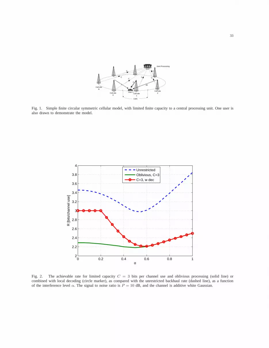
33

User 1

Cell 1

Cell-site1

Cell-site2Cell-site

0

Cell-siteN

RCPC

CC

C C

C

Joint Processing

aca

ab

Fig. 1. Simple finite circular symmetric cellular model, with limited finite capacity to a central processing unit. One user isalso drawn to demonstrate the model.

0 0.2 0.4 0.6 0.8 12

2.2

2.4

2.6

2.8

3

3.2

3.4

3.6

3.8

4

α

R [b

its/c

hann

el u

se]

UnrestrictedOblivious, C=3C=3, w dec

Fig. 2. The achievable rate for limited capacityC = 3 bits per channel use and oblivious processing (solid line) orcombined with local decoding (circle marker), as compared with the unrestricted backhaul rate (dashed line), as a functionof the interference levelα. The signal to noise ratio isP = 10 dB, and the channel is additive white Gaussian.

34

0 0.2 0.4 0.6 0.8 12.8

3

3.2

3.4

3.6

3.8

4

α

R [b

its/c

hann

el u

se]

UnrestrictedOblivious, C=6C=6, w dec

Fig. 3. The achievable rate for limited capacityC = 6 bits per channel use and oblivious processing (solid line) orcombined with local decoding (circle marker), as compared with the unrestricted backhaul rate (dashed line), as a functionof the interference levelα. The signal to noise ratio isP = 10 dB, and the channel is additive white Gaussian.

35

0 0.2 0.4 0.6 0.8 12

2.5

3

3.5

4

4.5

5

5.5

α

R [b

its/c

hann

el u

se]

Unrestricted fading K=1Unrestricted fading K=5

Unrestricted fading K=∞Oblivious, C=3 fading K=1Oblivious, C=3 fading K=5

Oblivious, C=3, fading K=∞fading, C=3, K=∞, w dec

Fig. 4. The achievable rate for limited capacityC = 3 bits per channel use and oblivious processing (solid lines)orcombined with local decoding (circle marker), as compared with the unrestricted backhaul rate (dashed lines), as a functionof the interference levelα. The average per-cell sum signal to noise ratios isP = 10 dB, and the channel is Rayleigh flatfading. Three access protocols are plotted, with TDMA (triangular marker), with WB for five users (square) and with WBfor infinitely many users (pluses).

36

0 0.2 0.4 0.6 0.8 12.5

3

3.5

4

4.5

5

α

R [b

its/c

hann

el u

se]

Unrestricted fading K=1Unrestricted fading K=5

Unrestricted fading K=∞Oblivious, C=6 fading K=1Oblivious, C=6 fading K=5

Oblivious, C=6, fading K=∞fading, C=6, K=∞, w dec

Fig. 5. The achievable rate for limited capacityC = 6 bits per channel use and oblivious processing (solid lines)orcombined with local decoding (circle marker), as compared with the unrestricted backhaul rate (dashed lines), as a functionof the interference levelα. The average per-cell sum signal to noise ratios isP = 10 dB, and the channel is Rayleigh flatfading. Three access protocols are plotted, with TDMA (triangular marker), with WB for five users (square) and with WBfor infinitely many users (pluses).

37

0 5 10 15 20 25 301

2

3

4

5

6

7

SNR [dB]

R [b

its/c

hann

el u

se]

Cut−setOblivious, C=6C=6, w dec

Fig. 6. The achievable rate for limited capacityC = 6 bits per channel use and oblivious processing (solid line) orcombined with local decoding (circle marker), as compared with the upper bound (minimum of unrestricted backhaul rate andthe backhaul rate - dashed line), as a function of the signal to noise ratioP [dB], and the channel is additive white Gaussian.The interference level isα = 0.15.

38

10 15 20 25 301.5

2

2.5

3

3.5

4

4.5

5

5.5

6

SNR [dB]

R [b

its/c

hann

el u

se]

Upper bound, fading K=1Upper bound, fading K=5

Upper bound, fading K=∞Oblivious, C=6 fading K=1Oblivious, C=6 fading K=5Oblivious, C=6, fading K=∞fading, C=6, K=∞, w dec

Fig. 7. The achievable rate for limited capacityC = 6 bits per channel use and oblivious processing (solid lines)orcombined with local decoding (circle marker), as compared with the upper bound (minimum of unrestricted backhaul rateand the backhaul rate - dashed lines), as a function of the average signal to noise ratioP [dB], when the channel is Rayleighfading. The interference level isα = 0.15. Three access protocols are plotted, with TDMA (triangularmarker), with WB forfive users (square) and with WB for infinitely many users (pluses).

39

0 1 2 3 4 5 6 7 80

0.5

1

1.5

2

2.5

3

3.5

C [bits per channel use]

R [b

its/c

hann

el u

se]

Upper boundOblivious, C=6C=6, w dec

Fig. 8. The achievable rate for limited capacityC bits per channel use and oblivious processing (solid line) or combined withlocal decoding (circle marker), as compared with the upper bound (minimum of unrestricted backhaul rate and the backhaulrate - dashed line), as a function of the backhaul capacity [bits per channel use]. The channel is additive white GaussianwithSNR P = 10 dB, and the interference level isα = 0.4.

40

0 1 2 3 4 5 6 7 80

0.5

1

1.5

2

2.5

3

3.5

4

C [bits per channel use]

R [b

its/c

hann

el u

se]

Upper bound, fading K=1Upper bound, fading K=5

Upper bound, fading K=∞Oblivious, fading K=1Oblivious, fading K=5Oblivious, fading K=∞fading, K=∞, w dec

Fig. 9. The achievable rate for limited capacityC bits per channel use and oblivious processing (solid lines)or combinedwith local decoding (circle marker), as compared with the upper bound (minimum of unrestricted backhaul rate and thebackhaul rate - dashed lines), as a function of the backhaul capacity [bits per channel use]. The channel is Rayleigh fadingwith average SNRP = 10 dB, and the interference levelα = 0.4. Three access protocols are plotted, with TDMA (triangularmarker), with WB for five users (square) and with WB for infinitely many users (pluses).

41

−2 −1.5 −1 −0.5 0 0.5 1 1.5 20

0.2

0.4

0.6

0.8

1

1.2

1.4

EbN0 [dB]

Per

−C

ell S

um−

Rat

e [b

its/s

ec/H

z]

Unlimited CapacityLocal Decoding (Approx)Local DecodingOblivious (Approx)Oblivious

Fig. 10. Low-SNR region of the per-cell sum-rate, as a function of Eb

N0for oblivious processing (solid line) and local

decoding (plus marker) along with the corresponding approximation (dashed) and the upper bound (upper dashed line). Thechannel is additive white Gaussian, with interference level α = 0.2, and backhaul capacity of 2 [bits/channel].

42

−2 −1.5 −1 −0.5 0 0.50

0.2

0.4

0.6

0.8

1

1.2

1.4

EbN0 [dB]

Per

−C

ell S

um−

Rat

e [b

its/s

ec/H

z]

Unlimited Capacity

Local Decoding (Approx)

Local Decoding

Oblivious (Approx)

Oblivious

Fig. 11. Low-SNR region of the per-cell sum-rate, as a function of Eb

N0

for oblivious processing (solid line) and localdecoding (plus marker) along with the corresponding approximation (dashed) and the upper bound (upper dashed line). Thechannel is additive white Gaussian, with interference level α = 0.2, and backhaul capacity of 4 [bits/channel].

−2 −1.8 −1.6 −1.4 −1.2 −1 −0.8 −0.6 −0.4 −0.2 00

0.1

0.2

0.3

0.4

0.5

0.6

0.7

0.8

0.9

1

EbN0 [dB]

Per

−C

ell S

um−

Rat

e [b

its/s

ec/H

z]

Unlimited CapacityLocal Decoding (Approx)Local DecodingOblivious (Approx)Oblivious

Fig. 12. Low-SNR region of the per-cell sum-rate, as a function of Eb

N0for oblivious processing (solid line) and local

decoding (plus marker) along with the corresponding approximation (dashed) and the upper bound (upper dashed line). Thechannel is additive white Gaussian, with interference level α = 0.2, and backhaul capacity of 6 [bits/channel].