use of chlorinated carbon materials to make - CORE

USE OF CHLORINATED CARBON MATERIALS TO MAKE

NITROGEN DOPED AND UN-DOPED CARBON

NANOMATERIALS AND THEIR USE IN WATER TREATMENT

by

Winny Kgabo Maboya

Student No: 0310549A

A thesis submitted to the Faculty of Science at the University of the Witwatersrand,

Johannesburg, in fulfilment of the requirements for the degree of

Doctor of Philosophy in Chemistry

Johannesburg, 2018

i | P a g e

DECLARATION

I declare that this thesis is my own work under the supervision of Prof. Sabelo D. Mhlanga and

Prof. Neil J. Coville. It is submitted for the degree of Doctor of Philosophy in the University of

the Witwatersrand, Johannesburg. It has not been submitted before for any degree or

examination in any other University.

------------------------------------------

(Signed) Winny Kgabo Maboya

On this _____________ day of ________________________________2018

ii | P a g e

ABSTRACT

Carbon nanomaterials (CNMs) and nitrogen doped CNMs (NCNMs) with different

morphologies were obtained by decomposition of various chlorinated organic solvents using a

chemical vapor deposition (CVD) bubbling and injection methods over a Fe-Co/CaCO3 catalyst.

CNFs, CNTs with secondary CNT or CNF growth, bamboo-compartmented and hollow CNTs

were obtained. Increasing the growth time to 90 min resulted in growth of ~ 90 % of secondary

CNFs on the surface of the main CNTs, using dichlorobenzene (DCB) as source of chlorine. The

secondary CNFs grew at defects sites of the CNT wall. Secondary CNFs were not observed at

other studied temperatures, 600, 650. 750 and 800 °C.

Using an injection CVD method, horn-, straw- and pencil-shaped closed and open-ended

CNTs/CNFs were obtained from CH3CN/DCB solutions of various volume ratios. CNT growth

was enhanced after addition of chlorine. Highly graphitic carbon materials were produced from

feed solutions containing low and high DCB concentrations. CNTs with defects were obtained

from solutions containing 66.7 vol.% DCB. Post-doping of the N-CNTs with chlorine and of the

chlorinated CNTs with nitrogen resulted in production of highly graphitic materials. Using a

bubbling CVD method, mixtures of CNMs namely, hollow and bamboo-compartmented CNTs

with and without intratubular junctions and carbon nano-onions filled with metal nanoparticles

were obtained from feed solutions containing TTCE.

MWCNT/PVP composite nanofibers were successfully synthesized using an electrospinning

technique. Adsorption capacities of 15–20 g/g were obtained in pure oil or in oil-water mixtures.

The adsorption capability of the MWCNT/PVP composite depended on the type of oil and its

viscosity.

iii | P a g e

DEDICATION

I would like to dedicate this thesis to the following people:

1. My husband (Hosea) and children (Kagiso, Reshoketswe and Phetogo) for bearing with me

throughout this journey.

2. My siblings (Judy, Stephina, Regina, Diana and Happy) for always putting me in their

prayers.

3. My late parents in law (Mr. Kgabo and Mrs. Johanna Maboya). It has always been my father

in law’s wish that I become a doctor one day, this is for him.

4. My parents for bringing me into this world and raising me to be a God fearing woman.

iv | P a g e

ACKNOWLEDGEMENTS

Firstly, I would like to thank God, for giving me strength throughout this journey.

Above all I would like to thank my co-supervisor Professor Neil J. Coville for his outstanding

contribution to this work. His knowledge and expertise enhanced my research and thinking

skills. He gave me a reason to complete this work.

My sincere gratitude to my supervisor Professor Sabelo D. Mhlanga (University of South Africa,

UNISA) for giving me an opportunity to study for my doctoral degree. His valuable contribution

to this work is highly appreciated.

Thank you to the University of the Witwatersrand for providing the facilities to conduct my

research. My sincere gratitude to the microscopy (MMU) unit at the University of the

Witwatersrand for providing instrumental facilities to characterize the materials produced in this

research. Special thanks to Professor Alexander Ziegler, Dr. Reddy, Mr. Geber, Dr. Tetana, Dr.

Maubane and Ms. Duduzile at the MMU unit for their invaluable training on the instruments.

I am grateful to the Vaal University of Technology for proving financial support throughout the

study. Special thanks to Professor Justice Moloto, for always being there especially when it was

tough. His words of encouragement, always trying to secure research money for me, I am

humbled by his kindness. Greatest appreciation to my boss and HOD, Professor Bobby Naidoo,

for always giving me time off when I needed it. Thanks to Dr. Postlet Shumbula from Mintek.

I would also like to extent my appreciation to all CATOMAT group members, past and present.

Special mention to Dr. Isaac Nogwe, Dr. William Dlamini, Ms. Boitumelo Matsoso, Ms. Alice

Magubane, and Mr. Thomas Mongwe.

Thank you to Ms. Dikeledi More for helping me get started on the electrospinning experiments.

Thank you to Mr. Lebea Nthunyane (UNISA), for selflessly helping me with the electrospinning

experiments at UNISA.

v | P a g e

PUBLICATIONS AND PRESENTATIONS

Publications:

1. Winny K. Maboya, Neil J. Coville and Sabelo D. Mhlanga, “The Synthesis of Carbon

Nanomaterials using Chlorinated Hydrocarbons over a Fe-Co/CaCO3 Catalyst”, South

African Journal of Chemistry, 2016, 69, 15–26.

2. Winny K. Maboya, Neil J. Coville and Sabelo D. Mhlanga, “One step synthesis of CNTs

with secondary nanofiber growth: the role of chlorine”, To be published.

3. Winny K. Maboya, Neil J. Coville and Sabelo D. Mhlanga, “Synthesis of chlorinated

nitrogen-doped MWCNTs by injection CVD method”, To be published.

4. Winny K. Maboya, Neil J. Coville and Sabelo D. Mhlanga, “Heteroatom of chlorine and

nitrogen doped carbon nanomaterials using acetonitrile with aromatic and aliphatic

chlorinated solvents: Post-doping treatments”, To be published.

5. Winny K. Maboya, Neil J. Coville and Sabelo D. Mhlanga, “Fabrication of MWCNT/PVP

composite fibers with enhanced interaction formed by chlorinating the MWCNT and their

use as adsorbents for oil”, To be published.

Presentations:

1. W.K. Maboya, “Role of chlorine on the morphology of carbon nanotubes synthesized over

Fe-Co/CaCO3 catalyst”, Poster presentation, Walter Sizulu University, South African

Chemical Institite (SACI) 2013 Conference,

2. W.K. Maboya, “The effect of chlorine in the synthesis of carbon nanomaterials using Fe-

Co/CaCO3 catalysts”, Oral presentation, Nano Africa International 2014 Conference,

vi | P a g e

3. W.K. Maboya, “The synthesis of carbon nanomaterials using chlorinated hydrocarbons over

a Fe-Co/CaCO3 catalyst”, Poster presentation, 27th Annual CATSA Conference 2016, 6 – 9

November 2016.

4. W.K Maboya, “One-step synthesis of CNTs with secondary growth: The role of chlorine”,

Poster presentation, DST/NRF CoE in strong materials research showcase, University of the

Witwatersrand, April 2017.

vii | P a g e

TABLE OF CONTENTS

Title Page Number

DECLARATION i

ABSTRACT ii

DEDICATION iii

ACKNOWLEDGEMENTS iv

PUBLICATIONS AND PRESENTATIONS v

TABLE OF CONTENTS vii

LIST OF FIGURES xiii

LIST OF TABLES xxvii

ABBREVIATIONS xxxii

CHAPTER 1

Introduction 1

1.1 Background and motivation 1

1.2 Aims and objectives 4

1.3 Outline of thesis 4

References 6

CHAPTER 2

Literature Review 8

2.1 Carbon nanotubes 8

2.1.1 Structure of carbon nanotubes 8

viii | P a g e

2.1.2 Synthesis of CNTs 10

(i) Arc discharge method 11

(ii) Laser ablation method 11

(iii)Chemical vapor deposition (CVD) method 12

(iv) The hydrothermal methods 13

2.1.3 Properties of CNTs 14

(i) Mechanical properties 14

(ii) Electrical properties 14

(iii)Thermal properties 15

(iv) Magnetic properties 15

2.2 Modification of carbon nanomaterials 15

2.2.1 Functionalization of carbon nanomaterials 15

2.2.2 Doping of carbon nanomaterials 17

2.2.3 Synthesis of Cl functionalized and chlorinated N-doped CNTs 18

2.3 Carbon nanotube polymer composites 18

2.3.1 Nanocomposites synthesis methods 20

(i) Solution processing 20

(ii) Melt processing 20

(iii)In-situ polymerization 21

(iv) Electrospinning 21

2.4 Treatment of oil-water emulsions by adsorption onto CNT/polymer composites 22

2.4.1 Adsorption studies 24

References 25

CHAPTER 3

The synthesis of carbon nanomaterials using chlorinated hydrocarbons over a Fe-

Co/CaCO3 catalyst 32

3.1 Introduction 32

3.2 Experimental 34

3.2.1 Preparation of catalyst by the wet impregnation method 34

3.2.2 Carbon nanotube synthesis 35

ix | P a g e

3.2.3 Purification of the CNTs 36

3.2.4 Characterization of the catalyst and CNTs 36

3.3 Results and discussion 37

3.3.1 Structural analysis of the Cl-MWCNTs 37

3.3.2 TGA and PXRD analysis 45

3.3.3 Raman spectral analysis 50

3.3.4 Energy dispersive X-ray spectroscopy analysis 52

3.3.5 XPS analysis 53

3.4 Conclusions 54

References 56

CHAPTER 4

One step synthesis of carbon nanotubes with secondary growth: role of chlorine 61

4.1 Introduction 61

4.2 Experimental 62

4.2.1 Materials and Chemicals 62

4.2.2 One-step synthesis of CNTs with secondary growth 62

4.2.3 Synthesis of secondary CNFs using CNTs as substrate 63

4.2.4 Synthesis of secondary CNFs onto primary CNTs using CNTs spread with catalyst

63

4.2.5 Characterization of CNTs 64


4.3.1 Structural analysis of the chlorinated CNTs: Effect of reaction time and

temperature 64

4.3.2 Thermogravimetric analysis of the chlorinated CNTs: Effect of reaction time and

temperature 78

4.3.3 Powder XRD analysis of the chlorinated CNTs: Effect of reaction temperature

83

4.3.4 Raman spectroscopy analysis of the chlorinated CNTs: Effect of reaction time and

temperature 85

x | P a g e

4.4 Conclusion 100

References 102

CHAPTER 5

The synthesis of chlorinated nitrogen-doped multi-walled carbon nanotubes using a Fe-

Co/CaCO3 catalyst by use of an injection CVD method 104

5.1 Introduction 104

5.2 Experimental 106

5.2.1 Chemicals 106

5.2.2 Catalyst preparation by wet impregnation method 107

5.2.3 Synthesis of chlorinated N-CNMs using an injection CVD method 107

5.2.4 Characterization of chlorinated N-MWCNTs 108


5.3.1 Structural analysis of N doped CNMs: Effect of DCB concentration and Injection

flow rate 109

5.3.2 Thermogravimetric analysis of N doped CNMs: Effect of DCB concentration and

injection flow rate 130

5.3.3 Raman spectroscopy analysis of N doped CNMs: Effect of DCB concentration and

injection flow rate 137

5.3.4 XPS analysis of N doped CNMs: Effect of DCB concentration 152

5.4 Conclusion 158

References 161

CHAPTER 6

Heteroatom of chlorine and nitrogen doped carbon nanomaterials using acetonitrile with

aromatic and aliphatic chlorinated solvents: Post-doping treatments 164



6.2.1 Materials and chemicals 167

6.2.2 Synthesis of chlorinated N-doped MWCNTs by a bubbling CVD method 167

xi | P a g e

6.2.3 Post doping of N-MWCNTs with chlorine and of chlorine functionalized MWCNTs

with nitrogen 167

6.2.4 Purification of the CNTs 168

6.2.5 Characterization of the CNTs 168


6.3.1 Synthesis of N-doped CNTs: Effect of DCB concentration 169

6.3.1.1 Structural analysis of the N-doped CNTs: Effect of DCB concentration 169

6.3.1.2 Thermogravimetric analysis of the N-doped CNTs: Effect of DCB concentration

176

6.3.1.3 Raman spectroscopy analysis of the N-doped CNTs: Effect of DCB concentration

180

6.3.1.4 XPS analysis of the N-doped CNTs: Effect of DCB concentration 186

6.3.2 Post doping of chlorinated CNTs and N-doped CNTs 191

6.3.2.1 Structural analysis of post-treated CNTs 192

6.3.2.2 Raman spectroscopy analysis of post-treated CNTs 195

6.3.3 Synthesis of N-doped CNMs: Effect of TTCE concentration and synthesis

temperature 200

6.3.3.1 Structural analysis of the N-doped CNMs: Effect of TTCE concentration and

synthesis temperature 200

6.3.3.2 Thermogravimetric analysis of the N-doped CNMs: Effect of TTCE concentration

and synthesis temperature 211

6.3.3.3 Powder XRD analysis of the N-doped CNMs: Effect of TTCE concentration and

synthesis temperature 218

6.3.3.4 Raman spectroscopy analysis of the N-doped CNMs: Effect of TTCE concentration

and synthesis temperature 222

6.3.3.5 CN elemental analysis of the N-doped CNMs: Effect of TTCE concentration 233

6.4 Conclusions 234

References 236

xii | P a g e

Chapter 7

Fabrication of chlorine functionalized MWCNT/polyvinylpyrrolidone composite nanofiber

mats by electrospinning for use in oil adsorption studies 239



7.2.1 Preparation of PVP and MWCNT/PVP composite nanofibers by electrospinning

243

7.2.2 Adsorption experiments 244

7.2.3 Characterization of the composite nanofibers 245


7.3.1 Study of the influence of electrospinning parameters on the morphology of PVP

nanofibers 246

7.3.2 Effect of the MWCNT content on the morphology of the electrospun PVP

nanofibers 250

7.3.2.1 X-ray diffraction, FTIR spectroscopy and TEM analysis of the materials 254

7.3.3 Oil adsorption capacity of the MWCNT/PVP composite nanofibers 257

7.4 Conclusion 262

References 264

Chapter 8

Summary of conclusions and recommendations 271

Appendix E: Supplementary data 275

xiii | P a g e

LIST OF FIGURES

Chapter 2

Figure 2.1 Schematic representation of carbon allotropes, (a) graphite, (b) diamond, (c)

fullerene, and (d) single wall carbon nanotube (SWCNTs) 9

Figure 2.2 XPS spectra of the O1s region after treatment of CNTs with nitric acid (HNO3) acid

and ozone (O3) 16

Figure 2.3 Chlorination of MWCNTs by mixing I2Cl6 solution with acetic acid or with carbon

tetrachloride 17

Chapter 3

Figure 3.1 Schematic diagram of apparatus used for CNTs synthesis 35

Figure 3.2 TEM image of the purified carbonaceous materials generated using chlorobenzene as

chlorine source 38

Figure 3.3 TEM image of the purified carbonaceous materials generated using dichlorobenzene

as chlorine source. Growth of small carbon materials on the surface of the CNTs. Insert shows

metal particles at tips of CNFs 39

Figure 3.4 TEM images of the purified carbonaceous materials generated using trichlorobenzene

40

Figure 3.5 TEM images of the purified carbonaceous materials generated using toluene 41

Figure 3.6 TEM image of the purified carbonaceous materials generated using dichloroethane as

chlorine source 42

Figure 3.7 TEM images of the purified carbonaceous materials generated using (a)

trichloroethane. Growth of small carbon materials of different shapes on the surface of the CNTs

can be seen in (b) and (c) 43


tetrachloroethane. Bamboo compartments can be seen in (b) 45

xiv | P a g e

Figure 3.9 TGA and corresponding derivative profiles of the purified MWCNT samples

produced using chlorinated benzenes (a and b) and ethanes (c and d) as Cl sources 47

Figure 3.10 XRD spectra of the purified CNTs produced from (a) DCE, (b) TCE, (c) TTCE, (d)

Fe-Co/CaCO3 without chlorine56 (e) CB, (f) DCB and (g) TCB 49

Figure 3.11 Raman spectra of the purified CNTs produced from CB, DCB, TCB and toluene

51

Figure 3.12 Raman spectra of the purified CNTs produced from DCE, TCE and TTCE 51

Chapter 4

Figure 4.1 TEM image of purified CNTs showing secondary CNFs generated using

dichlorobenzene as chlorine source at 60 min reaction time, using the following reaction

conditions: 700 °C, 240 mL/min (N2), 90 mL/min (C2H2) 65

Figure 4.2 TEM images of purified CNTs showing secondary CNFs generated using


conditions: 700 °C, 240 mL/min (N2), 90 mL/min (C2H2) 66

Figure 4.3 HRTEM image of purified CNTs showing the origin of the secondary CNFs growth

synthesized at a 90 min reaction time and 700 °C temperature 67

Figure 4.4 TEM images showing other interesting growth sites of the secondary CNFs from the

main CNTs, synthesized at 90 min and 700 °C 68

Figure 4.5 TEM images of (a) purified CNTs showing secondary CNFs generated using

dichlorobenzene as chlorine source and (b) showing where the secondary growth originates, at

following reaction conditions: 120 min, 700 °C, 240 mL/min (N2), 90 mL/min (C2H2) 70

Figure 4.6 TEM images of purified CNTs generated using dichlorobenzene as chlorine source at

a reaction time of 90 min and reaction temperature of 600 °C 71


a reaction time of 90 min and reaction temperature of 650 (a and b) and 750 (c and d) °C 72

xv | P a g e


a reaction time of 90 min and reaction temperature of 800 °C 73

Figure 4.9 Plot of the relationship between the synthesis temperature and the average outer

diameter of the CNTs produced at 90 min reaction time 75

Figure 4.10 TEM image of purified CNTs spread with catalysts particles over their surface and

bubbled with dichlorobenzene using the following reaction conditions: 60 min, 700 °C, 240

mL/min (N2), 90 mL/min (C2H2) 76

Figure 4.11 TEM image of un-purified CNTs post-doped with chlorine by bubbling

dichlorobenzene through the reactor at the following reaction conditions: 60 min, 700 °C, 240

mL/min (N2), 90 mL/min(C2H2) 77

Figure 4.12 TGA and DTGA curves of un-purified and purified CNTs generated from DCB at

different reaction times 79

Figure 4.13 TGA and DTGA curves of purified CNTs generated from DCB at different reaction

temperatures and a reaction time of 90 min 81

Figure 4.14 (a) Plot of the effect of the synthesis temperature on the amount of residual catalyst

that was left after purification and (b) plot of the effect of the synthesis temperature on carbon

purity, generated from DCB at 90 min and 700 °C 82

Figure 4.15 p-XRD curves of purified CNTs generated from DCB at a reaction time of 90 min

and at different reaction temperatures 84

Figure 4.16 Raman spectra of un-purified and purified chlorinated CNTs synthesized at 700 °C

for 60 min 86


for 90 min 88


for 120 min 90


for 90 min 92

xvi | P a g e


for 90 min 94


for 90 min 96


for 90 min 98

Chapter 5

Figure 5.1 Schematic diagram of the assembled injection CVD setup used for the synthesis of

CNMs 108

Figure 5.2 TEM images of purified MWCNTs generated from pure CH3CN (20 mL) by a CVD

injection method at the following reaction conditions: 0.24 mL/min, 800 °C, 1 h, 240 mL/min

N2, and 90 mL/min C2H2 110

Figure 5.3 TEM images of purified MWCNTs generated from DCB (20 mL) by a CVD injection

method at the following reaction conditions: 0.24 mL/min, 800 °C, 1 h, 240 mL/min N2, and 90

mL/min C2H2 111

Figure 5.4 SEM images and the diameter distribution curves of purified MWCNTs generated

from pure CH3CN (20 mL) by a CVD injection method at the following reaction conditions: 0.24

mL/min, 800 °C, 1 h, 240 mL/min N2, and 90 mL/min C2H2 112


from DCB (20 mL) by a CVD injection method at the following reaction conditions: 0.24

mL/min, 800 °C, 1 h, 240 mL/min N2, and 90 mL/min C2H2 113

Figure 5.6 TEM images of un-purified (a and b) and purified (c and d) CNMs generated from a

66.7:33.3 vol.% CH3CN:DCB reagent synthesized by a CVD injection at an injection rate of 0.24

mL/min 115



mL/min 116

xvii | P a g e


20:80 vol.% CH3CN:DCB reagent synthesized by a CVD injection at an injection rate of 0.24

mL/min. 117

Figure 5.9 SEM images of un-purified (a and b) and purified (c,d,e and f) CNMs generated from

a 66.7:33.3 vol.% CH3CN:DCB reagent synthesized by a CVD injection at an injection rate of

0.24 mL/min 119

Figure 5.10 High magnification SEM images of purified (a, b) CNMs and (c) carbon

nanospheres generated from a 66.7:33.3 vol.% CH3CN:DCB reagent synthesized by a CVD

injection at an injection rate of 0.24 mL/min 120

Figure 5.11 SEM images of un-purified (a and b) and purified (c (with its diameter distribution

curve (d), e and f) CNMs generated from a 33.3:66.7 vol.% CH3CN:DCB reagent synthesized by

a CVD injection at an injection rate of 0.24 mL/min 122


curve (d), e and f) CNMs generated from a 20:80 vol.% CH3CN:DCB reagent synthesized by a

CVD injection at an injection rate of 0.24 mL/min 123

Figure 5.13 High magnification SEM images of purified (a, b) CNMs generated from a 20:80

vol.% CH3CN:DCB reagent synthesized by a CVD injection at an injection rate of 0.24 mL/min

124



mL/min 125



mL/min 126

Figure 5.16 SEM images of un-purified (a and b), purified (c, and d) and high magnification

SEM images of CNMs generated from a 66.7:33.3 vol.% CH3CN:DCB reagent synthesized by a


xviii | P a g e




Figure 5.18 TGA and DTGA curves of un-purified and purified CNMs generated from pure

CH3CN (a & b) and pure DCB (c & d) synthesized by CVD injection at 0.24 mL/min 131

Figure 5.19 TGA and the corresponding derivative profiles of un-purified and purified CNMs

generated by varying the volume ratio of CH3CN:DCB synthesized by a CVD injection at an

injection rate of 0.24 mL/min 134

Figure 5.20 TGA and DTGA curves of the un-purified and purified chlorinated N-CNMs

generated at 0.16 mL/min (a and b) and 0.10 mL/min (c and d) using a CH3CN/DCB (66.7:33.3

vol.%) mixture 136

Figure 5.21 Deconvoluted Raman spectroscopy curves of purified CNMs generated from pure

CH3CN using an injection CVD method at an injection rate of 0.24 mL/min 139

Figure 5.22 Raman spectroscopy curves of un-purified and purified CNTs generated from pure

pure DCB using an injection CVD method at an injection rate of 0.24 mL/min 140

Figure 5.23 Deconvoluted Raman spectroscopy curves of un-purified CNMs generated from

various vol.% of CH3CN:DCB solution using an injection CVD method at an injection rate of

0.24 mL/min 143

Figure 5.24 Deconvoluted Raman spectroscopy curves of purified CNMs generated from various

vol.% of CH3CN:DCB solution using an injection CVD method at an injection rate of 0.24

mL/min 146

Figure 5.25 Deconvoluted Raman spectroscopy curves of un-purified and purified CNMs

generated from a solutions containing 66.7:33.3 vol.% of CH3CN:DCB using an injection CVD

method at an injection rate of 0.16 mL/min 149



method at various injection rates 151

xix | P a g e

Figure 5.27 N 1s XPS spectra of purified CNTs generated from (a) pure CH3CN, (b) 66.7:33.3

(c) 33.3:66.7 and (d) 20:80 vol.% of CH3CN:DCB synthesized by an injection CVD at 0.24

mL/min 155

Figure 5.28 Cl 2p XPS spectra of purified CNTs generated from (a) pure DCB, (b) 66.7:33.3 (c)

33.3:66.7 and (d) 20:80 vol.% of CH3CN:DCB synthesized by an injection CVD at 0.24 mL/min

157

Figure 5.29 XPS data analysis of N-MWCNT and chlorinated N-MWCNTs (a) relative

abundance behavior of different types of nitrogen as a function of chlorine content, bars are

labelled with the type of nitrogen, (b) Raman peak ratio (ID/IG) versus Cl 2p1/2 (C–Cl covalent

bonds) percent, squares on the graph are labelled with the DCB volume percent used 158

Chapter 6

Figure 6.1 TEM images of purified CNMs generated from pure CH3CN at 800 °C, and 240

mL/min N2 and 90 mL/min C2H2 flow 170

Figure 6.2 TEM images of purified CNMs generated from pure DCB at 700 °C, and 240

mL/min N2 and 90 mL/min C2H2 flow 171

Figure 6.3 TEM images of purified CNMs generated from CH3CN feed containing 33.3 vol.%

DCB by bubbling CVD method 172

Figure 6.4 SEM images and diameter distributions curves of purified CNMs generated from

CH3CN feed containing 33.3 vol.% DCB by bubbling CVD method 173

Figure 6.5 TEM images, SEM images and diameter distributions curves of purified CNMs

generated from CH3CN feed containing 66.7 vol.% DCB by bubbling CVD method 174


CH3CN feed containing 66.7 vol.% DCB by bubbling CVD method 175

Figure 6.7 TGA and DTGA curves of un-purified and purified CNMs generated from room

temperature solutions of pure CH3CN (a and b) and pure DCB (c and d) 177

xx | P a g e


temperatures solutions of acetonitrile containing various concentrations of DCB 179

Figure 6.9 Deconvoluted Raman spectra of purified MWCNTs generated from (a) CH3CN and

(b) DCB using a bubbling CVD method. 181

Figure 6.10 Deconvoluted Raman spectra of un-purified (a and b) and purified (c and d)

MWCNTs generated from a feed made of 66.7:33.3 vol.% CH3CN:DCB reagents using a

bubbling CVD method 183

Figure 6.11 Deconvoluted Raman spectra of un-purified (a) and purified (b) MWCNTs

generated from a feed made of 33.3:66.7 vol.% CH3CN:DCB reagents using a bubbling CVD

method 185

Figure 6.12 N 1s and Cl 2p XPS spectra of purified N-MWCNTs generated from (a and b)

66.7:33.3, (c and d) 33.3:66.7 vol.% of CH3CN:DCB and (e) Cl 2p XPS spectra of DCB alone

synthesized by bubbling CVD method 189

Figure 6.13 XPS data analysis of N-MWCNT and chlorine functionalized N-MWCNTs (a)

relative abundance behavior of different types of nitrogen as a function of chlorine content, bars

are labelled with the type of nitrogen, (b) Raman peak ratio (ID/IG) versus Cl 2p1/2 (C–Cl covalent

bonds) percent, squares on the graph are labelled with the DCB volume percent used 191

Figure 6.14 TEM images of purified N-CNTs (a and b) generated after post-doping with DCB as

chlorine source 192

Figure 6.15 TEM images of chlorinated CNTs (a and b) generated after post-doping with

CH3CN nitrogen source 193

Figure 6.16 SEM images and diameter distribution curve of purified N-CNTs post-doped with

chlorine 194

Figure 6.17 SEM images and diameter distribution curves of purified chlorinated CNTs post-

doped with nitrogen 195

Figure 6.18 Deconvoluted Raman spectra of purified N-doped CNTs generated from (a)

CH3CN, and (b and c) after post-treatment with DCB 197

xxi | P a g e

Figure 6.19 Deconvoluted Raman spectra of purified chlorinated CNTs generated from (a) DCB,

and (b and c) after post-treatment with CH3CN 198

Figure 6.20 TEM images of purified CNMs generated from (a and b) tetrachloroethane (TTCE),

(N2 = 280 mL/min, C2H2 = 50 mL/min, T = 700 °C, t = 60 min) 200

Figure 6.21 TEM images obtained from purified CNMs generated from a 75:25 vol.%

CH3CN:TTCE solution mixture (N2 = 280 mL/min, C2H2 = 50 mL/min, T = 800 °C, t = 60 min)

201

Figure 6.22 TEM images obtained from purified CNMs generated from a 66.7:33.3 vol.%


202



203

Figure 6.24 TEM images of purified CNMs generated from a heated solution of acetonitrile (90

°C) (N2 = 240 mL/min, C2H2 = 90 mL/min, T = 800 °C, t = 60 min) 205

Figure 6.25 TEM images of purified CNMs generated from heated solutions of

tetrachloroethane (100 °C) (N2 = 280 mL/min, C2H2 = 50 mL/min, T = 700 °C, t = 60 min)

206



208



209



210

xxii | P a g e


temperature solutions of pure CH3CN (a and b) and pure TTCE (c and d) 212


temperatures solutions of various concentration of TTCE in the acetonitrile feed 214

Figure 6.31 TGA and DTGA curves of un-purified (a and b) and purified (c and d) CNMs

generated from heated solutions of pure CH3CN (90 °C) and pure TTCE (100 °C) 216

Figure 6.32 TGA and DTGA curves of un-purified and purified CNMs generated from heated

(100 °C) solutions of various concentration of TTCE in the acetonitrile feed 217

Figure 6.33 P-XRD spectroscopy of purified CNMs generated from varying the volume ratio of

(a) room temperature and (b) hot (100 °C) mixture of CH3CN:TTCE 221

Figure 6.34 Raman spectra of purified CNTs generated from room temperature solutions of (a)

pure CH3CN and (b) pure TTCE 224

Figure 6.35 Raman spectra analysis of purified CNMs generated from varying the volume ratio

of CH3CN:TTCE solution at room temperature 226

Figure 6.36 Raman spectra of purified CNTs generated from heated solutions of (a) pure

CH3CN (90 °C) and (b) pure TTCE (100 °C). 229

Figure 6.37 Raman spectra of purified CNTs generated from heated solutions of CH3CN:TTCE

(100 °C) of various volume ratios 232

Chapter 7

Figure 7.1 Electrospinning set-up used for fabrication of nanofibers 244

Figure 7.2 SEM images obtained using various concentrations of PVP (a) 30, (b) 35, (c) 40 and

(d) 45 wt.%. The fibers were electrospun from a 1:1 v/v DMF/THF solvent mixture (spinning

conditions: voltage = 15 kV, distance = 16 cm and feed rate = 1 mL/h) 247

Figure 7.3 SEM images of electrospun nanofibers prepared from 40 wt.% PVP in a mixture of

DMF:THF (1:1v/v) applying the voltage of 15 kV at (a) 8, (b) 10, (c) 12, (d) 16 and (e) 18 cm

collector distances 249

xxiii | P a g e


DMF:THF (1:1 v/v) using a 16 cm needle to collector distance at an applied voltage of (a) 11, (b)

13, (c) 15 and (d) 17 kV 250

Figure 7.5 SEM images of nanofibers prepared from 40 wt.% PVP containing (a) 0.4 wt.% (b)

0.5 wt.%, (c) 0.6 wt.% and 0.7 wt.% MWCNTs, electrospun from a mixture of DMF:THF (1:1

v/v) at 15 kV , 16 cm and 1 mL/h applied voltage, collector distance and feed rate 252

Figure 7.6 SEM images of electrospun nanofibers prepared from 40 wt.% PVP_0.5 wt.%

MWCNTs in a mixture of DMF:THF (1:1 v/v) at 16 cm collector distance and an applied voltage

of (a) 11, (b) 13, (c) 15 and (d) 17 kV 253


MWCNTs in a mixture of DMF:THF (1:1) at 16 cm and 15 kV, collector distance and applied

voltage at various injection flow rates (a) 1, (b) 2, and (c) 3 mL/hr 254

Figure 7.8 XRD patterns of purified MWCNTs, pure PVP and PVP/MWCNT-0.5 wt.%

composite nanofibers electrospun from a 1:1 v/v DMF/THF solvent mixture 255

Figure 7.9 FTIR spectra of purified MWCNTs, pure PVP and PVP/MWCNT-0.5 wt.%

composite nanofibers electrospun from a 1:1 v/v DMF/THF solvent mixture 256

Figure 7.10 TEM image of PVP/MWCNT-0.5 wt.% composite nanofibers electrospun from a

1:1 v/v DMF/THF solvent mixture 257

Figure 7.11 Adsorption curves of (a) engine oil, and (b) mineral oil in oil-water mixture oil,

using CNT/PVP composite membranes as adsorbents 259

Figure 7.12 Snapshots showing oil adsorption of the CNT/PVP composite in an oil-water

mixture (a) before oil adsorption, (b) after 4 min of engine oil adsorption, (c) after 1 min and (d)

after 10 min of mineral oil adsorption and (e) after 1 s of dropping the composite in water

containing vegetable oil 259

Figure 7.13 Adsorption curves of pure (a) engine oil, (b) mineral oil and (c) vegetable oil using

CNT/PVP composite membranes as adsorbents 260

xxiv | P a g e

Appendix A: Supplementary Data

Figure S1 TEM images of CNMs generated from dichloroethane as a chlorine source, varying

the flow rate of nitrogen and acetylene 276





Figure S4 Secondary growth on TEM images of MWCNTs generated using dichlorobenzene

(DCB) as chlorine source 278

Figure S5 TEM images of segmented CNF generated using dichloroethane (DCE) as chlorine

source 279

Figure S6 TGA and corresponding derivative profiles of the un-purified MWCNT samples

produced using chlorinated benzenes (a and b) and ethanes (c and d) as chlorine sources 280

Figure S7 TGA and corresponding derivative profiles of the purified MWCNT samples

produced using chlorobenzene (CB) at different acid treatment times 281

Figure S8 Deconvoluted C 1s and Cl 2p XPS spectra of the purified MWCNT samples produced

using chlorobenzene (a and b), dichlorobenzene (c and d) and trichlorobenzene (e and f) 282


using dichloroethane (a and b), trichloroethane (c and d) and tetrachloroethane (e and f) 283

Figure S10 SEM images of purified CNTs generated using DCB at a 90 s reaction time and

reaction temperatures of (a) 600 °C, (b) 650 °C, (c) 700 °C and (d) 750 °C 284

Figure S11 Diameter distribution curves of purified CNTs generated from DCB at various

synthesis temperatures for 90 s 285

Figure S12 SEM images of purified CNTs generated from a 33:3:66.6 vol.% of CH3CN:DCB

synthesized by a CVD injection method at the following reaction conditions: 0.24 mL/min, 800

°C, 1 h, 240 mL/min N2, and 90 mL/min C2H2 286

xxv | P a g e

Figure S13 XPS spectra of purified chlorine functionalized and nitrogen doped CNTs generated

from DCB and CH3CN 287

Figure S14 C 1s XPS spectra of purified CNTs generated from (a) pure CH3CN, (b) pure DCB,

and various volume ratios (c) 66.7:33.3 (d) 33.3:66.3 and (e) 20:80 vol.% of CH3CN:DCB

synthesized by CVD injection at 0.24 mL/min 288

Figure S15 XPS spectra of purified chlorine functionalized nitrogen doped CNTs generated

from CH3CN:DCB solvent mixtures of various volume ratios 289

Figure S16 C 1s XPS spectra of chlorinated CNTs generated from DCB by bubbling CVD

method 289

Figure S17 XPS spectra of chlorinated N-doped CNTs generated from various CH3CN:DCB

solvent mixture by bubbling CVD method 290

Figure S18 C 1s XPS spectra of chlorinated N-doped CNTs generated from (a) 66.7:33.3 and (b)

33.3:66.7 vol.% CH3CN:DCB solvent mixture by bubbling CVD method 290

Figure S19 SEM images of CNMs generated from room temperature solutions of TTCE by a

bubbling CVD method 291

Figure S20 SEM images of CNMs generated from room temperature solution mixtures of

CH3CN:TTCE (75:25 vol.%) by a bubbling CVD method 291


CH3CN:TTCE (66.7:33.3 vol.%) by a bubbling CVD method 292


CH3CN:TTCE (66.7:33.3 vol.%) by a bubbling CVD method 292

Figure S23 SEM images of N-doped CNMs generated from heated solutions of CH3CN (90 °C).

[N2 = 240 mL/min, C2H2 = 90 mL/min, t = 1h and temperature = 800 °C) 293

Figure S24 SEM images of chlorinated CNMs generated from heated solution of TTCE (100

°C). [N2 = 240 mL/min, C2H2 = 90 mL/min, t = 1h and temperature = 800 °C) 294

Figure S25 TEM images of purified CNMs generated from a 75:25 volume ratio of heated

CH3CN:TTCE (heated at 100 °C) 295

xxvi | P a g e

Figure S26 TEM images of purified CNMs generated from a 66.7:33.3 volume ratio of heated




Figure S28 Diameter distribution curves of PVP nanofibers of various concentrations (a) 30

wt.%, (b) 35 wt.%, (c) 40 wt.% and (d) 45 wt.% electrospun from a (1:1 v/v) DMF/THF solvent

mixture 298

Figure S29 Diameter distribution curves of 40 wt.% PVP nanofibers electrospun at various

needle tip to collector distance (a) 8 cm, (b) 10 cm, (c) 12 cm and (d) 18 cm using a (1:1 v/v)

DMF/THF solvent mixture 299

Figure S30 Diameter distribution curves of 40 wt.% PVP nanofibers electrospun by varying the

applied voltage (a) 11 kV, (b) 13 kV, and (c) 17 kV using a (1:1 v/v) DMF/THF solvent mixture

300

Figure S31 Diameter distribution curves of nanofibers prepared from 40 wt.% PVP containing

(a) 0.4 wt.% (b) 0.5 wt.%, (c) 0.6 wt.% and 0.7 wt.% MWCNTs, electrospun from a mixture of

DMF/THF (1:1 v/v) at 15 kV, 16 cm and 1 mL/h applied voltage, collector distance and feed rate

301

Figure S32 Diameter distribution curve of a PVP/MWCNT-0.5 wt.% composite nanofibers

electrospun by varying the applied voltage (a) 11 kV, (b) 13 kV, and (c) 17 kV using a (1:1 v/v)

DMF/THF solvent mixture 302


electrospun by varying the feed rate (a) 2 mL/h, and (b) 3 mL/h 303

Figure S34 Second-order kinetic model for adsorption of (a) engine oil in oil-water emulsions,

(b) pure engine oil, (c) pure mineral oil and (d) pure vegetable oil by MWCNT/PVP composite

membrane 304

xxvii | P a g e

LIST OF TABLES

Chapter 3

Table 3.1 Effect of the reactants on the structure, outer and inner diameters of the purified

MWCNTs 41

Table 3.2 Decomposition temperatures and residual masses (determined by TGA) of the un-

purified and purified (P) chlorinated CNMs 48

Table 3.3 PXRD structural parameters of purified CNTs synthesized in the absence and presence

of chlorine 50

Table 3.4 D-bands, G-bands, 2D-bands and ID/IG ratios of the purified chlorinated CNMs 52

Table 3.5 EDX analysis of Chlorinated-CNMs grown using different chlorinated organic

solvents 52

Table 3.6 XPS analysis of purified chlorine functionalized CNTs grown using different chlorine

sources 54

Chapter 4

Table 4.1 Effect of temperature on the growth of secondary CNFs onto the primary CNTs

74


purified and purified (P) chlorinated MWCNTs generated by varying the reaction time at a

reaction temperature of 700 °C 80

Table 4.3 Decomposition temperatures and residual masses (determined by TGA) of purified (P)

chlorine functionalized CNTs generated by varying the reaction temperature at a reaction time of

90 min 82

Table 4.4 Powder X-ray structural parameters of chlorine functionalized CNTs generated at

various reaction temperatures for 90 min 84

xxviii | P a g e

Table 4.5 Raman bands of the un-purified and purified chlorinated CNTs generated from pure

DCB at 700 °C for 60 min 85













Chapter 5

Table 5.1 Diameters of purified CNMs generated from pure CH3CN and pure DCB synthesized

using an injection CVD method at a 0.24 mL/min injection rate 113

Table 5.2 Diameters analysis of CNMs generated from solutions containing various volume

ratios of CH3CN:DCB synthesized using an injection CVD method at an injection flow rate of

0.24 mL/min 118


purified and purified (P) chlorinated N-MWCNTs generated by injecting different volume ratios

of CH3CN and DCB 131



of CH3CN and DCB 133

xxix | P a g e

Table 5.5 Decomposition temperatures and residual masses of the un-purified and purified (P)

chlorinated N-MWCNTs generated by varying the injecting flow rate of a 66.7:33.3 vol.%

CH3CN/DCB solvent mixture 135


CH3CN using injection CVD method at an injection rate of 0.24 mL/min 138


DCB using injection CVD method at an injection rate of 0.24 mL/min 141

Table 5.8 Raman bands of the un-purified CNMs generated from various volume ratios of a

CH3CN:DCB solution mixture using injection CVD method at an injection rate of 0.24 mL/min

144

Table 5.9 Raman bands of the purified CNMs generated from various volume ratios of a


147

Table 5.10 Raman spectra analysis of the un-purified CNMs generated a 66.7:33.3 vol.%

CH3CN:DCB solution mixture using an injection CVD method at an injection rate of 0.16

mL/min 150



mL/min 152

Table 5.12 Nitrogen content and type of the N-species incorporated in the chlorinated N-

MWCNTs grown at various volume ratios of CH3CN:DCB solution 156

Table 5.13 Binding energy and atomic concentrations of chlorine in the chlorine functionalized

N-MWCNTs grown at various volume ratios of CH3CN:DCB solution 158

Chapter 6


using a bubbling CVD method 169

xxx | P a g e

Table 6.2 Diameters of purified CNMs generated from CH3CN feeds containing various

concentrations of DCB synthesized using a bubbling CVD method 176


purified and purified (P) chlorinated N-MWCNTs generated by bubbling different ratios of a

CH3CN and DCB 178


purified and purified (P) chlorinated N-CNTs generated from solutions containing different

CH3CN:DCB volume ratios 180

Table 6.5 Raman bands of the purified CNMs generated from pure CH3CN and pure DCB using

injection CVD method at an injection rate of 0.24 mL/min 182

Table 6.6 Raman bands of the un-purified and purified CNMs generated from a 66.7:33.3 vol.%


184



186


MWCNTs grown at various volume ratios of CH3CN:DCB solution 188

Table 6.9 Binding energy and atomic concentrations of chlorine in the chlorinated NCMTs

grown at various volume ratios of CH3CN:DCB solution 191

Table 6.10 Raman bands of the purified N-doped CNTs generated from pure CH3CN and after

post-treatment with DCB 196

Table 6.11 Raman bands of the purified chlorinated CNTs generated from pure DCB and after

post-treatment with CH3CN 199


purified and purified (P) chlorine functionalized NCNMs generated by bubbling different ratios

of CH3CN and TTCE at room temperature 215

xxxi | P a g e



of a CH3CN and TTCE at 100 °C 218

Table 6.14 Powder X-ray structural parameters of chlorine functionalized MWCNTs, N-

MWCNTs and chlorine functionalized NCNMs generated using room temperature solutions of

TTCE and CH3CN 219


MWCNTs and chlorinated NCNMs generated using room temperature solutions of TTCE and

CH3CN 220

Table 6.16. Raman bands of the purified CNMs generated from room temperature pure CH3CN

and pure TTCE 223

Table 6.17 Raman bands of the purified chlorinated N-doped CNTs generated from various

volume ratios of room temperature CH3CN and TTCE solution mixtures 227

Table 6.18. Raman bands of the purified CNMs generated from heated solutions of pure CH3CN

and pure TTCE 230


volume ratios of heated solutions of CH3CN containing various TTCE concentrations 233

Table 6.20 CN elemental analysis of the purified NCNTs and chlorine functionalized NCNMs

234

Chapter 7

Table 7.1 Physical properties of the oils and organic reagents used in this study 258

Table 7.2 Adsorption constant and saturation sorption capacity of MWCNT/PVP composite

membrane for various oils 262

xxxii | P a g e

ABBREVIATIONS

a.u. Arbitrary units

BET Brunauer-Emmet-Teller

CB Chlorobenzene

Cl-MWCNTs Chlorinated multi walled carbon nanotubes

CNFs Carbon nanofiber(s)

CNM(s) Carbon nanomaterial(s)

CNSs Carbon nanospheres

CNT(s) Carbon nanotube(s)

CVD Chemical vapor deposition

D Disorder-induced band

DCB Dichlorobenzene

DCE Dichloroethane

EDX Energy dispersive X-ray

FTIR Fourier transform infrared

G Graphitic band

ID/IG ratio Intensity ratio of D to G bands

min minutes

mL/min Milliliter per minute

MWCNTs Multi walled carbon nanotubes

N-CNMs Nitrogen-doped carbon nanomaterials

xxxiii | P a g e

N-CNTs Nitrogen-doped carbon nanotubes

N-MWCNTs Nitrogen-doped multi walled carbon nanotubes

PECVD Plasma-enhanced chemical vapor deposition

PVP Polyvinylpyrrolidone

s seconds

SEM Scanning electron microscopy

SWCNTs Single walled carbon nanotube

r.t. Room temperature

TCB Trichlorobenzene

TCE Trichloroethane

TEM Transmission electron microscopy

TGA Thermogravimetric analysis

TTCE Trichloroethane

XRD X-ray diffraction

XPS X-ray photoelectron spectroscopy

1 | P a g e

CHAPTER 1

Introduction

1.1 Background and motivation

Most materials fit into the following general categories, namely metals, ceramics, ceramics,

organic/inorganic polymers, composites, semi-conductors, biomaterials, and advanced materials,

with carbon nanomaterials being a type of an advanced material. Materials play a major role in

many technological fields and in human lives. Materials are the basis for improving human

production and their living standards1. Whenever there is a new material of great importance, a

huge development in productivity will be received and human society will leap forward1. There

is a need to create a new generation of materials in order to better our lives. In order to create the

new generation of materials, it is necessary to understand the relationship between the existing

materials and their structure. Combination of appropriate materials can result in production of

materials with desirable properties2. Nanoscience has paved the way to tailor the properties and

performance of materials to a new level, as researchers create new materials by working at the

atomic or molecular level.

The need for lightweight, high strength materials has been recognized since the invention of the

airplane. As the strength and stiffness of a material increases, the dimensions, and consequently,

the mass, of the material required for a certain load bearing application is reduced. This leads to

several advantages in the case of aircraft and automobiles such as increase in payload and

improvement of fuel efficiency3.

Since reported by Ijima4, carbon nanotubes (CNTs) proved to be excellent materials because of

their higher strength and low weight. CNTs have become the material of choice for many

applications due to their excellent thermal, mechanical and electronic properties. CNTs are

useful for any application where robustness and flexibility are desired, due to their stability under

extreme chemical environments, high temperatures and moisture5. The unique properties of

CNTs have aroused interest in their possible applications namely, as sensors6, in field emission

2 | P a g e

devices7, as flat panel displays8, for energy storage9, in biomedicine10, as adsorbent materials11,

and in composites12, to name a few.

Application of CNTs in materials and devices is hindered by the difficulty to process and

manipulate them and their inability to be dispersed in most solvents (both water and organic

solvents). Functionalization of CNTs by attaching appropriate chemical groups was found to

enhance their solubility.

In this study CNTs and nitrogen-doped CNTs (NCNTs) were functionalized with chlorine, and

the effect of chlorine on their morphology was studied. Due to the purification properties that

chlorine has, it is expected that the materials produced after chlorination will be more graphitic

and have less amorphous carbon. It has been shown that incorporation of Cl in the CNMs results

in surface functionalisation,13 ease of purification,14 increased yields15 and surface restructuring.16

The synthesized CNTs in this study will then be used as fillers in polymer matrices. The

combination of polymer matrix and CNT as nanofillers offer opportunities for future materials

that can be applied in various fields, namely, in aerospace technology17, drug delivery18,

filtration19, and as sensors20. CNTs have previously been used as fillers for polymer matrix.

However, use of chlorine functionalized CNTs with secondary carbon nanofiber growth as fillers

in polymer matrices has not been reported. The presence of secondary nanofibers on the surface

of the primary CNTs is expected to enhance the surface area of the nanomaterials and in turn

increase the interfacial bonding between the CNTs and the polymer matrix for mechanical

applications. It has been difficult to translate the mechanical properties of CNTs into useful

materials due to interfacial sliding, matrix/fiber dispersion, and the introduction of defects. Even

though these carbon nanotubes have exceptional strength and modulus the difficulty in

dispersing the unmodified nanotubes into polymers, as well as aligning them linearly, makes the

progress on their integration into fiber slow. This problem has been combated through the use of

CNT surface modification by oxidation, functionalization and by physical coating. Fixation of

oxygen is usually carried out by oxidation in a liquid or gas phase but this process is not selective

as it results in functionalization of CNTs with several types of oxygen containing groups, i.e.

COOH, C=O, OH.21 Functionalization of CNT surfaces with oxygen groups often result in

destruction of the CNT structure, mainly decapping at the end of the tubes and cutting and

3 | P a g e

breaking of the tube length. Destruction of the CNT structure may cause changes in their

mechanical properties.

The CNT/polymer composite materials will then be applied as adsorbents for oil in oil-spill

cleanups. Water scarcity has emerged as one of the most serious global challenges which

threatens over one-third of the world’s population22. Recovery and recycling of wastewater has

been two promising ways to combat the water scarcity. Oil is one of the pollutants that can enter

our water streams. Oil spills can affect wildlife, marine and coastal habitats, fisheries and

recreational activities. The oil harms the wildlife through toxic contamination (inhalation and

ingestion) or by physical contact. Use of adsorbents to clean oil-spill was found to be the most

effective. Polymeric materials such as polypropylene and polyurethane foams are the most

commonly used commercial sorbents in oil spill cleanup due to their oleophilic and hydrophobic

characteristics23,24. The disadvantage of using these polymeric materials is that they degrade very

slowly. Hence, in this study PVP was used as polymer since it is easily degradable. Since PVP is

soluble in water we embedded CNTs inside it in order to improve its properties and render it

useful in oil adsorption from oil-water emulsions.

The research questions posed were:

1. What effect does chlorine have on the morphology of the CNTs and NCNTs?

2. Can varying the concentration of chlorine in the feed have an impact on the morphology of

the CNTs and N-CNTs?

3. Does using an injection or bubbling CVD method have an impact on the morphology of

chlorine containing MWCNTs and N-MWCNTs?

4. Can use of chlorine functionalized MWCNTs improve their interaction with the polymer

matrix?

5. Can the chlorine functionalized MWCNT/PVP composite membranes be used as adsorbents

for oil in oil-spill cleanups.

4 | P a g e

1.2 Aims and objectives of the study

1. Investigation of the effect of chlorine on the morphology of carbon nanotubes (CNTs) using

acetylene as carbon source, dichlorobenzene as chlorine source and a Fe-Co/CaCO3 as

catalyst by chemical vapor deposition (CVD) method.

2. Investigation of the effect of chlorine on the morphology of nitrogen-doped carbon nanotubes

(N-MWCNTs) using acetylene as carbon source, dichlorobenzene as chlorine source,

acetonitrile as carbon and nitrogen source and a Fe-Co/CaCO3 as catalyst by injection

chemical vapor deposition (CVD) method.

3. Investigation of the effect of chlorine on the morphology of N-MWCNTs using acetylene as

carbon source, dichlorobenzene as chlorine source, acetonitrile as carbon and nitrogen source

and a Fe-Co/CaCO3 as catalyst by bubbling chemical vapor deposition (CVD) method.

4. Synthesis of chlorine functionalized CNTs/polyvinylpyrrolidone (PVP) composite

nanomaterials using an electrospinning method.

5. Application of the CNTs/PVP composite nanofiber membranes as adsorbents of oil in oil-

spill cleanups.

1.3 Outline of thesis

Chapter 1: Present the background and motivation as well as the aims and objectives of the

study.

Chapter 2: Present a literature review of carbon nanotubes (CNTs), their structure, synthesis

methods, growth mechanisms, their modification by functionalization and doping, and review of

CNT/polymer composites, their synthesis methods and applications and finally a brief review of

application of CNT/polymer composites as adsorbents in oil-spill cleanups.

Chapter 3: Presents the synthesis of chlorine functionalized MWCNTs, their method of synthesis

and various morphologies obtained using various chlorinated organic reagents by bubbling CVD

method.

Chapter 4: Present a one-step synthesis of CNTs with secondary nanofiber growth using

dichlorobenzene as chlorine source by bubbling CVD method. The effect of reaction time and

temperature on the morphology of the CNTs was investigated.

5 | P a g e

Chapter 5: Presents the study on the effect of chlorine on the morphology of N-doped MWCNTs,

and their synthesis method using dichlorobenzene as chlorine source by injection CVD method

Chapter 6: Presents the study on the effect of chlorine on the morphology of N-doped MWCNTs

and their synthesis method using dichlorobenzene and tetrachloroethane as chlorine sources by

bubbling CVD method.

Chapter 7: Presents synthesis of chlorine functionalized MWCNTs/PVP composite nanofiber

membranes by electrospinning method and their use as adsorbents of oil in oil-spill cleanups.

Chapter 8: General conclusions, summarizing the conclusions of all the results of this study and

recommendations from the study.

6 | P a g e

References

1. R.-M. Wang, S.-R. Zheng and Y.-P. Zheng, Polymer Matrix Composites and Technology, 1st

Edition, Science Press, Woodhead Publishing in Materials, 2011.

2. G. Mittal, V. Dhand, K.Y. Rhee, S,-J. Park and W.R. Lee, J. Ind. Eng. Che., 2005, 21, 11-25.

3. S.R. Bakshi, D. Lahiri and A. Agarwal, Int. Mat. Rev., 2010, 55, 41-64.

4. S. Ijima, Nature, 1991, 354, 56-66.

5. S. Sasmal, B. Bhuvaneshwari and N.R. Iyer, Progress in Nanotechnology and

Nanomaterials., 2013, 2, 117-129.

6. P. Soundarrajan, A. Patil, and D. Liming, Am. Vac. Soc., 2002, 1198 – 1201.

7. A.G. Rinzler, J.H. Hafner, P. Nikolaev, P. Nordlander, D.T. Colbert, R.E. Smalley, L. Lou,

S.G. Kim, and D. Tomanek, Science, 1995, 269, 1550 – 1553.

8. Q.H. Wang, A.A. Setlur, J.M. Lauerhaas, J.Y. Dai, E.W. Seelig, and R.H. Chang, Appl. Phys.

Lett., 1998, 72, 399 – 400.

9. M.S. Islam, Y. Deng, L. Tong, S.N. Faisal, A.K. Roy, A.I. Minett, and V.G. Gomes, Carbon,

2016, 96, 701–710.

10. A. Abarrategi, M.C. Gutierrez, C. Moreno-Vicente, V. Ramos, J.L. Lopez-Lacomba, M.L.

Ferrer, and F. del Monte, Biomaterials, 2008, 29, 94 – 102.

11. H.M. Al-Saidi, M.A. Abdel-Fadeel, A.Z. El-Sonbati, and A.A. El-Bindary, J. Mol. Liq.,

2016, 216, 693–698.

12. M. Irfan, H. Basri, M. Irfan and W.-J. Lau, RSC Adv., 2015, 5, 95421 – 95432.

13. W.H. Lee, S.J. Kim, W.J. Lee, J.G. Lee, R.C. Haddon, and P.J. Reucroft, Appl. Surf. Scie.,

2001, 181, 121–127.

14. I. Pełech, U.Narkiewicz, D. Moszyński, and R. Pelech, J. Mater. Res., 2012, 27, 2368–2374.

15. H. Qiu, Z. Shi, L. Guan, L. You, M. Gao, S. Zhang, J. Qiu, and Z. Gu, Carbon, 2006, 44,

516–521.

16. M. A. Keane, G. Jacobs, and P. M. Patterson, J. Colloid Interface Sci., 2006, 302, 576–588.

17. A.H. Esbati and S. Irani, Aerosp. Sci. Technol., 2016, 55, 120-130.

18. X. Zong, K.S. Kim, D. Fang, S. Ran, B.S. Hsiao and B. Chu, Polymer, 2002, 43, 4403 –

4412.

7 | P a g e

19. Z. Tang, C. Qiu, J.R. McCutcheon, K. Yoon, H. Ma, D. Fang, E. Lee, C. Kopp, B.S. Hsiao

and B. Chu, J. Polym. Sci., Part B: Polym. Phys., 2009, 47, 2288 – 2300.

20. Q. Liu, Y. Li, and M. Yang, Sensor Actuat. B Chem., 2012, 161, 967.

21. F. Avile’S, J.V. Cauich-RodríGuez and L. Moo-Tah, Carbon, 2009, 47, 2970-2975.

22. A.G. Volkov, Liquid-Liguid Interfaces: Theory and Methods, CRC Press, Florida, 1996.

23. The International Tanker Owner Pollution Federation Limited, Measures to Combat Oil

Pollution (Graham & Trotman Limited, London, 1980.

24. P. Schatzberg and D.F. Jackson, U.S. Coast Guard Report No. 734209.9 (U.S. Coast Guard

Headquarters, Washington, DC, 1972).

8 | P a g e

CHAPTER 2

Literature review

2.1 Carbon nanotubes

CNTs were first discovered in 1952 from the observation of the tubular nature of some nano-

sized carbon filaments that had been made and studied using transmission electron microscope

(TEM).1 Discovery of multi-walled carbon nanotubes (MWCNTs) was later reported and their

study popularised by Ijima in 1991.2 These MWCNTs were found in the hard deposit growing at

the cathode without a catalyst, during electric arc experiments to produce fullerenes. CNTs have

become the material of choice in most applications due to their excellent thermal, mechanical

and electronic properties. These properties have aroused interest in their possible applications

namely, as sensors and probes3,4, in field emission devices5,6, as flat panel displays7, in

electrochemical devices8,9, for energy storage10, in biomedicine11-13, as adsorbent materials14, and

in composites15-17.

2.1.1 Structure of carbon nanotubes

Based on the electronic configuration of carbon, there is a small energy difference between the

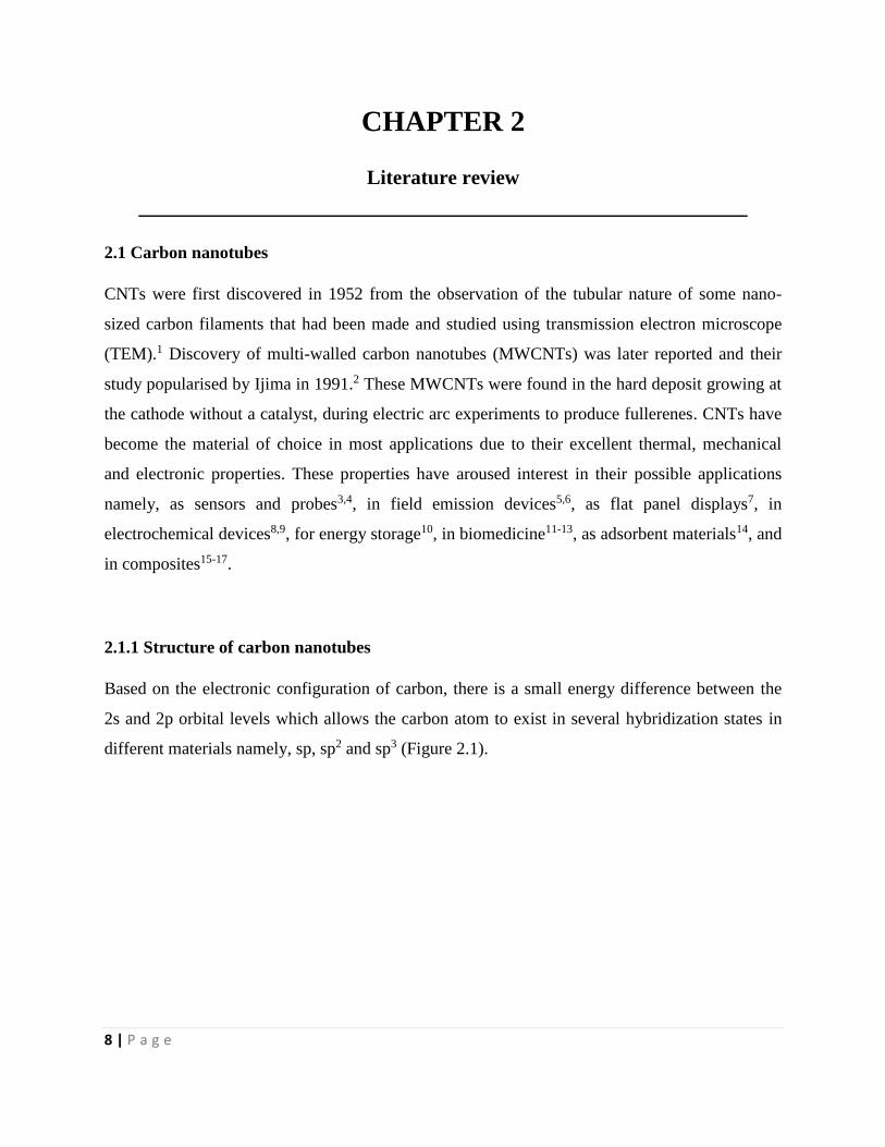
2s and 2p orbital levels which allows the carbon atom to exist in several hybridization states in

different materials namely, sp, sp2 and sp3 (Figure 2.1).

9 | P a g e

Figure 2.1 Schematic representation of carbon allotropes, (a) graphite, (b) diamond, (c)

fullerene, and (d) single wall carbon nanotube (SWCNTs)18.

The carbon atoms can arrange themselves in structures of different dimensions ranging from

diamond (3D), graphite (2D), carbon nanotubes (1D) and fullerene (0D) due to their

hybridization flexibility of the carbon orbitals (Figure 2.1).

In graphite, atoms of carbon form planar layers called graphene layers. Each layer is made up of

rings containing six carbon atoms, linked to each other in a hexagonal structure. Graphite is a

good conductor of electricity due to the presence of mobile electrons.

Diamond, is one of the hardest substances known to man and is a naturally occurring form of

carbon. Each carbon atom is bonded tetrahedrally to four other carbon atoms in an sp3 hybridized

fashion. Its hardness arises from the fact that all the four valence electrons of carbon are all

utilized, hence there are no free electrons available for bonding. Diamond is used in industrial

cutting tools due to its hardness and it is also used for making jewelry.

Amorphous carbon (Ac) is another form of carbon containing varying proportions of sp2 and sp3

bonded carbons. Amorphous carbon is usually formed when a carbon material burns in limited

amount of oxygen. Ac is given several names, such as a lampblack, gas black and channel

black19. It is not considered an allotrope of carbon because its structure is not well defined.

10 | P a g e

Fullerenes are closed-cage carbon molecules with three-coordinate carbon atoms comprising of

spherical or nearly-spherical surfaces. A well-known fullerene molecule is buckminsterfullerene,

C60, which has sixty carbon atoms forming a truncated-icosahedral structure with twelve

pentagonal rings and twenty hexagonal rings20. While regular hexagons can tile a plane,

pentagons can tile a sphere,20. Some sp3 character is present in the essentially sp2 carbons of

fullerenes. It has a structure of a soccer ball.

A carbon nanotube (CNT) is a tubular structure made of carbon atoms, having a nanometer

diameter and a large length/diameter ratio. Carbon nanotubes are a type of carbon fiber which

comprises coaxial cylinders of graphitic sheets, which range from 2 to 50 sheets.

CNT samples are usually found in one of two forms: multi-wall carbon nanotubes (MWCNTs)

consisting of an array of coaxial nanotubes and single-wall carbon nanotubes (SWCNTs)

composed of a single graphene sheet. Diameters of the CNTs usually range between 2 and 25 nm

and the distance between the sheets is about 0.34 nm21.

Three types of SWCNTs exist, namely armchair, chiral and zigzag and each depends on how the

graphene layer is “rolled up” during its creation process. The structure of a SWCNT is

characterized by a pair of indices (n, m) that describe the chiral vector and is directly linked to

the electrical properties of CNTs22. When m = 0 the nanotube is called zigzag, when n = m the

nanotube is called armchair and all other configurations are called chiral23.

MWCNTs can be formed in two structural models; the Russian Doll model and the Parchment

model. When a CNT contains another tube inside it and the outer nanotube has a greater

diameter than the thinner nanotube, it is called the Russian Doll model22. When a single

graphene sheet is wrapped around itself many times, the same as a rolled up scroll of paper, it is

called the Parchment model22.

2.1.2 Synthesis of CNTs

High temperature preparation techniques such as laser ablation and arc discharge have been used

earlier to produce CNTs. These methods have been replaced by low temperature chemical vapor

deposition (CVD) techniques which allow temperatures <800 °C to be used. CVD allows control

11 | P a g e

of the alignment, purity, orientation, length, diameter and density of the CNTs24. CVD can be

used with a wide range of hydrocarbons in any state (solid, liquid or gas. The method enables the

use of various substrates and offers better control of the growth parameters25. The methods used

to synthesis CNTs and other CNMs are discussed below.

(i) Arc discharge method

The electric arc discharge method was the first technique used to synthesize multi-walled and

single-walled CNTs. In this method an electric arc discharge is generated between two graphite

electrodes under an inert atmosphere of helium or argon. A very high temperature is obtained

which allows the sublimation of carbon. The synthesis can be performed by the arc evaporation

of pure graphite or co-evaporation of graphite and a metal26. For the CNTs to be obtained,

purification by gasification with oxygen or carbon dioxide is needed27. The first authors to

successfully produce MWCNTs at the gram level were Ebbesen and Ajayan in 199228.

Substantial amounts of SWCNTs grown over a metal catalyst as substrate, were first produced in

1993 by Bethune and coworkers29. The process parameters used were small gaps between

electrodes (<1 mm), a high current (100 A), and generation of a plasma between the electrode at

about 4000 K and a voltage range of 30–35 V, using controlled electrode dimensions30.

However, the use of an arc discharge method is limited by its drawbacks: the synthesis process is

non-continuous (CNT growth needs to be interrupted to remove the product from the chamber)

and poor product purity.

(ii) Laser ablation method

The second very useful and powerful technique used to produce CNTs is the laser ablation

method. In this process, a piece of graphite is vaporized by laser irradiation under an inert

atmosphere. This results in soot containing nanotubes which are cooled at the walls of a quartz

tube. Two kinds of products are possible: MWCNTs or SWCNTs26. In this process a purification

step by gasification to eliminate carbonaceous material is also needed. The effectiveness of the

gasification depends on the type of reactant used. Growth of high quality SWCNTs was first

12 | P a g e

achieved by Collins and coworkers31. Although the laser ablation method is known to produce

CNTs with high quality and high purity single walls32, it is more expensive to use than the arc

discharge method.

(iii) Chemical vapor deposition (CVD) method

Carbon filaments and fibers have been produced by thermal decomposition of hydrocarbons in

the presence of a catalyst since the 1960s33,34. In the CVD process, metal or bimetallic catalyst

nanoparticles (usually Fe35-37, Co37, Ni38, Fe-Co37,39, or Fe-Ni40) are used as substrates. They are

placed in a quartz boat which is placed in the furnace. The nanoparticles are then subjected to

reduction by heating under an inert carrier gas such as nitrogen or argon until the desired reaction

temperature is achieved. A hydrocarbon gas is then passed into the furnace to grow the

nanotubes. Methane and acetylene are the most widely used carbon sources. Carbon monoxide

can also be used as carbon source. In some cases, liquid carbon sources like toluene, benzene,

methanol, ethanol, etc., are heated and then the inert gas is bubbled through the liquid to

transport their vapors into the furnace. The diameters of the CNTs formed usually depend on the

size of the metal catalyst. The CNT growth can be explained by various mechanisms based on

the catalyst-metal interaction. In situ TEM studies have demonstrated that the nanotube growth

in CVD is initiated by the formation of a carbon cap at the surface of the particle.41 Kuznetsov et

al. hypothesized that the carbon nucleus has the form of a flat saucer whose edges are bent in

order to bond to the metal surface.42 They found that the change in Gibbs free energy for the

formation of the nucleus includes four contributions: the free energy of precipitation of the

carbon atoms from the particle, the free energy associated with the nucleus edges and the strain

energy arising from bending the graphene layer. The model predicts that the critical radius of

nucleus formation decreases with increasing temperature, increasing saturation of the metal-

carbon solution and decreasing specific edge free energy. A good agreement was observed

between the diameter and the average diameter of CNTs formed by different methods as a

function of the catalyst nature and synthesis temperature.42

When the interaction is weak, CNT precipitates out across the metal bottom, pushing the whole

metal particle off the substrate. This is called a “tip-growth model” (Figure 2.2a). When the

13 | P a g e

interaction between the substrate and the metal catalyst is strong, CNT precipitation emerges out

from the metal’s apex, which leads to CNT growing up with the catalyst particle rooted on its

base in a mechanism called “base-growth model” (Figure 2.2b). A stronger metal-support

distribution will improve dispersion, give a narrow size distribution and reduce sintering and

agglomeration of active metal sites. It will also hinder the reduction of the oxide precursors on

the active catalytic species41.

Plasma-enhanced chemical vapor deposition (PECVD) is another CVD method used to produce

CNTs. The PECVD method generates a glow discharge in a chamber or a reaction furnace by

means of a high frequency voltage applied to both electrodes. A substrate is placed on the

grounded electrode. The reaction gas is supplied from the opposite plate in order to form a

uniform film. Catalytic metals such as Co, Fe and Ni are used. They are placed on a Si, SiO2 or

glass substrate using thermal CVD or sputtering. The advantage of using PECVD over the arc

discharge and laser ablation methods is that the synthesis in PECVD uses feedstock gases such

as CH4 and CO, so there is no need for a solid graphite source. The argon-assisted plasma is used

to break down the feedstock gases into C2, CH and other reactive carbon species (CxHy) to

facilitate growth at low temperature and pressure43.

(iv) The hydrothermal methods

The sonochemical/hydrothermal technique is another method used to prepare different carbon

nanostructures such as carbon nano-onions, nanowires, nanorods, nanobelts and MWCNTs.

Horn-shaped CNTs were produced by hydrothermal processing where a mixture of

pentachloropyridine and metallic sodium are placed into a 25 mL stainless steel autoclave44. The

autoclave was sealed, heated to 350 °C and maintained at this temperature for 10 h, and cooled to

room temperature in the furnace. The product was washed sequentially with ethanol,

concentrated salt acid aqueous solution and distilled water to remove impurities. The final

product was then dried at 100 °C in air for 4 h44. The hydrothermal process has advantages when

compared to other methods namely, (i) the starting materials are easy to obtain and are stable in

14 | P a g e

ambient temperature, (ii) it is a low temperature process (about 150 – 180 °C), and (iii) there is

no hydrocarbon or carrier gas required for operation.

2.1.3 Properties of CNTs

CNTs are nanostructured materials which exhibit unique thermal, mechanical, magnetic and

electronic properties. CNT has the same hardness as diamond, but its thermal capacity is twice

that of pure diamond. Its current-carrying capacity is 1000 times higher than that of copper and

they are thermally stable up to 4000 K. CNTs can be metallic or semiconducting, depending on

their diameter and chirality.

(i) Mechanical properties

The mechanical properties of a solid must ultimately depend on the strength of its interatomic

bonds45. CNTs are predicted to have high stiffness and axial strength as a result of the carbon-

carbon sp2 bonding46. A perfect CNT exhibits an elastic modulus of the order 270–950 GPa and

has a reported tensile strength of 11–63 GPa47, which is 10–100 times higher than the strongest

steel and with less weight48. CNTs have the highest Young’s modulus when compared with

composite tubes such as CN, C3N4, BN, BC3, BC2N, etc., These properties, coupled with the

lightness of CNTs, makes them excellent candidates to use in the production of composite

materials for various applications.

(ii) Electrical properties

CNTs can be either metallic or semiconducting depending on their structural parameters, i.e.

chirality and diameter49-52. Carbon nanotubes conduct electricity better than metals. When

electrons travel through the metal there is some resistance to their movement. This resistance

happens when electrons bump into metal atoms. When an electron travels through a carbon

nanotube, it travels under the rules of quantum mechanics, and so it behaves like a wave

15 | P a g e

traveling down a smooth channel with no atoms to bump into. This quantum movement of an

electron within nanotubes is called ballistic transport.

(iii) Thermal properties

As diamond and graphite display the highest known thermal conductivity of all materials at

moderate temperatures, it is likely that nanotubes should be outstanding in this regard53. The

thermal properties of CNTs are related to their unique structure and small size. CNTs have

thermal conductivity values of up to 6600 Wm–1K–1 at low temperatures54.

(iv) Magnetic properties

The presence of encapsulated catalyst nanoparticles inside the CNTs can render them magnetic.

Catalytic nanoparticles can form inside the CNTs via three routes: (1) in situ during CNT growth

(e.g. from a metal especially an iron containing catalyst during CVD synthesis of MWCNTs), (2)

from added metallic catalyst particles e.g. from Fe, Co or Ni metal filled electrodes during

MWCNT or SWCNT synthesis via the arc discharge method, and (3) by filling the synthesized

open-ended CNTs with nonmagnetic liquid metals56. Studies suggested that the presence of iron

catalyst inside CNTs may be helpful in their magnetic manipulation, for example alignment of

CNTs in polymer composites57,58 or for targeted drug delivery59. Tethering of magnetic

nanoparticles onto the surface of the CNTs have been another way of enhancing their magnetic

properties60,61.

2.2 Modification of carbon nanomaterials

2.2.1 Functionalization of carbon nanomaterials

Translation of CNTs into useful materials is often hindered by their limited solubility in water

and most organic solvents. Scientists came up with ways to modify the surface of the CNTs in

order to combat this problem. The surface of the CNTs can be modified by oxidation,

functionalization or by physical coating. Oxidation involves use of oxidizing acids to add oxygen

onto the sidewalls of the CNTs. Fixation of oxygen is usually carried out by oxidation in a liquid

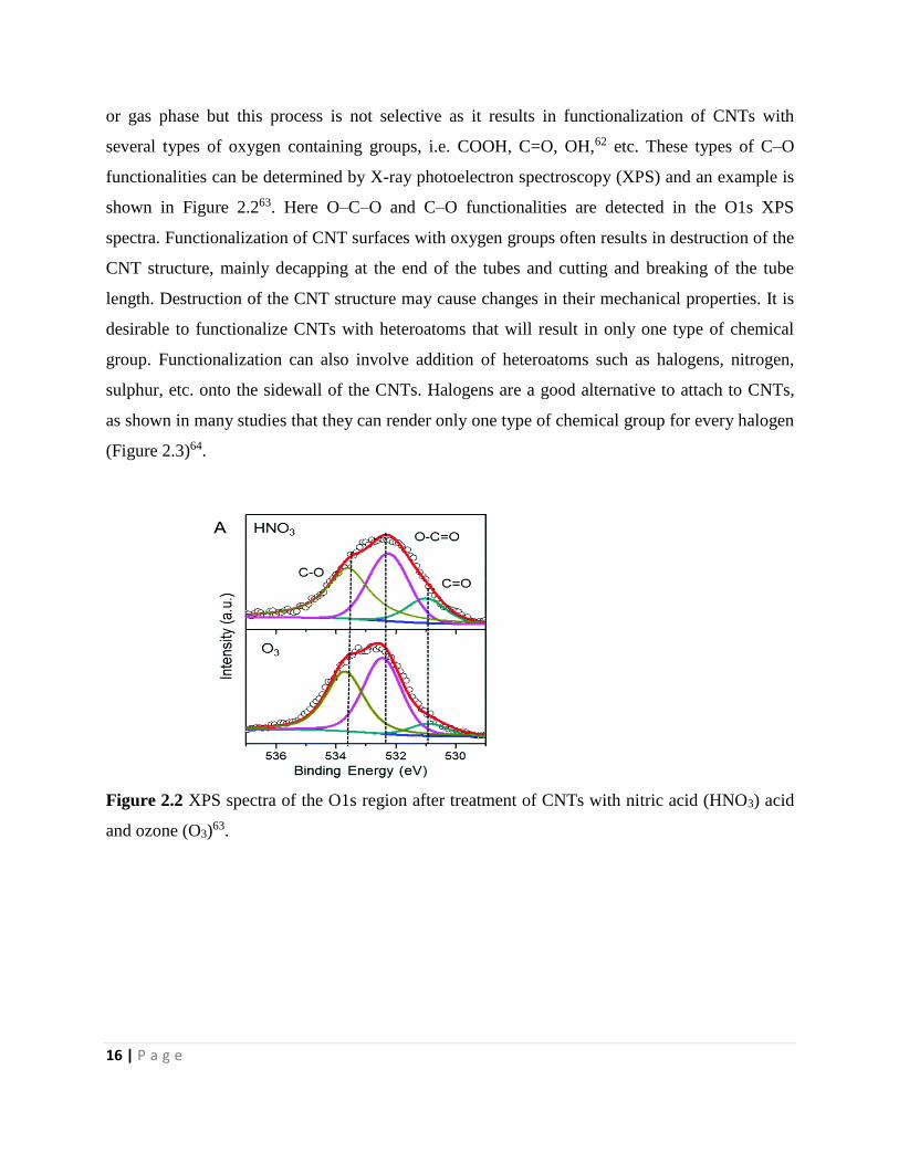
16 | P a g e

or gas phase but this process is not selective as it results in functionalization of CNTs with

several types of oxygen containing groups, i.e. COOH, C=O, OH,62 etc. These types of C–O

functionalities can be determined by X-ray photoelectron spectroscopy (XPS) and an example is

shown in Figure 2.263. Here O–C–O and C–O functionalities are detected in the O1s XPS

spectra. Functionalization of CNT surfaces with oxygen groups often results in destruction of the

CNT structure, mainly decapping at the end of the tubes and cutting and breaking of the tube

length. Destruction of the CNT structure may cause changes in their mechanical properties. It is

desirable to functionalize CNTs with heteroatoms that will result in only one type of chemical

group. Functionalization can also involve addition of heteroatoms such as halogens, nitrogen,

sulphur, etc. onto the sidewall of the CNTs. Halogens are a good alternative to attach to CNTs,

as shown in many studies that they can render only one type of chemical group for every halogen

(Figure 2.3)64.

Figure 2.2 XPS spectra of the O1s region after treatment of CNTs with nitric acid (HNO3) acid

and ozone (O3)63.

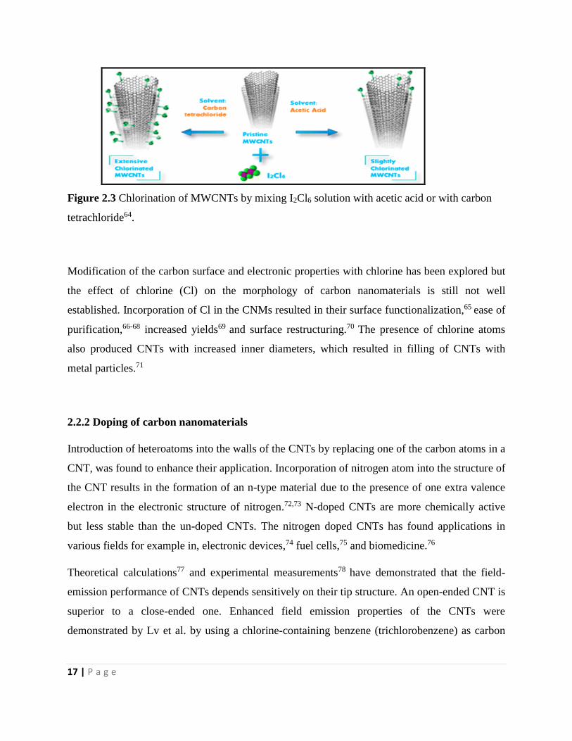
17 | P a g e

Figure 2.3 Chlorination of MWCNTs by mixing I2Cl6 solution with acetic acid or with carbon

tetrachloride64.

Modification of the carbon surface and electronic properties with chlorine has been explored but

the effect of chlorine (Cl) on the morphology of carbon nanomaterials is still not well

established. Incorporation of Cl in the CNMs resulted in their surface functionalization,65 ease of

purification,66-68 increased yields69 and surface restructuring.70 The presence of chlorine atoms

also produced CNTs with increased inner diameters, which resulted in filling of CNTs with

metal particles.71

2.2.2 Doping of carbon nanomaterials

Introduction of heteroatoms into the walls of the CNTs by replacing one of the carbon atoms in a

CNT, was found to enhance their application. Incorporation of nitrogen atom into the structure of

the CNT results in the formation of an n-type material due to the presence of one extra valence

electron in the electronic structure of nitrogen.72,73 N-doped CNTs are more chemically active

but less stable than the un-doped CNTs. The nitrogen doped CNTs has found applications in

various fields for example in, electronic devices,74 fuel cells,75 and biomedicine.76

Theoretical calculations77 and experimental measurements78 have demonstrated that the field-

emission performance of CNTs depends sensitively on their tip structure. An open-ended CNT is

superior to a close-ended one. Enhanced field emission properties of the CNTs were

demonstrated by Lv et al. by using a chlorine-containing benzene (trichlorobenzene) as carbon

18 | P a g e

precursor which resulted in the production of open-ended, thin-walled CNTs filled with long

continuous ferromagnetic metal nanowires.79

Doping of CNTs with nitrogen was also found to improve the field emission property of the

CNTs.80 Thin-walled, open-ended and well-aligned N-doped CNTs synthesized using

acetonitrile as carbon and nitrogen source were found to have enhanced field emission

properties.81 An increase in the amount of nitrogen incorporated into the CNTs was observed

when halogenated catalyst sources were used.82

2.2.3 Synthesis of Cl functionalized CNTs and chlorinated N-doped CNTs

Generally, chlorine functionalization of undoped and nitrogen-doped carbon structures can be

achieved using the same synthesis methods used to produce carbon nanomaterials. In the usual

approach the synthesis process involves pyrolysis of hydrocarbons, or other carbon feedstock

with the addition of a nitrogen source (e.g. nitrogen, ammonia, amines, nitriles) diluted in a

stream of an inert gas in the furnace system over the surface of the metal catalyst particles.

Detailed methods used in this study will be given in Chapters 3 – 6. In general, undoped and

nitrogen-doped carbon structures can be synthesized using two methods:73 (i) “in situ” doping,

where gases of liquids containing ad-atoms either mixed or individually are bubbled through to

the reactor containing a catalyst material using appropriate gases during the synthesis of carbon

nanomaterials, and (ii) post-doping, where the pre-synthesized carbon nanomaterials are post-

treated with a nitrogen precursor (either in liquid or gaseous form).

2.3 Carbon nanotube polymer composites

A composite is a multiphase material formed from a combination of materials which differ in

composition or form. Composites retain their own chemical and physical properties and maintain

an interface between components which act in concert to provide improved specific or

synergistic characteristics not obtainable by any of the original components acting alone.83,84 A

composite is usually made of two components of materials, namely, the reinforcement and the

matrix. The reinforcement provides useful properties such as mechanical, electrical, thermal,

19 | P a g e

optical, etc. needed to enhance the properties of the matrix. The unique mechanical and electrical

properties of carbon nanotubes make them ideal reinforcing agents in many applications. It is

because of their outstanding mechanical properties such as high Young’s modulus, high tensile

strength, high flexibility and high bulk modulus,85 that CNTs promise to be the ultimate fiber

reinforcements in strong, lightweight polymer composite materials. Use of CNTs as fillers in

polymer nanocomposites has been a subject of many studies. Challenges exist in the utilization of

CNTs as fillers in polymer composites, namely CNTs (i) are normally found as mixtures of

various chiralities, diameters and length, (ii) often contain impurities, (iii) occur as aggregates

and bundles which leads to non-uniform dispersion and (iv) have poor interfacial bonding with

the polymer matrix. There have been various reports focusing on increasing the strength and

modulus of the polymer matrices through the incorporation of CNTs. Improvement in tensile

modulus and break stress to about 36-42 and 25 % were achieved when 1 wt.% of MWCNTs

was added to a polystyrene matrix using a solution-evaporation method.86 The modulus and

hardness of the composite was increased by 1.8 and 1.6 times, when 1 wt.% of MWCNTs was

added to polyvinyl alcohol (PVA).87 An increase in the storage modulus was observed when the

MWCNTs loading increased due to a stiffening effect of the nanotubes, during preparation of

poly(methyl methacrylate) (PMMA)/MWCNTs composites by a melt processing method.88 The

indentation elastic modulus and micro-hardness characteristics increased when 1 wt.% of

functionalized and non-functionalized MWCNTs were added to the PMMA matrix.89 Addition of

1 wt.% of MWCNTs to a polycarbonate (PC) matrix resulted in enhancement of the tensile

strength and modulus by up to 23 and 75 % and reduction of their electrical resistivity

significantly from being an insulator to a semi-conductor, indicating a percolation threshold.90

An enhanced electrical conductivity was observed for nanofiber composites consisting of PVA,

MWCNTs and manganese dioxide synthesized by an electrospinning process.91 Alignment of the

MWCNTs into a polyvinylpyrrolidone (PVP) matrix was achieved and resulted in a composite

with improved electromagnetic interference shielding performance.92

20 | P a g e

2.3.1 Nanocomposite synthesis methods

Several synthesis methods have been developed to incorporate CNTs into polymer matrices. The

challenge of producing such nanocomposites is presented by the tendency of CNTs to occur in

bundles or aggregates which are difficult to break up and to disperse in solution which leads to

non-uniform distributions within the polymer matrix. In this section we will briefly describe the

most important processing techniques for synthesis of CNT/polymer nanocomposites.

(i) Solution processing

The most common and simplest technique to form CNT/polymer nanocomposites is solution

processing. The method involves intensive agitation (e.g. magnetic stirring, vigorous shaking,

refluxing, homogenization or even bath/probe sonication) which results in thorough mixing of

the CNTs with a polymer in a solvent, in order to facilitate nanotube de-bundling and their

dispersion inside a host polymer matrix.58,93,94 This processing technique is however limited to

polymers that are soluble in solvents. The process involves dispersion of nanotubes in a suitable

solvent and mixing with the polymer solution, followed by film casting and solvent evaporation

leaving behind a nanocomposite sheet. The solvent for the CNTs and a polymer may be the same

or different, but should be of good miscibility to realize intimate mixing between phases. In

some cases, CNTs are added directly to the polymer solution followed by intensive mixing

before film casting. Use of high power ultrasonication or shear mixing for long periods can lead

to shortening of tube lengths, leading to deterioration of composite properties.

(ii) Melt processing

Due to the fact that thermoplastic semicrystalline polymers soften when heated above their

melting point, melt processing has been a very valuable technique for the fabrication of CNT-

based composites. The method is suitable for polymers that cannot be processed with solution

techniques due to their insolubility in common solvents. In general, melt processing involves the

blending of a polymer melt with the CNT material by application of intense shear forces. The

melt mixing can be carried out in a batch or continuous operation using a high shear mixer (e.g.

21 | P a g e

Sigma mixer) and extruder, respectively. A sigma mixer is often used to prepare highly

concentrated nanocomposites called masterbatches, which may be used to synthesize desired

CNT-loading composites by mixing with appropriate amounts of neat matrix polymer using an

extruder. The polymer granules are caught by the rotating screws and pushed forward; they then

melt inside a heated melting zone due to the externally provided heat and shearing of the material

between screw and barrel. The CNTs are loaded into the extruder via a separate hopper, such that

melt-phase mixing takes place due to the combination of shearing and kneading action, and when

the molten-mixture reaches the homogenization zone, it has already achieved a significant degree

of mixing. Finally, the mixture passes to the die before coming out as semisolid strands, which

may be cooled (via air drying or passing through a water bath) and chopped into granules for

further use. In the melt mixing technique high shear forces and elevated temperatures need to be

properly addressed in order to avoid the deterioration of the nanocomposites.

(iii) In situ polymerization

In situ polymerization remains the only viable option for the preparation of composites based on

insoluble and thermally unstable matrix polymers, which cannot be processed by solution or melt

processing routes. The main advantage of this method is that it produces polymer-grafted tubes,

mixed with free polymer chains. Moreover, due to the small size of the molecules, the

homogeneity of the resulting composite adduct is much higher when compared to mixing CNTs

and polymer chains in solution. The method allows the preparation of composites with high CNT

weight percent. The synthesis involves dispersion of CNTs in a monomer, followed by in situ

polymerization leading to the formation of CNT/polymer nanocomposites. Exploitation of

functionalized CNTs or use of monomer-grafted CNTs are known to improve the initial

dispersion of the nanotubes in the monomer and consequently in the formed nanocomposites.

(iv) Electrospinning

Electrospinning is a versatile method used to produce continuous nanofibers mainly from

polymer solutions. Electrospinning involves pumping a polymer solution at a constant rate

22 | P a g e

through a needle tip that is placed a set distance away from a grounded or oppositely charged

collector. When a voltage is applied at the needle tip, an electrostatic field introduces charges in

the solution and when the mutual repulsions between charges reach a threshold value, a fluid jet

forms a conical droplet at the tip of a capillary tube, resulting in the formation of a Taylor cone.95

The jet travels in a straight path, called the jet’s length, and experiences bending instabilities to

form spiral motions. The polymer fiber is collected on a screen, which is either grounded or

connected to a DC supply of opposite polarity.

2.4 Treatment of oil-water emulsions by adsorption onto CNT/polymer composites

Water scarcity is becoming a huge problem all over the world due to contamination of water,

rapid growth of population, development of an economy and lack of rain. Recently, in Gauteng

and Cape Town, water restrictions were put into place due to alarming low water levels in the

water collection and distribution dams. Clean water is essential for both human life and the

ecosystem. A higher demand for fresh water has forced researchers to look for alternative

sources to treat wastewater.

Oil spillage in water bodies can have negative environmental and socio-economical impacts. Oil

spill pollution can be due to petroleum hydrocarbon discharged into the environment (marine or

land). This can be caused by accidental spillage or operational spillage whenever oil is produced

or transported.96 Oil spills can affect wildlife species, marine and coastal habitats, fisheries and

recreational arears. The oil harms the wildlife through toxic contamination (inhalation and

ingestion) or by physical contact. The adverse impacts to ecosystems and the long-term effects of

environmental pollution by these and other releases call for a need to develop a wide range of

materials for cleaning up oil from oil impacted areas. The effectiveness of oil treatment varies

with time, the type of oil and spill, the location and the weather conditions.97 Among all of the

oil spill cleanup methods that show good results in removal of oil from the water surface, the

sorbent cleaning-up is considered to be one of the most efficient method to remove oil.98 The

contact of oil with a highly adsorbent material can be a way to collect the oil that is present in

water.96 Stokes’ Law indicates that, given time and enough surface area, oil and water will

eventually separate, forming two layers. Oil will float on top of the water forming a thin layer

23 | P a g e

called a slick since it has a lower density than water. A wide range of adsorbents materials have

been used for oil remediation such as mineral products (zeolites, silica, perlite, graphite,

vermiculites, sorbent clay, diatomite),99,100 vegetable products (corn cob, straw, kenaf, cotton

fiber, wood fiber, peat moss, etc.,),100,101 organic synthetic products (propylene, polyurethane,

etc.,),102,103 activated carbon,104 and CNT sponges.105 Polymeric materials such as polypropylene

and polyurethane foams are the most commonly used commercial sorbents in oil spill cleanup

because of their oleophilic and hydrophobic characteristics.106,107 A major disadvantage of using

polymer materials is that they degrade very slowly in comparison with the mineral or vegetable

products and are not as naturally occurring as mineral products.101,106, 108,109

Effective dispersion of MWCNTs in PVP during creation of composite materials has been

reported, and PVP was found to reduce the aggregation effect of CNTs. However, application of

a nanocomposite of PVP with functionalized MWCNTs in water treatment has rarely been

reported. This is because PVP is a highly polar, non-ionic, amphiphilic, and water-soluble

polymer, that can swell in aqueous media.110-112 PVP has been used as a hydrophilizing additive

in a variety of CNT/polymer composites, since it increases the number and size of pores in the

composites.113,114 Chang et al. fabricated a graphene oxide/PVP based PVDF membrane via

hydrogen bonding and van der Waals forces.115 They observed that without graphene oxide, an

increasing amount of PVP tended to create larger pores in the PVDF/PVP membranes, and most

of the PVP was washed away during membrane fabrication.115 However, addition of graphene

oxide to the membrane resulted in its interaction with PVP, reducing PVP leaching and

enhancing the anti-fouling properties of the membranes.115

A few studies have been done on oil adsorption using CNT/PVP composite membranes. Nan et

al. fabricated CNT/PVP composite nanofibers by electrospinning for oil adsorption.116 CNTs

were found to be stuck and tightly embedded on the surface of PVP fibers, making it easy to

utilize CNTs in the adsorption of the oil. The composites showed a high oil adsorption capacity

of ~ 1 g/cm3, which is higher than that of a carbon sponge (~ 0.7 to 0.8 g/cm3).105 Castro et al.

fabricated silica-supported PVP filtration membranes via a graft polymerization process for use

in the treatment of oil-in-water emulsions. They found that incorporation of PVP improved

selectivity and reduced the fouling tendency of the membranes due to an increased hydrophilicity

of the membrane.117

24 | P a g e

2.4.1 Adsorption studies

The sorption capacity of the adsorbent is usually expressed in grams of pollutant (e.g. oil)

absorbed by an adsorbent per gram of the adsorbent used (i.e. g.g–1):

Qt = 0

0

m

mmt (1)

where Qt (g.g–1) is the adsorption capacity of the adsorbent at a certain time t(s), mt (g) is the

weight of the adsorbent after adsorption and m0 (g) is the initial weight of the adsorbent. The

sorption capacity will reach a saturated value Qm (g.g–1) when Qt does not change with t.

The sorption kinetics process has been used for CNT sponges105 and was described using a

second-order adsorption model.118,119

ktQQQ mtm

11 (2)

where Qt is the sorption capacity at time t, Qm is the saturated sorption capacity, t is the sorption

time, and k is the sorption constant, which is related to the viscosity, surface tension of the oil

and the pore structure of the CNT sponge. The slope of a t/qt vs t curve gives the saturated

sorption capacity, Qm and the intercept can be used to calculate the sorption constant, k.

In this study the role of chlorine on the morphology of un-doped and nitrogen-doped carbon

nanomaterials will be explored. The effect of using chlorine functionalized CNTs to facilitate

interaction between CNTs and polymer matrix in formation of CNT/polymer matrix will also be

investigated. The composite materials will then be applied as adsorbents for oil in oil spill

cleanups. To date, production of chlorine functionalized CNT/polymer matrices has never been

reported. Studies on use of chlorinated materials during synthesis of nitrogen-doped carbon

nanomaterials surfaced recently. The study involved use of chlorine containing catalysts rather

than chlorinated organic solvents as it is in our case. Hence this will also present some novelty.

25 | P a g e

References

1. L.V. Radushkevich, and V.M. Lukyanovich, Zurn Fisic Chim, 1952, 26, 88–89.

2. S. Ijima, Nature, 1991, 354, 56–66.

3. P. Soundarrajan, A. Patil, and D. Liming, Am. Vac. Soc., 2002, 1198–1201.

4. P. Kim, and C.M. Lieber, Science, 1999, 286, 2148.

5. A.G. Rinzler, J.H. Hafner, P. Nikolaev, P. Nordlander, D.T. Colbert, R.E. Smalley, L. Lou,

S.G. Kim, and D. Tomanek, Science, 1995, 269, 1550 – 1553.

6. W.A. de Heer, A. Châtelain and D. Ugarte, Science, 1995, 270, 1179 – 1180.

7. Q.H. Wang, A.A. Setlur, J.M. Lauerhaas, J.Y. Dai, E.W. Seelig, and R.H. Chang, Appl. Phys.

Lett., 1998, 72, 399 – 400.

8. J. Wu, W.-W. Liu, Y.-X. Wu, T.-C. Wei, D. Geng, J. Mei, H. Liu, W.-M. Lau and L.-M. Liu,

Electrochim. Acta, 2016, 203, 21 – 29.

9. V. Thirumal, A. Pandurangan, R. Jayavel, S.R. Krishnamoorthi and R. Ilangovan, Curr.

Appl. Phys., 2016, 16, 816 – 825.

10. M.S. Islam, Y. Deng, L. Tong, S.N. Faisal, A.K. Roy, A.I. Minett, V.G. Gomes, Carbon,

2016, 96, 701–710.

11. A. Abarrategi, M.C. Gutierrez, C. Moreno-Vicente, V. Ramos, J.L. Lopez-Lacomba, M.L.

Ferrer, and F. del Monte, Biomaterials, 2008, 29, 94 – 102.

12. N.W.S. Kam, M. O’Connell, J.A. Wisdom and H. Dai, Proc. Natl. Acad. Sci. USA, 2005,

102, 11600 – 11605.

13. M.I. Sajid, U. Jamshaid, T. Jamshaid, N. Zafar, H. Fessi, and A. Elaissari, Int. J. Pharm.,

2016, 501, 278–299.

14. H.M. Al-Saidi, M.A. Abdel-Fadeel, A.Z. El-Sonbati, A.A. El-Bindary, J. Mol. Liq., 2016,

216, 693–698.


16. Z. Rahimi, A.A.L. Zinatizadeh and S. Zinadini, J. Ind. Eng. Chem., 2015, 29, 366 – 374.

17. H. Yu, T. Huang, M. Lu, M. Mao, Q. Zhang and H. Wang, Nanotechnology, 2013, 24,

405401 (1 – 9), doi:10.1088/0657-4484/24/40/405401.

18. K. Singh, A. Ohlan and S.K. Dhawan, Nanocomposites – New Trends and Developments,

Intech Open Science, dx.doi.org/10.5772/50408, 2012.

26 | P a g e

19. H.O. Pierson, Handbook of Carbon, Graphite, Diamond and Fullerenes, William Andrew

Publishing, Norwich, 1993.

20. C.N.R. Rao, R. Seshadri, A. Govindaraj and R. Sen, Mat. Sci. Eng. R, 1997, 15, 209–262.

21. P.M. Ajayan, Chem. Rev., 1999, 99, 1787.

22. A. Eatemadi, H. Daraee, H. Karimkhanloo, M. Kouhi, N. Zarghami, A. Akbarzadeh, M.

Abasi, Y. Hanifepour and S.W. Joo, Nanoscale Res. Lett., 2014, 9, 393 (1–13).

23. N. Salfuddin, A.Z. Raziah and A.R. Junizah, J. Chem., 2013, 676815 (1–18),

dx.doi.org/10.1155/2013/676815.

24. Z.B. He, J.L. Maurice, C.S. Lee, C.S. Cojocaru and D. Pribat, Arabian J. Sci. Eng. Sect. B,

2010, 35, 19-28.

25. M. Kumar and Y. Ando, J. Nanosci. Nanotech., 2010, 10, 3739-3758.

26. C. Journet and P. Bemier, Appl. Phys. A, 1998, 1-9.

27. K. Morishita and T. Takarada, J. Mater. Sci., 1999, 34, 1169-1174.

28. T.W. Ebbesen and P.M. Ajayan, Nature, 1992, 358, 220-222.

29. D.S. Bethune, C.H. Kiang, M. de Vries, G. Gorman, R. Savoy, J. Vazquez, and R. Beyers,

Nature, 1993, 363, 605-607.

30. M. Paradise and T. Goswami, Mater. Des., 2007, 28, 1477-1489.

31. P.G. Collins, A. Zettl, H. Bando, A. Thess and R.E. Smalley, Science, 1997, 278, 100 – 103.

32. M. Chiang, K. Liu, T. Lai, C. Tsai, H. Cheng and I. Lin, J. Vac. Sci. Technol. B, 2001, 19,

1034-1039.

33. R.T.K. Baker, Carbon, 1989, 27, 315.

34. G.G. Tibbetts, Carbon, 1989, 27, 745.

35. M.C. Bahome, L.L. Jewell, D. Heidebrandt, D. Glasser and N.J. Coville, Appl. Catal., A,

2005, 287, 60-67.

36. S. Maghsoodi, A. Khodadadi and Y. Mortazavi, Appl. Surf. Sci., 2010, 256, 2769-2774.

37. E. Couteau, K. Hernadi, J.W. Seo, L. Thiên-Nga, Cs. Mikó, R. Gaál and F. Forró, Chem.

Phys. Lett., 2003, 378, 9-17.

27 | P a g e

38. C. Branca, F. Frusteri, V. Magazú and A. Mangione, J. Phys. Chem., B, 2004, 108, 3469-

3473.

39. T.C. Schmitt, A.S. Biris, D.W. Miller, A.R. Biris, D. Lupu, S. Trigwell and Z.U. Rahman,

Carbon, 2006, 44, 2032-2038.

40. T. Tsoufis, P. Xidas, L. Jankovic, D. Gournis, A. Saranti, T. Bakas and M.A. Karakassides,

Diamond Relat. Mater., 2007, 16, 155-160.

41. V. Jourdain, and C. Bichara, Carbon, 2013, 58, 2 – 39.

42. V.L. Kuznetsov, A.N. Usoltseva, A.L. Chuvilin, E.D. Obraztsova, and J.M. Bonard, Phys.

Rev. B, 2001, 64, 235 – 401.

43. K. Varshney, Int. J. Eng. Res. Gen. Sci., 2014, 2, 660-677.

44. X. Wu, Y. Tao, C. Mao, L. Wen and J. Zhu, Carbon, 2007, 45, 2253 – 2259.

45. V.K. Thakur, M.K. Thakur and M.R. Kessler, Handbook of Composites from Renewable

Materials, Nanocomposite: Science and Fundamentals, Volume 7, John Wiley & Sons, 2017.

46. S.J. Tans, R.M. Verschueren and C. Dekker, Nature, 1998, 393, 49 – 52.

47. M. Yu, Science, 2000, 287, 637-640.

48. E. Thoteson, Z. Ren and T. Chou, Compos. Sci. Technol., 2001, 61, 1899-1912.

49. H. Dai, E.W. Wong and C.M. Lieber, Science, 1996, 272, 523-526.

50. T.W. Odom, J.L. Huang, P. Kim and C.M. Lieber, Nature, 1998, 391, 62-64.

51. N. Hamada, S. Sawada and A. Oshiyama, Phys. Rev. Lett., 1992, 68, 1579.

52. R. Saito, M. Fujita, G. Dresselhaus and M.S. Dresselhaus, Phys. Rev. B, 1992, 45, 6234.

53. J. Hone, M.C. Llaguno, M.J. Biercuk, A.T. Johnson, B. Batlogg, Z. Benes and J.E. Ficher,

Appl. Phys. A, 2002, 74, 339-343.

54. S. Berber, Y.K. Kwon and D. Tomanek, Phys. Rev, Lett. 2000, 84, 4613.

55. P. M. Ajayan, T. W. Ebbesen, T. Ichihashi, S. Iijima, K. Tanigaki, and H. Hiura, Nature

(London), 1993, 362, 522–525.

56. P. M. Ajayan, and S. Ijima, Nature (London),1993, 361, 333–334.

57. D.A. Walters et al., Chem. Phys. Lett., 2001, 338, 14 – 20.

58. E. Thostenson, C. Li and T. Chou, Compos. Sci. Technol., 2005, 65, 491 – 516.

59. V. Gupta and R.K. Kotnala, Angew. Chem. Int. Ed., 2012, 51, 2916 – 2919.

60. S.T. Hussain, S.R. Gilani, S.D. Ali and H.S. Bhatti, J. Alloys Compd., 2012, 544, 99 – 104.

61. S.D. Ali, S.T. Hussain and S.R. Gilani, Appl. Surf. Sci., 2013, 271, 118 – 124.

28 | P a g e

62. F. Avile’S, J.V. Cauich-RodríGuez and L. Moo-Tah, Carbon, 2009, 47, 2970-2975.

63. J. Luo, Y. Liu, H. Wei, B. Wang, K.-H. Wu, B. Zhanga and D.S. Su, Green Chem., 2017, 19,

1052 – 1062.

64. V.K. Abdelkader, M. Domingo-García, M.D. Gutiérrez-Valero, R. López-Garzón, M.

Melguizo, C. García-Gallarín, F.J. López-Garzón, and M.J. Pérez-Mendoza, J. Phys. Chem.,

C, 2014, 118, 2641 – 2649.

65. W.H. Lee, S.J. Kim, W.J. Lee, J.G. Lee, R.C. Haddon, and P.J. Reucroft, Appl. Surf. Sci.,

2001, 181, 121–127.

66. J-M. Yuan, X-H. Chen, X-H Chen, Z-F Fan, X- Yang, and Z-H.Chen, Carbon, 2008, 46,

1266–1269.


68. J. Barkauskas, I. Stankevičiene, and A. Selskis, Sep. Pur. Tech., 2010, 71, 331–336.


516–521.

70. A.N. Márquez, J. L. Valverde, and M.A. Keane, Appl. Catal. A: Gen., 2007, 332, 237–246.

71. R. Lv, F. Kang, W. Wang, J. Wei, J. Gu, K. Wang, and D. Wu, Carbon, 2007, 45, 1433–

1438.

72. S.H. Lim, H.I. Elim, X.Y. Gao, A.T.S. Wee, W. Ji, J. Y. Lee and J. Lin, Phys. Rev., B, 2006,

73, 045402.

73. C.P. Ewels and M. Glerup, J. Nanosci. Nanotechnol., 2005. 5, 1345-1363.

74. P. Avouris, and J. Chen, Mater. Today., 2006, 9, 46 – 54.

75. S. Ratso, I. Kruusenberg, A. Sarapuu, P. Rauwel, R. Saar, U. Joost, J. Aruväli, P. Kanninen,

T. Kallio, and K.Tammeveski, J. Power Sources, 2016, 332, 129 – 138.

76. Y. Zhao, Y. Tang, Y. Chen, and A. Star, ACS. Nano, 2012, 6, 6912–6921.

77. G. Zhou, W.H. Duan and B.L. Gu, Phys. Rev. Lett., 2001, 8709(9):095504-1–4.

78. M.S. Wang, L.M. Peng, Y.J. Wang, C.H. Jin and Q. Chen, J. Phys. Chem. B, 2006, 110,

9349-9402.

79. R. Lv, F. Kang, D. Zhu, Y. Zhu, X. Gui, J. Wei, J. Gu, D. Li, K. Wang and D. Wu, Carbon,

2009, 47, 2709-2715.

http://www.sciencedirect.com/science/article/pii/S0378775316312319#!










29 | P a g e

80. Y.H. Lai, H.B. Lian and K.Y. Lee, Diamond Relat. Mater., 2009, 18, 544 – 547.

81. T. Cui, R. Lv, F. Kang, Q. Hu, J. Gu, K. Wang and D. Wu, Nanoscale Res. Lett., 2010, 5,

941-948.

82. L.M. Ombaka, P.G. Ndungu, B. Omondi, J.D. McGettrick, M.L. Davies, and V.O. Nyamori,

J. Solid State Chem., 2016, 235, 202–211.

83. I.M. Daniel, Engineering mechanics of composite materials, Oxford University Press, 2006.

84. P. Saini, Fundamentals of Conjugated Polymer Blends, Copolymers and Composites, John

Wiley & sons, Inc., 1-118, http://doi.wiley.com/10.1002/9781119137160.ch1, 2015.

85. M.M.J. Treacy, T.W. Ebbesen, and J.M. Gibson, Nature, 1996, 381, 678-680.

86. D. Qian, E.C. Dickey, R. Andrews and T. Rantell, Appl. Phys. Lett., 2000, 76, 2868 – 2870.

87. M. Cadek, J.N. Coleman, V. Barron, K. Hedicke and W.J. Blau, Appl. Phys. Lett., 2002, 81,

5123 – 5125.

88. Z. Jin, K.P. Pramoda, G. Xu and S.H. Goh, Chem. Phys. Lett., 2001, 337, 43-47.

89. G. Zamfirova, V. Gaydarov, F. Faraguna, E. Vidović and A. Jukić, Colloids Surf., A:

Physicochem. Eng. Aspects, 2016, 510, 169-175.

90. W. Thaithae, C. Antonio and P. Wattanachai, Asia-Pac. J. Chem. Eng., 2016, 11, 34-50.

91. M.F.M.A. Zamri, S.H.S. Zein, A.Z. Abdullah and N. I. Basir, Int. J. Eng. Technol. IJET-

IJENS., 2011, 11, 15-21.

92. K. Nasouri, A. Mousavi, and M.R.M. Mojtahedi, Polym. Compos., 2016, 23774, doi

10.1002/pc.23774.

93. P.-C. Ma, N.A. Siddiqui, G. Marom and J.-K. Kim, Compos. Part Appl. Sci. Manuf., 2010,

41, 1345-1367.

94. L. Jin, C. Bower and O. Zhou, Appl. Phys. Lett., 1998, 73, 1197-1199.

95. P.R. Kumar, N. Khan, S. Vivekanandhan, N. Satyanarayana, A.K. Mohanty and M. Misra, J.

Nanosci. Nanotechnol., 2012, 12, 1 – 25.

96. R.V. Maulion, S.A. Abacan, G.G. Allorde and Ma. C.S. Umali, Asia Pacific Journal of

Multidisciplinary Research, 2015, 3, 146 – 151.

97. M. Fingas, Chem. Ind., 1996, 24, 1005 – 1008.

98. Artemiev A.V., Pinkin A.V. Sorption Techniques to Clean Up Water from Oil Pollutions.

Water: Chemistry and Ecology. 2008; 1, 19-25.

http://doi.wiley.com/10.1002/9781119137160.ch1

30 | P a g e

99. R.W. Melvold, S.C. Gibson, and R. Scarberry, Sorbents for liquid Hazardous Substance

Cleanup and Control, Noyes Data Corp., Park Ridge, NJ, 1988.

100. P. Scharzberg, U.S. Coast Guard Report No.724110.1/2/1, U.S. Coast Guard

Headquarters, Washington, DC, 1971.

101. H.M. Choi and R.M. Cloud, Environ. Sci. Technol., 1992, 26, 772 – 776.

102. H.T.T. Duong, and R.P. Burford, J. Appl. Polym. Sci., 2006, 99, 360 – 367.

103. D. Ceylan, S. Dogu, B. Karacik, S.D. Yakan, O.S. Okay and O. Okay, Environ. Sci.

Technol., 2009, 43, 3846 – 3852.

104. K. Okiel, M. El-Sayed and M.Y. El-Kady, Egypt. J. Petroleum, 2011, 20, 9 – 15.

105. X. Gui, H. Li, K. Wang, J. Wei, Y. Jia, Z. Li, L. Fan, A. Cao, H. Zhu and D. Wu, Acta

Mater., 2011, 59, 4798 – 4804.

106. The International Tanker Owner Pollution Federation Limited, Measures to Combat Oil

Pollution: The improvement of oil spill response within the European Community, Graham

& Trotman Limited, London, 1980.

107. P. Schatzberg and D.F. Jackson, U.S. Coast Guard Report No. 734209.9, U.S. Coast

Guard Headquarters, Washington, DC, 1972.

108. M. Toyoda, J. Aizawa, and M. Inagaki, Desalination, 1998, 115, 199 – 201.

109. C. Teas, S. Kalligeros, F. Zanikos, S. Stournas, E. Lois, and G. Anastopoulos,

Desalination, 2001, 140, 259 – 264.

110. Q. Yang, T.-S. Chung and M. Weber, J. Membr. Sci., 2009, 326, 322 – 331.

111. M. Sun, Y. Su, C. Mu and Z. Jiang, Ind. Eng. Chem. Res., 2009, 49, 790 – 796.

112. J. Barzin, S. Madaeni, H. Mirzadeh, and M. Mehrabzadeh, J. Appl. Polym. Sci., 2004, 92,

3804 – 3813.


114. K. Zhu, G. Wang, S. Zhang, Y. Du, Y. Lu, R. Na, Y. Mu and Y. Zhang, RSC Adv., 2017,

7, 30564 – 30572.

115. X. Chang, Z. Wang, S. Quan, Y. Xu, Z. Jiang and L. Shao, Appl. Surf. Sci., 2014, 316,

537 – 548.

116. D. Nan, J. Wei, F. Guo, G. Fan, F. Xu, L. Li, H. Zhu, K. Wang and D. Wu, J. Nanosci.

Nanotechnol., 2014, 14, 6461 – 6465.

117. R.F. Castro, Y. Cohen, and H.G. Monbouquette, J. Membr. Sci., 1996, 115, 179 – 190.

31 | P a g e

118. D. Bastani, A.A. Safekordi, A. Alihosseini, and V. Taghikhani, Sep. Purif. Technol.,

2006, 52, 295 – 300.

119. Z. Yaneva, and B.J. Koumanova, J. Colloid Interf. Sci., 2006, 293, 303 – 311.

32 | P a g e

CHAPTER 3

The synthesis of carbon nanomaterials using chlorinated hydrocarbons over a

Fe-Co/CaCO3 catalyst

3.1 Introduction

Nanotechnology is a topic that is attracting the interest of scientists in academia, research

institutions and industry as well as government officials and journalists. Carbon nanotubes

(CNTs) and carbon nanomaterials (CNMs) in general are key components in the progress of

nanotechnology. Polyhedral carbon clusters (fullerenes) were discovered in 19851 and this

eventually led to the seminal studies on carbon nanotubes (CNTs) by Ijima in 1991.2 CNTs offer

opportunities for the development of novel material systems because they possess unique

electronic properties,3 exhibit high thermal conductivity,4 and mechanical properties5 such as

stiffness, strength and resilience. SWCNTs were observed to exhibit an electrical current density

of ~ 4 × 109 A cm–2 and single-layer graphene sheet was found to possess thermal conductivities

in the range ~ 4.84 × 103 to 5.30 × 103 W/mk.3,4 An effective increase in the strength to ~17 GPa

for of double-walled CNTs bundles5 and ~60 GPa for multi-walled carbon nanotubes (CNTs)6

was achieved by applying high-energy electron irradiation, which crosslinks inner shells and

tubes. These unique properties render CNTs suitable for application in various fields for

example, their use in environmental monitoring,7 in water purification,8 as tips for atomic force

microscope probes,9 as catalyst supports10, in field emission devices11, as chemical sensors12, and

in fuel cells.13 Methods for making CNTs such as arc discharge, laser ablation, and catalytic

chemical vapor deposition (CCVD) have been developed.14 To date the production of CNTs by

the CCVD method remains the preferred route for their large scale production.

A limitation related to the use of CNTs in many applications has always been the difficulty in

dispersing them in solvents. Scientists have thus functionalized the outer walls of CNTs with

various groups like halogens and carboxylic groups to improve their solubility. Chemical

modification of CNTs surface to fine tune their properties has thus led to the creation of new

materials.16 Doping of the carbonaceous materials with non-carbon atoms, such as nitrogen,12-19

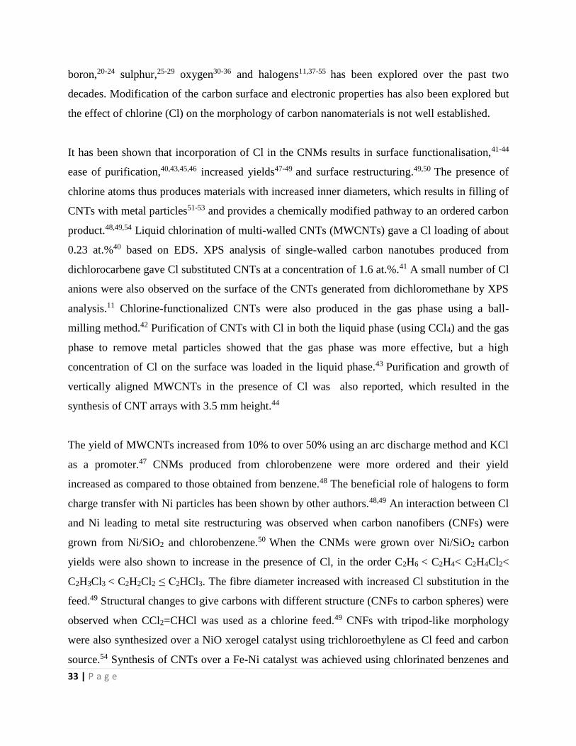
33 | P a g e

boron,20-24 sulphur,25-29 oxygen30-36 and halogens11,37-55 has been explored over the past two

decades. Modification of the carbon surface and electronic properties has also been explored but

the effect of chlorine (Cl) on the morphology of carbon nanomaterials is not well established.

It has been shown that incorporation of Cl in the CNMs results in surface functionalisation,41-44

ease of purification,40,43,45,46 increased yields47-49 and surface restructuring.49,50 The presence of

chlorine atoms thus produces materials with increased inner diameters, which results in filling of

CNTs with metal particles51-53 and provides a chemically modified pathway to an ordered carbon

product.48,49,54 Liquid chlorination of multi-walled CNTs (MWCNTs) gave a Cl loading of about

0.23 at.%40 based on EDS. XPS analysis of single-walled carbon nanotubes produced from

dichlorocarbene gave Cl substituted CNTs at a concentration of 1.6 at.%.41 A small number of Cl

anions were also observed on the surface of the CNTs generated from dichloromethane by XPS

analysis.11 Chlorine-functionalized CNTs were also produced in the gas phase using a ball-

milling method.42 Purification of CNTs with Cl in both the liquid phase (using CCl4) and the gas

phase to remove metal particles showed that the gas phase was more effective, but a high

concentration of Cl on the surface was loaded in the liquid phase.43 Purification and growth of

vertically aligned MWCNTs in the presence of Cl was also reported, which resulted in the

synthesis of CNT arrays with 3.5 mm height.44

The yield of MWCNTs increased from 10% to over 50% using an arc discharge method and KCl

as a promoter.47 CNMs produced from chlorobenzene were more ordered and their yield

increased as compared to those obtained from benzene.48 The beneficial role of halogens to form

charge transfer with Ni particles has been shown by other authors.48,49 An interaction between Cl

and Ni leading to metal site restructuring was observed when carbon nanofibers (CNFs) were

grown from Ni/SiO2 and chlorobenzene.50 When the CNMs were grown over Ni/SiO2 carbon

yields were also shown to increase in the presence of Cl, in the order C2H6 < C2H4< C2H4Cl2<

C2H3Cl3 < C2H2Cl2 ≤ C2HCl3. The fibre diameter increased with increased Cl substitution in the

feed.49 Structural changes to give carbons with different structure (CNFs to carbon spheres) were

observed when CCl2=CHCl was used as a chlorine feed.49 CNFs with tripod-like morphology

were also synthesized over a NiO xerogel catalyst using trichloroethylene as Cl feed and carbon

source.54 Synthesis of CNTs over a Fe-Ni catalyst was achieved using chlorinated benzenes and

34 | P a g e

it was observed that the hollow degree of the CNTs increased with an increase in Cl content in

the feed, which resulted in the CNTs being filled with a Fe-Ni alloy.51 Previous work in our

group has also shown that the use of chlorobenzene can facilitate growth of CNTs with a large

inner cavity.53 The participation of Cl was found to play an important role in the synthesis of

turbostratic CNFs by pyrolysis of a 1,2-dichloroethane/ethanol mixture in the presence of a

nickel catalyst.55 Ni-Cl bonding on the surface of the catalyst created a poor crystalline layer,

leading to a coarse surface which caused the disordered precipitation of carbon species and thus

the formation of turbostratic CNFs.55 Most of the studies of the role of chlorine on the

morphology of the CNMs have been investigated using a nickel or iron-nickel catalyst.

In previous studies by our group it was found that a Fe-Co/CaCO3 catalyst can be used to make

good quality CNTs56,57 and nitrogen doped CNTs.58 To further explore the role of this catalyst

we have investigated the role of chlorine on the morphology of CNTs produced by pyrolysis of

various chlorine-substituted benzene and ethane feeds using a CCVD method. The results of the

study are shown below.

3.2 Experimental

Fe(NO3)3·9H2O (Sigma Aldrich) ≥ 98 %, Co(NO3)2·6H2O (Sigma Aldrich) ≥ 98 %, CaCO3

(Sigma Aldrich) ≥ 99 %, HNO3 (Sigma Aldrich) ≥ 98 % ACS, chlorobenzene (CB) (Merck), >

99 % GC, 1,2-dichlorobenzene (DCB) (Sigma Aldrich) 99 % Reagent plus, 1,2,4-

trichlorobenzene (TCB) (Sigma Aldrich) 99 % GC, 1,2-dichloroethane (DCE) (BDH reagent)

AnalaR grade, 1,1,2-trichloroethane (TCE) (Fluka Chemika) > 98 % GC, 1,1,2,2-

tetrachloroethane (TTCE) (UniLAB SAARChem) 98 % GLC and toluene (UniLab SAARChem,

Merck) ACS reagent grade, were used. All the reagents were commercially available and used

without further purification.

3.2.1 Preparation of catalyst by the wet impregnation method56,57

Fe(NO3)3.9H2O and Co(NO3)2.6H2O were used to prepare the catalyst. Calculated amounts of

the Fe and Co nitrates were weighed and mixed in a beaker. The salts were then dissolved using

35 | P a g e

30 mL of distilled water to make a 0.3 mol/L Fe and 0.3 mol/L Co precursor solution. The metal

solution was then transferred to a burette and added dropwise while stirring to a 10 g CaCO3

support that was placed in a beaker. The mixture was stirred for 30 min. The beaker containing

the metal-support mixture was then dried paced in an oven for drying at 120 °C for 12 h. The

metal-support solid was then cooled to room temperature, transferred to a mortar and ground

with a pestle, followed by screening through a 150 µm molecular sieve. The catalyst powder was

then calcined at 400 °C for 16 h in a static air oven. This catalyst was completely characterized

as reported in an earlier article.56

3.2.2 Carbon nanotube synthesis

The catalyst (1.0 g) was spread in a quartz boat (120 mm × 15 mm) and the boat was placed in

the center of a quartz tube. The furnace was then heated to 700 °C at a rate of 10 °C/min under

flowing N2 (50 mL/min). Once the temperature reached 700 °C, the N2 flow rate was set to 240

mL/min and C2H2 was set at 90 mL/min for chlorinated benzenes; for chlorinated ethanes flow

rates were set at 280 mL/min N2 and 50 mL/min C2H2, respectively. Both gases were bubbled

through a chlorinated organic solvent, before introduction into a quartz tube. After 60 min of

reaction time, the C2H2 flow and bubbling was stopped and the system was left to cool down to

room temperature under a continuous flow of N2 (50 mL/min). The reaction setup is shown in

Fig. 1. The quartz boat was then removed from the reactor and the carbon deposit (Cl-

MWCNTs) that formed was weighed.

Figure 3.1 Schematic diagram of apparatus used for CNTs synthesis

36 | P a g e

3.2.3 Purification of the CNTs

Purification of the CNT materials was adapted from Mhlanga et al.56 The carbon materials

produced were added into a beaker, followed by addition of 30% HNO3. The material mixture

was stirred in acid at room temperature for at least 30 minutes. The acid-treated carbon materials

were then filtered over a Whatman No.1 filter paper and the deposits on the filter paper were

washed with distilled water until the filtrates were neutral (~ pH 7). A pH meter was used to

measure the final pH of the filtrates. The carbon materials obtained were then dried in an oven at

120 °C for 12h, weighed and stored in a glass vial.

3.2.4 Characterization of the CNTs

The morphology and size distribution of the CNTs before and after HNO3 acid treatment were

analyzed by transmission electron microscopy (TEM) using a FEI TECNAI G2 SPIRIT. The

samples for TEM analysis were prepared by sonication in ethanol and thereafter deposited on a

holey carbon-coated TEM Cu grid. The percentage yield of the carbon deposit (% C) was

determined as described elsewhere.59 The CNTs were also characterized by Raman spectroscopy

using a Jobin-Yvon T6400 micro-Raman spectrometer. Excitation was provided by the 532 nm

green laser with spectral resolution of 3-5 cm-1. The impurity content of the CNTs was monitored

by thermogravimetric analysis (TGA) using a Perkin Elmer TGA 7. The sample was loaded onto

a platinum pan and heated to 900 °C at a heating rate of 5 °C/min, in a flowing air and nitrogen

stream both at 20 mL/min. The phase composition of the samples was determined by powder X-

ray diffraction (PXRD) using a D2 Bruker PXRD with a continuous scan mode using CoKα

radiation. The scan range was 10–90 2θ degree. The presence of chlorine species in the CNT

samples was determined by energy dispersive X-ray spectroscopy (EDX) incorporated into the

SEM. XPS analysis was performed using a PHI 5000 Versaprobe – Scanning ESCA Microprobe

operating with a 100 µm 25 W 15 kV Al monochromatic X-ray beam. The samples were

sputtered with 2 kV 2 µA 1 ×1 mm raster – Ar ion gun at a sputter rate of about 18 nm/min for

60 seconds.

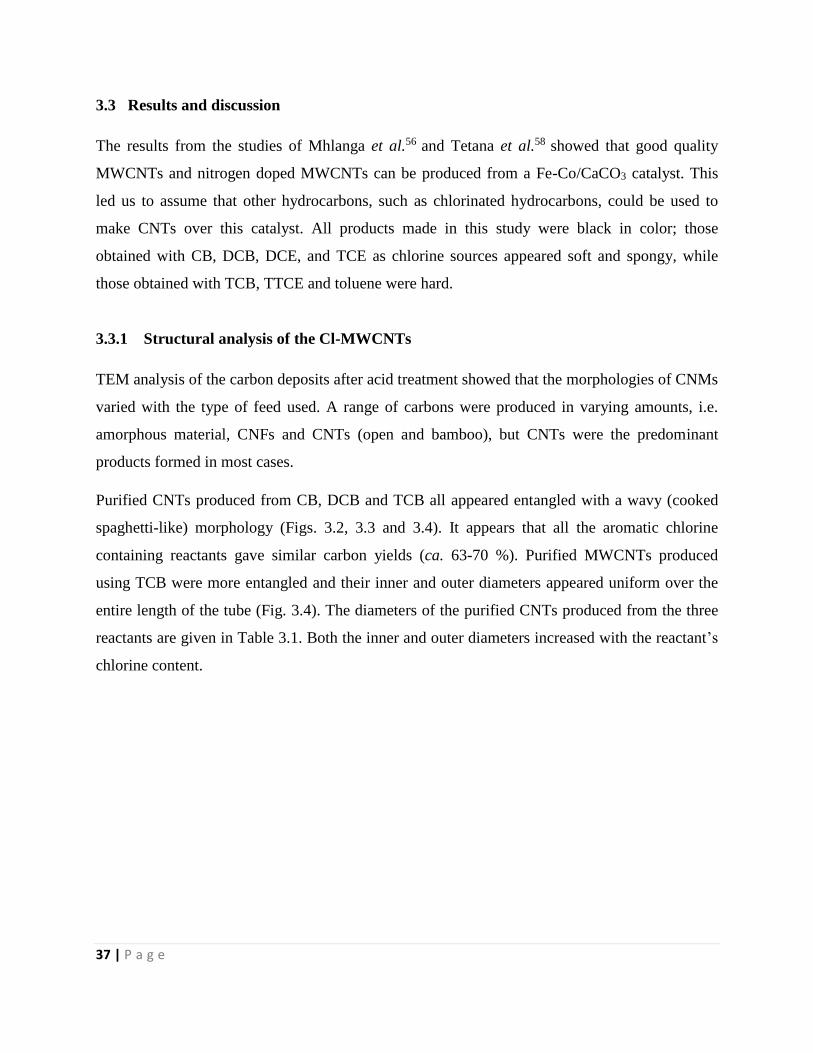
37 | P a g e

3.3 Results and discussion

The results from the studies of Mhlanga et al.56 and Tetana et al.58 showed that good quality

MWCNTs and nitrogen doped MWCNTs can be produced from a Fe-Co/CaCO3 catalyst. This

led us to assume that other hydrocarbons, such as chlorinated hydrocarbons, could be used to

make CNTs over this catalyst. All products made in this study were black in color; those

obtained with CB, DCB, DCE, and TCE as chlorine sources appeared soft and spongy, while

those obtained with TCB, TTCE and toluene were hard.

3.3.1 Structural analysis of the Cl-MWCNTs

TEM analysis of the carbon deposits after acid treatment showed that the morphologies of CNMs

varied with the type of feed used. A range of carbons were produced in varying amounts, i.e.

amorphous material, CNFs and CNTs (open and bamboo), but CNTs were the predominant

products formed in most cases.

Purified CNTs produced from CB, DCB and TCB all appeared entangled with a wavy (cooked

spaghetti-like) morphology (Figs. 3.2, 3.3 and 3.4). It appears that all the aromatic chlorine

containing reactants gave similar carbon yields (ca. 63-70 %). Purified MWCNTs produced

using TCB were more entangled and their inner and outer diameters appeared uniform over the

entire length of the tube (Fig. 3.4). The diameters of the purified CNTs produced from the three

reactants are given in Table 3.1. Both the inner and outer diameters increased with the reactant’s

chlorine content.

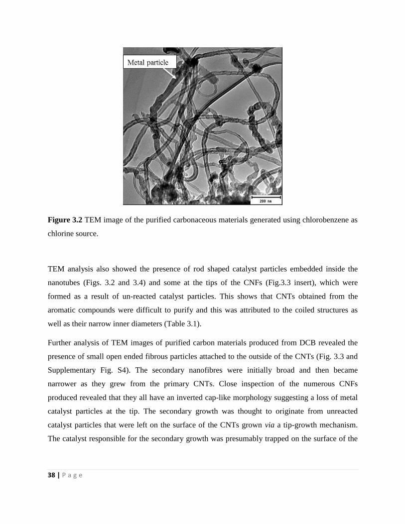
38 | P a g e

Figure 3.2 TEM image of the purified carbonaceous materials generated using chlorobenzene as

chlorine source.

TEM analysis also showed the presence of rod shaped catalyst particles embedded inside the

nanotubes (Figs. 3.2 and 3.4) and some at the tips of the CNFs (Fig.3.3 insert), which were

formed as a result of un-reacted catalyst particles. This shows that CNTs obtained from the

aromatic compounds were difficult to purify and this was attributed to the coiled structures as

well as their narrow inner diameters (Table 3.1).

Further analysis of TEM images of purified carbon materials produced from DCB revealed the

presence of small open ended fibrous particles attached to the outside of the CNTs (Fig. 3.3 and

Supplementary Fig. S4). The secondary nanofibres were initially broad and then became

narrower as they grew from the primary CNTs. Close inspection of the numerous CNFs

produced revealed that they all have an inverted cap-like morphology suggesting a loss of metal

catalyst particles at the tip. The secondary growth was thought to originate from unreacted

catalyst particles that were left on the surface of the CNTs grown via a tip-growth mechanism.

The catalyst responsible for the secondary growth was presumably trapped on the surface of the

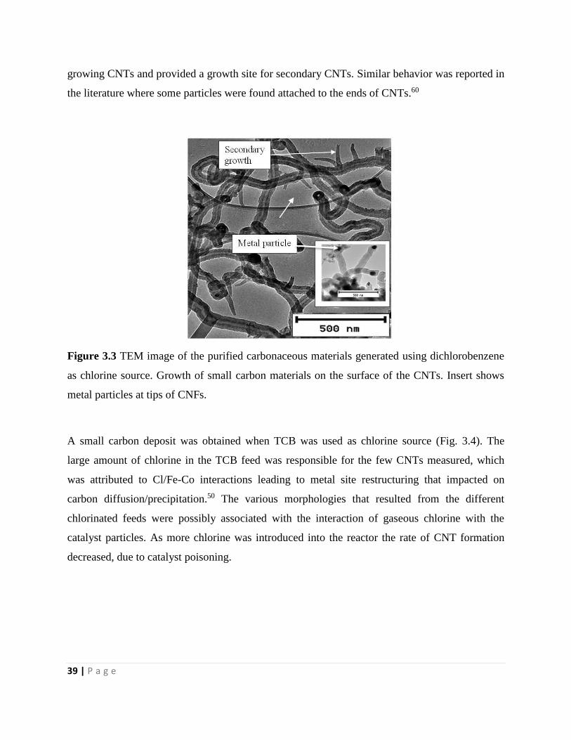
39 | P a g e

growing CNTs and provided a growth site for secondary CNTs. Similar behavior was reported in

the literature where some particles were found attached to the ends of CNTs.60

Figure 3.3 TEM image of the purified carbonaceous materials generated using dichlorobenzene

as chlorine source. Growth of small carbon materials on the surface of the CNTs. Insert shows

metal particles at tips of CNFs.

A small carbon deposit was obtained when TCB was used as chlorine source (Fig. 3.4). The

large amount of chlorine in the TCB feed was responsible for the few CNTs measured, which

was attributed to Cl/Fe-Co interactions leading to metal site restructuring that impacted on

carbon diffusion/precipitation.50 The various morphologies that resulted from the different

chlorinated feeds were possibly associated with the interaction of gaseous chlorine with the

catalyst particles. As more chlorine was introduced into the reactor the rate of CNT formation

decreased, due to catalyst poisoning.

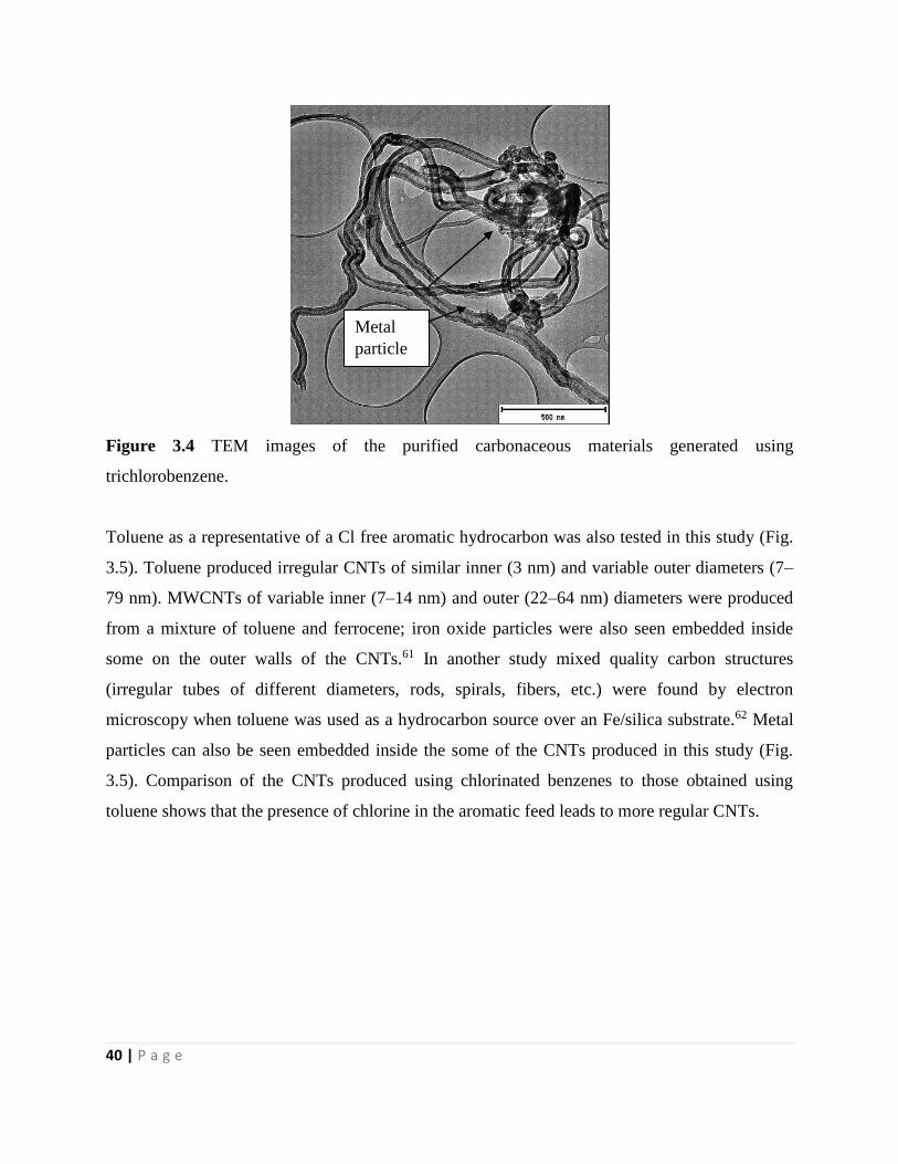
40 | P a g e

Figure 3.4 TEM images of the purified carbonaceous materials generated using

trichlorobenzene.

Toluene as a representative of a Cl free aromatic hydrocarbon was also tested in this study (Fig.

3.5). Toluene produced irregular CNTs of similar inner (3 nm) and variable outer diameters (7–

79 nm). MWCNTs of variable inner (7–14 nm) and outer (22–64 nm) diameters were produced

from a mixture of toluene and ferrocene; iron oxide particles were also seen embedded inside

some on the outer walls of the CNTs.61 In another study mixed quality carbon structures

(irregular tubes of different diameters, rods, spirals, fibers, etc.) were found by electron

microscopy when toluene was used as a hydrocarbon source over an Fe/silica substrate.62 Metal

particles can also be seen embedded inside the some of the CNTs produced in this study (Fig.

3.5). Comparison of the CNTs produced using chlorinated benzenes to those obtained using

toluene shows that the presence of chlorine in the aromatic feed leads to more regular CNTs.

Metal

particle

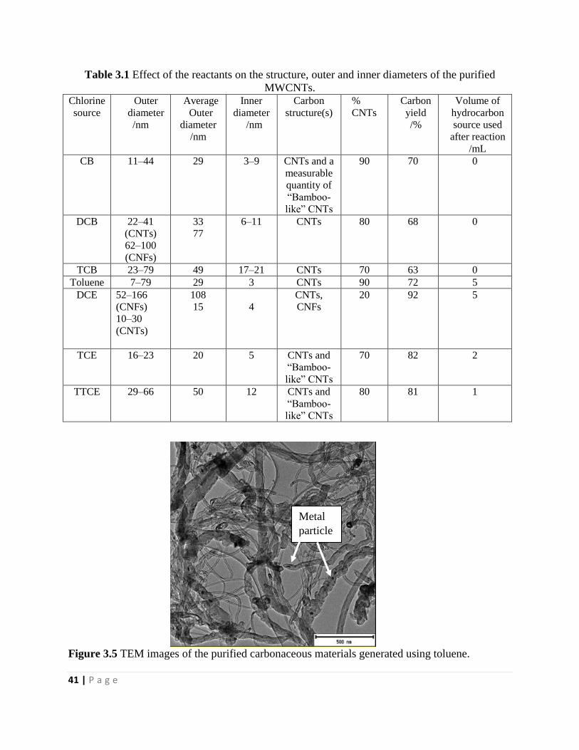
41 | P a g e

Table 3.1 Effect of the reactants on the structure, outer and inner diameters of the purified

MWCNTs. Chlorine

source

Outer

diameter

/nm

Average

Outer

diameter

/nm

Inner

diameter

/nm

Carbon

structure(s)

%

CNTs

Carbon

yield

/%

Volume of

hydrocarbon

source used

after reaction

/mL

CB 11–44 29 3–9 CNTs and a

measurable

quantity of

“Bamboo-

like” CNTs

90 70 0

DCB 22–41

(CNTs)

62–100

(CNFs)

33

77

6–11 CNTs 80 68 0

TCB 23–79 49 17–21 CNTs 70 63 0

Toluene 7–79 29 3 CNTs 90 72 5

DCE 52–166

(CNFs)

10–30

(CNTs)

108

15

4

CNTs,

CNFs

20 92 5

TCE 16–23 20 5 CNTs and

“Bamboo-

like” CNTs

70 82 2

TTCE 29–66 50 12 CNTs and

“Bamboo-

like” CNTs

80 81 1

Figure 3.5 TEM images of the purified carbonaceous materials generated using toluene.

Metal

particle

s

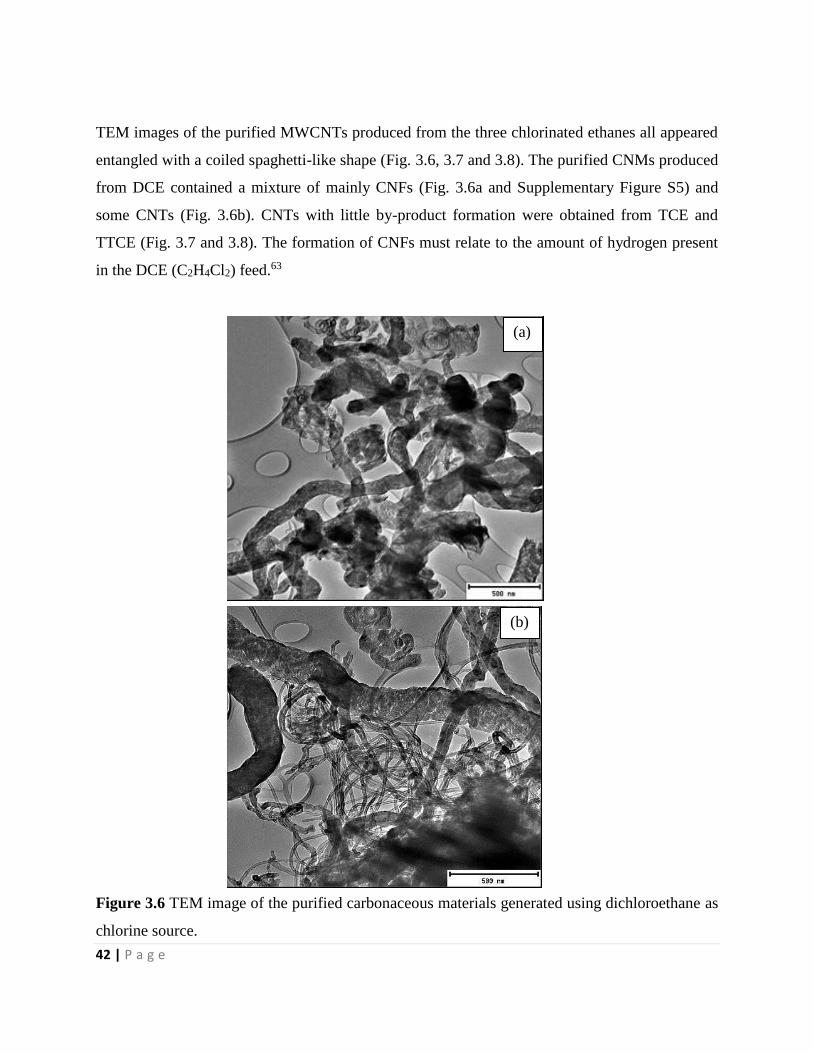
42 | P a g e

TEM images of the purified MWCNTs produced from the three chlorinated ethanes all appeared

entangled with a coiled spaghetti-like shape (Fig. 3.6, 3.7 and 3.8). The purified CNMs produced

from DCE contained a mixture of mainly CNFs (Fig. 3.6a and Supplementary Figure S5) and

some CNTs (Fig. 3.6b). CNTs with little by-product formation were obtained from TCE and

TTCE (Fig. 3.7 and 3.8). The formation of CNFs must relate to the amount of hydrogen present

in the DCE (C2H4Cl2) feed.63

Figure 3.6 TEM image of the purified carbonaceous materials generated using dichloroethane as

chlorine source.

(a)

(b)

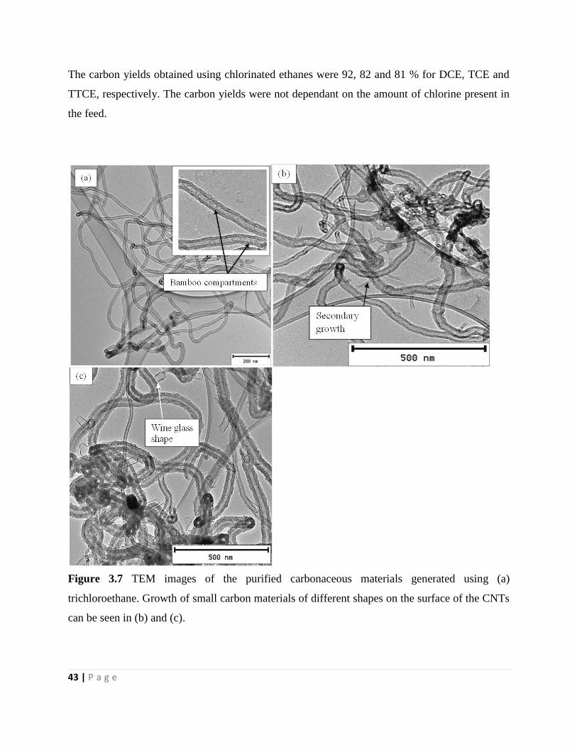
43 | P a g e

The carbon yields obtained using chlorinated ethanes were 92, 82 and 81 % for DCE, TCE and

TTCE, respectively. The carbon yields were not dependant on the amount of chlorine present in

the feed.


trichloroethane. Growth of small carbon materials of different shapes on the surface of the CNTs

can be seen in (b) and (c).

44 | P a g e

The TEM images of carbon materials produced from TCE are shown in Fig. 3.7. The three

figures reveal different features associated with the CNTs. Fig. 3.7a highlights the entangled

CNTs and many of these CNTs appear to show bamboo compartment features. Fig. 3.7b shows

secondary growth of short CNTs with hollow tips, which seem to originate from the main CNTs.

These are similar to those seen above in Fig. 3.3 when DCB was used as a reactant, but here

tubes do not taper and the hollow structures can be clearly seen. Finally, wine glass-like

secondary structures were also seen in Fig. 3.7c. These secondary structures had very thin walls

and did not show the presence of catalyst particles. The presence of un-reacted catalyst material

on the surface of the CNTs could be responsible for the secondary growth via a tip-growth

mechanism.

MWCNTs produced using TTCE also appeared entangled with different outer wall diameters

(Fig. 3.8a, b). Numerous small particles can also be observed on the surface of the CNTs, but no

secondary nanofibre growth was observed. This might also be attributed to the amount of

chlorine in the feed, which if present in large amounts inhibits the growth of secondary fibrous

particles. The inner diameters of the MWCNTs produced using chlorinated ethanes also

increased with an increase in the amount of Cl contained in the organic reagent (Table 3.1),

which suggests HCl-induced metal agglomeration, as has been demonstrated elsewhere.48,50

TEM images of carbon materials produced from TCE and TTCE (Fig. 3.7a and 3.8b

respectively) also revealed some morphological differences. The carbon materials showed

nanotubes with ‘segmented’ appearance i.e., a ‘bamboo-like’ structure. TEM images have been

reported previously in the literature where ‘bamboo-like’ nanofibers were produced when DCE,

dichloroethylene and TCE were used as sources of Cl over Ni/SiO2 catalyst and were attributed

to a seed metal reconstruction leading to unequal diffusion of carbon through the metal particle.49

In our case the bamboo structures might arise from effects related to the interaction of chlorine

with metal particles leading to catalysts restructuring. Bamboo structures were not seen for the

CNTs obtained in this study when DCE was used which might be due to their limited production

but the segmentation was observed from CNFs produced from DCE (Supplementary Fig. S2).

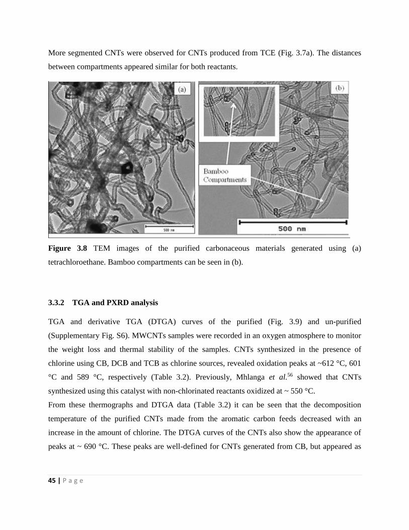
45 | P a g e

More segmented CNTs were observed for CNTs produced from TCE (Fig. 3.7a). The distances

between compartments appeared similar for both reactants.


tetrachloroethane. Bamboo compartments can be seen in (b).

3.3.2 TGA and PXRD analysis

TGA and derivative TGA (DTGA) curves of the purified (Fig. 3.9) and un-purified

(Supplementary Fig. S6). MWCNTs samples were recorded in an oxygen atmosphere to monitor

the weight loss and thermal stability of the samples. CNTs synthesized in the presence of

chlorine using CB, DCB and TCB as chlorine sources, revealed oxidation peaks at ~612 °C, 601

°C and 589 °C, respectively (Table 3.2). Previously, Mhlanga et al.56 showed that CNTs

synthesized using this catalyst with non-chlorinated reactants oxidized at ~ 550 °C.

From these thermographs and DTGA data (Table 3.2) it can be seen that the decomposition

temperature of the purified CNTs made from the aromatic carbon feeds decreased with an

increase in the amount of chlorine. The DTGA curves of the CNTs also show the appearance of

peaks at ~ 690 °C. These peaks are well-defined for CNTs generated from CB, but appeared as

46 | P a g e

shoulder peaks for DCB and TCB CNTs. These peaks are assigned to the presence of small

amounts of graphitic materials.64,65

Further evaluation of the thermographs obtained from chlorinated benzenes, revealed that the

CNTs contained residues even after purification in 30 % HNO3 for 30 min (~21 %, 6 % and 10

% for CB, DCB and TCB (Table 3.2)). An attempt was made to further purify the materials

generated from CB by stirring the product in 30% HNO3 for 2 h and 3 h (Supplementary Fig.

S7). The residual mass had not changed (~18% and 20%) after the 2 h and 3 h acid treatments. A

further harsher treatment was employed by refluxing the product in acid at 110 °C for 4 h which

resulted in destruction of the CNTs structure but a residual non-carbon mass of 8 % still

remained (Supplementary Fig. S7). This showed that catalyst particles remained intact and could

not be removed from the CNTs despite the harsh acid treatment used. The results correlated with

the TEM observations; where images showed the presence of many catalyst particles embedded

inside the CNTs (Fig. 3.2) as well as at the tip of a few CNFs made from materials produced

using DCB (Fig. 3.3 insert). This implied that the catalyst particles were embedded (i) inside

bamboo structures, (ii) within the graphitic layers of the CNTs and (iii) inside the tips of some

CNFs (Fig. 3.3 insert). Similar results were observed in the literature using FeNi catalyst when

the residual metal contents of 31, 27 and 24 wt.% were observed from TGA curves generated

from trichlorobenzene, dichlorobenzene and chlorobenzene as carbon sources; a 3 wt.% residue

was observed under the same conditions using xylene as carbon precursor.51

TGA (Fig. 3.9c) and DTGA (Fig. 3.9d) curves generated from chlorinated ethanes all show

similar oxidation peaks at ~ 619 °C (for DCE and TTCE) and ~ 621 °C for TCE. The chlorinated

materials are more thermally stable than those produced from chlorinated benzenes. Catalyst

particles were not embedded inside the CNTs (< 2 %) for the CNTs produced from chlorinated

alkanes.

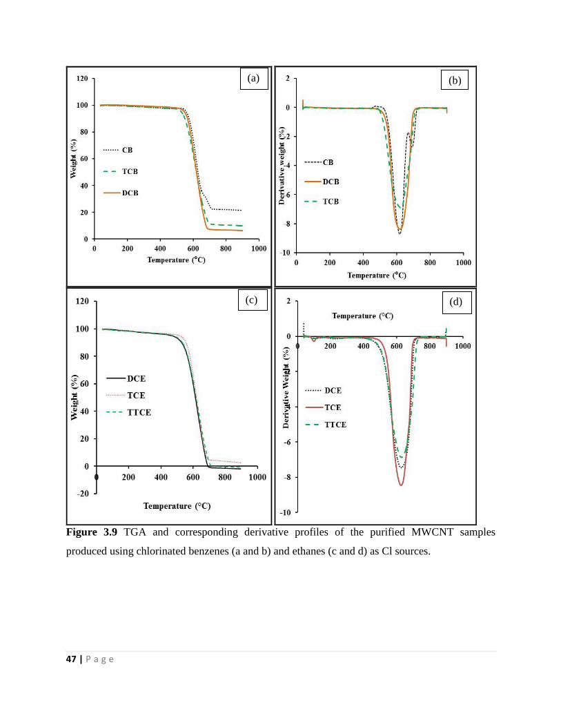
47 | P a g e

Figure 3.9 TGA and corresponding derivative profiles of the purified MWCNT samples

produced using chlorinated benzenes (a and b) and ethanes (c and d) as Cl sources.

(a) (b)

(c) (d)

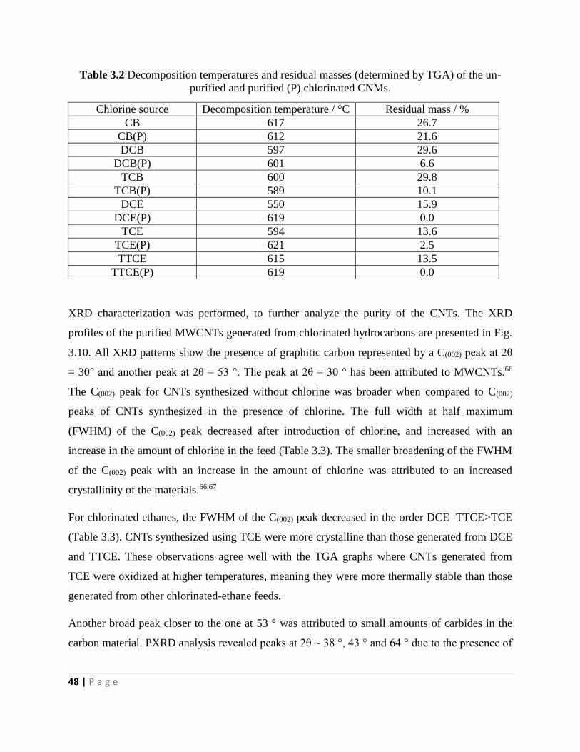
48 | P a g e


purified and purified (P) chlorinated CNMs.

Chlorine source Decomposition temperature / °C Residual mass / %

CB 617 26.7

CB(P) 612 21.6

DCB 597 29.6

DCB(P) 601 6.6

TCB 600 29.8

TCB(P) 589 10.1

DCE 550 15.9

DCE(P) 619 0.0

TCE 594 13.6

TCE(P) 621 2.5

TTCE 615 13.5

TTCE(P) 619 0.0

XRD characterization was performed, to further analyze the purity of the CNTs. The XRD

profiles of the purified MWCNTs generated from chlorinated hydrocarbons are presented in Fig.

3.10. All XRD patterns show the presence of graphitic carbon represented by a C(002) peak at 2θ

= 30° and another peak at 2θ = 53 °. The peak at 2θ = 30 ° has been attributed to MWCNTs.66

The C(002) peak for CNTs synthesized without chlorine was broader when compared to C(002)

peaks of CNTs synthesized in the presence of chlorine. The full width at half maximum

(FWHM) of the C(002) peak decreased after introduction of chlorine, and increased with an

increase in the amount of chlorine in the feed (Table 3.3). The smaller broadening of the FWHM

of the C(002) peak with an increase in the amount of chlorine was attributed to an increased

crystallinity of the materials.66,67

For chlorinated ethanes, the FWHM of the C(002) peak decreased in the order DCE=TTCE>TCE

(Table 3.3). CNTs synthesized using TCE were more crystalline than those generated from DCE

and TTCE. These observations agree well with the TGA graphs where CNTs generated from

TCE were oxidized at higher temperatures, meaning they were more thermally stable than those

generated from other chlorinated-ethane feeds.

Another broad peak closer to the one at 53 ° was attributed to small amounts of carbides in the

carbon material. PXRD analysis revealed peaks at 2θ ~ 38 °, 43 ° and 64 ° due to the presence of

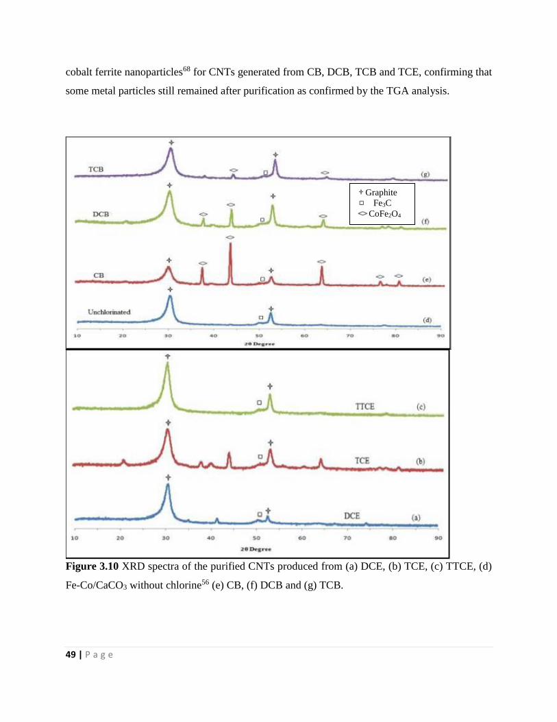
49 | P a g e

cobalt ferrite nanoparticles68 for CNTs generated from CB, DCB, TCB and TCE, confirming that

some metal particles still remained after purification as confirmed by the TGA analysis.

Figure 3.10 XRD spectra of the purified CNTs produced from (a) DCE, (b) TCE, (c) TTCE, (d)

Fe-Co/CaCO3 without chlorine56 (e) CB, (f) DCB and (g) TCB.

Graphite

Fe3C

CoFe2O4

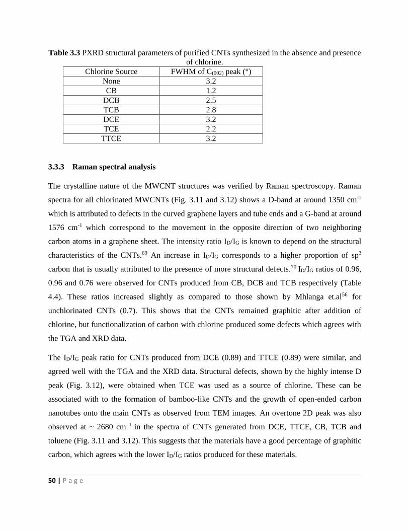
50 | P a g e

Table 3.3 PXRD structural parameters of purified CNTs synthesized in the absence and presence

of chlorine.

Chlorine Source FWHM of C(002) peak (°)

None 3.2

CB 1.2

DCB 2.5

TCB 2.8

DCE 3.2

TCE 2.2

TTCE 3.2

3.3.3 Raman spectral analysis

The crystalline nature of the MWCNT structures was verified by Raman spectroscopy. Raman

spectra for all chlorinated MWCNTs (Fig. 3.11 and 3.12) shows a D-band at around 1350 cm-1

which is attributed to defects in the curved graphene layers and tube ends and a G-band at around

1576 cm-1 which correspond to the movement in the opposite direction of two neighboring

carbon atoms in a graphene sheet. The intensity ratio ID/IG is known to depend on the structural

characteristics of the CNTs.69 An increase in ID/IG corresponds to a higher proportion of sp3

carbon that is usually attributed to the presence of more structural defects.70 ID/IG ratios of 0.96,

0.96 and 0.76 were observed for CNTs produced from CB, DCB and TCB respectively (Table

4.4). These ratios increased slightly as compared to those shown by Mhlanga et.al56 for

unchlorinated CNTs (0.7). This shows that the CNTs remained graphitic after addition of

chlorine, but functionalization of carbon with chlorine produced some defects which agrees with

the TGA and XRD data.

The ID/IG peak ratio for CNTs produced from DCE (0.89) and TTCE (0.89) were similar, and

agreed well with the TGA and the XRD data. Structural defects, shown by the highly intense D

peak (Fig. 3.12), were obtained when TCE was used as a source of chlorine. These can be

associated with to the formation of bamboo-like CNTs and the growth of open-ended carbon

nanotubes onto the main CNTs as observed from TEM images. An overtone 2D peak was also

observed at ~ 2680 cm–1 in the spectra of CNTs generated from DCE, TTCE, CB, TCB and

toluene (Fig. 3.11 and 3.12). This suggests that the materials have a good percentage of graphitic

carbon, which agrees with the lower ID/IG ratios produced for these materials.

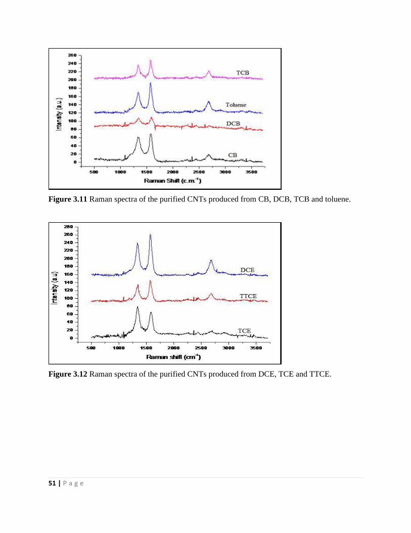
51 | P a g e

Figure 3.11 Raman spectra of the purified CNTs produced from CB, DCB, TCB and toluene.

Figure 3.12 Raman spectra of the purified CNTs produced from DCE, TCE and TTCE.

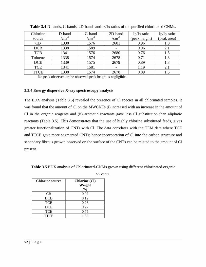
52 | P a g e

Table 3.4 D-bands, G-bands, 2D-bands and ID/IG ratios of the purified chlorinated CNMs.

Chlorine

source

D-band

/cm-1

G-band

/cm-1

2D-band

/cm-1

ID/IG ratio

(peak height)

ID/IG ratio

(peak area)

CB 1338 1576 2681 0.96 1.8

DCB 1338 1589 - 0.96 2.1

TCB 1341 1576 2680 0.76 1.5

Toluene 1338 1574 2678 0.71 1.3

DCE 1339 1575 2679 0.89 1.8

TCE 1341 1581 - 1.19 2.1

TTCE 1338 1574 2678 0.89 1.5 - No peak observed or the observed peak height is negligible.

3.3.4 Energy dispersive X-ray spectroscopy analysis

The EDX analysis (Table 3.5) revealed the presence of Cl species in all chlorinated samples. It

was found that the amount of Cl on the MWCNTs (i) increased with an increase in the amount of

Cl in the organic reagents and (ii) aromatic reactants gave less Cl substitution than aliphatic

reactants (Table 3.5). This demonstrates that the use of highly chlorine substituted feeds, gives

greater functionalization of CNTs with Cl. The data correlates with the TEM data where TCE

and TTCE gave more segmented CNTs; hence incorporation of Cl into the carbon structure and

secondary fibrous growth observed on the surface of the CNTs can be related to the amount of Cl

present.

Table 3.5 EDX analysis of Chlorinated-CNMs grown using different chlorinated organic

solvents.

Chlorine source Chlorine (Cl)

Weight

/%

CB 0.07

DCB 0.12

TCB 0.26

DCE 0.27

TCE 0.75

TTCE 1.53

53 | P a g e

3.3.5 XPS Analysis

The surface characteristics of purified MWCNTs were analysed by XPS. Supplementary Figure

S8 and S9 shows the deconvoluted XPS plots of C1s and Cl2p for all the studied chlorinated

organics. The C1s curve for all MWCNTs was deconvoluted into five components with binding

energies of ~284.0, 284.8, 285.4, 286.1 and 286.8 eV (Table 3.6). Four of these peaks are readily

assigned to Csp2, Csp3, C–OH and C=O; it is possible to tentatively assign the fifth peak at 285.4

to C covalently attached to Cl.71,72

The Cl2p spectrum of CNTs generated from chlorinated organics (Supplementary Figs. S8 and

S9) showed two signals at ~201 and 199 eV which are assigned to the 2p1/2 and 2p3/2 of a chloride

ion (e.g. as found in metal chlorides).72,73 Unfortunately the 2p1/2 peak associated with covalent

C-Cl bonds overlaps with the 2p3/2 associated with the presence of the chloride ion peak.

Furthermore, the low concentration of the Cl in the samples generates very small peaks for Cl

and this makes it difficult to quantify the amount of covalent Cl in the CNTs. However, the

2p1/2/2p3/2 ratios for the Cl peaks indicate values below ca.1.6, the value expected when only

ionic chloride is present (Table 3.6). This suggests that indeed small amounts of C-Cl bonds

have been made; the CNTs made from TTCE thus have the largest amount of C-Cl bonds. This

chlorine would be attached to sp2 carbons at the periphery of the aromatic structures, or at defect

sites.71 The low Cl content is not unexpected as C-Cl bonds are readily broken under the high

temperature condition employed in the CNT synthesis.

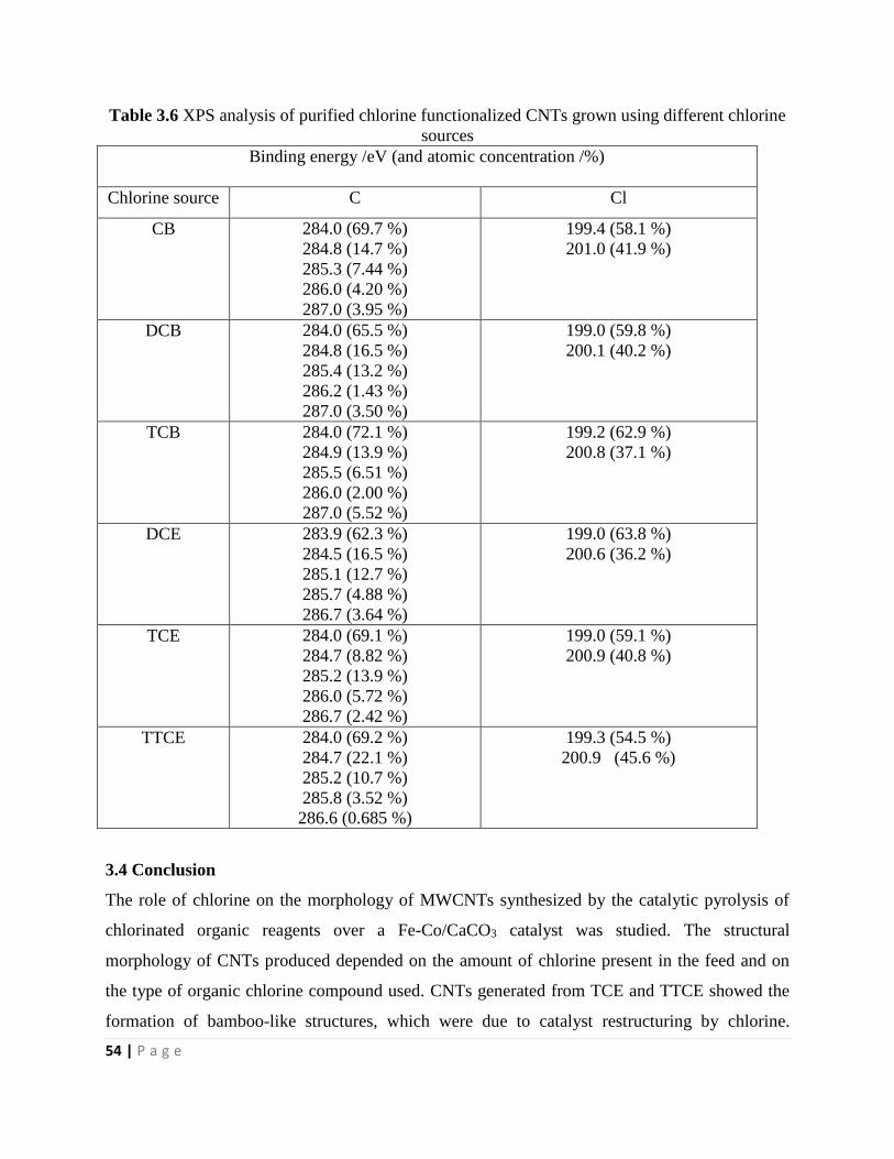
54 | P a g e

Table 3.6 XPS analysis of purified chlorine functionalized CNTs grown using different chlorine

sources

Binding energy /eV (and atomic concentration /%)

Chlorine source C Cl

CB 284.0 (69.7 %)

284.8 (14.7 %)

285.3 (7.44 %)

286.0 (4.20 %)

287.0 (3.95 %)

199.4 (58.1 %)

201.0 (41.9 %)

DCB 284.0 (65.5 %)

284.8 (16.5 %)

285.4 (13.2 %)

286.2 (1.43 %)

287.0 (3.50 %)

199.0 (59.8 %)

200.1 (40.2 %)

TCB 284.0 (72.1 %)

284.9 (13.9 %)

285.5 (6.51 %)

286.0 (2.00 %)

287.0 (5.52 %)

199.2 (62.9 %)

200.8 (37.1 %)

DCE 283.9 (62.3 %)

284.5 (16.5 %)

285.1 (12.7 %)

285.7 (4.88 %)

286.7 (3.64 %)

199.0 (63.8 %)

200.6 (36.2 %)

TCE 284.0 (69.1 %)

284.7 (8.82 %)

285.2 (13.9 %)

286.0 (5.72 %)

286.7 (2.42 %)

199.0 (59.1 %)

200.9 (40.8 %)

TTCE 284.0 (69.2 %)

284.7 (22.1 %)

285.2 (10.7 %)

285.8 (3.52 %)

286.6 (0.685 %)

199.3 (54.5 %)

200.9 (45.6 %)

3.4 Conclusion

The role of chlorine on the morphology of MWCNTs synthesized by the catalytic pyrolysis of

chlorinated organic reagents over a Fe-Co/CaCO3 catalyst was studied. The structural

morphology of CNTs produced depended on the amount of chlorine present in the feed and on

the type of organic chlorine compound used. CNTs generated from TCE and TTCE showed the

formation of bamboo-like structures, which were due to catalyst restructuring by chlorine.

55 | P a g e

Secondary nanofibre and nanotube growth onto the main CNTs was observed when DCB and

TCE chlorine sources were used. Carbon nanofibers were found to be dominant when chlorine

sources (i.e, DCE) that contained high concentration of hydrogen were used. Addition of

chlorine favoured the growth of carbon materials of high purity. Alkanes gave cleaner CNMs

with higher yields than those formed from the aromatic reactants. XPS studies revealed that most

of the Cl found in the CNTs was ionic chlorine, most probably associated with the Fe and in the

CNT tubes. Some surface functionalization of carbon with chlorine is suggested when TTCE was

used as a reagent. The amount of chlorine functionalized on the surface of CNTs was less than

1% for all chlorinated organics studied, evidenced by XPS and EDS. The role of chlorine on the

morphology of nitrogen-doped CNTs and the use of chlorinated MWCNTs as adsorbents for

selected heavy metals in wastewater treatment is underway.

56 | P a g e

References

1. H.W. Kroto, J.R. Heath, S.C. Ơ Brien, R.F. Curl, and R.E. Smalley, Nature, 1985, 318, 162–

163.

2. S. Ijima, Nature, 1991, 354, 56–66.

3. P.G. Collins, and P. Avouris, Scientific American, 2000, 283, 62–69.

4. Q. Zeng, Z. Li, and Y. Zhou, J. Nat. Gas Chem., 2006, 15, 235–246.

5. B.M. Endo, T. Hayashi, Y.A. Kim, M. Terrones, and M.S. Dresselhaus, Phil. Trans. Roy.

Soc. London. A., 2004, 362, 2223–2238.

6. M. Terrones, A. Jorio, M. Endo, Y.A. Kim, T. Hayashi, H. Terrones, J.-C. Charlier, G.

Dresselhaus, and M.S. Dresselhaus, Mater. Today, 2004, 7, 30–45.

7. H. Zeng, L. Zhu, G. Hao, and R. Sheng, Carbon, 1998, 36, 259–262.

8. A. Thess, R. Lee, P. Nikolaev, H. Dai, P. Petit, J. Robert, C. Xu, Y.H. Lee, S.G. Kim, A.G.

Rinzler, D.T. Colbert, G.E. Scuseria, D. Tombnek, and J.E. Fischer, Science, 1996, 273, 483–

487.

9. D.C. Li, L. Dai, S. Huang, A.W.H. Mau, and Z.L. Wang, Chem. Phys. Lett., 2000, 316,

349–355.

10. V. Ivanov, J.B. Nagy, P. Lambin, A. Lucas, X.B. Zhang, X.F. Zhang, D. Bernaerts, G. Van

Tendeloo, S. Amelinckx, and J. Van Landuyt, Chem. Phys. Lett., 1994, 223, 329–335.

11. S.Y. Brichka, G.P. Prikhod’ko, Y.I. Sementsov, A.V. Brichka, G.I. Dovbeshko, and O.P.

Paschuk, Carbon, 2004, 42, 2581–2587.

12. K. Chizari, A. Vena, L. Laurentius, and U. Sundararaj, Carbon, 2014, 68, 369–379.

13. C. Wang, Z. Huang, L. Zhan, Y. Wang, W. Qiao, X. Liang, and L. Ling, Diamond Relat.

Mater., 2011, 20, 1353–1356.

14. T. Sharifi, F. Nitze, H. R. Barzegar, C-W. Tai, M. Mazurkiewicz, A. Malolepszy, L.

Stobinski, and T. Wågberg, Carbon, 2012, 50, 3535–3541.

15. G. Bepete, Z. N. Tetana, S. Lindner, M. H. Rummeli, Z. Chiguvare, and N. J. Coville,

Carbon, 2013, 52, 316–325.

16. H. Liu, Y. Zhang, R. Li, X. Sun, and H. Abou-Rachid, J. Nanopart. Res., 2012, 14, 1016–

1023.

57 | P a g e

17. L. Faba, Y.A. Criado, E. Gallegos-Suáres, M. Pérez-cadenas, E. Díaz, I. Rodríquez-Ramos,

A. Guerrero-Ruiz, and S. Ordónez, Appl. Cat. A: Gen., 2013, 458, 155–161.

18. R. Czerw, M. Terrones, J.-C. Charlier, X. Blasé, B. Foley, R. Kamalakaran, N. Grobert, H.

Terrones, D. Tekleab, P.M. Ajayan, W. Blau, M. Rühle, and D.L. Carroll, Nano. Lett., 2001,

9, 457–560.

19. S. Maldonado, S. Morin, and K. Stevenson, Carbon, 2006, 44, 1429–1437.

20. P. L. Gai, O. Stephan, K. McGuire, A. M. Rao,M. S. Dresselhaus, G. Dresselhaus, and C.

Colliex, J. Mater. Chem., 2004, 14, 669-675.

21. R. Czerw, P.-W. Chiu, Y.-M. Choi, D.-S. Lee, D.L. Carroll, S. Roth, and Y.-W. Park, Curr.

Appl. Phys., 2002, 2, 473–477.

22. H. J. Ceragioli, A. C. Peterlevitz, J. C. R. Quispe, A. Larena, M. P. Pasquetto, M. A.

Sampaio, and V. Baranauskas, J. Phys.: Conf. Ser., 2008, 100, 052029 doi:10.1088/1742-

6596/100/5/052029.

23. K. McGuire, N. Gothard, P.L. Gai, M.S. Dresselhaus, G. Sumanasekera, and A.M. Rao,

Carbon, 2005, 43, 219–227.

24. F. H. Monteiro, D. G. Larrude, M. E. H. Maia da Costa, L. A. Terrazos, R. B. Capaz, and F.

L. Freire Jr, J. Phys. Chem. C, 2012, 116, 3281–3285.

25. T. Cui, R. Lv, Z.H. Huang, F. Kang, K. Wang, and D. Wu, Nanoscale. Res. Lett., 2011, 6,

77–82.

26. F. Bottger-Hiller, A. Mehner, S. Anders, L. Kroll, G. Cox, F. Simon, and S. Spange, Chem.

Comm., 2012, 48, 10568–10570.

27. C. Shan, W. Zhao, X.L. Lu, D.J. O’Brien, Y. Li, Z. Cao, A.L. Elias, R. Cruz-Silva, M.

Terrone, B. Wei, and J. Suhr, Nano. Lett., 2013, 13, 5514–5520.

28. Q. Shi, F. Peng, S. Liao, H. Wang, H. Yu, Z. Liu, B. Zhang and D. Su, J. Mater. Chem. A.,

2013, 1, 14853–14857.

29. J. Li, L. Wang, Y.J. Su, P. Liu, and Y.F. Zhang, Nano-Micro Lett., 2009, 1, 9–13.

30. X. Qu, P. J. J. Alvarez, and Q. Li, Environ. Sci. Technol., 2013, 47, 14080−14088.

31. B. Zhong, H. Liu, X. Gu, and D. S. Su, Chem. Cat. Chem., 2014, 6, 1553–1557.

32. D. Srivastava, T. Susi, M. Borghei, and L. Kari, RSC Adv., 2014, 4, 15225-15235.

33. G. D. Nessim, A. Al-Obeidi, H. Grisaru, E. S. Polsen, C. R. Oliver, T. Zimrin, A. J. Hart, D.

Aurbach, and C. V. Thompson, Carbon, 2012, 50, 4002–4009.

http://pubs.rsc.org/en/results?searchtext=Author%3APratibha%20L.%20Gai

http://pubs.rsc.org/en/results?searchtext=Author%3AOdile%20Stephan

http://pubs.rsc.org/en/results?searchtext=Author%3AKris%20McGuire

http://pubs.rsc.org/en/results?searchtext=Author%3AApparao%20M.%20Rao

http://pubs.rsc.org/en/results?searchtext=Author%3AMildred%20S.%20Dresselhaus

http://pubs.rsc.org/en/results?searchtext=Author%3AGene%20Dresselhaus

http://pubs.rsc.org/en/results?searchtext=Author%3AChristian%20Colliex

http://pubs.rsc.org/en/results?searchtext=Author%3AChristian%20Colliex

http://dx.doi.org/10.1088/1742-6596/100/5/052029

http://dx.doi.org/10.1088/1742-6596/100/5/052029

http://www.sciencedirect.com/science/article/pii/S0008622304006451






http://www.sciencedirect.com/science/journal/00086223

http://pubs.acs.org/action/doSearch?action=search&author=Monteiro%2C+F+H&qsSearchArea=author

http://pubs.acs.org/action/doSearch?action=search&author=Larrude%2C+D+G&qsSearchArea=author

http://pubs.acs.org/action/doSearch?action=search&author=Maia+da+Costa%2C+M+E+H&qsSearchArea=author

http://pubs.acs.org/action/doSearch?action=search&author=Terrazos%2C+L+A&qsSearchArea=author

http://pubs.acs.org/action/doSearch?action=search&author=Capaz%2C+R+B&qsSearchArea=author

http://pubs.acs.org/action/doSearch?action=search&author=Freire%2C+F+L&qsSearchArea=author

http://pubs.acs.org/action/doSearch?action=search&author=Freire%2C+F+L&qsSearchArea=author

http://pubs.rsc.org/en/results?searchtext=Author%3ADivya%20Srivastava

http://pubs.rsc.org/en/results?searchtext=Author%3AToma%20Susi

http://pubs.rsc.org/en/results?searchtext=Author%3AMaryam%20Borghei

http://pubs.rsc.org/en/results?searchtext=Author%3ALaasonen%20Kari

58 | P a g e

34. P. C. P. Watts, N. Mureau, Z. Tang, Y. Miyajima, J. D. Carey, and S. R. P. Silva,

Nanotechnol., 2007, 18, 175701, doi:10.1088/0957-4484/18/17/175701.

35. J. Zhao, and R-H. Xie, J. Nanosci. Nanotechnol., 2003, 3, 459–478.

36. S. Niyogi, M.A. Hamon, H. Hu, B. Zhao, P. Bhowmik, R. Sen, M.E. Itkis, and R.C. Haddon,

Acc. Chem. Res., 2002, 35, 1105–1113.

37. S.M. Kim, K.K. Kim, Y.W. Yo, M.H. Park, S.J. Chae, D.L. Duong, C.W. Yang, J. Kong, and

Y.H. Lee, ACS Nano., 2011, 5, 1236–1242.

38. J.K. Wassei, K.C. Cha, V.C. Tung, Y. Yang, and R.B. Kaner, J. Mater. Chem., 2011, 21,

3391–3396.

39. D.L. Duong, I.H. Lee, K.K. Kim, J. Kong, S.M. Lee, and Y.H. Lee, ACS Nano., 2010, 4,

5430–5436.

40. J-M. Yuan, X-H. Chen, X-H Chen, Z-F Fan, X- Yang, and Z-H.Chen, Carbon, 2008, 46,

1266–1269.

41. W.H. Lee, S.J. Kim, W.J. Lee, J.G. Lee, R.C. Haddon, and P.J. Reucroft, Appl. Surf. Sci.,

2001, 181, 121–127.

42. Z. Kónya, I. Vesselenyi, K. Niesz, A. Kukovecz, A. Demortier, A. Fonseca, J. Delhalle, Z.

Mekhalif, J.B. Nagy, A.A. Koós, Z. Osváth, A. Kocsonya, L.P. Biró, and I. Kiricsi, Chem.

Phys. Lett., 2002, 360, 429–435.


44. C. Ghemes, A. Ghemes, M. Okada, H. Mimura, T. Nakano, and Y. Inoue, Japanese J. Appl.

Phys., 2013, 52, 035202.

45. J. Barkauskas, I. Stankevičiene, and A. Selskis, Sep. Pur. Tech., 2010, 71, 331–336.

46. J.L. Zimmerman, R.K. Bradley, C.B. Huffman, R.H. Hauge, and J.L. Margrave, Chem.

Mater., 2000, 12, 1361–1366.


516–521.

48. L.D. Cherukuri, G. Yuan, and M.A. Keane, Top. Catal., 2004, 29, 119–128.

49. A.N. Márquez, J. L. Valverde, and M.A. Keane, Appl. Catal. A: Gen., 2007, 332, 237–246.

50. M. A. Keane, G. Jacobs, and P. M. Patterson, J. Colloid Interface Sci., 2006, 302, 576–588.

51. R. Lv, F. Kang, W. Wang, J. Wei, J. Gu, K. Wang, and D. Wu, Carbon, 2007, 45, 1433–

1438.

59 | P a g e

52. X. Gui, K. Wang, J. Wei, X. Zhang, R. Lv, Y. Jia, Q. Shu, F. Kang and D. Wu, Mater. Chem.

Phys., 2009, 113, 634 – 637.

53. M. Kao, Chemical Vapour Deposition Synthesis of Carbons From Halogen and Silicon

Sources, MSc. Dissertation, University of the Witwatersrand, Johannesburg, South Africa,

2010.

54. A. Shaikjee, and N.J. Coville, Mater. Lett., 2012, 68, 273–276.

55. W.-H. Lin, T.-T. Lee, and Y.-Y. Li, J. Taiwan Inst. Chem. Eng. E, 2014, 45, 1883–1891.

56. S.D. Mhlanga, K.C. Mondal, R. Carter, M.J. Witcomb, and N.J. Coville, S. Afr. J. Chem.,

2009, 62, 67–76.

57. S.D. Mhlanga, and N.J. Coville, Diamond Relat. Mater., 2008, 17, 1489–1497.

58. Z.N. Tetana, S.D. Mhlanga, G. Bepete, R.W.M. Krause, and N.J. Coville, S. Afr. J. Chem.,

2012, 65, 39–49.

59. H. Kathyayini, N. Nagaraju, A. Fonseca, and J.B. Nagy, J. Mol. Catal. A: Chem., 2004, 223,

129–136.

60. A.A. Hosseini, S. Mehralitabar, A.A. Hosseini, M. Pashaee, and F. Taleshi, Proceedings of

the 4th International Conference on Nanostructures (ICNS4). 12 – 14 March, 2012. Kish

Island. I.R. Iran. 1296–1298.

61. N. Das, A. Dalai, J. S. S. Mohammadzadeh, and J. Adjaye, Carbon, 2006, 44, 2236–2245.

62. K. Hernadi, A. Fonseca, J. B. Nagya, A. Siska, and I. Kiricsi, App. Cat. A: Gen., 2000, 199,

245–255.

63. F. Ohashi, G. Y. Chen, V. Stolojan,S. and R. P. Silva, Nanotechnol., 2008, 19, 445605.

64. C.H. See, and A.T. Harris, Particle Tech. Fluidization, 2008, 54, 657–664.

65. S. Santangelo, M. Lanza, and C. Milone, J. Phys. Chem. C, 2013, 117, 4815–4823.

66. I.D. Rosca, F. Watari, M. Uo, and T. Akasaka, Carbon, 2002, 43, 3124–3131.

67. L.M. Ombaka, P.G. Ndungu, and V.O. Nyamori, J. Mater. Sci., 2015, 50, 1187 – 1200.

68. M. Sajjia, M. Oubaha, M. Hasanuzzaman, and A.G. Olabi, Ceram. Int., 2014, 40, 1147–

1154.

69. L.G. Cancado, A. Jorio, E.H. Martins Ferreira, F. Stavale, C.A. Achete, R.B. Capaz, M.V.O.

Moutinho, A. Lombardo, T.S. Kulmala and A.C. Ferrari, Nano Letters, 2011, 11, 3190–3196.

70. L. Shao, G. Tobias, C.G. Salzmann, B. Ballesteros, S.Y. Hong, A. Crossley, B.G. Davis, and

M. L. H. Green, Chem. Commun., 2007, 5090–5092.

60 | P a g e

71. E. Papirer, R. Lacroix, J.-B. Donnet, G. Nanse, and P. Fioux, Carbon, 1995, 33, 63–72.

72. X. Zhang, A. Hsu, H. Wang, Y. Song, J. Kong, M.S. Dresselhaus and T. Palacios, ASC

Nano., 2013, 7, 7262–270.

73. L. Fan, H. Zhang, P. Zhang and X. Sun, Appl. Surf. Sci., 2015, 347, 632–635.

61 | P a g e

CHAPTER 4

One step synthesis of carbon nanotubes with secondary growth: role of

chlorine

4.1 Introduction

Since their discovery, the unique properties of carbon nanotubes (CNTs)1 and of their less

crystalline counterparts carbon nanofibers (CNFs)2 have attracted the interest of many scientific

communities. CNTs and CNFs possess excellent thermal properties,3,4 as well as unique

electronic5,6 and mechanical properties4,7 which exceed those of many currently applied

materials. CNTs have a low density, high transparency, large surface area, and high aspect ratio.8

This makes CNTs a good candidate for use as a nanoscale platform for sensors,9 transparent

electrodes,10 a catalytic surface for fuel cells,11 emitters for light sources based on field

emission,12,13 electron sources in transmission electron microscopes,14 etc. Synthesis of CNTs

with different shapes such as waved, coiled, crossed and branched has been a subject of many

investigations and the synthesis strategy has the potential to open the way to various

applications, such as in molecular electronics.15 In order to enhance the use of CNTs as a

nanoscale platform, a high density network structure of CNTs with chemically connected CNTs

must be formed.8 If the cross-links between the nanotubes establish a stable connection, then it

should also be possible to create very strong polymer compound materials.16 There are a few

reports that have discussed the chemical connection between CNTs, between CNTs and CNFs

and the synthesis of CNTs on graphite substrates. The limitations of any connections are due to

various reasons, (i) the inert surface characteristics of CNTs allow only physically aggregated

bundle structures without chemical connection between CNTs8; (ii) transition metals are easily

diffused into the carbon substrates; and (iii) the different phases of carbon materials are able to

form on the graphite substrate because the growth conditions are similar to the diamond or

diamond-like carbon growth.17,18 To overcome these issues it is proposed that covalent bonding

between different carbon structures be used. The first report of CNT growth on carbon fibers

was by Zhu, et al.19 In their report CNTs were synthesized on graphite fibers by first coating the

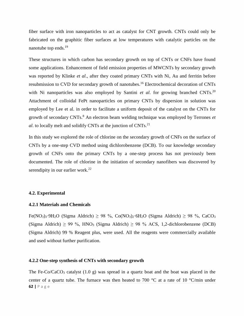
62 | P a g e

fiber surface with iron nanoparticles to act as catalyst for CNT growth. CNTs could only be

fabricated on the graphitic fiber surfaces at low temperatures with catalytic particles on the

nanotube top ends.19

These structures in which carbon has secondary growth on top of CNTs or CNFs have found

some applications. Enhancement of field emission properties of MWCNTs by secondary growth

was reported by Klinke et al., after they coated primary CNTs with Ni, Au and ferritin before

resubmission to CVD for secondary growth of nanotubes.16 Electrochemical decoration of CNTs

with Ni nanoparticles was also employed by Santini et al. for growing branched CNTs.20

Attachment of colloidal FePt nanoparticles on primary CNTs by dispersion in solution was

employed by Lee et al. in order to facilitate a uniform deposit of the catalyst on the CNTs for

growth of secondary CNTs.8 An electron beam welding technique was employed by Terrones et

al. to locally melt and solidify CNTs at the junction of CNTs.21

In this study we explored the role of chlorine on the secondary growth of CNFs on the surface of

CNTs by a one-step CVD method using dichlorobenzene (DCB). To our knowledge secondary

growth of CNFs onto the primary CNTs by a one-step process has not previously been

documented. The role of chlorine in the initiation of secondary nanofibers was discovered by

serendipity in our earlier work.22

4.2. Experimental

4.2.1 Materials and Chemicals


(Sigma Aldrich) ≥ 99 %, HNO3 (Sigma Aldrich) ≥ 98 % ACS, 1,2-dichlorobenzene (DCB)

(Sigma Aldrich) 99 % Reagent plus, were used. All the reagents were commercially available

and used without further purification.

4.2.2 One-step synthesis of CNTs with secondary growth

The Fe-Co/CaCO3 catalyst (1.0 g) was spread in a quartz boat and the boat was placed in the

center of a quartz tube. The furnace was then heated to 700 °C at a rate of 10 °C/min under

63 | P a g e

flowing N2 (50 mL/min). Once the required temperature has been reached, the N2 flow rate was

increased to 240 mL/min and the C2H2 flow rate was set at 90 mL/min. Both gases were bubbled

through dichlorobenzene, which was introduced into the quartz tube. After 60 min of reaction

time, the C2H2 flow and bubbling was stopped and the system was left to cool down to room

temperature under a continuous flow of N2 (50 mL/min). The quartz boat was then removed from

the reactor and the carbon deposit (chlorinated MWCNTs) that formed was weighed. The

reaction time was varied from 60 to 120 minutes, in order to establish the effect of reaction time.

The reaction temperature was also varied using the following temperatures, 600, 650, 700, 750,

and 800 °C, respectively while maintaining the reaction time of 90 min.

4.2.3 Synthesis of secondary CNFs using CNTs as substrate

About 0.3 g of as-synthesized CNTs prepared using a method by Mhlanga et al.23 In this method

a Fe-Co/CaCO3 catalyst, was spread in a quartz boat, which was placed in a quartz tube. The

tube was inserted into a furnace, which was heated gradually to 700 °C at a rate of 10 °C/min

under N2 (50 mL/min) flow. Once the required temperature has been reached, the N2 flow rate

was increased to 240 mL/min and the C2H2 flow was set at 90 mL/min. The CNT substrate were

then placed into the quartz boat, which was inserted into the quartz tube. The quartz tube was

inserted into the furnace, which was gradually heated to 700 °C in the presence of an inert gas

(N2). At 700 °C, N2 (240 mL/min) and C2H2 (90 mL/min) were bubbled through

dichlorobenzene, and the gas stream was introduced into a quartz tube. After 120 min of

reaction, the C2H2 flow and bubbling was stopped and the system was left to cool down to room

temperature under a continuous flow of N2 (50 mL/min). The quartz boat was then removed from

the reactor and the carbon deposit that formed was weighed.

4.2.4 Synthesis of secondary CNFs onto primary CNTs using CNTs spread with catalyst

About 0.2 g of purified CNTs prepared over a Fe-Co/CaCO3 catalyst using a method by Mhlanga

et.al23, was placed in a quartz boat and 0.2 g of Fe-Co/CaCO3 catalyst was spread on top of the

CNTs and submitted to a CVD process. A mixture of dichlorobenzene, N2 (240 mL/min), and

C2H2 (90 mL/min) was passed through the reactor for 60 min, while the CVD reactor was kept at

700 °C. The procedure employed was the same as the one used in 4.2.2.

64 | P a g e

4.2.5 Characterization of CNTs

The morphology and size distribution of the CNTs before and after HNO3 treatment were



holey carbon-coated TEM Cu grid. The CNTs were also characterized by Raman spectroscopy

using a Jobin-Yvon T6400 micro-Raman spectrometer. Excitation was provided by a 532 nm


by thermogravimetric analysis (TGA) using a Perkin Elmer TGA 7. The sample was loaded onto

a platinum pan and heated to 900 °C at a heating rate of 5 °C/min, in a flowing air stream at 20

mL/min.


4.3.1 Structural analysis of the chlorinated CNTs: Effect of reaction time and temperature

Figures 4.1 to 4.5 shows TEM images of CNTs generated from dichlorobenzene as a chlorine

source at different reaction times, 60, 90 and 120 minutes, respectively. Multiple secondary

CNFs with similar shapes and outer diameters were grown on various CNTs after 60 min of

reaction (Figure 4.1). The secondary CNFs were initially broad and then became narrower as

they grew. Close inspection of the numerous CNFs produced revealed that they all had an

inverted cap-like morphology. The length of the secondary CNTs was short, ca. 21–179 nm

(Figure 4.1). About 40 % of the primary CNTs had secondary CNFs after 60 min of reaction.

Other carbon nanostructures, carbon nano-onion and carbon nanofibers with metal particles at

their tips were observed at a 60 min reaction time. Increasing the reaction time to 90 min resulted

in an increase in the number of secondary CNFs formed (Figure 4.2). The secondary CNFs were

grown with consistency in terms of their size, length and shape compared to those obtained after

60 min of reaction (Figure 4.2). The secondary CNFs were also less graphitized and shorter in

length than the primary CNTs. The quantity of the secondary CNFs increased at longer reaction

times, with ~ 90 % observed after 90 min of reaction.

65 | P a g e

Figure 4.1 TEM image of purified CNTs showing secondary CNFs generated using


conditions: 700 °C, 240 mL/min (N2), 90 mL/min (C2H2)

Carbon platelets or some amorphous carbon materials were also observed from the images of the

CNTs obtained from a 90 min reaction time (Figure 4.2d circled parts). A CNT with funnel-like

open end was also observed from this TEM images (Figure 4.2d arrow).

(a)

(c) (d)

(b)

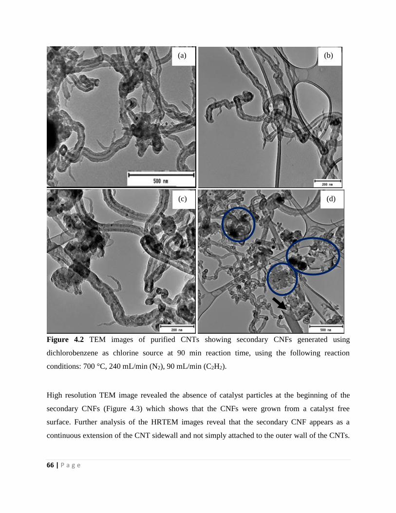
66 | P a g e

Figure 4.2 TEM images of purified CNTs showing secondary CNFs generated using


conditions: 700 °C, 240 mL/min (N2), 90 mL/min (C2H2).

High resolution TEM image revealed the absence of catalyst particles at the beginning of the

secondary CNFs (Figure 4.3) which shows that the CNFs were grown from a catalyst free

surface. Further analysis of the HRTEM images reveal that the secondary CNF appears as a

continuous extension of the CNT sidewall and not simply attached to the outer wall of the CNTs.

(a)

(d) (c)

(b)

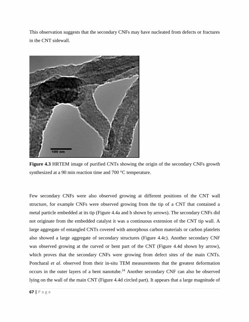
67 | P a g e

This observation suggests that the secondary CNFs may have nucleated from defects or fractures

in the CNT sidewall.

Figure 4.3 HRTEM image of purified CNTs showing the origin of the secondary CNFs growth

synthesized at a 90 min reaction time and 700 °C temperature.

Few secondary CNFs were also observed growing at different positions of the CNT wall

structure, for example CNFs were observed growing from the tip of a CNT that contained a

metal particle embedded at its tip (Figure 4.4a and b shown by arrows). The secondary CNFs did

not originate from the embedded catalyst it was a continuous extension of the CNT tip wall. A

large aggregate of entangled CNTs covered with amorphous carbon materials or carbon platelets

also showed a large aggregate of secondary structures (Figure 4.4c). Another secondary CNF

was observed growing at the curved or bent part of the CNT (Figure 4.4d shown by arrow),

which proves that the secondary CNFs were growing from defect sites of the main CNTs.

Poncharal et al. observed from their in-situ TEM measurements that the greatest deformation

occurs in the outer layers of a bent nanotube.24 Another secondary CNF can also be observed

lying on the wall of the main CNT (Figure 4.4d circled part). It appears that a large magnitude of

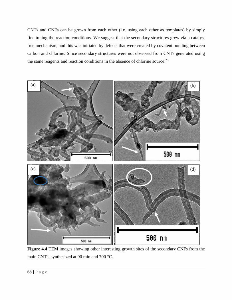
68 | P a g e

CNTs and CNFs can be grown from each other (i.e. using each other as templates) by simply

fine tuning the reaction conditions. We suggest that the secondary structures grew via a catalyst

free mechanism, and this was initiated by defects that were created by covalent bonding between

carbon and chlorine. Since secondary structures were not observed from CNTs generated using

the same reagents and reaction conditions in the absence of chlorine source.23

Figure 4.4 TEM images showing other interesting growth sites of the secondary CNFs from the

main CNTs, synthesized at 90 min and 700 °C.

(a) (b)

(c) (d)

69 | P a g e

Increasing the reaction time to 120 min, resulted in a negligible growth of secondary CNFs and

production of a measurable quantity of CNTs with rough surfaces (Figure 4.5). A single

secondary CNF was observed growing on the sidewall of the CNT in the TEM image taken

(Figure 4.5a, and b, see arrows). The secondary CNF in Figure 4.5c has grown from the tip of the

CNT. The length of the secondary CNTs were longer than for those obtained from a 60 and 90

min reactions, about 166.7, 360 and 75 nm for Figure 4.5a, b and c, respectively. Limited growth

of secondary CNFs at 120 min reaction time, shows that the secondary growth was time

dependent. The negligible quantity of the secondary CNFs at high reaction times, could probably

be as a result of lack or limited number of functionalized CNTs with chlorine which only

resulted in the formation of metal chlorides. The metal chlorides at the surface of the CNTs were

formed when the amount of chlorine that was purged into the system was too high. Metal

chlorides blocked the active sites or the defect sites and induced a change in the structure of the

CNT surface, hence inhibiting growth of the secondary CNFs.

Formation of amorphous carbon on the surface of the CNTs at longer reaction times was also

reported.25 We can also suggest that lack of secondary CNFs at longer reaction times was due to

blockage of the main CNT surface by amorphous carbon. Raman spectra and TGA analysis will

assist in making the final conclusion. The average outer diameters of the CNTs obtained using ~

200 CNT samples were 33, 47 and 82 nm, after 60, 90 and 120 min growth time, respectively.

70 | P a g e

Figure 4.5 TEM images of (a) purified CNTs showing secondary CNFs generated using

dichlorobenzene as chlorine source and (b) showing where the secondary growth originates, at

following reaction conditions: 120 min, 700 °C, 240 mL/min (N2), 90 mL/min (C2H2).

The effect of the synthesis temperature (600, 650, 700, 750, and 800 °C) on the growth of

secondary CNFs on the surface of the primary CNTs was also investigated. TEM images

revealed changes in the morphology of the carbon nanostructures with an increase in the

synthesis temperature. At lower synthesis temperatures of about 600, 650 and 700 °C, the CNTs

appeared hollow inside, and had smooth clean surfaces (Figure 4.6a and b, Figure 4.7a and b and

(a) (b)

(c)

71 | P a g e

Figure 4.2). CNTs generated at 750 °C started to have curved rough surfaces, some appeared

compartmented and others irregular (Figure 4.7c and d). Thin CNTs with hollow structures were

also observed at 750 °C (Figure 4.7c and d). At 800 °C, thinner hollow structured CNTs were

produced together with a few large compartmented CNTs with rough surfaces (Figure 4.8a).

Carbon nanospheres were also obtained from the CNMs generated at high reaction temperature

of 800 °C (Figure 4.8b). Secondary growth was not observed from CNTs generated at reaction

temperatures 600, 650, 750 and 800 °C, as shown by their TEM images (Figure 4.6 a–d). At low

temperatures < 650 °C, the reaction temperature was not sufficient for creation of defects needed

for growth of secondary CNFs, possibly due to limited amount of chlorine atoms functionalized

on the CNTs. At temperatures higher than 700 °C the synthesis temperature was too high and led

to increased supply of chlorine atoms into the system, which interacted with catalyst metal

particles. Interaction of chlorine with catalyst metal particles resulted in formation of metal

chlorides which covered the substrate hence inhibiting CNT growth.


a reaction time of 90 min and reaction temperature of 600 °C.

(a) (b)

72 | P a g e


a reaction time of 90 min and reaction temperature of 650 (a and b) and 750 (c and d) °C.

(c) (d)

(a) (b)

73 | P a g e


a reaction time of 90 min and reaction temperature of 800 °C.

SEM images revealed smooth surfaced CNTs with nearly uniform outer diameters at 600 to 700

°C synthesis temperatures (Supplementary Figure S10). At 750 °C the amount of CNTs formed

decreased, their length also decreased and they also had variable sizes and appeared open-ended

(Supplementary Figure S10d). Clumps were observed from the SEM images where CNTs

seemed to be originating and it was suggested that these clumps were metal chloride particles

(Supplementary Figure S10). Metal chloride were formed from interaction of chlorine atoms

with metal catalyst particles and blocked the surface of the substrate inhibiting carbon growth

rates. The average outer diameters were found to increase with an increase in the reaction

temperature up to 750 °C as follows, 23, 29, 47, and 72 nm at 600, 650, 700, and 750 °C

respectively (Figure 4.9, Supplementary Figure S11 and Table 4.1). At low temperatures the

catalyst particles had small sizes which favored growth of smaller diameter CNTs. Increasing the

temperature resulted in an increase in an average diameter of the catalyst particles which in turn

favored growth of large outer diameter CNTs. Hansen et al. observed an increase in particle size

from 5 nm to 10 nm when the temperature was increased from 650 to 750 °C.26 They explained

the phenomena as due to a catalyst sintering process, they observed the particles under the

electron beam of a TEM during temperature changes. They observed that particles at low

(a) (b)

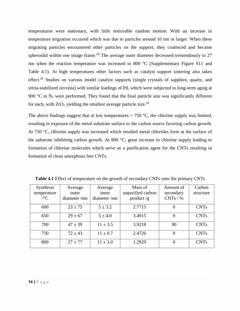
74 | P a g e

temperatures were stationary, with little noticeable random motion. With an increase in

temperature migration occurred which was due to particles around 10 nm or larger. When these

migrating particles encountered other particles on the support, they coalesced and became

spheroidal within one image frame.26 The average outer diameter decreased tremendously to 27

nm when the reaction temperature was increased to 800 °C (Supplementary Figure S11 and

Table 4.1). At high temperatures other factors such as catalyst support sintering also takes

effect.26 Studies on various model catalyst supports (single crystals of sapphire, quartz, and

yttria-stabilized zirconia) with similar loadings of Pd, which were subjected to long-term aging at

900 °C in N2 were performed. They found that the final particle size was significantly different

for each, with ZrO2 yielding the smallest average particle size.26

The above findings suggest that at low temperatures > 750 °C, the chlorine supply was limited,

resulting in exposure of the metal substrate surface to the carbon source favoring carbon growth.

At 750 °C, chlorine supply was increased which resulted metal chlorides form at the surface of

the substrate inhibiting carbon growth. At 800 °C, great increase in chlorine supply leading to

formation of chlorine molecules which serve as a purification agent for the CNTs resulting in

formation of clean amorphous free CNTs.

Table 4.1 Effect of temperature on the growth of secondary CNFs onto the primary CNTs

Synthesis

temperature

/°C

Average

outer

diameter /nm

Average

inner

diameter /nm

Mass of

unpurified carbon

product /g

Amount of

secondary

CNTs / %

Carbon

structure

600 23 ± 75 5 ± 3.2 2.7715 0 CNTs

650 29 ± 67 5 ± 4.0 3.4915 0 CNTs

700 47 ± 39 11 ± 3.5 3.9218 90 CNTs

750 72 ± 43 11 ± 0.7 2.4726 0 CNTs

800 27 ± 77 11 ± 3.0 1.2929 0 CNTs

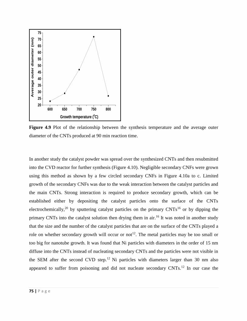
75 | P a g e

600 650 700 750 80020

25

30

35

40

45

50

55

60

65

70

75A

ve

ra

ge

ou

ter d

iam

ete

r (

nm

)

Growth temperature (0C)

Figure 4.9 Plot of the relationship between the synthesis temperature and the average outer

diameter of the CNTs produced at 90 min reaction time.

In another study the catalyst powder was spread over the synthesized CNTs and then resubmitted

into the CVD reactor for further synthesis (Figure 4.10). Negligible secondary CNFs were grown

using this method as shown by a few circled secondary CNFs in Figure 4.10a to c. Limited

growth of the secondary CNFs was due to the weak interaction between the catalyst particles and

the main CNTs. Strong interaction is required to produce secondary growth, which can be

established either by depositing the catalyst particles onto the surface of the CNTs

electrochemically,20 by sputtering catalyst particles on the primary CNTs16 or by dipping the

primary CNTs into the catalyst solution then drying them in air.16 It was noted in another study

that the size and the number of the catalyst particles that are on the surface of the CNTs played a

role on whether secondary growth will occur or not12. The metal particles may be too small or

too big for nanotube growth. It was found that Ni particles with diameters in the order of 15 nm

diffuse into the CNTs instead of nucleating secondary CNTs and the particles were not visible in

the SEM after the second CVD step.12 Ni particles with diameters larger than 30 nm also

appeared to suffer from poisoning and did not nucleate secondary CNTs.12 In our case the

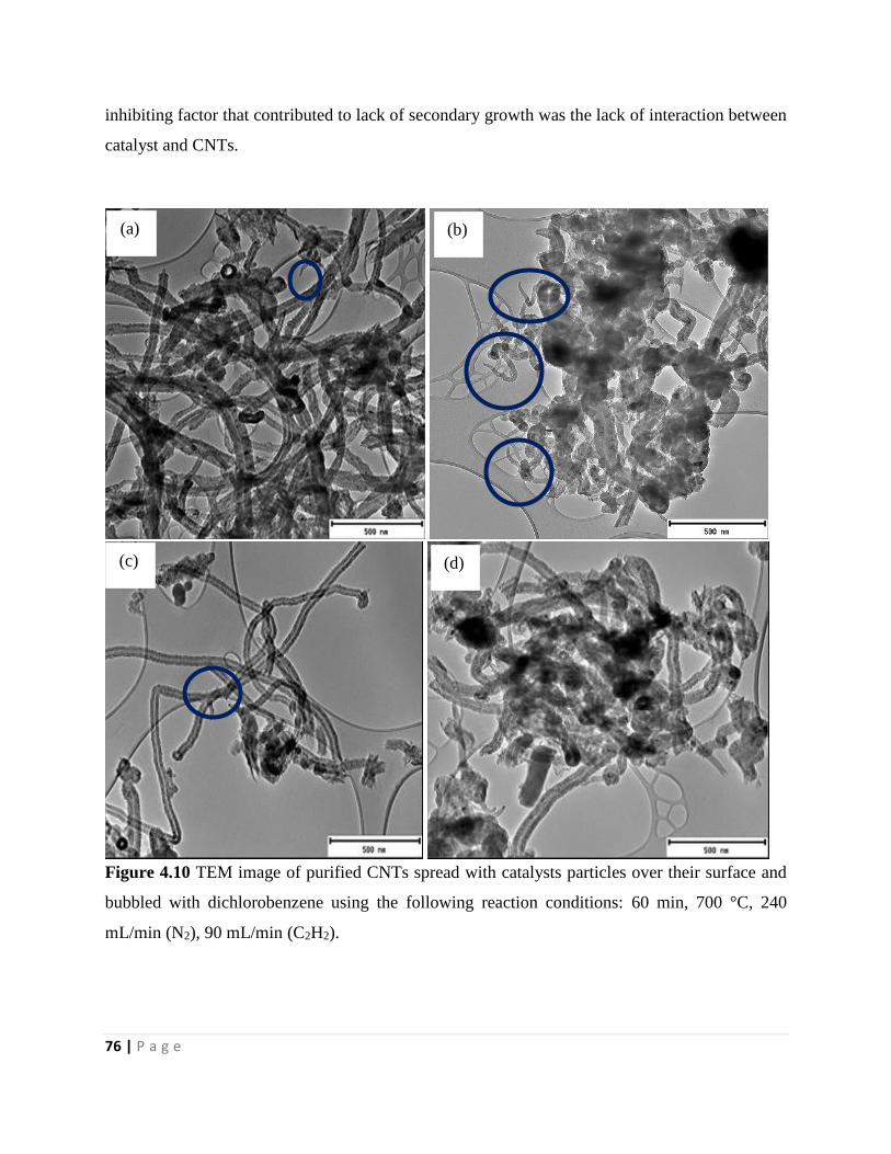
76 | P a g e

inhibiting factor that contributed to lack of secondary growth was the lack of interaction between

catalyst and CNTs.

Figure 4.10 TEM image of purified CNTs spread with catalysts particles over their surface and

bubbled with dichlorobenzene using the following reaction conditions: 60 min, 700 °C, 240

mL/min (N2), 90 mL/min (C2H2).

(c)

(b) (a)

(d)

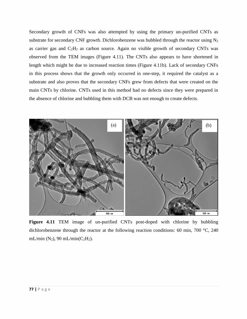
77 | P a g e

Secondary growth of CNFs was also attempted by using the primary un-purified CNTs as

substrate for secondary CNF growth. Dichlorobenzene was bubbled through the reactor using N2

as carrier gas and C2H2 as carbon source. Again no visible growth of secondary CNTs was

observed from the TEM images (Figure 4.11). The CNTs also appears to have shortened in

length which might be due to increased reaction times (Figure 4.11b). Lack of secondary CNFs

in this process shows that the growth only occurred in one-step, it required the catalyst as a

substrate and also proves that the secondary CNFs grew from defects that were created on the

main CNTs by chlorine. CNTs used in this method had no defects since they were prepared in

the absence of chlorine and bubbling them with DCB was not enough to create defects.

Figure 4.11 TEM image of un-purified CNTs post-doped with chlorine by bubbling

dichlorobenzene through the reactor at the following reaction conditions: 60 min, 700 °C, 240

mL/min (N2), 90 mL/min(C2H2).

(a) (b)

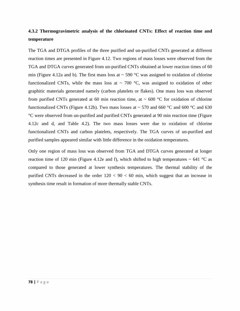
78 | P a g e

4.3.2 Thermogravimetric analysis of the chlorinated CNTs: Effect of reaction time and

temperature

The TGA and DTGA profiles of the three purified and un-purified CNTs generated at different

reaction times are presented in Figure 4.12. Two regions of mass losses were observed from the

TGA and DTGA curves generated from un-purified CNTs obtained at lower reaction times of 60

min (Figure 4.12a and b). The first mass loss at ~ 590 °C was assigned to oxidation of chlorine

functionalized CNTs, while the mass loss at ~ 700 °C, was assigned to oxidation of other

graphitic materials generated namely (carbon platelets or flakes). One mass loss was observed

from purified CNTs generated at 60 min reaction time, at ~ 600 °C for oxidation of chlorine

functionalized CNTs (Figure 4.12b). Two mass losses at ~ 570 and 660 °C and 600 °C and 630

°C were observed from un-purified and purified CNTs generated at 90 min reaction time (Figure

4.12c and d, and Table 4.2). The two mass losses were due to oxidation of chlorine

functionalized CNTs and carbon platelets, respectively. The TGA curves of un-purified and

purified samples appeared similar with little difference in the oxidation temperatures.

Only one region of mass loss was observed from TGA and DTGA curves generated at longer

reaction time of 120 min (Figure 4.12e and f), which shifted to high temperatures ~ 641 °C as

compared to those generated at lower synthesis temperatures. The thermal stability of the

purified CNTs decreased in the order 120 < 90 < 60 min, which suggest that an increase in

synthesis time result in formation of more thermally stable CNTs.

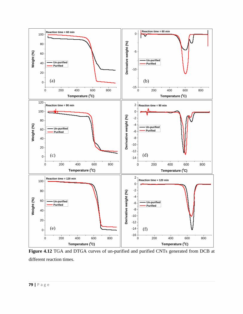
79 | P a g e

0 200 400 600 800

0

20

40

60

80

100W

eig

ht

(%)

Temperature (0C)

Un-purified

Purified

Reaction time = 60 min

0 200 400 600 800-15

-10

-5

0

Deri

va

tiv

e w

eig

ht

(%)

Temperature (0C)

Un-purified

Purified


0 200 400 600 800

0

20

40

60

80

100

120

We

igh

t (%

)

Temperature (0C)

Un-purified

Purified


0 200 400 600 800

-14

-12

-10

-8

-6

-4

-2

0

2

De

riv

ati

ve

we

igh

t (%

)

Temperature (0C)

Un-purified

Purified


0 200 400 600 800

0

20

40

60

80

100

We

igh

t (%

)

Temperature (0C)

Un-purified

Purified


0 200 400 600 800-16

-14

-12

-10

-8

-6

-4

-2

0

2

De

riv

ati

ve

we

igh

t (%

)

Temperature (0C)

Un-purified

Purified


Figure 4.12 TGA and DTGA curves of un-purified and purified CNTs generated from DCB at

different reaction times.

(a)

(c)

(b)

(e)

(d)

(f)

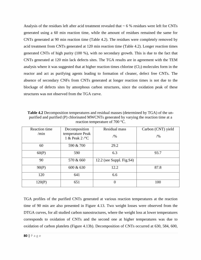
80 | P a g e

Analysis of the residues left after acid treatment revealed that ~ 6 % residues were left for CNTs

generated using a 60 min reaction time, while the amount of residues remained the same for

CNTs generated at 90 min reaction time (Table 4.2). The residues were completely removed by

acid treatment from CNTs generated at 120 min reaction time (Table 4.2). Longer reaction times

generated CNTs of high purity (100 %), with no secondary growth. This is due to the fact that

CNTs generated at 120 min lack defects sites. The TGA results are in agreement with the TEM

analysis where it was suggested that at higher reaction times chlorine (Cl2) molecules form in the

reactor and act as purifying agents leading to formation of cleaner, defect free CNTs. The

absence of secondary CNFs from CNTs generated at longer reaction times is not due to the

blockage of defects sites by amorphous carbon structures, since the oxidation peak of these

structures was not observed from the TGA curve.


purified and purified (P) chlorinated MWCNTs generated by varying the reaction time at a

reaction temperature of 700 °C.

Reaction time

/min

Decomposition

temperature Peak

1 & Peak 2 /°C

Residual mass

/%

Carbon (CNT) yield

/%

60 590 & 700 29.2

60(P) 590 6.3 93.7

90 570 & 660 12.2 (see Suppl. Fig.S4)

90(P) 600 & 630 12.2 87.8

120 641 6.6

120(P) 651 0 100

TGA profiles of the purified CNTs generated at various reaction temperatures at the reaction

time of 90 min are also presented in Figure 4.13. Two weight losses were observed from the

DTGA curves, for all studied carbon nanostructures, where the weight loss at lower temperatures

corresponds to oxidation of CNTs and the second one at higher temperatures was due to

oxidation of carbon platelets (Figure 4.13b). Decomposition of CNTs occurred at 630, 584, 600,

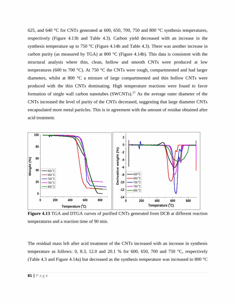
81 | P a g e

625, and 640 °C for CNTs generated at 600, 650, 700, 750 and 800 °C synthesis temperatures,

respectively (Figure 4.13b and Table 4.3). Carbon yield decreased with an increase in the

synthesis temperature up to 750 °C (Figure 4.14b and Table 4.3). There was another increase in

carbon purity (as measured by TGA) at 800 °C (Figure 4.14b). This data is consistent with the

structural analysis where thin, clean, hollow and smooth CNTs were produced at low

temperatures (600 to 700 °C). At 750 °C the CNTs were rough, compartmented and had larger

diameters, whilst at 800 °C a mixture of large compartmented and thin hollow CNTs were

produced with the thin CNTs dominating. High temperature reactions were found to favor

formation of single wall carbon nanotubes (SWCNTs).27 As the average outer diameter of the

CNTs increased the level of purity of the CNTs decreased, suggesting that large diameter CNTs

encapsulated more metal particles. This is in agreement with the amount of residue obtained after

acid treatment.

0 200 400 600 800

0

20

40

60

80

100

We

igh

t (%

)

Temperature (0C)

600 0C

650 0C

700 0C

750 0C

800 0C

0 200 400 600 800-14

-12

-10

-8

-6

-4

-2

0

2

De

riv

ati

ve

we

igh

t (%

)

Temperature (0C)

600 0C

650 0C

700 0C

750 0C

800 0C

Figure 4.13 TGA and DTGA curves of purified CNTs generated from DCB at different reaction

temperatures and a reaction time of 90 min.

The residual mass left after acid treatment of the CNTs increased with an increase in synthesis

temperature as follows: 0, 8.3, 12.0 and 20.1 % for 600, 650, 700 and 750 °C, respectively

(Table 4.3 and Figure 4.14a) but decreased as the synthesis temperature was increased to 800 °C

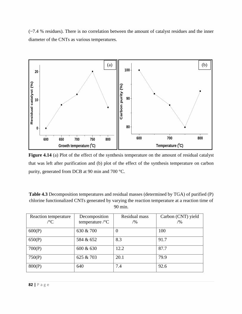
82 | P a g e

(~7.4 % residues). There is no correlation between the amount of catalyst residues and the inner

diameter of the CNTs as various temperatures.

600 650 700 750 800

0

10

20

Res

idu

al c

ata

lyst

(%)

Growth temperature (0C)

600 700 800

80

90

100

Carb

on

pu

rit

y (

%)

Temperature (0C)

Figure 4.14 (a) Plot of the effect of the synthesis temperature on the amount of residual catalyst

that was left after purification and (b) plot of the effect of the synthesis temperature on carbon

purity, generated from DCB at 90 min and 700 °C.

Table 4.3 Decomposition temperatures and residual masses (determined by TGA) of purified (P)

chlorine functionalized CNTs generated by varying the reaction temperature at a reaction time of

90 min.

Reaction temperature

/°C

Decomposition

temperature /°C

Residual mass

/%

Carbon (CNT) yield

/%

600(P) 630 & 700 0 100

650(P) 584 & 652 8.3 91.7

700(P) 600 & 630 12.2 87.7

750(P) 625 & 703 20.1 79.9

800(P) 640 7.4 92.6

(a) (b)

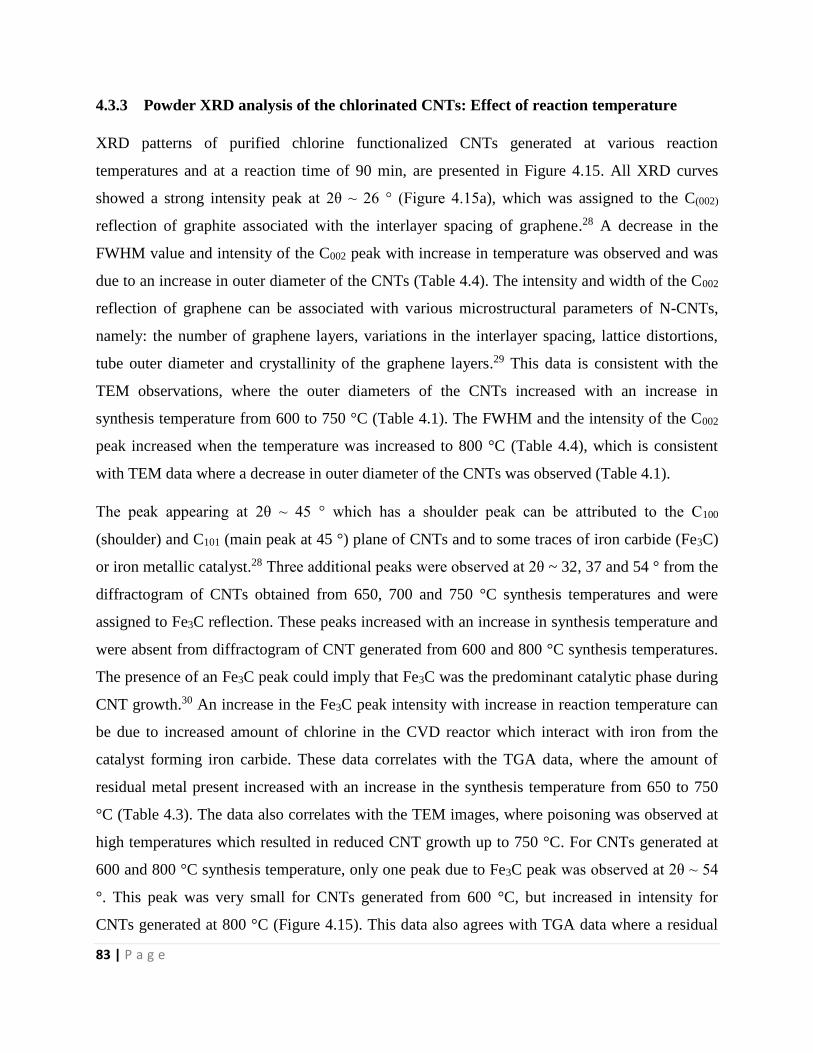
83 | P a g e

4.3.3 Powder XRD analysis of the chlorinated CNTs: Effect of reaction temperature

XRD patterns of purified chlorine functionalized CNTs generated at various reaction

temperatures and at a reaction time of 90 min, are presented in Figure 4.15. All XRD curves

showed a strong intensity peak at 2θ ~ 26 ° (Figure 4.15a), which was assigned to the C(002)

reflection of graphite associated with the interlayer spacing of graphene.28 A decrease in the

FWHM value and intensity of the C002 peak with increase in temperature was observed and was

due to an increase in outer diameter of the CNTs (Table 4.4). The intensity and width of the C002

reflection of graphene can be associated with various microstructural parameters of N-CNTs,

namely: the number of graphene layers, variations in the interlayer spacing, lattice distortions,

tube outer diameter and crystallinity of the graphene layers.29 This data is consistent with the

TEM observations, where the outer diameters of the CNTs increased with an increase in

synthesis temperature from 600 to 750 °C (Table 4.1). The FWHM and the intensity of the C002

peak increased when the temperature was increased to 800 °C (Table 4.4), which is consistent

with TEM data where a decrease in outer diameter of the CNTs was observed (Table 4.1).

The peak appearing at 2θ ~ 45 ° which has a shoulder peak can be attributed to the C100

(shoulder) and C101 (main peak at 45 °) plane of CNTs and to some traces of iron carbide (Fe3C)

or iron metallic catalyst.28 Three additional peaks were observed at 2θ ~ 32, 37 and 54 ° from the

diffractogram of CNTs obtained from 650, 700 and 750 °C synthesis temperatures and were

assigned to Fe3C reflection. These peaks increased with an increase in synthesis temperature and

were absent from diffractogram of CNT generated from 600 and 800 °C synthesis temperatures.

The presence of an Fe3C peak could imply that Fe3C was the predominant catalytic phase during

CNT growth.30 An increase in the Fe3C peak intensity with increase in reaction temperature can

be due to increased amount of chlorine in the CVD reactor which interact with iron from the

catalyst forming iron carbide. These data correlates with the TGA data, where the amount of

residual metal present increased with an increase in the synthesis temperature from 650 to 750

°C (Table 4.3). The data also correlates with the TEM images, where poisoning was observed at

high temperatures which resulted in reduced CNT growth up to 750 °C. For CNTs generated at

600 and 800 °C synthesis temperature, only one peak due to Fe3C peak was observed at 2θ ~ 54

°. This peak was very small for CNTs generated from 600 °C, but increased in intensity for

CNTs generated at 800 °C (Figure 4.15). This data also agrees with TGA data where a residual

84 | P a g e

mass of 0 and 7.4 % was obtained for CNTs generated at 600 and 800 °C synthesis temperature,

respectively (Table 4.3).

10 20 30 40 50 60 70 80 90

Inte

nsit

y (

a.u

)

2 theta (degree)

600 0C

650 0C

700 0C

750 0C

800 0C

Figure 4.15 p-XRD curves of purified CNTs generated from DCB at a reaction time of 90 min

and at different reaction temperatures.

Table 4.4 Powder X-ray structural parameters of chlorine functionalized CNTs generated at

various reaction temperatures for 90 min.

Reaction

temperature /°C

Position

of C(002)

peak

FWHM of

C(002) peak

/ °

Intensity of

C(002) peak

Intensity of

Fe3C peak

at 32 °

Intensity of Fe3C

peak at 37 °

600 25.8 2.8 862.0 – –

650 25.7 2.6 731.0 114.4 292.5

700 25.9 2.3 672.7 233.6 599.0

750 26.0 1.8 540.2 565.1 1338.8

800 25.8 2.2 620.0 – –

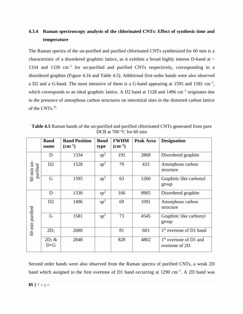
85 | P a g e

4.3.4 Raman spectroscopy analysis of the chlorinated CNTs: Effect of synthesis time and

temperature

The Raman spectra of the un-purified and purified chlorinated CNTs synthesized for 60 min is a

characteristic of a disordered graphitic lattice, as it exhibits a broad highly intense D-band at ~

1334 and 1330 cm–1 for un-purified and purified CNTs respectively, corresponding to a

disordered graphite (Figure 4.16 and Table 4.5). Additional first-order bands were also observed

a D2 and a G-band. The most intensive of them is a G-band appearing at 1595 and 1581 cm–1,

which corresponds to an ideal graphitic lattice. A D2 band at 1528 and 1496 cm–1 originates due

to the presence of amorphous carbon structures on interstitial sites in the distorted carbon lattice

of the CNTs.31


DCB at 700 °C for 60 min

Band

name

Band Position

(cm–1)

Bond

type

FWHM

(cm–1)

Peak Area Designation

60 m

in u

n-

puri

fied

D 1334 sp2 192 2868 Disordered graphite

D2 1528 sp3 79 433 Amorphous carbon

structure

G 1595 sp2 63 1260 Graphitic like carbonyl

group

60 m

in p

uri

fied



structure


group

2D1 2680 81 603 1st overtone of D1 band

2D2 &

D+G

2848 828 4802 1st overtone of D1 and

overtone of 2D

Second order bands were also observed from the Raman spectra of purified CNTs, a weak 2D

band which assigned to the first overtone of D1 band occurring at 1290 cm–1. A 2D band was

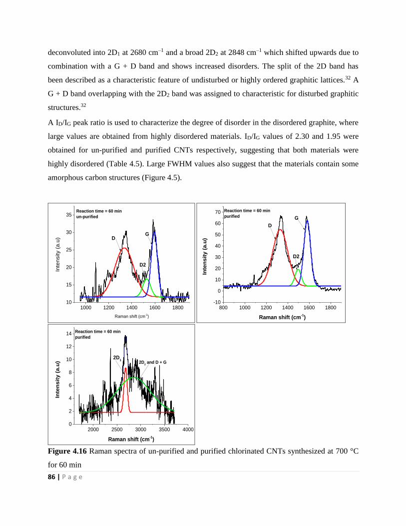
86 | P a g e

deconvoluted into 2D1 at 2680 cm–1 and a broad 2D2 at 2848 cm–1 which shifted upwards due to

combination with a G + D band and shows increased disorders. The split of the 2D band has

been described as a characteristic feature of undisturbed or highly ordered graphitic lattices.32 A

G + D band overlapping with the 2D2 band was assigned to characteristic for disturbed graphitic

structures.32

A ID/IG peak ratio is used to characterize the degree of disorder in the disordered graphite, where

large values are obtained from highly disordered materials. ID/IG values of 2.30 and 1.95 were

obtained for un-purified and purified CNTs respectively, suggesting that both materials were

highly disordered (Table 4.5). Large FWHM values also suggest that the materials contain some

amorphous carbon structures (Figure 4.5).

1000 1200 1400 1600 180010

15

20

25

30

35

Inte

nsity (

a.u

)

Raman shift (cm-1)

D

D2

G


un-purified

800 1000 1200 1400 1600 1800-10

0

10

20

30

40

50

60

70

Inte

nsit

y (

a.u

)

Raman shift (cm-1)


purified

D

D2

G

2000 2500 3000 3500 40000

2

4

6

8

10

12

14

Inte

nsit

y (

a.u

)

Raman shift (cm-1)


purified

2D1

2D2 and D + G


for 60 min

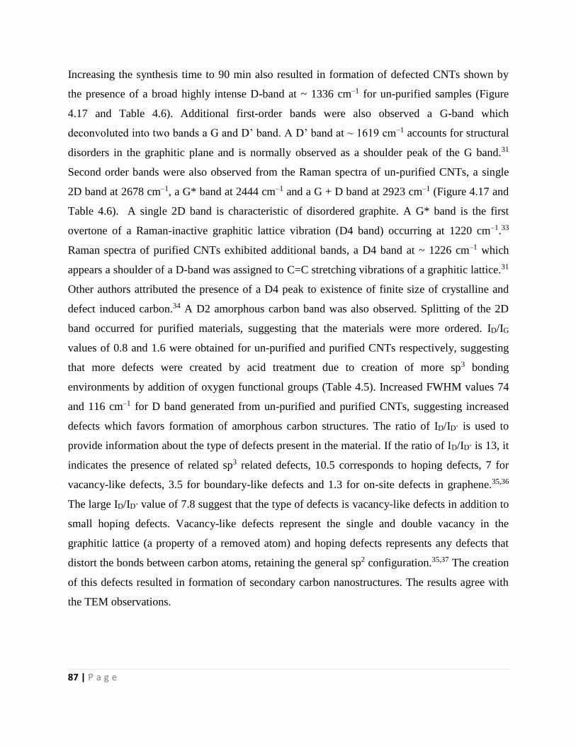
87 | P a g e

Increasing the synthesis time to 90 min also resulted in formation of defected CNTs shown by

the presence of a broad highly intense D-band at ~ 1336 cm–1 for un-purified samples (Figure

4.17 and Table 4.6). Additional first-order bands were also observed a G-band which

deconvoluted into two bands a G and D’ band. A D’ band at ~ 1619 cm–1 accounts for structural

disorders in the graphitic plane and is normally observed as a shoulder peak of the G band.31

Second order bands were also observed from the Raman spectra of un-purified CNTs, a single

2D band at 2678 cm–1, a G* band at 2444 cm–1 and a G + D band at 2923 cm–1 (Figure 4.17 and

Table 4.6). A single 2D band is characteristic of disordered graphite. A G* band is the first

overtone of a Raman-inactive graphitic lattice vibration (D4 band) occurring at 1220 cm–1.33

Raman spectra of purified CNTs exhibited additional bands, a D4 band at ~ 1226 cm–1 which

appears a shoulder of a D-band was assigned to C=C stretching vibrations of a graphitic lattice.31

Other authors attributed the presence of a D4 peak to existence of finite size of crystalline and

defect induced carbon.34 A D2 amorphous carbon band was also observed. Splitting of the 2D

band occurred for purified materials, suggesting that the materials were more ordered. ID/IG

values of 0.8 and 1.6 were obtained for un-purified and purified CNTs respectively, suggesting

that more defects were created by acid treatment due to creation of more sp3 bonding

environments by addition of oxygen functional groups (Table 4.5). Increased FWHM values 74

and 116 cm–1 for D band generated from un-purified and purified CNTs, suggesting increased

defects which favors formation of amorphous carbon structures. The ratio of ID/ID’ is used to

provide information about the type of defects present in the material. If the ratio of ID/ID’ is 13, it

indicates the presence of related sp3 related defects, 10.5 corresponds to hoping defects, 7 for

vacancy-like defects, 3.5 for boundary-like defects and 1.3 for on-site defects in graphene.35,36

The large ID/ID’ value of 7.8 suggest that the type of defects is vacancy-like defects in addition to

small hoping defects. Vacancy-like defects represent the single and double vacancy in the

graphitic lattice (a property of a removed atom) and hoping defects represents any defects that

distort the bonds between carbon atoms, retaining the general sp2 configuration.35,37 The creation

of this defects resulted in formation of secondary carbon nanostructures. The results agree with

the TEM observations.

88 | P a g e

1000 1200 1400 1600 1800-50

0

50

100

150

200

250

300

350In

ten

sit

y (

a.u

)

Raman shift (cm-1)


un-purified

D

G

D'

2000 2200 2400 2600 2800 3000 3200 3400

0

20

40

60

80

100

Inte

ns

ity

(a

.u)

Raman shift (cm-1)


un-purified

D + GG*

2D

1000 1200 1400 1600 1800

0

100

200

300

400

Inte

ns

ity

(a

.u)

Raman shift (cm-1)


purified

D4

D

D2

G

2000 2200 2400 2600 2800 3000

0

4

8

12

16

Inte

nsit

y (

a.u

)

Raman shift (cm-1)


purified

2D1

2D2


for 90 min

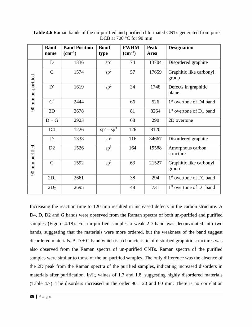
89 | P a g e



Band

name

Band Position

(cm–1)

Bond

type

FWHM

(cm–1)

Peak

Area

Designation

90 m

in u

n-p

uri

fied



group

D’ 1619 sp2 34 1748 Defects in graphitic

plane

G* 2444 66 526 1st overtone of D4 band

2D 2678 81 8264 1st overtone of D1 band

D + G 2923 68 290 2D overtone

90 m

in p

uri

fied

D4 1226 sp2 – sp3 126 8120



structure


group



Increasing the reaction time to 120 min resulted in increased defects in the carbon structure. A

D4, D, D2 and G bands were observed from the Raman spectra of both un-purified and purified

samples (Figure 4.18). For un-purified samples a weak 2D band was deconvoluted into two

bands, suggesting that the materials were more ordered, but the weakness of the band suggest

disordered materials. A D + G band which is a characteristic of disturbed graphitic structures was

also observed from the Raman spectra of un-purified CNTs. Raman spectra of the purified

samples were similar to those of the un-purified samples. The only difference was the absence of

the 2D peak from the Raman spectra of the purified samples, indicating increased disorders in

materials after purification. ID/IG values of 1.7 and 1.8, suggesting highly disordered materials

(Table 4.7). The disorders increased in the order 90, 120 and 60 min. There is no correlation

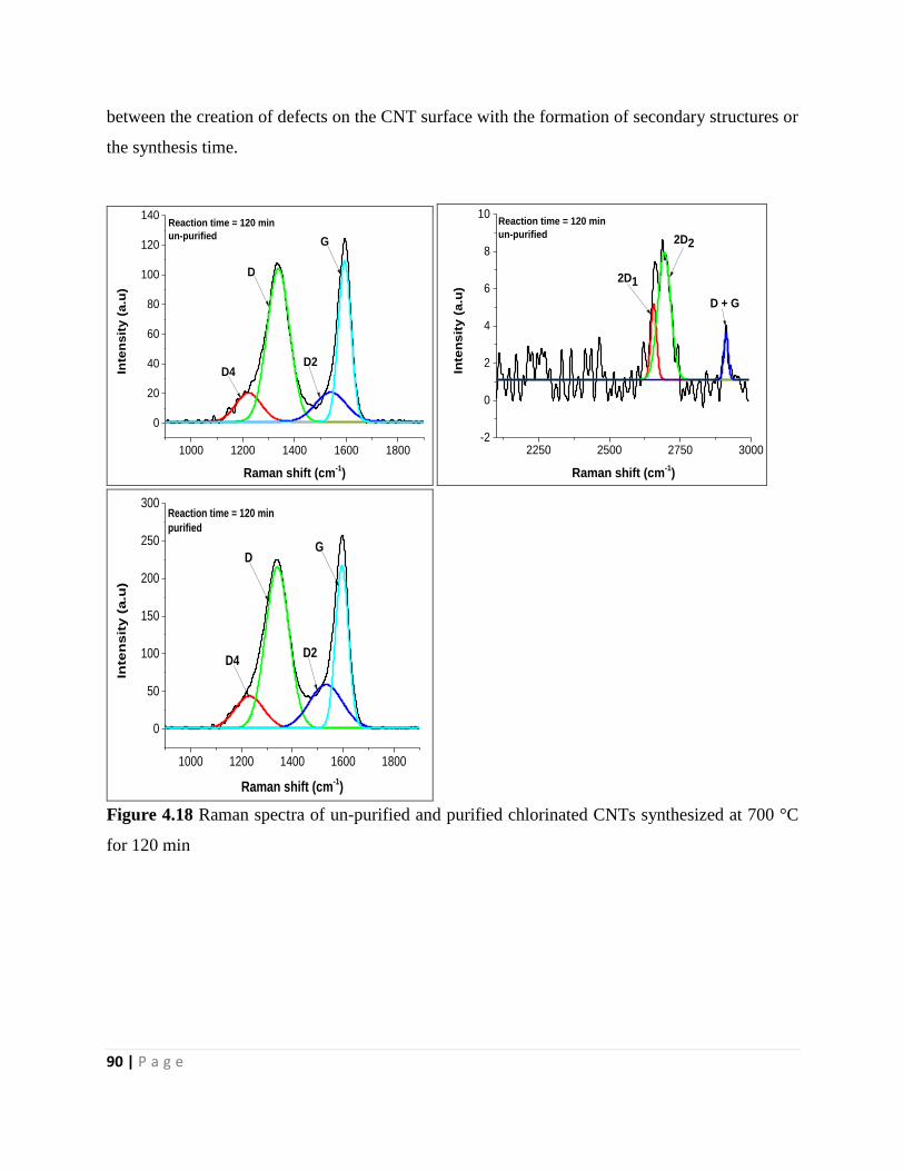
90 | P a g e

between the creation of defects on the CNT surface with the formation of secondary structures or

the synthesis time.

1000 1200 1400 1600 1800

0

20

40

60

80

100

120

140

Inte

nsit

y (

a.u

)

Raman shift (cm-1)


un-purified

D4

D

G

D2

2250 2500 2750 3000-2

0

2

4

6

8

10

Inte

nsit

y (

a.u

)

Raman shift (cm-1)


un-purified

2D1

2D2

D + G

1000 1200 1400 1600 1800

0

50

100

150

200

250

300

Inte

nsit

y (

a.u

)

Raman shift (cm-1)


purified

D4

D

D2

G


for 120 min

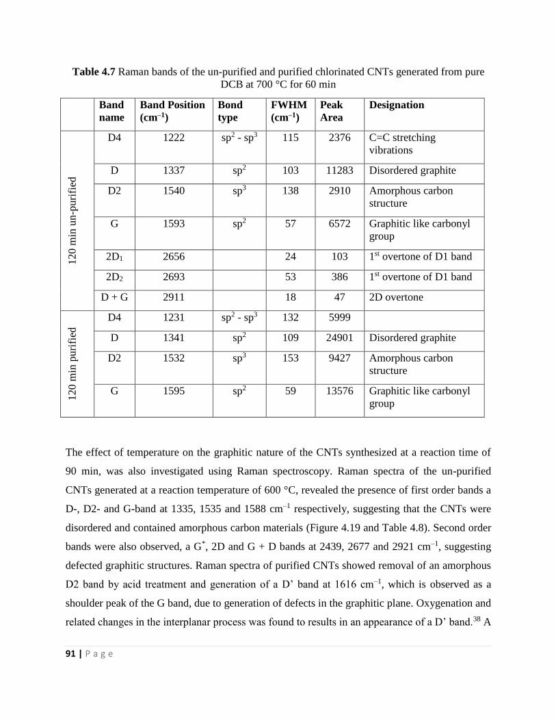
91 | P a g e



Band

name

Band Position

(cm–1)

Bond

type

FWHM

(cm–1)

Peak

Area

Designation

120 m

in u

n-p

uri

fied

D4 1222 sp2 - sp3 115 2376 C=C stretching

vibrations



structure


group



D + G 2911 18 47 2D overtone

120 m

in p

uri

fied

D4 1231 sp2 - sp3 132 5999



structure


group

The effect of temperature on the graphitic nature of the CNTs synthesized at a reaction time of

90 min, was also investigated using Raman spectroscopy. Raman spectra of the un-purified

CNTs generated at a reaction temperature of 600 °C, revealed the presence of first order bands a

D-, D2- and G-band at 1335, 1535 and 1588 cm–1 respectively, suggesting that the CNTs were

disordered and contained amorphous carbon materials (Figure 4.19 and Table 4.8). Second order

bands were also observed, a G*, 2D and G + D bands at 2439, 2677 and 2921 cm–1, suggesting

defected graphitic structures. Raman spectra of purified CNTs showed removal of an amorphous

D2 band by acid treatment and generation of a D’ band at 1616 cm–1, which is observed as a

shoulder peak of the G band, due to generation of defects in the graphitic plane. Oxygenation and

related changes in the interplanar process was found to results in an appearance of a D’ band.38 A

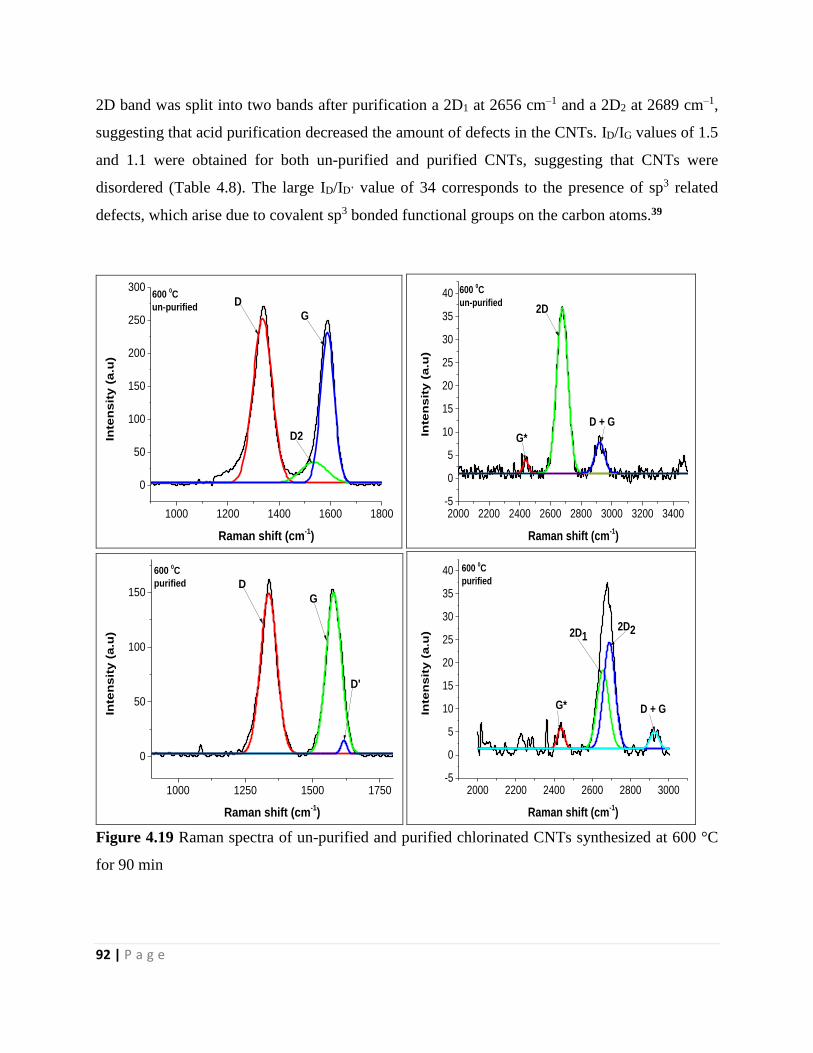
92 | P a g e

2D band was split into two bands after purification a 2D1 at 2656 cm–1 and a 2D2 at 2689 cm–1,

suggesting that acid purification decreased the amount of defects in the CNTs. ID/IG values of 1.5

and 1.1 were obtained for both un-purified and purified CNTs, suggesting that CNTs were

disordered (Table 4.8). The large ID/ID’ value of 34 corresponds to the presence of sp3 related

defects, which arise due to covalent sp3 bonded functional groups on the carbon atoms.39

1000 1200 1400 1600 1800

0

50

100

150

200

250

300

Inte

ns

ity

(a

.u)

Raman shift (cm-1)

D

D2

G

600 0C

un-purified

2000 2200 2400 2600 2800 3000 3200 3400-5

0

5

10

15

20

25

30

35

40

Inte

nsit

y (

a.u

)

Raman shift (cm-1)

600 0C

un-purified

G*

2D

D + G

1000 1250 1500 1750

0

50

100

150

Inte

nsit

y (

a.u

)

Raman shift (cm-1)

600 0C

purified D

D'

G

2000 2200 2400 2600 2800 3000-5

0

5

10

15

20

25

30

35

40

Inte

ns

ity

(a

.u)

Raman shift (cm-1)

600 0C

purified

G*

2D12D2

D + G


for 90 min

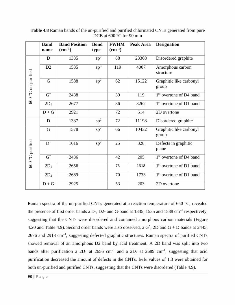
93 | P a g e



Band

name

Band Position

(cm–1)

Bond

type

FWHM

(cm–1)


600 °

C u

n-p

uri

fied



structure


group



D + G 2921 72 514 2D overtone

600 °

C p

uri

fied



group


plane




D + G 2925 53 203 2D overtone

Raman spectra of the un-purified CNTs generated at a reaction temperature of 650 °C, revealed

the presence of first order bands a D-, D2- and G-band at 1335, 1535 and 1588 cm–1 respectively,

suggesting that the CNTs were disordered and contained amorphous carbon materials (Figure

4.20 and Table 4.9). Second order bands were also observed, a G*, 2D and G + D bands at 2445,

2676 and 2913 cm–1, suggesting defected graphitic structures. Raman spectra of purified CNTs

showed removal of an amorphous D2 band by acid treatment. A 2D band was split into two

bands after purification a 2D1 at 2656 cm–1 and a 2D2 at 2689 cm–1, suggesting that acid

purification decreased the amount of defects in the CNTs. ID/IG values of 1.3 were obtained for

both un-purified and purified CNTs, suggesting that the CNTs were disordered (Table 4.9).

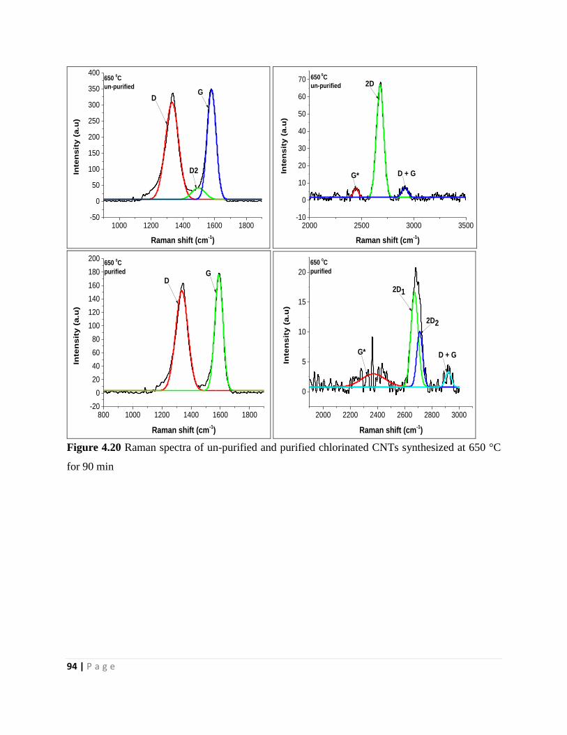
94 | P a g e

1000 1200 1400 1600 1800-50

0

50

100

150

200

250

300

350

400In

ten

sit

y (

a.u

)

Raman shift (cm-1)

650 0C

un-purified

D

D2

G

2000 2500 3000 3500-10

0

10

20

30

40

50

60

70

Inte

ns

ity

(a

.u)

Raman shift (cm-1)

650 0C

un-purified

G*

2D

D + G

800 1000 1200 1400 1600 1800-20

0

20

40

60

80

100

120

140

160

180

200

Inte

ns

ity

(a

.u)

Raman shift (cm-1)

650 0C

purified

DG

2000 2200 2400 2600 2800 3000

0

5

10

15

20

Inte

ns

ity

(a

.u)

Raman shift (cm-1)

650 0C

purified

G*

2D1

2D2

D + G


for 90 min

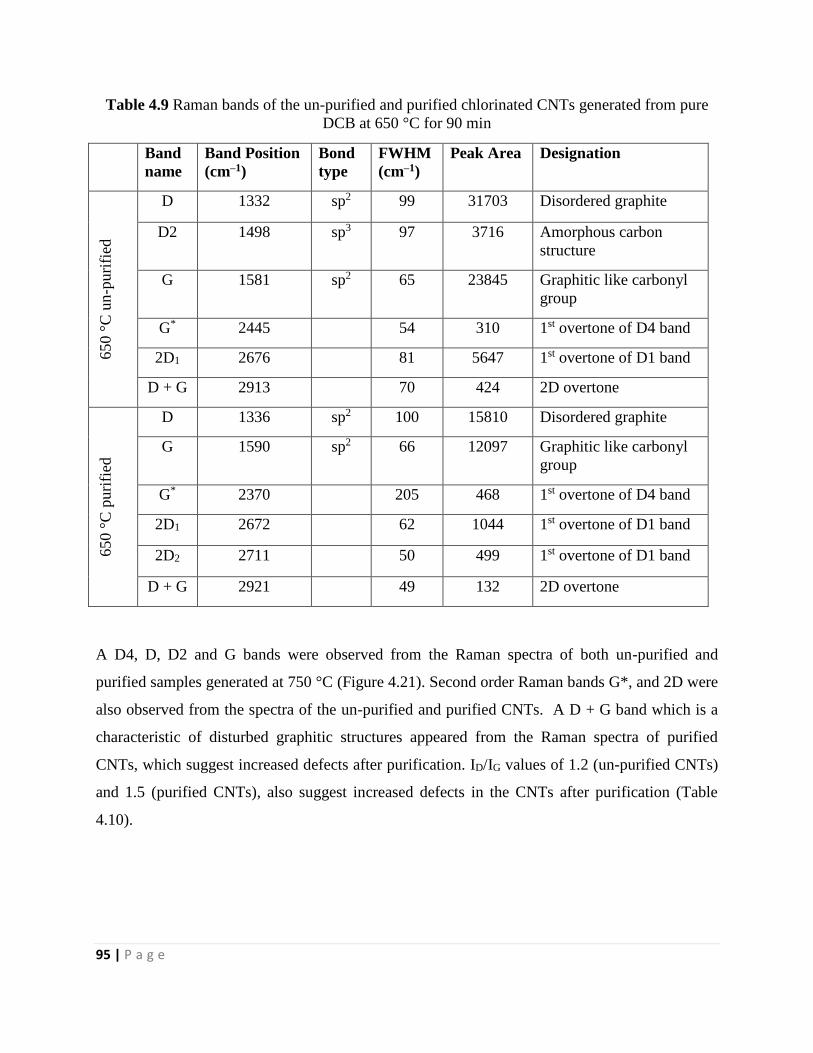
95 | P a g e



Band

name

Band Position

(cm–1)

Bond

type

FWHM

(cm–1)


650 °

C u

n-p

uri

fied



structure


group



D + G 2913 70 424 2D overtone

650 °

C p

uri

fied



group




D + G 2921 49 132 2D overtone

A D4, D, D2 and G bands were observed from the Raman spectra of both un-purified and

purified samples generated at 750 °C (Figure 4.21). Second order Raman bands G*, and 2D were

also observed from the spectra of the un-purified and purified CNTs. A D + G band which is a

characteristic of disturbed graphitic structures appeared from the Raman spectra of purified

CNTs, which suggest increased defects after purification. ID/IG values of 1.2 (un-purified CNTs)

and 1.5 (purified CNTs), also suggest increased defects in the CNTs after purification (Table

4.10).

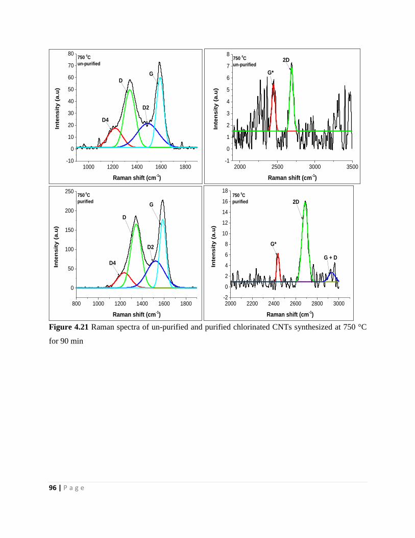
96 | P a g e

1000 1200 1400 1600 1800-10

0

10

20

30

40

50

60

70

80In

ten

sit

y (

a.u

)

Raman shift (cm-1)

750 0C

un-purified

D4

D

D2

G

2000 2500 3000 3500-1

0

1

2

3

4

5

6

7

8

Inte

ns

ity

(a

.u)

Raman shift (cm-1)

750 0C

un-purified

G*

2D

800 1000 1200 1400 1600 1800

0

50

100

150

200

250

Inte

nsit

y (

a.u

)

Raman shift (cm-1)

D4

D

D2

G

750 0C

purified

2000 2200 2400 2600 2800 3000-2

0

2

4

6

8

10

12

14

16

18

Inte

nsit

y (

a.u

)

Raman shift (cm-1)

750 0C

purified

G*

2D

G + D


for 90 min

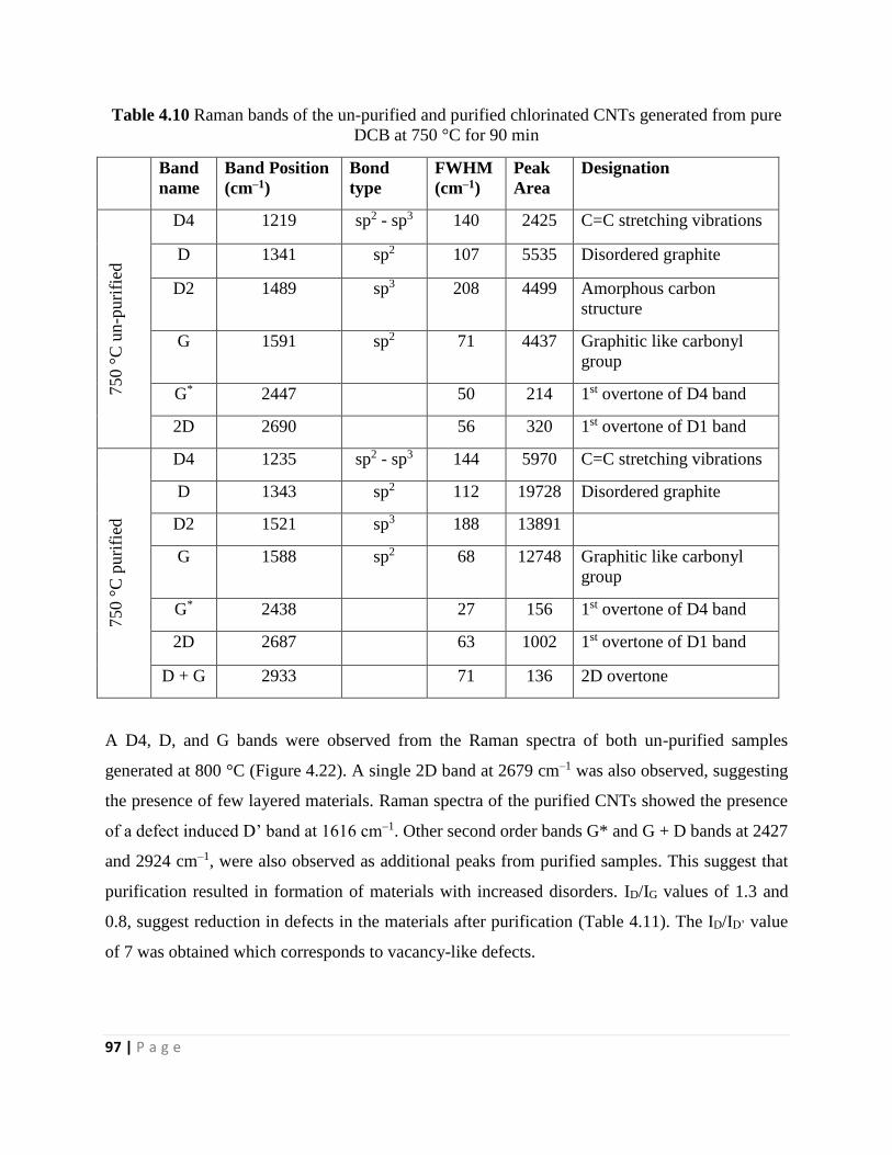
97 | P a g e



Band

name

Band Position

(cm–1)

Bond

type

FWHM

(cm–1)

Peak

Area

Designation

750 °

C u

n-p

uri

fied

D4 1219 sp2 - sp3 140 2425 C=C stretching vibrations



structure


group



750 °

C p

uri

fied

D4 1235 sp2 - sp3 144 5970 C=C stretching vibrations


D2 1521 sp3 188 13891


group



D + G 2933 71 136 2D overtone

A D4, D, and G bands were observed from the Raman spectra of both un-purified samples

generated at 800 °C (Figure 4.22). A single 2D band at 2679 cm–1 was also observed, suggesting

the presence of few layered materials. Raman spectra of the purified CNTs showed the presence

of a defect induced D’ band at 1616 cm–1. Other second order bands G* and G + D bands at 2427

and 2924 cm–1, were also observed as additional peaks from purified samples. This suggest that

purification resulted in formation of materials with increased disorders. ID/IG values of 1.3 and

0.8, suggest reduction in defects in the materials after purification (Table 4.11). The ID/ID’ value

of 7 was obtained which corresponds to vacancy-like defects.

98 | P a g e

1000 1200 1400 1600 1800

0

50

100

150

200

250

300In

ten

sit

y (

a.u

)

Raman shift (cm-1)

800 0C

un-purified

D4

D

G

2000 2200 2400 2600 2800 3000 3200 3400-5

0

5

10

15

20

25

30

35

40

Inte

nsit

y (

a.u

)

Raman shift (cm-1)

2D

800 0C

un-purified

1000 1200 1400 1600 1800-20

0

20

40

60

80

100

120

140

Inte

nsit

y (

a.u

)

Raman shift (cm-1)

800 0C

purified

D

G

D'

2000 2200 2400 2600 2800 3000

0

10

20

30

40

50

Inte

ns

ity

(a

.u)

Raman shift (cm-1)

800 0C

purified

G*

2D

G + D


for 90 min

99 | P a g e



Band

name

Band

Position

(cm–1)

Bond

type

FWHM

(cm–1)

Peak

Area

Designation

800 °

C u

n-p

uri

fied

D4 1189 sp2 - sp3 74 2180 C=C stretching

vibrations



group


800 °

C p

uri

fied



group


plane



D + G 2924 41 99 2D overtone

Structural information: Comparison of the Raman with other used techniques in this study

The following conclusions were deduced from the Raman spectra of the effect of synthesis time

and temperature:

1. Purified CNTs generated at a reaction time of 120 min exhibited the lowest D and G band

FWHM, which indicates that the highest degree of graphitization was achieved at this

synthesis time. The data is consistent with the TGA analysis where materials generated at

this synthesis temperature had increased thermal stability as compared to materials generated

at low synthesis times. The thermal stability was observed to increase with an increase in the

synthesis time as follows, 120 > 90 > 60 min.

2. Purified CNTs generated at 800 °C exhibited the lowest D and very low G band FWHM,

which indicated that the highest degree of graphitization among all investigated temperatures

100 | P a g e

and is consistent with the TGA analysis and TEM results. The second reaction temperature

that generated better graphitized materials was 600 °C. The number of defects (based on the

FWHM value of the D band) increased as a function of reaction temperature as follows: 700

(116 cm–1) < 750 (112 cm–1) < 650 (100 cm–1) < 600 (72 cm–1) < 800 °C (63 cm–1). There

was no correlation between the FWHM value and the reaction temperature. The ID/IG value

of purified CNTs generated at 800 °C is also the lowest, indicating that these materials were

more graphitic.

4.4 Conclusion

The structure and yield of the CNTs was affected by the growth time and temperature. Formation

of secondary CNFs on the surface of the main CNTs depended on the growth time and growth

temperature. Longer synthesis times favored formation of high purity CNTs with no secondary

growth and less defects. The largest number of secondary CNFs were observed at 90 min

reaction time. Secondary CNFs were found to grow at defects sites of the CNTs as an extension

of the CNT wall. For the first time, we have identified the type of defects for chlorinated CNTs.

Vacancy-like defects in addition to small hoping defects due to removal of carbon atoms from

the graphitic structure and distortion of bonds between carbon atoms as a result of carbon

removal, were observed from chlorinated CNTs generated at 90 min reaction temperature. These

type of defects seem to arise due to the presence of large magnitude of secondary CNFs observed

from their TEM images. CNTs generated at very low (600 °C) and very high (800 °C) were the

most graphitic, denoted by their low FWHM values of the D and G band and their high thermal

stabilities. Reduction in the CNT growth was observed at high temperatures (~ 750 °C) due to

poisoning of the CNT surface by iron carbides resulting from increased formation of chlorine in

the reactor. CNTs generated at 600 °C contained sp3 related defects, which arise due to covalent

sp3 bonded functional groups on the carbon atoms. This shows that greater functionalization of

CNTs with chlorine was achieved at low synthesis temperatures. The large value of ID/IG of 1.1

suggest that functionalization of CNTs with chlorine increased defects in the graphitic structure.

Vacancy like defects due to removal of some carbon atoms in the crystal lattice was obtained

from CNTs generated at 800 °C. This suggest less involvement of chlorine in forming functional

101 | P a g e

groups with the carbon atoms. It was suggested in the TGA studies that at high synthesis

temperature of 800 °C, a greater amount of chlorine atoms that are in close proximity are formed,

which resulted in them interacting with each other to form Cl2 molecules which escaped through

the trap. Formation of these Cl2 molecules resulted in them purifying the CNTs, leading to

formation of highly graphitized CNTs.

The synthesized CNTs with secondary growth can be used as fillers for polymer matrix in

production of polymer composites for water treatment. The presence of secondary CNFs is

expected to ease the interaction between the CNTs and the polymer matrix. CNTs with

secondary growth can also be used in electronics as their presence is expected to enhance the

electrical conductivity of the matrix.

The effect of chlorine on the morphology of N-doped CNTs was then evaluated in the next

chapter, because nitrogen-doped CNTs were also observed to enhance the electrical conductivity

of the carbon materials.

102 | P a g e

References

1. S. Ijima, Nature, 1991, 354, 56–66.

2. A. Oberlin and M. Endo, Journal of Crystal Growth, 1976, 32, 335 – 349.

3. V. Popov, Mater. Sci. Eng. R. Rep., 2004, 43, 61 – 102.

4. R. Ruoff, and D. Lorents, Carbon, 1995, 33, 925 – 930.

5. P.G. Collins, and P. Avouris, Sci. Am., 2000, 283, 62 – 69.

6. Y.K. Kwon, and D. Toma’nek, Phys. Rev. B, 1998, 58, R16001.

7. J.P. Delmotte, and A. Rubio, Carbon, 2002, 40, 1729 – 1734.

8. O.H. Lee, Q. Lu, Q. Hu, Y-J. Baek, Y-S. Lim and T-S. Yoon, Curr. Appl. Phys., 2013, 13,

S84 – S87.

9. J. Kong, N.R. Franklin, C.W. Zhou, M.G. Chapline, S. Peng, K.J. Cho, and H.J. Dai, Science,

2000, 287, 622.

10. W. Aloui, A. Ltaief, and A. Bouazizi, Superlattices Microstruct., 2013, 64, 581 – 589.

11. Z. Wen, Q. Wang and J. Li, Adv. Funct. Mater., 2008, 18, 959 – 964.

12. Y. Saito, S. Uemura, and K. Hamaguchi, Jpn. J. Appl. Phys., 1998, 37, 346.

13. J.M. Bonard, M. Croci, C. Klinke, R. Kurt, O. Noury and N. Weiss, Carbon, 2002, 40, 1715.

14. N. de Jonge, Y. Lamy, K. Schoots, and T.H. Oosterkamp, Nature, 2002, 420, 393 – 395.

15. M. Zhang, and J. Li, Mater. Today, 2009, 12, 12 – 18.

16. C. Klinke, E. Delvigne, J.V. Barth and K. Kern. J. Phys. Chem, B. 2005, 109, 21677–21680.

17. P.S. Weiser, S. Praoer, A. Hoffman, R.R. Manory, P.J.K. Puterson and S. Stuart, J. Appl.

Phys., 1992, 72, 4643.

18. S. Zhu, F. Shahedipour and H.W. White, J. Am. Ceram. Soc., 1998, 81, 1041.

19. S. Zhu, C-H. Su, S.L. Lehoczky, I. Muntele and D. Ila, Diamond Relat. Mater., 2003, 12,

1825 – 1828.

20. C. A. Santini, P. M. Vereecken, C. Van Haesendonck, Mater. Lett., 2012, 88, 33 – 35.

21. M. Terrones, F. Banhart, N. Grobert, J.-C. Charlier, H. Terrones and P.M. Ajayan, Phys. Rev.

Lett., 2002, 89, 075505-1 – 075505-4.

22. W.K. Maboya, N.J. Coville, and S.D. Mhlanga. S. Afr. J. Chem., 2016, 69, 15 – 26.


2009, 62, 67–76.

103 | P a g e

24. P. Poncharal,Z.L. Wang, D. Ugarte and W.A. de Heer, Science, 1999, 283, 1513.

25. A.B. Suriani, M.S. Azmina, M. Salina, A.R. Dalila, A.N. Falina, J. Rostly and M. Rusop,

IEEE International Conference on Electronics Design, Systems and Applications (ICEDSA),

978-1-4673-2163-1/12, 18 – 21, 2012.

26. T.W. Hansen, A.T. Delariva, S.R. Challa and A.K. Datye, Acc. Chem. Res., 2013, 46, 1720 –

1730.

27. M. Kumar and Y. Ando, J. Nanosci. Nanotechnol, 2010, 10, 3739 – 3758.

28. A. Hachimi, B.Merzougui, A.Hakeem, T.Laoui, G.M.Swain, Q.Chang, M.Shao, M.A.Atieh,

J. Nanomater., 2015, http://dx.doi.org/10.1155/2015/453725.

29. P. Lambin, A. Loiseau, C. Culot and L. Biro, Carbon, 2002, 40, 1635 – 1684.

30. Chiang YC, Lin W-H, Chang Y-C, Appl. Surf. Sci., 2011, 257, 2401 – 2410.

31. B. Manoj, Int. J. Coal Sci. Technol., 2016, 3, 123 – 132.

32. A. Cuesta, P. Dhamelincourt, J. Laureyns, A. Martinez-Alonso and J.M.D. Tascon, Carbon,

1994, 32, 1523 – 1532.

33. Y. Wang, D.C. Alsmeyer, and R.L. McCreery, Chem Mater., 1990, 2, 557 – 563.

34. A.C. Ferrari and J. Robertson, Phys. Rev. B. 2004, 64:075414-1-075414-13.

35. A. Eckmann, A. Felten, A. Mishchenko, L. Britnell, R. Krupke, K.S. Novoselov and C.

Casiraghi, Nano Lett, 2012, 12, 3925 – 3930.

36. P. Venezuela, M. Lazzeri and F. Mauri, Phys. Rev. B. 2011, 84, 035433.

37. K. Ganesan, S. Ghosh, N.G. Krishna, S. Ilango, M. Kamruddin and A.K. Tyagi, Phys. Chem.

Chem. Phys., 2016, 18, 22160 – 22167.

38. M. Mowry, D. Palaniuk, C.C. Luhrs and S. Osswald, RSC Adv, 2013, 3, 21763 – 21775.

39. P. Venezuela, M. Lazzeri and F. Mauri, Phys. Rev. B-Condens. Matter Matter. Phys., 2011,

84, 1 – 25.

http://dx.doi.org/10.1155/2015/453725

104 | P a g e

CHAPTER 5

The synthesis of chlorinated nitrogen-doped multi-walled carbon nanotubes

using a Fe-Co/CaCO3 catalyst by use of an injection CVD method

5.1 Introduction

The difficulty in producing CNTs with controlled morphology, limits their application as this

impact on the physicochemical properties of the CNTs. One way to overcome this limitation is to

introduce foreign atoms into the structure of the CNTs. Addition of foreign atoms into CNTs can

lead to either functionalization of the CNTs or introduction of a dopant into the walls of CNTs.

Heteroatom doping of a material is defined as the intentional introduction of foreign atoms,

known as dopants, into that material. Modification of the method of synthesis can also be used to

produce CNTs of controlled morphology.

Doping carbon with nitrogen atoms was shown to enhance their application in various fields such

as, in water purification, as fillers in composite materials, as supports in catalysis, for CO2

adsorption, and in energy storage (lithium batteries and supercapacitors). Most work has

appeared on use of N-doped carbon nanomaterials (N-CNMs) as an attractive electrode material

in supercapacitors.1-6 Use of N-doped CNMs as supercapacitors was encouraged by their high

surface area, excellent electronic conductivity, high reversibility and eco-friendliness.7 The

beneficial effect of nitrogen is strongly related to the specific bonds it forms with carbon.8 For

instance, pyrrolic structure enriched nitrogen was found to be efficient for supercapacitor

behavior.9 Electron transfer was enhanced in materials where quartenary and pyridinic-N-oxides

were dominating.10,11 The pyridinic-N and pyridinic-N-oxide nitrogen groups were found to

enhance the capacitance due to the positive charge.12

An increase in capacitance of about 4 times that of the pristine samples was produced from N

doped graphene based electrodes13, whilst capacitance of over 200 F/g which is about 2 times

higher than that of pristine samples was achieved from using N doped mesoporous carbon.14

105 | P a g e

A limited amount of work has been reported on use of N doped CNTs in supercapacitors.3,6, 15 A

capacitance of about 60 F/g was achieved from using N doped CNTs, which was relatively low

compared to other N doped carbon nanomaterials.15 Enhancement of field emission properties

and better electro-catalytic performance were observed from using open ended N-doped CNTs

because of their large specific surface area, as compared to closed ended N-doped CNTs.7,16

Enhanced electron conductivity was also observed when using open-ended N-doped CNTs

because they are able to form more electron transport pathways in open tips.17 A technique that is

normally used for opening the CNT caps is acid treatment or oxidation. The disadvantage of

opening CNT caps with acid oxidation is that it enhances the number of defects in CNTs and

also increases both the nitrogen and oxygen functionalities.18 The combined effect of N/O

functionalities and open-ended tips is shown to improve the supercapacitor performance of the

CNTs significantly. 19

Chemical doping of reduced graphene oxide sheets with chlorine by introducing extra charge

carriers was found to enhance their electrical conductivity.20 Chlorinated reduced graphene oxide

sheets were found to be very stable in solvents like N,N-dimethylformamide (DMF) possibly

because of the enhanced repulsive forces between the graphene oxide sheets arising from

absorbed Cl ions.21 Yeon et al. found that etching a polymer derived SiCN with chlorine resulted

in formation of carbon material that exhibited meso- and microporous and possessed a high

specific surface area.22 Zera et al. synthesized a nitrogen-doped carbide derived carbon aerogels

with high capacitance by chlorine etching of a SiCN aerogel.8

In our previous work, we studied the effect of chlorine on the morphology of carbon

nanomaterials prepared by catalytic pyrolysis of chlorinated organic hydrocarbons using C2H2

and N2 gases over a Fe-Co/CaCO3 catalyst.23 We have shown that the type of chlorinated organic

reagent used as a chlorine source influence the morphology of the CNMs.

The role of chlorine and chloride salts on the morphology of N-doped CNTs have been a subject

of a few studies using various synthesis methods. 30 % of N-doped horn-like CNTs with

dumbbell-shaped open-ends were prepared by reducing pentachloropyridine with metallic

sodium in a stainless steel autoclave; the reaction also produced hollow carbon nanospheres. The

horn-shaped CNTs were found to be initiated by the presence of sodium.24 Various N-doped

106 | P a g e

carbon nanostructures including particles, whiskers, square frameworks, lamellar layers, hollow

spheres and tubular structures have been synthesized by designed direct chemical reactions of

small molecule carbon halides (such as CCl4, C2Cl6) and nitridation reagents such as NaN3 in the

absence of any templates and catalysts in an autoclave at various temperatures.25 The rupture of

thick CNTs with arms or branches, which changed to a sharp nail structure with a further

increase in the concentration of NaCl in the byproduct trap were observed when using a

pyrolysis CVD method that was modified by adding NaCl into the water that was in the

byproduct trap.26 The nitrogen content was increased in N-doped CNTs synthesized using a

halogenated ferrocenyl catalyst. A fluorine substituted ferrocene catalyst produced a highest

nitrogen-doping level as compared to a chlorine substituted ferrocene catalyst, but the chlorine

substituted catalyst also yielded iron-filled N-CNTs.27

In this study, we continue to study the effect of chlorine on the morphology of N-doped CNTs.

The ultimate goal is to investigate if modification of N-doped CNTs with chlorine will improve

their electronic conductivity, by identifying the dominant nitrogen species in the final material.

To our knowledge, the role of chlorine on the morphology of N-CNTs using a Fe-Co supported

on CaCO3 as catalyst by an injection CVD method has not been studied. In this study the

concentration of both chlorine and nitrogen was varied to explore the effect of chlorine on the

morphology of the obtained CNTs. The effect of the injection flow rate of the liquid reagents

mixture on the morphology of the chlorinated N-MWCNTs was also.

5.2 Experimental

5.2.1 Chemicals



(Sigma Aldrich) 99 % Reagent plus, 1,1,2,2-tetrachloroethane (TTCE) (UniLAB SAARChem)

98 % GLC, acetonitrile (CH3CN) ≥ 99.8 % (Sigma Aldrich) were used. All reagents were

commercially available and used without further purification.

107 | P a g e

5.2.2 Catalyst preparation by wet impregnation method

Fe(NO3)3.9H2O and Co(NO3)2.6H2O were used to prepare the catalyst. Calculated amounts of

the Fe and Co nitrates were weighed and mixed in a beaker. The salts were then dissolved using

30 mL of distilled water to make a 0.3 mol/L Fe and 0.3 mol/L Co precursor solution. The metal

solution was then transferred to a burette and added dropwise while stirring to a 10 g CaCO3

support that was placed in a beaker. The mixture was stirred for 30 min. The beaker containing

the metal-support mixture was then dried paced in an oven for drying at 120 °C for 12 h. The

metal-support solid was then cooled to room temperature, transferred to a mortar and ground

with a pestle, followed by screening through a 150 µm molecular sieve. The catalyst powder was

then calcined at 400 °C for 16 h in a static air oven. This catalyst was completely characterized

as reported in an earlier article.28

5.2.3 Synthesis of chlorinated N-CNMs using an injection CVD method

Synthesis of chlorinated N-doped MWCNT was carried out at 800 °C under a nitrogen (N2) and

acetylene (C2H2) atmosphere. The flow rates were 240 and 90 ml/min for N2 and C2H2

respectively. A 20 mL mixture of CH3CN and DCB of various volume ratios were placed in a 20

mL syringe driven by a SAGE syringe pump. About 1 g of catalyst was placed in a quartz boat

which was then pushed into the middle of the quartz tube. The quartz tube was then placed inside

a furnace and ensured that a quartz boat is in the center of the furnace. After the temperature of

the furnace has reached 800 °C, the solution mixture was injected at a rate of 0.24 mL/min into a

quartz tube reactor (32 cm × 1 m) using a peristaltic pump over the flow of N2 and C2H2. The

reaction time was 1 h. At the end of the reaction the system was cooled down to room

temperature under an N2 atmosphere (40 mL/min). Carbon soot was removed from the tube,

weighed and some of the product purified with 30 % HNO3 by refluxing in acid at 110 °C for 4

h. The carbon product was then filtered and washed with distilled water until the pH of the

filtrates reached ~ 7. The carbon product was then dried in an oven at 120 °C overnight. A

schematic representation of the injection CVD setup is shown in Figure 5.1.

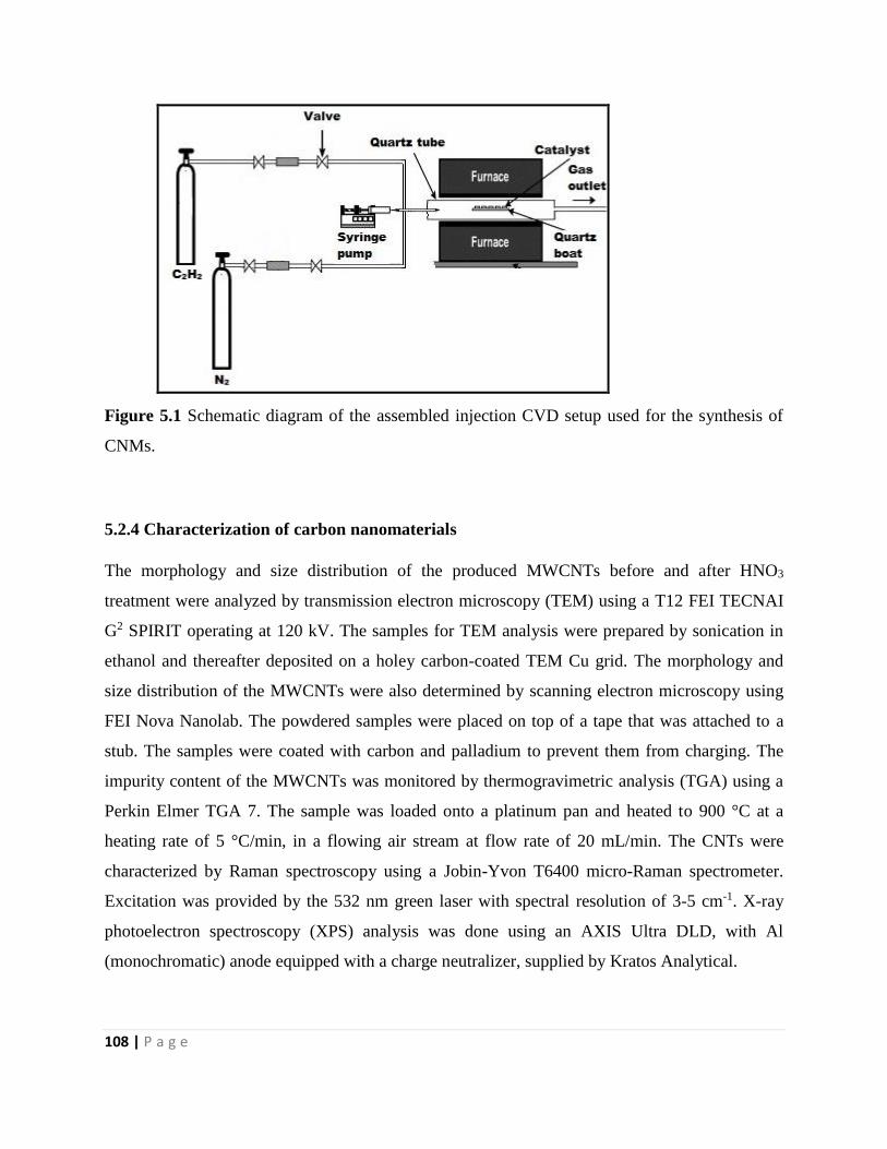
108 | P a g e

Figure 5.1 Schematic diagram of the assembled injection CVD setup used for the synthesis of

CNMs.

5.2.4 Characterization of carbon nanomaterials

The morphology and size distribution of the produced MWCNTs before and after HNO3

treatment were analyzed by transmission electron microscopy (TEM) using a T12 FEI TECNAI

G2 SPIRIT operating at 120 kV. The samples for TEM analysis were prepared by sonication in

ethanol and thereafter deposited on a holey carbon-coated TEM Cu grid. The morphology and

size distribution of the MWCNTs were also determined by scanning electron microscopy using

FEI Nova Nanolab. The powdered samples were placed on top of a tape that was attached to a

stub. The samples were coated with carbon and palladium to prevent them from charging. The

impurity content of the MWCNTs was monitored by thermogravimetric analysis (TGA) using a

Perkin Elmer TGA 7. The sample was loaded onto a platinum pan and heated to 900 °C at a

heating rate of 5 °C/min, in a flowing air stream at flow rate of 20 mL/min. The CNTs were

characterized by Raman spectroscopy using a Jobin-Yvon T6400 micro-Raman spectrometer.

Excitation was provided by the 532 nm green laser with spectral resolution of 3-5 cm-1. X-ray

photoelectron spectroscopy (XPS) analysis was done using an AXIS Ultra DLD, with Al

(monochromatic) anode equipped with a charge neutralizer, supplied by Kratos Analytical.

109 | P a g e


In this section the morphology of the CNMs were evaluated using TEM and SEM. The effect of

solvent mixture injection rate was optimized and the optimum flow rate used in the

investigations that follows. The effect of chlorine concentration of the morphology of the CNMs

was also evaluated. The TEM and SEM characterizations were confirmed by TGA, Raman

spectroscopy and XPS.

Dichlorobenzene (DCB) was selected as a chlorine source to use for the investigation of its role

on the morphology of the N doped CNMs. Our previous results showed that CNTs produced

using DCB had more uniform diameters and were produced in large quantities.

5.3.1 Structural analysis of N doped CNMs: Effect of DCB concentration and injection

flow rate

In order to study the role of chlorine on the morphology of the N-doped CNMs, we first had to

study the morphology of the CNMs obtained from pure CH3CN and pure DCB. To our

knowledge CNMs obtained using pure CH3CN as a nitrogen source and pure DCB as a chlorine

source over a Fe-Co/CaCO3 catalyst by using an injection CVD injection was never reported.

The reaction conditions used in this study were as follows: N2 flow rate = 240 mL/min, C2H2

flow rate = 90 mL/min, reaction temperature = 800 °C, reaction time = 1 h, injection rate = 0.24

mL/min.

The morphology of the CNMs using pure CH3CN and DCB were studied by TEM. TEM images

obtained from pure CH3CN revealed the presence of a mixture of CNMs, hollow thin-walled

CNTs (Figure 5.2a and b), bamboo compartmented CNTs (Figure 5.2c) and carbon nanospheres

(CNS) (Figure 5.2d). A rod-shaped CNF with a measuring-cylinder like tip or base (Figure 5.2a

shown by arrow) was also observed from a TEM image. Similar rod-shaped CNFs are presented

in Supplementary Figure S1a and b circled parts.

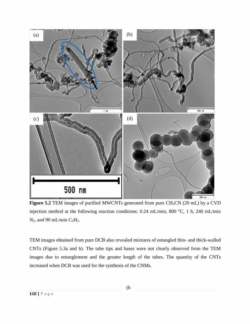
110 | P a g e

Figure 5.2 TEM images of purified MWCNTs generated from pure CH3CN (20 mL) by a CVD

injection method at the following reaction conditions: 0.24 mL/min, 800 °C, 1 h, 240 mL/min

N2, and 90 mL/min C2H2.

TEM images obtained from pure DCB also revealed mixtures of entangled thin- and thick-walled

CNTs (Figure 5.3a and b). The tube tips and bases were not clearly observed from the TEM

images due to entanglement and the greater length of the tubes. The quantity of the CNTs

increased when DCB was used for the synthesis of the CNMs.

(a)

(d)

(b)

(c)

(b

)

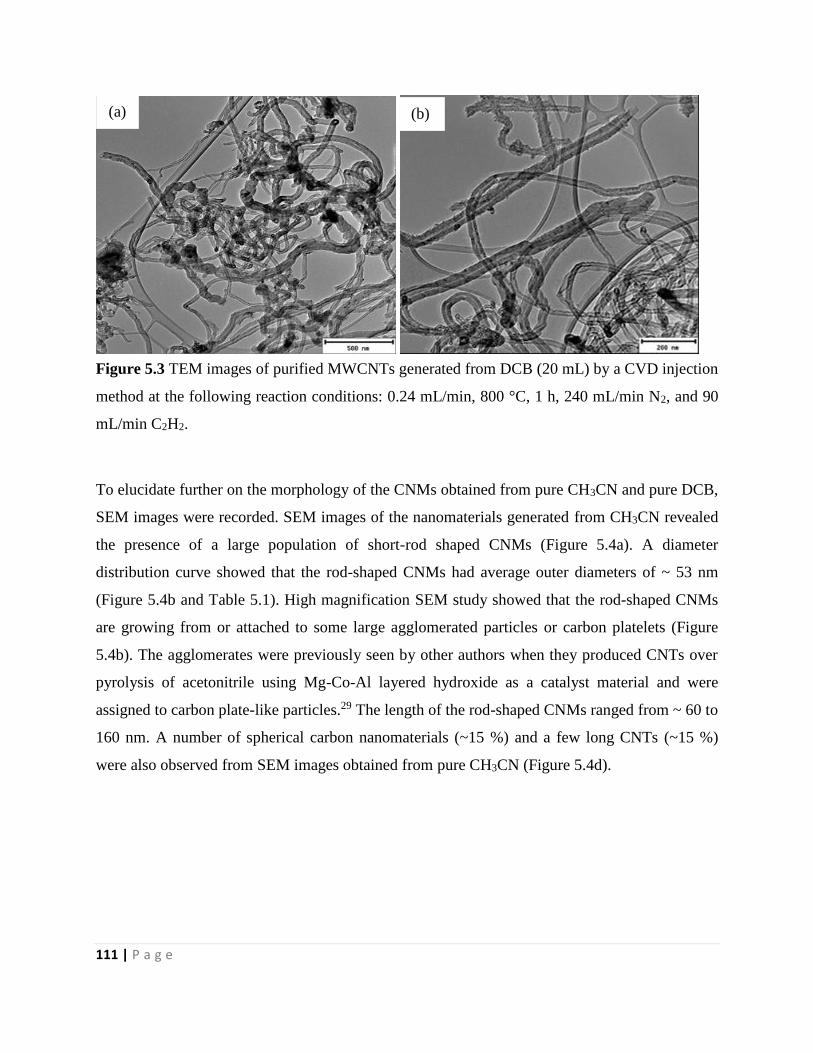
111 | P a g e

Figure 5.3 TEM images of purified MWCNTs generated from DCB (20 mL) by a CVD injection

method at the following reaction conditions: 0.24 mL/min, 800 °C, 1 h, 240 mL/min N2, and 90

mL/min C2H2.

To elucidate further on the morphology of the CNMs obtained from pure CH3CN and pure DCB,

SEM images were recorded. SEM images of the nanomaterials generated from CH3CN revealed

the presence of a large population of short-rod shaped CNMs (Figure 5.4a). A diameter

distribution curve showed that the rod-shaped CNMs had average outer diameters of ~ 53 nm

(Figure 5.4b and Table 5.1). High magnification SEM study showed that the rod-shaped CNMs

are growing from or attached to some large agglomerated particles or carbon platelets (Figure

5.4b). The agglomerates were previously seen by other authors when they produced CNTs over

pyrolysis of acetonitrile using Mg-Co-Al layered hydroxide as a catalyst material and were

assigned to carbon plate-like particles.29 The length of the rod-shaped CNMs ranged from ~ 60 to

160 nm. A number of spherical carbon nanomaterials (~15 %) and a few long CNTs (~15 %)

were also observed from SEM images obtained from pure CH3CN (Figure 5.4d).

(a) (b)

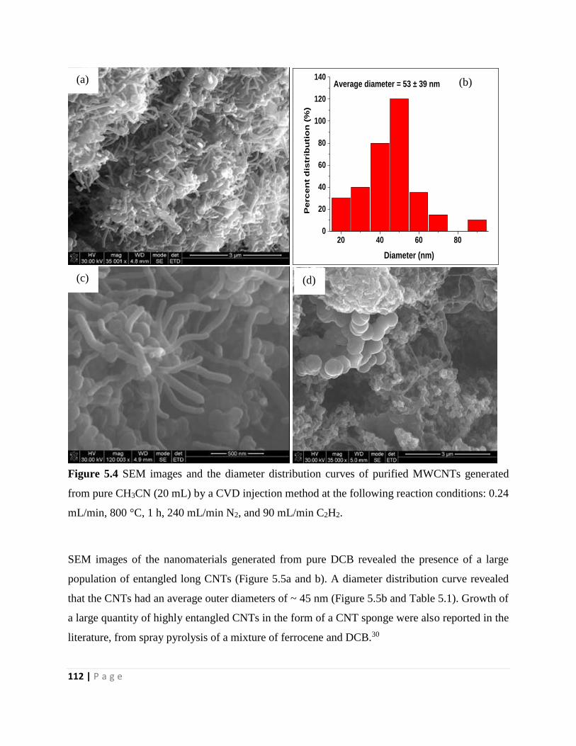
112 | P a g e

20 40 60 800

20

40

60

80

100

120

140

Perc

en

t d

istr

ibu

tio

n (

%)

Diameter (nm)

Average diameter = 53 ± 39 nm


from pure CH3CN (20 mL) by a CVD injection method at the following reaction conditions: 0.24

mL/min, 800 °C, 1 h, 240 mL/min N2, and 90 mL/min C2H2.

SEM images of the nanomaterials generated from pure DCB revealed the presence of a large

population of entangled long CNTs (Figure 5.5a and b). A diameter distribution curve revealed

that the CNTs had an average outer diameters of ~ 45 nm (Figure 5.5b and Table 5.1). Growth of

a large quantity of highly entangled CNTs in the form of a CNT sponge were also reported in the

literature, from spray pyrolysis of a mixture of ferrocene and DCB.30

(a)

(d)

(b)

(c)

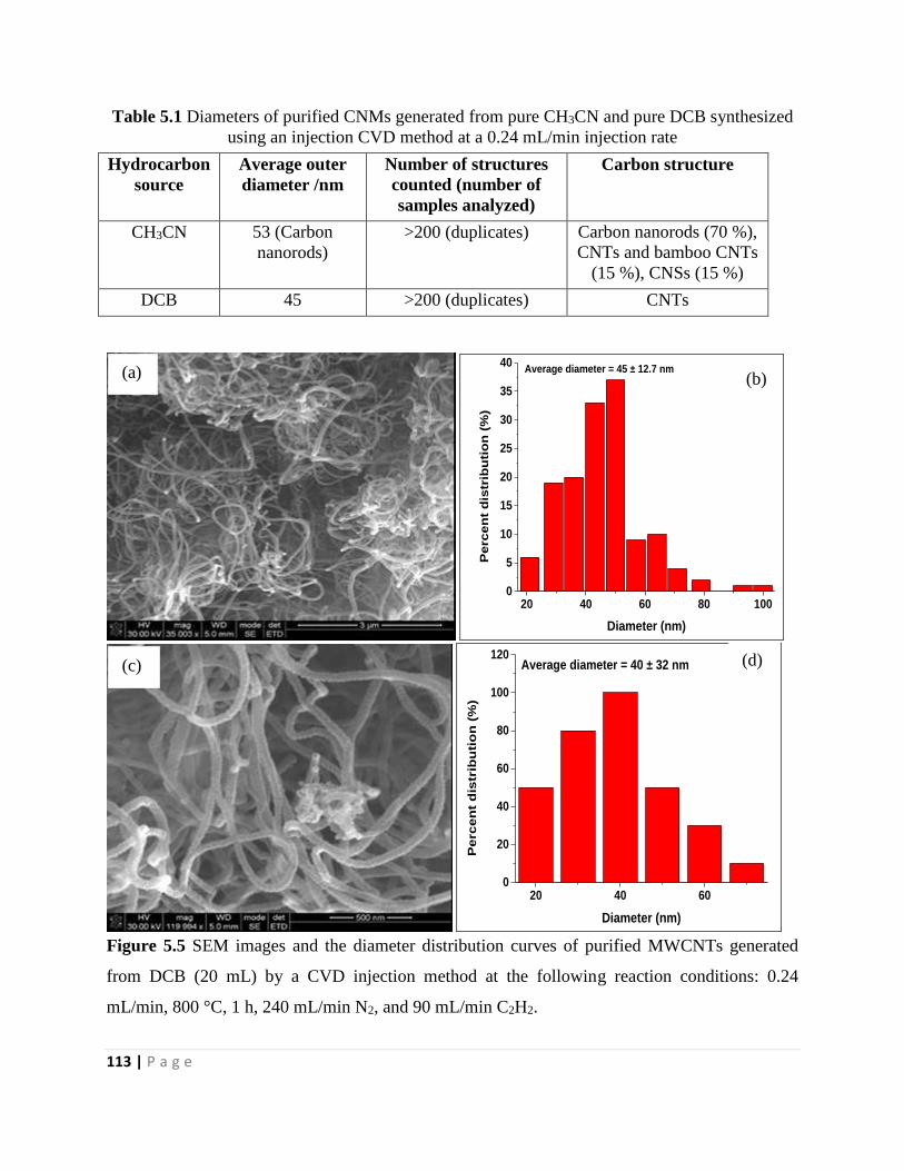
113 | P a g e


using an injection CVD method at a 0.24 mL/min injection rate

Hydrocarbon

source

Average outer

diameter /nm

Number of structures

counted (number of

samples analyzed)

Carbon structure

CH3CN 53 (Carbon

nanorods)

>200 (duplicates) Carbon nanorods (70 %),

CNTs and bamboo CNTs

(15 %), CNSs (15 %)

DCB 45 >200 (duplicates) CNTs

20 40 60 80 1000

5

10

15

20

25

30

35

40

Perc

en

t d

istr

ibu

tio

n (

%)

Diameter (nm)

Average diameter = 45 ± 12.7 nm

20 40 600

20

40

60

80

100

120

Perc

en

t d

istr

ibu

tio

n (

%)

Diameter (nm)



from DCB (20 mL) by a CVD injection method at the following reaction conditions: 0.24

mL/min, 800 °C, 1 h, 240 mL/min N2, and 90 mL/min C2H2.

(a) (b)

(c) (d)

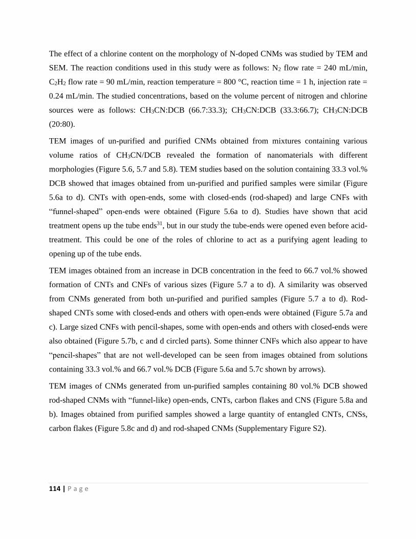
114 | P a g e

The effect of a chlorine content on the morphology of N-doped CNMs was studied by TEM and

SEM. The reaction conditions used in this study were as follows: N2 flow rate = 240 mL/min,

C2H2 flow rate = 90 mL/min, reaction temperature = 800 °C, reaction time = 1 h, injection rate =

0.24 mL/min. The studied concentrations, based on the volume percent of nitrogen and chlorine

sources were as follows: CH3CN:DCB (66.7:33.3); CH3CN:DCB (33.3:66.7); CH3CN:DCB

(20:80).

TEM images of un-purified and purified CNMs obtained from mixtures containing various

volume ratios of CH3CN/DCB revealed the formation of nanomaterials with different

morphologies (Figure 5.6, 5.7 and 5.8). TEM studies based on the solution containing 33.3 vol.%

DCB showed that images obtained from un-purified and purified samples were similar (Figure

5.6a to d). CNTs with open-ends, some with closed-ends (rod-shaped) and large CNFs with

“funnel-shaped” open-ends were obtained (Figure 5.6a to d). Studies have shown that acid

treatment opens up the tube ends31, but in our study the tube-ends were opened even before acid-

treatment. This could be one of the roles of chlorine to act as a purifying agent leading to

opening up of the tube ends.

TEM images obtained from an increase in DCB concentration in the feed to 66.7 vol.% showed

formation of CNTs and CNFs of various sizes (Figure 5.7 a to d). A similarity was observed

from CNMs generated from both un-purified and purified samples (Figure 5.7 a to d). Rod-

shaped CNTs some with closed-ends and others with open-ends were obtained (Figure 5.7a and

c). Large sized CNFs with pencil-shapes, some with open-ends and others with closed-ends were

also obtained (Figure 5.7b, c and d circled parts). Some thinner CNFs which also appear to have

“pencil-shapes” that are not well-developed can be seen from images obtained from solutions

containing 33.3 vol.% and 66.7 vol.% DCB (Figure 5.6a and 5.7c shown by arrows).

TEM images of CNMs generated from un-purified samples containing 80 vol.% DCB showed

rod-shaped CNMs with “funnel-like) open-ends, CNTs, carbon flakes and CNS (Figure 5.8a and

b). Images obtained from purified samples showed a large quantity of entangled CNTs, CNSs,

carbon flakes (Figure 5.8c and d) and rod-shaped CNMs (Supplementary Figure S2).

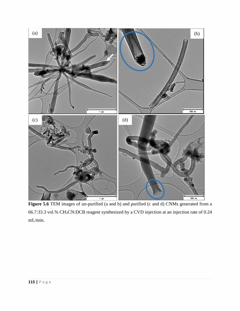
115 | P a g e



mL/min.

(a)

(d) (c)

(b)

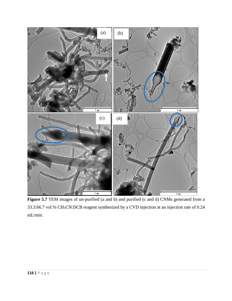
116 | P a g e



mL/min.

(a)

(d) (c)

(b)

117 | P a g e


20:80 vol.% CH3CN:DCB reagent synthesized by a CVD injection at an injection rate of 0.24

mL/min..

SEM images were also recorded in order to obtain more information on the morphology and

dominating carbon nanostructures. SEM images obtained from un-purified samples containing

33.3 vol.% DCB showed the presence of rod-shaped CNMs, covered by droplets of metal

catalyst particles (Figure 5.9a and b). SEM images of the purified samples revealed that the

majority of the CNMs in these feeds were “straw-shaped” CNTs with open-ends and of various

(a)

(d) (c)

(b)

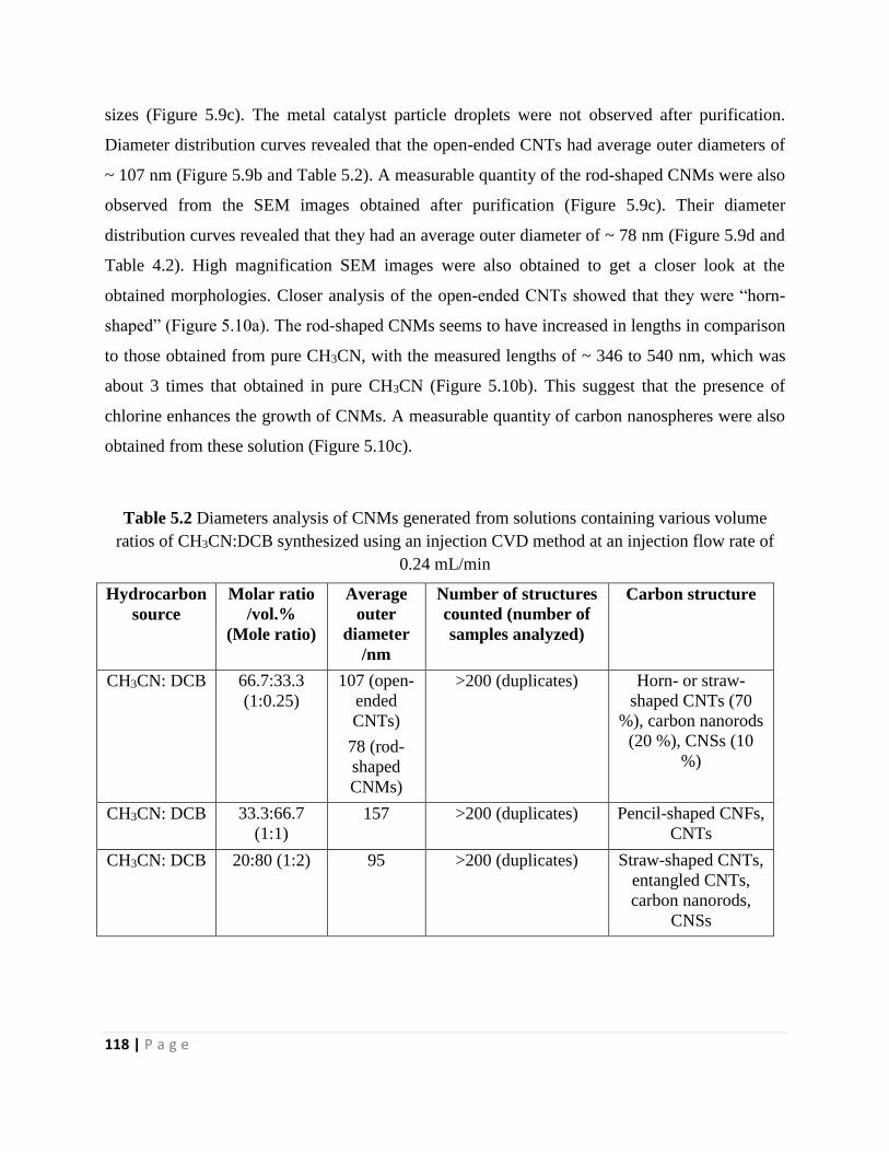
118 | P a g e

sizes (Figure 5.9c). The metal catalyst particle droplets were not observed after purification.

Diameter distribution curves revealed that the open-ended CNTs had average outer diameters of

~ 107 nm (Figure 5.9b and Table 5.2). A measurable quantity of the rod-shaped CNMs were also

observed from the SEM images obtained after purification (Figure 5.9c). Their diameter

distribution curves revealed that they had an average outer diameter of ~ 78 nm (Figure 5.9d and

Table 4.2). High magnification SEM images were also obtained to get a closer look at the

obtained morphologies. Closer analysis of the open-ended CNTs showed that they were “horn-

shaped” (Figure 5.10a). The rod-shaped CNMs seems to have increased in lengths in comparison

to those obtained from pure CH3CN, with the measured lengths of ~ 346 to 540 nm, which was

about 3 times that obtained in pure CH3CN (Figure 5.10b). This suggest that the presence of

chlorine enhances the growth of CNMs. A measurable quantity of carbon nanospheres were also

obtained from these solution (Figure 5.10c).

Table 5.2 Diameters analysis of CNMs generated from solutions containing various volume

ratios of CH3CN:DCB synthesized using an injection CVD method at an injection flow rate of

0.24 mL/min

Hydrocarbon

source

Molar ratio

/vol.%

(Mole ratio)

Average

outer

diameter

/nm


counted (number of

samples analyzed)

Carbon structure

CH3CN: DCB 66.7:33.3

(1:0.25)

107 (open-

ended

CNTs)

78 (rod-

shaped

CNMs)

>200 (duplicates) Horn- or straw-

shaped CNTs (70

%), carbon nanorods

(20 %), CNSs (10

%)

CH3CN: DCB 33.3:66.7

(1:1)

157 >200 (duplicates) Pencil-shaped CNFs,

CNTs

CH3CN: DCB 20:80 (1:2) 95 >200 (duplicates) Straw-shaped CNTs,

entangled CNTs,

carbon nanorods,

CNSs

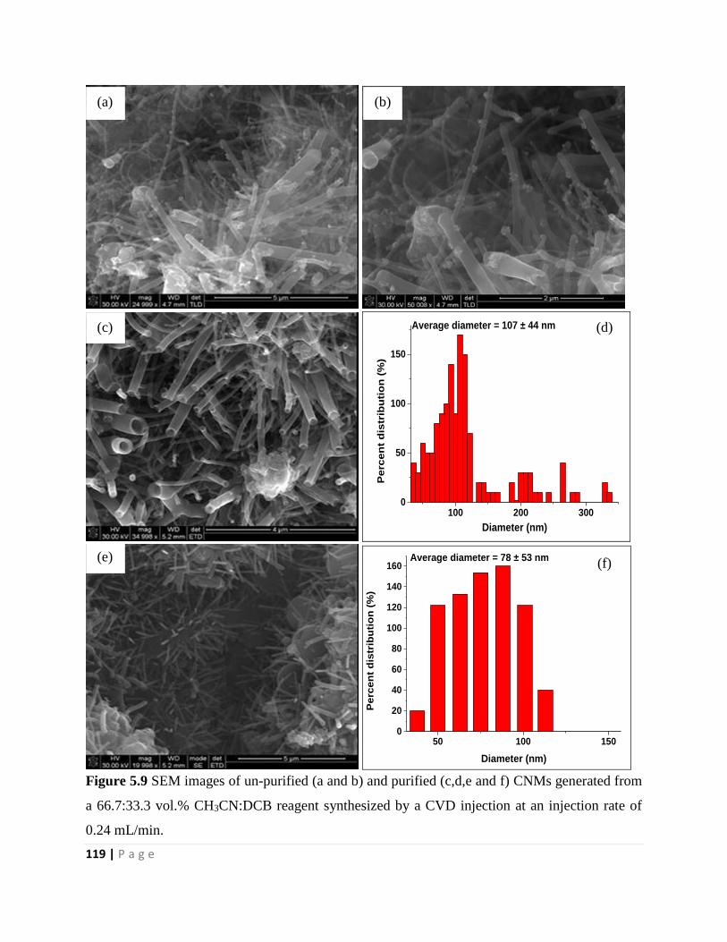
119 | P a g e

100 200 3000

50

100

150

Perc

en

t d

istr

ibu

tio

n (

%)

Diameter (nm)


50 100 1500

20

40

60

80

100

120

140

160

Pe

rce

nt

dis

trib

uti

on

(%

)

Diameter (nm)


Figure 5.9 SEM images of un-purified (a and b) and purified (c,d,e and f) CNMs generated from

a 66.7:33.3 vol.% CH3CN:DCB reagent synthesized by a CVD injection at an injection rate of

0.24 mL/min.

(a) (b)

(c)

(f) (e)

(d)

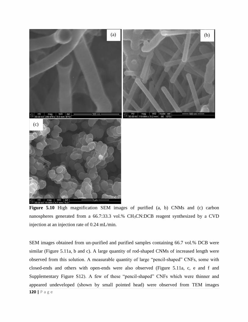
120 | P a g e

Figure 5.10 High magnification SEM images of purified (a, b) CNMs and (c) carbon

nanospheres generated from a 66.7:33.3 vol.% CH3CN:DCB reagent synthesized by a CVD

injection at an injection rate of 0.24 mL/min.

SEM images obtained from un-purified and purified samples containing 66.7 vol.% DCB were

similar (Figure 5.11a, b and c). A large quantity of rod-shaped CNMs of increased length were

observed from this solution. A measurable quantity of large “pencil-shaped” CNFs, some with

closed-ends and others with open-ends were also observed (Figure 5.11a, c, e and f and

Supplementary Figure S12). A few of these “pencil-shaped” CNFs which were thinner and

appeared undeveloped (shown by small pointed head) were observed from TEM images

(a)

(c)

(b)

121 | P a g e

generated from a solution containing 33.3 vol.% DCB. It appears that the presence of chlorine in

the feed results in structural changes of the “rod-shaped” CNMs to “pencil-shaped” CNFs. This

is shown by an increase in the thin ended part of the CNF resulting in a formation of a well-

developed “pencil-like” CNF. The open-ended “pencil-shaped” CNFs appears as if their tips

were broken, resulting in open-ends (Figure 5.11e). The reaction mechanism of this “pencil-

shaped” CNTs still needs to be investigated, but it appears that chlorine is responsible for this.

of covered by droplets of metal catalyst particles (Figure 5.9a and b). SEM images of the purified

samples revealed that the majority of the CNMs in these feeds were “pencil-shaped” CNFs with

most of them under developed shown by the small undefined tip-ends. The average outer

diameter of all the observed CNMs was about 154 nm (Figure 5.11c and Table 5.3).

SEM images obtained from solutions containing 80 vol.% DCB concentration revealed also a

mixture of CNMs. Un-purified samples showed rod-shaped CNMs covered by droplets of metal

catalyst particles (Figure 5.12a). SEM images of the purified samples revealed mixtures of clean

CNMs, CNSs, “straw-shaped” open-ended CNTs and entangled CNTs (Figure 5.12 b, c, and e

and Figure 5.13). The “straw-shaped” CNTs were dominating in this solution and their average

diameters were about 95 nm (Figure 5.12d and Table 5.3). The average outer diameter of the

entangled CNTs was about 72 nm (Figure 5.12f and Table 5.3). It appears that in all

concentrations studied, the tube length increased with an increase in amount of chlorine present

in the feed.

“Sharp nail structures as claws were observed by other researchers when they modified the CVD

method of producing N-doped CNTs by adding NaCl to the water that was in a by-product liquid

trap, using benzylamine and ferrocene as nitrogen source and catalyst28. They claimed that as

they increased the concentration of the salt in water changes in morphology of N-doped CNTs

occurred. The changes in morphology were probably due to the evaporation of water but the

authors claimed that it was due to the participation of Na and Cl atoms produced in the water as

they move back into the hot zone. “How can the ions move back against a flow and take part in

the reaction?” They also claimed that Na and Cl ions were participating in the catalysis, probably

reducing the sizes of the nanoparticles”.26

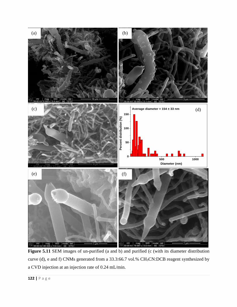
122 | P a g e

500 10000

50

100

150

Perc

en

t d

istr

ibu

tio

n (

%)

Diameter (nm)



curve (d), e and f) CNMs generated from a 33.3:66.7 vol.% CH3CN:DCB reagent synthesized by

a CVD injection at an injection rate of 0.24 mL/min.

(a) (b)

(c)

(f) (e)

(d)

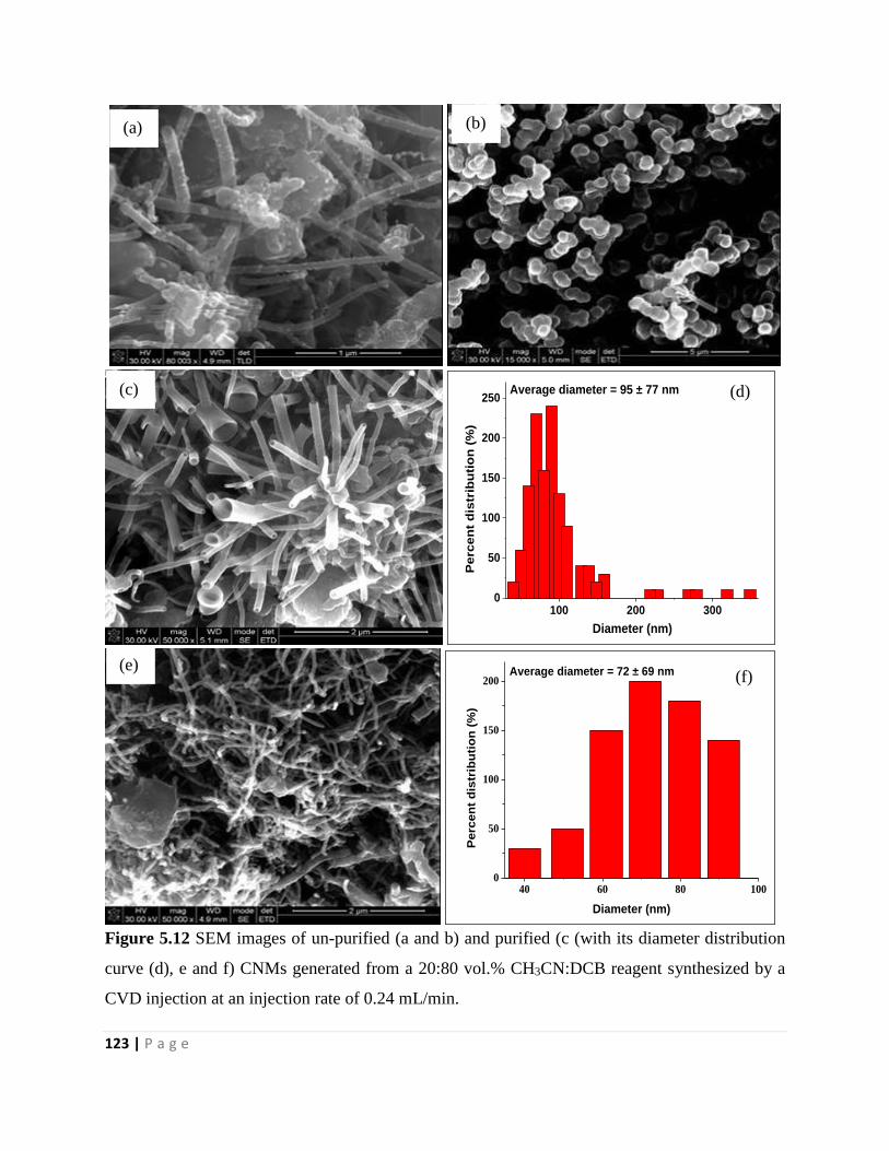
123 | P a g e

100 200 3000

50

100

150

200

250

Perc

en

t d

istr

ibu

tio

n (

%)

Diameter (nm)


40 60 80 1000

50

100

150

200

Pe

rce

nt

dis

trib

uti

on

(%

)

Diameter (nm)



curve (d), e and f) CNMs generated from a 20:80 vol.% CH3CN:DCB reagent synthesized by a

CVD injection at an injection rate of 0.24 mL/min.

(a)

(f) (e)

(d) (c)

(b)

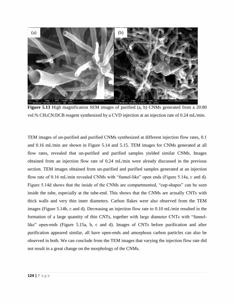
124 | P a g e

Figure 5.13 High magnification SEM images of purified (a, b) CNMs generated from a 20:80

vol.% CH3CN:DCB reagent synthesized by a CVD injection at an injection rate of 0.24 mL/min.

TEM images of un-purified and purified CNMs synthesized at different injection flow rates, 0.1

and 0.16 mL/min are shown in Figure 5.14 and 5.15. TEM images for CNMs generated at all

flow rates, revealed that un-purified and purified samples yielded similar CNMs. Images

obtained from an injection flow rate of 0.24 mL/min were already discussed in the previous

section. TEM images obtained from un-purified and purified samples generated at an injection

flow rate of 0.16 mL/min revealed CNMs with “funnel-like” open ends (Figure 5.14a, c and d).

Figure 5.14d shows that the inside of the CNMs are compartmented, “cup-shapes” can be seen

inside the tube, especially at the tube-end. This shows that the CNMs are actually CNTs with

thick walls and very thin inner diameters. Carbon flakes were also observed from the TEM

images (Figure 5.14b, c and d). Decreasing an injection flow rate to 0.10 mL/min resulted in the

formation of a large quantity of thin CNTs, together with large diameter CNTs with “funnel-

like” open-ends (Figure 5.15a, b, c and d). Images of CNTs before purification and after

purification appeared similar, all have open-ends and amorphous carbon particles can also be

observed in both. We can conclude from the TEM images that varying the injection flow rate did

not result in a great change on the morphology of the CNMs.

(a) (b)

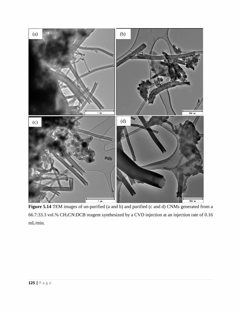
125 | P a g e



mL/min.

(a)

(d) (c)

(b)

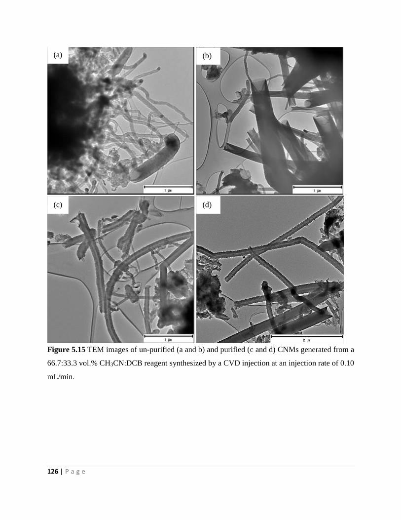
126 | P a g e



mL/min.

(a)

(d) (c)

(b)

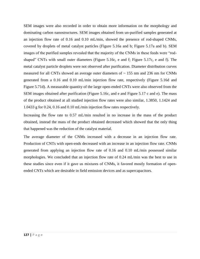
127 | P a g e

SEM images were also recorded in order to obtain more information on the morphology and

dominating carbon nanostructures. SEM images obtained from un-purified samples generated at

an injection flow rate of 0.16 and 0.10 mL/min, showed the presence of rod-shaped CNMs,

covered by droplets of metal catalyst particles (Figure 5.16a and b; Figure 5.17a and b). SEM

images of the purified samples revealed that the majority of the CNMs in these feeds were “rod-

shaped” CNTs with small outer diameters (Figure 5.16c, e and f; Figure 5.17c, e and f). The

metal catalyst particle droplets were not observed after purification. Diameter distribution curves

measured for all CNTs showed an average outer diameters of ~ 155 nm and 236 nm for CNMs

generated from a 0.16 and 0.10 mL/min injection flow rate, respectively (Figure 5.16d and

Figure 5.71d). A measurable quantity of the large open-ended CNTs were also observed from the

SEM images obtained after purification (Figure 5.16c, and e and Figure 5.17 c and e). The mass

of the product obtained at all studied injection flow rates were also similar, 1.3850, 1.1424 and

1.0433 g for 0.24, 0.16 and 0.10 mL/min injection flow rates respectively.

Increasing the flow rate to 0.57 mL/min resulted in no increase in the mass of the product

obtained, instead the mass of the product obtained decreased which showed that the only thing

that happened was the reduction of the catalyst material.

The average diameter of the CNMs increased with a decrease in an injection flow rate.

Production of CNTs with open-ends decreased with an increase in an injection flow rate. CNMs

generated from applying an injection flow rate of 0.16 and 0.10 mL/min possessed similar

morphologies. We concluded that an injection flow rate of 0.24 mL/min was the best to use in

these studies since even if it gave us mixtures of CNMs, it favored mostly formation of open-

ended CNTs which are desirable in field emission devices and as supercapacitors.

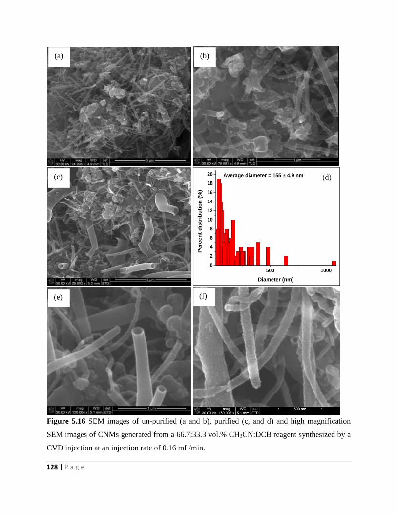
128 | P a g e

500 10000

2

4

6

8

10

12

14

16

18

20

Perc

en

t d

istr

ibu

tio

n (

%)

Diameter (nm)





(a)

(d) (c)

(b)

(e) (f)

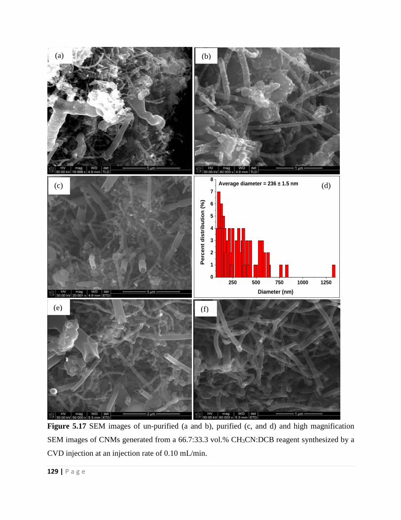
129 | P a g e

250 500 750 1000 12500

1

2

3

4

5

6

7

8

Perc

en

t d

istr

ibu

tio

n (

%)

Diameter (nm)





(a) (b)

(c) (d)

(e) (f)

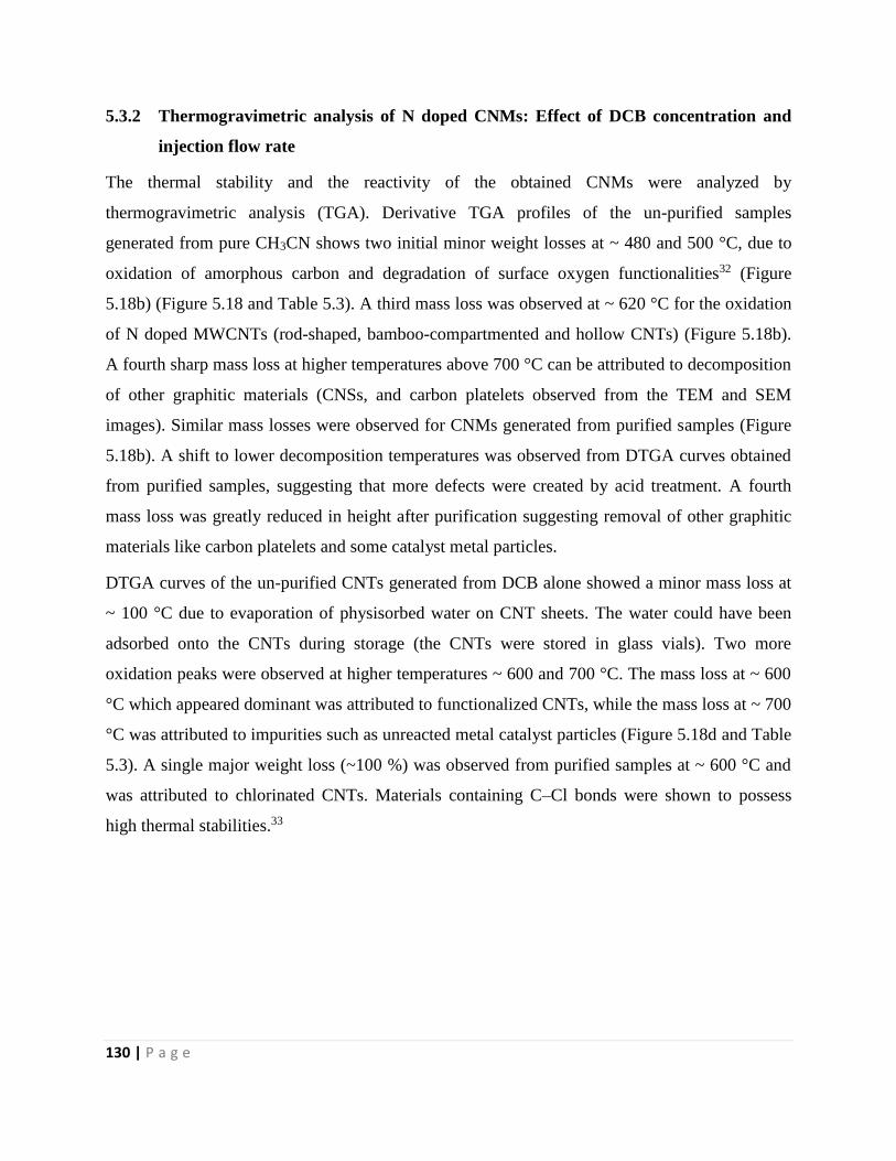
130 | P a g e

5.3.2 Thermogravimetric analysis of N doped CNMs: Effect of DCB concentration and

injection flow rate

The thermal stability and the reactivity of the obtained CNMs were analyzed by

thermogravimetric analysis (TGA). Derivative TGA profiles of the un-purified samples

generated from pure CH3CN shows two initial minor weight losses at ~ 480 and 500 °C, due to

oxidation of amorphous carbon and degradation of surface oxygen functionalities32 (Figure

5.18b) (Figure 5.18 and Table 5.3). A third mass loss was observed at ~ 620 °C for the oxidation

of N doped MWCNTs (rod-shaped, bamboo-compartmented and hollow CNTs) (Figure 5.18b).

A fourth sharp mass loss at higher temperatures above 700 °C can be attributed to decomposition

of other graphitic materials (CNSs, and carbon platelets observed from the TEM and SEM

images). Similar mass losses were observed for CNMs generated from purified samples (Figure

5.18b). A shift to lower decomposition temperatures was observed from DTGA curves obtained

from purified samples, suggesting that more defects were created by acid treatment. A fourth

mass loss was greatly reduced in height after purification suggesting removal of other graphitic

materials like carbon platelets and some catalyst metal particles.

DTGA curves of the un-purified CNTs generated from DCB alone showed a minor mass loss at

~ 100 °C due to evaporation of physisorbed water on CNT sheets. The water could have been

adsorbed onto the CNTs during storage (the CNTs were stored in glass vials). Two more

oxidation peaks were observed at higher temperatures ~ 600 and 700 °C. The mass loss at ~ 600

°C which appeared dominant was attributed to functionalized CNTs, while the mass loss at ~ 700

°C was attributed to impurities such as unreacted metal catalyst particles (Figure 5.18d and Table

5.3). A single major weight loss (~100 %) was observed from purified samples at ~ 600 °C and

was attributed to chlorinated CNTs. Materials containing C–Cl bonds were shown to possess

high thermal stabilities.33

131 | P a g e

0 200 400 600 800 10000

20

40

60

80

100W

eig

ht

(%)

Temperature (0C)

Un-purified

Purified

CH3CN

0 200 400 600 800-7

-6

-5

-4

-3

-2

-1

0

1

Deri

va

tiv

e w

eig

ht

(%)

Temperature (0C)

Un-purified

Purified

CH3CN

0 200 400 600 800 1000

0

20

40

60

80

100

We

igh

t (%

)

Temperature (0C)

Un-purified

Purified

DCB

0 200 400 600 800

-10

-5

0

Deri

va

tiv

e

weig

ht

(%)

Temperature (0C)

Un-purified

Un-purified

DCB

Figure 5.18 TGA and DTGA curves of un-purified and purified CNMs generated from pure

CH3CN (a & b) and pure DCB (c & d) synthesized by CVD injection at 0.24 mL/min.



of CH3CN and DCB.

CH3CN:DCB

vol.%

Peak 1

decomposition

temperature, °C

Peak 2

decomposition

temperature, °C

Residual

mass, %

100:0 643 744 28.5

100:0 (P) 540 621 8.9

0:100 601 695 25.7

0:100 (P) 607 – 0

(a) (b)

(c) (d)

132 | P a g e

Three mass losses were observed from DTGA curves generated from un-purified CNMs while

two mass losses were observed from purified CNMs synthesized from solutions containing 33.3

vol.% DCB (Figure 5.19b). The first mass loss at ~ 100 °C, was due to physisorbed water on the

CNT sheets. The second most intense weight losses at higher temperatures ~ 550, was attributed

to oxidation of chlorinated N-doped CNTs (Figure 5.19 and Table 5.4). The third mass loss

appeared at ~ 650 °C for purified CNMs and was at ~ 680 for un-purified CNMs. The third

weight loss was assigned to oxidation of other graphitic materials (CNSs, and carbon platelets).

These observations agree with the TEM observations were mixtures of CNMs were observed

from un-purified and purified samples.

DTGA obtained from solutions containing 66.7 vol.% DCB were also analyzed. Two mass losses

at lower temperatures were observed from un-purified samples at ~ 100 and 150 °C. The first

mass loss at ~ 100 °C was assigned to physisorbed water and the mass loss at ~ 150 °C was

assigned to decomposition of chemisorbed surface chloride groups32. A broad oxidation peak at

higher temperatures from 600 to 750 °C which shows three mass losses, of which two are sharp

at higher temperatures (Figure 5.19 and Table 5.4). The weight loss at ~ 600 °C can be attributed

to stable C–Cl bonds from chlorinated N-doped CNTs. Two small sharp weight losses at ~ 680

and 750 °C can be attributed to the presence of other graphitic materials (like large “pencil-

shaped” CNMs) respectively. Another broad oxidation peak at even higher temperatures ~ 800

°C (Figure 5.19d) was observed, which was assigned to the evolution of nitrogen which is known

to be released from N-doped carbons.33 Highest weight changes were observed for samples with

highest chlorine content.34 We can assume that the formation of large “pencil-shaped” CNTs

some with open-ends and others with closed-ends were enhanced in feeds containing a large

content of chlorine adatoms. The results agree with TEM images where large “pencil-shaped”

CNTs were produced from solutions containing 66.7 vol.% DCB that is assumed to release large

amounts of chlorine vapors into the feed. This situation prevails when formation of Cl2

molecules which can escape through the trap is hindered by formation of Cl adatoms at opposite

sides of the CNT tube.35 Formation of Cl2 molecules from two individual Cl atoms is

energetically favorable when the two Cl atoms are at close proximity to each other.35

We then analyzed DTGA profiles obtained from solutions containing 80 vol.% DCB. Two mass

losses at lower temperatures were observed from un-purified samples at ~ 100 and 150 °C

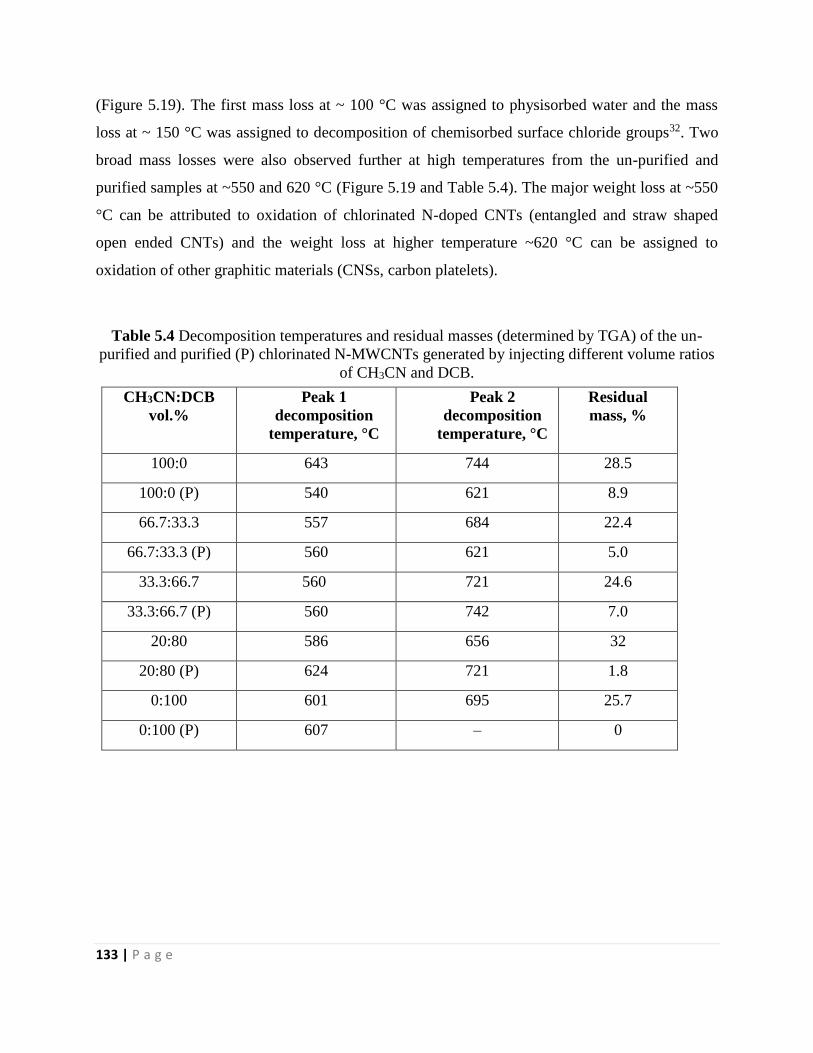
133 | P a g e

(Figure 5.19). The first mass loss at ~ 100 °C was assigned to physisorbed water and the mass

loss at ~ 150 °C was assigned to decomposition of chemisorbed surface chloride groups32. Two

broad mass losses were also observed further at high temperatures from the un-purified and

purified samples at ~550 and 620 °C (Figure 5.19 and Table 5.4). The major weight loss at ~550

°C can be attributed to oxidation of chlorinated N-doped CNTs (entangled and straw shaped

open ended CNTs) and the weight loss at higher temperature ~620 °C can be assigned to

oxidation of other graphitic materials (CNSs, carbon platelets).



of CH3CN and DCB.

CH3CN:DCB

vol.%

Peak 1

decomposition

temperature, °C

Peak 2

decomposition

temperature, °C

Residual

mass, %

100:0 643 744 28.5

100:0 (P) 540 621 8.9

66.7:33.3 557 684 22.4

66.7:33.3 (P) 560 621 5.0

33.3:66.7 560 721 24.6

33.3:66.7 (P) 560 742 7.0

20:80 586 656 32

20:80 (P) 624 721 1.8

0:100 601 695 25.7

0:100 (P) 607 – 0

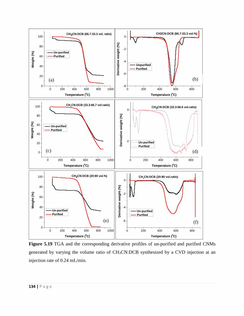
134 | P a g e

0 200 400 600 800 10000

20

40

60

80

100

Weig

ht

(%)

Temperature (0C)

Un-purified

Purified

CH3CN:DCB (66.7:33.3 vol. ratio)

0 200 400 600 800-8

-6

-4

-2

0

Deri

va

tiv

e w

eig

ht

(%)

Temperature (0C)

Unpurified

Purified

CH3CN:DCB (66.7:33.3 vol.%)

0 200 400 600 800 1000

0

20

40

60

80

100

Weig

ht

(%)

Temperature (0C)

Un-purified

Purified

CH3CN:DCB (33.3:66.7 vol.ratio)

0 200 400 600 800

-2

0

Deri

va

tiv

e w

eig

ht

(%)

Temperature (0C)

Un-purified

Purified

CH3CN:DCB (33.3:66.6 vol.ratio)

0 200 400 600 800 10000

20

40

60

80

100

We

igh

t (%

)

Temperature (0C)

Un-purified

Purified

CH3CN:DCB (20:80 vol.%)

0 200 400 600 800

-6

-4

-2

0

Deri

va

tiv

e w

eig

ht

(%)

Temperature (0C)

Un-purified

Purified

CH3CN:DCB (20:80 vol.ratio)

Figure 5.19 TGA and the corresponding derivative profiles of un-purified and purified CNMs

generated by varying the volume ratio of CH3CN:DCB synthesized by a CVD injection at an

injection rate of 0.24 mL/min.

(a) (b)

(c) (d)

(e) (f)

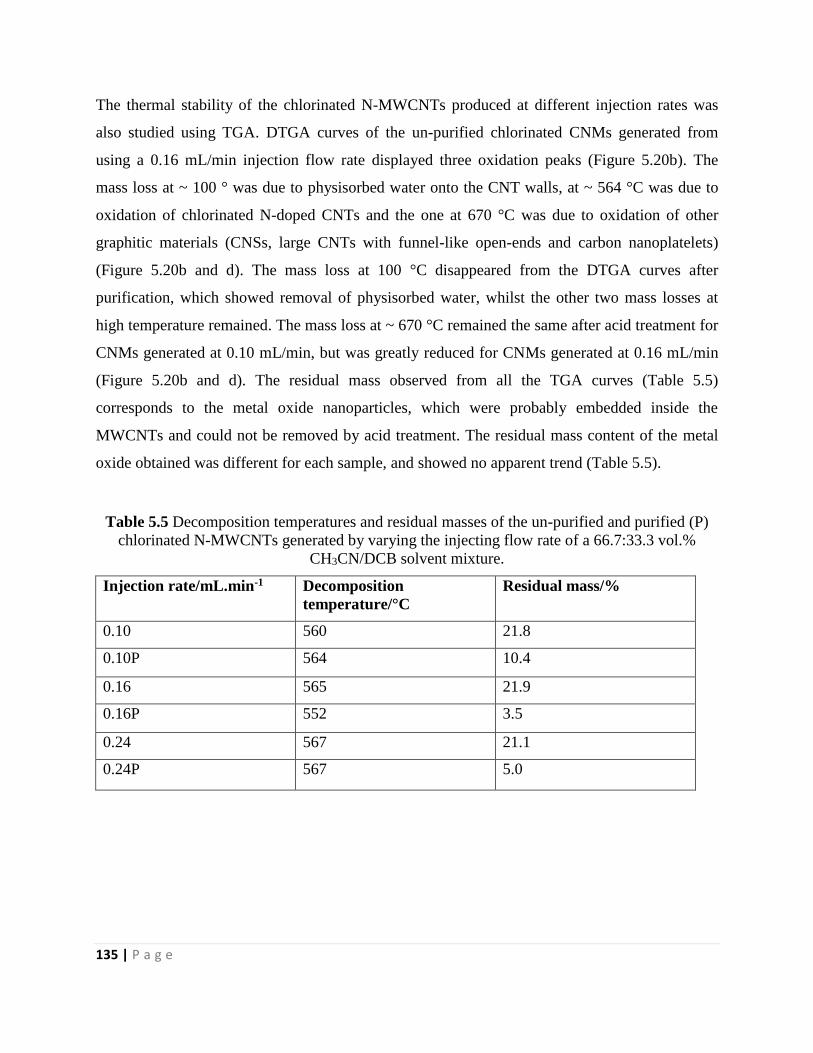
135 | P a g e

The thermal stability of the chlorinated N-MWCNTs produced at different injection rates was

also studied using TGA. DTGA curves of the un-purified chlorinated CNMs generated from

using a 0.16 mL/min injection flow rate displayed three oxidation peaks (Figure 5.20b). The

mass loss at ~ 100 ° was due to physisorbed water onto the CNT walls, at ~ 564 °C was due to

oxidation of chlorinated N-doped CNTs and the one at 670 °C was due to oxidation of other

graphitic materials (CNSs, large CNTs with funnel-like open-ends and carbon nanoplatelets)

(Figure 5.20b and d). The mass loss at 100 °C disappeared from the DTGA curves after

purification, which showed removal of physisorbed water, whilst the other two mass losses at

high temperature remained. The mass loss at ~ 670 °C remained the same after acid treatment for

CNMs generated at 0.10 mL/min, but was greatly reduced for CNMs generated at 0.16 mL/min

(Figure 5.20b and d). The residual mass observed from all the TGA curves (Table 5.5)

corresponds to the metal oxide nanoparticles, which were probably embedded inside the

MWCNTs and could not be removed by acid treatment. The residual mass content of the metal

oxide obtained was different for each sample, and showed no apparent trend (Table 5.5).

Table 5.5 Decomposition temperatures and residual masses of the un-purified and purified (P)

chlorinated N-MWCNTs generated by varying the injecting flow rate of a 66.7:33.3 vol.%

CH3CN/DCB solvent mixture.

Injection rate/mL.min-1 Decomposition

temperature/°C

Residual mass/%

0.10 560 21.8

0.10P 564 10.4

0.16 565 21.9

0.16P 552 3.5

0.24 567 21.1

0.24P 567 5.0

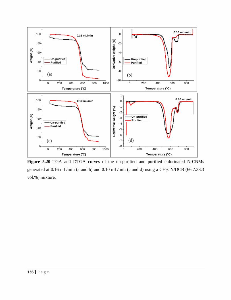
136 | P a g e

0 200 400 600 800 10000

20

40

60

80

100W

eig

ht

(%)

Temperature (0C)

Un-purified

Purified

0.16 mL/min

0 200 400 600 800-10

-8

-6

-4

-2

0

De

riv

ati

ve

we

igh

t (%

)

Temperature (0C)

Un-purified

Purified

0.16 mL/min

0 200 400 600 800 10000

20

40

60

80

100

Weig

ht

(%)

Temperature (0C)

Un-purified

Purified

0.10 mL/min

0 200 400 600 800-8

-7

-6

-5

-4

-3

-2

-1

0

1

Deri

va

tiv

e w

eig

ht

(%)

Temperature (0C)

Un-purified

Purified

0.10 mL/min

Figure 5.20 TGA and DTGA curves of the un-purified and purified chlorinated N-CNMs

generated at 0.16 mL/min (a and b) and 0.10 mL/min (c and d) using a CH3CN/DCB (66.7:33.3

vol.%) mixture.

(a) (b)

(c) (d)

137 | P a g e

5.3.3 Raman spectroscopy analysis of N doped CNMs: Effect of DCB concentration and

injection flow rate

Raman spectra of the un-purified and purified CNMs generated from pure CH3CN are presented

in Figure 5.21 and Table 5.6. Raman spectra provides information about the graphitic nature and

molecular structure of CNMs. Deconvoluted Raman spectra of the un-purified and purified

CNMs showed two first-order bands, at ~ 1342 and 1576 cm–1, attributed to defected graphite

(D-band) and graphitic band (G-band), respectively. For un-purified CNMs, the D-band could

only be deconvoluted into one band denoted as D3, the G-band was deconvoluted into two bands

at 1576 cm–1 attributed to graphitic like carbonyl groups (denoted as D’) and at 1621 cm–1

attributed to defected graphitic plane (Figure 5.21a). For purified CNMs, the D-band was

deconvoluted into two peaks at 1272 cm–1 attributed to a hexagonal diamond carbon (denoted as

D1) and a D3 band at 1344 cm–1. The G-band was also deconvoluted into a D’ at 1577 cm–1 and

a defected graphitic plane as 1624 cm–1. Second order bands were also observed in both Raman

spectra. 2D band attributed to 1st overtone of a D1 band was observed at 2681 cm–1 for both

spectra generated from pure CH3CN. Another weak band a G* band which is a 1st overtone of a

D4 band (which occurs at ~1200 cm–1) appearing at 2435 cm–1 was observed from un-purified

CNMs and is a defect activated peak. The order of crystallinity of the material can be estimated

from the corresponding full-width half-maximum (FWHM). An amorphous structure leads to a

FWHM of approximately 200 cm-1.36 FWHM values for all observed bands were low, suggesting

that the materials generated from pure CH3CN had no amorphous carbon. FWHM values of 60

and 63 cm–1 were observed for a D’ band and 58 and 62 for a 2D band obtained from un-purified

and purified CNMs, respectively (Table 5.6). Low ID/IG peak ratios of 0.56 for un-purified

samples and 0.68 for purified CNMs were obtained suggesting formation of graphitic materials

with less disorders (calculated from Table 5.6). There was not much difference between the un-

purified and purified CNMs. These results agree with TEM observations, where mixtures of

clean CNMs were obtained with no amorphous carbon materials observed, only lumps were

observed which were attributed to carbon platelets materials. The ratio of ID/ID’ was used to

provide information about the type of defects present in the material. If the ratio of ID/ID’ is 13, it

indicates the presence of related sp3 related defects, 10.5 corresponds to hoping defects, 7 for

vacancy-like defects, 3.5 for boundary-like defects and 1.3 for on-site defects in graphene. 37,38

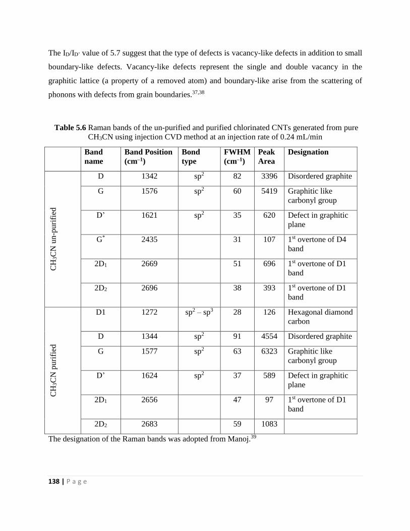
138 | P a g e

The ID/ID’ value of 5.7 suggest that the type of defects is vacancy-like defects in addition to small

boundary-like defects. Vacancy-like defects represent the single and double vacancy in the

graphitic lattice (a property of a removed atom) and boundary-like arise from the scattering of

phonons with defects from grain boundaries.37,38


CH3CN using injection CVD method at an injection rate of 0.24 mL/min

Band

name

Band Position

(cm–1)

Bond

type

FWHM

(cm–1)

Peak

Area

Designation

CH

3C

N u

n-p

uri

fied


G 1576 sp2 60 5419 Graphitic like

carbonyl group

D’ 1621 sp2 35 620 Defect in graphitic

plane

G* 2435 31 107 1st overtone of D4

band

2D1 2669 51 696 1st overtone of D1

band


band

CH

3C

N p

uri

fied

D1 1272 sp2 – sp3 28 126 Hexagonal diamond

carbon



carbonyl group


plane


band

2D2 2683 59 1083

The designation of the Raman bands was adopted from Manoj.39

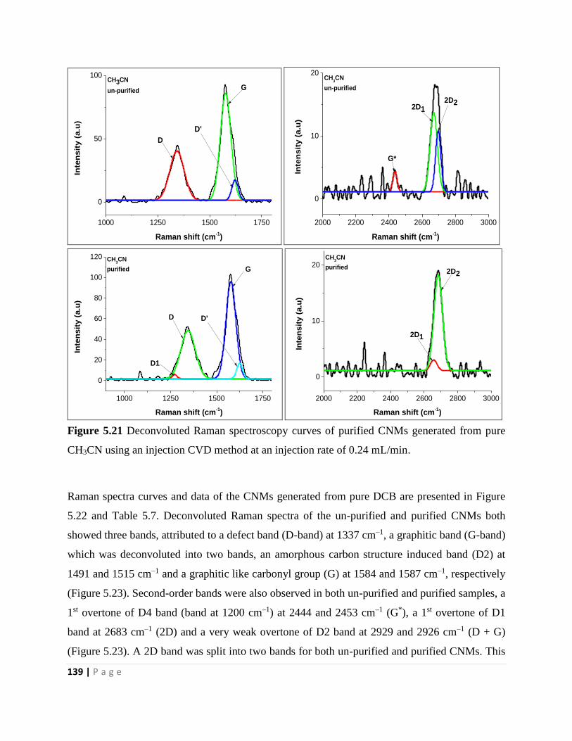
139 | P a g e

1000 1250 1500 1750

0

50

100In

ten

sit

y (

a.u

)

Raman shift (cm-1)

CH3CN

un-purified

D

G

D'

2000 2200 2400 2600 2800 3000

0

10

20

Inte

ns

ity

(a

.u)

Raman shift (cm-1)

CH3CN

un-purified

G*

2D12D2

1000 1250 1500 1750

0

20

40

60

80

100

120

Inte

nsit

y (

a.u

)

Raman shift (cm-1)

CH3CN

purified

D1

D

G

D'

2000 2200 2400 2600 2800 3000

0

10

20

Inte

nsit

y (

a.u

)

Raman shift (cm-1)

CH3CN

purified

2D1

2D2

Figure 5.21 Deconvoluted Raman spectroscopy curves of purified CNMs generated from pure

CH3CN using an injection CVD method at an injection rate of 0.24 mL/min.

Raman spectra curves and data of the CNMs generated from pure DCB are presented in Figure

5.22 and Table 5.7. Deconvoluted Raman spectra of the un-purified and purified CNMs both

showed three bands, attributed to a defect band (D-band) at 1337 cm–1, a graphitic band (G-band)

which was deconvoluted into two bands, an amorphous carbon structure induced band (D2) at

1491 and 1515 cm–1 and a graphitic like carbonyl group (G) at 1584 and 1587 cm–1, respectively

(Figure 5.23). Second-order bands were also observed in both un-purified and purified samples, a

1st overtone of D4 band (band at 1200 cm–1) at 2444 and 2453 cm–1 (G*), a 1st overtone of D1

band at 2683 cm–1 (2D) and a very weak overtone of D2 band at 2929 and 2926 cm–1 (D + G)

(Figure 5.23). A 2D band was split into two bands for both un-purified and purified CNMs. This

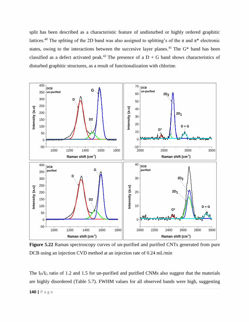
140 | P a g e

split has been described as a characteristic feature of undisturbed or highly ordered graphitic

lattices.40 The spliting of the 2D band was also assigned to splitting’s of the π and π* electronic

states, owing to the interactions between the succesive layer planes.41 The G* band has been

classified as a defect activated peak.42 The presence of a D + G band shows characteristics of

disturbed graphitic structures, as a result of functionalization with chlorine.

1000 1200 1400 1600 1800-50

0

50

100

150

200

250

300

350

400

Inte

ns

ity

(a

.u)

Raman shift (cm-1)

D

D2

GDCB

un-purified

2000 2500 3000 3500-10

0

10

20

30

40

50

60

70

Inte

ns

ity

(a

.u)

Raman shift (cm-1)

DCB

un-purified

G*

2D1

2D2

D + G

1000 1200 1400 1600 1800-50

0

50

100

150

200

250

300

350

400

Inte

ns

ity

(a

.u)

Raman shift (cm-1)

DCB

purified

D

D2

G

2000 2200 2400 2600 2800 3000

0

10

20

30

40

Inte

nsit

y (

a.u

)

Raman shift (cm-1)

DCB

purified

G*

2D1

2D2

D + G

Figure 5.22 Raman spectroscopy curves of un-purified and purified CNTs generated from pure

DCB using an injection CVD method at an injection rate of 0.24 mL/min

The ID/IG ratio of 1.2 and 1.5 for un-purified and purified CNMs also suggest that the materials

are highly disordered (Table 5.7). FWHM values for all observed bands were high, suggesting

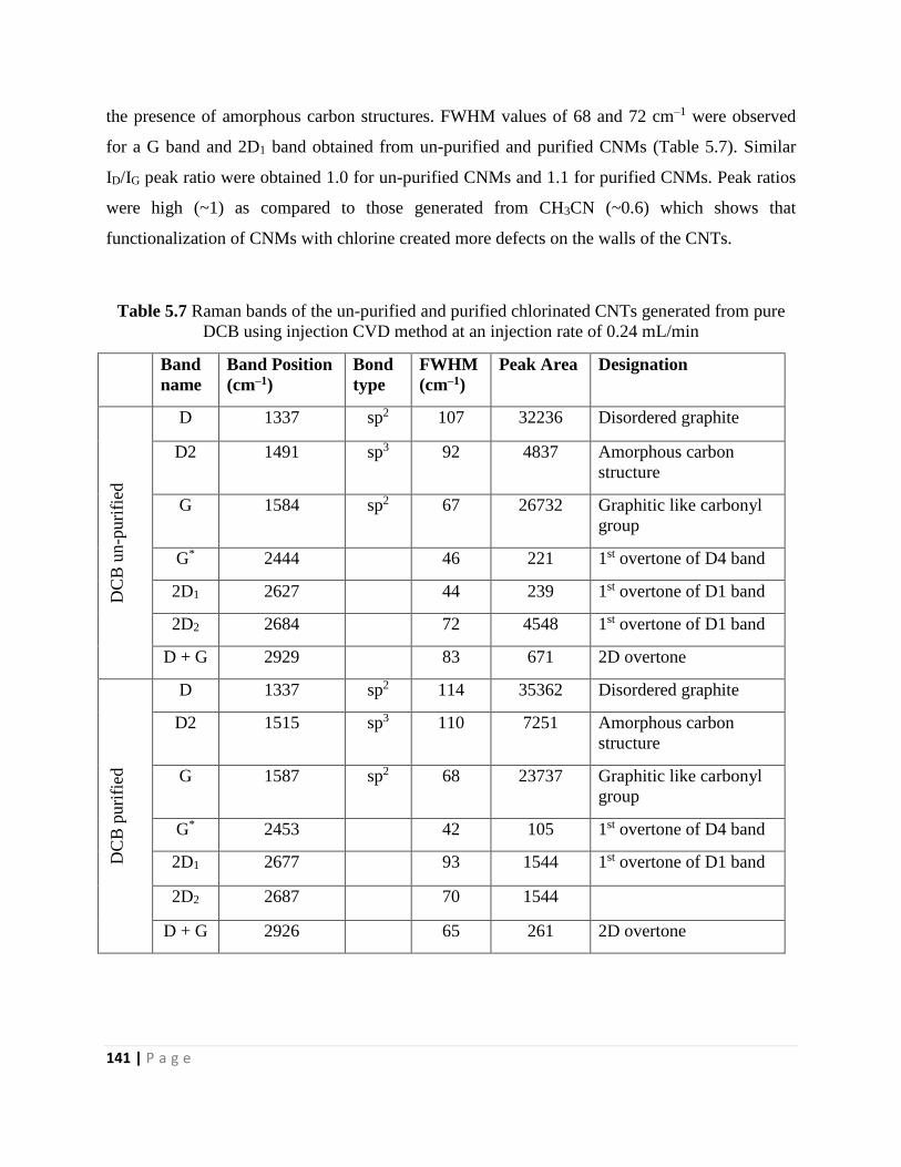
141 | P a g e

the presence of amorphous carbon structures. FWHM values of 68 and 72 cm–1 were observed

for a G band and 2D1 band obtained from un-purified and purified CNMs (Table 5.7). Similar

ID/IG peak ratio were obtained 1.0 for un-purified CNMs and 1.1 for purified CNMs. Peak ratios

were high (~1) as compared to those generated from CH3CN (~0.6) which shows that

functionalization of CNMs with chlorine created more defects on the walls of the CNTs.


DCB using injection CVD method at an injection rate of 0.24 mL/min

Band

name

Band Position

(cm–1)

Bond

type

FWHM

(cm–1)


DC

B u

n-p

uri

fied



structure


group




D + G 2929 83 671 2D overtone

DC

B p

uri

fied



structure


group



2D2 2687 70 1544

D + G 2926 65 261 2D overtone

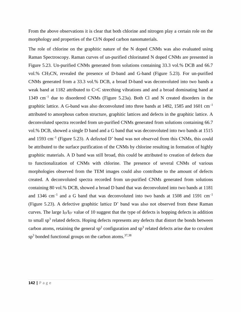
142 | P a g e

From the above observations it is clear that both chlorine and nitrogen play a certain role on the

morphology and properties of the Cl/N doped carbon nanomaterials.

The role of chlorine on the graphitic nature of the N doped CNMs was also evaluated using

Raman Spectroscopy. Raman curves of un-purified chlorinated N doped CNMs are presented in

Figure 5.23. Un-purified CNMs generated from solutions containing 33.3 vol.% DCB and 66.7

vol.% CH3CN, revealed the presence of D-band and G-band (Figure 5.23). For un-purified

CNMs generated from a 33.3 vol.% DCB, a broad D-band was deconvoluted into two bands a

weak band at 1182 attributed to C=C strecthing vibrations and and a broad dominating band at

1349 cm–1 due to disordered CNMs (Figure 5.23a). Both Cl and N created disorders in the

graphitic lattice. A G-band was also deconvoluted into three bands at 1492, 1585 and 1601 cm–1

attributed to amorphous carbon structure, graphitic lattices and defects in the graphitic lattice. A

deconvoluted spectra recorded from un-purified CNMs generated from solutions containing 66.7

vol.% DCB, showed a single D band and a G band that was deconvoluted into two bands at 1515

and 1593 cm–1 (Figure 5.23). A defected D’ band was not observed from this CNMs, this could

be attributed to the surface purification of the CNMs by chlorine resulting in formation of highly

graphitic materials. A D band was still broad, this could be attributed to creation of defects due

to functionalization of CNMs with chlorine. The presence of several CNMs of various

morphologies observed from the TEM images could also contribute to the amount of defects

created. A deconvoluted spectra recorded from un-purified CNMs generated from solutions

containing 80 vol.% DCB, showed a broad D band that was deconvoluted into two bands at 1181

and 1346 cm–1 and a G band that was deconvoluted into two bands at 1508 and 1591 cm–1

(Figure 5.23). A defective graphitic lattice D’ band was also not observed from these Raman

curves. The large ID/ID’ value of 10 suggest that the type of defects is hopping defects in addition

to small sp3 related defects. Hoping defects represents any defects that distort the bonds between

carbon atoms, retaining the general sp2 configuration and sp3 related defects arise due to covalent

sp3 bonded functional groups on the carbon atoms.37,38

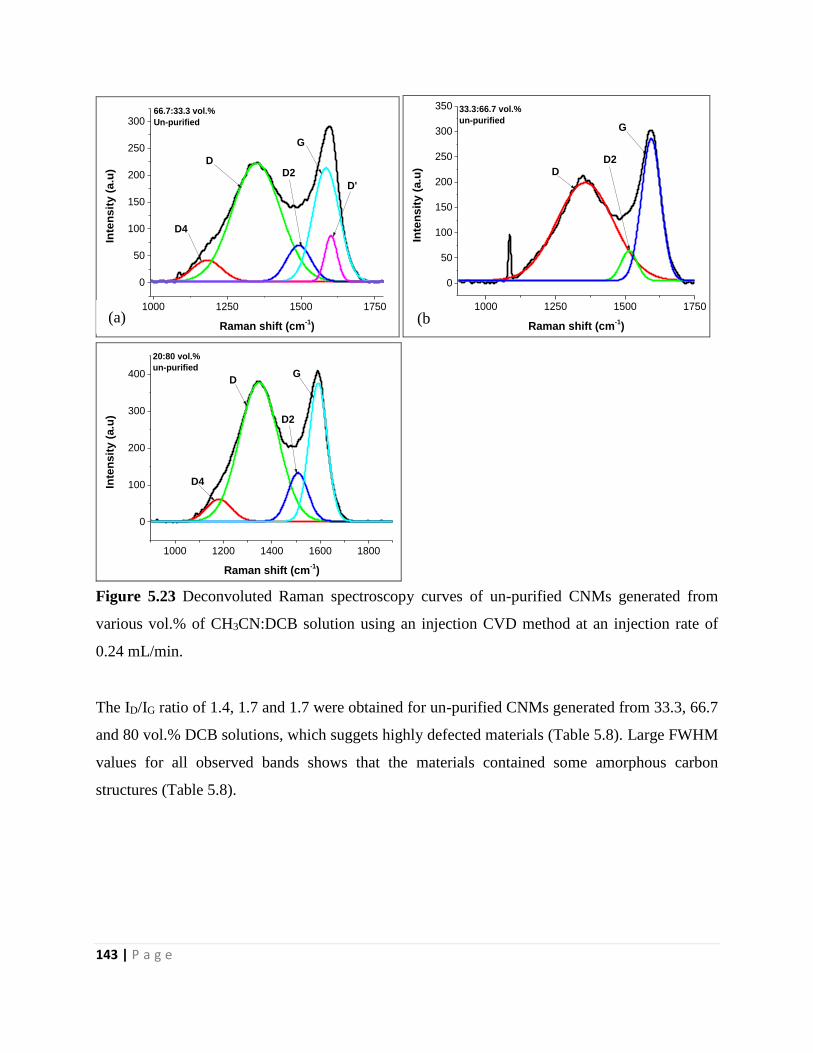
143 | P a g e

1000 1250 1500 1750

0

50

100

150

200

250

300In

ten

sit

y (

a.u

)

Raman shift (cm-1)

66.7:33.3 vol.%

Un-purified

D4

DD2

G

D'

1000 1250 1500 1750

0

50

100

150

200

250

300

350

Inte

ns

ity

(a

.u)

Raman shift (cm-1)

33.3:66.7 vol.%

un-purified

D

G

D2

1000 1200 1400 1600 1800

0

100

200

300

400

Inte

ns

ity

(a

.u)

Raman shift (cm-1)

20:80 vol.%

un-purified

D4

DG

D2

Figure 5.23 Deconvoluted Raman spectroscopy curves of un-purified CNMs generated from

various vol.% of CH3CN:DCB solution using an injection CVD method at an injection rate of

0.24 mL/min.

The ID/IG ratio of 1.4, 1.7 and 1.7 were obtained for un-purified CNMs generated from 33.3, 66.7

and 80 vol.% DCB solutions, which suggets highly defected materials (Table 5.8). Large FWHM

values for all observed bands shows that the materials contained some amorphous carbon

structures (Table 5.8).

(a) (b

)

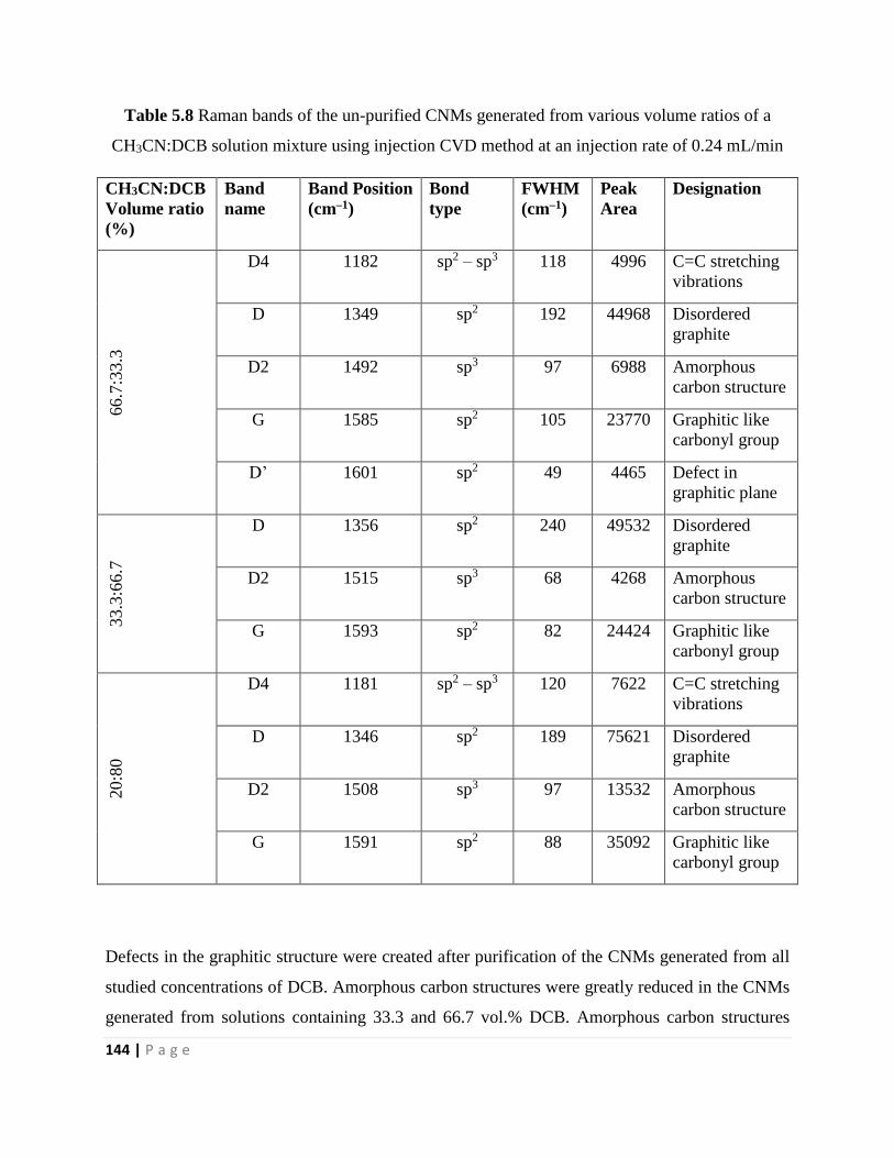
144 | P a g e

Table 5.8 Raman bands of the un-purified CNMs generated from various volume ratios of a


CH3CN:DCB

Volume ratio

(%)

Band

name

Band Position

(cm–1)

Bond

type

FWHM

(cm–1)

Peak

Area

Designation

66.7

:33.3

D4 1182 sp2 – sp3 118 4996 C=C stretching

vibrations

D 1349 sp2 192 44968 Disordered

graphite

D2 1492 sp3 97 6988 Amorphous

carbon structure


carbonyl group

D’ 1601 sp2 49 4465 Defect in

graphitic plane

33.3

:66.7


graphite


carbon structure


carbonyl group

20:8

0


vibrations


graphite


carbon structure


carbonyl group

Defects in the graphitic structure were created after purification of the CNMs generated from all

studied concentrations of DCB. Amorphous carbon structures were greatly reduced in the CNMs

generated from solutions containing 33.3 and 66.7 vol.% DCB. Amorphous carbon structures

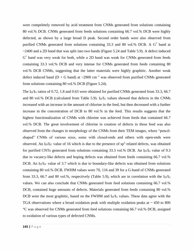
145 | P a g e

were compeletely removed by acid treatment from CNMs generated from solutions containing

80 vol.% DCB. CNMs generated from feeds solutions containing 66.7 vol.% DCB were highly

defected, as shown by a large broad D peak. Second order bands were also observed from

purified CNMs generated from solutions containing 33.3 and 80 vol.% DCB. A G* band at

~2400 and a 2D band that was split into two bands (Figure 5.24 and Table 5.9). A defect induced

G* band was very weak for both, while a 2D band was weak for CNMs generated from feeds

containing 33.3 vol.% DCB and very intense for CNMs generated from feeds containing 80

vol.% DCB CNMs, suggesting that the latter materials were highly graphitic. Another weak

defect induced band (D + G band) at ~2900 cm–1 was observed from purified CNMs generated

from solutions containing 80 vol.% DCB (Figure 5.24).

The ID/IG ratios of 0.72, 1.8 and 0.63 were obtained for purified CNMs generated from 33.3, 66.7

and 80 vol.% DCB (calculated from Table 5.9). ID/IG values showed that defects in the CNMs

increased with an increase in the amount of chlorine in the feed, but then decreased with a further

increase in the concentration of DCB to 80 vol.% in the feed. This results suggests that the

highest functionalization of CNMs with chlorine was achieved from feeds that contained 66.7

vol.% DCB. The great involvement of chlorine in creation of defects in these feed was also

observed from the changes in morphology of the CNMs from their TEM images, where “pencil-

shaped” CNMs of various sizes, some with closed-ends and others with open-ends were

observed. An ID/ID’ value of 16 which is due to the presence of sp3 related defects, was obtained

for purified CNTs generated from solutions containing 33.3 vol.% DCB. An ID/IG value of 9.3

due to vacancy-like defects and hoping defects was obtained from feeds containing 66.7 vol.%

DCB. An ID/ID’ value of 3.7 which is due to boundary-like defects was obtained from solutions

containing 80 vol.% DCB. FWHM values were 70, 116 and 39 for a G-band of CNMs generated

from 33.3, 66.7 and 80 vol.%, respectively (Table 5.9), which are in correlation with the ID/IG

values. We can also conclude that CNMs generated from feed solutions containing 66.7 vol.%

DCB, contained huge amounts of defects. Materials generated from feeds containing 80 vol.%

DCB were the most graphitic, based on the FWHM and ID/IG values. These data agree with the

TGA observations where a broad oxidation peak with multiple oxidation peaks at ~ 450 to 800

°C was observed for CNMs generated from feed solutions containing 66.7 vol.% DCB, assigned

to oxidation of various types of defected CNMs.

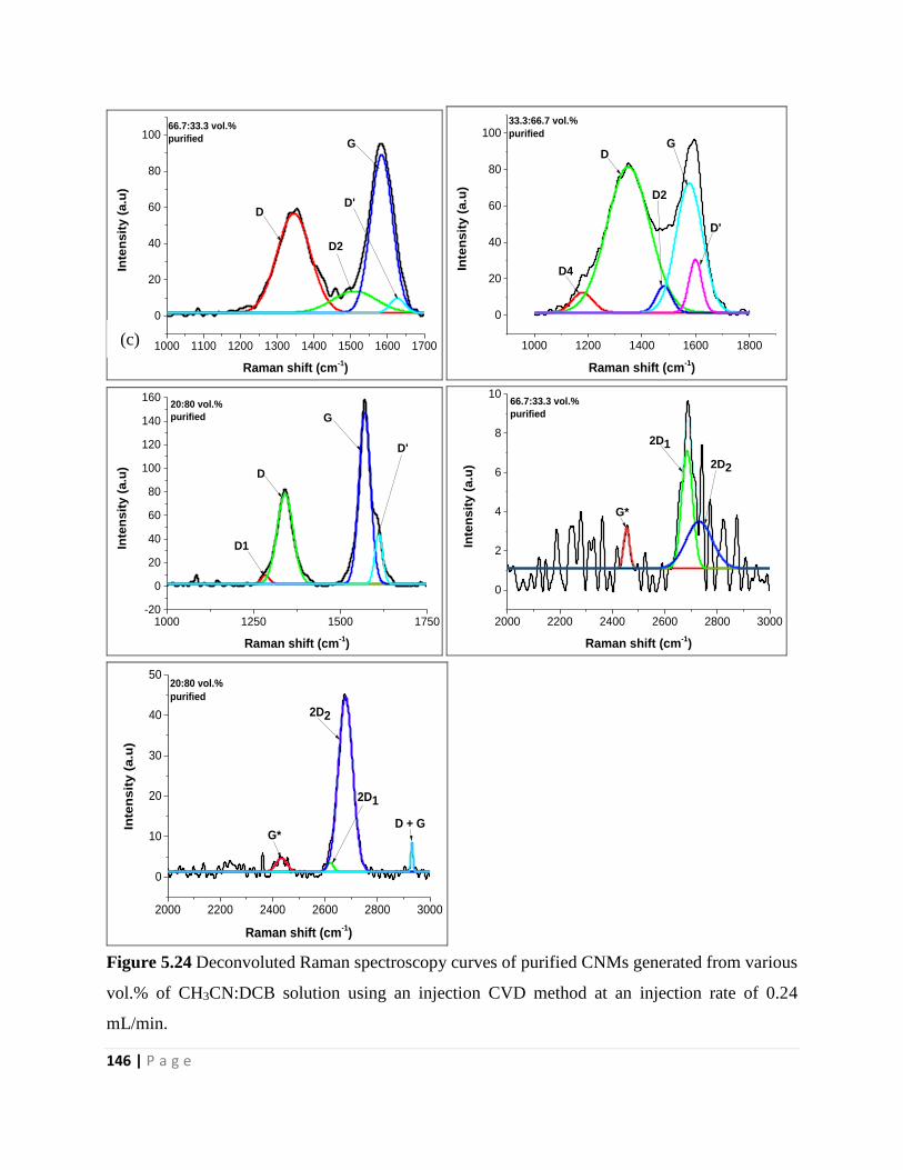
146 | P a g e

1000 1100 1200 1300 1400 1500 1600 1700

0

20

40

60

80

100In

ten

sit

y (

a.u

)

Raman shift (cm-1)

66.7:33.3 vol.%

purified

D

D2

G

D'

1000 1200 1400 1600 1800

0

20

40

60

80

100

Inte

ns

ity

(a

.u)

Raman shift (cm-1)

33.3:66.7 vol.%

purified

D4

D

D2

G

D'

1000 1250 1500 1750-20

0

20

40

60

80

100

120

140

160

Inte

ns

ity

(a

.u)

Raman shift (cm-1)

20:80 vol.%

purified

D1

D

G

D'

2000 2200 2400 2600 2800 3000

0

2

4

6

8

10

Inte

nsit

y (

a.u

)

Raman shift (cm-1)

66.7:33.3 vol.%

purified

G*

2D1

2D2

2000 2200 2400 2600 2800 3000

0

10

20

30

40

50

Inte

nsit

y (

a.u

)

Raman shift (cm-1)

G*

2D1

2D2

D + G

20:80 vol.%

purified

Figure 5.24 Deconvoluted Raman spectroscopy curves of purified CNMs generated from various

vol.% of CH3CN:DCB solution using an injection CVD method at an injection rate of 0.24

mL/min.

(c)

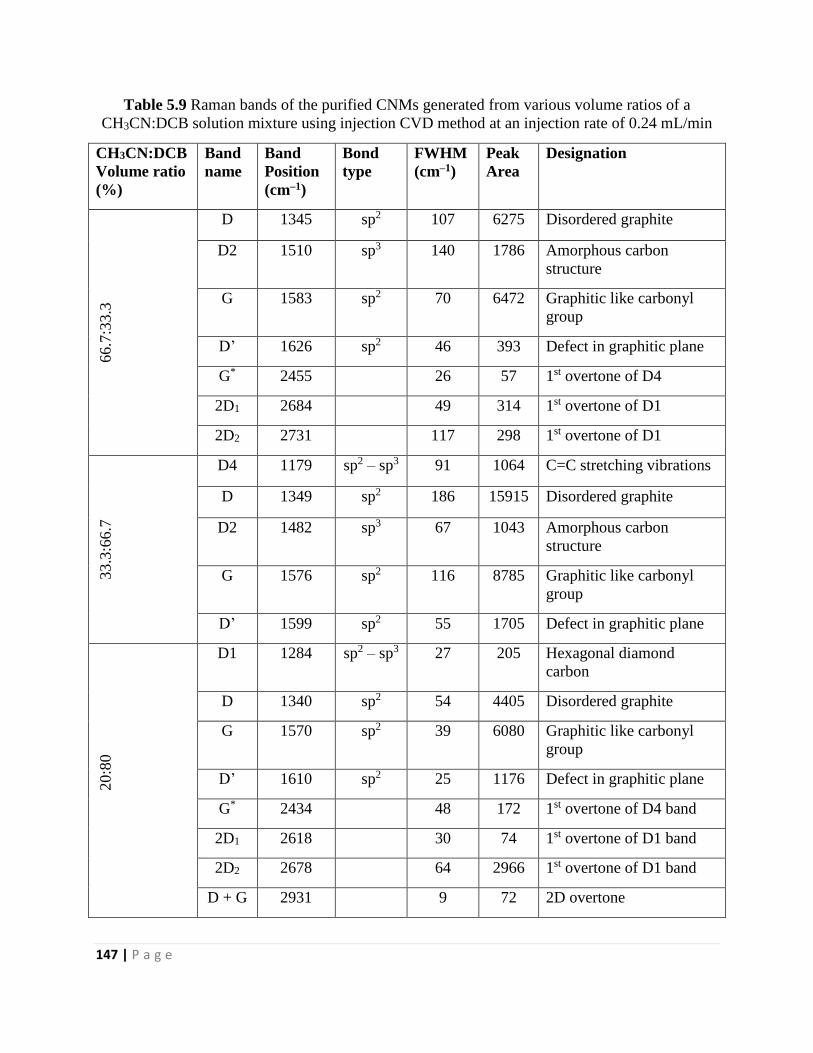
147 | P a g e

Table 5.9 Raman bands of the purified CNMs generated from various volume ratios of a


CH3CN:DCB

Volume ratio

(%)

Band

name

Band

Position

(cm–1)

Bond

type

FWHM

(cm–1)

Peak

Area

Designation

66.7

:33.3



structure


group

D’ 1626 sp2 46 393 Defect in graphitic plane




33.3

:66.7

D4 1179 sp2 – sp3 91 1064 C=C stretching vibrations



structure


group


20:8

0

D1 1284 sp2 – sp3 27 205 Hexagonal diamond

carbon



group





D + G 2931 9 72 2D overtone

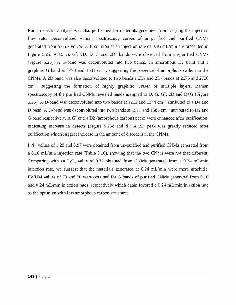
148 | P a g e

Raman spectra analysis was also performed for materials generated from varying the injection

flow rate. Deconvoluted Raman spectroscopy curves of un-purified and purified CNMs

generated from a 66.7 vol.% DCB solution at an injection rate of 0.16 mL/min are presented in

Figure 5.25. A D, G, G*, 2D, D+G and 2D’ bands were observed from un-purified CNMs

(Figure 5.25). A G-band was deconvoluted into two bands, an amorphous D2 band and a

graphitic G band at 1493 and 1581 cm–1, suggesting the presence of amorphous carbon in the

CNMs. A 2D band was also deconvoluted to two bands a 2D1 and 2D2 bands at 2676 and 2720

cm–1, suggesting the formation of highly graphitic CNMs of multiple layers. Raman

spectroscopy of the purified CNMs revealed bands assigned to D, G, G*, 2D and D+G (Figure

5.25). A D-band was deconvoluted into two bands at 1212 and 1344 cm–1 attributed to a D4 and

D band. A G-band was deconvoluted into two bands at 1511 and 1585 cm–1 attributed to D2 and

G band respectively. A G* and a D2 (amorphous carbon) peaks were enhanced after purification,

indicating increase in defects (Figure 5.25c and d). A 2D peak was greatly reduced after

purification which suggest increase in the amount of disorders in the CNMs.

ID/IG values of 1.28 and 0.97 were obtained from un-purified and purified CNMs generated from

a 0.16 mL/min injection rate (Table 5.10), showing that the two CNMs were not that different.

Comparing with an ID/IG value of 0.72 obtained from CNMs generated from a 0.24 mL/min

injection rate, we suggest that the materials generated at 0.24 mL/min were more graphitic.

FWHM values of 73 and 70 were obtained for G bands of purified CNMs generated from 0.16

and 0.24 mL/min injection rates, respectively which again favored a 0.24 mL/min injection rate

as the optimum with less amorphous carbon structures.

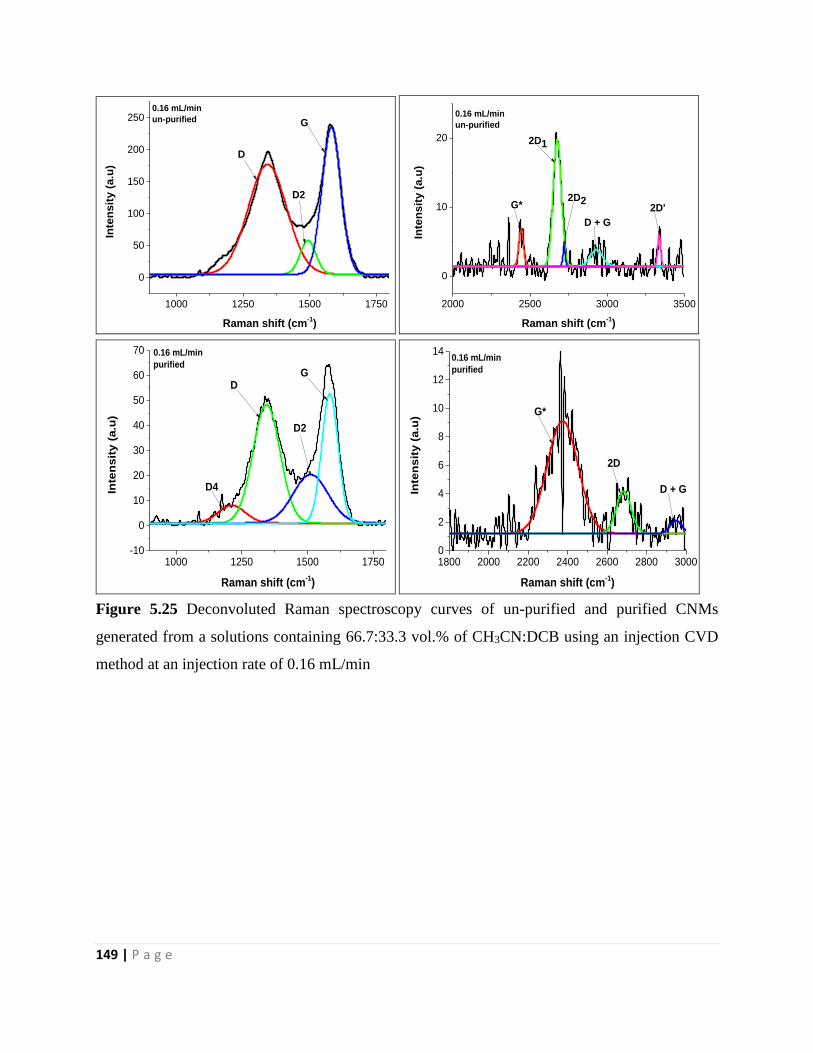
149 | P a g e

1000 1250 1500 1750

0

50

100

150

200

250In

ten

sit

y (

a.u

)

Raman shift (cm-1)

0.16 mL/min

un-purified

D

D2

G

2000 2500 3000 3500

0

10

20

Inte

nsit

y (

a.u

)

Raman shift (cm-1)

0.16 mL/min

un-purified

G*

2D1

2D2

D + G

2D'

1000 1250 1500 1750-10

0

10

20

30

40

50

60

70

Inte

ns

ity

(a

.u)

Raman shift (cm-1)

0.16 mL/min

purified

D4

D

D2

G

1800 2000 2200 2400 2600 2800 30000

2

4

6

8

10

12

14

Inte

ns

ity

(a

.u)

Raman shift (cm-1)

0.16 mL/min

purified

G*

2D

D + G



method at an injection rate of 0.16 mL/min

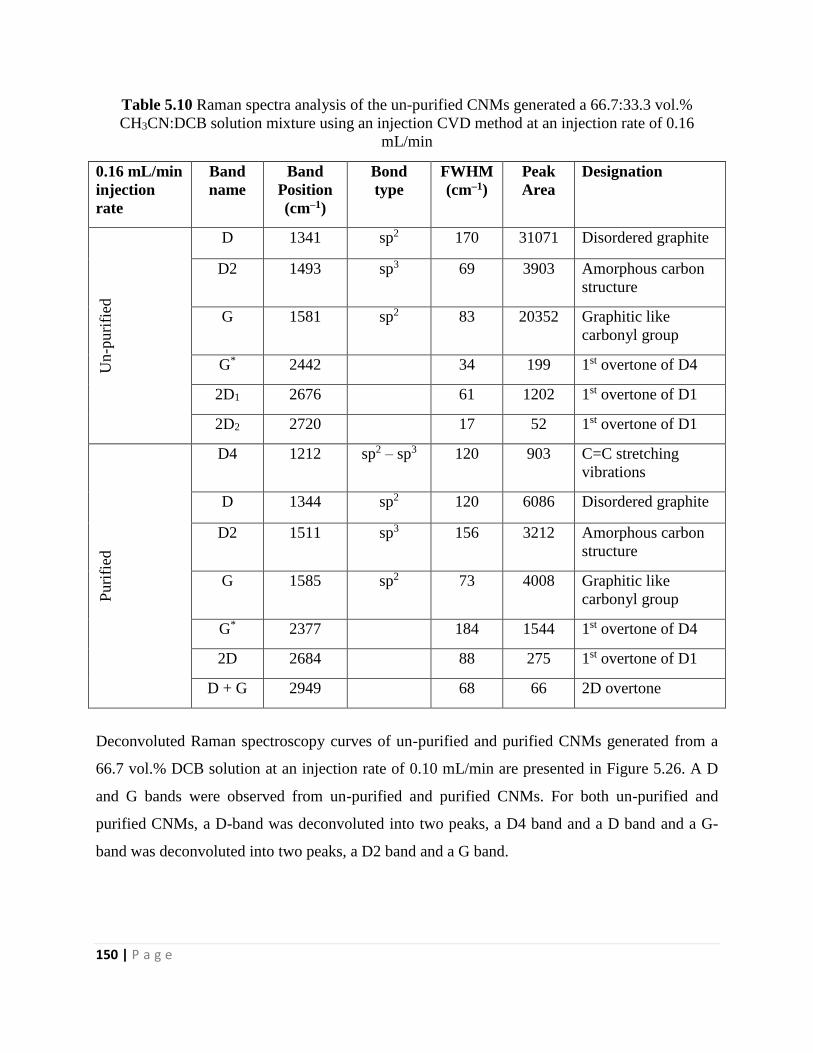
150 | P a g e



mL/min

0.16 mL/min

injection

rate

Band

name

Band

Position

(cm–1)

Bond

type

FWHM

(cm–1)

Peak

Area

Designation

Un-p

uri

fied



structure


carbonyl group




Puri

fied


vibrations



structure


carbonyl group


2D 2684 88 275 1st overtone of D1

D + G 2949 68 66 2D overtone

Deconvoluted Raman spectroscopy curves of un-purified and purified CNMs generated from a

66.7 vol.% DCB solution at an injection rate of 0.10 mL/min are presented in Figure 5.26. A D

and G bands were observed from un-purified and purified CNMs. For both un-purified and

purified CNMs, a D-band was deconvoluted into two peaks, a D4 band and a D band and a G-

band was deconvoluted into two peaks, a D2 band and a G band.

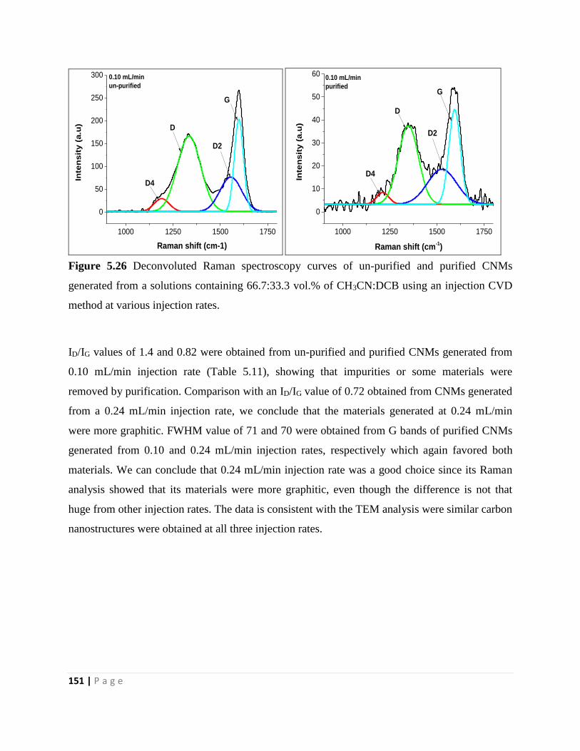
151 | P a g e

1000 1250 1500 1750

0

50

100

150

200

250

300In

ten

sit

y (

a.u

)

Raman shift (cm-1)

0.10 mL/min

un-purified

D4

D

D2

G

1000 1250 1500 1750

0

10

20

30

40

50

60

Inte

ns

ity

(a

.u)

Raman shift (cm-1)

0.10 mL/min

purified

D4

D

D2

G



method at various injection rates.

ID/IG values of 1.4 and 0.82 were obtained from un-purified and purified CNMs generated from

0.10 mL/min injection rate (Table 5.11), showing that impurities or some materials were

removed by purification. Comparison with an ID/IG value of 0.72 obtained from CNMs generated

from a 0.24 mL/min injection rate, we conclude that the materials generated at 0.24 mL/min

were more graphitic. FWHM value of 71 and 70 were obtained from G bands of purified CNMs

generated from 0.10 and 0.24 mL/min injection rates, respectively which again favored both

materials. We can conclude that 0.24 mL/min injection rate was a good choice since its Raman

analysis showed that its materials were more graphitic, even though the difference is not that

huge from other injection rates. The data is consistent with the TEM analysis were similar carbon

nanostructures were obtained at all three injection rates.

152 | P a g e



mL/min

0.10 mL/min

injection

rate

Band

name

Band Position

(cm–1)

Bond

type

FWHM

(cm–1)

Peak

Area

Designation

Un-p

uri

fied


vibrations


graphite


carbon structure


carbonyl group

Puri

fied


vibrations


graphite


carbon structure


carbonyl group

5.3.4 X-ray photoelectron analysis of N doped CNMs: Effect of DCB concentration

Three main peaks were observed from the wide scan XPS spectra of the N doped MWCNTs

produced from pure acetonitrile at 284.2, 400 and 531 eV and were attributed to C 1s, N 1s and

O 1s, respectively (Supplementary Figure S13). Three main peaks were also observed in the

wide scan XPS spectra of chlorine functionalized MWCNTs produced from pure DCB. This

peaks occured at 200, 284.2, and 531 eV and were attributed to Cl 2p, C 1s and O 1s,

respectively (Supplementary Figure S13).

The deconvoluted C 1s peak for materials obtained from pure CH3CN, was fitted into four

components with binding energies 283.5, 284.8, 287.4 and 290.7 eV, the first two peaks were

153 | P a g e

attributed to graphite-like C–C sp2 and sp3 bonds, the next two to C–N and O–C=O bonds,

respectively (Supplementary Figure S14). The relative broadness of the C–N peak was attributed

to the lattice distortion introduced by nitrogen doping and that of the O–C=O was attributed to

mixing of various CO-type bonds.43,44 The deconvoluted C 1s peak for materials obtained from

pure DCB, was fitted into four components with binding energies 283.4, 284.5, 287.7 and 290.1

eV, attributed to graphite-like C–C sp2, C–C sp3, C–Cl and O–C=O bonds, respectively

(Supplementary Figure S14).

The deconvoluted C 1s peaks of all the studied N-doped materials that contained chlorine, were

fitted into four components. The peaks were at the following binding energies 283.6–284.8, 287

and 287–290 eV and were attributed to C–C sp2 and sp3 carbon bonds, C–N or C–Cl groups and

O–C=O carboxylic groups, respectively (Supplementary Figure S6). CNTs generated from a

mixture of CH3CN/DCB showed a broad peak at ~ 287 eV which was attributed to overlap

between C–N and C–Cl groups. The intensity of this peak at ~287 eV increased after addition of

DCB in the feed, which suggest formation of new C–Cl bonds which overlap with a C–N bond.

Covalent bonding between carbon and chlorine was also suggested in the Raman data where the

degree of disorder was found to increase with addition of chlorine due to formation of new sp3

C–Cl bonds. The formation of sp3 C – Cl bonds was evidenced by the presence of an additional

peak an amorphous D2 peak, occuring from the Raman spectra of chlorinated CNMs (Figure

5.23 to 5.26).

The high resolution N 1s XPS spectra recorded for pure CH3CN consisted of four peak

components at 399.3, 401, 402.7 and 405.8 eV binding energies (Figure 5.27a). The peaks at

399.3 and 401.0 eV were attributed to pyrrolic (NPyr) and quaternary nitrogen (NQ). Quaternary

nitrogen corresponds to substitution of carbon atoms located in the graphene sheet by nitrogen.

The peak at 402.7 eV was attributed to oxidized nitrogen (NOx) which was bonded to oxygen.45

The peak at 405.8 eV was attributed to molecular nitrogen (NMo), since molecular nitrogen can

be encapsulated inside the tubes46 or can exist in an intercalated form between graphite layers

during the formation of CNx tubes.47 Molecular nitrogen was the dominant peak in this case and

pyridinic nitrogen was not observed. Other authors have attributed the N 1s peaks at 405.3 –

406.1 eV to the nitrogen atoms that form endohedral or exohedral complex with carbon-carbon

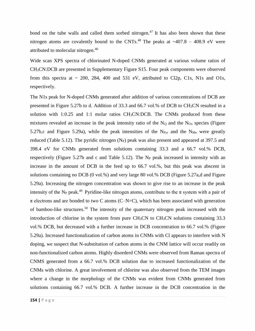
154 | P a g e

bond on the tube walls and called them sorbed nitrogen.47 It has also been shown that these

nitrogen atoms are covalently bound to the CNTs.48 The peaks at ~407.8 – 408.9 eV were

attributed to molecular nitrogen.46

Wide scan XPS spectra of chlorinated N-doped CNMs generated at various volume ratios of

CH3CN:DCB are presented in Supplementary Figure S15. Four peak components were observed

from this spectra at ~ 200, 284, 400 and 531 eV, attributed to Cl2p, C1s, N1s and O1s,

respectively.

The N1s peak for N-doped CNMs generated after addition of various concentrations of DCB are

presented in Figure 5.27b to d. Addition of 33.3 and 66.7 vol.% of DCB to CH3CN resulted in a

solution with 1:0.25 and 1:1 molar ratios CH3CN:DCB. The CNMs produced from these

mixtures revealed an increase in the peak intensity ratio of the NQ and the NOx species (Figure

5.27b,c and Figure 5.29a), while the peak intensities of the NPyr and the NMo were greatly

reduced (Table 5.12). The pyridic nitrogen (NP) peak was also present and appeared at 397.5 and

398.4 eV for CNMs generated from solutions containing 33.3 and a 66.7 vol.% DCB,

respectively (Figure 5.27b and c and Table 5.12). The NP peak increased in intensity with an

increase in the amount of DCB in the feed up to 66.7 vol.%, but this peak was abscent in

solutions containing no DCB (0 vol.%) and very large 80 vol.% DCB (Figure 5.27a,d and Figure

5.29a). Increasing the nitrogen concentration was shown to give rise to an increase in the peak

intensity of the NP peak.49 Pyridine-like nitrogen atoms, contribute to the π system with a pair of

π electrons and are bonded to two C atoms (C–N=C), which has been associated with generation

of bamboo-like structures.50 The intensity of the quaternary nitrogen peak increased with the

introduction of chlorine in the system from pure CH3CN to CH3CN solutions containing 33.3

vol.% DCB, but decreased with a further increase in DCB concentration to 66.7 vol.% (Figure

5.29a). Increased functionalization of carbon atoms in CNMs with Cl appears to interfere with N

doping, we suspect that N-substitution of carbon atoms in the CNM lattice will occur readily on

non-functionalized carbon atoms. Highly disorderd CNMs were observed from Raman spectra of

CNMS generated from a 66.7 vol.% DCB solution due to increased functionalization of the

CNMs with chlorine. A great involvement of chlorine was also observed from the TEM images

where a change in the morphology of the CNMs was evident from CNMs generated from

solutions containing 66.7 vol.% DCB. A further increase in the DCB concentration in the

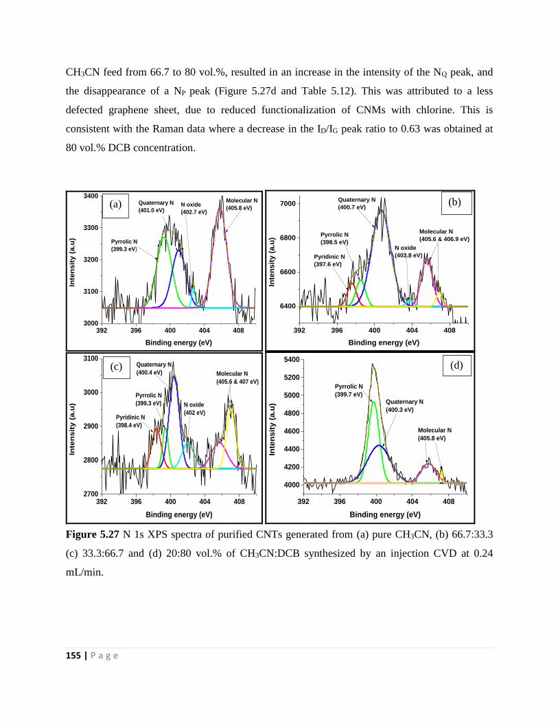
155 | P a g e

CH3CN feed from 66.7 to 80 vol.%, resulted in an increase in the intensity of the NQ peak, and

the disappearance of a NP peak (Figure 5.27d and Table 5.12). This was attributed to a less

defected graphene sheet, due to reduced functionalization of CNMs with chlorine. This is

consistent with the Raman data where a decrease in the ID/IG peak ratio to 0.63 was obtained at

80 vol.% DCB concentration.

392 396 400 404 4083000

3100

3200

3300

3400

Inte

ns

ity

(a

.u)

Binding energy (eV)

Pyrrolic N

(399.3 eV)

Quaternary N

(401.0 eV)N oxide

(402.7 eV)

Molecular N

(405.8 eV)

392 396 400 404 408

6400

6600

6800

7000

N oxide

(403.8 eV)

Molecular N

(405.6 & 406.9 eV)Pyrrolic N

(398.5 eV)

Quaternary N

(400.7 eV)

Pyridinic N

(397.6 eV)

Inte

nsit

y (

a.u

)

Binding energy (eV)

392 396 400 404 4082700

2800

2900

3000

3100

Molecular N

(405.6 & 407 eV)

N oxide

(402 eV)

Quaternary N

(400.4 eV)

Pyridinic N

(398.4 eV)

Pyrrolic N

(399.3 eV)

Inte

nsit

y (

a.u

)

Binding energy (eV)

392 396 400 404 408

4000

4200

4400

4600

4800

5000

5200

5400

Molecular N

(405.8 eV)

Quaternary N

(400.3 eV)

Pyrrolic N

(399.7 eV)

Inte

nsit

y (

a.u

)

Binding energy (eV)

Figure 5.27 N 1s XPS spectra of purified CNTs generated from (a) pure CH3CN, (b) 66.7:33.3

(c) 33.3:66.7 and (d) 20:80 vol.% of CH3CN:DCB synthesized by an injection CVD at 0.24

mL/min.

(b) (a)

(d) (c)

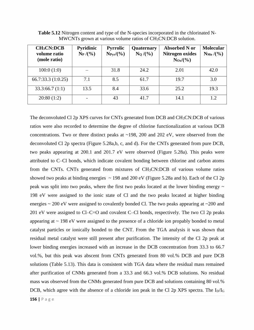
156 | P a g e


MWCNTs grown at various volume ratios of CH3CN:DCB solution.

CH3CN:DCB

volume ratio

(mole ratio)

Pyridinic

NP /(%)

Pyrrolic

NPyr/(%)

Quaternary

NQ /(%)

Absorbed N or

Nitrogen oxides

NOx/(%)

Molecular

NMo /(%)

100:0 (1:0) – 31.8 24.2 2.01 42.0

66.7:33.3 (1:0.25) 7.1 8.5 61.7 19.7 3.0

33.3:66.7 (1:1) 13.5 8.4 33.6 25.2 19.3

20:80 (1:2) - 43 41.7 14.1 1.2

The deconvoluted Cl 2p XPS curves for CNTs generated from DCB and CH3CN:DCB of various

ratios were also recorded to determine the degree of chlorine functionalization at various DCB

concentrations. Two or three distinct peaks at ~198, 200 and 202 eV, were observed from the

deconvoluted Cl 2p spectra (Figure 5.28a,b, c, and d). For the CNTs generated from pure DCB,

two peaks appearing at 200.1 and 201.7 eV were observed (Figure 5.28a). This peaks were

attributed to C–Cl bonds, which indicate covalent bonding between chlorine and carbon atoms

from the CNTs. CNTs generated from mixtures of CH3CN:DCB of various volume ratios

showed two peaks at binding energies ~ 198 and 200 eV (Figure 5.28a and b). Each of the Cl 2p

peak was split into two peaks, where the first two peaks located at the lower binding energy ~

198 eV were assigned to the ionic state of Cl and the two peaks located at higher binding

energies ~ 200 eV were assigned to covalently bonded Cl. The two peaks appearing at ~200 and

201 eV were assigned to Cl–C=O and covalent C–Cl bonds, respectively. The two Cl 2p peaks

appearing at ~ 198 eV were assigned to the presence of a chloride ion propably bonded to metal

catalyst particles or ionically bonded to the CNT. From the TGA analysis it was shown that

residual metal catalyst were still present after purification. The intensity of the Cl 2p peak at

lower binding energies increased with an increase in the DCB concentration from 33.3 to 66.7

vol.%, but this peak was abscent from CNTs generated from 80 vol.% DCB and pure DCB

solutions (Table 5.13). This data is consistent with TGA data where the residual mass remained

after purification of CNMs generated from a 33.3 and 66.3 vol.% DCB solutions. No residual

mass was observed from the CNMs generated from pure DCB and solutions containing 80 vol.%

DCB, which agree with the absence of a chloride ion peak in the Cl 2p XPS spectra. The ID/IG

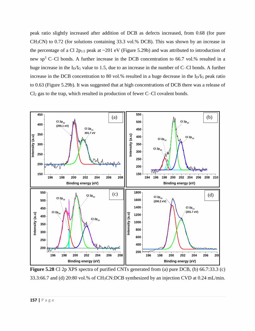
157 | P a g e

peak ratio slightly increased after addition of DCB as defects increased, from 0.68 (for pure

CH3CN) to 0.72 (for solutions containing 33.3 vol.% DCB). This was shown by an increase in

the percentage of a Cl 2p1/2 peak at ~201 eV (Figure 5.29b) and was attributed to introduction of

new sp3 C–Cl bonds. A further increase in the DCB concentration to 66.7 vol.% resulted in a

huge increase in the ID/IG value to 1.5, due to an increase in the number of C–Cl bonds. A further

increase in the DCB concentration to 80 vol.% resulted in a huge decrease in the ID/IG peak ratio

to 0.63 (Figure 5.29b). It was suggested that at high concentrations of DCB there was a release of

Cl2 gas to the trap, which resulted in production of fewer C–Cl covalent bonds.

196 198 200 202 204 206 208150

200

250

300

350

400

450

Inte

ns

ity

(a.u

)

Binding energy (eV)

Cl 2p3/2

(200.1 eV)Cl 2p

1/2

201.7 eV

194 196 198 200 202 204 206 208 210150

200

250

300

350

400

450

500

550

Inte

nsit

y (

a.u

)

Binding energy (eV)

Cl 2p3/2

Cl 2p1/2

Cl 2p3/2

Cl 2p1/2

196 198 200 202 204 206 208

200

250

300

350

400

450

500

550

Cl 2p1/2

Cl 2p3/2

Inte

ns

ity

(a

.u)

Binding energy (eV)

Cl 2p3/2

Cl 2p1/2

196 198 200 202 204 206 208200

400

600

800

1000

1200

1400

1600

1800

Cl 2p1/2

(201.7 eV)

Cl 2p3/2

(200.2 eV)

Inte

ns

ity

(a

.u)

Binding energy (eV)

Figure 5.28 Cl 2p XPS spectra of purified CNTs generated from (a) pure DCB, (b) 66.7:33.3 (c)

33.3:66.7 and (d) 20:80 vol.% of CH3CN:DCB synthesized by an injection CVD at 0.24 mL/min.

(a)

(d)

(b)

(c)

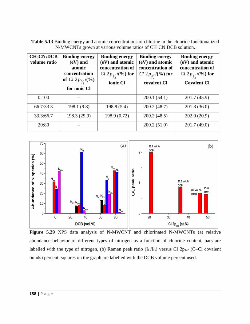
158 | P a g e

Table 5.13 Binding energy and atomic concentrations of chlorine in the chlorine functionalized

N-MWCNTs grown at various volume ratios of CH3CN:DCB solution.

CH3CN:DCB

volume ratio

Binding energy

(eV) and

atomic

concentration

of 2

32 pCl /(%)

for ionic Cl

Binding energy

(eV) and atomic

concentration of

212 pCl /(%) for

ionic Cl

Binding energy

(eV) and atomic

concentration of

232 pCl /(%) for

covalent Cl

Binding energy

(eV) and atomic

concentration of

212 pCl /(%) for

Covalent Cl

0:100 – 200.1 (54.1) 201.7 (45.9)

66.7:33.3 198.1 (9.8) 198.8 (5.4) 200.2 (48.7) 201.8 (36.0)

33.3:66.7 198.3 (29.9) 198.9 (0.72) 200.2 (48.5) 202.0 (20.9)

20:80 – 200.2 (51.0) 201.7 (49.0)

0 20 40 60 800

10

20

30

40

50

60

70

NMo

NMo

NMo

NP

NQ

NQ

NQ

NPyr

NPyr

NPyr

Ab

un

dan

ce

of

N s

pecie

s (

%)

DCB (vol.%)

NPyr

NQ

NP

NMo

20 30 40 500

1

2

I D/I

G p

ea

k r

ati

o

Cl 2p1/2

(at.%)

66.7 vol.%

DCB

33.3 vol.%

DCB

80 vol.%

DCB

Pure

DCB

Figure 5.29 XPS data analysis of N-MWCNT and chlorinated N-MWCNTs (a) relative

abundance behavior of different types of nitrogen as a function of chlorine content, bars are

labelled with the type of nitrogen, (b) Raman peak ratio (ID/IG) versus Cl 2p1/2 (C–Cl covalent

bonds) percent, squares on the graph are labelled with the DCB volume percent used.

(a) (b)

159 | P a g e

5.4 Conclusion

Synthesis of chlorine-functionalized nitrogen-doped and un-doped CNMs using a CVD injection

method over an Fe-Co/CaCO3 catalyst was successful. DCB was found to be an excellent

chlorine source that led to formation of a large quantity of CNTs. Chlorine influenced the

morphology, length, and outer diameters of the N-doped CNMs, as well as enhanced their

growth. Limited quantity of CNMs were obtained when pure CH3CN was used as a feed

solution. Horn-, straw- and pencil-shaped N-doped CNMs and CNFs were obtained from varying

the amount of DCB in the feed. TGA, Raman and XPS analysis showed that an increase in the

amount of DCB in the feed to 66.7 vol.% resulted in formation of highly defected CNMs, due to

an increase in the number of chlorine atoms functionalized on the surface of the CNMs. Defects

associated with sp3 hybridization (ID/ID’ = 16), were observed from purified CNMs generated

from a 33.3 vol.% mixture. We can conclude that addition of 33.3 vol.% DCB resulted in

formation of defects due to functionalization of carbon atoms with chlorine and the type of

covalent bonding that dominated. Vacancy-like and hopping defects (ID/ID’ = 9.3) were obtained

from CNMs generated from feed streams containing 66.7 vol.% DCB, suggesting various

bonding configurations between Cl and C, namely charge-transfer complexes, covalent bonding,

and doping. Boundary like defects (ID/ID’ = 3.7) were observed from purified CNMs generated

from 80 vol.% DCB solutions, suggesting non-bonding interactions between carbon and

chlorine. This shows that Cl atoms that were produced at 80 vol.% DCB were in close proximity

and hence they interated with each other to form Cl2 molecules which acted as purifying agents

for the CNMs resulting in production of CNMs with less defects and that were highly graphitic.

A high FWHM value of 116 cm–1 for the G band of purified CNMs generated from a 66.7 vol.%

DCB feed suggested that these materials were highly defected in comparison with the FWHM of

70 and 54 cm–1 found for CNMs generated from 33.3 vol.% and 80 vol.% DCB feeds. ID/IG value

was also the highest at 1.8 for CNMs generated from feeds containing 66.7 vol.% DCB. The

Raman data is thus consistent with the XPS analysis where all types of N-species were generated

in appreciable amounts for CNMs generated from feeds containing 66.7 vol.% DCB, which is

characteristic of highly defected materials. Graphitic nitrogen species dominated the XPS data of

CNMs generated from feeds containing 80 vol.% DCB, which is also consistent with the Raman

data. Raman data are also consistent with the TEM observations where various shaped and sized

160 | P a g e

CNMs were generated from feed solutions containing 66.7 vol.% DCB. Observation of the

molecular nitrogen peak from the XPS spectra is also consistent with the broad peaks that were

found when CNMs were oxidized at ~ 800 °C that led to nitrogen evolution, for CNMs generated

from feeds containing pure CH3CN and those containing 66.7 vol.% DCB. Effect of an injection

flow rate did not have much effect on the morphology and graphitic nature of the CNTs.

In this work we have shown that it is possible to control the morphology of N-doped CNMs by

adding chlorine, which can enhance their application in many fields. The open-ended CNTs

generated from a mixture of CH3CN and DCB can be applied in field emission devices, as

supercapacitor electrodes for an electrochemical storage of energy, as magnets in water treatment

by adding magnetic metals inside the open tubes and also as fillers in composite materials for

production of membrane systems for water treatment.

In the chapter that follows we will evaluate post-doping treatments of synthesized heteroatoms of

chlorine and nitrogen doped CNMs using acetonitrile with aromatic and non-aromatic

chlorinated solvents.

161 | P a g e

References

1. L.-F. Chen, X.-. Zhang, H.-W. Liang, M. Kong, Q.-F. Guan, P. Chen, Z.-Y. Wu, and S.-

H. Yu, ACS Nano, 2012, 6, 7092 – 7102.

2. J. Hou, C. Cao, F. Idrees, and X. Ma, ACS Nano, 2015, 9, 2556 – 2564.

3. W.H. Shin, H.M. Jeong, B.G. Kim, J.K. Kang, and J.W. Choi, Nano Lett., 2012, 12, 2283

– 2288.

4. B. Xu, S. Hou, G. Cao, F. Wu and Y. Yanga, J. Mater. Chem., 2012, 22, 19088 – 19093.

5. Y. Zheng, J. Xu, Y. Zhang, X. Yang, Y. Zhang and Y. Shang, New J. Chem., 2018, 42, 150

– 160.

6. D. Gueon and J. H. Moon, ACS Appl. Mater. Interfaces, 2015, 7, 20083 – 20089.

7. M. Igagaki, H. Konno, and O. Tanaike, J. Power Sources, 2010, 195, 7880 – 7903.

8. E. Zera, W. Nickel, G.P. Hao, L. Van Zetti, S. Kaskel and G.D. Sorarú, J. Mater. Chem.

A, 2016, 4, 4525 – 4533.

9. F.M. Hassan, V. Chabot, J. Li, B.K. Kim, L.R. Sandoval and A. Yu, J. Mater. Chem. A,

2013, 1, 2904 – 2912.

10. D.H. Jurcakova, M. Seredych, G.Q. Lu, and T.J. Bandosz, Adv. Funct. Mater., 2009, 19,

437 – 447.

11. M. Seredych, D.H. Jurcakova, G.Q. Lu and J.J. Bandosz, Carbon, 2008, 46, 1475 – 1488.

12. J.-I. Kim, and S.-J. Park, J. Solid State Chem., 2011, 184, 2184 – 2189.

13. H.M. Jeong, J.W. Lee, W.H. Shin, Y.J. Choi, H.J. Shin, J.K. Kang, and J.W. Choi, Nano

Lett. 2011, 11 (6), 2472−2477.

14. M. Li, and J. Xue, J. Phys. Chem. C 2014, 118 (5), 2507−2517.

15. M. Sevilla, L. Yu, L. Zhao, C.O. Ania, and M.-M. Titiricic, ACS Sustainable Chem. Eng.

2014, 2 (4), 1049−1055.

16. T. Cui, R. Lv, F. Kang, Q. Hu, J. Gu, K. Wang, and D. Wu, Nanoscale Res Lett., 2010, 5,

941 – 948.

17. S.C. Tsang, Y.K. Chen, P.J.F. Harris and M.I.H. Green, Nature, 1994, 372, 159 – 162.

18. H. Liu, Y. Zhang, R. Li, X. Sun and H.A. Rachid, J. Nanopart. Res. 2012, 14, 1016(1-8).

19. D.H. Jurcakova, M. Seredych, G.Q. Lu and T.J. Bandosz, Adv. Funct. Mater., 2009, 19,

438 – 447.

https://pubs.acs.org/author/Chen%2C+Li-Feng

https://pubs.acs.org/author/Zhang%2C+Xu-Dong

https://pubs.acs.org/author/Liang%2C+Hai-Wei

https://pubs.acs.org/author/Kong%2C+Mingguang

https://pubs.acs.org/author/Guan%2C+Qing-Fang

https://pubs.acs.org/author/Chen%2C+Ping

https://pubs.acs.org/author/Wu%2C+Zhen-Yu

https://pubs.acs.org/author/Yu%2C+Shu-Hong

https://pubs.acs.org/author/Yu%2C+Shu-Hong

https://pubs.acs.org/author/Hou%2C+Jianhua

https://pubs.acs.org/author/Cao%2C+Chuanbao

https://pubs.acs.org/author/Idrees%2C+Faryal

https://pubs.acs.org/author/Ma%2C+Xilan

https://pubs.acs.org/author/Shin%2C+Weon+Ho

https://pubs.acs.org/author/Jeong%2C+Hyung+Mo

https://pubs.acs.org/author/Kim%2C+Byung+Gon

https://pubs.acs.org/author/Kang%2C+Jeung+Ku

https://pubs.acs.org/author/Choi%2C+Jang+Wook

http://pubs.rsc.org/en/results?searchtext=Author%3AYayun%20Zheng

http://pubs.rsc.org/en/results?searchtext=Author%3AJie%20Xu

http://pubs.rsc.org/en/results?searchtext=Author%3AYan%20Zhang

http://pubs.rsc.org/en/results?searchtext=Author%3AXiaoshan%20Yang

http://pubs.rsc.org/en/results?searchtext=Author%3AYingjiu%20Zhang

http://pubs.rsc.org/en/results?searchtext=Author%3AYuanyuan%20Shang

162 | P a g e

20. D.H. Kim, J.K. Lae, J.H. Huh, Y.H. Kim, G.T. Kim, S. Roth, et al., Phys Status Solidi B,

2011, 248, 2668 – 2671.

21. J.Y. Kim, W.H. Lee, J.W. Suk, J.R. Potts, H. Chou, I.N. Kholmanov, R.D. Piner, J. Lee,

D. Akinwande and R.S. Ruoff, Adv. Mater., 2013, 25, 2308 – 2313.

22. S.H. Yeon, P. Reddington, Y. Gogotsi, Carbon, 2010, 48, 201 – 210.

23. W.K. Maboya, N.J. Coville, and S.D. Mhlanga. S. Afr. J. Chem., 2016, 69, 15 – 26.

24. X. Wu, Y. Tao, C. Mao, L. Wen, and J. Zhu, Carbon, 2007, 45, 2253-2259.

25. C. Wu, Q. G, P. Yin, T. Li, Q. Yang, and Y. Xie, J. Phys. Chem. B, 2005, 109, 2597-

2604.

26. M.L. García-Betancourt, Y.I. Vega-Cantu, S.M. Vega-Díaz, A. Morelos-Gómez, M.

Terrones, and E. Muñoz-Sandoval, J. Nanomater., 2015, 587416, 1-14.

27. L.M. Ombaka, P.G. Ngungu, B. Omondi, J.D. McGettrick, M.L.Davies, and V.O.

Nyamori, J. Solid State Chem., 2016, 235, 202-211.


2009, 62, 67–76.

29. A. Pacula, K. Uosaki, R. Socha, E. Bielańska, O. Pietrzyk, M. Zimowska, Electrochim.

Acta, 2016, 212, 47-58.

30. X. Gui, J. Wei, K. Wang, A. Cao, H. Zhu, Y. Jia, et al., Adv. Mater., 2010, 22, 617 – 621.

31. X.R. Ye, L.H. Chen, C. Wang, J.F. Aubuchon, I.C. Chen, A.I. Gapin, J.B. Talbot and S.

Jin, J Phys. Chem. B., 2006, 26, 12938 – 12942.

32. S.Y. Sawant, R.S. Somani, M.H. Cho and H.C. Bajaj, RSC Adv., 2015, 5, 46589 – 46597.

33. S. Zhang, S. Tsuzuki, K. Ueno, K. Dokko and M. Watanabe, Angew. Chem. Int. Ed.,

2015, 54, 1302 – 1306.

34. D. Bouša, J. Luxa, V. Mazánek, O. Jankovský, K. Klímová, M. Pumera and Z. Sofer,

RSC Adv., 2016, 6, 66884 – 66892.

35. H. Sahin and S. Ciraci, J. Phys. Chem. C, 2012, 116, 24075 – 24083.

36. D. Beeman, J. Silverman, R. Lynds and M.R. Anderson, Phys. Rev. B. 1984, 30, 870 –

875.

163 | P a g e

37. A. Eckmann, A. Felten, A. Mishchenko, L. Britnell, R. Krupke, K.S. Novoselov and C.

Casiraghi, Nano Lett, 2012, 12, 3925 – 3930.

38. K. Ganesan, S. Ghosh, N.G. Krishna, S. Ilango, M. Kamruddin and A.K. Tyagi, Phys.

Chem. Chem. Phys., 2016, 18, 22160 – 22167.

39. B. Manoj, Int. J. Coal Sci. Technol., 2016, 3, 123 – 132.

40. A. Cuesta, P. Dhamelincourt, J. Laureyns, A. Martinez-Alonso and J.M.D. Tascon,

Carbon, 1994, 32, 1523 – 1532.

41. L. Bokobza, J.-L. Bruneel and M. Couzi, Carbon, 2015, 1, 77 – 94.

42. A. Kaniyoor and S. Ramaprabhu, AIP Advances 2, 032183 (2012); doi:

10.1063/1.4756995.

43. 1. H. Ago, T. Kugler, F. Cacialli, W.R. Salaneck, M.S.F. Shaffer, A.H. Windle and R.H.

Friend, J. Phys. Chem. B, 1999, 103, 8116.

44. D. Marton, K.J. Boyd, A.H. Al-Bayati, S.S. Todorov and J.W. Rabalais, Phys. Rev. Lett.,

1994, 73, 118.

45. H. Liu, Y. Zhang, R. Li, X. Sun, S. Désilets, H. Abou-Rachid, M. Jaidann and L.-S.

Lussier, Carbon, 2010, 48, 1498 – 1507.

46. M. Reyes-Reyes, N. Grobert, R. Kamalakaran, T. Seeger, E. Goldberg, M. Ruhle, Y.

Bando, M. Terrones and M. Terrones, Chem. Phys. Lett., 2004, 396, 167 – 173.

47. H.C. Choi, S.Y. Baes, J. Park, K. Seo, C. Kim, B. Kim, H.J. Song, and H.J. Shin, Appl.

Phys. Lett., 2004, 85, 5742 – 5744.

48. M. Zhao, Y. Xia, Y. Ma, M. Ying, X. Liu, and L. Mei, Phys. Rev. B., 2002, 66, 155403.

49. J.W. Jang, C.E. Lee, S.C. Lyu, T.J. Lee and C.J. Lee, Appl. Phys. Lett., 2004, 84, 2877 –

2879.

50. P. Ayala, A. Grüneis, T. Gemming, D. Grimm, C. Kramberger, M.H. Rummeli, F.L.

Freire, H. Kuzmany, R. Pfeiffer, A. Barreiro, B. Buchner and T. Pichler, J. Phys. Chem.

C., 2007, 111, 2879 – 2884.

164 | P a g e

CHAPTER 6

Heteroatom of chlorine and nitrogen doped carbon nanomaterials using

acetonitrile with aromatic and aliphatic chlorinated solvents: Post-doping

treatments

6.1 Introduction

Properties of the carbon nanotubes (CNTs) can be tailored by their interaction with molecules

that can either withdraw of donate electrons. This phenomenon is referred to as doping which is

intentional replacement of carbon atoms on the walls of the CNTs by other elements. Tailoring

of the properties of the CNTs can also be achieved by their surface functionalization with

heteroatoms. Methods of synthesizing nitrogen heteroatom doped CNTs have been developed

and were categorized into in-situ and post treatment doping methods. In-situ doping methods

involve direct incorporation of nitrogen into the carbon matrix during the CNT synthesis process.

The most widely used in-situ techniques include catalytic vapor deposition (CVD), chemical

solvothermal, high temperature arc-discharge and laser ablation methods. In the post-treatments

methods, CNTs are first synthesized, then annealed at high temperatures together with the

nitrogen-containing precursors. Post treatments methods include thermal annealing, wet

chemical methods, plasma and arc-discharge approaches. Challenges remain for synthesis of N-

doped graphene materials with less defects via an in-situ method. Firstly, the mixed flow of

carbon and nitrogen precursors in the gas phase triggers a competition between nitrogen

incorporation and the NHx group, leading to increased defect densities.1 Secondly, even though

nitrogen doping is increased at low temperatures ~ 600 to 800 °C, defects are also created at low

temperatures.2

Post-treatments methods have not been used widely because they require, high temperatures

(800–1200 °C) and toxic precursors which limits their application. High temperatures required

for successful doping of graphene with nitrogen resulted in formation of defects on their

structures.3 High temperature post-treatments of CNTs were also found to favor formation of

graphitic nitrogen in the carbon framework with small amounts of defects.4

165 | P a g e

Thermal annealing is the most preferred post-treatment method, because of its high doping

efficiency5 and its ability to recover the sp2 carbon network.6 Most work reported on post-doping

with N was done on graphene and graphene oxide. Thermal annealing of graphene oxide with a

solid source of nitrogen is appealing because the materials can be scaled up without a catalyst.7

N-doped graphene material with ~ 5 % N doping was synthesized by post-treating graphene

oxide with 2-methylimidazole via thermal treatment.8 N-doped graphene materials which

exhibited outstanding catalytic performance were synthesized by post-treatment of graphene

oxide with urea at low-temperature in air.9 Post-treatment of graphene with ammonia resulted in

formation of N-doped graphene of which 80 % were graphitic N species with small amounts of

defects.10

N-doped few-wall CNT with 3–5 walls which possessed excellent electrocatalytic activity

towards electrocatalytic oxidation of dopamine, was successfully synthesized by post-treating

CNTs with urea via thermal annealing by a solvothermal method.11 N-doped CNTs were

synthesized by post-treatment of oxidized CNTs in NH3 at 300, 500 and 700 °C. It was found

that the type of N-species incorporated into the CNTs depended on the reaction temperature.12

High levels of nitrogen, sulphur and boron were produced by post-treating fluorinated carbon

nanomaterials (graphene, graphene quantum dots and single-wall CNTs) with a dopant source by

thermal annealing.4 By changing the degree of fluorination, the doping level was tuned over a

wide range, which was important for optimizing the performance of doped low-dimensional

graphitic materials.4 Functionalization of acid-treated and annealed graphene oxide with chlorine

was achieved by post-treatment of graphene oxide with thionylchloride (SOCl2).13 Covalently

bonded chlorine was suggested to develop at vacancy edges as a result of SOCl2 interaction with

hydroxyl groups.13 Doping of reduced graphene oxide (RGO) with chlorine was achieved by

post-treatment of RGO with a mixture of NaClO and H2SO4 by a wet chemical method.14 The

Cl-RGO was found to possess high specific capacitance and can be used as an electrode material

for high performance supercapacitors.14 Halogenation of graphene with chlorine, bromine and

iodine was achieved by exfoliation of graphene oxide in a halogen atmosphere by thermal

annealing.15

166 | P a g e

Doping of CNTs with nitrogen can also yield NCNTs with unusual shapes. Not only is it

possible to dope and make NCNTs in a one-step process, but it is also possible to make CNTs

that are covered by NCNTs. In this case the NCNTs are produced by post-treatment procedures.

For example, CNT/N-CNT interconnects were produced after post-doping CNTs synthesized

from C2H4 with CH3CN.16 The formation of multi-terminal junctions requires the presence of

topological defects between the nanotubes.17 CNTs with substitutional doped junctions such as

CNT/NCNT were used in rectifiers,18-20 photoelectrical switches,21 logic gates and circuits,18 etc.

Branched CNTs with nitrogen doped/un-doped intratubular junctions have been synthesized by a

simple one-step co-pyrolysis of hexamethylenetetramine and benzene over ferrocene as

catalyst.22 Nitrogen-doped bamboo-shaped Y-junction CNx nanotubes with 7.8 atomic.%

nitrogen were synthesized by pyrolysis of monoethanolamine and a ferrocene mixture at 950 °C

on a GaAs substrate.23 He et al. showed that the growth of carbon onions was enhanced in a

nitrogen environment due to incorporation of nitrogen in the carbon onion.24

Chlorine is also known to affect the growth of un-doped CNTs. For example, Nano-onion like

carbon structures were obtained from chlorinating TiC at 900 °C, with small amounts of

nanotube-like structures formed at the edges of the nano-onions.25

This poses a question: will incorporation of chlorine into the N-doped CNTs structure affect their

morphology and properties? The preparation of halogen containing NCNTs have been a subject

of very few studies. Ombaka et al. investigated the effect of halogens on NCNT growth using a

halogenated ferrocenyl catalyst.26 The authors observed an increase in nitrogen content when a

fluorine substituted catalyst was used as compared to a chlorine substituted catalyst.27

Thermolysis of an acetonitrile:ferrocene mixture, using bromine trifluoride vapor at room

temperature, that were grown on a silicon substrate, resulted in formation of a film of F-

containing MWNCNTs.28

In the previous chapter, we studied the role of chlorine on the morphology of N-doped CNTs

grown using a Fe-Co supported on CaCO3 as catalyst by injection of a mixture of acetonitrile and

dichlorobenzene. In this study the concentration of both chlorine and nitrogen will be varied to

explore their effect on the morphology of the CNMs using a CVD method. Post-treatments of the

167 | P a g e

N-doped CNTs with dichlorobenzene and of chlorinated CNTs with acetonitrile will also be

performed.

6.2 Experimental

6.2.1 Materials and chemicals



(Sigma Aldrich) 99 % Reagent plus, 1,1,2,2-tetrachloroethane (TTCE) (UniLAB SAARChem)

98 % GLC, acetonitrile (CH3CN) ≥ 99.8 % (Sigma Aldrich) were used. All reagents were

commercially available and used without further purification.

6.2.2 Synthesis of chlorinated N-doped CNTs by a bubbling CVD method

The catalyst (1.0 g) was spread in a quartz boat (120 mm × 15 mm) and the boat was placed in

the center of a quartz tube. The furnace was then heated to 800 °C at a rate of 10 °C/min under

flowing N2 (50 mL/min). Once the temperature reached 800 °C, the N2 flow rate was adjusted to

240 mL/min. C2H2 was also bubbled through the reactor at a flow rate of 90 mL/min for

acetonitrile, dichlorobenzene and their mixtures. For tetrachloroethane and its mixtures with

acetonitrile, flow rates were set at 280 mL/min N2 and 50 mL/min C2H2, respectively based on

optimized flow rates in chapter 3. Both gases were bubbled through a studied organic solvent,

before being introduced into the quartz tube. After 60 min of reaction time, the C2H2 flow and

bubbling was stopped and the system was left to cool down to room temperature under a

continuous flow of N2 (50 mL/min). The quartz boat was then removed from the reactor and the

carbon deposit that formed was weighed.

6.2.3 Post doping of N-MWCNTs with chlorine and of chlorine functionalized MWCNTs

with nitrogen

In the first experiment, we preheated the furnace with an empty quartz tube and the temperature

was allowed to increase gradually at a rate of 10 °C/min rate until it reached 800 °C. Once the

furnace reached a set temperature, a quartz boat containing purified N-doped CNTs was pushed

168 | P a g e

with an aluminum rod into the quartz tube to the center of the furnace. Dichlorobenzene was then

bubbled through using nitrogen as a carrier gas at a flow rate of 240 mL/min for 30 minutes. The

furnace was then allowed to cooled down to room temperature before analysis of the product. In

another experiment the same procedure was followed but as-synthesized chlorine functionalized

CNTs were post-doped with nitrogen by bubbling acetonitrile through the quartz tube using

nitrogen as a carrier gas at a flow rate of 240 mL/min for 30 minutes.

6.2.4 Purification of the CNTs

Purification of the CNT materials was performed as described elsewhere.28,29 The N-doped

CNTs, and the chlorinated N-doped CNTs were purified by refluxing them in 55 % HNO3 in an

oil bath at 110 °C for 4 h to remove catalyst residues. The acid-treated CNTs were then washed

with distilled water until the washings were neutral and the products were dried in an oven at 120

°C for 12 h. Chlorinated CNTs and the Cl functionalized CNTs post doped with nitrogen were

purified by stirring in 30 % HNO3 at room temperature for 2 h, followed by washing the

materials with distilled water until the washings were neutral and finally dried in an oven at 120

°C for 12 h. Nitrogen doped CNTs that were post-doped with chlorine were not purified since we

used purified samples as substrates for post-treatments.

6.2.5 Characterization of the CNTs

The morphology and size distribution of the CNTs before and after HNO3 treatment were



holey carbon-coated TEM Cu grid. The CNTs were also characterized by Raman spectroscopy

using a Jobin-Yvon T6400 micro-Raman spectrometer. Excitation was provided by a 532 nm


by thermogravimetric analysis (TGA) using a Perkin Elmer TGA 7. The sample was loaded into

a platinum pan and heated up to 900 °C at a heating rate of 5 °C/min, in a flowing air and

nitrogen stream both at 20 mL/min. The phase composition of the samples was determined by

powder X-ray diffraction (PXRD) using a D2 Bruker PXRD with a continuous scan mode using

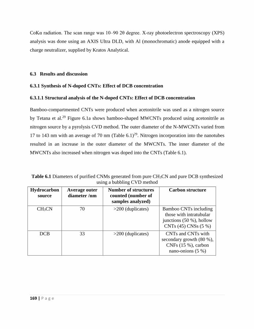
169 | P a g e

CoKα radiation. The scan range was 10–90 2θ degree. X-ray photoelectron spectroscopy (XPS)

analysis was done using an AXIS Ultra DLD, with Al (monochromatic) anode equipped with a

charge neutralizer, supplied by Kratos Analytical.


6.3.1 Synthesis of N-doped CNTs: Effect of DCB concentration

6.3.1.1 Structural analysis of the N-doped CNTs: Effect of DCB concentration

Bamboo-compartmented CNTs were produced when acetonitrile was used as a nitrogen source

by Tetana et al.29 Figure 6.1a shows bamboo-shaped MWCNTs produced using acetonitrile as

nitrogen source by a pyrolysis CVD method. The outer diameter of the N-MWCNTs varied from

17 to 143 nm with an average of 70 nm (Table 6.1)29. Nitrogen incorporation into the nanotubes

resulted in an increase in the outer diameter of the MWCNTs. The inner diameter of the

MWCNTs also increased when nitrogen was doped into the CNTs (Table 6.1).


using a bubbling CVD method

Hydrocarbon

source

Average outer

diameter /nm


counted (number of

samples analyzed)

Carbon structure

CH3CN 70 >200 (duplicates) Bamboo CNTs including

those with intratubular

junctions (50 %), hollow

CNTs (45) CNSs (5 %)

DCB 33 >200 (duplicates) CNTs and CNTs with

secondary growth (80 %),

CNFs (15 %), carbon

nano-onions (5 %)

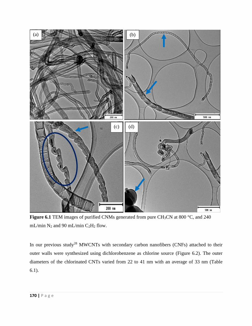
170 | P a g e

Figure 6.1 TEM images of purified CNMs generated from pure CH3CN at 800 °C, and 240

mL/min N2 and 90 mL/min C2H2 flow.

In our previous study28 MWCNTs with secondary carbon nanofibers (CNFs) attached to their

outer walls were synthesized using dichlorobenzene as chlorine source (Figure 6.2). The outer

diameters of the chlorinated CNTs varied from 22 to 41 nm with an average of 33 nm (Table

6.1).

(a) (b)

(c) (d)

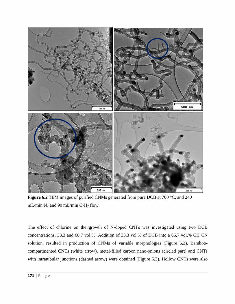
171 | P a g e

Figure 6.2 TEM images of purified CNMs generated from pure DCB at 700 °C, and 240

mL/min N2 and 90 mL/min C2H2 flow.

The effect of chlorine on the growth of N-doped CNTs was investigated using two DCB

concentrations, 33.3 and 66.7 vol.%. Addition of 33.3 vol.% of DCB into a 66.7 vol.% CH3CN

solution, resulted in production of CNMs of variable morphologies (Figure 6.3). Bamboo-

compartmented CNTs (white arrow), metal-filled carbon nano-onions (circled part) and CNTs

with intratubular junctions (dashed arrow) were obtained (Figure 6.3). Hollow CNTs were also

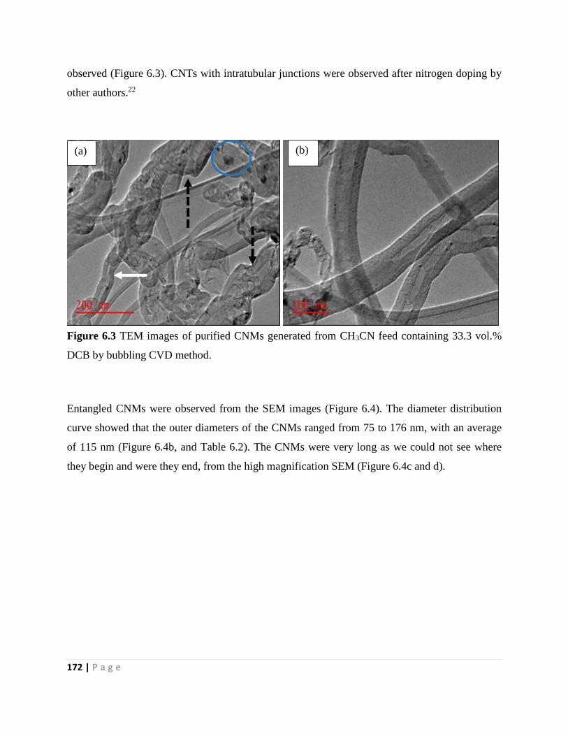
172 | P a g e

observed (Figure 6.3). CNTs with intratubular junctions were observed after nitrogen doping by

other authors.22

Figure 6.3 TEM images of purified CNMs generated from CH3CN feed containing 33.3 vol.%

DCB by bubbling CVD method.

Entangled CNMs were observed from the SEM images (Figure 6.4). The diameter distribution

curve showed that the outer diameters of the CNMs ranged from 75 to 176 nm, with an average

of 115 nm (Figure 6.4b, and Table 6.2). The CNMs were very long as we could not see where

they begin and were they end, from the high magnification SEM (Figure 6.4c and d).

(a) (b)

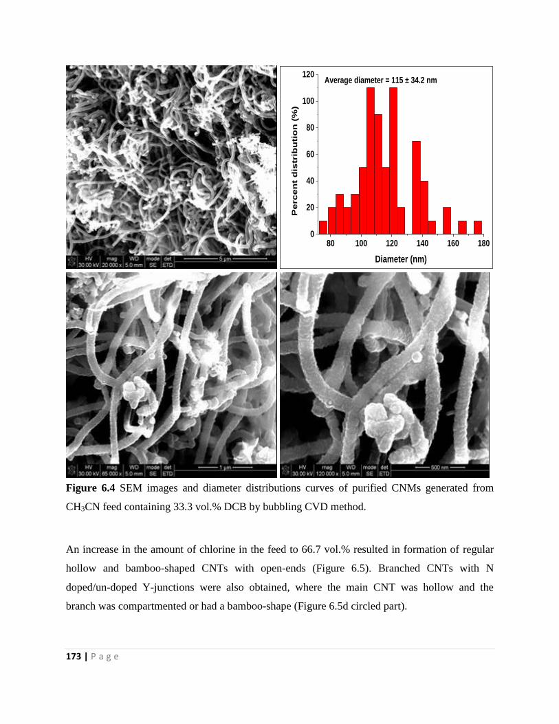
173 | P a g e

80 100 120 140 160 1800

20

40

60

80

100

120

Perc

en

t d

istr

ibu

tio

n (

%)

Diameter (nm)



CH3CN feed containing 33.3 vol.% DCB by bubbling CVD method.

An increase in the amount of chlorine in the feed to 66.7 vol.% resulted in formation of regular

hollow and bamboo-shaped CNTs with open-ends (Figure 6.5). Branched CNTs with N

doped/un-doped Y-junctions were also obtained, where the main CNT was hollow and the

branch was compartmented or had a bamboo-shape (Figure 6.5d circled part).

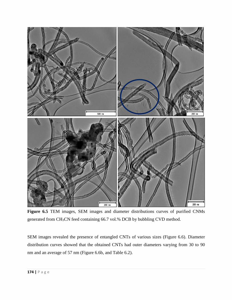
174 | P a g e

Figure 6.5 TEM images, SEM images and diameter distributions curves of purified CNMs

generated from CH3CN feed containing 66.7 vol.% DCB by bubbling CVD method.

SEM images revealed the presence of entangled CNTs of various sizes (Figure 6.6). Diameter

distribution curves showed that the obtained CNTs had outer diameters varying from 30 to 90

nm and an average of 57 nm (Figure 6.6b, and Table 6.2).

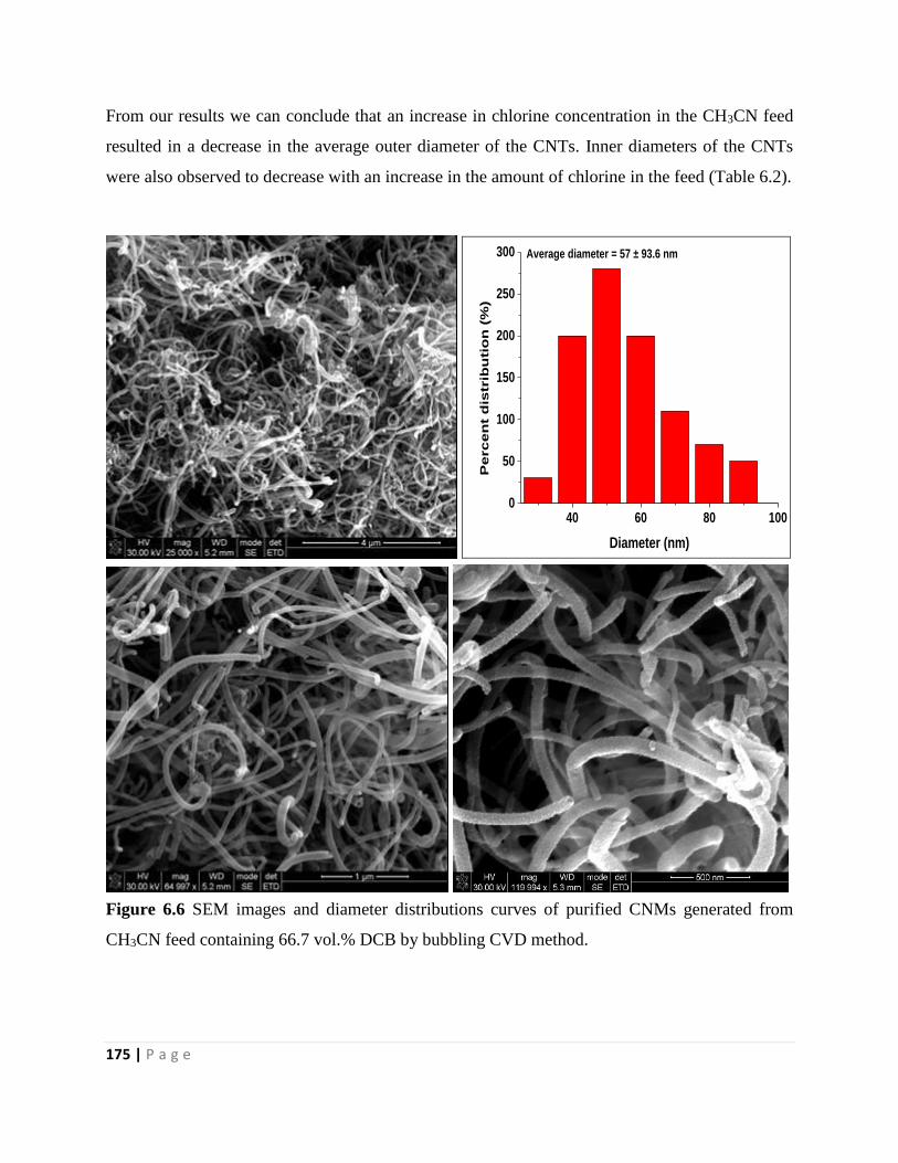
175 | P a g e

From our results we can conclude that an increase in chlorine concentration in the CH3CN feed

resulted in a decrease in the average outer diameter of the CNTs. Inner diameters of the CNTs

were also observed to decrease with an increase in the amount of chlorine in the feed (Table 6.2).

40 60 80 1000

50

100

150

200

250

300

Pe

rc

en

t d

istr

ibu

tio

n (

%)

Diameter (nm)



CH3CN feed containing 66.7 vol.% DCB by bubbling CVD method.

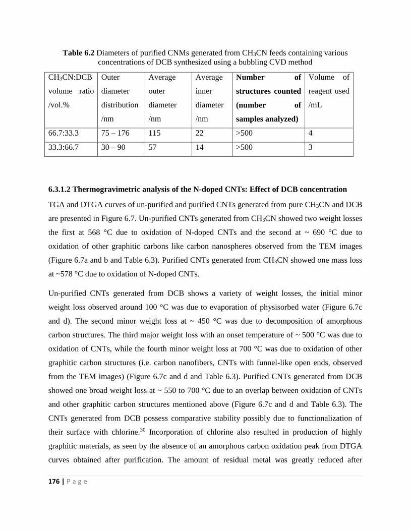
176 | P a g e

Table 6.2 Diameters of purified CNMs generated from CH3CN feeds containing various

concentrations of DCB synthesized using a bubbling CVD method

CH3CN:DCB

volume ratio

/vol.%

Outer

diameter

distribution

/nm

Average

outer

diameter

/nm

Average

inner

diameter

/nm

Number of

structures counted

(number of

samples analyzed)

Volume of

reagent used

/mL

66.7:33.3 75 – 176 115 22 >500 4

33.3:66.7 30 – 90 57 14 >500 3

6.3.1.2 Thermogravimetric analysis of the N-doped CNTs: Effect of DCB concentration

TGA and DTGA curves of un-purified and purified CNTs generated from pure CH3CN and DCB

are presented in Figure 6.7. Un-purified CNTs generated from CH3CN showed two weight losses

the first at 568 °C due to oxidation of N-doped CNTs and the second at ~ 690 °C due to

oxidation of other graphitic carbons like carbon nanospheres observed from the TEM images

(Figure 6.7a and b and Table 6.3). Purified CNTs generated from CH3CN showed one mass loss

at ~578 °C due to oxidation of N-doped CNTs.

Un-purified CNTs generated from DCB shows a variety of weight losses, the initial minor

weight loss observed around 100 °C was due to evaporation of physisorbed water (Figure 6.7c

and d). The second minor weight loss at ~ 450 °C was due to decomposition of amorphous

carbon structures. The third major weight loss with an onset temperature of ~ 500 °C was due to

oxidation of CNTs, while the fourth minor weight loss at 700 °C was due to oxidation of other

graphitic carbon structures (i.e. carbon nanofibers, CNTs with funnel-like open ends, observed

from the TEM images) (Figure 6.7c and d and Table 6.3). Purified CNTs generated from DCB

showed one broad weight loss at ~ 550 to 700 °C due to an overlap between oxidation of CNTs

and other graphitic carbon structures mentioned above (Figure 6.7c and d and Table 6.3). The

CNTs generated from DCB possess comparative stability possibly due to functionalization of

their surface with chlorine.30 Incorporation of chlorine also resulted in production of highly

graphitic materials, as seen by the absence of an amorphous carbon oxidation peak from DTGA

curves obtained after purification. The amount of residual metal was greatly reduced after

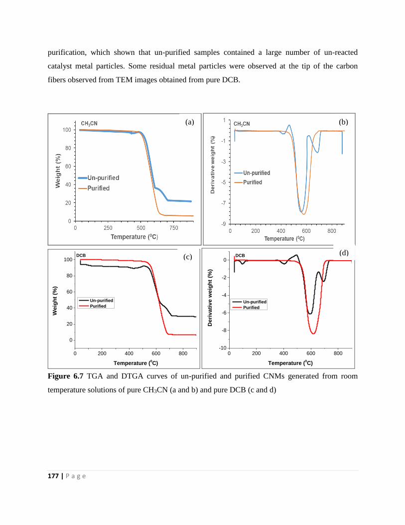
177 | P a g e

purification, which shown that un-purified samples contained a large number of un-reacted

catalyst metal particles. Some residual metal particles were observed at the tip of the carbon

fibers observed from TEM images obtained from pure DCB.

0 200 400 600 800

0

20

40

60

80

100

We

igh

t (%

)

Temperature (0C)

Un-purified

Purified

DCB

0 200 400 600 800-10

-8

-6

-4

-2

0

De

riv

ati

ve

we

igh

t (%

)

Temperature (0C)

Un-purified

Purified

DCB


temperature solutions of pure CH3CN (a and b) and pure DCB (c and d)

(a) (b)

(c) (d)

178 | P a g e


purified and purified (P) chlorinated N-MWCNTs generated by bubbling different ratios of a

CH3CN and DCB.

Hydrocarbon source Decomposition temperature /°C Residual mass /%

CH3CN 568 & 690 21.7

CH3CN (P) 578 5.6

DCB28 597 29.6

DCB28 600 6.6

TGA and DTGA curves of un-purified and purified CNTs generated from acetonitrile feeds

containing low concentration of DCB (33.3 vol.%) appeared similar. A broad oxidation peak was

observed at ~ 550 to 750 °C and ~ 550 to 800 °C for un-purified and purified materials

respectively (Figure 6.8 and Table 6.4), assigned to oxidation of chlorinated CNTs and other

graphitic carbon materials (carbon nanoonions, hollow CNTs and CNTs with junctions). This

oxidation peak had a shoulder peak at ~ 800 °C and above 800 °C for un-purified and purified

materials, due to evolution of nitrogen which is known to be released from N-doped carbons.31

These results agree with the TEM observations where various types of CNTs of various sizes and

morphologies were obtained.

Two regions of mass losses were observed from un-purified CNTs generated from acetonitrile

solutions containing 66.7 vol.% DCB (Figure 6.8c and d). The first major weight loss was

observed at ~ 600 to 650 °C, due to oxidation of chlorine functionalized bamboo N-doped CNTs

(Figure 6.8 and Table 6.4). The second minor weight loss at ~ 700 °C was due to oxidation of

functionalized hollow CNTs (Figure 6.8 and Table 6.4). DTGA curves of purified CNTs

generated from feed solutions containing 66.7 vol.% DCB showed only one broad region of mass

loss at 550 to 650 °C, which could be due to overlap between oxidation of chlorine

functionalized N-doped and hollow CNTs. TGA data agrees with the TEM observations where

bamboo-compartmented and hollow were observed. The results show that the carbon materials

of different morphologies can be obtained by varying the amount of chlorine in the feed.

We also analyzed the residual mass present in chlorinated N-doped samples after purification

with acid. The residual mass of 7.7 and 0 were obtained for N-CNTs generated from a feed

179 | P a g e

containing 33.3 and 66.7 vol.% DCB, respectively (Table 6.4). From this results it appears that

metal particles were completely removed from solutions that contained high concentrations of

DCB rather than those that contained lower concentrations of DCB. This can be attributed to

greater encapsulation of metal particles into large diameter CNTs generated from low

concentration of DCB, which were difficult to remove by acid treatment.

0 200 400 600 8000

20

40

60

80

100

Weig

ht

(%)

Temperature (0C)

Un-purified

Purified

66.7:33.3 vol.%

200 400 600 800

-6

-4

-2

0

Deri

va

tiv

e w

eig

ht

(%)

Temperature (0C)

Un-purified

Purified

66.7:33.3 vol.%

0 200 400 600 800

0

20

40

60

80

100

Weig

ht

(%)

Temperature (0C)

Purified

Un-purified

33.3:66.7 vol.%

0 200 400 600 800

-10

-8

-6

-4

-2

0

De

riv

ati

ve

we

igh

t (%

)

Temperature (0C)

Purified

Un-purified

33.3:66.7 vol.%


temperatures solutions of acetonitrile containing various concentrations of DCB.

(a) (b)

(c) (d)

180 | P a g e


purified and purified (P) chlorinated N-CNTs generated from solutions containing different

CH3CN:DCB volume ratios.

CH3CN:DCB volume ratio /% Decomposition temperature /°C Residual mass /%

66.7:33.3 651 & 737 19.3

66.7:33.3 (P) 671 7.7

33.3:66.7 610 & 643 11.0

33.3:66.7 (P) 600 0

6.3.1.3 Raman spectroscopy analysis of the N-doped CNTs: Effect of DCB concentration

Raman spectra analysis of the purified CNTs generated from pure CH3CN and pure DCB are

presented in Figure 6.9. A disorder-induced band (D-band) and a graphitic band (G-band) were

observed in both Raman spectra. For CNTs generated from pure CH3CN, a broad D-band was

deconvoluted into two bands, a D4-band at 1210 cm–1 attributed to C=C stretching vibrations and

a D-band at 1339 cm–1 attributed to topological defects on the CNT walls due to substitution of

carbon with nitrogen. A G-band was also deconvoluted into two peaks, a D2-band at 1513 cm–1

assigned to the presence of amorphous carbon structures and a G-band at 1585 cm–1 due to sp2

carbon atoms in a graphitic plane. An ID/IG value of 1.2 was obtained, which suggest the

materials are highly defected. Large FWHM values of 126 and 71 cm–1 for D and G-band

respectively also suggest the presence of amorphous carbon structures (Table 6.5).

Raman bands of purified CNTs generated from pure DCB also showed a D-band that was

deconvoluted into two peaks, a D4-band at 1236 cm–1 and a D-band at 1338 cm–1 (Figure 6.9). A

G-band was also deconvoluted into two peaks, a D2-band at 1498 cm–1 and a G-band at 1587

cm–1. The amorphous carbon D2-band also is very broad and intense as compared to the one

obtained from Raman curves generated from CH3CN, which suggest the formation of sp3 carbon

due to chlorine functionalization.

181 | P a g e

1000 1200 1400 1600 1800-10

0

10

20

30

40

50

60

70

80In

ten

sit

y (

a.u

)

Raman shift (cm-1)

CH3CN

purified

D4

D

D2

G

800 1000 1200 1400 1600 1800-10

0

10

20

30

40

50

60

70

80

Inte

nsit

y (

a.u

)

Raman shift (cm-1)

DCB

purified

D4

D

D2

G

Figure 6.9 Deconvoluted Raman spectra of purified MWCNTs generated from (a) CH3CN and

(b) DCB using a bubbling CVD method.

An ID/IG value of 1.0 was obtained, which suggest that the materials are highly defected due to

surface functionalization of the CNTs with chlorine. The lower value of ID/IG of 1.0 for CNTs

generated from DCB as compared to 1.2 for CNTs generated from CH3CN suggests that the

CNTs generated from DCB were less defected. This data agrees with the TGA analysis of the

materials. Also from comparison of FWHM values with those obtained from CH3CN samples,

lower FWHM values were obtained from CNTs generated from DCB 109 and 66 cm–1 for D and

G-band respectively (Table 6.5). This again suggest that the materials generated in DCB were

more graphitic than those generated from CH3CN.

(a) (b)

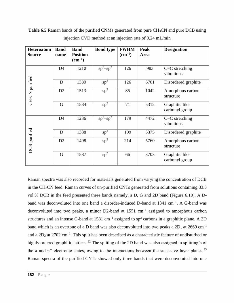
182 | P a g e

Table 6.5 Raman bands of the purified CNMs generated from pure CH3CN and pure DCB using

injection CVD method at an injection rate of 0.24 mL/min

Heteroatom

Source

Band

name

Band

Position

(cm–1)

Bond type FWHM

(cm–1)

Peak

Area

Designation

CH

3C

N p

uri

fied

D4 1210 sp2–sp3 126 983 C=C stretching

vibrations



structure


carbonyl group

DC

B p

uri

fied


vibrations



structure


carbonyl group

Raman spectra was also recorded for materials generated from varying the concentration of DCB

in the CH3CN feed. Raman curves of un-purified CNTs generated from solutions containing 33.3

vol.% DCB in the feed presented three bands namely, a D, G and 2D band (Figure 6.10). A D-

band was deconvoluted into one band a disorder-induced D-band at 1341 cm–1. A G-band was

deconvoluted into two peaks, a minor D2-band at 1551 cm–1 assigned to amorphous carbon

structures and an intense G-band at 1581 cm–1 assigned to sp2 carbons in a graphitic plane. A 2D

band which is an overtone of a D band was also deconvoluted into two peaks a 2D1 at 2669 cm–1

and a 2D2 at 2702 cm–1. This split has been described as a characteristic feature of undisturbed or

highly ordered graphitic lattices.32 The spliting of the 2D band was also assigned to splitting’s of

the π and π* electronic states, owing to the interactions between the succesive layer planes.33

Raman spectra of the purified CNTs showed only three bands that were deconvoluted into one

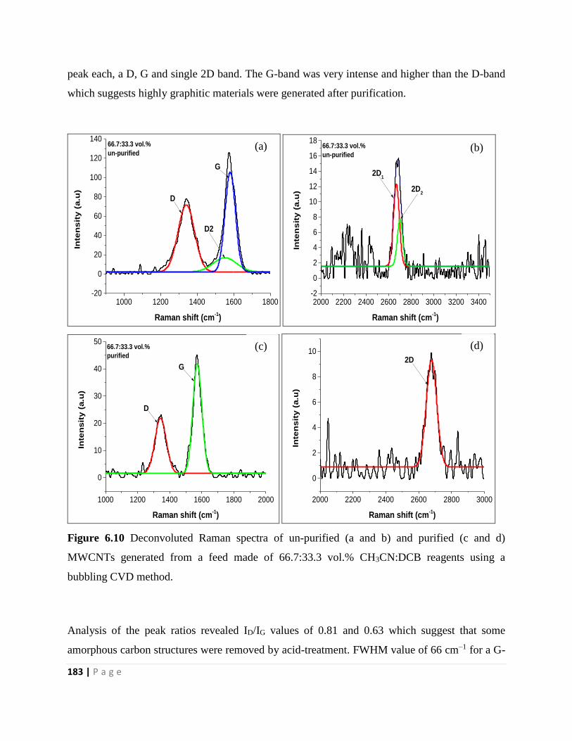
183 | P a g e

peak each, a D, G and single 2D band. The G-band was very intense and higher than the D-band

which suggests highly graphitic materials were generated after purification.

1000 1200 1400 1600 1800-20

0

20

40

60

80

100

120

140

Inte

nsit

y (

a.u

)

Raman shift (cm-1)

66.7:33.3 vol.%

un-purified

D

D2

G

2000 2200 2400 2600 2800 3000 3200 3400-2

0

2

4

6

8

10

12

14

16

18

Inte

ns

ity

(a

.u)

Raman shift (cm-1)

66.7:33.3 vol.%

un-purified

2D1

2D2

1000 1200 1400 1600 1800 2000

0

10

20

30

40

50

Inte

ns

ity

(a

.u)

Raman shift (cm-1)

66.7:33.3 vol.%

purified

D

G

2000 2200 2400 2600 2800 3000

0

2

4

6

8

10

Inte

nsit

y (

a.u

)

Raman shift (cm-1)

2D

Figure 6.10 Deconvoluted Raman spectra of un-purified (a and b) and purified (c and d)

MWCNTs generated from a feed made of 66.7:33.3 vol.% CH3CN:DCB reagents using a

bubbling CVD method.

Analysis of the peak ratios revealed ID/IG values of 0.81 and 0.63 which suggest that some

amorphous carbon structures were removed by acid-treatment. FWHM value of 66 cm–1 for a G-

(a)

(c)

(b)

(d)

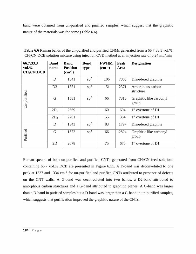
184 | P a g e

band were obtained from un-purified and purified samples, which suggest that the graphitic

nature of the materials was the same (Table 6.6).



66.7:33.3

vol.%

CH3CN:DCB

Band

name

Band

Position

(cm–1)

Bond

type

FWHM

(cm–1)

Peak

Area

Designation

Un-p

uri

fied



structure


group



Puri

fied



group


Raman spectra of both un-purified and purified CNTs generated from CH3CN feed solutions

containing 66.7 vol.% DCB are presented in Figure 6.11. A D-band was deconvoluted to one

peak at 1337 and 1334 cm–1 for un-purified and purified CNTs attributed to presence of defects

on the CNT walls. A G-band was deconvoluted into two bands, a D2-band attributed to

amorphous carbon structures and a G-band attributed to graphitic planes. A G-band was larger

than a D-band in purified samples but a D-band was larger than a G-band in un-purified samples,

which suggests that purification improved the graphitic nature of the CNTs.

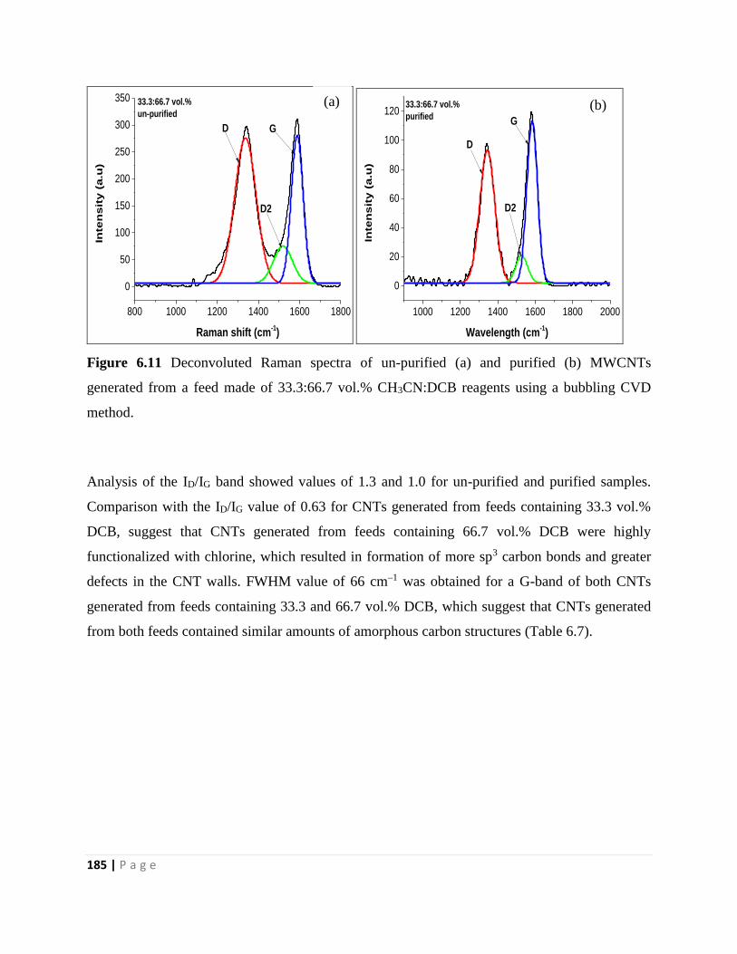
185 | P a g e

800 1000 1200 1400 1600 1800

0

50

100

150

200

250

300

350In

ten

sit

y (

a.u

)

Raman shift (cm-1)

33.3:66.7 vol.%

un-purified

D G

D2

1000 1200 1400 1600 1800 2000

0

20

40

60

80

100

120

Inte

nsit

y (

a.u

)

Wavelength (cm-1)

33.3:66.7 vol.%

purified

D

D2

G

Figure 6.11 Deconvoluted Raman spectra of un-purified (a) and purified (b) MWCNTs

generated from a feed made of 33.3:66.7 vol.% CH3CN:DCB reagents using a bubbling CVD

method.

Analysis of the ID/IG band showed values of 1.3 and 1.0 for un-purified and purified samples.

Comparison with the ID/IG value of 0.63 for CNTs generated from feeds containing 33.3 vol.%

DCB, suggest that CNTs generated from feeds containing 66.7 vol.% DCB were highly

functionalized with chlorine, which resulted in formation of more sp3 carbon bonds and greater

defects in the CNT walls. FWHM value of 66 cm–1 was obtained for a G-band of both CNTs

generated from feeds containing 33.3 and 66.7 vol.% DCB, which suggest that CNTs generated

from both feeds contained similar amounts of amorphous carbon structures (Table 6.7).

(a) (b)

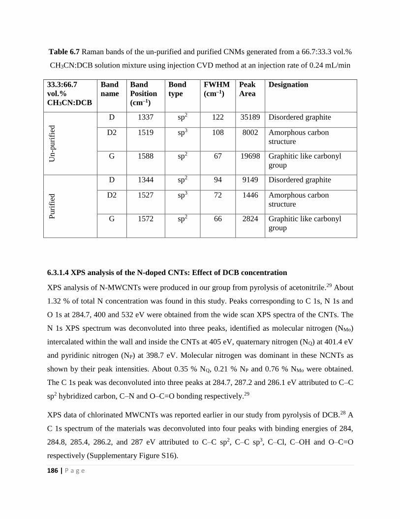
186 | P a g e



33.3:66.7

vol.%

CH3CN:DCB

Band

name

Band

Position

(cm–1)

Bond

type

FWHM

(cm–1)

Peak

Area

Designation

Un-p

uri

fied



structure


group

Puri

fied



structure


group

6.3.1.4 XPS analysis of the N-doped CNTs: Effect of DCB concentration

XPS analysis of N-MWCNTs were produced in our group from pyrolysis of acetonitrile.29 About

1.32 % of total N concentration was found in this study. Peaks corresponding to C 1s, N 1s and

O 1s at 284.7, 400 and 532 eV were obtained from the wide scan XPS spectra of the CNTs. The

N 1s XPS spectrum was deconvoluted into three peaks, identified as molecular nitrogen (NMo)

intercalated within the wall and inside the CNTs at 405 eV, quaternary nitrogen (NQ) at 401.4 eV

and pyridinic nitrogen (NP) at 398.7 eV. Molecular nitrogen was dominant in these NCNTs as

shown by their peak intensities. About 0.35 % NQ, 0.21 % NP and 0.76 % NMo were obtained.

The C 1s peak was deconvoluted into three peaks at 284.7, 287.2 and 286.1 eV attributed to C–C

sp2 hybridized carbon, C–N and O–C=O bonding respectively.29

XPS data of chlorinated MWCNTs was reported earlier in our study from pyrolysis of DCB.28 A

C 1s spectrum of the materials was deconvoluted into four peaks with binding energies of 284,

284.8, 285.4, 286.2, and 287 eV attributed to C–C sp2, C–C sp3, C–Cl, C–OH and O–C=O

respectively (Supplementary Figure S16).

187 | P a g e

Wide scan XPS spectra of both chlorine containing N-doped CNTs revealed peaks at 200, 284,

400 and 532 eV assigned to Cl 2p, C 1s, N 1s and O 1s, respectively (Supplementary Figure

S17). The deconvoluted C 1s peaks of the materials produced from various volume ratios of

DCB, was fitted into four components at 283–284 eV for C–C sp2 and sp3 carbon bonds, at ~ 286

eV for overlap between C–N and C–Cl groups and ~ 289 eV for O–C=O carboxylic groups

(Supplementary Figure S18). The peak at 286 eV assigned to overlap between C–N and C–Cl

carbon bonds, increased in intensity from 12.9 % to 20.1 % with an increase in DCB

concentration from 33.3 to 66.7 vol.% (Supplementary Figure S18).

The N 1s XPS spectra was deconvoluted into four and five peaks for both studied concentrations

of CH3CN and DCB (Figure 6.12a and c). For chlorinated N-CNTs generated from solutions

containing 33.3 vol.% DCB in the feed, the N1s was deconvoluted into five peaks appearing at

397.6 (6.3 %), 398.5 (10.9 %), 399.9 (0.94 %), 400.8 (60.1 %) and 405.7 (21.8 %) eV and were

assigned to tetrahedral nitrogen bonded to sp3–C (probably due to un-decomposed N–H bond),

pyridinic N (NP), pyrrolic N (NPry), quaternary N (NQ) and molecular N (NMo), respectively

(Table 6.8 and Figure 6.12a). The atomic percentages suggest that quaternary nitrogen was the

most predominant form of nitrogen present at this studied concentration. These results suggest a

more homogeneous distribution of nitrogen species in the CNTs. Graphitic N forms by merging

N atoms into the defect region of the graphene, resulting in a graphene with less defects.10 This

data is consistent with Raman data where low ID/IG value was obtained at this DCB

concentration, showing that the CNTs contained less defects.

N 1s XPS spectra of N-CNTs generated from CH3CN feed solutions containing 66.7 vol.% DCB

was deconvoluted into four peaks appearing at 398.2 (2.0 %), 400.2 (31.7 %), 401.9 (4.8 %) and

405.8 (61.6 %) eV attributed to NP, NPyr, NQ and NMo, respectively (Table 6.8 and Figure 6.12c).

An increase in the concentration of DCB resulted in a reduction of the amount of nitrogen

incorporated into the CNTs, as shown by a great reduction in the atomic percentage of

quaternary nitrogen species (Figure 6.13a). Molecular nitrogen was found to be the dominant

nitrogen species at this concentration (Figure 6.13a). An increase in peak intensity of the 400.2

eV peak which was assigned to pyrrolic nitrogen was also observed at this concentration (Figure

6.13a). The pyrrolic nitrogen is a substitutional nitrogen, that is part of a five-membered ring and

is sp3 hybridized. An increase in the contribution of pyrrolic nitrogen causes an increase in the

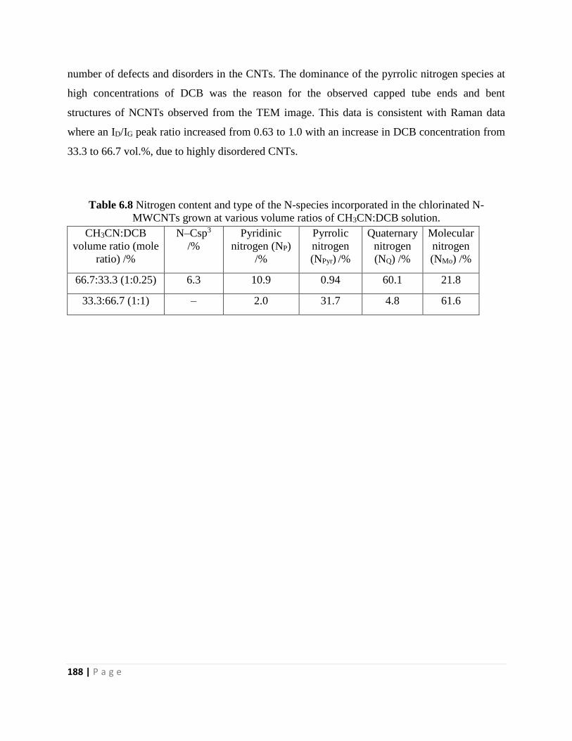
188 | P a g e

number of defects and disorders in the CNTs. The dominance of the pyrrolic nitrogen species at

high concentrations of DCB was the reason for the observed capped tube ends and bent

structures of NCNTs observed from the TEM image. This data is consistent with Raman data

where an ID/IG peak ratio increased from 0.63 to 1.0 with an increase in DCB concentration from

33.3 to 66.7 vol.%, due to highly disordered CNTs.


MWCNTs grown at various volume ratios of CH3CN:DCB solution.

CH3CN:DCB

volume ratio (mole

ratio) /%

N–Csp3

/%

Pyridinic

nitrogen (NP)

/%

Pyrrolic

nitrogen

(NPyr) /%

Quaternary

nitrogen

(NQ) /%

Molecular

nitrogen

(NMo) /%

66.7:33.3 (1:0.25) 6.3 10.9 0.94 60.1 21.8

33.3:66.7 (1:1) – 2.0 31.7 4.8 61.6

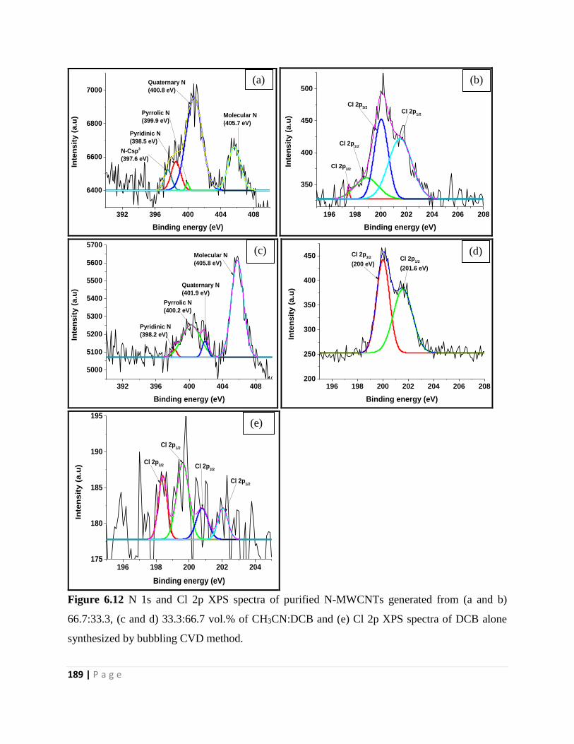
189 | P a g e

392 396 400 404 408

6400

6600

6800

7000

Inte

ns

ity

(a

.u)

Binding energy (eV)

N-Csp3

(397.6 eV)

Pyridinic N

(398.5 eV)

Pyrrolic N

(399.9 eV)

Quaternary N

(400.8 eV)

Molecular N

(405.7 eV)

196 198 200 202 204 206 208

350

400

450

500

Inte

ns

ity

(a

.u)

Binding energy (eV)

Cl 2p3/2

Cl 2p1/2

Cl 2p3/2

Cl 2p1/2

392 396 400 404 408

5000

5100

5200

5300

5400

5500

5600

5700

Inte

nsit

y (

a.u

)

Binding energy (eV)

Pyridinic N

(398.2 eV)

Pyrrolic N

(400.2 eV)

Quaternary N

(401.9 eV)

Molecular N

(405.8 eV)

196 198 200 202 204 206 208200

250

300

350

400

450

Inte

nsit

y (

a.u

)

Binding energy (eV)

Cl 2p3/2

(200 eV)Cl 2p

1/2

(201.6 eV)

196 198 200 202 204175

180

185

190

195

Inte

ns

ity

(a

.u)

Binding energy (eV)

Cl 2p3/2

Cl 2p1/2

Cl 2p3/2

Cl 2p1/2

Figure 6.12 N 1s and Cl 2p XPS spectra of purified N-MWCNTs generated from (a and b)

66.7:33.3, (c and d) 33.3:66.7 vol.% of CH3CN:DCB and (e) Cl 2p XPS spectra of DCB alone

synthesized by bubbling CVD method.

(a) (b)

(c) (d)

(e)

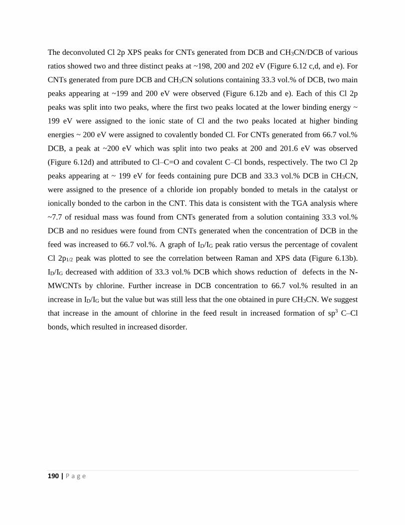
190 | P a g e

The deconvoluted Cl 2p XPS peaks for CNTs generated from DCB and CH3CN/DCB of various

ratios showed two and three distinct peaks at ~198, 200 and 202 eV (Figure 6.12 c,d, and e). For

CNTs generated from pure DCB and CH3CN solutions containing 33.3 vol.% of DCB, two main

peaks appearing at ~199 and 200 eV were observed (Figure 6.12b and e). Each of this Cl 2p

peaks was split into two peaks, where the first two peaks located at the lower binding energy ~

199 eV were assigned to the ionic state of Cl and the two peaks located at higher binding

energies ~ 200 eV were assigned to covalently bonded Cl. For CNTs generated from 66.7 vol.%

DCB, a peak at ~200 eV which was split into two peaks at 200 and 201.6 eV was observed

(Figure 6.12d) and attributed to Cl–C=O and covalent C–Cl bonds, respectively. The two Cl 2p

peaks appearing at ~ 199 eV for feeds containing pure DCB and 33.3 vol.% DCB in CH3CN,

were assigned to the presence of a chloride ion propably bonded to metals in the catalyst or

ionically bonded to the carbon in the CNT. This data is consistent with the TGA analysis where

~7.7 of residual mass was found from CNTs generated from a solution containing 33.3 vol.%

DCB and no residues were found from CNTs generated when the concentration of DCB in the

feed was increased to 66.7 vol.%. A graph of ID/IG peak ratio versus the percentage of covalent

Cl 2p1/2 peak was plotted to see the correlation between Raman and XPS data (Figure 6.13b).

ID/IG decreased with addition of 33.3 vol.% DCB which shows reduction of defects in the N-

MWCNTs by chlorine. Further increase in DCB concentration to 66.7 vol.% resulted in an

increase in ID/IG but the value but was still less that the one obtained in pure CH3CN. We suggest

that increase in the amount of chlorine in the feed result in increased formation of sp3 C–Cl

bonds, which resulted in increased disorder.

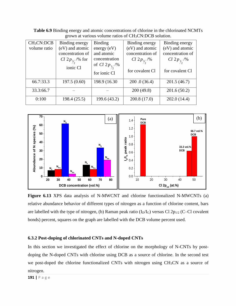
191 | P a g e

Table 6.9 Binding energy and atomic concentrations of chlorine in the chlorinated NCMTs

grown at various volume ratios of CH3CN:DCB solution.

CH3CN:DCB

volume ratio

Binding energy

(eV) and atomic

concentration of

232 pCl /% for

ionic Cl

Binding

energy (eV)

and atomic

concentration

of 2

12 pCl /%

for ionic Cl

Binding energy

(eV) and atomic

concentration of

232 pCl /%

for covalent Cl

Binding energy

(eV) and atomic

concentration of

212 pCl /%

for covalent Cl

66.7:33.3 197.5 (0.60) 198.9 (16.30 200 .0 (36.4) 201.5 (46.7)

33.3:66.7 – – 200 (49.8) 201.6 (50.2)

0:100 198.4 (25.5) 199.6 (43.2) 200.8 (17.0) 202.0 (14.4)

20 30 40 50 60 70 800

10

20

30

40

50

60

70

NMo

NQ

NPry

NP

Ab

un

da

nc

e o

f N

sp

ec

ies

(%

)

DCB concentration (vol.%)

NP

NPry

NQ

NMo

10 20 30 40 500.0

0.2

0.4

0.6

0.8

1.0

1.2

1.4

I D/I

G p

ea

k r

ati

o

Cl 2p1/2

(at.%)

Pure

DCB

33.3 vol.%

DCB

66.7 vol.%

DCB

Figure 6.13 XPS data analysis of N-MWCNT and chlorine functionalized N-MWCNTs (a)

relative abundance behavior of different types of nitrogen as a function of chlorine content, bars

are labelled with the type of nitrogen, (b) Raman peak ratio (ID/IG) versus Cl 2p1/2 (C–Cl covalent

bonds) percent, squares on the graph are labelled with the DCB volume percent used.

6.3.2 Post-doping of chlorinated CNTs and N-doped CNTs

In this section we investigated the effect of chlorine on the morphology of N-CNTs by post-

doping the N-doped CNTs with chlorine using DCB as a source of chlorine. In the second test

we post-doped the chlorine functionalized CNTs with nitrogen using CH3CN as a source of

nitrogen.

(a) (b)

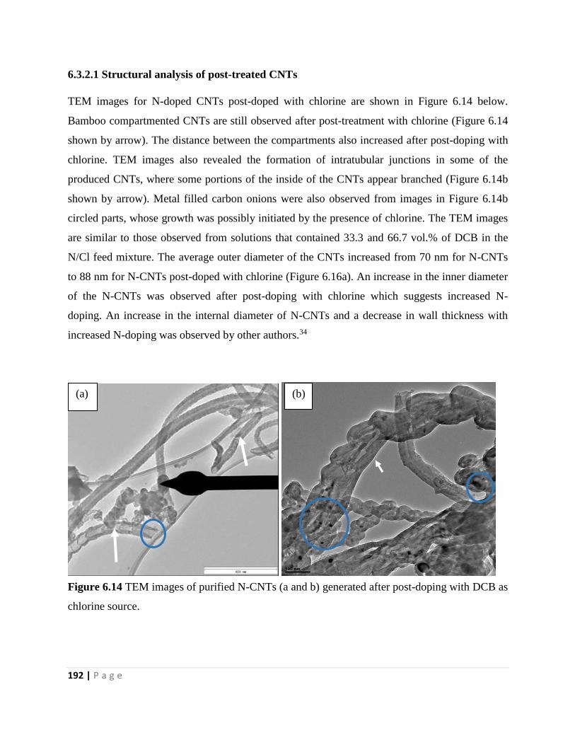
192 | P a g e

6.3.2.1 Structural analysis of post-treated CNTs

TEM images for N-doped CNTs post-doped with chlorine are shown in Figure 6.14 below.

Bamboo compartmented CNTs are still observed after post-treatment with chlorine (Figure 6.14

shown by arrow). The distance between the compartments also increased after post-doping with

chlorine. TEM images also revealed the formation of intratubular junctions in some of the

produced CNTs, where some portions of the inside of the CNTs appear branched (Figure 6.14b

shown by arrow). Metal filled carbon onions were also observed from images in Figure 6.14b

circled parts, whose growth was possibly initiated by the presence of chlorine. The TEM images

are similar to those observed from solutions that contained 33.3 and 66.7 vol.% of DCB in the

N/Cl feed mixture. The average outer diameter of the CNTs increased from 70 nm for N-CNTs

to 88 nm for N-CNTs post-doped with chlorine (Figure 6.16a). An increase in the inner diameter

of the N-CNTs was observed after post-doping with chlorine which suggests increased N-

doping. An increase in the internal diameter of N-CNTs and a decrease in wall thickness with

increased N-doping was observed by other authors.34

Figure 6.14 TEM images of purified N-CNTs (a and b) generated after post-doping with DCB as

chlorine source.

(b) (a)

193 | P a g e

TEM images of CNTs generated using DCB as a chlorine source, post-doped with nitrogen are

presented in Figure 6.12. About 50 % of bamboo-shaped CNTs which appeared as stacked cups

were generated after post-doping with nitrogen (Figure 6.15a), and the rest of the CNTs were

hollow (Figure 6.15b). CNTs with secondary CNF growth were also still present after post-

doping with nitrogen (Figure 6.15b insert and circled part). CNTs generated after post-doping

with nitrogen were mostly bamboo-compartmented (Figure 6.15a), suggesting that post-doping

was an effective method to introduce nitrogen into the CNTs by replacing one of the carbon

atoms. Some authors found that in-situ doping of nitrogen atoms into the structure of CNTs

during the growth gives much better nitrogen stabilities than the post-treatment method.35 The

average diameter of the chlorine containing CNTs decreased from 33 nm to 28 nm after post-

doping with nitrogen (Figure 6.17b).

Figure 6.15 TEM images of chlorinated CNTs (a and b) generated after post-doping with

CH3CN nitrogen source.

(a) (b)

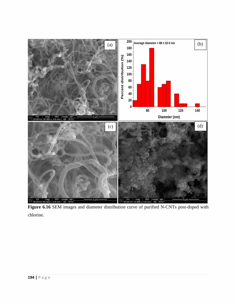
194 | P a g e

80 100 120 1400

20

40

60

80

100

120

140

160

180

200

Pe

rc

en

t d

istr

ibu

tio

n (

%)

Diameter (nm)


Figure 6.16 SEM images and diameter distribution curve of purified N-CNTs post-doped with

chlorine.

(a) (b)

(d) (c)

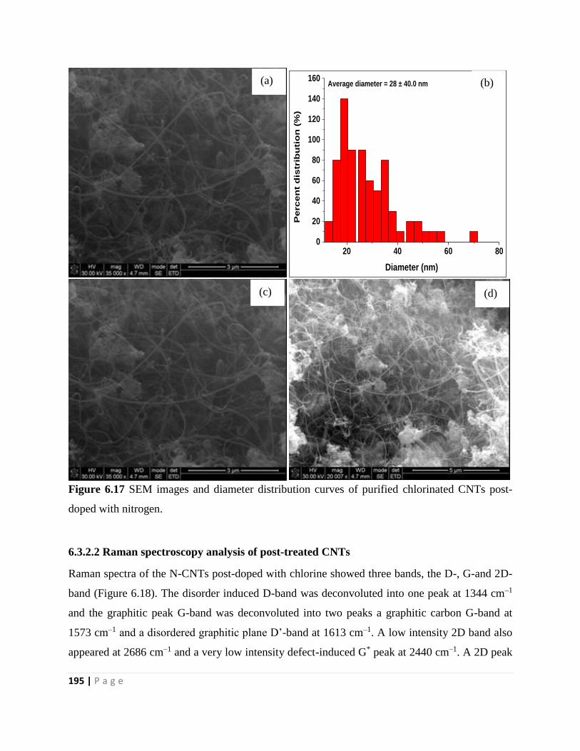
195 | P a g e

20 40 60 800

20

40

60

80

100

120

140

160

Perc

en

t d

istr

ibu

tio

n (

%)

Diameter (nm)


Figure 6.17 SEM images and diameter distribution curves of purified chlorinated CNTs post-

doped with nitrogen.

6.3.2.2 Raman spectroscopy analysis of post-treated CNTs

Raman spectra of the N-CNTs post-doped with chlorine showed three bands, the D-, G-and 2D-

band (Figure 6.18). The disorder induced D-band was deconvoluted into one peak at 1344 cm–1

and the graphitic peak G-band was deconvoluted into two peaks a graphitic carbon G-band at

1573 cm–1 and a disordered graphitic plane D’-band at 1613 cm–1. A low intensity 2D band also

appeared at 2686 cm–1 and a very low intensity defect-induced G* peak at 2440 cm–1. A 2D peak

(a)

(d) (c)

(b)

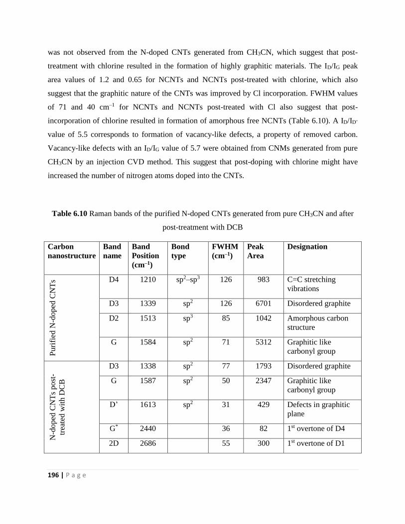
196 | P a g e

was not observed from the N-doped CNTs generated from CH3CN, which suggest that post-

treatment with chlorine resulted in the formation of highly graphitic materials. The ID/IG peak

area values of 1.2 and 0.65 for NCNTs and NCNTs post-treated with chlorine, which also

suggest that the graphitic nature of the CNTs was improved by Cl incorporation. FWHM values

of 71 and 40 cm–1 for NCNTs and NCNTs post-treated with Cl also suggest that post-

incorporation of chlorine resulted in formation of amorphous free NCNTs (Table 6.10). A ID/ID’

value of 5.5 corresponds to formation of vacancy-like defects, a property of removed carbon.

Vacancy-like defects with an ID/IG value of 5.7 were obtained from CNMs generated from pure

CH3CN by an injection CVD method. This suggest that post-doping with chlorine might have

increased the number of nitrogen atoms doped into the CNTs.

Table 6.10 Raman bands of the purified N-doped CNTs generated from pure CH3CN and after

post-treatment with DCB

Carbon

nanostructure

Band

name

Band

Position

(cm–1)

Bond

type

FWHM

(cm–1)

Peak

Area

Designation

Puri

fied

N-d

oped

CN

Ts


vibrations

D3 1339 sp2 126 6701 Disordered graphite


structure


carbonyl group

N-d

oped

CN

Ts

post

-

trea

ted w

ith D

CB

D3 1338 sp2 77 1793 Disordered graphite


carbonyl group


plane



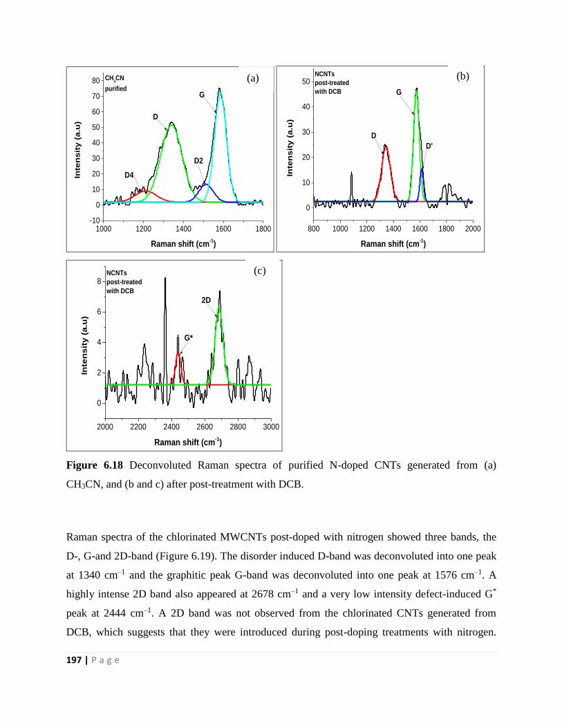
197 | P a g e

1000 1200 1400 1600 1800-10

0

10

20

30

40

50

60

70

80In

ten

sit

y (

a.u

)

Raman shift (cm-1)

CH3CN

purified

D4

D

D2

G

800 1000 1200 1400 1600 1800 2000

0

10

20

30

40

50

Inte

nsit

y (

a.u

)

Raman shift (cm-1)

NCNTs

post-treated

with DCB

D

G

D'

2000 2200 2400 2600 2800 3000

0

2

4

6

8

Inte

ns

ity

(a

.u)

Raman shift (cm-1)

NCNTs

post-treated

with DCB

G*

2D

Figure 6.18 Deconvoluted Raman spectra of purified N-doped CNTs generated from (a)

CH3CN, and (b and c) after post-treatment with DCB.

Raman spectra of the chlorinated MWCNTs post-doped with nitrogen showed three bands, the

D-, G-and 2D-band (Figure 6.19). The disorder induced D-band was deconvoluted into one peak

at 1340 cm–1 and the graphitic peak G-band was deconvoluted into one peak at 1576 cm–1. A

highly intense 2D band also appeared at 2678 cm–1 and a very low intensity defect-induced G*

peak at 2444 cm–1. A 2D band was not observed from the chlorinated CNTs generated from

DCB, which suggests that they were introduced during post-doping treatments with nitrogen.

(a)

(c)

(b)

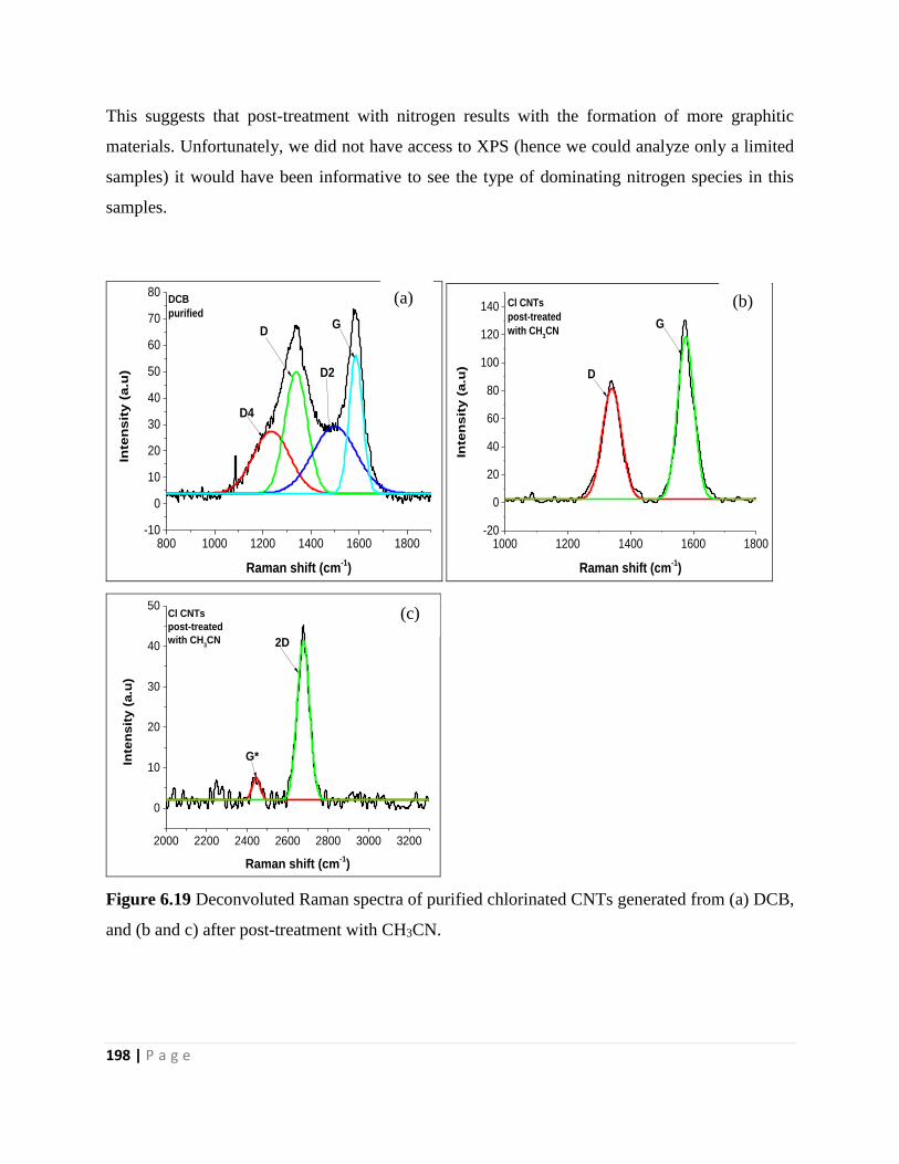
198 | P a g e

This suggests that post-treatment with nitrogen results with the formation of more graphitic

materials. Unfortunately, we did not have access to XPS (hence we could analyze only a limited

samples) it would have been informative to see the type of dominating nitrogen species in this

samples.

800 1000 1200 1400 1600 1800-10

0

10

20

30

40

50

60

70

80

Inte

nsit

y (

a.u

)

Raman shift (cm-1)

DCB

purified

D4

D

D2

G

1000 1200 1400 1600 1800-20

0

20

40

60

80

100

120

140

Inte

nsit

y (

a.u

)

Raman shift (cm-1)

Cl CNTs

post-treated

with CH3CN

D

G

2000 2200 2400 2600 2800 3000 3200

0

10

20

30

40

50

Inte

ns

ity

(a

.u)

Raman shift (cm-1)

Cl CNTs

post-treated

with CH3CN

G*

2D

Figure 6.19 Deconvoluted Raman spectra of purified chlorinated CNTs generated from (a) DCB,

and (b and c) after post-treatment with CH3CN.

(a)

(c)

(b)

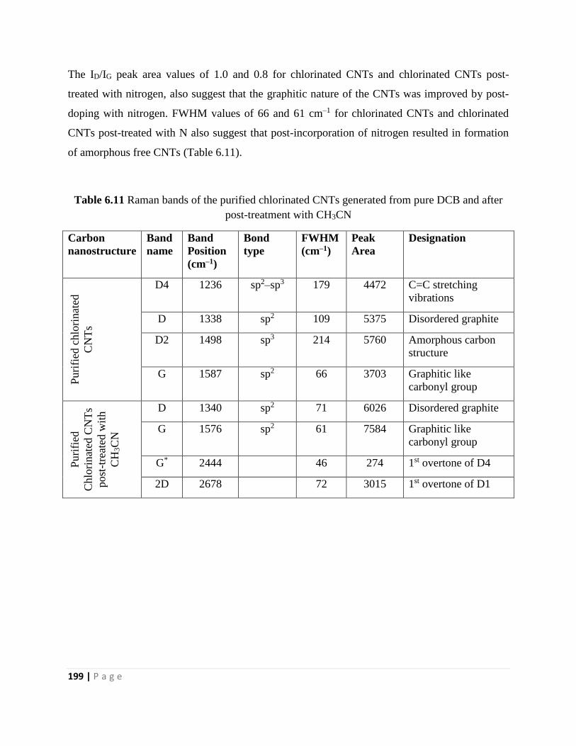
199 | P a g e

The ID/IG peak area values of 1.0 and 0.8 for chlorinated CNTs and chlorinated CNTs post-

treated with nitrogen, also suggest that the graphitic nature of the CNTs was improved by post-

doping with nitrogen. FWHM values of 66 and 61 cm–1 for chlorinated CNTs and chlorinated

CNTs post-treated with N also suggest that post-incorporation of nitrogen resulted in formation

of amorphous free CNTs (Table 6.11).

Table 6.11 Raman bands of the purified chlorinated CNTs generated from pure DCB and after

post-treatment with CH3CN

Carbon

nanostructure

Band

name

Band

Position

(cm–1)

Bond

type

FWHM

(cm–1)

Peak

Area

Designation

Puri

fied

chlo

rinat

ed

CN

Ts


vibrations



structure


carbonyl group

Puri

fied

Chlo

rinat

ed C

NT

s

post

-tre

ated

wit

h

CH

3C

N



carbonyl group



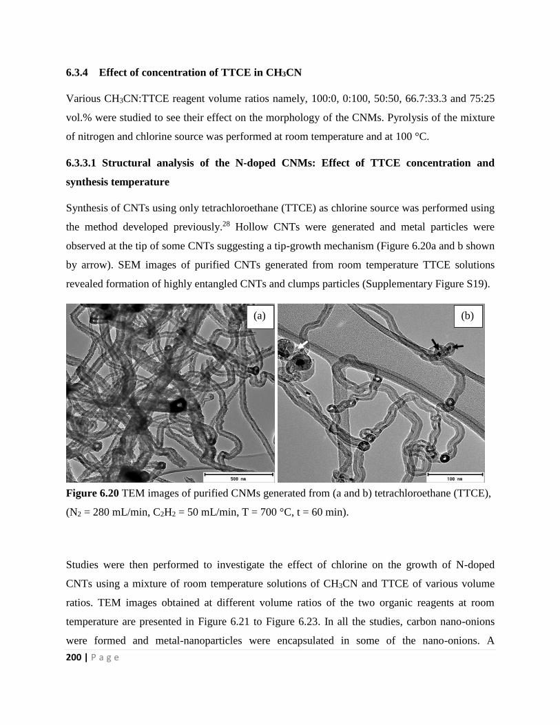
200 | P a g e

6.3.4 Effect of concentration of TTCE in CH3CN

Various CH3CN:TTCE reagent volume ratios namely, 100:0, 0:100, 50:50, 66.7:33.3 and 75:25

vol.% were studied to see their effect on the morphology of the CNMs. Pyrolysis of the mixture

of nitrogen and chlorine source was performed at room temperature and at 100 °C.

6.3.3.1 Structural analysis of the N-doped CNMs: Effect of TTCE concentration and

synthesis temperature

Synthesis of CNTs using only tetrachloroethane (TTCE) as chlorine source was performed using

the method developed previously.28 Hollow CNTs were generated and metal particles were

observed at the tip of some CNTs suggesting a tip-growth mechanism (Figure 6.20a and b shown

by arrow). SEM images of purified CNTs generated from room temperature TTCE solutions

revealed formation of highly entangled CNTs and clumps particles (Supplementary Figure S19).

Figure 6.20 TEM images of purified CNMs generated from (a and b) tetrachloroethane (TTCE),

(N2 = 280 mL/min, C2H2 = 50 mL/min, T = 700 °C, t = 60 min).

Studies were then performed to investigate the effect of chlorine on the growth of N-doped

CNTs using a mixture of room temperature solutions of CH3CN and TTCE of various volume

ratios. TEM images obtained at different volume ratios of the two organic reagents at room

temperature are presented in Figure 6.21 to Figure 6.23. In all the studies, carbon nano-onions

were formed and metal-nanoparticles were encapsulated in some of the nano-onions. A

(a) (b)

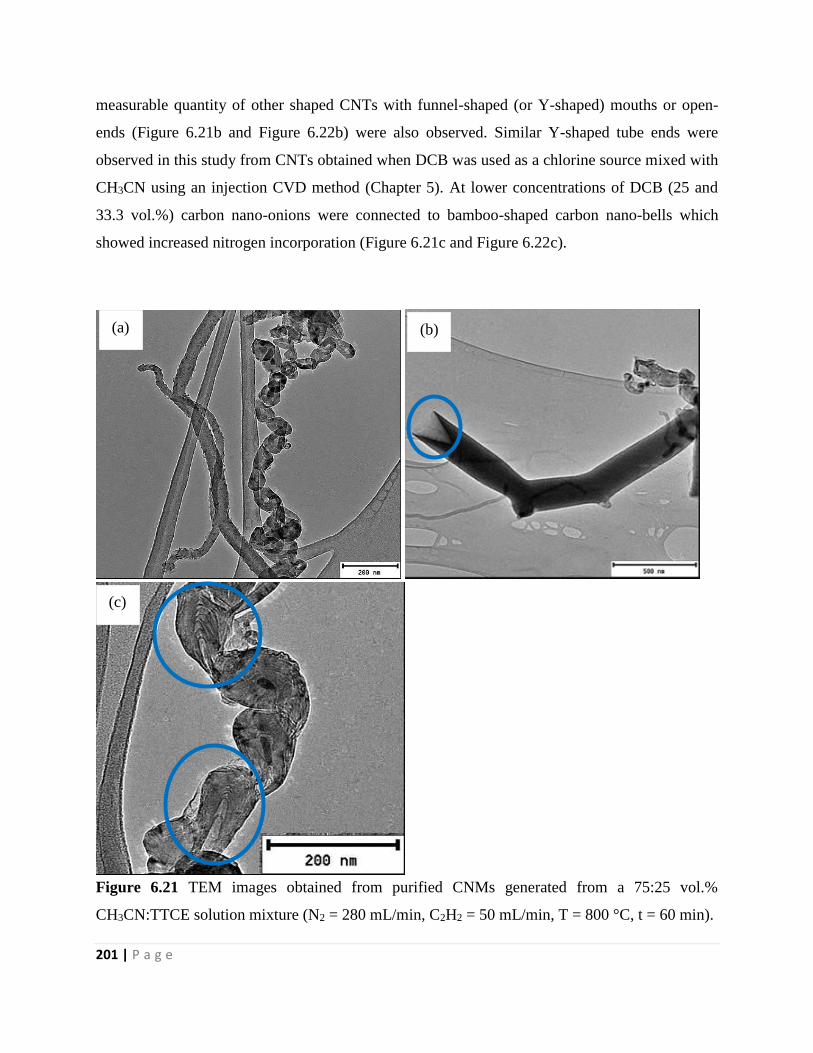
201 | P a g e

measurable quantity of other shaped CNTs with funnel-shaped (or Y-shaped) mouths or open-

ends (Figure 6.21b and Figure 6.22b) were also observed. Similar Y-shaped tube ends were

observed in this study from CNTs obtained when DCB was used as a chlorine source mixed with

CH3CN using an injection CVD method (Chapter 5). At lower concentrations of DCB (25 and

33.3 vol.%) carbon nano-onions were connected to bamboo-shaped carbon nano-bells which

showed increased nitrogen incorporation (Figure 6.21c and Figure 6.22c).


CH3CN:TTCE solution mixture (N2 = 280 mL/min, C2H2 = 50 mL/min, T = 800 °C, t = 60 min).

(a) (b)

(c)

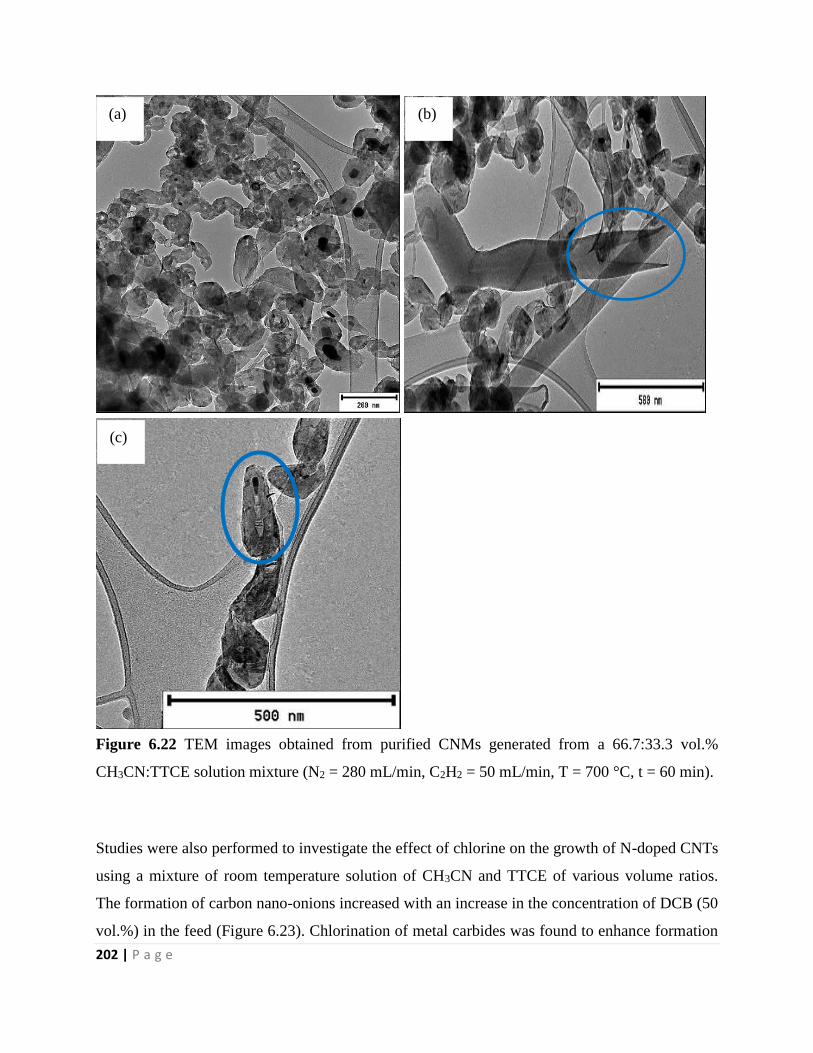
202 | P a g e



Studies were also performed to investigate the effect of chlorine on the growth of N-doped CNTs

using a mixture of room temperature solution of CH3CN and TTCE of various volume ratios.

The formation of carbon nano-onions increased with an increase in the concentration of DCB (50

vol.%) in the feed (Figure 6.23). Chlorination of metal carbides was found to enhance formation

(a) (b)

(c)

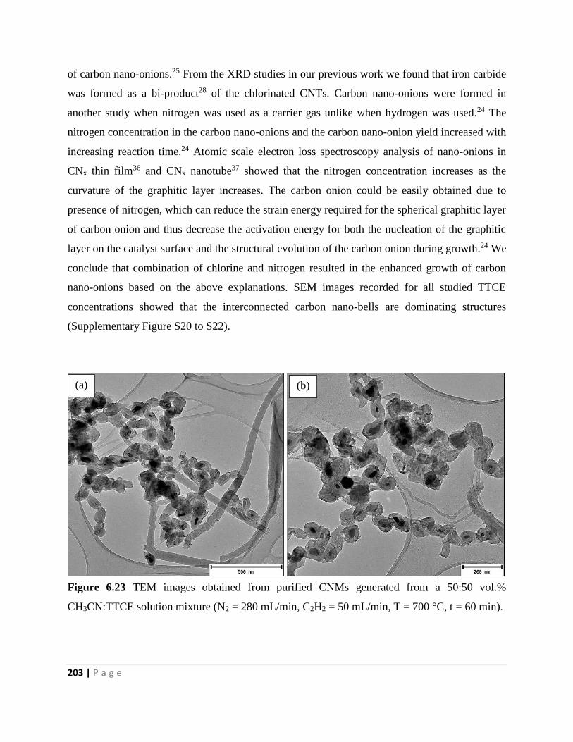
203 | P a g e

of carbon nano-onions.25 From the XRD studies in our previous work we found that iron carbide

was formed as a bi-product28 of the chlorinated CNTs. Carbon nano-onions were formed in

another study when nitrogen was used as a carrier gas unlike when hydrogen was used.24 The

nitrogen concentration in the carbon nano-onions and the carbon nano-onion yield increased with

increasing reaction time.24 Atomic scale electron loss spectroscopy analysis of nano-onions in

CNx thin film36 and CNx nanotube37 showed that the nitrogen concentration increases as the

curvature of the graphitic layer increases. The carbon onion could be easily obtained due to

presence of nitrogen, which can reduce the strain energy required for the spherical graphitic layer

of carbon onion and thus decrease the activation energy for both the nucleation of the graphitic

layer on the catalyst surface and the structural evolution of the carbon onion during growth.24 We

conclude that combination of chlorine and nitrogen resulted in the enhanced growth of carbon

nano-onions based on the above explanations. SEM images recorded for all studied TTCE

concentrations showed that the interconnected carbon nano-bells are dominating structures

(Supplementary Figure S20 to S22).



(a) (b)

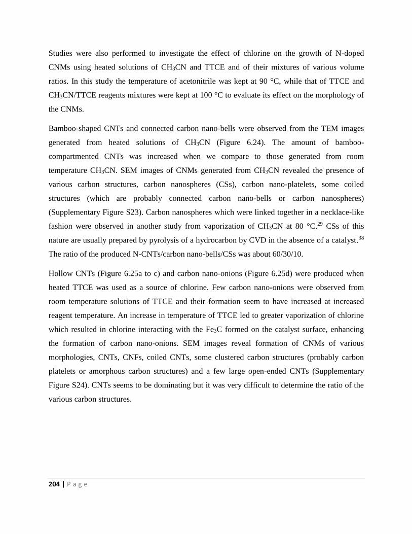
204 | P a g e

Studies were also performed to investigate the effect of chlorine on the growth of N-doped

CNMs using heated solutions of CH3CN and TTCE and of their mixtures of various volume

ratios. In this study the temperature of acetonitrile was kept at 90 °C, while that of TTCE and

CH3CN/TTCE reagents mixtures were kept at 100 °C to evaluate its effect on the morphology of

the CNMs.

Bamboo-shaped CNTs and connected carbon nano-bells were observed from the TEM images

generated from heated solutions of CH3CN (Figure 6.24). The amount of bamboo-

compartmented CNTs was increased when we compare to those generated from room

temperature CH3CN. SEM images of CNMs generated from CH3CN revealed the presence of

various carbon structures, carbon nanospheres (CSs), carbon nano-platelets, some coiled

structures (which are probably connected carbon nano-bells or carbon nanospheres)

(Supplementary Figure S23). Carbon nanospheres which were linked together in a necklace-like

fashion were observed in another study from vaporization of CH3CN at 80 °C.29 CSs of this

nature are usually prepared by pyrolysis of a hydrocarbon by CVD in the absence of a catalyst.38

The ratio of the produced N-CNTs/carbon nano-bells/CSs was about 60/30/10.

Hollow CNTs (Figure 6.25a to c) and carbon nano-onions (Figure 6.25d) were produced when

heated TTCE was used as a source of chlorine. Few carbon nano-onions were observed from

room temperature solutions of TTCE and their formation seem to have increased at increased

reagent temperature. An increase in temperature of TTCE led to greater vaporization of chlorine

which resulted in chlorine interacting with the Fe3C formed on the catalyst surface, enhancing

the formation of carbon nano-onions. SEM images reveal formation of CNMs of various

morphologies, CNTs, CNFs, coiled CNTs, some clustered carbon structures (probably carbon

platelets or amorphous carbon structures) and a few large open-ended CNTs (Supplementary

Figure S24). CNTs seems to be dominating but it was very difficult to determine the ratio of the

various carbon structures.

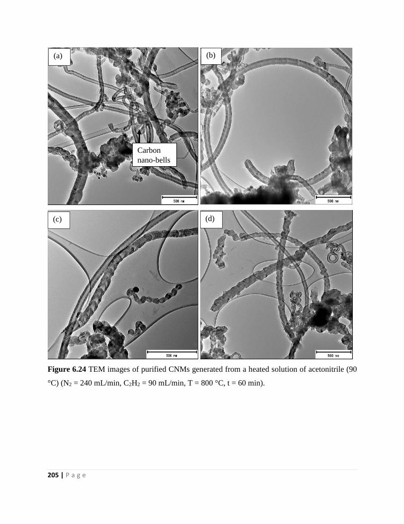
205 | P a g e

Figure 6.24 TEM images of purified CNMs generated from a heated solution of acetonitrile (90

°C) (N2 = 240 mL/min, C2H2 = 90 mL/min, T = 800 °C, t = 60 min).

(a) (b)

Carbon

nano-bells

(d) (c)

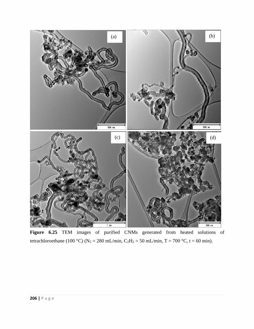
206 | P a g e

Figure 6.25 TEM images of purified CNMs generated from heated solutions of

tetrachloroethane (100 °C) (N2 = 280 mL/min, C2H2 = 50 mL/min, T = 700 °C, t = 60 min).

(a)

(d) (c)

(b)

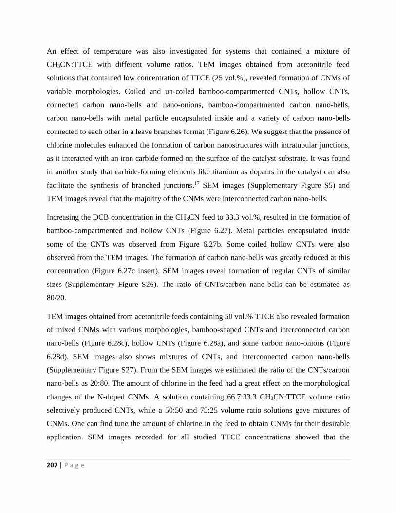
207 | P a g e

An effect of temperature was also investigated for systems that contained a mixture of

CH3CN:TTCE with different volume ratios. TEM images obtained from acetonitrile feed

solutions that contained low concentration of TTCE (25 vol.%), revealed formation of CNMs of

variable morphologies. Coiled and un-coiled bamboo-compartmented CNTs, hollow CNTs,

connected carbon nano-bells and nano-onions, bamboo-compartmented carbon nano-bells,

carbon nano-bells with metal particle encapsulated inside and a variety of carbon nano-bells

connected to each other in a leave branches format (Figure 6.26). We suggest that the presence of

chlorine molecules enhanced the formation of carbon nanostructures with intratubular junctions,

as it interacted with an iron carbide formed on the surface of the catalyst substrate. It was found

in another study that carbide-forming elements like titanium as dopants in the catalyst can also

facilitate the synthesis of branched junctions.17 SEM images (Supplementary Figure S5) and

TEM images reveal that the majority of the CNMs were interconnected carbon nano-bells.

Increasing the DCB concentration in the CH3CN feed to 33.3 vol.%, resulted in the formation of

bamboo-compartmented and hollow CNTs (Figure 6.27). Metal particles encapsulated inside

some of the CNTs was observed from Figure 6.27b. Some coiled hollow CNTs were also

observed from the TEM images. The formation of carbon nano-bells was greatly reduced at this

concentration (Figure 6.27c insert). SEM images reveal formation of regular CNTs of similar

sizes (Supplementary Figure S26). The ratio of CNTs/carbon nano-bells can be estimated as

80/20.

TEM images obtained from acetonitrile feeds containing 50 vol.% TTCE also revealed formation

of mixed CNMs with various morphologies, bamboo-shaped CNTs and interconnected carbon

nano-bells (Figure 6.28c), hollow CNTs (Figure 6.28a), and some carbon nano-onions (Figure

6.28d). SEM images also shows mixtures of CNTs, and interconnected carbon nano-bells

(Supplementary Figure S27). From the SEM images we estimated the ratio of the CNTs/carbon

nano-bells as 20:80. The amount of chlorine in the feed had a great effect on the morphological

changes of the N-doped CNMs. A solution containing 66.7:33.3 CH3CN:TTCE volume ratio

selectively produced CNTs, while a 50:50 and 75:25 volume ratio solutions gave mixtures of

CNMs. One can find tune the amount of chlorine in the feed to obtain CNMs for their desirable

application. SEM images recorded for all studied TTCE concentrations showed that the

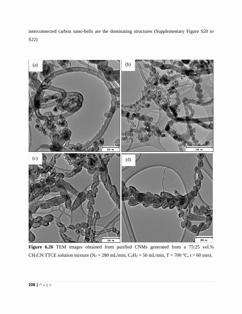
208 | P a g e

interconnected carbon nano-bells are the dominating structures (Supplementary Figure S20 to

S22)



(a)

(d) (c)

(b)

209 | P a g e



(a)

(d) (c)

(b)

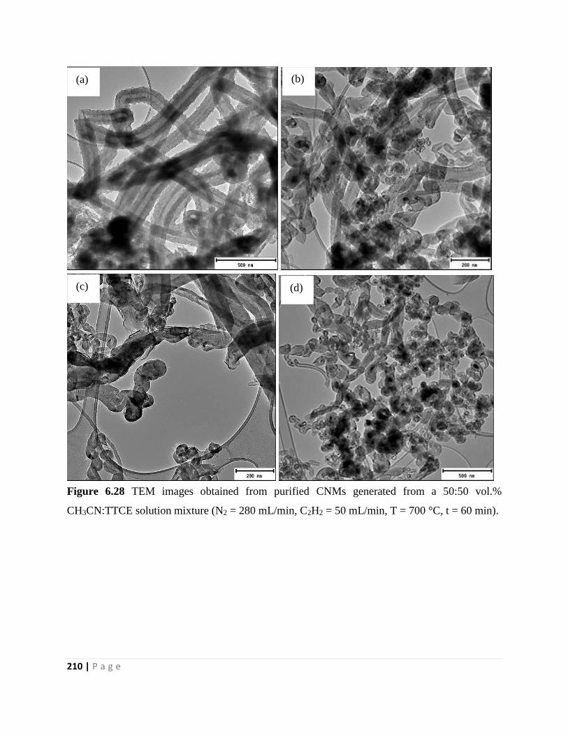
210 | P a g e



(a) (b)

(d) (c)

211 | P a g e

6.3.3.2 Thermogravimetric analysis of the N-doped CNMs: Effect of TTCE concentration

and synthesis temperature

TGA and DTGA curves of un-purified and purified CNTs generated from heated pure CH3CN

(90 °C) and TTCE (100 °C) are presented in Figure 6.29. Un-purified CNTs generated from

CH3CN showed a variety of weight losses, the initial minor weight loss observed around 100 to

300 °C was due to evaporation of physisorbed water at the onset temperature of 100 °C, together

with decomposition of chemisorbed water and surface chloride groups at ~ 150 to 300 °C. The

second minor weight loss at ~ 450 °C was due to decomposition of amorphous carbon structures.

The third major weight loss (~ 55 %) with an onset temperature of ~ 580 °C was due to oxidation

of CNTs, while the fourth minor weight loss at 700 °C was due to oxidation of other graphitic

carbon structures (i.e. carbon nano-bells, carbon nanospheres, observed from the TEM images).

Purified CNTs generated from CH3CN showed three mass losses. The weight loss due to

physisorbed and chemisorbed water together with surface chlorides was not observed after

purification. The water could have been removed during drying of the CNTs at high temperature

after purification and the surface chlorides could have reacted with the hydrogen from the acid

used for treatment. The first minor weight loss was observed at ~350 to 400 °C due to

amorphous carbon structures. The second major weight loss was observed at ~ 500 °C and was

assigned to oxidation of N-doped CNTs.

Only one major broad weight loss was observed from TGA curves of un-purified and purified

CNMs generated from room temperature TTCE solution (Figure 6.29). The weight loss occurred

at ~ 580 to 700 °C which could be attributed to oxidation of chlorinated CNMs (Figure 6.29).

The broadness of the oxidation peak suggest that various stable carbon nanostructures were

oxidized at this temperature range. This data is consistent with the TEM observations where

CNTs and carbon-nano-onions were generated, with CNTs dominating. The residual mass of ~

10 and 15 % was observed from the TGA curves obtained from CH3CN and TTCE before

purification, which was completely removed after purification shown by a residual mass of zero.

This shows that purification with acid was effective for removal of any catalyst metal particles

that remained on the surface of the CNMs after synthesis.

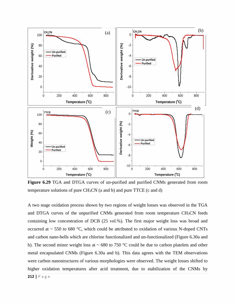
212 | P a g e

0 200 400 600 800

0

20

40

60

80

100D

eri

va

tiv

e w

eig

ht

(%)

Temperature (0C)

Un-purified

Purified

CH3CN

0 200 400 600 800

-10

-8

-6

-4

-2

0

De

riv

ati

ve

we

igh

t (%

)

Temperature (0C)

Un-purified

Purified

CH3CN

0 200 400 600 800

0

20

40

60

80

100

Weig

ht

(%)

Temperature (0C)

Un-purified

Purified

TTCE

0 200 400 600 800-10

-8

-6

-4

-2

0

De

riv

ati

ve

we

igh

t (%

)

Temperature (0C)

Un-purified

Purified

TTCE


temperature solutions of pure CH3CN (a and b) and pure TTCE (c and d)

A two stage oxidation process shown by two regions of weight losses was observed in the TGA

and DTGA curves of the unpurified CNMs generated from room temperature CH3CN feeds

containing low concentration of DCB (25 vol.%). The first major weight loss was broad and

occurred at ~ 550 to 680 °C, which could be attributed to oxidation of various N-doped CNTs

and carbon nano-bells which are chlorine functionalized and un-functionalized (Figure 6.30a and

b). The second minor weight loss at ~ 680 to 750 °C could be due to carbon platelets and other

metal encapsulated CNMs (Figure 6.30a and b). This data agrees with the TEM observations

were carbon nanostructures of various morphologies were observed. The weight losses shifted to

higher oxidation temperatures after acid treatment, due to stabilization of the CNMs by

(a)

(d) (c)

(b)

213 | P a g e

functionalization of the CNMs with oxygen functional groups (Figure 6.30a and b). Another

weight loss was observed at higher temperatures > 800 °C from purified CNMs due to evolution

of nitrogen. The residual mass was again reduced from ~ 20 % to zero, suggesting that acid

treatment was effective in removal of catalyst metal particles that could have been on the surface

of the CNMs.

TGA and DTGA curves of CNMs generated from room temperature solutions containing

increased concentration of TTCE in the acetonitrile feed to 33.3 vol.% are presented in Figure

6.30c and d. Two weight losses are observed from both the un-purified and purified samples. The

first major weight loss was at ~ 550 to 650 °C for un-purified CNMs and was at ~ 530 to 680 for

purified CNMs, due to oxidation of chlorinated and un-chlorinated N-doped CNTs. The second

weight loss at ~ 650 to 700 °C was due to oxidation of other graphitic materials like carbon

nano-bells observed from the TEM images. The residual mass loss was not reduced to zero after

acid treatment which suggest that some catalyst particles were still present after acid treatment.

Catalyst particles encapsulated into the CNTs were observed from the TEM images.

TGA and DTGA curve of un-purified CNMs generated from a further increase in the amount of

TTCE in the CH3CN feed to 50 vol.% was similar to the one obtained from solutions containing

33.3 vol.% (Figure 6.30e and f). Three weight losses were observed from purified CNMs

generated from solutions containing 50 vol.% TTCE concentration (Figure 6.30e and f). They

were at about 550, 600 and 700 °C which were assigned to oxidation of un-functionalized CNTs,

chlorine functionalized CNTs and other chlorine functionalized carbon structures (carbon nano-

bells and carbon nano-onions) observed from the TEM images.

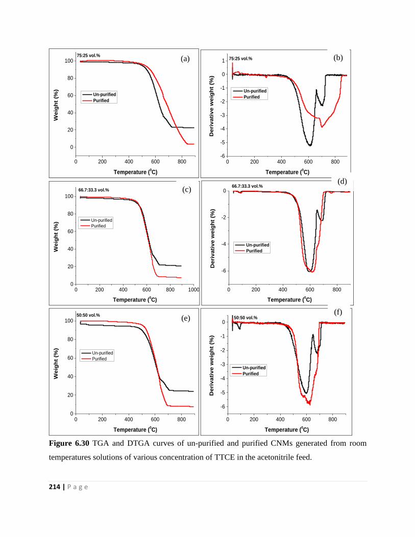
214 | P a g e

0 200 400 600 800

0

20

40

60

80

100W

eig

ht

(%)

Temperature (0C)

Un-purified

Purified

75:25 vol.%

0 200 400 600 800-6

-5

-4

-3

-2

-1

0

1

Deri

va

tiv

e w

eig

ht

(%)

Temperature (0C)

Un-purified

Purified

75:25 vol.%

0 200 400 600 800 10000

20

40

60

80

100

We

igh

t (%

)

Temperature (0C)

Un-purified

Purified

66.7:33.3 vol.%

0 200 400 600 800

-6

-4

-2

0

De

riv

ati

ve

we

igh

t (%

)

Temperature (0C)

Un-purified

Purified

66.7:33.3 vol.%

0 200 400 600 8000

20

40

60

80

100

Weig

ht

(%)

Temperature (0C)

Un-purified

Purified

50:50 vol.%

0 200 400 600 800

-6

-5

-4

-3

-2

-1

0

Deri

va

tiv

e w

eig

ht

(%)

Temperature (0C)

Un-purified

Purified

50:50 vol.%


temperatures solutions of various concentration of TTCE in the acetonitrile feed.

(a) (b)

(d) (c)

(f) (e)

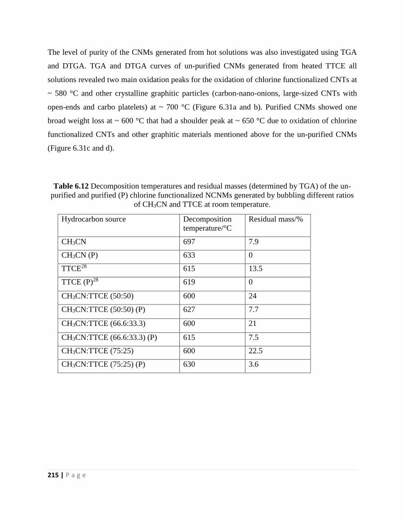
215 | P a g e

The level of purity of the CNMs generated from hot solutions was also investigated using TGA

and DTGA. TGA and DTGA curves of un-purified CNMs generated from heated TTCE all

solutions revealed two main oxidation peaks for the oxidation of chlorine functionalized CNTs at

~ 580 °C and other crystalline graphitic particles (carbon-nano-onions, large-sized CNTs with

open-ends and carbo platelets) at ~ 700 °C (Figure 6.31a and b). Purified CNMs showed one

broad weight loss at ~ 600 °C that had a shoulder peak at ~ 650 °C due to oxidation of chlorine

functionalized CNTs and other graphitic materials mentioned above for the un-purified CNMs

(Figure 6.31c and d).



of CH3CN and TTCE at room temperature.

Hydrocarbon source Decomposition

temperature/°C

Residual mass/%

CH3CN 697 7.9

CH3CN (P) 633 0

TTCE28 615 13.5

TTCE (P)28 619 0

CH3CN:TTCE (50:50) 600 24

CH3CN:TTCE (50:50) (P) 627 7.7

CH3CN:TTCE (66.6:33.3) 600 21

CH3CN:TTCE (66.6:33.3) (P) 615 7.5

CH3CN:TTCE (75:25) 600 22.5

CH3CN:TTCE (75:25) (P) 630 3.6

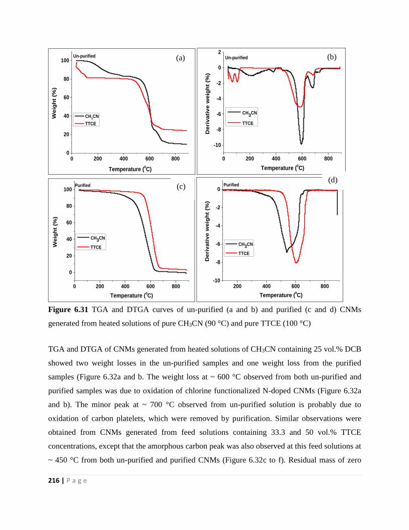
216 | P a g e

0 200 400 600 8000

20

40

60

80

100

Weig

ht

(%)

Temperature (0C)

CH3CN

TTCE

Un-purified

0 200 400 600 800

-10

-8

-6

-4

-2

0

2

De

riv

ati

ve

we

igh

t (%

)

Temperature (0C)

CH3CN

TTCE

Un-purified

0 200 400 600 800

0

20

40

60

80

100

We

igh

t (%

)

Temperature (0C)

CH3CN

TTCE

Purified

200 400 600 800-10

-8

-6

-4

-2

0

Deri

vati

ve w

eig

ht

(%)

Temperature (0C)

CH3CN

TTCE

Purified

Figure 6.31 TGA and DTGA curves of un-purified (a and b) and purified (c and d) CNMs

generated from heated solutions of pure CH3CN (90 °C) and pure TTCE (100 °C)

TGA and DTGA of CNMs generated from heated solutions of CH3CN containing 25 vol.% DCB

showed two weight losses in the un-purified samples and one weight loss from the purified

samples (Figure 6.32a and b. The weight loss at ~ 600 °C observed from both un-purified and

purified samples was due to oxidation of chlorine functionalized N-doped CNMs (Figure 6.32a

and b). The minor peak at ~ 700 °C observed from un-purified solution is probably due to

oxidation of carbon platelets, which were removed by purification. Similar observations were

obtained from CNMs generated from feed solutions containing 33.3 and 50 vol.% TTCE

concentrations, except that the amorphous carbon peak was also observed at this feed solutions at

~ 450 °C from both un-purified and purified CNMs (Figure 6.32c to f). Residual mass of zero

(a) (b)

(d) (c)

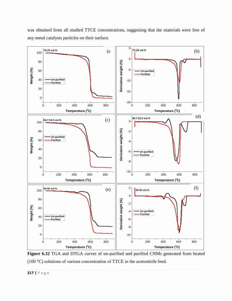
217 | P a g e

was obtained from all studied TTCE concentrations, suggesting that the materials were free of

any metal catalysts particles on their surface.

0 200 400 600 800

0

20

40

60

80

100

We

igh

t (%

)

Temperature (0C)

Un-purified

Purified

75:25 vol.%

0 200 400 600 800-20

-15

-10

-5

0

5

De

riv

ati

ve

we

igh

t (%

)

Temperature (0C)

Un-purified

Purified

75:25 vol.%

0 200 400 600 800

0

20

40

60

80

100

Weig

ht

(%)

Temperature (0C)

Un-purified

Purified

66.7:33.3 vol.%

0 200 400 600 800-10

-8

-6

-4

-2

0D

eri

va

tiv

e w

eig

ht

(%)

Temperature (0C)

Un-purified

Purified

66.7:33.3 vol.%

0 200 400 600 800

0

20

40

60

80

100

We

igh

t (%

)

Temperature (0C)

Un-purified

Purified

50:50 vol.%

0 200 400 600 800

-10

-8

-6

-4

-2

0

2

Deri

va

tiv

e w

eig

ht

(%)

Temperature (0C)

Un-purified

Purified

50:50 vol.%

Figure 6.32 TGA and DTGA curves of un-purified and purified CNMs generated from heated

(100 °C) solutions of various concentration of TTCE in the acetonitrile feed.

(a

)

(d) (c)

(b)

(e) (f)

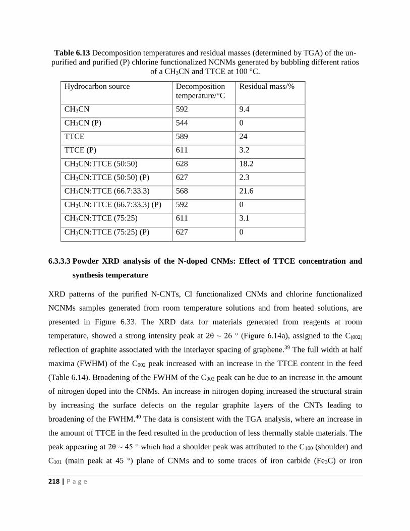
218 | P a g e



of a CH3CN and TTCE at 100 °C.

Hydrocarbon source Decomposition

temperature/°C

Residual mass/%

CH3CN 592 9.4

CH3CN (P) 544 0

TTCE 589 24

TTCE (P) 611 3.2

CH3CN:TTCE (50:50) 628 18.2

CH3CN:TTCE (50:50) (P) 627 2.3

CH3CN:TTCE (66.7:33.3) 568 21.6

CH3CN:TTCE (66.7:33.3) (P) 592 0

CH3CN:TTCE (75:25) 611 3.1

CH3CN:TTCE (75:25) (P) 627 0

6.3.3.3 Powder XRD analysis of the N-doped CNMs: Effect of TTCE concentration and


XRD patterns of the purified N-CNTs, Cl functionalized CNMs and chlorine functionalized

NCNMs samples generated from room temperature solutions and from heated solutions, are

presented in Figure 6.33. The XRD data for materials generated from reagents at room

temperature, showed a strong intensity peak at 2θ ~ 26 ° (Figure 6.14a), assigned to the C(002)

reflection of graphite associated with the interlayer spacing of graphene.39 The full width at half

maxima (FWHM) of the C002 peak increased with an increase in the TTCE content in the feed

(Table 6.14). Broadening of the FWHM of the C002 peak can be due to an increase in the amount

of nitrogen doped into the CNMs. An increase in nitrogen doping increased the structural strain

by increasing the surface defects on the regular graphite layers of the CNTs leading to

broadening of the FWHM.40 The data is consistent with the TGA analysis, where an increase in

the amount of TTCE in the feed resulted in the production of less thermally stable materials. The

peak appearing at 2θ ~ 45 ° which had a shoulder peak was attributed to the C100 (shoulder) and

C101 (main peak at 45 °) plane of CNMs and to some traces of iron carbide (Fe3C) or iron

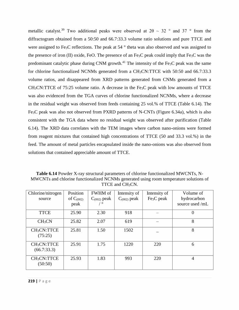
219 | P a g e

metallic catalyst.39 Two additional peaks were observed at 2θ ~ 32 ° and 37 ° from the

diffractogram obtained from a 50:50 and 66.7:33.3 volume ratio solutions and pure TTCE and

were assigned to Fe3C reflections. The peak at 54 ° theta was also observed and was assigned to

the presence of iron (II) oxide, FeO. The presence of an Fe3C peak could imply that Fe3C was the

predominant catalytic phase during CNM growth.41 The intensity of the Fe3C peak was the same

for chlorine functionalized NCNMs generated from a CH3CN:TTCE with 50:50 and 66.7:33.3

volume ratios, and disappeared from XRD patterns generated from CNMs generated from a

CH3CN:TTCE of 75:25 volume ratio. A decrease in the Fe3C peak with low amounts of TTCE

was also evidenced from the TGA curves of chlorine functionalized NCNMs, where a decrease

in the residual weight was observed from feeds containing 25 vol.% of TTCE (Table 6.14). The

Fe3C peak was also not observed from PXRD patterns of N-CNTs (Figure 6.34a), which is also

consistent with the TGA data where no residual weight was observed after purification (Table

6.14). The XRD data correlates with the TEM images where carbon nano-onions were formed

from reagent mixtures that contained high concentrations of TTCE (50 and 33.3 vol.%) in the

feed. The amount of metal particles encapsulated inside the nano-onions was also observed from

solutions that contained appreciable amount of TTCE.


MWCNTs and chlorine functionalized NCNMs generated using room temperature solutions of

TTCE and CH3CN.

Chlorine/nitrogen

source

Position

of C(002)

peak

FWHM of

C(002) peak

/ °

Intensity of

C(002) peak

Intensity of

Fe3C peak

Volume of

hydrocarbon

source used /mL

TTCE 25.90 2.30 918 – 0

CH3CN 25.82 2.07 619 – 8

CH3CN:TTCE

(75:25)

25.81 1.50 1502 _ 8

CH3CN:TTCE

(66.7:33.3)

25.91 1.75 1220 220 6

CH3CN:TTCE

(50:50)

25.93 1.83 993 220 4

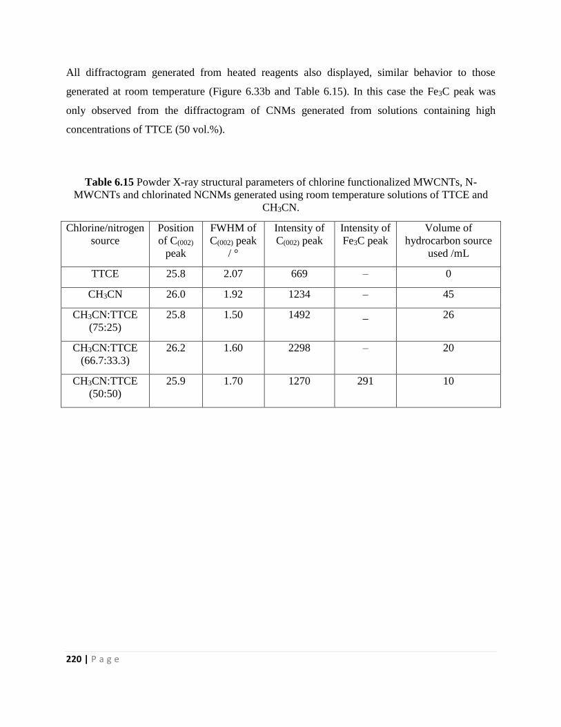
220 | P a g e

All diffractogram generated from heated reagents also displayed, similar behavior to those

generated at room temperature (Figure 6.33b and Table 6.15). In this case the Fe3C peak was

only observed from the diffractogram of CNMs generated from solutions containing high

concentrations of TTCE (50 vol.%).


MWCNTs and chlorinated NCNMs generated using room temperature solutions of TTCE and

CH3CN.

Chlorine/nitrogen

source

Position

of C(002)

peak

FWHM of

C(002) peak

/ °

Intensity of

C(002) peak

Intensity of

Fe3C peak

Volume of

hydrocarbon source

used /mL

TTCE 25.8 2.07 669 – 0

CH3CN 26.0 1.92 1234 – 45

CH3CN:TTCE

(75:25)

25.8 1.50 1492 _ 26

CH3CN:TTCE

(66.7:33.3)

26.2 1.60 2298 – 20

CH3CN:TTCE

(50:50)

25.9 1.70 1270 291 10

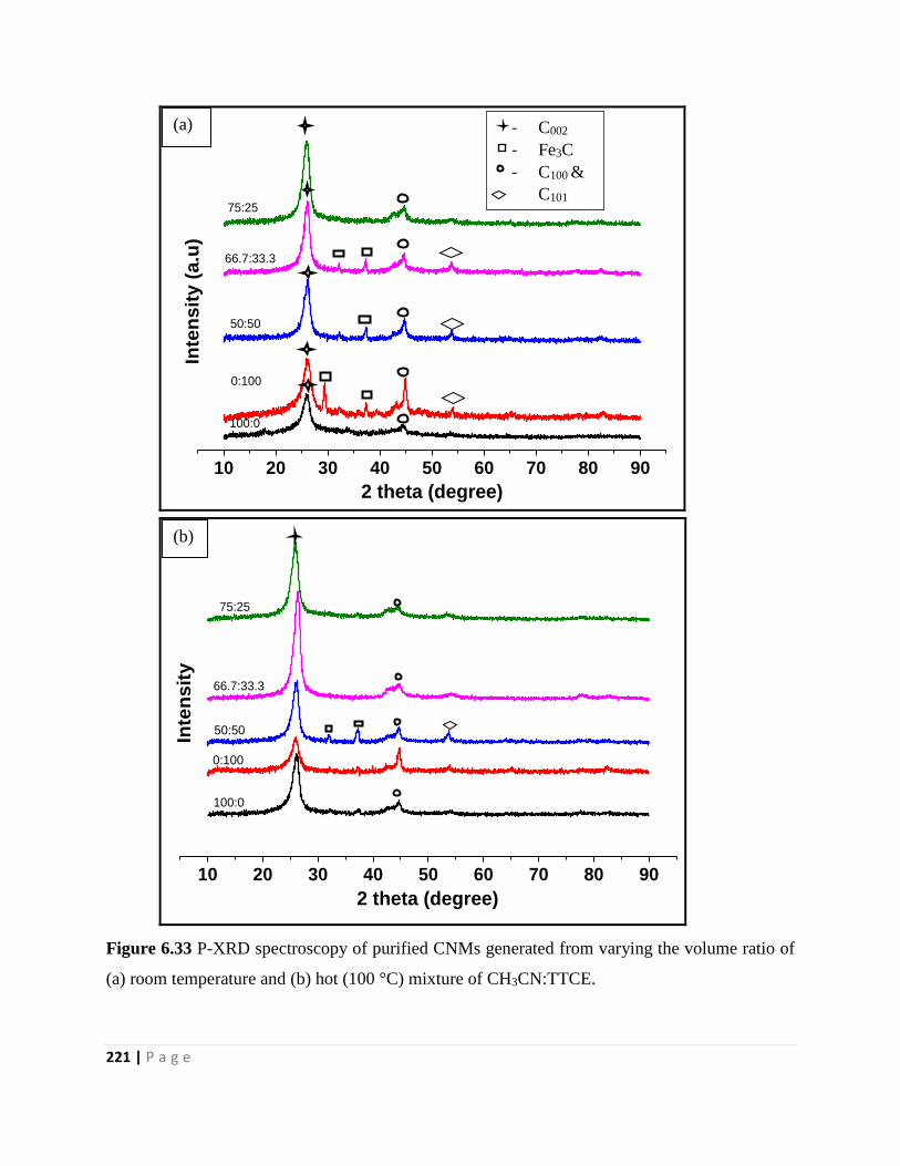
221 | P a g e

10 20 30 40 50 60 70 80 90

Inte

nsit

y (

a.u

)

2 theta (degree)

100:0

0:100

50:50

66.7:33.3

75:25

10 20 30 40 50 60 70 80 90

Inte

nsit

y

2 theta (degree)

100:0

0:100

50:50

66.7:33.3

75:25

Figure 6.33 P-XRD spectroscopy of purified CNMs generated from varying the volume ratio of

(a) room temperature and (b) hot (100 °C) mixture of CH3CN:TTCE.

(a)

(b)

- C002

- Fe3C

- C100 &

C101

- FeO

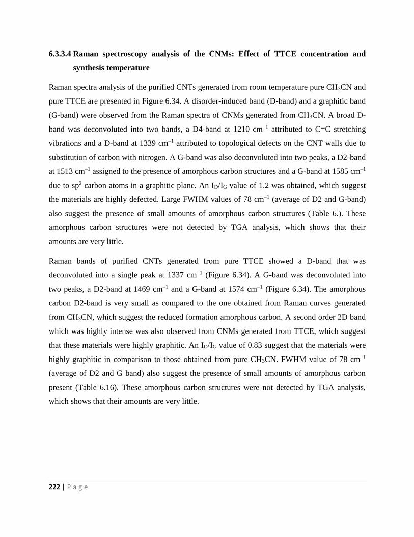
222 | P a g e

6.3.3.4 Raman spectroscopy analysis of the CNMs: Effect of TTCE concentration and


Raman spectra analysis of the purified CNTs generated from room temperature pure CH3CN and

pure TTCE are presented in Figure 6.34. A disorder-induced band (D-band) and a graphitic band

(G-band) were observed from the Raman spectra of CNMs generated from CH3CN. A broad D-

band was deconvoluted into two bands, a D4-band at 1210 cm–1 attributed to C=C stretching

vibrations and a D-band at 1339 cm–1 attributed to topological defects on the CNT walls due to

substitution of carbon with nitrogen. A G-band was also deconvoluted into two peaks, a D2-band

at 1513 cm–1 assigned to the presence of amorphous carbon structures and a G-band at 1585 cm–1

due to sp2 carbon atoms in a graphitic plane. An ID/IG value of 1.2 was obtained, which suggest

the materials are highly defected. Large FWHM values of 78 cm–1 (average of D2 and G-band)

also suggest the presence of small amounts of amorphous carbon structures (Table 6.). These

amorphous carbon structures were not detected by TGA analysis, which shows that their

amounts are very little.

Raman bands of purified CNTs generated from pure TTCE showed a D-band that was

deconvoluted into a single peak at 1337 cm–1 (Figure 6.34). A G-band was deconvoluted into

two peaks, a D2-band at 1469 cm–1 and a G-band at 1574 cm–1 (Figure 6.34). The amorphous

carbon D2-band is very small as compared to the one obtained from Raman curves generated

from CH3CN, which suggest the reduced formation amorphous carbon. A second order 2D band

which was highly intense was also observed from CNMs generated from TTCE, which suggest

that these materials were highly graphitic. An ID/IG value of 0.83 suggest that the materials were

highly graphitic in comparison to those obtained from pure CH3CN. FWHM value of 78 cm–1

(average of D2 and G band) also suggest the presence of small amounts of amorphous carbon

present (Table 6.16). These amorphous carbon structures were not detected by TGA analysis,

which shows that their amounts are very little.

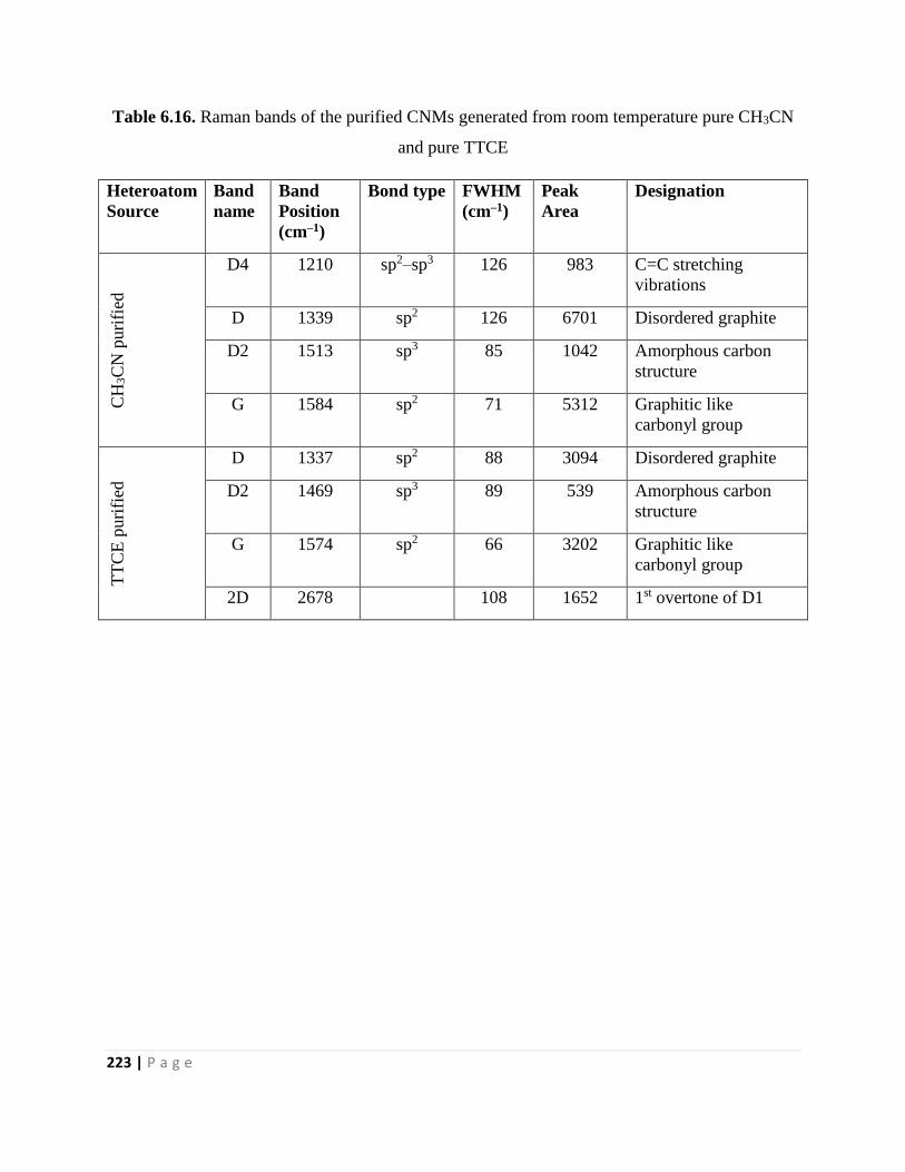
223 | P a g e

Table 6.16. Raman bands of the purified CNMs generated from room temperature pure CH3CN

and pure TTCE

Heteroatom

Source

Band

name

Band

Position

(cm–1)

Bond type FWHM

(cm–1)

Peak

Area

Designation

CH

3C

N p

uri

fied


vibrations



structure


carbonyl group

TT

CE

puri

fied



structure


carbonyl group


224 | P a g e

1000 1200 1400 1600 1800-10

0

10

20

30

40

50

60

70

80In

ten

sit

y (

a.u

)

Raman shift (cm-1)

CH3CN rt

purified

D4

D

D2

G

1000 1200 1400 1600 1800 2000

0

10

20

30

40

50

60

Inte

ns

ity

(a

.u)

Raman shift (cm-1)

TTCE rt

purified

D

D2

G

2000 2200 2400 2600 2800 3000 3200 3400

0

5

10

15

20

25

Inte

ns

ity

(a

.u)

Raman shift (cm-1)

TTCE rt

purified2D

Figure 6.34 Raman spectra of purified CNTs generated from room temperature solutions of (a)

pure CH3CN and (b and c) pure TTCE.

(a)

(c)

(b)

225 | P a g e

Raman spectra analysis of the purified CNMs generated from room temperature CH3CN feed

solutions containing 25 vol.% TTCE are presented in Figure 6.35. A disorder-induced band (D-

band), a graphitic band (G-band) and a second order 2D band were observed in the Raman

spectra. A D-band was deconvoluted into one peak at 1349 cm–1 attributed to topological defects

on the CNT walls due to substitution of carbon with nitrogen. A G-band was deconvoluted into

two peaks, a D’-band at 1616 cm–1 assigned to the defects in the graphitic plane and a G-band at

1585 cm–1 due to a perfect graphitic plane. A very weak defect induced G* band was also

observed at 2429 cm–1 due to the presence of defects in the CNMs. A 2D band which was split

into two bands a 2D1 at 2674 cm–1 and a 2D2 at 2702 cm–1. This split has been described as a

characteristic feature of undisturbed or highly ordered graphitic lattices32 and interaction of

succesive layers.33 An ID/IG value of 0.4 was obtained, which suggest that the materials were

highly graphitic. Small FWHM values of 40 cm–1 (average of D’ and G-band) also suggest that

the materials were free of amorphous carbon structures (Table 6.17). The Raman data is

consistent with the TGA data since amorphous carbon structures were not detected from the

TGA curves.

Similar Raman spectra were obtained from CNMs generated from CH3CN room temperature

feed solutions containing 33.3 and 50 vol.% TTCE (Figure 6.35c to f). ID/IG values of 0.4 and 0.6

were obtained for solutions containing 33.3 and 50 vol.% TTCE respectively, suggesting that the

materials are highly graphitic. Low FWHM values of 43 cm–1 also suggest materials with no

amorphous carbon as observed from the TGA curves (Table 6.17). An ID/ID’ value of 4.3 was

obtained from CNMs generated from feed solutions containing 25 vol.% TTCE due to vacancy-

like defects with additional small boundary-like defects. An ID/ID’ value of 3.17 was obtained

from CNMs generated from feed solutions containing 33.3 vol.% TTCE corresponding to

boundary-like defects and small on-site defects. On-site defects describe out-of-plane atoms

bonded to sp3 hybridized carbon atoms. An ID/ID’ value of 6.3 was obtained from CNMs

generated from feed solutions containing 50 vol.% TTCE corresponding to vacancy-like defects.

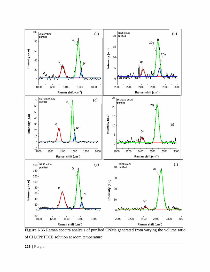
226 | P a g e

1000 1200 1400 1600 1800

0

20

40

60

80

100

Inte

nsit

y (

a.u

)

Raman shift (cm-1)

75:25 vol.%

purified

D

G

D'

2000 2200 2400 2600 2800 3000

0

5

10

15

20

Inte

nsit

y (

a.u

)

Raman shift (cm-1)

75:25 vol.%

purified

G*

2D1

2D2

1000 1200 1400 1600 1800 2000-10

0

10

20

30

40

50

60

70

Inte

nsit

y (

a.u

)

Raman shift (cm-1)

66.7:33.3 vol.%

purified

D

G

D'

2000 2200 2400 2600 2800 3000

0

5

10

15

20

25

Inte

nsit

y (

a.u

)

Raman shift (cm-1)

66.7:33.3 vol.%

purified

G*

2D

1000 1200 1400 1600 1800-20

0

20

40

60

80

100

120

140

160

Inte

ns

ity

(a

.u)

Raman shift (cm-1)

50:50 vol.%

purified

D

G

D'

2000 2200 2400 2600 2800 3000

0

10

20

30

40

Inte

nsit

y (

a.u

)

Raman shift (cm-1)

50:50 vol.%

purified

G*

2D

Figure 6.35 Raman spectra analysis of purified CNMs generated from varying the volume ratio

of CH3CN:TTCE solution at room temperature

(a)

(a)

(e)

(b)

(f)

(c)

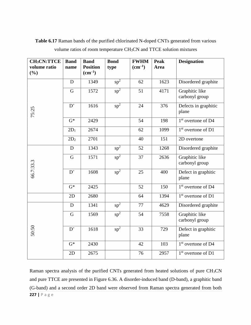
227 | P a g e


volume ratios of room temperature CH3CN and TTCE solution mixtures

CH3CN:TTCE

volume ratio

(%)

Band

name

Band

Position

(cm–1)

Bond

type

FWHM

(cm–1)

Peak

Area

Designation

75

:25



carbonyl group


plane



2D2 2701 40 151 2D overtone

66.7

:33.3



carbonyl group


plane



50:5

0



carbonyl group


plane



Raman spectra analysis of the purified CNTs generated from heated solutions of pure CH3CN

and pure TTCE are presented in Figure 6.36. A disorder-induced band (D-band), a graphitic band

(G-band) and a second order 2D band were observed from Raman spectra generated from both

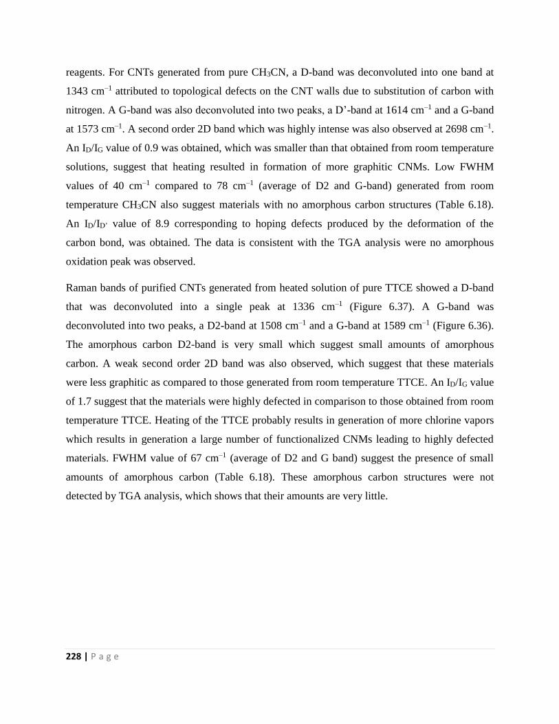
228 | P a g e

reagents. For CNTs generated from pure CH3CN, a D-band was deconvoluted into one band at

1343 cm–1 attributed to topological defects on the CNT walls due to substitution of carbon with

nitrogen. A G-band was also deconvoluted into two peaks, a D’-band at 1614 cm–1 and a G-band

at 1573 cm–1. A second order 2D band which was highly intense was also observed at 2698 cm–1.

An ID/IG value of 0.9 was obtained, which was smaller than that obtained from room temperature

solutions, suggest that heating resulted in formation of more graphitic CNMs. Low FWHM

values of 40 cm–1 compared to 78 cm–1 (average of D2 and G-band) generated from room

temperature CH3CN also suggest materials with no amorphous carbon structures (Table 6.18).

An ID/ID’ value of 8.9 corresponding to hoping defects produced by the deformation of the

carbon bond, was obtained. The data is consistent with the TGA analysis were no amorphous

oxidation peak was observed.

Raman bands of purified CNTs generated from heated solution of pure TTCE showed a D-band

that was deconvoluted into a single peak at 1336 cm–1 (Figure 6.37). A G-band was

deconvoluted into two peaks, a D2-band at 1508 cm–1 and a G-band at 1589 cm–1 (Figure 6.36).

The amorphous carbon D2-band is very small which suggest small amounts of amorphous

carbon. A weak second order 2D band was also observed, which suggest that these materials

were less graphitic as compared to those generated from room temperature TTCE. An ID/IG value

of 1.7 suggest that the materials were highly defected in comparison to those obtained from room

temperature TTCE. Heating of the TTCE probably results in generation of more chlorine vapors

which results in generation a large number of functionalized CNMs leading to highly defected

materials. FWHM value of 67 cm–1 (average of D2 and G band) suggest the presence of small

amounts of amorphous carbon (Table 6.18). These amorphous carbon structures were not

detected by TGA analysis, which shows that their amounts are very little.

229 | P a g e

1000 1200 1400 1600 1800 2000

0

10

20

30

40

50In

ten

sit

y (

a.u

)

Raman shift (cm-1)

CH3CN (90

0C)

purified

D

G

D'

2000 2200 2400 2600 2800 3000 3200 34000

2

4

6

8

10

12

14

16

Inte

nsit

y (

a.u

)

Raman shift (cm-1)

CH3CN (90

0C)

purified

2D

1000 1500 2000 2500 3000

10

20

30

40

50

Inte

nsit

y (

a.u

)

Raman shift (cm-1)

TTCE (1000C)

purified

D

G

2D

800 1000 1200 1400 1600 1800 2000

10

20

30

40

50

Inte

nsit

y (

a.u

)

Raman shift (cm-1)

TTCE (1000C)

purified

D

D2

G

Figure 6.36 Raman spectra of purified CNTs generated from heated solutions of (a) pure

CH3CN (90 °C) and (b) pure TTCE (100 °C).

Lorentz Gauss

(a)

(d) (c)

(b)

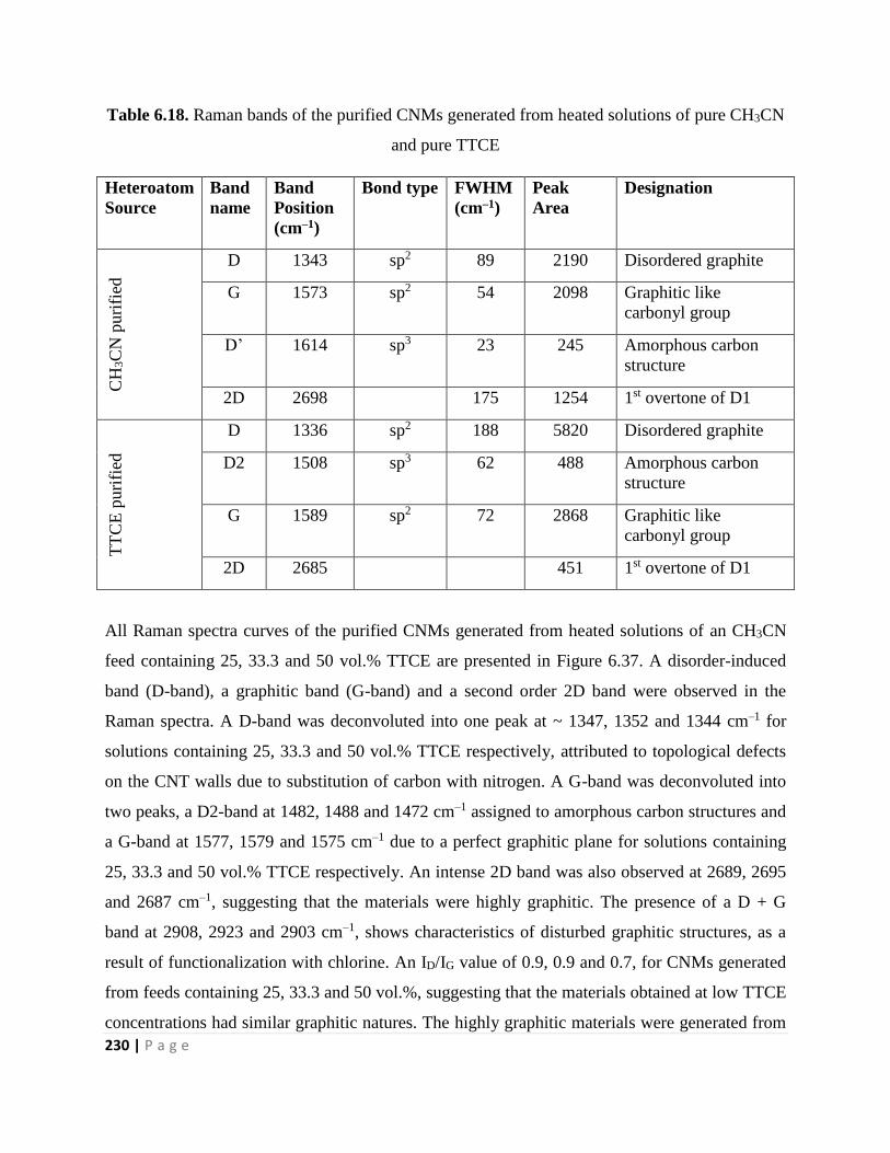
230 | P a g e

Table 6.18. Raman bands of the purified CNMs generated from heated solutions of pure CH3CN

and pure TTCE

Heteroatom

Source

Band

name

Band

Position

(cm–1)

Bond type FWHM

(cm–1)

Peak

Area

Designation

CH

3C

N p

uri

fied



carbonyl group

D’ 1614 sp3 23 245 Amorphous carbon

structure


TT

CE

puri

fied



structure


carbonyl group

2D 2685 451 1st overtone of D1

All Raman spectra curves of the purified CNMs generated from heated solutions of an CH3CN

feed containing 25, 33.3 and 50 vol.% TTCE are presented in Figure 6.37. A disorder-induced

band (D-band), a graphitic band (G-band) and a second order 2D band were observed in the

Raman spectra. A D-band was deconvoluted into one peak at ~ 1347, 1352 and 1344 cm–1 for

solutions containing 25, 33.3 and 50 vol.% TTCE respectively, attributed to topological defects

on the CNT walls due to substitution of carbon with nitrogen. A G-band was deconvoluted into

two peaks, a D2-band at 1482, 1488 and 1472 cm–1 assigned to amorphous carbon structures and

a G-band at 1577, 1579 and 1575 cm–1 due to a perfect graphitic plane for solutions containing

25, 33.3 and 50 vol.% TTCE respectively. An intense 2D band was also observed at 2689, 2695

and 2687 cm–1, suggesting that the materials were highly graphitic. The presence of a D + G

band at 2908, 2923 and 2903 cm–1, shows characteristics of disturbed graphitic structures, as a

result of functionalization with chlorine. An ID/IG value of 0.9, 0.9 and 0.7, for CNMs generated

from feeds containing 25, 33.3 and 50 vol.%, suggesting that the materials obtained at low TTCE

concentrations had similar graphitic natures. The highly graphitic materials were generated from

231 | P a g e

feeds containing high concentration of TTCE (50 vol.%). Small FWHM values of 74, 72, and 84

cm–1 (average of D’ and G-band) suggest that the materials contained some amorphous carbon

structures (Table 6.19). The Raman data is consistent with the TGA data since amorphous carbon

structures were also detected from the TGA curves.

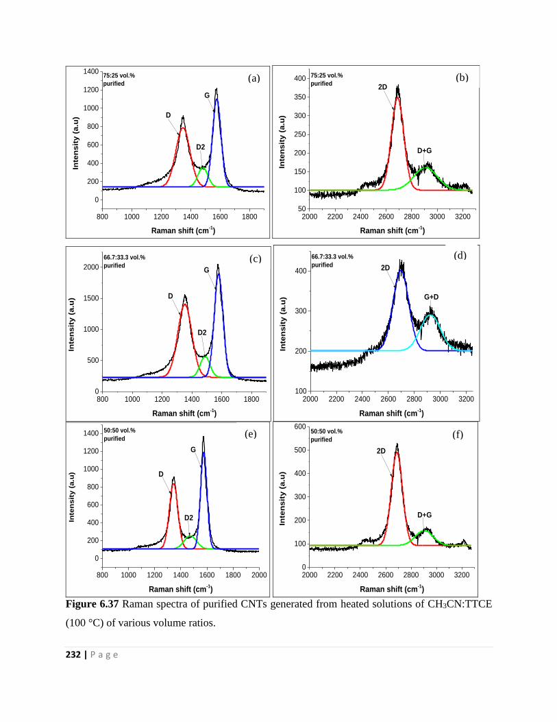
232 | P a g e

800 1000 1200 1400 1600 1800

0

200

400

600

800

1000

1200

1400In

ten

sit

y (

a.u

)

Raman shift (cm-1)

75:25 vol.%

purified

D

D2

G

2000 2200 2400 2600 2800 3000 320050

100

150

200

250

300

350

400

Inte

ns

ity

(a

.u)

Raman shift (cm-1)

75:25 vol.%

purified2D

D+G

800 1000 1200 1400 1600 18000

500

1000

1500

2000

Inte

ns

ity

(a

.u)

Raman shift (cm-1)

66.7:33.3 vol.%

purified

D

D2

G

2000 2200 2400 2600 2800 3000 3200100

200

300

400

Inte

ns

ity

(a

.u)

Raman shift (cm-1)

66.7:33.3 vol.%

purified 2D

G+D

800 1000 1200 1400 1600 1800 2000

0

200

400

600

800

1000

1200

1400

Inte

ns

ity (

a.u

)

Raman shift (cm-1)

50:50 vol.%

purified

D

D2

G

2000 2200 2400 2600 2800 3000 32000

100

200

300

400

500

600

Inte

ns

ity

(a

.u)

Raman shift (cm-1)

50:50 vol.%

purified

2D

D+G

Figure 6.37 Raman spectra of purified CNTs generated from heated solutions of CH3CN:TTCE

(100 °C) of various volume ratios.

(a)

(d) (c)

(b)

(e) (f)

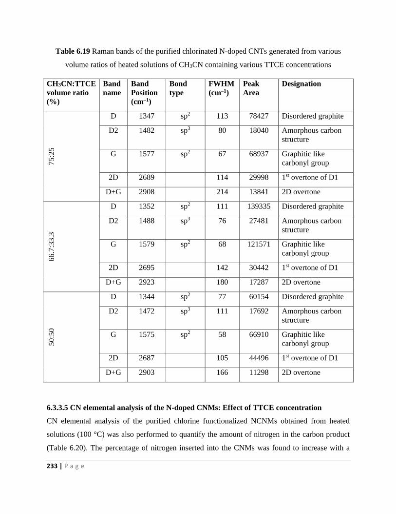
233 | P a g e


volume ratios of heated solutions of CH3CN containing various TTCE concentrations

CH3CN:TTCE

volume ratio

(%)

Band

name

Band

Position

(cm–1)

Bond

type

FWHM

(cm–1)

Peak

Area

Designation

75:2

5



structure


carbonyl group

2D 2689 114 29998 1st overtone of D1

D+G 2908 214 13841 2D overtone

66.7

:33.3



structure


carbonyl group

2D 2695 142 30442 1st overtone of D1

D+G 2923 180 17287 2D overtone

50:5

0



structure


carbonyl group

2D 2687 105 44496 1st overtone of D1

D+G 2903 166 11298 2D overtone

6.3.3.5 CN elemental analysis of the N-doped CNMs: Effect of TTCE concentration

CN elemental analysis of the purified chlorine functionalized NCNMs obtained from heated

solutions (100 °C) was also performed to quantify the amount of nitrogen in the carbon product

(Table 6.20). The percentage of nitrogen inserted into the CNMs was found to increase with a

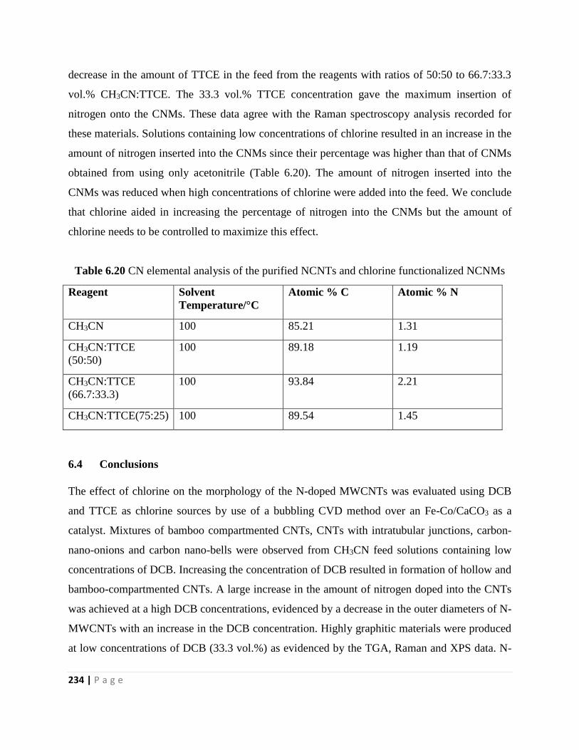
234 | P a g e

decrease in the amount of TTCE in the feed from the reagents with ratios of 50:50 to 66.7:33.3

vol.% CH3CN:TTCE. The 33.3 vol.% TTCE concentration gave the maximum insertion of

nitrogen onto the CNMs. These data agree with the Raman spectroscopy analysis recorded for

these materials. Solutions containing low concentrations of chlorine resulted in an increase in the

amount of nitrogen inserted into the CNMs since their percentage was higher than that of CNMs

obtained from using only acetonitrile (Table 6.20). The amount of nitrogen inserted into the

CNMs was reduced when high concentrations of chlorine were added into the feed. We conclude

that chlorine aided in increasing the percentage of nitrogen into the CNMs but the amount of

chlorine needs to be controlled to maximize this effect.

Table 6.20 CN elemental analysis of the purified NCNTs and chlorine functionalized NCNMs

Reagent Solvent

Temperature/°C

Atomic % C Atomic % N

CH3CN 100 85.21 1.31

CH3CN:TTCE

(50:50)

100 89.18 1.19

CH3CN:TTCE

(66.7:33.3)

100 93.84 2.21

CH3CN:TTCE(75:25) 100 89.54 1.45

6.4 Conclusions

The effect of chlorine on the morphology of the N-doped MWCNTs was evaluated using DCB

and TTCE as chlorine sources by use of a bubbling CVD method over an Fe-Co/CaCO3 as a

catalyst. Mixtures of bamboo compartmented CNTs, CNTs with intratubular junctions, carbon-

nano-onions and carbon nano-bells were observed from CH3CN feed solutions containing low

concentrations of DCB. Increasing the concentration of DCB resulted in formation of hollow and

bamboo-compartmented CNTs. A large increase in the amount of nitrogen doped into the CNTs

was achieved at a high DCB concentrations, evidenced by a decrease in the outer diameters of N-

MWCNTs with an increase in the DCB concentration. Highly graphitic materials were produced

at low concentrations of DCB (33.3 vol.%) as evidenced by the TGA, Raman and XPS data. N-

235 | P a g e

MWCNTs that were thermally stable, had a small value of the ID/IG peak ratio and had graphitic

N species dominating in their N1s XPS spectra were produced when low concentrations of DCB

(33.3 vol.%) were used, as compared to N-MWCNTs obtained from pure CH3CN and high DCB

(66.7 vol.%.) concentration. Post-doping of the N-MWCNTs with chlorine and of the chlorinated

CNTs with nitrogen resulted in production of highly graphitic materials, as evidenced by the low

ID/IG peak ratios obtained after post-doping. Carbon nano-onions were observed from NCNMs

when TTCE was used as a source of chlorine. The formation of carbon nano-onions increased at

a low TTCE concentration, which was attributed to greater incorporation of nitrogen into the

CNMs. An increase in the TTCE concentration resulted in the formation of mixtures of carbon

nano-onions and bamboo-compartmented carbon nano-bells. NCNMs generated from heated

solutions of CH3CN and TTCE mixtures, resulted in formation of mixtures of CNMs, especially

at high concentrations of TTCE. Selectivity was achieved at low concentrations (33.3 and 25

vol.%) of TTCE. Hollow and bamboo-compartmented NCNTs were observed from 33.3 vol.%

TTCE feed solutions and bamboo-compartmented carbon nano-bells with intratubular junctions

were obtained from 25 vol.% TTCE solutions. NCNMs generated from 25 vol.% TTCE solutions

were thermally stable, had little residual catalyst material, had a small narrow FWHM value for

the C002 peak, and a small ID/IG peak ratio values, suggesting that the materials were highly

graphitic. Chlorine functionalization of the CNTs with DCB gave selective CNMs as compared

to when TTCE was used, where mixtures of CNMs were produced. Aromatic chlorinated organic

compounds are better suited for use in studies of the effect of chlorine on the morphology of the

CNMs than are aliphatic chlorinated organic compounds. Chlorinated NCNTs that contained

smaller amounts of DCB (33.3 vol.%) can be used to enhance the electrical conductivity of

NCNMs due to a better wetting with the electrolyte.42 This appears to be related to quaternary

nitrogen being the dominant nitrogen species.

Selective carbon nanomaterials were obtained for chlorinated NCNMs generated using an

injection CVD method rather than when using the bubbling CVD method.

236 | P a g e

References

1. S. Christiansen, E. Fau, and B. Staudtstrasse, ACS Appl. Mater. 2017, 9, 10003–10011.

2. B. Liu, C.-M. Yang, Z. Liu and C.-S. Lai, Nanomaterials, 2017, 7, 302 (1–12).

3. P. Chen, T.Y. Xiao, Y.H. Qian, S.S. Li, and S.H. Yu, Adv. Mater. 2013, 25, 3192–3196.

4. T. Sharifi, G. Hu, X. Jia, and T. Wagberg, ACS Nano, 2012, 6, 8904–8912.

5. Y. Liu, Y. Shen, L. Sun, J. Li, C. Liu, W. Ren, F. Li, L. Gao, J. Chen, F. Liu, Y. Sun, N.

Tang, H.-M. Cheng and Y. Du, Nature Communications, 2016, 7, 10921 (1–9).

6. X. Wang, G. Sun, P. Routh, D.-H. Kim, W. Huang and P. Chen, Chem. Soc. Rev., 2014, 43,

7067–7098.

7. Z. Lin, G. Waller, Y. Liu, M. Liu and C.-P. Wong, Adv. Energy Mater., 2012, 2, 884–888.

8. E. Haque, Md. M. Islam, S.N. Faisal, A.K. Roy, S. Ansari, D. Cardillo, K. Konstantinov and

E. Haque, J. Nanotech Mater. Sci, 2015, 2(1), 1-5.

9. D. Li, X. Duan, H. Sun, J. Kang, H. Zhang, M.O. Tade, and S. Wang,

https://espace.curtin.edu.au/bitstream/handle/20.500.11937/50850/248286.pdf?sequence=2

10. R. Lv, Q. Li, A.R. Botello-Mendez, T. Hayashi, B. Wang, A. Berkdemir, Q. Hao, A.L. Elías,

R. Cruz-Silva, H.R. Gutiérrez, Y.A. Kim, H. Muramatsu, J. Zhu, M. Endo, H. Terrones, J.-C.

Charlier, M. Pan and M. Terrones, Sci. Rep., 2012, 2, 586.

11. J. Xu, D. Huang, L. Nie, C. Wang, and Z. Xu, Int. J. Electrochem. Sci., 2016, 11, 944–952.

12. K.F. Ortega, R. Arrigo, B. Frank, R. Schlogl, and A. Trunschke, Chem. Mater., 2016, 28,

6826−6839.

13. V. A. Tur1, A. V. Okotrub, Yu. V. Shubin, B. V. Senkovskiy, and L. G. Bulusheva, Phys.

Status Solidi B, 2014, 251, 2613–2619.

14. K. Kakaei, M. Hamidi and S. Husseindoost, J. Colloid Int. Sci., 2016, 479, 121–126.

15. H.L. Poh, P. Šimek, Z. Sofer and M. Pumera, Chem. Eur. J. 2013, 19, 2655–266.

16. G-L. Tian, M-Q. Zhao, Q. Zhang, J-Q. Huang, and F. Wei, Carbon, 2012, 50, 5323-5330.

17. D. Wei and Y. Liu, Adv. Mater., 2008, 20, 2815–2841.

18. P.A. Hu, K. Xiao, Y.Q. Liu, G. Yu, X.B. Wang, L. Fu, G.L. Cui and D.B. Zhu, Appl. Phys.

Lett., 2004, 84, 4932.

19. K. Xiao, Y.Q. Liu, P.A. Hu, G. Yu, L. Fu, and D.B. Zhu, Appl. Phys. Lett., 2003, 83, 4824.

20. Y. Chai, X.L. Zhou, P.J. Li, W.J. Zhang, and J.L. Wu, Nanotechnology, 2005, 16, 2134.

https://onlinelibrary.wiley.com/doi/10.1002/aenm.201200038/abstract

https://espace.curtin.edu.au/bitstream/handle/20.500.11937/50850/248286.pdf?sequence=2

237 | P a g e

21. K. Xiao, Y. Fu, Y.Q. Liu, G. Yu, J. Zhai, L. Jiang, W.P. Hu, Z.G. Shuai, Y. Luo and D.B.

Zhu, Adv. Funct. Mater, 2007, 17, 2842.

22. G.K. Goswami, R. Nandan, and K.K. Nanda, Carbon, 2013, 56, 97-102.

23. P. Ghosh, M. Subramanian, R.A. Afre, M. Zamri, T. Soga, T. Jimbo, V. Filip, and M.

Tanemura, Appl. Surf. Sci., 2009, 255, 4611–4615.

24. C. He, N. Zhao, C. Shi, X. Du, J. Li, L. Cui and F. He, Scr. Mater., 2006, 54, 1739 – 1743.

25. J. Zheng, T.C. Ekström, S.K. Gordeev and M. Jacob, J. Mater. Chem., 2000, 10, 1039–1041.

26. L.M. Ombaka, P.G. Ndungu, B. Omondi, J.D. McGettrick, M.L. Davies and V.O. Nyamori,

J. Solid State Chem., 2016, 235, 202–211.

27. L.G. Bulusheva, A.V. Okotrub, A.G. Kudashov, N.F. Yudanov, E.M. Pazhetnov, A.I.

Boronin, O.G. Abrosimov, and N.A. Rudina, Russ. J. Inorg. Chem., 2006, 51, 613–618.

28. W.K. Maboya, N.J. Coville and S.D. Mhlanga, S. Afr. J. Chem., 2016, 69, 15–26.

29. Z.N. Tetana, S.D. Mhlanga, G. Bepete, R.W.M. Krause, and N.J. Coville, S. Afr. J. Chem.,

2012, 65, 39–49.

30. C. Yuan, W. Chen and L. Yan, J. Mater. Chem., 2012, 22, 7456–7460.

31. S. Zhang, S. Tsuzuki, K. Ueno, K. Dokko and M. Watanabe, Angew. Chem. Int. Ed., 2015,

54, 1302–1306.

32. A. Cuesta, P. Dhamelincourt, J. Laureyns, A. Martinez-Alonso and J.M.D. Tascon, Carbon,

1994, 32, 1523–1532.

33. L. Bokobza, J.-L. Bruneel and M. Couzi, Carbon, 2015, 1, 77–94.

34. M.I. Ionescu, Y. Zhang, R. Li, H. Abou-Rachid and X. Sun, Appl. Surf. Sci., 2012, 258,

4563–4568.

35. D. Goldberg, Y. Bando, L, Bourgeois, K. Kurashima, and T. Sato, Carbon, 2000, 38, 2017–

2027.

36. Z. Czigany, IF. Brunell, J. Neidhardt, L. Hultman and K. Suenaga, Appl. Phys. Lett., 2001,

79, 2639.

37. W.Q. Han, P. Kohler-Redlich, T. Seeger, F. Ernst, M. Ruhle, N. Grobert, W.K. Hsu, B.H.

Chang, Y.Q. Zhu, H.W. Kroto, M. Terrones and H. Terrones, Appl. Phys. Lett., 2000, 77,

1807–1809.

38. A.A. Deshmukh, S.D. Mhlanga, and N.J. Coville, Mater. Sci. Eng., R, 2010, 70, 1–28.

238 | P a g e

39. A. Hachimi, B. Merzougui, A. Hakeem, T. Laoui, G.M. Swain, Q. Chang, M. Shao, and

M.A. Atieh, J. Nanomater., 2015, http://dx.doi.org/10.1155/2015/453725.

40. Y.C, Chiang, W.-H. Lin, and Y.-C. Chang, Appl. Surf. Sci., 2011, 257, 2401–2410.

41. C.T. Wirth, B.C. Bayer, A.D. Gamalski, S. Esconjaurequi, R.S. Weatherup, C. Ducati, C.

Baehtz, J. Robertson, and S. Hofmann, Chem. Mater., 2012, 24, 4633–4640.

42. I. Kunadian, S.M. Lipka, C.R. Swartz, D. Qian, and R. Andrews, J. Electrochem. Soc., 2009,

156, K110eK115.

239 | P a g e

CHAPTER 7

Fabrication of chlorine functionalized MWCNT/polyvinylpyrrolidone

composite nanofiber mats by electrospinning for use in oil adsorption studies

7.1 Introduction

Materials play a key role in every field of technology with the aim of making our lives more

comfortable. As technology advances there is a need to develop new materials with improved

properties. In order to create new generation materials, it is necessary to understand the

relationship between the existing materials and their structure. By combining appropriate

materials, new desired properties can be achieved.1 Nanocomposites are made by placing a

nanomaterial into a matrix, in order to introduce new functionalities into the matrix to harness

new properties. A nanocomposite thus consists of a matrix to which nanoparticles (a filler) has

been added to improve a particular property of the material. Polymer composites containing

fillers such as carbon nanotubes (CNTs) have been studied.2-13 CNT/polymer nanocomposites are

promising materials with excellent mechanical and physical properties, due to the extraordinary

properties introduced by the CNTs coupled with easily tailored characteristics of polymers.14-23

Polymer materials have properties such as low density, good insulation, flexibility and

outstanding mechanical properties and they are cheap. CNTs possess high flexibility, low mass

density, large aspects ratio, and extremely high tensile moduli and strength. CNT/polymer

composites have been applied in various fields, namely in sensors,24-26 electromagnetic

interference shielding,6,27 electronic packaging,28 aerospace technology,29 drug delivery,30 in

filtration,31-36 as biomaterials for wound dressing,37 and for tissue engineering.38 Challenges still

arise in the fabrication of CNT/polymer nanocomposites, such as lack of uniform dispersion of

CNTs and orientation of nanotubes within the polymer matrix. The challenges arise due to the

fact that (a) CNTs tend to aggregate to form tight bundles due to strong van der Waals

interactions and their small size which leads to non-uniform dispersion39,40 and (b) the poor

interfacial bonding of the CNTs with the polymer matrix which results in production of non-

oriented CNTs within the polymer.41,42 As a result of these problems, the mechanical and

physical properties of the composite material can be considerably lower than expected.

240 | P a g e

Interaction between CNTs and polymers can be enhanced by functionalization of CNTs.

Functionalization can create defects on the side walls,43,44 which decrease the Young’s modulus

and strength of CNTs.45 CNT/polymer composites have been fabricated using solution casting,46

melt processing,47 electrospinning48 and in-situ polymerization49 with the aim of

deagglomerating the CNTs to realize a uniform dispersion inside the polymer matrix. It has been

demonstrated that electrospinning is a potential method for aligning and debundling CNTs.50

Electrospinning is a relatively low cost, fast and versatile method to produce continuous

nanofibers mainly from polymer solutions. The resultant fibers have unique properties, namely,

high surface area-to-volume ratio, small pore sizes, high porosity and the potential for controlled

release of active materials.51,37 The principle of electrospinning operation involve the use of a

high-voltage electrostatic field to draw a jet from a polymer solution. When this jet travels

toward the collector electrode, the solvent evaporates and a polymer fiber is formed.

Electrospinning is used to produce a conductive polymer by combining additives with a

spinnable polymer.52 Factors that affects the electrospinning process and the nanofiber

morphology are the structural properties of the polymer, polymer solution parameters, processing

conditions and ambient parameters.6 Polymer concentration is one of the most significant

parameter that affect the morphology of the nanofibers. At very low polymer concentration, the

viscosity of the solution is low and not enough polymer entanglements occur for fiber formation,

resulting in formation of particles due to instabilities a process called “electrospraying”.

Electrospinning of low polymer concentration solutions can also result in formation of beaded

fibers, due to low viscosity solution which possesses a low viscoelastic force which is not able to

match the electrostatic and columbic repulsion forces that stretch the electrospinning jet. This

causes the jet to break up.53 Electrospinning of a low 5 wt.% poly(vinylidene fluoride) (PVDF)

solution resulted in formation of droplets. However, using a 10 and 15 wt.% PVDF solution

resulted in formation of smooth fibers, with the fiber diameters increasing with an increase in

polymer concentration.54 Highly concentrated solutions have been shown to produce more

uniform fibers with fewer beads. The shape of the beads also changed from spherical to

spindlelike when a polymer concentration increased.55 Very high polymer concentrations also

produced flattened nanofibers with a ribbon shape, due to solvent evaporation which get reduced

with higher solution viscosity, resulting in wet fibers that reach the collector and are flattened by

the impact forming ribbon-like structures.56 A needle-tip to collector distance is another

241 | P a g e

parameter that greatly affects the shape of the fibers. An increase in nanofiber diameter was

observed when a short needle-tip to collector distance ~ 8 cm was used, during electrospinning

of TiO2/PVP nanofibers. A reduction in the nanofiber diameter was obtained by increasing the

needle-tip to collector distance to 11 cm.57 Nanofibers produced from electrospinning

polycaprolactone were found to decrease in diameter with an increase in needle-tip to collector

distance to ~ 20 cm.58 As the distance increased the jet became more stretched, thereby reducing

the jet diameter. This was attributed to lower electric field found for longer needle-tip to

collector distance, which result in breaks in solution flow.58

The feasibility of using an electrospinning method to embed CNTs into polymer nanofibers has

been demonstrated by various authors. Ajayan et al. were the first to report polymer

nanocomposites using CNTs as fillers.59 There have been numerous reports dedicated to the

fabrication of polymer nanocomposites and the study of their mechanical, thermal and electrical

properties. A series of polymers have been studied for their ability to suspend individual CNTs,

namely polyvinyl alcohol (PVA),9 polyvinyl pyrrolidone (PVP),7 poly(ethylene oxide) (PEO),60

polyacrylonitrile (PAN),61 polymethyl methacrylate (PMMA),62 polyurethane,63

polycaprolactone,64 polycarbonate,65 nylon 6,6,66 polystyrene,67 to name a few.

PVP was chosen in our study because it is an important synthetic polymer with good

complexation and adhesion properties, excellent physiological compatibility, low chemical

toxicity and reasonable solubility in water and most organic solvents. Blending of PVP with

SWCNTs by electrospinning resulted in formation of nanofibers containing aligned individual

SWCNTs.2 Addition of MWCNTs to PVP to form nanocomposite fibers resulted in an increased

charge carrier concentration and polarizability, and reduction of the porosity of the electrospun

fiber films.7 Highly dispersed MWCNTs/PVP composite nanofibers were synthesized by

electrospinning and found to be used as an effective, light weight electromagnetic interference

shielding material.6

The need to provide clean water to communities, in both urban and rural arears is now a huge

challenge. Clean water is essential for both human life and for our ecosystem. An increasing

growth of population; rapid development of an economy and urbanization; as well as domestic,

agricultural, environmental and climate change are great contributors to water pollution. About 3

242 | P a g e

billion people will be forced to survive under water scarcity by year 2025, as estimated by World

Water Council.68 The increasing pressure on water scarcity issues requires cost-effective water

treatment technologies to produce high-quality clean water. 69-71

Polymeric membranes are currently the most widely used membrane type for water treatment.

The polymers have straight pores, higher flexibility, small footprints required for installation and

are of relatively low cost compared to their inorganic membrane equivalents.72 However, use of

polymeric membranes is hindered by several challenges for example, low resistance to fouling

and a trade-off relationship between permeability and selectivity.73 Development of cost-

effective and energy efficient membranes with good antifouling properties and high permeability

and rejection is essential for water treatment. CNT-based composite membranes have been one

popular type of separation membrane used for water treatment, since it combines the excellent

performances of traditional membrane materials with those of CNTs.74

Separation of oil and water is becoming more crucial due to oil spill accidents occurring during

transportation, utilization, transfer and storage.75 Oily wastewaters are produced in many

industries such as in the production of crude oil,76 lubricants,77 and in the metallurgical,78

petroleum refinery,79 food80 and textile processing81 industries. This makes it one of the most

common pollutant all over the world. Frequent oil spill accidents result in energy loss and waste

of resources while posing long-term threats to the ecological environment on which our society

depends.82-84

Membrane technology has been proved to be one of the best methods for the separation of oil

from oil-water mixtures.85 Membrane separation technology offers higher oil removal efficiency,

stable effluent quality and a low energy cost making it one of the most effective ways to separate

oil-water mixtures for a wide range of industrial effluents.86,87 Membrane filtration including

microfiltration (MF), ultrafiltration (UF), and nanofiltration (NF) has been applied widely for oil-

water treatment with distinct advantages of high quality water produced, low energy

consumption and small footprint.88-90 The difficulty in using these membranes has resulted from

the deformable nature of oil droplets, which renders the use of size exclusion separation

ineffective for fully removing oil from water.84 CNTs are hydrophobic and have adequate

adsorption site for oil molecules in water. Hence the use of CNTs incorporated into polymers to

243 | P a g e

make composite materials have been proposed as a way to make effective membranes to treat an

oil-in-water emulsion.

Most electrospun fibers used for oil-water separations have superhydrophobic/superoleophilic

surface.85 Due to the hydrophobic properties of the surface, the separation membranes/sponges

are unlikely to be contaminated by bacteria.85 CNT/PVP surface composite were fabricated by

electrospinning and found to demonstrate high oil adsorption capabilities.91 Incorporation of

MWCNTs into a PVA barrier layer was found to improve the water flux and showed a high

rejection rate during separation of an oil/water emulsion.92

7.2 Experimental

A polyvinylpyrrolidone (PVP) powder with molecular weight of 40,000 g/mol, was supplied by

Sigma Aldrich. Chlorine functionalized multi-walled carbon nanotubes (MWCNTs) were

prepared in this study and purified by stirring in hot (110 °C) HNO3 for 24 h, washed with

distilled water and dried in an oven for 12 h. The dichlorobenzene (DCB) that was used as

chlorine source for the synthesis of MWCNTs was supplied by Sigma Aldrich.

Dimethylformamide (DMF, Merck), and tetrahydrofuran (THF, Associated Chemical Enterprises

(ACE)) were used to disperse the PVP and MWCNT/PVP compounds. Engine oil (Total SAE 40

diesel and gasoline engine oil) was purchased from Builders Warehouse in South Africa. The

mineral oil (Shell Spirax S2 ATF D2 power steering and hydraulic oil) was purchased from a

Shell garage. Vegetable oil (Sunfoil, triple refined sunflower oil) was purchased from Pick ‘n

Pay grocery store.

7.2.1 Preparation of PVP and MWCNT/PVP composite nanofibers by electrospinning

The optimization of the electrospinning parameters for PVP was first established. Solutions with

various concentrations of PVP were prepared by dissolving appropriate amounts of PVP in a 1:1

vol/vol (v/v) mixture of DMF and THF using a magnetic stirrer at room temperature for 12 h to

form a homogeneous solution. Solutions with 30, 35, 40 and 45 wt.% PVP in DMF/THF were

prepared.

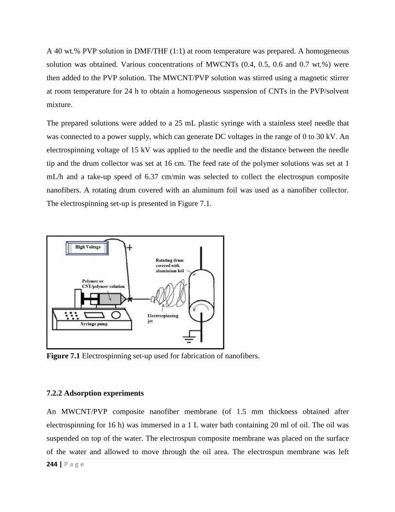
244 | P a g e

A 40 wt.% PVP solution in DMF/THF (1:1) at room temperature was prepared. A homogeneous

solution was obtained. Various concentrations of MWCNTs (0.4, 0.5, 0.6 and 0.7 wt.%) were

then added to the PVP solution. The MWCNT/PVP solution was stirred using a magnetic stirrer

at room temperature for 24 h to obtain a homogeneous suspension of CNTs in the PVP/solvent

mixture.

The prepared solutions were added to a 25 mL plastic syringe with a stainless steel needle that

was connected to a power supply, which can generate DC voltages in the range of 0 to 30 kV. An

electrospinning voltage of 15 kV was applied to the needle and the distance between the needle

tip and the drum collector was set at 16 cm. The feed rate of the polymer solutions was set at 1

mL/h and a take-up speed of 6.37 cm/min was selected to collect the electrospun composite

nanofibers. A rotating drum covered with an aluminum foil was used as a nanofiber collector.

The electrospinning set-up is presented in Figure 7.1.

Figure 7.1 Electrospinning set-up used for fabrication of nanofibers.

7.2.2 Adsorption experiments

An MWCNT/PVP composite nanofiber membrane (of 1.5 mm thickness obtained after

electrospinning for 16 h) was immersed in a 1 L water bath containing 20 ml of oil. The oil was

suspended on top of the water. The electrospun composite membrane was placed on the surface

of the water and allowed to move through the oil area. The electrospun membrane was left

245 | P a g e

immersed in the oil for 1 min. The membrane was then removed from the oil-water solution, held

for about 60 s to allow the residual oil that is on the surface to drip away and the membrane was

then weighed. In the second experiment, an electrospun membrane was immersed in 20 mL oil

bath, for about 10 minutes. The residual oil on the membrane was then allowed to drip off for 60

s and then the membrane was weighed. The sorption capacity of the CNT/PVP electrospun

membrane was expressed in grams of the oil absorbed per gram of composite membrane (g/g):

Qt = 0

0

m

mmt (1)

where Qt (g/g) is the sorption capacity on the CNT/PVP composite at a certain time t(s), mt (g) is

the weight of the CNT/PVP composite after adsorption and m0 (g) is the initial weight of the

CNT/PVP composite. The sorption capacity reached a saturation value Qe, when Qt did not

change with time.

7.2.3 Characterization of the composite nanofibers

The CNTs, PVP nanofibers and PVP/CNT composite nanofibers mats were characterized by

scanning electron microscopy (SEM, FEI Nova NanoLab FIB/SEM), transmission electron

microscopy (TEM, FEI TECNAI G2 SPIRIT), Raman (Jobin-Yvon T6400), X-Ray diffraction

(D2 Bruker PXRD with a continuous scan mode using CuKα radiation), and Fourier transform

infrared (FTIR) spectroscopy. BET surface areas and pore sizes of the chlorinated MWCNT and

MWCNT/PVP composites were obtained through N2 adsorption using a ASAP 2000

Micrometrics TriStar and Pore Analyzer.

246 | P a g e

7.3 Results and Discussion

7.3.1. Study of the influence of electrospinning parameters on the morphology of PVP

nanofibers

Uniform spinning or ejection of the charged jet requires that the concentration, viscosity,

conductivity and surface tension of the polymer solution be optimized. Therefore, prior to

electrospinning, parameters that were used to produce CNT/polymer mats were optimized. These

parameters included concentration, collector to needle distance, applied voltage and polymer

solution feed rate.

The effect of PVP polymer concentration on the morphology of the electrospun nanofibers was

investigated using 30, 35, 40 and 45 wt.% PVP concentrations in a 1:1 v/v DMF:THF solvent

mixture. SEM images of the electrospun mats are presented in Figure 7.2. The diameter

distribution curves at all concentrations are presented in the Supplementary Section Figure S28.

At 30 wt.% PVP, only about 4 cm of a 50 cm Al foil was covered with smooth nanofibers of

large diameters ~ 879 nm (Figure 7.2a). At this concentration the solution viscosity was below

the limit required for molecular entanglement and fiber formation.93 At 35 wt.% PVP

concentration, the amount of nanofibers formed on the collector increased. Thin nanofibers with

outer diameters of ~ 385 nm were obtained but they contained beads (Figure 7.2b). A 35 wt.%

solution, generated jets with insufficient viscoelastic forces to fully suppress droplet breakup due

to the Rayleigh instability to reduce surface area resulting in beads formation.94 Uniform smooth

nanofibers with diameters of ~ 532 nm were produced when the PVP concentration was

increased to 40 wt.% (Figure 7.2c). This is due to the increased solution conductivity which led

to more charge density and more elongation forces imposed to the jet under the electric field.5 A

further increase in PVP concentration to 45 wt.% resulted in the formation of nanofibers with

very large diameters ~ 2078 nm (Figure 7.2d). Some nanofibers appeared branched and partially

fused together, forming fiber doublets. The increase in polymer concentration caused the solvent

to dry faster and thus less time was needed for the repulsive columbic force to stretch the fiber,

resulting in formation of larger diameter fibers.95

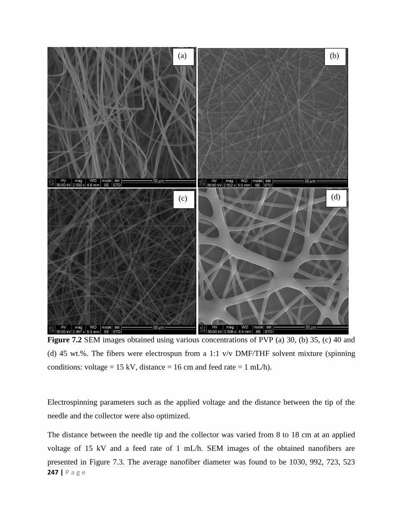
247 | P a g e

Figure 7.2 SEM images obtained using various concentrations of PVP (a) 30, (b) 35, (c) 40 and

(d) 45 wt.%. The fibers were electrospun from a 1:1 v/v DMF/THF solvent mixture (spinning

conditions: voltage = 15 kV, distance = 16 cm and feed rate = 1 mL/h).

Electrospinning parameters such as the applied voltage and the distance between the tip of the

needle and the collector were also optimized.

The distance between the needle tip and the collector was varied from 8 to 18 cm at an applied

voltage of 15 kV and a feed rate of 1 mL/h. SEM images of the obtained nanofibers are

presented in Figure 7.3. The average nanofiber diameter was found to be 1030, 992, 723, 523

(a)

(d) (c)

(b)

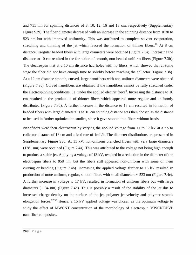
248 | P a g e

and 711 nm for spinning distances of 8, 10, 12, 16 and 18 cm, respectively (Supplementary

Figure S29). The fiber diameter decreased with an increase in the spinning distance from 1030 to

523 nm but with improved uniformity. This was attributed to complete solvent evaporation,

stretching and thinning of the jet which favored the formation of thinner fibers.96 At 8 cm

distance, irregular beaded fibers with large diameters were obtained (Figure 7.3a). Increasing the

distance to 10 cm resulted in the formation of smooth, non-beaded uniform fibers (Figure 7.3b).

The electrospun mat at a 10 cm distance had holes with no fibers, which showed that at some

stage the fiber did not have enough time to solidify before reaching the collector (Figure 7.3b).

At a 12 cm distance smooth, curved, large nanofibers with non-uniform diameters were obtained

(Figure 7.3c). Curved nanofibers are obtained if the nanofibers cannot be fully stretched under

the electrospinning conditions, i.e. under the applied electric force8. Increasing the distance to 16

cm resulted in the production of thinner fibers which appeared more regular and uniformly

distributed (Figure 7.3d). A further increase in the distance to 18 cm resulted in formation of

beaded fibers with large diameters. The 16 cm spinning distance was then chosen as the distance

to be used in further optimization studies, since it gave smooth thin fibers without beads.

Nanofibers were then electrospun by varying the applied voltage from 11 to 17 kV at a tip to

collector distance of 16 cm and a feed rate of 1mL/h. The diameter distributions are presented in

Supplementary Figure S30. At 11 kV, non-uniform branched fibers with very large diameters

(1381 nm) were obtained (Figure 7.4a). This was attributed to the voltage not being high enough

to produce a stable jet. Applying a voltage of 13 kV, resulted in a reduction in the diameter of the

electrospun fibers to 958 nm, but the fibers still appeared non-uniform with some of them

curving or bending (Figure 7.4b). Increasing the applied voltage further to 15 kV resulted in

production of more uniform, regular, smooth fibers with small diameters ~ 523 nm (Figure 7.4c).

A further increase in voltage to 17 kV, resulted in formation of uniform fibers but with large

diameters (1184 nm) (Figure 7.4d). This is possibly a result of the stability of the jet due to

increased charge density on the surface of the jet, polymer jet velocity and polymer strands

elongation forces.97,98 Hence, a 15 kV applied voltage was chosen as the optimum voltage to

study the effect of MWCNT concentration of the morphology of electrospun MWCNT/PVP

nanofiber composites.

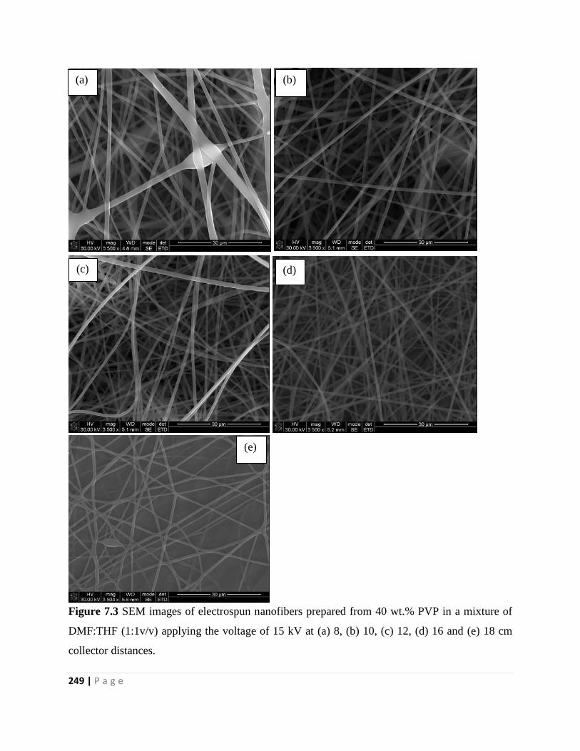
249 | P a g e


DMF:THF (1:1v/v) applying the voltage of 15 kV at (a) 8, (b) 10, (c) 12, (d) 16 and (e) 18 cm

collector distances.

(a) (b)

(c) (d)

(e)

250 | P a g e


DMF:THF (1:1 v/v) using a 16 cm needle to collector distance at an applied voltage of (a) 11, (b)

13, (c) 15 and (d) 17 kV.

7.3.2 Effect of the MWCNT content on the morphology of the electrospun PVP nanofibers

The concentration of chlorine functionalized MWCNTs was varied from 0.4 to 1 wt.% to obtain

the critical viscosity/concentration required to prepare electrospun MWCNTs/PVP solutions.

Addition of 0.4 wt.% MWCNTs into the PVP solution resulted in formation of smooth

nanofibers of variable diameters with an average diameter of 1828 nm (Figure 7.5a). A PVP

solution containing 0.5 wt.% MWCNTs produced nanofibers with highly reduced average

(a) (b)

(c) (d)

251 | P a g e

diameters of 402 nm (Figure 7.5b). A further increase in CNT concentration to 0.6 wt.% resulted

in formation of curved smooth nanofibers with largely increased average diameter of 2486 nm

(Figure 7.5c). A reduction in the average diameter to ~ 1203 nm, was observed again for

composites generated from a solution containing 0.7 wt.% of CNTs (Figure 7.5d). CNTs with 1

wt.% concentration could not be dispersed in the solvent mixture, they were insoluble. As a

result, we could only electrospin solutions up to 0.7 wt.%. The diameter distribution curves are

presented in Supplementary Figure S31. As a result, a 0.5wt.% MWCNT concentration was

chosen as an optimum as it gave smooth, uniform thin fibers and was used in further studies.

Electrospinning parameters such as feed rate and voltage were also evaluated for a PVP solution

containing 0.5 wt.% CNTs at a spinning distance of 16 cm. At 11 kV beaded curved nanofibers

with large diameters (2429 nm) were obtained (Figure 7.6a). Fiber breakage was also observed

from the solutions electrospun at an applied voltage of 11 kV (Figure 7.5a circled parts). At a

low applied voltage there is a decrease in the concentration of water vapor molecules in the

atmosphere (low humidity environments) which result in a decreased amount of electrostatic

discharge leading to higher charge density on the jet causing fiber breakage.94 At 13 kV the size

and amount of beads on the nanofibers were greatly reduced due to the increased charge density,

but the nanofiber diameter was still large at ~1943 nm. The number of nanofiber breakages were

also reduced at 13 kV. At a 15 kV applied voltage smooth, thin, more uniform nanofibers with an

average diameter of 402 nm were obtained. Increasing the voltage further to 17 kV resulted in

formation of non-uniform branched nanofiber doublets with a very large average diameters of ~

2293 nm. The formation of branches in jets and fibers occurs with more concentrated and

viscous solutions and unusually high electric fields are used.99 If the excess charge density on the

surface of the jet was high undulations are predicted to form on the surface of a cylindrical jet.

These undulations grow large enough to become unstable and initiate branches which grow

outward from the primary jet.99 The diameter distribution curves showing the average diameters

of the electrospun nanofibers are presented in Supplementary Figure S32.

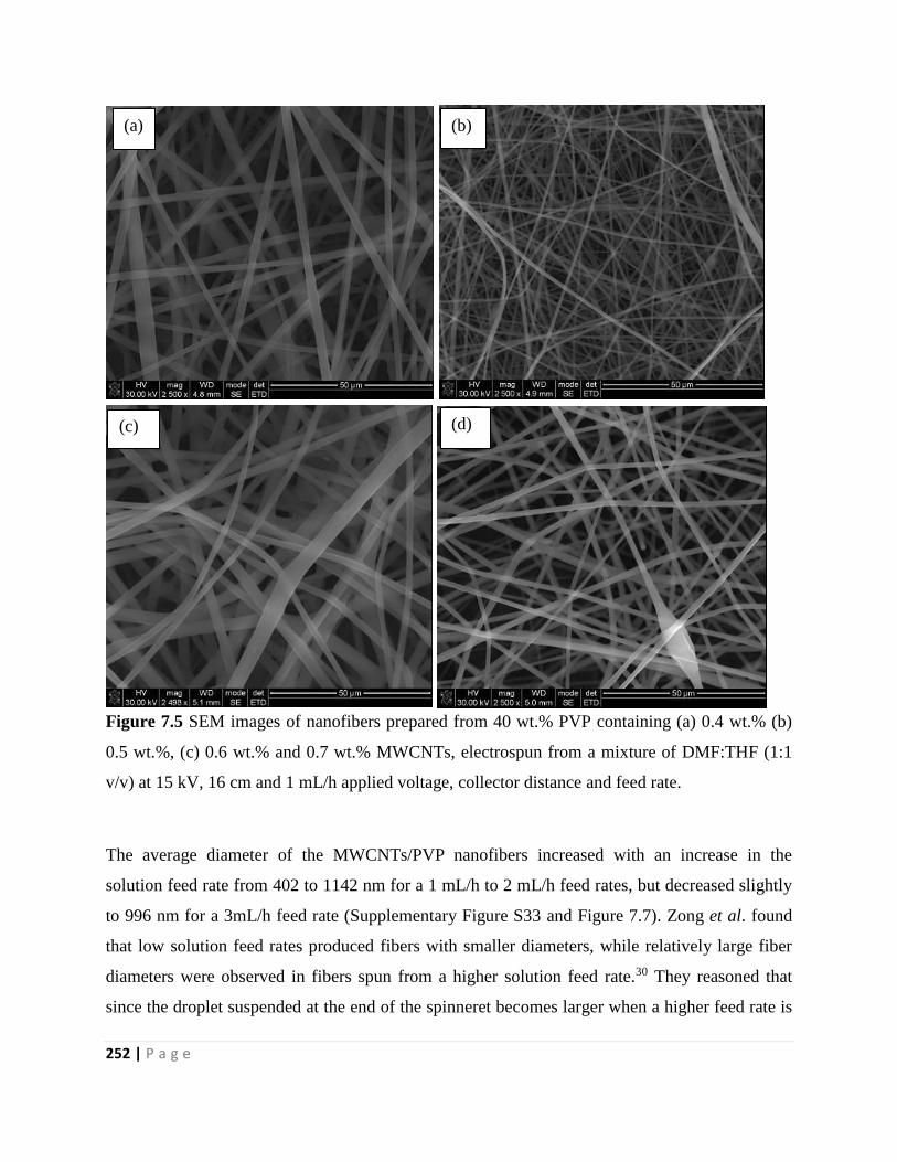
252 | P a g e

Figure 7.5 SEM images of nanofibers prepared from 40 wt.% PVP containing (a) 0.4 wt.% (b)

0.5 wt.%, (c) 0.6 wt.% and 0.7 wt.% MWCNTs, electrospun from a mixture of DMF:THF (1:1

v/v) at 15 kV, 16 cm and 1 mL/h applied voltage, collector distance and feed rate.

The average diameter of the MWCNTs/PVP nanofibers increased with an increase in the

solution feed rate from 402 to 1142 nm for a 1 mL/h to 2 mL/h feed rates, but decreased slightly

to 996 nm for a 3mL/h feed rate (Supplementary Figure S33 and Figure 7.7). Zong et al. found

that low solution feed rates produced fibers with smaller diameters, while relatively large fiber

diameters were observed in fibers spun from a higher solution feed rate.30 They reasoned that

since the droplet suspended at the end of the spinneret becomes larger when a higher feed rate is

(a) (b)

(c) (d)

253 | P a g e

used, the solution jet can carry the fluid away with faster velocity. Therefore, the electrospun

fibers may not be completely dry when they reach the target.30


MWCNTs in a mixture of DMF:THF (1:1 v/v) at 16 cm collector distance and an applied voltage

of (a) 11, (b) 13, (c) 15 and (d) 17 kV.

(a) (b)

(c) (d)

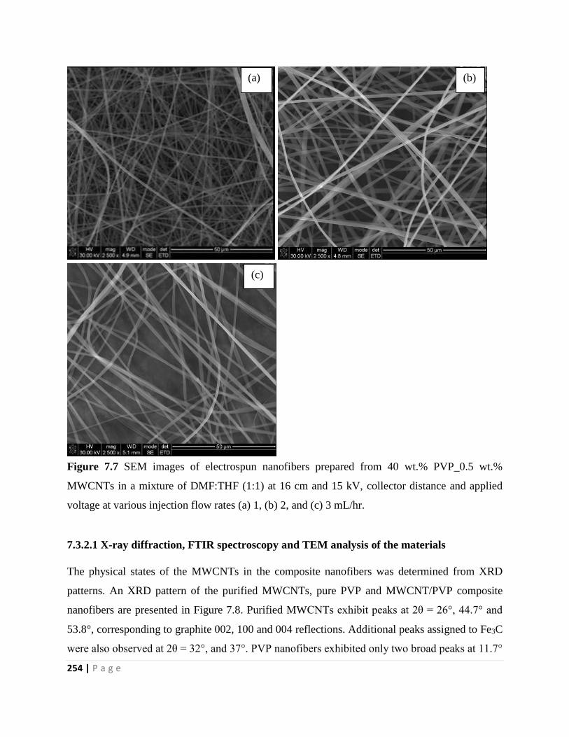
254 | P a g e


MWCNTs in a mixture of DMF:THF (1:1) at 16 cm and 15 kV, collector distance and applied

voltage at various injection flow rates (a) 1, (b) 2, and (c) 3 mL/hr.

7.3.2.1 X-ray diffraction, FTIR spectroscopy and TEM analysis of the materials

The physical states of the MWCNTs in the composite nanofibers was determined from XRD

patterns. An XRD pattern of the purified MWCNTs, pure PVP and MWCNT/PVP composite

nanofibers are presented in Figure 7.8. Purified MWCNTs exhibit peaks at 2θ = 26°, 44.7° and

53.8°, corresponding to graphite 002, 100 and 004 reflections. Additional peaks assigned to Fe3C

were also observed at 2θ = 32°, and 37°. PVP nanofibers exhibited only two broad peaks at 11.7°

(a) (b)

(c)

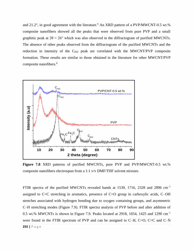
255 | P a g e

and 21.2°, in good agreement with the literature.6 An XRD pattern of a PVP/MWCNT-0.5 wt.%

composite nanofibers showed all the peaks that were observed from pure PVP and a small

graphitic peak at 2θ = 26° which was also observed in the diffractogram of purified MWCNTs.

The absence of other peaks observed from the diffractogram of the purified MWCNTs and the

reduction in intensity of the C002 peak are correlated with the MWCNT/PVP composite

formation. These results are similar to those obtained in the literature for other MWCNT/PVP

composite nanofibers.6

10 20 30 40 50 60 70 80 90

Fe3C

C002

Inte

nsit

y (

a.u

)

2 theta (degree)

PVP

PVP/CNT-0.5 wt.%

CNTs

C002

C100

C004

Fe3C

Figure 7.8 XRD patterns of purified MWCNTs, pure PVP and PVP/MWCNT-0.5 wt.%

composite nanofibers electrospun from a 1:1 v/v DMF/THF solvent mixture.

FTIR spectra of the purified MWCNTs revealed bands at 1539, 1716, 2328 and 2896 cm–1

assigned to C=C stretching in aromatics, presence of C=O group in carboxylic acids, C–OH

stretches associated with hydrogen bonding due to oxygen containing groups, and asymmetric

C–H stretching modes (Figure 7.9). FTIR spectra analysis of PVP before and after addition of

0.5 wt.% MWCNTs is shown in Figure 7.9. Peaks located at 2918, 1654, 1425 and 1290 cm–1

were found in the FTIR spectrum of PVP and can be assigned to C–H, C=O, C=C and C–N

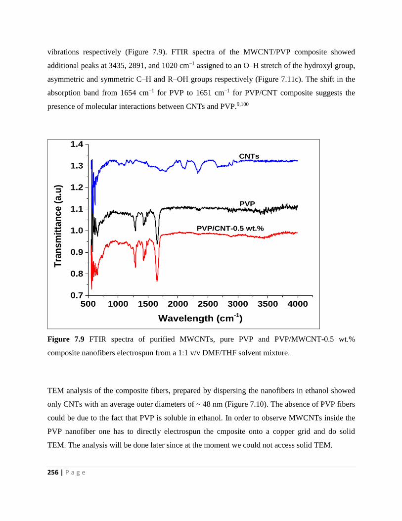
256 | P a g e

vibrations respectively (Figure 7.9). FTIR spectra of the MWCNT/PVP composite showed

additional peaks at 3435, 2891, and 1020 cm–1 assigned to an O–H stretch of the hydroxyl group,

asymmetric and symmetric C–H and R–OH groups respectively (Figure 7.11c). The shift in the

absorption band from 1654 cm–1 for PVP to 1651 cm–1 for PVP/CNT composite suggests the

presence of molecular interactions between CNTs and PVP.9,100

500 1000 1500 2000 2500 3000 3500 40000.7

0.8

0.9

1.0

1.1

1.2

1.3

1.4

PVP

PVP/CNT-0.5 wt.%

Tra

ns

mit

tan

ce

(a

.u)

Wavelength (cm-1)

CNTs

Figure 7.9 FTIR spectra of purified MWCNTs, pure PVP and PVP/MWCNT-0.5 wt.%

composite nanofibers electrospun from a 1:1 v/v DMF/THF solvent mixture.

TEM analysis of the composite fibers, prepared by dispersing the nanofibers in ethanol showed

only CNTs with an average outer diameters of ~ 48 nm (Figure 7.10). The absence of PVP fibers

could be due to the fact that PVP is soluble in ethanol. In order to observe MWCNTs inside the

PVP nanofiber one has to directly electrospun the cmposite onto a copper grid and do solid

TEM. The analysis will be done later since at the moment we could not access solid TEM.

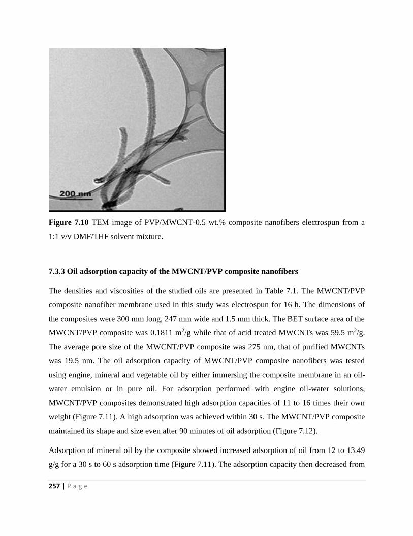
257 | P a g e

Figure 7.10 TEM image of PVP/MWCNT-0.5 wt.% composite nanofibers electrospun from a

1:1 v/v DMF/THF solvent mixture.

7.3.3 Oil adsorption capacity of the MWCNT/PVP composite nanofibers

The densities and viscosities of the studied oils are presented in Table 7.1. The MWCNT/PVP

composite nanofiber membrane used in this study was electrospun for 16 h. The dimensions of

the composites were 300 mm long, 247 mm wide and 1.5 mm thick. The BET surface area of the

MWCNT/PVP composite was 0.1811 m2/g while that of acid treated MWCNTs was 59.5 m2/g.

The average pore size of the MWCNT/PVP composite was 275 nm, that of purified MWCNTs

was 19.5 nm. The oil adsorption capacity of MWCNT/PVP composite nanofibers was tested

using engine, mineral and vegetable oil by either immersing the composite membrane in an oil-

water emulsion or in pure oil. For adsorption performed with engine oil-water solutions,

MWCNT/PVP composites demonstrated high adsorption capacities of 11 to 16 times their own

weight (Figure 7.11). A high adsorption was achieved within 30 s. The MWCNT/PVP composite

maintained its shape and size even after 90 minutes of oil adsorption (Figure 7.12).

Adsorption of mineral oil by the composite showed increased adsorption of oil from 12 to 13.49

g/g for a 30 s to 60 s adsorption time (Figure 7.11). The adsorption capacity then decreased from

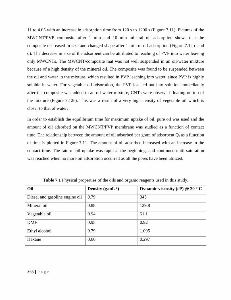
258 | P a g e

11 to 4.05 with an increase in adsorption time from 120 s to 1200 s (Figure 7.11). Pictures of the

MWCNT/PVP composite after 1 min and 10 min mineral oil adsorption shows that the

composite decreased in size and changed shape after 1 min of oil adsorption (Figure 7.12 c and

d). The decrease in size of the adsorbent can be attributed to leaching of PVP into water leaving

only MWCNTs. The MWCNT/composite mat was not well suspended in an oil-water mixture

because of a high density of the mineral oil. The composite was found to be suspended between

the oil and water in the mixture, which resulted in PVP leaching into water, since PVP is highly

soluble in water. For vegetable oil adsorption, the PVP leached out into solution immediately

after the composite was added to an oil-water mixture, CNTs were observed floating on top of

the mixture (Figure 7.12e). This was a result of a very high density of vegetable oil which is

closer to that of water.

In order to establish the equilibrium time for maximum uptake of oil, pure oil was used and the

amount of oil adsorbed on the MWCNT/PVP membrane was studied as a function of contact

time. The relationship between the amount of oil adsorbed per gram of adsorbent Qt as a function

of time is plotted in Figure 7.11. The amount of oil adsorbed increased with an increase in the

contact time. The rate of oil uptake was rapid at the beginning, and continued until saturation

was reached when no more oil adsorption occurred as all the pores have been utilized.

Table 7.1 Physical properties of the oils and organic reagents used in this study.

Oil Density (g.mL-1) Dynamic viscosity (cP) @ 20 ° C

Diesel and gasoline engine oil 0.79 345

Mineral oil 0.88 129.8

Vegetable oil 0.94 51.1

DMF 0.95 0.92

Ethyl alcohol 0.79 1.095

Hexane 0.66 0.297

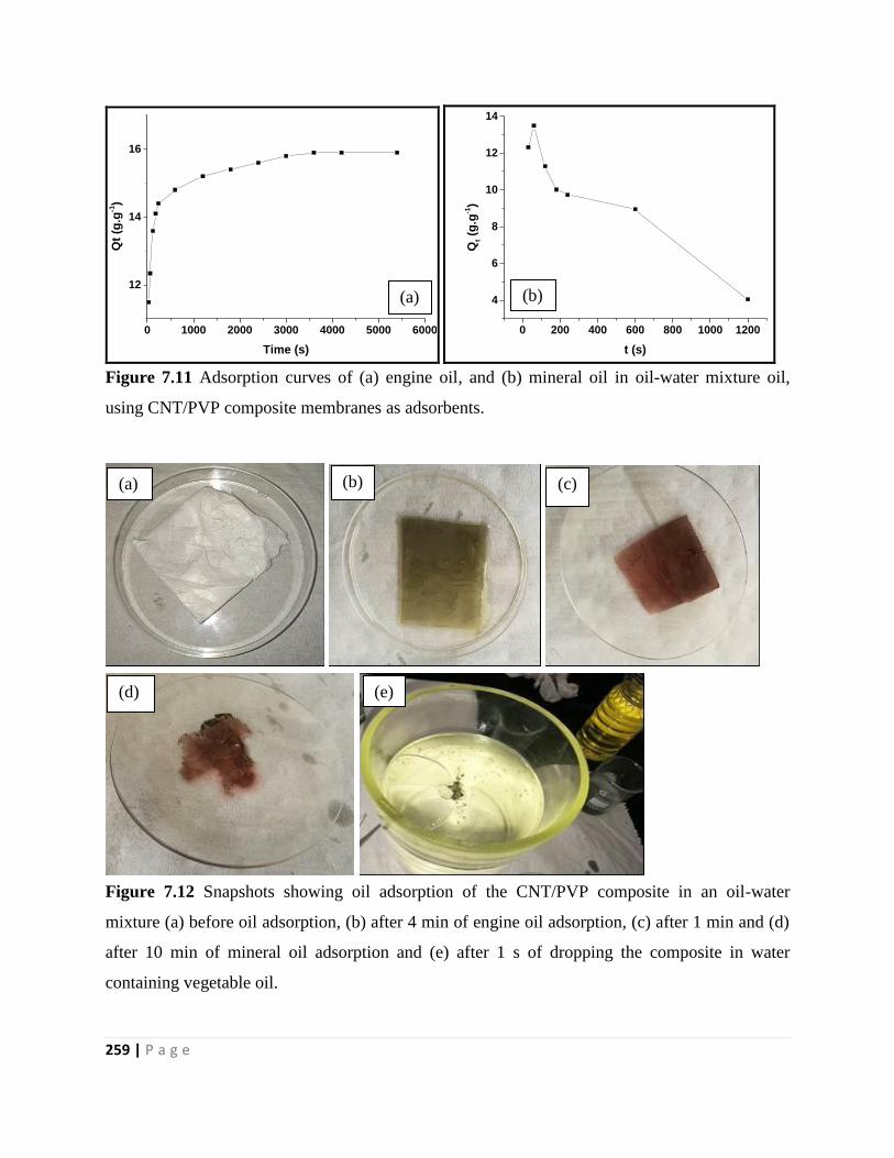
259 | P a g e

0 1000 2000 3000 4000 5000 6000

12

14

16

Qt

(g.g

-1)

Time (s)

0 200 400 600 800 1000 1200

4

6

8

10

12

14

Qt (g

.g-1)

t (s)

Figure 7.11 Adsorption curves of (a) engine oil, and (b) mineral oil in oil-water mixture oil,

using CNT/PVP composite membranes as adsorbents.

Figure 7.12 Snapshots showing oil adsorption of the CNT/PVP composite in an oil-water

mixture (a) before oil adsorption, (b) after 4 min of engine oil adsorption, (c) after 1 min and (d)

after 10 min of mineral oil adsorption and (e) after 1 s of dropping the composite in water

containing vegetable oil.

(a) (b)

(a) (b) (c)

(d) (e)

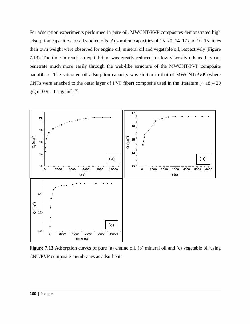
260 | P a g e

For adsorption experiments performed in pure oil, MWCNT/PVP composites demonstrated high

adsorption capacities for all studied oils. Adsorption capacities of 15–20, 14–17 and 10–15 times

their own weight were observed for engine oil, mineral oil and vegetable oil, respectively (Figure

7.13). The time to reach an equilibrium was greatly reduced for low viscosity oils as they can

penetrate much more easily through the web-like structure of the MWCNT/PVP composite

nanofibers. The saturated oil adsorption capacity was similar to that of MWCNT/PVP (where

CNTs were attached to the outer layer of PVP fiber) composite used in the literature (~ 18 – 20

g/g or 0.9 – 1.1 g/cm3).85

0 2000 4000 6000 8000 1000012

14

16

18

20

Qt (

g.g

-1)

t (s)

0 1000 2000 3000 4000 5000 600013

14

15

16

17

Qt (

g.g

-1)

t (s)

0 2000 4000 6000 8000 1000010

12

14

Qt (g

.g-1)

Time (s)

Figure 7.13 Adsorption curves of pure (a) engine oil, (b) mineral oil and (c) vegetable oil using

CNT/PVP composite membranes as adsorbents.

(a) (b)

(c)

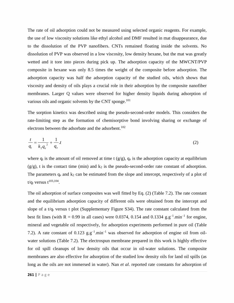
261 | P a g e

The rate of oil adsorption could not be measured using selected organic reagents. For example,

the use of low viscosity solutions like ethyl alcohol and DMF resulted in mat disappearance, due

to the dissolution of the PVP nanofibers. CNTs remained floating inside the solvents. No

dissolution of PVP was observed in a low viscosity, low density hexane, but the mat was greatly

wetted and it tore into pieces during pick up. The adsorption capacity of the MWCNT/PVP

composite in hexane was only 8.5 times the weight of the composite before adsorption. The

adsorption capacity was half the adsorption capacity of the studied oils, which shows that

viscosity and density of oils plays a crucial role in their adsorption by the composite nanofiber

membranes. Larger Q values were observed for higher density liquids during adsorption of

various oils and organic solvents by the CNT sponge.101

The sorption kinetics was described using the pseudo-second-order models. This considers the

rate-limiting step as the formation of chemisorptive bond involving sharing or exchange of

electrons between the adsorbate and the adsorbent.102

tqqkq

t

eet

.11

2

2

(2)

where qt is the amount of oil removed at time t (g/g), qe is the adsorption capacity at equilibrium

(g/g), t is the contact time (min) and k2 is the pseudo-second-order rate constant of adsorption.

The parameters qe and k2 can be estimated from the slope and intercept, respectively of a plot of

t/qt versus t103,104.

The oil adsorption of surface composites was well fitted by Eq. (2) (Table 7.2). The rate constant

and the equilibrium adsorption capacity of different oils were obtained from the intercept and

slope of a t/qt versus t plot (Supplementary Figure S34). The rate constant calculated from the

best fit lines (with R = 0.99 in all cases) were 0.0374, 0.154 and 0.1334 g.g–1.min–1 for engine,

mineral and vegetable oil respectively, for adsorption experiments performed in pure oil (Table

7.2). A rate constant of 0.123 g.g–1.min–1 was observed for adsorption of engine oil from oil-

water solutions (Table 7.2). The electrospun membrane prepared in this work is highly effective

for oil spill cleanups of low density oils that occur in oil-water solutions. The composite

membranes are also effective for adsorption of the studied low density oils for land oil spills (as

long as the oils are not immersed in water). Nan et al. reported rate constants for adsorption of

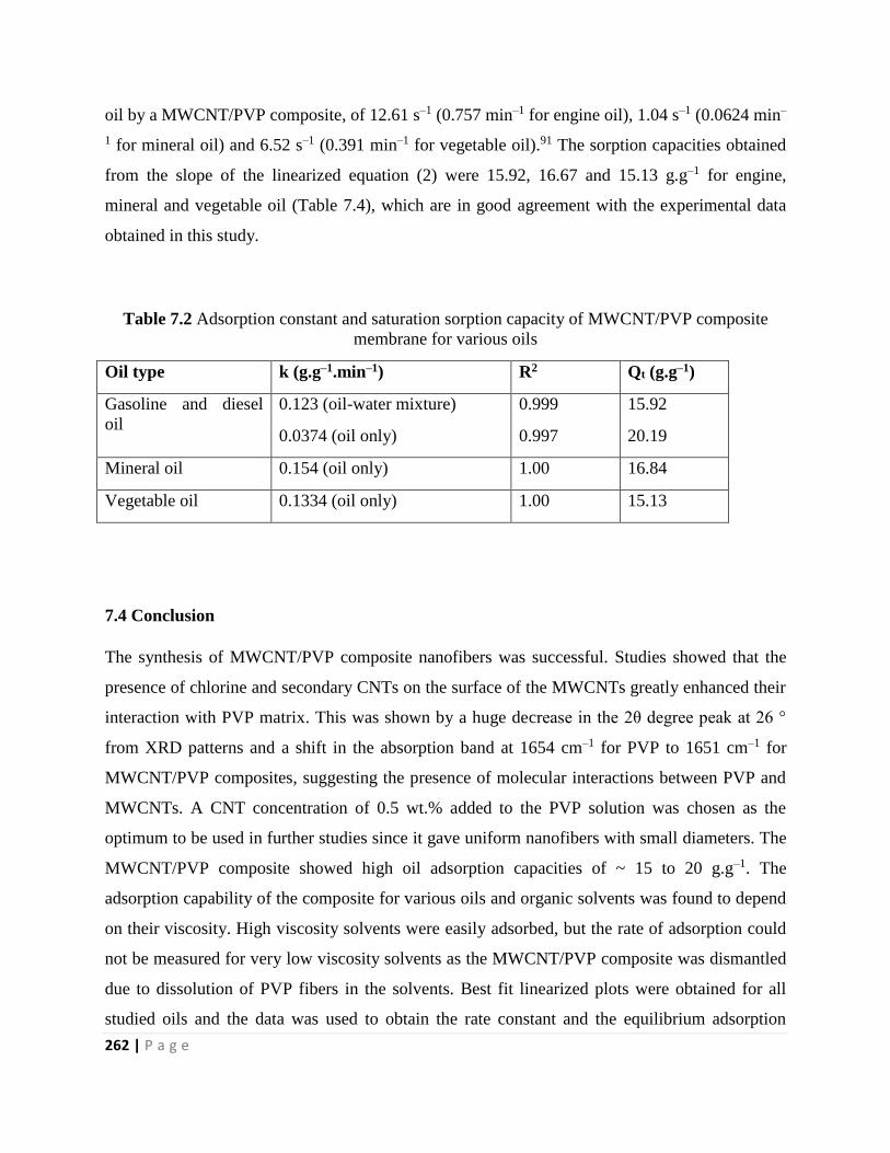
262 | P a g e

oil by a MWCNT/PVP composite, of 12.61 s–1 (0.757 min–1 for engine oil), 1.04 s–1 (0.0624 min–

1 for mineral oil) and 6.52 s–1 (0.391 min–1 for vegetable oil).91 The sorption capacities obtained

from the slope of the linearized equation (2) were 15.92, 16.67 and 15.13 g.g–1 for engine,

mineral and vegetable oil (Table 7.4), which are in good agreement with the experimental data

obtained in this study.

Table 7.2 Adsorption constant and saturation sorption capacity of MWCNT/PVP composite

membrane for various oils

Oil type k (g.g–1.min–1) R2 Qt (g.g–1)

Gasoline and diesel

oil

0.123 (oil-water mixture)

0.0374 (oil only)

0.999

0.997

15.92

20.19

Mineral oil 0.154 (oil only) 1.00 16.84

Vegetable oil 0.1334 (oil only) 1.00 15.13

7.4 Conclusion

The synthesis of MWCNT/PVP composite nanofibers was successful. Studies showed that the

presence of chlorine and secondary CNTs on the surface of the MWCNTs greatly enhanced their

interaction with PVP matrix. This was shown by a huge decrease in the 2θ degree peak at 26 °

from XRD patterns and a shift in the absorption band at 1654 cm–1 for PVP to 1651 cm–1 for

MWCNT/PVP composites, suggesting the presence of molecular interactions between PVP and

MWCNTs. A CNT concentration of 0.5 wt.% added to the PVP solution was chosen as the

optimum to be used in further studies since it gave uniform nanofibers with small diameters. The

MWCNT/PVP composite showed high oil adsorption capacities of ~ 15 to 20 g.g–1. The

adsorption capability of the composite for various oils and organic solvents was found to depend

on their viscosity. High viscosity solvents were easily adsorbed, but the rate of adsorption could

not be measured for very low viscosity solvents as the MWCNT/PVP composite was dismantled

due to dissolution of PVP fibers in the solvents. Best fit linearized plots were obtained for all

studied oils and the data was used to obtain the rate constant and the equilibrium adsorption

263 | P a g e

capacity. A good correlation between the equilibrium adsorption capacity obtained from the

linearized equation (2) with the experimental data was obtained.

264 | P a g e

References

1. G. Mittal, V. Dhand, K.Y. Rhee, S.-J. Park and W.R. Lee, J. Ind. Eng. Chem., 2015, 21, 11–

25.

2. J. Gao, A. Yu, M.E. Itkis, E. Bekyarova, B. Zhao, S. Niyogi, and R.C. Haddon, J. Am. Chem.

Soc, 2004, 126, 16698–16699.

3. M. Park, H. Kim, J. P. Youngblood, S.W. Han, E. Verplogen and A.J. Hart, Nanotechnology,

2011, 22, 415703 (1–12).

4. S.Y. Ebadi, A. Fakhrali, A.A. Gharehaghaji, S. Mazinani and S.O. Ranaei-Siadat, Polym.

Compos., 2016, 3149 – 3159, doi.10.1002/pc.23512.

5. F.A. Chayad, A.R. Jabur and N.M. Jalal, Karbala Int. J. Modern Sci., 2015, 1, 187–193.

6. K. Nasouri, A.M. Shoushtari, and M.R.M. Mojtahedi, Polym. Compos., 2016, 1–9,

doi.10.1002/pc.23774.

7. W.S. Khan, R. Asmatulu, and M.M. Eltabey, J. Nanomater., 2013, 1–9,

doi.org/10.1155/2013/160931.

8. S-H. Wang, Y. Wan, B. Sun, L-Z. Liu and W. Xu, Nanoscale Res. Lett., 2014, 9, 522–528.

9. N. Diouri, M. Baitoul and M. Maaza, J. Nanomater., 2013, 1–6,

doi.org/10.1155/2013/949108.

10. M.Z. Islam, M. Mahboob and R.L. Lowe, Polym. Compos., 2016, 305–314,

doi.10.1002/pc.23182.

11. O-K. Park, W. Lee, J.Y. Hwang, N-H. You, Y. Jeong, S.M. Kim and B-C. Ku, Composites

Part A, 2016, 91, 22–228.

12. M. Tarfaoui, K. Lafdi and A. El Moumen, Composites Part B, 2016, 103, 113–121.

13. A. Shameli and E. Ameri, Chem. Eng. J., 2017, 309, 381–396.

14. P.-C. Ma, N.A. Siddiqui, G. Marom and J.-K. Kim, Composite Part A, 2010, 41, 1345–1367.

15. P. Saini and V. Choudhary, J. Nanoparticle Res., 2013, 15, 1415 (1–7).

16. Q. Yao, L. Chen, W. Zhang, S. Liufu and X. Chen, ACS Nano., 2010, 4, 2445–2451.

17. C. Yu, Y.S. Kim, D. Kim and J.C. Grunlan, Nano. Lett., 2009, 9, 1283–1283.

18. E. Thostenson, C. Li and T. Chou, Compos. Sci. Technol. 2005, 65, 491–516.

265 | P a g e

19. P. Saini, V. Choudhary, B.P. Sigh, R.B. Mathur and S.K. Dhawan. Mater. Chem. Phys. 2009,

113, 919–926.

20. K.S.V. Santhanam, R. Sangoi and L. Fuller, Sensors Actuators B Chem., 2005, 106, 766–

771.

21. J.A. Rud, L.S. Lovell, J.W. Senn, Q. Qiao and J.T. Mcleskey, J. Mater. Sci., 2005, 40, 1455–

1458.

22. Y. Kanai and J.C. Grossman, Nano. Lett., 2008, 8, 908–912.

23. Z. Zhu, G. Wang, M. Sun, X. Li and C. Li, Electrochim. Acta, 2011, 56, 1366–1372.

24. Q. Liu, Y. Li, and M. Yang, Sensor Actuat. B Chem., 2012, 161, 967.

25. L. Dai, Carbon Nanotechnology: Recent Developments in Chemistry, Physics, Material

Science and Device Applications, Oxford: Elsevier, Amsterdam, 1st Edition, 2006.

26. D. Aussawasathien, J.-H. Dong, and L. Dai, Synth. Met., 2005, 154, 37–40.

27. D.M. Bigg and D.E. Stutz, Polym. Compos., 1993, 4, 40–46.

28. E.S.A. Rachid, K. Ariffin, H.M. Akil, and C.C. Kooi, J. Reinf. Plast. Compos., 2008, 27,

1573–1584.

29. X. Ma, F. Scarpa, H.-X. Peng, G. Allegri, J. Yuan and R. Ciobanu, Aerosp. Sci. Technol.,

2015, 47, 367–377.

30. X. Zong, K.S. Kim, D. Fang, S. Ran, B.S. Hsiao and B. Chu, Polymer, 2002, 43, 4403–4412.

31. Z. Tang, C. Qiu, J.R. McCutcheon, K. Yoon, H. Ma, D. Fang, E. Lee, C. Kopp, B.S. Hsiao

and B. Chu, J. Polym. Sci., Part B: Polym. Phys., 2009, 47, 2288–2300.

32. M.O. Daramola, P. Hlanyane, O.O. Sadare, O.O. Oluwasina and S.E. Iyuke, Membranes,

2017, 7, 14 (1–15), doi:10.3390/membranes7010014.

33. L. Wang, X.J. Song, T. Wang, S. Wang, Z. Wang, and C. Gao, Appl. Surf. Sci., 2015, 330,

118–125.

266 | P a g e

34. Y. Baek, D.K. Seo, J.H. Choi, B. Lee, Y.H. Kim, S.M. Park, J. Jung, S. Lee, and J. Yoon,

Desalin. Water Treat., 2016, 57, 28133–28140.

35. S. Maphutha, K. Moothi, M. Meyyapan and S.E. Iyuke, Sci. Rep., 2013, 3, 1509.

36. P. Shah, and C.N. Murthy, J. Membr. Sci., 2013, 437, 90–98.

37. K.H. Hong, Polym. Eng. Sci., 2007, 47, 43.

38. P.R. Supronowicz, P.M. Ajayan, K.R. Ullmann, B.P. Arulanandam, D.W. Metzger and R.

Bizios, J. Biomed. Mater. Res., 2002, 59, 499–506.

39. R. Tucknott, and S.N. Yaliraki, Chem. Phys., 2002, 281, 455.

40. Y. Dror, W. Salalha, R.L. Khalfin, Y. Cohen, A.L. Yarin and E. Zussman, Langmuir, 2003,

19, 7012–7020.

41. H. Peng, J. Am. Chem. Soc., 2008, 130, 42–43.

42. E.J. García, A.J. Hart, B.L. Wardle and A.H. Slocum, Nanotechnology, 2007, 18, 165602 (1–

11).

43. I. Jang, S.B. Sinnot, D. Danailov and P. Keblinski, Nano Lett., 2004, 4, 109–114.

44. Y. Hu, O.A. Shenderova, Z. Hu, C.W. Padgett and D.W. Brenner, Rep. Prog. Phys. 2006, 69,

1847–1895.

45. G. Withers, J. Souza, Y. Yu, L. Cercone, V. Khabashesku and D. Davis, J. Compos. Mater.,

2015, 783–793, http://dx.doi.org/10.1177/0021998315581510.

46. Z. Spitalsky, D. Tasis, K. Papagelis and C. Galiotis, Prog. Polym. Sci. 2010, 35, 357–401.

47. P. Verma, P. Saini and V. Choudhary, Mater. Des., 2015, 88, 269–277.

48. Z.M. Huang, Y.Z. Zhang, M. Kotaki and S. Ramakrishna, Compos. Sci. Technol., 2003, 63,

2223–2253.

49. P. Saini. Fundamentals of Conjugated Polymer Blends, Copolymers and Composites, John

Wiley & Sons, Inc., 1–118, http://doi.wiley.com / 10.1002/ 9781119137160.ch1, 2015.

http://dx.doi.org/10.1177/0021998315581510

267 | P a g e

50. P. Kannan, R.J. Young and S.J. Eichhorn, Small, 2008, 4, 930–933.

51. M. Bourourou, M. Holzinger, F. Bossard, F. Hugenell, A. Maaref and S. Cosnier, Carbon,

2015, 87, 233–238.

52. W. Nuasing, Electrospinning of Biomolecules, PhD Thesis, Department of Physics,

University of Pais Vasco, Donostia, Spain, 2014.

53. C. Mit-uppatham, M. Nithitanakul, P. Supaphol, Macromol. Chem. Phys., 2004, 205, 2327–

2338.

54. L.M.M. Costa, R.E.S. Bretas, R. Gregorio, Mater. Sci. Appl., 2010, 1, 247–252.

55. X. Zong, K. Kim, D. Fang, S. Ran, B.S. Hsiao and B. Chu, Polymer, 2002, 42, 4403.

56. S Koombhogse, W. Liu and D.H. Reneker, J. Polym. Sci., 2001, 39, 2598.

57. H. Albetran, Y. Dong and I.M. Low, J. Asian Ceram. Soc., 2015, 3, 292–300.

58. S. Sarabi-Mianeji, J. Scott and D.J.Y.S. Page, Polym. Eng. Sci., 2015, 55, 2576–2582.

59. P. Ajayan, O. Stephan, C. Colliex and D. Trauth, Science, 1994, 265, 1212–1214.

60. Y. Dror, W. Salalha, R.L. Khalfin, Y. Cohen, A.L. Yarin and E. Zussman, Am. Chem. Soc.,

2003, 7012–7020.

61. J.J. Ge, H.Q. Hou, Q. Li, M.J. Graham, A. Greiner, D.H. Reneker, F.W. Harris and S.Z.D.

Cheng, J. Am. Chem. Soc., 2004, 126, 15754–15761.

62. H.S. Kim, J.H. Sung, H.J. Choi, I. Chin and H. Jin, Polym. Prepr. 2005, 46, 736.

63. R. Sen, B. Zhao, D. Perea, M.E. Itkis, H. Hu, J. Love, E. Bekyarova, and R.C. Haddon, Nano

Lett., 2004, 4, 459–464.

64. K. Saeed, S.Y. Park, H.J. Lee, J.B. Baek and W.S. Huh, Polymer, 2006, 47, 8019–8025.

65. G.M. Kim, G.H. Michlera and P. Pötschke, Polymer, 2005, 46, 7346–7351.

66. J.S. Jeong, S.Y. Jeon, T.Y. Lee, J.H. Park, J.H. Shin, P.S. Alegaonkar, A.S. Berdinsky and

J.B. Yoo, Diamond Relat. Mater., 2006, 15, 1839–1843.

268 | P a g e

67. C. Pan, L.Q. Ge and Z.Z. Gu, Composites Science and Technology, 2007, 67, 3271–3277.

68. Urban Urgency, Water Caucus Summary, World Water Council (WWC), Marseille, France,

2007.

69. M. Elimelech and W.A. Phillip, Science, 2011, 333, 712–717.

70. M.A. Shannon, P.W. Bohn, M. Elimelech, J.G. Georgiadis, B.J. Marinas and A.M. Mayes,

Nature, 2008, 452, 301–310.

71. D. Zhou, L. Zhu, Y. Fu, M. Zhu and I. Xue, Desalination, 2015, 376, 109–116.

72. L.Y. Ng, A.W. Mohammad, C.P. Leo, N. Hilal, Desalination, 2013, 308, 15–33.

73. J. Yin, and B. Deng, J. Membr. Sci., 2015, 479, 256–275.

74. L. Ma, X. Dong, M. Chen, L. Zhu, C. Wang, F. Yang and Y. Dong, Membranes, 2017, 7, 16

(1–21), doi:10.3390/membranes7010016.

75. J. Albaiges, Int. J. Environ. Anal. Chem., 2014, 94, 1–3.

76. Q. Li, C. Kang and C. Zhang, Process Biochem, 2005, 40, 873–877.

77. A.R. Pendashteh, A. Fakhru’l-Razi, S.S. Madaeni, L.C. Abdullah, Z.Z. Abidin and D.R.A.

Biak, Chem. Eng. J., 2011, 168, 140–150.

78. J. Rubio, M.L. Souza and R.W. Smith, Miner. Eng., 2002, 15, 139–155.

79. E. Yuliwati and A.F. Ismail, Desalination, 2011, 273, 226–234.

80. J. Zhong, X. Sun and C. Wang, Sep. Purif. Technol., 2003, 32, 93–98.

81. M.R. Kumar, C.V. Koushik and K. Saravanan, J. Elixir Chem. Eng., A, 2013, 54, 12713–

12717.

82. W.M. Graham, R.H. Condon, R.H. Carmichael, I. D’Ambra, H.K. Patterson, L.J. Linn and

F.J. Hernandez, Jr. Environ. Res. Lett., 2010, 5, 045301.

83. C.M. Reddy, J.S. Arey, J.S. Seewald, S.P. Sylva, K.L. Lemkau, R.K. Nelson, C.A.

Carmichael, C.P. McIntyre, J. Fenwick and G.T. Ventura, Proc. Natl. Acad. Sci. U.S.A.,

2012, 109, 20229–20234.

84. M.C. Redmond and D.L. Valentine, Proc. Natl. Acad. Sci. U.S.A., 2012, 109, 20292–20297.

269 | P a g e

85. W. Ma, Q. Zhang, D. Hua, R. Xiong, J. Zhao, W. Rao, S. Huang, X. Zhan, F. Chen, and C.

Huang, RSC Adv. 2016, 6, 12868-12888.

86. Z. Shi, W. Zhang, F. Zhang, X. Liu, D. Wang, J. Jin and L. Jiang, Adv. Mater., 2013, 25,

2422–2427.

87. Z.X. Xue, S.T. Wang, L.Lin, L. Chen, M.J. Liu, L. Feng and L. Jiang, Adv. Mater., 2011, 23,

4270–4273.

88. M. Padaki, R.S. Murali, M.S. Abdullah, N. Misdan, A. Moslehyani, M.A. Kassim, N. Hilal,

and A.F. Ismail, Desalination, 2015, 357, 197–207.

89. L. Zhu, M. Chen, Y. Dong, C.Y. Tang, A. Huang and L. Li, Water Res., 2016, 90, 277–285.

90. M. Chen, L. Zhu, Y. Dong, L. Li and J. Liu, ACS Sustainable Chem. Eng., 2016, 4, 2098–

2106.

91. D. Nan, J. Wei, F. Guo, G. Fan, F. Xu, L. Li, H. Zhu, K. Wang and D. Wu, J. Nanosci.

Nanotechnol., 2014, 14, 6461–6465.

92. H. You, X. Li, Y. Yang, B. Wang, Z. Li, X. Wang, M. Zhu and B.S. Hsiao, Sep. Purif.

Technol., 2013, 108, 143–151.

93. M. Ozdemir, E. Celik, and U. Cocen, Mater. Technol., 2013, 47, 735–738.

94. M. Roya, BS. Nezarati, B. Michelle, BS. Eifert, and E. Cosgriff-Hermandez, Tissue Eng.,

2013, 19, 810–818.

95. T. Vongsetskul, T.C.P. Wongsomboom, and R. Rangkupan, Chiang Mai J. Sci, 2015, 42,

436–442.

96. T. Mozoochi, M. Hamadanian, M. Ahmadi and V. Jabbari, Int. Ind. Chem., 2012, 3, 1–8,

doi:10.1186/2228-5547-3-2.

97. W. Ding, S. Wei, J. Zhu, X. Chen, D. Rutman and Z. Guo, Macromol. Mater. Eng., 2010,

295, 958–965.

98. J.M. Deitzel, J. Kleinmeyer, H.D. Beck and N.C. Tan, Polymer, 2001, 42, 261–272.

270 | P a g e

99. D.H. Reneker and A.L. Yarin, Polymer, 2008, 49, 2387-2425.

100. S. Huang, L. Zhou, M.-C. Li, Q. Wu, Y. Kojima and D. Zhou, Materials, 2016, 6, 523 (1-

14).

101. Z. Li and C. Wang, One dimensional nanostructures: Electrospinning Technique and

unique nanofibers, Springer, 2013, doi:10.1007/978-3-642-36427-3_2.

102. M.M. Rahman, S.B. Khan, H.M. Marwani and A.M. Asiri, PLOS ONE, 2014,

doi:10.1371/journal.pone.0114084, 1-23.

103. Y. Ho, Water Res., 2006, 40, 119-125.

104. M. Faisai, S.B. Khan, M.M. Rahman, A. Jamal, A.M. Asiri, et al., App. Surf. Sci., 2012,

258, 7515-7522.

271 | P a g e

CHAPTER 8

Summary of Conclusions and recommendations

The synthesis of chlorinated MWCNTs and chlorinated N-MWCNTs was achieved by means of

a fixed-bed CVD method using various chlorinated organic solvents as sources of chlorine and

acetonitrile as a source of nitrogen over an Fe-Co/CaCO3 catalyst. The morphology of the

synthesized carbon materials and composites were confirmed by various characterization

techniques such as SEM, TEM, TGA, XRD, BET, XPS, FTIR and Raman spectroscopy.

The number of chlorine atoms substituted on the organic compound had a huge effect on the

morphology, yield, diameter, and quality of the MWCNTs produced. XPS analysis confirmed

that functionalization of carbon from MWCNTs with chlorine was successful. The average outer

diameters and inner diameters of the MWCNTs increased with an increase in the amount of

chlorine atoms substituted on the organic compound. CNFs, CNTs, CNTs with secondary

growth, and hollow CNTs were produced when DCE, CB, DCB and TCE, TCB and TTCE were

used as chlorine sources, respectively. About 10 and 40 % of the CNTs generated from TCE and

DCB respectively showed secondary growth on top of the MWCNTs. Raman spectroscopy

showed that the materials contained defects, due to the creation of new sp3 C–Cl bonds. CNTs

that had secondary growth were highly disordered. Alkanes gave cleaner CNMs with higher

yields than those formed from the aromatic reactants.

Growth of secondary carbon nanostructures on the surface of the primary CNTs was investigated

by varying the reaction time and temperature using DCB as a chlorine source. DCB was chosen

since from our previous study, it produced an appreciable quantity of CNTs with secondary

growth. The graphitic nature, structure, yield of the CNTs and the formation of secondary CNFs

on the surface of the main CNTs were affected by the growth time and temperature. Longer

synthesis times resulted in formation of highly graphitic CNTs of high purity with no secondary

CNF growth and with less defects. The largest number of secondary CNFs were observed at a 90

min reaction time at 700 °C. The average diameters of the CNTs increased with an increase in

temperature due to catalyst sintering. Small catalyst particles were formed at lower temperatures

272 | P a g e

and large catalyst particles were formed at higher temperatures. The presence of secondary CNFs

induced defects and disorders in the materials produced as evidenced by the Raman spectral

analysis. Growth of the CNTs was greatly reduced at high temperatures. Poisoning of the CNT

surface by iron carbides was observed with an increase in reaction temperature due to increased

formation of chlorine in the reactor.

Synthesis of chlorine-functionalized nitrogen-doped MWCNTs by injection CVD over a Fe-

Co/CaCO3 was successful. DCB was found to be an excellent chlorine source that led to

formation of large amounts of CNTs. Chlorine influenced the morphology, length, yield and

outer diameter of the N-doped MWCNTs. A limited quantity of rod-shaped MWCNTs were

obtained when CH3CN was used alone as a feed. Horn-, straw- and pencil-shaped N-MWCNTs

and CNFs were obtained by varying the amount of DCB in the feed. TGA, Raman and XPS

analysis showed that an increase in the amount of DCB in the feed to 66.7 vol.% resulted in

formation of CNTs with large defects, due to an increase in the concentration of nitrogen

incorporated into the CNT walls. TGA and XPS analysis also confirmed the presence of chloride

ions on the surface of the CNTs bound to metal ions. Covalent functionalization of carbon with

chlorine was also confirmed by Raman and XPS analysis. Addition of chlorine favored

formation of graphitic nitrogen atoms, but the amount of chlorine in the feed has to be controlled.

Highly graphitic carbon materials were produced at low (33.3 vol.%) and high (80 vol.%) DCB

concentrations. TTCE was found to be a poor chlorine source to make N-doped MWCNTs, and

resulted in the production of very little product. The carbon materials produced mostly contained

lumps of carbon platelets.

Synthesis of chlorine-functionalized N-doped MWCNTs by a bubbling CVD method was also

successful. DCB and TTCE were used as chlorine sources and acetonitrile as a nitrogen source.

The morphology of the CNMs depended on the amount of chlorine in the feed. Bamboo-

compartmented CNTs and CNTs with intratubular junctions were obtained from solutions

containing at a low concentration of DCB (33.3 vol.%). Hollow and bamboo-compartmented

CNTs were obtained from solutions containing a high concentration of DCB (66.7 vol.%). A

large increase in the amount of nitrogen atoms doped into the CNTs was achieved at low DCB

concentration, evidenced by a decrease in the outer diameters of the N-MWCNTs with an

increase in DCB concentration. Highly graphitic materials were produced after post-doping of N-

273 | P a g e

MWCNTs with chlorine and of the chlorinated MWCNTs with nitrogen. Highly graphitic

materials were produced at a low concentration of DCB (33.3 vol.%) as evidenced by TGA,

Raman and XPS analysis. Thermally stable CNTs with a smaller value of the ID/IG peak ratio,

which had graphitic N species dominant in the N1s XPS spectra were observed at a low

concentration of DCB. Carbon nano-onions were formed when TTCE was used as a source of

chlorine. The formation of carbon nano-onions increased at low TTCE concentrations, which

was attributed to greater incorporation of nitrogen into the CNMs. Increase in the TTCE

concentration resulted in mixtures of carbon nano-onions and bamboo-compartmented carbon

nano-bells. NCNMs generated from heated solutions of CH3CN and TTCE resulted in formation

of mixtures of CNMs, especially at high concentrations of TTCE. Selectivity was achieved at

low concentrations (33.3 and 25 vol.%) of TTCE. CNTs were produced when DCB was used as

a source of chlorine while mixtures of CNMs were produced when TTCE was used. Aromatic

chlorinated organic compounds rather than aliphatic chlorinated organic compounds are better

suited for use in studies in which the effect of chlorine on the morphology of CNMs is studied.

An MWCNT/PVP composite membrane was successfully synthesized. XRD and FTIR studies

showed that the MWCNTs were embedded inside the PVP matrix. The MWCNT/PVP composite

membrane is capable of adsorbing oil from land or oil-water mixtures. High adsorption

capacities of 15 – 20 g/g were achieved. The adsorption capability of the composite membrane

depended on the viscosity of the solvents or oils.

The dependence of the adsorption capability of the MWCNT/PVP composite membrane

synthesized in this study on the viscosity of the solvents, limits its use for the adsorption of

various solvents and oils. This is mainly attributed to the ability of PVP to dissolve in low

viscosity solvents like water.

PVP is indeed a pore former and easily biodegradable, and this warrants its use in these types of

applications. It is therefore recommended that PVP must be cross-linked with other chemicals

like glutaraldehyde, maleic acid, etc., together with MWCNTs in order to make them water

resistant.

Chlorine functionalized CNTs that contains secondary CNFs on their surface can be used as

nanoscale templates in various applications, since in this applications materials that form high

274 | P a g e

density network structures with chemically connected CNTs are required. Chlorinated NCNTs

can be applied in electronics to enhance their field emission properties as they are open-ended.

The chlorinated NCNTs can also be applied in water treatment as magnets to attract metal

pollutants, by first filling them with magnetic metal nanoparticles to render them magnetic.

275 | P a g e

Appendix A: Supplementary Materials

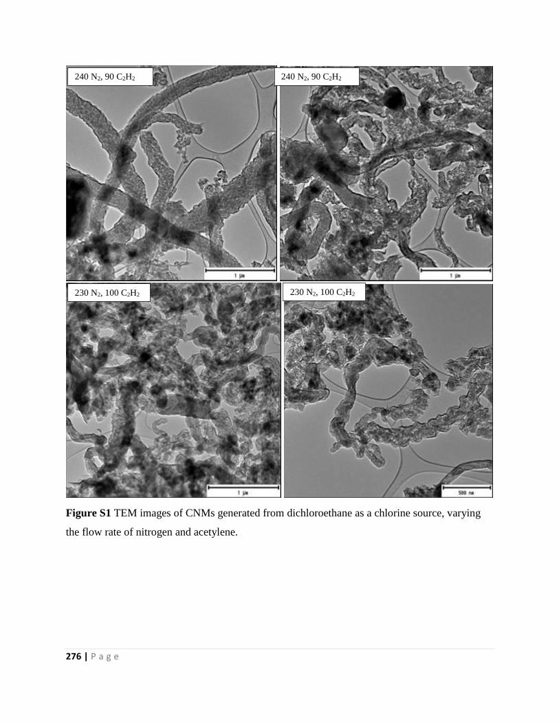
276 | P a g e


the flow rate of nitrogen and acetylene.

240 N2, 90 C2H2 240 N2, 90 C2H2

230 N2, 100 C2H2 230 N2, 100 C2H2

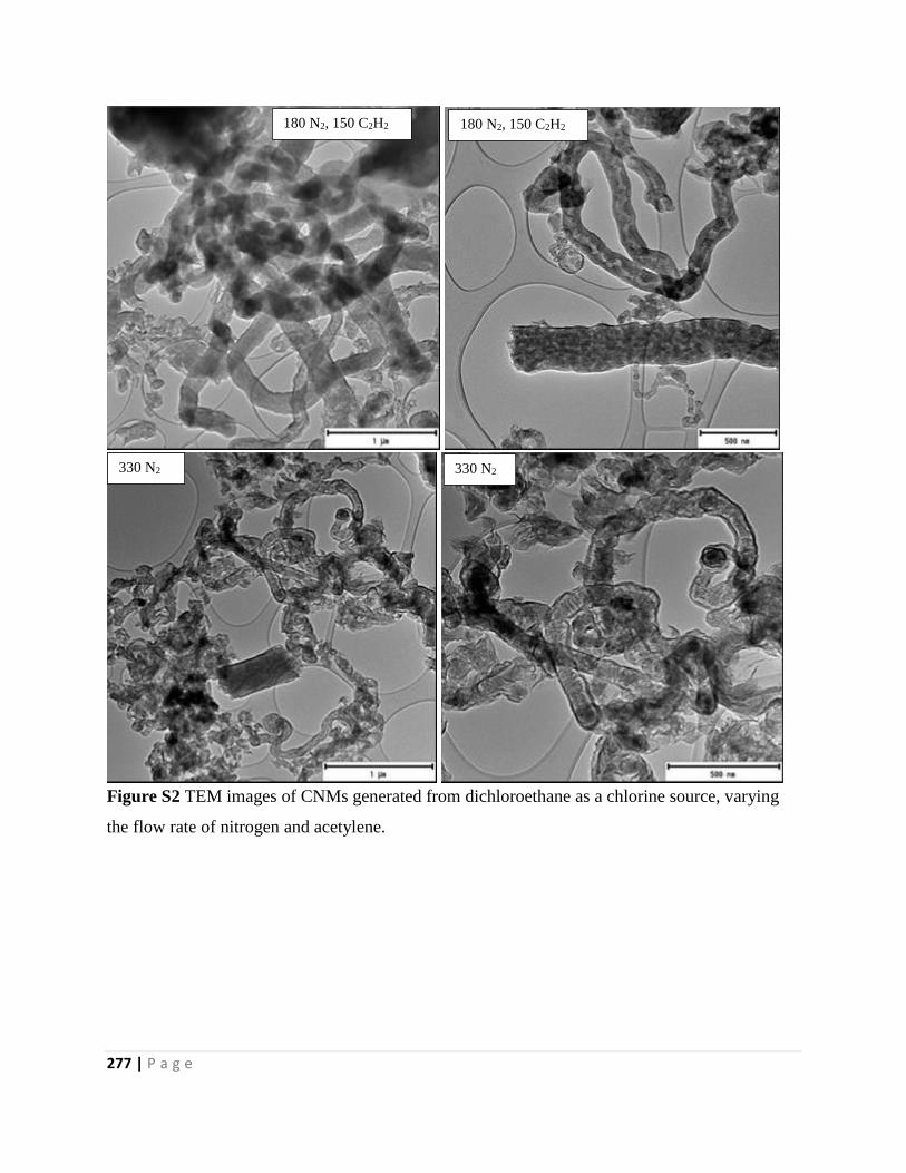
277 | P a g e



180 N2, 150 C2H2 180 N2, 150 C2H2

330 N2 330 N2

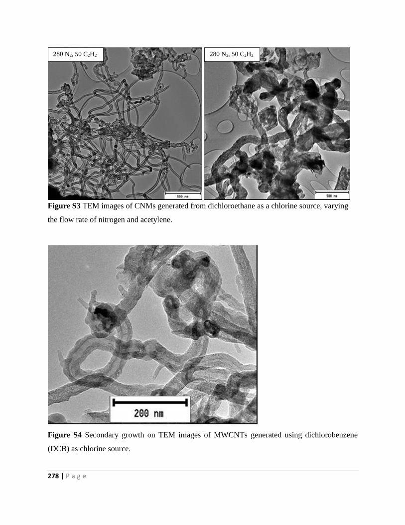
278 | P a g e



Figure S4 Secondary growth on TEM images of MWCNTs generated using dichlorobenzene

(DCB) as chlorine source.

280 N2, 50 C2H2 280 N2, 50 C2H2

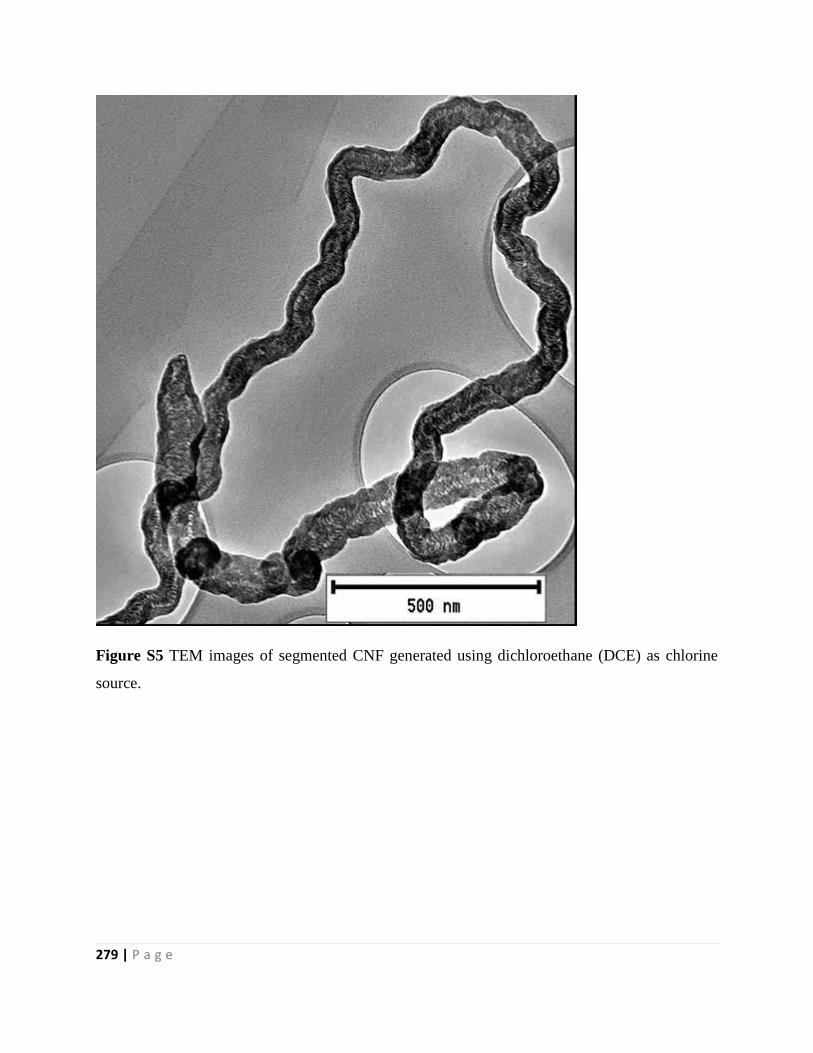
279 | P a g e

Figure S5 TEM images of segmented CNF generated using dichloroethane (DCE) as chlorine

source.

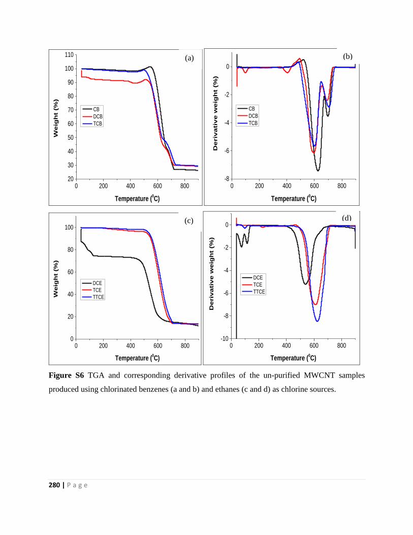
280 | P a g e

0 200 400 600 80020

30

40

50

60

70

80

90

100

110W

eig

ht

(%)

Temperature (0C)

CB

DCB

TCB

0 200 400 600 800-8

-6

-4

-2

0

De

riv

ati

ve

we

igh

t (%

)

Temperature (0C)

CB

DCB

TCB

0 200 400 600 8000

20

40

60

80

100

Weig

ht

(%)

Temperature (0C)

DCE

TCE

TTCE

0 200 400 600 800-10

-8

-6

-4

-2

0

Deriv

ati

ve w

eig

ht

(%)

Temperature (0C)

DCE

TCE

TTCE

Figure S6 TGA and corresponding derivative profiles of the un-purified MWCNT samples

produced using chlorinated benzenes (a and b) and ethanes (c and d) as chlorine sources.

(a)

(d) (c)

(b)

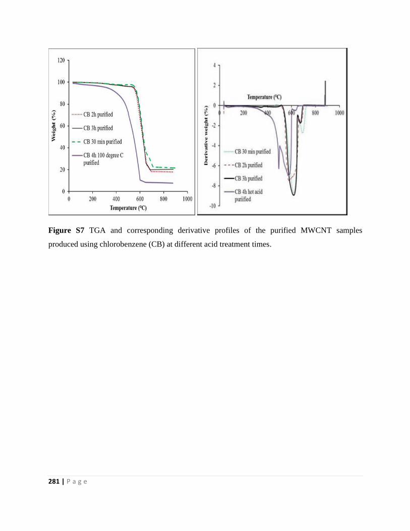
281 | P a g e

Figure S7 TGA and corresponding derivative profiles of the purified MWCNT samples

produced using chlorobenzene (CB) at different acid treatment times.

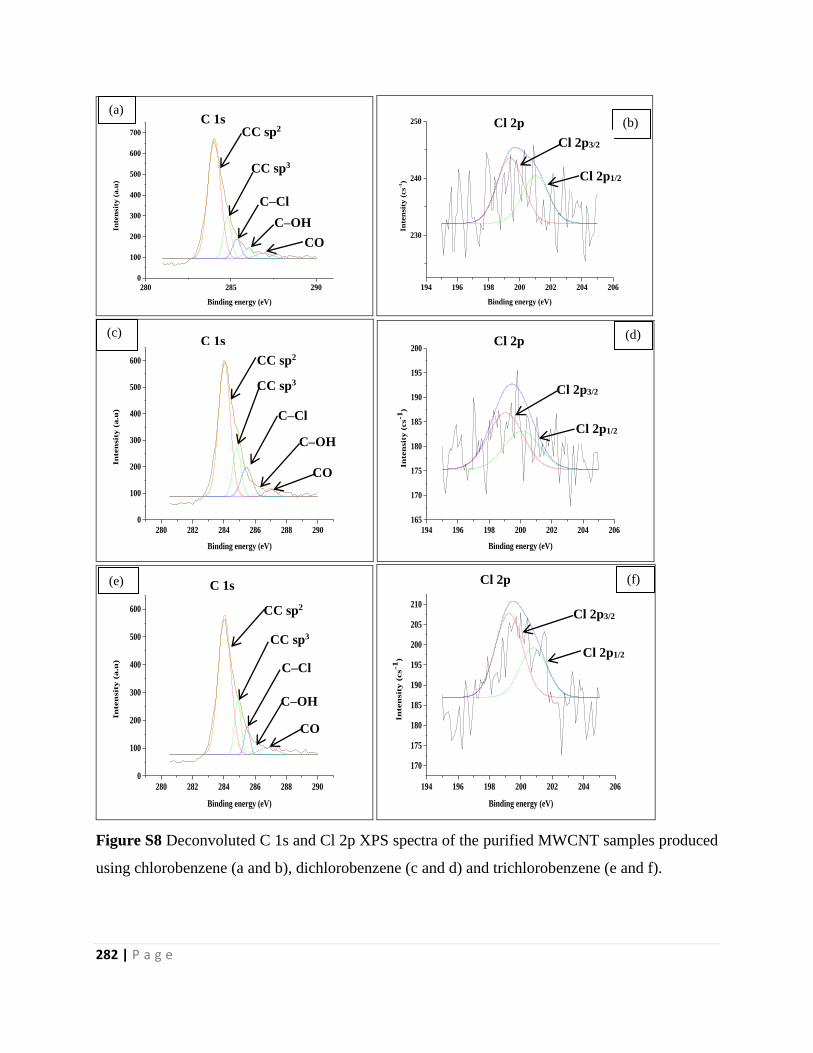
282 | P a g e

280 285 2900

100

200

300

400

500

600

700

Inte

nsi

ty (

a.u

)

Binding energy (eV)

194 196 198 200 202 204 206

230

240

250

Inte

nsi

ty (

cs-1

)

Binding energy (eV)

280 282 284 286 288 2900

100

200

300

400

500

600

In

ten

sit

y (

a.u

)

Binding energy (eV)

194 196 198 200 202 204 206165

170

175

180

185

190

195

200

In

ten

sit

y (

cs-1

)

Binding energy (eV)

280 282 284 286 288 2900

100

200

300

400

500

600

In

ten

sit

y (

a.u

)

Binding energy (eV)

194 196 198 200 202 204 206

170

175

180

185

190

195

200

205

210

In

ten

sit

y (

cs-1

)

Binding energy (eV)


using chlorobenzene (a and b), dichlorobenzene (c and d) and trichlorobenzene (e and f).

(a) (b)

(c) (d)

(e) (f)

C 1s CC sp2

284.0

eV

C–OH

286.0

eV

CO

286.

8 eV

CC sp3

284.8

eV C–Cl

285.3

eV

Cl 2p

Cl 2p3/2

199.4

eV Cl 2p1/2

201 eV

Cl 2p

Cl 2p3/2

199 eV Cl 2p1/2

200.1

eV

C 1s

CC sp2

284.0

eV

C–OH

285 eV CO

286.

4

eV

CC sp3

284.8 eV C–Cl

285.3

eV

C–OH

285 eV CO

286.

2 eV

C 1s

CC sp2

284.0 eV CC sp3

284.8 eV C–Cl

285.3

eV

Cl 2p

Cl 2p3/2

199.2 eV Cl 2p1/2

200.8 eV

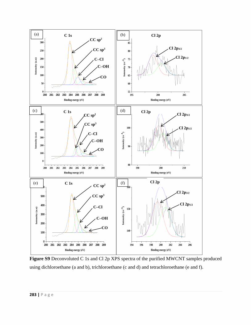
283 | P a g e

280 281 282 283 284 285 286 287 288 2890

50

100

150

200

250

300

In

ten

sit

y (

a.u

)

Binding energy (eV)

195 200 20555

60

65

70

75

80

85

In

ten

sit

y (

cs-1

)

Binding energy (eV)

280 281 282 283 284 285 286 287 288 289

0

100

200

300

400

500

600

In

ten

sit

y (

a.u

)

Binding energy (eV)

190 200 21080

90

100

In

ten

sit

y (

cs-1

)

Binding energy (eV)

280 281 282 283 284 285 286 287 288 2890

100

200

300

400

500

600

In

ten

sit

y (

a.u

)

Binding energy (eV)

194 196 198 200 202 204 206

140

150

160

In

ten

sit

y (

cs-1

)

Binding energy (eV)


using dichloroethane (a and b), trichloroethane (c and d) and tetrachloroethane (e and f).

(a) (b)

(c) (d)

(e) (f)

C 1s

C–OH

285.7

eV

CC sp2

289.9

eV CC sp3

284.5

eV C–Cl

285.1

eV

CO

286.7

eV

Cl 2p3/2

199.0 eV Cl 2p1/2

200.6

eV

Cl 2p

C 1s

CO

286.7

eV

CC sp2

284.0

eV CC sp3

284.7

eV C–Cl

285.2

eV

C–OH

286

eV

Cl 2p Cl 2p3/2

199.0 eV

Cl 2p1/2

200.9

eV

C 1s CC sp2

284.0

eV CC sp3

284.7

eV C–Cl

285.2

eV C–OH

285.8

eV CO

286

.6

eV

Cl 2p

Cl 2p3/2

199.3 eV Cl 2p1/2

200.9 eV

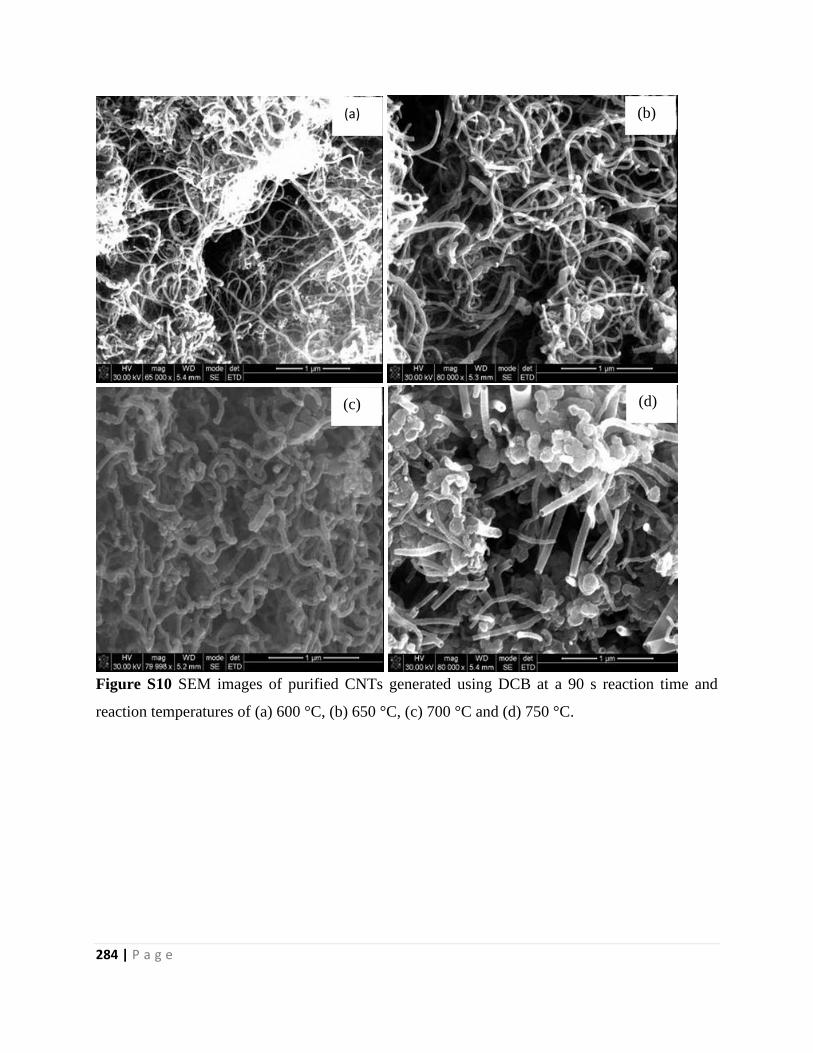
284 | P a g e

Figure S10 SEM images of purified CNTs generated using DCB at a 90 s reaction time and

reaction temperatures of (a) 600 °C, (b) 650 °C, (c) 700 °C and (d) 750 °C.

(a)

(d) (c)

(b)

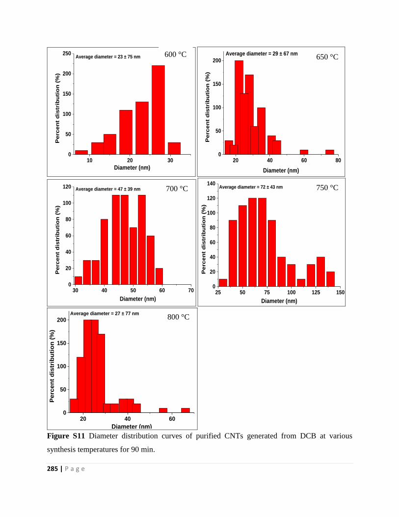
285 | P a g e

10 20 300

50

100

150

200

250P

erc

en

t d

istr

ibu

tio

n (

%)

Diameter (nm)


20 40 60 800

50

100

150

200

Pe

rce

nt

dis

trib

uti

on

(%

)

Diameter (nm)


30 40 50 60 700

20

40

60

80

100

120

Perc

en

t d

istr

ibu

tio

n (

%)

Diameter (nm)


25 50 75 100 125 1500

20

40

60

80

100

120

140

Perc

en

t d

istr

ibu

tio

n (

%)

Diameter (nm)


20 40 600

50

100

150

200

Pe

rce

nt

dis

trib

uti

on

(%

)

Diameter (nm)


Figure S11 Diameter distribution curves of purified CNTs generated from DCB at various

synthesis temperatures for 90 min.

600 °C

800 °C

750 °C 700 °C

650 °C

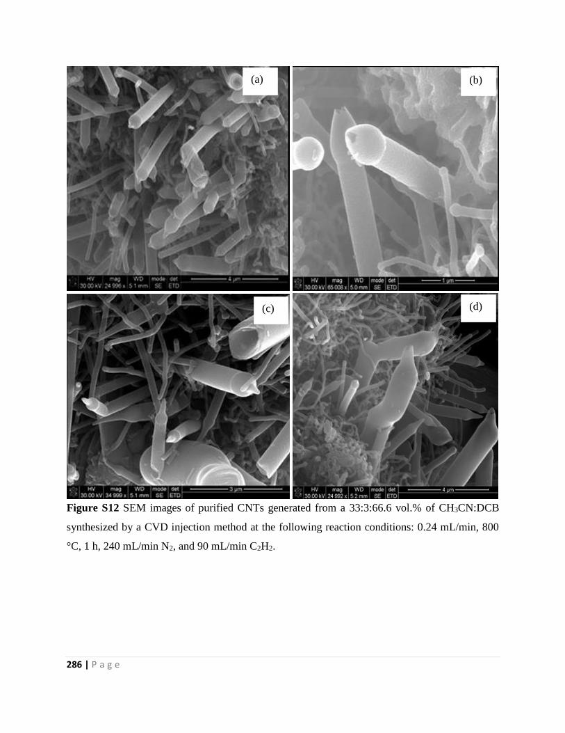
286 | P a g e

Figure S12 SEM images of purified CNTs generated from a 33:3:66.6 vol.% of CH3CN:DCB

synthesized by a CVD injection method at the following reaction conditions: 0.24 mL/min, 800

°C, 1 h, 240 mL/min N2, and 90 mL/min C2H2.

(a)

(d) (c)

(b)

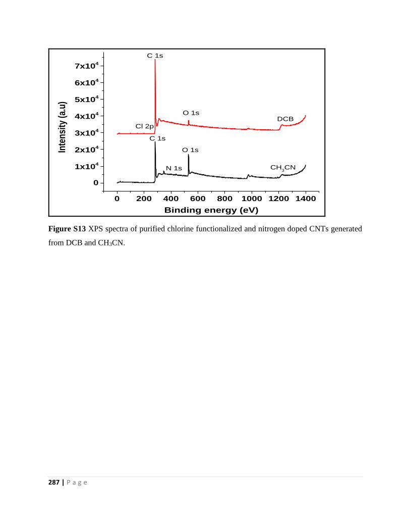
287 | P a g e

0 200 400 600 800 1000 1200 1400

0

1x104

2x104

3x104

4x104

5x104

6x104

7x104

Inte

nsi

ty (

a.u

)

Binding energy (eV)

CH3CN

DCB

N 1s

O 1s

O 1s

Cl 2p

C 1s

C 1s

Figure S13 XPS spectra of purified chlorine functionalized and nitrogen doped CNTs generated

from DCB and CH3CN.

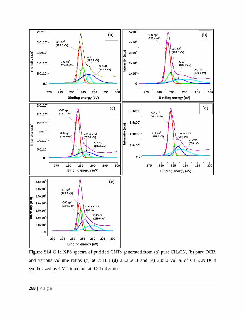
288 | P a g e

270 275 280 285 290 295 300

0.0

5.0x103

1.0x104

1.5x104

2.0x104

2.5x104

Inte

ns

ity

(a

.u)

Binding energy (eV)

C-C sp2

(283.6 eV)

C-C sp3

(284.8 eV)

C-N

(287.4 eV)

O-C=O

(295.1 eV)

275 280 285 290 295 300

0

1x104

2x104

3x104

4x104

5x104

Inte

ns

ity (

a.u

)

Binding energy (eV)

C-C sp2

(283.4 eV)

C-C sp3

(284.5 eV)

C-Cl

(287.7 eV)

O-C=O

(290.1 eV)

275 280 285 290 295 300

0.0

5.0x103

1.0x104

1.5x104

2.0x104

2.5x104

3.0x104

Inte

ns

ity

(a

.u)

Binding energy (eV)

C-C sp2

(283.7 eV)

C-C sp3

(285.0 eV)C-N & C-Cl

(287.1 eV)

O-C=O

(287.1 eV)

275 280 285 290 295 300

0.0

5.0x103

1.0x104

1.5x104

2.0x104

Inte

nsit

y (

a.u

)

Binding energy (eV)

C-C sp2

(283.9 eV)

C-C sp3

(285.4 eV)C-N & C-Cl

(287 eV)O-C=O

(288 eV)

270 275 280 285 290 295 300

0.0

5.0x103

1.0x104

1.5x104

2.0x104

2.5x104

3.0x104

3.5x104

Inte

ns

ity

(a

.u)

Binding energy (eV)

C-C sp2

(283.3 eV)

C-C sp3

(284.1 eV) C-N & C-Cl

(286 eV)

O-C=O

(289.6 eV)

Figure S14 C 1s XPS spectra of purified CNTs generated from (a) pure CH3CN, (b) pure DCB,

and various volume ratios (c) 66.7:33.3 (d) 33.3:66.3 and (e) 20:80 vol.% of CH3CN:DCB

synthesized by CVD injection at 0.24 mL/min.

(a) (b)

(c) (d)

(e)

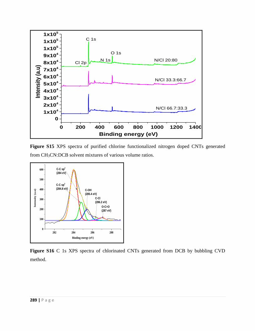
289 | P a g e

0 200 400 600 800 1000 1200 1400

0

1x104

2x104

3x104

4x104

5x104

6x104

7x104

8x104

9x104

1x105

1x105

1x105

N 1s

Inte

nsi

ty (

a.u

)

Binding energy (eV)

N/Cl 66.7:33.3

N/Cl 33.3:66.7

N/Cl 20:80Cl 2p

C 1s

O 1s

Figure S15 XPS spectra of purified chlorine functionalized nitrogen doped CNTs generated

from CH3CN:DCB solvent mixtures of various volume ratios.

282 284 286 2880

100

200

300

400

500

600

In

ten

sit

y (

a.u

)

Binding energy (eV)

C-C sp2

(284 eV)

C-C sp3

(284.8 eV) C-OH

(285.4 eV)

C-Cl

(286.2 eV)

O-C=O

(287 eV)

Figure S16 C 1s XPS spectra of chlorinated CNTs generated from DCB by bubbling CVD

method.

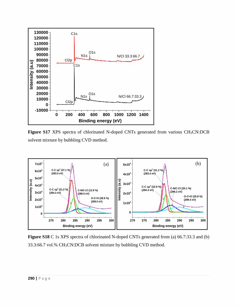
290 | P a g e

0 200 400 600 800 1000 1200 1400-10000

0

10000

20000

30000

40000

50000

60000

70000

80000

90000

100000

110000

120000

130000

O1sN1s

C1s

Cl2p

Inte

nsit

y (

a.u

)

Binding energy (eV)

N/Cl 33.3:66.7

N/Cl 66.7:33.3

Cl2p

C1s

O1sN1s

Figure S17 XPS spectra of chlorinated N-doped CNTs generated from various CH3CN:DCB

solvent mixture by bubbling CVD method.

275 280 285 290 295 300

0

1x104

2x104

3x104

4x104

5x104

6x104

7x104

Inte

ns

ity

(a

.u)

Binding energy (eV)

C-C sp2 (37.1 %)

(283.5 eV)

C-C sp3 (21.2 %)

(284.3 eV)C-N/C-Cl (12.9 %)

(286.0 eV)

O-C=O (28.9 %)

(289.0 eV)

270 275 280 285 290 295 300

0

1x104

2x104

3x104

4x104

5x104

Inte

nsit

y (

a.u

)

Binding energy (eV)

C-C sp2 (31.2 %)

(283.4 eV)

C-C sp3 (22.8 %)

(284.3 eV)C-N/C-Cl (20.1 %)

(286.2 eV)

O-C=O (25.8 %)

(289.4 eV)

Figure S18 C 1s XPS spectra of chlorinated N-doped CNTs generated from (a) 66.7:33.3 and (b)

33.3:66.7 vol.% CH3CN:DCB solvent mixture by bubbling CVD method.

(a) (b)

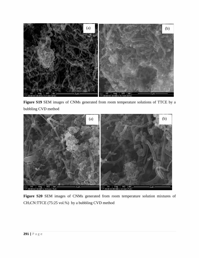
291 | P a g e

Figure S19 SEM images of CNMs generated from room temperature solutions of TTCE by a

bubbling CVD method


CH3CN:TTCE (75:25 vol.%) by a bubbling CVD method

(a) (b)

(a) (b)

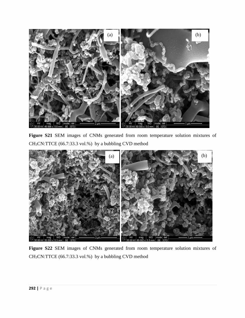
292 | P a g e


CH3CN:TTCE (66.7:33.3 vol.%) by a bubbling CVD method


CH3CN:TTCE (66.7:33.3 vol.%) by a bubbling CVD method

(a) (b)

(a) (b)

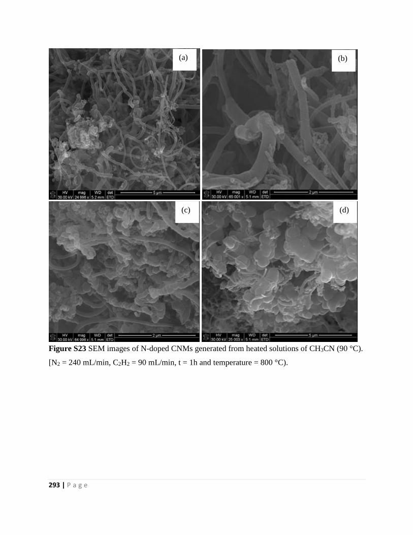
293 | P a g e

Figure S23 SEM images of N-doped CNMs generated from heated solutions of CH3CN (90 °C).

[N2 = 240 mL/min, C2H2 = 90 mL/min, t = 1h and temperature = 800 °C).

(a)

(c) (d)

(b)

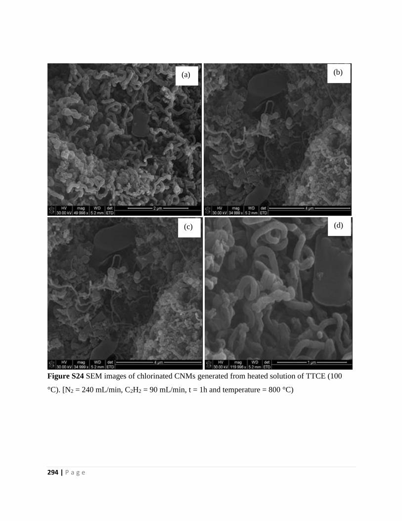
294 | P a g e

Figure S24 SEM images of chlorinated CNMs generated from heated solution of TTCE (100

°C). [N2 = 240 mL/min, C2H2 = 90 mL/min, t = 1h and temperature = 800 °C)

(a)

(d) (c)

(b)

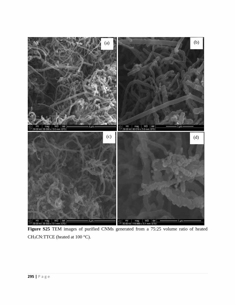
295 | P a g e


CH3CN:TTCE (heated at 100 °C).

(a)

(d) (c)

(b)

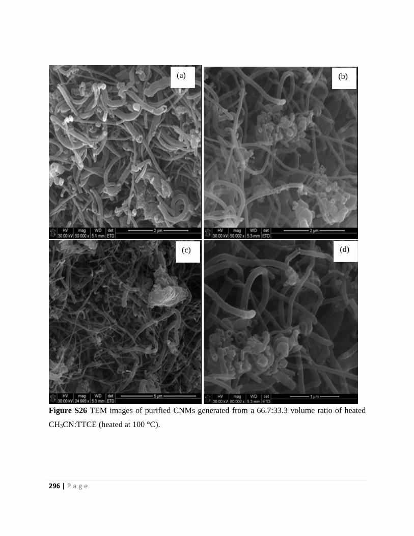
296 | P a g e

Figure S26 TEM images of purified CNMs generated from a 66.7:33.3 volume ratio of heated


(a)

(d) (c)

(b)

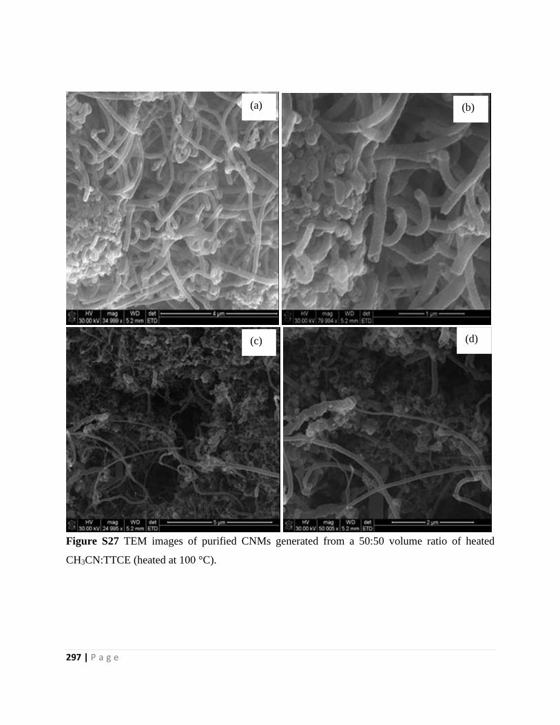
297 | P a g e



(a)

(d) (c)

(b)

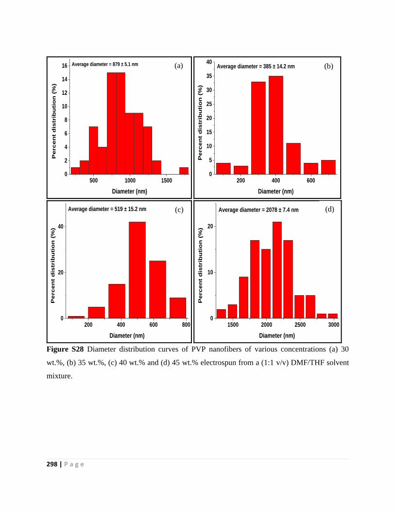
298 | P a g e

500 1000 15000

2

4

6

8

10

12

14

16

Perc

en

t d

istr

ibu

tio

n (

%)

Diameter (nm)


200 400 6000

5

10

15

20

25

30

35

40

Perc

en

t d

istr

ibu

tio

n (

%)

Diameter (nm)


200 400 600 8000

20

40

Pe

rc

en

t d

istr

ibu

tio

n (

%)

Diameter (nm)


1500 2000 2500 30000

10

20

Pe

rc

en

t d

istr

ibu

tio

n (

%)

Diameter (nm)


Figure S28 Diameter distribution curves of PVP nanofibers of various concentrations (a) 30

wt.%, (b) 35 wt.%, (c) 40 wt.% and (d) 45 wt.% electrospun from a (1:1 v/v) DMF/THF solvent

mixture.

(a)

(d) (c)

(b)

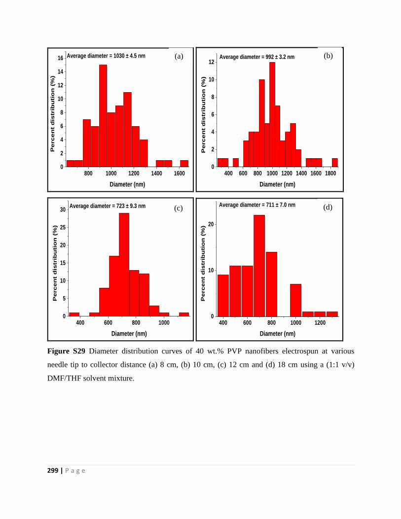
299 | P a g e

800 1000 1200 1400 16000

2

4

6

8

10

12

14

16P

erc

en

t d

istr

ibu

tio

n (

%)

Diameter (nm)


400 600 800 1000 1200 1400 1600 18000

2

4

6

8

10

12

Pe

rc

en

t d

istr

ibu

tio

n (

%)

Diameter (nm)


400 600 800 10000

5

10

15

20

25

30

Pe

rc

en

t d

istr

ibu

tio

n (

%)

Diameter (nm)


400 600 800 1000 12000

10

20

Perc

en

t d

istr

ibu

tio

n (

%)

Diameter (nm)


Figure S29 Diameter distribution curves of 40 wt.% PVP nanofibers electrospun at various

needle tip to collector distance (a) 8 cm, (b) 10 cm, (c) 12 cm and (d) 18 cm using a (1:1 v/v)

DMF/THF solvent mixture.

(a)

(d) (c)

(b)

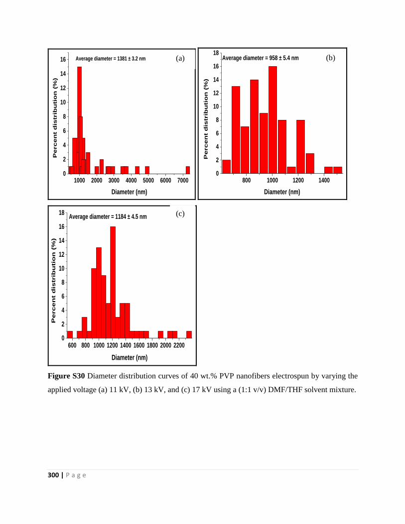
300 | P a g e

1000 2000 3000 4000 5000 6000 70000

2

4

6

8

10

12

14

16P

erc

en

t d

istr

ibu

tio

n (

%)

Diameter (nm)


800 1000 1200 14000

2

4

6

8

10

12

14

16

18

Pe

rc

en

t d

istr

ibu

tio

n (

%)

Diameter (nm)


600 800 1000 1200 1400 1600 1800 2000 22000

2

4

6

8

10

12

14

16

18

Perc

en

t d

istrib

utio

n (

%)

Diameter (nm)


Figure S30 Diameter distribution curves of 40 wt.% PVP nanofibers electrospun by varying the

applied voltage (a) 11 kV, (b) 13 kV, and (c) 17 kV using a (1:1 v/v) DMF/THF solvent mixture.

(a)

(c)

(b)

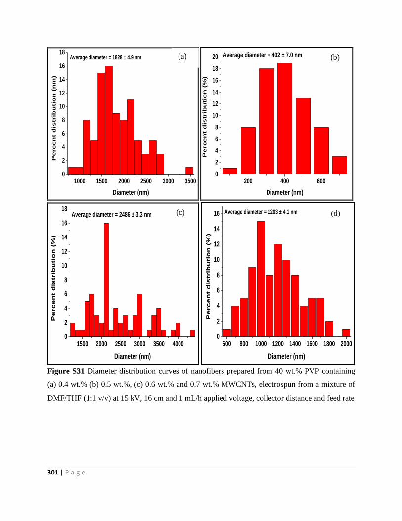
301 | P a g e

1000 1500 2000 2500 3000 35000

2

4

6

8

10

12

14

16

18P

erc

en

t d

istr

ibu

tio

n (

nm

)

Diameter (nm)


200 400 6000

2

4

6

8

10

12

14

16

18

20

Perc

en

t d

istr

ibu

tio

n (

%)

Diameter (nm)


1500 2000 2500 3000 3500 40000

2

4

6

8

10

12

14

16

18

Perc

en

t d

istr

ibu

tio

n (

%)

Diameter (nm)


600 800 1000 1200 1400 1600 1800 20000

2

4

6

8

10

12

14

16P

erc

en

t d

istr

ibu

tio

n (

%)

Diameter (nm)


Figure S31 Diameter distribution curves of nanofibers prepared from 40 wt.% PVP containing

(a) 0.4 wt.% (b) 0.5 wt.%, (c) 0.6 wt.% and 0.7 wt.% MWCNTs, electrospun from a mixture of

DMF/THF (1:1 v/v) at 15 kV, 16 cm and 1 mL/h applied voltage, collector distance and feed rate

(a)

(d) (c)

(b)

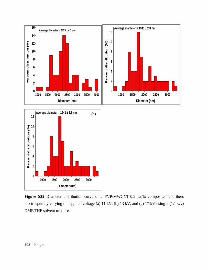
302 | P a g e

1000 1500 2000 2500 3000 3500 40000

2

4

6

8

10

12

14

16P

erc

en

t d

istr

ibu

tio

n (

%)

Diameter (nm)


1000 1500 2000 2500 30000

2

4

6

8

10

12

Pe

rc

en

t d

istr

ibu

tio

n (

%)

Diameter (nm)


1000 1500 2000 2500 30000

2

4

6

8

10

12

Pe

rc

en

t d

istr

ibu

tio

n (

%)

Diameter (nm)



electrospun by varying the applied voltage (a) 11 kV, (b) 13 kV, and (c) 17 kV using a (1:1 v/v)

DMF/THF solvent mixture.

(e)

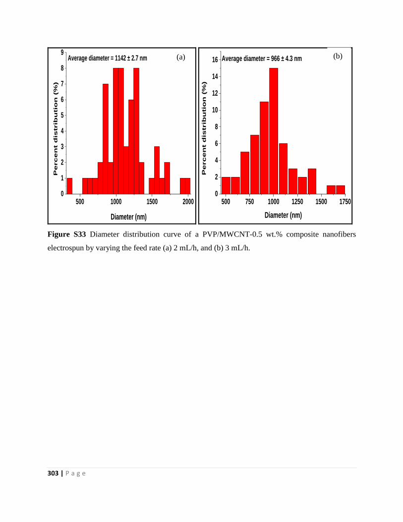
303 | P a g e

500 1000 1500 20000

1

2

3

4

5

6

7

8

9P

erc

en

t d

istrib

utio

n (

%)

Diameter (nm)


500 750 1000 1250 1500 17500

2

4

6

8

10

12

14

16

Pe

rc

en

t d

istrib

utio

n (

%)

Diameter (nm)



electrospun by varying the feed rate (a) 2 mL/h, and (b) 3 mL/h.

(a) (b)

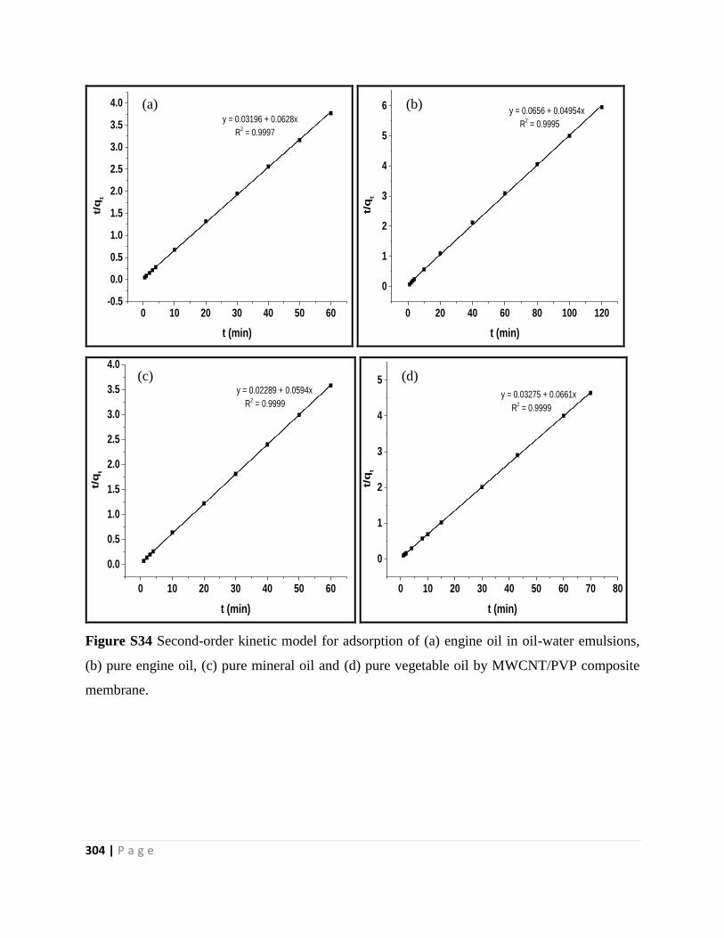
304 | P a g e

0 10 20 30 40 50 60-0.5

0.0

0.5

1.0

1.5

2.0

2.5

3.0

3.5

4.0t/

qt

t (min)

y = 0.03196 + 0.0628x

R2 = 0.9997

0 20 40 60 80 100 120

0

1

2

3

4

5

6

t/q

t

t (min)

y = 0.0656 + 0.04954x

R2 = 0.9995

0 10 20 30 40 50 60

0.0

0.5

1.0

1.5

2.0

2.5

3.0

3.5

4.0

t/q

t

t (min)

y = 0.02289 + 0.0594x

R2 = 0.9999

0 10 20 30 40 50 60 70 80

0

1

2

3

4

5

t/q

t

t (min)

y = 0.03275 + 0.0661x

R2 = 0.9999

Figure S34 Second-order kinetic model for adsorption of (a) engine oil in oil-water emulsions,

(b) pure engine oil, (c) pure mineral oil and (d) pure vegetable oil by MWCNT/PVP composite

membrane.

(a)

(d) (c)

(b)

Documents

use of chlorinated carbon materials to make - CORE