International Conference on Mathematical and Statistical Modeling in Honor of Enrique Castillo. June 28-30, 2006

Useful Differential Formulations for Geometric Processing in Computer Aided Geometric Design

Jaime Puig-Pey*, Akemi Gálvez, Andrés Iglesias,

Pedro Corcuera, José Rodríguez

Dept. of Applied Mathematics and Computational Sciences, University of Cantabria.

Av. de los Castros, s/n, 39005 SANTANDER (SPAIN)

Abstract

This work is about curves lying on surfaces. We use orthogonality as a relevant property for defining some of these curves, such as section by a plane, intersection between surfaces, calculation of the silhouette of a surface. We apply scalar and vector fields, to construct gradient curves on a surface, to deal with the problem of minimum distance between a point and a surface and to calculate initial points of intersection between two surfaces. Curves on a surface which are parallel to a given one, or a curve with its points at a given distance from a fixed point, or helical curves forming a constant angle with a direction, need to be determined as trajectories for mechanical tools in numerically controlled processing of surface machining. For all these problems we introduce some techniques based on differential formulations. They provide a common framework, leading in most cases to explicit first order systems of ordinary differential equations (ODEs) with initial conditions that can be solved efficiently by standard step-by-step integration methods.

Key Words: Geometric processing, Differential Geometry, Tracing curves on surfaces, Scalar and vector fields, CAGD.

1. Introduction

Geometric processing usually means the calculation of geometric properties of entities such as curves, surfaces and solids. In geometric modelling, more attention has been paid to constructive processing for design and less to the

* Correspondence to: Jaime Puig-Pey, E-mail: puigpeyj@unican.es,

analysis of geometric properties, as reported by Barnhill (1992). This work is about curves lying on surfaces related with geometric processing. As a general comment it can be said that a diversity of geometric problems, like belonging, orthogonality, minimization of distances, etc., are represented as equations or systems, nonlinear in general, which are often solved by means of algebraic techniques as made by Bajaj et al (1988), Krishnan and Manocha (1991). But other methods based on differential equations are receiving increasing attention. Thus, Grandine (2000) formulates geometric problems as boundary problems in systems of algebraic-differential equations. Patrikalakis and Maekawa (2002) present both algebraic and differential lines.

In this paper we concentrate on some techniques based on differential formulations (Puig-Pey et al (2003, 2004, 2005)). They provide a common framework, leading in most cases to explicit first order systems of ordinary differential equations with initial conditions, that can be solved efficiently by standard step by step integration methods, available in most numerical libraries (Press et al (1992), The Mathworks Inc. (1999), the Netlib Repository). Basic definitions and properties from classical Differential Geometry, see Struik (1982), are very important tools in this work. We apply them to surfaces expressed in implicit form, f(x,y,z)=0, and also to parametric surfaces, S(u,v)= [x(u,v),y(u,v),z(u,v)], in particular NURBS (Non Uniform Rational B-Splines), a rational piecewise model very common for the definition of free form curves and surfaces in Computer Aided Geometric Design (see a recent overview of CAGD in Farin et al, eds. (2002). Efficient algorithms for evaluation of functions and derivatives associated to NURBS curves and surfaces can be found in the book by Piegl and Tiller (1997), and we make use of them all along our work.

The guidelines of this paper are as follows. First we remind some basic properties related with surfaces and differential arcs of curves. Then we consider the problem of sectioning a surface by a plane, connecting this with scalar and gradient vector fields, and an application to the problem of point-surface distance. After that, we present how to trace the intersection curve between two surfaces using differential geometry arguments. We continue with trajectories on surfaces related with distances and angles: parallel curves and helices; they are used as trajectories for mechanical tools in numerically controlled processing of surface machining, for example the case of dies in the car body industry. And finally the problem of tracing the silhouette of a surface, which is reduced to some of previously studied problems.

2 Mathematical preliminaries for surfaces and curves

We will consider differentiable surfaces given in both parametric and implicit forms. In the first case, they are described by a vector-valued function of two variables S(u,v) = [x(u,v), y(u,v), z(u,v)] , u,v Œ W , W à R2 , where u and v are the surface parameters and W is their domain.

At regular points, the partial derivatives Su(u,v) and Sv(u,v) do not vanish simultaneously. For u=u0; v=v0, Su and Sv are vectors on the tangent plane to the surface at the point S(u0,v0), each being tangent to the parametric or coordinate curve v=v0 and u=u0, respectively. These vectors define the unit normal vector N to S(u,v) (¥ denotes cross vector and || ||2 Euclidean norm):

N = (Su¥ Sv) / || Su¥ Sv ||2 (2.1)

On the other hand, any arbitrary curve C on the surface can be described in parametric form by u=u(t); v=v(t). This expression defines a three dimensional curve on the surface S given by C(t) = S(u(t),v(t)). Applying the chain rule, the tangent vector to curve C at a point C(t) becomes:

C’(t) = dC(t)/dt = Su du(t)/dt + Sv dv(t)/dt , (2.2a)

or as a differential arc of C(t): dC = Su du + Sv dv (2.2b)

It is useful to consider the case in which the curve C is parameterized by the arc-length s. A practical application in computer controlled milling operations is that the curve path followed by the cutter must be parameterized in such a way that neither speeds up nor slows down along the path. Consequently, the arc-length s on the surface is optimal in that case. The differential relation among s, t, u, and v comes from the First Fundamental Form of the Surface, given by:

(ds(t)/dt)2 = E(du(t)/dt)2 + 2F(du(t)/dt)(dv(t)/dt) + G(dv(t)/dt)2 (2.3a)

or in differential form:

ds2= Edu2 + 2Fdudv + Gdv2 (2.3b)

where coefficients E, F, G are ( '·' means dot product):

E = Su·Su , F = Su·Sv , G = Sv·Sv (2.3c)

In some cases, it can be useful to consider s as arc-length measured in the parametric domain for (u,v). The Pythagorean differential relation is then:

ds2= du2 + dv2 (2.3d)

D

dC

S

P

D

dC

S

PCC

For a surface given in implicit form, f(x,y,z)=0, calling fx, fy, fz to the corresponding partial derivatives, the unit normal vector at a nonsingular point P0 = [x0,y0,z0] (the three partials do not vanish simultaneously at P0) is:

N = [fx ,fy, fz]/||fx,fy,fz||2 , (2.4)

A parametrically defined curve C(s)= [x(s),y(s), (s)], has the tangent vector:

dC/ds = [dx/ds, dy/ds, dz/ds] (2.5)

If C(s) is lying on f(x,y,z)=0, the tangent vector is orthogonal to the surface normal N, and then:

fxdx/ds + fydy/ds + fzdz/ds=0 , (2.6a)

or calling dC=[dx, dy, dz] to the differential arc of C, one has the following differential expression:

fxdx + fydy + fzdz = 0 (2.6b)

Further, the elementary arc-length ds of differential arc dC and its components are related by the Pythagorean relationship:

ds2=dx2 + dy2 + dz2 , (2.7a)

or equivalently (tangent vector dC/ds is unitary):

(dx/ds)2+(dy/ds)2+(dz/ds)2 = 1 (2.7b) 3 Surface Sectioning by a plane

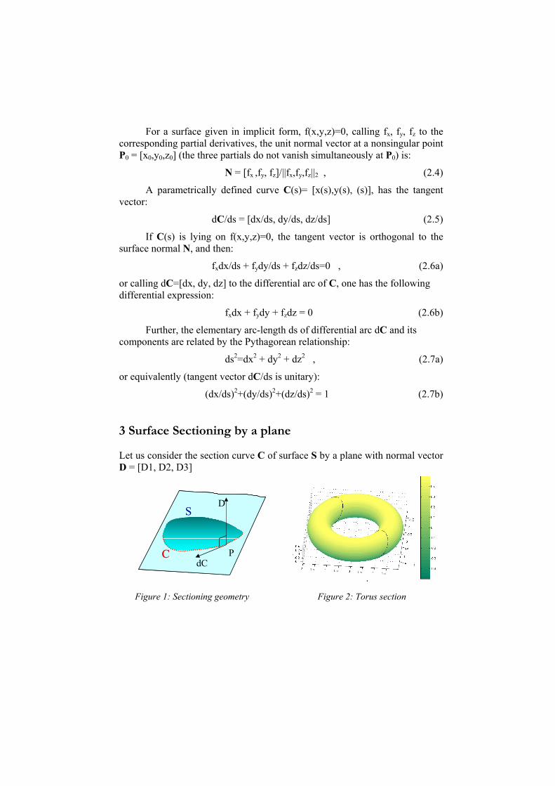
Let us consider the section curve C of surface S by a plane with normal vector D = [D1, D2, D3]

Figure 1: Sectioning geometry Figure 2: Torus section

3.1 Surface in implicit form

For the surface f(x,y,z)=0, we are looking for differential equations verified by C(s). We will take 3 unknowns, dx/ds, dy/ds, dz/ds, the components of the unit tangent vector dC/ds to C. We can consider 3 equations: (2.6a), orthogonality between N and dC/ds; equation (2.7b) , because dC/ds is unitary; and the next one, expressing the orthogonality between dC/ds and the plane normal vector D (Figure 1):

D1 (dx/ds) + D2 (dy/ds) + D3 (dz/ds) = 0 (3.1)

We can solve these 3 equations (2 linear and 1 quadratic) resulting an explicit system of exact first order ordinary differential equations (ODEs). If one gives an initial point of the section curve, we have an initial value problem that can be integrated efficiently with standard routines (Runge-Kutta type, for example). The section of a torus is shown in Figure 2. Observe the 2 components. The differential method permits the tracing of each of the components, but does not inform on the existence of both.

As a particular case, the section of f(x,y,z)=0 by the plane z=0, with normal vector D=[0,0,1], is represented by the 2 ODEs: fy(s)d,fx(s)d xy =±= m

ffdsffds 2y

2x

2y

2x ++ (3.2)

Starting from a known section point one can perform a step-by-step integration. The double signs come from quadratic equation (2.7b), and represent the two pieces of the section curve, one to each side of the initial point. Opposite signs must be chosen, that is, if + in one equation, - must be for the other. This formulation allows to trace a plane curve f(x,y)=0, considered as section of z=f(x,y) by z=0. Notice also that equation fxdx+fydy=0 representing the orthogonality between dC and the normal vector to the curve f(x,y)=0, can be written as a differential equation dy/dx=-fx/fy , or dx/dy = - fy/fx and could be integrated if these explicit formulations are more convenient. The formulation of C(s) as a parametric curve using dx/ds and dy/ds is more adequate if the section curve is not a uniform function involving x and y. 3.2 Surface in parametric form

Given S(u,v)=[x(u,v),y(u,v),z(u,v)], a curve C(s) on S(u,v) can be defined by expressions u(s), v(s) for the parameters, as functions of a variable s that can be a distance parameter. The curve is then: C(s) =[x(u(s),v(s)), y(u(s),v(s)),

z(u(s),v(s))]. If s is taken as the arc length in the image of C(s) in the (u,v) domain, the Pythagorean relation in this case is:

ds2=du2+dv2 or (du/ds)2+(dv/ds)2=1 (3.3)

The tangent direction to C(s) is given by (2.2a) and, as in the implicit case, it must be orthogonal to the sectioning plane normal D, that is D·dC/ds = 0, or using (2.2a),

(D·Su) (du/ds)+ (D·Sv) (dv/ds) = 0 (3.4)

Combining (3.3) with (3.4) and solving:

du/ds= (±) (Sv·D)/denom , dv/ds= (°) (Su·D)/denom , (3.5) denom= 2

v2

u ·· )()( DSDS + ,

which are exact differential equations for the section curve. Starting from a known initial point on it, we have an initial value problem for that explicit first order system of ODEs, in terms of the surface parameters as dependent variables. Double signs must be taken + with - or - with +; they express the two possible pieces of section curve, one to each side of the initial point.

If the arc length on the surface in 3D space is taken, expression (2.3b) must be used; combining it with (3.4) it results:

du/ds= (±) (Sv·D)/ denom , dv/ds= (°) (Su·D)/ denom (3.6)

denom= 2

vvu2 ·G··F2 )())(( DSDSDS +−u ·E )( DS

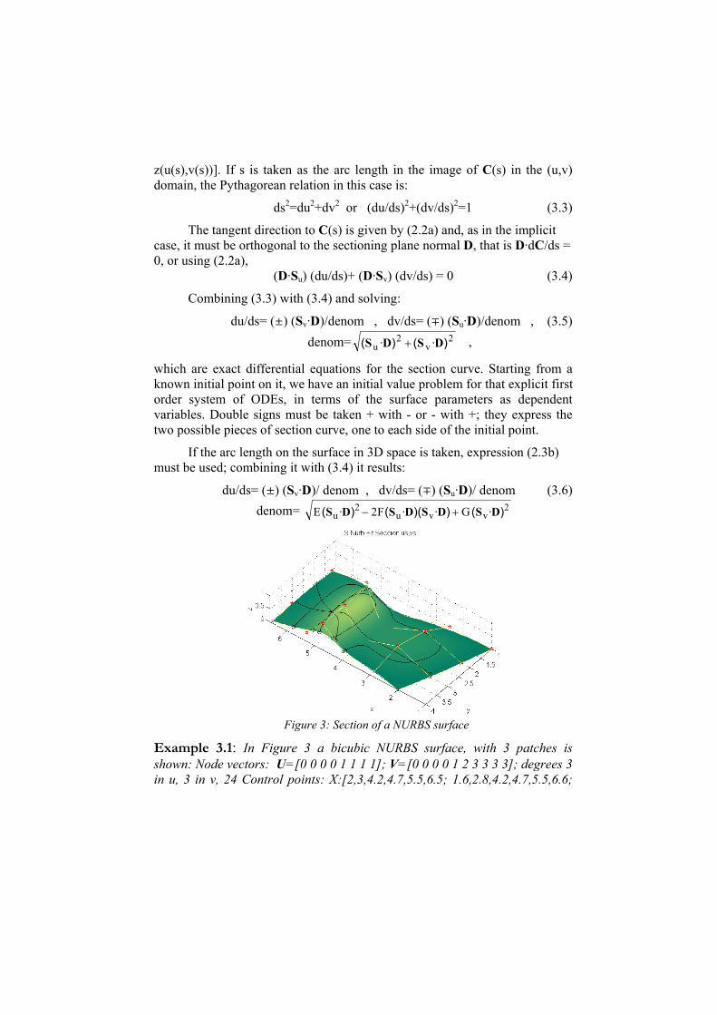
Figure 3: Section of a NURBS surface

Example 3.1: In Figure 3 a bicubic NURBS surface, with 3 patches is shown: Node vectors: U=[0 0 0 0 1 1 1 1]; V=[0 0 0 0 1 2 3 3 3 3]; degrees 3 in u, 3 in v, 24 Control points: X:[2,3,4.2,4.7,5.5,6.5; 1.6,2.8,4.2,4.7,5.5,6.6;

1.3,2.6,4,4.7,5.5,6.6;1,2.5,4,5,5.5,6.5]; Y:[4,3.8,3.7,4,3.7,4;3,3,3,3,3,3;2,2, 2.2,2,2,2;1,1,1.5,1.3,1,1.3]; Z:[0,0,0,1,0,0.1;0,0.5,0,1,0,0;0,0.5,0,1,0,0; 0,0,0,0,0,0.1]; Weights vector W:[1,2,3,1,1,1;1,1,3,2,1,1;1,1,3,4,1,1;1,1,3,1, 1, 1]; Normals to 4 sectioning planes: D: [0,0,1]; [1,1,1]; [0,1,0]; [0,0,1]; 4 Projection curves of a vector field on a surface

-15 -10 -5 0 5 10 15-15

-10

-5

0

5

10

15

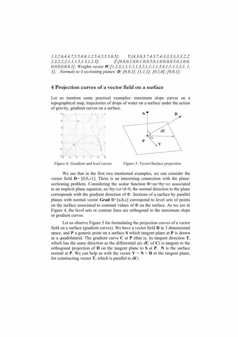
Let us mention some practical examples: maximum slope curves on a topographical map, trajectories of drops of water on a surface under the action of gravity, gradient curves on a surface.

P

dC

V

D N Figure 4: Gradient and level curves Figure 5: Vector/Surface projection

We see that in the first two mentioned examples, we can consider the vector field D= [0,0,±1]. There is an interesting connection with the plane-sectioning problem. Considering the scalar function Φ=ax+by+cz associated to an implicit plane equation, ax+by+cz+d=0, the normal direction to the plane corresponds with the gradient direction of Φ. Sections of a surface by parallel planes with normal vector Grad Φ=[a,b,c] correspond to level sets of points on the surface associated to constant values of Φ on the surface. As we see in Figure 4, the level sets or contour lines are orthogonal to the maximum slope or gradient curves.

Let us observe Figure 5 for formulating the projection curves of a vector field on a surface (gradient curves). We have a vector field D in 3 dimensional space, and P a generic point on a surface S which tangent plane at P is drawn as a quadrilateral. The gradient curve C at P (that is, its tangent direction T, which has the same direction as the differential arc dC of C) is tangent to the orthogonal projection of D on the tangent plane to S at P. N is the surface normal at P. We can help us with the vector V = N × D in the tangent plane, for constructing vector T, which is parallel to dC:

T = N × V = (N·N)D– (N·D)N, (4.1) 4.1 Implicit case

For the differential arc of gradient curve C, dC = [dx, dy, dz, ] we have the Pythagorean expression (2.7a) for the arc length s on C. Considering the components of T=[T1, T2, T3], that can be calculated from (4.1), it must be:

dx/T1 = dy/T2 = dz/T3, (4.2)

Solving from (2.7a) and (4.2), we have for C(s) the following exact first order explicit system of ODEs (||T||2=T12+T22+T32):

dx/ds = ± T1 / ||T||2 dy/ds = ± T2 / ||T||2 (4.3) dz/ds = ± T3 / ||T||2 ,

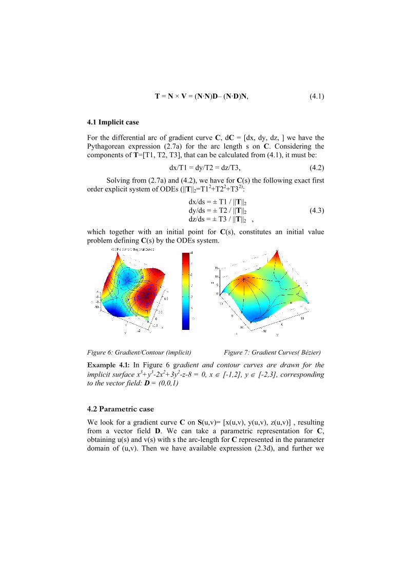
which together with an initial point for C(s), constitutes an initial value problem defining C(s) by the ODEs system. Figure 6: Gradient/Contour (implicit) Figure 7: Gradient Curves( Bézier)

Example 4.1: In Figure 6 gradient and contour curves are drawn for the implicit surface x3+y3-2x2+3y2-z-8 = 0, x ∈ [-1,2], y ∈ [-2,3], corresponding to the vector field: D = (0,0,1) 4.2 Parametric case

We look for a gradient curve C on S(u,v)= [x(u,v), y(u,v), z(u,v)] , resulting from a vector field D. We can take a parametric representation for C, obtaining u(s) and v(s) with s the arc-length for C represented in the parameter domain of (u,v). Then we have available expression (2.3d), and further we

impose the orthogonality between dC and vector V in Figure 5, this is dC·V = dC·(D¥N) = 0 , and remembering (2.2b):

Su·(D¥N) du + Sv·(D¥N) dv = 0 (4.4)

Combining (2.3d) and (4.4), we can solve for du/ds and dv/ds, giving:

2v

2u

v

))())(

·(dsdu

NDSNDS

NDS

××

×

+±=

·(·(

))(

(4.5)

2v

2u

u

))())(

·(dsdv

NDSNDS

NDS

××

×

+±=

·(·(

))(

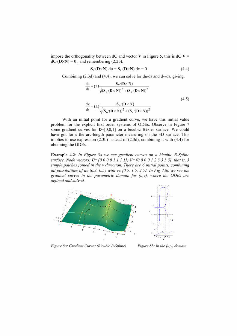
With an initial point for a gradient curve, we have this initial value problem for the explicit first order systems of ODEs. Observe in Figure 7 some gradient curves for D=[0,0,1] on a bicubic Bézier surface. We could have got for s the arc-length parameter measuring on the 3D surface. This implies to use expression (2.3b) instead of (2.3d), combining it with (4.4) for obtaining the ODEs. Example 4.2: In Figure 8a we see gradient curves on a bicubic B-Spline surface. Node vectors: U=[0 0 0 0 1 1 1 1]; V=[0 0 0 0 1 2 3 3 3 3], that is, 3 simple patches joined in the v direction. There are 6 initial points, combining all possibilities of u∈{0.3, 0.5} with v∈{0.5, 1.5, 2.5}. In Fig 7.8b we see the gradient curves in the parametric domain for (u,v), where the ODEs are defined and solved. Figure 8a: Gradient Curves (Bicubic B-Spline) Figure 8b: In the (u,v) domain

4.3 Application to minimum distance between a surface and an external point

The closest point problem is a classic of geometric problems for curves and surface. It continues to be analyzed to optimize its calculation, as in Ma and Hewitt (2003). An external point Q =[Q1,Q2,Q3] to a surface S is given, and one tries to obtain a point on S which is the closest to Q according to the usual Euclidean distance. We consider the continuous problem, that is, when in the area of interest on S, the distance from its points to Q varies continuously. The key idea is to use as vector field D, the gradient vector field induced on S by the scalar field associated to the squared Euclidean distance between the fixed point Q and a generic 3D point, that is:

Φ = (x-Q1)2+(y-Q2) 2+(z-Q3)2 (4.6)

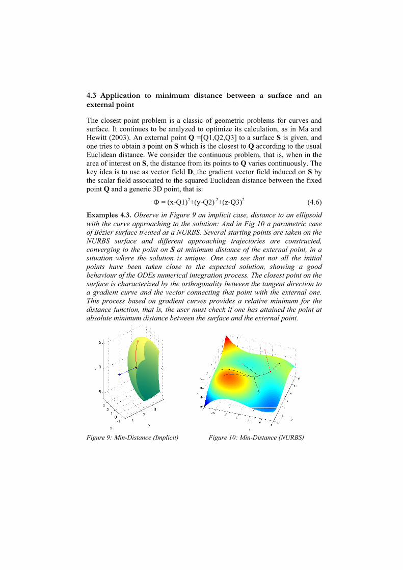
Examples 4.3. Observe in Figure 9 an implicit case, distance to an ellipsoid with the curve approaching to the solution: And in Fig 10 a parametric case of Bézier surface treated as a NURBS. Several starting points are taken on the NURBS surface and different approaching trajectories are constructed, converging to the point on S at minimum distance of the external point, in a situation where the solution is unique. One can see that not all the initial points have been taken close to the expected solution, showing a good behaviour of the ODEs numerical integration process. The closest point on the surface is characterized by the orthogonality between the tangent direction to a gradient curve and the vector connecting that point with the external one. This process based on gradient curves provides a relative minimum for the distance function, that is, the user must check if one has attained the point at absolute minimum distance between the surface and the external point.

Figure 9: Min-Distance (Implicit) Figure 10: Min-Distance (NURBS)

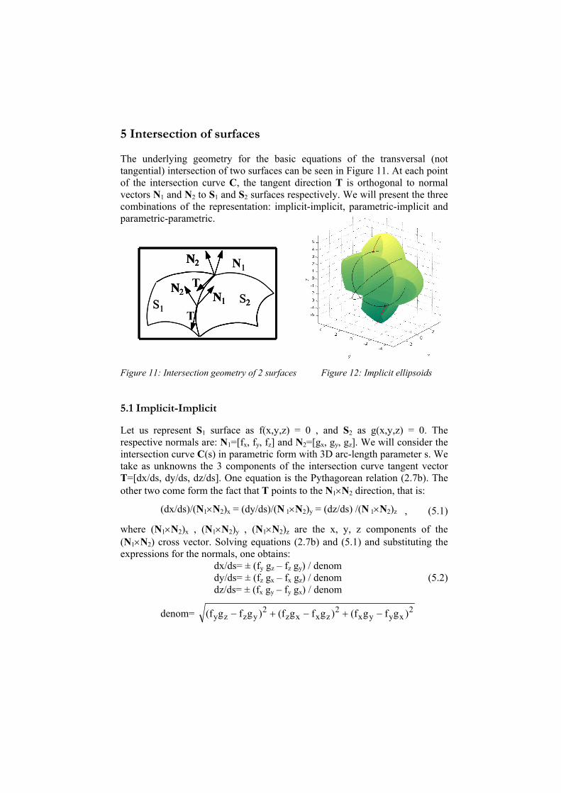
5 Intersection of surfaces

The underlying geometry for the basic equations of the transversal (not tangential) intersection of two surfaces can be seen in Figure 11. At each point of the intersection curve C, the tangent direction T is orthogonal to normal vectors N1 and N2 to S1 and S2 surfaces respectively. We will present the three combinations of the representation: implicit-implicit, parametric-implicit and parametric-parametric.

T

1 1NN

1 1 SS NNNN 1 1 1 1 2 22 2SS

NNNN 2 2 2 2

NNNN 2 2 2 2

T

Figure 11: Intersection geometry of 2 surfaces Figure 12: Implicit ellipsoids 5.1 Implicit-Implicit

Let us represent S1 surface as f(x,y,z) = 0 , and S2 as g(x,y,z) = 0. The respective normals are: N1=[fx, fy, fz] and N2=[gx, gy, gz]. We will consider the intersection curve C(s) in parametric form with 3D arc-length parameter s. We take as unknowns the 3 components of the intersection curve tangent vector T=[dx/ds, dy/ds, dz/ds]. One equation is the Pythagorean relation (2.7b). The other two come form the fact that T points to the N1×N2 direction, that is:

(dx/ds)/(N1×N2)x = (dy/ds)/(N 1×N2)y = (dz/ds) /(N 1×N2)z , (5.1)

where (N1×N2)x , (N1×N2)y , (N1×N2)z are the x, y, z components of the (N1×N2) cross vector. Solving equations (2.7b) and (5.1) and substituting the expressions for the normals, one obtains:

dx/ds= ± (fy gz – fz gy) / denom dy/ds= ± (fz gx – fx gz) / denom (5.2) dz/ds= ± (fx gy – fy gx) / denom

denom= 2xyyx

2zxxz

2yzzy )gfg(f)gfg(f)gfg(f −+−+−

System (5.2) contains exact explicit first order ODEs for the intersection curve. Knowing an initial intersection point as initial value, the intersection curve can be traced by numerical integration.

Example 5.1. Figure 12 shows the intersection of two ellipsoids. There are more than one curve component, then it is necessary to obtain one initial point for each of the components before proceeding with the integration. One can see two approaching curves for attaining these initial points. 5.2 Implicit-Parametric

Let us consider S1 as S(u,v) and S2 as f(x,y,z) = 0 , and its normal N2 = [fx, fy, fz]. We look for a parametric representation C(s)=S(u(s),v(s)), for the intersection curve, with s the arc-length of C(s) as a 3D curve, being the unknowns du/ds and dv/ds. From the First Fundamental Form (2.3a) we have one equation. The other comes from the orthogonality between the tangent to C(s), T=dC/ds (expression (2.2a) and s as parameter), and the normal N2 to the implicit S2: (dC/ds)·N2 = 0 , that is, (Su ·N2)du/ds+(Sv ·N2) dv/ds = 0. Solving these equations, it results:

du/ds = ± (Sv·N2) / denom dv/ds = ° (Su·N2) / denom (5.3)

22u2u2v

22v )·G()·)(·2F()·(E NSNSNSNS +−denom=

Adding an initial point on S1: u(0)=u0, v(0)=v0, we have an initial value problem for this explicit first order system of ODEs.

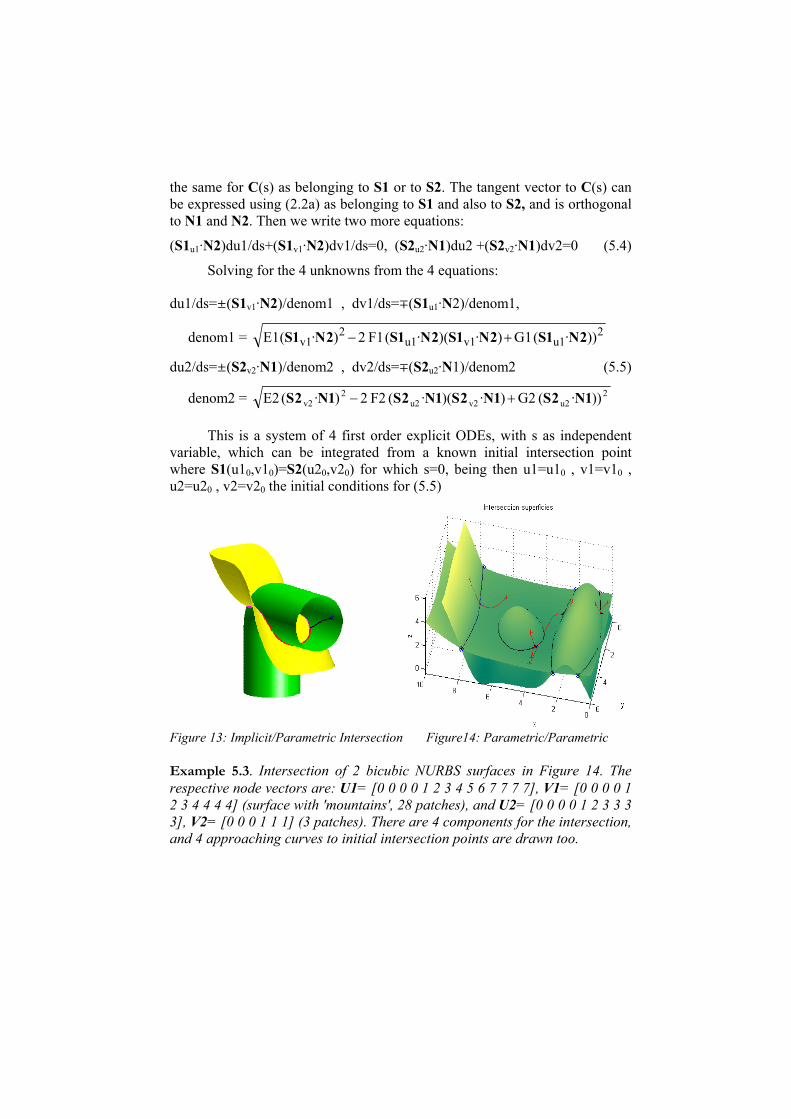
Example 5.2. Figure 13 shows the 'cubic chair' (x/2)3–(y/2)3– z/2=0, and a parametric biquadratic B-Spline with 5×9 control points and node vectors: U= [0,0,0,1/3,2/3,1,1,1], V = [0,0,0,1/4,1/4,1/2,1/2, 3/4,3/4,1,1,1]. The surface contains 3×4=12 different patches. One can distinguish an approaching curve to an initial point on the intersection curve. 5.3 Parametric-Parametric

Let us consider the parametric surfaces: S1: S1(u1,v1) and S2: S2(u2,v2). The respective normals: N1=S1u1×S1v1 , N2=S2u2×S2v2 , the respective differential arc-lengths: dC1 = S1u1du1+S1v1dv1, dC2 = S2u2du2+ S2v2dv2 . We will take as unknowns the derivatives du1/ds, dv1/ds, du2/ds, dv2/ds, with s the 3D arc-length of the intersection curve C(s) . Two equations come from the First Fundamental Form (2.3a) applied to each surface. Observe that parameter s is

the same for C(s) as belonging to S1 or to S2. The tangent vector to C(s) can be expressed using (2.2a) as belonging to S1 and also to S2, and is orthogonal to N1 and N2. Then we write two more equations:

(S1u1·N2)du1/ds+(S1v1·N2)dv1/ds=0, (S2u2·N1)du2 +(S2v2·N1)dv2=0 (5.4)

Solving for the 4 unknowns from the 4 equations:

du1/ds=±(S1v1·N2)/denom1 , dv1/ds=°(S1u1·N2)/denom1,

denom1 = 2u1v1u1

2v1 ))·( G1)·)(·( F1 2)·(E1 2N1S2N1S2N1S2N1S +−

du2/ds=±(S2v2·N1)/denom2 , dv2/ds=°(S2u2·N1)/denom2 (5.5)

denom2 = 2u2v2u2

2v2 ))·( G2)·)(·( F2 2)·(E2 1N2S1N2S1N2S1N2S +−

This is a system of 4 first order explicit ODEs, with s as independent variable, which can be integrated from a known initial intersection point where S1(u10,v10)=S2(u20,v20) for which s=0, being then u1=u10 , v1=v10 , u2=u20 , v2=v20 the initial conditions for (5.5) Figure 13: Implicit/Parametric Intersection Figure14: Parametric/Parametric Example 5.3. Intersection of 2 bicubic NURBS surfaces in Figure 14. The respective node vectors are: U1= [0 0 0 0 1 2 3 4 5 6 7 7 7 7], V1= [0 0 0 0 1 2 3 4 4 4 4] (surface with 'mountains', 28 patches), and U2= [0 0 0 0 1 2 3 3 3 3], V2= [0 0 0 1 1 1] (3 patches). There are 4 components for the intersection, and 4 approaching curves to initial intersection points are drawn too.

5.4 Gradient curves for obtaining initial intersection points

Scalar and vector field ideas can be applied for obtaining different initial points of the intersection curve. There are other ways for these points, see Patrikalakis and Maekawa (2002), Abdel-Malek and Yeh (1997), but we will describe now how gradient curves are useful for this task. 5.4.1 Implicit-Implicit case

The surfaces are represented by f(x,y,z)=0 and g(x,y,z)=0 (Figure 15, left: 2 ellipsoids, I-I case). We describe schematically the ideas.

. The function g(x,y,z) associated to the implicit surface g(x,y,z)=0 can be considered as a scalar field in R3 , and this field defines 2 disjoint regions: g(x,y,z)>0 and g(x,y,z)<0. . A path from one region to the other crosses the implicit surface g(x,y,z)=0 . A point on g(x,y,z) can be identified by the change of sign of g(x,y,z) when walking and traversing g=0 along the path. This is like a 'curved ray tracing' for meeting a point on g(x,y,z)=0. . For the vector field in R3: Grad(g) = (gx, gy, gz), at a given 3D point P, Grad(g) points to the direction of maximum increase of g moving from P.

Basic process: > Take an arbitrary point Pi on f(x,y,z)=0 > 'Walk' on the implicit surface f(x,y,z)=0 from Pi, along a gradient curve on f=0, according to the vector field D=(±)Grad(g(x,y,z)), choosing sign according to the value of g at Pi, for increasing or decreasing that value. > Until a point where the sign of g(x,y,z) changes, that is, an intersection point.

5.4.2 Parametric-Implicit case

The surfaces are represented by S(u,v) and f(x,y,z)=0 (see in Figure 15, center, P-I case: parametric biquadratic NURBS and implicit x2+y3+z5-1=0). The process is quite similar to the implicit-implicit situation.

. The function f(x,y,z) associated to the implicit surface f(x,y,z)=0 defines a scalar field in R3 . For this scalar field there are 2 disjoint regions: f(x,y,z)>0 and f(x,y,z)<0.

The basic process is: > Take an arbitrary point Pi on S(u,v) . > 'Walk' on S(u,v) from Pi, along a gradient curve on it, defined by D=(±)Grad(f(x,y,z)), choosing sign according to the value of f at Pi.

right): I-I, P-I, P-P

> Until a point where f(x,y,z) changes its sign, that is, an intersection point.

5.4.3 Parametric-Parametric case

The surfaces are S1(u1,v1) and S2(u2,v2) (Figure 15, right, P-P case: cylinder and sphere in cylindrical and spherical coordinates). Now we have not scalar fields directly as f(x,y,z) or g(x,y,z) in the other cases. We use a new scalar field, the distance between two generic points on S1(u1,v1) and S2(u2,v2):

D2= (S1(u1,v1)-S2(u2,v2)) · (S1(u1,v1)-S2(u2,v2)) (5.6)

This scalar field is defined in the 4-dimension space W, Cartesian product of the parametric domains of S1 and S2, with variables u1,v1,u2,v2. We will consider flux or gradient curves in this space defined by -Grad(D2), because we look for trajectories in W reducing the value of D2. Taking the Euclidean arc-length in W, defined by:

ds2 = du12+dv12 +du22 +dv22 , (5.7)

those flux curves are defined by:

du1/ds = - ∂D2/∂u1 / ||Grad(D2)||2 dv1/ds = - ∂D2/∂v1 / ||Grad(D2)||2 (5.8) du2/ds = - ∂D2/∂u2 / ||Grad(D2)||2 dv2/ds = - ∂D2/∂v2 / ||Grad(D2)||2 ,

again an explicit first order system of ODEs.

The basic scheme for obtaining one intersection point between S1 and S2 is:

> Take an arbitrary initial point Pi=(u1i, v1i, u2i, v2i) in W > Walk from Pi along a flux curve given by (5.8), which follows the minimizing direction of (-Grad(D2)). > Until a point in W where D2=0 (with a predetermined precision), which will be an intersection point.

Figure 15: Initial intersection point (left to

Example 5.4. Observe in Figure 15 right, the P-P example of cylinder-sphere intersection, both in parametric form, where 2 approaching curves, one on each surface, can be distinguished. They converge simultaneously towards an intersection point. The presence of these 2 approaching curves corresponds to the fact that the search is made in the 4-dimensional space W, based on the parameters of the 2 surfaces. 6 Trajectories on surfaces related with distances and angles 'Parallel curves' and 'helicoidal curves' on surfaces are interesting in geometric processing for understanding shapes and also in Computer Aided Manufacturing for defining working paths for tools of numerically controlled machines (see Choi and Jerard (1998), and Patrikalakis and Maekawa (2002)). They can be also relevant when designing curves lying on a surface where de control of distances or slopes is important, like in railways, roads, etc. 6.1 Parallel curves on surfaces

We can consider parallel curves to a given one, with their points displaced a constant distance in some sense with respect to the reference curve, as in Figure 16, or curves whose points maintain a constant distance with respect a given polar point on the surface, polar isodistance curves, as in Figure 17. Figure 16: Curve parallel curves Figure 17: Polar isodistance curves

We will comment the case of a surface in parametric form, S(u,v). The underlying idea for the construction of 'parallel' curves is as follows. From each point of the base curve C0, a curve is traced on the surface, with some

criteria for the connection to C0, orthogonality, for example. An arc of that traced curve, with predetermined length L from the origin point measured on the surface (L-length arc), is considered. Repeating this process on many points of the base curve, one obtains a set of points at distance L from the base curve, which constitute the 'parallel' curve. The definition of this parallel curve by a discrete set of points can be improved for practical purposes considering an interpolating cubic spline of the obtained points at distance L. If the L-length arcs are constructed using geodesic curves orthogonal to the base curve, one has 'geodesic' offsets (see Patrikalakis and Maekawa (2002)). Those geodesic arcs are constructed by solving a 4 ODEs system with initial conditions (initial point and orthogonality to C0). Geodesics have the property of minimum distance between points.

A different approach is to use plane sections of S(u,v) for the L-length arcs. The formulation is simpler, similar to the presented in paragraph 3. The normal vector D for the sectioning plane is in this case the tangent direction to the base curve C0 at the initial point of each L-length arc. According to expression (2.2a), if C0 is defined by u=u0(t), v=v0(t), this normal vector will be D=Sudu0(t)/dt+Svdv0(t)/dt. The arc of the corresponding normal section curve Cn(s) can be calculated by integration of a system of ODEs. It is convenient to obtain for Cn(s) a parametric representation u=u(s), v=v(s) where s is the arc-length of Cn in 3D on the surface, instead of taking s as the arc length in the parametric domain of (u,v), as we made in paragraph 3. Then, the differential equations involving du/ds and dv/ds result from the First Fundamental Form (2.3a) and equation D·dCn/ds=0 , which express the orthogonality between the normal section curve tangent and the normal to the sectioning plane:

22 )·G()·)(·2F()·(E

·)(

dsdu

uvuv

v

DSDSDSDS

DS

+−±=

(6.1)

22 )·G()·)(·2F()·(E

·)(

dsdv

uvuv

u

DSDSDSDS

DS

+−= m ,

One takes as initial conditions u(0)=u0(t) , v(0)=v0(t), the parametric values of the initial point on C0(t). The signs must be chosen + with - or - with +, attending to which side of C0(t) the L-length normal arc has to be traced. The integration is performed step by step until attaining the value L for s. The trajectories obtained for these normal sections have not the minimum distance property of geodesics, but the fact that normal sections are plane curves lying on S(u,v) can be adequate for the dynamics of numerical controlled machines,

in comparison with geodesics which in general are not plane. The process for tracing polar isodistance curves on S(u,v) with respect a pole point needs some analysis to characterize the family of rotating planes containing the normal to S(u,v) at the pole. If the tangent vector Sv is considered at the pole, it can be shown that, with F = Su·Sv , G = Sv·Sv,

Sv^ = - G Su + F Sv, (6.2)

2v2v

2v

2v

v

2v

v αsinαcosSSSS

SSSn

+=⊥⊥⊥

⊥

is an orthogonal vector to Sv, belonging to the tangent plane at the pole. Consequently, a unit vector n forming angle α with Sv, can be calculated in the tangent plane by:

vuαsin FαcosGαsin SS · ++−= (6.3)

This vector n is taken as normal vector to each plane belonging to the family of rotating planes. For different rotation angles and the corresponding normal planes, L-length arcs are calculated for different normal section curves. Joining limit points on those arcs at distance L from the pole, the isodistance curve for L is obtained.

Examples 6.1 Figure 16 shows a family of 'parallel curves' on a NURBS surface. As can be seen, 'parallel' curves often have self-intersection points, and some post-processing can be necessary to deal with them. Figure 17 shows a family of polar isodistance curves on a NURBS surface. 6.2 Helicoidal curves on surfaces

The problem is how to obtain a helix curve C(s) lying on a surface, with a parametric representation where s is the 3D arc-length on the surface. Helix curve C(s) has to maintain a constant angle φ with the constant direction of a given unit vector D. 6.2.1 Implicit Surface

For the surface f(x,y,z)=0, we take as unknowns the components of the unit tangent vector to C(s), T=dC/ds=[dx(ds, dy/ds, dz/ds]. The conditions will be: orthogonality between T and the normal to the surface (expression (2.6a)); Pythagorean relation for the differentials (expression (2.7b) , and the given angle φ between T and D, dC/ds)·D=cos(φ).

For the particular case of D=[0,0,1], solving for dx/ds, dy/ds, dz/ds, gives:

2y

2x

zx

ffdiscrimcosff

dsdx

+

±ϕ−=

2y

2x

zy

ff

discrimcosffdsdy

+

ϕ−=

m (6.4)

ϕ= cosdsdz ,

discrim = (fx2+fy

2) sin2(φ)-fz2cos2(φ)

Taking an initial point (x0,y0,z0) on f(x,y,z)=0 as initial condition for the previous system of ODEs, x(0)=x0, y(0)=y0 , z(0) = z0, a helix from this point can be obtained. If discrim is negative at a point, there is no helix through that point. There are 2 possible helices for a valid angle φ . They correspond to select + with -, or - with + , before the square roots in (6.4).

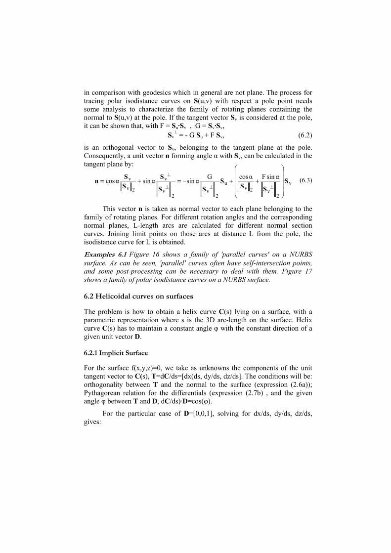
Examples 6.2. At the left of the Figure 18, the two possible helices on a cone for a valid angle φ are drawn. At the right, a helix lying on the implicit surface (x2+y2)z2 +0.25(x2+y2)-0.25=0 is shown. ϕ D Figure 18: Left, 2 helices on a cone. Right, helix on (x2+y2)z2 +0.25(x2+y2)-0.25=0 6.2.2 Parametric Surface

For a surface S(u,v), we will take now as unknowns the derivatives du/ds, dv/ds, for obtaining an helix curve C(s) in parametric form, calculating u(s), v(s), with s the 3D arc-length on the surface. The underlying equations will be the First Fundamental Form (2.3a) and, as in the implicit case, the angle condition (dC/ds)·D=cos(φ) , using expression (2.2a) for the tangent. The resulting system of explicit first order ODE is:

2Adiscrim)·2(B

dsdu v DS±−

=

ϕ D D

(6.5a)

2Adiscrim)·2(*B

dsdv u DSm−

=

discrim = (F2-EG) cos2φ+A , E, F, G the First Fundamental Form coefficients

2uvu

2v )·G()·)(·2F()·E(A DSDSDSDS +−=

))·G()·F(cos2B uv DSDS −ϕ= ( ))·E()·F(cos2B* vu DSDS −ϕ= ( (6.5b)

There are two solutions if discrim >0 and no solution if discrim<0. The helix is constructed starting at a surface point u(0)=u0, v(0)=v0 , as initial condition for the integration.

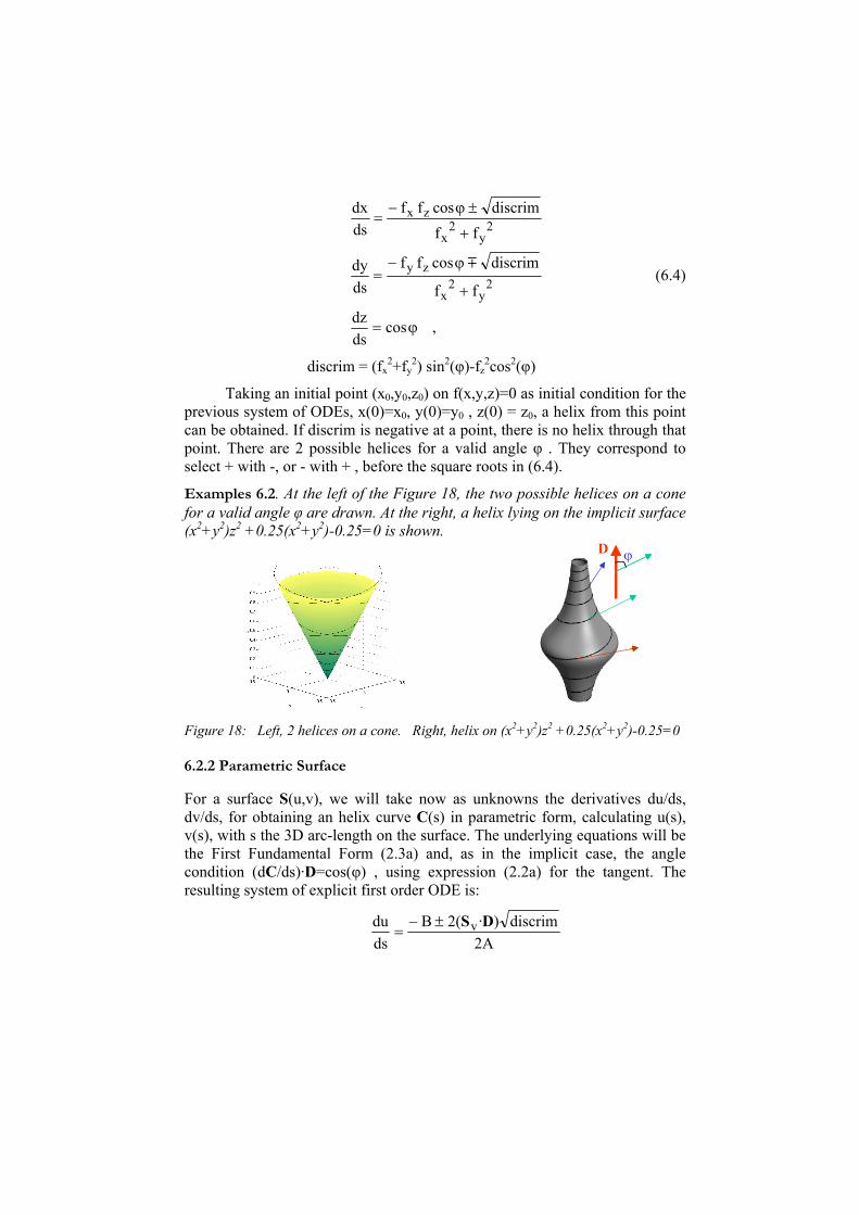
Examples 6.3. At the left of Figure 19 there is an helix on a NURBS surface, of degree 2 for u and v, node vectors U=[0,0,0,1,1,2,2,3,3,4,4,4], V= [0,0,0,1,2,3,4,4,4], 6×9 control points, 16 patches and C1 continuity between them. With this continuity, the integration runs softly between patches because the equations are first order only. At the right it is shown a helix on a bicubic simple Bézier surface patch. Figure 19: Left , helix on a biquadratic NURBS . Right, helix on a bicubic Bézier 7. Silhouette curve on a surface

This problem appears in robotics and computer vision for control of visibility, etc. An efficient method for calculating the silhouette of a canal surface is presented by Kim and Lee (2003). The general problem is equivalent to the construction of the curve of contact between the surface and the cone circumscribing the surface, with its vertex at the observation point. If the vision is parallel, similar statements can be made, referring to the cylinder

circumscribing the surface, with its axis in the direction of the observation. In the case of conic vision, the condition is that the line joining each point of the silhouette curve with the cone vertex, must be orthogonal to the surface normal at the considered silhouette point. The formulation for this case of conic vision is presented in the following. 7.1 Surface in implicit form

Let f(x,y,z)=0 be the implicit equation of a surface S. At a point [x,y,z] of S placed on the silhouette curve, with the vision point Q = [Q1,Q2,Q3], the two following conditions must be verified:

f(x,y,z)=0 (7.1a) ([x,y,z]-Q) · [fx, fy, fz]=0 ≡ (x-Q1)fx+(y-Q2)fy + (z-Q3)fz=0 , (7.1b)

This system of 2 equations with 3 unknowns, represents the silhouette, and can be understood as the intersection of two surfaces given in implicit form, that we have studied previously.

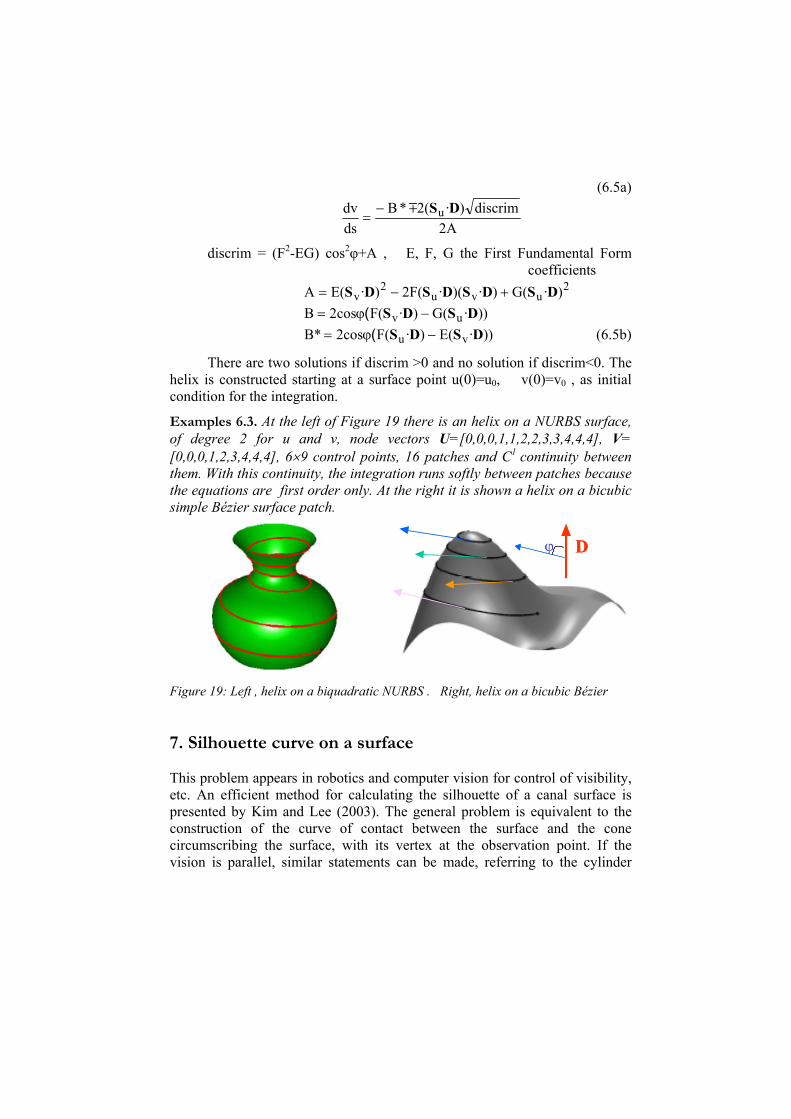
Example 7.1. In the left of Figure 20 it is shown a silhouette on a revolution paraboloid. The curve has only one component. The gradient curve for approaching an initial point of the silhouette is also drawn.

Figure 20: Silhouette and approaching curves. Left: Implicit surface. Right: Parametric (NURBS)

7.2 Surfaces in parametric form

If the surface is in parametric form, S(u,v)=[x(u,v),y(u,v),z(u,v)], the points on the silhouette verify:

(S(u,v)-Q)·(Su(u,v)×Sv(u,v))=0 ≡ c(u,v)=0 (7.2),

that is, the silhouette appears as an implicit equation that we have called c(u,v)=0. Its graphical representation is a plane curve in the parametric domain of the u,v parameters of S. If c(u,v) is algebraic, González-Vega and Necula (2002) introduced a method for deducing precisely the topology of this curve. As we commented in paragraph 3.1 the curve can be traced efficiently by using a differential formulation.

An initial point is needed, and it can be obtained by solving the scalar equation (7.2) when a value is assigned to u or v. As an alternative, the scalar and vector field idea can be fruitful. The scalar function c(u,v) in the u,v domain plays the role of a Φ scalar field, and, a gradient curve or flux line following Gradient(Φ) is obtained in a step by step integration process, advancing in the gradient direction with the adequate orientation, starting at an ‘freely chosen‘ initial point (recommended not far from the expected silhouette curve) in the u,v domain, until detecting a change in sign in the value of c(u,v), thus getting the point verifying c(u,v)=0, which will be an initial point for tracing the silhouette curve.

Example 7.2. Figure 20 (right) shows a silhouette example on a NURBS surface, with the image on the surface of the approaching gradient curves in the u,v domain. The point of view has been carefully chosen such that the silhouette curve has two different components. Both are calculated after using Gradient(c(u,v)) to obtain one initial point on each of the two components. Due to the fact that the surface has limiting borders, the whole silhouette curve observed from the point of view consists of the two calculated curves and four border pieces, delimited on the borders by the other two curves. 8. Other practical considerations

The methodology presented here has the advantage of being quite general, because it is valid for any type of smooth functions involved in the surface equations, and it does not depend on being polynomial, or rational or other. For the formulation to have sense, it is merely necessary that they can be differentiated. In the case of surfaces consisting of several patches, the ODEs are valid inside each patch, and special attention has to be paid in the transition from one patch to another, taking into account the continuity between them. If there are not strong discontinuities, one can progress smoothly between patches, because only low order derivatives appear in the ODEs. In other case, the border crossing point must be carefully identified, with the integration of the ODEs starting from it as the initial point for traversing the next patch.

The first order explicit ODEs systems associated with initial value problems can be treated numerically with methods that are widely available, fast and reliable. In our case we have used the integrator function ode45 of MATLAB (The Mathworks Inc. (1999)), which is based on an adaptive step-by-step technique combining 4th and 5th order Runge-Kutta methods for controlling the error and the step integration size. The user can specify values for absolute and relative error tolerances. The routine allows for using stopping criteria in simple ways, controlling common conditions for values of the variables or for certain functions appearing in the problem. There is no perfect numerical procedure for solving all cases of initial value ODEs problems, but to our experience this integrator function has shown a very good behaviour. Let us mention too the routines odeint, rkqs, rkck, in the book Numerical Recipes by Press et al (1992) that are available in C and C++, Fortran 77 and 90 languages. They are adaptive step size integration procedures based on a Runge-Kutta technique as well. In The Netlib Repository one can find also a wide variety of tested computer codes for different numerical problems, including ODEs.

Regarding stopping criteria for the step-by-step integration processes in the problems included here, one case will appear when going beyond some limit in the domain of definition of the x,y,z variables or for the u,v parameters. Or when constructing a L-length arc for parallel curves the arc-length parameter attains that value L. In the case of a closed intersection, silhouette, etc. curve, the obtaining of a repeated point when constructing the curve needs to be checked in order to identify the situation. In the closest point problem, an orthogonality condition is met for the tangent to a gradient curve when arriving to a minimum distance. The crossing of a curve or surface following a gradient curve identifies a point for an intersection or a silhouette curve. And other cases that could be happen depending on the studied problem

The presence of singular points on a surface (zero values for partial derivatives, undefined normals) introduces singularities in the ODEs. Although floating point calculations make it more difficult to obtain exact zero values, they can lead to numerical instabilities when the integration arrives in the neighbourhood of such points.

The explained methods are deduced from the analysis of a local behaviour at differential level. In the case of a solution curve with several components, these techniques are not sufficient for an automatic identification of all the simple components. Any criteria for generating different trajectories in the associated initial value problem will be useful for approaching the different components. A similar comment can be made for the closest point problem when the solution point is not unique.

Acknowledgements

This work has been partially supported by the Spanish Ministry of Education and Science (research projects MTM2005-00287 and DPI2001-1288) and the Department of Applied Mathematics and Computational Science of the University of Cantabria (Santander, Spain). References

ABDEL-MALEK, K., YEH, H.J. (1997). On the determination of starting points for parametric surface intersections. Computer-Aided Design, 28: 21–35.

BAJAJ,C.L., HOFFMANN,C.M., LYNCH,R.E., HOPCROFT,J.E.H. (1988). Tracing surface intersections. Computer Aided Geometric Design: 5(4):285-307.

BARNHILL R.E., editor. (1992). Geometry Processing for Design and Manufacturing. SIAM.

CHOI, B.K. and JERARD, R.B. (1998). Sculptured Surface Machining. Theory and Applications. Kluwer Academic Publishers, Dordrecht.

FARIN, G., HOSCHEK, J., KIM, M.S. (2002). Handbook of Computer Aided Geometric Design. Elsevier Science, Amsterdam

GONZÁLEZ-VEGA, L, NECULA, I. (2002). Efficient topology determination of implicitly defined algebraic plane curves. Computer Aided Geometric Design, 19(9): 719-743.

GRANDINE, T.A. (2000). Applications of Contouring. SIAM Review, 42(2): 297-316.

KIM, K.J. and LEE, I.K. (2003). The Perspective Silhouette of a Canal Surface. COMPUTER GRAPHICS Forum, 22(1): 15-22.

KRISHNAN, S. and MANOCHA, D. (1997). An efficient surface intersection algorithm based on lower dimensional formulation. ACM Transactions on Graphics, 16(1): 74-106.

MA, Y.L. and HEWITT, W.T. (2003). Point inversion and projection for NURBS curve and surface: Control polygon approach. Computer Aided Geometric Design, 20(2): 79-99.

PATRIKALAKIS, N.M. and MAEKAWA, T. (2002). Shape Interrogation for Computer Aided Design and Manufacturing. Springer-Verlag, Berlin.

PIEGL, L. and TILLER, W. (1997). The NURBS Book. 2nd ed. Springer-Verlag. Berlin.

PRESS, W.H., TEUKOLSKY, S.A., VETTERLING, W.T., FLANNERY, B.P. (1992). Numerical Recipes. 2nd ed. Cambridge University Press.

PUIG-PEY, J., GÁLVEZ A., IGLESIAS, A., RODRÍGUEZ, J., CORCUERA, P. (2003). Intersection of Surfaces using Differential Geometry and Field Functions. In R. Quirós et al, ed., Spanish Conference on Computer Graphics CEIG 2003, pp. 205-218 (in Spanish). Univ. of Coruña and Eurographics Spanish Chapter.

PUIG-PEY J., GÁLVEZ A., IGLESIAS A. (2004) Helical Curves on Surfaces for Computer-Aided Geometric Design and Manufacturing. Lecture Notes in Computer Science, 3044: 771-778.

PUIG-PEY, J., GÁLVEZ, A., IGLESIAS A., RODRÍGUEZ, J., CORCUERA P., GUTIÉRREZ, F. (2005). Some applications of scalar and vector fields to geometric processing of surfaces. Computers and Graphics, 29:719-725

STRUIK, D.J. (1988). Lectures on Classical Differential Geometry, 2nd ed. Dover Publications, New York.

THE MATHWORKS INC. (1999). Using Matlab. Natick, MA. Mathworks.

THE NETLIB REPOSITORY. Oak Ridge Lab. U.S. Department of Energy. http://www.netlib.org