1

Using statistical control charts to monitor duration-based performance of

project

Nooshin Yousefia, Ahmad Sobhanib, Leila Moslemi Naenic, Kenneth R. Curried

a Department of Industrial & Systems Engineering, Rutgers University, Piscataway, NJ, 08854 b Department of decision and Information sciences, scholl of business administration Oakland University

c School of Built Environment, University of Technology Sydney, Australia d Department of Industrial Engineering, West Virginia University, Morgantown, WV,26505

Abstract

Monitoring of project performance is a crucial task of project managers that significantly affect

the project success or failure. Earned Value Management (EVM) is a well-known tool to

evaluate project performance and effective technique for identifying delays and proposing

appropriate corrective actions. The original EVM analysis is a monetary-based method and it

can be misleading in the evaluation of the project schedule performance and estimation of the

project duration. Earned Duration Management (EDM) is a more recent method which

introduces metrics for the project schedule performance evaluation and improves EVM

analysis. In this paper, we apply statistical control charts on EDM indices to better investigate

the variations of project schedule performance. Control charts are decision support tools to

detect the out of control performance. Usually project performance measurements are auto-

correlated and not following the normal distribution. Hence, in this paper, a two-step

adjustment framework is proposed to make the control charts applicable to non-normal and

auto-correlated measurements. The case study project illustrates how the new method can be

implemented in practice. The numerical results conclude that that employing control chart

method along with analyzing the actual values of EDM indices increase the capability of project

management teams to detect cost and schedule problems on time.

Keywords: Earned Duration Management, Statistical Control Charts, Project Performance

Evaluation.

1. Introduction

Project management is the application of processes, methods, knowledge, skills, and

experience to achieve project objectives and minimize the risk of project failure (Meredith,

Mantel, & Shafer 2015). With respect to the complexity of today’s projects, many project

management tools are developed to support managers in controlling and aligning projects with

their planned timelines, scopes and budgets (Project Management Institute, 2008). One of the

important project management methods is Earned Value Management (EVM) that measures

the performance and progress of a project in an objective manner by integrating scope, schedule

2

and cost elements of the project (Project Management Institute, 2005; Salehipour, Naeni,

Khanbabaei, & Javaheri 2015). The Project Management Institute (PMI) extensively discussed

the basic terminology and formulas of the EVM method in 2000. This terminology was

simplified, and more details on EVM were provided in the 3rd edition of Project Management

Body Of Knowledge (PMBOK) (Project Management Institute, 2004). EVM mainly focuses

on the accurate measurement of the work in progress against a detailed plan of the project by

creating performance indices for cost, time and project completion (Fleming & Koppelman,

1996; Chen, Chen, & Lin,2016). Comparing the planned values of these performance indices

(determined according to the baseline plan) with their actual records, will enable managers to

keep the project on the track and figure out how will be the project future performance (Project

management Institute, 2013).

There has been some research discussed the application of EVM methodology and associated

benefits to control/monitor projects in different disciplines (e.g., Cioffo, 2006; Vandevoorde &

Vanhoucke, 2006; Abba & Niel, 2010; Turner, 2010). For instance, Rodríguez et al., (2017)

discussed the benefits of applying EVM for managing large projects in the aerospace industry.

Batselier & Vanhoucke (2015a) used empirical data from 51 real-life projects to evaluate the

accuracy of EVM time and cost indicators. Several studies have also challenged the accuracy

of EVM in predicting the progress of a project and proposed extensions for the EVM

methodology to provide more accurate results (e.g., Lipke, 2003; Henderson, 2003;

Vandevoorde & Vanhoucke, 2006; Lipke, Zwikael, Henderson, & Anbari, 2009; Azman,

Abdul-Samad, & Ismail 2013; Colin & Vanhoucke, 2014; Narbaev & Marco, 2015, Salari,

Yousefi & Asgary 2016).

Lipke (2003) argued the shortcomings of the schedule indicators of EVM and their inaccurate

estimated values when projects are close to their ends and their performances are poor. To

improve the accuracy of EVM schedule performance indicators, Lipke introduced the concept

of Earned Schedule (ES). ES is a straightforward translation of EV into time units by

determining when the EV should have been earned in the baseline. Although this extension

improves the accuracy of indices and project forecasts but still include the major drawbacks of

EVM by considering monetary-based factors in evaluating the project schedule performance.

EVM method uses monetary based factors as proxies to estimate the schedule/duration

performance of a project through its life cycle. However, the employment of cost-based metrics

to control the duration/schedule of a project is misleading as cost and schedule profiles are not

generally the same during the project life cycle (Khamooshi & Golafshani, 2014).

3

Although EDM method has improved the accuracy of managers’ prediction about the schedule

performance of projects, there are no studies consider EDM indices to evaluate the deviations

of a project from the baseline plan throughout the project life cycle. Due to several reasons

such as unavailability of the resources and delays in completing tasks, the project may

experience the schedule and budget overruns. Monitoring the project, detecting cost and

schedule performance variations, and accomplishing corrective actions are necessary to lead a

project management team towards the successful completion of the project.

One of the innovative approaches to monitoring performance deviations of a project from the

base plan is to use methods that statistically track the trends of performance indices of projects

(e.g., Barraza & Bueno, 2007; Aliverdi, Naeni, & Salehipour, 2013). These statistical methods

will let practitioners know the acceptable range of project performance deviations. They also

help project management practitioners to figure out the cause of unacceptable (non-random)

deviations which may generate unexpected costs and delays in the future. Using statistical

methods to analyse project data also reveals informative insights to project performance trends,

especially in high priority projects (Aliverdi, Naeni, & Salehipour, 2013). This information

helps project managers better understand the tendency and the direction of a project’s

performance in advance. Hence, these methods can minimize the project’s overtime and over

budget in a right time during the project life. Several studies applied statistical models to

manage project performance deviations by controlling EVM indices throughout the project life

cycle (e.g., Lipke, & Vaughn, 2000, Leu & Lin 2008; Aliverdi, Naeni, & Salehipour, 2013).

This paper aims to extend and improve the capability of traditional project management tools

in dealing with project performance variations from the baseline plan with respect to EDM

methodology that decouples schedule and cost dimensions of projects. Shewhart individuals

control charts are generated individually for EDM cost and schedule performance indices to

detect the presence of unacceptable (non-random) variations. According to the theory,

individuals control charts are valid when the distribution of data is normal and there is no

dependency/autocorrelation between them. However, these assumptions are not always valid

in real-world projects. To overcome these limitations and achieve more reliable results, this

study proposes a two-step adjustment framework that checks the normality data and normalizes

the distribution of on-normal measurements. Also, the proposed framework also introduces the

application of Autoregressive Integrated Moving Average models to remove autocorrelation

effects. The results of this research demonstrate the employment of a more accurate project

performance factors in controlling the deviations of a project from its baseline plan.

4

The remainder of the paper is organized as follows. First, an overview of EDM is provided.

Second, statistical process control method and the normality and independency assumptions in

using statistical control charts technique are discussed. Our proposed adjustment framework

that lets users apply control charts technique on non-normal and auto correlated data sets is

also introduced. Third, the numerical results of evaluating a project’s cost and schedule

performance deviations based on EDM measurements, estimated from a construction project

case study are presented. Finally, the conclusion of the paper and the future line of research

are provided.

2. Overview of Earned Duration Management (EDM)

Khamooshi and Golafshani (2014) discussed the deficiencies of EVM and Earned Schedule

indices and introduced EDM. This method aims to decouple the cost and schedule dimensions

completely. Therefore, schedule performance measures are all developed according to

duration-based factors and are now accurate enough to be used in monitoring and predicting

the duration trend of a project. While EVM is evaluating project progress based on comparing

PV (planned value) and AC (actual cost) with EV (earned value), in EDM methodology

introduced three new concepts: 1) Total Planned Duration or TPD, 2) Total Actual Duration or

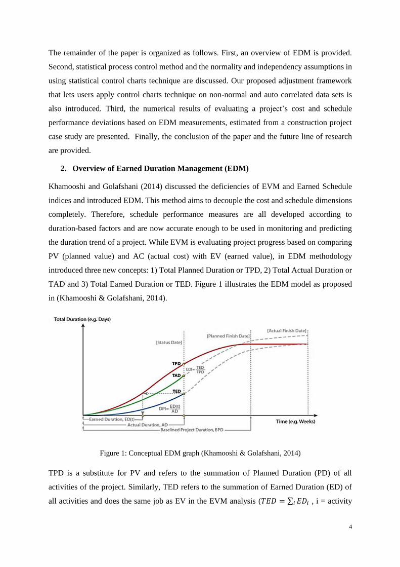
TAD and 3) Total Earned Duration or TED. Figure 1 illustrates the EDM model as proposed

in (Khamooshi & Golafshani, 2014).

Figure 1: Conceptual EDM graph (Khamooshi & Golafshani, 2014)

TPD is a substitute for PV and refers to the summation of Planned Duration (PD) of all

activities of the project. Similarly, TED refers to the summation of Earned Duration (ED) of

all activities and does the same job as EV in the EVM analysis (𝑇𝐸𝐷 = ∑ 𝐸𝐷𝑖𝑖 , i = activity

5

index). TPD is also calculated according to the summation of all Planned Duration (PD) and of

the same activities (𝑇𝑃𝐷 = ∑ 𝑃𝐷𝑖𝑖 , 𝑖 = activity index).

In EDM terminology, a schedule performance index is introduced as Earned Duration Index

(EDI) which is defined as follows.

𝐸𝐷𝐼 =𝑇𝐸𝐷

𝑇𝑃𝐷

(1)

𝐸𝐷𝐼 is defined as a duration-based measurement indicator that specifies the overall work

performed in terms of the duration aspect of the project by comparing it with the work planned

up to any given point in time.

In EVM system, Earned Schedule (ES) is calculated by projecting the EV curve on to the PV

curve. Similarly, the TED can be projected on TPD which shows the ED(t), as shown in Fig.

1. ED(t) identifies the time that achieving the current ED was expected to occur. Using ED(t)

and Actual Duration (AD) a new schedule index is introduced which is called Duration

Performance Index (DPI) and calculated as follows.

𝐷𝑃𝐼 =𝐸𝐷(𝑡)

𝐴𝐷

(2)

𝐷𝑃𝐼 shows how well the project is performing to meet the final completion date from the

schedule performance points of view. It provides a more accurate result than 𝑆𝑃𝐼𝑡 and is

usually compared with 1. If 𝐷𝑃𝐼 > 1, it indicates a good schedule performance for the project.

Hence, the project is ahead of its planned schedule. If 𝐷𝑃𝐼 < 1, it indicates poor schedule

performance for the project and it may behind the planned schedule. If 𝐷𝑃𝐼 = 1, it shows that

the project is on the plan and it does not have any delays with the respect of the planned

schedule.

Using duration-based schedule performance indices enables the EDM system to provide more

precisions for managers in evaluating and controlling the project from both time (schedule) and

cost points of view (Khamooshi & Golafshani, 2014, Yousefi 2018). EDM indices will be used

in our proposed project management control approach to track and analyze the deviations of a

given project from the scheduled plan during its life cycle.

In this paper, EDI and DPI together with CPI (cost performance index which is defined as

EV/AC) will be used in the proposed project management control approach to track and analyse

the deviations of a given project from the scheduled plan during its life cycle.

6

3. Evaluating the Behaviour of Project Performance by Applying Individuals

Control Charts

Cost and schedule indices of EDM are measured based on what has been achieved and what

was going to be attained. The deviations of these performance measurement indicators would

be the signs of an improper progress for the project. Generally speaking, deviations of a

project’s performance from the baseline plan can be clustered as controlled and uncontrolled

deviations (e.g., Thor, Lundberg, Ask, Olsson, Carli, Härenstam, & Brommels 2007).

Controlled deviations that are also called random or acceptable deviations, are mostly inherent

in a project and are not identified very important. In contrast, the uncontrolled deviations that

are also called unacceptable or non-random are often due to some deficiencies in the progress

of the project that have not been noticed in the baseline plan. These unacceptable deficiencies

may result in unexpected delays or over budget runs. To prevent or reduce these undesirable

time and cost losses, it is necessary to monitor the behaviour of the project performance by

analyzing the deviations of EDM indices during the project life cycle. The Shewhart individual

statistical control charts technique is an analytical method that provides valuable information

to distinguish between controlled (acceptable) and uncontrolled (unacceptable) deviations in

EDM indices. This information supports project manager decisions on how to keep the project

on track by detecting deficiencies in the progress of the project and taking corrective actions

on time.

In the next section, we review Shewhart individual control charts technique applied in this

paper to control the deviations of EDM indices over time. We also discuss the limitations of

this technique and introduce our two-step adjustment framework, which overcomes these

limitations and enhances the validity and practicality of the Shewhart control charts application

in real world projects.

4. Individual Statistical Control Charts

Statistical Process Control (SPC) is a branch of statistics, which is used to monitor and control

processes. Applying SPC helps managers to detect performance variations through a project

life cycle and identify important factors affecting the project (Oakland, 2007). Many types of

SPC tools exist for controlling, but statistical control charts technique is one of the most

operational methods among them.

7

Shewhart proposed the fundamentals of statistical control charts in the 1920’s. Although some

other researchers tried to improve statistical control charts, Shewhart control charts technique

is still the most useful and accurate method (Oakland, 2007). The Shewhart control charts can

divide variations into two types (also called type A and B here) in a way to distinguish between

sources of variations (Montgomery, 2009). Type A variations are due to chance and random

causes, resulted from inherent features of the process. These variations are inevitable and also

called acceptable variations. Type B variations are taken place by assignable and special

causes, resulting from a problem such as human and/or machine errors (e.g., Russo, Camargo,

& Fabris 2012). These variations are also called unacceptable variations. In reality, it is

important to detect assignable causes that may result time and financial losses for projects. The

Shewhart control charts technique is widely used because of the simplicity of the method to

implement. This technique has also a high accuracy to detect even small deviations and

associated sources (Franco et al., 2014). For the purpose of this study, we applied Shewhart

individuals control charts to monitor measurements associated with CPI, EDI, and DPI

separately.

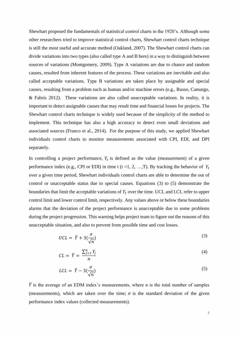
In controlling a project performance, 𝑌𝑡 is defined as the value (measurement) of a given

performance index (e.g., CPI or EDI) in time t (t =1, 2, …,T). By tracking the behavior of 𝑌𝑡

over a given time period, Shewhart individuals control charts are able to determine the out of

control or unacceptable status due to special causes. Equations (3) to (5) demonstrate the

boundaries that limit the acceptable variations of 𝑌𝑡 over the time. UCL and LCL refer to upper

control limit and lower control limit, respectively. Any values above or below these boundaries

alarms that the deviation of the project performance is unacceptable due to some problems

during the project progression. This warning helps project team to figure out the reasons of this

unacceptable situation, and also to prevent from possible time and cost losses.

𝑈𝐶𝐿 = �̅� + 3(𝜎

√𝑛) (3)

𝐶𝐿 = �̅� = ∑ 𝑌𝑗

𝑛𝑗=1

𝑛

(4)

𝐿𝐶𝐿 = �̅� − 3(𝜎

√𝑛) (5)

�̅� is the average of an EDM index’s measurements, where n is the total number of samples

(measurements), which are taken over the time; 𝜎 is the standard deviation of the given

performance index values (collected measurements).

8

In order to estimate the control limits used for monitoring the progress of a project, we need an

initial set of samples. These samples are used to estimate the initial control limits (Montgomery,

2009; Salehipour, Naeni, Khanbabaei, & Javaheri 2015). Then, we check the status of samples

and remove the out of control ones, if assignable causes were found. New control limits are

estimated after removing the out of control samples. Again, the status of the remained samples

will be checked. If any out of control samples exist, they will be removed and the new control

limits will be determined according to the remained samples. This procedure is repeated until

all samples are inside control limits (reasoning behind repeating this procedure is well

explained by Montgomery, 2009). From this point, the final control limit estimations can be

used to monitor the deviation of samples (measurements). According to Xie, Goh and

Kuralmani, (2002), Shewhart individuals control charts provide valid results only if

measurements evaluated by this technique satisfy the following conditions:

A. There is a normal distribution for measurements;

B. There is no independency (autocorrelation) between measurements

However, in a real-world situation, project performance measurements, such as EDI and CPI

values may not have a normal distribution and independency conditions. For this reason, before

using control charts, we need to make sure that the project performance measurements are

normally distributed and independent. Therefore, we introduce a two-step adjustment

framework to make sure that measurements used by the control charts technique are

independent and normally distributed. Figure 2 demonstrates the diagram of the proposed

adjustment framework.

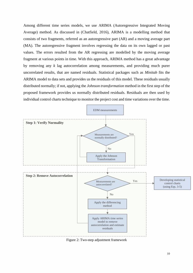
5. Two-step Adjustment Framework

As illustrated in Figure 2, in the first step, the normality of measurements is statistically tested

by using Anderson- Darling hypothesis (D’Agostino and Stephens, 1986). This test can be

performed by statistical packages such as Minitab. In this study, we test the normality of EDI

and DPI values collected over the time. According to the normality test includes the following

hypothesis:

H0: Measurements follow a normal distribution

H1: Measurements do not follow a normal distribution

The results of the normality test would lead us to reject or accept the null hypothesis. If the null

hypothesis is not rejected, it is implied that the distribution of data is most likely normal.

9

Otherwise, the null hypothesis is rejected, which is confirming that the distribution is not

normal.

If measurements are not distributed normally, an appropriate transformation method should be

applied in order to generate a normal distribution for them. The normality of transformed

results is checked again until the distribution of measurements becomes normal. In this

research, Johnson transformation is applied in order to obtain normally distributed data.

In the second step, time series analysis is completed to remove the autocorrelation of the data.

Because statistical theory shows that the existence of autocorrelation in data would result in

generating false alarms when the control charts technique is used to monitor deviations. This

analysis is completed by checking the autocorrelation among measurements and verifying the

stationary of data. Statistical software uses different ways to check the autocorrelation of the

data and depict autocorrelation graphs on different lags. If data are autocorrelated, time series

models can be applied to remove the autocorrelation of the data; however, the stationarity of

data must be verified to accurately apply time series methods and remove the dependency from

autocorrelated data. Non-stationary data are very difficult to be modelled and forecasted as its

mean value is usually changing over time.

Therefore, we define a “stationary checking” procedure that evaluates the statistical structure

of measurements, resulted from step 1. If the statistical structure of measurements is not

stationary, the differencing method is used to convert it to a stationary phase. Differencing

method converts each element of time series data (𝑌𝑡) to �́�𝑡 with respect to its difference from

𝑡 − 𝑘 element (𝑌𝑡−𝑘) which means �́�𝑡 = 𝑌𝑡 − 𝑌𝑡−𝑘 , here k is the autocorrelation lag. Now

the stationary data is ready to feed time series models that remove the autocorrelation among

measurements.

Time series analysis deals with a set of measurements {𝑌𝑡: 𝑡 = 1,2, … , 𝑇}, which are collected

at regular time intervals such as hourly, daily, monthly, or yearly. Time series methods use

mathematical techniques to extract meaningful statistical information and predict the future

values of measurements with respect to the sequence of previous data. This capability enables

the proposed two-step adjustment framework to statistically model the correlations among

measurements (𝑌𝑡) and remove their autocorrelation by extracting a set of residuals from data

(Bisgaard & Kulahci, 2011). Then according to the framework, we will use these residuals to

feed Shewhart individuals control charts.

10

Among different time series models, we use ARIMA (Autoregressive Integrated Moving

Average) method. As discussed in (Chatfield, 2016), ARIMA is a modelling method that

consists of two fragments, referred as an autoregressive part (AR) and a moving average part

(MA). The autoregressive fragment involves regressing the data on its own lagged or past

values. The errors resulted from the AR regressing are modelled by the moving average

fragment at various points in time. With this approach, ARIMA method has a great advantage

by removing any k lag autocorrelation among measurements, and providing much purer

uncorrelated results, that are named residuals. Statistical packages such as Minitab fits the

ARIMA model to data sets and provides us the residuals of this model. These residuals usually

distributed normally; if not, applying the Johnson transformation method in the first step of the

proposed framework provides us normally distributed residuals. Residuals are then used by

individual control charts technique to monitor the project cost and time variations over the time.

Step 2: Remove Autocorrelation

Step 1: Verify Normality

EDM measurements

Measurements are

normally distributed?

Apply the Johnson

Transformation

Measurements are autocorrelated?

No

Yes

Apply the differencing

method

Apply ARIMA time series

model to remove

autocorrelation and estimate

residuals

No

Developing statistical

control charts (using Eqs. 3-5)

Yes

Figure 2: Two-step adjustment framework

11

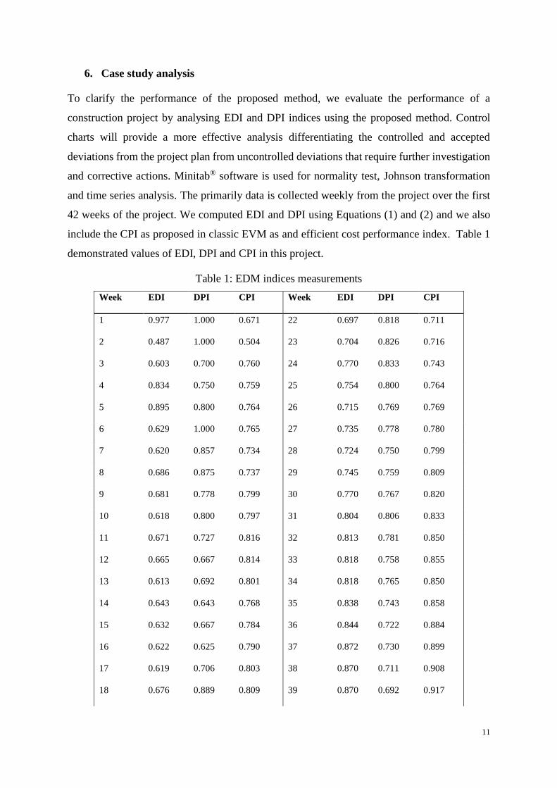
6. Case study analysis

To clarify the performance of the proposed method, we evaluate the performance of a

construction project by analysing EDI and DPI indices using the proposed method. Control

charts will provide a more effective analysis differentiating the controlled and accepted

deviations from the project plan from uncontrolled deviations that require further investigation

and corrective actions. Minitab® software is used for normality test, Johnson transformation

and time series analysis. The primarily data is collected weekly from the project over the first

42 weeks of the project. We computed EDI and DPI using Equations (1) and (2) and we also

include the CPI as proposed in classic EVM as and efficient cost performance index. Table 1

demonstrated values of EDI, DPI and CPI in this project.

Table 1: EDM indices measurements

Week EDI DPI CPI Week EDI DPI CPI

1 0.977 1.000 0.671 22 0.697 0.818 0.711

2 0.487 1.000 0.504 23 0.704 0.826 0.716

3 0.603 0.700 0.760 24 0.770 0.833 0.743

4 0.834 0.750 0.759 25 0.754 0.800 0.764

5 0.895 0.800 0.764 26 0.715 0.769 0.769

6 0.629 1.000 0.765 27 0.735 0.778 0.780

7 0.620 0.857 0.734 28 0.724 0.750 0.799

8 0.686 0.875 0.737 29 0.745 0.759 0.809

9 0.681 0.778 0.799 30 0.770 0.767 0.820

10 0.618 0.800 0.797 31 0.804 0.806 0.833

11 0.671 0.727 0.816 32 0.813 0.781 0.850

12 0.665 0.667 0.814 33 0.818 0.758 0.855

13 0.613 0.692 0.801 34 0.818 0.765 0.850

14 0.643 0.643 0.768 35 0.838 0.743 0.858

15 0.632 0.667 0.784 36 0.844 0.722 0.884

16 0.622 0.625 0.790 37 0.872 0.730 0.899

17 0.619 0.706 0.803 38 0.870 0.711 0.908

18 0.676 0.889 0.809 39 0.870 0.692 0.917

12

19 0.748 0.842 0.773 40 0.874 0.675 0.930

20 0.733 0.800 0.741 41 0.895 0.683 0.944

21 0.682 0.762 0.731 42 0.893 0.667 0.959

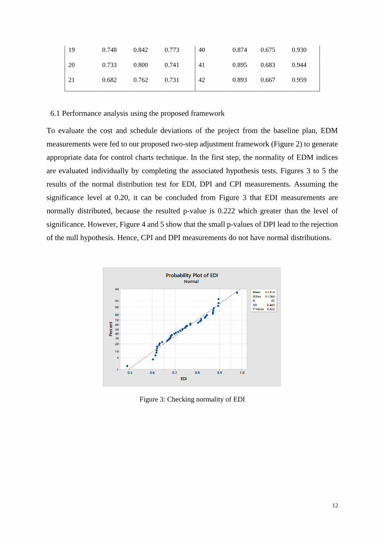
6.1 Performance analysis using the proposed framework

To evaluate the cost and schedule deviations of the project from the baseline plan, EDM

measurements were fed to our proposed two-step adjustment framework (Figure 2) to generate

appropriate data for control charts technique. In the first step, the normality of EDM indices

are evaluated individually by completing the associated hypothesis tests. Figures 3 to 5 the

results of the normal distribution test for EDI, DPI and CPI measurements. Assuming the

significance level at 0.20, it can be concluded from Figure 3 that EDI measurements are

normally distributed, because the resulted p-value is 0.222 which greater than the level of

significance. However, Figure 4 and 5 show that the small p-values of DPI lead to the rejection

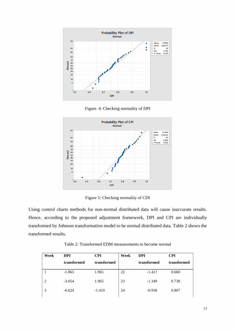
of the null hypothesis. Hence, CPI and DPI measurements do not have normal distributions.

Figure 3: Checking normality of EDI

13

Figure. 4: Checking normality of DPI

Figure 5: Checking normality of CDI

Using control charts methods for non-normal distributed data will cause inaccurate results.

Hence, according to the proposed adjustment framework, DPI and CPI are individually

transformed by Johnson transformation model to be normal distributed data. Table 2 shows the

transformed results.

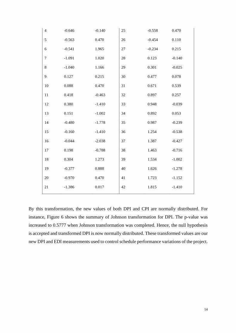
Table 2: Transformed EDM measurements to become normal

Week DPI

transformed

CPI

transformed

Week DPI

transformed

CPI

transformed

1 -1.865 1.965 22 -1.417 0.660

2 -3.054 1.965 23 -1.349 0.738

3 -0.624 -1.410 24 -0.936 0.807

14

4 -0.646 -0.140 25 -0.558 0.470

5 -0.563 0.470 26 -0.454 0.110

6 -0.541 1.965 27 -0.234 0.215

7 -1.091 1.020 28 0.123 -0.140

8 -1.040 1.166 29 0.301 -0.025

9 0.127 0.215 30 0.477 0.078

10 0.088 0.470 31 0.671 0.539

11 0.418 -0.463 32 0.897 0.257

12 0.380 -1.410 33 0.948 -0.039

13 0.151 -1.002 34 0.892 0.053

14 -0.480 -1.778 35 0.987 -0.239

15 -0.160 -1.410 36 1.254 -0.538

16 -0.044 -2.038 37 1.387 -0.427

17 0.198 -0.788 38 1.463 -0.716

18 0.304 1.273 39 1.534 -1.002

19 -0.377 0.888 40 1.626 -1.278

20 -0.970 0.470 41 1.723 -1.152

21 -1.386 0.017 42 1.815 -1.410

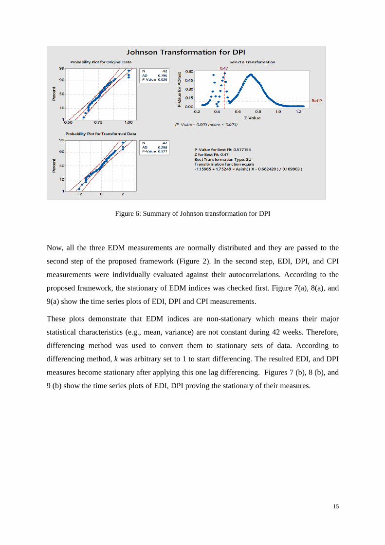
By this transformation, the new values of both DPI and CPI are normally distributed. For

instance, Figure 6 shows the summary of Johnson transformation for DPI. The p-value was

increased to 0.5777 when Johnson transformation was completed. Hence, the null hypothesis

is accepted and transformed DPI is now normally distributed. These transformed values are our

new DPI and EDI measurements used to control schedule performance variations of the project.

15

Figure 6: Summary of Johnson transformation for DPI

Now, all the three EDM measurements are normally distributed and they are passed to the

second step of the proposed framework (Figure 2). In the second step, EDI, DPI, and CPI

measurements were individually evaluated against their autocorrelations. According to the

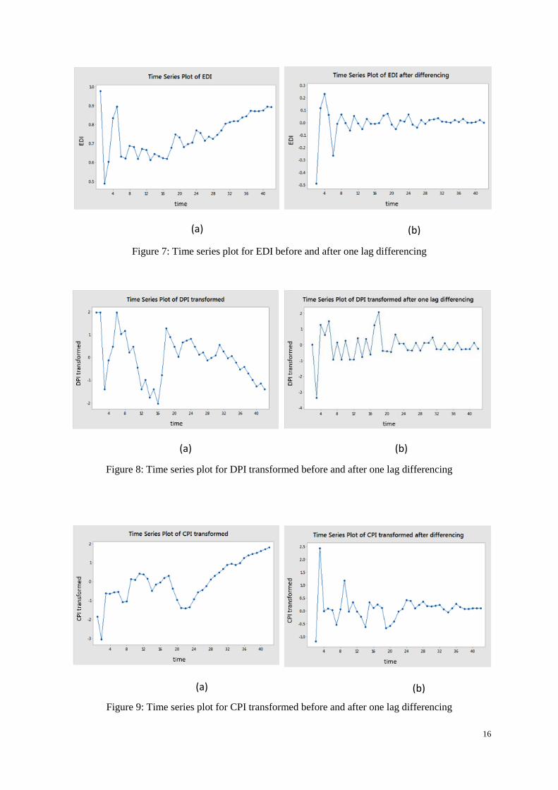
proposed framework, the stationary of EDM indices was checked first. Figure 7(a), 8(a), and

9(a) show the time series plots of EDI, DPI and CPI measurements.

These plots demonstrate that EDM indices are non-stationary which means their major

statistical characteristics (e.g., mean, variance) are not constant during 42 weeks. Therefore,

differencing method was used to convert them to stationary sets of data. According to

differencing method, k was arbitrary set to 1 to start differencing. The resulted EDI, and DPI

measures become stationary after applying this one lag differencing. Figures 7 (b), 8 (b), and

9 (b) show the time series plots of EDI, DPI proving the stationary of their measures.

16

Figure 7: Time series plot for EDI before and after one lag differencing

Figure 8: Time series plot for DPI transformed before and after one lag differencing

Figure 9: Time series plot for CPI transformed before and after one lag differencing

(a) (b)

(a) (b)

(a) (b)

17

In the next step, the autocorrelation among EDM measurements was checked separately. For

this reason, the autocorrelation and partial autocorrelation functions are used. Autocorrelation

function uncovers the possible correlation (dependence) of a variable with its own past and

future values during a time. Partial autocorrelation function estimates the partial correlation of

a variable with its own lagged values. According to the statistical theory (Chatfield, 2016),

using both autocorrelation and partial autocorrelation functions helps practitioners to construct

a more reliable ARIMA model for each index by determining the best order (kth lag) of the

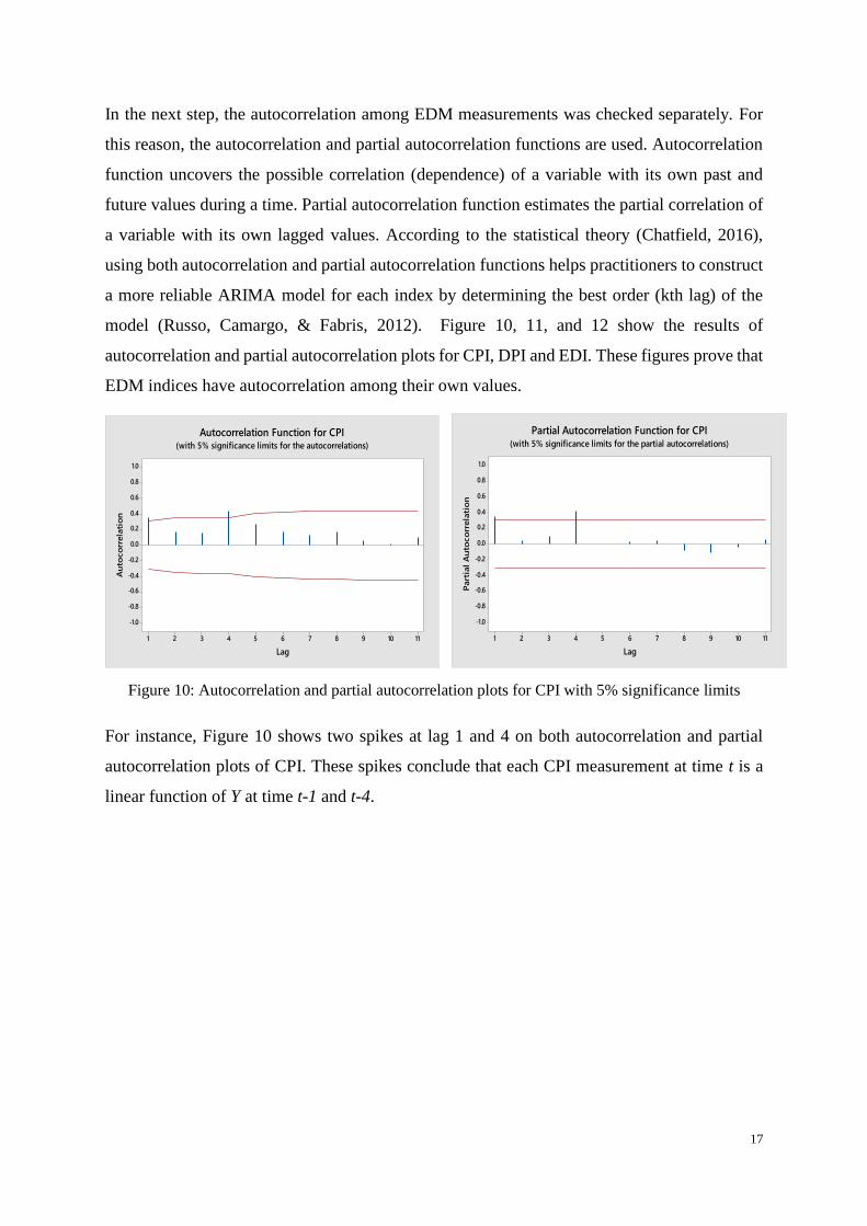
model (Russo, Camargo, & Fabris, 2012). Figure 10, 11, and 12 show the results of

autocorrelation and partial autocorrelation plots for CPI, DPI and EDI. These figures prove that

EDM indices have autocorrelation among their own values.

\

(a) Autocorrelation of CPI (b) Partial autocorrelation of CPI

Figure 10: Autocorrelation and partial autocorrelation plots for CPI with 5% significance limits

For instance, Figure 10 shows two spikes at lag 1 and 4 on both autocorrelation and partial

autocorrelation plots of CPI. These spikes conclude that each CPI measurement at time t is a

linear function of Y at time t-1 and t-4.

1110987654321

1.0

0.8

0.6

0.4

0.2

0.0

-0.2

-0.4

-0.6

-0.8

-1.0

Lag

Au

toco

rrela

tio

n

Autocorrelation Function for CPI(with 5% significance limits for the autocorrelations)

1110987654321

1.0

0.8

0.6

0.4

0.2

0.0

-0.2

-0.4

-0.6

-0.8

-1.0

Lag

Part

ial

Au

toco

rrela

tio

n

Partial Autocorrelation Function for CPI(with 5% significance limits for the partial autocorrelations)

18

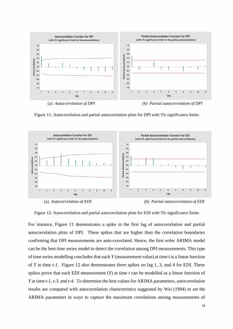
(a) Autocorrelation of DPI (b) Partial autocorrelation of DPI

Figure 11: Autocorrelation and partial autocorrelation plots for DPI with 5% significance limits

(a) Autocorrelation of EDI (b) Partial autocorrelation of EDI

Figure 12: Autocorrelation and partial autocorrelation plots for EDI with 5% significance limits

For instance, Figure 11 demonstrates a spike in the first lag of autocorrelation and partial

autocorrelation plots of DPI. These spikes that are higher than the correlation boundaries

confirming that DPI measurements are auto-correlated. Hence, the first order ARIMA model

can be the best time series model to detect the correlation among DPI measurements. This type

of time series modelling concludes that each Y (measurement value) at time t is a linear function

of Y at time t-1. Figure 12 also demonstrates three spikes on lag 1, 3, and 4 for EDI. These

spikes prove that each EDI measurement (Y) at time t can be modelled as a linear function of

Y at time t-1, t-3, and t-4. To determine the best values for ARIMA parameters, autocorrelation

results are compared with autocorrelation characteristics suggested by Wei (1994) to set the

ARIMA parameters in ways to capture the maximum correlations among measurements of

1110987654321

1.0

0.8

0.6

0.4

0.2

0.0

-0.2

-0.4

-0.6

-0.8

-1.0

Lag

Au

toco

rrela

tio

n

Autocorrelation Function for DPI(with 5% significance limits for the autocorrelations)

1110987654321

1.0

0.8

0.6

0.4

0.2

0.0

-0.2

-0.4

-0.6

-0.8

-1.0

Lag

Part

ial

Au

toco

rrela

tio

n

Partial Autocorrelation Function for DPI(with 5% significance limits for the partial autocorrelations)

1110987654321

1.0

0.8

0.6

0.4

0.2

0.0

-0.2

-0.4

-0.6

-0.8

-1.0

Lag

Au

toco

rrela

tio

n

Autocorrelation Function for EDI(with 5% significance limits for the autocorrelations)

1110987654321

1.0

0.8

0.6

0.4

0.2

0.0

-0.2

-0.4

-0.6

-0.8

-1.0

Lag

Part

ial

Au

toco

rrela

tio

n

Partial Autocorrelation Function for EDI(with 5% significance limits for the partial autocorrelations)

19

each EDM indices. Our final results conclude to use ARIMA (4,1,1) for CPI, ARIMA (1,1,1)

for DPI, and ARIMA (4,1,1) for EDI. These ARIMA time series models removed the

autocorrelation among all EDM measurements. Therefore, their corresponding residuals are

ready to develop control charts.

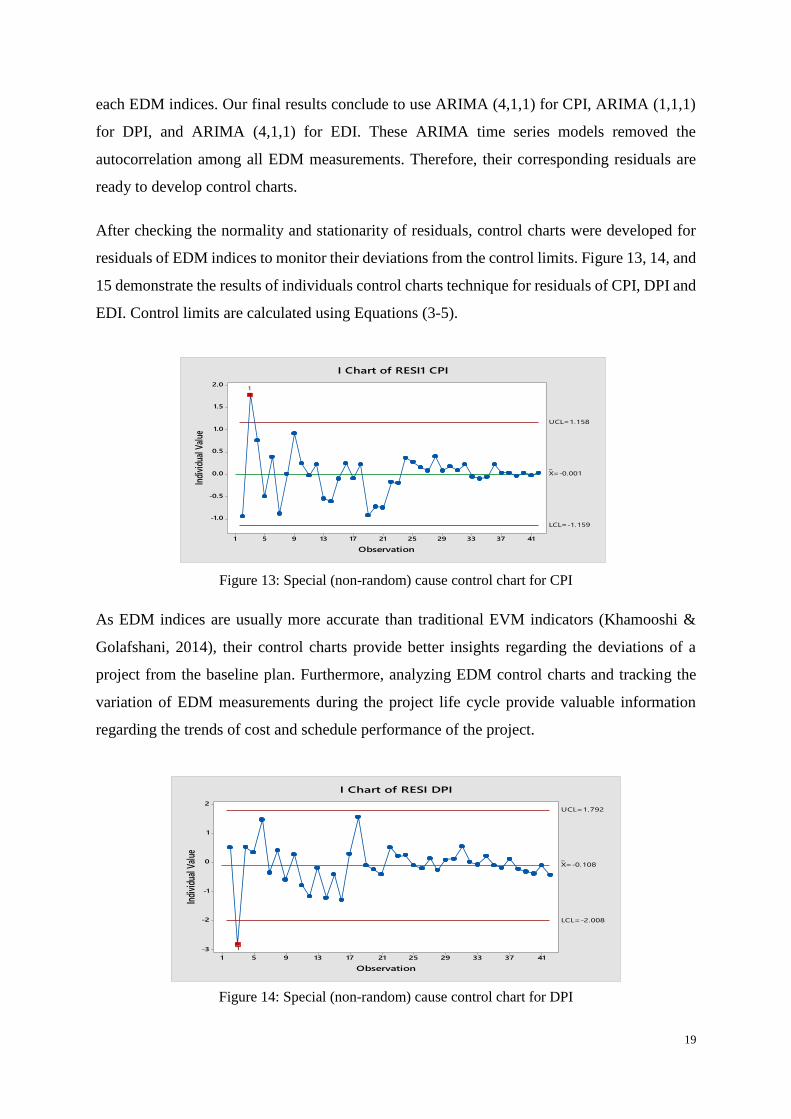
After checking the normality and stationarity of residuals, control charts were developed for

residuals of EDM indices to monitor their deviations from the control limits. Figure 13, 14, and

15 demonstrate the results of individuals control charts technique for residuals of CPI, DPI and

EDI. Control limits are calculated using Equations (3-5).

Figure 13: Special (non-random) cause control chart for CPI

As EDM indices are usually more accurate than traditional EVM indicators (Khamooshi &

Golafshani, 2014), their control charts provide better insights regarding the deviations of a

project from the baseline plan. Furthermore, analyzing EDM control charts and tracking the

variation of EDM measurements during the project life cycle provide valuable information

regarding the trends of cost and schedule performance of the project.

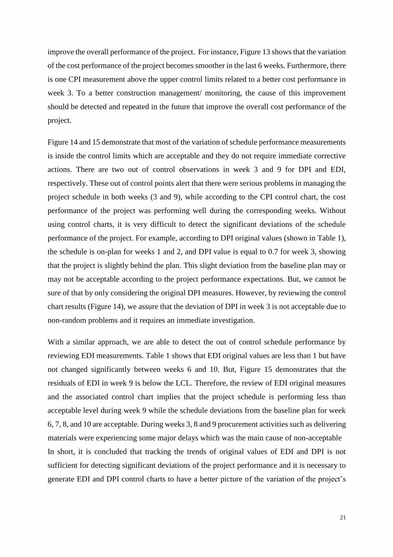
Figure 14: Special (non-random) cause control chart for DPI

4137332925211713951

2.0

1.5

1.0

0.5

0.0

-0.5

-1.0

Observation

Indi

vidu

al V

alue

_X=-0.001

UCL=1.158

LCL=-1.159

1

I Chart of RESI1 CPI

4137332925211713951

2

1

0

-1

-2

-3

Observation

Indi

vidu

al V

alue _

X=-0.108

UCL=1.792

LCL=-2.008

1

I Chart of RESI DPI

20

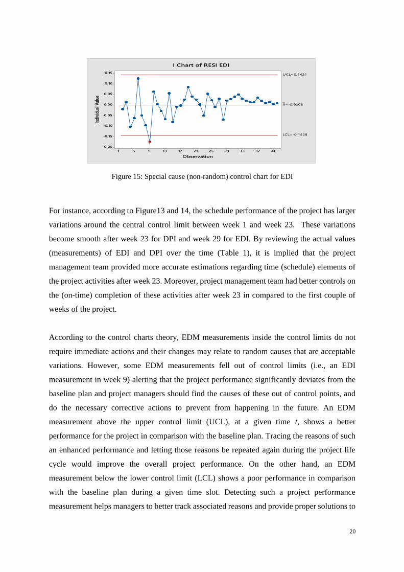
Figure 15: Special cause (non-random) control chart for EDI

For instance, according to Figure13 and 14, the schedule performance of the project has larger

variations around the central control limit between week 1 and week 23. These variations

become smooth after week 23 for DPI and week 29 for EDI. By reviewing the actual values

(measurements) of EDI and DPI over the time (Table 1), it is implied that the project

management team provided more accurate estimations regarding time (schedule) elements of

the project activities after week 23. Moreover, project management team had better controls on

the (on-time) completion of these activities after week 23 in compared to the first couple of

weeks of the project.

According to the control charts theory, EDM measurements inside the control limits do not

require immediate actions and their changes may relate to random causes that are acceptable

variations. However, some EDM measurements fell out of control limits (i.e., an EDI

measurement in week 9) alerting that the project performance significantly deviates from the

baseline plan and project managers should find the causes of these out of control points, and

do the necessary corrective actions to prevent from happening in the future. An EDM

measurement above the upper control limit (UCL), at a given time t, shows a better

performance for the project in comparison with the baseline plan. Tracing the reasons of such

an enhanced performance and letting those reasons be repeated again during the project life

cycle would improve the overall project performance. On the other hand, an EDM

measurement below the lower control limit (LCL) shows a poor performance in comparison

with the baseline plan during a given time slot. Detecting such a project performance

measurement helps managers to better track associated reasons and provide proper solutions to

4137332925211713951

0.15

0.10

0.05

0.00

-0.05

-0.10

-0.15

-0.20

Observation

Indi

vidu

al V

alue

_X=-0.0003

UCL=0.1421

LCL=-0.1428

1

I Chart of RESI EDI

21

improve the overall performance of the project. For instance, Figure 13 shows that the variation

of the cost performance of the project becomes smoother in the last 6 weeks. Furthermore, there

is one CPI measurement above the upper control limits related to a better cost performance in

week 3. To a better construction management/ monitoring, the cause of this improvement

should be detected and repeated in the future that improve the overall cost performance of the

project.

Figure 14 and 15 demonstrate that most of the variation of schedule performance measurements

is inside the control limits which are acceptable and they do not require immediate corrective

actions. There are two out of control observations in week 3 and 9 for DPI and EDI,

respectively. These out of control points alert that there were serious problems in managing the

project schedule in both weeks (3 and 9), while according to the CPI control chart, the cost

performance of the project was performing well during the corresponding weeks. Without

using control charts, it is very difficult to detect the significant deviations of the schedule

performance of the project. For example, according to DPI original values (shown in Table 1),

the schedule is on-plan for weeks 1 and 2, and DPI value is equal to 0.7 for week 3, showing

that the project is slightly behind the plan. This slight deviation from the baseline plan may or

may not be acceptable according to the project performance expectations. But, we cannot be

sure of that by only considering the original DPI measures. However, by reviewing the control

chart results (Figure 14), we assure that the deviation of DPI in week 3 is not acceptable due to

non-random problems and it requires an immediate investigation.

With a similar approach, we are able to detect the out of control schedule performance by

reviewing EDI measurements. Table 1 shows that EDI original values are less than 1 but have

not changed significantly between weeks 6 and 10. But, Figure 15 demonstrates that the

residuals of EDI in week 9 is below the LCL. Therefore, the review of EDI original measures

and the associated control chart implies that the project schedule is performing less than

acceptable level during week 9 while the schedule deviations from the baseline plan for week

6, 7, 8, and 10 are acceptable. During weeks 3, 8 and 9 procurement activities such as delivering

materials were experiencing some major delays which was the main cause of non-acceptable

In short, it is concluded that tracking the trends of original values of EDI and DPI is not

sufficient for detecting significant deviations of the project performance and it is necessary to

generate EDI and DPI control charts to have a better picture of the variation of the project’s

22

schedule performance. These numerical results confirm the validity of our developed approach

in detecting events that result in significant delays for the project.

7. Conclusion

One of the most critical problems that project managers encounter is the management of their

project performance, which may result in project cost and time overrun. Some unpredictable

issues may occur during the duration of a project, but a proper planning and monitoring system

can help managers to assuage these issues. Traditional EVM methods were developed to help

managers better understand and control the project performance by determining the current

status and predicting the future status of the project. Nevertheless, the traditional EVM have

some deficiencies which may lead to inaccurate results in some situations. Too much emphasis

on cost factors and using monetary-based indices as the main proxies for measuring the

schedule performance of a project are the most important shortcomings of the traditional EVM

methods. Decoupling the cost and schedule dimensions of a project can solve the problem of

traditional EVM systems in calculating the schedule and duration performance of projects. In

this regards, Khamooshi & Golafshani (2014) introduced the new concept of “earned duration”

to focus on the duration/schedule aspect of the project. The advantages of EDM in the

evaluation of the project performance have been addressed in several studies. However, EDM

is not established to discriminate between acceptable and non-acceptable levels of deviations

from the baseline. This study applied statistical control charts to monitor the three key indices

of EDM: EDI, DPI and CPI. We proposed a two-step adjustment framework that checks the

normality and dependency of EDM measurements and provides solutions for non-normally

distributed and auto correlated measurements which are very common in practice. In the first

adjustment step, the normality of EDM indices was analyzed and non-normal data were

transformed by using the Johnson technique to be normally distributed. In the second

adjustment step, the autocorrelation statistical hypothesis tests were employed to check the

independency of the cost and schedule performance indices. In practice, usually CPI, DPI, and

EDI indices have dependencies (autocorrelation) among their own values with different lags.

Therefore, ARIMA time series model was applied for each EDM index to remove the

autocorrelation among its measurements. ARIMA is a robust time series model that maximizes

the reduction of the autocorrelations and provides more accurate results in compared with

applying simple time series models. After removing autocorrelations, the statistical control

23

charts technique was applied to monitor the variations of EDM indices during the project life

cycle.

Our numerical findings in the case study prove that applying the statistical control charts

technique provides valuable information about the project performance and its deviation from

the plan. This information supports project managers to better control projects and detect

unacceptable variations in the project performance that may result in unexpected cost and time

losses. Furthermore, the results conclude that employing the control charts method along with

analyzing the original values of EDM performance indices over the project life cycle will

increase the capability of project management teams to detect cost and schedule problems on

time, prevent the problems from happening in the future, and make sure about the acceptable

completion of their projects.

The main purpose of EVM and EDM is to predict the future of projects, however, projects are

surrounded by a variety of uncertainties which make the prediction a very difficult task. As a

future research, our proposed approach can be improved by utilizing fuzzy time series to

provide a more practical solutions in predicting values in situations with no trend in the

previous performance.

Reference

Abba, W., & Niel, F.A., (2010). Integrating technical performance measurement with earned value

management. Measurable News, 4, 6-8.

Aliverdi, R., Naeni, L.M. & Salehipour, A., (2013). Monitoring project duration and cost in a

construction project by applying statistical quality control charts. International Journal of

Project Management, 31(3), 411- 423.

Azman, M. A., Abdul-Samad, Z. & Ismail, S., (2013). The accuracy of preliminary cost estimates

in Public Works Department (PWD) of Peninsular Malaysia. International Journal of Project

Management, 31(7), 994-1005.

Barraza, G. A., & Bueno, R.A., (2007). Probabilistic control of project performance using control

limit curves. Journal of Construction Engineering and Management-ASCE. 133 (12), 957–965.

Batselier, J., & Vanhoucke, M., 2015a. Evaluation of deterministic state-of-the-art forecasting

approaches for project duration based on earned value management. International Journal of

Project Management, 33(7), 1588-1596.

Bisgaard, S., & Kulahci, M. (2011). Time series analysis and forecasting by example. Wiley.

24

Book, S. A. (2006). Earned schedule and its possible unreliability as an indicator. The Measurable

News, 7-12.

Chatfield, C., (2016). The analysis of time series: An introduction. CRS press.

Chen, H. L., Chen, W. T., & Lin, Y .L., (2016). Earned value project management: Improving the

predictive power of planned value. International Journal of Project Management. 34(1), 22-29.

Colin, J., & Vanhoucke, M. 2014. Setting tolerance limits for statistical project control using

earned value management. Omega. The International Journal of Management Science, 49,

107–122.

Colin, J., Martens, A., Vanhoucke, M., & Wauters, M., 2015. A multivariate approach for top-

down project control using earned value management. Decision Support Systems, 79, 65-76.

D’Agostino, R.B., & Stephens, M.A., (1986). Goodness of Fit Techniques. Marcel Dekker Inc.

Fleming, W., & Koppelman, J.M., (1996). Earned Value Project Management. 2nd edition, Upper

Darby, PA: Project Management Institute.

Franco, B.C., Celano, G., Castagliola, P. & Costa, A.F.B., (2014). Economic design of Shewhart

control charts for monitoring auto-correlated data with skip sampling strategies. International

Journal of Production Economics, 151, 121-130.

Henderson, K. (2003). Earned schedule: A breakthrough extension to earned value theory? A

retrospective analysis of real project data. The Measurable News, 6.

Khamooshi, H., & Golafshani, H., (2014). EDM: Earned Duration Management, a new approach

to schedule performance management and measurement. International Journal of Project

Management, 32, 1019–1041.

Leu, S.S., & Lin, Y.C., (2008). Project performance evaluation based on statistical process control

techniques. Journal of Construction Engineering and Management-ASCE 134 (10), 813–819.

Lipke, W., (2003). “Schedule is different. The Measurable News Summer, 31–34.

Lipke, W., & Vaughn, J., (2000). Statistical process control meets earned value. The Journal of

Defense Software Engineering 16-20.

Lipke, W., Zwikael, O., Henderson, K., & Anbari, F., (2009). Prediction of project outcome: the

application of statistical methods to earned value management and earned schedule

performance indexes. International Journal of Project Management, 27, 400–407.

Meredith, J.R., Mantel, S.J., & Shafer, S. (2015). Project management: A Managerial Approach

9th edition. John Wiley & Sons Inc.

Montgomery, D. C. (2009). Introduction to statistical quality control, 6th Ed. John Wiley & Sons

Inc.

25

Narbaev, T., & Marco, A.D., (2014). An earned schedule-based regression model to improve cost

estimate at completion. International Journal of Project Management. 32 (6), 1007–1018.

Oakland, J.S., (2007). Statistical process control. Routledge.

Project Management Institute, (2004). A guide to project management body of knowledge, 3rd

edition. Project Management Institute, Newtown Square, PA.

Project Management Institute, (2005). Practice standard for Earned Value Management, 2nd

edition. Project Management Institute, Newtown Square, PA.

Project Management Institute, (2008). A guide to project management body of knowledge, 4th

edition. Project Management Institute, Newtown Square, PA.

Project Management Institute, (2013). A guide to the Project management body of knowledge.

Project Management Institute, Newtown Square, PA.

Rodríguez, J.C.M, Pascual, J.L., Molina, P.C., Marquez, F.P.C., (2017). In An overview of earned

value management in airspace industry. Proceedings of the Tenth International Conference on

Management Science and Engineering Management, 2017, Springer, 1465-1477.

Russo, S. L., Camargo,M. E., & Fabris, J. P. (2012). Practical concepts of quality control. In-Tech,

Rijeka, Croatia.

Salari, Mostafa, Nooshin Yousefi, and Mohhmad Mahdi Asgary. "Cost Performance Estimation

in Construction Projects Using Fuzzy Time Series." Project Management: Concepts,

Methodologies, Tools, and Applications. IGI Global, 2016. 359-370.

Salehipour, A., Naeni, L.M., Khanbabaei, R. & Javaheri, A., (2015). Lessons Learned from

Applying the Individuals Control Charts to Monitoring Autocorrelated Project Performance

Data. Journal of Construction Engineering and Management, 142(5), 15-27.

Thor, J., Lundberg, J., Ask, J., Olsson, J., Carli, C., Härenstam, K.P. & Brommels, M., (2007).

Application of statistical process control in healthcare improvement: systematic

review. Quality and Safety in Health Care, 16(5), 387-399.

Turner, J.R., (2010). Evolution of project management as evidenced by papers published in the

International Journal of Project Management. International Journal of Project Management,

28(1), 1-6.

Vandevoorde, S., & Vanhoucke, M., (2006). A comparison of different project duration

forecasting methods using earned value metrics. International Journal of Project Management,

24 (4), 289-302.

Wei, W.S., (1994). Time series analysis. Addison-Wesley publication.

Xie, M., Goh, T.N., & Kuralmani, N. (2002). Statistical models and control charts for high quality

processes. Springer publication. 207-235.

26

Yousefi, Nooshin. "Considering financial issues to estimate the project final cost in earned

duration management." Iberoamerican Journal of Project Management 9.2 (2018): 01-13.