econstorMake Your Publications Visible.

A Service of

zbwLeibniz-InformationszentrumWirtschaftLeibniz Information Centrefor Economics

Filoso, Valerio; Papagni, Erasmo

Working Paper

Fertility Choice and Financial Development

EERI Research Paper Series, No. 02/2011

Provided in Cooperation with:Economics and Econometrics Research Institute (EERI), Brussels

Suggested Citation: Filoso, Valerio; Papagni, Erasmo (2011) : Fertility Choice and FinancialDevelopment, EERI Research Paper Series, No. 02/2011, Economics and EconometricsResearch Institute (EERI), Brussels

This Version is available at:http://hdl.handle.net/10419/142609

Standard-Nutzungsbedingungen:

Die Dokumente auf EconStor dürfen zu eigenen wissenschaftlichenZwecken und zum Privatgebrauch gespeichert und kopiert werden.

Sie dürfen die Dokumente nicht für öffentliche oder kommerzielleZwecke vervielfältigen, öffentlich ausstellen, öffentlich zugänglichmachen, vertreiben oder anderweitig nutzen.

Sofern die Verfasser die Dokumente unter Open-Content-Lizenzen(insbesondere CC-Lizenzen) zur Verfügung gestellt haben sollten,gelten abweichend von diesen Nutzungsbedingungen die in der dortgenannten Lizenz gewährten Nutzungsrechte.

Terms of use:

Documents in EconStor may be saved and copied for yourpersonal and scholarly purposes.

You are not to copy documents for public or commercialpurposes, to exhibit the documents publicly, to make thempublicly available on the internet, or to distribute or otherwiseuse the documents in public.

If the documents have been made available under an OpenContent Licence (especially Creative Commons Licences), youmay exercise further usage rights as specified in the indicatedlicence.

www.econstor.eu

EERIEconomics and Econometrics Research Institute

EERI Research Paper Series No 02/2011

ISSN: 2031-4892

Copyright © 2011 by Valerio Filoso and Erasmo Papagni

Fertility Choice and Financial Development

Valerio Filoso and Erasmo Papagni

EERIEconomics and Econometrics Research Institute Avenue de Beaulieu 1160 Brussels Belgium

Tel: +322 299 3523 Fax: +322 299 3523 www.eeri.eu

FERTILITY CHOICE AND

FINANCIAL DEVELOPMENT

VALERIO FILOSO

Department of EconomicsUniversity of Naples

ERASMO PAPAGNI

Department of Law and EconomicsSecond University of Naples

November 28, 2010

Abstract

We study the consequences of broader access to credit and to capital markets onhousehold’s decisions over the number of children. In a life-cycle model of choice withforward and backward caring between parents and children, we analyze the effects ofrelaxing adults’ borrowing constrains and broadening the opportunities for financialinvestment, and show how the sign of these effects depends on the role of childrenas a normal or inferior good in parents’ preferences. We estimate the quantitativeimplications of our theoretical model on data from 145 countries over the period1980–2006. Empirical results indicate that improved access to credit reduces fertilityin poor countries and increases fertility in high-income countries. The effect of thedevelopment of capital markets on the number of children is negative in low-incomecountries and positive in the rich. When the analysis includes public pensions themain results remain the same. We also estimate the effect of the real interest rate,which proves significant and negative.

JEL Codes: D1, J13, G1.Keywords: Fertility, Financial Markets Development, Old-Age Security.

Contents1 Introduction 3

2 Literature review 5

3 Theory 73.1 Timing and budget constraints . . . . . . . . . . . . . . . . . . . . . . . . 83.2 Solving the model. Perfect capital markets . . . . . . . . . . . . . . . . . 93.3 The model with borrowing constraints . . . . . . . . . . . . . . . . . . . . 113.4 The model with saving constraints . . . . . . . . . . . . . . . . . . . . . . 13

4 Empirical estimation 154.1 Model specification . . . . . . . . . . . . . . . . . . . . . . . . . . . . . . . . 154.2 Data description . . . . . . . . . . . . . . . . . . . . . . . . . . . . . . . . . 164.3 Estimation technique . . . . . . . . . . . . . . . . . . . . . . . . . . . . . . 204.4 Borrowing constraints . . . . . . . . . . . . . . . . . . . . . . . . . . . . . . 224.5 Investment opportunities . . . . . . . . . . . . . . . . . . . . . . . . . . . . 224.6 The role of public pensions . . . . . . . . . . . . . . . . . . . . . . . . . . . 23

5 Final remarks 25

A Appendix: Data description 34

List of Tables1 Description of variables . . . . . . . . . . . . . . . . . . . . . . . . . . . . . 172 Sample description . . . . . . . . . . . . . . . . . . . . . . . . . . . . . . . . 183 Basic regressions . . . . . . . . . . . . . . . . . . . . . . . . . . . . . . . . . 194 Linear Model 1 . . . . . . . . . . . . . . . . . . . . . . . . . . . . . . . . . . 275 Linear Model 2 . . . . . . . . . . . . . . . . . . . . . . . . . . . . . . . . . . 286 Alternative specification . . . . . . . . . . . . . . . . . . . . . . . . . . . . 297 Partially Standardized variables . . . . . . . . . . . . . . . . . . . . . . . 308 The role of public pensions . . . . . . . . . . . . . . . . . . . . . . . . . . . 319 The role of public pensions, continued . . . . . . . . . . . . . . . . . . . . 3210 Robustness check: Complete sample 1960–2006 . . . . . . . . . . . . . . 33

2

1 IntroductionFertility behavior and financial development have seen dramatic changes in recentdecades, both showing distinctive patterns: as financial development spreads world-wide, enhancing the possibility of credit and intertemporal trade for households andfirms, fertility shows a clear downward trend which is cause for concern, especiallyin developed countries that will be facing decreasing populations in the near future.

Do these two phenomena simply show a spurious temporal correlation or doesone cause the other? Financial development may be among the driving forces thatchange fertility behavior. To raise children requires a significant transfer of par-ents’ resources toward them which can be driven not only by caring, but also by theexpectation that some resources will be returned during the parents’ old age: thisexchange is not synchronous and requires coordination of individual actions thatcan be best achieved through the means of specialized institutions. Since the ba-sic function of financial markets is to facilitate intertemporal trade, making currentconsumption less dependent on current income, then better organized and diversifiedfinancial markets would make these transfers easier. Nevertheless, the developmentof financial markets reduces the demand for children for the purpose of receiving oldage support. The impact of financial development on fertility is therefore undeter-mined and should be assessed empirically.

A glimpse at the figures involved can give an idea of the radical change that hastaken place. At the world level, the fertility rate – the average number of childrenper woman over her lifetime – has dropped from 4.91 in 1960–1965 to 2.56 in 2005–2008, with large differences between country groups. While more developed regionshave registered a decrease from 2.67 to 1.64, the rate in least developed countries hasdeclined from 6.73 to 4.39.1 Unlike fertility, financial development is a multifacetedphenomenon; many of its indicators also reveal a similarly striking trend. For exam-ple, the ratio of deposit money bank assets to GDP, a measure of liquidity availableto the general public, has risen from 0.26 in 1960–65 to 0.6 in 2005–08; in the sameperiod, more developed countries (MDCs) have recorded a considerable increase from0.42 to 1.32, while less developed countries (LDCs) a more modest change from 0.14to 0.38. By the same token, the ratio of private credit to GDP, has risen from 0.39 to1.14 in high income countries and from 0.13 to 0.31 in LDCs. Similar patterns arefollowed by other financial variables, like stock market capitalization and life insur-ance premium volume, both compared to GDP, whose values measure the breadth ofopportunities for financial investment.2

Despite the relevance of the causal relationship between financial developmentand fertility, theoretical and empirical analyses on the subject are still sparse. Onthe theoretical level, a life-cycle model integrating fertility choices and financial mar-kets is lacking. Cigno and Rosati (1992) investigate the effects of households’ accessto capital markets on fertility. They put forward two models of life-cycle fertility, find-ing empirical support for a positive effect of financial development on fertility. Someevidence on this issue comes from the literature on microcredit programs: thesestudies show some controversial effects of increased financial availability on fertil-ity. Nonetheless, these programs of financial empowerment are generally aimed atvery poor people living in LDCs; accordingly, the external validity of these studies is

1The figures on fertility rates are accessible at http://data.un.org/.2The figures on financial structure are accessible at http://data.un.org/ and at Ross Levine’s per-

sonal website.

3

questionable.In this paper we attempt to provide a comprehensive account of the relations be-

tween households’ choice of fertility and the availability of credit and opportunitiesfor financial investment. In the theoretical section we introduce a four periods life-cycle model of fertility choice in which agents care for their children and for theirparents too. In this setting young adults might choose to borrow some resources and,when older, to save and invest in the capital market. In this model, we also retrievethe distinction between two main types of imperfections of financial markets (Pollin,1997; McKinnon, 1973): borrowing constraints – the difficulties encountered by in-dividuals when trying to reach their optimal level of debt – and saving constraints,which pertain to the uneasiness encountered by individuals who wish to invest theirsavings in a private financial market. We show that in the context of fertility deter-mination, this distinction has both theoretical relevance and a significant empiricalcounterpart.

In the empirical section, we estimate the quantitative implications of our theoret-ical model for 145 countries over the period 1980–2006, merging the data on fertility,social and economic indicators from World Development Indicators (2007) with thoseprovided by Beck, Demirgüç-Kunt, and Levine (2000) who describe the level of finan-cial development and structure at the country level with a variety of indicators. Theeconometric model used to test the implications of the theoretical model uses a fixed-effects panel estimator which takes into account heterogeneity between countriesand time-invariant unobserved factors influencing fertility, also possibly correlatedto our selected regressors.

Our key theoretical findings concern the multiple channels through which bor-rowing constraints and saving constraints affect fertility. These results are obtainedby a decomposition of the equilibrium conditions accounting for the twofold nature ofchildren as both consumption and investment goods. In particular, the effect of relax-ing the borrowing constraint on fertility is determined by the balance between (1) aninvestment effect, whose positive sign is due to the reduction of future resources andto a corresponding greater investment in children, and (2) an income effect, whosesign can be either positive or negative. Hence, fertility will unambiguously increaseonly when children are normal goods in a household’s preferences. Broader access tocapital markets allows parents to rely less on children to fund their old age welfare.Nonetheless, larger savings imply lower debt in the early years of adulthood: in thiscase the household will command a smaller amount of resources for consumptionand children. If children are inferior goods, the effect of greater saving will be am-biguous. An innovative feature of these results lies in their identification power. Anyempirical finding of a positive effect on the number children due to a lift in borrowingconstraints, other things being equal, would not reveal the nature of the underlyingpreferences toward children, while only a negative effect would. An analogous im-plication for identification regards any positive estimate of the effect of improvedcapital market access on fertility.

Our empirical results indicate that both borrowing constraints and investmentopportunities do impact fertility and that the sign of these effects critically dependson a country’s stage of economic growth. An increase in private credit of one standarddeviation decreases fertility of 1.7%–5% in low-income countries, while high-incomecountries register an increase by 3.7%–5%. Analogously, a standard deviation in-crease in the ratio of deposit money bank assets and the sum of deposit money andcentral bank assets decreases the number of children by 1.8%–3.8% in low-income

4

countries, while in high-income countries the same change produces an increase of3.2%–17.2%.

Financial investment opportunities are approximated by two variables: the ra-tio of the value of life insurance premiums to GDP, and the ratio of stock marketcapitalization to GDP. A one standard deviation increase in life insurance premiumsincreases fertility by 2.0%–3.1% in high-income countries, while in low income coun-tries the effect of the same variation is negative and around 3.5% and 5.2%.

In the econometric analysis, we also check the role of the public pension systemin determining fertility. This role arises because pensions are potential substitutesfor voluntary savings. Using data on public pension expenditure from the ILO, weare able to show that private financial markets continue to play a significant role inexplaining fertility changes. These results provide an additional perspective to theestimated differences among countries of the effect of financial markets on fertility.These differences also depend on the positive correlation, usually found in sectionaldata, between capital market development and social security. LDCs typically lackprivate and public saving institutions, while high-income countries have developedfinancial institutions in both sectors. Hence, the reaction of households to financialdevelopment crucially depends on the complementary presence of social security.

As far as we know, our econometric analysis provides the first test of the influ-ence of the interest rate on fertility in a large sample of countries. We show thathigh real interest rates have a significant negative influence on fertility, a fact whichcan be easily reconciled with our theoretical approach. These results extend thoseobtained by Cigno and Rosati (1992, 1996) on data for Germany, Italy, the UK andUSA. Various checks of robustness substantially confirm our theory that the struc-ture of private financial markets does matter for fertility choices and help explainingthe historical decreasing trend of fertility in LDCs and MDCs which has taken placeafter the demographic transition.

The remainder of the paper is organized as follows: Section 2 surveys the theoret-ical and empirical literature on the impact of financial variables on fertility; Section3 describes the model determining intertemporal allocation of income and fertilitydetermination; Section 4 describes the empirical implementation of the theoreticalmodel, specification and identification issues, the data used for estimation and therelative results; Section 5 discusses policy implications and concludes.

2 Literature reviewEconomic models of fertility can be partitioned into two broad streams: those inwhich children are an intermediate good in the production of lifetime wealth, andthose in which children are final consumption goods.

The models in the first stream date back to the pioneering contribution of Leiben-stein (1957). In this work the hypothesis was advanced that children, rather thanbeing net consumers of family resources, actually increase their families’ lifetimewealth. Although infants are completely dependent upon their family for their per-sonal consumption, as they grow up they become capable of working and transferringincome back to their families. As long as the value of resources being returned bygrown-up children exceeds the value of resources consumed as infants, fertility isa financially profitable trade from the standpoints of parents’ and children. In thisframework, fertility choices are driven by the behavior of parents, whose only objec-

5

tive is to maximize their lifetime wealth: instrumental to this financial program isthe production of children.

When the demand for children depends only on purely financial return, the avail-ability of alternative assets becomes crucial. When financial markets start providingassets which offer high returns, some families would drop fertility as an investmentand turn to the market as the return on financial assets exceeds the return on chil-dren. This hypothesis of complete substitutability between children and financialassets may be found in the development economics literature (Willis, 1980; Schultz,1974; Neher, 1971) and has invariably given raise to the statement that better ac-cess to financial markets and investment opportunities would invariably lead to adecrease in planned fertility. In a general equilibrium analysis context, Razin andSadka (1995) have shown that financial deepening does not necessarily carry a dropin fertility. Introducing heterogeneity in preferences and technologies, as well as thebasic equilibrium identity between aggregate saving and aggregate borrowing, finan-cial trade opportunities allow some families to invest more in market assets and lessin fertility, but at the same time other families must do the opposite, thus increasingfertility. The net balance between these competing forces may well result in higheroverall fertility.

The models in the second stream of literature allow for children as durable con-sumption goods (Hotz, Klerman, and Willis, 1997; Willis, 1973; Becker and Lewis,1973; Becker, 1960). It is generally assumed that parents are interested in childrenper se and may find it profitable to borrow against the future in order to finance theirchildren’s consumption and investment in human capital. In this case, financialdeepening and credit consumption availability may induce an increase in fertility.

In their main contribution on this subject to date, Cigno and Rosati (1996) developa model of joint determination of fertility and saving. In their framework, fertilitybehavior can be driven by two mutually exclusive reasons: altruism or selfishness. Inthe first case, altruism in the utility function runs either backwards, from parents tochildren, or forwards from children to parents. In the second case, the impossibilityof intertemporal trade and the decreasing value of human capital across time makefertility the only available technology for saving for the old age: accordingly, childrenare instrumental goods in the production of their parents’ future utility. In this case,when the return from market investment exceeds the return from fertility, the modelpredicts that intergenerational family links break up and fertility inevitably declines.Using cointegration analysis, the authors find evidence compatible with the selfishmotivation for fertility, although the econometric specification is unable to identifyexactly the underlying heterogeneity in the aggregate data, such that the possibilityof both motivations for fertility cannot be rejected.

As stated above, there is scant evidence on the effects of financial availabilityon fertility. Cigno and Rosati (1992), employing cointegration analysis on Italiandata, find evidence of a positive effect of capital market accessibility on fertility. Thelagged ratio of currency held by the non-bank public to bank deposits is the vari-able selected to proxy for financial backwardness and the corresponding estimatedelasticity on fertility lies between -0.662 and -0.711. Using calibrated data, Boldrin,De Nardi, and Jones (2005) find that better access to capital markets accounts forhalf of the observed drop in fertility in developed countries over the last 70 years;according to their estimates, a reduction in the rate of return on capital of about 20%would increase fertility by 30%. An alternative model by Scotese Lehr (1999) findsthat financial intermediation can influence fertility in an indirect fashion. In an econ-

6

omy with two sectors – a traditional one with low capitalization and a modern onewith high capitalization – an increase in the level of financial intermediation lowersthe cost of capital, driving up wages in the modern sector. Households then find it op-timal to reduce fertility as their members shift labor supply from the labor-intensivesector to the capital-intensive sector. Employing a reduced-form VAR model withpanel data on 87 countries from 1965 to 1980, the author finds that some measuresof the extent of financial intermediation Granger-cause a drop in fertility. Specifi-cally, the estimated elasticity of fertility with regard to the ratio of money to GDP is-7.7% and the elasticity with regard to the ratio of private credit to GDP is -5.7%.

The link between financial empowerment of women and fertility is also a subjectof investigation in the literature on evaluation of microcredit programs, althoughin this regard the empirical evidence is inconclusive. Since most of such programstarget women, the additional financial resources provided tend to shift individual ef-fort from childbearing to income-generating activities. At the same time, the wealtheffect can increase the demand for children when these are normal goods. For exam-ple, some econometric studies of the Grameen Bank program in Bangladesh (Steele,Amin, and Naved, 2001; Schuler and Hashemi, 1994) observe an increased use ofcontraceptives resulting in lower fertility, while others (Pitt, Khandker, McKernan,and Latif, 1999; Schuler, Hashemi, and Riley, 1997) find that the impact of the sameprogram on contraceptive use is in fact negligible.

3 TheoryThe model represents the choices of a household over the life cycle as determinedby the caring relations with its children, and by the trading relations with financialmarkets. In the following sections the terms household, adult, and agent will be usedinterchangeably, since we do not model explicitly the interactions between parents;basically, we assume a frictionless unitary setting for family decisions. We also as-sume parents derive satisfaction from living with their children; similarly, childrenhave an altruistic attitude towards their parents (Ehrlich and Lui, 1991; Nishimuraand Zhang, 1992). Given these links, adults spend resources to rear their childrenand to fund the consumption of their retired parents.

The time sequences of household expenditure and income over the life cycle im-ply the need to borrow resources in the first years of adulthood and the incentiveto save and invest in the capital market later on. Capital markets can be perfect,meaning that households can borrow and save the optimal amounts consistent withtheir intertemporal budget constraint. Several forms of imperfections, nonetheless,may limit credit availability to households with significant consequences on their de-cisions. Similarly, opportunities for financial investment can be scarce in economieswhere property rights are not well enforced and informational asymmetries betweenlenders and borrowers are severe; in this case, investing in children is an alternativeto poor financial market conditions.

We model consumer choice under rationing as a case of the more general theoryby Tobin and Houthakker (1950-51). In what follows, for expository convenience, wefirst present the model with perfect financial markets, and then we turn to the dis-tinct cases of borrowing constraints and limited access to capital markets. Thoughreal economies often present both types of market imperfections, this expositorystrategy affords a better understanding of the consequences of each kind of market

7

failure on fertility choice.

3.1 Timing and budget constraintsA household lives for four periods: it is young in the first, young adult in the second,adult in the third, and old in the fourth. Children live with their parents who rearthem and take any decisions on their behalf. A young adult works and takes careof her nt children during the first period of adulthood; she still works when adultand takes care of her old parents; she retires when old. The choice problem starts inthe second period of life and spans three periods. The life-cycle utility function of ahousehold who is a young adult at t is:

U =U(c1t , nt, c2

t+1, c3t+2, c3

t+1) (1)

where c1t is private consumption during early adulthood, c2

t+1 is private consump-tion during late adulthood, c3

t+2 is private consumption during old age, and c3t+1 is

private consumption of the parents during their own old age. Each agent’s utilityis increasing in her private consumption, in the number of her children, and in theconsumption of her parents. This function is assumed to be separable across timeperiods, such that:

U = v(c1

t , nt)+u

(c2

t+1, c3t+1

)+ g

(c3

t+2)

(2)

The functions v(.), u(.), g(.) are assumed strictly concave and to satisfy Inada condi-tions. During each period, choices are constrained by intertemporal and intratempo-ral requirements.

• In the first period (t−1) agents have no control variable, for their consump-tion level is entirely determined by their parents. During this period, agentscomplete their formal education. No choice problem is present.

• In the second period of their life (t) agents become adult and start working,get married, become parents, and use debt to finance their consumption andthe cost of their children; they may face borrowing constraints. The budgetconstraint is:

c1t = (1−τnt)w1

t +Dt (3)

where τ is the cost of raising one child as a share of the labor income, w1t , and

Dt is the amount of debt.

• In the third period (t+1) parents keep working, pay back their debt, and savefor their own old age. In addition, they support their parents by transferringmoney to them. At the beginning of the same period, their children leaveparental house and start working. The budget constraint is:

c2t+1 = w2

t+1−Rt+1Dt − qt+1− st+1 (4)

where w2t+1 is labor income, Rt+1 ≡ 1+ rt+1 and rt+1 is the interest rate, qt+1 is

a money transfer towards parents, and st+1 is the value of saving. During thesame time period the agent’s parents face the following budget constraint:

c3t+1 = Rt+1st+nt−1qt+1 (5)

where qt+1 is the amount of transfers received by the parents from each child.

8

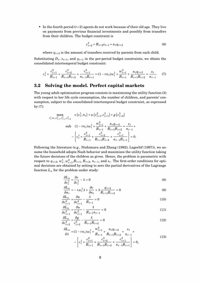
• In the fourth period (t+2) agents do not work because of their old age. They liveon payments from previous financial investments and possibly from transfersfrom their children. The budget constraint is

c3t+2 = Rt+2st+1+ntqt+2 (6)

where qt+2 is the amount of transfers received by parents from each child.

Substituting Dt, st+1, and qt+1 in the per-period budget constraints, we obtain theconsolidated intertemporal budget constraint:

c1t +

c2t+1

Rt+1+

c3t+2

Rt+1Rt+2+

c3t+1

nt−1Rt+1= (1−τnt)w1

t +w2

t+1

Rt+1+

ntqt+2

Rt+1Rt+2+

st

nt−1. (7)

3.2 Solving the model. Perfect capital marketsThe young adult optimization program consists in maximizing the utility function (2)with respect to her life cycle consumption, the number of children, and parents’ con-sumption, subject to the consolidated intertemporal budget constraint, as expressedby (7):

maxc1

t ,nt,c2t+1,c3

t+1,c3t+2

v(c1

t , nt)+u

(c2

t+1, c3t+1

)+ g

(c3

t+2)

sub (1−τnt)w1t +

w2t+1

Rt+1+

ntqt+2

Rt+1Rt+2+

st

nt−1+

−

[c1

t +c2

t+1

Rt+1+

c3t+2

Rt+1Rt+2+

c3t+1

nt−1Rt+1

]= 0.

Following the literature (e.g., Nishimura and Zhang (1992); Lagerlöf (1997)), we as-sume the household adopts Nash behavior and maximizes the utility function takingthe future decisions of the children as given. Hence, the problem is parametric withrespect to qt+2, w1

t , w2t+1,Rt+1, Rt+2, nt−1, and st. The first-order conditions for opti-

mal decisions are obtained by setting to zero the partial derivatives of the Lagrangefunction Lu for the problem under study:

∂Lu

∂c1t

=

∂v

∂c1t

−λ= 0 (8)

∂Lu

∂nt=−τw1

t λ+

∂v∂nt

+λqt+2

Rt+1Rt+2= 0 (9)

∂Lu

∂c2t+1

=

∂u

∂c2t+1

−

λ

Rt+1= 0 (10)

∂Lu

∂c3t+1

=

∂u

∂c3t+1

−

λ

Rt+1nt−1= 0 (11)

∂Lu

∂c3t+2

=

∂g

c3t+2

−

λ

Rt+1Rt+2= 0 (12)

∂Lu

∂λ= (1−τnt)w1

t +w2

t+1

Rt+1+

ntqt+2

Rt+1Rt+2+

st

nt−1+

−

[c1

t +c2

t+1

Rt+1+

c3t+2

Rt+1Rt+2+

c3t+1

nt−1Rt+1

]= 0,

(13)

9

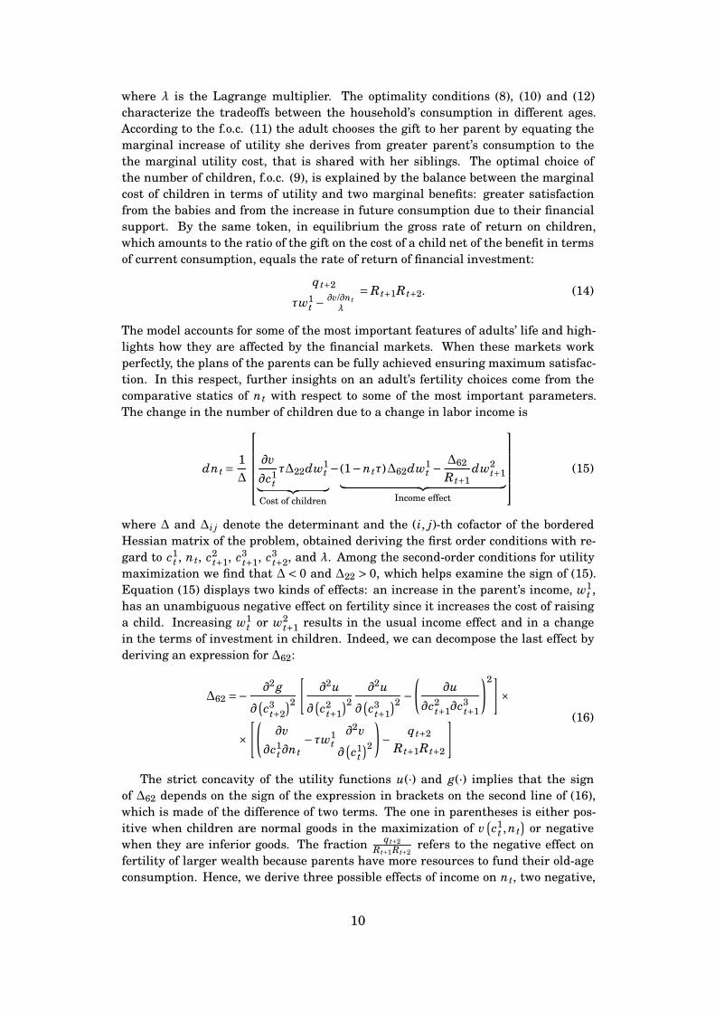
where λ is the Lagrange multiplier. The optimality conditions (8), (10) and (12)characterize the tradeoffs between the household’s consumption in different ages.According to the f.o.c. (11) the adult chooses the gift to her parent by equating themarginal increase of utility she derives from greater parent’s consumption to thethe marginal utility cost, that is shared with her siblings. The optimal choice ofthe number of children, f.o.c. (9), is explained by the balance between the marginalcost of children in terms of utility and two marginal benefits: greater satisfactionfrom the babies and from the increase in future consumption due to their financialsupport. By the same token, in equilibrium the gross rate of return on children,which amounts to the ratio of the gift on the cost of a child net of the benefit in termsof current consumption, equals the rate of return of financial investment:

qt+2

τw1t −

∂v/∂ntλ

= Rt+1Rt+2. (14)

The model accounts for some of the most important features of adults’ life and high-lights how they are affected by the financial markets. When these markets workperfectly, the plans of the parents can be fully achieved ensuring maximum satisfac-tion. In this respect, further insights on an adult’s fertility choices come from thecomparative statics of nt with respect to some of the most important parameters.The change in the number of children due to a change in labor income is

dnt =1Δ

⎡⎢⎢⎢⎢⎣

∂v

∂c1t

τΔ22dw1t︸ ︷︷ ︸

Cost of children

− (1−ntτ)Δ62dw1t −

Δ62

Rt+1dw2

t+1︸ ︷︷ ︸Income effect

⎤⎥⎥⎥⎥⎦ (15)

where Δ and Δi j denote the determinant and the (i, j)-th cofactor of the borderedHessian matrix of the problem, obtained deriving the first order conditions with re-gard to c1

t , nt, c2t+1, c3

t+1, c3t+2, and λ. Among the second-order conditions for utility

maximization we find that Δ < 0 and Δ22 > 0, which helps examine the sign of (15).Equation (15) displays two kinds of effects: an increase in the parent’s income, w1

t ,has an unambiguous negative effect on fertility since it increases the cost of raisinga child. Increasing w1

t or w2t+1 results in the usual income effect and in a change

in the terms of investment in children. Indeed, we can decompose the last effect byderiving an expression for Δ62:

Δ62 =−

∂2 g

∂(c3

t+2

)2[

∂2u

∂(c2

t+1

)2 ∂2u

∂(c3

t+1

)2 −

(∂u

∂c2t+1∂c3

t+1

)2]×

×

[(∂v

∂c1t∂nt

−τw1t

∂2v

∂(c1

t

)2)−

qt+2

Rt+1Rt+2

] (16)

The strict concavity of the utility functions u(·) and g(·) implies that the signof Δ62 depends on the sign of the expression in brackets on the second line of (16),which is made of the difference of two terms. The one in parentheses is either pos-itive when children are normal goods in the maximization of v

(c1

t , nt)

or negativewhen they are inferior goods. The fraction qt+2

Rt+1Rt+2refers to the negative effect on

fertility of larger wealth because parents have more resources to fund their old-ageconsumption. Hence, we derive three possible effects of income on nt, two negative,

10

and one positive or negative according to the role children have in young adults’preferences.

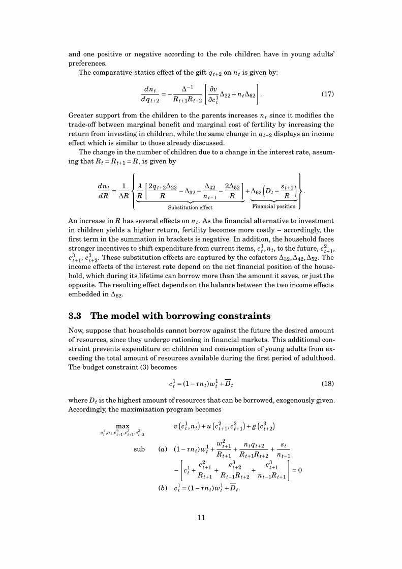
The comparative-statics effect of the gift qt+2 on nt is given by:

dnt

dqt+2=−

Δ−1

Rt+1Rt+2

[∂v

∂c1tΔ22+ntΔ62

]. (17)

Greater support from the children to the parents increases nt since it modifies thetrade-off between marginal benefit and marginal cost of fertility by increasing thereturn from investing in children, while the same change in qt+2 displays an incomeeffect which is similar to those already discussed.

The change in the number of children due to a change in the interest rate, assum-ing that Rt = Rt+1 = R, is given by

dnt

dR=

1ΔR

⎧⎪⎪⎪⎨⎪⎪⎪⎩

λ

R

[2qt+2Δ22

R−Δ32 −

Δ42

nt−1−

2Δ52

R

]︸ ︷︷ ︸

Substitution effect

+Δ62

(Dt−

st+1

R

)︸ ︷︷ ︸Financial position

⎫⎪⎪⎪⎬⎪⎪⎪⎭ .

An increase in R has several effects on nt. As the financial alternative to investmentin children yields a higher return, fertility becomes more costly – accordingly, thefirst term in the summation in brackets is negative. In addition, the household facesstronger incentives to shift expenditure from current items, c1

t , nt, to the future, c2t+1,

c3t+1, c3

t+2. These substitution effects are captured by the cofactors Δ32,Δ42,Δ52. Theincome effects of the interest rate depend on the net financial position of the house-hold, which during its lifetime can borrow more than the amount it saves, or just theopposite. The resulting effect depends on the balance between the two income effectsembedded in Δ62.

3.3 The model with borrowing constraintsNow, suppose that households cannot borrow against the future the desired amountof resources, since they undergo rationing in financial markets. This additional con-straint prevents expenditure on children and consumption of young adults from ex-ceeding the total amount of resources available during the first period of adulthood.The budget constraint (3) becomes

c1t = (1−τnt)w1

t +Dt (18)

where Dt is the highest amount of resources that can be borrowed, exogenously given.Accordingly, the maximization program becomes

maxc1

t ,nt,c2t+1,c3

t+1,c3t+2

v(c1

t , nt)+u

(c2

t+1, c3t+1

)+ g

(c3

t+2)

sub (a) (1−τnt)w1t +

w2t+1

Rt+1+

ntqt+2

Rt+1Rt+2+

st

nt−1

−

[c1

t +c2

t+1

Rt+1+

c3t+2

Rt+1Rt+2+

c3t+1

nt−1Rt+1

]= 0

(b) c1t = (1−τnt)w1

t +Dt.

11

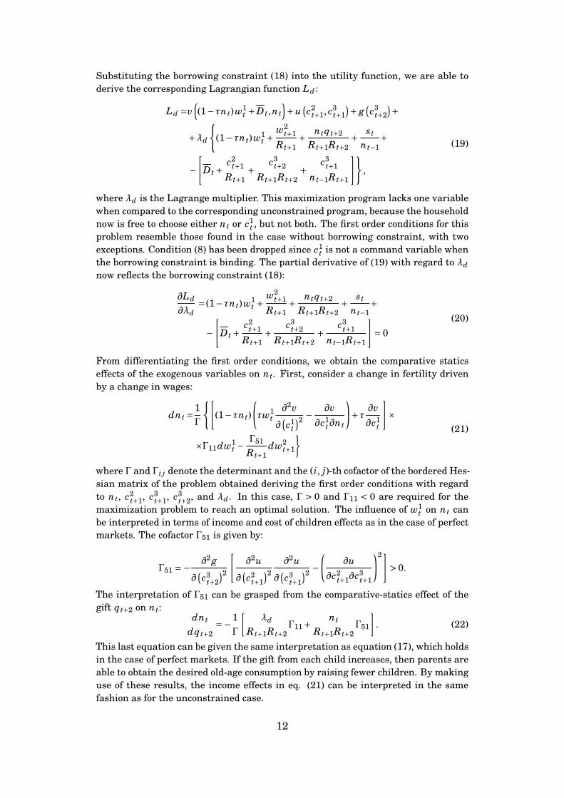
Substituting the borrowing constraint (18) into the utility function, we are able toderive the corresponding Lagrangian function Ld:

Ld =v((1−τnt)w1

t +Dt, nt

)+u

(c2

t+1, c3t+1

)+ g

(c3

t+2)+

+λd

{(1−τnt)w1

t +w2

t+1

Rt+1+

ntqt+2

Rt+1Rt+2+

st

nt−1+

−

[Dt +

c2t+1

Rt+1+

c3t+2

Rt+1Rt+2+

c3t+1

nt−1Rt+1

]},

(19)

where λd is the Lagrange multiplier. This maximization program lacks one variablewhen compared to the corresponding unconstrained program, because the householdnow is free to choose either nt or c1

t , but not both. The first order conditions for thisproblem resemble those found in the case without borrowing constraint, with twoexceptions. Condition (8) has been dropped since c1

t is not a command variable whenthe borrowing constraint is binding. The partial derivative of (19) with regard to λd

now reflects the borrowing constraint (18):

∂Ld

∂λd= (1−τnt)w1

t +w2

t+1

Rt+1+

ntqt+2

Rt+1Rt+2+

st

nt−1+

−

[Dt +

c2t+1

Rt+1+

c3t+2

Rt+1Rt+2+

c3t+1

nt−1Rt+1

]= 0

(20)

From differentiating the first order conditions, we obtain the comparative staticseffects of the exogenous variables on nt. First, consider a change in fertility drivenby a change in wages:

dnt =1Γ

{[(1−τnt)

(τw1

t∂2v

∂(c1

t

)2 −

∂v

∂c1t∂nt

)+τ

∂v

∂c1t

]×

×Γ11dw1t −

Γ51

Rt+1dw2

t+1

} (21)

where Γ and Γi j denote the determinant and the (i, j)-th cofactor of the bordered Hes-sian matrix of the problem obtained deriving the first order conditions with regardto nt, c2

t+1, c3t+1, c3

t+2, and λd. In this case, Γ > 0 and Γ11 < 0 are required for themaximization problem to reach an optimal solution. The influence of w1

t on nt canbe interpreted in terms of income and cost of children effects as in the case of perfectmarkets. The cofactor Γ51 is given by:

Γ51 =−

∂2 g

∂(c3

t+2

)2[

∂2u

∂(c2

t+1

)2 ∂2u

∂(c3

t+1

)2 −

(∂u

∂c2t+1∂c3

t+1

)2]> 0.

The interpretation of Γ51 can be grasped from the comparative-statics effect of thegift qt+2 on nt:

dnt

dqt+2=−

1Γ

[λd

Rt+1Rt+2Γ11+

nt

Rt+1Rt+2Γ51

]. (22)

This last equation can be given the same interpretation as equation (17), which holdsin the case of perfect markets. If the gift from each child increases, then parents areable to obtain the desired old-age consumption by raising fewer children. By makinguse of these results, the income effects in eq. (21) can be interpreted in the samefashion as for the unconstrained case.

12

The problem of utility maximization is parametric with respect to the credit ceil-ing D. Higher credit availability will impact on household fertility according to thefollowing expression:

dnt

dDt=

1Γ

⎧⎪⎪⎪⎪⎪⎪⎪⎨⎪⎪⎪⎪⎪⎪⎪⎩

(τw1

t∂2v

∂(c1

t

)2 −

∂v

∂c1t nt

)︸ ︷︷ ︸

> 0 if fertility is inferior good< 0 if fertility is normal good

×Γ11+Γ51

⎫⎪⎪⎪⎪⎪⎪⎪⎬⎪⎪⎪⎪⎪⎪⎪⎭

(23)

Equation (23) clearly shows two causal effects of credit availability on fertility. As thevalue of D grows – more credit is available to households – young parents command agreater amount of their future resources, and spend these resources on consumptionand children. If children are normal goods in household’s preferences then nt willincrease; otherwise, it will decrease. Furthermore, the same increase in D implieslower income available for consumption during retirement. Hence, the householdwill react by increasing investment in children, i.e., raising the number of childrennt. The sign of dnt/dDt is undetermined from a theoretical point of view if childrenare inferior goods. This hypothesis finds support in the empirical analysis of fertilityafter World War II showing a strong correlation between income growth and fertilitydecline (Jones, Schoonbroodt, and Tertilt, 2008).

3.4 The model with saving constraintsAs mentioned above, the desire to smooth consumption over the life cycle providesa major incentive to save. Since children can also provide support to their retiredparents, fertility becomes crucial in determining the optimal amount of saving. Ac-cordingly, households interact with the financial markets not only as borrowers, butas lenders too. In this role of lenders, households may face a different type of marketimperfection: a poorly organized financial market – possibly for technological or in-stitutional reasons – can either provide few opportunities to invest and for effectiverisk diversification, or may impose severe costs upon those accessing them. This sit-uation has been termed saving constraint in the literature (Pollin, 1997) and refersto the adverse role on savings played by a low level of financial deepening (McKin-non, 1973; Shaw, 1973). When access to financial investment as lenders is limitedby saving constraints, investment in children becomes an attractive alternative.

Assume now that financial markets are so poorly developed that economic agentsface significant access costs. In the following, we analyze the model of householdchoice by assuming that the optimal desired value of saving st+1 is higher than theceiling st+1. Hence, adults face the following constraint:

c3t+2 = Rt+2st+1+ntqt+2, (24)

which shows that both financial investment and fertility contribute to ensure old age

13

consumption. Accordingly, the maximization program becomes:

maxc1

t ,nt,c2t+1,c3

t+1,c3t+2

v(c1

t , nt)+u

(c2

t+1, c3t+1

)+ g

(c3

t+2)

sub (a) (1−τnt)w1t +

w2t+1

Rt+1+

ntqt+2

Rt+1Rt+2+

st

nt−1

−

[c1

t +c2

t+1

Rt+1+

c3t+2

Rt+1Rt+2+

c3t+1

nt−1Rt+1

]= 0

(b) c3t+2 = Rt+2st +ntqt+2,

where we assume that household borrowing is not restricted. Plugging the savingconstraint into the utility function and into the consolidated intertemporal budgetconstraint, we can write the new Lagrangian function Ls as

Ls =v(c1

t , nt)+u

(c2

t+1, c3t+1

)+ g (Rt+2st+1+ntqt+2)+

+λs

{(1−τnt)w1

t +w2

t+1− st+1

Rt+1+

st

nt−1

−

[c1

t +c2

t+1

Rt+1+

c3t+1

nt−1Rt+1

]}.

(25)

The first order conditions for this problem resemble those found in the case withoutborrowing constraint, with two exceptions. Condition (10) has been dropped sincec3

t+2 is no longer a command variable as the saving constraint is binding. The partialderivative of (25) with regard to λs now reflects the saving constraint

∂Ls

∂λs= (1−τnt)w1

t +w2

t+1− st+1

Rt+1+

st

nt−1−

[c1

t +c2

t+1

Rt+1+

c3t+1

nt−1Rt+1

]= 0 (26)

As in the previous subsection, we are interested in the change of nt in response to ex-ogenous changes in the model’s parameters, especially that related to capital marketaccessibility. First, consider how fertility changes as labour income increases:

dnt =1Φ

{[λsτΦ22 − (1−τnt)Φ52] dw1

t −Φ52

Rt+1dw2

t+1

}

where Φ and Φi j denote the determinant and the (i, j)-th cofactor of the borderedHessian matrix of the problem, obtained deriving the first order conditions with re-gard to c1

t , nt, c2t+1, c3

t+1, and λs. Among the second order conditions for a maximumof the problem (25) we have Φ> 0 and Φ22 < 0. Since Φ52 equals

Φ52 =−

[∂2u

∂(c2

t+1

)2 ∂2u

∂(c3

t+1

)2 −

(∂u

∂c2t+1∂c3

t+1

)2](∂v

∂c1t∂nt

−τw1t

∂2v

∂(c1

t

)2)

,

the interpretation of the effects of labour income on fertility can follow along thelines of the preceding cases. The same arguments can be used to justify the effectsof qt+2 and R on nt. The case of constrained access to financial markets, by contrast,raises a novel question concerning the reaction of a household’s fertility to greaterinvestment opportunities, given by

dnt

dst+1=

1Φ

(Φ52

Rt+1− qt+2Rt+2

∂2 g

∂(c3

t+2

)2Φ22

). (27)

14

In this expression, the term

−qt+2Rt+2∂2 g

∂(c3

t+2

)2Φ22 < 0

refers to the trade-off between the investment in children and that in financial activi-ties. The sign of the term is negative because greater financial investment opportuni-ties reduce the need to raise children for old age consumption. The other componentof the effect of st+1 on nt has the opposite sign of the income effect of wages, deter-mined by the sign of Φ52. If parent appreciate children as normal good, then fertilitywill increase with w1

t (or with w2t+1), and will decrease with st+1. Indeed, given the

intertemporal budget constraint, when st+1 increases young adults reduce their debt.As a result, their resources will be lower and fertility will drop. The case of childrenas inferior goods implies the opposite positive effect.

Our comparative statics results so far suggest that, when children are normalgoods in the household’s preferences, fertility unambiguously decreases with easieraccess to financial markets; by contrast, when children are inferior goods, the signof the effect of financial markets accessibility on fertility remains theoretically inde-terminate.

4 Empirical estimationIn this section the demand functions for fertility derived from the theoretical modelare estimated empirically using data from a panel of countries, including both MDCsand LDCs, since the theoretical model is general enough to be applied to any type ofpopulation, regardless of its stage of economic development. The econometric exer-cise is carried out to find evidence for an economically significant impact of financialmarkets on fertility behavior and to check for alternative explanations.

We first introduce our empirical specification, then turn to data description, andfinally show various estimates along with some robustness checks.

4.1 Model specificationOur theoretical model predicts that desired fertility should be responsive, amongother things, both to borrowing constraints and to opportunities to access the capitalmarkets. While borrowing constraints reflect the uneasiness of borrowing resourcesin the first section of the life cycle to finance transfers to children, saving constraintsreflect the limited availability of instruments to allocate savings in the second sectionof the life cycle. When both these aspects play a distinct role in determining fertility,these two variables need to be accounted for separately. This is a peculiar featureof our approach, since the previous literature does not distinguish among differentsources of imperfections in financial markets.

Our previous discussion established the following reduced-form equation for fer-tility, in which the number of children per woman is determined by a set of exogenousvariables:

nt = n(w1

t ,w2t+1,Rt+1,Rt+2, qt+2,τ,Dt, st+1

)(28)

In what follows, we assume that the parameters qt+2 and τ differ across countries,but stay constant across time for each country. Accordingly, we are in a position to

15

formulate an empirical counterpart of eq. (28) based on a panel specification of thefollowing type:

TFRi,t =β0+X′

i,t−1β1+BOR′

i,t−1β2+FIN′

i,t−1β3 +ui +φt +εi,t (29)

where TFR is the natural logarithm of the total fertility rate, BOR is a vector ofvariables used to approximate the easiness of access to borrowing, FIN is a vector ofvariables describing the development of investment opportunities in capital markets,X is a set of additional ancillary controls, u is a country-specific, time-unvarying,error term, φ is a time effect, and ε is an error term with E[ε]= 0. The subscript i isfor countries, while t is for time periods.

The structure of time subscripts needs some explanations. Since the model de-veloped in the theoretical section can be considered an approximation of long-runfertility behavior, the construction of the dataset was conducted according to twobasic premises about fertility decisions: (a) they take time to develop their conse-quences and (b) involve expectations about the long run. The first of these premisesimplies that a dynamic specification for eq. (29) is needed, while the second impliessome sort of smoothing to approximate the long-run values of the variables of inter-est in order to increase the signal-to-noise ratio. Consequently, each observation isobtained averaging the value of a given variable over a period of non-overlapping fiveyears,3 with all variables representing ratios being averaged by harmonic means.

4.2 Data descriptionOur fundamental dependent variable, the number of children per family, has its de-mographic counterpart in the total fertility rate. This rate amounts to the numberof children born to an average woman over her reproductive years (15–49), obtainedas the sum of the age-specific fertility ratios. Unlike the net reproduction rate, thismeasure is independent of a population’s age structure. This variable is extractedfrom the World Bank’s World Development Indicators (2007), a wide dataset of obser-vations on demographic, economic and social aspects of life collected at the countrylevel from 1960 to 2006.

The set of additional controls included in the variable X contains: the log of GDPper capita (GDP), the participation rate of women in the labor force (FLFP), theurbanization rate (URBAN) and the real interest rate (INTRATE). These controls,extracted from World Bank’s World Development Indicators (2007), are indicated inthe literature (e.g., Schultz (1997) and Ehrlich and Kim (2007)) as relevant covari-ates in the determination of fertility. While the majority of these variables have beencollected since 1960, the participation of women in the labor force is a major excep-tion, for its availability is limited to a time window running only from 1980 onward.A further variable, included in some specifications of our empirical model,4 is the ra-tio of public pensions to GDP, extracted from the ILO’s database. The description ofeach variable is reported in table 1, while basic statistics for the sample are reportedin table 2. These figures are for the complete sample, while the various subsamplesused for estimation are made up of observations for which the whole set of variables

3This temporal smoothing is used, among others, by Ehrlich and Kim (2007) in the study of fertility andby Beck, Demirgüç-Kunt, and Levine (2004) in the study of financial development.

4See subsection 4.6 for further details.

16

– dependent and independent – are non-missing. Accordingly, each estimation ta-ble reports the number of countries and the number of observations included in thecalculation.

TABLE 1DESCRIPTION OF VARIABLES

Availability

Variable Description From Until

TFR Log of total fertility rate: number of children born to an averagewoman over her reproductive years ∗

1960 2006

GDP Log of per capita gross domestic product ∗ 1960 2006HIGHINC Dummy for high income countries ∗ 1960 2006URBAN Urbanization rate, as the ratio of population living in urban areas

divided by total population ∗

1960 2006

FLFP Female labor force participation ∗ 1980 2006INTRATE Real interest rate ∗ 1960 2006

DBACBA Ratio of deposit money bank claims on domestic nonfinancial realsector to the sum of deposit money bank and Central Bank claimson domestic nonfinancial real sector ∗∗

1960 2006

INSLIFE Life insurance premium volume as a share of GDP ∗∗ 1960 2006STMKCAP Value of listed shares to GDP, deflated ∗∗ 1975 2006PRIVCRED Private credit by deposit money banks to GDP, deflated ∗∗ 1960 2006PENSIONS Public pensions expenses to GDP ∗∗∗ 1985 1999

Source: Variables denoted by ∗ are from World Development Indicators (2007). Variables denotedby ∗∗ are from Thorsten Beck, Asli Demirgüç-Kunt and Ross Levine, (2000), A New Database on Fi-nancial Development and Structure, World Bank Economic Review 14, 597-605. Variable denoted by∗∗∗ is from the International Labor Office’s Social Security Expenditure Database, available onlineat https://www.ilo.org/dyn/sesame/ifpses.socialdbexp.Note: All variables averaged over non-overlapping five years.

With the exception of the real interest rate, the financial variables are ex-tracted from the study published by Beck, Demirgüç-Kunt, and Levine (2000).Since borrowing constraints and access to financial markets are multidimen-sional phenomena, we consider these variables as reliable proxies for thefinancial difficulties actually experienced by families and we try alternativespecifications to check for the robustness of our results.

For borrowing constraints we have two main indicators: DBACBA andPRIVCRED. The first variable is the ratio of deposit money bank claims onthe domestic nonfinancial real sector to the sum of deposit money bank andCentral Bank claims on the domestic nonfinancial real sector. The secondvariable is the value of private credit by deposit money banks to GDP. Coun-tries with high values of DBACBA have a high proportion of credit allocatedin the banking sector, while in countries with low values money is held bycentral banks: with high values, a larger fraction of liquidity can be used byfamilies to borrow against the future. High values of PRIVCRED testify aflourishing market for credit in general and also for credit to households.

Financial opportunities variables are represented in our estimates by IN-SLIFE and STMKCAP: the first is the volume of life insurance premium toGDP, the second is the value of listed shares to GDP. Life insurance is a kindof long-term financial investment made by households who are worried abouta sharp fall in their wellbeing during old age. Indeed, if one of the spouses

17

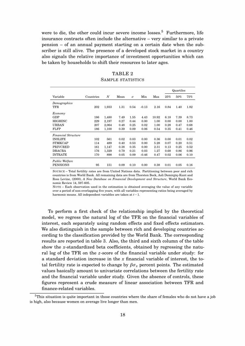
were to die, the other could incur severe income losses.5 Furthermore, lifeinsurance contracts often include the alternative – very similar to a privatepension – of an annual payment starting on a certain date when the sub-scriber is still alive. The presence of a developed stock market in a countryalso signals the relative importance of investment opportunities which canbe taken by households to shift their resources to later ages.

TABLE 2SAMPLE STATISTICS

Quartiles

Variable Countries N Mean σ Min Max 25% 50% 75%

DemographicsTFR 202 1,933 1.31 0.54 -0.13 2.16 0.84 1.40 1.82

EconomyGDP 186 1,480 7.49 1.55 4.43 10.92 6.18 7.39 8.73HIGHINC 229 2,197 0.27 0.44 0.00 1.00 0.00 0.00 1.00URBAN 207 2,064 0.48 0.25 0.02 1.00 0.28 0.47 0.68FLFP 186 1,100 0.39 0.09 0.06 0.54 0.35 0.41 0.46

Financial StructureINSLIFE 102 561 0.02 0.03 0.00 0.36 0.00 0.01 0.02STMKCAP 114 489 0.40 0.53 0.00 5.28 0.07 0.20 0.51PRIVCRED 161 1,147 0.38 0.35 0.00 2.31 0.13 0.25 0.52DBACBA 176 1,329 0.79 0.21 0.03 1.27 0.68 0.86 0.96INTRATE 170 898 0.05 0.09 -0.46 0.47 0.02 0.06 0.10

Public WelfarePENSIONS 95 151 0.09 0.10 0.00 0.38 0.01 0.05 0.16

SOURCE – Total fertility rates are from United Nations data. Partitioning between poor and richcountries is from World Bank. All remaining data are from Thorsten Beck, Asli Demirgüç-Kunt andRoss Levine, (2000), A New Database on Financial Development and Structure, World Bank Eco-nomic Review 14, 597-605.NOTE – Each observation used in the estimation is obtained averaging the value of any variableover a period of non-overlapping five years, with all variables representing ratios being averaged byharmonic means. All independent variables are taken at t−1.

To perform a first check of the relationship implied by the theoreticalmodel, we regress the natural log of the TFR on the financial variables ofinterest, each separately using random effects and fixed effects estimators.We also distinguish in the sample between rich and developing countries ac-cording to the classification provided by the World Bank. The correspondingresults are reported in table 3. Also, the third and sixth column of the tableshow the x-standardized beta coefficients, obtained by regressing the natu-ral log of the TFR on the z-score of the financial variable under study: fora standard deviation increase in the x financial variable of interest, the to-tal fertility rate is expected to change by βσx percent points. The estimatedvalues basically amount to univariate correlations between the fertility rateand the financial variable under study. Given the absence of controls, thesefigures represent a crude measure of linear association between TFR andfinance-related variables.

5This situation is quite important in those countries where the share of females who do not have a jobis high, also because women on average live longer than men.

18

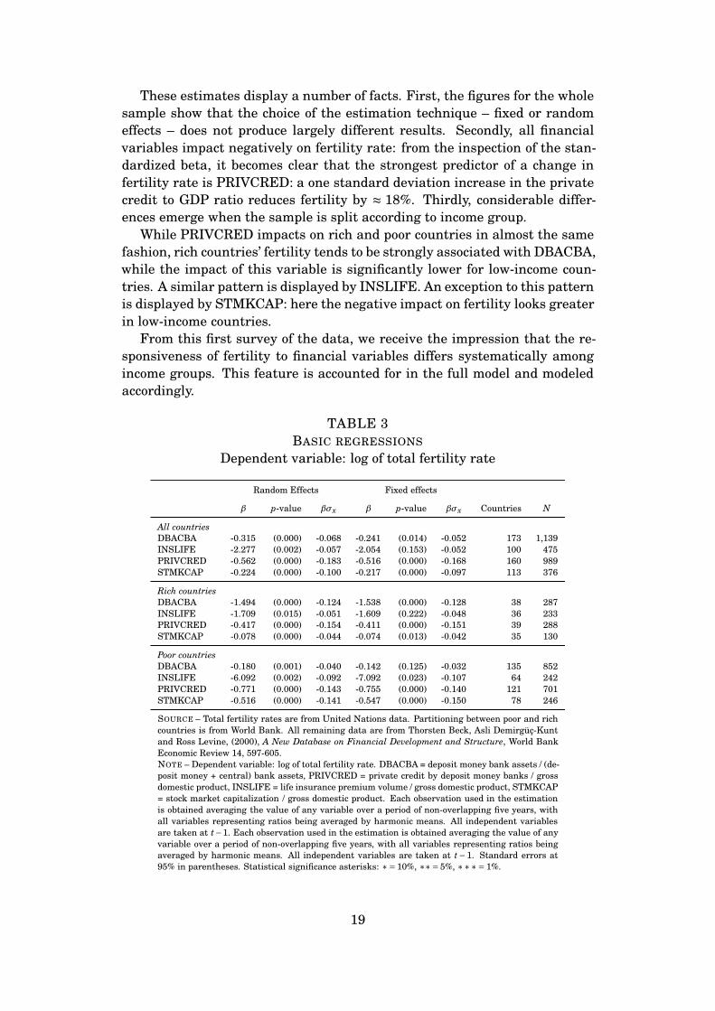
These estimates display a number of facts. First, the figures for the wholesample show that the choice of the estimation technique – fixed or randomeffects – does not produce largely different results. Secondly, all financialvariables impact negatively on fertility rate: from the inspection of the stan-dardized beta, it becomes clear that the strongest predictor of a change infertility rate is PRIVCRED: a one standard deviation increase in the privatecredit to GDP ratio reduces fertility by ≈ 18%. Thirdly, considerable differ-ences emerge when the sample is split according to income group.

While PRIVCRED impacts on rich and poor countries in almost the samefashion, rich countries’ fertility tends to be strongly associated with DBACBA,while the impact of this variable is significantly lower for low-income coun-tries. A similar pattern is displayed by INSLIFE. An exception to this patternis displayed by STMKCAP: here the negative impact on fertility looks greaterin low-income countries.

From this first survey of the data, we receive the impression that the re-sponsiveness of fertility to financial variables differs systematically amongincome groups. This feature is accounted for in the full model and modeledaccordingly.

TABLE 3BASIC REGRESSIONS

Dependent variable: log of total fertility rate

Random Effects Fixed effects

β p-value βσx β p-value βσx Countries N

All countriesDBACBA -0.315 (0.000) -0.068 -0.241 (0.014) -0.052 173 1,139INSLIFE -2.277 (0.002) -0.057 -2.054 (0.153) -0.052 100 475PRIVCRED -0.562 (0.000) -0.183 -0.516 (0.000) -0.168 160 989STMKCAP -0.224 (0.000) -0.100 -0.217 (0.000) -0.097 113 376

Rich countriesDBACBA -1.494 (0.000) -0.124 -1.538 (0.000) -0.128 38 287INSLIFE -1.709 (0.015) -0.051 -1.609 (0.222) -0.048 36 233PRIVCRED -0.417 (0.000) -0.154 -0.411 (0.000) -0.151 39 288STMKCAP -0.078 (0.000) -0.044 -0.074 (0.013) -0.042 35 130

Poor countriesDBACBA -0.180 (0.001) -0.040 -0.142 (0.125) -0.032 135 852INSLIFE -6.092 (0.002) -0.092 -7.092 (0.023) -0.107 64 242PRIVCRED -0.771 (0.000) -0.143 -0.755 (0.000) -0.140 121 701STMKCAP -0.516 (0.000) -0.141 -0.547 (0.000) -0.150 78 246

SOURCE – Total fertility rates are from United Nations data. Partitioning between poor and richcountries is from World Bank. All remaining data are from Thorsten Beck, Asli Demirgüç-Kuntand Ross Levine, (2000), A New Database on Financial Development and Structure, World BankEconomic Review 14, 597-605.NOTE – Dependent variable: log of total fertility rate. DBACBA = deposit money bank assets / (de-posit money + central) bank assets, PRIVCRED = private credit by deposit money banks / grossdomestic product, INSLIFE = life insurance premium volume / gross domestic product, STMKCAP= stock market capitalization / gross domestic product. Each observation used in the estimationis obtained averaging the value of any variable over a period of non-overlapping five years, withall variables representing ratios being averaged by harmonic means. All independent variablesare taken at t−1. Each observation used in the estimation is obtained averaging the value of anyvariable over a period of non-overlapping five years, with all variables representing ratios beingaveraged by harmonic means. All independent variables are taken at t−1. Standard errors at95% in parentheses. Statistical significance asterisks: ∗= 10%, ∗∗= 5%, ∗∗∗= 1%.

19

4.3 Estimation technique

From the empirical point of view, fertility choice is a very complex phe-nomenon, deeply intertwined with a large number of economic and socialvariables. Many of these variables are unobservable in the publicly avail-able data collections while others are intrinsically nonmeasurable, like thoserelated to deeply rooted mental habits, cultural influences, religious tradi-tions, and the like. Given that these variables change only slowly, the electivemethod of estimation must allow for the exclusion of relevant variables whilereducing to zero the omitted variable bias. In our context, this method is afixed-effect panel estimator with robust standard errors.

Some variables, such as per capita GDP and female labor force participa-tion, could also be influenced by fertility itself. This problem could in prin-ciple constitute a threat to a causal interpretation of regression results. Tocheck for this source of bias, several tests of endogeneity of GDP and FLFPwere performed, but the results cannot reject the exogeneity assumption.

The empirical model to be estimated is also prone to display spurious cor-relation: even in the absence of a precise causal link, it is likely that thecountries with high levels of financial development also display low levels offertility since both aspects could be side effects of economic development. Wedeal with this issue in several ways. First, the use of a five year averagesmooths out short-run movements in the variables that could induce serialcorrelation which is not present in the steady state.6 Second, the dynamicformulation of the empirical models accounts only for links between actionstaken at t−1 and outcomes happening at t: in this case, the simultaneousdetermination of fertility and financial variables is ruled out by construction.

Unobserved heterogeneity can be a serious issue when modeling fertil-ity. Some countries, during a demographic transition, experience a sharpdecrease in the number of children per woman, while fertility in countrieswhich have already reached a steady-state nirvana changes only marginallyfrom year to year. This feature drives us to adopt a heteroskedasticity-robustestimator for the standard errors of the model.

The exercise shown in table 3 reveals the presence of nonlinearities in ourkey financial variables with regard to their effect on fertility. We take thisissue seriously and we systematically interact the financial variables withthe dummy for high income (HIGHINC).

Results

The results of the estimated models are presented in table 4 and table 5. Tomodel financial market imperfections, in the first model’s specification we useDBACBA and PRIVCRED, while in the second we use INSLIFE and STMK-CAP. Table 7 elaborates the results of preceding tables using z-scores instead

6The presence of a time trend in the dependent variable is in principle capable of distorting OLS esti-mates. However, we find no evidence of serial correlation in our model.

20

of levels for the independent variables. With this transformation, the esti-mated parameters reflect the percentage change in the fertility rate due toa one-standard deviation change in an independent variable. Since the mag-nitude and variance of the independent variables vary considerably acrosscountries and time, this adjustment may prove useful in interpreting the es-timates. Accordingly, our comments mostly focus on table 7.

The first four columns of table 4 and the first three of table 5 present es-timated coefficients for the fixed effect model, while the remaining columnsadd the year-specific term φt, as mentioned in eq. (29). Columns 1 and 5 dis-play the coefficients for the models stripped of all finance-related variables:this basic formulation of the model affords appreciation of the backbone vari-ables used as controls. The intercepts are not displayed because they are notparticularly informative.

The overall fit of the two alternative specifications – with and withouttime effects – is satisfactory, ranging from 48% to 63% of the total observedvariability. Unsurprisingly, the models with time dummies display a higherR2 when compared with the corresponding models without dummies, sincemost OECD countries displayed a common tendency to reduce fertility, prob-ably captured by the time term. However, the inclusion of this variable doesnot dramatically change the value of the estimated parameters. Given thesenegligible discrepancies in the models estimated with and without a commontemporal trend, table 7 elaborates on estimates obtained without temporaldummies.

The effect of interest rate on fertility is uniformly negative. A one standarddeviation change in the interest rate produces a 1.5%–2.9% drop in the fertil-ity rate, as shown in table 7. This evidence can be easily rationalized in theframework of our theoretical model. Whether children are an investment or aconsumption good, a higher return of financial investment increases their rel-ative price with regard to alternative options. In the first case, when childrenare an investment good and their return is exogenously given, higher inter-est rates decrease their relative return and drive down fertility rates. In thesecond case, when children are a durable consumption good, an increase inthe interest rate reduces fertility to the benefit of other types of consumptiongoods.

Consistently with the literature on the determinants of fertility, we alsofound that higher levels of participation of women in the labor force andhigher urbanization rates are associated with lower TFR. The effect of anincrease in GDP is also associated with a reduction of fertility, even thoughthe effect becomes very imprecisely estimated once temporal dummies andfinancial variables are added to the model.7

7More on the relationship between income and fertility can be found in Jones, Schoonbroodt, and Tertilt(2008) and in Jones and Tertilt (2006).

21

4.4 Borrowing constraints

The variables used to capture the presence of borrowing constraints areDBACBA and PRIVCRED. Since higher values of DBACBA correspond toa higher fraction of bank credit to total credit, this presumably translates ina larger credit availability and weaker borrowing constraints. We find thatthis variable displays an influence on the TFR and that influence is depen-dent upon income. Indeed, the use of a dummy to distinguish poor and richcountries seems useful since the effect of financial variables changes signfrom one group of countries to the other. More specifically, in LDCs, the effectof a one standard deviation increase in the DBACBA ratio reduces fertilityby 1.8%–3.8%. On the contrary, the same variable has a positive impact onthe fertility in the high income countries, with a change of 3.2%–17.2%.

The other variable used for borrowing constraints is PRIVCRED: com-pared to DBACBA, its effect on fertility displays a similar pattern. In devel-oping countries, a one standard deviation increase in the PRIVCRED ratio re-duces fertility by 1.7%–5.1%, while in rich countries the effect is an increasewhich goes from a negligible 0.5% to a considerable 5%. The simultaneousinclusion of STMKCAP results in a loss of statistical significance which sug-gests a high level of collinearity between these two variables. The Wald testfor joint statistical significance reported in table 5 shows that including PRIV-CRED enhances overall estimation precision when STMKCAP is included.

These findings corroborate our main assumption that the availability ofprivate credit systematically relates to fertility behavior. They also revealsome interesting features of this relation. The negative sign of credit avail-ability parameters in LDCs can be ascribed to a negative income effect whichcharacterizes children as an inferior good in poor countries, which seems toprevail over the positive one predicted by the theory due to the larger in-vestment in children. Interpretation of the positive effect of the variablesDBACBA and PRIVCRED on fertility which is distinctive of high incomecountries, relies on the role of children as a means to ensure their parents’old age consumption. Indeed, if households are allowed larger credit amountslater in the life cycle, they will also need some resources to pay back theirdebt. Hence, when the young adult borrows she will enjoy a higher welfareand reduce the number of children, but will also feel the need to have morechildren to achieve the planned consumption during retirement.

4.5 Investment opportunities

The variables we used to describe the degree of development of capital mar-kets, INSLIFE and STMKCAP show in our estimates significant parametersboth for high- and low-income countries. These estimates appear quite robustto the joint inclusion of credit constraint variables.

As in the case of borrowing constraints variables, the estimated param-eters differ with regard to income groups. In the subsample of developingcountries, one standard deviation increase in INSLIFE decreases fertility by

22

3.5%–5.2%, while in the subsample of rich countries the same increase givesraise to an increase of 2%–3.1% in the fertility rate.

Finally, the alternative specification of the regression model with the inclu-sion of the ratio of stock market capitalization to GDP shows that an increaseof one standard deviation of STMKCAP results in a decrease of 7.4%–10.1%in the fertility rate for developing countries, while the same change in STMK-CAP increases fertility by 1%–1.6% in high-income countries.

In low-income countries families may well encounter greater obstacles ininvesting their savings: there might be serious problems in the supply side offinancial market services which prevent an efficient provision of intergenera-tional transfers towards the elderly. Hence, the expansion of capital marketsinduces a reduction in fertility. The same effect of better access to capital mar-kets should be less important in high-income countries where opportunitiesfor saving are already high. The positive sign of the parameters INSLIFE andSTMKCAP in this group of countries confirms the finding that children areinferior goods also there. This effect of greater savings opportunities seemsto prevail over that of considering children as an investment good.

4.6 The role of public pensions

Private capital markets are not the only device to save for old age and toobtain consumption smoothing across the life cycle. In many countries, gov-ernments provide elders with publicly-funded pensions financed through apay-as-you-go system. This intergenerational transfer is made up by taxa-tion on youths and a corresponding transfer to elders. As neither of theseactions is voluntary, it is questionable whether they actually implement asocial optimum. Nonetheless, public pension systems diminish the need toaccess private financial markets for old age support, resulting at least in apartial offset of freely-chosen savings. In other words, a public pension sys-tem, though not a market in the proper sense, provides a very similar kind ofintertemporal trade.

The literature about the impact of public pensions on fertility almostinvariably conjectures that the massive increase in the volume of state-provided pensions could be responsible for the marked decline in fertilitywhich has been observed in developed countries since the 1970s and which isbeginning to show in LDCs.

This explanation for the drop in fertility due to the increase in publicly-funded pensions constitutes an alternative framework in which (1) economicgrowth explains both the development of private financial markets and thedevelopment of public pension systems, but (2) the main driving force beyondthe change in fertility is the expansion of the public pension system. If thisexplanation is true, then the inclusion of some measure of public pensionsin eq. (29) would result in a strong coefficient for pensions and in a negligi-ble coefficient for private financial markets. Hence, the observed correlationbetween financial opportunities and fertility would simply mask a genuinecausal relation running from public pensions to fertility.

23

We tackle this potential threat to internal validity with a new regressionmodel. To test for the significance of opportunity for employing private sav-ings, on condition that the public sector provides pensions, we estimate thefollowing model

TFRi,t = γ0+X′

i,t−1γ1+γ2PENi,t−1+γ3FINi,t−1+γ4(FINi,t−1PENi,t−1

)+ui+εi,t

(30)in which PEN is the ratio of public pensions to GDP, FIN is alternatively theratio of life insurance to GDP or stock market capitalization, and X is theset of additional controls already included in the previous model. The resultsfrom the estimation of this model are displayed in table 8.

Now, pensions are also being interacted with the variables representingcredit availability because these variables can be complements or substitutesin determining fertility. Consequently, the full effect of private finance orpensions on fertility is obtained using also the interaction parameter γ4 timessome statistics of the other variable. For example, the expected change infertility in response to a unitary change in a private finance variable is

∂E[TFRi,t

]∂FINi,t−1

= γ3 +γ4E[PENi,t−1

].

Since the estimated value of γ3 is negative while that of γ4 is positive, thesign of the full derivative will depend on the expected value of PEN. For thisderivative to be positive we must have

E[PENi,t−1

]≥−γ3/γ4

and similar conditions hold for the other derivatives. The systematic inspec-tion of these thresholds for positivity of derivatives is displayed in table 9.

The econometric technique used for estimating the model is the panelbetween-effects estimator. Although an estimator allowing for unobservedheterogeneity would be preferable to obtain a comparison closer to the pre-viously estimated regression models, the limited availability of the pensions’time series severely restricts our choice of estimators.

The figures reported in table 8 show the overall significance in the esti-mated models of the financial variables INSLIFE and STMKCAP with PEN-SIONS. Hence, there is evidence that INSLIFE and STMKCAP keep playinga substantial role in explaining the change in the TFR, even when the regres-sion model includes public pensions. Complete analysis of the effects requiresa close look at the effect of interactions, as reported in table 9.

Such estimates afford a new view on the effect of life insurance on fertilityonce the role of public pensions is taken into account. We find that the effectof life insurance premiums is positive when the ratio of public pensions toGDP is higher than 11.5%. Since the mean value of PENSIONS is 4.1% forlow-income countries, while it is 19.7% for high-income countries, the effectof life insurance is negative for many low-income countries and positive formany high-income countries.

24

The effect of stock market capitalization is also positive as the ratio ofpublic pensions to GDP exceeds 3.8%. Given that the distribution of PEN-SIONS in low-income countries is dispersed around a mean of 4.1% with astandard deviation of 5.9%, for most poor countries the impact of STMKCAPmay well be negative. A positive effect of STMKCAP can be found for severalhigh-income countries which are characterized by higher PENSIONS ratios.

Conversely, also the effect of public pensions depends on access to financialmarkets. The effect of PENSIONS becomes positive as the life insuranceratio exceeds 3.5% which can be observed mainly in high-income countries.Moreover, public pensions impact positively on fertility when stock marketcapitalization exceeds 81.7%: these figures are likely to be observed mostlyin the right-hand tail of high-income countries distribution.

Given the high correlation between the variables PENSIONS and GDP(r = 0.64), the whole set of econometric results looks consistent with those ob-tained in the models of the previous subsections where a dummy was used todistinguish between poor and rich countries. Indeed, extension of the modelto PENSIONS highlights to what extent the differences between MDCs andLDCs are amplified by the system of social security. In other words, in richcountries there are more opportunities for investing savings in private mar-kets and a substantial presence of government social security. Hence house-holds rely less on children to ensure their old-age welfare. By contrast, inmany LDCs neither the state nor the market can help families take care ofretired parents. In such environments the improvement in saving opportuni-ties has significant negative effects on fertility.

5 Final remarks

The objective of this paper was twofold: to explore the role of financial mar-kets imperfections in determining fertility and to find evidence using interna-tional data. The first goal was pursued by putting forward an eclectic model ofthe family in which parents care for their children and children provide sup-port for their parents in old age. Putting together altruistic and selfish moti-vations for fertility behavior, we managed to reconcile two major approachesto fertility choice. In this framework there naturally emerges a crucial rolefor the interactions of households with financial markets. Households arenet borrowers during the first years of parenthood, while they become saverslater on as children leave home and retirement draws closer. Financial de-velopment affects adult behavior in both periods and in different ways. Sincechildren are one of a family’s main concerns and resources, fertility choice isone important component of this influence and our model shows how its signcannot be determined a priori.

The second objective of the paper, that of gathering relevant empirical evi-dence, was pursued with econometric analysis of a panel of data from a largegroup of countries. From the estimation results it transpires that allowinghouseholds greater credit to brings about a reduction in fertility in poor coun-

25

tries, while it causes an increase in fertility in high-income countries. Effectson fertility of the same signs derive from estimates of proxy parameters ofaccess to capital markets.

Our results appear useful to interpret the differential trends in fertilitybetween less developed and more developed countries occurring in recentdecades. In the first group, fertility dropped sharply from high values to oth-ers which are still remarkable. According to our estimates, the developmentof financial markets played a significant role in driving this phenomenon.Children emerge as inferior goods in the preferences of parents in the wholeset of countries considered in the econometric analysis. Families channelhigher credit flows towards improving their own welfare which drives a re-duction in family size, since children are perceived as inferior goods. Suchfamilies may also have benefited from the development of capital marketswhich provided new ways to secure consumption in old age which offset fer-tility. Both sides of financial market development seem part of the samephenomenon of households’ welfare improvement and fertility reduction.

The demographic transition of high-income countries was already com-plete after World War II when fertility dropped from an already low level.This reduction was fundamentally caused by growing income and humancapital and wider participation of females in the labor force. In the last fewdecades household indebtness is known (Harvey, 2004) to have sharply in-creased in these countries while financial markets further developed with aburst of innovation. According to our estimates, the development of finan-cial markets in high-income countries has positively influenced the fertilityrate. Indeed, household behavior has led to a significant shift of resources inthe life cycle from the later stages of adulthood to the earlier ones. Greaterdebt brought about an incentive to invest in children to compensate the neg-ative effects on old-age consumption. Broader access to financial investmenthad an important income effect (negative) on fertility choice of young adults.Finally, with the transition of LDCs towards higher levels of economic devel-opment, it is reasonable to expect that the years to come will show furthersigns of decline in fertility rates.

26

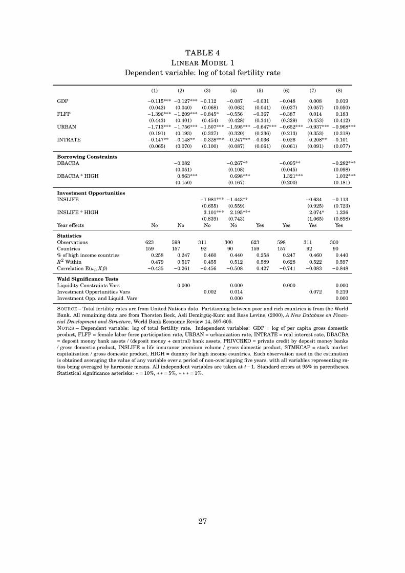
TABLE 4LINEAR MODEL 1

Dependent variable: log of total fertility rate

(1) (2) (3) (4) (5) (6) (7) (8)

GDP −0.115*** −0.127*** −0.112 −0.087 −0.031 −0.048 0.008 0.019(0.042) (0.040) (0.068) (0.063) (0.041) (0.037) (0.057) (0.050)

FLFP −1.396*** −1.209*** −0.845* −0.556 −0.367 −0.387 0.014 0.183(0.443) (0.401) (0.454) (0.428) (0.341) (0.329) (0.453) (0.412)

URBAN −1.713*** −1.756*** −1.507*** −1.595*** −0.647*** −0.652*** −0.937*** −0.968***(0.191) (0.193) (0.337) (0.320) (0.236) (0.213) (0.353) (0.318)

INTRATE −0.147** −0.148** −0.328*** −0.247*** −0.036 −0.026 −0.208** −0.101(0.065) (0.070) (0.100) (0.087) (0.061) (0.061) (0.091) (0.077)

Borrowing ConstraintsDBACBA −0.082 −0.267** −0.095** −0.282***

(0.051) (0.108) (0.045) (0.098)DBACBA * HIGH 0.863*** 0.698*** 1.321*** 1.032***

(0.150) (0.167) (0.200) (0.181)

Investment OpportunitiesINSLIFE −1.981*** −1.443** −0.634 −0.113

(0.655) (0.559) (0.925) (0.723)INSLIFE * HIGH 3.101*** 2.195*** 2.074* 1.236

(0.839) (0.743) (1.065) (0.898)Year effects No No No No Yes Yes Yes Yes

StatisticsObservations 623 598 311 300 623 598 311 300Countries 159 157 92 90 159 157 92 90% of high income countries 0.258 0.247 0.460 0.440 0.258 0.247 0.460 0.440R2 Within 0.479 0.517 0.455 0.512 0.589 0.628 0.522 0.597Correlation E(ui, Xβ) −0.435 −0.261 −0.456 −0.508 0.427 −0.741 −0.083 −0.848

Wald Significance TestsLiquidity Constraints Vars 0.000 0.000 0.000 0.000Investment Opportunities Vars 0.002 0.014 0.072 0.219Investment Opp. and Liquid. Vars 0.000 0.000

SOURCE – Total fertility rates are from United Nations data. Partitioning between poor and rich countries is from the WorldBank. All remaining data are from Thorsten Beck, Asli Demirgüç-Kunt and Ross Levine, (2000), A New Database on Finan-cial Development and Structure, World Bank Economic Review 14, 597-605.NOTES – Dependent variable: log of total fertility rate. Independent variables: GDP = log of per capita gross domesticproduct, FLFP = female labor force participation rate, URBAN = urbanization rate, INTRATE = real interest rate, DBACBA= deposit money bank assets / (deposit money + central) bank assets, PRIVCRED = private credit by deposit money banks/ gross domestic product, INSLIFE = life insurance premium volume / gross domestic product, STMKCAP = stock marketcapitalization / gross domestic product, HIGH = dummy for high income countries. Each observation used in the estimationis obtained averaging the value of any variable over a period of non-overlapping five years, with all variables representing ra-tios being averaged by harmonic means. All independent variables are taken at t−1. Standard errors at 95% in parentheses.Statistical significance asterisks: ∗= 10%, ∗∗= 5%, ∗∗∗= 1%.

27

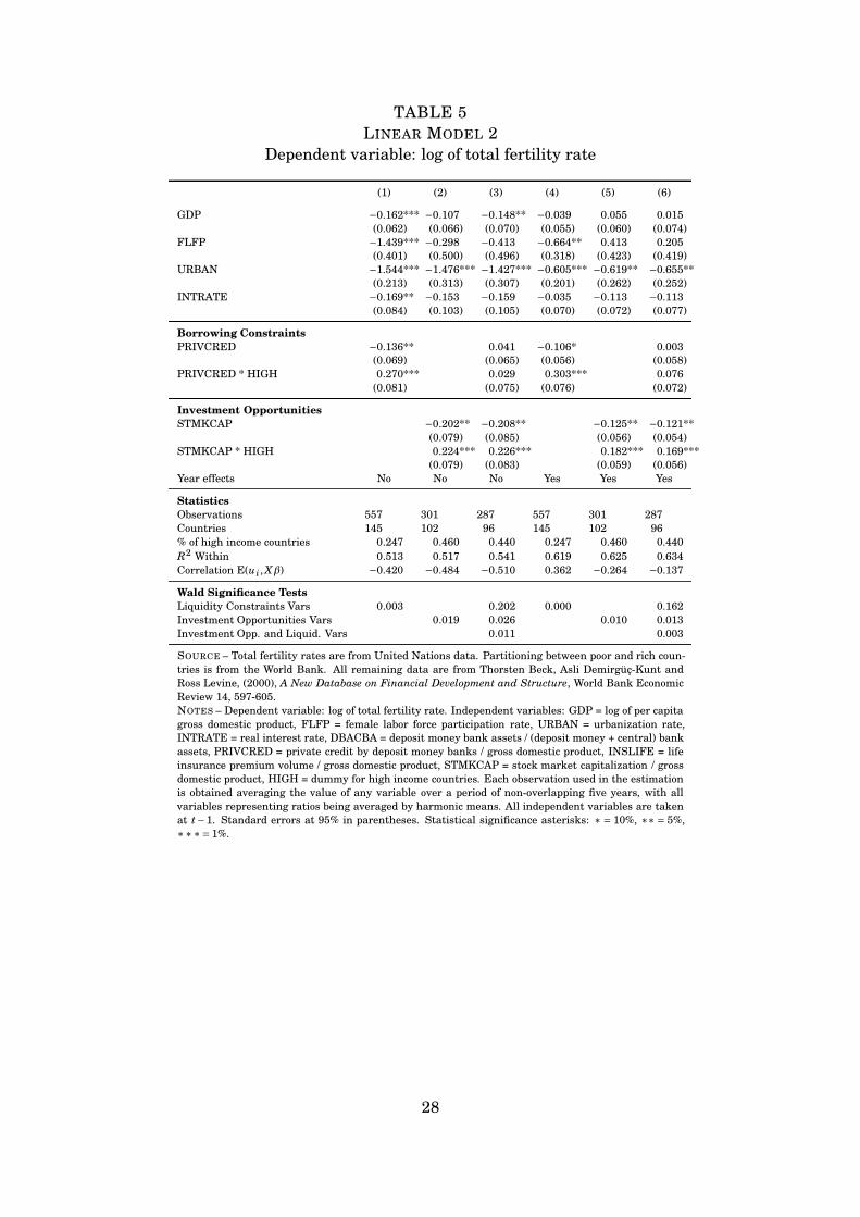
TABLE 5LINEAR MODEL 2

Dependent variable: log of total fertility rate

(1) (2) (3) (4) (5) (6)

GDP −0.162*** −0.107 −0.148** −0.039 0.055 0.015(0.062) (0.066) (0.070) (0.055) (0.060) (0.074)

FLFP −1.439*** −0.298 −0.413 −0.664** 0.413 0.205(0.401) (0.500) (0.496) (0.318) (0.423) (0.419)

URBAN −1.544*** −1.476*** −1.427*** −0.605*** −0.619** −0.655**(0.213) (0.313) (0.307) (0.201) (0.262) (0.252)

INTRATE −0.169** −0.153 −0.159 −0.035 −0.113 −0.113(0.084) (0.103) (0.105) (0.070) (0.072) (0.077)

Borrowing ConstraintsPRIVCRED −0.136** 0.041 −0.106* 0.003

(0.069) (0.065) (0.056) (0.058)PRIVCRED * HIGH 0.270*** 0.029 0.303*** 0.076

(0.081) (0.075) (0.076) (0.072)

Investment OpportunitiesSTMKCAP −0.202** −0.208** −0.125** −0.121**

(0.079) (0.085) (0.056) (0.054)STMKCAP * HIGH 0.224*** 0.226*** 0.182*** 0.169***

(0.079) (0.083) (0.059) (0.056)Year effects No No No Yes Yes Yes

StatisticsObservations 557 301 287 557 301 287Countries 145 102 96 145 102 96% of high income countries 0.247 0.460 0.440 0.247 0.460 0.440R2 Within 0.513 0.517 0.541 0.619 0.625 0.634Correlation E(ui, Xβ) −0.420 −0.484 −0.510 0.362 −0.264 −0.137

Wald Significance TestsLiquidity Constraints Vars 0.003 0.202 0.000 0.162Investment Opportunities Vars 0.019 0.026 0.010 0.013Investment Opp. and Liquid. Vars 0.011 0.003

SOURCE – Total fertility rates are from United Nations data. Partitioning between poor and rich coun-tries is from the World Bank. All remaining data are from Thorsten Beck, Asli Demirgüç-Kunt andRoss Levine, (2000), A New Database on Financial Development and Structure, World Bank EconomicReview 14, 597-605.NOTES – Dependent variable: log of total fertility rate. Independent variables: GDP = log of per capitagross domestic product, FLFP = female labor force participation rate, URBAN = urbanization rate,INTRATE = real interest rate, DBACBA = deposit money bank assets / (deposit money + central) bankassets, PRIVCRED = private credit by deposit money banks / gross domestic product, INSLIFE = lifeinsurance premium volume / gross domestic product, STMKCAP = stock market capitalization / grossdomestic product, HIGH = dummy for high income countries. Each observation used in the estimationis obtained averaging the value of any variable over a period of non-overlapping five years, with allvariables representing ratios being averaged by harmonic means. All independent variables are takenat t−1. Standard errors at 95% in parentheses. Statistical significance asterisks: ∗ = 10%, ∗∗ = 5%,∗∗∗= 1%.

28

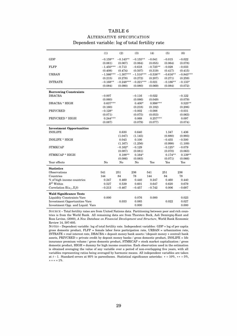
TABLE 6ALTERNATIVE SPECIFICATION

Dependent variable: log of total fertility rate

(1) (2) (3) (4) (5) (6)

GDP −0.159** −0.143** −0.155** −0.041 −0.015 −0.022(0.061) (0.067) (0.064) (0.055) (0.064) (0.078)

FLFP −1.450*** −0.713 −0.618 −0.725** −0.028 −0.033(0.408) (0.474) (0.507) (0.319) (0.417) (0.415)

URBAN −1.566*** −1.307*** −1.510*** −0.538** −0.616** −0.843***(0.215) (0.278) (0.272) (0.207) (0.271) (0.259)

INTRATE −0.168** −0.248*** −0.221*** −0.021 −0.186** −0.133*(0.084) (0.090) (0.080) (0.069) (0.084) (0.072)

Borrowing ConstraintsDBACBA −0.007 −0.116 −0.022 −0.122

(0.060) (0.086) (0.049) (0.079)DBACBA * HIGH 0.637*** 0.400* 0.998*** 0.525**

(0.160) (0.218) (0.182) (0.206)PRIVCRED −0.128* −0.002 −0.088 −0.031

(0.071) (0.075) (0.053) (0.063)PRIVCRED * HIGH 0.244*** 0.068 0.257*** 0.097

(0.087) (0.079) (0.077) (0.074)

Investment OpportunitiesINSLIFE 0.630 0.640 1.347 1.436

(1.047) (1.145) (0.880) (0.993)INSLIFE * HIGH 0.043 0.100 −0.455 −0.500

(1.167) (1.256) (0.998) (1.109)STMKCAP −0.162* −0.129 −0.125* −0.079

(0.087) (0.081) (0.070) (0.063)STMKCAP * HIGH 0.188** 0.164* 0.174** 0.139**

(0.086) (0.083) (0.071) (0.066)Year effects No No No Yes Yes Yes

StatisticsObservations 541 251 236 541 251 236Countries 144 84 78 144 84 78% of high income countries 0.247 0.460 0.440 0.247 0.460 0.440R2 Within 0.527 0.539 0.601 0.647 0.620 0.679Correlation E(ui, Xβ) −0.213 −0.467 −0.457 −0.742 0.006 −0.687

Wald Significance TestsLiquidity Constraints Vars 0.000 0.076 0.000 0.023Investment Opportunities Vars 0.033 0.085 0.022 0.027Investment Opp. and Liquid. Vars 0.000 0.000

SOURCE – Total fertility rates are from United Nations data. Partitioning between poor and rich coun-tries is from the World Bank. All remaining data are from Thorsten Beck, Asli Demirgüç-Kunt andRoss Levine, (2000), A New Database on Financial Development and Structure, World Bank EconomicReview 14, 597-605.NOTES – Dependent variable: log of total fertility rate. Independent variables: GDP = log of per capitagross domestic product, FLFP = female labor force participation rate, URBAN = urbanization rate,INTRATE = real interest rate, DBACBA = deposit money bank assets / (deposit money + central) bankassets, PRIVCRED = private credit by deposit money banks / gross domestic product, INSLIFE = lifeinsurance premium volume / gross domestic product, STMKCAP = stock market capitalization / grossdomestic product, HIGH = dummy for high income countries. Each observation used in the estimationis obtained averaging the value of any variable over a period of non-overlapping five years, with allvariables representing ratios being averaged by harmonic means. All independent variables are takenat t−1. Standard errors at 95% in parentheses. Statistical significance asterisks: ∗ = 10%, ∗∗ = 5%,∗∗∗= 1%.

29

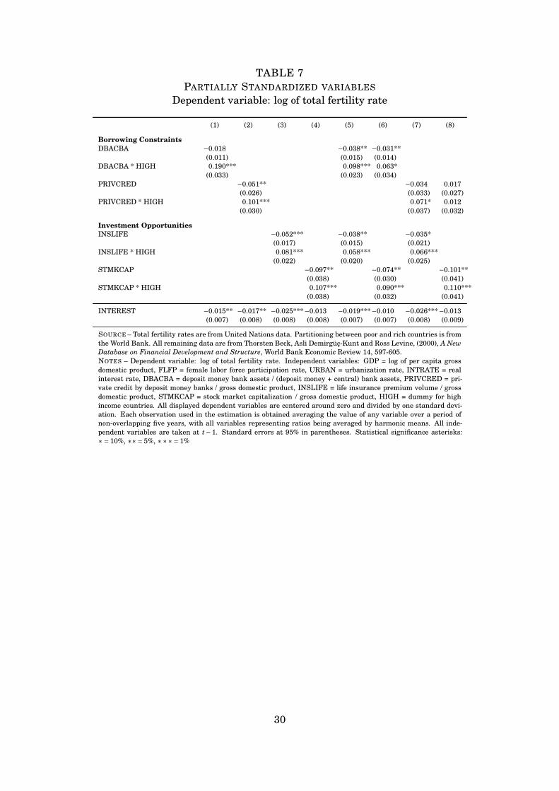
TABLE 7PARTIALLY STANDARDIZED VARIABLES

Dependent variable: log of total fertility rate

(1) (2) (3) (4) (5) (6) (7) (8)

Borrowing ConstraintsDBACBA −0.018 −0.038** −0.031**

(0.011) (0.015) (0.014)DBACBA * HIGH 0.190*** 0.098*** 0.063*

(0.033) (0.023) (0.034)PRIVCRED −0.051** −0.034 0.017

(0.026) (0.033) (0.027)PRIVCRED * HIGH 0.101*** 0.071* 0.012

(0.030) (0.037) (0.032)

Investment OpportunitiesINSLIFE −0.052*** −0.038** −0.035*

(0.017) (0.015) (0.021)INSLIFE * HIGH 0.081*** 0.058*** 0.066***

(0.022) (0.020) (0.025)STMKCAP −0.097** −0.074** −0.101**

(0.038) (0.030) (0.041)STMKCAP * HIGH 0.107*** 0.090*** 0.110***

(0.038) (0.032) (0.041)

INTEREST −0.015** −0.017** −0.025***−0.013 −0.019***−0.010 −0.026***−0.013(0.007) (0.008) (0.008) (0.008) (0.007) (0.007) (0.008) (0.009)

SOURCE – Total fertility rates are from United Nations data. Partitioning between poor and rich countries is fromthe World Bank. All remaining data are from Thorsten Beck, Asli Demirgüç-Kunt and Ross Levine, (2000), A NewDatabase on Financial Development and Structure, World Bank Economic Review 14, 597-605.NOTES – Dependent variable: log of total fertility rate. Independent variables: GDP = log of per capita grossdomestic product, FLFP = female labor force participation rate, URBAN = urbanization rate, INTRATE = realinterest rate, DBACBA = deposit money bank assets / (deposit money + central) bank assets, PRIVCRED = pri-vate credit by deposit money banks / gross domestic product, INSLIFE = life insurance premium volume / grossdomestic product, STMKCAP = stock market capitalization / gross domestic product, HIGH = dummy for highincome countries. All displayed dependent variables are centered around zero and divided by one standard devi-ation. Each observation used in the estimation is obtained averaging the value of any variable over a period ofnon-overlapping five years, with all variables representing ratios being averaged by harmonic means. All inde-pendent variables are taken at t−1. Standard errors at 95% in parentheses. Statistical significance asterisks:∗= 10%, ∗∗= 5%, ∗∗∗= 1%

30

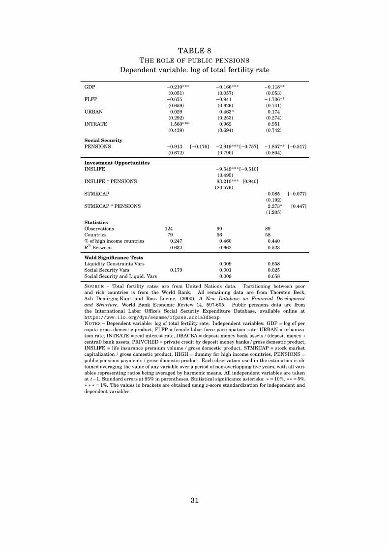
TABLE 8THE ROLE OF PUBLIC PENSIONS

Dependent variable: log of total fertility rate

GDP −0.210*** −0.166*** −0.118**(0.051) (0.057) (0.053)

FLFP −0.675 −0.941 −1.706**(0.659) (0.626) (0.741)

URBAN 0.029 0.463* 0.174(0.292) (0.253) (0.274)

INTRATE 1.560*** 0.962 0.951(0.439) (0.694) (0.742)

Social SecurityPENSIONS −0.913 [−0.176] −2.919*** [−0.757] −1.857** [−0.517]

(0.672) (0.790) (0.804)

Investment OpportunitiesINSLIFE −9.549*** [−0.510]

(3.495)INSLIFE * PENSIONS 83.210*** [0.940]

(20.576)STMKCAP −0.085 [−0.077]

(0.192)STMKCAP * PENSIONS 2.273* [0.447]

(1.205)

StatisticsObservations 124 90 89Countries 79 56 58% of high income countries 0.247 0.460 0.440R2 Between 0.632 0.662 0.523

Wald Significance TestsLiquidity Constraints Vars 0.009 0.658Social Security Vars 0.179 0.001 0.025Social Security and Liquid. Vars 0.009 0.658

SOURCE – Total fertility rates are from United Nations data. Partitioning between poorand rich countries is from the World Bank. All remaining data are from Thorsten Beck,Asli Demirgüç-Kunt and Ross Levine, (2000), A New Database on Financial Developmentand Structure, World Bank Economic Review 14, 597-605. Public pensions data are fromthe International Labor Office’s Social Security Expenditure Database, available online athttps://www.ilo.org/dyn/sesame/ifpses.socialdbexp.NOTES – Dependent variable: log of total fertility rate. Independent variables: GDP = log of percapita gross domestic product, FLFP = female labor force participation rate, URBAN = urbaniza-tion rate, INTRATE = real interest rate, DBACBA = deposit money bank assets / (deposit money +central) bank assets, PRIVCRED = private credit by deposit money banks / gross domestic product,INSLIFE = life insurance premium volume / gross domestic product, STMKCAP = stock marketcapitalization / gross domestic product, HIGH = dummy for high income countries, PENSIONS =public pensions payments / gross domestic product. Each observation used in the estimation is ob-tained averaging the value of any variable over a period of non-overlapping five years, with all vari-ables representing ratios being averaged by harmonic means. All independent variables are takenat t−1. Standard errors at 95% in parentheses. Statistical significance asterisks: ∗= 10%, ∗∗= 5%,∗∗∗= 1%. The values in brackets are obtained using z-score standardization for independent anddependent variables.

31

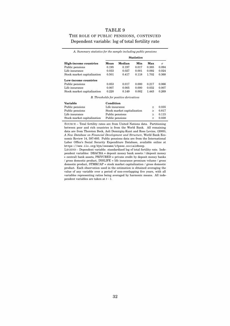
TABLE 9THE ROLE OF PUBLIC PENSIONS, CONTINUED

Dependent variable: log of total fertility rate

A. Summary statistics for the sample including public pensions

Statistics

High-income countries Mean Median Min Max σ

Public pensions 0.195 0.197 0.017 0.385 0.094Life insurance 0.033 0.027 0.001 0.092 0.024Stock market capitalization 0.501 0.417 0.118 1.702 0.368

Low-income countriesPublic pensions 0.053 0.017 0.000 0.217 0.066Life insurance 0.007 0.005 0.000 0.032 0.007Stock market capitalization 0.220 0.149 0.002 1.443 0.269

B. Thresholds for positive derivatives

Variable ConditionPublic pensions Life insurance ≥ 0.035Public pensions Stock market capitalization ≥ 0.817Life insurance Public pensions ≥ 0.115Stock market capitalization Public pensions ≥ 0.038

SOURCE – Total fertility rates are from United Nations data. Partitioningbetween poor and rich countries is from the World Bank. All remainingdata are from Thorsten Beck, Asli Demirgüç-Kunt and Ross Levine, (2000),A New Database on Financial Development and Structure, World Bank Eco-nomic Review 14, 597-605. Public pensions data are from the InternationalLabor Office’s Social Security Expenditure Database, available online athttps://www.ilo.org/dyn/sesame/ifpses.socialdbexp.LEGEND – Dependent variable: standardized log of total fertility rate. Inde-pendent variables: DBACBA = deposit money bank assets / (deposit money+ central) bank assets, PRIVCRED = private credit by deposit money banks/ gross domestic product, INSLIFE = life insurance premium volume / grossdomestic product, STMKCAP = stock market capitalization / gross domesticproduct. Each observation used in the estimation is obtained averaging thevalue of any variable over a period of non-overlapping five years, with allvariables representing ratios being averaged by harmonic means. All inde-pendent variables are taken at t−1.

32

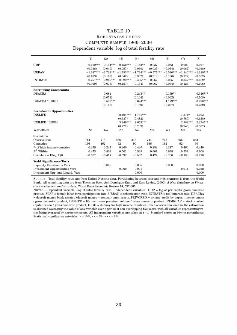
TABLE 10ROBUSTNESS CHECK:

COMPLETE SAMPLE 1960–2006Dependent variable: log of total fertility rate

(1) (2) (3) (4) (5) (6) (7) (8)

GDP −0.179*** −0.191*** −0.152*** −0.153** −0.037 −0.053 −0.029 −0.027(0.036) (0.040) (0.057) (0.060) (0.039) (0.034) (0.067) (0.058)

URBAN −1.687*** −1.722*** −1.753*** −1.764*** −0.577*** −0.590*** −1.140*** −1.189***(0.169) (0.165) (0.342) (0.332) (0.210) (0.196) (0.372) (0.352)

INTRATE −0.257*** −0.245*** −0.529*** −0.405*** −0.062 −0.035 −0.342*** −0.189*(0.069) (0.075) (0.157) (0.134) (0.062) (0.064) (0.123) (0.106)

Borrowing ConstraintsDBACBA −0.084 −0.243** −0.159** −0.316***

(0.074) (0.104) (0.062) (0.108)DBACBA * HIGH 0.536*** 0.624*** 1.179*** 0.990***

(0.160) (0.189) (0.227) (0.259)

Investment OpportunitiesINSLIFE −2.104*** −1.761*** −1.371* −1.023

(0.537) (0.482) (0.780) (0.628)INSLIFE * HIGH 3.249*** 2.655*** 2.884*** 2.234***

(0.777) (0.739) (0.945) (0.837)Year effects No No No No Yes Yes Yes Yes

StatisticsObservations 744 713 356 343 744 713 356 343Countries 166 162 92 90 166 162 92 90% of high income countries 0.258 0.247 0.460 0.440 0.258 0.247 0.460 0.440R2 Within 0.473 0.509 0.501 0.539 0.601 0.638 0.558 0.608Correlation E(ui, Xβ) −0.587 −0.417 −0.597 −0.502 0.424 −0.706 −0.138 −0.778

Wald Significance TestsLiquidity Constraints Vars 0.005 0.005 0.000 0.000Investment Opportunities Vars 0.000 0.001 0.011 0.032Investment Opp. and Liquid. Vars 0.000 0.000

SOURCE – Total fertility rates are from United Nations data. Partitioning between poor and rich countries is from the WorldBank. All remaining data are from Thorsten Beck, Asli Demirgüç-Kunt and Ross Levine, (2000), A New Database on Finan-cial Development and Structure, World Bank Economic Review 14, 597-605.NOTES – Dependent variable: log of total fertility rate. Independent variables: GDP = log of per capita gross domesticproduct, FLFP = female labor force participation rate, URBAN = urbanization rate, INTRATE = real interest rate, DBACBA= deposit money bank assets / (deposit money + central) bank assets, PRIVCRED = private credit by deposit money banks/ gross domestic product, INSLIFE = life insurance premium volume / gross domestic product, STMKCAP = stock marketcapitalization / gross domestic product, HIGH = dummy for high income countries. Each observation used in the estimationis obtained averaging the value of any variable over a period of non-overlapping five years, with all variables representing ra-tios being averaged by harmonic means. All independent variables are taken at t−1. Standard errors at 95% in parentheses.Statistical significance asterisks: ∗= 10%, ∗∗= 5%, ∗∗∗= 1%.

33

A Appendix: Data description

The samples used for estimation of the regression models are basically two: the firstsample includes those countries which have observations for the variable DBACBAand for the control variables. This sample is used to estimate the column 2 and6 of table 4. These countries are Albania, Algeria, Angola, Argentina, Armenia,Australia, Austria, Azerbaijan, Bahamas, Bahrain, Bangladesh, Belarus, Belgium,Belize, Benin, Bhutan, Bolivia, Botswana, Brazil, Brunei Darussalam, Bulgaria,Burkina Faso, Burundi, Cambodia, Cameroon, Canada, Cape Verde, Central AfricanRepublic, Chad, Chile, China, Colombia, Comoros, Congo, Costa Rica, Croatia,Cyprus, Czech Republic, Denmark, Djibouti, Dominican Republic, Ecuador, Egypt,El Salvador, Equatorial Guinea, Estonia, Ethiopia, Fiji, Finland, France, Gabon,Gambia, Georgia, Germany, Ghana, Greece, Guatemala, Guinea, Guinea Bissau,Guyana, Haiti, Honduras, Hungary, Iceland, India, Indonesia, Iran, Ireland, Israel,Italy, Ivory Coast, Jamaica, Japan, Jordan, Kenya, Kuwait, Kyrgyz Republic, Laos,Latvia, Lebanon, Lesotho, Liberia, Libya, Lithuania, Luxembourg, Macao, Mace-donia, Madagascar, Malawi, Malaysia, Maldives, Mali, Malta, Mauritania, Mauri-tius, Mexico, Moldova, Mongolia, Morocco, Mozambique, Namibia, Nepal, Nether-lands, New Zealand, Nicaragua, Niger, Nigeria, Norway, Oman, Panama, Papua NewGuinea, Paraguay, Peru, Philippines, Poland, Portugal, Russian Federation, Rwanda,Samoa, Sao Tome and Principe, Senegal, Sierra Leone, Singapore, Slovak Republic,Slovenia, Solomon Islands, South Africa, South Korea, Spain, Sri Lanka, St. Lu-cia, St. Vincent and the Grenadines, Suriname, Swaziland, Sweden, Switzerland,Syrian Arab Republic, Tajikistan, Tanzania, Thailand, Togo, Tonga, Trinidad andTobago, Tunisia, Uganda, Ukraine, United Arab Emirates, United Kingdom, UnitedStates, Uruguay, Vanuatu, Venezuela, Vietnam, Yemen, Zaire, Zambia, Zimbabwe.

A second, more restricted, sample was used to estimate the regression model withthe simultaneous inclusion of the variables DBACBA and INSLIFE: for this last vari-able, less countries provide valid observations. These countries are Algeria, Angola,Argentina, Australia, Austria, Bahrain, Bangladesh, Belgium, Botswana, Brazil,Bulgaria, Cameroon, Canada, Chile, China, Colombia, Costa Rica, Croatia, Cyprus,Czech Republic, Denmark, Dominican Republic, Ecuador, Egypt, El Salvador, Esto-nia, Finland, France, Germany, Greece, Guatemala, Honduras, Hungary, Iceland,India, Indonesia, Iran, Ireland, Israel, Italy, Ivory Coast, Jamaica, Japan, Jordan,Kenya, Kuwait, Latvia, Lebanon, Libya, Lithuania, Luxembourg, Macao, Malaysia,Malta, Mauritius, Mexico, Morocco, Namibia, Netherlands, New Zealand, Nigeria,Norway, Oman, Panama, Paraguay, Peru, Philippines, Poland, Portugal, RussianFederation, Singapore, Slovak Republic, Slovenia, South Africa, South Korea, Spain,Sri Lanka, Sweden, Switzerland, Syrian Arab Republic, Thailand, Trinidad and To-bago, Tunisia, Ukraine, United Kingdom, United States, Uruguay, Venezuela, Viet-nam, Zimbabwe.

34

References

BECK, T., A. DEMIRGÜÇ-KUNT, AND R. LEVINE (2000): “A New Database onthe Structure and Development of the Financial Sector,” The World BankEconomic Review, 14(3), 597–605.

(2004): Financial structure and economic growth: A cross-countrycomparison of banks, markets, and development. The MIT Press.

BECKER, G. S. (1960): “An economic analysis of fertility,” in Demographicand economic change in developed countries, ed. by R. Easterlin, vol. 11,pp. 209–231. Princeton University Press, Princeton.

BECKER, G. S., AND H. LEWIS (1973): “On the Interaction between the Quan-tity and Quality of Children,” The Journal of Political Economy, 81(2), 279–288.

BOLDRIN, M., M. DE NARDI, AND L. JONES (2005): “Fertility and socialsecurity,” Working Paper 11146, National Bureau of Economic Research,Cambridge, MA.

CIGNO, A., AND F. C. ROSATI (1992): “The effects of financial markets andsocial security on saving and fertility behaviour in Italy,” Journal of Popu-lation Economics, 5(4), 319–341.

(1996): “Jointly Determined Saving and Fertility Behaviour: Theoryand Estimates for Germany, Italy, UK, and USA,” European Economic Re-view, 40(8), 1561–1589.

EHRLICH, I., AND J. KIM (2007): “Social security and demographic trends:Theory and evidence from the international experience,” Review of Eco-nomic Dynamics, 10(1), 55–77.

EHRLICH, I., AND F. LUI (1991): “Intergenerational trade, longevity, andeconomic growth,” Journal of Political Economy, 99(5), 1029–1059.

FEYRER, J., B. SACERDOTE, AND A. D. STERN (2008): “Will the stork returnto Europe and Japan? Understanding fertility within developed nations,”Journal of Economic Perspectives, 22(3), 3–22.

HARVEY, R. (2004): “Comparison of household saving ratios: Euroarea/United States/Japan,” Statistics Brief 8, Organisation for EconomicCo-operation and Development (OECD).

HOTZ, J. V., J. KLERMAN, AND R. WILLIS (1997): “The economics of fertilityin developed countries,” in Handbook of Population and Family Economics,ed. by M. R. Rosenzweig, and O. Stark, vol. 1a, chap. 3, pp. 275–347. Else-vier Science, Amsterdam.

35

JONES, L. E., A. SCHOONBROODT, AND M. TERTILT (2008): “Fertility theo-ries: can they explain the negative fertility-income relationship?,” WorkingPaper 14266, National Bureau of Economic Research, Cambridge, MA.

JONES, L. E., AND M. TERTILT (2006): “An economic history of fertility inthe US: 1826–1960,” Working Paper 12796, National Bureau of EconomicResearch, Cambridge, MA.

LAGERLÖF, N.-P. (1997): “Endogenous fertility and the old-age security hy-pothesis: A note,” Journal of Public Economics, 64(2), 279–286.

LEIBENSTEIN, H. (1957): Economic backwardness and economic growth:Studies in the theory of economic development. Wiley, New York, NY.

MCKINNON, R. I. (1973): Money and capital in economic development. TheBrookings Institution, Washington, D.C.

NEHER, P. A. (1971): “Peasants, procreation, and pensions,” American Eco-nomic Review, 61(3), 380–389.

NISHIMURA, K., AND J. ZHANG (1992): “Pay-as-you-go public pensions withendogenous fertility.,” Journal of Public Economics, 48(2), 239.

PITT, M. M., S. R. KHANDKER, S. M. MCKERNAN, AND M. A. LATIF (1999):“Credit programs for the poor and reproductive behavior in low-incomecountries: are the reported causal relationships the result of heterogene-ity bias?,” Demography, 36(1), 1–21.

POLLIN, R. (1997): “Financial intermediation and the variability of the sav-ing constraint,” in The macroeconomics of saving, finance, and investment,ed. by R. Pollin, chap. 5, pp. 309–366. University of Michigan Press, AnnArbor, MI.

RAZIN, A., AND E. SADKA (1995): Population Economics. The MIT Press,Cambridge, MA.

SCHULER, S. R., AND S. M. HASHEMI (1994): “Credit programs, women’s em-powerment, and contraceptive use in rural Bangladesh,” Studies in FamilyPlanning, 25(2), 65–76.

SCHULER, S. R., S. M. HASHEMI, AND A. P. RILEY (1997): “The influenceof women’s changing roles and status in Bangladesh’s fertility transition:evidence from a study of credit programs and contraceptive use,” WorldDevelopment, 25(4), 563–575.

SCHULTZ, T. P. (1997): “Demand for Children in Low Income Countries,” inHandbook of Population and Family Economics, ed. by M. R. Rosenzweig,and O. Stark, vol. 1a, chap. 8, pp. 349–430. Elsevier Science, Amsterdam.

SCHULTZ, T. W. (ed.) (1974): Economics of the family: Marriage, children,and human capital. University of Chicago Press, Chicago, IL.

36

SCOTESE LEHR, C. (1999): “Banking on fewer children: Financial interme-diation, fertility and economic development,” Journal of Population Eco-nomics, 12(4), 567–590.

SHAW, E. (1973): Financial Deepening in Economic Development. Oxford Uni-versity Press, Oxford, UK.

STEELE, F., S. AMIN, AND R. T. NAVED (2001): “Savings/Credit Group For-mation and Change in Contraception,” Demography, 38(2), 267–282.

THE WORLD BANK (2007): “World Development Indicators,” .

WILLIS, R. J. (1973): “A new approach to the economic theory of fertilitybehavior,” The Journal of Political Economy, 81(2), 14–64.

(1980): “The old age security and population growth,” in Demographicbehavior: Interdisciplinary perspectives on decision making, ed. by T. K.Burch. Westview Press, Boulder, CO.

37