Validation of atmospheric propagationmodels in littoral waters

Arie N. de JongPiet B. W. SchweringAlexander M. J. van EijkWillem H. Gunter

Validation of atmospheric propagation modelsin littoral waters

Arie N. de JongPiet B. W. SchweringAlexander M. J. van EijkOrganisation for Applied Scientific ResearchP.O. Box 96864The Hague, The NetherlandsE-mail: anejdejong@hetnet.nl

Willem H. GunterInstitute for Maritime TechnologySimon’s Town 7995, South Africa

Abstract. Various atmospheric propagation effects are limiting the long-range performance of electro-optical imaging systems. These effectsinclude absorption and scattering by molecules and aerosols, refractiondue to vertical temperature gradients and scintillation and blurring dueto turbulence. In maritime and coastal areas, ranges up to 25 km are rel-evant for detection and classification tasks on small targets (missiles,pirates). From November 2009 to October 2010 a measurement campaignwas set-up over a range of more than 15 km in the False Bay in SouthAfrica, where all of the propagation effects could be investigated quanti-tatively. The results have been used to provide statistical information onbasic parameters as visibility, air-sea temperature difference, absolutehumidity and wind speed. In addition various propagation models on aero-sol particle size distribution, temperature profile, blur and scintillationunder strong turbulence conditions could be validated. Examples of col-lected data and associated results are presented in this paper.© 2013Societyof Photo-Optical Instrumentation Engineers (SPIE) [DOI: 10.1117/1.OE.52.4.046002]

Subject terms: atmospheric transmission; refraction; turbulence; scintillation; atmos-pheric blur; beam wander; marine boundary layer.

Paper 121557P received Oct. 25, 2012; revised manuscript received Mar. 4, 2013;accepted for publication Mar. 5, 2013; published online Apr. 8, 2013.

1 IntroductionThe range performance of electro-optical sensors is generallydetermined by three major contributors: the signature of thetarget (size, shape, and reflection) and its background (radi-ance distribution), the characteristics of the interveningmedium (transmission, refraction, blur, and scintillation)and the sensor parameters (sensitivity, resolution). Formost of these issues, models have been developed, predictingranges for a variety of weather conditions and locations. Inthis paper, characteristics of atmospheric propagation effectswill be discussed, especially for littoral waters. In coastal andmaritime locations, the uncertainty of the model predictionsincreases due to the long horizon distances and the pooravailability of basic atmospheric parameters. In practicalapplications, such as detection and classification of smallboats from a coastal location or from a tall ship, identifica-tion at the longest possible ranges is required (for example3 × 3 m targets at 25 km).

Atmospheric propagation models are available for mosttopics: extinction due to aerosols and molecules, refractiondue to temperature gradients in the vertical direction andturbulence. For maritime conditions, locally measured par-ticle size distributions (PSD) are used,1 from which scatter-ing is calculated via Mie calculations, included in theMODTRAN transmission code.2 In coastal areas, the PSDmay be disturbed by breaking waves in the surf zone, creat-ing additional large particles, influencing the wavelengthdependent scattering. By using a retrieval method, basedupon data from a path-averaging multiband transmissometer,it should be possible to obtain more detailed information onthe real PSD characteristics. Refraction effects, responsiblefor distortion of the atmospheric point spread function (PSF)

and variations of the optical horizon range, follow from theMonin-Obukhov (MO) boundary layer theory,3 predictingvertical profiles and implemented in the turbulence andrefraction model over the sea (TARMOS) code, developedat TNO. These profiles can be implemented in ray tracingschemes, providing the angle of arrival (AOA), underwhich a distant source is observed. The MO theory, basedupon atmospheric input parameters as wind speed, relativehumidity, air temperature, sea temperature and air pressure,also predicts Cn

2, the structure parameter for refractiveindex, describing turbulence effects such as scintillationand blur. Quantitative measurement of these effects asdescribed by the theory (Andrews4), was one of the majorissues during the experiments. As a result of the blurdata, range performance can be predicted for given targetand sensor characteristics (Holst5).

For the validation of these models it is highly recom-mended to arrange an experiment covering a long periodwith a variety of weather conditions. Moreover it is essentialthat the main wind direction is coming from the open ocean.The location of the selected validation campaign, calledFalse Bay atmospheric experiment (FATMOSE) is indicatedin Fig. 1, showing the range of 15.7 km between the Instituteof Maritime Technology (IMT) in Simon’s Town and theNational Sea Rescue Institute (NSRI) in Strandfontein.

Sensors were located at IMT at 14.5 m above mean sealevel (AMSL) and Roman rock lighthouse (RRL) at 15 mAMSL (9 m for the visibility meter). The sources weremounted on the roof of NSRI at different heights: 9.7 and5.8 m for the two central sources and 8.7 m AMSL forthe two outer sources. The mean weather characteristics inthe False Bay, as collected by the weather stations at IMTand RRL during the FATMOSE trial from November2009 to October 2010, are shown in Fig. 2.0091-3286/2013/$25.00 © 2013 SPIE

Optical Engineering 046002-1 April 2013/Vol. 52(4)

Optical Engineering 52(4), 046002 (April 2013)

Figure 2 shows a large variability in the visibility with amean value of 15 km, about the length of the measurementpath. This value, measured locally at RRL with a VaisalaFS11 visibility meter, is a perfect distance for PSD retrievalstudies carried out with the multiband transmissometer,located at IMT. It is also shown that wind speeds up to20 m∕s may occur from a dominating southeastern direc-tion (from the open ocean). Statistics on the air sea temper-ature difference (ASTD), having an impact on the behaviorof Cn

2, are also shown in Fig. 2, where it is noted that thewater temperature was measured radiometrically at RRL.The ASTD values were ranging from roughly −4 to þ8 K,introducing various temperature profiles. From buoy mea-surements and satellite imagery it was found that thewater temperature in the Bay is not constant, mainly dueto the mixing of warm and cool currents in the area. As aconsequence, it is very likely that the ASTD is not constantalong the path. Other parameters such as air temperature, rel-ative humidity, and wind speed were found to be very similarat the two weather stations (at IMT and RRL).

The mean value of Cn2, as measured between IMT and

RRL (range 1.8 km) with a Scintec BLS 900 scintillometer,was found to be 10−15 m−2∕3, which is significantly lowerthan for land conditions where values of 10−14 and higherare commonly measured.

The plots in Fig. 2 illustrate the attractiveness of theFalse Bay location for atmospheric propagation experiments

Fig. 1 Location of the FATMOSE trial in the False Bay (South Africa).

Fig. 2 Review of the mean weather statistics in the False Bay area during FATMOSE. (a) Absolute humidity (AH) and air temperature. (b) Visibilityand relative humidity (RH). (c) Wind speed and wind direction. (d) Air-sea temperature difference (ASTD) and Cn

2.

Optical Engineering 046002-2 April 2013/Vol. 52(4)

De Jong et al.: Validation of atmospheric propagation models in littoral waters

thanks to the fact that the campaign could be run for a periodof more than 10 months. This allows the selection of inter-mediate periods with “good” weather with stable conditionsfor at least several hours where the validation of propagationmodels can be carried out in a successful manner. Detaileddescriptions of the set-up of FATMOSE and results of thevarious investigations have been presented in several SPIEconference papers. In the paper on transmission6 a newmethod for the retrieval of aerosol PSDs has been introduced,based upon multiband transmission data. The paper on re-fraction contains a comparison of measured angle of arrival(AOA) with predictions via ray tracing through MO theorybased vertical temperature profiles.7 Atmospheric blur,8

directly related to the target identification range, wasshown to be smaller than expected from former coastalCn

2 data. For scintillation9 a comparison of measured datawith predictions from the strong turbulence theory wasmade, due to the longer range used in FATMOSE, wherethe weak turbulence theory is no longer valid. In thispaper, a summary of the main validation results, includingtheir theoretical background, as discussed in these papersis given. In addition, long term statistics are presented ofthe transmission levels in various spectral bands, as wellas the statistics of blur and scintillation, being of importancefor operational purpose.

2 Transmission and Aerosol RetrievalThe MSRT transmissometer, developed at TNO, providestransmission data in five spectral bands, ranging from0.40 to 0.49 μm (band 1), 0.57 to 0.65 μm (band 2), 0.78to 1.04 μm (band 3), 1.39 to 1.67 μm (band 4) and 2.12to 2.52 μm (band 5). The source has a diameter of 20 cmand is modulated with a frequency of 1000 Hz. At thereceiver, with an aperture of 4 cm, the integration timewas set to 21 s for transmission purpose and 10 ms for scin-tillation, with a sampling time of 5 ms. The first issue, beingof importance for operational use, concerns the long-termtransmission statistics in each of the five bands, which isshown in Fig. 3. This figure shows quantitatively the benefitof using sensors operating at longer wavelengths. The reasonfor this effect is, of course, the decrease of the aerosol par-ticle density with particle diameter, as shown in Ref. 1,resulting in less scattering for longer wavelengths.

This is precisely the basic idea for using the MSRT inthe determination of the PSD. In this investigation, the gen-erally accepted PSD, as discussed1 and based upon threeor four lognormal neighboring components, is approachedby a well-known Junge distribution with one lognormalcomponent for particles smaller than 0.16 μm and with amaximum for a particle diameter of 0.08 μm. The Jungedistribution is given by logðdN∕dDÞ ¼ Jc þ Je · logðDÞ ordN∕dD ¼ 10Jc · DJe , in which D is the particle diameter(in μm) and dN∕dD the number of particles per μm percm3. For a Junge coefficient, Jc ¼ 2 and two Junge expo-nents Je ¼ −3.5 and −4.5, distributions are shown inFig. 4(a). Considering Beer’s law, τ ¼ expð−σRÞ, where τis the transmission for the path length R (15.7 km) and σthe extinction coefficient (km−1), we can convert this intologf− lnðτiÞg ¼ logð15.7σiÞ, where τi and σi deal withthe i’th waveband. For the centers of the five MSRT wave-bands, logð15.7σiÞ was calculated for a number of Jungeexponents, Je between −3 and −5, using a standard Miecode for the extinction coefficient of spherical particles(pure water).10 The result of this calculation is shown inFig. 4(b) for Je ¼ −3.5 and −4.5 and Jc ¼ 0. It is notedthat in a real atmosphere, water can be contaminated, intro-ducing a complex index of refraction which may lead todeviating (stronger) Mie extinctions at certain wavelengths,which are neglected here because of the broad spectralbands.

Fig. 3 Statistics of the (total) transmission levels during 230 days ofmeasurements for the five spectral bands of the MSRT system.

Fig. 4 Characteristics of the adopted Junge particle size distribution for two values of Je and Jc ¼ 2 (a). In (b) the corresponding aerosol extinctionas function of wavelength is shown for two values of Je , Jc ¼ 0 and a range of 15.7 km, as calculated with the Mie code.

Optical Engineering 046002-3 April 2013/Vol. 52(4)

De Jong et al.: Validation of atmospheric propagation models in littoral waters

If the plotted curves are approximated by straight lines, itis found that the slope s of these lines varies with Je in anearly linear way, as shown in Fig. 5(a), for the case ofthree selected wavelengths. The regression line for threewavelengths is found to be Je ¼ 2.54s − 2.84 and for thefive wavelengths Je ¼ 2.85s − 2.82, so the measurementof s directly delivers Je. In order to obtain Jc, it has tobe realized that variation of Jc results in a vertical shift ofthe plots in Fig. 4(b) according to logð15.7σiÞ þ Jc. The val-ues of logð15.7σiÞ were calculated with the Mie code asfunction of Je. The results for three of the MSRT wavebandcenters are shown in Fig. 5(b), where it appears that theplots fit perfectly with third order polynomials, such aslogð15.7σiÞ¼ 0.042Je3þ0.6983Je2þ3.723Jeþ4.8317 forband 3 (0.91 μm). When these five (or three) valuesof logð15.7σiÞ are compared with the measured values oflogf− lnðτiÞg, it is realized that Jc is just the differencebetween both.

It is noted that this method of determination of Je and Jcfails if the transmission level is too low (<0.02) or too high(>1), such as occurring in cases of refractive gain6 (Fig. 13).It is further noted that the transmission levels as discussedbefore are considered to be just due to the extinction by aero-sols. A correction has to be made to the measured total trans-mission levels τtot, realizing that τtot ¼ τmolτaer, where τmol

and τaer are representing the transmission by molecules

and aerosols, respectively. The total transmission data aretherefore divided by the molecular transmission in orderto obtain the transmission by aerosols only. For each ofthe spectral bands, the molecular transmission for thepath length of 15.7 km is approximated via a linearrelationship with AH (absolute humidity) deduced fromMODTRAN. For example, for band 3 (around 0.91 μm)is found τmol ¼ −0.0072AHþ 0.754; AH is related to therelative humidity RH and the air temperature TðCÞ by AH ¼ð0.02T2 þ 0.1874T þ 5.5304ÞRH∕100. These relations arevalid for the domain of AH as occurring in the False Bay(5 to 15 g∕m3).

In Fig. 6, plots are shown of the transmissions in bands 2and 4, including the retrieved associated values of Jc and Jefor a 2.5 days period in which the wind speed decreases andthe visibility increases on the 31st of January around 13.00.At this time, the slope s is increasing, resulting in a decreaseof Je and Jc. It is noted that the total transmission was about0.27 for band 2, which corresponds to a visibility of 47 km.This value corresponds quite well with the measured (local)visibility of 40 km at RRL.

In addition to the data in Fig. 6, a selection of six periodsof about five days was made where the weather conditionsdid meet the requirements (no rain, fog or refraction). For alldata of these days, retrieved Je and Jc data were correlatedwith the transmission levels, of which the result is shown in

Fig. 5 Junge exponent Je as function of the slope s in the plot of the extinction logð15.7σÞ versus wavelength (a). Plots of logð15.7σi Þ versus Je ,supporting the Jc retrieval for three wavelengths, being the centers of bands 2, 3, and 4 are shown in (b). Jc is obtained by comparing logð15.7σi Þwith logf− lnðτi Þg for the three (or five) MSRT wavebands.

Fig. 6 Transmission plots for the MSRT spectral bands 2 and 4 during 2.5 days. From the slope s of logð15.7σÞ (where σ is the extinction coefficient)versus the wavelength, values of Je and Jc were retrieved, showing variations in the particle size distribution.

Optical Engineering 046002-4 April 2013/Vol. 52(4)

De Jong et al.: Validation of atmospheric propagation models in littoral waters

Fig. 7(a). Despite some sudden changes in wind directionduring the selected periods from southeast to northwest(or vice-versa) introducing different air masses, the cor-relation is remarkably good both Je and Jc decrease forhigher transmission levels (band 4). It is interesting tonote the increase of Je and Jc with wind speed as shownin Fig. 7(b), as expected from the MODTRAN model. Inthis case, only data with values for relative humidity RHsmaller than 80% were taken. In a similar plot an increaseof Je and Jc with RH (for wind speeds less than 10 m∕s)was found.

3 RefractionAtmospheric refraction is a well-known phenomenon, fre-quently visible near sunrise and sunset and showing distor-tions of the sun disc. The reason for this effect is the presenceof a gradient in the refractive index of air in the lower part ofthe boundary layer. Consequently, rays bend upward whenthe air is cooler than the water and bend downward when theair is warmer than the water. Optically this means that thehorizon is observed under a lower angle with the tangentto the earth in the first case and a higher angle in the secondcase. During the FATMOSE experiment, a fixed source atNSRI was constantly observed with a Topcon theodolitecoupled to a CCD camera. By means of special analysissoftware, the AOA (angle between the source and the

geometrical horizon) was determined ten times per minute.This AOA can also be calculated if the vertical profile of therefractive index (or temperature) is known, as shownbefore.11 The related ray-tracing program is based upon cal-culation of the ray curvature Kc at a number of points alongthe ray via Kc ¼ ðdn∕dzÞ∕n, where n is the refractive indexand z is the altitude (in m) above water. Following Beland,12

n is approximated by n ¼ 1þ 786 · 10 − 8P∕T where P isthe barometric pressure (in N∕m2) and T the air temperature(K). The derivative follows from dn∕dz ¼ −ðdT∕dzþ0.0348Þ · 786 · 10 − 9 · P∕T2, where the value of 0.0348results from the pressure decrease with altitude.

Three examples of temperature profiles and their deriva-tives are shown in Fig. 8(a) for an ASTD of −2 K.One profile follows from the turbulence and refractionmodel over the sea (TARMOS) code, which is basedupon the MO theory,3 and developed at TNO. This profileTz−T0¼−0.1513 · ½lnðz∕0.000021Þ−2 ·lnf0.5ð1þð1þ15z∕352Þ0.5Þg� and its derivative dT∕dz is associated with a windspeed of 15 m∕s and a relative humidity of 70%. Theseparameters, together with two air temperatures, one atwater level and one at a standard height and the air pressureare input parameters for the TARMOS code.7 They basicallydetermine the vertical exchanges of heat, moisture andmomentum in the marine boundary layer. The other two pro-files are basically power profiles, defined by Tz − T0 ¼ BzA

Fig. 7 Plots showing a decrease of Je and Jc with increasing total transmission (a) and an increase with increasing wind speed (b) for 29 days oftransmission data. Increase of Je and Jc implies bigger particles with a higher concentration, as can be expected with rough seas or decreasingvisibility.

Fig. 8 Vertical profiles of the temperature and the temperature gradient for two power law profiles and one predicted from TARMOS (ASTD ¼ −2 K@ z ¼ 15 m, wind speed 15 m∕s) (a). Predictions of the angle of arrival AOA and the differential angle of arrival Dy versus ASTD for the profiles,predicted from TARMOS for wind speeds of 5 and 15 m∕s (b).

Optical Engineering 046002-5 April 2013/Vol. 52(4)

De Jong et al.: Validation of atmospheric propagation models in littoral waters

determined by the two parameters A and B. In our exampleof ASTD equaling −2 K, we take for the exponent A 0.2 and0.05 and for the constant B, respectively −1.167 and −1.747.In the ray-tracing program, an additional term for the adia-batic temperature decrease with altitude is always added tothese profiles, specifically −0.006z.

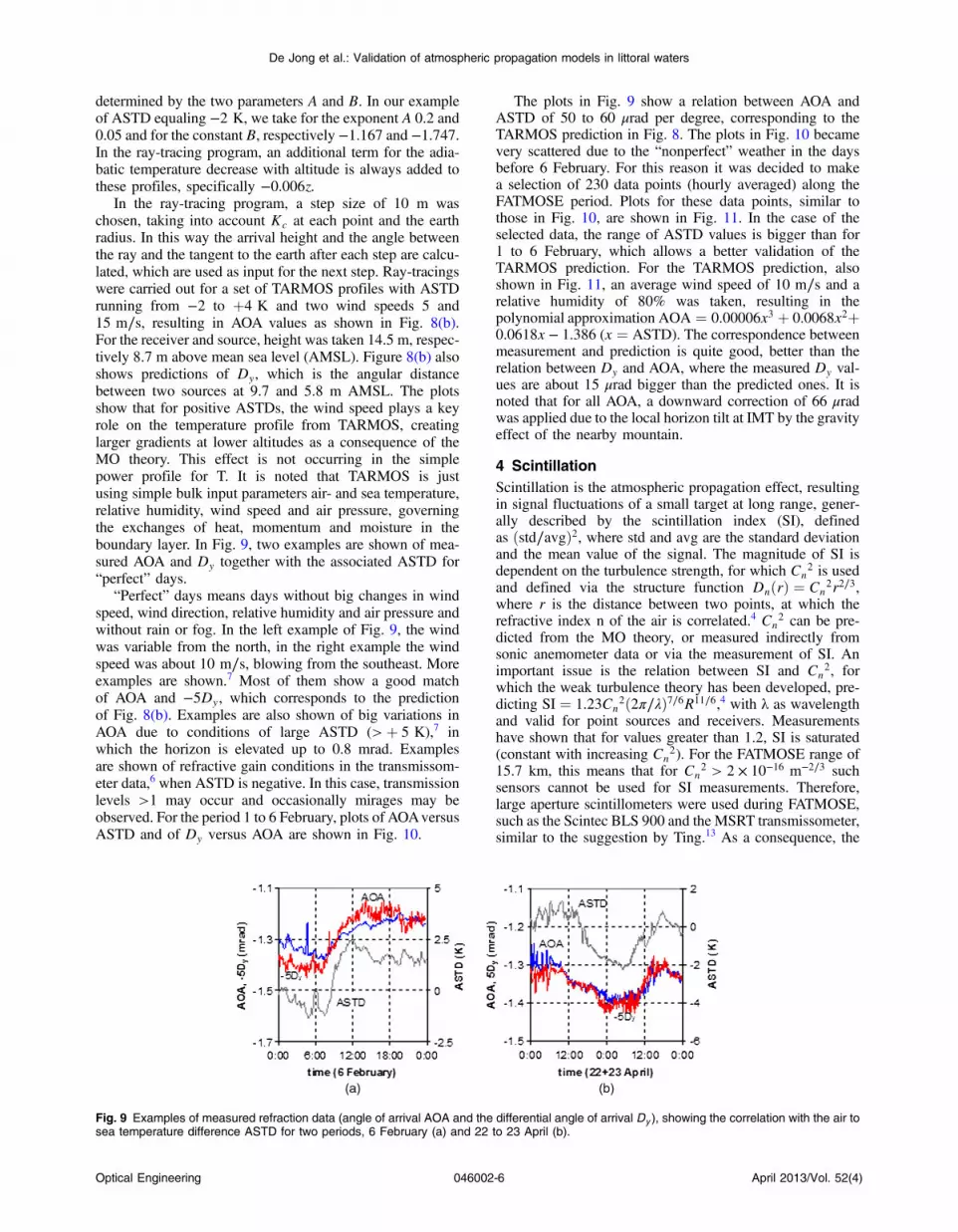
In the ray-tracing program, a step size of 10 m waschosen, taking into account Kc at each point and the earthradius. In this way the arrival height and the angle betweenthe ray and the tangent to the earth after each step are calcu-lated, which are used as input for the next step. Ray-tracingswere carried out for a set of TARMOS profiles with ASTDrunning from −2 to þ4 K and two wind speeds 5 and15 m∕s, resulting in AOA values as shown in Fig. 8(b).For the receiver and source, height was taken 14.5 m, respec-tively 8.7 m above mean sea level (AMSL). Figure 8(b) alsoshows predictions of Dy, which is the angular distancebetween two sources at 9.7 and 5.8 m AMSL. The plotsshow that for positive ASTDs, the wind speed plays a keyrole on the temperature profile from TARMOS, creatinglarger gradients at lower altitudes as a consequence of theMO theory. This effect is not occurring in the simplepower profile for T. It is noted that TARMOS is justusing simple bulk input parameters air- and sea temperature,relative humidity, wind speed and air pressure, governingthe exchanges of heat, momentum and moisture in theboundary layer. In Fig. 9, two examples are shown of mea-sured AOA and Dy together with the associated ASTD for“perfect” days.

“Perfect” days means days without big changes in windspeed, wind direction, relative humidity and air pressure andwithout rain or fog. In the left example of Fig. 9, the windwas variable from the north, in the right example the windspeed was about 10 m∕s, blowing from the southeast. Moreexamples are shown.7 Most of them show a good matchof AOA and −5Dy, which corresponds to the predictionof Fig. 8(b). Examples are also shown of big variations inAOA due to conditions of large ASTD (>þ 5 K),7 inwhich the horizon is elevated up to 0.8 mrad. Examplesare shown of refractive gain conditions in the transmissom-eter data,6 when ASTD is negative. In this case, transmissionlevels >1 may occur and occasionally mirages may beobserved. For the period 1 to 6 February, plots of AOAversusASTD and of Dy versus AOA are shown in Fig. 10.

The plots in Fig. 9 show a relation between AOA andASTD of 50 to 60 μrad per degree, corresponding to theTARMOS prediction in Fig. 8. The plots in Fig. 10 becamevery scattered due to the “nonperfect” weather in the daysbefore 6 February. For this reason it was decided to makea selection of 230 data points (hourly averaged) along theFATMOSE period. Plots for these data points, similar tothose in Fig. 10, are shown in Fig. 11. In the case of theselected data, the range of ASTD values is bigger than for1 to 6 February, which allows a better validation of theTARMOS prediction. For the TARMOS prediction, alsoshown in Fig. 11, an average wind speed of 10 m∕s and arelative humidity of 80% was taken, resulting in thepolynomial approximationAOA ¼ 0.00006x3 þ 0.0068x2þ0.0618x − 1.386 (x ¼ ASTD). The correspondence betweenmeasurement and prediction is quite good, better than therelation between Dy and AOA, where the measured Dy val-ues are about 15 μrad bigger than the predicted ones. It isnoted that for all AOA, a downward correction of 66 μradwas applied due to the local horizon tilt at IMT by the gravityeffect of the nearby mountain.

4 ScintillationScintillation is the atmospheric propagation effect, resultingin signal fluctuations of a small target at long range, gener-ally described by the scintillation index (SI), definedas ðstd∕avgÞ2, where std and avg are the standard deviationand the mean value of the signal. The magnitude of SI isdependent on the turbulence strength, for which Cn

2 is usedand defined via the structure function DnðrÞ ¼ Cn

2r2∕3,where r is the distance between two points, at which therefractive index n of the air is correlated.4 Cn

2 can be pre-dicted from the MO theory, or measured indirectly fromsonic anemometer data or via the measurement of SI. Animportant issue is the relation between SI and Cn

2, forwhich the weak turbulence theory has been developed, pre-dicting SI ¼ 1.23Cn

2ð2π∕λÞ7∕6R11∕6,4 with λ as wavelengthand valid for point sources and receivers. Measurementshave shown that for values greater than 1.2, SI is saturated(constant with increasing Cn

2). For the FATMOSE range of15.7 km, this means that for Cn

2 > 2 × 10−16 m−2∕3 suchsensors cannot be used for SI measurements. Therefore,large aperture scintillometers were used during FATMOSE,such as the Scintec BLS 900 and the MSRT transmissometer,similar to the suggestion by Ting.13 As a consequence, the

Fig. 9 Examples of measured refraction data (angle of arrival AOA and the differential angle of arrival Dy ), showing the correlation with the air tosea temperature difference ASTD for two periods, 6 February (a) and 22 to 23 April (b).

Optical Engineering 046002-6 April 2013/Vol. 52(4)

De Jong et al.: Validation of atmospheric propagation models in littoral waters

signals did not show saturation effects as illustrated inFig. 12(a), showing a histogram of 4200 data points (channel4) under strong scintillation conditions. The plot showsnicely the well-known log-normal distribution, as proposedin the theory of Rytov.4

The prediction of Cn2 from the MO theory, as applied in

the TARMOS code, is based upon the knowledge of scalingparameters for wind speed, temperature and humidity, u�,T�, and q�, which determine indirectly the Obukhov lengthL ðmÞ. This parameter is roughly related to ASTD for a windspeed of 5 m∕s, 1∕L ¼ 0.02ASTD (K). For wind speeds lessthan 4 m/s, L is dropping rapidly. Knowledge of T� and Lallow the approximation of CT

2, the structure parameter fortemperature, which is directly linked with Cn

2 via Cn2 ¼

fðn − 1Þ∕Tg2CT2, where T is the absolute temperature

(K).12 The sonic anemometer delivers wind speed in threeorthogonal directions together with the air temperature ina data rate of 100 samples per second. The covariance of thefluctuations of the wind speed in vertical direction w and thefluctuations of the wind speed in the main wind directionu; hwui, delivers by definition −u�2. T� follows from T�u� ¼−hwti, where t stands for the temperature fluctuations.Similar to the TARMOS calculation, CT

2 can be obtainedand thus Cn

2. It is clear that in all these calculations severalassumptions and approximations are made. One of them isthe spectrum of the fluctuations, for which basically the spa-tial spectrum from the Kolmogorov theory is taken.4 Thispredicts on a log-log scale for the one dimensional spectruma drop of the amplitude with κ−5∕3, where κ is the spatialfrequency. Figure 12(b) shows that this prediction is nearlycorrect for both strong and weak scintillation conditions.

It is noted, however, that these spectra are taken from tem-poral MSRT signals. This can only be explained by Taylor’shypothesis,4 based upon the assumption that crosswinds areblowing the turbulence structure unchanged through the lineof sight. A deviation of Kolmogorov is found in the positionof the knee in the spectrum, which is occurring at 10 Hz,while the theory assumes 1 Hz.

A comparison of Cn2 measurements and predictions and

ASTD is shown in Fig. 13 for two periods in April. Thesetime plots show that the trends of Cn

2 follow reasonably wellthe predictions via ASTD, but that deviations occur in thevarious sources of Cn

2, probably due to inhomogeneitiesalong the path. It is also found that SI values of 0.01 andless have been measured, indicating that Cn

2 values farbelow 10−16 m−2∕3 occur in the False Bay area, which isbelow the range of the BLS scintillometer.

The conversion of measured SI values to Cn2 follows

from the strong turbulence theory.4 Andrews derives an equa-tion for the aperture averaging factor A, defined as the ratioof SI for aperture D and (SIR) for aperture zero. The factor Ais depending heavily on SIR and the parameter ðπD2Þ∕ð2λRÞ,where D is the diameter of the aperture and ðλRÞ0.5 repre-sents the Fresnel scale, related to the first Fresnel zone, deter-mining the intensity of an incoming wave front at range R.Plots of A as function of D are shown in Fig. 14(a) for anumber of Cn

2 values, λ ¼ 0.8 μm and L ¼ 15.7 km. Aappears to be less than 0.2 for D ¼ 20 cm, which is furtherillustrated in Fig. 14(b), where A is plotted as function of Cn

2

and D as parameter.Actually, aperture averaging occurs for the source

(Celestron 9 cm, MSRT 20 cm) and for the receiver(Celestron 20 cm, MSRT 4 cm). The two different apertureaveraging factors have to be multiplied. It is, therefore, inter-esting to compare SI values of both instruments, such asshown in Fig. 15(a), where for the MSRT, channel 3 hasbeen taken which has about the same waveband as theCelestron. It is noted that MSRT data in the morninghours from 10 to 12 o’clock have been removed due tosun glint effects in the sea. Both data series correlatequite well with a correlation coefficient of 0.90. The mainreason for the spread in the data is due to the smaller signalto noise ratio of the Celestron data. A rough approximationof the factor A can also be obtained by realizing that insidethe aperture D, coherent wave front patches (radius ρ0) areaveraged by the factor D∕ρ0. The spatial coherence width ρ0

Fig. 11 Correlation plots as in Fig. 11 for a selection of 230 hourlyaveraged data series in comparison with predictions, based on theTARMOS and the power temperature profile. Both 11(a) with AOAversus ASTD and 11(b) with Dy versus AOA show that theTARMOS based prediction gives a better correspondence with themeasured data.

Fig. 12 (a) Histograms of the intensity I and logðIÞ for 21 s of MSRTdata for a case of strong scintillation index (SI ¼ 0.34). (b) ShowsFourier spectra of MSRT data for weak (0.034) and strong SI(0.34). All data are taken in spectral band 4.

Fig. 10 Correlation between the angle of arrival AOA and the air tosea temperature difference ASTD (a), and the differential angle ofarrival Dy and AOA (b) for the refraction data of 1 to 6 February.In both plots the correlation coefficient is about 0.50, which is lowdue to some “nonperfect” weather moments in the measurementperiod.

Optical Engineering 046002-7 April 2013/Vol. 52(4)

De Jong et al.: Validation of atmospheric propagation models in littoral waters

is related to Cn2 by ρ0 ¼ f1.46ð2π∕λÞ2Cn

2Rg−3∕5, predict-ing ρ0 values of a few cm, resulting in aperture averagingA values of 0.1 to 0.2, which corresponds roughly with thepreviously mentioned prediction.

It was further found that the SI values of the three MSRTbands correlate extremely well and were nearly equal, asshown in Fig. 15(b). This shows that during FATMOSE,scintillation was not originating from small eddies, whichcreate wavelength dependence (as in the SI value for theweak turbulence case14). In the False Bay, scintillationoccurred rather in the refraction regime. Applying the factorA to the SI data from the MSRT system allows a comparisonof its Cn

2 and the Cn2, measured by the Scintec scintillom-

eter. The result, presented in Fig. 16(a), shows data points fora selected series of 458 events during the FATMOSE period(with “correct” weather). Each event was chosen inside

several hours of constant weather, while averages weretaken over a 2-h period.

Both data sets correspond reasonably well for Cn2 values

above 10−16 m−2∕3; the Scintec system is limited to valuesabove 10−16 m−2∕3. The predicted data in Fig. 16(a) arebased upon Cn

2 values as low as 10−17 m−2∕3, convertedfrom hypothetical SI data for the MSRT and Celestron sys-tems via the relation logðCn

2Þ ¼ 0.6623x4 þ 4.2334x3þ9.9979x2 þ 11.458x − 10.623, in which x ¼ logðSIÞ basedupon the aperture averaging factor A. Figure 16(b) showsa cumulative probability plot of the SI values from theCelestron camera for the same selected data series, wherecare was taken that the weather statistics were about thesame as those in Fig. 2. It is clear that 50% of the SI datais below 0.2% and 90% below 0.4. This means that the mag-nitude of the atmospheric scintillation over the False Bayarea is generally low to moderate.

5 Atmospheric BlurThe main purpose of the Celestron camera, mentioned inthe previous section for the collection of scintillation data,was the measurement of the atmospheric line spread function(LSF). The 8-inch telescope with a focal length of 2030 mm,was provided with a 10 bits Marlin F-033B camera with640 × 480 pixels, a 30 Hz frame rate and a near-IR cut-onfilter. With a pixel size of 5 × 5 μrad, the total field ofview of the camera is 3.2 × 2.4 mrad. The camera integrationtime was generally less than 1 ms, with a minimum of0.1 ms, depending on the actual visibility and illumination

Fig. 14 Aperture averaging Factor A, determining the reduction ofscintillation due to increased sensor and receiver apertures, predictedfrom the strong turbulence theory. (a) A as function of the receiverdiameter D and in (b) as a function of Cn

2 ðm−2∕3Þ.

Fig. 15 (a) Comparison of the scintillation index SI for a representa-tive data set, collected by MSRT and Celestron (correlation coefficient0.90). (b) A similar comparison of SI from different MSRT bands (cor-relation coefficient 0.99).

Fig. 16 (a) The dots show a comparison of SI and Cn2 for a selected

data series collected under “correct”weather conditions, measured bythe Celestron and the scintillometer, the curve through the squarespresents SI, predicted after correction for aperture averaging.(b) Shows the cumulative probability of SI for the whole FATMOSEperiod.

Fig. 13 Plots of measured SI, ASTD and Cn2 (structure parameter for the refractive index) for 22 to 24 April (a) and 11 April (b) in comparison to

Cn2, predicted from the MO theory based TARMOS code.

Optical Engineering 046002-8 April 2013/Vol. 52(4)

De Jong et al.: Validation of atmospheric propagation models in littoral waters

conditions. A series of 150 frames (5 s) were collected every5 min. Some examples of the Celestron imagery are shown inFig. 17 with long (9 ms) integration times in conditions ofgood visibility and low turbulence (a) and two images of thefour sources for low (b) and high (c) turbulence conditions.The two central sources are used for measuring the LSF,while the left source (modulated) and right source are usedfor transmission (MSRT), respectively, refraction (Topcon)measurements.

Figure 17 also shows the LSF LðxÞ and LðyÞ in X- andY-direction for the two images (b) and (c) for low andhigh turbulence conditions. Both LSFs are found fromLðxÞ ¼ ∫ Sðx; yÞdy and LðyÞ ¼ ∫ Sðx; yÞdx, where Sðx; yÞis the signal level at position ðx; yÞ in the focalplane above a certain threshold above the mean backgroundlevel in an area around the spot. It is found that generally theLSFs can reasonably well be approximated by a Gaussiandistribution. In each frame, the centers of “gravity” xc andyc are obtained from xc ¼

RRxSðx; yÞdxdy∕ RR Sðx; yÞdxdy

and yc ¼RRySðx; yÞdxdy∕ RR Sðx; yÞdxdy with mean values

for all 150 frames of xcm and ycm. The beam wanderBW is defined as the mean value of BW ¼ pfðxcn − xcmÞ2þðycn − ycmÞ2g (n ¼ 1 to 150). The blur for each framefollows from the second moments M20 and M02 of Sðx; yÞin both directions M20 ¼

RR ðx − xcÞ2Sðx; yÞdxdy∕RRSðx; yÞ

dxdy and M02 ¼RR ðy − ycÞ2Sðx; yÞdxdy∕

RRSðx; yÞdxdy.

The final blur value for each frame σt is found from thegeometrical average σt ¼

pðpM20

pM02Þ in number of pix-

els (multiplied with five for blur values in μrad). To obtainthe atmospheric blur σa, the system blur σs has to be sub-tracted quadratically from σt: σa ¼

pðσt2 − σs2Þ. In the sys-

tem blur, three contributions are taken into account: thesource diameter (5.7 μrad), the pixel size (5 μrad), andthe diffraction from the aperture of the telescope (20 cm),resulting in a σs value of 2.89 μrad.8 Finally, the meanvalue of σa is calculated for the 150 frames.

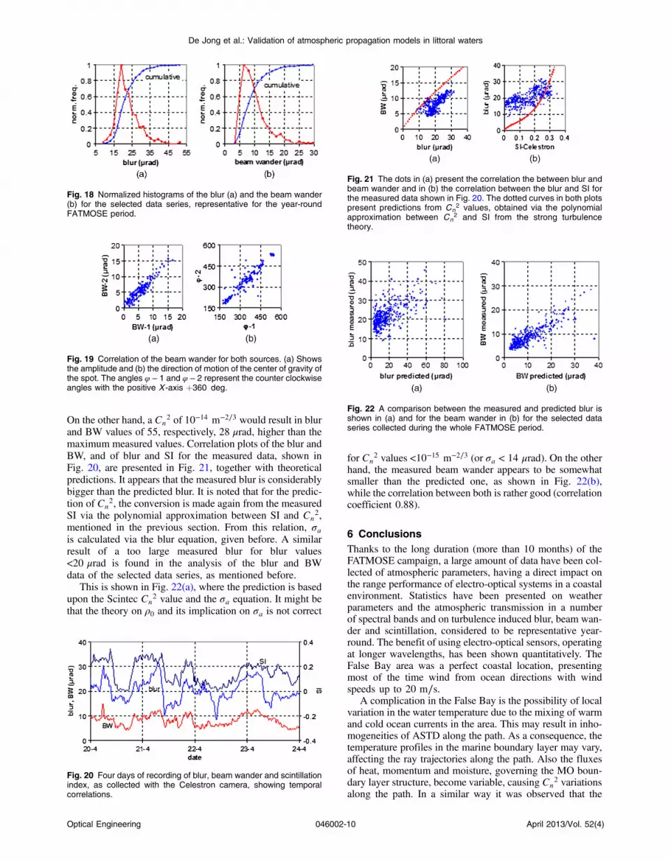
In Fig. 18 the statistics for blur and beam wander areshown for the same selected series as discussed in the pre-vious section, being representative for the year-round condi-tions in the False Bay. It appears that 50% of the blur and thebeam wander is smaller than 20 μrad, respectively, 8 μrad. It

is interesting that the distribution of the blur [Fig. 18(a)] isroughly log normal, which is not the case for the beam wan-der distribution [Fig. 18(b)]. It is noted that the blur valuesmay vary considerably within one series of 150 frames,showing standard deviations of 10%, sometimes 20% to30% of the mean value. The smallest blur within one series(lucky shot) may be 50% of the mean, but the biggest blurmay be twice the mean value. The LSF profiles LðxÞ ¼expf−ðx∕σaÞ2∕2g imply that the atmospheric MTF alsohas a Gaussian shape, MTFaðfÞ ¼ expf−2ðπσafÞ2g, inwhich f is the spatial frequency (cycles∕μrad), which allowsa good estimation of the optical resolution for a given blur σa.

It is also noted,15 that two line sources, separated by atransverse distance of 2.43σa (at 15.7 km), are just discern-ible by a remaining contrast of 10%. Another interestingissue which appeared regularly, was the synchronousbeam wander (amplitude and phase) of the upper andlower source, as shown in Fig. 19. It appeared as if thewhole image was moving in the same direction with thesame amplitude, apparently tilting due to large intermediateeddies. The predicted atmospheric MTFap is according toFried,16 MTFapðfÞ ¼ expf−ðf∕fcÞ5∕3g, with the cut-offfrequency fc ¼ ρ0∕λ and ρ0 the transverse coherencewidth as specified in the previous section ρ0 ¼ f1.46ð2π∕λÞ2Cn

2Rg−3∕5. This means that σa ≈ λ∕ðρ0πp2Þ ¼ 2.56λ−0.2

ðCn2RÞ0.6; with λ ¼ 0.8 · 10−6 m and R ¼ 15.7 · 103 m

follows: σa ¼ 14.0 · 109ðCn2Þ0.6 μrad. For the mean Cn

2

value of 10−15 m−2∕3, σ2 becomes 14 μrad, which is reason-ably in agreement with the measured values. Beam wander ispredicted by the relation given by Beland, BW ¼ð2.91D−1∕3Cn

2RÞ0.5. For D ¼ 0.2 m and R ¼ 15.7 · 103 mfollows BW ¼ 2.8 · 108ðCn

2Þ0.5 μrad, resulting in a BWvalue of 8.9 μrad for a Cn

2 value of 10−15 m−2∕3, which,again, is close to the observed mean value.

An example of a time plot where blur, BW and SI (mea-sured data from the Celestron camera) correspond reason-ably well, is shown in Fig. 20. It is noted that the blurand BW are not becoming extremely small when the Cn

2

value is small. For example, according to the theory, a Cn2 ¼

10−16 m−2∕3 would result in blur and BW values of 3.5,respectively, 2.8 μrad, which have never been measured.

Fig. 17 Impression of the four sources on the roof of the NSRI building (a) and examples of small and large blur conditions [(b) and (c)] withassociated line spread functions [(d) respectively (e)].

Optical Engineering 046002-9 April 2013/Vol. 52(4)

De Jong et al.: Validation of atmospheric propagation models in littoral waters

On the other hand, a Cn2 of 10−14 m−2∕3 would result in blur

and BW values of 55, respectively, 28 μrad, higher than themaximum measured values. Correlation plots of the blur andBW, and of blur and SI for the measured data, shown inFig. 20, are presented in Fig. 21, together with theoreticalpredictions. It appears that the measured blur is considerablybigger than the predicted blur. It is noted that for the predic-tion of Cn

2, the conversion is made again from the measuredSI via the polynomial approximation between SI and Cn

2,mentioned in the previous section. From this relation, σais calculated via the blur equation, given before. A similarresult of a too large measured blur for blur values<20 μrad is found in the analysis of the blur and BWdata of the selected data series, as mentioned before.

This is shown in Fig. 22(a), where the prediction is basedupon the Scintec Cn

2 value and the σa equation. It might bethat the theory on ρ0 and its implication on σa is not correct

for Cn2 values <10−15 m−2∕3 (or σa < 14 μrad). On the other

hand, the measured beam wander appears to be somewhatsmaller than the predicted one, as shown in Fig. 22(b),while the correlation between both is rather good (correlationcoefficient 0.88).

6 ConclusionsThanks to the long duration (more than 10 months) of theFATMOSE campaign, a large amount of data have been col-lected of atmospheric parameters, having a direct impact onthe range performance of electro-optical systems in a coastalenvironment. Statistics have been presented on weatherparameters and the atmospheric transmission in a numberof spectral bands and on turbulence induced blur, beam wan-der and scintillation, considered to be representative year-round. The benefit of using electro-optical sensors, operatingat longer wavelengths, has been shown quantitatively. TheFalse Bay area was a perfect coastal location, presentingmost of the time wind from ocean directions with windspeeds up to 20 m∕s.

A complication in the False Bay is the possibility of localvariation in the water temperature due to the mixing of warmand cold ocean currents in the area. This may result in inho-mogeneities of ASTD along the path. As a consequence, thetemperature profiles in the marine boundary layer may vary,affecting the ray trajectories along the path. Also the fluxesof heat, momentum and moisture, governing the MO boun-dary layer structure, become variable, causing Cn

2 variationsalong the path. In a similar way it was observed that the

Fig. 19 Correlation of the beam wander for both sources. (a) Showsthe amplitude and (b) the direction of motion of the center of gravity ofthe spot. The angles φ − 1 and φ − 2 represent the counter clockwiseangles with the positive X -axis þ360 deg.

Fig. 20 Four days of recording of blur, beam wander and scintillationindex, as collected with the Celestron camera, showing temporalcorrelations.

Fig. 21 The dots in (a) present the correlation the between blur andbeam wander and in (b) the correlation between the blur and SI forthe measured data shown in Fig. 20. The dotted curves in both plotspresent predictions from Cn

2 values, obtained via the polynomialapproximation between Cn

2 and SI from the strong turbulencetheory.

Fig. 22 A comparison between the measured and predicted blur isshown in (a) and for the beam wander in (b) for the selected dataseries collected during the whole FATMOSE period.

Fig. 18 Normalized histograms of the blur (a) and the beam wander(b) for the selected data series, representative for the year-roundFATMOSE period.

Optical Engineering 046002-10 April 2013/Vol. 52(4)

De Jong et al.: Validation of atmospheric propagation models in littoral waters

visibility (aerosol content) may vary locally due to the pres-ence of fog patches.

The variability of the weather conditions did often occurin short time notices, which made it necessary to carefullyselect periods of several hours with constant weatherfor model validation. In this way an aerosol model, basedupon a Junge particle size distribution, was proposed.Differences in aerosol transmission in the five spectralbands of the TNO multiband spectral radiometer transmiss-ometer MSRTwere used to successfully determine the Jungecoefficients Je and Jc. Of course, this method of retrievalfails in adverse weather conditions, such as low visibilityand rain. The effect of wind speed as well as transmissionlevel on Je and Jc was illustrated, showing that both param-eters increase with wind speed. Alternatively, both Je and Jcwere decreasing with increasing transmission level due to theassociated decrease of relative humidity impacting the par-ticle size distribution of the aerosols.

In a similar way, the environmental parameters wereused as input for the TARMOS model, predicting the boun-dary layer structure, in particular the temperature profileand the structure parameter for the refractive index Cn

2.Another selection of events was chosen allowing the suc-cessful validation of the predicted logarithmic temperatureprofile for ASTD values between −2 and þ4 K. This val-idation was carried out by using a high resolution theodolite(7.5 μrad pixel), providing absolute angle of arrival datafrom sources at NSRI. In addition, differential angles ofarrival were measured from two vertically separatedsources at NSRI by means of a high resolution telescope(5 μrad pixel).

The parameter Cn2 was also locally measured in the Bay

by means of a scintillometer, running over a 1.8 km pathbetween IMT and RRL, and a sonic anemometer mountedat RRL. These sensors provided opportunities to validatethe TARMOS prediction model on Cn

2 and associated mod-els on scintillation, blur (short term) and beam wander.Because of the long range, the weak turbulence theory isnot valid anymore for Cn

2 values 2 × 10−16 m−2∕3. Forthis reason, the strong turbulence theory was used to calcu-late the aperture averaging factor for the large-aperture longrange scintillometers. Measured scintillation indices SI didcompare very well with the predictions, based upon theCn

2 data from the local scintillometer. Apparently, the SIwas independent of wavelength, indicating that in thiscase, scintillation was mainly due to refraction effects oflarger turbulence eddies and instead of diffraction bysmall eddies.

Scintillation spectra did show the expected shape accord-ing to the Kolmogorov theory, although the knee in the log-log scale was occurring at 10 Hz instead of 1 Hz. The meanvalue of the measured blur, which was of the order of20 μrad, corresponds well with the predictions from themean Cn

2. The blur was, however, staying too big for lowCn

2 values. It was further found that the blur values canvary considerably within one data series, the reason whyoccasionally “lucky shots” did occur with 50% less blur.Beam wander measurements did correlate quite well withthe predictions, where it was found that for low Cn

2 values,the predictions corresponded better than with the blur.

It was shown that the value of the beam wander is gen-erally about 40% of the blur value. The blur values have an

impact on the resolution of sensors. First of all, the blur hasto be translated to other ranges. Secondly, the blur, defined asthe root of the geometrical mean of the variances of the inten-sity distribution for a point source in X- and Y-direction, hasto be multiplied by a factor 2.43 in order to obtain the opticalresolution. This factor results from the consideration of theseparation of two line sources at such a distance that they arejust discernible. A mean blur value of 20 μrad implies thus anoptical resolution of 49 μrad, which corresponds to a dis-tance of two point sources of 0.77 m at a range of 15.7 km.

AcknowledgmentsThe authors want to thank Michael Saunders (Station 16Commander) and Mario Fredericks (Station 16 DeputyCommander) from the National Sea Rescue Institute forpermission for mounting the sources on the building atStrandfontein and their support during the trial. AlsoIMT personnel, in particular Faith February and GeorgeVrahimis, are greatly acknowledged for their support inkeeping the system running and handling the data. AtTNO, we thank Peter Fritz for his efforts in preparing thetrial and installing the systems. Koen Benoist, Leo Cohen,Koos van der Ende and Marco Roos are acknowledgedfor preparing hardware and software for data acquisitionand analysis.

References

1. C. D. O’Dowd and G. de Leeuw, “Marine aerosol production: a reviewof the current knowledge,” Phil. Trans. R. Soc. A 365, 1753–1774(2007).

2. F. X. Kneizis et al., “The MODTRAN 2/3 report and Lowtran 7 model,”Phillips Laboratory, Geophysics Directorate, PL/GPOS, Hanscom AFB,MA (1996).

3. S. P. Arya, “Introduction to Micrometeorology,” InternationalGeophysics Series, Vol. 79, Academic Press, London (2001).

4. L. C. Andrews and R. L. Philips, Laser Beam Propagation throughRandom Media, 2nd ed., SPIE Press, Bellingham (2005).

5. G. C. Holst, Electro-Optical Imaging System Performance, 3rd ed.,Vol. 121, SPIE Press, Bellingham (2003).

6. A. N. de Jong et al., “Application of year-round atmospheric transmis-sion data, collected with the MSRT multiband transmissometer duringthe FATMOSE trial in the False Bay area,” Proc. SPIE 8161, 81610A(2011).

7. A. N. de Jong et al., “Marine boundary layer investigations in the FalseBay, supported by optical refraction and scintillation measurements,”Proc. SPIE 8178, 817808 (2011).

8. A. N. de Jong et al., “Long-term measurements of atmospheric pointspread functions over littoral waters, as determined by atmospheric tur-bulence,” Proc. SPIE 8355, 83550M (2012).

9. A. N. de Jong et al., “Characteristics of long-range scintillation dataover maritime coastal areas,” Proc. SPIE 8535, 853504 (2012).

10. H. C. van de Hulst, Light Scattering by Small Particles, DoverPublications, Inc., New York (1981).

11. A. N. de Jong et al., “Atmospheric refraction effects on optical/IR sensorperformance in a littoral-maritime environment,” Appl. Opt. 43(34),6293–6303 (2004).

12. R. R. Beland, “Propagation through atmospheric optical turbulence,”The Infrared & Electro-Optical Systems Handbook, Vol. 2, SPIE,Bellingham (1993).

13. T.-i Wang, G. R. Ochs, and S. F. Clifford, “A saturation-resistant opticalscintillometer to measure Cn

2,” JOSA 68(3), 334–338 (1978).14. R. J. Hill and G. R. Ochs, “Fine calibration of large-aperture optical

scintillometers and an optical estimate of inner scale of turbulence,”Appl. Opt. 17(22), 3608–3612 (1978).

15. A. N. de Jong, E. M. Franken, and J. Winkel, “Alternative measurementtechniques for infrared sensor performance,” Opt. Eng. 42(3), 712–724(2003).

16. D. L. Fried, “Optical resolution through a randomly inhomogeneousmedium,” JOSA 56, 1372–1379 (1966).

Biographies and photographs for all authors are not available.

Optical Engineering 046002-11 April 2013/Vol. 52(4)

De Jong et al.: Validation of atmospheric propagation models in littoral waters