VALUE-ADDED TRADE AND REGIONALIZATION Guillaume Daudin, Christine Rifflart, Danielle Schweisguth

OFCE, Sciences Po Paris

This version: July 23rd, 2008

Preliminary version: please do not quote

For nearly two decades, growth of international trade has been underpinned by the

development of intermediate goods cross exchanges resulting from a new international

division of labour. The share of trade in inputs, also called vertical trade, has dramatically

increased. Simultaneously, there has been some fear of excessive regionalization in trade.

In this situation, the traditional trade measures based on the values of goods crossing

borders are inappropriate to measure how self-centred are different regions. This paper

suggests a new measure of international trade: “value-added trade”. Compared to “standard”

trade, “value-added trade” is net of double-counted vertical trade and reallocates trade flows

to input-producing industries. A database of value-added trade is made using the GTAP trade

and input-output database for 66 regions (mostly countries) and 55 sectors in 1997 and 2001.

In 2001, 26% of international trade were "only" vertical specialization trade, up from

25% in 1997. The share of services in value-added trade is much more important than in

standard trade. East Asia still relies more heavily on extra-regional final markets than North

America or Europe.

Keywords: Globalization, Vertical trade, Regionalization

JEL: F15, F19

1

Introduction

The recent development of regional trade agreements has sparked the fear of the

emergence of antagonist regional trade blocks1. It is not actually clear that the spaghetti bowl

of regional trade agreements really can have this kind of effects by itself2. Yet, it is clear that

East Asia has recently experienced a growing regionalization of its trade3. It could be possible

that its development is becoming more self-centred.

Yet, cross-border production networking, encouraged by extensive FDI flows has been an

important part of this growing regionalization. In this context, international trade statistics fail

to offer a good picture of trade integration and global division of labour because they cannot

answer the question “who produces for whom?”. Let us take an example. Burberry sends

bottles of French perfume to Shanghai to be decorated with Scottish pattern before bringing

them back to be sold on the French market. Yet, no one should conclude that France is

importing perfumes from China and is dependant for part of its cosmetic consumption on

China4. Yet, that is what international trade statistics suggest. It would be more useful to

restrict the measure of trade to goods and services intended for consumption. In our example,

France does not export anything for Chinese consumption, as perfumes are consumed in

France. China, for its part, only exports decoration to France. In some cases, that requires

tracking goods through long supply chains. Suppose the pigments used for the decoration of

these perfume bottles are imported to China from Japan. While trade statistics will indicate

that they are imported from Japan to China, one would be wrong to believe that this pigment

trade has no bearing on the shape of the Franco-Japanese economic integration. Unravelling

these long supply chains is impossible using simply trade statistics.

This paper advocates the study of regionalisation using “value-added trade”5. Compared

to “standard” trade, “value-added trade” is net of double-counted vertical specialization trade6

and reallocates trade flows to the input-producing industries. This alternative measure of trade

1 World Bank (2000). 2 Baldwin (2006),Ethier (1998) 3 Kwan (2001), Chortareas and Pelagidis (2004). 4 Examples from Benhamou (2005), p. 19, 25 and 96. 5 It has long been recognized that trade and GDP are not directly comparable because trade is not measured in terms of exchanged value-added: Irwin (1996), Feenstra (1998), Cameron and Cross (1999). 6 Vertical trade sometimes designates intra-industry trade in goods of different qualities. This is not the object of this paper.

2

is all the more important since internationalisation of production plays a great role in the

recent increase of international trade. Rising vertical specialization reinforces the divergence

between value-added trade flows and standard trade statistics. There is a large literature on

measuring vertical trade. Two broad methods have been employed. The first method measures

vertical trade by looking at the fine composition of trade to isolate trade flows of parts and

components7. This is useful and allows the examination of very fine-grained data, but cannot

be extended to measure value-added trade. Another method uses both input/output data and

trade data to measure the share of imports embedded in exports8. Our paper relies on this

literature and extends it by suggesting a method not only to measure the share of vertical

specialization trade in each country and industry’s trade, but also to reconstruct value-added

bilateral trade by industry for 66 regions. However, we are only able to do the computation

for two years: 1997 and 2001.

The difficulty of measuring value-added trade lies in taking into account all the stages of

production of a final good in every country and every sector in order to track all the value-

added contributions coming into its production. First, second, third… stage inputs must be

isolated. This can only be done thanks to a coherent worldwide set of intermediate delivery

matrices and bilateral trade matrices. The GTAP database has been built to run general

equilibrium analysis of the effects of international trade. It includes the necessary

information9.

This paper presents a method to compute value-added international trade and re-examine

the issue of regionalization. In a first section, the paper presents vertical specialization trade,

and its existing measures. In a second section, it presents a method to compute value-added

trade. In a third section, it presents some results for 1997 and 2001 and compares them to

results obtained by other methods. It then compares the regionalization in different parts of

the world. This paper builds on an earlier application focused on France using a more

aggregated database10.

7 Ng and Yeats (2003), Egger and Egger (2005), Athukorala and Yamashita (2006). 8 Hummels, Rapoport, and Yi (1998), Hummels, Ishii, and Yi (1999), Hummels, Ishii, and Yi (2001); Yi (2003); Chen, Kondratowicz, and Yi (2005), Chinn (2005), Council (2006). 9 Dimaranan (2006). 10 Daudin, Rifflart, Schweisguth, and Veroni (2006).

3

1. Vertical specialization trade

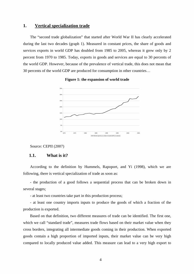
The “second trade globalization” that started after World War II has clearly accelerated

during the last two decades (graph 1). Measured in constant prices, the share of goods and

services exports in world GDP has doubled from 1985 to 2005, whereas it grew only by 2

percent from 1970 to 1985. Today, exports in goods and services are equal to 30 percents of

the world GDP. However, because of the prevalence of vertical trade, this does not mean that

30 percents of the world GDP are produced for consumption in other countries…

Figure 1: the expansion of world trade

0%

5%

10%

15%

20%

25%

30%

35%

1970 1975 1980 1985 1990 1995 2000 2005

World exports as a share of world GDP (in volume)

Source: CEPII (2007)

1.1. What is it?

According to the definition by Hummels, Rapoport, and Yi (1998), which we are

following, there is vertical specialization of trade as soon as:

- the production of a good follows a sequential process that can be broken down in

several stages;

- at least two countries take part in this production process;

- at least one country imports inputs to produce the goods of which a fraction of the

production is exported.

Based on that definition, two different measures of trade can be identified. The first one,

which we call “standard trade”, measures trade flows based on their market value when they

cross borders, integrating all intermediate goods coming in their production. When exported

goods contain a high proportion of imported inputs, their market value can be very high

compared to locally produced value added. This measure can lead to a very high export to

4

GDP ratio, sometimes exceeding 100% (as in the cases of Malaysia and Singapore). The other

measure, called “value-added trade”, measures trade net of vertical trade. It reallocates the

value added produced at the different stages of the production process to each of the

participating countries and industry.

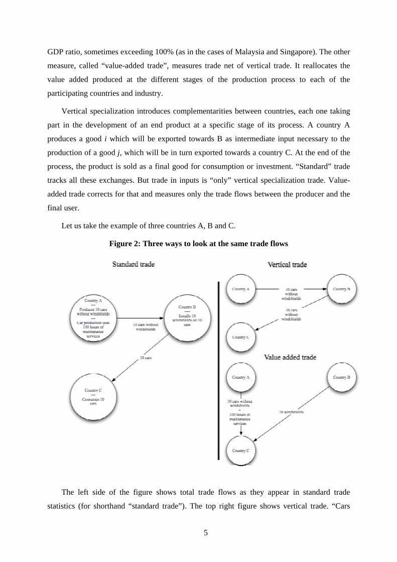
Vertical specialization introduces complementarities between countries, each one taking

part in the development of an end product at a specific stage of its process. A country A

produces a good i which will be exported towards B as intermediate input necessary to the

production of a good j, which will be in turn exported towards a country C. At the end of the

process, the product is sold as a final good for consumption or investment. “Standard” trade

tracks all these exchanges. But trade in inputs is “only” vertical specialization trade. Value-

added trade corrects for that and measures only the trade flows between the producer and the

final user.

Let us take the example of three countries A, B and C.

Figure 2: Three ways to look at the same trade flows

The left side of the figure shows total trade flows as they appear in standard trade

statistics (for shorthand “standard trade”). The top right figure shows vertical trade. “Cars

5

without windshields” are counted twice in standard trade statistics: once when they are

exported to become inputs to B’s production and once when they are embedded into B’s

exports. The bottom right figure shows “value added” trade. This is obtained through three

operations: first by removing vertical trade flows from standard trade flows; second by re-

allocating vertical trade flows to the producer / consumer country pair; third by allocating

trade flows to the industries that actually produce the value-added.

Value-added trade flows imply that country A does not actually trade with country B in

the sense that no final user in country B utilizes goods from country A. All the final users of

country A’s exports are in country C. Similarly, the industrial picture of trade is changed.

Standard trade flows suggest that country A does not export services. Yet, its services

production is being consumed, once it is embedded in cars, in country C. In that sense,

country A is actually exporting services.

Value-added trade flows can change our assessment of regionalization. Imagine that

country A and country B are in the same region. Standard trade flows suggest that intra-

regional trade flows are nearly as important as extra-regional trade flows. Yet, value-added

trade flows suggest that intra-regional trade flows are nil in the sense that no one in country A

or B is consuming goods produced in another country in the same region. Both countries are

producing for country C’s consumption. This is a very different case of regionalization than

one in which country B actually depends on country A for its final consumption. Applied to

the study of Asian trade, the examination of value-added trade confirms and refines the result

that despite its apparent regionalization, Asia’s trade is still very dependent on external

consumption11.

1.2. Why vertical specialization?

The Fordist organization of production put in place at the end of the WW II at a national

scale has been transformed into a disintegrated process, where stages of production are spread

across a range of production sites in multiple countries. This vertical specialisation of

production is based on a new international division of labour moving away from the

traditional division where production is split up between primary and manufactured goods.

Segmentation of production is becoming increasingly subtle, maybe in order to take the best

11 Athukorala and Yamashita (2006).

6

of the comparative advantages of each country. The segmentation of production processes has

led to foreign outsourcing of some production activities.

This new international division of labour has logically induced the acceleration of trade

flows since the end of the 1980s as a growing number of inputs are crossing several borders.

This finally results in a rapid expansion of trade in inputs, some of which are intermediate

goods. The multiplication of input trade has been facilitated by the cut in tariff and nontariff

barriers following the rise of economic liberalism and the multiplication of bilateral and

multilateral trade agreements concluded within the framework of the GATT and the WTO.

This has had a larger effect on vertical specialization of trade than on the other types of trade

as the internationalisation of the production process implies an increase in the number of

borders crossed by each goods12.

Micro-economic explanations of this movement give a by analysing the role of

multinational entreprises (MNE) in trade of intermediate goods. They have been inspired by

the new international trade theories integrating new findings in firm theory13. The stock of

foreign direct investment (FDI) worldwide accounts for a quarter of world GDP today against

6-7% in the 1980s14. This growing FDI led to the expansion of multinational firm networks.

Empirical evidence suggest that multinational firms have a leading role in the rise of vertical

specialization trade, even if the actual link between vertical specialization trade flows and FDI

is closely dependent on the inner strategy of each firm.

On this subject, Kleinert underlines there is a strong correlation between MNE production

in a host country and the propensity of this country to import intermediate goods. However,

the links between MNE production and the sale of inputs from the host country to the original

country is less clear15. Hanson et alii show that American firms practising outsourcing import

more intermediate goods if their subsidiary companies operate in countries where commercial

costs, wages, and companies’ taxation are weak16. Bardhan and Jaffee provide contrasting

results, as they report that in the case of the United States, arm-length transactions dominate

input trade flows even if network trade remains substantial17.

12 Yi (2003). 13 Jones (2000) ; Grossman and Helpman (2005), Ravix and Sautel (2007). 14 UNCTAD (2005). 15 Kleinert (2003). 16 Hanson, Mataloni Jr, and Slaughter (2005). 17 Bardhan and Jaffee (2005).

7

On the macro side, and to come back to the issue of regionalization, an already rich

literature details the reasons behind the high intensity of vertical trade in regional trade in East

Asia18. The first reason is a more favourable policy setting for international production (for

example China applied a lower tax rate on profits made by foreign companies to attract FDI).

Second, Asian countries are experiencing the benefits arising from the early entry into this

form of specialisation, which started in the 80s when Japan started to delocalise the assembly

stage in Korea, Taiwan or Singapore. Third, inter-country wage differentials have always

been very high in Asia. When some countries develop faster and labour cost increases,

production is moved to poorer countries in order to optimise the production cost. Fourth, trade

and transport costs are relatively low within the region. And fifth, the region has specialised

in products with increasing return to scale, taking advantage of the abundant labour force

available.

1.3. How can it be measured?

Whatever the causes of vertical trade, it can be measured in two ways: either using very

fine industrial classification or using input-output tables.

In the context of the SITC, Rev 3, the first method is possible for the goods belonging to

categories 7 (machinery and transport equipment) and 8 (miscellaneous manufactured

articles), in the five-digit SITC classification. It has been conducted by Athukorala and

Yamashita for most countries in the world. They find that world trade in components

increased from 18,5 percent to 22 percent of world manufacturing exports from 1992 and

200319.

Yi and his various co-authors (these papers are subsequently referred as “Yi and alii”) use

the second method, as does this paper20. They calculated international vertical specialisation

trade, defined as the share of imported inputs in exports, using input-output matrices of 10

OCDE and 3 non-OECD countries21. In their computation, Yi and alii take into account

imported goods directly used as inputs for the production of exports, but also imported inputs

used for the production of domestic inputs used in the production of exports: they call all

these flows “VS” for vertical specialization trade. Hummels, Ishii, and Yi (2001) extrapolate

18 See the review in Haddad (2007). 19 Athukorala and Yamashita (2006) 20 Ishii and Yi (1997), Hummels, Rapoport, and Yi (1998), Hummels, Ishii, and Yi (1999), Hummels, Ishii, and Yi (2001); Yi (2003); Chen, Kondratowicz, and Yi (2005). 21 Hummels, Rapoport, and Yi (1998), Hummels, Ishii, and Yi (2001).

8

their results to the rest of the world. They find that the share of vertical trade in world exports

was equal to 18% in 1970 and 23,6% in 199022.

But vertical trade is wider than VS. Purely domestic-produced exports can also be part of

vertical specialization trade if they are subsequently used by another country as inputs to its

export goods: Yi and alii call this flow “VS1”. While VS measures vertical specialization of a

country from its use of imported inputs in its exports, VS1 measures vertical specialization of

a country from the use of a country’s exported goods as inputs into the importer’s further

exports. Computing VS1 is more difficult than computing VS. VS can be computing using

solely the delivery matrix of the reporting country whether VS1 requires matching bilateral

trade flow data with intermediate delivery matrices for all trading partners23. By construction,

remark that VS in the exports of country A is equal to VS1 in the exports of all other

countries to country A. For the world as a whole, VS is equal to VS1.

To avoid double-counting in the worldwide measure of vertical trade, this paper further

distinguishes the part of VS1 that comes back to the country of origin: VS1*. VS1* is defined

as the exports that are, further down the production chain, re-imported as inputs embedded in

their imports for investment or final consumption. VS1* is the domestic content of invested or

consumed imports. A typical example is trade in motor vehicles and parts between the US and

Mexico and Canada. When the US import cars from Mexico for its own consumption, made

in US motors must be deducted from US imports measured in value added. In our paper, the

total value of value added trade is equal to standard trade minus VS and VS1*24. Total world

vertical exports are equal to VS+VS1*.

Our paper’s method is similar to Hummel et alii’s, but we compute VS for many more

countries in two years: 1997 and 2001. Furthermore, because we use world wide input-output

tables reconciled with bilateral trade statistics, we compute VS1, VS1* and we reallocate

vertical trade to its initial producer.

22 Hummels, Ishii, and Yi (2001), table 1. Also see Hummels, Ishii, and Yi (1999), table 5. 23 VS1 is computed from some case studies in Hummels, Rapoport, and Yi (1998) and from input-output tables in Hummels, Ishii, and Yi (1999). 24 Something similar is found in Chen, Kondratowicz, and Yi (2005), pp. 58-60, though it seems that they assimilate VS1 and VS1*.

9

2. How to compute trade flows in value added

2.1. GTAP database

Computing international trade flows in value added requires the use of input-output tables

and in particular of intermediate deliveries matrices reconciled with bilateral trade data. The

first input-output tables had been developed by Leontief in the 1930s and set the foundations

of the input-output analysis25. This branch of economics has in turn nourished general

equilibrium modelling, allowing for the construction of simple computable economic models

relying on the Leontief inverse matrix26. Such models make possible the analysis of direct and

indirect effects of changes in one economic variable on all others. They have also been used

for the study of international trade, in the more specific context of Computable General

Equilibrium Models. In this context, they must be reconciled with bilateral trade data. That

has been done by the GTAP project (Global Trade Analysis Project).

The project started in 1993 at Purdue University (United States). It associates 24

international organisations and research centres among which the United Nations, WTO, the

European Commission, OECD and CEPII. GTAP's goal is to improve the quality of

quantitative analysis of global economic issues within an economy-wide framework. It

provides databases and programmes for CGEM. We work with versions 5 (for 1997) and 6

(for 2001) of the GTAP database, which cover 57 sectors for 66 « regions » in 1997 and 87

« regions » in 2001 (countries or countries groups) respectively. We work with 66 regions in

both years. The database provides final demand and input-output tables differentiating

domestic and imported intermediate deliveries for each region. In each input-output tables,

two full intermediate deliveries matrices are available: one for domestic inputs and one for

imported inputs. It also provides information on bilateral international trade by industry.

25 Leontief (1936). 26 Shoven and Wholley (1992).

10

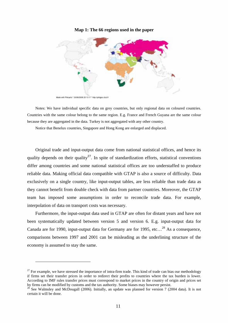
Map 1: The 66 regions used in the paper

Notes: We have individual specific data on grey countries, but only regional data on coloured countries.

Countries with the same colour belong to the same region. E.g. France and French Guyana are the same colour

because they are aggregated in the data. Turkey is not aggregated with any other country.

Notice that Benelux countries, Singapore and Hong Kong are enlarged and displaced.

Original trade and input-output data come from national statistical offices, and hence its

quality depends on their quality27. In spite of standardization efforts, statistical conventions

differ among countries and some national statistical offices are too understaffed to produce

reliable data. Making official data compatible with GTAP is also a source of difficulty. Data

exclusively on a single country, like input-output tables, are less reliable than trade data as

they cannot benefit from double check with data from partner countries. Moreover, the GTAP

team has imposed some assumptions in order to reconcile trade data. For example,

interpolation of data on transport costs was necessary.

Furthermore, the input-output data used in GTAP are often for distant years and have not

been systematically updated between version 5 and version 6. E.g. input-output data for

Canada are for 1990, input-output data for Germany are for 1995, etc…28 As a consequence,

comparisons between 1997 and 2001 can be misleading as the underlining structure of the

economy is assumed to stay the same.

27 For example, we have stressed the importance of intra-firm trade. This kind of trade can bias our methodology if firms set their transfer prices in order to redirect their profits to countries where the tax burden is lower. According to IMF rules transfer prices must correspond to market prices in the country of origin and prices set by firms can be modified by customs and the tax authority. Some biases may however persist. 28 See Walmsley and McDougall (2006). Initially, an update was planned for version 7 (2004 data). It is not certain it will be done.

11

Lastly, reconciliation between input-output data and trade data is fraught with difficulty.

Input-output data is less reliable than trade data: they bear the brunt of the changes necessary

for reconciliation. The shape of input-output tables can sometimes be dramatically changed,

but this happens mainly for small countries or regional aggregates: usage shares change by an

average of 71% for Cyprus, 51% for Malta, 38% for “rest of SADC” in GTAP 6. Still, usage

shares change by an average of 5% or less for all G7 countries, India, China, Korea, Brazil…

Still, some individual changes in Germany and the United States are important29.

The GTAP team is conscious of such quality problems. Nevertheless, the database has

been used by a network of more than 3,500 researchers for longer than a decade. The

organisation of the GTAP project allows remarks to be systematically registered and

integrated for the improvement of the database. The GTAP database is therefore a reference

for experts and researchers in international trade30. Still, all these defects make the GTAP

database a markedly inferior source for the computation of vertical trade than the data used up

to now in the existing literature. However, the originality of this paper is not to compute the

value of vertical trade, but rather to re-allocate input trade flows to their initial producers. The

only way to do that is to use reconciled input-output and trade data, and GTAP is the best

source that provides this information, as recognized by the community of CGE economists.

We can only hope better quality data will arise in time.

2.2. Theoretical foundation of the calculation31

In the context of a closed economy, equilibrium between output and final demand

requires that output is equal to the sum of intermediate deliveries and of final demand.

P=A*P + FD

Where P is a vector of output for each product, FD a vector of final demand for each

product, A a matrix of input coefficients taken from the intermediate deliveries matrix. It

consists of elements aij, defined as the amount of product i required for the production of one

unit of product j.

As a result, a well-known result in input-output analysis links changes in the final

demand of each product and production:

P =(I-A)-1*FD (1)

29 McDougall (2006). 30 For additional information, refer to http://www.gtap.agecon.purdue.edu 31 This is extended in Daudin, Rifflart, Schweisguth, and Veroni (2006).

12

Where I is the identity matrix. Each output vector P is itself associated with a value added

vector VA which gives each industry value-added required by the output vector.

VA=P – diag(P)A’I (2)

Where diag(P) is the square matrix having the elements of P on its diagonal, A’ is the

transpose of matrix A and i is the summation vector, a column vector filled by 1s.32 Hence, the

value added vector VA associated with the final demand vector FD is equal to:

VA = (I – A)-1∗FD – diag((I – A)-1∗FD)A’I (3)

This can be extended to the case of a world including many inter-linked open economies.

The world can be treated as a single economy where each sector in each country produces a

specific product, which is produced nowhere else. There is an “extended” intermediate

deliveries matrix G of dimension number of products*number of countries which gives the

amount of product i from country m required per unit of product j in country n. G is similar to

an usual domestic intermediate deliveries matrix where each pair product*producing country

is treated as a different product or industry33.

As we have written (2) and (3), we can write:

VA = P – diag(P)G’i (4)

VA = (I – G)-1*FD – diag((I – G)-1FD)G’I (5)

Where VA and P are vectors of dimension number of products*number of countries. This

formula allows the computation of the value-added production (VA) linked to the

consumption or investment of some final product (P). Practically, P is taken from trade and

final usage statistics. It allows the computation of VA from which value-added trade values

are extracted.

2.3. Some necessary hypotheses

2.3.1. Input-output coefficients

However, the matrix G is unknown. As far as we know, no statistical institute diffuses

such details. Data on whether inputs and final use goods are imported or domestic exist and

are reported in GTAP though: they can be used to approximate G. This is what Hoen calls the

“limited information multi-country input-output model”.

32 This last relation is easier to understand if one keeps in mind that P-P*A is equal to the vector of total ouput not used as inputs for further production; this is not the same thing as value-added. 33 See Hoen (2002), pp. 51-58 for a discussion of this method and a formal discussion of the G matrix.

13

The approximation is obtained, in the input-output tradition, by a fixed-proportion

assumption. The assumption is that the share of each partner country in imported products is

independent of its use (as a final demand item or as an intermediate consumption). This

assumption means that the share of US grain is the same in the imported grain used by

Mexican households and in the imported grain used as input in Mexican manufacture34.

A more severe limitation is that the origin of inputs used in exports is probably different

from the origin of inputs used in to produce for domestic consumption. Multinational firms

producing in process-heavy countries, like China, are more likely to import more foreign

goods as inputs and export more than the average of the industry. This is encouraged by the

existence of fiscal support to process activities, e.g. duty-drawbacks systems like in China and

Vietnam or more generally “Export Processing Zones” (more than 3,500 exist in 130

countries35). This can also be encouraged by higher quality requirements in foreign markets.

This issue has long been recognized36. It has been extensively studied in the case of China37.

Koopmans, Wang and Wei show that the method we use underestimates by 50% the amount

of imported content in Chinese exports38. Implementing their method to China and other

countries in our data would require using more detailed trade statistics than the ones available

in GTAP. This extension is past the ambition of this paper. Rather than trying to measure

finely vertical trade, the ambition of this paper is to give a first approximation of the effects of

re-allocating input trade to its original producer. It must be kept in mind that this paper

underestimates vertical trade throughout, especially for developing Asian countries.

2.3.2. Taking into account margin services

Data on foreign trade flows also need some price amendments. Imported goods volumes

are measured by GTAP — for example in the intermediate deliveries tables — in import

prices. Such prices include production prices, transport costs, insurance costs as well as taxes

levied on imports. However, to make the link between imports and production in the origin

country, we must measure volumes of imported goods used as intermediate deliveries or as

final demand at production prices. To transform import prices into production prices, we

34 This hypothesis is very common, and is used e.g. in Campa and Goldberg (1997) and Feenstra and Hanson (1997). 35 Singa Boyenge (2007). Countries with more than 500,000 workers in EPZs are: China (40 M), Indonesia (6 M), Bengladesh (3.4 M), Mexico (1.2 M), Philippines (1.1 M), Vietnam (1 M), Pakistan (0.9 M), UAE (0.6 M) and South Africa (0.5 M). 36 Hummels, Rapoport, and Yi (1998). 37 Chen, Cheng, Fung, and Lau (2005), Dean, Fung, and Whang (2007), Koopman, Wang, and Wei (2008). 38 Koopman, Wang, and Wei (2008).

14

apply a constant ratio along the different usage of different goods. This is equivalent to

assuming that that goods originated from the same country and from the same industry bear

the same transport cost and the same import duties whatever their use in the importing

country. This is a reasonable assumption. However, because our industry aggregation is not

very fine it might be the case that composition makes a difference between different uses.

The difference between import values and export – containing transport, maintenance and

insurance costs and called margin services utilisation in the GTAP database. Ideally, we

would like to be able to allocate it to trade flows of the transport industry. However, there is

no good way of doing that. The database does not indicate whether transport services linked

to a trade flow were provided by a firm in the importing country, a firm in the exporting

country or a firm in a third country. The only data available are the share of each country in

the total supply of transport services linked to total international trade flows. We have

therefore decided to exclude margin services trade from our computation.

3. Results

3.1. Value-added trade in general

3.1.1. Comparing with previous measures

Before developing our own results, we compare them with those found by Yi et alii. Our

framework is very similar to their framework: we use the same definition of vertical trade and

compute from input-output tables. They use more recent input-output data on a more limited

number of countries than we do: they have a better measure of VS than us. However, they do

not use reconciled trade / input-output data and cannot reallocate vertical trade flows to their

original producers.

Yi et alii calculated VS (i.e. the share of imported of inputs, including inputs for inputs,

in exports) for 10 OECD countries and 4 emerging countries, using OECD Inputs-Outputs

tables up to the end of the 1990s39. For comparison purposes, we compute VS using the same

method for all the countries in our sample: our data cover 1997 and 2001. The results are

given in Figure 3.

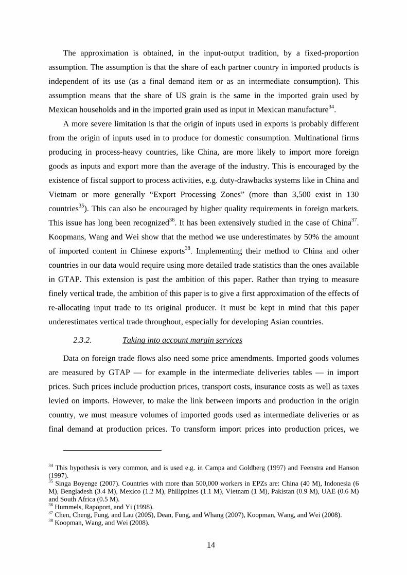
On the whole, our results are similar to theirs. The fit is very good for the United States,

Japan, Germany, Canada, the Netherlands, and Korea. Our estimates are lower than theirs for

39 Hummels, Ishii, and Yi (1999) tables 2 and 3, Hummels, Ishii, and Yi (2001), pp 84-85, Chen, Kondratowicz, and Yi (2005), p 42, table 2.

15

Australia, France, the United Kingdom and Taiwan. Our estimates are higher than theirs for

Denmark, Italy and Ireland. This is not correlated with the amount of change imposed on

Input-Output table by the trade / Input-Output reconciliation process, nor does it seems to be

linked to the origin of Input-Output tables in GTAP40. We do not seem to diverge

systematically in any way from the results by Yi and alii.

Figure 3: Vertical specialization in OECD countries: comparing our results to Chen

and alii’s

0%

5%

10%

15%

20%

25%

30%

35%

40%

45%

50%

1960 1965 1970 1975 1980 1985 1990 1995 2000

Italy CKY Italy DRS Denmark CKYDenmark DRS Ireland CKY Ireland DRS

0%

5%

10%

15%20%

25%

30%

35%40%

45%

1960 1965 1970 1975 1980 1985 1990 1995 2000

US CKY US DRS Netherlands CKYNetherlands DRS Japan CKY Japan DRSCanada CKY Canada DRS Korea CKYKorea DRS Germany CKY Germany DRS

0%

5%

10%

15%

20%

25%

30%

35%

40%

45%

1965 1970 1975 1980 1985 1990 1995 2000

Australia CKY Australia DRS France CKY France DRSUK CKY UK DRS Taiwan CKY Taiwan DRS

Sources: Hummels, Ishii, and Yi (2001), Chen and alii (2005), authors’ calculations based on GTAP data for

1997 and 2001.

3.1.2. Value-added trade at the country level

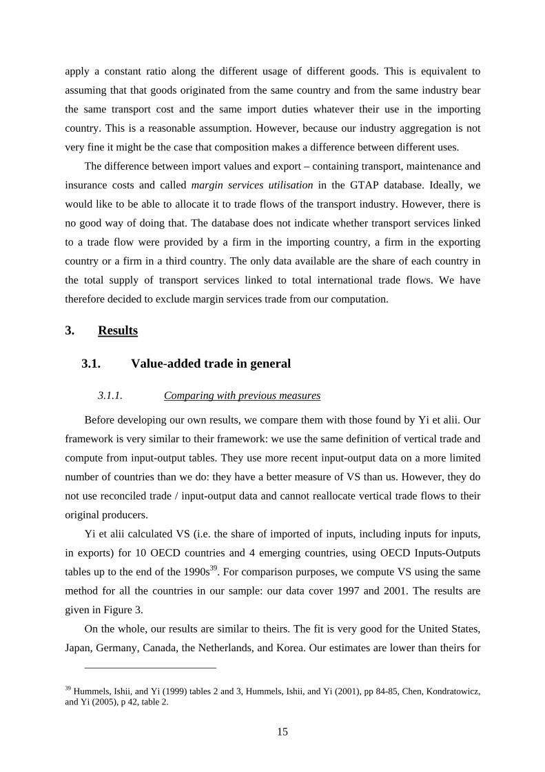
Map 2 gives the share of imported inputs (VS) in total exports for each country in the

world. Exports of small countries have a bigger share of imported inputs. The world mean is

24,2%. Imported inputs make up to 40 % of exports in some Asian and European countries. It

40 McDougall (2006), table 19-4. Walmsley and McDougall (2006), table 11.A.1.

16

is the highest in Singapore: 66% (Dutch and Hong Kong trade is already modified in GTAP to

remove transit trade: this explains the relatively small values of vertical exports)41.

Map 2: Share of VS in total exports

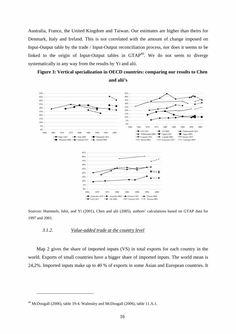
Map 3 compares VS1 (the share of exports that are further re-exported in partners’

exports) and VS. As worldwide VS1 and VS are equal, the world mean is equal to 1. Two

very different kinds of countries are integrated in vertical trade through the production of

inputs for further exports: primary producers (Former Soviet Union, Venezuela…) and

producers of industrial inputs for processing countries (Japan, the United States…).

Map 3: VS1/VS by country

Map 4 gives VS1* (the domestic content of imports, or exported intermediates embodied

in further imports to the initial exporter) as a share of total exports. The world mean of VS1*

is 2.1%. In most countries, it is much smaller than 2.5%. The only exception is the United

States, where VS1* is equal to 10% in 2001. We assume that the inputs of all production from

an industry in a particular country have the same origin. This probably underestimates VS1*

41 Gehlhar (2006).

17

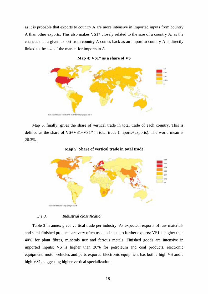
as it is probable that exports to country A are more intensive in imported inputs from country

A than other exports. This also makes VS1* closely related to the size of a country A, as the

chances that a given export from country A comes back as an import to country A is directly

linked to the size of the market for imports in A.

Map 4: VS1* as a share of VS

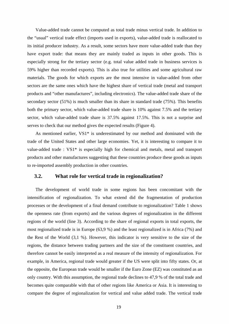
Map 5, finally, gives the share of vertical trade in total trade of each country. This is

defined as the share of VS+VS1+VS1* in total trade (imports+exports). The world mean is

26.3%.

Map 5: Share of vertical trade in total trade

3.1.3. Industrial classification

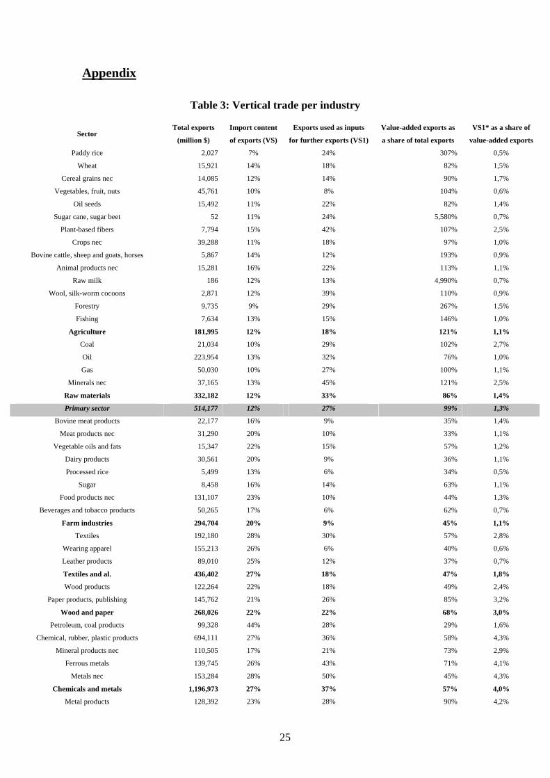
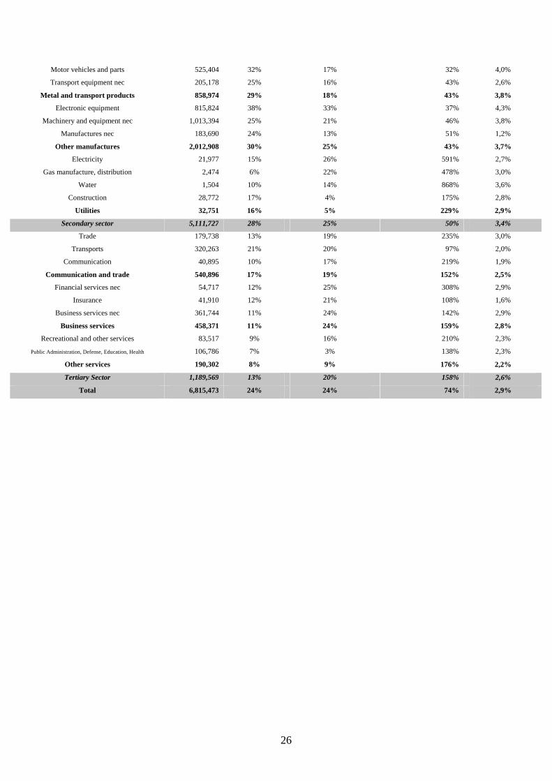
Table 3 in annex gives vertical trade per industry. As expected, exports of raw materials

and semi-finished products are very often used as inputs to further exports: VS1 is higher than

40% for plant fibres, minerals nec and ferrous metals. Finished goods are intensive in

imported inputs: VS is higher than 30% for petroleum and coal products, electronic

equipment, motor vehicles and parts exports. Electronic equipment has both a high VS and a

high VS1, suggesting higher vertical specialization.

18

Value-added trade cannot be computed as total trade minus vertical trade. In addition to

the “usual” vertical trade effect (imports used in exports), value-added trade is reallocated to

its initial producer industry. As a result, some sectors have more value-added trade than they

have export trade: that means they are mainly traded as inputs in other goods. This is

especially strong for the tertiary sector (e.g. total value added trade in business services is

59% higher than recorded exports). This is also true for utilities and some agricultural raw

materials. The goods for which exports are the most intensive in value-added from other

sectors are the same ones which have the highest share of vertical trade (metal and transport

products and “other manufactures”, including electronics). The value-added trade share of the

secondary sector (51%) is much smaller than its share in standard trade (75%). This benefits

both the primary sector, which value-added trade share is 10% against 7.5% and the tertiary

sector, which value-added trade share is 37.5% against 17.5%. This is not a surprise and

serves to check that our method gives the expected results (Figure 4).

As mentioned earlier, VS1* is underestimated by our method and dominated with the

trade of the United States and other large economies. Yet, it is interesting to compare it to

value-added trade : VS1* is especially high for chemical and metals, metal and transport

products and other manufactures suggesting that these countries produce these goods as inputs

to re-imported assembly production in other countries.

3.2. What role for vertical trade in regionalization?

The development of world trade in some regions has been concomitant with the

intensification of regionalization. To what extend did the fragmentation of production

processes or the development of a final demand contribute to regionalization? Table 1 shows

the openness rate (from exports) and the various degrees of regionalization in the different

regions of the world (line 3). According to the share of regional exports in total exports, the

most regionalized trade is in Europe (63,9 %) and the least regionalized is in Africa (7%) and

the Rest of the World (3,1 %). However, this indicator is very sensitive to the size of the

regions, the distance between trading partners and the size of the constituent countries, and

therefore cannot be easily interpreted as a real measure of the intensity of regionalization. For

example, in America, regional trade would greater if the US were split into fifty states. Or, at

the opposite, the European trade would be smaller if the Euro Zone (EZ) was constituted as an

only country. With this assumption, the regional trade declines to 47,9 % of the total trade and

becomes quite comparable with that of other regions like America or Asia. It is interesting to

compare the degree of regionalization for vertical and value added trade. The vertical trade

19

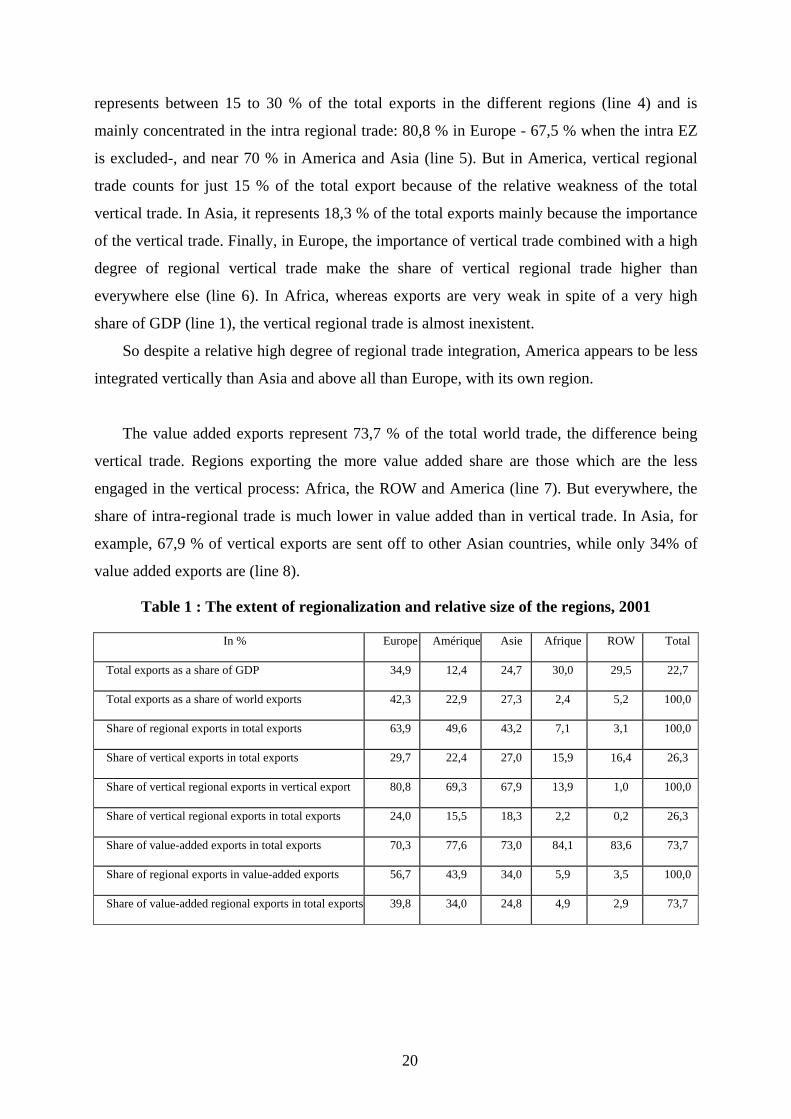
represents between 15 to 30 % of the total exports in the different regions (line 4) and is

mainly concentrated in the intra regional trade: 80,8 % in Europe - 67,5 % when the intra EZ

is excluded-, and near 70 % in America and Asia (line 5). But in America, vertical regional

trade counts for just 15 % of the total export because of the relative weakness of the total

vertical trade. In Asia, it represents 18,3 % of the total exports mainly because the importance

of the vertical trade. Finally, in Europe, the importance of vertical trade combined with a high

degree of regional vertical trade make the share of vertical regional trade higher than

everywhere else (line 6). In Africa, whereas exports are very weak in spite of a very high

share of GDP (line 1), the vertical regional trade is almost inexistent.

So despite a relative high degree of regional trade integration, America appears to be less

integrated vertically than Asia and above all than Europe, with its own region.

The value added exports represent 73,7 % of the total world trade, the difference being

vertical trade. Regions exporting the more value added share are those which are the less

engaged in the vertical process: Africa, the ROW and America (line 7). But everywhere, the

share of intra-regional trade is much lower in value added than in vertical trade. In Asia, for

example, 67,9 % of vertical exports are sent off to other Asian countries, while only 34% of

value added exports are (line 8).

Table 1 : The extent of regionalization and relative size of the regions, 2001

In % Europe Amérique Asie Afrique ROW Total

Total exports as a share of GDP 34,9 12,4 24,7 30,0 29,5 22,7

Total exports as a share of world exports 42,3 22,9 27,3 2,4 5,2 100,0

Share of regional exports in total exports 63,9 49,6 43,2 7,1 3,1 100,0

Share of vertical exports in total exports 29,7 22,4 27,0 15,9 16,4 26,3

Share of vertical regional exports in vertical export 80,8 69,3 67,9 13,9 1,0 100,0

Share of vertical regional exports in total exports 24,0 15,5 18,3 2,2 0,2 26,3

Share of value-added exports in total exports 70,3 77,6 73,0 84,1 83,6 73,7

Share of regional exports in value-added exports 56,7 43,9 34,0 5,9 3,5 100,0

Share of value-added regional exports in total exports 39,8 34,0 24,8 4,9 2,9 73,7

20

3.3. How is production organised inside the regions ? …

Behind that continental approach, it would be interesting to analyse the nature of relation

existing between their different constitutive sub areas. Inside each one, we try to distinguish

core and peripheral countries according to establish their ties in the production process and

with the market of final use. Because the regionalisation process recovers multiple forms of

trading (intensity of vertical trade, dependence to final demand in one country,..), we can use

our data to learn more about that request.

Concerning the intra regional trade, it appears that:

- In Europe, the euro zone represents a very important channel of trading for itself,

the Eastern Europe and the Northern Europe in terms of both value added trade and

vertical trade. It represents between 38 % and 48 % of the total value added export.

Nevertheless, with a 35,2 % of extra Europe exports, the EZ exports 42,2 % of

value added outside Europe. Northern Europe provides an important market for

European export: between 10 and 15 % of its value added exports. These zones

depend on the final demand in northern Europe in a non negligible extent (15 % for

the EZ) too. The northern Europe is quite integrated with the EZ, more than what is

currently admitted.

- In America, the US export 66 % of its total exports outside America and 72,2 % of

its total value added exports, against respectively 35,2 % and 42,2 % for the EZ.

But these results can partly be explained by the size effect (see upper).

Nevertheless, it exports too 21,6 % of the value added export to its closest

neighbours

- In Asia, Japan exports 60 % of its total exports outside Asia and 70,5 % of its value

added exports. China and the rest of Asia depend largely on the extra zone for the

final demand but maintain strong ties together (mainly China with south East Asia

and inside the south east Asia). The Asia Oceania is very integrated with japan and

south and East Asia, in term of value added trade and vertical trade.

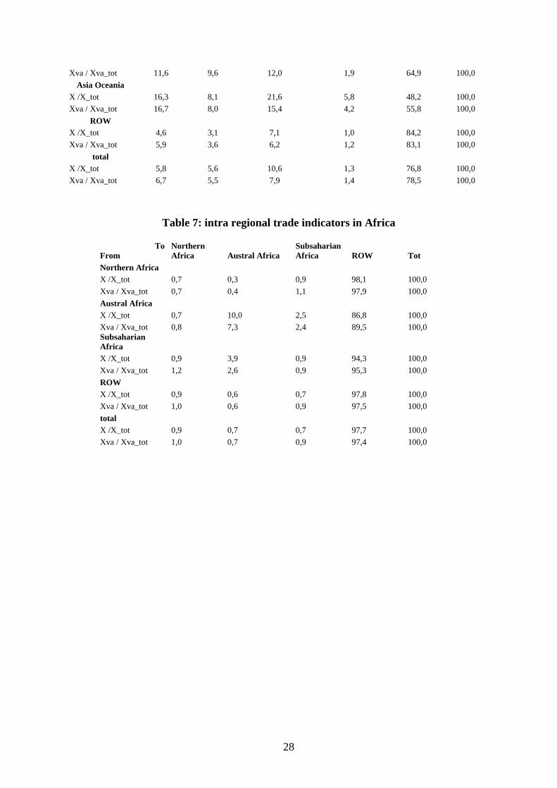
- Finally the African integration does not really appear. Nevertheless, the austral

Africa exports 10 % of its value added exports towards itself and 21,8 % of its

vertical trade.

Not surprisingly, the share of vertical trade is much higher in intra-regional trade than in

total trade. Production processes integration is more intense between geographically close

countries, or countries in a free trade area. Asia is the region where the share of vertical trade

21

in regional exports is the highest: 46%. This confirms the traditional literature on East Asian

(see supra).

As we said before, it appears that the size effect of the trading partners can affect

indicators concerning the intensity of their trade. To avoid that, we build an indicator of

relative bilateral intensity, developed by the CEPII42. It consists to build theoretical

exports in assuming that the bilateral flow between two countries is determined by the

trading size of the partners in the world trade. In dividing the effective bilateral flow with

the theoretical one, we obtain an indicator of bilateral relative intensity that should be

equal to 1 if there were no others specific factors such as geographical proximity,

historical context,…

The tables 8 and 9 confirm the regionalisation process both in standard measure and,

more surprisingly, in value added terms. The indicator is higher than 1 between partners

of a same large region. That is particularly true in America between in one side, and in

the both ways, the US and the rest of the northern America and, in another side, South

America with South America, and in lesser extent with the US. In Africa, the integration

process within the Austral Africa is largely confirmed as well as with the sub-Saharan

Africa. In Asia, the bilateral ratios do not exceed 1,7 except for Asia-Oceania trade with

itself and with Japan. We have to notice too that except the eastern Europe, all regions

increased its trading intensity with the US once expressed in value added term.

But above all, in the table 10, we can see countries which tend to privilege its value added

trade (a ratio higher than 1) and those countries that gets more distant in term of intensity

in value added trade. In this way, we observe that the asian trade tends to lessen its

relation in value added trade and reinforce its vertical integration. That is not the case in

America. In Europe, the ratio is lower than 1 but not too low. It means that the intensity

of the Europe trade passes by the vertical trade too but less than in Asia.

Although the intra regional trade is predominant, notably with the integration of

production process generating vertical trade within a region, and also a nearby market of final

goods used to be consumed in the three main regions, it appears that the extra region trade can

be different of what we use to see.

42 Freudenberg, Gaulier et Unal-Kesinci, (1998)

22

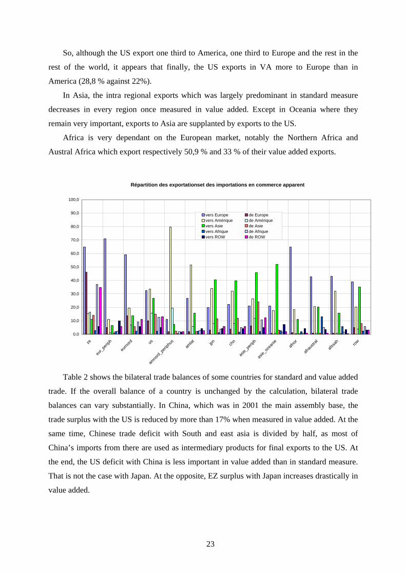
So, although the US export one third to America, one third to Europe and the rest in the

rest of the world, it appears that finally, the US exports in VA more to Europe than in

America (28,8 % against 22%).

In Asia, the intra regional exports which was largely predominant in standard measure

decreases in every region once measured in value added. Except in Oceania where they

remain very important, exports to Asia are supplanted by exports to the US.

Africa is very dependant on the European market, notably the Northern Africa and

Austral Africa which export respectively 50,9 % and 33 % of their value added exports.

Répartition des exportationset des importations en commerce apparent

0,0

10,0

20,0

30,0

40,0

50,0

60,0

70,0

80,0

90,0

100,0

ze

eur_p

eriph

eurno

rd us

amno

rd_pe

riphu

sam

lat jpn chn

asie_

perip

h

asie_

ocea

nieafn

or

afrau

stral

afssa

hrow

vers Europe de Europevers Amérique de Amériquevers Asie de Asievers Afrique de Afriquevers ROW de ROW

Table 2 shows the bilateral trade balances of some countries for standard and value added

trade. If the overall balance of a country is unchanged by the calculation, bilateral trade

balances can vary substantially. In China, which was in 2001 the main assembly base, the

trade surplus with the US is reduced by more than 17% when measured in value added. At the

same time, Chinese trade deficit with South and east asia is divided by half, as most of

China’s imports from there are used as intermediary products for final exports to the US. At

the end, the US deficit with China is less important in value added than in standard measure.

That is not the case with Japan. At the opposite, EZ surplus with Japan increases drastically in

value added.

23

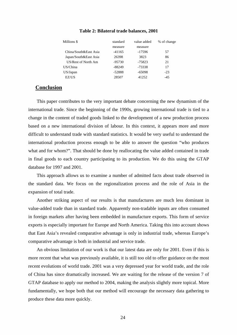
Table 2: Bilateral trade balances, 2001

Millions $ standard value added % of change measure measure

China/South&East Asia -41165 -17596 57 Japan/South&East Asia 26398 3823 86 US/Rest of North Am -95730 -75823 21

US/China -88249 -73338 17 US/Japan -52888 -65098 -23

EZ/US 28507 41252 -45

Conclusion

This paper contributes to the very important debate concerning the new dynamism of the

international trade. Since the beginning of the 1990s, growing international trade is tied to a

change in the content of traded goods linked to the development of a new production process

based on a new international division of labour. In this context, it appears more and more

difficult to understand trade with standard statistics. It would be very useful to understand the

international production process enough to be able to answer the question “who produces

what and for whom?”. That should be done by reallocating the value added contained in trade

in final goods to each country participating to its production. We do this using the GTAP

database for 1997 and 2001.

This approach allows us to examine a number of admitted facts about trade observed in

the standard data. We focus on the regionalization process and the role of Asia in the

expansion of total trade.

Another striking aspect of our results is that manufactures are much less dominant in

value-added trade than in standard trade. Apparently non-tradable inputs are often consumed

in foreign markets after having been embedded in manufacture exports. This form of service

exports is especially important for Europe and North America. Taking this into account shows

that East Asia’s revealed comparative advantage is only in industrial trade, whereas Europe’s

comparative advantage is both in industrial and service trade.

An obvious limitation of our work is that our latest data are only for 2001. Even if this is

more recent that what was previously available, it is still too old to offer guidance on the most

recent evolutions of world trade. 2001 was a very depressed year for world trade, and the role

of China has since dramatically increased. We are waiting for the release of the version 7 of

GTAP database to apply our method to 2004, making the analysis slightly more topical. More

fundamentally, we hope both that our method will encourage the necessary data gathering to

produce these data more quickly.

24

Appendix

Table 3: Vertical trade per industry

Sector Total exports

(million $)

Import content

of exports (VS)

Exports used as inputs

for further exports (VS1)

Value-added exports as

a share of total exports

VS1* as a share of

value-added exports

Paddy rice 2,027 7% 24% 307% 0,5%

Wheat 15,921 14% 18% 82% 1,5%

Cereal grains nec 14,085 12% 14% 90% 1,7%

Vegetables, fruit, nuts 45,761 10% 8% 104% 0,6%

Oil seeds 15,492 11% 22% 82% 1,4%

Sugar cane, sugar beet 52 11% 24% 5,580% 0,7%

Plant-based fibers 7,794 15% 42% 107% 2,5%

Crops nec 39,288 11% 18% 97% 1,0%

Bovine cattle, sheep and goats, horses 5,867 14% 12% 193% 0,9%

Animal products nec 15,281 16% 22% 113% 1,1%

Raw milk 186 12% 13% 4,990% 0,7%

Wool, silk-worm cocoons 2,871 12% 39% 110% 0,9%

Forestry 9,735 9% 29% 267% 1,5%

Fishing 7,634 13% 15% 146% 1,0%

Agriculture 181,995 12% 18% 121% 1,1%

Coal 21,034 10% 29% 102% 2,7%

Oil 223,954 13% 32% 76% 1,0%

Gas 50,030 10% 27% 100% 1,1%

Minerals nec 37,165 13% 45% 121% 2,5%

Raw materials 332,182 12% 33% 86% 1,4%

Primary sector 514,177 12% 27% 99% 1,3%

Bovine meat products 22,177 16% 9% 35% 1,4%

Meat products nec 31,290 20% 10% 33% 1,1%

Vegetable oils and fats 15,347 22% 15% 57% 1,2%

Dairy products 30,561 20% 9% 36% 1,1%

Processed rice 5,499 13% 6% 34% 0,5%

Sugar 8,458 16% 14% 63% 1,1%

Food products nec 131,107 23% 10% 44% 1,3%

Beverages and tobacco products 50,265 17% 6% 62% 0,7%

Farm industries 294,704 20% 9% 45% 1,1%

Textiles 192,180 28% 30% 57% 2,8%

Wearing apparel 155,213 26% 6% 40% 0,6%

Leather products 89,010 25% 12% 37% 0,7%

Textiles and al. 436,402 27% 18% 47% 1,8%

Wood products 122,264 22% 18% 49% 2,4%

Paper products, publishing 145,762 21% 26% 85% 3,2%

Wood and paper 268,026 22% 22% 68% 3,0%

Petroleum, coal products 99,328 44% 28% 29% 1,6%

Chemical, rubber, plastic products 694,111 27% 36% 58% 4,3%

Mineral products nec 110,505 17% 21% 73% 2,9%

Ferrous metals 139,745 26% 43% 71% 4,1%

Metals nec 153,284 28% 50% 45% 4,3%

Chemicals and metals 1,196,973 27% 37% 57% 4,0%

Metal products 128,392 23% 28% 90% 4,2%

25

Motor vehicles and parts 525,404 32% 17% 32% 4,0%

Transport equipment nec 205,178 25% 16% 43% 2,6%

Metal and transport products 858,974 29% 18% 43% 3,8%

Electronic equipment 815,824 38% 33% 37% 4,3%

Machinery and equipment nec 1,013,394 25% 21% 46% 3,8%

Manufactures nec 183,690 24% 13% 51% 1,2%

Other manufactures 2,012,908 30% 25% 43% 3,7%

Electricity 21,977 15% 26% 591% 2,7%

Gas manufacture, distribution 2,474 6% 22% 478% 3,0%

Water 1,504 10% 14% 868% 3,6%

Construction 28,772 17% 4% 175% 2,8%

Utilities 32,751 16% 5% 229% 2,9%

Secondary sector 5,111,727 28% 25% 50% 3,4%

Trade 179,738 13% 19% 235% 3,0%

Transports 320,263 21% 20% 97% 2,0%

Communication 40,895 10% 17% 219% 1,9%

Communication and trade 540,896 17% 19% 152% 2,5%

Financial services nec 54,717 12% 25% 308% 2,9%

Insurance 41,910 12% 21% 108% 1,6%

Business services nec 361,744 11% 24% 142% 2,9%

Business services 458,371 11% 24% 159% 2,8%

Recreational and other services 83,517 9% 16% 210% 2,3%

Public Administration, Defense, Education, Health 106,786 7% 3% 138% 2,3%

Other services 190,302 8% 9% 176% 2,2%

Tertiary Sector 1,189,569 13% 20% 158% 2,6%

Total 6,815,473 24% 24% 74% 2,9%

26

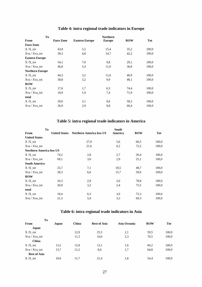
Table 4: intra regional trade indicators in Europe

To From Euro Zone Eastern Europe

Northern Europe ROW Tot

Euro Zone X /X_tot 43,8 5,5 15,4 35,2 100,0 Xva / Xva_tot 38,3 4,8 14,7 42,2 100,0 Eastern Europe X /X_tot 54,1 7,0 9,8 29,1 100,0 Xva / Xva_tot 46,8 5,4 11,0 36,8 100,0 Northern Europe X /X_tot 44,3 3,2 11,6 40,9 100,0 Xva / Xva_tot 38,8 3,2 9,9 48,1 100,0 ROW X /X_tot 17,6 1,7 6,3 74,4 100,0 Xva / Xva_tot 18,9 1,9 7,4 71,9 100,0 total X /X_tot 29,0 3,1 9,6 58,2 100,0 Xva / Xva_tot 26,9 2,9 9,8 60,4 100,0

Table 5: intra regional trade indicators in America

To From United States Northern America less US

South America ROW Tot

United States X /X_tot 27,9 5,6 66,5 100,0 Xva / Xva_tot 21,6 6,2 72,2 100,0 Northern America less US X /X_tot 74,2 2,8 2,7 20,4 100,0 Xva / Xva_tot 69,1 3,0 2,9 25,1 100,0 South America X /X_tot 25,7 7,1 18,5 48,7 100,0 Xva / Xva_tot 28,3 6,0 15,7 50,0 100,0 ROW X /X_tot 16,3 2,9 2,0 78,8 100,0 Xva / Xva_tot 20,8 3,2 2,4 73,5 100,0 total X /X_tot 18,4 6,3 3,0 72,3 100,0 Xva / Xva_tot 21,3 5,9 3,5 69,3 100,0

Table 6: intra regional trade indicators in Asia

To From Japan China Rest of Asia Asia Oceania ROW Tot

Japan X /X_tot 12,9 25,5 2,1 59,5 100,0 Xva / Xva_tot 11,2 16,0 2,3 70,5 100,0

China X /X_tot 13,2 12,8 12,1 1,6 60,2 100,0 Xva / Xva_tot 13,7 11,2 8,6 1,7 64,8 100,0

Rest of Asia X /X_tot 10,6 11,7 21,4 1,8 54,4 100,0

27

Xva / Xva_tot 11,6 9,6 12,0 1,9 64,9 100,0 Asia Oceania

X /X_tot 16,3 8,1 21,6 5,8 48,2 100,0 Xva / Xva_tot 16,7 8,0 15,4 4,2 55,8 100,0

ROW X /X_tot 4,6 3,1 7,1 1,0 84,2 100,0 Xva / Xva_tot 5,9 3,6 6,2 1,2 83,1 100,0

total X /X_tot 5,8 5,6 10,6 1,3 76,8 100,0 Xva / Xva_tot 6,7 5,5 7,9 1,4 78,5 100,0

Table 7: intra regional trade indicators in Africa

ToFrom

Northern Africa Austral Africa

Subsaharian Africa ROW Tot

Northern Africa X /X_tot 0,7 0,3 0,9 98,1 100,0 Xva / Xva_tot 0,7 0,4 1,1 97,9 100,0 Austral Africa X /X_tot 0,7 10,0 2,5 86,8 100,0 Xva / Xva_tot 0,8 7,3 2,4 89,5 100,0 Subsaharian Africa X /X_tot 0,9 3,9 0,9 94,3 100,0 Xva / Xva_tot 1,2 2,6 0,9 95,3 100,0 ROW X /X_tot 0,9 0,6 0,7 97,8 100,0 Xva / Xva_tot 1,0 0,6 0,9 97,5 100,0 total X /X_tot 0,9 0,7 0,7 97,7 100,0 Xva / Xva_tot 1,0 0,7 0,9 97,4 100,0

28

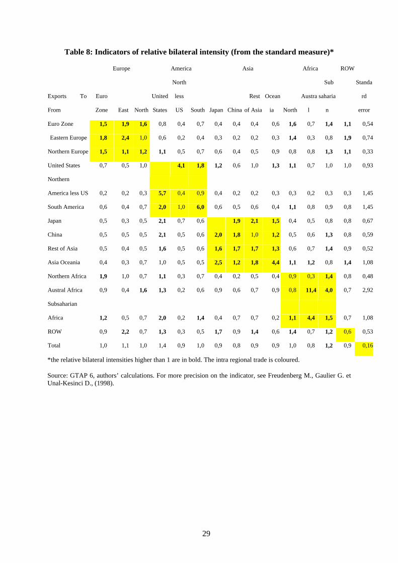
Table 8: Indicators of relative bilateral intensity (from the standard measure)*

Europe America Asia Africa ROW

Exports To

From

Euro

Zone East North

United

States

North

less

US South Japan China

Rest

of Asia

Ocean

ia North

Austra

l

Sub

saharia

n

Standa

rd

error

Euro Zone 1,5 1,9 1,6 0,8 0,4 0,7 0,4 0,4 0,4 0,6 1,6 0,7 1,4 1,1 0,54

Eastern Europe 1,8 2,4 1,0 0,6 0,2 0,4 0,3 0,2 0,2 0,3 1,4 0,3 0,8 1,9 0,74

Northern Europe 1,5 1,1 1,2 1,1 0,5 0,7 0,6 0,4 0,5 0,9 0,8 0,8 1,3 1,1 0,33

United States 0,7 0,5 1,0 4,1 1,8 1,2 0,6 1,0 1,3 1,1 0,7 1,0 1,0 0,93

Northern

America less US 0,2 0,2 0,3 5,7 0,4 0,9 0,4 0,2 0,2 0,3 0,3 0,2 0,3 0,3 1,45

South America 0,6 0,4 0,7 2,0 1,0 6,0 0,6 0,5 0,6 0,4 1,1 0,8 0,9 0,8 1,45

Japan 0,5 0,3 0,5 2,1 0,7 0,6 1,9 2,1 1,5 0,4 0,5 0,8 0,8 0,67

China 0,5 0,5 0,5 2,1 0,5 0,6 2,0 1,8 1,0 1,2 0,5 0,6 1,3 0,8 0,59

Rest of Asia 0,5 0,4 0,5 1,6 0,5 0,6 1,6 1,7 1,7 1,3 0,6 0,7 1,4 0,9 0,52

Asia Oceania 0,4 0,3 0,7 1,0 0,5 0,5 2,5 1,2 1,8 4,4 1,1 1,2 0,8 1,4 1,08

Northern Africa 1,9 1,0 0,7 1,1 0,3 0,7 0,4 0,2 0,5 0,4 0,9 0,3 1,4 0,8 0,48

Austral Africa 0,9 0,4 1,6 1,3 0,2 0,6 0,9 0,6 0,7 0,9 0,8 11,4 4,0 0,7 2,92

Subsaharian

Africa 1,2 0,5 0,7 2,0 0,2 1,4 0,4 0,7 0,7 0,2 1,1 4,4 1,5 0,7 1,08

ROW 0,9 2,2 0,7 1,3 0,3 0,5 1,7 0,9 1,4 0,6 1,4 0,7 1,2 0,6 0,53

Total 1,0 1,1 1,0 1,4 0,9 1,0 0,9 0,8 0,9 0,9 1,0 0,8 1,2 0,9 0,16

*the relative bilateral intensities higher than 1 are in bold. The intra regional trade is coloured.

Source: GTAP 6, authors’ calculations. For more precision on the indicator, see Freudenberg M., Gaulier G. et Unal-Kesinci D., (1998).

29

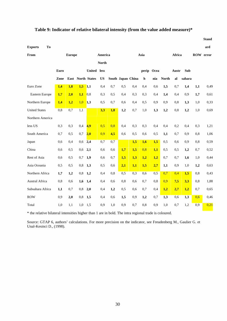
Table 9: Indicator of relative bilateral intensity (from the value added measure)*

Exports To

From Europe America Asia Africa ROW

Stand

ard

error

Euro

Zone East North

United

States

North

less

US South Japan China

perip

h

Ocea

nia North

Austr

al

Sub

sahara

Euro Zone 1,4 1,8 1,5 1,1 0,4 0,7 0,5 0,4 0,4 0,6 1,5 0,7 1,4 1,1 0,49

Eastern Europe 1,7 2,0 1,1 0,8 0,3 0,5 0,4 0,3 0,3 0,4 1,4 0,4 0,9 1,7 0,61

Northern Europe 1,4 1,2 1,0 1,3 0,5 0,7 0,6 0,4 0,5 0,9 0,9 0,8 1,3 1,0 0,33

United States 0,8 0,7 1,1 3,3 1,8 1,2 0,7 1,0 1,3 1,2 0,8 1,2 1,0 0,69

Northern America

less US 0,3 0,3 0,4 4,9 0,5 0,8 0,4 0,3 0,3 0,4 0,4 0,2 0,4 0,3 1,21

South America 0,7 0,5 0,7 2,0 0,9 4,5 0,6 0,5 0,6 0,5 1,1 0,7 0,9 0,8 1,06

Japan 0,6 0,4 0,6 2,4 0,7 0,7 1,5 1,6 1,5 0,5 0,6 0,9 0,8 0,59

China 0,6 0,5 0,6 2,1 0,6 0,6 1,7 1,5 0,8 1,1 0,5 0,5 1,2 0,7 0,52

Rest of Asia 0,6 0,5 0,7 1,9 0,6 0,7 1,5 1,3 1,2 1,2 0,7 0,7 1,6 1,0 0,44

Asia Oceania 0,5 0,5 0,8 1,3 0,5 0,6 2,1 1,1 1,5 2,7 1,1 0,9 1,0 1,2 0,63

Northern Africa 1,7 1,2 0,8 1,2 0,4 0,8 0,5 0,3 0,6 0,5 0,7 0,4 1,5 0,8 0,43

Austral Africa 0,8 0,6 1,6 1,4 0,4 0,6 0,8 0,6 0,7 0,8 0,9 7,5 3,3 0,8 1,88

Subsahara Africa 1,1 0,7 0,8 2,0 0,4 1,2 0,5 0,6 0,7 0,4 1,2 2,7 1,2 0,7 0,65

ROW 0,9 2,0 0,8 1,5 0,4 0,6 1,5 0,9 1,2 0,7 1,3 0,6 1,3 0,6 0,46

Total 1,0 1,1 1,0 1,5 0,9 1,0 0,9 0,7 0,8 0,9 1,0 0,7 1,2 0,9 0,21

* the relative bilateral intensities higher than 1 are in bold. The intra regional trade is coloured.

Source: GTAP 6, authors’ calculations. For more precision on the indicator, see Freudenberg M., Gaulier G. et Unal-Kesinci D., (1998).

30

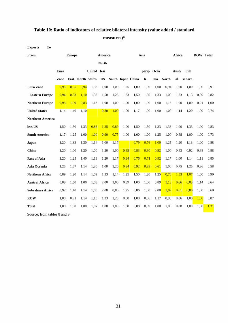
Table 10: Ratio of indicators of relative bilateral intensity (value added / standard

measures)*

Exports To

From Europe America Asia Africa ROW Total

Euro

Zone East North

United

States

North

less

US South Japan China

perip

h

Ocea

nia North

Austr

al

Sub

sahara

Euro Zone 0,93 0,95 0,94 1,38 1,00 1,00 1,25 1,00 1,00 1,00 0,94 1,00 1,00 1,00 0,91

Eastern Europe 0,94 0,83 1,10 1,33 1,50 1,25 1,33 1,50 1,50 1,33 1,00 1,33 1,13 0,89 0,82

Northern Europe 0,93 1,09 0,83 1,18 1,00 1,00 1,00 1,00 1,00 1,00 1,13 1,00 1,00 0,91 1,00

United States 1,14 1,40 1,10 0,80 1,00 1,00 1,17 1,00 1,00 1,09 1,14 1,20 1,00 0,74

Northern America

less US 1,50 1,50 1,33 0,86 1,25 0,89 1,00 1,50 1,50 1,33 1,33 1,00 1,33 1,00 0,83

South America 1,17 1,25 1,00 1,00 0,90 0,75 1,00 1,00 1,00 1,25 1,00 0,88 1,00 1,00 0,73

Japan 1,20 1,33 1,20 1,14 1,00 1,17 0,79 0,76 1,00 1,25 1,20 1,13 1,00 0,88

China 1,20 1,00 1,20 1,00 1,20 1,00 0,85 0,83 0,80 0,92 1,00 0,83 0,92 0,88 0,88

Rest of Asia 1,20 1,25 1,40 1,19 1,20 1,17 0,94 0,76 0,71 0,92 1,17 1,00 1,14 1,11 0,85

Asia Oceania 1,25 1,67 1,14 1,30 1,00 1,20 0,84 0,92 0,83 0,61 1,00 0,75 1,25 0,86 0,58

Northern Africa 0,89 1,20 1,14 1,09 1,33 1,14 1,25 1,50 1,20 1,25 0,78 1,33 1,07 1,00 0,90

Austral Africa 0,89 1,50 1,00 1,08 2,00 1,00 0,89 1,00 1,00 0,89 1,13 0,66 0,83 1,14 0,64

Subsahara Africa 0,92 1,40 1,14 1,00 2,00 0,86 1,25 0,86 1,00 2,00 1,09 0,61 0,80 1,00 0,60

ROW 1,00 0,91 1,14 1,15 1,33 1,20 0,88 1,00 0,86 1,17 0,93 0,86 1,08 1,00 0,87

Total 1,00 1,00 1,00 1,07 1,00 1,00 1,00 0,88 0,89 1,00 1,00 0,88 1,00 1,00 1,31

Source: from tables 8 and 9

31

Bibliography Arthus, Patrick and Lionel Fontagné. 2006. Une analyse de l'évolution récente du commerce

extérieur français, Rapport du CAE. Paris.

Athukorala, Prema-Chandra and Nobuaki Yamashita. 2006. "Production Fragmentation and

Trade Integration: East Asia in a Global Context." North American Journal of Economics and

Finance, 17 3, pp. 233-56.

Baldwin, Richard. 2006. "Multilateralising Regionalism: Spaghetti Bowls as Building Blocs

on the Path to Global Free Trade." World Economy, 29:11.

Bardhan, Ashok Deo and Dwight Jaffee. 2005. "On Intra-Firm Trade and Manufacturing

Outsourcing and Offshoring," in Edward Monty Graham (ed.), The Role of Foreign Direct

Investment and Multinational Corporations in Economic Development Palgrave.

Benhamou, Laurence. 2005. Le grand Bazar mondial : la folle aventure de ces produits

apparemment "bien de chez nous". Paris: Bourin.

Cameron, G. and P. Cross. 1999. "The importance of exports to GDP and jobs." Canadian

Economic Observer:Nov.

Campa, José M. and Linda S. Goldberg. 1997. "The Evolving External Orientation of

Manufacturing: A Profile of Four Countries." Economic Policy Review, 3:2.

CEPII. 2007. "CHELEM."

Chen, Hogan, Matthew Kondratowicz, and Kei-mu Yi. 2005. "Vertical specialization and

three facts about U.S. international trade." North American Journal of Economics & Finance,

16:1, pp. 35-59.

Chen, X., L. K. Cheng, K. C. Fung, and L. J. Lau. 2005. "The Estimation of Domestic Value-

Added and Employment Induced by Exports: An Application to Chinese Exports to the

United States." meeting of the American Economic Association, 8.

Chinn, M. D. 2005. "Supply Capacity, Vertical Specialization and Tariff Rates: The

Implications for Aggregate US Trade Flow Equations." NBER Working Paper:11719.

Chortareas, G. E. and T. Pelagidis. 2004. "Trade flows: a facet of regionalism or

globalisation?" Cambridge Journal of Economics, 28:2, pp. 253-271.

Council, National Research. 2006. Analyzing the U.S. Content of Imports and the Foreign

Content of Exports. Washington DC: Committee on Analyzing the U.S. Content of Imports

and the Foreign Content of Exports. Center for Economic, Governance, and International

Studies, Division of Behavioral and Social Sciences and Education, National Academy Press.

32

Daudin, Guillaume, Christine Rifflart, Dannielle Schweisguth, and Paola Veroni. 2006. "Le

commerce extérieur en valeur ajoutée." Revue de l'OFCE : Observations et diagnostics

économiques:98, pp. 129-165.

Dean, Judith, K. C. Fung, and Zhi Whang. 2007. "Measuring the Vertical Specialization in

Chinese Trade." U.S. International Trade Commission Office of Economics Working

Paper:2007-01-A.

Dimaranan, Betina V. ed. 2006. Global Trade, Assistance, and Production: The GTAP 6 Data

Base: Center for Global Trade Analysis, Purdue University.

Egger, Hartmut and Peter Egger. 2005. "The Determinants of EU Processing Trade." World

Economy, 28 2, pp. 147-68.

Ethier, Wilfred J. 1998. "The New Regionalism." The Economic Journal, 108:449, pp. 1149-

1161.

Feenstra, Robert C. 1998. "Integration of Trade and Disintegration of Production in the

Global Economy." Journal of Economic Perspectives, 12:4, pp. 31-50.

Feenstra, Robert C. and Gordon H. Hanson. 1997. "Productivity Measurement and the Impact

of Trade and Technology on Wages : Estimates from the U.S., 1972-1990 " NBER Working

Paper:6052.

Freudenberg M., Gaulier G. et Unal-Kesinci D., 1998, "La régionalisation du commerce

international : une évaluation par les intensités relatives bilatérales", CEPII, Document de

travail 98-05.

Gehlhar, Mark. 2006. "Re-Export Trade for Hong Kong and the Netherlands," in GTAP (ed.),

GRAP 6 Data Base documentation.

Grossman, Gene M. and Elhanan Helpman. 2005. "Outsourcing in a Global Economy."

Review of Economic Studies, 72 1, pp. 135-59.

Haddad, Mona. 2007. "Trade Integration in East Asia: the Role of China and Production

Networks." World Bank Policy Research Working Paper:4160, pp. 36.

Hanson, G. H., Mataloni Jr, and Slaughter. 2005. "Vertical production networks in

multinational firms." Review of Economics and Statistics, 87:4.

Hoen, Alex R. . 2002. An Input-Output Analysis of European Integration. Amsterdam: North-

Holland.

Hummels, David, Jun Ishii, and Kei-Mu Yi. 1999. "The Nature and Growth of Vertical

Specialization in World Trade." Staff Reports of the Federal Reserve Bank of New York:72,

pp. 39.

33

Hummels, David, Jun Ishii, and Kei-Mu Yi. 2001. "The Nature and Growth of Vertical

Specialization in World Trade." Journal of International Economics, 54 1, pp. 75-96.

Hummels, David, Dana Rapoport, and Kei-Mu Yi. 1998. "Vertical Specialization and the

Changing Nature of World Trade." Federal Reserve Bank of New York Economic Policy

Review, 4 2, pp. 79-99.

Irwin, Douglas A. 1996. "The United States in a New Global Economy? A Century's

Perspective." American Economic Review, 86 2, pp. 41-46.

Ishii, Jun and Kei-Mu Yi. 1997. "The Growth of World Trade." Research Paper of the

Federal Reserve Bank of New York:9718.

Jones, Ronald W. 2000. Globalization and the theory of input trade. Cambridge: MIT Press.

Kleinert, Jörn. 2003. "Growing Trade in Intermediate Goods: Outsourcing, Global Sourcing,

or Increasing Importance of MNE Networks?" Review of International Economics, 11, pp.

464-482.

Koopman, Robert, Zhi Wang, and Shang-Jin Wei. 2008. "How Much of Chinese Exports is

Really Made In China? Assessing Domestic Value-Added When Processing Trade is

Pervasive." National Bureau of Economic Research Working Paper Series, No. 14109.

Kwan, C.H. 2001. Yen bloc: Toward economic integration in Asia: Brookings Institution

Press, Washington DC.

Leontief, W. W. 1936. "Quantitative input and ouput relations in the economic system of the

United States." Review of Economics and Statistics, 18, pp. 105-125.

McDougall, Robert A. 2006. "19. Updating and Adjusting the Regional Input-Output Tables,"

in Betina V. Dimaranan (ed.), Global Trade, Assistance, and Production: The GTAP 6 Data

Base Center for Global Trade Analysis, Purdue University.

Ng, F. and A Yeats. 2003. "Major trade trends in East Asia: What are their implications for

regional cooperation and growth?" Policy Research Working Paper: 3084.

Ravix, Joël Thomas and Olivier Sautel. 2007. "Comportement des firmes et commerce

international." Revue de l'OFCE, 100:1.

Shoven, J. B. and J. Wholley. 1992. Applying General Equilibrium: Cambridge University

Press.

Singa Boyenge, Jean-Pierre. 2007. "ILO Database on export processing zones (Revised)."

ILO Working Papers:WP. 251.

UNCTAD. 2005. World Investment Report.

34

Walmsley, Terrie L. and Robert A. McDougall. 2006. "11. A. Overview of Regional Input-

Output Tables," in Betina V. Dimaranan (ed.), Global Trade, Assistance, and Production: The

GTAP 6 Data Base Center for Global Trade Analysis, Purdue University.

World Bank. 2000. Trade Blocs. Oxford: Oxford University Press.

Yi, Kei-Mu. 2003. "Can Vertical Specialization Explain the Growth of World Trade?"

Journal of Political Economy, 111:February.

35