Value-at-risk: Applying the extreme value approach to Asian markets in the recent financial turmoil

Ž .Pacific-Basin Finance Journal 8 2000 249–275www.elsevier.comrlocatereconbase

Value-at-risk: Applying the extreme valueapproach to Asian markets in the recent

financial turmoil

Lan-Chih Ho a,), Peter Burridge b, John Cadle a,Michael Theobald a

a Department of Accounting and Finance, UniÕersity of Birmingham, Edgbaston,Birmingham B15 2TT, UK

b Department of Economics, UniÕersity of Birmingham, Birmingham, UK

Abstract

Ž .Value-at-risk VaR measures are generated using extreme value theory by modellingthe tails of the return distributions of six Asian financial markets during the recent volatilemarket conditions. The maxima and minima of these return series were found to besatisfactorily modelled within an extreme value framework and the value at risk measuresgenerated within this structure were found to be different to those generated by variance–covariance and historical methods, particularly for markets characterised by high degrees ofleptokurtosis such as Malaysia and Indonesia. q 2000 Published by Elsevier Science B.V.All rights reserved.

JEL classification: G15; G18

Keywords: Variance–covariance; Leptokurtic; Asia

1. Introduction

Ž .Value-at-risk VaR has been widely promoted by regulatory groups andembraced by financial institutions as a way of monitoring and managing marketrisk — the risk of loss due to adverse movements in interest rate, exchange rate,

) Corresponding author.

0927-538Xr00r$ - see front matter q 2000 Published by Elsevier Science B.V. All rights reserved.Ž .PII: S0927-538X 00 00008-1

( )L.-C. Ho et al.rPacific-Basin Finance Journal 8 2000 249–275250

equity and commodity exposures — and as a basis for setting regulatory minimumcapital standards. The revised Basle Accord, implemented in January 1998, allowsbanks to use VaR as a basis for determining how much additional capital must beset aside to cover market risk beyond that required for credit risk. Market relatedrisk has become more prevalent and important due to the trading activities andmarket positions taken by large banks. Another impetus for such a measure hascome from the numerous and substantial losses that have arisen due to shortcom-ings in risk management procedures that failed to detect errors in derivatives

Ž . Žpricing NatWest, UBS , excessive risk taking Orange County, Proctor and. Ž .Gamble , as well as fraudulent behaviour Barings and Sumitomo .

The attraction of VaR is its conceptual simplicity. In a single statistic itprovides an estimate of the potential loss to which a bank is exposed over a givenperiod of time with a given degree of confidence. However, the wide range ofassets, currencies and markets in which a global bank will have an interest meanthat the implementation of VaR fraught with difficulties and it is very demandingin terms of data requirements.

Although very significant advances have been made in modelling VaR, there isas yet no agreement on which methodology is best. Three approaches arecommonly used. The analytical or Riskmetrics approach proposed by J.P. Morganis widely used. It assumes that all prices are jointly log-normally distributed, andits key element is a huge variance–covariance matrix that is updated daily. Itsmajor weakness is that financial returns typically have fat tails and are not

Ž .log-normally distributed e.g., Duffie and Pan, 1997 . Hence, large losses occurmore frequently than predicted by the variance–covariance method. The historicalmethod makes no such assumptions but presumes a history of portfolio pricechanges that can be ranked so that the loss at the 1% or 5% confidence level canbe determined in a straightforward fashion. Its major drawbacks are a lack offlexibility in testing the sensitivity of VaR to differing assumptions and thesensitivity of the VaR estimate to the time period selected. The stochastic orMonte-Carlo simulation method can combine historical data and scenarios togenerate a portfolio of profits and losses from which VaR can be determined at theappropriate confidence interval. Its shortcomings are its judgmental inputs and

Ž Ž . Ž . Ž .computational requirements see Jorion 1997 , Dowd 1998 or Risk 1998 for amore detailed discussion of the strengths and weaknesses of the above methods

Ž . Ž . Ž ..and, of VaR itself, see Beder 1995 , Taleb 1997 , Arzner et al. 1998 .The VaR obtained by the above methods is a threshold value, and as such,

gives no insight into the magnitude of possible losses that can occur as one movesfurther out into the tail of the distribution. The tails are the regions of rare andpotentially catastrophic events that can result in institutional failure and so are theareas of most interest to regulators and risk managers. Stress testing is advocatedto overcome this deficiency. It attempts to assess the impact on VaR of a shock inone or more specific markets that is significantly more unlikely and severe than a

Ž .1 or 5% event see, for example, Kupiac, 1998; Risk, 1998 .

( )L.-C. Ho et al.rPacific-Basin Finance Journal 8 2000 249–275 251

A more recent approach to estimating VaR focuses on modelling the tail of thedistribution rather than getting the tail as an outcome of modelling the entire

Ž .density function which is the primary objective of the above methods . ThisŽ .approach is based on extreme value theory EVT , which has its history in the

study of catastrophic events, such as natural phenomena and disasters and theŽinsurance field. The theory itself is developing rapidly see Reiss and Thomas,.1991; Leadbetter et al., 1993; Embrechts et al., 1997 and there have been a

Žnumber of notable applications in the field of finance see Longin, 1996; Longin,1998; Longin and Solnik, 1998; Danielsson and De Vries, 1997, 1998; Danielssonet al., 1998; Diebold et al., 1999; Emmer et al., 1998; McNeil, 1998; McNeil and

.Frey, 1998, and the references therein .EVT uses statistical techniques that focus only on those parts of a sample of

return data that carry information about extreme behaviour. Typically, the sampleis divided into N blocks of non-overlapping returns with say n returns in eachblock. From each block the largest rise and the biggest fall in returns are extractedto create a maxima and a minima series each with a total of m returns. Theseseries are used to model both tails of the sample return distribution that can thenbe employed to extrapolate the return behaviour beyond the particular data setemployed. An alternative method of estimating the tail is to define the extremes in

Ž . Žterms of exceedances or peaks over threshold POT see Emmer et al., 1998;.Longin and Solnik, 1998 . The former method is used in this study.

The recent turmoil that has occurred in Asian financial markets providesinteresting exploratory opportunities within which to estimate and compare tradi-tionally estimated VaRs with values estimated by extreme value theory. The planof the paper is as follows. In Section 2, important elements of the extreme valuetheory as they apply to this paper are presented. Section 3 reports the results of theempirical analysis conducted on stock market index data for the Indonesian,Japanese, Korean, Malaysian, Taiwanese and Thai markets. The period beginning1984 through 1996 is used for estimating various parameters, which are then usedto generate VaR estimates from an extreme value perspective and compared to thetraditional analytical and historic VaR measures. The three methods of computingVaR are then evaluated in terms of the number of times the actual daily returns,firstly during 1996, and secondly over the two years 1997–1998, exceed theestimated VaR values. In Section 4 the implications of the analyses presented inthe paper for the measurement of VARs are summarised. Conclusions are pre-sented in Section 5.

2. Theory of extremes

Extreme value theory is a branch of the theory of order statistics, which datesŽ . Ž .back to the pioneering works by Frechet 1927 and Fisher and Tippett 1928 , and´

Ž . Ž .the celebrated external type theorem of Gnedenko 1943 . Gumbel 1958 gives a


clear presentation of the important elements of the theory and more recent andadvanced treatments can be found in the references cited earlier in this paper. Theremainder of this section sets out the basic theory used in the present study.

We use the following notation:

R: the return of a variable. R , R , . . . , R are the returns observed on days 1,1 2 n

2, . . . , n.Ž . Ž .F r sPr RFr : a cumulative distribution function of R.RŽ .f r : a probability density function of R for Rsr.R

Ž .X : the biggest riserfall in return the maximumrminimum observed over nn

trading days. X is the largest return from the first n observations contained inn,1

the dataset R , R , . . . , R . X is the largest return from the next n1 2 n n ,2

observations contained in the dataset R , R , . . . , R . From a total of nNnq1 nq2 2 n

returns, N observed maxima, X , X , . . . , X , are obtained along with Nn,1 n,2 n, N

minima.

In the presentation below we focus on the upper tail of the distribution; thetreatment of the lower tail is similar. The upper tail is of importance for a shortposition and the lower tail for a long position.

2.1. Exact results

If the returns R are drawn independently from the same distribution, then thedistribution function of the sample maximum, X , isn

nF r s F r . 1Ž . Ž . Ž .X Rn

Ž . Ž .From Eq. 1 we can see that for any r such that F r -1, the limitRŽ . Ž .distribution will have F r s0, so Eq. 1 must be normalised to be interestingX`

for large n. The required normalisation transforms both location, b , and scale a :n n

ys X yb raŽ .n n n

where both parameters are positive. If n is large, or if F is not known exactly, itRŽ .is preferable to work with asymptotic distributions rather than Eq. 1 .

2.2. The extreme Õalue theorem

Ž .Gnedenko 1943 proves that the limit distribution of the normalised extreme,y, is one of the following:

The Gumbel distribution: F y sexp yeyy for ygR , 2Ž . Ž . Ž .X

0 for yF0,The Frechet distribution: F y s 3Ž . Ž .´ X yk½exp yy for y)0 k)0 ,Ž .Ž .

ykexp y yy for y-0 k-0 ,Ž . Ž .Ž .The Weibull distribution: F y sŽ .X ½1 for yG0.

4Ž .


The shape of the tail of the parent distribution is reflected in the parameter, k,the negative inverse of which is referred to as the tail index, t . The smaller the

< <value of k , the fatter is the tail. If the parent distribution is normal, then the limitŽ Ž ..distribution is the Gumbel distribution Eq. 2 . A generalised extreme value

Ž . Ž .distribution GEV , which nests the three types, is provided by Jenkinson 1955 ,using the von Mises parameterisation:

y1for y)t , if t-0,1rtF y sexp y 1yt y 5Ž . Ž . Ž .X y1½for y-t , if t)0,

where tsy1rk.The tail index characterises the distribution: t-0 corresponds to a Frechet´

Ž .distribution, t)0 to a Weibull distribution, and the intermediate case ts0corresponds to a Gumbel distribution. The Gumbel distribution can be regarded asa transitional limiting form between the Frechet and the Weibull distributions, as´

Ž .1rt yy Žin the limit as t tends to zero 1yt y tends to e . For small values of t or.large values of k , the Frechet and Weibull distributions are very close to the´

Gumbel distribution.The evidence in the literature suggests that the Frechet distribution results in the´

best fit to financial time series data. Estimates of the tail index are negative andŽare generally less than y0.5 for example, see Longin, 1996, 1997; Danielsson

.and De Vries, 1997; McNeil, 1998 .Financial risk management is concerned primarily with tail quantiles of the

GEV distribution, that is, we seek x such thatq

P X Fx sq ,� 4n q

or in terms of the asymptotic GEV distribution,

P YFy sq� 4q

Ž .where y is the normalised transform x yb ra .q qŽ .For the GEV we obtain from Eq. 5 ,

1rtqsexp y 1yt x yb raŽ .n

which yieldsa t

x sbq 1 y ylnq . 6Ž . Ž .qt

There are various ways to estimate the values of the three parameters: a , b , t .1

ŽMaximum likelihood estimation is commonly used see Gumbel, 1958; Longin,.1996 , and provides consistent, unbiased and efficient estimates in large samples.

1 Ž .Such as the moments method, the L-moments method Kottegoda and Rosso, 1997 , and theŽ .nonparametric method Longin, 1996 .


The underlying principle is that the parameter estimates are obtained by solving aŽ .set of non-linear equations given by the first-order conditions FOC of the

maximisation problem.Ž . X Ž .The explicit form of the density f y sF y for a generalised extreme valueX X

distribution is given by

11rty1 1rtf y s 1yt y exp y 1yt yŽ . Ž . Ž .Ž .Xa

for y)ty1 , ift-0,7Ž .y1½for y-t , if t)0.

2.3. Estimation error of the q-quantile

For arbitrary distributions, the q-quantile can be empirically determined fromthe historical distribution. Of course, some sample error is associated with thestatistic. Defining X X as the maximum variable ranked in ascending order and a

X Ž .variate, y , as the ordered standardised extremes, Gumbel 1958 demonstratedŽ X.that the asymptotic standard error of the qth standardised variate, s y is derivedq

as

(q 1yqŽ .X'N s y s 8Ž . Ž .Xq f yŽ .

which is a pure number. Therefore, given a the standard error of the qth orderedmaximum variable can be obtained by the following relationship:

X X' 'N s X sa N s y . 9Ž . Ž . Ž .q q

Ž . Ž .Substituting the density function 7 into Eq. 8 , the standard error of theq-maximum becomes2, 3

tX' 'a N s y 1rqy1 yln qŽ . Ž .qXs X s sa . 10Ž . Ž .q ' 'yln qN N

2 Ž . Ž .1rt Ž .y1 Ž .yt w Ž .1rt xf y s 1yt y 1yt y qsylnq ylnq q, where qsexp y 1yt y .X3 Ž . Ž . Ž .For minimum series, 1y F y s F y y , consequently, the distribution function is F y s1yZ X ZŽ . w Ž Ž ..1rt x Ž .F y y s1yexp y 1yt y y , where y ys b y X ra . The density function becomesXŽ . Ž . Ž .Ž Ž ..yt Ž . Ž . Ž Ž ..1rtf y s f y y s ln 1y q yln 1y q 1y q , where ln 1y q sy 1yt y y . Therefore,Z X

t'y a qr 1y q yln 1y qŽ . Ž .Ž .XŽ .the standard error of the q-minimum is s X s .q 'ln 1y qŽ . N


Once the standard error is obtained, the control band of the qth ordered maximumŽ Ž . .can be constructed. Note that Eq. 10 neglects uncertainty about a .

3. Empirical analysis

4 ŽDaily logarithmic returns for stock market indices in Taiwan Taiwan SE. Ž .Composite-Price Index , Japan Nikkei 225 Stock Average-Price Index , Korea

Ž Ž . . ŽKorea SE Composite KOSPI -Price Index , Indonesia Jakarta SE Composite-. Ž . ŽPrice Index , Thailand Bangkok S.E.T.-Price Index , and Malaysia Kuala Lumpur

.Composite-Price Index are analysed using data from Datastream. Tests of theassumption that each index return series5 is normally distributed are reported inSection 3.1. In Section 3.2 the results of the extreme value approach to characteris-ing the tails of each index’s return distribution are reported for the 13 years endingDecember 1996. In Section 3.3, the VaRs calculated by the Variance–Covariancemethod, using both the normal and t-distributions, the historical method and theextreme value approach are compared, for each country, in terms of the number oftimes in 1997 and 1997–1998 that they are exceeded by actual daily returns.Conclusions are presented in Section 4.

3.1. Normality tests

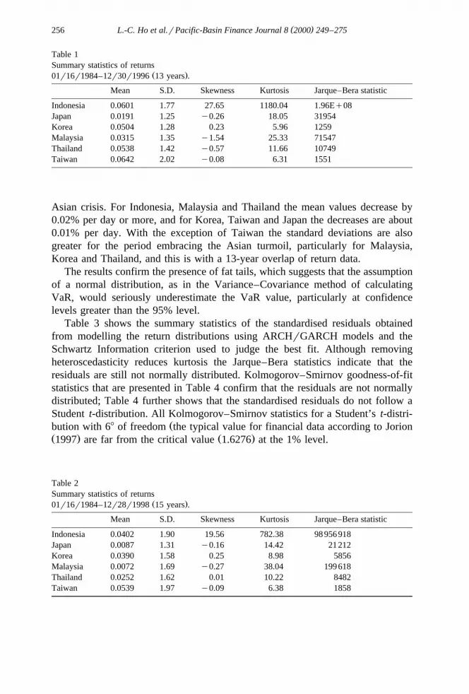
Table 1 indicates that the daily returns over the 13-year period of all six indicesare not normally distributed. In all cases skewness is evident, kurtosis is greaterthan 3 and the Jarque–Bera statistics are highly significant6. However, somedifferences are found between countries. Indonesia stands apart from the rest with

Ž .a distribution that is positively skewed 27.6 and in terms of its high degree ofŽ .kurtosis 1180 . Malaysia, Thailand, Japan and Taiwan all have negatively skewed

distributions whereas Korea’s is positively skewed.A comparison of the 13-year period ending December 1996 with the 15-year

Ž .period ending December 1998 Table 2 demonstrates, as might be anticipated,that the mean daily returns for each index are more negative after the onset of the

4 Percentage returns are also analysed in order to avoid any potential pdf truncation. The results donot change significantly across the return definitions.

5 Percentage returns were also analysed in US dollar terms, but in the interests of brevity the resultsare not reported. As might be expected the minima series are more strongly affected due to thedepreciation of Asian currencies against the dollar.

6 Kolmogorov–Smirnov goodness-of-fit statistics further confirm this result. Plots of empiricalquantiles against theoretical quantiles provide further evidence, together with strong visual evidence of‘‘fat tails’’.


Table 1Summary statistics of returns

Ž .01r16r1984–12r30r1996 13 years .

Mean S.D. Skewness Kurtosis Jarque–Bera statistic

Indonesia 0.0601 1.77 27.65 1180.04 1.96Eq08Japan 0.0191 1.25 y0.26 18.05 31954Korea 0.0504 1.28 0.23 5.96 1259Malaysia 0.0315 1.35 y1.54 25.33 71547Thailand 0.0538 1.42 y0.57 11.66 10749Taiwan 0.0642 2.02 y0.08 6.31 1551

Asian crisis. For Indonesia, Malaysia and Thailand the mean values decrease by0.02% per day or more, and for Korea, Taiwan and Japan the decreases are about0.01% per day. With the exception of Taiwan the standard deviations are alsogreater for the period embracing the Asian turmoil, particularly for Malaysia,Korea and Thailand, and this is with a 13-year overlap of return data.

The results confirm the presence of fat tails, which suggests that the assumptionof a normal distribution, as in the Variance–Covariance method of calculatingVaR, would seriously underestimate the VaR value, particularly at confidencelevels greater than the 95% level.

Table 3 shows the summary statistics of the standardised residuals obtainedfrom modelling the return distributions using ARCHrGARCH models and theSchwartz Information criterion used to judge the best fit. Although removingheteroscedasticity reduces kurtosis the Jarque–Bera statistics indicate that theresiduals are still not normally distributed. Kolmogorov–Smirnov goodness-of-fitstatistics that are presented in Table 4 confirm that the residuals are not normallydistributed; Table 4 further shows that the standardised residuals do not follow aStudent t-distribution. All Kolmogorov–Smirnov statistics for a Student’s t-distri-

Žbution with 68 of freedom the typical value for financial data according to JorionŽ . Ž .1997 are far from the critical value 1.6276 at the 1% level.

Table 2Summary statistics of returns

Ž .01r16r1984–12r28r1998 15 years .

Mean S.D. Skewness Kurtosis Jarque–Bera statistic

Indonesia 0.0402 1.90 19.56 782.38 98 956918Japan 0.0087 1.31 y0.16 14.42 21212Korea 0.0390 1.58 0.25 8.98 5856Malaysia 0.0072 1.69 y0.27 38.04 199618Thailand 0.0252 1.62 0.01 10.22 8482Taiwan 0.0539 1.97 y0.09 6.38 1858


Table 3Summary statistics of the standardised residuals

Ž .01r16r1984–12r30r1996 13 years .

Model type Skewness Kurtosis Jarque–Bera statistic

Ž . Ž .Indonesia AR 1 qGARCH 1, 1 4.50 150.62 3 079551Ž .Japan GARCH 1, 1 y0.67 13.67 16281

Ž . Ž .Korea AR 2 qGARCH 2, 2 0.17 4.59 373Ž . Ž .Malaysia AR 1, 5 qARCH 1 y1.21 18.10 32898Ž . Ž .Thailand AR 1 qGARCH 2, 2 y0.33 6.73 2021Ž . Ž .Taiwan AR 3 qGARCH 1, 1 y0.10 5.59 952

3.2. The extreme Õalue approach

The estimation of VaR using the extreme value approach involves a number ofsteps. The first step entails a choice of the return frequency, which in general is

Ž .influenced by liquidity and position risk Longin, 1998 . In this study, since weare dealing with indexes, daily returns are used. The next step involves the choiceof the length of the selection period, or block length, which is the number of returndays from which the largest increase and the largest fall are extracted to form themaxima and minima series, respectively. Clearly the number of returns in theseries created in this manner depends on the choice of block length and the total

Ž .sample size. Christoffersen et al. 1998 suggest that 10 to 15 trading days areŽ .required for independent and identically distributed observations. Longin’s 1998

Žstudy of S&P 500 Index returns suggests that a selection period of a month 21. Ž .trading days is appropriate. Danielsson and De Vries 1997 recommend that a

minimum total sample size of a 1000 returns are needed with 1500 being a moreprudent choice for estimating the asymptotic extreme distribution parameters.

Table 4Kolmogorov–Smirov goodness-of-fit test of residuals

Mean S.D. Normal distribution Student’s t-distribution

Ž .Indonesia T s3379 0.0389 1.85 15.12 11.42Ž .Japan T s3380 0.0191 1.25 5.17 3.68Ž .Korea T s3378 0.0460 1.28 4.04 2.16

Ž .Malaysia T s3379 0.0271 1.34 6.01 3.69Ž .Thailand T s3379 0.0445 1.40 6.44 3.65

Ž .Taiwan T s3379 0.0530 2.01 5.27 4.10

Ž . Ž . Ž .5% 1% critical values for Kolmogorov–Smirov statistic KS s D )6T is 1.3581 1.6276 .0.05 T,0.05Ž .The degree of freedom for Student’s t-distribution is 6, which is from Jorion 1997 .

()

L.-C

.Ho

etal.r

Pacific-B

asinF

inanceJournal8

2000249

–275

258

Table 5Ž .Tail parameter values 01r16r84–12r27r96 13 years

Ž . Ž .Key: 1 V Indicates the Sherman statistic and the corresponding p-value is in the bracket. 2 t s tail index; a and b are the scale and location normalisingŽ . Ž .parameters, respectively defined at Eq. 6 . 3 Standard errors for t , a and b are contained in parentheses.

a b t V VAR 95 VAR 99

Panel A. MaxIndonesia

Ž . Ž . Ž . Ž . Ž .dr2w ns10, Ns338 0.628 0.064 0.547 0.072 y0.355 0.063 1.80 ps0.036 – –Ž . Ž . Ž . Ž . Ž . w x w xdr4w ns20, Ns169 0.711 0.134 0.750 0.129 y0.658 0.190 y1.83 ps0.967 7.30 6.54, 8.07 22.0 21.2, 22.8

JapanŽ . Ž . Ž . Ž . Ž . w x w xdr2w ns10, Ns338 0.621 0.063 1.080 0.070 y0.307 0.087 y0.721 ps0.764 4.10 3.88, 4.31 7.37 7.15, 7.58Ž . Ž . Ž . Ž . Ž . w x w xdr4w ns20, Ns169 0.720 0.110 1.430 0.125 y0.362 0.143 0.373 ps0.354 5.27 4.87, 5.66 9.95 9.56, 10.3

KoreaŽ . Ž . Ž . Ž . Ž . w x w xdr2w ns10, Ns338 0.873 0.077 1.450 0.105 y0.0178 0.077 0.112 ps0.456 4.11 3.96, 4.27 5.64 5.48, 5.79Ž . Ž . Ž . Ž . Ž . w x w xdr4w ns20, Ns169 0.906 0.113 1.960 0.160 y0.0207 0.111 y0.405 ps0.657 4.73 4.50, 4.96 6.33 6.10, 6.56

MalaysiaŽ . Ž . Ž . Ž . Ž . w x w xdr2w ns10, Ns338 0.745 0.073 1.160 0.090 y0.206 0.093 1.15 ps0.124 4.21 4.01, 4.42 6.87 6.67, 7.08Ž . Ž . Ž . Ž . Ž . w x w xdr4w ns20, Ns169 0.872 0.123 1.670 0.160 y0.190 0.141 0.393 ps0.347 5.15 4.82, 5.47 8.07 7.75, 8.40

ThailandŽ . Ž . Ž . Ž . Ž . w x w xdr2w ns10, Ns338 0.845 0.085 1.110 0.100 y0.233 0.102 0.591 ps0.277 4.73 4.49, 4.98 8.09 7.84, 8.33Ž . Ž . Ž . Ž . Ž . w x w xdr4w ns20, Ns169 1.080 0.014 1.580 0.190 y0.160 0.129 0.415 ps0.339 5.68 5.30, 6.05 8.90 8.53, 9.28

TaiwanŽ . Ž . Ž . Ž . Ž . w x w xdr2w ns10, Ns338 1.430 0.120 1.940 0.170 y0.0139 0.056 y0.333 ps0.630 6.28 6.02, 6.53 8.74 8.48, 8.99Ž . Ž . Ž . Ž . Ž . w x w xdr4w ns20, Ns169 1.370 0.180 2.520 0.240 y0.103 0.126 y0.544 ps0.707 7.30 6.87, 7.72 10.6 10.2, 11.0

()

L.-C

.Ho

etal.r

Pacific-B

asinF

inanceJournal8

2000249

–275

259

Panel B. MinIndonesia

Ž . Ž . Ž . Ž . Ž .dr2w ns10, Ns338 0.442 0.056 y0.358 0.056 y0.565 0.126 4.49 ps0.000 – –Ž . Ž . Ž . Ž . Ž .dr4w ns20, Ns169 0.663 0.104 y0.686 0.116 y0.400 0.150 2.35 ps0.009 – –

JapanŽ . Ž . Ž . Ž . Ž . w x w xdr2w ns10, Ns338 0.714 0.073 y0.974 0.086 y0.257 0.102 y0.475 ps0.683 4.16 4.12, 4.20 7.26 7.22, 7.31Ž . Ž . Ž . Ž . Ž . w x w xdr4w ns20, Ns169 0.828 0.121 y1.380 0.150 y0.245 0.146 y1.07 ps0.859 5.00 4.93, 5.07 8.44 8.37, 8.51

KoreaŽ . Ž . Ž . Ž . Ž . w x w xdr2w ns10, Ns338 0.751 0.068 y1.190 0.090 y0.089 0.083 1.40 ps0.080 3.74 3.69, 3.79 5.46 5.41, 5.51Ž . Ž . Ž . Ž . Ž . w x w xdr4w ns20, Ns169 0.836 0.109 y1.600 0.150 y0.084 0.121 0.459 ps0.323 4.42 4.35, 4.50 6.30 6.22, 6.38

MalaysiaŽ . Ž . Ž . Ž . Ž . w x w xdr2w ns10, Ns338 0.733 0.073 y0.984 0.086 y0.280 0.084 y0.161 ps0.564 4.38 4.34, 4.42 7.85 7.81, 7.90Ž . Ž . Ž . Ž . Ž . w x w xdr4w ns20, Ns169 0.857 0.121 y1.470 0.140 y0.298 0.115 y0.515 ps0.697 5.56 5.49, 5.63 9.92 9.85, 9.99

ThailandŽ . Ž . Ž . Ž . Ž . w x w xdr2w ns10, Ns338 0.764 0.089 y0.851 0.096 y0.440 0.119 y0.840 ps0.799 5.53 5.49, 5.57 12.3 12.2, 12.4Ž . Ž . Ž . Ž . Ž . w x w xdr4w ns20, Ns169 0.930 0.152 y1.280 0.170 y0.410 0.172 y0.471 ps0.681 6.68 6.62, 6.75 14.0 13.9, 14.1

TaiwanŽ . Ž . Ž . Ž . Ž . w x w xdr2w ns10, Ns338 1.260 0.120 y1.620 0.160 y0.194 0.102 y0.827 ps0.796 6.69 6.61, 6.76 11.0 10.9, 11.1Ž . Ž . Ž . Ž . Ž . w x w xdr4w ns20, Ns169 1.300 0.190 y2.270 0.230 y0.199 0.153 y1.69 ps0.954 7.52 7.41, 7.63 12.0 11.9, 12.1


In this study 10- and 20-day block lengths are used with a sample size in excessof 3000 daily returns7. The goodness-of-fit of the asymptotic behaviour of the

Ž .distribution of extremes is evaluated using the Sherman 1957 test at the 95%confidence level; this test compares the probability given by the asymptoticdistribution to the observed frequency used as a proxy of the exact distribution. Inthe case of Indonesia both the maxima and minima series based on a 10-day blocklength failed the Sherman test as did their minima series for the 20-day blocklength. These results are due to the extreme positive skewness of its return

Ž . Ž .distribution 27.6 . Except in the case of Japan maxima series and ThailandŽ .minima series the better Sherman test results are obtained with the 20-day blocklength, and the discussion below relates to the 20-day block length unless statedotherwise.

The three parameters a , b and t , defined previously, are estimated by themaximum likelihood method8. The results are shown in Panels A and B of Table5. The scale factor values, a , differ slightly across countries, more so for themaxima series, which generally have the higher values, than for the minima series.

Ž . ŽIndonesia has the smallest 0.711 and 0.663 and Taiwan has the largest 1.370.and 1.300 values. The averages for the 10-day block length are typically 10% to

15% smaller than the corresponding 20-day values.The location parameter, b , systematically increases with block length. The

20-day block values are on average some 30–40% larger than the 10-day blockestimates. The maxima series have slightly larger b values than the minima series.The b values for Indonesia are about 50% lower and those for Taiwan some 40%higher than the next highestrlowest estimates of the other countries.

The most important factor in terms of characterising the limiting extremedistribution of the tail is the tail index. The tail estimates for the minima series, ingeneral, exhibit smaller differences in values for the 10-day and 20-day blocklengths than is the case for the maxima series. The tail index values for themaxima series of Indonesia, Japan and Korea are much more negative than thecorresponding minima values while the reverse is the case for Malaysia, Thailandand Taiwan.

All tail index values are negative, which is generally consistent with theŽfindings of other studies of financial time series return data Danielsson and De

.Vries, 1997; Longin, 1996, 1997; McNeil, 1998 . The degree of statisticalprecision of the tail index estimates is highest for the 10-day block length simplybecause the sample size is twice that of the 20-day block length. The negativelysigned tail index values suggest that the limiting extreme distributions are charac-terised by a Frechet type distribution. This observation applies to all countries, to´

7 Several other sample lengths were investigated, e.g. the 5-year period ending June, 1997, but againin the interests of brevity the results are not reported here but are available on request from the authors.

8 Using the CML routines in GAUSS.


both maxima and minima series. The results for Japan contrast somewhat withŽ .those found by Longin and Solnik 1998 who used the return exceedances

approach to estimate a tail index in their study of the dependence structure ofinternational equity markets. For Japan they found mainly positive, though notstatistically significant, tail index values that are indicative of a Weibull distribu-tion.

As might be anticipated a comparison of the a , b and t parameters valuesŽ .estimated for the 13-year period Table 5 with the values obtained for the 15-yearŽ .period ending December 1998 Table 6 demonstrates some evidence of the

impact of the Asian financial turmoil. The a , b and t values for Taiwan areessentially unchanged for both the maxima and minima series. For the other fivecountries the alpha values are on average about 15% larger for the 15-year period,and the absolute values of their b values are some 6% to 10% larger for thelonger period. The differences in the tail index values are more varied. For themaxima series the estimates for Japan are nearly the same as is the case forTaiwan. The values for Indonesia and Thailand are modestly more negative,

Ž .whereas the reverse is the case with Korea. The Malaysian tail index y0.3659estimated from the 15-year period is almost double the size of that from the

Ž .13-year period y0.190 . For the minima series, Indonesia and Malaysia are some25% more negative in value, while Korea more than doubles in magnitudeŽ .y0.084 vs. y0.210 . On the other hand Japan, Thailand and Taiwan becomemore positive by 20%, 14% and 11%, respectively. For the maxima series there islittle difference in the estimates from the two samples for Japan and Taiwan.Malaysia shows the biggest change falling from y0.190 to y0.366. Thailand fallsin value by almost 30% and Indonesia by a more modest amount. The tail indexfor Korea moves in the opposite direction, increasing in value by about 14%.

The asymptotic distribution of extreme returns can be used to estimate the VaRfor different confidence levels or probability values. The limiting extreme valuecumulative distribution, assuming it can be written as

1rtF y s1yexp y 1qt yyb ra .Ž . Ž .Ž .Ž .y

Hence, the confidence level or probability, p, is

1rtps1yF y syexp y 1qt yyb ra .Ž . Ž .Ž .Ž .y

Ž long .Expressing VaR in percentage terms and then setting psProb y GyVARn

gives the probability that the minimum return will not exceed a threshold valueequal to VARlong and it is a simple matter to rearrange the above expression toyield

mina minn tlong min nVAR syb q 1y yln p .Ž .n mintn

()

L.-C

.Ho

etal.r

Pacific-B

asinF

inanceJournal8

2000249

–275

262

Table 6Ž .Tail parameter values 01r16r84–12r28r98 15 years

Ž . Ž .Key: 1 V Indicates the Sherman statistic and the corresponding p-value is in the bracket. 2 t s tail index; a and b are the scale and location normalisingŽ . Ž .parameters, respectively defined at Eq. 6 . 3 Standard errors for t , a and b are contained in parentheses.

a b t V VAR 95 VAR 99

Panel A. MaxIndonesia

Ž . Ž . Ž . Ž . Ž .dr2w ns10, Ns390 0.720 0.036 0.629 0.0392 y0.411 0.033 3.34 ps0.000 – –Ž . Ž . Ž . Ž . Ž . w x w xdr4w ns20, Ns195 0.8508 0.0782 0.864 0.073 y0.697 0.092 y1.17 ps0.879 9.32 8.4, 10.2 29.78 28.9, 30.7

JapanŽ . Ž . Ž . Ž . Ž . w x w xdr2w ns10, Ns390 0.676 0.033 1.153 0.039 y0.310 0.043 y0.88 ps0.811 4.45 4.23, 4.67 8.05 7.83, 8.27Ž . Ž . Ž . Ž . Ž . w x w xdr4w ns20, Ns195 0.774 0.056 1.502 0.064 y0.361 0.070 y0.50 ps0.691 5.62 5.22, 6.02 10.64 10.3, 11.0

KoreaŽ . Ž . Ž . Ž . Ž . w x w xdr2w ns10, Ns390 0.977 0.043 1.507 0.056 y0.163 0.040 0.09 ps0.464 5.24 5.02, 5.46 8.21 7.98, 8.44Ž . Ž . Ž . Ž . Ž . w x w xdr4w ns20, Ns195 1.035 0.066 2.045 0.084 y0.179 0.057 0.55 ps0.291 6.10 5.75, 6.45 9.43 9.08, 9.78

MalaysiaŽ . Ž . Ž . Ž . Ž . w x w xdr2w ns10, Ns390 0.820 0.040 1.211 0.0471 y0.326 0.044 0.85 ps0.198 5.32 5.05, 5.59 9.96 9.68, 10.2Ž . Ž . Ž . Ž . Ž . w x w xdr4w ns20, Ns195 0.959 0.0694 1.7042 0.0792 y0.366 0.069 0.05 ps0.480 6.85 6.35, 7.35 13.2 12.7, 13.7

ThailandŽ . Ž . Ž . Ž . Ž . w x w xdr2w ns10, Ns390 0.953 0.048 1.185 0.057 y0.287 0.051 y0.57 ps0.716 5.65 5.36, 5.94 10.3 10.0, 10.6Ž . Ž . Ž . Ž . Ž . w x w xdr4w ns20, Ns195 1.235 0.082 1.73 0.102 y0.205 0.065 0.48 ps0.316 6.79 6.34, 7.24 11.2 10.8, 11.6

TaiwanŽ . Ž . Ž . Ž . Ž . w x w xdr2w ns10, Ns390 1.369 0.053 1.918 0.075 y0.010 0.025 y0.18 ps0.571 6.05 5.82, 6.28 8.37 8.15, 8.59Ž . Ž . Ž . Ž . Ž . w x w xdr4w ns20, Ns195 1.306 0.080 2.511 0.106 y0.096 0.056 y0.18 ps0.571 7.00 6.63, 7.37 10.07 9.7, 10.44

()

L.-C

.Ho

etal.r

Pacific-B

asinF

inanceJournal8

2000249

–275

263

Panel B. MinIndonesia

Ž . Ž . Ž . Ž . Ž .dr2w ns10, Ns390 0.543 0.035 y0.427 0.033 y0.674 0.063 4.46 ps0.000 – –Ž . Ž . Ž . Ž . Ž .dr4w ns20, Ns195 0.801 0.064 y0.787 0.067 y0.518 0.077 2.60 ps0.005 – –

JapanŽ . Ž . Ž . Ž . Ž . w x w xdr2w ns10, Ns390 0.793 0.038 y1.087 0.047 y0.216 0.049 y0.26 ps0.602 4.39 4.35, 4.43 7.34 7.30, 7.38Ž . Ž . Ž . Ž . Ž . w x w xdr4w ns20, Ns195 0.910 0.061 y1.512 0.076 y0.197 0.066 y1.52 ps0.936 5.18 5.11, 5.25 8.32 8.24, 8.40

KoreaŽ . Ž . Ž . Ž . Ž . w x w xdr2w ns10, Ns390 0.862 0.040 y1.266 0.050 y0.213 0.042 1.07 ps0.142 4.84 4.79, 4.89 8.00 7.95, 8.05Ž . Ž . Ž . Ž . Ž . w x w xdr4w ns20, Ns195 0.972 0.064 y1.714 0.080 y0.210 0.062 y0.03 ps0.512 5.72 5.64, 5.80 9.25 9.17, 9.33

MalaysiaŽ . Ž . Ž . Ž . Ž . w x w xdr2w ns10, Ns390 0.830 0.041 y1.072 0.047 y0.334 0.042 y1.06 ps0.855 5.29 5.25, 5.33 10.15 10.1, 10.2Ž . Ž . Ž . Ž . Ž . w x w xdr4w ns20, Ns195 0.977 0.069 y1.569 0.078 y0.369 0.058 y0.33 ps0.629 6.85 6.78, 6.92 13.4 13.3, 13.5

ThailandŽ . Ž . Ž . Ž . Ž . w x w xdr2w ns10, Ns390 0.911 0.050 y1.011 0.056 y0.400 0.060 y0.37 ps0.644 6.20 6.16, 6.24 13.05 13.0, 13.1Ž . Ž . Ž . Ž . Ž . w x w xdr4w ns20, Ns195 1.112 0.085 y1.485 0.097 y0.352 0.086 y0.32 ps0.626 7.31 7.23, 7.39 14.25 14.2, 14.3

TaiwanŽ . Ž . Ž . Ž . Ž . w x w xdr2w ns10, Ns390 1.234 0.058 y1.622 0.072 y0.179 0.047 y1.05 ps0.853 6.46 6.39, 6.53 10.45 10.4, 10.5Ž . Ž . Ž . Ž . Ž . w x w xdr4w ns20, Ns195 1.275 0.085 y2.250 0.107 y0.177 0.070 y1.26 ps0.896 7.23 7.13, 7.33 11.3 11.2, 11.4


Table 7Ž .Comparisons of VARs: 01r16r1984–12r30r1996 13 years

VAR 95 VAR 99

GEV VarrCov T His GEV VarrCov T His

( )Panel A: Max — Short position expressed as a % of the positionIndonesia

2.98 3.52 1.22 4.18 5.64 2.66Ž .dr2w ns10 – –Ž .dr4w ns20 7.30 22.0

Japan2.07 2.44 1.81 2.92 3.94 3.49

Ž .dr2w ns10 4.10 7.37Ž .dr4w ns20 5.27 9.95

Korea2.16 2.55 2.20 3.03 4.09 3.92

Ž .dr2w ns10 4.11 5.64Ž .dr4w ns20 4.73 6.33

Malaysia2.25 2.66 1.98 3.17 4.28 3.48

Ž .dr2w ns10 4.21 6.87Ž .dr4w ns20 5.15 8.07

Thailand2.38 2.81 2.04 3.35 4.52 3.96

Ž .dr2w ns10 4.73 8.09Ž .dr4w ns20 5.68 8.90

Taiwan3.39 4.00 3.16 4.77 6.44 5.90

Ž .dr2w ns10 6.28 8.74Ž .dr4w ns20 7.30 10.6

( )Panel B: Min — Long position expressed as a % of the positionIndonesia

2.86 3.37 1.12 4.06 5.48 2.35Ž .dr2w ns10 – –Ž .dr4w ns20 – –

Japan2.03 2.40 1.94 2.88 3.89 3.53

Ž .dr2w ns10 4.16 7.26Ž .dr4w ns20 5.00 8.44

Korea2.06 2.43 1.90 2.93 3.96 3.25

Ž .dr2w ns10 3.74 5.46Ž .dr4w ns20 4.42 6.30

Malaysia2.19 2.58 1.78 3.10 4.19 3.35

Ž .dr2w ns10 4.38 7.85Ž .dr4w ns20 5.56 9.92


Ž .Table 7 continued

VAR 95 VAR 99


( )Panel B: Min — Long position expressed as a % of the positionThailand

2.28 2.69 1.99 3.24 4.37 4.75Ž .dr2w ns10 5.53 12.3Ž .dr4w ns20 6.68 14.0

Taiwan3.26 3.85 3.39 4.64 6.26 6.18

Ž .dr2w ns10 6.69 11.0Ž .dr4w ns20 7.52 12.0

Ž short.Similarly for the short position, psProb Y GVAR is the probability that then

maximal return will be above the threshold VARshort, and the corresponding VaRis defined as

maxa maxn tshort max nVAR sb q 1y yln p .Ž .n maxtn

The VaR values determined by the extreme value method, at both the 95% and99% levels, are presented in Table 5. The VaR values using the 10-day blocklength for Japan, Korea, and Malaysia are just over 4.1 for the maxima series,

Ž .Thailand is somewhat larger 4.7 , and the values for Indonesia and Taiwan, 6.28and 7.30, respectively, are appreciably larger than the VaR values of the othercountries. The VaR values for the minima series are, with the exception of KoreaŽ .which has a value of 3.7 , slightly larger than the corresponding values in themaxima series. The VaR values for the six countries for the 20-day block lengthaverage about 20% more than the equivalent 10-day block length values.

At the 99% level the VaR values for the maxima series range from 35%Ž . Ž .Korea to 90% Japan larger than the equivalent values at the 95% level. The

Ž .VaR values for the 20-day block length are from about 10% Thailand to 35%Ž .Japan higher than the corresponding 10-day block length values for the short

Ž . Ž .position and from 9% Taiwan to 26% Malaysia for the short position. For themaxima series Indonesia has a particularly high VaR value of 22.0, and for theminima series, Thailand and Taiwan have the highest values, 14.0 and 12.0,respectively. There appears to be no simple, discernible pattern to the changes.

3.3. Comparison of extreme Õalue VaRs with VaRs estimated using traditionalmeasures

The results obtained using the extreme value approach can be usefully com-Žpared to those VaR values calculated by the variance–covariance hereafter

.Var–Cov method using both normal and t-distributions and the Historical method.Table 7 presents the VaR estimates by the three methods for both long and short

()

L.-C

.Ho

etal.r

Pacific-B

asinF

inanceJournal8

2000249

–275

266

Table 8Number of actual loss exceeds VAR

aŽ .dr4w ns20 VAR 95 VAR 99


Panel A: MaxIndonesia

b cŽ . Ž . Ž . Ž . Ž . Ž . Ž . Ž . Ž .1997 T s260 1 0.004 10 0.039 7 0.027 23 0.089 0 0 6 0.023 3 0.012 11 0.042Ž . Ž . Ž . Ž . Ž . Ž . Ž . Ž . Ž .1997 and 1998 T s518 7 0.014 42 0.081 32 0.062 89 0.172 0 0 28 0.054 13 0.025 49 0.095

JapanŽ . Ž . Ž . Ž . Ž . Ž . Ž . Ž . Ž .1997 T s260 1 0.004 25 0.096 19 0.073 27 0.104 0 0 10 0.039 2 0.008 3 0.012

Ž . Ž . Ž . Ž . Ž . Ž . Ž . Ž . Ž .1997 and 1998 T s520 3 0.006 48 0.092 36 0.069 54 0.104 0 0 20 0.039 8 0.015 9 0.017Korea

Ž . Ž . Ž . Ž . Ž . Ž . Ž . Ž . Ž .1997 T s260 7 0.027 24 0.092 19 0.073 24 0.092 5 0.019 15 0.058 8 0.031 9 0.035Ž . Ž . Ž . Ž . Ž . Ž . Ž . Ž . Ž .1997 and 1998 T s520 30 0.058 77 0.148 65 0.125 77 0.148 16 0.031 55 0.106 36 0.069 40 0.077

MalaysiaŽ . Ž . Ž . Ž . Ž . Ž . Ž . Ž . Ž .1997 T s260 5 0.019 16 0.061 13 0.05 20 0.077 2 0.008 12 0.046 9 0.035 12 0.046

Ž . Ž . Ž . Ž . Ž . Ž . Ž . Ž . Ž .1997 and 1998 T s520 17 0.033 56 0.108 45 0.087 69 0.133 9 0.017 39 0.075 23 0.044 32 0.062Thailand

Ž . Ž . Ž . Ž . Ž . Ž . Ž . Ž . Ž .1997 T s260 6 0.023 24 0.092 22 0.085 31 0.119 0 0 15 0.058 9 0.035 11 0.042Ž . Ž . Ž . Ž . Ž . Ž . Ž . Ž . Ž .1997 and 1998 T s520 16 0.031 70 0.135 61 0.117 83 0.160 3 0.0058 46 0.089 27 0.052 31 0.060

TaiwanŽ . Ž . Ž . Ž . Ž . Ž . Ž . Ž . Ž .1997 T s260 0 0 4 0.015 2 0.008 4 0.015 0 0 1 0.004 0 0 0 0

Ž . Ž . Ž . Ž . Ž . Ž . Ž . Ž . Ž .1997 and 1998 T s520 0 0 10 0.019 4 0.008 12 0.023 0 0 2 0.004 0 0 0 0

()

L.-C

.Ho

etal.r

Pacific-B

asinF

inanceJournal8

2000249

–275

267

Panel B: MinIndonesia

b cŽ . Ž . Ž . Ž . Ž . Ž . Ž .1997 T s260 – 19 0.073 14 0.054 50 0.192 – 10 0.039 5 0.019 24 0.092Ž . Ž . Ž . Ž . Ž . Ž . Ž .1997 and 1998 T s518 – 50 0.097 38 0.073 130 0.251 – 28 0.054 12 0.023 63 0.122

JapanŽ . Ž . Ž . Ž . Ž . Ž . Ž . Ž . Ž .1997 T s260 3 0.012 27 0.104 22 0.085 29 0.112 0 0 14 0.054 7 0.027 7 0.027

Ž . Ž . Ž . Ž . Ž . Ž . Ž . Ž . Ž .1997 and 1998 T s520 5 0.010 59 0.114 38 0.073 63 0.121 0 0 22 0.042 9 0.017 9 0.017Korea

Ž . Ž . Ž . Ž . Ž . Ž . Ž . Ž . Ž .1997 T s260 14 0.054 39 0.150 32 0.123 42 0.162 7 0.027 26 0.100 20 0.077 22 0.085Ž . Ž . Ž . Ž . Ž . Ž . Ž . Ž . Ž .1997 and 1998 T s520 30 0.058 96 0.185 84 0.162 105 0.202 11 0.021 65 0.125 42 0.081 53 0.102

MalaysiaŽ . Ž . Ž . Ž . Ž . Ž . Ž . Ž . Ž .1997 T s260 6 0.023 40 0.154 28 0.108 44 0.169 1 0.004 20 0.077 8 0.031 14 0.054

Ž . Ž . Ž . Ž . Ž . Ž . Ž . Ž . Ž .1997 and 1998 T s520 10 0.019 93 0.179 70 0.135 102 0.196 3 0.006 48 0.092 18 0.035 38 0.073Thailand

Ž . Ž . Ž . Ž . Ž . Ž . Ž . Ž . Ž .1997 T s260 0 0 45 0.173 33 0.127 57 0.219 0 0 21 0.081 5 0.019 4 0.015Ž . Ž . Ž . Ž . Ž . Ž . Ž . Ž . Ž .1997 and 1998 T s520 3 0.006 90 0.173 70 0.135 110 0.212 0 0 42 0.081 11 0.021 9 0.017

TaiwanŽ . Ž . Ž . Ž . Ž . Ž . Ž . Ž . Ž .1997 T s260 0 0 7 0.027 3 0.012 5 0.019 0 0 3 0.012 1 0.004 1 0.004

Ž . Ž . Ž . Ž . Ž . Ž . Ž . Ž . Ž .1997 and 1998 T s520 0 0 13 0.025 5 0.010 10 0.019 0 0 4 0.008 1 0.002 1 0.002

a The block length in GEV is 20 days.b Total number of observations.c Ž .Percentage of exceedance Number of ExceedancerTotal Number of Observations is in brackets.


Ž Ž .positions and for the 95% and 99% levels See Longin 1998 for a discussion of. Ž .the relationship between the differing probability values . The Var–Cov normal

VaR estimates at the 95% level are, in the majority of cases, somewhat larger thanthose found by the Historical method ranging from a low of 5% for Japan to ahigh of 23% greater for Malaysia. In Indonesia’s case the difference is excep-tional, the Var–Cov is more than 2.5 times that of the Historical method. For

Ž . Ž .Korea maxima series and Taiwan minima series the historical value ismarginally the greater. At the 99% level the Historical VaR estimates are generally

Ž . Ž .the greater and they range from 10% greater Malaysia to almost 30% Korea .Again Indonesia is the exception with a Var–Cov estimate around 60–70% greaterthan the corresponding Historical estimates.

A comparison of the VaR values determined by the extreme value methodshows they are significantly larger than the corresponding VaR values estimatedby the Var–Cov using a Student’s t-distribution with 6 degrees of freedom9 and

Ž .greater still than those estimated by the Var–Cov normal method. The extremeŽ .value estimated VaRs are about double the Var–Cov t-distribution values at the

Ž . Ž .95% confidence level for both the long minima and short maxima positions. Atthe 99% level a similar, though more variable, pattern is apparent ranging from a

Ž .multiple of 1.5 for Korea to over 3 for Indonesia maxima series and ThailandŽ .minima series .

These results are economically significant both for long or short positions forall countries studied. Moreover, they are strongly supportive of the view that fat

Ž .tails cause the Var–Cov method normal distribution assumption to seriouslyunderestimate VaR as the confidence level increases and moves further out intothe tail of a distribution of financial returns. The results suggest that if banks wereto use the extreme value method as an internal model they would require twice asmuch capital as the Var–Cov method to satisfy the BIS capital adequacy require-ment for market risk. These results suggest that the extreme value method ofestimating VaR is a more conservative approach to determining capital require-ments than the Var–Cov or Historical methods. A similar result was found by

Ž .Danielsson et al. 1998 who suggested that banks might have little incentive touse a better VaR model if it leads to a substantially higher capital requirement.

3.4. EÕaluation of VaR estimates

The above estimates, which were obtained using a 13-year history of dailyreturns for each country that ended December 1996, are used here as a basis forevaluating the performance of the different VaR estimation methods. The difficul-

Žties of evaluating the forecasts of risk models is well documented see for.example, Kupiac, 1995; Christoffersen, 1998; Berkowitz, 1999 . It is assumed that

9 Ž .Jorion 1997 suggests that 6 degrees of freedom is appropriate for financial times series data.


Fig. 1. Excess of VaR generated by extreme value theory: Japan.

the VaR values would not be updated over the next two years10 and theperformance of the different VaR estimates is judged on the basis of the number oftimes that the actual returns exceed the VaR estimate. The results for all methodsstudied are reported in Table 8 and in Figs. 1–5. Based on the confidence levelsabout 3 exceedances a year can be expected at the 99% level and 12 a year at the95% level. Hence, for the two years 1997–1998 double these values can beexpected.

As anticipated the number of exceedances is greatest at the 95% level for bothlong and short positions with the extreme value method having the least and theHistorical method the most. With the extreme value method only Korea has a

Ž . Ž .greater number of exceedances, 14 long in 1997 and 30 long in the two-yearperiod 1997–98, than the expected number of 12 per year. Taiwan by contrast hasnone for the two-year period either for the maxima or minima series. For theStudent’s t-distribution VaR values the expected value is exceeded in 1997 by

Ž . Ž .Indonesia long only , Japan, Korea, Malaysia long only , and Thailand. Only inthe case of Taiwan is the number of exceedances less than anticipated, which isalso true for the Var–Cov normal distribution case.

At the 99% level only in Korea, both for years 1997 and 1998, and the long andŽ .short positions, and Malaysia short case only in 1998 is the VaR estimate by the

extreme value method exceeded a greater number of times than expected onprobabilistic grounds. Once again Taiwan has no exceedances in any of the cases.

Ž .With the Student’s t-distribution Indonesia and Japan in 1997 short position ,

10 This procedure clearly assumes constant moments; we are currently developing procedures whichincorporate changing moments into the measurement and estimation process.


Fig. 2. Excess of VaR generated by extreme value theory: Korea.

Ž .Japan in 1998 long position and Taiwan both long and short in 1997 and 1998are cases where the number of exceedances are less than or equal to the expectedvalue of 3 per year. In nearly all other cases the Student’s t VaR estimate isexceeded by a factor of two or more than the expected number. The results ingeneral indicate that 1998 had the greater number of exceedances, particularly forthe short position.

For the Var–Cov normal distribution VaR estimates only in Taiwan for allcases and Indonesia in 1997 for the short position is the number of exceedances

Fig. 3. Excess of VaR generated by extreme value theory: Malaysia.


Fig. 4. Excess of VaR generated by extreme value theory: Thailand.

less than expected. The Historical method fairs little better than the Var–Covnormal distribution method and in most cases a lot worse.

Figs. 1–6 illustrate the daily returns over the two-year period, 1997–1998.Superimposed in each case are the 95% and 99% VaR values estimated by theextreme value theory. The 95% confidence ranges for these values are relativelysmall given the 13-year history used to estimate the three parameters that underpinthe Extreme value theory VaRs, and hence, they are not shown in the figures. Thefigures show that Indonesia and Malaysia, in particular, experienced little volatility

Fig. 5. Excess of VaR generated by extreme value theory: Taiwan.


Fig. 6. Excess of VaR generated by extreme value theory: Indonesia.

in the first 6 months of 1997. Thailand shows the greatest volatility during thisperiod and the contagion effects as the crisis spread are evident in the final monthsof 1997 for Korea, Malaysia and Indonesia and to a lesser extent Japan also.Taiwan suffers some effects but the alleged government control of the stockmarket resulted in less volatile conditions than found in the other markets.

It is apparent from the figures that for Malaysia, Korea and Thailand that thereare several cases where the daily changes were far in excess of the 99% VaRvalues estimated by the extreme value theory. Clearly these changes would havebeen greater still than the VaR values estimated by the Var–Cov methods usingthe Student’s t and normal distributions. The potential magnitude of these lossesreinforces the need for stress testing whatever method is used to estimate VaR.

4. Impications for the measurement of VaRs

The empirical analyses that are conducted throughout this paper have a numberof implications for the measurement of VaRs, which we have summarised in thissection.

The return distributions for the Asian countries that are analysed are allcharacterised by fat tails which will mean that VaR measures based upon thenormal distribution will underestimate VaR.

The extreme value approach, by modelling the tails of the return distributions,focuses upon those parts of the distributions that are more relevant to measuringVaR. While the estimates of the tail index values suggest the Frechet type for all´countries and estimation periods, the parameters do change through time and withthe length of the sample period chosen. However, even with this limiting assump-tion of constant moments, the performance of extreme value VaRs is still much


stronger than the other techniques investigated, particularly in terms of the numberof exceedances of VaR estimates. The performance of extreme value basedmethods will be enhanced further by incorporating changes in the parameters thatoccur through time into the measurement procedures.

The need for incorporating stress testing into the overall risk managementprocess should be emphasised even when using extreme value based methodssince, as our previous results have indicated, there can still be a number ofscenarios that occur where return realisations are far in excess of confidence levelsfor extreme value generated VaR’s.

Finally, it should be emphasised that if banks and financial institutions were toadopt extreme value theory methods for internal modelling of market risk theamount of capital required to meet the revised Basle requirements would besignificantly increased. In our study the extreme value theory VaR values weregenerally two or more times higher than the highest of the VaRs estimated by

Žother methods. Since Basle requires three times the VaR 99% confidence level,.10-day horizon estimated by a Bank’s internal models it appears that banks have

little incentive to use extreme value theory for this purpose. However, the extremevalue approach does offer the potential to explore the probability of rare eventsbeyond the 99% confidence level and the magnitude of the losses associated withsuch events.

5. Conclusions

Ž .The standard methods of determining value-at-risk VaR measures focus onthe whole probability density function. However, it would appear more satisfac-tory, when assessing the probability of incurring extreme losses, to place greateremphasis upon the tails of the probability distribution and in the modelling of thedistribution tails.

The financial turmoil that has occurred in Asian markets recently indicates theneed for robust financial control mechanisms of the VaR type.11 Since the Asianfinancial markets have been so volatile at varying times over the sample frame, theneed for modelling the distribution tails is all the more apparent.

The empirical tests conducted in this paper indicate that the return distributionsŽ .are not characterised by normality even when corrected for heteroscedasticity

and that the maxima and the minima return distributions can be described withinan extreme value theory framework.

VaR measures generated via the extreme value theory are substantially differentfrom those generated by traditional methods, such as the variance–covariance,

11 Ž .See Euromoney 1999 for a view on the need for joint modelling of both credit risk and marketŽ .risk and some recent work on this by Jarrow and Turnbull 1998 .


both using Student’s t and normal distributions, and Historical methods. This isparticularly the case in markets that are characterised by very fat tailed distribu-tions, such as in Southeast Asia during the recent financial market crisis.

References

Arzner, P., Debaen, F., Eber, J., Heath, D., 1998. Coherent Measures of Risk. Department ofMathematics, ZH, Zurich.

ŽBeder, T., 1995. VaR’s seductive but dangerous. Financial Analysts Journal 51, 12–24 September–.October .

Berkowitz, J., 1999. Evaluating the Forecasts of Risk Models. Board of Governors Federal ReserveBoard, Washington, DC.

Christoffersen, P.F., 1998. Evaluating interval forecasts. International Economic Review, in prepara-tion.

Christoffersen, P.F., Diebold, F.X., Schuermann, T., 1998. Horizon problems and extreme events infinancial risk management, Working Paper Series. The Wharton Financial Institutions Centre,Philadelphia, PA.

Danielsson, J., de Vries, C., 1997. Value-at-Risk and extreme returns. LSE Financial Markets GroupDiscussion Paper, No. 273, London School of Economics.

Danielsson, J., De Vries, C., 1998. Beyond the Sample: Extreme Quantile and Probability Estimation,LSE Financial Markets Growth Discussion Paper, No. 298, London School of Economics.

Ž .Danielsson, J., Hartmann, P., De Vries, C., 1998. The cost of conservatism. Risk 11 1 , 103–107,January.

Diebold, F.X., Schuermann, T., Stroughair, J.D., 1999. Pitfalls and opportunities in the use of extremevalue theory in risk management. Advances in Computational Finance, in preparation.

Dowd, K., 1998. Beyond Value at Risk. Wiley, Chichester.Duffie, D., Pan, J., 1997. An overview of value-at-risk. The Journal of Derivatives, Spring, 7–49.Embrechts, P., Kluppelberg, C., Mikoach, T., 1997. Modelling Extreme Events. Springer-Verlag,

Berlin.Emmer, S., Kluppelberg, C., Trustedt, M., 1998. VaR — A Measure for the Extreme Risk. Centre for

Mathematical Sciences, Munich University of Technology.Euromoney, 1999. Risk scientists look beyond their silos. Euromoney 1, 32–33, May.Fisher, R.A., Tippett, L.H.C., 1928. Limiting forms of the frequency distribution of the largest or

smallest member of a sample. Proceedings of the Cambridge Philosophical Society 24, 180–190.Frechet, M., 1927. Sur la loi de probabilite de l’ecart maximum. Annales de la Societe Polonaise de´ ´ ´ ´

Ž .Mathematique Cracow 6, 93–117.´Gnedenko, B.V., 1943. Sur la distribution limite du terme maximum d’une serie aleatoire. Annuals of´ ´

Mathematiks 44, 423–453.Gumbel, E.J., 1958. Statistics of Extremes. Columbia University Press, New York.Jarrow, R., Turnbull, S., 1998. The Intersection of Market and Credit Risk, Paper presented at the Bank

of England Conference on Credit Risk Modelling and Regulatory Implications. September 21–22,1998.

Ž .Jenkinson, A.F., 1955. The frequency distribution of the annual maximum or minimum values ofmeteorological elements. Quarterly Journal of the Royal Meteorological Society 81, 145–158.

Jorion, P., 1997. Value at Risk. Irwin, Chicago.Kottegoda, N.T., Rosso, R., 1997. Statistics, Probability, and Reliability for Civil and Environmental

Engineers. McGraw-Hill, New York.Ž .Kupiac, P., 1998. Stress testing in a value at risk framework. The Journal of Derivatives 6 1 , 7–25.


Leadbetter, M.R., Lindberg, G., Rootzen, H., 1993. Extremes and Related Properties of RandomSequences and Processes. Springer-Verlag, Berlin.

Longin, F.M., 1996. The asymptotic distribution of extreme stock market returns. Journal of BusinessŽ .69 3 , 383–408.

Longin, F.M., 1998. From value at risk to stress testing: The extreme value approach. Journal ofBanking and Finance, in preparation.

Longin, F., Solnik, B., 1998. Correlation structure of international equity markets during extremevolatile periods, Working Paper, Department of Finance, Essec Graduate School, France.

McNeil, A.J., 1998. Calculating quantile risk measures for financial return series using extreme valuetheory. Department Mathematik, ETH, Zentrum, Zurich.

McNeil, A.J., Frey, R., 1998. Estimation of tail-related risk measures for heteroscedastic financial timeseries: An extreme value approach. Department Mathematik, ETH, Zentrum, Zurich.

Reiss, R.D., Thomas, M., 1991. Statistical Analysis of Extreme Values. Birkhauser-Verlag.Sherman, L.K., 1957. Percentiles of the n-statistic. Annals of Mathematical Statistics 28, 259–268.

Ž .Taleb, 1997. The Jorion–Taleb debate. Derivatives Strategy 2 4 .

Documents

Value-at-risk: Applying the extreme value approach to Asian markets in the recent financial turmoil