This article was downloaded by: [Arnab Gupta]On: 08 October 2013, At: 21:56Publisher: Taylor & FrancisInforma Ltd Registered in England and Wales Registered Number: 1072954 Registeredoffice: Mortimer House, 37-41 Mortimer Street, London W1T 3JH, UK

Journal of Interdisciplinary MathematicsPublication details, including instructions for authors andsubscription information:http://www.tandfonline.com/loi/tjim20

Vector optimal control problem on adifferentiable manifold: A realisticapproachArnab Guptaa

a Department of Mathematics Narula Institute of Technology 81Nilgunge Road, Agarpara Kolkata - 700 109 IndiaPublished online: 02 Oct 2013.

To cite this article: Arnab Gupta (2013) Vector optimal control problem on a differentiablemanifold: A realistic approach, Journal of Interdisciplinary Mathematics, 16:2-3, 117-135, DOI:10.1080/09720502.2013.800303

To link to this article: http://dx.doi.org/10.1080/09720502.2013.800303

PLEASE SCROLL DOWN FOR ARTICLE

Taylor & Francis makes every effort to ensure the accuracy of all the information (the“Content”) contained in the publications on our platform. However, Taylor & Francis,our agents, and our licensors make no representations or warranties whatsoever as tothe accuracy, completeness, or suitability for any purpose of the Content. Any opinionsand views expressed in this publication are the opinions and views of the authors,and are not the views of or endorsed by Taylor & Francis. The accuracy of the Contentshould not be relied upon and should be independently verified with primary sourcesof information. Taylor and Francis shall not be liable for any losses, actions, claims,proceedings, demands, costs, expenses, damages, and other liabilities whatsoever orhowsoever caused arising directly or indirectly in connection with, in relation to or arisingout of the use of the Content.

This article may be used for research, teaching, and private study purposes. Anysubstantial or systematic reproduction, redistribution, reselling, loan, sub-licensing,systematic supply, or distribution in any form to anyone is expressly forbidden. Terms &Conditions of access and use can be found at http://www.tandfonline.com/page/terms-and-conditions

*E-mail: arnab_math@yahoo.co.in

Vector optimal control problem on a diff erentiable manifold: A realistic approach

Arnab Gupta *

Department of MathematicsNarula Institute of Technology81 Nilgunge Road, AgarparaKolkata - 700 109India

Abstract The present paper discusses vector optimal control of a functional whose domain of

defi nition is a product manifold M N# , where M is a diff erentiable manifold of dimension M and N is a diff erentiable manifold of dimension N with diff erentiable variety as its boundary

respectively; N can be viewed as a set of control parameters. It also gives a new concept viz.

vector valued semi optimal control of a functional on the said restricted domain. Finally, the

paper establishes some examples in favour of such type of optimal control problem.

Keywords and Phrases: Diff erentiable manifold with boundary, Diff erentiable variety, Integral curve of a vector fi eld, Pontryagin’s maximum principle, Vector optimization problem, Properly eff icient solution.

Subject Classifi cation Code [2010]: 51H25; 34C05; 34K35; 49K15; 90C30.

1. Introduction

An optimal control problem (management problem) includes a

system of ordinary diff erential equations in real variables and an objective

function expressed in terms of an integrals in those variables and con-

trol parameters. The main problem is to optimize (maximize/minimize)

this integral (functional) for some suitable choice of control parameters

belonging to the known domain. The necessary condition for optimal-

ity is called Pontryagin’s maximum principle [9]. The control theoretic

Journal of Interdisciplinary MathematicsVol. 16 (2013), No. 2&3, pp. 117–135

© Taru Publications

Dow

nloa

ded

by [

Arn

ab G

upta

] at

21:

56 0

8 O

ctob

er 2

013

118 A. GUPTA

optimization on state space (i.e. on a stable domain as well as parameter

domain) has been theoretically studied by Berkovitz L.D. in [2] and Mond

B., Morgan M. in [8]. In this case, the necessary condition for optimality

is Berkovitz criteria. Some ideas of such type of optimization problem on

state space (viz., a diff erentiable manifold with diff erentiable variety as its

boundary) has been studied (in realistic problems) by Bhattacharya D.K.,

Gupta A. and Aman T.E. in [5]. Again, if we think vector generalization

of optimal control (multi objective control problem or MOCP) and also a

fractional forms of such problems (multi objective fractional control prob-

lem or MOFCP), an attempt has been made successfully by Bhattacharya

D.K and Aman T.E. in [4]. The optimal solution of MOCP (respectively

MOFCP) when it exists may be expressed in terms of fi nding out the opti-

mal solution to a suitable kth entry scalar maximum optimal control prob-

lem (SMCP) which is equivalent to a kth entry properly eff icient solution

of MOCP (respectively properly eff icient point of MOFCP). But MOCP/

MOFCP has not yet been developed on global domain of defi nition viz.,

a diff erentiable manifold. Therefore, it remains open to see whether it is

possible to reduce the study of vector optimal control problem and that

of fractional optimal control problem of the said type to the study of a

single objective optimal control of the same type with restricted domain

of defi nition.

Diff erentiable manifold are global concept of p-dimensional Euclid-

ean space (here p is fi nite). Moreover, a diff erentiable p-manifold is gener-

ally defi ned by more than one charts. Naturally under a change of basis

more than one vector fi elds would occur corresponding to each chart and

the latter vector fi elds will depends on the former [6]. In fact, due to occur-

rence of more than one system of diff erential equations on a diff erentiable

manifold, there arises the question of studying more than one integral

curve simultaneously. Such concept of diff erentiable manifold may be

used as a global domain to fi t in some realistic problems in most general

setting to study the qualitative behaviour of a system of ordinary diff er-

ential equations and it has already been established by Bhattacharya D.K.

and Gupta A. in [3].

The present paper discusses a properly eff icient solution of vector

valued optimal control (viz, MOCP) on the state space viz., M N# where M is a diff erentiable manifold of dimension M and N is a diff erentiable

manifold of dimension N with diff erentiable variety as its boundary, N can be viewed as a set of control parameters, and the controls are bounded

measurable functions on the interval [0,T(u)] in R+ and taking their values

in N. Thus for a MOCP on a manifold M N# , the objective function that

Dow

nloa

ded

by [

Arn

ab G

upta

] at

21:

56 0

8 O

ctob

er 2

013

VECTOR OPTIMAL CONTROL PROBLEM 119

has to be optimized (maximized/minimized) is expressed in terms of vec-

tor valued functionals involving variables which are nothing but an inte-

gral curve of the vector fi elds from M N# to TM (a tangent bundle of M).

The properly eff icient solution to this vector optimal control problem is

equivalent to the optimal solution of some kth entry SMCP, which is noth-

ing but an optimal solution of a single optimal control problem restricted

on the said domain of defi nition. As mentioned above, on a diff erentiable

manifold more than one chart exists, consequently more than one objec-

tive function (vector valued) has to be optimized as there may occur more

than one integral curve of vector fi elds corresponding to each chart do-

main. This gives rise to a new idea viz., semi MOCP.

The whole matter of the paper divided into fi ve sections. Section 1 is

the introductory one. Section 2 discusses a general single optimal control

problem on the restricted domain and its solutions. Section 3 discusses the

basic diff erence between a system of ordinary diff erential equation on Rn

and on a diff erentiable n-manifold with boundary. This section also gives

the defi nition of diff erentiable variety and some results associated with it.

Section 4 discusses a vector valued optimal control of a functional whose

domain of defi nition is a diff erentiable manifold M N# with diff erentiable

variety as its boundary. A modifi ed defi nition of MOCP/ non MOCP will

also introduce in this section. Moreover, it gives an idea of semi optimal

control problem of the said type. Finally, section 5 gives an example in

favour of such type of optimal control problem and establish a theorem

associated with this example.

2. Statement of the constrained optimal control problem with restrictions in the state space

The material of this section is taken from [2], [7].

The system to be controlled is described by the vector diff erential

equation

( , , ), ( )x f t x u x t x0= =0o (2.1)

where ( , , ....., )x x x x1 2 n= is the state, ( , , ....., )u u u u1 2 m= is the control and t is the time. A bounded and piecewise continuous ( )u t having piecewise

continuous fi rst and second derivatives will be called admissible control. The constrained on u may depend on t and x, and are expressed by

( , , ) , ( , , , )G t x u G G G G0 r1 2 f# = (2.2).

Dow

nloa

ded

by [

Arn

ab G

upta

] at

21:

56 0

8 O

ctob

er 2

013

120 A. GUPTA

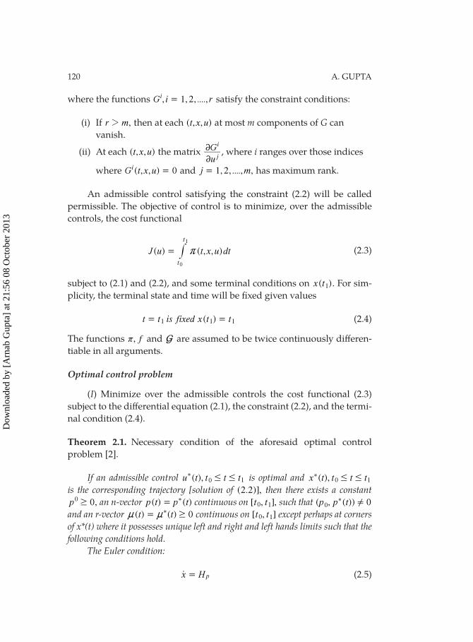
where the functions , 1,2, ....,G i ri = satisfy the constraint conditions:

(i) If ,r m2 then at each ( , , )t x u at most m components of G can

vanish.

(ii) At each ( , , )t x u the matrix G

u

i

2

2j

, where i ranges over those indices

where ( , , ) 0G t x ui = and 1,2, ...., ,j m= has maximum rank.

An admissible control satisfying the constraint (2.2) will be called

permissible. The objective of control is to minimize, over the admissible

controls, the cost functional

t

( ) ( , , )J u t x u dtt

r=1

0

# (2.3)

subject to (2.1) and (2.2), and some terminal conditions on ( )x t1 . For sim-

plicity, the terminal state and time will be fi xed given values

( )t t is fixed x t t= =1 1 1 (2.4)

The functions ,π f and G are assumed to be twice continuously diff eren-

tiable in all arguments.

Optimal control problem

(I) Minimize over the admissible controls the cost functional (2.3)

subject to the diff erential equation (2.1), the constraint (2.2), and the termi-

nal condition (2.4).

Theorem 2.1. Necessary condition of the aforesaid optimal control

problem [2].

If an admissible control 1( ),u t t t t# #*

0 is optimal and 1( ),x t t t t# #0*

is the corresponding trajectory [solution of (2.2)], then there exists a constant 0,p0

$ an n-vector ( ) ( )p t p t= * continuous on [ , ],t t0 1 such that ( , ( )) 0p p t !0*

and an r-vector ( ) ( ) 0t t $n n= * continuous on [ , ]t t0 1 except perhaps at corners of x*(t) where it possesses unique left and right and left hands limits such that the following conditions hold.

The Euler condition:

x H p=o (2.5)

Dow

nloa

ded

by [

Arn

ab G

upta

] at

21:

56 0

8 O

ctob

er 2

013

VECTOR OPTIMAL CONTROL PROBLEM 121

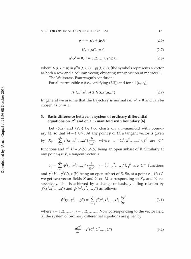
( )p H Gx xn=- +o (2.6)

H G 0x un+ = (2.7)

, , , , . .u G i r0 1 2 0i i f $n= = (2.8)

where ( , , , ) ( , , ) ( , , ),πH t x u p p t x u pf t x u0= + [the symbols represents a vector

as both a row and a column vector, obviating transposition of matrices].

The Weirstrass-Pontryagin’s condition:

For all permissible u (i.e., satisfying (2.3)) and for all [ , ]t t0 1 ,

*( , , , ) ( , , , )H t x u p H t x u p#* * * (2.9)

In general we assume that the trajectory is normal i.e. 0p0 ! and can be

chosen as 1p0 = .

3. Basic diff erence between a system of ordinary diff erential equations on Rn and on a n - manifold with boundary [6]

Let ( , )U x and ( , )V y be two charts on a n-manifold with bound-

ary M, so that M U V,= . At any point p of U, a tangent vector is given

by ( , , ....., ) ,X f x x xx

pi n

ii

n1 2

1 2

2==

/ where ( , , ., ),…x x x x fn1 2= i are C ∞

functions and : ( ), ( )x U x U x Ui i i" being an open subset of R. Similarly at

any point ,q V! a tangent vector is

( , , ....., ) ,Y y y yy

qi n

ii

n1 2

1 2

2z==

/ , , , ,y y y yn i1 2 f z= ^ h are C ∞ functions

and : ( ), ( )y V y V y Vi i i" being an open subset of R. So, at a point ,r VU +!

we get two vector fi elds X and Y on M corresponding to X p and Yq re-

spectively. This is achieved by a change of basis, yielding relation by

( , , , )f x x n1 2 f xi and ( , , , )y y yj n1 2 fz as follows:

( , , ...., ) ( , , , )y y y f x x xx

yj n ni

j

i

n1 2 1 2

1 2

2fz =

=

i/ (3.1)

where 1,2, ., ; 1,2, .., .… …i n j n= = Now corresponding to the vector fi eld

X, the system of ordinary diff erential equations are given by

( , , ....., )dt

dC f C C Ci

i n1 2= (3.2)

Dow

nloa

ded

by [

Arn

ab G

upta

] at

21:

56 0

8 O

ctob

er 2

013

122 A. GUPTA

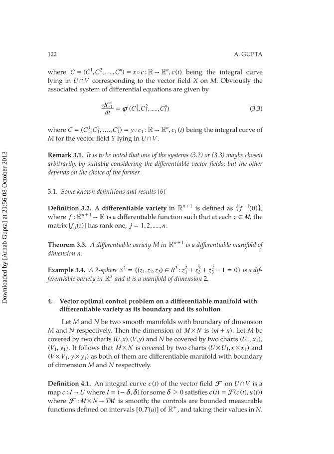
where ( , , ., ) : , ( )…C C C C x c c tR R1 2 n n"= = 5 being the integral curve

lying in VU + corresponding to the vector fi eld X on M. Obviously the

associated system of diff erential equations are given by

( , , ....., )dt

dCC C C

ii n1

11

12

1{= (3.3)

where 11( , , ., ) : , ( )…C C C C c c ty R Rn n1

2"= =1

11 5 being the integral curve of M for the vector fi eld Y lying in VU + .

Remark 3.1. It is to be noted that one of the systems (3.2) or (3.3) maybe chosen arbitrarily, by suitably considering the diff erentiable vector fi elds; but the other depends on the choice of the former.

3.1. Some known defi nitions and results [6]

Defi nition 3.2. A diff erentiable variety in R 1n + is defi ned as (0) ,f 1-" ,

where :f R R"n 1+ is a diff erentiable function such that at each ,z M! the

matrix [ ( )]f z, j has rank one, 1,2, .....,j n= .

Theorem 3.3. A diff erentiable variety M in R 1n + is a diff erentiable manifold of dimension n.

Example 3.4. A 2-sphere {( , , ) : 1 0}S z z z R z z z2 3 2 2 2!= + + - =1 2 1 3 33 is a dif-

ferentiable variety in R3 and it is a manifold of dimension 2.

4. Vector optimal control problem on a diff erentiable manifold with diff erentiable variety as its boundary and its solution

Let M and N be two smooth manifolds with boundary of dimension M and N respectively. Then the dimension of M N# is ( )m n+ . Let M be

covered by two charts ( , ), ( , )U x V y and N be covered by two charts ( , ),U x1 1

( , ) .V y1 1 It follows that M N# is covered by two charts ( , )U U x x1# # 1 and

( , )V V y y# #1 1 as both of them are diff erentiable manifold with boundary

of dimension M and N respectively.

Defi nition 4.1. An integral curve ( )c t of the vector fi eld F on U V+ is a

map :c I U" where ( , )I d d= - for some 02d satisfi es ( ) ( ( ), ( ))c t c t u tF=

where : M N TMF "# is smooth; the controls are bounded measurable

functions defi ned on intervals [0, ( )]T u of R+ , and taking their values in N.

Dow

nloa

ded

by [

Arn

ab G

upta

] at

21:

56 0

8 O

ctob

er 2

013

VECTOR OPTIMAL CONTROL PROBLEM 123

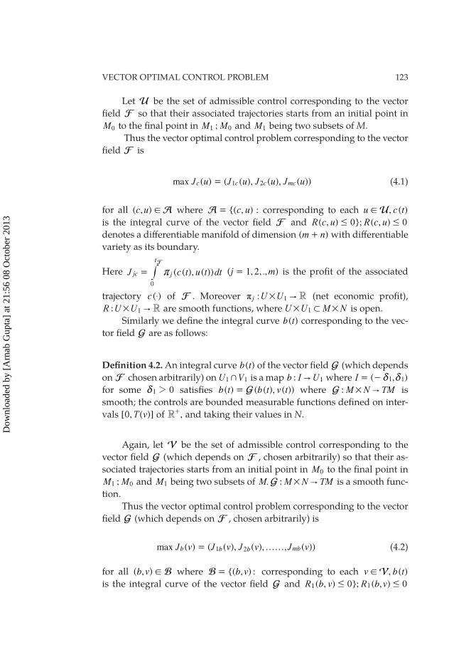
Let U be the set of admissible control corresponding to the vector

fi eld F so that their associated trajectories starts from an initial point in

M0 to the fi nal point in ;M M1 0 and M1 being two subsets of M.

Thus the vector optimal control problem corresponding to the vector

fi eld F is

( ) ( ( ), ( ), ( ))max J u J u J u J u1 2c c c mc= (4.1)

for all ( , )c u A! where {( , ) :c uA = corresponding to each , ( )u c tU! is the integral curve of the vector fi eld F and ( , ) 0}; ( , ) 0 R c u R c u# #

denotes a diff erentiable manifold of dimension ( )m n+ with diff erentiable

variety as its boundary.

Here j ( ( ), ( ))J c t u t dtjc

0

r=

tF

# ( 1,2, ., )j m= is the profi t of the associated

trajectory ( )c $ of F . Moreover j :π U U R"# 1 (net economic profi t),

:R U U R"# 1 are smooth functions, where U U M N1# #1 is open.

Similarly we defi ne the integral curve ( )b t corresponding to the vec-

tor fi eld G are as follows:

Defi nition 4.2. An integral curve ( )b t of the vector fi eld G (which depends

on F chosen arbitrarily) on U V+1 1 is a map :b I U" 1 where ( , )I 1 1d d= -

for some 01 2d satisfi es ( ) ( ( ), ( ))b t b t v tG= where : M N TMG "# is

smooth; the controls are bounded measurable functions defi ned on inter-

vals [0, ( )]T v of ,R+ and taking their values in N.

Again, let V be the set of admissible control corresponding to the

vector fi eld G (which depends on F , chosen arbitrarily) so that their as-

sociated trajectories starts from an initial point in M0 to the fi nal point in

;M M1 0 and M1 being two subsets of . :M M N TMG "# is a smooth func-

tion.

Thus the vector optimal control problem corresponding to the vector

fi eld G (which depends on F , chosen arbitrarily) is

( ) ( ( ), ( ), , ( ))……max J v J v J v J vb mb= 1b 2b (4.2)

for all ( , )b v B! where {( , ) : b vB = corresponding to each , ( )v b tV!

is the integral curve of the vector fi eld G and ( , ) 0}; ( , ) 0 R b v R b v1# #1

Dow

nloa

ded

by [

Arn

ab G

upta

] at

21:

56 0

8 O

ctob

er 2

013

124 A. GUPTA

denotes a diff erentiable manifold of dimension ( )m n+ with diff erentiable

variety as its boundary.

Here jj

t

( ( ), ( )) ( 1,2, ...., )J b t v t dt j mb

0

}= =

G

# is the profi t of the associated

trajectory ( )b $ of G . Moreover j : V V R"#} 1 (net economic profi t),

:R V V R"#1 1 are smooth functions, where V V M N# #11 is open.

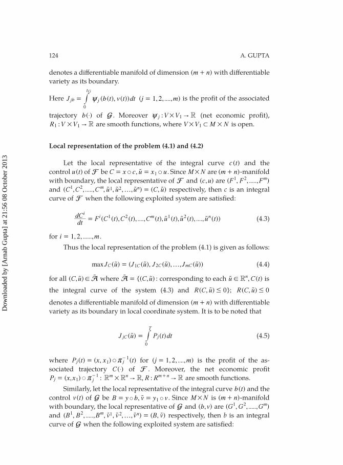
Local representation of the problem (4.1) and (4.2)

Let the local representative of the integral curve ( )c t and the

control ( )u t of F be ,C x c u x u& &= = 1u . Since M N# are ( )m n+ -manifold

with boundary, the local representative of F and ( , )c u are ( , , ....., )F F F1 2 m

and 2( , , ....., , , , , ) ( , )C C C u u u C u1 2 nf =1m u u u u respectively, then c is an integral

curve of F when the following exploited system are satisfi ed:

( ( ), ( ), ...., ( ), ( ), ( ), ...., ( ))dt

dC F C t C t C t u t u t u ti

i m n1 2 1 2= u u u (4.3)

for 1,2, ......,i m= .

Thus the local representation of the problem (4.1) is given as follows:

( ) ( ( ), ( ), , ( ))max J u J u J u J u2C C mCf= 1Cu u u u (4.4)

for all ( , )C u A!u u where {( , ) :C uA =u u corresponding to each , ( )u C tRn!u is

the integral curve of the system (4.3) and ( , ) ;}R C u 0#u ( , ) 0R C u #u

denotes a diff erentiable manifold of dimension ( )m n+ with diff erentiable

variety as its boundary in local coordinate system. It is to be noted that

( ) ( )J u P t dtjC j

T

0

=u # (4.5)

where &( ) ( , ) ( )P t x x tj1r= -

j 1 for ( 1,2, ...., )j m= is the profi t of the as-

sociated trajectory ( )C $ of F . Moreover, the net economic profi te( , ) :P x xj

1r= -1 j , :R RR R RR m nnm

" "# + are smooth functions.

Similarly, let the local representative of the integral curve ( )b t and the

control ( )v t of G be & &,B y b v y v= = 1u . Since M N# is ( )m n+ -manifold

with boundary, the local representative of G and ( , )b v are ( , , ....., )G G G1 2 m

and 1( , , ....., , , , , ) ( , )B B B v v v B vm1 2 f =n2u u u u respectively, then b is an integral

curve of G when the following exploited system are satisfi ed:

Dow

nloa

ded

by [

Arn

ab G

upta

] at

21:

56 0

8 O

ctob

er 2

013

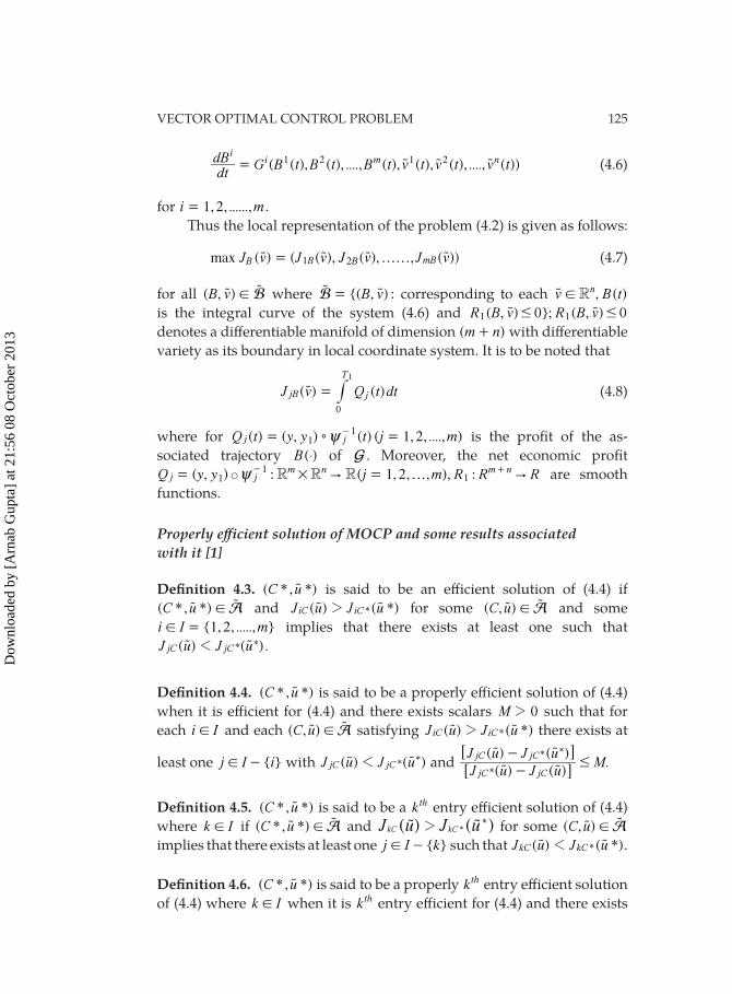
VECTOR OPTIMAL CONTROL PROBLEM 125

( ( ), ( ), ...., ( ), ( ), ( ), ...., ( ))dt

dB G B t B t B t v t v t v ti

i m n1 2 1 2= u u u (4.6)

for 1,2, ......,i m= .

Thus the local representation of the problem (4.2) is given as follows:

B ( ) ( ( ), ( ), , ( ))……max J v J v J v J vmB= B1 B2u u u u (4.7)

for all ( , )B v B!u u where {( , ) :B vB =u u corresponding to each , ( )v B tRn!u

is the integral curve of the system (4.6) and ( , ) 0}; ( , ) 0R B v R B v# #1 1u u

denotes a diff erentiable manifold of dimension ( )m n+ with diff erentiable

variety as its boundary in local coordinate system. It is to be noted that

j( ) ( )J v Q t dtjB

T

0

1

=u # (4.8)

where for ( ) ( , ) ( ) ( 1,2, ...., )Q t y y t j mj j1

1 %}= =- is the profi t of the as-

sociated trajectory ( )B $ of G . Moreover, the net economic profi t

( , ) : ( , , , ), :Q y y j m R R R1 2R R Rj jm n m n1

" "#& f}= =- +11 are smooth

functions.

Properly eff icient solution of MOCP and some results associated with it [1]

Defi nition 4.3. ( *, *)C uu is said to be an eff icient solution of (4.4) if

( *, *)C u A!u u and ( ) ( *)J u J u*iC iC2u u for some ( , )C u A!u u and some

{1,2, ....., }i I m! = implies that there exists at least one such that

( ) ( ) .J u J uj jCC 1 **u u

Defi nition 4.4. ( *, *)C uu is said to be a properly eff icient solution of (4.4)

when it is eff icient for (4.4) and there exists scalars 0M 2 such that for

each i I! and each ( , )C u A!u u satisfying ( ) ( *)J u J u*iC iC2u u there exists at

least one { }Ij i! - with ( ) ( )J u J ujC jC1 **u u and ( ) ( )

( ) ( ).

J u J u

J u J uM

jC jC

jC jC#

-

- **

* u uu u

6

6

@

@

Defi nition 4.5. ( *, *)C uu is said to be a kth entry eff icient solution of (4.4)

where k I! if ( *, *)C u A!u u and ( ) ( )J u J u*kC kC2 *u u for some ( , )C u A!u u

implies that there exists at least one { }j I k! - such that ( ) ( *)J u J u*kC kC1u u .

Defi nition 4.6. ( *, *)C uu is said to be a properly kth entry eff icient solution

of (4.4) where k I! when it is kth entry eff icient for (4.4) and there exists

Dow

nloa

ded

by [

Arn

ab G

upta

] at

21:

56 0

8 O

ctob

er 2

013

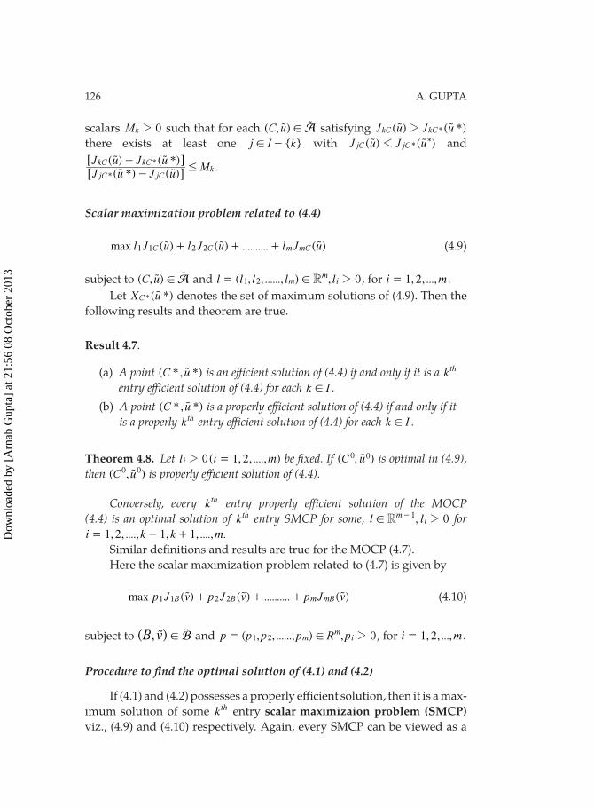
126 A. GUPTA

scalars 0Mk 2 such that for each ( , )C u A!u u satisfying ( ) ( *)J u J u*kC kC2u u

there exists at least one { }j I k! - with ( ) ( )J u J u*jC jC1 *u u and

( *) ( )( ) ( *)

J u J uJ u J u

M*

*

jC jC

kC kCk#

--

u uu u

6

5

@

?.

Scalar maximization problem related to (4.4)

( ) ( ) .......... ( )max l J u l J u l J uC C m mC1 1 2 2+ + +u u u (4.9)

subject to ( , )C u A!u u and ( , , ......, ) ,l l l l l 0Rmm

i1 2 2!= , for 1,2, ...,i m= .

Let ( *)X u*C u denotes the set of maximum solutions of (4.9). Then the

following results and theorem are true.

Result 4.7.

(a) A point ( *, *)C uu is an eff icient solution of (4.4) if and only if it is a kth entry eff icient solution of (4.4) for each k I! .

(b) A point ( *, *)C uu is a properly eff icient solution of (4.4) if and only if it is a properly kth entry eff icient solution of (4.4) for each k I! .

Theorem 4.8. Let 0( 1,2, ...., )l i mi 2 = be fi xed. If ( , )C u0 0u is optimal in (4.9), then ( , )C u0 0u is properly eff icient solution of (4.4).

Conversely, every kth entry properly eff icient solution of the MOCP (4.4) is an optimal solution of kth entry SMCP for some, ,l l 0Rm

i1 2!

- for 1,2, ...., 1,i k= - 1, ...., .k m+

Similar defi nitions and results are true for the MOCP (4.7).

Here the scalar maximization problem related to (4.7) is given by

( ) ( ) .......... ( )max p J v p J v p J vB B m mB1 1 2 2+ + +u u u (4.10)

subject to ( , )B v B!uu and ( , , ......, ) , 0p p p p R pm

mi1 2 2!= , for 1,2, ...,i m= .

Procedure to fi nd the optimal solution of (4.1) and (4.2)

If (4.1) and (4.2) possesses a properly eff icient solution, then it is a max-

imum solution of some kth entry scalar maximizaion problem (SMCP) viz., (4.9) and (4.10) respectively. Again, every SMCP can be viewed as a

Dow

nloa

ded

by [

Arn

ab G

upta

] at

21:

56 0

8 O

ctob

er 2

013

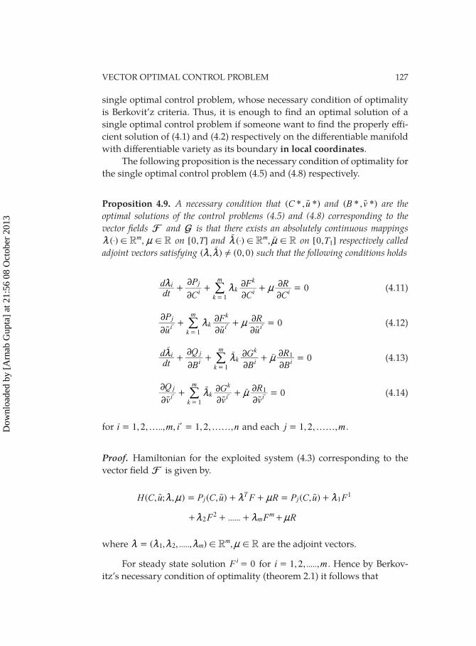
VECTOR OPTIMAL CONTROL PROBLEM 127

single optimal control problem, whose necessary condition of optimality

is Berkovit’z criteria. Thus, it is enough to fi nd an optimal solution of a

single optimal control problem if someone want to fi nd the properly eff i-

cient solution of (4.1) and (4.2) respectively on the diff erentiable manifold

with diff erentiable variety as its boundary in local coordinates.

The following proposition is the necessary condition of optimality for

the single optimal control problem (4.5) and (4.8) respectively.

Proposition 4.9. A necessary condition that ( *, *)C uu and ( *, *)B vu are the optimal solutions of the control problems (4.5) and (4.8) corresponding to the vector fi elds F and G is that there exists an absolutely continuous mappings

( ) ,R Rm$ ! !m n on [0, ]T and ( ) ,R Rm$ ! !m nr r on [0, ]T1 respectively called adjoint vectors satisfying ( , ) (0,0)!m mr such that the following conditions holds

0dt

d

C

P

C

F

C

Rii

jk

k

m

i

k

i12

2

2

2

2

2m m n+ + + ==

/ (4.11)

0u

P

u

F

u

Ri

jk

k

m

i

k

i12

2

2

2

2

2m n+ + ==

l l lu u u/ (4.12)

0dt

d

B

Q

B

G

B

Rii

jk

k

m

i

k

i1

1

2

2

2

2

2

2m m n+ + + ==

rr r/ (4.13)

0v

Q

v

G

v

Ri

jk

k

m

i

k

i1

1

2

2

2

2

2

2m n+ + ==

l l lur

ur

u/ (4.14)

for 1,2, .., , 1,2, ,… ……i m i n= =l and each 1,2, ,……j m= .

Proof. Hamiltonian for the exploited system (4.3) corresponding to the

vector fi eld F is given by.

( , ; , ) ( , ) ( , )H C u P C u F R P C u FjT

j 11m n m n m= + + = +u u u

......F Fmm

22m m+ + + Rn+

where ( , , ....., ) ,R Rmm

1 2 ! !m m m m n= are the adjoint vectors.

For steady state solution 0F =i for 1,2, .....,i m= . Hence by Berkov-

itz’s necessary condition of optimality (theorem 2.1) it follows that

Dow

nloa

ded

by [

Arn

ab G

upta

] at

21:

56 0

8 O

ctob

er 2

013

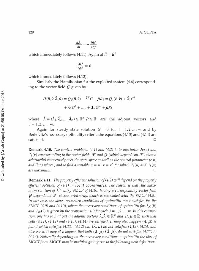
128 A. GUPTA

dt

d

C

Hii2

2m=-

which immediately follows (4.11). Again at u u= *u u

0u

Hi2

2 =lu

which immediately follows (4.12).

Similarly the Hamiltonian for the exploited system (4.6) correspond-

ing to the vector fi eld G given by

( , ; , ) ( , ) ( , )H B v Q B v G R Q B v GjT

j1 11m n m n m= + + = +u r r u r r u r

......G Gmm

22m m+ + +r r R1n+ r

where ( , , ....., ) ,R Rmm

1 2 ! !m m m m n=r r r r r are the adjoint vectors and

1,2, ..,…j m= .

Again for steady state solution 0Gi = for 1,2, .....,i m= and by

Berkovitz’s necessary optimality criteria the equations (4.13) and (4.14) are

satisfi ed. 4

Remark 4.10. The control problems (4.1) and (4.2) is to maximize ( )Jc u and ( )J vb corresponding to the vector fi elds F and G (which depends on F , chosen

arbitrarily) respectively over the state space as well as the control parameter (c,u) and (b,v) where , and to fi nd a suitable ,u u v v= = ** for which ( )J uc and ( )J vb are maximum. 4

Remark 4.11. The properly eff icient solution of (4.2) will depend on the properly eff icient solution of (4.1) in local coordinates. The reason is that, the maxi-mum solution of kth entry SMCP of (4.10) having a corresponding vector fi eld G depends on F chosen arbitrarily, which is associated with the SMCP (4.9). In our case, the above necessary conditions of optimality must satisfi es for the SMCP (4.9) and (4.10), where the necessary conditions of optimality for ( )J ujC u and ( )J vjB u is given by the proposition 4.9 for each 1,2, ...., .j m= In this connec-tion, one has to fi nd out the adjoint vectors , Rm

!m mr and , R!n nr such that both (4.11), (4.12) and (4.13), (4.14) are satisfi ed. It may also happen ( , )m n is found which satisfi es (4.11), (4.12) but ( , )m nr r do not satisfi es (4.13), (4.14) and vice versa. It may also happen that both , ,,m n m nr r^ ^h h, do not satisfi es (4.11) to (4.14). Naturally depending on the necessary conditions o optimality the idea of MOCP/ non MOCP may be modifi ed giving rise to the following new defi nitions.

Dow

nloa

ded

by [

Arn

ab G

upta

] at

21:

56 0

8 O

ctob

er 2

013

VECTOR OPTIMAL CONTROL PROBLEM 129

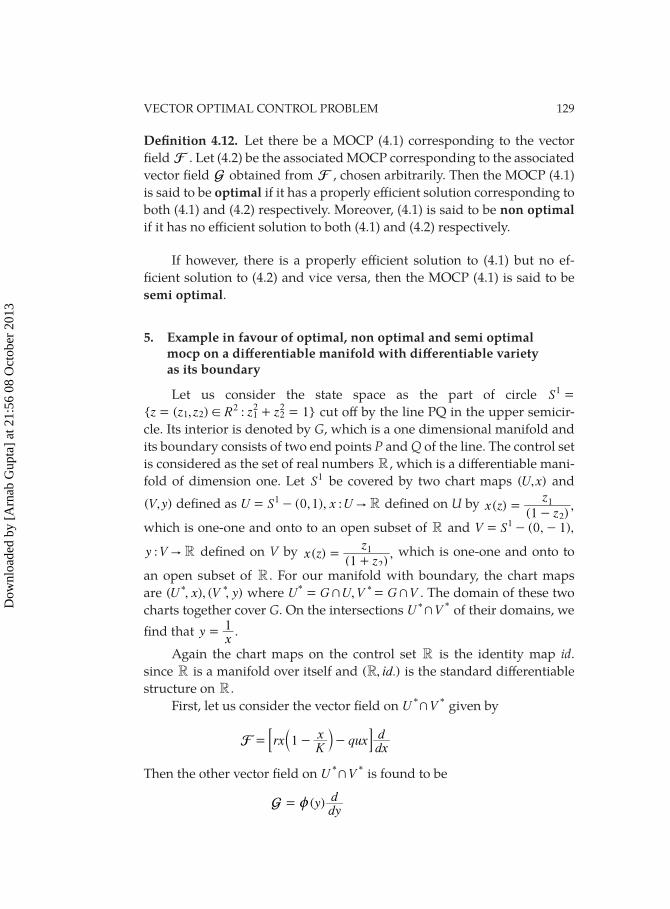
Defi nition 4.12. Let there be a MOCP (4.1) corresponding to the vector

fi eld F . Let (4.2) be the associated MOCP corresponding to the associated

vector fi eld G obtained from F , chosen arbitrarily. Then the MOCP (4.1)

is said to be optimal if it has a properly eff icient solution corresponding to

both (4.1) and (4.2) respectively. Moreover, (4.1) is said to be non optimal if it has no eff icient solution to both (4.1) and (4.2) respectively.

If however, there is a properly eff icient solution to (4.1) but no ef-

fi cient solution to (4.2) and vice versa, then the MOCP (4.1) is said to be

semi optimal.

5. Example in favour of optimal, non optimal and semi optimal mocp on a diff erentiable manifold with diff erentiable variety as its boundary

Let us consider the state space as the part of circle S1 =

{ ( , ) : }z z z R z z 11 22

12

22

!= + = cut off by the line PQ in the upper semicir-

cle. Its interior is denoted by G, which is a one dimensional manifold and

its boundary consists of two end points P and Q of the line. The control set

is considered as the set of real numbers R , which is a diff erentiable mani-

fold of dimension one. Let S1 be covered by two chart maps ( , )U x and

( , )V y defi ned as (0,1), :U S x U R1"= - defi ned on U by z

( )(1 )

,x zz

=-

1

2

which is one-one and onto to an open subset of R and ( , ),V S 0 11= - -

:y V R" defi ned on V by z( )

(1 ),x z

z1=

+ 2

which is one-one and onto to

an open subset of R . For our manifold with boundary, the chart maps

are ( , ), ( , )U x V y* * where ,U G U V G V* + += =* . The domain of these two

charts together cover G. On the intersections U V+* * of their domains, we

fi nd that yx1= .

Again the chart maps on the control set R is the identity map id.

since R is a manifold over itself and ( , .)idR is the standard diff erentiable

structure on R .

First, let us consider the vector fi eld on U V+* * given by

rxKx qux

dxd1F = - -b l: D

Then the other vector fi eld on U V+* * is found to be

( )ydydG z=

Dow

nloa

ded

by [

Arn

ab G

upta

] at

21:

56 0

8 O

ctob

er 2

013

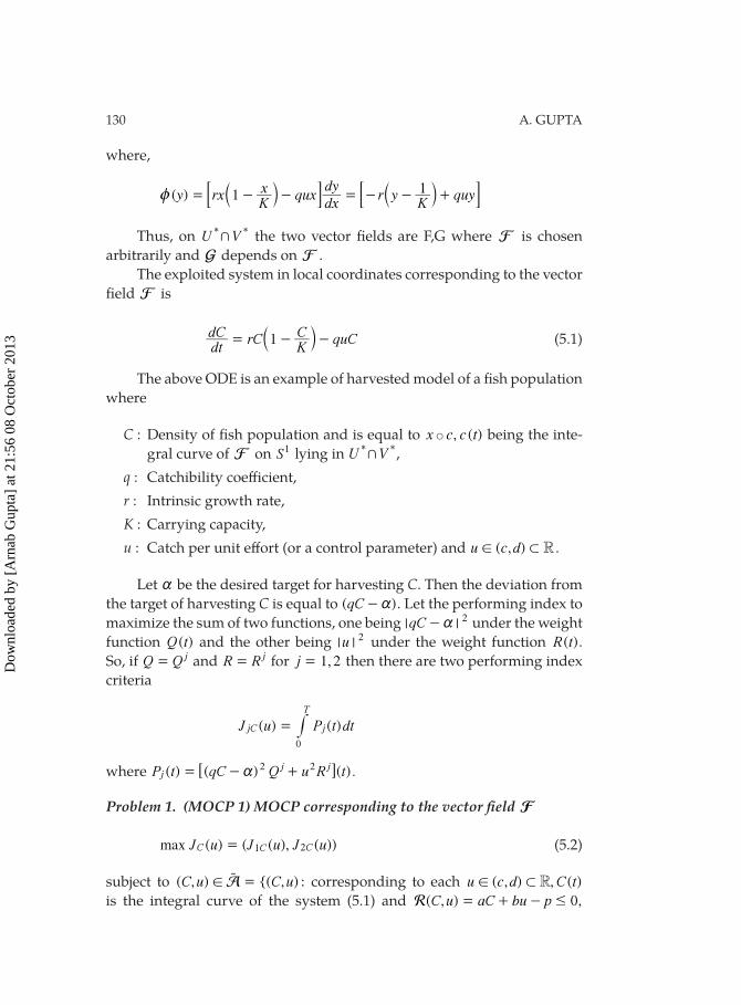
130 A. GUPTA

where,

( )y rxKx qux

dxdy

r yK

quy1 1z = - - = - - +b bl l: :D D

Thus, on U V+* * the two vector fi elds are F,G where F is chosen

arbitrarily and G depends on F .

The exploited system in local coordinates corresponding to the vector

fi eld F is

dtdC rC

KC quC1= - -b l (5.1)

The above ODE is an example of harvested model of a fi sh population

where

C : Density of fi sh population and is equal to , ( )x c c t& being the inte-

gral curve of F on S1 lying in U V+* *,

q : Catchibility coeff icient,

r : Intrinsic growth rate,

K : Carrying capacity,

u : Catch per unit eff ort (or a control parameter) and ( , )u c d R! 1 .

Let a be the desired target for harvesting C. Then the deviation from

the target of harvesting C is equal to ( )qC a- . Let the performing index to

maximize the sum of two functions, one being | |qC 2a- under the weight

function ( )Q t and the other being | |u 2 under the weight function ( )R t .

So, if Q Q j= and R R j= for 1,2j = then there are two performing index

criteria

( ) ( )J u P t dtjC j

T

0

= #

where j ( ) ( ) ( ) .P t qC Q u R t2 2j ja= - +6 @

Problem 1. (MOCP 1) MOCP corresponding to the vector fi eld F

( ) ( ( ), ( ))max J u J u J u2C C= 1C (5.2)

subject to ( , ) {( , ) :C u C uA! =u corresponding to each ( , ) , ( )u c d C tR! 1

is the integral curve of the system (5.1) and ( , ) 0,C u aC bu pR #= + -

Dow

nloa

ded

by [

Arn

ab G

upta

] at

21:

56 0

8 O

ctob

er 2

013

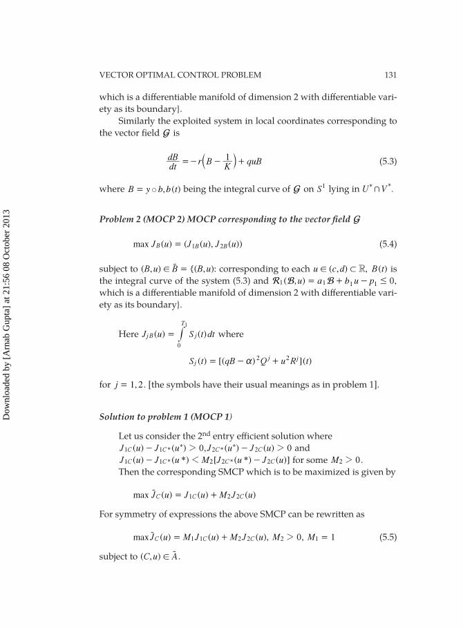
VECTOR OPTIMAL CONTROL PROBLEM 131

which is a diff erentiable manifold of dimension 2 with diff erentiable vari-

ety as its boundary}.

Similarly the exploited system in local coordinates corresponding to

the vector fi eld G is

dtdB r B

KquB1=- - +b l (5.3)

where & , ( )B y b b t= being the integral curve of G on S1 lying in .U V+* *

Problem 2 (MOCP 2) MOCP corresponding to the vector fi eld G

( ) ( ( ), ( ))max J u J u J uB = 1 2B B (5.4)

subject to ( , ) {( , ):B u B B u! =u corresponding to each ( , ) ,u c d R! 1 ( )B t is

the integral curve of the system (5.3) and 11( , ) ,u a b u p 0R B B1 #= + -1

which is a diff erentiable manifold of dimension 2 with diff erentiable vari-

ety as its boundary}.

Here j ( ) ( )J u S t dtB j

T

0

1

= # where

j ( ) [( ) ] ( )S t qB Q u R t2 2j ja= - +

for 1,2j = . [the symbols have their usual meanings as in problem 1].

Solution to problem 1 (MOCP 1)

Let us consider the 2nd entry eff icient solution where

( ) ( ) 0, ( ) ( ) 0J u J u J u J u* *C C C C1 1 2 22 2- -* * and

( ) ( *) [ ( *) ( )]J u J u M J u J u* *C C C C1 1 2 2 21- - for some 0M2 2 .

Then the corresponding SMCP which is to be maximized is given by

( ) ( ) ( )max J u J u M J uC C C1 2 2= +u

For symmetry of expressions the above SMCP can be rewritten as

( ) ( ) ( ), 0, 1max J u M J u M J u M MC C C1 1 2 2 2 12= + =u (5.5)

subject to ( , )C u A!u .

Dow

nloa

ded

by [

Arn

ab G

upta

] at

21:

56 0

8 O

ctob

er 2

013

132 A. GUPTA

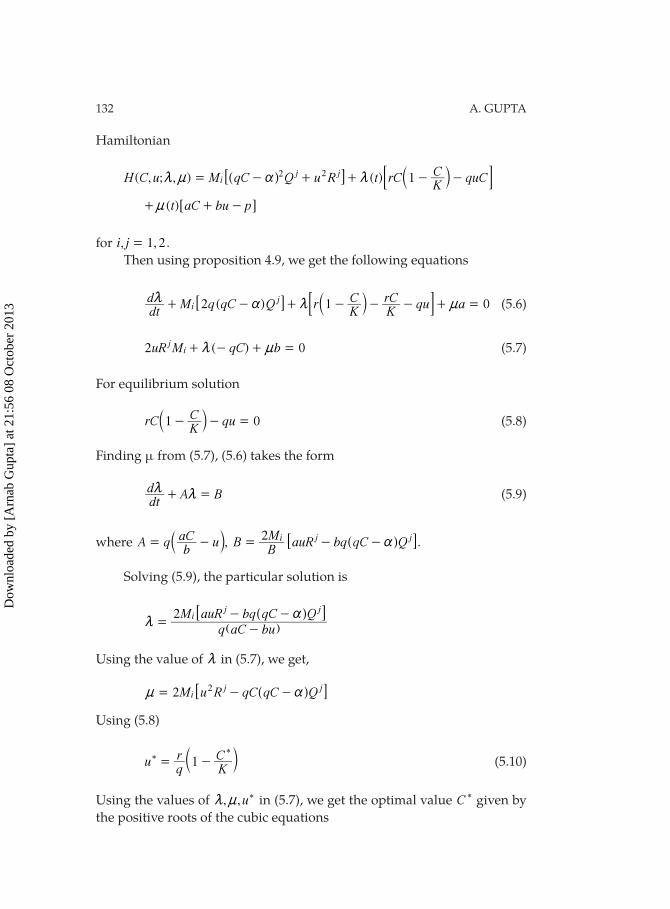
Hamiltonian

( , ; , ) ( )H C u M qC Q u R t rCKC quC1i

j j2 2m n a m= - + + - -] bg l7 :A D

( )t aC bu pn+ + -6 @

for , 1,2i j = .

Then using proposition 4.9, we get the following equations

( ) 0dtd M q qC Q r

KC

KrC qu a2 1i

jm a m n+ - + - - - + =b l7 :A D (5.6)

2 ( ) 0uR M qC bji m n+ - + = (5.7)

For equilibrium solution

0rCKC qu1 - - =b l (5.8)

Finding μ from (5.7), (5.6) takes the form

dtd A Bm m+ = (5.9)

where , A qb

aC u BBM

auR bq qC Q2 i j ja= - = - -b ]l g7 A.

Solving (5.9), the particular solution is

q aC bu

M auR bq qC Q2 ij j

ma

=-

- -]

]g

g7 A

Using the value of m in (5.7), we get,

2M u R qC qC Qij j2n a= - -] g7 A

Using (5.8)

uqr

KC1= -*

*c m (5.10)

Using the values of , ,um n * in (5.7), we get the optimal value C * given by

the positive roots of the cubic equations

Dow

nloa

ded

by [

Arn

ab G

upta

] at

21:

56 0

8 O

ctob

er 2

013

VECTOR OPTIMAL CONTROL PROBLEM 133

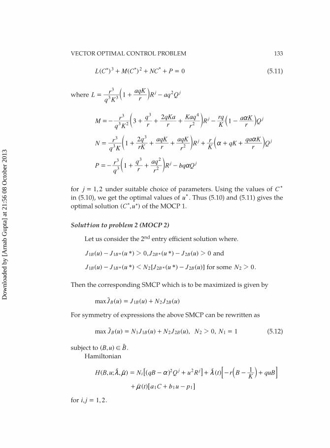
( ) ( )L C M C NC P 03 2 *+ + + =** (5.11)

where Lq K

rr

aqKR aq Q1 j j

3 3

32= + -b l

Mq K

rr

qr

qKa

r

KaqR

Krq

ra K Q3

21j j

3 2

3 3

2

4a=- + + + - -d bn l

Nq K

rrKq

raqK

r

aqKR

Kr qK

rqa K

Q12 j j

3

3 3

2a

a= + + + + + +d bn l

Pq

rr

q

r

aqR bq Q1 j j

3

3 3

2

2

a=- + + -d n

for 1,2j = under suitable choice of parameters. Using the values of C *

in (5.10), we get the optimal values of u* . Thus (5.10) and (5.11) gives the

optimal solution ( , )C u** of the MOCP 1.

Solut†ion to problem 2 (MOCP 2)

Let us consider the 2nd entry eff icient solution where.

( ) ( *) 0, ( *) ( ) 0J u J u J u J u* *B B B B1 1 2 22 2- - and

( ) ( *) [ ( *) ( )]J u J u N J u J u* *B B B B1 1 2 2 21- - for some N 02 2 .

Then the corresponding SMCP which is to be maximized is given by

( ) ( ) ( )max J u J u N J uB B B1 2 2= +u

For symmetry of expressions the above SMCP can be rewritten as

( ) ( ) ( ), , max J u N J u N J u N N0 1B B B1 1 2 2 2 12= + =u (5.12)

subject to ( , )B u B! u .

Hamiltonian

( , ; , ) ( )H B u N qB Q u R t r BK

quB1i

j j2 2m n a m= - + + - - +r r r] bg l7 :A D

( )t a C b u p1 1 1n+ + -r 6 @

for , 1,2i j = .

Dow

nloa

ded

by [

Arn

ab G

upta

] at

21:

56 0

8 O

ctob

er 2

013

134 A. GUPTA

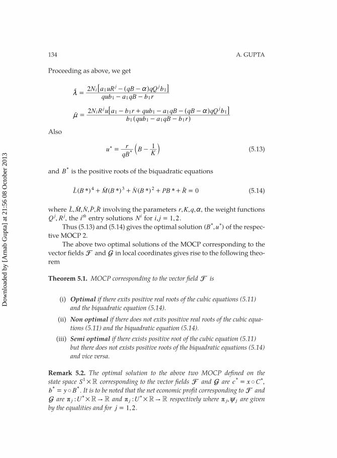
Proceeding as above, we get

qub a qB b r

N a uR qB qQ b2 ij j

1 1 1

1 1m

a=

- -- -r ] g7 A

b qub a qB b r

N R u a b r qub a qB qB qQ b2 ij j

1 1 1 1

1 1 1 1 1n

a=

- -- + - - -

r]

]

g

g7 A

Also

uqB

r BK1

*= -* b l (5.13)

and B* is the positive roots of the biquadratic equations

( *) ( *) ( *) * 0L B M B N B PB R4 3 2+ + + + =r r r r (5.14)

where , , , ,L M N P Rr r r r r involving the parameters , , , ,r K q a the weight functions

, ,Q Rj j the ith entry solutions Ni for , 1,2i j = .

Thus (5.13) and (5.14) gives the optimal solution ( , )B u* * of the respec-

tive MOCP 2.

The above two optimal solutions of the MOCP corresponding to the

vector fi elds F and G in local coordinates gives rise to the following theo-

rem

Theorem 5.1. MOCP corresponding to the vector fi eld F is

(i) Optimal if there exits positive real roots of the cubic equations (5.11) and the biquadratic equation (5.14).

(ii) Non optimal if there does not exits positive real roots of the cubic equa-tions (5.11) and the biquadratic equation (5.14).

(iii) Semi optimal if there exists positive root of the cubic equation (5.11) but there does not exists positive roots of the biquadratic equations (5.14) and vice versa.

Remark 5.2. The optimal solution to the above two MOCP defi ned on the state space S R1 # corresponding to the vector fi elds F and G are & ,c x C* = *

& .b y B* *= It is to be noted that the net economic profi t corresponding to F and G are j :π U R R"#* and j :π U R R"#* respectively where j,π }j are given by the equalities and for 1,2j = .

Dow

nloa

ded

by [

Arn

ab G

upta

] at

21:

56 0

8 O

ctob

er 2

013

VECTOR OPTIMAL CONTROL PROBLEM 135

6. Acknowledgement

The author is thankful to Prof. D.K.Bhattacharya (Dept. of Pure

Mathematics, University of Calcutta, INDIA) for his kind support and in-

spiration for preparing this paper. Author also express his deep reverence

to his better half Mrs. Sharmistha Gupta who stood by his side constantly

and encouraged him patiently at every time.

References

[1] Benson H. P. and Morin T. L. The vector maximization problem

Proper eff iciency and stability. SIAM J. Appl. Math. Vol. 32(1), 1977,

pp. 64–72.

[2] Berkovitz L. D. Variational methods in problems of control and pro-

gramming. J. Math Anal. Appl. Vol. 3, 1961, pp. 145–169.

[3] Bhattacharya D. K. and Gupta A. Permanence and Extinction of solution of ordinary diff erential equations on a diff erentiable manifol. Ganita, Vol.

56(2), 2005, pp. 105–117.

[4] Bhattacharya D. K. and Aman T. E. Multi-Objective control problem. Rev. Acad. canar. XVI (Nums 1-2), 2004, pp. 105–117.

[5] Bhattacharya D. K., Gupta A and Aman T. E. Optimization of a

functional on an open manifold with diff erentiable variety as its

boundary. Rev. Acad. canar. Vol. XX(Nums 1-2), 2008. pp. 33–47.

[6] Brickell F. and Clark R. S. Diff erentiable Manifold, An introduction.

University of Southampton, Van Nostrand Reinhold Company-

London, 1970.

[7] Elizer Kreindler. Reciporcal optimal control problems. Journal of Mathematical Analysis and Applications, Vol. 14, 1966, pp. 141–152.

[8] Mond B. and Morgan M, Duality for control problems. SIAM Jor. Control, Vol. 6(1), 1968, pp. 114–120.

[9] Pontryagin’s L. S., Bolytyanski V. S., Gamkrelidze R. V. and Ischenko

E. F. The mathematical theory of optimal process. Wiley Interscience,

NewYork, 1962.

Received November, 2011

Dow

nloa

ded

by [

Arn

ab G

upta

] at

21:

56 0

8 O

ctob

er 2

013